helioseismology with solar orbiter

Noname manuscript No.(will be inserted by the editor)

Helioseismology with Solar Orbiter

Bjorn Loptien · Aaron C. Birch · Laurent Gizon ·Jesper Schou · Thierry Appourchaux ·Julian Blanco Rodrıguez · Paul S. Cally ·Carlos Dominguez-Tagle · Achim Gandorfer ·Frank Hill · Johann Hirzberger ·Philip H. Scherrer · Sami K. Solanki

Received: date / Accepted: date

Abstract The Solar Orbiter mission, to be launched in July 2017, will carry a suite of re-mote sensing and in-situ instruments, including the Polarimetric and Helioseismic Imager(PHI). PHI will deliver high-cadence images of the Sun in intensity and Doppler velocitysuitable for carrying out novel helioseismic studies. The orbit of the Solar Orbiter spacecraftwill reach a solar latitude of up to 21◦ (up to 34◦ by the end of the extended mission) andthus will enable the first local helioseismology studies of the polar regions. Here we con-sider an array of science objectives to be addressed by helioseismology within the baselinetelemetry allocation (51 Gbit per orbit, current baseline) and within the science observingwindows (baseline 3×10 days per orbit). A particularly important objective is the measure-ment of large-scale flows at high latitudes (rotation and meridional flow), which are largelyunknown but play an important role in flux transport dynamos. For both helioseismologyand feature tracking methods convection is a source of noise in the measurement of longitu-dinally averaged large-scale flows, which decreases as T−1/2 where T is the total durationof the observations. Therefore, the detection of small amplitude signals (e.g., meridionalcirculation, flows in the deep solar interior) requires long observation times. As an example,one hundred days of observations at lower spatial resolution would provide a noise level of

B. Loptien · L. Gizon (�)Institut fur Astrophysik, Georg-August Universitat Gottingen, 37077 Gottingen, GermanyE-mail: [email protected]

A. C. Birch · L. Gizon · J. Schou · A. Gandorfer · J. Hirzberger · S. K. SolankiMax-Planck-Institut fur Sonnensystemforschung, Justus-von-Liebig-Weg 3, 37077 Gottingen, Germany

T. Appourchaux · C. Dominguez-TagleInstitut d’Astrophysique Spatiale, CNRS - Universite Paris Sud, 91405 Orsay, France

J. Blanco RodrıguezGACE/IPL, Universidad de Valencia, 46980 Valencia, Spain

P. S. CallyMonash Centre for Astrophysics and School of Mathematical Sciences, Monash University, Clayton, Victoria3800, Australia

F. HillNational Solar Observatory, Tucson, Arizona 85719, USA

P. H. ScherrerHansen Experimental Physics Laboratory, Stanford University, Stanford, CA 94305-4085, USA

arX

iv:1

406.

5435

v1 [

astr

o-ph

.SR

] 2

0 Ju

n 20

14

2 Bjorn Loptien et al.

about three m/s on the meridional flow at 80◦ latitude. Longer time-series are also needed tostudy temporal variations with the solar cycle. The full range of Earth-Sun-spacecraft anglesprovided by the orbit will enable helioseismology from two vantage points by combiningPHI with another instrument: stereoscopic helioseismology will allow the study of the deepsolar interior and a better understanding of the physics of solar oscillations in both quietSun and sunspots. We have used a model of the PHI instrument to study its performance forhelioseismology applications. As input we used a 6 hr time-series of realistic solar magneto-convection simulation (Stagger code) and the SPINOR radiative transfer code to synthesizethe observables. The simulated power spectra of solar oscillations show that the instrumentis suitable for helioseismology. In particular, the specified point spread function, image jitter,and photon noise are no obstacle to a successful mission.

Keywords Helioseismology · Space missions: Solar Orbiter · Solar Physics · SolarDynamo

Helioseismology with Solar Orbiter 3

Contents

1 Introduction: Solar Orbiter . . . . . . . . . . . . . . . . . . . . . . . . . . . . . . . . . . . . . . 42 Mission Profile . . . . . . . . . . . . . . . . . . . . . . . . . . . . . . . . . . . . . . . . . . . . 4

2.1 Orbit Design . . . . . . . . . . . . . . . . . . . . . . . . . . . . . . . . . . . . . . . . . . . 42.2 Instrument Suite . . . . . . . . . . . . . . . . . . . . . . . . . . . . . . . . . . . . . . . . . 52.3 PHI: Observables and Operation . . . . . . . . . . . . . . . . . . . . . . . . . . . . . . . . 5

3 Helioseismology: Science Objectives . . . . . . . . . . . . . . . . . . . . . . . . . . . . . . . . . 83.1 Near-Surface Rotation, Meridional Circulation, and Solar-Cycle Variations at High Latitudes 93.2 Deep and Large-Scale Solar Dynamics . . . . . . . . . . . . . . . . . . . . . . . . . . . . . 113.3 Convection at High Latitudes . . . . . . . . . . . . . . . . . . . . . . . . . . . . . . . . . . 123.4 Deep Convection and Giant Cells . . . . . . . . . . . . . . . . . . . . . . . . . . . . . . . . 123.5 Active Regions and Sunspots . . . . . . . . . . . . . . . . . . . . . . . . . . . . . . . . . . 123.6 Physics of Oscillations (Stereoscopic Observations) . . . . . . . . . . . . . . . . . . . . . . 133.7 Low Resolution Observations . . . . . . . . . . . . . . . . . . . . . . . . . . . . . . . . . . 14

4 Helioseismology: Selected Requirements . . . . . . . . . . . . . . . . . . . . . . . . . . . . . . . 144.1 Example Telemetry Requirements . . . . . . . . . . . . . . . . . . . . . . . . . . . . . . . 144.2 Thoughts on Compression . . . . . . . . . . . . . . . . . . . . . . . . . . . . . . . . . . . 15

4.2.1 Binning, Subsampling, and Cropping . . . . . . . . . . . . . . . . . . . . . . . . . 154.2.2 Truncation . . . . . . . . . . . . . . . . . . . . . . . . . . . . . . . . . . . . . . . 154.2.3 Lossless Compression . . . . . . . . . . . . . . . . . . . . . . . . . . . . . . . . . 164.2.4 Lossy Compression . . . . . . . . . . . . . . . . . . . . . . . . . . . . . . . . . . . 164.2.5 Some Further Thoughts . . . . . . . . . . . . . . . . . . . . . . . . . . . . . . . . 16

4.3 Other Requirements . . . . . . . . . . . . . . . . . . . . . . . . . . . . . . . . . . . . . . . 175 Polarimetric and Helioseismic Imager . . . . . . . . . . . . . . . . . . . . . . . . . . . . . . . . 17

5.1 Observables . . . . . . . . . . . . . . . . . . . . . . . . . . . . . . . . . . . . . . . . . . . 175.2 Instrument Concept and Implementation . . . . . . . . . . . . . . . . . . . . . . . . . . . . 17

6 Simulation Tool: SOPHISM . . . . . . . . . . . . . . . . . . . . . . . . . . . . . . . . . . . . . 207 Simulating PHI Time-Series for Helioseismology . . . . . . . . . . . . . . . . . . . . . . . . . . 21

7.1 Steps in the Generation of Synthetic Data . . . . . . . . . . . . . . . . . . . . . . . . . . . 237.1.1 Simulations of Solar Convection . . . . . . . . . . . . . . . . . . . . . . . . . . . . 237.1.2 Computation of Line Profiles . . . . . . . . . . . . . . . . . . . . . . . . . . . . . . 237.1.3 Using SOPHISM . . . . . . . . . . . . . . . . . . . . . . . . . . . . . . . . . . . . 237.1.4 Spacecraft Jitter . . . . . . . . . . . . . . . . . . . . . . . . . . . . . . . . . . . . . 247.1.5 Point Spread Function . . . . . . . . . . . . . . . . . . . . . . . . . . . . . . . . . 247.1.6 Photon Noise . . . . . . . . . . . . . . . . . . . . . . . . . . . . . . . . . . . . . . 26

7.2 Synthetic Intensity and Velocity Maps . . . . . . . . . . . . . . . . . . . . . . . . . . . . . 267.3 Oscillation Power Spectra . . . . . . . . . . . . . . . . . . . . . . . . . . . . . . . . . . . . 28

8 Lessons Learned from MDI and HMI . . . . . . . . . . . . . . . . . . . . . . . . . . . . . . . . 29


1 Introduction: Solar Orbiter

Solar Orbiter1 is an ESA M-Class mission and Europe’s follow-up to the highly successfulSOHO mission of ESA and NASA. It was selected in 2011 with a baseline launch date ofJuly 2017. An important feature of Solar Orbiter is its orbit; the spacecraft will approach theSun as closely as 0.28 AU and reach heliographic latitudes of up to 34◦, which will allowSolar Orbiter to directly observe the solar poles at a much lower angle than is possible fromEarth. The spacecraft will host a suite of in-situ and remote-sensing instruments. Directmeasurements within the inner heliosphere can be related directly to observations of thedifferent layers of the solar atmosphere, from the photosphere through the chromosphere,the corona, and the inner heliosphere. This will provide unique opportunities for studyingthe connection between the Sun and the heliosphere. As described in the Solar OrbiterDefinition Study Report (Marsden and Muller 2011) and in Muller et al. (2013), the centralscience goal of the mission is:How does the Sun create and control the heliosphere?In order to answer this question, Solar Orbiter will address four separate science questions:

– How and where do the solar wind plasma and magnetic field originate in the corona?– How do solar transients drive heliospheric variability?– How do solar eruptions produce the energetic particle radiation that fills the heliosphere?– How does the solar dynamo work and drive the connections between the Sun and the

heliosphere?

One key aspect for addressing these science questions, particularly the last one, will be prob-ing the solar interior by using helioseismology. Helioseismology is expected to contributesignificantly to the determination of subsurface flows in the upper solar convection zone,especially in the polar regions. This will offer unique opportunities to study the dynamicsof plasma flows and the solar dynamo. By combining observations from other instrumentsin space or on the ground, it will also be possible to experiment with stereoscopic helioseis-mology to probe the deep solar interior.

2 Mission Profile

2.1 Orbit Design

Solar Orbiter draws its unique capabilities from its special orbit characteristics. After sep-aration from the launch vehicle, Solar Orbiter will start its 3 year cruise phase. Subject toseveral Gravity-Assist-Maneuvers (GAMs) at Venus and Earth, the spacecraft will lose or-bital energy, which will allow Solar Orbiter to reduce the distance to the Sun. After a secondGAM at Venus, Solar Orbiter begins its operational phase. From then on its orbit is in res-onance with Venus with an initial period of about 180 days, such that the inclination of theorbital plane with respect to the ecliptical plane can be increased by Venus gravity assists.This particular and unique feature gives Solar Orbiter access to the high latitude regions ofthe Sun (see Figure 1 and Table 1). The final orbit will be highly eccentric with a periheliondistance of 0.28 AU. At perihelion, Solar Orbiter will have a low angular velocity relative tothe Sun. This will allow Solar Orbiter to follow the evolution of surface structures and solarfeatures for a longer time than possible from Earth (19 days with a viewing angle between

1 The web page of the mission is located here: http://sci.esa.int/solar-orbiter/

http://sci.esa.int/solar-orbiter/


Nominal mission Extended mission

Starting date 2020 2025Closest distance [AU] 0.28 0.28Max. solar latitude [◦] 21 34Max. relative velocity [km/s] 25 23

Table 1 Orbit parameters for a launch in July 2017

±75◦). The nominal mission phase lasts for about 4.5 years. Afterward, the mission couldbe extended for another 3.5 years.

2.2 Instrument Suite

One of the most important aspects of the Solar Orbiter mission is the combination of re-mote observing with in-situ measurements. Further, the high-resolution instruments are alldesigned to observe the same target region on the solar surface. This will allow relatingobservations of different atmospheric layers, which will be seen using the different instru-ments. The instruments of Solar Orbiter are described in detail in the Solar Orbiter Defini-tion Study Report (Marsden and Muller 2011). They can be grouped in three major packages,each consisting of several instruments:

– Field Package: Radio and Plasma Waves Instrument (RPW) and Magnetometer (MAG).– Particle Package: Energetic Particle Detector (EPD) and Solar Wind Plasma Analyzer

(SWA).– Solar remote sensing instrumentation: Polarimetric and Helioseismic Imager (PHI), Ex-

treme Ultraviolet Imager (EUI), Multi Element Telescope for Imaging and Spectroscopy(METIS), Solar Orbiter Heliospheric Imager (SoloHI), Spectral Imaging of the CoronalEnvironment (SPICE) and Spectrometer/Telescope for Imaging X-Rays (STIX).

The Polarimetric and Helioseismic Imager (PHI) will provide the vector magnetic field andline-of-sight (LOS) velocity on the visible solar surface at high spatial resolution, thanksto the close-by observing conditions during the perihelion passages. The magnetic field an-chored at the solar surface produces most of the structures and energetic events in the uppersolar atmosphere and significantly influences the heliosphere. Extrapolations of the mag-netic field observed by PHI into the Sun’s upper atmosphere and heliosphere will providethe information needed for other optical and in-situ instruments to analyze and understandthe data recorded by them in a proper physical context. In addition, the Dopplergrams orintensity images obtained with PHI will be used to measure solar oscillations and therebyallow probing of the solar interior using helioseismology.

2.3 PHI: Observables and Operation

PHI is based on a tunable narrow-band filtergraph which is designed to scan the Fe I 6173 Aline (the same as observed by HMI, Schou et al. 2012a) with a planned cadence of 60 s.This line forms in a broad range of heights, ranging from about 100 to 400 km above thephotosphere (Fleck et al. 2011). Due to telemetry constraints, the instrument will performonboard inversion for line-of-sight velocity and magnetic field vector. In addition to the


Fig. 1 Orbit of Solar Orbiter (July 2017 baseline launch). From top to bottom: Solar latitude as a functionof time, solar latitude as a function of distance to the Sun and the angle Sun-Earth-spacecraft as a functionof time. The black dots show the orbit for the science nominal mission and the gray and blue dots denote thecruise phase and the extended mission phase. The current baseline for the remote-sensing instruments is toobserve in only three science windows per orbit (at perihelion and maximum northern/southern heliographiclatitude). The science windows are given by the red X-symbols (perihelion) and large green crosses (maximumlatitude). The small symbols show the perihelion and the maximum latitude during the cruise phase. Thespacecraft will reach a maximum solar latitude of 21◦ during the nominal mission and up to 34◦ during theextended mission. The closest perihelion is at 0.28 AU


x [arcsec]

y [a

rcse

c]

0 2000 4000 60000

2000

4000

6000

x [arcsec]y

[arc

sec]

0 2000 4000 60000

2000

4000

6000

Fig. 2 Field-of-view (FOV) of PHI at 0.28 AU (left) and 0.8 AU (right) solar distance. The full imagesshow the FOV of the FDT and the small squares that of the HRT. Although PHI will not have a pointingmechanism of its own, observations close to the limb with the HRT will be possible by changing the pointingof the spacecraft (upper small square in the image on the left)

inverted quantities the continuum intensity, which will be measured directly by PHI, will betransferred to ground.

PHI will consist of two telescopes that cannot be used simultaneously, a Full Disk Tele-scope (FDT) with a field of view of 2◦, sufficient for observing the entire solar disk duringthe whole orbit with a spatial resolution of about 9′′ (∼ 1800 km at disk center at perihe-lion) and a High Resolution Telescope (HRT) that will image a fraction of the Sun with highspatial resolution. The HRT has a field of view of 16.8′ and a spatial resolution of about 1′′,corresponding to 200 km at disk center at perihelion. As can be seen in Figure 2, the FOVand the resolution of the HRT and FDT vary significantly over the course of the orbit.

The current baseline for PHI and the other remote sensing instruments is to observeonly during three science windows per orbit (see Figure 1), at perihelion and at maximumnorthern/southern heliographic latitude. Each science window is planned to last for 10 days.Observations outside of the science windows are in principle possible but they require thespacecraft to provide accurate pointing and thermal stability. Also, operating the remote-sensing instruments might interfere with measurements taken by the in-situ instruments.Helioseismology, however, requires long observing times and is thus a strong argument forincreasing the length of the science windows.

PHI is also affected by the low telemetry rate of Solar Orbiter. PHI has an allocatedtelemetry rate of 51 Gbits per science orbit, which corresponds to ∼ 3.3 kbps on average.This is not sufficient for transmitting continuous observations with full resolution to Earth.Telemetry is thus a constraint for helioseismology and motivates a well-planned observingstrategy. PHI will perform extensive onboard processing of the data, consisting of imageprocessing and radiative transfer equation (RTE) inversion. For larger data volumes, addi-tional compression will be applied. Since the same computational resources are used fordata acquisition and processing, the processing can only be made when no observations areperformed. The instrument will host 4 Tbits of flash memory, which will allow storage ofraw and processed data. Data obtained within the science windows can be processed dur-ing the whole orbit and transmitted to Earth whenever telemetry is available. In addition to


Parameter Options Baseline for helioseismology (this paper)

Observables Doppler (Vlos), Ic, Blos VlosCadence, dt > 10 s 60 sDuration, T Set by telemetry 10 days nominal, hopefully much moreTelescope FDT, HRT Depends on applicationSpatial sampling Open A few samples per min. wavelengthCompression Set by desired p-mode S/N 5 bit per observableVantage point Set by orbit High inclination to study polar regions;

Full range of Earth-Sun-spacecraft angles forstereoscopy

Table 2 Choices that have to be made in planning an observing scheme for helioseismology

the inverted quantities, raw data will be transferred as well from time to time for testingpurposes. When obtaining data for helioseismology only, a full inversion is not required. In-stead, a simple algorithm for determining the LOS velocity can be used, as was successfullydone by MDI (Scherrer et al. 1995).

3 Helioseismology: Science Objectives

The helioseismology science objectives for Solar Orbiter include measuring differential ro-tation, torsional oscillations, meridional flow, and convective flows at high latitudes and,also, in combination with another instrument (e.g., HMI or GONG++, Hill et al. 2003)using stereoscopic helioseismology to probe the deep convection zone and the tachocline.These science objectives are discussed in the Solar Orbiter Definition Study Report (Mars-den and Muller 2011). Discussions of the science objectives involving helioseismology arealso given in Marsch et al. (2000), Gizon et al. (2001) and Woch and Gizon (2007).

Here we present an array of science objectives for helioseismology that could be ad-dressed by PHI. We focus on science targets that we expect will go beyond what is possible,or will be possible, with current or future observations from HMI, MDI, GONG++, or Bi-SON (Chaplin et al. 1996). For all of the science objectives presented here we make sugges-tions for an observing strategy, in all cases we give both the observing time and the numberof pixels (see Table 2 for a list of parameters). In order to reduce telemetry, we suggestrebinning the data to a given resolution (a certain number of pixels across the solar disk).Most of the time, observations would be performed using the FDT. For some science goals,this resolution cannot be achieved when using the FDT when observing around aphelion. Inthis case, observations should be performed using the HRT, which will also cover a largefraction of the solar disk around aphelion (see Figure 2).

The observing strategies for the science goals are summarized in Table 3. More detailsfor the individual science objectives are given in the following subsections. For all scienceobjectives, maps of the magnetic field should be transferred from time to time to providecontext information. We expect that a duty cycle greater than 80% may be acceptable forhelioseismology.

Some of the science goals are not within the limitations of the baseline telemetry al-location and observing windows (three science windows per orbit). As discussed in Sec-tion 4.2, it might be possible to decrease the required telemetry by compressing the data.However, reducing the observing duration would severely affect the signal-to-noise ratio.Probing large-scale flows is affected by the realization noise of the solar oscillations and


noise arising from supergranulation. Both decrease with T−1/2, where T is the observingtime.

In addition to the observing duration and telemetry, many of the science goals describedbelow have some requirements regarding the orbit. This is especially the case for the mea-surements at high latitudes. These should be performed while the spacecraft is at high lat-itudes. During the extended mission, Solar Orbiter will reach a maximum solar latitude of34◦ and will be above 30◦ for up to 23 consecutive days. This is comparable to the requiredobserving time for high-latitude measurements.

We note that helioseismology of PHI data will require some (potentially complicated)modifications to standard methods to account for the time-varying image geometry.

0 20 40 60 800

1

2

3

4

5

latitude, λ [deg]

supe

rgra

nula

tion

nois

e [m

/s]

30 days120 days

Fig. 3 Noise level due to supergranulation in a sur-face average of rotation or meridional circulationover longitude in 30 days (solid curve) and 120days (dashed curve) of continuous measurements asa function of heliographic latitude, λ . The noiselevel for an observing time of 30 days scales as∼ (1 m/s)× (cosλ )−1/2, where 1 m/s is the typicalnoise level at the equator (Figure 6 of Gizon et al.2001), and cosλ is the ratio of the supergranule num-ber between the equator and latitude λ . The same es-timate follows from simple assumptions for rms am-plitude, lifetime, and length scale of the supergranu-lation pattern. In order to reduce the noise from su-pergranulation, time averaging (or time sampling) isrequired. The noise due to solar convective flows isnot only important for helioseismology, but must alsobe considered for correlation tracking and other sur-face measurements

3.1 Near-Surface Rotation, Meridional Circulation, and Solar-Cycle Variations at HighLatitudes

One major science objective of Solar Orbiter is to understand large scale flows near thesolar poles, which are in turn important for understanding solar dynamics and the solarcycle. Differential rotation and meridional circulation are essential components in dynamomodels, especially flux transport dynamos. The importance of these large scale flows at highlatitudes has been discussed by, e.g., Jiang et al. (2009); Dikpati and Gilman (2012). Whilehelioseismology has mapped differential rotation in most of the solar interior (e.g., see thereview by Howe (2009) and references therein), the cycle dependence of differential rotation(“torsional oscillations”, > 20 m/s) is not well measured for the full Hale cycle at latitudesabove about sixty degrees. Variations from one sunspot cycle to the next have been seenin the differential rotation at high latitude (Hill et al. 2009). The Sun might also exhibit apolar vortex (Gilman 1979), as already seen on planets (e.g., Fletcher et al. 2008). In somedynamo models, the meridional circulation sets the cycle period and thus is an importanttarget. The meridional circulation has an amplitude of less than fifteen m/s at mid-latitudes(and less at high latitudes) and is thus a challenging objective. Progress has been made usinglocal helioseismology (Zhao et al. 2013), although a lot of uncertainty remains in the deepconvection zone and at high latitudes.


Sciencetarget

#Spatialpoints

Observing

time

Observables

Approx.telem

etry(5

bits/observable)

Near-surface

rotation,m

eridionalcirculation,

andsolar-

cyclevariationsathigh

latitudes-H

elioseismology

512×512

30days

Vlos

every60

s60

Gbit

-Solar-cyclevariations

fromhelioseism

ology512×

5124×

30days,2

yearsapart

Vlos

every60

s4×

60G

bit

-Meridionalcirculation

to3

m/s

at75 ◦(see

Fig.3)512×

512100+

daysV

los ,Ic&

Blos

method

dependent-G

ranulationand

magnetic-feature

tracking2048×

204830

daysIc

&B

los ,tw

oconsecutive

images

every8

h8

Gbit

-Supergranulationtracking

512×512

30days

Vlos

every60

min

1G

bitD

eepand

large-scalesolar

dynamics

-MD

I-likem

edium-lprogram

128×128

continuousV

losevery

60s

40G

bit/year-Stereoscopic

helioseismology

(PHI+

otherinstrument)

128×128

continuousV

losevery

60s

40G

bit/yearC

onvectionathigh

latitudes-H

elioseismology

1024×1024

7days

Vlos

every60

s50

Gbit

-Featuretracking

2048×2048

7days

Ic&

Blos ,

two

consecutiveim

agesevery

8h

2G

bit

Deep

convectionand

giantcells-H

elioseismology

128×128

continuousV

losevery

60s

40G

bit/year-Feature

tracking512×

5124×

60days

Vlos

every60

min

4×2

Gbit

Active

regionsandsunspots

-Active

regionflow

s&

structure512×

51220

daysV

losevery

60s

40G

bit-Sunspotoscillations

1024×1024

2days

Vlos ,Ic

&B

every60

s80

Gbit

-Calibration

far-sidehelioseism

ology128×

1285×

2days

Blos ,Ic ,&

Vlos

every60

s5×

0.3G

bitPhysicsofoscillations(stereoscopic

obs.)-E

ffectofgranulationon

oscillations2048×

2561

day6

filtergrams

every60

s20

Gbit

-Two

components

ofvelocity512×

51210

daysV

losevery

60s

20G

bit-M

agneticoscillations

2048×2048

1day

Vlos ,Ic ,B

los every60

s&

Bat

max.cadence

100G

bit

Low

resolutionobservations

-L

OI-like

observations(solar-cycle

variations,active

longi-tudes)

4×

4for

Vlos

&Ic ,

32×32

forBlos

continuousV

los&

Icevery

60s

&B

losonce

perday0.1

Gbit/year

-Shapeofthe

Sun10×

6000E

veryfew

months

Icat12

anglesduring

rolls4

Mbitforone

roll

Table3

Tableof

helioseismology

scienceobjectives.Som

escience

goalsexceed

thecurrently

allocatedobserving

time

ortelem

etry(highlighted

inred,green

colorsindicate

thattheparam

eterisw

ithinthe

allocation)


Near the surface, the limiting factor in the measurement of longitudinally-averaged flowsis the noise introduced by the supergranulation flows (∼ 200 m/s rms). The noise introducedby supergranulation flows goes up with latitude, as the number of supergranules at fixedlatitude goes down. This is illustrated in Figure 3, which is based on a very simple modelthat does not take account of the inclination of the orbit. Time averaging over long peri-ods is necessary to measure longitudinally-averaged flows at high latitudes (e.g. Howe et al.2013; Komm et al. 2013). One month of data will result in a noise level of two m/s at alatitude of 75◦, using time-distance helioseismology. A noise level of one m/s at 75◦ wouldrequire ∼ 120 days of observations. These noise estimates are not specific to the particularmethod employed (helioseismology or other); it is inherently due to noise from solar con-vective flows. One m/s at 85◦ would require continuous coverage for a significant fractionof the mission. Standard local helioseismology requires spatially resolved observations withresolution of at least 512× 512 pixels across the solar disk. All helioseismology applica-tions require a cadence of at least 60 s. In order to look for solar-cycle variations of theselarge-scale flows, we suggest to repeat these observations several times during the mission.

It should be noted that the helioseismology observations (e.g., Vlos or Ic) will be usedfor non-helioseismic purposes. For example, flows at the surface can also be determinedby correlation tracking of granulation or supergranulation. Granulation tracking requiresobservations at full spatial resolution (e.g. Roudier et al. 2013) and pairs of images taken60 s apart, with at least a few pairs taken per day.

Another way to determine the flows near the surface is to track the supergranulationin Dopplergrams (e.g. Hathaway et al. 2013). This has the advantage that only temporallyaveraged Dopplergrams with low cadence (one hour) and modest resolution (512× 512 isknown to be sufficient, but 256×256 may be acceptable) are needed. Schou (2003) used 60days of data to detect the meridional flow up to about ∼ 75◦ latitude, but without resolutionin depth.

3.2 Deep and Large-Scale Solar Dynamics

One of the main science goals of Solar Orbiter is to measure flows in the deep interior of theSun. These are currently not well characterized. Recently, Zhao et al. (2013) reported thediscovery of multiple cells of the meridional circulation throughout the convection zone buthigh latitudes have not been explored. In addition, the 1.3-year oscillations in the rotationrate near the tachocline (Howe et al. 2000) remain a puzzling result. These oscillations havean amplitude that increases with latitude and could be measured with Solar Orbiter.

Only low spatial resolution is needed for deeper flows. On the other hand, the mea-surement of flows in the deep interior requires long time-series. Braun and Birch (2008)estimated that up to ten years would be required to measure a few m/s return meridionalflow at the base of the convection zone. However, a noise level of 5 m/s could already beachieved with 6 months of data.

By combining observations from Solar Orbiter with those from space or the ground tomaximize the spatial coverage, improvements are expected. Thanks to its unique orbit, SolarOrbiter will be the first mission to study the advantages of stereoscopic helioseismology.For the purpose of stereoscopic helioseismology of the deep interior, observations with aresolution of 128×128 should be sufficient. Observing the Sun from opposing angles offersthe opportunity to perform time-distance helioseismology using ray-paths probing the deepinterior of the Sun. This method has never been used before and may lead to new discoveries.Other than the preliminary estimates of Ruzmaikin and Lindsey (2003), models have not yet


been developed to predict the signal-to-noise ratios that will be possible using this method.For this science target, the duty cycle should be above 80%. The data for this represents onlya fraction of the currently allocated telemetry, but does require observations over very longperiods of time.

3.3 Convection at High Latitudes

Another major objective is to understand the properties of convection, in particular super-granulation, which almost 60 years after its discovery still remains enigmatic (e.g. preferredlength scale of convection, wavelike properties). This in turn will allow us to better under-stand issues such as flux transport and thus the solar dynamo.

Supergranulation is one of the strongest signals in time-distance helioseismology andwill no doubt be a feasible science target for PHI within the baseline resources. There areseveral reasons to expect an unusual behavior of the supergranulation at high latitudes. Ac-cording to Nagashima et al. (2011) supergranules may preferentially align in the North-South direction at high latitudes. Furthermore, the effects of the Coriolis force on super-granulation flows (see Gizon et al. 2010) is expected to be strongest in the polar regions.Finally, the wavelike properties reported for supergranulation (Gizon et al. 2003; Schou2003) show a clear latitude dependence.

A snapshot of supergranulation flows near the surface can be obtained using local he-lioseismology with a few hours of observations of moderate spatial resolution (1024×1024pixels). The study of the evolution of the supergranulation pattern requires at least a weekof data (a few lifetimes). In addition to helioseismology, local correlation tracking with highresolution (2048×2048) but low cadence (two consecutive images every 8 hours) could beused to study the supergranulation flows at the surface.

3.4 Deep Convection and Giant Cells

Recent helioseismology results call into question current models of deep solar convection.Hanasoge et al. (2012) found much lower flow velocities for deep convection than predicted.Extending this work with Solar Orbiter would require continuous observations over a largefraction of the mission, with a spatial resolution of 128×128 pixels.

Recently, Hathaway et al. (2013), using correlation tracking, reported the detection ofpersistent giant cells at the solar surface, but were unable to observe close to the poles. Giantcells may play an important role in transporting angular momentum. This presents a newand exciting opportunity for PHI. For studying giant cells, we will need several months ofobservations consisting of 512×512 pixels with a cadence of 60 min (Hathaway et al. 2013).This could either be achieved using a single but very long time-series (of order a full orbit)or using a few moderately long (2-3 months) time-series with a similar combined length.It may also be desirable to repeat this after a substantial period to look for any solar-cycledependence in the giant cell pattern. This analysis could also be done with helioseismologyover the same observing time, but with a cadence of 60 s.

3.5 Active Regions and Sunspots

Another interesting possibility is to be able to increase the temporal coverage of evolvingactive regions using both helioseismology and correlation tracking, as well as to observe the


flux dispersal over longer times than currently possible. This will require 20 days of data (20days in combination with, e.g., HMI observations would allow continuous observations ofthe active region for more than a full solar rotation) with a cadence of 60 s and a resolutionof 512×512 pixels.

Stereoscopic observations would also greatly benefit sunspot seismology since it wouldbe possible to observe two components of MHD waves. These observations will likely notrequire extensive observations. Previous studies (e.g. Schunker et al. 2005; Zhao and Koso-vichev 2006) were able to probe sunspots with local helioseismology using MDI data witha length of a few days. We estimate that 2 days of data should be sufficient with a spatialresolution of 1024×1024 pixels. However, in order to study MHD waves, in addition to theDoppler velocity, the vector magnetic field and the continuum intensity will be required. Co-ordination with an additional instrument will be necessary, meaning that the active regionsbeing investigated will need to be on the nearside of the Sun.

Since Solar Orbiter will be able to observe the farside of the Sun, it can be used to cali-brate farside helioseismology (Lindsey and Braun 2000). Active regions not visible from theEarth may be imaged with Solar Orbiter (Blos, Ic) and compared with helioseismic farsidemaps derived from a near-Earth vantage point. In addition, combining Solar Orbiter andother helioseismology datasets would improve farside imaging (e.g., using different skipgeometries). Since farside helioseismology relies on medium-degree modes, this would bepossible with a few days of data obtained for the low resolution helioseismology (128×128pixels).

3.6 Physics of Oscillations (Stereoscopic Observations)

Vector velocities, utilizing two vantage points to observe the same location, also presentexciting possibilities. Recent attempts at measuring deep meridional flows using local he-lioseismology are affected by apparent center-to-limb effects (Zhao et al. 2012), which aresuspected to be caused by asymmetries in granular flows (Baldner and Schou 2012). Stereo-scopic observations would allow the evaluation of the dependence of this effect on the ob-servation angle. We suggest to observe a strip with a size of 2048× 256 pixels, coveringall heliocentric angles, for about a day. In order to study the dependence of this effect withheight in the atmosphere, the filtergrams could be transmitted instead of Dopplergrams ob-tained onboard.

Obtaining vector velocities would allow observations of the relation between radial andhorizontal velocities in supergranulation or the phase relationships between different veloc-ity components of helioseismic waves near the solar surface and thus give insight to thephysics of p- and f-modes. Observing supergranulation does not require a high spatial res-olution (e.g. 512× 512 pixels) but it is necessary to observe for several lifetimes of thesupergranulation (e.g. 10 days).

In addition, vector velocities in combination with the full magnetic field vector wouldgive insight to MHD waves in active regions (e.g. Norton and Ulrich 2000). This wouldrequire stereoscopic observations of an active region with high spatial resolution (2048×2048 pixels). Norton and Ulrich (2000) used a few hours of data, so we estimate that anobserving length of the order of one day should be sufficient here.


3.7 Low Resolution Observations

Additional helioseismology observation modes that should be considered are unresolved ob-servations or observations with very low resolution. Sun-as-a-star time-series fromSOHO/VIRGO (Frohlich et al. 1995) are used regularly for testing concepts for asteroseis-mic data analysis (e.g., Garcıa 2009; Sato et al. 2010; Gizon et al. 2013). PHI would providea unique data set in this regard as it would allow observations from outside of the eclipticplane. For this purpose (nearly) continuous observations (Ic and Vlos) with very low resolu-tion (e.g. 4×4 pixels) using the FDT would be appropriate.

Another case for observations using only few pixels is the study of the shape of theSun (e.g., Kuhn et al. 2012). This would require rolls of the spacecraft, which perhaps wouldhave to be coordinated with calibrations of the in-situ instruments on Solar Orbiter. In orderto save telemetry, only a band of pixels along the limb would have to be transmitted.

4 Helioseismology: Selected Requirements

4.1 Example Telemetry Requirements

The last column of Table 3 shows a set of example telemetry estimates made using somesimple assumptions. Here we have used 5 bits/pixel, regardless of the type of observable orcadence and have not distinguished between the two telescopes (FDT or HRT). For someobjectives it is possible to only transmit parts of the images (e.g. the parts that are not seenfrom the Earth), but this has not been accounted for. In addition, we have not taken intoaccount the number of pixels that are off the solar disk when computing the data rates forfull-disk images. Given that the spacecraft-Sun distance will be changing it will be neces-sary to have variable binning and extraction as a function of time, but here we have simplyassumed that the images have the desired size.

Some science objectives in the Table are within the baseline of telemetry (51 Gbit/orbit,Marsden and Muller 2011) and others require more telemetry. We are currently investigatingways (compression algorithms) to optimize data rates. As will be discussed in Sect. 4.2 thereare many possibilities for reducing the amount of telemetry and a factor of two to five gainin compression efficiency may be possible. These estimates are based on the experienceon compression from previous space missions, as for example MDI (Scherrer et al. 1995;Kosovichev et al. 1997).

One promising avenue for refining the very simplistic example estimates shown here isdirect numerical simulation of both wave propagation and synthetic PHI observations (seeSect. 6 and 7). In particular for the case of stereoscopic helioseismology of the tachocline,it will be useful to have wave propagation simulations in spherical geometry. These simu-lations will help in the exploration of methods for getting the most out of stereoscopic orother helioseismic observations.

An important consideration in planning observations is that many of the most importantphenomena on the Sun change with time. Snapshots of solar interior structure and dynam-ics are important but are not as informative as continuous coverage. In the ideal case, wewould be able to track the temporal evolution of flows at high latitudes and in the tachoclinethroughout the Solar Orbiter mission. For this reason, it may be important to consider thevalue of carrying out low data rate but continuous observations in addition to, or in place of,a few short intervals of high data-rate observations. This would, of course, require observa-tions outside of the science windows.


4.2 Thoughts on Compression

The issue of how to best trade off data coverage versus compression is a complex one.Obviously good temporal coverage at high cadence, with good S/N and good resolutionis desired, but the telemetry is limited and so something has to give. In some cases, suchas reducing the length of observations, it is fairly straightforward to evaluate the impacts.For many other options, it will probably be necessary to simulate data or use existing datafrom other instruments, which can then be degraded. This study is underway (Loptien et al.submitted).

4.2.1 Binning, Subsampling, and Cropping

These methods are perhaps the simplest ways to reduce the amount of data. Indeed, thesewere the main methods applied for MDI. Straight binning and subsampling tends to be nei-ther efficient from a compression point of view, nor optimal from a science point of view.A large amount of spatial aliasing is generated leading to artifacts on e.g. power spectraand the data are not efficiently compressed. To overcome these problems, the data shouldbe smoothed with a low-pass filter before subsampling. An example of how to do this isthe MDI Medium-l program where the images are convolved with a 2D Gaussian beforesubsampling, which greatly reduces the amount of aliasing and associated artifacts (Koso-vichev et al. 1996, 1997). Note that filtering the data leads to a significant reduction in thecompressed size, even in the absence of subsampling, at least for most lossless compressionalgorithms.

The MDI Medium-l program also crops the images at 0.9 R�. Even more substantial re-ductions are also possible, such as was done in some MDI campaigns where only a subsec-tion of the images were downlinked. While the MDI Medium-l program has been extremelysuccessful, it is also clear that a better trade-off could have been made. The images wereprobably too severely cropped and the anti-aliasing filter could have been better designed.Originally it was planned to do an onboard Spherical Harmonic Transform (SHT) insteadof the Medium-l program, but this was not done for a variety of reasons. The advantage ofsuch a scheme (onboard SHT or similar) is that it allows for filtering that is more uniform inphysical scale on the Sun than does a simple smoothing and subsampling. While impossiblegiven the MDI hardware, it would also be possible to apply a spatially variable filtering,which would have a similar effect. For PHI it may be worth it to consider some of theseoptions if the hardware and software allow.

4.2.2 Truncation

This is another simple way of reducing the amount of data. The data are divided by a scalefactor and then rounded. As long as the scale factor is small compared to the range of thedata, this is almost equivalent to adding white noise. Such a rounding comparable to thephoton noise is certainly reasonable, but the effect of larger numbers is currently beingevaluated.

In the case of intensity data it may make sense to pass the data through a square rootlookup table instead. This results in a constant fractional increase in the noise relative to thephoton noise. This scheme is used for HMI and MDI.


4.2.3 Lossless Compression

For both MDI and HMI the compression (beyond truncation and sqrt lookup) was losslessand in both cases done by first differencing the numbers in the readout direction (roughlyparallel to the equator) and passing the result through a Rice compression. This was, ofcourse, combined with transmitting the first pixel and various data to prevent excessive dataloss in case one packet is lost.

A compression scheme like this can be considered to consist of two parts: a predictionof the current pixel (it is the same as the previous one) and an encoding of the difference.This view leads to two obvious directions for improvement: better prediction and bettercompression of the differences. For the prediction several improvements can be made. In-stead of using the preceding value one can use multiple preceding values. Since the datahave significant high frequency power, this does not lead to a very large improvement. Afurther improvement can be made by looking in two dimensions, e.g. by using the averageof the nearest preceding pixels in x and y (both of which have already been transmitted).This leads to a modest improvement and is similar to what is done in the standard losslessJPEG algorithm (Wallace 1992). This can also be extended to using the preceding image(s)in time, which in some case can lead to a significant improvement. It may be noted thatusing a substantial number of images back in time is more or less equivalent to numericallypropagating the observed wavefield.

Rice compression has similar performance to a Huffman coding (Huffman 1952), whichis in turn optimal if the probabilities are known and we restrict ourselves to encoding onedifference at a time. Obvious improvements on a Huffman coding include making it dependon the position in the image, using longer symbol length and going to an arithmetic coding.

Finally it may be possible to use standard lossless compression algorithms, like variousLZ algorithms (Ziv and Lempel 1977, 1978), JPEG and so forth.

4.2.4 Lossy Compression

It may also be worth it to test various lossy algorithms, like JPEG. However, there are someserious issues to consider regarding this. First of all the oscillations look essentially likewhite noise (filtered by the PSF) in a single image. This makes it very difficult to compressaway noise while keeping the signal. Another problem is that algorithms such as lossy JPEGdivide images into (e.g. 8×8 pixel) blocks. Likely this will cause strong artifacts at the scaleof the blocks.

4.2.5 Some Further Thoughts

It may also be possible to employ further tricks to reduce the data volume. One approach isto use more advanced filtering than a simple convolution by a smooth (e.g. Gaussian) kernel.SHTs and variable width Gaussians are some possibilities, but there may be other options.More interesting is to also use the time dimension. One simple possibility is to suppressthe signal at low (granulation) and high (above acoustic cutoff) temporal frequencies. Butin principle more advanced filtering schemes could be employed on full 3D transforms.Similarly it may be possible to encode the transform directly instead of going back intothe space-time domain. Transmitting SHT or temporal Fourier Transform coefficients is onepossibility, but others exist.

Clearly some of the various ideas are easy to test. In particular the lossless compressionalgorithms where the success criteria are straightforward (i.e. the compression efficiency


and computational cost). Others are more tricky as they involve evaluating if the damageintroduced by various lossy algorithms is acceptable. We are currently working on evaluatingsome of these methods.

4.3 Other Requirements

In addition to the requirements on duration, resolution, spatial and temporal coverage al-ready mentioned, several other things are needed to make optimal use of the data.

First of all it is important that the image geometry is well known. The image scale andpointing for the FDT telescope should be derived onboard using the solar limb. For the HRTthis is more difficult, as the limb is not in general visible. For that it will be necessary tocross-correlate FDT and HRT images. Unfortunately the offset and scale difference is un-likely to be constant. There will be long term drifts due to thermal effects and so measure-ments will have to be made under various conditions. Also, the offset has a certain randomcomponent which will have to be characterized.

Some of the science objectives are achieved with FDT data for which the requirementsare easily met. A subset of the rest of the objectives either involve studies where the absolutepointing is not critical (e.g. convection in polar regions, active region science) or ones wherewe have a simultaneous view from HMI (e.g. observations of the same area from differentdirections). For some science objectives, it may be necessary to observe the limb in the HRTfield of view.

A more difficult requirement is that of knowing the roll angle of the instrument. Toavoid that the solar rotation leaks into the measurement of the meridional flow, the absoluteroll must be known to about one arcmin. Likely the only way this can be achieved is bycross-correlating with HMI or a ground-based instrument, but this will have to be repeatedto check for any thermally induced variations. The roll cannot be determined using the star-trackers of the spacecraft because there might be an offset between the instrument and thestar-tracker which needs to be determined. This offset could depend on temperature and,thus, change during the orbit. HMI and Solar Orbiter do not need to have the same viewingangle for this purpose. It will be sufficient if both spacecraft see the same region on the Sun.

Some further thoughts based on lessons learned from MDI and HMI are in section 8.

5 Polarimetric and Helioseismic Imager

5.1 Observables

PHI will obtain two-dimensional intensity images for six wavelength points within the FeI 6173 A line, while measuring four polarization states at each wavelength. The currentbaseline is to measure at five wavelength positions within the line (−160, −80, 0, 80, and160 mA from the line center) and at one continuum point (−400 mA from the line center).

5.2 Instrument Concept and Implementation

PHI will consist of two telescopes, which feed one filtergraph and one focal plane array:the High Resolution Telescope (HRT) is designed as an off-axis Ritchey-Chretien telescope


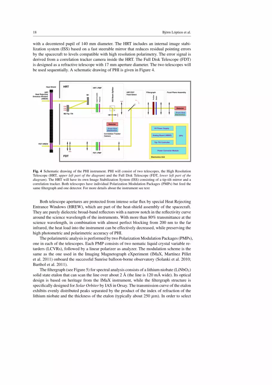
with a decentered pupil of 140 mm diameter. The HRT includes an internal image stabi-lization system (ISS) based on a fast steerable mirror that reduces residual pointing errorsby the spacecraft to levels compatible with high resolution polarimetry. The error signal isderived from a correlation tracker camera inside the HRT. The Full Disk Telescope (FDT)is designed as a refractive telescope with 17 mm aperture diameter. The two telescopes willbe used sequentially. A schematic drawing of PHI is given in Figure 4.

��

��

��

��

��

��

FDT

HRT

Correlation Tracker

Pre

filt

er

Eta

lon

Detector

Detector

Front−EndElectronics

Front−End

FiltergraphHRT/FDT

Electronics Unit

Power Converter Module

DPUAnalog Board (AMHD)

Tip−Tilt Controller

HV Power Supply

Focal Plane Assembly

ISS

Be

am

Sp

litt

er

Camera

Feed SelectM1

M2/Tip−Tilt

FDT−PMP

HRT−PMP

Liq

uid

Cry

sta

ls

Po

lari

ze

r

Heat Shield

HRTHeat Rejecting

(HREW)

Entrance Window

FDT HREW

Electronics

Fig. 4 Schematic drawing of the PHI instrument. PHI will consist of two telescopes, the High ResolutionTelescope (HRT, upper left part of the diagram) and the Full Disk Telescope (FDT, lower left part of thediagram). The HRT will have its own Image Stabilization System (ISS) consisting of a tip-tilt mirror and acorrelation tracker. Both telescopes have individual Polarization Modulation Packages (PMPs) but feed thesame filtergraph and one detector. For more details about the instrument see text

Both telescope apertures are protected from intense solar flux by special Heat RejectingEntrance Windows (HREW), which are part of the heat-shield assembly of the spacecraft.They are purely dielectric broad-band reflectors with a narrow notch in the reflectivity curvearound the science wavelength of the instruments. With more than 80% transmittance at thescience wavelength, in combination with almost perfect blocking from 200 nm to the farinfrared, the heat load into the instrument can be effectively decreased, while preserving thehigh photometric and polarimetric accuracy of PHI.

The polarimetric analysis is performed by two Polarization Modulation Packages (PMPs),one in each of the telescopes. Each PMP consists of two nematic liquid crystal variable re-tarders (LCVRs), followed by a linear polarizer as analyzer. The modulation scheme is thesame as the one used in the Imaging Magnetograph eXperiment (IMaX, Martınez Pilletet al. 2011) onboard the successful Sunrise balloon-borne observatory (Solanki et al. 2010;Barthol et al. 2011).

The filtergraph (see Figure 5) for spectral analysis consists of a lithium niobate (LiNbO3)solid state etalon that can scan the line over about 2 A (the line is 120 mA wide). Its opticaldesign is based on heritage from the IMaX instrument, while the filtergraph structure isspecifically designed for Solar Orbiter by IAS in Orsay. The transmission curve of the etalonexhibits evenly distributed peaks separated by the product of the index of refraction of thelithium niobate and the thickness of the etalon (typically about 250 µm). In order to select


6172 6172.5 6173 6173.5 6174 6174.50

0.2

0.4

0.6

0.8

1

Wavelength [Angstroem]

Nor

mal

ized

Inte

nsity

Fig. 5 Left: Cut of the filtergraph. The filtergraph consists of a freely tunable etalon in a telecentric mount-ing and two prefilters on either side of the etalon, a narrow-band prefilter and a wide-band prefilter. Right:Schematic representation of the filter curves of PHI. The Fe I 6173 A line (solid black line) will be scannedby using three filters, the wide-band prefilter (not shown here), the order-selecting narrow-band prefilter (bluecurve) and a freely tunable etalon (example profile shown by the red curve). The current baseline is to scanthe line at six wavelength positions (vertical dotted lines). Due to the large orbital motion of the spacecraft(up to 25 km/s), the line will be subject to a large Dopplershift (up to ±0.5 A, denoted by the dotted blacklines). The etalon has a sufficiently large tuning range to account for this (given by the solid green lines)

the correct transmission peak, the etalon is used in tandem with a set of two prefilters:the wide-band prefilter and the narrow-band prefilter having a Full Width at Half Maximum(FWHM) of 100 A and 2.7 A respectively (see right part of Figure 5). Before the light entersthe etalon, the narrow-band prefilter selects the working-order of the etalon. This filter alsotransmits green light that is used for ground-based calibrations. The green light is removedby the narrow-band prefilter, located behind the etalon. The tuning over the line is performedby using the piezoelectric effect of the lithium niobate, affecting both the thickness and theindex of refraction. A change of ∼ 6 kV allows tuning the etalon over 2 A. The width ofthe narrow-band prefilter and the tuning range of the etalon are sufficient to account forDopplershifts of the line caused by the orbit (up to ±0.5 A).

The etalon is used in a telecentric beam, i.e. all the points in the solar image see a cone oflight with the same opening impinging on the etalon at normal incidence angle. The stabilityof the filtergraph is driven by two main design constraints: the thermal stability for periodsshorter than 30 min, and by the wavelength repeatability induced by the high voltage powersupply. The thermal design of the filtergraph ensures that the inertia is about 7 hours, therebymaking the instrument extremely stable to variations from the environment. A stability betterthan 0.01◦ C peak-to-peak for periods shorter than 30 min was measured during thermal testsof the breadboard corresponding to 20 m/s; this should allow the measurement of modeswith degree higher than four. The high voltage repeatability was also measured in the lab tovalue of 3 m/s, this is 50 times lower than specified.

The focal plane assembly is built around a 2048×2048 pixel Active Pixel Sensor (APS),which is especially designed and manufactured for the instrument. It will deliver 10 framesper second which are read out in synchronism with the switching of the polarization modu-lators. In order to increase the signal-to-noise ratio, PHI will accumulate several images forevery wavelength position and polarization state.


6 Simulation Tool: SOPHISM

SOPHISM is a software simulator aimed at a full representation of the PHI instrument(both hardware and software) and is applicable to both telescopes of the instrument. Startingfrom 2D maps of line profiles for the Fe I 6173 A line computed from MHD simulations,SOPHISM generates synthetic 2D maps of the observables that will be measured by PHI.This allows estimates of the performance of PHI, which helps optimize the instrument de-sign and the onboard processing. The hardware part of the simulations takes into account allthe elements affecting solar light from when it enters the telescope (including some pertur-bations due to the spacecraft) up to the registering of this light on the detector. The softwarepart deals with the data pipeline and processing that takes place onboard.

The simulator is programmed in the Interactive Data Language2 (IDL) in a modularstructure, each module deals with one aspect of the instrument. The modules are mostlyindependent from each other and can individually be enabled or disabled. The simulationruns can be saved at each step and made available for subsequent calculations. Also, thecode is very flexible, with various parameters that can be modified. Presently, the modulesand effects covered are the following:

– Input: this module prepares the input data to be used in the simulation run. If needed,temporal interpolation is performed, as well as spatial operations such as replicationof the FOV (for simulation data with periodic boundary conditions) or, considering theSun-spacecraft distance, scaling from the original spatial resolution to that of the detec-tor.

– Jitter: this module represents the vibrations induced by the spacecraft, including alsothe correction by the ISS. A random shift of the FOV is generated and then filteredin frequency according to different possibilities, including a jitter model similar to theHinode spacecraft (Katsukawa et al. 2010). Next, the resulting jitter is diminished bymeans of the ISS attenuation function.

– Polarization: the polarization modulation of the incoming light is parametrized in thismodule. This comprises the Mueller matrix of the system and the liquid crystal variableretarders (LCVRs) settings, such as orientation and retardances, to produce the desiredmodulation of the data.

– Spectral Profile: the spectral transmission profile of the instrument is calculated here atthe user-defined wavelength positions. The resulting transmission curve, a combinationof the prefilter and etalon transmissions, is convolved with the data. An example of asimulated spectral transmission profile can be seen in Figure 5.

– Optical Aberrations: the MTF of the system with its different aberrations (e.g. defocus,astigmatism, coma,...) is characterized and convolved with the data.

– Pupil apodization: since the etalon is placed in a telecentric mounting, close to focus,the light is converging over it and enters as a cone. This produces the so-called pupilapodization (Beckers 1998; von der Luhe and Kentischer 2000), which results in a radialgradient of intensity and phase over the pupil. This effect has consequences for thespatial resolution and spectral transmission which are taken into account in this module.

– Focal Plane: all the detector effects are included in this module (e.g. dark current, read-out noise, flat-field, shutter, etc.).

– Accumulation: a given number of exposures are added directly on the instrument inorder to achieve a better signal-to-noise ratio.

2 IDL is a product of EXELIS Visual Information Solutions, http://www.exelisvis.com/

http://www.exelisvis.com/


– Demodulation: the Stokes vector is recovered here using the demodulation matrices cal-culated at the polarization module.

– Inversion: the MILOS inversion code (Orozco Suarez and Del Toro Iniesta 2007), basedon a Milne-Eddington approximation, is used to retrieve the full vector magnetic fieldand LOS velocities maps from the demodulated Stokes vector obtained by the instru-ment.

Figure 6 shows an example of a simulation run. Although in the following part of this paperwe only use Stokes I, we present here results for the magnetic Stokes parameters as well.The left panels correspond to the input data (MURaM MHD simulations with an averagemagnetic field of 50 G, Vogler et al. 2005), the right panels to the output of SOPHISM. Theimages presented here are intensity at line center and in the continuum, and

√Q2 +U2/I

and V/I at−80 mA in the line wing, corresponding to the degree of linear and circular polar-ization, respectively. The simulations represent an observation at disk center from perihelion(0.28 AU) and have a size of 12×12 Mm (the original simulations have a size of 6×6 Mm,but are replicated in the horizontal spatial dimensions in order to increase the FOV, takingadvantage of its periodic boundary conditions). The simulations presented in this sectionhave the following main characteristics: jitter with an RMS normalized to 0.5′′ and attenu-ated by the ISS; polarization modulation with identity Mueller matrix and ideal modulation;a prefilter with a FWHM of 3 A and the etalon at the six positions given in Sect. 5 with aresulting transmission FWHM of ∼ 90 mA along with pupil apodization considerations; anaberrated wavefront normalized to λ /10; dark current and photon and readout noises; and12 accumulations.

In the intensity images presented in Figure 6, the most evident effect of the simulatedinstrument is a loss of spatial and spectral resolution. Because of the lower signal of themagnetic Stokes parameters Q, U , and Vlos, other effects become apparent in the linear andcircular polarization images, mainly crosstalk from Stokes I due to spacecraft jitter andnoise components. The random parts of the simulation, like the jitter generation, noises,etc., are produced in every run. So, a different simulation run, even with the same settings,will yield different results. This is especially noticeable with the jitter crosstalk in the Q,U , Vlos parameters, which may show different contributions in the same parameter at thesame spectral position because of larger or smaller jitter shifts coinciding in the same dataproduct.

The output of SOPHISM depends significantly on the initial settings mentioned above.Although the configuration used for the results shown in Figure 6 corresponds to the presentassumptions for the behavior of PHI, these simulations will not be identical with the actualinstrument. The default settings and characteristics of most elements are taken from otherinstruments or calculated from a theoretical point of view. For example, the frequency filterfor the spacecraft jitter is taken from Hinode and the prefilter curve is computed theoret-ically. As the design of PHI proceeds, more precise settings can be used in the simulator,including parameters derived from measurements in the lab. The development of the codewill continue during the following years to represent further realistic characteristics of theinstrument, such as temperature dependencies, aging (radiation effects, inefficiencies,...),FOV dependent Mueller matrices, etc.

7 Simulating PHI Time-Series for Helioseismology

We are now at the stage where a detailed strategy has to be developed to maximize the helio-seismology output of the mission given the various limitations imposed by the mission (e.g.,


Fig. 6 Example of the influence of SOPHISM on intensity and polarization. The left column of panelsshows the original data from an MHD simulation, the right column of panels show the results after runningSOPHISM. From top to bottom: Stokes I at−400 mA from line center, Stokes I at line center,

√Q2 +U2/I at

−80 mA and V/I at−80 mA from line center. The last two correspond to the degree of linear and circular po-larization. Note the change of the colorbars from the original data to the simulation results. The configurationof SOPHISM that was used here and further details about the images are described in the text


challenging orbit, and an expected telemetry allocation of 51 Gbit per orbit). In this sectionwe present synthetic data with the same properties as expected from the High ResolutionTelescope of the PHI instrument on Solar Orbiter and begin characterizing the propertiesof the data for helioseismic studies (e.g. the expected power spectra). Starting from realis-tic radiative MHD simulations computed with the Stagger code (Stein and Nordlund 2000),computing line profiles with the SPINOR code (Frutiger et al. 2000), and simulating thePHI instrument using SOPHISM (see Sect. 6), we have generated a time-series of syntheticDopplergrams. These Dopplergrams are models for what should be available onboard theSolar Orbiter satellite.

7.1 Steps in the Generation of Synthetic Data

7.1.1 Simulations of Solar Convection

We start from simulations of solar surface convection for the quiet Sun computed with theStagger code. These simulations exhibit solar oscillations and have previously been usedin helioseismic studies, mostly for analyzing the excitation mechanism of solar oscilla-tions (e.g. Stein and Nordlund 2001; Nordlund and Stein 2001; Samadi et al. 2003; Steinet al. 2004) but also for testing methods used in helioseismology (e.g. Zhao et al. 2007;Georgobiani et al. 2007; Braun et al. 2007; Couvidat and Birch 2009) or for modeling he-lioseismic observations (e.g. Baldner and Schou 2012).

We use a simulation run with a size of 96× 96× 20 Mm, corresponding to 2016×2016×500 grid points. The horizontal resolution is constant (about 48 km) and the verticalresolution varies with height between 12 and 79 km. We analyze 359 minutes of the simu-lation, for which we have snapshots of the entire state of the system with a cadence of oneminute corresponding to the planned cadence of PHI. We assume in this work that variationson shorter timescales have a negligible effect. We plan to test this assumption using a shortrun of the simulations with a high cadence.

In order to reduce computation time we analyze a 48× 48 Mm sub-domain from thesimulations. This is a small patch of the field of view of the HRT of PHI (16.8′, correspond-ing to ∼ 200 Mm at perihelion) but it is sufficient for studying the solar oscillations in thesynthetic data.

7.1.2 Computation of Line Profiles

We synthesize line profiles for the Fe I 6173 A line for every single pixel of the sim-ulations using the SPINOR code with atomic parameters taken from the Kurucz atomicdatabase (logg f =−2.880, Fuhr et al. 1988) and the iron abundance (AFe = 7.43) from Bel-lot Rubio and Borrero (2002). Note that SPINOR allows simulations of observations at he-liocentric angles ρ > 0 by a synthesis of spectra obtained from inclined ray paths.

7.1.3 Using SOPHISM

Since we want to analyze a relatively long time-series, we configure SOPHISM in a waythat minimizes the computation time while still covering all relevant effects for helioseis-mology. One of the computationally most demanding parts of SOPHISM is the polarimetry.Polarimetry is not of great importance for helioseismology, so we do not include it in thefollowing. We further reduce the computation time by decreasing the number of simulated


exposures. When scanning the Fe I 6173 A line, PHI will make several exposures for eachof the wavelength positions over a total time of 60 s. We assume observations at six wave-length positions, located at −400, −160, −80, 0, 80, and 160 mA relative to the line center.During this time, the Sun evolves, causing small differences between the individual expo-sures. This means that the order in which the wavelengths are observed affects the resultingimage. The Stagger simulation data we use are sampled at a cadence of 60 s, so we cancompute only one exposure. The number of exposures and the order in which they are takenare also important for the impact of spacecraft jitter and photon noise. So, in order to getrealistic results when computing only one exposure, in this section we treat the jitter andphoton noise in a slightly different way than the standard SOPHISM.

7.1.4 Spacecraft Jitter

The exact behavior of the spacecraft jitter of Solar Orbiter is not known yet. When modelingthe jitter, we follow the spacecraft requirement that the RMS of the jitter with frequenciesabove 0.1 Hz must not be higher than 0.5′′ (or 0.1′′ when the ISS is turned on). We use amodel for the jitter that depends on frequency with a power spectral density similar to thatof the Hinode spacecraft. For frequencies higher than 0.1 Hz, we model the power spectraldensity with a power law fit of the Hinode jitter curve (see left part of Figure 7) normalizedto an RMS of 0.5′′. We are not aware of specifications for the jitter at lower frequencies.Here we assume a constant power spectral density of the jitter, corresponding to the powerat ν = 0.1 Hz. This low frequency part increases the RMS from 0.5′′ to 0.7′′. We also modela jitter curve when the ISS is activated by dividing the power spectral density of the jitter bya modeled attenuation curve of the ISS (black curve in Figure 7). The attenuation is strongestat low frequencies and reduces the RMS from 0.7′′ to 0.03′′, which is much less than thepixel size (0.5′′). We express the jitter in the Fourier domain by using a fixed amplitude foreach frequency (derived from the power spectral density) and a random phase. We generatea time-series of the jitter by taking the inverse Fourier transformation.

The influence of the jitter depends on the order in which the filtergrams are measured.We assume the jitter to act on all wavelengths in the same manner by using the same time-series for all wavelengths. Since we compute only one exposure, we do not model the jitterby shifting individual images. Instead, we convolve the image with a distribution corre-sponding to the accumulated shifts introduced by the jitter within the PHI cadence. Theright part of Figure 7 shows an example for this distribution. Since the jitter is derived fromHinode, it does not correspond to the jitter of the final Solar Orbiter spacecraft. However,as will be shown in Sect. 7.3, the influence of the jitter on the power spectrum is very small.Hence, we do not expect that our conclusions are affected by selecting a specific model forthe jitter.

7.1.5 Point Spread Function

An important characteristic of PHI is the Modulation Transfer Function (MTF). Since theMTF is mostly determined by the optical properties of the HREW when it is exposed to theenvironmental conditions in the orbit, the final MTF is still subject to tests and simulations.For this work, we use two different Modulation Transfer Functions corresponding to the bestand the worst possible outcome. The first MTF represents a diffraction-limited instrument,we assume the Point Spread Function (PSF) to be an Airy function corresponding to theaperture of the High Resolution Telescope (14 cm). The second one is an MTF that wascomputed from a model of the PHI instrument, where the entrance window was located at


10−2

100

102

10−20

10−10

100

Frequency [Hz]

Pow

er [a

rcse

c2 /s2 H

z−1 ]

100

100

1010

1020

ISS

atte

nuat

ion

fact

or

ISS onISS offISS att. curve

−3 −2 −1 0 1 2 30

0.02

0.04

0.06

0.08

Shift [arcsec]

Pro

babi

lity

Fig. 7 Left: Power spectral density of the shift introduced by the modeled spacecraft jitter. We assume thejitter to be similar to that of the Hinode spacecraft and to follow the spacecraft requirement (see text fordetails). When the ISS is turned off (dashed curve), we use a power law to model the power spectral densityof the Hinode jitter at frequencies above 0.1 Hz (P(ν) ∝ ν−1.98) and a constant power spectral density forfrequencies smaller than 0.1 Hz. We model the influence of the ISS by dividing the power spectral density ofthe jitter (dashed curve) by a model for the attenuation curve of the ISS (dash-dotted curve). When the ISS isturned on, the jitter is reduced significantly (solid curve). The ISS works most efficiently at low frequencies.Right: Example of a histogram of the shifts introduced by the jitter (ISS turned off). We used a time-serieswith a duration of 60 s, which corresponds to the cadence of PHI. The distribution has an RMS of 0.7′′

kx R

sun

k y Rsu

n

−40000 0 40000

−40000

0

40000

0

0.2

0.4

0.6

0.8

1

0 5000 10000 15000 20000 250000

0.2

0.4

0.6

0.8

1

kRsun

Nor

mal

ized

MT

F

MTF PHIIdeal MTF

Fig. 8 Modulation Transfer Functions used in this study as a function of wavenumber when observing atperihelion (0.28 AU). Left: MTF computed from a modeled instrument, where the entrance window is notdesigned in the best possible way, Right: Azimuthal average of this MTF (solid curve) and an MTF corre-sponding to a diffraction-limited instrument (dashed curve)

a suboptimal position within the heat shield of the spacecraft3 (see Figure 8). Compared tothe MTF for the diffraction-limited instrument, the MTF computed from the model of PHIstrongly decreases with the wavenumber and is also very asymmetric.

3 Recently, preliminary results from a study for the optimum HREW location have shown that a nearlydiffraction-limited telescope under all orbit conditions is feasible.


7.1.6 Photon Noise

The last step is modeling the detector. Here we resample the data to the detector plate scale(0.5′′ per pixel, corresponding to ∼ 100 km at perihelion) and add photon noise to the data.

PHI will accumulate several exposures to generate one final image in order to increasethe signal-to-noise ratio. The requirement for PHI for polarimetry is an accuracy of ±10 Gper pixel for determining the LOS magnetic field, ±200 G for the transverse component ofthe magnetic field and ±15 m/s for the LOS velocity. This demands an instrument require-ment for the signal-to-noise ratio of the mean continuum of at least 1000. Here we assumethe noise to follow the requirement.

Since we simulate only one image, representing the accumulation of many individualexposures, we can add the noise directly to the intensity images using a normal distributionwith dispersion

σ(λ ,x,y) = 10−3√

I(λ ,x,y)〈Ic〉. (1)

Here, I(λ ,x,y) is the intensity at a given wavelength and a given pixel and 〈Ic〉 is the spatiallyaveraged continuum intensity at disk center. This results in the desired signal-to-noise ratio:

Iσ

= 103

√I(λ ,x,y)〈Ic〉

. (2)

Since PHI will perform an onboard correction of the raw images for darks and flat-fields,we do not model their influence here. We also neglect quantization noise. The raw imagesprovided by the detector will have a size of 14 bits per pixel, so the influence of quantizationnoise is far below the photon noise level. Another source of noise is caused by variations ofthe exposure time. The requirement for this noise is 7 m/s, demanding a target accuracy ofthe exposure time of 450 ppm (Appourchaux 2011).

7.2 Synthetic Intensity and Velocity Maps

Applying the individual steps described in Sect. 7.1 results in a time-series of intensityimages at different wavelengths as will be available for onboard processing on Solar Orbiter.Here we determined the LOS velocities by computing the barycenter of the intensity at thesix wavelength positions that we have selected.

We generated two such time-series with a length of 359 min each, one correspondingto an observation of the disk center and another one for an observation closer to the limb(heliocentric angle ρ = 60◦). This corresponds to an observation of the solar poles from asolar latitude of 30◦, as it will be done by Solar Orbiter. In both cases we have assumed thespacecraft to observe from perihelion (0.28 AU). Since the length of the time-series is rathershort, we have neglected spacecraft motion. Examples for intensity and velocity maps areshown in Figure 9 for disk center and in Figure 10 for ρ = 60◦.

At disk center, granulation is clearly visible in the intensity images and Dopplergrams.When observing at ρ = 60◦, the granulation can still be resolved in the intensity images butthe contrast between granules and intergranular lanes is reduced. The Dopplergrams at thelimb are dominated by horizontal outflows from the granules to the intergranular lanes. Afterrunning SOPHISM, the contrast of both the intensity and the velocity is reduced significantly(see Table 4) due to the MTF. There are strong differences between the two MTFs that weuse here, the worst-case MTF reduces the RMS both for intensity and velocity by about afactor of two.

Helioseismology with Solar Orbiter 27y

[Mm

]

0

10

20

30

40

Inte

nsity

Con

tras

t

0.6

0.7

0.8

0.9

1

1.1

1.2

1.3

1.4

x [Mm]

y [M

m]

0 10 20 30 400

10

20

30

40

x [Mm]

0 10 20 30 40

v LOS [k

m/s

]

−4

−2

0

2

4

Fig. 9 Influence of the modeled High Resolution Telescope of PHI on intensity (top) and line-of-sight veloc-ity (bottom) when observing disk center from perihelion (0.28 AU). We compare data from the line profiles(left) with our results for the modeled PHI instrument (right). The dominant signal in these images is gran-ulation. The Dopplergrams clearly show the upflows in the granules and the downflows in the intergranularlanes. In the modeled PHI data, the spatial resolution is reduced due to the MTF. The edges of the SOPHISMdata are smooth, because SOPHISM apodizes the image before applying the MTF in order to avoid artifactsin the Fourier spectrum. Here we use an MTF corresponding to a diffraction-limited instrument. The imageis only a fraction of the full FOV for the HRT

RMS of intensity contrast RMS of LOS velocity [km/s]Disk center ρ = 60◦ Disk center ρ = 60◦

SPINOR 0.17 0.14 1.20 1.54SOPHISM (diff.-limited MTF) 0.12 0.10 0.72 1.08SOPHISM (worst-case MTF) 0.06 0.05 0.37 0.62

Table 4 RMS for continuum intensity contrast and LOS velocity both for disk center and ρ = 60◦. Wecompare data from SPINOR with our results from SOPHISM. Both the MTF corresponding to a diffraction-limited instrument and a worst-case MTF are considered

28 Bjorn Loptien et al.y

[Mm

]

0

20

40

Inte

nsity

Con

tras

t

1

1.5

2

x [Mm]

y [M

m]

0 10 20 30 400

20

40

x [Mm]

0 10 20 30 40

v LOS [k

m/s

]

−5

0

5

Fig. 10 Same as Figure 9 for an observation at ρ = 60◦. Again, we assume an observation from perihelion(0.28 AU). Due to foreshortening the images are squeezed in y-direction. The top of the box is directedtowards the limb. While the intensity images show granulation, as for the disk center data, the Dopplergramsare now dominated by flows in the horizontal direction, which originate from outflows from the granules

7.3 Oscillation Power Spectra

We have a time-series of Dopplergrams and thus we can evaluate the effect of the PHI instru-ment on the measurement of solar oscillations. The most basic of helioseismic diagnosticsis the power spectrum as a function of horizontal wavenumber, k, and frequency, ν . In Fig-ure 11 we compare two power spectra for an observation at disk center: one generated fromsynthetic PHI data (i.e. after running SOPHISM) and another one without any influence ofthe instrument (i.e. for velocity maps derived from the SPINOR line profiles). We see thatthe power resulting from the synthetic PHI data is lower than the power originating fromthe line profiles at high-k modes. This is caused by the MTF, which we assume here tocorrespond to a diffraction-limited instrument.

The impact of the MTF on the power spectrum strongly differs between the two MTFsused in this study (see Sect. 7.1.5). Figure 12 shows the azimuthal averages of power spectrafor different setups of the instrument. The worst-case MTF reduces the power significantlymore at high wavenumbers than the diffraction-limited one. The MTF has a much largerinfluence on the power spectrum than other instrumental effects, like spacecraft jitter orphoton noise. We also show in Figure 12 power spectra, where the ISS is turned off andthe photon noise is increased (S/N = 50). Photon noise and jitter only influence the powerspectra if they are much worse than the PHI requirements. The photon noise leads to aconstant offset in the power spectrum which is negligible compared to the power of theoscillation modes for any noise level that we expect. The spacecraft jitter reduces the powerof the high-k modes, if the ISS is turned off. All these effects barely affect the oscillations.

When observing at ρ = 60◦, the power of the p-modes is lower than at disk center, sincethe displacement caused by the oscillations is mostly radial. On the other hand, the powerresulting from convection is increased. Foreshortening leads to a stronger influence of the


kRsun

ν [m

Hz]

1000 2000 3000 40000

1

2

3

4

5

6

7

8

kRsun

1000 2000 3000 4000

log

(Pow

er/(

km2 /s

2 Hz−

1 rad

−2 M

m2 ))

−2

−1.5

−1

−0.5

0

0.5

1

1.5

2

2.5

Fig. 11 Azimuthal average of two power spectra at disk center. Left: Power for velocities determined directlyfrom the line profiles, right: Power for velocities computed from simulated instrumental data after runningSOPHISM. Both images reveal the solar oscillations and granulation. However, the simulated instrumentdecreases the power, especially for high wavenumbers. This is caused mostly by the Modulation TransferFunction. Here we use an MTF corresponding to a diffraction-limited instrument (the PSF is an Airy function)

MTF and spacecraft jitter. Also, the intensity is lower due to limb darkening, which leads toan increased photon noise level.

In short, the most important instrumental effect is the MTF, which attenuates p-modepower at high spatial frequencies. The two MTFs used in this study lead to strong differencesin the power spectrum. By comparison, the uncertainties in the jitter or photon noise levelhave less of an effect. However, we find that oscillations are still easy to observe even withthe worst-case MTF.

8 Lessons Learned from MDI and HMI

While the MDI and HMI instruments and associated spacecraft (SOHO and SDO) are insome way quite different from PHI and Solar Orbiter, the experience from those investiga-tions may nonetheless provide some guidance for PHI.

MDI is in many ways similar to PHI. Telemetry is severely restricted, observables com-putations are done onboard and the onboard software is complex. A major difference is thatSolar Orbiter has significantly more onboard storage, which may permit post-event dataselection.


0 1000 2000 3000 400010

−1

100

101

102

kRsun

Pow

er [k

m2 /s

2 Hz−

1 rad

−2 M

m2 ]

SPINOR velocityNom. PHI perf.No ISSS/N = 50Worst−case MTFNom. perf. (ρ = 60°)

f−modep

1−mode

0 2 4 6 8

100

101

102

103

ν [mHz]

Pow

er [k

m2 /s

2 Hz−

1 rad

−2 M

m2 ]

Nominal performance (ρ = 0°)

S/N = 50 (ρ = 0°)

Nominal performance (ρ = 60°)

S/N = 50 (ρ = 60°)

Fig. 12 Left: Azimuthal average of the power as a function of wavenumber at ν = 3.41 mHz. Six configu-rations are shown, black squares: Power derived from SPINOR velocities, blue thick solid curve: NominalPHI performance, red dots: ISS turned off, black dashed curve: Enhanced photon noise (S/N = 50), bluethick dashed curve: Worst-case MTF, red solid curve: Nominal PHI performance at ρ = 60◦. Right: Poweras a function of frequency at kR� = 456. Red thick solid line: Nominal PHI performance when observing atdisk center, blue solid line: Nominal PHI performance at ρ = 60◦, black thick dashed line: Enhanced photonnoise (S/N = 50) at disk center, red dashed line: Enhanced photon noise (S/N = 50) at ρ = 60◦. We do notshow the jitter with the ISS off, since it does not depend on frequency. The photon noise enhances the back-ground power. For the nominal PHI performance, the influence of jitter and photon noise is negligible. If theISS is turned off, the high-k power is reduced, a higher photon noise level increases the background power.However, a signal-to-noise ratio (S/N) of 50 is much lower than anything we expect

HMI is significantly different in these respects. The telemetry rate is not a limiting factor,(nearly) raw CCD images are downlinked and the onboard software is quite simple. Havingsaid that, PHI is closer to HMI than to MDI in some respects, including thermal perturbations(due to eclipses), rapid LOS velocity changes (due to the orbit), and the ability to make fullpolarimetric measurements.

One major lesson learned from MDI is that fragmentation of data has to be controlled.Excessive changes between observing modes make it difficult to find good sequences forother uses than those initially envisioned and make it difficult to search through the data. Forhelioseismology, it is often particularly important that long sequences are available. In theextreme case of global mode analysis, typical lengths are several months and it is essentialthat the duty cycle is not too low. Duty cycles from existing helioseismic instruments rangesfrom 80-90% for GONG and up to well over 99% for MDI Medium-l for some 72 dayperiods. As such we expect that a duty cycle greater than 80% may be acceptable. However,the amount of degradation will depend on the structure of the gaps. Variable duty cyclescan lead to variations in the observed quantities which can in turn be confused with solarvariations. But even in the case of local helioseismology, time-series of a significant length


are needed and for the study of such things as active region evolution it is essential to observecontinuously for several days.

Similarly, uncomplicated regular observations from MDI have provided most of the dataused for publications. This includes the regular 96 minute cadence magnetograms, the so-called structure program (in particular the Medium-l program, Kosovichev et al. 1996,1997) and the yearly dynamics programs. The Medium-l program, for example, has proba-bly provided the frequencies and splittings used for most publications in global mode seis-mology. Open and easy access to data have also been essential to ensure the maximum useof the data.

Well calibrated data are also highly desirable. MDI was not particularly well calibratedfrom the outset, which combined with the onboard observable calculation led to some issues,especially regarding the magnetograms (Liu et al. 2004, 2007, 2012). Another problem forMDI has been that the noise in the shutter (Liu et al. 2004) also leads to an error in thevelocity zero point, which in turn introduces a lot of noise in the low degree modes. HMI, bycomparison, was substantially better calibrated from the start (Couvidat et al. 2012; Wachteret al. 2012; Schou et al. 2012b).

The issue of calibrations is particularly difficult for PHI, due to the need to do onboardobservables calculations and the massive thermal perturbations. For HMI all the raw dataare available on the ground, which means that computations can be done and, if neces-sary, redone. For PHI this will not be the case and it is thus essential that enough data aredownlinked early in the mission to ensure that good calibrations can be derived and ade-quate onboard algorithms can be developed and tested before regular observations start. Itwill also be necessary to find some way to ensure that any drifts in the calibrations will bedetected and corrected.

Having said that, some of these programs were not designed as well as they could havebeen, especially in hindsight. In particular, some of the data products could probably havebeen compressed more (e.g. by truncating more of the bottom bits) and a better trade-offbetween truncation noise, smoothing, subsampling density and crop radius could probablyhave been done for the Medium-l program. It might have been better to truncate more bitswhile keeping a larger FOV. Given the desire to have long and uniform time-series the trade-off was not adjusted during the mission.

A possibility with Solar Orbiter is to take data, store it on board and decide later ifit should be downlinked. This may be particularly interesting for emerging active regions,flares, and so forth. There is obviously a trade-off involved here, as this will increase opera-tional complexity and fragmentation of the data.

Acknowledgements This work is supported by the European Commission through FP7 project “Exploita-tion of Space Data for Innovative Helio- and Asteroseismology” (SpaceInn). We are very grateful to R. Steinfor making the Stagger simulation data available. We thank A. Lagg for his support with using the SPINORcode. B.L. is a member of the International Max Planck Research School for Solar System Science at theUniversity of Gottingen. B.L. designed and performed the research described in section 7 and wrote thissection. B.L. performed research for section 3 and contributed to the writing of sections 1,2,3 and 5.

References

T. Appourchaux, PHI filtergraph requirements and specifications. Technical report (2011)C.S. Baldner, J. Schou, Effects of Asymmetric Flows in Solar Convection on Oscillation Modes. Astrophys.

J. Letters 760, 1 (2012). doi:10.1088/2041-8205/760/1/L1P. Barthol, A. Gandorfer, S.K. Solanki, M. Schussler, B. Chares, W. Curdt, W. Deutsch, A. Feller, D. Ger-

merott, B. Grauf, K. Heerlein, J. Hirzberger, M. Kolleck, R. Meller, R. Muller, T.L. Riethmuller, G.


Tomasch, M. Knolker, B.W. Lites, G. Card, D. Elmore, J. Fox, A. Lecinski, P. Nelson, R. Summers,A. Watt, V. Martınez Pillet, J.A. Bonet, W. Schmidt, T. Berkefeld, A.M. Title, V. Domingo, J.L. GasentBlesa, J.C. Del Toro Iniesta, A. Lopez Jimenez, A. Alvarez-Herrero, L. Sabau-Graziati, C. Widani, P.Haberler, K. Hartel, D. Kampf, T. Levin, I. Perez Grande, A. Sanz-Andres, E. Schmidt, The SunriseMission. Solar Phys. 268, 1–34 (2011). doi:10.1007/s11207-010-9662-9

J.M. Beckers, On the effect of narrow-band filters on the diffraction limited resolution of astronomical tele-scopes. Astron. Astrophys. Suppl. 129, 191–194 (1998). doi:10.1051/aas:1998180

L.R. Bellot Rubio, J.M. Borrero, Iron abundance in the solar photosphere. Application of a two-componentmodel atmosphere. Astron. Astrophys. 391, 331–337 (2002). doi:10.1051/0004-6361:20020656

D.C. Braun, A.C. Birch, Prospects for the Detection of the Deep Solar Meridional Circulation. Astrophys. J.Letters 689, 161–165 (2008). doi:10.1086/595884

D.C. Braun, A.C. Birch, D. Benson, R.F. Stein, A. Nordlund, Helioseismic Holography of Simulated SolarConvection and Prospects for the Detection of Small-Scale Subsurface Flows. Astrophys. J. 669, 1395–1405 (2007). doi:10.1086/521782

W.J. Chaplin, Y. Elsworth, R. Howe, G.R. Isaak, C.P. McLeod, B.A. Miller, H.B. van der Raay, S.J. Wheeler,R. New, BiSON Performance. Solar Phys. 168, 1–18 (1996). doi:10.1007/BF00145821

S. Couvidat, A.C. Birch, Helioseismic Travel-Time Definitions and Sensitivity to Horizontal Flows Obtainedfrom Simulations of Solar Convection. Solar Phys. 257, 217–235 (2009). doi:10.1007/s11207-009-9371-4

S. Couvidat, J. Schou, R.A. Shine, R.I. Bush, J.W. Miles, P.H. Scherrer, R.L. Rairden, Wavelength Depen-dence of the Helioseismic and Magnetic Imager (HMI) Instrument onboard the Solar Dynamics Obser-vatory (SDO). Solar Phys. 275, 285–325 (2012). doi:10.1007/s11207-011-9723-8

M. Dikpati, P.A. Gilman, Theory of Solar Meridional Circulation at High Latitudes. Astrophys. J. 746, 65(2012). doi:10.1088/0004-637X/746/1/65

B. Fleck, S. Couvidat, T. Straus, On the Formation Height of the SDO/HMI Fe 6173 A Doppler Signal. SolarPhys. 271, 27–40 (2011). doi:10.1007/s11207-011-9783-9

L.N. Fletcher, P.G.J. Irwin, G.S. Orton, N.A. Teanby, R.K. Achterberg, G.L. Bjoraker, P.L. Read, A.A. Simon-Miller, C. Howett, R. de Kok, N. Bowles, S.B. Calcutt, B. Hesman, F.M. Flasar, Temperature and Com-position of Saturn’s Polar Hot Spots and Hexagon. Science 319, 79 (2008). doi:10.1126/science.1149514

C. Frohlich, J. Romero, H. Roth, C. Wehrli, B.N. Andersen, T. Appourchaux, V. Domingo, U. Telljohann, G.Berthomieu, P. Delache, J. Provost, T. Toutain, D.A. Crommelynck, A. Chevalier, A. Fichot, W. Dappen,D. Gough, T. Hoeksema, A. Jimenez, M.F. Gomez, J.M. Herreros, T.R. Cortes, A.R. Jones, J.M. Pap,R.C. Willson, VIRGO: Experiment for Helioseismology and Solar Irradiance Monitoring. Solar Phys.162, 101–128 (1995). doi:10.1007/BF00733428

C. Frutiger, S.K. Solanki, M. Fligge, J.H.M.J. Bruls, Properties of the solar granulation obtained from theinversion of low spatial resolution spectra. Astron. Astrophys. 358, 1109–1121 (2000)

J.R. Fuhr, G.A. Martin, W.L. Wiese, Atomic transition probabilities. Iron through Nickel. Journal of Physicaland Chemical Reference Data 17 (1988)

R.A. Garcıa, The Sun as a Star: 13 Years of Soho, in American Institute of Physics Conference Series, ed. byJ.A. Guzik, P.A. Bradley American Institute of Physics Conference Series, vol. 1170, 2009, pp. 560–565.doi:10.1063/1.3246562

D. Georgobiani, J. Zhao, A.G. Kosovichev, D. Benson, R.F. Stein, A. Nordlund, Local Helioseismologyand Correlation Tracking Analysis of Surface Structures in Realistic Simulations of Solar Convection.Astrophys. J. 657, 1157–1161 (2007). doi:10.1086/511148

P.A. Gilman, Model calculations concerning rotation at high solar latitudes and the depth of the solar convec-tion zone. Astrophys. J. 231, 284–292 (1979). doi:10.1086/157191

L. Gizon, A.C. Birch, H.C. Spruit, Local Helioseismology: Three-Dimensional Imaging of the Solar Interior.ARA&A 48, 289–338 (2010). doi:10.1146/annurev-astro-082708-101722

L. Gizon, T.L. Duvall, J. Schou, Wave-like properties of solar supergranulation. Nature 421, 43–44 (2003).doi:10.1038/nature01287

L. Gizon, A.C. Birch, R.I. Bush, T.L. Duvall Jr., A.G. Kosovichev, P.H. Scherrer, J. Zhao, Time-distance He-lioseismology and the Solar Orbiter Mission, in Solar encounter. Proceedings of the First Solar OrbiterWorkshop, ed. by B. Battrick, H. Sawaya-Lacoste, E. Marsch, V. Martinez Pillet, B. Fleck, R. Marsden.ESA Special Publication, vol. 493, 2001, pp. 227–231

L. Gizon, J. Ballot, E. Michel, T. Stahn, G. Vauclair, H. Bruntt, P.-O. Quirion, O. Benomar, S. Vauclair, T.Appourchaux, M. Auvergne, A. Baglin, C. Barban, F. Baudin, M. Bazot, T. Campante, C. Catala, W.Chaplin, O. Creevey, S. Deheuvels, N. Dolez, Y. Elsworth, R. Garcia, P. Gaulme, S. Mathis, S. Mathur,B. Mosser, C. Regulo, I. Roxburgh, D. Salabert, R. Samadi, K. Sato, G. Verner, S. Hanasoge, K.R.Sreenivasan, Seismic constraints on rotation of Sun-like star and mass of exoplanet. Proceedings of theNational Academy of Science 110, 13267–13271 (2013). doi:10.1073/pnas.1303291110


S.M. Hanasoge, T.L. Duvall, K.R. Sreenivasan, Anomalously weak solar convection. Proceedings of theNational Academy of Science 109, 11928–11932 (2012). doi:10.1073/pnas.1206570109

D.H. Hathaway, L. Upton, O. Colegrove, Giant Convection Cells Found on the Sun. Science 342, 1217–1219(2013). doi:10.1126/science.1244682

F. Hill, J. Bolding, C. Toner, T. Corbard, S. Wampler, B. Goodrich, J. Goodrich, P. Eliason, K.D. Hanna, TheGong++ Data Processing Pipeline, in GONG+ 2002. Local and Global Helioseismology: the Presentand Future, ed. by H. Sawaya-Lacoste ESA Special Publication, vol. 517, 2003, pp. 295–298

F. Hill, R. Howe, R. Komm, I. Gonzallez Hernandez, S. Tripathy, K. Jain, A Helioseismic Comparison ofthe Solar Minima Preceding Cycles 23 and 24, in AAS/Solar Physics Division Meeting #40. AAS/SolarPhysics Division Meeting, vol. 40, 2009, pp. 24–01

R. Howe, Solar Interior Rotation and its Variation. Living Reviews in Solar Physics 6, 1 (2009).doi:10.12942/lrsp-2009-1

R. Howe, J. Christensen-Dalsgaard, F. Hill, R.W. Komm, R.M. Larsen, J. Schou, M.J. Thompson, J.Toomre, Dynamic Variations at the Base of the Solar Convection Zone. Science 287, 2456–2460 (2000).doi:10.1126/science.287.5462.2456

R. Howe, J. Christensen-Dalsgaard, F. Hill, R. Komm, T.P. Larson, M. Rempel, J. Schou, M.J. Thompson,The High-latitude Branch of the Solar Torsional Oscillation in the Rising Phase of Cycle 24. Astrophys.J. Letters 767, 20 (2013). doi:10.1088/2041-8205/767/1/L20

D.A. Huffman, A Method for the Construction of Minimum-Redundancy Codes. Proceedings of the I.R.E.40, 1098–1102 (1952). doi:10.1109/JRPROC.1952.273898

J. Jiang, R. Cameron, D. Schmitt, M. Schussler, Countercell Meridional Flow and Latitudinal Distribu-tion of the Solar Polar Magnetic Field. Astrophys. J. Letters 693, 96–99 (2009). doi:10.1088/0004-637X/693/2/L96

Y. Katsukawa, Y. Masada, T. Shimizu, S. Sakai, K. Ichimoto, Pointing stability of Hinode and requirementsfor the next solar mission Solar-C. International Conference on Space Optics (2010)

R. Komm, I. Gonzalez Hernandez, F. Hill, R. Bogart, M.C. Rabello-Soares, D. Haber, Subsurface MeridionalFlow from HMI Using the Ring-Diagram Pipeline. Solar Phys. 287, 85–106 (2013). doi:10.1007/s11207-012-0073-y

A.G. Kosovichev, T.L. Duvall, P.H. Scherrer, Simulation of Vector-Weighted Binning for the Medium-l Pro-gram. SOI Technical Notes (1996)

A.G. Kosovichev, J. Schou, P.H. Scherrer, R.S. Bogart, R.I. Bush, J.T. Hoeksema, J. Aloise, L. Bacon, A.Burnette, C. de Forest, P.M. Giles, K. Leibrand, R. Nigam, M. Rubin, K. Scott, S.D. Williams, S. Basu,J. Christensen-Dalsgaard, W. Dappen, E.J. Rhodes Jr., T.L. Duvall Jr., R. Howe, M.J. Thompson, D.O.Gough, T. Sekii, J. Toomre, T.D. Tarbell, A.M. Title, D. Mathur, M. Morrison, J.L.R. Saba, C.J. Wolfson,I. Zayer, P.N. Milford, Structure and Rotation of the Solar Interior: Initial Results from the MDI Medium-L Program. Solar Phys. 170, 43–61 (1997). doi:10.1023/A:1004949311268

J.R. Kuhn, R. Bush, M. Emilio, I.F. Scholl, The Precise Solar Shape and Its Variability. Science 337, 1638(2012). doi:10.1126/science.1223231

C. Lindsey, D.C. Braun, Seismic Images of the Far Side of the Sun. Science 287, 1799–1801 (2000).doi:10.1126/science.287.5459.1799

Y. Liu, A.A. Norton, P.H. Scherrer, A Note on Saturation Seen in the MDI/SOHO Magnetograms. Solar Phys.241, 185–193 (2007). doi:10.1007/s11207-007-0296-5

Y. Liu, X. Zhao, J.T. Hoeksema, Correction of Offset in MDI/SOHO Magnetograms. Solar Phys. 219, 39–53(2004). doi:10.1023/B:SOLA.0000021822.07430.d6

Y. Liu, J.T. Hoeksema, P.H. Scherrer, J. Schou, S. Couvidat, R.I. Bush, T.L. Duvall, K. Hayashi, X.Sun, X. Zhao, Comparison of Line-of-Sight Magnetograms Taken by the Solar Dynamics Observa-tory/Helioseismic and Magnetic Imager and Solar and Heliospheric Observatory/Michelson DopplerImager. Solar Phys. 279, 295–316 (2012). doi:10.1007/s11207-012-9976-x

B. Loptien, A.C. Birch, L. Gizon, J. Schou, Image Compression in Local Helioseismology. Astron. Astro-phys.(submitted)

E. Marsch, E. Antonucci, P. Bochsler, J.-L. Bougeret, R. Harrison, R. Schwenn, J.-C. Vial, First Solar OrbiterAssessment Study Report. ESA-SCI(2000)6 (2000)

R.G. Marsden, D. Muller, Solar Orbiter Exploring the Sun-Heliosphere Connection, Solar Orbiter DefinitionStudy Report. ESA/SRE(2011)14 (2011)

V. Martınez Pillet, J.C. Del Toro Iniesta, A. Alvarez-Herrero, V. Domingo, J.A. Bonet, L. GonzalezFernandez, A. Lopez Jimenez, C. Pastor, J.L. Gasent Blesa, P. Mellado, J. Piqueras, B. Aparicio, M. Bal-aguer, E. Ballesteros, T. Belenguer, L.R. Bellot Rubio, T. Berkefeld, M. Collados, W. Deutsch, A. Feller,F. Girela, B. Grauf, R.L. Heredero, M. Herranz, J.M. Jeronimo, H. Laguna, R. Meller, M. Menendez,R. Morales, D. Orozco Suarez, G. Ramos, M. Reina, J.L. Ramos, P. Rodrıguez, A. Sanchez, N. Uribe-Patarroyo, P. Barthol, A. Gandorfer, M. Knoelker, W. Schmidt, S.K. Solanki, S. Vargas Domınguez, The


Imaging Magnetograph eXperiment (IMaX) for the Sunrise Balloon-Borne Solar Observatory. SolarPhys. 268, 57–102 (2011). doi:10.1007/s11207-010-9644-y

D. Muller, R.G. Marsden, O.C. St. Cyr, H.R. Gilbert, Solar Orbiter. Exploring the Sun-Heliosphere Connec-tion. Solar Phys. 285, 25–70 (2013). doi:10.1007/s11207-012-0085-7

K. Nagashima, J. Zhao, A.G. Kosovichev, T. Sekii, Detection of Supergranulation Alignment in Polar Regionsof the Sun by Helioseismology. Astrophys. J. Letters 726, 17 (2011). doi:10.1088/2041-8205/726/2/L17

A. Nordlund, R.F. Stein, Solar Oscillations and Convection. I. Formalism for Radial Oscillations. Astrophys.J. 546, 576–584 (2001). doi:10.1086/318217

A.A. Norton, R.K. Ulrich, Measuring Magnetic Oscillations in the Solar Photosphere: Coordinated Observa-tions with MDI, ASP and MWO. Solar Phys. 192, 403–413 (2000). doi:10.1023/A:1005290616918

D. Orozco Suarez, J.C. Del Toro Iniesta, The usefulness of analytic response functions. Astron. Astrophys.462, 1137–1145 (2007). doi:10.1051/0004-6361:20066201

T. Roudier, M. Rieutord, V. Prat, J.M. Malherbe, N. Renon, Z. Frank, M. Svanda, T. Berger, R. Burston, L. Gi-zon, Comparison of solar horizontal velocity fields from SDO/HMI and Hinode data. Astron. Astrophys.552, 113 (2013). doi:10.1051/0004-6361/201220867

A. Ruzmaikin, C. Lindsey, Helioseismic Probing of the Solar Dynamo, in GONG+ 2002. Local and GlobalHelioseismology: the Present and Future, ed. by H. Sawaya-Lacoste ESA Special Publication, vol. 517,2003, pp. 71–74

R. Samadi, A. Nordlund, R.F. Stein, M.J. Goupil, I. Roxburgh, Numerical constraints on the model of stochas-tic excitation of solar-type oscillations. Astron. Astrophys. 403, 303–312 (2003). doi:10.1051/0004-6361:20030356

K.H. Sato, R.A. Garcia, S. Pires, J. Ballot, S. Mathur, B. Mosser, E. Rodriguez, J.L. Starck, K. Uytterhoeven,Inpainting: A powerful interpolation technique for helio- and asteroseismic data. ArXiv e-prints (2010)

P.H. Scherrer, R.S. Bogart, R.I. Bush, J.T. Hoeksema, A.G. Kosovichev, J. Schou, W. Rosenberg, L. Springer,T.D. Tarbell, A. Title, C.J. Wolfson, I. Zayer, MDI Engineering Team, The Solar Oscillations Investiga-tion - Michelson Doppler Imager. Solar Phys. 162, 129–188 (1995). doi:10.1007/BF00733429

J. Schou, Wavelike Properties of Solar Supergranulation Detected in Doppler Shift Data. Astrophys. J. Letters596, 259–262 (2003). doi:10.1086/379529

J. Schou, P.H. Scherrer, R.I. Bush, R. Wachter, S. Couvidat, M.C. Rabello-Soares, R.S. Bogart, J.T. Hoek-sema, Y. Liu, T.L. Duvall, D.J. Akin, B.A. Allard, J.W. Miles, R. Rairden, R.A. Shine, T.D. Tarbell,A.M. Title, C.J. Wolfson, D.F. Elmore, A.A. Norton, S. Tomczyk, Design and Ground Calibration of theHelioseismic and Magnetic Imager (HMI) Instrument on the Solar Dynamics Observatory (SDO). SolarPhys. 275, 229–259 (2012a). doi:10.1007/s11207-011-9842-2

J. Schou, J.M. Borrero, A.A. Norton, S. Tomczyk, D. Elmore, G.L. Card, Polarization Calibration of theHelioseismic and Magnetic Imager (HMI) onboard the Solar Dynamics Observatory (SDO). Solar Phys.275, 327–355 (2012b). doi:10.1007/s11207-010-9639-8

H. Schunker, D.C. Braun, P.S. Cally, C. Lindsey, The Local Helioseismology of Inclined Magnetic Fieldsand the Showerglass Effect. Astrophys. J. Letters 621, 149–152 (2005). doi:10.1086/429290

S.K. Solanki, P. Barthol, S. Danilovic, A. Feller, A. Gandorfer, J. Hirzberger, T.L. Riethmuller, M. Schussler,J.A. Bonet, V. Martınez Pillet, J.C. del Toro Iniesta, V. Domingo, J. Palacios, M. Knolker, N. BelloGonzalez, T. Berkefeld, M. Franz, W. Schmidt, A.M. Title, SUNRISE: Instrument, Mission, Data, andFirst Results. Astrophys. J. Letters 723, 127–133 (2010). doi:10.1088/2041-8205/723/2/L127

R.F. Stein, A. Nordlund, Realistic Solar Convection Simulations. Solar Phys. 192, 91–108 (2000).doi:10.1023/A:1005260918443

R.F. Stein, A. Nordlund, Solar Oscillations and Convection. II. Excitation of Radial Oscillations. Astrophys.J. 546, 585–603 (2001). doi:10.1086/318218

R. Stein, D. Georgobiani, R. Trampedach, H.-G. Ludwig, A. Nordlund, Excitation of Radial P-Modes in theSun and Stars. Solar Phys. 220, 229–242 (2004). doi:10.1023/B:SOLA.0000031458.35121.33

A. Vogler, S. Shelyag, M. Schussler, F. Cattaneo, T. Emonet, T. Linde, Simulations of magneto-convectionin the solar photosphere. Equations, methods, and results of the MURaM code. Astron. Astrophys. 429,335–351 (2005). doi:10.1051/0004-6361:20041507

O. von der Luhe, T.J. Kentischer, High spatial resolution performance of a triple Fabry-Perot filtergraph.Astron. Astrophys. Suppl. 146, 499–506 (2000). doi:10.1051/aas:2000283

R. Wachter, J. Schou, M.C. Rabello-Soares, J.W. Miles, T.L. Duvall, R.I. Bush, Image Quality of the Helio-seismic and Magnetic Imager (HMI) Onboard the Solar Dynamics Observatory (SDO). Solar Phys. 275,261–284 (2012). doi:10.1007/s11207-011-9709-6

G.K. Wallace, The JPEG still picture compression standard. IEEE Transactions on Consumer Electronics 38,18–34 (1992). doi:10.1109/30.125072

J. Woch, L. Gizon, The Solar Orbiter mission and its prospects for helioseismology. AstronomischeNachrichten 328, 362 (2007). doi:10.1002/asna.200710743


J. Zhao, A.G. Kosovichev, Surface Magnetism Effects in Time-Distance Helioseismology. Astrophys. J. 643,1317–1324 (2006). doi:10.1086/503248

J. Zhao, D. Georgobiani, A.G. Kosovichev, D. Benson, R.F. Stein, A. Nordlund, Validation of Time-DistanceHelioseismology by Use of Realistic Simulations of Solar Convection. Astrophys. J. 659, 848–857(2007). doi:10.1086/512009

J. Zhao, K. Nagashima, R.S. Bogart, A.G. Kosovichev, T.L. Duvall Jr., Systematic Center-to-limb Variationin Measured Helioseismic Travel Times and its Effect on Inferences of Solar Interior Meridional Flows.Astrophys. J. Letters 749, 5 (2012). doi:10.1088/2041-8205/749/1/L5

J. Zhao, R.S. Bogart, A.G. Kosovichev, T.L. Duvall Jr., T. Hartlep, Detection of Equatorward MeridionalFlow and Evidence of Double-cell Meridional Circulation inside the Sun. Astrophys. J. Letters 774, 29(2013). doi:10.1088/2041-8205/774/2/L29

J. Ziv, A. Lempel, A Universal Algorithm for Sequential Data Compression. IEEE Transactions on Informa-tion Theory 23, 337–343 (1977). doi:10.1109/TIT.1977.1055714

J. Ziv, A. Lempel, Compression of Individual Sequences via Variable-Rate Coding. IEEE Transactions onInformation Theory 24, 530–536 (1978). doi:10.1109/TIT.1978.1055934

helioseismology with solar orbiter

Documents