the dynamics of currency crashes and fundamental

The Dynamics of Currency Crashes and Fundamental Reversions

Bjarni Kristinn Torfason

Submitted in partial fulfillment of the

requirements for the degree of

Doctor of Philosophy

under the Executive Committee

of the Graduate School of Arts and Sciences

COLUMBIA UNIVERSITY

2012

ABSTRACT

The Dynamics of Currency Crashes and Fundamental Reversions


This dissertation is composed of three chapters. In Chapter 1 I look at the role of real

exchange rates in the asset pricing of currencies. I construct portfolios based on signals about

the real exchange rate and analyze the returns of these portfolios as they relate to traditional

asset pricing factors and especially how they correlate with carry trade portfolios. Deviations

from long term averages of real exchange rates are found to be predictors of crash risk. I also

show that there is significant information in real exchange rate signals that does not seem to

be priced. In addition to demonstrating this in outright currency markets I provide evidence

suggesting that this is also the case in options markets. A relationship between real exchange

rates and the VIX volatility over long periods is also demonstrated.

The distribution of returns depends on state variables. For currencies an important

variable is the deviations of real exchange rates from their long run means and for stocks the

market-to-book ratio serves a similar purpose. Chapter 2 introduces a variant of a mixture of

normals that allows for dependence of this kind. The model is estimated using Markov chain

Monte Carlo. The results clearly indicate conditionality on the state variables and how high

prices of assets predict negative skewness (large losses) for as well as negative returns.

The Icelandic financial collapse, which occurred in the fall of 2008, is without precedent.

Never before in modern history has an entire financial system of a developed country

collapsed so dramatically. Chapter 3 describes the country’s path towards financial

liberalization and the economic background that lead to an initially flourishing banking

sector. In doing so the paper elaborates on the economic oversights that were made during

the financial build-up of the country and how such mistakes contributed to the crash. The

focus is thus on identifying the main factors that contributed to the financial collapse and on

drawing conclusions about how these missteps could have been avoided. Also summarized

are the mistakes that followed in the attempted rescue phase after the disaster had struck. The

paper discusses these issues from a general perspective in order to provide an overview of the

pitfalls that any fast growing market may be exposed to. The paper concludes that the

economic collapse was primarily home-brewed and a consequence of an unbound, risk-

seeking banking sector and ineffective (or non-existent) actions of the Icelandic authorities.

i

Table of Contents

1 Real Exchange Rate Information in Currency Strategies ......................................1

1.1 Introduction ....................................................................................................1

1.2 Literature ........................................................................................................3

1.3 Data ................................................................................................................4

1.4 Real Exchange Rates and their Predictive Power ..........................................7

1.4.1 Purchasing Power Parity and Real Overpricing .....................................7

1.4.2 Predicting the Distribution of Returns ....................................................9

1.5 Currency Strategies ......................................................................................15

1.5.1 The strategies ........................................................................................15

1.5.2 Correlation with Asset Pricing Factors .................................................24

1.6 Currency Options and Options Strategies ....................................................31

1.7 The Carry Trade, Real Exchange Rates and the VIX ..................................41

1.7.1 The Carry Trade in Real Terms in a Certain World .............................41

1.7.2 Enter Uncertainty and Friction .............................................................44

1.7.3 Going Nominal .....................................................................................46

1.7.4 Implications for the Real Exchange Rate and Real Overpricing ..........47

1.8 Conclusions ..................................................................................................50

2 Bayesian Modeling of Conditional Return Distributions ....................................51

2.1 Introduction ..................................................................................................51

2.2 Model ...........................................................................................................53

2.2.1 Mixture of Normals ..............................................................................53

2.2.2 Model Estimation - Gibbs Sampler ......................................................56

2.3 Exchange Rate Results .................................................................................58

2.3.1 PPP and Real Overpricing ....................................................................58

2.3.2 Data .......................................................................................................59

ii

2.3.3 Setup and Priors ....................................................................................60

2.3.4 Results ..................................................................................................61

2.4 Stock Results ................................................................................................65

2.4.1 Data .......................................................................................................65

2.4.2 Setup and Priors ....................................................................................66

2.4.3 Results ..................................................................................................66

2.5 Properties of the Model and Possible Model Extensions.............................68

2.6 Conclusions ..................................................................................................70

3 Iceland’s Economic Eruption and Meltdown ......................................................70

3.1 Introduction ..................................................................................................70

3.2 Setting the Stage ..........................................................................................74

3.3 Growth, Prosperity and Credit for All .........................................................77

3.3.1 Excessive Bank Growth........................................................................77

3.3.2 Booming Economy ...............................................................................81

3.3.3 Inside the Banks....................................................................................90

3.4 The Crisis Unfolds – Weaknesses Uncovered .............................................97

3.4.1 Liquidity Squeeze and Currency Crisis ................................................97

3.4.2 Lack of Authoritative Response .........................................................101

3.4.3 Less than Excellent Institutions ..........................................................104

3.5 Concluding Remarks ..................................................................................114

4 Bibliography ......................................................................................................116

Appendix A ................................................................................................................123

Appendix B ................................................................................................................131

iii

List of Figures

Chapter 1 – Real Exchange Rate Information in Currency Strategies

Figure 1 – Real Exchange Rate Dispersion and the VIX – pp. 48

Figure 2 – Real Exchange Rate Dispersion and the VIX - HP filtered – pp.49

Chapter 2 – Bayesian Modeling of Conditional Return Distributions

Figure 3 – An Example of a Mixture of Normals – pp. 55

Figure 4 – The Distribution of Parameters of the Conditional Mixture for Currencies – pp. 63

Figure 5 – An Example of the Estimated Conditional Mixture Distribution for Currencies – pp. 64

Figure 6 – The Conditional Moments of the Estimated Distribution for Currency Returns – pp. 64

Figure 7 – The Distribution of Parameters of the Conditional Mixture for Stocks– pp. 67

Figure 8 – The Conditional Moments of the Estimated Distribution for Stock Returns – pp. 64

Chapter 3 – Iceland’s Economic Eruption and Meltdown

Figure 9 – The Size of the Three Icelandic Banks – pp. 79

Figure 10 – Household Credit and Real Estate Prices – pp. 82

Figure 11 – Collaterization of Icelandic Stocks and Stock Prices – pp. 83

Figure 12 – Economic Growth and Government Expenditure – pp. 85

Figure 13 – Policy Rate, Inflation Rate and the Exchange Rate Index – pp. 86

Figure 14 – Kaupthing Proprietary Trading in the Bank’s Own Stock – pp. 96

Figure 15 – Implied Interest Rate Differential between EUR and ISK – pp. 99

Figure 16 – Loans through the Central Bank’s main Lending Facility – pp. 108

iv

Acknowledgements

I thank Bob Hodrick for all his support, advice, helpful conversations and generally guiding me home from the, at times, quite rough sea. I thank Kent Daniel for his support, helpful advice and continued encouragement and positivity.

I thank Morten Sørensen for trying to push me in the right direction when I was drifting. I am also forever grateful to Elizabeth Elam Chang for being there for me when I needed it the most.

I thank Rich Clarida and Jón Steinsson for being on my PhD committee and for helpful comments.

I thank David Beim for inviting me to participate in case writings and travelling with him to Kenya for case research.

I thank Ravi Sastry for enduring with me and relentlessly telling me that I am a Bayesian.

I am thankful to JPMorgan for valuable options data and to Kent Daniel for helping me get that data. I also thank Zhongjin Lu for help with data and helpful comments.

I thank Úlf Níelsson for co-authoring the third chapter of this dissertation with me and Sigríður Benediktsdóttir, Rene Kallestrup and Herdis Steingrímsdóttir for helpful comments. I also thank Sigríður Benediktsdóttir for giving me the opportunity to help perform the autopsy on the late Icelandic banking system.

Finally I thank my parents, my brothers and sister in law for continued love and support. Ber er hver að baki nema sér bróður eigi.

1

1 Real Exchange Rate Information in Currency Strategies

1.1 Introduction

The currency market is perhaps the most liquid market in the world with daily global

turnover around $4 trillion.1 In comparison the US bond market turns over about $1 trillion

each day and the global on-exchange equity market turnover is around $250 billion,

approximately half of which is in the US.2 Because of the highly liquid nature of the currency

market any apparent pricing anomaly inconsistent with an efficient markets hypothesis is

very interesting.

Probably the most extensively documented phenomenon in foreign exchange is the

failure of the uncovered interest rate parity (UIRP). It states that forward exchange rates are

unbiased predictors of future spot exchange rates and is widely rejected, especially at short

horizons. The “carry trade” exploits the failure of the UIRP and has been documented to be

profitable but economic explanations for this profitability vary. A recent strand of literature

focuses on the role of crash risks as a source for risk premia in the carry trade.

In this paper I look at how information about the real exchange rates between currencies

can help predict the distribution of returns of those exchange rates. Deviations from long

1 http://www.bis.org/publ/rpfxf10t.pdf

2 Bonds: http://www.sifma.org/research/statistics.aspx

Stocks: http://www.world-exchanges.org/statistics/annual/2010/equity-markets/total-value-share-trading

2

term averages of the real exchange rate between currencies turn out to predict crash risks.

Utilising the predictability that is demonstrated I construct “real convergence strategies” that

use the real exchange rate information to form portfolios. Since the real exchange rates

predicts crashes these strategies can help mitigate crash risks of carry trades. This weakens

the crash risk explanation of the profitability of carry trades as Jorda and Taylor (2009) also

point out. Some of the strategies I will construct in this paper will be centered on the dollar as

often is the case in the literature but I also try to present analysis not centered on the dollar

and so construct comparable strategies that do not rely as heavily on just the dollar. I also

look at currency options markets which seem to fail to incorporate signals about the real

exchange rate even more strongly than the outright currency markest. I analyse the pricing of

the options and construct simple strategies to exploit that mispricing.

In addition to the analysis of the carry trade and real convergence strategies I look at two

other strategies, the momentum strategy and an “interest rate lag strategy” and look at how

they relate to the carry trade and real convergence strategies. The profitability of the

momentum strategy has been documented by Okunev and White (2003) and discussed more

recently by, for example, Burnside et al. (2011b). The interest rate lag strategy has not been

documented before, to the author’s knowledge, but is motivated by documented persistent

effects of interest rate shocks on exchange rates, for example by Eichenbaum and Evans

(1995).

Furthermore I establish a link between real exchange rate and the VIX volatility index. In

the long term there is a strong relationship between the dispersion of real exchange rates and

the VIX indicating that in times of high risk aversion (high VIX) exchange rates are close to

3

the long run mean of their real exchange rate but in times of low risk aversion investors load

up on risky currencies, e.g. buy the carry trade, and real exchange rates move away from the

mean.

1.2 Literature

As stated above, the UIRP is central in the exchange rate literature and it has been widely

rejected at short horizons, dating back to Bilson (1981), Longworth (1981) and Meese and

Rogoff (1983). Not only do high interest rate currencies fail to depreciate at short horizons

but they even tend to appreciate although this has been argued not to be the case at longer

horizons by Chinn and Meredith (2004). Important papers in the early literature also include

Hansen and Hodrick (1980) and Fama (1984). Hodrick (1987) offers a good review of this

early literature on the UIRP and efficiency in forward rate markets and Frankel and Rose

(1994) provide a more recent survey on the empirical research on nominal exchange rates.

The strategy that attempts to monetize this market “inefficiency” is the so called “carry

trade”, where the investor borrows money in a low interest rate currency, sells it into a high

interest currency and invests in that currency’s interest rate. Numerous studies have

documented the profitability of this strategy and recent papers offer different explanations.

Brunnermeier et al. (2009), focus on the negative skewness of the carry trade, so called crash

risks. They argue that crashes are caused by decreased funding liquidity or reduced risk

appetite that drives the unwinding of carry trade positions. Explanations of the carry trade by

negative skewness are put into question by Jorda and Taylor (2009). They show that the

return properties of the carry trade can be enhanced, yielding a high Sharpe ratio without

4

negative skewness, by incorporating information from real exchange rates and deviations

from the relative purchasing power parity. Lustig et al. (2011) identify a “slope” factor in

exchange rates that is essentially designed to capture the returns of carry trades and argue

that global risk explains the carry trade. Farhi and Gabaix (2008) offer a similar explanation

and argue for the explanation of rare disaster risk and Menkhoff et al. (2011) argue the

importance of global foreign exchange volatility and use that to construct a systematic risk

factor. Burnside et al. (2011a) analyze the empirical properties of the carry trade and they

argue that the profitability for these strategies is explained by a peso event where losses are

moderate but where the value of the stochastic discount factor is high.

1.3 Data

The analysis of this paper rests on the G10 currencies, i.e. the USD, AUD, CAD, CHF, GBP,

JPY, NOK, NZD, SEK and a currency (DEU) that consists of the Euro (EUR) from 1999 and

the Deutsche Mark (DEM) before that. Spot exchange rate data for these currencies is

retrieved from Reuters Datastream and Bloomberg. To calculate returns, one month forward

rates for currencies against the USD are used. The forward rate data come from Datastream.

For all currencies except for AUD, JPY and NZD the data go back to January 1976. For the

JPY forward rates are available back to June 1978. Forward rates for AUD and NZD are only

available from May 1990 in Datastream. To augment the data AUD, NZD and USD interest

rates are used to construct forward rates of AUD and NZD against USD. For AUD one

month libor rates are available back to September 1986 and before that I use the rate of 90

day Austalia dealer bills and for NZD I use 30 day bank bill rates going back to January

1985. The USD interest used is 1 month libor back to January 1986 and the 1 month

5

eurodollar deposit rate before that. This provides forward rates against the US dollar for

seven of the nine currencies all the way back to January 1976, for the JPY from June 1978

and for the NZD from January 1985. Interest rate differentials used are those implied by the

one month forward rates.

Data for the consumer price index in each country is from the OECD statistics database.

The data is monthly for all countries involved except for Australia and New Zealand, which

only publish CPI data at quarterly frequencies. Since the data is publicly available only with

a lag, I use the data with a two months’ lag for all countries except for Australia and New

Zealand where the lag is four months. Monthly data is constructed by interpolating the

quarterly data.

In much of the analysis I will use the currency basket, the “BAS”. The basket is

constructed as a simple average of the ten currencies and the basket’s return is the equally

weighted average of returns to investing one dollar in each of the 10 currencies. The interest

rate differential of the BAS against the USD is defined as the average of the interest rate

differentials of the individual currencies against the USD. When currency returns are said to

be “against the BAS” in what follows this means that a position is taken in the currency

against the USD and the opposite position is taken in the BAS against the USD. The resulting

return thus reflects the returns to a specific currency relative to the basket. Returns are still all

measured in USD but the exposure to innovations in the USD don’t affect the returns any

more than the other currencies.

6

Currency options data come from J.P.Morgan. The data contain implied volatilies for 10

and 25 delta put and call options on ten currency pairs. From 1996 the data are available for

seven major currencies against the USD and from 1998 for ten currency pairs. 3 The data end

in September 2010.

Fama-French factor data are retrieved from Kenneth French’s website as well as the

momentum factor for stocks introduced by Carhart (1997). The liquidity factor from Pastor

and Stambaugh (2003) is from Lubos Pastor’s website. A global excess stock return series is

also constructed. For each of the ten currencies’ countries the national MSCI stock index

returns measured in the local currency are retrieved from Datastream. Excess returns in the

local returns are then constructed by deducting the local risk free returns from the index

returns. This excess returns series is then converted into US dollar returns by multiplying the

excess returns by the gross exchange rate change of the local currency against the dollar over

the respective period.4 Finally excess returns of the S&P GSCI commodities index are used

and they also come from Datastream.

3 AUD, CAD, CHF, GBP, JPY, NOK, NZD against USD are available for the whole period and EUR/USD, EUR/CHF, EUR/JPY for the slightly shorter period

4 The dollar converted excess return series for each country is thus: (Rlocal,t+1-Rflocal,t)*St+1/St where St is the exchange rate quoted in FCU per dollar.

7

1.4 Real Exchange Rates and their Predictive Power

1.4.1 Purchasing Power Parity and Real Overpricing

The concept of “Purchasing Power Parity” (PPP) was introduced into modern economics by

Cassel (1918a) and further developed in the aftermath of the First World War.5 At its

simplest PPP is the statement that the same freely traded goods should, converted to a

common currency, cost the same in different countries. The absolute version of PPP is

generally rejected as purchasing power between countries is not equal. Balassa (1964) and

Samuelson (1964) pointed out that prices are higher in richer countries that have higher

productivity, especially in the traded goods sector. The higher productivity in the traded

goods sector raises wages both in the traded and non-traded sectors which raises prices of

non-traded goods and services. So the real exchange rate is increasing in productivity of

traded goods and hence in GDP per capita. The relative purchasing power parity is not as

easily rejected and it states that over time the ratio of consumer prices in two countries

should change as much as the nominal exchange rate between these countries, i.e. the

following standard measure of the real exchange rate should stay constant over time:

�� ,��,�

Where Et is the nominal exchange rate, measured as the amount of the domestic currency

per unit of the foreign currency, and CPIf,t and CPId,t are the all-items consumer price indexes

in the foreign and domestic country respectively as reported by OECD Statistics. For the

5 Cassel (1918b, 1921, 1922)

8

relative PPP to hold perfectly the real exchange rate should be constant over time. However,

real exchange rates tend to fluctuate over shorter periods as described by, for example,

Rogoff (1996). I will use this to construct a variable to predict exchange rate movements

expecting the real exchange rate to converge to the long term equilibrium exchange rate. As a

proxy for that long term exchange rate I will use a 10 year trailing mean of the real exchange

rate. A feature of this trailing mean approach is that it allows for very long term changes of

the real exchange rate. As countries grow at different rates there is a natural divergence that

occurs, in line with the observations of Balassa and Samuelson. Structural changes affecting

measurements of the CPI, such as changes in taxation or varying composition of the

representative basket of goods, also get smoothed out in the long run mean. I will therefore

define the real overpricing of a currency, relative to the USD, as:

� �� :� � 1

This definition creates values ranging from -0.4 to 0.7 for the ten currencies from 1976 to

2011 and the real overpricing of the USD of course always equals unity under this definition.

Summary statistics for the real overpricing data series and the interest rate differentials can

be seen in table 1. For the currency basket, its real overpricing against the USD is considered

to be the mean of the ten currencies’ real overpricings.

9

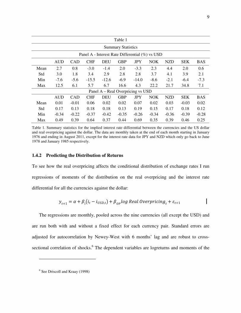
Table 1

Summary Statistics

Panel A - Interest Rate Differential (%) vs USD

AUD CAD CHF DEU GBP JPY NOK NZD SEK BAS

Mean 2.7 0.8 -3.0 -1.4 2.0 -3.3 2.3 4.4 2.0 0.6 Std 3.0 1.8 3.4 2.9 2.8 2.8 3.7 4.1 3.9 2.1 Min -7.6 -5.6 -15.5 -12.6 -6.9 -14.0 -8.6 -2.1 -6.4 -7.3 Max 12.5 6.1 5.7 6.7 16.6 4.3 22.2 21.7 34.8 7.1

Panel A – Real Overpricing vs USD AUD CAD CHF DEU GBP JPY NOK NZD SEK BAS

Mean 0.01 -0.01 0.06 0.02 0.02 0.07 0.02 0.03 -0.03 0.02 Std 0.17 0.13 0.18 0.18 0.13 0.19 0.15 0.17 0.18 0.12 Min -0.34 -0.22 -0.37 -0.42 -0.35 -0.26 -0.34 -0.36 -0.39 -0.28 Max 0.49 0.39 0.64 0.37 0.44 0.69 0.35 0.39 0.46 0.25

Table 1. Summary statistics for the implied interest rate differential between the currencies and the US dollar and real overpricing against the dollar. The data are monthly taken at the end of each month starting in January 1976 and ending in August 2011, except for the interest rate data for JPY and NZD which only go back to June 1978 and January 1985 respectively.

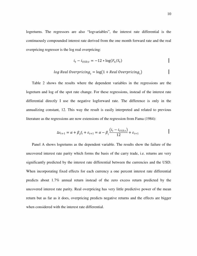
1.4.2 Predicting the Distribution of Returns

To see how the real overpricing affects the conditional distribution of exchange rates I run

regressions of moments of the distribution on the real overpricing and the interest rate

differential for all the currencies against the dollar:

!"1 � #" $i&�! � �'(),!*" $+,�-�� ! " .!"1

The regressions are monthly, pooled across the nine currencies (all except the USD) and

are run both with and without a fixed effect for each currency pair. Standard errors are

adjusted for autocorrelation by Newey-West with 6 months’ lag and are robust to cross-

sectional correlation of shocks.6 The dependent variables are logreturns and moments of the

6 See Driscoll and Kraay (1998)

10

logreturns. The regressors are also “logvariables”, the interest rate differential is the

continuously compounded interest rate derived from the one month forward rate and the real

overpricing regressor is the log real overpricing:

�� /01,� � �12 ∗ log78�/(�:

�-�� ! � log&1 " � �� !*

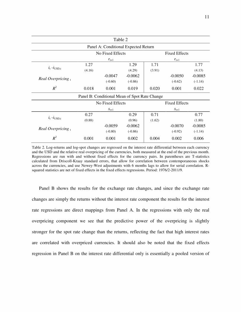
Table 2 shows the results where the dependent variables in the regressions are the

logreturn and log of the spot rate change. For these regressions, instead of the interest rate

differential directly I use the negative logforward rate. The difference is only in the

annualizing constant, 12. This way the result is easily interpreted and related to previous

literature as the regressions are now extensions of the regression from Fama (1984):

∆<!"1 � #" $i=! " .!"1 � #� $i &�! � �'(),!*12 " .!"1

Panel A shows logreturns as the dependent variable. The results show the failure of the

uncovered interest rate parity which forms the basis of the carry trade, i.e. returns are very

significantly predicted by the interest rate differential between the currencies and the USD.

When incorporating fixed effects for each currency a one percent interest rate differential

predicts about 1.7% annual return instead of the zero excess return predicted by the

uncovered interest rate parity. Real overpricing has very little predictive power of the mean

return but as far as it does, overpricing predicts negative returns and the effects are bigger

when considered with the interest rate differential.

11

Table 2

Panel A: Conditional Expected Return

No Fixed Effects Fixed Effects rt+1 rt+1

it -iUSD,t 1.27 1.29 1.71 1.77 (4.16) (4.29) (3.91) (4.13)

Real Overpricing t -0.0047 -0.0062 -0.0050 -0.0085 (-0.60) (-0.86) (-0.62) (-1.14)

R2 0.018 0.001 0.019 0.020 0.001 0.022

Panel B: Conditional Mean of Spot Rate Change

No Fixed Effects Fixed Effects st+1 st+1

it -iUSD,t 0.27 0.29 0.71 0.77 (0.88) (0.96) (1.62) (1.80)


R2 0.001 0.001 0.002 0.004 0.002 0.006

Table 2. Log-returns and log-spot changes are regressed on the interest rate differential between each currency and the USD and the relative real overpricing of the currencies, both measured at the end of the previous month. Regressions are run with and without fixed effects for the currency pairs. In parentheses are T-statistics calculated from Driscoll-Kraay standard errors, that allow for correlation between contemporaneous shocks across the currencies, and use Newey-West adjustments with 6 months lags to allow for serial correlation. R-squared statistics are net of fixed effects in the fixed effects regressions. Period: 1976/2-2011/9.

Panel B shows the results for the exchange rate changes, and since the exchange rate

changes are simply the returns without the interest rate component the results for the interest

rate regressions are direct mappings from Panel A. In the regressions with only the real

overpricing component we see that the predictive power of the overpricing is slightly

stronger for the spot rate change than the returns, reflecting the fact that high interest rates

are correlated with overpriced currencies. It should also be noted that the fixed effects

regression in Panel B on the interest rate differential only is essentially a pooled version of

12

the Fama regression and the resulting coefficient, 0.71, is not far from previously reported

results. Clarida et al. (2009) talk about 0.85 as the average estimate across many studies.7

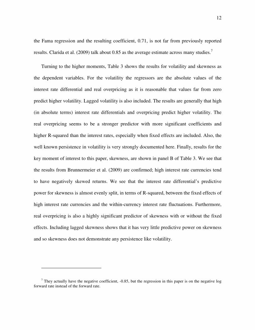
Turning to the higher moments, Table 3 shows the results for volatility and skewness as

the dependent variables. For the volatility the regressors are the absolute values of the

interest rate differential and real overpricing as it is reasonable that values far from zero

predict higher volatility. Lagged volatility is also included. The results are generally that high

(in absolute terms) interest rate differentials and overpricing predict higher volatility. The

real overpricing seems to be a stronger predictor with more significant coefficients and

higher R-squared than the interest rates, especially when fixed effects are included. Also, the

well known persistence in volatility is very strongly documented here. Finally, results for the

key moment of interest to this paper, skewness, are shown in panel B of Table 3. We see that

the results from Brunnermeier et al. (2009) are confirmed; high interest rate currencies tend

to have negatively skewed returns. We see that the interest rate differential’s predictive

power for skewness is almost evenly split, in terms of R-squared, between the fixed effects of

high interest rate currencies and the within-currency interest rate fluctuations. Furthermore,

real overpricing is also a highly significant predictor of skewness with or without the fixed

effects. Including lagged skewness shows that it has very little predictive power on skewness

and so skewness does not demonstrate any persistence like volatility.

7 They actually have the negative coefficient, -0.85, but the regression in this paper is on the negative log forward rate instead of the forward rate.

13

Table 3

Panel A: Conditional Volatility of Returns

No Fixed Effects Fixed Effects Volt+1 Volt+1

abs(it -iUSD,t) 0. 293 0.249 0.126 0.160 0.132 0. 086 (3.57) (3.39) (2.83) (1.87) (1.69) (1.75)

abs(Real Overpricingt) 0.098 0.088 0.044 0.077 0.073 0.040 (3.96) (3.76) (3.33) (3.09) (3.08) (2.78)

Volt 0.584 0.529 (10.98) (8.58)

R2 0.026 0.037 0.056 0.381 0.008 0.024 0.030 0.311

Panel B: Conditional Skewness of Returns

No Fixed Effects Fixed Effects Skewnesst+1 Skewnesst+1

it -iUSD,t -2.83 -2.72 -2.79 -2.62 -2.35 -2.40 (-6.43) (-6.31) (-6.29) (-4.06) (-3.61) (-3.63)

Real Overpricing t -0.45 -0.41 -0. 41 -0.47 -0.42 -0.43 (-5.05) (-4.40) (-4.33) (-5.39) (-4.60) (-4.52)

Skewnesst -0.028 -0.032 (-1.00) (-1.15)

R2 0.026 0.011 0.035 0.036 0.014 0.013 0.024 0.025

Table 3. In Panel A annualized volatility of returns against the USD, estimated by each month's daily observations, is regressed on the absolute values of the interest rate differential and relative overpricing at the end of the previous month. In Panel B return skewness is the dependent variable. Regressions are run with and without fixed effects for each currency.In parentheses are T-statistics calculated from Driscoll-Kraay standard errors that allow for correlation between contemporaneous shocks across the currencies, and use Newey-West adjustments with 6 months lags to allow for serial correlation. R-squared statistics are net of fixed effects in the fixed effects regressions. Period: 1976/2-2011/9.

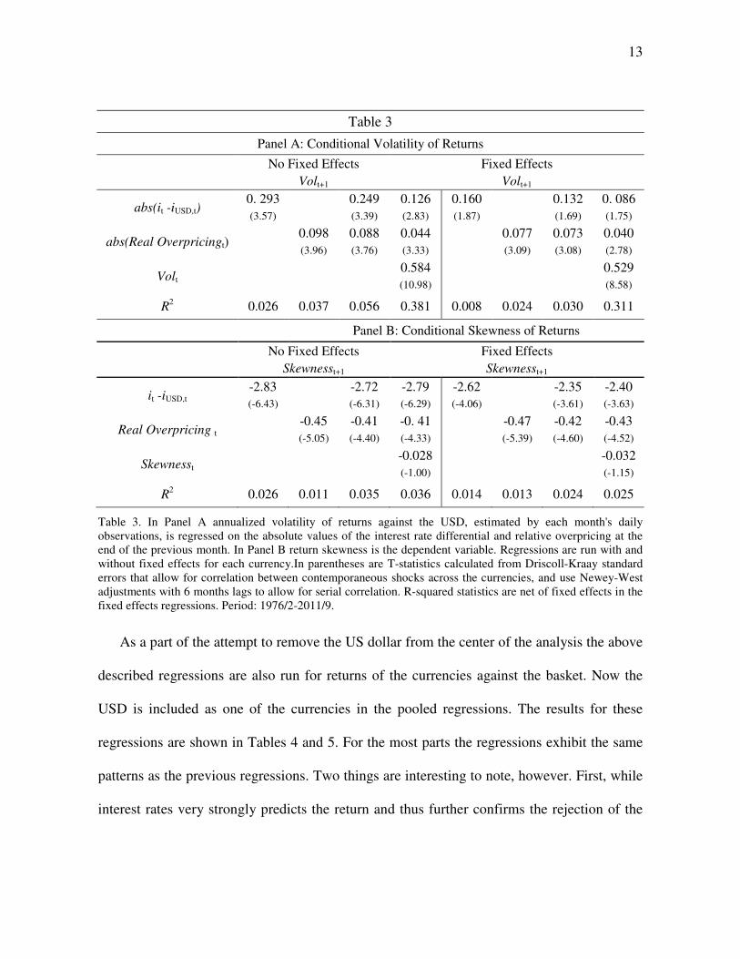
As a part of the attempt to remove the US dollar from the center of the analysis the above

described regressions are also run for returns of the currencies against the basket. Now the

USD is included as one of the currencies in the pooled regressions. The results for these

regressions are shown in Tables 4 and 5. For the most parts the regressions exhibit the same

patterns as the previous regressions. Two things are interesting to note, however. First, while

interest rates very strongly predicts the return and thus further confirms the rejection of the

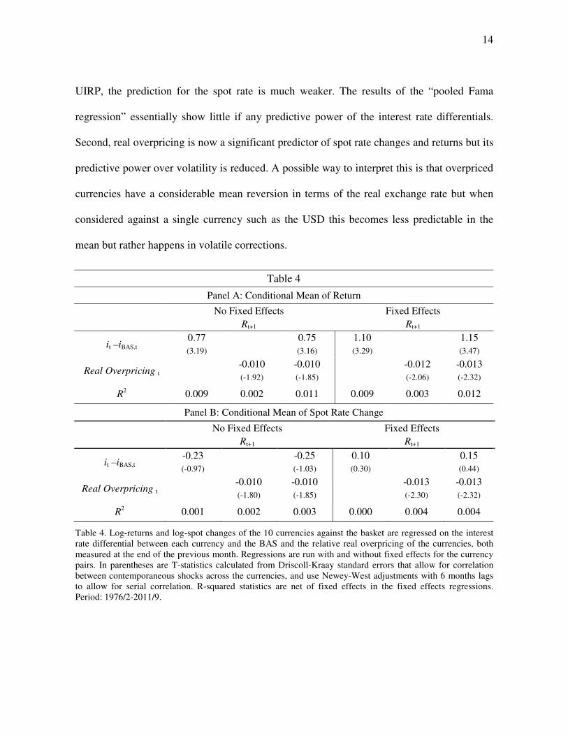
14

UIRP, the prediction for the spot rate is much weaker. The results of the “pooled Fama

regression” essentially show little if any predictive power of the interest rate differentials.

Second, real overpricing is now a significant predictor of spot rate changes and returns but its

predictive power over volatility is reduced. A possible way to interpret this is that overpriced

currencies have a considerable mean reversion in terms of the real exchange rate but when

considered against a single currency such as the USD this becomes less predictable in the

mean but rather happens in volatile corrections.

Table 4

Panel A: Conditional Mean of Return

No Fixed Effects Fixed Effects Rt+1 Rt+1

it –iBAS,t 0.77 0.75 1.10 1.15 (3.19) (3.16) (3.29) (3.47)


R2 0.009 0.002 0.011 0.009 0.003 0.012

Panel B: Conditional Mean of Spot Rate Change


it –iBAS,t -0.23 -0.25 0.10 0.15 (-0.97) (-1.03) (0.30) (0.44)


R2 0.001 0.002 0.003 0.000 0.004 0.004

Table 4. Log-returns and log-spot changes of the 10 currencies against the basket are regressed on the interest rate differential between each currency and the BAS and the relative real overpricing of the currencies, both measured at the end of the previous month. Regressions are run with and without fixed effects for the currency pairs. In parentheses are T-statistics calculated from Driscoll-Kraay standard errors that allow for correlation between contemporaneous shocks across the currencies, and use Newey-West adjustments with 6 months lags to allow for serial correlation. R-squared statistics are net of fixed effects in the fixed effects regressions. Period: 1976/2-2011/9.

15

Table 5

Panel A: Conditional Volatility of Returns

No Fixed Effects Fixed Effects Volt+1 Volt+1

abs(it –iBAS,t) 0.351 0. 346 0.202 0.207 0. 196 0. 141 (4.20) (4.11) (3.82) (2.22) (2.10) (2.31)

abs(Real Overpricingt) 0.027 0.010 0.006 0.034 0.024 0.015 (1.69) (0.62) (0.67) (1.99) (1.47) (1.43)

Volt 0.509 0.451 (9.77) (7.85)

R2 0.037 0.002 0.037 0.289 0.012 0.003 0.014 0.222

Panel B: Conditional Skewness of Returns

No Fixed Effects Fixed Effects Skewnesst+1 Skewnesst+1

it –iBAS,t -3.20 -3.25 -3.26 -2.95 -2.77 -2.79 (-6.75) (-7.41) (-7.40) (-3.97) (-3.92) (-3.94)

Real Overpricing t -0.54 -0.58 -0.58 -0.66 -0.62 -0.62 (-4.13) (-4.87) (-4.84) (-5.81) (-5.45) (-5.40)

Skewnesst -0.004 -0.009 (-0.18) (-0.40)

R2 0.025 0.008 0.034 0.034 0.011 0.011 0.020 0.020

Table 5. In Panel A annualized volatility of returns against the BAS, estimated by each month's daily observations, is regressed on the absolute values of the interest rate differential and relative overpricing at the end of the previous month. In Panel B return skewness is the dependent variable. Regressions are run with and without fixed effects for each currency.In parentheses are T-statistics calculated from Driscoll-Kraay standard errors that allow for correlation between contemporaneous shocks across the currencies, and use Newey-West adjustments with 6 months lags to allow for serial correlation. R-squared statistics are net of fixed effects in the fixed effects regressions. Period: 1976/2-2011/9.

1.5 Currency Strategies

1.5.1 The strategies

We now take the results and motivations from the previous section and put them into trading

strategies. Carry trade strategies are of course central to this analysis and to put the

overpricing information to good use real convergence strategies are constructed. I also show

results for momentum strategies and lastly I use the predictability of the previous month’s

16

interest rate change for a final strategy. It is interesting to compare these strategies and see

how they correlate to the strategies of our main interest.

The carry trade is the widely known strategy of borrowing in low interest rate currencies

and investing the funds in high interest rate currencies. While this is universal, the particular

implementation varies. Most often the strategy is defined as comparing each currency’s

interest rate to that of the US dollar and depending on whether it is higher or lower the

currency is bought or sold against the dollar. This strategy is clearly very centered on the

dollar and can load very heavily on fluctuations of the dollar. For example if the dollar has

the lowest interest rate of all currencies in the group considered, then the long part of the

strategy would be an evenly distributed portfolio of all the currencies except for the dollar

and the short part would be all dollar, making any innovations particular to the dollar very

important for the returns. While it is interesting to analyze the trading strategy with such

focus on the dollar I will, both for the carry trade and other strategies, emphasize portfolios

that are not so centered on the dollar. These strategies will take two forms. First there will be

strategies that do exactly as described as above but instead of comparing with and trading

against the dollar the reference point will be a basket of currencies, the BAS described in the

data section. While the position will be against a basket, the returns will still be measured in

dollars. The concentrated exposure to the dollar is simply removed by shorting all the

currencies in the basked rather than just the dollar. The dollar is still a part of the basket and

is itself one of the currencies analyzed to either go long or short but it is no longer a central

feature of the portfolio. Second, I create strategies that rank the currencies by their interest

rates (and later other features) and go long the highest ranking currencies and short the

17

lowest ranking currencies. These strategies I will refer to as long/short and they are

implemented with different number of currencies bought and sold.

To utilize the real overpricing signal described in the data section I implement real

convergence strategies, i.e. betting that the currencies that are most overpriced by this

measure will converge to its long run mean. To do that portfolios are formed in the same way

as for the carry trade but instead of using the interest rate as a signal we now use the

overpricing signal. And to be clear, whereas we bought the currencies that had the highest

interest rates in the carry trade we now buy those currencies that are most underpriced.

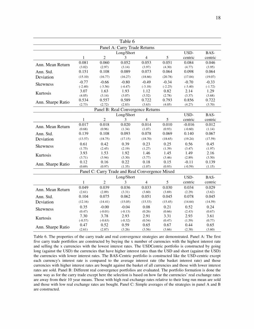
The results from implementing these strategies are shown in Table 6. The returns are all

excess returns and T-statistics are shown in parenteses. Panel A shows the results for the

carry trade. First it shall be noted that all strategies deliver statistically significant excess

returns and Sharpe-ratios. Furthermore they are all negatively skewed though with varying

degree of significance. For the long/short strategies one can observe a trend, both the mean

return and standard deviation decrease as the the number of currencies that are bought and

sold increases. The standard deviation decreases more rapidly however, resulting in an

increasing Sharpe ratio. The negative skewness of the returns also decreases with the number

of currencies. Moving on to the USD- and BAS-centric strategies we see slightly higher

Sharpe ratios. The returns are also both negatively skewed, the dollar strategy has skewness

in the higher end of the long/short strategies but the basket strategy turns out to have quite a

bit lower skewness.

18

Table 6 Panel A: Carry Trade Returns

Long/Short USD-centric

BAS-centric 1 2 3 4 5

Ann. Mean Return 0.081 0.060 0.052 0.053 0.051 0.084 0.046 (3.02) (2.97) (3.14) (3.97) (4.30) (4.77) (3.95)

Ann. Std. Deviation

0.151 0.108 0.089 0.073 0.064 0.098 0.064 (15.10) (16.77) (16.27) (18.66) (20.78) (17.04) (19.07)

Skewness -0.77 -0.66 -0.80 -0.49 -0.34 -0.70 -0.33 (-2.40) (-3.56) (-4.47) (-3.18) (-2.25) (-3.40) (-1.72)

Kurtosis 3.07 1.63 1.93 1.12 0.82 2.14 1.29 (4.05) (3.14) (3.07) (3.52) (2.78) (3.37) (3.68)

Ann. Sharpe Ratio 0.534 0.557 0.589 0.722 0.793 0.856 0.722 (2.73) (2.72) (2.83) (3.63) (4.05) (4.27) (3.70)

Panel B: Real Convergence Returns Long/Short USD-

centric BAS-centric 1 2 3 4 5

Ann. Mean Return 0.017 0.018 0.020 0.014 0.010 -0.016 0.012 (0.68) (0.96) (1.34) (1.07) (0.93) (-0.60) (1.14)

Ann. Std. Deviation

0.139 0.108 0.093 0.078 0.069 0.140 0.067 (13.57) (18.75) (17.15) (18.70) (18.65) (19.24) (17.59)

Skewness 0.61 0.42 0.39 0.23 0.25 0.56 0.45 (1.75) (2.45) (2.19) (1.27) (1.39) (3.47) (1.97)

Kurtosis 3.93 1.53 1.92 1.46 1.45 1.49 2.16 (3.71) (3.94) (3.30) (3.77) (3.46) (2.89) (3.50)

Ann. Sharpe Ratio 0.12 0.16 0.22 0.18 0.15 -0.11 0.139 (0.69) (0.97) (1.35) (1.07) (0.93) (-0.59) (1.15)

Panel C: Carry Trade and Real Convergence Mixed Long/Short USD-

centric BAS-centric 1 2 3 4 5

Ann. Mean Return 0.049 0.039 0.036 0.033 0.030 0.034 0.029 (2.61) (2.89) (3.31) (3.60) (3.69) (2.29) (3.62)

Ann. Std. Deviation

0.104 0.075 0.062 0.051 0.045 0.078 0.045 (12.16) (14.41) (15.05) (15.53) (15.45) (14.64) (14.59)

Skewness 0.35 -0.00 -0.04 0.08 0.21 0.52 0.24 (0.47) (-0.01) (-0.13) (0.26) (0.66) (2.43) (0.67)

Kurtosis 7.30 3.78 2.93 2.91 3.31 2.93 3.61 (-0.57) (-0.63) (-0.32) (0.54) (0.47) (1.59) (0.77)

Ann. Sharpe Ratio 0.47 0.52 0.59 0.65 0.67 0.44 0.65 (2.61) (2.87) (3.26) (3.56) (3.66) (2.38) (3.60)

Table 6. The properties of the carry trade and real convergence strategies are demonstrated. Panel A: The first five carry trade portfolios are constructed by buying the x number of currencies with the highest interest rate and selling the x currencies with the lowest interest rates. The USDCentric portfolio is constructed by going long (against the USD) the currencies that have higher interest rates than the USD and short (against the USD) the currencies with lower interest rates. The BAS-Centric portfolio is constructed like the USD-centric except each currency's interest rate is compared to the average interest rate (the basket interest rate) and those currencies with higher interest rates are bought against the basket of all currencies and those with lower interest rates are sold. Panel B: Different real convergence portfolios are evaluated. The portfolio formation is done the same way as for the carry trade except here the selection is based on how far the currencies’ real exchange rates are away from their 10 year means. Those with high real exchange rates relative to their long run mean are sold and those with low real exchange rates are bought. Panel C: Simple averages of the strategies in panel A and B are constructed.

19

Panel B shows the results for the real convergence strategies. While the point estimates of

the Sharpe ratios are positive in all cases except for the USD-centric portfolio, none of them

are significant. The skewness of all the strategies are positive and significant or marginally

significant in most cases. For the USD- and BAS-centric strategies the skewness is

reasonably significant. These strategies do not look particularly interesting alone but their

value emerges when we use them to enhance the carry trade.

We have seen that the carry trade offers substantial excess returns but they come with

significant crash risk, i.e. negative skewness. The real convergence strategies however offer

little in terms of excess return but do have positive skewness. When we combine the carry

trade and the real convergence strategy in the simplest way possible, by simply averaging

across the two strategies, we see how the different properties generate more favorable

returns. Panel C shows the results for this strategy. In terms of the Sharpe ratios all the

long/short strategies demonstrate slightly lower ratios than for the carry trade. The skewness,

however, is greatly reduced in all cases and even turns (very slightly and insignificantly)

positive for most of the strategies. The USD-centric results are mixed as the real convergence

strategy did not provide a clear positive contribution to the carry trade. The Sharpe ratio is

just about half of that of the USD-centric carry trade although the strategy is now has a

decent positive skewness instead of a quite big negative skewness. Different weights between

the strategies might therefore create a portfolio that might be superior to the carry trade on its

own. The BAS-centric mixed strategy, however, shows a clear benefit of mixing the

strategies. The Sharpe ratio is only slightly reduced but the skewness is turned around. It

should also be noted that the excess kurtosis of the return distributions are in all strategies

20

higher in the mixed strategies than in the individual carry trade or real convergence

strategies. This reflects the fact that while some of the reduced negative skewness comes

from canceling out large negative returns, some of the positive skewness added is by adding

large positive returns rather than canceling out negative returns.

The carry trade and the real convergence strategies are very much oriented towards

fundamentals. The interest rate is a defining characteristic of each currency and deviations

from, and convergence to, the long term mean of the real exchange rates are very much in

line with the literature of the purchasing power parity. These properties are also long term in

nature. While short term fluctuations may affect the carry trade returns the interest rate wins

in the end and while the real exchange rate can deviate from its fundamental value it will

revert to it eventually, often very quickly. There are, however, also some short-term effects in

exchange rate movements that provide profitable information. So called momentum

strategies capitalize on the fact that exchange rate changes tend to be persistent and so buying

currencies that have appreciated recently is profitable. This has been documented before, for

example by Okunev and White (2003). Another short term effect is that shocks to interest

rates tend to have persistent effects on exchange rates. This was shown by Eichenbaum and

Evans (1995) in the case of monetary policy shocks to the USD interest rate. This effect

motivates a strategy, since interest rate changes are not instantly reflected in the price but

actually predict exchange rate changes going forward. We now move to turn these anomalies

into strategies.

For the momentum strategy I construct strategies both centered on the USD and BAS in

the following way. First for the USD-centric strategies the current spot exchange rate of each

21

currency against the dollar is compared against its own moving average. If the spot rate is

higher than the moving average then the currency is bought against the dollar and if it is

lower then the currency is sold. This is done for four different periods for the moving

average, comparing the spot against the last one, three, six and twelve months. The same

exercise is performed for the BAS-centric strategy except now the currencies’ spot rate

against the basket is compared against its own moving average. The positions are then taken

against the basket.

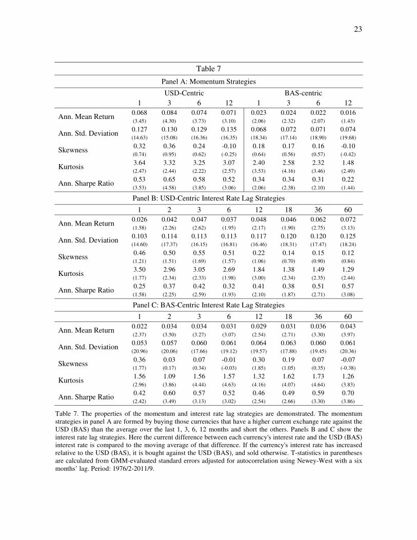
The results can be seen in panel A of Table 7. We can see that the strategy is quite

succesful, especially for the USD-centric portfolio where the Sharpe ratios are similar to

those of the carry trade. The BAS-centric portfolio has considerably lower Sharpe ratios but

they are still significant for all but the longest average. In both cases the strategies seem to

perform best when the moving average is taken for the last 3-6 months. Also, the skewness of

the strategies is marginally positive at the shorter end but turns negative as the moving

average is extended across more months.

Panels B and C of the same table show results for strategies that are here called interest

rate lag strategies. These strategies utilize the predictability of the spot rate by changes in

interest rates. For each currency the difference between its interest rate and the interest rate of

the USD (or the BAS in the BAS-centric case) is calculated and compared to the trailing

average of that difference over the last months. If a currency’s interest rate has gone up

relative to the USD (BAS) interest rate it is bought against the USD (BAS) and sold

otherwise. For both currencies the Sharpe ratios are significant for most of the moving

average periods considered. Both at the short end, where the change in last month’s interest

22

rate differential is the signal, as well as at the long period of five years is the change in the

interest rate differential a profitable predictor of the exchange rates. It is intuitive that if there

is a lag in the market’s reaction then it should affect the short end. The longer end is more of

a puzzle. Two explanations come to mind. First the persistence is just so strong that it lasts

over such a long period. The second is that as the horizon is extended then the strategy really

approaches a version of the carry trade. This is not quite the carry trade though as the carry

trade compares the interest rate of a currency directly to that of the USD (BAS). This version

looks at how far the current interest rate is above its longer term average and compares

whether it is farther above that long term average than the USD (BAS) interest rate is

currently above its long term average. This version could therefore be considered a “relative”

carry trade to the more common “absolute” carry trade. The relative carry trade thus possibly

focuses more on the relative positions of the economies in the business cycles whereas the

absolute carry trade both captures that as well as the general long term interest rate levels in

the countries. Looking at the skewness, particularly of the USD-centric strategy, we see a

similar trend as for the momentum strategies. At the short end we see higher skewness and

thus expect upward jumps rather than downwards as the currency reacts positively to a

changing trend.

23

Table 7

Panel A: Momentum Strategies

USD-Centric BAS-centric 1 3 6 12 1 3 6 12

Ann. Mean Return 0.068 0.084 0.074 0.071 0.023 0.024 0.022 0.016 (3.45) (4.30) (3.73) (3.10) (2.06) (2.32) (2.07) (1.43)

Ann. Std. Deviation 0.127 0.130 0.129 0.135 0.068 0.072 0.071 0.074 (14.63) (15.08) (16.36) (16.35) (18.34) (17.14) (18.90) (19.68)

Skewness 0.32 0.36 0.24 -0.10 0.18 0.17 0.16 -0.10 (0.74) (0.95) (0.62) (-0.25) (0.64) (0.56) (0.57) (-0.42)

Kurtosis 3.64 3.32 3.25 3.07 2.40 2.58 2.32 1.48 (2.47) (2.44) (2.22) (2.57) (3.53) (4.16) (3.46) (2.49)

Ann. Sharpe Ratio 0.53 0.65 0.58 0.52 0.34 0.34 0.31 0.22 (3.53) (4.58) (3.85) (3.06) (2.06) (2.38) (2.10) (1.44)

Panel B: USD-Centric Interest Rate Lag Strategies

1 2 3 6 12 18 36 60

Ann. Mean Return 0.026 0.042 0.047 0.037 0.048 0.046 0.062 0.072 (1.58) (2.26) (2.62) (1.95) (2.17) (1.90) (2.75) (3.13)


Skewness 0.46 0.50 0.55 0.51 0.22 0.14 0.15 0.12 (1.21) (1.51) (1.69) (1.57) (1.06) (0.70) (0.90) (0.84)

Kurtosis 3.50 2.96 3.05 2.69 1.84 1.38 1.49 1.29 (1.77) (2.34) (2.33) (1.98) (3.00) (2.34) (2.35) (2.44)

Ann. Sharpe Ratio 0.25 0.37 0.42 0.32 0.41 0.38 0.51 0.57 (1.58) (2.25) (2.59) (1.93) (2.10) (1.87) (2.71) (3.08)

Panel C: BAS-Centric Interest Rate Lag Strategies

1 2 3 6 12 18 36 60

Ann. Mean Return 0.022 0.034 0.034 0.031 0.029 0.031 0.036 0.043 (2.37) (3.50) (3.27) (3.07) (2.54) (2.71) (3.30) (3.97)


Skewness 0.36 0.03 0.07 -0.01 0.30 0.19 0.07 -0.07 (1.77) (0.17) (0.34) (-0.03) (1.85) (1.05) (0.35) (-0.38)

Kurtosis 1.56 1.09 1.56 1.57 1.32 1.62 1.73 1.26 (2.96) (3.86) (4.44) (4.63) (4.16) (4.07) (4.64) (3.83)

Ann. Sharpe Ratio 0.42 0.60 0.57 0.52 0.46 0.49 0.59 0.70 (2.42) (3.49) (3.13) (3.02) (2.54) (2.66) (3.30) (3.86)

Table 7. The properties of the momentum and interest rate lag strategies are demonstrated. The momentum strategies in panel A are formed by buying those currencies that have a higher current exchange rate against the USD (BAS) than the average over the last 1, 3, 6, 12 months and short the others. Panels B and C show the interest rate lag strategies. Here the current difference between each currency's interest rate and the USD (BAS) interest rate is compared to the moving average of that difference. If the currency's interest rate has increased relative to the USD (BAS), it is bought against the USD (BAS), and sold otherwise. T-statistics in parentheses are calculated from GMM-evaluated standard errors adjusted for autocorrelation using Newey-West with a six months’ lag. Period: 1976/2-2011/9.

24

1.5.2 Correlation with Asset Pricing Factors

While we have seen that the currency strategies described above have significant Sharpe

ratios these strategies might simply be loading on traditional asset pricing factors and earning

the premia associated with those factors. Before we turn to that question, how the different

trading strategies’ returns are correlated with the asset pricing factors, it is in order to first

look at the correlations between the strategies themselves which are demonstrated in Table 8.

To limit the size of the tables following only one long/short strategy is considered from now

on, the one with three curencies long and short. Also, the momentum and interest rate lag

strategies considered are those using the three month lag. Not surprisingly the different

variations of the same strategy are highly correlated, i.e. the three version of the carry trade

are positively correlated with each other and the same goes for the other strategies. The

correlations across groups are more interesting. First we see that the working assumption for

building the mixed strategies, that the carry trade and real convergence are generally

negatively correlated, seems to be true though the correlation between individual strategies

varies a lot. The momentum strategy and the carry trade do not exhibit any significant

correlation between them, positive or negative. Real convergence and momentum, on the

other hand, are overall negatively correlated, with varying significance though and real

convergence is positively correlated with the interest rate lag strategy. The relationship

between momentum and real convergence provides the insight that currencies tend to trend in

the short term and mean revert in the long term. The correlation between the interest rate lag

strategies and the real convergenge suggests that interest rate changes can provide useful

signals about the timing of reversions to fundamentals. Not so surprisingly the interest rate

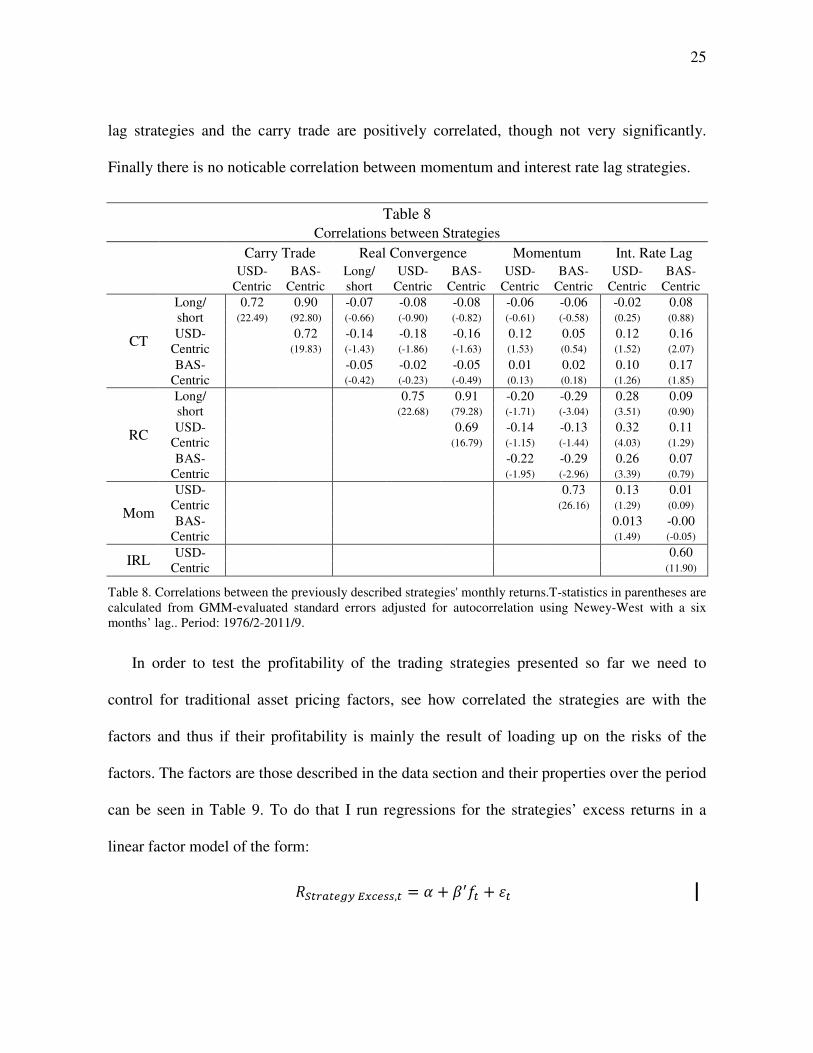
25

lag strategies and the carry trade are positively correlated, though not very significantly.

Finally there is no noticable correlation between momentum and interest rate lag strategies.

Table 8 Correlations between Strategies

Carry Trade Real Convergence Momentum Int. Rate Lag

USD-

Centric BAS-

Centric Long/ short

USD-Centric

BAS-Centric

USD-Centric

BAS-Centric

USD-Centric

BAS-Centric

CT

Long/ short

0.72 0.90 -0.07 -0.08 -0.08 -0.06 -0.06 -0.02 0.08 (22.49) (92.80) (-0.66) (-0.90) (-0.82) (-0.61) (-0.58) (0.25) (0.88)

USD-Centric

0.72 -0.14 -0.18 -0.16 0.12 0.05 0.12 0.16

(19.83) (-1.43) (-1.86) (-1.63) (1.53) (0.54) (1.52) (2.07)

BAS-Centric

-0.05 -0.02 -0.05 0.01 0.02 0.10 0.17

(-0.42) (-0.23) (-0.49) (0.13) (0.18) (1.26) (1.85)

RC

Long/ short

0.75 0.91 -0.20 -0.29 0.28 0.09

(22.68) (79.28) (-1.71) (-3.04) (3.51) (0.90)

USD-Centric

0.69 -0.14 -0.13 0.32 0.11

(16.79) (-1.15) (-1.44) (4.03) (1.29)

BAS-Centric

-0.22 -0.29 0.26 0.07

(-1.95) (-2.96) (3.39) (0.79)

Mom

USD-Centric

0.73 0.13 0.01

(26.16) (1.29) (0.09)

BAS-Centric

0.013 -0.00

(1.49) (-0.05)

IRL USD-

Centric 0.60

(11.90)

Table 8. Correlations between the previously described strategies' monthly returns.T-statistics in parentheses are calculated from GMM-evaluated standard errors adjusted for autocorrelation using Newey-West with a six months’ lag.. Period: 1976/2-2011/9.

In order to test the profitability of the trading strategies presented so far we need to

control for traditional asset pricing factors, see how correlated the strategies are with the

factors and thus if their profitability is mainly the result of loading up on the risks of the

factors. The factors are those described in the data section and their properties over the period

can be seen in Table 9. To do that I run regressions for the strategies’ excess returns in a

linear factor model of the form:

�0�>?�@ABCDE@FF,� � # " $G=� " .�

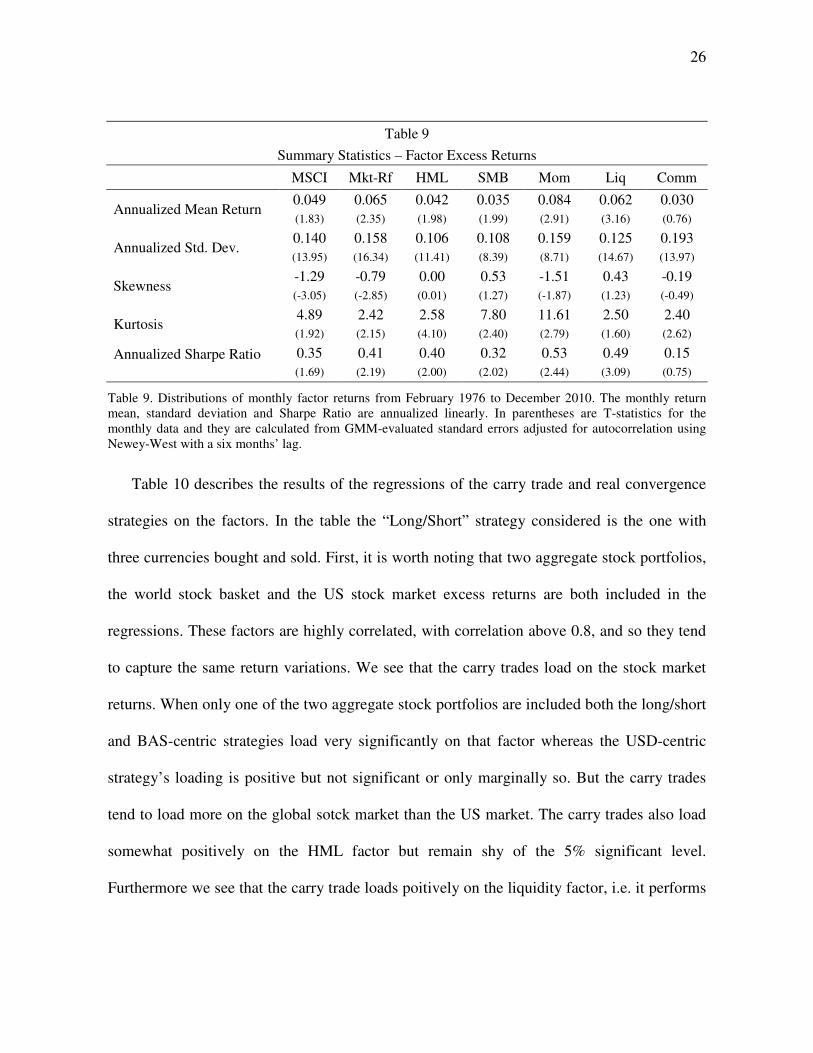
26

Table 9

Summary Statistics – Factor Excess Returns

MSCI Mkt-Rf HML SMB Mom Liq Comm

Annualized Mean Return 0.049 0.065 0.042 0.035 0.084 0.062 0.030 (1.83) (2.35) (1.98) (1.99) (2.91) (3.16) (0.76)

Annualized Std. Dev. 0.140 0.158 0.106 0.108 0.159 0.125 0.193 (13.95) (16.34) (11.41) (8.39) (8.71) (14.67) (13.97)

Skewness -1.29 -0.79 0.00 0.53 -1.51 0.43 -0.19 (-3.05) (-2.85) (0.01) (1.27) (-1.87) (1.23) (-0.49)

Kurtosis 4.89 2.42 2.58 7.80 11.61 2.50 2.40 (1.92) (2.15) (4.10) (2.40) (2.79) (1.60) (2.62)

Annualized Sharpe Ratio

0.35 0.41 0.40 0.32 0.53 0.49 0.15 (1.69) (2.19) (2.00) (2.02) (2.44) (3.09) (0.75)

Table 9. Distributions of monthly factor returns from February 1976 to December 2010. The monthly return mean, standard deviation and Sharpe Ratio are annualized linearly. In parentheses are T-statistics for the monthly data and they are calculated from GMM-evaluated standard errors adjusted for autocorrelation using Newey-West with a six months’ lag.

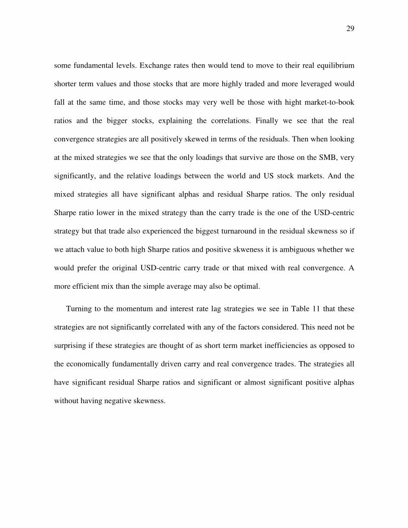
Table 10 describes the results of the regressions of the carry trade and real convergence

strategies on the factors. In the table the “Long/Short” strategy considered is the one with

three currencies bought and sold. First, it is worth noting that two aggregate stock portfolios,

the world stock basket and the US stock market excess returns are both included in the

regressions. These factors are highly correlated, with correlation above 0.8, and so they tend

to capture the same return variations. We see that the carry trades load on the stock market

returns. When only one of the two aggregate stock portfolios are included both the long/short

and BAS-centric strategies load very significantly on that factor whereas the USD-centric

strategy’s loading is positive but not significant or only marginally so. But the carry trades

tend to load more on the global sotck market than the US market. The carry trades also load

somewhat positively on the HML factor but remain shy of the 5% significant level.

Furthermore we see that the carry trade loads poitively on the liquidity factor, i.e. it performs

27

well when stocks that are generally illiquid perform well. All three trades have significant

positive alphas. For a more direct comparison between strategies the alphas don’t tell the

whole story since the strategies can have differing underlying amounts, for example when the

carry trade and real convergence strategies are combined some positions will be netted out

between the strategies and thus the “underlying amount” is not the same. Therefore I

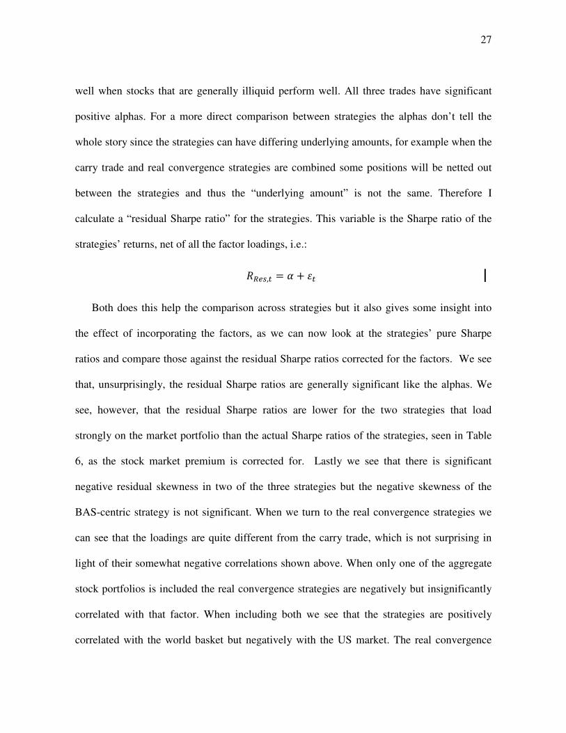
calculate a “residual Sharpe ratio” for the strategies. This variable is the Sharpe ratio of the

strategies’ returns, net of all the factor loadings, i.e.:

�H@F,� � # " .�

Both does this help the comparison across strategies but it also gives some insight into

the effect of incorporating the factors, as we can now look at the strategies’ pure Sharpe

ratios and compare those against the residual Sharpe ratios corrected for the factors. We see

that, unsurprisingly, the residual Sharpe ratios are generally significant like the alphas. We

see, however, that the residual Sharpe ratios are lower for the two strategies that load

strongly on the market portfolio than the actual Sharpe ratios of the strategies, seen in Table

6, as the stock market premium is corrected for. Lastly we see that there is significant

negative residual skewness in two of the three strategies but the negative skewness of the

BAS-centric strategy is not significant. When we turn to the real convergence strategies we

can see that the loadings are quite different from the carry trade, which is not surprising in

light of their somewhat negative correlations shown above. When only one of the aggregate

stock portfolios is included the real convergence strategies are negatively but insignificantly

correlated with that factor. When including both we see that the strategies are positively

correlated with the world basket but negatively with the US market. The real convergence

28

strategies all have negative, though insignificant, coefficients for loadings on the HML

factor. They do, however, load quite strongly on the SMB factor, a result that is quite robust

to different portfolios and periods. The intuition for this eludes the author as of this writing.

Hahn and Lee (2006) highlight the mapping between the SMB and HML factors on the one

hand and the default spread and term spread on the other. In short they show that small firms

and therefore the SMB factor depend on the default premium, i.e. when credit spreads are

high this affects small firms more negatively than bigger firms. In light of this one might

imagine that the real convergence SMB loading may just be reflecting correlation with the

credit spread. This is however not the case as real convergence strategies tend, if anything, to

perform better when credit spreads rise, a result consistent with the general pattern that real

convergence performs well in generally adverse and illiquid circumstances. Inclusion of the

credit spread in the regression thus only enhances the SMB loading. One might also imagine

(as this author did) that the effect could be due either mainly to positive correlation with

small stocks or negative correlation with big stocks (the author expected the latter). When

using factors to separate the two effects, the loading is however simply split between the two,

leaving no better understanding of the phenomenon.8 Real convergence loads to some extent

negatively on Carhart’s momentum, the liquidity, and commodities factors. These results

may suggest that the real convergence strategies perform well when lending liquidity is low

and leverage is hard to maintain and assets that rely on future cash flow may be pulled to

8 The two factors were constructed from Fama-French size sorted tertile portofolios. One factor is constructed as the returns of the big firm tertile minus the middle tertile and the other factor similarly constructed from the small firm tertile and the middle tertile.

29

some fundamental levels. Exchange rates then would tend to move to their real equilibrium

shorter term values and those stocks that are more highly traded and more leveraged would

fall at the same time, and those stocks may very well be those with hight market-to-book

ratios and the bigger stocks, explaining the correlations. Finally we see that the real

convergence strategies are all positively skewed in terms of the residuals. Then when looking

at the mixed strategies we see that the only loadings that survive are those on the SMB, very

significantly, and the relative loadings between the world and US stock markets. And the

mixed strategies all have significant alphas and residual Sharpe ratios. The only residual

Sharpe ratio lower in the mixed strategy than the carry trade is the one of the USD-centric

strategy but that trade also experienced the biggest turnaround in the residual skewness so if

we attach value to both high Sharpe ratios and positive skweness it is ambiguous whether we

would prefer the original USD-centric carry trade or that mixed with real convergence. A

more efficient mix than the simple average may also be optimal.

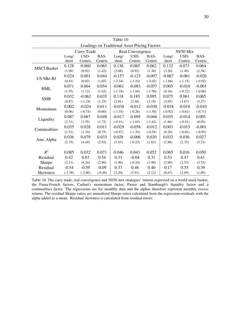
Turning to the momentum and interest rate lag strategies we see in Table 11 that these

strategies are not significantly correlated with any of the factors considered. This need not be

surprising if these strategies are thought of as short term market inefficiencies as opposed to

the economically fundamentally driven carry and real convergence trades. The strategies all

have significant residual Sharpe ratios and significant or almost significant positive alphas

without having negative skewness.

30

Table 10 Loadings on Traditional Asset Pricing Factors

Carry Trade Real Convergence 50/50 Mix

Long/ short

USD-Centric

BAS-Centric

Long/ short

USD-Centric

BAS-Centric

Long/ short

USD-Centric

BAS-Centric

MSCI Basket 0.128 0.060 0.065 0.136 0.085 0.062 0.132 0.073 0.064 (1.99) (0.92) (1.42) (2.08) (0.92) (1.38) (3.20) (1.49) (2.38)

US Mkt-Rf 0.024 0.001 0.044 -0.157 -0.123 -0.097 -0.067 -0.061 -0.026 (0.41) (0.02) (1.02) (-2.34) (-1.24) (-2.02) (-1.66) (-1.15) (-0.92)

HML 0.071 0.064 0.054 -0.061 -0.083 -0.057 0.005 -0.010 -0.001 (1.55) (1.12) (1.62) (-1.18) (-1.04) (-1.50) (0.16) (-0.22) (-0.06)

SMB 0.032 -0.062 0.035 0.118 0.185 0.095 0.075 0.061 0.065 (0.87) (-1.24) (1.25) (2.81) (2.46) (3.19) (3.05) (1.67) (3.27)

Momentum 0.002 -0.024 0.011 -0.038 -0.012 -0.030 -0.018 -0.018 -0.010 (0.06) (-0.74) (0.60) (-1.35) (-0.26) (-1.50) (-0.92) (-0.61) (-0.71)

Liquidity 0.087 0.067 0.048 -0.017 -0.095 -0.046 0.035 -0.014 0.001 (2.31) (1.55) (1.72) (-0.41) (-1.65) (-1.62) (1.66) (-0.41) (0.05)

Commodities 0.035 0.028 0.011 -0.029 -0.058 -0.012 0.003 -0.015 -0.001 (1.51) (1.10) (0.75) (-0.97) (-1.34) (-0.58) (0.20) (-0.62) (-0.05)

Ann. Alpha 0.036 0.079 0.033 0.028 -0.006 0.020 0.032 0.036 0.027 (2.19) (4.44) (2.92) (1.63) (-0.23) (1.63) (2.88) (2.35) (3.23)

R2 0.085 0.032 0.071 0.046 0.043 0.052 0.065 0.016 0.050

Residual Sharpe

0.42 0.83 0.54 0.31 -0.04 0.31 0.53 0.47 0.61 (2.11) (4.24) (2.90) (1.90) (-0.24) (1.90) (2.90) (2.53) (3.33)

Residual Skewness

-0.54 -0.59 -0.09 0.37 0.46 0.40 0.17 0.55 0.39 (-3.58) (-2.80) (-0.48) (2.20) (3.91) (2.12) (0.67) (2.69) (1.09)

Table 10. The carry trade, real convergence and 50/50 mix strategies’ returns regressed on a world stock basket, the Fama-French factors, Carhart's momentum factor, Pastor and Stambaugh's liquidity factor and a commodities factor. The regressions are for monthly data and the alphas therefore represent monthly excess returns. The residual Sharpe ratios are annualized Sharpe ratios calculated from the regression residuals with the alpha added as a mean. Residual skewness is calculated from residual errors.

31


Momentum Interest Rate Lag

USD-Centric BAS-Centric USD-Centric BAS-Centric

MSCI Basket -0.113 -0.052 0.070 -0.020 (-1.26) (-0.88) (1.01) (-0.43)

US Mkt-Rf -0.018 0.023 -0.125 0.006 (-0.18) (0.46) (-1.49) (0.14)

HML -0.043 -0.012 -0.027 0.039 (-0.57) (0.32) (-0.33) (0.98)

SMB -0.043 -0.006 -0.078 -0.028 (-0.68) (-0.17) (-1.41) (-0.91)

Momentum -0.036 -0.001 0.054 0.029 (-0.74) (-0.05) (1.25) (1.26)

Liquidity -0.009 -0.012 0.001 -0.005 (-0.14) (-0.36) (0.02) (-0.16)

Commodities 0.004 -0.035 -0.036 0.000 (0.08) (-1.48) (-0.84) (0.01)

Alpha 0.097 0.027 0.046 0.031 (3.68) (1.92) (2.06) (2.61)

R2 0.021 0.016 0.032 0.016

Residual Sharpe 0.75 0.38 0.42 0.52 (5.17) (2.72) (2.65) (2.90)

Residual Skewness 0.24 0.00 0.28 0.11 (0.74) (0.01) (1.19) (0.54)

Table 11. The currency momentum and interest rate lag strategies regressed on a world stock basket, the Fama-French factors, Carhart's momentum factor, Pastor and Stambaugh's liquidity factor and a commodities factor. The regressions are for monthly data and the alphas therefore represent monthly excess returns. The residual Sharpe ratios are annualized Sharpe ratios calculated from the regression residuals with the alpha added as a mean. Residual skewness is calculated from residual errors. T-statistics in parenthesis are calculated from heteroskedasticity-consistent GMM errors adjusted for autocorrelation using Newey-West with a six months’ lag. Period: 1976/2-2010/12.

1.6 Currency Options and Options Strategies

We have seen how the real overpricing signal predicts negative skewness and crash risks. It

is therefore natural to consider the implications for currency options and to what extent this

signal is incorporated into their prices.

32

Recent papers have studied the role of options in hedging currency crash risks. Most

notably does Jurek (2008) find that when options are used to hedge away crash risks of the

carry trade the excess returns of USD-neutral versions of the carry trade are indistinguishable

from zero. For strategies not constrained to be USD-neutral, what has been called USD-

centric strategies in this paper, there is still an unexplained premium even with crash risk

hedging. Jurek however, only hedges the carry trade, i.e. selects options based on the interest

rates, but here the real convergence signal will also be used.

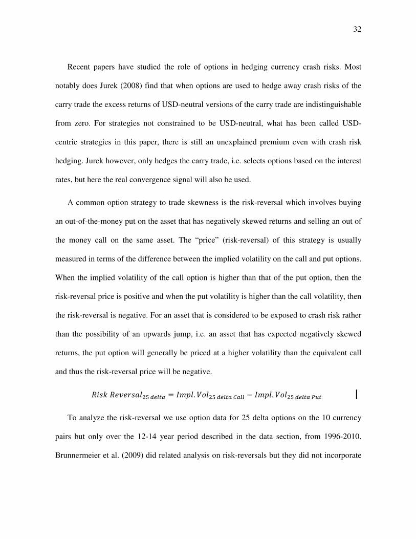
A common option strategy to trade skewness is the risk-reversal which involves buying

an out-of-the-money put on the asset that has negatively skewed returns and selling an out of

the money call on the same asset. The “price” (risk-reversal) of this strategy is usually

measured in terms of the difference between the implied volatility on the call and put options.

When the implied volatility of the call option is higher than that of the put option, then the

risk-reversal price is positive and when the put volatility is higher than the call volatility, then

the risk-reversal is negative. For an asset that is considered to be exposed to crash risk rather

than the possibility of an upwards jump, i.e. an asset that has expected negatively skewed

returns, the put option will generally be priced at a higher volatility than the equivalent call

and thus the risk-reversal price will be negative.

��<I� � �<��JK�@L�? � M��. O-�JK�@L�?P?LL � M��. O-�JK�@L�?,Q�

To analyze the risk-reversal we use option data for 25 delta options on the 10 currency

pairs but only over the 12-14 year period described in the data section, from 1996-2010.

Brunnermeier et al. (2009) did related analysis on risk-reversals but they did not incorporate

33

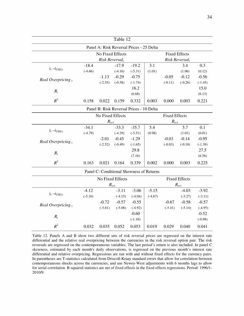
information about the real exchange rate, which turns out to be a very important variable.

Table 12 shows the price and realized skewness regressed on the interest rate differential

between the currencies and the relative real overpricing. The regressions are of the same kind

as in section 3, they are pooled across currencies and are both run with and without fixed

effects for each currency pair. In panels A and B results are shown where the risk reversal

prices of two different risk reversals, 10 delta and 25 delta, are regressed on the

contemporaneous interest rate differential and real overpricing of the currency pairs. Last

period’s return of the currency pair is also included. We see that the interest rate differential

has a strong negative effect on the high interest rate currency’s risk-reversal, i.e. it is more

expensive to insure against the high interest rate currency’s crash than against the crash of

the low interest rate currency. Furthermore we see that the overpricing has a similar effect

when it is the only regressor. When controlled for the interest rate differential, however, the

effect of the overpricing becomes insignificant, though still negative. When fixed effects are

included for the currency crosses the effects of both the interest rate and overpricing become

insignificant. In that case the currency crosses with high positive interest rate differential

have high negative fixed effects on the risk-reversal.

34

Table 12

Panel A: Risk Reversal Prices - 25 Delta

No Fixed Effects Fixed Effects Risk Reversalt Risk Reversalt

it –iUSD,t -18.4 -17.9 -19.2 3.1 3.4 0.3 (-4.66) (-4.16) (-5.31) (1.01) (1.06) (0.12)


Rt 16.2 15.0 (6.68) (6.13)

R2 0.158 0.022 0.159 0.332 0.003 0.000 0.003 0.221

Panel B: Risk Reversal Prices - 10 Delta


it –iUSD,t -34.1 -33.3 -35.7 5.4 5.7 0.1 (-4.79) (-4.29) (-5.51) (0.98) (1.01) (0.01)


Rt 29.8 27.5 (7.16) (6.56)

R2 0.163 0.021 0.164 0.339 0.002 0.000 0.003 0.225

Panel C: Conditional Skewness of Returns


it –iUSD,t -4.12 -3.11 -3.06 -5.15 -4.03 -3.92 (-5.16) (-4.15) (-4.04) (-4.67) (-3.27) (-3.11)


Rt -0.60 -0.52 (-1.18) (-0.98)

R2 0.032 0.035 0.052 0.053 0.019 0.029 0.040 0.041

Table 12. Panels A and B show two different sets of risk reversal prices are regressed on the interest rate differential and the relative real overpricing between the currencies in the risk reversal option pair. The risk reversals are regressed on the contemporaneous variables. The last period’s return is also included. In panel C skewness, estimated by each month's daily observations, is regressed on the previous month’s interest rate differential and relative overpricing. Regressions are run with and without fixed effects for the currency pairs. In parentheses are T-statistics calculated from Driscoll-Kraay standard errors that allow for correlation between contemporaneous shocks across the currencies, and use Newey-West adjustments with 6 months lags to allow for serial correlation. R-squared statistics are net of fixed effects in the fixed effects regressions. Period: 1996/1-2010/9.

35

Adding the lagged return we see a clear effect on the risk reversal prices; it is cheap to

hedge downside risk for currencies that performed well last month and expensive for last

month’s losers. This effect is very strong, explaining over 20% of the price variation when

fixed effects have been accounted for. If lagged return skewness would be included instead

of the lagged return the effect would be similar, though not quite as big. So, for such a short

time period we can only conclude that risk-reversals are most expensive for currencies that

have performed poorly recently and for currency crosses that generally have high positive

interest rate differentials but within-currency-cross variation of interest rates and overpricing

has little effect. In panel C we see how the realized skewness for the same period is predicted

by both the interest rate differential and the overpricing and the effects survive the fixed

effects. The lagged return (or the lagged skewness) on the other hand has little predictive

power and in the wrong direction compared to the risk reversal prices.

So the crash risk is mainly priced on a currency pair and recent performance basis and

much more correlated with the interest rate than the real overpricing. The realization of the

return skewness, however, is very much influenced by the real overpricing. This apparent

inconsistency suggests that it might be profitable to buy risk-reversals on currencies that are

highly overpriced. I implement this strategy on a monthly basis and for comparison the same

strategy using the interest rate differential signal. For each month a zero-cost strategy is

implemented for each currency pair. Whenever the risk-reversal price is not zero it is implied

that a 25 delta call and put do not have the same price. The size of the put option is scaled in

such a way that its value matches the call price and so for each point in time the strategy is

zero-cost. Both for the interest rate differential and the overpricing based strategies I use two

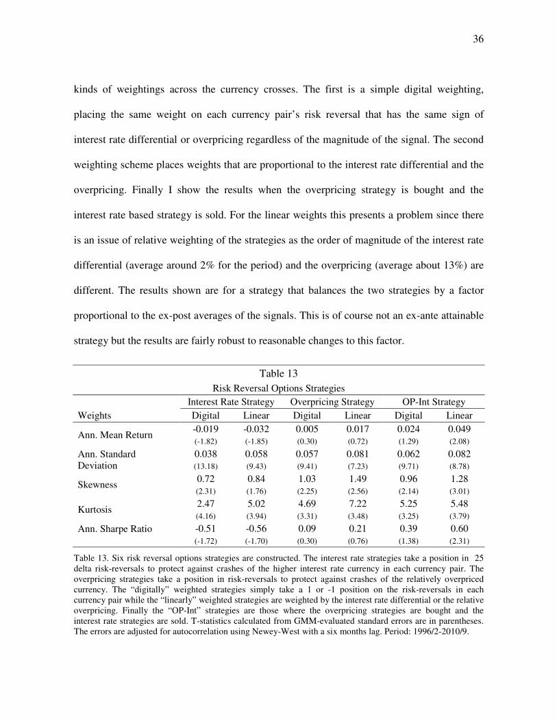
36

kinds of weightings across the currency crosses. The first is a simple digital weighting,

placing the same weight on each currency pair’s risk reversal that has the same sign of

interest rate differential or overpricing regardless of the magnitude of the signal. The second

weighting scheme places weights that are proportional to the interest rate differential and the

overpricing. Finally I show the results when the overpricing strategy is bought and the

interest rate based strategy is sold. For the linear weights this presents a problem since there

is an issue of relative weighting of the strategies as the order of magnitude of the interest rate

differential (average around 2% for the period) and the overpricing (average about 13%) are

different. The results shown are for a strategy that balances the two strategies by a factor

proportional to the ex-post averages of the signals. This is of course not an ex-ante attainable

strategy but the results are fairly robust to reasonable changes to this factor.

Table 13 Risk Reversal Options Strategies

Interest Rate Strategy Overpricing Strategy OP-Int Strategy Weights Digital Linear Digital Linear Digital Linear

Ann. Mean Return -0.019 -0.032 0.005 0.017 0.024 0.049 (-1.82) (-1.85) (0.30) (0.72) (1.29) (2.08)

Ann. Standard Deviation

0.038 0.058 0.057 0.081 0.062 0.082 (13.18) (9.43) (9.41) (7.23) (9.71) (8.78)

Skewness 0.72 0.84 1.03 1.49 0.96 1.28 (2.31) (1.76) (2.25) (2.56) (2.14) (3.01)

Kurtosis 2.47 5.02 4.69 7.22 5.25 5.48 (4.16) (3.94) (3.31) (3.48) (3.25) (3.79)

Ann. Sharpe Ratio

-0.51 -0.56 0.09 0.21 0.39 0.60 (-1.72) (-1.70) (0.30) (0.76) (1.38) (2.31)

Table 13. Six risk reversal options strategies are constructed. The interest rate strategies take a position in 25 delta risk-reversals to protect against crashes of the higher interest rate currency in each currency pair. The overpricing strategies take a position in risk-reversals to protect against crashes of the relatively overpriced currency. The “digitally” weighted strategies simply take a 1 or -1 position on the risk-reversals in each currency pair while the “linearly” weighted strategies are weighted by the interest rate differential or the relative overpricing. Finally the “OP-Int” strategies are those where the overpricing strategies are bought and the interest rate strategies are sold. T-statistics calculated from GMM-evaluated standard errors are in parentheses. The errors are adjusted for autocorrelation using Newey-West with a six months lag. Period: 1996/2-2010/9.

37

The results for the strategies can be seen in Table 13. In general the results are not very

significant. The returns are unsurprisingly positively skewed. The interest rate base strategies

yield negative Sharpe ratios whereas the overpricing based strategies have positive Sharpe

ratios. The only really significant Sharpe ratio is that of the difference strategy, where a

significant positive Sharpe ratio along with positive skewness is attained. So by buying the

overpricing based strategy against the interest rate based strategy one can get a decent Sharpe

ratio and still have a healthy positive skewness. As with the previous trading strategies the

returns of the options strategies are regressed on the traditional asset pricing factors as

before. The results of that can be seen in Table 14. The results show the same general pattern

as the un-risk-adjusted results of Table 13. The strategies are generally negatively correlated

with the factors included which pushes up the Sharpe ratios. The exception from this rule is

the overpricing based strategy’s loading on the SMB factor which, as noted earlier, remains a

mystery.

Finally I construct the carry trade, both in the normal way and also by using options to

hedge crash risks. In this analysis I only use the eight currencies that have available options

data against the USD. Therefore it is only sensible to construct four currency long/short

portfolios. Furthermore, the BAS-centric carry trade is here constructed by comparing the

interest rate of each currency against the basket rate and currencies with higher interest rates

are bought and others sold. Here this is nevertheless done against the dollar as we only have

options for the currencies against the USD, not the BAS, available and the idea is to construct

protfolios easily hedged by the options. In each of the hedged portfolios, an options portfolio

is constructed on top of the carry trade portfolio.

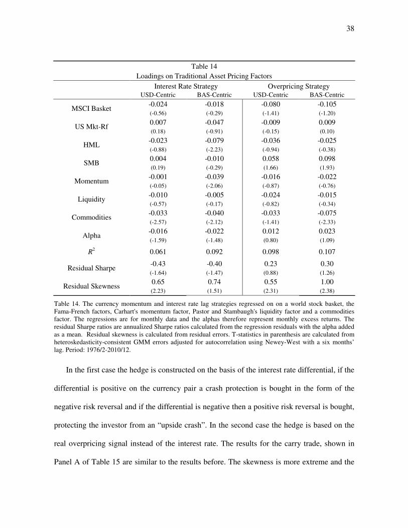
38


Interest Rate Strategy Overpricing Strategy

USD-Centric BAS-Centric USD-Centric BAS-Centric

MSCI Basket -0.024 -0.018 -0.080 -0.105 (-0.56) (-0.29) (-1.41) (-1.20)

US Mkt-Rf 0.007 -0.047 -0.009 0.009 (0.18) (-0.91) (-0.15) (0.10)

HML -0.023 -0.079 -0.036 -0.025 (-0.88) (-2.23) (-0.94) (-0.38)

SMB 0.004 -0.010 0.058 0.098 (0.19) (-0.29) (1.66) (1.93)

Momentum -0.001 -0.039 -0.016 -0.022 (-0.05) (-2.06) (-0.87) (-0.76)

Liquidity -0.010 -0.005 -0.024 -0.015 (-0.57) (-0.17) (-0.82) (-0.34)

Commodities -0.033 -0.040 -0.033 -0.075 (-2.57) (-2.12) (-1.41) (-2.33)

Alpha -0.016 -0.022 0.012 0.023 (-1.59) (-1.48) (0.80) (1.09)

R2 0.061 0.092 0.098 0.107

Residual Sharpe -0.43 -0.40 0.23 0.30 (-1.64) (-1.47) (0.88) (1.26)

Residual Skewness 0.65 0.74 0.55 1.00 (2.23) (1.51) (2.31) (2.38)

Table 14. The currency momentum and interest rate lag strategies regressed on on a world stock basket, the Fama-French factors, Carhart's momentum factor, Pastor and Stambaugh's liquidity factor and a commodities factor. The regressions are for monthly data and the alphas therefore represent monthly excess returns. The residual Sharpe ratios are annualized Sharpe ratios calculated from the regression residuals with the alpha added as a mean. Residual skewness is calculated from residual errors. T-statistics in parenthesis are calculated from heteroskedasticity-consistent GMM errors adjusted for autocorrelation using Newey-West with a six months’ lag. Period: 1976/2-2010/12.

In the first case the hedge is constructed on the basis of the interest rate differential, if the

differential is positive on the currency pair a crash protection is bought in the form of the

negative risk reversal and if the differential is negative then a positive risk reversal is bought,

protecting the investor from an “upside crash”. In the second case the hedge is based on the

real overpricing signal instead of the interest rate. The results for the carry trade, shown in

Panel A of Table 15 are similar to the results before. The skewness is more extreme and the

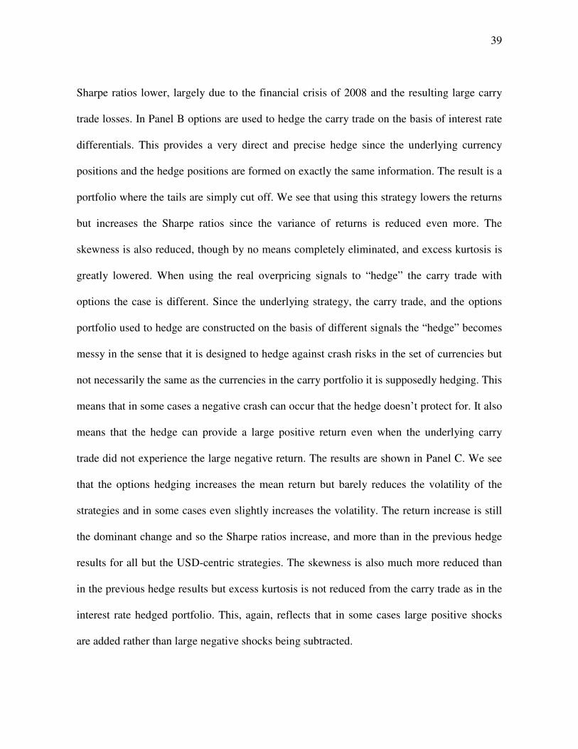
39

Sharpe ratios lower, largely due to the financial crisis of 2008 and the resulting large carry

trade losses. In Panel B options are used to hedge the carry trade on the basis of interest rate

differentials. This provides a very direct and precise hedge since the underlying currency

positions and the hedge positions are formed on exactly the same information. The result is a

portfolio where the tails are simply cut off. We see that using this strategy lowers the returns

but increases the Sharpe ratios since the variance of returns is reduced even more. The

skewness is also reduced, though by no means completely eliminated, and excess kurtosis is

greatly lowered. When using the real overpricing signals to “hedge” the carry trade with

options the case is different. Since the underlying strategy, the carry trade, and the options

portfolio used to hedge are constructed on the basis of different signals the “hedge” becomes

messy in the sense that it is designed to hedge against crash risks in the set of currencies but

not necessarily the same as the currencies in the carry portfolio it is supposedly hedging. This

means that in some cases a negative crash can occur that the hedge doesn’t protect for. It also

means that the hedge can provide a large positive return even when the underlying carry

trade did not experience the large negative return. The results are shown in Panel C. We see

that the options hedging increases the mean return but barely reduces the volatility of the

strategies and in some cases even slightly increases the volatility. The return increase is still

the dominant change and so the Sharpe ratios increase, and more than in the previous hedge

results for all but the USD-centric strategies. The skewness is also much more reduced than

in the previous hedge results but excess kurtosis is not reduced from the carry trade as in the

interest rate hedged portfolio. This, again, reflects that in some cases large positive shocks

are added rather than large negative shocks being subtracted.

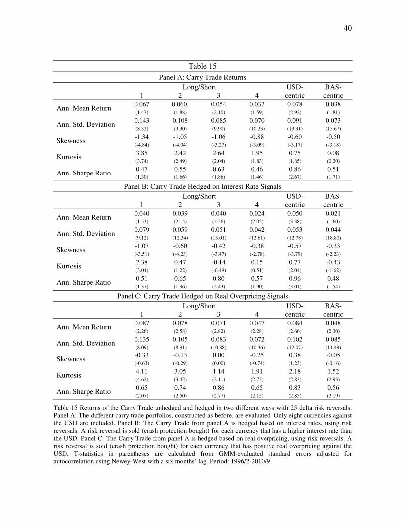
40

Table 15 Panel A: Carry Trade Returns

Long/Short USD-centric

BAS-centric 1 2 3 4

Ann. Mean Return 0.067 0.060. 0.054 0.032 0.078 0.038 (1.47) (1.88) (2.10) (1.59) (2.92) (1.81)

Ann. Std. Deviation 0.143 0.108 0.085 0.070 0.091 0.073 (8.32) (9.30) (9.90) (10.23) (13.91) (15.67)

Skewness -1.34 -1.05 -1.06 -0.88 -0.60 -0.50 (-4.84) (-4.04) (-3.27) (-3.09) (-3.17) (-3.18)

Kurtosis 3.85 2.42 2.64 1.95 0.75 0.08 (3.74) (2.49) (2.04) (1.83) (1.85) (0.20)

Ann. Sharpe Ratio 0.47 0.55 0.63 0.46 0.86 0.51 (1.30) (1.66) (1.86) (1.46) (2.67) (1.71)

Panel B: Carry Trade Hedged on Interest Rate Signals Long/Short USD-

centric BAS-centric 1 2 3 4

Ann. Mean Return 0.040 0.039 0.040 0.024 0.050 0.021 (1.53) (2.15) (2.56) (2.02) (3.38) (1.60)


Skewness -1.07 -0.60 -0.42 -0.38 -0.57 -0.33 (-3.51) (-4.23) (-3.47) (-2.78) (-3.79) (-2.23)

Kurtosis 2.38 0.47 -0.14 0.15 0.77 -0.43 (3.04) (1.22) (-0.49) (0.51) (2.04) (-1.62)

Ann. Sharpe Ratio 0.51 0.65 0.80 0.57 0.96 0.48 (1.37) (1.96) (2.43) (1.90) (3.01) (1.54)

Panel C: Carry Trade Hedged on Real Overpricing Signals Long/Short USD-

centric BAS-centric 1 2 3 4

Ann. Mean Return 0.087 0.078 0.071 0.047 0.084 0.048 (2.26) (2.58) (2.82) (2.28) (2.66) (2.30)


Skewness -0.33 -0.13 0.00 -0.25 0.38 -0.05 (-0.63) (-0.29) (0.00) (-0.74) (1.23) (-0.16)

Kurtosis 4.11 3.05 1.14 1.91 2.18 1.52 (4.62) (3.42) (2.11) (2.73) (2.83) (2.93)

Ann. Sharpe Ratio 0.65 0.74 0.86 0.65 0.83 0.56 (2.07) (2.50) (2.77) (2.15) (2.85) (2.19)

Table 15 Returns of the Carry Trade unhedged and hedged in two different ways with 25 delta risk reversals. Panel A: The different carry trade portfolios, constructed as before, are evaluated. Only eight currencies against the USD are included. Panel B: The Carry Trade from panel A is hedged based on interest rates, using risk reversals. A risk reversal is sold (crash protection bought) for each currency that has a higher interest rate than the USD. Panel C: The Carry Trade from panel A is hedged based on real overpricing, using risk reversals. A risk reversal is sold (crash protection bought) for each currency that has positive real overpricing against the USD. T-statistics in parentheses are calculated from GMM-evaluated standard errors adjusted for autocorrelation using Newey-West with a six months’ lag. Period: 1996/2-2010/9

41

1.7 The Carry Trade, Real Exchange Rates and the VIX

Recent papers such as Brunnermeier et al. (2009) and Clarida et al. (2009) have pointed out

correlation between the carry trade and the volatility index, VIX. The VIX measures implied

volatility of options on the S&P 500 stock index. While it measures only stock volatility it

has been shown to be an important variable for credit spreads and other assets and so is often

thought of capturing a general risk-aversion of investors. The interpretation of the

relationship between the VIX and the carry trade is thus that when risk-aversion increases

carry traders unwind their positions and the carry trade suffers. It is therefore interesting to

consider the relationship between the VIX and real exchange rates, real overpricing and

possibly real convergence strategies.

1.7.1 The Carry Trade in Real Terms in a Certain World

To understand the carry trade it is useful to first look at a single currency economy. To begin

with let’s think only in real terms. In this economy there are households with concave utility

functions that produce goods and consume them. The households want to smooth their

consumption through time so if there is an expected increase in productivity a household will

be willing to pay an interest rate to borrow and consume today. Thus a given level of

productivity growth results in a given level of the interest rate in the economy. A shock to

expectations about growth will then result in a shock to the interest rate. In this closed

economy no actual borrowing or lending occurs (or at least everyone is indifferent between

borrowing or not), only the price of borrowing, the interest rate, changes.

42

Now let’s look at two economies in a Balassa-Samuelson framework. Let’s assume the

economies are populated by people with the same preferences but each with their own

currency. There is a traded and untraded sector, the productivity in the untraded sector is the

same but there can be differing productivity in the traded sector. If the productivity (in the

traded sector) is higher in one country then wages in that sector will be higher in the high

productivity country. The market for labor in that country clears and so the wages in the

untraded and traded sectors are equal and so, in the high productivity country the price of

goods in the untraded sector will be higher and so consumption prices overall are higher in

the high productivity country. This “Balassa-Samuleson effect” causes the absolute

purchasing power parity to fail and creates a real exchange rate between the countries that

does not equal unity and the larger the productivity difference the higher the exchange rate.

Let’s call the economies USA (economy 1) and Europe (economy 2) and assume that they

use the dollar and euro, respectively. Now, if we assume that the productivity levels at time t

are represtented by ��,� and �J,� we can then write the real exchange rate as:

(� � = R�J,��,�S

Where (� is the number of dollars per euro and f is an increasing function.

Having set the stage let’s further assume that at time t=0 the productivity levels are the

same in both economies and so the absolute purchasing power parity holds. We now learn

that the productivity in both countries will rise over the next period but that European

productivity will rise more than in the US and that there is no uncertainty about this. In the

absence of financial flows between the two economies we will, in each economy, see exactly

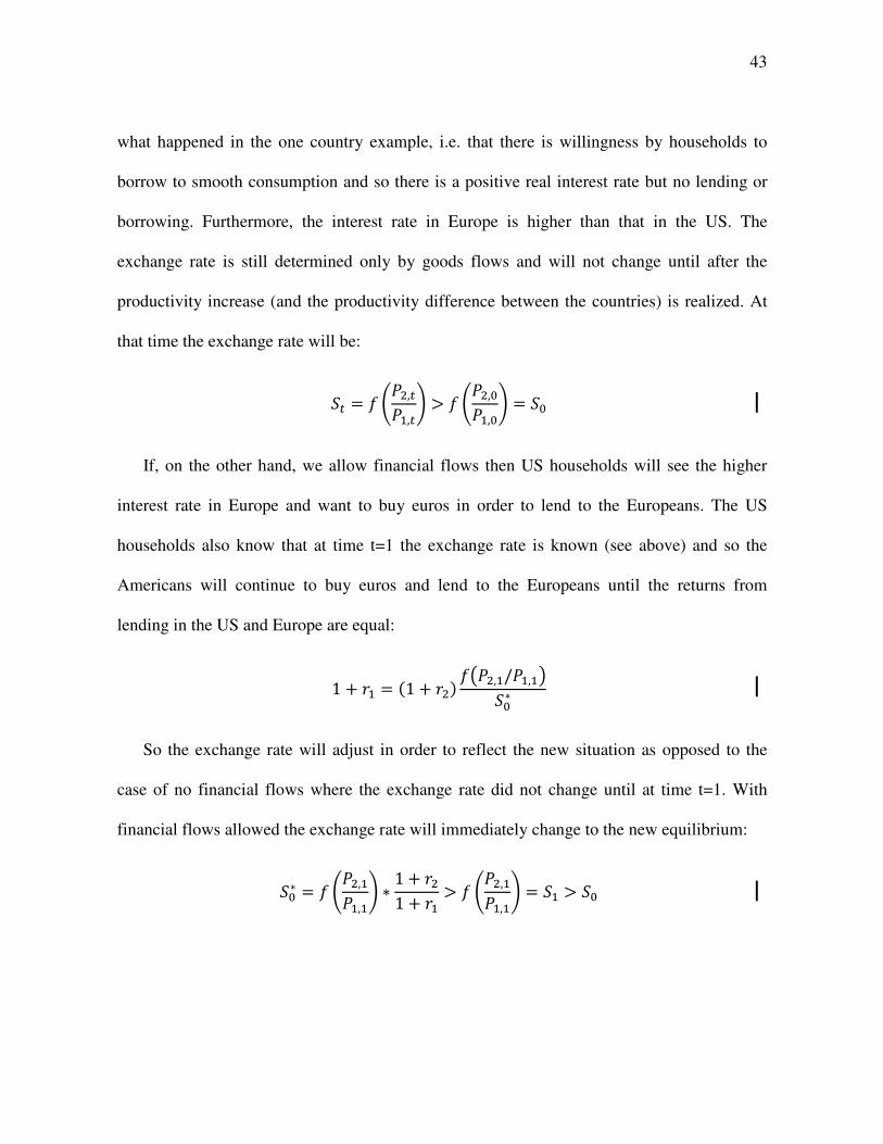
43

what happened in the one country example, i.e. that there is willingness by households to

borrow to smooth consumption and so there is a positive real interest rate but no lending or

borrowing. Furthermore, the interest rate in Europe is higher than that in the US. The

exchange rate is still determined only by goods flows and will not change until after the

productivity increase (and the productivity difference between the countries) is realized. At

that time the exchange rate will be:

(� � = R�J,��,�S T = R�J,��,�S � (�

If, on the other hand, we allow financial flows then US households will see the higher

interest rate in Europe and want to buy euros in order to lend to the Europeans. The US

households also know that at time t=1 the exchange rate is known (see above) and so the

Americans will continue to buy euros and lend to the Europeans until the returns from

lending in the US and Europe are equal:

1 " �� 71 " �J: =&�J,�/��,�*(�∗

So the exchange rate will adjust in order to reflect the new situation as opposed to the

case of no financial flows where the exchange rate did not change until at time t=1. With

financial flows allowed the exchange rate will immediately change to the new equilibrium:

(�∗ � = R�J,��,�S ∗1 " �J1 " �� T = R�J,��,�S � (� T (�

44

In this world of perfect information, no uncertainty and free financial flows the exchange

rate will jump at the arrival of the news and then depreciated in line with the interest rate

differential and so the uncovered interest rate parity holds.

It is worth noting that the interest rates in the free financial flow world need not be, and

in general are not, the same as in the constrained world. As productivity in one of the

countries rises, the income of that country’s population clearly increases and thus the

expected utility does as well. For the other country, whose productivity stays the same, there

is, or at least may be, gains from trade that is split between the two countries. The higher

productivity in one country thus increases the expected utility in the other country. So, when

a future increase is suddenly expected this means that the interest rate in the unchanged

country also goes up, even in the absence of financial flows. With financial flows another

factor contributes to changes in the interest rate. The jump in the exchange rate, above what

is expected to be permanent, makes consumption in the less productive country more

expensive and less expensive in the more productive country, relative to what it is expected

to be. This provides a further incentive for the less productive country to save and the more

productive country to consume and so the interest rate in the less productive country will be

pushed further up and the interest rate in the more productive country goes down.

1.7.2 Enter Uncertainty and Friction

In the world described above the carry trade does not deliver an expected excess returns. In

the world without financial flows there is simply no carry trade possible and if fully free

financial flows are allowed the uncovered interest rate parity holds and so the carry trade

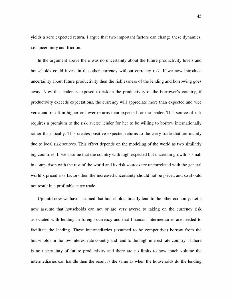
45

yields a zero expected return. I argue that two important factors can change these dynamics,

i.e. uncertainty and friction.

In the argument above there was no uncertainty about the future productivity levels and

households could invest in the other currency without currency risk. If we now introduce

uncertainty about future productivity then the risklessness of the lending and borrowing goes

away. Now the lender is exposed to risk in the productivity of the borrower’s country, if

productivity exceeds expectations, the currency will appreciate more than expected and vice

versa and result in higher or lower returns than expected for the lender. This source of risk

requires a premium to the risk averse lender for her to be willing to borrow internationally

rather than locally. This creates positive expected returns to the carry trade that are mainly

due to local risk sources. This effect depends on the modeling of the world as two similarly

big countries. If we assume that the country with high expected but uncertain growth is small

in comparison with the rest of the world and its risk sources are uncorrelated with the general

world’s priced risk factors then the increased uncertainty should not be priced and so should

not result in a profitable carry trade.

Up until now we have assumed that households directly lend to the other economy. Let’s

now assume that households can not or are very averse to taking on the currency risk

associated with lending in foreign currency and that financial intermediaries are needed to

facilitate the lending. These intermediaries (assumed to be competitive) borrow from the

households in the low interest rate country and lend to the high interest rate country. If there

is no uncertainty of future productivity and there are no limits to how much volume the

intermediaries can handle then the result is the same as when the households do the lending

46

in a certain world. If we now place some restrictions on the intermediaries’ trading the result

is somewhere between those where financial flows are completely free and where they are

not allowed. The currency of the high productivity country will appreciate as some of the

borrowing need is met but not to the level where the financial flows fully dominate the goods

flows.

1.7.3 Going Nominal

So far all the analysis has been in real terms. In reality, however, the vast majority of

currency trading is done in nominal terms and interest rates, particularly in the short term are

nominal. What I argue is needed to take the real analysis from above and extrapolate it to the

nominal world is a “reasonable and sound” monetary policy in the economies involved.

Monetary policy where inflation is very predictable creates an almost one-to-one mapping

between real and nominal interest rates. If the inflation is constant across economies then the

real and nominal interest rates are interchangable but if inflation is highly predictable but

different in levels between economies then one still needs to compare the real interest rates,

i.e. the nominal interest rates minus inflation. Where monetary policy, on the other hand, is

not sound or unpredictable then this should add further to the risk premium of the carry trade.

The monetary policy recipe most often referred to is the one introduced by Taylor (1993)

and since dubbed the “Taylor rule”. If the economy is in balance, i.e. inflation is at its target

level and there is no output gap then the Taylor rule suggests that the nominal policy rate

should simply be the real equilibrium interest rate plus the target inflation. This fits well with

the discussion above. If however inflation is not in line with its target level or current output

is above or below “potential output” there is a monetary element in the interest rate that is not

47

reflecting the underlying equilibrium interest rate and so investing in a currency with a high

monetary element is somewhat different than investing in the equilibrium interest rate.

1.7.4 Implications for the Real Exchange Rate and Real Overpricing

In a world where the financial intermediaries are constrained by the world’s general risk

aversion, for example the VIX, either because they themselves prefer less risk or because

their capacity to absorb the risk is diminished, we have a reasonable framwork that suggests

that high (real) interest rate currencies should be temporarily overvalued in PPP terms. It

would also suggest that this overpricing would depend on the level of the VIX; the lower the

VIX the higher the overpricing should be and so the carry trade should be less profitable

when initiated in low VIX times. This would also suggest that changes to the VIX should be

reflected in the exchange rate and thus affect the carry trade. Empirically this seems to be

true as noted earlier. If all information is reflected in the interested rates and the exchange

rate simply depends perfectly on the interest rates then the real convergence trade should

simply be a mirror image of the carry trade. This is not the case. There of course exists more

relevant information than just the nominal short term interest rate differential between to

currencies and there are frictions. In the financial crisis the VIX spiked, carry trades crashed

and real exchange rates did indeed converge with a large positive return to the real

convergence trades. In general, however, the relationship between the VIX and real

convergence strategies is very weak. There is still an interesting relationship between the

VIX and real overpricing but on a longer horizon. Real exchange rate dispersion is here

defined as the standard deviation of real overpricing of all the currencies at each point in

time. When the real exchange rates are all exactly equal to their long run means the real

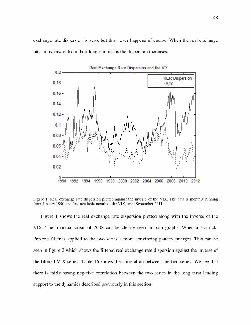
48

exchange rate dispersion is zero, but this never happens of course. When the real exchange

rates move away from their long run means the dispersion increases.

Figure 1. Real exchange rate dispersion plotted against the inverse of the VIX. The data is monthly running from January 1990, the first available month of the VIX, until September 2011.

Figure 1 shows the real exchange rate dispersion plotted along with the inverse of the

VIX. The financial crisis of 2008 can be clearly seen in both graphs. When a Hodrick-

Prescott filter is applied to the two series a more convincing pattern emerges. This can be

seen in figure 2 which shows the filtered real exchange rate dispersion against the inverse of

the filtered VIX series. Table 16 shows the correlation between the two series. We see that

there is fairly strong negative correlation between the two series in the long term lending

support to the dynamics described previously in this section.

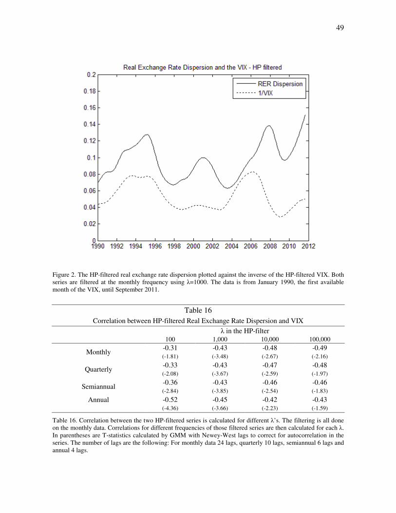
49

Figure 2. The HP-filtered real exchange rate dispersion plotted against the inverse of the HP-filtered VIX. Both series are filtered at the monthly frequency using λ=1000. The data is from January 1990, the first available month of the VIX, until September 2011.

Table 16 Correlation between HP-filtered Real Exchange Rate Dispersion and VIX

λ in the HP-filter

100 1,000 10,000 100,000

Monthly -0.31 -0.43 -0.48 -0.49 (-1.81) (-3.48) (-2.67) (-2.16)

Quarterly -0.33 -0.43 -0.47 -0.48 (-2.08) (-3.67) (-2.59) (-1.97)

Semiannual -0.36 -0.43 -0.46 -0.46 (-2.84) (-3.85) (-2.54) (-1.83)

Annual

-0.52 -0.45 -0.42 -0.43 (-4.36) (-3.66) (-2.23) (-1.59)

Table 16. Correlation between the two HP-filtered series is calculated for different λ’s. The filtering is all done on the monthly data. Correlations for different frequencies of those filtered series are then calculated for each λ. In parentheses are T-statistics calculated by GMM with Newey-West lags to correct for autocorrelation in the series. The number of lags are the following: For monthly data 24 lags, quarterly 10 lags, semiannual 6 lags and annual 4 lags.

50

1.8 Conclusions

Despite being the most heavily traded financial products in the world currencies don’t seem

to incorporate all available information. Using fairly simple signals returns can to some

extent be predicted and profitable trading strategies constructed. This includes seeming

inefficiencies in the short term where recent exchange rate and interest rate changes predict

returns. More interesting are predictions driven by fundamental economic variables such as

the absolute level of the interest rate and the real exchange rate. An argument was presented

in this paper for rationally expected excess returns of the carry trade where risk

diversification is limited between countries as financial intermediators are constrained in

their capacity to transfer and absorb risks. In the simplest view one can imagine that there is a

complete mapping between the interest rates and exchange rates and so the real convergence

strategies presented in this paper should be the mirror image of the carry trade. This turns out

not to be the case. While these strategies are negatively correlated they are in no way

absolute mirror images of each other. Of course the signals used to construct the strategies in

this paper are not perfect. For example the economic rational presented is for the real interest

rate which we do not observe and a “true real exchange rate”, also unobservable.

Nevertheless there seems to be significant information in real exchange rates that is not

captured by interest rates and can thus be used to improve return predictions. The strategies

in this paper are all constructed on the basis of one signal at a time and then combined. This

was done to try to highlight the characteristics of each signal. In reality one would naturally

use the combination of signals and use that directly to construct portfolios.

51

An interesting pattern is also shown between the deviations of real exchange rates from

their long run means and the VIX volatility index. In times when the VIX is high, real

exchange rates tend to be closer to their long run means and vice versa which lends support

to the idea of limits to arbitrage and risk sharing between countries.

2 Bayesian Modeling of Conditional Return Distributions

2.1 Introduction

The mean and variance of return distributions have for the most parts been the focus of asset

pricing literature. Indeed the fundamental CAPM framework developed by Sharpe (1964)

and Lintner (1965) is based on these two moments. Already in 1976, however, skewness was

introduced by Kraus and Litzenberger (1976) into a three moment capital asset pricing

model. That inclusion of skewness in asset pricing rests on the fact that investors with

concave utility functions have a preference for positive skewness. More recently there has

been an increase in empirical research of crash risks and negative skewness, often in a

conditional sense. Indeed Harvey and Siddique (2000) present a three-moment conditional

CAPM, extending Kraus and Litzenberger’s work on the conditionality. Chen, Hong and

Stein (2000) analyze the predictors of conditional skewness of individual stocks and find that

high recent trading volume and high recent past returns predict negative skewness.

Charonerook and Daouk (2008) strengthen these findings by demonstrating that past returns

of stock indices across the world negatively predict skewness, both do positive past returns

predict negative skewness and negative returns predict positive skewness. The sources for

this conditional skewness are less obvious. Hong and Stein (2003) argue that investor

52

heterogeneity is the key to the conditional skewness. Investors have asymmetric information

and some investors face short-selling constraints. Under these circumstances, the authors

argue, negative information is not adequately reflected in prices as only some of the investors

have the negative information but are unable to trade on them. So when stock prices go up,

those who have negative information sell whatever stocks they have but no more. Thus high

returns and turnover have occurred while the negative information looms and causes the

conditional skewness. In the international finance literature crash risks and negative

skewness have also been highlighted recently, most notably by Brunnermeier et al. (2009).

They emphasize the role of liquidity and rapidly unwinding positions as key driver of

negative skewness and trades that a lot of leveraged investors have positions in are

vulnerable in the face of such liquidity risks. They use the interest rate of currencies as the

conditioning variable to predict skewness; carry traders have leveraged positions in high

interest rate currencies and those positions get liquidated when risk aversion increases.

Torfason (2012) extends this analysis by demonstrating that real exchange rates are also

central to predicting skewness, and in some sense even more so than interest rates.

This paper’s focus is not so much on why conditional skewness exists but rather how to

model conditional skewness in the data. The idea at the back of the author’s mind is,

however, one of rapid reversion to some fundamental characteristics. This could be caused

by overoptimism, bubbles, or pessimism or it could be caused by high expectations about the

future which may be considered likely to come true but in the unlikely case that these

expectations fail to be realized a sharpe price reduction occurs. In the case of exchange rates

the idea is very close to that of Brunnermeier et al.’s. High interest rate currencies represent

53

expectations of rapid growth that investors in other countries can invest in and thus drive

currencies away from their fundamental goods and services driven exchange rate. If the

ability or willingness of investors is reduced by, for example, a rise in risk aversion they exit

their positions and the currency experiences rapid depreciation.

The model introduced in the paper is tested on two sets of data. First there is currency

data conditioning on real exchange rates and secondly market-to-book ratios of stocks are

used as conditioning variables for stock returns. In that case the assets used are the Fama-

French book-to-market assets are used. In short the model is succesful in capturing the

conditional skewness and indeed also conditional returns. The model, a mixture of normals,

is estimated using Markov chain Monte Carlo methods.

2.2 Model

While the conditioning variable in the model could in theory be anything the discussion in

this paper focuses on some form of “overpricing”, an indicator of how far the current price of

the asset is from the “fundamental value”.

2.2.1 Mixture of Normals

To characterize the distribution of returns or price changes it is natural to start with the

normal distribution. The normal distribution does, however, fail to describe price movements

of many asset prices in two main ways. First, the normal distribution is symmetric and so

does not allow for skewness. Secondly, the distributions of asset price movements generally

exhibit higher kurtosis then the normal distribution does, i.e. the tails are fatter. The model I

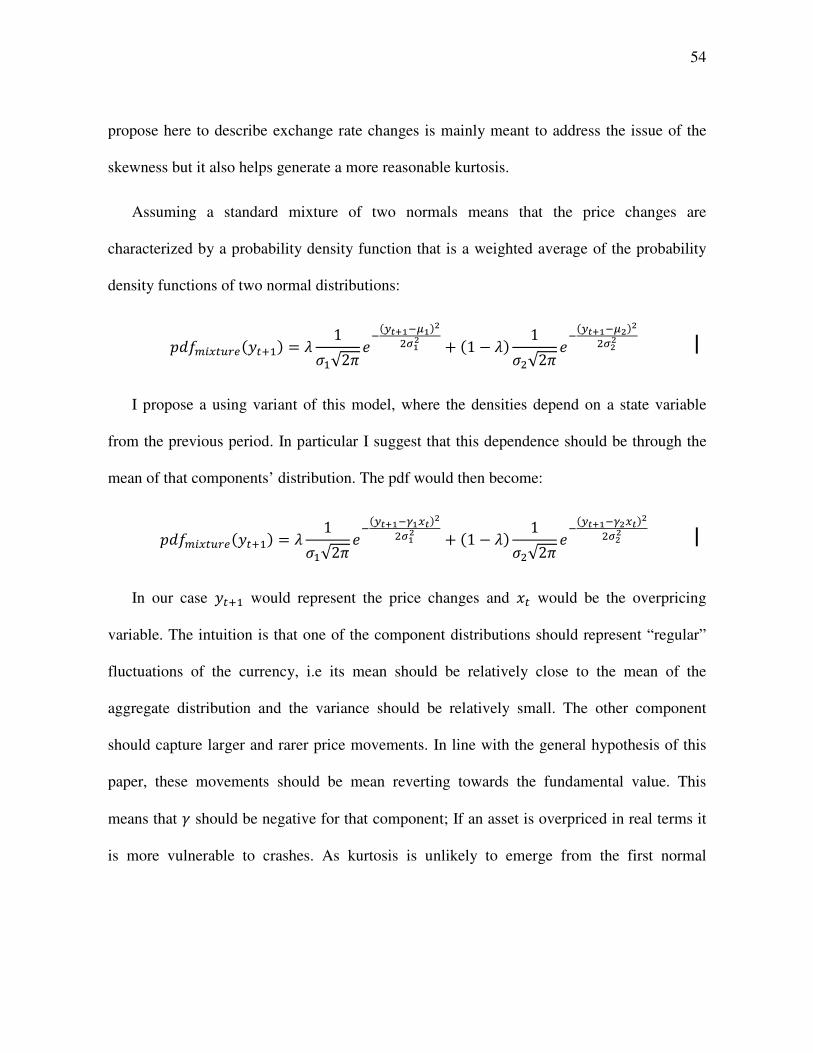
54

propose here to describe exchange rate changes is mainly meant to address the issue of the

skewness but it also helps generate a more reasonable kurtosis.

Assuming a standard mixture of two normals means that the price changes are

characterized by a probability density function that is a weighted average of the probability

density functions of two normal distributions:

�U=VWD�Q>@7 �X�: � Y 1Z�√2\

�7B]^_�`_:aJb_a " 71 � Y: 1ZJ√2\

�7B]^_�`a:aJbaa

I propose a using variant of this model, where the densities depend on a state variable

from the previous period. In particular I suggest that this dependence should be through the

mean of that components’ distribution. The pdf would then become:

�U=VWD�Q>@7 �X�: � Y 1Z�√2\

�7B]^_�c_D]:aJb_a " 71 � Y: 1ZJ√2\

�7B]^_�caD]:aJbaa

In our case �X� would represent the price changes and �� would be the overpricing

variable. The intuition is that one of the component distributions should represent “regular”

fluctuations of the currency, i.e its mean should be relatively close to the mean of the

aggregate distribution and the variance should be relatively small. The other component

should capture larger and rarer price movements. In line with the general hypothesis of this

paper, these movements should be mean reverting towards the fundamental value. This

means that d should be negative for that component; If an asset is overpriced in real terms it

is more vulnerable to crashes. As kurtosis is unlikely to emerge from the first normal

55

component, one would expect the standard deviation of the second component to also capture

some of the kurtosis in general and so we expect ZJ to be bigger than Z�.

An example of how a mixture of this kind could look like can be seen on figure 3. In this

example the asset is “overpriced” in (has a high ��) and so the second component has a

negative mean, the mixture distribution is negatively skewed and the tails are fatter than for a

normal distribtuion, both because the mean of the second component is different from that of

the first but more importantly because the variance of the second component is much higher

than that of the first component.

Figure 3: An example of a mixture of normals. One component has zero mean and a low standard deviation. The other has a negative mean and a high standard deviation. The resulting mixtur is a negatively skewed distribution with a slightly negative mean and some excess kurtosis.

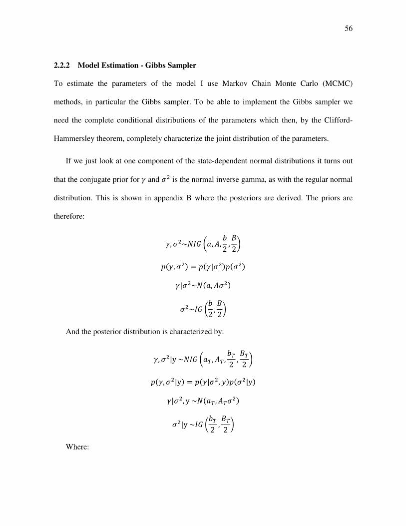
56

2.2.2 Model Estimation - Gibbs Sampler

To estimate the parameters of the model I use Markov Chain Monte Carlo (MCMC)

methods, in particular the Gibbs sampler. To be able to implement the Gibbs sampler we

need the complete conditional distributions of the parameters which then, by the Clifford-

Hammersley theorem, completely characterize the joint distribution of the parameters.

If we just look at one component of the state-dependent normal distributions it turns out

that the conjugate prior for d and ZJ is the normal inverse gamma, as with the regular normal

distribution. This is shown in appendix B where the posteriors are derived. The priors are

therefore:

d, ZJ~fg h�, i, j2 , k2l

�7d, ZJ: � �7d|ZJ:�7ZJ: d|ZJ~f7�, iZJ: ZJ~g hj2 , k2l

And the posterior distribution is characterized by:

d, ZJ|y~fg h�o , io , jo2 , ko2 l

�7d, ZJ|y: � �7d|ZJ, :�7ZJ|y: d|ZJ, y~f7�o , ioZJ: ZJ|y~g hjo2 , ko2 l

Where:

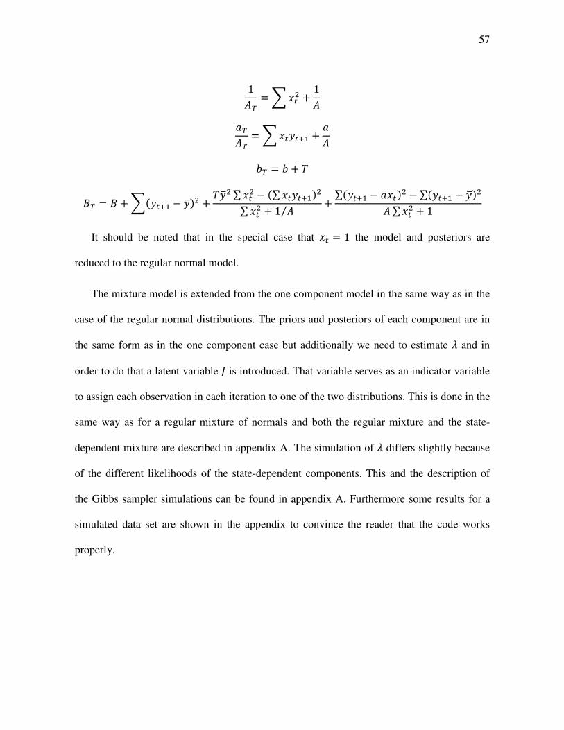
57

1io �p��J " 1i

�oio � p�� X� " �i

jo � j " q

ko � k "p7 �X� � r:J " q rJ∑��J � 7∑�� X�:J∑��J " 1 i⁄ " ∑7 �X� � ��:J � ∑7 �X� � r:Ji∑��J " 1

It should be noted that in the special case that �� 1 the model and posteriors are

reduced to the regular normal model.

The mixture model is extended from the one component model in the same way as in the

case of the regular normal distributions. The priors and posteriors of each component are in

the same form as in the one component case but additionally we need to estimate Y and in

order to do that a latent variable u is introduced. That variable serves as an indicator variable

to assign each observation in each iteration to one of the two distributions. This is done in the

same way as for a regular mixture of normals and both the regular mixture and the state-

dependent mixture are described in appendix A. The simulation of Y differs slightly because

of the different likelihoods of the state-dependent components. This and the description of

the Gibbs sampler simulations can be found in appendix A. Furthermore some results for a

simulated data set are shown in the appendix to convince the reader that the code works

properly.

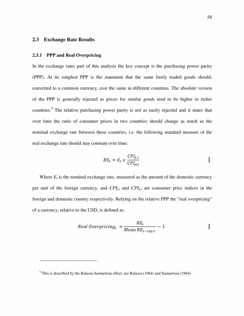
58

2.3 Exchange Rate Results

2.3.1 PPP and Real Overpricing

In the exchange rates part of this analysis the key concept is the purchasing power parity

(PPP). At its simplest PPP is the statement that the same freely traded goods should,

converted to a common currency, cost the same in different countries. The absolute version

of the PPP is generally rejected as prices for similar goods tend to be higher in richer

countries.9 The relative purchasing power parity is not as easily rejected and it states that

over time the ratio of consumer prices in two countries should change as much as the

nominal exchange rate between these countries, i.e. the following standard measure of the

real exchange rate should stay constant over time:

�� ,��,�

Where Et is the nominal exchange rate, measured as the amount of the domestic currency

per unit of the foreign currency, and CPIf,t and CPId,t are consumer price indices in the

foreign and domestic country respectively. Relying on the relative PPP the “real overpricing”

of a currency, relative to the USD, is defined as:

� �� :� � 1

9 This is described by the Balassa-Samuelson effect, see Balassa (1964) and Samuelson (1964)

59

Real overpricing is therefore defined as how far the current real exchange rate is above its

10 year mean, which is intended to capture a long term fundamental value that the real

exchange rate will revert to. The relative PPP does not provide a particular insight as to how

the mean reversion should happen, but that is important for market participants exposed to

risks in the currencies. The hypothesis of this paper is that these mean reversions tend to be

rapid, implying a negative skewness for overpriced currencies (in our real sense).

2.3.2 Data

The data used are for the G10 currencies and dates from October 1986 to September 2011.10

The data are weekly and returns are calculated from forward rates. These data come from

Datastream. Consumer price indices are only available monthly and, in the cases of Australia

and New Zealand, only quarterly. The data ares interpolated to facilitate the weekly

calculation of the real exchange rate. The CPI data are also used with a lag as the CPI

numbers are observed with a lag in reality.

Exchange rates are generally quoted against the US dollar. If the analysis would be done

with all currencies’ returns calculated against the dollar, however, the dollar would be central

to the analysis as innovation to the dollar would feed into all of the other results. In order to

avoid this effect a basket of currencies is introduced. The basket is constructed by investing

one dollar evenly in the ten currencies. The returns of that investment define the returns of

the basket. The position in each currency is then taken against this basket and so the dollar no

10 The G10 currencies are the US, Australian, Canadian and New Zealand dollars, the Swedish and Norwegian krone, the Swiss franc the British Pound, the Japanese yen and the Euro (which, before 1999, is spliced using the Deutsche Mark).

60

longer plays a bigger role in a currency’s return than all the other currencies. The real

overpricing variable of the basket (against the dollar) is taken to be the mean of the

overpricing of the ten currencies and the overpricing of each currency is then its real

overpricing against the dollar divided by the real overpricing of the basket against the dollar.

2.3.3 Setup and Priors

The data that we are looking at is weekly return data of currencies and as noted in the data

section, the returns are measured against a basket of currencies. For each return data point

( �X�: there is a respective real overpricing data point (��:, measured at the end of the period

previous to the return. Both the return data and the overpricing data is therefore in panel

form. In the estimation the data are stacked into one time series.

As noted above, the intuition for the distribution of the data is that one component

represents regular daily fluctuations of the currencies, with a mean relatively close to zero.

The other component should, on the other hand, represent more infrequent but larger

movements and presumably in the mean reverting direction, i.e. in negative proportion to the

real overpricing of the currencies. This view is introduced into the priors in the way that the

prior for the standard deviation of the second component has a higher mean and variance

than that of the first component. The dispersion of these priors is also such that they do put

very little weight on absurdly high variances. The prior for Y also incorporates the view that

the first component is more likely to govern the returns than the second. For the d’s we don’t

want to impose too much and therefore I allow very disperse priors for those with mean zero.

So the priors strongly encourage the separation into a high-volatility and low-volatity

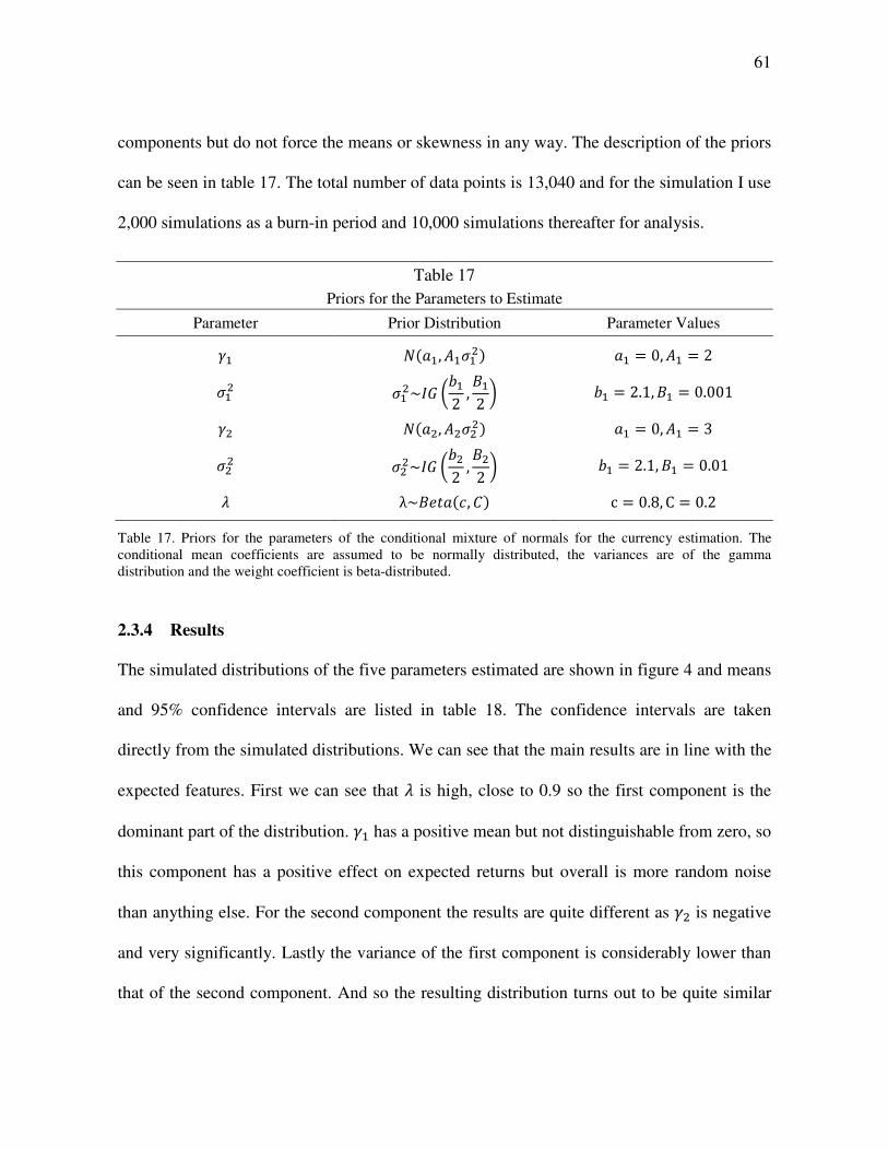
61

components but do not force the means or skewness in any way. The description of the priors

can be seen in table 17. The total number of data points is 13,040 and for the simulation I use

2,000 simulations as a burn-in period and 10,000 simulations thereafter for analysis.

Table 17 Priors for the Parameters to Estimate

Parameter Prior Distribution Parameter Values

d� f7��, i�Z�J: �� 0,i� � 2

Z�J Z�J~g hj�2 , k�2 l j� � 2.1, k� � 0.001

dJ f7�J, iJZJJ: �� 0,i� � 3

ZJJ ZJJ~g hjJ2 , kJ2 l j� � 2.1, k� � 0.01

Y λ~k !�7�, �: c � 0.8, C � 0.2

Table 17. Priors for the parameters of the conditional mixture of normals for the currency estimation. The conditional mean coefficients are assumed to be normally distributed, the variances are of the gamma distribution and the weight coefficient is beta-distributed.

2.3.4 Results

The simulated distributions of the five parameters estimated are shown in figure 4 and means

and 95% confidence intervals are listed in table 18. The confidence intervals are taken

directly from the simulated distributions. We can see that the main results are in line with the

expected features. First we can see that Y is high, close to 0.9 so the first component is the

dominant part of the distribution. d� has a positive mean but not distinguishable from zero, so

this component has a positive effect on expected returns but overall is more random noise

than anything else. For the second component the results are quite different as dJ is negative

and very significantly. Lastly the variance of the first component is considerably lower than

that of the second component. And so the resulting distribution turns out to be quite similar

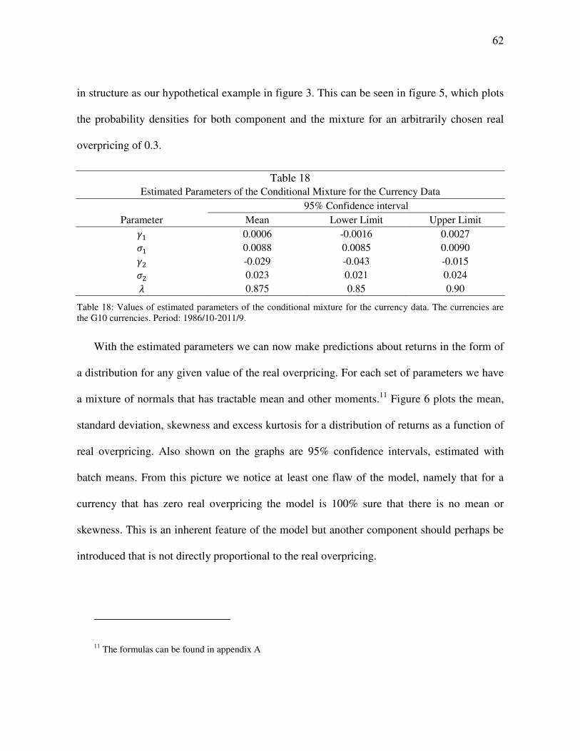
62

in structure as our hypothetical example in figure 3. This can be seen in figure 5, which plots

the probability densities for both component and the mixture for an arbitrarily chosen real

overpricing of 0.3.

Table 18 Estimated Parameters of the Conditional Mixture for the Currency Data 95% Confidence interval

Parameter Mean Lower Limit Upper Limit d� 0.0006 -0.0016 0.0027 Z� 0.0088 0.0085 0.0090 dJ -0.029 -0.043 -0.015 ZJ 0.023 0.021 0.024 Y 0.875 0.85 0.90

Table 18: Values of estimated parameters of the conditional mixture for the currency data. The currencies are the G10 currencies. Period: 1986/10-2011/9.

With the estimated parameters we can now make predictions about returns in the form of

a distribution for any given value of the real overpricing. For each set of parameters we have

a mixture of normals that has tractable mean and other moments.11 Figure 6 plots the mean,

standard deviation, skewness and excess kurtosis for a distribution of returns as a function of

real overpricing. Also shown on the graphs are 95% confidence intervals, estimated with

batch means. From this picture we notice at least one flaw of the model, namely that for a

currency that has zero real overpricing the model is 100% sure that there is no mean or

skewness. This is an inherent feature of the model but another component should perhaps be

introduced that is not directly proportional to the real overpricing.

11 The formulas can be found in appendix A

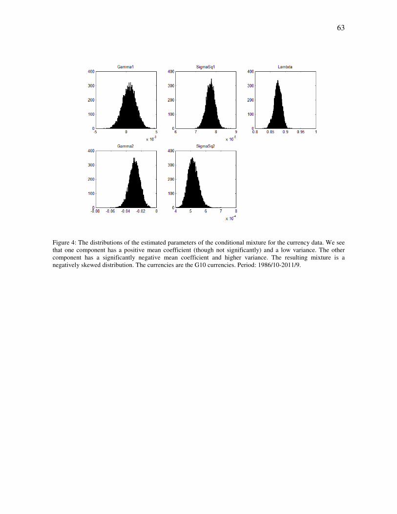
63

Figure 4: The distributions of the estimated parameters of the conditional mixture for the currency data. We see that one component has a positive mean coefficient (though not significantly) and a low variance. The other component has a significantly negative mean coefficient and higher variance. The resulting mixture is a negatively skewed distribution. The currencies are the G10 currencies. Period: 1986/10-2011/9.

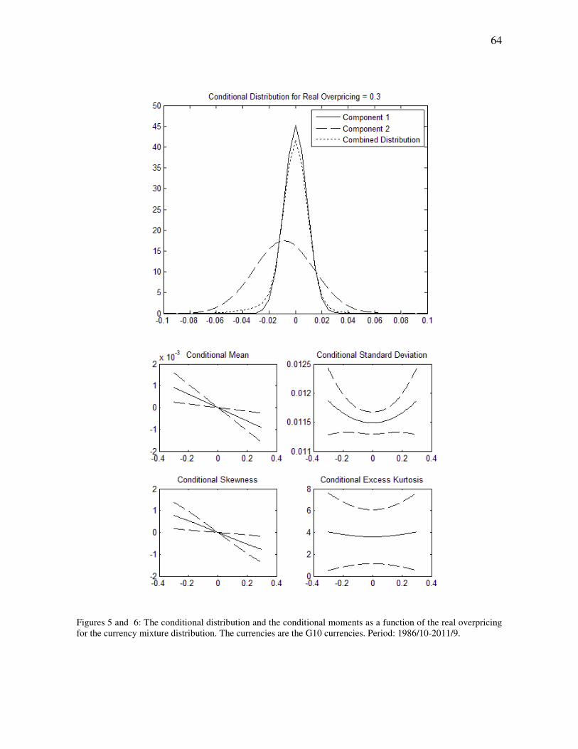
64

Figures 5 and 6: The conditional distribution and the conditional moments as a function of the real overpricing for the currency mixture distribution. The currencies are the G10 currencies. Period: 1986/10-2011/9.

65

2.4 Stock Results

2.4.1 Data

For the stock analysis the data set used is the ten decile book-to-market sorted portfolios

constructed by Fama and French and is retrieved from Kenneth French’s website. The return

data, whose distribution we are seeking to characterize, are monthly from July 1926 to June

2011. The conditioning variable, the book-to-market, or rather the market-to-book as it is

used in the analysis, is only available annually. The book-to-market ratios in the data are

calculated at the end of June from the book value at the end of the preceding year and the

current stock price. In order to get monthly data for the market-to-book it is therefore

necessary to interpolate the data in some way. Assuming a constant ratio over the year would

be a possible way to go but this approach would fail to incorporate price changes during the

year, which may be important in the conditioning. Therefore each portfolio’s market-to-book

ratio is multiplied by the cumulative return of that portfolio from the latest June. Since

returns are on average positive this would lead to a within-year drift of the ratio, which

would be higher just before new book value data is introduced. To rectify this it is assumed

that the book value for each decile portfolio grows constantly by the average return over the

whole sample period. This is of course not true but it is still a decent approximation for the

book value. It is also the market price that drives variation of the market-to-book ratio in the

short run, which makes the inaccuracy of the assumption less important. Furthermore the

actual conditioning variable, ��, is defined to be the demeaned market-to-book ratio, i.e. the

market-to-book ratio of the relevant portfolio minus the mean of all the portfolios at that

point in time. This gives us a conditioning variable that is zero on average.

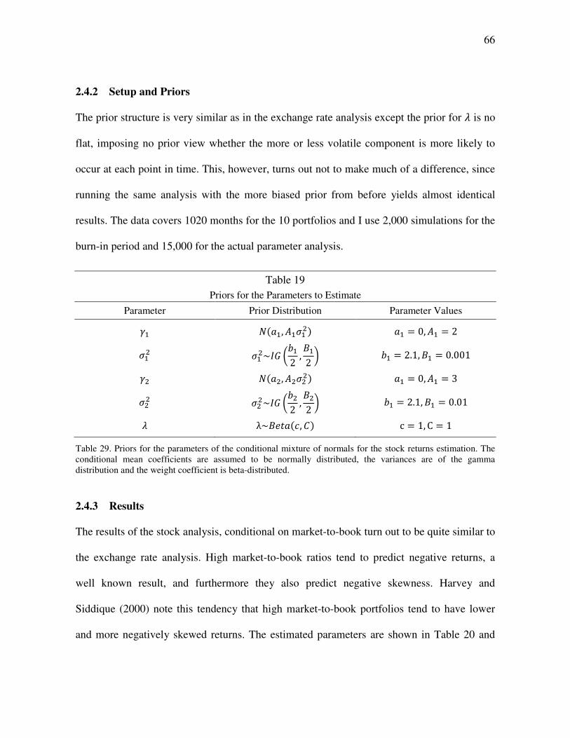
66

2.4.2 Setup and Priors

The prior structure is very similar as in the exchange rate analysis except the prior for Y is no

flat, imposing no prior view whether the more or less volatile component is more likely to

occur at each point in time. This, however, turns out not to make much of a difference, since

running the same analysis with the more biased prior from before yields almost identical

results. The data covers 1020 months for the 10 portfolios and I use 2,000 simulations for the

burn-in period and 15,000 for the actual parameter analysis.

Table 19 Priors for the Parameters to Estimate

Parameter Prior Distribution Parameter Values

d� f7��, i�Z�J: �� 0,i� � 2

Z�J Z�J~g hj�2 , k�2 l j� � 2.1, k� � 0.001

dJ f7�J, iJZJJ: �� 0,i� � 3

ZJJ ZJJ~g hjJ2 , kJ2 l j� � 2.1, k� � 0.01

Y λ~k !�7�, �: c � 1, C � 1

Table 29. Priors for the parameters of the conditional mixture of normals for the stock returns estimation. The conditional mean coefficients are assumed to be normally distributed, the variances are of the gamma distribution and the weight coefficient is beta-distributed.

2.4.3 Results

The results of the stock analysis, conditional on market-to-book turn out to be quite similar to

the exchange rate analysis. High market-to-book ratios tend to predict negative returns, a

well known result, and furthermore they also predict negative skewness. Harvey and

Siddique (2000) note this tendency that high market-to-book portfolios tend to have lower

and more negatively skewed returns. The estimated parameters are shown in Table 20 and

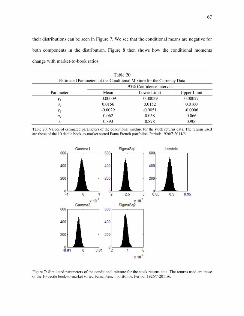
67

their distributions can be seen in Figure 7. We see that the conditional means are negative for

both components in the distribution. Figure 8 then shows how the conditional moments

change with market-to-book ratios.

Table 20 Estimated Parameters of the Conditional Mixture for the Currency Data 95% Confidence interval

Parameter Mean Lower Limit Upper Limit d� -0.00009 -0.00039 0.00027 Z� 0.0156 0.0152 0.0160 dJ -0.0029 -0.0051 -0.0006 ZJ 0.062 0.058 0.066 Y 0.893 0.878 0.906

Table 20: Values of estimated parameters of the conditional mixture for the stock returns data. The returns used are those of the 10 decile book-to-market sorted Fama French portfolios. Period: 1926/7-2011/6.

Figure 7: Simulated parameters of the conditional mixture for the stock returns data. The returns used are those of the 10 decile book-to-market sorted Fama French portfolios. Period: 1926/7-2011/6.

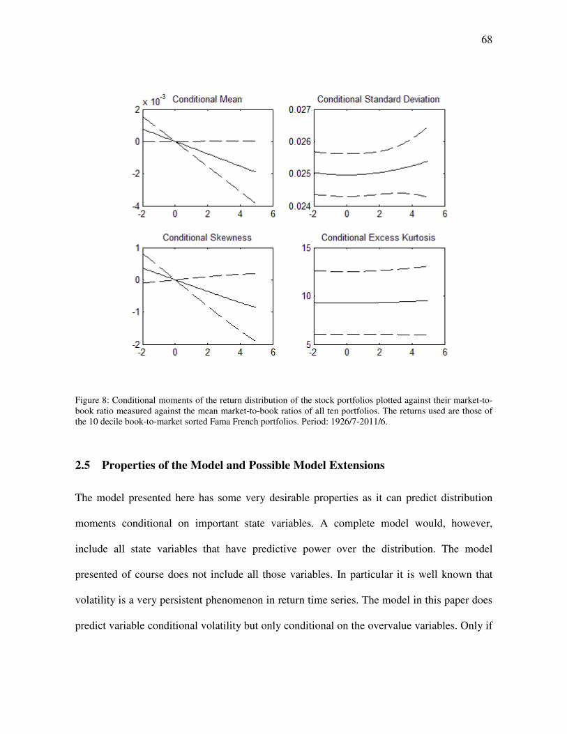
68

Figure 8: Conditional moments of the return distribution of the stock portfolios plotted against their market-to-book ratio measured against the mean market-to-book ratios of all ten portfolios. The returns used are those of the 10 decile book-to-market sorted Fama French portfolios. Period: 1926/7-2011/6.

2.5 Properties of the Model and Possible Model Extensions

The model presented here has some very desirable properties as it can predict distribution

moments conditional on important state variables. A complete model would, however,

include all state variables that have predictive power over the distribution. The model

presented of course does not include all those variables. In particular it is well known that

volatility is a very persistent phenomenon in return time series. The model in this paper does

predict variable conditional volatility but only conditional on the overvalue variables. Only if

69

volatility is generally due to this conditioning variable would the model capture the

persistence in volatility. We can test this in the following way. At each point in time we can

calculate the conditional mean, |}, and standard deviation, Z}, of returns for each asset. From

those we can then form standardized errors:

.�X� � �X� � |}Z}

And then we can run the regression of the squared standardized error on its own lag:

.�X�J � # " $.�J " ~�X�

Under the null, that all relevant information about volatility is captured by the

conditioning variable $ should be zero. When running this regression on the two data sets,

this is quite clearly not the case.

Table 21

Autocorrelation of the Standardized Errors

Currency Data Stock Data

$ 0.20 0.27 T-Statistic (6.86) (5.16)

Table 21. Autocorrelation of squared standardized errors. Both are very autocorrelated implying a persistence in volatility not captured in the model.

So, taking this model to usage it would probably need to be extended to include

correlation in volatility. This could be done by conditioning the volatility parameters on some

measure of past volatility, either some form of the squared standardized error over the last

period or last within-period daily volatility. One could also make Y, the parameter that

determines the probability of being in each component of the mixture, dependent on the the

70

overvalue. It is entirely conceivable that not only is the size of potential crashes dependent on

the overvalue but also the probability of those crashes occurring.

2.6 Conclusions

In this paper I have modelled asset returns as mixtures of normals that allow for the mean

and skewness to depend on a state variable such as real overpricing of currencies and the

market-to-book ratio of stock portfolios. The model clearly demonstrates how the mean and

skewness of returns depend very much on these variables. The model allows to estimate the

distribution of returns going forward at each point in time, conditional on the state variables,

which can be very useful in practice.

3 Iceland’s Economic Eruption and Meltdown

3.1 Introduction

In 2007 the financial crises hit the world economy. Nowhere, however, did it strike as

fiercely as in the remote island state of Iceland, a nation of only 300,000 inhabitants. In

Iceland the entire banking system, which had vastly outgrown the country’s economy in just

a few years, collapsed in a two-week period. A currency crisis ensued, and the country

entered into a rescue program with the International Monetary Fund and imposed strict

capital constraints.

The key objective of this paper is to shed light on the causes of the abrupt meltdown of

the Icelandic economy. In order to do so, we describe the dramatic ascent of the country’s

banking system following bank privatization and liberalization, as well as the economic

71

boom in the economy in general. In our discussion we highlight the risks that were being

built up in the financial system and try to understand the climate, politically and

economically, that allowed for the banking system’s extraordinary growth and the build-up

of these risks to unmanagable proportions. The focus is thus on identifying the overall

catastrophic causes of the financial collapse and on drawing conclusions on how these

missteps could have been avoided.

The Icelandic crisis was both a currency- and a banking crisis, as generally described by

Kaminsky and Reinhart (1999) and dubbed “Twin crises”. Kaminsky and Reinhart give an

overview of a number of such crises in the last few decades, often in developing economies

but also in more advanced countries, as with the crises in Norway, Sweden and Finland in the

late 1980s and early 1990s. As Demirgüç-Kunt and Detragiache (1999) find, banking crises

are more common in countries that have liberalized their financial systems. These findings

provide a framework in which the Icelandic crisis can be analyzed, and we revisit these ideas

throughout the paper in our effort to identify the key factors that led to the crisis. We also

attempt to describe how these key factors interacted and, in particular, how the Icelandic

crisis provides an insight into the interaction between banking and currency problems.

A number of studies by industry or academics were written on particular aspects of the

Icelandic economy in the midst of the financial boom. This paper reviews and draws out the

main arguments and conclusions of these studies in order to give a compact overview of the

main factors that were associated with the collapse. Thus, with the benefit of hindsight, this

paper strives to give a more concise overview of the main catastrophic causes of the

Icelandic financial collapse than previously offered. At the dawn of the crisis, the first

72

writings on the topic were produced by e.g. the International Monetary Fund, the

Organization of Economic Cooperation and Development and several foreign banks and

rating agencies.12 Most of these reports highlighted a negative outlook on the Icelandic

economy, but were later questioned by other studies. Most notably, the Iceland Chamber of

Commerce commissioned two pairs of academics to analyze the economic outlook, which

resulted in two reports arguing the contrary and finding previous reports to be misleading.13

One of the Icelandic banks also approached Buiter and Sibert (2008) to analyze the Icelandic

financial system, but as the report was quite critical the paper was not made public until after

the collapse. The same year, Gros (2008) produced a report critical of the large increase in

the foreign assets and liabilities of the Icelandic banks, and Gylfason (2008) highlighted the

banks’ dubious business model, which he concisely described as using an implicit state

guarantee to borrow huge amounts internationally to lend domestically at higher rates of

interest. Daníelsson and Zoëga (2009) then provided one of the first post-collapse

descriptions of the rise and fall of the Icelandic banking system. Our paper builds on and

highlights the main conclusions from these studies – and numerous others – in order to give a

complete overview of this boom-bust era and the concurrent analysis of the situation by both

academics and practitioners. In order to keep the discussion concise and to the point,

previous studies on the topic will be periodically revisited throughout the paper and

discussed in the relevant context of their contributions. Lastly, it should also be noted that

12 IMF (2005, 2006, 2007), OECD (2005, 2006, 2008), Merrill Lynch (2006), Christensen and Valgreen (2006), Fitch (2006).

13 Mishkin and Herbertsson (2006), Portes and Baldursson (2007).

73

most of the detailed writings on the topic have so far only been available in Icelandic. For

example, the paper draws to a large extent on the work of a Special Investigation

Commission, which was established in 2008 by the Icelandic parliament to investigate and

analyze the events leading to the collapse of the three main banks in Iceland.14 Our paper

highlights the main findings from the report produced by the Commission, which was

completed and delivered to the Icelandic parliament in April 2010 (consisting of more than

2300 pages, which to date is only fully available in Icelandic). In short, our paper contributes

to the literature by providing a coherent collection of the key events that led to the Icelandic

banking collapse and thereby provides an overview of the pitfalls to be avoided by other fast-

growing economies.

The paper discusses the events leading to the collapse in the order that they occurred.

Thus, the paper proceeds by first setting the stage in section 2 and providing a brief historical

background on the Icelandic economy. This includes the financial liberalization process of

the 1990’s and the following bank privatization process that paved the way for future growth.

Next, section 3 describes the boom period in terms of the excessive growth of the banks (3.1)

and the macro-economic factors that contributed the economic imbalances of the country

(3.2). Further, the build-up of risk and lack of prudence inside the banks (3.3) are also

discussed as contributing factors to the collapse. Section 4 describes how the crisis unfolded

and the institutional weaknesses revealed throughout the collapse. Finally, section 5

concludes.

14 Special Investigation Commission (2010).

74

3.2 Setting the Stage

Historically the Icelandic economy was rather simple and isolated, having been built around

its fishing industry. As Daníelsson and Zoëga note, the Icelandic economy had traditionally

been more regulated and politicized than in the neighboring countries, it was more based on

discretion than rules, and private sector firms were tightly connected with the political

parties. The capital markets were also heavily controlled by the government until the 1980’s

when interest rates were gradually liberalized. Then, in the early 1990’s the economy opened

up for cross-border capital movements in connection with Iceland’s entrance into the

European Economic Area in 1994. Iceland has long had an independent currency (the krona)

and in the last decades of the 20th century it followed an adjustable peg; or as argued by

Guðmundsson et al. (2000), it could rather be characterized as a “managed float” regime

where devaluations were frequent. In the 1990’s, with increasingly free capital movements,

the krona was allowed to float within a band, which was periodically widened. At the turn of

the century, a new monetary policy was deemed appropriate and in 2001 legislation was

passed that gave the Central Bank instrument independence to pursue an inflation targeting

policy.

Bank privatization

As the Icelandic economy was opening up to free flow of foreign capital in and out of the

country and a new monetary policy was being adopted, the banking sector was undergoing

dramatic changes. Central to this transformation were four banks. The biggest Icelandic bank

at the turn of the century was Islandsbanki (later Glitnir), which had recently been formed

75

through a merger of a number of smaller banks. Two other commercial banks, Landsbanki

and Bunadarbanki, were government-owned, and finally Kaupthing was a growing

investment bank. A decision was made by the government in 1997 to privatize Landsbanki

and Bunadarbanki, and in the following years shares were sold to the public in public

offerings. The government’s share in the banks was also reduced through mergers where the

banks issued stock to pay for acquisitions. The sale of the banks was finalized in January

2003 when the government’s remaining share of 45.8% in each bank was sold.15 Unlike the

previous public offerings, these remaining holdings were sold in bulk sales. One investment

group, Samson, bought the government’s entire holdings in Landsbanki and another, the ‘S-

Group’, bought the Bunadarbanki holdings.

The final bulk sale has been widely criticized and allegations made that the buyers of the

banks were chosen on a political basis. For example, Wade and Sigurgeirsdottir (2011) note

that the sale “…excluded foreign buyers, and favored nationals with good connections in the

Independence Party and the Progressive Party, the governing coalition at the time”.

Gylfason (2008) and Gylfason et al. (2010) take an even stronger stance, respectively

describing the privatization process as ‘Iceland became Russia’ and ‘privatization among

friends’. Furthermore the report of the Special Investigation Commission (2010) supports the

critical view of the privatization. As noted in that report, Steingrímur Ari Arason was the

finance minister’s representative in the privatization committee until he resigned his position

in late 2002 after serving on the committee from its start in 1991. Arason made serious

15 A press release with the details of these sales can be found on the website of the Ministry of Industry, Energy and Tourism: http://www.idnadarraduneyti.is/frettir/frettabref/nr/1043.

76

objections to how these sales were conducted, saying he was “99.9% sure that [the two party

leaders of the government coalition] decided to sell both banks at the same time, to enter into

discussions with the S-Group about the purchase of Bunadarbanki and the Samson-group

about the purchase of Landsbanki”.16 The report also reveals an e-mail from an employee of

HSBC, which served as the government’s advisor, to an employee of the government’s

privatization committee wherein he said: “By defining the criteria and weighting carefully, it

is possible to arrive at the “right” result in selecting the preferred party, whilst having a

semi-scientific justification for the decision that will withstand external critical scrutiny”.17

The Special Investigation Commission concludes that the initial criteria and stated goals of

the sales were “unstable”, that requirements were repeatedly relaxed and political objectives

of finalizing the sale before elections in the spring of 2003 became increasingly dominant.18

In the spring of 2003, a few months after the government’s sale of Bunadarbanki, the

bank merged with the investment Kaupthing. Under the latter name it would, along with

Landsbanki and Glitnir, become one of Iceland’s three big international banks. In 2003 all

three banks were publicly listed companies, but all had a similar ownership structure where

one or two large shareholders controlled around 40% of the bank and the rest was dispersed

among smaller investors.

16 Special Investigation Commission (2010), ch. 6.3, p. 267. Davíð Oddsson, then prime minister, and Halldór Ásgrímsson, then foreign minister, led the Independence Party and the Progressive Party, respectively. The quote is based on authors’ own translation.

17 Special Investigation Commission (2010), ch. 6.3, p. 263.

18 Special Investigation Commission (2010), ch. 6.6, pp. 300-302.

77

Opening up to the global capital markets

In brief, as Iceland entered the 21st century it was opening up to the forces of global and free

capital markets. But financial liberalization comes with additional economic risks, previously

unfamiliar to the relatively closed and regulated Icelandic economy. Stiglitz (2001) addresses

the risks facing small open economies and in particular how Iceland faced these risks at the

time. Stiglitz warns of the potential effects of full capital account liberalization, the risks of

credit growth and how unhedged foreign denominated firm debt could turn into credit risk

and cause problems for the banking sector. He also makes policy suggestions, mainly to

stabilize capital flows and put speed limits on bank growth. The contrary occurred in Iceland,

as described in the next section. Specifically, increased capital flows would play a large role

in the coming years and – on top of the new openness of the Icelandic economy – a flow of

credit was about to hit the global economy as interest rates would be held at dangerously low

levels, as noted by Taylor (2007).

3.3 Growth, Prosperity and Credit for All

3.3.1 Excessive Bank Growth

The Icelandic banking sector grew astonishingly fast. At the end of the year 2000, the total

assets of the three big banks amounted to 109% of the GDP of Iceland. Seven years later this

ratio was around 870%, growing around 35% faster per year than the overall economy, which

78

itself had a healthy 4.6% average real annual growth over the period.19 This extraordinary

growth is depicted in figure 9. The rapid growth of the Icelandic banks can be said to have

started in 2003 when the combined assets of the banks grew by 40% in real terms. The most

rapid growth, however, happened in the next two years with real assets almost doubling in

the year 2004 and growing by 76% in 2005. This growth included large acquisitions of

foreign banks in Norway, Denmark and Britain, but can also be contributed to a strong

organic growth, as shown in table 22.20

The growth of the banking sector initially faced little scrutiny, but this changed in

February 2006 following an announcement by the rating agency Fitch to change the outlook

for the government’s credit rating to negative.21 Negative reports by Merrill Lynch and

Danske Bank followed, which triggered the so-called ”Mini crisis”.22 These reports

highlighted concerns about the Icelandic banking system, in particular its fast-paced growth

and sustainability. The reports caused turbulence in both stock and currency markets as noted

by Aliber and Zoëga (2011). Specifically, the spread on the banks’ credit default swaps rose

sharply and the Icelandic currency fell by around a quarter over a period of two months. In

the fall of 2006, investor confidence seemed to have been regained as the average spreads of

19 Growth rates of the banks are authors’ calculations based on data from annual accounts of Glitnir, Kaupthing and Landsbanki (and its predecessors), GDP and consumer price data from Statistics Iceland (www.statice.com) and exchange rate data from the Central Bank

20 Organic growth of a bank refers to increased lending and securities investments of the bank as opposed to external growth where the bank grows by purchasing another firm or bank.

21 Fitch (2006).

22 Merrill Lynch (2006). Christensen and Valgreen (2006).

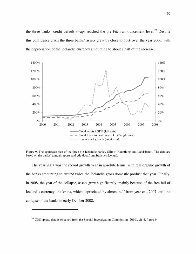
79

the three banks’ credit default swaps reached the pre-Fitch-announcement level.23 Despite

this confidence crisis the three banks’ assets grew by close to 50% over the year 2006, with

the depreciation of the Icelandic currency amounting to about a half of the increase.

Figure 9. The aggregate size of the three big Icelandic banks, Glitnir, Kaupthing and Landsbanki. The data are based on the banks’ annual reports and gdp data from Statistics Iceland.

The year 2007 was the record growth year in absolute terms, with real organic growth of

the banks amounting to around twice the Icelandic gross domestic product that year. Finally,

in 2008, the year of the collapse, assets grew significantly, mainly because of the free fall of

Iceland’s currency, the krona, which depreciated by almost half from year end 2007 until the

collapse of the banks in early October 2008.

23 CDS-spread data is obtained from the Special Investigation Commission (2010), ch. 4, figure 9.

0%

20%

40%

60%

80%

100%

120%

140%

0%

200%

400%

600%

800%

1000%

1200%

1400%

2000 2001 2002 2003 2004 2005 2006 2007 2008

Total assets / GDP (left axis)Total loans to customers / GDP (right axis)1 year asset growth (right axis)

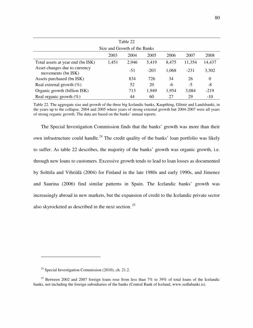
80

Table 22

Size and Growth of the Banks

2003 2004 2005 2006 2007 2008

Total assets at year end (bn ISK) 1,451 2,946 5,419 8,475 11,354 14,437 Asset changes due to currency

movements (bn ISK) -51 -203 1,068 -231 3,302

Assets purchased (bn ISK) 834 726 34 26 0 Real external growth (%) 52 20 -6 -5 -8 Organic growth (billion ISK) 713 1,949 1,954 3,084 -219 Real organic growth (%) 44 60 27 29 -10

Table 22. The aggregate size and growth of the three big Icelandic banks, Kaupthing, Glitnir and Landsbanki, in the years up to the collapse. 2004 and 2005 where years of strong external growth but 2004-2007 were all years of strong organic growth. The data are based on the banks’ annual reports.

The Special Investigation Commission finds that the banks’ growth was more than their

own infrastructure could handle.24 The credit quality of the banks’ loan portfolio was likely

to suffer. As table 22 describes, the majority of the banks’ growth was organic growth, i.e.

through new loans to customers. Excessive growth tends to lead to loan losses as documented

by Solttila and Vihriälä (2004) for Finland in the late 1980s and early 1990s, and Jimenez

and Saurina (2006) find similar patterns in Spain. The Icelandic banks’ growth was

increasingly abroad in new markets, but the expansion of credit to the Icelandic private sector

also skyrocketed as described in the next section. 25

24 Special Investigation Commission (2010), ch. 21.2.

25 Between 2002 and 2007 foreign loans rose from less than 7% to 39% of total loans of the Icelandic banks, not including the foreign subsidiaries of the banks (Central Bank of Iceland, www.sedlabanki.is).

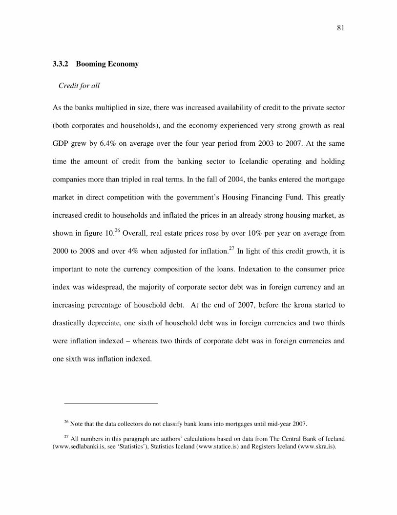
81

3.3.2 Booming Economy

Credit for all

As the banks multiplied in size, there was increased availability of credit to the private sector

(both corporates and households), and the economy experienced very strong growth as real

GDP grew by 6.4% on average over the four year period from 2003 to 2007. At the same

time the amount of credit from the banking sector to Icelandic operating and holding

companies more than tripled in real terms. In the fall of 2004, the banks entered the mortgage

market in direct competition with the government’s Housing Financing Fund. This greatly

increased credit to households and inflated the prices in an already strong housing market, as

shown in figure 10.26 Overall, real estate prices rose by over 10% per year on average from

2000 to 2008 and over 4% when adjusted for inflation.27 In light of this credit growth, it is

important to note the currency composition of the loans. Indexation to the consumer price

index was widespread, the majority of corporate sector debt was in foreign currency and an

increasing percentage of household debt. At the end of 2007, before the krona started to

drastically depreciate, one sixth of household debt was in foreign currencies and two thirds

were inflation indexed – whereas two thirds of corporate debt was in foreign currencies and

one sixth was inflation indexed.

26 Note that the data collectors do not classify bank loans into mortgages until mid-year 2007.

27 All numbers in this paragraph are authors’ calculations based on data from The Central Bank of Iceland (www.sedlabanki.is, see ‘Statistics’), Statistics Iceland (www.statice.is) and Registers Iceland (www.skra.is).

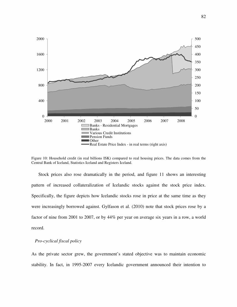
82

Figure 10: Household credit (in real billions ISK) compared to real housing prices. The data comes from the Central Bank of Iceland, Statistics Iceland and Registers Iceland.

Stock prices also rose dramatically in the period, and figure 11 shows an interesting

pattern of increased collateralization of Icelandic stocks against the stock price index.

Specifically, the figure depicts how Icelandic stocks rose in price at the same time as they

were increasingly borrowed against. Gylfason et al. (2010) note that stock prices rose by a

factor of nine from 2001 to 2007, or by 44% per year on average six years in a row, a world

record.

Pro-cyclical fiscal policy

As the private sector grew, the government’s stated objective was to maintain economic

stability. In fact, in 1995-2007 every Icelandic government announced their intention to

0

50

100

150

200

250

300

350

400

450

500

0

400

800

1200

1600

2000

2000 2001 2002 2003 2004 2005 2006 2007 2008Banks - Residential MortgagesBanksVarious Credit InstitutionsPension FundsOtherReal Estate Price Index - in real terms (right axis)

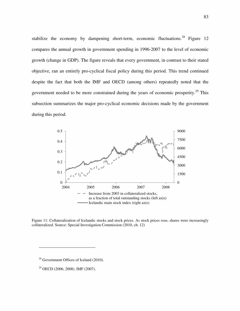
83

stabilize the economy by dampening short-term, economic fluctuations.28 Figure 12

compares the annual growth in government spending in 1996-2007 to the level of economic

growth (change in GDP). The figure reveals that every government, in contrast to their stated

objective, ran an entirely pro-cyclical fiscal policy during this period. This trend continued

despite the fact that both the IMF and OECD (among others) repeatedly noted that the

government needed to be more constrained during the years of economic prosperity.29 This

subsection summarizes the major pro-cyclical economic decisions made by the government

during this period.

Figure 11: Collateralization of Icelandic stocks and stock prices. As stock prices rose, shares were increasingly collateralized. Source: Special Investigation Commission (2010, ch. 12)

28 Government Offices of Iceland (2010).

29 OECD (2006, 2008). IMF (2007).

0

1500

3000

4500

6000

7500

9000

0

0.1

0.2

0.3

0.4

0.5

2004 2005 2006 2007 2008

Increase from 2003 in collateralized stocks,as a fraction of total outstanding stocks (left axis)Icelandic main stock index (right axis)

84

First, at the turn of the century the government heavily increased investment in public

power plants, which thereby facilitated private aluminum production and initiated some of

the most dramatic expansions in large scale industry in the history of Iceland. In addition to

increasing the production capacity of existing power plants, two new power plants were built.

The end result was that the production capacity of the power intensive aluminum industry in

Iceland tripled. The Central Bank estimated that these expansionary projects would drive

economic growth approximately 4.0-4.5% above the long-term, equilibrium growth rate,

which in return would lead to a 4% increase in inflation if no counter-cyclical measures

would be taken.30 In order to maintain economic stability, the Central Bank estimated it

would need to raise interest rates by 4.5% and the government would need to cut its budget

by 20%.31

Second, the government reorganized the housing market by changing the mortgage

regulations associated with the public Housing Financing Fund. This primarily entailed

raising the maximum amount households could borrow and increasing the mortgage loan

ratio (as a percentage of house value) from 65-70% up to 90%. These policy changes

gradually took effect starting in 2004. The private banking industry reacted by offering

competitive mortgages, i.e. by offering more generous mortgages, which in some cases

covered the full value of the collateralized housing property. This lead to a large increase in

30 Monetary Bulletin (2003).


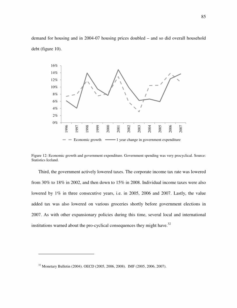
85

demand for housing and in 2004-07 housing prices doubled – and so did overall household

debt (figure 10).

Figure 12: Economic growth and government expenditure. Government spending was very procyclical. Source: Statistics Iceland.

Third, the government actively lowered taxes. The corporate income tax rate was lowered

from 30% to 18% in 2002, and then down to 15% in 2008. Individual income taxes were also

lowered by 1% in three consecutive years, i.e. in 2005, 2006 and 2007. Lastly, the value

added tax was also lowered on various groceries shortly before government elections in

2007. As with other expansionary policies during this time, several local and international

institutions warned about the pro-cyclical consequences they might have.32

32 Monetary Bulletin (2004). OECD (2005, 2006, 2008). IMF (2005, 2006, 2007).

0%

2%

4%

6%

8%

10%

12%

14%

16%19

96

1997

1998

1999

2000

2001

2002

2003

2004

2005

2006

2007

Economic growth 1 year change in government expenditure

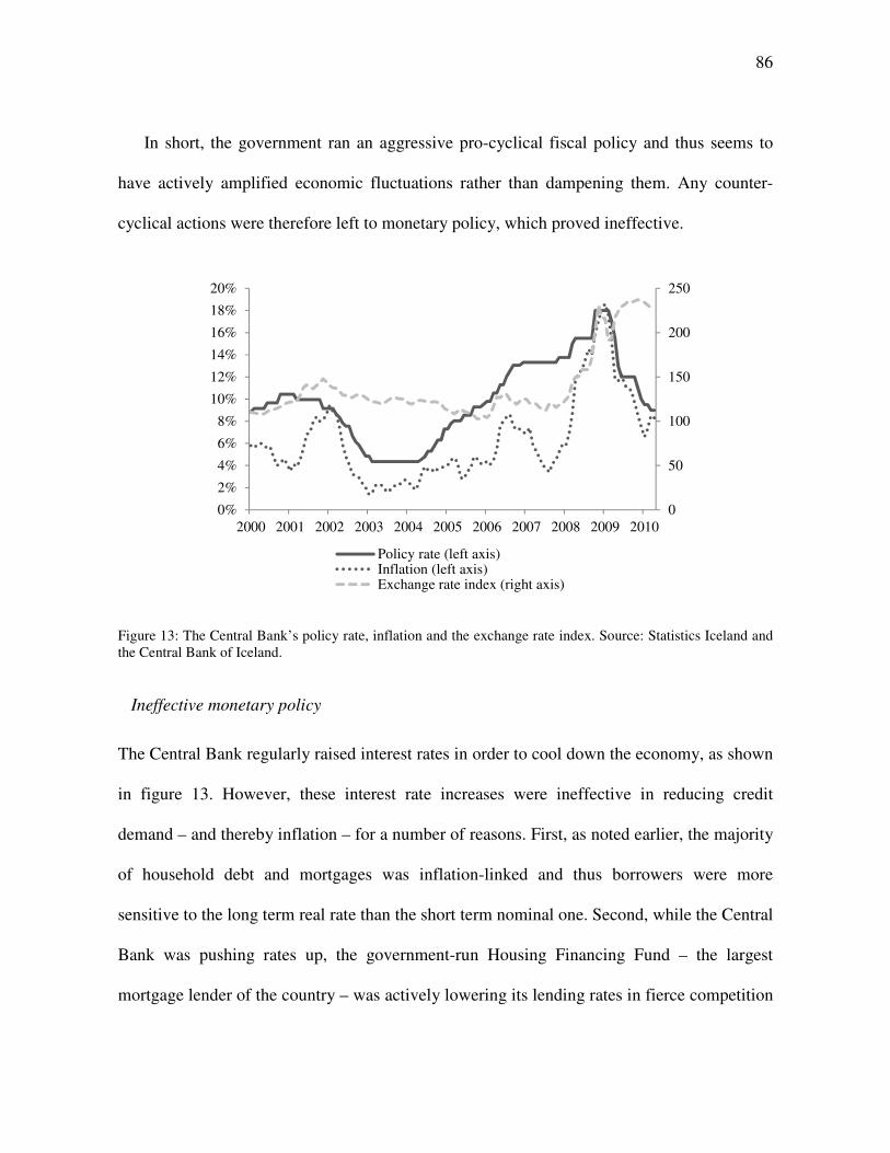
86

In short, the government ran an aggressive pro-cyclical fiscal policy and thus seems to

have actively amplified economic fluctuations rather than dampening them. Any counter-

cyclical actions were therefore left to monetary policy, which proved ineffective.

Figure 13: The Central Bank’s policy rate, inflation and the exchange rate index. Source: Statistics Iceland and the Central Bank of Iceland.

Ineffective monetary policy

The Central Bank regularly raised interest rates in order to cool down the economy, as shown

in figure 13. However, these interest rate increases were ineffective in reducing credit

demand – and thereby inflation – for a number of reasons. First, as noted earlier, the majority

of household debt and mortgages was inflation-linked and thus borrowers were more

sensitive to the long term real rate than the short term nominal one. Second, while the Central

Bank was pushing rates up, the government-run Housing Financing Fund – the largest

mortgage lender of the country – was actively lowering its lending rates in fierce competition

0

50

100

150

200

250

0%

2%

4%

6%

8%

10%

12%

14%

16%

18%

20%

2000 2001 2002 2003 2004 2005 2006 2007 2008 2009 2010

Policy rate (left axis)Inflation (left axis)Exchange rate index (right axis)

87

with the banks. Finally, as discussed above, corporate debt was largely in foreign debt and as

the cost of borrowing in the domestic currency increased with rising interest rates, the public

increasingly responded by borrowing in foreign currency rather than in the domestic one. The

public did not seem to sense the danger and the ultimate exchange rate adjustment the

interest rate differential entailed. Also, the private banks encouraged foreign lending without

sufficiently explaining the inherent risks thereof. This foreign lending behavior leads us to

the discussion of how the currency regime contributed to the downfall.

Carry trade and currency risks

As previously noted, when the economy started to boom the Central Bank responded by

raising interest rates (see figure 13). Gradually the interest rate differential between Iceland

and other countries became sizable. Carry trades, where investors borrow low-yielding

currencies and invest in high-yielding ones, became extensive. For example, foreign banks,

such as the European Investment Bank, Rabobank and the German KFW, issued to krona

denominated bonds, called “Glacier bonds”, which were sold to retail investors.33 The banks

would then swap their funding into foreign currency with the Icelandic banks. In the summer

of 2007, this foreign investment in the glacier bonds amounted to about 30% of that year’s

GDP.34 As noted above, the public was generally not fully aware of the risks involved. In

particular, the interest rate differential is reflected in expectations on exchange rate

adjustments (the so-called “interest rate parity”), i.e. the Icelandic krona was bound to

33 Ásbjörnsson and Jónsson (2007).


88

depreciate sooner or later. Since Iceland relies heavily on imports in its consumption, a

depreciation of the krona affects the consumer price index significantly.35 So with the

widespread indexation and currency denomination of loans, the private sector, both

corporates and households, was to be severely affected by the krona depreciation in 2008 and

the accompanying inflation.

A related risk factor associated with the extensive increase of foreign currency flows into

Iceland was the danger that capital inflows would come to a sudden stop, as described by e.g.

Calvo et al. (2004). Note that if foreigners would later withdraw their investments in a

gradual manner it would probably pose limited economic challenges, but the danger was that

foreigners would quickly move out of krona investments. This would bring the economy to a

sudden stop, i.e. the real economy would take a sudden blow rather than follow gradual

adjustment. This was indeed how events unfolded as the financial crisis hit the world

economy in 2008, which finally led to the imposition of capital controls, which still remain in

effect. Figure 13 displays the substantial drop in the value of the Icelandic krona, starting in

2008.36 Such a dramatic depreciation could partly have been avoided if the Central Bank had

held large amounts of foreign exchange reserves. This would have signaled the Central

Bank’s capacity to counteract such fluctuations in the currency, thereby decreasing the risk of

35 Mishkin and Herbertsson (2006), p. 45, note that the “rule of thumb is that a 10% lasting depreciation increases inflation by 3.5% and debt service approximately in the same proportion”.

36 Note that an increase in the exchange rate index indicates a depreciation of the krona. Also, as a result of capital controls, two krona markets arose – namely the on-shore and off-share markets. The depreciation of the krona in the off-shore market was even more dramatic than the one depicted in figure 13.

89

sudden capital outflow occurring in the first place.37 Also, the Icelandic krona had rarely

been stronger than in the years leading up to the collapse, which would therefore have

minimized the costs of accumulating reserves.

The Icelandic exchange rate is particularly sensitive to foreign capital movements due to

the relatively small size of the economy. On an international comparison, relatively small

transactions cause relatively large movements in the exchange rate. This is particularly

problematic in a small, open economy which relies heavily on foreign exports and imports.

Exchange rate fluctuations therefore translate directly into instability in consumer income

and consumption. Thus, a natural question to ask is whether an independent currency with

floating exchange rates is an optimal currency regime in a small, open economy? As for the

Icelandic economic collapse, it is clear that the weak currency contributed to the economic

dilemmas – in particular as this regime was combined with poor governance of the Central

Bank (as previously described and later revisited in ch. 4.3). Similarly, the feasibility of an

inflation targeting regime in a small, open economy with a volatile currency is questionable.

The case can, however, be made that an independent currency helped the economy adjust in

the aftermath of the crisis (an option not available to e.g. euro-denominated countries such as

Greece). Since the issue of the optimal currency regime naturally remains heavily debated in

the academic literature, this paper does not elaborate further on the issue of currency choice

and optimal monetary policy.

37 Although the Central Bank objective was inflation targeting, the exchange rate is an important factor in the inflation rate (as in any small, open economy). Therefore it would have been justifiable to use the foreign exchange reserves to dampen exchange rate fluctuations.

90

3.3.3 Inside the Banks

The kind of phenomenal growth, where the Icelandic banking system outgrew the economy

so fast and by so much, could not have been funded domestically. International funding was,

however, readily available, as the banks enjoyed favorable credit ratings by the ratings

agencies. These ratings seem to have been partly based on the assumption that the Icelandic

government would stand behind the banks if they got into trouble; for example Moody’s

noted that a primary strength of the banks was the “strong likelihood of state support in the

event of systemic shock”.38 In the early years of the growth, bond issuance in European

markets was the main source of funding. The year 2005 was the peak year of bond issuance

for all the three banks – but as the amounts issued by the banks rose, the demand for their

bonds fell in Europe and thus in 2006-07 all three banks turned to U.S. markets and made

successful bond sales there. Whereas 2004-05 were years of growth with limited repayments

of earlier debt, the years 2007-08 had increasingly high repayments that needed funding.

While bond issuance was still quite high in 2007, a large part of that issuance went to repay

old debt. 39

Fragile capital and false equity

As already noted, cheap foreign borrowing is what fuelled the Icelandic banks’ growth, i.e.

they borrowed abroad and lent both domestically and internationally. To support that growth,

38 Moody’s (2006), p. 2.

39 Information on bond issuance and repayment schedules in this section is taken from the Special Investigation Commission (2010), ch. 7.

91

however, the banks needed growing capital to meet the capital requirements set by the Basel

Accord of 1988 and its replacement Basel II Framework. Although the capital adequacy ratio

(the ratio of regulatory capital to risk weighted assets) of the Icelandic banks was always

significantly above the required minimum of 8%,40 taking a closer look at the capital reveals

certain weaknesses. Two main points are to be made.

First, a bank’s regulatory capital is made up of two main parts: the bank’s equity capital,

i.e. the value of the assets exceeding debts, and subordinated debt contracts with certain

features. As the banks grew and needed to hold increased capital, their reliance on

subordinated debt increased. At the end of the year 2003, subordinated debt amounted to

27% of the three banks’ combined regulatory capital, but only four years later, that ratio was

49%41. This increased reliance on subordinated debt in regulatory capital was worrisome

since such debt cannot absorb losses in ongoing operations. More specifically, while

subordinated debt will in general absorb losses before senior lenders suffer any losses, it can

only do so in bankruptcy or some sort of a debt restructuring process. Moreover, increased

reliance on subordinated debt exacerbates problems of moral hazard. Namely, when the

shareholders’ equity is a small part of the bank’s capital, the shareholders’ potential loss is

reduced in comparison with their possible gains. This increases the incentive for

shareholders, who ultimately control the bank, to take on more risk.

40 Usually around or above 12%, based on information from the annual accounts of the banks. See detailed information on Basel II at the website of the Bank for International Settlements, http://www.bis.org/publ/bcbsca.htm and http://www.bis.org/publ/bcbs128b.pdf.

41 Annual reports of the three big banks for 2003 and 2007.

92

Second, a more substantial problem with the banks’ capital was the actual quality of the

banks’ accounted equity. In general, a bank’s capital – and in particular the equity – is the

shareholders’ stake in the bank and the amount of loss that can be absorbed before lenders of

the bank suffer losses. However, if a bank has financed its own stock (bought its own shares

or lent out capital to buy shares without other collateral), the bank will incur losses when the

equity of the bank falls in value and therefore that amount is not a true buffer against losses;

it is false equity. The Special Investigation Commission estimates that the extent of false

equity, i.e. the three banks’ financing of their own stock, was around a quarter of the total

banks’ regulatory capital at the end of 2007.42 If only the core part of the capital

(shareholders’ equity less goodwill) is considered, then the false equity was close to half the

equity capital. Finally, when also considering the amounts that the three banks financed of

each other’s stock, the total summed up to around 70% of the shareholders’ equity less

goodwill.43 With so much of the price risk of the banks’ stock borne by the banks themselves,

the previously mentioned moral hazard problem was made all the worse.

In the case of Kaupthing and Glitnir, their largest shareholders were two holding

companies listed on the Icelandic stock exchange, Exista and FL Group respectively. Besides

lending for purchases of the banks’ stock, the banks also lent customers significant amounts


43 Examples of such cross-financing methods dates as far back as 2001, when Kaupthing placed just under 5% of its shares into a separate legal entity, controlled by one of the other banks, Landsbanki. Kaupthing and Landsbanki then went on to make contracts insuring that all financial risk because of the stocks would indeed still be borne by Kaupthing Special Investigation Commission (2010, chapter 9). These transactions therefore caused Kaupthing to underreport its own stock ownership.

93

to buy the stocks of these two holding companies as noted by the Special Investigation

Commission.44 So, as the banks’ stock prices would fall, the holding companies incurred

losses and saw their stock value decline. That, in turn, fed back into the banks through loan

losses. This kind of structure was really a form of cross-ownership where losses in one firm

were likely to spread out to many others. Aliber (2008) notes that this type of ownership

structure was similar to the one prevalent in Japan in the 1980s. While the Japanese banks

owned the stock directly, the Icelandic banks financed the stock through lending, but the

general effect was the same.

Connected lending and systematic risk

A noteworthy characteristic of the Icelandic banking system was how prevalent lending to

the banks’ owners truly was. In all three banks the largest groups of borrowers were indeed

the banks’ owners, either directly or indirectly.45 Also, one business group, operating around

the retail-oriented holding company Baugur, was a very large borrower in all banks. This

group did in fact hold a controlling stake in Glitnir, one of the three banks. Combined across

the banks’ credit to the Baugur group amounted to more than 50% of the banks’ total

regulatory capital, making the group a significant systemic risk factor for the banking system

as a whole.46


45 Special Investigation Commission (2010), ch. 8.

46 In order to prevent large concentrations of credit risks, there were rules limiting credit exposure to a group of connected lenders to 25% of a bank’s regulatory capital. However, as discussed later in ch. 4.3, these

94

The apparent easy access of the banks’ owners to credit from their banks also manifested

itself in the investments of the so-called money market funds in Iceland, according to the

Special Investigation Commission.47 All of the big three banks owned asset management

firms that operated money market funds, which grew rapidly in 2007-08. As with the banks’

lending, there was a clear correlation between each fund’s holdings and the bank that

ultimately ran it through its asset management firm. Specifically, the money market funds

were heavily investing in firms related to the banks’ owners. Thus, even though the funds

were supposed to operate independently from the banks that owned the asset management

firms, these findings put that into doubt.

This kind of lending to insiders, such as bank owners, has been argued to be a

manifestation of looting. La Porta et al. (2003) make this argument in the case of Mexico in

the 1990s, Charumilind et al. (2006) show the same occurred in Thailand before the crisis

there, and Laeven (2001) documents the prevalence of insider lending in Russia in the 1990s.

The extent of lending to bank owners in Iceland was therefore worrisome, expecially in light

of the poor supervision they were operating under as discussed in section 3.4.2.

Market manipulation

Since the banks held large amounts of “false equity” and were exposed to groups connected

to their largest shareholders, the banks found themselves in a situation where a substantial

rules were not sufficiently enforced by the regulatory authorities and the definition of connected lenders seems to have been open to interpretation.

47 Special Investigation Commission, Aðdragandi (2010), ch.14.

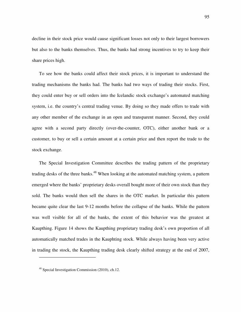
95

decline in their stock price would cause significant losses not only to their largest borrowers

but also to the banks themselves. Thus, the banks had strong incentives to try to keep their

share prices high.

To see how the banks could affect their stock prices, it is important to understand the

trading mechanisms the banks had. The banks had two ways of trading their stocks. First,

they could enter buy or sell orders into the Icelandic stock exchange’s automated matching

system, i.e. the country’s central trading venue. By doing so they made offers to trade with

any other member of the exchange in an open and transparent manner. Second, they could

agree with a second party directly (over-the-counter, OTC), either another bank or a

customer, to buy or sell a certain amount at a certain price and then report the trade to the

stock exchange.

The Special Investigation Committee describes the trading pattern of the proprietary

trading desks of the three banks.48 When looking at the automated matching system, a pattern

emerged where the banks’ proprietary desks overall bought more of their own stock than they

sold. The banks would then sell the shares in the OTC market. In particular this pattern

became quite clear the last 9-12 months before the collapse of the banks. While the pattern

was well visible for all of the banks, the extent of this behavior was the greatest at

Kaupthing. Figure 14 shows the Kaupthing proprietary trading desk’s own proportion of all

automatically matched trades in the Kauphting stock. While always having been very active

in trading the stock, the Kaupthing trading desk clearly shifted strategy at the end of 2007,

48 Special Investigation Commission (2010), ch.12.

96

when the stock’s price had started to fall significantly. The report also documents that the

proprietary trading desk tended, in 2008, to gradually accumulate Kaupthing shares and then

sell large chunks to clients, who in most cases borrowed from Kaupthing, largely without

other collateral, to purchase the stock. This moved the shares off Kaupthing’s books, while

the bank often retained a large part of the risk. The other two banks, Glitnir and Landsbanki,

also engaged in this kind of behavior albeit on a smaller scale.

Figure 14: Kaupthing proprietary trading in the bank's own stock. The amounts are measured in Kaupthing's trading as a percentage of total matched trades in the stock exchange. Source: Special Investigation Commission (2010, ch. 12)

Finally, the SIC report shows both Kaupthing and Glitnir relieved some selling pressure

in 2008 by lending large shareholders large amounts to repay loans to foreign banks that

were collateralized by Kaupthing and Glitnir’s stocks. Without those repayments the foreign

banks might have decided to collect the collateral and sell it off to recover the loans. In some

cases the banks collaborated. An example includes “a deal Kaupthing and Glitnir made

0

200

400

600

800

1000

1200

1400

-60%

-40%

-20%

0%

20%

40%

60%

80%

2004 2005 2006 2007 2008

Kaupthing buys (left axis)

Kaupthing sells (left axis)

Kaupthing stock price (right axis)

97

where Glitnir committed to lend against Kaupthing shares and Kaupthing committed to lend

against Glitnir shares.”49

3.4 The Crisis Unfolds – Weaknesses Uncovered

3.4.1 Liquidity Squeeze and Currency Crisis

In the spring of 2007, global liquidity was peaking by many measures, such as the TED

spread.50 As the summer passed, however, there were increasing signs of quickly shrinking

liquidity as detailed by Brunnermeier (2009). For the Icelandic banks the same was true, but

the effects were even stronger. After having reached an all-time low in June 2007, the

average CDS spread of the three banks rose sharply in the fall of that year.51 By the end of

August, it had risen from under 30 basis points to more than 70, and at the end of 2007 it

would stand at 200, the highest ever.52 This marked the beginning of the end for the three

Icelandic banks and 2008 would be a year of a constant battle for them to stay liquid.

The strong link between the banks’ liquidity position and the krona became evident in

early 2008. As the global liquidity squeeze tightened further, the average CDS spread of the

Icelandic banks skyrocketed and at the end of February 2008 it was around 600 basis points;

49 The quote is taken from a loan application submitted before Kaupthing’s Board Credit Committee, May 29. The quote was made available in the report provided by the Special Investigation Commission, ch. 9.6, p. 21.

50 The TED spread is the difference between the USD LIBOR rate and US Treasury bill rate.

51 CDS refers to Credit Default Swap and is a form of insurance that protects the lender if a borrower of capital defaults on its loan. Thus, it can also be taken as a probability measure of bankruptcy.

52 CDS-spread data is obtained from the Special Investigation (2010), ch.7, figure 23.

98

global credit markets were effectively closed to the banks. With the panic surrounding the

fall of Bear Stearns in March 2008, the foreign currency liquidity all but dried up in the

Icelandic banks, as evidence from the Icelandic currency swap market shows.53 Figure 15

shows the spread between the euro and krona interest rate implied by the currency swap

market. More specifically, since the difference between the Icelandic Central Bank’s and the

ECB’s policy rate was around 12% at the time,54 the currency swap spread should, in normal

times, have been close to that level, because of covered interest parity.55 However, when

liquidity dried up in March 2008, this spread sharply fell to around 2%. This meant that the

Icelandic banks were charging each other virtually the same interest rate for euros as krona.

Figure 15 also shows the exchange rate between EUR and ISK, and it can be seen that the

ISK plunged at the same time as the swap market dried up. The Icelandic banks could still

access liquidity from the Icelandic Central Bank in ISK, as described in section 4.3, and they

were essentially using that liquidity to cover their foreign currency needs. In this way the

price of foreign currency in Iceland jumped both in the currency swap market as well as the

exchange rate market itself.

53 A currency swap market is an interbank market where one bank lends to another bank in one currency and borrows from that bank in a different currency. A currency swap can also be thought of as a bilateral contract that combines a spot contract and a forward contract, i.e. one party buys an exchange rate spot and sells it forward, leaving only the interest rate component of the forward contract.

54 Data obtained from the website of the Central Bank of Iceland and the European Central Bank.

55 Baba et al. (2008), describe how covered interest parity (CIP) should force the interest rates implied by currency swap agreements towards the cash rate. The cash rate they consider is the LIBOR rate, which in normal times is close to the policy rate, the Fed funds rate.

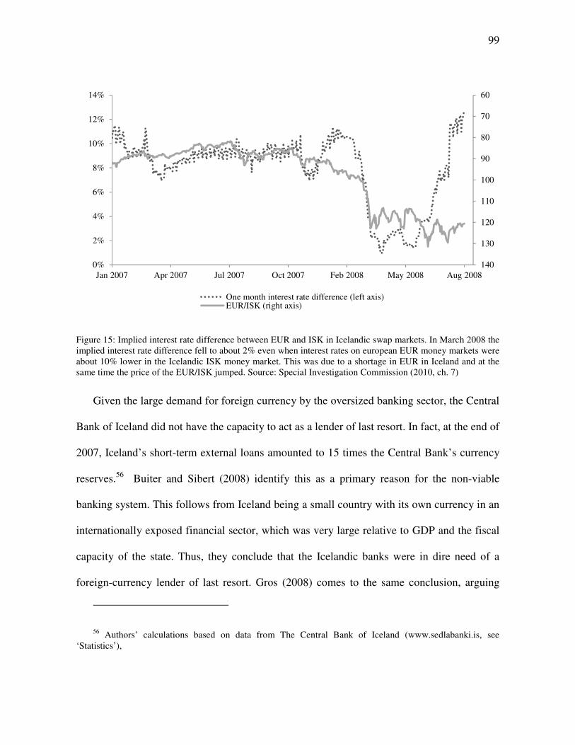
99

Figure 15: Implied interest rate difference between EUR and ISK in Icelandic swap markets. In March 2008 the implied interest rate difference fell to about 2% even when interest rates on european EUR money markets were about 10% lower in the Icelandic ISK money market. This was due to a shortage in EUR in Iceland and at the same time the price of the EUR/ISK jumped. Source: Special Investigation Commission (2010, ch. 7)

Given the large demand for foreign currency by the oversized banking sector, the Central

Bank of Iceland did not have the capacity to act as a lender of last resort. In fact, at the end of

2007, Iceland’s short-term external loans amounted to 15 times the Central Bank’s currency

reserves.56 Buiter and Sibert (2008) identify this as a primary reason for the non-viable

banking system. This follows from Iceland being a small country with its own currency in an

internationally exposed financial sector, which was very large relative to GDP and the fiscal

capacity of the state. Thus, they conclude that the Icelandic banks were in dire need of a

foreign-currency lender of last resort. Gros (2008) comes to the same conclusion, arguing

56 Authors’ calculations based on data from The Central Bank of Iceland (www.sedlabanki.is, see ‘Statistics’),

60

70

80

90

100

110

120

130

1400%

2%

4%

6%

8%

10%

12%

14%

Jan 2007 Apr 2007 Jul 2007 Oct 2007 Feb 2008 May 2008 Aug 2008

One month interest rate difference (left axis)EUR/ISK (right axis)

100

that the oversized banking sector turned the country into a hedge fund, which the Icelandic

authorities did not have the capacity to save. Only 6 months after these warnings, the banks

were insolvent. In the end, the fall of Lehman Brothers in the autumn of 2008 and the

ensuing credit crunch proved too much for the banks. On September 22nd it was announced

that the Central Bank of Iceland would take 75% in Glitnir for an injection of much needed

foreign currency. Over the next two weeks, it became clear, however, that the problems could

not be overcome by the Central Bank and by October 9th all three banks were in receivership.

While the fall of Lehman Brothers proved to be the event that triggered the Icelandic

banks’ downfall, we do not mean to say that without the liquidity squeeze the Icelandic

banking system would have survived. The system was inherently risky, having lent heavily in

new markets, flooding the local market with unsustainable amount of credit and by relying

on false and increasingly manipulated equity. Other authors share this view. For example,

Gylfason et al. note that that banks “… blamed the fall of Lehman Brothers for their own

demise, implying that had Lehman Brothers endured, they, too, could have survived the

turmoil… True, the collapse of confidence in world financial markets generated the spark

that ignited the flames which quickly engulfed Iceland, but the house would have caught fire

anyway though perhaps a little later”.57 Wade and Sigurgeirsdottir similarly note: “The

Lehman collapse … was the trigger. But a crash would have come anyway because of the

57 Gylfason et al. (2010), p. 138.

101

giant structural imbalances, the overreaching of financiers, and the vulnerability to reversal

of short-term capital inflows.”58

3.4.2 Lack of Authoritative Response

The government

As the banking sector grew internationally and its foreign assets became many multiplies of

GDP, the government did not recommend that the banking sector moved its headquarters

abroad. In fact, it was the announced policy of the government to keep the banks in Iceland.59

Moreover, the government encouraged further growth of the banking sector, rather than

recommending that the banks would decrease their balance sheets or break up their

operations into separate units (two weeks before the collapse, one of the banks decided to

initiate their own plan of moving its headquarters abroad). The Special Investigation

Commission further concludes that the government ministers – in particular the Minister of

Economic Affairs – were ill informed and did not manage to initiate any analysis of the

soundness of the financial system, despite the media at times displaying severe concerns

about the economic outlook (e.g. lower credit ratings, increasing rates on banks’ credit

default swaps, etc.).60

One of the few initiatives taken by the government was to establish a work group to

increase information flow between ministries and official financial institutions. More

58 Wade and Sigurgeirsdottir (2011), p. 66.

59 Special Investigation Commission (2010), ch.5.2 & 19.6.1.

60 Special Investigation Commission (2010), ch.19.

102

specifically, in February 2006 the government established a group consisting of

representatives from the Prime Minister’s Office, the Ministry of Finance, the Ministry of

Economic Affairs, the Central Bank and the Financial Supervisory Authority, the objective of

which was to create a platform for communication between these institutions in case of a

financial shock. The group was also meant to provide recommendations for actions in case of

a crisis. However, this group was not established by law and did not have access to

confidential data and other information that was necessary in order to give proper guidance

following a market downfall.61 Furthermore, the group did not start to draft an emergency

plan until March 2008 and the ministry representatives in the group were halting the creation

of a clear reaction strategy up until the collapse.62 Thus, no thought-out plan existed when the

banks collapsed in October 2008. Thus, at the time of the collapse, the reactions of the

ministers were not based on pre-prepared plans or strategies. For example, after the banking

collapse the Minister of Economic Affairs ensured the Icelandic population that all deposits

were government guaranteed, but there was no underlying analysis showing that the state had

the financial capacity to measure up to such promises.

The Financial Supervisory Authority

The Icelandic Financial Supervisory Authority (FSA), which is the primary surveillance

agency in the country, also failed in taking proper action. In late 2007 a special work group

which was to report on the soundness of the financial system was established within the FSA.

61 Special Investigation Commission (2010), ch.19.4.4.


103

The group was formed in light of the rapid growth and the Mini crisis in 2006, but primarily

it was created because a joint Nordic emergency plan was being set up as a response to the

gradual spread of the international credit crunch.63 This group collected substantial

information on the banking sector, but their results were neither precise nor proposed

concrete actions. Up until the collapse the chief officers of the FSA genuinely felt that there

were no major problematic issues facing the Icelandic financial sector (partly due to an

overestimation of the banks' retained earnings and flawed stress tests). It was the FSA’s

assessment that the Icelandic banks were just as strong – or even stronger – as their

continental European counterparts.64 There was only partial awareness of warnings signs a

few months before the collapse,65 but none of these concerns seem to have been shared with

the above-mentioned working group of the ministries, the Central Bank and the FSA.

Furthermore, the information gathered by the FSA work group did not seem to be openly

accessible to others than the director of the institution.66 In short, the FSA did not respond in

any concrete way to the any of the alarms that began buzzing in 2006-08.

The Central Bank

Leading up to the collapse, the Central Bank periodically received information or comments

from various foreign authorities (e.g. the Bank of England, credit rating agencies, etc.) on the


64 Jónsson, speech given on January 10 (2008).

65 See e.g. Special Investigation Commission (2010), ch.16.10.4, p. 160.

66 Special Investigation Commission (2010), ch.16.10.4, p. 160.

104

grave situation of the Icelandic banks. The Special Investigation Commission concludes that

this information was not conveyed to the government in a formalized and proper manner, but

rather through conversations with the main ministers.67 Due to a deep distrust between the

chairman of the board of governors of the Central Bank (a former prime minister and a

highly political figure) and the ministers of one of the government coalition parties, these

warnings were written off. A more formalized method of communication would therefore

have been in order.

Overall, the government, the Central Bank and the FSA all failed in creating an

emergency plan and thus had no concrete responses to the course of events that followed the

banking collapse. The country lacked a decisive and driving FSA, credible and professional

management of the Central Bank and an alert government with a prepared plan of action.

3.4.3 Less than Excellent Institutions

As previously noted, Demirgüç-Kunt and Detragiache (1999) find that banking crises are

more common in countries that have liberalized their financial systems, but they also find

that financial liberalization is less risky in countries that have a strong institutional

environment. Mishkin and Herbertsson (2006) place very strong emphasis on the importance

of the institutional environment. Although they list a number of risks posed to the Icelandic

financial system at the time, they nevertheless conclude that real worries were not warranted

and base that conclusion significantly on the strength of Icelandic institutions and repeatedly

express their confidence in the Icelandic Financial Supervisory Authority (FSA). Similarly,


105

Portes and Baldursson (2007) also regard the Icelandic institutional and regulatory

framework as highly advanced and strong. Indeed Iceland was a developed country with

strong legal rights and enforceability of contracts – leading it to be ranked very high in

various development indices. For example, Iceland was on top when it came to political

rights and civil liberties – and it also had the lowest perceived corruption in the world.68

Nevertheless there were frailties in key institutions, both in the Central Bank and the FSA, as

described in the remainder of this section. Furthermore, we also discuss how the

effectiveness of both institutions – and the general willingness to criticize the economic

situation – was undermined by the political state of affairs.

The Central Bank

In 2001 the Central Bank took up an inflation targeting regime and simultaneously gained

independence from the government in order to prevent political interference and establish

credibility of the goals chosen. The credibility was, however, never really achieved as

Daníelsson and Zoëga (2009) note. The government appointed political figures as governors

of the Central Bank, which harmed the credibility and entangled politics with economic

decisions in a time of financial distress. Most notably, in 2005 the former prime minister

became the chairman of the board of governors. Leading up to the collapse in 2008, the

communication flow between the Central Bank and the government was harmed by this fact,

due to distrust and animosity between the chairman of the board of governors and one of the

68 Transparency International (2003).

106

government coalition parties – a former political rival. Thus any information received from

the Central Bank about financial concerns was either taken with a grain of salt or ignored.69

A further loss of credibility occurred as a result of a number of ill-advised and random

decisions made by the board of governors. In particular, many decisions were made against

the recommendations of the bank’s chief economist.70 The most dramatic examples thereof

occurred in the aftermath of the financial collapse. Foreign investors were rapidly

withdrawing from Iceland, which put the Icelandic currency under pressure and thus the

Central Bank kept interest rates high (since the exchange rate strongly affects inflation).

However, as interest rates had become very high, there was political pressure to lower them

and the chairman of board of governors pushed for lowering of interest rates by a massive

3.5% (under the IMF plan interest rates were raised by 6% shortly after in order to mend the

damage done by this unilateral decision). The chief economist was informed of the change

only five minutes before it was announced publicly.71 Another decision that was initiated by

the chairman of the board of governors was to unexpectedly fix the exchange rate. A

particular exchange rate was chosen more or less randomly without reflection or discussion

with the bank’s economists.72 Thus, for a while the bank had to defend an arbitrary exchange

rate while still running an independent monetary policy without capital constraints – an

impossible task for any Central Bank controlling only one economic variable (interest rates).


70 Special Investigation Commission (2010), ch. 4.5.4.



107

As Buiter and Sibert (2008) note, this policy mistake resulted in one of the shortest-lived

currency pegs in history. Moreover, the foreign currency reserves were far too small to

preserve this fixed level of exchange rates. The end result was to stop free capital flows and

close the economy. To date, Icelandic currency cannot be freely sold by either locals or

foreigners – a special permission for such transactions is needed by the authorities. These

examples of unconscionable actions depict an utter lack of understanding of monetary policy

by the chairman of the board of governors, and this severely damaged the credibility of the

Central Bank, which is the cornerstone to establishing an effective monetary policy.

Besides issues of political economy, the implementation of the monetary policy was also

a source of difficulties for the Central Bank. The bank’s main instrument was the interest rate

on a short-term lending facility where the Icelandic banks borrowed weekly against

collateral. While the collateral provided by the banks had previously consisted mainly of

government bonds (and bonds with government guarantees), this changed dramatically in the

last two years before the collapse. Wider collateral requirements allowed for new types of

collateral, such as credit-backed securities and bonds denominated in foreign currencies.

Most troublesome, however, was the fact that the Icelandic banks’ own unsecured bonds

were increasingly used in these transactions.73 Each bank could not borrow against its own

bonds, but by issuing bonds that the other big banks (and some smaller banks) bought and

borrowed against, the banks could effectively borrow from the Central Bank. In other words,

the banks acquired bonds from each other and posted these as collateral for more credit. The


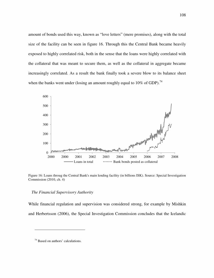
108

amount of bonds used this way, known as “love letters” (mere promises), along with the total

size of the facility can be seen in figure 16. Through this the Central Bank became heavily

exposed to highly correlated risk, both in the sense that the loans were highly correlated with

the collateral that was meant to secure them, as well as the collateral in aggregate became

increasingly correlated. As a result the bank finally took a severe blow to its balance sheet

when the banks went under (losing an amount roughly equal to 10% of GDP).74

Figure 16: Loans throug the Central Bank's main lending facility (in billions ISK). Source: Special Investigation Commission (2010, ch. 4)

The Financial Supervisory Authority

While financial regulation and supervision was considered strong, for example by Mishkin

and Herbertsson (2006), the Special Investigation Commission concludes that the Icelandic

74 Based on authors’ calculations.

0

100

200

300

400

500

600

2000 2000 2001 2002 2003 2004 2005 2006 2007 2008

Loans in total Bank bonds posted as collateral

109

FSA severely failed to fulfill its duties during the country’s economic turmoil.75 Overall, the

FSA lacked an initiative spirit and strong firmness in its general approach to handling the

financial sector.

The main missteps of the FSA highlighted by the Special Investigation Commission are

broadly categorized as follows.76 First, the guidelines of the FSA for what defined a

reprehensible market behavior were unclear. As an example, the definition of related

business parties was very vague, which allowed the banks to interpret such relations very

narrowly – opening up gateways for connected lending and market misuse. Also, while the

FSA made objections to the banks’ narrow interpretations on occasion, the agency’s efforts

to get the banks to follow its view were weak.77 Second, the Commission concludes that the

monitoring and stress testing of the FSA was weak. For example, the FSA required financial

firms to report various data to them regularly, but there was a lack of sufficient analysis of

this data in order to get a proper overview of the soundness of the financial system. Similarly,

automatic (electronic) warning systems had also been set in place, but they were not fully

used and/or did not work properly, making employees skeptical about their results.

Furthermore, stress tests executed by FSA were not proper indicators of the market risk that

the banking sector faced (they e.g. ignored drastic drops in prices). Third, in cases of clear

misdemeanor the FSA lacked decisive action. For example, although the FSA was in a good

75 Special Investigation Commission (2010), ch. 16.13 & 21.5.5.



110

position to monitor the close ties between many financial firms and related market

manipulation (e.g. where banks and related identities bought up their own shares in order to

keep prices high), it did not take any concrete actions such as aggressively using forfeits or

recommending prosecution. This was despite having the same legal resources available as

other supervisory authorities in the Nordic countries. Overall, the majority of investigated

cases were simply not properly pursued and there was a severe lack of determination in

ensuring the enforcement of the financial regulations.78

Gylfason et al. (2010) also come to this conclusion, arguing that the FSA ought to have

applied more stringent stress tests and paid attention to the dubious quality of the banks’

assets. They also note that the FSA did little to counter the impression that the banks still

enjoyed state guarantees after privatization, for example the FSA allowed itself to be featured

prominently in brochures from Landsbanki introducing the Icesave internet accounts in the

United Kingdom and Netherlands (attracting 300,000 and 100,000 depositors, respectively,

compared to an Icelandic population of only 320,000).

In summary, the FSA was a passive and relatively inactive institution. Also, even though

the FSA may have been aware of some of these problematic issues, any improvement thereof

was slow. The expansion of the FSA did not keep up with the growth of the banking sector

and the Special Investigation Commission notes that responsibility lies with the management

of the FSA, which did not push aggressively enough for a higher operating budget.79



111

Furthermore, the general attitude within the FSA was that the financial sector was healthy

and could cope with significance market risks. The FSA’s director stated in a speech in April

2008 – only 6 months before the collapse – that foreign comments (e.g. from Moody’s) about

the overwhelming size of the banking sector might just be due to lack of knowledge about the

Icelandic financial environment – and thus that the Icelandic financial sector primarily faced

“bad publicity risk”.80 In other words, the main surveillance authority in Iceland was utterly

unaware that a systematic banking failure was probable, as becomes evident when reading

statements that the deputy director of the FSA made to Special Investigation Commission.

Loosely translated, he notes that “ until late September I was clueless that everything was

about to collapse, that everything would have collapsed just a few weeks later“.81

Political economy and industry response

Overall, it is puzzling why the key public institutions in the economy did not react to the

warning signs – neither in the wake of the crisis nor in the many years preceding it. One

explanation that has been put forth regards Iceland’s political economy. Even though Iceland

is typically viewed to have little corruption, the political state of affairs made it difficult to

raise concerns on the economic direction of the country. Wade and Sigurgeirsdottir (2011)

point out that although Iceland enjoyed the least corrupt public administration in the world in

2007 (according to an international corruption perceptions index) there were nonetheless

close ties between politics and the industry. In particular, they emphasize the stronghold that

80 Special Investigation Commission (2010), ch. 16.10.2., p. 157.

81 Special Investigation Commission (2010), ch. 16, p. 162.

112

the prime minister in 1991-2004 had on both public and private entities. Gylfason et al. also

emphasize the tight embrace between the political parties and the banks, which programmed

virtually the entire political class and civil service to think that it was not a good idea to get

in the way of the banks. They also note that public institutions which dared to disagree with

the idea of a full throttle free market economy were quickly reorganized or abolished.82

Wade and Sigurgeirsdottir similarly point out that the civil service in Iceland has little

independence from the ministers. Both of these studies argue that the primus motor behind

political decisions interfering with the private sector was the prime minister at the time, who

then became Central Bank governor. They note that this state of political economy may e.g.

explain why the Financial Supervisory Authority looked the other way when the banks ran

amok.

A second – but related – issue is the immediate and strong response of the industry to any

suggestions that the economy might be heading for disaster. A prominent example is a report

published by Danske Bank in 2006 which was very explicit in its grave outlook of the

Icelandic economy. The report e.g. states that Iceland is “the most overheated in the OECD

areas” and that “Iceland looks worse on almost all measures than Thailand did before its

82 Gylfaon et al., Nordics (2010), p.148, argue that the banks could e.g. have been constrained through special taxation, but add that this was not well received within the government since ‘you do not tax your friends, especially not when they fund your party directly and indirectly.’ They also name two examples of institutes that were discontinued once they did not follow the party line. First, the National Economic Institute, which was set up to offer impartial economic counsel, was disbanded on the grounds that the continuously optimistic economic departments of the banks could fill the gap. Also, the Competition authority was abolished and reincarnated under new management after having raided the offices of oil companies (that were later found guilty of illegal price collusion).

113

crisis in 1997”.83 Such warnings were quickly counteracted with other reports stating the

contrary. In particular, two studies initiated by the Iceland Chamber of Commerce concluded

that much of the recent criticism of Iceland’s economy was not justified. Portes and

Baldursson (2007) noted that the Mini crisis of 2006 was an informational crisis and Mishkin

and Herbertsson (2006) found that overall Iceland had very good institutions, including a

strong supervisory authority. This finding seems, however, to have been based on the general

perception of Iceland as an advanced economy rather than being the result of a critical

evaluation of the institutions themselves. Wade and Sigurgeirsdottir express the view that

these reports were not independent since they were largely written by the Icelandic

collaborators, and the more high profile foreign academics were paid handsomely by the

Chamber of Commerce for the use of their names and for endorsing the “right” conclusions.

Furthermore, other industry initiated studies were not even made public due to the negative

nature of the conclusions. For example, Landsbanki approached two foreign academics to

write a report on the Icelandic situation and received its conclusions in April 2008, six

months before the collapse. The report found that the Icelandic banking model was not

viable, due to a lack of a lender of last resort and argued that a short-term solution would be

to establish more foreign reserves, while a more long-term solution would be joining the

Eurozone.84 This report, however, was deemed too market-sensitive to be put in the public

83 Christensen and Valgreen (2006), p.1

84 Buiter and Sibert (2008).

114

domain and was therefore kept confidential.85 Thus, the public discussion was one-sided and

blinded the general public to the crack in the financial system. Thus it is perhaps not

surprising that the atmosphere in Iceland during the dawn of the collapse was such that

anyone in disagreement with the strong fundamentals of the economy would be harshly

criticized as being ill informed or having bad intentions. Speaking out against the new

economy was met with strong objections from banks, financial authorities, the government

and, more often than not, the general public. Everyone got caught up in a spectacle of

indestructible economic prosperity.

3.5 Concluding Remarks

In this paper we have described how the Icelandic financial system was set up for a

catastrophic collapse. In some ways the Icelandic crisis was a classic story of a liberalization

that led to crisis, but it also had its own characteristics.

The fundamental problem in Iceland was that an enormous banking system was allowed

to grow and rise on very weak foundations, both internally and institutionally. The equity

capital of the system was inflated by the banks’ efforts to fund their own equity stock. The

banks were perceived to be prudently supervised and received good credit ratings, partly on

the grounds that they would be backed by the Icelandic government. While the supervision

turned out to be seriously flawed and the government simply did not have the capacity to bail

out the system, this nevertheless facilitated the banks’ massive foreign borrowing especially

85 Aliber and Zoega (2011), p.21.

115

since the privatization and aggressive growth strategy of the banks coincided with an

international credit boom. So a large part of their balance sheets was in foreign currency and

as the banks grew their reliance on short term funding increased. Without a credible lender of

last resort in foreign currency, the banks would be open to runs, even if their balance sheets

had been healthy. In this way the business model was inherently flawed and in the end a

funding crisis in foreign currency brought the banks down.

For the Icelandic economy as a whole, the large foreign currency balance sheets also

represented fundamental risks. More specifically, the problems with international funding of

the banks would, and in fact did, put selling pressure on the currency and cause high

fluctuations and devaluations. The Central Bank of Iceland, without adequate currency

reserves, would be unable to stabilize such turbulence. As Icelandic firms and homes were

increasingly borrowing in foreign currency – and otherwise largely in inflation-linked krona

– a large devaluation of the currency would have serious consequences for the private sector

outside the banks. The banks’ growth was increasingly in foreign markets, where the banks

had less knowledge than in their home market. The big increase in domestic lending also

weakened the banks’ balance sheets. They were lending into a housing bubble, a stock

market bubble and massively increasing lending into a general economic boom. With a

significant drop in the currency – which given historically high levels was likely to occur

even without a liquidity crisis in the banks – the balance sheet of the private sector would

deteriorate significantly and create serious credit risks for the banks. Furthermore, the banks’

asset quality was adversely affected by the fact that loans to holding companies were a

growing part of the balance sheet. Also, lending to the banks’ owners was prevalent and the

116

owners were in fact the biggest borrowers of the banks, which raises concerns about conflicts

of interests.

Finally, during the bank expansion and economic boom, the government ran

expansionary policies. At the same time as the bank privatization was being finalized, a plan

was made to build a large hydroelectric power plant to provide energy for a new aluminum

smelter. Then, as the economic growth peaked, taxes were repeatedly lowered despite serious

and repeated warnings from the Central Bank. This made the Central Bank’s already difficult

task, of slowing the economy down in a global environment of low interest rates, even worse.

So, in less than a decade, Iceland and its banking system embarked on an unprecedented

borrowing spree to finance a massive boom only to face a subsequent bust. Even though the

final trigger for the collapse came from abroad, the fundamental problems were, as we have

discussed in this paper, home-brewed and wholly Icelandic.

4 Bibliography

Aliber, Robert Z. 2008. “Monetary turbulence and the Icelandic Economy”, manuscript, http://www.hi.is/files/skjol/icelandlecutre-May-2008.pdf, June.

Aliber, Robert Z. and Gylfi Zoëga. 2011. Preludes to the Icelandic Financial Crisis, eds. Robert Aliber and Gylfi Zoëga, London: Palgrave.

Ásbjörnsson, Þórhallur and Ásgeir Jónsson. 2007. “Secondary Market for Glacier Bonds”, Kaupthing Research. Available at http://www.bonds.is/assets/files/glacier%20bonds.pdf, (accessed May 2011).

Baba, Naohiko, Frank Packer and Teppei Nagano. 2008. “The Spillover of Money Market Turbulence to FX Swap and Cross-Currency Swap Markets”, BIS Quarterly

Review, March, pp. 73–86.

117

Balassa, Bela. 1964. "The Purchasing Power Parity Doctrine: A Reappraisal", Journal of Political Economy, Vol. 72, No. 6 (December), pp. 584-96.

Bilson John F.O. 1981. “The ‘Speculative Efficiency’ hypothesis”, Journal of Business, Vol. 54, No. 3 (June), pp. 435-451.

Brunnermeier, Markus K. 2009. “Deciphering the Liquidity and Credit Crunch 2007-2008“, Journal of Economic Perspectives, Vol. 23, no. 1, pp. 77-100.

Brunnermeier, Markus K., Stefan Nagel and Lasse H. Pedersen. 2009. “Carry Trades and Currency Crashes”, NBER Macroeconomics Annual, Vol. 23, pp 313-47.

Buiter, Willem B. and Anne Sibert. 2008. “The Icelandic Banking Crisis and what to do about it: The Lender of Last Resort Theory of Optimal Currency Areas”, Policy

Insight, Vol. 26, Centre for Economic Policy Research (CEPR), October.

Burnside, Craig, Martin S. Eichebaum, Isaac Kleshchelski and Sergio Rebelo. 2011. “Do Peso Problems Explain the Returns to the Carry Trade”, Review of Financial Studies, Vol. 24, No. 3 (March), pp. 853-891.

Burnside, Craig, Martin S. Eichenbaum and Sergio Rebelo. 2011. “Carry Trade and Momentum in Currency Markets”, NBER Working Paper Series, Working Paper no. 16942.

Calvo, Guillerom A., Alejandro Izquierdo and Luis-Fernando Mejía. 2004. “On the Empirics of Sudden Stops: The Relevance of Balance-Sheet Effects“, NBER Working

Paper Series, Working Paper No. 10520.

Carhart, Mark K. 1997. “On persistence in Mutual Fund Performance”, The Journal of

Finance, Vol. 52, No. 1 (March), pp. 57-82.

Cassel, Gustav. 1918. “Abnormal Deviations in International Exchanges”, Economic

Journal, Vol 28, No. 112 (December), pp. 413-15.

Cassel, Gustav. 1918. Theoretische Sozialökonomie. Leipzig: C. F. Winter. English translation 1923: The Theory of Social Economy, London: T. F. Unwin.

Cassel, Gustav 1921. The world's money problems. New York: E.P. Dutton and Co.

Cassel, Gustav 1922. Money and foreign exchange after 1914: New York: MacMillan.

Charouenrook, Anchada and Hazem Daouk. 2008. “Conditional Skewness of Aggregate Market Returns”, Working Paper, Cornell University.

118

Charumilind, Chutatong, Raja Kali and Yupana Wiwattanakantang. 2006. “Connected Lending: Thailand before the Financial Crisis“, Journal of Business, Vol.79, pp. 181–217.

Chen, Joseph, Harrison Hong and Jeremy C. Stein. 2001. “Forecasting Crashes: Trading Volume, Past Returns, and Conditional Skewness in Stock Prices”, Journal of

Financial Economics, Vol. 61, pp. 345-381.

Chinn, Menzie D., and Guy Meredith. 2004. “Monetary Policy and Long-Horizon Uncovered Interest Rate Parity”, IMF Staff Papers, Vol. 51, No. 3, pp. 409-430.

Christensen, Lars and Carsten Valgreen. 2006. “Iceland: Geyser Crisis”, Danske Bank. Available at http://www.mbl.is/media/98/398.pdf, (accessed May 2011).

Clarida, Richard, Josh Davis and Niels Pedersen. 2009. “Currency Carry Trade Regimes: Beyond the Fama regression”, Journal of International Money and Finance, Vol. 28, pp. 1375-1389.

Collin-Dufresne, Pierre, Kent D. Daniel, Robert J. Hodrick and Zhongjin Lu. 2011. “Risks of the Carry Trade”, working paper, Columbia University.

Daníelsson, Jón and Gylfi Zoëga. 2009. “The Collapse of a Country”,manuscript. Available at http://www.riskresearch.org/files/e.pdf, (accessed May 2011).

Demirgüç-Kunt, Asli and Enrica Detragiache. 1999. “Financial liberalization and financial fragility”, Proceedings of the 1998 World Bank Conference on Development

Economics, ed. by Boris Pleskovic/Joseph E. Stiglitz, The World Bank, Washington, DC.

Driscoll, John C., and Aart C. Kraay. 1998. “Consistent Covariance Matrix Estimation with Spatially Dependent Panel Data”, Review of Economics and Statistics Vol. 80, No. 3 (November), pp. 549–560.

Eichenbaum, Martin S., and Charles L. Evans. 1995. “Some Empirical Evidence on the Effects of Shocks to Monetary Policy on Exchange Rates”, The Quarterly Journal of

Economics, Vol. 110, No. 4 (November), pp. 975-1009.

Fama, Eugene F. 1984. “Forward and Spot Exchange Rates”, Journal of Monetary

Economics, Vol. 14, No. 3 (November), pp. 319–38.

Fama, Eugene F., and Kenneth R. French. 1993. “Common Risk Factors in the Returns on Stocks and Bonds”, Journal of Financial Economics, Vol 33, No. 1 (February), pp. 3-56.

119

Farhi, Emmanuel, and Zavier Gabaix. 2008. “Rare Disasters and Exchange Rates”, working paper, Harvard University.

Fitch. 2006. “Iceland – Macro Imbalances Trigger Negative Outlook”. Available at www.fitchratings.com, (accessed February 2011).

Frankel, Jeffrey A., and Andrew K. Rose. 1994. “A Survey of Empirical Research on Nominal Exchange Rates”, NBER Working Paper Series, Working Paper No. 4865.

Government Offices of Iceland. 2010. Government policy statements. Available at http://www.stjornarrad.is/Stefnuyfirlysing, (accessed May 2010).

Gros, Daniel. 2008. “Iceland on the brink?”, CEPS Policy brief, Centre for European Policy Studies, no. 157, April.

Guðmundsson, Már, Þórarinn G. Pétursson and Arnór Sighvatsson. 2000. “Optimal Exchange Rate Policy: The Case of Iceland”, Central Bank of Iceland, Working

Paper, No. 8.

Gylfason, Þorvaldur. 2008. “Events in Iceland: Skating on thin ice?”, VOX, www.voxeu.org/index.php?q=node/1033, (accessed April 2011).

Gylfason, Þorvaldur, Bengt Holmström, Sixten Korkman, Hans T. Söderström and Vesa Vihriälä. 2010. Nordics in Global Crisis: Vulnerability and Resilience, The Research Institute of the Finnish Economy (ETLA), Taloustieto Oy.

Hahn, Jaehoon, and Hangyoung Lee. 2006. “Yield Spreads as Alternative Risk Factors for Size and Book-to-Market”, Journal of Financial and Quantitative Analysis, Vol 41, No. 2 (June), pp. 245-269.

Hansen, Lars P., and Robert J. Hodrick. 1980. “Forward Exchange Rates as Optimal Predictors of Future Spot Rates: An Econometric Analysis”, The Journal of Political

Economy, Vol. 88, No. 5 (October), pp. 829-853.

Harvey, Campbell R. and Akhtar Siddique. 2000. “Conditional Skewness in Asset Pricing Tests”, Journal of Finance, Vol. 55, No. 3 (June), pp. 1263-1295.

Hodrick, Robert J. 1987. The Empirical Evidence on the Efficiency of Forward and Futures Foreign Exchange Markets, Chur, Switzerland: Harwood Academic Publishers.

Hong, Harrison and Jeremy C. Stein. 2003. “Differences of Opinion, Short-Sales Constraints, and Market Crashes”, Review of Financial Studies, Vol. 16, No. 2, pp. 487-525.

120

IMF. 2005. “Iceland: Staff Report for the 2005 Article IV Consultation”, October, Washington, DC, International Monetary Fund.

IMF. 2006. “Iceland: Staff Report for the 2006 Article IV Consultation”, August, Washington, DC, International Monetary Fund.

IMF. 2007. “Iceland: Staff Report for the 2007 Article IV consultation”, August, Washington, DC, International Monetary Fund.

Isard, Peter. 1977. "How Far Can We Push the Law of One Price?", American Economic

Review, Vol. 67, No. 5 (December), pp. 942-48.

Jiménez, Gabriel and Jesús Saurina. 2006. “Credit Cycles, Credit Risk, and Prudential Regulation“, International Journal of Central Banking, Vol. 2, No. 2, pp. 65–98.

Jónsson, Jónas Fr. (2008), Speech given on January 10 by the director of the Financial Supervisory Authority. Available at http://www.fme.is/?PageID=14&NewsID=248, (accessed February 2011)

Jorda, Oscar and Alan M. Taylor. 2009. “The Carry Trade and Fundamentals: Nothing to Fear but FEER itself”, NBER Working Paper, Working Paper No. 15518.

Jurek, Jakub W. 2008. “Crash-Neutral Currency Carry Trades”, Mimeo, Princeton University. SSRN Paper 1262934.

Kaminsky, Graciela L. and Carmen M. Reinhart. 1999. “The Twin Crises: The Causes of Banking and Balance-Of-Payments Problems”, The American Economic Review, Vol. 89, No.3, pp. 473-500.

Kraus, Alan and Robert H. Litzenberger. 1976. “Skewness Preference and the Valuation of Risk Assets”, Journal of Finance, Vol. 31, No. 4 (September), pp. 1085-1100.

La Porta, Rafael, Florencio López-de-Silanes and Guillermo Zamarripa. 2003. “Related Lending“, The Quarterly Journal of Economics, Vol. 118, pp. 231–268.

Laeven, Luc. 2001. “Insider Lending and Bank Ownership: The Case of Russia“, Journal

of Comparative Economics, Vol. 29, pp. 207–229.

Lintner, John. 1965. “The Valuation of Risk Assets and the Selection of Risky Investments in Stock Portfolios and Capital Budgets”, The Review of Economics and

Statistics, Vol. 47, No. 1 (February), pp. 13-37.

Longworth, David, 1981, “Testing the Efficiency of the Canadian–U.S. Exchange Market Under the Assumption of No Risk Premium,” Journal of Finance, Vol. 36, No. 1, pp. 43–49.

121

Lustig, Hanno, Nikolai Roussanov and Adrien Verdelhan. 2011. “Common Risk Factors in Currency Markets”, Review of Financial Studies, forthcoming.

Markowitz, Harry. 1952. “Portfolio Selection”, Journal of Finance, Vol 7, No. 1 (March), pp. 77-91.

Meese Richard A., and Kenneth Rogoff 1983. “Empirical exchange rate models of the seventies: Do they fit out of sample?”, Journal of International Economics, Vol 14, No. (1-2), pp. 3-24.

Menkhoff, Lukas, Lucio Sarno, Maik Schmeling and Andreas Schrimpf. 2011. “Carry Trades and Global Foreign Exchange Volatility”, Journal of Finance, forthcoming.

Merrill Lynch. 2006. Icelandic Banks: Not What You Are Thinking, 7 March.

Mishkin, Frederic S. and Tryggvi Þ. Herbertsson. 2006. “Financial Stability in Iceland”, Iceland Chamber of Commerce, May. Available at http://www.vi.is/files/555877819Financial%20Stability%20in%20Iceland%20Screen%20Version.pdf, (accessed August 2010).

Monetary Bulletin (2003), “Viðauki: Mat á þjóðhagslegum áhrifum fyrirhugaðra stóriðjuframkvæmda og möguleg hagstjórnarviðbrögð við þeim”, Peningamál, Vol. 5, No. 1, The Central Bank of Iceland.

Monetary Bulletin (2004), Peningamál, Vol 6, no. 3, The Central Bank of Iceland.

Monetary Bulletin (2007). “Financial Markets and Central Bank Measures”, Peningamál 9, No.2, Central Bank of Iceland.

Moody’s. 2006. “Banking System Outlook: Iceland“, December, Moody’s Investor Service.

Newey, Whitney K., and Kenneth D. West. 1987. “A Simple, Positive, Semi-Definite, Heteroskedasticity and Autocorrelation Consistent Covariance Matrix”, Econometrica, Vol 55, No. 3 (May), pp. 703-708.

OECD. 2005. “Policy Brief: Economic Survey of Iceland”, February.

OECD. 2006. “Policy Brief: Economic Survey of Iceland”, July.

OECD. 2008. “Policy Brief: Economic Survey of Iceland”, February.

Pastor, Lubos, and Robert F. Stambaugh. 2003. “Liquidity Risk and Expected Stock Returns”, Journal of Political Economy, Vol. 111, No. 3 (June), pp. 642-685.

122

Portes, Richard and Fridrik M. Baldursson. 2007. “The Internationalisation of Iceland’s Financial Sector”, Iceland Chamber of Commerce, November. Available at http://www.vi.is/files/15921776Vid4WEB.pdf, (accessed August 2010).

Rogoff, Kenneth. 1996. “The Purchasing Power Parity Puzzle”, Journal of Economic

Literature, Vol 34, No. 2 (June), pp. 647-668.

Samuelson, Paul A. 1964. "Theoretical Notes on Trade Problems," The Review of

Economics and Statistics, Vol. 46, No. 2 (May), pp. 145-54.

Sharpe, William. 1964. “Capital Asset Prices: A Theory of Market Equilibrium under Conditions of Risk”, Journal of Finance, Vol. 19, No. 3, pp 425-442.

Solttila, Heikki and Vesa Vihriälä. 1994. “Finnish Banks' Problem Assets: Result of Unfortunate Asset Structure or Too Rapid Growth?”, Bank of Finland Discussion

Papers no. 23/94.

Special Investigation Commission. 2010. “Aðdragandi og orsakir falls íslensku bankanna 2008 og tengdir atburðir”, Skýrsla rannsóknarnefndar Alþingis, April, http://rna.althingi.is/.

Stiglitz, Joseph E. 2001. “Monetary and Exchange Rate Policy in Small Open Economies: The Case of Iceland”, Central Bank of Iceland, Working Paper, No. 15.

Taylor, John B. 1993. “Discreation versus Policy Rules in Practice,” Carnegie-Rochester

Conference Series on Public Policy, Vol 39, pp. 195-214.

Taylor, John B. 2007. “Housing and Monetary Policy”, Working Paper Series, Working Paper No.

Transparency International (2003), Transparency International Corruption Perceptions

Index 2003. Available at www.transparency.org/content/download/3222/19543/file/cpi2003.pressrelease.en.pdf, (accessed August 2010).

Wade, Robert H. and Silla Sigurgeirsdóttir. 2011. “Iceland’s meltdown: The rise and fall of international banking in the North Atlantic”, Real-World Economics Review, Vol. 56.

123

Appendix A

A.1 Priors and Posteriors of the Mixture Components

The distribution proposed in the paper is a mixture of two normals, one conditional on a state

variable, the other a regular normal variable. As noted below, the conjugate priors for the

mixture include the same prior and posterior forms for the mean and variance parameters,

except that the posteriors for each normal component in the mixture are calculated

conditional on latent mixture state variables and only include the part of the data that is

attributed to the respective mixture component (see further below). So, it is helpful to write

out the prior and posterior forms for the components.

124

Normally Distributed Observations – Unkown Variance and Mean

For the regular normal mixture component the data is assumed to follow a normal

distribution:

�7 �X�: � f7|, ZJ: The conjugate prior for |, ZJ is the normal inverse gamma distribution:

|, ZJ~fg h�, i, j2 , k2l

�7|, ZJ: � �7||ZJ:�7ZJ: ||ZJ~f7�, iZJ: ZJ~g hj2 , k2l

And the posterior is:

|, ZJ|y~fg h�o , io , jo2 , ko2 l

�7|, ZJ|y: � �7||ZJ, :�7ZJ|y: ||ZJ, y~f7�o , ioZJ: ZJ|y~g hjo2 , ko2 l

Where:

1io � T " 1i

�oio � r1 q⁄ " �i

jo � j " q

ko � k "p7 �X� � r:J " 7 r � �:J1 q⁄ " i

125

Normally Distributed Observations, Mean Conditional on State Variable

For the component conditional on the state variable the structure of the data is slightly

different than in the regular normal component:

p7y}X�|x}: � N7γx}, σJ:The two parameters d, ZJ are still considered to be unknown and the conjugate prior turns out

to have the same structure as for the regular normal component:

γ, σJ~NIG ha, A, b2 , B2lp7γ, σJ: � p7γ|σJ:p7σJ:

γ|σJ~N7a, AσJ:σJ~IG hb2 , B2l

The posterior is derived in appendix B and is characterized by the following:

γ, σJ|y~NIG ha�, A�, b�2 , B�2 lp7γ, σJ|y: � p7γ|σJ, y:p7σJ|y:

γ|σJ, y~N7a�, A�σJ:σJ|y~IG hb�2 , B�2 l

Where:

1A� �px}J " 1Aa�A� � px}y}X� " aAb� � b " T

B� � B "p7y}X� � yr:J " TyrJ∑x}J � 7∑x}y}X�:J∑x}J " 1 A⁄ " ∑7y}X� � ax}:J �∑7y}X� � yr:JA∑ x}J " 1

126

A.2 Mixture of Normals

The Standard Case

A standard mixture of two normal distributions is defined by the following probability

density function:

�U=VWD�Q>@7 �X�: � λ 1Z�√2\

�7B]^_�`_:aJb_a " 71 � λ: 1ZJ√2\

�7B]^_�`a:aJbaa

A standard way to write this model is by introducing a latent variable u� indicating which

mixture component of the two applies to the t-th observation and so that �X� can be written

as:

y}X� � J}�7μ� " σ�ε}�: " J}J7μJ " σJε}J:Where .��, .�J are standard normals and the latent variable u� follows a Bernoulli distribution:

P�J}� � 1� � λJ}J � 1 � J}�

The conjugate priors for parameters � � �|�, Z�, |J, ZJ� are the same as for the regular

normals and the prior for λ is beta distributed:

λ~Beta7c, C:The conditional posteriors are:

μ�, σ�J|y~NIG Ra�� , A�� , b��2 , B��2 Sλ|θ, J, y~Beta7c�, C�:J}|θ, λ, y~Ber7λ}:

Where

1A�� T� " 1A�

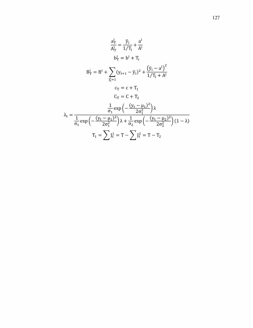
127

a��A�� yr�1 T�⁄ " a�A�b�� b� " T�

B�� B� " p7y}X� � yr�:J��

" &yr� � a�*J1 T�⁄ " A� c� � c " T�C� � C " TJ

λ} �1σ� exph� 7y} � μ�:J2σ�J l λ

1σ� exp h� 7y} � μ�:J2σ�J l λ " 1σJ exph� 7y} � μJ:J2σJJ l 71 � λ:

T� �pJ}� � T �pJ}J � T � TJ

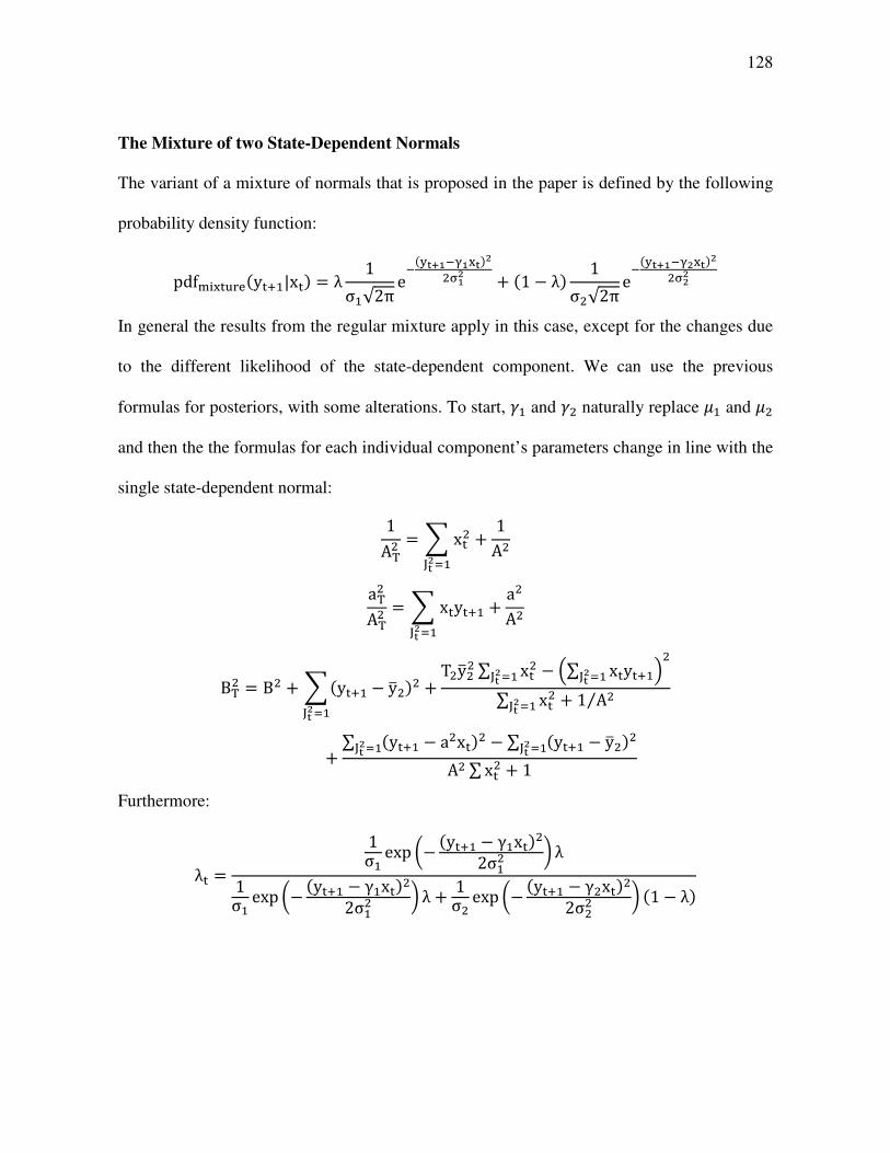
128

The Mixture of two State-Dependent Normals

The variant of a mixture of normals that is proposed in the paper is defined by the following

probability density function:

pdf �¡}¢£¤7y}X�|x}: � λ 1σ�√2π e

�7��^_�¦_¡�:aJ§_a " 71 � λ: 1σJ√2π e

�7��^_�¦a¡�:aJ§aa In general the results from the regular mixture apply in this case, except for the changes due

to the different likelihood of the state-dependent component. We can use the previous

formulas for posteriors, with some alterations. To start, d� and dJ naturally replace |� and |J

and then the the formulas for each individual component’s parameters change in line with the

single state-dependent normal:

1A�J � p x}J��a��

" 1AJa�JA�J � p x}y}X�

��a��" aJAJ

B�J � BJ " p7y}X� � yrJ:J��a��

" TJyrJJ∑ x}J��a�� ¨∑ x}y}X��a�� ©J∑ x}J��a�� " 1 AJ⁄

" ∑ 7y}X� � aJx}:J��a�� ∑ 7y}X� � yrJ:J��a��AJ ∑x}J " 1 Furthermore:

λ} �1σ� exph� 7y}X� � γ�x}:J2σ�J l λ

1σ� exp h� 7y}X� � γ�x}:J2σ�J l λ " 1σJ exph� 7y}X� � γJx}:J2σJJ l 71 � λ:

129

A.3 The Gibbs Sampler

Armed with all the conditional posteriors above we can now set up the Gibbs sampler. And

the steps are then the following:

Step 1: Initialize:

7μ, σ�J:�~NIG Ra�� , A�� , b��2 , B��2 S7γ, σJJ:�~NIG Ra�J , A�J , b�J2 , B�J2 S

λ�~Beta7c, C:J�~Ber7λ�:

Step 2: Sample:

For n=1,2,…,N, draw:

7μ, σ�J:7ª:~NIG R7a�� :7ª��:, 7A�� :7ª��:, 7b��:7ª��:2 , 7B��:7ª��:2 S7γ, σJJ:7ª:~NIG R7a�J:7ª��:, 7A�J :7ª��:, 7b�J:7ª��:2 , 7B�J:7ª��:2 S

J}~Ber7λ}:fort�1,2,…,Tλ7ª:~Beta7c�, C�:

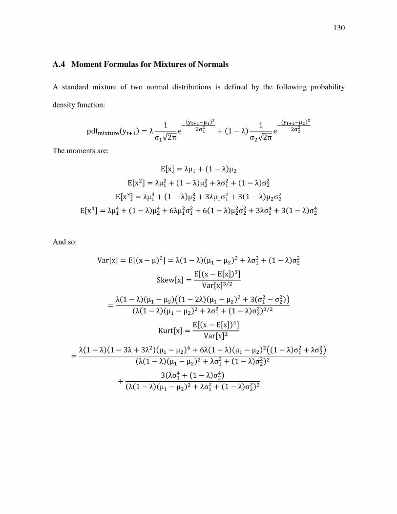
130

A.4 Moment Formulas for Mixtures of Normals

A standard mixture of two normal distributions is defined by the following probability

density function:

pdf �¡}¢£¤7y}X�: � λ 1σ�√2π e

�7��^_�¬_:aJ§_a " 71 � λ: 1σJ√2π e

�7��^_�¬a:aJ§aa The moments are:

E�x� � λμ� " 71 � λ:μJE�xJ� � λμ�J " 71 � λ:μJJ " λσ�J " 71 � λ:σJJ

E�x®� � λμ�® " 71 � λ:μJ® " 3λμ�σ�J " 371 � λ:μJσJJE�x¯� � λμ�̄ " 71 � λ:μJ̄ " 6λμ�Jσ�J " 671 � λ:μJJσJJ " 3λσ�̄ " 371 � λ:σJ̄

And so:

Var�x� � E�7x � μ:J� � λ71 � λ:7μ� � μJ:J " λσ�J " 71 � λ:σJJSkew�x� � E�7x � E�x�:®�Var�x�® J⁄

� λ71 � λ:7μ� � μJ:&71 � 2λ:7μ� � μJ:J " 37σ�J � σJJ:*7λ71 � λ:7μ� � μJ:J " λσ�J " 71 � λ:σJJ:® J⁄ Kurt�x� � E�7x � E�x�:¯�Var�x�J

� λ71 � λ:71 � 3λ " 3λJ:7μ� � μJ:¯ " 6λ71 � λ:7μ� � μJ:J&71 � λ:σ�J " λσJJ*7λ71 � λ:7μ� � μJ:J " λσ�J " 71 � λ:σJJ:J" 37λσ�̄ " 71 � λ:σJ̄:7λ71 � λ:7μ� � μJ:J " λσ�J " 71 � λ:σJJ:J

131

Appendix B

B.1 Model of Conditional Normal

The assumed underlying distribution for the data is a “conditional normal”:

p7y}X�|x}: � N7γx}, σJ:So the pdf is:

p7y}X�|γ, σ, x}: � 1σ√2π e�

7��^_�¦¡�:aJ§a ∝ 1σ e�7��^_�¦¡�:aJ§a

As when we have data with the regular normal distribution, the conjugate prior turns out to

be normal inverse gamma:

γ, σJ~NIG ha, A, b2 , B2lp7γ, σJ: � p7γ|σJ:p7σJ:

γ|σJ~N7a, AσJ:σJ~IG hb2 , B2l

And so:

p7γ|σJ: � 1σ√2πA e�

7¦�¸:aJ¹§a ∝ 1σ e�7¦�¸:aJ¹§a

p7σJ: � 7B 2⁄ :º J⁄Г7b 2⁄ : 1

7σJ:¼a^_ e�½ J⁄§a ∝ 1σºXJ e�

½J§aB.2 Posterior Derivation

The posterior therefore becomes:

p7γ, σJ|y, x: � p7y|γ, σJ, x:p7γ|σJ:p7σJ:p7y|x:

132

∝ p7y|γ, σJ, x:7γ|σJ:p7σJ:∝ 1σ� e�

∑7��^_�¦¡�:aJ§a 1σ e�7¦�¸:aJ¹§a 1σºXJ e�

½J§a� 1σºX�X® e�

½J§ae� �J§ah∑7��^_�¦¡�:aX7¦�¸:a¹ l

Looking just at the the term within the parentesis, and calling it we see that:

p7y}X� � γx}:J " 7γ � a:JA �py}X�J � 2pγx}y}X� " γJpx}J " 1AγJ � 2Aaγ " aJA �py}X�J " hpx}J " 1Al γJ � 2¨px}y}X� " aA© γ " aJA

�py}X�J " hpx}J " 1AlRγ � ∑x}y}X� " a A⁄∑x}J " 1 A⁄ SJ � hpx}J " 1AlR∑x}y}X� " a A⁄∑ x}J " 1 A⁄ SJ " aJA � hpx}J " 1AlRγ � ∑x}y}X� " a A⁄∑ x}J " 1 A⁄ SJ "py}X�J � hpx}J " 1AlR∑x}y}X� " a A⁄∑ x}J " 1 A⁄ SJ " aJA

For ease let’s rename:

C � hpx}J " 1AlRγ � ∑x}y}X� " a A⁄∑x}J " 1 A⁄ SJD �py}X�J � hpx}J " 1AlR∑ x}y}X� " a A⁄∑x}J " 1 A⁄ SJ " aJA

We can now write:

p7γ, σJ|y, x: ∝ 1σ e�¿J§a 17σJ:ºX�J X� e�

½XÀJ§a And so we can write the posterior in the form:

p7γ, σJ|y, x: � p7γ|σJ, y, x:p7σJ|y, x:Where the posterior for d is defined by:

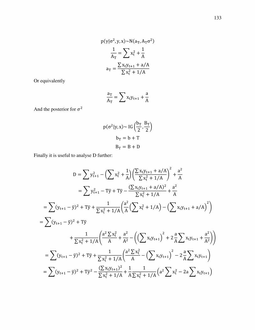
133

p7γ|σJ, y, x:~N7a�, A�σJ:1A� �px}J " 1Aa� � ∑x}y}X� " a A⁄∑ x}J " 1 A⁄

Or equivalently

a�A� � px}y}X� " aAAnd the posterior for ZJ

p7σJ|y, x:~IG hb�2 , B�2 lb� � b " TB� � B " D

Finally it is useful to analyse D further:

D �py}X�J � hpx}J " 1AlR∑ x}y}X� " a A⁄∑x}J " 1 A⁄ SJ " aJA �py}X�J � Tyr " Tyr � 7∑x}y}X� " a A⁄ :J∑x}J " 1 A⁄ " aJA

� p7y}X� � yr:J " Tyr " 1∑x}J " 1 A⁄ RaJA ¨px}J " 1 A⁄ © � ¨px}y}X� " a A⁄ ©JS�p7y}X� � yr:J " Tyr

" 1∑x}J " 1 A⁄ ÁaJ∑x}JA " aJAJ � R¨px}y}X�©J " 2 aApx}y}X� " aJAJSÂ�p7y}X� � yr:J " Tyr " 1∑ x}J " 1 A⁄ RaJ∑x}JA � ¨px}y}X�©J � 2 aApx}y}X�S�p7y}X� � yr:J " TyrJ � 7∑x}y}X�:J∑x}J " 1 A⁄ " 1A 1∑ x}J " 1 A⁄ ¨aJpx}J � 2apx}y}X�©

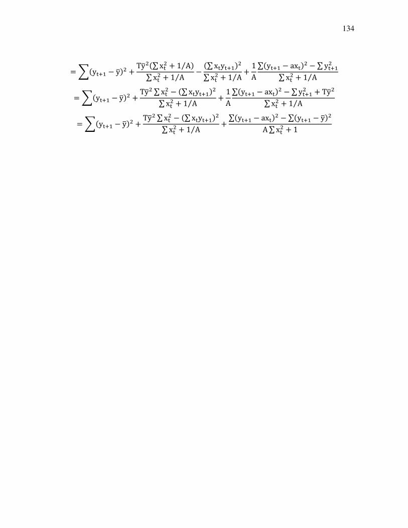
134

� p7y}X� � yr:J " TyrJ7∑ x}J " 1 A⁄ :∑ x}J " 1 A⁄ � 7∑x}y}X�:J∑x}J " 1 A⁄ " 1A∑7y}X� � ax}:J � ∑y}X�J∑x}J " 1 A⁄

� p7y}X� � yr:J " TyrJ∑x}J � 7∑x}y}X�:J∑x}J " 1 A⁄ " 1A∑7y}X� � ax}:J � ∑y}X�J " TyrJ∑x}J " 1 A⁄ �p7y}X� � yr:J " TyrJ∑x}J � 7∑x}y}X�:J∑x}J " 1 A⁄ " ∑7y}X� � ax}:J � ∑7y}X� � yr:JA∑x}J " 1

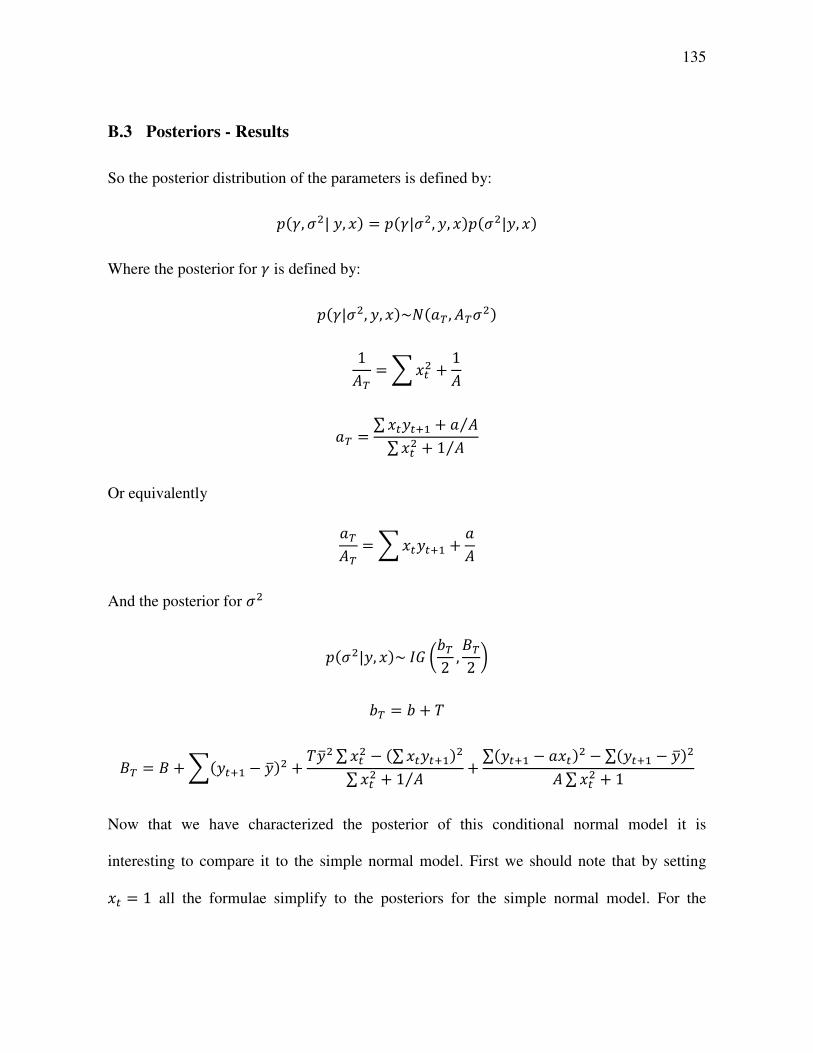
135

B.3 Posteriors - Results

So the posterior distribution of the parameters is defined by:

�7d, ZJ| , �: � �7d|ZJ, , �:�7ZJ| , �: Where the posterior for d is defined by:

�7d|ZJ, , �:~f7�o , ioZJ: 1io �p��J " 1i

�o � ∑�� X� " � i⁄∑��J " 1 i⁄

Or equivalently

�oio � p�� X� " �i

And the posterior for ZJ

�7ZJ| , �:~g hjo2 , ko2 l

jo � j " q

ko � k "p7 �X� � r:J " q rJ∑��J � 7∑�� X�:J∑��J " 1 i⁄ " ∑7 �X� � ��:J � ∑7 �X� � r:Ji∑��J " 1

Now that we have characterized the posterior of this conditional normal model it is

interesting to compare it to the simple normal model. First we should note that by setting

�� 1 all the formulae simplify to the posteriors for the simple normal model. For the

136

coefficient d the mean now does not approach (as the data grows) the sample mean of as in

the simple normal model but rather it approaches the regression coefficient of on �. The

variance of d is now not only increasing in the sample size but depends on the conditioning

variable �. For the distribution of ZJ there are also clear similarities to the normal model.

The jo parameter is the same for both models and the first two terms in the ko parameter are

the same as in the simple normal model. The last term of ko also corresponds to the term in

the simple normal model that depends on the prior parameters but becomes insignificant as

the sample grows. The distinguishing term is the third term which captures the uncertainty in

ZJ due to how good the linear fit is.

the dynamics of currency crashes and fundamental

Documents