266 IEEE JOURNAL OF OCEANIC ENGINEERING, VOL. 31, NO. 2, APRIL 2006

Stratigraphic Model Predictionsof Geoacoustic Properties

Barbara J. Kraft, Member, IEEE, Irina Overeem, Charles W. Holland, Lincoln F. Pratson, James P. M. Syvitski,and Larry A. Mayer

Abstract—Geoacoustic properties of the seabed have a con-trolling role in the propagation and reverberation of sound inshallow-water environments. Several techniques are availableto quantify the important properties but are usually unable toadequately sample the region of interest. In this paper, we ex-plore the potential for obtaining geotechnical properties from aprocess-based stratigraphic model. Grain-size predictions fromthe stratigraphic model are combined with two acoustic models toestimate sound speed with distance across the New Jersey conti-nental shelf and with depth below the seabed. Model predictionsare compared to two independent sets of data: 1) Surficial soundspeeds obtained through direct measurement using in situ com-pressional wave probes, and 2) sound speed as a function of depthobtained through inversion of seabed reflection measurements.In water depths less than 100 m, the model predictions producea trend of decreasing grain-size and sound speed with increasingwater depth as similarly observed in the measured surficial data.In water depths between 100 and 130 m, the model predictionsexhibit an increase in sound speed that was not observed in themeasured surficial data. A closer comparison indicates that thegrain-sizes predicted for the surficial sediments are generally toosmall producing sound speeds that are too slow. The predictedsound speeds also tend to be too slow for sediments 0.5–20 mbelow the seabed in water depths greater than 100 m. However, inwater depths less than 100 m, the sound speeds between 0.5–20-msubbottom depth are generally too fast. There are several reasonsfor the discrepancies including the stratigraphic model was lim-ited to two dimensions, the model was unable to simulate biologicprocesses responsible for the high sound-speed shell materialcommon in the model area, and incomplete geological recordsnecessary to accurately predict grain-size.

Index Terms—Geoacoustic inversion, in situ measurements, NewJersey shelf, stratigraphic models.

I. INTRODUCTION

ACOUSTIC propagation and reverberation predictions inshallow-water environments require knowledge of the

seabed properties. The physical properties of the seabed thatcontrol propagation and reverberation are termed geoacoustic

Manuscript received September 22, 2004; revised November 17, 2005; ac-cepted January 5, 2006. This work was supported in part by the U.S. Office ofNaval Research under Code 321OA. Guest Editor: J. A. Goff.

B. J. Kraft and L. A. Mayer are with the Center for Coastal and OceanMapping, University of New Hampshire, Durham, NH 03824 USA (e-mail:bjkraft@ccom.unh.edu; larry.mayer@unh.edu).

I. Overeem and J. P. M. Syvitski are with the Environmental Computation andImaging Facility, INSTAAR, University of Colorado, Boulder, CO 80309 USA(e-mail: irina.overeem@colorado.edu; syvitski@colorado.edu).

C. W. Holland is with the Applied Research Laboratory, Pennsylvania StateUniversity, State College, PA 16804 USA (e-mail: cwh10@psu.edu).

L. F. Pratson is with the Division of Earth and Ocean Sciences, Duke Univer-sity, Durham, NC 27708 USA (e-mail: lp14@duke.edu).

Digital Object Identifier 10.1109/JOE.2006.875235

properties. A geoacoustic model is environment specific andincludes property values that influence the main physical mech-anisms controlling the interaction of sound with the seabed.For low-to-mid frequency (50–5000 Hz) acoustic propagation,a geoacoustic model might include sediment compressionalsound speed, attenuation, and density as a function of depth andrange. The frequency dependence of the compressional soundspeed and attenuation, and shear sound speed and attenuationmay be important in some cases.

There are several methods employed to obtain geoacousticproperties of the seabed. One way is via direct measurement,which may include laboratory measurements on cores or inser-tion of in situ probes into the seabed. Another method is geoa-coustic inversion and it involves the measurement of an acousticparameter (e.g., transmission loss, reverberation, or the seabedreflection coefficient) that is later inverted for the desired geoa-coustic properties. A third method measures the intrinsic prop-erties of the sediments (e.g., porosity, permeability, or grain-sizedistribution) and it may use either phenomenological models(e.g., Biot theory [1]–[3]) or empirical models [4], [5] to relatethese parameters to the geoacoustic properties. In this paper, apossible new method for obtaining geoacoustic properties of theseabed is described using a state-of-the-art process-based strati-graphic model SedFlux-2D (discussed in Section II). The pur-pose of this comparison is to test the present capability of Sed-Flux-2D as a predictive model. Stratigraphic models have beenunder development over the last 15 years (e.g., [6]) and havethe potential to contribute to the development of geoacousticmodels. Ideally, a stratigraphic model could provide the geoa-coustic community the ability to simulate the stratigraphic evo-lution of a specific shelf region and provide the intrinsic prop-erties of the seabed without a priori geoacoustic knowledge. Aswill be shown, SedFlux-2D still has a ways to go before it can beused for this purpose. However, this comparison provides veryvaluable constraints needed to push SedFlux-2D toward moreaccurate realizations.

The region modeled by SedFlux-2D and presented here isan area of the New Jersey outer continental shelf (Fig. 1). Themajor advantage of this region is that it is one of the best-docu-mented continental shelves in the world. Numerous field studieshave amassed a vast set of physical, geotechnical, and acousticproperty measurements over a large range of water depths andextending from the seafloor to kilometers below. The seabed andsubbottom strata also have been exceptionally well mapped anddated relative to other continental shelves. Thus, from a mea-surement standpoint, the New Jersey outer shelf is an excellentlocation for validating model predictions.

0364-9059/$20.00 © 2006 IEEE

KRAFT et al.: STRATIGRAPHIC MODEL PREDICTIONS OF GEOACOUSTIC PROPERTIES 267

Fig. 1. Location map indicating the area of the stratigraphic modeling off NewJersey. The black lines (907 and 910) mark the location of two high-resolutionseismic lines. A regional stratigraphic horizon, the R-reflector, interpreted alongLine 910, was used to define a part of the initial surface used in the SedFluxsimulation.

SedFlux-2D predicts the distribution of grain sizes as afunction of position on the modeled shelf region relative tothe sediment source and depth in the seabed [the model em-ployed here is two-dimensional (2-D)]. The method of relatingthe SedFlux-2D intrinsic property predictions to geoacousticproperties (i.e., sound-speed estimates were obtained usingseveral empirical and phenomenological models) is discussedin Section III. Described in Section IV are two experimentaltechniques that were previously employed on the New Jerseyshelf. The first used an in situ probe to obtain surficial measure-ments of sediment sound speed. The second method acquiredbroadband seabed reflection data that was inverted to obtainestimates of sound speed in the upper few tens of meters of thesediment column. The geoacoustic data from these experimentsare compared to the SedFlux model predictions in Section V.Results of the comparisons show that there remains consider-able deviation between the model predictions, the subsequentlymodeled geoacoustic properties, and the observations. Sec-tion VI discusses a number of reasons for the discrepanciesidentifying model processes or inputs needing improvements.

II. STRATIGRAPHIC MODEL DESCRIPTION

A. SedFlux Modeling Methodology

SedFlux-2D, hereafter referred to as SedFlux, is a 2-Dprocess-based stratigraphic model that predicts spatially

varying stratigraphy. The model consists of a series of processmodules (described below) that interact to distribute sedimentthroughout an evolving coastal zone over a period of time.Sediment is supplied to the modeled environment by a singleriver. Floodplain sediment and coarse bedload are depositedby fluvio-deltaic processes. Suspended sediment carried bythe river is dispersed in the ocean through buoyant surface(hypopycnal) plumes. Seabed sediment is dispersed and sortedby ocean storms, and the failure of margin deposits and theirsubsequent transport as sediment gravity flows. SedFlux alsoconsiders basinal processes that affect the accommodationspace, such as time-varying sea-level changes, downwarddisplacement of the earths crust due to large sediment loading(isostatic subsidence), and sediment consolidation [7]–[13].

SedFlux predicts the thickness of the deposited sediment andthe distribution of grain-sizes. Sediment permeability, porosity,and bulk density are dynamically derived and averaged overtime and over specified bins (typically 0.1 m) along a longitu-dinal profile. The 2-D character of SedFlux requires interpre-tation of the profile as a spatially averaged “corridor” normalto the shore. This study focuses on shallow shelf (up to 150-mwater depth) stratigraphy. Relevant process modules are sum-marized in the following section. For additional details on theSedFlux process modules and sensitivity tests that were per-formed to explore the ranges in the input parameters see [14].

1) River Discharge and Sediment Load: Details on the rivermouth dynamics for each time step (years) of the simula-tion are determined using the hydrologic-transport model HY-DROTREND [8], [15]. HYDROTREND numerically simulatesthe water and sediment discharge at a river mouth based on cli-mate trends and drainage basin characteristics. HYDROTRENDpredicts the rivers water discharge (m s ) and the rateat which sediment, comprised of suspended sediment (kgs ) and sediment carried as bedload (kg s ), is deliveredbased on drainage basin properties, hydrological parameters,steady-state groundwater budget, and glacier dynamics [12].Suspended sediment is composed of a user-specified numberof distinct grain sizes while sediment transported as bedload iscomposed of a single grain size.

2) Fluvial Erosion and Deposition: We have adopted the ap-proach of Paola et al. [16], based on first principles of massand momentum conservation, to predict erosion and depositionalong the subaerial river profile

(1)

where is the bed height (m), is time (s), is the position alongthe longitudinal profile (m), and is the diffusion coefficient(m s ) given by

(2)

In (2), is the time-averaged water discharge (m s ) nor-malized by the basin width, is a dimensionless drag coeffi-cient, is the initial volume concentration of sediment in thebed, SG is the sediment specific gravity, and RT is a river-typedependent constant. In SedFlux, channels are not modeled as

268 IEEE JOURNAL OF OCEANIC ENGINEERING, VOL. 31, NO. 2, APRIL 2006

specific features and an assumption is made that RT 1 (a typ-ical value for meandering rivers).

3) Plume: The SedFlux plume equations follow those of Al-bertson et al. [17] developed for a submerged jet flowing into asteady ocean. Plumes of similar shape but differing concentra-tions result for each grain-size in the SedFlux model [9]. Plumedynamics are governed by the steady 2-D advection-diffusionequation

(3)

where is distance in the longitudinal or axial direction (m),is distance in the lateral direction (m), is longitudinal velocity(m s ), is lateral velocity (m s ), is the sediment inven-tory or mass per unit area of the plume (kg m ), is thefirst-order removal rate constant (s ), and is the sedimentdiffusivity driven by turbulence (m s ). Sediment concentra-tion falls off exponentially in both the longitudinal and lateraldirections.

4) Bedload Dumping: Floodplain sedimentation in the sub-aerial part of the profile is modeled as deposition of coarse sed-iments by “pseudocrevasse splays.” A user-specified fraction ofthe bedload at the river mouth is uniformly spread over the sub-aerial domain to mimic this process. The fluvial bedload(kg s ) that enters the marine environment is spread over auser-specified distance designed to reflect the zone of mouthbar deposition on a delta front determined from the tidal range.The sedimentation rate of bedload (m s ) over this bedloaddumping distance (m) is given by

(4)

where is the basin width (m) and is the uncompacteddensity of bedload sands (kg m ).

5) Avulsion: Avulsion is the primary process that deter-mines the location of the river mouth and is a controllinginfluence on the distribution of river sediment on a delta plain.To mimic avulsion of a river, the river mouth position at aspecific time is determined by a distance and angle from theapex. The river mouth angle at time step changes byan amount drawn from a Gaussian distribution given by

(5)

where the rate of switching is controlled by the scaling factorof the Gaussian deviate . This is an approximation that takesinto account changes in the river mouth position. The choiceof a Gaussian deviate implies that large changes of location dooccur but occur less frequently than small changes. In SedFlux,an avulsion results in a reduction of the sediment flux distributedtoward the modeled corridor.

6) Ocean Storm Reworking: SedFlux generates specificocean storm conditions for each time step from a log normaldistribution of wave heights. This distribution is set by the100-year storm for each environment modeled and can vary

under different climate conditions. Storm reworking is deter-mined as the net effect of separate storm erosion and depositionalgorithms. Storm erosion is modeled after Storms [18], [19]as

(6)

where is the time-dependent erosion efficiency and

(7)

In (7), is the topographic profile height, is sea levelheight, is the wave base, and the exponent represents thedependence of erosion rate on water depth [18], [19].Deep water waves are typically low amplitude waves with wave-lengths greater than 25 times that of the wave heights. Based onthis large ratio of wavelength to wave height, Airy (linearized)wave theory is assumed. The wave base is assumed to be halfthe wavelength. The erosion efficiency is modeled as

(8)

where is the grain-size independent erodibility of the sedi-ment and equal to 0.2. Erosion occurs between the coastlineand the location of the wave base . Volume fractions of thedifferent grain-size classes within the potentially eroded volumeare determined. SedFlux checks whether each grain-size frac-tion can be picked up by using empirically derived thresholds forgrain motion [20], [21]. The total sediment flux of grain-size

available for deposition is given by

(9)

where is the erosion function given in (6). Deposition dependson grain-size and water depth. We assume that the threshold forthe initiation of motion can be used for each grain-size to definethe start of the (depth) zone of deposition. Sediment is depositedwith increasing water depth according to Weibull distributionfunctions. Different values of the Weibull shape parameter canhave marked effects on the behavior of the distribution. Theshape of the Weibull distribution is such, that for bedload, thedeposition falls off exponentially. The shapes of the suspendedload depositional curves are set so that the coarser fractions aretransported over a limited distance, whereas the finest grains aretransported the furthest.

7) Consolidation: Sediment consolidation is an importantprocess determining acoustic sediment properties. The degreeto which a sediment layer consolidates depends on the load in-duced by the overlying sediment [13], [22]. The sediment mayconsolidate until it reaches a “closest-packed” arrangement cor-responding to a minimum porosity. The porosity of a sedimentlayer is found through

(10)

where is the porosity, is the load (Pa), is the consolida-tion coefficient (Pa ), and the porosity of the sediment in

KRAFT et al.: STRATIGRAPHIC MODEL PREDICTIONS OF GEOACOUSTIC PROPERTIES 269

its closest-packed arrangement. Both and are a functionof sediment mean grain-size and taken from empirical data sets[5], [23]. The load is based on the burden of the overlying sedi-ment and takes into account pore water pressure.

B. New Jersey Shelf Example

1) Model Input: The shallow stratigraphy of the NewJersey continental shelf (Fig. 1) has been studied extensively[24]–[31]. Interpretation of high-resolution seismic data hasshown that a prominent regional stratigraphic horizon reflector,the R-horizon reflector, exists below the seafloor. Several Cradiocarbon analyses [29], [32] date the R-reflector at greaterthan 40 kyr (kilo-years). Although the R-reflector probably hasa complex diachronous history, the New Jersey simulation wassimplified by using R as the initial surface. A part of the surfacewas defined from one of the high-resolution seismic lines (Line910 in Fig. 1) and the simulation limited to the last 40 kyr ofsedimentary evolution.

Changes in sea level over the duration of the SedFlux sim-ulation were significant. Sea level curves covering part of thesimulated time span were combined into one continuous curve[33]–[36]. The combined curve indicates a fluctuating sea level(at 50 m) over the period between 40–30 kyr and then a steepsea level fall to 120 m at approximately 20–18 kyr coincidingwith the growth of a large ice sheet over North America. Sealevel rose rapidly during melting of the ice sheet, roughly be-tween 18 and 10 kyr, and a slower rise in sea level was recon-structed for the last 10 kyr.

The Hudson River is the main source of sediment deliveredto the New Jersey shelf. Information on the range of sedimentgrain-sizes carried by the Hudson River over time is limited. Itis known that the sediment load carried by rivers varies underdifferent climatic conditions. The initial five grain-size classes,specified by the user, were selected to represent a wide range ofsediment types, from coarse sands to clay (Table I). Three char-acteristic time periods were included in the simulation: 40–20,20–10, and 10–0 kyr. In the Late Pleistocene, between 40–20kyr, North America experienced a glaciation. The LaurentideIce Sheet existed in the drainage basin of the Hudson River. Theice sheet advanced over time and reached its maximum extentat roughly 20 kyr. During deglaciation enormous amounts ofmelt water drained toward the New Jersey shelf [37]. The meltwater contributed to the Hudson River stopped abruptly whenthe ice sheet retreated north of the St. Lawrence River. Presentday conditions were assumed for the Holocene period between10–0 kyr. River-water discharge, suspended sediment load, andbedload for these three characteristic periods are based on HY-DROTREND simulations (Table II). We assumed that undercolder glacial conditions there was an increased proportion offloodplain sedimentation (Table II). The spreading zone for theriver bedload and the rate of river avulsion were kept constantover the entire simulation (Table II).

Storm climate over long time spans is difficult to reconstruct.Dust and glacio-chemical records as retrieved from ice-coresprovide proxy records of the storminess [38]. The magnitudeand variability of dust and sea-spray related ions vary signif-icantly over the last 40 kyr in the Greenland ice sheet project2 (GISP2) ice-core. These components are higher and more

TABLE IINPUT PARAMETERS FOR SEDFLUX MODEL

TABLE IISEDFLUX INPUT PARAMETERS FOR THREE CHARACTERISTIC TIME PERIODS

variable during cold conditions, indicating increased storminessand higher wave heights in the Northern Hemisphere [38], [39].Proxy studies indicate that a generally stormier system was ex-pected for the two early periods (40–20 and 20–10 kyr), but thechanges are not accurately quantified. Present-day wave condi-tions were based on observed data. WAVEWATCH III [40], [41]was used to retrieve the peak storm wave height and associatedstatistics at the New Jersey margin and to set the probability den-sity function from which SedFlux sampled storm wave heights.Table II shows the wave heights, storm duration, and storm fre-quencies used for the three characteristic time periods.

The uncertainty in the different boundary conditions is con-siderable. The further back in geologic time, the more uncertainthe estimate of a specific parameter. The uncertainty associated

270 IEEE JOURNAL OF OCEANIC ENGINEERING, VOL. 31, NO. 2, APRIL 2006

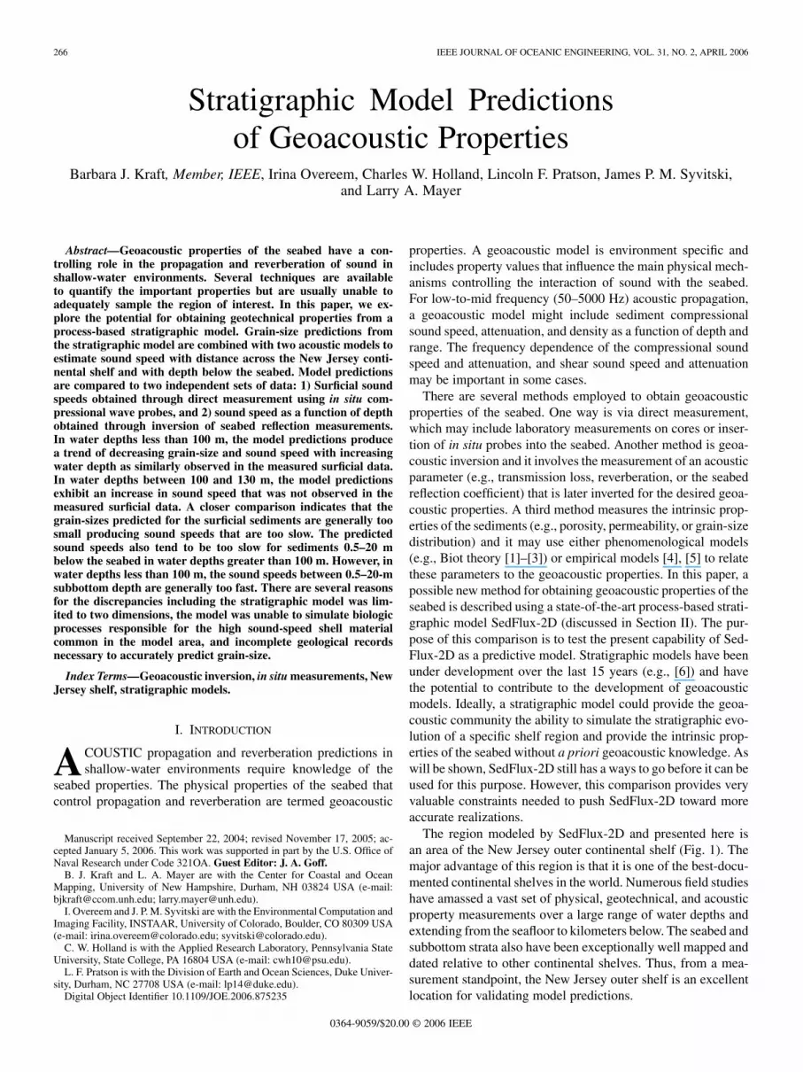
Fig. 2. (a) SedFlux simulation of shallow-water stratigraphy of the New Jersey continental shelf. (b) Schematic of dip profile showing the shallow-waterstratigraphy of the New Jersey margin compiled using chirp sonar profiles landward of the�50-m isobath and Huntec boomer profiles from �50 to 100 m [29].

with each input of SedFlux was explored in a series of sensi-tivity simulations [14]. The effect of these uncertainties on thecompressional sound speed is discussed in Section VI.

2) Model Output: A 40 000 year simulation was run withthe input parameters as described before. Shown in Fig. 2(a)is a 100-km cross-section of the simulated stratigraphy. Thegeneral picture is that of a sea-level-rise-controlled retrogradingsystem. The Late Pleistocene deposition rate was high whichproduced an extensive deltaic wedge close to the shelf slopeat 140–170 m below present water depth. Storm activity re-worked the seabed intensely and moved the depocenter (areaof thickest deposition) of the delta toward deeper water, so thata significant sediment wedge builds in to about 160-m waterdepth. A large part of the shallow shelf has only a thin veneer(less than 20 m) of sediment. Terrestrial coarse fluvial sedi-ment and near-shore sands (bright yellow) sit at the base of themidshelf zone. During the Holocene (10–0 kyr), the rise in sealevel slowed considerably allowing sediment to accumulate inthe present-day near-shore region. The wedge is not as exten-sive, due to the river contributing less sediment after the “decou-pling” of the ice-sheet drainage. At that time, storm reworkingon the New Jersey shelf carried the younger fine sediment todeeper water.

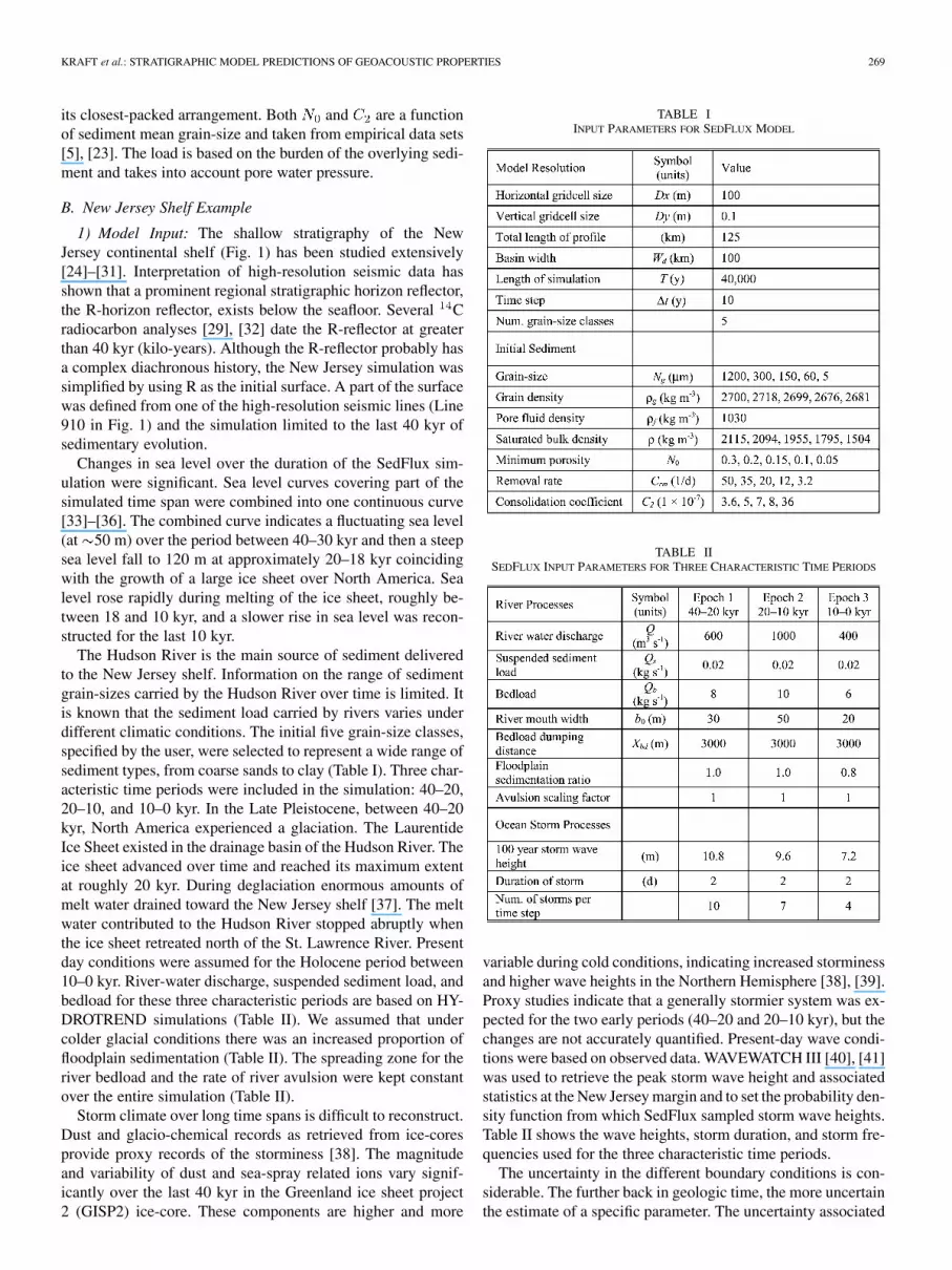
The geometry of the deposited sediments can be qualita-tively compared with a compilation of the known stratigraphy(Fig. 2(b), after [29]). As described from high-resolutionseismic data, a midshelf wedge and an outer-shelf wedgeare distinguished at 40–60-m water depth and at 65–100-mwater depth, respectively. The SedFlux simulation shows anouter-shelf wedge that extends into deeper water, a locationwhere observed data were not available. The midshelf wedge isless evident in the predicted stratigraphy than in the observeddata. Since SedFlux cannot reproduce distinct channels, the ob-served channels were not explicitly matched in the prediction.However, terrestrial coarse fluvial sediment (bright yellow) isthe typical environment that would contain channel bodies ina full three-dimensional (3-D) stratigraphic model. A quanti-tative analysis between simulated and observed data is madeby comparing sediment thickness. Fig. 3 shows the thicknessof sediment deposited versus water depth over the duration ofthe SedFlux simulation. Similarly, a 3-D interpretation (overa small area) of the R-reflector depth has been reconstructedbased on regional seismic surveying [31]. This surface was col-lapsed into a mean thickness of sediments above the R-reflectorper water depth. The predicted thickness matches the observedthickness closely (less than 6-m difference in water depths near

KRAFT et al.: STRATIGRAPHIC MODEL PREDICTIONS OF GEOACOUSTIC PROPERTIES 271

Fig. 3. Comparison of the predicted sediment thickness after the 40 kyr SedFlux simulation with the observed sediment thickness above the R-reflector based onreconstruction of the regional seismic data (average over all seismic lines).

50 and 130 m), as shown in Fig. 3. The predicted thickness ofthe outer shelf wedge is up to m in the simulation, whereasthe thickness of the midshelf deposit is locally only m. Thiscomparison shows that SedFlux was able to predict the grossstructure of the shallow stratigraphy for the New Jersey margin.

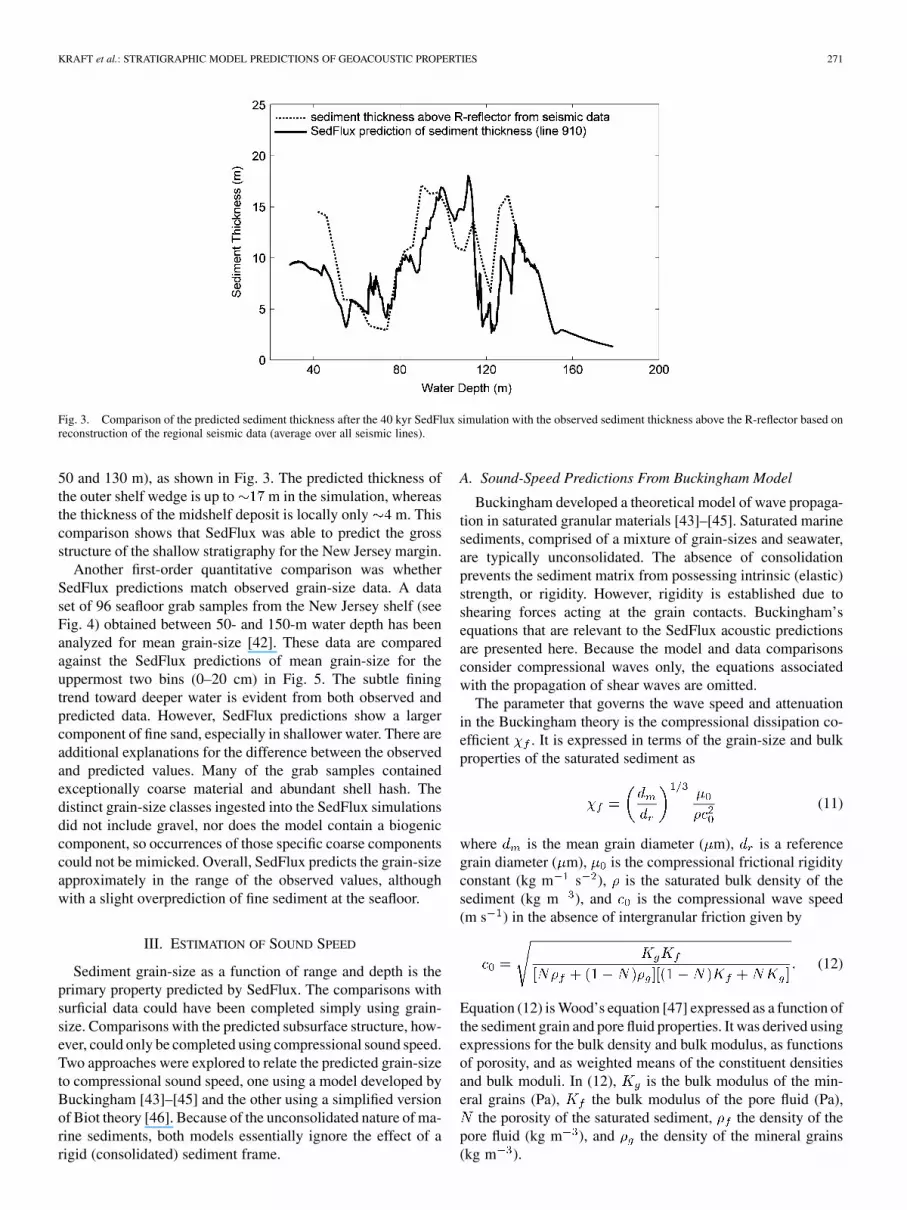
Another first-order quantitative comparison was whetherSedFlux predictions match observed grain-size data. A dataset of 96 seafloor grab samples from the New Jersey shelf (seeFig. 4) obtained between 50- and 150-m water depth has beenanalyzed for mean grain-size [42]. These data are comparedagainst the SedFlux predictions of mean grain-size for theuppermost two bins (0–20 cm) in Fig. 5. The subtle finingtrend toward deeper water is evident from both observed andpredicted data. However, SedFlux predictions show a largercomponent of fine sand, especially in shallower water. There areadditional explanations for the difference between the observedand predicted values. Many of the grab samples containedexceptionally coarse material and abundant shell hash. Thedistinct grain-size classes ingested into the SedFlux simulationsdid not include gravel, nor does the model contain a biogeniccomponent, so occurrences of those specific coarse componentscould not be mimicked. Overall, SedFlux predicts the grain-sizeapproximately in the range of the observed values, althoughwith a slight overprediction of fine sediment at the seafloor.

III. ESTIMATION OF SOUND SPEED

Sediment grain-size as a function of range and depth is theprimary property predicted by SedFlux. The comparisons withsurficial data could have been completed simply using grain-size. Comparisons with the predicted subsurface structure, how-ever, could only be completed using compressional sound speed.Two approaches were explored to relate the predicted grain-sizeto compressional sound speed, one using a model developed byBuckingham [43]–[45] and the other using a simplified versionof Biot theory [46]. Because of the unconsolidated nature of ma-rine sediments, both models essentially ignore the effect of arigid (consolidated) sediment frame.

A. Sound-Speed Predictions From Buckingham Model

Buckingham developed a theoretical model of wave propaga-tion in saturated granular materials [43]–[45]. Saturated marinesediments, comprised of a mixture of grain-sizes and seawater,are typically unconsolidated. The absence of consolidationprevents the sediment matrix from possessing intrinsic (elastic)strength, or rigidity. However, rigidity is established due toshearing forces acting at the grain contacts. Buckingham’sequations that are relevant to the SedFlux acoustic predictionsare presented here. Because the model and data comparisonsconsider compressional waves only, the equations associatedwith the propagation of shear waves are omitted.

The parameter that governs the wave speed and attenuationin the Buckingham theory is the compressional dissipation co-efficient . It is expressed in terms of the grain-size and bulkproperties of the saturated sediment as

(11)

where is the mean grain diameter ( m), is a referencegrain diameter ( m), is the compressional frictional rigidityconstant (kg m s ), is the saturated bulk density of thesediment (kg m ), and is the compressional wave speed(m s ) in the absence of intergranular friction given by

(12)

Equation (12) is Wood’s equation [47] expressed as a function ofthe sediment grain and pore fluid properties. It was derived usingexpressions for the bulk density and bulk modulus, as functionsof porosity, and as weighted means of the constituent densitiesand bulk moduli. In (12), is the bulk modulus of the min-eral grains (Pa), the bulk modulus of the pore fluid (Pa),

the porosity of the saturated sediment, the density of thepore fluid (kg m ), and the density of the mineral grains(kg m ).

272 IEEE JOURNAL OF OCEANIC ENGINEERING, VOL. 31, NO. 2, APRIL 2006

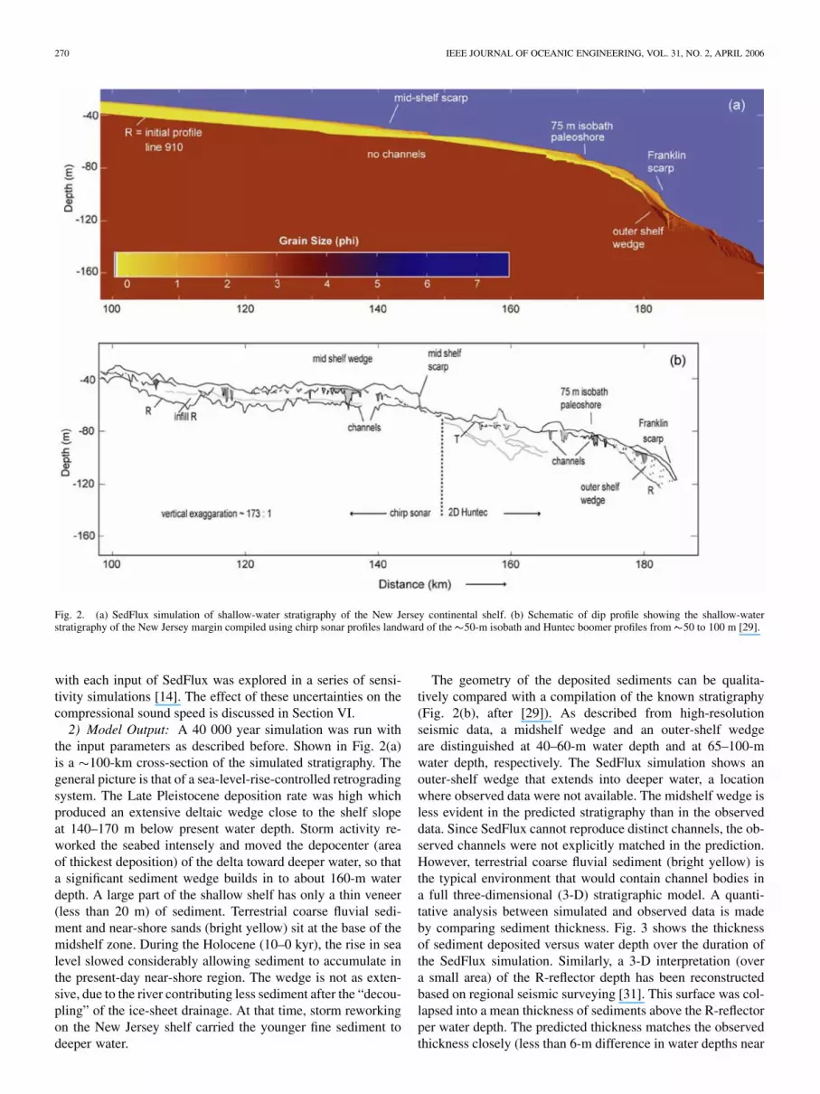
Fig. 4. Backscatter imagery of the GEOCLUTTER field area on the continental shelf off New Jersey, collected with a 95-kHz multibeam sonar. Lighter shadescorrespond to higher backscatter intensity. Symbols indicate station locations for ISSAP data and grab samples [42]. Contours are in meters.

Fig. 5. Comparison of the SedFlux predicted sediment mean grain-size(uppermost 20 cm) with mean grain-size observations consisting of 96 grabsamples taken between 50–150-m water depth at the New Jersey shelf [42].

Although Buckingham does provide a frequency-dependentexpression for the compressional wave speed [43], the simpli-fied frequency-independent equation was used assuming weaksound-speed dispersion. The near frequency independence ofthe critical angle (hence sound speed) from 100–6300 Hz indi-cates that this was reasonable at least at one site in this area [48].The compressional wave speed (m s ) is expressed as

(13)

Buckingham also derived an expression to predict porosity fromonly the grain-size. The derivation is based on a model of ran-domly packed sediment grains and takes into consideration theroughness of the sand grains

(14)

In (14), is the packing factor for a random arrangement ofsmooth spheres of uniform size and is the root mean square(rms) roughness height ( m) relative to the mean radius.

The Buckingham model was run in two ways: 1) Using theSedFlux predicted mean grain-size and empirically derivedporosity (SedFlux-B1), and 2) using only the SedFlux predictedmean grain-size (SedFlux-B2) and estimating the porosity using(14). Input parameters used in the Buckingham model are givenin Table III. The compressional frictional rigidity constant is amaterial-independent constant and was determined from a bestfit to surficial sound speed (discussed in Section IV-A) versusmean grain-size data.

B. Sound-Speed Predictions From the Effective DensityFluid Model

The effective density fluid model (EDFM) proposed byWilliams [46] is a simplified version of the Biot model [1]–[3].In the EDFM, the bulk and shear modulus of the consolidatedsediment frame are assumed to be negligible. Williams basedthis assumption on the several orders of magnitude differencebetween the frame bulk and shear moduli and the other moduli(bulk modulus of grains and fluid bulk modulus). This greatly

KRAFT et al.: STRATIGRAPHIC MODEL PREDICTIONS OF GEOACOUSTIC PROPERTIES 273

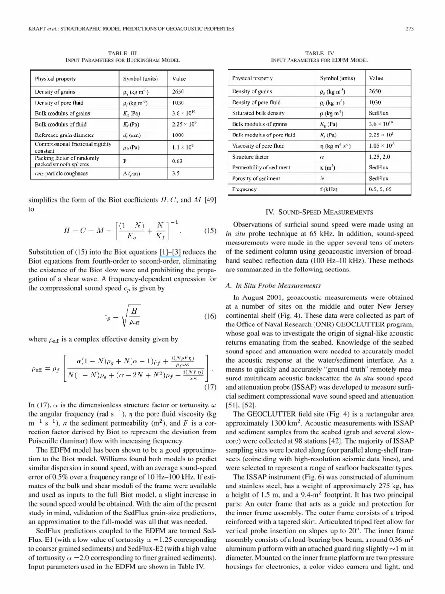
TABLE IIIINPUT PARAMETERS FOR BUCKINGHAM MODEL

simplifies the form of the Biot coefficients , and [49]to

(15)

Substitution of (15) into the Biot equations [1]–[3] reduces theBiot equations from fourth-order to second-order, eliminatingthe existence of the Biot slow wave and prohibiting the propa-gation of a shear wave. A frequency-dependent expression forthe compressional sound speed is given by

(16)

where is a complex effective density given by

(17)

In (17), is the dimensionless structure factor or tortuosity,the angular frequency (rad s ), the pore fluid viscosity (kgm s ), the sediment permeability (m ), and is a cor-rection factor derived by Biot to represent the deviation fromPoiseuille (laminar) flow with increasing frequency.

The EDFM model has been shown to be a good approxima-tion to the Biot model. Williams found both models to predictsimilar dispersion in sound speed, with an average sound-speederror of 0.5% over a frequency range of 10 Hz–100 kHz. If esti-mates of the bulk and shear moduli of the frame were availableand used as inputs to the full Biot model, a slight increase inthe sound speed would be obtained. With the aim of the presentstudy in mind, validation of the SedFlux grain-size predictions,an approximation to the full-model was all that was needed.

SedFlux predictions coupled to the EDFM are termed Sed-Flux-E1 (with a low value of tortuosity 1.25 correspondingto coarser grained sediments) and SedFlux-E2 (with a high valueof tortuosity 2.0 corresponding to finer grained sediments).Input parameters used in the EDFM are shown in Table IV.

TABLE IVINPUT PARAMETERS FOR EDFM MODEL

IV. SOUND-SPEED MEASUREMENTS

Observations of surficial sound speed were made using anin situ probe technique at 65 kHz. In addition, sound-speedmeasurements were made in the upper several tens of metersof the sediment column using geoacoustic inversion of broad-band seabed reflection data (100 Hz–10 kHz). These methodsare summarized in the following sections.

A. In Situ Probe Measurements

In August 2001, geoacoustic measurements were obtainedat a number of sites on the middle and outer New Jerseycontinental shelf (Fig. 4). These data were collected as part ofthe Office of Naval Research (ONR) GEOCLUTTER program,whose goal was to investigate the origin of signal-like acousticreturns emanating from the seabed. Knowledge of the seabedsound speed and attenuation were needed to accurately modelthe acoustic response at the water/sediment interface. As ameans to quickly and accurately “ground-truth” remotely mea-sured multibeam acoustic backscatter, the in situ sound speedand attenuation probe (ISSAP) was developed to measure surfi-cial sediment compressional wave sound speed and attenuation[51], [52].

The GEOCLUTTER field site (Fig. 4) is a rectangular areaapproximately 1300 km . Acoustic measurements with ISSAPand sediment samples from the seabed (grab and several slow-core) were collected at 98 stations [42]. The majority of ISSAPsampling sites were located along four parallel along-shelf tran-sects (coinciding with high-resolution seismic data lines), andwere selected to represent a range of seafloor backscatter types.

The ISSAP instrument (Fig. 6) was constructed of aluminumand stainless steel, has a weight of approximately 275 kg, hasa height of 1.5 m, and a 9.4-m footprint. It has two principalparts: An outer frame that acts as a guide and protection forthe inner frame assembly. The outer frame consists of a tripodreinforced with a tapered skirt. Articulated tripod feet allow forvertical probe insertion on slopes up to 20 . The inner frameassembly consists of a load-bearing box-beam, a round 0.36-maluminum platform with an attached guard ring slightly 1 m indiameter. Mounted on the inner frame platform are two pressurehousings for electronics, a color video camera and light, and

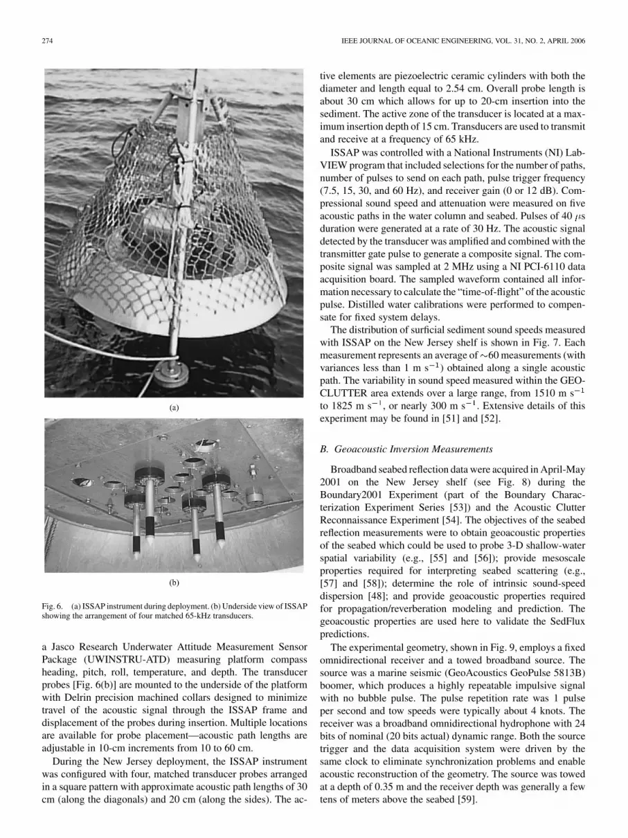
274 IEEE JOURNAL OF OCEANIC ENGINEERING, VOL. 31, NO. 2, APRIL 2006

Fig. 6. (a) ISSAP instrument during deployment. (b) Underside view of ISSAPshowing the arrangement of four matched 65-kHz transducers.

a Jasco Research Underwater Attitude Measurement SensorPackage (UWINSTRU-ATD) measuring platform compassheading, pitch, roll, temperature, and depth. The transducerprobes [Fig. 6(b)] are mounted to the underside of the platformwith Delrin precision machined collars designed to minimizetravel of the acoustic signal through the ISSAP frame anddisplacement of the probes during insertion. Multiple locationsare available for probe placement—acoustic path lengths areadjustable in 10-cm increments from 10 to 60 cm.

During the New Jersey deployment, the ISSAP instrumentwas configured with four, matched transducer probes arrangedin a square pattern with approximate acoustic path lengths of 30cm (along the diagonals) and 20 cm (along the sides). The ac-

tive elements are piezoelectric ceramic cylinders with both thediameter and length equal to 2.54 cm. Overall probe length isabout 30 cm which allows for up to 20-cm insertion into thesediment. The active zone of the transducer is located at a max-imum insertion depth of 15 cm. Transducers are used to transmitand receive at a frequency of 65 kHz.

ISSAP was controlled with a National Instruments (NI) Lab-VIEW program that included selections for the number of paths,number of pulses to send on each path, pulse trigger frequency(7.5, 15, 30, and 60 Hz), and receiver gain (0 or 12 dB). Com-pressional sound speed and attenuation were measured on fiveacoustic paths in the water column and seabed. Pulses of 40 sduration were generated at a rate of 30 Hz. The acoustic signaldetected by the transducer was amplified and combined with thetransmitter gate pulse to generate a composite signal. The com-posite signal was sampled at 2 MHz using a NI PCI-6110 dataacquisition board. The sampled waveform contained all infor-mation necessary to calculate the “time-of-flight” of the acousticpulse. Distilled water calibrations were performed to compen-sate for fixed system delays.

The distribution of surficial sediment sound speeds measuredwith ISSAP on the New Jersey shelf is shown in Fig. 7. Eachmeasurement represents an average of 60 measurements (withvariances less than 1 m s ) obtained along a single acousticpath. The variability in sound speed measured within the GEO-CLUTTER area extends over a large range, from 1510 m sto 1825 m s , or nearly 300 m s . Extensive details of thisexperiment may be found in [51] and [52].

B. Geoacoustic Inversion Measurements

Broadband seabed reflection data were acquired in April-May2001 on the New Jersey shelf (see Fig. 8) during theBoundary2001 Experiment (part of the Boundary Charac-terization Experiment Series [53]) and the Acoustic ClutterReconnaissance Experiment [54]. The objectives of the seabedreflection measurements were to obtain geoacoustic propertiesof the seabed which could be used to probe 3-D shallow-waterspatial variability (e.g., [55] and [56]); provide mesoscaleproperties required for interpreting seabed scattering (e.g.,[57] and [58]); determine the role of intrinsic sound-speeddispersion [48]; and provide geoacoustic properties requiredfor propagation/reverberation modeling and prediction. Thegeoacoustic properties are used here to validate the SedFluxpredictions.

The experimental geometry, shown in Fig. 9, employs a fixedomnidirectional receiver and a towed broadband source. Thesource was a marine seismic (GeoAcoustics GeoPulse 5813B)boomer, which produces a highly repeatable impulsive signalwith no bubble pulse. The pulse repetition rate was 1 pulseper second and tow speeds were typically about 4 knots. Thereceiver was a broadband omnidirectional hydrophone with 24bits of nominal (20 bits actual) dynamic range. Both the sourcetrigger and the data acquisition system were driven by thesame clock to eliminate synchronization problems and enableacoustic reconstruction of the geometry. The source was towedat a depth of 0.35 m and the receiver depth was generally a fewtens of meters above the seabed [59].

KRAFT et al.: STRATIGRAPHIC MODEL PREDICTIONS OF GEOACOUSTIC PROPERTIES 275

Fig. 7. Distribution of ISSAP measured sound speed on the New Jersey mid-to-outer continental shelf (GEOCLUTTER field area). Each measurement representsthe average of �60 obtained along one of the ISSAP acoustic paths.

Fig. 8. Seabed reflection measurement locations (circles) in the Boundary2001 study, New Jersey shelf. Depth contours are in meters.

Fig. 9. Geometry of reflection experiment.

In addition to the fixed receiver, a single-channel seismicstreamer was towed on the opposite side of the vessel (approxi-mately 15 m offset) to provide collocated seismic reflection dataalong the track. These data provided a qualitative indication of

the sediment layering structure. A conductivity, temperature,depth (CTD) cast was made before and expendable bathyther-mograph (XBT) casts during the reflection measurements.Core data were collected using a 1.3-m gravity corer. Coresobtained in the sandy sediments were generally only a few tensof centimeters in length.

Techniques for extracting geoacoustic information fromthe measurements are discussed in [59]–[61]. The inversionapproach used exploited data in both the space-time domain(these data were used to determine the location, thickness,and interval sound speed of each sediment layer) and in thespace-frequency domain, i.e., reflection loss as a functionof angle and frequency (these data were used to refine thesound-speed estimates and obtain density and attenuation).

1) Space-Time Domain Processing: An example of the rawreflection data time series are shown in Fig. 10, decimated toshow every third ping. At the closest point of approach, the di-rect path arrived at 0.05 s, the seabed reflected path at 0.08 s, and

276 IEEE JOURNAL OF OCEANIC ENGINEERING, VOL. 31, NO. 2, APRIL 2006

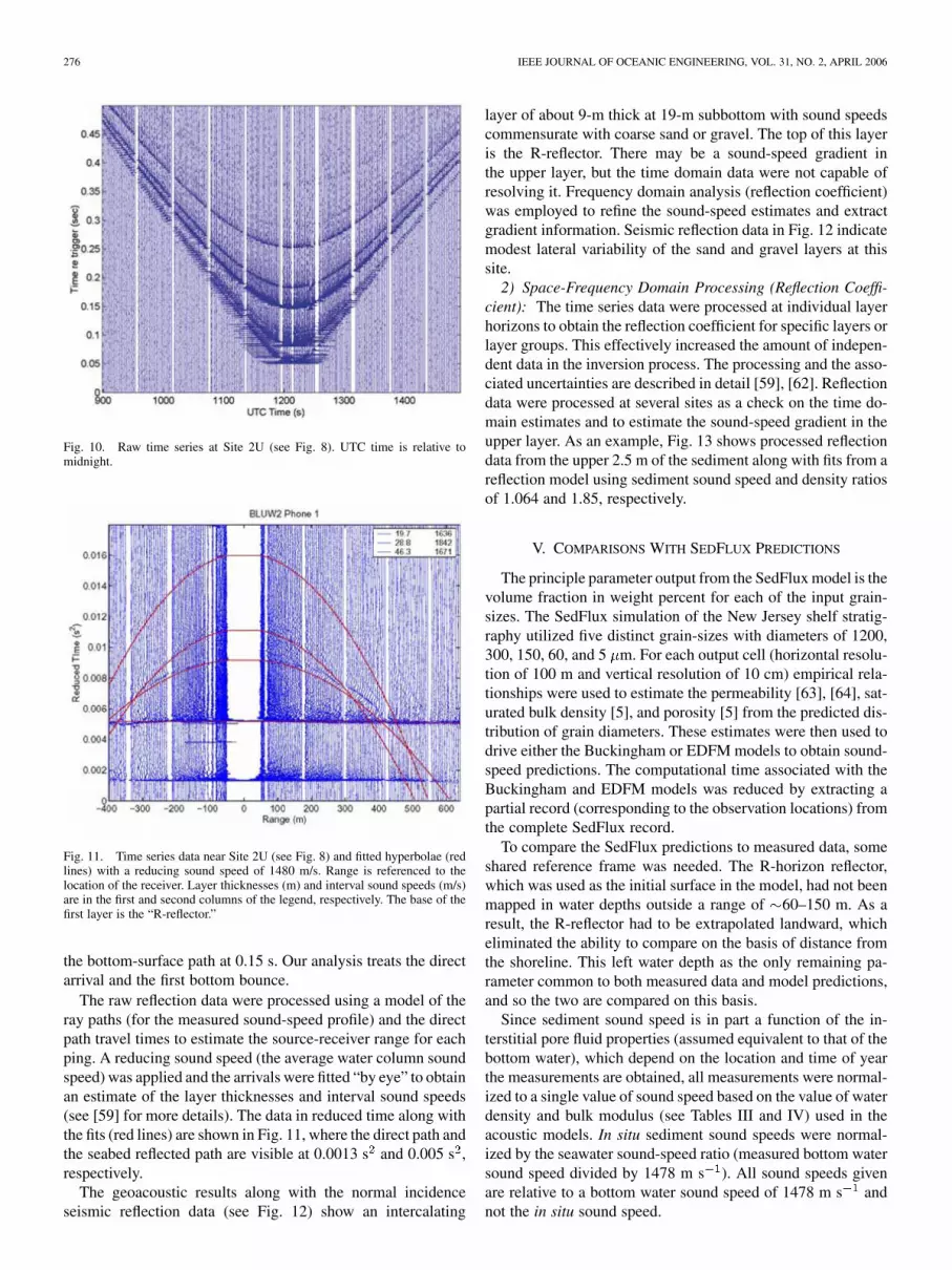
Fig. 10. Raw time series at Site 2U (see Fig. 8). UTC time is relative tomidnight.

Fig. 11. Time series data near Site 2U (see Fig. 8) and fitted hyperbolae (redlines) with a reducing sound speed of 1480 m/s. Range is referenced to thelocation of the receiver. Layer thicknesses (m) and interval sound speeds (m/s)are in the first and second columns of the legend, respectively. The base of thefirst layer is the “R-reflector.”

the bottom-surface path at 0.15 s. Our analysis treats the directarrival and the first bottom bounce.

The raw reflection data were processed using a model of theray paths (for the measured sound-speed profile) and the directpath travel times to estimate the source-receiver range for eachping. A reducing sound speed (the average water column soundspeed) was applied and the arrivals were fitted “by eye” to obtainan estimate of the layer thicknesses and interval sound speeds(see [59] for more details). The data in reduced time along withthe fits (red lines) are shown in Fig. 11, where the direct path andthe seabed reflected path are visible at 0.0013 s and 0.005 s ,respectively.

The geoacoustic results along with the normal incidenceseismic reflection data (see Fig. 12) show an intercalating

layer of about 9-m thick at 19-m subbottom with sound speedscommensurate with coarse sand or gravel. The top of this layeris the R-reflector. There may be a sound-speed gradient inthe upper layer, but the time domain data were not capable ofresolving it. Frequency domain analysis (reflection coefficient)was employed to refine the sound-speed estimates and extractgradient information. Seismic reflection data in Fig. 12 indicatemodest lateral variability of the sand and gravel layers at thissite.

2) Space-Frequency Domain Processing (Reflection Coeffi-cient): The time series data were processed at individual layerhorizons to obtain the reflection coefficient for specific layers orlayer groups. This effectively increased the amount of indepen-dent data in the inversion process. The processing and the asso-ciated uncertainties are described in detail [59], [62]. Reflectiondata were processed at several sites as a check on the time do-main estimates and to estimate the sound-speed gradient in theupper layer. As an example, Fig. 13 shows processed reflectiondata from the upper 2.5 m of the sediment along with fits from areflection model using sediment sound speed and density ratiosof 1.064 and 1.85, respectively.

V. COMPARISONS WITH SEDFLUX PREDICTIONS

The principle parameter output from the SedFlux model is thevolume fraction in weight percent for each of the input grain-sizes. The SedFlux simulation of the New Jersey shelf stratig-raphy utilized five distinct grain-sizes with diameters of 1200,300, 150, 60, and 5 m. For each output cell (horizontal resolu-tion of 100 m and vertical resolution of 10 cm) empirical rela-tionships were used to estimate the permeability [63], [64], sat-urated bulk density [5], and porosity [5] from the predicted dis-tribution of grain diameters. These estimates were then used todrive either the Buckingham or EDFM models to obtain sound-speed predictions. The computational time associated with theBuckingham and EDFM models was reduced by extracting apartial record (corresponding to the observation locations) fromthe complete SedFlux record.

To compare the SedFlux predictions to measured data, someshared reference frame was needed. The R-horizon reflector,which was used as the initial surface in the model, had not beenmapped in water depths outside a range of 60–150 m. As aresult, the R-reflector had to be extrapolated landward, whicheliminated the ability to compare on the basis of distance fromthe shoreline. This left water depth as the only remaining pa-rameter common to both measured data and model predictions,and so the two are compared on this basis.

Since sediment sound speed is in part a function of the in-terstitial pore fluid properties (assumed equivalent to that of thebottom water), which depend on the location and time of yearthe measurements are obtained, all measurements were normal-ized to a single value of sound speed based on the value of waterdensity and bulk modulus (see Tables III and IV) used in theacoustic models. In situ sediment sound speeds were normal-ized by the seawater sound-speed ratio (measured bottom watersound speed divided by 1478 m s ). All sound speeds givenare relative to a bottom water sound speed of 1478 m s andnot the in situ sound speed.

KRAFT et al.: STRATIGRAPHIC MODEL PREDICTIONS OF GEOACOUSTIC PROPERTIES 277

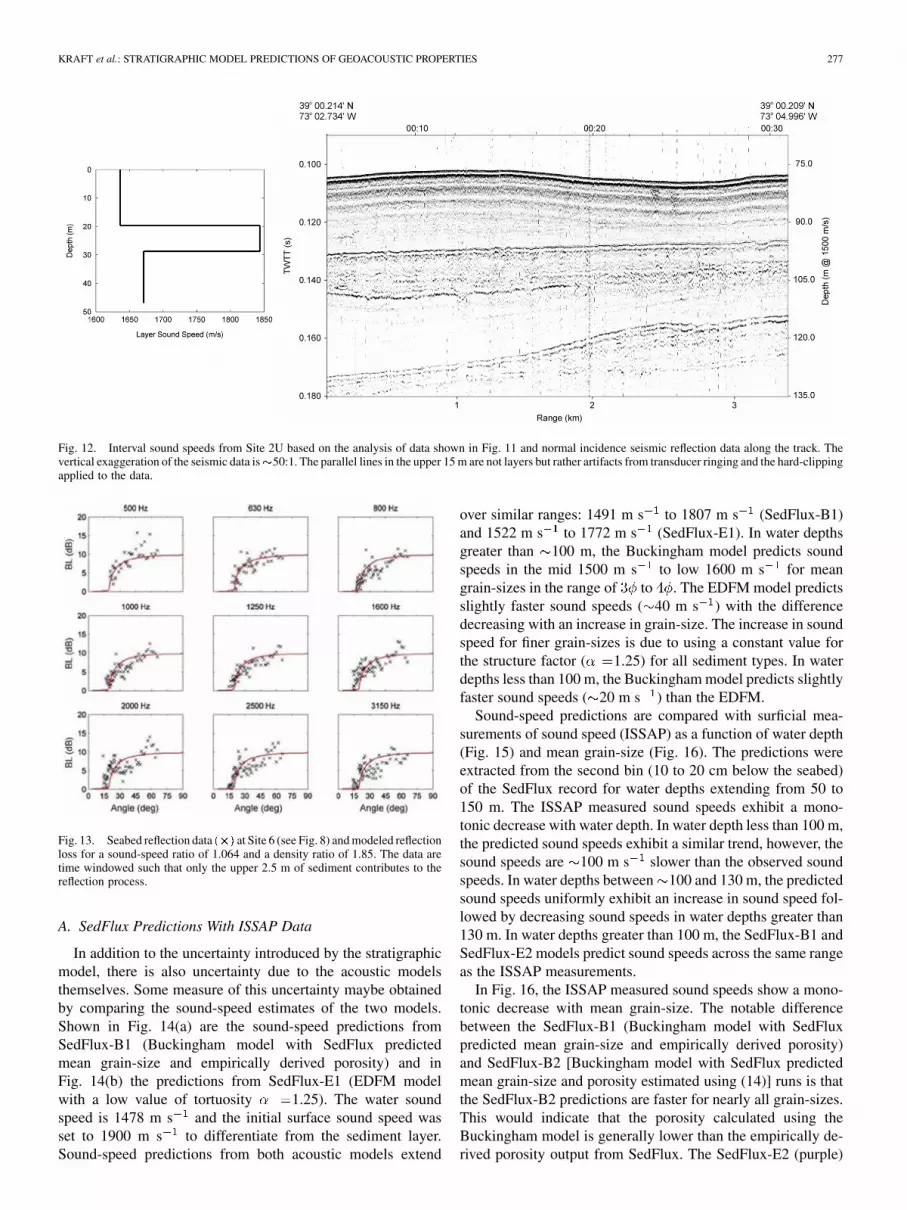
Fig. 12. Interval sound speeds from Site 2U based on the analysis of data shown in Fig. 11 and normal incidence seismic reflection data along the track. Thevertical exaggeration of the seismic data is�50:1. The parallel lines in the upper 15 m are not layers but rather artifacts from transducer ringing and the hard-clippingapplied to the data.

Fig. 13. Seabed reflection data (�) at Site 6 (see Fig. 8) and modeled reflectionloss for a sound-speed ratio of 1.064 and a density ratio of 1.85. The data aretime windowed such that only the upper 2.5 m of sediment contributes to thereflection process.

A. SedFlux Predictions With ISSAP Data

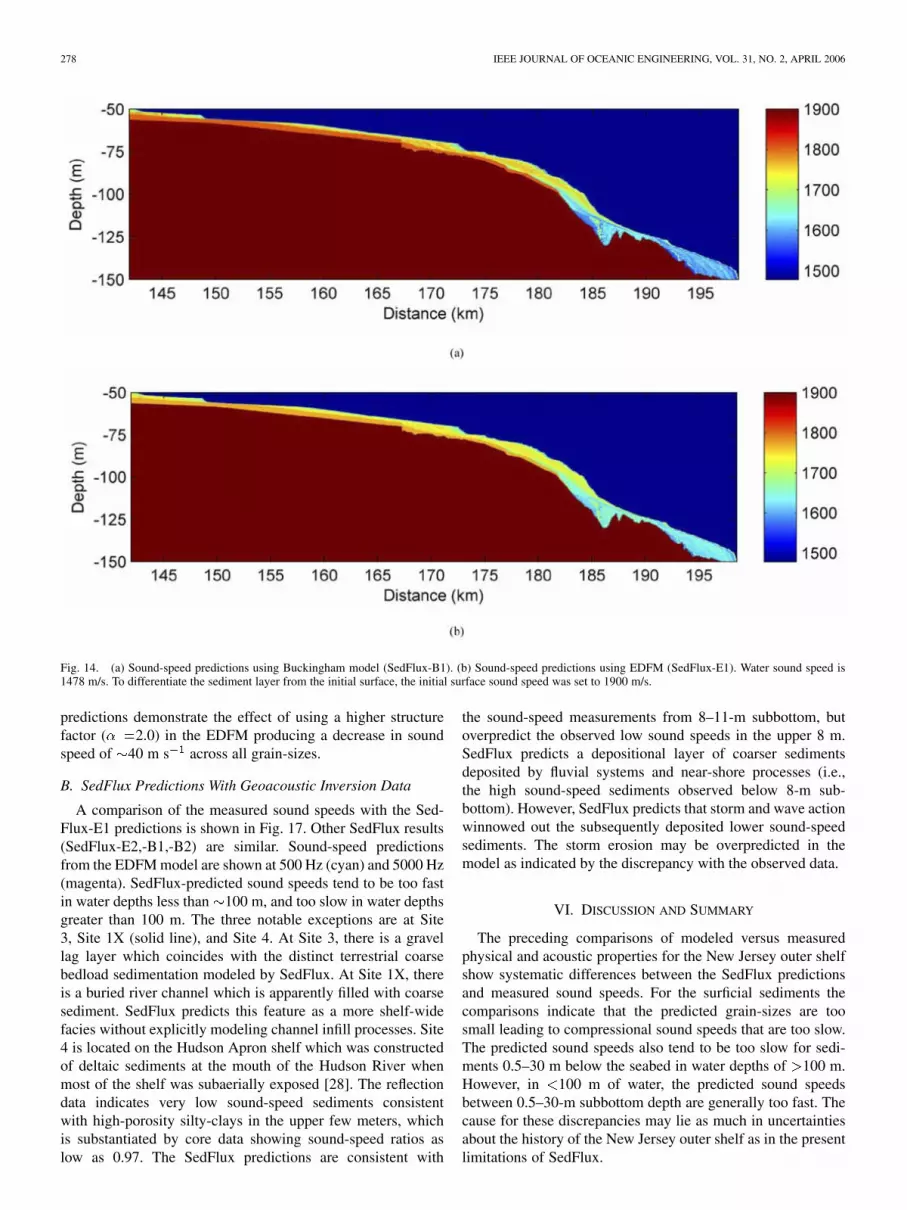
In addition to the uncertainty introduced by the stratigraphicmodel, there is also uncertainty due to the acoustic modelsthemselves. Some measure of this uncertainty maybe obtainedby comparing the sound-speed estimates of the two models.Shown in Fig. 14(a) are the sound-speed predictions fromSedFlux-B1 (Buckingham model with SedFlux predictedmean grain-size and empirically derived porosity) and inFig. 14(b) the predictions from SedFlux-E1 (EDFM modelwith a low value of tortuosity 1.25). The water soundspeed is 1478 m s and the initial surface sound speed wasset to 1900 m s to differentiate from the sediment layer.Sound-speed predictions from both acoustic models extend

over similar ranges: 1491 m s to 1807 m s (SedFlux-B1)and 1522 m s to 1772 m s (SedFlux-E1). In water depthsgreater than 100 m, the Buckingham model predicts soundspeeds in the mid 1500 m s to low 1600 m s for meangrain-sizes in the range of to . The EDFM model predictsslightly faster sound speeds ( 40 m s ) with the differencedecreasing with an increase in grain-size. The increase in soundspeed for finer grain-sizes is due to using a constant value forthe structure factor ( 1.25) for all sediment types. In waterdepths less than 100 m, the Buckingham model predicts slightlyfaster sound speeds ( 20 m s ) than the EDFM.

Sound-speed predictions are compared with surficial mea-surements of sound speed (ISSAP) as a function of water depth(Fig. 15) and mean grain-size (Fig. 16). The predictions wereextracted from the second bin (10 to 20 cm below the seabed)of the SedFlux record for water depths extending from 50 to150 m. The ISSAP measured sound speeds exhibit a mono-tonic decrease with water depth. In water depth less than 100 m,the predicted sound speeds exhibit a similar trend, however, thesound speeds are 100 m s slower than the observed soundspeeds. In water depths between 100 and 130 m, the predictedsound speeds uniformly exhibit an increase in sound speed fol-lowed by decreasing sound speeds in water depths greater than130 m. In water depths greater than 100 m, the SedFlux-B1 andSedFlux-E2 models predict sound speeds across the same rangeas the ISSAP measurements.

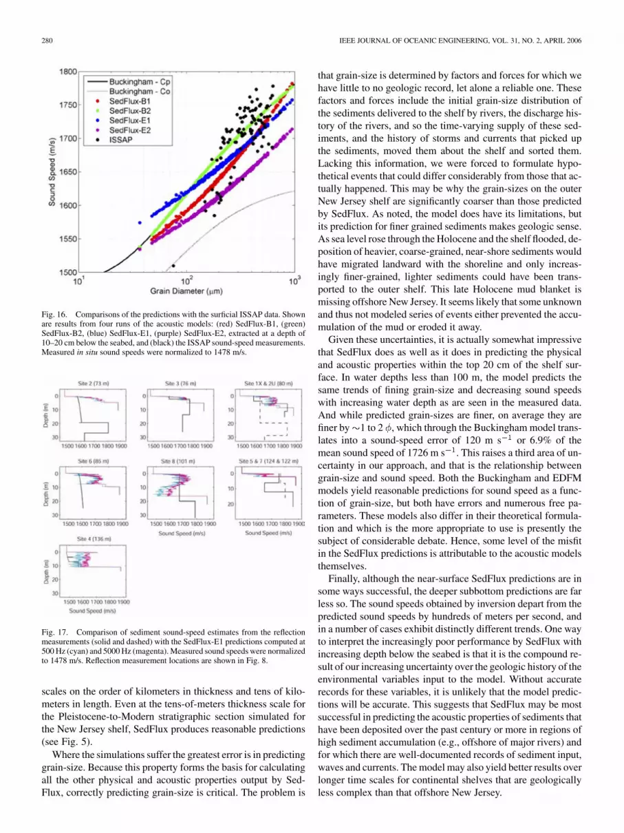
In Fig. 16, the ISSAP measured sound speeds show a mono-tonic decrease with mean grain-size. The notable differencebetween the SedFlux-B1 (Buckingham model with SedFluxpredicted mean grain-size and empirically derived porosity)and SedFlux-B2 [Buckingham model with SedFlux predictedmean grain-size and porosity estimated using (14)] runs is thatthe SedFlux-B2 predictions are faster for nearly all grain-sizes.This would indicate that the porosity calculated using theBuckingham model is generally lower than the empirically de-rived porosity output from SedFlux. The SedFlux-E2 (purple)

278 IEEE JOURNAL OF OCEANIC ENGINEERING, VOL. 31, NO. 2, APRIL 2006

Fig. 14. (a) Sound-speed predictions using Buckingham model (SedFlux-B1). (b) Sound-speed predictions using EDFM (SedFlux-E1). Water sound speed is1478 m/s. To differentiate the sediment layer from the initial surface, the initial surface sound speed was set to 1900 m/s.

predictions demonstrate the effect of using a higher structurefactor ( 2.0) in the EDFM producing a decrease in soundspeed of 40 m s across all grain-sizes.

B. SedFlux Predictions With Geoacoustic Inversion Data

A comparison of the measured sound speeds with the Sed-Flux-E1 predictions is shown in Fig. 17. Other SedFlux results(SedFlux-E2,-B1,-B2) are similar. Sound-speed predictionsfrom the EDFM model are shown at 500 Hz (cyan) and 5000 Hz(magenta). SedFlux-predicted sound speeds tend to be too fastin water depths less than 100 m, and too slow in water depthsgreater than 100 m. The three notable exceptions are at Site3, Site 1X (solid line), and Site 4. At Site 3, there is a gravellag layer which coincides with the distinct terrestrial coarsebedload sedimentation modeled by SedFlux. At Site 1X, thereis a buried river channel which is apparently filled with coarsesediment. SedFlux predicts this feature as a more shelf-widefacies without explicitly modeling channel infill processes. Site4 is located on the Hudson Apron shelf which was constructedof deltaic sediments at the mouth of the Hudson River whenmost of the shelf was subaerially exposed [28]. The reflectiondata indicates very low sound-speed sediments consistentwith high-porosity silty-clays in the upper few meters, whichis substantiated by core data showing sound-speed ratios aslow as 0.97. The SedFlux predictions are consistent with

the sound-speed measurements from 8–11-m subbottom, butoverpredict the observed low sound speeds in the upper 8 m.SedFlux predicts a depositional layer of coarser sedimentsdeposited by fluvial systems and near-shore processes (i.e.,the high sound-speed sediments observed below 8-m sub-bottom). However, SedFlux predicts that storm and wave actionwinnowed out the subsequently deposited lower sound-speedsediments. The storm erosion may be overpredicted in themodel as indicated by the discrepancy with the observed data.

VI. DISCUSSION AND SUMMARY

The preceding comparisons of modeled versus measuredphysical and acoustic properties for the New Jersey outer shelfshow systematic differences between the SedFlux predictionsand measured sound speeds. For the surficial sediments thecomparisons indicate that the predicted grain-sizes are toosmall leading to compressional sound speeds that are too slow.The predicted sound speeds also tend to be too slow for sedi-ments 0.5–30 m below the seabed in water depths of 100 m.However, in 100 m of water, the predicted sound speedsbetween 0.5–30-m subbottom depth are generally too fast. Thecause for these discrepancies may lie as much in uncertaintiesabout the history of the New Jersey outer shelf as in the presentlimitations of SedFlux.

KRAFT et al.: STRATIGRAPHIC MODEL PREDICTIONS OF GEOACOUSTIC PROPERTIES 279

Fig. 15. SedFlux predicted sound speed compared with surficial ISSAP data ( � ) as a function of water depth. Results are shown from four runs of the acousticmodels: (a) SedFlux-B1, (b) SedFlux-B2, (c) SedFlux-E1, and (d) SedFlux-E2, extracted from the SedFlux simulation for water depths between 50–150 m and ata depth of 10–20 cm below the seabed. Measured in situ sound speeds were normalized to 1478 m/s.

There are pros and cons to having carried out this first-timeassessment of predicting acoustic properties from stratigraphicmodels using the New Jersey outer continental shelf as the testbed. As stated previously, a major advantage of this region isthat it is one of the best-documented continental shelves in theworld. The major disadvantage of the region is that it is geolog-ically complex. In fact, it is this very complexity that has been amajor motivation for so many studies of the New Jersey margin.The shelf surface is largely a relict one. The seabed sedimentswere initially laid down by river and near-shore processes whenthe shoreline was near the shelf edge during the last glaciationand the early stages of the ensuing rise in sea level. The pro-cesses affecting the New Jersey shelf today are waves and cur-rents, and their impacts on the seabed are different. Furthermore,all of these processes have, over geologic time, reworked theseabed such that it is composed of sediments that are of mixedages and multiple origins. As a result, our understanding of howthe modern New Jersey shelf formed is based on geologic inter-pretations of the seabed that continue to be debated. Simulatingseabed properties for this type of setting using a deterministicforward model such as SedFlux is a significant challenge, for theaccuracy of the results produced by the model depends on the

accuracy of the environmental inputs used to drive it. In the caseof the New Jersey shelf, many of these inputs are poorly con-strained; so while the physical measurements of the New Jerseyshelf clearly reveal errors in the SedFlux predictions, it is notpossible to establish equally clear-cut reasons as to why.

However, several general reasons for the prediction discrep-ancies are apparent. One is that while SedFlux is sophisticatedenough to simulate many of the complications intrinsic inseabed evolution, the model in its current configuration hasa number of important limitations. Principal among theseperhaps is that it is 2-D. As a result, the model cannot simulatealong-shelf variations in the seabed created by sediment trans-port processes that by nature are spatially heterogeneous in thealong-shelf as well as seaward directions. Furthermore, Sed-Flux does not simulate biologic processes. Hence, the modelpredictions lack high sound-speed shell material common inthe outer New Jersey shelf sediments.

Also are the aforementioned uncertainties concerning the en-vironmental inputs used to drive SedFlux. Long-term, slowlyvarying inputs, such as basin subsidence and even changes inglobal sea level are well constrained. Using these, SedFlux doesa good job at reproducing the stratal architecture of the shelf at

280 IEEE JOURNAL OF OCEANIC ENGINEERING, VOL. 31, NO. 2, APRIL 2006

Fig. 16. Comparisons of the predictions with the surficial ISSAP data. Shownare results from four runs of the acoustic models: (red) SedFlux-B1, (green)SedFlux-B2, (blue) SedFlux-E1, (purple) SedFlux-E2, extracted at a depth of10–20 cm below the seabed, and (black) the ISSAP sound-speed measurements.Measured in situ sound speeds were normalized to 1478 m/s.

Fig. 17. Comparison of sediment sound-speed estimates from the reflectionmeasurements (solid and dashed) with the SedFlux-E1 predictions computed at500 Hz (cyan) and 5000 Hz (magenta). Measured sound speeds were normalizedto 1478 m/s. Reflection measurement locations are shown in Fig. 8.

scales on the order of kilometers in thickness and tens of kilo-meters in length. Even at the tens-of-meters thickness scale forthe Pleistocene-to-Modern stratigraphic section simulated forthe New Jersey shelf, SedFlux produces reasonable predictions(see Fig. 5).

Where the simulations suffer the greatest error is in predictinggrain-size. Because this property forms the basis for calculatingall the other physical and acoustic properties output by Sed-Flux, correctly predicting grain-size is critical. The problem is

that grain-size is determined by factors and forces for which wehave little to no geologic record, let alone a reliable one. Thesefactors and forces include the initial grain-size distribution ofthe sediments delivered to the shelf by rivers, the discharge his-tory of the rivers, and so the time-varying supply of these sed-iments, and the history of storms and currents that picked upthe sediments, moved them about the shelf and sorted them.Lacking this information, we were forced to formulate hypo-thetical events that could differ considerably from those that ac-tually happened. This may be why the grain-sizes on the outerNew Jersey shelf are significantly coarser than those predictedby SedFlux. As noted, the model does have its limitations, butits prediction for finer grained sediments makes geologic sense.As sea level rose through the Holocene and the shelf flooded, de-position of heavier, coarse-grained, near-shore sediments wouldhave migrated landward with the shoreline and only increas-ingly finer-grained, lighter sediments could have been trans-ported to the outer shelf. This late Holocene mud blanket ismissing offshore New Jersey. It seems likely that some unknownand thus not modeled series of events either prevented the accu-mulation of the mud or eroded it away.

Given these uncertainties, it is actually somewhat impressivethat SedFlux does as well as it does in predicting the physicaland acoustic properties within the top 20 cm of the shelf sur-face. In water depths less than 100 m, the model predicts thesame trends of fining grain-size and decreasing sound speedswith increasing water depth as are seen in the measured data.And while predicted grain-sizes are finer, on average they arefiner by 1 to 2 , which through the Buckingham model trans-lates into a sound-speed error of 120 m s or 6.9% of themean sound speed of 1726 m s . This raises a third area of un-certainty in our approach, and that is the relationship betweengrain-size and sound speed. Both the Buckingham and EDFMmodels yield reasonable predictions for sound speed as a func-tion of grain-size, but both have errors and numerous free pa-rameters. These models also differ in their theoretical formula-tion and which is the more appropriate to use is presently thesubject of considerable debate. Hence, some level of the misfitin the SedFlux predictions is attributable to the acoustic modelsthemselves.

Finally, although the near-surface SedFlux predictions are insome ways successful, the deeper subbottom predictions are farless so. The sound speeds obtained by inversion depart from thepredicted sound speeds by hundreds of meters per second, andin a number of cases exhibit distinctly different trends. One wayto interpret the increasingly poor performance by SedFlux withincreasing depth below the seabed is that it is the compound re-sult of our increasing uncertainty over the geologic history of theenvironmental variables input to the model. Without accuraterecords for these variables, it is unlikely that the model predic-tions will be accurate. This suggests that SedFlux may be mostsuccessful in predicting the acoustic properties of sediments thathave been deposited over the past century or more in regions ofhigh sediment accumulation (e.g., offshore of major rivers) andfor which there are well-documented records of sediment input,waves and currents. The model may also yield better results overlonger time scales for continental shelves that are geologicallyless complex than that offshore New Jersey.

KRAFT et al.: STRATIGRAPHIC MODEL PREDICTIONS OF GEOACOUSTIC PROPERTIES 281

ACKNOWLEDGMENT

I. Overeem would like to thank J. A. Goff and S. Gulick, Uni-versity of Texas Institute for Geophysics, Austin, TX, for pro-cessing regional seismic data and making available the GEO-CLUTTER grab sample data. C. W. Holland would like to thankthe NATO SACLANT Undersea Research Centre, La Spezia,Italy, for its role in the collection of the seabed reflection dataas part of the Boundary2001 experiment. Editor J. A. Goff, andreviewers C. Nittrouer and M. Rabineau, and an anonymous re-viewer greatly improved this manuscript.

REFERENCES

[1] M. A. Biot, “Theory of propagation of elastic waves in a fluid-saturatedporous solid. II. Higher frequency range,” J. Acoust. Soc. Amer., vol. 28,no. 2, pp. 179–191, Mar. 1956.

[2] , “Theory of propagation of elastic waves in a fluid-saturated poroussolid. I. Low frequency range,” J. Acoust. Soc. Amer., vol. 28, no. 2, pp.168–178, Mar. 1956.

[3] , “Mechanics of deformation and acoustic propagation in porousmedia,” J. Appl. Phys., vol. 33, pp. 1482–1498, Jul. 1962.

[4] E. L. Hamilton, “Geoacoustic modeling of the sea floor,” J. Acoust. Soc.Amer., vol. 68, no. 5, pp. 1313–1340, Nov. 1980.

[5] E. L. Hamilton and R. T. Bachman, “Sound velocity and related prop-erties of marine sediments,” J. Acoust. Soc. Amer., vol. 72, no. 6, pp.1891–1904, Dec. 1982.

[6] E. W. H. Hutton and J. P. M. Syvitski, “Advances in the numericalmodeling of sediment failure during the development of a continentalmargin,” Mar. Geol., vol. 203, no. 3-4, pp. 367–380, Jan. 2004.

[7] J. P. M. Syvitski and E. W. H. Hutton, “2D SEDFLUX 1.0 C: an ad-vanced process-response numerical model for the fill of marine sedi-mentary basins,” Comput. Geosci., vol. 27, pp. 731–753, 2001.

[8] J. P. M. Syvitski, M. Morehead, and M. Nicholson, “HYDROTREND:A climate-driven hydrologic transport model for predicting dischargeand sediment to lakes and oceans,” Comput. Geosci., vol. 24, no. 1, pp.51–68, 1998.

[9] J. P. M. Syvitski, K. I. Skene, K. Nicholson-Murray, and M. Morehead,“PLUME 1.1: Deposition of sediment from a fluvial plume,” Comput.Geosci., vol. 24, no. 2, pp. 159–171, 1998.

[10] M. D. Morehead and J. P. M. Syvitski, “River plume sedimentation mod-eling for sequence stratigraphy: Application to the Eel margin, northernCalifornia,” Mar. Geol., vol. 154, pp. 29–41, 1999.

[11] J. P. M. Syvitski and M. D. Morehead, “Estimating river-sediment dis-charge to the ocean: Application to the Eel margin, northern California,”Mar. Geol., vol. 154, pp. 13–28, 1999.

[12] M. D. Morehead, J. P. M. Syvitski, E. W. H. Hutton, and S. D. Peckham,“Modeling the temporal variability in the flux of sediment from un-gauged river basins,” Global and Planetary Change, vol. 39, no. 1–2,pp. 95–110, 2003.

[13] D. B. Bahr, E. W. H. Hutton, J. P. M. Syvitski, and L. Pratson, “Exponen-tial approximations to compacted sediment porosity profiles,” Comput.Geosci., vol. 27, no. 6, pp. 691–700, 2001.

[14] I. Overeem, J. P. M. Syvitski, E. W. H. Hutton, and A. J. Kettner, “Strati-graphic variability due to uncertainty in model boundary conditions: Acase-study of the New Jersey shelf over the last 40 000 years,” Mar.Geol., vol. 224, no. 1-4, pp. 23–41, Nov. 2005.

[15] J. P. M. Syvitski, S. P. Peckham, R. Hilberman, and T. Mulder, “Pre-dicting the terrestrial flux of sediment to the global ocean: A planetaryperspective,” Sedimentary Geol., vol. 162, no. 1-2, pp. 5–24, Nov. 2003.

[16] C. Paola, P. L. Heller, and C. L. Angevine, “The large-scale dynamicsof grain-size variation in alluvial basins, 1: Theory,” Basin Res., vol. 4,no. 2, pp. 73–90, 1992.

[17] M. L. Albertson, Y. B. Dai, R. A. Jensen, and R. Hunter, “Diffusionof submerged jets,” Amer. Soc. Civil Engineers Trans., vol. 115, pp.639–697, 1950.

[18] J. E. A. Storms, “Controls on Shallow-Marine Stratigraphy: A Process-Response Approach,” Ph.D. dissertation, Dept. Appl. Earth Sci., DelftUniv. Tech., Delft, The Netherlands, 2002.

[19] , “Event-based stratigraphic simulation of wave-dominatedshallow-marine environments,” Mar. Geol., vol. 199, no. 1-2, pp.83–100, Aug. 2003.

[20] P. D. Komar and M. C. Miller, “The threshold of sediment movementunder oscillatory water waves,” J. Sedimentary Petrol., vol. 43, no. 4,pp. 1101–1110, 1973.

[21] P. J. Rance and N. F. Warren, “The threshold of movement of coarsematerial in oscillatory flow,” in Proc. 11th Conf. Coastal Eng., vol. 1,London, 1969, pp. 487–491.

[22] L. F. Athy, “Density, porosity, and compaction of sedimentary rocks,”AAPG Bulletin, vol. 14, no. 1, pp. 1–24, 1930.

[23] Initial Reports of the Deep Sea Drilling Project. vol. 1–96. U.S. Gov-ernment Printing Office, Washington, DC, 1969–1986.

[24] D. J. P. Swift, J. W. Kofoed, F. P. Saulsbury, and P. Sears, “Holocene evo-lution of the shelf surface, central and southern atlantic shelf of northamerica,” in Shelf Sediment Transport; Process and Pattern, D. J. P.Swift, D. B. Duane, and O. H. Pilkey, Eds. Stroudsburg, PA: Dowden,Hutchinson, and Ross, 1972, pp. 499–574.

[25] D. J. P. Swift, R. Moir, and G. L. Freeland, “Quaternary rivers on theNew Jersey shelf: Relation of seafloor to buried valleys,” Geology, vol.8, no. 6, pp. 276–280, 1980.

[26] J. D. Milliman, Z. Jiezao, L. Anchun, and J. Ewing, “Late quaternarysedimentation on the outer and middle New Jersey continental Shelf;result of two local deglaciations?,” J. Geol., vol. 98, no. 6, pp. 966–976,Nov. 1990.

[27] T. A. Davies and J. A. Austin Jr., “High-resolution reflection and coringtechniques applied to periglacial deposits on the New Jersey shelf,” Mar.Geol., vol. 143, no. 1-4, pp. 137–149, Nov. 1997.

[28] J. A. Goff, D. J. P. Swift, C. L. Schuur, L. A. Mayer, and J. E. Hughes-Clarke, “High resolution swath sonar investigation of sand ridge andsand ribbon morphology in the offshore environment of the New Jerseymargin,” Mar. Geol., vol. 161, no. 2-4, pp. 307–337, Oct. 1999.

[29] C. S. Duncan, “Late Quaternary Stratigraphy and Seafloor Morphologyof the New Jersey Continental Shelf,” Ph.D. dissertation, Dept. Geosci.,Univ. Texas, Austin, TX, 2001.

[30] E. Uchupi, N. Driscoll, R. D. Ballard, and S. T. Bolmer, “Drainageof the Late Wisconsin glacial lakes and the morphology and late Qua-ternary stratigraphy of the New Jersey—Southern New England conti-nental shelf and slope,” Mar. Geol., vol. 172, no. 1-2, pp. 117–145, Jan.2001.

[31] S. P. S. Gulick, J. A. Goff, J. A. Austin, C. R. Alexander, S. Nordfjord,and C. S. Fulthorpe, “Basal inflection-controlled shelf-edge wedges offNew Jersey track sea-level fall,” Geology, vol. 33, no. 5, pp. 429–432,May 2005.

[32] C. Alexander, C. Sommerfield, J. A. Austin Jr., B. Christensen, C. S.Fulthorpe, J. A. Goff, S. P. S. Gulick, S. Nordfjord, D. Nielson, and S.Schock, “Sedimentology and age control of late quaternary New Jerseyshelf deposits,” EOS Trans., 2003. AGU 84, Fall Meeting Suppl. Ab-stract OS52B-0909.

[33] J. Chappell and N. J. Shackleton, “Oxygen isotopes and sea level,” Na-ture, vol. 324, no. 6093, pp. 137–140, Nov. 1986.

[34] R. G. Fairbanks, “A 17 000-year glacio-eustatic sea level record: Influ-ence of glacial melting rates on the Younger Dryas event and deep-oceancirculation,” Nature, vol. 342, no. 6250, pp. 637–642, Dec. 1989.

[35] E. Bard, B. Hamelin, R. G. Fairbanks, and A. Zindler, “Calibration ofthe C time-scale over the past 30 000 years using mass spectrometricU-Th age from Barbados corals,” Nature, vol. 345, no. 6274, pp.405–410, May 1990.

[36] K. Lambeck and J. Chappell, “Sea level change through the last glacialCycle,” Science, vol. 292, no. 5517, pp. 679–686, Apr. 2001.

[37] S. J. Marshall and G. K. C. Clarke, “Modeling North American fresh-water runoff through the last glacial cycle,” Quaternary Res., vol. 52,no. 3, pp. 300–315, 1999.

[38] P. A. Mayewski, L. D. Meeker, S. Whitlow, M. S. Twickler, M. C. Mor-rison, P. Bloomfield, G. C. Bond, R. B. Alley, A. J. Gow, P. M. Grootes,D. A. Meese, M. Ram, K. C. Taylor, and W. Wumkes, “Changes in atmo-spheric circulation and ocean ice cover over the North Atlantic duringthe last 41 000 years,” Science, vol. 263, no. 5154, pp. 1747–1751, 1994.

[39] H. Günther, W. Rosenthal, M. Stawarz, J. C. Carretero, M. Gomez, I.Lozano, O. Serrrano, and M. Reistad, “The wave climate of the North-east Atlantic over the period 1955–1994: The WASA wave hindcast,”Global Atm. Oc. Syst., vol. 6, pp. 121–163, 1998.

[40] H. L. Tolman, “User Manual and System Documentation of WAVE-WATCH-III,” NOAA/NWS/NCEP/OMB, version 1.18, Tech. Note 166,1999.

282 IEEE JOURNAL OF OCEANIC ENGINEERING, VOL. 31, NO. 2, APRIL 2006

[41] H. L. Tolman, B. Balasubramaniyan, L. D. Burroughs, D. V. Chalikov,Y. Y. Chao, H. S. Chen, and V. M. Gerald, “Development and implemen-tation of wind generated ocean surface wave models at NCEP,” WeatherForecasting, vol. 17, no. 2, pp. 311–333, Apr. 2002.

[42] J. A. Goff, B. J. Kraft, L. A. Mayer, S. G. Schock, C. K. Sommerfield, H.C. Olson, S. P. Gulick, and S. Nordfjord, “Seabed characterization on theNew Jersey middle and outer shelf: Correlatability and spatial variabilityof seafloor sediment properties,” Mar. Geol., vol. 209, pp. 147–172, Aug.2004.

[43] M. J. Buckingham, “Theory of acoustic attenuation, dispersion, andpulse propagation in unconsolidated granular materials including ma-rine sediments,” J. Acoust. Soc. Amer., vol. 102, no. 5, pp. 2579–2596,Nov. 1997.

[44] , “Theory of compressional and shear waves in fluidlike marinesediments,” J. Acoust. Soc. Amer., vol. 103, no. 1, pp. 288–299, Jan.1998.

[45] , “Wave propagation, stress relaxation, and grain-to-grain shearingin saturated, unconsolidated marine sediments,” J. Acoust. Soc. Amer.,vol. 108, no. 6, pp. 2796–2815, Dec. 2000.

[46] K. L. Williams, “An effective density fluid model for acoustic propaga-tion in sediments derived from Biot theory,” J. Acoust. Soc. Amer., vol.110, no. 5, pp. 2276–2281, Nov. 2001.

[47] A. B. Wood, A Textbook of Sound. London, U.K.: Bell and Sons, 1964.[48] C. W. Holland, S. E. Dosso, and J. Dettmer, “A technique for measuring

in-situ compressional wave speed dispersion in marine sediments,” IEEEJ. Ocean. Eng., vol. 30, no. 4, pp. 748–763, Oct. 2005.

[49] R. D. Stoll, Sediment Acoustics, Lecture Notes in Earth Sci-ences. Berlin, Germany: Springer-Verlag, 1989.

[50] D. L. Johnson, J. Koplik, and R. Dashen, “Theory of dynamic perme-ability and tortuosity in fluid-saturated porous media,” J. Fluid Mech.,vol. 176, pp. 379–402, Mar. 1987.

[51] L. A. Mayer, B. J. Kraft, P. Simpkin, P. Lavoie, E. Jabs, and E. Lynskey,“In-situ determination of the variability of seafloor acoustic properties:An example from the ONR GEOCLUTTER area,” in Impact of LittoralEnvironmental Variability on Acoustic Predictions and Sonar Perfor-mance, N. G. Pace and F. B. Jensen, Eds, The Netherlands: Kluwer,2002, pp. 115–122.

[52] B. J. Kraft, L. A. Mayer, P. Simpkin, P. Lavoie, E. Jabs, E. Lynskey, andJ. A. Goff, “Calculation of in-situ acoustic wave properties in marinesediments,” in Impact of Littoral Environmental Variability on AcousticPredictions and Sonar Performance, N. G. Pace and F. B. Jensen, Eds,The Netherlands: Kluwer, 2002, pp. 123–130.

[53] C. W. Holland, R. Gauss, P. Hines, P. Nielsen, D. Ellis, J. Preston, K. D.LePage, C. Harrison, J. Osler, R. Nero, and D. Hutt, “Boundary char-acterization experiment series overview,” IEEE J. Ocean. Eng., vol. 30,no. 4, pp. 784–806, Oct. 2005.

[54] P. Ratilal, Y. Lai, D. Symonds, L. Ruhlman, J. R. Preston, E. Scheer,M. T. Garr, C. Holland, J. Goff, and N. Makris, “Long range acousticimaging of the continental shelf environment: The acoustic clutter re-connaissance experiment 2001,” J. Acoust. Soc. Amer., pt. 1, vol. 117,no. 4, pp. 1977–1998, Apr. 2005.

[55] C. W. Holland, “Intra- and inter-regional geoacoustic variability in thelittoral,” in Impact of Littoral Environmental Variability on Acoustic Pre-dictions and Sonar Performance, N. G. Pace and F. B. Jensen, Eds, TheNetherlands: Kluwer, 2002, pp. 73–82.

[56] , “Regional extension of geoacoustic data,” in Proc. Fifth EuropeanConf. Underwater Acoustics (ECUA 2000), P. Chevret and M. E. Za-kharia, Eds., Lyon, France, 2000, pp. 793–798.

[57] C. W. Holland, R. Hollett , and L. Troiano, “A measurement techniquefor bottom scattering in shallow water,” J. Acoust. Soc. Amer., pt. 1 of 2,vol. 108, no. 3, pp. 997–1011, Sep. 2000.

[58] C. W. Holland, “Coupled scattering and reflection measurements inshallow water,” IEEE J. Ocean. Eng., vol. 27, no. 3, pp. 454–470, Jul.2002.

[59] C. W. Holland and J. Osler, “High-resolution geoacoustic inversionin shallow water: A joint time- and frequency-domain technique,” J.Acoust. Soc. Amer., vol. 107, no. 3, pp. 1263–1279, Mar. 2000.

[60] C. W. Holland, “Geoacoustic inversion for fine-grained sediments,” J.Acoust. Soc. Amer., vol. 111, no. 4, pp. 1560–1564, Apr. 2002.

[61] S. E. Dosso and C. W. Holland, “Geoacoustic uncertainties from vis-coelastic inversion of seabed reflection data,” IEEE J. Ocean. Eng., 2006,to be published.

[62] C. W. Holland, “Seabed reflection measurement uncertainty,” J. Acoust.Soc. Amer., pt. 1 of 2, vol. 114, no. 4, pp. 1861–1873, Oct. 2003.

[63] J. Kozeny, “Ueber kapillare Leitung des Wassers im Boden,” Wien, Akad.Wiss, vol. 136, no. 2a, p. 271, 1927.

[64] P. C. Carman, “Fluid flow through a granular bed,” Trans. Inst. Chem.Eng., vol. 15, pp. 150–156, 1937.

Barbara J. Kraft (M’04) received the B.S. and Ph.D.degrees in mechanical engineering at the Universityof New Hampshire, Durham, in 1991 and 1999, re-spectively.

In the years before graduate school, she workedin industry for several companies as an Electro-Me-chanical Designer. From June 2001 until March2004, she was the TYCO Postdoctoral Fellow inOcean Mapping at the Center for Coastal and OceanMapping (CCOM), University of New Hampshire,Durham. She is presently employed as a Research

Scientist II at CCOM where her research has focused on the in in situ mea-surement of sediment properties and seabed characterization from multibeambackscatter.

Dr. Kraft is a member of the Acoustical Society of America and the AmericanGeophysical Union.

Irina Overeem was born in Den Haag, The Nether-lands, in 1972. She received the M.S. degree withhonors in soil, water, and atmosphere from Wa-geningen University, The Netherlands, in 1996 andthe Ph.D. degree is in civil engineering and appliedearth sciences from Delft University of Technology,The Netherlands, in 2002.

Presently, she works as a Research Scientist II atthe Institute of Arctic and Alpine Research, Univer-sity of Colorado, Boulder. Her specialty is in numer-ical modeling of sedimentary systems. She published

on the Eridanos delta in the North Sea, and on the modeling of the Volga delta inthe Caspian Sea. Her work with Delft University of Technology’s Applied Geo-physicists resulted in several publications on the development and use of seismicattribute analysis. Her long-term objective is to develop predictive models thatform a tool to quantify responses of sedimentary systems to changing environ-mental conditions. She has a keen interest in using field studies to criticallyassess model performance.

Dr. Overeem is a member of the American Geophysical Union, the EuropeanGeosciences Union, and the International Association of Mathematical Geolo-gists.

Charles W. Holland was born in Ponca City, OK,in 1958. He received the B.S. degree in engineeringfrom the University of Hartford, West Hartford, CT,in 1983 and the M.S. and Ph.D. degrees, both inacoustics, from the Pennsylvania State University,State College, in 1985 and 1991, respectively. HisPh.D. dissertation focused on acoustic propagationthrough poroviscoelastic marine sediments.

In 1985, he began working for Planning Sys-tems Inc., VA, on geoacoustic modeling, seafloorclassification techniques, high-frequency seafloor

acoustic penetration, and low-to-mid frequency bottom loss/bottom scatteringmeasurement and modeling techniques. His approach for treating reflectionfrom a stochastic-layered seafloor is employed in the Fleet today. He wasassociated with the CST program from 1993 to 1996, and served as BottomWorking Group Leader and Chairman of the Environmental Acoustics WorkingGroup. He joined the research staff at the SACLANT Centre in La Spezia,Italy, in 1996, where he focused on developing seabed reflection and scatteringmeasurement techniques. In 2001, he joined the Applied Research Laboratoryat the Pennsylvania State University, State College, where he continues hisresearch in seabed acoustics.

Dr. Holland is a member of the Acoustical Society of America and has servedas a Guest Editor for the IEEE JOURNAL OF OCEANIC ENGINEERING.

KRAFT et al.: STRATIGRAPHIC MODEL PREDICTIONS OF GEOACOUSTIC PROPERTIES 283

Lincoln F. Pratson received the B.S. degree in ge-ology from Trinity University, San Antonio, TX, in1983, the M.S. degree in oceanography from the Uni-versity of Rhode Island, Kingston, in 1987, and theM.Ph. and Ph.D. degrees in geology from ColumbiaUniversity, New York, in 1993.

He was a Research Scientist at Lamont-DohertyEarth Observatory of Columbia University, a Re-search Scientist at the Institute of Arctic and AlpineResearch of the University of Colorado (where he isstill an affiliate), and a member of the faculty in the

Nicholas School of the Environment and Earth Sciences at Duke University,Durham, NC, where he currently holds the rank of Associate Professor andis Director of the Energy and Environment Program. He researches seascapeevolution and strata formation along continental margins through numericaland experimental modeling, and the analysis of sedimentologic, stratigraphicand geophysical data.

Dr. Pratson is a member of the American Geophysical Union and the Societyof Exploration Geophysicists. He has been an Associate Editor for the Journal ofSedimentary Research and Geology and a Guest Editor for Marine GeophysicalResearches.

James P. M. Syvitski received the B.Sc. degree ingeology and the H.B.Sc. degree in geochemistryfrom Lakehead University, Canada, in 1974 and1975, respectively, and the Ph.D. degree in oceanog-raphy and geological sciences from the Universityof British Columbia, BC, Canada, in 1978.

He has worked in industry for Falconbridge as aGeophysicist, from 1973 to 1975, as a Consultant forCanadian Marine Geotechnical Engineering, in 1980,and the U.S. Department of Justice, in 1992, as a Se-nior Government Scientist at the Bedford Institute of

Oceanography, from 1981 to 1995, and in academia at the University of Calgary,from 1978 to 1981, Adjunct Professor at Laval University, Memorial University,Dalhousie University, INRS-Océanologie. Since 1995, he has been Director andFellow of the Institute of Arctic and Alpine Research, and Professor at the Uni-versity of Colorado, Boulder. He has published over 425 books, journal publi-cations, and reports, and is listed by Science Direct as one of the world’s mostcited Geoscientists. He is currently developing surface-dynamic models to de-scribe the earth’s evolving landscape and seascape, and the sedimentary depositsthat they create, by characterizing climate-ocean-landscape interactions, acrosshighly dynamic and deforming boundaries.

Dr. Syvitski is a member of the International Association of Sedimentol-ogists, the Society of Sedimentary Research, The Oceanography Society, theAmerican Geophysical Union, and the International Association of Mathemat-ical Geology. He has been Editor, Associate Editor, and Guest Editor of teninternational journals, including Oceanography.

Larry A. Mayer received the B.Sc. degree in ge-ology from the University of Rhode Island, Kingston,in 1973 and the Ph.D. degree in marine geophysicsfrom the Scripps Institution of Oceanography, LaJolla, CA, in 1979.

He is currently a Professor of Earth Sciences andOcean Engineering at the University of New Hamp-shire, Durham, and is the Director of the Center forCoastal and Ocean Mapping and Codirector of theNOAA/UNH Joint Hydrographic Center. His mainresearch interests are in seafloor mapping technolo-

gies, seafloor characterization, and applications of advanced visualization tech-niques to ocean mapping problems.