Automatic Transition Predictions Using Simplified Methods

Jean Perraud,∗ Daniel Arnal,† Grégoire Casalis,‡ and Jean-Pierre Archambaud§

ONERA, 31055 Toulouse, France

and

Raffaele Donelli¶

Centro Italiano Ricerche Aerospaziali, 81043 Capua, Italy

DOI: 10.2514/1.42990

Laminar-turbulent transition remains a critical issue in a number of cases, including drag reduction, performance

prediction of high-lift systems, improved accuracy in general computational fluid dynamics, and reduction of

computation cycles for development of optimization tools. Transition delay remains one of the most promising

technologies for reducing air transport energy consumption, throughnatural or hybrid laminarflowcontrol. Theuse

of linear stability theory, either local or nonlocal, remains rather demanding in terms of knowledge and user

interaction. Hence, a demand exists for simplified, robust, and accurate transition prediction tools to be inserted into

general flow solvers, of boundary-layer or Reynolds-averaged Navier–Stokes types. The problem can be solved by

developing transition criteria or databasemethods. In this last case, characteristics of an actualfloware derived from

known solutions of model flows. ONERA, the French Aerospace Laboratory, has long been involved in the

development of such methods, and the present paper aims at providing a comprehensive view of the tools developed

in the second category, applicable from low-speed two-dimensional to transonic three-dimensional flows, and even to

three-dimensional supersonic flows.

Nomenclature

F = reduced frequencyf = frequencyHi = incompressible shape factorPi = characteristic parameter for the crossflow

modelsRk = Reynolds number based on length kTw = wall temperatureUe,We, Te = velocity components and temperature at the

boundary-layer edgeUi = velocity at the location yi of the inflection pointu, w, T = velocity and temperature components of the

boundary-layer profileVg, ’g = modulus and direction of the group velocity�, � = complex, reduced wave numbers (�� ���1).

Their real parts are the components of the wavevector k.

�� = crossflow wave number. As �i is usually forcedto zero, �� represents the real part.

�1 = displacement thickness� = angle between the local x direction and the

external velocity vector�1 = momentum thickness�� = wavelength of the instability

�� � 2��1=�����������������������2r � �2

r�p

� = kinematic viscosity� = density = amplification rate’ = angle between the wave vector and the local

x direction’w = wing sweep angle = angle between the wave vector and the local

external velocity vector!r = reduced pulsation

I. Introduction

AUTOMATIC and robust laminar-turbulent transition predictiontools are still in demand for improving accuracy of flow

computation or development of optimization tools. A number ofmodels have been developed at ONERA, and have been combinedinto a fairly complete prediction tool which may be inserted intoboundary layers or Reynolds-averaged Navier–Stokes (RANS)codes. The aim of the present paper is to provide a comprehensiveview of these models, including their use as transition predictiontools inside the 3-D boundary-layer code 3C3D. Selected exampleswill demonstrate the range of applications by providing comparisonsto exact results of linear stability (LST). Ways to implement thedatabase method inside a RANS code will also be discussed,although this remains to be accomplished. Because this paper dealswith model presentation and validation, examples will compare N-factor curves obtained using the database and exact LST, andwill notdiscuss practical applications involving method calibration, specificdata preparation, and statistical analysis of the results. This wouldgrant a separate paper.

The traditional approach for transition prediction is based on thelinear stability theory, either local or nonlocal. The addition of thesecond-order terms curvature and nonparallelism in the nonlocalapproach does not significantly improve correlation of computationto experimental results. Therefore, local theory remains widely usedfor practical applications.

Whereas stability analysis describes how small, preexistingperturbations will grow in the boundary layer through a normalmoderesponse, the eN method [1,2] correlates an amplitude level with thebeginning of turbulence. Here, N � log�A=Ao�, where A=Ao is theamplitude ratio between the current location and a reference,upstream one. The two most common strategies, envelope andNCF=NTS, will be discussed later.

Presented as Paper 1144 at the 47th Aerospace Science Meeting, Orlando,FL, 5–8 January 2009; received 30December 2008; revision received 22 June2009; accepted for publication 23 June 2009. Copyright © 2009 by ONERA.Published by the American Institute of Aeronautics and Astronautics, Inc.,with permission. Copies of this paper may be made for personal or internaluse, on condition that the copier pay the $10.00 per-copy fee to the CopyrightClearance Center, Inc., 222 Rosewood Drive, Danvers, MA 01923; includethe code 0001-1452/09 and $10.00 in correspondence with the CCC.

∗Research Engineer, Models for Aerodynamics and Energetics Depart-ment; Jean.Perraud@onera.fr. Member AIAA.

†Director of Research, Models for Aerodynamics and EnergeticsDepartment; Daniel.Arnal@onera.fr.

‡Professor, Models for Aerodynamics and Energetics Department;Gregoire.Casalis@onera.fr. Member AIAA.

§Research Engineer, Models for Aerodynamics and Energetics Depart-ment; Jean-Pierre.Archambaud@onera.fr.

¶Research Engineer, AppliedAerodynamics Laboratory, ItalianAerospaceResearch Center; r.donelli@cira.it.

AIAA JOURNALVol. 47, No. 11, November 2009

2676

Exact stability calculations are rather demanding in terms of userinteraction (no fully automatic code yet) and require a precisedescription of the boundary layer, imposing conditions on the meshdefinition (at least about 40 points in the boundary layer) and on thenumerical scheme (low dissipation) in case of a RANS approach.Adequate quality of the boundary-layer profiles may also be ensuredusing a boundary-layer code. Two separate questions arise: first,the development of simplified stability methods, and second, theircoupling to RANS codes.

Concerning the first point, a number of contributions have beenmade (see [3–12]) that generally fall into the database approach,where solution for an actual boundary-layer profile is obtained fromthe knowledge of the precomputed stability solutions for a family ofprofiles, typically of a self-similar family like the Falkner–Skanone in 2-D. The procedure then intends to predict the stabilitycharacteristics of actual (nonsimilar) profiles from those of themodelprofiles. Various procedures and models have been developed thatfall into three categories: lookup tables [3,5,12], analytical models[7,10], and neural networks [8,9]. In the two first cases, the stabilitycharacteristics of a given profile will be determined using aninterpolation table or some analytical functions of selected param-eters, and in the last case a neural network will provide the desiredparameters after a specific training of the network.

The range explored by the family of similar profiles may varydepending on the applications. Because of his interest with inter-active boundary layers, Drela [12] introduced in his database 2-Dprofiles with separation. Other contributors concentrated on attachedflows, in relation to direct mode boundary-layer solvers consideringconfiguration without separation. Most published models are re-stricted to Tollmien–Schlichting (TS) instabilities, with the excep-tion of Fuller et al. [8], Crouch et al. [9], and Langlois et al. [11]. Inthe first, neural network approach, model parameters include cross-flow displacement thickness Reynolds number and a six pointsampling of both longitudinal and crossflow velocity profiles.Predicted N factors are within 1N-factor count from local stabilitytheory, with the best results in the case of pure crossflow. Langloisuseswmax as the crossflow parameter together with a specific similarsolution for 3-D compressible boundary layers. Difficulties appar-ently stem from the limitation of this family of similar solutions torepresent actual profiles computed near an attachment line. In thecase of ONERA [3,4], the self-similar Falkner–Skan family was con-sidered for the development of a model for Tollmien—Schlichtinginstabilities, whereas models for crossflow modes [7,10] were basedon typical profiles obtained downstream of the attachment line for aseries of low-speed and transonic realistic swept wing flow cases. Asimilar model was developed for TS instabilities by Stock andDegenhart [5]. In the case of ONERA, three separate models weredeveloped dealing with longitudinal (or TS) instabilities, travelingcrossflow (or CF) instabilities, and stationary crossflow modes,which we call CF0, respectively.

Concerning the coupling of stability-based methods to RANScodes, several approaches have been explored. ONERA [13]introduced into the elsA code transition criteria for longitudinal andcrossflow instabilities. These criteria were developed from results oflinear stability and transition correlations. Examples were presentedin [14] in the context of high-lift flows. The German AerospaceCenter (DLR) [15], the Spanish National Institute for AerospaceTechnology (INTA) [16], and others have developed, for wing sur-faces, an automatic coupling to a boundary-layer code inside whichdatabasemethods are used for transition prediction.Apresentation ofEuropean activities in this field was recently published (see [17]). Asthere is no example of automatic, internal coupling of a RANS codewith a stability approach capable of using directly theRANSvelocityprofiles, there is still room for much progress.

II. Linear Stability and the Solution Form

Consider the swept wing depicted in Fig. 1, with sweep angle ’w.A local wing coordinate system is defined taking x as the normal tothe leading edge, y the normal to thewall, and z in spanwise direction.The velocity components of the mean flow are U, W in x and z

directions. The angle between x and xc is �, with xc the tangent to theexternal streamline at a point.

In the frame of local stability theory, derivatives@G=@x and @G=@zwhereG�U,W are eliminated from the formulation, that is, forcedto zero. The linear growth of small perturbations, added to the baseflow, is considered using stability theory. In the context of spatialtheory, solutions are written in the form g�x; t� � g�y�ei��x��z�!rt�where !r � 2�f�1

Ue, �1 �

R�1 � U�y�

Ue�dy, and g is any fluctuating

quantity.Real parts of the wave numbers define the wave vector k, see

Fig. 2, at angle ’ from the x direction, and from the local velocitydirection:’� tan�1��r=�r�,’� � �. Given these definitions, theLST for a 2-D incompressible flow is the well-known Orr—Sommerfeld equation, of fourth order, whereas for 3-D compressibleflow a sixth-order system is obtained [18]. In 3-D flow, theincompressible equation is

bv0000 � 2��2 � �2�v00 � ��2 � �2�2vc=Rl � ib��U� �W � !��v00

� ��2 � �2�v� � ��U00 � �W 00�vc � 0@

with homogeneous boundary conditions on the vertical velocityperturbation v and v0. Here, the primes denote derivatives with

respect to the y coordinate, andRl � �Uele

is a Reynolds number based

on a reference length l. Because boundary conditions are homo-geneous, this is an eigenvalue problem for which solutions only existfor particular combinations of (�, �, !), referred to as a dispersionrelation. Because there are more unknowns than equations, param-eters need to be imposed before solving the equations. Typically, (�,!) or ( , !) are imposed, and � is obtained as an eigenvalue of thesystem. The growth rate of solutions is then given by the imaginarypart��i � , and theN factor is obtained by integrating this growthrate.

Several methods exist, referred to as integration strategies. Acomplete discussion (see [19,20]) is outside the scope of this work. Inthe present context two approaches are considered, the envelopemethod and the two N-factor methods NTS=NCF, with the followingdefinitions:

The envelope N factor is obtained by integrating the largestamplification rate,

Nenv �maxf�Zx

xo

max �� dx�

where xo is the critical point in which becomes positive. Theinner maximization may be defined over , �� � �r=�1, or ��. The

Fig. 1 Wing geometry and coordinates.

Fig. 2 Geometrical definitions.

PERRAUD ETAL. 2677

longitudinal N-factor is defined by integrating ��j �0, consideringwaves with wave vectors parallel to the outside velocity

NTS �maxf�Zx

xo

��j �0 dx�

This definition may be extended to consider longitudinal obliquewaves, with

Nenv �maxf�Zx

xo

max < max

�� dx�

where max lies in the range 60–80 deg. The envelope of envelopecrossflow N-factor is obtained by evaluating the envelope overvarious frequencies and either the wavelength or spanwise wavenumber

NCF �maxf�max��CF

Zx

xo

�j���ct� dx�

NCF may be strictly based on stationary modes (f� 0),suppressing the outer maximization, or in a concurrent definitionmay include traveling waves (f > 0). NTS and NCF may also becomputed based on incompressible stability equations. Whateverthe definitions used, each method needs to be calibrated using someexperimental database.

As the envelopemethodwas themost commonly used at ONERA,the first database developments were restricted to this approach. Anextension to stationary modes and a NTS=NCF method were lateradded with modified definitions for NCF and NCF0, as follows:

NCF �maxf�Zx

xo

max��CF�� dx�

and

NCF0 �Zx

xo

max���jf�0� dx

Themaximization is nowmoved under the integral, corresponding tospecialized envelopes. The impact of these definitions is visiblein Figs. 3 and 4 , obtained for a low-speed (80 m=s) swept(’w � 50 deg) ONERA-D profile of 0.3 m chord, at �1 degincidence. The database NTS can be considered equivalent to theexact stability constant � 0 N-factor, and the stationary databaseNCF0 can be considered equivalent to the zero-frequency envelopecalculation (because only crossflow modes exist at zero frequency),as can be seen in Fig. 3. Figure 4 illustrates the different ways toestimate NCF and NCF0 for the same low-speed case. It can be seenthat, because of the integration method, the zero-frequency envelopeN-factor is larger than the NCF envelope of envelope even thoughtraveling crossflow modes are more unstable than stationary ones.Very different results are obtained depending on the definition;hence, for transition prediction, calibration must be determined foreach formulation.

III. Database Approach for Longitudinal Instabilities

Longitudinal, or TS instabilities, are governed by viscosity. A firstmodel of such instabilities for 2-D low-speed flow was proposed byVialle andArnal [4] in 1984 based on a set of exact stability solutionsof attached Falkner–Skan self-similar profiles in 2-D flow. The

incompressible shape factor Hi� �1=�1, where �1 �RU�y�Ue�1 �

U�y�Ue�dy is the momentum thickness, was used as the key parameter.

The simplified stability approach, or databasemethod, provides anestimation of the growth rate directly from mean flow parametersand the boundary-layer profile characteristics. The starting idea isthat the Reynolds number variation of growth rates obtained solvingthe exact Orr—Sommerfeld equations can be represented, for a givenprofile, using two half parabolas as shown in Fig. 5. Extension todeceleratedflow (Hi > 2:59) can be obtained using an added inviscidparabola, as shown in Fig. 6. The effect of compressibility wasintroduced into the model, using the external Mach number as anadditional parameter [3].

For a given mean flow (Hi, Me) and reduced frequency

F� 2�fe�eU

2e� !r

R�1, the amplification curve is approximated as

�max �V; I � V;I � M�1 �

�R�1 � RMRK � RM

�2�

RK �R0 if R�1 < RMR1 if R�1 > RM

where M, R0, R1, and RM are associated with both the viscous andthe inviscid parabolas of Fig. 6.

Fig. 3 ComparingNTS andNCF0 for LST and database for a low-speed

case.

Fig. 4 Consequences of various definitions for NCF.

Fig. 5 Basic parabola model.

Fig. 6 Extended parabola model for TS waves.

2678 PERRAUD ETAL.

RM � k1FE1

R1 � k2FE2for viscous or inviscid parts

R0V� R0I

� RMV�1� C�Fc � F�� MI

� BI�1 � F

FoI

�

MV�min

�BV

�1 � F

FoV

�; MVMAX

�

Using these definitions, 15 parameters need to be determined asfunctions of Hi andMe:

�B;Fo; K1; E1; K2; E2�I;V ; C; Fc; MVMAX

This is realized using a two-entry lookup table. Amplification ratesare then obtained as a function of the Reynolds number R�1 based onthe incompressible (respectively compressible) displacement thick-ness for incompressible (respectively compressible) flow. Moreover,the effect of wall temperature Tw can be modeled using four moreparameters modifying the previous 15.

Tables are defined for 2:22<Hi < 4:023 and 0<Me < 1:3. Useis limited to profiles without backflow. To calculate stabilizingregions, where N-factors decrease, extension to stable amplificationrates has been added by extrapolating the parabolas with a linetangent at the zero crossing point, as shown in Fig. 6.

There are two ways to use this model. First, as originallyconceived, it can be applied to the velocity component profile in thedirection of the external streamline. This defines a TS amplificationrate, which can be integrated intoN-factor curves, producing theNTS

N-factors after a frequency envelope. For transonic flows, theamplification rates generated by the method correspond to the mostunstable oblique wave in exact calculation.

Second, velocity profiles projected in the � direction can beconsidered, using Gaster’s relation and the Stuart theorem in thewaydescribed in the next section. This allows optimization in the �direction, and can be used to define an envelopeN-factor (still limitedto viscous instabilities). This second method slightly improves thelongitudinalN-factor computation, and generates a� dependence. Itmay also complement the computation of the envelope by includinghighly oblique longitudinal waves (see Fig. 7 and correspondingdiscussion).

IV. Simplified Model for Inflectional Instabilities

Crossflow instabilities are inflectional in nature, and they aredetermined by the location and characteristics of the velocity profileinflection point. Considering Falkner–Skan 2-D profiles with reverse

flownear thewall, it was first shown [21] in 1986 that two parametershad to be used, related to the characteristics of the inflection point.These were Ui � u�yi� and Pi � yi�@u@y�yi , where yi is the location ofthe highest inflection point. A first model was developed based onsimilar profiles that was found inadequate when looking atinflectional profiles like those causing crossflow instabilities in 3-Dboundary layers. A newmodel was then created during the ELFIN IIproject by Casalis and Arnal [7] based on a series of actual profilescomputed near the attachment line of swept profiles, and successfullyapplied to propagating crossflow instabilities.

To extend a 2-D model to 3-D mean flow, use of Stuart’s theorem[22] and Gaster’s relation [23] are necessary. In temporal theory, andfor incompressible flow, Stuart’s theorem states that the growth rate� in any direction � can be determined from the stability of the 2-Dvelocity profile resulting from the projection of the original 3-Dvelocity in that same� direction. This projected 2-D profile is defined

as U� � �rkU� �r

kW, where k�

������������������2r � �2

r

pis the modulus of the

wave vector k. This applies in the case of temporal theory, whereasboundary-layer stability usually uses spatial theory. Gaster’s relationgives a relation expressing spatial growth rate in some � direction interms of temporal amplification !i, group velocity modulus Vg, anddirection ’g. The group velocity direction is ’g with respect to thelocal x direction. In most cases, ’g remains very close to �, within afew degrees (i.e., the group velocity direction remains very close tothat of the external velocity). This property is used here, as well as inmany instances of exact LST resolutions. Gaster’s relation may bewritten as

� ’ �!i

Vg cos�’ � ’g�

In x direction, ’� 0 and �x � !iVg cos�’g�

.

The amplification �x may be expressed in terms of �’computed in some ’ direction

x � ’cos� � � � ’g�

cos�’g�

and, noting ’g �,

x ’cos� �cos���

This relation gives the amplification in x direction, used forN-factorintegration, as a function of the amplification in the ’ direction,computed using the velocity profile projected in that direction.

In the case of an inflectional profile, the amplification rate isdefined as before

Fig. 7 Comparing viscous and inflectional models to the exact

amplification (3-D low-speed case).

Fig. 8 Zero-frequency exact stability solutions for three stations.

PERRAUD ETAL. 2679

� M�1 �

�R�1 � RMRj � RM

�2�

Rj �R0 if R�1 < RMR1 if R�1 > RM

now with the following definitions:

M � aF� b����Fp� 0 RM � kMF�mM R0 � k0F�m0

R1 � k1F�m1

where a, b, and 0 are analytical functions of Ui, Pi, and the (k, m)coefficients are functions of 0.

Extension to compressible flow has been achieved by using thegeneralized inflection point, @

@y�� @u

@y� � 0, and introducing the

density value into Pi:Pi � ��yi�yi�@u@y�yi .In the case of multiple inflection points, the highest is always

selected. In regions where modes are damped, growth rates are againapproximated using linear extensions of parabolas, as shown inFig. 6. The final model applies only to traveling crossflow insta-bilities (F > 0), and in a range j j< max < 90 deg. In practice, max is set between 88.5 and 89 deg. For nonzero frequencies, thetwo models for longitudinal and crossflow instabilities were latercombined. The resulting database method produces, with highefficiency, an estimation of the stability characteristics of 3-Dboundary layers. Figure 7 compares the TS and CF growth rates toexact LST solutions, for a swept wing low-speed case at a givennonzero frequency. The method of profile projection is used here forboth TS and CF. It can be seen in Fig. 7 that database TS growth ratesremain close to exact growth rates up to about � 70 deg, andmisses completely the CF contribution for larger . On the otherhand, around � 80 deg, the CFmodel produces a good estimationof themost amplifiedCF instability. In general, when unstablemodesexist the TS models produce quite a good approximation of � �over a wide range, whereas the CF model only produces a goodestimation of CF;max.

V. Stationary Modes

The previously described model is strictly limited to travelinginstabilities, and indeed its precision increases with frequency. It iswell-suited for transition predictions on transonic swept wings, butdoes not allow comparisons to results obtained using two N-factormethods.With the objectives of extending the previousmodel, and toallow such comparison, stationary modes were later considered.

This model was created based on exact stationary stabilitysolutions of a set of low-speed and transonic wing flows, withvalidation using quite an extensive set of cases. This part was realized

by Perraud and Donelli [10] in the application of hybrid laminar flowtechnology on transport aircraft (ALTTA) European project. In thiscase, the maximum growth rate is generally located at the junction ofbranchesB1 andB2, as shown in Fig. 8, for exact stationary solutionsfor three stations of a low-speed case (60 swept ONERA-D profile).At each station, the solution curve is obtained by varying �� froma small value up to about 8000 m�1. In the selected representation ( ,�i), these solutions are composed of three branches: B0 corre-sponding to small ��, then B1 and B2 for increasing ��. The largestamplification is observed at the junction of B1 and B2 (between 82and 85 deg at the first station), hence only these two branches need tobe considered in a model.

In this case, the Reynolds variations of projected amplificationrates should not be represented by parabolas, but by hyperbolas asvisible in Fig. 9. Plotting the variations of �iR’ versus R’ producesalmost straight lines, hence amplifications can be estimated as�i’R’ � A:R’ � B.

Based on the results shown in Fig. 9, this expression may bewritten for branch one as �i’ � 1�1 � Rc=R’�, where 1 repre-sents the asymptotic value of the growth rate when the Reynoldsnumber R’ tends to infinity, and Rc is a critical projected Reynoldsnumber. These two parameters are equivalent to the coefficients Aand B in the previous equation. Parametric variations show that Rcessentially depends on parameter Pi, whereas 1 is a function ofUi.

The two branches need to be modeled independently. In bothcases, 1 is represented using a polynomial expression function onlyofUi, of third order for branch one and second order for branch two.An exponential function ofPi is used forRc for branch one, and againa second-order polynomial in Rc for branch two.

An additional condition, based onPi, allows to determine an upper limit. A spline function is used to represent the junction betweenthe two branches, because using the crossing point between the twobranches would strongly overestimate the growth rate. The localextremum gives the maximum growth rate and the corresponding .This produces the largest stationary growth rate at any given station,so that the NCF is equivalent to an envelope over all values of thecrossflow wave number ��.

Figure 10 shows a comparison of the exact and modeled amplifi-cation rates for a typical transonic case for three different stations.Actual amplification rates (for the 3-D profile) are shown, for which avery good agreement is obtained.

VI. Methods for Transition Prediction

Shooting methods are the classical tools for solving this type ofproblem, but they require the initial guess of a solution that shouldnot be too far from the real solution. This initial guess creates a

Fig. 9 Reynolds variations of the two branches.

86.5 87 87.5 88 88.5 89ψ

-αi

-100

-80

-60

-40

-20

0

20

40

60

163200224

Fig. 10 Exact and modeled growth rate curves (thin line represents

exact, dashed line represents model).

2680 PERRAUD ETAL.

difficulty in applying these methods. The TS growth rates onlydepend on integral boundary-layer parameters and Reynolds andMach number, and the CF and CF0 mostly depend on the char-acteristics of the highest inflection point in the velocity profile. Thethree models were then combined to produce growth rates for thevarious kinds of boundary-layer instabilities. These growth ratesmaybe integrated to produce envelopeN-factors exactly as in the case ofexact stability theory,

Nenv �maxf�Z

max�TS; CF0; CF�dx�

In practice, a method based on the Fibonacci series is used to locatethe wave direction producing the largest growth rate after thedefinition of the range of variation of the angle. This is doneseparately for NTS and NCF. In the case of the envelope, carefuloptimization has ensured that, in general, the most amplifiedfrequencies are represented with a precision of about one count inN-factor, for N 10, or about 10%. The transition N-factor must thenbe determined exactly as it is determined when using an exactstability code, with values at transition depending on the type ofenvironment (flight or wind-tunnel) and of the dominant type ofinstability, see [20].

The two N-factors’ transition prediction method may also beused, with two options. The first tries to resemble the classicalNTS=NCF method, based onNCF0 andNTS with � 0 deg (but usesthe compressible approach for compressible flows). The secondtakes into account a larger set of modes, as it includes travelingwaves into NCF.

Concerning crossflowmodels, there remains a lack of precision forlow frequencies at the junction of the two models. Growths of low-frequency traveling crossflow instabilities are underestimated, butzero-frequency modes are correctly estimated. This does notseriously impact the N-factor curves and the quality of transitionprediction.

The resulting code allows complete stability calculation withabout 2 orders of magnitude reduction in computing time comparedto exact stability calculation. Another important advantage of themethod is that it does not require any initial values, and is thus welladapted for insertion into boundary-layer codes for fully automaticusage, like it has been done in the ONERA 3-D boundary-layer code3C3D, but also in codes used by the European Research CentersInstituto Nacional de Tecnica Aeroespacial (INTA, Spain), SwedishDefense Research Agency (FOI, Sweden), Centro Italiano RicercheAerospaziali (CIRA, Italy), andDLR (Germany), in the course of theEuropean projects EUROLIFT, EUROLIFT 2, and SUPERTRAC. Inthe case of 3C3D, this allows the stability computation over the

complete surface of a vehicle, with a 3-D mean flow (local stabilityhypotheses are still contained in the models).

Regarding the coupling to RANS codes, several difficulties haveto be addressed: first, assessing the conditions to obtain an adequateprecision of the velocity profiles and boundary-layer description;second, reducing the computation time to become compatible withiterative formulations; and third, allowing the transition to move inboth upstream and downstream directions in the course of thecomputation. A number of tests have been conducted regarding thefirst point; required precision may be obtained using a Roe schemewith low-dissipation settings, whereas a centered Jameson scheme isnot adapted, evenwith very small numerical dissipation. The numberof points in the boundary layer should be at least about 40, avoidingtoo much wall clustering. The second and third points have beentreated already with the use of transition criterion and the automaticcoupling to a boundary-layer code for swept wing flows. It should benoted that although the TS model could be adapted to the RANSprecision without much difficulty, the two crossflow modelsdefinitely require a precise description of the inflection point.

VII. Applications

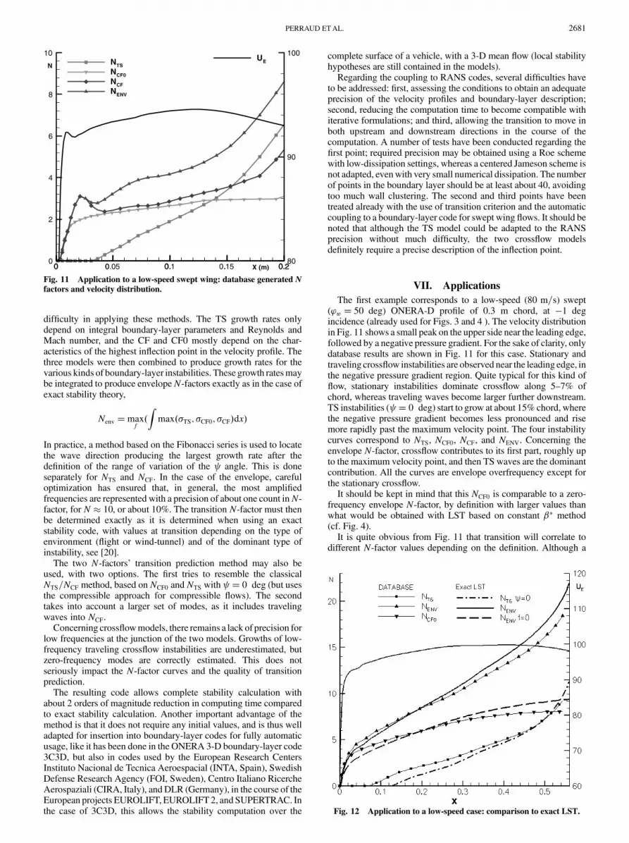
The first example corresponds to a low-speed (80 m=s) swept(’w � 50 deg) ONERA-D profile of 0.3 m chord, at �1 degincidence (already used for Figs. 3 and 4 ). The velocity distributionin Fig. 11 shows a small peak on the upper side near the leading edge,followed by a negative pressure gradient. For the sake of clarity, onlydatabase results are shown in Fig. 11 for this case. Stationary andtraveling crossflow instabilities are observed near the leading edge, inthe negative pressure gradient region. Quite typical for this kind offlow, stationary instabilities dominate crossflow along 5–7% ofchord, whereas traveling waves become larger further downstream.TS instabilities ( � 0 deg) start to grow at about 15% chord, wherethe negative pressure gradient becomes less pronounced and risemore rapidly past the maximum velocity point. The four instabilitycurves correspond to NTS, NCF0, NCF, and NENV. Concerning theenvelope N-factor, crossflow contributes to its first part, roughly upto the maximum velocity point, and then TS waves are the dominantcontribution. All the curves are envelope overfrequency except forthe stationary crossflow.

It should be kept in mind that this NCF0 is comparable to a zero-frequency envelope N-factor, by definition with larger values thanwhat would be obtained with LST based on constant �� method(cf. Fig. 4).

It is quite obvious from Fig. 11 that transition will correlate todifferent N-factor values depending on the definition. Although a

0 0.05 0.1 0.15 0.20

2

4

6

8

10NTS

NCF0

NCF

NENV

0 0 0. . 0.280

90

100UE

N

X (m)

Fig. 11 Application to a low-speed swept wing: database generated N

factors and velocity distribution.

Fig. 12 Application to a low-speed case: comparison to exact LST.

PERRAUD ETAL. 2681

single N-factor is used with the envelope method, a curve has to bedefined in the case of two N-factor methods, transition beingpredicted when the point of coordinates (NCF, NTS) crosses it. See[24] for examples of application.

A second case, corresponding to a low-speed DTP-B wing modelat 40 deg sweep is next considered (U1 � 70 m=s, ���4 deg).Figure 12 shows the velocity distribution and compares database N-factors with their exact LST counterparts. Again, this upper side atnegative incidence shows an extended negative pressure gradientwithout any leading-edge peak, which promotes crossflow insta-bilities. TS waves start further downstream, resulting in a mixed CFand TS case. Comparison to exact LST results shows differencesbelow two points inN-factors, or about 10%, on the envelope curve,and even smaller for NTS and NCF.

A third example, presented in Fig. 13 with the same curves asFig. 12, corresponds to a transonic case from the Fokker 100 naturallaminar flow flight experiments, which were run in the frame of theEuropean project ELFIN [19]. Boundary layers were computedusing a conical wing hypothesis, whereas stability calculations wereobtained here assuming an infinite swept wing. The vertical arrowindicates where transition occurs, and the velocity distribution is alsoplotted on the figure. The database results are again compared withexact LST computations, with a fair agreement in this difficult testcase. Departure from exact results remains lower than two at thetransition location, but with increasing difference as the databaseNCF0 remains at a constant value while the LST result continuesgrowing.

Five similar Fokker 100 cases were analyzed, bringing out thefollowing correlations at transition in flight conditions: NTS � 9,NCF � 15, NCF0 � 11, and Nenv � 22 for TS-dominated cases, andNenv � 15 for crossflow-dominated cases.

In wind-tunnel studies with the proposed databasemethod, typicalvalues for crossflow cases are NCF � 7 and NCF0 � 5, but thesevalues should be adapted for each test.

Application to transonic cryogenic tests (transonic smallmodels atlarge Reynolds numbers) showed that the crossflow model is notwell-adapted at present because boundary layers become extremelythin, outside the validity domain of the model. On the other hand, theNTS=NCF0 approach remains valid in these configurations.

After application to a number of swept profiles, the completedatabase method has been introduced as a transition prediction toolinto the 3C3D boundary-layer code [25], allowing the computationof amplification for 3-D flows over the complete surface of a wing ora vehicle. In 3C3D, growth rates are calculated in the course of theparabolic boundary-layer equations resolution, and then N-factorsare integrated along external streamline directions, until transition (ora separation) is predicted. Note that 3C3D also includes a transitionzone calculation based on an intermittency function. To illustrate theuse of this tool, an application to the slat of a high-lift configuration ispresented in Fig. 14. The KH3Y configuration was extensivelystudied within the European projects EUROLIFT I and II [14].Results are presented here for the upper slat, for a wing incidence of8.5 deg and a chord Reynolds number of 4:15 � 106.

Three methods are used in this case, envelope, NTS=NCF, andNTS=NCF0. In the first case, the three models (for TS, CF, and CF0)contribute to the envelope curve. In the second case, NCF includeswaves with a direction such that j j< 60, and NCF is based ontraveling and stationary waves. In the last one, NTS is restricted to � 0 andNCF0 to f� 0. Figure 14 shows the various regions of theflow according to the three methods, but with the N-factors attransition given in Table 1.

The outer slat is characterized by a large region (25% of span)where transition is caused by laminar separation. On each side of thisseparated zone, transition is predicted by 3C3D between 30 and 50%chord, followed by an extended transition region up to the trailingedge. Early transition is only predicted near the slat root withNTS=NCF0, resulting in a transition zone followed by a turbulent one.In each case, the unstable region is delimited into TS and CF regions,depending on the largest of the two N-factors. Comparison of theresults seems to show the equivalence of the three methods providedthat proper settings are used for transitionN-factors. It would bemost

interesting to compare the spanwise evolution of transition withexperimental results, but in most experiments transition measure-ments are usually done in a limited spanwise region.

A final example is presented in Fig. 15 that corresponds to aMach 2 highly swept (’w 60 deg) laminar wing designed andflight tested by the Japan Aerospace Exploration Agency (JAXA)[26]. ONERA cooperated with JAXA on the pre- and postflightnumerical transition analysis and performed wind-tunnel tests in theONERA S2. Figure 15 shows, for a postflight case, a comparison ofenvelopeN-factor curves obtainedwith two exact stability codes andwith the database method. The agreement on the envelope curves ishere again very satisfying. An extended version of the TSmodel was

0 0.5 1 1.50

5

10

15

20

0 0.5 1 1.5100

150

200

250

300

350

UEN

Envelope

NTS

NCF0

ScST0 0.5 1 1.5

0

5

10

15

20

0 0.5 1 1.50

5

10

15

20

Fig. 13 Application to a transonic Fokker 100 flight-test case. (Samelegend as Fig. 12. Arrow shows the transition location).

Fig. 14 Application to the upper side of the KH3Y slat (8.5� incidence,

ReC � 4:15 106.

Table 1 Transition N-factor settingsfor the KH3Y slat

NENV or NTS NCF

Envelope 7.15NTS=NCF 7.15 7NTS=NCF0 7.15 5

2682 PERRAUD ETAL.

used for this case, which includes the wall temperature Tw as an ad-ditional parameter.NTS=NCF curves are also shown but not comparedto exact calculation. Nevertheless, these curves confirm that cross-flow is effectively contributing to themost upstream instabilities, andis quite correctly predicted even for this supersonic case.

VIII. Conclusions

Three separate models were developed for simplified predictionof longitudinal (TS), traveling crossflow (CF), and stationaryinstabilities (CF0), aimed at allowing fast and automatic transitionpredictions. These three models rely heavily on Stuart theorem,stating in temporal theory the equivalence of the stability charac-teristics of a 3-D velocity profile in direction with that of theprojected 2-D profile in the same direction, and on Gaster’s relationto transform the spatial growth rates. Although integration should inprinciple be conducted along the group velocity direction, it isassumed that this direction remains very close to the external velocitydirection. The same hypothesis is often used in exact stability codes.

These models have been inserted inside the 3-D boundary-layercode 3C3D, and allow fully automatic transition predictions in abroad range of configurations. Extension to high-lift cases withstrong acceleration was realized with application to the KH3Y threeelements wing. The two main advantages of these methods are thatthey do not require determination of initial values, and the computingtime is about 2 orders of magnitude smaller compared with exact,local stability.

These methods are presented as engineering tools; they do notintend to replace exact stability codes. They aremost useful in designand when parametric variations are considered, like for optimizationpurposes.

Emphasis has been placed here on 3-D transonic configurations,but there exists an extension of the TS model to supersonic flows upto Mach 4. This extension was used for the highly swept JAXAwingpresented in the paper. CIRA and ONERA also used the databaseapproach in the design of the Mach 2 SUPERTRAC wing, in whichcase it was introduced into an optimization process.

In the case of a boundary layer computation time is very small, andin 3C3D the three models and N-factor curves are in fact computed,allowing comparison of the results. For the integration into a RANScode, selection of a single method would be necessary to reducecomputing time to a minimum because of the iterative process.Two methods are most cost effective, the envelope method and theNTS=NCF0. Introduction into a RANS code has not yet been realized,although conditions for using velocity profiles extracted fromRANSfields have been established.

ONERA database methods were developed for transonic aero-nautic applications with emphasis on crossflow instabilities, and arenot applicable to separated boundary layers. It should also be notedthat the traveling crossflowmodel has been inserted into the ONERAlocal stability code CASTET to provide automatic initialization for

crossflow-dominated cases, from low-speed to transonic flows, withgood success. The models presented can also be used to estimate apriori the range of variation of various parameters before conductinga complete stability analysis with a local or nonlocal code.

Acknowledgments

The work presented here received support from the EuropeanCommission, under the contracts ELFIN II, EUROTRANS,EUROLIFT, and EUROLIFT II. Support was also granted fromCentre National d’Etudes Spatiales and from Service desProgrammes Aéronautiques. The preparation of the present paperwas supported by internal ONERA funding.

References

[1] Smith, A. M. O., and Gamberoni, N., “Transition, Pressure Gradientand Stability Theory,”Douglas Aircraft Co., CARept. ES 26388, LongBeach, CA, Sept. 1956.

[2] van Ingen, J. L., “A Suggested Semi-Empirical Method for theCalculation of the Boundary-Layer Transition Region,” Univ. of Delft,Rept. VTH-74, Dept. of Aerospace Engineering, Oct. 1956.

[3] Arnal, D., “Transition Prediction in Transonic Flow,” IUTAM

Symposium Transsonicum III DFVLR-AVA, Springer–Verlag, Berlin,1988, pp. 253–262.

[4] Vialle, F., “Transition Sur un Ellipsoïde de Révolution,” ONERA,Student Training Rept., Sept. 1984.

[5] Stock, H.-W., and Degenhart, E., “A Simplified eN Method forTransition Prediction in Two-Dimensional Incompressible BoundaryLayers,”Zeitschrift fur Flugwissenschaften und Weltraumforschung,Vol. 13, No. 1, 1989, pp. 16–30.

[6] Gaster, M., and Jiang, F., “Rapid Scheme for Estimating Transition onWings by Linear Stability Theory,” 19th Congress of International

Council for the Aeronautical Sciences (ICAS), ICAS Paper 1994-243.[7] Casalis, G., and Arnal, D., “ELFIN II Subtask 2.3: Database method,

Development and Validation of the Simplified Method for PureCrossflow Instability at Low Speed,” ELFIN II, Technical Rept.,No. 145; also ONERA, Rept. No. 119/5618.16 DERAT, Dec. 1996.

[8] Fuller, R., Saunders, W. R., and Vandsburger, U., “Neural NetworkEstimation of Disturbance Growth Using a Linear Stability NumericalModel,” AIAA Paper 1997-0559, Jan. 1997.

[9] Crouch, J. D., Crouch, I.W.M., andNg, L. L., “Estimating the Laminar/Turbulent Transition Location in Three-Dimensional Boundary Layersfor CFD Applications,” AIAA Paper 2001-2989, Jan. 2001.

[10] Perraud, J., Donelli, R. S., and Casalis, G., “Database Approach:Treatment of Stationary Modes,”ALTTA, Technical Rept. No. 24; alsoONERA, Rept. No. RT 140/03828 DAAP/DMAE.

[11] Langlois, M., Masson, C., Kafyeke, F., and Paraschivoiu, I.,“Automated Method for Transition Prediction on Wings in TransonicFlows,” Journal of Aircraft, Vol. 39, No. 3, 2002, pp. 460–468.doi:10.2514/2.2951

[12] Drela, M., “Implicit Implementation of the Full eN TransitionCriterion,” AIAA Paper 2003-4066, Jan. 2003.

[13] Cliquet, J., Houdeville, R., and Arnal, D., “Application of Laminar-Turbulent Transition Criteria in Navier–Stokes Computations,” AIAA

Journal, Vol. 46, No. 5, 2008, pp. 1182–1190.doi:10.2514/1.30215

[14] Perraud, J., Cliquet, J., Houdeville, R., Arnal, D., and Moens, F.,“Transport Aircraft 3-D High-Lift Wing Numerical TransitionPrediction,” Journal of Aircraft, Vol. 45, No. 5, 2008, pp 1554–1563.doi:10.2514/1.32529

[15] Krumbein, A. M., “Automatic Transition Prediction and Application toThree-DimensionalWing Configurations,” Journal of Aircraft, Vol. 44,No. 1, 2007, pp. 119–133.doi:10.2514/1.22254

[16] Toulorge, T., Ponsin, J., Perraud, J., and Moens, F., “AutomaticTransition Prediction for RANS Computations Applied to a GenericHigh-Lift Wing,” AIAA Paper 2007-1086, Jan. 2007.

[17] Moens, F., Perraud, J., Iannelli, P., Toulorge, T., Eliasson, P., andKrumbein, A., “Transition Prediction and Impact on 3-D High-LiftWing Configuration,” Journal of Aircraft, Vol. 45, No. 5, 2008,pp. 1751–1766.doi:10.2514/1.36238

[18] Mack, L. M., “Boundary-Layer Linear Stability Theory,” Special

Course on Stability and Transition of Laminar Flow, AGARD Rept.No. 709, 1984.

[19] Schrauf, G., Perraud, J., Vitiello, D., and Lam, F., “Comparison of

Fig. 15 Application to the Mach 2 JAXA wing; comparison to exact

LST.

PERRAUD ETAL. 2683

Boundary-Layer Transition Predictions using Flight Test Data,”Journal of Aircraft, Vol. 35, No. 6, 1998, pp. 891–897.doi:10.2514/2.2409

[20] Arnal, D., Casalis, G., and Houdeville, R., “Practical TransitionPrediction Methods: Subsonic and Transonic Flows,” Advances in

Laminar Turbulent Transition Modeling, von Karman Inst. LectureSeries, 2008 (to be published); also ONERARept. RF 1/13639DMAE,Sept. 2008.

[21] Delbez, J., and Hallouard, J. M., “Etude de la Stabilité des Profils deCouche Limite Laminaire Avec Courant de Retour,” ONERA, StudentTraining Rept., June 1986.

[22] Gregory, N., Stuart, J. T., andWalker, W. S., “On the Stability of Three-Dimensional Boundary Layer with Application to the Flow Due to aRotating Disc,” Philosophical Transactions of the Royal Society of

London, Series A: Mathematical and Physical Sciences, Vol. 248,No. 943, 1955, pp. 155–199.doi:10.1098/rsta.1955.0013

[23] Gaster, M., “A Note on the Relation Between Temporally Increasingand Spatially Increasing Disturbances in Hydrodynamic Stability,”Journal of Fluid Mechanics, Vol. 14, No. 2, 1962, pp. 222–224.doi:10.1017/S0022112062001184

[24] Schrauf, G., “Large-Scale Laminar Flow Tests Evaluated With LinearStability Theory,” AIAA Paper 2001-2444, Jan. 2001.

[25] Houdeville, R., Mazin, C., and Corjon, A., “Method of Characteristicsfor Computing Three-Dimensional Boundary Layers,” La Recherche

Aerospatiale, Vol. 1, 1993, pp. 37–49.[26] Tokugawa, N., Kwak, D.-Y., Yoshida, K., and Ueda, Y., “Transition

Measurements of Natural Laminar Flow Wing on SupersonicExperimental Airplane NEXT-1,” Journal of Aircraft, Vol. 45, No. 5,2008, pp. 1495–1504.doi:10.2514/1.33596

A. TuminAssociate Editor

2684 PERRAUD ETAL.