development of simplified......pdf - sust repository

بسم هللا الرحمن الرحيم

Sudan University of Science and Technology (SUST)

College of Graduate Studies

Development of a Simplified Method for Non-Linear Analysis

of Tall Buildings

تطوير طريقة مبسطة للتحليل الالخطي للمباني العالية

A Thesis Submitted in Fulfillment of the Requirements for the Degree of Doctor of Philosophy in Civil Engineering

To the Dept. of Civil Engineering, College of Engineering, (SUST)

By:

Maaz Siddig Ibrahim Mohamed Tom

Supervisor:

Prof. Abdel Rahman Elzubeir Mohamed

November 2016

بسم هللا الرحمن الرحيم

خلق اإلنسان من علق *قرأ باسم ربك الذي خلق ا *علم *الذي علم بالق لم * اقرأ و ربك األكرم *

* اإلنسان مالم يعلم صدق هللا العظيم

I

ABSTRACT

In this research, a simplified numerical method of static and dynamic, linear and

nonlinear analysis of tall buildings is presented. The method is a development and

generalization of the moment distribution methods. The first version named the

moment transformation method (MT) was based on the rotations as the only degrees

of freedom with lateral translations permitted. A computer program named MTProg

was developed based on the method. The method is used for the analysis of tall

buildings with axial deformations in the vertical members ignored. The method has

then been developed to the moment-force transformation method (MFT), which

incorporates the axial deformations in the vertical members in order to enable the

analysis of super-tall buildings. The programs MFTProg and MFTProgV2 (Nonlinear

version) were developed based on MTProg. The global and local second order P-

Delta analysis of tall buildings subjected to vertical and horizontal loads were also

incorporated by coupling the axial force and the bending moments in each of the

vertical members with large lateral displacements at floor levels. Accordingly

buckling cases have also been studied. The method was further developed to extract

the dynamic properties of tall buildings. Displacements and different structural

responses due to dynamic loadings are computed using the proposed method with the

response spectrum and the time-history methods for both linear and second order

analyses. Validity of the method was established by comparing the results of 2D and

3D buildings with those resulting from reliable finite element packages. The

comparisons show that, the results are in good agreement thus verifying the accuracy

of the proposed method. The MFT method shows the ability to analyze adequately

and very fast tall buildings composed of hundreds of floors that can not be analyzed

accurately using the established methods of analysis. The saving in computer storage

and computing time provided by MFTProgV2 allow rapid re-analysis of the building

to be accomplished in the preliminary analysis and design stages, and in the cases of

repeated analysis types such as buckling and dynamic analyses of building. The ease

in data preparation and interpretation of final results, compared with finite element

packages is one of the main advantages of the method. For all these reasons the

developed program MFTProgV2 is recommended to be used for the linear/nonlinear,

static/dynamic and stability analyses of tall buildings.

II

:مستخلصال

طة عدديةطريقة بحث هذا اليعرض ة العالية. ألبنيالخطي والالخطي ل ،اإلستاتيكي والديناميكي لتحليللُمَبسَّ

نقل العزوم، وفيها استخدمتطريقة األولى هي صيغةالطريقة هي تطوير وتعميم لطرق توزيع العزوم. ال

البرنامج طوير تو بتصميمتها تمت حوسبو ،انبيةكدرجات حرية مع السماح بالتحركات الج الدورانات فقط

(MTProg.) ستخدامها في تحليل المباني التي يمكن تجاهل اإلزاحات المحورية في إيمكن هذه الطريقة و

لمحورية الطريقة نقل العزوم و القوى لتأخذ في اإلعتبار التشوهات صيغة األولى طورت ال. وقد الرأسية أعضائها

ينالبرنامجتطوير تم ستخدام في تحليل المباني شاهقة العلو.مما يمكنها من اإلاألعضاء الرأسية في

MFTProg و MFTProgV2 النسخة الالخطية( بناًء على(MTProg . الالخطية في أيضاً دمجتا

ة يات جانباألعضاء الرأسية في وجود إزاح كل من العالقة بين العزوم و القوى المحورية في الناتجة عنالتحليل،

خواص تم تطوير الطريقة للقيام بحساب ال . بعاجاتبناًء على ذلك تمت دراسة الحاالت الالزمة لإلنو ،كبيرة

ستجاباتنىالديناميكية للمب لخطية لتين افي الحا لألحمال الديناميكية المختلفةالمبنى ، كما تم حساب اإلزاحات وا

ستجابة التحليل الديناميكية المختلفة كطريقة طيف اإلوبمساعدة طرق المقترحة والالخطية، بإستخدام الطريقة

حددة العناصر الم برامجستخدام المتحصل عليها بنتائج حصل عليها بإوطريقة التاريخ الزمني. قورنت النتائج

كد يؤ لنتائجًا بين اأن هنالك توافقًا جيد ات. وقد أثبتت المقارنثالثية األبعاد وأخرى ثنائية األبعاد القياسية لمباني

لمباني لالطريقة إمكانية إستخدامها بفاعلية في التحليل الدقيق والسريع أوضحتكما الطريقة المقترحة. دقة

جمح التوفير فيو يستحيل أو يصعب تحليلها بالطرق القياسية. شاهقة العلو المكونة من مئات الطوابق والتي

اتهمتصمي احلان من التحليل السريع والمتكرر للمبنى في مر يوفرهما البرنامج يمكن ن يذزمن الحل اللفي الذاكرة و

وأات اجبعفي الحاالت التي تحتاج إلى التحليل المتكرر للوصول للحل كما في حاالت تحليل اإلنة وأيضًا األولي

ستخراج وعرض النتائج النهائعند دخال المعلومات وا ية حساب الخواص الديناميكية للمبنى. سهولة تجهيز وا

يوصي لكل هذه األسباب يعتبران من المميزات األساسية للطريقة. طرق العناصر المحددة القياسيةرنة مع مقا

راريةودراسة إستق ،واإلستاتيكي والديناميكي ،في التحليل الخطي والالخطي (MFTProgV2) بإستخدام البرنامج

لمباني العالية.ا

III

DEDICATION

To the cherished memory of my father.

To my mother, whose prayers supplication gave me support and confidence.

To my patient family, whose forbearance has been incentive to work hard on this

research.

To the new generation my kids, Rayyan, Mahmoud, Baddory, Riham and

Mohamed, I hope for them good future.

IV

ACKNOWLEDGMENTS

I would like to express my sincere gratitude to:

Prof. Abdel Rahman Elzubeir Mohamed

For his guidance and supervision, patience, encouragement, support and

friendly approach towards me throughout the lengthy process of this work.

I wish to thank my wife Eng. Manahil for all the patience and support she has

provided.

I am thankful to my dear brother, Automation Engineer Osama, who put me

in the right track.

Thanks a lot to my brothers Engineers Aymen, Ahmed Saeed, Amro, Elhadi,

Ahmed Norein, for their continuous help and support.

Lastly but not least the individuals whose names are over looked and not

mentioned above for every kind of support, help and cooperation in this work.

V

TABLE OF CONTENTS

ABSTRACT I

ARABIC ABSTRACT II

DEDICATION III

ACKNOWLEDGMENTS IV

TABLE OF CONTENTS V

LIST OF FIGURES XI

LIST OF TABLES XVIII

CHAPTER ONE: 1

General Introduction 1

1.1 Introduction 1

1.2 Problem Statement 2

1.3 Objectives 3

1.4 Methodology of Research 4

1.5 Outlines of thesis 4

CHAPTER TWO: 5

Literature Review 5

2.1 Introduction 5

2.2 Simple Manual Arithmetical Methods 6

2.3 Differential Equations and Continuum Methods of Analysis 7

2.4 Simplified Finite Element and Matrix Methods of Analysis 11

2.5 Methods of Simplifying the Models and Reduction Techniques 14

2.6 Miscellaneous Researches Conducted to Study and Improve the

Structural Systems of the Tall Buildings 16

2.7 Review to the Moment Transformation Method 21

2.8 Summary 21

CHAPTER THREE: 23

The Moment-Force Transformation Method Theory 23

3.1 Introduction 23

3.2 Reduction of Total Degrees of Freedom by Considering Rotations Only 23

VI

3.3 Analysis of Structural Systems using rotational degrees of freedom 24

3.4 Sway Fixed-End Moments 25

3.5 The Moment Transformation method 26

3.5.1 Column of two members 26

3.5.2 Generalization of the Method to Two and Three Dimensional Multi-

storey buildings 26

3.5.3 Equivalent stiffness matrix and moment transformation factors

matrix 27

3.5.4 Total Transformation Factors matrix from one level to a far level 28

3.5.5 Transformation of the moments from level # j to level # i 28

3.5.6 The joints rotations and the final moments at each level 28

3.5.7 The condensed Stiffness and the Carryover Moment for single

member 29

3.5.8 The condensed Stiffness and the Carryover Moments matrices for

two members 32

3.6 The Moment-Force Transformation Method 34

3.6.1 Consideration of the axial deformations in the vertical members 34

3.6.2 Multi-Bay Multi-Storey Buildings 37

3.6.3 Condensed Stiffness and Carryover Matrix for Multiple Vertical

Members including axial deformations 37

3.7 Second order P-Delta analysis of tall buildings 38

3.7.1 Condensed Stiffness and Carryover Matrices for Multiple Vertical

Members, including P-Delta effects 38

3.7.2 Linear-displacement assumptions 40

3.7.3 Cubic-displacement assumptions 40

3.7.4 Euler Stability Functions 42

3.8 The level rotation-translation stiffness 44

3.9 The Lateral Joints Displacements and the Shear Forces in the Vertical

Members 45

3.10 Concluding Remarks on the transformation methods 47

3.11 Modal Analysis using the Transformation Methods 48

3.11.1 Introduction 48

3.11.2 Fundamental Mode Analysis 48

VII

3.11.3 Analysis of Higher Modes 50

3.11.4 Inverse Iteration (Stodola Concept) using the Transformation

Method 52

3.12 Buckling Analysis by Matrix Iteration (Vianello Method) 54

3.13 The Improved Vianello Method 57

3.14 The conventional buckling incremental method 57

3.15 Buckling Analysis using the transformation method 58

3.16 Buckling Analysis using the transformation method with the aid of the

bisection method 60

3.17 Review to the earthquake design response spectra 60

3.17.1 Modal analysis procedure 62

3.17.2 Design response spectrum analysis 63

3.17.3 SRSS Modal Combination Method 65

3.17.4 CQC Modal Combination Method 65

3.18 The time history analysis method 66

3.18.1 Time history problem, the proposed numerical solution 67

3.18.2 Time history problem, the proposed closed-form solution 69

3.18.3 The normal coordinates system 70

3.18.4 Response of structures to ground motion 71

3.18.5 Structural response history using the transformation method 72

3.19 Response spectrum analysis using the transformation method 78

3.20 The Mass matrix 78

3.21 Column Shortening Calculations for Reinforced and Composite

Concrete Structures 79

CHAPTER FOUR: 80

Computer Program MFTProgV2 80

4.1 Introduction 80

4.2 Description of the Program MFTProgV2 80

4.2.1 The two Dimensional analysis 80

4.2.2 The Three Dimensional analysis 91

CHAPTER FIVE: 98

Program Applications and Verification of Results 98

VIII

5.1 Introduction 98

5.2 Numerical Examples 98

5.2.1 Two Floor One-bay Portal Frame 98

5.2.2 Two Floor Two-bay Portal Frame 99

5.2.3 Model of a hypothetical fifteen storey building subjected to

unsymmetrical lateral loading 100

5.2.3.1 Verification of Results 101

5.3 Summary 114

CHAPTER SIX: 115

Cases Study and Analysis of Results 115

6.1 Introduction 115

6.2 Dynamic Analysis using the transformation method 115

6.2.1 The vibration Modes 116

6.2.2 Participating Mass Ratios 116

6.2.3 The top floor lateral displacement 116

6.2.4 The Base Reactions 116

6.2.5 Response Spectrum Analysis 116

6.2.6 Time History Analysis 117

6.3 The fifteen floors 2D building Model 118

6.3.1 Static Linear and second order Analysis of the 2D building model 118

6.3.2 Buckling Analysis of the 2D building model 121

6.3.3 Dynamic analysis of the 2D model 125

6.3.4 Response spectra Analysis for the 2D model 128

6.3.5 P-Delta response spectra analysis 133

6.3.6 Time History Analysis for the 2D model 136

6.3.7 P-Delta Time History Analysis 143

6.4 The twenty five floors 3D building Model 149

6.4.1 Static Linear and second order Analysis of the 3D building model 150

6.4.1.1 Effect of Finite Element Formulation Accuracy 159

6.4.1.2 Comparison of Numbers of Unknowns 163

6.4.1.3 Analysis of a 150 floors Building using MFTProg 163

6.4.1.4 Running time and numbers of unknowns for N numbers of floors 168

6.4.2 Buckling Analysis of the 3D building model 171

IX

6.4.3 Dynamic analysis for the 3D model 173

6.4.4 Response spectra Analysis for the 3D model 175

6.4.5 P-Delta response spectra analysis 181

6.4.6 Time History Analysis for the 3D model 186

6.4.7 P-Delta time history analysis for the 3D model 196

CHAPTER SEVEN: 204

Conclusions and Recommendations 204

7.1 General Conclusions 204

7.2 Results Conclusion 205

7.3 Recommendations Drawn from Results Obtained 212

7.4 Recommendations for Future Research 213

References 214

APPENDICES: 230

Appendix A1: 231

A Three Segments Cantilever Example 231

Appendix A2: 232

The Moment Distribution Procedure 232

Appendix A3: 234

The Moment Transformation Procedure 234

Appendix A4: 236

A Three Segments Column Example 236

Appendix A5: 238

Further Optimization of the Transformation Procedure 238

Appendix B: 239

Flow Chart of the Conventional Buckling Incremental Method 239

Appendix C: 241

Buckling of Column Subjected to Axial Load P 241

Appendix D: 242

StaadPro Buckling Analysis, the basic solver 242

Appendix E: 243

Buckling Analysis – the advanced Solver in STAAD package 243

X

Appendix F: 244

Column shortening calculations for reinforced and composite concrete

structures (Proposed future study) 244

APPENDIX G: 248

Manual Check for the Results of the Square Building 248

XI

LIST OF FIGURES

Figure 3.1: Single post model 24

Figure 3.2: Intermediate storey of a multistory frame 25

Figure 3.3: Transformation of Moment 26

Figure 3.4: Multi-Storey 2D or 3D Building 27

Figure 3.5: Moments of the Concerned Level 28

Figure 3.6: Rotation and Translation DOF s of a Single Member 29

Figure 3.7: Condensed rotation Stiffness with Translation Permitted 30

Figure 3.8: Carryover Moment for a Single Member 31

Figure 3.9: Rotations and Translation DOF s of a two Members System 32

Figure 3.10: Condensed Stiffness Coefficient Corresponding To Displacement D1 33

Figure 3.11: Condensed Stiffness Coefficient Corresponding to Displacement D2 33

Figure 3.12: Carryover Moment Coefficient t*ij 34

Figure 3.13: Column of two segments 35

Figure 3.14: Rotations and Translations DOF s of a Two Vertical Members System 37

Figure 3.15: Rotations and Translations DOFs of Two Vertical Members System,

(with large displacements) 39

Figure 3.16: Translational Stiffness of a member including P-Delta effect 39

Figure 3.17: Carryover moment including P-Delta effect 39

Figure 3.18: End-rotational stiffness and carryover moment for a prismatic member

subjected to axial force 42

Figure 3.19: Degrees of Freedom of the Two Ends of Member # I 45

Figure 3.20: Physical interpretation of Stodola iteration sequence. 49

Figure 3.21: Transformation of coordinates for oriented column 57

Figure 3.22: Flow chart for elastic critical loads of plane frame 59

Figure 3.23: Response spectra. El Centro earthquake, N-S direction 61

Figure 3.24: Idealized design response spectrum, Cheng (2001) 62

Figure 3.25: General force-time relation 66

Figure 3.26: Numerical Solution of time history linear loadings between ordinates 68

Figure 3.27: Total structural response due to displacements at time to 73

Figure 3.28: Partial structural response due to unit displacement at level k 76

Figure 4.1-a: Flow chart of the moment-force transformation main solver-Part 1 81

XII

Figure 4.1-b: Flow chart of the moment-force transformation main solver-Part2 82

Figure 4.1-c: Flow chart of the moment-force transformation main solver-Part3 83

Figure 4.2-a: Flow chart of dynamic properties extraction of 2D frames-Part 1 84

Figure 4.2-b: Flow chart of dynamic properties extraction of 2D frames-Part 2 85

Figure 4.3-a: Flow Chart of the proposed buckling analysis solver 86

Figure 4.3-b: Flow Chart of the bisection subroutine 87

Figure 4.3-c: Flow Chart of the determinant subroutine 88

Figure 4.4: The program MFTProgV2 Layout (3D mode) 89

Figure 4.5: The multi-page data input of the two dimensional analyses mode 89

Figure 4.6: The results page of the two dimensional analysis mode 91

Figure 4.7: Local and global equilibrium checks 91

Figure 4.8: The building floor dimensions form 92

Figure 4.9: Main form of the three dimensional analysis 93

Figure 4.10: Walls and columns properties entering 93

Figure 4.11: Floors heights and lateral loading entering 94

Figure 4.12: Global equilibrium check at the different floors levels 95

Figure 4.13: Global deformed shape 96

Figure 4.14: StaadPro Floor stiffness and Fixing Moments form 96

Figure 4.15: Exaggerated deformed shape of a concerned floor 97

Figure 4.16: Moment contour of a concerned floor 97

Figure 5.1: One-bay Frame properties and loading 98

Figure 5.2: Two-bay Frame properties and loading 99

Figure 5.3: 12m x 12m floor plan for 15 Storey, Square Building 100

Figure 5.4: Displacements of the origin (Column # 5) in x-direction. 101

Figure 5.5: Displacements of the origin (Column # 5) in y-direction. 102

Figure 5.6: Twist rotations of the floor at the different levels. 102

Figure 5.7: MFTProg shear force diagram for shear wall #1 103

Figure 5.8: MFTProg bending moment diagram for shear wall #1 103






XIII


Figure 5.15: Comparisons of displacements of column #5 in x-direction 107

Figure 5.16: Comparisons of displacements of column#5 in y-direction 108

Figure 5.17: Comparisons of twist rotations of the floors in radians 108

Figure 5.18: Comparisons of S.F.D. for shear wall #1 109

Figure 5.19: Comparisons of B.M.D. for shear wall #1 109







Figure 6.1: UBC-1997 Design Response Spectra 117

Figure 6.2: N-S component of El Centro Earthquake records, 18 May 1940

(www.vibrationdata.com) 118

Figure 6.3: Fifteen floors 2D Frame, properties and loading 119

Figure 6.4: MFTProgV2, Buckling mode shape No. 1 122






Figure 6.10: First Mode Shape (Linear) 126

Figure 6.11: Second Mode Shape (Linear) 127

Figure 6.12: Third Mode Shape (Linear) 127

Figure 6.13: History of displacement in x-direction at the top floor level using

MFTProgV2 137

Figure 6.14: History of displacement in x-direction at the top floor level using the

StaadPro2004 137

Figure 6.15:History of displacement in x-direction at the top floor level using

ETABS 138


SAP2000V16 138

XIV

Figure 6.17: History of base Shear in x-direction using MFTProgV2 139

Figure 6.18: History of base Shear in x-direction using ETABS 140

Figure 6.19: History of base Shear in x-direction using SAP2000V16 140

Figure 6.20: History of Base overturning moment about y-direction using

MFTProgV2 141

Figure 6.21: History of base overturning moment about y-direction using ETABS 142

Figure 6.22: History of base overturning moment about y-direction using

SAP2000V16 142

Figure 6.23: History of P-Delta displacement in x-direction at the top level using

MFTProgV2 143

Figure 6.24: History of P-Delta displacement in x-direction at the top floor level

using StaadProV8i 144

Figure 6.25: History of P-Delta displacement in x-direction at the top floor level

using ETABS 144

Figure 6.26: History of P-Delta base Shear in x-direction using MFTProgV2 145

Figure 6.27: History of P-Delta base Shear in x-direction using ETABS 146

Figure 6.28: History of P-Delta base overturning moment about y-direction using

MFTProgV2 147


ETABS 147

Figure 6.30: 24 m x 12 m floor plan for 25 Storey Building 149

Figure 6.31: P-Delta Analysis, Displacements in y-direction 150

Figure 6.32: P-Delta Analysis, Rotations in radians 151

Figure 6.33: P-Delta Analysis, Rotations in radians (torsion released) 151

Figure 6.34: Linear Analysis, B.M.D. for U-Shaped Core 152

Figure 6.35: Linear Analysis, S.F.D. for U-Shaped Core 152

Figure 6.36: Linear Analysis, B.M.D. for edge shear wall 153

Figure 6.37: Linear Analysis, S.F.D. for edge shear wall 153

Figure 6.38: P-Delta Analysis, B.M.D. for U-Shaped Core 154

Figure 6.39: P-Delta Analysis, S.F.D. for U-Shaped Core 154

Figure 6.40: P-Delta Analysis, B.M.D. for edge shear wall 155

Figure 6.41: P-Delta Analysis, S.F.D. for edge shear wall 155

Figure 6.42: MFTProg moment My contour in kN.m/m for bottom floor slab 157

XV

Figure 6.43: StaadPro moment My contour in kN.m/m for bottom floor slab 157

Figure 6.44: MFTProg P-Delta analysis moment My contour in kN.m/m for bottom

floor slab 158

Figure 6.45: StaadPro P-Delta analysis moment My contour in kN.m/m for bottom

floor slab 158

Figure 6.46: MFTProg + StaadPro one floor model moment My contour in kN.m/m

for bottom floor slab 161

Figure 6.47: StaadPro (Full model) moment My contour in kN.m/m for bottom floor

slab 161

Figure 6.48: MFTProg + StaadPro one floor model P-Delta analysis moment My

contour in kN.m/m for bottom floor slab 162

Figure 6.49: StaadPro (Full model) P-Delta analysis moment My contour in kN.m/m

for bottom floor slab 162

Figure 6.50: 150 Floors Building, Bending Moment Diagram for U-Shaped Core

(kN.m). 164

Figure 6.51: 150 Floors Building, Shear Force Diagram for U-Shaped Core (kN). 164

Figure 6.52: 150 Floors Building, Bending Moment Diagram for Edge shear wall

(kN.m). 165

Figure 6.53: 150 Floors Building, Shear Force Diagram for Edge shear wall (kN). 165

Figure 6.54: 150 Floors Building, Displacements in y-direction (m). 166

Figure 6.55: 150 Floors Building, Axial Displacements in column #10 (m). 166

Figure 6.56: 150 Floors Building, Floors Twist Rotations in radians. 167

Figure 6.57: Perspective view for the deformed shape of the 150 Floors Building. 167

Figure 6.58: Elapsed running time in seconds using MFTProg 169

Figure 6.59: Comparisons of the numbers of unknowns 170

Figure 6.60: Buckling modes 1 to 6 172

Figure 6.61: Mass polar inertia for 4 lumped masses, (Proposal 1) 173

Figure 6.62: Mass polar inertia for uniformly distributed mass, (Proposal 2) 174

Figure 6.63: History of displacement in y-direction at the top floor level using

MFTProgV2 187


StaadProV8i 187

Figure 6.65: History of displacement in y-direction at the top floor level using 188

XVI

ETABS (thin plate)


ETABS (thick plate) 188


SAP2000V16 (thin plate) 189


SAP2000V16 (thick plate). 189

Figure 6.69: History of base Shear in y-direction using MFTProgV2 190

Figure 6.70: History of base Shear in y-direction using ETABS (thin plate) 191

Figure 6.71: History of base Shear in y-direction using ETABS (thick plate) 191

Figure 6.72: History of base Shear in y-direction using SAP2000V16 (thin plate) 192

Figure 6.73: History of base Shear in y-direction using SAP2000V16 (thick plate) 192

Figure 6.74: History of base overturning moment about x-direction using

MFTProgV2 193

Figure 6.75: History of base overturning moment about x-direction using ETABS

(thin plate) 194

Figure 6.76: History of base overturning moment about x-direction using ETABS

(thick plate) 194


SAP2000V16 (thin plate) 195


SAP2000V16 (thick plate) 195

Figure 6.79: History of P-Delta displacement in y-direction at the top floor level

using MFTProgV2 197


using StaadProV8i 197


using ETABS (thin plate) 198


using ETABS (thick plate) 198

Figure 6.83: History of P-Delta base Shear history in y-direction using MFTProgV2 199

Figure 6.84: History of P-Delta base Shear in y-direction using ETABS (thin plate) 200

Figure 6.85: History of P-Delta base Shear in y-direction using ETABS (thick plate) 200

XVII

Figure 6.86: History of P-Delta base overturning moment about x-direction using

MFTProgV2 201


ETABS (thin plate) 202


ETABS (thick plate) 202

Figure A1.1: Single post example 231

Figure A2.1: Ordinary rotational stiffness of a member 232

Figure A2.2: No-shear rotational stiffness with translation permitted 232

Figure A2.3: No-shear moment distribution between two members 233

Figure A2.4: Continuous beam model 233

Figure A3.1: Moment transformation of continuous beam 234

Figure A3.2: Moment transformation from joint 1 to 2 in a single post frame 235

Figure A3.3: Moment transformation from joint 2 to 3 in a single post frame 235

Figure A4.1: Three segments column 236

Figure C.1: The condensed translational and rotational stiffnesses 241

Figure F.1: The proposed analysis two models 247

Figure G.1: Simplified sketch of the Square building 248

XVIII

LIST OF TABLES

Table 5.1: Comparison of moments and forces at joints 3, 6 and 4 (2 Floor 1 bay

Frame) 99

Table 5.2: Comparison of moments at joints 1, 3 and 6 (2 Floor 2 bay Frame) 99

Table 5.3: Comparisons of the maximum shear force (kN) and bending moment

(kN.m) 113

Table 5.4: Displacements of the origin (column 5), in mm and radians 113

Table 6.1: Displacements in the top floor level (mm), (2D Frame), Linear Analysis 119

Table 6.2: Maximum bending moment in columns (kN.m), (2D Frame), Linear

Analysis 119

Table 6.3: Displacements in the top floor level (mm), (2D Frame), P-Delta

Analysis 120

Table 6.4: Maximum bending moment in columns (kN.m), (2D Frame), P-Delta

Analysis 120

Table 6.5: Minimum Buckling factor using the different packages 121

Table 6.6: Buckling factors of the first six modes using the different packages 121

Table 6.7: Floor Masses of the 2D Building (Mass in kg) 125

Table 6.8: Comparisons of the first six Natural frequencies of 2D Building

(cycles/second) 126

Table 6.9: Comparisons of the first three modes shape ordinates 128

Table 6.10: Comparison of the modal masses participating ratios 129

Table 6.11: Comparison of the accumulated modal masses participating ratios 129

Table 6.12: MFTProgV2 Response acceleration using the UBC response spectra

curve 129

Table 6.13: Modal Cross-correlation Coefficients method and the other packages. 130

Table 6.14: Comparison of the lateral displacement response at the top floor (m),

Proposal 1 130


Proposal 2 130

Table 6.16: Comparisons of the Response Spectrum Base Shear force 131

Table 6.17: Comparisons of the Response Spectrum Base Overturning Moment 132

Table 6.18: Comparisons of the first six P-Delta natural frequencies (cycle/second) 133

XIX

Table 6.19: Comparisons of percentage P-Delta modal Mass Participating ratios 133

Table 6.20: Comparison of percentage accumulated P-Delta modal Mass

Participating ratios 134

Table 6.21: Comparison of the P-Delta lateral displacement response at the top

floor (m), MFTProgV2 Proposal 1 134


floor (m), MFTProgV2 Proposal 2 134

Table 6.23: Comparison of Response Spectrum P-Delta Base Shear Reactions (kN) 135

Table 6.24: Comparison of Response Spectrum P-Delta Base overturning moment 136

Table 6.25: Minimum and maximum displacements at the top floor (mm) 139

Table 6.26: Minimum and maximum base shear (kN) 141

Table 6.27: Minimum and maximum base overturning moment (kN.m) 142

Table 6.28: Minimum and maximum P-Delta displacements at the top floor (mm) 145

Table 6.29: Minimum and maximum P-Delta base shear (kN) 146

Table 6.30: Minimum and maximum P-Delta base overturning moment (kN.m) 148

Table 6.31: Displacements and rotation in the top floor level (mm, rad), (3D

Frame). 156

Table 6.32: Maximum bending moment in U-Shaped Core (kN.m), (3D Frame). 156

Table 6.33: Maximum bending moment in Edge Shear Wall (kN.m), (3D Frame). 156


Frame), (Borrowed StaadPro Floor) 160

Table 6.35: Maximum bending moment in U-Shaped Core (kN.m), (3D Frame),

(Borrowed StaadPro Floor) 160

Table 6.36: Maximum bending moment in Edge Shear Wall (kN.m), (3D Frame),

(Borrowed StaadPro Floor) 160

Table 6.37: Displacements and rotation in the top floor level (mm, rad), (150 Floor

model) 168

Table 6.38: Maximum bending moment (kN.m) and Shear Force (kN), in U-Shaped

Core, (150 Floor model) 168

Table 6.39: Maximum bending moment (kN.m) and Shear Force (kN), in Edge

Shear Wall, (150 Floor model) 168

Table 6.40: Elapsed running time in seconds using MFTProg 168

Table 6.41: Comparison of numbers of unknowns 169

XX

Table 6.42: Minimum Buckling factor using the different packages 171

Table 6.43: Buckling factors of the first six modes using the different packages 171

Table 6.44: Floor Masses and Moments of Inertia of the 3D Building (Mass in kg

and Moment of Inertia in kg.m2) 175

Table 6.45: Comparisons of the first nine Natural frequencies of 3D Building

(cycles/second) 175

Table 6.46: Comparison of the modal masses participating ratios in x-direction 176

Table 6.47: Comparison of the accumulated modal masses participating ratios in x-

direction 176

Table 6.48: Comparison of the modal masses participating ratios in y-direction 177

Table 6.49: Comparison of the accumulated modal masses participating ratios in y-

direction 177


Proposal 1 178


Proposal 2 178

Table 6.52: Comparisons of the Response Spectrum Base Shear force (kN): 179

Table 6.53: Comparisons of the Response Spectrum Base Overturning Moment

(kN.m) 180

Table 6.54: Comparisons of the first nine P-Delta natural frequencies

(cycle/second) 181

Table 6.55: Comparison of the P-Delta modal masses participating ratios in x-

direction 182

Table 6.56: Comparison of the accumulated P-Delta modal masses participating

ratios in x-direction 182

Table 6.57: Comparison of the P-Delta modal masses participating ratios in y-

direction 183

Table 6.58: Comparison of the accumulated P-Delta modal masses participating

ratios in y-direction 183


floor (m), Proposal 1 184


floor (m), Proposal 2 184

XXI

Table 6.61.: Comparisons of the Response Spectrum P-Delta Base Shear force (kN) 185

Table 6.62: Comparisons of the Response Spectrum P-Delta Base Overturning

Moment (kN.m) 186

Table 6.63: Minimum and maximum displacements at the top floor (mm) 190

Table 6.64: Minimum and maximum base shear (kN) 193

Table 6.65: Minimum and maximum base overturning moment (kN.m) 196

Table 6.66: Minimum and maximum P-Delta displacements at the top floor (mm) 199

Table 6.67: Minimum and maximum P-Delta base shear (kN) 201

Table 6.68: Minimum and maximum P-Delta base overturning moment (kN.m) 203

Table A1.1: Displacements of the original structure 231

Table A1.2: Displacements of the split systems 231

Table A4.1: Equivalent Stiffness and Transformation Factors from Top to Bottom. 236

Table A4.2: Equivalent Stiffness and Transformation Factors from Bottom to Top. 236

1

CHAPTER ONE

General Introduction

1.1 Introduction

Tall buildings are highly affected by lateral loadings such as wind and earthquake

loads. The effects of these lateral forces may be resisted by lateral stiff elements such as

shear walls available around elevator shafts and staircases. The unsymmetrical

arrangement of the vertical members in the building plan cause twist deformations in the

level of the floors plans. In this case the problem becomes more complex and a three

dimensional analysis should be carried out instead of the simplified two dimensional

analysis. In practice, a full three-dimensional finite element analysis of tall buildings is

not simple because of the computer storage problem and the computing time cost factors

especially in the design stage when the structure has to be modified several times.

A lot of researches have been conducted in the field of computerized solution of large

scale problems with huge numbers of unknowns as the case of three dimensional full

finite element model of tall building. Research is also ongoing for the simplification of

analyses of tall buildings so as to be carried out with minimum cost. For all these reasons

accurate simplified methods of analysis of tall buildings are required.

In most of the simplified methods of analysis, there exist assumptions that lead to

wrong results in some of the practical cases. For example methods based on the

continuum theory or the equivalent column theory which should always be applied for

buildings of equal floor heights, buildings with no set back, cases of contra flexure (zero

moments) in the mid of the members, sometimes neglecting the flexural stiffness of the

floors, or for very regular structures where the geometric and stiffness characteristics of

structural elements are constant throughout the building’s height, Bozdogan and Ozturk

(2010), Parv and Nicoreac (2012).

A good simplified method must be reliable and supported by physical reality. It must be

able to include a wide range of design parameters, such as the positions of a structural

member as well as its orientation and dimensions. It should not require large computer

storage or long computing time so that a preliminary analysis can be carried out and

modified several times before the final design stage.

2

1.2 Problem Statement

The importance of performing the nonlinear analysis for tall buildings has been pointed

out by various researchers, Moghadam and Aziminejad (2004) and Ikago Kohju (2012). If

the building to be analyzed is very tall and slender and the axial forces are large or the

individual columns are slender, then the lateral displacements become very large and

affect the building geometry. This problem results in extra increase of the displacements

and stresses, and second order or P-Delta analysis should be carried out, Smith and Coull

(1991), Dobson and Arnott (2002).

In some of the available commercial analysis packages, the considerations of the

nonlinearity in the static and the dynamic analysis of tall buildings are subjected to

several limitations. Examples of these are incorporation of the global geometric stiffness

while neglecting the local stress stiffening of the members due to the effects of the axial

loads, Dobson and Arnott (2002). Sometimes in some commercial packages there is no

possibility to include the effects of geometric nonlinearity during the dynamic analysis

mode. In the iterative methods of P-Delta analysis used by most of the analysis packages,

the results tend to diverge when the vertical loads tend to reach the critical buckling load

at any of the vertical members. Since the critical forces are not known before performing

the analysis, the convergence of the results to the correct answers will not be ensured.

Also in the design codes, the effects of the nonlinearity are incorporated approximately

by modifying some of the design parameters, e.g. amplified moments, as in UBC-97 and

ACI 318-14, and, extended effective lengths as in BS8110 (1997). In methods of analysis

of tall buildings and in order to include the P-Delta effects, some authors suggest the

introduction of an equivalent fictitious member of negative properties, Wilson and

Habibullah (1987), Smith and Coull (1991), and this is not acceptable in most of the

analysis packages.

As stated above, the analysis of tall buildings needs some simplifications especially in

the preliminary analysis and design stages, in order to reduce the large amount of

unknowns when using the conventional exact methods of analysis. The problem becomes

more severe in the nonlinear analyses (e.g. P-Delta, Buckling, dynamic, time dependant

columns shortening), which need extra storage and extra time because most of these

methods require several iterations for the results to be converged to final values.

3

With all these requirements, this work presents development of a simplified method

used to analyze two dimensional and three dimensional tall buildings and suitable for the

analysis of framed shear walls buildings and for super tall buildings such as tube and

outrigger buildings subjected to both vertical and horizontal loading. The proposed

method has been developed to incorporate linear and nonlinear static and dynamic

analyses. Due to its simplicity, the method greatly saves the effort faced from the

difficulties of the data entry and the interpretation of the vast amount of the output results

when using the conventional finite elements methods of analysis. The saving in computer

storage and computing time provided by the developed program that based on the

proposed method, allow rapid re-analysis of the building to be accomplished in the

preliminary analysis and design stages, and in the cases of repeated analysis types such as

in the buckling and vibration problems. The future use of the proposed simplified method

on the more compacted very low memory today's devices (e.g. handhelds, pocket

computers and even mobile phones) is also a possibility.

1.3 Objectives

1) To carry out a comprehensive literature review in the field of the linear and

nonlinear static and dynamic analysis and elastic stability of tall buildings.

2) To develop a simplified theoretical approach for the linear and nonlinear, static

and dynamic analysis of tall buildings.

3) To develop computer programs to be used for advanced analysis of tall buildings

easily, both in the data entering and in the interpretation of the output results.

4) To develop an optimized theory, such as a development based on generalization

of the simple moment distribution methods, and optimized algorithms used for

analysis of tall buildings that can be implemented in very low memory devices,

such as pocket PCs and smart phones devices.

5) To verify the accuracy of the results obtained by comparisons with results from

known solvers.

6) To demonstrate the capability of the developed theory and programs to analyze

accurately tall buildings that are impossible or very difficult to be analyzed by

established accurate methods.

4

1.4 Methodology of Research

The research has been carried out as follows:

1- Literature Review and study of theoretical background.

2- Formulation of the proposed theory.

3- Development of the computer programs based on the formulated theory.

4- Application of the programs for different structures, analysis and verifications of

results, and the comments and conclusions.

5- Drawing recommendations for tall buildings analysis and recommendations for future

studies.

1.5 Outlines of thesis

The thesis includes the following:

1- Chapter one presents a general introduction.

2- Chapter two presents a literature review of the methods of analysis of tall buildings.

3- Chapter three presents the proposed theory.

4- Chapter four presents the developed computer program.

5- Chapter five presents the program applications and solution of some problems.

6- Chapter six presents two cases study, the results obtained and the analysis and

discussion of the results.

7- Chapter seven includes the conclusions and recommendations.

5

CHAPTER TWO

Literature Review

2.1 Introduction

Simplified methods of static and dynamic analysis for the effects of vertical and

horizontal loads on tall building are required, especially in the preliminary design stage

when the proposed structural system has to be analyzed several times before the final

agreement.

Due to the huge gravity loads and the possible large lateral displacements, the nonlinear

analysis should be carried out to adequately design the tall buildings.

In the analysis of large structural systems such as the tall buildings which include huge

numbers of unknowns, there arise a lot of difficulties such as:

The capability of the hardware of the computing machine.

The machine running time which is proportional to the total number of unknowns.

The interpretation of the vast amount of the analysis results.

The need that may arise for new rearrangements or changing of the structural

system.

In literature, there are lots of conducted researches, which can be classified into

different types of problems formulation and solution methods, such as:

Simple manual arithmetical methods, e.g. Portal and Cantilever methods.

Differential equations and Continuum methods of analysis.

Simplified finite element and matrix methods of analysis.

Methods of Simplifying the models and Reduction Techniques.

Each one of the mentioned methods is used with limitations and sometimes tailored for

a certain type of structural system.

6

In the following sections the available simplified analysis methods are reviewed and

classified.

2.2 Simple Manual Arithmetical Methods

For preliminary design of tall frames, as information regarding stress resultants due to

lateral loads is required even before member dimensions are known, the cantilever and

portal methods are sought in practice for the specific reason that they do not require cross

sectional areas for the analysis. When using these methods of analysis for lateral loads,

the analysis for vertical loads can be made in the same way as for the braced frames by

using any of the sub-frame methods.

According to Manicka and Bindhu (2011), there are two versions of the portal method.

One is the simplified portal method and the other is the improved portal method.

In the simplified portal method, the storey shear is distributed among the columns

considering that each of the outer columns resists half the shear resisted by any of the

internal columns, and in the improved portal method, the storey shear is distributed

among the columns in proportion to the tributary length of the spans between the

columns. Manicka et al, proposed an alternative analysis method which they called the

Split frame method. The method splits vertically the whole frames into separated simple

frames each of one containing only one bay subjected to lateral loads calculated from the

dimensions of all the bays. The method gives almost the same answer as that of the

improved portal method.

As a conclusion, the cantilever and the simplified and improved portal methods of

analysis together with the Split method proposed by Manicka et al, can be used only for

analysis of relatively short un-braced portal frames subjected to lateral wind loads or

equivalent static seismic loads, also they can’t be used to calculate the dynamic properties

of the frames (e.g. natural frequencies and mode shapes), and have no ability to calculate

the lateral stiffness of the building frame and therefore the drift and the lateral

displacements of the frame.

7

2.3 Differential Equations and Continuum Methods of Analysis

Based on the continuum theory, the researchers developed and solved approximately

miscellaneous types of problems, ranging from a very simple problem used to distribute

the lateral loads between the vertical members in a relatively short building, up to the

analysis of a more complicated tube and outrigger structural systems used in the ultra tall

buildings. The type of the problems also can be classified ranging from a simple static

problem up to a more complicated dynamic one, used to calculate the dynamic properties

of the building such as the vibration frequencies and their corresponding mode shapes.

Following are some researches and developments based on these types of analyses:

Jaeger, Mufti and Mamet (1973), proposed an analytical theory for the analysis of tall

three dimensional multiple shear wall buildings. The basis of their theory was the

continuum approach in which the floors of the building are replaced by an equivalent

continuous medium. Their results were compared with data obtained by the finite element

method and experiments conducted on a seven storey multiple, shear wall model.

A Simplified method was presented by Coull, Bose and Abdulla Khogali (1982), used

for the analysis of bundled tube structures subjected to lateral loads. In the method, the

rigidly-jointed perimeter and interior web frame panels were replaced by equivalent

orthotropic plates. The force and stress distributions in the substitute panels were

assumed to be represented by polynomial series in the horizontal coordinates, the

coefficients of the series being functions of the height only. The unknown functions were

determined from the principle of the least work. By incorporating simplifying

assumptions regarding the form of stress distribution in the frame panels, the structural

behavior was reduced to the solution of a single second-order linear differential equation,

enabling closed-form solutions to be obtained for the standard load cases, and solutions

were obtained from design curves.

A simplified approximate analysis of lateral load distribution in structures composed of

different assemblies was presented by Coull and Tag Eldeen Husein (1983). The load

distribution on each assembly was assumed to be represented by a polynomial in the

height coordinate, together with a concentrated interactive force at the top. A set of

8

flexibility influence coefficients, relating the deflection at any level to any particular load

component, was established for each assembly, the continuum approach was used to

analyze individual assemblies. By making use of the equilibrium and compatibility

equations at any desired set of reference levels, the load distribution on each assembly

was determined. Good results were achieved for regular structures by using no more than

about six reference levels.

As an alternative a simplified analysis of shear-lag in framed-tube structures with

multiple internal tubes was presented by Lee, Guan and Loo (2000). In their work a

simple numerical modeling technique was proposed for estimating the shear-lag behavior

of framed-tube systems with multiple internal tubes. The system was analyzed using an

orthotropic box beam analogy approach in which each tube is individually modeled by a

box beam that accounts for the flexural and shear deformations, as well as the shear-lag

effects. The method idealizes the tube(s)-in-tube structure as a system of equivalent

multiple tubes, each composed of four equivalent orthotropic plates capable of carrying

loads and shear forces. The numerical analysis so developed was based on the minimum

potential energy principle in conjunction with the variational approach. The shear-lag

phenomenon of such structures was studied taking into account the additional bending

stresses in the tubes. Structural parameters governing the shear-lag behavior in tube(s)-in-

tube structures were also investigated through a series of numerical examples. The

method results were verified through the comparisons with a 3-D frame analysis

program.

An approximate hand-method for seismic analysis of asymmetric building structure

having constant properties along its height was presented by Meftah, Tounsi and El

Abbas (2007). The method used the continuum technique and D’Alembert’s principle to

derive the governing equations of free vibration and the corresponding eigenvalue

problem. By applying the Galerkin technique, a generalized method was proposed for the

free vibration analysis. Simplified formulae were given to calculate the circular

frequencies and internal forces of a building structure subjected to earthquakes. The

accuracy of the method was demonstrated by a numerical example, in which the results

obtained were compared with finite element package.

9

A method for lateral stability analysis of wall-frame buildings including shear

deformations of walls was presented by Bozdogan and Ozturk (2010). Their study

presented an approximate method based on the continuum approach and transfer matrix

method. In the method, the whole structure was idealized as an equivalent sandwich

beam which includes all deformations. The effect of shear deformations of walls was

taken into consideration and incorporated in the formulation of the governing equations.

Initially the stability differential equation of this equivalent sandwich beam was

presented, and then shape function for each storey was obtained by the solution of the

differential equations. By using boundary conditions and stability storey transfer matrices

obtained by shape functions, system buckling load were calculated. To verify the

presented method, four numerical examples were solved. The results of the samples

demonstrated the comparison between the presented method and the other methods given

in the literature.

Also Bozdogan and Ozturk (2010), presented a Vibration analysis method of asymmetric

shear wall structures using the transfer matrix method. In the method the whole structure

was assumed as an equivalent bending-warping torsion beam. The governing differential

equations of equivalent bending-warping torsion beam were formulated using the

continuum approach and were posed in the form of a simple storey transfer matrix. By

using the storey transfer matrices and point transfer matrices, which take into account the

inertial forces, the system transfer matrix was obtained. Natural frequencies were

calculated by applying the boundary conditions. The structural properties of the building

may change in the proposed method. A numerical example were solved and presented by

means of a program written in MATLAB to verify the proposed method. The results

obtained were compared with other valid method given in the literature.

Bozdogan (2011), developed a differential quadrature method (DQM). In his work, free

vibration analysis of wall-frame structures were studied. A wall-frame structure was

modeled as a cantilever beam and the governing differential equations were solved using

the (DQM). At the end of the study, a sample taken from literature was solved and the

results were evaluated in order to test the convenience of the method.

10

A simplified method for high-rise buildings was developed by Takabatake (2012). In his

work an analytical theory for doubly symmetric frame-tube structures was established by

applying ordinary finite difference method to the governing equations proposed by the

one-dimensional extended rod theory. Takabatake, claims that his theory can be usable in

the preliminary design stages of the static and dynamic analyses for a doubly symmetric

single or double frame-tube with braces in practical use, and it would be applicable to

hyper high-rise buildings, e.g. over 600m in the total height, because the calculation is

very simple and very fast. Also the approximate method for natural frequencies of high-

rise buildings was presented in the closed-form solutions and it was stated to be necessary

for seismic retrofitting of existing high-rise buildings subject to earthquake wave

included relatively long period.

Another simplified method for nonlinear dynamic analysis of shear-critical frames is

developed by Guner and Vecchio (2012). In their work, an approach was presented by

which a static analysis method can be modified for a dynamic load analysis capability in

a total-load secant-stiffness formulation, and a nonlinear static analysis method was

developed for the performance assessment of plane frames. The primary advantage of the

method is its ability to represent shear effects coupled with axial and flexural behaviors

through a simple modeling approach. In the study, the method was further developed to

enable a dynamic load analysis. Among the developed and implemented formulations

there are an explicit three-parameter time-step integration method, based on a total-load

secant-stiffness formulation, and dynamic increase factor formulations for the

consideration of strain rates. The method was applied to eleven previously tested

specimens, subjected to impact and seismic loads, to examine its accuracy, reliability, and

practicality. The method was found to simulate the overall experimental behaviors.

Strengths, peak displacements, stiffness, damage, and failure modes and vibrational

characteristics were calculated.

An approach to static analysis of tall buildings with a combined tube-in-tube and

outrigger-belt truss system subjected to lateral loading was presented by Jahanshahi,

Rahgozar and Malekinejad (2012). The method was presented a technique for static

analysis of the system while considering shear lag effects. In the process of replacing the

11

discrete structure with an elastically equivalent continuous one, the structure was

modeled as two parallel cantilevered flexural-shear beams that are constrained at the

outrigger-belt truss location by a rotational spring. Based on the principle of minimum

total potential energy, simple closed form solutions were derived for stress and

displacement distributions. Standard load cases were considered. The formulas proposed

in the method were compared to a finite element computer package. Results obtained

from the proposed method for 50 and 60 storey tall buildings were compared to those

obtained using SAP2000.

A “Global structural analysis of central cores supported tall buildings compared with

FEM” was presented by Prav and Nicoreac (2012). The focus of their article was to

present an approximate method of calculation based on the equivalent column theory. By

applying the geometrical and stiffness characteristics of the structure the displacements in

the two directions, the rotation of the structure, critical load, shear forces, bending

moments for each resisting element and the torsional moment of the structure may be

determined. The results obtained using the approximate method was compared with the

results obtained using an exact calculation based on Autodesk Robot Structural Analysis

and ANSYS 12.1. The equivalent column theory is an approximate method used for

comparing and checking the results obtained by the Finite Element Method (FEM).

2.4 Simplified Finite Element and Matrix Methods of Analysis

Simplified methods of solution for the two and three dimensional frames based on the

matrix and finite element methods of analysis were developed.

In Macginely and Choo (1990) and Ghali et al (2009), a two dimensional analysis based

on building composed of parallel assemblies and on the shear wall frame interaction

system were presented. A three dimensional analysis of shear walls structures was

proposed by Ghali et al. In their method, the total degrees of freedom were reduced to

three per each floor. The global stiffness matrix was constructed from all shear walls,

with the assumptions of the rigid diaphragm and neglection of the floor out of plane

stiffness. The external lateral loads were applied at the assumed origin, the global

12

displacements were obtained and the local displacements and stresses were calculated

accordingly.

A two-level finite element technique of constructing a frame super-element was created

by Leung and Cheung (1981), to reduce the computational effort for solving large scale

frame problems. The ordinary finite element method was used first to yield matrices for

the beam members. Then the nodal displacements of all the nodes were related to those of

a small number of selected joints (master nodes) in the frame by means of global finite

element interpolating functions. Thus the frame was considered as a super-element

connected to other elements by means of the master nodes. The accuracy of solution may

be improved either with finer subdivision or by taking more master nodes inside each

super-element.

Also Leung (1983) presented another method, for the analysis of plane frames by

microcomputer. The method was based on the assumptions that, the distribution of the

vertical and rotational displacements at the nodes of a story is characterized by the

concept of distribution factors which are relative nodal displacements. The distribution

factors were allowed to vary from floor to floor and were determined by using three

floors at a time. These are calculated once only for floors having identical members. By

means of the distribution factors, the number of degrees of freedom was reduced to three

at any one floor. Therefore, it was possible for a micro-computer to handle a large

number of stories without difficulty. The resulting displacements and internal forces were

compared with full finite element analyses for a number of cases even with sudden

changes of stiffness.

The two dimensional method was further generalized by Leung (1985) to solve three

dimensional frames. It was also based on the fact that the deformation pattern at the

nodes of a particular floor may be predetermined before loading. These relative

displacements were called distribution factors which govern the distribution of

displacements. A number of free parameters were determined in the global analysis from

the applied loading. These parameters were called mixing factors. The linear

combinations of the distribution factors with mixing factors as weighting factors give the

actual displacements at the nodes. Structural idealizations of coupled shear walls by

13

beams and columns were recommended. In order to improve the results another three

additional sets of global distribution factors were introduced by Leung (1988) to account

for the uneven elongation (shortening) of the columns having unevenly distributed

stiffness along the height and across the floor plane. The total number of unknowns per

floor was reduced. Using the concept of the two-level finite-element method, the global

distribution factors of the building frame were obtained. The global and local distribution

factors together predicted the lateral and torsion deflections and internal nodal

displacements accurately.

In a similar manner, Wong and Lau (1989), presented a simplified finite element for

analysis of tall buildings. It was based on the assumption that the warping displacement

modes of a floor and the differences between neighboring floors are mainly determined

by the local structural characteristics. Once the warping modes are determined, these

modes are taken as the basis of generalized coordinates. Then, the problem can be

reduced to a formulation in which only the rigid body displacements and the warping

generalized coordinates of each floor are unknown. Results obtained from the examples

show that the simplified analysis method was satisfactory in displacements as well as in

internal forces when suitable warping modes from a multi-storey sub-model are chosen.

The authors claimed that the proposed simplified finite element method using a multi-

storey sub-model one-floor-unknown scheme is inexpensive and is able to yield

sufficiently good results for practical design purposes. The method can also be

generalized to solve dynamic problems.

A finite strip analysis method was developed by Swaddiwudhipong, Lim and Lee

(1988). The method was presented for the analysis of coupled frame-shear wall buildings

subjected to lateral loads. Appropriate displacement functions of admissible class were

adopted such that the problem is uncoupled and can be conveniently solved term by term.

Although this uncoupling property is valid only when the building is uniform throughout

its height, the method was extended to buildings with non-uniform section by employing

the concept of equivalent uniform section. Several numerical examples were presented to

show the accuracy and validity of the proposed scheme. The method required a small

14

core storage and short computing time and suitable for implementation on any of the

personal computers commonly available in most engineering design offices.

Giovanni (2009), in his PhD thesis dissertation showed the different types of the

structural condensations which can be used in the structures simplification, and these

were, the static condensation, the dynamic condensation (Guyan’s reduction method) and

the exact dynamic condensation method developed by Leung (1978). Leung method

efficiently reduces the order of dynamic matrices without introducing further

approximation by representing the passive co-ordinates in terms of the active ones

exactly. The resulting frequency dependent eigenvalue problem is solved by a combined

technique of Sturm sequence and subspace iteration. The method is a condensation

method in dynamic economization and dynamic substructure analysis and it converges to

the natural modes of interest always, even for the extreme case that the natural modes of

the overall structure are multiple and very close to the partial modes of its substructures, a

case when the normal methods fail.

A method for lateral static and dynamic analyses was presented by Bozdogan (2011).

The study presented an approximate method which was based on the continuum approach

and one dimensional finite element method to be used for lateral static and dynamic

analyses of wall-frame buildings. In the method, the whole structure was idealized as an

equivalent sandwich beam which includes all deformations. The effect of shear

deformations of walls was considered and incorporated in the formulation of the

governing equations. Initially the differential equations of the equivalent sandwich beam

were written and the shape functions and stiffness matrix were obtained by solving the

differential equations. For static and dynamic analysis the lateral forces and masses were

applied on the storey levels. Angular frequency and modes were obtained by using

system mass and system stiffness matrices. Numerical examples were solved using

MATLAB to verify the presented method.

2.5 Methods of Simplifying the Models and Reduction Techniques

The simplification of the modeling can be treated in the structural analysis stage in order

to reduce and simplify the problem solution. The reduction technique can be classified in

the following types:

15

1. Symmetry and anti-symmetry of the building plan

2. Two-dimensional model of non-twisting structures.

3. Two-dimensional models of structures that translate and twist.

4. Lumping Techniques which can be classified into lateral lumping and vertical lumping

5. Wide-column and deep-beam analogies.

In the work of Akis (2004), the main purpose of the study was to model and analyze

the non-planar shear wall assemblies of shear wall-frame structures. Two types of three

dimensional models, for open and closed section shear wall assemblies, were developed.

Those models were based on conventional wide column analogy, in which a planar shear

wall was replaced by an idealized frame structure consisting of a column and rigid beams

located at floor levels. The rigid diaphragm floor assumption was also taken into

consideration. The connections of the rigid beams were released against torsion in the

model proposed for open section shear walls. For modeling closed section shear walls, in

addition to that the torsional stiffness of the wide columns were adjusted by using a series

of equations. Several shear wall-frame systems having different shapes of non-planar

shear wall assemblies were analyzed by static lateral load, response spectrum and time

history methods where the proposed methods were used. The results of those analyses

were compared with the results obtained by using common shear wall modeling

techniques.

A simplified finite element modeling of multi-storey buildings was proposed by Li,

Duffield and Hutchinson (2008). The study discussed how to substructure different parts

of a multi-storey building with cubes having equivalent stiffness properties. As a result,

the mesh density of the whole building is reduced significantly and the computational

time and memory normally consumed by such complex structural dimensions and

material properties will also be reduced. The simplified analysis results of a high-rise

frame structure with a concrete core were used to explore the reliability of the proposed

method. In the study a typical 32-storey high-rise building was modeled with one storey

blocks. Force-Displacement relationship calibration was carried out to find the proper

simplified cubic model. According to the study, the equivalent cubic method was not

suitable for dynamic analysis. Further investigation focusing on the overall behavior of

16

the structural model built using the equivalent cubic method needs to be conducted to

ensure the connection properties between floors work correctly.

2.6 Miscellaneous Researches Conducted to Study and Improve the

Structural Systems of the Tall Buildings

Otani (1979), showed that, the nonlinear analysis of a reinforced concrete building is

difficult because inelastic deformation is not confined at critical sections, but spreads

throughout the structure and because stiffness of the reinforced concrete is dependent on

a strain history. The paper reviewed the behavior of reinforced concrete members and

their sub-assemblies observed during laboratory tests. Then different hysteresis and

analytical models of reinforced concrete members were reviewed, and their application to

the simulation of building model behavior was discussed. In the paper the behavior of

reinforced concrete buildings, especially under earthquake motion, was briefly reviewed.

Otani concluded that, his method is useful and reliable, when a structure can be idealized

as plane structures, but more research required to understand the effect of slabs, gravity

loads, and biaxial ground motion on nonlinear behavior of a three-dimensional reinforced

concrete structure.

A study conducted by Moghadam and Aziminejad (2004), for the interaction of torsion

and P-Delta effects in tall buildings”, evaluated the importance of asymmetry of building

on the P-Delta effects in elastic and inelastic ranges of behavior. The contributions of

lateral load resisting system, number of stories, degree of asymmetry, and sensitivity to

ground motion characteristics were assessed. In the study four buildings with 7, 14, 20

and 30 story were designed based on typical design procedures, and then their elastic and

inelastic static and dynamic behavior, with and without considering P-Delta effects, were

investigated. Each building was considered for 0%, 10%, 20% and 30% eccentricity

levels. The results indicated that the type of lateral load resisting system played an

important role in degree that torsion modifies the P-Delta effects. It was also shown that

although in the elastic static analyses, torsion always magnified the P-Delta effects, but

the same not always true for dynamic analyses. The results of dynamic analyses also

showed high level of sensitivity to ground motion characteristics.

17

The main results of the study were as follows:

1. In the elastic static analyses, effect of P-Delta always is increasing, as number of

stories of buildings or their eccentricity increased.

2. In the elastic or inelastic dynamic analyses, the effects of P-Delta sometimes increased

the response and sometimes decreased the responses.

3. “Importance of interaction of torsion and P-Delta effect” mainly depends on the type

of lateral load resisting system of building. The results indicated that the type of lateral

load resisting system played an important role in degree that torsion modifies the P-Delta

effects. It was concluded that the characteristics of lateral load resisting system had far

more importance compared with the number of stories in building.

4. It was seen that the effects of P-Delta is quite sensitive to ground motion

characteristics such as the frequency content of earthquake. In inelastic analyses, the

sensitivity is still important but less than the elastic dynamic cases. In general, the

sensitivity to ground motion increased, as the eccentricity increased.

5. In elastic or inelastic dynamic analyses, increase in eccentricity caused change in the

effect of P-Delta. The change is very important in elastic analyses and is somewhat less

important in inelastic analyses. However, the variation is not have a constant increasing

or decreasing trend. One of the reasons is the fact that with increase in the eccentricity,

the mass moment of inertia has not increased in all cases.

A nonlinear finite element analysis of tall buildings was presented by Marsono and Wee

(2006). The structural behaviors and mode of failure of reinforced concrete tube in tube

tall building via application of computer program namely COSMOS/M were presented.

Three dimensional quarter model was carried out and the method used for the study was

based on non-linearity of material. A substantial improvement in accuracy was achieved

by modifying a quarter model leading deformed shape of overall tube in tube tall building

to double curvature. The ultimate structural behaviors of reinforced concrete tube in tube

tall building were achieved by concrete failed in cracking and crushing. The model

presented in the paper put an additional recommendation to practicing engineers in

conducting non-linear finite element analysis (NLFEA) quarter model of tube in tube

type of tall building structures.

The findings of the study were summarizing as follow:

18

1. The quarter model was capable to perform non-linearity behavior up to ultimate limit

state.

2. Modified boundary condition by assigning restraint at X-direction at all slab edges,

fully restraint at wall bottom ends was considered appropriate in generating a double

curvature profile as expected in tube in tube model.

3. NLFEA in tube in tube building performed well using non-linear concrete stress-strain

curve up to 32 steps of non-linearity and yields the ultimate behavior of tall building.

4. Modified quarter model, which included the full configuration of shear wall, was found

to be appropriate in modeling the tube in tube tall building as quarter section. Thus, the

behavior of coupling beams was successfully presented out.

A study conducted by Bayati, Mahdikhani and Rahaei (2008) presented to optimize the

use of multi-outriggers system to stiffen tall buildings. They stated that “in modern tall

buildings, lateral loads induced by wind or earthquake forces are often resisted by a

system of multi-outriggers”. An outrigger is a stiff beam that connects the shear walls to

exterior columns. When the structure is subjected to lateral forces, the outrigger and the

columns resist the rotation of the core and thus significantly reduce the lateral deflection

and base moment, which would have arisen in a free core. During the last decades,

numerous studies have been carried out on the analysis and behavior of outrigger

structures. But the question remained that how many outriggers system are needed in tall

buildings? The paper presented the results of an investigation on drift reduction in

uniform belted structures with rigid outriggers, through the analysis of a sample structure

built in Tehran’s Vanak Park. Results showed that using optimized multi-outriggers

system can effectively reduce the seismic response of the building. In addition, the results

showed that a multi-outriggers system can decrease elements and foundation dimensions.

Jameel et al (2012), were carried a research to optimize structural modeling for tall

buildings. They were concluded that it is a common practice to model multi-storey tall

buildings as frame structures where the loads for structural design are supported by

beams and columns. Intrinsically, the structural strength provided by the walls and slabs

are neglected. The consideration of walls and slabs in addition to the frame structure

modeling shall theoretically lead to improved lateral stiffness. Thus, a more economic

structural design of multi-storey buildings can be achieved. In their research, modeling

19

and structural analysis of a 61-storey building were performed to investigate the effect of

considering the walls, slabs and wall openings in addition to frame structure modeling.

Sophisticated finite element approach was adopted to configure the models, and various

analyses were performed. Parameters, such as maximum roof displacement and natural

frequencies, were chosen to evaluate the structural performance. It was observed that the

consideration of slabs alone with the frame modeling may have negligible improvement

on structural performance. However, when the slabs are combined with walls in addition

to frame modeling, significant improvement in structural performance can be achieved.

In the research, different combinations of structural components of multi-storey buildings

were modeled to investigate the optimum design solution. Static as well as free vibration

analyses were carried out aiming at evaluating the structural performance and responses.

The following conclusions were drawn from the research:

1. Among the applied modeling concepts, (frame, wall, slab) is recommended for

economical design.

2. (Frame, wall, slab) modeling provides higher lateral stiffness and lower shear and

moment as compared with conventional frame and (frame, slab) modeling, which is an

expected trend.

3. The size of the structural member or the steel reinforcement in (frame, wall, slab)

modeling can be reduced, while satisfying the safety and serviceability requirement.

4. Wall openings, which would reduce lateral stiffness of a structure, should be taken into

consideration in structural analysis.

5. To fully understand the significance of walls and slabs in modeling and analysis of

multi-storey buildings, more modeling with a different plan view arrangement (such as

anti-symmetrical, non-symmetrical or more complex building shapes) were

recommended.

6. Further extensive study can be performed to generalize the effect of wall openings, by

modeling with different percentages of wall openings.

7. In the research, besides eigenvector analysis, only equivalent static analysis was

performed.

20

Static pushover analysis and response spectrum analysis could also be performed to

further investigation of the response of multi-storey buildings under seismic loading

conditions.

A seismic analysis of building with and without shear wall was studied by Chandurkar

and Pajgade (2013). They were concluded that, in the seismic design of buildings,

reinforced concrete structural walls, or shear walls, act as major earthquake resisting

members, providing an efficient bracing system and offer great potential for lateral load

resistance. The properties of these seismic shear walls dominate the response of the

buildings, and therefore, it is important to evaluate the seismic response of the walls

appropriately. In their study, main focus was to determine the solution for shear wall

location in multi-storey building. Effectiveness of shear wall has been studied with the

help of four different models. One model was bare frame structural system and other

three models are dual type structural system. An earthquake load was applied to a

building of ten stories located in zone II, zone III, zone IV and zone V. Parameters like

Lateral displacement, story drift and total cost required for ground floor were calculated

in both the cases replacing column with shear wall.

The conclusions of the paper were:

From all the conducted analyses, they observed that in 10 story building, constructing

building with shear wall in short span at corner was economical as compared with other

models. From this it can be concluded that large dimension of shear wall is not effective

in 10 stories or below 10 stories buildings. It was observed that the shear wall was

economical and effective in high rise building. Also observed that:

1. Changing the position of shear wall will affect the attraction of forces, so that wall

must be in proper position.

2. If the dimensions of shear wall are large then major amount of horizontal forces are

taken by shear wall.

3. Providing shear walls at adequate locations substantially reduces the displacements due

to earthquake.

21

2.7 Review to the Moment Transformation Method

The Moment Transformation method (MT) was presented by Ibrahim (2013), and

Ibrahim and Mohamed (2013). The method was used firstly to simplify the analysis of

the continuous beams and sub frames connected by a single or double upper and lower

columns at the joints, same as the direct moment distribution procedure but with different

formulation.

The no-shear moment distribution (sometimes also known as the cantilever moment

distribution), is based on the concept of distribution of the sway fixed end moments

without changing the sway-moment equation during the distribution procedure, Ghali and

Neville (1978).

The concept of the direct moment distribution was suggested by Lin, [Williams

(2009)], as a means of eliminating the iteration required in the standard moment

distribution procedure. Several alternative methods have also been developed for the

direct distribution of moments, e.g. the precise moment distribution (some times called

the coefficient of restraints), Reynolds and Steedman (1999).

Then the method was used to solve the problems of the single post connected by

horizontal members and subjected to lateral forces, and permitted to sway freely such as

in the substitute frame method. In this type of analysis, the concept of the no-shear

moment distribution is applied.

The method has then been developed and generalized to solve the wall-frame interaction

problems, and also developed to solve the more complex two dimensional, and three

dimensional multi-bay multi-floor buildings with irregular arrangement and orientation of

the vertical members and subjected to both vertical and horizontal loads.

A computer program (MTProg) has been developed based on Visual Basic Environment

and implemented for the method.

2.8 Summary

The exact solution for tall buildings is very expensive in terms of time and computer

storage. For this reason the need for simplified methods of analysis is arise.

The simplified methods of analysis always require some assumptions e.g.

(a) Neglection of the axial deformations.

(b) The in-plane rigid body movement.

22

(c) Assumption of the contra-flexural points in the middle of the columns and the beams.

(d) Assumption of equal floor heights.

(e) Assumption of uniform properties throughout the building height.

This is mainly shown in the continuum methods of analysis. The results obtained by the

continuum methods are less accurate when compared with the solutions obtained by the

simplified matrix based methods, especially if the walls are not symmetrical or the

members stiffnesses are largely different from each other, or if there is a setback in the

building as this affects the locations of the contra-flexure points. Analysis methods based

on simplified matrix and finite elements analysis give relatively accurate solutions.

Simplifications of the models, such as the optimized modeling schemes proposed by

Akis (2004), assist in analyzing the tall buildings with a lesser cost and effort.

Therefore, a simplified method of analysis that is based on reasonable assumptions is

required, in order to reach a more simple and accurate solution when compared with the

exact methods. In this research, such a simplified method is proposed and verified.

23

CHAPTER THREE

The Moment-Force Transformation

Method Theory

3.1 Introduction

In simplified analysis methods of tall buildings, the following assumptions are widely

used and are found to be reasonable for the majority of building structures:

(1) The floors are rigid in their own plane. The whole structural assembly in each floor

moves as a rigid body in the horizontal direction. The structural stiffness matrix is formed

under the assumption that all frames are connected at each floor level by a diaphragm,

which is rigid in its own plane. Due to the high in-plane stiffness, the lateral loads are

transferred to the columns and shear walls through these diaphragms.

(2) The out-of-plane stiffness of the floor can either be neglected or incorporated

approximately into corresponding equivalent beams.

In three dimensional analyses, there are some factors that influence how fast

results can be obtained and how accurate they are. The most important factors are the

amount of required data, computer running time and the vast output results that should be

interpreted. These should be optimized in such a way that sufficient results can be

obtained by entering lesser data and having a relatively short computing time. The

computer running time is mostly affected by the total number of degrees of freedom in

the system. Generally it may be decreased by:

(a) A reduction in the total number of elements used in the analysis and,

(b) The use of elements having the least degrees of freedom.

3.2 Reduction of Total Degrees of Freedom by Considering Rotations

Only

Instead of considering the whole degrees of freedom and applying all the forces

directly in the joints, the problem can be reduced to a system that includes only the

rotational degrees of freedom and fixed end moments. The known methods using such

assumptions are the slope deflection method, the ordinary moment distribution method,

the no-shear moment distribution and the successive sway correction method.

24

3.3 Analysis of Structural Systems using rotational degrees of freedom

Any structural system subjected to both vertical and/or horizontal loads can be split into

two loading systems (a) and (b), as shown in Figure 3.1. This simplifies the problem and

reduces the total degrees of freedom to only rotational degrees of freedom. System (a) is

a system in which the lateral degrees of freedom are released and the rotations are

completely restrained by the fixed moments for all the joints in the structure. The system

is used to calculate the fixed-end moments due to the external loading, the fixed moments

produced from the carryover moments and the transformed moments. System (b) is a

system with all the translational and rotational degrees of freedom released and used for

the released moments (the balancing moments).

Figure 3.1: Single post model

The released or the balancing moments, which are the reverse of the restraining

moments of the structural system (a), will be applied as concentrated moments in the

joints of the structural system (b). The induced moments e.g. the carryover moments and

the transformed moments are considered as fixed moments and should be applied again

in the structural system (a).

Appendix A1 shows an example illustrates the use of the two loading systems.

The example yields the following two important notes:

25

(1) The joints rotations can be that obtained only from the structural system (b), as the

structural system (a) has no rotations at the joints.

(2) The total translations of the joints are produced from the two structural systems by

superimposing the translations obtained from each system.

Based on the illustrated two structural systems concept, the moment distribution and the

moment transformation procedures are illustrated as shown in Appendix A2 and A3.

3.4 Sway Fixed-End Moments

In order to obtain the sway fixed end moments in the vertical members, let us consider

the structure shown in Figure 3.2, which shows an intermediate storey in a multi-bay

plane frame subjected to horizontal loads at floor levels. Assume that the frame is

allowed to sway without joint rotation. Neglecting the axial deformations in the

horizontal members, the top ends of all the columns in one storey translate relative to

their bottom ends by the same amount D. This sway induces end-moments and shearing

forces in all the columns. For equilibrium, the sum of the shearing forces in the columns

of one storey must be equal to the sum P of the horizontal forces acting on all the higher

floors; thus P and the column end-moments are related by:

P = h

1∑ M ...(3.1)

Where the summation is for the end-moments M at top and bottom of all the columns in

the given storey, and h is the floor height, Ghali and Neville (1978).

Figure 3.2: Intermediate storey of a multistory frame

26

3.5 The Moment Transformation method

3.5.1 Column of two members

Figure 3.3: Transformation of Moment

Referring to Figure 3.3, and using the displacement method of analysis, the equivalent

rotational stiffness Se of the two members 1 and 2 at joint 2, and the transformation factor

TF for the moment transformed from joint 1 to joint 2, are given as follows:

21

2

22

SS

tSSe

…(3.2)

21

2

SS

tTF

…(3.3)

where:

Si is the rotational stiffness of member # i.

ti is the carryover moment of the member # i.

3.5.2 Generalization of the Method to Two and Three Dimensional

Multi-storey buildings

Instead of transformation from joint to joint through members, as in the case of the

two columns, Figure 3.3, the system now is composed of multiple bays and multiple

floors as in Figure 3.4, and the transformation will be carried out through the floors from

top to bottom and from bottom to top.

Instead of the joints, the transformation in this case will be carried out from one level

to another level, Ibrahim (2013).

27

Figure 3.4: Multi-Storey 2D or 3D Building

The transformation procedure is generalized and given in a matrix form as shown in the

following sections.

3.5.3 Equivalent stiffness matrix and moment transformation factors

matrix

Moments Transformation procedure from top to bottom,

[SR] = [ NN ] i , ( if i = 1 ) …(3.4a)

[SR] = [ NN ] i + [GG] i-1 , ( if i ≠ 1 ) …(3.4b)

[AA] = [A] i + [SR] …(3.5)

[FF] i = -[ BC ]T i [AA]-1 …(3.6)

[GG] i = [A] i + [FF] i [BC] i …(3.7)

where;

[ NN ] i , is the Over All Rotation Stiffness Matrix of the Level # i .

[GG] i-1 , is the Equivalent Rotation Stiffness Matrix of The Floor # i-1 .

[A] i , is the Condensed Rotation Stiffness Matrix of The Floor # i .

[ FF ] i , is the Transformation Factors Matrix of The Floor # i .

[BC] i , is the Carryover Moments Matrix of The Floor # i .

[BC]Ti , is the Transpose of The Carryover Moments Matrix of The Floor # i .

[GG] i , is the Equivalent Rotation Stiffness Matrix of The Floor # i .

28

The same procedure can be carried out for transformation from bottom to top.

3.5.4 Total Transformation Factors matrix from one level to a far level

The total transformation factors matrix is calculated as follows:

[ FT ]K→K+2 = [ FT ]K→K+1 [ FF ]K+1→K+2 …(3.8)

where:

[ FT ]K→K+1 , is the total transformation factors matrix used to transform the moments at

level # K toward the level # K+1 .

[ FT ]K→K+2 , is the total transformation factors matrix used to transform the moments at

level # K toward the level # K+2 .

[ FF ]K+1→K+2, is the Transformation Factors Matrix of Floor between level #K+1

and level K+2 .

3.5.5 Transformation of the moments from level # j to level # i

Transformation of the moment vectors from level j to level i can be carried out as shown

in Equation 3.9.

{ MT }i = { MT }i + [ FT ] j→i { MT + MB + MS }j …(3.9)

Figure 3.5, shows the arrangement of the fixed ends moments at the level # i.

Figure 3.5: Moments of the Concerned Level

3.5.6 The joints rotations and the final moments at each level

The rotations and the moments at the joints of the level # i are calculated as shown

below:

The rotation of all the joints of level # i is given as follows:

{ ROT } i = -[KT] i -1 { MTOT } i …(3.10)

[ KT ] i = [ KT ] i + [ KB ] i + [ KS ] i …(3.11)

29

{ MTOT }i = { MT } i + { MB } i + { MS } i …(3.12)

Final moments of the level # i:

{ MTf }i = { MT }i + [ KT ] i { ROT }i …(3.13a)

{ MBf }i = { MB }i + [ KB ] i { ROT }i …(3.13b)

{ MSf }i = { MS }i + [ KS ] i { ROT }i …(3.13c)

where:

[ KT ] i , is the total stiffness matrix at the level # i .

{ MTOT } i , is the total moments vector at level # i .

{ ROT } i , is the rotations of the joints vector at the level # i .

{ MT } i , is the original and the transformed moments vector just above the level # i .

{ MB } i , is the original and the transformed moments vector just below the level # i .

{ MS } i , is the original moments vector at the beams ends of the level # i .

{ MTf } i , is the final moments vector just above the level # i .

{ MBf } i , is the final moments vector just below the level # i .

{ MSf } i , is the final moments vector at the beams ends of the level # i .

3.5.7 The condensed Stiffness and the Carryover Moment for single

member

The rotation stiffness for single post subjected to side sway with no shear produced can

be obtained as follows:

Figure 3.6: Rotation and Translation DOF s of a Single Member

The two DOFs are shown in Figure 3.6 and the corresponding system matrix equation is

as follows:

S11 S12 D1 F1

= …(3.14)

S21 S22 D2 F2

30

In order to obtain the condensed stiffness matrix, substitute for F1= S*, F2 = 0, D1 = 1,

D2 = D in equation 3.14, yields

S11 S12 1 S*

= …(3.15)

S21 S22 D 0

Figure 3.7: Condensed rotation Stiffness with Translation Permitted

where S* is the condensed stiffness or rotation stiffness with translation not prevented.

The matrix Equation 3.15 contains the following two equations:

S11 + S12 . D = S* …(3.16a)

S21 + S22 . D = 0 …(3.16b)

From equation (3.16b)

D = - S22-1 . S21 …(3.17)

Substitute equation (3.17) into equation (3.16a), gives:

S* = S11 – S12 . S22-1 . S21 …(3.18)

These relations can be formulated in a general matrix form as shown below:

[S11] [ S12] [ I ] [ S*]

= …(3.19)

[S21] [S22] [ D ] [ 0 ]

where:

[ I ] : Identity matrix .

[ 0 ] : Null matrix .

[ D ] : Displacement matrix corresponding to the condensed stiffness matrix .

[Sij] : Sub-Matrices of the main matrix .

[ S*] : The condensed rotation stiffness matrix .

31

Equation (3.17) and (3.18) becomes as follows:

[ D ] = - [S22 ]-1 . [S21 ] …(3.20)

[S11*] = [ S11] – [S12 ] . [S22]

-1 . [S21] …(3.21)

For a single member, shown in Figure 3.6, the stiffness matrix of the two degrees of

freedom in the general form, is as follows:

S ( S + t )/L

( S + t )/L 2*( S + t )/L2

Considering bending deformation and neglecting shear deformations, the stiffness matrix

will be as shown below:

4 EI/L 6 EI/L2

[S ] =

6 EI/L2 12 EI/L3

Using equation (3.17) and equation (3.18):

D = - ( 6 EI/L2 ) / ( 12 EI/L3 ) = -0.5 L

S* = 4 EI/L - ( 6 EI/L2 )2 / ( 12 EI/L3 ) = 4 EI/L - 3 EI/L = EI/L

where:

S* is the condensed rotation stiffness with the lateral sway permitted.

Figure 3.8: Carryover Moment for a Single Member

For equilibrium of the post:

t* = - S* …(3.22)

Where: t* is the carryover moment corresponding to the condensed rotation stiffness S*.

32

The lateral loads are applied in terms of side sway fixed moments with no rotation of the

joints permitted.

The final moments and the rotation at each joint is obtained directly by the

transformation method from which we can get the joint lateral displacements and the

shear forces in all members.

3.5.8 The condensed Stiffness and the Carryover Moments matrices for

two members

The previous procedure that used to obtain the condensed stiffness for a single member

subjected to side sway is now generalized to a bundle of members. To simplify the

presentation we consider a system of two vertical members (columns or walls),

Figure 3.9: Rotations and Translation DOF s of a two Members System

The system equation corresponding to the three degrees of freedom shown in Figure 3.9

including the condensed rotation stiffness matrix with the translation of the joints

permitted is as shown below:

S11 S12 S13 1 0 S11*

S12*

S21 S22 S23 0 1 = S21*

S22*

S31 S32 S33 [ D1 D2 ] [ 0 0 ]

…(3.23)

Applying equation (3.20) shown in the previous illustration, we get the displacements

corresponding to the condensed stiffness matrix:

[ D1 D2 ] = - [ S33]-1 [ S31 S32 ] = - [ (S31/ S33) (S32/ S33) ]

= [ -(S31/ S33) -(S32/ S33) ] …(3.24)

33

Figure 3.10: Condensed Stiffness Coefficient Corresponding To Displacement D1

Figure 3.11: Condensed Stiffness Coefficient Corresponding to Displacement D2

From equation (3.21) the condensed rotation stiffness matrix is:

S11*

S12* S11- S13. S33

-1 .S31 S12- S13. S33-1 .S32

= …(3.25)

S21*

S22* S21- S23. S33

-1 .S31 S22- S23. S33-1 .S32

The internal interaction force is obtained from the local stiffness matrix of the member

that free in one end and fixed in the other end, the considered degrees of freedom are the

rotation and the translation of the free end, as shown below:

Si ( Si + ti ) / L 1 S*ij

= ( For i = j ) …(3.26)

( Si + ti ) / L 2 ( Si + ti ) / L2 Dj (Fi)Dj

and,

Si ( Si + ti ) / L 0 S*ij

= ( For i ≠ j ) …(3.27)

( Si + ti ) / L 2 ( Si + ti ) / L2 Dj (Fi)Dj

34

where:

Si & ti are the ordinary rotation and carryover moment of member # i respectively.

Dj is the displacements corresponding to the stiffness configuration #j.

Figure 3.12: Carryover Moment Coefficient t*ij

For equilibrium of the member shown in Figure 3.12, the carryover moment matrix

element t*ij can be calculated as follows:

t*ij = - S*

ij+(Fi)Dj* L …(3.28)

3.6 The Moment-Force Transformation Method

The moment transformation (MT) method was developed to analyze moderate tall

buildings neglecting the axial deformations in the vertical members. In this research the

MT method has been further developed to the Moment-Force Transformation (MFT)

method, which included the axial deformation in the vertical members in the analysis.

The two methods are used for linear static analysis of tall buildings. The algorithm of the

moment transformation program MTProg has been further developed to the moment-

force transformation program MFTProg.

In the moment distribution methods, the moments are distributed between the end joints

of each individual member. In the moment transformation (MT) method the distributions

are carried out for a coupled group of moments at the same time from one level toward

the next level. Using this stream or bundle of distribution, permits the axial deformation

(shortening/elongation) of the vertical members to be incorporated in the analysis.

3.6.1 Consideration of the axial deformations in the vertical members

In this part, the axial deformation in the vertical members is incorporated in the

analysis. The procedure start using a single post composed of different members and then

35

generalized to any system composed of multiple vertical members. To simplify the

presentation a post composed of two elements is considered as shown in Figure 3.13.

The stiffness matrix for each individual member is as follows:

KK

KK

or

Kt

tK

Figure 3.13: Column of two segments

Where: K is the axial stiffness (K= EA/L) and t=-K = carryover force (Similar to the

carryover moment). The carryover moment or force, actually are the moment or the force

reactions of the restrained far end of the member.

The matrix equation of the structural system shown in Figure 3.13 is as follows:

22

221

KK

KKK

2

1

D

D =

2

1

F

F …(3.29)

Where:

K1 and K2 are the axial stiffnesses of the members 1 and 2 respectively.

F1 and F2 are forces acting at joints 1 and 2 respectively.

D1 and D2 are the axial displacements of the joints 1 and 2 respectively.

From which:

(K1+K2) D1-K2 D2 = F1 …(3.30)

-K2 D1+K2 D2 = F2 …(3.31)

From equation 3.30

21

12

21

21

KK

FD

KK

KD

…(3.32)

36

Substituting from equation 3.32 into 3.31 and rearranging, yields:

1)21

2(22)

21

2.1( F

KK

KFD

KK

KK

…(3.33)

or

1.22.2* FTFFDK …(3.33a)

where

)21

2.1(*2

KK

KKK

…(3.34)

21

2

KK

KTF

…(3.35)

K2*: is the equivalent axial stiffness replacing the two members 1 and 2, in the place of

member 2.

TF: is the factor used to transform the axial force from joint 1 to joint 2.

The form of the produced equation is similar to the moment transformation equations, so

that the axial stiffness can be introduced in the transformation procedure together with

the rotational stiffness.

For multiple vertical members, the axial stiffnesses of the vertical members are coupled

with the transverse stiffness of the beams in the case of the two dimensional analyses and

by the whole transverse (out of plane) stiffness of the floor slab in the case of the three

dimensional analyses.

The transformation of the moment and the force from joint (1) to joint (2) is carried out

as shown in the following steps:

(1) Restraining of joint (2).

(2) Application of the force (F1) at joint (1).

(3) Finding the force reaction (R) at joint (2).

(4) Reversing the reaction (R) to get active force (F’21=-R).

The reaction (F’21) is part of the force (F1) , and is given by:

F’21=a.F1 …(3.36)

Where: a = TF

37

The equivalent stiffness of the two members is match with the equation used to

calculate the equivalent axial stiffness of (n) members. The equivalent stiffness of (n)

members is obtained from:

For axial force, F, acting at the top of a vertical cantilever composed of members

connected in series, the total displacement is equal to the summation of all the

member’s displacements:

Dtot= D1+D2+…+Dn

Kn

F

k

F

k

F

Ke

F ...

21

Or;

KnkkKe

1...

2

1

1

11 …(3.37)

The axial displacements for a three segments column were calculated using the force

transformation method is presented in Appendix A4.

3.6.2 Multi-Bay Multi-Storey Buildings

By combining the moments and the forces transformation procedures, the moment-

force transformation procedure can be generalized to calculate the equivalent stiffness

matrix and the transformation factors matrix of tall building.

3.6.3 Condensed Stiffness and Carryover Matrix for Multiple Vertical

Members including axial deformations

Considering a system of two vertical members, Figure 3.14, the stiffness matrix

equation corresponding to the three degrees of freedom 1,2 and 3, as before, is

condensed into degrees of freedom 1 and 2, as follows:

Figure 3.14: Rotations and Translations DOF s of a Two Vertical Members System

38

00

10

01*

22

*

21

*

12

*

11

21333231

232221

131211

SS

SS

DDSSS

SSS

SSS

… (3.38)

As in the moment transformation method, the internal interaction force, (Fi)Dj is

obtained from the different rotational stiffness configurations and hence the elements of

the carryover moments matrix, t*ij, are calculated from equation 3.39:

LFStDjiijij .** …(3.39)

Where; L is the floor height.

Since the axial stiffness of the vertical members are uncoupled with each other and also

uncoupled with the rotational and the lateral translation stiffness of the members, then the

axial stiffness of each member can be added to the condensed rotational stiffness, S*ij, of

the members after the condensation procedure. Similarly, the axial force carryover

elements are also added to the carryover matrix.

3.7 Second order P-Delta analysis of tall buildings

By coupling of the moments and the axial forces in each of the vertical members for

large lateral displacements at the floors levels during the moment-force transformation

procedure, the second order P-Delta effects are directly included in the analysis and

structural instability with reference to overall buckling or failure of individual members is

also studied.

3.7.1 Condensed Stiffness and Carryover Matrices for Multiple Vertical

Members, including P-Delta effects

Considering a system of two vertical members, Figure 3.15, the stiffness matrix

equation 3.38, corresponding to the three degrees of freedom 1, 2 and 3, are condensed

into 1 and 2, as follows:

The translational stiffness S33 (Equation 3.38), is a summation of the translational

stiffness (ST) of each vertical member including its global P-Delta effect (i.e. -P/L, where

P is the axial force in the vertical member), as shown in Figure 3.16. The effect of the

local p-delta in any member may be incorporated by using the Euler stability functions

where the rotational stiffness, S, and the carryover moment, t, of the member, are

39

trigonometric functions of axial compression forces for positive P values, or hyperbolic

functions of axial tension forces for negative P values, Ghali et al. (2009).

Figure 3.15: Rotations and Translations DOFs of Two Vertical Members System,

(with large displacements)

Figure 3.16: Translational Stiffness of a member including P-Delta effect

Figure 3.17: Carryover moment including P-Delta effect

The lateral displacement, D, and the internal interaction force, F, Figure 3.17, are

obtained from the different rotational stiffness configurations and hence the elements of

the carryover moment matrix, including the P-Delta effects, are calculated from equation

3.40:

DPLFSt jiji ..** … (3.40)

40

3.7.2 Linear-displacement assumptions

In the case of the linear-displacement assumption, the end rotational stiffness S and the

carryover moment t of a beam element are assumed not to be affected by the axial load.

The affected term is the lateral stiffness ST, as shown in equation 3.41:

L

P

L

tSST

2

)(2 …(3.41 )

For beam element with shear deformations considered, the ordinary end rotational

stiffness and the carryover moment are given, as follows:

L

EIS

)1(

)4(

…(3.42 )

, and L

EIt

)1(

)2(

…(3.43 )

Where

2

12

LGa

EI

r

And, for members with shear deformations neglected stiffness factors are:

L

EIS

4 , and

L

EIt

2

The term )(L

P is the linear geometric stiffness of the beam element affecting the lateral

stiffness.

The term geometric stiffness is introduced so that the stiffness matrix has a different

name from the mechanical stiffness matrix, which is based on the physical properties of

the element. The geometric stiffness exists in all structures but it becomes important only

if it is large compared to the mechanical stiffness of the structural system, Wilson (2000).

3.7.3 Cubic-displacement assumptions

In the case of a beam element with bending properties in which the deformed shape is

assumed to be a cubic function caused by the rotations φi and φj at the beam ends,

additional moments Mi and Mj are developed. Considering the cubic function, the force-

displacement relationship is given by Equation 3.44, Wilson (2000):

41

…(3.44)

The well-known elastic force deformation relationship for a prismatic beam neglecting

shear deformations is:

…(3.45)

Therefore, the total stiffness matrix, kT, of the beam element is as follows:

kT = kE + kG …(3.46)

where;

kE is the elastic (mechanical) stiffness matrix, and kG, is the geometric stiffness matrix.

So, to account for the cubic displacement function, it is only required to incorporate the

total rotational stiffness and the carryover moment including the terms shown circled in

the geometric and the mechanical stiffness matrices, therefore:

30

44 PL

L

EIS …(3.47)

, and 30

2 PL

L

EIt …(3.48)

If shear deformations are considered in both the geometric and mechanical stiffness

matrices, the rotational stiffness and the carryover moment become as follows:

2

2

)1(

)12/6/15/2(

)1(

)4(

LLLP

L

EIS …(3.49)

, and

42

2

2

)1(

)12/6/30/(

)1(

)2(

LLLP

L

EIt …(3.50)

The translational stiffness ST, can directly be obtained by maintaining the equilibrium of

the element.

L

P

L

tSSST

233

)(2 …(3.51)

Considering bending deformations only,

30

44 PL

L

EIS , and

30

2 PL

L

EIt

L

P

L

P

L

EIST

30

6123

L

P

L

EI

30

36123

ST is the summation of the elements shown squared in the geometric and mechanical

stiffness matrices.

3.7.4 Euler Stability Functions

The rotational stiffness and the carryover moment for a member subjected to an axial

force P, are shown in Figure 3.18.

Figure 3.18: End-rotational stiffness and carryover moment for a prismatic member

subjected to an axial force

43

For member subjected to axial compression, S and t are given as follows, Ghali and

Neville (1978):

l

EI

usc

ucsuS

)22(

)(

… (3.52)

, and

l

EI

usc

suut

)22(

)(

…(3.53)

Where:

us sin , uc cos , )/(EIPlu

For member subjected to axial tension, S and t are given as follows:

)/(EIPliu , 1i

iuiu sinsinh , iuu coscosh

l

EI

uuu

uuuuS

)sinhcosh22(

)sinhcosh(

…(3.54)

, and

l

EI

uuu

uuut

)sinhcosh22(

)(sinh

…(3.55)

Where:

)/(EIPlu , P: the absolute value of the axial tension force

If shear deformation is considered, the rotational stiffness and the carryover moment are

adjusted as follows:

l

EI

uuu

uuuuS

)sinhcosh22(

)sinhcosh(]

)1(4

)4([

…(3.56)

, and

l

EI

uuu

uuut

)sinhcosh22(

)(sinh]

)1(2

)2([

…(3.57)

44

3.8 The level rotation-translation stiffness

The level rotation and rotation-translation stiffness matrices used in all the

transformation methods presented in Ibrahim (2013), and in this research is calculated

using the four node rectangular plate finite element presented by Ghali and Neville

(1978), and beams members used to represent the different floor beams and also the rigid

parts of the slabs or beams intersecting with the wide shear walls.

The displacement function used in the formulation was a polynomial with twelve

generalized coordinates as shown below:

w = A1 + A2.x + A3.y + A4.x2 + A5.x.y + A6.y

2 + A7.x3 + A8.x

2.y

+ A9.x.y2 + A10.y3 + A11.x

3.y + A12.x.y3 …(3.58)

The rotation or the rotation-translation stiffness matrices are calculated after

constructing the whole stiffness matrix of the floor and assigning the different shear

walls, by applying a unit rotation in each of the two principal directions and unit

translation of each shear wall with all the other directions restrained. The corresponding

calculated support reactions are then arranged systematically to form the required level

stiffness matrix. At the same time during the construction of the level stiffness matrix,

another three matrices corresponding to the translation and the two rotations of all the

floor joints are constructed. The elements of these matrices are constructed from the same

applied unit rotations and translation that are used in the level stiffness matrix

construction. After finalizing the transformation procedure, the vertical translation and

rotations of all the joints in any floor level can be obtained directly by multiplying each

of the three matrices by the rotation and translation vector of the corresponding level. By

using the calculated translation and rotations of all the floor joints, the deformed shape of

the floor can be plotted, and the stress contour can be calculated and plotted.

45

3.9 The Lateral Joints Displacements and the Shear Forces in the

Vertical Members

By using the calculated rotations and the final moments in any member calculated using

the transformation methods. The shear forces and the joint transverse displacements can,

then, be calculated by using the following procedure;

Figure 3.19: Degrees of Freedom of the Two Ends of Member # I

The system equation 3.59, corresponding to the member with the degrees of freedom,

shown in Figure 3.19 is as follows:

S ( S + t ) / L t -( S + t ) / L R(I) MR(I)

( S + t ) / L 2*( S + t ) / L2 ( S + t ) / L -2*( S + t ) / L2 D(I) VR(I)

=

t ( S + t ) / L S -( S + t ) / L R(I+1) ML(I+1)

-( S + t ) / L -2*( S + t ) / L2 -( S + t ) / L 2*( S + t ) / L2 D(I+1) VL(I+1)

…(3.59)

Where

S = [(4+α)/(1+α)].(EI/L) and t = [(2-α)/(1+α)].(EI/L), α =(12EI)/(G.ar.L2)

From the first row:

46

R(I)*S+(S+t)/L*D(I)+t*R(I+1)-(S+t)/L*D(I+1)=MR(I)

D(I) is obtained as:

D(I)=[(MR(I)-R(I)*S-t*R(I+1)+(S+t)/L*D(I+1)]L/(S+t)

D(I)=[MR(I)-R(I)*S-t*R(I+1)]*L/(S+T)+D(I+1) …(3.60)

The numbering sequence is from top to bottom, and the displacement at the bottom is

fixed, i.e. the displacement D(N+1) =0, where N is the number of floors.

The other displacements are obtained by reverse order from bottom to top, i.e. from

floor number N up to floor number 1.

The shear force is calculated directly from the calculated moments MR(I) and ML(I+1)

, and also can be cross checked as follows :

After calculating the whole displacements D(1) to D(N), the shear forces at the two ends

can be calculated from the second and fourth rows of the matrix equation 3.59 as follows:

VR(I) = (S+t)/L*R(I)+ 2*(S+t)/L2*D(I)+(S+t)/L*R(I+1)-2*(S+t)/L2*D(I+1)

and;

VL(I+1) = -(S+t)/L*R(I)- 2*(S+t)/L2*D(I)-(S+t)/L*R(I+1)+2*(S+t)/L2*D(I+1) …(3.61)

= -VR(I)

47

3.10 Concluding Remarks on the transformation methods

The transformation methods simplify the 2D and 3D analysis of tall buildings in three

ways, summarized as follows:

The typical floors are analyzed only once, by condensation of the floor degrees of

freedom (DOFs) into only the supported DOFs with all the other remaining DOFs

translating and rotating freely.

In 3D analyses, the considered DOFs in the vertical members are only two principal

rotations in each floor level, as manipulated in the (MT) method, which can be

reasonably used for moderate tall buildings or shear wall structures with negligible

axial deformations in the vertical members. But for super tall buildings with the axial

deformation in the vertical members dominant (e.g. tube and outrigger systems),

(MFT) method can be used with one translational DOF added to each of the vertical

members in each floor level, to represent their axial deformations. Hence, with some

modifications in stiffness and carryover moment, the second order analysis can be

incorporated with no extra cost.

The solution for the unknowns are carried out in each floor level separately by use of

the calculated equivalent rotational-translational stiffness matrices and balancing the

fixed and the transformed moments and forces in the concerned level.

Appendix A5, presents a further optimization of the transformation procedure and a new

faster subroutine developed and implemented in the program MFTProgV2.

48

3.11 Modal Analysis using the Transformation Methods

3.11.1 Introduction

As described by Clough and Penzien (1995), the mode displacement superposition

method provides an efficient means of evaluating the dynamic response of structures. The

response analysis for the individual modal equations requires very little computational

effort, and in most cases only a relatively small number of the lowest modes of vibration

need be included in the superposition. The mathematical models developed to solve

practical problems in structural dynamics range from very simplified systems having only

a few degrees of freedom (e.g. determinant method) to highly sophisticated finite element

models including hundreds or even thousands of degrees of freedom in which as many as

a relatively very few modes may contribute significantly to the response. To deal

effectively with these practical problems, much more efficient means of vibration

analysis are needed than the determinant solution procedure.

The basic concept is explained first with reference to the simplest application, the

evaluation of the fundamental (or first mode) shape and frequency of an N degree of

freedom system. Using the original dynamic matrix force, iteration will converge to the

first mode properties.

3.11.2 Fundamental Mode Analysis

The use of iteration to evaluate the fundamental vibration mode of a structure is a very

old concept that was originally called the Stodola method. The starting point of this

formulation is the statement of the un-damped free vibration equations of motion given

by equation 3.62:

nnn mvkv 2 …(3.62)

Equation 3.62 expresses the fact that in an un-damped free vibration, the inertial forces

induced by the motion of the masses, m, must be equilibrated by the elastic forces

resulting from the system deformations.

This equilibrium will be satisfied only if the displacements vn are in the shape of the nth

mode of vibration and are varying harmonically at the nthmode frequency ωn.

The inertial forces are that shown in the right hand side of Equation 3.62. Expressing the

inertial forces as:

49

…(3.63)

The displacements resulting from these forces may be calculated by solving the

following static deflection problem:

Inn fkv 1 …(3.64)

Or,

nnn mvkv 12 …(3.65)

The matrix product in this expression summarizes the dynamic properties of the

structure. It is called the dynamic matrix, and denoted as:

mkD 1 …(3.66)

Therefore, Equation 3.65, becomes:

…(3.67)

In the conventional methods, the flexibility matrix of the structure could be obtained

easily by inversion of the stiffness matrix (i.e. k-1), it will also be derived by applying a

unit load to each degree of freedom successively and the deflections resulting from these

unit loads represent the flexibility influence coefficients. In the transformation methods,

the first option is not possible because the method has no direct lateral degrees of

freedom, and the unit load option is used to calculate the flexibility matrix. Therefore,

multiplying the flexibility matrix by the mass matrix yields the dynamic matrix.

The Stodola method can be demonstrated as follows: first computing the inertial forces

corresponding to any assumed shape, then computing the deflections resulting from those

forces, computing again the inertial forces due to the computed deflections. Repeating the

procedure yields the correct shape vector and the corresponding vibration frequency.

. The concept is well illustrated in Figure 3.20.

Figure 3.20: Physical interpretation of Stodola iteration sequence.

nnIn mvf 2

nnn Dvv 2

50

Using the original dynamic matrix (D=k-1m), the Stodola iteration process must

converge to the first mode shape. The contributions of the higher modes to the

displacements vector can be made as small as desired by iterating for a sufficient number

of cycles; thus the procedure converges to the first mode shape.

3.11.3 Analysis of Higher Modes

I- Second Mode Analysis

In the vibration theory, the proof of the convergence of the matrix iteration procedure to

the first mode of vibration also suggests the manner in which matrix iteration can be used

to evaluate higher modes as well.

The way of obtaining the second mode properties is by introducing a matrix called the

sweeping matrix (S1) used to purify the current shape vector from any first mode

contribution, Clough and Penzien (1995):

mM

IS T

11

1

1

1 …(3.68)

Where:

M1 is the first mode generalized mass = Ø1Tm Ø1

Ø1 is the shape vector of the first mode.

m is the mass matrix.

Thus, if this component is removed from the assumed shape, the vector which remains

may be said to be purified: This purified vector will now converge toward the second

mode shape in the iteration process. The matrix iteration procedure can now be

formulated with this sweeping matrix so that it converges toward the second mode of

vibration. In this case, the equations used in the iteration procedures can be written which

state that a second mode trial shape which contains no first mode components will

converge toward the second mode.

Multiplying the dynamic matrix by the sweeping matrix yields a new dynamic matrix,

(D2=DS1), which eliminates the first mode component from any trial shape and thus

automatically converges toward the second mode. When D2 is used, the second mode

analysis is entirely equivalent to the first mode analysis procedures.

It is clear that the first mode must be evaluated before the second mode can be

determined by this method.

51

Instead of modifying the dynamic matrix by using the sweeping matrix, the alternative

procedure used in the Transformation methods is to modify the mass matrix using the

sweeping matrix to get a new purified mass matrix (m2=mS1) (which may not be a

diagonal matrix as m). Instead of using the flexibility matrix, the solver of the

transformation method is used here by receiving the inertial applied loads produced from

the trial shape vector and producing a new corrected shape vector. This approach (based

on Stodola method) is better compared with the direct iteration method where the

flexibility matrix should by constructed by applying unit loads at all the directions of the

degrees of freedom (i.e. N loading conditions). Using this modified approach yields a fast

solution because the needed mode shapes are very few compared with the large amount

of the whole degrees of freedom, especially in the very large systems such as the super-

tall buildings.

The approach can be used also for the coupled mass matrices (e.g. consistent mass

matrix or purified mass matrix), because the applied inertial forces are a vector produced

from the multiplication of the vibration frequency, the mass matrix and the trial

displacements vector. These multiplications result in an inertial load vector containing

only one column.

II- Analysis of Third and Higher Modes

The same sweeping process can be extended to purify a trial vector of both the first and

second mode components, with the result that the iteration procedure will converge

toward the third mode. Hence this modified dynamic matrix D3, or the modified mass

matrix m3, performs the function of sweeping out first and second mode components

from the recent trial vector, and thus produces convergence toward the third mode shape.

The process can be extended successively to the analysis of higher modes of the system

in turn. The most important limitation of this procedure is that all the lower mode shapes

must be calculated before any given higher mode can be evaluated.

The general form of the sweeping matrix is as follows:

mM

SS T

nn

n

nn 1

1 …(3.69)

Where:

Mn is the nth mode generalized mass = ØnTm Øn

52

Øn is the shape vector of the nth mode.

m is the mass matrix.

3.11.4 Inverse Iteration (Stodola Concept) using the Transformation

Method

In the previous discussions of matrix iteration, the improvement in calculated shape

achieved during each cycle of iteration is obtained by simply multiplying the vector for

the preceding cycle by the dynamic matrix D=k-1m. For this reason the procedure is

called direct iteration. Because the method is based on the flexibility version of the

dynamic matrix, it converges toward the shape of the lowest vibration mode, as is

necessary as a general tool for structural dynamics. The major disadvantage of this

procedure is that the flexibility matrix is fully populated, and this leads to computational

inefficiency in comparison with what can be achieved by operating with the narrowly

banded stiffness matrix. But direct iteration with the stiffness based dynamic matrix

E=m-1k is not appropriate because it will converge to the highest mode shape. Also the

dynamic matrix E is not narrowly banded even though both k and m are. For these

reasons another alternative technique is considered.

Inverse iteration is the preferred method for taking advantage of the narrow banding of

the stiffness matrix. Because it is applied inversely, it converges toward the lowest mode

shape. In order to retain the narrow banding of k, the dynamic matrix E is never formed.

Instead, the mass matrix is combined with the assumed displacement vector to obtain an

inertial load vector. Then the stiffness based simultaneous equations of equilibrium are

solved to obtain the improved displacement vector. As in the direct iteration method, the

initial displacement vector will be assumed then the inertial forces due to harmonic

motions with this shape are calculated. However, noting that the effect of the frequency

will be removed subsequently by the normalization step, in this formulation the

frequency is assumed to be unity and the resulting inertial forces are formed. Now the

improved displacement vector resulting from the action of these forces is obtained by

solving the equilibrium equations of the structure subjected to these forces. One way to

solve these equations would be to calculate the flexibility matrix by inversion of the

stiffness matrix (f = k-1) and to multiply the inertial forces by the produced flexibility

matrix. This procedure actually would be entirely equivalent to the direct iteration

53

analysis and would be inefficient because of the need to invert and then multiply by a

fully populated flexibility matrix. In the inverse iteration procedure, the equilibrium

equations are solved after first using Gauss elimination method to decompose the

stiffness matrix to the Lower (L) and Upper (U) triangular matrices. The simultaneous

solution then is carried out in two fast direct and backward substitution steps.

As was described, this derived vector then is normalized by dividing by its largest

element to obtain the improved first mode shape that is the final result of the first

iteration cycle. It is important to note that the narrow banded character of the stiffness

matrix k is retained in the triangular matrices L and U. Consequently the efficiency of

this inverse displacement analysis is greatly enhanced relative to the flexibility matrix

formulation used with direct iteration. Because the only difference between this inverse

iteration procedure and the previously described direct iteration lies in the more efficient

Gauss decomposition technique used to calculate the derived displacement vector, the

entire earlier description of direct matrix iteration is equally applicable to inverse

iteration if the equation that was used previously to calculate the displacements vector is

replaced by the simultaneous equation solution described above. However, even though

this difference may appear to be minor, the tremendous computational advantage of

inverse iteration must not be overlooked, especially when the system being analyzed has

a large number of degrees of freedom.

In principle, the inverse iteration procedure can be combined with sweeping matrix

concept to obtain a more efficient method for calculating the second and higher modes of

vibration, as discussed before.

Repeated calculation of the displacements is very fast using the Transformation method,

thus the method is proposed to be used as a simple alternative of the inverse iteration

method.

As a conclusion, the un-damped free vibration equation that expresses the equilibrium

between the vibration inertial forces and the elastic resisting forces will be adopted here

as the basic eigenproblem. Because the dynamic matrix D contains both the flexibility

and the mass properties of the structure, each cycle of the iteration solution for the mode

shapes involves merely multiplication by D as in the direct iteration method or solving

for the displacements as in the inverse iteration method, followed by normalization

54

(scaling) which is accomplished by dividing the improved displacement vector by its

largest element in order to isolate the vibration frequency and obtain the new trial vector.

This iteration procedure converges toward the lowest mode shape because the eigenvalue

is in the denominator of the eigenproblem equation.

3.12 Buckling Analysis by Matrix Iteration (Vianello Method)

As for the vibration problem, the matrix iteration procedure for evaluating eigenvalues

and eigenvectors is applicable also when axial forces act in the members of the structure,

Clough and Penzien (1995). For any specified condition of axial loading, a similar

equation may be formulated as:

)0(

1

_2

1

)1(

1 vDv …(3.70)

In which

mkD

1__

…(3.71)

Where 0

_

Gkkk is the combined stiffness matrix, taking account of the geometric

stiffness effect kG0. The vibration mode shapes and frequencies can be determined by

iteration, as if they are without axial loads. The effect of compressive axial forces is to

reduce the stiffnesses of the members of the structure, thus tending to reduce the

frequencies of vibration. In the limiting (buckling) case, the vibration frequency goes to

zero, and the static eigenvalue equation takes the form

0)(^

0 vkk GG …(3.72)

Pre-multiplying equation 3.72 by _

)/1( fG gives

^^1vGv

G

…( 3.73)

In which

0

_

GkfG …(3.74)

Where, _

f is the flexibility matrix of the syatem.

Equation 3.74 has the same form as the vibration eigenvalue equations and may be solved

by the same type of iterative procedure. The eigenvalues which permit nonzero values of

55

^

v to be developed are the buckling loads, which are represented by the values of the load

parameter λG. Thus, if a trial shape for the first buckling mode is designated )0(

1v , the

iterative process is indicated by

)0(

1

)1(

1

0

1Gvv

G

…(3.75)

When the iterative procedure is used to evaluate buckling modes in this way, it is named

the Vianello method, Clough and Penzien (1995). The matrix iteration analysis of

buckling is identical in principle and technique to the iteration analysis of vibration. Even

the orthogonality conditions can also be used in evaluating the higher buckling modes but

generally only the lowest mode of buckling is of interest, and there is little need to

consider procedures for evaluating higher buckling modes.

The influence of geometric stiffness on the vibration frequency of the structure can also

be calculated by matrix iteration, but if the critical load value is reached, the vibration

frequency will be zero. However, for any value of a smaller portion of critical loads, a

corresponding frequency can be determined. Then the geometric stiffness is given by

substituting this value into the expression for kGo. The elastic stiffness of the column is

obtained and the combined stiffness matrix which takes account of the axial force effects

is formulated by subtracting the geometric stiffness from the elastic stiffness. Finally, the

vibration analyses could be carried out by iterating with a modified dynamic matrix

calculated from the flexibility matrix produced from the inverse of the combined stiffness

matrix.

Vianello method can also be formulated using the transformation method in order to

calculate the buckling loads of buildings. By applying the transformation method, the

linear displacement approximation can be directly used in the formulation of the

geometric stiffness matrix. This approach can be directly applied in the case of two

dimensional problems, because the geometric stiffness can be easily formulated using the

total loads at each floor. The problem becomes more complicated in the case of three

dimensional analysis of a buildings subjected to lateral loads producing twist rotations in

the floor levels, because some of the terms in the geometric stiffness matrix depend on

the axial loads in the individual vertical members. This can be solved with continuous

corrections of the axial forces in the geometric stiffness matrix during the iterations

56

procedure. As for the vibration analysis, inverse iteration or Stodola concept can also be

modified and incorporated in the Vianello buckling analysis.

In the two dimensional analysis, a parabolic shape is taken as a reasonable first guess for

the first mode buckled shape.

To illustrate the analysis using Vianello method, assume a cantilevered column with 3

concentrated weights of magnitudes from top to bottom equal to N1, N2 and N3

respectively, and segments lengths l1, l2 and l3. When the linear-displacement

approximation is used, the geometric stiffness of this cantilevered column is given as:

3

3

2

2

2

2

2

2

2

2

1

1

1

1

1

1

1

1

0

0

0

l

N

l

N

l

N

l

N

l

N

l

N

l

N

l

N

l

N

kG … (3.76)

For the torsional effects, the analysis is carried out as for the fictitious column illustrated

by Smith and Coull (1991), which is located at the centroid of the total gravity loading

above the concerned story. As illustrated by Smith and Coull, this column should be

incorporated in the model to cater for the torsional P-Delta effect. The column has a

negative torsional constant calculated from:

i

i

i

i

xijyijij

i h

GJrP

hddP

h i

222 1)]([

1 …(3.77)

In which Pij is the gravity load in column or wall j in story i, dyij and dxij are its Y and X

distances from the center of gravity loading in story i, and ri is the radius of inertia of the

total load Pi about the center.

Using same concept as in Equation 3.77, the coordinate origin of the proposed program

MFTProgV2 is located at the center of the total gravity loadings. The inertias are

calculated approximately for each column or wall from the axial forces in column or wall

computed from linear elastic analysis of the whole frame.

In MFTProgV2, if the column or wall is oriented in the building plane, the column or

wall coordinates should be transformed to the coordinates corresponding to the principal

axes of the column or wall as shown in Figure 3.21.

57

Figure 3.21: Transformation of coordinates for orient column

With reference to Figure 3.21, the new coordinates considered in the inertia calculations

are obtained using the following transformation matrix equation:

0

0

'

0

'

0

cossin

sincos

y

x

y

x

…(3.78)

The inertia part in the 3D building geometric stiffness matrix is constructed using the

same arrangement as the loads parts, as shown in equation 3.76.

3.13 The Improved Vianello Method

Buckling analysis using Vianello method and the transformation method uses the linear-

displacement function. The method can be improved by adjusting the end rotational

stiffness and the carryover moment of the member by incorporating the axial load

multiplied by the calculated buckling factor, using the Euler stability functions or the

cubic shape function. The procedure is repeated until reaching a negligible difference

between the last two buckling factors. The procedure should be carried out for each

buckling mode after sweeping out the buckling matrix. The results converge towards the

exact value faster than in the cases of the incremental and the bisection methods.

In this research, the proposed improved Vianello method is used in MFTProgV2

instead of the conventional eign solution as that used in the advanced buckling analysis

solver of STAAD shown in Appendix E.

3.14 The conventional buckling incremental method

The elastic critical loads of plane frame can be obtained using the flow chart shown in

Figure 3.22 which is based on the method described by Coates et al (1990). Illustration of

58

the method is shown in Appendix B. The method involves repeated stiffness method

analysis of the structure at progressively increasing load factors. As shown by Coates et

al (1990), the stiffness matrix Ks of a stable structure has the property of positive-

definiteness, and a test for this property can be performed at each load level. As soon as a

load factor is used for which Ks ceases to be positive-definite and becomes singular it is

known that the critical load has been reached. The test applied is to the determinant of

the matrix which should be positive until singularity when it becomes zero, but in

practice exact singularity cannot be obtained and the sign becomes negative

corresponding to a state of unstable equilibrium.

The determinant is used here as a convenient quantity for which a standard computer

library routine is likely to be developed, but an alternative is presented in the end of this

section.

An alternative to the use of eignvalues in checking singularity in a stability analysis if a

Choleski solution is used, is to observe the sign in the square-rooting operation required

for the calculation of diagonal terms in the decomposed matrix. For a positive-definite

matrix these signs should all be positive, but one term will become negative as soon as

the singular condition is passed. The method has the advantage that, apart from

examining terms as they are calculated, no additional operations are required, but has the

disadvantage that it provides no information from which mode shapes can be calculated.

3.15 Buckling Analysis using the transformation method

The incremental subroutine described in section 3.14 above is modified to be

incorporated in the transformation method. The transformation method uses the rotational

degrees of freedom in place of the lateral translational one. For this reason, the rotational

stiffness is used to examine the singularity, as illustrated in Appendix C.

As shown in Appendix C, the condensed translation and rotation DOFs produce the

same results. This fact, results in a generalized rule used in the buckling analysis by using

the transformation method. In this case the minimum determinant of all the floors

rotational stiffness matrices is used to examine the singularity.

I. Because in structural analysis the determinate of the stiffness matrix can be very

large or very small (in stability analysis), the natural logarithm of the determinate is

calculated and used instead of the determinant.

59

II. Although the algorithm is originally designed for plane frame, it is developed and

used in both the 2D and 3D analyses.

Figure 3.22: Flow chart for elastic critical loads of plane frame

60

3.16 Buckling Analysis using the transformation method with the aid of

the bisection method

The sequence of the basic Solver in STAAD, shown in Appendix D, was followed

partially in the proposed program MFTProgV2. The procedure followed in MFTProgV2

is as follows: 1) Linear static analysis based on the provided external loading is carried

out. 2) Calculate member axial forces. These forces are used to calculate the rotational

stiffness and the carryover moments, and are adjusted at each trial. Both the large delta

effects and the small delta effects are calculated. 3) MFTProgV2 starts an iterative

procedure with a buckling factor (LF) estimate of 1.0. If that LF causes buckling, then a

new, lower LF estimate (new LF = previous LF/2) is used in the next trial. If the LF does

not cause buckling, then a higher LF estimate (new LF = previous LF*2) is used. 4) After

a few iterations, MFTProgV2 will have the largest LF that did not cause buckling (lower

bound) and the lowest LF that did cause buckling (upper bound). Then each trial will use

a LF estimate that is halfway between the current upper and lower bounds for LF

(bisection method). 5) After the default iteration limit is reached or the maximum

iteration limit is reached or when two consecutive LF estimates are within 0.1% of each

other; then the iteration is terminated. 6) Result for this analysis is based on the average

of the two values.

3.17 Review to the earthquake design response spectra

Earthquake is irregular ground motion and time-dependant acceleration function. The

response spectrum can simplify the analysis by providing a graphic representation of the

maximum response of a damped single-degree-of-freedom (SDOF) mass-spring system

with continuously varying natural periods to a given ground excitation. By solving the

equation of motion of the system, the relative displacement can be obtained. For any

input acceleration, the solution will yield the maximum absolute value of the relative

displacement u, termed the spectral displacement Sd, which will be a function of natural

frequency, ω (or period) and damping factor, Smith and Coull (1991).

61

Figure 3.23: Response spectra. El Centro earthquake, N-S direction, Smith and Coull

(1991)

The maximum pseudo relative velocity Sv, and maximum absolute pseudo acceleration

Sa are then given by:

Sv = ω Sd …(3.79)

Sa = ω2 Sd …(3.80)

The pseudo acceleration is identical to the maximum acceleration when there is no

damping, which, for normal levels of structural damping, is practically the same as the

maximum acceleration, Smith and Coull (1991).

As a result of the relationships described in the equations, the complete response

spectrum may be represented on a plot of the form shown in Figure 3.23. The response

spectra shown refer to the El Centro earthquake of May 1940. N-S direction, Smith and

Coull (1991), and are for different damping factors. Although the actual response spectra

for earthquake motions are quite irregular, they have the general shape of a trapezoid

when plotted in tripartite logarithmic form as shown in Figure 3.24. For design purposes,

the actual response spectrum is normally smoothed to produce a curve that consists only

of straight line portions, as shown in Figure 3.24, Cheng (2001).

62

Figure 3.24: Idealized design response spectrum, Cheng (2001)

With the response spectra method, if the natural frequency of a structure is calculated,

and the damping ratio is estimated, the important design parameters such as the

maximum displacement and maximum acceleration can be obtained directly from the

response spectrum diagram. Using the modal method of analysis, the peak response of

any building to the design earthquake can be easily obtained.

3.17.1 Modal analysis procedure

To avoid solving the coupled dynamic equations of motion simultaneously, the modal

methods of analysis can be used to determine all displacements that define the motions of

the structure. The method employs the superposition of a limited number of modal peak

responses, as determined from a prescribed response spectrum, and with appropriate

modal combination rules it will yield results that compare closely with those from a time-

history analysis, Smith and Coull (1991).

This method of analysis is based on the fact that for certain forms of damping that are

reasonable approximations for many buildings, the equations of motion can be uncoupled

63

so that the response in each natural mode of vibration can be calculated independently of

the others.

The advantage of this method is that an independent analysis can be made of a single-

degree-of-freedom system for each natural mode of vibration. The response generally

needs to be determined for only the first few modes since the total response to earthquake

is primarily due to the lowest modes of vibration. Sufficiently accurate design values of

forces and deformations in tall buildings could be achieved by combining no more than

about six modes in each component direction. Three would probably be sufficient for

medium-rise buildings, Smith and Coull (1991).

The earthquake response is obtained by combining the contributions of all the modes of

vibration involved. And this can be used to give a complete time-history of the structural

actions. However, only the evaluation of the peak response is of importance in design,

and this may be derived directly from the design response spectrum.

3.17.2 Design response spectrum analysis

Since in the modal analysis the response of the structure in each mode of vibration is

derived from a single-degree-of-freedom system, the maximum response in that mode

can be obtained directly from the earthquake design response spectrum.

The maximum response in the Nth mode can be expressed in terms of the ordinates of

the displacement Sd, Pseudo velocity Sv and pseudo acceleration Sa, which correspond to

the frequency ωn and damping ratio βn. The three quantities are related by:

Sa = ω Sv = ω2 Sd …(3.81)

Expressed in terms of the modal participation factor γn the maximum values of the modal

response quantities then become:

Maximum modal displacement:

dnnn SY

…(3.82)

Maximum displacement at jth floor:

jndnnjn Su

…(3.83)

φn is the nth modes of vibration and φnj is the ordinate of the nth at the floor j.

Maximum value of equivalent lateral force at jth floor P:

64

jnjannjn mSP

…(3.84)

Where, mj is the mass at the level j.

The modal participation factor γn is given by:

n

n

nM

L …(3.85)

Where, in

N

i

in mL

1

, and the modal mass 2

1

in

N

i

in mM

In the equations, a bar above a particular variable is used to denote the maximum value of

the quantity concerned.

The maximum values of the internal forces in the building, particularly the story shear

and moments, are then obtained by a static analysis of the structure.

The maximum modal response can thus be expressed in terms of the displacements or

accelerations, evaluated for the particular frequency and damping ratio for the mode,

from the design response spectrum.

The total response R of the building to earthquake motions is the sum of the individual

responses r of the natural modes. However, the maximum total response R is not

generally equal to the absolute sum of the maximum modal responses, r, since they will

not normally occur simultaneously. Such a sum would, however, give an upper bound to

the maximum likely total response.

A more realistic design estimate of the maximum response is to combine the modal

maxima according to the square root of the sum of squares (SRSS) method, Smith and

Coull (1991).

)(

2

nrR

…(3.86)

The maximum values of displacements, inter-story drifts, story shears, and moments

may all be evaluated using the SRSS method.

This formula will generally give realistic estimates of peak response for structures in

which the natural frequencies of vibration are well separated, a property that is usually

valid for idealized building structures in which lateral displacements in one plane are

considered (2D analysis). If this is not the case, and some natural frequencies are so close

that the motions may be coupled together, a more realistic combination, such as the

65

complete quadratic combination method (CQC), should be undertaken, Smith and Coull

(1991).

It is necessary to consider only the modes that contribute most to the response of the

structure. Since most of the energy of vibration is contained in the lower modes of

vibration. A convenient rule is to include a sufficient number of modes, r, so that an

effective modal mass, e, of at least 90% of the total mass of the building is represented by

the modes chosen, Smith and Coull (1991), that is,

90

100/

1

1

N

j

j

r

n

nn

m

L

e

…(3.87)

3.17.3 SRSS Modal Combination Method

The SRSS method can be expressed as

N

n

n

kk xx1

2 ;)( …(3.88)

N = number of modes considered

In which superscript k represents the kth degree of freedom of the structural system.

This method of combination is known to give a good approximation of the response for

frequencies distinctly separated in neighboring modes, Cheng (2000).

3.17.4 CQC Modal Combination Method

In general, the CQC method may offer a significant improvement in estimating

maximum structural response. The CQC combination is expressed as:

N

i

N

j

k

jij

k

i

k xxx1 1

N

i

N

ijj

N

i

k

jij

k

i

k

i xxx1 )(1 1

2)( …(3.89)

i,j = 1 – N

Where: αij is called the cross-correlation coefficient, indicating the cross-correlation

between modes i and j. αij is a function of model frequency and damping ratio of a

structure, and can be expressed as:

2222

2/32

141

18

qqq

qqij

…(3.90)

66

q=Pj/Pi

The correlation coefficient diminishes when q is small, i.e. pi and pj are distinctly

separate natural frequencies, particularly when damping is small, such as ρ = 0.05 or less.

The CQC method is significant only for a narrow range of q. Note that when αij is small,

the second term of equation 3.89 can be neglected; consequently CQC is reduced to

SRSS, Cheng (2000).

3.18 The time history analysis method

The dynamic loading resulting from blast, gusts of wind, or seismic forces is generally

irregular. In such case the equation of motion has to be solved numerically, and a solution

in exact form can be obtained only if some idealized loading is used to represent the true

loading. Analysis for a general dynamic loading resulting from time-dependant effect is

accomplished by considering the loading as a sequence of impulse loads, and integrating

for the effect of these impulses to obtain the system response. This integration can either

be carried out in closed form, if the load function is fairly simple, or numerically, if the

function is complex.

Figure 3.25: General force-time relation

For a damped single-degree-of-freedom system subjected to a randomly varying time-

dependant force, P(t), as shown in Figure 3.25, the response to the total force can be

evaluated as the cumulative action of the individual increases.

When initial displacement and velocity are zero, the final displacement at time τ caused

by the impulse applied at earlier time t is equal to:

0

)( )sin(1

dttPem

D dd

t

d

…(3.91)

m

c

2

67

Where

c = damping coefficient

m = lumped mass

21 d

ζ = damping ratio, ωd = damped natural frequency

This integration represents the displacement response of a single-degree-of-freedom

system subjected to a regular or irregular time-dependant force.

This type of integration is named Duhamel’s superposition integral (or convolution

integral). It can be easily evaluated numerically using step-by-step methods of integration

to give the required displacement, Ghali et al (2009).

In this research, numerical and analytical methods are developed. The numerical

method was developed first and verified using simple problems. It was seen that the

numerical method is not efficient in the analysis using real problems such as in the case

of solving for seismic time-dependant forces e.g. El Centro earthquake

(www.vibrationdata.com). With 31.2 seconds duration of the earthquake and 0.02

seconds time step, the total segments of linear problem is about 1560 segments. The

need for a more efficient method arises, and a close form solution was developed and

used in all the verification works.

3.18.1 Time history problem, the proposed numerical solution

Figure 3.26, shows a linear relation between two ordinates of time-dependant loading

with multiple of segments. Each segment start and end times are measured from a

reference time 0. The numerical integration is carried out for each segment by division to

a number of sub-segments. The effects are summed starting from the earlier segment, to

give the total displacement at the end of the time duration.

With reference to Figure 3.26, the total displacement is given using equation 3.91 as

follows:

68

Figure 3.26: Numerical Solution of time history linear loadings between ordinates

N

i

n

j

dd

t

j

d

ttePm

D1 1

)( )sin(1

…(3.92)

Where:

t1i is the start time of the loading segment number i.

t2i is the end time of the loading segment number i.

P1i is the loading at the start of the loading segment number i.

P2i is the loading at the end of the loading segment number i.

n

ttt ii )( 12 …(3.93)

21

ttt i

For j=1 …(3.94)

ttt For j>1 …(3.95)

)()(

)(1

12

12

1 i

ii

ii

ij tttt

PPPP

…(3.96)

N = No. of segments between any two readings.

n = number of sub-segments in each segment (can be increased for more accurate

solution).

Where;

t is the time at the mid of the sub-segment j within the loading segment number i.

69

Pj is the loading ordinate at the mid of the sub-segment j within the loading segment

number i at time t.

3.18.2 Time history problem, the proposed closed-form solution

The linear relation between the two forces of any two adjacent points is introduced in

equation 3.91 as follows. The integration is carried out for each segment and the total

displacement is obtained by the summation as shown in the following equations:

0

)( )sin(1

dttPem

D dd

t

d

0

)]cos()sin()cos()[sin(1

dtttePem

D dddd

t

d

})]cos()sin()cos()[sin()({1

2

1

21

1

it

it

dddd

t

ii

N

id

dttteePtPm

D

})]cos()sin()cos()[sin()({

2

1

21

1

it

it

dddd

t

ii

N

id

dtttePtPm

e

it

it

d

t

id

N

id

dtttePm

eD

2

1

1

1

)cos()sin({

it

it

d

t

id dttteP

2

1

1 )sin()cos(

it

it

d

t

id dtteP

2

1

2 )cos()sin(

it

it

d

t

id dtteP

2

1

2 )sin()cos( } …(3.97)

Where: N is the number of segments.

t is the time within the loading segment number i.

P is the loading ordinate within the loading segment number i at time t.

Equation 3.97, includes the following forms of integrations, which are carried out and

used to formulate the closed-form solution for the total displacement due to the time

history applied loads or, acceleration acting in the building base.

dxgxxeI bx .cos1 …(3.98)

dxgxxeI bx .sin2 …(3.99)

70

dxgxeI bx .cos3 …(3.100)

dxgxeI bx .sin4 …(3.101)

The integrations are carried out for equations 3.98 to 3.101 using integration by parts and

are as shown below:

223

)]cossin([

bg

gxbgxgeI

bx

…(3.102)

224

)]cossin([

bg

gxggxbeI

bx

…(3.103)

22

43

1

])cossin([

bg

gIbIgxxbgxxgeI

bx

…(3.104)

22

34

2

])sincos([

bg

gIbIgxxbgxxgeI

bx

…(3.105)

The final displacement is related to a single-degree-of-freedom system, and for multi-

degrees-of-freedom systems, the coupled differential equations of motion need

uncoupling using the modal methods as shown in the following sections.

3.18.3 The normal coordinates system

In derivation of the equation of motion of a forced un-damped system in coordinates

{D}, the stiffness matrix [S] in the equation is generally not a diagonal matrix. The

equations become uncoupled if both the mass matrix [m] and the stiffness matrix [S] are

diagonal matrices.

Transformation of the n coordinates {D} into another system with the same number of

coordinates {η}, is given by:

{D} = [Ø]{η} …(3.106)

Where [Ø] is the transformation matrix. This gives an equation of motion in which both

[m] and [S] are transformed into [M] and [K] which are generally diagonal matrices and

hence the equations of motion become uncoupled.

The coordinates {η} are called normal coordinates, Ghali et al (2009).

71

The generalized [M] and [K] matrices transformed to the normal coordinates, and the

transformed force, {L}, are:

[M]= [Ø]T [m] [Ø] …(3.107)

[K]= [Ø]T [S] [Ø] …(3.108)

{L}= [Ø]T {P} …(3.109)

Using the orthogonality relationships, the transformation matrix [Ø] can be formed by

the eign vectors of the considered modes.

The uncoupled form of the equation of motion is useful when considering response to

time-dependent forces. It makes it possible to determine the response in each normal

mode separately as an independent system with one degree of freedom, The displacement

{η} are then transformed to the displacement {D}. Equation 3.106 superimposes the

modes to obtain the total displacement.

3.18.4 Response of structures to ground motion

In an analysis of seismic effects, the response of structures is determined due to a given

motion of the supports rather than due to the application of external forces. The support

motion may be described by an acceleration-time curve obtained from records of

previous earthquakes, as in El Centro earthquake.

The effect of the support motion is the same as that a force )(..

mu s acting on the

building. The equations of motion are solved for the normal displacements {η}, and the

final displacements {D} are obtained using equation 3.106.

72

3.18.5 Structural response history using the transformation method

The previous sections determine time history displacements in the directions of the

respective degrees of freedom. In this section a procedure is adopted for the calculations

of the different structural responses due to the already obtained displacements, by using

the transformation method. In the conventional methods the calculated time history

displacements are applied as prescribed displacements in the directions of the lateral

degrees of freedom and the structural responses are obtained accordingly. In the

transformation method these lateral degrees of freedom do not exist and the adopted

procedure to calculate the structural responses is based on distributing the fixed-end

moments produced from the time history displacements. The responses include the

internal stresses in the different members, the local displacements and the supports

reactions.

Calculation of the time history responses of the structure, in the existence of the given

displacements, can be carried out using one of two different ways based on the following

cases:

Case (1): If the time history records are less than the structure total degrees of freedom,

the structural responses can be obtained by applying the known displacements in the

structure and calculating the induced fixed-end moments in the vertical members, then

the structure analyzed, and the structural responses can be directly obtained for each time

ordinate.

Case (2): If the time history records are much greater than the total degrees of freedom,

as in the El Centro earthquake records, it is more efficient to construct a structural

response matrix built from successively applying unit displacements at the different

degrees of freedom and obtaining the partial different structural responses due to the unit

displacements. Thus, the final responses can be obtained by multiplying the structural

responses matrix by the known displacements vector at the concerned time.

The theory is illustrated firstly for 2D analysis and then generalized to the 3D analysis.

In the 2D analysis, calculation of the structural responses using the transformation

methods can be carried out using the following procedure:

73

Figure 3.27: Total structural response due to displacements at time to

74

For Case (1), with reference to Figure 3.27:

(1) Apply all the displacements set at any time to, at the respective DOFs, keep all the

rotations of the DOFs restrained.

(2) Calculate the fixed-end moments in all the vertical members produced from the

displacements set at time to, using the following equations:

)]()([])(

[ 1 oioiii tDtDL

tSMb

…(3.110)

ii MbMt 1 …(3.111)

Where:

Di(to) = Displacement of joint i, at time to.

Di+1(to) = Displacement of joint i+1, at time to.

S = Rotational stiffness.

t = Carryover moment.

Mbi = Fixed Moment in member i, just below joint i.

Mti+1 = Fixed Moment in member i, just above joint i+1.

(3) Analyze the frame by distributing the calculated fixed-end moments using the

moment-force transformation method with the axial deformation of the vertical members

considered. Use in the analysis, the ordinary rotational stiffnesses and the carryover

moments of the members, with the joints laterally restrained to be prevented from extra

translations, using the matrices shown below (shear deformations considered in the

elements):

Assuming 5 vertical members:

The condensed rotational stiffness matrix of the group is a diagonal uncoupled matrix

composed of the rotational stiffness of the individual vertical members and is given as

follows:

75

[S*] =

5

4

3

2

1

])1(

)4([0000

0])1(

)4([000

00])1(

)4([00

000])1(

)4([0

0000])1(

)4([

L

EI

L

EI

L

EI

L

EI

L

EI

…(3.112)

And the carryover moment matrix of the group is also a diagonal uncoupled matrix

composed of the carryover moment of the individual vertical members and is given as

follows:

[t*] =

5

4

3

2

1

])1(

)2([0000

0])1(

)2([000

00])1(

)2([00

000])1(

)2([0

0000])1(

)2([

L

EI

L

EI

L

EI

L

EI

L

EI

…(3.113)

Where: 2

12

LGa

EI

r

(4) Obtain from the analysis results, the total responses for any action (e.g. shear,

moment, axial force), due to the applied displacements set at the concerned time.

In the analysis, it is worthwhile to note that:

A- The equivalent stiffness and the transformation factors matrices may be calculated

only once and used several times for the different displacements sets, in order to

accelerate and optimize the calculations.

B- The response matrix can include many responses at the same time (e.g. base shear,

overturning moment, moment in one column, rotation in the member end or axial

deformation.)

76

Figure 3.28: Partial structural response due to unit displacement at level k

77

For Case (2), with reference to Figure 3.28:

(1) Apply unit displacement at the first DOF with all the joints in the other levels remain

in positions. The rotations of all the joints should be restrained.

(2) Calculate the fixed-end moments in the vertical members produced from the unit

displacement, at joint i, for the affected members i and i-1 as follows:

For unit displacement at joint i, the affected members are member i and member i-1

And the induced fixed-end moments are:

For member i-1:

11 ])

[

ii

L

tSMb , (i≠1) …(3.114)

1 ii MbMt …(3.115)

For member i:

iiL

tSMb ]

)[

…(3.116)

ii MbMt 1 …(3.117)

(3) Analyze the frame by distributing the calculated fixed-end moments using the

moment-force transformation method with the axial deformation of the vertical members

considered. Use in the analysis, the ordinary rotational stiffnesses and the carryover

moments of the members, with the joints laterally restrained to be prevented from extra

translations, using the same matrices as in case (1).

(4) Obtain from the analysis results, the partial response due to the applied unit

displacement.

(5) Repeat steps 1 to 3 with the next degree of freedom, until finishing all the degrees of

freedom.

(6) Use the constructed structural response matrix, that contains all the required

responses, and multiply the matrix by the displacements set vector at any concerned time

to, to get the complete response at that time.

In the analysis, the notes presented for Case (1) are also apply for Case (2).

78

In the 3D analysis, for the two cases, the displacement sets in case (1) or the unit

displacements in case (2), will be applied in the building global coordinates directions.

The global displacements are then transformed to obtain the local displacements of the

vertical members using equation 3.118 as follows:

rz

y

x

YX

YX

rw

v

u

i

i

i

100

sincoscossin

cossinsincos

00

00

…(3.118)

And the same steps used in the 2D analysis to obtain the structural responses are carried

out also in the 3D analysis.

3.19 Response spectrum analysis using the transformation method

The illustrated procedure discussed in section 3.17 is directly used in the proposed

program MFTProgV2. The lateral response forces obtained using the spectra curve, are

calculated for each mode and applied directly on the structure. The transformation

procedure is carried out and the required response for each mode is calculated. The total

responses are calculated using the methods of combinations (namely SRSS and CQC).

3.20 The Mass matrix

The mass matrix for any lumped mass in any floor of 3D model, considering the

responses in the two horizontal coordinates x and y and neglecting the vertical inertia

force and the rotary inertias about axes x and y which are very small and can be

eliminated, is given as follows:

22

0

msymsx

msyy

msxx

XmYmsymm

Xmm

Ymm

M …(3.119)

And for the ith floor with L lumped masses. The mass matrix is:

79

L

j

msjyjmsjxj

L

j

msjyj

L

j

yj

L

j

msjxj

L

j

xj

i

XmYmsymm

Xmm

Ymm

M

1

22

11

11

)(

)(

)(0

…(3.120)

If the coordinate origin is chosen to coincide with the total masses center, then the mass

matrix becomes a diagonal matrix, which will simplify the problem solution, and the final

simplified mass matrix becomes:

L

j

msjyjmsjxj

L

j

yj

L

j

xj

i

XmYmsymm

m

m

M

1

22

1

1

)(

0

00

…(3.121)

3.21 Column Shortening Calculations for Reinforced and Composite

Concrete Structures

A procedure for calculation of time dependent column shortening in tall building by

using the transformation method is proposed as a future study. A brief illustration shows

the efficiency of the procedure is presented in Appendix F.

80

CHAPTER FOUR

Computer Program MFTProgV2

4.1 Introduction

In this chapter the program MFTProgV2 (Nonlinear version) developed on the basis of

the proposed theory and presented in this research, is described briefly.

4.2 Description of the Program MFTProgV2

The computer programs have been written in Visual Basic 6 and are developed based

on the transformation methods presented in chapter three and in Ibrahim (2013), and can

be used in any personal computer. The program utilizes graphical user interface (GUI)

both in the data input and output modes.

Flow charts illustrate the general algorithm of the moment-force transformation

procedure, extraction of the dynamic properties of the building and the buckling analysis

using the bisection method described in section 3.16, are shown in Figures 4.1-a to 4.3-c.

Same as the previous versions, MTProg and MFTProg, the program MFTProgV2

includes two modes of analysis:

1- Two dimensional analyses. 2- Three dimensional analyses.

The layout of the program is shown in Figure 4.4. The two and three dimensional

analysis modes buttons are shown in the figure, with different buttons used in the two

analysis modes.

4.2.1 The two Dimensional analysis

This type of analysis is used to solve problems of portal frames, coupled shear walls

(Walls with openings), symmetrical frames subjected to symmetrical loadings with

absence of floors twist rotations.

Pressing the two dimensional button results in showing the multi-page form shown in

the Figure 4.5

81

Figure 4.1-a: Flow chart of the moment-force transformation main solver

A

Start 2D analysis

4- Calculate the rotational-translational

stiffness matrix of the floor supported

DOFs with all the other DOFs rotating

and translating freely.

5- At all the supported DOFs of the

floor, calculate the vector of the fixed

moments and the fixed forces due to the

applied vertical loading.

8- For all vertical members at all floors, Calculate the ordinary

rotational stiffness, S, and the carryover moment, t, (S =4EI/L and

t=2EI/L, if considering bending deformation only).

2- Input Data of all the horizontal

members of the typical floor (for all

members: L, I, ar, …).

3- Input Data of the floor applied

vertical loading.

1- Input the number of floors, Nf, and

the total number of the vertical

members (Columns and walls) in the

building plan, Nw.

7- Input Data of the horizontal loads at

all the floors levels.

6- Input Data of all the vertical members

(Columns or walls), (I, ax, ar,…), of all

the floors, from top to bottom.

82

Figure 4.1-b: Flow chart of the moment-force transformation main solver

10- Condense the calculated rotational-lateral translational

stiffness matrix into a rotational stiffness matrix with the lateral

translations permitted.

A

11- Construct the axial stiffness diagonal matrix of all the vertical

members of the concerned floor, (K=E.ax/L for each member).

13- Calculate the carryover moment-forces matrix. For nonlinear

analysis the part of the carryover moment will be modified using

the member axial force.

12- Combine the condensed rotational stiffness matrix and the

axial stiffness matrix in one stiffness matrix considering the axial

stiffness of the vertical members.

14- Calculate the sway fixed moments in all the vertical members

at all floors levels due to the applied horizontal loads, and

construct the vectors of the fixed moments just above and below

the concerned level. For nonlinear analysis these fixed moments

will be modified using the member axial force.

B

15- For all floors calculate the equivalent stiffness matrix and the

transformation matrix from top to bottom and from bottom to top.

9- For each floor, use S and t of the entire vertical members in the

floor to construct the rotational-lateral translational stiffness

matrix of the floor. For nonlinear analysis the rotational stiffness,

S, and the carryover moment, t, and the lateral translational

stiffness of the vertical members should be modified using the

member axial force calculated from a previous analysis.

83

Figure 4.1-c: Flow chart of the moment-force transformation main solver

B 16- Use the transformation matrices of the floors from top

to bottom and from bottom to top, to transform the total

vector of the moments and forces to the concerned level.

18- Use the calculated vector of the rotations and the axial

displacements at the concerned level to calculate the level

final moments and axial forces in all the vertical members.

17- Use the fixed and the transformed moments and forces

vectors of the level and the total equivalent stiffness matrix

composed of the floor level stiffness and the equivalent

stiffness matrices of the floors above and below the

concerned level, to calculate the vector of the rotations and

the axial displacements of all the vertical members at the

concerned level.

20- Use the calculated vector of the rotations and the axial

displacements at the concerned level to calculate the final

moments and shear forces in the horizontal members of the

typical floor.

19- Use the calculated rotations and moments to calculate

the lateral translations of all the levels in reverse order from

bottom to top.

End

Print the results

84

Figure 4.2-a: Flow chart of dynamic properties extraction of 2D frames

Set I=1

P(I)=1 (Unit Lateral Load)

Go To the main solver of the Transformation Method. Calculate

the lateral displacements due to the applied unit load.

Set J=1

Construct the flexibility matrix

coefficients from the lateral

displacements at the different

levels; fji = D(J,I)- D0(J)

is

J=N? Set J=J+1

is I=N? Set I=I+1

D

Calculate the lateral

displacements, D0(J), produced

from the applied vertical and

lateral loads.

is

J=N? Set J=J+1

Yes

Set J=1 Start

No

Yes

Yes

No

No

Data Input

85

Figure 4.2-b: Flow chart of dynamic properties extraction of 2D frames

Set S0 =1 : Set I=1

Construct the Dynamic matrix =

[Flexibility matrix].[Mass matrix], or D=f m

()

Di = D Si-1

Use the Direct Iteration Method

to calculate the Vibration

frequency of the mode # I and the

corresponding mode shape.

is I=1 ?

Is

I=Nmodes?

Set I=I+1

D

mM

SS T

ii

i

ii 1

1

End

mM

IS T

11

1

1

1

Yes

Yes

No

No

Print the results

86

Figure 4.3-a: Flow Chart of the proposed buckling analysis solver

CNT=0

LF=1

DETERMINANT

SUBROUTINE

IS

DETSGN

= +1?

RT1=DETSGN

LF1=LF: LF=LF*2:

LF2=LF

DETERMINANT

SUBROUTINE

RT2=DETSGN

IS

DETSGN

= -1?

RT2=DETSGN

LF2=LF: LF=LF/2:

LF1=LF

DETERMINANT

SUBROUTINE

RT1=DETSGN

IS

DETSGN

= +1?

BISECTION

SUBROUTINE

PRINT THE RESULTS

END

YES NO YES

YES NO

NO

87

Figure 4.3-b: Flow Chart of the bisection subroutine

LF3=(LF1+LF2)/2

LF=LF3

DETERMINANT

SUBROUTINE

IS

ABS(LF1-LF2)

<=

ACCURACY?

IS

RT2=RT3?

RT3=DETSGN

IS

RT1=RT3?

LF2=LF3 LF1=LF3

INPUT

OUTPUT

YES YES

YES

NO

88

Figure 4.3-c: Flow Chart of the determinant subroutine

CNT=CNT+1

ICNT=0

IS

DELTA_AXIAL>1?

AND

ICNT<=5?

ICNT=ICNT+1

GENERAL SOLVER: CALCULATE THE

MINIMUM DETERMINANT OF ALL THE

LEVELS ROTATIONAL STIFFNESS MATRICES

OUTPUT

INPUT

YES

NO

89

Figure 4.4: The program MFTProgV2 Layout (3D mode)

Figure 4.5: The multi-page data input of the two dimensional analyses mode

90

The Two Dimensional multi-page form includes the following pages:

A) General page used to input the following data: The members Elasticity and Poisson's

ratio, Number of floors, Number of shear walls.

B) Level stiffness page. This page contains a flex-grid used to enter the rotational and

translational stiffness of the different levels. There are also three radio buttons used

for the selection of the different support conditions; fixed bases, pinned bases or other

spring rotational and translational stiffness.

C) Beams information page. This page includes a flex-grid used to input the different

data of portal frame beams e.g. length, inertia, shear area and U.D. loads, from which

the level stiffness and the fixed moments and forces will be calculated and

automatically send to the level stiffness and loads information pages.

D) Loads information page, which includes a flex-grid used to enter the level fixed

moments and forces and the lateral forces acting at the different levels.

E) Walls properties page, which includes a flex-grid used to enter the different floors

heights and the properties of the different walls or columns, inertias and shear areas.

There are two buttons in the bottom of the form one used for analyzing the frame and

the other is used to quit the analysis mode. There is a check box used to select the type of

the analysis: Linear or P-Delta analyses, global and local.

Pressing the analyze button results in performing the analysis and showing the results

page, see the Figure 4.6.

The results page includes a picture box used for plotting the bending moment and the

shear force diagrams and the deformed shape of the frame. There are also two flex-grids

used to show the different output results in a tabulated form.

The tabulated outputs are the rotations and translations of the different joints and the

bending moments and shear forces in the different levels and floors. A global equilibrium

check can be ensured by comparing the applied shear with the calculated shear and a

local equilibrium check can be insured by checking the summation of the moments at the

different levels as shown in Figure 4.7.

91

Figure 4.6: The results page of the two dimensional analysis mode

Figure 4.7: Local and global equilibrium checks

4.2.2 The Three Dimensional analysis

Pressing the three dimensional button results in showing the building dimensions

form, Figure 4.8. The form includes text boxes for entering the overall building

dimensions in both x and y directions and the number of segments or plates in each

direction.

92

Figure 4.8: The building floor dimensions form

The finite elements constructed in this way can be modified and adjusted for

dimensions; also one can add or reduce rows and/or columns of elements. After preparing

the floor data, one has the option to add shear walls, beams and columns graphically by

selecting the appropriate joints.

The materials and properties of plates, beams and added columns can be entered by

using the related buttons and forms.

The plate loads can also be entered. At this stage only uniformly distributed loads can

be added.

After finishing entering all the floor information, then one can go to the program menu

and select from the file menu the item: "Calculate Level Stiffness…"

By clicking this item, the stiffness of the floor will be calculated and incorporated in the

analysis as a floor level stiffness, the fixed end moments are also calculated if there are

any applied vertical loads.

The building and material information e.g. number of floors, number of shear walls,

Elasticity and Poisson's ratio of shear walls , and number of the different building parts

can be entered in one page, Figure 4.9.

The shear walls properties, i.e. widths, depths, inertias shear areas, the location

coordinates in the plan and the orientation of the principal axes are all entered in flex-grid

available in shear walls information page, Figure 4.10.

The plate number and the floor heights and the global forces and moments in the

different levels are entered in one page as shown in Figure 4.11.

93

Figure 4.9: Main form of the three dimensional analysis

Figure 4.10: Walls and columns properties entering

94

Figure 4.11: Floors heights and lateral loading entering

After finish entering all the required data and pressing the "Analyze" button, the

analysis is performed and the output result form appears. This form includes a picture

box that presents the different diagrams (e.g. Bending moments, Shear forces, Twist

moments, Axial force diagrams), for each selected shear walls. Also a flex-grid is

available to tabulate the moments and forces at each level for each shear wall as shown in

Figure 4.12. The same flex-grid presents a complete global equilibrium check.

The deformed shape for each shear wall can be shown in the same picture box.

The moments per unit width Mx, My and Mxy and shear stress Qx and Qy contours for

each floor can also be calculated and plotted from the resulting rotations and vertical

displacements for all shear walls of the concerned floor level, Figures 4.15 and 4.13.

A global perspective deformed shape of the whole building can also be shown, as in

Figure 4.13.

Instead of using the finite elements floor of the program, the MFTProgV2 has a feature

of importing and calculating floor stiffness from a StaadPro one floor fixed supported

model to be incorporated in the analysis, Figure 4.14. This procedure is performed by

sending unit displacements to the StaadPro package model in different load conditions.

After running the StaadPro model, the support reactions are retrieved in a form of

rotational-translational floor stiffness and can be used in the transformation procedure.

95

Figure 4.12: Global equilibrium check at the different floors levels

96

Figure 4.13: Global deformed shape

Figure 4.14: StaadPro Floor stiffness and Fixing Moments form

97

Figure 4.15: Deformed shape of a concerned floor

Figure 4.16: Moment contour of a concerned floor

98

CHAPTER FIVE

Program Applications and Verification of Results

5.1 Introduction

In order to demonstrate the effectiveness of the program, several different two

dimensional and three dimensional problems are analyzed. The results obtained are

compared with published results and with results obtained using commercial packages:

StaaPro2004, StaadProV8i and ETABS.

In the following sections, several examples analyzed using MFTProg are presented.

Some examples are chosen from published references and analyzed by using the two

dimensional option of the program.

5.2 Numerical Examples

Using MFTProg, two simple portal frames examples were studied. A model of a fifteen

floors symmetric building with non-symmetrical lateral loadings was also carried out.

The results were compared with those obtained by MTProg (with axial deformations in

the vertical members neglected, Ibrahim, 2013), and with those obtained using

StaadPro2004 and ETABS.

5.2.1 Two Floor One-bay Portal Frame

The bending moments and support reactions were obtained using the simplified method

for a two storey frame under the vertical and horizontal loading shown in the Figure 5.1.

Figure 5.1: One-bay Frame properties and loading

99

The results obtained are compared with the results from McCormac and Elling (1988)

and StaadPro2004 results as shown in Table 5.1.

Table 5.1: Comparison of moments and forces at joints 3, 6 and 4 (2 Floor 1 bay Frame)

Results M3, kip-ft M6, kip-ft H4, kip

Reference 141.90 206.30 31.16

StaadPro2004 145.79 (2.74) 209.03 (1.32) 31.18 (0.06)

MFTProg1 145.98 (2.88) 208.84 (1.23) 31.21 (0.16)

MFTProg2 142.06 (0.11) 206.06 (-0.12) 31.20 (0.13)

1 Considering shear deformation. 2 Neglecting shear deformation. (%diff.)

The comparison of the results shows very close agreement.

5.2.2 Two Floor Two-bay Portal Frame

The bending moments were obtained using the simplified method for a two storey

frame under the vertical and horizontal loading shown in the Figure 5.2.

Figure 5.2: Two-bay Frame properties and loading

The bending moments results obtained were compared with the results from McCormac

and Elling (1988), and StaadPro2004 as shown in Table 5.2.

Table 5.2: Comparison of moments at joints 1, 3 and 6 (2 Floor 2 bay Frame)

Results M1, kip-in M3, kip-in M6, kip-in

Reference 1147.00 1462.00 1750.00

StaadPro2004 1150.30 (0.29) 1461.85 (-0.01) 1748.63 (-0.08)

MFTProg1 1145.71 (-0.11) 1463.50 (0.10) 1750.87 (0.05)

MFTProg2 1142.05 (-0.43) 1463.70 (0.12) 1752.24 (0.13)

1 Considering shear deformation. 2 Neglecting shear deformation. (%diff.)

100

Comparison of the published results and the results obtained using StaadPro2004 with

those obtained by MFTProg, show very close agreement.

5.2.3 Model of a hypothetical fifteen storey building subjected to

unsymmetrical lateral loading

The plan shown in Figure 5.3 is for a 12m x 12m floor slab of thickness = 0.25 m. The

hypothetical building is composed of 15 floors of floor height = 3.5 m for all floors

except the lower floor which is of height = 5.5 m.

All building members are concrete of elasticity, E = 21718500 kN/m2,

and Poisson's ratio, v = 0.17

Figure 5.3: 12m x 12m floor plan for 15 Storey, Square Building

The section properties of the vertical elements (in meters) are:

Columns: Corners: 0.60 x 0.60 and Interior: 0.85 x 0.85

Shear walls: The lower 7 floors: 0.30 x 3.00 and The upper 8 floors: 0.25 x 3.00

The building is subjected to the lateral loads shown in Figure 5.3, (30 kN and 50 kN) at

all floor levels.

101

5.2.3.1 Verification of Results

The building has been analyzed by using MFTProg with the axial deformation in the

vertical members considered. The accuracy of the results is verified by using MTProg,

Ibrahim (2013), and the structural analysis packages StaadPro2004 and ETABS.

The MFTProg displacements, shear forces and bending moment results are shown in

Figures 5.4 to 5.14.

Comparison of the top displacements of the origin (Column #5) as a bench mark,

obtained using MFTProg and the different packages is shown in Figures 5.15, 5.16 and

5.17 and Table 5.4. Comparison of the maximum shear force and maximum bending

moment of shear walls 1 to 4 are shown in Figures 5.18 to 5.25 and Table 5.3.

Figure 5.4: Displacements of Column # 5 in x-direction.

102

Figure 5.5: Displacements of Column # 5 in y-direction.

Figure 5.6: Twist rotations of the floor at the different levels.

103

Figure 5.7: MFTProg shear force diagram for shear wall #1

Figure 5.8: MFTProg bending moment diagram for shear wall #1

104



105



106



107

X-Direction

0

10

20

30

40

50

60

0.00E+00 2.00E-02 4.00E-02 6.00E-02 8.00E-02 1.00E-01

Displacement (m)

Hig

ht

(m)

MTProg

ETABS thick

ETABS thin

StaadPro

M_F_T_Prog

Figure 5.15: Comparisons of displacements of Column #5 in x-direction

108

Y-Direction

0

10

20

30

40

50

60

0.00E+00 1.00E-02 2.00E-02 3.00E-02 4.00E-02

Displacement (m)

Heig

ht

(m)

MTProg

ETABS thick

ETABS thin

StaadPro

M_F_T_Prog

Figure 5.16: Comparisons of displacements of Column #5 in y-direction

Rotation

0

10

20

30

40

50

60

0.00E+0

0

2.00E-03 4.00E-03 6.00E-03 8.00E-03

Rotation (Radians)

Heig

ht

(m)

MTProg

ETABS thick

ETABS thin

StaadPro

M_F_T_Prog

Figure 5.17: Comparisons of twist rotations of the floors in radians

109

Shear Force Diagram

0

10

20

30

40

50

60

-50050100150200

Shear Force (KN)

Heig

ht

(m)

MTProg

ETABS thick

ETABS thin

StaadPro

M_F_T_Prog

Figure 5.18: Comparisons of S.F.D. for shear wall #1

Bending Moment Diagram

0

10

20

30

40

50

60

-5000500100015002000

Bending Moment (KN.m)

Heig

ht

(m)

MTProg

ETABS Thick

ETABS thin

StaadPro

M_F_T_Prog

Figure 5.19: Comparisons of B.M.D. for shear wall #1

110

Shear Force Diagram

0

10

20

30

40

50

60

-1000100200300400500600

Shear Force (KN)

Heig

ht

(m)

MTProg

ETABS thick

ETABS thin

StaadPro

M_F_T_Prog



0

10

20

30

40

50

60

-200002000400060008000


Heig

ht

(m)

MTProg

ETABS Thick

ETABS thin

StaadPro

M_F_T_Prog


111

Shear Force Diagram

0

10

20

30

40

50

60

-1000100200300400

Shear Force (KN)

Heig

ht

(m)

MTProg

ETABS thick

ETABS thin

StaadPro

M_F_T_Prog



0

10

20

30

40

50

60

-1000010002000300040005000


Heig

ht

(m)

MTProg

ETABS Thick

ETABS thin

StaadPro

M_F_T_Prog


112

Shear Force Diagram

0

10

20

30

40

50

60

-20-100102030

Shear Force (KN)

Heig

ht

(m)

MTProg

ETABS thick

ETABS thin

StaadPro

M_F_T_Prog



0

10

20

30

40

50

60

-50050100150200250


Heig

ht

(m)

MTProg

ETABS Thick

ETABS thin

StaadPro

M_F_T_Prog


113

Table 5.3: Comparisons of the maximum shear force (kN) and bending moment (kN.m)

Table 5.3 (continued)

Wall # Wall 3 Wall 4

Package Shear % Diff. Moment % Diff. Shear % Diff. Moment % Diff.

MFTProg 369.2 0 4163.9 0 24.2 0 201.1 0

MTProg3 369.1 -0.03 4120.5 -1.04 24.2 0.00 157.7 -21.58

StaadPro2004 365.6 -0.98 4261 2.33 27.3 12.81 174.5 -13.23

ETABS1 364.1 -1.38 4016.9 -3.53 26.1 7.85 200.7 -0.20

ETABS2 365.8 -0.92 4240.5 1.84 27.2 12.40 214.6 6.71

1 Thick Slab. 2 Thin Slab. 3Ibrahim (2013).

Table 5.4: Displacements of the origin (column 5), in mm and radians

Package X(mm) % Diff. Y(mm) % Diff. Twist(rad) % Diff.

MFTProg 85.53 0 32.92 0 0.00685 0

MTProg3 82.21 -3.88 27.38 -16.83 0.00685 0.00

StaadPro2004 90.86 6.23 31.7 -3.71 0.00669 -2.34

ETABS1 80 -6.47 30.7 -6.74 0.00591 -13.72

ETABS2 89.7 4.88 33.9 2.98 0.00662 -3.36

In all the comparisons, the differences were found to be very small for large stress values

(shear forces and bending moments in shear walls 1, 2 & 3). The largest percentage

difference is found in shear wall #4, but this resists very small stresses compared with its

section. Appendix G, presents more discussion of the results.

As shown in Figures 5.15 to 5.25, and Tables 5.3 and 5.4, consideration of the axial

deformations in the vertical members has affected the bending moments in all shear

walls, and also the displacements in x and y directions.

Wall # Wall 1 Wall 2

Package Shear % Diff. Moment % Diff. Shear % Diff. Moment % Diff.

MFTProg 155.4 0 1656.1 0 500.3 0 5618.9 0

MTProg3 155.4 0.00 1583.7 -4.37 500.3 0.00 5546.6 -1.29

StaadPro2004 157.8 1.54 1651.4 -0.28 497.1 -0.64 5741.2 2.18

ETABS1 155.7 0.19 1604.8 -3.10 494.6 -1.14 5424.3 -3.46

ETABS2 157.7 1.48 1697.9 2.52 497.2 -0.62 5727.2 1.93

114

5.3 Summary:

In this chapter, verification for the program MFTProg has been carried out by solving

different two and three dimensional examples, using linear static analysis. The results

obtained for the two portal frames were compared with published results and with

StaadPro2014 results. The obtained results of the hypothetical square building was

compared with results obtained using the commercial computer analysis packages

StaadPro2004 and ETABS.

115

CHAPTER SIX

Cases Study and Analysis of Results

6.1 Introduction

In this chapter two case studies were considered. A case of a 2D frame of 15 floors

subjected to vertical and lateral loads, and a case of a 3D asymmetrical 25 floors building

subjected to vertical and wind loads. In the 3D problem, the floor stiffness was modeled

by using rectangular plate bending finite element incorporated in the program to account

for the out of plane stiffness of the level's floor slabs. The degrees of freedom, DOFs, are

corresponding to the two rotations about the principal axes and one translation in the

vertical direction of the system.

The results obtained were compared with those obtained using StaadPro2004,

StaadProV8i, SAP200V16 and ETABS. In StaadPro packages, the second order P-Delta

results were obtained from 10 iterations, and in ETABS, the results were obtained from

displacements relative tolerance of 1x10-3 and maximum 10 iterations.

The performed analyses using the proposed transformation methods, for the 2D and 3D

models were:

(1) Static analysis considering the axial deformations in the vertical members.

(2) Nonlinear second order P-Delta analysis.

(3) Dynamic analysis considering linear effects.

(4) Dynamic analysis considering the nonlinear second order effects.

(5) Elastic stability and buckling analysis.

6.2 Dynamic Analysis using the transformation method

As shown in chapter three, the dynamic properties of the building, the natural

frequencies and the corresponding mode shapes, are obtained from the un-damped free

vibrated system using the direct iteration method or the inverse iteration method (Stodola

concept). Using these dynamic properties, the dynamic analyses were performed. The

dynamic analyses performed for the two buildings were the response spectra method and

the time history method.

116

6.2.1 The vibration Modes

The first natural frequencies and their modes are important in the dynamic analyses. In

these two models analyses, the first 6 vibration modes of the 2D building and the first 9

modes of the 3D building were obtained and used in the dynamic analysis. For the 3D

model, these are the minimum number of the modes required to capture at least 90

percent of the total building mass in the two directions separately. Although, more than

90% is captured in two modes in the case of the 2D model, 6 modes were considered in

the analysis to capture more than 99%, (refer to section 3.17).

6.2.2 Participating Mass Ratios

In the response spectrum analysis, enough number of modes should be included in the

calculations as it is a measure of accuracy of the analysis. Most of the design codes of

practice require that the computations of the responses should include enough modes to

capture at least 90 percent of the total building mass. In the analyses, the number of

modes required to capture 90 percent of the total masses are determined for each

direction separately.

6.2.3 The top floor lateral displacement

The lateral translation of the building top floor was obtained using the MFT method and

compared with the results obtained from the other packages. The lateral displacement is

important response affecting the building performance.

6.2.4 The Base Reactions

The base reactions (base shear and overturning moment), were obtained using the MFT

method and compared with the results from the other packages. The base reactions are

measure of the total effect of the lateral inertial forces acting on the structure.

6.2.5 Response Spectrum Analysis

In response spectrum analysis it is necessary to find out the natural frequencies, the

mode shapes and the lumped masses, from which the participation factors are calculated

and used with the acceleration period curve (the response spectrum curve) to calculate the

responses of the structure for each vibration mode.

The response spectrum used in the proposed analyses was taken from the UBC code,

Figure 6.1, with assumed seismic zone of factor Z = 0.075 and soil profile SE. The

corresponding seismic coefficients Ca and Cv were 0.19 and 0.26 respectively.

117

A damping ratio of 5 % was assumed in the analyses and the SRSS (The square root of

the sum of squares) and the CQC (complete quadratic combination) methods were used

in combining the individual modal contributions.

The results of the proposed response spectrum analysis of the two 2D and 3D models

were compared with those obtained from StaadProVi8, SAP2000V16 and ETABS and

are shown in the following sections.

Figure 6.1: UBC-1997 Design Response Spectra

6.2.6 Time History Analysis

The time history analysis was performed for the two models using the proposed method

and the obtained results were compared with the results obtained from the different

structural packages. The results of the two 2D and 3D models are presented as shown in

this section. The same mass and inertia values used in the response spectrum analyses

were also used in the time history analyses.

The acceleration-time record of N-S component of El Centro Earthquake, 18 May 1940

shown in Figure 6.2, was directly applied to the base of the building models in x-direction

for the case of 2D model and in y-direction for the case of 3D model. The record of the

first 31.2 seconds of the earthquake, having a step-size of 0.02 seconds, was used in the

118

two analyses. A damping ratio of 5 % was used in the analyses of the 2D and 3D models.

The modal superposition method which provides a highly efficient and accurate

procedure for performing time-history analysis was used in this study. Closed-form

integration of the modal equations was used to compute the response, assuming linear

variation of the time functions between the input data time points. The following time

history responses were computed and plotted for each model:

1. Lateral displacement at the top floor.

2. Induced total base shear force.

3. Induced total base overturning moment.

Figure 6.2: N-S component of El Centro Earthquake records, 18 May 1940

(www.vibrationdata.com)

6.3 The fifteen floors 2D building Model

The displacements and bending moments were obtained using the proposed method for

a fifteen multi-storey 2D frame under the vertical and horizontal loading shown in Figure

6.3. All building members are concrete of elasticity, E = 29x106 kN/m2,


6.3.1 Static Linear and second order Analysis of the 2D building model

Linear and second-order (P-Delta) analyses were carried out, and comparisons of the

results with exact results are shown in Tables 6.1 to 6.4.

119

Figure 6.3: Fifteen floors 2D Frame, properties and loading

The displacements and the bending moments results obtained using the proposed method

compared with results obtained using StaadPro2004, are shown in Tables 6.1 to 6.4.

Table 6.1: Displacements in the top floor level (mm), (2D Frame), Linear Analysis:

Results Columns (1) Columns (2) Columns (3) Columns (4)

Lateral Axial Lateral Axial Lateral Axial Lateral Axial

MFTProgV2 88.28 -14.82 88.28 -23.43 88.28 -28.83 88.28 -25.12

StaadPro2004 88.45 -14.81 88.39 -23.44 88.15 -28.84 88.04 -25.11

% Diff. -0.19 0.07 -0.12 -0.04 0.15 -0.03 0.27 0.04

Table 6.2: Maximum bending moment in the lower floor, (kN.m), (2D Frame), Linear

Analysis:


MFTProgV2 122.26 280.55 307.13 152.87

StaadPro2004 121.76 279.21 307.86 153.89

% Diff. 0.41 0.48 -0.24 -0.66

120

Table 6.3: Displacements in the top floor level (mm), (2D Frame), P-Delta Analysis:


Lateral Axial Lateral Axial Lateral Axial Lateral Axial

MFTProgV2 (1) 97.03 -14.59 97.03 -23.41 97.03 -28.85 97.03 -25.34

MFTProgV2 (2) 97.47 -14.58 97.47 -23.42 97.47 -28.86 97.47 -25.34

StaadPro2004 97.19 -14.57 97.13 -23.42 96.89 -28.86 96.78 -25.33

% Diff.(1) -0.16 0.14 -0.10 -0.04 0.14 -0.03 0.26 0.04

(1) Including only Global P-Delta. (2) Including Global and local P-Deltas.

Table 6.4: Maximum bending moment in the lower floor (kN.m), (2D Frame), P-Delta

Analysis:


MFTProgV2 (1) 143.01 328.30 354.00 172.95

MFTProgV2 (2) 143.16 325.69 350.28 171.13

StaadPro2004 142.51 326.95 354.72 173.99

% Diff.(1) 0.35 0.41 -0.20 -0.60

The comparison of the results shows very close agreement and some times the results are

identical, both in the linear and second-order analysis.

As shown in Tables 6.1 to 6.4, the lateral displacements which are calculated including

the P-Delta effects are greater than those calculated using ordinary linear analysis. In

general, the second order analysis values may be increased with the increase of the

vertical loads and/or increase in the building height. Including the local p-delta effects in

the analysis, results in extra increase in the lateral displacements.

121

6.3.2 Buckling Analysis of the 2D building model

The buckling analysis for the 2D building model was carried out, using the incremental

method described by Coates et al (1990), the eign solution (Vianello method), described

by Clough and Penzien (2003), and the proposed improved Vianello method.

Comparisons between the results assuming linear shape, cubic shape and Euler buckling

using the stability functions were also studied.

Table 6.5 shows the results of the fundamental buckling factor calculated using the

proposed program with the aid of the incremental subroutine of Coates et al. The results

are compared with those obtained using StaadPro2014 (Stardyne Advanced Engine),

StaadProV8i and ETABS 2013.

Table 6.5: Minimum Buckling factor using the different packages

Buckling Analysis Package Minimum buckling factor

MFTProgV2, Linear Shape 7.9764

MFTProgV2, Cubic Shape 7.1040

MFTProgV2, Euler stability functions 7.0281

StaadPro2014 (Stardyne Advanced Engine) 7.1061

StaadProV8i 7.1016

ETABS2013 7.1360

The buckling analysis was carried out using the eign solution. The Vianello method and

the proposed improved Vianello method were carried out for the first six buckling modes,

for the linear and the cubic deformed shape functions and the Euler stability functions.

The results obtained are compared with those obtained from ETABS2013. The results are

shown in Table 6.6 and the buckling mode shapes are shown in Figures 6.4 to 6.9.

Table 6.6: Buckling factors of the first six modes using the different packages

Buckling Analysis Mode1 Mode2 Mode3 Mode4 Mode5 Mode6

MFTProgV2 (Linear) 7.976 10.569 12.934 15.195 17.612 20.067

MFTProgV2 (Cubic) 7.100 9.982 12.005 13.879 15.829 17.800

MFTProgV2 (Euler) 7.049 9.960 11.955 13.805 15.712 17.675

ETABS2013 7.136 10.037 12.069 13.957 15.931 17.925

122

In Table 6.5, the MFTProgV2 cubic shape give results that are very close to the results

of StaadPro2014 (Stardyne advanced Engine), the percentage difference is -0.03%.

The MFTProgV2 (Euler stability functions) gives the exact solution and shows lesser

buckling factor.

The results of the proposed program linear deformed shape show greater values of the

buckling factors than the cubic shape values and the results of the cubic shape show

greater values than the Euler buckling values. This can be seen in Table 6.6, for all

buckling modes. These differences are very small. The explanation of greater buckling

load of the linear shape compared with the cubic shape and the cubic shape greater than

the Euler exact solution lies in the fact that an assumed deflected shape implies the

application of constraints in order to force the column to take up an artificial shape. This,

as has been seen, has the effect of stiffening the column with a consequent increase in

critical load.

Figure 6.4: MFTProgV2, Buckling mode shape No. 1

123



124



125


6.3.3 Dynamic analysis of the 2D model

The dynamic analysis was performed for the 2D building model, Figure 6.3. The

response spectra method was performed first with linear effects and then the method was

performed including the P-Delta second order effects. The time history was then

performed including the linear and second order effects.

Mass Source

The lumped mass for the 2D model in any floor level was calculated as follows and

shown in Table 6.7:

mtot = 75*(4+7+6)/9.80665 = 130.0138 kg

Table 6.7: Floor Masses of the 2D Building (Mass in kg)

Floor Mass (kg)

1 to 15 130.0138

126

Table 6.8: Comparisons of the first six Natural frequencies of 2D Building

(cycles/second)

Mode MFTProgV2 StaadPro(%Diff) ETABS(%Diff) SAP2000V16(%Diff)

1 0.27 0.27 (0) 0.27 (0) 0.27 (0)

2 0.825 0.825 (0) 0.825 (0) 0.823 (-0.24)

3 1.467 1.468 (0.07) 1.467 (0) 1.466 (-0.07)

4 2.112 2.112 (0) 2.111 (-0.05) 2.109 (-0.14)

5 2.793 2.793 (0) 2.792 (-0.04) 2.789 (-0.14)

6 3.5 3.5 (0) 3.499 (-0.03) 3.461 (-1.11)

Table 6.8, shows the comparison between the natural frequencies using the proposed

method and the different analysis packages. The table shows negligible differences and

identical results. Some slight deviations in comparing the results with those obtained

from SAP2000V16 are noticed.

Figure 6.10: First Mode Shape (Linear Analysis)

127

Figure 6.11: Second Mode Shape (Linear Analysis)

Figure 6.12: Third Mode Shape (Linear Analysis)

128

Table 6.9: Comparisons of the first three modes shape ordinates (Linear Analysis)

Mode 1 Mode 2 Mode 3

Floor MFTProg

V2

StaadPro ETABS

MFTProg

V2

StaadPro ETABS

MFTProg

V2

StaadPro ETABS

1 1 1 1 1 1 1 1 1 1

2 0.975 0.975 0.975 0.868 0.868 0.868 0.721 0.720 0.720

3 0.942 0.942 0.942 0.675 0.675 0.675 0.289 0.288 0.288

4 0.902 0.902 0.902 0.434 0.433 0.433 -0.204 -0.204 -0.204

5 0.855 0.855 0.855 0.162 0.162 0.162 -0.646 -0.645 -0.645

6 0.801 0.801 0.801 -0.119 -0.119 -0.119 -0.935 -0.934 -0.935

7 0.741 0.740 0.741 -0.388 -0.388 -0.388 -1.006 -1.005 -1.006

8 0.675 0.675 0.675 -0.624 -0.624 -0.624 -0.843 -0.842 -0.842

9 0.604 0.604 0.604 -0.809 -0.809 -0.809 -0.483 -0.483 -0.483

10 0.530 0.530 0.530 -0.929 -0.928 -0.928 -0.009 -0.009 -0.009

11 0.452 0.452 0.452 -0.974 -0.974 -0.974 0.470 0.470 0.470

12 0.372 0.372 0.372 -0.942 -0.942 -0.941 0.845 0.844 0.844

13 0.291 0.291 0.291 -0.835 -0.834 -0.834 1.028 1.028 1.028

14 0.210 0.210 0.210 -0.661 -0.660 -0.660 0.978 0.978 0.978

15 0.127 0.127 0.127 -0.426 -0.426 -0.426 0.695 0.695 0.695

The comparison between the first three mode shapes using MFTProgV2, StaadProV8i

and ETABS packages shows almost identical modes shapes as shown in Table 6.9.

6.3.4 Response spectra Analysis for the 2D model

Response spectra analysis was performed for the 2D model. The excited response

acceleration was taken from the UBC design code with assumed damping ratio of 5%.

The considered modal combination methods used in this analysis were the SRSS and the

CQC methods. Comparison of the modal masses participating ratios and their

accumulations are shown in Tables 6.10 and 6.11. Comparisons of the lateral

displacement at the top floor, the base shear and the base overturning moment for

MFTProgV2 and the different packages are shown in Tables 6.14 to 6.17.

129

Table 6.10: Comparison of the modal masses participating ratios:

Mode MFTProgV2 StaadProV8i(%Diff) ETABS(%Diff) SAP2000V16(%Diff)

1 83.603 83.603 (0) 83.604 (0) 83.559 (-0.05)

2 11.101 11.102 (0.01) 11.101 (0) 11.137 (0.32)

3 2.893 2.893 (0) 2.893 (0) 2.896 (0.1)

4 1.166 1.165 (-0.09) 1.166 (0) 1.168 (0.17)

5 0.55 0.549 (-0.18) 0.55 (0) 0.55 (0)

6 0.291 0.291 (0) 0.291 (0) 0.092 (-68.38)

Table 6.11: Comparison of the accumulated modal masses participating ratios:


1 83.603 83.603 (0) 83.604 (0) 83.559 (-0.05)

2 94.704 94.705 (0) 94.704 (0) 94.696 (-0.01)

3 97.597 97.598 (0) 97.597 (0) 97.592 (-0.01)

4 98.763 98.763 (0) 98.762 (0) 98.759 (0)

5 99.312 99.312 (0) 99.312 (0) 99.309 (0)

6 99.603 99.603 (0) 99.603 (0) 99.401 (-0.2)

The comparisons between modal masses participating ratios using MFTProgV2,

StaadProV8i and ETABS packages show almost identical results. Some difference

between the results of SAP2000V16 and the other packages is noticed.

The response spectra acceleration obtained using the UBC curve was calculated and is

shown in Table 6.12. The modal cross-correlation coefficients used in the CQC

combination method were calculated and are shown in Table 6.13.

Table 6.12: MFTProgV2 Response acceleration using the UBC response spectra curve

Mode Natural frequency Hz Period (seconds) Response

Acceleration m/s2

1 0.270 3.704 0.691

2 0.825 1.212 2.106

3 1.467 0.681 3.877

4 2.112 0.474 4.658

5 2.793 0.358 4.658

6 3.500 0.286 4.658

130

Table 6.13: Modal Cross-correlation Coefficients

Mode 1 2 3 4 5 6

1 1 0.0062 0.0020 0.0011 0.0007 0.0005

2 0.0062 1 0.0273 0.0094 0.0050 0.0032

3 0.0020 0.0273 1 0.0683 0.0217 0.0112

4 0.0011 0.0094 0.0683 1 0.1117 0.0358

5 0.0007 0.0050 0.0217 0.1117 1 0.1623

6 0.0005 0.0032 0.0112 0.0358 0.1623 1

I- Lateral Displacement at the top floor of the 2D building model

Tables 6.14 and 6.15, show the lateral displacement response at the top floor of the

building model due to the UBC design code acceleration response curve, obtained by

response spectra analysis in x-direction using MFTProgV2 method and the other

packages.


Proposal 1

Response MFTProgV2 StaadProV8i(%Diff) ETABS(%Diff) SAP2000V16(%Diff)

ALL

SRSS 0.320198 0.320157 (-0.01) 0.320213 (0) 0.3202 (0)

ALL

CQC 0.319952 0.320115 (0.05) 0.319967 (0) 0.31987 (-0.03)


Proposal 2

Response MFTProgV2 StaadProV8i(%Diff) ETABS (%Diff) SAP2000V16(%Diff)

ALL

SRSS 0.33953 0.320157 (-5.71) 0.320213 (-5.69) 0.3202 (-5.69)

ALL

CQC 0.33989 0.320115 (-5.82) 0.319967 (-5.86) 0.31987 (-5.89)

Proposal 1 used the displacements responses calculated from the acceleration response

(Sd = Sa/ω2), and the participation factor of the mode, while Proposal 2 used the

displacement obtained from a full frame analysis using the equivalent static forces

obtained from the acceleration responses.

131

According to Ghali et al. (2009), the equivalent static forces should be applied on the

structure to calculate the displacements, internal forces, or reactions (as required) for the

concerned mode (Proposal 2).

In Table 6.14, the lateral displacement results obtained by performing response

spectrum analysis are presented for proposal 1. The table gives the total lateral

displacement at the top floor of the building structures. For the SRSS, the closest result to

the MFTProgV2 result is obtained from SAP2000V16 which is of 0.0006 % difference,

and for the CQC, the closest results is obtained from ETABS which is of 0.0047 %

difference.

And in Table 6.15, the lateral displacement results obtained by performing response

spectrum analysis are presented for proposal 2. The table gives the total lateral

displacement at the top floor of the building structures. For the SRSS, the closest result to

MFTProgV2 result is obtained from ETABS and SAP2000V16 which is of -5.69 %

difference, and for the CQC, the closest results is obtained from StaadProV8i which is of

-5.82 % difference. MFTProgV2 proposal 1 gives closer results than proposal 2.

II- Resultant Shear Force at the Base of the 2D building model

Table 6.16, shows the resultant shear force response at the base of the building due to

the UBC design code acceleration response curve, obtained by response spectra analysis

in x-direction using MFTProgV2 and the other packages.

Table 6.16: Comparisons of the Response Spectrum Base Shear force:


1 1122.43 1127.73 (0.47) 1127.26 (0.43) -

2 455.32 456.18 (0.19) 455.93 (0.13) -

3 211.09 218.78 (3.64) 218.71 (3.61) -

4 105.89 105.85 (-0.04) 105.88 (-0.01) -

5 49.93 49.91 (-0.04) 49.93 (0) -

6 26.43 26.42 (-0.04) 26.43 (0) -

ALL

SRSS 1235.37 1241.83 (0.52) 1241.3 (0.48) 1240.624 (0.43)

ALL

CQC 1243.25 1246.26 (0.24) 1249.31 (0.49) 1248.417 (0.42)

132

In Table 6.16, the base shear results obtained by performing response spectrum analysis

are presented. The table gives the total shear forces at the base of the building structures.

For the SRSS, the closest result to MFTProgV2 result is obtained from SAP2000V16

which is of 0.43 % difference, and for the CQC, the closest results is obtained from

StaadProV8i which is of 0.24 % difference.

III- Resultant overturning moment at the Base of the 2D building model

Table 6.17, shows the resultant overturning moment response at the base of the building

due to the UBC design code acceleration response curve, obtained by response spectra

analysis in x-direction using MFTProgV2 and the other packages.

Table 6.17: Comparisons of the Response Spectrum Base Overturning Moment:


1 40737.25 40748.97 (0.03) 40732.05 (-0.01) -

2 -3390.03 -3390.4 (0.01) -3389.47 (-0.02) -

3 1205.56 1205.35 (-0.02) 1205.365 (-0.02) -

4 -472.95 -472.99 (0.01) -473.038 (0.02) -

5 158.36 158.32 (-0.03) 158.449 (0.06) -

6 -92.71 -92.76 (0.05) -92.774 (0.07) -

ALL

SRSS 40898.98 40910.68 (0.03) 40893.75 (-0.01) 41047.3189 (0.36)

ALL

CQC 40876.52 40888.2 (0.03) 40871.29 (-0.01) 41025.7514 (0.37)

In Table 6.17, the base overturning moment results obtained by performing response

spectrum analysis are presented. The table gives the total overturning moment at the base

of the building structures. For the SRSS, the closest results to MFTProgV2 is obtained

from ETABS which is of -0.01 % difference, and for the CQC, the closest results is

obtained from ETABS which is of -0.01 % difference.

For the base overturning moment in all packages, the CQC results are less than the

SRSS results due to the effect of the reverse response, i.e. some responses in the different

modes have different signs as shown in Table 6.17.

133

6.3.5 P-Delta response spectra analysis

The P-Delta second order analysis was incorporated in the dynamic analysis using the

direct iteration method and the inverse iteration method (Stodola concept), and using the

cubic-displacement shape. As for the linear dynamic analysis, the first six natural

frequencies together with the corresponding mode shapes were computed.

Table 6.18: Comparisons of the first six P-Delta natural frequencies (cycle/second):

Mode MFTProgV2 StaadProV8i(%Diff) ETABS(%Diff)

1 0.255 0.255 (0) 0.255 (0)

2 0.791 0.791 (0) 0.791 (0)

3 1.415 1.416 (0.07) 1.415 (0)

4 2.043 2.044 (0.05) 2.043 (0)

5 2.710 2.710 (0) 2.709 (-0.04)

6 3.404 3.404 (0) 3.404 (0)

From Table 6.18, the comparison between the natural frequencies using the proposed

method and the different analysis packages shows negligible differences and mostly

identical results.

Table 6.19: Comparisons of percentage P-Delta modal Mass Participating ratios:


1 84.332 84.330 (0) 84.329 (0)

2 10.752 10.770 (0.17) 10.773 (0.2)

3 2.725 2.710 (-0.55) 2.713 (-0.44)

4 1.064 1.070 (0.56) 1.069 (0.47)

5 0.499 0.500 (0.2) 0.498 (-0.2)

6 0.259 0.260 (0.39) 0.262 (1.16)

134

Table 6.20: Comparison of percentage accumulated P-Delta modal Mass Participating

ratios:

Mode MFTProgV2(%Diff) StaadProV8i(%Diff) ETABS(%Diff)

1 84.332 84.333 (0) 84.329 (0)

2 95.084 95.105 (0.02) 95.102 (0.02)

3 97.809 97.816 (0.01) 97.814 (0.01)

4 98.873 98.885 (0.01) 98.883 (0.01)

5 99.372 99.382 (0.01) 99.381 (0.01)

6 99.631 99.644 (0.01) 99.643 (0.01)

Comparisons of percentage modal Mass Participating ratios and their accumulations

show good agreement between MFTProgV2 and the other packages, as can be seen from

Tables 6.19 and 6.20.




response spectra analysis in x-direction using MFTProgV2 and the other packages, for

proposals 1 and 2 respectively.

Table 6.21: Comparison of the P-Delta lateral displacement response at the top floor (m),

MFTProgV2 Proposal 1

Response MFTProgV2 StaadProV8i(%Diff) ETABS(%Diff)

ALL SRSS 0.335827 0.335779 (-0.01) 0.335823 (0)

ALL CQC 0.335586 0.335739 (0.05) 0.335581 (0)


MFTProgV2 Proposal 2


ALL SRSS 0.35664 0.335779 (-5.85) 0.335823 (-5.84)

ALL CQC 0.35705 0.335739 (-5.97) 0.335581 (-6.01)





135

Table 6.21 gives the total lateral displacement at the top floor of the building structures,

proposal 1. For the SRSS, the closest results to MFTProgV2 result is obtained from

ETABS which is of -0.00119 % difference, and for the CQC, the closest results is

obtained from ETABS which is of -0.00149 % difference. Table 6.22 gives the total

lateral displacement at the top floor of the building structures, proposal 2. For the SRSS,

the closest results to MFTProgV2 result is obtained from ETABS which is of -5.84 %

difference, and for the CQC, the closest results is obtained from StaadProV8i which is of

-5.97 % difference.

MFTProgV2 proposal 1 gives closer results to the different packages than proposal 2.




in x-direction using MFTProgV2 and the other packages.

Table 6.23: Comparison of Response Spectrum P-Delta Base Shear Reactions (kN):


1 1073.43 1073.86 (0.04) 1073.57 (0.01)

2 425.12 426.05 (0.22) 425.95 (0.2)

3 198.29 197.36 (-0.47) 197.39 (-0.45)

4 96.67 97.06 (0.4) 97.13 (0.48)

5 45.29 45.17 (-0.26) 45.22 (-0.15)

6 23.51 23.79 (1.19) 23.82 (1.32)

ALL SRSS 1176.54 1177.15 (0.05) 1176.86 (0.03)

ALL CQC 1183.59 1180.98 (-0.22) 1183.91 (0.03)

Table 6.23 gives the total shear forces at the base of the building structures. For the

SRSS, the closest results to MFTProgV2 result is obtained from ETABS which is of 0.03

% difference, and for the CQC, the closest result is obtained from ETABS which is of

0.03 % difference.




analysis in x-direction using MFTProgV2 and the other packages.

136

Table 6.24: Comparison of Response Spectrum P-Delta Base overturning moment:


1 38585.55 38600.94 (0.04) 38591.43 (0.02)

2 -3666.84 -3656.84 (-0.27) -3654.23 (-0.34)

3 1166.4 1141.68 (-2.12) 1142.244 (-2.07)

4 -500.53 -494.63 (-1.18) -494.515 (-1.2)

5 156.68 153.27 (-2.18) 153.502 (-2.03)

6 -99.1 -94.63 (-4.51) -94.622 (-4.52)

ALL SRSS 38780.61 38794.14 (0.03) 38784.45 (0.01)

ALL CQC 38756.73 38770.4 (0.04) 38760.7 (0.01)

Table 6.24 gives the total overturning moment at the base of the building structures. For

the SRSS, the closest result to the MFTProgV2 is obtained from ETABS which is of 0.01

% difference, and for the CQC, the closest results is obtained from ETABS which is of

0.01 % difference.

6.3.6 Time History Analysis for the 2D model

Time history analysis was performed for the 2D model. The natural frequencies and

the corresponding mode shapes calculated in the previous section and used in the

response spectra method were used together with the El Centro earthquake time history

acceleration records assumed applied at the base of the building. The assumed damping

ratio is 5%. Comparisons of the lateral displacement at the top floor level, the base shear

and the base overturning moment for the proposed method and the different packages are

shown in the following sections.


Figures 6.13 to 6.16, give the graphs for the lateral displacement history at the top floor

of the building model due to El Centro earthquake, obtained by time history analysis in x-

direction using MFTProgV2 and the other packages. The minimum and the maximum

responses are shown in Table 6.25.

137

TOP DISPLACEMENT CURVE

-0.4

-0.32

-0.24

-0.16

-0.08

0

0.08

0.16

0.24

0.32

0.4

0.48

0 4 8 12 16 20 24 28 32 36T IM E

DIS

PL

AC

EM

EN

T


MFTProgV2

Figure 6.14: History of displacement in x-direction at the top floor level using the

StaadPro2004

138

Figure 6.15: History of displacement in x-direction at the top floor level using ETABS


SAP2000V16

139

Table 6.25: Minimum and maximum displacements at the top floor (mm):

Response MFTProgV2 StaadProV8i(%Diff) SAP2000V16(%Diff) ETABS(%Diff)

Minimum -321.26 -321 (-0.08) -321 (-0.08) -321.3 (0.01)

At time 3.5 3.49 4.8 3.5

Maximum 398.5 399 (0.13) 397.7 (-0.2) 398.6 (0.03)

At time 5.08 5.08 5.08 5.08

The diagrams shown in Figures 6.13 to 6.16 are similar and show very good agreement.

Table 6.25 gives the maximum and minimum response values together with the

corresponding time. For the minimum response, the closest result to MFTProgV2 is

obtained from ETABS which is of 0.01 % difference, and for the maximum response, the

closest result is obtained also from ETABS which is of 0.03 % difference.


Figures 6.17 to 6.19 give the graphs for the resultant shear force history at the base of the

building obtained by time history analysis in x-direction using MFTProgV2 and the other

packages. The minimum and the maximum responses are shown in Table 6.26.

RESPONSE CURVE

-1800

-1500

-1200

-900

-600

-300

0

300

600

900

1200

1500

0 4 8 12 16 20 24 28 32 36

T IM E

RE

SP

ON

SE

Figure 6.17: History of base Shear in x-direction using MFTProgV2

140

Figure 6.18: History of base Shear in x-direction using ETABS

Figure 6.19: History of base Shear in x-direction using SAP2000V16

141

Table 6.26: Minimum and maximum base shear (kN):

Response MFTProgV2 StaadProV8i(*) SAP2000V16 ETABS

Minimum -1477.73 -1481.713 (0.27) -1478 (0.02) -1478 (0.02)

At time 4.92 4.927778 4.94 4.92

Maximum 1310.39 N.A. 1316 (0.43) 1311 (0.05)

At time 6.64 N.A. 6.64 6.64

(*): Obtained from output results.

The diagrams in Figures 6.17 to 6.19 are similar and show very good agreement. Table

6.26 gives the maximum and minimum total shear forces at the base of the building

structure with the corresponding time. For the minimum response, the closest results to

MFTProgV2 result is obtained from ETABS and SAP2000V16 which is of 0.02 %

difference, and for the maximum response, the closest result is obtained from ETABS

which is of 0.05 % difference.


Figures 6.20 to 6.22 give the graphs for the resultant overturning moment history at the

base of the building obtained by time history analysis in x-direction using the proposed

method and the other packages. The minimum and the maximum responses are shown in

Table 6.27

RESPONSE CURVE

-60000

-48000

-36000

-24000

-12000

0

12000

24000

36000

48000

0 4 8 12 16 20 24 28 32 36

T IM E

RE

SP

ON

SE

Figure 6.20: History of Base overturning moment about y-direction using MFTProgV2

142

Figure 6.21: History of base overturning moment about y-direction using ETABS

Figure 6.22: History of base overturning moment about y-direction using SAP2000V16

Table 6.27: Minimum and maximum base overturning moment (kN.m):

Response MFTProgV2 ETABS(%Diff) SAP2000V16(%Diff)

Minimum -50587 -50590 (0.01) -49870 (-1.42)

At time 5.08 5.08 5.14

Maximum 40026.94 40030 (0.01) 42380 (5.88)

At time 3.48 3.48 3.44

143


6.27 gives the maximum and minimum response values together with the corresponding

time. For the minimum response, the closest result to MFTProgV2 result is obtained from

ETABS which is of 0.01 % difference, and for the maximum response, the closest result

is obtained from ETABS which is of 0.01 % difference.

6.3.7 P-Delta Time History Analysis

P-Delta second order time history analysis was incorporated in the dynamic time

history analysis using the direct iteration method and the inverse iteration method

(Stodola concept), and using the cubic-displacement shape. As for the linear dynamic

analysis, the first six natural frequencies together with the corresponding mode shapes

were computed and used in the analysis.


Figures 6.23 to 6.25 give the graphs for the lateral displacement at the top floor of the

building model obtained by time history analysis in x-direction using the proposed

method and the other packages. The minimum and the maximum responses are shown in

Table 6.28.

Figure 6.23: History of P-Delta displacement in x-dir. at the top level using MFTProgV2

144

Figure 6.24: History of P-Delta displacement in x-direction at the top floor level using

StaadProV8i

Figure 6.25: History of P-Delta displacement in x-direction at the top floor level using

ETABS

145

Table 6.28: Minimum and maximum P-Delta displacements at the top floor (mm):


Minimum -325.6 -326 (0.12) -325.7 (0.03)

At time 3.6 3.6 3.6

Maximum 366.272 366 (-0.07) 366.4 (0.03)

At time 5.12 5.13 5.12


6.28 gives the maximum and minimum response values together with the corresponding

time. For the minimum response, the closest result to MFTProgV2 result is obtained from

ETABS which is of 0.03 % difference, and for the maximum response, the closest result

is obtained from ETABS which is of 0.03 % difference.


Figures 6.26 and 6.27 give the graphs for the resultant shear force history at the base of

the building obtained by time history analysis in x-direction using MFTProgV2 and the

other packages. The minimum and the maximum responses are shown in Table 6.29.

Figure 6.26: History of P-Delta base Shear in x-direction using MFTProgV2

146

Figure 6.27: History of P-Delta base Shear in x-direction using ETABS

Table 6.29: Minimum and maximum P-Delta Base Shear (kN):


Minimum -1223.9 -1215.244 (-0.71) -1225 (0.09)

At time 4.96 4.945834 4.96

Maximum 1110.844 N.A. 1111 (0.01)

At time 3.24 N.A. 3.24

The diagrams in Figures 6.26 and 6.27 are similar and show very good agreement. Table

6.29 gives the maximum and minimum total shear forces at the base of the building

structure with the corresponding time. For the minimum response, the closest result to

MFTProgV2 is obtained from ETABS which is of 0.09 % difference, and for the

maximum response, the closest result is obtained from ETABS which is of 0.01 %

difference.

147


Figures 6.28 and 6.29 give the graphs for the resultant overturning moment history at the

base of the building obtained by time history analysis in x-direction using MFTProgV2

and the other packages. The minimum and the maximum responses are shown in Table

6.30.


MFTProgV2

Figure 6.29: History of P-Delta base overturning moment about y-direction using ETABS

148

Table 6.30: Minimum and maximum P-Delta base overturning moment (kN.m):


Minimum -46412.4 N.A. -46590 (0.38)

At time 5.12 N.A. 5.12

Maximum 40579.84 N.A. 40680 (0.25)

At time 3.6 N.A. 3.6

The diagrams in Figures 6.28 and 6.29 are similar and show very good agreement.


corresponding time. For the minimum response, the closest result to MFTProgV2 result is

obtained from ETABS which is of 0.38 % difference, and for the maximum response, the

closest result is obtained from ETABS which is of 0.25 % difference.

149

6.4 The twenty five floors 3D building Model

The building plan area, shown in Figure 6.30 is: 24 m x 12 m. The floor slab is of

thickness = 0.2 m. The building is composed of 25 floors of floor height = 3.5 m for all

floors except the lower floor which is of height = 5.5 m.

All building members are concrete of elasticity, E = 29x106 kN/m2,


Figure 6.30: 24 m x 12 m floor plan for 25 Storey Building

The section properties of the vertical elements (in meters) are:

All Columns: 0.60 m x 0.60 m for the 10 lower floors, 0.50 m x 0.50 m for the 10 middle

floors, and 0.40 m x 0.40 m for the 5 upper floors

The Shear walls are of lengths 3.0 m (walls 1, 2 and 20), and 4.0 m (wall 3), and

thicknesses are: 0.30 m for the 10 lower floors and 0.25 m for the 15 upper floors.

The building is subjected to vertical area load of 18 kN/m2 at all floors, and to lateral

loads (F, in Y-direction and in the location shown in Figure 6.30, at column 13), of 151.2

kN at the lower floor level, and 117.6 kN at all other floors levels.

The slab was modeled by finite plate elements presented by Ghali and Neville (1978), of

meshes size 0.5 m x 0.5 m. The columns and walls were modeled by frame members. The

150

edge shear wall and the U-shaped core were connected at the floor levels with torsion

released rigid beams represent the rigid parts of the walls, Akis (2004).

6.4.1 Static Linear and second order Analysis of the 3D building model

Linear and second-order (P-Delta) analyses were carried out, and comparisons of the

obtained results with exact results from different packages, ETABS and StaadPro2004,

based on FEM, are shown in Tables 6.31 to 6.33 and Figures 6.31 to 6.41.

Analysis using ETABS, were performed for two options. The first option was based on

thin-plate (Kirchhoff) formulation, which neglects the transverse shearing deformations,

and the second option used thick-plate (Mindline/Reissner) formulation which includes

the effects of transverse shearing deformations, (CSI Analysis Reference Manual).

Comparison of displacements in Y-direction and the twist rotation of the floors at the

building center (Column 10), obtained using MFTProg and the different packages is

shown in Table 6.31 and Figures 6.31 to 6.33. Comparisons of the bending moments and

shear forces of the U-shaped core (assembly of walls 1, 2 and 3) and the edge shear wall

(wall 20) are shown in Tables 6.32 and 6.33, and Figures 6.34 and 6.41.

Comparisons of the moment My contour in the bottom floor using MFTProg and

StaadPro2014 for both linear and second order P-Delta analyses are also plotted in

Figures 6.42 to 6.45.

Y-Direction

0

10

20

30

40

50

60

70

80

90

100

0 0.1 0.2 0.3 0.4 0.5

Displacement (m)

Heig

ht

(m)

Proposed

ETABS thick

ETABS thin

StaadPro2004

Figure 6.31: P-Delta Analysis, Displacements in y-direction

151

Twist Rotation

0

10

20

30

40

50

60

70

80

90

100

0 0.01 0.02 0.03

Rotation (Rad)

Heig

ht

(m) Proposed

ETABS thick

ETABS thin

StaadPro2004

Figure 6.32: P-Delta Analysis, Rotations in radians

Twist Rotation

0

10

20

30

40

50

60

70

80

90

100

0 0.01 0.02 0.03

Rotation (Rad)

Heig

ht

(m) Proposed

ETABS thick

ETABS thin

StaadPro2004

Figure 6.33: P-Delta Analysis, Rotations in radians (torsion released)

152


0

10

20

30

40

50

60

70

80

90

100

-1000001000020000300004000050000

Bending Moment (kN.m)

Heig

ht

(m)

Proposed

ETABS Thick

ETABS thin

StaadPro2004

Figure 6.34: Linear Analysis, B.M.D. for U-Shaped Core

Shear Force Diagram

0

10

20

30

40

50

60

70

80

90

100

-5000500100015002000

Shear Force (kN)

Heig

ht

(m)

Proposed

ETABS Thick

ETABS thin

StaadPro2004

Figure 6.35: Linear Analysis, S.F.D. for U-Shaped Core

153


0

10

20

30

40

50

60

70

80

90

100

-5000050001000015000


Heig

ht

(m)

Proposed

ETABS Thick

ETABS thin

StaadPro2004

Figure 6.36: Linear Analysis, B.M.D. for edge shear wall

Shear Force Diagram

0

10

20

30

40

50

60

70

80

90

100

-20002004006008001000

Shear orce (kN)

Heig

ht

(m)

Proposed

ETABS Thick

ETABS thin

StaadPro2004

Figure 6.37: Linear Analysis, S.F.D. for edge shear wall

154


0

10

20

30

40

50

60

70

80

90

100

-100000100002000030000400005000060000


Heig

ht

(m)

Proposed

ETABS Thick

ETABS thin

StaadPro2004

Figure 6.38: P-Delta Analysis, B.M.D. for U-Shaped Core

Shear Force Diagram

0

10

20

30

40

50

60

70

80

90

100

-5000500100015002000

Shear Force (kN)

Heig

ht

(m)

Proposed

ETABS Thick

ETABS thin

StaadPro2004

Figure 6.39: P-Delta Analysis, S.F.D. for U-Shaped Core

155


0

10

20

30

40

50

60

70

80

90

100

-500005000100001500020000


Heig

ht

(m)

Proposed

ETABS Thick

ETABS thin

StaadPro2004

Figure 6.40: P-Delta Analysis, B.M.D. for edge shear wall

Shear Force Diagram

0

10

20

30

40

50

60

70

80

90

100

-20002004006008001000

Shear Force (kN)

Heig

ht

(m)

Proposed

ETABS Thick

ETABS thin

StaadPro2004

Figure 6.41: P-Delta Analysis, S.F.D. for edge shear wall

156


Frame):

Table 6.32: Maximum bending moment in U-Shaped Core (kN.m), (3D Frame):

Package Linear Second order

MFTProg 43505.86 49183.91

StaadPro2004 44108.82 50071.03

%Diff. -1.37 -1.77

Table 6.33: Maximum bending moment in Edge Shear Wall (kN.m), (3D Frame):


MFTProg 13130.94 15985.60

StaadPro2004 13431.23 16541.75

%Diff. -2.24 -3.36

In all the comparisons of the displacements and the bending moments, for both linear

and second order analysis, the differences are found to be very small.

The differences in the models displacements are proportional to the building height.

ETABS (thick-plate) model has more rigid floor and less displacements and twist

rotations than the other exact models, Figures 6.31 and 6.32. The assumption of the rigid

diaphragm in MFTProg is further resisting and reducing the twist rotations in the lower

levels of the building compared with StaadPro2004 and ETABS (thin-plate) models,

Figure 6.32. This is due to the fact that, the torsion stiffness of the vertical members in

the lower levels are very large compared with that in the upper levels, and the twist

rotations in the vertical members are constrained to follow the rigid diaphragms twist

rotations. This effect may be illustrated by comparing the results of the models with all

the vertical members released for torsion, Figure 6.33. In this case the differences in the

models twist rotations are almost proportional to the building height.

Package Linear Second order (P-Delta)

Trans. & Rot. Y-Dir Axial Twist Y-Dir Axial Twist

MFTProg 319.60 36.21 0.0120 396.36 37.73 0.0172

StaadPro2004 331.20 36.04 0.0130 415.61 37.60 0.0189

%Diff. -3.50 0.47 -7.69 -4.63 0.35 -8.99

157

Figure 6.42: MFTProg moment My contour in kN.m/m for bottom floor slab

Figure 6.43: StaadPro moment My contour in kN.m/m for bottom floor slab

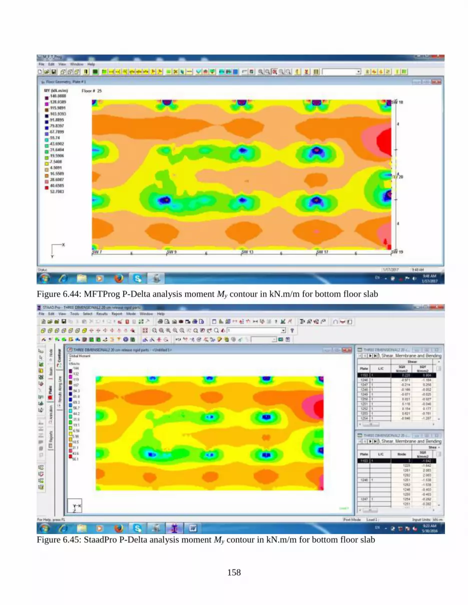
158

Figure 6.44: MFTProg P-Delta analysis moment My contour in kN.m/m for bottom floor slab

Figure 6.45: StaadPro P-Delta analysis moment My contour in kN.m/m for bottom floor slab

159

6.4.1.1 Effect of Finite Element Formulation Accuracy

The differences in the results of the different programs models may be due to the

following factors:

1- The differences in the finite element formulation accuracy of the different programs,

which affect the floor rotational-translational stiffness, and accordingly the building

deformations and stresses.

2- The small deformations in the floor slab of the exact models due to the induced in-

plane stresses, compared with the non-deformable rigid diaphragm of the proposed

model. These deformations proofed to be negligible, as the differences in the twist

rotations of the different models were not much affected by releasing the torsional

stiffness of the vertical members, (Figures 6.32 and 6.33).

In order to examine the effects of the finite element formulation accuracy on the results

of the different models, a special subroutine was created and implemented in the

developed program. The subroutine was designed to calculate the floor rotational-

translational stiffness from StaadPro one floor model. Therefore it enabled MFTProg to

use the Finite elements formulation of StaadPro program. By using this subroutine, the

floor stiffness of StaadPro was borrowed and used in the proposed method instead of the

embedded one.

The subroutine has been created using the capabilities of OpenStaad, the Application

Programming Interface (API), of StaadPro package, and executed by constructing a one

floor StaadPro model supported by fully enforced supports in the locations of the

columns and walls. A unit rotation or translation was exerted in each support in the

directions of the different DOFs, and the corresponding reactions in all supports were

retrieved and arranged systematically to construct the rotational-translational stiffness of

the floor. Comparison of the results of the proposed model including the borrowed floor,

with the results obtained using StaadPro2004 exact model, show zero or very small

differences, as shown in Tables 6.34 to 6.36. Comparisons of the moment My contour in

the bottom floor using MFTProg with borrowed StaadPro floor and Full StaadPro2014

model for both linear and second order P-Delta analyses are also plotted in Figures 6.46

to 6.49.

160

Table 6.34: Displacements and rotation in the top floor level (mm, rad), (3D Frame),

(Borrowed StaadPro Floor):

Table 6.35: Maximum bending moment in U-Shaped Core (kN.m), (3D Frame),



MFTProg 44106.59 50074.39

StaadPro2004 44108.82 50071.03

%Diff. -0.01 0.01

Table 6.36: Maximum bending moment in Edge Shear Wall (kN.m), (3D Frame),



MFTProg 13467.59 16571.60

StaadPro2004 13431.23 16541.75

%Diff. 0.27 0.18

Package Linear Second order (P-Delta)

Trans. & Rot. Y-Dir Axial Twist Y-Dir Axial Twist

MFTProg 331.02 36.04 0.0130 415.09 37.60 0.0189

StaadPro2004 331.20 36.04 0.0130 415.61 37.60 0.0189

%Diff. -0.05 0.00 0.00 -0.13 0.00 0.00

161

Figure 6.46: MFTProg+StaadPro one floor model moment My contour for bottom floor slab

Figure 6.47: StaadPro (Full model) moment My contour for bottom floor slab

162

Figure 6.48: MFTProg + StaadPro one floor model P-Delta analysis moment My for bottom slab

Figure 6.49: StaadPro (Full model) P-Delta analysis moment My contour for bottom slab

163

6.4.1.2 Comparison of Numbers of Unknowns

The floor slab idealized by 48 x 24 finite elements with 20 vertical members (columns

and walls) shown in Figure 6.30, was used to compare the proposed method with the

conventional matrix methods of analysis. The total number of unknowns for a building

with same floor and of total N floors is:

(a) Conventional matrix methods (6 DOFs/joint):

S1 = [(49×25×N+20) ×6]

(b) Proposed Method:

The unknowns in the proposed method are composed of two parts:

1-Coupled unknowns for one floor with 3 DOFs/joint, solved simultaneously and used to

obtain the floors level stiffness.

2-Two Rotations plus one axial translation for each column/wall at all levels including

the supports level. The unknowns solved separately, each (20x3) unknowns per each

level.

S2 = [49×25×3] + [20×3] . (N+1)

Note: coupled unknowns are in square brackets [ ].

For N= 150 floors: S1= 1,102,620 Coupled unknowns and, S2 = 12,735 unknowns

(partially coupled), Ratio = S1/S2 = 86 times.

6.4.1.3 Analysis of a hypothetical 150 floors Building using MFTProg

To evaluate the program running time, the floor, Figure 6.30, was used in a 150 floors

hypothetical building, but with slab thickness of 0.25 m, and all floors height = 3.0 m.

The building members are of elasticity, E = 40x106 kN/m2 and Poisson's ratio, v = 0.2

The section properties of the vertical elements are:

All Columns: 1.00 m x 1.00 m

All shear walls are of thicknesses 0.5 m.

The building is subjected to lateral loads (F = 1.0 kN).

The problem was solved for elastic linear analysis using MFTProg. The elapsed running

time was 83 seconds only. The displacement and twist rotation of the floors at the

location of column#10, the bending moment and the shear force diagrams for the U-

Shaped core and the edge shear wall are shown in Figures 6.50 to 6.56 and Tables 6.37 to

6.39. The global deformed shape of the building is shown in Figure 6.57.

164

Figure 6.50: 150 Floors Building, Bending Moment Diagram for U-Shaped Core (kN.m).

Figure 6.51: 150 Floors Building, Shear Force Diagram for U-Shaped Core (kN).

165

Figure 6.52: 150 Floors Building, Bending Moment Diagram for Edge shear wall (kN.m).

Figure 6.53: 150 Floors Building, Shear Force Diagram for Edge shear wall (kN).

166

Figure 6.54: 150 Floors Building, Displacements in y-direction (m).

Figure 6.55: 150 Floors Building, Axial Displacements in column #10 (m).

167

Figure 6.56: 150 Floors Building, Floors Twist Rotations in radians.

Figure 6.57: Perspective view for the deformed shape of the 150 Floors Building.

168

Table 6.37: Displacements and rotation in the top floor level (mm, rad), (150 Floor

model):

Table 6.38: Maximum bending moment (kN.m) and Shear Force (kN), in U-Shaped Core,

(150 Floor model):

Package Shear Moment

MFTProg 80.973(*) 3290.189

(*) Maximum value: at level 149.

Table 6.39: Maximum bending moment (kN.m) and Shear Force (kN), in Edge Shear

Wall, (150 Floor model):

Package Shear Moment

MFTProg 32.313(*) 578.573

(*) Maximum value: at level 149.

6.4.1.4 Running time and numbers of unknowns for N numbers of floors

The same floor, Figure 6.30, was analyzed for different assumed numbers of floors.

The elapsed running time and the comparison of the numbers of unknowns are shown in

Figures 6.58 and 6.59 respectively, and in Tables 6.40 and 6.41.

Table 6.40: Elapsed running time in seconds using MFTProg

No. of Floors Running time (sec.)

150 82.9

300 119.7

600 193.4

900 267.4

1000 292.1

Package Y-Dir Axial (col.#10) Twist

MFTProg 135.873 1.958 0.000528

169

MFTProg Running Time

0

50

100

150

200

250

300

350

0 200 400 600 800 1000 1200

No. of Floors

Ru

nn

ing

tim

e (

sec.)

Figure 6.58: Elapsed running time in seconds using MFTProg

Table 6.41: Comparison of numbers of unknowns

No. of Floors Conventional (S1) MFTProg (S2) Ratio= S1/S2

150 1,102,620 12,735 86.6

300 2,205,120 21,735 101.5

600 4,410,120 39,735 111.0

900 6,615,120 57,735 114.6

1000 7,350,120 63,735 115.3

170

Comparison of Number of Unknowns

0.0E+00

1.0E+06

2.0E+06

3.0E+06

4.0E+06

5.0E+06

6.0E+06

7.0E+06

8.0E+06

0 200 400 600 800 1000 1200

No. of Floors

Nu

mb

er

of

Un

kn

ow

ns

Conventional

MFTProg

Figure 6.59: Comparisons of the numbers of unknowns

From the above presentation, it is clearly seen that the analysis of super tall buildings

can be easily performed and with very low cost by using MFTProg.

These comparisons have been carried out by using computer: Dell Inspiron, Intel(R)

Core™i3-2350M CPU @ 2.30 GHz, 4.00 GB of RAM.

171

6.4.2 Buckling Analysis of the 3D building model

The buckling analysis for the 3D building model was carried out, using the proposed

bisection method and by using the eign solution (Vianello method). Comparisons

between the results assuming linear shape, cubic shape and Euler buckling with stability

functions were also studied.

Table 6.42 shows the results of the fundamental buckling factor calculated using

MFTProgV2 with the proposed bisection subroutine. The results are compared with those

obtained using StaadProV8i and ETABS 2013.

Table 6.42: Minimum Buckling factor using the different packages

Buckling Analysis Package Minimum buckling factor

MFTProgV2, Linear Shape 4.181

MFTProgV2, Cubic Shape 4.165

MFTProgV2, Euler stability functions 4.157

StaadProV8i 4.152

ETABS2013 (thin) 3.983

ETABS2013 (thick) 4.731

The analysis was also carried out using the eign solution. The Vianello method was

carried out for the first six buckling modes for the linear shape function. The results

obtained were compared with those obtained from ETABS2013 thin and thick plate. The

results are shown in Table 6.43, and the buckling mode shapes are shown in Figure 6.60.

Table 6.43: Buckling factors of the first six modes using the different packages

Buckling Analysis Mode1 Mode2 Mode3 Mode4 Mode5 Mode6

MFTProgV2 (Linear) 4.373 5.167 8.184 9.883 9.945 13.832

ETABS2013 (thin) 3.983 4.832 7.724 9.129 9.375 12.943

ETABS2013 (thick) 4.731 5.815 8.739 9.991 10.673 14.060

In Table 6.42, the MFTProgV2 Euler buckling analysis give very close result to the

result of StaadProV8i, the percentage difference is 0.11%.

The MFTProgV2 (Euler stability functions) is exact solution and gives less buckling

factor compared to the cubic and the linear shapes buckling values.

172

In Table 6.42, the results of MFTProgV2 linear deformed shape show greater values of

the buckling factors than the cubic shape values and the results of the cubic shape show

greater values than the Euler buckling values. The reason for these cases was already

explained in the 2D model case. In Table 6.43, the buckling factors for all modes of

MFTProgV2 (Linear), fall in-between the values of ETABS (thin) and ETABS (thick)

and show good agreement.

Figure 6.60: Buckling modes 1 to 6

The following cross check for the proposed bisection subroutine was carried out:

173

The calculated buckling factor found for the cubic shape was (4.165), which is greater

than 1. Because the starting buckling factor is 1, this is means that the load factor is

increased until the correct buckling factor is reached. The total load was multiplied by 10

to keep the applied load greater than the building buckling load. By running MFTProgV2

for the new applied loads, the load factor starts with 1.0 and then decreases until the

correct buckling factor is reached. The calculated new buckling factor obtained was

(0.41656) which is match with the value (4.165/10), and proves the efficiency of the

proposed subroutine.

6.4.3 Dynamic analysis for the 3D model

The dynamic analysis was performed for the 3D model. The response spectra method

was performed first with linear effects and then the spectra was also performed including

the P-Delta second order effects. The time history was then performed including the

linear and also the second order effects.

The lumped mass and the mass polar inertia for the 3D model in any floor level were

calculated as follows:

Figure 6.61: Mass polar inertia for 4 lumped masses, (Proposal 1)

174

Figure 6.62: Mass polar inertia for uniformly distributed mass, (Proposal 2)

In the three dimensional model, the total mass in any floor was calculated for the two

proposals shown in Figures 6.61 and 6.62, as follows:

mxtot = mytot = 18*12*24/9.80665 = 528.62 kg

The lumped masses in the x and y directions and the polar inertia for the 4 lumped

masses in Proposal 1, were calculated as follows:

For, a = b = 5.5 m:

The lumped masses in the x and y directions were:

mxlumped = mylumped = 18*12*24/4/9.80665 = 132.155 kg

and the polar inertia was:

mro = 18*(12*24/4)*5.52*8/9.80665 = 31981.56 kg.m2

The polar inertia for the uniform mass in Proposal 2, was calculated as follows:

mro = 18*(12*243/12+24*123/12)/9.80665

= 31717.25 kg.m2

The lumped masses in Proposal 1, is an approximation used in some packages to

simplify and accelerate the eign solution. The relative percentage difference between the

two proposals is:

= (31981.56-31717.25)/31717.25*100

= 0.83 %

The masses and moments of inertias for all floors of the two illustrated proposals of the

3D building model are shown in Table 6.44.

175

Table 6.44: Floor Masses and Moments of Inertia of the 3D Building (Mass in kg and

Moment of Inertia in kg.m2)

Floor Mass, mxtot

(kg)

Mass, mytot

(kg)

Inertia mro

(4 lumped

masses)(kg.m2)

Inertia mro

(distributed)

(kg.m2)

1 to 25 528.62 528.62 31981.56 31717.25

Table 6.45: Comparisons of the first nine Natural frequencies of 3D Building

(cycles/second)

Mode StaadProV8i1(%Diff) MFTProgV21

(%Diff) MFTProgV22

ETABS(thin)2

(%Diff)

ETABS(thick)2

(%Diff)

1 0.141 (0) 0.141 (0) 0.141 0.136 (-3.55) 0.149 (5.67)

2 0.151 (0.67) 0.15 (0) 0.150 0.145 (-3.33) 0.159 (6)

3 0.213 (0.95) 0.21 (-0.47) 0.211 0.206 (-2.37) 0.218 (3.32)

4 0.494 (2.49) 0.481 (-0.21) 0.482 0.468 (-2.9) 0.505 (4.77)

5 0.532 (3.3) 0.515 (0) 0.515 0.503 (-2.33) 0.541 (5.05)

6 0.828 (3.5) 0.798 (-0.25) 0.800 0.789 (-1.38) 0.822 (2.75)

7 1.033 (3.3) 0.998 (-0.2) 1.000 0.979 (-2.1) 1.031 (3.1)

8 1.112 (4.02) 1.069 (0) 1.069 1.052 (-1.59) 1.106 (3.46)

9 1.785 (4.32) 1.708 (-0.18) 1.711 1.683 (-1.64) 1.743 (1.87)

The superscripts 1 and 2 refer to Proposal 1 and Proposal 2 respectively.

As shown in table 6.45, the difference is very small and therefore, the two proposed

cases were assumed identical. In all the comparisons StaadPro2004 and StaadProV8i

packages used proposal 1 and all the other packages include MFTProgV2 are using the

Proposal 2. The comparisons between the natural frequencies obtained using

MFTProgV22 and the different analysis packages, show good agreement.

6.4.4 Response spectra Analysis for the 3D model

The response spectra analysis was performed for the 3D model. As for the 2D model,

the excited response acceleration was taken from the UBC design code with assumed

damping ratio of 5%. The considered modal combination methods used in this analysis

were the SRSS and the CQC methods. Comparisons of the lateral displacement, the base

176

shear and the base overturning moment for MFTProgV2 and the different packages are

shown in Tables 6.50 to 6.53.

Table 6.46: Comparison of the modal masses participating ratios in x-direction:

Mode MFTProgV2 StaadProV8i(%Diff) ETABS(thin)

(%Diff)

ETABS(thick)

(%Diff)

1 0 0 0 0

2 73.147 73.48 (0.46) 72.864 (-0.39) 73.488 (0.47)

3 0 0 0 0

4 0 0 0 0

5 12.983 13.13 (1.13) 13.105 (0.94) 12.845 (-1.06)

6 0 0 0 0

7 0 0 0 0

8 5.405 5.28 (-2.31) 5.463 (1.07) 5.292 (-2.09)

9 0 0 0 0

Table 6.47: Comparison of the accumulated modal masses participating ratios in x-

direction:


(%Diff)

ETABS(thick)

(%Diff)

1 0 0 0 0

2 73.147 73.477 (0.45) 72.864 (-0.39) 73.488 (0.47)

3 73.147 73.477 (0.45) 72.864 (-0.39) 73.488 (0.47)

4 73.147 73.477 (0.45) 72.864 (-0.39) 73.488 (0.47)

5 86.13 86.609 (0.56) 85.969 (-0.19) 86.334 (0.24)

6 86.13 86.609 (0.56) 85.969 (-0.19) 86.334 (0.24)

7 86.13 86.609 (0.56) 85.969 (-0.19) 86.334 (0.24)

8 91.535 91.891 (0.39) 91.432 (-0.11) 91.626 (0.1)

9 91.535 91.891 (0.39) 91.432 (-0.11) 91.626 (0.1)

177

Table 6.48: Comparison of the modal masses participating ratios in y-direction:


(%Diff)

ETABS(thick)

(%Diff)

1 48.499 49.21 (1.47) 47.754 (-1.54) 48.675 (0.36)

2 0 0 0 0

3 22.148 21.74 (-1.84) 22.679 (2.4) 22.081 (-0.3)

4 8.095 8.22 (1.54) 8.048 (-0.58) 8.045 (-0.62)

5 0 0 0 0

6 6.994 7.01 (0.23) 7.115 (1.73) 7.052 (0.83)

7 3.062 3.05 (-0.39) 3.087 (0.82) 2.982 (-2.61)

8 0 0 0 0

9 2.231 2.09 (-6.32) 2.097 (-6.01) 1.935 (-13.27)

Table 6.49: Comparison of the accumulated modal masses participating ratios in y-

direction:


(%Diff)

ETABS(thick)

(%Diff)

1 48.499 49.212 (1.47) 47.754 (-1.54) 48.675 (0.36)

2 48.499 49.212 (1.47) 47.754 (-1.54) 48.675 (0.36)

3 70.646 70.952 (0.43) 70.433 (-0.3) 70.756 (0.16)

4 78.742 79.167 (0.54) 78.481 (-0.33) 78.801 (0.07)

5 78.742 79.167 (0.54) 78.481 (-0.33) 78.801 (0.07)

6 85.736 86.18 (0.52) 85.596 (-0.16) 85.853 (0.14)

7 88.799 89.228 (0.48) 88.682 (-0.13) 88.835 (0.04)

8 88.799 89.228 (0.48) 88.682 (-0.13) 88.835 (0.04)

9 91.029 91.321 (0.32) 90.78 (-0.27) 90.77 (-0.28)

The comparisons between the modal masse participating ratios and their accumulations

in the x and y directions using the proposed method, StaadProV8i and ETABS thin and

thick plates show a very small differences, as shown in Tables.

178


Tables 6.50 and 6.51 show the lateral displacement response at the top floor of the


response spectra analysis in y-direction using MFTProgV2 and the other packages for

proposal 1 and 2 respectively.


Proposal 1

Response MFTProg

V2

StaadProV8i

(%Diff)

ETABS(thin)

(%Diff)

ETABS(thick)

(%Diff)

SAP2000

(thin)

(%Diff)

SAP2000

(thick)

(%Diff)

ALL SRSS 0.46146 0.463041

(0.34)

0.474174

(2.76)

0.436886

(-5.33)

0.46662

(1.12)

0.43056

(-6.7)

ALL CQC 0.468434 0.470168

(0.37)

0.481418

(2.77)

0.445146

(-4.97)

0.47289

(0.95)

0.43792

(-6.51)


Proposal 2

Response MFTProg

V2

StaadProV8i

(%Diff)

ETABS(thin)

(%Diff)

ETABS(thick

) (%Diff)

SAP2000

(thin)

(%Diff)

SAP2000

(thick)

(%Diff)

ALL SRSS 0.44462 0.463041

(4.14)

0.474174

(6.65)

0.436886

(-1.74)

0.46662

(4.95)

0.43056

(-3.16)

ALL CQC 0.45571 0.470168

(3.17)

0.481418

(5.64)

0.445146

(-2.32)

0.47289

(3.77)

0.43792

(-3.9)






proposal 1. For the SRSS, the closest results to MFTProgV2 result is obtained from

StaadProV8i which is of 0.34 % difference, and for the CQC, the closest result is also

obtained from StaadProV8i which is of 0.37 % difference.


proposal 2. For the SRSS, the closest result to MFTProgV2 result is obtained from

ETABS (thick) which is of -1.74 % difference, and for the CQC, the closest result is also

obtained from ETABS (thick) which is of -2.32 % difference.

179





in y-direction using the proposed method and the other packages.

Table 6.52: Comparisons of the Response Spectrum Base Shear force (kN):

Mode MFTProg

V2

StaadProV

8i(%Diff)

ETABS

(thin)

(%Diff)

ETABS

(thick)

(%Diff)

SAP2000

(thin)

(%Diff)

SAP2000

(thick)

(%Diff)

1 2305.62 2333.19

(1.2)

2191.59

(-4.95)

2454.66

(6.46) - -

2 0 0 0 0 - -

3 1572.23 1564.77

(-0.47)

1580.22

(0.51)

1622.56

(3.2) - -

4 1314.65 1370.1

(4.22)

1280.28

(-2.61)

1367.77

(4.04) - -

5 0 0 0 0 - -

6 1884.42 1958.62

(3.94)

1897.17

(0.68)

1951.38

(3.55) - -

7 1032.11 1067.59

(3.44)

1020.79

(-1.1)

1041.16

(0.88) - -

8 0 0 0 0 - -

9 1286.22 1267.96

(-1.42)

1213.97

(-5.62)

1150.01

(-10.59) - -

ALL

SRSS

3973.26

4043.87

(1.78)

3879.98

(-2.35)

4091.85

(2.98)

3871.973

(-2.55)

4092.598

(3.00)

ALL

CQC

4168.21

4228.81

(1.45)

4073.39

(-2.27)

4298.29

(3.12)

4140.134

(-0.67)

4346.12

(4.27)

Table 6.52 gives the total shear forces at the base of the building structure in y-direction.

For the SRSS, the closest result to MFTProgV2 is obtained from StaadProV8i which is of

1.78 % difference, and for the CQC, the closest result is obtained from SAP2000V16

(thin) which is of -0.67 % difference.

180




analysis in y-direction using the proposed method and the other packages.

Table 6.53: Comparisons of the Response Spectrum Base Overturning Moment (kN.m):

Mode MFTProgV2

StaadProV8

i(%Diff)

ETABS

(thin)

(%Diff)

ETABS

(thick)

(%Diff)

SAP2000

(thin)

(%Diff)

SAP2000

(thick)

(%Diff)

1 -145366.59 -146700.9

(0.92)

-138438

(-4.77)

-154679

(6.41) - -

2 0 0 0 0 - -

3 -102515.18

-102117.5

(-0.39)

-103282

(0.75)

-106080

(3.48) - -

4 -9221.24

-9097.35

(-1.34)

-9143.45

(-0.84)

-8846.03

(-4.07) - -

5 0 0 0 0 - -

6 -22382.84

-21819.11

(-2.52)

-22445

(0.28)

-22616.1

(1.04) - -

7 -12626.8

-13035.05

(3.23)

-12716.9

(0.71)

-12760.3

(1.06) - -

8 0 0 0 0 - -

9 -8686.49

-8260.81

(-4.9)

-7851.48

(-9.61)

-6884.64

(-20.74) - -

ALL

SRSS

180171.37

180958.9

(0.44)

175051.4

(-2.84)

189680.1

(5.28)

160393.43

(-10.98)

173203.79

(-3.87)

ALL

CQC

185357.62

185888.57

(0.29)

179882.5

(-2.95)

195681.3

(5.57)

164315.07

(-11.35)

178126.49

(-3.9)

Table 6.53 gives the total overturning moment at the base of the building structure

about x-axis. For the SRSS, the closest result to MFTProgV2 result is obtained from

StaadProV8i which is of 0.44 % difference, and for the CQC, the closest result is


181

6.4.5 P-Delta response spectra analysis

The P-Delta second order analysis was incorporated in the dynamic analysis using the

direct iteration method and the inverse iteration method (Stodola concept), and using the

cubic-displacement shape. As for the linear dynamic analysis, the natural first nine

natural frequencies together with the corresponding mode shapes were computed.

Table 6.54: Comparisons of the first nine P-Delta natural frequencies (cycle/second):

Mode StaadProV8i1

(%Diff)

MFTProgV21

(%Diff) MFTProgV22

ETABS(thin)2

(%Diff)

ETABS(thick)2

(%Diff)

1 0.124 (0) 0.124 (0) 0.124 0.118 (-4.84) 0.133 (7.26)

2 0.136 (0.74) 0.135 (0) 0.135 0.129 (-4.44) 0.145 (7.41)

3 0.202 (1) 0.199 (-0.5) 0.200 0.195 (-2.5) 0.206 (3)

4 0.466 (2.64) 0.453 (-0.22) 0.454 0.438 (-3.52) 0.477 (5.07)

5 0.507 (3.47) 0.49 (0) 0.490 0.476 (-2.86) 0.516 (5.31)

6 0.812 (3.7) 0.782 (-0.13) 0.783 0.771 (-1.53) 0.803 (2.55)

7 0.996 (3.43) 0.961 (-0.21) 0.963 0.941 (-2.28) 0.994 (3.22)

8 1.08 (4.25) 1.036 (0) 1.036 1.016 (-1.93) 1.072 (3.47)

9 1.745 (4.62) 1.665 (-0.18) 1.668 1.637 (-1.86) 1.697 (1.74)

The superscripts 1 and 2 refer to Proposal 1 and Proposal 2 respectively.

As shown in Table 6.54, the comparison between the natural frequencies using

MFTProgV2 and the different analysis packages shows good agreement.

182

Table 6.55: Comparison of the P-Delta modal masses participating ratios in x-direction:


(%Diff)

ETABS(thick)

(%Diff)

1 0 0 0 0

2 73.313 73.65 (0.46) 73.025 (-0.39) 73.656 (0.47)

3 0 0 0 0

4 0 0 0 0

5 12.802 12.96 (1.23) 12.925 (0.96) 12.673 (-1.01)

6 0 0 0 0

7 0 0 0 0

8 5.398 5.26 (-2.56) 5.458 (1.11) 5.28 (-2.19)

9 0 0 0 0

Table 6.56: Comparison of the accumulated P-Delta modal masses participating ratios in

x-direction:


(%Diff)

ETABS(thick)

(%Diff)

1 0 0 0 0

2 73.313 73.647 (0.46) 73.025 (-0.39) 73.656 (0.47)

3 73.313 73.647 (0.46) 73.025 (-0.39) 73.656 (0.47)

4 73.313 73.647 (0.46) 73.025 (-0.39) 73.656 (0.47)

5 86.116 86.611 (0.57) 85.95 (-0.19) 86.328 (0.25)

6 86.116 86.611 (0.57) 85.95 (-0.19) 86.328 (0.25)

7 86.116 86.611 (0.57) 85.95 (-0.19) 86.328 (0.25)

8 91.513 91.875 (0.4) 91.408 (-0.11) 91.608 (0.1)

9 91.513 91.875 (0.4) 91.408 (-0.11) 91.608 (0.1)

183

Table 6.57: Comparison of the P-Delta modal masses participating ratios in y-direction:


(%Diff)

ETABS(thick)

(%Diff)

1 47.881 48.63 (1.56) 46.719 (-2.43) 47.473 (-0.85)

2 0 0 0 0

3 22.784 22.34 (-1.95) 23.733 (4.17) 23.312 (2.32)

4 7.979 8.12 (1.77) 7.917 (-0.78) 7.91 (-0.86)

5 0 0 0 0

6 7.04 7.04 (0) 7.173 (1.89) 7.118 (1.11)

7 3.082 3.07 (-0.39) 3.105 (0.75) 2.991 (-2.95)

8 0 0 0 0

9 2.016 1.86 (-7.74) 1.954 (-3.08) 1.813 (-10.07)

Table 6.58: Comparison of the accumulated P-Delta modal masses participating ratios in

y-direction:


(%Diff)

ETABS(thick)

(%Diff)

1 47.881 48.633 (1.57) 46.719 (-2.43) 47.473 (-0.85)

2 47.881 48.633 (1.57) 46.719 (-2.43) 47.473 (-0.85)

3 70.666 70.972 (0.43) 70.452 (-0.3) 70.785 (0.17)

4 78.645 79.091 (0.57) 78.369 (-0.35) 78.695 (0.06)

5 78.645 79.091 (0.57) 78.369 (-0.35) 78.695 (0.06)

6 85.685 86.135 (0.53) 85.542 (-0.17) 85.813 (0.15)

7 88.767 89.204 (0.49) 88.647 (-0.14) 88.804 (0.04)

8 88.767 89.204 (0.49) 88.647 (-0.14) 88.804 (0.04)

9 90.783 91.064 (0.31) 90.601 (-0.2) 90.616 (-0.18)

The comparisons between the modal mass participating ratios and their accumulations in

the x and y directions using MFTProgV2, StaadProV8i and ETABS thin and thick plates

show very small differences, as shown in Tables 6.55 to 6.58.

184




response spectra analysis in y-direction using MFTProgV2 and the other packages for

proposals 1 and 2 respectively.


Proposal 1

Response MFTProgV2 StaadProV8i(%Diff) ETABS(thin)

(%Diff)

ETABS(thick)

(%Diff)

ALL SRSS 0.510297 0.512864 (0.5) 0.527419 (3.36) 0.474082 (-7.1)

ALL CQC 0.515622 0.518369 (0.53) 0.532894 (3.35) 0.480804 (-6.75)


Proposal 2

Response MFTProgV2 StaadProV8i(%Diff) ETABS(thin)

(%Diff)

ETABS(thick)

(%Diff)

ALL SRSS 0.49683 0.512864 (3.23) 0.527419 (6.16) 0.474082 (-4.58)

ALL CQC 0.50595 0.518369 (2.45) 0.532894 (5.33) 0.480804 (-4.97)





Table 6.59 gives the total lateral displacement at the top floor of the building structure

for proposal 1. For the SRSS, the closest results to MFTProgV2 result is obtained from



Table 6.60 gives the total lateral displacement at the top floor of the building structure

for proposal 2. For the SRSS, the closest result to MFTProgV2 is obtained from




185




in y-direction using MFTProgV2 and the other packages.

Table 6.61.: Comparisons of the Response Spectrum P-Delta Base Shear force (kN):


(%Diff)

ETABS(thick)

(%Diff)

1 2005.87 2030.48 (1.23) 1860.32 (-7.26) 2130.75 (6.23)

2 0 0 0 0

3 1533.88 1523.34 (-0.69) 1559.43 (1.67) 1625.35 (5.96)

4 1234.13 1287.42 (4.32) 1183.01 (-4.14) 1280.35 (3.75)

5 0 0 0 0

6 1868.76 1933.81 (3.48) 1873.58 (0.26) 1935.15 (3.55)

7 1005.49 1030.98 (2.54) 991.11 (-1.43) 1002.33 (-0.31)

8 0 0 0 0

9 1160.49 1107.51 (-4.57) 1107.15 (-4.6) 1057.38 (-8.89)

ALL SRSS 3708.017 3758.99 (1.37) 3607.01 (-2.72) 3832.58 (3.36)

ALL CQC 3892.608 3936.16 (1.12) 3791.92 (-2.59) 4024.72 (3.39)

Table 6.61 gives the total shear forces at the base of the building structure in y-

direction. For the SRSS, the closest result to MFTProgV2 result is obtained from






analysis in y-direction using MFTProgV2 and the other packages.

186

Table 6.62: Comparisons of the Response Spectrum P-Delta Base Overturning Moment:


(%Diff)

ETABS(thick)

(%Diff)

1 126256.2 127431.8 (0.93) 117317 (-7.08) 134041 (6.17)

2 0 0 0 0

3 100202.5 99637.42 (-0.56) 102035 (1.83) 106332 (6.12)

4 8114.251 8042.87 (-0.88) 7886.82 (-2.8) 7688.28 (-5.25)

5 0 0 0 0

6 22219.54 21529.95 (-3.1) 22205.3 (-0.06) 22448.3 (1.03)

7 12864.73 13152.42 (2.24) 12925.8 (0.47) 12812.3 (-0.41)

8 0 0 0 0

9 7775.739 7106.545 (-8.61) 7166.84 (-7.83) 6317.45 (-18.75)

ALL SRSS 163605.25 164067.6 (0.28) 157949.6 (-3.46) 173322.3 (5.94)

ALL CQC 167270.83 167570.2 (0.18) 161333.1 (-3.55) 177753 (6.27)

Table 6.62 gives the total overturning moment (in kN.m), at the base of the building

structure about x-axis. For the SRSS, the closest result to MFTProgV2 result is obtained

from StaadProV8i which is of 0.28 % difference, and for the CQC, the closest result is

also obtained from StaadProV8i which is of 0.18 % difference.

6.4.6 Time History Analysis for the 3D model

Time history analysis was performed for the 3D model. The natural frequencies and

the corresponding mode shapes calculated in the previous section and used in the

response spectra method were used with the El Centro earthquake time history

acceleration records assumed applied at the base of the building. The assumed damping

ratio is 5%. Comparisons of the lateral displacement at the top floor level, the base shear

and the base overturning moment for MFTProgV2 and the different packages are

presented.


Figures 6.63 to 6.68 give the graphs for the lateral displacement history at the top floor

of the building model due to El Centro earthquake, obtained by time history analysis in y-

direction using MFTProgV2 and the other packages. The minimum and the maximum

responses are shown in Table 6.63.

187


MFTProgV2


StaadProV8i

188

Figure 6.65: History of displacement in y-direction at the top floor level using ETABS

(thin plate)

Figure 6.66: History of displacement in y-direction at the top floor level using ETABS

(thick plate)

189


SAP2000V16 (thin plate)


SAP2000V16 (thick plate).

190

Table 6.63: Minimum and maximum displacements at the top floor (mm):

Response MFTProgV2

StaadProV8i

(%Diff)

ETABS(thin)

(%Diff)

ETABS(thick)

(%Diff)

SAP(thin)

(%Diff)

SAP(thick)

(%Diff)

Minimum -390.3

-398

(1.97)

-388.5

(-0.46)

-381.9

(-2.15)

-403.9

(3.48)

-355.8

(-8.84)

At time 12.3 12.2 12.7 18.1 12.7 3.86

Maximum 399.3

394

(-1.33)

411

(2.93)

382.8

(-4.13)

413.4

(3.53)

360.2

(-9.79)

At time 15.64 15.6 15.84 15 15.76 1.492




obtained from ETABS (thin) which is of -0.46 % difference, and for the maximum

response, the closest result is obtained from StaadProV8i which is of -1.33 % difference.


Figures 6.69 to 6.73 give the graphs for the resultant shear force history in kN at the base

of the building obtained by time history analysis in y-direction using MFTProgV2 and the

other packages. The minimum and the maximum responses are shown in Table

6.64.

Figure 6.69: History of base Shear in y-direction using MFTProgV2

191

Figure 6.70: History of base Shear in y-direction using ETABS (thin plate)

Figure 6.71: History of base Shear in y-direction using ETABS (thick plate)

192

Figure 6.72: History of base Shear in y-direction using SAP2000V16 (thin plate)

Figure 6.73: History of base Shear in y-direction using SAP2000V16 (thick plate)

193

Table 6.64: Minimum and maximum base shear (kN):

Response MFTProgV2

StaadProV8i(

%Diff)

ETABS(thin)

(%Diff)

ETABS(thick)

(%Diff)

SAP(thin)

(%Diff)

SAP(thick)

(%Diff)

Minimum -4640 N.A

-4055

(-12.61)

-5152

(11.03)

-3478

(-25.04)

-4276

(-7.84)

At time 6.14 N.A 6.18 6.1 4.44 6.04

Maximum 4931.9

5190.859

(5.25)

4758

(-3.53)

4982

(1.02)

5187

(5.17)

5259

(6.63)

At time 3 2.951389 3.02 2.98 2.98 2.96


Table 6.64 gives the maximum and minimum total shear forces at the base of the building


MFTProgV2 result is obtained from SAP2000V16 (thick) which is of -7.84 % difference,

and for the maximum response, the closest result is obtained from ETABS (thick) which

is of 1.02 % difference.


Figures 6.74 to 6.78 give the graphs for the resultant overturning moment history in kN.m

at the base of the building about x-axis obtained by time history analysis in y-direction

using MFTProgV2 and the other packages. The minimum and the maximum responses

are shown in Table 6.65.

Figure 6.74: History of base overturning moment about x-direction using MFTProgV2

194

Figure 6.75: History of base overturning moment about x-direction using ETABS (thin

plate)

Figure 6.76: History of base overturning moment about x-direction using ETABS (thick

plate)

195

Figure 6.77: History of base overturning moment about x-direction using SAP2000V16

(thin plate)

Figure 6.78: History of base overturning moment about x-direction using SAP2000V16

(thick plate)

196

Table 6.65: Minimum and maximum base overturning moment (kN.m):

Response MFTProgV2

StaadProV8i

(%Diff)

ETABS(thin)

(%Diff)

ETABS(thick)

(%Diff)

SAP(thin)

(%Diff)

SAP(thick)

(%Diff)

Minimum -154288.9 N.A.

-143900

(-6.73)

-177500

(15.04)

-151700

(-1.68)

-176500

(14.4)

At time 3.96 N.A. 3.94 3.94 3.94 3.92

Maximum 162225.3 N.A.

150500

(-7.23)

163500

(0.79)

134100

(-17.34)

146000

(-10)

At time 15.48 N.A. 15.5 15.44 15.46 15.08




obtained from SAP2000V16(thin) which is of -1.68 % difference, and for the maximum

response, the closest result is obtained from ETABS (thick) which is of 0.79 %

difference.

6.4.7 P-Delta time history analysis for the 3D model

The P-Delta second order analysis for the 3D model was incorporated in the dynamic

time history analysis using the direct iteration method and the inverse iteration method

(Stodola concept) and using the cubic-displacement shape. As for the linear dynamic

analysis, the first nine natural frequencies together with the corresponding mode shapes

were computed and used in the analysis.


Figures 6.79 to 6.82 give the graphs for the lateral displacement at the top floor of the

building model obtained by time history analysis in y-direction using MFTProgV2 and

the other packages. The minimum and the maximum responses are shown in Table 6.66.

197

Figure 6.79: History of P-Delta displacement in y-direction at the top floor level using

MFTProgV2


StaadProV8i

198


ETABS (thin plate)


ETABS (thick plate)

199

Table 6.66: Minimum and maximum P-Delta displacements at the top floor (mm):

Response MFTProgV2

StaadProV8i

(%Diff)

ETABS(thin)

(%Diff)

ETABS(thick)

(%Diff)

Minimum -404.6 -410 (1.33) -363.4 (-10.18) -390.9 (-3.39)

At time 12.84 12.8 12.92 12.7

Maximum 380.411 368 (-3.26) 314.6 (-17.3) 399.4 (4.99)

At time 16.26 16.2 16.38 15.92




obtained from StaadProV8i which is of 1.33 % difference, and for the maximum

response, the closest result is also obtained from StaadProV8i which is of -3.26 %

difference.


Figures 6.83 to 6.85 give the graphs for the resultant shear force history in kN at the base

of the building obtained by time history analysis in y-direction using MFTProgV2 and the

other packages. The minimum and the maximum responses are shown in Table 6.67.

Figure 6.83: History of P-Delta base Shear history in y-direction using MFTProgV2

200

Figure 6.84: History of P-Delta base Shear in y-direction using ETABS (thin plate)

Figure 6.85: History of P-Delta base Shear in y-direction using ETABS (thick plate)

201

Table 6.67: Minimum and maximum P-Delta base shear (kN):

Response MFTProgV2

StaadProV8i

(%Diff)

ETABS(thin)

(%Diff)

ETABS(thick)

(%Diff)

Minimum -3398.81 N.A. -3135 (-7.76) -4205 (23.72)

At time 6.2 N.A. 1.62 6.14

Maximum 4547.363 4888.243 (7.5) 4432 (-2.54) 4713 (3.64)

At time 3.02 2.973611 3.04 3


Table 6.67 gives the maximum and minimum total shear forces at the base of the building


MFTProgV2 result is obtained from ETABS (thin) which is of -7.76 % difference, and

for the maximum response, the closest result is also obtained from ETABS (thin) which

is of -2.54 % difference.


Figures 6.86 to 6.88 give the graphs for the resultant overturning moment history in kN.m

at the base of the building about x-axis obtained by time history analysis in y-direction

using MFTProgV2 and the other packages. The minimum and the maximum responses

are shown in Table 6.68.


MFTProgV2

202

Figure 6.87: History of P-Delta base overturning moment about x-direction using ETABS

(thin plate)

Figure 6.88: History of P-Delta base overturning moment about x-direction using ETABS

(thick plate)

203

Table 6.68: Minimum and maximum P-Delta base overturning moment (kN.m):

Response MFTProgV2

StaadProV8i

(%Diff)

ETABS(thin)

(%Diff)

ETABS(thick)

(%Diff)

Minimum -149895 N.A. -137600 (-8.2) -166500 (11.08)

At time 28.78 N.A. 28.88 3.96

Maximum 117620.2 N.A. 118200 (0.49) 165200 (40.45)

At time 15.6 N.A. 26.2 15.54




obtained from ETABS (thin) which is of -8.2 % difference, and for the maximum

response, the closest result is also obtained from ETABS (thin) which is of 0.49 %

difference.

204

CHAPTER SEVEN

Conclusions and Recommendations

7.1 General Conclusions

1. A comprehensive review and study of the linear and nonlinear, static and dynamic, and

stability analyses of tall buildings have been carried out. The study clearly shows the

need for and importance of simplifying these complicated analyses methods.

2. Based on the moment transformation method (MT), the moment-force transformation

method (MFT) has been developed to incorporate the axial deformations in the vertical

members so as to be used in the analysis of super-tall buildings such as the tube and

outrigger structures.

3. The moment-force transformation method (MFT) has been further developed to solve

instability problems, nonlinear static, and linear and nonlinear dynamic analysis of tall

buildings using the response spectra and the time-history analysis methods.

4. The computer program MFTProg has been developed and used in the static linear 2D

and 3D analysis of tall buildings neglecting and/or including the axial deformations in the

vertical members.

5. The computer program MFTProgV2 has been developed and used in the buckling

analysis and the static and dynamic, linear and nonlinear 2D and 3D analysis of tall

buildings.

6. The developed programs allow the use of different plates to represent slabs of different

shapes or thicknesses in one model.

7. The accuracy of the results obtained using the developed programs were verified by

comparison with results from known finite elements solvers.

8. The saving in computer storage and computing time provided by the proposed

programs allow rapid re-analysis of the building to be accomplished in the preliminary

analysis and design stages, and in the cases of repeated analysis types such as in the

buckling and vibration problems.

9. The ease in data preparation and interpretation of final results, compared with finite

element packages, is one of the main advantages of the method.

10. The simplicity in programming the method is an added advantage.

205

7.2 Results Conclusion

1- The maximum differences in the results obtained using MFTProg to analyze a two

floor one-bay portal frame subjected to both vertical and horizontal loads compared with

the published results were found to be -0.12 % for the bending moments and 0.13 % for

the horizontal support reaction (neglecting shear deformations).

2- The maximum difference in the obtained moments results using MFTProg in the

analysis of a two floor two-bay portal frame with setback subjected to both vertical and

horizontal loads compared with the published results was found to be -0.11 %

(considering shear deformations).

3- A fifteen floors multistory square building including four shear walls and subjected to

unsymmetrical lateral loads was analyzed using MFTProg. The closest differences in the

maximum shear forces and the bending moments and the displacements and rotations

measured in the upper left corner of the building plan compared with the results obtained

using the structural analysis packages ETABS and STAADPro2004, were as follows:

4.88 % for displacement in x-direction.

2.98 % for displacement in y-direction.

-2.34 % floor twist rotation.

The percentage difference of 7.85 % in the shear force was noticed in shear wall #4 with

a difference of -0.2 % in bending moment. Shear wall #4 resists very small values of

stresses compared with its section.

The differences in results of the other walls were:

0.19 % and -0.28 % for shear force and bending moment respectively, in shear wall #1.

-0.62 % and 1.93 % for shear force and bending moment respectively, in shear wall #2.

-0.92 % and 1.84 % for shear force and bending moment respectively, in shear wall #3.

4- As case study 1, the analysis of a 2D frame of 15 floors Building model subjected to

vertical and lateral loads was carried out. The results obtained using MFTProgV2 were

compared with those obtained using StaadPro2004, StaadProV8i, SAP200V16 and

ETABS, for different analysis types as follows:

A-Static Linear and second order Analysis

In Static Linear and second order Analysis of the building model the maximum

differences in the results with exact results were as follows:

206

0.27 % for lateral displacement at the top floor level in linear analysis.

0.07 % for axial displacement at the top floor level in linear analysis.

-0.66 % for maximum bending moment in the lower level of the columns in linear

analysis.

0.26 % for lateral displacement at the top floor level in P-Delta analysis.

0.14 % for axial displacement at the top floor level in P-Delta analysis.

-0.60 % for maximum bending moment in the lower level of the columns in P-Delta

analysis.

B-Buckling Analysis of the building model

The MFTProgV2 cubic shape results show very close critical buckling result compared to

the values of StaadPro2014 (Stardyne advanced Engine), with a percentage difference of

-0.03%.

C-Dynamic analysis of the building model

In a linear and second order dynamic analysis of the model, comparison between the

natural frequencies, the mode shapes and the mass participation ratios show almost

identical results.

D-Response Spectra Linear Analysis:

The lateral displacement results obtained by performing response spectrum analysis were

calculated. For the SRSS method, very close results were obtained by the proposed

method and SAP2000V16 with a maximum of 0.0006 % difference. For the CQC

method, very close results were obtained from the proposed method and ETABS with a

maximum of 0.0047 % difference.

The base shear results obtained by performing response spectrum analysis were

calculated. For the SRSS method, the closest results to the proposed method results were

obtained from SAP2000V16 with a maximum of 0.43 % difference, and for the CQC

method, the closest results to the proposed method were obtained from StaadProV8i with

0.24 % maximum difference.

The base overturning moment results obtained by performing response spectrum analysis

were calculated. For the SRSS method, the closest results to the proposed method results

were obtained from ETABS with -0.01 % maximum difference, and for the CQC method,

207

the closest results to the proposed method results were obtained from ETABS which is of

-0.01 % difference.

E-Response Spectra P-Delta Analysis

The lateral displacement results obtained by performing response spectrum P-Delta

analysis were calculated. For the SRSS method, the closest results to the proposed

method results were obtained from ETABS with a maximum of -0.00119 % difference,

and for the CQC method, the closest results to the proposed method were obtained from

ETABS with -0.00149 % maximum difference.

The base shear results obtained by performing response spectrum P-Delta analysis were


obtained from ETABS with a maximum of 0.03 % difference, and for the CQC method,

the closest results to the proposed method results were obtained from ETABS with 0.03%

maximum difference.

For the SRSS method, the closest results for the base overturning moment results

obtained by performing response spectrum P-Delta analysis to the proposed method

results were obtained from ETABS with 0.01 % maximum difference, and for the CQC

method, the closest results to the proposed method results were obtained from ETABS

with 0.01 % maximum difference.

F-Time History Linear Analysis

The top floor lateral displacement results obtained by performing the time history

analysis using the proposed method were calculated and compared with the results

obtained from different analysis packages. The results variation curves were similar and

show very close agreement. For the minimum response, the closest results to the

proposed method results were obtained from ETABS with 0.01 % maximum difference,

and for the maximum response, the closest results to the proposed method results were

obtained also from ETABS with a maximum of 0.03 % difference.

The base shear results obtained by performing the time history analysis were calculated.

The results variation curves were similar and show a very close agreement. For the

minimum response, the closest results to the proposed method results were obtained from

ETABS and SAP2000V16 with a maximum of 0.02 % difference, and for the maximum

208

response, the closest results to the proposed method results were obtained from ETABS


The base overturning moment results obtained by performing the time history analysis

were calculated. The results variation curves were similar and show a very close

agreement. For the minimum response, the closest results to the proposed method were

obtained from ETABS with a maximum of 0.01 % difference, and for the maximum



G-Time History P-Delta Analysis

The top floor lateral displacement results obtained by performing the time history P-Delta




proposed method results were obtained from ETABS with 0.03 % maximum difference,

and for the maximum response, the closest results to the proposed method results were

obtained also from ETABS with a maximum of 0.03 % difference.

The base shear results obtained by performing the time history P-Delta analysis were

calculated. The results variation curves were similar and show a very close agreement.

For the minimum response, the closest results to the proposed method results were




The base overturning moment results obtained by performing the time history P-Delta

analysis were calculated. The results variation curves were similar and show a very close





5- As case study 2, the analysis of a 3D frame of 25 floors Building model subjected to

vertical and wind loads was carried out. The results obtained using MFTProgV2 were

209

compared with those obtained using StaadPro2004, StaadProV8i, SAP200V16 and

ETABS, for different analysis types as follows:

A-Static Linear and second order Analysis

In Static Linear and second order Analysis of the building model the maximum

differences in the results with exact results in the building center (column#10), were as

follows:

-3.5 % for lateral displacement in y-direction in linear analysis.

0.47 % for axial deformation in linear analysis.

-7.69 % floor twist rotation, in linear analysis.

-4.63 % for lateral displacement in y-direction in P-Delta analysis.

0.35% for axial deformation in P-Delta analysis.

-8.99 % floor twist rotation in P-Delta analysis.

-1.37 % for maximum bending moment in U-Shaped Core, in linear analysis.

-1.77 % for maximum bending moment in U-Shaped Core, in P-Delta analysis.

-2.24 % for maximum bending moment in Edge Shear Wall, in linear analysis.

-3.36 % for maximum bending moment in Edge Shear Wall, in P-Delta analysis.

In additional discussion of the results, an alternative analysis has been carried out using a

borrowed StaadPro Floor stiffness. The analysis yields the following results:

Displacements and rotation in the top floor level in the building center (column #10):

-0.05 % for lateral displacement in y-direction in linear analysis.

0.00 % for axial deformation in linear analysis.

0.00 % floor twist rotation, in linear analysis.

-0.13 % for lateral displacement in y-direction in P-Delta analysis.

0.00 % for axial deformation in P-Delta analysis.

-0.00 % floor twist rotation in P-Delta analysis.

-0.01 % for maximum bending moment in U-Shaped Core, in linear analysis.

0.01 % for maximum bending moment in U-Shaped Core, in P-Delta analysis.

0.27 % for maximum bending moment in Edge Shear Wall, in linear analysis.

0.18 % for maximum bending moment in Edge Shear Wall, in P-Delta analysis.

The elapsed running time by MFTProg used in solving a 150 floor model was 83 seconds

only. Comparison between the number of unknowns using MFTProg and the

210

conventional matrix methods for the 150 floors model showed that there were 1,102,620

coupled unknowns in the case of conventional matrix methods compared to 12,735

partially coupled unknowns when using MFTProg which is a ratio of 86 times.

B-Buckling Analysis of the building model

The MFTProgV2 Euler functions results show very close critical buckling result

compared to the value of StaadProV8i, with a percentage difference of 0.11%.

C-Dynamic analysis of the building model

In a linear and second order dynamic analysis of the model, comparison between the

natural frequencies and the mass participation ratios in the two directions show very close

agreement.

D-Response Spectra Linear Analysis:

The lateral displacement results obtained by performing response spectrum analysis were

calculated. For the SRSS method, very close results were obtained by the proposed

method and StaadProV8i with a maximum of 0.34 % difference. For the CQC method,

very close results were obtained from the proposed method and StaadProV8i with a

maximum of 0.37 % difference.

The base shear results obtained by performing response spectrum analysis were


obtained from StaadProV8i with a maximum of 1.78 % difference, and for the CQC

method, the closest results to the proposed method were obtained from SAP2000V16

with -0.67 % maximum difference.

The base overturning moment results obtained by performing response spectrum analysis

were calculated. For the SRSS method, the closest results to the proposed method results

were obtained from StaadProV8i with 0.44 % maximum difference, and for the CQC

method, the closest results to the proposed method results were obtained from

StaadProV8i which is of 0.29 % difference.

E-Response Spectra P-Delta Analysis

The lateral displacement results obtained by performing response spectrum P-Delta

analysis were calculated. For the SRSS method, the closest results to the proposed

method results were obtained from StaadProV8i with a maximum of 0.50 % difference,

211

and for the CQC method, the closest results to the proposed method were obtained from

StaadProV8i with 0.53 % maximum difference.

The base shear results obtained by performing response spectrum P-Delta analysis were


obtained from StaadProV8i with a maximum of 1.37 % difference, and for the CQC

method, the closest results to the proposed method results were obtained from


For the SRSS method, the closest results for the base overturning moment results

obtained by performing response spectrum P-Delta analysis to the proposed method

results were obtained from StaadProV8i with 0.28 % maximum difference, and for the

CQC method, the closest results to the proposed method results were obtained from


F-Time History Linear Analysis

The top floor lateral displacement results obtained by performing the time history




proposed method results were obtained from ETABS (thin) with -0.46 % maximum

difference, and for the maximum response, the closest results to the proposed method

results were obtained also from StaadProV8i with a maximum of -1.33 % difference.

The base shear results obtained by performing the time history analysis were calculated.

The results variation curves were similar and show a very close agreement. For the

minimum response, the closest results to the proposed method results were obtained from

SAP2000V16 (thick) with a maximum of -7.84 % difference, and for the maximum


(thick) with 1.02 % maximum difference.

The base overturning moment results obtained by performing the time history analysis

were calculated. The results variation curves were similar and show a very close


obtained from SAP2000V16 (thin) with a maximum of -1.68 % difference, and for the

212

maximum response, the closest results to the proposed method results were obtained from

ETABS (thick) with 0.79 % maximum difference.

G-Time History P-Delta Analysis

The top floor lateral displacement results obtained by performing the time history P-Delta




proposed method results were obtained from StaadProV8i with 1.33 % maximum

difference, and for the maximum response, the closest results to the proposed method

results were obtained also from StaadProV8i with a maximum of -3.26 % difference.

The base shear results obtained by performing the time history P-Delta analysis were

calculated. The results variation curves were similar and show a very close agreement.

For the minimum response, the closest results to the proposed method results were

obtained from ETABS (thin) with a maximum of -7.76 % difference, and for the

maximum response, the closest results to the proposed method results were obtained from

ETABS (thin) with -2.54 % maximum difference.

The base overturning moment results obtained by performing the time history P-Delta

analysis were calculated. The results variation curves were similar and show a very close


obtained from ETABS (thin) with a maximum of -8.2 % difference, and for the maximum

response, the closest results to the proposed method results were also obtained from

ETABS (thin) with 0.49 % maximum difference.

7.3 Recommendations Drawn from Results Obtained

It is recommended to use the nonlinear version of the moment-force transformation

method in the static and dynamic, linear and nonlinear analysis of tall buildings together

with the buckling analysis for the following:

1. Static and dynamic, linear and nonlinear analyses of super-tall buildings in which the

axial deformation of the vertical members is dominant and should be considered.

2. Static and dynamic, linear and nonlinear analyses of ordinary portal frames and shear

wall-frame interaction problem.

213

3. Static and dynamic, linear and nonlinear 2D analysis of shear walls with openings, by

considering the beams stiffness including also the infinite stiffness of the rigid parts of

the walls.

4. Static and dynamic, linear and nonlinear three dimensional analyses of buildings with

vertical members irregularly arranged and oriented in the building plan and with different

sections in the different levels and with different floor heights.

5. Elastic instability analysis of 2D and 3D tall buildings.

7.4 Recommendations for Future Research

For future research it is recommended to:

1- Develop method to take into account elastic-plastic analysis incorporating both elastic

instability and plastic yielding in members.

2- Further develop the program to incorporate the elastic-plastic responses, by

formulating the stiffness and the carryover moment matrices using the various Hysteresis

models, e.g. elasto-plastic, bilinear and curvilinear models.

3. For more simplification of the problem solution, columns or vertical members not

contributing to the resistance of the lateral loads can be included in the floor rotation

stiffness and the problem solution will include only the walls or the vertical members that

actually contribute to the resistance of the lateral loads.

4. For more optimization of the analysis, the stiffness of the floor can be calculated by

using simplified rules instead of calculations by finite elements, e.g. for slabs with beams

construction considering the properties of the equivalent T and L sections.

5. For flexible supports, the rotational and axial stiffness of the supports may also be

incorporated in the analysis.

6. Columns shortening in reinforced concrete and composite tall buildings due to time-

dependant creep, shrinkage and elastic modulus could be also analyzed.

214

References

1- ACI 318-14 (2014), American Concrete Institute, “Building Code Requirements for

Structural Concrete”, Farmington Hills, Mich.

2- Abdur Rahman, Fancy Saiada Fuadi and Bobby Shamim Ara, (2012), “Analysis of

drift due to wind loads and earthquake loads on tall structures by programming

language c”, International Journal of Scientific & Engineering Research, Volume 3,

Issue 6, June-2012, ISSN 2229-5518, IJSER © 2012, http://www .ijser.org

3- Akis Tolga (2004),”Lateral Load Analysis of Shear Wall-Frame Structures”, PhD

Thesis Dissertation, The Graduate School of Natural And Applied Sciences of The

Middle East Technical University.

4- Albrecht James T., Chan Cy P., And Edelman Alan, (2009) “Sturm Sequences and

Random Eigenvalue Distributions”, Foundations of Computational mathematics,

Volume 9 Issue 4, June 2009, Pages 461-483.

5- Ali Mir M. and Moon Kyoung Sun, (2007), “Structural Developments in Tall

Buildings Current Trends and Future Prospects” , Structures Division, School of

Architecture, University of Illinois at Urbana-Champaign, USA, Architectural Science

Review Volume 50.3, pp 205-223.

6- Almeida J.P., Correia A.A. and Pinho R., (2008), “Development of a 3d Force-

Based Beam Element for Nonlinear Analysis of RC Frame Structures Considering

Flexure-Shear Coupling”, The 14th World Conference on Earthquake Engineering

October 12-17, 2008, Beijing, China.

7- Aly, Aly Mousaad, Zasso Alberto and Resta Ferruccio, “Tall Buildings under

Multidirectional Winds: Response Prediction and Reduction”, “Wind Tunnels and

Experimental Fluid Dynamics Research”, Published online 27, July, 2011.

215

8- American National Standards Institute, ANSI-A58.1. (1982), “Minimum Design

Loads for Buildings and Other Structures”.

9- Applied Technology Council, May 2007, “Proceedings of Workshop on Tall

Building Seismic Design and Analysis Issues”.

10- BS 8110 (1997), British Standards Institution. Structural use of Concrete, Part 1:

“Code of Practice for Design and Construction”, London.

11- BS 8110 (1997), British Standards Institution. Structural use of Concrete, Part 2:

“Code of Practice for Special Circumstances”, London.

12- Barbi Jernej, (2012), “Exact Corotational Linear FEM Stiffness Matrix”,

Technical Report, University of Southern California.

13- Bathe Klaus Jurgen And Wilson Edward L., (1973), “Solution Methods for

Eigenvalue Problems in Structural Mechanics”, International Journal For Numerical

Methods In Engineering, Vol. 6, 21 3-226 (1973), University Of California, Berkeley,

California, U.S.A.

14- Bayati Z., Mahdikhani M. and Rahaei A., (2008), “Optimized Use of Multi-

Outriggers System to Stiffen Tall Buildings”, The 14th World Conference on

Earthquake Engineering, October 12-17, 2008, Beijing, China.

15- Berkley, “STAADProVi8, Structural Analysis and Design Software”.

16- Bozdogan K.B. and Ozturk D., (2010), “Vibration Analysis of Asymmetric shear

wall structures using the transfer matrix method”, Iranian Journal of Science and

Technology, Transaction B, Engineering, Vol. 34, No B1,PP 1-14.

17- Bozdogan Kanat Burak and Ozturk Duygu, (2010), “An approximate method for

lateral stability analysis of Wall-frame buildings including shear deformations of

216

walls”, Sadhana Vol. 35, Part 3, June 2010, pp. 241–253.Indian Academy of Sciences,

Department of Civil Engineering, Ege University, Izmir, 35040 Turkey, e-mail:

[email protected]

18- Bozdogan Kanat Burak, (2011), “A method for lateral static and dynamic analyses

of wall-frame buildings using one dimensional finite element”, Scientific Research and

Essays Vol. 6(3), pp. 616-626, 4 February, 2011, Available online at

http://www.academicjournals.org/SRE , DOI: 10.5897/SRE10.863, ISSN 1992-2248,

2011 Academic Journals.

19- Bozdogan Kanat Burak, (2011), “Free Vibration Analysis of Wall-Frame

Structures by Differential Quadrature Method”, International Journal of Engineering

and Applied Sciences (IJEAS), Vol.3, Issue 4(2011)7-20.

20- CSI Analysis Reference Manual for SAP2000, ETABS, and SAFE, Computers and

Structures, Inc., Berkeley, California, USA, June 2008.

21- Causevic Mehmed and Mitrovic Sasa, (2010), “Comparison between non-linear

dynamic and static seismic analysis of structures according to European and US

provisions”, Bull Earthquake Eng DOI 10.1007/s10518-010-9199-1.

22- Chan Gordon, (2005), “Nonlinear Analysis of Multistory Structures Using

NONLIN”, MSc. Thesis dissertation, Faculty of the Virginia Polytechnic Institute and

State University.

23- Chandurkar P. P. and Pajgade P. S., (2013), “Seismic Analysis of RCC Building

with and Without Shear Wall”, International Journal of Modern Engineering Research

(IJMER), www.ijmer.com Vol. 3, Issue. 3, May - June 2013 pp-1805-1810 ISSN:

2249-6645

24- Chen Xinzhong and Kareem Ahsan, (2005), “Coupled Dynamic Analysis and

Equivalent Static Wind Loads on Buildings with Three-Dimensional Modes”,

217

JOURNAL OF STRUCTURAL ENGINEERING © ASCE.

25- Chopra Anil, K., (2000), solution manual “Dynamics of Structures - Theory and

Applications to Earthquake Engineering”, Third Edition.

26- Christenson Richard E., (2001), “Semi-active Control of Civil Structures for

Natural Hazard Mitigation: Analytical And Experimental Studies”, Ph.D. Dissertation,

(December 2001), The Graduate School of the University of Notre Dame.

27- Clough Ray W. and Penzien Joseph, (1995), “Dynamics of Structures”, Third

Edition, Computers & Structures, Inc. University Ave. Berkeley, CA 94704, USA.

28- Coates R. C., Coutie M. G., and Kong F. K., (1990), “Structural Analysis”, Third

Edition, Chapman and Hall.

29- Coull Alex, Mohammed and T. H., (1983), “Simplified analysis of lateral load

distribution in structures consisting of frames, coupled shear walls, and cores”, The

Structural Engineer, Volume 61B/No. 1/March 1983.

30- Coull Alexander, ASCE F., Bose Bishwanath, and Ahmed Abdulla Khogali,

(1982), “A Simplified analysis of bundled tube structures”, Journal of the structural

division, Proceedings of the American Society of Civil Engineers, © ASCE, Vol. 108,

No. ST5, May 1982.

31- Dagnew Agerneh K., Bitsuamalk Girma T. and Merrick Ryan, (2009)

“Computational evaluation of wind pressures on tall buildings”, 11th Americas

Conference on Wind Engineering, San Juan, Puerto Rico, June 22-26 2009.

32- Deierlein Gregory G., Reinhorn Andrei M. and Willford Michael R., (2010),

“Nonlinear Structural Analysis for Seismic Design, A Guide for Practicing

Engineers”, NEHRP Seismic Design Technical Brief No. 4, NIST GCR 10-917-5,

October 2010.

218

33- Ding Kun, Su Ningfen, Chen Xuefeng, Zhou Ying and Lu Xilin, “Finite Element

Analysis and Experimental Verification of A Setback Tall Building”, 3rd International

Conference on Advances in Experimental Structural Engineering, Oct 15-16, San

Francisco, USA, State Key Laboratory of Disaster Reduction in Civil Engineering,

Tongji University, Shanghai, China.

34- Diotallevi Pier Paolo, Landi Luca and Cardinetti Filippo, (2008), “A Fibre Beam

Column Element for Modelling the Flexureshear Interaction in the Non-Linear

Analysis of RC Structures”, The 14th World Conference on Earthquake Engineering,

October 12-17, 2008, Beijing, China.

35- Dobson Richard and Arnott Kenny, (2002), “A Brief Overview of 2nd Order (or P-

Delta) Analysis”. ,Technical Director for FASTRAK, 3D+ and TEDDS, CSC (UK) Ltd

and Product Manager for S-Frame, CSC (UK) Ltd.

36- Elcentro Earthquake May 18 -1940, North-South Component,

www.vibrationdata.com/elcentro.htm

37- EN 1992-1-1 (2004) (English): Eurocode 2: Design of concrete structures - Part 1-

1: General rules and rules for buildings.

38- Eads Laura, Miranda Eduardo, Krawinkler Helmut and Lignos Dimitrios G., “An

efficient method for estimating the collapse risk of structures in seismic regions”,

EARTHQUAKE ENGINEERING & STRUCTURAL DYNAMICS 2013; 42:25–41,

Published online 30 March 2012 in Wiley Online Library (wileyonlinelibrary.com).

39- Eleni Chatzi, (2012),” The Finite Element Method for the Analysis of Non-Linear

and Dynamic Systems and Dynamic Systems”, Swiss federal institute of technology

Zurich,Lecture 3 - 9 October, 2012.

40- Fukuwa N., Tobita J., Mori M., Koide E. and Hanai T.,(2008), “Development of

219

Vibration Experiment Education Materials for Structural and Soil Dynamics”, The

14th World Conference on Earthquake Engineering October 12-17, 2008, Beijing,

China.

41- Gavin Henri P.,(2012),” Structural Element Stiffness Matrices and Mass

Matrices”, Duke University, Department of Civil and Environmental Engineering,

CEE 541. Structural Dynamics, Fall 2012.

42- Gavin Henri, (2012), “Geometric Stiffness Effects in 2D and 3D Frames”, Duke

University,Department of Civil and Environmental Engineering, CEE 421L, Matrix

Structural Analysis.

43- Ghali A. and Neville A. M. (1978), “Structural Analysis – A Unified Classical and

Matrix Approach”, Second edition, New York, Chapman and Hall Ltd.

44- Ghali A., Neville A. M., and Brown T. G., (2009), “Structural Analysis – A

Unified Classical and Matrix Approach”, Sixth edition, Taylor and Francis, London

and New York.

45- Giovanni Rebecchi, (2009), “Beam Axial Load Identification Using One Vibration

Mode Shape”, PhD Thesis dissertation, Universita Degli Studi Di Ferrara.

46- Gu Ming, (2009), “Study on Wind Loads and Responses of Tall Buildings and

Structures”, The 7th Asia-Pacific Conference on Wind Engineering, November 8-12,

2009,Taipei, Taiwan

47- Guner Serhan and Vecchio Frank J., (2012), “Simplified Method for Nonlinear

Dynamic Analysis of Shear-Critical Frames”, ACI STRUCTURAL JOURNAL

TECHNICAL PAPER, ACI Structural Journal, V. 109, No. 5, September-October

2012.

48- Gustafsson David and Hehir Joseph, (2005), “Stability of Tall Buildings”, M.Sc.

220

Dissertation, Department of Civil and Environmental Engineering, Division of

Structural Engineering, Chalmers University of Technology, Göteborg, Sweden.

49- Hagen Garrett Richard, (2012), “Performance-Based Analysis of a Reinforced

Concrete Shear Wall Building”, M.Sc. Dissertation, Faculty of California Polytechnic

State University, San Luis Obispo, June 2012.

50- Hutt Carlos Molina, (2013), “Non-Linear Time History Analysis of Tall Steel

Moment Frame Buildings in LS-DYNA”, 9th European LS-DYNA Conference 2013.

51- Ibrahim M. S. (2013), “Analysis of Tall Buildings using The Moment

Transformation Method”, M.Sc. Thesis dissertation, Sudan University of Science and

Technology.

52- Ibrahim M. S. and Mohamed A. E. (2013), “Analysis of Shear Wall Structures

using the Moment Transformation Method”, Journal of Science and Technology -

Engineering and Computer Sciences, Vol. 14, No. 3, June 2013.

53- Ikago Kohju, (2012), “Dynamic Instability in High-Rise Steel Structures Subjected

to Strong Ground Motions”, 14th U.S. - Japan Workshop on improvement of Structural

Design and Construction Practices, 3-5 December 2012. , Tohoku University, Japan.

54- Jaeger G. Mufti A. A. and Mamet J. C. (1973), “The Structural Analysis of Tall

Buildings Having Irregularly Positioned Shear Walls.” ,Build. Sci. Vol. 8, pp. 11-22.

Pergamon Press.

55- Jahanshahi M. R., Rahgozar R.,and Malekinejad M., (2012), “ A Simple Approach

to Static Analysis of Tall Buildings with a Combined Tube-in-tube and Outrigger-belt

Truss System Subjected to Lateral Loading”, IJE TRANSACTIONS A: Basics Vol. 25,

No. 3, 289-299,International Journal of Engineering.

56- Jameel Mohammed, Saiful Islam A.B.M., Hussain Raja Rizwan, Khaleel M. and

221

Zaheer M. M., (2012), “The Structural Design of Tall and Special Buildings, Optimum

structural modeling for tall buildings”, Published online in Wiley Online Library

(wileyonlinelibrary.com/journal/tal). DOI: 10.1002/tal.1004

57- Jayachandran P. (2003), “Design of Tall Buildings Preliminary Design and

Optimization”, Ph.D, M.ASCE., Worcester Polytechnic Institute, Worcester,

Massachusetts, 01609, USA, [email protected], International Conference on Tall

Buildings and Industrial Structures, PSG College of Technology, Coimbatore, India,

Keynote Lecture.

58- Jónsson Örvar,(2014), “The dynamic behavior of multi-story reinforced concrete

building in a seismic and windy environment”, M.Sc. Dissertation, The School of

Science and Engineering at Reykjavík University, January 2014.

59- Kouhia Reijo, (1990), “Simple Finite Elements for Nonlinear Analysis of Framed

Structures”, Rakenteiden Mekaniikka Vol. 23, No 4 1990, s. 3 – 49

60- Lebofsky Sonia, (2013), “Numerically Generated Tangent Stiffness Matrices for

Geometrically Non-Linear Structures”, M.Sc. Dissertation, University of Washington.

61- Lee Kang-Kun, Guan Hong and Loo Yew-Chaye (2000), “Simplified Analysis of

Shear-Lag in Framed-Tube Structures with Multiple Internal Tubes”. Griffith

University Gold Coast Campus, Australia.

62- Leung A. Y. T. (1983), “Low Cost Analysis of Building Frames for Lateral Loads

“Computers & Structures Vol. 11. No. 4. pp. 475-483.

63- Leung A. Y. T. (1985), “Micro-Computer Analysis of Three-Dimensional Tall

Buildings “, Computers & Structures Vol. 21, No. 4, pp. 639-661.

64- Leung A. Y. T. and Cheung Y. K. (1981), “ Dynamic Analysis of Frames by a

Two-Level Finite Element Method “ , Journal of Sound and Vibration 74(l), l-9

222

65- Leung A. Y. T. and Wong S. C. (1988),”Local-Global Distribution Factors

Method for Tall Building Frames.”, Computer & structures Vol.29, No.3. pp. 491-502

66- Leung A. Y. T. and Zeng S. P., (1994), “Analytical Formulation of Dynamic

Stiffness”, Journal of Sound and Vibration.

67- Leung Andrew Yee-Tak (1978),” An Accurate Method of Dynamic Condensation

In Structural Analysis”, International. Journal For Numerical Methods In Engineering.

Vol. 12, 1705-1715 (1978).

68- Li B., Duffield C. F. and Hutchinson G. L., (2008),” Simplified Finite Element

Modeling of Multi-storey Buildings: The Use of Equivalent Cubes”, Electronic Journal

of Structural Engineering.

69- Li Guo-Qiang and Li Jin-Jun (2007), “ Advanced Analysis and Design of Steel

Frames “ , John Wiley & Sons, Ltd.

70- Li Q. S. and Wu J. R., (2004), “Correlation of dynamic characteristics of a super-

tall building from full-scale measurements and numerical analysis with various Finite

element models”, Earthquake Engineering and Structural Dynamics, Earthquake Engng

Struct. Dyn. 2004: 33:1311–1336 (DOI: 10.1002/eqe.405).

71- Liao W.Y., Chen W.H., Ni Y.Q. and Ko J.M., (2008), “Post-Earthquake Damage

Identification of Tall Building Structures: Experimental Verification”, The 14th World

Conference on Earthquake Engineering October 12-17, 2008, Beijing, China.

72- Lodi Sarosh H., Mohammed Aslam F., Khan Rashid A. and Gunay M. Selim,

(2011), “A Practical Guide to Nonlinear Static Analysis of Reinforced Concrete

Buildings with Masonry Infill Walls”, NED University of Engineering and

Technology, University of California, Berkeley, Supported by the Pakistan-US Science

and Technology Cooperation Program.

223

73- MacGinley T.J. and Choo B. S. (1990), “ Reinforced Concrete: Design Theory &

Examples “E & FN Spon Second edition.

74- MacLeod, Iain A. (1998), “Shear Wall-Frame Interaction a Design Aid”, Portland

cement association .1970 reprinted 1998.

75- Manicka Selvam V.K, Bindhu K.R., (2011), “Split frame method for lateral load

analysis of short frames”, International Journal of Civil and Structural Engineering,

Volume 1, No 4, 2011, Research article ISSN 0976 – 4399 835.

76- Marsono Abdul Kadir and Wee. Lee Siong, (2006), “Nonlinear Finite Element

Analysis of Reinforced Concrete Tube in Tube of Tall Buildings”, Proceedings of the

6th Asia-Pacific Structural Engineering and Construction Conference (APSEC 2006), 5

– 6 September 2006, Kuala Lumpur, Malaysia, A-161,

77- Mathisen Kjell Magne, (2012), “ Solution Methods for Nonlinear Finite Element

Analysis (NFEA)”, Department of Structural Engineering,Norwegian University of

Science and Technology, Lecture 11, Geilo Winter School.

78- Matjaž Dolšek., (2013), “Concept of Risk-Based Seismic Design of Buildings using

Methods of Nonlinear Analysis”, COMPDYN 2013 4th ECCOMAS Thematic

Conference on Computational Methods in Structural Dynamics and Earthquake

Engineering.

79- Mattacchione Angelo (1991), “Equivalent Frame Method Applied to concrete

Shear walls”, November l99l lssue of ACI Concrete International.

80- McCormac Jack and Elling Rudolf E., (1988), “Structural Analysis - A Classical

and Matrix Approach”, Harper and Row, published, 1988.

81- McHugh Peter, (2007), “Non-Linear Finite Element Analysis: Finite Element

224

Solution Schemes I & II”, European Society of Biomechanics thematic workshop on

Finite Element Modeling in Biomechanics and Mechanobiology, Department of

Mechanical and Biomedical Engineering, National Centre for Biomedical Engineering

Science, National University of Ireland, Galway.

82- Meftah Sid Ahmed, Tounsi Abdelouahed and El Abbas Adda Bedia, (2007), “A

Simplified Approach for Seismic Calculation of a Tall Building Braced by Shear Walls

And Thin-Walled Open Section Structures.” ,Science-direct.

83- Megson T. H. G., (2000), “Structural and Stress Analysis”, Butterworth-

Heinemann. A division of Reed Educational and Professional Publishing Ltd.

84- Merritt Richard George, (1953), “Effect Of Foundation Compliance on the

Earthquake Stresses In Typical Tall Buildings”, Ph.D. thesis dissertation, California

institute of technology.

85- Moghadam A.S. and Aziminejad A., ”Interaction of Torsion and P-Delta Effects in

Tall Buildings”, 13th World Conference on Earthquake Engineering, Vancouver, B.C.,

Canada,August 1-6, 2004,Paper No. 799.

86- Mora Rodrigo, Bédard Claude and Rivard Hugues,(2004), “A Framework for

Computer-Aided Conceptual Design of Building Structures”. International Conference

on Computing in Civil and Building Engineering, ICCCBE, 10, 2004.06.02-04,

Weimar, Bauhaus-Universitat.

87- NEHRP Consultants Joint Venture, (2013), “Nonlinear Analysis Research and

Development Program for Performance-Based Seismic Engineering”, Prepared for

U.S. Department of Commerce, National Institute of Standards and Technology,

Engineering Laboratory, Gaithersburg, MD 20899, A partnership of the Applied

Technology Council and the Consortium of Universities for Research in Earthquake

Engineering, December 2013.

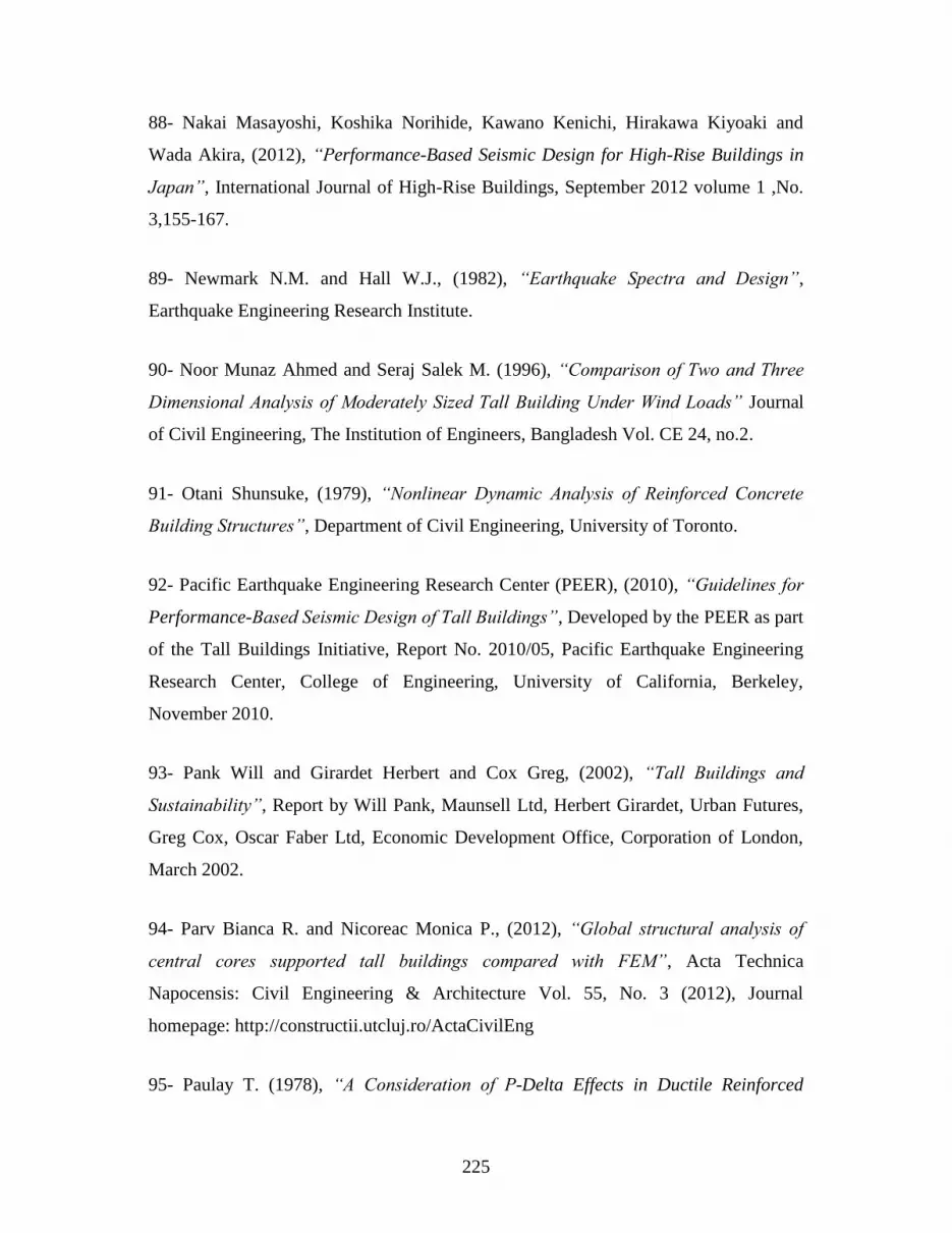
225

88- Nakai Masayoshi, Koshika Norihide, Kawano Kenichi, Hirakawa Kiyoaki and

Wada Akira, (2012), “Performance-Based Seismic Design for High-Rise Buildings in

Japan”, International Journal of High-Rise Buildings, September 2012 volume 1 ,No.

3,155-167.

89- Newmark N.M. and Hall W.J., (1982), “Earthquake Spectra and Design”,

Earthquake Engineering Research Institute.

90- Noor Munaz Ahmed and Seraj Salek M. (1996), “Comparison of Two and Three

Dimensional Analysis of Moderately Sized Tall Building Under Wind Loads” Journal

of Civil Engineering, The Institution of Engineers, Bangladesh Vol. CE 24, no.2.

91- Otani Shunsuke, (1979), “Nonlinear Dynamic Analysis of Reinforced Concrete

Building Structures”, Department of Civil Engineering, University of Toronto.

92- Pacific Earthquake Engineering Research Center (PEER), (2010), “Guidelines for

Performance-Based Seismic Design of Tall Buildings”, Developed by the PEER as part

of the Tall Buildings Initiative, Report No. 2010/05, Pacific Earthquake Engineering

Research Center, College of Engineering, University of California, Berkeley,

November 2010.

93- Pank Will and Girardet Herbert and Cox Greg, (2002), “Tall Buildings and

Sustainability”, Report by Will Pank, Maunsell Ltd, Herbert Girardet, Urban Futures,

Greg Cox, Oscar Faber Ltd, Economic Development Office, Corporation of London,

March 2002.

94- Parv Bianca R. and Nicoreac Monica P., (2012), “Global structural analysis of

central cores supported tall buildings compared with FEM”, Acta Technica

Napocensis: Civil Engineering & Architecture Vol. 55, No. 3 (2012), Journal

homepage: http://constructii.utcluj.ro/ActaCivilEng

95- Paulay T. (1978), “A Consideration of P-Delta Effects in Ductile Reinforced

226

Concrete Frames”, Bulletin of the New Zealand National Society for Earthquake

Engineering, Vol.11, No. 3, September, 1978.

96- Paulino Madison R, (2010), “Preliminary Design of Tall Buildings”, Msc Thesis

dissertation, Dept of Civil engineering, Worcester Polytechnic Institute.

97- Petrolito J. and Legge K.A., (2007) , “General Non-Linear Analysis of Frames”,

5th Australian Congress on Applied Mechanics ,ACAM 2007, 10-12 December

2007,Brisbane, Australia.

98- Research Engineer International, “STAADPro2004, Structural Analysis and Design

Software”, California.

99- Reynolds Charles E. and Steedman James C., (2008), “Reynolds’s Reinforced

Concrete Designer’s Handbook”, Eleventh edition, Taylor & Francis.

100- Rezaghasemi Hamid, (2012), “Approximate Analysis of Strength of Tehran’s Tall

Buildings Reinforced with Spandrel Frame Against Lateral Forces”, Indian J. Sci. Res.

3(2) : 25-32 , 2012.

101- Samuelsson A. and Zienkiewicz O. C., (2006), “History of the stiffness method”,

International Journal For Numerical Methods In Engineering, 67:149–157.

102- Sarkar and Manohar C.S.,(1996), “Dynamic stiffness matrix of a general cable

Element”, Archive of Applied Mechanics 66 (1996) 315-325© springer-verlag.

103- Shi, Weixing, (2000), “Shaking Table Experimental Study of Reinforced Concrete

High-Rise Building”, 12WCEE 2000.

104- Smith. Bryan Stafford and Coull. Alex. (1991), “Tall Buildings Structures:

Analysis & Design“ John Wiley & Sons ,Inc. 1991 Edition.

227

105- Swaddiwudhipong S., Lim Y. B. and Lee S. L. (1988),”An Efficient Finite Strip

Analysis of Frame-Shear Wall Tall Building”, Computers & Structures Vol. 29. No. 6,

pp. 1111-1118.

106- Takabatake Hideo,(2012), “A Simplified Analytical Method for High-Rise

Buildings”, [email protected], Department of Architecture, Kanazawa

Institute of Technology, Institute of Disaster and Environmental Science, Japan.

107- Taranath Bungale S., (2011), “Differential shortening of tall steel building

columns”, Professional Development Advertising Section-Bentley Systems, Inc.

108- Taranath, B. S. (1988), “Structural analysis and design of tall buildings” New

York, McGraw-Hill.

109- Thool Kushal P., Ashok K. Ahuja and Anupam Chakrabarti, (May 2013), “Effect

of interference on Wind loads on Tall Buildings”, Dept. of Civil Eng., Indian Institute

of Technology Roorkee, Roorkee, India., J. Acad. Indus. Res. Vol. 1(12)

110- Timoshenko, S. P. (1948), “Strength of Materials”, part II 2nd edition, van

Nostrand, New York.

111- Tuan Hiep Pham, (2008), “Seismic Design Considerations for Tall Buildings”,

M.Sc. Dissertation, (April 2008), Instituto Universitario di studi superiori Pavia.

112- UBC-97, “Uniform Building Code”, International Conference of Building

Officials, Whittier, California, 1997.

113- Urs Amit (2002), “Stability Analysis of Frame Tube Tall Buildings”, MSc Thesis

dissertation, Dept of Civil engineering, Worcester Polytechnic Institute.

114- Vafaeihosseini Ehsan, Sagheb Azadeh and Ramancharla Pradeep Kumar, (2011),

“Analysis of High-rise Building using Computational Fluid Dynamics Approach: A

228

Case Study on 38-Storey High-rise Building”, Structural Engineering World Congress,

Report No: IIIT/TR/2011/-1,Centre for Earthquake Engineering, International Institute

of Information Technology, Hyderabad - 500 032, INDIA,April 2011.

115- Ventura C.E., Brincker R., Andersen P. and Dascotte E., (2005), “FEM updating

of tall buildings using ambient vibration data”, Eurodyn 2005 C. Soize and G.I.

Schueller, Millpress ,Rotterdam.

116- Ventura C.E., Lord J.F. and Turek M.,(2005), “FEM Updating of Tall Buildings

Using Ambient Vibration Data”, Structural Dynamics EURODYN 2005: Proceedings

of 6th International Conference on Structural Dynamics, Paris, France, 4-7 September

2005.

117- Warden Brandon, Browning Joann P. and Matamoros Adolfo, (2006), “A

simplified Method to estimate nonlinear response with an approximate linear analysis

for reinforced concrete structures”, a report on research sponsored by: structural

engineering and materials laboratory, university of Kansas, SM report no. 83.

118- Williams Alan (2009), “Structural Analysis in Theory and Practice”,

International Codes Council.

119- Wilson Edward , (2000), “Three Dimensional Static and Dynamic Analysis of

Structures”, Third Edition, Computer and Structures Inc., Berkeley, California, USA

120- Wilson, E. L. and Habibullah A., (1987), “Static and Dynamic Analysis of Multi-

Story Buildings Including P-Delta Effect” Earthquake Spectra. Vol.3, No.3.

Earthquake Engineering Research Institute. May 1987.

121- Wilson, E. L., Dovey, H. H. and Habibullah. A., “ETABS V13, (2013), Three

Dimensional Analysis of Building Systems”, Computers and Structures Inc., Berkeley,

California.

229

122- Wilson, E. L., Dovey, H. H. and Habibullah. A., “ETABS, (2006), Three

Dimensional Analysis of Building Systems”, Computers and Structures Inc., Berkeley,

California.

123- Wong C. W. and Lau S. L. (1989), “Simplified Finite Element Analysis of Three-

Dimensional Tall Building Structures”, Computers & Structures Vol. 33, No. 3, pp.

821-830.

124- Yu Chih-Peng and Roesset Jose M., (2001), “Dynamic Stiffness Matrices for

Linear Members with Distributed Mass”, Tamkang Journal of Science and

Engineering, Vol. 4, No. 4, pp. 253-264

230

APPENDICES

231

Appendix A1

A Three Segments Cantilever Example

The translations and the rotations of the joint of a cantilever of unit elasticity consists of

three segments and subjected to lateral forces as shown in Figure A1.1, were obtained.

Figure A1.1: Single post example

The translations and rotations of the three free joints of the cantilever are given in

shown Tables A1.1 and A1.2. From the two tables, the translations and the rotations of

the original structure are equal to the summations of the systems (a) and (b).

Table A1.1: Displacements of the original structure

JOINT# TRANSLATION ROTATION

1 9754 940.5

2 6955 918

3 1744 792

Table A1.2: Displacements of the split systems:

System System(a) System(b) System(a) + System(b)

Joint # TRANSLATION ROTATION TRANSLATION ROTATION TRANSLATION ROTATION

1 252.25 0 9501.75 940.5 9754 940.5

2 241 0 6714 918 6955 918

3 160 0 1584 792 1744 792

232

Appendix A2

The Moment Distribution Procedure

The moment distribution procedure (ordinary or no-shear Figures A2.1 and A2.2) uses

the two loading systems (a) and (b) illustrated previously as follows. The first step in the

procedure is by obtaining from the system (a), the fixed-end moments produced from the

applied loads and from which the restraining moments at the joints are obtained, then the

balancing moments are applied in system (b), the induced carryover moments at the far

end of the members are then considered as a fixed moments and are again applied in

system (a). This procedure is repeated until the carryover moments become negligible.

Then the summations of all the resulting moments in the two systems are obtained and

represent the final end moments.

From this illustration it is seen that, the moment distribution procedure is actually

equivalent to the two systems (a) and (b) when separately analyzed and the resulting

joints moments are superimposed.

Figure A2.1: Ordinary rotational stiffness of a member

Figure A2.2: No-shear rotational stiffness with translation permitted

233

Figure A2.3: No-shear moment distribution between two members

Figure A2.4 shows the split of a continuous beam into the two loading systems (a) and

(b):

Figure A2.4: Continuous beam model

234

Appendix A3

The Moment Transformation Procedure

The moment transformation procedure (ordinary or no-shear) can be carried out by

considering the two loading systems (a) and (b) described before and also shown in

Figure A2.4. In system (a), the fixed-end moments induced from the external applied

loads and the restraining moments are obtained then in the system (b) the balancing

moment (the reverse of the restraining moment) are applied with special sequence. For

example, in joint (1) from which the transformation procedure will be carried out to joint

(2), due to the applied moment at joint (1) there will be an induced moment at joint (2).

Superimposing the two systems (a) and (b) will eliminate the moment at joint (1) and

produce the equivalent moment at joint (2), then joint (1) will be relieved and will never

be considered in the analysis again. Same procedure will be carried out to the next joint

(3) until reaching the concerned joint. The transformation will be carried out in the other

direction until also reaching the concerned joint. By releasing and balancing the fixed

moments at the concerned joint, the rotation of the joint and the final moments in the

extremities to the left and to the right of the concerned joint can be calculated using the

equivalent stiffness of the connected members. The procedure will be carried out for all

the joints of the continuous frame.

Figure A3.1: Moment transformation of continuous beam

235

The Figures A3.2 and A3.3 show the moment transformation procedure for structural

system subjected to horizontal loads and permitted to side sway at the floor levels. The

sway fixed-end moments induced in the vertical members, due to the applied horizontal

loads are shown in Figure A3.2.

The illustrated transformation procedure is in the direction from top to bottom. Figure

A3.2 shows the transformation from joint (1) to joint (2), and Figure A3.3 shows the

transformation from joint (2) to joint (3).

Figure A3.2: Moment transformation from joint 1 to 2 in a single post frame

Figure A3.3: Moment transformation from joint 2 to 3 in a single post frame

236

Appendix A4

A Three Segments Column Example

Figure A4.1: Three segments column

The axial translations of the joints are calculated using the force transformation

procedure for the shown three columns structural system, with material elasticity,

E=1000 kN/m2, Figure A4.1.

Using equations 3.34 and 3.35, the transformation factors and the axial equivalent

stiffness from top to bottom and from bottom to top, are calculated and shown in Tables

A4.1 and A4.2:

Table A4.1: Equivalent Stiffness and Transformation Factors from Top to Bottom.

Member 1 2 3

Equivalent Stiffness 0 0 0

Transformation Factors 1 1 1

Table A4.2: Equivalent Stiffness and Transformation Factors from Bottom to Top.

Member 3 2 1

Equivalent Stiffness 800 307.7 173.9

Transformation Factors 0 0.3846 0.5652

237

By using the transformation procedure illustrated in section 3.6, the axial displacements

at the joints are calculated as follows:

Displacement at joint 1:

Total force = [(60*0.3846) + 80]*0.5652+50 = 108.2586 kN

Equivalent Stiffness = (173.9+0) = 173.9 kN/m

D1= 108.2586/173.9 = 0.6225 m


Total force =50*1 + 80 + 60* 0.3846 = 153.076 kN

Equivalent Stiffness = (307.7+0) = 307.7 kN/m

D2= 153.076/307.7 = 0.4975 m


Total force =50*1 + 80*1 + 60 = 190 kN

Equivalent Stiffness = (800 +0) = 800 kN/m

D3= 190/800 = 0.2375 m

The displacement in the concerned level can also be calculated using the following

equation, Taranath (1988):

k

i

kii

iN

nin P

EA

LD

1.

Where:

N= total numbers of levels.

n= number of the concerned level.


D1= (2.5/1/1000)*(50)+(4/2/1000)*(50+80)+(5/4/1000)*(50+80+60) = 0.6225 m


D2= (4/2/1000)*(50+80)+(5/4/1000)*(50+80+60) = 0.4975 m


D3= (5/4/1000)*(50+80+60) = 0.2375 m

238

Appendix A5

Further Optimization of the Transformation Procedure

Based on the subroutines of the transformation procedure presented by Ibrahim (2013),

a new faster subroutine was developed and implemented in MFTProgV2. The new

subroutine is based on two modifications:

(1) Introducing new indexed variable to store the inverse of the equivalent stiffness of the

concerned level.

The equivalent stiffness matrix of the level is calculated as follows:

Ktot = KT+KB+KF

Where:

Ktot: the total Stiffness of the level.

KT: the equivalent stiffness of the structure part above the floor.

KB: the equivalent stiffness of the structure part below the floor.

KF: the stiffness of the floor.

This modification is very useful and optimizing the computer running time especially in

the cases of repeated analysis as in the construction of the global flexibility matrix where

the structure is solved for applied unit loads several times, and in the inverse iteration

method used in the dynamic analysis.

(2) Introducing new indexed variables used to store the fixed-end moments plus the

transformed moments during the transformation procedure in the two directions.

The indexed variable may be calculated as follows:

MD1(i)=M1(i)+FT*MDtot(i-1)

Where:

MD1(i):the resultant moment vector below level i.

M1(i):the fixed moment vector below level i.

FT*MDtot(i-1): the transformed moment from level i-1.

These indexed variables are calculated only once and may be used several times during

the program execution.

239

Appendix B

Flow Chart of the Conventional Buckling Incremental Method

Based on Figure 3.22, the following notes are made as illustrated by Coates et al (1990):

(1) The input data is very similar to that required by a stiffness analysis, the only

difference is the use of the stability functions. The preliminary data must include

an initial value for the load factor (LF), the increment to be applied to it (INC),

and the required accuracy in the final result (ACC).

(2) N is used to count the number of loading cycles and DET1, DET2, DET3 are

values of the determinant of the stiffness matrix. The axial forces in the members

of the structure are not generally known before the analysis begins, and this is

unlikely to provide much overall saving in computing time.

(3) A check on N might be inserted to limit the number of load cycles in the event of

any ill-conditioning preventing convergence.

(4) As the axial forces at each load level are initially only known approximately, a

number of solutions (counted by I ) are performed.

(5) The structure stiffness matrix is set up, but the member stiffness matrices used are

those involving the stability functions. The functions are calculated as required

using the current estimates of the axial forces.

(6) The repetition of the analysis performed at each load level should be terminated

when the terms of the stiffness matrix converge to a steady state at successive

cycles. The determinant (DET2) is used here as a convenient quantity whose

value depends on the stiffness matrix terms- if its values have reach a steady state,

it is also likely that the terms of the matrix have done so. The alternative is to

check the convergence of the individual displacements.

(7) The repeated analysis is terminated when the proportionate change in determinant

is less than 0.1%. This limit is quite arbitrary, but seems to be reasonable in

practice. The final value of determinant obtained is stored in DET3 and its sign is

used as the test of positive-definiteness.

(8) When the loading approaches the critical level, the stiffness matrix becomes

increasingly ill-conditioned and successive values of the determinant are found to

vary widely. In this case there is no virtue in continuing with repeated analyses,

240

and the chart shows their termination at I=6. If this termination is found necessary

on the first load level attempted (N=1) then obviously the initial loading is too

near the critical level for any satisfactory analysis to be performed. In this case the

analysis is stopped and must be repeated with a smaller set of loads. Otherwise

the load factor can be increased, the axial forces increased by the same ratio as a

good initial guess of their new values, and a further load level examined.

(9) When satisfactory convergence is achieved at any load level as described in Step

7 the value of the determinant obtained is compared with that from the previous

load cycle. If no sign change is found then the load factor and axial forces are

increased by one step and a new load level studied. At the first load level this

comparison is impossible, and is bypassed.

(10) If a sign change is found in Step 9, i.e. a change from positive to negative, then

the critical value of load factor has been passed. The load factor is then

decreased to its previous value, and increased again by smaller steps. If the

reduced increment is below some prescribed accuracy and great accuracy is not

warranted, then the analysis is ended.

(11) Although output is shown only at this final stage it is generally desirable to trace

the progress of the iterations by printing frequent intermediate results.

241

Appendix C

Buckling of Column Subjected to Axial Load P

Figure C.1: The condensed translational and rotational stiffnesses

The buckling load for a column subjected to axial load P, Figure C.1, is obtained. With

linear-deformed shape assumption, the stiffness matrix of the system is as follows:

[S] =

L

EI

L

EIL

EI

L

P

L

EI

46

612

2

23

Condensation of the matrix in the translation direction with the rotation of the free joint

permitted, yields:

21

1

221211

*

11 SSSSS

)4

/()6

()12

( 2

23

*

11L

EI

L

EI

L

P

L

EIS

If P is the critical buckling load, then, 0*

11 S

From which the buckling load 3

3

L

EIPCritical

Same results can be obtained by condensation of the stiffness matrix in the rotational

direction with the translation of the free joint permitted:

12

1

112122

*

22 SSSSS

)12

/()6

()4

(3

2

2

*

22L

P

L

EI

L

EI

L

EIS

For 0*

22 S , The buckling load can also be obtained as:

3

3

L

EIPCritical

242

Appendix D

StaadPro Buckling Analysis, the basic solver

In StaadPro, a simple procedure has been adopted to incorporate the calculation of the

Buckling Factor for any number of primary load cases. The buckling factor is the amount

by which all of the loadings in a load case must be factored to cause global buckling of

the structure. The procedure followed is: 1) First, the primary deflections are calculated

by linear static analysis based on the provided external loading. 2) Primary deflections

are used to calculate member axial forces and plate center membrane stresses. These

forces and stresses are used to calculate geometric stiffness terms. Both the large delta

effects and the small delta effects are calculated. These terms are the terms of the Kg

matrix which are multiplied by the estimated LF (buckling factor) and then added to the

global stiffness matrix K. For compressive cases, the Kg matrix is negative definite. If the

buckling factor is large enough, then [ [K]+LF*[Kg] ] will also be negative definite which

indicates that LF times the applied loads is greater than the loading necessary to cause

buckling. 4) STAAD starts an iterative procedure with a LF estimate of 1.0. If that LF

causes buckling, then a new, lower LF estimate is used in the next trial. If the LF does not

cause buckling, then a higher LF estimate is used. In STAAD, on the first iteration, if the

determinant of the K matrix is positive and lower than the determinant of the K+Kg

matrix, then the loads are in the wrong direction to cause buckling; and STAAD will stop

the buckling calculation for that case. 5) After a few iterations, STAAD will have the

largest LF that did not cause buckling (lower bound) and the lowest LF that did cause

buckling (upper bound). Then each trial will use a LF estimate that is halfway between

the current upper and lower bounds for LF (bisection method). 6) After the default

iteration limit is reached or the user specified iteration limit, MAXSTEPS, is reached or

when two consecutive LF estimates are within 0.1% of each other; then the iteration is

terminated. 7) Results for this load case are based on the last lower bound LF calculated.

243

Appendix E

Buckling Analysis – the advanced Solver in STAAD package

In STAAD, a second procedure has been adopted to incorporate the calculation of the

Buckling Factor for one primary load case. This procedure is an eigenvalue calculation to

get buckling factors and buckling shapes.

1) First, the primary deflections are calculated by linear static analysis based on the

provided external loading.

2) Primary deflections are used to calculate member axial forces and plate center

membrane stresses. These forces and stresses are used to calculate geometric stiffness

terms. Both the large delta effects and the small delta effects for members are calculated.

These terms are the terms of the Kg matrix.

3) An eigenvalue problem is formed. | [ K ] - LFi*[ Kg ] | = 0 There will be up to 4

buckling factors (LF) and associated buckling mode shapes calculated. LF less than 1.0

means that the load causes buckling; LF greater than 1.0 means buckling has not

occurred. If LF is negative, then the static loads are in the opposite direction of the

buckling load.

244

Appendix F

Column shortening calculations for reinforced and composite concrete

structures (Proposed future study)

This section illustrates briefly a proposal for computing column shortening using the

transformation method. The main concept of the calculations is taken from the,

Reinforced Concrete Council, Spreadsheet to EC2 Axial Column Shortening to EN 1992-

1: 2003

The proposed subroutine is based on the Euro Code, EC2 (prEN 1992-1: 2001) clauses

3.1.3 Elastic deformation (1) and (3) and Annex B (Creep and Shrinkage Strain). It works

from the roof down and assumes that time “0” equates to construction of the lowest

column. A detailed construction history is input so that time-dependent creep and

shrinkage factors may be computed. The proposed program is feed by the materials and

dimensional data. Then loads are calculated using the proposed program.

The following physical quantities are used in the proposed analysis:

A- Shortenings between Floors

These are the amounts by which individual column lifts may be reduced in length

following construction of the floor immediately above, Figure F.1 (b).

B- Floor Displacements

These are long-term net displacements of floors from the level at which they were

constructed; the particular shape of the curve being defined by effects of incremental

loading and the assumption that any shortening occurring prior to a floor's construction is

compensated for, Figure F.2 (a).

Any differential shortening between connected vertical members will generate a transfer

of vertical load. If connecting slabs or beams are stiff and/or short, such load transfer can

be substantial and in tall buildings, may even be critical at ultimate limit state.

C- Creep and shrinkage

Creep and shrinkage of the concrete depend on the ambient humidity, the dimensions of

the element and the composition of the concrete. Creep is also influenced by the maturity

of the concrete when the load is first applied and depends on the duration and magnitude

of the loading.

245

Creep and Shrinkage are time-dependent properties of concrete. Their effects should

generally be taken into account for the verification of serviceability limit states. The

effects of shrinkage and creep should be considered at ultimate limit states only where

their effects are significant, for example in the verification of ultimate limit states of

stability where second order effects are of importance.

The total shrinkage strain is composed of two components, the drying shrinkage strain

and the autogenous shrinkage strain. The drying shrinkage strain develops slowly, since it

is a function of the migration of the water through the hardened concrete. The autogenous

shrinkage strain develops during hardening of the concrete: the major part therefore

develops in the early days after casting. Autogenous shrinkage is a linear function of the

concrete strength. It should be considered specifically when new concrete is cast against

hardened concrete.

D- Elastic deformation

The elastic deformations of concrete largely depend on its composition (especially the

aggregates). The modulus of elasticity of a concrete with quartzite aggregates, are

tabulated in the code and for limestone and sandstone aggregates the value should be

reduced by some amount. For basalt aggregates the value should be increased by some

amount. The Modulus of elasticity is also varying with time.

Column shortening using the transformation method

In this part, the steps of performing the column shortening in tall buildings are

described briefly. The proposed analysis procedure can be summarized in the following

steps:

1- For all loaded floors, firstly, with zero prescribed displacements, calculate the

supports fixed moments with no rotations permitted.

2- Analyze the frame by distributing the moments only using the moment

transformation method, with the axial deformations in the vertical members

ignored, Figure F.1, Model (a). The elasticity of the members should be the time-

dependant long term elasticity at the time concerned, after the required

adjustments. The output results are joints rotations and supports vertical reactions.

Use the no-shear rotational stiffness and the corresponding carryover moment

matrices to permit for possible lateral translations. Use the following equations:

246

Assuming, m = 5 vertical members:

[S*] =

*

55

*

54

*

53

*

52

*

51

*

45

*

44

*

43

*

42

*

41

*

35

*

34

*

33

*

32

*

31

*

25

*

24

*

23

*

22

*

21

*

15

*

14

*

13

*

12

*

11

SSSSS

SSSSS

SSSSS

SSSSS

SSSSS

Where

k

m

k

jjL

tS

L

tSD ]

)(2[/]

)([

12

jiiij D

L

tSSS ]

)([][*

for i=j

jiij D

L

tSS ]

)([*

for i≠j

And

[t*] =

*

55

*

54

*

53

*

52

*

51

*

45

*

44

*

43

*

42

*

41

*

35

*

34

*

33

*

32

*

31

*

25

*

24

*

23

*

22

*

21

*

15

*

14

*

13

*

12

*

11

ttttt

ttttt

ttttt

ttttt

ttttt

Where

LFSt Djiijij )(**

DjiF )( : The interaction force acting on the member i due to displacement Dj

3- Use the vertical reactions obtained to calculate the time dependent displacements

due to the elasticity, creep and shrinkage.

4- Deduct the displacements compensating by the construction of the floor

immediately above, using Model (b), Figure F.1. The reactions are calculated by

iterations or approximately using the short term Elasticity, but using the force-

moment transformation method with the axial deformation in the vertical members

considered (no prescribed displacements are applied in this model), use these

reactions to calculate the displacements due to creep, shrinkage and elasticity.

5- Again, for all loaded floors and with the prescribed net displacements obtained

from 3 and 4, calculate the supports fixed moments with no rotations permitted, the

247

fixed moments due to the prescribed displacements can be obtained using the

matrix equation, {F} = [S]{D}, where {F} is the fixed moments and forces, [S] is

the floor stiffness matrix and {D} is the displacements vector which is contains two

parts, one part is zero rotations and the other part is the prescribed displacements.

6- Analyze the frame by distributing the moments as in 2, using the moment

transformation method, with the axial deformations in the vertical members

ignored. The elasticity of the members should be the time-dependant elasticity at

the time concerned, after the required adjustments. Use the no-shear rotational

stiffness and the corresponding carryover moment matrices to permit for lateral

translations. Obtain the resulting supports vertical reactions, using the new

rotations and the prescribed displacements.

7- Repeat the procedures from 3 to 6 until a balance is reached (i.e. residual transfer is

close to zero).

NOTE: transfer of loads from the floors to the columns should be damped by a

constant factor.

Figure F.1: The proposed analysis two models

248

APPENDIX G

Manual Check for the Results of the Square Building

A simple manual check for the forces resisted by the four shear walls for the hypothesis

square building in Figure 5.3, was carried out, by considering a sample of one floor with

the in-plane resistance of the walls considered and the out of plane ignored, and

neglecting the effects of the frame action (the flexural rigidity of the floor and the

columns lateral stiffnesses). As shown in Figure G.1, the external forces acting on the

structure are 50 kN in the y-direction at 6 meter eccentricity from the center of the

building, and 30 kN in the x-direction coincide with the center of the building.

With these assumptions, the twist moment produced from the eccentricity of the force

50 kN, is resisted equally by the four shear walls.

Figure G.1: Simplified sketch of the Square building

The force resisted by each shear wall can be calculated from the following relations:

2 ( ft W ) = F.e

or ft = F.e / (2W)

249

Where

W is the width of the square building.

ft = 50*6/(12*2) = 12.5 kN

Therefore, the forces resisted by the shear walls are calculated as follows:

Shear wall 1, F1 = fy - ft = 25-12.5 = 12.5 kN

Shear wall 2, F2 = fy + ft = 25+12.5 = 37.5 kN

Shear wall 3, F3 = fx + ft = 15+12.5 = 27.5 kN

Shear wall 4, F4 = fx - ft = 15-12.5 = 2.5 kN

The calculated forces resisted by the different shear walls show that shear wall #4 is

resist very small force compared with the other walls. If considering the effects of the

frame action, the force resisted by the wall will be even smaller.

The effect of the different finite elements formulation of the different packages results

in small differences in the forces resisted by the different shear walls. The small

difference resulted from the different packages may produce a large percentage

difference in shear wall 4 due to the already small force resisted by the wall.

In other words, in all the comparisons, the differences are found to be very small for

large stresses values (shear forces and bending moments in shear walls 1, 2 & 3), and the

largest percentage difference is found in shear wall #4, which resists very small stresses

compared with its section. The variations are noticed in the results of all packages as

shown in the shear force and the bending moment diagrams of shear wall 4, Figures 5.24

and 5.25.

development of simplified......pdf - sust repository

Documents