1

CHAPTER ONE 1. Introduction

1.1 Sudan Sudan is situated in Northern Africa (latitudes 8° and 23°N) with an area

853 km (530 mi) along Red Sea shore. Sudan borders Egypt, Eritrea,

Ethiopia, South Sudan, the Central African Republic, Chad, and Libya,

covering an area of 1.886.068 km² (728.215 mi²). Sudan is the third largest

country in Africa after Algeria and Democratic Republic of the Congo) and

the sixteenth largest in the world. The terrain is generally flat plains, broken

by several mountain ranges; in the west the Deriba Caldera (3042 m or

9980 ft), located in the Marrah Mountains, is the highest point; in the east

are the Red Sea Hills (https://en.wikipedia.org/wiki/Sudan). The amount of

rainfall increases towards the south. The central and the northern parts have

extremely dry desert areas such as the Nubian Desert to the northeast and

the Bayuda Desert to the east. Sudan’s rainy season lasts for about three

months (July to September) in the north, and up to six months (June to

November) in the southern parts. The dry regions are plagued

by sandstorms, known as haboob, which can completely block out the sun.

In the northern and western semi-desert areas, people rely on the scant

rainfall for basic agriculture and many are nomadic, travelling with their

herds of sheep and camels. Nearer the River Nile, there are well-

irrigated farms growing cash crops. The sunshine duration is very high all

over the country, especially in deserts where it could soar to over 4.000 h per

year (https://en.wikipedia.org/wiki/Sudan).

Sudan is derived by three permanent rivers: the Blue Nile, the White Nile

and the River Nile. The Blue Nile originates from Ethiopia, the White Nile

2

from Kenya and Uganda, the two rivers meet at Khartoum, the capital of

Sudan to form the River Nile which flows northwards through Egypt to

the Mediterranean Sea. The Blue Nile's course through Sudan is nearly

800 km (497 mi) long and is joined by the Dinder and Rahad seasonal

rivers between Sinnar and Khartoum. The White Nile within Sudan has no

significant tributaries. All rivers run from south to north. The River Nile

system is a barrier that divides Sudan into two major geographic regions, the

western region and eastern region as well as a third region between the Blue

Nile and the White Nile.

There are several dams on the Blue Nile and the White Nile. Among these

are the Sinnar and Roseires Dams on the Blue Nile, the Jebel Aulia Dam on

the White Nile and Marwe dam on the River Nile. There is also Lake

Nubia on the Sudanese-Egyptian border. The nation's wildlife is threatened

by hunting and habitat destruction. As of 2001, 21 mammalian species and

nine bird species are endangered, as well as two species of plants.

Endangered species include: the Waldrapp,(Geronticus eremita), tora

hartebeest (Alcelaphus buselaphus tora), slender-horned gazelle (Gazella

leptoceros), Red-fronted gazelle (Eudorcas rufifrons )and hawksbill turtle

(Eretmochelys imbricate). The Sahara Oryx (Oryx dammah)and Addax

(Addaxnasomaculatus) have become extinct in the wild

(https://en.wikipedia.org/wiki/Sudan).

The order of Lagomorpha are found throughout the world either as native or

introduced species. Their distribution extends from the equator to 80˚N and

from sea level to over 5000 m in the mountains in diverse habitats from

desert to tropical forest. Sizes of Lagomorphs range from the small, rodent-

like pikas (some less than100 g) to rabbits (one to four kilograms) to the

largest hares (in excess of five kilograms). There are about 78 living species,

3

including 25 pikas, 29 hares and 24 rabbits. The pikas have 26 teeth, rabbits

and hares 28 teeth (Chapman and Flux, 1990). Lagomorphs are almost

exclusively herbivorous, with a diet consisting of herbs, as well as fruit,

roots, buds, seeds and bark. The only known case of meat- eating as a

necessary part of the diet is pika (Ochotona collaris) (Smith, 2004).

The two Lagomorphs’ families, Ochotonidae and Leporidae, are easily

distinguishable. The Ochotonidae (pikas) have hind legs not much longer

than the forelegs; are very small; have rounded ears as wide as they are long;

and a skull with no supraorbital bones and a relatively short nasal region.

The Leporidae (rabbits and hares) on the other hand, are larger, with hind

legs longer than the forelegs; have long ears; and a skull with prominent

supraorbital bones and a long nasal region (Angermann et al., 1990).

Lagomorpha tend to be highly reproductive, especially the leporids, with

many species producing large litters each year and young becoming sexually

mature at a younger age. Burrowing pikas also tend to have several

sequential, large litters or small litters and normally only successful one a

year. Lagomorphs are known for their lack of parental care. Some mothers

only nurse the young about one time a day, although the milk is highly

nutritious (Smith, 2004). On the other hand, hares are distinguished from

rabbits by giving birth to precocial young fully furred and with the eyes open

versus the rabbits that have atricial young born without any fur and with

eyes closed (Smith, 2004).

Most hares do not dig burrows, instead they rely on camouflage, speed and

thick brush cover to escape danger, but cape hare use shallow scrapes in the

ground to escape high desert temperatures (Chapman and Flux, 1990).

Hares appear to be essentially silent, solitary animals; but their behavioral

interactions must be complex as they can regulate population density at

4

levels normally far below the carrying capacity of the environment (Keith

and Windberg, 1978). Rabbits live in groups numbering between a single

pair and up to 30 individuals (Leach, 1989).

The behavior of the European rabbit has been studied more than any other

lagomorphs, but it should be remembered that much of this work has been

done in Australia and the United Kingdom, where rabbit control is of great

importance. These rabbits are now thought to be feral populations derived

from escaped domestic stock, which may be atypical in lacking intrinsic

population control behavior (Flux,2001).

In Africa little information is available about diversity and distribution of

Lagomorphs. The situation is more complicated when Sudan, lying in the

centre of Africa is considered because of knowledge gap about studies small

mammals; while few studies about mammals in general are available in

West, East and North African countries bordering Sudan, almost no studies

have been conducted in Sudan particularly for Lagomorphs. In Sudan there

are no records for the Lagomorphs’ species occurrence, distribution, habitat

and ecology. This study aims at addressing these parameters.

1.2 Hypothesis H0 (Null hypothesis): Hare and wild rabbit populations in three regions of

Sudan have maintained sufficient gene flow to sustain a genetically admixed

population.

H1: Hare and wild rabbit populations are separated by geographical barriers,

hindering gene-flow and leading to genetically differentiated populations.

H2: Genetic population differentiation follows an IBD model; the contrast

would be that drift is shaping the populations, which is very likely if they are

small.

5

1.3Objectives Overall objective

1-To determine the morphological characterization of the hares in Sudan.

Specific objective

1- Specific objective wasto determine genetic characterization of the hares in

Eastern, Western regions andbetween the Blue and the White Niles region.

6

CHAPTER TWO 2. Literature Review

2.1 Lagomorpha The order Lagomorpha is represented by 13 genera and 93 species belonging

to three families (Ochotonidae, Leporidae, and Prolagidae) in the world. The

family Leporidae (hares, rabbits and jackrabbit) comprises 11 genera and 61

species. The genus Lepus L. is represented by 32 species (Wilson and

Reeder, 2005).

2.1.1Diversity

The family Leporidae, comprising primarily rabbits and hares, includes 54

species from 11 genera. Leporids’ biomass ranges from 300 g (1.4 lbs) in

pygmy rabbits to 5 kg (11 lbs) in arctic hares. Domestic leporids can be sig-

nificantly larger, with an average weight of 7 kg. Adult head and body

length ranges from 250 to 750 mm. Leporids have long hind limbs and feet,

short bushy tales that are sometimes conspicuously marked, and the soles of

their hind feet are covered with hair. The toes terminate in long, slightly

curved claws (Angerbjörn, 2011).The ears, which are also relatively long,

are proximally tubular with the lowest point of the external auditory meatus

situated well above the skull. Rabbits and hares are often differentiated from

Pikas by the length of their tails and ears. Tail length in leporids ranges from

1.5 cm to 12 cm. Rabbits and hares are characterized by their elongated hind

limbs and feet and their ears, which can reach 17 cm in antelope jackrabbit;

Pikas have short, rounded ears (Nowak, 1999).

The European hare (Lepus europaeusis) is one of the largest living members

of Lagomorpha. Its head and body length can range from 48 cm to 75 cm

(19 in to 30 in), and a tail length of 7 to 13 cm (2.8 to 5.1 in). The body mass

can range from 2.5 to 7 kg (5.5 to 15.4 lb) (Burnie and Wilson, 2005). As

7

with all leporids, the hare has an elongated ear which, in this species, ranges

from 9.4 to 11.0 cm (3.7 to 4.3 in) from the notch. It also has long hind feet,

measuring 14 to 16 cm (5.5 to 6.3 in). The fur colour is grizzled yellow-

brown on the back; rufous on the shoulders, legs, neck and throat; white on

the underside and black on the tail and ear tips. The European hare’s fur

does not turn completely white in the winter (Naughton, 2012) although the

sides of the head and base of the ears do develop white areas (Chapman and

Flux, 1991). Historically, up to 30 subspecies of European hare have been

classified, although their status has been variable (Chapman and Flux,

1991).

The African savanna hare (Lepus microtis) is a medium-sized species

growing to a length of 41 to 58 cm (16 to 23 in), weighing 1.5 to 3

kilograms (3.3 to 6.6 lb.). The ears have black tips, the dorsal surface of

head and body is greyish-brown, the flanks and limbs are reddish-brown and

the underparts are white. The general colouring is richer in tone than other

hares, especially in mountain regions where the hares are a rather darker

shade. The tail is black above and white below. This hare looks very similar

to the Cape hare in appearance but can be told apart by its distinctively

grooved incisors (Riegler, 2013).

Monotypic riverine rabbit is the only species of lagomorpha on the African

continent categorized as endangered. Their category is based on the degree

of threat to the population, which is exacerbated by its extremely small

numbers and habitat specificity (Duthie et al., 1989) as well as on its

taxonomic uniqueness (Robinson and Skinner, 1983). The riverine rabbit

superficially resembles the Cape hare L. capensis, in external and cranial

morphology (Robinson and Dippenaar, 1987).Some leporids are extremely

social, living in large communal dens, while others are solitary, coming to-

8

gether in groups or pairs for mating purposes only. The term 'true hares' in-

cludes hares and jackrabbit and consists of those species in the genus Lepus;

all remaining species are referred to as rabbits. While hares are well adapted

for running long distances, rabbits run in short bursts and have modified

limbs adapted for digging. Hares have long muscle fibers in contrast to the

short fibers found in rabbit muscle. Hares are often larger than rabbits, have

black tipped ears, and have distinctly different skull morphologies. (Gould

and McKay, 1998 , Schneider, 1990)

Members of the Leporidae have a nearly worldwide distribution; A Leporid

evolutionary relationship, particularly among genera, has proven difficult

with conventional phylogenetic approaches. In large part, this is due to

convergence in anatomical features, an absence of chromosomal

synapomorphies, and the saturation of mitochondrial DNA sequences. Of the

early phylogenetic attempts, those based on premolar tooth patterns were the

most definitive (Dawson, 1981). And the most recent of these incorporated 9

of the 11 leporid generaPoelagus and Bunolagus were not included.

An analysis of the morphological characters defining L. capensis has never

been performed, in spite of the compelling need of comparing the nominal

subspecies with other L. capensis populations and with other species of the

genus Lepus. The lack of a precise characterization of L. capensis is also a

result of the absence of holotype material. Moreover, the description of

several African hare populations as subspecies of L. capensis led to the

acceptance of a high morphological variability within this species and to the

recognition of L. capensis in regions so far away from South Africa as

Europe or Asia (Fernando et al., 2007). The extent of genetic and

morphological diversity suggests that any consideration of population

augmentation via translocations must be made cautiously. Although it may

9

be desirable to manage genetic diversity within areas, a shift of genotypic

frequency could be disastrous if haplotypic diversity reflects adaptation

(Shan et al., 2011).

2.1.2 Geographic Range

Similar to its parent order, Lagomorpha, the family Leporidae has a wide ge-

ographic range. Leporids occupy most of the world’s land masses with the

exception of Southern South America, the West Indies, Madagascar, and

most islands southeast of Asia. Although originally absent from South

America, Australia, New Zealand, Java, leporids have been introduced to

these locations during the last few centuries. The broad geographic range of

leporids is largely due to introduction by humans (Angerbjörn, 2011).

At least eight of the genera (Brachylagus, Pentalagus, Caprolagus,

Bunolagus, Poelagus, Romerolagus, Oryctolagus, and Nesolagus) have

geographically restricted distributions. Apart from Nesolagus which includes

two species (Can et al., 2001), all these genera are monotypic. Of the more

widely distributed taxa, Sylvilagus contains more than 16 species restricted

to North, Central, and South America (Chapman et al., 1992; Frey et al.,

1997), whereas the African genus Pronolagus includes at least four species

(Angermann et al., 1990; Matthee and Robinson, 1996). The genus Lepus

(hares and jackrabbit) is characterized by approximately 26 species and is

the only taxon with an almost cosmopolitan distribution (Flux and

Angermann, 1990).

2.1.3 Habitat

Leporids are widely distributed and have adapted to a broad range of habitat

types. Their habitats types are open deserts to boreal forests. These habitat

types and cursorial ability are tightly linked, and as a result, hares and rab-

bits have distinct habitat requirements. Hares are most often found in open

10

habitat where they can use their speed to evade potential predators. They

also rely on their well camouflaged pelage to hide from predators among the

shrubs and rocks. However, some hare species, such as snowshoe hares

(Lepus americanus) and Manchurian hares (lepus mandshuricus), are well-

adapted forest dwellers. While hares are most often found in open habitats,

rabbits are confined to habitats with dense cover where they can hide

amongst the vegetation or in burrows. Some species of rabbits, such as

swamp rabbits and marsh rabbits are excellent swimmers and are considered

semi-aquatic. In short, cursorily adapted leporids reside in open habitats,

whereas cursorily challenged species reside in closed habitats. (Angerbjörn,

2011; Hutchins, 2004).

Color patterns vary between species and among seasons, and range from

black to reddish brown to white. Although spots are relatively common in

domestic leporids, most wild species have relatively subdued coloration that

helps them blend in with their surroundings. The Sumatran rabbit

(Nesolagus netscheri) is one of two species with stripes. Neither albinism

nor melanism are uncommon in leporids, and some species that inhabit

higher latitudes have white coats during the winter, which are then molted

during spring. Most leporids are counter colored, with dark-colored dorsal

pelage and light-colored ventral pelage. Pelage texture can be thick and soft

or coarse and woolly (hispid hares) and may become increasingly sparse

along the length of the ears.

Leporid skulls are unmistakable; they have an arched profile and are only

slightly constricted between the orbits, unlike those of their close relatives,

the pikas. They have prominant post- and supraorbital processes and the

parietal, occipital and maxillae are fenestrated. In some species, the

squamosals are fenestrated as well. They have a moderately robust zygo-

11

matic arch, a relatively short jugal and tubular external auditory meatuses

that are vertically positioned. The dental formula of most leporids is 2/1, 0/0,

3/2, 3/3 = 28. The primary incisors are enlarged, and the secondary are

small, peg like, and located immediately posterior to the primaries. The pri-

mary incisors resemble those of rodents, except that they are completely en-

cased in enamel. Canines are absent, and a large diastema separates the in-

cisors from the cheek teeth. Their cheek teeth (molars and premolars) have

relatively simple cusp morphology, with the occlusal surface being made up

of two transverse ridges (bilophodont). The cheek teeth are strongly hyp-

sodont in most species(Feldhamer et al., 2003).

2.1.4 Mating Season

Some members of the family Leporidae do not have a specific breeding sea-

son while others breed during spring and summer. Female ovulation is in-

duced during copulation, about twelve hours after insemination, and females

can come into estrus at various times throughout the year. Many species

mate immediately after or just before parturition, as females are able to carry

two different litters at once (superfetation).

2.1.5 Reproduction

Most leporid species are polygynandrous. During mating season males and

females form small groups in which males compete for access to estrus fe-

males and establish a social hierarchy. European Rabbits serve as an excep-

tion as they are highly social and have established hierarchies prior to mat-

ing season. Males find and attract mates by flagging their tail, involuntary

urination, and rubbing against the female prior to copulation. Both sexes

have multiple mates and females mate soon after giving birth or while carry-

ing a litter. Gestation typically lasts longer in hares than in rabbits. For ex-

ample, gestation lasts approximately 55 days in mountain hares and 30 days

12

in European rabbits. Hares are born in a precocial state, fully furred with

their eyes open, and are able to run a few hours after parturition. Rabbits are

born in an altricial state and are able to see a few days after parturition.

(Feldhamer et al., 2003; Gould and McKay, 1998; Hutchins, 2004;

Nowak, 1999)

Leporids have high reproductive potential and can produce several litters per

breeding season, with several young per litter. Litters usually consist of 2 to

8 young with a maximum of 15 young rabbits (kittens) or hares (leverets)

per litter. Resource abundance and quality play a major role in fecundity.

For example, Alaskan hares and arctic hares are subjected to prolonged peri-

ods of resource scarcity during the winter and have only one litter per year.

Black-tailed jackrabbit and antelope jackrabbit live in desert environments

and produce several litters a year; however, the litters of these two species

are relatively small, containing only 1 to 3 young (Hutchins, 2004).

Rabbits are born with no hair and closed eyes but often have full pelage and

open eyes within a couple of days after birth. Sexual maturity and weaning

can occur at a young age for both groups but varies according to species.

Generally, sexual maturation can occur from 3 to 9 months after birth in rab-

bits and 1 to 2 years after birth for hares which is unusual in mammals, and

are able to reproduce before males. Weaning age is also species-specific, but

females generally nurse young for at least 3 to 4 weeks, beginning the wean-

ing process about 10 days after parturition (Hutchins, 2004; Schneider

1990).

2.1.6 Lifespan

Leporid’s face a number of factors that affect their longevity, the most no-

table being heavy predation from a variety of mammalian, reptilian, and

avian predators. In their natural environment, populations of certain species

13

have been shown to have an average lifespan of less than a year. The oldest

recorded age for European hares in the wild was 12.5 years with the maxi-

mum age estimated to be between 12 to 13 years (Feldhamer et al., 2003)

2.1.7 Behavior

Some leporids are known to dig burrows or occupy those abandoned by

other species. Only 4 species of rabbit (European rabbits (Oryctolagus

cuniculus), pygmy rabbits (Brachylagus idahoensis), Amami rabbits

(Pentalagus furnessi) and Bunyoro rabbits (Poelagus marjorita) are known

to dig their own burrows, while some hares are known to dig burrows to es-

cape extreme temperatures. For example, black-tailed jackrabbit and cape

hares are desert species and dig burrows to escape high temperatures,

whereas arctic hares dig burrows in the snow to escape the bitter cold. Many

species create forms, depressions in the ground or surrounding vegetation,

for rest and protection (Hutchins, 2004).

Predation is a constant threat in the lives of leporids and has likely served as

significant selective force in their evolution. For example, the musculoskele-

tal morphology of hares allows for prolonged periods of high speed running,

which helps them escape predators. Rabbits, which have shorter legs and

more compact musculature than hares, are less efficient runners and elude

predators by running into holes and burrows. These markedly different

predator avoidance strategies define the rabbit’s and hare’s differing

movement patterns. Hares typically travel long distances and have larger

home ranges than rabbits, which are usually restricted to the vicinity of their

subterranean safe havens and have relatively smaller home ranges and terri-

tories. Leporids are generally solitary and typically only congregate during

mating season or as a predator defense mechanism during spring feeding

bouts. For example, while arctic hares are solitary for a large portion of the

14

year, they also form large groups during the spring as a means of reducing

per-capita risk of predation. European rabbits have a uniquely complex so-

cial system involving large subterranean communities and a highly devel-

oped burrow system (Hutchins, 2004).

2.1.8 Food Habits

Leporids are obligate herbivores, with diets consisting of grasses, and lim-

ited amounts of cruciferous (plants from the Brassicaceae family such as

broccoli and brussels sprouts) and composite plants. They are opportunistic

feeders and also eat fruits, seeds, roots, buds, and the bark of trees. During

periods of high resource abundance, leporids tend to select forage in pre-re-

productive and early reproductive stages of development. In general, the lep-

orid diet is deficient in essential vitamins and micro-nutrients. Plant forage is

high in fiber and contains cellulose and lignin as well. Mammals do not pos-

sess the digestive enzymes needed to breakdown these compounds. To com-

pensate for this, however, the leporid caecum is up to ten times longer than

their stomach and contains a diverse microbial community that helps break

down cellulose and lignin. In addition, gut flora passing from the cecum into

the small intestine are a significant source of protein for leporids, which

have a notoriously protein deficient diet. Leporids are also coprophagic, re-

ingesting soft green fecal pellets produced by the cecum. In addition to off-

setting their dietary deficiencies, it has been suggested that coprophagy in

leporids developed as a predator defense mechanism, allowing them to sub-

sist in the safety of their burrows (Hutchins, 2004; Whitaker, 1996).

2.2 Conservation Status Thirteen species within Leporidae are considered threatened or near-threat-

ened by the International Union for the Conservation of Nature (IUCN), 7 of

which are either endangered or critically endangered. Of the 62 species

15

listed by the IUCN, those threatened with extinction are often the most prim-

itive. As leporid habitat is being destroyed to create room for crops, irriga-

tion, and ranch lands, many species of rabbits and hares are forced to persist

on remnant habitat islands that result in significantly decreased genetic di-

versity and ultimately, genetic inbreeding. Many native species are also vul-

nerable to increased competition for resources with invasive rabbits, the in-

troduction of new pathogens, and the introduction of new predators. While

habitat destruction poses the biggest threat to many native leporids, they are

also vulnerable to competition with livestock for food resources, over hunt-

ing, and poisoning by farmers. Suggested conservation measures include the

eradication of exotic predators, reducing habitat destruction and fragmenta-

tion, creating strict hunting regulations and enforcing those already in place,

the establishment of habitat reserves, and increasing public awareness about

the importance of leporid conservation efforts (IUCN, 2008).

2.3 Taxonomy of Hares Hares belong to the order Lagomorpha. This order was recognized in 1912,

when a review by Gridley separated lagomorphs from rodents (order

Rodentia), to which they were previously allocated. The distinction is based

on some morphological characters, as the presence of a second set of

incisors teeth (named peg) behind the upper front incisors in lagomorphs. An

elongated rostrum of the skull (Flux and Angermann, 1990) and the

presence of a leporine lip are other characteristic anatomical traits of

Lagomorpha in comparison with Rodentia. Within Lagomorpha, two

families are currently recognized, Ochotonidae and Leporidae. While the

former is a monotypic family harbouring the genus Ochotona (pikas), the

latter contains eleven genera, divided in true rabbits (ten of the eleven

genera) and true hares (genus Lepus).

16

The species of the family Leporidae have long hind legs and large movable

ears, being adapted to quick movement and flight from danger, as well as

large eyes, suited to their crepuscular and nocturnal habits (Flux and

Angermann, 1990). The genus Lepus comprises jackrabbits and hares, with

some controversy in the number of species. According to Flux and

Angermann (1990), this monophyletic genus has 29 species, but depending

on the authors, the number varies between 18 and more than 30. A more

recent survey by Wilson and Reeder (2005) considers the existence of 33

hare species. The genus Lepus is very homogeneous in cytogenetic

characteristics, with every species displaying 2n=48 chromosomes and

identical G-banded karyotype (Robinson and Matthee, 2005). Indeed, the

level of variability in cytogenetic markers is generally very low in the

Leporidae, suggesting a fast expansion of this family. Within Lagomorpha,

the most exclusive characteristic of hares is the fact that their young are born

fully furred, with their eyes open and ready to move within minutes (Corbet,

1983).Compared with rabbits, this feature leads to a difference in behaviour,

since rabbits build nests or elaborate warrens in order to protect their young

while hares will only use a shallow depression (Flux and Angermann,

1990).

Lepus is a widely distributed genus. In fact, hares are the lagomorphs with

the most widespread natural distribution, occurring in North and Central

America, Europe, Africa and Asia (Flux and Angermann, 1990). In general,

hares are open country grazers, and so have benefited from habitat changes

caused by traditional agriculture. Hare species fit Bergmann's rule, which

states that animals tend to be larger in colder regions, in higher latitudes,

presumably for reasons of thermoregulation. Another latitude-related

characteristic is the fur coloration. The alpine or northern species of hares

17

change from a darker colour to white in the winter, while the rest of the

species have relatively similar "agouti" colorations in various shades of

brown on the back and white or pale buff below (Flux and Angermann,

1990).

The genus Lepus includes hares and jackrabbits. Due to their exemplary

ability of adaptation and some specialized physiological characteristics,

members of this genus are spread on all continents except for Antartica

(Chapman and Flux, 2008; Mengoni, 2011; Ristić et al., 2012). These

species have a wide spectrum of phenotypic variations. Additionally, hare

furs are valuable commercially and their hairs are used as a disgnostic tool in

ecology, wildlife biology, and nature management (Hausman, 1920;

Nowak, 1999; Teerink, 2003). Brown hare (Lepus europaeus Pallas, 1778)

the most widespread across the world, is the single hare species distributed

in Turkey, the Turkish brown hares (Kasapidis et al., 2005; Chapman and

Flux, 2008; Demirbaş, 2010; Demirbaş et al., 2013). For instance,

Chapman and Flux (1990) suggested 30 subspecies and Hoffman and

Smith (2005) found 15 subspecies of Lepus europaeus.

2.4 Sexual Dimorphism

Is a phenotypic differentiation between males and females of the

same species; this differentiation happens in organisms that reproduce

through sexual reproduction, with the prototypical example being for

differences in characteristics of reproductive organs. Other possible

examples are for secondary sex characteristics, body size, physical strength

and morphology, ornamentation, behavior and other bodily traitssuch as

ornamentation and breeding behavior found in only one sex imply

that sexual selection over an extended period of time leads to sexual

18

dimorphism (Dimijian, 2005). Body mass variation was analyzed separately

for males and females; as females are heavier than males the two sexes

might differ in their energetic ecology (García-Berthou, 2001).

That originated before the dispersal of L. europaeus in Western Europe. L.

europaeus probably originated from an African ancestor and then spread to

Europe, perhaps recently and by two different settlements: evidence for the

first settlement would be the oldest haplotypes found in three altitude zones

in the Apennines. In historical times and in particular during the last century,

there has been a massive spread of individuals with different haplotypes

from Europe and South America, due to the translocation of hares for

hunting purposes. DNA sequences have become the most frequently used

taxonomic characters to infer phylogenetic history (Hillis et al., 1996) and

mtDNA is a highly sensitive genetic marker suitable for studies of closely

related taxa or populations of a variety of species (Sunnucks, 2000).

2.5 The coloration of Lagomorph 2.5.1 Behavior and Physiological Adaptation

Lagomorphs’ pelage coloration was matched to habitat type, geographical

region, altitude and behavior. First, overall body coloration across

lagomorphs tends to match the background as shown for pale and red

coloration and perhaps seasonal pelage change. The case for counter shading

being a methodof concealment is far less strong. Second, ear tips appear to

have a communicative role since they are conspicuous in many different

habitats. Third, hypotheses for tail tips having a communicative role, for

extremities being dark for physiological reasons, and for Gloger’s rule

received only partial support (Chanta et al., 2003).

Detailed accounts of species natural histories have pointed to the importance

of camouflage, communication and physiological processes as evolutionary

19

causes for coloration patterns in mammals (Cott, 1940).Explored four

mechanisms contributing to an animal’s concealment: general colour

resemblance, variable colour resemblance, obliterative shading, and

disruptive coloration. General colour resemblance (background matching)

refers to situations in which an animal’s coloration generally resembles that

of its surroundings (Cott, 1940; Kiltie, 1989). Variable colour resemblance

occurs when an animal’s coloration alters with its changing surroundings. In

some mammals, this colour change occurs seasonally. For example, some

mammals that live in regions subject to seasonal snowfall(mountain hares,

Lepus timidus) mould into a white pelage in winter, presumably to blend in

with the white environment. Obliterative shading, or ‘counter shading’

(Thayer, 1909), refers to pelage coloration where an animal sports a ventral

surface lighter than its dorsum, which is thought to counteract the dark

shadows cast upon the animal’s lower body by the sun (Kiltie, 1988). A

possible example in lagomorphs comes from the Sumatran rabbit (Nesolagus

netscheri) which displays striking dark stripes over its shoulders and across

its back (Surridge et al., 1999). Coloration may also play a role in

communication. For example, some species, such as the arctic hare (Lepus

arcticus), mould into a white pelage in winter but retain their conspicuous

black ear tips. It is possible that these black ear tips are used for signaling

since Holley (1993) has argued that European hares (Lepus europaeus)

signal to foxes (Vulpes vulpes) that they have seen them by standing upright

with ears held erect. Similarly, conspicuous white or dark tails may be used

to signal to predators or to conspecifics since they are prominent when

viewed from behind during flight. Poulton (1890) suggested that the rabbit’s

white tail shows conspecifics the way to a burrow. Coloration may also be

related to physiological processes. As examples, the presence of dark

20

coloration on ear tips and tails in many mammals could be related to

conditions associated with low temperatures and Gloger’s rule states that

dark pelages are found in moist, warm habitats, although the underlying

mechanism for this association remains unclear (Gloger, 1833; Huxley,

1942). The subspecies have been distinguished by differences in pelage

colouration, body size, external body measurements, and skull and tooth

shape (Suchentrunk et al., 2003). Unlike most mammals, females are usu-

ally larger than males.

2.6 Genetics Characterization A recent phylogenetic study suggests that brown hare (Lepus europaeus)

originated in Anatolia (Mamuris et al., 2010). Turkish brown hares have

high genetical and morphological variations because Anatolia has been a

host for hares of north latitudes during the latest Pleistocene and early

Holocene, owing to its suitable climatic conditions and biogeographic

location (Kasapidis et al., 2005, Sert et al., 2009; Demirbaş et al., 2012).

Five species of genus Lepus occur naturally in Europe: L. europaeus, L.

timidus, L. granatensis, L. corsicanus, and L. castroviejoi. Of these, the

latter two have restricted ranges, L. castroviejoi in the Iberian Peninsula and

L. corsicanus in central and southern Italy.Morphological data show that L.

castroviejoi and L. corsicanus have extensive phenetic similarities, and

might be sister taxa, which seems to be supported by a close genetic

relationship at the mitochondrial DNA level. This marker also suggests a

strong genetic similarity between both L. castroviejoi and L. corsicanus and

L. timidus.However, mtDNA introgression seems to be a common

phenomenon in hares and may confound any phylogeny based solely on this

type of marker.Paulo and Melo-Ferreira (2007) confirms a very close

relationship between L. corsicanus and L. castroviejoi, whereas the other

21

species are phylogenetically clearly separated from each other. L. corsicanus

and L. castroviejoi have a strong genetic similarity, supporting the

hypothesis that these species are most likely conspecific.

Currently, all hares from North Africa are considered cape hares (Lepus

capensis L., 1758), except for one isolated population of savanna hare

(Lepus victoriaeThomas, 1823) in north-western Algeria. Some partial

mitochondrial (mt) cytochrome b (cyt b) gene sequences suggest that hares

from at least some regions in North Africa (Morocco) might represent a

species (Lepus mediterraneus) different from L. capensis (Pierpaoli et al.,

1999; Alves etal., 2003). Similarly, a restriction fragment length

polymorphism (RFLP) analysis of total mtDNA revealed distinct

evolutionary divergence between some Moroccon hares (L.

capensisschlumbergeri) and Spanish brown hares (Perez-Suarez et al.,

1994). Several molecular studies have been conducted so far to assess the

genetic diversity and the phylogenetic relationships of the European hare

species (Thulin et al., 1997; Pierpaoli et al., 1999; Suchentrunk et al.,

1999; Alves et al. 2000; Estonba et al. 2006; Ben Slimen et al., 2005).

However, only Alves et al., (2003) included all five species simultaneously

and analyzed both mitochondrial DNA (mtDNA) and a nuclear marker (the

transferrin gene). Apart from the latter study, the most comprehensive

analyses of the evolutionary relationships among European hare species

focused on RFLPs of the total mtDNA (Pérez-Suárez et al., 1994) and on

mtDNA control region and cytochrome b sequences (Pierpaoli et al., 1999).

The former, however, did not include L. corsicanus and L.timidus, and the

latter did not include L. castroviejoi, but suggested that L. corsicanus is

clearly different from L. europaeus as it was traditionally classified (Flux

and Angermann, 1990).

22

On the other hand, analysis based on mtDNA by Alves et al.,(2003) showed

that these two taxa are closely related to L. timidus (2.2%-2.7% of

divergence), and that the level of differentiation between them is very low

when compared with the typical levels among hare species (circa 1.4% vs.

9% average between Lepus species). Moreover, these authors suggested that

this mtDNA similarity to L. timidus could be due to ancient mitochondrial

introgression similar to the one that occurred into the Iberian species (Melo-

Ferreira et al., 2007).

These mtDNA resemblances led Wu et al., (2005) to suggest that both L.

castroviejoi and L. corsicanus should be considered subspecies of L.

timidus. However, this work did not consider that the mtDNA in hares seems

to be the subject of recurrent introgression either due to ongoing or ancient

contact and hybridisation (Thulin et al., 2006; Alves et al., 2006). Thus,

within genus Lepus, the analyses based solely on mtDNA sequences can be

misleading and only data from several unlinked markers should produce

reliable estimates of the phylogenetic relationships (Robinson and Matthee,

2005; Alves et al., 2006; Ben Slimen et al., 2007).

In 1999 Pierpaoli et al., assessed the genetic distinction of L. corsicanus,

investigated the genetic variation among populations of the peninsula and

Sicily, and reconstructed the phylogenetic relationships between the Italian

hare and other species of hares from Europe and Africa. This research, based

on mitochondrial DNA (mtDNA), has provided the first evidence that L.

corsicanus is genetically distinct and deeply divergent from the other

Eurasian and African.In addition it was shown that Italian and European

hares did not share any mitochondrial haplotype, suggesting the absence of

interspecific flow past a long separate evolutionary history between the two

23

species and reproductive isolation. From the study of the Eurasian and

African hares we can identify two main groups of haplotypes:

- Group A: includes L. granatensis, L. corsicanus and L. timidus.

- Group B: includes L. c. mediterraneus, L. habessinicus, L. starcki, L.

europaeus. These results suggest that the three species belonging to group A,

with a common ancestor, would have colonized Europe independent of L.

europaeus and would have originated for isolation during the Pleistocene

glaciations in the southern or northern areas of refuge. A surprising result is

the close relationship between the Italian hare and the Mountains hare: times

of divergence and bio-geographical structure of the evolution of the genus

Lepus in Europe indicates that L. corsicanus and L. timidus are relict species

that originated before the dispersal of L. europaeus in Western Europe. L.

europaeus probably originated from an African ancestor and then spread to

Europe, perhaps recently and by two different settlements: evidence for the

first settlement would be the oldest haplotypes found in three altitude zones

in the Apennines. In historical times and in particular during the last century,

there has been a massive spread of individuals with different haplotypes

from Europe and South America, due to the translocation of hares for

hunting purposes. DNA sequences have become the most frequently used

taxonomic characters to infer phylogenetic history (Hillis et al., 1996) and

mtDNA is a highly sensitive genetic marker suitable for studies of closely

related taxa or populations of a variety of species (Sunnucks, 2000).

2.7 Morphological Characterization Krunoslav et al., (2104) suggested that the variations of morphological

features might reflect genetic variations, but considering habitat type,

variations of morphological features are caused by species adaptation to

climatic conditions and habitat type. Despite these earlier controversies, the

24

latest taxonomic view accepts five species of genus Lepus occurring

naturally in Europe: L. europaeus, L. timidus, L. granatensis, L. corsicanus,

and L. castroviejoi. Of these, the latter two have allopatric and very

restricted ranges, the broom hare (L. castroviejoi) occurring in the

Cantabrian Mountains of the Iberian Peninsula, and the Italian hare (L.

corsicanus) being present in the Apennines from central and southern Italy,

and also in Sicily.

Based on morphological data results correspond to the classification of

North African hares into two or more species, such as Lepus atlanticus de

Winton, 1898 from Morocco and L. capensis (with many subspecies) by

Ellerman and Morrison- Scott (1951). However, they contradict Petter’s

(1959, 1961, 1972) concept that all these hares belong to L. capensis. The

latter author even included brown hares (Lepuseuropaeus Pallas, 1778) from

Europe and other parts of the western Palearctis (Anatolia etc.) into L.

capensis. Angermann (1965) too, based on morphological and

morphometric data, considered hares from northern Tunisia very similar to

brown hares, but was later on (Angermann, 1983) this seemed more

insecure. The current taxonomic view lists brown hares as a species separate

from L. capensis (Flux and Angermann, 1990; Wilson and Reeder, 1993;

Nowak, 1999).

Indeed, recent data show a clear morphometric differentiation between L.

corsicanus and L. europaeus (Riga et al., 2001). Nonetheless, in a previous

morphological study on the Italian hare, Palacios (1996) showed that

despitesome morphological peculiarities, L. corsicanus had extensive

phenetic similarities to L. castroviejoi, and both were clearly different from

L. europaeus, suggesting that L. corsicanus and L. castroviejoi might be

sister taxa.

25

2.8 Skulls Characterization of Hares The term skull has been used to describe the entire skeleton of the head. The

skull is both a highly modular and a highly integrated structure. The skull is

divided into three primary units, the face, neurocranium and basicranium.

The brain case provides protection for the brain and opening for cranial

nerve connections, the bone of the face provide a location and protection for

the organs of special senses and openings for the digestive and respiratory

system. The skull is a mosaic of many bones, mostly paired, but some

median and unpaired, that fit closely together to form a single rigid

construction (Reece, 2009; Dyce, 2010). The shape of the head and skull

influence the dynamic of the locomotion and balance. The specific

characteristics of a skull often reflect the animal methods of feeding and

effect on the muscle of mastication (Olude and Olopade, 2010). Skulls

differ largely, not only between different species and breed but also between

individuals of same breed, age and sex (Koing and Liebich, 2004).

Craniometric studies of the skull of different animal species continue to be a

growing area of applied research, the values obtained from such studies a,

apart from being important in osteoarcheological and morphological fields,

improve clinical diagnosis and regional anaesthesia of the head and

treatment of cranial skeletal disorders (Shawulu et al., 2011; Yahaya et al.,

2011).Historically, subspecies of hares were classified based on the

morphological features of the skull and teeth (Suchentrunk et al., 2003;

Palacios et al., 2008). Besides morphometric, application of molecular

methods over the last years contributed also in elucidating the systematics

and distribution of subspecies.

26

2.9 Relationship between Environmental Factors and

Morphological Characterization Environmental factors are one of the important determinants of postnatal

skull ontogeny (Hall, 1990) and final size (Yom-Tov and Geffen, 2006).

The body and skull sizes of animals are usually considered positively

correlated with a decrease in temperature. This is known as Bergmann’s

rule. Although body mass is the most common reference point for size

(Meiri et al., 2004), food availability and fasting endurance are the main

determinants of body size (Millar and Hickling, 1990), and seasonal

changes in body mass have been observed in many mammals species. Thus,

unlike body mass, the skeleton of mammals is a comparatively stable

feature. Liao et al., (2006) revealed that Bergmann’s rule is not universally

valid for interpreting animal body size clines, particularly in large

mammalian species. On the contrary, Yom-Tov, (1967) stated that Israeli

hares showed direct clinal variation from south to north in body and cranial

measurements depending on the mean annual temperature and precipitation.

Sert (2006) recorded that condylobasal length shows a significant variation

in specimens separated by distance (between Europe, Anatolia and South

African populations), and it reaches the highest value in the Europe, which

has the lowest mean temperature. Temizer and Onel (2011) determined that

there was no difference in terms of cranial measurements between Malatya

and Elazığ specimens in Anatolia, where the populations are close to each

other. Mitchell-Jones et al., (1999) reported that Lepuseuropaeus subspecies

in Europe have different coat color types. Suchentrunk et al., (2000)

discussed the effects of ecogenetic factors on coat color and body size in

Israeli hares. The authors stated that regional variations in their external

27

appearances, such as coat coloration, fur texture, body size and ear length,

are governed mainly by ecogenetic factors, and Israeli hares have retained a

broad phenotypic plasticity in external appearance.

Demirbaş et al., (2013) determined that specimens of Turkish hare varied in

types of coat color, body weight and hind-foot length depending on

geography, body weight and measurements were even observed in different

geographical regions. These differences might be based on polymorphism.

Moreover, the morphometric analysis confirmed that they were all Lepus

europaeus, despite any variations in pelage coloration reflecting local

adaptation. The hares of Turkey have comparatively diverse seasonal and

regional coat color types; however, winter coat colors differ slightly from

summer coat color. They presumed that the diversity and admixture

observed in the same region and between geographic regions in terms of

coat color types in Turkish hares might be a clear signal of different gene

flows into Anatolia from neighboring regions (Demirbaş et al., 2013). Sert

et al., (2005) suggested that there was little genetic differentiation between

the two forms with different coat color (brownish and yellowish ones) in

Anatolian hares. On the other hand, Demirbas et al., (2010) recorded that

the yellowish samples in southeastern Anatolia have a low-level

chromosomal difference from the brownish ones. Sert et al., (2005) pointed

out that Anatolian hares have a high genetic diversity. This information may

be also confirmed through differences in coat color. Namely, these

differences in coat color may reflect different gene pools in Anatolia.

Hares (genus Lepus) were a taxonomically notoriously difficult group,

mainly due to high degree of morphological variations and the potential of

rapid adaptation to the environmental factors. They can live in a variety of

terrestrial ecosystems due to their high adaptability (Flux and Angermann,

28

1990).Hares from Turkey are considered as European hares (Lepus

europaeus) and initial molecular and morphometric analyses (Sert et al.,

2009; Demirbaş et al., 2010, Demirbaş et al., 2013) found the Turkish hares

varied in types of coat color, body weight and hind-foot length, depending

on geography, and similar variations in coat coloration, body weight and

measurements were even observed in different geographical regions; It is

assumed that all these differences might be based on polymorphism.

Moreover, the morphometric analysis confirmed that they were all Lepus

europaeus, despite any variations in pelage coloration reflecting local

adaptation.

The leporids express significant variations of morphological features under

the influence of environment and diet (Yom-Tov and Geffen, 2006). Due to

great variations within genera, some authors assume that the phylogenesis

and systematics of hares has not been completely clarified (Chapman and

Flux, 1990; Pierpaoli et al., 2003; Ben Slimen et al., 2008).Xin (2003)

suggests that analysis of skull development between different animal species

exposed to different selection pressure can contribute to understanding of

geographical variations of particular populations, as well as life history

strategies and evolutionary change.

Mammals' body size is most frequently described by means of body weight

and certain linear measurements- usually the body length; other

measurements, like sternum length or chest circumference, are less often

used (Szuba et al., 1988; Schmidt-Nielsen, 1994). In small mammals, apart

from body weight and body length, ear height and hind foot length

measurements are also used (Pucek, 1984). The mentioned parameters are

used in systematic, morphological, ontogenetic, and ecological studies;

29

sometimes also in establishing appropriate relations of allometric character

(Gould, 1966; Szuba et al., 1988; Reiss, 1991).

Temporal and geographical variation in body size of animals is a common

phenomenon, and has been related to many factors (Yom-Tov and Geffen,

2011). Among these factors is predation, ambient temperature, fluctuations

in various climatic phenomena including climate change, interspecific

competition and food availability (Grant and Grant, 1995; Yom-Tov, 2003;

Yom-Tov et al., 2003; Ozgul et al., 2009). Observed reduction in body size

of many species was generally attributed to global climate change (Gardner

et al., 2011; Sheridan and Bickford, 2011). On the other hand, an increase

in body or skull size was attributed to increased food availability, either by

human activity or higher primary productivity in northern latitudes (Yom-

Tov and Geffen, 2011). Recently, McNab (2010) argued that the tendency

of mammals to vary in size depends on the abundance, availability and size

of resources, and termed this pattern the “resource rule”. Among mammals,

food availability, especially during the growth period, is a key predictor in

determining final body size. Quantity and quality of nutrition during this

period affects growth rates and final body size, and these effects on skeletal

size carry over into adulthood (Read and Gaskin, 1990; Ulijaszek et al.,

1998; Ohlsson and Smith, 2001; Ho et al., 2010). Food availability is

influenced by both biotic and abiotic factors and fluctuates accordingly in

time and space, in turn affecting body size. In Israel, man-made food

resources, such as from garbage and agriculture, have increased greatly

during the last 60 years.Yoram and Shlomith (2012) found that skull size of

the red fox increased significantly during the 20th century, possibly due to

improved food availability from man-made resources such as agricultural

produce and garbage. No temporal trend in body size was detected for the

30

jackal and hare.Scholander (1955) argued that heat dissipation and

conservation are not as efficient as other mechanisms such as vascular

control and fur insulation. Others have suggested that body size is better

correlated with basal metabolic rate, cost of transport, dominance in a

community, success in mating, size and type of food, and competition

(Calder, 1984; Schmidt-Nielsen, 1984; Dayan et al., 1989). James (1970)

suggested that body size variation is related to a combination of climatic

factors, mainly moisture and temperature, and that small body size is

associated with hot and humid conditions and larger size with cooler and

drier conditions. Roedenbeck and Voser (2008) found that edge habitat,

especially in conjunction to forest, is the most important habitat factor for

hares, and lack of shelter possibly limit juvenile survival in some habitats

(Smith et al., 2004; Jennings et al., 2006).

31

CHAPTER THREE 3. Material and Methods 3.1 Base of the Study

This study was conducted in three ecologically isolated regions. These are

the western region separated by the White Nile and the River Nile, the

eastern region separated by the Blue Nile and the River Nile and the region

lying between the Blue and the White Niles as shown in (Fig. 3.1).

Figure 3.1: The signs show the three geographic regions lying west of the

Nile, between the White and the Blue Niles and East of the Nile.

(Soures : https://en.wikipedia.org/wiki/Sudan.)

32

3.2 Study Area Climate Sudan is divided to seven zonesaccording to Sudan Meteorological

Authority (http://www.ersad.gov.sd/seasonalar)as shown in (Fig 3.2). Rise in

temperature in all parts of the Sudan in the period from March to July, is

rated42 °C at day time and 23°C at night. Low temperatures in the period

from November to February are up to 30°C at noon and 16 °C at night,

especially in the North as shown in (Appendix 1). Rainfall rate ranges

between 75 to 300 mm in the central regions, 400 to 800 mm in the Southern

and Alooasit regions, and 800 to 1500 mm in the tropics as shown in

(Appendix 2). The most important soil types for farming in Sudan are

dominated by expanding clay. Such soils cover most of central Sudan and

the Eastern plains. They are calcareous and moderately well drained, but

generally contain little nitrogen. The Eastern plains lying North, Southeast

and East of the Gadaref town and the central plains from Gezira to Rosaries

on the Blue Nile, are the best example of soils: loam, deep and generally

well drained. The soils of the Northern agricultural zones along the flood

plain of the Nile are Loam, stratified and calcareous (Osman, 2005).

Harrisonand Jackson (1958) classified the vegetation cover of the study

area into three major vegetation zones: semi desert vegetation cover in the

north followed by low woodland savannah in the central part of the state and

high woodland savannah in the far south.

33

Figure (3.2):Climatic zones in Sudan where samples were collected. Sours.

: http://www.ersad.gov.sd/seasonalar (see Appendices1

and 2 for rain fall and temperature data)

3.2.1Eastern Region 3.2.1.1Dongla Area

Is located at Northern state of Sudan (zone 1). It is Lay between latitudes 16-

22° North and longitudes 32-35° east. It is characterized by a desert climate

with very low and irregular rainfall, very hot summers and cool winters.

With the short rainy season and the highest average the temperature apart

from the winter months (El Belattagey, 2000).The vegetation caver includes

34

Acacia ehrenbergiana (Salm), Moura crassifolia (Sarah)

andAcaciatortilis(Samar)

3.2.1.2Aldamer Area

It is located at River Nile State (zone 1)between Latitudes 16-22°N, and

Longitudes 32-35°S. The annual average of maximum temperature is 42.6

C° while the maximum temperature is 47C° (May-June) and the annual

average of minimum temperature is 29C° while its minimum temperature is

8C° (January-February). Acacia ehrenbergiana (Salm), Moura crassifolia

(Sarah) and Acaciatortilis(Samar), Capparis decidua (Tondub), Acacia seyal

(Taleh), Prosopis juliflora (Mesquite) the area covered Alfalfa and Potato.

3.2.1.3 GadarifArea

Is located in the eastern part of Sudan (zone 4)between 33-37° E and

Longitudes 12-16° N. The state is bordered to the east by Ethiopia and

Eritrea. The mean temperature is 29°C, the mean maximum is 37°C and the

mean minimum is 21°C. The annual rainfall in the area ranges between less

than 300mm in the North to more than 800mm in the South.The dominant

soil in the study area is dark, heavy, deep clay belonging to the vertisol

(Sulieman and Elagib, 2012). The vegetation includes, Acacia mellifera

(Kitir); Acacia oerfota (Laout); Acacia Senegal (Hashab).

3.2.1.4 Wad-Ais Area

The area is located near Singatownat Sinnar State (Zone 4). It is located in

an area (12.7653° N, 33.6176° E). The State lies within the low rainfall

Savanna zone, where the average annual rainfall is between 400-600 mm,

while the Southern part lies in the high rainfall Savanna zone, with the

average annual rainfall of about 800mm. The mean temperature ranges from

35ºC to 40ºC in summer and from 20ºC to 25ºC in winter (Abdelaziz,

2010).The vegetation is a complex mixture of grasses, herbs and woody

35

species.Acacia oerfota(Laout);Acacia mellifera (Kitir)Capparis

decidua(Tondub);Acacia nilotica (Sonut); Ziziphus spina-chiristi (Sedir),

Damblab (Aristida mutabilis) and Trianthma pentndra(Rabaa). Also the area

included the residue of many crops (sorghum, onion and watermelons).

3.2.1.5 Algayle Area

Is located at Northern of Khartoum state (Zone 3)the coordinates

(14°49'48"N 33°14'40"E) with an annual average rainfall of 160 mm.

Temperatures peak at the end of the dry season. During the warmest months

(May and June), the temperature can reach 48 °C contributing to average

highs of 41°C (Metz, 1992). The plant includes; Acacia mellifera (Kitir) and

Acacia oerfota (Laout), vegetablesand onion.

3.2.2 Western Region

3.2.2.1Aldamer Area

It is located at River Nile State (Zone 1)between Latitudes 16-22°N, and

Longitudes 32-35°S. The annual average of maximum temperature is 42.6

C° while the maximum temperature is 47C° (May-June) and the annual

average of minimum temperature is 29C° while its minimum temperature is

8C° (January-February). In general, this season is characterized by being

short and warm in Sudan. However, the River Nile State has relatively cold

and long winters. Acacia tortilis(Samar),Capparis

decidua(Tondub),Lpomoea cardofana (Tabar)and thecrops are including

wheat, legumes and vegetables.

3.2.2.2Rahad Abu-Dakana

It is located at Northern Kordofan State (Zone 6)is located

12° 42' 56" N, 31° 31' 29" E lies in the arid and semi-arid zones the region in

rainfall which generally vary from 150-450 mm/year. The region is

bordering the desert zone, there is a persistent threat associated with shifting

36

sand Acacia mellifera (Kitir)Acacia seyal(Taleh) andAcacia

Senegal(Hashab).

3.2.2.3 Alfasher Area

Alfasher situatedat North Darfur state (zone 7) at latitude 13°37'N and

longitude 25°22' E. The average maximum monthly temperatures vary from

32°C in Dec. and Jan. to 40°C in May and June while the average minimum

monthly temperatures lie between 10 and 20°C. The average Rainfallannual

precipitation in North Darfur State ranges from zero in the north to some 600

mm in the south, the rainy season in the state extends from June to

September every year (Institute of Environmental Studies(I.E.S.)1988).The

plants included; Acacia Senegal (Hashab); Acacia mellifera (Kitir);Balanites

aegyptica (Heglig), Cucumis melo (Humaidh).

3.2.3 Between the White and the Blue Niles Region

3.2.3.1 GanibArea

It is located at the Gezira states (Zone 3)and lies between the Blue Nile and

the White Nile in the east-central region of the country

Coordinates14°49'48"N 33°14'40"E. the soil type the heavy dark clay.

Dominant vegetation are; Acacia mellifera (Kitir); Acacia oerfota

(Laotu);Capparis decidua(Tondub);Acacia nilotica (Sonut); Ziziphus spina-

chiristi (Sedir).Dinebra retroflexa (Um mamlaiha), Cyperus rotundus

(Seida), Cajanus Cajan (pea) andSorghum vulgar(AbouSabeen) Cassia

senna (Sana Maka). Also the area closed to Blue River include the residue of

many crops (onion, Watermelons and vegetables).

3.3 Samples’ Collection Ninety sex of hares were collected from three geographical regions from

Sudan (Table 3.1) after permission from the Wildlife Conservation General

Administration (WCGA) the hares were shot by local hunters during the

37

period 2012 to 2015. Specimens collected for the present purpose were

weighed and measured in the field, or immediately after they were brought

to the laboratory of Fisheries in College of Animal Production Science and

Technology (SUST).Tissues samples for DNA extraction were cut from

liver, kidney, heart or ear of individual hares either immediately in the field

or when the specimens were brought to the laboratory. The tissue was

transferred to an “Eppendorf” test tube containing 80% ethanol, and then

stored in Fridge until Carried to Liebniz Institute for Zoo and Wildlife

Research (IZW) in Berlin.

Table 3.1: Sample size collected from three geographic regions in Sudan..

3.4 Lab Work 3.4.1 Morphometric

Tail length, ear length, total length, hind foot length, Length of font leg,

Length of back leg, distance between ears, distance between eyes, Neck

length, Height and Back length were measuredusing a tape according to

Anthony andRobert (1979) and the weights were recorded from 96

fresh(immediately after collected) animals during field work and weighed by

Geographic region

Description Females Males

West of the Nile

Embraces the area west of the White Nile, and the River Nile.

9 8

East of the Nile

Embraces the area east of the, Blue Nile and the River Nile.

29 30

Between the two rivers

Embraces the area lying between the White Nile and the Blue Nile.

14 6

38

digital balance to the nearest 0.05 mm (Nagorsen, 1985; Harrison and

Bates, 1991).

3.4.2 Craniometric

Twenty measurements were taken from each skull (96 samples) using a

digital Vernierto the nearest of 0.01 mm, following Palacios (1996). These

measurements included, anterior nasal width (ANW); external nasal length

(ENL); foramen incisivum length (FIL); foramina incisive width (FIW);

facial tubercle length (FTL); internal nasal length (INL); lower cheek tooth-

row length (LCTRL); upper cheek tooth-row length (UCTRL); mandible

height (MH); mandible length (ML); palatal length (PL); posterior nasal

width (PNW); post palatal width (PPW); posterior zigomatic width (PZW);

rostral width (RW); smallest frontal width (SFW); tympanic bulla length

(TBL); tympanic bulla width (TBW); total length (TL); and width between

facial tubercles (WFT) (see Fig 3.3).

3.4.3 Dental Shape Examination

All the skulls of hares collected during the field work were examined after

boiling for one hour and then all meat and muscles were removed from the

bones by scalpel to examination the labial groove of the first upper incisorof

the all skullsusing the Dissection Microscope(Suchentrunk et al., 1991).

3.4.4 Species Identification

According to the present collection, different morphological typesseen in

plates (4.1, 4.2, 4.3,4.4 and 4.5) were identified from external morphological

features. To diagnostic features for L. capencies were assessed of the ear,

surface of the fur and upper and lowersidesand also tail sides (Flux and

Angermann, 1990).

3.5 Molecular Analyses

39

3.5.1 Extraction of DNA

Total DNA was extracted from tissues (liver, kidney, heart and ear) of 94

animals, using standard extraction method, the all -tissue DNA Kit described

by Gen-Ial(2007). A piece of tissue sample was taken from each individual

and put in 2 ml tube. Then 550µl lyse (500µl Lyse1 and 50 µl Lyse2) and

10µl Enzyme (proteinase k) were added, the material was completely

covered by Lyse1 and Lyse2. The mixture was incubated overnight at 65°C.

After that 375 µl Lyse 3(Ca 75 volume% of the Lysate) were added. Then

the mixture was kept in freezer at (-15˚to-22˚C) for 5 minutes then

centrifuged for 10 minutes at 13.525 rpm. Then 640 µl (0.8vol %)

isopropanol was added, mixed carefully by inversion and carefully

transferred 800µl from supernatant into new 2ml tube. The supernatant was

incubated overnight at 4°C. The tubes were centrifuged again for 15 min at

13.525 rpm. Then the supernatant was completely removed and washed

with 150 µl cold 70% ethanol and centrifuge for 5 minutes at 13.525 rpm to

allow DNA pellet to dry at room temperate. Then the DNA pellet was

dissolved in 100 µl ddH2O. The quantity of DNA was checked through

spectrophotometer.

40

Figure 3.3: Characters measured on the skull and the mandible of hares

(Lepus spp.). See text for explanation of abbreviations (Riga et al., 2001).

41

3.5.2 Sequences of Cytochrome b (Cyt b) and D-loop

From 94 specimens Cytochrome b (Cyt b) gene and control region (D-Loop)

were amplified, using primers CB1L

5′CCATCCAACATCTCAGCATGATGAAA3′ and CB2H 5′

CCCTCAGAATGATATTTGTCCTCA3′ (Kocher et al., 1989) and

LeCTR1L 5′ATCCAAGTAACTTGTCACTTG3′ and LeCTR2L

5′GGGCGATCTTAGGGTTATGG 3′ designed by Fickel et al., (1999),

respectively.

The PCR reaction following, the Promega manufacturers for master mix

comprised the following: 1× PCR buffer, 2mM MgCl 2, 0.4μM dNTP-Mix,

1.25μM GoTaq DNA Polymerase and for each primer 0.5μM and 150μg

template DNA. PCR amplification conditions were followed as: 95°C initial

start for 2 Minutes, followed by 35 cycles of denaturation at 95°C for 30 sec,

annealing at 50°C for 30 sec and extension at 72°C for 30 sec, a final

extension at 72°C for 7 minutes. To see the positive results of PCR products,

5μl PCR products and 1μl loading dye in 1.5% Agarose gel were loaded and

run at Gel photograph (Mupid-one) for 18 minutes with 135V and binding

DNA with an UV (Gel Red). PCR products were purified, using 5μl of a

mixture included Exonuclease 0.1μl, Termosensitive 0.25μl and 4.65μl H2O,

using the following thermo cycling program: (37°C x 15 minutes → 80°C x

15 minutes) →4°C.

The PCR Sequencing was carried out by Big DyeR Terminator v1.1 cycle

sequencing kits protocol (2007) for 1μl of PCR product with 6μl master

mixes, the mixer included, 1μl primer, 1μlBig Dye terminator, 1.5μl the

buffer and 1.5μl H2O,using the following thermo cycling program: (95°C x

10sec → 50°C x 5sec → 60°C x 1.5 minutes) for 18 cycles → 4°C.

42

The Big DyeR XTerminatorTMpurification Kit protocol (2010) were added to

purified PCR sequences to finish the reaction with 35μl, the master mix

included 29μl (SAM) solution Buffer and 6μl Big Dye and vortexes for all

plats for 2 seconds.

The sequencing was carried out on an ABI (3130XlGenetic Analyzer Fig

3.4), using Big Dye version 1.1 (Applied Biosystems) to run capillary

electrophoresis system after putting all plates with PCR sequence products

to obtain and to recognize the sequences results. Then sequences data were

checked carefully, queried by BLAST searches versus Gen-Bank to confirm

homology.

Figure 3.4: The sequencing process allows to read sequences of DNA by

theuse of automated sequencers (3130Xl ABI Genetic Analyzer).

43

3.5.3 Microsatellites Amplification

PCR products were analyzed, using the GIAGEN Multiplex kit (2011). Nine

microsatellites were chosen for this study (Table 3.2), based on their known

used Mix (1) (Sat8, D7UTR, Sol33), Mix2 (OCELAMB, Sol28, Sol3) and

Mix3 (Sol8, Sol44, Sol3) table (3.3). 85μl 2xQiagen, Primer Mix17μl

(BioTez), 42. 5μl and 1. 5μl PCR products. Sequences were analyzed using

Gene Mapper analysis date collection v3.0, and genotyper1.1software. All

PCR sequences started with decreasing the annealing temperature by 2°C,

the cycling conditions were optimized for each multiplex, starting from the

following general PCR program: 95°C x 5’→ (94°C x 30’’→63 °Cx1’

30’’→72°C x 30'') → (94°C x 30’’ →61°C x 1’ 30’’ →72°C x 30’’) →

(94°C x 30’’→61° Cx1’ 30’’→72°C x 30’’) → (94°C x 30’’→59° Cx1’

30’’→72°C x 30’’) for one cycles→ (95°C x 30’’→57° Cx1’ 30’’→72°C x

30’’) 31 cycles→(95°C x 30’’→52° C x 1’ 30’’→ closed 72°C x 30’) for 4

cycles→.

All sequences were analyzed using Gene Mapper analysis, date collection

v3.0, and genotyper1.1software.To Analysis phylogenetic 94 sequences

were aligned to converted Cyt b (297bp) and D-loop (413bp) used Bio Edit

v0.6. To test Phenotypes analyzed by MEGA to construct a neighbor joining

tree based on Tamura-3 and 1000 bootstraps (TN92) HKY+G+I], α = 0.21

distances and evaluated the robustness of the tree topology by bootstrap

robustness of the tree topology by bootstrap support values .

44

Table 3. 2: Microsatellite loci used for genotyping of hares.

Locus Size of Primer

(bp)

Sequence (5'-3') Reference

Sat08

20

22

F: CAGACCCGGCAGTTGCAGAG

R: GGGAGAGAGGGATGGAGGTATG

Mougel et al., (1997)

Sol03

24

24

F: TACCGAGCACCAGATATTAGTTAC

R: GTTGCCTGTGTTTTGGAGTTCTTA

Rico et al. (1994)

Sol08

24

25

F: GGATTGGGCCCTTTGCTCACACTT

R: ATCGCAGCCARATCTGAGAGAACTC

Rico et al., (1994)

Sol28

23

25

F: ATTGCGGCCCTGGGGAATGAACC

R: TTGGGGGGATATCTTCAATTTCAGA

Rico et al., (1994)

Sol33

20

24

F: GAAGGCTCTGAGATCTAGAT

R: GGGCCAATAGGTACTGATCCATGT

Surridge, (1997)

Sol44

22

22

F: GGCCCTAGTCTGACTCTGATTG

R: GGTGGGGCGGCGGGTCTGAAAC

Surridge, (1997)

D7UTR

23

21

F: ACACCTGGGGAATAAACAACAAG

R: GAGGGAGGCAGAGGGATAAGA

Korstannje et al.,

(2003)

OCELAM

B

22

24

F: AGTCACATTTGGCATTTCGTGA

R: TCCTTTGAATTTAGGATCCACAGC

VanHearingen et al.,

(1997)

OCLS1B

24

24

F: ACTGCTATATCAAAGGCATGACCC

R: TCAGGTATTTGGAAAGTGAATCCC

VanHearingen et al.,

(1997)

45

Table 3.3: Multiplex dye used for genotyping of hares.

3.5.4 Microsatellites Analysis

Microsatellite analysis consists in clearly separates 2 alleles present for six

fragments in automated capillary sequencers the electrophoresis does not

require the gel preparation because they could automatically inject it in a

series of capillaries through which fragment migration takes place

(mechanism of operation of an automated sequencer was described in the

previous paragraph). When the labelled DNA fragment passes a pre-set

location the fluorescent dye is picked up by a laser and the emission of

fluorescence is detected and measured by the all sequences were analyzed

using Gene Mapper analysis data collection v3.0, and genotyper1.1software.

To see the different alleles in an image file and in an electropherogram in

which the molecular weights of the alleles is precisely determined by the use

of internal standards (Fig.3.5).

Locus Multiplex Dye References

Sat8 1 6FAM Rico et al.,(1994)

D7UTR Korstannje, (2003)

Sol33 Surridge,(1997)

OCELAMB, 2 HEX VanHearingen,

(1997)

Sol28 Rico et al., (1994)

Sol3 Rico et al., (1994)

Sol8 3 6FAM Rico et al.,(1994)

Sol44 Surridge, (1997)

Sol3 Rico et al., (1994)

46

Figure 3.5: Gene Mapper analysis to see the different alleles in image.

3.5.5 Population Genetic Allele frequencies, mean number of alleles (A), observed (Ho), expected

(He) heterozygosity, as well as Fis values (indicating a deficit of

heterozygous genotypes) were calculated separately for each locus and for

each sampling region, i.e., for samples from (1) East of the Nile, (2) between

the two rivers and (3) West of the Nile with GENETIX 4. 05.02 (Belhhir,

2004). Numbers of alleles shared by all three regions, and numbers of

“private alleles“, i.e., those that occurred only in one of the three regions,

were counted from the GENETIX output table.

Microsatellite loci were tested for deviation from Hardy-Weinberg

equilibrium (HWE) using the Markov chain method implemented in

GENEPOP version 4.5.1 (Raymond and Rousset, 1995) and the default

parameter settings of 1000 demomorizations, 100 batches, and 1000

iterations per batch. The same program was also used to test for genotypic

linkage disequilibrium (non-independence of loci) separately for each

region, applying the following Markov chain parameters: 10000

dememorisation, 20 batches and 50000 iterations per batch. In those test runs

47

and in all further test series significance levels (α = 0.05) were adjusted

using strict Bonferroni correction for multiple comparisons (Rice, 1989).

The GENETIX software was used to calculate pairwise Cavalli-Sforza

Edwards chord (CSE) distances (absolute genetic distances) between the

three regions and to run a factorial correspondence analysis (FCA, ten

factors) based on individual composite genotypes, to infer potential spatial

differentiation between the three regions. The ARLEQUIN 3.11. software

(by L. Excoffier 1998-2007: Computational and Molecular Population

Genetics Lab CMPG, Zool. Inst., University of Berne, Switzerland) was

used to run an Analysis of Molecular Variance (AMOVA) to test for

significant partitioning of relative genetic variation into the three sampling

regions were East,Between the two rivers and West. Weir and Cockerham´s

(1984) estimators of Fst values of relative genetic differentiation between all

pairs of sampling regions were calculated with the Fstat program

2.9.3.2/Feb. 2002 (J. Goudet, Inst. of Ecology, Univ. Lausanne, Switzerland;

Windows NT 6.1. (Build 7601: Service Pack 1) and significance was

determined by permutation tests (60). The Fstat program was also used to

calculate mean locus-specific(allelic richness), based on a rarefaction

approach to account for different sample sizes. Region-specific allelic

richness (AR) was calculated as arithmetic mean over all locus-specific

values, respectively, and a Kruskal-Wallis test as well as a Friedmann test

was used to test for significant variation of AR across the three regions (by

using the SPSS program). Whereas the Kruskal-Wallis test was based on

untied locus-specific allelic richness values, the Friedman test used tied

locus-specific values, which allows for inference on whether or not there is a

systematic change of locus-specific values across the regions.

48

The Geneclass 2.0, 11/2003 software (Piry et al., 2004) was used to assign

each individual hare to one of the three sample regions using a Bayesian

statistical approach (Paetkau et al., 1995) based on obtained individual

composite genotypes and simulating 10000 individuals according to the

algorithm of Paetkau et al., (2004). A high proportion of individuals being

assigned to the regions where they were collected indicated onthe one hand a

significant geographical differentiation and that the applied molecular

marker system is capable of detecting the underlying geographical structure.

Finally, the geographical genetic structure and admixture of composite

genotypes of individuals was inferred from a STRUCTURE analysis

(Pritchard et al., 2000; Falush et al., 2003) using a Bayesian statistical

approach, i.e. a likelihood analysis to assess the most likely number of

population groupings (clusters) compatible with the observed genotypic

distribution. The likelihood when assuming different numbers of genetic

clusters (k) was calculated under the following specifications: admixture

model, correlated allele frequencies among regions, burn-in 150.000,

MCMC 500.000, 1–10 k and 10 iterations for each k. Mean, maximum,

minimum, and standard deviation of ln [Pr(XIk)] were calculated for each k,

and delta K for each k, based on the second order rate of change of the

likelihood function with respect to k (Evano et al., 2005) was calculated by

using the on-line Structure Harvester Platform. In a second approach,

STRUCTURE runs were repeated with the same specifications as above but

with using the region information as prior, and for 1-4 k and 8 iterations per

k.

49

3.6StatisticsAanalysis SPSS 20.0 statistical package was used for analyses of morphometric and

Craniometric, whereas means were separated by least significant difference

(LSD)

50

CHAPTER FOUR 4. Results

4.1 Morphometric Parameters for body measurements were body weight (kg), total

length (cm), tail length (cm), hind foot length (cm), ear length (cm), length

of fore leg (cm), length of hind leg (cm), distance between ears (cm),

distance between eyes (cm), neck length (cm), height (cm) and back length

(cm) (Table 4.1).

Tail length, height and the distance between eyes were different among the

three geographic regions. The tail length was longer (P < 0.0001) in the

Western geographic region followed by the region between the two Rivers.

Hares in the Eastern Region were taller (P < 0.04), followed by those

between the two Rivers. The distance between eyes was wider (P < 0.0001)

for hares between the two Rivers followed those on the Western region, and

finally the distance between ears was slightly wider (P < 0.084) in hares

between the two Rivers followed by hares in the Western region.

51

Table 4.1: Morphometricof hares collected from three geographical regions in Sudan during 2012 -2015.

a,b,cmeans within the same column followed by different superscript are at significantly(p <0.05)

Geographical region

Parameters

Body weight (kg)

Total length (cm)

Ear length (cm)

Tail length (cm)

Hind foot (cm)

Length of fore leg

(cm)

Length of hind leg

(cm)

Distance between ears (cm)

Distance between

eyes (cm)

Neck length (cm)

Height (cm) Back length (cm)

East (n=59) 1.42±0.3 43.13±6.4 10.75±1.4 7.37± 1.5c 10.02±1.2

22.55±3.4 27.63±3.8 3.25±0.9 2.87±0.5c 4.15±1.3 16.91±3.2a 26.84±3.8

West (n=19) 1.57±0.4 42.71±4.4 10.59± 1.0 9.12±0. 9a 9.85± 0.5 21.53±2.2 26.94±2.0 3.00±0.7 3.33±0.8b 3.91±0.6 14.18±2.9b 28.29±1.9

Between Blue and White Niles (n=18)

1.34±0.3 41.81±4.1 10.00± 0.7 8.18±0.8b 10.28 ± 0.6 22.95±1.9 28.60±2.5 3.58±0.6 4.25±0.7a 4.63±0.8 15.53±2.4 ab

27.65±2.7

95% confidence 1.36-1.5

41.46-43.61 10.41-10.92

7.56-8.14 9.84-10.25 21.85-23.05 27.03-28.39

3.11-3.43 3.11-3.43 3.98-4.44 15.5-16.77 26.59-27.94

P-values 0.129 0.884 0.724 0.000 0.432 0.324 0.313 0.084 0.000 0.293 0.004 0.242

52

4.1.1 Sexual Dimorphism

Paired t-test (Table 4.1 and Table 4.2) revealed that sex morphometric

weresimilar (P ranges from < 0.171 to P < 0.995) except the live weight and

neck length: females were heavier (P < 0.003) than males with longer necks

(P < 0.034).

53

Table 4.2: Sex morphometricof hares collected from three geographical regions in Sudan during 2012 - 2015.

Sex

Parameters

Body weight(Kg).

Total length (cm)

Ear length (cm)

Tail length(cm)

Hind foot (cm)

Length of fore leg (cm)

Length of hind leg (cm)

Distance between ears (cm)

Distance between eyes (cm)

Neck length (cm)

Height (cm) Back length (cm)

Male(n=43) 1.36±0.3b 42.22±5.1 10.57±1.8 7.81± 1.6 10.08±1.1

22.68±2.8 27.78±3.6 3.25±0.7 3.18±0.7 4.46±1.3 16.11±3.4 27.11±3.4

Female(n=51) 1.49±0.4a 42.81±5.4 10.75± 1.3 7.89±1.3 10.01 ± 0.9 22.26±3.1 27.64±3.1 3.29±0.9 3.45±0.8 4.00±0.9 16.15±3.0

27.39±3.3

P-value 0.003 0.637 0.290 0.256 0.269 0.373 0.695 0.356 0.171 0.034 0.414 0.995

54

Correlation matrix of hares’ morphometric (Table 4.3) indicated three types of

correlations. First, there were fair, positive correlations with most of the variables,

the strongest being between the lengths of the fore leg and lengths of hind leg (r =

0.828, P < 0 .01), foot length and total length (r =0.815, P < 0.01), length of hind

leg and length of hind foot (r = 0.801, P < 0.01). Second, there were weak, positive

correlations between the following variables: Body weight (BW) and distance

between eyes (r = 0.096, P > 0.05), BW and height (r = 0.009, p > 0.05), total

length (TL) and distance been eyes (r= 0.194, P > 0.05), ear length (EL) and tail

length (r = 0.195, P > 0.05), EL and distance between eyes (r = 0.194, P > 0.05),

tail length (TL) and Body weight (r 0.146, P > 0.05), TL and EL (r = 0.195, P >

0.05), TL and distance between ears (r = 0.12, P > 0.05), distance between ears

(DBE) and BW (r = 0.096, P > 0.05), DBE and TL (r = 0.12, P > 0.05), DBE and

TL (r = 0.12, P > 0.05), DB eyes and TL (r = 0.149, P > 0.05, DB eyes and EL (r =

0.04, P > 0.05), NL and EL (r = 0.119, P > 0.05), height and BW (r = 0.009, P >

0.05) Third, variables that indicated weak, negatively correlation were Height and

TL ( r = - 0.142, P > 0.05), Height and distance between eyes (r = - 0.132, P >

0.05), Height and NL (r = - 0.074).

It is worth mentioning that the morphometric of hind foot, fore leg, hind leg and

the back are all strongly and positively correlated with morphometric of the

remaining variables.

55

Table 4.3: Morphometric correlation matric of hares collected from three geographic regions* in Sudan 2012 - 2015.

Body weight(cm)

Total length(cm)

Ear length(cm)

Tail length(cm)

Hind foot (cm)

Length of fore leg(cm)

Length of hind leg(cm)

Distances between ears(cm)

Distances between eyes(cm)

Neck length(cm) Height(cm) Back

length(cm)

Body weight (cm) 1 0.706** 0.322** 0.146 0.553** 0.467** 0.469** 0.096 0.219* 0.315** 0.009 0.528**

Total Length (cm) 0.706** 1 0.692** 0.428** 0.815** 0.678** 0.738** 0.375** 0.194 0.399** 0.338** 0.735**

Ear length(cm) 0.322** 0.692** 1 0.195 0.684** 0.623** 0.600** 0.260* 0.04 0.119 0.626** 0.623**

Tail length (cm). 0.146 0.428** 0.195 1 0.434** 0.292** 0.348** 0.12 0.429** 0.308** -0.142ª 0.379**

Hind foot (cm) 0.553** 0.815** 0.684** 0.434** 1 0.763** 0.801** 0.355** 0.281** 0.519** 0.385** 0.692**

Length of foreleg (cm). 0.467** 0.678** 0.623** 0.292** 0.763** 1 0.828** 0.222** 0.202* 0.560** 0.377** 0.739**

Length of hind leg (cm). 0.469** 0.738** 0.600** 0.348** 0.801** 0.828** 1 0.449** 0.316** 0.637** 0.372** 0.762**

Distance between ears(cm)

0.096 0.375** 0.260* 0.12 0.355** 0.222** 0.449** 1 0.238* 0.283** 0.303** 0.343**

Distance between eyes (cm)

0.219** 0.194 0.04 0.429** 0.281** 0.202* 0.316** 0.238* 1 0.285** -0.132ª 0.310**

Neck length (cm) 0.315** 0.399** 0.119 0.308** 0.519** 0.560** 0.637** 0.283** 0.285** 1 -0.074ª 0.353**

Height (cm) 0.009 0.338** 0.626** - 0.142ª 0.385** 0.377** 0.372** 0.303** -0.132ª -0.074ª 1 0.401** Back length (cm) 0.528** 0.735** 0.623** 0.379** 0.692** 0.739** 0.762** 0.343** 0.310** 0.353** 0.401** 1

*The geographic regions were: West of the Nile, East of the Nile and between the two Rivers (White Nile and the Blue Nile). Shaded areas correlations were insignificant (P > 0.05); ª Insignificant negative correlations (P > 0.05).

56

4.2 Craniometric Craniometric of the hares collected from the three geographic regions are shown in

(Table 4.4) anterior nasal width (ANW) was wider (P < 0.001) for the Western

region, followed by the region between the two rivers. The external nasal length

(ENL) was longer (P < 0.03) for hares in Western region followed by that of the

Eastern region. The internal nasal length (INL) was slightly longer (P < 0.076) in

hares in the Western region followed by that in hares in the Eastern region. The

Lower cheek-tooth row length (LCTRL) was longer for Western region followed

by that of hares Between the Two Rivers. The upper cheek-tooth row length

(UCTRL) was longer (P < 0.027) for hares in Western region but about equal in

the remaining two regions. The Mandible height was larger (P < 0.045) for hares in

the Western region followed by that of hares in the Eastern region. These findings

suggest that hares in the Western region are distinct from those in the Eastern and

thosebetween the two rivers region, whereas; no difference was apparent between

hares in Eastern Region and those occurring between the two rivers.

The Craniometricindicated three groups: in the first group, means were higher in

the Western region for (ENL (P < 0.023), ANW (P < 0.001), PNW (P < 0.01),

LCTRL (P < 0.007), MH (P < 0.04), and TBL (P < 0.001), followed by the Eastern

region and lastly the Region between the two rivers; in the second group, UCTRL

mean is higher (P < 0.02) in the Western region but about equal in the Eastern

region and the Region between the two rivers; and in the third group, TBW mean

was higher (P < 0.0001) in the Eastern region, followed by the Western region and

lastly the region between the two Rivers. There was no variation in measurement

for smallest frontal width (SFW) (P < 0.751), internal nasal length (INL) (P <

0.076), mandible length (ML) (0.14), posterior zigomatic width (PZW) (P <

0.678), post palatal width (PPW) (P < 0.431), total length (TL) (P < 0.124),

palatal length (PL) (P <0.256),

57

Foramen incisivum length (FIL) (P < 0.390), facial tubercle length (FTL) (P <

0.350), FIW (P < 0.823), rostral width (RW) (P < 0.88), and width between facial

tubercle (WFT) (P < 0.094) (Table 4.4) among the groups in the three geographic.

Most Craniometricwere passively correlated (Table 4.5).

Craniometric correlation matrix is presented in Table (4.5) the Craniometric of all

bones are more or less strongly and positively correlated (P < 0.05) except the

smallest frontal width (SFW). The measurement of this bones was weakly and

oftentimes negatively correlated with measurements of many bones: SFW showed

weak correlations (P > 0.05) with the 14 bones; among these, its correlations were

positive with ENL, NL, ANW, PNW, LUCTL, PZW, negative with the remaining

8 bones.

58

Table 4.4: Craniometric of hares collected from the Western, Eastern and between the two Rivers Regions in

Sudan, 2013 – 2015.

a,b, means within the same column followed by different superscript are at significantly(p <0.05)

Region Parameters

ANW (mm) ENL (mm) FIW (mm) FTL (mm) INL (mm) FIL (mm) LCTRL

(mm)

UCTRL (mm) MH (mm) ML (mm)

East (n=59) 11.43±1.1a 31.77±3.5a 8.71±0.9 8.46±0.9 28.64±3.4 19.65±2.2 13.69±1.2b 13.62±1.3 b 36.35±3.6 a 57.17±5.0

West (n=19) 11.70±0.9a 31.87±2.7a 8.74±0.9 8.38±0.6 29.04±2.5 19.73±2.2 14.62±1.0a 14.47±1.0 a 37.10±2.6 a 58.41±4.2

Between the two

Rivers (n =18)

10.59±0.5b 29.46±3.4b 8.57±0.8 8.11±0.9 26.76±3.9 18.78±2.2 14.10±1.1 a 13.69±1.1 ab 34.46±2.8 b 55.31±4.4

95%Confidence 11.12-11.53 30.66-32.05 8.51-8.87 8.20-8.55 27.68-29.06 19.06-

19.94

13.73-14.21 13.55-14.05 35.45-36.83 56.09-58.04

Significance level 0.001 0.032 0.823 0.350 0.076 0.290 0.007 0.027 0.045 0.140

ANW: anterior nasal width. FIL: foramen incisivum length.

ENL: external nasal length. LCTRL: lower cheek-tooth row length.

FIW: foramina incisive width. UCTRL: upper cheek-tooth row length.

INL: internal nasal length. MH: mandible height.

FTL: facial tubercle length. ML: mandible length.

59

Table 4.4: continued

a,b, means within the same column followed by different superscript are at significantly (p <0.05).

Region Parameters PNW (mm) PPW

(mm) RW (mm) SFW

(mm) TBL (mm) TBW

(mm) PL (mm) PZW

(mm)East(n=59) 16.92±2.1a 7.02±0.8 21.51±1.4 12.33±0.8 13.17±1.2a 8.52±0.9a 31. 17±3.2 37.60±2.6

West(n=19) 17.12±1.8a 6.96±0.6 21.67±1.1 12.31±0.9 13.50±0.7a 8.43±0.6a 31.38±3.0 38.10±1.9Between Blue and White Niles (n=19)

15.51±1.7b 6.77±0.6 21.61±0.9 12.31±0.9 12.22±0.9b 6.77±1.3b 29.86±3.1 37.48±2.0

95%Confidence 16.29-17.11

6.82-7.11 21.30-21.82

12.10-12.45

12.83-13.29 7.59-8.13 30.32-31.61

37.2038.15

P-values 0.019 0.431 0.88 0.751 0.001 0.000 0.256 0.678 PNW: posterior nasal width. TBW: tympanic bulla width. PPW: post palatal width. PL: palatal length. RW: rostral width. PZW: posterior zigomatic width SFW: smallest frontal width TL: Total length. WFT: width between facial tubercles. TBL: tympanic bulla.

60

Table 4.5: Craniometric correlation matrix of hares collected from three geographic regions* in Sudan, 2013

Shaded areas indicate weak correlations; ª negatively correlated.

SFW ENL NL ANW PNW ML LUCTL MH UCTL TBL PZW PPW TBW PL FIL

SFW 1 0.001 0.029 0.015 0.078 -0.061ª 0.052 -0.061ª -0.059ª -0.132ª 0.127 -0.112ª -0.094ª -0.029ª -0.007ª

ENL 0.001 1 0.922 0.779 0.832 0.874 0.703 0.854 0.720 0.592 0.781 0.703 0.568 0.908 0.895

NL 0.029 0.922 1 0.756 0.825 0.837 0.652 0.818 0.655 0.551 0.768 0.672 0.521 0.868 0.876 ANW 0.015 0.779 0.756 1 0.784 0.734 0.545 0.788 0.609 0.527 0.684 0.587 0.570 0.788 0.770 PNW 0.078 0.832 0.825 0.784 1 0.765 0.604 0.782 0.669 0.539 0.736 0.633 0.538 0.810 0.841

ML -0.061ª 0.874 0.837 0.734 0.765 1 0.821 0.912 0.811 0.581 0.79 0.679 0.480 0.892 0.885

LUCTL 0.052 0.703 0.652 0.545 0.604 0.821 1 0.728 0.846 0.404 0.778 0.606 0.222 0.718 0.731 MH -0.061ª 0.854 0.818 0.788 0.782 0.912 0.728 1 0.786 0.610 0.763 0.627 0.537 0.882 0.867 UCTL -0.059ª 0.720 0.655 0.609 0.669 0.811 0.846 0.786 1 0.474 0.807 0.630 0.357 0.761 0.783 TBL -0.132ª 0.592 0.551 0.527 0.539 0.581 0.404 0.610 0.474 1 0.480 0.425 0.470 0.544 0.555 PZW 0.127 0.781 0.768 0.684 0.736 0.790 0.778 0.763 0.807 0.480 1 0.635 0.413 0.796 0.811 PPW -0.112ª 0.703 0.672 0.587 0.633 0.679 0.606 0.627 0.630 0.425 0.635 1 0.377 0.697 0.727 TBW -0.094 0.568 0.521 0.570 0.538 0.480 0.222 0.537 0.357 0.470 0.414 0.377 1 0.463 0.476 PL -0.029ª 0.908 0.868 0.788 0.810 0.892 0.718 0.882 0.761 0.544 0.796 0.697 0.463 1 0.954

FIL -0.007ª 0.895 0.876 0.770 0.841 0.585 0.731 0.867 0.783 0.555 0.811 0.727 0.476 0.954 1

FTL -0.008ª 0.649

0.644 0.604 0.579 0.660 0.520 0.700 0.588 0.536 0.623 0.439 0.443 0.682 0.654

FIW 0.102 0.710 0.673 0.645 0.714 0.699 0.644 0.670 0.672 0.443 0.731 0.610 0.342 0.718 0.777 RW 0.024 0.737 0.691 0.670 0.666 0.811 0.743 0.830 0.804 0.419 0.812 0.599 0.341 0.808 0.823

WFT 0.032 0.781

0.758

0.763 0.749 0.852 0.742 0.876 0.832 0.508 0.802 0.599 0.460 0.847 0.852

61

4.2.1 Sex Craniometric

Sex Craniometric are presented in table (4.6)apparently, there were no differences

(P ranges from < 0.09 to < 0.868) among all bone measurements except the

Tympanic bulla width (TBW) which was wider (P < 0.013) for males than females.

62

Table 4.6: Sex Craniometric of hares collected from three geographic regions* in Sudan, 2013 – 2015.

Sex Parameters

ANW

(mm)

ENL (mm) FIW

(mm)

FTL

(mm)

INL (mm) FIL (mm) LCTRL

(mm)

UCTRL

(mm)

MH (mm) ML (mm)

Male 11.29±1.0 31.48±3.5 8.64±0.9 8.4±0.8 28.36±3.4 19.49±2.0 14.06±1.3 13.88±1.3 36.17±3.4 57.47±4.80

Female 11.33±2.0 31.14±3.4 8.71±0.9 8.35±0.9 28.28±3.5 19.40±2.3 13.87±1.1 13.71±1.3 36.01±3.5 56.62±4.86

P-values 0.728 0.686 0.760 0.096 0.785 0.176 0.692 0.349 0.513 0.313

ANW: anterior nasal width. FIL: foramen incisivum length.

ENL: external nasal length. LCTRL: lower cheek-tooth row length.

FIW: foramina incisive width. UCTRL: upper cheek-tooth row length.

INL: internal nasal length. MH: mandible height.

FTL: facial tubercle length. ML: mandible length.

*The geographic regions were: West of the Nile, East of the Nile and between the White Nile and the Blue Nile.

63

Table 4.6: continued:

Sex Parameters PNW (mm) RW (mm) PPW

(mm) SFW (mm) TBW

(mm) TBL (mm) PL (mm) PZW (mm)

Male 16.74±2.0 21.47±1.3 7.07±0.8 12.07±0.8 8.0±1.1 13.14±1.1 30. 98±3.1 37.65±2.8Female 16.58±2.0 21.62±1.3 6.9±0.7 12.47±0.9 7.72±1.5 12.95±1.2 30.83±3.3 37.63±2.0P-values 0.810 0.795 0.868 0.739 0.013 0.361 0.156 0.09 PNW: posterior nasal width. TBW: tympanic bulla width. PPW: post palatal width. PL: palatal length. RW: rostral width. PZW: posterior zigomatic width SFW: smallest frontal width TL: Total length. WFT: width between facial tubercles. TBL: tympanic bulla. *The geographic regions were: West of the Nile, East of the Nile and between the White Nile and the Blue Nile.

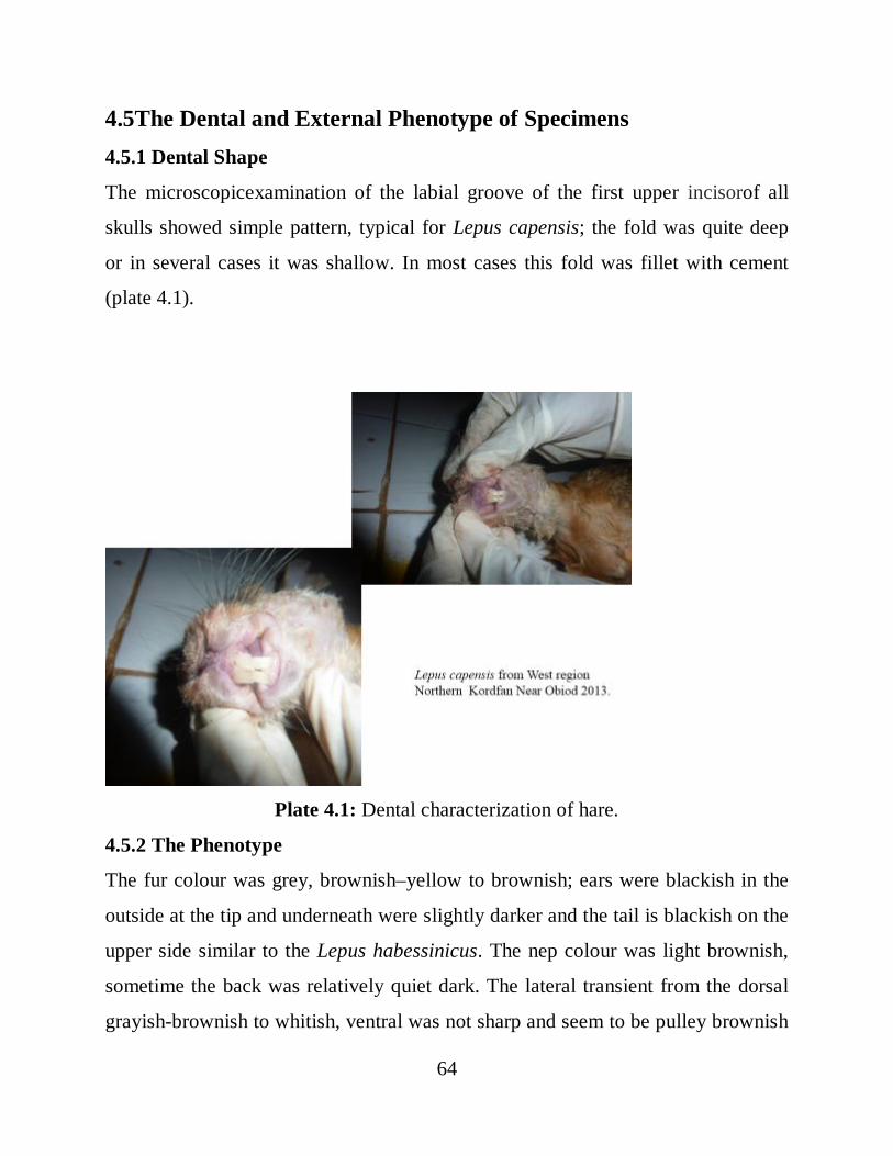
64

4.5The Dental and External Phenotype of Specimens 4.5.1 Dental Shape

The microscopicexamination of the labial groove of the first upper incisorof all

skulls showed simple pattern, typical for Lepus capensis; the fold was quite deep

or in several cases it was shallow. In most cases this fold was fillet with cement

(plate 4.1).

Plate 4.1: Dental characterization of hare.

4.5.2 The Phenotype

The fur colour was grey, brownish–yellow to brownish; ears were blackish in the

outside at the tip and underneath were slightly darker and the tail is blackish on the

upper side similar to the Lepus habessinicus. The nep colour was light brownish,

sometime the back was relatively quiet dark. The lateral transient from the dorsal

grayish-brownish to whitish, ventral was not sharp and seem to be pulley brownish

65

at transient zoneas shownin plates (4.2, 4.3, 4.4 and 4.5). All these results, namely,

dental analysis and external phenotype as well as the skull shape indicated that all

specimens belong to Lepus capensis in a wide sense.

Plate 4.2: Samples from West region.

Plate 4.3: Samples from Eastern region.

66

Plate 4.4: Samples from Easternregion.

Plate 4.5: Samples from Region Between two rivers

67

4.6. Molecular Genetics 4.6.1 Cyt (b) Sequences of Samples and D-loop

The median joining network in (Fig. 4.1)is not meant to present a complete

phylogenetic model for these hare species from Africa, because not all available

scrub hare sequences and no cape hare sequences from Africa except from Sudan

are included. The preliminary alignment of all respective sequences on GenBank

was not successful for all available African sequences. This needs further

exploration. Moreover, for a comprehensive phylogenetic analysis of the Sudanese

hares, all available and reliable sequences of other Lepus species should be

included. Currently, there is only one cyt b sequence of the African savanna hare,

L. victoriae, available from GenBank, but there are a few more L. saxatilis

sequences available. However, until today there is no clarity about the

phylogenetic relationship between L.saxatilis and L. victoriae they may be

conspecific or two good species. In South Africa, the scrub hare has originally

been described only from the SW of the country, and unknown sample locations

(as is the case for most sequences on GenBank) may be either from the range of L.

saxatilis or L. victoriae. Due to all these reasons, the median joining network

includes only few selected haplotypes with reliable regional assignment. In the

network, each open circle represents a cyt b haplotype, circle size is proportional to

the number of hares harboring the respective haplotype, black continuous lines

between haplotypes indicate the modelled evolutionary trajectories between

haplotypes and numbers along lines indicate substitutions (numbers of point

mutations) if more than one; if there is only one substitution between two

haplotypes no number is given. The dashed circle encompasses all Sudanese

haplotypes found presently.All mtDNA-lineages of the Sudanese hares are

phylogenetically closely related (Fig. 4.2) without major phylogenetic gaps. This

68

parallels the population genetic results based on the microsatellite allele

frequencies indicating only shallow gene pool differentiation.

4.6.2 Variation of Population Genetics

As shown in table (Table 4.7)a total of 89 alleles were identified at the nine loci

studied, 84 in the East region, 38 in the sample from the region between the two

rivers and 72 from West region. Of all alleles 32 (38.1%) were shared by all three

regions and 16 (19.05%) were private allelesthat occurred in only one region.Most

of private alleles (12) were occurred in the East region; the region between the two

rivers harboured one, and the West region three private alleles. All but one locus

(Sol33) harbored at least one private allele. Frequencies of all private alleles were

generally low, with a mean of 4.504% and ranging from 0.81% to

16.67%.According to the Genepop software results there were no significant

deviations from linkeage equilibrium, but there was an overall highly significant

deviation of genotype frequencies from Hardy-Weinberg expectations. The latter

result indicated a significant substructuring of the overall genotypic data set.The

following indices of genetic variability are given for each locus and regional

sample in (Table 4.7) total number of alleles detected (AN), most frequent allele

(AF) and respective allele frequency (F), mean observed heterozygosity (Ho),

expected heterozyogsity corrected for small sample sizes (He n.b.). For each region

the mean number of alleles per locus (A), the number of “private alleles” (AP), the

mean allelic richness (AR) as calculated by a rarefaction approach to account for

sample sizes using Fstat (see Material and Methods), and the Fis value is also

given.

69

Cyt b sequences(297bp alignment)

Figure 4.1: Median Joining Network (Bandelt et al., 1999) of cyt b sequences (297bp) of all

currently sequenced hare samples from Sudan, including three sequences of scrub hares (L.

saxatilis) from the Republic of South Africa and one sequence of the African savanna hare (L.

victoriae) from Ghana, as example to demonstrate the evolutionary mtDNA differentiation

between Sudanese cape hares and the other two currently acknowledged Lepus species of which

sequences were available from GenBank.

L. saxatilis from R.S.A. (AY292730, AF009731, HQ596480)

L. victoriae from Ghana (KJ193321)

L. capensis from Sudan

3

2

15

20

70

Figure 4.2: Neighbor-joining (NJ) phylogenetic tree computed by Mega using toalign 94

sequences were converted Cyt b (297bp) and D-loop (413bp) of hares from Sudan.

71

The Fis value indicates whether there is a heterozygote deficit or surplus at the

population level (significant deviation from zero is indicated by an asterisk;

significance at a nominal alpha = 0.05, after strict Bonferroni corrections for

multiple testing). A significant deviation of Fis from zero means that there is a

significant deviation from the Hardy-Weinberg equilibrium in the

region/population.

Kruskal-Wallis and Friedmann tests were used to carry outwhether allelic richness

varies significantly locus-by-locus across populations(Table 4.7 and Fig. 4.3).

Allelic richness was similarly high in the regions East and West, but significantly

lower in richness in the region between the two rivers (P< 0.016, Kruskal-Wallis

test andP< 0.011, Friedmann test) (Appendixes3 and 4).

Based on all nine microsatellite loci, there was a shallow but significant genetic

differentiation between all three regions currently considered (East, between the

two rivers and West); values of absolute (CSE distances) and relative (FST values)

genetic differentiation between these regions are given in table (4.8). This shallow

significant genetic differentiation was confirmed by the AMOVA (analysis of

molecular variance) that revealed that 6.76% (p<0.0001) of the overall relative

genetic variability was due to partitioning into the three discriminated regions,

whereas 8.81% (p<0.0001) were due to partitioning among individuals within

regions, and the biggest portion of 84.43% (p<0.0001) were due to partitioning

within individuals (Appendix 5).

72

Table 4.7: Overview of allelic variability of cape hares from the three regions East, between the two rivers and West. The total number of alleles found at each locus is given with the locus name. Separately for each region, the following locus-specific values are given: AN – total number of alleles, R – length range of alleles, AF – length of the most frequent allele, F – frequency estimate of the most frequent allele, He n.b. – expected heterozygosity (corrected for small sample sizes), Ho – observed heterozygosity, AR – allelic richness, AP – number of “private alleles“. Further, for each region the mean number of alleles per locus (A) and the FIS value are given (significant departure from zero is indicated by an asterisk; 95% confidence intervals are given in parentheses).

Region Loci Mean (A)

FIS

D7UTR 12

Sat 8 10

Sol 33 5

OCELAMB 7

Sol 03 16

Sol 28 8

OCLS1B 12

Sol 08 7

Sol 44 12

East AR=6.5 AP=12

AN R AF F He n.b. Ho

11 121-143 133 0.23 0.88 0.88

10 89-109 93 0.52 0.67 0.66

5 212-222 214 0.66 0.52 0.38

7 109-121 117 0.40 0.76 0.79

15 233-279 253 0.29 0.86 0.65

7 155-171 161 0.60 0.60 0.46

11 152-172 164/166 0.19 0.87 0.76

7 125-137 127 0.45 0.73 0.67

11 138-160 150 0.19 0.89 0.89

9.33 0.754 0.682

0.096* (0.041 - 0.133)

Between Blue and White Nile AR=3.9 AP=1

AN R AF F He n.b. Ho

6 119-143 135 0.50 0.71 0.54

5 89-105 89 0.46 0.63 0.84

4 212-222 214 0.77 0.41 0.0

3 115-119 117 0.69 0.46 0.46

8 233-279 245 0.31 0.84 0.85

3 155-163 161 0.58 0.56 0.08

4 152-166 158 0.58 0.59 0.54

1 127-127 127 1.0 0.0 0.0

4 150-156 150 0.55 0.60 0.50

4.22 0.533 0,423

0.214* (0.002 - 0.337)

West. AR=6.9 AP=3

AN R AF F He n.b. Ho

9 125-141 131/133/135 0.18 0.88 0.89

8 98-107 93 0.52 0.70 0.53

4 212-220 220 0.47 0.66 0.42

6 109-119 115 0,29 0.80 0.74

11 233-277 253 0.22 0.89 0.72

7 157-175 161 0.44 0.74 0.44

10 152-174 162 0.24 0.86 0.84

6 125-135 127 0.34 0.77 0.58

11 132-160 142 0.23 0.91 0.73

8.00 0.801 0.656

0.186* ( 0.058 - 0.250)

73

Figure 4.3: Thedistribution of the nine locus-specific allelic richnessvalues forthe

three regions.

Table 4. 8: Genetic differentiation of cape hares from the three regions (East (E),

between the two rivers (B), and West (W) studied in Sudan, as based on allele

frequencies at the nine microsatellite loci and as calculated as relative (FST values)

and absolute (Cavalli-Sforza-Edwards chord distances -CSEd) genetic

differentiation. Pairwise FST values are above the diagonal and pairwise CSEd

values are below the diagonal. Significance (i.e., values higher than zero) are

marked by asterisks.

Region E B W E - 0.112* 0.024*

B 0.132*

- 0.134*

W 0.046*

0.147* -

74

The overall shallow genetic divergence pattern between the three regions was also

evident by the FCA (factorial correspondence analysis); though it revealed some

little divergence of individual scores (but no significant gaps) of individual scores

along the first three factorial correspondence axes (Fig.4.4) that conveyed only

14.85% of the total allelic variation.

Moreover, the first ten factors covered only 38.28% of the total allelic variability

harbored by all studied hares, which accords to the interpretation of a shallow

pattern of genetic differentiation.

Nevertheless, the overall likelihood to assign each hare to the region where it was

collected based on its composite genotypes was unexpectedly high: using the

GENECLASS software (see Material and Methods), only eleven (11.6%) out of

hares used for microsatellite analysis could not be assigned “correctly” to the

region where they were collected. Whereas all hares from West regionwere

assigned to their collection region, 84.6% of the hares from between the two rivers

region were assigned to this region, and 85.7% of the hares from East regionwere

assigned to the region where they originated from.

Finally, the Bayesian STRUCTURE analysis indicated that there were two or three

most likely genetic clusters (groupings/populations) that were underlying the

composite data set; those two to three clusters coincided more or less nicely with

the three geographical regions (Fig.4.5).

Whereas the admixture model runs with no prior regional information for the

individuals resulted in a most likely number of two genetic clusters (supported by

the probability statistics and the delta K statistics according to Evanno), the runs

with prior region information for each individual resulted in most likely three

genetic clusters (K = 3) underlying the overall data set. The latter result reflected

very well the results as obtained by the other population genetic statistics of

differentiation.

75

Figure 4.4: Factorial correspondence analysis for genetic divergence of individual

between the three regions.

Region East Region “between Blue and White Nile

Region West

76

Moreover, the results of the STRUCTURE analysis indicated relatively little

genetic admixture on the individual level (Fig. 4.5).

Three-dimensional plots (Fig.4.6) of individual scores for the first three factors

from the Factorial Correspondence Analysis (FCA) based on allele frequencies at

all nine studied microsatellite loci. Each of the three graphics shows the total

individual scores scattered across the three-dimensional space (as defined by the

three axes), and the score positions of respective individuals from the three regions

are highlighted in red (first plot is for the East region; second plot for the region

between the two rivers, and third plot for the West region.

Moreover, the first ten factors covered only 38.28% of the total allelic variability

harbored by all studied hares, which accords to the interpretation of a shallow

pattern of genetic differentiation. Nevertheless, the overall likelihood to assign

each hare to the region where it was collected based on its composite genotypes

was astonishingly high: using the GENECLASS software (see Material and

Methods), only eleven (11.6%) out of hares used for microsatellite analysis could

not be assigned “correctly” to the region where they were collected. Whereas all

hares from West regionwere assigned to their collection region, 84.6% of the hares

from between the two rivers region were assigned to this region, and 85.7% of the

hares from East regionwere assigned to the region where they originated from.

77

K = 2 genetic clusters

K = 3 genetic clusters

Q

Q

East Region West Region

between White & Blue Nile Region

A

B

C D

Figure 4.5:Genetic STRUCTURE results for Sudanese cape hares. Upper charts A and B depict the genetic admixture of individuals and structure across the three regions, when assuming the presence of two (A) and three (B) genetic clusters (K). The Q value indicates the percentage of anIndividual´s genetic composition belonging to a certain cluster. According to the Likelihood values (C) for the data as obtained from 10 iterations per K and from Evanno´s delta K statistics (D), two genetic clusters are likely better describing the overall microsatellite variation than three genetic clusters. This is also indicated by chart B showing that three clusters (colours) do notadd any further meaningful information for understanding the geographic distribution of genetic

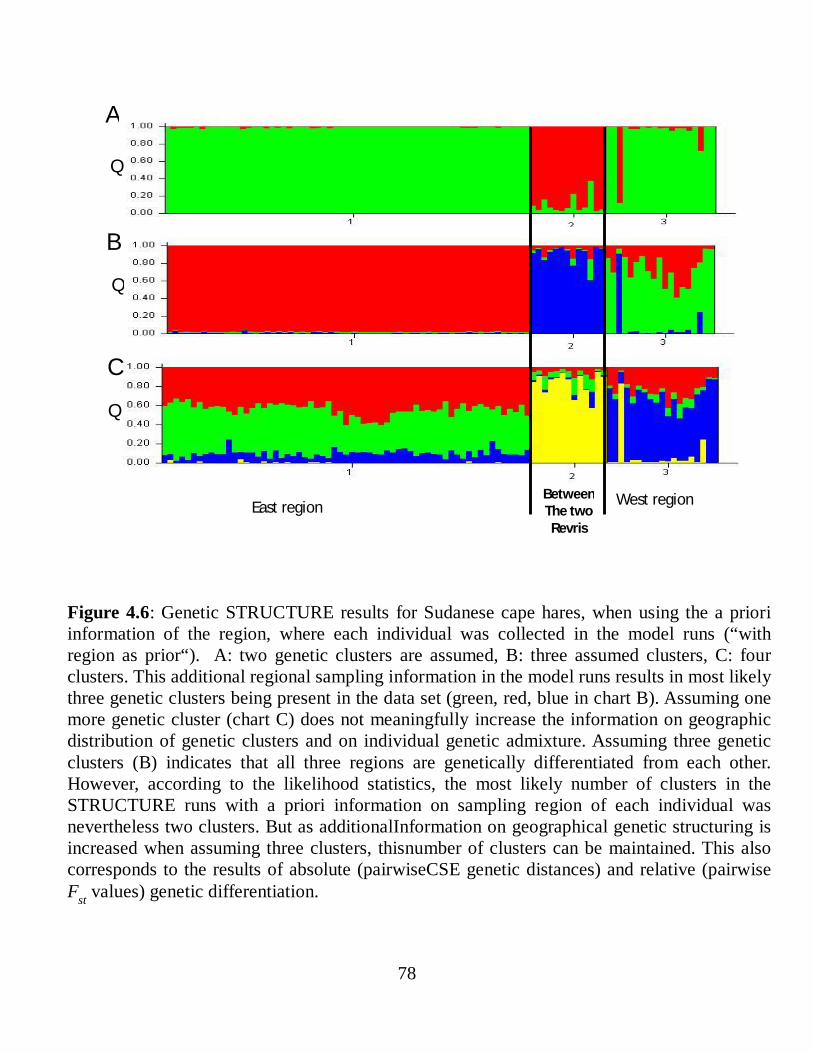
78

Figure 4.6: Genetic STRUCTURE results for Sudanese cape hares, when using the a priori information of the region, where each individual was collected in the model runs (“with region as prior“). A: two genetic clusters are assumed, B: three assumed clusters, C: four clusters. This additional regional sampling information in the model runs results in most likely three genetic clusters being present in the data set (green, red, blue in chart B). Assuming one more genetic cluster (chart C) does not meaningfully increase the information on geographic distribution of genetic clusters and on individual genetic admixture. Assuming three genetic clusters (B) indicates that all three regions are genetically differentiated from each other. However, according to the likelihood statistics, the most likely number of clusters in the STRUCTURE runs with a priori information on sampling region of each individual was nevertheless two clusters. But as additionalInformation on geographical genetic structuring is increased when assuming three clusters, thisnumber of clusters can be maintained. This also corresponds to the results of absolute (pairwiseCSE genetic distances) and relative (pairwise Fst values) genetic differentiation.

A

B

C

East region West region

Between The two Revris

Q

Q

Q

79

CHAPTER FIVE 5. Dissection

5.1Morphometrics The research findings revealed that there are considerable variations in tail length,

height and distance between eyes among hares collected from East of the Nile,

West of the Nile and between the Blue Nile and the White Nile.Differences in

these morphometrics implied that different species occur in the three geographic

regions. However, the conclusion drawn from phenotypic and dental analysis that

all specimens collected from the three geographic regions belong to one species,

Lepus capensis, comply with findings of many researcher worldwideYom-Tov and

Geffen, 2006Freckelton et al., 2003; Meiri, and Dayan, 2003Demirbaş et al.,

2013. Geographical variation in body size of both homeotherms and ectotherms is

a very common phenomenon (Freckelton et al., 2003; Meiri, and Dayan, 2003)

and has been related to many factors, including inter- and intraspecific

competition, food availability and reaction to ambient temperature in accordance

with Bergmann’s rule which states that within a broadly distributed taxonomic

clade, populations and species of larger size are found in colder environments, and

species of smaller size are found in warmer regions(Yom-Tov and Geffen, 2006).

Burnett (1983) work reveals that moisture has a statistically more significant

influence on wing and skull size of the bat Eptesicus fuscus than temperature, and

attributed this correlation to the need to conserve water in hot and dry

environments. Research in Turkish hares indicates variations in body weight and

hind foot length, depending on geographic regions (Demirbaş et al., 2013). James

(1970) suggests that body size variation is related to a combination of climatic

factors, mainly moisture and temperature, and that small body size is associated

with hot and humid conditions and larger size with cooler and drier conditions. In

80

Australia, body size variation in five species of mammals is better correlated with

moisture index and precipitation than is temperature, leading to the conclusion that

food supply is the main factor determining body size (Yom-Tov and Nix, 1986).

Studies on the geographical variation of L. capensis (Yom-Tov, 1967), A. cahirinus

(Nevo, 1989) and S. ehrenbergi (Nevo et al., 1986) in Israel and Sinai, show that in

these species northern animals are larger than southern ones, and that body size is

negatively correlated with temperature variables and positively so with plant cover

(reflecting productivity or food resources) and water-related parameters such as the

number of rainy days, annual rainfall and relative humidity. Comparing body

weights of brown hares living in Poland to representatives of this species from

Western Europe (Mace et al., 1981; Voss et al., 1990), fully grown up individuals

from Poland are about twice as heavy, reflecting the adaptation of the species to

different environments in these regions. Our findings that there are variations in

body size agreed with the findings many researches (Krunoslav et al.,

2014;Demirbaş et al., 2013;Riga et al., 2001). In fact, morphological variation

may determine individual performance and may be driven by ecological and

behavioural adaptations (Garland and Carter, 1994; Garland and Losos, 1994;

Harris and Steudel, 1997). Due to great variations within genera, some authors

assume that the phylogenesis and systematics of hares has not been completely

clarified (Pierpaoli et al., 2003; Ben Slimen et al., 2008).It is difficult, however, to

decide which factor influences the variation in body morphometrics and to assume

the relative effect of each factor.

Results of the present study revealed that morphometric procedure is useful for

determining hare’s sex, as females are always heavier than males with longer

necks. These findings have never been reported by (Riga et al., 2001; Cervantes

and Lorenzo, 1997) have found no sexual dimorphism in body size. Piotr et

81

al.,(2004) have attempted morphometric comparisons between males and females

with no positive results.

Morphometric correlation matrix (Table 4.3) has some implications statistical

models could be developed to predict easily measured morphs from those that are

difficult to measure. For example, the length of the back could be predicted from

the length of the fore foot, Total length from foot length and so forth.

5.2 Craniometric Like morphometric, cranometric also varied among the three geographic regions

(Table 4.4).The specific characteristics of a skull often reflect the animal methods

of feeding and effect on the muscle of mastication (Olude et al., 2010). Skulls

differ largely, not only between different species and breed but also between

individuals of same breed and sex (Koing and Liebich, 2004). Historically,

subspecies of hares were classified on the basis of the morphological features of

the skull and teeth (Suchentrunk et al., 2003; Palacios et al., 2008). Xin (2003)

suggests that analysis of skull development between different animal species

exposed to different selection pressures can contribute to the understanding of

geographical variations of particular populations, as well as life history strategies

and evolutionary change. On the other hand, an increase in skull size is attributed

to increased food availability, either by human activity or higher primary

productivity (Yom-Tov and Geffen, 2011).

Like morphometric, craniometric correlation matrix (Table 4.5) is useful for

developing predictive statistical models. For example, ENL could be usefully

predicted from NL, Pl from ENL, and so forth. That SFW relationship with the

cranial bones is weak, and either positive or negative suggests that it is useless to

be included in developing predictive models. Its negative correlations with MH,

UCTL, TBL, PPW, TBW, PL and FIL need further investigations.

82

5.3 Sex Craniometric One important finding is that craniometric is similar for males and females except

Tympanic bulla width (TBW) which is wider for males; this finding is useful for

determining sexual dimorphism in hares. This contradicts the findings by

Krunoslav et al., (2014) in the island of Vir and in continental north-west Croatia,

that no variations in craniometric, based on sex, is apparent although significant

variations among geographical regions are evident.

5.4 PopulationGenetics

By and large,the allelic diversity found presently in the overall sample of Sudanese

cape hares is compatible to that found in other cape hares (L. capensis senu stricto

and L. capensis s.l.) from South (Kryger, 2002; Suchentrunk et al., 2009) and

North Africa as well as in brown hares (L. europaeus) from different locations in

Europe (Fickel et al., 2005; Ben Slimen et al., 2008). The level of allelic diversity

is similar in the regions East and West of the Nile but significantly lower in the

population studied in the region between the two rivers. In this latter population

allelic diversity amounts to roughly half of that found in the hares regions East and

West and between the two rivers. This is indicated by all population genetic

parameters indicative of allelic diversity. The reason for the lower genetic diversity

in this region is not clear. But the relatively small sample size for this population

might have contributed to the low diversity, as many alleles that may occur at

relatively low frequencies would not have been samples by the few individuals.

Nevertheless, the “allelic richness“ value, which accounts for unbalanced (also

small) sample sizes in the comparison with the values for the other two regions is

significantly reduced for the population from between the two rivers. This latter

finding may suggest some underlying biological cause for the low allelic diversity

there. A potential effect of frequent presence of null alleles (i.e., alleles that are

83

missed due to technical reasons, such as amplification failures in the PCR runs)

cannot be excluded, particularly when considering the absence of any heterozygous

genotypes at two loci – Sol33, Sol08, and the very low frequency of heterozygotes

at the Sol28 locus). However, a likelihood test for the presence of null alleles in

this population could not be carried out, due to the small sample size.

A potential biological reason for the low genetic diversity of the population

between the Blue and White Nile could be one or repeated genetic bottlenecks in

the recent past, i.e., very low population density for short time or extending over

many generations, possibly due to flooding, bush fires, too strong natural predation

pressure, overharvesting by humans, parasitic or other infectious diseases etc. A

clear answer would necessitate an intensive ecological, pathological,

parasitological etc. study of the population. Also, the current results do not allow to

generalize the finding of low genetic diversity in the local population where the

samples have been collected for the whole region between the two rivers. An

investigation of clearly more samples in the whole region between the two rivers in

genetic, parasitologic, phathologic etc. terms may shed light on the underlying

biological causes that could have led to the low genetic diversity in this area.

In addition to the relatively low genetic diversity found in the population sample

from between the Blue and White Nile, this population is also clearly genetically

different from the hares roaming the region East and West region. The cape hares

from the latter two regions are also differing to some extent in their overall genetic

make-up; overall, genetic differentiation is significant, but at a low level,

compatible to what can be expected between diverse cape hare populations in

South and North Africa (Kryger, 2002, Ben Slimen et al., 2008, Suchentrunk et

al., 2009) or in brown hares from central Europe (Fickel et al., 2005). A recent

investigation on genetic differentiation of Indian Hares (L. nigricollis dayanus)

from east and west of the River Indus in Pakistan did not show any significant

84

genetic divergence (Ali et al., 2016). In general, low genetic differentiation among

populations across large geographic areas in diverse hare species, indicating

relatively high gene flow suggests large “effective population sizes“ (i.e.,

population sizes that are genetically/evolutionarily relevant), and this may be

associated with long speciation times in many species of the genus. Further

microsatellite analyses combining Sudanese cape hares and cape hares from North

and South Africa should help to understand gene flow patterns and levels of

genetic differentiation across large ranges and should help to prove or disprove

conspecificity of all hares in Africa currently considered Lepus capensis sensu lato.

They should also help inferring the systematic position of L. habessinicus form

Ethiopia that is currently considered a separate species (Gebremariam, 2016) and

help to understand evolutionary genetics of the cape hares of Africa.

The currently studied cyt b sequences of Sudanese cape hares are on the one hand

all closely related and on the other hand clearly differentiated evolutionarily from

the haplotype of the three scrub hares (L. saxatilis) from the Republic of South

Africa (that have identical sequences of the 297bp alignment) and the haplotype of

the single African Savanna hare (L. victoriae) from Ghana. The evolutionary

position of the Sudanese cape hares within L. capensis s.l. from Sudan needs

further comprehensive molecular analysis and should include reliable sequences

with known sampling locality. The comparison of cyt b sequences obtained in the

course of the present thesis with all reliable cyt b sequences of cape hares (L.

capensis s.l.) and other Lepus species available from GenBank and several tree-

building approaches (neighbor joining, maximum likelihood, and Bayesian

inference – not shown in details in the current thesis) suggest close phylogenetic

relationships to haplotypes of North African cape hares, hares considered L.

europaeus (brown hares) from the Near East, and also to Asian forms considered

L. capensis s. l. Whether or not the taxon “Lepus capensis sensu lato” represents a

85

single species, a complex of closely related species (perhaps indicating incipient

speciation), or even a group of partially not very closely related species remains to

be investigated by a combination of phylogenetic, phylogeographic, and population

genetic analyses, accompanied by analyses of external phenotypes and skull

morphometric. Importantly, for all individuals in such a study, unambiguous

information on collection locations must be available. Currently, quite a fair

number of cyt b sequences of “L. capensis” are available from GenBank for such

comparisons, but seemingly the taxonomic information associated with many is not

always clear (e.g., sometime “L. capensis” is used for brown hares that are

currently considered L. europaeus), and in many cases no clear information on

sampling locations or morphological/phenotypical characteristics is available.

Therefore, currently it is too premature to work out comprehensive phylogenetic

relationships based on cyt b sequences (this may rather add to tentative confusion

that already exists for this taxon). The systematic relationship between African

cape hares and European brown hares (L. europaeus) from the Near East needs

further study, but so far the conspecificity hypothesis of Petter (1959) cannot be

refuted as shown by a first microsatellite study by Ben Slimen et al., (2008). In

any case, the currently analyzedcyt b sequences of Sudanese hares fit nicely to

sequences of African L. capensis s.l. and are also closely related to sequences of

what is currently consideredL. europaeus from the Near East. Should both

currently acknowledged species turn out in the future to be indeed conspecific, the

correct species name for the currently studied Sudanese hares will be maintained L.

capensis, provided African L. capensis is not partitioned into different species, due

to future molecular results.

86

CONCLUSIONS AND RECOMMENDATIONS Conclusions In this study, analyses of morphometric and craniometric have indicated

considerable variations of these measurements among the three geographic regions

from which hares were collected. The implication is that different species of hares

might have occurred in the geographic regions. Further investigation on

morphological, phenotypic and dental features; however, confirm that the

specimens belong to Lepus capensis. This supports the abundant literature that

environmental factors in different geographic regions influence morphometric and

craniometric features. Both morphometric and craniometric measures are useful for

determining sexual dimorphism, based on the findings that females are always

heavier than males, with longer necks; and that tympanic bulla width is always

wider in males compared with females. Correlation matrices of morphometric

parameter and Craniometric could be used to develop statistical models to predict a

particular easily measurable variable from the one variable that is difficult to

measure.

Low genetic diversity found in the population sample from between the two rivers

this population is also clearly genetically different from the hares roaming the East

of the Nile and West of the Nile. The study identified 89 alleles in nine loci and 32

were found in three regions while the private alleles were 16 that occurred in only

one region.

87

Recommendations There are some gaps in knowledge that need to be addressed in the future to

reinforce the findings of this study. These are:

1. Collection of metrological data and assessment of habitat condition are essential in

determining variations in environmental factors in the geographic regions from

which hares are collected.

2. Basic information about food quality and quantity in the three geographic regions

is essential to assess variations in hares’ morphometric and craniometric.

3. Long-term Studies of reproductive biology, ecology and behavior of hares relative

to food quantity and quality in the three regions are needed to determine how these

variables affect hares’ population dynamics.

4. Future research is needed about trans boundary hares in order to determine the

gene flow between the countries.

5. Further analyses of mtDNA cytochrome b gene with additional specimens of hares

from Sudan are needed to clarify the taxonomic status.

88

REFERENCES Abdelaziz A.A (2010). The effect of some management practices ondecertified

range lands in Sinnar Sate. PhD Thesis, U of K: 33-34.

Ali, H., Shafiq A., Stefanovic, M., Shahid, I. and Suchentrunk, F. (2016).

Spatial population genetics of desert hares in Pakistan. Abstr. 90th Annual

Meeting of the German Society of Mammalogy, Berlin, Germany, 4th–7th

September. Mammalian biology journal. Suppl.

Altschul, S., Madden, T. and Schäffer, A. (1997). Gapped BLAST and PSI-

BLAST: A new generation of protein database search programs. Nucleic Acids

Research, (25):3389-3402.

Alves, P., Branco, M., Matias, O. and Ferrand, N. (2000). New genetic variation

in European hares, Lepus granatensis and L. europaeus.Biochemical Genetics,(38):

87-96.

Alves, P., Ferrand N., Suchentrunk, F. and Harris, D. J. (2003). Ancient

introgression of Lepus timidus mtDNA into L. granatensis and L. europaeus in the

Iberian Peninsula. Molecular Phylogenetics and Evolution, (27): 70-80.

Alves, P., Harris, D., Melo-Ferreira, J., Branco, M., Suchentrunk, F., Boursot,

P. and Ferrand, N. (2006). Hares on thin ice: introgression of mitochondrial DNA

in hares and its implications for recent phylogenetic analyses. Molecular

Phylogenetics and Evolution, (40): 640-641.

Angerbjörn, A. (2011).Hares and Rabbits (Leporidae) Grzimek’s Animal Life

(On-line). At http:www//animals.galegroup.com.proxy.lib.umich.edu.

Angerman, R., Flux, J., Chapman, J. and Smith, A. (1990). Lagomorph

Classification. Pages 7–13 in Rabbits, hares and pikas: Status conservation action

plan International Union for Conservation of Nature and Natural Resources, Gland,

Switzerland.

89

Angermann, R. (1965). Revision der pala ( arktschen und a) thiopischen Arten der

Angermann, R. (1983).The taxonomy of Old World Lepus.Acta Zoologica

Fennica,(174):17–21.

Applied Bio-systems Protocol (A.B.P) (2007).Big DyeR

XTerminatorTMpurification Kit protocol. Lincoln Centre Drive, Forest City

California 94404 USA. Part Number 4374408 Rev C/07.

Ashton, K., Tracy, M. and Queiroz, A. (2000). Is Bergmann’s rule valid for

mammals? Journal of American Naturalist,(156):390–415.

Gattung Lepus (Leporidae, Lagomorpha). Diss. Thesis. Humboldt University of

Berlin, Berlin.

Bandelt, H., Forster, P. and Rohl, A.(1999). Median joining networks for

inferring intraspecific phylogenies. Molecular Biology and Evolution,(16): 37–48.

Belhhir, K. (2004). GENETIX v.4.0 logiciel sous WindowsTM pour la genetique

des populations. Laboratorio Genome, Populations, Interaction CNRS UMR 5000,

Universite de Montpellier II, Montpellier, France.

Ben Slimen, H., Suchentrunk, F., Memmi, A. and Ben Ammar Elgaaied, A.

(2005). Biochemical Genetic Relationships among Tunisian Hares (Lepus sp.)

South African Hares (L. capensis), and European brown hare (L.

europaeus).Biochemical Genetics,(43): 577-596.

Ben Slimen, H., Suchentrunk, F., Shahin, A., Ben Ammar Elgaaied, A., (2007).

Phylogenetic analysis of mtCR-1 sequences of Tunisian and Egyptian hares (Lepus

sp. or spp., Lagomorpha) with different coat colures. Mammalian Biology (72):

224-239.

Ben SLimen, H., Suchentrunk, F., Stamtis, C., Mmurisa, Z., Sert, H., Alves,

P., Krygen, U., Shahin, A. and Elgaaied, A. (2008). Population genetics of cape

and brown hares (Lepus capensis and L. europaeus): A test of Petter’s hypothesis

of conspecifi city. Biochemical Systematics and Ecology,(36): 22-39.

90

Burnett, C. (1983). Geographic and climate correlates on morphological variation

in Eptesicus fuscus. Journal of Mammalogy,(64):437–444.

Burnie, D and Wilson, D. (2005). Animal: The Definitive Visual Guide to the

World's Wildlife. DK Adult. p. 143. ISBN 0789477645.

Calder, W. (1984).Size, function and life history. Harvard University Press,

Cambridge.

Can, D., Abramov, A., Tikhonov, A. and Averianov, A. (2001). Annamite

striped rabbit Nesolagus timminsi in Vietnam. Acta Theriologica,(46):437–440.

Cervantes, F. and Lorenzo, C. (1997). Morphometric differentiation of rabbits

(Romerolagus and Sylvilagus) and jackrabbits (Lepus) of Mexico. Gibier Faune

Sauvage, Game Wildlife. (14): 405-425.

Chanta, J., Stoner, O., Bininda-Emonds R. and Tim., C. (2003). The adaptive

significance of coloration in lagomorphs. Biological Journal of the Linnean

Society. (79):309-328.

Chapman, J. and Flux, J. (1991). Rabbits, Hares and Pikas: Status Survey and

Conservation Action Plan. IUCN. (62): 76-78. ISBN 2831700191.

Chapman, J.and Flux, J. (1990).Rabbits, Hares and Pikas: Status Survey and

Conservation Action Plan. Chapter 4. International Union for Conservation of

Nature and Natural Resources, Gland, Switzerland. pp. 61-65.

Chapman, J., Cramer, K., Dippenaar, N., and Robinson, T. (1992).

Systematics and biogeography of the New England cottontail, Sylvilagus

transitionalis (Bangs, 1895), with the description of a new species from the

Appalachian Mountains. Proceedings of the Biological Society of Washington,

(105):841-866.

Chapman; J. and Flux, J (2008). Introduction to the Lagomorpha. In:

Lagomorpha biology: Evolution, ecology, and conservation (eds. P.C. Alves, N.

Ferrand and K. Hackländer), Springer Press, Berlin, pp. 1-9.

91

Corbet, G.B. (1983). A review of classification in the family Leporidae. Acta

Zoologica Fennica, (174): 11-15.

Cott HB. (1940). Adaptive coloration in animals. London: Metheun.

Dawson, M. R. (1981). Evolution of modern leporids. pp 1–8 in Proceedings of

the World Lagomorph Conference University of Guelph Press, Ontario.

Dayan, T., Tchernov, E., Yom-Tov, Y. and Simberloff, D. (1989). Ecological

character displacement in Saharo-Arabian Vulpes: outfoxing Bergmann’s rule.

Oikos(55):263–272.

Demirbaş, Y. (2010).Türkiye Lepus Linnaeus, 1758 Cinsinin Taksonomik Durumu

(Mammalia: Lagomorpha). PhD thesis. University of Kırıkkale, Turkey.

Demirbaş, Y., Albayrak, I. and Suchentrunk, F. (2012). Population genetics of

Turkish hares. Proceedings 4th World Lagomorph Conference, Vienna, Austria,

pp. 45.

Demirbaş, Y., Albayyrak, N., and Yilmaz. A. (2013). Studies of

ecomorphological variation of this European hare (Lepus europaeus) in Turkey.

Archives of Biological Sciences,Belgrade, (65): 559-566.

Demirbaş, Y., Aşan, N., and Albayrak, I. (2010). Cytogenetic study on the

European brown hare (Lepus europaeus Pallas, 1778) (Mammalia: Lagomorpha) in

Turkey. Turkish Journal of Biology,(34):247-252.

Dimijian, G. G. (2005). Evolution of sexuality: Biology and Behavior.

Proceedings (Baylor University. Medical Center). (18): 244-258.

Duthie, A., Skinner, J. and Robinson, T. (1989). The distribution and status of

the endangered riverine rabbit (Bunolagus monticularis).Conservation Biology,

(47):195-202.

Dyce, K., Sacks, W. and Wensing, C. (2010). Textbook of veterinary anatomy

4thed.Saunders Else vie.

92

El-Belattagey,A.A.(2000).Technology Generation and Dissemination for

Sustainable Production of Cereals and Cool-Season Food Legumes, Progress

Report, ICARDA and NVRSRP,Cario,Egypt.

Ellerman, J. and Morrison-Scott, T. (1951). Checklist of Palaearctic and Indian

mammals (1758–1946). British Museum (London), Natural History, pp. 810.

Ellerman, J., Morrison-Scott, T.and Hayman R. (1953). Southern Africa

mammals. A reclassification. British Museum(London). Natural History, pp.1758-l

951.

Estonba, A., Solís, A., Iriondo, M., Sanz-Martin, M.J., Pérez-Suárez, G.,

Markov, G. and Palacios, F. (2006). The genetic distinctiveness of the three

Iberian hare species: Lepus europaeus, L. granatensis and L. castroviejoi.

Mammalian Biology,(71): 52-59.

Evano, G., Regnaut, S. and Goudet, J. (2005). Detecting the number of Clusters

of individuals using the software structure: a simulation study. Molecular Ecology,

(14): 2611-2620.

Falush, D., Stepphens, M. and Pritchard, J. (2003). Inference of Population

Structure Using Multlocus Genotype Data: Linked loci and Correlated Allele

Frequencies. American Journal of Medical Genetics,(164): 1567-1587.

Feldhamer, G., Thompson, B. and Chapman, J.(2003).Wild Mammals of North

America. Baltimore and London: Johns Hopkins University Press.

Fernando, P., Chiara, A., German, A. and Santiago, R. (2007). Morphological

evidence of species differentiation within Lepus capensis Linnaeus,(Leporidae,

Lagomorpha) in Cape Province, South Africa.Mammalian Biology, (73): 358-370.

Fickel, J., Schmidt, A., Putze, M., Spittler, H., Ludwig, A., Streich, W. and

Pitra, Ch. (2005).Genetic Structure of Populations of European Brown Hare:

Implications for Management.Journal of Wildlife Management,(69): 760-770.

93

Fickel, J., Lieckfeldt, D. and Pitra, C. (1999). Analysis of genetic diversity and

structure in neighboring populations of the European brown hare (Lepus

europaeus, Pallas 1778). Zeitschrift Fur Jagdwissenschaft.(45): 230–237.

Flux, J. and Angermann, R. (1990). The hares and jackrabbits. pp 61–94 in

Rabbits, hares and pikas: Status conservation action plan (J. A. Chapman and J. E.

C. Flux, eds.). International Union for Conservation of Nature and Natural

Resources, Gland, Switzerland.

Flux, J. and Chapman, J. (1990) Rabbits, Hares and Pikas: Status Survey and

Conservation Action Plan. Chapter 1. International Union for Conservation of

Nature and Natural Resources, Gland, Switzerland. pp 1-7.

Flux, J. (1981). Reproductive strategies in the genus Lepus. In: Myers, K. and

MacInnes, C.D. (Eds), Proceedings of the World Lagomorph Conference,

University of Guelph. pp. 155-174.

Flux, J. (1983). Introduction to taxonomic problems in hares. Acta Zoologica

Fennica, (174):7-10.

Flux, J. (2001). Evidence of self-limitation in wild vertebrates. Oikos(92):555-557.

Freckelton, RP., Harvey, PH. and Pagel, M. (2003). Bergmann rule and body

size in mammals. The American Naturalis,(161):821-825.

Frey, J. K., Fisher, R. D. and Ruedas, L. A. (1997). Identification and restriction

of the type locality of the Manzano Mountains cottontail, Sylvilagus cognatus

Nelson, and 1907 (Mammalia: Lagomorpha: Leporidae). Proceedings of the

Biological Society of Washington,(110):329-331.

García-Berthou, E(2001). On misuse of residuals in ecology:testing regression

residuals vs.the analysis of covariance. Journal of Animal Ecology. (70):708-711.

Gardner, J., Peters, A., Kearney, M., Josef, L. and Heinsohn, R.(2011).

Declining body size: a third universal response to warming.Trends in

EcologyandEvolution,(26): 285-291.

94

Garland, T. and Carter, P. (1994). Evolutionary physiology. Annual Review of

Physiology,(56): 579-621.

Garland, T. and Losos, J. (1994).Ecological morphology of locomotor

performance in squamate reptiles.In Ecological morphology: Integrative

organismal biology. pp 240-302.

Garland, T., Dickerman, A., Janis, C. and Jones, J. (1993). Phylogenetic

analysis of covariance by computer simulation. Systematic Biology, (42):265-292.

Gebremariam, Z. (2016). Evolutionary Relationships among Hares (Lepus spp.)

from Ethiopia: Multivariate Morphometry, Molecular Phylogenetics and

Population Genetics. PhD thesis, University of Addis-Ababa.

Geist, V. (1987). Bergmann’s rule is invalid. Canadian Journal of Zoology,

(65):1035-1038.

Gloger, C. (1833). Das Abandern der Vogel durch Einfluss des Klimas. [The

effect of climatic change on birds]. Breslau:A. Schulz. (In German).

Gompper, M. E. and Gittleman, J. L. (1991). Home range scaling: In

transpacific and comparative trends. Oecologia,(87): 540-554.

Gosler, A., Greenwood, J. and Perrins, C. (1995). Predation risk and the cost of

being fat. Nature,(377): 621-623.

Gould, E. and McKay, M. (1998).The encyclopedia of mammals. Sydney.

Gould, S.J. (1966). Allometry and size in ontogeny and phylogeny. Microbiology

and Molecular Biology Reviews, (41): 587-640.

Grant, P.R. and Grant, B.R.,(1995). Predicting micro evolutionary responses to

directional selection on heritable variation. Evolution,(49): 241-251.

Hall, B. (1990). Genetic and epigenetic control of vertebrate embryonic

development. Netherlands Journal of Zoology, (40): 352-361.

Harris, M. and Steudel, K. (1997). Ecological correlates of hind limb length in

the Carnivora. Journal of Zoology. (London.) (241): 381-408.

95

Harrison, D. and Bates, P. (1991). The Mammals of Arabia. Harrison Zoological

Museum, Kent, UK.

Hausman, L. (1920). The Microscopic Identification of Commercial Fur Hairs.

Scientific MonthlyMagazine, (10): 70-78.

Henry, C. and Ulijaszek, S. (1996). Long-term consequences of early

environment. Cambridge University press, Cambridge.

Hewitt G. (1996). Some genetic consequences of ice ages, and their role in

divergence and speciation. Biological Journal of Linnean Society, (58):247-279.

Hewitt G. (1999). Post-glacial recolonization of European biota. Biological

Journal of Linnean Society, (68):1-2.

Hillis, D., Moritz, C., and Mable, B. (1996). Molecular Systematics, 2nd Ed.,

Sinauer Associates, Massachusetts.

Ho, C., Pennings, S. and Carefoot, T. (2010). Is diet quality an overlooked

mechanismfor Bergmann’s Rule? The American Naturalist,(175): 269-276.

Hoffman, R. andSmith, A. (2005). Order Lagomorpha. In: Mammal Species of

the World. 3rd Ed. University Press. pp. 198-199.

Hoffmann, R.S., (1993).Order Lagomorpha. In: Wilson, D.E., Reeder, D.M.

(Eds.), Mammal Species of the World. A Taxonomic and Geographic Reference.

Smithsonian Institution Press, Washington and London, pp. 807-827.

Holley AJ. (1993). Do brown hares signal to foxes? Ethology,(94): 21-30.

Huxley J. (1942). Evolution: the modern synthesis. New York: Harper and Brown.

https://en.wikipedia.org/wiki/Sudan.

Hutchins, M. (2004). Lagomorpha. in DKleiman, V Geist, M McDade, eds.

Grzimek's 2th Ed. New York: Thomson and Gale. Animal Life Encyclopedia, (16):

417-516.

96

Institute of Environmental Studies (IES) (1988). Baseline survey for Darfur

Region Prepared by U of K and the Government of Darfur Region. Final Report,

Jun.

IUCN (2008). Red list of threatened species on-line. http://www.iucnredlist.org/.

James, F, C. (1970). Geographic size variation in birds and its relationship with

climate. Ecology,(51):365-390.

Jennings, N., Smith, R., Hackländer, K., Harris, S. and White, P. (2006).

Variation in demography, condition and dietary quality of hares Lepus europaeus

from high density and low-density populations. Wildlife Biology, (12):179-189.

Kasapidis, P., Suchentrunk, F., Magoulas, A. and Kotoulas, G. (2005). The

shaping of mitochondrial DNA phylogeographic patterns of the Brown hare (Lepus

europaeus) under the combined influence of Late Pleistocene climatic fluctuations

and anthropogenic translocations. Molecular Phylogenetics and Evolution, (34):

55-66.

Keith, L. and Windberg, L. (1978). A demographic analysis of the snowshoe

hare cycle. Wildlife Monographs, (58):70.

Kiltie RA. (1988). Countershading: universally deceptive of deceptively

universal? Trends in Ecology and Evolution,(3): 21-23.

Kiltie, R. (1989). Testing Thayer’s countershading hypothesis: an image

processing approach. Animal Behavior,(38):542- 544.

Koing, H. and Liebich, H. (2004).Veterinary anatomy of domestic mammals

Textbook and colour atlas .Schattauer GmbH. Germany pp: 27-50.

Kolb, H. (1978).Variation in size of foxes in Scotland. Biological Journal of the

Linnean Society,(10):291-304.

Korstanje.R., Gillissen.G., Versteeg. S., Van Oost, B., Bosma, A., Rogel-

Gaillard, C., Van Zutphen, L. and Van Lith,H. (2003). Mapping of Rabbit

97

Microsatellite Markers Using Chromosome-SpecificLibraries.The American

Genetic Association.Journal ofHeredity,(94):161-169.

Krunoslav, P., Nino, D., Ivan, St., Nina, P. and Vedran, S. (2014). Craniometric

features of European hare (Lepus europaeus Pall.) from North-west Croatia and the

island of Vir. Vetrinarski Arhiv,(84): 387-400.

Kryger, U.(2002). Genetic variation among South African hares (Lepus spec.) as

inferred from mitochondrial DNA and microsatellites. Ph.D. Thesis, University of

Pretoria, R.S.A.

Leach, M. (1989). The rabbit. Shire Natural History.Shire publications, Aylesbury.

Liao, J., Zhang, Z. and Liu, N. (2006). Altitudinal Variation of Skull Size in

Daurian Pika (Ochotona daurica Pallas, 1868). Acta Zoologica Academiae

Scientiarum Hungaricae, (52):319-329.

Mace, G., Harvey, P. and Clutton-Brock, T. (1981). Brain size and Ecology in

small mammals. Journal of Zoology, (193): 333-354.

Mamuris, Z., Moutou, K., Stamatis, T. and Suchentrunk, F., (2010). DNA and

Mitochondrial lineages in European and Asian populations of the brown hare

(Lepus europaeus)Mammalian Biology,(75): 233-242.

Matthee, C. and Robinson T. (1996). Mitochondrial DNA differentiation among

geographical populations of Pronolagus rupestris, Smith’s red rock rabbit

(Mammalia: Lagomorpha). Heredity(76):514- 523.

McNab, K.(2010). Geographic and temporal correlations of mammalian size

reconsidered: a resource rule. Oecologia(164): 13-23.

Meiri, S. and Dayan, T. (2003). On the validity of Bergmann’s rule. Journal of

Biogeography, (30):331-351.

Meiri, S., Dayan, T., and Simberloff, D. (2004). Carnivores, biases and

Bergmann’s rule. BiologicalJournal of the Linnean Society,(81): 579-588.

98

Melo-Ferreira J., Boursot P. and Randi, E. (2007). The rise and fall of the

mountain hare (Lepus timidus) during Pleistocene glaciations: expansion and

retreat with hybridization in the IberianPeninsula. Molecular Ecology, (16):605-

618.

Mengoni, C. (2011). Phylogeny and genetic diversity of Italian species of hares

(genus Lepus). Ph.D. thesis.University of Bologna, Italy.

Metz, HC., (1992). Sudan: a country study. Washington DC, Federal Research

Division.

Millar, J.S., and Hickling, G.J. (1990). Fasting endurance and the evolution of

mammalian body size. Functional Ecology,(4): 5-12.

Mitchell-Jones, A., Amori, G., Bogdanowicz, W., Krystufek, B., Reijnders, P.,

Spitzenberger, F., Stubbe, M., Thissen, J., Vohralik, V. and Zima, J. (1999).

The Atlas of European Mammals. 166-167. Academic Press, London.

Mougel, F. (1997). Nine polymorphic microsatellite loci in the rabbit, Oryctolagus

cuniculus. Animal Genatices, (28):58-59.

Naughton, D. (2012). Thenatural history of Canadian mammals. University of

Toronto Press. pp. 235–38. ISBN 1442644834.

Nevo, E. (1989). Natural selection of body size differentiation in Spiny mice,

Acomys. Z Saugertierkund (54):81-99.

Nevo, E., Beiles, A., Heth, G. and Simson, S. (1986). Adaptive differentiation of

body size in speciating mole rats. Oecologia,(69):327–333.

Niethammer, J. and Krapp, F. (2003). Handbuch der Sugetiere Europas, Band

3/II: Hasentiere Lagomorpha. Aula-Verlag, Wiebelsheim.

Nogorsen, D. (1985). A morphometric study of geographic variation in the

snowshoe hare (Lepus americanus). Canadian Journal of Zoology, (63): 567–579.

99

Nowak, R. (1999).Hares or Jack Rabbits. pp. 1733-1738 in R.M. Nowak, ed.

Walker's Mammals of the World, 6th Ed, Vol.1.Baltimore and London: The Johns

Hopkins University Press.

Ohlsson, T. and Smith, G.(2001). Early nutrition causes persistent effects on

pheasant morphology. Physiological and Biochemical Zoology,(74): 212-218.

Olude, M. and Olopade, J. (2010).Morphometric studies of the axial skeleton of

the African giant rat (cricetomysg ambianus waterhouse) part(1) skull Typology

Journal of Veterinary Anatomy, (3):1-12.

Osman MG (2005). Evaluation of Soil Erosion in Sudan. Space Technology

Centre, Computer Man College, Khartoum, Sudan. (LinkCpings university,

Olagunju Emmanuel Gbenga LIU-IDA/FFK-UP-A--08/021-SE, (1): 5-6.

Ozgul, A., Tuljapurkar, S., Benton, T.G., Pemberton, J.M., Clutton-Brock,

T.H., Coulson, T., (2009). The dynamics of phenotypic change and the shrinking

sheep of St. Kilda. Science(325): 464–467.

Paetkau, D., Slade,R., Burden, M. and Estoup, A. (2004). Genetice assignment

methods for the direct, real-time estimation for migration rate: asimulation-based

exploration of accuracy and power. Molecular Ecology,(13): 55-65.

Paetkau, D., Calvert, W., Stirling, I. and Strobeck,C. (1995).Microsatellite

analysis of population structure I Canadian polar bears.Molecular Ecology,

(4):347-354.

Palacios F., (1996). Systematics of the indigenous hares of Italy traditionally

identified as Lepus europaeus Pallas, 1778 (Mammalia: Leporidae). Bonner

Zoologische Beitragen, (56):59-91.

Palacios, F., Angelone, C., Alonso, G. and Reig, S. (2008). Morphological

evidence of species differentiation within Lepus capensis (Leporidae,

Lagomorpha) in Cape Province, South Africa. Mammalian Biology, (73):358-370.

100

Paulo Célio, A. and Melo-Ferreira,J. (2007). Are Lepus corsicanusand L.

castroviejoi conspecific? Evidence from the analysis of nuclear marker. CIBIO,

Centro de investigação em Biodiversidade e Recursos Genéticos, and Faculdade de

Ciências da Universidade do Porto, CampusAgrário de Vairão,IGF publ.4485-661.

Perez-Suarez, G., Palacios, F. and Boursot, P. (1994). Speciation and paraphyly

in western mediterranean hares (Lepus castrovejoi, L. europaeus, L. granatensis,

and L. capensis) revealed by mitochondrial DNA phylogeny. Biochemical

Genetics,(32): 423-436.

Petter F. (1961). Elements d’une révision des lièvres européens et asiatiques du

sous-genre Lepus. Zeitschrift für Säugetierkunde, (26):30-40.

Petter, F. (1972). Order the mammals of Africa an identification manual.

Smithsonian Institute Press, Washington. Rautenbach, I.L. 1982. Mammals of

Transvaal. Ecoplan Monograph No. 1 Ecoplan, Pretoria.

Petter, F. (1959). Ele´ments d’une re´vision des lie`vres africains du sousgenre

Lepus. Mammalia,(23): 41-67.

Pierpaoli, M., Riga, F., Trocchi V. and Randi, E. (1999). Species distinction and

evolutionary relationships of the Italian hare (Lepus corsicanus) as described by

mitochondrial DNA sequencing. Molecular Ecology,(8):1805-1817.

Pierpaoli, M., Riga, F., Trocchi, V. and Randi, E. (2003). Hare populations in

Europe: intra and interspecific analysis of mtDNA variation. Biology,(326): S80-

S84.

Piotr, M., Elzbieta, K. and Bartlomiej, B. (2004).Size of the brown hares (lepus

europaeus Pallas, 1778) Living in central Pomerania in Poland. Zoologica

Poloniae, (49): 237-244

Piry, S., Alapetite, A., Cornuet, J., Paetkau, D., Baudouin, L. and Estoup, A.

(2004). GeneClass2: a software for genetic assignment and first generation

migrants detection.Journal of Heredity, (95): 536-539.

101

Poulton, EB. (1890). The colours of animals: their meaning and use, especially

considered in the case of insects.London: Kegan Paul, Trench, Trübner.

Pritchard, J., Stephens, M. and Donelly. P. (2000). Inforence of population

structure using multilocus genotype data. Genetic. (155): 945-959.

Pucek, Z.(1984). Klucz do oznaczania ssaków Polski. PWN, Warszawa.

Quick-Start Protocol(2011). QIAGEN® Multiplex PCR Kit, Sample and Assay

Technologies. Trademarks: Q-Solution® (QIAGEN Group). N.1067518 01/2011,

QIAGEN. QIAGEN kit handbook. www.qiagen.com/handbooks.

Raymond, M. and Rousset, F. (1995). GENEPOP (version 1.2): Population

genetics software for ecact tests and ecumenicism. Journal of Heredity,(86): 248-

249.

Read, A. Gaskin, D. (1990). Changes in growth and reproduction of harbour

porpoises, Phocoena phocoena, from the Bay of Fundy. Canadian Journal

ofFisheries and Aquatic Sciences,(47):2158–2163.

Reece,W. (2009). Functional Anatomy and Physiology of Domestic animal. 4th ed.

Weley-Black well: P.p180.

Reiss, M. (1991).The allometry of growth and reproduction. Cambridge University

Press.

Rice, W. (1989). Analyzing tables of statistical tests. Evaluation, (43): 223-225.

Rico, C., Rico, C. and Webb, N. (1994). Four polymorphic microsatellite loci for

the European wild rabbit, Oryctolagus cuniculus. Animal Genetics, (25):367.

Riegler, D (.2013).Lepus microtis: African savanna hare. Animal Diversity.

Riga, F., Trocchi, V., Randi, E. and Toso, S. (2001). Morphometric

differentiation between the Italian hare (Lepus corsicanus De Winton, 1898) and

the European Brown hare (Lepus europaeus Pallas, 1778). Journal of

Zoology,(253): 241-252.

102

Riga, F., Trocchi, V., Angelici, F., Randi, E. and Pierpaoli, M. (2003). Lepus

corsicanus De Winton, 1898 - Apenninenhase. - In: Krapp, F. (Ed.); Handbuch der

Sa¨ugetiere Europas. Band 3/II: Hasentiere - Lagomorpha. AULA-Verlag,

Wiebelsheim, pp. 117-135. (In German).

Ristić, Z., Marković, V., Barović, V. and Nasiljevic, D. (2012). Loss calculation

model of brown hare (Lepus europaeus Pall) and its applicationin the hunting

grounds of Vojvodina region (north Serbia). Pakistan Journal of Zoology,(44): 1-5.

Robinson T. J. and Matthee C. A. (2005). Phylogeny and evolutionary origins of

the Leporidae: A review of cytogenetics, molecular analyses and a supermatrix

analysis. Mammal Review,(35): 231-247.

Robinson, T. and Dippenaar, N. (1987).Morphometric of the South African

leporidae. II: Lepus Linnaeus, 1758, and Bunolagus Thomas, 1929.Annals of the

Transvaal Museum, (34): 379-403.

Roedenbeck, I. and Voser, P. (2008). Effects of roads on spatial distribution,

abundance and mortality of brown hare (Lepus europaeus) in

Switzerland.European Journal of Wildlife Research,(54): 425-437.

Schmidt-Nieisen, K. (1994). Dlaczego tak wa¿ne s¹ rozmiary zwierz¹t.

Skalowanie. PWN, Warszawa.

Schmidt-Nielsen, K. (1984). Scaling:why is animal size so important? Cambridge

University Press, Cambridge.

Schneider, E. (1990).Hares and rabbits in Parker. ed Grzimek,sencyclopedia of

mammals. (4):254-299 English Edition New York and New Jersey. McGraw. Hill.

Publishing company.

Scholander, P. (1955). Evolution of climatic adaptation in homoeotherms.

Evolution(9):15-26.

Sert, H. (2006). Akdeniz ve Güneydoğu Anadolu B ِ ◌lgesi ile Orta, Avrupa,

Ortadoğu ve Güney Afrika Yaban Tavşanı Populasyonlarında Ekomorfolojik ve

103

Moleküler Varyasyonlar (Lagomorpha: Lepus). PhD Thesis. University of Akdeniz

(in Turkish, English summary).

Sert, H., Ben Slimen, H., Erdoğan, A., and Suchentrunk, F. (2009).

Mitochondrial HVI sequence variation in Anatolian hares (Lepus europaeus Pallas,

1778). Mammalian Biology(74): 286-297.

Sert, H., Suchentrunk, F. and Erdoğan, A. (2005). Genetic diversity within

Anatolian brown hares (Lepus europaeus Pallas, 1778) and differentiation among

Anatolian and European populations. Mammalian Biology,(70):171-186.

Shan,W., Liu, J., Jiang., Yu, Li., Robertw, Murphy., Mahmut, Halik., and

Zhang, Y (2011). Genetic consequences of postglacial colonization by the

endemic Yarkand hare (Lepus yarkandensis) of the arid Tarim Basin.Chinese

Science Bull,(56): 1370-1382.

Shawulu,J., Kwari, H. and Olopade,J. (2011). Morphology of the Bones of the

skull in sahel Ecotypes of goats (Capra Hircus) inNigeria.Journal of Veterinary

Anatomy,(2):1-13.

Sheridan, J., and Bickford, D.(2011). Shrinking body size as an ecological

response to climate change. Nature Climate Change, (1): 401-406.

Smith, A. (2004). Lagomorpha (Pikas, rabbits, and hares). Animal Life

Encyclopedia. pp. 479 -489 in Grzimek's Detroit, Thomson/Gale. ISBN

0787657921.

Smith, R., Vaughan, N., Robinson, A. and Harris, S. (2004). Conservation of

European hares Lepus europaeus in Britain: is increasing habitat heterogeneity in

farmland the answer? Journal of Apply Ecology. (41):1092-1102.

Suchentrunck, F., Mamuris, Z., Sfougraris, A. and Stamatis, C. (2003).

Biochemical genetic variability in brown hares (Lepus europaeus) from Greece.

Biochemical Genetic, (41): 127-140.

104

Suchentrunk, F., Alkon, P., Willing, R., and Yom-Tov, Y. (2000). Epigenetic

dental variability of Israeli hares (Lepus sp.): ecogenetic or phylogenetic

causation? Journal of Zoology. London. (252): 503-515.

Suchentrunk, F., Ben Slimen, H. and Kryger, U.(2009). Molecular evidence of

conspecificity of South African hares conventionally considered Lepus capensis L.,

1758. MammalianBiology, (74): 325-343.

Suchentrunk, F., Janusz, M., Tomasz, J. and Günthern, B. (1992). Dental and

cranial anomalies In Austrian and Polish Brown hare (Lepus Europaeus)

populations. Acta Theriologica, (37): 241-257

Suchentrunk, F., Polster, K., Giacometti, M., Ratti, P., Thulin, C., Ruhle, C.,

Vasilev, A. and Slotta-Bachmayr, L. (1999). Spatial partitioning of allozyme

variability in European mountain hares (Lepus timidus): gene pool divergence

across a disjunct distributional range? Ugetierkunde,(64): 1-11.

Sulieman, H.M. and Elagib N.A. (2012). Implications of climate, land‐use and

land‐cover changes for pastoralism in Eastern Sudan, Journal of Arid

Environments, (85): 132‐141.

Sunnucks, P. (2000). Efficient genetic markers for population biology. Tree

15:199.

Surridge, AK. Bell, DJ. Rico, C. and Hewitt, GM. (1997). Polymorphic

microsatellite loci in the European rabbit, Oryctolagus cuniculus and also

amplified in other lagomorph species.Animal Genetics,(28):302-305.

Surridge, AK., Timmins, RG., Hewitt, GM. and Bell DG. (1999). Striped

rabbits in Southeast Asia. Nature (London)(400):726.

Szuba, Z., Kalisinska, E., and Babula, Z. (1988). Grown of body weight and

length of bovine fetuses. Anatomia, Histologia, Embryologia, (17): 53-59.

Teerink, B. (2003). Hair of West-European mammals. Cambridge University

Press, Cambridge.

105

Temizer, A., and Onel, A. (2011). Elazığ ve Malatya İlleri Yabani Tavşanı (Lepus

europaeus Pallas, 1778)’ nın Geometrik ve Morfometrik Y ِ ◌ntemler Kullanılarak

Karşılaştırılması. Fırat Univ. Journal of Science. (23):1-12 (in Turkish, English

summary).

Thayer GH. (1909). Concealing-coloration in the animal kingdom. New York:

MacMillan.

The First-DNA all-tissue Kit (2007). DNA extraction Kits from all-tissue. GEN-

IAL, Version 01/14.

Thomas, O. (1903).On a remarkable new hare from the Cape Colony. Annals and

Magazine of Natural History.

Thulin C., Jaarola M. and Tegelström H. (1997). The occurrence of mountain

hare mitochondrial DNA in wild brown hares. Molecular Ecology,(6):463-467.

ThulinC., Stone, J., Tegelström, H. and Walker C. (2006). Species assignment

and hybrid identification among Scandinavian hares Lepus europaeus and L.

timidus. Wildlife Biology,(12): 29-38.

Toschi, A. (1965).Fauna d’Italia: Mammalia. Lagomorpha - Rodentia - Carnivora -

Artiodactyla - Cetacea. Calderini, Bologna, Italy, pp.647 (In Italian).

Trocino., A, and Xiccato., G. (2006). Animal welfare in reared rabbits: A review

with emphasis on housing systems. World Rabbit Science,(14): 77-93.

Ulijaszek, S., Jonhston, F., and Preece, M. (1998).Human Growth and

Development. Cambridge University Press,Cambridge.

Van-Haeringen, W., Den-Bieman, M., van-Zutphen, L., and van-Lith, H.

(1997).Polymorphic microsatellite DNA markers in the rabbit (Oryctolagus

cuniculus). Journal of Experimental Animal Science,(38):49-57.

Vigne, J. (1992). Zooarchaeology and the biogeographical history of the mammals

of Corsica and Sardinia since the last ice age. Mammal Review,(2):87-89.

106

Voss, R., Marcus, L. and Escalante, P. (1990). Morphological Evolution in

muroid rodents. I. Conservative patterns ofcraniometric covariance and their

ontogenetic basis in the neotropical genus Zygodontomys. Evolution,(44): 1568-

1587.

Weir, B. and Cockerham, C. (1984). Estimating F-statistics for the analysis of

population structure. Evolution, (38): 1350-1370.

Whitaker, J. (1996).National Audoban Society Field guide to North American

Mammals. New You: Alfred A. Kopf.

Wilson, D. and Reeder, D. (1993). Mammal species of the world taxonomic and

geographic reference, 2nd Ed. Washington, London: Smithsonian Inst. Press, pp.

1–1207.

Wilson, D. and Reeder, D. (2005). Mammals Species of the World: A Taxonomic

and Geographic Reference. 3rd Ed. The Johns Hopkins University Press,

Wu, C., Wu J., Bunch, T., Li, Q., Wang, Y. and Zhang, Y. (2005). Molecular

phylogenetics and biogeography of Lepus in Eastern Asia based on mitochondrial

DNA sequences. Molecular Phylogenetics and Evolution(37): 45-61.

XIN, L. (2003).Postnatal growth of skull linear measurements of Cape Hare Lepus

capensis in northern China: an analysis in an adaptive context. Biological Journal

of the Linnean Society, (78):343-353.

Yahaya, A., OlopadeJ, O. and Kwari, H. (2011).Clinical implication of

craniometric indices of the one Humped camel (Camelus dromedaries to oral

Health and clinical Regional an aesthesia of the head. Journal of Veterinary

Anatomy, (1):19-31.

Yom-Tov, Y. (1967). On the taxonomic status of the hares (Genus Lepus) in Israel.

Mammalia,(31):246-259.

Yom-Tov, Y. (2003). Body sizes of carnivore's commensal with humans have

increased over the past 50 years.Functional Ecology,(17): 323-327.

107

Yom-Tov, Y. and Geffen, E.(2011). Recent spatial and temporal changes in body

size of terrestrial vertebrates: probable causes and pitfalls. Biological

Reviews,(86): 531-541.

Yom-Tov, Y. and Nix, H. (1986). Climatological correlates for body size of five

species of Australian mammals. Biological Journal of the Linnean Society,

(29):245- 262.

Yom-Tov, Y. and Geffen, E. (2006). Geographic variation in body size: the

effects of ambient temperature and precipitation. Oecologia 148:213-218.

Yom-Tov, Y., Yom-Tov, S., Baagoe, H., (2003) Increase of skull size in the red

fox (Vulpes vulpes) and Eurasian badger (Meles meles) in Denmark during the 20th

century: an effect of improved diet? Evolutionary Ecology Research,(5):1037-

1048.

Yoram, Yom-Tov. and Geffen,Eli. (2006). Geographic variation in body size: the

effects of ambient temperature and precipitation. Oecologia,(148):213-218.

Yoram,Yom-Tov. and Shlomith, Yom-Tov. (2012).Observations on variation in

skull size of three mammals in Israel during the 20th century. Department of

Zoology, Tel Aviv University, Israel. Zoologischer Anzeiger,(251):331- 334.

Yu, N., Zheng, C., Zhang Y. and Li, W. (2000). Molecular systematic of pikas

(genus Ochotona) inferred from mitochondrial DNA sequences.Molecular

Phylogenetics and Evolution, (16):85-95.

108

Appendix (1): Mean of temperature (c° ) in (6) climatic zones of Sudan.

Year Obied (zone

5)

Aldamer

(zone 1)

Alfashir

(zone 7)

Khartoum

(zone 3)

Sinnar

(zone 4)

Gadarif

(zone 4)

Wadmadeni

(zone 3)

Dongola

(zone 1)

Max Min Max Min Max Min Max Min Max Min Max Min Max Min Max Min 1961 33.5 19.0 36.3 21.8 33.7 16.0 36.0 21.8 36.9 20.4 35.9 21.1 36.3 19.4 35.1 18.0

1962 34.1 19.4 37.6 22.6 34.9 17.0 37.2 22.7 37.0 20.7 36.3 21.4 36.7 19.9 37.0 19.6

1963 34.6 20.0 38.2 23.2 34.8 17.2 37.7 23.2 36.8 21.0 36.3 21.4 33.8 18.7 37.9 17.7

1964 33.6 19.1 36.5 21.7 34.1 16.5 36.3 21.9 35.9 19.6 35.5 20.7 35.9 19.8 36.0 17.9

1965 34.3 19.3 37.3 22.2 34.7 16.3 37.4 22.5 36.6 20.2 36.5 21.1 33.2 19.9 36.7 18.6

1966 34.7 20.3 38.0 22.9 34.7 17.5 37.9 23.4 36.9 21.0 36.5 21.5 37.1 20.5 36.9 18.9

1967 33.9 19.5 36.7 21.9 34.1 16.2 36.4 21.9 36.1 19.9 35.6 20.8 35.9 19.6 35.4 18.3

1968 34.4 19.7 37.1 22.2 34.4 16.3 36.9 22.0 36.2 20.0 36.0 21.0 36.4 19.5 36.4 17.9

1969 35.3 21.1 38.0 22.9 35.2 17.4 38.1 23.2 37.8 21.3 37.2 21.5 37.5 20.6 37.4 18.5

1970 34.6 20.2 37.5 22.2 34.8 17.3 37.3 22.7 36.9 20.9 36.3 21.5 36.7 20.3 36.3 17.2

1971 34.3 19.8 37.2 21.6 34.7 16.9 36.8 20.9 36.4 19.8 35.8 21.0 30.7 19.8 36.5 17.5

1972 34.8 20.2 37.5 22.1 35.4 18.1 37.4 22.7 36.8 20.9 36.4 21.4 37.0 20.4 36.5 17.5

1973 35.5 21.0 38.2 22.5 35.6 18.2 37.8 23.0 37.2 21.1 36.8 22.0 37.6 21.2 36.9 17.9

1974 34.1 20.0 37.2 22.0 34.2 17.2 36.6 22.4 36.5 20.3 35.7 20.9 36.5 20.0 36.3 17.5

1975 34.4 20.4 37.1 21.8 34.4 17.6 36.8 22.6 36.7 20.3 36.0 21.1 36.3 20.3 36.2 17.5

1976 35.2 20.7 37.3 22.7 35.2 18.5 37.2 22.9 36.9 20.8 36.5 20.8 37.0 20.6 36.8 18.4

1977 34.2 19.8 36.3 21.6 34.0 17.3 36.2 22.1 36.6 20.4 36.4 20.7 36.5 19.3 35.7 17.1

1978 34.7 20.3 37.1 22.2 34.5 17.9 37.0 22.3 36.6 19.5 36.5 21.1 36.6 19.8 36.6 17.9

1979 35.3 20.9 37.8 22.9 35.3 18.4 37.5 23.0 36.7 19.7 36.9 21.3 37.2 20.9 37.4 19.0

109

Appendix ( 1 ) continued

1980 35.4 20.7 37.9 22.9 35.0 17.9 37.5 22.9 36.9 20.4 36.8 21.3 37.4 21.0

1981 34.8 20.4 37.5 22.8 34.6 17.5 37.0 22.6 36.8 20.0 36.6 20.1 37.0 20.8

1982 34.9 20.3 36.8 22.1 34.6 17.8 36.8 22.2 36.7 19.4 36.5 20.0 36.9 20.5

1983 34.5 20.2 36.8 21.9 34.6 17.8 36.9 22.7 36.9 19.5 36.7 21.3 33.7 20.3

1984 35.7 21.3 37.9 22.5 35.1 17.0 37.7 23.5 38.0 20.2 38.0 22.0 34.9 21.6

1985 34.6 21.2 37.7 22.7 34.5 18.4 37.0 21.5 36.9 20.0 36.6 21.5 36.6 21.9

1986 34.7 20.6 37.3 21.7 34.8 16.2 36.8 22.6 36.9 19.5 36.8 21.1 37.8 20.4

1987 35.1 21.1 37.9 22.7 35.0 17.5 37.5 23.2 37.7 20.2 37.1 22.0 37.8 20.9

1988 34.3 20.8 37.3 22.5 34.6 15.3 36.9 23.3 36.7 19.6 36.9 21.6 37.2 21.7

1990 35.6 19.1 38.1 22.7 35.0 17.2 38.0 24.1 38.6 20.7 38.1 22.0 38.4 21.1

1991 35.0 20.3 38.2 21.5 34.7 15.5 37.3 23.8 36.8 18.9 37.3 22.0 30.9 20.6

1992 34.0 17.8 37.1 21.1 33.7 17.8 36.0 22.4 35.7 18.0 36.7 21.1 36.5 19.2

1993 34.7 19.6 38.4 22.7 34.6 19.0 30.8 23.7 36.7 18.4 37.1 21.7 37.3 20.1

1994 34.3 18.0 37.9 21.4 33.9 17.8 36.2 22.7 36.6 17.8 36.7 21.7 36.8 19.9

1995 34.7 18.7 38.4 22.3 34.8 18.8 37.0 22.7 37.1 17.5 37.1 21.5 37.2 19.8

1996 35.3 19.2 38.6 22.1 35.1 19.0 37.2 23.0 36.9 18.8 36.9 21.6 37.1 20.0

1997 34.6 19.6 38.0 22.6 34.8 19.2 37.0 22.8 37.0 20.2 36.5 21.8 37.2 20.4

1998 34.9 19.4 38.3 22.4 34.9 19.0 37.4 23.6 37.2 20.3 36.8 22.1 37.0 19.8

1999 34.7 19.6 39.1 22.9 34.9 18.8 37.6 23.3 36.9 20.7 36.8 21.9 37.4 19.7

2000 34.4 20.7 38.5 22.7 34.8 18.4 37.5 21.8 36.7 20.4 36.8 21.8 37.6 21.2

2001 34.1 20.9 38.6 23.0 35.2 19.1 37.4 22.9 37.0 20.6 37.2 22.2 37.5 21.0

2002 35.2 21.3 38.6 22.3 35.1 19.5 37.5 23.1 37.5 20.3 37.8 22.2 -48.9 20.9

2003 35.0 21.5 38.5 21.8 35.3 19.7 37.2 23.6 37.4 20.4 37.4 22.2 37.7 21.2

2004 35.2 21.2 38.7 22.3 34.4 19.1 37.9 23.5 37.7 20.4 37.3 22.2 38.1 21.2

110

Appendix ( 1 ) continued

2005 35.3 21.5 39.0 22.7 35.0 19.4 37.9 23.8 37.7 20.7 37.8 22.4 38.0 21.4

2006 34.6 21.0 38.6 22.2 34.5 20.0 37.4 21.3 37.0 20.1 37.0 21.9 37.4 21.1

2007 34.6 20.6 38.6 22.8 34.6 19.1 37.4 23.3 36.5 20.1 37.0 22.3 36.9 20.8

2008 33.6 20.3 38.9 22.6 34.7 18.5 38.2 23.8 36.7 20.3 37.3 22.3 38.0 20.9

2009 35.7 21.7 34.2 23.5 35.5 20.1 38.1 24.2 37.7 20.6 38.4 22.9 38.2 21.1

2010 35.6 21.8 35.0 24.3 35.6 20.0 38.3 24.3 37.3 21.2 37.8 23.1 38.5 21.1

2011 34.9 20.7 33.4 23.1 34.8 18.8 37.6 21.8 37.3 19.7 37.7 22.4 38.3 20.6

2012 34.6 20.6 38.8 23.5 34.7 19.0 38.1 21.9 37.5 18.1 37.4 22.2 37.9 21.0

2013 37.6 21.3 38.6 23.4 35.1 19.3 37.7 24.6 37.4 19.6 37.8 22.8 38.2 21.4

2014 34.8 21.3 38.0 23.6 34.9 19.8 36.7 23.8 36.8 20.9 36.8 22.7 37.1 21.6

2015 34.9 21.2 39.3 24.8 36.0 20.2 38.1 25.0 38.0 21.5 38.3 23.6 39.1 22.1

111

Appendix (2): Mean of rain fall in (7) climatic zones of Sudan.

Appendix (3): Indicates significant differences of allelic diversity among

the three regions by Kruskal-Wallis-Test.

The Zones

One Two Three four five Six Seven

6 5 153 410 558 422 311

Regions Number of alleles Ranges

East 9 16.50

Between 9 7.56

West 9 17.94

Significant 27 0.011

112

Appendix (4): Indicates significant differences of allelic diversity among

the three regions by Friedman-Test.

Appendix (5): Analysis of Molecular Variance (AMOVA) results of the overall

genetic variability among population in the regions.

Regions Number of alleles Ranges

East 9 2.33

Between 9 1.22

West 9 2.44

Significant 27 0.016

Source of variation.

Degree of freedom

Sum of square

Variance components

Percentage variation

of Variance

p-values

Among populations

2 27.93 0.22 6.76% 0.0001

among individuals

within populations

92 308.99 0.29 8.81% 0.0001

within individuals

95 264.00 2.78 84.43% 0.0001

Total 189 600.916 3.29

113