interactive learning for sequential decisions and predictions
TRANSCRIPT

Interactive Learning for SequentialDecisions and Predictions
Stephane Ross
CMU-RI-TR-13-24
Submitted in partial fulfillment of therequirements for the degree of
Doctor of Philosophy in Robotics.
The Robotics InstituteCarnegie Mellon University
Pittsburgh, Pennsylvania 15213
June 2013
Thesis CommitteeJ. Andrew Bagnell, Chair
Geoffrey J. GordonChristopher G. Atkeson
John Langford, Microsoft Research
c© Stephane Ross 2013All rights reserved

i
Abstract
Sequential prediction problems arise commonly in many areas of robotics andinformation processing: e.g., predicting a sequence of actions over time to achieve agoal in a control task, interpreting an image through a sequence of local image patchclassifications, or translating speech to text through an iterative decoding procedure.
Learning predictors that can reliably perform such sequential tasks is challeng-ing. Specifically, as predictions influence future inputs in the sequence, the data-generation process and executed predictor are inextricably intertwined. This canoften lead to a significant mismatch between the distribution of examples observedduring training (induced by the predictor used to generate training instances) andtest executions (induced by the learned predictor). As a result, naively applyingstandard supervised learning methods – that assume independently and identicallydistributed training and test examples – often leads to poor test performance andcompounding errors: inaccurate predictions lead to untrained situations where moreerrors are inevitable.
This thesis proposes general iterative learning procedures that leverage interac-tions between the learner and teacher to provably learn good predictors for sequentialprediction tasks. Through repeated interactions, our approaches can efficiently learnpredictors that are robust to their own errors and predict accurately during test ex-ecutions. Our main approach uses existing no-regret online learning methods toprovide strong generalization guarantees on test performance.
We demonstrate how to apply our main approach in various sequential predictionsettings: imitation learning, model-free reinforcement learning, system identification,structured prediction and submodular list predictions. Its efficiency and wide appli-cability are exhibited over a large variety of challenging learning tasks, ranging fromlearning video game playing agents from human players and accurate dynamic mod-els of a simulated helicopter for controller synthesis, to learning predictors for sceneunderstanding in computer vision, news recommendation and document summariza-tion. We also demonstrate the applicability of our technique on a real robot, usingpilot demonstrations to train an autonomous quadrotor to avoid trees seen throughits onboard camera (monocular vision) when flying at low-altitude in natural forestenvironments.
Our results throughout show that unlike typical supervised learning tasks whereexamples of good behavior are sufficient to learn good predictors, interaction is afundamental part of learning in sequential tasks. We show formally that some level ofinteraction is necessary, as without interaction, no learning algorithm can guaranteegood performance in general.


iii
For my wife, Sandra


v
AcknowledgementsThroughout my graduate studies, I had the privilege to work with extraordinary
people who have supported and helped me along this journey.First and foremost, I am very thankful to my advisor, Drew Bagnell, who has
pointed me toward great research problems, provided countless insightful discussionsand thoughts, and has been very helpful throughout the development of this research.He has been a great advisor, more than I could ever hope for, and for that, I am forevergrateful.
I would also like to thank the members of my thesis committee, Geoffrey J. Gor-don, Christopher G. Atkeson, and John Langford, who have provided helpful discussion,comments and insights on this research at various stage of its development. In addition,many thanks to John Langford for giving me the opportunity to intern at MicrosoftResearch, and collaborate closely with him on very important and interesting researchproblems. Working with him has been a pleasure and a great privilege.
I am also grateful to my previous research advisors, Brahim Chaib-draa, my under-graduate research advisor at Laval University, and Joelle Pineau, my Master’s thesisadvisor at McGill University. They have contributed greatly to my interest for researchin artificial intelligence and machine learning, and supported me toward pursuing a PhD.
I had the chance to collaborate with great colleagues and students who have providedinvaluable help on many of the applications of my research. First, I would like to thankDaniel Munoz and Martial Hebert, for their collaboration on the application of this workto computer vision applications (Chapter 6). Daniel contributed to some of the ideas,provided me with easy to use datasets, code and helped run part of the experiments. Ialso thank Yucheng Low for providing me with his code for the kart racing game exper-iments (Section 5.1). I would also like to thank Jiaji Zhou, Yisong Yue and DebadeeptaDey for collaborating with me for applications of this research on list optimization tasks(Chapter 7): News Recommendation (Yisong Yue), Document Summarization (JiajiZhou), Trajectory Optimization and Grasps Selection tasks (Debadeepta Dey). Theyalso provided help and insightful discussions throughout the development of the researchrelated to these applications. Additionally, I would like to thank all the people whocollaborated with me on the BIRD project (autonomous quadrotor, Section 5.3): NarekMelik-Barkhudarov, Kumar Shaurya Shankar, Andreas Wendel, Debadeepta Dey andMartial Hebert. Several of these members contributed extensively to the code and havetaken part in the countless field tests. This project was a great team effort and would nothave been a success without the significant contribution of each member. In addition,Martial Hebert and Drew Bagnell provided great supervision and practical insights tolead this project to a success.
My journey through graduate school would not have been as much of a pleasure with-out all the great students and friends I interacted with throughout the years. My initialroommates, David Silver and Michael Furlong, who have welcomed me in Pittsburgh, in-troduced me to many of my friends and showed me the great things to do in Pittsburgh.My officemates, Daniel Munoz, Edward Hsiao, Scott Satkin, Yuandong Tian and CarlDoersh. All the members of the LairLab, throughout the years: Nathan Ratliff, BrianZiebart, David Bradley, Boris Sofman, Andrew Maas, Daniel Munoz, Alex Grubb, KevinWaugh, Kris Kitani, Paul Vernaza, Debadeepta Dey, Tommy Liu, Shervin Javdani, Ku-
vi
mar Shaurya Shankar, Jiaji Zhou, Arun Venkatraman and Nicholas Rhinehart, whohave provided feedback on my work, presentations and entertaining discussions duringour regular lab meetings. A very special thanks to all my friends who provided a contin-uous source of entertainment throughout the years: Daniel Munoz, David Silver, MichaelFurlong, Nathan Wood, Edward Hsiao, Scott Satkin, Alex Grubb, Kevin Waugh, FelixDuvallet, Krzysztof Skonieczny, Scott Moreland, Eric Whitman, Alex Styler, NathanBrooks, Matthew Swanson and Ryan Waliany.
Many thanks as well to my close friends back home, who have kept in touch withme and supported me throughout the years: Alexandre Berube, Sylvain Filteau, Math-ieu Audet, Isabelle Lechasseur, Chloe Poulin, Jonathan Moore, Julien Demers, MaudeRicher, Fannie Nadeau, Simon Johnson-Begin.
To my parents, Sylvianne Drolet and Danny Ross, I am forever indebted to you andvery thankful for giving me all your support, the education and life experience that mademe who I am today.
Last but not least, a very special thank you to my wife-to-be, Sandra Champagne,who made countless sacrifice and endured a long-distance relationship until she couldmove with me to Pittsburgh, loved me unconditionally through the years, supported methrough the ups and downs, and has filled my life with joy and happiness.
Contents
1 Introduction 31.1 Motivation and Examples . . . . . . . . . . . . . . . . . . . . . . . . . . . 71.2 Categorization of Learning Tasks . . . . . . . . . . . . . . . . . . . . . . . 91.3 The Challenge of Learning Sequential Predictions . . . . . . . . . . . . . . 111.4 Leveraging Interaction for Efficient and Robust Learning . . . . . . . . . . 151.5 Related Approaches . . . . . . . . . . . . . . . . . . . . . . . . . . . . . . 171.6 Learning and Interaction Complexity of Sequential Predictions . . . . . . 201.7 Applications . . . . . . . . . . . . . . . . . . . . . . . . . . . . . . . . . . . 211.8 Contributions . . . . . . . . . . . . . . . . . . . . . . . . . . . . . . . . . . 23
2 Background 272.1 Data-Driven Learning Methods: Algorithms and Theory . . . . . . . . . . 272.2 Reductions between Learning Tasks . . . . . . . . . . . . . . . . . . . . . 342.3 Formal Models of Sequential and Decision Processes . . . . . . . . . . . . 38
3 Learning Behavior from Demonstrations 453.1 Preliminaries . . . . . . . . . . . . . . . . . . . . . . . . . . . . . . . . . . 453.2 Problem Formulation and Notation . . . . . . . . . . . . . . . . . . . . . . 493.3 Supervised Learning Approach . . . . . . . . . . . . . . . . . . . . . . . . 513.4 Iterative Forward Training Approach . . . . . . . . . . . . . . . . . . . . . 563.5 Stochastic Mixing Training . . . . . . . . . . . . . . . . . . . . . . . . . . 633.6 Dataset Aggregation: Iterative Interactive Learning Approach . . . . . . . 67
4 Learning Behavior using Cost Information 814.1 Forward Training with Cost-to-Go . . . . . . . . . . . . . . . . . . . . . . 824.2 DAGGER with Cost-to-Go . . . . . . . . . . . . . . . . . . . . . . . . . . 884.3 Reinforcement Learning via DAGGER with Learner’s Cost-to-Go . . . . . 934.4 Discussion . . . . . . . . . . . . . . . . . . . . . . . . . . . . . . . . . . . . 96
5 Experimental Study of Learning from Demonstrations Techniques 975.1 Super Tux Kart : Learning Driving Behavior . . . . . . . . . . . . . . . . 975.2 Super Mario Bros. . . . . . . . . . . . . . . . . . . . . . . . . . . . . . . . 995.3 Robotic Case Study: Learning Obstacle Avoidance for Autonomous Flight 103
6 Learning Inference for Structured Prediction 1196.1 Preliminaries . . . . . . . . . . . . . . . . . . . . . . . . . . . . . . . . . . 1206.2 Inference Machines . . . . . . . . . . . . . . . . . . . . . . . . . . . . . . . 128
viii CONTENTS
6.3 Learning Inference Machines . . . . . . . . . . . . . . . . . . . . . . . . . . 1336.4 Case Studies in Computer Vision and Perception . . . . . . . . . . . . . . 140
7 Learning Submodular Sequence Predictions 1517.1 Preliminaries . . . . . . . . . . . . . . . . . . . . . . . . . . . . . . . . . . 1537.2 Context-free List Optimization . . . . . . . . . . . . . . . . . . . . . . . . 1577.3 Contextual List Optimization with Stationary Policies . . . . . . . . . . . 1617.4 Case Studies . . . . . . . . . . . . . . . . . . . . . . . . . . . . . . . . . . 165
8 Learning Dynamic Models for Good Control Performance 1738.1 Preliminaries . . . . . . . . . . . . . . . . . . . . . . . . . . . . . . . . . . 1748.2 Problem Formulation and Notation . . . . . . . . . . . . . . . . . . . . . . 1788.3 Batch Off-policy Learning Approach . . . . . . . . . . . . . . . . . . . . . 1798.4 Interactive Learning Approach . . . . . . . . . . . . . . . . . . . . . . . . 1838.5 Optimistic Exploration for Realizable Settings . . . . . . . . . . . . . . . . 1918.6 Experiments . . . . . . . . . . . . . . . . . . . . . . . . . . . . . . . . . . . 196
9 Stability as a Sufficient Condition for Data Aggregation 2079.1 Online Stability . . . . . . . . . . . . . . . . . . . . . . . . . . . . . . . . . 2089.2 Online Stability is Sufficient for Batch Learners . . . . . . . . . . . . . . . 2099.3 Discussion . . . . . . . . . . . . . . . . . . . . . . . . . . . . . . . . . . . . 210
10 The Complexity of Learning Sequential Predictions 21110.1 Interaction Complexity . . . . . . . . . . . . . . . . . . . . . . . . . . . . . 21210.2 Preliminaries: The Hard MDP . . . . . . . . . . . . . . . . . . . . . . . . 21410.3 Inevitability of Poor Guarantees for Non-Iterative Methods . . . . . . . . 21510.4 Linear Dependency of the Interaction Complexity on the Task Horizon . . 217
11 Conclusion 22311.1 Open Problems and Future Directions . . . . . . . . . . . . . . . . . . . . 225
Appendices 231
A Analysis of Dagger for Imitation Learning 233A.1 Dagger with Imitation Loss . . . . . . . . . . . . . . . . . . . . . . . . . . 233A.2 Dagger with Cost-to-Go . . . . . . . . . . . . . . . . . . . . . . . . . . . . 240A.3 DAGGER with Learner’s Cost-to-Go . . . . . . . . . . . . . . . . . . . . . 245
B Analysis of SCP for Submodular Optimization 249
C Analysis of Batch and DAGGER for System Identification 257C.1 Relating Performance to Error in Model . . . . . . . . . . . . . . . . . . . 257C.2 Relating L1 distance to observable losses . . . . . . . . . . . . . . . . . . . 259C.3 Analysis of the Batch Algorithm . . . . . . . . . . . . . . . . . . . . . . . 262C.4 Analysis of the DAGGER Algorithm . . . . . . . . . . . . . . . . . . . . . 266
Bibliography 279
List of Figures
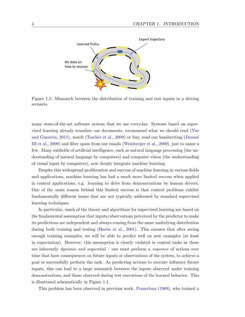
1.1 Mismatch between the distribution of training and test inputs in a drivingscenario. . . . . . . . . . . . . . . . . . . . . . . . . . . . . . . . . . . . . . . . 4
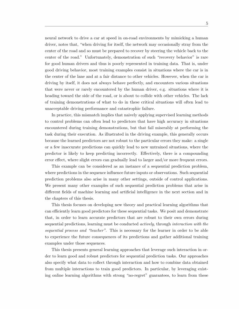
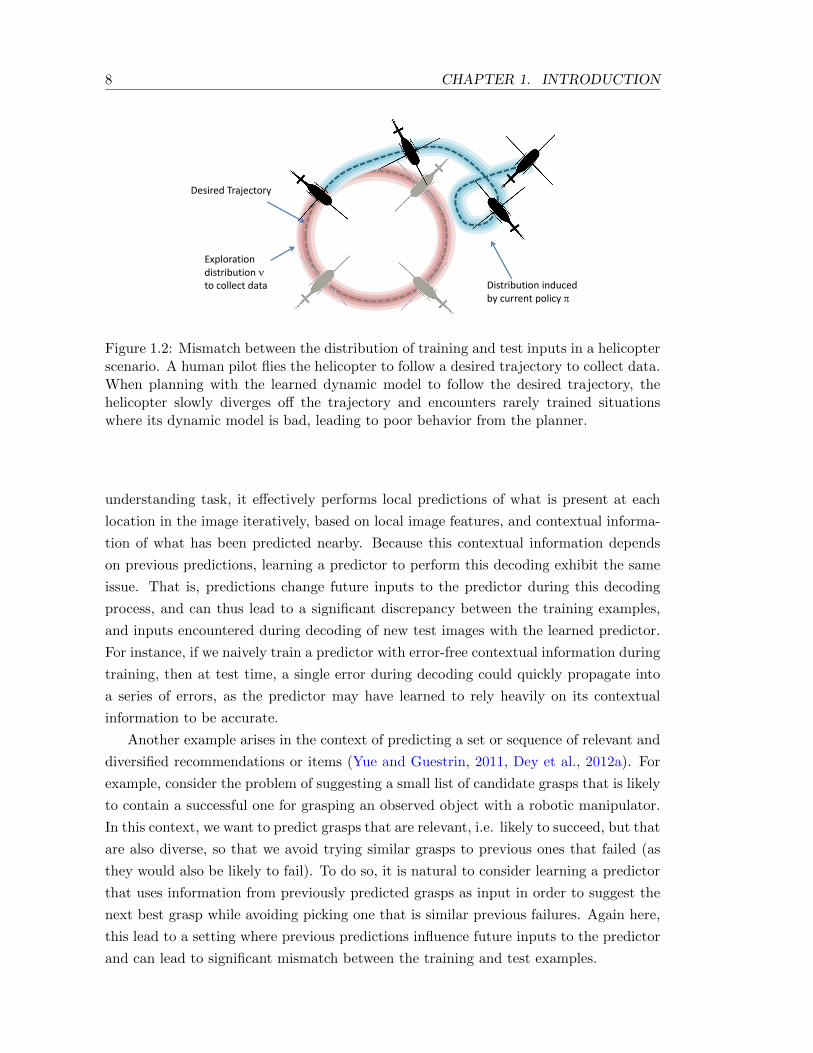
1.2 Mismatch between the distribution of training and test inputs in a helicopterscenario. A human pilot flies the helicopter to follow a desired trajectoryto collect data. When planning with the learned dynamic model to followthe desired trajectory, the helicopter slowly diverges off the trajectory andencounters rarely trained situations where its dynamic model is bad, leadingto poor behavior from the planner. . . . . . . . . . . . . . . . . . . . . . . . . 8
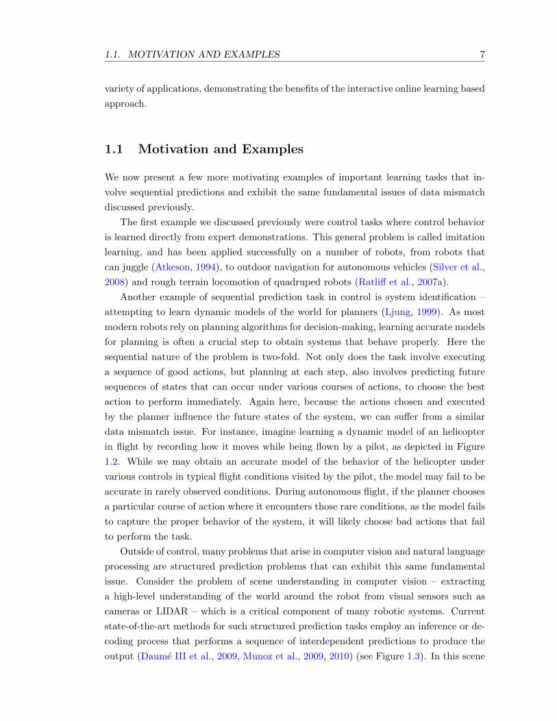
1.3 Depiction of the inference or decoding process of structured prediction meth-ods in the context of image labeling. Effectively, a sequence of predictionsare made at each pixel/image segments over the image, using local imagefeatures, and previous computations/predictions at nearby pixels/image seg-ments. This is often iterated many times over the images until predictions“converge”. . . . . . . . . . . . . . . . . . . . . . . . . . . . . . . . . . . . . . 9
1.4 Categorization of various learning tasks. . . . . . . . . . . . . . . . . . . . . . 9
1.5 Example of learning with a low complexity hypothesis in a realizable setting.Target function is a linear function. No matter where we sample data, fittinga linear function leads to roughly the same hypothesis, and obtains a goodfit of the entire function. . . . . . . . . . . . . . . . . . . . . . . . . . . . . . . 13
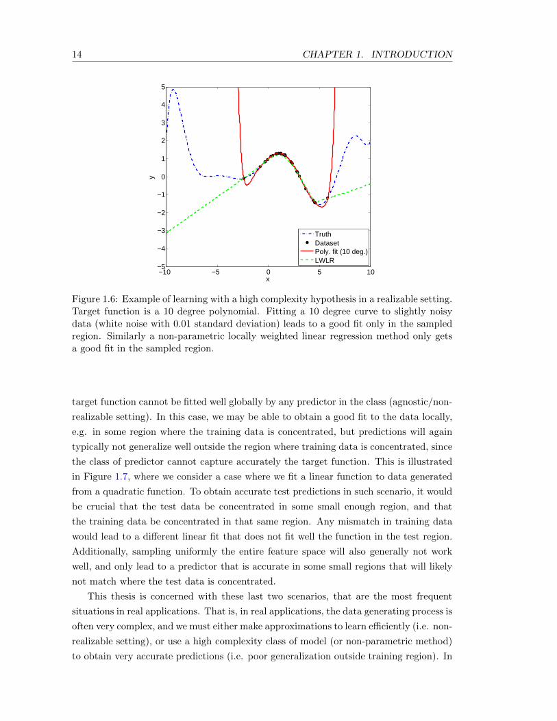
1.6 Example of learning with a high complexity hypothesis in a realizable setting.Target function is a 10 degree polynomial. Fitting a 10 degree curve to slightlynoisy data (white noise with 0.01 standard deviation) leads to a good fit onlyin the sampled region. Similarly a non-parametric locally weighted linearregression method only gets a good fit in the sampled region. . . . . . . . . . 14
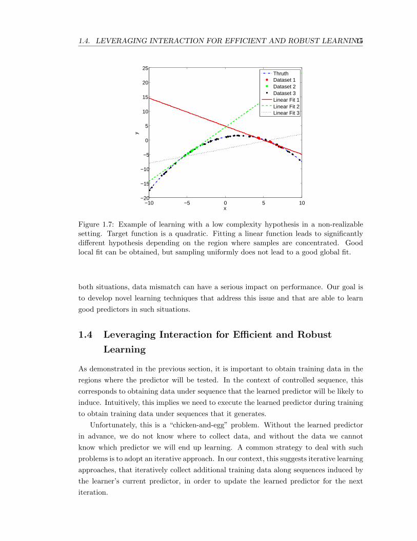
1.7 Example of learning with a low complexity hypothesis in a non-realizablesetting. Target function is a quadratic. Fitting a linear function leads tosignificantly different hypothesis depending on the region where samples areconcentrated. Good local fit can be obtained, but sampling uniformly doesnot lead to a good global fit. . . . . . . . . . . . . . . . . . . . . . . . . . . . 15
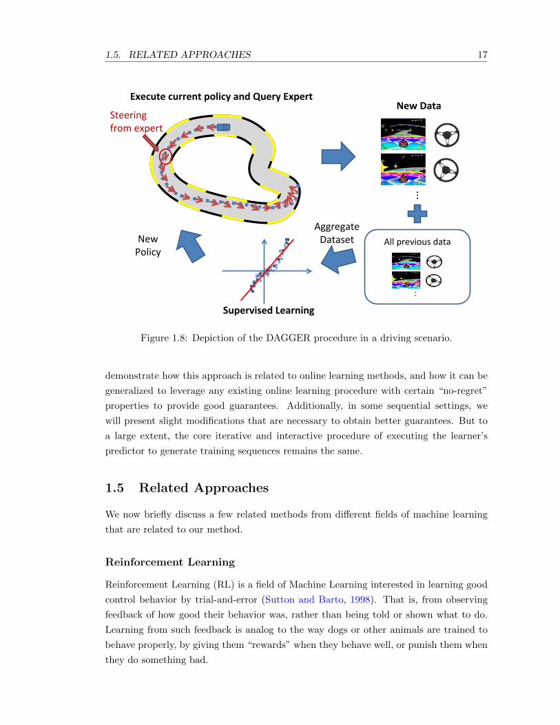
1.8 Depiction of the DAGGER procedure in a driving scenario. . . . . . . . . . . 17
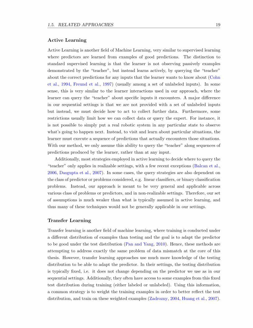
1.9 Imitation Learning Applications. (Left) Learning to drive in Super Tux Kart,(Center) Learning to play Super Mario Bros, (Right) Learning Obstacle-Avoidance for Flying through Natural Forest. . . . . . . . . . . . . . . . . . . 21
1.10 Structured Prediction Applications in Computer Vision. (Left) Parsing 3DPoint Cloud from LIDAR Sensors, (Right) Estimating 3D geometry of 2Dimages. . . . . . . . . . . . . . . . . . . . . . . . . . . . . . . . . . . . . . . . 22
x LIST OF FIGURES
3.1 Depiction of a typical supervised learning approach to imitation learning in adriving scenario. Initially, the expert demonstrates the desired driving behav-ior (top left). Input observations (camera image) and desired output actions(steering) are recorded in a dataset (top right) during the demonstration. Asupervised learning algorithm is applied to fit a policy (bottom right), e.g.linear regression of the camera image features to steering angle. The learnedpolicy is then used to drive the car autonomously (bottom left). . . . . . . . 47
3.2 Generalization of the expert’s behavior by Inverse Optimal Control methods(images from Ratliff et al. (2006)). The expert demonstrates to follow the roadbetween the start and goal location on an overhead satelite image (left). Acost function is learned from local image features that explains this behavior.The cost function is applied to a new test image (middle) (black = low cost,white = high cost). Planning with the learned cost function predicts to followthe road to the goal location on the test image (right). . . . . . . . . . . . . . 48
3.3 Example MDP where the supervised learning approach can lead to poor per-formance. There are 3 states (s0, s1, s2) and 2 actions (a1, a2), and arrowsrepresent the deterministic transitions. . . . . . . . . . . . . . . . . . . . . . . 54
3.4 Diagram of the DAGGER algorithm for imitation learning. . . . . . . . . . . 68
3.5 Depiction of the DAGGER procedure for imitation learning in a driving sce-nario. . . . . . . . . . . . . . . . . . . . . . . . . . . . . . . . . . . . . . . . . 69
3.6 Diagram of the DAGGER algorithm with a general online learner for imita-tion learning. . . . . . . . . . . . . . . . . . . . . . . . . . . . . . . . . . . . . 69
5.1 Image from Super Tux Kart’s Star Track. . . . . . . . . . . . . . . . . . . . . 98
5.2 Average falls/lap as a function of training data. . . . . . . . . . . . . . . . . . 99
5.3 Captured image from Super Mario Bros. . . . . . . . . . . . . . . . . . . . . . 100
5.4 Average distance/level as a function of data. . . . . . . . . . . . . . . . . . . 102
5.5 Application of DAGGER for autonomous MAV flight through dense forestareas. The system uses purely visual input from a single camera and imitateshuman reactive control. . . . . . . . . . . . . . . . . . . . . . . . . . . . . . . 104
5.6 The Parrot ARDrone, a cheap commercial quadrotor. . . . . . . . . . . . . . 104
5.7 One frame from MAV camera stream. The white line indicates the currentleft-right velocity commanded by the drone’s current policy πn−1 while thered line indicates the pilot’s commanded left-right velocity. In this frameDAGGER is wrongly heading for the tree in the middle while the expert isproviding the correct yaw command to go to the right instead. These expertcontrols are recorded for training later iterations but not executed in thecurrent run. . . . . . . . . . . . . . . . . . . . . . . . . . . . . . . . . . . . . . 107
5.8 Left: Indoor setup in motion capture arena with fake plastic trees and cam-ouflage in background. Right: The 11 obstacle arrangements used to trainDAGGER for every iteration in the motion capture arena. The star indicatesthe goal location. . . . . . . . . . . . . . . . . . . . . . . . . . . . . . . . . . . 108
LIST OF FIGURES xi
5.9 Left: Improvement of trajectory by DAGGER over the iterations. The right-most green trajectory is the pilot demonstration. The short trajectories in red& orange show the controller learnt in the 1st and 2nd iterations respectivelythat failed. The 3rd iteration controller successfully avoided both obstaclesand its trajectory is similar to the demonstrated trajectory. Right: Percent-age of scenarios the pilot had to intervene and the imitation loss (averagesquared error in controls of controller to human expert on hold-out data) af-ter each iteration of DAGGER. After 3 iterations, there was no need for thepilot to intervene and the UAV could successfully avoid all obstacles . . . . . 109
5.10 Common failures over iterations. While the controller has problems withtree trunks during the 1st iteration (left), this improves considerably towardsthe 3rd iteration, where mainly foliage causes problems (middle). Over alliterations, the most common failures are due to the narrow FOV of the camerawhere some trees barely appear to one side of the camera or are just hiddenoutside the view (right). When the UAV turns to avoid a visible tree a bitfarther away it collides with the tree to the side. . . . . . . . . . . . . . . . . 110
5.11 Percentage of failures of each type for DAGGER over the iterations of trainingin the high-density region. Blue: Large Trees, Orange: Thin Trees, Yellow:Leaves and Branches, Green: Other obstacles (poles, signs, etc.), Red: TooNarrow FOV. Clearly, a majority of the crashes happen due to a too narrowFOV and obstacles which are hard to perceive, such as branches and leaves. . 111
5.12 Average distance flown autonomously by the drone before a failure. Left:Low-Density Region, Right: High-Density Region. . . . . . . . . . . . . . . . 112
5.13 Example flight in dense forest. Images ordered from top (t = 0s) to bottom (t = 6.6s);
with color-coded commands issued by DAGGER (in MAV’s view). After avoiding tree A
(frame 3), drone still rolls strongly to the left (frame 4), in part due to latency. Then tree
B is avoided on the left (frame 5-7), rather than on the more intuitive right. Drone prefers
this due to the drift feature, as inertia is already pushing it further to the left. . . . . . . 114
5.14 Breakdown of the contribution of the different features for different controlprediction strengths, averaged over 9389 datapoints. Laws and Radon aremore significant in cases where small controls are performed (e.g. emptyscenes), whereas the structure tensor and optical flow are responsible forstrong controls (e.g. in cases where the scene contains an imminent obstacle).A slight bias to the left can be seen, which is consistent to observations inthe field. Best viewed in color. . . . . . . . . . . . . . . . . . . . . . . . . . . 115
5.15 Visualization of the contribution of the different features to the predictedcontrol. The overall control was a hard left command. The arrows show thecontribution of a given feature at every window. Structure tensor featureshave the largest contribution in this example, while Radon has the least. . . . 116
6.1 Example structured prediction application of image labeling. Images fromCamSeq01 dataset (Fauqueur et al., 2007). . . . . . . . . . . . . . . . . . . . 120
xii LIST OF FIGURES
6.2 Graphical Model approach to Structured Prediction in the context of imagelabeling. Pairwise potentials model dependencies between objects at neigh-boring pixels and unary potentials model the likehood of an object present ata pixel given the local image features. Inference, such as loopy belief propa-gation, is performed to find an approximate minimum energy solution whichis returned as output. . . . . . . . . . . . . . . . . . . . . . . . . . . . . . . . 121
6.3 Example predictions obtained by independently classifying each 3D pointindependently in a LIDAR point cloud with a SVM, using only local featuresof the point cloud. Red: Building, Green: Tree, Blue: Shrubbery, Gray:Ground. Significant noise is present in the classifications and many pointsin the building are incorrectly classified as tree. Image from Anguelov et al.(2005). . . . . . . . . . . . . . . . . . . . . . . . . . . . . . . . . . . . . . . . 125
6.4 Sequence of predictions made by Auto-Context on a test image (images fromTu and Bai. (2009)). Left: Input image. Middle-Left: Predictions of the1st predictor using only image features. Middle-Right: Predictions of the3rd predictor, using image features and predictions of the 2nd predictor asinput. Right: Predictions of the 5th (final) predictor, using image features andpredictions of the 4th predictor as input. Predictions are shown in grayscale,where black indicates probability 0 of horse and white indicates probability1 of horse. . . . . . . . . . . . . . . . . . . . . . . . . . . . . . . . . . . . . . . 126
6.5 Depiction of how LBP unrolls into a sequence of predictions for 3 passes onthe graph on the left with 3 variables (A,B,C) and 3 factors (1,2,3); for thecase where LBP starts at A, followed by B and C (and alternating betweenforward/backward order). Sequence of predictions on the right, where e.g.,A1 denotes the prediction (message) of A sent to factor 1, while the output(final marginals) are in gray and denoted by the corresponding variable letter.Input arrows indicate the previous outputs that are used in the computationof each message. . . . . . . . . . . . . . . . . . . . . . . . . . . . . . . . . . . 130
6.6 Depiction of the computations that the predictor represents in LBP for (a)a message to a neighboring factor and (b) the final marginal of a variableoutputed by LBP. . . . . . . . . . . . . . . . . . . . . . . . . . . . . . . . . . 131
6.7 Depiction of the inference machine in the context of image labeling. . . . . . 132
6.8 Depiction of the DAGGER algorithm for Structured Prediction in the contextof an image labeling task. . . . . . . . . . . . . . . . . . . . . . . . . . . . . . 138
6.9 Character accuracy as a function of iteration. . . . . . . . . . . . . . . . . . . 141
6.10 3D point cloud classification application. Each point is assigned to one of 5object classes: Building (red), Ground (orange), Poles/Tree-Trunks (blue),Vegetation (green), and Wire (cyan). . . . . . . . . . . . . . . . . . . . . . . . 142
6.11 Average test error as a function of pass for each message-passing method onthe 3D classification task. . . . . . . . . . . . . . . . . . . . . . . . . . . . . . 145
6.12 Estimated 3D point cloud labels with M3N-F (top left), M3N-P (top right),MFIM (bottom left), Ground truth (bottom right). . . . . . . . . . . . . . . 146
6.13 3D Geometry estimation application. Each superpixel is assigned to one of7 classes: sky, ground, left-perspective, right-perspective, center-perspective,solid or porous. . . . . . . . . . . . . . . . . . . . . . . . . . . . . . . . . . . . 147

LIST OF FIGURES xiii
6.14 Estimated 3D geometric surface layouts on a city scene with M3N-F (topleft), Hoiem et al. (2007) (top right), BPIM-D (bottom left), Ground truth(bottom right). . . . . . . . . . . . . . . . . . . . . . . . . . . . . . . . . . . 148
6.15 Estimated 3D geometric surface layouts on a street scene with M3N-F (topleft), Hoiem et al. (2007) (top right), BPIM-D (bottom left), Ground truth(bottom right). . . . . . . . . . . . . . . . . . . . . . . . . . . . . . . . . . . 149
7.1 Example Recommendation Applications. Left: Ad placement, where we wantto display a small list of ads the user is likely going to click on. Center: NewsRecommendation, where we want to display a small list of news article likelyto interest the user. Right: Grasp Selection, where we want to select a smalllist of grasps likely to succeed at picking an object. . . . . . . . . . . . . . . . 152
7.2 Depiction of an ordering selected in the Grasp Selection Task . . . . . . . . . 166
7.3 Average depth of the list searched before finding a successful grasps. SCPperforms better at low data availability but eventually ConSeqOpt performsbetter as it can order grasps better by using different distributions at eachposition in the list. . . . . . . . . . . . . . . . . . . . . . . . . . . . . . . . . . 168
7.4 Depiction of the Trajectory Optimization Application. A list of initial seedtrajectories is suggested to a local optimization procedure (CHOMP). CHOMPtries to locally optimize the current seed trajectory, and if stuck at a localminima in collision, restarts with the next seed trajectory in the list, until itobtains a local minima that is collision-free. . . . . . . . . . . . . . . . . . . . 168
7.5 Probability of failure of each method on the test environments. SCP per-forms better at even low data availability while ConSeqOpt suffers from datastarvation issues. . . . . . . . . . . . . . . . . . . . . . . . . . . . . . . . . . . 169
7.6 Probability of no click on the test users on the news recommendation task.With increase in slots SCP predicts news articles which have lower probabilityof the user not clicking on any of them compared to ConSeqOpt . . . . . . . 170
7.7 Rouge-1R scores on the test documents with respect to the size of trainingdata. . . . . . . . . . . . . . . . . . . . . . . . . . . . . . . . . . . . . . . . . . 172
8.1 Depiction of the DAGGER algorithm for System Identification in the contextof helicopter control. . . . . . . . . . . . . . . . . . . . . . . . . . . . . . . . 184
8.2 Depiction of the swing-up task. First 10 frames at 0.5s intervals of a near-optimal controller. Top Left: Initial State at 0s. Following frames in top rowat 0.5s intervals from left to right, then continued from left to right in thebottom row. Bottom Right: Frame at 4.5s illustrates the inverted positionthat must be maintained until the end of the 10s trajectory. . . . . . . . . . . 197
8.3 Average total cost on test trajectories at the swing-up task as a function ofdata collected so far. . . . . . . . . . . . . . . . . . . . . . . . . . . . . . . . . 199
8.4 Average total cost on test trajectories as a function of data collected so far,averaged over 20 repetitions of the experiments, each starting with a differentrandom seed (all approaches use the same 20 seeds) From top to bottom:hover with no delay, hover with delay of 1, nose-in funnel. Dt, De and Den
denotes DAGGER using exploration distribution νt, νe and νen respectively,similarly Bt, Be and Ben for the Batch algorithm, A for Abbeel’s algorithm,and L for the linearized model’s optimal controller. . . . . . . . . . . . . . . 204

xiv LIST OF FIGURES
8.5 Average total cost on test trajectories as a function of data collected so far,averaged over 20 repetitions of the experiments, each starting with a differ-ent random seed (all approaches use the same 20 seeds) From top to bottom:hover with no delay, hover with delay of 1, nose-in funnel. AbN denotesAbbeel’s algorithm where the first N iterations collect data with the expert(exploration distribution νe); Dag and B denotes DAGGER and Batch us-ing exploration distribution νe respectively, and L for the linearized model’soptimal controller. . . . . . . . . . . . . . . . . . . . . . . . . . . . . . . . . . 205
10.1 Depiction of the Tree MDP. State represents the entire action sequence sofar, transitions are deterministic as represented by the arrows, and simplyappends the action to the current state. The initial state is the root. Thetree has branching factor A and extends to infinite depth. . . . . . . . . . . . 214

List of Tables
6.1 Comparisons of test performance on the 3D point cloud dataset. . . . . . . . 1446.2 Comparisons of test performance on the 3D Geometry Estimation dataset. . 147
7.1 ROUGE unigram score on the DUC 2004 test documents. . . . . . . . . . . . 172


Chapter 1
Introduction
One of the main goal of robotics and artificial intelligence is the development of au-
tonomous systems and software agents that can aid humans in their everyday tasks.
Programming such systems however, has proven to be a remarkably challenging and
time consuming task. Despite the many advances in planning and control for developing
advanced automated decision-making software, these methods rely on key pieces of infor-
mation that are often very hard to specify by humans. In particular, accurate dynamic
models of the world, that can correctly predict the long-term consequences of various
courses of actions, and a suitable cost function, that properly trades-off the desirability
or utility of various outcomes to the designer of the system. While this information can
often be easily provided for simple board games (e.g. chess), or simple robots operating
in very controlled environments (e.g. robot arm in a factory), it is a much harder task
for complex robotic systems deployed in uncontrolled environments (e.g. robot walking
outdoors or autonomous driving in an urban environment). Properly specifying all these
parameters to obtain the desired behavior of the system is often a very daunting task
of informed “guess-and-check” that can require hundreds or thousands of man hours
depending on the complexity of the system, and that often only leads to subpar perfor-
mance due to inaccurate and suboptimal specification of these parameters (Ratliff, 2009,
Silver, 2010).
While specifying all these parameters is a complex task for human engineers, the
desired behavior of the system is often clear and can often be easily demonstrated by
humans. For instance, humans can easily drive in urban environments, or walk-around
on various terrains. This motivates the use of data-driven machine learning approaches
that can effectively leverage such demonstrations of good behavior to optimize these
parameters or learn directly a controller that replicates the desired behavior.
Machine learning, in particular supervised learning, where predictors are learned
from examples of good behaviors/predictions, has already had a large impact in various
fields and applications. In fact, this has become the de facto method of choice behind
4 CHAPTER 1. INTRODUCTION
Expert trajectory
Learned Policy
No data on
how to recover
Figure 1.1: Mismatch between the distribution of training and test inputs in a drivingscenario.
many state-of-the-art software system that we use everyday. Systems based on super-
vised learning already translate our documents, recommend what we should read (Yue
and Guestrin, 2011), watch (Toscher et al., 2009) or buy, read our handwriting (Daume
III et al., 2009) and filter spam from our emails (Weinberger et al., 2009), just to name a
few. Many subfields of artificial intelligence, such as natural language processing (the un-
derstanding of natural language by computers) and computer vision (the understanding
of visual input by computers), now deeply integrate machine learning.
Despite this widespread proliferation and success of machine learning in various fields
and applications, machine learning has had a much more limited success when applied
in control applications, e.g. learning to drive from demonstrations by human drivers.
One of the main reason behind this limited success is that control problems exhibit
fundamentally different issues that are not typically addressed by standard supervised
learning techniques.
In particular, much of the theory and algorithms for supervised learning are based on
the fundamental assumption that inputs/observations perceived by the predictor to make
its predictions are independent and always coming from the same underlying distribution
during both training and testing (Hastie et al., 2001). This ensures that after seeing
enough training examples, we will be able to predict well on new examples (at least
in expectation). However, this assumption is clearly violated in control tasks as these
are inherently dynamic and sequential : one must perform a sequence of actions over
time that have consequences on future inputs or observations of the system, to achieve a
goal or successfully perform the task. As predicting actions to execute influence future
inputs, this can lead to a large mismatch between the inputs observed under training
demonstrations, and those observed during test executions of the learned behavior. This
is illustrated schematically in Figure 1.1.
This problem has been observed in previous work. Pomerleau (1989), who trained a
5
neural network to drive a car at speed in on-road environments by mimicking a human
driver, notes that, “when driving for itself, the network may occasionally stray from the
center of the road and so must be prepared to recover by steering the vehicle back to the
center of the road.” Unfortunately, demonstration of such “recovery behavior” is rare
for good human drivers and thus is poorly represented in training data. That is, under
good driving behavior, most training examples consist in situations where the car is in
the center of the lane and at a fair distance to other vehicles. However, when the car is
driving by itself, it does not always behave perfectly, and encounters various situations
that were never or rarely encountered by the human driver, e.g. situations where it is
heading toward the side of the road, or is about to collide with other vehicles. The lack
of training demonstrations of what to do in these critical situations will often lead to
unacceptable driving performance and catastrophic failure.
In practice, this mismatch implies that naively applying supervised learning methods
to control problems can often lead to predictors that have high accuracy in situations
encountered during training demonstrations, but that fail miserably at performing the
task during their execution. As illustrated in the driving example, this generally occurs
because the learned predictors are not robust to the particular errors they make: a single
or a few inaccurate predictions can quickly lead to new untrained situations, where the
predictor is likely to keep predicting incorrectly. Effectively, there is a compounding
error effect, where slight errors can gradually lead to larger and/or more frequent errors.
This example can be considered as an instance of a sequential prediction problem,
where predictions in the sequence influence future inputs or observations. Such sequential
prediction problems also arise in many other settings, outside of control applications.
We present many other examples of such sequential prediction problems that arise in
different fields of machine learning and artificial intelligence in the next section and in
the chapters of this thesis.
This thesis focuses on developing new theory and practical learning algorithms that
can efficiently learn good predictors for these sequential tasks. We posit and demonstrate
that, in order to learn accurate predictors that are robust to their own errors during
sequential predictions, learning must be conducted actively, through interaction with the
sequential process and “teacher”. This is necessary for the learner in order to be able
to experience the future consequences of its predictions and gather additional training
examples under those sequences.
This thesis presents general learning approaches that leverage such interaction in or-
der to learn good and robust predictors for sequential prediction tasks. Our approaches
also specify what data to collect through interaction and how to combine data obtained
from multiple interactions to train good predictors. In particular, by leveraging exist-
ing online learning algorithms with strong “no-regret” guarantees, to learn from these
6 CHAPTER 1. INTRODUCTION
interactions, our methods can guarantee learning good predictors for sequential tasks.
We demonstrate how to apply these methods in various sequential prediction settings,
from control problems to general structured prediction problems that arise commonly
in computer vision and natural language processing, as well as recommendation tasks
where sequences of relevant and diversified items must be predicted.
In each of these settings, we provide a complete theoretical analysis of our methods,
showing strong performance guarantees and data efficiency (low sample complexity). We
also validate our methods empirically, and demonstrate state-of-the-art performance in
various important and challenging learning tasks, ranging from learning video game play-
ing agents from human players and accurate dynamic models of a simulated helicopter
for controller synthesis, to learning predictors for scene understanding in computer vi-
sion, news recommendation and document summarization. We also demonstrate the
applicability of our main technique on a real robot, using pilot demonstrations to train
an autonomous quadrotor to avoid trees seen through its onboard camera (monocular
vision) when flying at low-altitude in natural forest environments.
On the more philosophical side, we also show that at a fundamental level, interaction
is necessary for learning in these sequential settings. Unlike supervised learning, learning
only from observing examples of good behavior is not sufficient. In particular, it is shown
that any non interactive learning algorithm cannot provide good guarantees in general
and may always learn predictors that are not robust to their own errors. We present a
tight theoretical lower bound on the minimum number of rounds of interactions required
that is achieved (within a constant factor) by one of the algorithm presented in Chapter
3. Our lower bound demonstrates that the number of rounds must inevitably scale
linearly with the length of the sequential prediction problems (task horizon).
Thesis Statement
We now make the main statement of this thesis:
Learning actively through interaction is necessary to obtain good
and robust predictors for sequential prediction tasks. No-regret
online learning methods provide a useful class of algorithms to learn
efficiently from these interactions, and provide good performance
both theoretically and empirically.
We validate this claim by 1) presenting detailed theoretical analysis of non-interactive
learning procedures and active interactive learning procedures, based on online learning
methods, in various sequential prediction settings and showing improved guarantees; 2)
proving formally that no learning algorithm can provide good guarantees without some
minimum number of interactions; and 3) empirically comparing performance in a large
1.1. MOTIVATION AND EXAMPLES 7
variety of applications, demonstrating the benefits of the interactive online learning based
approach.
1.1 Motivation and Examples
We now present a few more motivating examples of important learning tasks that in-
volve sequential predictions and exhibit the same fundamental issues of data mismatch
discussed previously.
The first example we discussed previously were control tasks where control behavior
is learned directly from expert demonstrations. This general problem is called imitation
learning, and has been applied successfully on a number of robots, from robots that
can juggle (Atkeson, 1994), to outdoor navigation for autonomous vehicles (Silver et al.,
2008) and rough terrain locomotion of quadruped robots (Ratliff et al., 2007a).
Another example of sequential prediction task in control is system identification –
attempting to learn dynamic models of the world for planners (Ljung, 1999). As most
modern robots rely on planning algorithms for decision-making, learning accurate models
for planning is often a crucial step to obtain systems that behave properly. Here the
sequential nature of the problem is two-fold. Not only does the task involve executing
a sequence of good actions, but planning at each step, also involves predicting future
sequences of states that can occur under various courses of actions, to choose the best
action to perform immediately. Again here, because the actions chosen and executed
by the planner influence the future states of the system, we can suffer from a similar
data mismatch issue. For instance, imagine learning a dynamic model of an helicopter
in flight by recording how it moves while being flown by a pilot, as depicted in Figure
1.2. While we may obtain an accurate model of the behavior of the helicopter under
various controls in typical flight conditions visited by the pilot, the model may fail to be
accurate in rarely observed conditions. During autonomous flight, if the planner chooses
a particular course of action where it encounters those rare conditions, as the model fails
to capture the proper behavior of the system, it will likely choose bad actions that fail
to perform the task.
Outside of control, many problems that arise in computer vision and natural language
processing are structured prediction problems that can exhibit this same fundamental
issue. Consider the problem of scene understanding in computer vision – extracting
a high-level understanding of the world around the robot from visual sensors such as
cameras or LIDAR – which is a critical component of many robotic systems. Current
state-of-the-art methods for such structured prediction tasks employ an inference or de-
coding process that performs a sequence of interdependent predictions to produce the
output (Daume III et al., 2009, Munoz et al., 2009, 2010) (see Figure 1.3). In this scene
8 CHAPTER 1. INTRODUCTION
Exploration
distribution to collect data Distribution induced
by current policy
Desired Trajectory
Figure 1.2: Mismatch between the distribution of training and test inputs in a helicopterscenario. A human pilot flies the helicopter to follow a desired trajectory to collect data.When planning with the learned dynamic model to follow the desired trajectory, thehelicopter slowly diverges off the trajectory and encounters rarely trained situationswhere its dynamic model is bad, leading to poor behavior from the planner.
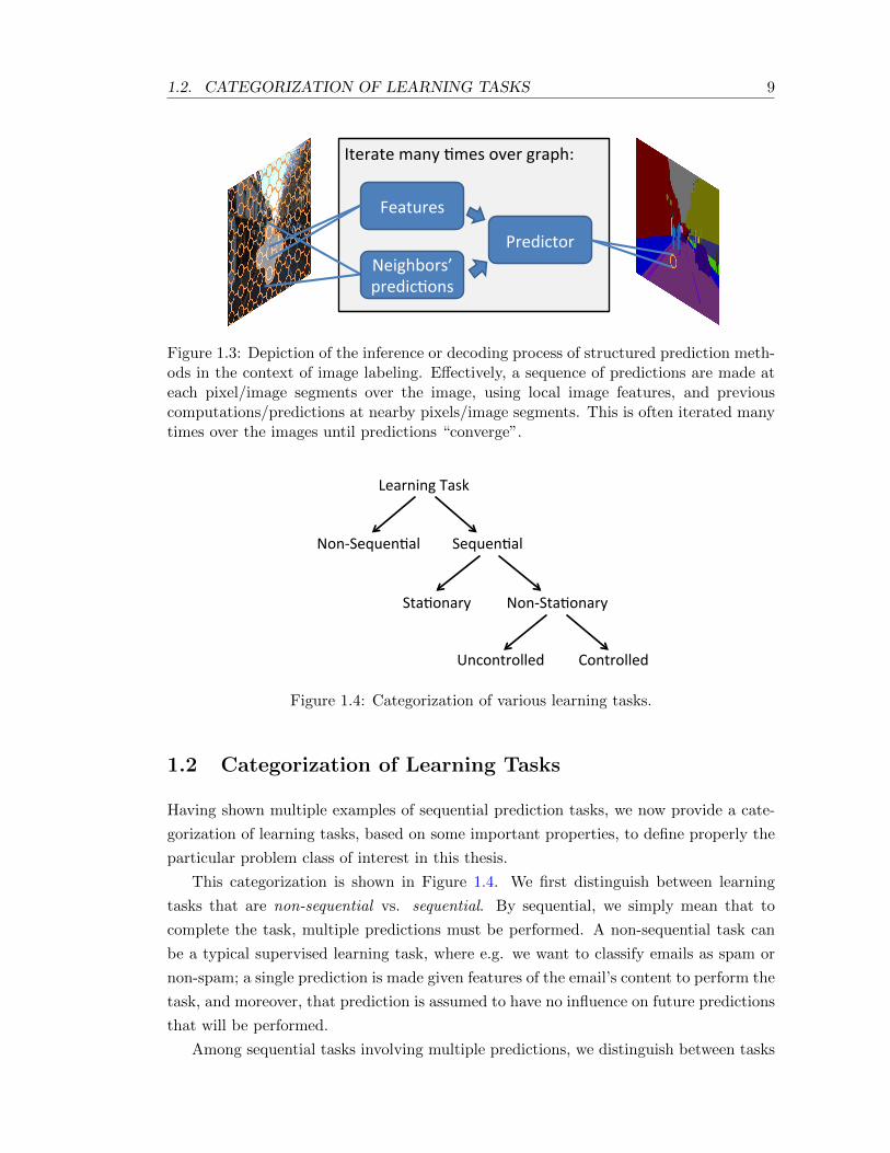
understanding task, it effectively performs local predictions of what is present at each
location in the image iteratively, based on local image features, and contextual informa-
tion of what has been predicted nearby. Because this contextual information depends
on previous predictions, learning a predictor to perform this decoding exhibit the same
issue. That is, predictions change future inputs to the predictor during this decoding
process, and can thus lead to a significant discrepancy between the training examples,
and inputs encountered during decoding of new test images with the learned predictor.
For instance, if we naively train a predictor with error-free contextual information during
training, then at test time, a single error during decoding could quickly propagate into
a series of errors, as the predictor may have learned to rely heavily on its contextual
information to be accurate.
Another example arises in the context of predicting a set or sequence of relevant and
diversified recommendations or items (Yue and Guestrin, 2011, Dey et al., 2012a). For
example, consider the problem of suggesting a small list of candidate grasps that is likely
to contain a successful one for grasping an observed object with a robotic manipulator.
In this context, we want to predict grasps that are relevant, i.e. likely to succeed, but that
are also diverse, so that we avoid trying similar grasps to previous ones that failed (as
they would also be likely to fail). To do so, it is natural to consider learning a predictor
that uses information from previously predicted grasps as input in order to suggest the
next best grasp while avoiding picking one that is similar previous failures. Again here,
this lead to a setting where previous predictions influence future inputs to the predictor
and can lead to significant mismatch between the training and test examples.
1.2. CATEGORIZATION OF LEARNING TASKS 9
Iterate many *mes over graph:
Neighbors’
predic*ons
Features
Predictor
Figure 1.3: Depiction of the inference or decoding process of structured prediction meth-ods in the context of image labeling. Effectively, a sequence of predictions are made ateach pixel/image segments over the image, using local image features, and previouscomputations/predictions at nearby pixels/image segments. This is often iterated manytimes over the images until predictions “converge”.
Learning Task
Non‐Sequen2al Sequen2al
Sta2onary Non‐Sta2onary
Uncontrolled Controlled
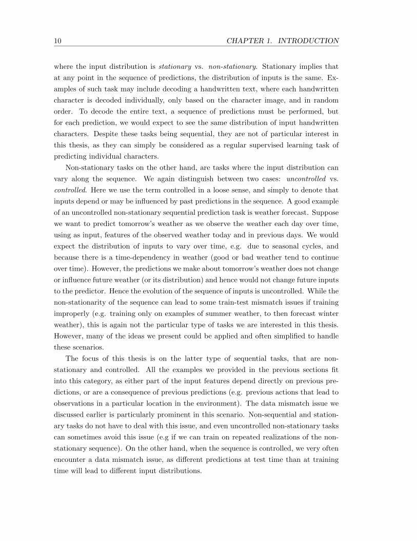
Figure 1.4: Categorization of various learning tasks.
1.2 Categorization of Learning Tasks
Having shown multiple examples of sequential prediction tasks, we now provide a cate-
gorization of learning tasks, based on some important properties, to define properly the
particular problem class of interest in this thesis.
This categorization is shown in Figure 1.4. We first distinguish between learning
tasks that are non-sequential vs. sequential. By sequential, we simply mean that to
complete the task, multiple predictions must be performed. A non-sequential task can
be a typical supervised learning task, where e.g. we want to classify emails as spam or
non-spam; a single prediction is made given features of the email’s content to perform the
task, and moreover, that prediction is assumed to have no influence on future predictions
that will be performed.
Among sequential tasks involving multiple predictions, we distinguish between tasks
10 CHAPTER 1. INTRODUCTION
where the input distribution is stationary vs. non-stationary. Stationary implies that
at any point in the sequence of predictions, the distribution of inputs is the same. Ex-
amples of such task may include decoding a handwritten text, where each handwritten
character is decoded individually, only based on the character image, and in random
order. To decode the entire text, a sequence of predictions must be performed, but
for each prediction, we would expect to see the same distribution of input handwritten
characters. Despite these tasks being sequential, they are not of particular interest in
this thesis, as they can simply be considered as a regular supervised learning task of
predicting individual characters.
Non-stationary tasks on the other hand, are tasks where the input distribution can
vary along the sequence. We again distinguish between two cases: uncontrolled vs.
controlled. Here we use the term controlled in a loose sense, and simply to denote that
inputs depend or may be influenced by past predictions in the sequence. A good example
of an uncontrolled non-stationary sequential prediction task is weather forecast. Suppose
we want to predict tomorrow’s weather as we observe the weather each day over time,
using as input, features of the observed weather today and in previous days. We would
expect the distribution of inputs to vary over time, e.g. due to seasonal cycles, and
because there is a time-dependency in weather (good or bad weather tend to continue
over time). However, the predictions we make about tomorrow’s weather does not change
or influence future weather (or its distribution) and hence would not change future inputs
to the predictor. Hence the evolution of the sequence of inputs is uncontrolled. While the
non-stationarity of the sequence can lead to some train-test mismatch issues if training
improperly (e.g. training only on examples of summer weather, to then forecast winter
weather), this is again not the particular type of tasks we are interested in this thesis.
However, many of the ideas we present could be applied and often simplified to handle
these scenarios.
The focus of this thesis is on the latter type of sequential tasks, that are non-
stationary and controlled. All the examples we provided in the previous sections fit
into this category, as either part of the input features depend directly on previous pre-
dictions, or are a consequence of previous predictions (e.g. previous actions that lead to
observations in a particular location in the environment). The data mismatch issue we
discussed earlier is particularly prominent in this scenario. Non-sequential and station-
ary tasks do not have to deal with this issue, and even uncontrolled non-stationary tasks
can sometimes avoid this issue (e.g if we can train on repeated realizations of the non-
stationary sequence). On the other hand, when the sequence is controlled, we very often
encounter a data mismatch issue, as different predictions at test time than at training
time will lead to different input distributions.

1.3. THE CHALLENGE OF LEARNING SEQUENTIAL PREDICTIONS 11
1.3 The Challenge of Learning Sequential Predictions
We now explain in more detail the particular challenges of learning in these controlled
sequential tasks.
Data Mismatch : When is it Significant?
As mentioned earlier, one of the major difficulties that occur in sequential prediction
problems is that there can be a large discrepancy between the training and test distribu-
tion of examples, when the predictions made by the learned predictor differ from those
on the observed sequence during training. In large and real world applications, where
some degree of approximation is often inevitable, it is rarely the case that the learned
behavior is able to reproduce exactly an observed behavior during training. Thus such
discrepancy between training and test inputs/observations often occur. However there
are different cases where this effect is more important than others. We here explain
various cases and how they impact the data mismatch. These will be important cases to
keep in mind to understand when the data mismatch can become a significant issue.
Highly Stochastic vs. Near-Deterministic Sequences
In some tasks, stochasticity can play a large role on the evolution of the input of the
sequence, and limit to a large extent the effects of the predictions. An example of this
is the game of Backgammon, where the evolution of the game is highly randomized and
depends significantly on die rolls. While the players still choose which pieces to move,
and have an effect on the evolution of the game, they have limited control over the future
outcomes or situations encountered during the course of a game. To a large extent, the
distribution of board configurations encountered over many games may cover almost all
board configurations, and be only slightly more concentrated in some areas of the feature
space, depending on the strategy used. Thus if we would attempt to learn to play this
game, e.g. from observing other players, we would expect to observe inputs that covers
most of the feature space during training. Since there is no situations that are much
more likely under some strategy than observed during human player play, a fairly good
estimate on the performance of any game playing strategy could be obtained, even if
there is a slight mismatch on where the inputs are more or less concentrated. In this
case we may expect the data mismatch to be a non-issue, or only have a limited impact
on performance.
On the other hand, the opposite occur in situations where the evolution of the se-
quence is near-deterministic and largely determined by the past predictions. This is the
case encountered by most robotic systems where the movement of the robot is determin-
istic (or nearly so), and to a large extent determined by the previously predicted actions.
12 CHAPTER 1. INTRODUCTION
Often even small changes in the actions can lead to a large change in configuration after
some time (e.g. robot walking where a small perturbation can lead a stable walker to
lose balance). Thus in such setting, data mismatch can be very important and critical
to address to obtain good performance. These are the settings that are of most interest
in this thesis, given their frequent occurrence in robotic applications.
Relevance of Controlled Features
In some situations, only a fraction of the features (information used to make predictions)
depends on previous predictions. This is the case in some of the examples presented
earlier. For instance, in the scene understanding example where the local image features
used do not depend on past predictions in the sequence, and only features related to
neighboring predictions depend on past predictions. The data mismatch issue only affects
these features which depend on previous predictions and how to use them appropriately.
If there is a large fraction of features that do not depend on previous predictions, and the
contribution of each feature to the final prediction is limited (e.g. linear classifier with
regularization), then the data mismatch can be a non-issue, as improving how we use a
small fraction of the features will have a very limited effect on the predictions. In general,
if good predictions can be obtained by relying heavily on only the independent features
(e.g. the local image features), then the data mismatch may be irrelevant. However, if it
is critical to use significantly the features depending on previous predictions, compared
to the independent features, then it will be critical to properly deal with this issue to
obtain good performance. We will be particularly interested to these situations where
using these features is critical for good performance.
Realizability and Generalizability of Hypothesis Class
Even though we may be in a situation where there is a significant mismatch in the
distribution of training and testing examples, depending on how the data is generated
and what class of predictors we are considering, the data mismatch may be a non-issue.
To illustrate this, imagine a case where the generated data is a linear function of
the features, with some noise, and we attempt to learn a linear predictor. Then no
matter where data is sampled we may be able to recover the correct linear function, and
generalize well to any region of the input space that we didn’t observe during training.
Therefore even if we are tested mostly in a different region, we would still be able to
predict accurately. This is illustrated in Figure 1.5. This shows that in situations where
both 1) the class of predictors contains predictors that can fit very well the observed
data (realizable settings) and 2) that generalize well across the entire feature space (e.g.
with a low complexity class), then where data is collected often doesn’t matter. These

1.3. THE CHALLENGE OF LEARNING SEQUENTIAL PREDICTIONS 13
−10 −5 0 5 10−6
−4
−2
0
2
4
6
8
x
y
ThruthDataset 1Dataset 2Linear Fit 1Linear Fit 2
Figure 1.5: Example of learning with a low complexity hypothesis in a realizable setting.Target function is a linear function. No matter where we sample data, fitting a linearfunction leads to roughly the same hypothesis, and obtains a good fit of the entirefunction.
are easy cases that are not of concern in this thesis. This has been the most common
paradigm for analyzing performance in control problems (Ljung, 1999).
On the other hand, when at least one of these two properties does not hold, then
where data is collected has a significant impact. For instance, even in a realizable setting
where we can obtain a very good fit to any observed training data, if we are learning a
high complexity predictor (which is usually necessary to be able to fit the training data
well everywhere), the predictor will typically not generalize too well to regions of the
feature space that were never or rarely observed. This is shown in Figure 1.6. This is
because high complexity class allows for a wide range of functions that fit the training
data well, but vary greatly outside the region where training data was collected. This
implies that correct predictions outside of the training region is highly undetermined
or uncertain. Thus, in such setting data mismatch can lead to very bad predictions at
test time. In particular, it is important that the training data covers well the regions
where the predictor is tested, in order to predict accurately at test time. While we may
attempt to sample uniformly the entire input space to ensure sufficient coverage of any
possible test regions, this does not scale well to high-dimensions (covering the volume of
the input space would require an exponential number of samples in the dimensionality
of the input).
Similarly, where data is collected has a significant impact in situations where the
14 CHAPTER 1. INTRODUCTION
−10 −5 0 5 10−5
−4
−3
−2
−1
0
1
2
3
4
5
x
y
TruthDatasetPoly. fit (10 deg.)LWLR
Figure 1.6: Example of learning with a high complexity hypothesis in a realizable setting.Target function is a 10 degree polynomial. Fitting a 10 degree curve to slightly noisydata (white noise with 0.01 standard deviation) leads to a good fit only in the sampledregion. Similarly a non-parametric locally weighted linear regression method only getsa good fit in the sampled region.
target function cannot be fitted well globally by any predictor in the class (agnostic/non-
realizable setting). In this case, we may be able to obtain a good fit to the data locally,
e.g. in some region where the training data is concentrated, but predictions will again
typically not generalize well outside the region where training data is concentrated, since
the class of predictor cannot capture accurately the target function. This is illustrated
in Figure 1.7, where we consider a case where we fit a linear function to data generated
from a quadratic function. To obtain accurate test predictions in such scenario, it would
be crucial that the test data be concentrated in some small enough region, and that
the training data be concentrated in that same region. Any mismatch in training data
would lead to a different linear fit that does not fit well the function in the test region.
Additionally, sampling uniformly the entire feature space will also generally not work
well, and only lead to a predictor that is accurate in some small regions that will likely
not match where the test data is concentrated.
This thesis is concerned with these last two scenarios, that are the most frequent
situations in real applications. That is, in real applications, the data generating process is
often very complex, and we must either make approximations to learn efficiently (i.e. non-
realizable setting), or use a high complexity class of model (or non-parametric method)
to obtain very accurate predictions (i.e. poor generalization outside training region). In
1.4. LEVERAGING INTERACTION FOR EFFICIENT AND ROBUST LEARNING15
−10 −5 0 5 10−20
−15
−10
−5
0
5
10
15
20
25
x
y
ThruthDataset 1Dataset 2Dataset 3Linear Fit 1Linear Fit 2Linear Fit 3
Figure 1.7: Example of learning with a low complexity hypothesis in a non-realizablesetting. Target function is a quadratic. Fitting a linear function leads to significantlydifferent hypothesis depending on the region where samples are concentrated. Goodlocal fit can be obtained, but sampling uniformly does not lead to a good global fit.
both situations, data mismatch can have a serious impact on performance. Our goal is
to develop novel learning techniques that address this issue and that are able to learn
good predictors in such situations.
1.4 Leveraging Interaction for Efficient and Robust
Learning
As demonstrated in the previous section, it is important to obtain training data in the
regions where the predictor will be tested. In the context of controlled sequence, this
corresponds to obtaining data under sequence that the learned predictor will be likely to
induce. Intuitively, this implies we need to execute the learned predictor during training
to obtain training data under sequences that it generates.
Unfortunately, this is a “chicken-and-egg” problem. Without the learned predictor
in advance, we do not know where to collect data, and without the data we cannot
know which predictor we will end up learning. A common strategy to deal with such
problems is to adopt an iterative approach. In our context, this suggests iterative learning
approaches, that iteratively collect additional training data along sequences induced by
the learner’s current predictor, in order to update the learned predictor for the next
iteration.
16 CHAPTER 1. INTRODUCTION
This iterative interaction with the learner during training will be the main idea behind
the learning approaches we present in this thesis. Using such interaction will allow the
learner to obtain training data under sequences where it errors, and observe the proper
behavior to recover from these errors. For example, in the previously discussed driving
scenario where we learn a driving controller, executing the learner’s current behavior
and observing the corresponding human “corrections”, would allow it to observe that it
must perform harder turns to get back near the center of the road if it is heading off the
road, or that it must brake more aggressively if it is about to rear-end another vehicle.
With these learner interactions, the learner will be able to learn these recovery behaviors
and obtain a predictor that is robust to errors it frequently makes during its sequence
of predictions.
We now give a brief high-level overview of the main approach that we present in
this thesis and use to learn good predictors in various sequential prediction settings.
The approach is called DAGGER, for Dataset Aggregation, as it proceeds iteratively
by aggregating training data to learn over many iterations. At each iteration, this
approach interacts with the learner by using its current predictor to simulate or generate
sequences of inputs that occur under this predictor. For instance in a control application,
this involves executing the learner’s controller. Under these generated sequences, the
“teacher” 1 provides the desired predictions. This new data is then aggregated with all
collected data at previous iteration, and then the learner trains on this aggregate dataset
to obtain its new predictor for the next iteration. This is iterated for some large enough
number of iterations. Initially, the initial sequences can be generated from some initial
guess of what a good predictor is, or if possible, from sequences induced by the teacher’s
predictions (e.g. human driving the car). This approach is depicted in the context of
the driving scenario in Figure 1.8
Intuitively, this approach builds a dataset of the inputs the learner is likely to en-
counter during its sequence of predictions from past experience (previous iterations) and
choose predictors that predict well under these frequent inputs. Additionally, as the
fraction of new data compared to the size of the aggregate dataset becomes smaller and
smaller, the chosen predictor will tend to change more and more slowly, and stabilize
around some behavior that produces good predictions under inputs that were collected
in a large part by similar predictors. In later sections we will show formally that this
technique as strong performance guarantees if a good predictor on the training data
exists.
This is our proposed method in its simplest form. Later in this thesis, we will
1We use teacher very loosely here to denote the process that provides the target predictions. In somesetting, this is not necessarily a human, but can simply correspond to labeled data in a file (e.g. labeledimages in scene understanding), or corresponds directly to observations generated by the environment(e.g. if we want to learn a model that predicts the next state for planning).
1.5. RELATED APPROACHES 17
Execute current policy and Query Expert New Data
Supervised Learning
All previous data
Aggregate
Dataset
Steering
from expert
New
Policy
Figure 1.8: Depiction of the DAGGER procedure in a driving scenario.
demonstrate how this approach is related to online learning methods, and how it can be
generalized to leverage any existing online learning procedure with certain “no-regret”
properties to provide good guarantees. Additionally, in some sequential settings, we
will present slight modifications that are necessary to obtain better guarantees. But to
a large extent, the core iterative and interactive procedure of executing the learner’s
predictor to generate training sequences remains the same.
1.5 Related Approaches
We now briefly discuss a few related methods from different fields of machine learning
that are related to our method.
Reinforcement Learning
Reinforcement Learning (RL) is a field of Machine Learning interested in learning good
control behavior by trial-and-error (Sutton and Barto, 1998). That is, from observing
feedback of how good their behavior was, rather than being told or shown what to do.
Learning from such feedback is analog to the way dogs or other animals are trained to
behave properly, by giving them “rewards” when they behave well, or punish them when
they do something bad.

18 CHAPTER 1. INTRODUCTION
To a large extent, most RL methods learn exclusively from interaction of the learner
with its environment, where the learner will explore various sequences of actions to find
out which is the best. In this sense, our approach is similar to RL methods in that it
also learns from interaction and executing the learner’s own actions. Especially similar
are “on-policy” RL methods Sutton and Barto (1998) which learns from execution of the
learner’s current policy/controller (often with additional exploration). However, in most
of the settings we consider, our approach will have access to a different feedback that
tells it directly what it should predict. This is different than RL, and leads to a simpler
learning problem, as the learner does not necessarily have to explore different course of
actions to find out which one is best, e.g. it is shown directly which one is the best.
Despite some difference to RL, several RL methods exhibit similarities to our pro-
posed approach. In particular Conservative Policy Iteration (CPI) (Kakade and Lang-
ford, 2002) and its variant, Search-Based Structured Prediction (SEARN) (Daume III
et al., 2009) for structured prediction problems, operate in a similar iterative fashion,
where at each iteration the learner’s current controller is executed, with additional ex-
ploration, to obtain new feedback on how the current controller may be improved. Then
the controller is updated by making a “small change” towards the best controller for
the new data. The small change makes the distribution of data change slowly over
the iterations as the controller changes and allows the learner to adapt to the changing
distribution and converge to a good behavior. Other methods such as Policy-Search by
Dynamic Programming (PSDP) (Bagnell et al., 2003) use this same idea of making small
changes over many iterations of learning to learn a controller with good guarantees. We
will see that in many ways, our approach exploits this same strategy of making “small
changes” indirectly through the use of online learning algorithms with “no-regret” prop-
erties. These online algorithms are implicitly adapting towards the best predictor while
making small changes (this is made more formal in Chapter 9). To some extent, our re-
sults generalize these previous methods and demonstrate that a wide variety of learning
procedures, with such “no-regret” property, can be adopted.
Perhaps most closely related to our approach, are the iterative algorithms of Atkeson
and Schaal (1997) and Abbeel and Ng (2005). Both of these approaches also proceed by
using the learner’s current controller to collect more data at each iteration, and aggregate
data from all iterations to update the controller, just like our proposed approach in its
simplest form. Our approach is heavily inspired by these methods, and our work can
be seen as a generalization of these approaches, by showing that the procedure can also
be conducted with any online learning procedure rather than specifically with this data
aggregation method, and extending their application to various sequential prediction
settings. In addition, we develop significant new theory to justify this kind of approach.
1.5. RELATED APPROACHES 19
Active Learning
Active Learning is another field of Machine Learning, very similar to supervised learning
where predictors are learned from examples of good predictions. The distinction to
standard supervised learning is that the learner is not observing passively examples
demonstrated by the “teacher”, but instead learns actively, by querying the “teacher”
about the correct predictions for any inputs that the learner wants to know about (Cohn
et al., 1994, Freund et al., 1997) (usually among a set of unlabeled inputs). In some
sense, this is very similar to the learner interactions used in our approach, where the
learner can query the “teacher” about specific inputs it encounters. A major difference
in our sequential settings is that we are not provided with a set of unlabeled inputs
but instead, we must decide how to act to collect further data. Furthermore, some
restrictions usually limit how we can collect data or query the expert. For instance, it
is not possible to simply put a real robotic system in any particular state to observe
what’s going to happen next. Instead, to visit and learn about particular situations, the
learner must execute a sequence of predictions that actually encounters those situations.
With our method, we only assume this ability to query the “teacher” along sequences of
predictions produced by the learner, rather than at any input.
Additionally, most strategies employed in active learning to decide where to query the
“teacher” only applies in realizable settings, with a few recent exceptions (Balcan et al.,
2006, Dasgupta et al., 2007). In some cases, the query strategies are also dependent on
the class of predictor or problems considered, e.g. linear classifiers, or binary classification
problems. Instead, our approach is meant to be very general and applicable across
various class of problems or predictors, and in non-realizable settings. Therefore, our set
of assumptions is much weaker than what is typically assumed in active learning, and
thus many of these techniques would not be generally applicable in our settings.
Transfer Learning
Transfer learning is another field of machine learning, where training is conducted under
a different distribution of examples than testing and the goal is to adapt the predictor
to be good under the test distribution (Pan and Yang, 2010). Hence, these methods are
attempting to address exactly the same problem of data mismatch at the core of this
thesis. However, transfer learning approaches use much more knowledge of the testing
distribution to be able to adapt the predictor. In their settings, the testing distribution
is typically fixed, i.e. it does not change depending on the predictor we use as in our
sequential settings. Additionally, they often have access to some examples from this fixed
test distribution during training (either labeled or unlabeled). Using this information,
a common strategy is to weight the training examples in order to better reflect the test
distribution, and train on these weighted examples (Zadrozny, 2004, Huang et al., 2007).

20 CHAPTER 1. INTRODUCTION
Because these methods assume a fixed test distribution, independent of the learned
predictor, these methods are typically not directly applicable to our sequential settings.
However, they could potentially be used, in combination with our approaches, to itera-
tively adapt to the changing test distribution. This is briefly mentioned in more details
in Chapter 11.
Online Learning
Online learning is used extensively within our work to provide good guarantees. Online
learning typically studies problems where a single stream of data is observed, and we
must make predictions along the way as we observe more and more data, e.g. in problems
like weather forecast or stock market predictions. In these applications, the goal is to
purely make good predictions on this stream, as we continuously observe more training
data, and there is no explicit notion of generalization to a new test stream, where we
stop observing labeled training examples to keep adapting the predictor. In our work,
we use online learning for this particular purpose: to learn predictors that generalize to
the distribution of sequences they may observe during their test execution (where it will
not observe more labeled examples). This is similar to work in online-to-batch learning
that have analyzed the generalization ability of “no-regret” online learning methods
for learning good predictors for test data, by going through a batch of training data
in sequence (Cesa-Bianchi et al., 2004, Kakade and Tewari, 2009). The generalization
guarantees in this case assume i.i.d. properties of the batch of training and test data. Our
work can be seen as extending and generalizing further this line of work, in showing that
no-regret online learning can lead to good generalization performance even in non-i.i.d.
settings.
1.6 Learning and Interaction Complexity of Sequential
Predictions
Another focus of our theoretical analysis is on determining the learning efficiency of var-
ious learning methods. As with typical supervised learning methods, a common measure
of efficiency we will be interested in analyzing is the sample complexity – how many
data points is required to obtain a good predictor with high probability. We will ana-
lyze thoroughly each method we present and demonstrate that using interaction during
training can also reduce the total number of samples required compared to standard
non-interactive supervised methods.
Another measure of complexity that we introduce that is relevant for these iterative
and interactive learning procedures is what we call the interaction complexity – how many
rounds of interaction or training is required to obtain a good predictor. This is another
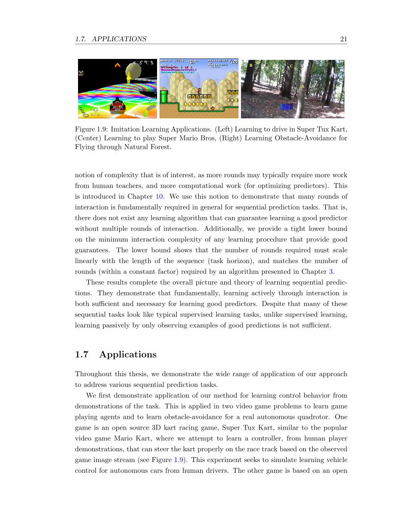
1.7. APPLICATIONS 21
Figure 1.9: Imitation Learning Applications. (Left) Learning to drive in Super Tux Kart,(Center) Learning to play Super Mario Bros, (Right) Learning Obstacle-Avoidance forFlying through Natural Forest.
notion of complexity that is of interest, as more rounds may typically require more work
from human teachers, and more computational work (for optimizing predictors). This
is introduced in Chapter 10. We use this notion to demonstrate that many rounds of
interaction is fundamentally required in general for sequential prediction tasks. That is,
there does not exist any learning algorithm that can guarantee learning a good predictor
without multiple rounds of interaction. Additionally, we provide a tight lower bound
on the minimum interaction complexity of any learning procedure that provide good
guarantees. The lower bound shows that the number of rounds required must scale
linearly with the length of the sequence (task horizon), and matches the number of
rounds (within a constant factor) required by an algorithm presented in Chapter 3.
These results complete the overall picture and theory of learning sequential predic-
tions. They demonstrate that fundamentally, learning actively through interaction is
both sufficient and necessary for learning good predictors. Despite that many of these
sequential tasks look like typical supervised learning tasks, unlike supervised learning,
learning passively by only observing examples of good predictions is not sufficient.
1.7 Applications
Throughout this thesis, we demonstrate the wide range of application of our approach
to address various sequential prediction tasks.
We first demonstrate application of our method for learning control behavior from
demonstrations of the task. This is applied in two video game problems to learn game
playing agents and to learn obstacle-avoidance for a real autonomous quadrotor. One
game is an open source 3D kart racing game, Super Tux Kart, similar to the popular
video game Mario Kart, where we attempt to learn a controller, from human player
demonstrations, that can steer the kart properly on the race track based on the observed
game image stream (see Figure 1.9). This experiment seeks to simulate learning vehicle
control for autonomous cars from human drivers. The other game is based on an open
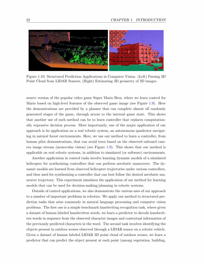
22 CHAPTER 1. INTRODUCTION
Figure 1.10: Structured Prediction Applications in Computer Vision. (Left) Parsing 3DPoint Cloud from LIDAR Sensors, (Right) Estimating 3D geometry of 2D images.
source version of the popular video game Super Mario Bros, where we learn control for
Mario based on high-level features of the observed game image (see Figure 1.9). Here
the demonstrations are provided by a planner that can complete almost all randomly
generated stages of the game, through access to the internal game state. This shows
that another use of such method can be to learn controller that replaces computation-
ally expensive decision process. More importantly, one of the major application of our
approach is its application on a real robotic system, an autonomous quadrotor navigat-
ing in natural forest environments. Here, we use our method to learn a controller, from
human pilot demonstrations, that can avoid trees based on the observed onboard cam-
era image stream (monocular vision) (see Figure 1.9). This shows that our method is
applicable on real robotic systems, in addition to simulated (or software) environments.
Another application in control tasks involve learning dynamic models of a simulated
helicopter for synthesizing controllers that can perform aerobatic maneuvers. The dy-
namic models are learned from observed helicopter trajectories under various controllers,
and then used for synthesizing a controller that can best follow the desired aerobatic ma-
neuver trajectory. This experiment simulates the application of our method for learning
models that can be used for decision-making/planning in robotic systems.
Outside of control applications, we also demonstrate the various uses of our approach
to a number of important problems in robotics. We apply our method to structured pre-
diction tasks that arise commonly in natural language processing and computer vision
problems. The first one is a simple benchmark handwriting recognition task, where given
a dataset of human labeled handwritten words, we learn a predictor to decode handwrit-
ten words in sequence from the observed character images and contextual information of
the previously predicted characters in the word. The second task involves identifying the
objects present in outdoor scenes observed through a LIDAR sensor on a robotic vehicle.
Given a dataset of human labeled LIDAR 3D point cloud of outdoor scenes, we learn a
predictor that can predict the object present at each point (among vegetation, building,
1.8. CONTRIBUTIONS 23
road, poles and wires) in a LIDAR point cloud, from local shape features of the point
cloud, and contextual information of objects predicted nearby (see Figure 1.10). We also
apply our method for estimating the 3D geometry of an outdoor scene in a 2D camera
image. Given a dataset of human annotated outdoor images, we learn a predictor that
can estimate the 3D geometry of each image segment (between ground, sky, a vertical
structure facing left, front-facing or facing right, or a solid or porous object), from local
image features (texture, color histogram, etc.) and contextual information of the nearby
predicted 3D geometry (see Figure 1.10).
Finally, we also demonstrate applications of our method for recommendation tasks
where we must select a small list of relevant and diverse items. We apply our method to
two relevant problems in robotics. The first one consists in learning to suggest a small
list of grasps for a robotic manipulator to pick a nearby object that is likely to contain
a successful grasp, based on a dataset of training environments where we observe the
successful grasps. The second one consists in learning to suggest a small list of initial
trajectories to seed a local trajectory optimization procedure for a robotic manipulator
based on features of the environment that is likely to lead to a collision free trajectory,
again given a dataset of training environments. Outside of robotics, we also apply our
method for personalized news recommendation, recommending a small set of diverse
articles a user is likely to be interested in, and to extractive document summarization,
picking a few sentences out of a document that provides a good summary.
These experiments demonstrate the wide range and variety of settings where our
method can be applied and its potential impact in many fields. This is by no means
an exhaustive list. We believe our method can have many other applications, and be
applied in other settings we haven’t considered here. In fact, various work by other
authors building on our work have already showed a number of new applications of
our method to other structured prediction problems in computational biology (Vlachos,
2012) as well as for learning dynamic feature selection strategies (He et al., 2012). In
general, we believe that many tasks exhibiting a similar “chicken-and-egg” problem may
benefit from using our proposed method.
1.8 Contributions
This thesis makes a number of important algorithmic and theoretical contributions to
machine learning in sequential problems.
In chapter 3, we first provide a complete analysis of standard supervised learning
methods in imitation learning tasks to demonstrate their poor performance guarantees in
such sequential settings. We develop two novel learning strategies with good guarantees:
1) A forward training procedure that leverages interaction and the sequential structure
24 CHAPTER 1. INTRODUCTION
of the task, but that is not practical for long sequence of predictions; 2) a more practical
iterative training procedure described briefly in this chapter that leverages interaction
and the strong guarantees of no-regret online learning methods. The guarantees of these
methods are state-of-the-art and the best known for this setting.
In chapter 4, we extend these methods to imitation learning settings where cost
information is observed and can be used to provide improved guarantees. We show how
one of these techniques also lead to an approach that can handle general model-free
reinforcement learning problems, and provide good guarantees given a good exploration
distribution. Our guarantees in this case match the best known guarantees of other
agnostic model-free reinforcement learning methods.
In chapter 5, we perform extensive experimental comparison of these methods and
demonstrate that our methods achieve state-of-the-art performance for imitation learning
in video game domains and for training an autonomous UAV to fly in natural forest
environments.
In chapter 6, we demonstrate how the same methods can be applied in structured
prediction tasks, and have the same guarantees. Our experimental results demonstrate
that our approach can match and sometimes exceed slightly the performance of other
state-of-the-art structured prediction approaches, while being more computationally ef-
ficient.
In chapter 7, we show that these methods can be used in submodular list prediction
tasks such as relevant and diverse recommendations. We introduce a few small mod-
ifications to our approach, with improved analysis specific to this setting, that allows
it to provide even stronger guarantees on global optimality in this setting. Our guar-
antees match the best known guarantees for this setting. In addition our experimental
results are state-of-the-art on several recommendation tasks, and demonstrate improved
learning efficiency over previous state-of-the-art methods.
In chapter 8, we show how the same methods can be slightly modified for system
identification, i.e. to learn good dynamic models for planning or controller synthesis,
with near-optimality guarantees. Our results provide some of the first agnostic analysis
of system identification methods and are the best known guarantees for agnostic settings.
While in agnostic settings, our near-optimality guarantees are dependent on the quality
of a given fixed exploration distribution used during training, for realizable settings, we
propose an optimistic exploration strategy that must end up learning a model that can
synthesize an optimal controller for the task. In this case, our guarantees are state-of-the-
art and improve over guarantees of previous state-of-the-art model-based reinforcement
learning methods. All these results extend beyond learning of linear systems, to arbitrary
class of systems where no-regret online learning is possible, and shows that learning
models that recovers the optimal controller is possible for much more general class of
1.8. CONTRIBUTIONS 25
systems. Experimentally, we also demonstrate state-of-the-art performance at learning
models of a simulated helicopter for performing aerobatic maneuvers.
In chapter 9, we provide an alternate sufficient condition for providing good per-
formance guarantees with our data aggregation procedure based on notions of stability.
These conditions relates no-regret online learning to stability and minimization of loss
in hindsight. At a high level, these results indicate that we can expect a data aggrega-
tion strategy to work well in practice, as for common practical scenarios, most decent
supervised learners will typically exhibit these stability properties. They also give the in-
tuition that no-regret methods are implicitly learning by making “small changes” as well,
as in previous learning procedures for reinforcement learning and structured prediction
(Kakade and Langford, 2002, Bagnell et al., 2003, Daume III et al., 2009).
In chapter 10, we introduce and formalize the notion of interaction complexity and
present a lower bound on the minimum number of rounds of interactions necessary
to learn good predictors. These results demonstrate that no learning algorithm can
guarantee learning good predictors in general without multiple interactions with the
learner. We show that the number of rounds must scale linearly with the length of the
sequence (task horizon). This bound is tight and match the number of rounds required
by the Forward Training algorithm introduced in Chapter 3. At a high-level, these
results demonstrate that learning actively through interaction is necessary to learn good
predictors for sequential tasks, and that one cannot simply learn passively by observing
examples of good predictions.

Chapter 2
Background
In this chapter, we briefly review common machine learning techniques, algorithms and
theory, that we will use throughout this thesis, as well as common models and algorithms
for sequential decision-making and optimally performing sequential tasks.
2.1 Data-Driven Learning Methods: Algorithms and
Theory
We start by introducing commonly used learning methods in the field of machine learning
that will be leveraged for learning predictors in our work. We first introduce statistical
learning techniques for classification, regression and density estimation. Then we intro-
duce online learning algorithms and the concept of regret. Finally we describe the idea
of a reduction between learning tasks.
Batch Statistical Learning
Statistical learning techniques allow to learn a function or predictor from a set of observed
data that can make predictions about unseen or future data. These techniques provide
guarantees on the performance of the learned predictor on the future unseen data based
on statistical assumption on the data-generating process. For instance, it is typically
assumed that the observed data for training and future unseen data where the learned
predictor is evaluated are both drawn i.i.d. from the same unknown distribution.
In general, a statistical learning problem can be defined formally as follows. Given a
hypothesis spaceH, an instance space Z and a subset of m instances S = z1, z2, . . . , zmdrawn i.i.d. from some unknown distribution D over Z, find a hypothesis h ∈ H which
minimizes some loss function ` : H×Z → R in expectation with respect to the distribu-
tion D. That is, we seek to find an hypothesis h∗ such that:
Ez∼D[`(h∗, z)] = minh∈H
Ez∼D[`(h, z)]. (2.1)

28 CHAPTER 2. BACKGROUND
However, because the distribution D is unknown and only observed through the sampled
instances in S, this objective cannot be minimized exactly. Nevertheless, statistical
learning methods can often provide guarantees on the quality of their solution as a
function of the number of samples m, and achieve optimality in the limit. An approach
often used by many statistical learning methods is to minimize the empirical loss on the
sampled dataset of instances S. That is, they return an hypothesis h such that:
m∑i=1
f(h, zi) = minh∈H
m∑i=1
`(h, zi). (2.2)
This is justified by the fact that for many classes of hypothesis H and loss functions `, we
can guarantee that∑m
i=1 `(h, zi) converges to Ez∼D[f(h, z)] uniformly over the class Has m→∞. This implies that the empirical minimizer h must converge to a population
minimizer h∗ in the limit.
We briefly review a few examples of common statistical learning tasks that we will
need to solve in this thesis, and then introduce the common PAC learning framework,
used in this thesis to provide guarantees and analyze the number of samples required for
obtaining good hypothesis.
Classification
In classification tasks, the instance space Z = X × Y, where X is the space of observed
input features and Y is the space of output class, H is a set of classifiers h : X → Y and
the classification loss function `(h, (x, y)) = I(h(x) 6= y), for I the indicator function (i.e.
the loss is 0 if h predicts the target class y of input x and the loss is 1 otherwise). For
example for detecting spam in emails, X may correspond to features of the content of
the email, such as a binary vector indicating the presence of words or not in the email,
and the output Y = −1, 1 indicates whether the email is spam or not. This is an
example of a binary classification problem where the output is one of 2 class. In general,
multi class classification problems can be considered with more than 2 possible outputs.
This will occur commonly in this thesis, e.g. when we will learn predictors that predicts
an action among a discrete set of many potential actions.
Many algorithms have been developed for learning classifiers such as support vector
machines (SVM) (Cortes and Vapnik, 1995), decision trees (Breiman et al., 1984), neural
networks and nearest neighbor among others (Hastie et al., 2001). In this thesis we will
make use of SVMs as they are a class of classifiers that can be optimized efficiently and
exactly via convex optimization. In its simplest form in the binary classification setting
(Y = −1, 1), a SVM optimizes a linear classifier1 to maximize the classification margin.
1H = Rd for d the number of input features. For w ∈ Rd, hw(x) is 1 if w>x ≥ 0, −1 otherwise
2.1. DATA-DRIVEN LEARNING METHODS: ALGORITHMS AND THEORY 29
This is equivalent to minimizing the following regularized hinge loss:
arg minw
[1
m
m∑i=1
max(0, 1− yiw>xi) +λ
2||w||22], (2.3)
where λ is a regularization constant. SVM can also be applied in the multiclass setting
(by training many weight vectors, one for each class), or train non-linear classifiers using
kernels (Cortes and Vapnik, 1995), and still be optimized exactly via convex optimization.
Regression
In regression, the target output is a continuous value (e.g. predicting the future price
of a stock) so that Y ⊆ R and the loss function is usually defined as the squared loss
f(h, (x, y)) = (h(x) − y)2. Linear regression is a well known example of a regression
problem where we seek to learn the best linear regressor2. In this thesis, we will often
make use of regression techniques, e.g. for predicting continuous actions (like a steering
angle in a driving task), or to predict the cost of different actions. In particular, we
will often make use of a regularized version of linear regression in this thesis where an
extra regularization is used or on weight vector w, called Ridge Regression. The ridge
regression objective solves:
arg minw
1
m
m∑i=1
(w>xi − yi)2 +λ
2||w||22, (2.4)
where λ is a regularization constant. This can be solved in closed form and the optimal
solution is w = (X>X + mλId)−1X>Y , where X is a m × d matrix where the ith row
corresponds to input xi, Y is a m × 1 column vector where the ith element is output
yi and Id is the d × d identity matrix. Regression trees (Breiman et al., 1984), neural
networks, nearest neighbor and kernel methods can also be used for regression (Hastie
et al., 2001).
Density Estimation
In density estimation, we seek to learn a probability model that can measure the proba-
bility or density of some event (e.g. the probability density function (pdf) of the unknown
distribution D itself, or some conditional pdf of some output variable Y given the input
variables X ). The latter is common when dealing with classification tasks where we not
only want to predict a class, but instead assign a probability that the input belongs
to each class, allowing to reason about uncertainty of the predictions. In this case, a
common choice for the loss is the negative log likelihood of the instance z (or conditional
2H = Rd for d the number of input features. For w ∈ Rd, hw(x) = w>x
30 CHAPTER 2. BACKGROUND
likelihood of y given x) under the density model h (i.e. f(h, z) = − log(h(z))). This leads
to maximizing the likelihood of the data, as in common maximum likelihood methods.
A commonly used method for conditional density estimation is logistic regression
(Hastie et al., 2001). Given the input x, logistic regression predicts a distribution over
outputs y using an exponential family model of the form:
P (y|x) ∝ exp(w>y x) (2.5)
where wyy∈Y are the weight parameters to optimize. Optimization of these parameters
to minimize the logistic loss (negative log likelihood) leads to a convex optimization
problem that can be solved efficiently, e.g. using gradient descent methods.
We will use such methods in the context of predicting a distribution over possible
objects present at a particular location in a scene, in computer vision/perception appli-
cations.
PAC Learning
Probably Approximately Correct (PAC) Learning (Valiant, 1984, Kearns et al., 1994) is
a learning framework that has been introduced to analyze learning algorithms and their
statistical efficiency – how many samples (data points) are needed to obtain, with high
probability, a near-optimal hypothesis h within the class H.
For any desired near-optimality threshold ε > 0 and small probability of failure
δ > 0, a PAC learning algorithm guarantees that for any distribution D, after a sufficient
number of samples m, it will find with high probability 1−δ an hypothesis h that achieves
expected loss (under the unknown distribution D) within ε of optimal, i.e.:
Ez∼D
[`(h, z)] ≤ minh∈H
Ez∼D
[`(h, z)] + ε
The number of samples m required to guarantee this with high probability 1 − δ will
typically scale as a function of 1/δ, 1/ε, and the complexity of the class of hypothesis H(e.g. the VC dimension if H is a class of binary classifiers). In general, m is typically
O(C(H)+log(1/δ)ε2
), for C(H) a measure of the complexity of the class H. In certain ideal
cases, e.g. in realizable scenarios, faster convergence rate can be obtained and m may
only need to be O(C(H)+log(1/δ)ε ).
Under the common statistical assumption that both training and test examples are
drawn i.i.d. from the distribution D, then such PAC learning algorithms guarantee
that after a sufficient amount of data, with high probability, the performance of the
learned predictor on test examples must be near-optimal (in expectation). In particular,
if predictors with low error/loss could be found during training, then this must imply
the learned predictor has low loss/error on the new test instances (in expectation). Note
also that these guarantees are agnostic – i.e. they hold without assuming the data is
2.1. DATA-DRIVEN LEARNING METHODS: ALGORITHMS AND THEORY 31
generated according to any particular hypothesis in the class. Of course, low test error
is only achieved if a low training error hypothesis exists on the training data.
In this thesis, we will also seek to analyze our learning algorithms and provide guar-
antees that look similar to these PAC guarantees. In particular, we will provide similar
agnostic guarantees that hold with high probability, and relate test performance at the
sequential prediction task, to the performance of the best predictor/hypothesis in the
class on the training distribution of examples. If low loss/error predictors can be found
during training, this will imply good test performance of the learned predictor at the
sequential prediction task.
Online Learning with Streaming Data
Online learning algorithms are a key component of our main approach to learn good
predictors for sequential prediction tasks. In particular, they will be used for updating
the predictor we learn over many iterations of training, as more data is being collected.
We review here some important background material related to online learning, and
present a few common online learning algorithms used in this thesis.
Online learning has been developed to deal with learning tasks where we must make
predictions over time as we are learning from a stream of data (Vovk, 1992, Littlestone
and Warmuth, 1994, Cesa-Bianchi and Lugosi, 2006). An example of such task may be
weather forecast, where we must predict tomorrow’s weather each day, and then get to
observe the weather the next day as additional training data to update our predictor.
Another example is stock market prediction, where we may want to predict how the
price of a stock will change each day, and then get to observe the change in price at the
end of the day as additional data to update our predictor.
Formally, the online algorithm is presented with a sequence of training instances
z1, z2, . . . , zN , one at a time. At each round n, before observing the instance zn, the
learner chooses a predictor hn ∈ H, to make its next prediction, and incurs loss `(hn, zn)
on the instance zn. Then it observes zn and can choose a new predictor hn+1 for the
next round.
The goal in online learning is to minimize the regret with respect to the best fixed
hypothesis the learner could have chosen in hindsight (i.e. knowing all the training
instances in advance). Formally, the average regret RN after N rounds of the online
learning algorithm is defined as:
RN =1
N
N∑n=1
`(hn, zn)−minh∈H
1
N
N∑n=1
`(h, zn) (2.6)
Small average regret intuitively implies that, on average, before seeing the training
example at each round, the learner made as good predictions, as if it had known all the
32 CHAPTER 2. BACKGROUND
training instances in advance and had picked the best predictor to predict on all this
data.
A no-regret algorithm is an algorithm that guarantees that in the limit, as N →∞,
RN goes to 0 (or is negative), for any sequence of training instances. In other words, a
no-regret algorithm indicates that in the limit, the average loss incurred by the learner,
when making its predictions before seeing each training example, is no worse than the
average loss of the best predictor it could have picked, knowing all the training instances
in advance.
A concrete scenario where online learning has been applied is for managing investment
portfolios (Argawal et al., 2006). In this case, we might consider k possible financial in-
struments (cash, bonds, stocks, etc.) to invest in and defineH to be the set of all portfolio
allocations to these k instruments (i.e. the set of all distributions on the k instruments).
Each day, we consider allocating our money to different instruments according to some
portfolio allocation in H. We then observe the return of each instruments for the day
(the training instance zn), which we use to update our portfolio allocation for the next
day. Using a no-regret algorithm to update the portfolio allocation after each day would
guarantee that in the limit, the average return of the portfolio is no worse than the av-
erage return of the best constantly-rebalanced3 fixed portfolio allocation in H over that
time period. In other words, the average return of the learner will be as good as if we
had known how the stock market is going to evolve in the future, and had chosen the
best (constantly rebalanced) allocation for this future.
Unlike statistical learning techniques that assumes data is drawn i.i.d. from some
unknown distribution, online learning is a more game-theoretic4 learning framework
that makes no assumption about how the instances are chosen. In particular, as no-
regret algorithms work for any sequence of instances, the no-regret guarantees hold
even if the instances are chosen adversarially. The trade-off however, is that no-regret
is only a statement about relative performance, i.e. relative to the best hypothesis
in the class on this sequence of instances. Thus no-regret does not necessarily imply
good absolute performance, e.g. when no hypothesis performs well on the sequence of
instances. However, under the additional assumption that good hypothesis exists for
the sequence, then no-regret implies good performance, in absolute terms. These strong
3A fixed portfolio allocation in this scenario, for instance 50% in AAPL stock and 50% in MSFTstock, implies that after each day, after the price of these assets change, we would buy/sell stocks ofeach so that the overall value of the portfolio is rebalanced to 50% in AAPL stock and 50% in MSFT.For instance if AAPL increases more in value than MSFT, at the end of the day our money may nowbe allocated as 52% AAPL and 48% MSFT; to bring back to 50-50, we would sell AAPL stock andbuy more MSFT stock with that money. This is what is called a constantly rebalanced portfolio (Coverand Thomas, 1991). Such constantly rebalanced portfolio are powerful investment strategies, as theyimplicitly make you sell high and buy low.
4Online learning can be thought as a two-player repeated game played between a learner, choosinghypothesis in some class H, and an adversary picking training instances.
2.1. DATA-DRIVEN LEARNING METHODS: ALGORITHMS AND THEORY 33
no-regret properties, that hold even for non-i.i.d. data, will be key to provide good
guarantees in our sequence prediction settings, where i.i.d assumptions do not hold.
Many no-regret algorithms have been developed in the literature for different scenar-
ios. We review the most common ones and their guarantees that will be leveraged in
this work.
Weighted Majority and Hedge
When the number of hypothesis is finite (i.e. H is finite) randomized no-regret algo-
rithms have been proposed such as Weighted Majority (Littlestone and Warmuth, 1994)
and Hedge (Freund and Schapire, 1997). These algorithms essentially assign to each
hypothesis a probability that decreases exponentially in their total loss so far and pick a
hypothesis randomly according to this distribution at each iteration. That is, at round
n, the probability distribution Pn over hypothesis to choose hn is defined as:
Pn(h) ∝ exp(−ηn−1∑i=1
`(h, zi)),
for some learning rate parameter η. By choosing η to be Θ(1/√N), these methods are
no-regret at rate O( 1√N
) (Littlestone and Warmuth, 1994, Freund and Schapire, 1997).
They can also be no-regret at faster rates of O(log(N)/N) if some hypothesis in the set
H have small loss and the loss of the best hypothesis (after N rounds) is used to define η
appropriately. A doubling trick to adapt the parameter η can be used as well to achieve
the same optimal rate, up to a small constant factor, without knowing the loss of the
best hypothesis in advance (Cesa-Bianchi et al., 1997).
As these methods are randomized algorithms, they guarantee that the expected re-
gret, under the chosen distributions P1, P2, . . . , PN , goes to 0 as N → ∞. It can also
be shown that with high probability, the regret on the sampled hypothesis h1, h2, . . . hN
converges at the same rate with high probability. 5
Subgradient Descent and Follow-the-(Regularized)-Leader
When the set of hypothesis H is a convex set and the loss `(·, z) is convex in the hypoth-
esis for all z ∈ Z, then other online learning algorithms such as Projected Subgradient
Descent (Zinkevich, 2003) and Follow-the-(Regularized)-Leader are no-regret (Kakade
and Shalev-Shwartz, 2008). Projected Subgradient Descent simply updates the hypoth-
esis in the direction opposite to a subgradient of the loss at the current iteration:
hn+1 = hn − αn∇h`n(hn)
5Under the assumption that the adversary cannot choose zn based on knowing the result of sampling,i.e. hn, but can potentially choose zn based on knowledge of Pn.
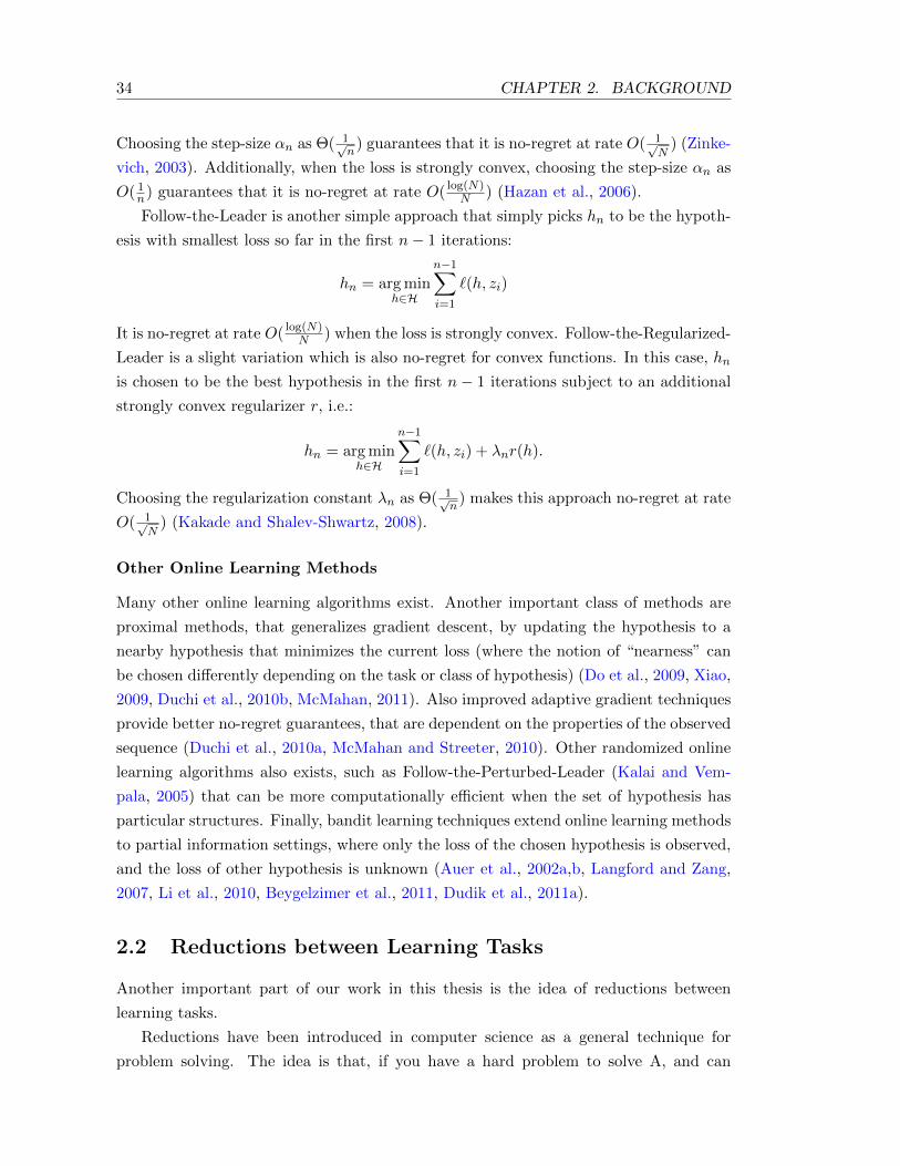
34 CHAPTER 2. BACKGROUND
Choosing the step-size αn as Θ( 1√n
) guarantees that it is no-regret at rate O( 1√N
) (Zinke-
vich, 2003). Additionally, when the loss is strongly convex, choosing the step-size αn as
O( 1n) guarantees that it is no-regret at rate O( log(N)
N ) (Hazan et al., 2006).
Follow-the-Leader is another simple approach that simply picks hn to be the hypoth-
esis with smallest loss so far in the first n− 1 iterations:
hn = arg minh∈H
n−1∑i=1
`(h, zi)
It is no-regret at rate O( log(N)N ) when the loss is strongly convex. Follow-the-Regularized-
Leader is a slight variation which is also no-regret for convex functions. In this case, hn
is chosen to be the best hypothesis in the first n− 1 iterations subject to an additional
strongly convex regularizer r, i.e.:
hn = arg minh∈H
n−1∑i=1
`(h, zi) + λnr(h).
Choosing the regularization constant λn as Θ( 1√n
) makes this approach no-regret at rate
O( 1√N
) (Kakade and Shalev-Shwartz, 2008).
Other Online Learning Methods
Many other online learning algorithms exist. Another important class of methods are
proximal methods, that generalizes gradient descent, by updating the hypothesis to a
nearby hypothesis that minimizes the current loss (where the notion of “nearness” can
be chosen differently depending on the task or class of hypothesis) (Do et al., 2009, Xiao,
2009, Duchi et al., 2010b, McMahan, 2011). Also improved adaptive gradient techniques
provide better no-regret guarantees, that are dependent on the properties of the observed
sequence (Duchi et al., 2010a, McMahan and Streeter, 2010). Other randomized online
learning algorithms also exists, such as Follow-the-Perturbed-Leader (Kalai and Vem-
pala, 2005) that can be more computationally efficient when the set of hypothesis has
particular structures. Finally, bandit learning techniques extend online learning methods
to partial information settings, where only the loss of the chosen hypothesis is observed,
and the loss of other hypothesis is unknown (Auer et al., 2002a,b, Langford and Zang,
2007, Li et al., 2010, Beygelzimer et al., 2011, Dudik et al., 2011a).
2.2 Reductions between Learning Tasks
Another important part of our work in this thesis is the idea of reductions between
learning tasks.
Reductions have been introduced in computer science as a general technique for
problem solving. The idea is that, if you have a hard problem to solve A, and can

2.2. REDUCTIONS BETWEEN LEARNING TASKS 35
transform that problem into another easier problem B that you know how to solve, then
you can solve the hard problem A by solving the transformed problem B instead.
This idea has been used in machine learning to tackle harder learning tasks via
existing learning algorithms that can only tackle simple tasks (Beygelzimer et al., 2005,
Langford and Beygelzimer, 2005, Balcan et al., 2008, Beygelzimer et al., 2009, Daume III
et al., 2009). For instance, a well known reduction is the all-pairs reduction of multiclass
classification to binary classification. This reduction constructs a multiclass classifier by
training a binary classifier for every pair of labels (Hastie and Tibshirani, 1998). The
approach proceeds by training each binary classifier on the subset of the training set
that are labeled as one of the two labels it is trying to distinguish. Then when given
a test input, all binary classifiers are evaluated and each output count as a vote for
the predicted label. The label with most votes is the predicted label for the multiclass
classifier constructed from these binary classifiers.
Reductions can also be used as a way to provide theoretical guarantees on the quality
of the solution found as a function of the quality of the solutions for the subproblems.
Therefore, if high-quality solutions can be found for the subproblems, we can guarantee
that we obtain a high-quality solution for the original problem. For instance, in the
previous reduction, if the binary classifiers have error rate ε, it can be shown that the
multiclass classifier has error rate of at most (k−1)ε at the multiclass classification task,
for k the number of labels.
In this thesis, the algorithms we present can be understood as reductions of sequential
prediction tasks, to simpler learning tasks that can be solved using standard supervised
learning algorithms, or online learning algorithms. By doing so, we will be able to
guarantee good performance at the original sequential prediction task, whenever good
performance can be achieved at the simpler supervised/online learning tasks.
We will also make use of a number of existing learning reductions to tackle gen-
eral cost-sensitive classification tasks that arise in our work. We present below a few
reductions that exist to tackle such tasks.
Reductions of Cost-Sensitive Classification
In cost-sensitive classification, instead of incurring a 0-1 loss, a different loss is associated
to predicting each class, at every input x. In this case, the instances z ∈ Z, can be
thought as tuples (x, c), where c is a cost-vector associating a cost to each output class
y ∈ Y. In this case, the goal is to find the predictor h∗ ∈ H with minimum expected
cost under the unknown distribution D:
h∗ = arg minh∈H
E(x,c)∼D[c(h(x))].
Minimizing this cost-sensitive classification loss directly is often computationally in-
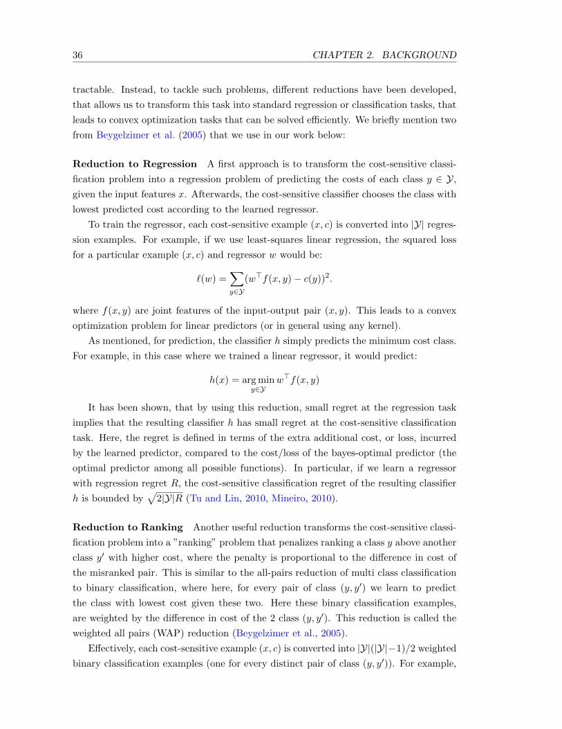
36 CHAPTER 2. BACKGROUND
tractable. Instead, to tackle such problems, different reductions have been developed,
that allows us to transform this task into standard regression or classification tasks, that
leads to convex optimization tasks that can be solved efficiently. We briefly mention two
from Beygelzimer et al. (2005) that we use in our work below:
Reduction to Regression A first approach is to transform the cost-sensitive classi-
fication problem into a regression problem of predicting the costs of each class y ∈ Y,
given the input features x. Afterwards, the cost-sensitive classifier chooses the class with
lowest predicted cost according to the learned regressor.
To train the regressor, each cost-sensitive example (x, c) is converted into |Y| regres-
sion examples. For example, if we use least-squares linear regression, the squared loss
for a particular example (x, c) and regressor w would be:
`(w) =∑y∈Y
(w>f(x, y)− c(y))2.
where f(x, y) are joint features of the input-output pair (x, y). This leads to a convex
optimization problem for linear predictors (or in general using any kernel).
As mentioned, for prediction, the classifier h simply predicts the minimum cost class.
For example, in this case where we trained a linear regressor, it would predict:
h(x) = arg miny∈Y
w>f(x, y)
It has been shown, that by using this reduction, small regret at the regression task
implies that the resulting classifier h has small regret at the cost-sensitive classification
task. Here, the regret is defined in terms of the extra additional cost, or loss, incurred
by the learned predictor, compared to the cost/loss of the bayes-optimal predictor (the
optimal predictor among all possible functions). In particular, if we learn a regressor
with regression regret R, the cost-sensitive classification regret of the resulting classifier
h is bounded by√
2|Y|R (Tu and Lin, 2010, Mineiro, 2010).
Reduction to Ranking Another useful reduction transforms the cost-sensitive classi-
fication problem into a ”ranking” problem that penalizes ranking a class y above another
class y′ with higher cost, where the penalty is proportional to the difference in cost of
the misranked pair. This is similar to the all-pairs reduction of multi class classification
to binary classification, where here, for every pair of class (y, y′) we learn to predict
the class with lowest cost given these two. Here these binary classification examples,
are weighted by the difference in cost of the 2 class (y, y′). This reduction is called the
weighted all pairs (WAP) reduction (Beygelzimer et al., 2005).
Effectively, each cost-sensitive example (x, c) is converted into |Y|(|Y|−1)/2 weighted
binary classification examples (one for every distinct pair of class (y, y′)). For example,
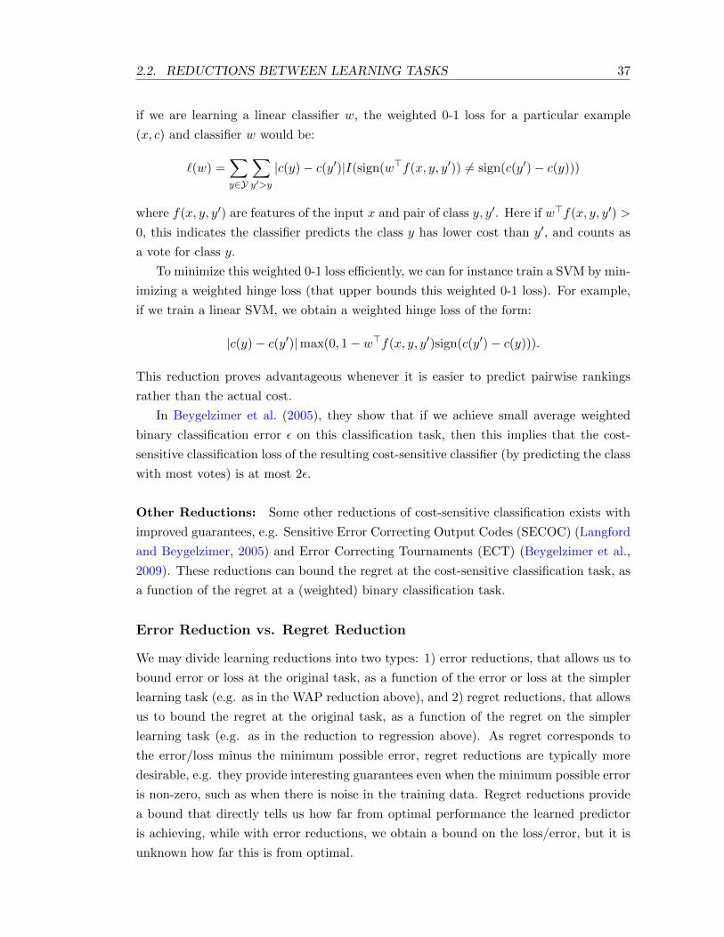
2.2. REDUCTIONS BETWEEN LEARNING TASKS 37
if we are learning a linear classifier w, the weighted 0-1 loss for a particular example
(x, c) and classifier w would be:
`(w) =∑y∈Y
∑y′>y
|c(y)− c(y′)|I(sign(w>f(x, y, y′)) 6= sign(c(y′)− c(y)))
where f(x, y, y′) are features of the input x and pair of class y, y′. Here if w>f(x, y, y′) >
0, this indicates the classifier predicts the class y has lower cost than y′, and counts as
a vote for class y.
To minimize this weighted 0-1 loss efficiently, we can for instance train a SVM by min-
imizing a weighted hinge loss (that upper bounds this weighted 0-1 loss). For example,
if we train a linear SVM, we obtain a weighted hinge loss of the form:
|c(y)− c(y′)|max(0, 1− w>f(x, y, y′)sign(c(y′)− c(y))).
This reduction proves advantageous whenever it is easier to predict pairwise rankings
rather than the actual cost.
In Beygelzimer et al. (2005), they show that if we achieve small average weighted
binary classification error ε on this classification task, then this implies that the cost-
sensitive classification loss of the resulting cost-sensitive classifier (by predicting the class
with most votes) is at most 2ε.
Other Reductions: Some other reductions of cost-sensitive classification exists with
improved guarantees, e.g. Sensitive Error Correcting Output Codes (SECOC) (Langford
and Beygelzimer, 2005) and Error Correcting Tournaments (ECT) (Beygelzimer et al.,
2009). These reductions can bound the regret at the cost-sensitive classification task, as
a function of the regret at a (weighted) binary classification task.
Error Reduction vs. Regret Reduction
We may divide learning reductions into two types: 1) error reductions, that allows us to
bound error or loss at the original task, as a function of the error or loss at the simpler
learning task (e.g. as in the WAP reduction above), and 2) regret reductions, that allows
us to bound the regret at the original task, as a function of the regret on the simpler
learning task (e.g. as in the reduction to regression above). As regret corresponds to
the error/loss minus the minimum possible error, regret reductions are typically more
desirable, e.g. they provide interesting guarantees even when the minimum possible error
is non-zero, such as when there is noise in the training data. Regret reductions provide
a bound that directly tells us how far from optimal performance the learned predictor
is achieving, while with error reductions, we obtain a bound on the loss/error, but it is
unknown how far this is from optimal.
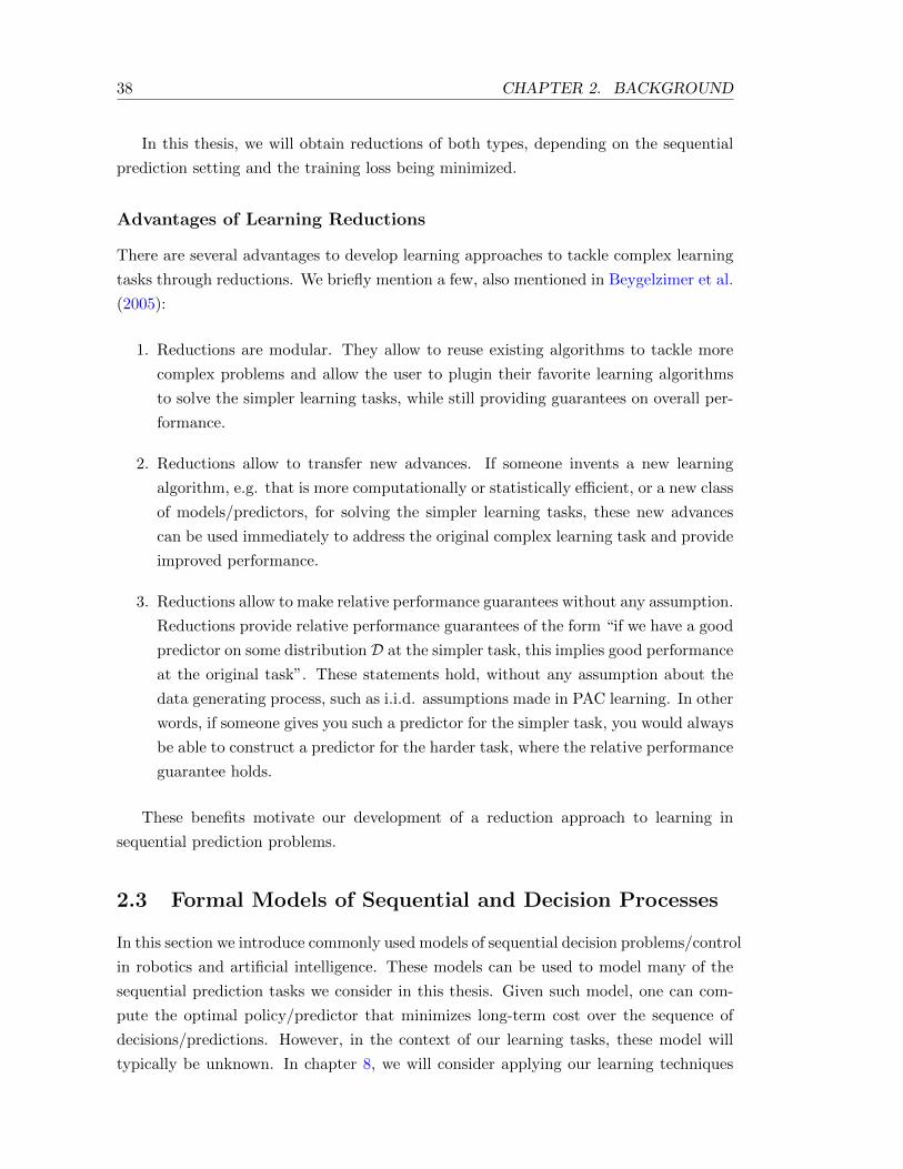
38 CHAPTER 2. BACKGROUND
In this thesis, we will obtain reductions of both types, depending on the sequential
prediction setting and the training loss being minimized.
Advantages of Learning Reductions
There are several advantages to develop learning approaches to tackle complex learning
tasks through reductions. We briefly mention a few, also mentioned in Beygelzimer et al.
(2005):
1. Reductions are modular. They allow to reuse existing algorithms to tackle more
complex problems and allow the user to plugin their favorite learning algorithms
to solve the simpler learning tasks, while still providing guarantees on overall per-
formance.
2. Reductions allow to transfer new advances. If someone invents a new learning
algorithm, e.g. that is more computationally or statistically efficient, or a new class
of models/predictors, for solving the simpler learning tasks, these new advances
can be used immediately to address the original complex learning task and provide
improved performance.
3. Reductions allow to make relative performance guarantees without any assumption.
Reductions provide relative performance guarantees of the form “if we have a good
predictor on some distribution D at the simpler task, this implies good performance
at the original task”. These statements hold, without any assumption about the
data generating process, such as i.i.d. assumptions made in PAC learning. In other
words, if someone gives you such a predictor for the simpler task, you would always
be able to construct a predictor for the harder task, where the relative performance
guarantee holds.
These benefits motivate our development of a reduction approach to learning in
sequential prediction problems.
2.3 Formal Models of Sequential and Decision Processes
In this section we introduce commonly used models of sequential decision problems/control
in robotics and artificial intelligence. These models can be used to model many of the
sequential prediction tasks we consider in this thesis. Given such model, one can com-
pute the optimal policy/predictor that minimizes long-term cost over the sequence of
decisions/predictions. However, in the context of our learning tasks, these model will
typically be unknown. In chapter 8, we will consider applying our learning techniques

2.3. FORMAL MODELS OF SEQUENTIAL AND DECISION PROCESSES 39
to learn such models in the context of control tasks, that will allow us to plan optimal
sequence of actions.
We first introduce models where perfect information about the world is known and
then models taking into account uncertainty related to partial observability of the world.
Markov Decision Processes
One of the simplest class of dynamic models of robotic systems is the Markov Decision
Process (MDP) (Puterman, 1994). A MDP is defined by a tuple (S,A, T, C) where:
• S is the set of all possible states of the system. A state is a sufficient statistic
of everything that occured in the past to predict future states (configurations),
i.e. knowing previous states and actions does not give us more information about
future states if the current state is known. In the context of robotics system, the
state would encode the configuration of the robot, its velocity, etc.
• A is the set of actions that can perform at any step.
• P is the transition function, where Psa(·) specifies the probability distribution over
the next state after executing action a in state s. This represents our uncertainty
about what the next state of the system is going to be. The transition function
uses the Markov assumption, i.e. that the current state is a sufficient statistic to
predict the next state.
• C is the cost function, where C(s, a) specifies the immediate cost of doing action a
in state s. The cost encodes how desirable is a particular action and/or state with
respect to the task we want to perform.
MDPs can represent a wide range of systems. For instance a simple model of a car in
a static environment might consider the state to be the car’s current position, orientation
and velocity; the action to be the steering and acceleration; and the transition function
could be specified via a simple physical model of a point particle. If the task consists in
reaching a particular goal location as fast as possible while avoiding hitting obstacles,
then the cost function might be designed to be such that every action in every state has
a small cost, except in the goal state where no cost is incurred, and actions that causes
collisions with obstacles have large cost.
The goal in a MDP is to find a policy π : S → ∆A, mapping state to action (or
distribution over actions), that minimizes the expected sum of costs over the task horizon.
In this thesis, we will usually consider cases where the task horizon is finite, except in
chapter 8 where we will consider infinite horizons with a discount factor γ ∈ [0, 1). The
discount factor discounts costs obtained t steps in the future by a factor γt.
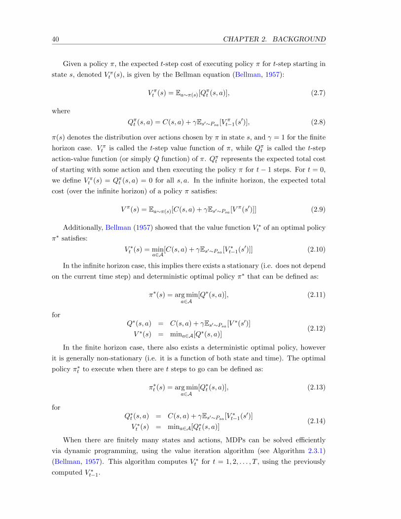
40 CHAPTER 2. BACKGROUND
Given a policy π, the expected t-step cost of executing policy π for t-step starting in
state s, denoted V πt (s), is given by the Bellman equation (Bellman, 1957):
V πt (s) = Ea∼π(s)[Q
πt (s, a)], (2.7)
where
Qπt (s, a) = C(s, a) + γEs′∼Psa [V πt−1(s′)], (2.8)
π(s) denotes the distribution over actions chosen by π in state s, and γ = 1 for the finite
horizon case. V πt is called the t-step value function of π, while Qπt is called the t-step
action-value function (or simply Q function) of π. Qπt represents the expected total cost
of starting with some action and then executing the policy π for t− 1 steps. For t = 0,
we define V πt (s) = Qπt (s, a) = 0 for all s, a. In the infinite horizon, the expected total
cost (over the infinite horizon) of a policy π satisfies:
V π(s) = Ea∼π(s)[C(s, a) + γEs′∼Psa [V π(s′)]] (2.9)
Additionally, Bellman (1957) showed that the value function V ∗t of an optimal policy
π∗ satisfies:
V ∗t (s) = mina∈A
[C(s, a) + γEs′∼Psa [V ∗t−1(s′)]] (2.10)
In the infinite horizon case, this implies there exists a stationary (i.e. does not depend
on the current time step) and deterministic optimal policy π∗ that can be defined as:
π∗(s) = arg mina∈A
[Q∗(s, a)], (2.11)
forQ∗(s, a) = C(s, a) + γEs′∼Psa [V ∗(s′)]
V ∗(s) = mina∈A[Q∗(s, a)](2.12)
In the finite horizon case, there also exists a deterministic optimal policy, however
it is generally non-stationary (i.e. it is a function of both state and time). The optimal
policy π∗t to execute when there are t steps to go can be defined as:
π∗t (s) = arg mina∈A
[Q∗t (s, a)], (2.13)
forQ∗t (s, a) = C(s, a) + γEs′∼Psa [V ∗t−1(s′)]
V ∗t (s) = mina∈A[Q∗t (s, a)](2.14)
When there are finitely many states and actions, MDPs can be solved efficiently
via dynamic programming, using the value iteration algorithm (see Algorithm 2.3.1)
(Bellman, 1957). This algorithm computes V ∗t for t = 1, 2, . . . , T , using the previously
computed V ∗t−1.
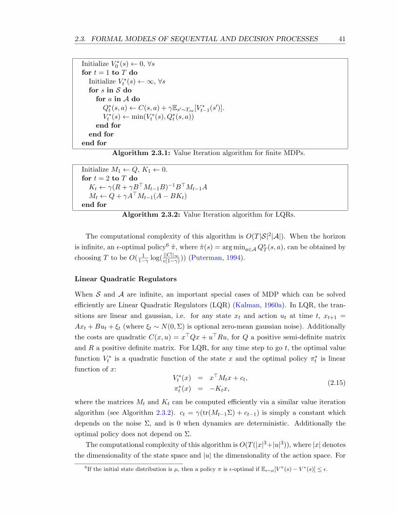
2.3. FORMAL MODELS OF SEQUENTIAL AND DECISION PROCESSES 41
Initialize V ∗0 (s)← 0, ∀sfor t = 1 to T do
Initialize V ∗t (s)←∞, ∀sfor s in S do
for a in A doQ∗t (s, a)← C(s, a) + γEs′∼Tsa [V ∗t−1(s′)].V ∗t (s)← min(V ∗t (s), Q∗t (s, a))
end forend for
end for
Algorithm 2.3.1: Value Iteration algorithm for finite MDPs.
Initialize M1 ← Q, K1 ← 0.for t = 2 to T doKt ← γ(R+ γB>Mt−1B)−1B>Mt−1AMt ← Q+ γA>Mt−1(A−BKt)
end for
Algorithm 2.3.2: Value Iteration algorithm for LQRs.
The computational complexity of this algorithm is O(T |S|2|A|). When the horizon
is infinite, an ε-optimal policy6 π, where π(s) = arg mina∈AQ∗T (s, a), can be obtained by
choosing T to be O( 11−γ log( ||C||∞ε(1−γ))) (Puterman, 1994).
Linear Quadratic Regulators
When S and A are infinite, an important special cases of MDP which can be solved
efficiently are Linear Quadratic Regulators (LQR) (Kalman, 1960a). In LQR, the tran-
sitions are linear and gaussian, i.e. for any state xt and action ut at time t, xt+1 =
Axt +But + ξt (where ξt ∼ N(0,Σ) is optional zero-mean gaussian noise). Additionally
the costs are quadratic C(x, u) = x>Qx + u>Ru, for Q a positive semi-definite matrix
and R a positive definite matrix. For LQR, for any time step to go t, the optimal value
function V ∗t is a quadratic function of the state x and the optimal policy π∗t is linear
function of x:V ∗t (x) = x>Mtx+ ct,
π∗t (x) = −Ktx,(2.15)
where the matrices Mt and Kt can be computed efficiently via a similar value iteration
algorithm (see Algorithm 2.3.2). ct = γ(tr(Mt−1Σ) + ct−1) is simply a constant which
depends on the noise Σ, and is 0 when dynamics are deterministic. Additionally the
optimal policy does not depend on Σ.
The computational complexity of this algorithm is O(T (|x|3+|u|3)), where |x| denotes
the dimensionality of the state space and |u| the dimensionality of the action space. For
6If the initial state distribution is µ, then a policy π is ε-optimal if Es∼µ[V π(s)− V ∗(s)] ≤ ε.
42 CHAPTER 2. BACKGROUND
finite horizon T , this algorithm can also be adapted to non-stationary linear dynamics
and cost function (i.e. xt+1 = Atxt + Btut + ξt and C(xt, ut, t) = x>t Qtxt + u>t Rtut) by
simply replacing A, B, Q and R by AT−t+1, BT−t+1, QT−t+1 and RT−t+1 in the inner
loop of the previous algorithm, and initializing M1 = QT . This can be used to solve
approximately non-linear systems with non-quadratic cost functions using iterative lin-
earization/“quadraticization” techniques such as iterated LQR (iLQR) (Li and Todorov,
2004) and Differential Dynamic Programming (DDP) (Jacobson and Mayne, 1970).
Partially Observable Markov Decision Processes
In practice, robots rarely know exactly what the current state s is. They only observe
the world through noisy sensors that give them partial information about the current
state s. MDPs can be extended to handle this partial observability, and obtain policies
that reason about state uncertainty to minimize long-term costs.
The Partially Observable Markov Decision Process (POMDP) provides such an ex-
tension (Sondik, 1971). It adds 2 additional components to the MDP model:
• Z is the set of all possible observations that can be made by the system.
• O is the observation function, where Oas′(·) specifies the probability distribution
over the observation we obtain after executing action a and arriving in state s′.
In a POMDP, the uncertainty about the current state is represented as a probability
distribution over states, called the belief state, that captures the likelihood that we are
in each state. This belief state can be updated using simple applications of bayes’ rule,
each time a new action a is performed and we obtain a new observation z ∈ Z (Sondik,
1971).
A policy in a POMDP maps belief states to actions, and the optimal policy can be
found by planning in a belief MDP (where the state is the belief state, and transitions
specify possible next belief after observing different observations), e.g. using similar
techniques presented above or simple receding horizon control approaches (Ross, 2008).
More sophisticated planning algorithms for POMDPs exist that leverage the particular
structure of the value function over this belief space (Sondik, 1971, Pineau et al., 2003,
Spaan and Vlassis, 2005, Smith and Simmons, 2005). However, in all cases solving
POMDPs is very computationally expensive, and often does not scale to real world
applications (unless they are significantly abstracted or simplified).
Linear Quadratic Gaussian
An important special case of POMDP that can be solved efficiently is in the context of
continuous control problems such as LQR presented above. In this case, the observations
2.3. FORMAL MODELS OF SEQUENTIAL AND DECISION PROCESSES 43
are assumed to be a linear function of the current state xt and action ut at time t
with additional white gaussian noise, i.e. yt = Cxt + Dut + N(0,Σ′). In this case the
distribution over states is Gaussian, and can be maintained via a Kalman Filter (Kalman,
1960b). The optimal policy simply consists in applying the same LQR controller, as
computed above, to the expected state of the Kalman Filter. This is often referred to as
Linear Quadratic Gaussian Control (LQG).
Access Models
We describe here different access model to the real system that are commonly used in dif-
ferent algorithms for computing or learning a (near-)optimal policy in a MDP/POMDP.
This formalizes our assumptions about how we can interact with the system and collect
data. In particular, in this thesis, we will typically assume access only to a reset model,
as described below.
Full Probabilistic Model: This is the strongest access model and requires full knowl-
edge of all transition and observation probabilities of the real system. This allows compu-
tation of the Bellman equation exactly by summing over all possible next states/observations
to evaluate expectations. Planning methods typically assumes this type of access.
Generative Model: This is a weaker access model that allows setting the real system
in any particular state and sampling transitions/observations by doing any action in
that state. This allows to evaluate the Bellman equation to any degree of accuracy (with
high probability) by sampling next states/observations several times from the generative
model. This is an access model which is often encountered in software applications or
for systems for which we have access to a simulation, but not the full probabilistic model
description. The software can be started in any particular state and then any particular
action can be taken to obtain a sample transition/observation. Such access models are
used by many techniques for efficiently obtaining approximate solutions to MDPs (such
as Fitted Value Iteration (Gordon, 1995, Szepesvari, 2005), Sparse Sampling (Kearns
et al., 2002)).
Reset Model: This is the next weakest access model where we can only sample
state/observation in the real system along trajectories starting in the initial state dis-
tribution, by executing different sequences of actions. In this model, we can perform a
“reset”, which initializes the real system to a new initial state. Actions can be performed
to simulate the system forward in time and obtain sample next state/observation along
the current trajectory. Reset models can be used to model the type of access we have
with robots performing repeated tasks in the real world starting from some distribution

44 CHAPTER 2. BACKGROUND
of initial configurations. We cannot put the robot in any particular state, as in the gen-
erative model, but we might be able to reset it to one of its possible initial configuration.
For instance, a robotic arm might have a controller that can put back the arm into some
default configuration, from which the arm always starts its interactions with surrounding
objects. A human might also supervise the robot during the learning phase and be able
to reset the robot to a particular initial configuration between trials. Reset models are
commonly assumed in many learning algorithms (e.g. in PSDP (Bagnell et al., 2003),
CPI (Kakade and Langford, 2002) and policy gradient methods (Williams, 1992, Bagnell
and Schneider, 2003, Peters and Schaal, 2008)). This is the type of access model we will
assume in this thesis.
Trace Model: This is the weakest access model and corresponds to the reset model
without the possibility of reset. This model only allows simulating the system forward
in time by performing further actions. This models life as we experience it in our daily
lives: we cannot go back to when we were a baby and change our decisions along the
way to experiment and see what would happen later on, we must always live with the
consequences of our previous actions. Some learning algorithms only assume this type of
access model (Strehl et al., 2009, Jaksch et al., 2010), but it typically leads to optimality
guarantees that are weaker in some sense.
Chapter 3
Learning Behavior from
Demonstrations
We begin our investigation of learning sequential predictions in the particular setting of
learning control behavior from demonstrations, often called imitation learning (Schaal,
1999, Argall et al., 2009). Imitation learning is perhaps one of the sequential prediction
problem that is the most closely related to well studied statistical learning problems
such as supervised classification, but exhibits the fundamental problems and difficulties
of learning to perform sequential tasks. Therefore, imitation learning presents itself as a
natural starting point for studying the nature of learning in sequential tasks and under-
standing its fundamental difficulties, as well as building algorithms and methodologies
for theoretical analysis that can be used as building blocks in more complex sequential
prediction problems studied later on.
3.1 Preliminaries
Imitation learning is concerned with the problem of learning to perform a control task
(e.g. navigate safely and efficiently across a terrain from point A to point B) from demon-
strations by an expert. These techniques allow programming autonomous behavior in
robotic systems easily via demonstrations of the desired behavior, e.g. by human ex-
perts. This avoids time-consuming engineering required by traditional control methods
that rely on accurate dynamic models of the system and well-engineered cost functions
to synthesize controllers that produce the desired behavior. As the tasks performed by
robotic systems continuously increase in complexity, it is becoming increasingly harder
to provide good models and cost functions. As a result, learning by demonstration tech-
niques are becoming more and more popular and have led to state-of-the-art performance
in a number of recent applications, including, e.g. outdoor mobile robot navigation (Sil-
ver et al., 2008), legged locomotion (Ratliff et al., 2006), advanced manipulation (Schaal,
46 CHAPTER 3. LEARNING BEHAVIOR FROM DEMONSTRATIONS
1999), and electronic games (Ross and Bagnell, 2010).
In its simplest form, learning to perform a repeated task can sometimes be achieved
by simply replaying demonstrated trajectories (or sequence of actions). Unfortunately
such approach can be very brittle and fail as soon as initial conditions can vary slightly
or some small external disturbances can change the outcome of the action sequence.
Additionally, such approach are very task specific and cannot generalize the learned
behavior to perform other similar tasks (e.g. drive on a different road or in different
traffic conditions).
Thus we will be interested in imitation learning techniques that attempt to generalize
the observed behavior and could be applied to perform similar tasks in similar conditions
to the observed demonstrations. We briefly give an overview of the two common approach
to imitation learning, which we classify as Behavior Cloning and Inverse Optimal Control,
following Ratliff (2009).
Behavior Cloning
A first approach to generalize the observed behavior, is to learn a controller or policy that
maps input observations to output actions. In this view, imitation learning looks like a
typical supervised learning problem. The learner is provided with a set of trajectories
demonstrating the desired behavior, that consists in a sequence of input observations
encountered by the expert and associated output actions performed by the expert after
each of these observations. Behavior cloning methods reduce imitation learning prob-
lems to such supervised learning problem, e.g. by learning a classifier or regressor that
predicts the action given the input state or observation, from data collected during ex-
pert demonstrations (Bain and Sammut, 1995). An example of how this approach would
proceed in a driving scenario is depicted in Figure 3.1. Such methods have been used
since the early 80’s to attempt to learn controllers for robot manipulators in factories
(Dufay and Latombe, 1984) and Pomerleau (1989) demonstrated early success of such
approach for more complex task such as training a neural network to drive a car on
highways from camera input. Such methods are still commonly used to learn controllers
for various tasks (Schaal, 1999, Argall et al., 2009, Chernova and Veloso, 2009).
As mentioned in the introduction, one shortcoming of this learning strategy is that
the policy learned via supervised learning will generally induce a different distribution
of states than the expert when executed to perform the task (due to errors made by the
learned policy). This discrepancy between the training and test distributions can lead
to quite poor performance at executing the task, even though the learned policy has low
error on the training set. This is made more formal in the next section. The focus of
this entire thesis is on developing methods that address this major issue.
Another shortcoming of behavior cloning is that the expert is usually optimizing (at
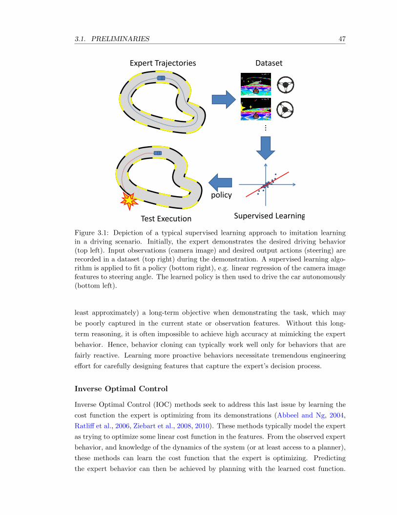
3.1. PRELIMINARIES 47
Expert Trajectories Dataset
Supervised LearningTest Execution
policy
...
Figure 3.1: Depiction of a typical supervised learning approach to imitation learningin a driving scenario. Initially, the expert demonstrates the desired driving behavior(top left). Input observations (camera image) and desired output actions (steering) arerecorded in a dataset (top right) during the demonstration. A supervised learning algo-rithm is applied to fit a policy (bottom right), e.g. linear regression of the camera imagefeatures to steering angle. The learned policy is then used to drive the car autonomously(bottom left).
least approximately) a long-term objective when demonstrating the task, which may
be poorly captured in the current state or observation features. Without this long-
term reasoning, it is often impossible to achieve high accuracy at mimicking the expert
behavior. Hence, behavior cloning can typically work well only for behaviors that are
fairly reactive. Learning more proactive behaviors necessitate tremendous engineering
effort for carefully designing features that capture the expert’s decision process.
Inverse Optimal Control
Inverse Optimal Control (IOC) methods seek to address this last issue by learning the
cost function the expert is optimizing from its demonstrations (Abbeel and Ng, 2004,
Ratliff et al., 2006, Ziebart et al., 2008, 2010). These methods typically model the expert
as trying to optimize some linear cost function in the features. From the observed expert
behavior, and knowledge of the dynamics of the system (or at least access to a planner),
these methods can learn the cost function that the expert is optimizing. Predicting
the expert behavior can then be achieved by planning with the learned cost function.
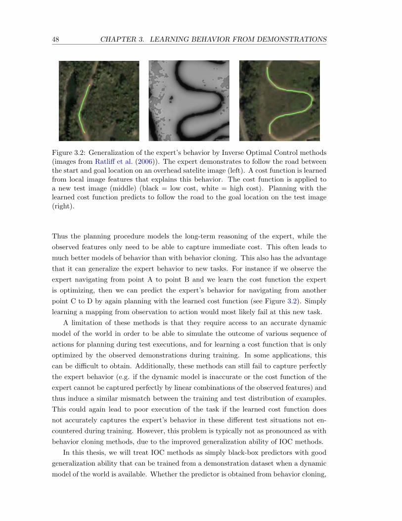
48 CHAPTER 3. LEARNING BEHAVIOR FROM DEMONSTRATIONS
Figure 3.2: Generalization of the expert’s behavior by Inverse Optimal Control methods(images from Ratliff et al. (2006)). The expert demonstrates to follow the road betweenthe start and goal location on an overhead satelite image (left). A cost function is learnedfrom local image features that explains this behavior. The cost function is applied toa new test image (middle) (black = low cost, white = high cost). Planning with thelearned cost function predicts to follow the road to the goal location on the test image(right).
Thus the planning procedure models the long-term reasoning of the expert, while the
observed features only need to be able to capture immediate cost. This often leads to
much better models of behavior than with behavior cloning. This also has the advantage
that it can generalize the expert behavior to new tasks. For instance if we observe the
expert navigating from point A to point B and we learn the cost function the expert
is optimizing, then we can predict the expert’s behavior for navigating from another
point C to D by again planning with the learned cost function (see Figure 3.2). Simply
learning a mapping from observation to action would most likely fail at this new task.
A limitation of these methods is that they require access to an accurate dynamic
model of the world in order to be able to simulate the outcome of various sequence of
actions for planning during test executions, and for learning a cost function that is only
optimized by the observed demonstrations during training. In some applications, this
can be difficult to obtain. Additionally, these methods can still fail to capture perfectly
the expert behavior (e.g. if the dynamic model is inaccurate or the cost function of the
expert cannot be captured perfectly by linear combinations of the observed features) and
thus induce a similar mismatch between the training and test distribution of examples.
This could again lead to poor execution of the task if the learned cost function does
not accurately captures the expert’s behavior in these different test situations not en-
countered during training. However, this problem is typically not as pronounced as with
behavior cloning methods, due to the improved generalization ability of IOC methods.
In this thesis, we will treat IOC methods as simply black-box predictors with good
generalization ability that can be trained from a demonstration dataset when a dynamic
model of the world is available. Whether the predictor is obtained from behavior cloning,
3.2. PROBLEM FORMULATION AND NOTATION 49
or IOC, we will present iterative interactive learning procedures that can be used to
address the train-test mismatch both of these methods can suffer from and improve
their performance. In the remainder of this chapter, we will focus entirely on behavior
cloning approaches, in part for simplicity, and in part because many of the applications
we consider cannot be tackled by IOC methods, due to the unavailability of a dynamic
model of the world that can predict future sequence of observations. Nevertheless, the
same iterative learning strategy could be applied with IOC methods.
3.2 Problem Formulation and Notation
We now define formally the imitation learning problem, our objective and notation used
for later analysis.
We consider a T -step control task where the learner must predict a sequence of T
actions. We denote by Π the class of policies the learner is considering (e.g. a set of
linear classifiers or regressors). As the distribution of states encountered by different
policies is of particular importance to our analysis, we denote:
• dtπ: The distribution of states at time t if the learner executed policy π from time
step 1 to t− 1.
• dπ = 1T
∑Tt=1 d
tπ: The average distribution of states if we follow policy π for T
steps.
Given a state s, we denote C(s, a) the expected immediate cost of performing ac-
tion a in state s for the task we are considering and denote Cπ(s) = Ea∼π(s)[C(s, a)]
the expected immediate cost of π in s. We assume C is bounded in [0, Cmax]. The
total cost of executing policy π for T -steps (i.e., the cost-to-go) is denoted J(π) =∑Tt=1 Es∼dtπ [Cπ(s)] = T Es∼dπ [Cπ(s)].
In imitation learning, we may not necessarily know or observe true costs C(s, a) for
the particular task. Instead, we observe expert demonstrations and seek to bound J(π)
for any (bounded) cost function C based on how well π mimics the expert’s policy π∗.
In particular, we would like to show that the total cost of the learned policy is not much
worse than the total cost of the expert. Denote ` the observed surrogate loss function
we minimize instead of C. For instance, if the action a is continuous and we are training
a regressor π, then `(s, a, π) may be the squared loss, `(s, a, π) = (π(s)− a)2. If actions
are discrete, then ` may be the expected 0-1 loss `(s, a, π) = Ea′∼πs [I(a′ 6= a)] or if π is
a multiclass SVM, then ` may be the hinge loss, `(s, a, π) = maxa′∈A[π(s, a′) + I(a′ 6=a)] − π(s, a), for π(s, a) the SVM score associated with predicting a in s, and I the
indicator function. Importantly, in many instances, C and ` may be the same function–
for instance, if we are interested in optimizing the learner’s ability to predict the actions
50 CHAPTER 3. LEARNING BEHAVIOR FROM DEMONSTRATIONS
chosen by an expert. For this objective, we will also be interested in measuring the total
expected regret (in surrogate loss) of the learned policy π over T steps, compared to
other predictors in the class, under its own induced sequences, denoted R(π):
R(π) = TEs∼dπ ,a∼π∗(s)[`(s, a, π)]− minπ′∈Π
TEs∼dπ ,a∼π∗(s)[`(s, a, π′)]
Our goal is to find a policy π which minimizes the observed surrogate loss under its
induced distribution of states with respect to expert’s actions in those states, i.e.:
π = arg minπ∈Π
Es∼dπ ,a∼π∗(s)
[`(s, a, π)] (3.1)
As system dynamics are assumed both unknown and complex, we cannot compute dπ
and can only sample it by executing π in the system. Hence this is a non-i.i.d. supervised
learning problem due to the dependence of the input distribution on the policy π itself.
The interaction between policy and the resulting distribution makes optimization difficult
as it results in a non-convex objective even if the loss `(s, a, ·) is convex in π for all states
s and actions a.
Assumptions: We do not make any assumption about the dynamics of the system or
the way the states are generated (in particular we do make any markovian assumption).
Our only assumption is that the initial state of any trajectory during training and testing
is drawn i.i.d. from the same distribution, but the distribution of states at any time t
may depend on the entire history of previous states and actions. The “state” is only
assumed a sufficient statistic of the history for determining immediate cost (under C),
the expert’s action and the action of any policy in Π (but not necessarily the next
“state”). Even though we define the learned policy as a function of state, we do not
assume the state is observable. Only some features of the current state (or observation)
are observed and available to the policy for making its predictions (e.g. we can think
that the state contains these features and that the policy class is restricted to only using
these features, rather than the entire state). Thus our analysis throughout this section
applies also to partially observable systems and systems with delays (that are unknown
to the learner). In addition, we do not assume that the task is always exactly the same
for every trajectory during training and testing. There can be a distribution over tasks
(e.g. driving different routes), and in this case the current task would be encoded as part
of the state. Thus when there are many tasks, our i.i.d. assumption on the initial state
simply implies that we assume the distribution of tasks is i.i.d. at training and testing.
We also do not assume the class of policy Π contains the expert policy π∗. That
is, there may be no policy that can mimic perfectly the expert in every state. The test
performance guarantees we present will end up depending on how well policies in the

3.3. SUPERVISED LEARNING APPROACH 51
class Π can predict the actions of the expert π∗ in expectation during training. The
more accurate they can be, the closer their performance will be to the expert.
3.3 Supervised Learning Approach
We now formalize and analyze the traditional supervised learning approach to imitation
adopted in behavior cloning methods. This analysis will illustrate the poor guarantees
of these methods, in addition to serve as a baseline to improve upon.
As mentioned previously, these methods simply train a policy π that best mimics
the expert’s actions under the distribution of states encountered by the expert dπ∗ . This
can be achieved using any standard supervised learning algorithm. Formally, they try
to optimize the following objective:
minπ∈Π
Es∼dπ∗ ,a∼π∗(s)
[`(s, a, π)] (3.2)
In practice, this optimization can only be achieved approximately, due to observation of
only a finite set of sampled state-action pairs along sampled trajectories (demonstrations)
of the expert. Hence, if (si, a∗i )mi=1 is a set of m observed state-action pairs observed
from expert demonstrations, supervised learning methods would return the policy πsup
that minimizes the empirical loss:
πsup = arg minπ∈Π
m∑i=1
`(si, a∗i , π) (3.3)
Analysis
We now provide a theoretical analysis of this supervised learning method. Our analysis
seeks to answer the following question: if we can achieve low error at mimicking the
expert on the training data, what guarantee can we provide on the total cost of the
learned policy, when used to perform the task?
First suppose we obtain a policy πsup such that its expected loss under the training
distribution is ε, i.e. ε = Es∼dπ∗ ,a∼π∗(s)[`(s, a, πsup)]. Then if ` is the 0-1 loss (or an
upper bound on the 0-1 loss, such as the hinge or logistic loss), we have the following
performance guarantee with respect to any task cost function C bounded in [0, Cmax],
as shown in our previous work (Ross and Bagnell, 2010):
Theorem 3.3.1. (Ross and Bagnell, 2010) Let ε = Es∼dπ∗ ,a∼π∗(s)[`(s, a, π)]. If ` upper
bounds the 0-1 loss, and C is bounded in [0, Cmax], then:
J(π) ≤ J(π∗) + CmaxT2ε.
52 CHAPTER 3. LEARNING BEHAVIOR FROM DEMONSTRATIONS
Proof. Due to a slight inaccuracy in the proof in (Ross and Bagnell, 2010) and that some
steps in the proof assumed π∗ was deterministic, we present here an accurate proof for
the fully general case where π and π∗ may be stochastic. Despite this, it does not change
the result of (Ross and Bagnell, 2010).
Let d1, d2, . . . , dT the distribution of states at each time step while executing the
learned policy π. Now imagine that while π is executed, we look at the actions that
would be picked by the expert π∗ in each encountered state (or sample an action from
the expert if π∗ is stochastic). Consider the event where the policy π picked the same
action as the expert π∗ in all the first t states encountered so far. Let pt the probability
that this event holds. Then by conditioning on this event, each dt can be expressed as
dt = pt−1d(c)t + (1 − pt−1)d
(e)t , where d
(c)t is the distribution of states at time t if we
always executed π, conditioned on π having picked always the correct action, i.e. the
same action as π∗ in all previously encountered states, and d(e)t is the distribution of
states at time t if we always executed π, conditioned on π having made at least 1 error,
i.e. it chose a different action than the expert in at least one of the previously encountered
states. Similarly, if we look at the distribution of states d∗1, d∗2, . . . , d
∗T , encountered by
the expert while executing π∗, and imagine that while π∗ is executed, we look at the
actions that would be picked by π in each encountered state (or sample an action from
π if it is stochastic). Again we can condition on the event where both π∗ and π picked
the same action in all states encountered so far. Thus each d∗t can be expressed as
d∗t = pt−1d(c)t + (1− pt−1)d
∗(e)t , where d
∗(e)t would the distribution of states encountered
by the expert at time t, conditioned on π picking an action different than π∗ in at least
one of the previous states encountered by the expert π∗. We can express d∗t this way
because conditioned on both π∗ and π having always picked the same actions up to time
t− 1, they must be in the same distribution of states d(c)t , and because this holds for all
t, the probability that this event holds at t is also pt−1 in both cases.
Now during training, the learner is trained under the distribution 1T
∑Tt=1 d
∗t . Let εt
the probability that π picks a different action than π∗ in the state distribution d∗t . By
definition of ε, we have 1T
∑Tt=1 εt ≤ ε. Now let ε
(c)t and ε
∗(e)t be the probability that π
picks a different action than π∗ in the state distributions d(c)t and d
∗(e)t respectively. Then
we have εt = pt−1ε(c)t + (1− pt−1)ε
∗(e)t . Since ε
∗(e)t ≥ 0, then εt ≥ pt−1ε
(c)t . Additionally,
the probability that the learner made at least 1 error in the first t steps (1 − pt) =
(1 − pt−1) + pt−1ε(c)t . So (1 − pt) ≤ (1 − pt−1) + εt. Solving this recurrence we have
(1− pt) ≤∑t
i=1 εt.
Using all these facts, now consider the expected total cost J(π) of executing the policy
π. Let Ct, C(c)t and C
(e)t the expected immediate cost (under cost function C) of executing
π in state distribution dt, d(c)t and d
(e)t respectively. We have J(π) =
∑Tt=1Ct and
Ct = pt−1C(c)t +(1−pt−1)C
(e)t . Now since C ∈ [0, Cmax], then C
(e)t ≤ Cmax. Additionally,
3.3. SUPERVISED LEARNING APPROACH 53
consider the immediate cost C∗t and C∗(c)t of executing π∗ in state distributions d∗t and
d(c)t . Then J(π∗) =
∑Tt=1C
∗t and because costs are non-negative, we must have C∗t ≥
pt−1C∗(c)t . Now in state distribution d
(c)t , whenever both π and π∗ picks the same action,
then π must incur the same cost as the expert, and when π picks a different action, π
must incur at most cost Cmax more than the expert. Since the probability π picks a
different action is ε(c)t , then this implies C
(c)t ≤ C
∗(c)t + ε
(c)t Cmax. Combining with the
above, we obtain:
Ct = pt−1C(c)t + (1− pt−1)C
(e)t
≤ pt−1C∗(c)t + pt−1ε
(c)t Cmax + (1− pt−1)Cmax
= pt−1C∗(c)t + (1− pt)Cmax
≤ C∗t + (1− pt)Cmax
≤ C∗t + Cmax∑t
i=1 εt
Hence summing over t, we obtain:
J(π) ≤ J(π∗) + Cmax∑T
t=1
∑ti=1 εt
= J(π∗) + Cmax∑T
t=1(T + 1− t)εt≤ J(π∗) + CmaxT
∑Tt=1 εt
≤ J(π∗) + CmaxT2ε
Similar results (although not as tight), were also independently developed in later
work in Syed and Schapire (2010).
More importantly our bound is tight, i.e. there exist problems such that a policy
π with ε expected loss under the training distribution dπ∗ can incur extra cost that
grows quadratically in T . Kaariainen (2006) previously demonstrated this in a sequence
prediction example1. We also provided an imitation learning example in Ross and Bagnell
(2010) where J(πsup) = (1− εT )J(π∗) + T 2ε. We include it here for completeness.
Theorem 3.3.2. (Ross and Bagnell, 2010) There exists MDPs and policies π with ε ∈[0, 1/T ] expected 0-1 loss under the expert’s training distribution, i.e. ε = Es∼dπ∗ ,a∼π∗(s)[I(π(s) 6=a)], such that J(π) = (1− εT )J(π∗) + CmaxT
2ε.
Proof. Consider the following problem with 3 states (s0, s1, s2) and 2 actions (a1, a2).
The learner always starts in s0 and transitions are deterministic as specified in Figure
3.3. The expert’s policy π∗ is to perform a2 in s1, and a1 in s0 and s2, and consider
the cost function C(s, a) = CmaxI(π∗(s) 6= a) + cI(π∗(s) = a), where I is the indicator
function and for all states s, 0 ≤ c ≤ Cmax).
1In their example, an error rate of ε > 0 when trained to predict the next output in sequence with
the previous correct output as input can lead to an expected number of mistakes of T2− 1−(1−2ε)T+1
4ε+ 1
2
over sequences of length T at test time. This is bounded by T 2ε and behaves as Θ(T 2ε) for small ε.
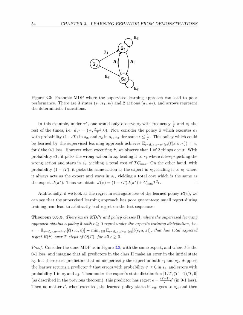
54 CHAPTER 3. LEARNING BEHAVIOR FROM DEMONSTRATIONS
s0
s1
s2
a1
a2
a1 a1
a2
a2
Figure 3.3: Example MDP where the supervised learning approach can lead to poorperformance. There are 3 states (s0, s1, s2) and 2 actions (a1, a2), and arrows representthe deterministic transitions.
In this example, under π∗, one would only observe s0 with frequency 1T and s1 the
rest of the times, i.e. dπ∗ = ( 1T ,
T−1T , 0). Now consider the policy π which executes a1
with probability (1− εT ) in s0, and a2 in s1, s2, for some ε ≤ 1T . This policy which could
be learned by the supervised learning approach achieves Es∼dπ∗ ,a∼π∗(s)(`(s, a, π)) = ε,
for ` the 0-1 loss. However when executing π, we observe that 1 of 2 things occur. With
probability εT , it picks the wrong action in s0, leading it to s2 where it keeps picking the
wrong action and stays in s2, yielding a total cost of TCmax. On the other hand, with
probability (1− εT ), it picks the same action as the expert in s0, leading it to s1 where
it always acts as the expert and stays in s1, yielding a total cost which is the same as
the expert J(π∗). Thus we obtain J(π) = (1− εT )J(π∗) + CmaxT2ε.
Additionally, if we look at the regret in surrogate loss of the learned policy R(π), we
can see that the supervised learning approach has poor guarantees: small regret during
training, can lead to arbitrarily bad regret on the test sequences:
Theorem 3.3.3. There exists MDPs and policy classes Π, where the supervised learning
approach obtains a policy π with ε ≥ 0 regret under the expert’s training distribution, i.e.
ε = Es∼dπ∗ ,a∼π∗(s)[`(s, a, π)] − minπ∈Π Es∼dπ∗ ,a∼π∗(s)[`(s, a, π)], that has total expected
regret R(π) over T steps of O(T ), for all ε ≥ 0.
Proof. Consider the same MDP as in Figure 3.3, with the same expert, and where ` is the
0-1 loss, and imagine that all predictors in the class Π make an error in the initial state
s0, but there exist predictors that mimic perfectly the expert in both s1 and s2. Suppose
the learner returns a predictor π that errors with probability ε′ ≥ 0 in s1, and errors with
probability 1 in s0 and s2. Then under the expert’s state distribution [1/T, (T − 1)/T, 0]
(as described in the previous theorem), this predictor has regret ε = (T−1)T ε′ (in 0-1 loss).
Then no matter ε′, when executed, the learned policy starts in s0, goes to s2, and then
3.3. SUPERVISED LEARNING APPROACH 55
stays in s2, making an error at every step. Its total 0-1 loss is T under test executions, yet
a predictor in the class which is correct in s2 has 0-1 loss of 1 under this same sequence
of states. Thus the total expected regret of the learned policy R(π) = T − 1.
These results also have some implications on the number of samples required to learn
good performance with such methods. That is, due to the factor T 2, one may need a
larger number of samples to obtain good performance with this method. We briefly
analyze the sample complexity below to demonstrate this.
Sample Complexity
As mentioned previously, in practice one cannot minimize directly the expected surrogate
loss Es∼dπ∗ ,a∼π∗(s)[`(s, a, π)]. Instead the surrogate loss is minimized on a finite set of
samples (si, a∗i )mi=1 collected during expert demonstrations, as described in Equation 3.3.
Nevertheless, as we collect more and more samples, we would be able to guarantee that
with high probability, we obtain a policy which is not much worse than the policy with
smallest expected loss under the training distribution.
In particular, let εclass = minπ∈Π Es∼dπ∗ ,a∼π∗(s)(`(s, a, π)) the expected surrogate loss
of the best policy in the class. Suppose we collect m i.i.d. samples from the expert
demonstrations, then using standard PAC learning bounds, the policy π that minimizes
the empirical loss on these samples will typically guarantee that with probability at
least 1 − δ, its expected loss ε ≤ εclass + O(
√C(Π)+log(1/δ)
m ), for C(Π) a measure of the
complexity of the class of policy Π (for instance its VC dimension (Vapnik, 1995) if
it is a class of binary classifiers, or analogous multi class equivalent (Natarajan, 1989)).
Because the performance guarantees scale with CmaxT2ε, then to ensure that CmaxT
2ε ≤CmaxT
2εclass+α with high probability 1−δ for some desired α, we would need the number
of samples m to be order O(C2maxT
4(C(Π) + log(1/δ))/α2).
Discussion
In the context of learning reductions, this approach can be interpreted as an error reduc-
tion of imitation learning to a supervised learning problem. It is an error reduction, as
task performance is related to the error, or loss, on the supervised learning task, rather
than the regret2. Importantly, it is not a very good reduction, as performance at the
imitation learning task does not degrade nicely as error at the supervised learning task
increases. We also demonstrated that in terms of regret, this reduction does not provide
any guarantee, as small or even 0 training regret on the supervised learning task can
lead to arbitrarily large regret during testing.
2Here the regret on the supervised learning task is the difference in error of the learned predictorto the minimum error achievable; e.g. when the expert is noisy, the minimum error would be non-zero,even for the bayes-optimal predictor.
56 CHAPTER 3. LEARNING BEHAVIOR FROM DEMONSTRATIONS
These results and example demonstrate that the traditional supervised learning ap-
proach can learn policies with poor guarantees that are not robust to the errors they
make, leading to a compounding growth in cost. Unless one can find predictors with
arbitrary small error at mimicking the expert, one could always find a sufficiently large
horizon T , where the learned policy may achieve the worst possible total cost. Hence
even small training error can lead to performance arbitrarily close to the worst total
cost. In addition, even in cases where good policies exists, one may need a lot of data to
find them (that grows as O(T 4)). This also illustrates how guarantees are much worse
than in the i.i.d. classification settings, where if we learn a policy with expected ε 0-1
loss during training, its expected classification loss for classifying T new examples at test
time is Tε (and not T 2ε). This leads to the following question: can we develop alternate
learning procedures for sequential problems with guarantees that are similar to the i.i.d.
setting? In the following sections, we present several approaches that can achieve this.
3.4 Iterative Forward Training Approach
We now present a first iterative and interactive training approach that can provide better
performance than the traditional supervised learning approach. This approach exploits
the structure of the time dependency between predictions, and interaction with the
learner, to provide better performance guarantees.
Intuitively, the traditional supervised approach fails to give good performance bounds
due to the discrepancy between the testing and training distribution when π 6= π∗ and
because the learner does not learn how to recover from mistakes it makes. The intuition
behind the next approach, called Forward Training algorithm, is that both of these
problems can be solved if we allow the training to occur over several iterations, where
at each iteration we train one policy for one particular time step. If we do this training
sequentially, starting from the first time step to the last, then at the tth iteration, we
can sample states from the actual testing distribution at time step t by executing the
learned policies for each previous step, and then asks the expert what to do at the tth
time step to train the next policy. Furthermore, if the learner makes mistakes, the expert
demonstrates how to recover at future steps, allowing the learner to learn the necessary
recovery behaviors. The algorithm terminates once it has learned a policy for all T
steps. This is similar to the Sequential Stacking algorithm (Cohen and Carvalho, 2005)
for sequence classification.
More formally, Forward Training proceeds as follows. At the first iteration, it trains
a policy π1 for the first time step to best mimic the actions chosen by the expert π∗ on
states visited at time 1 (initial states). Then at iteration t, it trains a policy πt for time
step t, by collecting data though interaction as follows: the learner executes its learned
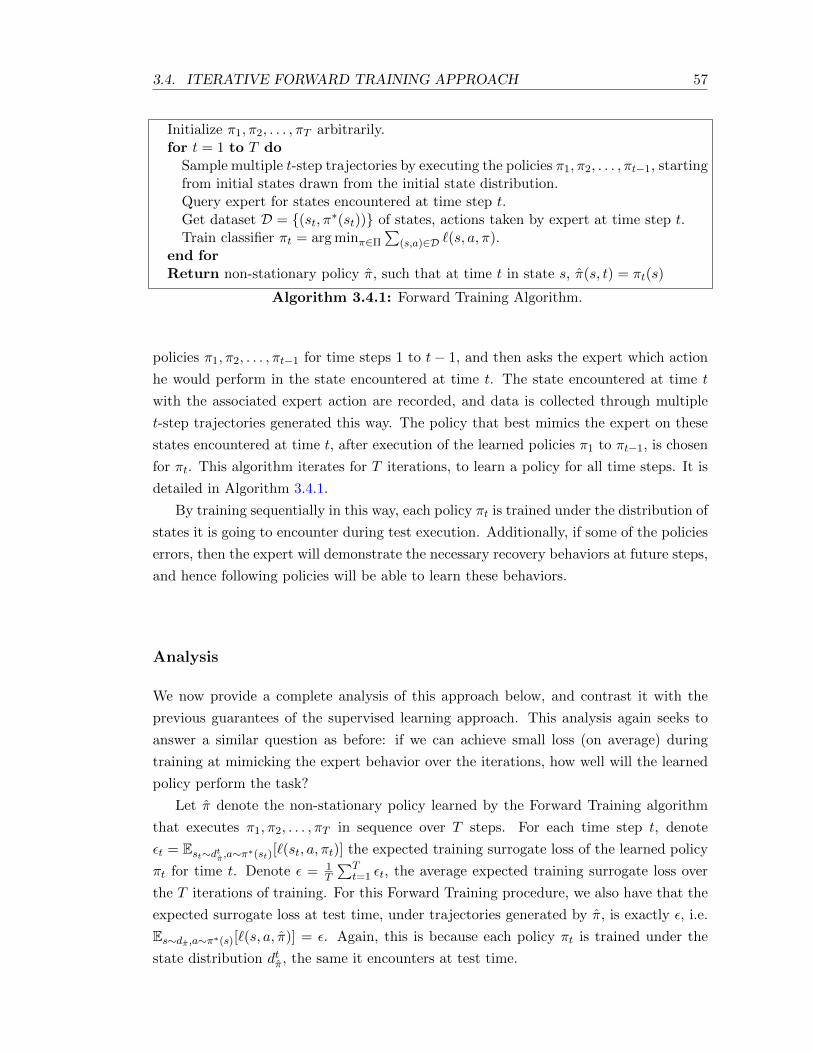
3.4. ITERATIVE FORWARD TRAINING APPROACH 57
Initialize π1, π2, . . . , πT arbitrarily.for t = 1 to T do
Sample multiple t-step trajectories by executing the policies π1, π2, . . . , πt−1, startingfrom initial states drawn from the initial state distribution.Query expert for states encountered at time step t.Get dataset D = (st, π∗(st)) of states, actions taken by expert at time step t.Train classifier πt = arg minπ∈Π
∑(s,a)∈D `(s, a, π).
end forReturn non-stationary policy π, such that at time t in state s, π(s, t) = πt(s)
Algorithm 3.4.1: Forward Training Algorithm.
policies π1, π2, . . . , πt−1 for time steps 1 to t− 1, and then asks the expert which action
he would perform in the state encountered at time t. The state encountered at time t
with the associated expert action are recorded, and data is collected through multiple
t-step trajectories generated this way. The policy that best mimics the expert on these
states encountered at time t, after execution of the learned policies π1 to πt−1, is chosen
for πt. This algorithm iterates for T iterations, to learn a policy for all time steps. It is
detailed in Algorithm 3.4.1.
By training sequentially in this way, each policy πt is trained under the distribution of
states it is going to encounter during test execution. Additionally, if some of the policies
errors, then the expert will demonstrate the necessary recovery behaviors at future steps,
and hence following policies will be able to learn these behaviors.
Analysis
We now provide a complete analysis of this approach below, and contrast it with the
previous guarantees of the supervised learning approach. This analysis again seeks to
answer a similar question as before: if we can achieve small loss (on average) during
training at mimicking the expert behavior over the iterations, how well will the learned
policy perform the task?
Let π denote the non-stationary policy learned by the Forward Training algorithm
that executes π1, π2, . . . , πT in sequence over T steps. For each time step t, denote
εt = Est∼dtπ ,a∼π∗(st)[`(st, a, πt)] the expected training surrogate loss of the learned policy
πt for time t. Denote ε = 1T
∑Tt=1 εt, the average expected training surrogate loss over
the T iterations of training. For this Forward Training procedure, we also have that the
expected surrogate loss at test time, under trajectories generated by π, is exactly ε, i.e.
Es∼dπ ,a∼π∗(s)[`(s, a, π)] = ε. Again, this is because each policy πt is trained under the
state distribution dtπ, the same it encounters at test time.
58 CHAPTER 3. LEARNING BEHAVIOR FROM DEMONSTRATIONS
Imitation Loss Guarantee
These observations already imply a first interesting result for the case where the surrogate
loss is the same as the task cost function (or an upper bound on it), i.e. Ea∼π∗(s)[`(s, a, π)] ≥Cπ(s) for all states s. For instance we may measure task performance directly in terms of
the ability of the learner to mimic the actions of the expert (in terms of the 0-1 imitation
loss), or for continuous action problems, in terms of a squared loss penalizing deviations
from the actions of the expert.
For such task cost function that are related directly to the surrogate imitation loss
we have the following guarantee:
Theorem 3.4.1. Let ε = Es∼dπ ,a∼π∗(s)[`(s, a, π)], the average training loss of the learned
policy π with Forward Training, and ` be the same as the cost function C (or an upper
bound on it), then J(π) ≤ Tε.
Proof. Follows directly from the fact that:
J(π) =∑T
t=1 Es∼dtπ [Cπt(s)]
≤∑T
t=1 Es∼dtπ ,a∼π∗(s)[`(s, a, πt)]= Tε
This result has particularly useful applications when we just want to measure how
well the learner can mimic the expert. In particular, in continuous settings where we use
a squared loss to expert’s action, this result indicates that under test trajectories of the
learned policy, the expected total squared distance to expert’s actions will be the same
as during training. In comparison, we did not have any guarantee for the supervised
learning approach in such continuous settings3.
Additionally, we can also show an interesting guarantee for the regret (in surrogate
loss) of the learned policy with Forward. Let
rt = Es∼dtπ ,a∼π∗(s)
[`(s, a, πt)]−minπ∈Π
Es∼dtπ ,a∼π∗(s)
[`(s, a, π)],
denote the regret of the learned policy πt for time t under the training distribution
dtπ. Then let r = 1T
∑Tt=1 rt, the average regret of the learned policy returned by the
supervised learning algorithm, then we have that the total expected regret R(π) of the
learned policy π, under its own sequences of T steps, is at most Tr:
3In continuous settings, the supervised learning approach may be shown to have a similar compound-ing growth of the cost, as in the analyzed discrete setting, under Lipschitz continuity assumption of theexpert’s policy and system transition. Without such assumptions, its performance can be arbitrarilybad.
3.4. ITERATIVE FORWARD TRAINING APPROACH 59
Theorem 3.4.2. Let r = 1T
∑Tt=1 rt, the average regret of the learned policies π1, π2, . . . , πT
returned by the supervised learning algorithm over the iterations of Forward, then the
learned policy π with Forward is such that R(π) ≤ Tr.
Proof.
R(π)
=∑T
t=1 Es∼dtπ ,a∼π∗(s)[`(s, a, πt)]−minπ′∈Π
∑Tt=1 Es∼dtπ ,a∼π∗(s)[`(s, a, π
′)]
≤∑T
t=1[Es∼dtπ ,a∼π∗(s)[`(s, a, πt)]−minπ′t∈Π Es∼dtπ ,a∼π∗(s)[`(s, a, π′t)]]
=∑T
t=1 rt
= Tr
Thus, in contrast with the typical supervised learning approach to imitation, where
small regret during training can lead to arbitrarily bad regret during test executions
(as shown in previous Theorem 3.3.3), Forward Training guarantees that small average
regret during training, also implies small regret during test execution.
General Cost Function Guarantee
More generally, when the task cost function C is not related directly to the surrogate
loss `, we can still show that the extra task cost incurred by the learned policy, compared
to the expert, grows linearly in T when the expert’s behavior is robust in some sense.
This is formalized below.
Let Q∗t (s, π) denote the t-step cost of executing policy π in state s and then following
the expert policy π∗ and V ∗t (s) the t-step cost of executing the expert starting in s. We
quantify the robustness of the expert’s policy π∗ as follows:
Definition 3.4.1. Consider any policy π ∈ Π such that Es∼dπ ,a∼π∗(s)[`(s, a, π)] ≤ ε and
let εt = Es∼dtπ ,a∼π∗(s)[`(s, a, π)]. We say the expert’s policy π∗ is uT,ε-robust if under
the task cost function C, Es∼dtπ [Q∗T−t+1(s, π)−V ∗T+t+1(s)] ≤ uT,εεt for any such policy π
and any time t.
The subscript T and ε indicates that uT,ε is typically a function of T and ε and
increases as T and/or ε increases. To ease the notation in our results below, we will
simply say the expert is u-robust, where the subscript T and ε implicitly used should
be clear from context. This notion of robustness measures whether policies that are
similar to the expert, i.e. small ε, can lead to state distributions where acting differently
than the expert for one more step, can increase significantly the expected cost-to-go
of the expert. It intuitively measures the ability of the expert to recover from errors
made by such similar policies. For example, consider a task that involves driving near
60 CHAPTER 3. LEARNING BEHAVIOR FROM DEMONSTRATIONS
a cliff. In this case, a policy can potentially lead to a situation where doing a single
erroneous action falls off the cliff, at which point the expert cannot recover, leading to
large cost, whereas if the expert would have been executed immediately, he could have
avoided falling off the cliff, leading to small cost. In such case where the expert cannot
recover from single errors, uT,ε can be large (it can be as large as TCmax for discrete
actions and cost functions C bounded in [0, Cmax]). However when looking at similar
policies to the expert (small ε), we could still expect uT,ε to be small in this example if
the expert policy is driving safely far enough from the cliff. This is because the further
off the cliff the expert is driving, the larger ε would need to be for the learned policy to
encounter situations where it can fall off the cliff and the expert cannot recover. Thus in
some sense, this notion of robustness can often capture a similar notion to the stability
margin of the expert in control (Ljung, 1999). If the expert can always recover, from
execution of similar policies within some threshold of error ε, then uT,ε will be small.
Importantly, in many situations, uT,ε can be bounded by a small constant indepen-
dent of T and ε. First, if C = ` is the 0-1 loss, then uT,ε = 1, as the 0-1 loss of the
expert in all future states would be 0 (assuming π∗ is deterministic), and for any time t
and policy π we have Es∼dtπ [Q∗T−t+1(s, π)− V ∗T+t+1(s)] = εt. Another example may be a
robot navigation task with an omnidirectional robot where one can always perform an
action to come back to the previous state we were (e.g. if we went left, we can then
go right to get back to where we were). In such task, if for instance the cost of any
action is Cmax, until one reaches the goal state where cost is 0, then uT,ε ≤ 2Cmax for
good experts. That is, in any state s, for any policy that would be executed first before
the expert, the expert can then always do an action to undo the policy’s action, and
then follow the same course of action as he would have starting is s. The difference
between these two course of actions would be ≤ 2Cmax, and the expert only needs to
do this when the policy acts differently then he would (i.e. with probability less than
εt at time t if ` is the 0-1 loss or upper bounds it). Thus for any policy π and time t,
Es∼dtπ [Q∗T−t+1(s, π)−V ∗T+t+1(s)] ≤ 2Cmaxεt. More generally, in MDPs where the Markov
Chain defined by the system dynamics and expert policy π∗ is mixing, then uT,ε can be
related to the mixing rate of the chain4: if π∗ is rapidly mixing, i.e. it always recovers
quickly from errors, then uT,ε is small.
We now show the importance of this robustness notion:
Theorem 3.4.3. Let ε = Es∼dπ [`(s, a, π)], the average training loss of the learned policy
π with Forward Training, and suppose the expert π∗ is u-robust under the task cost
function C (as in Definition 3.4.1). Then J(π) ≤ J(π∗) + uTε.
Proof. We here follow a similar proof to Ross and Bagnell (2010). Given our policy π,
4In particular, if it is α-mixing with exponential decay rate δ then u is O(Cmax1
1−exp(−δ) )
3.4. ITERATIVE FORWARD TRAINING APPROACH 61
consider the policy π1:t, which executes π in the first t-steps and then executes the expert
π∗. Then
J(π)
= J(π∗) +∑T−1
t=0 [J(π1:T−t)− J(π1:T−t−1)]
= J(π∗) +∑T
t=1 Es∼dtπ [Q∗T−t+1(s, π)− V ∗T−t+1(s)]
≤ J(π∗) + u∑T
t=1 εt
= J(π∗) + uTε
The inequality follows from the definition of robustness.
For discrete actions and cost functions bounded in [0, Cmax], u ≤ TCmax, so this
guarantee is always better than the guarantee of the supervised learning approach. In
scenarios where u is much smaller, then forward training can provide significant im-
provement over the supervised learning approach. In some sense, this bound says that
Forward Training can learn good and robust behavior if the expert itself is robust. In this
case, low average training error, always imply good test task performance, unlike with
the supervised learning approach. As in many real applications we can expect the expert
behavior to be somewhat robust and tolerant to some error (e.g. human drivers typically
drive near the center of the lane, at a fair distance to other vehicles or obstacles), then
we can often expect this method to provide improved performance in practice.
The previous example in Figure 3.3 also provides a concrete scenario where Forward
Training leads to improved performance compared to the supervised learning approach.
In this example, it can be seen that u ≤ (Cmax− c), and if we learn policies with average
expected training 0-1 loss of ε, we would be guaranteed to obtain a non-stationary policy
π with performance J(π) ≤ J(π∗) + (Cmax − c)Tε. However in that same example the
supervised learning method could learn a policy π with expected training 0-1 loss of ε
with performance J(π) = J(π∗) + (Cmax− c)T 2ε 5. Thus the forward training procedure
is a factor T better in this example. The intuitive reason for this is that now, if the
learned policy errors in the first step, it can collect training examples in state s2 and
learn what to do in this state, whereas with the supervised learning approach, s2 was
never visited during training.
Sample Complexity
Another advantage of this approach is that it can sometimes learn good behavior in fewer
samples than the supervised learning approach when uT,ε is small, due to the improved
dependency on T . Suppose for example that we collect m i.i.d. datapoints at each iter-
ation of training, and εclass,t = minπ∈Π Es∼dtπ ,a∼π∗(s)[`(s, a, π)] is the minimum expected
surrogate loss with policies from class Π at iteration t. Let εclass = 1T
∑Tt=1 εclass,t, the
5Using the fact that since J(π∗) = cT , (1− εT )J(π∗) + CmaxT2ε = J(π∗) + (Cmax − c)T 2ε

62 CHAPTER 3. LEARNING BEHAVIOR FROM DEMONSTRATIONS
minimum average expected surrogate loss. Then using standard PAC learning bounds
and a union bound over all time steps t, the expected training surrogate loss of the
learned non-stationary policy ε ≤ εclass + O(
√C(Π)+log(1/δ)+log(T )
m ) with probability at
least 1 − δ. Again here C(Π) denotes a measure of complexity of the class Π. As per-
formance decreases with uTε, then to guarantee this is not worse than uTεclass + α
with high probability 1 − δ for some desired α > 0, we would require m to be order
O(u2T 2(C(Π) + log(1/δ) + log(T ))/α2). As m is the number of samples per iteration,
we would require a total of O(u2T 3(C(Π) + log(1/δ) + log(T ))/α2) samples to complete
all T iterations. This is a reduction by a factor T , compared to the supervised learning
approach, when u is constant or independent of T (e.g. O(Cmax)). However in the worst
case where u is O(T ), then this method may need a factor T more samples then the
supervised learning approach, i.e. O(T 5), in order to guarantee the same performance.
Discussion
The Forward Training algorithm provides a first method to obtain better guarantees and
learn more efficiently than the supervised learning approach when the expert’s policy
has good robustness properties. Unlike the supervised learning approach, where small
training error can lead to arbitrarily bad task performance, the forward training method
guarantees that small training error will lead to good task performance. In addition,
small training regret also lead to small regret under the test distribution.
In the context of learning reductions, this approach can be interpreted as an error
reduction of imitation learning to a sequence of supervised learning problems. It is again
an error reduction, as task performance is related to the average error, or loss, on the
supervised learning tasks, rather than the average regret6. It can also be interpreted as a
regret reduction for the surrogate loss objective, where regret under the test trajectories
is related to the regret on the supervised learning problems. It is a much better reduction
than the previous supervised learning reduction, as here performance at the imitation
learning task degrades nicely (linearly in T ) as error (or regret) at the supervised learning
task increases. This is the best we can hope for, as it matches the same guarantees we
would have in an i.i.d. classification setting for classifying T new i.i.d. examples.
A drawback of the Forward algorithm is that it is impractical when T is large (or un-
defined) as we must train T different policies sequentially and cannot stop the algorithm
before we complete all T iterations. Hence it can not be applied to many real-world ap-
plications. Additionally, in some sense, it is still inefficient at learning the demonstrated
behavior, as it does not generalize the behavior across time steps and may need to learn
6Here the average regret on the supervised learning tasks is the average difference in error of thelearned predictors to the minimum error achievable on each task; e.g. when the expert is noisy, theminimum error would be non-zero, even for the bayes-optimal predictor.

3.5. STOCHASTIC MIXING TRAINING 63
the same (or similar behavior) repeatedly from scratch across many steps. This is not
very satisfactory and we should intuitively be able to do better than this by generalizing
the behavior across time. Despite this, it can be still a useful algorithm in other sequen-
tial prediction settings where small sequence of predictions are more common (e.g. the
recommendation tasks we consider in Chapter 7).
In the next two sections, we present approaches that address these limitations, while
still providing similar performance guarantees.
3.5 Stochastic Mixing Training
To avoid the limitations of having to train a separate policy for each step, which is
often impractical and inefficient as just discussed, we would like instead to train a fixed
stationary policy, that is executed for all time steps. Before we introduce the main
approach of this thesis that allows learning such stationary policy efficiently, we briefly
discuss some other related work that allows learning a stationary stochastic policy, with
guarantees similar to Forward.
One of the intuition behind the Forward training algorithm is that it can achieve
good performance by training the policy slowly, i.e. training one step at a time per
iteration, in a way that it allows the policy to adapt to the changing distribution of
states. The two approaches we review here, SEARN (Daume III et al., 2009) and SMILE
(Ross and Bagnell, 2010), train a stationary stochastic policy using a similar strategy of
training the policy slowly. In particular, these methods also proceed iteratively, learning
from interactions with the learner, by changing the distribution of actions picked by the
stationary stochastic policy slowly over the iterations. The slow change in the policy is
related to the Forward approach in the following sense: from one iteration to the next,
with high probability the policy changes at most 1 action over the entire sequence of T
steps. Hence, in some sense, these methods can be interpreted as randomized versions of
the Forward training procedure. By making the changes small enough from one iteration
to the next, these methods can provide similar guarantees to Forward.
We begin by reviewing SEARN (Daume III et al., 2009), an existing approach that
was proposed in the context of Structured Prediction, that we describe more extensively
when applying our methods to such problems in Chapter 6. SEARN can be adapted
for imitation learning problems and we describe here how it can be applied in such
settings. Then we discuss a variant of this approach, called SMILE, that we introduced
in our previous work (Ross and Bagnell, 2010), that is often more practical than SEARN
for imitation learning problems, while still providing improved guarantees over naive
supervised learning.
64 CHAPTER 3. LEARNING BEHAVIOR FROM DEMONSTRATIONS
SEARN for Imitation Learning
In the context of imitation learning, SEARN can be applied to train iteratively a station-
ary stochastic policy as follows. Starting from a policy π0 = π∗, that queries the expert
π∗ and executes its action, SEARN first trains a policy π1 by collecting data from execu-
tion of π0. This new policy is then stochastically mixed with π0 to obtain the next policy
π1 = (1−α)π0 +απ1, for some small α > 0. This update is interpreted as follows: in each
step π1 executes π0 with probability (1−α) and with probability α, executes π1. SEARN
keeps iterating in a similar fashion: at each iteration n, it interacts with the learner to
collect new data from execution of the learner’s current policy πn−1. This new data is
used to train a new policy πn, that is stochastically mixed with πn−1, to obtain the next
policy πn = (1−α)πn−1+απn. In other words, the stochastic policy trained in SEARN is
represented as a distribution over policies, such that πn = (1−α)nπ0+α∑n
i=1(1−α)n−iπi.
After n iterations, the probability that πn queries the expert to execute its action (i.e.
picks π0) at any step is (1 − α)n, i.e. it becomes exponentially small as this procedure
is iterated. After some large number of iterations N , SEARN terminates and returns a
final policy πN that does not query the expert, by renormalizing the distribution over
learned policies, i.e. πN = α1−(1−α)N
∑Ni=1(1− α)N−iπi.
At each iteration n, SEARN trains πn to pick actions that minimize future total
cost, if the current policy πn−1 would be executed from then on, under the distribution
of states visited by πn−1. This requires knowledge of the task cost function C. When C
is unknown, SEARN can be applied to minimize future surrogate loss ` of the current
policy. To do so, SEARN collects training examples, by executing the current policy
πn−1, and at some random time t, for the current state s, explores an action a and
then executes πn−1 until time T , to observe the total future loss Q action a induces in
state s when πn−1 is executed afterwards. Each trajectory generates a single example
(s, a,Q), that associates cost Q to executing action a in state s. In structured prediction,
SEARN typically proceeds by trying all predictions, from the current state, and rolling
out the current policy πn−1, to obtain cost estimates Q for all predictions/actions in
the current state. This is possible in imitation learning only if we can put back the
system exactly in the same state s to try all possible actions. While this may be possible
in simulated environments, on real robots this is often impossible or very hard. In
this case, SEARN can still be applied from the cost estimate of only a single explored
action in each visited state using techniques described later in Chapter 4. From the
dataset of examples (s, a,Q) collected at iteration n, SEARN then solves a cost-sensitive
classification problem to obtain the policy πn (the classifier that picks actions with
minimum cost on the training examples).
In Daume III et al. (2009), they show that if the learning parameter α is chosen small
enough, i.e. order O(1/T 3), and SEARN is iterated for long enough, N order O(T 3),
3.5. STOCHASTIC MIXING TRAINING 65
then SEARN provides good guarantees, i.e. it will learn a stationary stochastic policy
πN that performs the task well, under its own trajectories (assuming policies in the class
Π can solve the cost-sensitive classification tasks well on average).
The guarantees are similar to Forward as above: i.e. J(πN ) ≤ J(π∗) + T log(T )ε +
O(log T ) (Daume III et al., 2009), except here, ε corresponds to the average cost-sensitive
classification regret7 of the learned policies πn over the training iterations. When SEARN
is applied to minimize the surrogate loss `, a similar argument, involving the robustness
properties of the expert π∗, could be made to show that small surrogate loss ` implies
good task performance under the cost function C, i.e. J(πN ) ≤ J(π∗) + uT log(T )ε +
O(u log T ) if the expert π∗ is u-robust as in Definition 3.4.1.
In theory, SEARN needs a much larger number of iterations N than Forward, i.e.
O(T 3) instead of T . However in practice, SEARN can be applied with larger α, say
α = 0.1, and iterated for a small number of iterations (10-20 iterations) and obtain good
policies that perform the task well.
One of the drawback of SEARN is that it involves simulating an entire trajectory to
collect each datapoint. This can often be impractical as it requires a lot of effort from
human experts to collect any significant amount of data. A variant of SEARN can be
used to address this issue and is presented below.
SMILE: Stochastic Mixing Iterative Learning
In Ross and Bagnell (2010), we presented a technique called SMILE, that provides a
more practical variant of SEARN for learning from human experts in imitation learning
tasks. SMILE proceeds iteratively exactly like SEARN, and updating the policy through
stochastic mixing exactly as in SEARN, except that it chooses the policies πn differently.
The main idea is that instead of attempting to find a policy that minimizes future loss
of the current policy πn−1, we can simply try to find a policy that does not increase
its loss, and/or cost. In particular, this is achieved if we can find a policy πn that
behaves exactly like πn−1, i.e. as if πn = πn−1, then πn = πn−1. Since we know
πn−1 = (1 − α)n−1π∗ + α∑n−1
i=1 (1 − α)n−1−iπi, the only component of πn−1 that needs
to be learned is the expert π∗. Thus SMILE does the following, at iteration n, it learns
a policy π′n, that mimics well the expert under the distribution of states encountered by
πn−1, which is used to construct πn = (1− α)n−1π′n + α∑n−1
i=1 (1− α)n−1−iπi, and then
update πn = (1 − α)πn−1 + απn. Effectively, this update leads to πn = (1 − α)nπ∗ +
α∑n
i=1(1−α)i−1π′i. Thus we do not need to construct the intermediate policies πn, but
can simply maintain the distribution that associates probability α(1− α)n to executing
policy π′n to represent πn. After N iterations, SMILE also returns the renormalized
7By regret here we mean the difference in cost-sensitive classification loss of the learned classifier tothe bayes-optimal classifier that achieves minimum cost on the training data.
66 CHAPTER 3. LEARNING BEHAVIOR FROM DEMONSTRATIONS
policy πN that does not query the expert π∗.
SMILE is more practical than SEARN, as at each iteration, it only needs to record the
actions the expert would perform in every visited states along trajectories from execution
of πn−1. This allows for recording as many as T data points per trajectory, instead of
only 1 for SEARN. Training the policy π′n, simply involves solving a classification or
regression task to minimize the surrogate loss ` on this training data.
When training the policies in this way, SMILE leads to a distinction compared to
SEARN: older policies trained earlier have more weights (higher probability) than newer
policies. This is the opposite of SEARN, where newer policies have higher probability.
In Ross and Bagnell (2010), we showed that by choosing α = O( 1T 2 ) and perform-
ing O(T 2 log T ) iterations leads good guarantees for SMILE. Again in practice, one can
typically apply this algorithm with much larger α and iterate for a few iterations to
obtain a practical method that still improves over naive supervised learning. The guar-
antees of SMILE are similar to Forward and lead to an improvement over the standard
supervised training approach when the expert has good robustness properties. However
the guarantees are weaker than Forward, as it requires a stronger notion of robustness,
where during training the intermediate stochastic policies πn must themselves be robust.
In particular, if πn is un-robust, and at iteration n, π′n achieves εn 0-1 loss under the
distribution of πn−1 (or surrogate loss that upper bounds the 0-1 loss), then SMILE
guarantees that (Ross and Bagnell, 2010):
J(πN ) ≤ J(π∗) +O
(1 +
α
1− (1− α)NT
N∑n=1
(1− α)n−1un−1εn
).
This leads to good guarantees as long as the stochastic policies do not degrade too
fast, in terms of their robustness properties. For instance if un−1 is O(Cmax/(1−α)n−1),
as was shown in Ross and Bagnell (2010) for the example MDP in Figure 3.3, then this
leads SMILE to guarantee J(πN ) ≤ J(π∗) +O(CmaxT log(T )ε), for ε the average 0-1 loss
of the learned classifiers π′n over the training iterations.
However, there are some class of problems where Forward still provides good guaran-
tees (i.e. performance degrading linear in T and ε) but where SMILE does not improve
much over supervised learning. This can occur in problems where πn encounters sit-
uations where the only way for πn to recover, is if the expert policy π∗ is sampled to
be executed multiple time steps in a row by πn. In this case the robustness term can
degrade quickly, i.e. un can increase faster than O(1/(1 − α)n) as n increases, making
un reach the maximum TCmax quickly, and be TCmax for most iterations. This leads to
performance that degrades as O(CmaxT2ε), just like the supervised learning approach.
3.6. DATASET AGGREGATION: ITERATIVE INTERACTIVE LEARNINGAPPROACH 67
Discussion
These stochastic mixing approaches present an alternative to Forward that can learn
a stationary policy, instead of a non-stationary policy, while still providing improved
guarantees. This has the advantage of allowing to generalize the behavior across time
steps, making learning more efficient, and in practice allows training the policy over
fewer iterations, e.g. much less than T .
On the other hand, these methods still have several limitations and drawbacks in
practice. SEARN can be impractical by requiring expensive rollouts of the current
policy to collect each data point. Its more practical variant, SMILE, does not enjoy as
strong guarantees as Forward or SEARN. Additionally, both methods ultimately learn
a stochastic policy. This can be undesirable in practical applications. For instance, we
will not obtain a fixed reproducible behavior, and failures may occur sometimes due to
some “unlucky” sampling of the policies during execution.
The method we present next addresses these issues, by allowing to learn a stationary
deterministic policy, while still obtaining similar guarantees as Forward and without
requiring stronger robustness properties like SMILE.
3.6 Dataset Aggregation: Iterative Interactive Learning
Approach
We now present the main approach of this thesis, that allows learning efficiently a sta-
tionary deterministic policy guaranteed to perform well under its induced distribution
of states (number of mistakes/costs that grows linearly in T and classification cost ε).
The approach is called DAGGER, for Dataset Aggregation, originally presented in our
prior work (Ross et al., 2011), and is closely related to no-regret online learning algo-
rithms (Cesa-Bianchi et al., 2004, Hazan et al., 2006, Kakade and Shalev-Shwartz, 2008)
(in particular Follow-The-Leader). This approach leverages the strong learning guaran-
tees of no-regret online learning algorithms, combined with learner interactions for data
collection, to ensure good generalization performance on sequential problems.
In its simplest form, DAGGER proceeds as follows. At the first iteration, it uses
the expert’s policy to gather a dataset of trajectories D and train a policy π2 that best
mimics the expert on those trajectories. Then at iteration n, it interacts with the learner
by letting the learner execute its current policy πn to observe states occurring under this
policy and query the expert in those states. This new data is added to the dataset D.
The next policy πn+1 is the policy that best mimics the expert on the whole dataset D.
In other words, DAGGER proceeds by collecting a dataset at each iteration under the
current policy and trains the next policy under the aggregate of all collected datasets.
A diagram depicting the DAGGER algorithm for imitation learning is shown in Figure
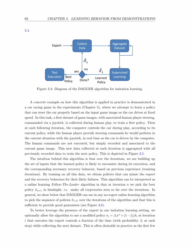
68 CHAPTER 3. LEARNING BEHAVIOR FROM DEMONSTRATIONS
3.4.
Test
Execution
Collect
Data
Supervised
Learning
Expert
Learned
Policy
Aggregate
Dataset
Done?
yesno
iBest
Policy
i
Figure 3.4: Diagram of the DAGGER algorithm for imitation learning.
A concrete example on how this algorithm is applied in practice is demonstrated in
a car racing game in the experiments (Chapter 5), where we attempt to learn a policy
that can steer the car properly based on the input game image as the car drives at fixed
speed. In this task, a first dataset of game images, with associated human player steering,
commanded via a joystick, is collected during human play, to train a first policy. Then
at each following iteration, the computer controls the car during play, according to its
current policy, while the human player provide steering commands he would perform in
the current situation with the joystick, in real time as the car is driven by the computer.
The human commands are not executed, but simply recorded and associated to the
current game image. This new data collected at each iteration is aggregated with all
previously recorded data to train the next policy. This is depicted in Figure 3.5.
The intuition behind this algorithm is that over the iterations, we are building up
the set of inputs that the learned policy is likely to encounter during its execution, and
the corresponding necessary recovery behavior, based on previous experience (training
iterations). By training on all this data, we obtain policies that can mimic the expert
and the recovery behaviors for their likely failures. This algorithm can be interpreted as
a online learning Follow-The-Leader algorithm in that at iteration n we pick the best
policy πn+1 in hindsight, i.e. under all trajectories seen so far over the iterations. In
general, we show below that DAGGER can use in any no-regret online learning algorithm
to pick the sequence of policies π1:N over the iterations of the algorithm and that this is
sufficient to provide good guarantees (see Figure 3.6).
To better leverage the presence of the expert in our imitation learning setting, we
optionally allow the algorithm to use a modified policy πi = βiπ∗+(1−βi)πi at iteration
i that executes the expert controls a fraction of the time (with probability βi at each
step) while collecting the next dataset. This is often desirable in practice as the first few
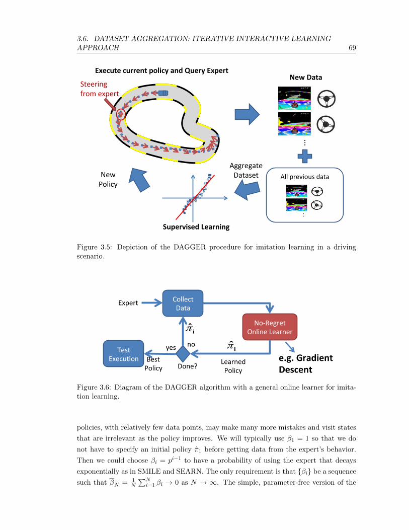
3.6. DATASET AGGREGATION: ITERATIVE INTERACTIVE LEARNINGAPPROACH 69
Execute current policy and Query Expert New Data
Supervised Learning
All previous data
Aggregate
Dataset
Steering
from expert
New
Policy
Figure 3.5: Depiction of the DAGGER procedure for imitation learning in a drivingscenario.
Test
Execu*on
Collect
Data
No‐Regret
Online Learner
Expert
Learned
Policy Done?
yes no i
π
Best
Policy
iπ
e.g. Gradient
Descent
Figure 3.6: Diagram of the DAGGER algorithm with a general online learner for imita-tion learning.
policies, with relatively few data points, may make many more mistakes and visit states
that are irrelevant as the policy improves. We will typically use β1 = 1 so that we do
not have to specify an initial policy π1 before getting data from the expert’s behavior.
Then we could choose βi = pi−1 to have a probability of using the expert that decays
exponentially as in SMILE and SEARN. The only requirement is that βi be a sequence
such that βN = 1N
∑Ni=1 βi → 0 as N → ∞. The simple, parameter-free version of the

70 CHAPTER 3. LEARNING BEHAVIOR FROM DEMONSTRATIONS
Initialize D ← ∅.Initialize π1 to any policy in Π.for i = 1 to N do
Let πi = βiπ∗ + (1− βi)πi.
Sample T -step trajectories using πi.Get dataset Di = (s, π∗(s)) of visited states by πi and actions given by expert.Aggregate datasets: D ← D
⋃Di.
Train classifier πi+1 on D (or use online learner to get πi+1 given new data Di).end forReturn best πi on validation.
Algorithm 3.6.1: DAGGER Algorithm.
algorithm described above is the special case βi = I(i = 1) for I the indicator function,
which often performs best in practice (see Chapter 5). The general DAGGER algorithm
is detailed in Algorithm 3.6.1.
Analysis
We now provide a complete analysis of this DAGGER procedure, and show how the
strong no-regret property of online learning procedures can be leveraged, in this inter-
active learning procedure, to obtain good performance guarantees. Again here, we seek
to provide a similar analysis to previously analyzed methods that seeks to answer the
following question : if we can find good policies at mimicking the expert on the aggre-
gate dataset we collect during training, then how well the learned policy will perform
the task?
The theoretical analysis of DAGGER relies primarily on seeing how learning iter-
atively in this algorithm can be viewed as an online learning problem and using the
no-regret property of the underlying Follow-The-Leader algorithm on strongly convex
losses (Kakade and Tewari, 2009) which picks the sequence of policies π1:N . Hence, the
presented results also hold more generally if we use any other no-regret online learning
algorithm we would apply to our imitation learning setting. In particular, we can con-
sider the results here a reduction of imitation learning to no-regret online learning where
we treat mini-batches of trajectories under a single policy as a single online-learning
example. In addition, in Chapter 9, we also show that the data aggregation procedure
works generally whenever the supervised learner applied to the aggregate dataset has
sufficient stability properties. We refer the reader to Chapter 2 for a review of concepts
related to online learning and no regret that is used for this analysis. All the proofs of
the results presented here are in Appendix A.
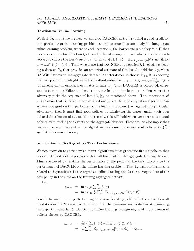
3.6. DATASET AGGREGATION: ITERATIVE INTERACTIVE LEARNINGAPPROACH 71
Relation to Online Learning
We first begin by showing how we can view DAGGER as trying to find a good predictor
in a particular online learning problem, as this is crucial to our analysis. Imagine an
online learning problem, where at each iteration i, the learner picks a policy πi ∈ Π that
incurs loss on the loss function `i chosen by the adversary. In particular, consider the ad-
versary to choose the loss `i such that for any π ∈ Π, `i(π) = Es∼dπi ,a∼π∗(s)[`(s, a, π)], for
πi = βiπ∗+ (1−βi)πi. Then we can see that DAGGER, at iteration i, is exactly collect-
ing a dataset Di, that provides an empirical estimate of this loss `i. Additionally, when
DAGGER trains on the aggregate dataset D at iteration i to choose πi+1, it is choosing
the best policy in hindsight as in Follow-the-Leader, i.e. πi+1 = arg minπ∈Π
∑ij=1 `j(π)
(or at least on the empirical estimates of each `j). Thus DAGGER as presented, corre-
sponds to running Follow-the-Leader in a particular online learning problem where the
adversary picks the sequence of loss `iNi=1 as mentioned above. The importance of
this relation that is shown in our detailed analysis is the following: if an algorithm can
achieve no-regret on this particular online learning problem (i.e. against this particular
adversary), then it must find good policies at mimicking the expert under their own
induced distribution of states. More precisely, this will hold whenever there exists good
policies at mimicking the expert on the aggregate dataset. These results also imply that
one can use any no-regret online algorithm to choose the sequence of policies πiNi=1
against this same adversary.
Implication of No-Regret on Task Performance
We now move on to show how no-regret algorithms must guarantee finding policies that
perform the task well, if policies with small loss exist on the aggregate training dataset.
This is achieved by relating the performance of the policy at the task, directly to the
performance of DAGGER on the online learning problem. That is, task performance is
related to 2 quantities: 1) the regret at online learning and 2) the surrogate loss of the
best policy in the class on the training aggregate dataset.
Let
εclass = minπ∈Π∑N
i=1 `i(π)
= minπ∈Π1N
∑Ni=1 Es∼dπi ,a∼π∗(s)[`(s, a, π)]
denote the minimum expected surrogate loss achieved by policies in the class Π on all
the data over the N iterations of training (i.e. the minimum surrogate loss at mimicking
the expert in hindsight). Denote the online learning average regret of the sequence of
policies chosen by DAGGER,
εregret = 1N [∑N
i=1 `i(πi)−minπ∈Π∑N
i=1 `i(π)]
= 1N
∑Ni=1 Es∼dπi ,a∼π∗(s)[`(s, a, πi)]− εclass.
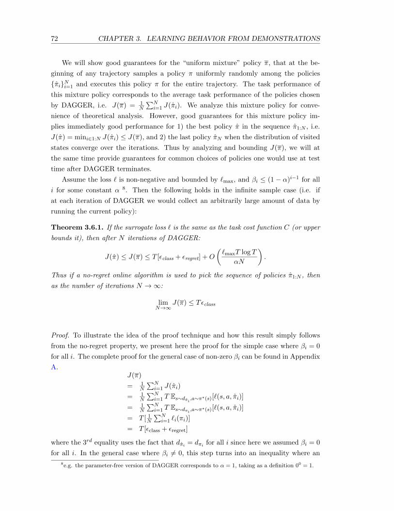
72 CHAPTER 3. LEARNING BEHAVIOR FROM DEMONSTRATIONS
We will show good guarantees for the “uniform mixture” policy π, that at the be-
ginning of any trajectory samples a policy π uniformly randomly among the policies
πiNi=1 and executes this policy π for the entire trajectory. The task performance of
this mixture policy corresponds to the average task performance of the policies chosen
by DAGGER, i.e. J(π) = 1N
∑Ni=1 J(πi). We analyze this mixture policy for conve-
nience of theoretical analysis. However, good guarantees for this mixture policy im-
plies immediately good performance for 1) the best policy π in the sequence π1:N , i.e.
J(π) = mini∈1:N J(πi) ≤ J(π), and 2) the last policy πN when the distribution of visited
states converge over the iterations. Thus by analyzing and bounding J(π), we will at
the same time provide guarantees for common choices of policies one would use at test
time after DAGGER terminates.
Assume the loss ` is non-negative and bounded by `max, and βi ≤ (1− α)i−1 for all
i for some constant α 8. Then the following holds in the infinite sample case (i.e. if
at each iteration of DAGGER we would collect an arbitrarily large amount of data by
running the current policy):
Theorem 3.6.1. If the surrogate loss ` is the same as the task cost function C (or upper
bounds it), then after N iterations of DAGGER:
J(π) ≤ J(π) ≤ T [εclass + εregret] +O
(`maxT log T
αN
).
Thus if a no-regret online algorithm is used to pick the sequence of policies π1:N , then
as the number of iterations N →∞:
limN→∞
J(π) ≤ Tεclass
Proof. To illustrate the idea of the proof technique and how this result simply follows
from the no-regret property, we present here the proof for the simple case where βi = 0
for all i. The complete proof for the general case of non-zero βi can be found in Appendix
A.J(π)
= 1N
∑Ni=1 J(πi)
= 1N
∑Ni=1 T Es∼dπi ,a∼π∗(s)[`(s, a, πi)]
= 1N
∑Ni=1 T Es∼dπi ,a∼π∗(s)[`(s, a, πi)]
= T [ 1N
∑Ni=1 `i(πi)]
= T [εclass + εregret]
where the 3rd equality uses the fact that dπi = dπi for all i since here we assumed βi = 0
for all i. In the general case where βi 6= 0, this step turns into an inequality where an
8e.g. the parameter-free version of DAGGER corresponds to α = 1, taking as a definition 00 = 1.
3.6. DATASET AGGREGATION: ITERATIVE INTERACTIVE LEARNINGAPPROACH 73
additional term is introduced. This adds a term that is O(`maxT log T
αN
)to the overall
bound (when βi = (1−α)i−1). See Appendix A. Finally, J(π) ≤ J(π) since the minimum
is always lower or equal to the average.
This last result also implies good regret guarantees (in surrogate loss) for the uniform
mixture policy π under its induced test trajectories:
Corollary 3.6.1. After N iterations of DAGGER:
R(π) ≤ Tεregret +O
(`maxT log T
αN
).
Thus if a no-regret online algorithm is used to pick the sequence of policies π1:N , then
as the number of iterations N →∞:
limN→∞
R(π) ≤ 0
Proof. It suffice to note that when the task cost function is the surrogate loss (as in the
previous theorem), then R(π) = J(π) − Tεclass, and thus the last theorem proves this
corollary.
This indicates the total expected regret of the mixture policy is directly related to
the average online regret of the learner on the online learning problem, and goes to 0
whenever DAGGER uses a no-regret procedure.
More generally, when the cost function C is unknown and different from `, we can
still provide good performance bounds when the expert is robust, as discussed in the
analysis of the Forward Training algorithm:
Theorem 3.6.2. If the expert π∗ is u-robust with respect to cost function C (as in
Definition 3.4.1), then after N iterations of DAGGER:
J(π) ≤ J(π) ≤ J(π∗) + uT [εclass + εregret] +O
(u`maxT log T
αN
).
Thus if a no-regret online algorithm is used to pick the sequence of policies π1:N , then
as the number of iterations N →∞:
limN→∞
J(π) ≤ J(π∗) + uTεclass
In addition, when the distribution of state-action pairs of the policies in the sequence
converge, the performance of πN must be close to the performance of π:
Theorem 3.6.3. If there exists a state-action distribution D∗, scalar ε∗conv ≥ 0 and a
sequence εconv,i∞i=1 that is o(1), such that ||Dπi −D∗||1 ≤ ε∗conv + εconv,i for all i. Then
for any cost function bounded in [0, Cmax]:
limN→∞
J(πN ) ≤ limN→∞
J(π) + CmaxTε∗conv
74 CHAPTER 3. LEARNING BEHAVIOR FROM DEMONSTRATIONS
In theory, such convergence is not guaranteed to occur, although it often tend to
occur in practice as the online algorithm makes smaller and smaller changes to the policy
as N gets larger. In practice, this result reflects the typical observed behavior of the
algorithm: performance tends to improve in the first few iterations and then stabilizes,
and the last policy often achieves the best performance (or nearly so) among all policies
in the sequence. After all, the last policy is the one trained with most data, and should
intuitively tend to be better.
These results indicate how the task performance of the learned policy is related to
the online regret at online learning and the training loss of the best policy. In the limit
of iterations, the guarantees for DAGGER ends up very similar to the guarantees of
Forward Training, i.e. performance degrades linearly with T (or uT ) and the training
loss εclass. However it is not necessary to perform an arbitrarily large number of iterations;
we only need N to be large enough to make the average online regret term negligible.
By leveraging existing online learning results, the following corollaries indicate that the
number of iterations required is often of order O(T ) or O(T 2) for common loss ` and
no-regret algorithms:
Corollary 3.6.2. Suppose ` is strongly convex in π for all s, a and DAGGER uses
Follow-the-Leader to pick the sequence of policies, then: If ` upper bounds C, then for
any ε > 0 after O(T/ε) iterations of DAGGER:
J(π) ≤ J(π) ≤ Tεclass +O(ε).
For arbitrary cost C, if the expert π∗ is u-robust with respect to C (as in Definition
3.4.1), then for any ε > 0 after O(uT/ε) iterations of DAGGER:
J(π) ≤ J(π) ≤ J(π∗) + uTεclass +O(ε).
Corollary 3.6.3. Suppose ` is convex in π for all s, a and DAGGER uses Follow-the-
Regularized-Leader to pick the sequence of policies, then: If ` upper bounds the cost C,
then for any ε > 0 after O(T 2/ε2) iterations of DAGGER:
J(π) ≤ J(π) ≤ Tεclass +O(ε).
For arbitrary cost C, if the expert π∗ is u-robust with respect to C (as in Definition
3.4.1), then for any ε > 0 after O(u2T 2/ε2) iterations of DAGGER:
J(π) ≤ J(π) ≤ J(π∗) + uTεclass +O(ε).
While in theory, these results indicate that DAGGER needs more iterations than
the Forward training procedure to obtain good guarantees, in practice, it often only
takes very few iterations for DAGGER to find very good policies. For instance, in

3.6. DATASET AGGREGATION: ITERATIVE INTERACTIVE LEARNINGAPPROACH 75
most experiments we obtain good performance after only 3 to 5 iterations, and then
performance improves more slowly (see Chapter 5). Thus in practice, DAGGER can be
run for much fewer iterations than T , and still often obtain a very good policy. This
makes DAGGER much more practical than Forward, as Forward can never be stopped
before iterating and training T policies.
Despite needing more iterations in theory, in the following finite sample analysis, we
show that DAGGER needs less total samples than Forward to obtain good guarantees.
Intuitively, this is because by learning a single policy for all time steps, DAGGER can
generalize the behavior across time step, and thus avoid having to learn from scratch the
behavior at each step separately.
Sample Complexity
The previous results hold if during the execution of DAGGER, we would collect an
infinite number of samples at each iteration, such that the online learning algorithm can
evaluate exactly the expected loss `i, i.e. the loss on the exact distribution of states
induced by the current policy πi9. In practice however, we only collect a small sample
of trajectories (or states), such that the online learning algorithm only has access to an
empirical estimate of `i when updating the policy. We show below that this does not
change our main results, and that we can still guarantee to obtain a good policy with
high probability after a sufficient number of iterations and enough total samples have
been collected.
Suppose we sample m trajectories with πi at each iteration i (or simply m i.i.d.
states from dπi with their associated target expert action), and denote this dataset Di.
Let εclass = minπ∈Π1N
∑Ni=1 E(s,a)∼Di [`(s, a, π)] be the empirical training surrogate loss
of the best policy on the sampled data, then using Azuma-Hoeffding’s inequality leads
to the following generalization of the previous guarantees:
Theorem 3.6.4. If the surrogate loss ` is the same as the task cost function C (or upper
bounds it), then after N iterations of DAGGER collecting m i.i.d. samples per iteration,
with probability at least 1− δ:
J(π) ≤ J(π) ≤ T [εclass + εregret] +O
(`maxT log T
αN+ `maxT
√log(1/δ)
mN
).
Here εregret simply denotes the average regret on the empirical loss over the iterations.
Similarly:
9However note that in the case of deterministic systems, with deterministic policies and experts,then only 1 trajectory is needed to evaluate the expected loss. So this infinite sample analysis applies inpractice to deterministic settings as well.
76 CHAPTER 3. LEARNING BEHAVIOR FROM DEMONSTRATIONS
Theorem 3.6.5. If the expert π∗ is u-robust with respect to cost function C (as in
Definition 3.4.1), then after N iterations of DAGGER collecting m i.i.d. samples per
iteration, with probability at least 1− δ:
J(π) ≤ J(π) ≤ J(π∗) + uT [εclass + εregret] +O
(u`maxT log T
αN+ `maxuT
√log(1/δ)
mN
).
Thus we can see that DAGGER, over all iterations, only needs a total of O(T 2)
samples to guarantee good performance:
Corollary 3.6.4. Suppose ` is convex in π for all s, a and DAGGER uses Follow-the-
Regularized-Leader to pick the sequence of policies, then: If ` upper bounds the cost C,
then for any ε > 0 after O(T 2 log(1/δ)/ε2) iterations of DAGGER collecting m = 1 i.i.d.
samples per iteration, with probability at least 1− δ:
J(π) ≤ J(π) ≤ T εclass +O(ε).
For any cost function C, if the expert π∗ is u-robust with respect to C (as in Definition
3.4.1), then for any ε > 0, after O(u2T 2 log(1/δ)/ε2) iterations of DAGGER collecting
m = 1 i.i.d. samples per iteration, with probability at least 1− δ:
J(π) ≤ J(π) ≤ J(π∗) + uT εclass +O(ε).
This result shows that DAGGER can be run by collecting a single sample at each
iteration (e.g. by querying the expert at only a single state, randomly chosen among
all time steps, along a single sampled trajectory of the current policy). After a total
of O(T 2) iterations, and a total of O(T 2) samples, DAGGER guarantees a good policy
with high probability. 10
These finite sample results indicate that for tasks where the expert is robust (e.g.
u is a small constant), DAGGER only needs order O(T 2) samples over all iterations
to obtain good guarantees. This is an improvement by a factor T compared to the
Forward training procedure with the same robust expert conditions, and by a factor T 2
compared to the supervised learning approach. Here DAGGER improves on the sample
complexity of Forward Training because it can generalize the learned behavior across
many time steps, by learning a single policy, rather than learning the behavior from
scratch at each time step.
10When the loss is strongly convex, a more refined analysis taking advantage of the strong convexityof the loss function (Kakade and Tewari, 2009) may lead to tighter generalization bounds that requireN only of order O(T log(1/δ)), and thus only order O(T ) samples in total.

3.6. DATASET AGGREGATION: ITERATIVE INTERACTIVE LEARNINGAPPROACH 77
Discussion
DAGGER as a Reduction
DAGGER departs from the previous reductions, in that it effectively reduces the imi-
tation learning problem to an online learning problem, rather than a typical supervised
learning problem. This is not as strong as the general error or regret reductions consid-
ered in (Beygelzimer et al., 2005, Ross and Bagnell, 2010, Daume III et al., 2009) which
require only classification: we require a no-regret method or a (strongly) convex surrogate
loss function, a stronger (albeit common) assumption. While the performance guarantee
is in part related to the online regret, DAGGER should still be interpreted as an error
reduction, as in the limit of iterations with a no-regret algorithm, task performance is
related to the error, or loss, of the best policy in the class in hindsight. However, for
the surrogate loss objective (or imitation loss), DAGGER can be interpreted as a regret
reduction, as the regret on test trajectories is directly related to the online regret of the
online learning task. In other sequential settings, or when cost information is available,
we will also see that DAGGER can lead to regret reductions for the task performance
with a similar learning strategy, where control performance is instead related directly to
only the online regret and/or the regret on the aggregate dataset of the best predictor
in the class to the bayes-optimal predictor (e.g. in Chapters 4, 7 and 8).
Remarks on Guarantees
It is important to note that our guarantees are reduction statements, i.e. they are relative
guarantees to how well we can do at finding policies that mimic well the expert on the
training data. Thus DAGGER may sometimes fail at finding good policies if no policies
can mimic well the expert during training. It should be noted that all presented methods
fail in this case, i.e. whenever there does not exist any policy that can mimic well the
expert on the training data, εclass is large, and no method has good performance. When
this occurs, it suggests we may need a better class of predictors and/or better features.
The distinction to the typical supervised learning approach is when good predictors exist
on the training data. In this case, with DAGGER (and Forward), we always obtain a
good policy. In contrast, the typical supervised learning approach may find policies with
low training error, but still fail at obtaining a good policy to accomplish the task, due
to the mismatch in training and testing distributions.
Using DAGGER with a randomized online algorithm
Our current presentation of DAGGER assumes that the online learner picks a policy
πi from the policy class Π at each iteration i. If instead we use a randomized online
78 CHAPTER 3. LEARNING BEHAVIOR FROM DEMONSTRATIONS
learning algorithm, such as Weighted Majority (or Hedge), the online algorithm would
instead pick a distribution over policies in Π. In this case, DAGGER can be applied with
such randomized online algorithms, where the policy πi is simply the stochastic policy
defined by this distribution over policies; i.e. at each time step in the trajectory, we
would randomly pick a policy from the distribution to execute in the current state. Note
that it is important to randomize at each time step in the trajectory, and not simply pick
a random policy at the beginning of the trajectory to execute for the entire trajectory.
The latter would violate the common assumption made by randomized online algorithms
that the particular examples they incur loss on are independent of the realization of the
sampling by the online algorithm, to guarantee no-regret. By resampling a policy at
every time step in the trajectory, the current state is always independent of the sampled
policy that incurs loss on that state, and ensures that the randomized online algorithm
will be no-regret on the generated trajectories during training. Resampling from the
distribution picked by the online learner at every time step in the trajectory is required
generally in all the sequential settings we present in latter chapters as well, whenever a
randomized online algorithm is used (see Chapter 7 for a more detailed example of this).
Why not just collect data everywhere?
The main reason why DAGGER (and Forward) provide improved guarantees is that
they can explore different course of actions where error occurs, and learn the proper
recovery behavior. One may wonder why not simply collect data everywhere (e.g. by
executing random actions or introducing noise in the actions, to collect data about the
expert behavior) to allow observing all recovery behaviors. There are two reasons why
this is a bad strategy. First it is very inefficient. Such learning strategy would require
an exponential number of trajectories to explore all possibilities. As we only need to
learn the proper behavior where the learned policy goes, this wastes a lot of effort on
acquiring data which may be irrelevant. Instead, DAGGER focus its efforts on only the
most relevant regions, and can get good performance with only a polynomial number of
trajectories. The second reason why sampling everywhere is bad is in agnostic settings,
where we may not be able to fit observed behavior well everywhere. In this case, the
learner must tradeoff accuracy in different regions (as shown previously in Figure 1.7).
Sampling everywhere could make the learner fit correctly regions that are irrelevant.
Hence DAGGER, by focusing on collecting only data in regions that are likely to be
encountered, forces the learner to be most accurate in these important regions.
Why not just use the last collected dataset as in Policy Iteration?
A typical policy iteration approach, applied to this imitation learning problem, would
look only at the distribution of states induced by the last policy πi, and minimize the

3.6. DATASET AGGREGATION: ITERATIVE INTERACTIVE LEARNINGAPPROACH 79
surrogate loss on this dataset to choose the next policy πi+1. This is similar to many
policy iteration methods in reinforcement learning. In our context, such methods can
tend to be very unstable and keep oscillating between various policies, none of which
performing the task well. Our experiments in Chapter 5 demonstrate that this is the
common observed behavior of this approach.


Chapter 4
Learning Behavior using Cost
Information
In this chapter we continue our investigation of techniques for learning behavior in scenar-
ios where an expert may be present, but where additional cost information is available.
All learning approaches presented in the Chapter 3 considered the task cost function
C to be unknown. In scenarios where C is known, taking advantage of this extra cost
information should intuitively lead to better performance. In particular, when we are
simply minimizing a surrogate (classification or regression) loss `, instead of the task
cost function C, all errors at mimicking the expert are somewhat treated equally, and
we ignore that some errors can be much more costly than others. For instance, errors
that lead the learner to crash, or fall off a cliff, should be considered much more costly,
than other errors that only slightly increase the time it takes to successfully complete the
task. By taking into account the importance of accurately predicting the expert’s action
in different situations, the learner should be able to better tradeoff in which situations
it potentially errors, in order to avoid very costly errors at all costs. For instance, it
will prefer predictors that error slightly more often, but only in low cost situations, to
predictors that makes fewer but more costly errors.
The algorithms we presented, Forward Training and DAGGER, can be extended to
take this extra cost information into account in a straightforward fashion. In particular,
in discrete action settings, where currently a classification loss is minimized over the
iterations of training, we will instead minimize a cost-sensitive classification loss, where
the classification loss associated with each action is related to its long-term cost for
performing the task. Here, we will focus our exposition on discrete action settings;
although continuous action settings may additionally be handled.
We first present an extension of Forward with this cost information, and then move on
to show how this can be used within DAGGER. For DAGGER, we present two variants,
where the second one can be applied to handle general model-free reinforcement learning
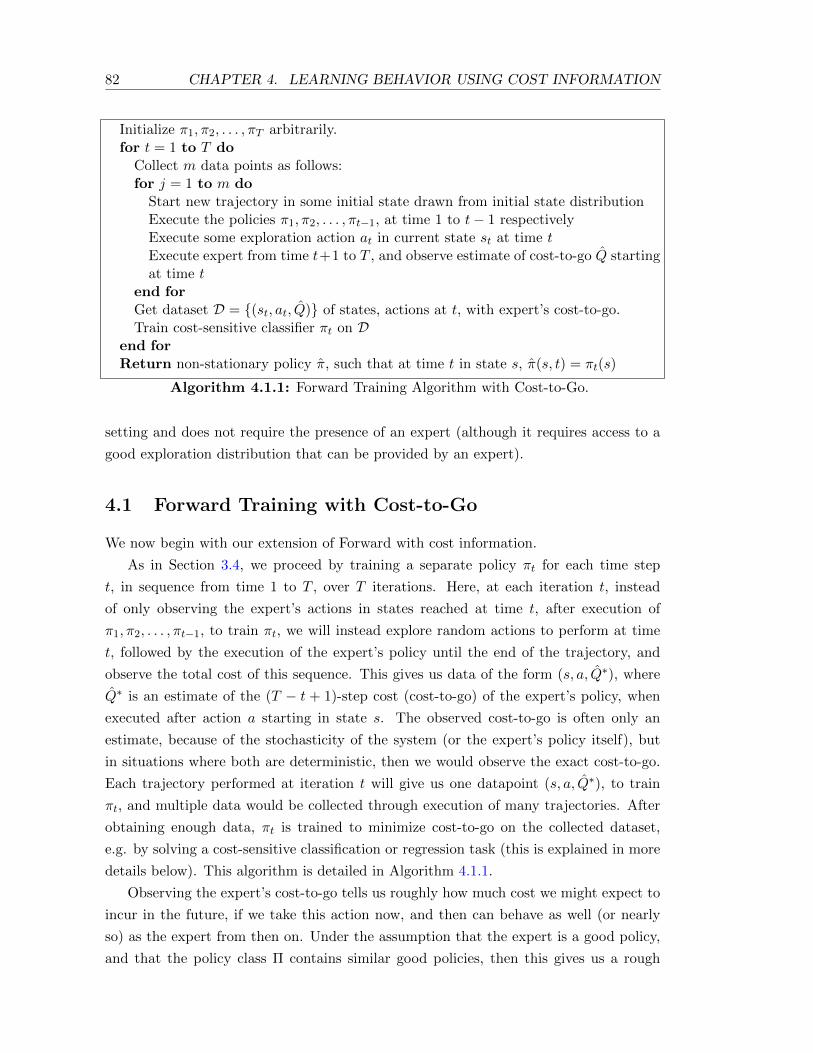
82 CHAPTER 4. LEARNING BEHAVIOR USING COST INFORMATION
Initialize π1, π2, . . . , πT arbitrarily.for t = 1 to T do
Collect m data points as follows:for j = 1 to m do
Start new trajectory in some initial state drawn from initial state distributionExecute the policies π1, π2, . . . , πt−1, at time 1 to t− 1 respectivelyExecute some exploration action at in current state st at time tExecute expert from time t+1 to T , and observe estimate of cost-to-go Q startingat time t
end forGet dataset D = (st, at, Q) of states, actions at t, with expert’s cost-to-go.Train cost-sensitive classifier πt on D
end forReturn non-stationary policy π, such that at time t in state s, π(s, t) = πt(s)
Algorithm 4.1.1: Forward Training Algorithm with Cost-to-Go.
setting and does not require the presence of an expert (although it requires access to a
good exploration distribution that can be provided by an expert).
4.1 Forward Training with Cost-to-Go
We now begin with our extension of Forward with cost information.
As in Section 3.4, we proceed by training a separate policy πt for each time step
t, in sequence from time 1 to T , over T iterations. Here, at each iteration t, instead
of only observing the expert’s actions in states reached at time t, after execution of
π1, π2, . . . , πt−1, to train πt, we will instead explore random actions to perform at time
t, followed by the execution of the expert’s policy until the end of the trajectory, and
observe the total cost of this sequence. This gives us data of the form (s, a, Q∗), where
Q∗ is an estimate of the (T − t + 1)-step cost (cost-to-go) of the expert’s policy, when
executed after action a starting in state s. The observed cost-to-go is often only an
estimate, because of the stochasticity of the system (or the expert’s policy itself), but
in situations where both are deterministic, then we would observe the exact cost-to-go.
Each trajectory performed at iteration t will give us one datapoint (s, a, Q∗), to train
πt, and multiple data would be collected through execution of many trajectories. After
obtaining enough data, πt is trained to minimize cost-to-go on the collected dataset,
e.g. by solving a cost-sensitive classification or regression task (this is explained in more
details below). This algorithm is detailed in Algorithm 4.1.1.
Observing the expert’s cost-to-go tells us roughly how much cost we might expect to
incur in the future, if we take this action now, and then can behave as well (or nearly
so) as the expert from then on. Under the assumption that the expert is a good policy,
and that the policy class Π contains similar good policies, then this gives us a rough

4.1. FORWARD TRAINING WITH COST-TO-GO 83
estimate of what good policies in Π will be able to achieve at future steps. Thus by
minimizing this cost-to-go at each step, we will choose policies that lead to situations
where incurring low future cost-to-go is possible. For instance, we will be able to observe
that if some actions put the expert in situations where it cannot avoid falling off a cliff
or crash, then these actions should be avoided at all cost, in favor of others where the
expert is still able to recover at later steps.
We now describe in more details how to perform exploration, and train the policy at
each iteration.
Full Information vs. Partial Information Setting
In standard cost-sensitive classification problems, a cost vector is given for each input
features x in the training data, that indicates the cost of predicting each class or label
for this input. This is a full information setting, where the cost of all predictions at
a given input is known. This is not the case in the setting presented here, where for
an observed input state s, we only have partial information of the cost vector, i.e. we
only know the cost of one sampled action, and the cost of other actions are unknown.
In some scenarios, especially those involving simulated environments, it is sometimes
possible to obtain data as in a full information setting. To do so, when entering a state
where we explore an action a, we would instead need to create multiple “copies” of
the current state, and simulate a trajectory with the expert after the execution of each
action a ∈ A in this state, to obtain an estimate of the cost-to-go for all actions in
that state. This is only possible when we can “copy” the state, or are able to put back
the system directly in that state repeatedly. As mentioned, this is typically possible
only in simulated environments. On real robots, it is typically not possible to put back
the system in exactly the same state and one is typically only able to try one action
in any visited state. However, even if we can only have partial information about the
cost of a single action, it is still possible to transform this into a standard cost-sensitive
classification problem, through importance weighting techniques, or use directly some
cost-sensitive classification reductions, such as regression, that do not necessarily require
cost information for all actions in every training input state. We describe this in detail
below.
Training the Policy to Minimize Cost-to-Go
In the full information setting, the data collected at each iteration corresponds to a
set of cost-sensitive classification examples. Training the policy at each iteration then
simply corresponds to solving a cost-sensitive classification problem. That is, if we
collect a dataset of m samples, (si, Qi)mi=1, where Qi is a cost vector of cost-to-go esti-
mates for each action in si, then we would solve the cost-sensitive classification problem:
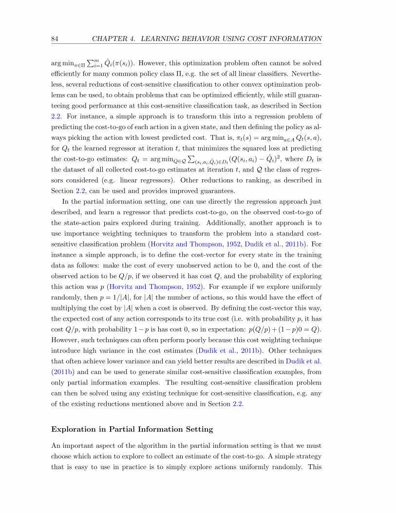
84 CHAPTER 4. LEARNING BEHAVIOR USING COST INFORMATION
arg minπ∈Π
∑mi=1 Qi(π(si)). However, this optimization problem often cannot be solved
efficiently for many common policy class Π, e.g. the set of all linear classifiers. Neverthe-
less, several reductions of cost-sensitive classification to other convex optimization prob-
lems can be used, to obtain problems that can be optimized efficiently, while still guaran-
teeing good performance at this cost-sensitive classification task, as described in Section
2.2. For instance, a simple approach is to transform this into a regression problem of
predicting the cost-to-go of each action in a given state, and then defining the policy as al-
ways picking the action with lowest predicted cost. That is, πt(s) = arg mina∈AQt(s, a),
for Qt the learned regressor at iteration t, that minimizes the squared loss at predicting
the cost-to-go estimates: Qt = arg minQ∈Q∑
(si,ai,Qi)∈Dt(Q(si, ai) − Qi)2, where Dt is
the dataset of all collected cost-to-go estimates at iteration t, and Q the class of regres-
sors considered (e.g. linear regressors). Other reductions to ranking, as described in
Section 2.2, can be used and provides improved guarantees.
In the partial information setting, one can use directly the regression approach just
described, and learn a regressor that predicts cost-to-go, on the observed cost-to-go of
the state-action pairs explored during training. Additionally, another approach is to
use importance weighting techniques to transform the problem into a standard cost-
sensitive classification problem (Horvitz and Thompson, 1952, Dudik et al., 2011b). For
instance a simple approach, is to define the cost-vector for every state in the training
data as follows: make the cost of every unobserved action to be 0, and the cost of the
observed action to be Q/p, if we observed it has cost Q, and the probability of exploring
this action was p (Horvitz and Thompson, 1952). For example if we explore uniformly
randomly, then p = 1/|A|, for |A| the number of actions, so this would have the effect of
multiplying the cost by |A| when a cost is observed. By defining the cost-vector this way,
the expected cost of any action corresponds to its true cost (i.e. with probability p, it has
cost Q/p, with probability 1−p is has cost 0, so in expectation: p(Q/p) + (1−p)0 = Q).
However, such techniques can often perform poorly because this cost weighting technique
introduce high variance in the cost estimates (Dudik et al., 2011b). Other techniques
that often achieve lower variance and can yield better results are described in Dudik et al.
(2011b) and can be used to generate similar cost-sensitive classification examples, from
only partial information examples. The resulting cost-sensitive classification problem
can then be solved using any existing technique for cost-sensitive classification, e.g. any
of the existing reductions mentioned above and in Section 2.2.
Exploration in Partial Information Setting
An important aspect of the algorithm in the partial information setting is that we must
choose which action to explore to collect an estimate of the cost-to-go. A simple strategy
that is easy to use in practice is to simply explore actions uniformly randomly. This
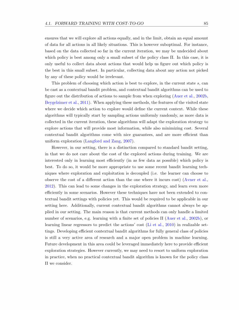
4.1. FORWARD TRAINING WITH COST-TO-GO 85
ensures that we will explore all actions equally, and in the limit, obtain an equal amount
of data for all actions in all likely situations. This is however suboptimal. For instance,
based on the data collected so far in the current iteration, we may be undecided about
which policy is best among only a small subset of the policy class Π. In this case, it is
only useful to collect data about actions that would help us figure out which policy is
the best in this small subset. In particular, collecting data about any action not picked
by any of these policy would be irrelevant.
This problem of choosing which action is best to explore, in the current state s, can
be cast as a contextual bandit problem, and contextual bandit algorithms can be used to
figure out the distribution of actions to sample from when exploring (Auer et al., 2002b,
Beygelzimer et al., 2011). When applying these methods, the features of the visited state
where we decide which action to explore would define the current context. While these
algorithms will typically start by sampling actions uniformly randomly, as more data is
collected in the current iteration, these algorithms will adapt the exploration strategy to
explore actions that will provide most information, while also minimizing cost. Several
contextual bandit algorithms come with nice guarantees, and are more efficient than
uniform exploration (Langford and Zang, 2007).
However, in our setting, there is a distinction compared to standard bandit setting,
in that we do not care about the cost of the explored actions during training. We are
interested only in learning most efficiently (in as few data as possible) which policy is
best. To do so, it would be more appropriate to use some recent bandit learning tech-
niques where exploration and exploitation is decoupled (i.e. the learner can choose to
observe the cost of a different action than the one where it incurs cost) (Avner et al.,
2012). This can lead to some changes in the exploration strategy, and learn even more
efficiently in some scenarios. However these techniques have not been extended to con-
textual bandit settings with policies yet. This would be required to be applicable in our
setting here. Additionally, current contextual bandit algorithms cannot always be ap-
plied in our setting. The main reason is that current methods can only handle a limited
number of scenarios, e.g. learning with a finite set of policies Π (Auer et al., 2002b), or
learning linear regressors to predict the actions’ cost (Li et al., 2010) in realizable set-
tings. Developing efficient contextual bandit algorithms for fully general class of policies
is still a very active area of research and a major open problem in machine learning.
Future development in this area could be leveraged immediately here to provide efficient
exploration strategies. However currently, we may need to resort to uniform exploration
in practice, when no practical contextual bandit algorithm is known for the policy class
Π we consider.
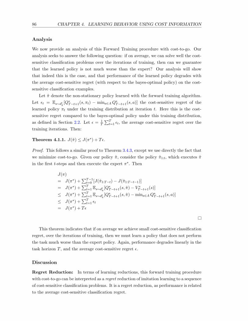
86 CHAPTER 4. LEARNING BEHAVIOR USING COST INFORMATION
Analysis
We now provide an analysis of this Forward Training procedure with cost-to-go. Our
analysis seeks to answer the following question: if on average, we can solve well the cost-
sensitive classification problems over the iterations of training, then can we guarantee
that the learned policy is not much worse than the expert? Our analysis will show
that indeed this is the case, and that performance of the learned policy degrades with
the average cost-sensitive regret (with respect to the bayes-optimal policy) on the cost-
sensitive classification examples.
Let π denote the non-stationary policy learned with the forward training algorithm.
Let εt = Es∼dtπ [Q∗T−t+1(s, πt) − mina∈AQ∗T−t+1(s, a)] the cost-sensitive regret of the
learned policy πt under the training distribution at iteration t. Here this is the cost-
sensitive regret compared to the bayes-optimal policy under this training distribution,
as defined in Section 2.2. Let ε = 1T
∑Tt=1 εt, the average cost-sensitive regret over the
training iterations. Then:
Theorem 4.1.1. J(π) ≤ J(π∗) + Tε.
Proof. This follows a similar proof to Theorem 3.4.3, except we use directly the fact that
we minimize cost-to-go. Given our policy π, consider the policy π1:t, which executes π
in the first t-steps and then execute the expert π∗. Then
J(π)
= J(π∗) +∑T−1
t=0 [J(π1:T−t)− J(π1:T−t−1)]
= J(π∗) +∑T
t=1 Es∼dtπ [Q∗T−t+1(s, π)− V ∗T−t+1(s)]
≤ J(π∗) +∑T
t=1 Es∼dtπ [Q∗T−t+1(s, π)−mina∈AQ∗T−t+1(s, a)]
≤ J(π∗) +∑T
t=1 εt
= J(π∗) + Tε
This theorem indicates that if on average we achieve small cost-sensitive classification
regret, over the iterations of training, then we must learn a policy that does not perform
the task much worse than the expert policy. Again, performance degrades linearly in the
task horizon T , and the average cost-sensitive regret ε.
Discussion
Regret Reduction: In terms of learning reductions, this forward training procedure
with cost-to-go can be interpreted as a regret reduction of imitation learning to a sequence
of cost-sensitive classification problems. It is a regret reduction, as performance is related
to the average cost-sensitive classification regret.
4.1. FORWARD TRAINING WITH COST-TO-GO 87
Relation to PSDP: The approach we present here as some similarities to PSDP
(Bagnell et al., 2003). Both train a non-stationary policy over many iterations, training
one policy for a particular time step at each iteration to minimize cost-to-go, except
that PSDP does so in reverse order. That is, in this imitation learning setting, PSDP
would start by training the policy for time T , then the one for T − 1, and so on, going
backward in time up to time 1, and at iteration t, the policy for time step T −t+1 would
be chosen to minimize the cost-to-go of the already trained policies at later time steps,
under the distribution of states of the expert at time T − t + 1. In some sense, PSDP
assumes that in earlier steps (from time 1 to T − t) the expert (or policies very similar
to it) are going to be executed, while Forward with cost-to-go, assumes that in future
time steps, the expert (or policies very similar to it) are going to be executed. Forward
may suffer from too optimistic cost-to-go estimates (e.g. if no policies in the policy class
are as good as the expert), while PSDP may suffer from a train-test mismatch (it may
choose policies that minimize cost-to-go for the wrong distribution of states).
Limitations: As just mentioned, in cases where the expert is much better than any
policy in Π, then the expert’s cost-to-go may be a very optimistic estimate of the future
cost that the learner will incur in future steps after taking a certain action. In this case,
this approach may fail to learn policies that performs the task well, even though some
good policies that can perform the task (but not as well as the expert) exists in the
policy class. For example, consider a driving scenario, where one can take 2 roads to
reach the goal, one of these roads is much shorter, but involves driving on a very narrow
road next to cliffs on each side, while the other road, is much longer and takes more
time to reach the goal, but is safer (wider and not next to any cliff). If in this example,
the expert takes the short narrow road to reach the goal faster and there is no policy in
the class Π that can drive without falling on this narrow road, but there exists policies
that can take the longer road and safely reach the goal, this algorithm would fail to find
these policies. The reason for this is that, as we minimize cost-to-go of the expert, we
would always favor policies that heads toward the shorter narrow road. But once we are
on that road, inevitably at some point we will encounter a scenario where no policies in
the class can predict the same low cost-to-go actions as the expert (i.e. making ε large
in the previous guarantee). The end result is that Forward will learn a policy that takes
the short narrow road and eventually falls off the cliff, in these pathological scenarios.
PSDP may lead to a better policy in this case, but this is unclear. While PSDP would
be able to see that the trained policies it learned at later time steps cannot drive well
on this narrow road and have high cost-to-go, the state distribution of examples, from
the expert policy, would be states starting on this narrow road. It is unclear that PSDP
would learn policies that can drive well on the other longer road, based on minimizing
cost-to-go on examples from the narrow road. If PSDP do happen to learn policies that
88 CHAPTER 4. LEARNING BEHAVIOR USING COST INFORMATION
can drive on the other longer road, then at the early time steps, PSDP will be able to
learn that it is better to take the longer road. But if it doesn’t learn to drive well on
the longer road, then PSDP would still fail. Note also that the theoretical guarantee of
PSDP in this example would be no better than Forward: inevitably at some time t (e.g.
near the end of the narrow road), future policies trained by PSDP reaches the goal, but
under the state distribution of the expert on the narrow road at time t, no policy can
avoid falling off the cliff and minimize cost-to-go of future trained policies as well as the
expert. This makes the ε term in the guarantee of PSDP large, and the guarantee of
PSDP would be similarly bad to Forward.
4.2 DAGGER with Cost-to-Go
As mentioned before, a drawback of Forward in practice is that it needs to learn a
separate policy for each time step, which can be impractical if T is large, and is also less
efficient, in terms of sample complexity, as it does not allow to generalize the behavior
across time steps. The DAGGER approach addresses these issues and can be applied
with similar cost-to-go as Forward to provide similar guarantees.
Just as with Forward, the only modification to DAGGER to take into account cost-
to-go, is to instead minimize the cost-to-go of the expert, rather than the classification
loss of mimicking its actions. That is, in its simplest form, DAGGER would on the
first iteration, collect data by simply observing the expert perform the task, and in each
trajectory, at a uniformly random time t, explore an action a in the current state s, and
observe the cost-to-go of the expert after performing this action, to generate cost example
(s, a,Q). It would then train a policy π2 to minimize the cost-to-go on this dataset. At
following iterations n, DAGGER would collect data through interaction with the learner
as follows: for each trajectory, start by using the current learner’s policy πn to perform
the task, and at some uniformly random time t, explore an action a in the current state
s, after which control is given to the expert and he gets executed up to time T , and we
observe the cost-to-go, starting from s. This generates new examples of the cost-to-go of
the expert (s, a,Q), under the distribution of states visited by the current policy πn. This
new data would be aggregated with all previous data to train the next policy πn+1, or in
general, used by a no-regret online learner to update the policy and obtain πn+1. This
is iterated for some number of iterations N and the best policy found is returned. Just
as before, we optionally allow the algorithm to keep executing the expert’s actions with
small probability βn, instead of always executing πn, up to the random time t where an
action is explored and control is shifted to the expert. The general DAGGER algorithm
with Cost-to-Go is detailed in Algorithm 4.2.1.
As discussed previously for the Forward approach with cost-to-go, in imitation learn-
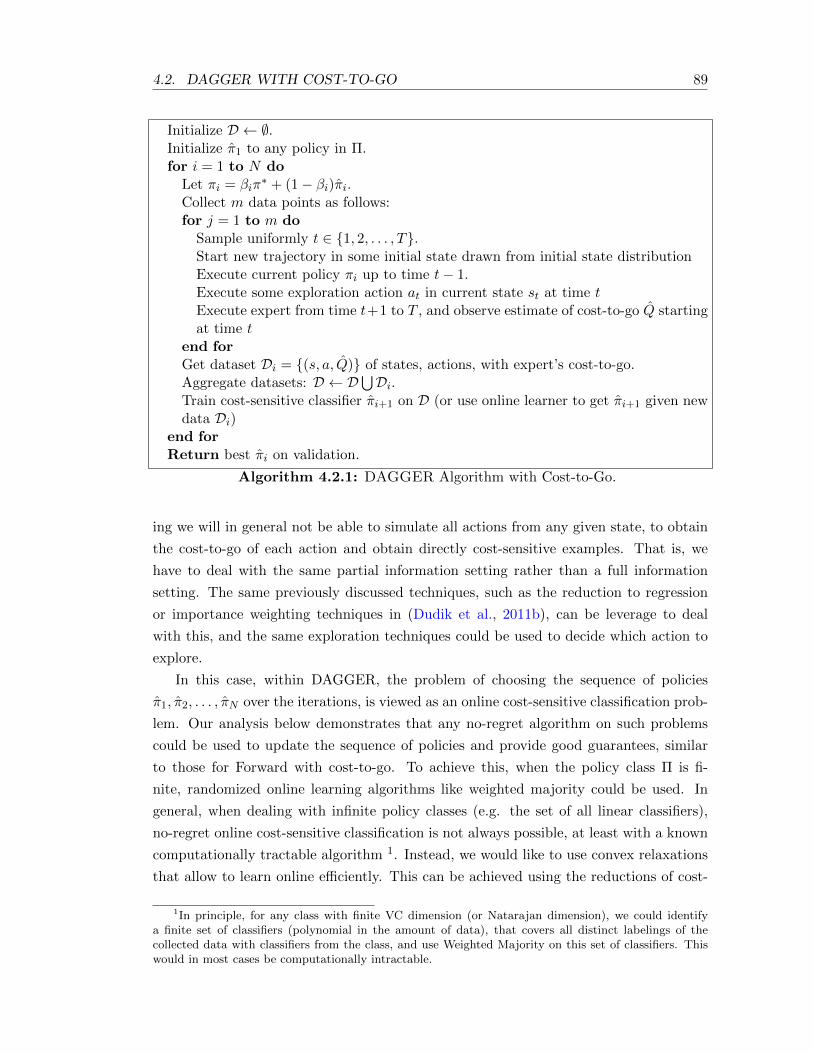
4.2. DAGGER WITH COST-TO-GO 89
Initialize D ← ∅.Initialize π1 to any policy in Π.for i = 1 to N do
Let πi = βiπ∗ + (1− βi)πi.
Collect m data points as follows:for j = 1 to m do
Sample uniformly t ∈ 1, 2, . . . , T.Start new trajectory in some initial state drawn from initial state distributionExecute current policy πi up to time t− 1.Execute some exploration action at in current state st at time tExecute expert from time t+1 to T , and observe estimate of cost-to-go Q startingat time t
end forGet dataset Di = (s, a, Q) of states, actions, with expert’s cost-to-go.Aggregate datasets: D ← D
⋃Di.
Train cost-sensitive classifier πi+1 on D (or use online learner to get πi+1 given newdata Di)
end forReturn best πi on validation.
Algorithm 4.2.1: DAGGER Algorithm with Cost-to-Go.
ing we will in general not be able to simulate all actions from any given state, to obtain
the cost-to-go of each action and obtain directly cost-sensitive examples. That is, we
have to deal with the same partial information setting rather than a full information
setting. The same previously discussed techniques, such as the reduction to regression
or importance weighting techniques in (Dudik et al., 2011b), can be leverage to deal
with this, and the same exploration techniques could be used to decide which action to
explore.
In this case, within DAGGER, the problem of choosing the sequence of policies
π1, π2, . . . , πN over the iterations, is viewed as an online cost-sensitive classification prob-
lem. Our analysis below demonstrates that any no-regret algorithm on such problems
could be used to update the sequence of policies and provide good guarantees, similar
to those for Forward with cost-to-go. To achieve this, when the policy class Π is fi-
nite, randomized online learning algorithms like weighted majority could be used. In
general, when dealing with infinite policy classes (e.g. the set of all linear classifiers),
no-regret online cost-sensitive classification is not always possible, at least with a known
computationally tractable algorithm 1. Instead, we would like to use convex relaxations
that allow to learn online efficiently. This can be achieved using the reductions of cost-
1In principle, for any class with finite VC dimension (or Natarajan dimension), we could identifya finite set of classifiers (polynomial in the amount of data), that covers all distinct labelings of thecollected data with classifiers from the class, and use Weighted Majority on this set of classifiers. Thiswould in most cases be computationally intractable.
90 CHAPTER 4. LEARNING BEHAVIOR USING COST INFORMATION
sensitive classification to regression or ranking problems, as mentioned previously and
in Section 2.2. This leads to convex online learning problems for common policy classes,
for which tractable no-regret online learning algorithms exist (e.g. gradient descent).
Analysis
We now provide the analysis of this DAGGER procedure with cost-to-go, and show how
the strong no-regret property of online learning procedures can be leveraged, in this
interactive learning procedure, to obtain good performance guarantees. Again here, we
seek to provide a similar analysis to previously analyzed methods that seeks to answer the
following question : if we can find good policies, that can incur cost-sensitive classification
loss not much worse than the expert on the aggregate dataset we collect during training,
then how well the learned policy will perform the task?
Again our analysis of DAGGER relies on seeing how learning iteratively in this
algorithm can be viewed as an online learning problem and using the no-regret property
of the underlying online learning algorithm picking the sequence of policies π1:N . Here,
the online learning problem is defined as follows: at each iteration i, the learner picks
a policy πi ∈ Π that incurs loss on the loss function `i chosen by the adversary, and
defined as `i(π) = Et∼U(1:T ),s∼dtπi[Q∗T−t+1(s, π)] for U(1 : T ) the uniform distribution on
the set 1, 2, . . . , T and πi = βiπ∗+ (1− βi)πi. We can see that DAGGER, at iteration
i, is exactly collecting a dataset Di, that provides an empirical estimate of this loss `i.
Let εclass = minπ∈Π1N
∑Ni=1 Et∼U(1:T ),s∼dtπi
[Q∗T−t+1(s, a)−minaQ∗T−t+1(s, a)] denote
the minimum expected cost-sensitive classification regret achieved by policies in the
class Π on all the data over the N iterations of training. Denote the online learning
average regret of the sequence of policies chosen by DAGGER, εregret = 1N [∑N
i=1 `i(πi)−minπ∈Π
∑Ni=1 `i(π)].
We again show good guarantees for the “uniform mixture” policy π, that at the
beginning of any trajectory samples a policy π uniformly randomly among the policies
πiNi=1 and executes this policy π for the entire trajectory. As before, this implies
immediately good performance for the best policy π in the sequence π1:N , i.e. J(π) =
mini∈1:N J(πi) ≤ J(π), and the last policy πN when the distribution of visited states
converge over the iterations.
Assume the cost-to-go of the expert Q∗ is non-negative and bounded by Q∗max, and
βi ≤ (1 − α)i−1 for all i for some constant α 2. Then the following holds in the infinite
sample case (i.e. if at each iteration of DAGGER we would collect an arbitrarily large
amount of data by running the current policy):
2e.g. the parameter-free version of DAGGER corresponds to α = 1, using 00 = 1.

4.2. DAGGER WITH COST-TO-GO 91
Theorem 4.2.1. After N iterations of DAGGER with cost-to-go:
J(π) ≤ J(π) ≤ J(π∗) + T [εclass + εregret] +O
(QmaxT log T
αN
).
Thus if a no-regret online algorithm is used to pick the sequence of policies π1:N , then
as the number of iterations N →∞:
limN→∞
J(π) ≤ J(π∗) + Tεclass
Proof. The proofs of this result is presented in Appendix A.
This theorem indicates that, after a sufficient number of iterations, DAGGER must
find policies that perform the task not much worse than the expert, if there are policies
in the class Π that have small cost-sensitive classification regret on the aggregate dataset
(i.e. policies with cost-sensitive classification loss not much larger than that of the bayes-
optimal classifier on this dataset).
This guarantee is similar to the guarantee of Forward with cost-to-go. In both cases,
performances degrades linearly with T and the cost-sensitive classification regret. When
reductions of cost-sensitive classification to other regression/ranking/classification prob-
lems are used, then our results can be combined with the existing cost-sensitive reduction
results, to relate directly the task performance of the learned policy to the performance
on the regression/ranking/classification problem.
Also note that the analysis we presented so far for both Forward and DAGGER with
cost-to-go, abstracted away the issue of exploration and learning from finite data. These
issues come into play in the sample complexity analysis. Such analysis here depends on
many factors, such as which reduction and exploration method is used. To illustrate
how such results can be derived, we provide a result for the special case where actions
are explored uniformly randomly and the reduction of cost-sensitive classification to
regression is used.
In particular, if εregret denotes the empirical average online learning regret on the
training regression examples collected over the iterations, and Rclass denotes the empirical
regression regret of the best regressor in the class, on the aggregate dataset of regression
examples, compared to the bayes-optimal regressor on this data, we have that :
Theorem 4.2.2. After N iterations of DAGGER with cost-to-go, collecting m regression
examples (s, a, t, Q) per iteration, guarantees that with probability at least 1-δ:
J(π) ≤ J(π) ≤ J(π∗)+2√|A|T
√Rclass + εregret +O(
√log(1/δ)/Nm)+O
(QmaxT log T
αN
).
Thus if a no-regret online algorithm is used to pick the sequence of regressors Q1:N , then
as the number of iterations N →∞, with probability 1:
limN→∞
J(π) ≤ J(π∗) + 2√|A|T
√Rclass
92 CHAPTER 4. LEARNING BEHAVIOR USING COST INFORMATION
Proof. The proofs of this result is presented in Appendix A.
This result demonstrates how the task performance of the learned policies with DAG-
GER, can be related all the way down to the regret on the regression loss at predicting
the observed cost-to-go during training. In particular, it relates task performance to the
square root of the online learning regret, on this regression loss, and the regression regret
of the best regressor in the class to the bayes-optimal regressor on this training data.
The appearance of the square root is particular to the use of this reduction to regression.
The implications of this square root is that learning may take significantly longer, i.e.
we may need the number of iterations N to be order O(T 4), with the number of samples
per iteration m = 1, to guarantee that the average online regret term and generalization
error terms are negligible, instead of O(T 2). However, other cost-sensitive classification
reductions, such as those presented in (Langford and Beygelzimer, 2005, Beygelzimer
et al., 2009) does not introduce this square root and would still allow efficient learning.
Discussion
DAGGER as a reduction: The DAGGER approach with cost-to-go can be inter-
preted as a regret reduction of imitation learning to no-regret online learning. It is a
regret reduction, as here, performance is related directly to the online regret, and the
cost-sensitive classification regret on the aggregate dataset. By minimizing cost-to-go,
we obtain a regret reduction, rather than an error reduction when simply minimizing
immediate classification loss as in Section 3.6.
Comparison to SEARN: DAGGER with cost-to-go presents many similarities to
SEARN. From our point of view, DAGGER provides a more general learning approach
by providing a reduction to online learning and allowing various schemes to update the
policy, at each iteration, rather than the particular stochastic mixing update of SEARN.
In fact, in many ways SEARN can be thought as a particular case of DAGGER, where
the policy class is the set of distributions over policies, and an online coordinate descent
algorithm is used in this space of distributions to update the distribution over policies at
each iteration. An advantage of the more general view from DAGGER, is that we can
use various update schemes by considering a variety of online learning algorithms, that
are potentially more convenient or efficient in practice.
Both methods collect data in a similar fashion at each iteration, by executing the cur-
rent policy up to a random time in the current trajectory and then collecting cost-to-go
estimates for explored actions in the current state. A distinction is that SEARN collects
cost-to-go of the current policy, after execution of the random action, instead of the cost-
to-go of the expert. While SEARN is often used in practice with the approximation of

4.3. REINFORCEMENT LEARNING VIA DAGGER WITH LEARNER’SCOST-TO-GO 93
collecting cost-to-go of the expert (Daume III et al., 2009), rather than the current pol-
icy, using the cost-to-go of the expert can lead both approaches to suffer from the same
issues discussed previously for Forward with cost-to-go. That is, in cases where there are
no policies in Π that can perform the task as well as the expert, the cost-to-go estimates
of the expert will be optimistic, and this may lead the algorithm to learn policies that
encounter situations where no policy in the class can perform the proper behavior of the
expert, leading to bad performance. Again this would be reflected in the guarantee by
making εclass large. When collecting cost-to-go of the current policy, SEARN, just as
with PSDP, may be able to learn that some regions should be avoided when no policy in
the class can do well there. Additionally, by training under the distribution of states of
the current policy, SEARN avoids the data mismatch issue that can affect PSDP. This
suggests that DAGGER should be applied by collecting cost-to-go of the current policy
as well, rather than the expert. We present such a version of DAGGER below. However,
in this case, to provide good guarantees, we must collect cost-to-go of the current policy,
under the state distribution of the expert (and not the current policy as in SEARN).
This version of DAGGER is in some sense more similar to PSDP. This is discussed in
more details below.
4.3 Reinforcement Learning via DAGGER with Learner’s
Cost-to-Go
Here, we present an alternate version of DAGGER with cost-to-go, where instead of
executing the current policy, and then switching to the expert to observe a cost-to-go,
we instead execute the expert policy, and then switch to the current policy to collect
cost-to-go of the learner’s current policy. This alternate version has similar guarantees
to the previous version, but may work better in cases where no policy in the class is
as good as the expert. For instance, it can learn to avoid regions of where no policy in
the class performs well by observing these cost-to-go. In addition it can be generalized
to address a general model-free reinforcement learning setting, where we simply have
a state exploration distribution we can sample from, from which we collect examples
of the current policy’s cost-to-go. This is very similar to how PSDP (Bagnell et al.,
2003) proceeds, and in some sense, the algorithm we present here provides a DAGGER
equivalent to PSDP. However, by learning a stationary policy instead of a non-stationary
policy, DAGGER can generalize across time-steps and potentially lead to more efficient
learning than PSDP, and be practical in problems where T is large or infinite. We now
describe this alternate version of DAGGER with cost-to-go and present its analysis.
As in PSDP, we assume that we are given a state exploration distribution νt for all
time t in 1, 2, . . . , T . As will be justified by our theoretical analysis, ideally, these state
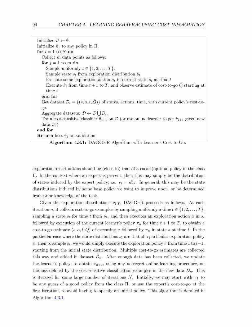
94 CHAPTER 4. LEARNING BEHAVIOR USING COST INFORMATION
Initialize D ← ∅.Initialize π1 to any policy in Π.for i = 1 to N do
Collect m data points as follows:for j = 1 to m do
Sample uniformly t ∈ 1, 2, . . . , T.Sample state st from exploration distribution νt.Execute some exploration action at in current state st at time tExecute πi from time t+ 1 to T , and observe estimate of cost-to-go Q starting attime t
end forGet dataset Di = (s, a, t, Q) of states, actions, time, with current policy’s cost-to-go.Aggregate datasets: D ← D
⋃Di.
Train cost-sensitive classifier πi+1 on D (or use online learner to get πi+1 given newdata Di)
end forReturn best πi on validation.
Algorithm 4.3.1: DAGGER Algorithm with Learner’s Cost-to-Go.
exploration distributions should be (close to) that of a (near-)optimal policy in the class
Π. In the context where an expert is present, then this may simply be the distribution
of states induced by the expert policy, i.e. νt = dtπ∗ . In general, this may be the state
distributions induced by some base policy we want to improve upon, or be determined
from prior knowledge of the task.
Given the exploration distributions ν1:T , DAGGER proceeds as follows. At each
iteration n, it collects cost-to-go examples by sampling uniformly a time t ∈ 1, 2, . . . , T,sampling a state st for time t from νt, and then executes an exploration action a in st
followed by execution of the current learner’s policy πn for time t+ 1 to T , to obtain a
cost-to-go estimate (s, a, t, Q) of executing a followed by πn in state s at time t. In the
particular case where the state distributions νt are that of a particular exploration policy
π, then to sample st, we would simply execute the exploration policy π from time 1 to t−1,
starting from the initial state distribution. Multiple cost-to-go estimates are collected
this way and added in dataset Dn. After enough data has been collected, we update
the learner’s policy, to obtain πn+1, using any no-regret online learning procedure, on
the loss defined by the cost-sensitive classification examples in the new data Dn. This
is iterated for some large number of iterations N . Initially, we may start with π1 to
be any guess of a good policy from the class Π, or use the expert’s cost-to-go at the
first iteration, to avoid having to specify an initial policy. This algorithm is detailed in
Algorithm 4.3.1.
4.3. REINFORCEMENT LEARNING VIA DAGGER WITH LEARNER’SCOST-TO-GO 95
Analysis
Consider the online learning loss function Ln given to the online learning algorithm
within DAGGER at iteration n. Assuming infinite data, it assigns the following loss to
each policy π ∈ Π:
Ln(π) = Et∼U(1:T ),s∼νt [QπnT−t+1(s, π)].
This loss represents the expected cost-to-go of executing π immediately for 1 step followed
by current policy πn, under the exploration distributions ν1:T .
This sequence of loss over the iterations of training corresponds to an online cost-
sensitive classification problem, as in the previous DAGGER with cost-to-go algorithm.
Let εregret be the average regret of the online learner on this online cost-sensitive classi-
fication problem after the N iterations of DAGGER:
εregret =1
N
N∑i=1
Li(πi)−minπ∈Π
1
N
N∑i=1
Li(π).
For any policy π ∈ Π, denote the average L1 distance between νt and dtπ over time
steps t as:
D(ν, π) =1
T
T∑t=1
||νt − dtπ||1.
Note that if νt = dtπ for all t, then D(ν, π) = 0.
Now assume the cost-to-go of the learned policies π1, π2, . . . , πN are bounded byQmax,
for any state s and time t (in the worst case this is TCmax). Denote π the best policy
found by DAGGER over the iterations, and π the uniform mixture policy over π1:N
defined as before. Then we have to following guarantee with this version of DAGGER
with learner’s cost-to-go:
Theorem 4.3.1. For any policy π′ ∈ Π:
J(π) ≤ J(π) ≤ J(π′) + Tεregret + TQmaxD(ν, π′)
Thus, if a no-regret online cost-sensitive classification algorithm is used, then:
limN→∞
J(π) ≤ J(π′) + TQmaxD(ν, π′)
This theorem indicates that DAGGER must find policies that are as good as any
other policy π′ ∈ Π, whose state distribution dtπ′ is close to νt (on average over time
t). Note however, that since TQmax is generally O(T 2), this only provides meaningful
guarantees when dtπ′ is very close to νt (on average over time t). Importantly, if ν1:T
corresponds to the state distribution of an optimal policy in class Π, then this theorem
guarantees that DAGGER will find an optimal policy (within the class Π) in the limit.
96 CHAPTER 4. LEARNING BEHAVIOR USING COST INFORMATION
This theorem provides a similar performance guarantee to the results for PSDP
presented in (Bagnell et al., 2003). However, DAGGER has the advantage of learning a
single stationary policy for test execution, instead of a non-stationary policy, allowing for
improved generalization and more efficient learning. Note that DAGGER has stronger
requirements: it needs a no-regret online cost-sensitive classification procedure, instead
of simply a cost-sensitive supervised learner for PSDP. For finite policy classes Π, or
using reductions of cost-sensitive classification as mentioned previously and in Section
2.2, we can still obtain convex online learning problems for which efficient no-regret
algorithms exists.
The result presented here can be interpreted as a reduction of model-free reinforce-
ment learning to no-regret online learning. It is a regret reduction, as performance is
related directly to the online regret at the online cost-sensitive classification task. How-
ever its performance are limited by the quality of the exploration distribution. One could
consider trying to adapt the exploration distributions ν1:T over the iterations of training.
It can be shown that if νi1:T are the exploration distributions at iteration i, and we have
a mechanism for making νi1:T converge to the state distributions of an optimal policy in
Π, as i→∞, then we would always be guaranteed to find an optimal policy in Π in the
limit (see appendix A). However, at this point we do not know of any method that could
be used to achieve this.
4.4 Discussion
Drawback of using Cost-to-Go: In practice, using DAGGER, Forward, or SEARN,
with cost-to-go can often be impractical. This is because, collecting each cost-to-go
estimate for a single state-action pair, involves executing an entire trajectory. In many
settings, minimizing directly an imitation loss with DAGGER, as in Section 3.6, is much
more practical as we can observe the action chosen by the expert in every visited state
along a trajectory, and thus collect T data points per trajectory instead of only one. This
makes a big difference in practice when T is large. A potential combination of the two
approaches could be considered, where first a policy is found by DAGGER through simple
imitation loss minimization, to get a good estimate of a reasonable policy, and then refine
this policy by using the cost-to-go version of DAGGER (e.g. through additional gradient
descent steps). By doing so, we may need fewer (expensive) iterations of DAGGER with
cost-to-go to obtain a good policy.
Chapter 5
Experimental Study of Learning
from Demonstrations Techniques
In the chapter, we demonstrate the efficacy and scalability of DAGGER experimentally
in imitation learning settings, by comparing its performance to several methods we pre-
viously discussed, such as the naive supervised learning approach, SMILe and SEARN.
We compare these methods extensively for learning game playing agents from game play
data in two video game applications. The first is a racing game, called Super Tux Kart,
where we attempt to learn to control the car from the observed game image, from data
collected by observing human players. In the second application, we attempt to learn an
agent that can play the popular video game Super Mario Bros. given only the objects
observed in the current game image, from game play data of a planner that has full
access to the entire level (upcoming unobserved terrain, enemies, objects, etc.) to make
its decisions. These results were originally presented in Ross et al. (2011).
We additionally demonstrate the applicability of DAGGER on real robots, by apply-
ing it to train an autonomous quadrotor to fly through forest environments while avoid
trees using its front facing camera (monocular vision). We also discuss several practical
considerations when applying DAGGER in practice.
5.1 Super Tux Kart : Learning Driving Behavior
Super Tux Kart is a 3D racing game similar to the popular Mario Kart. Our goal is to
train the computer to steer the kart moving at fixed speed on a particular race track,
based on the current game image features as input (see Figure 5.1). A human player is
used to provide demonstrations of the correct steering (analog joystick value in [-1,1])
for each of the observed game images in real time during play.
For this task, we attempt to learn a linear controller that updates the steering at
5Hz based on the current vector of image features. That is, if x is the vector of features

98CHAPTER 5. EXPERIMENTAL STUDY OF LEARNING FROM
DEMONSTRATIONS TECHNIQUES
Figure 5.1: Image from Super Tux Kart’s Star Track.
of the image, the linear controller predicts and executes the steering y = w>x + b,
where w and b are the parameters that we learn from training data. Given the current
800x600 RGB pixel game image, we use as features directly the LAB color values of
each pixel in a 25x19 resized image. Given a dataset of observed features and associated
steering (xi, yi)ni=1, we optimize (w, b) by minimizing the ridge regression objective
L(w, b) = 1n
∑ni=1(w>xi + b − yi)2 + λ
2w>w, with regularizer λ = 10−3 chosen from a
preliminary validation dataset.
We compare performance on a race track called Star Track. As this track floats in
space, the kart can fall off the track at any point (the kart is repositioned at the center
of the track when this occurs). We measure performance in terms of the average number
of falls per lap. We compare two other approaches to DAGGER on this task: 1) the
traditional supervised learning approach, and 2) another approach, called SMILE, from
our previous work in (Ross and Bagnell, 2010), which is an imitation learning variant of
SEARN (described in more details in the next chapter) that also has similar guarantees
to Forward Training and DAGGER.
For SMILE and DAGGER, we used 1 lap of training per iteration (∼1000 data
points) and run both methods for 20 iterations. For SMILE we choose parameter α = 0.1
as in Ross and Bagnell (2010), and for DAGGER the parameter βi = I(i = 1) for I the
indicator function. Figure 5.2 shows 95% confidence intervals on the average falls per
lap of each method after 1, 5, 10, 15 and 20 iterations as a function of the total number
of training data collected.
We first observe that with the baseline supervised approach where training always
occurs under the human player’s trajectories that performance does not improve as more
data is collected. This is because most of the training laps are all very similar and do not

5.2. SUPER MARIO BROS. 99
0 0.5 1 1.5 2 2.5x 10
4
0
0.5
1
1.5
2
2.5
3
3.5
4
4.5
Number of Training Data
Ave
rag
e F
alls
Per
Lap
DAgger (βi = I(i=1))
SMILe (α = 0.1)Supervised
Figure 5.2: Average falls/lap as a function of training data.
help the learner to learn how to recover from mistakes it makes. With SMILE we obtain
some improvements but the policy after 20 iterations still falls off the track about twice
per lap on average. This is in part due to the stochasticity of the policy learned with
this method which sometimes makes bad choices of actions. For DAGGER, we were
able to obtain a policy that never falls off the track after 15 iterations of training. Even
after 5 iterations, the policy we obtain almost never falls off the track and is significantly
outperforming both SMILE and the baseline supervised approach. Furthermore, the
policy obtained by DAGGER is smoother and looks qualitatively better than the policy
obtained with SMILE. A video available on YouTube (Ross, 2010a) shows a qualitative
comparison of the behavior obtained with each method.
5.2 Super Mario Bros.
Super Mario Bros. is a platform video game where the character, Mario, must move
across each level by avoiding being hit by enemies and falling into gaps, and before
running out of time. We used the simulator from a recent Super Mario Bros. AI com-
petition (Togelius and Karakovskiy, 2009) that randomly generates levels of varying
difficulty (more difficult gaps and types of enemies). Our goal is to train the computer
to play this game based on the current game image features as input (see Figure 5.3).
Our expert in this scenario is a near-optimal planning algorithm that has full access to
the game’s internal state and can simulate exactly the consequence of future actions. In
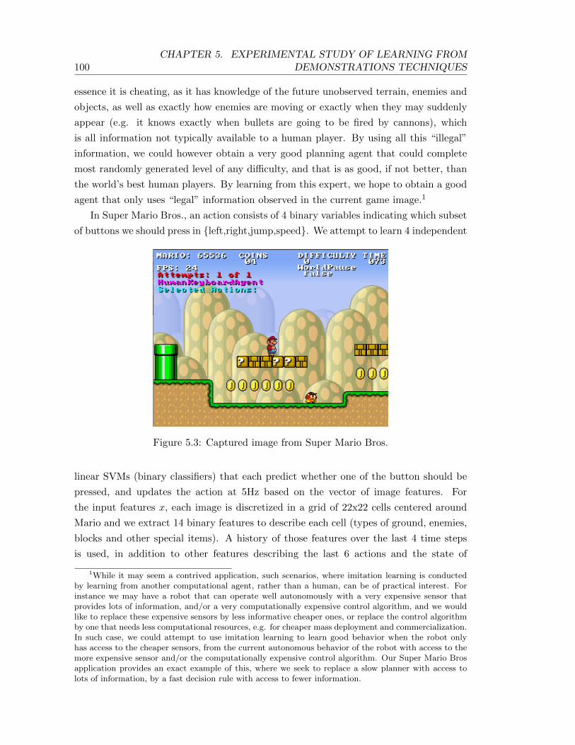
100CHAPTER 5. EXPERIMENTAL STUDY OF LEARNING FROM
DEMONSTRATIONS TECHNIQUES
essence it is cheating, as it has knowledge of the future unobserved terrain, enemies and
objects, as well as exactly how enemies are moving or exactly when they may suddenly
appear (e.g. it knows exactly when bullets are going to be fired by cannons), which
is all information not typically available to a human player. By using all this “illegal”
information, we could however obtain a very good planning agent that could complete
most randomly generated level of any difficulty, and that is as good, if not better, than
the world’s best human players. By learning from this expert, we hope to obtain a good
agent that only uses “legal” information observed in the current game image.1
In Super Mario Bros., an action consists of 4 binary variables indicating which subset
of buttons we should press in left,right,jump,speed. We attempt to learn 4 independent
Figure 5.3: Captured image from Super Mario Bros.
linear SVMs (binary classifiers) that each predict whether one of the button should be
pressed, and updates the action at 5Hz based on the vector of image features. For
the input features x, each image is discretized in a grid of 22x22 cells centered around
Mario and we extract 14 binary features to describe each cell (types of ground, enemies,
blocks and other special items). A history of those features over the last 4 time steps
is used, in addition to other features describing the last 6 actions and the state of
1While it may seem a contrived application, such scenarios, where imitation learning is conductedby learning from another computational agent, rather than a human, can be of practical interest. Forinstance we may have a robot that can operate well autonomously with a very expensive sensor thatprovides lots of information, and/or a very computationally expensive control algorithm, and we wouldlike to replace these expensive sensors by less informative cheaper ones, or replace the control algorithmby one that needs less computational resources, e.g. for cheaper mass deployment and commercialization.In such case, we could attempt to use imitation learning to learn good behavior when the robot onlyhas access to the cheaper sensors, from the current autonomous behavior of the robot with access to themore expensive sensor and/or the computationally expensive control algorithm. Our Super Mario Brosapplication provides an exact example of this, where we seek to replace a slow planner with access tolots of information, by a fast decision rule with access to fewer information.
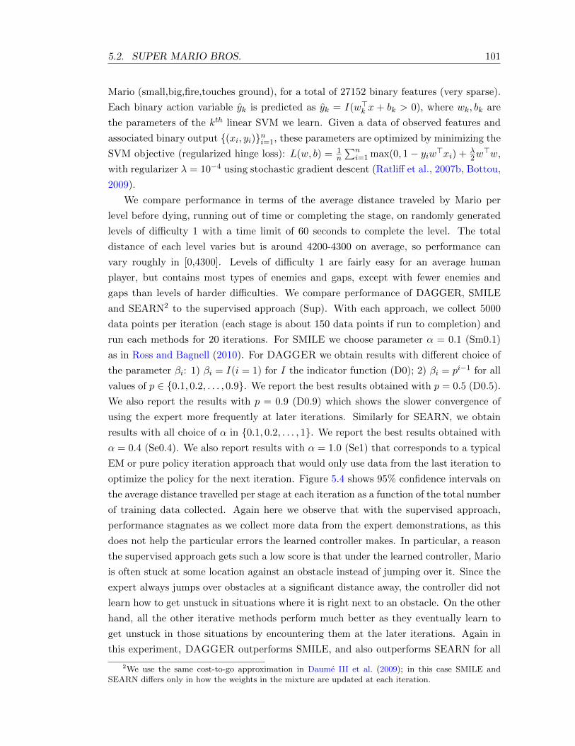
5.2. SUPER MARIO BROS. 101
Mario (small,big,fire,touches ground), for a total of 27152 binary features (very sparse).
Each binary action variable yk is predicted as yk = I(w>k x + bk > 0), where wk, bk are
the parameters of the kth linear SVM we learn. Given a data of observed features and
associated binary output (xi, yi)ni=1, these parameters are optimized by minimizing the
SVM objective (regularized hinge loss): L(w, b) = 1n
∑ni=1 max(0, 1− yiw>xi) + λ
2w>w,
with regularizer λ = 10−4 using stochastic gradient descent (Ratliff et al., 2007b, Bottou,
2009).
We compare performance in terms of the average distance traveled by Mario per
level before dying, running out of time or completing the stage, on randomly generated
levels of difficulty 1 with a time limit of 60 seconds to complete the level. The total
distance of each level varies but is around 4200-4300 on average, so performance can
vary roughly in [0,4300]. Levels of difficulty 1 are fairly easy for an average human
player, but contains most types of enemies and gaps, except with fewer enemies and
gaps than levels of harder difficulties. We compare performance of DAGGER, SMILE
and SEARN2 to the supervised approach (Sup). With each approach, we collect 5000
data points per iteration (each stage is about 150 data points if run to completion) and
run each methods for 20 iterations. For SMILE we choose parameter α = 0.1 (Sm0.1)
as in Ross and Bagnell (2010). For DAGGER we obtain results with different choice of
the parameter βi: 1) βi = I(i = 1) for I the indicator function (D0); 2) βi = pi−1 for all
values of p ∈ 0.1, 0.2, . . . , 0.9. We report the best results obtained with p = 0.5 (D0.5).
We also report the results with p = 0.9 (D0.9) which shows the slower convergence of
using the expert more frequently at later iterations. Similarly for SEARN, we obtain
results with all choice of α in 0.1, 0.2, . . . , 1. We report the best results obtained with
α = 0.4 (Se0.4). We also report results with α = 1.0 (Se1) that corresponds to a typical
EM or pure policy iteration approach that would only use data from the last iteration to
optimize the policy for the next iteration. Figure 5.4 shows 95% confidence intervals on
the average distance travelled per stage at each iteration as a function of the total number
of training data collected. Again here we observe that with the supervised approach,
performance stagnates as we collect more data from the expert demonstrations, as this
does not help the particular errors the learned controller makes. In particular, a reason
the supervised approach gets such a low score is that under the learned controller, Mario
is often stuck at some location against an obstacle instead of jumping over it. Since the
expert always jumps over obstacles at a significant distance away, the controller did not
learn how to get unstuck in situations where it is right next to an obstacle. On the other
hand, all the other iterative methods perform much better as they eventually learn to
get unstuck in those situations by encountering them at the later iterations. Again in
this experiment, DAGGER outperforms SMILE, and also outperforms SEARN for all
2We use the same cost-to-go approximation in Daume III et al. (2009); in this case SMILE andSEARN differs only in how the weights in the mixture are updated at each iteration.
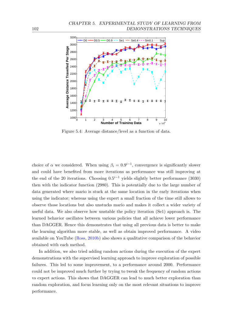
102CHAPTER 5. EXPERIMENTAL STUDY OF LEARNING FROM
DEMONSTRATIONS TECHNIQUES
0 1 2 3 4 5 6 7 8 9 10x 10
4
1000
1200
1400
1600
1800
2000
2200
2400
2600
2800
3000
3200
Number of Training Data
Ave
rag
e D
ista
nce
Tra
velle
d P
er S
tag
e
D0 D0.5 D0.9 Se1 Se0.4 Sm0.1 Sup
Figure 5.4: Average distance/level as a function of data.
choice of α we considered. When using βi = 0.9i−1, convergence is significantly slower
and could have benefited from more iterations as performance was still improving at
the end of the 20 iterations. Choosing 0.5i−1 yields slightly better performance (3030)
then with the indicator function (2980). This is potentially due to the large number of
data generated where mario is stuck at the same location in the early iterations when
using the indicator; whereas using the expert a small fraction of the time still allows to
observe those locations but also unstucks mario and makes it collect a wider variety of
useful data. We also observe how unstable the policy iteration (Se1) approach is. The
learned behavior oscillates between various policies that all achieve lower performance
than DAGGER. Hence this demonstrates that using all previous data is better to make
the learning algorithm more stable, as well as obtain improved performance. A video
available on YouTube (Ross, 2010b) also shows a qualitative comparison of the behavior
obtained with each method.
In addition, we also tried adding random actions during the execution of the expert
demonstrations with the supervised learning approach to improve exploration of possible
failures. This led to some improvement, to a performance around 2000. Performance
could not be improved much further by trying to tweak the frequency of random actions
vs expert actions. This shows that DAGGER can lead to much better exploration than
random exploration, and focus learning only on the most relevant situations to improve
performance.

5.3. ROBOTIC CASE STUDY: LEARNING OBSTACLE AVOIDANCE FORAUTONOMOUS FLIGHT 103
5.3 Robotic Case Study: Learning Obstacle Avoidance
for Autonomous Flight
While the previous section demonstrates the applicability of DAGGER in simulated
environments, we also demonstrate that DAGGER can be successfully applied on real
robotic systems. In particular, we demonstrate an application of DAGGER for learning a
reactive controller for a small aircraft that can fly autonomously at low altitude in natural
forest environments, while avoiding trees, using only a cheap camera for perception. This
section covers an application of DAGGER that was presented in detail in Ross et al.
(2013a).
Motivation
In the past decade Unmanned Aerial Vehicles (UAVs) have enjoyed considerable success
in many applications such as search and rescue, monitoring, research, exploration, or
mapping. While there has been significant progress in making the operation of UAVs
increasingly autonomous, obstacle avoidance is still a crucial hurdle. For Micro Aerial
Vehicles (MAVs) with very limited payloads it is infeasible to carry state-of-the-art radars
(Bernier et al., 2005). Many impressive advances have recently been made using laser
range finders (lidar) (Bachrach et al., 2009, Bry et al., 2012, Scherer et al., 2007) or
Microsoft Kinect cameras (RGB-D sensors) (Bachrach et al., 2012). Both sensors are
heavy and active, which leads to increased power consumption and decreased flight time.
In contrast, passive vision is promising for producing a feasible solution for autonomous
MAV navigation (Roberts et al., 2012, Dey et al., 2011, Wendel et al., 2012).
This application is primarily concerned with navigating MAVs that have very low
payload capabilities, and operate close to the ground where they cannot avoid dense
obstacle fields. We present a system that allows the MAV to autonomously fly at speeds
of up to 1.5 m/s and altitudes of up to 4 meters above the ground through a cluttered
forest environment (Figure 5.5), using passive monocular vision as its only exteroceptive
sensor. We use DAGGER to train reactive “heading” policies based on flight trajecto-
ries through forest environments of a human pilot. Visual features extracted from the
corresponding camera image are mapped to the control input provided by the pilot.
System
We use a cheap (∼ $300), commercially available quadrotor helicopter, namely the Parrot
ARDrone, as our airborne platform (see Figure 5.6). The ARDrone weights only 420g
and has a size of 0.3 × 0.3m. It features a front-facing camera of 320 × 240 pixels
and a 93 degree field of view (FOV), an ultrasound altimeter, a low resolution down-
facing camera and an on-board Inertial Measurement Unit (IMU). The drone’s on-board
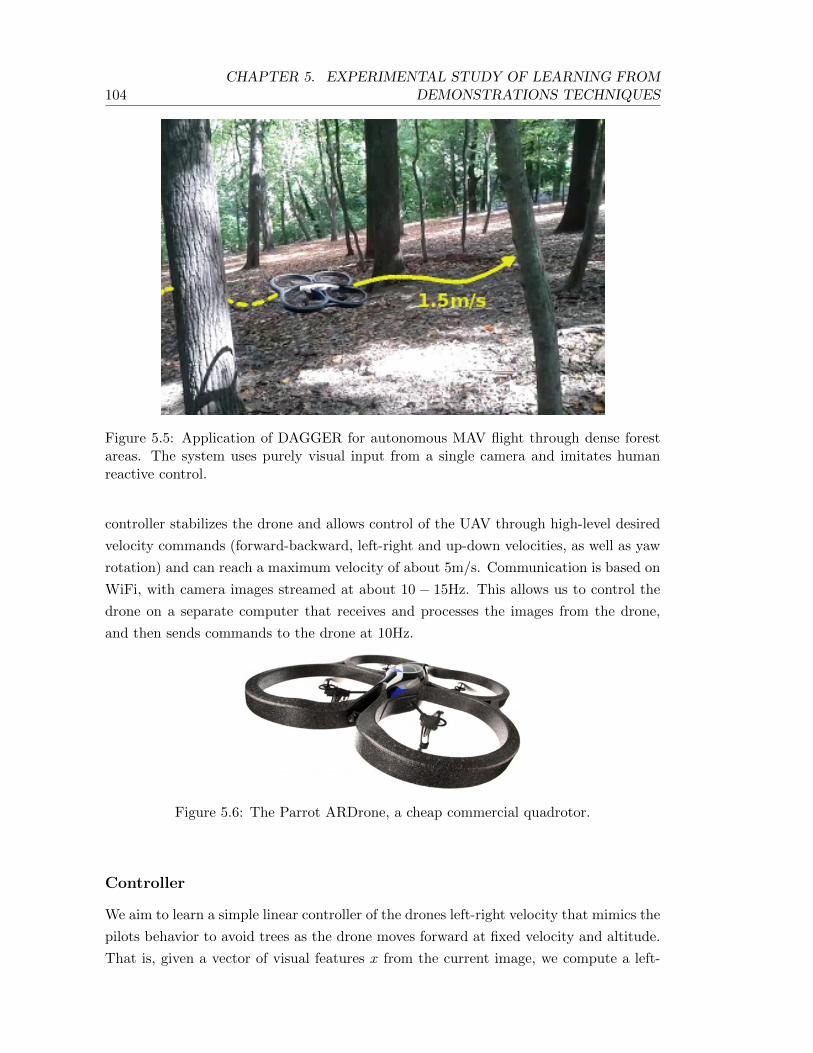
104CHAPTER 5. EXPERIMENTAL STUDY OF LEARNING FROM
DEMONSTRATIONS TECHNIQUES
Figure 5.5: Application of DAGGER for autonomous MAV flight through dense forestareas. The system uses purely visual input from a single camera and imitates humanreactive control.
controller stabilizes the drone and allows control of the UAV through high-level desired
velocity commands (forward-backward, left-right and up-down velocities, as well as yaw
rotation) and can reach a maximum velocity of about 5m/s. Communication is based on
WiFi, with camera images streamed at about 10 − 15Hz. This allows us to control the
drone on a separate computer that receives and processes the images from the drone,
and then sends commands to the drone at 10Hz.
Figure 5.6: The Parrot ARDrone, a cheap commercial quadrotor.
Controller
We aim to learn a simple linear controller of the drones left-right velocity that mimics the
pilots behavior to avoid trees as the drone moves forward at fixed velocity and altitude.
That is, given a vector of visual features x from the current image, we compute a left-
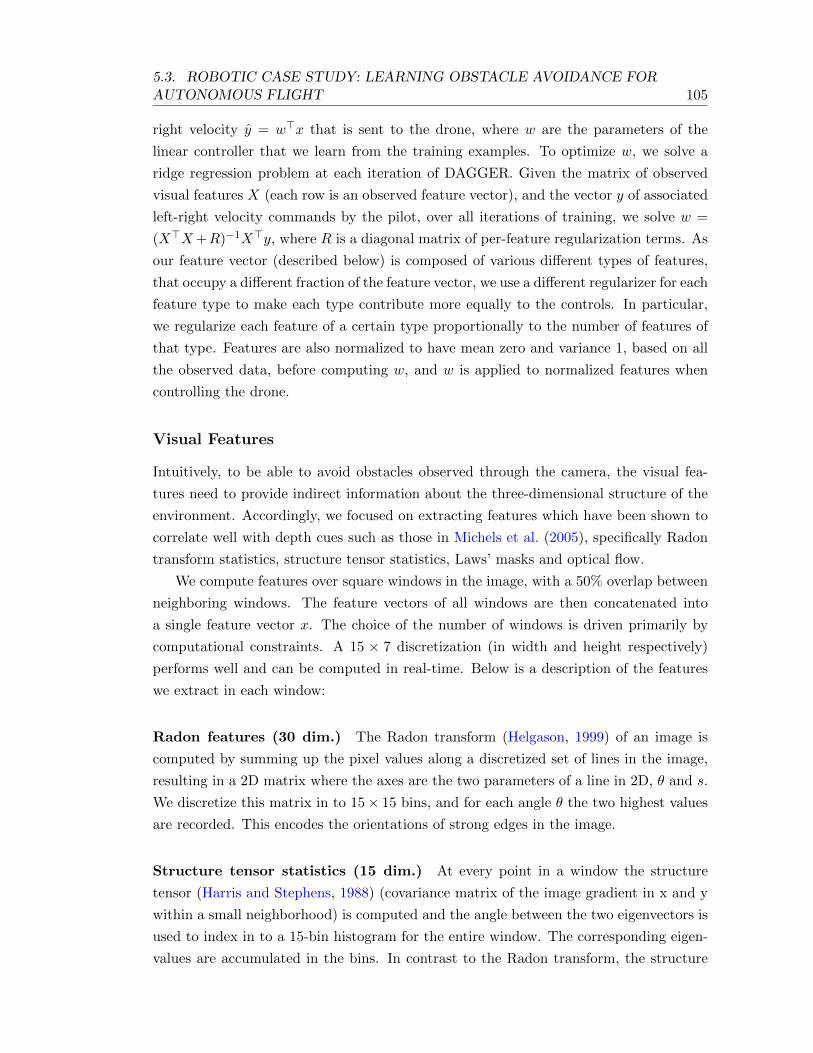
5.3. ROBOTIC CASE STUDY: LEARNING OBSTACLE AVOIDANCE FORAUTONOMOUS FLIGHT 105
right velocity y = w>x that is sent to the drone, where w are the parameters of the
linear controller that we learn from the training examples. To optimize w, we solve a
ridge regression problem at each iteration of DAGGER. Given the matrix of observed
visual features X (each row is an observed feature vector), and the vector y of associated
left-right velocity commands by the pilot, over all iterations of training, we solve w =
(X>X+R)−1X>y, where R is a diagonal matrix of per-feature regularization terms. As
our feature vector (described below) is composed of various different types of features,
that occupy a different fraction of the feature vector, we use a different regularizer for each
feature type to make each type contribute more equally to the controls. In particular,
we regularize each feature of a certain type proportionally to the number of features of
that type. Features are also normalized to have mean zero and variance 1, based on all
the observed data, before computing w, and w is applied to normalized features when
controlling the drone.
Visual Features
Intuitively, to be able to avoid obstacles observed through the camera, the visual fea-
tures need to provide indirect information about the three-dimensional structure of the
environment. Accordingly, we focused on extracting features which have been shown to
correlate well with depth cues such as those in Michels et al. (2005), specifically Radon
transform statistics, structure tensor statistics, Laws’ masks and optical flow.
We compute features over square windows in the image, with a 50% overlap between
neighboring windows. The feature vectors of all windows are then concatenated into
a single feature vector x. The choice of the number of windows is driven primarily by
computational constraints. A 15 × 7 discretization (in width and height respectively)
performs well and can be computed in real-time. Below is a description of the features
we extract in each window:
Radon features (30 dim.) The Radon transform (Helgason, 1999) of an image is
computed by summing up the pixel values along a discretized set of lines in the image,
resulting in a 2D matrix where the axes are the two parameters of a line in 2D, θ and s.
We discretize this matrix in to 15× 15 bins, and for each angle θ the two highest values
are recorded. This encodes the orientations of strong edges in the image.
Structure tensor statistics (15 dim.) At every point in a window the structure
tensor (Harris and Stephens, 1988) (covariance matrix of the image gradient in x and y
within a small neighborhood) is computed and the angle between the two eigenvectors is
used to index in to a 15-bin histogram for the entire window. The corresponding eigen-
values are accumulated in the bins. In contrast to the Radon transform, the structure
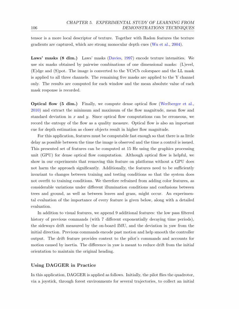
106CHAPTER 5. EXPERIMENTAL STUDY OF LEARNING FROM
DEMONSTRATIONS TECHNIQUES
tensor is a more local descriptor of texture. Together with Radon features the texture
gradients are captured, which are strong monocular depth cues (Wu et al., 2004).
Laws’ masks (8 dim.) Laws’ masks (Davies, 1997) encode texture intensities. We
use six masks obtained by pairwise combinations of one dimensional masks: (L)evel,
(E)dge and (S)pot. The image is converted to the YCrCb colorspace and the LL mask
is applied to all three channels. The remaining five masks are applied to the Y channel
only. The results are computed for each window and the mean absolute value of each
mask response is recorded.
Optical flow (5 dim.) Finally, we compute dense optical flow (Werlberger et al.,
2010) and extract the minimum and maximum of the flow magnitude, mean flow and
standard deviation in x and y. Since optical flow computations can be erroneous, we
record the entropy of the flow as a quality measure. Optical flow is also an important
cue for depth estimation as closer objects result in higher flow magnitude.
For this application, features must be computable fast enough so that there is as little
delay as possible between the time the image is observed and the time a control is issued.
This presented set of features can be computed at 15 Hz using the graphics processing
unit (GPU) for dense optical flow computation. Although optical flow is helpful, we
show in our experiments that removing this feature on platforms without a GPU does
not harm the approach significantly. Additionally, the features need to be sufficiently
invariant to changes between training and testing conditions so that the system does
not overfit to training conditions. We therefore refrained from adding color features, as
considerable variations under different illumination conditions and confusions between
trees and ground, as well as between leaves and grass, might occur. An experimen-
tal evaluation of the importance of every feature is given below, along with a detailed
evaluation.
In addition to visual features, we append 9 additional features: the low pass filtered
history of previous commands (with 7 different exponentially decaying time periods),
the sideways drift measured by the on-board IMU, and the deviation in yaw from the
initial direction. Previous commands encode past motion and help smooth the controller
output. The drift feature provides context to the pilot’s commands and accounts for
motion caused by inertia. The difference in yaw is meant to reduce drift from the initial
orientation to maintain the original heading.
Using DAGGER in Practice
In this application, DAGGER is applied as follows. Initially, the pilot flies the quadrotor,
via a joystick, through forest environments for several trajectories, to collect an initial
5.3. ROBOTIC CASE STUDY: LEARNING OBSTACLE AVOIDANCE FORAUTONOMOUS FLIGHT 107
Figure 5.7: One frame from MAV camera stream. The white line indicates the currentleft-right velocity commanded by the drone’s current policy πn−1 while the red lineindicates the pilot’s commanded left-right velocity. In this frame DAGGER is wronglyheading for the tree in the middle while the expert is providing the correct yaw commandto go to the right instead. These expert controls are recorded for training later iterationsbut not executed in the current run.
dataset and train a first policy π1. At following iterations, the drone is placed in various
forest environments and flies autonomously using its current policy πn−1. The pilot
provides the correct controls he would perform in the situations encountered along the
autonomous trajectories flown by the drone, via the joystick. This allows the drone to
collect data in new situations visited by the current policy, and learn the proper recovery
behavior when these are encountered. The next policy πn+1 is obtained by training a
policy on all the training data collected over all iterations (from iteration 1 to n).
Figure 5.7 shows the DAGGER control interface used to provide correct actions to
the drone. As mentioned, at iteration n > 1, the drone’s current policy πn−1 is in
control and the pilot just provides the correct controls for the scenes that the MAV
visits. The pilot controls are recorded but not executed on the MAV. This results in
some human-computer-interaction challenges:
1) After the first iteration, the pilot must be able to provide the correct controls
without feedback of how the drone would react to the current command. While deciding
whether the drone should go left or right is easy for the pilot, it can be hard to input the
correct magnitude of the turn the drone should perform without feedback. In particular,
we observed that this often makes the pilot turn excessively when providing the training
examples after the first iteration. Performance can degrade quickly if the drone starts to
mimic these imperfect actions. To address this issue, we provided partial feedback to the
pilot by showing a vertical line in the camera image seen by the pilot that would slide
left or right based on the current joystick command performed. As the line indicated
roughly where the drone would move under the current joystick command, this interface

108CHAPTER 5. EXPERIMENTAL STUDY OF LEARNING FROM
DEMONSTRATIONS TECHNIQUES
Figure 5.8: Left: Indoor setup in motion capture arena with fake plastic trees andcamouflage in background. Right: The 11 obstacle arrangements used to train DAGGERfor every iteration in the motion capture arena. The star indicates the goal location.
led to improved actions provided by the pilot (Figure 5.7).
2) In addition to the lack of feedback, providing the correct actions in real-time after
the first iteration when the drone is in control can be hard for the pilot as he must
react to what the drone is doing and not what he expects to happen: e.g., if the drone
suddenly starts turning towards a tree nearby, the pilot must quickly start turning the
other way to indicate the proper behavior. The pilot’s reaction time to the drone’s
behavior can lead to extra delay in the correct actions specified by the pilot. By trying
to react quickly, he may provide imperfect actions as well. This becomes more and more
of an issue the faster the drone is flying. To address this issue, we allow the pilot to
indicate the correct actions offline while the camera stream from the drone is replayed
at slower speed (proportional to the drone’s speed), using the interface seen in Figure
5.7. By replaying the stream slower the pilot can provide more accurate commands and
react more quickly to the drone’s behavior.
3) The third challenge is that DAGGER needs to collect data for all situations en-
countered by the current policy in later iterations. This would include situations where
the drone crashes into obstacles if the current policy is not good enough. For safety rea-
sons, we allow the pilot to take over or force an emergency landing to avoid crashes as
much as possible. This implies that the training data used is not exactly what DAGGER
would need, but instead a subset of training examples encountered by the current policy
when it is within a “safe” region. Despite this modification, the guarantees of DAGGER
still hold as long as a policy that can stay within this “safe” region can be learnt.
Indoor Experiments
We first tested our approach indoors in a motion capture arena. We used fake indoor trees
as obstacles and camouflage to hide background clutter (Figure 5.8). Although being a

5.3. ROBOTIC CASE STUDY: LEARNING OBSTACLE AVOIDANCE FORAUTONOMOUS FLIGHT 109
Figure 5.9: Left: Improvement of trajectory by DAGGER over the iterations. Therightmost green trajectory is the pilot demonstration. The short trajectories in red &orange show the controller learnt in the 1st and 2nd iterations respectively that failed.The 3rd iteration controller successfully avoided both obstacles and its trajectory issimilar to the demonstrated trajectory. Right: Percentage of scenarios the pilot had tointervene and the imitation loss (average squared error in controls of controller to humanexpert on hold-out data) after each iteration of DAGGER. After 3 iterations, there wasno need for the pilot to intervene and the UAV could successfully avoid all obstacles
very controlled environment that lacked many of the complexities of real outdoor scenes,
it allowed us to obtain better quantitative results to determine the effectiveness of our
approach.
The motion capture system was only used to track the drone and to adjust its heading
so that it always headed straight towards a given goal location. The drone moved at a
fixed altitude and forward velocity of 0.35m/s and we learnt a controller that controlled
the left-right velocity using DAGGER over 3 training iterations. At each iteration, we
used 11 fixed scenarios to collect training data, including 1 scenario with no obstacles, 3
with one obstacle and 7 with two obstacles (Figure 5.8).
Figure 5.9 qualitatively compares the trajectories taken by the MAV in the mocap
arena after each iteration of training on one of the particular scenarios. In the first
iteration, the green trajectory to the farthest right is the demonstrated trajectory by the
human expert pilot. The short red and orange trajectories are the trajectories taken by
the MAV after the 1st and 2nd iterations were completed. Note that both failed to avoid
the obstacle. After the 3rd iteration, however, the controller learnt a trajectory which
avoided both obstacles. The percentage of scenarios where the pilot had to intervene
for the learnt controller after each iteration can be found in Figure 5.9. The number of

110CHAPTER 5. EXPERIMENTAL STUDY OF LEARNING FROM
DEMONSTRATIONS TECHNIQUES
Figure 5.10: Common failures over iterations. While the controller has problems withtree trunks during the 1st iteration (left), this improves considerably towards the 3rd
iteration, where mainly foliage causes problems (middle). Over all iterations, the mostcommon failures are due to the narrow FOV of the camera where some trees barelyappear to one side of the camera or are just hidden outside the view (right). When theUAV turns to avoid a visible tree a bit farther away it collides with the tree to the side.
required interventions decreased between iterations and after 3 iterations there was no
need to intervene as the MAV successfully avoided all obstacles in all scenarios.
Outdoor Experiments
After validating our approach indoors in the motion capture arena, we conducted outdoor
experiments to test in real-world scenarios. As we could not use the motion capture
system outdoors to make the drone head towards a specific goal location, we made the
drone move forward at a fixed speed and aimed for learning a controller that would
swerve left or right to avoid any trees on the way, while maintaining the initial heading.
Training and testing were conducted in forest areas while restraining the aircraft using
a light-weight tether.
We performed two experiments with DAGGER to evaluate its performance in dif-
ferent regions, one in a park with relatively low tree density, and another in a dense
forest.
Low-density region
The first area is a park area with a low tree density of approximately 1 tree per 12×12m,
consisting mostly of large trees and a few thinner trees. In this area we flew at a fixed
velocity of around 1m/s, and learnt a heading (left-right) controller for avoiding trees
using DAGGER over 3 training iterations, representing training data acquired over a
total of 1km of flight. Then, we exhaustively tested the final controller over an additional
800m in the training area and a separate test area.
Qualitatively, we observed that the behavior of the drone improved over iterations.
After the first iteration of training, the drone sometimes failed to avoid large trees even
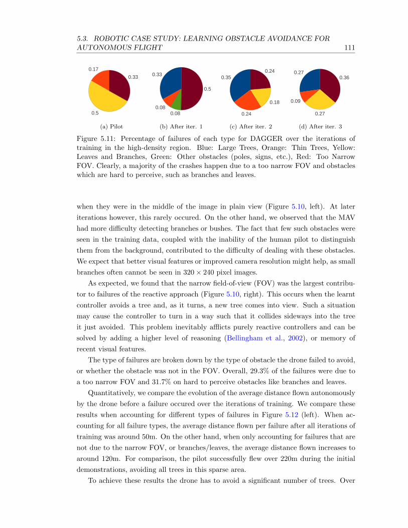
5.3. ROBOTIC CASE STUDY: LEARNING OBSTACLE AVOIDANCE FORAUTONOMOUS FLIGHT 111
0.17
0.5
0.33 Large Trees
Thin Trees
Leaves & Branches
Other Obstacle
Narrow FOV
(a) Pilot
0.33
0.08
0.08
0.5
Large Trees
Thin Trees
Leaves & Branches
Other Obstacle
Narrow FOV
(b) After iter. 1
0.35
0.24
0.18
0.24Large Trees
Thin Trees
Leaves & Branches
Other Obstacle
Narrow FOV
(c) After iter. 2
0.27
0.09
0.27
0.36Large Trees
Thin Trees
Leaves & Branches
Other Obstacle
Narrow FOV
(d) After iter. 3
Figure 5.11: Percentage of failures of each type for DAGGER over the iterations oftraining in the high-density region. Blue: Large Trees, Orange: Thin Trees, Yellow:Leaves and Branches, Green: Other obstacles (poles, signs, etc.), Red: Too NarrowFOV. Clearly, a majority of the crashes happen due to a too narrow FOV and obstacleswhich are hard to perceive, such as branches and leaves.
when they were in the middle of the image in plain view (Figure 5.10, left). At later
iterations however, this rarely occured. On the other hand, we observed that the MAV
had more difficulty detecting branches or bushes. The fact that few such obstacles were
seen in the training data, coupled with the inability of the human pilot to distinguish
them from the background, contributed to the difficulty of dealing with these obstacles.
We expect that better visual features or improved camera resolution might help, as small
branches often cannot be seen in 320× 240 pixel images.
As expected, we found that the narrow field-of-view (FOV) was the largest contribu-
tor to failures of the reactive approach (Figure 5.10, right). This occurs when the learnt
controller avoids a tree and, as it turns, a new tree comes into view. Such a situation
may cause the controller to turn in a way such that it collides sideways into the tree
it just avoided. This problem inevitably afflicts purely reactive controllers and can be
solved by adding a higher level of reasoning (Bellingham et al., 2002), or memory of
recent visual features.
The type of failures are broken down by the type of obstacle the drone failed to avoid,
or whether the obstacle was not in the FOV. Overall, 29.3% of the failures were due to
a too narrow FOV and 31.7% on hard to perceive obstacles like branches and leaves.
Quantitatively, we compare the evolution of the average distance flown autonomously
by the drone before a failure occured over the iterations of training. We compare these
results when accounting for different types of failures in Figure 5.12 (left). When ac-
counting for all failure types, the average distance flown per failure after all iterations of
training was around 50m. On the other hand, when only accounting for failures that are
not due to the narrow FOV, or branches/leaves, the average distance flown increases to
around 120m. For comparison, the pilot successfully flew over 220m during the initial
demonstrations, avoiding all trees in this sparse area.
To achieve these results the drone has to avoid a significant number of trees. Over
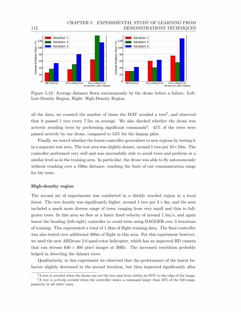
112CHAPTER 5. EXPERIMENTAL STUDY OF LEARNING FROM
DEMONSTRATIONS TECHNIQUES
Figure 5.12: Average distance flown autonomously by the drone before a failure. Left:Low-Density Region, Right: High-Density Region.
all the data, we counted the number of times the MAV avoided a tree3, and observed
that it passed 1 tree every 7.5m on average. We also checked whether the drone was
actively avoiding trees by performing significant commands4. 41% of the trees were
passed actively by our drone, compared to 54% for the human pilot.
Finally, we tested whether the learnt controller generalizes to new regions by testing it
in a separate test area. The test area was slightly denser, around 1 tree per 10×10m. The
controller performed very well and was successfully able to avoid trees and perform at a
similar level as in the training area. In particular, the drone was able to fly autonomously
without crashing over a 100m distance, reaching the limit of our communication range
for the tests.
High-density region
The second set of experiments was conducted in a thickly wooded region in a local
forest. The tree density was significantly higher, around 1 tree per 3× 3m, and the area
included a much more diverse range of trees, ranging from very small and thin to full-
grown trees. In this area we flew at a faster fixed velocity of around 1.5m/s, and again
learnt the heading (left-right) controller to avoid trees using DAGGER over 3 iterations
of training. This represented a total of 1.2km of flight training data. The final controller
was also tested over additional 400m of flight in this area. For this experiment however,
we used the new ARDrone 2.0 quad-rotor helicopter, which has an improved HD camera
that can stream 640 × 360 pixel images at 30Hz. The increased resolution probably
helped in detecting the thinner trees.
Qualitatively, in this experiment we observed that the performance of the learnt be-
havior slightly decreased in the second iteration, but then improved significantly after
3A tree is avoided when the drone can see the tree pass from within its FOV to the edge of the image.4A tree is actively avoided when the controller issues a command larger than 25% of the full range,
passively in all other cases.
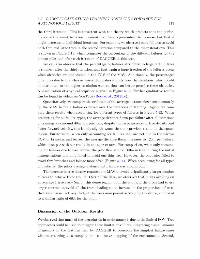
5.3. ROBOTIC CASE STUDY: LEARNING OBSTACLE AVOIDANCE FORAUTONOMOUS FLIGHT 113
the third iteration. This is consistent with the theory which predicts that the perfor-
mance of the learnt behavior averaged over time is guaranteed to increase, but that it
might decrease on individual iterations. For example, we observed more failures to avoid
both thin and large trees in the second iteration compared to the other iterations. This
is shown in Figure 5.11, which compares the percentage of the different failures for the
human pilot and after each iteration of DAGGER in this area.
We can also observe that the percentage of failures attributed to large or thin trees
is smallest after the third iteration, and that again a large fraction of the failures occur
when obstacles are not visible in the FOV of the MAV. Additionally, the percentages
of failures due to branches or leaves diminishes slightly over the iterations, which could
be attributed to the higher resolution camera that can better perceive these obstacles.
A visualization of a typical sequence is given in Figure 5.13. Further qualitative results
can be found in videos on YouTube (Ross et al., 2013b,c).
Quantitatively, we compare the evolution of the average distance flown autonomously
by the MAV before a failure occurred over the iterations of training. Again, we com-
pare these results when accounting for different types of failures in Figure 5.12. When
accounting for all failure types, the average distance flown per failure after all iterations
of training was around 40m. Surprisingly, despite the large increase in tree density and
faster forward velocity, this is only slightly worse than our previous results in the sparse
region. Furthermore, when only accounting for failures that are not due to the narrow
FOV or branches and leaves, the average distance flown increases to 120m per failure,
which is on par with our results in the sparser area. For comparison, when only account-
ing for failures due to tree trunks, the pilot flew around 500m in total during the initial
demonstrations and only failed to avoid one thin tree. However, the pilot also failed to
avoid thin branches and foliage more often (Figure 5.11). When accounting for all types
of obstacles, the pilots average distance until failure was around 80m.
The increase in tree density required our MAV to avoid a significantly larger number
of trees to achieve these results. Over all the data, we observed that it was avoiding on
an average 1 tree every 5m. In this dense region, both the pilot and the drone had to use
larger controls to avoid all the trees, leading to an increase in the proportions of trees
that were passed actively. 62% of the trees were passed actively by the drone, compared
to a similar ratio of 66% for the pilot.
Discussion of the Outdoor Results
We observed that much of the degradation in performance is due to the limited FOV. Two
approaches could be used to mitigate these limitations: First, integrating a small amount
of memory in the features used by DAGGER to overcome the simplest failure cases
without resorting to a complete and expensive mapping of the environment. Second,
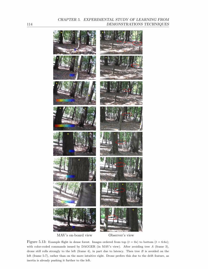
114CHAPTER 5. EXPERIMENTAL STUDY OF LEARNING FROM
DEMONSTRATIONS TECHNIQUES
MAV’s on-board view Observer’s view
Figure 5.13: Example flight in dense forest. Images ordered from top (t = 0s) to bottom (t = 6.6s);
with color-coded commands issued by DAGGER (in MAV’s view). After avoiding tree A (frame 3),
drone still rolls strongly to the left (frame 4), in part due to latency. Then tree B is avoided on the
left (frame 5-7), rather than on the more intuitive right. Drone prefers this due to the drift feature, as
inertia is already pushing it further to the left.
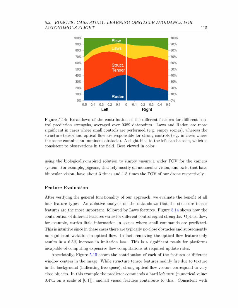
5.3. ROBOTIC CASE STUDY: LEARNING OBSTACLE AVOIDANCE FORAUTONOMOUS FLIGHT 115
Figure 5.14: Breakdown of the contribution of the different features for different con-trol prediction strengths, averaged over 9389 datapoints. Laws and Radon are moresignificant in cases where small controls are performed (e.g. empty scenes), whereas thestructure tensor and optical flow are responsible for strong controls (e.g. in cases wherethe scene contains an imminent obstacle). A slight bias to the left can be seen, which isconsistent to observations in the field. Best viewed in color.
using the biologically-inspired solution to simply ensure a wider FOV for the camera
system. For example, pigeons, that rely mostly on monocular vision, and owls, that have
binocular vision, have about 3 times and 1.5 times the FOV of our drone respectively.
Feature Evaluation
After verifying the general functionality of our approach, we evaluate the benefit of all
four feature types. An ablative analysis on the data shows that the structure tensor
features are the most important, followed by Laws features. Figure 5.14 shows how the
contribution of different features varies for different control signal strengths. Optical flow,
for example, carries little information in scenes where small commands are predicted.
This is intuitive since in these cases there are typically no close obstacles and subsequently
no significant variation in optical flow. In fact, removing the optical flow feature only
results in a 6.5% increase in imitation loss. This is a significant result for platforms
incapable of computing expensive flow computations at required update rates.
Anecdotally, Figure 5.15 shows the contribution of each of the features at different
window centers in the image. While structure tensor features mainly fire due to texture
in the background (indicating free space), strong optical flow vectors correspond to very
close objects. In this example the predictor commands a hard left turn (numerical value:
0.47L on a scale of [0,1]), and all visual features contribute to this. Consistent with
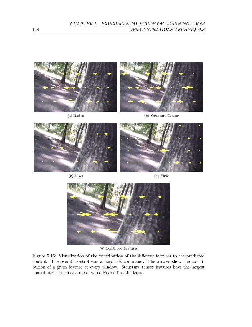
116CHAPTER 5. EXPERIMENTAL STUDY OF LEARNING FROM
DEMONSTRATIONS TECHNIQUES
(a) Radon (b) Structure Tensor
(c) Laws (d) Flow
(e) Combined Features
Figure 5.15: Visualization of the contribution of the different features to the predictedcontrol. The overall control was a hard left command. The arrows show the contri-bution of a given feature at every window. Structure tensor features have the largestcontribution in this example, while Radon has the least.

5.3. ROBOTIC CASE STUDY: LEARNING OBSTACLE AVOIDANCE FORAUTONOMOUS FLIGHT 117
the above analysis, the contribution of the structure tensor was greatest (0.38L), Laws
masks and optical flow contribute the same (0.05L) while Radon features provide the
least contribution (0.01L). In this particular example, the non-visual features actually
predict a small right command (0.02R).

Chapter 6
Learning Inference for Structured
Prediction
After studying how iterative and interactive learning methods can learn good predictors
for imitation learning tasks, we here show how the same techniques can be generalized
and applied to general structured prediction tasks.
Structured prediction problems arise very frequently in many fields and have im-
portant applications in Natural Language Processing (e.g. Name-Entity Recognition,
Part-of-Speech tagging, Machine Translation) (Daume III et al., 2009, Zhao and Xing,
2007), Computer Vision (e.g. Scene Understanding, Depth Estimation, Image Denoising)
(Munoz et al., 2009, Scharstein and Pal, 2007, Tappen et al., 2007) and Computational
Biology (e.g. Protein Folding, Genomic Analysis, Phylogenetic Tree Estimation) (Liu,
2006, Xing, 2004, Felsenstein, 1981), among others. Inspired by the approaches of Tu and
Bai. (2009), Daume III et al. (2009), Munoz et al. (2010), we will tackle these problems
by effectively reducing structured prediction tasks to sequential prediction tasks, where
the same iterative and interactive learning strategies developed for imitation learning
can be directly applied to tackle this problem. In particular, our approach will train
directly an “inference” (or parsing/decoding) procedure, composed of a single or many
predictors, that produces the high-dimensional output prediction from the observed in-
put features by making a sequence of interdependent predictions. As will be made more
clear below, the main idea behind our approach will be to train a procedure that “mim-
ics” ideal inference. Again, by leveraging interaction with the learner, we will be able to
provide strong guarantees on performance, as in the imitation learning setting.
We begin by briefly reviewing background material and state-of-the-art methods for
structured prediction. We then present our sequence prediction approach, and how the
previous methods we introduced for imitation learning, such as Forward Training, and
DAGGER, can be applied directly in this setting. We then present a number of ap-
plications in Computer Vision and Perception, to demonstrate the effectiveness of our
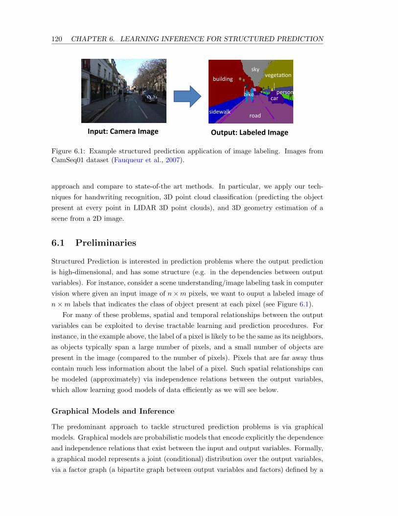
120 CHAPTER 6. LEARNING INFERENCE FOR STRUCTURED PREDICTION
Input: Camera Image Output: Labeled Image
road
building vegeta/on
car
sidewalk
bike person
sky
Figure 6.1: Example structured prediction application of image labeling. Images fromCamSeq01 dataset (Fauqueur et al., 2007).
approach and compare to state-of-the art methods. In particular, we apply our tech-
niques for handwriting recognition, 3D point cloud classification (predicting the object
present at every point in LIDAR 3D point clouds), and 3D geometry estimation of a
scene from a 2D image.
6.1 Preliminaries
Structured Prediction is interested in prediction problems where the output prediction
is high-dimensional, and has some structure (e.g. in the dependencies between output
variables). For instance, consider a scene understanding/image labeling task in computer
vision where given an input image of n×m pixels, we want to ouput a labeled image of
n×m labels that indicates the class of object present at each pixel (see Figure 6.1).
For many of these problems, spatial and temporal relationships between the output
variables can be exploited to devise tractable learning and prediction procedures. For
instance, in the example above, the label of a pixel is likely to be the same as its neighbors,
as objects typically span a large number of pixels, and a small number of objects are
present in the image (compared to the number of pixels). Pixels that are far away thus
contain much less information about the label of a pixel. Such spatial relationships can
be modeled (approximately) via independence relations between the output variables,
which allow learning good models of data efficiently as we will see below.
Graphical Models and Inference
The predominant approach to tackle structured prediction problems is via graphical
models. Graphical models are probabilistic models that encode explicitly the dependence
and independence relations that exist between the input and output variables. Formally,
a graphical model represents a joint (conditional) distribution over the output variables,
via a factor graph (a bipartite graph between output variables and factors) defined by a
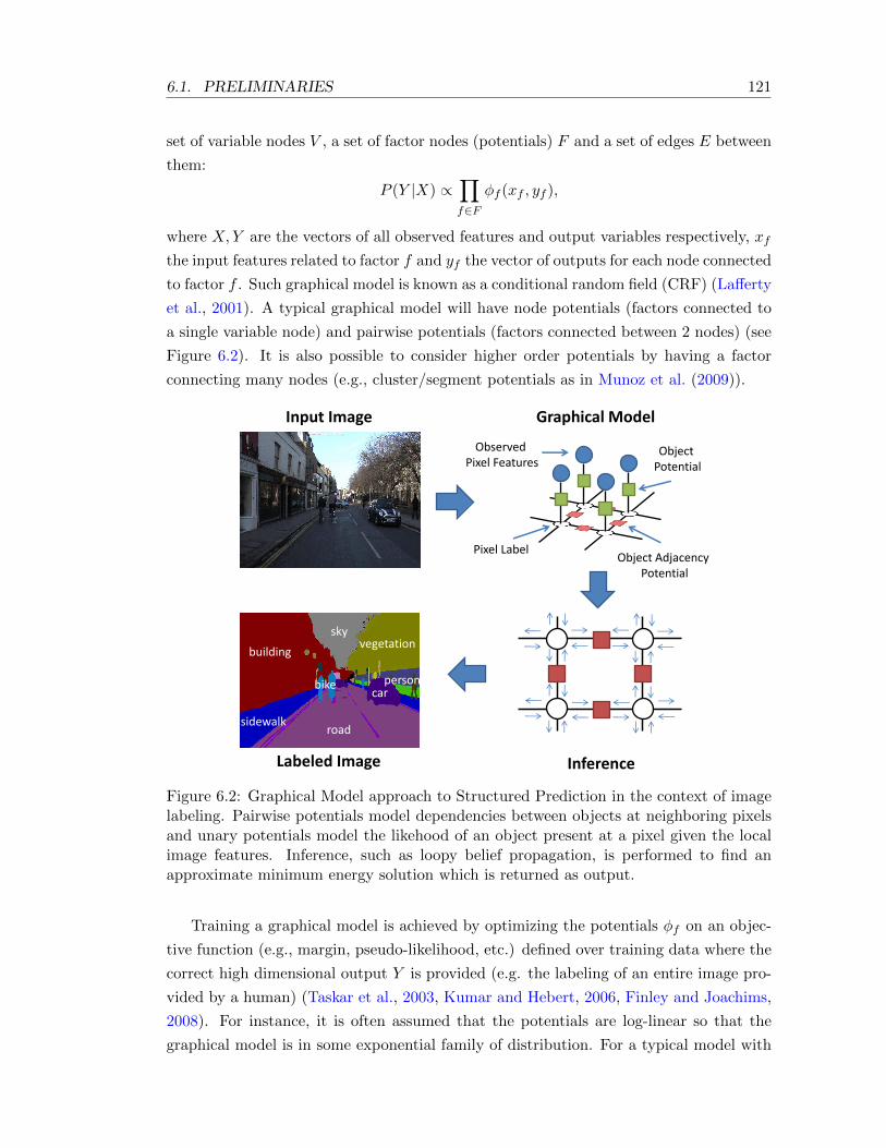
6.1. PRELIMINARIES 121
set of variable nodes V , a set of factor nodes (potentials) F and a set of edges E between
them:
P (Y |X) ∝∏f∈F
φf (xf , yf ),
where X,Y are the vectors of all observed features and output variables respectively, xf
the input features related to factor f and yf the vector of outputs for each node connected
to factor f . Such graphical model is known as a conditional random field (CRF) (Lafferty
et al., 2001). A typical graphical model will have node potentials (factors connected to
a single variable node) and pairwise potentials (factors connected between 2 nodes) (see
Figure 6.2). It is also possible to consider higher order potentials by having a factor
connecting many nodes (e.g., cluster/segment potentials as in Munoz et al. (2009)).
Observed
Pixel FeaturesObject
Potential
Pixel LabelObject Adjacency
Potential
Input Image Graphical Model
Labeled Image
road
buildingvegetation
car
sidewalk
bike person
sky
Inference
Figure 6.2: Graphical Model approach to Structured Prediction in the context of imagelabeling. Pairwise potentials model dependencies between objects at neighboring pixelsand unary potentials model the likehood of an object present at a pixel given the localimage features. Inference, such as loopy belief propagation, is performed to find anapproximate minimum energy solution which is returned as output.
Training a graphical model is achieved by optimizing the potentials φf on an objec-
tive function (e.g., margin, pseudo-likelihood, etc.) defined over training data where the
correct high dimensional output Y is provided (e.g. the labeling of an entire image pro-
vided by a human) (Taskar et al., 2003, Kumar and Hebert, 2006, Finley and Joachims,
2008). For instance, it is often assumed that the potentials are log-linear so that the
graphical model is in some exponential family of distribution. For a typical model with
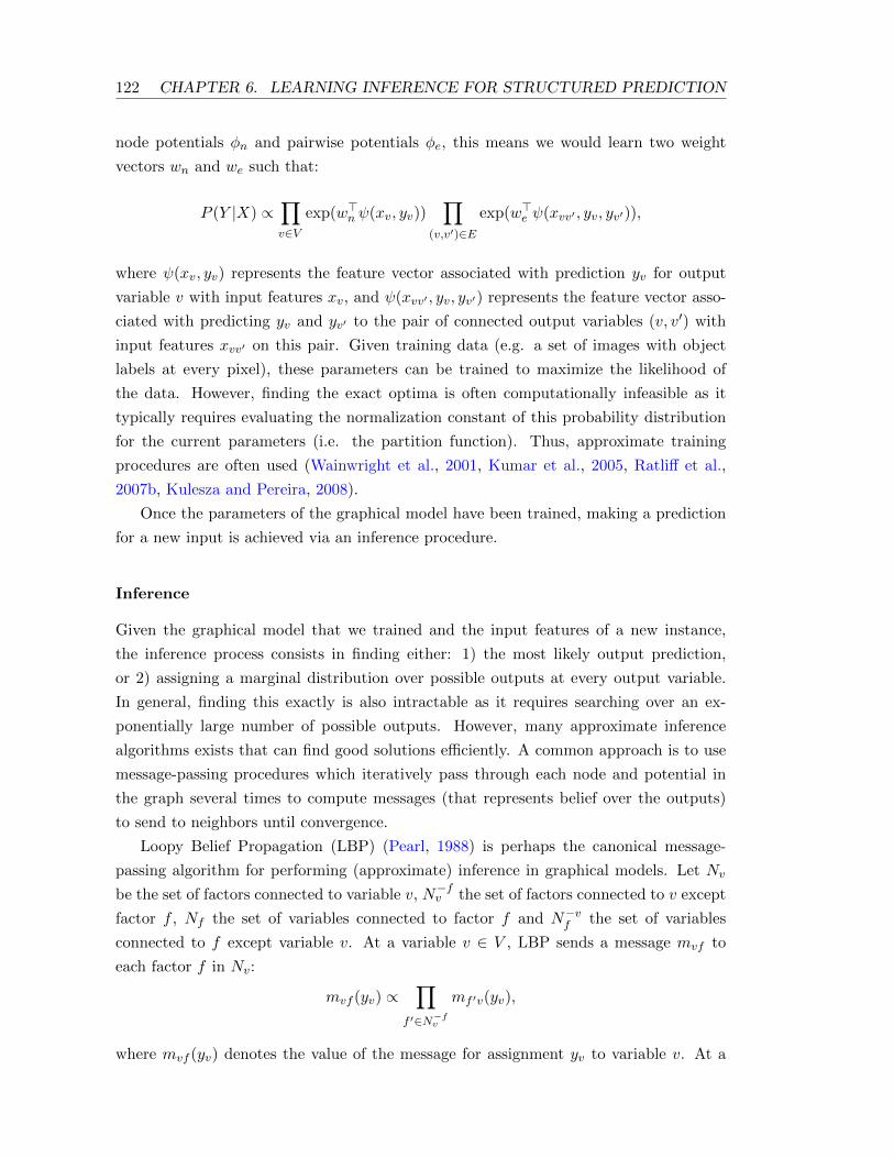
122 CHAPTER 6. LEARNING INFERENCE FOR STRUCTURED PREDICTION
node potentials φn and pairwise potentials φe, this means we would learn two weight
vectors wn and we such that:
P (Y |X) ∝∏v∈V
exp(w>n ψ(xv, yv))∏
(v,v′)∈E
exp(w>e ψ(xvv′ , yv, yv′)),
where ψ(xv, yv) represents the feature vector associated with prediction yv for output
variable v with input features xv, and ψ(xvv′ , yv, yv′) represents the feature vector asso-
ciated with predicting yv and yv′ to the pair of connected output variables (v, v′) with
input features xvv′ on this pair. Given training data (e.g. a set of images with object
labels at every pixel), these parameters can be trained to maximize the likelihood of
the data. However, finding the exact optima is often computationally infeasible as it
typically requires evaluating the normalization constant of this probability distribution
for the current parameters (i.e. the partition function). Thus, approximate training
procedures are often used (Wainwright et al., 2001, Kumar et al., 2005, Ratliff et al.,
2007b, Kulesza and Pereira, 2008).
Once the parameters of the graphical model have been trained, making a prediction
for a new input is achieved via an inference procedure.
Inference
Given the graphical model that we trained and the input features of a new instance,
the inference process consists in finding either: 1) the most likely output prediction,
or 2) assigning a marginal distribution over possible outputs at every output variable.
In general, finding this exactly is also intractable as it requires searching over an ex-
ponentially large number of possible outputs. However, many approximate inference
algorithms exists that can find good solutions efficiently. A common approach is to use
message-passing procedures which iteratively pass through each node and potential in
the graph several times to compute messages (that represents belief over the outputs)
to send to neighbors until convergence.
Loopy Belief Propagation (LBP) (Pearl, 1988) is perhaps the canonical message-
passing algorithm for performing (approximate) inference in graphical models. Let Nv
be the set of factors connected to variable v, N−fv the set of factors connected to v except
factor f , Nf the set of variables connected to factor f and N−vf the set of variables
connected to f except variable v. At a variable v ∈ V , LBP sends a message mvf to
each factor f in Nv:
mvf (yv) ∝∏
f ′∈N−fv
mf ′v(yv),
where mvf (yv) denotes the value of the message for assignment yv to variable v. At a

6.1. PRELIMINARIES 123
factor f ∈ F , LBP sends a message mfv to each variable v in Nf :
mfv(yv) ∝∑
y′f |y′v=yv
φf (y′f , xf )∏
v′∈N−vf
mv′f (y′v′),
where y′f is an assignment to all variables v′ connected to f , y′v′ is the particular assign-
ment to v′ (in y′f ), and φf is the potential function associated to factor f which depends
on y′f and potentially other observed features xf (e.g., in the CRF). Finally the marginal
of variable v is obtained as:
P (v = yv) ∝∏f∈Nv
mfv(yv).
The messages in LBP can be sent synchronously (i.e., all messages over the graph are
computed before they are sent to their neighbors) or asynchronously (i.e., by sending the
message to the neighbor immediately). When proceeding asynchronously, LBP usually
starts at a random variable node, with messages initialized uniformly, and then pro-
ceeds iteratively through the factor graph by visiting variables and factors in a breath-
first-search manner (forward and then in backward/reverse order) several times or until
convergence. The final marginals at each variable are computed using the last equa-
tion. Asynchronous message passing often allows faster convergence and methods such
as Residual Belief Propagation (Elidan et al., 2006) have been developed to achieve still
faster convergence by prioritizing the messages to compute.
Structured Margin Approaches
An alternate approach when training graphical models is to maximize a margin objective
similar to the objective when training a SVM. This is justified from the observation that
in a log-linear model, finding the most likely output prediction Y given the input features
X boils down to finding:
arg maxY
∑v∈V
w>n ψ(xv, yv) +∑
(v,v′)∈E
w>e ψ(xvv′ , yv, yv′)
It can be noticed that this is very similar to the way a linear SVM predicts in multiclass
classification problems. Hence a natural idea is to train the weights wn and we to
maximize the margin between the ground truth outputs and other outputs. In this case,
the margin is structured so that the ground truth should have larger margin with respect
to outputs that differ significantly from it. For instance if we are predicting a label at
every pixel in an image, we might specify that the margin between the ground truth and
some arbitrary output Y should be at least the number of pixels in Y that are labeled
incorrectly. A number of approaches proceeds in this way, such as M3N (Taskar et al.,
2003) and the structured SVM (Tsochantaridis et al., 2005, Finley and Joachims, 2008).
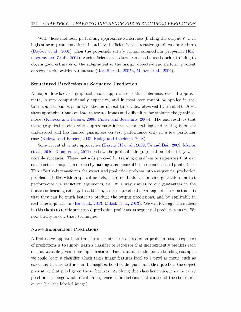
124 CHAPTER 6. LEARNING INFERENCE FOR STRUCTURED PREDICTION
With these methods, performing approximate inference (finding the output Y with
highest score) can sometimes be achieved efficiently via iterative graph-cut procedures
(Boykov et al., 2001) when the potentials satisfy certain submodular properties (Kol-
mogorov and Zabih, 2004). Such efficient procedures can also be used during training to
obtain good estimates of the subgradient of the margin objective and perform gradient
descent on the weight parameters (Ratliff et al., 2007b, Munoz et al., 2009).
Structured Prediction as Sequence Prediction
A major drawback of graphical model approaches is that inference, even if approxi-
mate, is very computationally expensive, and in most case cannot be applied in real
time applications (e.g. image labeling in real time video observed by a robot). Also,
these approximations can lead to several issues and difficulties for training the graphical
model (Kulesza and Pereira, 2008, Finley and Joachims, 2008). The end result is that
using graphical models with approximate inference for training and testing is poorly
understood and has limited guarantees on test performance only in a few particular
cases(Kulesza and Pereira, 2008, Finley and Joachims, 2008).
Some recent alternate approaches (Daume III et al., 2009, Tu and Bai., 2009, Munoz
et al., 2010, Xiong et al., 2011) eschew the probabilistic graphical model entirely with
notable successes. These methods proceed by training classifiers or regressors that can
construct the output prediction by making a sequence of interdependent local predictions.
This effectively transforms the structured prediction problem into a sequential prediction
problem. Unlike with graphical models, these methods can provide guarantees on test
performance via reduction arguments, i.e. in a way similar to our guarantees in the
imitation learning setting. In addition, a major practical advantage of these methods is
that they can be much faster to produce the output predictions, and be applicable in
real-time applications (Hu et al., 2013, Miksik et al., 2013). We will leverage these ideas
in this thesis to tackle structured prediction problems as sequential prediction tasks. We
now briefly review these techniques.
Naive Independent Predictions
A first naive approach to transform the structured prediction problem into a sequence
of predictions is to simply learn a classifier or regressor that independently predicts each
output variable given some input features. For instance, in the image labeling example,
we could learn a classifier which takes image features local to a pixel as input, such as
color and texture features in the neighborhood of the pixel, and then predicts the object
present at that pixel given those features. Applying this classifier in sequence to every
pixel in the image would create a sequence of predictions that construct the structured
ouput (i.e. the labeled image).
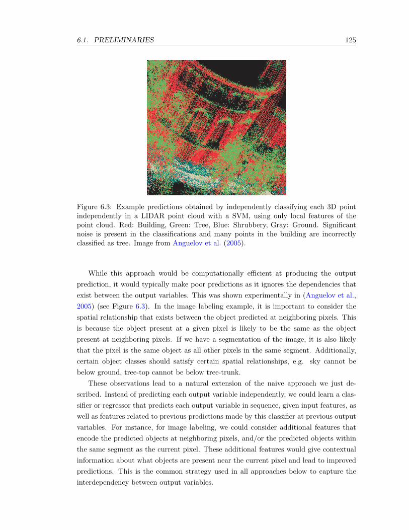
6.1. PRELIMINARIES 125
Figure 6.3: Example predictions obtained by independently classifying each 3D pointindependently in a LIDAR point cloud with a SVM, using only local features of thepoint cloud. Red: Building, Green: Tree, Blue: Shrubbery, Gray: Ground. Significantnoise is present in the classifications and many points in the building are incorrectlyclassified as tree. Image from Anguelov et al. (2005).
While this approach would be computationally efficient at producing the output
prediction, it would typically make poor predictions as it ignores the dependencies that
exist between the output variables. This was shown experimentally in (Anguelov et al.,
2005) (see Figure 6.3). In the image labeling example, it is important to consider the
spatial relationship that exists between the object predicted at neighboring pixels. This
is because the object present at a given pixel is likely to be the same as the object
present at neighboring pixels. If we have a segmentation of the image, it is also likely
that the pixel is the same object as all other pixels in the same segment. Additionally,
certain object classes should satisfy certain spatial relationships, e.g. sky cannot be
below ground, tree-top cannot be below tree-trunk.
These observations lead to a natural extension of the naive approach we just de-
scribed. Instead of predicting each output variable independently, we could learn a clas-
sifier or regressor that predicts each output variable in sequence, given input features, as
well as features related to previous predictions made by this classifier at previous output
variables. For instance, for image labeling, we could consider additional features that
encode the predicted objects at neighboring pixels, and/or the predicted objects within
the same segment as the current pixel. These additional features would give contextual
information about what objects are present near the current pixel and lead to improved
predictions. This is the common strategy used in all approaches below to capture the
interdependency between output variables.
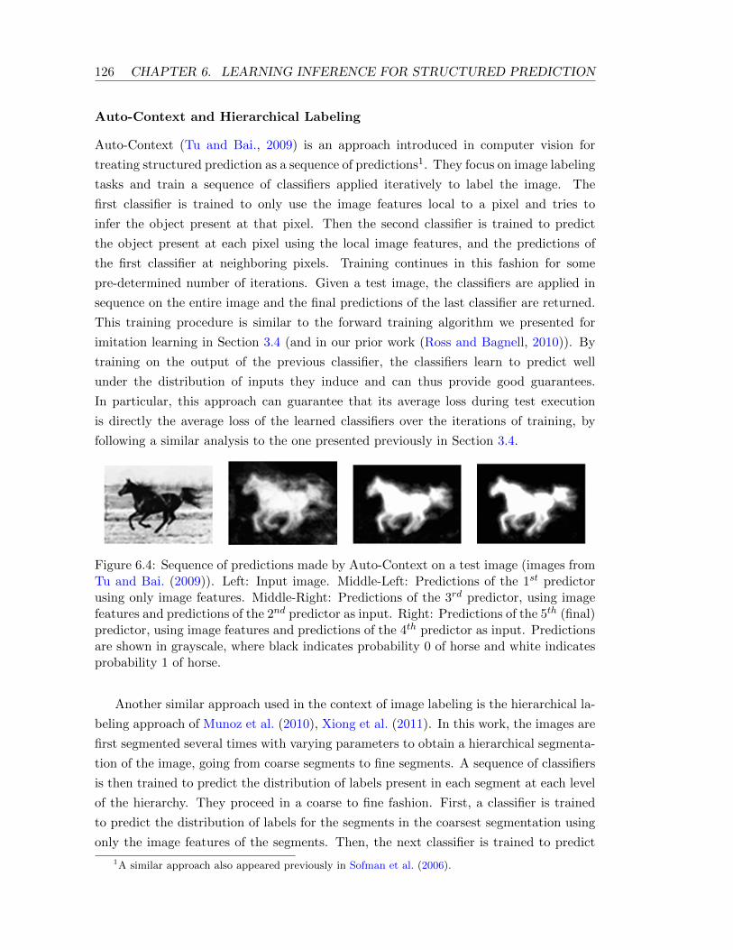
126 CHAPTER 6. LEARNING INFERENCE FOR STRUCTURED PREDICTION
Auto-Context and Hierarchical Labeling
Auto-Context (Tu and Bai., 2009) is an approach introduced in computer vision for
treating structured prediction as a sequence of predictions1. They focus on image labeling
tasks and train a sequence of classifiers applied iteratively to label the image. The
first classifier is trained to only use the image features local to a pixel and tries to
infer the object present at that pixel. Then the second classifier is trained to predict
the object present at each pixel using the local image features, and the predictions of
the first classifier at neighboring pixels. Training continues in this fashion for some
pre-determined number of iterations. Given a test image, the classifiers are applied in
sequence on the entire image and the final predictions of the last classifier are returned.
This training procedure is similar to the forward training algorithm we presented for
imitation learning in Section 3.4 (and in our prior work (Ross and Bagnell, 2010)). By
training on the output of the previous classifier, the classifiers learn to predict well
under the distribution of inputs they induce and can thus provide good guarantees.
In particular, this approach can guarantee that its average loss during test execution
is directly the average loss of the learned classifiers over the iterations of training, by
following a similar analysis to the one presented previously in Section 3.4.
Figure 6.4: Sequence of predictions made by Auto-Context on a test image (images fromTu and Bai. (2009)). Left: Input image. Middle-Left: Predictions of the 1st predictorusing only image features. Middle-Right: Predictions of the 3rd predictor, using imagefeatures and predictions of the 2nd predictor as input. Right: Predictions of the 5th (final)predictor, using image features and predictions of the 4th predictor as input. Predictionsare shown in grayscale, where black indicates probability 0 of horse and white indicatesprobability 1 of horse.
Another similar approach used in the context of image labeling is the hierarchical la-
beling approach of Munoz et al. (2010), Xiong et al. (2011). In this work, the images are
first segmented several times with varying parameters to obtain a hierarchical segmenta-
tion of the image, going from coarse segments to fine segments. A sequence of classifiers
is then trained to predict the distribution of labels present in each segment at each level
of the hierarchy. They proceed in a coarse to fine fashion. First, a classifier is trained
to predict the distribution of labels for the segments in the coarsest segmentation using
only the image features of the segments. Then, the next classifier is trained to predict
1A similar approach also appeared previously in Sofman et al. (2006).
6.1. PRELIMINARIES 127
the distribution of labels for the segments in the second coarsest segmentation, using the
predictions made by the previous classifier at the coarser level, and the image features of
the segment as input. The approach continues iteratively until a classifier is trained at
the finest level. Then for prediction on a test image, the hierarchical segmentation of the
image is first obtained with the same segmentation algorithm and the classifiers are ap-
plied in sequence on the entire image from coarse to fine, and the predictions at the finest
level are used as the final predictions. This approach again proceeds similarly the to the
forward training algorithm, and thus provide similar guarantees to the ones presented
in Section 3.4. This training procedure can also be iterated longer back-and-forth, by
going from coarse-to-fine, and fine-to-coarse, for several iterations, to allow propagating
contextual information further during parsing (Xiong et al., 2011). Additionally, it was
showed recently that this technique can lead to real-time scene analysis in streaming
video (Miksik et al., 2013) and streaming 3D point cloud data from LIDAR sensors (Hu
et al., 2013).
SEARN: Search-based Structured Prediction
SEARN is a technique that we mentioned previously in the imitation learning setting and
compared to experimentally by adapting it for imitation learning. However, it was orig-
inally developed for structured prediction tasks. We briefly mention how this approach
is applied in the context of Structured Prediction. Just like DAGGER and Forward
Training, SEARN is a technique that can be used to learn predictors for sequential tasks
that are trained to be good under their own sequence of predictions.
In Daume III et al. (2009), structured prediction is treated as a problem of training
a search procedure that can construct the high-dimensional output from a sequence
of predictions. In the simplest case, a greedy-search procedure is trained, where the
structured output is constructed by predicting the value of one variable at a time, given
the previous predictions made so far. For instance in a handwriting recognition task,
the approach would predict each character in the handwritten word in sequence, using
previously predicted characters to help disambiguate among several candidates for the
next character. However, the approach is general enough to be applied with other search
procedures, such as beam-search that would maintain a set of sequences of previous
predictions.
The search procedure is trained by training a stochastic classifier over several iter-
ations to make the predictions. As described for imitation learning in section 3.5, at
each iteration n, it proceeds by collecting data of cost-to-go examples of the current
predictor hn−1 in states visited by this predictor, training a policy hn to minimize a
cost-sensitive classification loss on this data, and updating hn = (1 − α)hn−1 + αhn
(where this is interpreted as a stochastic mixing, see Section 3.5). Initially, the approach

128 CHAPTER 6. LEARNING INFERENCE FOR STRUCTURED PREDICTION
starts with an “expert” classifier h0 which can make good predictions on the training
data (e.g. by directly looking up the target output in the training data itself). After
N iterations, it returns the renormalized classifier which do not use the “expert” classi-
fier for test execution: hN = 11−(1−α)N
[hN − (1 − α)Nh0]. In the context of structured
prediction, when collecting cost-to-go estimates, SEARN proceeds by trying all possible
predictions y at the current point in the sequence, and then rolling out the current policy
to estimate cost-to-go of all possible prediction in the current context x. This generates
cost-sensitive classification examples (i.e. full information setting as described in section
4.1). As mentioned in section 3.5, choosing α to be O( 1T 3 ) and N to be O(T 3), leads to
good performance guarantees.
In practice, because collecting the costs for each prediction y for the current input
x is time-consuming when executing the current predictor hn−1 until the end of the
sequence, an approximation often done is to execute the expert h0 until the end of the
sequence instead as this is often much faster (e.g. if it only involves looking up labels in
the training data to determine future predictions), and produces less noisy examples (as
h0 is deterministic, whereas hn−1 is stochastic). While Daume III et al. (2009) presents
this approximation as purely practical, with no performance guarantees, it is interesting
to note that this corresponds exactly to the cost-to-go of the expert’s policy we are
collecting in our previous imitation learning approaches, for which we could provide
performance guarantees.
6.2 Inference Machines
We now present the particular sequential prediction procedure that we will seek to train
for tackling structured prediction task.
As reviewed in the previous section, current state-of-the-art methods for Structured
Prediction are divided between 1) methods that learn a graphical model and use an
inference procedure for predictions, and 2) methods that eschew the probability graphical
model entirely in favor of training a sequential prediction approach. However, we would
ideally like to have the best of both worlds: the proven success of error-correcting iterative
decoding methods used for inference in graphical models, along with a tight relationship
between learning and inference, as achieved in sequential prediction approach, that allows
providing guarantees on performance.
To enable this combination, we propose an alternate view of the approximate infer-
ence process as a long sequence of computational modules to optimize Bengio (2009)
such that the sequence results in correct predictions. We focus on message-passing infer-
ence procedures, such as Belief Propagation, that compute marginal distributions over
output variables by iteratively visiting all nodes in the graph and passing messages to
6.2. INFERENCE MACHINES 129
neighbors which consist of “cavity marginals”, i.e., a series of marginals with the effect
of each neighbor removed. Such message-passing inference can be viewed as a sequential
prediction procedure that iteratively applies a function to each variable, that takes as
input local observations/features and local computations on the graph (messages) and
provides as output the intermediate messages/marginals. In this view, we can attempt
to train such a sequential prediction procedures directly, by training a predictor that
predicts a current variable’s marginal2 given local features and a subset of neighbors’
cavity marginals. In other words, we will seek to learn predictors that produce the over-
all structured output through a sequence of predictions, where the sequential prediction
process follows the same proven error-correcting algorithmic structure of message-passing
inference procedures. We will seek to train this predictor to “mimic” an ideal inference
procedure, i.e. where at each intermediate inference steps, we train the predictor to
predict the ideal output in our training data (i.e., a marginal with probability 1 to the
correct class). By training such a predictor, there is no need to have a probabilistic
graphical model of the data, and there need not be any probabilistic model that cor-
responds to the computations performed by the predictor. The inference procedure is
instead thought of as a black box function that is trained to yield correct predictions.
This is analogous to many discriminative learning methods; it may be easier to simply
discriminate between classes than build a generative probabilistic model of them. We
will refer to a predictor that is sequentially applied in this way to construct the output
prediction as an inference machine, due to the similarities with inference procedures
for graphical models. This inference machine approach follows ideas from Munoz et al.
(2010), Xiong et al. (2011).
We now show in more details how graphical model approaches can be viewed as
training a sequential prediction procedure, that can be shown to be a special case of our
general inference machine approach.
Understanding Message-Passing Inference as Sequential Probabilistic
Classification
As mentioned in Section 6.1, LBP builds the output prediction by iteratively sending
messages mvf from variables v ∈ V to factors f ∈ F , and messages from factors to vari-
ables mvf , until convergence. By comparing the computations performed for computing
the marginals P (v = yv) and the message mvf , we observe that mvf can be interpreted
as the marginal of variable v when the factor f (and its influence) is removed from the
graph. This is often referred as the cavity method in statistical mechanics (Csato et al.,
2001) and mvf are known as cavity marginals. By expanding the definition of mvf , we
2For lack of a better term, we will use marginal throughout to mean a distribution over one variable’slabels.

130 CHAPTER 6. LEARNING INFERENCE FOR STRUCTURED PREDICTION
A
B
C
1
23
A1
A2
B3 C2
C3
B1
A1
A2
AB3
B
C
Figure 6.5: Depiction of how LBP unrolls into a sequence of predictions for 3 passes onthe graph on the left with 3 variables (A,B,C) and 3 factors (1,2,3); for the case whereLBP starts at A, followed by B and C (and alternating between forward/backward order).Sequence of predictions on the right, where e.g., A1 denotes the prediction (message) ofA sent to factor 1, while the output (final marginals) are in gray and denoted by thecorresponding variable letter. Input arrows indicate the previous outputs that are usedin the computation of each message.
can see that it depends only on the messages mv′f ′ sent by all variables v′ connected to
v by a factor f ′ 6= f :
mvf (yv) ∝∏
f ′∈N−fv
∑y′f ′ |y′v=yv
φf ′(y′f ′ , xf ′)
∏v′∈N−v
f ′
mv′f ′(y′v′). (6.1)
Hence the messages mvf leaving a variable v toward a factor f in LBP can be thought as
a probabilistic classification of the current variable v (marginal distribution over classes)
using the cavity marginals mv′f ′ sent by variables v′ connected to v through a factor f ′ 6=f . In this view, LBP is iteratively classifying the variables in the graph by performing a
sequence of probabilistic classifications (marginals) for each message leaving a variable.
The final marginals P (v = yv) are then obtained by “classifying” v using all messages
from all variables v′ connected to v through some factor.
An example of how LBP unrolls to a sequence of interdependent local classifications
is shown in Figure 6.5 for a simple graph. In this view, the job of the predictor is not
only to emulate the computation going on during LBP at variable nodes, but also em-
ulate the computations going on at all the factors connected to the variable which it is
not sending the message to, as shown in Figure 6.6. During inference, LBP effectively
employs a probabilistic predictor that has the form in Equation 6.1, where the inputs
are the messages m′v′f ′ and local observed features xf ′ . Training graphical models can
thus be understood as training a message-passing algorithm (i.e. an inference machine)
with a particular class of predictors defined by Equation 6.1, which have as parameters
the potential functions φf , and use as input features the local features and the mes-
sages (probabilistic classification) sent from neighbors. Under this general view, there is
no reason to restrict attention to only predictors of the form of Equation 6.1. We can
consider general inference machines that use different classes of predictors (e.g., Logistic
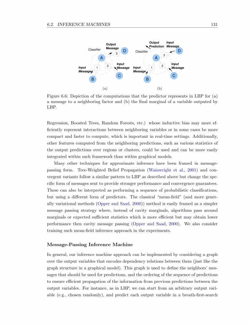
6.2. INFERENCE MACHINES 131
Input Message
A
B
D
C
1 2
3Classifier
Input Message
Output Message
(a)
Input Message
A
B
D
C
1 2
3Classifier
Input Message
Input Message
Output Prediction
(b)
Figure 6.6: Depiction of the computations that the predictor represents in LBP for (a)a message to a neighboring factor and (b) the final marginal of a variable outputed byLBP.
Regression, Boosted Trees, Random Forests, etc.) whose inductive bias may more ef-
ficiently represent interactions between neighboring variables or in some cases be more
compact and faster to compute, which is important in real-time settings. Additionally,
other features computed from the neighboring predictions, such as various statistics of
the output predictions over regions or clusters, could be used and can be more easily
integrated within such framework than within graphical models.
Many other techniques for approximate inference have been framed in message-
passing form. Tree-Weighted Belief Propagation (Wainwright et al., 2001) and con-
vergent variants follow a similar pattern to LBP as described above but change the spe-
cific form of messages sent to provide stronger performance and convergence guarantees.
These can also be interpreted as performing a sequence of probabilistic classifications,
but using a different form of predictors. The classical “mean-field” (and more gener-
ally variational methods (Opper and Saad, 2000)) method is easily framed as a simpler
message passing strategy where, instead of cavity marginals, algorithms pass around
marginals or expected sufficient statistics which is more efficient but may obtain lower
performance then cavity message passing (Opper and Saad, 2000). We also consider
training such mean-field inference approach in the experiments.
Message-Passing Inference Machine
In general, our inference machine approach can be implemented by considering a graph
over the output variables that encodes dependency relations between them (just like the
graph structure in a graphical model). This graph is used to define the neighbors’ mes-
sages that should be used for predictions, and the ordering of the sequence of predictions
to ensure efficient propagation of the information from previous predictions between the
output variables. For instance, as in LBP, we can start from an arbitrary output vari-
able (e.g., chosen randomly), and predict each output variable in a breath-first-search
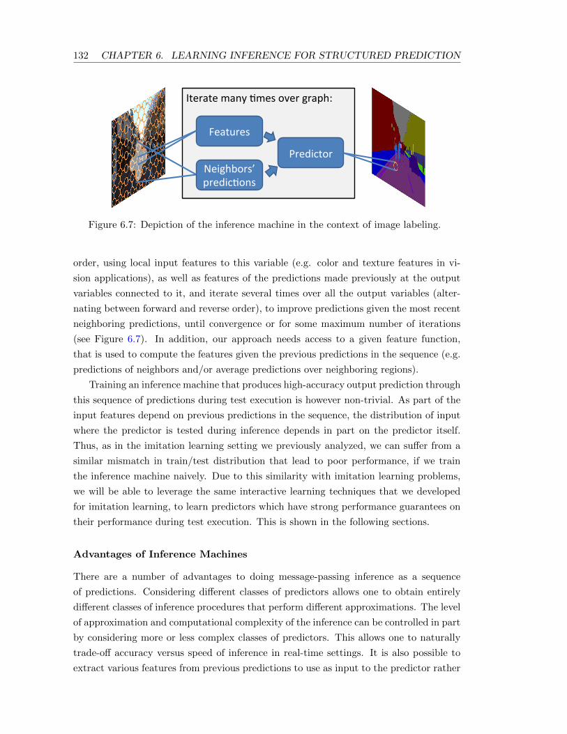
132 CHAPTER 6. LEARNING INFERENCE FOR STRUCTURED PREDICTION
Iterate many *mes over graph:
Neighbors’
predic*ons
Features
Predictor
Figure 6.7: Depiction of the inference machine in the context of image labeling.
order, using local input features to this variable (e.g. color and texture features in vi-
sion applications), as well as features of the predictions made previously at the output
variables connected to it, and iterate several times over all the output variables (alter-
nating between forward and reverse order), to improve predictions given the most recent
neighboring predictions, until convergence or for some maximum number of iterations
(see Figure 6.7). In addition, our approach needs access to a given feature function,
that is used to compute the features given the previous predictions in the sequence (e.g.
predictions of neighbors and/or average predictions over neighboring regions).
Training an inference machine that produces high-accuracy output prediction through
this sequence of predictions during test execution is however non-trivial. As part of the
input features depend on previous predictions in the sequence, the distribution of input
where the predictor is tested during inference depends in part on the predictor itself.
Thus, as in the imitation learning setting we previously analyzed, we can suffer from a
similar mismatch in train/test distribution that lead to poor performance, if we train
the inference machine naively. Due to this similarity with imitation learning problems,
we will be able to leverage the same interactive learning techniques that we developed
for imitation learning, to learn predictors which have strong performance guarantees on
their performance during test execution. This is shown in the following sections.
Advantages of Inference Machines
There are a number of advantages to doing message-passing inference as a sequence
of predictions. Considering different classes of predictors allows one to obtain entirely
different classes of inference procedures that perform different approximations. The level
of approximation and computational complexity of the inference can be controlled in part
by considering more or less complex classes of predictors. This allows one to naturally
trade-off accuracy versus speed of inference in real-time settings. It is also possible to
extract various features from previous predictions to use as input to the predictor rather

6.3. LEARNING INFERENCE MACHINES 133
than limiting only to using neighboring predictions. Better features of the previous
predictions may allow faster convergence or improved predictions. Additionally, while we
focus mainly on tasks where our objective is to simply maximize accuracy (or likelihood
of the ground truth predictions), in certain tasks other objectives can better represent the
quality of a solution, e.g. the BLEU score in machine translation (Papineni et al., 2002).
In this case, we can optimize the predictor to optimize directly these objectives, rather
than likelihood, something which is not possible with graphical model. Finally, most
approaches to learning graphical models with approximate inference have no theoretical
guarantees and are not well understood (Kulesza and Pereira, 2008, Finley and Joachims,
2008). In contrast, we are able to provide rigorous reduction-style guarantees on the
performance of the resulting inference procedure, as we demonstrate below.
6.3 Learning Inference Machines
We now present how to use the same techniques we presented for imitation learning,
namely Forward and DAGGER, for training an inference machine, and provide good
guarantees on test performance. To do so, the key idea is that we can view the inference
process as an imitation learning problem, where we seek to learn a predictor that can
mimic well an “expert” predictor, that at any point in the sequence on training instances,
predicts the “ideal” marginal – a marginal with probability 1 for the correct class. This
expert is essentially defined by the labeled training data. For instance in image labeling,
the labeled image in the training data would define the prediction of the expert to mimic
whenever we predict a marginal at a certain pixel. By learning to mimic this “expert”
predictor, we hope to learn inference machines that can generalize from the training
data, and that can then be applied to new test data (e.g. predict objects in a new image
observed by the robot that is not labeled by a human).
Learning Synchronous Inference with Forward Training
As was mentioned in Section 6.1, message-passing inference procedures such as LBP
can be applied in synchronous or asynchronous fashion. The predictor we train, within
our inference machine, can be applied to propagate predictions in a similar synchronous
or asynchronous fashion. We will begin here by considering learning a predictor for the
simpler synchronous case and show that the Forward Training strategy can be a practical
algorithm for this case.
When applied synchronously, the predictor predicts messages/marginals at each out-
put variable, over the entire graph first, before updating the neighboring messages used
as input features to make these predictions. This implies that predictions within the
same “pass” over the graph are independent, whereas the input features used at future

134 CHAPTER 6. LEARNING INFERENCE FOR STRUCTURED PREDICTION
for t = 1 to T doUse h1:t−1 to perform synchronous message-passing on training graphs up to passn.Get dataset Dt of inputs encountered at pass n, with the ideal marginals as target.
Train ht on Dt to minimize a loss (e.g., logistic).end forReturn the sequence of predictors h1:T .
Algorithm 6.3.1: Forward Training Algorithm for Learning Synchronous InferenceMachine
passes are influenced by the current pass’ predictions. Concretely, in the context of im-
age labeling, such a procedure would proceed similarly to the Auto-Context approach
mentioned previously in Section 6.1, i.e. at each pass we would make a prediction at
each pixel over the entire image, using only predictions from the previous pass as input.
To learn an inference machine that is trained on the distribution of inputs it expects
to see during test execution, and does not suffer from a train-test mismatch, we can
consider a similar training strategy to the forward training algorithm introduced for
imitation learning. That is, instead of learning a single predictor, we would learn a
sequence of predictors h1, h2, . . . , hT , where hi is the predictor used on the ith prediction
pass, and we would need to learn a total of T predictors to learn an inference machine that
performs T passes. As in most applications, the number of pass is not too large, Forward
training can be a practical approach in this context. To train these T predictors, we
would proceed iteratively, by training them in sequence going forward in time, i.e. from
the first pass to the last pass. At the first iteration, we would start by training h1 to mimic
the expert predictor h∗. As for the first pass there is no features of neighboring/previous
predictions, this would come down to learn a predictor that attempts to predict the ideal
marginals (correct class) immediately, using only the local input features (e.g. the image
features). At iteration t, for each training structured prediction example (e.g. each
training image), we would generate a dataset Dt of training data through interaction
with the learner as follows: perform t − 1 inference pass using the previously trained
predictors h1, h2, . . . , ht−1 in sequence (i.e. hi for the ith pass), and then record in
dataset Dt the observed input features at the tth pass (e.g. the vector of features that
includes both image features and features related to neighboring predictions), associated
with their ideal marginal (or correct class) from the expert predictor h∗ for each of these
input. The predictor ht for the tth pass would then be trained on this data. This is
detailed in Algorithm 6.3.1.
The Auto-Context approach presented previously in Section 6.1 can be seen as the
particular case of this approach, where we learn a synchronous inference machine, that
uses mean-field style message-passing – i.e. the case where the neighboring marginals
6.3. LEARNING INFERENCE MACHINES 135
used as input features were predicted using all neighbors at the previous pass. However
this same Forward procedure could be used to train other type of synchronous inference
machines, e.g. using LBP style message-passing instead where the messages passed
to neighbors are cavity marginals (a marginal predicted with evidence/features from
the neighbor we are sending the message to removed), which can be beneficial3. To
illustrate the difference, in the image labeling example, if using a standard 2D lattice
graph structure, where each pixel is connected to the pixels above,below,left and right,
then with LBP style message-passing, at each pass, except the last one, the inference
machine would make 4 different predictions at each pixel (each obtained by removing
one of the neighbor’s message/marginal from the input features), and at the last pass,
a single prediction at each pixel would be made, using all 4 neighbor’s messages in the
input features. In other words, at each pass, except the last one, we would produce 4
different labelings of the image, a “left”, “right”, “above” and “below” labeling, where
e.g. the “left” labeling is the labeling produced with all the predictions made without
the left neighbor’s message from the previous pass in the input features. The neighbor’s
messages in the input features at any pass would be coming from these different labelings,
e.g. the message from the neighbor below is the marginal at the pixel below in the
“above” labeling produced at the previous pass (as the current pixel is the neighbor
above this neighbor, and we want the neighbor’s prediction without the current pixel’s
message). Training this synchronous LBP inference machine means that when generating
the training data at each pass, data would be generated for all these 4 different predictions
(i.e. 4 data points with the same target class, but 4 different input feature vectors would
be generated for each pixel).
Similarly, from our point of view, Munoz et al. (2010), Xiong et al. (2011) implement
a hierarchical mean-field inference machine by sending mean-field style messages across
the hierarchy to make contextual predictions. We demonstrate in our experiments the
benefits of enabling more general (LBP-style) message passing.
Theoretical Guarantee: As we have effectively transformed the structured prediction
problem into an imitation learning problem, the same guarantees for Forward, hold in
this structured prediction setting. In particular, suppose we are interested in minimizing
the logistic loss, and we use this loss as the surrogate loss `. The result in Theorem 3.4.1
would indicate that if ε is the average logistic loss per prediction of the learned predictors
h1:T , then over the T pass of inference, the average logistic loss per prediction would be
3Basically, in mean-field style message-passing, we can suffer from “double-counting” of evidence.If the neighbor’s prediction is wrong, we may predict something, based on this wrong prediction as“evidence”, which then, at the next pass, is reused at the neighbor as further evidence that reinforcesits initial wrong prediction. This leads to a runaway effect where both can become very confident in awrong prediction, due to an initially wrong prediction. The use of cavity marginals in LBP resolves thisproblem.
136 CHAPTER 6. LEARNING INFERENCE FOR STRUCTURED PREDICTION
ε. As we are interested only in the final predictions, this would naively tell us that, in
the worst case, the per prediction logistic loss at the last pass is bounded by T ε (e.g., in
the worst case where all the loss occurs at the last pass) and would suggest that fewer
inference passes is better (making N small). However, for convex loss functions, such
as the logistic loss, simply averaging the marginals at each variable over the inference
pass, and using those average marginals as final output, guarantees4 achieving logistic
loss no worse than ε. Hence, using those average marginals as final output enables using
an arbitrary number of passes to ensure we can effectively find the best decoding. In
practice, however, we typically found that the marginals at the last pass incurred lower
loss than the average marginals, so we only used the last pass’ predictions.
Asynchronous Inference: Learning asynchronous inference machines is often of in-
terest, since as mentioned for LBP, it allows propagating information faster between
output variables, and potentially converge faster to good predictions within fewer pass,
or obtain better predictions when the number of pass is very limited. Forward can also be
applied for learning asynchronous inference machines. However this is often impractical.
This is because, when applied asynchronously, the predictor predicts messages/marginals
at each output variable, and these messages are used immediately at neighbors to com-
pute messages within the same pass. This means that predictions within the same pass
are now interdependent and influence the input features used immediately at the next
predictions within the same pass. To deal with such interdependencies, Forward would
need to train a separate predictor for each individual prediction in the sequence. This
is feasible for problems where there is a small number of output variables (e.g. in hand-
writing recognition, where within one word, we only have a few characters to predict).
However for most applications in computer vision, such as image labeling, the number of
predictions per pass is very large (in the order of number of pixels or image segments).
For example, in our 3D point cloud classification experiments below, each pass over the
point cloud consists in O(105) predictions. In such scenarios, Forward is impractical as
it would require learning a prohibitively large number of predictors (e.g. O(106) pre-
dictors to perform all the pass over the point cloud). To learn asynchronous inference
machines, DAGGER provides a much more practical algorithm, as it can learn within a
few iterations, a single predictor that can be applied to perform the entire sequence of
predictions.
Learning Asynchronous Inference with DAGGER
We now show how to apply the same Dataset Aggregation (DAGGER) approach, de-
veloped for imitation learning, for learning inference machines for structured prediction.
4 By Jensen’s inequality, if f is convex and p = 1N
∑Ni=1 pi, then f(p) ≤ 1
N
∑Ni=1 f(pi).
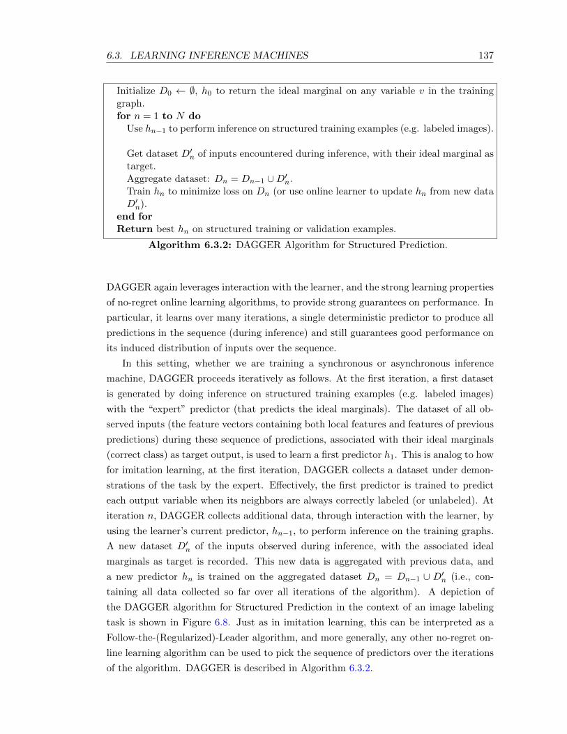
6.3. LEARNING INFERENCE MACHINES 137
Initialize D0 ← ∅, h0 to return the ideal marginal on any variable v in the traininggraph.for n = 1 to N do
Use hn−1 to perform inference on structured training examples (e.g. labeled images).
Get dataset D′n of inputs encountered during inference, with their ideal marginal astarget.Aggregate dataset: Dn = Dn−1 ∪D′n.Train hn to minimize loss on Dn (or use online learner to update hn from new dataD′n).
end forReturn best hn on structured training or validation examples.
Algorithm 6.3.2: DAGGER Algorithm for Structured Prediction.
DAGGER again leverages interaction with the learner, and the strong learning properties
of no-regret online learning algorithms, to provide strong guarantees on performance. In
particular, it learns over many iterations, a single deterministic predictor to produce all
predictions in the sequence (during inference) and still guarantees good performance on
its induced distribution of inputs over the sequence.
In this setting, whether we are training a synchronous or asynchronous inference
machine, DAGGER proceeds iteratively as follows. At the first iteration, a first dataset
is generated by doing inference on structured training examples (e.g. labeled images)
with the “expert” predictor (that predicts the ideal marginals). The dataset of all ob-
served inputs (the feature vectors containing both local features and features of previous
predictions) during these sequence of predictions, associated with their ideal marginals
(correct class) as target output, is used to learn a first predictor h1. This is analog to how
for imitation learning, at the first iteration, DAGGER collects a dataset under demon-
strations of the task by the expert. Effectively, the first predictor is trained to predict
each output variable when its neighbors are always correctly labeled (or unlabeled). At
iteration n, DAGGER collects additional data, through interaction with the learner, by
using the learner’s current predictor, hn−1, to perform inference on the training graphs.
A new dataset D′n of the inputs observed during inference, with the associated ideal
marginals as target is recorded. This new data is aggregated with previous data, and
a new predictor hn is trained on the aggregated dataset Dn = Dn−1 ∪ D′n (i.e., con-
taining all data collected so far over all iterations of the algorithm). A depiction of
the DAGGER algorithm for Structured Prediction in the context of an image labeling
task is shown in Figure 6.8. Just as in imitation learning, this can be interpreted as a
Follow-the-(Regularized)-Leader algorithm, and more generally, any other no-regret on-
line learning algorithm can be used to pick the sequence of predictors over the iterations
of the algorithm. DAGGER is described in Algorithm 6.3.2.
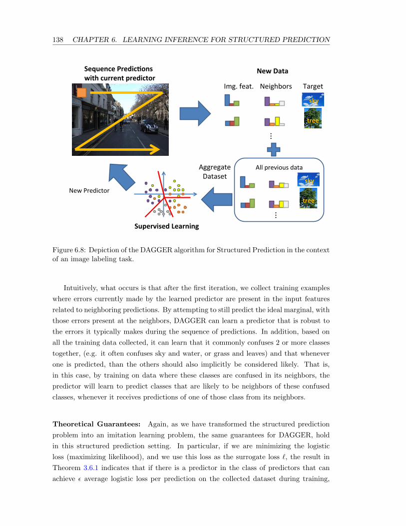
138 CHAPTER 6. LEARNING INFERENCE FOR STRUCTURED PREDICTION
road
building vegeta/on
car
sidewalk
bike person
sky
Sequence Predic,ons
with current predictor
New Predictor
Supervised Learning
New Data
All previous data Aggregate
Dataset
Img. feat. Neighbors Target
sky
tree
sky
tree
... ...
Figure 6.8: Depiction of the DAGGER algorithm for Structured Prediction in the contextof an image labeling task.
Intuitively, what occurs is that after the first iteration, we collect training examples
where errors currently made by the learned predictor are present in the input features
related to neighboring predictions. By attempting to still predict the ideal marginal, with
those errors present at the neighbors, DAGGER can learn a predictor that is robust to
the errors it typically makes during the sequence of predictions. In addition, based on
all the training data collected, it can learn that it commonly confuses 2 or more classes
together, (e.g. it often confuses sky and water, or grass and leaves) and that whenever
one is predicted, than the others should also implicitly be considered likely. That is,
in this case, by training on data where these classes are confused in its neighbors, the
predictor will learn to predict classes that are likely to be neighbors of these confused
classes, whenever it receives predictions of one of those class from its neighbors.
Theoretical Guarantees: Again, as we have transformed the structured prediction
problem into an imitation learning problem, the same guarantees for DAGGER, hold
in this structured prediction setting. In particular, if we are minimizing the logistic
loss (maximizing likelihood), and we use this loss as the surrogate loss `, the result in
Theorem 3.6.1 indicates that if there is a predictor in the class of predictors that can
achieve ε average logistic loss per prediction on the collected dataset during training,
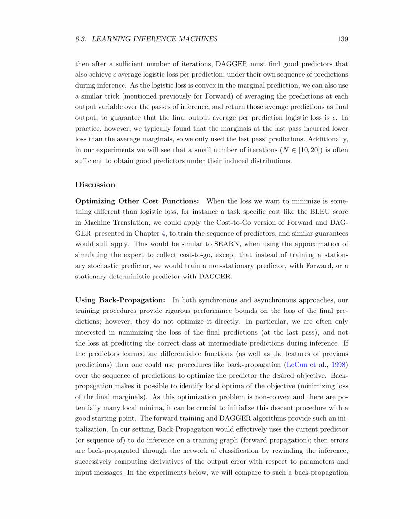
6.3. LEARNING INFERENCE MACHINES 139
then after a sufficient number of iterations, DAGGER must find good predictors that
also achieve ε average logistic loss per prediction, under their own sequence of predictions
during inference. As the logistic loss is convex in the marginal prediction, we can also use
a similar trick (mentioned previously for Forward) of averaging the predictions at each
output variable over the passes of inference, and return those average predictions as final
output, to guarantee that the final output average per prediction logistic loss is ε. In
practice, however, we typically found that the marginals at the last pass incurred lower
loss than the average marginals, so we only used the last pass’ predictions. Additionally,
in our experiments we will see that a small number of iterations (N ∈ [10, 20]) is often
sufficient to obtain good predictors under their induced distributions.
Discussion
Optimizing Other Cost Functions: When the loss we want to minimize is some-
thing different than logistic loss, for instance a task specific cost like the BLEU score
in Machine Translation, we could apply the Cost-to-Go version of Forward and DAG-
GER, presented in Chapter 4, to train the sequence of predictors, and similar guarantees
would still apply. This would be similar to SEARN, when using the approximation of
simulating the expert to collect cost-to-go, except that instead of training a station-
ary stochastic predictor, we would train a non-stationary predictor, with Forward, or a
stationary deterministic predictor with DAGGER.
Using Back-Propagation: In both synchronous and asynchronous approaches, our
training procedures provide rigorous performance bounds on the loss of the final pre-
dictions; however, they do not optimize it directly. In particular, we are often only
interested in minimizing the loss of the final predictions (at the last pass), and not
the loss at predicting the correct class at intermediate predictions during inference. If
the predictors learned are differentiable functions (as well as the features of previous
predictions) then one could use procedures like back-propagation (LeCun et al., 1998)
over the sequence of predictions to optimize the predictor the desired objective. Back-
propagation makes it possible to identify local optima of the objective (minimizing loss
of the final marginals). As this optimization problem is non-convex and there are po-
tentially many local minima, it can be crucial to initialize this descent procedure with a
good starting point. The forward training and DAGGER algorithms provide such an ini-
tialization. In our setting, Back-Propagation would effectively uses the current predictor
(or sequence of) to do inference on a training graph (forward propagation); then errors
are back-propagated through the network of classification by rewinding the inference,
successively computing derivatives of the output error with respect to parameters and
input messages. In the experiments below, we will compare to such a back-propagation

140 CHAPTER 6. LEARNING INFERENCE FOR STRUCTURED PREDICTION
approach, and show that without proper initialization, such as starting from the predic-
tor learned with DAGGER, it typically performs worse than the predictor learned with
DAGGER alone. However, applying Back-Propagation, from the learned predictor by
DAGGER can sometime increase performance further.
6.4 Case Studies in Computer Vision and Perception
We now demonstrate the efficacy of our approach. We compared our performance to
state-of-the-art algorithms on 3 separate structured prediction tasks: (1) a benchmark
handwriting recognition task, involving decoding handwritten words sequentially; (2) a
3D point cloud classification task of predicting the object present at every point in 3D
point clouds of outdoor scenes perceived from a LIDAR sensor; and (3) estimating the
3D geometry of an outdoor scenes from a 2D image.
Handwriting Recognition
We first begin by demonstrating the efficacy of our approach on a structured prediction
problem involving recognizing handwritten words given the sequence of images of each
character in the word.
We use the dataset of Taskar et al. (2003) which has been used extensively in the
literature to compare several structured prediction approaches. This dataset contains
roughly 6600 words (for a total of over 52000 characters) partitioned in 10 folds. We
consider the large dataset experiment which consists of training on 9 folds and testing
on 1 fold and repeating this over all folds. Performance is measured in terms of the
character accuracy on the test folds.
We consider predicting the word by predicting each character in sequence in a left
to right order, using the previously predicted character to help predict the next. A
single pass over the word is performed, and we learn a multi class linear SVM to pre-
dict each character based on the input features. This can be interpreted as learning a
greedy search procedure within the framework of SEARN, where we learn a predictor
that predicts greedily the current character based on previously predicted characters in
the word. Within the context of inference machines, this can also be thought as learning
an asynchronous inference machine that performs a single pass of inference, and where
the marginals/messages predicted by the SVM always assigns probability 1 for the class
predicted. As in this case, DAGGER is effectively training a greedy-search procedure
as in SEARN, we perform this experiment mainly to compare performance of DAG-
GER with SEARN when learning the same type of sequential prediction procedures, on
structured prediction tasks.
For each prediction while we parse/decode the word, the input features are defined as
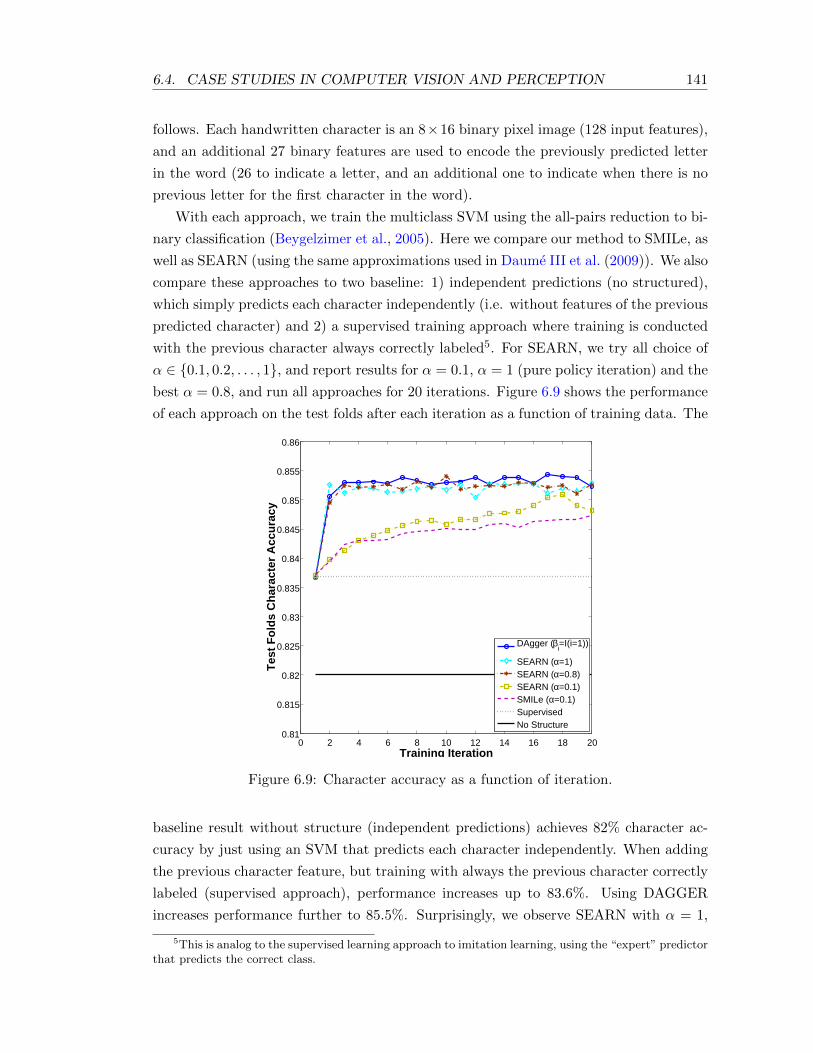
6.4. CASE STUDIES IN COMPUTER VISION AND PERCEPTION 141
follows. Each handwritten character is an 8×16 binary pixel image (128 input features),
and an additional 27 binary features are used to encode the previously predicted letter
in the word (26 to indicate a letter, and an additional one to indicate when there is no
previous letter for the first character in the word).
With each approach, we train the multiclass SVM using the all-pairs reduction to bi-
nary classification (Beygelzimer et al., 2005). Here we compare our method to SMILe, as
well as SEARN (using the same approximations used in Daume III et al. (2009)). We also
compare these approaches to two baseline: 1) independent predictions (no structured),
which simply predicts each character independently (i.e. without features of the previous
predicted character) and 2) a supervised training approach where training is conducted
with the previous character always correctly labeled5. For SEARN, we try all choice of
α ∈ 0.1, 0.2, . . . , 1, and report results for α = 0.1, α = 1 (pure policy iteration) and the
best α = 0.8, and run all approaches for 20 iterations. Figure 6.9 shows the performance
of each approach on the test folds after each iteration as a function of training data. The
0 2 4 6 8 10 12 14 16 18 200.81
0.815
0.82
0.825
0.83
0.835
0.84
0.845
0.85
0.855
0.86
Training Iteration
Tes
t F
old
s C
har
acte
r A
ccu
racy
DAgger (βi=I(i=1))
SEARN (α=1)SEARN (α=0.8)SEARN (α=0.1)SMILe (α=0.1)SupervisedNo Structure
Figure 6.9: Character accuracy as a function of iteration.
baseline result without structure (independent predictions) achieves 82% character ac-
curacy by just using an SVM that predicts each character independently. When adding
the previous character feature, but training with always the previous character correctly
labeled (supervised approach), performance increases up to 83.6%. Using DAGGER
increases performance further to 85.5%. Surprisingly, we observe SEARN with α = 1,
5This is analog to the supervised learning approach to imitation learning, using the “expert” predictorthat predicts the correct class.
142 CHAPTER 6. LEARNING INFERENCE FOR STRUCTURED PREDICTION
Figure 6.10: 3D point cloud classification application. Each point is assigned to one of5 object classes: Building (red), Ground (orange), Poles/Tree-Trunks (blue), Vegetation(green), and Wire (cyan).
which is a pure policy iteration approach performs very well on this experiment, similarly
to the best α = 0.8 and DAGGER. Because there is only a small part of the input that
is influenced by the current policy (the previous predicted character feature) this makes
this approach not as unstable as in general reinforcement/imitation learning problems
(as we saw in the previous imitation learning experiments of Section 5.2). SEARN and
SMILe with small α = 0.1 performs similarly but significantly worse than DAGGER.
Note that we chose the simplest (greedy, one-pass) decoding to illustrate the benefits of
the DAGGER approach with respect to existing reductions. Similar techniques can be
applied to multi-pass or beam-search decoding leading to results that are competitive
with the state-of-the-art. Nevertheless this shows that DAGGER can be just as effective
as state-of-the-art methods like SEARN with the best parameter α, but DAGGER does
not need to tune any such parameter. In the next 2 experiments, we compare our infer-
ence machine framework, training with DAGGER, to state-of-the-art graphical model
approaches.
3D Point Cloud Classification
Next, we evaluate on a 3D point cloud classification task – predicting the object present
at every point in a point cloud, or laser scan, of an outdoor scene observed from a LIDAR
sensor. We evaluate on the 3D point cloud dataset used in Munoz et al. (2009). This
dataset consists of 17 full 3D laser scans (total of ∼1.6 million 3D points) of an outdoor
environment collected from a LIDAR sensor. It contains 5 object labels: Building,
Ground, Poles/Tree-Trunks, Vegetation, and Wires (see Figure 6.10). We use the same
neighbor structure as in Munoz et al. (2009) (to define the predictions/messages used
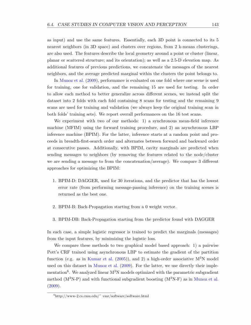
6.4. CASE STUDIES IN COMPUTER VISION AND PERCEPTION 143
as input) and use the same features. Essentially, each 3D point is connected to its 5
nearest neighbors (in 3D space) and clusters over regions, from 2 k-means clusterings,
are also used. The features describe the local geometry around a point or cluster (linear,
planar or scattered structure; and its orientation); as well as a 2.5-D elevation map. As
additional features of previous predictions, we concatenate the messages of the nearest
neighbors, and the average predicted marginal within the clusters the point belongs to.
In Munoz et al. (2009), performance is evaluated on one fold where one scene is used
for training, one for validation, and the remaining 15 are used for testing. In order
to allow each method to better generalize across different scenes, we instead split the
dataset into 2 folds with each fold containing 8 scans for testing and the remaining 9
scans are used for training and validation (we always keep the original training scan in
both folds’ training sets). We report overall performances on the 16 test scans.
We experiment with two of our methods: 1) a synchronous mean-field inference
machine (MFIM) using the forward training procedure, and 2) an asynchronous LBP
inference machine (BPIM). For the latter, inference starts at a random point and pro-
ceeds in breadth-first-search order and alternates between forward and backward order
at consecutive passes. Additionally, with BPIM, cavity marginals are predicted when
sending messages to neighbors (by removing the features related to the node/cluster
we are sending a message to from the concatenation/average). We compare 3 different
approaches for optimizing the BPIM:
1. BPIM-D: DAGGER, used for 30 iterations, and the predictor that has the lowest
error rate (from performing message-passing inference) on the training scenes is
returned as the best one.
2. BPIM-B: Back-Propagation starting from a 0 weight vector.
3. BPIM-DB: Back-Propagation starting from the predictor found with DAGGER
In each case, a simple logistic regressor is trained to predict the marginals (messages)
from the input features, by minimizing the logistic loss.
We compare these methods to two graphical model based approach: 1) a pairwise
Pott’s CRF trained using asynchronous LBP to estimate the gradient of the partition
function (e.g. as in Kumar et al. (2005)), and 2) a high-order associative M3N model
used on this dataset in Munoz et al. (2009). For the latter, we use directly their imple-
mentation6. We analyzed linear M3N models optimized with the parametric subgradient
method (M3N-P) and with functional subgradient boosting (M3N-F) as in Munoz et al.
(2009).
6http://www-2.cs.cmu.edu/˜ vmr/software/software.html
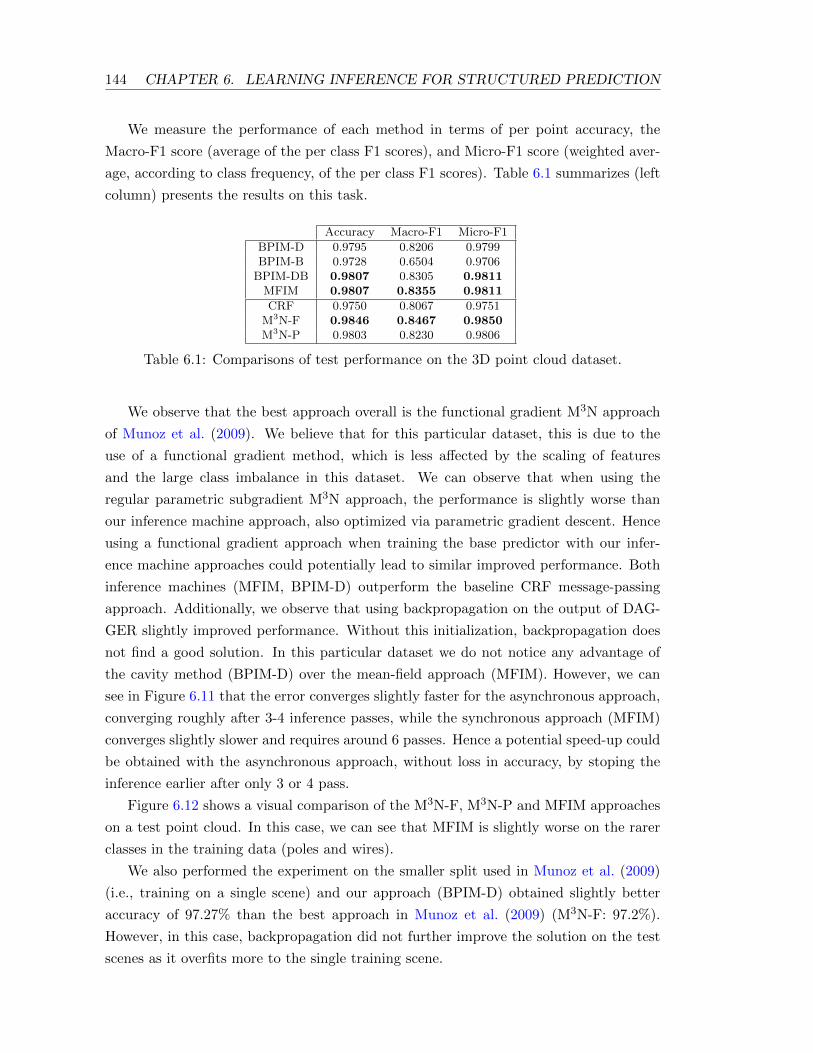
144 CHAPTER 6. LEARNING INFERENCE FOR STRUCTURED PREDICTION
We measure the performance of each method in terms of per point accuracy, the
Macro-F1 score (average of the per class F1 scores), and Micro-F1 score (weighted aver-
age, according to class frequency, of the per class F1 scores). Table 6.1 summarizes (left
column) presents the results on this task.
Accuracy Macro-F1 Micro-F1
BPIM-D 0.9795 0.8206 0.9799BPIM-B 0.9728 0.6504 0.9706
BPIM-DB 0.9807 0.8305 0.9811MFIM 0.9807 0.8355 0.9811
CRF 0.9750 0.8067 0.9751M3N-F 0.9846 0.8467 0.9850M3N-P 0.9803 0.8230 0.9806
Table 6.1: Comparisons of test performance on the 3D point cloud dataset.
We observe that the best approach overall is the functional gradient M3N approach
of Munoz et al. (2009). We believe that for this particular dataset, this is due to the
use of a functional gradient method, which is less affected by the scaling of features
and the large class imbalance in this dataset. We can observe that when using the
regular parametric subgradient M3N approach, the performance is slightly worse than
our inference machine approach, also optimized via parametric gradient descent. Hence
using a functional gradient approach when training the base predictor with our infer-
ence machine approaches could potentially lead to similar improved performance. Both
inference machines (MFIM, BPIM-D) outperform the baseline CRF message-passing
approach. Additionally, we observe that using backpropagation on the output of DAG-
GER slightly improved performance. Without this initialization, backpropagation does
not find a good solution. In this particular dataset we do not notice any advantage of
the cavity method (BPIM-D) over the mean-field approach (MFIM). However, we can
see in Figure 6.11 that the error converges slightly faster for the asynchronous approach,
converging roughly after 3-4 inference passes, while the synchronous approach (MFIM)
converges slightly slower and requires around 6 passes. Hence a potential speed-up could
be obtained with the asynchronous approach, without loss in accuracy, by stoping the
inference earlier after only 3 or 4 pass.
Figure 6.12 shows a visual comparison of the M3N-F, M3N-P and MFIM approaches
on a test point cloud. In this case, we can see that MFIM is slightly worse on the rarer
classes in the training data (poles and wires).
We also performed the experiment on the smaller split used in Munoz et al. (2009)
(i.e., training on a single scene) and our approach (BPIM-D) obtained slightly better
accuracy of 97.27% than the best approach in Munoz et al. (2009) (M3N-F: 97.2%).
However, in this case, backpropagation did not further improve the solution on the test
scenes as it overfits more to the single training scene.
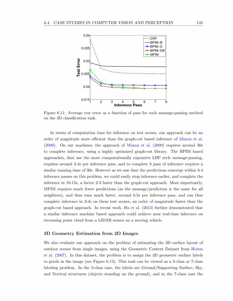
6.4. CASE STUDIES IN COMPUTER VISION AND PERCEPTION 145
1 2 3 4 5 6 7 80.015
0.02
0.025
0.03
0.035
0.04
Inference Pass
Te
st
Erro
r
CRF
BPIM−B
BPIM−D
BPIM−DB
MFIM
Figure 6.11: Average test error as a function of pass for each message-passing methodon the 3D classification task.
In terms of computation time for inference on test scenes, our approach can be an
order of magnitude more efficient than the graph-cut based inference of Munoz et al.
(2009). On our machines, the approach of Munoz et al. (2009) requires around 30s
to complete inference, using a highly optimized graph-cut library. The BPIM based
approaches, that use the more computationally expensive LBP style message-passing,
requires around 3-4s per inference pass, and to complete 8 pass of inference requires a
similar running time of 30s. However as we saw that the predictions converge within 3-4
inference passes on this problem, we could easily stop inference earlier, and complete the
inference in 10-15s, a factor 2-3 faster than the graph-cut approach. More importantly,
MFIM requires much fewer predictions (as the message/prediction is the same for all
neighbors), and thus runs much faster, around 0.5s per inference pass, and can thus
complete inference in 3-4s on these test scenes, an order of magnitude faster than the
graph-cut based approach. In recent work, Hu et al. (2013) further demonstrated that
a similar inference machine based approach could achieve near real-time inference on
streaming point cloud from a LIDAR sensor on a moving vehicle.
3D Geometry Estimation from 2D Images
We also evaluate our approach on the problem of estimating the 3D surface layout of
outdoor scenes from single images, using the Geometric Context Dataset from Hoiem
et al. (2007). In this dataset, the problem is to assign the 3D geometric surface labels
to pixels in the image (see Figure 6.13). This task can be viewed as a 3-class or 7-class
labeling problem. In the 3-class case, the labels are Ground/Supporting Surface, Sky,
and Vertical structures (objects standing on the ground), and in the 7-class case the
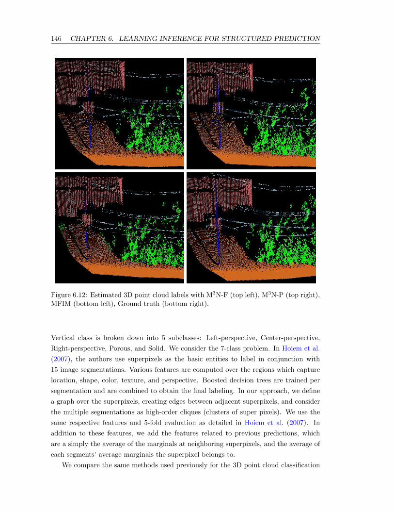
146 CHAPTER 6. LEARNING INFERENCE FOR STRUCTURED PREDICTION
Figure 6.12: Estimated 3D point cloud labels with M3N-F (top left), M3N-P (top right),MFIM (bottom left), Ground truth (bottom right).
Vertical class is broken down into 5 subclasses: Left-perspective, Center-perspective,
Right-perspective, Porous, and Solid. We consider the 7-class problem. In Hoiem et al.
(2007), the authors use superpixels as the basic entities to label in conjunction with
15 image segmentations. Various features are computed over the regions which capture
location, shape, color, texture, and perspective. Boosted decision trees are trained per
segmentation and are combined to obtain the final labeling. In our approach, we define
a graph over the superpixels, creating edges between adjacent superpixels, and consider
the multiple segmentations as high-order cliques (clusters of super pixels). We use the
same respective features and 5-fold evaluation as detailed in Hoiem et al. (2007). In
addition to these features, we add the features related to previous predictions, which
are a simply the average of the marginals at neighboring superpixels, and the average of
each segments’ average marginals the superpixel belongs to.
We compare the same methods used previously for the 3D point cloud classification
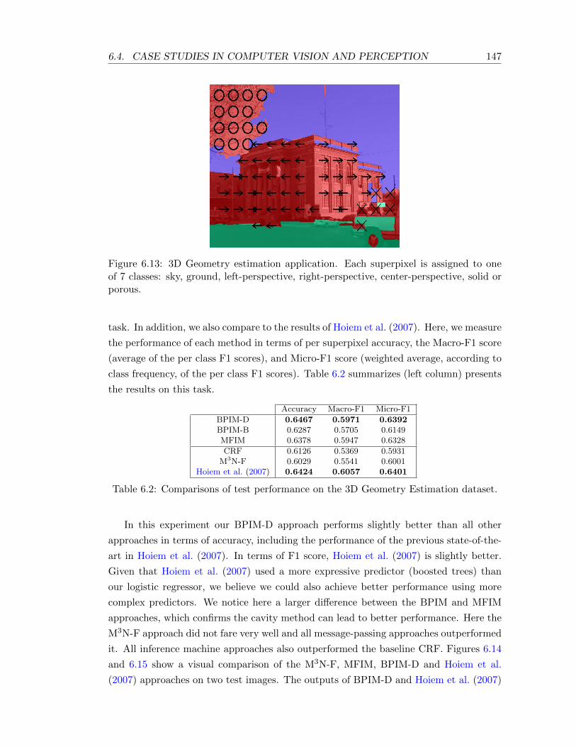
6.4. CASE STUDIES IN COMPUTER VISION AND PERCEPTION 147
Figure 6.13: 3D Geometry estimation application. Each superpixel is assigned to oneof 7 classes: sky, ground, left-perspective, right-perspective, center-perspective, solid orporous.
task. In addition, we also compare to the results of Hoiem et al. (2007). Here, we measure
the performance of each method in terms of per superpixel accuracy, the Macro-F1 score
(average of the per class F1 scores), and Micro-F1 score (weighted average, according to
class frequency, of the per class F1 scores). Table 6.2 summarizes (left column) presents
the results on this task.
Accuracy Macro-F1 Micro-F1
BPIM-D 0.6467 0.5971 0.6392BPIM-B 0.6287 0.5705 0.6149MFIM 0.6378 0.5947 0.6328
CRF 0.6126 0.5369 0.5931M3N-F 0.6029 0.5541 0.6001
Hoiem et al. (2007) 0.6424 0.6057 0.6401
Table 6.2: Comparisons of test performance on the 3D Geometry Estimation dataset.
In this experiment our BPIM-D approach performs slightly better than all other
approaches in terms of accuracy, including the performance of the previous state-of-the-
art in Hoiem et al. (2007). In terms of F1 score, Hoiem et al. (2007) is slightly better.
Given that Hoiem et al. (2007) used a more expressive predictor (boosted trees) than
our logistic regressor, we believe we could also achieve better performance using more
complex predictors. We notice here a larger difference between the BPIM and MFIM
approaches, which confirms the cavity method can lead to better performance. Here the
M3N-F approach did not fare very well and all message-passing approaches outperformed
it. All inference machine approaches also outperformed the baseline CRF. Figures 6.14
and 6.15 show a visual comparison of the M3N-F, MFIM, BPIM-D and Hoiem et al.
(2007) approaches on two test images. The outputs of BPIM-D and Hoiem et al. (2007)

148 CHAPTER 6. LEARNING INFERENCE FOR STRUCTURED PREDICTION
Figure 6.14: Estimated 3D geometric surface layouts on a city scene with M3N-F (topleft), Hoiem et al. (2007) (top right), BPIM-D (bottom left), Ground truth (bottomright).
are very similar, but we can observe more significant improvements over the M3N-F.
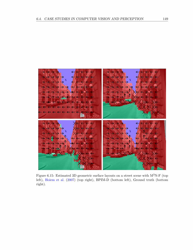
6.4. CASE STUDIES IN COMPUTER VISION AND PERCEPTION 149
Figure 6.15: Estimated 3D geometric surface layouts on a street scene with M3N-F (topleft), Hoiem et al. (2007) (top right), BPIM-D (bottom left), Ground truth (bottomright).

Chapter 7
Learning Submodular Sequence
Predictions
We now move on to study another important class of sequential prediction tasks : rec-
ommendation tasks where we must learn to suggest lists of options or items.
Many problem domains, ranging from web applications (ad placement, content rec-
ommendation) to robotics (identifying small subset of grasps, or trajectories to try to
successfully perform the task) require predicting lists of items/options (see Figure 7.1).
Such applications are often budget-limited and the goal is to choose the best list of items,
from a large set of possible items, with maximal utility. In ad placement, we must pick
a small list of ads with high click-through rate. For robotic manipulation, we must pick
a small set of initial grasp trajectories to maximize the chance of finding a successful
trajectory via more extensive evaluation or simulation. In extractive document summa-
rization, we want to find a few sentences from the text that provide a good summary of
the entire document.
In all of these problems, the predicted list of items should be both relevant and
diverse. For example, recommending a diverse set of news articles increases the chance
that a user would like at least one article (Radlinski et al., 2008). As such, recommending
multiple redundant articles on the same topic would do little to increase this chance.
This notion of diminishing returns due to redundancy is often captured formally using
submodularity (Guestrin and Krause, 2008).
In this chapter, we study the general learning problem of training a policy to construct
lists (by predicting, in sequence, items to add to the list) that maximizes a submodular
reward function – a reward with this property of diminishing return. We consider prob-
lems where the submodular reward function is only directly measured on a finite training
set, and our goal is to learn to make good predictions on new test examples where the
reward function is not directly measurable. For example in document summarization, we
have access to a few training documents, where humans have provided summaries, and

152 CHAPTER 7. LEARNING SUBMODULAR SEQUENCE PREDICTIONS
Figure 7.1: Example Recommendation Applications. Left: Ad placement, where wewant to display a small list of ads the user is likely going to click on. Center: NewsRecommendation, where we want to display a small list of news article likely to interestthe user. Right: Grasp Selection, where we want to select a small list of grasps likely tosucceed at picking an object.
we would like to learn to generate good summaries for new documents, where human
summaries are not available.
To learn such a policy, it is natural to consider policies that use, as part of their input,
features related to the items in the current list. As these features are related to previous
predictions made by the policy, a similar train-test mismatch, as in previous sequential
prediction settings, can occur if the policy is not trained carefully. We will show that the
previous learning strategies, such as DAGGER, can be adapted to this setting to deal
with this issue and learn policies that can recommend good lists of relevant and diverse
items.
While DAGGER as presented could be applied “as is” for such setting, e.g. by at-
tempting to minimize a 0-1 classification loss in order to mimic a greedy list construction
strategy, this would not leverage the particular properties of the reward function. Instead
we will present an adaptation of DAGGER, that leverages the particular submodular
properties of the reward, and provides improved near-optimality guarantees.
We begin by formalizing the notion of submodularity and reviewing prior work re-
lated to submodular optimization, and learning. We then present our adaptation of
DAGGER and its analysis, that provides strong near-optimality guarantees. We then
demonstrate the improved performance of this method compared to prior work on var-
ious recommendation tasks: 1) Grasp Selection, recommending a small list of grasps to
a robotic manipulator that is likely to contain a successful one for picking a nearby ob-
ject, 2) Trajectory Optimization, recommending a small list of initial “seed” trajectories,
to be used in a local trajectory optimization procedure, that is likely going to contain

7.1. PRELIMINARIES 153
one that leads to a collision-free trajectory; 3) News Recommendation, recommending
a small set of news article the user is likely going to be interested in reading, and 4)
Document Summarization: extracting a few sentences from documents that provide a
good summary. This adaptation of DAGGER and these results were originally presented
in Ross et al. (2013d).
7.1 Preliminaries
We now begin by formalizing the problem of maximizing submodular rewards and exist-
ing results and approaches.
Submodularity and the Concept of Diminishing Return
Formally, the problem we are trying to address can be defined as follows. We have a
large set S that represents the set of all possible items we can choose from (e.g. ads,
sentences, grasps). Our objective is to pick a list of items L ⊆ S to maximize a reward
function f , under a budget constraint that we can only pick a small list of k items, i.e.
|L| ≤ k.1 We consider reward functions f that obey the following properties:
1. Monotonicity: For any lists L1, L2, f(L1) ≤ f(L1⊕L2) and f(L2) ≤ f(L1⊕L2)
2. Submodularity: For any lists L1, L2 and item s ∈ S, f(L1 ⊕ s) − f(L1) ≥f(L1 ⊕ L2 ⊕ s)− f(L1 ⊕ L2).
Here, ⊕ denotes the concatenation operator. Intuitively, monotonicity implies that
adding more elements never hurts, and submodularity captures the notion of dimin-
ishing returns (i.e. adding an item to a long list increases the objective less than when
adding it to a shorter sublist). We further assume for simplicity that f takes values in
[0, 1], and that f(∅) = 0 where ∅ denotes the empty list. We will also use the shorthand
b(s|L) = f(L⊕ s)− f(L) to denote the marginal benefit of adding the item s to list L.
The optimal solution to this problem is the list of length k, that we denote L∗k, that
maximizes this objective:
L∗k = arg maxL:|L|≤k
f(L) (7.1)
Finding this optimal list is in general intractable, it is a combinatorial optimization
problem that requires searching over an exponentially large set of possible lists (of size
|S|k). In fact, it is well known that this problem is NP-Hard (Nemhauser et al., 1978).
1“Lists” generalize the notion of “set” more commonly used in submodular optimization, and enablesreasoning about item order and repeated items (Streeter and Golovin, 2008). One may consider sets whereappropriate.

154 CHAPTER 7. LEARNING SUBMODULAR SEQUENCE PREDICTIONS
Greedy Algorithm
While finding the optimal list is NP-Hard, a simple greedy algorithm provides good
approximation with near-optimality guarantees. That is, the greedy algorithm that
starts from the empty list L0 = ∅, and then successively adds the item with largest
marginal benefit to the current list, i.e. Li+1 = Li ⊕ si for si = arg maxs∈S b(s|Li), until
a list of length k is obtained, guarantees that the list Lk is within a factor (1 − 1/e) of
the optimal list L∗k, i.e. f(Lk) ≥ (1 − 1/e)f(L∗k). Obtaining any better approximation
ratio than (1 − 1/e) is known to be NP-Hard (Nemhauser et al., 1978). Hence greedy
provides the best polynomial time approximation, unless P = NP .
It has also been observed in many applications that this greedy procedure typically
works very well (Guestrin and Krause, 2008). Thus, given access to the submodular
reward function f , one could simply employ greedy to construct good lists. However
in our learning setting, f is only measurable on training examples, making this greedy
algorithm inapplicable to new test examples. We formalize our learning setting below.
Learning with Submodular Rewards
In our learning task, we consider reward functions that may depend on some underlying
state x ∈ X (e.g. a user, environment of the robot, a document, etc.). We denote fx
the reward function for state x, and assume that fx is monotone submodular for all x.
We also use the state to encode randomness, if any, in the objective. For instance, if
a user clicks on an ad with some probability, the different random events are encoded
by different states. As such, we do not assume the state is fully observed. It may be
completely unknown, or only partially observed through some features (e.g. previous
queries or websites visited by the user).
A simple example submodular function fx that repeatedly arises in many domains is
one that takes value 0 until a suitable item is found, and then takes on value 1 thereafter.
Examples include the notion of “multiple choice” learning as in Dey et al. (2012a),
Guzman-Rivera et al. (2012) where a predicted set of options is considered successful if
any predicted item is deemed correct for the current example x, and abandonment in ad
placement (Radlinski et al., 2008) where success is measured by whether any predicted
advertisement is clicked on by the current user x.
Our task consists in learning to construct good lists of pre-specified length k under
some unknown distribution of states D (e.g. distribution of users or documents we have
to summarize). We consider two cases: context-free and contextual.
Context-Free: In the context-free case, we have no side-information about the
current state (i.e. we do not observe anything about x). For example, we may want to
learn the best list of news articles to display on a news website, when no information is
available about the user who is viewing the website. In this case, we would like to find a
7.1. PRELIMINARIES 155
fixed list L that has good performance on average. That is, we quantify the performance
of any list L by its expected value:
F (L) = Ex∼D[fx(L)]. (7.2)
Note that F (L) is also monotone submodular. Thus the clairvoyant greedy algorithm
with perfect knowledge of D can find a list Lk such that F (Lk) ≥ (1−1/e)F (L∗k), where
L∗k = arg maxL:|L|=k F (L). Although D is unknown, we assume that we observe samples
of the objective fx during training. Our goal is thus to develop a learning approach
that efficiently converges, both computationally and statistically, to the performance of
the clairvoyant greedy algorithm. In other words, we would like to achieve a similar
guarantee to the clairvoyant greedy algorithm in the limit as we observe more and more
training data.
Contextual: In the contextual case, we observe side-information in the form of
features regarding the state x. We would like to use this observed side-information to
suggest better lists for the particular context (e.g. a list of news articles personalized to
the preference of the user x). We “lift” this problem to a hypothesis space of policies
(i.e. multi-class predictors) that maps features to items.
We denote Π our policy class, and π(x) the prediction of policy π ∈ Π given side-
information describing state x. We consider a list of k policies Lπ,k = (π1, π2, . . . , πk),
where in state x, this list of policies predicts the list of items Lπ,k(x) = (π1(x), π2(x), . . . , πk(x)).
We quantify the performance of such list of policies by its expected value:
F (Lπ) = Ex∼D[fx(Lπ(x))].
It can be shown that F obeys both monotonicity and submodularity with respect to
appending policies to a list of policy (Dey et al., 2012a). Thus, a clairvoyant greedy algo-
rithm that sequentially picks the policy with highest expected marginal benefit will con-
struct a list Lπ,k such that F (Lπ,k) ≥ (1−1/e)F (L∗π,k), where L∗π,k = arg maxLπ :|Lπ |=k F (Lπ).
As before, our goal is to develop a learning approach (for learning a list of policies) that
efficiently competes with the performance of the clairvoyant greedy algorithm.
Related Work
The problem of learning to optimize submodular reward functions from data, both with
and without contextual features, has become increasingly important in machine learning
due to its diverse application areas. Broadly speaking, there are two main approaches for
this setting. The first aims to identify a model within a parametric family of submodular
functions and then use the resulting model for new predictions. The second attempts to
learn a strategy to directly predict a list of elements by decomposing the overall problem
into multiple simpler learning tasks.

156 CHAPTER 7. LEARNING SUBMODULAR SEQUENCE PREDICTIONS
The first approach (Yue and Joachims, 2008, Yue and Guestrin, 2011, Lin and Bilmes,
2012, Raman et al., 2012) involves identifying the parameterization that best matches
the submodular rewards of the training instances. For prediction, they then simply use
the greedy algorithm on the learned submodular reward function. These methods are
largely limited to learning non-negative linear combinations of features that are them-
selves submodular, which often restricts their expressiveness. Furthermore, while good
sample complexity results are known, these guarantees only hold under strong realiz-
ability assumptions where submodular rewards can be modeled exactly by such linear
combinations (Yue and Guestrin, 2011, Raman et al., 2012). Recent work on Deter-
minental Point Processes (DPPs) (Kulesza and Taskar, 2011) provides a probabilistic
model of sets, which can be useful for the tasks that we consider. These approaches,
while appealing, solve a potentially unnecessarily hard problem in first learning a holis-
tic list evaluation model, and thus may compound errors by first approximating the
submodular function and then approximately optimizing it.
The second, a learning reduction approach, by contrast, decomposes list prediction
into a sequence of simpler learning tasks that attempts to mimic the greedy strategy
(Streeter and Golovin, 2008, Radlinski et al., 2008, Streeter et al., 2009, Dey et al.,
2012a). In Streeter and Golovin (2008), they address the context-free case, and show
that by running a simple no-regret online learning algorithm2 at each position in the
list (where experts are items s ∈ S and losses are the negative benefits at that position)
suffices to learn a distribution over lists with expected value F that matches the guarantee
of greedy in the limit as more and more training examples are observed. In Dey et al.
(2012a), an approach called ConSeqOpt extends this strategy to the contextual setting
by a reduction to cost-sensitive classification. Essentially, the predictor at each position
aims to best predict an item to add to the list, given features, so as to maximize the
expected marginal utility. This approach is flexible, in that it can be used with most
common hypothesis classes and arbitrary features. Because of this decomposition, the full
model class (all possible sequences of predictors) is often quite expressive, and allows for
agnostic learning guarantees.3 This generality comes at the expense of being significantly
less data-efficient than methods that make realizability assumptions such as Yue and
Guestrin (2011), Raman et al. (2012), as these existing approaches learn a different
predictor for each position in the list. In many ways, these methods adopt a similar
learning strategy to Forward, as presented in previous chapters, and suffer from the same
limitations : learning is less efficient as a separate predictor is learned for each position,
not allowing to generalize across positions. Another issue that afflict these methods in
2E.g. weighted majority (Cesa-Bianchi et al., 1997).3This first strategy of learning the parameters of a submodular function can be seen as a special case
of this second approach, e.g. when the second approach uses the reduction of cost-sensitive classificationto regression (see Section 7.3).
7.2. CONTEXT-FREE LIST OPTIMIZATION 157
this particular setting, is that they can exhibit a data starvation phenomenon where
later positions in the list have fewer and fewer examples to train on. This occurs due
to the diminishing return property, e.g. if previous predictors in the list already found
a successful item, there is no benefit left for the remaining positions. This effectively as
the effect of discarding the current training example at these later positions in the list,
and thus predictors far in the list may only have very few examples to train on.
To address these limitations, we present below an adaptation of the DAGGER learn-
ing strategy presented in previous chapters. Compared with related work, this approach
enjoys the benefits of being both data-efficient while ensuring strong agnostic perfor-
mance guarantees. We do so by developing new analysis for online submodular opti-
mization which yields agnostic learning guarantees while learning a single data-efficient
policy. By learning a single policy that can be used to construct the entire list, we also
avoid the data starvation issue, as the policy is able to generalize to notions of relevance
and diversity across positions in the list, and pick good items to add far in the list.
7.2 Context-free List Optimization
We first consider the context-free setting. For this setting, as there are no features, the
stationary policy is represented as a fixed distribution over items, that is sampled from
to add elements to the list.4
Our algorithm, called Submodular Contextual Policy (SCP), adapts the DAGGER
learning strategy to this submodular sequence setting. Unlike in previous settings, here
there is no expert telling us which action, or item to select. Instead we learn directly
from feedback of the benefits of adding items to the list. SCP uses a similar strategy of
interacting with the learner, to observe the benefits of adding items to list constructed
by the current policy, and leverages the strong “no-regret” properties of online learning
algorithms to provide strong guarantees on performance.
SCP, for the context-free setting, is described in Algorithm 7.2.1. SCP requires an
online learning algorithm subroutine (denoted by Update) that is no-regret with respect
to a bounded positive loss function, maintains an internal distribution over items for
prediction, and can be queried for multiple predictions (i.e. multiple samples).5 In
contrast to prior work (Streeter and Golovin, 2008), SCP employs only a single online
learning algorithm in the inner loop, instead of one at each position.
4Note that while there is no observed features of the state, we could also potentially consider learninga policy that uses features of the elements in the list. The algorithm we present in the next section forthe contextual case, that uses both features of the state and list, could be applied in this case but withoutfeatures of the state.
5Algorithms that meet these requirements include Randomized Weighted Majority (Littlestone andWarmuth, 1994), Follow the Perturbed Leader (Kalai and Vempala, 2005), EXP3 (Auer et al., 2002b),and many others.
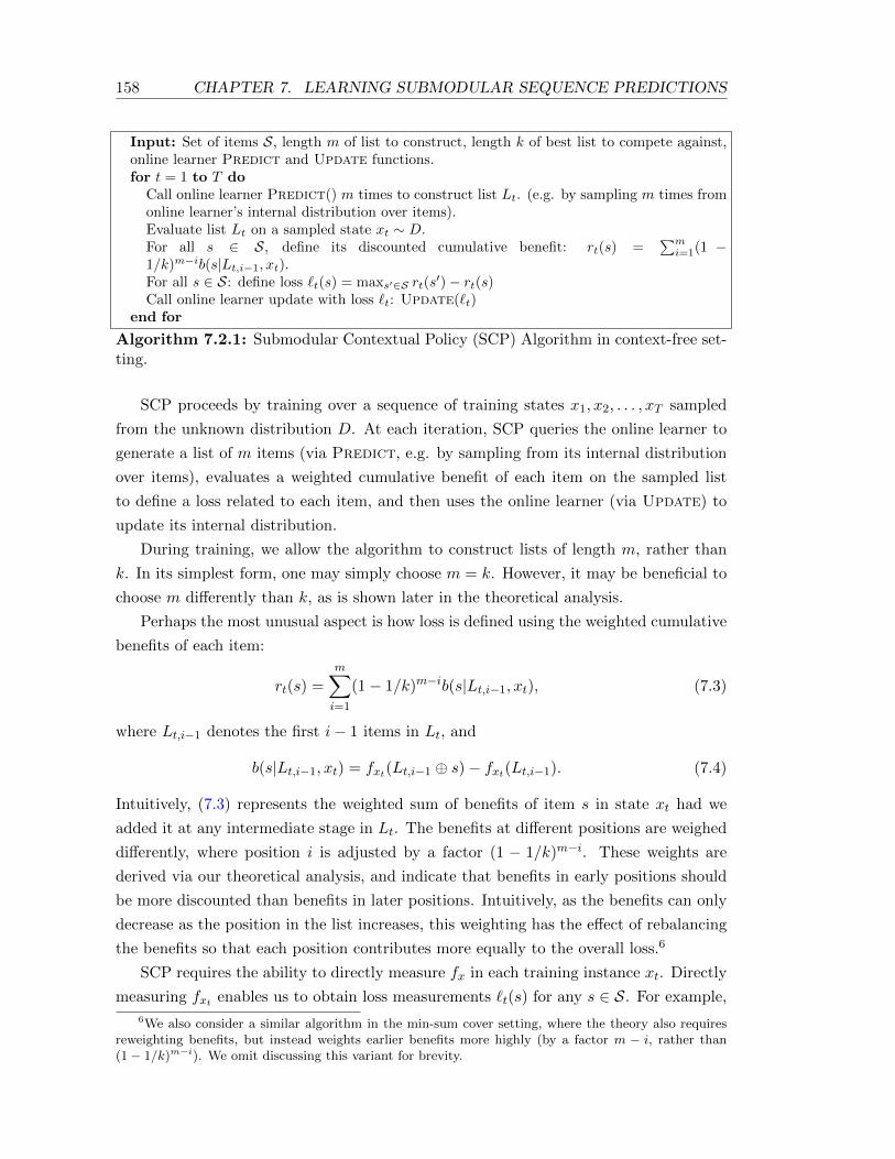
158 CHAPTER 7. LEARNING SUBMODULAR SEQUENCE PREDICTIONS
Input: Set of items S, length m of list to construct, length k of best list to compete against,online learner Predict and Update functions.for t = 1 to T do
Call online learner Predict() m times to construct list Lt. (e.g. by sampling m times fromonline learner’s internal distribution over items).Evaluate list Lt on a sampled state xt ∼ D.For all s ∈ S, define its discounted cumulative benefit: rt(s) =
∑mi=1(1 −
1/k)m−ib(s|Lt,i−1, xt).For all s ∈ S: define loss `t(s) = maxs′∈S rt(s
′)− rt(s)Call online learner update with loss `t: Update(`t)
end for
Algorithm 7.2.1: Submodular Contextual Policy (SCP) Algorithm in context-free set-ting.
SCP proceeds by training over a sequence of training states x1, x2, . . . , xT sampled
from the unknown distribution D. At each iteration, SCP queries the online learner to
generate a list of m items (via Predict, e.g. by sampling from its internal distribution
over items), evaluates a weighted cumulative benefit of each item on the sampled list
to define a loss related to each item, and then uses the online learner (via Update) to
update its internal distribution.
During training, we allow the algorithm to construct lists of length m, rather than
k. In its simplest form, one may simply choose m = k. However, it may be beneficial to
choose m differently than k, as is shown later in the theoretical analysis.
Perhaps the most unusual aspect is how loss is defined using the weighted cumulative
benefits of each item:
rt(s) =m∑i=1
(1− 1/k)m−ib(s|Lt,i−1, xt), (7.3)
where Lt,i−1 denotes the first i− 1 items in Lt, and
b(s|Lt,i−1, xt) = fxt(Lt,i−1 ⊕ s)− fxt(Lt,i−1). (7.4)
Intuitively, (7.3) represents the weighted sum of benefits of item s in state xt had we
added it at any intermediate stage in Lt. The benefits at different positions are weighed
differently, where position i is adjusted by a factor (1 − 1/k)m−i. These weights are
derived via our theoretical analysis, and indicate that benefits in early positions should
be more discounted than benefits in later positions. Intuitively, as the benefits can only
decrease as the position in the list increases, this weighting has the effect of rebalancing
the benefits so that each position contributes more equally to the overall loss.6
SCP requires the ability to directly measure fx in each training instance xt. Directly
measuring fxt enables us to obtain loss measurements `t(s) for any s ∈ S. For example,
6We also consider a similar algorithm in the min-sum cover setting, where the theory also requiresreweighting benefits, but instead weights earlier benefits more highly (by a factor m − i, rather than(1− 1/k)m−i). We omit discussing this variant for brevity.

7.2. CONTEXT-FREE LIST OPTIMIZATION 159
in document summarization fx corresponds to the ROUGE score (Lin, 2004), which
can be evaluated for any generated summary given expert annotations which are only
available for training instances.
Partial Information Setting
In principle, SCP can also be applied in partial feedback settings, e.g. ad placement
where the value fxt is only observed for some items (e.g. only the displayed ads), by
using bandit learning algorithms instead (e.g. EXP3 (Auer et al., 2002b)).7 We briefly
mention how this algorithm can be applied in partial feedback settings. However, as this
is an orthogonal issue, most of our focus and analysis later is on the full information
case.
In a partial information setting, we consider that we can only observe the benefits of
the elements we added to the sampled list at each iteration. That is, our only observations
about fxt are the benefits of each item in the constructed list Lt, i.e. for each position
i, we only observe b(sti|xt, Lt,i−1) for sti the item in position i in the list Lt, and for any
other item s′ 6= sti we consider the benefit b(s′|xt, Lt,i−1) unknown. If we construct a
list of m items, we would only observe m benefits. For example, in ad placement, all
displayed ads would have observed benefits 0, except the first ad in the list that is clicked
on, would have an observed benefit of 1.
Based on this information, we can use an algorithm like EXP3 (Auer et al., 2002b),
to update the internal distribution over items. Effectively, we can treat each of these m
observed benefits as a separate learning example for EXP3, and perform m updates with
these m examples. In particular, EXP3 would use the same importance weighting trick,
mentioned in Section 4.1, to assign a reward of 0 to any unobserved benefit, and for the
item s with observed benefit b, it would assign a reward of b/p, if p was the probability
of picking that item when it was sampled. As our examples are weighted, by the factor
(1 − 1/k)m−i for the example at position i, we would also multiply the reward by this
weight. This reward vector, constructed for each observed benefit would then be used
to update the internal distribution over items, as described in Auer et al. (2002b).
Theoretical Guarantees
We now show that Algorithm 7.2.1 is no-regret with respect to the clairvoyant greedy al-
gorithm’s expected performance over the training instances. Our main theoretical result
provides a reduction to an online learning problem and directly relates the performance
of our algorithm on the submodular list optimization problem to the standard online
7Partial information settings arise, e.g., when f is derived using real-world trials that preclude theability to evaluate b(s|L, x) (7.4) for every possible s ∈ S.
160 CHAPTER 7. LEARNING SUBMODULAR SEQUENCE PREDICTIONS
learning regret incurred by the subroutine. The proofs of these results are presented in
appendix B.
Although Algorithm 7.2.1 uses only a single instance of an online learner subroutine,
it achieves the same performance guarantee as prior work (Streeter and Golovin, 2008,
Dey et al., 2012a) that employ k separate instances of an online learner. This leads to
a surprising fact: it is possible to sample from a stationary distribution over items to
construct a list that achieves the same guarantee as the clairvoyant greedy algorithm. 8
For a sequence of training states xtTt=1, let the sequence of loss functions `tTt=1
defined in Algorithm 7.2.1 correspond to the sequence of losses incurred in the reduction
to the online learning problem. The expected regret of the online learning algorithm is
E[R] =T∑t=1
Es′∼pt [`t(s′)]−min
s∈S
T∑t=1
`t(s), (7.5)
where pt is the internal distribution of the online learner used to construct list Lt. Note
that an online learner is called no-regret if R is sublinear in T .
Let F (p,m) = ELm∼p[Ex∼D[fx(Lm)]] denote the expected value of constructing
lists by sampling (with replacement) m elements from distribution p, and let p =
arg maxt∈1,2,...,T F (pt,m) denote the best distribution found by the algorithm.
We define a mixture distribution p over lists that constructs a list as follows: sample
an index t uniformly in 1, 2, . . . , T, then sample m elements (with replacement) from
pt. Note that F (p,m) = 1T
∑Tt=1 F (pt,m) and F (p,m) ≥ F (p,m). Thus it suffices to
show that F (p,m) has good guarantees. We show that in expectation p (and thus p)
constructs lists with performance guarantees close to the clairvoyant greedy algorithm:9
Theorem 7.2.1. Let α = exp(−m/k) and k′ = min(m, k). For any δ ∈ (0, 1), with
probability ≥ 1− δ:
F (p,m) ≥ (1− α)F (L∗k)−E[R]
T− 3
√2k′ ln(2/δ)
T
Corollary 7.2.1. If a no-regret algorithm is used on the sequence of loss `t, then as
T →∞, E[R]T → 0, and with probability 1:
limT→∞
F (p,m) ≥ (1− α)F (L∗k)
Theorem 7.2.1 provides a general approximation ratio to the best list of size k when
constructing a list of a different size m. For m = k, we obtain the typical (1 − 1/e)
8This fact can also be seen as a special case of a more general result proven in prior related workthat analyzed randomized set selection strategies to optimize submodular functions (Feige et al., 2011).
9Additionally, if the distributions pt converge, then the last distribution pT+1 must have performancearbitrarily close to p as T → ∞. In particular, we can expect this to occur when the examples arerandomly drawn from a fixed distribution that does not change over time.
7.3. CONTEXTUAL LIST OPTIMIZATION WITH STATIONARY POLICIES 161
approximation ratio (Guestrin and Krause, 2008). As m increases, this provides approx-
imation ratios that converge exponentially closer to 1.
In particular we can see how the choice of m and k affects the performance guarantee
of our algorithm, and that choosing m 6= k can sometimes lead to better guarantees.
For instance, imagine that our budget is m = 12, but we know that the optimal list of
size k = 4 has F (L∗k) close to 1. Then running our algorithm with such (m, k), would
guarantee that we can achieve at least 95% of the best list of size 4 in the limit, and
thus F (p,m) would be guaranteed to be close to 0.95. On the other hand, if we choose
m = k = 12, F (L∗k) would be at most 1, and running our algorithm with such (m, k),
would only guarantee that we can achieve at least 63% of the best list of size 12 in the
limit, and thus F (p,m) would only be guaranteed to be close to 0.63.
Naively, one might expect regret E[R]/T to scale linearly in k′ as it involves loss
in [0, k′]. However, we show that regret actually scales as O(√k′), e.g. using Weighted
Majority (Kalai and Vempala, 2005) with the optimal learning rate (or with the doubling
trick (Cesa-Bianchi et al., 1997)). Our result matches the best known results for this
setting (Streeter and Golovin, 2008) while using a single online learner, and is especially
beneficial in the contextual setting due to improved generalization (see Section 7.3).
Corollary 7.2.2. Using weighted majority with the optimal learning rate guarantees
with probability ≥ 1− δ:
F (p,m) ≥ (1− α)F (L∗k)−O
(√k′ log(1/δ)
T+
√k′ log |S|
T
).
7.3 Contextual List Optimization with Stationary Policies
We now consider the contextual setting where features of each state xt are observed
before choosing the list. As mentioned, our goal here is to compete with the best list of
policies (π1, π2, . . . , πk) from a hypothesis class Π. Each of these policies are assumed to
choose an item solely based on features of the state xt.
We consider embedding Π within a larger class, Π ⊆ Π, where policies Π are functions
of both state and a partially chosen list. Then for any π ∈ Π, π(x, L) corresponds to
the item that policy π selects to append to list L given state x. We will learn a policy,
or distribution of policies, from Π that attempts to generalize list construction across
multiple positions.10
We now present SCP for the general contextual setting (Algorithm 7.3.1). At each
iteration, SCP interacts with the learner to collect additional data by constructing a list
10Competing against the best list of policies in Π is difficult in general as it violates submodularity:policies can perform better when added later in the list (due to list features). Nevertheless, we can stilllearn from class Π and compete against the best list of policies in Π.
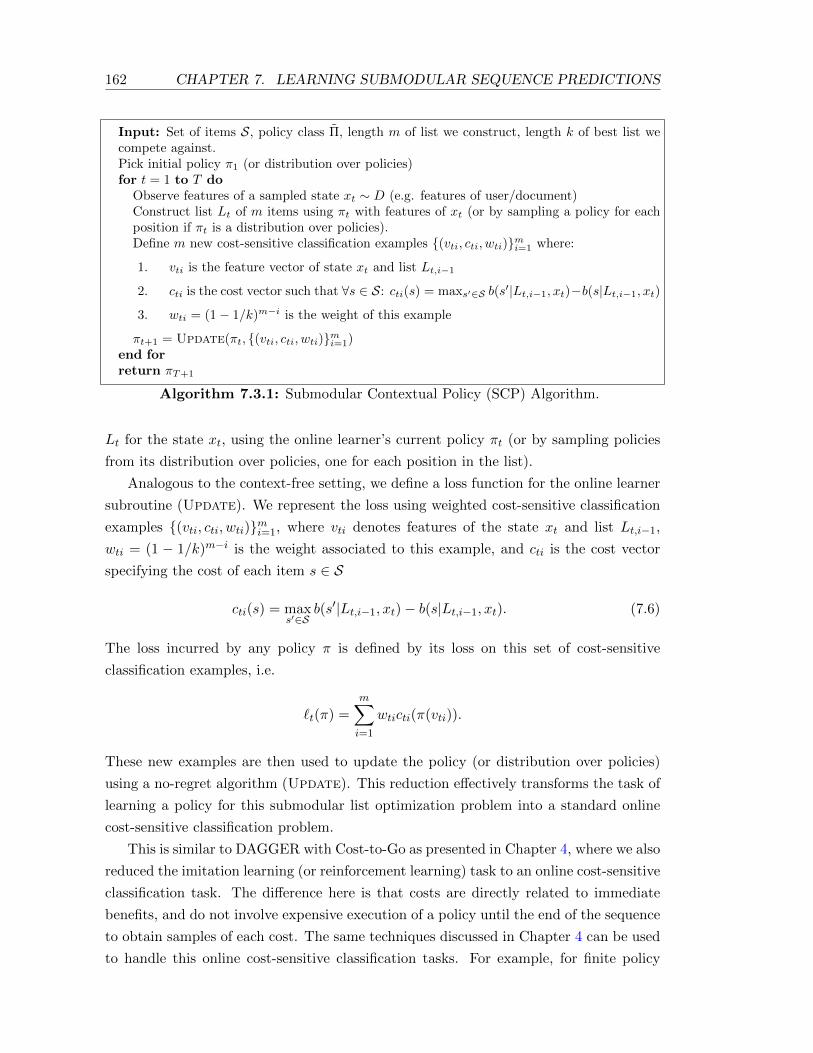
162 CHAPTER 7. LEARNING SUBMODULAR SEQUENCE PREDICTIONS
Input: Set of items S, policy class Π, length m of list we construct, length k of best list wecompete against.Pick initial policy π1 (or distribution over policies)for t = 1 to T do
Observe features of a sampled state xt ∼ D (e.g. features of user/document)Construct list Lt of m items using πt with features of xt (or by sampling a policy for eachposition if πt is a distribution over policies).Define m new cost-sensitive classification examples (vti, cti, wti)mi=1 where:
1. vti is the feature vector of state xt and list Lt,i−1
2. cti is the cost vector such that ∀s ∈ S: cti(s) = maxs′∈S b(s′|Lt,i−1, xt)−b(s|Lt,i−1, xt)
3. wti = (1− 1/k)m−i is the weight of this example
πt+1 = Update(πt, (vti, cti, wti)mi=1)end forreturn πT+1
Algorithm 7.3.1: Submodular Contextual Policy (SCP) Algorithm.
Lt for the state xt, using the online learner’s current policy πt (or by sampling policies
from its distribution over policies, one for each position in the list).
Analogous to the context-free setting, we define a loss function for the online learner
subroutine (Update). We represent the loss using weighted cost-sensitive classification
examples (vti, cti, wti)mi=1, where vti denotes features of the state xt and list Lt,i−1,
wti = (1 − 1/k)m−i is the weight associated to this example, and cti is the cost vector
specifying the cost of each item s ∈ S
cti(s) = maxs′∈S
b(s′|Lt,i−1, xt)− b(s|Lt,i−1, xt). (7.6)
The loss incurred by any policy π is defined by its loss on this set of cost-sensitive
classification examples, i.e.
`t(π) =m∑i=1
wticti(π(vti)).
These new examples are then used to update the policy (or distribution over policies)
using a no-regret algorithm (Update). This reduction effectively transforms the task of
learning a policy for this submodular list optimization problem into a standard online
cost-sensitive classification problem.
This is similar to DAGGER with Cost-to-Go as presented in Chapter 4, where we also
reduced the imitation learning (or reinforcement learning) task to an online cost-sensitive
classification task. The difference here is that costs are directly related to immediate
benefits, and do not involve expensive execution of a policy until the end of the sequence
to obtain samples of each cost. The same techniques discussed in Chapter 4 can be used
to handle this online cost-sensitive classification tasks. For example, for finite policy
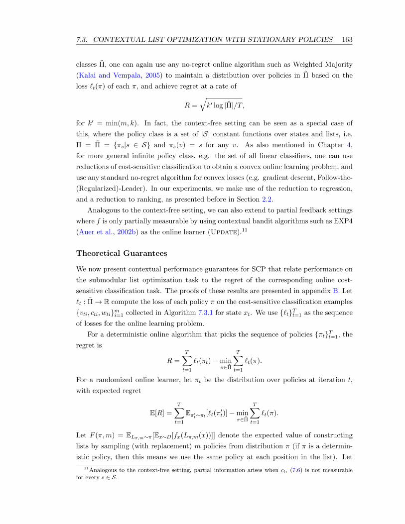
7.3. CONTEXTUAL LIST OPTIMIZATION WITH STATIONARY POLICIES 163
classes Π, one can again use any no-regret online algorithm such as Weighted Majority
(Kalai and Vempala, 2005) to maintain a distribution over policies in Π based on the
loss `t(π) of each π, and achieve regret at a rate of
R =
√k′ log |Π|/T ,
for k′ = min(m, k). In fact, the context-free setting can be seen as a special case of
this, where the policy class is a set of |S| constant functions over states and lists, i.e.
Π = Π = πs|s ∈ S and πs(v) = s for any v. As also mentioned in Chapter 4,
for more general infinite policy class, e.g. the set of all linear classifiers, one can use
reductions of cost-sensitive classification to obtain a convex online learning problem, and
use any standard no-regret algorithm for convex losses (e.g. gradient descent, Follow-the-
(Regularized)-Leader). In our experiments, we make use of the reduction to regression,
and a reduction to ranking, as presented before in Section 2.2.
Analogous to the context-free setting, we can also extend to partial feedback settings
where f is only partially measurable by using contextual bandit algorithms such as EXP4
(Auer et al., 2002b) as the online learner (Update).11
Theoretical Guarantees
We now present contextual performance guarantees for SCP that relate performance on
the submodular list optimization task to the regret of the corresponding online cost-
sensitive classification task. The proofs of these results are presented in appendix B. Let
`t : Π→ R compute the loss of each policy π on the cost-sensitive classification examples
vti, cti, wtimi=1 collected in Algorithm 7.3.1 for state xt. We use `tTt=1 as the sequence
of losses for the online learning problem.
For a deterministic online algorithm that picks the sequence of policies πtTt=1, the
regret is
R =
T∑t=1
`t(πt)−minπ∈Π
T∑t=1
`t(π).
For a randomized online learner, let πt be the distribution over policies at iteration t,
with expected regret
E[R] =
T∑t=1
Eπ′t∼πt [`t(π′t)]−min
π∈Π
T∑t=1
`t(π).
Let F (π,m) = ELπ,m∼π[Ex∼D[fx(Lπ,m(x))]] denote the expected value of constructing
lists by sampling (with replacement) m policies from distribution π (if π is a determin-
istic policy, then this means we use the same policy at each position in the list). Let
11Analogous to the context-free setting, partial information arises when cti (7.6) is not measurablefor every s ∈ S.
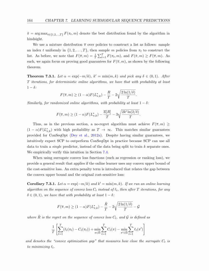
164 CHAPTER 7. LEARNING SUBMODULAR SEQUENCE PREDICTIONS
π = arg maxt∈1,2,...,T F (πt,m) denote the best distribution found by the algorithm in
hindsight.
We use a mixture distribution π over policies to construct a list as follows: sample
an index t uniformly in 1, 2, . . . , T, then sample m policies from πt to construct the
list. As before, we note that F (π,m) = 1T
∑Tt=1 F (πt,m), and F (π,m) ≥ F (π,m). As
such, we again focus on proving good guarantees for F (π,m), as shown by the following
theorem.
Theorem 7.3.1. Let α = exp(−m/k), k′ = min(m, k) and pick any δ ∈ (0, 1). After
T iterations, for deterministic online algorithms, we have that with probability at least
1− δ:
F (π,m) ≥ (1− α)F (L∗π,k)−R
T− 2
√2 ln(1/δ)
T.
Similarly, for randomized online algorithms, with probability at least 1− δ:
F (π,m) ≥ (1− α)F (L∗π,k)−E[R]
T− 3
√2k′ ln(2/δ)
T.
Thus, as in the previous section, a no-regret algorithm must achieve F (π,m) ≥(1 − α)F (L∗π,k) with high probability as T → ∞. This matches similar guarantees
provided for ConSeqOpt (Dey et al., 2012a). Despite having similar guarantees, we
intuitively expect SCP to outperform ConSeqOpt in practice because SCP can use all
data to train a single predictor, instead of the data being split to train k separate ones.
We empirically verify this intuition in Section 7.4.
When using surrogate convex loss functions (such as regression or ranking loss), we
provide a general result that applies if the online learner uses any convex upper bound of
the cost-sensitive loss. An extra penalty term is introduced that relates the gap between
the convex upper bound and the original cost-sensitive loss:
Corollary 7.3.1. Let α = exp(−m/k) and k′ = min(m, k). If we run an online learning
algorithm on the sequence of convex loss Ct instead of `t, then after T iterations, for any
δ ∈ (0, 1), we have that with probability at least 1− δ:
F (π,m) ≥ (1− α)F (L∗π,k)−R
T− 2
√2 ln(1/δ)
T− G
where R is the regret on the sequence of convex loss Ct, and G is defined as
1
T
[T∑t=1
(`t(πt)− Ct(πt)) + minπ∈Π
T∑t=1
Ct(π)− minπ′∈Π
T∑t=1
`t(π′)
]
and denotes the “convex optimization gap” that measures how close the surrogate Ct is
to minimizing `t.

7.4. CASE STUDIES 165
This result implies that using a good surrogate convex loss for no-regret convex
optimization will lead to a policy that has a good performance relative to the optimal
list of policies. Note that the gap G often may be small or non-existent. For instance,
in the case of the reduction to regression or ranking, G = 0 in realizable settings where
there exists a “perfect” predictor in the class. Similarly, in cases where the problem is
near-realizable we would expect G to be small.12
Discussion
The SCP procedure provides a reduction of contextual submodular list optimization
to an online cost-sensitive classification problem. Here we obtain a regret reduction,
where no-regret on this online learning task directly implies that we will find policies for
constructing lists with near-optimal performance guarantees (in particular with the same
guarantee as a clairvoyant greedy algorithm). The result here is stronger than in the
prior imitation learning and structured prediction setting, as there is no dependency on
the regret to the bayes-optimal classifier, as was present when using cost-to-go. Although
this was in part due to the fact that in prior settings, performance was compared to the
expert, which is a policy potentially outside of the class of policies. Here by comparing
directly to the best sequence of policies from within the class Π, we obtain a guarantee
that does not involve this term. In addition here, the submodularity property allows us
to guarantee near-globally optimal performance, whereas in imitation learning, we could
only guarantee good relative performance compared to the expert.
7.4 Case Studies
We now demonstrate experimentally the improved efficiency of SCP over previous meth-
ods. We compare performance on 4 different tasks. A context-free Grasp Selection task,
and 3 contextual tasks: Trajectory Optimization, News Recommendation and Document
Summarization.
Grasp Selection
We first applied SCP to a context-free task of grasp selection for a robot manipulator
introduced in Dey et al. (2012b) (see Figure 7.2). The goal is to order the grasps in a
library of grasps in such a way that good grasps can be found quickly (by going through
the list in sequence) to pick up the object in front of the robot.
12We conjecture that this gap term G is not specific to our particular scenario, but rather is (im-plicitly) always present whenever one attempts to optimize classification accuracy via surrogate convexoptimization. For instance, when training a SVM in standard batch supervised learning, we would onlyexpect that minimizing the hinge loss is a good surrogate for minimizing the 0-1 loss when the analogousconvex optimization gap is small.
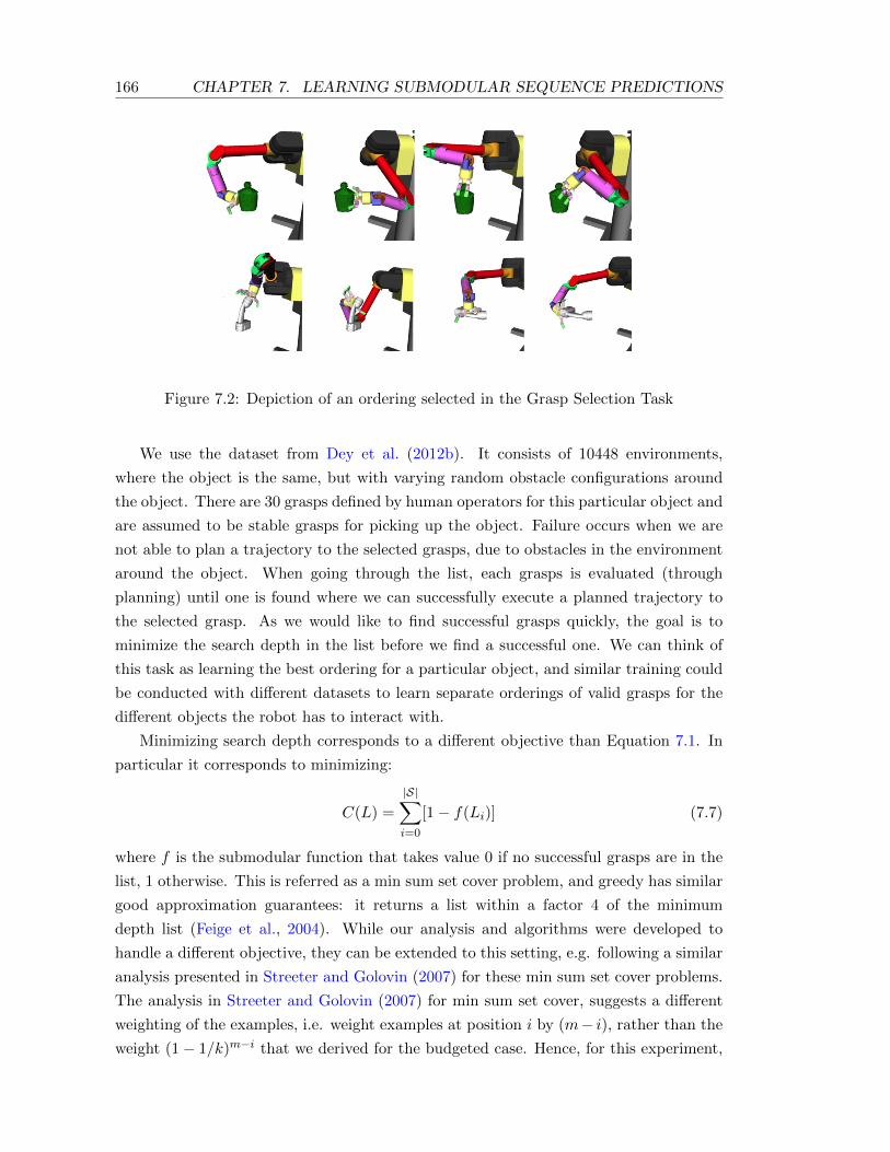
166 CHAPTER 7. LEARNING SUBMODULAR SEQUENCE PREDICTIONS
Figure 7.2: Depiction of an ordering selected in the Grasp Selection Task
We use the dataset from Dey et al. (2012b). It consists of 10448 environments,
where the object is the same, but with varying random obstacle configurations around
the object. There are 30 grasps defined by human operators for this particular object and
are assumed to be stable grasps for picking up the object. Failure occurs when we are
not able to plan a trajectory to the selected grasps, due to obstacles in the environment
around the object. When going through the list, each grasps is evaluated (through
planning) until one is found where we can successfully execute a planned trajectory to
the selected grasp. As we would like to find successful grasps quickly, the goal is to
minimize the search depth in the list before we find a successful one. We can think of
this task as learning the best ordering for a particular object, and similar training could
be conducted with different datasets to learn separate orderings of valid grasps for the
different objects the robot has to interact with.
Minimizing search depth corresponds to a different objective than Equation 7.1. In
particular it corresponds to minimizing:
C(L) =
|S|∑i=0
[1− f(Li)] (7.7)
where f is the submodular function that takes value 0 if no successful grasps are in the
list, 1 otherwise. This is referred as a min sum set cover problem, and greedy has similar
good approximation guarantees: it returns a list within a factor 4 of the minimum
depth list (Feige et al., 2004). While our analysis and algorithms were developed to
handle a different objective, they can be extended to this setting, e.g. following a similar
analysis presented in Streeter and Golovin (2007) for these min sum set cover problems.
The analysis in Streeter and Golovin (2007) for min sum set cover, suggests a different
weighting of the examples, i.e. weight examples at position i by (m− i), rather than the
weight (1− 1/k)m−i that we derived for the budgeted case. Hence, for this experiment,
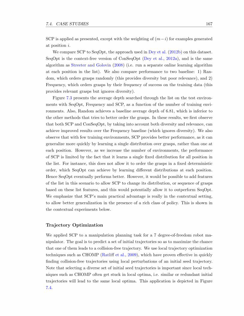
7.4. CASE STUDIES 167
SCP is applied as presented, except with the weighting of (m− i) for examples generated
at position i.
We compare SCP to SeqOpt, the approach used in Dey et al. (2012b) on this dataset.
SeqOpt is the context-free version of ConSeqOpt (Dey et al., 2012a), and is the same
algorithm as Streeter and Golovin (2008) (i.e. run a separate online learning algorithm
at each position in the list). We also compare performance to two baseline: 1) Ran-
dom, which orders grasps randomly (this provides diversity but poor relevance), and 2)
Frequency, which orders grasps by their frequency of success on the training data (this
provides relevant grasps but ignores diversity).
Figure 7.3 presents the average depth searched through the list on the test environ-
ments with SeqOpt, Frequency and SCP, as a function of the number of training envi-
ronments. Also, Random achieves a baseline average depth of 6.81, which is inferior to
the other methods that tries to better order the grasps. In these results, we first observe
that both SCP and ConSeqOpt, by taking into account both diversity and relevance, can
achieve improved results over the Frequency baseline (which ignores diversity). We also
observe that with few training environments, SCP provides better performance, as it can
generalize more quickly by learning a single distribution over grasps, rather than one at
each position. However, as we increase the number of environments, the performance
of SCP is limited by the fact that it learns a single fixed distribution for all position in
the list. For instance, this does not allow it to order the grasps in a fixed deterministic
order, which SeqOpt can achieve by learning different distributions at each position.
Hence SeqOpt eventually performs better. However, it would be possible to add features
of the list in this scenario to allow SCP to change its distribution, or sequence of grasps
based on these list features, and this would potentially allow it to outperform SeqOpt.
We emphasize that SCP’s main practical advantage is really in the contextual setting,
to allow better generalization in the presence of a rich class of policy. This is shown in
the contextual experiments below.
Trajectory Optimization
We applied SCP to a manipulation planning task for a 7 degree-of-freedom robot ma-
nipulator. The goal is to predict a set of initial trajectories so as to maximize the chance
that one of them leads to a collision-free trajectory. We use local trajectory optimization
techniques such as CHOMP (Ratliff et al., 2009), which have proven effective in quickly
finding collision-free trajectories using local perturbations of an initial seed trajectory.
Note that selecting a diverse set of initial seed trajectories is important since local tech-
niques such as CHOMP often get stuck in local optima, i.e. similar or redundant initial
trajectories will lead to the same local optima. This application is depicted in Figure
7.4.
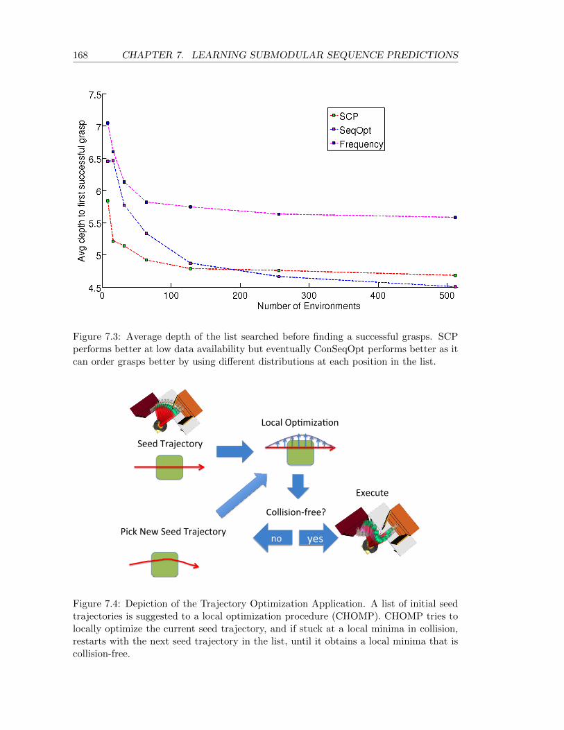
168 CHAPTER 7. LEARNING SUBMODULAR SEQUENCE PREDICTIONS
Figure 7.3: Average depth of the list searched before finding a successful grasps. SCPperforms better at low data availability but eventually ConSeqOpt performs better as itcan order grasps better by using different distributions at each position in the list.
Seed Trajectory
Local Op1miza1on
Collision‐free?
Pick New Seed Trajectory
Execute
yes no
Figure 7.4: Depiction of the Trajectory Optimization Application. A list of initial seedtrajectories is suggested to a local optimization procedure (CHOMP). CHOMP tries tolocally optimize the current seed trajectory, and if stuck at a local minima in collision,restarts with the next seed trajectory in the list, until it obtains a local minima that iscollision-free.
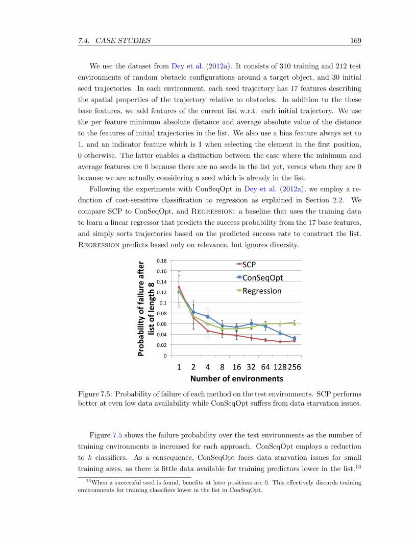
7.4. CASE STUDIES 169
We use the dataset from Dey et al. (2012a). It consists of 310 training and 212 test
environments of random obstacle configurations around a target object, and 30 initial
seed trajectories. In each environment, each seed trajectory has 17 features describing
the spatial properties of the trajectory relative to obstacles. In addition to the these
base features, we add features of the current list w.r.t. each initial trajectory. We use
the per feature minimum absolute distance and average absolute value of the distance
to the features of initial trajectories in the list. We also use a bias feature always set to
1, and an indicator feature which is 1 when selecting the element in the first position,
0 otherwise. The latter enables a distinction between the case where the minimum and
average features are 0 because there are no seeds in the list yet, versus when they are 0
because we are actually considering a seed which is already in the list.
Following the experiments with ConSeqOpt in Dey et al. (2012a), we employ a re-
duction of cost-sensitive classification to regression as explained in Section 2.2. We
compare SCP to ConSeqOpt, and Regression: a baseline that uses the training data
to learn a linear regressor that predicts the success probability from the 17 base features,
and simply sorts trajectories based on the predicted success rate to construct the list.
Regression predicts based only on relevance, but ignores diversity.
0"
0.02"
0.04"
0.06"
0.08"
0.1"
0.12"
0.14"
0.16"
0.18"
1" 2" 4" 8" 16" 32" 64" 128"256"
Probability*of*failure*a.er**
list*of*length*8*
Number*of*environments*
SCP"
ConSeqOpt"
Regression"
Figure 7.5: Probability of failure of each method on the test environments. SCP performsbetter at even low data availability while ConSeqOpt suffers from data starvation issues.
Figure 7.5 shows the failure probability over the test environments as the number of
training environments is increased for each approach. ConSeqOpt employs a reduction
to k classifiers. As a consequence, ConSeqOpt faces data starvation issues for small
training sizes, as there is little data available for training predictors lower in the list.13
13When a successful seed is found, benefits at later positions are 0. This effectively discards trainingenvironments for training classifiers lower in the list in ConSeqOpt.

170 CHAPTER 7. LEARNING SUBMODULAR SEQUENCE PREDICTIONS
0"
0.2"
0.4"
0.6"
1" 2" 3" 4" 5"
Probabilty*of*no*
click*
Slots*
ConSeqOpt"
SCP"
Figure 7.6: Probability of no click on the test users on the news recommendation task.With increase in slots SCP predicts news articles which have lower probability of theuser not clicking on any of them compared to ConSeqOpt
In contrast, SCP has no data starvation issue and learns a single good policy to construct
the list much more quickly. The worse performance of Regression also demonstrates
that SCP and ConSeqOpt (after sufficient data) can better capture the importance of
diversity when recommending list of options.
News Recommendation
In the news recommendation setting the task, the goal is to present a sequence of news
articles to a user so as to maximize the probability of the user clicking on at least 1
recommended article.
We built a stochastic user simulation based on 75 user preferences derived from a user
study in Yue and Guestrin (2011). Using this simulation as a training oracle, our goal is
to learn to recommend articles to any user (depending on their contextual features) to
minimize the failure case where the user does not like any of the recommendations.14
Articles are represented by features, and user preferences by linear weights. We
derived user contexts by soft-clustering users into groups, and using corrupted group
memberships as contexts.
We perform five-fold cross validation. In each fold, we train SCP and ConSeqOpt on
40 users’ preferences, use 20 users for validation, and then test on the held-out 15 users.
Training, validation and testing are all performed via simulation.
Figure 7.6 shows the results, where we see the recommendations made by SCP
achieves significantly lower failure rate as the number of recommendations is increased
from 1 to 5.
14Also known as abandonment (Radlinski et al., 2008).
7.4. CASE STUDIES 171
Document Summarization
In the extractive multi-document summarization task, the goal is to extract sentences
(with character budget B) to maximize coverage of human-annotated summaries. Fol-
lowing the experimental setup from Lin and Bilmes (2010) and Kulesza and Taskar
(2011), we use data from the Document Understanding Conference (DUC) 2003 and
2004 (Task 2) (Dang, 2005). Each training or test instance corresponds to a cluster of
documents, and contains approximately 10 documents belonging to the same topic and
four human reference summaries. We train on the 2003 data (30 clusters) and test on
the 2004 data (50 clusters). The budget is B = 665 bytes, including spaces.
We use the ROUGE (Lin, 2004) unigram statistics (ROUGE-1R, ROUGE-1P,ROUGE-
1F) for performance evaluation. Our method directly attempts to optimize the ROUGE-
1R objective with respect to the reference summaries, which can be easily shown to be
monotone submodular (Lin and Bilmes, 2011).
We aim to predict sentences that are both short and informative. Therefore we
maximize the normalized marginal benefit,
b′(s|Lt,i−1) = b(s|Lt,i−1)/l(s), (7.8)
where l(s) is the length of the sentence s.15 We use a reduction to ranking as described in
Section 2.2 using (7.8) to train a SVM that ranks the sentences. While not performance-
optimized, our approach takes less than 15 minutes to train.
Following Kulesza and Taskar (2011), we consider features fi for each sentence con-
sisting of quality features qi and similarity features φi (fi = [qTi , φTi ]T ). The quality
features, attempt to capture the representativeness for a single sentence. Similarity
features qi for sentence si as we construct the list Lt measure a notion of distance of
a proposed sentence to sentences already included in the set. A variety of similarity
features were considered, with the simplest being average squared distance of TF-IDF
vectors. Performance was very stable across different features. The experiments pre-
sented use three types: 1) following the idea in Kulesza and Taskar (2011) of similarity
as a volume metric, we compute the squared volume of the parallelopiped spanned by
the TF-IDF vectors of sentences in the list Lt,k⊕ si; 2) the product between this volume
and the quality features; 3) the minimum absolute distance of quality features between
si and each element in Lt,k.
Table 7.1 shows the performance (Rouge unigram statistics) comparing SCP with ex-
isting algorithms. We observe that SCP outperforms existing state-of-the-art approaches,
15Because each sentence contains a different number of characters/bytes, this results in a knapsackconstrained optimization problem where items have different weights. Under such constraint, the greedyalgorithm picks items with highest normalized benefits. This is why we also normalized the benefits forour algorithm. We expect our approach to perform well in this setting, but defer a formal analysis forfuture work.
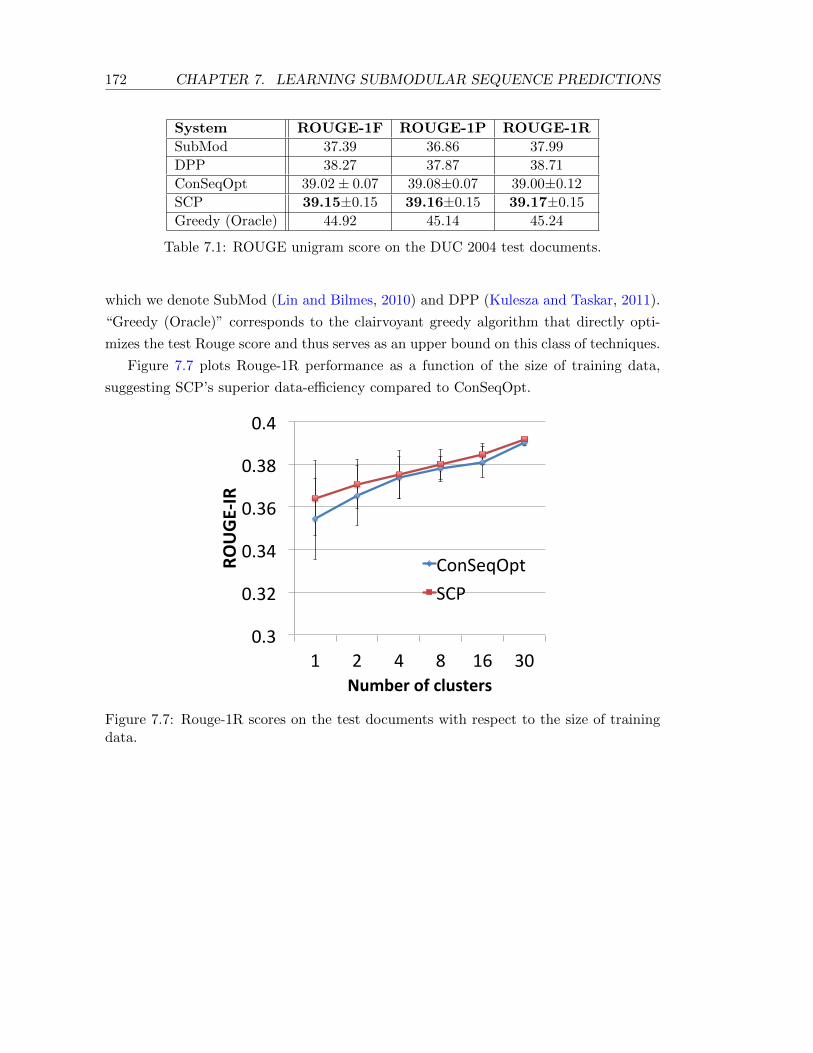
172 CHAPTER 7. LEARNING SUBMODULAR SEQUENCE PREDICTIONS
System ROUGE-1F ROUGE-1P ROUGE-1R
SubMod 37.39 36.86 37.99
DPP 38.27 37.87 38.71
ConSeqOpt 39.02± 0.07 39.08±0.07 39.00±0.12
SCP 39.15±0.15 39.16±0.15 39.17±0.15
Greedy (Oracle) 44.92 45.14 45.24
Table 7.1: ROUGE unigram score on the DUC 2004 test documents.
which we denote SubMod (Lin and Bilmes, 2010) and DPP (Kulesza and Taskar, 2011).
“Greedy (Oracle)” corresponds to the clairvoyant greedy algorithm that directly opti-
mizes the test Rouge score and thus serves as an upper bound on this class of techniques.
Figure 7.7 plots Rouge-1R performance as a function of the size of training data,
suggesting SCP’s superior data-efficiency compared to ConSeqOpt.
0.3$
0.32$
0.34$
0.36$
0.38$
0.4$
1$ 2$ 4$ 8$ 16$ 30$
ROUGE&IR(
Number(of(clusters(
ConSeqOpt$
SCP$
Figure 7.7: Rouge-1R scores on the test documents with respect to the size of trainingdata.
Chapter 8
Learning Dynamic Models for
Good Control Performance
We now move on to investigate a final and important sequential prediction task : system
identification – learning a dynamic model of a system from observations that is useful for
planning and controller synthesis. As most robotic systems use some form of planning
algorithms for decision-making, having good predictive models of the future outcomes of
different courses of action is crucial in many control applications. We focus on learning
models that ultimately provide good control performance guarantees for the particular
task of interest (and not simply high accuracy at predicting future states under the
execution of a particular controller).
As mentioned in Chapter 1, in system identification, a similar train-test mismatch
can occur as the policy resulting from controller synthesis is often very different from the
“exploration” policy used to collect data and fit the dynamic model. While we might
expect the model to make good predictions at states frequented by the exploration policy,
the learned policy usually induces a different state distribution, where the model may
poorly capture system behavior (as in Figure 1.2 in Chapter 1), and lead to poor control
performance.
In this chapter, we present how the DAGGER learning strategy can be adapted in this
setting to obtain an iterative and interactive learning procedure that learns a good model
for controller synthesis. Unlike prior work in this setting, our method provides strong
control performance guarantees in fully agnostic settings where the real system may not
be modeled perfectly by any model in the class considered by the learning algorithm.
Good control performance is guaranteed under the weaker agnostic assumption that
some model in the class can achieve statistically good prediction on the training data.
We begin by briefly reviewing previous and related work, and defining formally our
objective and notation. We then provide an agnostic analysis of the common text-
book/batch system identification approach that consists in simply treating system iden-
174CHAPTER 8. LEARNING DYNAMIC MODELS FOR GOOD CONTROL
PERFORMANCE
tification as a standard statistical learning problem, learning only from data collected by
some exploration policy (e.g. open loop controls, an expert performing the task, or some
other base controller we want to improve upon), and then planning with the resulting
learned model. Our analysis formalizes the train-test mismatch this approach can suf-
fer from and its resulting poor control guarantees. We then present our adaptation of
DAGGER to this setting, with its improved agnostic guarantees on control performance.
Finally we demonstrate the efficacy of our approach on a challenging domain from the
literature: learning to perform aerobatic maneuvers with a simulated helicopter (Abbeel
and Ng, 2005). This adaptation of DAGGER and part of the results presented here were
originally presented in Ross and Bagnell (2012a).
8.1 Preliminaries
We here review previous and related work in system identification. The literature on this
topic is vast and distributed across many fields of engineering and computer science. We
begin by giving a brief overview of the work in the control literature, and then in artificial
intelligence on model-based reinforcement learning. We then discuss more specifically
methods closely related to our work.
System Identification
In the system identification literature on the control side, much of the work has focused
on continuous systems, and particularly on learning linear dynamical systems. The prob-
lem of interest is to learn dynamic models that can predict future output observations,
by observing a stream of observations and input controls. Different methods have been
developed to learn such systems in the frequency domain, or the time domain. Tradi-
tional identification methods have exploited the linear properties of the model to learn
the model in the frequency domain (Ljung, 1999). Namely, they exploit the fact that the
frequency response of a linear system to any linear combination of basis control signals
is simply the linear combination of the frequency response to each basis signals. This
makes learning easy as these approaches can simply record the frequency response of
the system to a set of basis control signals, typically chosen to cover the range of fre-
quencies the controller will use. For state-space time domain linear models, two main
approaches were developed: 1) methods based on deterministic/stochastic realization,
which learns the system based on spectral learning methods, such as SVD, that can
recover the parameters of the linear systems through matrix factorization of a Hankel or
covariance matrix (Ho and Kalman, 1965, Akaike, 1975, Overschee and Moor, 1996), and
2) methods based on prediction error/maximum likelihood, that adopts a more statisti-
cal learning/regression approach, e.g. learning an ARX model that predicts the future
8.1. PRELIMINARIES 175
output observation from the past few controls and observations (Astrom, 1965, 1971,
Ljung, 1978, 1999). To our knowledge, the theoretical analysis of both types of methods
assume that the real system is linear, and guarantees identifying the true parameters (or
up to an equivalent transformation) of the system under some conditions on the controls
(e.g. white noise, persistent excitation, open loop controls), that prevents correlations
between control and state, and sufficiently explore all modes of the linear system.
Much work has also been done in non-linear system identification, where most of the
work are methods based on learning complex parametric models, such as neural networks,
for minimizing prediction error, or using a wide variety of non-parametric methods (see
Sjoberg et al. (1995) for a nice survey). Much of the theoretical results in this case are
concerned with convergence of the prediction error to the minimum under the training
distribution, e.g. assuming data is observed from a stationary markov process (Juditsky
et al., 1995). As these non-parametric methods can fit arbitrarily well any function,
again this is essentially assuming realizability. In addition, in this case, not much can
be said about control performance, if such non-linear model would be used for control
(e.g. due to the train-test mismatch, we may still obtain a poor controller).
Much of the earlier work up to the late eighties rarely considered the relation of
system identification performance to control performance. More recent developments, in
what’s called “identification for control”, have started analyzing the problem of system
identification for purposes of obtaining a good controller (Gevers and Ljung, 1986, Hjal-
marsson et al., 1996, Forssell and Ljung, 1999, 2000). Work in this area have showed
the benefits of using iterative identification procedures under closed-loop control, e.g. by
using the current controller, synthesized under the current model to collect more data
(Hjalmarsson et al., 1996). Theoretical analysis in this case again typically assumes
a realizable setting with linear models, and is typically concerned with analyzing the
bias/variance of the estimator of the linear model, and analyzing what would be the
optimal experiment design (i.e. controller to execute) to, e.g., minimize the variance
(Gevers and Ljung, 1986, Hjalmarsson et al., 1996, Forssell and Ljung, 1999, 2000).
Our work fits into this later category of identification for control, and suggests a
similar iterative system identification procedure with closed-loop controllers. However
our results extend beyond learning of linear models and provide analysis for a general
agnostic setting and general conditions under which we may expect to find good con-
trollers.
Model-Based Reinforcement Learning
In the model-based reinforcement learning (MBRL) literature, most methods have fo-
cused on discrete control problems where a finite MDP model of the system is learned.
In this case the next state distribution for each state-action pair is directly estimated
176CHAPTER 8. LEARNING DYNAMIC MODELS FOR GOOD CONTROL
PERFORMANCE
from the observed empirical distribution of next states. More complex models were also
proposed that attempts to improve generalization across states/actions, such as hierar-
chical models (Dietterich, 2000, Jong and Stone, 2008), factorized models (Kearns and
Koller, 1999, Ross and Pineau, 2008, Hester and Stone, 2009) and relational models
(Walsh et al., 2009). Some work also consider continuous MDP, and often uses state ag-
gregation based models (tree-based/grid based discretization)(Uther and Veloso, 1998,
Bernstein and Shinkin, 2010), linear models (Strehl and Littman, 2007, Walsh et al.,
2009), and more recent techniques have used non-parametric bayesian Gaussian Process
models (Deisenroth and Rasmussen, 2011).
A significant part of the work in reinforcement learning has focused on the exploration-
exploitation issue: where should data be collected to improve performance and when
should we stop exploring and simply exploit current knowledge of the system to achieve
the task. State-of-the-art RL methods have addressed this issue by either 1) being op-
timistic about the value of state-action pairs that have not been visited often enough
and planning an optimal policy in a resulting optimistic model to compute the policy to
execute (Strehl et al., 2009, Jaksch et al., 2010) or 2) using a bayesian approach where
a prior on the transition model is used and solving a POMDP to compute an optimal
exploration-exploitation strategy under this prior (Poupart et al., 2006, Ross, 2008).
Similar bayesian approaches were also proposed in the adaptive control and dual control
literature (Fel’dbaum, 1965, Bar-Shalom, 1981, Astrom and Wittenmark, 1989). Other
techniques have proposed using apprenticeship learning techniques for exploration, where
expert demonstrations are initially used to collect data and fit a first model (Abbeel and
Ng, 2005). Then at subsequent iterations, the current optimal policy is used to collect
more data and improve the model until a policy is found that is at least as good as the
expert.
Theoretical analysis in model-based reinforcement learning also assumes realizable
settings, i.e. that the real system has the same structure as the class of model considered.
The optimistic exploration strategy of many model-based RL methods also assumes
realizability in order to provide good results (Strehl et al., 2009, Jaksch et al., 2010).
Spectral Learning of Dynamic Models
In addition to spectral learning methods developed in the system identification literature,
other spectral methods have been developed recently in the machine learning literature
for learning discrete hidden state dynamic models from a stream of observations. Hsu
et al. (2009) first introduced a spectral algorithm for learning hidden markov models1
(HMM) of a stream of observation, which was then generalized in Siddiqi et al. (2010)
to learn more rich and compact representations, called Reduced-Rank HMM. The latter
1A HMM is a POMDP without actions and costs
8.1. PRELIMINARIES 177
was also applied for learning hidden state models for control, called predictive state
representations2 (PSR) (Siddiqi et al., 2010, Boots et al., 2011, Boots and Gordon, 2011).
The analysis of these spectral learning methods also rely on realizability assumptions,
in that they guarantee that in the limit they will learn an equivalent model to the true
model, if the true model belongs to the model class. In addition, their analysis focuses
on statistical consistency, and does not relate the estimation error (from finite sampled
data) of the model to the resulting control performance.
Iterative Methods in Practice
In practice control engineers often proceed iteratively to build good models for controller
synthesis, as suggested in recent identification for control methods. For instance, they
may collect a first batch of data to fit a model and obtain a controller, which is then
tested in the real system. If performance is unsatisfactory, data collection is repeated
with different sampling distributions to improve the model where needed, until control
performance is satisfactory. By doing so, engineers can use feedback of the policies found
during training to decide how to collect data and improve performance. Such methods
are commonly used in practice and have demonstrated good performance in the work of
Atkeson and Schaal (1997), Abbeel and Ng (2005). In both works, the authors proceed
by fitting a first model from state transitions observed during expert demonstrations of
the task, and at following iterations, using the optimal policy under the current model
to collect more data and fit a new model with all data seen so far. Abbeel and Ng
(2005) show this approach has good guarantees in realizable settings (for finite MDPs or
LQRs), in that it must find a policy that performs as well as the expert providing the
initial demonstrations. Our method can be seen as making algorithmic this engineering
practice, extending and generalizing the previous methods of Atkeson and Schaal (1997),
Abbeel and Ng (2005) and other similar iterative identification methods, and suggesting
slight modifications that provide good guarantees even in agnostic settings.
Agnostic Exploration
Our approach leverages the way agnostic model-free RL algorithms perform exploration.
Methods such as Conservative Policy Iteration (CPI) (Kakade and Langford, 2002) and
Policy-Search by Dynamic Programming (PSDP) (Bagnell et al., 2003) learn a policy
directly by updating policy parameters iteratively. For exploration, they assume access
to a state exploration distribution ν that they can restart the system from and can
guarantee finding a policy performing nearly as well as any policies inducing a state
distribution (over a whole trajectory) close to ν (e.g. similar to the result for DAGGER
2A PSR is an alternate, more rich and compact representation of POMDPs.
178CHAPTER 8. LEARNING DYNAMIC MODELS FOR GOOD CONTROL
PERFORMANCE
with learner’s cost-to-go presented in Section 4.3). Similarly, our approach below uses
a state-action exploration distribution to sample transitions and allows us to guarantee
good performance compared to any policy with a state-action distribution close to this
exploration distribution. If the exploration distribution is close to that of a near-optimal
policy, then our approach guarantees near-optimal performance, provided a good model
of data exists. This allows our model-based method to match the strongest agnostic
guarantees of existing model-free methods. Good exploration distributions can often be
obtained in practice; e.g., from human expert demonstrations, domain knowledge, or
from a desired trajectory we would like the system to follow. Additionally, if we have a
base policy we want to improve, it can be used to generate the exploration distribution
– with potentially additional random exploration in the actions.
8.2 Problem Formulation and Notation
We now formalize our system identification setting, objectives and notation.
We assume the real system behaves according to some unknown MDP, represented
by a set of states S and actions A (both potentially infinite and continuous), an unknown
transition function T , where Tsa denotes the next state distribution if we do action a
in state s, and the initial state distribution µ at time 1. We assume the cost function
C : S × A → R is known and seek to minimize the expected sum of discounted costs
over an infinite horizon with discount γ. We assume for simplicity of exposition that the
states are observed, but our algorithms and analysis also extend to partially observable
settings. This is discussed further in Section 8.4.
For any policy π, we denote:
• π(s) the action distribution performed by π in state s;
• Dtω,π the state-action distribution at time t if we started in state distribution ω at
time 1 and followed π;
• Dω,π = (1− γ)∑∞
t=1 γt−1Dt
ω,π the “discounted” state-action distribution over the
infinite horizon if we follow π, starting in ω at time 1;
• Vπ(s) = Ea∼πs,s′∼Tsa [C(s, a) + γVπ(s′)] the value function of π (the expected sum
of discounted costs of following π starting in state s);
• Qπ(s, a) = C(s, a) + γEs′∼Tsa [Vπ(s′)] the action-value function of π (the expected
sum of discounted costs of following π after starting in s and performing action a);
• Jω(π) = Es∼ω[Vπ(s)] = 11−γE(s,a)∼Dω,π [C(s, a)] the expected sum of discounted
costs of following π starting in ω.
8.3. BATCH OFF-POLICY LEARNING APPROACH 179
Our goal is to obtain a policy π with small regret, i.e. for any policy π′, Jµ(π)−Jµ(π′)
is small (or negative). This is achieved indirectly by learning a model T of the system
and solving for a (near-)optimal policy (under T and the known cost function C); e.g.,
using dynamic programming (Puterman, 1994) or approximate methods (Gordon, 1995,
Williams, 1992, Li and Todorov, 2004, Jacobson and Mayne, 1970).
8.3 Batch Off-policy Learning Approach
We now describe a simple algorithm, referred to as Batch, that can be used to analyze
many common approaches from the literature, e.g., learning from a generative model3,
open loop excitation or by watching an expert (Ljung, 1999).
Let T denote the class of transition models considered, and ν a state-action explo-
ration distribution we can sample the system from. Batch first observes m sampled
transitions in the real system, occurring in m state-action pairs sampled i.i.d. from ν.
Then it finds the best model T ∈ T of observed transitions, and solves (potentially ap-
proximately) the optimal control (OC) problem with T and known cost function C to
return a policy π for test execution.
Analysis
Our analysis seeks to answer the following question: if Batch learns a model T with small
error on training data, and solves the OC problem well (e.g. finds a near-optimal policy
for T ), what guarantees does it provide on control performance of π in the real system?
Our results illustrate the drawbacks of a purely batch method due to the mismatch in
train-test distribution. The proofs of all results presented here can be found in appendix
C.
First, we measure the quality of the OC problem’s solution as follows. For any policy
π′, let
επ′
oc = Es∼µ[V π(s)− V π′(s)]
denote how much better π′ is compared to π on model T (V π and V π′ are the value
functions of π and π′ under learned model T respectively). If π is an ε-optimal policy
on T within some class of policies Π, then επ′
oc ≤ ε for all π′ ∈ Π.
Next, to measure model error, a natural notion of error that arises from our analysis
is the L1 distance between the predicted and true next state’s distributions. That is, we
define:
εL1prd = E(s,a)∼ν [||Tsa − Tsa||1],
the predictive error of T , measured in L1 distance, under the training distribution ν.
3With a generative model, we can set the system to any state, perform any action to obtain a sampletransition.

180CHAPTER 8. LEARNING DYNAMIC MODELS FOR GOOD CONTROL
PERFORMANCE
A drawback of this L1 distance is that it cannot be evaluated or optimized from
sampled transitions observed during training (we observe next states sampled from Tsa
but not the distribution itself). Therefore we also provide our bounds in terms of other
notions of error/loss we can minimize from training samples. This allows to directly
relate control performance to the model’s training loss. A convenient loss is the KL
divergence between Tsa and Tsa:
εKLprd = E(s,a)∼ν,s′∼Tsa [log(Tsa(s
′))− log(Tsa(s′))].
Minimizing KL corresponds to maximizing the log likelihood of the sampled transitions.
This is convenient for common model classes, such as linear models (as in LQR), where
it amounts to solving a linear regression problem. For particular cases where T is a set
of deterministic models and the real system has finitely many states, the predictive error
can be related to a classification loss at predicting the next state:
εclsprd = E(s,a)∼ν,s′∼Tsa [`(T , s, a, s′)],
for ` the 0-1 loss of whether T predicts s′ for (s, a), or any upper bound on the 0-1 loss,
e.g., the multi-class hinge loss if T is a set of SVMs. In this case, model fitting is a
supervised classification problem and the guarantee is directly related to the training
classification loss. These different notions of error are related as follows:
Lemma 8.3.1.
εL1prd ≤√
2εKLprd,
εL1prd ≤ 2εclsprd.
The latter holds with equality if ` is the 0-1 loss.
In general, we could also use any other loss that can be minimized from samples and
that upper bounds εL1prd for models in the class.
Another important component of our analysis is the mismatch between the explo-
ration distribution ν and the distribution induced by executing another policy π starting
in µ. We measure this mismatch as follows:
cπν = sups,a
Dµ,π(s, a)
ν(s, a).
Intuitively, cπν captures whether there exists state-action pairs (s, a) that are encountered
often by the policy π, but that were rarely explored under the exploration distribution
ν. When that’s the case cπν is large (it can be arbitrarily large and potentially infinite
if some state-action pair (s, a) is likely under π, but have probability 0 to be explored
under ν). In the ideal case where there is no mismatch, i.e. ν = Dµ,π, then cπν = 1.
8.3. BATCH OFF-POLICY LEARNING APPROACH 181
We will also assume the costs are bounded in some range, i.e. C(s, a) ∈ [Cmin, Cmax]
∀(s, a). Let Crng = Cmax − Cmin and H =γCrng
(1−γ)2. H is a scaling factor that relates
model error to error in total cost predictions. Then the policy learned by Batch has the
following performance guarantee when performing the task in the real system:
Theorem 8.3.1. The policy π is s.t. for any policy π′:
Jµ(π) ≤ Jµ(π′) + επ′
oc +cπν + cπ
′ν
2HεL1prd
This also holds as a function of εKLprd or εclsprd using the relations in Lemma 8.3.1.
This bound indicates that if Batch solves the OC problem well and T has small
enough error under the training distribution ν, then it must find a good policy. Impor-
tantly, this bound is tight: i.e. we can construct examples where it holds with equality
(see appendix C).
More interestingly is what happens as we collect more and more data. If we use
consistent learning procedures that converge to the best transition model T ∗ in the class
T asymptotically, then we can relate this guarantee to the capacity of the model class to
achieve low predictive error under the training distribution ν. We denote the modeling
error, measured in L1 distance, as:
εL1mdl = inf
T ′∈TE(s,a)∼ν [||Tsa − T ′sa||1].
Similarly, we define the modeling error in terms of the KL divergence and the classifica-
tion loss as follows:
εKLmdl = inf
T ′∈TE(s,a)∼ν,s′∼Tsa [log(Tsa(s
′))− log(T ′sa(s′))],
εclsmdl = inf
T ′∈TE(s,a)∼ν,s′∼Tsa [`(T ′, s, a, s′)].
These modeling errors are all 0 in realizable settings, but generally non-zero in agnos-
tic settings. After observing m sampled transitions, the generalization error εL1gen(m, δ)
bounds with high probability 1 − δ the quantity εL1prd − εL1
mdl. Similarly, εKLgen(m, δ) and
εclsgen(m, δ) denote the generalization error for the KL and classification loss respectively.
For instance, εclsgen(m, δ) can be related to the VC dimension, or analogous multi-class
equivalent, in finite state MDPs (as in standard PAC Learning analysis for classification
problems).
This implies that when learning from a finite amount of data, the guarantee on
control performance with the learned policy by Batch has the following form:
Corollary 8.3.1. After observing m transitions, with probability at least 1− δ, for any
policy π′:
Jµ(π) ≤ Jµ(π′) + επ′
oc +cπν + cπ
′ν
2H[εL1mdl + εL1gen(m, δ)].
182CHAPTER 8. LEARNING DYNAMIC MODELS FOR GOOD CONTROL
PERFORMANCE
This also holds as a function of εKLmdl + εKL
gen(m, δ) (or εclsmdl + εclsgen(m, δ)) using Lem. 8.3.1.
In addition, if the fitting procedure is consistent in terms of L1 distance (or KL, classifi-
cation loss), then εL1gen(m, δ)→ 0 (or εKLgen(m, δ)→ 0, εclsgen(m, δ)→ 0) as m→∞ for any
δ > 0.
As mentioned in Section 2.1, the generalization error typically scales with the com-
plexity of the class T and goes to 0 at a rate of O( 1√m
) (or O( 1m) in ideal conditions).
Given enough samples, the dominating factor limiting performance becomes the model-
ing error: i.e. the term cπν+cπ′ν
2 HεL1mdl (or its equivalent in terms of the KL/classification
loss) quantifies how performance degrades for agnostic settings.
Drawback of Batch: The two factors cπν and cπ′ν are qualitatively different. cπ
′ν mea-
sures how well ν explores state-actions visited by the policy π′ we compare to. This
factor is inevitable: we cannot hope to compete against policies that spend most of their
time in regions that we rarely explore. On the other hand, cπν measures the mismatch in
train-test distribution, i.e. the mismatch between the exploration and where our learned
policy goes during its execution. Its presence is the major drawback of Batch. As π can-
not be known in advance, we can only bound cπν by considering all policies we could learn:
supπ∈Π cπν . This worst case is likely to be realized in practice: if ν rarely explores some
state-action regions, the model could be bad for these and significantly underestimate
their cost. The learned policy is thus encouraged to visit these low-cost regions where
few data were collected. To minimize supπ∈Π cπν , the best ν for Batch is often a uniform
distribution, when possible. This introduces a dependency on the number of states and
actions (or state-action space volume) (i.e. cπν + cπ′ν is O(|S||A|)) multiplying the mod-
eling error. Sampling from a uniform distribution often requires access to a generative
model. If we only have access to a reset model4 and a base policy π0 inducing ν when
executed in the system, then cπν could be arbitrarily large (e.g., if π goes to 0 probability
states under π0), and π arbitrarily worse than π0. This indicates that in general, with
Batch, even if some model in the class T achieves very small training error, performance
at the control task can still be arbitrarily bad. To prevent this, Batch must explore as
uniformly as possible, but then only provides good guarantees if the modeling error is
very small, i.e. O( 1H|S||A|). For small γ, or large systems with many states/actions, this
implies that Batch must achieve near-zero training error. Under uniform exploration,
near-zero training error is only possible if we are in a realizable setting (or nearly so).
Thus effectively, we can conclude that this Batch approach only works in realizable sce-
narios (or nearly-so), and can lead to arbitrarily bad performance in general agnostic
settings. In addition, learning by sampling uniformly is undesirable. This requires learn-
ing about every state-action, which is inefficient as it is often not necessary (we only
4See Section 2.3 for descriptions of generative and reset access models.

8.4. INTERACTIVE LEARNING APPROACH 183
need to learn about regions where good policies go and our learned policy goes). Hence
from a learning efficiency point of view, we see that Batch is not very efficient (we would
necessarily need a number of samples that scales with the dimensionality of the system).
In the next section, we show that by adapting DAGGER to this setting, we can
leverage interaction with the learner to obtain bounds that do not depend on cπν . This
leads to better guarantees when we have a good exploration distribution ν (e.g., that
of a near-optimal policy). It also leads to more efficient learning, as we will show that
the sample complexity can have no dependency on the dimensionality of the system if
we have access to a good exploration distribution (only on the complexity of the model
class T ). In practice, this leads to more efficient learning and better performance, as
shown in the experiments.
8.4 Interactive Learning Approach
Our extension of DAGGER to the system identification setting proceeds as follows.
Starting from an initial model T 1 ∈ T , solve (potentially approximately) the OC problem
with T 1 to obtain policy π1. At each iteration n, collect data about the system by
sampling state-action pairs from distribution ρn = 12ν + 1
2Dµ,πn : i.e. w.p. 12 , sample a
transition occurring from an exploratory state-action pair drawn from ν and add it to
dataset D, otherwise, interact with the learner to sample a state transition occurring
from running the learner’s current policy πn starting in µ, stopping the trajectory w.p.
1 − γ at each step and adding the last transition to D. The dataset D contains all
transitions observed so far over all iterations. Once data is collected, find the best model
Tn+1 ∈ T that minimizes an appropriate loss (e.g. regularized negative log likelihood)
on D, and solve (potentially approximately) the OC problem with Tn+1 to obtain the
next policy πn+1. This is iterated for N iterations. This algorithm is depicted in Figure
8.1 in the context of an helicopter control task.
At test time, we could either find and use the policy with lowest expected total cost
in the sequence π1:N , or use the uniform “mixture” policy5 over π1:N . We guarantee good
performance for these two choices. Using the last policy πN often works equally well, as
it has been trained with most data. Our experimental results confirm this intuition. In
theory, the last policy has good guarantees when the distributions Dµ,πi converge to a
small region in the space of distributions as i → ∞, although we do not guarantee this
occurs in general.
5At start of any trajectory, the mixture policy picks uniformly randomly a policy in π1:N , and usesit for the whole trajectory.
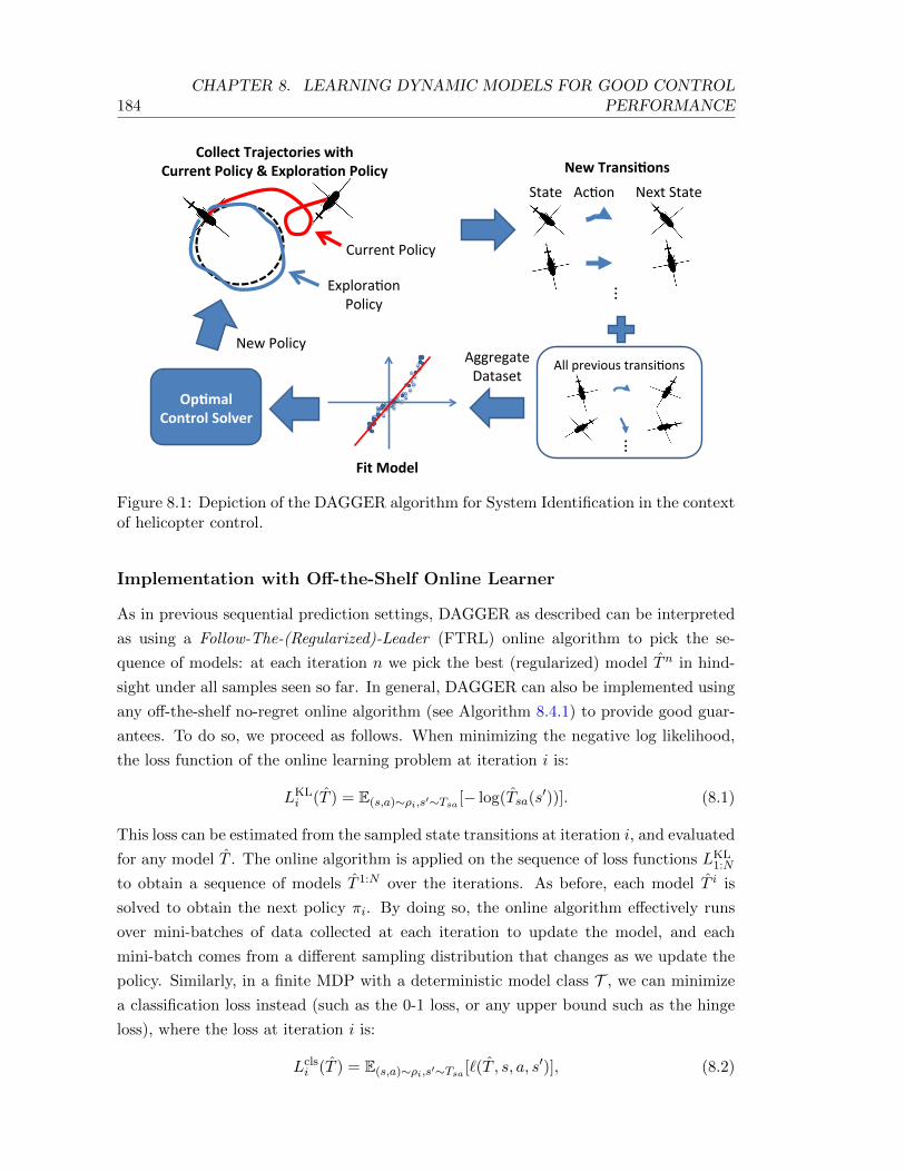
184CHAPTER 8. LEARNING DYNAMIC MODELS FOR GOOD CONTROL
PERFORMANCE
Explora(on
Policy
Current Policy
New Policy
Fit Model
New Transi1ons
All previous transi(ons Aggregate
Dataset
Collect Trajectories with
Current Policy & Explora1on Policy
Op1mal
Control Solver
State Ac(on Next State
... ...
Figure 8.1: Depiction of the DAGGER algorithm for System Identification in the contextof helicopter control.
Implementation with Off-the-Shelf Online Learner
As in previous sequential prediction settings, DAGGER as described can be interpreted
as using a Follow-The-(Regularized)-Leader (FTRL) online algorithm to pick the se-
quence of models: at each iteration n we pick the best (regularized) model Tn in hind-
sight under all samples seen so far. In general, DAGGER can also be implemented using
any off-the-shelf no-regret online algorithm (see Algorithm 8.4.1) to provide good guar-
antees. To do so, we proceed as follows. When minimizing the negative log likelihood,
the loss function of the online learning problem at iteration i is:
LKLi (T ) = E(s,a)∼ρi,s′∼Tsa [− log(Tsa(s
′))]. (8.1)
This loss can be estimated from the sampled state transitions at iteration i, and evaluated
for any model T . The online algorithm is applied on the sequence of loss functions LKL1:N
to obtain a sequence of models T 1:N over the iterations. As before, each model T i is
solved to obtain the next policy πi. By doing so, the online algorithm effectively runs
over mini-batches of data collected at each iteration to update the model, and each
mini-batch comes from a different sampling distribution that changes as we update the
policy. Similarly, in a finite MDP with a deterministic model class T , we can minimize
a classification loss instead (such as the 0-1 loss, or any upper bound such as the hinge
loss), where the loss at iteration i is:
Lclsi (T ) = E(s,a)∼ρi,s′∼Tsa [`(T , s, a, s′)], (8.2)

8.4. INTERACTIVE LEARNING APPROACH 185
Input: exploration distribution ν, number of iterations N , number of samples periteration m, cost function C, online learning procedure OnlineLearner, optimalcontrol procedure OCSolver.
Get initial guess of model: T 1 ← OnlineLearner().π1 ← OCSolver(T 1, C).for n = 2 to N do
for k = 1 to m doWith prob. 1
2 sample (s, a) ∼ Dµ,πn−1 using πn−1, otherwise sample (s, a) ∼ ν.Obtain s′ ∼ TsaAdd (s, a, s′) to Dn−1.
end forUpdate model: Tn ← OnlineLearner(Dn−1).πn ← OCSolver(Tn, C).
end forReturn the sequence of policies π1:N .
Algorithm 8.4.1: DAGGER algorithm for Agnostic System Identification/MBRL.
for ` the particular classification loss we’re minimizing. This corresponds to an online
classification problem. For many model classes, the negative log likelihood and convex
upper bounds on the 0-1 loss (such as hinge loss) lead to convex online learning problems,
for which no-regret algorithms exist (e.g., gradient descent, FTRL). As shown below, if
the sequence of models is no-regret on these loss functions, then performance can be
related to the smallest expected KL divergence (or classification loss) achievable with
model class T under the overall training distribution ρ = 1N
∑Ni=1 ρi (i.e. a quantity akin
to εKLmdl or εcls
mdl for Batch).
Important Distinction to Previous Settings: We emphasize here an important
distinction of DAGGER in this setting. Unlike previous sequential prediction settings,
here DAGGER does not only collect data from running the current policy at each it-
eration, it also collects an equal amount of exploration data. This is suggested by our
theoretical analysis below. Intuitively, this is necessary to ensure that we do not con-
verge to a model T that only models well the behavior of the system under the previous
policies π1:n, and does not model well the behavior of the system where good policies
go. In agnostic settings where we cannot model the data perfectly, the model fitting
procedure must tradeoff where it makes mistakes. If we would only collect more data
from the current policy at each iteration, the exploration data would occupy a vanish-
ingly small fraction of the dataset and potentially lead the learner to pick models that
have large error on this exploration data and low error where the learned policies go.
If we would end up with such model, we would likely get stuck in a local minima and
not be able to learn better policies. By keeping an even balance of exploration data and
data from execution of our learned policies, we ensure that the learned model must also

186CHAPTER 8. LEARNING DYNAMIC MODELS FOR GOOD CONTROL
PERFORMANCE
predict well the behavior of the system for other policies (that visit frequently explored
state-actions), and thus that when solving the OC problem, we must be able to find
good policies compared to any policy that spends most of its time where we explore.
Note that DAGGER could also be implemented by only collecting more data from
the current policy at each iteration, if for instance, we collect all the exploration data
up front, and then at each iteration when defining the loss for the online learner, we
weight the training examples such that half the weight is assigned to the exploration
data, and half the weight to the newly collected data. That is if we have a dataset of
exploration data D0, and Dn is the dataset of state transitions collected at iteration n
by only running the current policy πn, we could define the loss for the online algorithm
LKLn (T ) = − 1
2|D0|∑
(s,a,s′)∈D0log(Tsa(s
′))− 12|Dn|
∑(s,a,s′)∈Dn log(Tsa(s
′)).
Analysis
Similar to our analysis of Batch, we seek to answer the following: if there exists a low
error model of training data, and we solve each OC problem well, what guarantees does
DAgger provide on control performance? Our results show that by sampling data from
the learned policies, DAgger provides guarantees that have no train-test mismatch factor,
leading to improved performance. Again, the proofs are deferred to appendix C.
For any policy π′, define
επ′
oc =1
N
N∑i=1
Es∼µ[Vi(s)− V π′i (s)],
where Vi and V π′i are respectively the value function of πi and π′ under model T i. This
measures how well we solved each OC problem on average over the iterations. For
instance, if at each iteration i we found an εi-optimal policy within some class of policies
Π on learned model T i, then επ′oc ≤ 1
N
∑Ni=1 εi for all π′ ∈ Π.
As in Batch, the average predictive error of the models T 1:N can be measured in
terms of the L1 distance between the predicted and true next state distribution:
εL1prd =
1
N
N∑i=1
E(s,a)∼ρi [||Tisa − Tsa||1].
However, as was discussed, the L1 distance is not observed from samples which makes
it hard to minimize. Instead we can define other measures which upper bounds this L1
distance and can be minimized from samples, such as the KL divergence or classification
loss, i.e.:
εKLprd =
1
N
N∑i=1
E(s,a)∼ρi,s′∼Tsa [log(Tsa(s))− log(T isa(s′))]
8.4. INTERACTIVE LEARNING APPROACH 187
and
εclsprd =
1
N
N∑i=1
E(s,a)∼ρi,s′∼Tsa [`(T i, s, a, s′)].
Now, given the sequence of policies π1:N , let π = arg minπ∈π1:N Jµ(π) be the best policy
in the sequence and π the uniform mixture policy on π1:N .
Lemma 8.4.1. The policies π1:N are s.t. for any policy π′:
Jµ(π) ≤ Jµ(π) ≤ Jµ(π′) + επ′
oc + cπ′ν Hε
L1prd
This also holds as a function of εKLprd or εclsprd using Lemma 8.3.1.
Using Equations 8.1 and 8.2, we note that
εKLprd =
1
N
N∑i=1
LKLi (T i)− LKLi (T ),
and
εclsprd =
1
N
N∑i=1
Lclsi (T i).
Using a no-regret algorithm on the sequence of losses LKL1:N implies
1
N
N∑i=1
LKLi (T i) ≤ infT ′∈T
1
N
N∑i=1
LKLi (T ′) + εKLrgt ,
for εKLrgt the average regret of the algorithm after N iterations, s.t. εKL
rgt → 0 as N →∞.
This relates εKLprd to the modeling error of the class T :
εKLmdl = inf
T ′∈TE(s,a)∼ρ,s′∼Tsa [log(Tsa(s))− log(T ′sa(s
′))],
i.e. εKLprd ≤ εKL
mdl + εKLrgt , for εKL
rgt → 0. Similarly define
εclsmdl = inf
T ′∈TE(s,a)∼ρ,s′∼Tsa [`(T ′, s, a, s′)]
and by using a no-regret algorithm on Lcls1:N :
εclsprd ≤ εcls
mdl + εclsrgt
for εclsrgt → 0. In some cases, even if the L1 distance cannot be estimated from samples,
statistical estimators can still be no-regret with high probability on the sequence of loss
LL1i (T ′) = E(s,a)∼ρi [||Tsa−T ′sa||1]. This is the case in finite MDPs if we use the empirical
estimator of T based on data seen so far (see appendix C). If we define
εL1mdl = inf
T ′∈TE(s,a)∼ρ[||Tsa − T ′sa||1],
this implies that
εL1prd ≤ εL1
mdl + εL1rgt,
for εL1rgt → 0. Our main result follows:

188CHAPTER 8. LEARNING DYNAMIC MODELS FOR GOOD CONTROL
PERFORMANCE
Theorem 8.4.1. The policies π1:N are s.t. for any policy π′:
Jµ(π) ≤ Jµ(π) ≤ Jµ(π′) + επ′
oc + cπ′ν H[εL1mdl + εL1rgt]
This also holds as a function of εKLmdl + εKL
rgt (or εclsmdl + εclsrgt) using Lem. 8.3.1. If the fitting
procedure is no-regret w.r.t the sequence of losses LL11:N (or LKL1:N , Lcls1:N ), then εL1rgt → 0
(or εKLrgt → 0,εclsrgt → 0) as N →∞.
Additionally, the performance of πN can be related to π if the distributions Dµ,πi
converge to a small region:
Lemma 8.4.2. If there exists a distribution D∗ and some ε∗cnv ≥ 0 s.t. ∀i, ||Dµ,πi −D∗||1 ≤ ε∗cnv + εicnv for some sequence εicnv∞i=1 that is o(1), then πN is s.t.:
Jµ(πN ) ≤ Jµ(π) +Crng
2(1− γ)[2ε∗cnv + εNcnv +
1
N
N∑i=1
εicnv]
Thus: lim supN→∞ Jµ(πN )− Jµ(π) ≤ Crng
1−γ ε∗cnv
Theorem 8.4.1 illustrates how we can reduce the original system identification (or
MBRL) problem to a no-regret online learning problem on a particular sequence of loss
functions. In general, no-regret algorithms have average regret of O( 1√N
) (O( 1N ) in ideal
cases) such that the regret term goes to 0 at a similar rate to the generalization error term
for Batch in Corollary 8.3.1. Here, given enough iterations, the term cπ′ν Hε
L1mdl determines
how performance degrades in the agnostic setting (or cπ′ν H
√2εKL
mdl or 2cπ′ν Hε
clsmdl if we use
a no-regret algorithm on the sequence of KL or classification loss respectively). Unlike
for Batch, there is no dependence on cπν , only on cπ′ν . Thus, if a low error model exists
under training distribution ρ, no-regret methods are guaranteed to learn policies that
performs well compared to any policy π′ for which cπ′ν is small. Hence, ν is ideally Dµ,π
of a near-optimal policy π (i.e. explore where good policies go).
Finite Sample Analysis: A remaining issue is that the current guarantees apply if
we can evaluate the expected loss (LL1i , LKL
i or Lclsi ) exactly. This requires infinite
samples at each iteration. If we run the no-regret algorithm on estimates of these loss
functions, i.e. loss on m sampled transitions, we can still obtain good guarantees using
martingale inequalities as in online-to-batch (Cesa-Bianchi et al., 2004) techniques. The
extra generalization error term is typically O(
√log(1/δ)Nm ) with high probability 1 − δ.
While our focus is not on providing such finite sample bounds, we illustrate how these
can be derived for two scenarios in appendix C. For instance, in finite MDPs with |S|states and |A| actions, if T i is the empirical estimator of T based on samples collected in
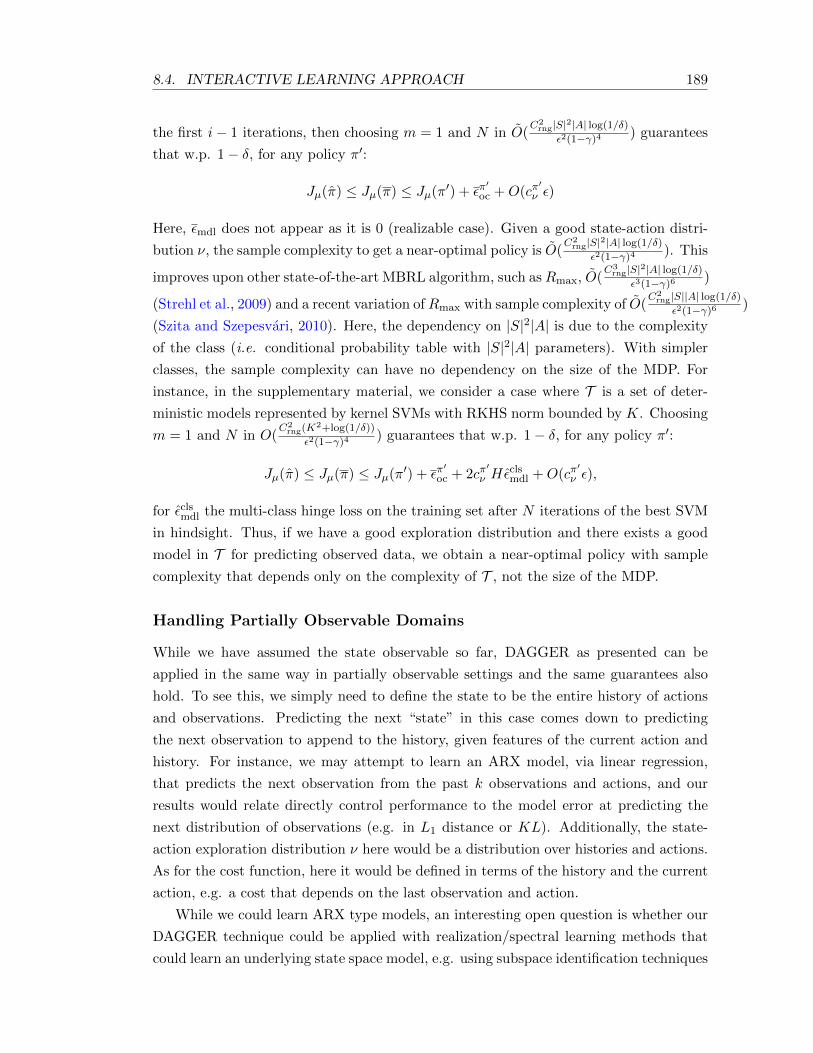
8.4. INTERACTIVE LEARNING APPROACH 189
the first i− 1 iterations, then choosing m = 1 and N in O(C2
rng|S|2|A| log(1/δ)
ε2(1−γ)4) guarantees
that w.p. 1− δ, for any policy π′:
Jµ(π) ≤ Jµ(π) ≤ Jµ(π′) + επ′
oc +O(cπ′ν ε)
Here, εmdl does not appear as it is 0 (realizable case). Given a good state-action distri-
bution ν, the sample complexity to get a near-optimal policy is O(C2
rng|S|2|A| log(1/δ)
ε2(1−γ)4). This
improves upon other state-of-the-art MBRL algorithm, such asRmax, O(C3
rng|S|2|A| log(1/δ)
ε3(1−γ)6)
(Strehl et al., 2009) and a recent variation ofRmax with sample complexity of O(C2
rng|S||A| log(1/δ)
ε2(1−γ)6)
(Szita and Szepesvari, 2010). Here, the dependency on |S|2|A| is due to the complexity
of the class (i.e. conditional probability table with |S|2|A| parameters). With simpler
classes, the sample complexity can have no dependency on the size of the MDP. For
instance, in the supplementary material, we consider a case where T is a set of deter-
ministic models represented by kernel SVMs with RKHS norm bounded by K. Choosing
m = 1 and N in O(C2
rng(K2+log(1/δ))
ε2(1−γ)4) guarantees that w.p. 1− δ, for any policy π′:
Jµ(π) ≤ Jµ(π) ≤ Jµ(π′) + επ′
oc + 2cπ′ν Hε
clsmdl +O(cπ
′ν ε),
for εclsmdl the multi-class hinge loss on the training set after N iterations of the best SVM
in hindsight. Thus, if we have a good exploration distribution and there exists a good
model in T for predicting observed data, we obtain a near-optimal policy with sample
complexity that depends only on the complexity of T , not the size of the MDP.
Handling Partially Observable Domains
While we have assumed the state observable so far, DAGGER as presented can be
applied in the same way in partially observable settings and the same guarantees also
hold. To see this, we simply need to define the state to be the entire history of actions
and observations. Predicting the next “state” in this case comes down to predicting
the next observation to append to the history, given features of the current action and
history. For instance, we may attempt to learn an ARX model, via linear regression,
that predicts the next observation from the past k observations and actions, and our
results would relate directly control performance to the model error at predicting the
next distribution of observations (e.g. in L1 distance or KL). Additionally, the state-
action exploration distribution ν here would be a distribution over histories and actions.
As for the cost function, here it would be defined in terms of the history and the current
action, e.g. a cost that depends on the last observation and action.
While we could learn ARX type models, an interesting open question is whether our
DAGGER technique could be applied with realization/spectral learning methods that
could learn an underlying state space model, e.g. using subspace identification techniques
190CHAPTER 8. LEARNING DYNAMIC MODELS FOR GOOD CONTROL
PERFORMANCE
in Overschee and Moor (1996), Boots and Gordon (2011). An important requirement
for this to be possible would be to show that such spectral methods are no-regret, e.g.
in the squared loss (or log likelihood) of their predictions, when applied to learn online.
Not much work has been done in this area, with the exception of a randomized online
PCA method that has been shown to be no-regret (Warmuth and Kuzmin, 2008).
Discussion
Remarks on Guarantees. We emphasize again that we provide reduction-style guar-
antees. DAGGER may sometimes fail to find good policies, e.g., when no model in the
class achieves low error on the training data. When no model achieves low error on the
training data, whether we are using Batch or DAGGER, both will fail to provide good
performance, and this suggests we need a better class of models. However, the distinc-
tion to Batch is in the case where good models exist on the training data. In this case,
DAGGER is guaranteed to find a good policy, in contrast, Batch can still fail at obtain-
ing a policy with good control performance, due to train/test mismatch. This occurs
even in scenarios where DAGGER finds good policies, as shown in the experiments.
DAGGER as a reduction. In this setting DAGGER can be interpreted as a reduc-
tion of system identification, or model-based reinforcement learning, to no-regret online
learning and optimal control. Depending on the loss minimized to fit the model, it can
be interpreted as an error or a regret reduction. In the case of the KL (negative log
likelihood), we obtain a reduction that relates performance to the regret in log likelihood
of the best model in the class to the true model (bayes-optimal model). Thus in this
case, this can be interpreted as a regret reduction. For the classification loss however,
performance is related directly to the classification loss/error, and this can be interpreted
as an error reduction.
Solving the OC problems. DAGGER needs to solve many OC problems. This
can be computationally expensive, e.g., with non-linear or high-dimensional models.
Many approximate methods can be used, e.g., policy gradient (Williams, 1992), fitted
value iteration (Gordon, 1995, Szepesvari, 2005), iLQR (Li and Todorov, 2004) or DDP
(Jacobson and Mayne, 1970). As the models often change only slightly from one iteration
to the next, we can often run only a few iterations of dynamic programming/policy
gradient from the last value function/policy to obtain a good policy for the current
model. As long as we get good solutions on average, επ′
oc remains small and does not
hinder performance.
8.5. OPTIMISTIC EXPLORATION FOR REALIZABLE SETTINGS 191
Relation to previous iterative identification methods. DAGGER generalizes the
approach of Atkeson and Schaal (1997) and Abbeel and Ng (2005) so that we can use
any no-regret algorithm to update the model, as well as any exploration distribution.
A key difference is that DAGGER keeps an even balance between exploration data and
data from running the learned policies. This is crucial to avoid settling on suboptimal
performance in agnostic settings as the exploration data could be ignored if it occupies
only a small fraction of the dataset, in favor of models with lower error on the data from
the learned policies. With this modification, our main contribution is showing that such
methods have good guarantees even in agnostic settings.
Realizable Settings. Another important result that follows from this analysis is when
we are in a realizable setting. This result indicates that recovering the optimal policy
is always possible if we have access to a good exploration distribution, and no-regret
learning is possible for the given class of models T that contains the true model. As
no-regret can be achieved on a much broader class of models than linear systems (e.g.
kernel based models), these results show that learning models that synthesize the optimal
controller is possible for much more general class of non-linear systems. The requirement
of having access to a good exploration distribution can also be dropped in realizable
settings, by adopting instead an optimistic exploration strategy presented below.
8.5 Optimistic Exploration for Realizable Settings
Our current DAGGER approach to system identification assumes that it is given a good
state-action exploration distribution ν in order to guarantee that it can find a near-
optimal policy efficiently. In domains where prior knowledge of the task is limited, or
where we don’t have access to an expert, it might be hard to provide this information
to the algorithm. We present here an adaptive exploration strategy that can be used,
which guarantees finding the optimal policy in realizable settings.
The exploration strategy uses the principle of optimism in the face of uncertainty,
which is used in many other state-of-the-art RL algorithms such as Rmax (Strehl et al.,
2009) and UCRL/UCRL2 (Auer and Ortner, 2007, Jaksch et al., 2010). It essentially
involves being optimistic about the value of states and actions that have not been ex-
plored enough before. In particular, the exploration strategy is obtained by essentially
computing a lower bound (with high probability) on the total cost of the optimal policy
in the real system based on the observed data so far. The lower bound becomes tighter
as more data is collected and converges toward the optimal value function. Executing
the optimal policy of this optimistic value function ensures that we will explore all areas
that are potentially visited by an optimal policy.
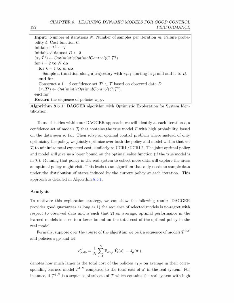
192CHAPTER 8. LEARNING DYNAMIC MODELS FOR GOOD CONTROL
PERFORMANCE
Input: Number of iterations N , Number of samples per iteration m, Failure proba-bility δ, Cost function C.Initialize T 1 ← TInitialized dataset D ← ∅(π1,T 1)← OptimisticOptimalControl(C, T 1).for i = 2 to N do
for k = 1 to m doSample a transition along a trajectory with πi−1 starting in µ and add it to D.
end forConstruct a 1− δ confidence set T i ⊂ T based on observed data D.(πi,T
i)← OptimisticOptimalControl(C, T i).end forReturn the sequence of policies π1:N .
Algorithm 8.5.1: DAGGER algorithm with Optimistic Exploration for System Iden-tification.
To use this idea within our DAGGER approach, we will identify at each iteration i, a
confidence set of models Ti that contains the true model T with high probability, based
on the data seen so far. Then solve an optimal control problem where instead of only
optimizing the policy, we jointly optimize over both the policy and model within that set
Ti to minimize total expected cost, similarly to UCRL/UCRL2. The joint optimal policy
and model will give us a lower bound on the optimal value function (if the true model is
in Ti). Running that policy in the real system to collect more data will explore the areas
an optimal policy might visit. This leads to an algorithm that only needs to sample data
under the distribution of states induced by the current policy at each iteration. This
approach is detailed in Algorithm 8.5.1.
Analysis
To motivate this exploration strategy, we can show the following result: DAGGER
provides good guarantees as long as 1) the sequence of selected models is no-regret with
respect to observed data and is such that 2) on average, optimal performance in the
learned models is close to a lower bound on the total cost of the optimal policy in the
real model.
Formally, suppose over the course of the algorithm we pick a sequence of models T 1:N
and policies π1:N and let
επ′
oc-lb =1
N
N∑i=1
Es∼µ[Vi(s)]− Jµ(π′),
denotes how much larger is the total cost of the policies π1:N on average in their corre-
sponding learned model T 1:N compared to the total cost of π′ in the real system. For
instance, if T 1:N is a sequence of subsets of T which contains the real system with high
8.5. OPTIMISTIC EXPLORATION FOR REALIZABLE SETTINGS 193
probability, and at each iteration i, we found an εi-optimal policy and model pair (πi, Ti)
in Π× T i, then for any π′ ∈ Π, επ′
oc-lb ≤1N
∑Ni=1 εi with high probability.
Additionally, define the average predictive error of the chosen models T 1:N , measured
in L1 distance, under the corresponding state-action distribution induced by the chosen
policies as
εL1prd =
1
N
N∑i=1
E(s,a)∼Dµ,πi [||Tsa − Tisa||1].
Similarly, define
εKLprd =
1
N
N∑i=1
E(s,a)∼Dµ,πi ,s′∼Tsa [log(Tsa(s′))− log(T isa(s
′))].
and
εclsprd =
1
N
N∑i=1
E(s,a)∼Dµ,πi ,s′∼Tsa [`(T i, s, a, s′)].
the predictive error, measured in KL and classification loss respectively. Note here the
difference is that these quantities are directly defined as an expectation under the distri-
bution of state-actions Dµ,πi , rather than a mixture with a fixed exploration distribution
ν.
The following holds:
Theorem 8.5.1. For all policies π′:
Jµ(π) ≤ Jµ(π) ≤ Jµ(π′) + επ′
oc-lb +H
2εL1prd
This also holds in terms of εKLprd or εclsprd using the relations in Lemma 8.3.1.
The predictive error can be related to a modeling error, and the average regret as in
the previous section. However, for realizable settings, the modeling error is 0, implying
the predictive error is directly the average regret.
Thus in realizable settings, this theorem implies that if we can pick a sequence of
models T iNi=1, which satisfies the following: 1) with high probability, the sequence has
no-regret on the observed data with respect to the true model T ∈ T (i.e. εL1prd → 0 as
N → ∞) ; 2) with high probability, the average total cost of the policy in the learned
model lower bounds the total cost of the optimal policy (i.e. επ′
oc-lb ≤ 0 for all π′); then
we are guaranteed to find an optimal policy in the limit.
While the algorithm chooses subsets T i, and the optimistic optimal control algorithm
can potentially pick any model T i ∈ T i at each iteration i, we can still guarantee that
the chosen sequence of models T i is no-regret if we choose the subsets T i properly. For
instance, suppose T 1:N would be the sequence of chosen models by a no-regret algorithm
on the observed data over the iterations of the algorithm, and the loss at each iteration
194CHAPTER 8. LEARNING DYNAMIC MODELS FOR GOOD CONTROL
PERFORMANCE
is Lipschitz continuous under some norm || · || over the space of models T . Then if at
each iteration i, we define the subsets T i = T ′|||T ′ − T i|| ≤ εiconf for some sequence
εiconf that is o(1), then any sequence of models T 1:N is no-regret if for all i, T i ∈ T i.Typical generalization error bounds will yield confidence regions where εnconf is O( 1√
n).
In this case, the sequence of T 1:N can be no-regret at rate O( 1√N
).
Realizable Case in Finite MDPs
We can illustrate what this algorithm would do and its guarantees in a finite MDP setting
with |S| states and |A| actions, where the set of models T contains all transition matrix
(the set of all conditional probability tables with |S|2|A| parameters).
First, at each iteration i, we would construct the empirical estimate T i of the true
model as T isa(s′) =
n<isas′
n<isa, where n<isas′ is the number of times we observed transition
(s, a, s′) in the first i− 1 iterations and n<isa =∑
s′ n<isas′ . Then from standard results in
Wasserman (2003), defining
T i = T ′|∀(s, a) : ||T ′sa − T isa||1 ≤√
c
n<isa,
for c = 2|S| ln(2) + 2 log(|S||A|N/δ) guarantees that with probability at least 1− δ, the
true model T ∈ T i for all iterations i ∈ 1, 2, . . . , N. Additionally, if T ∈ Ti for all i,
we can show that any sequence of models T 1:N such that T i ∈ T i for all i, is such that
εL1prd is O(
√c|S||A|Nm ) (see finite sample analysis for finite MDPs in appendix C). Once we
defined the set T i, we would solve for a joint near-optimal policy πi and model T i ∈ T i
that minimizes total expected cost, and move on to execute πi to collect more data at
the next iteration. If we can find such ε-optimal policy and model pair at each iteration,
then if we run the algorithm for O(γ2C2
range|S|2|A|(1−γ)4ε2
) iterations and collect O(1) sample at
each iteration, we will obtain an ε-optimal policy in the real system with high probability.
This compares favorably against state-of-the-art RL algorithm such as Rmax, which has
sample complexity of O(γ3C3
rng|S|2|A|(1−γ)6ε3
) (Strehl et al., 2009), and is also an improvement
over our previous approach as it does not depend on the factor cπ∗ν anymore.
Solving for Joint Optimal Policy and Model
The mentioned algorithm requires solving jointly over policy πi and model Ti ∈ Ti.In general this may be intractable. However in some cases this can be achieved with
computational complexity that is no greater than the complexity of solving a typical
optimal control problem via dynamic programming. We show this is the case for the
finite MDP scenario above where the set of models Ti has the form Ti = T ′|∀(s, a) :
||T ′sa − Tsa||1 ≤ csa for some nominal model T and confidence region csa on the L1
distance to the true model for each state-action pair.

8.5. OPTIMISTIC EXPLORATION FOR REALIZABLE SETTINGS 195
input: Nominal model T , L1 confidence region csa for all (s, a), Cost function C.∀s, a : Q(s, a)← C(s, a), ∀s : V (s)← mina[Q(s, a)]for t = 2 to H do
Sort states in ascending order of value in V , breaking ties arbitrarily.Let sj denote the jth state in sorted list.for each s do
for each a do∀s′ : T ′sa(s′)← Tsa(s
′), l← 1, h← |S|, d← 0.while l < h and d < csa doδ ← min(1− T ′sa(sl), T ′sa(sh), (csa − d)/2).T ′sa(sl)← T ′sa(sl) + δ, T ′sa(sh)← T ′sa(sh)− δ, d← d+ 2δ.if T ′sa(sl) = 1 then l← l + 1.if T ′sa(sh) = 0 then h← h− 1.
end whileQ′(s, a)← C(s, a) + γ
∑s′ T′sa(s
′)V (s′)end for
end for∀s, a : Q(s, a)← Q′(s, a), ∀s : V (s)← mina[Q
′(s, a)]end forreturn Q
Algorithm 8.5.2: DP Algorithm for solving optimistic optimal control problem.
In this scenario we have to solve the following equation:
V ∗(s) = mina
[C(s, a) + γ minT ′sa|||T ′sa−Tsa||1≤csa
Es′∼T ′sa [V ∗(s′)]]
In general this can be solved via dynamic programming and solving a linear program
with O(|S|) constraints for each state-action pair at each dynamic programming itera-
tion. Such an approach would however be intractable. There is a much more efficient
approach which simply involves sorting the states according to their value at each dy-
namic programming iteration in order to solve for the optimal T ′sa in O(|S|) work for
each state-action pair. This algorithm, detailed in Algorithm 8.5.2, was proposed in
Strehl and Littman (2004) and we present it here for completeness.
Intuitively, this algorithm proceeds by putting as much probability mass on states
which have lowest cost-to-go and as few probability mass on states which have highest
cost-to-go. This is done efficiently using the sorted list of states according to their cost-to-
go values, greedily moving probability mass from states with highest cost-to-go to states
with lowest cost-to-go, starting from the nominal solution T ′sa = Tsa, while enforcing the
constraint that T ′sa must be a probability distribution with L1 distance within csa of Tsa.
For each s, a and iteration t, finding the optimal T ′sa (i.e. the while loop) terminates
in less than |S| iterations and each iteration is O(1) work. So at each iteration t, finding
the optimal T ′ for all s, a requires O(|S|2|A|+ |S| log |S|) work which is O(|S|2|A|). Once
we found the optimal T ′, doing the value function update for all (s, a) is O(|S|2|A|) as
196CHAPTER 8. LEARNING DYNAMIC MODELS FOR GOOD CONTROL
PERFORMANCE
well. So each iteration of dynamic programming is still O(|S|2|A|). Running the above
algorithm is thus O(H|S|2|A|) for H iterations. Since each iteration is a γ-contraction of
||V −V ∗||∞, choosing H in O( 11−γ log(
Crng
(1−γ)ε)) guarantees that we will find an ε-optimal
solution. Finding an ε-optimal solution is thus O( |S|2|A|
1−γ log(Crng
(1−γ)ε)). This is the same
complexity as the value iteration algorithm when solving for an ε-optimal policy with
fixed model.
Discussion
This exploration strategy is well motivated and can be implemented efficiently in finite
MDPs when learning the full conditional probability table. For practical applications
with other class of models, we would need similar efficient dynamic programming algo-
rithms for jointly finding an optimal policy and model. We believe this may be possible
for the case of linear systems (LQR). In particular, in this case a similar approach to H∞
robust control where a dynamic game between the controller and a disturbance player
is solved (Basar and Bernhard, 1995) could potentially be leveraged, but where instead,
the disturbance player tries to minimize cost, subject to a constraint on the size of the
deviation. For instance, based on the results in Walsh et al. (2009), it is likely that a
similar result could be derived to show that the deviation in next state, from the state
predicted by the nominal model, is bounded within some L2 ball, leading to an optimal
strategy for the disturbance player that is also a linear function of the state and allowing
to compute the optimistic optimal value function in closed form as a quadratic function.
For more general class of models, the optimistic optimal control problem may poten-
tially be solved approximately, for instance using a gradient based method.
It would be interesting to see if this exploration strategy can be extended to agnostic
setting, or provide guarantees for this strategy in agnostic settings. For instance, it
might be possible to bound the quantity επ′
oc-lb, e.g. as a function of how well we can
do at prediction during training within the class of model T , or by making some other
assumption about how well the class of model T can approximate the real system T .
8.6 Experiments
We now demonstrate the efficacy of DAGGER for System Identification on two control
tasks: a simple benchmark inverted pendulum swing-up task, and a more challenging
task of learning to perform aerobatic maneuvers with a simulated helicopter.
Inverted Pendulum Swing-Up
The control of an inverted pendulum has been commonly used in the control literature
and is often used as a simple benchmark problem. We consider learning to perform

8.6. EXPERIMENTS 197
Figure 8.2: Depiction of the swing-up task. First 10 frames at 0.5s intervals of a near-optimal controller. Top Left: Initial State at 0s. Following frames in top row at 0.5sintervals from left to right, then continued from left to right in the bottom row. BottomRight: Frame at 4.5s illustrates the inverted position that must be maintained until theend of the 10s trajectory.
the swing-up task, which consists in, starting from a pendulum near its equilibrium
position at rest, swinging it to bring it in an inverted position, and then maintaining
it in equilibrium in this inverted position, in the presence of small random external
disturbances. We consider the case where the pendulum is torque controlled at the
rotary joint, and is under actuated6. This task is depicted in Figure 8.2.
The pendulum is described by a two-dimensional continuous state [θ, θ], where θ is
the angle in [−π, π] (off the inverted equilibrium position), and θ its angular velocity,
and a one-dimensional continuous control (torque) τ . We simulate an ideal pendulum
(all its mass concentrated at the end of the pendulum) without friction, described by
the following differential equation:
θ =g
lsin(θ)− τ
l2m
where θ is the angular acceleration, l and m are the length (in meters) and mass (in kg)
of the pendulum respectively, g is the gravitational force. We consider the case where
m = l = 1, under Earth’s gravity (g = 9.81). To make the pendulum under actuated,
we limit τ ∈ [−4, 4]. We simulate external disturbances through random small additive
torques7 applied to the pendulum. We always start the pendulum in initial state (2.8, 0)
(i.e. top left frame in Figure 8.2).
We would like to synthesize a controller than can update the torque at 10hz and
perform this task during 10s. We define a cost function that penalizes deviations from
the inverted position, angular velocities and torques at each time step (of 0.1s):
C(θ, θ, τ) = 10θ2 + θ2 + 0.1τ2.6By under actuated, we mean that we must build velocity by swinging the pendulum back and forth
to bring it from the start position to its inverted position, we cannot simply drive the pendulum directlyto its inverted position by constantly applying maximum torque in one direction.
7White gaussian noise with standard deviation 0.05

198CHAPTER 8. LEARNING DYNAMIC MODELS FOR GOOD CONTROL
PERFORMANCE
For each method, we attempt to learn a dynamic model that predicts the change in
state of the pendulum, given the current state and torque, using locally weighted linear
regression8 (LWLR) (Atkeson et al., 1997), starting from the 0 model (i.e. that predicts
the state never changes), and solve the optimal control problem through dynamic pro-
gramming with a finely discretized grid over the state space (linearly interpolating the
value function and policy between grid points). We compare DAGGER, to Batch, and
the iterative approach of Abbeel and Ng (2005) and Atkeson and Schaal (1997). For the
exploration distribution ν, we observe the pendulum under the expert controller obtained
by solving the optimal control problem with the known model of the simulator. This
expert controller can swing-up the pendulum to its inverted position quickly and then
maintains it in this position for the remaining time (see Figure 8.2). We also compare
performance to this expert controller as the desired target level of performance.
We perform 10 iterations of training with each approach, where at each iteration, two
additional trajectories are collected. For DAGGER, this corresponds to one trajectory
from the expert controller and one trajectory from the learner’s current controller at
each iteration; for Batch, this corresponds to two additional trajectories from the expert
controller at each iteration; and for Abbeel’s approach, this is two trajectories from the
expert at the first iteration, then two trajectories from the learner’s current controller
at each iteration. This difference in how data is collected is the only difference between
all these methods.
Figure 8.3 compares the performance of these methods at the swing-up task over the
iterations of training as a function of training data collected so far.
We first observe that the batch method does not perform well. Looking at the
execution of its learned controllers, we observe that it never learns to properly swing-up
the pendulum to its inverted position. On the other hand, both DAGGER and Abbeel
eventually obtain a controller that is as good as the expert controller. Abbeel performs
slightly better than DAGGER, by obtaining such a controller after 6 iterations instead
of 7 for DAGGER. We believe that Abbeel performs well in this application as it is
essentially a realizable setting, and the LWLR model can fit perfectly the observed data
(up to noise), so it doesn’t have to tradeoff where it makes error as in agnostic settings.
In essence, in such realizable cases, the balance/weighting between data from exploration
and the learned policies in the dataset is not as important; sufficient coverage of both
is what’s important. In the next experiment, we will see that having a good balance is
important in non-realizable settings and that Abbeel’s method can get stuck in a bad
local minima when insufficient exploration data is present in the dataset.
8We use a gaussian kernel, where distance is computed between normalized features, and the band-width parameter is optimized at each iteration using cross-validation, where the data collected at differentiteration are treated as different folds.
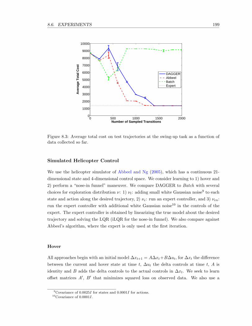
8.6. EXPERIMENTS 199
0 500 1000 1500 20000
1000
2000
3000
4000
5000
6000
7000
8000
9000
10000
Number of Sampled Transitions
Ave
rag
e T
ota
l Co
st
DAGGERAbbeelBatchExpert
Figure 8.3: Average total cost on test trajectories at the swing-up task as a function ofdata collected so far.
Simulated Helicopter Control
We use the helicopter simulator of Abbeel and Ng (2005), which has a continuous 21-
dimensional state and 4-dimensional control space. We consider learning to 1) hover and
2) perform a “nose-in funnel” maneuver. We compare DAGGER to Batch with several
choices for exploration distribution ν: 1) νt: adding small white Gaussian noise9 to each
state and action along the desired trajectory, 2) νe: run an expert controller, and 3) νen:
run the expert controller with additional white Gaussian noise10 in the controls of the
expert. The expert controller is obtained by linearizing the true model about the desired
trajectory and solving the LQR (iLQR for the nose-in funnel). We also compare against
Abbeel’s algorithm, where the expert is only used at the first iteration.
Hover
All approaches begin with an initial model ∆xt+1 = A∆xt+B∆ut, for ∆xt the difference
between the current and hover state at time t, ∆ut the delta controls at time t, A is
identity and B adds the delta controls to the actual controls in ∆xt. We seek to learn
offset matrices A′, B′ that minimizes squared loss on observed data. We also use a
9Covariance of 0.0025I for states and 0.0001I for actions.10Covariance of 0.0001I.
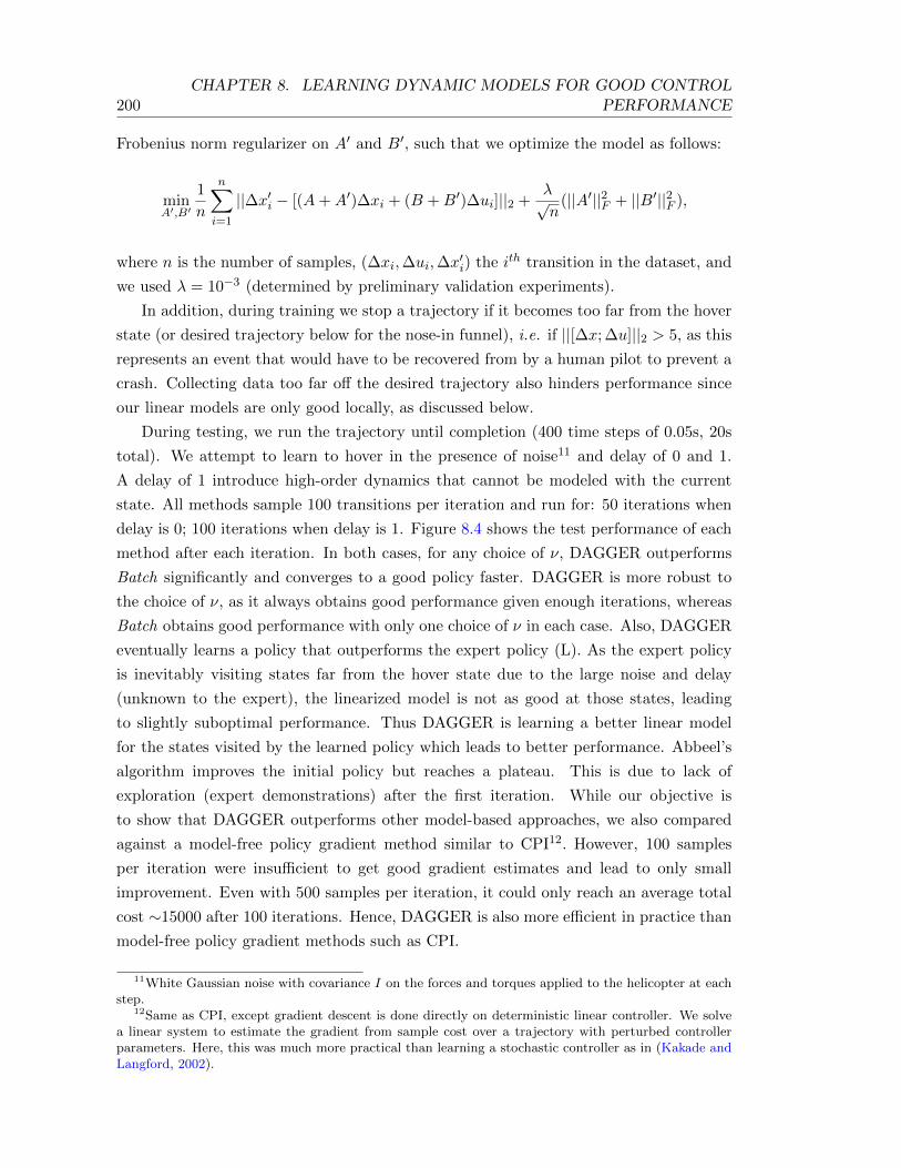
200CHAPTER 8. LEARNING DYNAMIC MODELS FOR GOOD CONTROL
PERFORMANCE
Frobenius norm regularizer on A′ and B′, such that we optimize the model as follows:
minA′,B′
1
n
n∑i=1
||∆x′i − [(A+A′)∆xi + (B +B′)∆ui]||2 +λ√n
(||A′||2F + ||B′||2F ),
where n is the number of samples, (∆xi,∆ui,∆x′i) the ith transition in the dataset, and
we used λ = 10−3 (determined by preliminary validation experiments).
In addition, during training we stop a trajectory if it becomes too far from the hover
state (or desired trajectory below for the nose-in funnel), i.e. if ||[∆x; ∆u]||2 > 5, as this
represents an event that would have to be recovered from by a human pilot to prevent a
crash. Collecting data too far off the desired trajectory also hinders performance since
our linear models are only good locally, as discussed below.
During testing, we run the trajectory until completion (400 time steps of 0.05s, 20s
total). We attempt to learn to hover in the presence of noise11 and delay of 0 and 1.
A delay of 1 introduce high-order dynamics that cannot be modeled with the current
state. All methods sample 100 transitions per iteration and run for: 50 iterations when
delay is 0; 100 iterations when delay is 1. Figure 8.4 shows the test performance of each
method after each iteration. In both cases, for any choice of ν, DAGGER outperforms
Batch significantly and converges to a good policy faster. DAGGER is more robust to
the choice of ν, as it always obtains good performance given enough iterations, whereas
Batch obtains good performance with only one choice of ν in each case. Also, DAGGER
eventually learns a policy that outperforms the expert policy (L). As the expert policy
is inevitably visiting states far from the hover state due to the large noise and delay
(unknown to the expert), the linearized model is not as good at those states, leading
to slightly suboptimal performance. Thus DAGGER is learning a better linear model
for the states visited by the learned policy which leads to better performance. Abbeel’s
algorithm improves the initial policy but reaches a plateau. This is due to lack of
exploration (expert demonstrations) after the first iteration. While our objective is
to show that DAGGER outperforms other model-based approaches, we also compared
against a model-free policy gradient method similar to CPI12. However, 100 samples
per iteration were insufficient to get good gradient estimates and lead to only small
improvement. Even with 500 samples per iteration, it could only reach an average total
cost ∼15000 after 100 iterations. Hence, DAGGER is also more efficient in practice than
model-free policy gradient methods such as CPI.
11White Gaussian noise with covariance I on the forces and torques applied to the helicopter at eachstep.
12Same as CPI, except gradient descent is done directly on deterministic linear controller. We solvea linear system to estimate the gradient from sample cost over a trajectory with perturbed controllerparameters. Here, this was much more practical than learning a stochastic controller as in (Kakade andLangford, 2002).
8.6. EXPERIMENTS 201
Nose-In Funnel
This maneuver consists in rotating at a fixed speed and distance around an axis normal
to the ground with the helicopter’s nose pointing towards the axis of rotation (it is the
desired trajectory depicted in Figure 1.2). We attempt to learn to perform 4 complete
rotations of radius 5 in the presence of noise13 but no delay. We start each approach
with a linearized model about the hover state and learn a time-varying linear model. For
each time step t, we learn offset matrices A′t, B′t such that ∆xt+1 = (A+A′t)∆xt + (B+
B′t)∆ut + x∗t+1 − x∗t , for x∗t the desired state at time t and A,B the given hover model.
All methods collect 500 samples per iteration over 100 iterations. Figure 8.4 (bottom)
shows the test performance after each iteration. With the initial model (0 data), the
controller fails to produce the maneuver and performance is quite poor. Again, with any
choice of ν, DAGGER outperforms Batch, and unlike Batch, it performs well with all
choices of ν. A video comparing qualitatively the learned maneuver with DAGGER and
Batch is available on YouTube (Ross, 2012). Abbeel’s method improves performance
slightly but again suffers from lack of expert demonstrations after the first iteration.
In-Depth Comparisons to Previous Iterative Methods
In the previous experiments, we observed that the previous iterative method of Abbeel
and Ng (2005) (and similarly Atkeson and Schaal (1997)) does not perform well and
seems to reach a plateau or get stuck in a local minima. We demonstrate here that
this is clearly due to insufficient exploration data in the collected dataset. By collecting
more exploration data initially, these methods can lead to similar good performance
to DAGGER, albeit, often requiring more iterations than DAGGER overall, to reach
near-optimal performance.
Figure 8.5, shows the performance of Abbeel’s method, as we vary the number
Nexp of initial iterations where data under execution of the expert controller is col-
lected (1, 6, 12, 25, 50). This effectively corresponds to collecting an initial batch of data
from the expert which is larger, before we start collecting data from running the current
learned policies.
There are a number of trends we can observe from these figures. First, increasing
Nexp, seems to lead to more stable and better asymptotic performance, at the price of
requiring more iterations to reach near-optimal performance. On the other hand, when
Nexp is smaller, performance improves more quickly initially, but asymptotic performance
degrades (either getting stuck in local minima, or being less stable). To achieve the best
performance, Nexp needs to be carefully chosen to balance these 2. In all of these figures,
Nexp = 12 seems to give the best tradeoff. DAGGER on the other hand, by collecting
13Zero-mean spherical Gaussian with standard deviation 0.1 on the forces and torques applied to thehelicopter at each step.
202CHAPTER 8. LEARNING DYNAMIC MODELS FOR GOOD CONTROL
PERFORMANCE
an equal amount of exploration data and data from the current policy at each iteration,
achieves performance similar and often better to this best tradeoff automatically.
These results also give further empirical evidence that supports our theoretical re-
sults. In agnostic system identification settings, one cannot simply learn by only collect-
ing data from execution of the current policy, one needs to collect a significant fraction
of exploration data as well, to ensure we can predict well the system’s behavior under
execution of other policies during planning. Similarly, only collecting exploration data
may not lead to good performance, and collecting a fraction of data from execution of
the current policy can help tremendously.
Practical Considerations when using DAGGER for System
Identification
In the previous helicopter experiments with DAGGER, to ensure learning a good linear
model, we had to discard data points from the current policy’s trajectory that went too
far off the desired trajectory. When performing the experiments without discarding such
data, DAGGER, and the other iterative methods did not perform well. This is because
in this particular experiment, we were fitting a linear model that could only capture the
behavior of the system well in a small region. If we attempt to fit data over a too large
region, data far off the desired trajectory interfere, and does not lead to a good fit in the
region of importance (i.e. near the desired trajectory). This appears in the guarantee
of DAGGER by making εmdl large on the training data if we do not discard these data
points, and hence indicates that DAGGER would not work well in this case.
Because for these tasks, we knew that any good policy must operate near the desired
trajectory, we could safely discard data too far off the desired trajectory, as asymptot-
ically, if we find a good policy, this data would not be useful. In fact, when discarding
such data, a similar guarantee for DAGGER still holds (with an extra penalty term that
scales with the fraction of points discarded). As long as in the limit of iterations, the
fraction of discarded data goes to 0 (i.e. we find a policy that can stay within the region
where we keep all data), good performance would be guaranteed if we can find a good
model on the (non-discarded) training data.
There are a number of other potential solutions to deal with this issue:
• This issue may in part be caused by the sensitivity of least squares regression to
outliers. Using more robust versions of linear regression may help to deal with this
issue, if the fraction of points far off the region of importance remains small.
• To limit the number of points generated too far off the desired trajectory, it may
also be desired to use more robust control methods (that are robust to imper-
fect models) when optimizing the controller with the learned model. For instance,

8.6. EXPERIMENTS 203
efficient robust H∞ control methods where an adversary can introduce small dis-
turbance at each step (Basar and Bernhard, 1995) could be used.
• In general, using non-parametric model fitting methods, such as kernel regression or
locally weighted linear regression, resolves this issue. However using these methods
may require collecting much more data (as they are high complexity models),
and/or lead to a more difficult OC problem to solve.
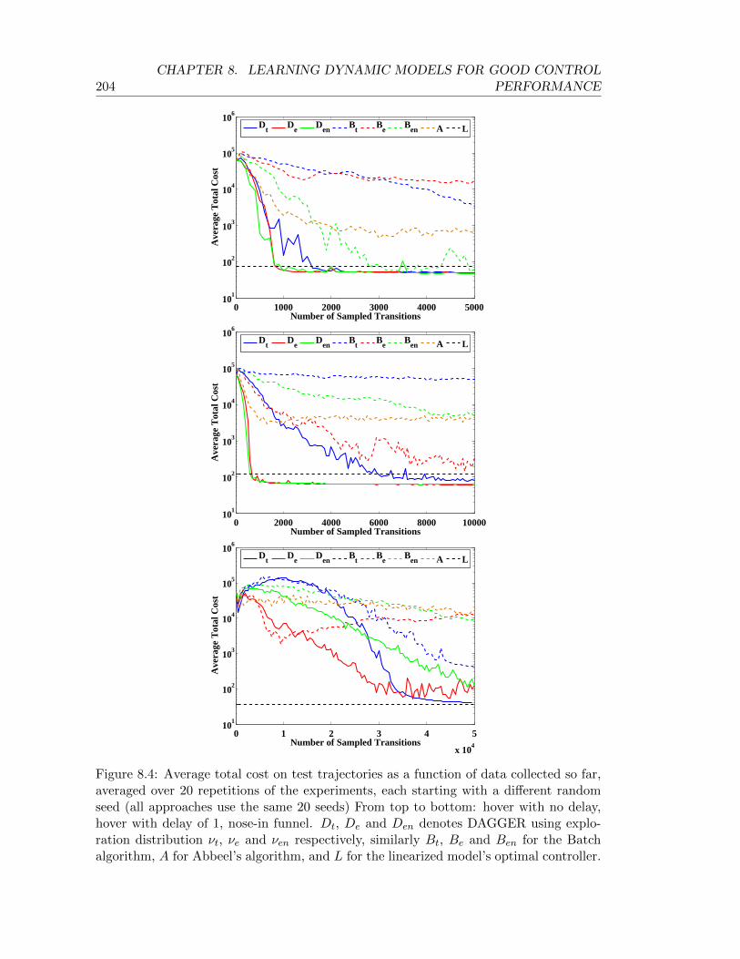
204CHAPTER 8. LEARNING DYNAMIC MODELS FOR GOOD CONTROL
PERFORMANCE
0 1000 2000 3000 4000 500010
1
102
103
104
105
106
Number of Sampled Transitions
Ave
rage
Tot
al C
ost
Dt
De
Den
Bt
Be
Ben A L
0 2000 4000 6000 8000 1000010
1
102
103
104
105
106
Number of Sampled Transitions
Ave
rage
Tot
al C
ost
Dt
De
Den
Bt
Be
Ben A L
0 1 2 3 4 5
x 104
101
102
103
104
105
106
Number of Sampled Transitions
Ave
rage
Tot
al C
ost
Dt
De
Den
Bt
Be
Ben A L
Figure 8.4: Average total cost on test trajectories as a function of data collected so far,averaged over 20 repetitions of the experiments, each starting with a different randomseed (all approaches use the same 20 seeds) From top to bottom: hover with no delay,hover with delay of 1, nose-in funnel. Dt, De and Den denotes DAGGER using explo-ration distribution νt, νe and νen respectively, similarly Bt, Be and Ben for the Batchalgorithm, A for Abbeel’s algorithm, and L for the linearized model’s optimal controller.
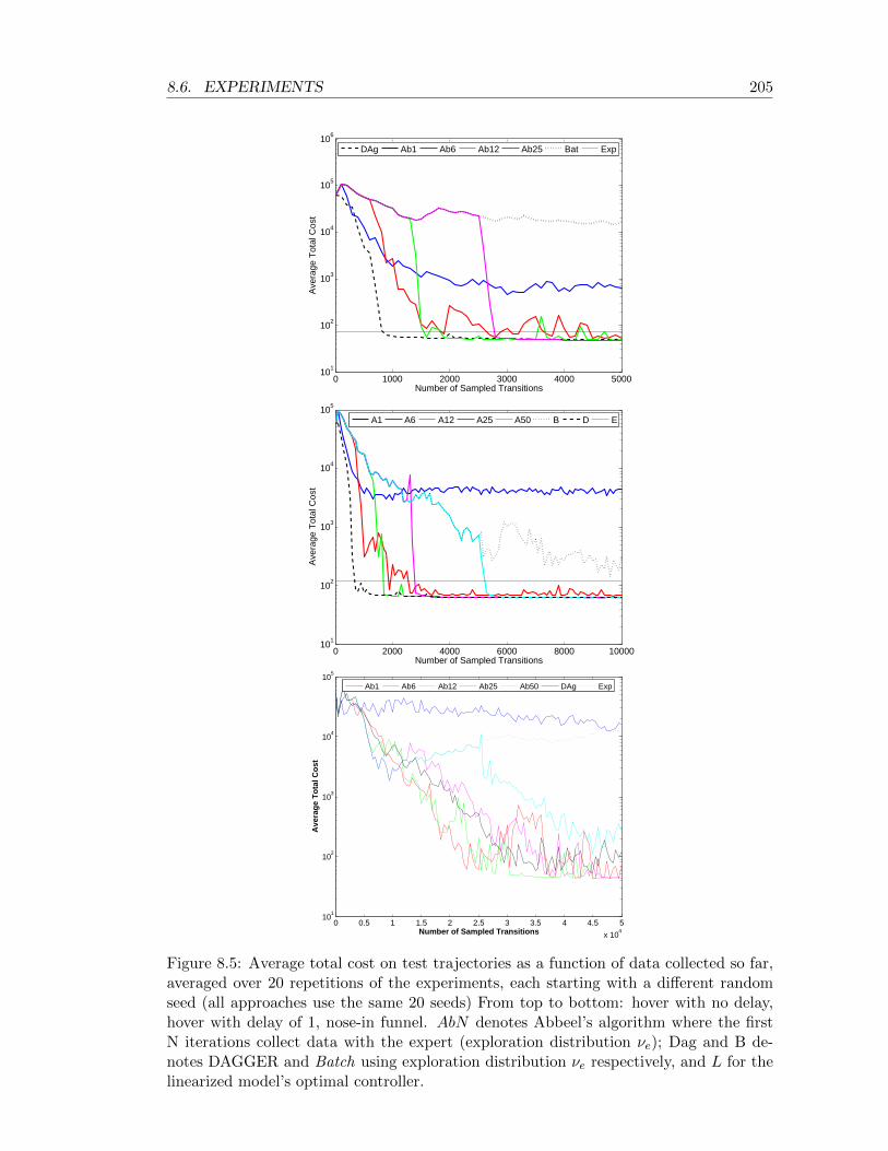
8.6. EXPERIMENTS 205
0 1000 2000 3000 4000 500010
1
102
103
104
105
106
Number of Sampled Transitions
Ave
rage
Tot
al C
ost
DAg Ab1 Ab6 Ab12 Ab25 Bat Exp
0 2000 4000 6000 8000 1000010
1
102
103
104
105
Number of Sampled Transitions
Ave
rage
Tot
al C
ost
A1 A6 A12 A25 A50 B D E
0 0.5 1 1.5 2 2.5 3 3.5 4 4.5 5
x 104
101
102
103
104
105
Number of Sampled Transitions
Ave
rag
e T
ota
l Co
st
Ab1 Ab6 Ab12 Ab25 Ab50 DAg Exp
Figure 8.5: Average total cost on test trajectories as a function of data collected so far,averaged over 20 repetitions of the experiments, each starting with a different randomseed (all approaches use the same 20 seeds) From top to bottom: hover with no delay,hover with delay of 1, nose-in funnel. AbN denotes Abbeel’s algorithm where the firstN iterations collect data with the expert (exploration distribution νe); Dag and B de-notes DAGGER and Batch using exploration distribution νe respectively, and L for thelinearized model’s optimal controller.

Chapter 9
Stability as a Sufficient Condition
for Data Aggregation
The guarantees of our DAGGER approach throughout rely on the strong no-regret prop-
erty of an underlying online learner, used to pick the sequence of predictors/models over
the iterations of training. In general, no-regret online learning is not always possible
(at least computationally efficiently) depending on the class of hypothesis and loss con-
sidered (e.g. there is no known efficient online learner for rich model class like decision
trees (Breiman et al., 1984), random forests (Breiman, 2001) or neural networks (Hastie
et al., 2001)). This may in principle, limit the applicability of our approach with certain
classes of hypothesis.
To address this potential limitation, we have recently introduced sufficient conditions
for online algorithms to be no-regret that do not rely on properties of the loss or hy-
pothesis class, but instead, rely on properties of the algorithm choosing the sequence of
hypotheses (Ross and Bagnell, 2012b). In particular, we have showed that if the algo-
rithm is: (1) “stable”, under a appropriate notion of stability, and (2) asymptotically
chooses hypotheses that minimize the loss in hindsight, then it must be no-regret.
These results have major implications for DAGGER. The aggregation approach (i.e.
Follow-the-(Regularized)-Leader), where at each iteration a batch supervised learning
problem is solved to return the best predictor on the aggregate dataset, must have
good guarantees whenever the supervised learner has sufficient stability properties on
the observed sequence of data. Thus in principle, DAGGER can still provide good
guarantees with rich hypothesis classes such as decision trees or neural networks, by
simply solving supervised learning problems at each iteration on the aggregate dataset,
if the returned hypothesis over the iterations are sufficiently stable for the observed
sequence of data.
A high-level interpretation of this result is the following: if you aggregate data and
you are following the (regularized) leader; most decent supervised learners will be rea-
208CHAPTER 9. STABILITY AS A SUFFICIENT CONDITION FOR DATA
AGGREGATION
sonably stable (especially in common problems where the observed sequence of data is
not as if it was coming from a worst case adversary); therefore we’d expect them to be-
have like no-regret algorithms, and provide good guarantees. This approach motivates
the particular variant of DAGGER we typically use in practice that involves aggregation
of data together with batch learning.
We briefly summarize these results in this chapter, and refer the reader to (Ross and
Bagnell, 2012b) for a more in depth discussion and analysis.
9.1 Online Stability
We now introduce the notion of stability required to provide good guarantees for the
aggregation approach.
The stability condition is related to stability notions that were recently introduced
to study learnability in the batch setting (Shalev-Shwartz et al., 2010). These stability
notions measure how the output of the learning algorithm changes upon removal, or
replacement, of a single training instance in the training set. At a high-level, these
conditions specify that an algorithm is stable if the change in loss on the held out instance
is guaranteed to become arbitrarily small as the training set becomes arbitrarily large.
Some stability notions are stronger that others, e.g. depending on whether this holds for
all possible training set, or only in expectation under sampled sets.
For online learning, we introduced the notion of online stability (Ross and Bagnell,
2012b). It specifies that an algorithm is online stable if for any sequence of training
instances picked by an adversary, the loss `(hn, zn) of the current hypothesis hn on the
current instance zn, compared to the loss of the next hypothesis hn+1 on zn, becomes
arbitrarily small as the number of iterations n become arbitrarily large:
Definition 9.1.1. Given a sequence of training instances z1, z2, . . . , let Sn denote the
subset of the first n instances and hn = A(Sn−1) the hypothesis returned by learning
algorithm A after observing the first n− 1 instances. A learning algorithm A is online
stable with respect to loss ` if there exists a sequence εon-stable(n)∞n=1 that is o(1), such
that for any sequence of training instances, |`(A(Sn−1), zn)−`(A(Sn), zn)| ≤ εon-stable(n)
for all n.
Intuitively, this notion of stability captures how sensitive the hypothesis returned
by the learning algorithm is to the addition of a single training example. As the size
of the dataset increases, an online-stable algorithm becomes less and less sensitive to
the addition of a single example. Intuitively, we can expect this to hold for most com-
mon practical scenario with common supervised learning algorithms, especially if some
regularization is used.
9.2. ONLINE STABILITY IS SUFFICIENT FOR BATCH LEARNERS 209
9.2 Online Stability is Sufficient for Batch Learners
Now we will consider the particular class of learning algorithms, that return the best
hypothesis on the data so far (potentially subject to a regularization term), and show
that for such algorithms, online stability implies no-regret.
We formalize this class of algorithms using the following notion of a Regularized
Empirical Risk Minimizer (RERM):
Definition 9.2.1. A learning algorithm A is a Regularized Empirical Risk Mini-
mizer (RERM) if for all m and any dataset Sm = z1, z2, . . . , zm of m instances:
m∑i=0
ri(A(Sm)) +m∑i=1
`(A(Sm), zi) = minh∈H
[m∑i=0
ri(h) +m∑i=1
`(h, zi)] (9.1)
where rimi=0 is a sequence of regularizer functionals (ri : H → R), which measure the
complexity of a hypothesis h, and that satisfy suph,h′∈H |ri(h)−ri(h′)| ≤ ρi for all i where
ρi∞i=0 is a sequence that is o(1).
Note that this definition considers general learning algorithms that may adapt the
regularizer as it observes data. For common approaches that keep a fixed regularizer,
but adapts only the regularization constant, then this implies ri(h) = λir(h), for some
sequence of regularization constants λi and regularizer r. The regularizer r may be the
squared norm of the parameters of the hypothesis h, as is commonly used. The terms
ρi represent a bound on the contribution of the regularization term to the loss. If the
regularizer is a squared norm, then this will imply that we assume the hypothesis class in
bounded within some set (e.g. we only consider hypothesis with squared norm ≤ C for
some C). This is a common assumption for online learning algorithms. Additionally, in
many cases, such bounds can be determined on the norm of the optimal solution based
on the loss `, such that the hypothesis space can be reduced to only consider hypothesis
within a certain norm. The assumption that ρi∞i=0 is a sequence that is o(1) indicates
that in the limit, the contribution of regularization vanishes, and the algorithm returns
the best hypothesis with respect to the loss `. Note also that this definition includes
algorithms that do not use regularization, by considering ri to be 0 functions (in this
case the ρi are 0).
In Ross and Bagnell (2012b), we have showed that any RERM algorithm which is
online stable, is no-regret. This result is formalized below:
Theorem 9.2.1. After m instances, an online stable RERM A has average online regret:
εregret(m) ≤ 1
m
m∑i=1
εon-stable(i) +2
m
m−1∑i=0
ρi +ρmm
(9.2)
210CHAPTER 9. STABILITY AS A SUFFICIENT CONDITION FOR DATA
AGGREGATION
Thus, as εon-stable(m) → 0 and ρm → 0 as m → ∞, an online stable RERM A is
no-regret:
limm→∞
εregret(m) ≤ 0 (9.3)
This result applies to any sequence of instances we might observe, including adver-
sarial sequences. A similar sequence specific statement can be made, that would indicate
that for any particular sequence of instances where the algorithm is online-stable, then
it would be no-regret on that sequence.
In Ross and Bagnell (2012b), we also showed how most common online learning
algorithms can be analyzed in terms of these online stability and RERM properties
(including gradient descent and randomized algorithms). In essence, most online learners
can be modeled as trying to track the best hypothesis in hindsight, while being stable.
9.3 Discussion
In the context of DAGGER in sequential prediction problems, as we may often expect
that the sequence of training data does not behave as if it was coming from a worst
case adversary, we can expect that common supervised learners, applied to the aggre-
gate dataset (and with appropriate regularization), often lead to a sufficiently stable
sequence of hypothesis. This implies that in common practical scenarios, we can ex-
pect the aggregation approach to often behave like a no-regret algorithm and provide
good guarantees (even if we can’t guarantee the learner is no-regret for all worst case
adversarial sequences).
This notion of stability generalizes, in some sense, previous learning approaches for
Reinforcement Learning and Structured Prediction that operated by iteratively making
small changes over several iterations of training (Kakade and Langford, 2002, Bagnell
et al., 2003, Daume III et al., 2009). Hence our results can be understood as generalizing
this strategy, and showing that many update schemes can be used, such as any no-regret
online algorithm, or stable batch learning algorithms. This allows a greater flexibility
for choosing procedures that are more practical or appropriate for the given application
and class of predictors.
Chapter 10
The Complexity of Learning
Sequential Predictions
Throughout this thesis, we have seen how algorithms training over multiple iterations
can achieve good guarantees in various sequential prediction problems. At the same
time, we have shown that supervised learning methods that attempt to learn only from
examples of good behavior, without interaction with the learner, cannot provide good
guarantees, as the learned behavior is not robust to its own errors in predictions.
These observations indicate that multiple rounds of interactions with the learner may
be necessary in general, for any learning algorithm to provide good guarantees. In the
following sections, we investigate how many rounds any learning algorithm must interact
with the learner to achieve good performance.
For simplicity, we will focus on canonical sequential prediction problems from the
imitation learning setting. Among the various approaches we have presented, we have
seen that for problems with a task horizon of T predictions, T rounds of interaction is
sufficient, e.g. using the Forward training algorithm. The question we are interested in
answering is whether it may be possible that other learning algorithms can learn good
behaviors in fewer iterations, e.g. in a constant number of iterations, or with a smaller
dependency on T .
The number of rounds of interactions required by the learning algorithm captures
a notion of complexity for learning in these sequential prediction tasks. We will refer
to this notion of complexity as the interaction complexity. We formalize this notion in
the next section, and then provide lower bounds on the interaction complexity of any
learning algorithm to provide good guarantees.

212CHAPTER 10. THE COMPLEXITY OF LEARNING SEQUENTIAL
PREDICTIONS
10.1 Interaction Complexity
Intuitively, by interaction complexity, we want to measure the number of predictors we
will need to train, in order to obtain one or construct one that has good performance. To
formalize this notion, we consider learning algorithms which have access to a “learning
oracle”, that for any input distribution of examples, returns a predictor with error rate
ε > 0, or regret ε > 0, for this input distribution:
Definition 10.1.1. An ε-error learning oracle O : ∆→ H is a learning procedure, such
that for any distribution of examples D ∈ ∆, returns a predictor h ∈ H with error rate
lower or equal to ε under D: i.e. E(x,y)∼D,y∼h(x)[I(y 6= y)] ≤ ε.
Definition 10.1.2. An ε-regret learning oracle O : ∆→ H is a learning procedure, such
that for any distribution of examples D ∈ ∆, returns a predictor h ∈ H with regret lower
or equal to ε under D: i.e. E(x,y)∼D,y∼h(x)[I(y 6= y)] − minh′∈H E(x,y)∼D,y∼h′(x)[I(y 6=y)] ≤ ε.
For example, the learning oracle may be a typical supervised learning algorithm.
When considering an ε-error oracle, the error rate ε may be attributed to the fact that
the oracle is sampling from the input distribution D to learn, or that even if it collects an
arbitrarily large number of samples from D, the target predictions cannot be represented
perfectly within the class of hypothesis considered H, or simply because the optimization
procedure is approximated or stopped once it is within ε of optimal. Similarly, when
considering an ε-regret oracle, the regret ε may be attributed to the fact that the oracle
may be optimizing on a finite sample from D, or stopping optimization when it is within
ε of optimal.
With these notions of a learning oracle, we simply define the interaction complexity
as follows:
Definition 10.1.3. Given access to an ε-error (or ε-regret) learning oracle O, the in-
teraction complexity of a learning algorithm is the number of queries it performs to O to
construct/obtain the final learned policy for test execution.
For example, the Forward algorithm has interaction complexity of T , as it queries
a learning oracle T times, once for each time step. Given access to an ε-regret oracle,
Forward constructs a policy that has an expected total regret of Tε over T steps on
its test trajectories. On the other hand, the typical supervised learning approach has
interaction complexity of 1, but has O(T ) expected total regret in general on the test
10.1. INTERACTION COMPLEXITY 213
trajectories when given access to an ε-regret oracle. Similarly, when given access to an
ε-error learning oracle, Forward guarantees a policy with Tε expected mistakes over T
steps, while the supervised learning approach only guarantees a predictor that has an
expected number of mistakes of O(T 2ε) over T steps.
In our analysis of interaction complexity, we will not limit the learning algorithm to
use precisely one of the predictor returned by the learning oracle. Instead, we consider
general learning algorithms that can potentially combine the predictors returned by the
learning oracle in some way to obtain the final predictor used for test execution. The
Forward training algorithm is an example of this, where the predictors returned by the
learning oracle are combined together, a different one used at each time step, to define
the final policy. In general, we will allow the learning algorithm to potentially use a
different distribution over policies returned by the learning oracle in every state and/or
time step.
Given these definitions, we are interested in analyzing the minimum interaction com-
plexity of any learning algorithm that can guarantee to construct a policy with expected
number of mistakes O(Tε), or expected total regret of O(Tε), over T steps.
Relation to Sample Complexity
For most learning algorithm, it is typical to analyze its sample complexity, i.e. the
number of samples required to achieve error (or regret) below some level of tolerance.
While sample complexity is also an interesting notion to analyze for sequential prediction
tasks, that indicates the total number of samples required to obtain a good policy, it
does not capture that we may need to adapt the distribution of samples, and that
simply sampling more from the same distribution may not help improve performance.
This is precisely what the notion of interaction complexity seeks to measure. Hence, the
interaction complexity complements the notion of sample complexity. In the context of
interaction complexity, the sample complexity is abstracted into the learning oracle, as
we potentially allow the learning oracle to collect an infinite number of samples from
the input distribution D. However, even with infinite samples (per query to the learning
oracle), the interaction complexity may indicate that we still need to adapt the sampling
distribution several times before we can obtain a good policy. The interaction complexity
may also be useful to determine the sample complexity of an algorithm. For instance if
we know that each query to the learning oracle will require a certain number of samples
to guarantee a predictor with error (or regret) ε, then multiplying this number by the
interaction complexity will provide a bound on the overall sample complexity of the
learning algorithm.
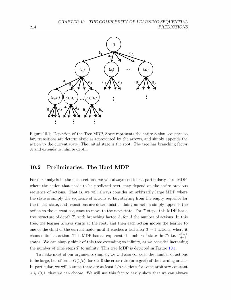
214CHAPTER 10. THE COMPLEXITY OF LEARNING SEQUENTIAL
PREDICTIONS
a1
a2 aA
a1,a1 a1,a2 a1,aA
…
…
…
… …
…
…
a1 a2
aA
a1 a2
aA a1 aA a1 aA
a1 aA a1 aA a1 aA
Figure 10.1: Depiction of the Tree MDP. State represents the entire action sequence sofar, transitions are deterministic as represented by the arrows, and simply appends theaction to the current state. The initial state is the root. The tree has branching factorA and extends to infinite depth.
10.2 Preliminaries: The Hard MDP
For our analysis in the next sections, we will always consider a particularly hard MDP,
where the action that needs to be predicted next, may depend on the entire previous
sequence of actions. That is, we will always consider an arbitrarily large MDP where
the state is simply the sequence of actions so far, starting from the empty sequence for
the initial state, and transitions are deterministic: doing an action simply appends the
action to the current sequence to move to the next state. For T steps, this MDP has a
tree structure of depth T , with branching factor A, for A the number of actions. In this
tree, the learner always starts at the root, and then each action moves the learner to
one of the child of the current node, until it reaches a leaf after T − 1 actions, where it
chooses its last action. This MDP has an exponential number of states in T : i.e. AT−1A−1
states. We can simply think of this tree extending to infinity, as we consider increasing
the number of time steps T to infinity. This tree MDP is depicted in Figure 10.1.
To make most of our arguments simpler, we will also consider the number of actions
to be large, i.e. of order O(1/ε), for ε > 0 the error rate (or regret) of the learning oracle.
In particular, we will assume there are at least 1/αε actions for some arbitrary constant
α ∈ (0, 1] that we can choose. We will use this fact to easily show that we can always

10.3. INEVITABILITY OF POOR GUARANTEES FOR NON-ITERATIVEMETHODS 215
find some action that was rarely explored in any state, that must lead to some subtree
of the MDP that was rarely explored. However, most of our arguments could also be
carried if the number of actions is smaller, by considering small sequences of actions, in
that from any state, one can always find sequences of O(log(1/ε)) actions that would
lead to a subtree that has rarely been explored.
In this exponentially large MDP, we will also consider policies that are represented
by a separate distribution over actions in every state, i.e. a policy represented by SA
parameters (probabilities), for S the number of states. While the complexity of this
policy class is exponential in T (as S is exponential in T ), as we allow for potentially
infinite samples for each query to the oracle, we can always assume that the oracle can
still learn a good policy in this class.
Our interaction complexity results will make use of these exponentially large MDP
and policy class to prove that we must need a certain number of iterations. It remains an
open question whether similar results could be instead directly related to the complexity
of the MDP and/or policy class. Despite this, our results demonstrate that without
further assumptions on the size of the MDP or complexity of the policy class, one will
need several iterations to guarantee good performance.
10.3 Inevitability of Poor Guarantees for Non-Iterative
Methods
We begin our analysis by first showing that there cannot exist any learning algorithm that
can provide good guarantees in general with only a single query to the learning oracle.
In particular, we show that, given access to an ε-error learning oracle, any algorithm
with interaction complexity of 1, obtains a policy with expected number of mistakes of
Ω(min(T 2ε, T )) over sequences of T steps, for some arbitrarily large MDP and policy
class. Additionally, we also show that given access to an ε-regret learning oracle, any
algorithm with interaction complexity of 1, obtains a policy with expected total regret
of Ω(T ), over sequences of T steps, for some arbitrarily large MDP and policy class.
These results generalize our analysis of the supervised learning method that trains
only from expert demonstrations, and shows that even if some form of exploration would
be used, to query the expert in states that are rarely or never visited under the expert
behavior, this does not improve performance in the worst case.
Theorem 10.3.1. Given access to an ε-error learning oracle, there exist MDPs and
policy classes where any learning algorithm with interaction complexity of 1 obtains a
policy with expected number of mistakes Ω(min(T 2ε, T )) over sequences of T steps.
Proof. This follows from a fairly straightforward observation due to the large number of
216CHAPTER 10. THE COMPLEXITY OF LEARNING SEQUENTIAL
PREDICTIONS
actions and states in this hard MDP. First consider states along the expert’s trajectory
in this tree MDP. There are dT/2e states in the first dT/2e time steps, and under any
training distribution, there would exist at least one state among these with probability
≤ 2/T . Pick any such state and denote it s′. Now in s′, suppose the learned predictor
makes a mistake with probability min((1−α)Tε/2, 1), and all other states s at previous
steps along the expert trajectory have error 0. Additionally, since there are at least 1αε
actions that one can take from state s′, under any training distribution over states, there
would always exists at least one action whose probability mass over its entire subtree
is lower or equal to αε. Pick such action and denote it a′. Therefore, one can assign
error 1 in every state in the subtree of action a′, and we can make the learned predictor
always pick a′ when it makes a mistake in s′. This leads to a learned predictor that has
error ≤ 2/T min((1 − α)Tε/2, 1) + αε ≤ ε under the training distribution, which could
therefore be returned by the learning oracle. Yet, when executing this predictor, we
would always reach state s′, and then if it makes a mistake, i.e. pick a′, it would incur
at least T/2 mistakes over the entire sequence. This implies that the expected number
of mistakes of this predictor is at least min((1− α)T 2ε/4, T/2).
Theorem 10.3.2. Given access to an ε-regret learning oracle, there exist MDPs and
policy classes where any learning algorithm with interaction complexity of 1 obtains a
policy π with expected total regret R(π) of Ω(T ) under its own sequences of T steps.
Proof. Follows from a similar argument as in the previous theorem. Again consider states
along the expert’s trajectory in this tree MDP, and denote s0 the initial state. Consider
a policy class where in all states, except s0, there exist predictors with 0 error, but in
s0, all predictors in the class make an error with probability at least 12 . Additionally,
since there are at least 1αε actions that one can take from state s0, under any training
distribution over states, there would always exists at least one action whose probability
mass over its entire subtree is lower or equal to αε. Pick such action and denote it a′. So
now consider the learned predictor to be a predictor that never makes an error, except
in state s0 and in the subtree of a′, where in s0 it errors with probability 12 and picks a′,
and in the subtree of a′ it errors with probability 1 in all states in that subtree. Now
since we assumed there exists a predictor in the class that achieves 0 error everywhere,
except in s0 where it errors with probability 12 , then the regret of the learned predictor
under the training distribution is at most αε, and could thus be returned by the learning
oracle. On the other hand, during test execution, the learned predictor always starts in
s0, at which point with probability 12 , it picks action a′, and performs T mistakes over
the sequence. On the other hand, on this same sequence, there exist predictors that
error with probability 12 in s0, but then never errors until the end of the sequence. When
10.4. LINEAR DEPENDENCY OF THE INTERACTION COMPLEXITY ON THETASK HORIZON 217
the learned predictor doesn’t error in s0, then it never errors, and the same occurs for
the best predictor in the class. Thus the total expected regret of the learned predictor
is 12(T − 1).
10.4 Linear Dependency of the Interaction Complexity
on the Task Horizon
We now show that in general, the number of queries to the learning oracle must scale
linearly with the number of time steps T in order to obtain a policy with good guarantees.
In particular, given access to an ε-error learning oracle, our analysis will show that at
least Ω(Tε) queries are required, to obtain a policy with O(Tε) expected mistakes over T
steps. Additionally, we will show that, given access to an ε-regret learning oracle, Ω(T )
queries are required in general to obtain a policy with order O(Tε) expected total regret
over T steps.
Lemma 10.4.1. Given access to an ε-error learning oracle, there exist MDPs and policy
classes where any learning algorithm with interaction complexity of k obtains a policy
whose expected number of mistakes is at least:
k−1∑i=1
i
(T
i
)εi(1− ε)T−i +
T∑t=k
(t− 1
k − 1
)εk(1− ε)t−k(T − t+ k)
Proof. Consider the hard tree MDP presented previously. On the first query to the
learning oracle, we can make the learning oracle return the following predictor: for the
T states s1, s2, . . . , sT , along the expert trajectory, the learned predictor makes a mistake
with probability (1−α)ε in each si. Because in each of these states there are at least 1αε
actions that can be taken, all leading to different regions of the state space, there must
exist a set of actions a1, a2, . . . , aT , where ai denotes an action taken in si, where the
sum of the probability mass over all the states in the subtrees of a1, a2, . . . , aT is at most
αε. Thus for all these subtrees, we can assign a probability 1 of mistake in every state.
Additionally, when the predictor makes a mistake in state si, we can make it always
choose action ai. We obtain that under any training distribution, for the first query to
the learning oracle, we can return such predictor that has error ≤ (1 − α)ε + αε ≤ ε
under the training distribution. Now for all remaining iterations, we can always return a
predictor that is exactly the same in states s1, s2, . . . , sT , but potentially changes in the
subtrees of a1, a2, . . . , aT . At the second iteration we can apply the same reasoning over
each of the subtrees of a1, a2, . . . , aT , and construct a predictor that has the same error
structure as the first learned predictor, but within each of the subtree. That is for the
second iteration, consider the error of the learned predictor to be (1−α)ε in every state

218CHAPTER 10. THE COMPLEXITY OF LEARNING SEQUENTIAL
PREDICTIONS
along the expert trajectory after each of the erroneous actions a1, a2, . . . , aT . Since we
keep the learned predictor to be the same along the expert trajectory, then this second
learned predictor has error (1− α)ε in every states where the predictor has made 0 or 1
mistake so far. But again we can find a set of actions that represent the mistakes this
second predictor can makes in states reached after 1 mistake has been done, whose sum
of probability mass in all their subtrees would be at most αε, such that we can still assign
error 1 in every state in those subtrees. Note that because these subtrees are themselves
subtrees of a1, a2, . . . , aT , all these states must also had error 1 in the first iteration. This
implies that for any combination of the first 2 predictors, we can only obtain a predictor
which has probability of mistakes (1 − α)ε, as long as it has made 0 or 1 mistake so
far, but then after 2 mistakes, must make a mistake with probability 1 in every future
state. It is also clear that this second learned predictor satisfies the constraint that it
has error ≤ ε under any training distribution (there is probability mass ≤ 1 on states
with error ε(1−α) and probability mass ≤ αε on states with error 1). The end result is
that after 2 iterations, we can always obtain a predictor that errors with probability 1,
after 2 mistakes has been done, or errors with probability (1− α)ε otherwise. The same
reasoning can be applied recursively, to see that after k iterations, we can always obtain
a predictor that errors with probability 1 after k mistakes, or errors with probability
(1 − α)ε otherwise. Let ε′ = (1 − α)ε. Then if we have such a predictor, it can be seen
that its expected number of mistakes over T steps is:
k−1∑i=1
i
(T
i
)ε′i(1− ε′)T−i +
T∑t=k
(t− 1
k − 1
)ε′k(1− ε′)t−k(T − t+ k)
The first summation can be seen as summing over all the paths with i mistakes, for
i ≤ k− 1, while the second summation sums over all the paths with k or more mistakes,
conditioning on the time t where the kth mistake occur (there are(t−1k−1
)paths whose kth
mistake occur on the tth step). The lemma follows from the fact that we can always pick
a large enough number of actions so that ε′ = (1−α)ε is arbitrarily close to ε (although
it should be noted that this is not necessary, even α = 1/2, is sufficient to prove our
main result in the next theorem).
Theorem 10.4.1. Given access to an ε-error learning oracle, there exist MDPs and
policy classes where any learning algorithm must have interaction complexity of Ω(Tε)
to obtain a policy with an expected number of mistakes of O(Tε) over sequences of T
steps.
Proof. Consider the lower bound on the number of mistakes after k iterations obtained
in the previous lemma:
k−1∑i=1
i
(T
i
)εi(1− ε)T−i +
T∑t=k
(t− 1
k − 1
)εk(1− ε)t−k(T − t+ k)
10.4. LINEAR DEPENDENCY OF THE INTERACTION COMPLEXITY ON THETASK HORIZON 219
The first summation is ≤ Tε and tends to this quantity as k → T (it tends to the
expectation of a Binomial(T, ε)). Hence this lower bound on the number of mistakes is
O(Tε) if the second summation is O(Tε).
The second summation resembles the expectation of a quantity under a negative
binomial distribution. That is, let r = t− k, the number of times we picked the expert’s
action before making k mistakes, F (·; 1 − ε, k) the cumulative density function of a
negative binomial, with probability of success 1 − ε, and stopping after k failures, and
E[r] the expectation of this negative binomial distribution, then:
∑Tt=k
(t−1k−1
)εk(1− ε)t−k(T − t+ k)
=∑T−k
r=0
(k+r−1r
)εk(1− ε)r(T − r)
= T∑T−k
r=0
(k+r−1r
)εk(1− ε)r −
∑T−kr=0
(k+r−1r
)εk(1− ε)rr
= TF (T − k; 1− ε, k)−∑T−k
r=0
(k+r−1r
)εk(1− ε)rr
≥ TF (T − k; 1− ε, k)−∑∞
r=0
(k+r−1r
)εk(1− ε)rr
= TF (T − k; 1− ε, k)− E[r]
Since E[r] = (1− ε)k/ε, we obtain
T∑t=k
(t− 1
k − 1
)εk(1− ε)t−k(T − t+ k) ≥ TF (T − k; 1− ε, k)− (1− ε)k/ε
Now 1−F (T−k, 1−ε, k) is the probability that it takes more than T−k trials to get k
failures, when the probability of success is (1− ε). In other words, this is the probability
that out of T − k trials, we get less than k failures, i.e. P (X < k) if X ∼ Bin(T − k, ε)is a binomial distributed random variable with probability of success ε. We will seek to
upper bound P (X < k) (i.e. 1− F (T − k, 1− ε, k)) in order to obtain a lower bound on
F (T − k, 1− ε, k). We know X is concentrated around its mean E[X] = (T − k)ε, so we
will consider k smaller than the mean, i.e. k < (T − k)ε, which implies k < Tε/(1 + ε),
to show that when it is small enough, F (T − k, 1− ε, k) becomes close to 1, making the
expected number of mistakes of the predictor Ω(T ).
Using Chernoff’s bound, we know that P (X < (1 − δ)µ) ≤ exp(−δ2µ/2), for µ the
mean of X (i.e. µ = (T −k)ε here). Suppose k = βTε for some β ∈ [0, 1/(1+ε)], then we
have (T −k)ε = T (1−βε)ε and k = (1−δ)µ for δ = 1−β/(1−βε). Hence we obtain that
P (X < k) ≤ exp(−(1− βε− β)2Tε/(2(1− βε))). This implies that 1−F (T − k, 1− ε, k)
is exponentially small in T , and thus that F (T − k, 1 − ε, k) is arbitrarily close to 1 as
T → ∞, when k ≤ βTε. In particular this is the case when k = Tε/2. Yet we can see
that at k = Tε/2, TF (T − k; 1− ε, k)− (1− ε)k/ε would tend to T/2 + Tε/2 as T →∞,
i.e the expected number of mistakes of the predictor is Ω(T ) after only Tε/2 iterations.
On the other hand, with the lower bound TF (T −k; 1−ε, k)−(1−ε)k/ε, we observe that
at k = Tε, this lower bound would be O(Tε). Thus it is possible that Tε iterations is

220CHAPTER 10. THE COMPLEXITY OF LEARNING SEQUENTIAL
PREDICTIONS
sufficient. We conclude that we need k at least in Ω(Tε), to make the expected number
of mistakes order O(Tε).
Lemma 10.4.2. Given access to an ε-regret learning oracle, there exist MDPs and policy
classes where any learning algorithm with interaction complexity of k obtains a policy
whose expected total regret is at least:
maxε′∈[0,1]
k−1∑i=1
i
(T
i
)ε′i(1− ε′)T−i +
T∑t=k
(t− 1
k − 1
)ε′k(1− ε′)t−k(T − t+ k)− Tε′
Proof. We use a similar argument to lemma 10.4.1. Consider the hard tree MDP pre-
sented previously. Additionally, consider a policy class where in all states that minimum
possible error is ε′ > 0, and there exist a predictor achieving ε′ error in all states. On
the first query to the learning oracle, we can make the learning oracle return the fol-
lowing predictor: for the T states s1, s2, . . . , sT , along the expert trajectory, the learned
predictor makes a mistake with probability ε′ in each si. Because in each of these states
there are at least 1αε actions that can be taken, all leading to different regions of the
state space, there must exist a set of actions a1, a2, . . . , aT , where ai denotes an action
taken in si, where the sum of the probability mass over all the states in the subtrees of
a1, a2, . . . , aT is at most αε. Thus for all these subtrees, we can assign a probability 1
of mistake in every state. Additionally, when the predictor makes a mistake in state si,
we can make it always choose action ai. We obtain that under any training distribution,
for the first query to the learning oracle, we can return such predictor that has regret
≤ αε ≤ ε under the training distribution. Now for all remaining iterations, we can al-
ways return a predictor that is exactly the same in states s1, s2, . . . , sT , but potentially
changes in the subtrees of a1, a2, . . . , aT . At the second iteration we can apply the same
reasoning over each of the subtrees of a1, a2, . . . , aT , and construct a predictor that has
the same error structure as the first learned predictor, but within each of the subtree.
That is for the second iteration, consider the error of the learned predictor to be ε′ in
every state along the expert trajectory after each of the erroneous actions a1, a2, . . . , aT .
Since we keep the learned predictor to be the same along the expert trajectory, then this
second learned predictor has error ε′ in every states where the predictor has made 0 or
1 mistake so far. But again we can find a set of actions that represent the mistakes this
second predictor can makes in states reached after 1 mistake has been done, whose sum
of probability mass in all their subtrees would be at most αε, such that we can still assign
error 1 in every state in those subtrees. Note that because these subtrees are themselves
subtrees of a1, a2, . . . , aT , all these states must also had error 1 in the first iteration.
This implies that for any combination of the first 2 predictors, we can only obtain a
predictor which has probability of mistakes ε′, as long as it has made 0 or 1 mistake so

10.4. LINEAR DEPENDENCY OF THE INTERACTION COMPLEXITY ON THETASK HORIZON 221
far, but then after 2 mistakes, must make a mistake with probability 1 in every future
state. It is also clear that this second learned predictor satisfies the constraint that it
has regret ≤ ε under any training distribution (there is probability mass ≤ 1 on states
with regret 0 and probability mass ≤ αε on states with regret (1− ε′)). The end result
is that after 2 iterations, we can always obtain a predictor that errors with probability
1, after 2 mistakes has been done, or errors with probability ε′ otherwise. The same
reasoning can be applied recursively, to see that after k iterations, we can always obtain
a predictor that errors with probability 1 after k mistakes, or errors with probability ε′
otherwise. Then if we have such a predictor, it can be seen that its expected number of
mistakes over T steps is:
k−1∑i=1
i
(T
i
)ε′i(1− ε′)T−i +
T∑t=k
(t− 1
k − 1
)ε′k(1− ε′)t−k(T − t+ k)
The first summation can be seen as summing over all the paths with i mistakes, for
i ≤ k− 1, while the second summation sums over all the paths with k or more mistakes,
conditioning on the time t where the kth mistake occur (there are(t−1k−1
)paths whose kth
mistake occur on the tth step). Now under the test sequences of this learned predictor,
there exists a predictor in the class with only Tε′ expected mistakes, thus the regret of
the learned predictor is at least:
k−1∑i=1
i
(T
i
)ε′i(1− ε′)T−i +
T∑t=k
(t− 1
k − 1
)ε′k(1− ε′)t−k(T − t+ k)− Tε′
The lemma follows from the fact that we can pick any ε′ ∈ [0, 1] to make this quantity
as large as possible.
Theorem 10.4.2. Given access to an ε-regret learning oracle, there exist MDPs and
policy classes where any learning algorithm must have interaction complexity of Ω(T ) to
obtain a policy with an expected total regret of O(Tε) over sequences of T steps.
Proof. Using the result in the previous lemma, and the same argument as in Theorem
10.4.1 to lower bound the term∑T
t=k
(t−1k−1
)ε′k(1− ε′)t−k(T − t+ k), we can see that the
expected total regret of the learned predictor after k queries is at least:
TF (T − k; 1− ε′, k)− E[r]− Tε′,
for F (T − k; 1 − ε′, k) the cumulative density function of a negative binomial, with
probability of success 1 − ε′, and stopping after k failures, and E[r] = (1 − ε′)k/ε′ the
expectation of this negative binomial distribution. Again, following a similar argument
as in Theorem 10.4.1, we can show that for k = Tε′/2, TF (T − k; 1− ε′, k)− (1− ε′)k/ε′

222CHAPTER 10. THE COMPLEXITY OF LEARNING SEQUENTIAL
PREDICTIONS
would tend to T/2 + Tε′/2 as T → ∞. This implies that after k = Tε′/2, the expected
regret of the algorithm is at least T/2 − Tε′/2. As we can choose any ε′ ∈ [0, 1], we
can see that for ε′ = 12 , this indicates that there exist problems where after k = T/4
iterations, the expected total regret is still at least T/4. Thus we conclude that at least
Ω(T ) iterations must be necessary, to make the expected total regret O(Tε).
This lower bound of Ω(T ) queries match directly our upper bound of T (with the
Forward algorithm) on the required interaction complexity of any algorithm guaranteeing
a policy with O(Tε) regret over T steps. Hence this shows our lower bound is tight, that
any algorithm must need a number of iterations of the same order as the number of time
steps T , and that Forward achieves the lower bound within a constant factor.
On the other hand, when an ε-error learning oracle is available, we obtained a lower
bound of Ω(Tε) queries. In this case, this does not match directly our upper bound of T
(with the Forward algorithm) on the interaction complexity of any algorithm guarantee-
ing a policy with O(Tε) mistakes over T steps. Hence it potentially suggests that when
low error is possible (rather than just low regret), better algorithms than the Forward
Training procedure might exists that would require only a fraction ε of the number of
queries currently performed by the Forward algorithm. Despite this fact, it shows that
in general the number of iterations, or queries to the learning oracle, must inevitably
scale linearly with the number of time steps T .
Chapter 11
Conclusion
We now conclude by discussing the contributions of this thesis with regards to our original
thesis statement:
Learning actively through interaction is necessary to obtain good
and robust predictors for sequential prediction tasks. No-regret
online learning methods provide a useful class of algorithms to learn
efficiently from these interactions, and provide good performance
both theoretically and empirically.
Passive Supervised Learning and the Data Mismatch
Many of the sequential prediction settings we presented in this thesis look like typical
statistical supervised learning problems, where a dataset of labeled examples can be
obtained. However, we provided a detailed theoretical analysis of such naive supervised
learning techniques in various sequential prediction settings and demonstrated their poor
performance guarantees due to the mismatch between the training and test distribution
of examples that can occur. In addition, in the context of imitation learning and system
identification, we presented examples of simple MDPs where such methods fail and match
the poor guarantee.
The train-test mismatch is often induced by errors made by the learned predictors.
As these errors can lead to new untrained situations, a single error can propagate into
a large series of errors. As such, the learned predictors, obtained by naive supervised
learning, are non-robust to their own errors.
Leveraging Interaction to Learn Robust Predictors
We presented several learning techniques that interact with the sequential process and
learner to deal with this train-test mismatch: 1) Forward, which learns sequentially a

224 CHAPTER 11. CONCLUSION
different predictor for each step; 2) SMILE, which learns a stationary stochastic policy
iteratively through small changes; and 3) DAGGER and SCP, that can learn stationary
deterministic policies, via no-regret online learning methods. We analyzed thoroughly
these techniques and demonstrated their improved guarantees in various sequential pre-
diction settings: imitation learning, reinforcement learning, structured prediction, list
optimization and system identification.
Through interaction, these methods are able to collect new examples of correct pre-
dictions after the learned predictor makes errors, allowing the learner to learn more
robust behaviors that can “recover” from its typical errors.
Necessity of Interaction
In chapter 10, we showed that interaction is necessary to learn good and robust predictors
for sequential tasks. In particular, there exists no learning approach that can provide
good guarantees without interaction. We proved lower bounds on the minimum number
of rounds of interactions necessary to provide good guarantees, that scale linearly with
the length of the sequence. In addition, in the context of guaranteeing small regret
(excess error) on the test trajectories, the lower bound is tight and matches the number
of rounds used by the Forward algorithm presented in chapter 3.
Practicality and Efficiency of the Interactive Online Learning
Approach
Our main learning approach, DAGGER, offers many practical advantages over other
methods in practice:
1. Simple: It is very simple, easy to implement and apply to various tasks.
2. Modular: It can be used in combination with any of your favorite online learning
methods, and/or class of predictors, and can easily be wrapped around existing
off-the-shelf software packages.
3. Scalable: By relying on no-regret learning methods that scale well to large learning
problems, DAGGER scales naturally to large-scale problems, e.g. using computa-
tionally efficient gradient descent methods.
4. Statistically Efficient: The improved guarantees of DAGGER reduce the impact
of the generalization error on performance, allowing DAGGER to learn a good
predictor with fewer data. Additionally, by learning a single stationary policy,
it can generalize the behavior across time steps and learn more efficiently than
methods training a separate predictor for each step.

11.1. OPEN PROBLEMS AND FUTURE DIRECTIONS 225
Applications and Empirical Evidence
We demonstrated the scalability and efficiency of DAGGER in practice on a large variety
of applications in several sequential prediction settings:
1. Improved performance over naive supervised training and other sequential predic-
tion methods, such as SMILE and SEARN, in the context of learning video game
playing agents.
2. Matched the performance of state-of-the-art Structured Prediction methods on
three computer vision tasks: handwriting recognition, 3D Point Cloud classification
and 3D geometry estimation.
3. Improved performance and learning efficiency over state-of-the-art list optimiza-
tion methods on various recommendation tasks, such as grasp selection, trajectory
optimization, news recommendation and document summarization.
4. Improved performance and learning efficiency for system identification over stan-
dard system identification methods and common iterative identification approaches,
in the context of learning models of a simulated helicopter for performing aerobatic
maneuvers.
5. Additionally, we demonstrated that DAGGER can be applied successfully on real
robotic systems, training a quadrotor to fly autonomously through natural forest
environments while avoiding trees.
11.1 Open Problems and Future Directions
Throughout this work, we have come across a number of interesting open problems
and future directions for research. We briefly conclude with important areas of future
research.
More Practical Interactions with Human Experts
In the context of imitation learning, DAGGER, when learning from a human expert,
leads to challenging human-computer interaction issues. In particular, a major difficulty
for the human expert is to provide the correct actions when not in control of the system
(without feedback of the actions he is executing). This was discussed in detail in Section
5.3, where we also discussed some practical solutions. Ideally, however, a more natural
interactive procedure for collecting additional examples from the human expert would be
desired. For instance, a natural one may be to let the system execute its own controller,
and only when the expert deems unsatisfactory behavior is being performed, he takes
226 CHAPTER 11. CONCLUSION
over control of the system until the system is placed back on a correct course, after which
control is returned to the system. By only having to provide actions when the expert
is in control, this would allow the expert to provide more accurate actions. However
such interactions can lead to other issues. For instance, there would be a delay between
the time when a serious error was committed by the system, versus the time when the
expert takes over, therefore not allowing the system to observe the correct actions it
should have executed in the first place to prevent the expert from having to take over.
We additionally do not know how such interaction could be analyzed theoretically to
provide good guarantees.
Iterative Transfer Learning
An alternate solution to the above human-computer interaction issue is to avoid asking
new actions from the human expert entirely, after the first iteration (where the expert
is always fully in command). In other words, only collect labeled examples under the
state distribution of the expert dπ∗ , and at later iterations, DAGGER executes the
current learned policy, but only to collect new unlabeled examples, where the expert’s
action is unknown. To update the predictor, based on the unlabeled data, transfer
learning methods, such as Zadrozny (2004), Huang et al. (2007), could in principle be
used to reweigh the labeled examples in the expert dataset, so that we obtain a weighted
labeled dataset that matches more closely the distribution of examples DAGGER needs
to train on at iteration n, i.e. 1n
∑ni=1 dπi . However, for this to work, the expert dataset
would need to cover the input feature space very well, which is usually not the case,
when the expert is executing on its own (e.g. no examples of what to do when the
car is about to go off the road, or collide with other vehicles). Reweighting would
not help if coverage is poor in the regions where unlabeled data is collected. Coverage
of the initial demonstrations could be increased by introducing random noise in the
actions of the expert during its execution; however, this may still explore poorly, as the
important failure cases that will occur at later iterations of learning may be explored
with exponentially small probability. In preliminary experiments with the technique of
Zadrozny (2004) in the Super Mario Bros. domain of Section 5.2, we did not obtain
much improvement over the baseline supervised learning approach. This could be due
to several factors, such as the particular transfer learning technique used, and perhaps
in other applications, such technique could be used successfully.
Extensions to Other List Optimization Objectives
In Chapter 7, we studied SCP for the particular context of maximizing a submodular
objective under a cardinality constraint on the list. Many other important applications
have different but related objectives. For instance in the Grasp Selection experiment

11.1. OPEN PROBLEMS AND FUTURE DIRECTIONS 227
we were interested in minimizing search depth, which corresponds to a different “min
sum set cover” objective. In extractive document summarization, where the constraint
is on the length of the summary (in characters), this implies that items have different
weight (sentences have different length), and we are subject to a more general knapsack
constraint on the sum of the weights of the items in the list. These variations affect
the particular weighting of the examples that should be used to properly minimize the
desired objective. For instance, to minimize search depth, the analysis in Streeter and
Golovin (2007), suggests weighting examples from early positions in the list more highly.
A more careful analysis of SCP with these variations would be necessary to ensure proper
weighting of the training examples is used and understanding the resulting guarantees
of SCP in these variants. An analysis for the knapsack constraint variant appears in the
recent follow-up work of Zhou et al. (2013).
List Optimization for Structured Prediction
In structured prediction tasks, it can also be desired to obtain multiple possible struc-
tured outputs. For instance, given an input camera image, we may be interested in
obtaining a diverse and relevant set of possible labelings of this image. This may be
important for robots, so that they can carefully take into account possible alternate
interpretations of the world, and adopt a behavior that is robust to these various in-
terpretations. Some recent work has begun to look into this problem (Kulesza and
Taskar, 2010, Guzman-Rivera et al., 2012). It would be interesting to extend SCP to
this scenario.
Agnostic Exploration
In the context of model-free reinforcement learning (Section 4.3), and system identifica-
tion (Chapter 8), our DAGGER approach provides agnostic guarantees, but performance
is limited by the quality of the given fixed exploration distribution. For realizable sys-
tem identification settings, we showed that an optimistic exploration strategy could be
used to guarantee finding a near-optimal policy. However, this strategy relies on the
realizability assumption, and developing adaptive exploration strategies that would lead
to good guarantees in general agnostic settings is an important open problem. Work on
similar exploration issues in contextual bandit learning (Auer et al., 2002b, Beygelzimer
et al., 2011) and agnostic active learning (Dasgupta et al., 2007, Beygelzimer et al., 2010)
may provide ideas that could be extended to these reinforcement learning settings.
228 CHAPTER 11. CONCLUSION
Subspace Identification
For system identification in partially observable settings, our current DAGGER approach
can be applied as is to learn models that predict the future observation from past actions
and observations, and provide similar good agnostic guarantees. However, learning more
compact representations, that can learn an underlying hidden state space model, would
be desirable, especially in situations where observations are high dimensional. This
could allow learning more efficiently. Spectral learning methods have been developed to
learn such models, however their analysis often relies on strong realizability assumptions
(Overschee and Moor, 1996, Boots and Gordon, 2011). A no-regret analysis of such
methods in online settings would be necessary to ensure that they can be used within
DAGGER and provide similar good guarantees. For instance, developing approaches for
doing no-regret online reduced rank regression would provide techniques for achieving
this in the context of learning linear state space models.
Online Regret Reductions
In many settings, we reduced our sequential prediction task to a no-regret online cost-
sensitive classification tasks (e.g. in Chapters 4 and 7). Typical regret reductions for cost-
sensitive classification, bound the cost-sensitive classification regret to the bayes-optimal
predictor, as a function of the regret to the bayes-optimal predictor on a new classification
or regression task (Langford and Beygelzimer, 2005, Beygelzimer et al., 2009, Mineiro,
2010). This does not allow us to bound the online cost-sensitive classification regret
(with respect to only hypothesis in the class), in terms of the online classification or
regression regret (with respect to only hypothesis in the class), without introducing an
additional penalty term: a term that depends on the classification or regression regret of
the best hypothesis in the class to the bayes-optimal predictor. It would be of interest to
provide reductions, that transform online regret at the cost-sensitive classification task,
directly into online regret at the other task, without introducing this additional penalty
term. This would provide improved relative performance guarantees for DAGGER when
comparing to other predictors in the class.
This is perhaps a more general fundamental question worth further investigation,
e.g. can you reduce no-regret learning for various common learning tasks, to a no-regret
online binary classification task, where being no-regret on the binary classification loss
implies no-regret on the original online task. In other words, can you build no-regret
learners for various tasks, starting from a single common primitive, e.g. a no-regret
learner for binary classification.

11.1. OPEN PROBLEMS AND FUTURE DIRECTIONS 229
Efficient Contextual Bandit Learning with General Hypothesis Class
In Chapters 4 and 7, we also observed that we may sometimes only be able to obtain
partial cost-sensitive examples, where the cost of only one or a few predictions are known.
To deal with such partial feedback, contextual bandit algorithms are necessary, rather
than online learning methods. However, current contextual bandit learning methods have
been limited mostly to finite hypothesis class (Auer et al., 2002b), or for learning linear
predictors in realizable settings (Li et al., 2010). Some more involved techniques have
been developed for dealing with more general infinite class of predictors (Dudik et al.,
2011a), but the resulting algorithm remains impractical1 and currently only handles the
stochastic setting, whereas we require no-regret in adversarial settings. DAGGER could
benefit from improved contextual bandit algorithms for dealing with partial feedback
settings.
Are Weaker Notions than No-Regret Sufficient?
DAGGER relies on the availability of a no-regret online learner and our analysis demon-
strates that no-regret is a sufficient property of the learner to provide good guarantees.
In Chapter 9 (and (Ross and Bagnell, 2012b)), we also showed how certain strong stabil-
ity properties of the learner, in combination with asymptotic minimization of the loss in
hindsight, are also sufficient properties to achieve no-regret. As these strong no-regret (or
stability) property cannot always be achieved (at least computationally efficiently) with
all class of hypothesis, weakening these strong requirements is of practical importance
to increase the applicability of our methods to broader and richer class of predictors.
Perhaps weaker stability conditions, such as those in Shalev-Shwartz et al. (2010), with
certain assumptions on the sequential process, may be sufficient for DAGGER to provide
good guarantees in these sequential prediction settings.
1At each update, the algorithm involves running an ellipsoid algorithm, in a space that grows withthe number of data points seen so far, that repeatedly calls a cost-sensitive classification learner for theseparation oracle. The complexity of the update after seeing t data points is of order O(t7), and thusquickly becomes intractable as we collect more data.

Appendices

Appendix A
Analysis of Dagger for Imitation
Learning
In this appendix, we provide the proofs and detailed analysis of Dagger in the imitation
learning setting. We begin with the analysis where surrogate classification/regression
loss is minimized, and then present results for Dagger with cost-to-go.
A.1 Dagger with Imitation Loss
We begin with a useful general lemma that is needed for bounding the expected loss
under different distributions. This will be used several times here and for the analysis of
Dagger in other settings. Here this will be useful for bounding the expected loss under
the state distribution of π in terms of the expected loss under the state distribution of
πi:
Lemma A.1.1. Let P and Q be any distribution over elements x ∈ X , and f : X → R,
any bounded function such that f(x) ∈ [a, b] for all x ∈ X . Let the range r = b−a. Then
|Ex∼P [f(x)]− Ex∼Q[f(x)]| ≤ r2 ||P −Q||1
Proof. We provide the proof for X discrete, a similar argument can be carried for Xcontinuous, using integrals instead of sums.
|Ex∼P [f(x)]− Ex∼Q[f(x)]|= |
∑x P (x)f(x)−Q(x)f(x)|
= |∑
x f(x)(P (x)−Q(x))|

234 APPENDIX A. ANALYSIS OF DAGGER FOR IMITATION LEARNING
Additionally, since for any real c ∈ R,∑
x P (x)c =∑
xQ(x)c, then we have for any c:
|∑
x f(x)(P (x)−Q(x))|= |
∑x(f(x)− c)(P (x)−Q(x))|
≤∑
x |f(x)− c||P (x)−Q(x)|≤ maxx |f(x)− c|
∑x |P (x)−Q(x)|
= maxx |f(x)− c|||P −Q||1
This holds for all c ∈ R. This upper bound is minimized for c = a + r2 , making
maxx |f(x)− c| ≤ r2 . This proves the lemma.
The L1 distance between the distribution of states encountered by πi, the policy
chosen by Dagger, and πi, the policy used to collect data that continues to execute the
expert’s actions with probability βi is bounded as follows:
Lemma A.1.2. ||dπi − dπi ||1 ≤ 2 min(1, Tβi).
Proof. Let d the distribution of states over T steps conditioned on πi picking the expert
π∗ at least once over T steps. Since πi always executes πi (never executes the expert
action) over T steps with probability (1−βi)T we have dπi = (1−βi)Tdπi+(1−(1−βi)T )d.
Thus||dπi − dπi ||1= (1− (1− βi)T )||d− dπi ||1≤ 2(1− (1− βi)T )
≤ 2Tβi
The last inequality follows from the fact that (1−β)T ≥ 1−βT for any β ∈ [0, 1]. Finally,
since for any 2 distributions p, q, we always have ||p − q||1 ≤ 2, then ||dπi − dπi ||1 ≤2 min(1, Tβi).
Assume βi is non-increasing and define nβ the largest n ≤ N such that βn > 1T .
As mentioned in the Section 3.6, Dagger can be seen as using an online learning algo-
rithm on a sequence of loss functions `iNi=1 chosen such that for any π ∈ Π, `i(π) =
Es∼dπi ,a∼π∗(s)[`(s, a, π)]. Let εclass = minπ∈Π1N
∑Ni=1 `i(π) the loss of the best policy
in hindsight after N iterations and assume ` is non-negative and bounded by `max, i.e.
0 ≤ `(s, a, πi) ≤ `max for all policies πi, action a and state s such that dπi(s) > 0.
Additionally, let εregret = 1N
∑Ni=1 `i(πi)− εclass, the average online learning regret of the
sequence of policies π1, π2, . . . , πN chosen by Dagger after N iterations.
Denote the expected loss of a policy π at mimicking the expert under its own distri-
bution of states L(π) = Es∼dπ ,a∼π∗(s)[`(s, a, π)]. Consider the “uniform mixture” policy
π, that at the beginning of any trajectory samples a policy π uniformly randomly among
the policies πiNi=1 and executes this policy π for the entire trajectory. We have the
following guarantee for π and the best policy in the sequence:
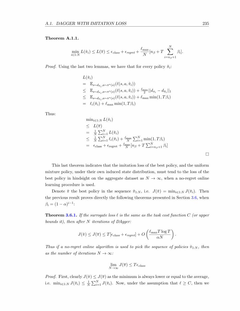
A.1. DAGGER WITH IMITATION LOSS 235
Theorem A.1.1.
mini∈1:N
L(πi) ≤ L(π) ≤ εclass + εregret +`max
N[nβ + T
N∑i=nβ+1
βi].
Proof. Using the last two lemmas, we have that for every policy πi:
L(πi)
= Es∼dπi ,a∼π∗(s)(`(s, a, πi))≤ Es∼dπi ,a∼π∗(s)(`(s, a, πi)) + `max
2 ||dπi − dπi ||1≤ Es∼dπi ,a∼π∗(s)(`(s, a, πi)) + `max min(1, Tβi)
= `i(πi) + `max min(1, Tβi)
Thus:
mini∈1:N L(πi)
≤ L(π)
= 1N
∑Ni=1 L(πi)
≤ 1N
∑Ni=1 `i(πi) + `max
N
∑Ni=1 min(1, Tβi)
= εclass + εregret + `maxN [nβ + T
∑Ni=nβ+1 βi]
This last theorem indicates that the imitation loss of the best policy, and the uniform
mixture policy, under their own induced state distribution, must tend to the loss of the
best policy in hindsight on the aggregate dataset as N → ∞, when a no-regret online
learning procedure is used.
Denote π the best policy in the sequence π1:N , i.e. J(π) = mini∈1:N J(πi). Then
the previous result proves directly the following theorems presented in Section 3.6, when
βi = (1− α)i−1:
Theorem 3.6.1. If the surrogate loss ` is the same as the task cost function C (or upper
bounds it), then after N iterations of DAgger:
J(π) ≤ J(π) ≤ T [εclass + εregret] +O
(`maxT log T
αN
).
Thus if a no-regret online algorithm is used to pick the sequence of policies π1:N , then
as the number of iterations N →∞:
limN→∞
J(π) ≤ Tεclass
Proof. First, clearly J(π) ≤ J(π) as the minimum is always lower or equal to the average,
i.e. mini∈1:N J(πi) ≤ 1N
∑Ni=1 J(πi). Now, under the assumption that ` ≥ C, then we

236 APPENDIX A. ANALYSIS OF DAGGER FOR IMITATION LEARNING
have for any policy π, J(π) ≤ TL(π). And since J(π) = 1N
∑Ni=1 J(πi), we conclude by
using the last theorem that:
J(π) ≤ T [εclass + εregret] +T`max
N[nβ + T
N∑i=nβ+1
βi]
For βi = (1 − α)i−1, then we have that for i ≥ 1 + log Tα , we have βi ≤ 1/T . So
nβ ≤ 1 + log Tα . Additionally
∑Ni=nβ+1 βi = (1−α)
nβ+1−(1−α)N+1
α ≤ 1Tα . Hence we have
that 1N [nβ + T
∑Ni=nβ+1 βi] ≤
1Nα [log T + 2]. Thus we obtain:
J(π) ≤ T [εclass + εregret] +T`max
αN[log(T ) + 2]
This proves the first part of the theorem. The second part follows immediately from the
fact that εregret → 0 as N →∞ for no-regret algorithms.
Theorem 3.6.2. If the expert π∗ is u-robust with respect to cost function C (as in
Definition 3.4.1), then after N iterations of DAgger:
J(π) ≤ J(π) ≤ J(π∗) + uT [εclass + εregret] +O
(u`maxT log T
αN
).
Thus if a no-regret online algorithm is used to pick the sequence of policies π1:N , then
as the number of iterations N →∞:
limN→∞
J(π) ≤ J(π∗) + uTεclass
Proof. Theorem 3.4.3 indicates that J(π) ≤ J(π∗) + uTL(π). Hence combining with
theorem A.1.1, and a similar argument to bound the extra term as in theorem 3.6.1
proves the first part of the theorem. Similarly the second part follows from the fact that
εregret → 0 as N →∞ for no-regret algorithms.
The following corollaries in Section 3.6 also follows immediately from existing results
of no-regret algorithms:
Corollary 3.6.2. Suppose ` is strongly convex in π for all s, a and Dagger uses Follow-
the-Leader to pick the sequence of policies, then: If ` upper bounds C, then for any ε > 0
after O(T/ε) iterations of DAgger:
J(π) ≤ J(π) ≤ Tεclass +O(ε).
For arbitrary cost C, if the expert π∗ is u-robust with respect to C (as in Definition
3.4.1), then for any ε > 0 after O(uT/ε) iterations of DAgger:
J(π) ≤ J(π) ≤ J(π∗) + uTεclass +O(ε).

A.1. DAGGER WITH IMITATION LOSS 237
Proof. For Follow-the-Leader on strongly convex loss functions, after N iterations εregret
is O(log(N)/N). Thus by choosing N to be O(T log(T/ε)ε ), Tεregret is O(ε). The other
extra term O(T`maxαN [log(T ) + 2]) is also O(ε) for such N . Similarly for the second part of
the theorem, uTεregret is O(ε) by choosing N to be O(uT log(uT/ε)ε ), and the extra term
as well.
Corollary 3.6.3. Suppose ` is convex in π for all s, a and Dagger uses Follow-the-
Regularized-Leader to pick the sequence of policies, then: If ` upper bounds the cost C,
then for any ε > 0 after O(T 2/ε2) iterations of DAgger:
J(π) ≤ J(π) ≤ Tεclass +O(ε).
For arbitrary cost C, if the expert π∗ is u-robust with respect to C (as in Definition
3.4.1), then for any ε > 0 after O(u2T 2/ε2) iterations of DAgger:
J(π) ≤ J(π) ≤ J(π∗) + uTεclass +O(ε).
Proof. For Follow-the-Regularized-Leader on convex loss functions, after N iterations
εregret is O(1/√N). Thus by choosing N to be O(T 2/ε2), Tεregret is O(ε). The other
extra term O(T`maxαN [log(T ) + 2]) is also O(ε) for such N . Similarly for the second part
of the theorem, uTεregret is O(ε) by choosing N to be O(u2T 2/ε2), and the extra term
as well.
In addition, when the distribution of state-action pairs of the policies in the sequence
converge, the performance of πN must be close to the performance of π:
Theorem 3.6.3. If there exists a state-action distribution D∗, scalar ε∗conv ≥ 0 and a
sequence εconv,i∞i=1 that is o(1), such that ||Dπi −D∗||1 ≤ ε∗conv + εconv,i for all i. Then
for any cost function bounded in [0, Cmax]:
lim supN→∞
J(πN )− J(π) ≤ CmaxTε∗conv
Proof. Using the first lemma, for all i we have that:
TE(s,a)∼D∗ [C(s, a)]−TCmax
2(ε∗conv+εconv,i) ≤ J(πi) ≤ TE(s,a)∼D∗ [C(s, a)]+
TCmax
2(ε∗conv+εconv,i)
Thus:
J(πN )− J(π)
= J(πN )− 1N
∑Ni=1 J(πi)
≤ TCmax2 (2ε∗conv + εconv,N + 1
N
∑Ni=1 εconv,i)
Taking the limit as N →∞ proves the result, since the sequence εconv,i∞i=1 is o(1).
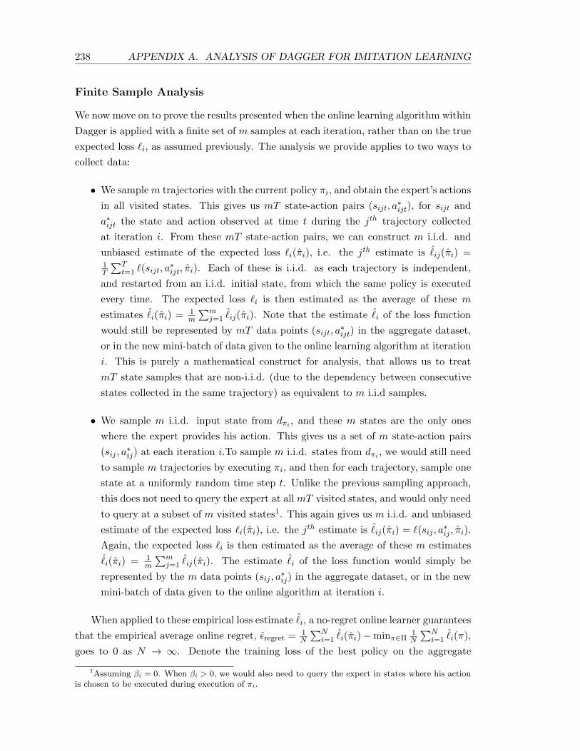
238 APPENDIX A. ANALYSIS OF DAGGER FOR IMITATION LEARNING
Finite Sample Analysis
We now move on to prove the results presented when the online learning algorithm within
Dagger is applied with a finite set of m samples at each iteration, rather than on the true
expected loss `i, as assumed previously. The analysis we provide applies to two ways to
collect data:
• We samplem trajectories with the current policy πi, and obtain the expert’s actions
in all visited states. This gives us mT state-action pairs (sijt, a∗ijt), for sijt and
a∗ijt the state and action observed at time t during the jth trajectory collected
at iteration i. From these mT state-action pairs, we can construct m i.i.d. and
unbiased estimate of the expected loss `i(πi), i.e. the jth estimate is ˆij(πi) =
1T
∑Tt=1 `(sijt, a
∗ijt, πi). Each of these is i.i.d. as each trajectory is independent,
and restarted from an i.i.d. initial state, from which the same policy is executed
every time. The expected loss `i is then estimated as the average of these m
estimates ˆi(πi) = 1
m
∑mj=1
ˆij(πi). Note that the estimate ˆ
i of the loss function
would still be represented by mT data points (sijt, a∗ijt) in the aggregate dataset,
or in the new mini-batch of data given to the online learning algorithm at iteration
i. This is purely a mathematical construct for analysis, that allows us to treat
mT state samples that are non-i.i.d. (due to the dependency between consecutive
states collected in the same trajectory) as equivalent to m i.i.d samples.
• We sample m i.i.d. input state from dπi , and these m states are the only ones
where the expert provides his action. This gives us a set of m state-action pairs
(sij , a∗ij) at each iteration i.To sample m i.i.d. states from dπi , we would still need
to sample m trajectories by executing πi, and then for each trajectory, sample one
state at a uniformly random time step t. Unlike the previous sampling approach,
this does not need to query the expert at all mT visited states, and would only need
to query at a subset of m visited states1. This again gives us m i.i.d. and unbiased
estimate of the expected loss `i(πi), i.e. the jth estimate is ˆij(πi) = `(sij , a
∗ij , πi).
Again, the expected loss `i is then estimated as the average of these m estimatesˆi(πi) = 1
m
∑mj=1
ˆij(πi). The estimate ˆ
i of the loss function would simply be
represented by the m data points (sij , a∗ij) in the aggregate dataset, or in the new
mini-batch of data given to the online algorithm at iteration i.
When applied to these empirical loss estimate ˆi, a no-regret online learner guarantees
that the empirical average online regret, εregret = 1N
∑Ni=1
ˆi(πi)−minπ∈Π
1N
∑Ni=1
ˆi(π),
goes to 0 as N → ∞. Denote the training loss of the best policy on the aggregate
1Assuming βi = 0. When βi > 0, we would also need to query the expert in states where his actionis chosen to be executed during execution of πi.
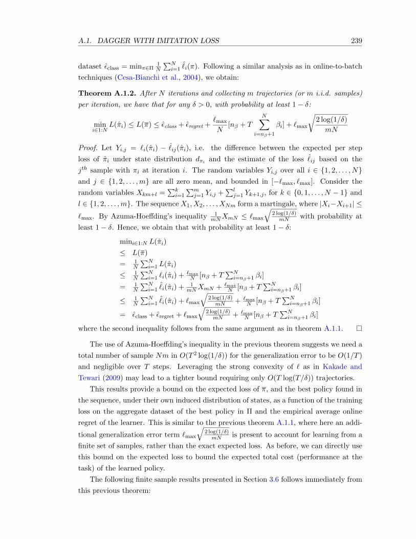
A.1. DAGGER WITH IMITATION LOSS 239
dataset εclass = minπ∈Π1N
∑Ni=1
ˆi(π). Following a similar analysis as in online-to-batch
techniques (Cesa-Bianchi et al., 2004), we obtain:
Theorem A.1.2. After N iterations and collecting m trajectories (or m i.i.d. samples)
per iteration, we have that for any δ > 0, with probability at least 1− δ:
mini∈1:N
L(πi) ≤ L(π) ≤ εclass + εregret +`max
N[nβ + T
N∑i=nβ+1
βi] + `max
√2 log(1/δ)
mN
Proof. Let Yi,j = `i(πi) − ˆij(πi), i.e. the difference between the expected per step
loss of πi under state distribution dπi and the estimate of the loss ˆij based on the
jth sample with πi at iteration i. The random variables Yi,j over all i ∈ 1, 2, . . . , Nand j ∈ 1, 2, . . . ,m are all zero mean, and bounded in [−`max, `max]. Consider the
random variables Xkm+l =∑k
i=1
∑mj=1 Yi,j +
∑lj=1 Yk+1,j , for k ∈ 0, 1, . . . , N − 1 and
l ∈ 1, 2, . . . ,m. The sequence X1, X2, . . . , XNm form a martingale, where |Xi−Xi+1| ≤`max. By Azuma-Hoeffding’s inequality 1
mNXmN ≤ `max
√2 log(1/δ)mN with probability at
least 1− δ. Hence, we obtain that with probability at least 1− δ:
mini∈1:N L(πi)
≤ L(π)
= 1N
∑Ni=1 L(πi)
≤ 1N
∑Ni=1 `i(πi) + `max
N [nβ + T∑N
i=nβ+1 βi]
= 1N
∑Ni=1
ˆi(πi) + 1
mNXmN + `maxN [nβ + T
∑Ni=nβ+1 βi]
≤ 1N
∑Ni=1
ˆi(πi) + `max
√2 log(1/δ)mN + `max
N [nβ + T∑N
i=nβ+1 βi]
= εclass + εregret + `max
√2 log(1/δ)mN + `max
N [nβ + T∑N
i=nβ+1 βi]
where the second inequality follows from the same argument as in theorem A.1.1.
The use of Azuma-Hoeffding’s inequality in the previous theorem suggests we need a
total number of sample Nm in O(T 2 log(1/δ)) for the generalization error to be O(1/T )
and negligible over T steps. Leveraging the strong convexity of ` as in Kakade and
Tewari (2009) may lead to a tighter bound requiring only O(T log(T/δ)) trajectories.
This results provide a bound on the expected loss of π, and the best policy found in
the sequence, under their own induced distribution of states, as a function of the training
loss on the aggregate dataset of the best policy in Π and the empirical average online
regret of the learner. This is similar to the previous theorem A.1.1, where here an addi-
tional generalization error term `max
√2 log(1/δ)mN is present to account for learning from a
finite set of samples, rather than the exact expected loss. As before, we can directly use
this bound on the expected loss to bound the expected total cost (performance at the
task) of the learned policy.
The following finite sample results presented in Section 3.6 follows immediately from
this previous theorem:
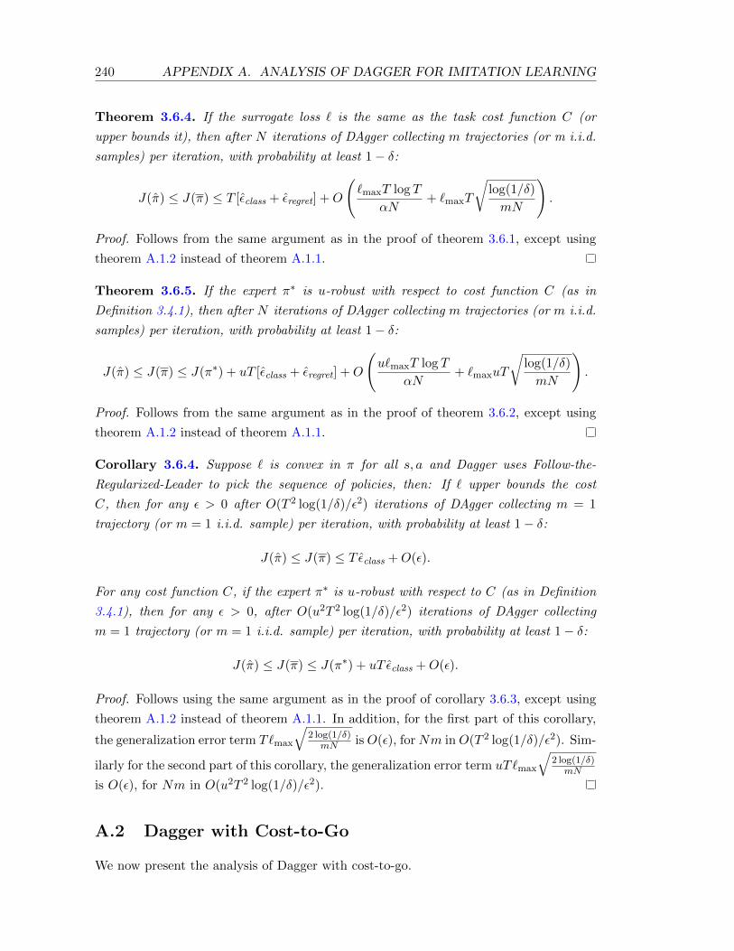
240 APPENDIX A. ANALYSIS OF DAGGER FOR IMITATION LEARNING
Theorem 3.6.4. If the surrogate loss ` is the same as the task cost function C (or
upper bounds it), then after N iterations of DAgger collecting m trajectories (or m i.i.d.
samples) per iteration, with probability at least 1− δ:
J(π) ≤ J(π) ≤ T [εclass + εregret] +O
(`maxT log T
αN+ `maxT
√log(1/δ)
mN
).
Proof. Follows from the same argument as in the proof of theorem 3.6.1, except using
theorem A.1.2 instead of theorem A.1.1.
Theorem 3.6.5. If the expert π∗ is u-robust with respect to cost function C (as in
Definition 3.4.1), then after N iterations of DAgger collecting m trajectories (or m i.i.d.
samples) per iteration, with probability at least 1− δ:
J(π) ≤ J(π) ≤ J(π∗) + uT [εclass + εregret] +O
(u`maxT log T
αN+ `maxuT
√log(1/δ)
mN
).
Proof. Follows from the same argument as in the proof of theorem 3.6.2, except using
theorem A.1.2 instead of theorem A.1.1.
Corollary 3.6.4. Suppose ` is convex in π for all s, a and Dagger uses Follow-the-
Regularized-Leader to pick the sequence of policies, then: If ` upper bounds the cost
C, then for any ε > 0 after O(T 2 log(1/δ)/ε2) iterations of DAgger collecting m = 1
trajectory (or m = 1 i.i.d. sample) per iteration, with probability at least 1− δ:
J(π) ≤ J(π) ≤ T εclass +O(ε).
For any cost function C, if the expert π∗ is u-robust with respect to C (as in Definition
3.4.1), then for any ε > 0, after O(u2T 2 log(1/δ)/ε2) iterations of DAgger collecting
m = 1 trajectory (or m = 1 i.i.d. sample) per iteration, with probability at least 1− δ:
J(π) ≤ J(π) ≤ J(π∗) + uT εclass +O(ε).
Proof. Follows using the same argument as in the proof of corollary 3.6.3, except using
theorem A.1.2 instead of theorem A.1.1. In addition, for the first part of this corollary,
the generalization error term T`max
√2 log(1/δ)mN isO(ε), forNm inO(T 2 log(1/δ)/ε2). Sim-
ilarly for the second part of this corollary, the generalization error term uT`max
√2 log(1/δ)mN
is O(ε), for Nm in O(u2T 2 log(1/δ)/ε2).
A.2 Dagger with Cost-to-Go
We now present the analysis of Dagger with cost-to-go.
A.2. DAGGER WITH COST-TO-GO 241
We begin with a lemma that will be useful to bound the difference in performance to
the expert in terms of the difference cost-to-go. This is a general lemma that applies to
bound the difference in performance of any 2 policies. It has been proven before in prior
work (Bagnell et al., 2003, Kakade and Langford, 2002) and has been called the perfor-
mance difference lemma. We present this results and its proof here for completeness.
Lemma A.2.1. Let π and π′ be any two policy and denote V ′t and Q′t the t-step value
function and Q-value function of policy π′ respectively, then:
J(π)− J(π′) = T Et∼U(1:T ),s∼dtπ
[Q′T−t+1(s, π)− V ′T−t+1(s)]
for U(1 : T ) the uniform distribution on the set 1, 2, . . . , T.
Proof. Let πt denote the non-stationary policy that executes π in the first t time steps,
and then switches to execute π′ at time t + 1 to T . Then we have J(π) = J(πT ) and
J(π′) = J(π0). Thus:
J(π)− J(π′)
=∑T
t=1[J(πt)− J(πt−1)]
=∑T
t=1[Es∼dtπ [Q′T−t+1(s, π)− V ′T−t+1(s)]]
= T Et∼U(1:T ),s∼dtπ [Q′T−t+1(s, π)− V ′T−t+1(s)]
Now let εclass = minπ∈Π1N
∑Ni=1 Et∼U(1:T ),s∼dtπi
[Q∗T−t+1(s, a)−minaQ∗T−t+1(s, a)] de-
note the minimum expected cost-sensitive classification regret achieved by policies in the
class Π on all the data over the N iterations of training. Denote the online learning av-
erage regret on the cost-to-go examples of the sequence of policies chosen by Dagger,
εregret = 1N [∑N
i=1 `i(πi)−minπ∈Π∑N
i=1 `i(π)], where `i(π) = Et∼U(1:T ),s∼dtπi[Q∗T−t+1(s, π)].
Assume the cost-to-go of the expert Q∗ is non-negative and bounded by Q∗max, and that
βi are chosen such that βi ≤ (1− α)i−1 for some α. Then we have the following:
Theorem 4.2.1. After N iterations of DAgger with cost-to-go:
J(π) ≤ J(π) ≤ J(π∗) + T [εclass + εregret] +O
(Q∗maxT log T
αN
).
Thus if a no-regret online algorithm is used to pick the sequence of policies π1:N , then
as the number of iterations N →∞:
limN→∞
J(π) ≤ J(π∗) + Tεclass
242 APPENDIX A. ANALYSIS OF DAGGER FOR IMITATION LEARNING
Proof. For every policy πi, we have:
J(πi)− J(π∗)
= T Et∼U(1:T ),s∼dtπi[Q∗T−t+1(s, πi)− V ∗T−t+1(s)]
=∑T
t=1 Es∼dtπi[Q∗T−t+1(s, πi)− V ∗T−t+1(s)]
≤∑T
t=1 Es∼dtπi [Q∗T−t+1(s, πi)− V ∗T−t+1(s)] +Q∗max
∑Tt=1 ||dtπi − d
tπi||1
≤∑T
t=1 Es∼dtπi [Q∗T−t+1(s, πi)− V ∗T−t+1(s)] + 2Q∗max
∑Tt=1 min(1, tβi)
≤∑T
t=1 Es∼dtπi [Q∗T−t+1(s, πi)− V ∗T−t+1(s)] + 2TQ∗max min(1, Tβi)
= T Et∼U(1:T ),s∼dtπi[Q∗T−t+1(s, πi)− V ∗T−t+1(s)] + 2TQ∗max min(1, Tβi)
where we use lemma A.2.1 in the first equality, lemma A.1.1 in the first inequality, and
a similar argument to lemma A.1.2 for the second inequality.
Thus:
J(π)− J(π∗)
= 1N
∑Ni=1[J(πi)− J(π∗)]
≤ 1N
∑Ni=1[T Et∼U(1:T ),s∼dtπi
[Q∗T−t+1(s, πi)− V ∗T−t+1(s)] + 2TQ∗max min(1, Tβi)]
= T [minπ∈Π1N
∑Ni=1 Et∼U(1:T ),s∼dtπi
[Q∗T−t+1(s, π)− V ∗T−t+1(s)]] + Tεregret
+2TQ∗maxN [nβ + T
∑Ni=nβ+1 βi]
≤ T [minπ∈Π1N
∑Ni=1 Et∼U(1:T ),s∼dtπi
[Q∗T−t+1(s, π)−minaQ∗T−t+1(s, a)] + Tεregret
+2TQ∗maxN [nβ + T
∑Ni=nβ+1 βi]
= Tεclass + Tεregret + 2TQ∗maxN [nβ + T
∑Ni=nβ+1 βi]
Again, J(π) ≤ J(π) since the minimum is always better than the average, i.e.
mini J(πi) ≤ 1N
∑Ni=1 J(πi). Finally, using the same argument as in the proof of theorem
3.6.1, we have that when βi = (1 − α)i−1, [nβ + T∑N
i=nβ+1 βi] ≤log(T )+2
α . This proves
the first part of the theorem.
The second part follows immediately from the fact that εregret → 0 as N → ∞, and
similarly for the extra term O(Q∗maxT log T
αN
).
Finite Sample Result
We here consider the finite sample case where actions are explored uniformly randomly
and the reduction of cost-sensitive classification to reduction is used. We consider learn-
ing an estimate Q-value function Q of the expert’s cost-to-go, and we consider a general
case where the cost-to-go predictions may depend on features f(s, a, t) of the state s,
action a and time t, e.g. Q could be a linear regressor s.t. QT−t+1(s, a) = w>f(s, a, t)
is the estimate of the cost-to-go Q∗T−t+1(s, a), and w are the parameters of the linear
regressor we learn. Given such estimate Q, we consider executing the policy π, such that
in state s at time t, π(s, t) = mina∈A QT−t+1(s, a).
A.2. DAGGER WITH COST-TO-GO 243
Theorem 4.2.2. After N iterations of DAgger with cost-to-go, collecting m regression
examples (s, a, t, Q) per iteration, guarantees that with probability at least 1-δ:
J(π) ≤ J(π) ≤ J(π∗)+2√|A|T
√Rclass + εregret +O(
√log(1/δ)/Nm)+O
(QmaxT log T
αN
).
Thus if a no-regret online algorithm is used to pick the sequence of regressors Q1:N , then
as the number of iterations N →∞, with probability 1:
limN→∞
J(π) ≤ J(π∗) + 2√|A|T
√Rclass
Proof. Consider π, the bayes-optimal non-stationary policy that minimizes loss on the
cost-to-go examples. That is, π(s, t) = mina∈AQ∗T−t+1(s, a), i.e. it picks the action
with minimum expected expert cost-to-go conditioned on being in state s and time t.
Additionally, given the observed noisy Q-values from each trajectory, the bayes-optimal
regressor is simply the Q-value function Q∗ of the expert that predicts the expected
cost-to-go.
At each iteration i, we execute a policy πi, such that πi(s, t) = arg mina∈A QiT−t+1(s, a),
where Qi is the current regressor at iteration i from the base online learner. The cost-
sensitive regret of policy πi, compared to π, can be related to the regression regret of Qi
as follows:
Consider any state s and time t. Let ai = πi(s, t) and consider the action a′ of any
other policy. We have that:
Q∗T−t+1(s, ai)−Q∗T−t+1(s, a)
≤ QiT−t+1(s, ai)− QiT−t+1(s, a′) +Q∗T−t+1(s, ai)− QiT−t+1(s, ai) + QiT−t+1(s, a′)−Q∗T−t+1(s, a′)
≤ Q∗T−t+1(s, ai)− QiT−t+1(s, ai) + QiT−t+1(s, a′)−Q∗T−t+1(s, a′)
≤ 2 maxa∈A |Q∗T−t+1(s, a)− QiT−t+1(s, a)|
Additionally, for any joint distribution D over (s, t), and U(A) the uniform distribu-
tion over actions, we have that:
(E(s,t)∼D[maxa∈A |Q∗T−t+1(s, a)− QiT−t+1(s, a)|])2
≤ E(s,t)∼D[maxa∈A |Q∗T−t+1(s, a)− QiT−t+1(s, a)|2]
≤ E(s,t)∼D[∑
a∈A |Q∗T−t+1(s, a)− QiT−t+1(s, a)|2]
= |A|E(s,t)∼D,a∼U(A)[|Q∗T−t+1(s, a)− QiT−t+1(s, a)|2]
Thus we obtain that for every πi:
Et∼U(1:T ),s∼dtπi[Q∗T−t+1(s, πi)−Q∗T−t+1(s, π)]
≤ 2Et∼U(1:T ),s∼dtπi[maxa∈A |Q∗T−t+1(s, a)− QiT−t+1(s, a)|]
≤ 2√|A|√Et∼U(1:T ),s∼dtπi ,a∼U(A)[|Q∗T−t+1(s, a)− QiT−t+1(s, a)|2]
244 APPENDIX A. ANALYSIS OF DAGGER FOR IMITATION LEARNING
Thus
J(π)− J(π∗)
= TN
∑Ni=1 Et∼U(1:T ),s∼dtπi
[Q∗T−t+1(s, πi)−Q∗T−t+1(s, π∗)]
≤ TN
∑Ni=1 Et∼U(1:T ),s∼dtπi
[Q∗T−t+1(s, πi)−Q∗T−t+1(s, π∗)] + 2TQ∗maxN [nβ + T
∑Ni=nβ+1 βi]
≤ TN
∑Ni=1 Et∼U(1:T ),s∼dtπi
[Q∗T−t+1(s, πi)−Q∗T−t+1(s, π)] + 2TQ∗maxN [nβ + T
∑Ni=nβ+1 βi]
≤ 2√|A|TN
∑Ni=1
√Et∼U(1:T ),s∼dtπi ,a∼U(A)[|Q∗T−t+1(s, a)− QiT−t+1(s, a)|2]
+2TQ∗maxN [nβ + T
∑Ni=nβ+1 βi]
≤ 2√|A|T
√1N
∑Ni=1 Et∼U(1:T ),s∼dtπi ,a∼U(A)[|Q∗T−t+1(s, a)− QiT−t+1(s, a)|2]
+2TQ∗maxN [nβ + T
∑Ni=nβ+1 βi]
Now in state s at time t, when performing a and then following the expert, consider
the distribution ds,a,t over observed cost-to-go Q, such that EQ∼ds,a,t [Q] = Q∗T−t+1(s, a).
For any regressor Q, define the expected squared loss in predictions of the observed
cost-to-go at iteration i as `i(Q) = Et∼U(1:T ),s∼dtπi ,a∼U(A),Q∼ds,t,a [|Q − QT−t+1(s, a)|2].
Then since for any random variable X with mean µ, if we have an estimate µ of the
mean, |µ− µ|2 = Ex[(x− µ)2 − (x− µ)2], we have that:
1
N
N∑i=1
Et∼U(1:T ),s∼dtπi ,a∼U(A)[|Q∗T−t+1(s, a)− QiT−t+1(s, a)|2] =1
N
N∑i=1
`i(Qi)− `i(Q∗)
Now, in the finite sample case, consider collecting m samples at each iteration i:
(sij , aij , tij , Qij)mj=1. The expected squared loss `i is estimated as ˆi(Q) = 1
m
∑mj=1(QT−tij+1(sij , aij)−
Qij)2, and the no-regret algorithm is run on the estimated loss ˆ
i.
Define Yi,j = `i(Qi) − (QiT−tij+1(sij , aij) − Qij)
2 − `i(Q∗) + (Q∗T−tij+1(sij , aij) −
Qij)2, the difference between the expected squared loss and the empirical square loss
at each sample for both Qi and Q∗. Conditioned on previous trajectories, each Yi,j
has expectation 0. Then the sequence of random variables Xkm+l =∑k
i=1
∑mj=1 Yi,j +∑l
j=1 Y(k+1),j , for k ∈ 0, 1, 2, . . . , N − 1 and l ∈ 1, 2, . . . ,m, forms a martingale, and
if the squared loss at any sample is bounded by `max, we obtain that |Xi − Xi+ 1| ≤2`max. By Azuma-Hoeffding’s inequality, this implies that with probability at least 1−δ,
1NmXNm ≤ 2`max
√2 log(1/δ)Nm .
Denote the empirical average online regret on the training squared loss εregret =1N
∑Ni=1
ˆi(Q
i) − minQ∈Q1N
∑Ni=1
ˆi(Q). Let Q∗ be the bayes-optimal regressor on the
finite training data, and define the empirical regression regret of the best regressor in
the class as Rclass = minQ∈Q1N
∑Ni=1[ˆi(Q)− ˆ
i(Q∗)].
Then we obtain that with probability at least 1− δ:
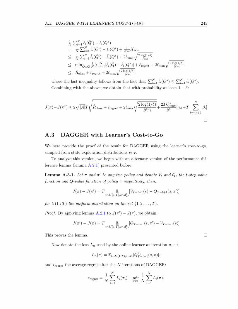
A.3. DAGGER WITH LEARNER’S COST-TO-GO 245
1N
∑Ni=1 `i(Q
i)− `i(Q∗)= 1
N
∑Ni=1
ˆi(Q
i)− ˆi(Q∗) + 1
NmXNm
≤ 1N
∑Ni=1
ˆi(Q
i)− ˆi(Q∗) + 2`max
√2 log(1/δ)Nm
≤ minQ∈Q1N
∑Ni=1[ˆi(Q)− ˆ
i(Q∗)] + εregret + 2`max
√2 log(1/δ)Nm
≤ Rclass + εregret + 2`max
√2 log(1/δ)Nm
where the last inequality follows from the fact that∑N
i=1ˆi(Q∗) ≤
∑Ni=1
ˆi(Q∗).
Combining with the above, we obtain that with probability at least 1− δ:
J(π)−J(π∗) ≤ 2√|A|T
√Rclass + εregret + 2`max
√2 log(1/δ)
Nm+
2TQ∗max
N[nβ+T
N∑i=nβ+1
βi]
A.3 DAGGER with Learner’s Cost-to-Go
We here provide the proof of the result for DAGGER using the learner’s cost-to-go,
sampled from state exploration distributions ν1:T .
To analyze this version, we begin with an alternate version of the performance dif-
ference lemma (lemma A.2.1) presented before:
Lemma A.3.1. Let π and π′ be any two policy and denote Vt and Qt the t-step value
function and Q-value function of policy π respectively, then:
J(π)− J(π′) = T Et∼U(1:T ),s∼dt
π′
[VT−t+1(s)−QT−t+1(s, π′)]
for U(1 : T ) the uniform distribution on the set 1, 2, . . . , T.
Proof. By applying lemma A.2.1 to J(π′)− J(π), we obtain:
J(π′)− J(π) = T Et∼U(1:T ),s∼dt
π′
[QT−t+1(s, π′)− VT−t+1(s)]
This proves the lemma.
Now denote the loss Ln used by the online learner at iteration n, s.t.:
Ln(π) = Et∼U(1:T ),s∼νt [QπnT−t+1(s, π)].
and εregret the average regret after the N iterations of DAGGER:
εregret =1
N
N∑i=1
Li(πi)−minπ∈Π
1
N
N∑i=1
Li(π).
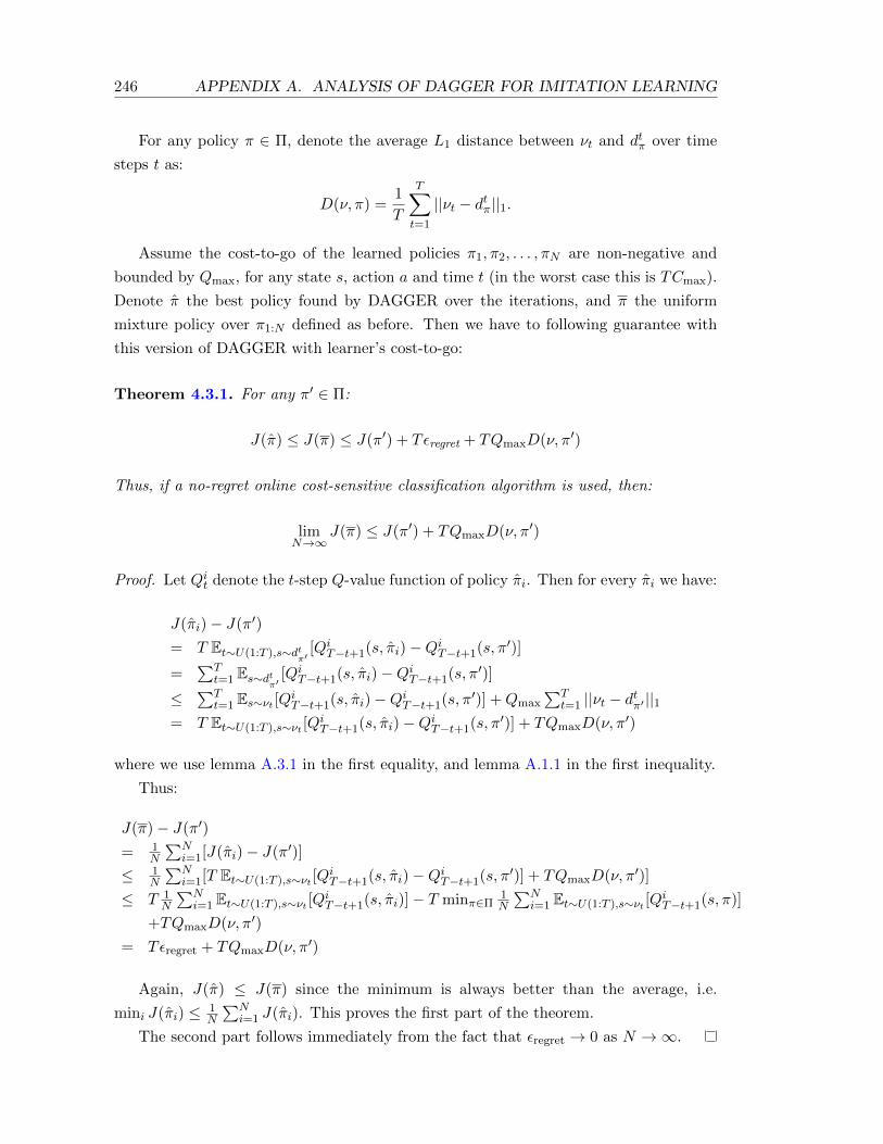
246 APPENDIX A. ANALYSIS OF DAGGER FOR IMITATION LEARNING
For any policy π ∈ Π, denote the average L1 distance between νt and dtπ over time
steps t as:
D(ν, π) =1
T
T∑t=1
||νt − dtπ||1.
Assume the cost-to-go of the learned policies π1, π2, . . . , πN are non-negative and
bounded by Qmax, for any state s, action a and time t (in the worst case this is TCmax).
Denote π the best policy found by DAGGER over the iterations, and π the uniform
mixture policy over π1:N defined as before. Then we have to following guarantee with
this version of DAGGER with learner’s cost-to-go:
Theorem 4.3.1. For any π′ ∈ Π:
J(π) ≤ J(π) ≤ J(π′) + Tεregret + TQmaxD(ν, π′)
Thus, if a no-regret online cost-sensitive classification algorithm is used, then:
limN→∞
J(π) ≤ J(π′) + TQmaxD(ν, π′)
Proof. Let Qit denote the t-step Q-value function of policy πi. Then for every πi we have:
J(πi)− J(π′)
= T Et∼U(1:T ),s∼dtπ′
[QiT−t+1(s, πi)−QiT−t+1(s, π′)]
=∑T
t=1 Es∼dtπ′
[QiT−t+1(s, πi)−QiT−t+1(s, π′)]
≤∑T
t=1 Es∼νt [QiT−t+1(s, πi)−QiT−t+1(s, π′)] +Qmax∑T
t=1 ||νt − dtπ′ ||1= T Et∼U(1:T ),s∼νt [Q
iT−t+1(s, πi)−QiT−t+1(s, π′)] + TQmaxD(ν, π′)
where we use lemma A.3.1 in the first equality, and lemma A.1.1 in the first inequality.
Thus:
J(π)− J(π′)
= 1N
∑Ni=1[J(πi)− J(π′)]
≤ 1N
∑Ni=1[T Et∼U(1:T ),s∼νt [Q
iT−t+1(s, πi)−QiT−t+1(s, π′)] + TQmaxD(ν, π′)]
≤ T 1N
∑Ni=1 Et∼U(1:T ),s∼νt [Q
iT−t+1(s, πi)]− T minπ∈Π
1N
∑Ni=1 Et∼U(1:T ),s∼νt [Q
iT−t+1(s, π)]
+TQmaxD(ν, π′)
= Tεregret + TQmaxD(ν, π′)
Again, J(π) ≤ J(π) since the minimum is always better than the average, i.e.
mini J(πi) ≤ 1N
∑Ni=1 J(πi). This proves the first part of the theorem.
The second part follows immediately from the fact that εregret → 0 as N →∞.
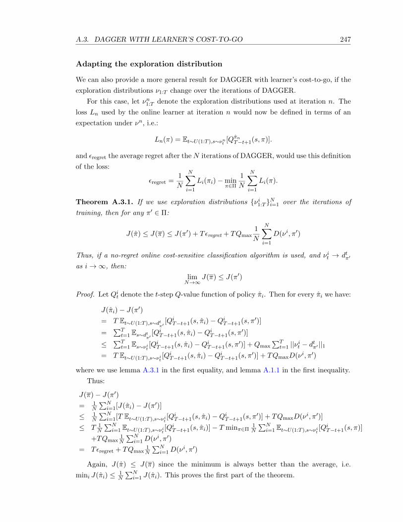
A.3. DAGGER WITH LEARNER’S COST-TO-GO 247
Adapting the exploration distribution
We can also provide a more general result for DAGGER with learner’s cost-to-go, if the
exploration distributions ν1:T change over the iterations of DAGGER.
For this case, let νn1:T denote the exploration distributions used at iteration n. The
loss Ln used by the online learner at iteration n would now be defined in terms of an
expectation under νn, i.e.:
Ln(π) = Et∼U(1:T ),s∼νnt [QπnT−t+1(s, π)].
and εregret the average regret after the N iterations of DAGGER, would use this definition
of the loss:
εregret =1
N
N∑i=1
Li(πi)−minπ∈Π
1
N
N∑i=1
Li(π).
Theorem A.3.1. If we use exploration distributions νi1:T Ni=1 over the iterations of
training, then for any π′ ∈ Π:
J(π) ≤ J(π) ≤ J(π′) + Tεregret + TQmax1
N
N∑i=1
D(νi, π′)
Thus, if a no-regret online cost-sensitive classification algorithm is used, and νit → dtπ′
as i→∞, then:
limN→∞
J(π) ≤ J(π′)
Proof. Let Qit denote the t-step Q-value function of policy πi. Then for every πi we have:
J(πi)− J(π′)
= T Et∼U(1:T ),s∼dtπ′
[QiT−t+1(s, πi)−QiT−t+1(s, π′)]
=∑T
t=1 Es∼dtπ′
[QiT−t+1(s, πi)−QiT−t+1(s, π′)]
≤∑T
t=1 Es∼νit [QiT−t+1(s, πi)−QiT−t+1(s, π′)] +Qmax
∑Tt=1 ||νit − dtπ′ ||1
= T Et∼U(1:T ),s∼νit [QiT−t+1(s, πi)−QiT−t+1(s, π′)] + TQmaxD(νi, π′)
where we use lemma A.3.1 in the first equality, and lemma A.1.1 in the first inequality.
Thus:
J(π)− J(π′)
= 1N
∑Ni=1[J(πi)− J(π′)]
≤ 1N
∑Ni=1[T Et∼U(1:T ),s∼νit [Q
iT−t+1(s, πi)−QiT−t+1(s, π′)] + TQmaxD(νi, π′)]
≤ T 1N
∑Ni=1 Et∼U(1:T ),s∼νit [Q
iT−t+1(s, πi)]− T minπ∈Π
1N
∑Ni=1 Et∼U(1:T ),s∼νit [Q
iT−t+1(s, π)]
+TQmax1N
∑Ni=1D(νi, π′)
= Tεregret + TQmax1N
∑Ni=1D(νi, π′)
Again, J(π) ≤ J(π) since the minimum is always better than the average, i.e.
mini J(πi) ≤ 1N
∑Ni=1 J(πi). This proves the first part of the theorem.
248 APPENDIX A. ANALYSIS OF DAGGER FOR IMITATION LEARNING
The second part follows immediately from the fact that εregret → 0 as N → ∞ and
D(νi, π′)→ 0 as i→∞.
This theorem suggests that if we would have a method that can adapt the exploration
distribution νit in a way that it converges to dtπ∗ of an optimal policy π∗ ∈ Π, for all time
t, as i → ∞, then using a no-regret procedure, we would always find an optimal policy
in Π in the limit. However, at this point we do not know of a method that could adapt
νi to guarantee this.
Appendix B
Analysis of SCP for Submodular
Optimization
This appendix contains the proofs of the various theoretical results for SCP presented
in chapter 7.
Preliminaries
We begin by proving a number of lemmas about monotone submodular functions, which
will be useful to prove our main results.
Lemma B.0.2. Let S be a set and f be a monotone submodular function defined on list
of items from S. For any lists A,B, we have that:
f(A⊕B)− f(A) ≤ |B|(Es∼U(B)[f(A⊕ s)]− f(A))
for U(B) the uniform distribution on items in B.
Proof. For any list A and B, let Bi denote the list of the first i items in B, and bi the
ith item in B. We have that:
f(A⊕B)− f(A)
=∑|B|
i=1 f(A⊕Bi)− f(A⊕Bi−1)
≤∑|B|
i=1 f(A⊕ bi)− f(A)
= |B|(Eb∼U(B)[f(A⊕ b)]− f(A))
where the inequality follows from the submodularity property of f .
Lemma B.0.3. Let S be a set, and f a monotone submodular function defined on lists of
items in S. Let A,B be any lists of items from S. Denote Aj the list of the first j items
in A, U(B) the uniform distribution on items in B and define εj = Es∼U(B)[f(Aj−1 ⊕s)] − f(Aj), the additive error term in competing with the average marginal benefits of
250 APPENDIX B. ANALYSIS OF SCP FOR SUBMODULAR OPTIMIZATION
the items in B when picking the jth item in A (which could be positive or negative).
Then:
f(A) ≥ (1− (1− 1/|B|)|A|)f(B)−|A|∑i=1
(1− 1/|B|)|A|−iεi
In particular if |A| = |B| = k, then:
f(A) ≥ (1− 1/e)f(B)−k∑i=1
(1− 1/k)k−iεi
and for α = exp(−|A|/|B|) (i.e. |A| = |B| log(1/α)):
f(A) ≥ (1− α)f(B)−|A|∑i=1
(1− 1/|B|)|A|−iεi
Proof. Using the monotone property and previous lemma B.0.2, we must have that:
f(B)− f(A) ≤ f(A⊕B)− f(A) ≤ |B|(Eb∼U(B)[f(A⊕ b)]− f(A)).
Now let ∆j = f(B)− f(Aj). By the above we have that
∆j
≤ |B|[Es∼U(B)[f(Aj ⊕ s)]− f(Aj)]
= |B|[Es∼U(B)[f(Aj ⊕ s)]− f(Aj+1) + f(Aj+1)− f(B) + f(B)− f(Aj)]
= |B|[εj+1 + ∆j −∆j+1]
Rearranging terms, this implies that ∆j+1 ≤ (1 − 1/|B|)∆j + εj+1. Recursively
expanding this recurrence from ∆|A|, we obtain:
∆|A| ≤ (1− 1/|B|)|A|∆0 +
|A|∑i=1
(1− 1/|B|)|A|−iεi
Using the definition of ∆|A| and rearranging terms, we obtain f(A) ≥ (1−(1−1/|B|)|A|)f(B)−∑|A|i=1(1−1/|B|)|A|−iεi. This proves the first statement of the theorem. The following two
statements follow from the observations that (1− 1/|B|)|A| = exp(|A| log(1− 1/|B|)) ≤exp(−|A|/|B|) = α. Hence (1 − (1 − 1/|B|)|A|)f(B) ≥ (1 − α)f(B). When |A| = |B|,α = 1/e and this proves the special case where |A| = |B|.
For the greedy list construction strategy, the εj in the last lemma are always ≤ 0,
such that Lemma B.0.3 implies that if we construct a list of size k with greedy, it must
achieve at least 63% of the value of the optimal list of size k, but also that it must
achieve at least 95% of the value of the optimal list of size bk/3c, and at least 99.9%
of the value of the optimal list of size bk/7c.A more surprising fact that follows from the last lemma is that constructing a list
stochastically, by sampling items from a particular fixed distribution, can provide the
same guarantee as greedy:
251
Lemma B.0.4. Let S be a set, and f a monotone submodular function defined on lists
of items in S. Let B be any list of items from S and U(B) the uniform distribution on
elements in B. Suppose we construct the list A by sampling k items randomly from U(B)
(with replacement). Denote Aj the list obtained after j samples, and Pj the distribution
over lists obtained after j samples. Then:
EA∼Pk [f(A)] ≥ (1− (1− 1/|B|)k)f(B)
In particular, for α = exp(−k/|B|):
EA∼Pk [f(A)] ≥ (1− α)f(B)
Proof. The proof follows a similar proof to the previous lemma. Recall that by the
monotone property and lemma B.0.2, we have that for any list A: f(B) − f(A) ≤f(A ⊕ B) − f(A) ≤ |B|(Eb∼U(B)[f(A ⊕ b)] − f(A)). Because this holds for all lists,
we must also have that for any distribution P over lists A, f(B) − EA∼P [f(A)] ≤|B|EA∼P [Eb∼U(B)[f(A ⊕ b)] − f(A)]. Also note that by the way we construct sets, we
have that EAj+1∼Pj+1 [f(Aj+1)] = EAj∼Pj [Es∼U(B)[f(Aj ⊕ s)]]Now let ∆j = f(B)− EAj∼Pj [f(Aj)]. By the above we have that:
∆j
≤ |B|EAj∼Pj [Es∼U(B)[f(Aj ⊕ s)]− f(Aj)]
= |B|EAj∼Pj [Es∼U(B)[f(Aj ⊕ s)]− f(B) + f(B)− f(Aj)]
= |B|(EAj+1∼Pj+1 [f(Aj+1)]− f(B) + f(B)− EAj∼Pj [f(Aj)])
= |B|[∆j −∆j+1]
Rearranging terms, this implies that ∆j+1 ≤ (1− 1/|B|)∆j . Recursively expanding this
recurrence from ∆k, we obtain:
∆k ≤ (1− 1/|B|)k∆0
Using the definition of ∆k and rearranging terms we obtain EA∼Pk [f(A)] ≥ (1 − (1 −1/|B|)k)f(B). The second statement follows again from the fact that (1−(1−1/|B|)k)f(B) ≥(1− α)f(B)
Corollary B.0.1. There exists a distribution that when sampled k times to construct a
list, achieves an approximation ratio of (1 − 1/e) of the optimal list of size k in expec-
tation. In particular, if A∗ is an optimal list of size k, sampling k times from U(A∗)
achieves this approximation ratio. Additionally, for any α ∈ (0, 1], sampling dk log(1/α)etimes must construct a list that achieves an approximation ratio of (1−α) in expectation.
Proof. Follows from the last lemma using B = A∗.
This surprising result can also be seen as a special case of a more general result
proven in prior related work that analyzed randomized set selection strategies to optimize
submodular functions (lemma 2.2 in Feige et al. (2011)).
252 APPENDIX B. ANALYSIS OF SCP FOR SUBMODULAR OPTIMIZATION
Proofs of Main Results
We now provide the proofs of the main results in chapter 7. We provide the proofs for the
more general contextual case where we learn over a policy class Π. All the results for the
context-free case can be seen as special cases of these results when Π = Π = πs|s ∈ Sand πs(x, L) = s for any state x and list L.
We refer the reader to the notation defined in Sections 7.1 and 7.3 for the definitions
of the various terms used.
Theorem 7.3.1. Let α = exp(−m/k) and k′ = min(m, k). After T iterations, for any
δ, δ′ ∈ (0, 1), we have that with probability at least 1− δ:
F (π,m) ≥ (1− α)F (L∗π,k)−R
T− 2
√2 ln(1/δ)
T
and similarly, with probability at least 1− δ − δ′:
F (π,m) ≥ (1− α)F (L∗π,k)−E[R]T −
√2k′ ln(1/δ′)
T − 2
√2 ln(1/δ)
T
Proof.
F (π,m)
= 1T
∑Tt=1 F (πt,m)
= 1T
∑Tt=1 ELπ,m∼πt [Ex∼D[fx(Lπ,m(x))]]
= (1− α)Ex∼D[fx(L∗π,k(x))]− [(1− α)Ex∼D[fx(L∗π,k(x))]
− 1T
∑Tt=1 ELπ,m∼πt [Ex∼D[fx(Lπ,m(x))]]]
Now consider the sampled states xtTt=1 and the policies πt,i sampled i.i.d. from πt to
construct the lists LtTt=1 and denote the random variablesXt = (1−α)(Ex∼D[fx(L∗π,k(x))]−fxt(L
∗π,k(xt)))−ELπ,m∼πt [Ex∼D[fx(Lπ,m(x))]]− fxt(Lt)]. If πt is deterministic, then sim-
ply consider all πt,i = πt. Because the xt are i.i.d. from D, and the distribution of policies
used to construct Lt only depends on xτt−1τ=1 and Lτt−1
τ=1, then the Xt conditioned on
Xτt−1τ=1 have expectation 0, and because fx ∈ [0, 1] for all state x ∈ X , Xt can vary
in a range r ⊆ [−2, 2]. Thus the sequence of random variables Yt =∑t
i=1Xi, for t =1
to T , forms a martingale where |Yt − Yt+1| ≤ 2. By the Azuma-Hoeffding’s inequality,
we have that P (YT /T ≥ ε) ≤ exp(−ε2T/8). Hence for any δ ∈ (0, 1), we have that with
probability at least 1 − δ, YT /T ≤ 2
√2 ln(1/δ)
T . Hence we have that with probability at
least 1− δ:
F (π,m)
= (1− α)Ex∼D[fx(L∗π,k(x))]− [(1− α)Ex∼D[fx(L∗π,k(x))]
− 1T
∑Tt=1 ELπ,m∼πt [Ex∼D[fx(Lπ,m(x))]]]
= (1− α)Ex∼D[fx(L∗π,k(x))]− [(1− α) 1T
∑Tt=1 fxt(L
∗π,k(xt))−
1T
∑Tt=1 fxt(Lt)]
−YT /T= (1− α)Ex∼D[fx(L∗π,k(x))]− [(1− α) 1
T
∑Tt=1 fxt(L
∗π,k(xt))−
1T
∑Tt=1 fxt(Lt)]
−2
√2 ln(1/δ)
T
253
Let wi = (1− 1/k)m−i. From Lemma B.0.3, we have:
(1− α) 1T
∑Tt=1 fxt(L
∗π,k(xt))−
1T
∑Tt=1 fxt(Lt)
≤ 1T
∑Tt=1
∑mi=1wi(Eπ∼U(L∗π,k)[fxt(Lt,i−1 ⊕ π(xt))]− fxt(Lt,i))
= Eπ∼U(L∗π,k)[1T
∑Tt=1
∑mi=1wi(fxt(Lt,i−1 ⊕ π(xt))− fxt(Lt,i))]
≤ maxπ∈Π[ 1T
∑Tt=1
∑mi=1wi(fxt(Lt,i−1 ⊕ π(xt))− fxt(Lt,i))]
≤ maxπ∈Π[ 1T
∑Tt=1
∑mi=1wi(f(Lt,i−1 ⊕ π(xt))− fxt(Lt,i))]
= R/T
Hence combining with the previous result proves the first part of the theorem.
Additionally, for the sampled environments xtTt=1 and the policies πt,i, consider the
random variables Qm(t−1)+i = wiEπ∼πt [fxt(Lt,i−1⊕ π(xt, Lt,i−1))]−wifxt(Lt,i). Because
each draw of πt,i is i.i.d. from πt, we have that again the sequence of random variables
Zj =∑j
i=1Qi, for j = 1 to Tm forms a martingale and because each Qi can take
values in a range [−wj , wj ] for j = 1 + mod(i − 1,m), we have |Zi − Zi−1| ≤ wj .
Since∑Tm
i=1 |Zi − Zi−1|2 ≤ T∑m
i=1(1 − 1/k)2(m−i) ≤ T min(k,m) = Tk′, by Azuma-
Hoeffding’s inequality, we must have that P (ZTm ≥ ε) ≤ exp(−ε2/2Tk′). Thus for any
δ′ ∈ (0, 1), with probability at least 1−δ′, ZTm ≤√
2Tk′ ln(1/δ). Hence combining with
the previous result, it must be the case that with probability at least 1 − δ − δ′, both
YT /T ≤ 2
√2 ln(1/δ)
T and ZTm ≤√
2Tk′ ln(1/δ′) holds.
Now note that:
maxπ∈Π[ 1T
∑Tt=1
∑mi=1wi(f(Lt,i−1 ⊕ π(xt))− fxt(Lt,i))]
= maxπ∈Π[ 1T
∑Tt=1
∑mi=1wi(fxt(Lt,i−1 ⊕ π(xt))− Eπ′∼πt [f(Lt,i−1 ⊕ π′(xt, Lt,i−1))])]
+ZTm/T
= E[R]/T + ZTm/T
Using this additional fact, and combining with previous results we must have that
with probability at least 1− δ − δ′:
F (π,m)
≥ (1− α)F (L∗π,k)− [(1− α) 1T
∑Tt=1 fxt(L
∗π,k(xt))−
1T
∑Tt=1 fxt(Lt)]− 2
√2 ln(1/δ)
T
≥ (1− α)F (L∗π,k)− E[R]/T − ZTm/T − 2
√2 ln(1/δ)
T
≥ (1− α)F (L∗π,k)− E[R]/T −√
2k′ ln(1/δ′)T − 2
√2 ln(1/δ)
T
We now show that the expected regret must grow with√k′ and not k′, hen using
Weighted Majority with the optimal learning rate (or with the doubling trick).
Corollary 7.2.2. Under the event where Theorem 7.3.1 holds (the event that occurs
w.p. 1− δ− δ′), if Π is a finite set of policies, using Weighted Majority with the optimal
254 APPENDIX B. ANALYSIS OF SCP FOR SUBMODULAR OPTIMIZATION
learning rate guarantees that after T iterations:
E[R]/T ≤ 4k′ ln |Π|T + 2
√k′ ln |Π|T + 29/4(k′/T )3/4(ln(1/δ′))1/4
√ln |Π|
For large enough T in Ω(k′(ln |Π|+ ln(1/δ′))), we obtain that:
E[R]/T ≤ O(
√k′ ln |Π|T
)
Proof. We use a similar argument to Lemma 4 in Streeter and Golovin (2007) to bound
E[R] in the result of theorem 7.3.1. Consider the sum of the benefits accumulated
by the learning algorithm at position i in the list, for i ∈ 1, 2, . . . ,m, i.e. let yi =∑Tt=1 b(πt,i(xt, Lt,i−1)|xt, Lt,i−1), where πt,i corresponds to the particular sampled policy
by Weighted Majority for choosing the item at position i, when constructing the list Lt
for state xt. Note that∑m
i=1(1−1/k)m−iyi ≤∑m
i=1 yi ≤ T by the fact that the monotone
submodular function fx is bounded in [0, 1] for all state x. Now consider the sum of the
benefits you could have accumulated at position i, had you chosen the best fixed policy
in hindsight to construct all list, keeping the policy fixed as the policy is constructed,
i.e. let zi =∑T
t=1 b(π∗(xt, Lt,i−1)|xt, Lt,i−1), for
π∗ = arg maxπ∈Π
m∑i=1
(1− 1/k)m−iT∑t=1
b(π∗(xt, Lt,i−1)|xt, Lt,i−1),
and let ri = zi − yi. Now denote Z =√∑m
i=1(1− 1/k)m−izi. We have Z2 =∑m
i=1(1−1/k)m−izi =
∑mi=1(1−1/k)m−i(yi+ri) ≤ T+R, where R is the sample regret incurred by
the learning algorithm. Under the event where theorem 7.3.1 holds (i.e. the event that
occurs with probability at least 1− δ− δ′), we had already shown that R ≤ E[R] +ZTm,
for ZTm ≤√
2Tk′ ln(1/δ′), in the second part of the proof of theorem 7.3.1. Thus
when theorem 7.3.1 holds, we have Z2 ≤ T +√
2Tk′ ln(1/δ′) + E[R]. Now using the
generalized version of weighted majority with rewards (i.e. using directly the benefits
as rewards) Arora et al. (2012), since the rewards at each update are in [0, k′], we have
that with the best learning rate in hindsight 1: E[R] ≤ 2Z√k′ ln |Π|. Thus we obtain
Z2 ≤ T +√
2Tk′ ln(1/δ′) + 2Z√k′ ln |Π|. This is a quadratic inequality of the form
Z2 − 2Z√k′ ln |Π| − T −
√2Tk′ ln(1/δ′) ≤ 0, with the additional constraint Z ≥ 0.
This implies Z is less than or equal to the largest non-negative root of the polynomial
Z2 − 2Z√k′ ln |Π| − T −
√2Tk′ ln(1/δ′). Solving for the roots, we obtain
Z ≤√k′ ln |Π|+
√k′ ln |Π|+ T +
√2Tk′ ln(1/δ′)
≤ 2√k′ ln |Π|+
√T + (2Tk′ ln(1/δ′))1/4
1if not a doubling trick can be used to get the same regret bound within a small constant factorCesa-Bianchi et al. (1997)
255
Plugging back Z into the expression E[R] ≤ 2Z√k′ ln |Π|, we obtain:
E[R] ≤ 4k′ ln |Π|+ 2√Tk′ ln |Π|+ 2(2T ln(1/δ′))1/4(k′)3/4
√ln |Π|
Thus the average regret:
E[R]T ≤ 4k′ ln |Π|
T + 2
√k′ ln |Π|T + 29/4(k′/T )3/4(ln(1/δ′))1/4
√ln |Π|
For T in Ω(k′(ln Π + ln(1/δ′))), the dominant term is 2
√k′ ln |Π|T , and thus E[R]
T is
O(
√k′ ln |Π|T ).
Corollary 7.3.1. Let α = exp(−m/k) and k′ = min(m, k). If we run an online learning
algorithm on the sequence of convex loss Ct instead of `t, then after T iterations, for any
δ ∈ (0, 1), we have that with probability at least 1− δ:
F (π,m) ≥ (1− α)F (L∗π,k)−R
T− 2
√2 ln(1/δ)
T− G
where R is the regret on the sequence of convex loss Ct, and G = 1T [∑T
t=1(`t(πt) −Ct(πt)) + minπ∈Π
∑Tt=1Ct(π) − minπ′∈Π
∑Tt=1 `t(π
′)] is the “convex optimization gap”
that measures how close the surrogate losses Ct is to minimizing the cost-sensitive losses
`t.
Proof. Follows immediately from Theorem 7.3.1 using the definition of R, R and G, since
G = R−RT

Appendix C
Analysis of Batch and DAGGER
for System Identification
This appendix contains the detailed proofs and analysis of the theoretical results pre-
sented in Chapter 8.
The proof of these results will make use of some additional notation not used in
this chapter. In particular, we define dtω,π the distribution of states at time t if we
executed π from time step 1 to t− 1, starting from distribution ω at time 1, and dω,π =
(1−γ)∑∞
t=1 γt−1dtω,π the discounted distribution of states over the infinite horizon if we
follow π, starting in ω at time 1.
C.1 Relating Performance to Error in Model
This subsection presents a number of useful lemmas for relating the performance (in
terms of expected total cost) of a policy in the real system to the predictive error in the
learned model from which the policy was computed.
Lemma C.1.1. Suppose we learned an approximate model T instead of the true model
T and let V π represent the value function of π under T . Then for any state distribution
ω:Es∼ω[V π(s)− V π(s)]
= γ1−γE(s,a)∼Dω,π [Es′∼Tsa [V π(s′)]− Es′∼Tsa [V π(s′)]]
Proof.
Es∼ω[V π(s)− V π(s)]
= Es∼ω,a∼πs [C(s, a) + γEs′∼Tsa [V π(s′)]− C(s, a)− γEs′∼Tsa [V π(s′)]]
= γEs∼ω,a∼πs [Es′∼Tsa [V π(s′)]− Es′∼Tsa [V π(s′)]]
= γEs∼ω,a∼πs [Es′∼Tsa [V π(s′)]− Es′∼Tsa [V π(s′)] + Es′∼Tsa [V π(s′)]− Es′∼Tsa [V π(s′)]]
= γEs∼d2ω,π [V π(s)− V π(s)] + γE(s,a)∼D1ω,π
[Es′∼Tsa [V π(s′)]− Es′∼Tsa [V π(s′)]]

258APPENDIX C. ANALYSIS OF BATCH AND DAGGER FOR SYSTEM
IDENTIFICATION
This gives us a recurence. Solving this recurence proves the lemma.
Corollary C.1.1. Suppose for all s, a: C(s, a) ∈ [Cmin, Cmax], or for all s: V π(s) ∈[Vmin, Vmax], then:
Es∼ω[V π(s)− V π(s)]
≤ γ(Vmax−Vmin)2(1−γ) ||E(s,a)∼Dω,π [Tsa − Tsa]||1
≤ γ(Cmax−Cmin)2(1−γ)2
E(s,a)∼Dω,π [||Tsa − Tsa||1]
Proof. Let ∆T = E(s,a)∼Dω,π [Tsa − Tsa]. Note that∑
s′ ∆T (s′) = 0, so that for any
constant c ∈ R,∑
s′ c∆T (s′) = 0. Then by the previous lemma we have that for any
constant c ∈ R:Es∼ω[V π(s)− V π(s)]
= γ1−γ
∑s′ ∆T (s′)Vπ(s′)
= γ1−γ
∑s′ ∆T (s′)(Vπ(s′)− c)
≤ γ1−γ ||∆T ||1 sups |Vπ(s)− c|
In particular, if Vπ(s) ∈ [Vmin, Vmax] for all s, we can choose c = Vmax−Vmin2 to guarantee
that sups |Vπ(s) − c| ≤ Vmax−Vmin2 . Thus Es∼ω[V π(s) − V π(s)] ≤ γ(Vmax−Vmin)
2(1−γ) ||∆T ||1. If
C(s, a) ∈ [Cmin, Cmax] for all (s, a), then this implies Vπ(s) ∈ [Vmin, Vmax] for all s for
Vmin = Cmin1−γ and Vmax = Cmax
1−γ . Plugin in those values for Vmin and Vmax, and the fact
that || · ||1 is convex with Jensen’s inequality, proves the second result. The proof also
applies in the continuous case by replacing the sum over s′ by an integral over the state
space in the first and second equality.
Lemma C.1.2. Suppose we learned an approximate model T instead of the true model
T and let V π represent the value function of π under T . Then for any state distribution
ω and policies π, π′:
Jω(π)− Jω(π′)
= Es∼ω[V π(s)− V π′(s)] + γ1−γE(s,a)∼Dω,π [Es′∼Tsa [V π(s′)]− Es′∼Tsa [V π(s′)]]
+ γ1−γE(s,a)∼Dω,π′ [Es′∼Tsa [V π′(s′)]− Es′∼Tsa [V π′(s′)]]
Proof.
Jω(π)− Jω(π′)
= Es∼ω[V π(s)− V π′(s)]
= Es∼ω[(V π(s)− V π′(s)) + (V π(s)− V π(s))− (V π′(s)− V π′(s))]
Applying lemma C.1.1 to Es∼ω[V π(s) − V π(s)] and −Es∼ω[V π′(s) − V π′(s)] proves the
lemma.
Suppose that C(s, a) ∈ [Cmin, Cmax] for all s, a and let Crng = Cmax − Cmin and
H =γCrng
(1−γ)2.

C.2. RELATING L1 DISTANCE TO OBSERVABLE LOSSES 259
Corollary C.1.2. Suppose we learned an approximate model T and solved it approxi-
mately to obtain π. For any policy π′, let επ′
oc = Es∼ω[V π(s)− V π′(s)] denote how much
larger is the expected total cost of π in the learned model T compared to π′ for start
distribution ω. Then for any policy π′:
Jω(π)− Jω(π′) ≤ επ′oc +HE(s,a)∼D[||Tsa − Tsa||1]
for D = 12Dω,π + 1
2Dω,π′
Proof. Using lemma C.1.2, we first note that the term Es∼ω[V π(s)− V π′(s)] = επ′
oc. The
other two terms can be bounded by 12HE(s,a)∼Dω,π [||Tsa−Tsa||1] and 1
2HE(s,a)∼Dω,π′ [||Tsa−Tsa||1] respectively, following similar steps as in the proof of corollary C.1.1. Combining
those two terms proves the corollary.
This corollary forms the basis of much of our analysis of the Batch and DAgger
algorithms. In fact, this corollary already provides a performance bound for Batch, albeit
with a major caveat: it bounds test performance of the learned policy π as a function of
an error notion in the learned model T that cannot be minimized or controlled by the
algorithm. That is, when collecting data under exploration distribution ν and fitting the
model T based on this data, Batch could be making the quantity E(s,a)∼D[||Tsa− Tsa||1]
arbitrarily close to its maxima (i.e. 2) in order to achieve low expected error under the
training distribution ν. Even if there exists a model T ′ ∈ T where E(s,a)∼D[||Tsa−T ′sa||1]
is small, Batch would not pick this model if it has larger error under ν compared to other
models in the class T . As is, this bound only says that: if by chance Batch ends up
picking a model that has low error under distribution D, then it must find a policy π not
much worse than π′. Instead we would like to be able to say something much stronger
of the form: if there exists a model with low error on training data, then we must find
a policy that performs well compared to other policies π′. To do so, we must bound the
term E(s,a)∼D[||Tsa− Tsa||1] by a training error term that the algorithm is minimizing. A
first issue is bounding the L1 distance by a loss we can minimize from observed samples.
We present several possibilities for this in the next section. Then the remaining part will
simply involve performing a change of distribution to bound the error under distribution
D in terms of the error under the training distribution.
C.2 Relating L1 distance to observable losses
This subsection presents a number of useful lemmas for relating the predictive error in
L1 distance that we would ideally need to minimize to other losses that are easier to
minimize when learning a model from sampled transitions. These results prove Lemma
8.3.1 in Chapter 8.
260APPENDIX C. ANALYSIS OF BATCH AND DAGGER FOR SYSTEM
IDENTIFICATION
Relation to Classification Loss
We first show how the L1 distance can be related to a classification loss when learning
deterministic transition models in MDPs with finitely many states. Namely, given a
model T which predicts next state s′sa when doing action a in state s, then we define the
0-1 classification loss of T when observing transition (s, a, s′) as:
`0−1(T , s, a, s′) = I(s′ 6= s′sa),
for I the indicator function. We show below that the L1 distance is related to this
classification loss by the following:
E(s,a)∼D[||Tsa − Tsa||1] = 2E(s,a)∼D,s′∼Tsa [`0−1(T , s, a, s′)]
This is proven in the following lemma:
Lemma C.2.1. Suppose T is a deterministic transition function (i.e. for any s, a, Tsa
has probability 1 on a particular next state s′sa), e.g. a multiclass classifier. Then for any
joint state-action distribution D, E(s,a)∼D[||Tsa−Tsa||1] = 2E(s,a)∼D,s′∼Tsa [`0−1(T , s, a, s′)].
Proof.
E(s,a)∼D[||Tsa − Tsa||1]
= E(s,a)∼D[∑
s′ |Tsa(s′)− Tsa(s′)|]= E(s,a)∼D[1− Tsa(s′sa) +
∑s′ 6=s′sa Tsa(s
′)]
= 2E(s,a)∼D[Ps′∼Tsa(s′ 6= s′sa)]
= 2E(s,a)∼D,s′∼Tsa [I(s′ 6= s′sa)]]
Additionally, any surrogate loss ` that upper bounds the 0-1 loss that are often used
when learning classifiers (e.g. hinge loss when learning SVMs) could be used to upper
bound the L1 distance. In this case, we have E(s,a)∼D[||Tsa−Tsa||1] ≤ 2E(s,a)∼D,s′∼Tsa [`(T , s, a, s′)]
from the fact that `(T , s, a, s′) ≥ `0−1(T , s, a, s′). This proves the statement εL1prd ≤ 2εcls
prd
in Lemma 8.3.1 of Chapter 8.
Relation to Negative Log Likelihood
We now show that for arbitrary MDPs and set of models, we can minimize the negative
log likelihood to minimize a bound on the L1 distance. Namely, for any model T , define
the negative log likelihood loss on transition (s, a, s′) as:
`nlh(T , s, a, s′) = − log(Tsa(s′)).
Then this loss can be related to the L1 distance as follows:
E(s,a)∼D[||Tsa − Tsa||1]
≤√
2E(s,a)∼D,s′∼Tsa [`nlh(T , s, a, s′)− `nlh(T, s, a, s′)].
C.2. RELATING L1 DISTANCE TO OBSERVABLE LOSSES 261
This is shown in the lemma below:
Lemma C.2.2. For any joint state-action distribution D, E(s,a)∼D[||Tsa − Tsa||1] ≤√2E(s,a)∼D,s′∼Tsa [`nlh(T , s, a, s′)− `nlh(T, s, a, s′)].
Proof. We know that ||Tsa − Tsa||1 = 2||Tsa − Tsa||tv for ||Tsa − Tsa||tv the total vari-
ation distance between Tsa and Tsa. Additionally, Pinsker’s inequality tells us that
||Tsa − Tsa||tv ≤√
KL(Tsa||Tsa)2 for KL(Tsa||Tsa) = Es′∼Tsa [log(Tsa(s′)
Tsa(s′))] the Kullback-
Leibler divergence. Thus we have ||Tsa − Tsa||1 ≤√
2KL(Tsa||Tsa). Hence:
E(s,a)∼D[||Tsa − Tsa||1]
≤ E(s,a)∼D[
√2KL(Tsa||Tsa)]
≤√
2E(s,a)∼D[KL(Tsa||Tsa)]
=√
2E(s,a)∼D,s′∼Tsa [`nlh(T , s, a, s′)− `nlh(T, s, a, s′)]
where the second inequality follows from the Jensen’s inequality since√· is concave.
This proves the statement εL1prd ≤
√2εKL
prd in Lemma 8.3.1 in Chapter 8.
Relation to Squared Loss in the Mean
Another interesting special case not discussed in Chapter 8 is for continuous MDPs
with additive gaussian noise and known covariance matrix where we seek to learn to
predict the mean next state. In this case, we can relate the L1 distance to a squared
loss in predicting the mean next state. Namely, suppose that for all s, a, Tsa and Tsa are
gaussian distributions, both with covariance matrix Σ 0. Let µsa and µsa denote the
mean of Tsa and Tsa respectively. We define the squared loss of T on transition (s, a, s′)
as:
`sq(T , s, a, s′) = ||µsa − s′||22.
This loss can be related to the L1 distance between Tsa and Tsa as follows:
E(s,a)∼D[||Tsa − Tsa||1]
≤ c√
E(s,a)∼D,s′∼Tsa [`sq(T , s, a, s′)− `sq(T, s, a, s′)],
for c =√
2πσmin(Σ) and σmin(Σ) the minimum singular value of the noise covariance
matrix Σ. This is proven in the two lemmas below:
Lemma C.2.3. Suppose X1 and X2 are 2 independent gaussian random variables such
that X1 ∼ N(µ1,Σ) and X2 ∼ N(µ2,Σ) and denote G1 and G2 the pdf of X1 and X2.
Then ||G1 − G2||1 ≤√
2πσmin(Σ) ||µ1 − µ2||2, for σmin(A) the minimum singular value of
matrix A.

262APPENDIX C. ANALYSIS OF BATCH AND DAGGER FOR SYSTEM
IDENTIFICATION
Proof. We have that ||G1 − G2||1 = 2[P (X1 ∈ A) − P (X2 ∈ A)] for A = x|G1(x) ≥G2(x). It can be seen thatG1(x) ≥ G2(x) when θ>(x−µ1) ≤ τ , for θ> = (µ2−µ1)>Σ−1
||Σ−1/2(µ2−µ1)||2,
τ = ||Σ−1/2(µ2−µ1)||22 and Σ−1/2 denote the matrix square root of Σ−1 (which exists since
Σ−1 if symmetric positive definite). Thus A = x|θ>(x − µ1) ≤ τ. Define random
variables Z1 = θ>(X1 − µ1) and Z2 = θ>(X2 − µ1). Then we have that Z1 ∼ N(0, 1)
(i.e. a standard normal distribution) and Z2 ∼ N(2τ, 1). Thus:
||G1 −G2||1= 2[P (X1 ∈ A)− P (X2 ∈ A)]
= 2[P (Z1 ≤ τ)− P (Z2 ≤ τ)]
= 4Φ(τ)− 2
For Φ the cumulative density function (cdf) of a standard normal variable. Because
τ ≥ 0 and Φ(x) is concave for x ≥ 0, then we can upperbound Φ(τ) with a first-order
taylor series expansion about 0. Let φ denote the probability density function (pdf) of
a standard normal distribution and σmax(A) the maximum singular value of a matrix A,
then we obtain:4Φ(τ)− 2
≤ 4(Φ(0) + τφ(0))− 2
= 4τφ(0)
=√
2π ||Σ
−1/2(µ1 − µ2)||2≤
√2πσmax(Σ−1/2)||µ1 − µ2||2
=√
2πσmin(Σ) ||µ1 − µ2||2
Lemma C.2.4. Suppose that for all s, a, Tsa and Tsa are gaussian distributions, both
with covariance matrix Σ 0. Then for any joint state-action distribution D, E(s,a)∼D[||Tsa−Tsa||1] ≤
√2
πσmin(Σ)E(s,a)∼D,s′∼Tsa [`sq(T , s, a, s′)− `sq(T, s, a, s′)], for σmin(Σ) the mini-
mum singular value of matrix Σ.
Proof. From Lemma C.2.3, we directly have that E(s,a)∼D[||Tsa−Tsa||1] ≤√
2πσmin(Σ)E(s,a)∼D[||µsa−
µsa||2]. Using the fact that ||µsa − µsa||22 = Es′∼Tsa [||µsa − s′||22 − ||µsa − s′||22] and that√· is concave with Jensen’s inequality proves the lemma.
C.3 Analysis of the Batch Algorithm
We now present the detailed analysis of the Batch Algorithm. As mentioned previously
after corollary C.1.2, this corollary already provides a performance bound for Batch, with
the caveat that its performance is related to an error notion in the model that is not
minimized by the algorithm, and could be made arbitrarily large when Batch attempts
C.3. ANALYSIS OF THE BATCH ALGORITHM 263
to minimize error under the training distribution ν. As is, it only states that Batch gets
good performance if by chance it picks a model with low error under the distribution
D = 12Dω,π + 1
2Dω,π′ . To bound performance with respect to the model error Batch
is minimizing, the proof will simply involve using Corollary C.1.2, applying a change
of distribution, as well as bounding the L1 distance with an alternate loss Batch can
minimize from sample transitions using the results from the previous section.
Let’s define επ′
oc = Es∼µ[V π(s)−V π′(s)], for V π and V π′ the value functions of π and π′
under learned model T respectively. The term επ′
oc measures how much better of a solution
π′ is compared to π (in terms of expected total cost) on the optimal control problem
we solved (with the learned model T ). For instance, if we found an ε-optimal policy π
within some class of policies Π for learned model T , then επ′
oc ≤ ε for all π′ ∈ Π. Define
the predictive error of T on training distribution ν, measured in L1 distance, as εL1prd =
E(s,a)∼ν [||Tsa − Tsa||1]. Similarly, define εKLprd = E(s,a)∼ν,s′∼Tsa [log(Tsa(s
′))− log(Tsa(s′))]
and εclsprd = E(s,a)∼ν,s′∼Tsa [`(T , s, a, s′)] the training predictive error of T in terms of KL
and classification loss respectively (` is the 0-1 loss or any upper bound on the 0-1
loss such as hinge loss). Additionally, let cπν = sups,a[Dµ,π(s,a)ν(s,a) ] represent the mismatch
between the exploration state-action distribution ν, and the state-action distribution
induced by policy π starting in µ.
Theorem 8.3.1. The policy π is s.t. for any policy π′:
Jµ(π) ≤ Jµ(π′) + επ′
oc +cπν + cπ
′ν
2HεL1prd
Equivalently, using the relations in Section C.2:
Jµ(π) ≤ Jµ(π′) + επ′
oc +cπν + cπ
′ν
2H√
2εKLprd
Jµ(π) ≤ Jµ(π′) + επ′
oc + (cπν + cπ′ν )Hεclsprd
Proof.
Jµ(π)− Jµ(π′)
≤ επ′
oc + H2 [E(s,a)∼Dµ,π [||Tsa − Tsa||1] + E(s,a)∼Dµ,π′ [||Tsa − Tsa||1]]
≤ επ′
oc + H2 [cπνE(s,a)∼ν [||Tsa − Tsa||1] + cπ
′ν E(s,a)∼ν [||Tsa − Tsa||1]]
= επ′
oc + cπν+cπ′ν
2 HE(s,a)∼ν [||Tsa − Tsa||1]
where the first inequality follows from corollary C.1.2, and the second inequality follows
from the fact that for any non-negative function f and distributions p, q, Ex∼p[f(x)] ≤supx[p(x)
q(x) ]Ex∼q[f(x)]. We now have proven the first statement of the theorem. Applying
lemma C.2.2 proves that εL1prd ≤
√2εKL
prd, from which the second statement follows. Simi-
larly, lemma C.2.1 proves that εL1prd ≤ 2εcls
prd, from which the third statement follows.
264APPENDIX C. ANALYSIS OF BATCH AND DAGGER FOR SYSTEM
IDENTIFICATION
This theorem relates performance of the learned policy π to the training error (under
the exploration distribution ν) the algorithm is minimizing in the model fitting proce-
dure. The factor cπνH represents by how much the error in the model T under training
distribution ν can scale to larger errors in predicting total cost of the learned policy π
in the real system T . Similarly cπ′ν H represents by how much the error in the model T
under training distribution ν can scale to larger errors in predicting total cost of another
policy π′ in the real system T . Together, with the error in solving the optimal control
problem under T , this bounds how much worse π can be compared to π′.
More interestingly, we can use this result to provide a strong guarantee of the
form: if there exists a model in the class which achieves small enough error under
the training distribution ν, Batch must find a policy with good test performance. We
can guarantee this if we use consistent fitting procedures that converge to the best
model in the class asymptotically, as we collect more and more data. This allows us
to relate the predictive error to the capacity of the model class to achieve low pre-
dictive error under the training distribution ν. We denote the modeling error, mea-
sured in L1 distance, as εL1mdl = infT ′∈T E(s,a)∼ν [||Tsa − T ′sa||1]. Similarly, define εKL
mdl =
infT ′∈T E(s,a)∼ν,s′∼Tsa [log(Tsa(s′))−log(T ′sa(s
′))] and εclsmdl = infT ′∈T E(s,a)∼ν,s′∼Tsa [`(T ′, s, a, s′)].
These are all 0 in realizable settings, but generally non-zero in agnostic settings. After
observing m sampled transitions, the generalization error εL1gen(m, δ) (or consistency rate)
bounds with high probability 1 − δ the quantity εL1prd − εL1
mdl. Similarly, εKLgen(m, δ) and
εclsgen(m, δ) denote the generalization error for the KL and classification loss respectively.
By definition, all these quantities are such that after observing m samples, with
probability at least 1 − δ: εL1prd ≤ εL1
mdl + εL1gen(m, δ), εKL
prd ≤ εKLmdl + εKL
gen(m, δ) and εclsprd ≤
εclsmdl +ε
clsgen(m, δ). If the procedure is consistent in minimizing the L1 distance, this means
εL1gen(m, δ)→ 0 as m→∞ for any δ > 0. Similarly, εKL
gen(m, δ)→ 0 and εclsgen(m, δ)→ 0 as
m → ∞ for any δ > 0 if the procedure is consistent in minimizing the KL and classifi-
cation loss respectively. Combining with the previous result, this proves the following:
Corollary 8.3.1. After observing m transitions, with probability at least 1− δ, for any
policy π′:
Jµ(π) ≤ Jµ(π′) + επ′
oc +cπν + cπ
′ν
2H[εL1mdl + εL1gen(m, δ)].
Equivalently, using the relations in Section C.2:
Jµ(π) ≤ Jµ(π′) + επ′
oc + cπν+cπ′ν
2 H√
2[εKLmdl + εKL
gen(m, δ)].
Jµ(π) ≤ Jµ(π′) + επ′
oc + (cπν + cπ′ν )[εclsmdl + εclsgen(m, δ)].
Additionally, if it is consistent in the L1 distance, KL loss or classification loss then
εL1gen(m, δ)→ 0, εKLgen(m, δ)→ 0, or εclsgen(m, δ)→ 0 respectively as m→∞ for any δ > 0.
C.3. ANALYSIS OF THE BATCH ALGORITHM 265
This corollary can be used to prove sample complexity results for Batch. For example,
with the classification loss, one could immediately leverage existing generalization error
results from the supervised learning literature to determine the quantity εclsgen(m, δ) based
on the particular class of hypothesis T . These results would, e.g., express εclsgen(m, δ) as a
function of the VC dimension (or multi-class equivalent) of T . In many cases, Hoeffding’s
inequality combined with covering number arguments and a union bound can be used
to compute these generalization error terms.
The Batch Algorithm’s Performance Bound is Tight
As mentioned in Chapter 8, the previous performance bound for Batch in Theorem 8.3.1
is tight, in that we can construct examples where the bound is achieved to an arbitrarily
small additive constant. We here present such an example.
Consider the real system to be a MDP with 3 states (s1, s2, s3) and 2 actions (a1, a2).
The initial state is always s1 (i.e. µ = [1; 0; 0]). Executing action a1 in s1 and s2 transits
to s1 with probability 1. Executing action a2 in s1 transits to s2 with probability 1 and
executing a2 in s2 transits to s2 with large probability 1 − ε, and transits to s3 with
small probability ε. Doing any action in s3 transits back to s3 with probability 1. There
is small cost δ > 0 for executing any action in s1 and large cost of C > δ(1 + 1−γγε ) for
doing any action in s3. Doing action a2 in s2 has 0 cost, and action a1 is s2 has cost δ.
In this system, an optimal policy always executes a1 in s2 and can execute any action
in s1 and s3. So let’s consider an optimal policy π∗ that is uniform over (a1, a2) in s1
and s3. It achieves expected total cost of Jµ(π∗) = δ1−γ .
Now consider that we learned a model T which is the same as the real system, except
that the learned model predicts that when executing a2 in s2 it transits to s2 with
probability 1. The optimal policy under the learned model is to execute a2 in s1 and
s2, and to execute any action in s3. So let’s consider the policy π which is uniform
over (a1, a2) in s3 and picks a2 in both s1 and s2. The distribution dµ,π induced by this
policy can be computed as dµ,π = (1− γ)(I − γT π)−1µ where I is |S| × |S| the identity
matrix, T π is the transition matrix induced by π (element (i,j) corresponds to probability
of transitioning from state j to state i when executing π in state j), and µ the vector
containing the initial state distribution. It can be seen that the distribution dµ,π =
[1− γ; γ(1−γ)1−γ(1−ε) ; γ2ε
1−γ(1−ε) ] and the performance of the learned policy π in the real system
is Jµ(π) = δ + γ2εC(1−γ)(1−γ(1−ε)) . So we have that Jµ(π)− Jµ(π∗) = γ2εC
(1−γ)(1−γ(1−ε)) −γδ
1−γ .
Suppose the exploration distribution ν is induced by executing the policy π0, which
picks actions uniformly randomly in s1 and s3, and picks a2 with small probability
α > 0 in s2 (a1 with large probability 1 − α in s2). It can be seen that ν = dµ,π0 =1
(1−γ)(1+γ/2−γα(1−ε))+γ2αε/2 [(1 − γ)(1 − γα(1 − ε)); γ(1 − γ)/2; γ2αε/2]. Because the L1
distance between the real system and learned model is 0 for all state-action pairs, except
266APPENDIX C. ANALYSIS OF BATCH AND DAGGER FOR SYSTEM
IDENTIFICATION
2ε for state-action pair (s2, a2), we obtain that the predictive error during training is
E(s,a)∼ν [||Tsa − Tsa||1] = γ(1−γ)αε(1−γ)(1+γ/2−γα(1−ε))+γ2αε/2 , which becomes arbitrarily small as
α → 0. Thus the learned model could likely be picked by a model fitting procedure in
practice for small α. The learned model is also an optimal model among deterministic
models, so if T contains only deterministic models, T would likely be picked.
Now we have that cπν = 2cα for c = (1−γ)(1+γ/2−γα(1−ε))+γ2αε/2
1−γ(1−ε) . Similarly, we have
dµ,π∗ = 1(1−γ)(1+γ/2) [1− γ; γ(1−γ)
2 ; 0] so that cπ∗ν = (1−γ)(1+γ/2−γα(1−ε))+γ2αε/2
(1−α)(1−γ)(1+γ/2) .
For this problem we have Cmax = C and Cmin = 0. Also since Es∼µ[V π(s)] = δ and
Es∼µ[V π∗(s)] = δ1−γ we have επ
∗oc = − γδ
1−γ . So using these quantities, we obtain that our
bound says that:
Jµ(π)− Jµ(π∗)
≤ επ∗
oc + cπν+cπ∗ν
2 HεL1prd
= γC2(1−γ)2
(cπν + cπ∗ν ) γ(1−γ)αε
(1−γ)(1+γ/2−γα(1−ε))+γ2αε/2 −γδ
1−γ
= γ2αεC2(1−γ) [ 2
α(1−γ(1−ε)) + 1(1−α)(1−γ)(1+γ/2) ]− γδ
1−γ
= γ2εC(1−γ)(1−γ(1−ε)) [1 + α(1−γ(1−ε))
(1−α)(1−γ)(2+γ) ]− γδ1−γ
As mentioned previously, we know that Jµ(π) − Jµ(π∗) = γ2εC(1−γ)(1−γ(1−ε)) −
γδ1−γ . We
observe that we can pick α arbitrarily close to 0 in the example above so that in the
limit, as α becomes closer to 0, the bound becomes the exact value of Jµ(π) − Jµ(π∗).
This shows that there exists examples where our bound is tight to an arbitrarily small
additive constant.
C.4 Analysis of the DAGGER Algorithm
We now present the detailed analysis of the DAGGER Algorithm. Let’s define επ′
oc =1N
∑Ni=1 Es∼µ[Vi(s)−V π′
i (s)], for Vi and V π′i the value functions of πi and π′ under learned
model T i respectively. The term επ′
oc measures how much better of a solution π′ is on aver-
age compared to the policies π1:N (in terms of expected total cost) on the optimal control
problems we solved (with the learned models T 1:N ). For instance, if at each iteration i we
found an εi-optimal policy πi within some class of policies Π on learned model T i, then
επ′
oc ≤ 1N
∑Ni=1 εi for all π′ ∈ Π. Additionally, define the average predictive error of T 1:N
over the training iterations, measured in L1 distance, as εL1prd = 1
N
∑Ni=1 E(s,a)∼ρi [||T isa −
Tsa||1] for ρi = 12Dµ,πi + 1
2ν the state-action distribution used at iteration i to col-
lect data. Similarly define εKLprd = 1
N
∑Ni=1 E(s,a)∼ρi,s′∼Tsa [log(Tsa(s
′))− log(T isa(s′))] and
εclsprd = 1
N
∑Ni=1 E(s,a)∼ρi,s′∼Tsa [`(T , s, a, s′)] the average training predictive error of T 1:N
measured in KL and classification loss respectively (` is 0-1 loss or any upper bound on
the 0-1 loss such as hinge loss).
C.4. ANALYSIS OF THE DAGGER ALGORITHM 267
Lemma 8.4.1. The policies π1:N are s.t. for any policy π′:
Jµ(π) ≤ Jµ(π) ≤ Jµ(π′) + επ′
oc + cπ′ν Hε
L1prd
Equivalently, using the results from Section C.2:
Jµ(π) ≤ Jµ(π) ≤ Jµ(π′) + επ′
oc + cπ′ν H
√2εKL
prd
Jµ(π) ≤ Jµ(π) ≤ Jµ(π′) + επ′
oc + 2cπ′ν Hε
clsprd
Proof.
minπ∈π1:N Jµ(π)− Jµ(π′)
≤ 1N
∑Ni=1[Jµ(πi)− Jµ(π′)]
≤ επ′
oc + H2
1N
∑Ni=1[E(s,a)∼Dµ,πi [||Tsa − T
isa||1] + E(s,a)∼Dµ,π′ [||Tsa − T
isa||1]]
≤ επ′
oc + H2
1N
∑Ni=1[E(s,a)∼Dµ,πi [||Tsa − T
isa||1] + cπ
′ν E(s,a)∼ν [||Tsa − T isa||1]]
≤ επ′
oc + cπ′ν H2
1N
∑Ni=1[E(s,a)∼Dµ,πi [||Tsa − T
isa||1] + E(s,a)∼ν [||Tsa − T isa||1]]
= επ′
oc + cπ′ν H
1N
∑Ni=1[E(s,a)∼ρi [||Tsa − T isa||1]
= επ′
oc + cπ′ν Hε
L1prd
where the second inequality follows from applying corollary C.1.2 to each term Jµ(πi)−Jµ(π′).
The last lemma relates the performance of DAGGER to the training loss of the
sequence of models picked over the iterations of training. However it is only an inter-
mediate step, and as is, it is unclear why it is meaningful. In particular, it is unclear
why the term εL1prd (or εKL
prd, εclsprd) should be small as it corresponds to an average loss of
the models on out-of-training samples. That is, T i is trained based on data seen so far
from the distributions ρ1, ρ2, . . . , ρi−1, but then its loss is evaluated under the distribu-
tion ρi in the term E(s,a)∼ρi [||Tsa − T isa||1] (or E(s,a)∼ρi,s′∼Tsa [log(Tsa(s′))− log(T isa(s
′))],
E(s,a)∼ρi,s′∼Tsa [`(T i, s, a, s′)]) contributing to εL1prd (or εKL
prd, εclsprd). So as is, it could be that
εL1prd (or εKL
prd, εclsprd) is large even if we achieve low error on the aggregate dataset at each
iteration when fitting each T i. However we can observe that the quantity εL1prd (or εKL
prd,
εclsprd) can be interpreted as the average loss of an online learner on a particular online
learning problem. This is where the no-regret property is crucial and makes this result
interesting: no-regret guarantees that εL1prd (or εKL
prd, εclsprd) must be small relative to the
error of the best model in hindsight. So the combination of no-regret, and existence of a
model with low error on the aggregate dataset, implies that εL1prd (or εKL
prd, εclsprd) must be
small. This is emphasized in the following theorem that constitutes our main result for
DAGER.
We denote the modeling error under the overal training distribution ρ = 1N
∑Ni=1 ρi,
measured in L1 distance as
εL1mdl = inf
T ′∈TE(s,a)∼ρ[||Tsa − T ′sa||].
268APPENDIX C. ANALYSIS OF BATCH AND DAGGER FOR SYSTEM
IDENTIFICATION
Similarly, denote
εKLmdl = inf
T ′∈TE(s,a)∼ρ,s′∼Tsa [log(Tsa(s
′))− log(T ′sa(s′))]
and
εclsmdl = inf
T ′∈TE(s,a)∼ρ,s′∼Tsa [`(T ′, s, a, s′)]
the modeling error measured in terms of KL and classification loss. The modeling error
represents the error of the best model in hindsight after the N iterations of training. To
relate the predictive error to this modeling error when using no-regret algorithms, we
first need to express the predictive error in terms of an online learning loss on a particular
online learning problem. For each iteration i ∈ 1 : N , define the following loss functions:
LL1i (T ) = E(s,a)∼ρi [||Tsa − Tsa||1],
LKLi (T ) = E(s,a)∼ρi,s′∼Tsa [− log(Tsa(s
′))],
and
Lclsi (T ) = E(s,a)∼ρi,s′∼Tsa [`(T , s, a, s′)].
Now it can be seen that εL1prd = 1
N
∑Ni=1 L
L1i (T i), εL1
mdl = infT ′∈T1N
∑Ni=1 L
L1i (T ′), εKL
prd =1N
∑Ni=1 L
KLi (T i)−LKL
i (T ), εKLmdl = infT ′∈T
1N
∑Ni=1 L
KLi (T ′)−LKL
i (T ), εclsprd = 1
N
∑Ni=1 L
clsi (T i)
and εclsmdl = infT ′∈T
1N
∑Ni=1 L
clsi (T ′). DAGGER uses a no-regret algorithm on one
of the sequence of loss function LL11:N , LKL
1:N or Lcls1:N . If for instance we use the no-
regret algorithm on the sequence of loss LKL1:N , then this implies that εKL
prd − εKLmdl =
1N
∑Ni=1 L
KLi (T i) − infT ′∈T
1N
∑Ni=1 L
KLi (T ′) → 0 as N → ∞. If we define εKL
rgt the
average regret of the online learning algorithm after N iterations when using the KL
loss, then we have εKLprd ≤ εKL
mdl + εKLrgt for εKL
rgt → 0 as N → ∞. Similarly, if we use
the classification loss, a no-regret algorithm on the sequence of loss Lcls1:N implies that
εclsprd − εcls
mdl = 1N
∑Ni=1 L
clsi (T i) − infT ′∈T
1N
∑Ni=1 L
clsi (T ′) → 0 as N → ∞. If we define
εclsrgt the average regret of the online learning algorithm after N iterations when using
the classification loss, then we have εclsprd ≤ εcls
mdl + εclsrgt for εcls
rgt → 0 as N → ∞. While
the L1 distance cannot be evaluated from samples, some statistical estimators can be
no-regret on the sequence of loss LL11:N with high probability without explicitly trying
to minimize this loss. This is the case in finite MDPs if we use the empirical estimator
of the transition matrix T based on all data seen so far over the iterations (see section
C.4). If we have a such sequence of models T1:N which is no-regret on the sequence of
loss LL11:N , then εL1
prd− εL1mdl = 1
N
∑Ni=1 L
L1i (T i)− infT ′∈T
1N
∑Ni=1 L
L1i (T ′)→ 0 as N →∞.
If we define εL1rgt the average regret of T1:N after N iterations on the L1 distance, then
we have εL1prd ≤ εL1
mdl + εL1rgt for εcls
L1 → 0 as N →∞. Combining with the previous lemma,
this proves our main result:
C.4. ANALYSIS OF THE DAGGER ALGORITHM 269
Theorem 8.4.1. The policies π1:N are s.t. for any policy π′:
Jµ(π) ≤ Jµ(π) ≤ Jµ(π′) + επ′
oc + cπ′ν H[εL1mdl + εL1rgt]
Equivalently, using the results from Section C.2:
Jµ(π) ≤ Jµ(π) ≤ Jµ(π′) + επ′
oc + cπ′ν H
√2[εKL
mdl + εKLrgt ]
Jµ(π) ≤ Jµ(π) ≤ Jµ(π′) + επ′
oc + 2cπ′ν H[εclsmdl + εclsrgt]
Additionally, the fitting procedure is no-regret w.r.t LL11:N , LKL
1:N , or Lcls1:N , then εL1rgt → 0,
εKLrgt → 0, or εclsrgt → 0 respectively, as N → 0.
In cases where the distributions Dµ,πn converge to a small region in the space of
distributions as n → ∞ (which tend to occur in practice), we can also guarantee good
performance if we pick the last policy πN , for N large enough:
Lemma 8.4.2. Suppose there exists a distribution D∗ and some ε∗cnv ≥ 0 such that for
all i, ||Dµ,πi −D∗||1 ≤ ε∗cnv + εicnv for some sequence εncnv∞i=1 that is o(1). Then the last
policy πN produced by DAGGER is such that:
Jµ(πN ) ≤ Jµ(π) +Crng
2(1− γ)[2ε∗cnv + εNcnv +
1
N
N∑i=1
εicnv]
Thus:
lim supN→∞
Jµ(πN )− Jµ(π) ≤ Crng
1− γε∗cnv
Proof. We have that Dµ,π = 1N
∑Ni=1Dµ,πi . By our assumptions, ||Dµ,πN − Dµ,π||1 ≤
2ε∗cnv + εNcnv + 1N
∑Ni=1 ε
icnv. Thus:
Jµ(πN )
= 11−γE(s,a)∼Dµ,πN [C(s, a)]
≤ 11−γE(s,a)∼Dµ,π [C(s, a)] +
Crng
2(1−γ) ||Dµ,πN −Dµ,π||1≤ Jµ(π) +
Crng
2(1−γ) [2ε∗cnv + εNcnv + 1N
∑Ni=1 ε
icnv]
where the first inequality follows from the fact that for any function f , constant c,
and distributions p, q, Ex∼p[f(x)] ≤ Ex∼q[f(x)] + supx |f(x) − c|||p − q||1. Here since
C(s, a) ∈ [Cmin, Cmax], choosing c =Crng
2 minimizes the term sups,a |C(s, a)− c|.
Finite Sample Analysis for DAGGER in Particular Scenarios
This subsection presents sample complexity results to achieve near-optimal performance
with DAGGER in two particular scenarios.
270APPENDIX C. ANALYSIS OF BATCH AND DAGGER FOR SYSTEM
IDENTIFICATION
Finite MDP with Empirical Estimator
Consider the real system to be an arbitrary finite MDP with |S| states and |A| actions,
and the model T i used at iteration i to be the empirical estimator of T from the observed
transitions in the first i − 1 iterations. That is let nisas′ be the number of times we
observed transition (s, a, s′) at iteration i (i.e. when sampling s, a from distribution
ρi = 12Dµ,πi + 1
2ν). Let n<isas′ =∑i−1
k=1 nksas′ the total number of times we observed state
transition (s, a, s′) in the first i−1 iterations, and n<isa =∑
s′ n<isas′ the number of times we
picked sampled transitions from state action pair (s, a) in the first i− 1 iterations. Then
the empirical estimator at iteration i is such that T isa(s′) =
n<isas′
n<isa. If n<isa = 0, then simply
define T isa(s′) = 1
|S| . We seek to bound εL1prd after N iterations with high probability when
using this empirical estimator and sampling m transitions at each iteration.
Let (sij , aij , s′ij) denote the jth transition sampled at iteration i. For i ∈ 1, 2, . . . , N
and j ∈ 1, 2, . . . ,m, define the random variables Y(i−1)m+j = E(s,a)∼ρi [||Tsa − T isa||1]−||Tsijaij − T isijaij ||1. Then E[Y(i−1)m+j |Y1, Y2, . . . , Y(i−1)m+j−1] = 0. Thus the random
variables Xk =∑k
l=1 Yl for k ∈ 1, 2, . . . , Nm form a martingale. Since Yl ∈ [−2, 2],
then by the Azuma-Hoeffding inequality we have XNmNm ≤ 2
√2 log(1/δ)Nm with probability
at least 1− δ. Hence we must have that with probability at least 1− δ:
1N
∑Ni=1 E(s,a)∼ρi ||T isa − Tsa||1
≤ 1Nm
∑Ni=1
∑mj=1 ||T isijaij − Tsijaij ||1 + 2
√2 log(1/δ)Nm
= 1Nm
∑Ni=1
∑s,a n
isa||T isa − Tsa||1 + 2
√2 log(1/δ)Nm
By applying a result from Wasserman (2003), we know that if we havem samples from
a distribution P over k events and P denotes the empirical estimate of this distribution,
then with probability at least 1 − δ′, ||P − P ||1 ≤√
2 ln(2)k+2 log(1/δ′)m . Using an union
bound, we conclude that with probability at least 1 − δ′, we must have that for all
state-action pair s, a and iteration i:
||T isa − Tsa||1 ≤
√2 log(2)|S|+ 2 log(|S||A|N/δ′)
n<isa
It is also clear that ||T isa − Tsa||1 ≤ 2 always hold. Thus we must have that with
probability at least 1− δ − δ′:
1N
∑Ni=1 E(s,a)∼ρi ||T isa − Tsa||1
≤ 1Nm
∑Ni=1
∑s,a n
isa min(2,
√2 log(2)|S|+2 log(|S||A|N/δ′)
n<isa)
+2
√2 log(1/δ)Nm
The term min(2,√
2 ln(2)|S|+2 log(|S||A|N/δ′)n<isa
) = 2 when n<isa ≤ m0 form0 = 2 log(2)|S|+2 log(|S||A|N/δ′)4 .
Let ksa ∈ 1, 2, . . . , N be the largest iteration such that n<ksasa ≤ m0. Then we have
C.4. ANALYSIS OF THE DAGGER ALGORITHM 271
that for all s, a:
∑Ni=1 n
isa min(2,
√2 ln(2)|S|+2 ln |S||A|N/δ′
n<isa)
= 2∑ksa
i=1 nisa + 2
√m0∑N
i=ksa+1nisa√n<isa
≤ 2(m0 +m) + 2√m0∑N
i=ksa+1nisa√
m0+∑i−1j=ksa+1 n
jsa
Thus we obtain that with probability at least 1− δ − δ′:
1N
∑Ni=1 E(s,a)∼ρi [||T isa − Tsa||1]
≤ 2m0|S||A|Nm + 2|S||A|
N + 2
√2 log(1/δ)Nm
+2√m0
Nm
∑s,a
∑Ni=ksa+1
nisa√m0+
∑i−1j=ksa+1 n
jsa
To upper bound this term, we will seek to upper bound∑
s,a
∑Ni=ksa+1
nisa√m0+
∑i−1j=ksa+1 n
jsa
with respect to any choice of nisa an adversary might pick under the constraint that∑s,a n
jsa = m for all j. We have that:
maxnisa∑
s,a
∑Ni=ksa+1
nisa√m0+
∑i−1j=ksa+1 n
jsa
≤ maxnisa∑
s,a
∑Ni=1
nisa√m0+
∑i−1j=1 n
jsa
= maxnisa∑
s,a
∑Ni=1
nisa√m0+n<isa
The inequality holds because for any assignment of nisa, we can create a new
assignment n′isa such that∑
s,a
∑Ni=1
n′isa√m0+
∑i−1j=1 n
′jsa
≥∑
s,a
∑Ni=ksa+1
nisa√m0+
∑i−1j=ksa+1 n
jsa
(namely by setting n′isa = nksa+isa for i ∈ 1, 2, . . . , N − ksa and n′isa arbitrarily for
i > N − ksa for all s, a).
Now, it can be seen that∑
s,a
∑Ni=1
nisa√m0+n<isa
is maximized by sequentially setting
the nisa equal to m to the pair (s, a) with smallest n<isa and nis′a′ = 0 for all other (s′, a′)
(and breaking ties arbitrarily). This implies that for iteration i such that k|S||A| ≤ i <(k + 1)|S||A| for some non-negative integer k,
∑s,a
nisa√m0+n<isa
≤ m√m0+km
. For any N ,
let us express N = k|S||A|+ l for some non-negative integers k and l < |S||A|, then we
have:
272APPENDIX C. ANALYSIS OF BATCH AND DAGGER FOR SYSTEM
IDENTIFICATION
maxnisa∑
s,a
∑Ni=1
√nisa
m0+n<isa
≤ |S||A|m∑k−1
j=01√
m0+jm+ lm 1√
m0+km
= (|S||A| − l)m∑k−1
j=01√
m0+jm+ lm
∑kj=0
1√m0+jm
= |S||A|m√m0
+ (|S||A| − l)m∑k−1
j=11√
m0+jm
+lm∑k
j=11√
m0+jm
≤ |S||A|m√m0
+ (|S||A| − l)m∫ k−1
0dx√
m0+xm
+lm∫ k
0dx√
m0+mx
= |S||A|m√m0
+ 2(|S||A| − l)√m0 + xm|k−1
0
+2l√m0 +mx|k0
≤ |S||A|m√m0
+ 2(|S||A| − l)√
(k − 1)m+ 2l√km
≤ |S||A|m√m0
+ 2|S||A|√km
≤ |S||A|m√m0
+ 2√|S||A|Nm
Putting all together, we conclude that with probability at least 1− δ − δ′:
1N
∑Ni=1 E(s,a)∼ρi [||T isa − Tsa||1]
≤ 4|S||A|N + log(2)|S|2|A|
Nm + |S||A| log(|S||A|N/δ′)Nm
+2
√2 log(2)|S|2|A|+2|S||A| log(|S||A|N/δ′)
Nm + 2
√2 log(1/δ)Nm
This is an interesting result in itself: it shows that using the empirical estimator of
T at each iteration based on observed samples so far is a no-regret algorithm under this
L1 distance penalty.
Combining with the result from Lemma 8.4.1, this implies that for any ε > 0, we can
choose m = 1, N = O(C2
rng[|S|2|A|+|S||A| log(1/δ′)+log(1/δ)]
ε2(1−γ)4) to ensure that with probability
at least 1− δ − δ′, for any policy π′:
Jµ(π) ≤ Jµ(π) ≤ Jµ(π′) + επ′
oc +O(cπ′ν ε)
Thus if we solve each optimal control problem with high enough accuracy, and we have
access to a good state-action exploration distribution, we can obtain an ε-optimal policy
with high probability with sample complexity that is O(C2
rng|S|2|A|ε2(1−γ)4
) (ignoring log factors).
This is an improvement over other model-based RL methods that have been analyzed
in this particular scenario, such as Rmax, which has sample complexity of O(C3
rng|S|2|A|ε3(1−γ)6
)
(Strehl et al., 2009), and a recent improved version of Rmax which has sample complexity
of O(C2
rng|S||A|ε2(1−γ)6
) (Szita and Szepesvari, 2010).
Finite MDP with Kernel SVM Model
Consider the true model to be an arbitrary finite MDP, and the set of models T be a
set of multiclass SVM in a Reproducing Kernel Hilbert Space (RKHS) induced by some
C.4. ANALYSIS OF THE DAGGER ALGORITHM 273
kernel k. For any state-action pair s, a, and hypothesis h in the RKHS, the associated
transition model T hsa puts probability 1 on next state s′ = arg maxs′′ h(fs′′sa ) for fs
′sa the
feature vector associated with transition (s, a, s′) (e.g. in a grid world domain, this might
encode the relative location of s′ with respect to s, direction in which a is moving the
robot, and configuration of nearby obstacles or type of terrain we’re on). Without loss of
generality, we assume the kernel k inducing the RKHS has RKHS norm ||k(·, fs′sa)|| ≤ 1
for any transition (s, a, s′) (we can scale any bounded kernel over the feature space to
satisfy this), and we restrict T to only functions h with bounded RKHS norm ||h|| ≤ K.
In the case of a linear SVM, this corresponds to assuming that the features are scaled
so that ||fs′sa||2 ≤ 1 and we restrict ourselves to weight vector w, such that ||w||2 ≤ K.
To optimize the model, we consider proceeding by doing online learning on the fol-
lowing multiclass hinge loss functional L. Given any observed transition (s, a, s′) in our
dataset and SVM h, we define the loss as:
`(h, s, a, s′) = max[0, 1− h(fs′sa) + max
s′′ 6=s′h(fs
′′sa )]
We note that the loss `(h, s, a, s′) upper bounds the 0-1 classification loss `0−1(h, s, a, s′)
(as defined in lemma C.2.1)
We will now seek to bound εclsprd with high probability as a function of the regret and
minimum loss in the class on the sampled training data. Let (sij , aij , s′ij) denote the jth
sample transition at iteration i (i.e. sampled from ρi = 12Dµ,πi+
12ν). For i ∈ 1, 2 . . . , N
and j ∈ 1, 2, . . . ,m, define the random variables
Y(i−1)m+j = E(s,a)∼ρi,s′∼Tsa [`0−1(hi, s, a, s′)]− `0−1(hi, sij , aij , s′ij).
Then E[Y(i−1)m+j |Y1, Y2, . . . , Y(i−1)m+j−1] = 0 and thus the random variables Xk =∑kl=1 Yl for k ∈ 1, 2, . . . , Nm form a martingale.
Since `0−1(h, s, a, s′) ∈ [0, 1] for all h, s, a, s′ then |Yl| ≤ 1 with probability 1. By
Azuma-Hoeffding’s inequality, we obtain that XNmNm ≤
√2 log(1/δ)Nm with probability at
least 1− δ. Thus, using lemma C.2.1, we have that with probability at least 1− δ:
εL1prd
= 2 1N
∑Ni=1 E(s,a)∼ρi,s′∼Tsa [`0−1(hi, s, a, s′)]
≤ 2[ 1Nm
∑Ni=1
∑mj=1 `0−1(hi, sij , aij , s
′ij) +
√2 log(1/δ)Nm ]
≤ 2[ 1Nm
∑Ni=1
∑mj=1 `(h
i, sij , aij , s′ij) +
√2 log(1/δ)Nm ]
Now with these samples, the online algorithm is run on the sequence of loss functionals
Li(h) = 1m
∑mj=1 `(h, sij , aij , s
′ij). Because the Li are all convex in h, for any (s, a, s′),
then an online algorithm such as gradient descent, or follow-the-regularized-leader is
no-regret. In particular, suppose we run the projected subgradient descent algorithm
from Zinkevich (2003). Because for any h, h′ in the RKHS, ||h − h′|| ≤ 2K and for
274APPENDIX C. ANALYSIS OF BATCH AND DAGGER FOR SYSTEM
IDENTIFICATION
any h, s, a, s′, the norm of the subgradient ||∇L|| = ||k(·, fs′sa) − k(·, fs∗sa )|| ≤ 2 (for
s∗ = arg maxs′′ 6=s′ h(fs′′sa )), then using learning rate K√
nat iteration n we can guarantee
that 1N
∑Ni=1 Li(h
i) ≤ minh1N
∑Ni=1 Li(h) + 6K√
Nfrom the result in Zinkevich (2003). Let
εclsmdl = minh
1Nm
∑Ni=1
∑mj=1 `(h, sij , aij , s
′ij) the predictive error of the best model in
hindsight on the training set. Then combining with the previous equation, we obtain
that with probability at least 1− δ:
εL1prd ≤ 2[εcls
mdl +6K√N
+
√2 log(1/δ)
Nm]
Combining with the result from Lemma 8.4.1, this implies that for any ε > 0, we can
choose m = 1, N = O(C2
rng(K2+log(1/δ))
ε2(1−γ)4) to ensure that with probability at least 1 − δ,
for any policy π′:
Jµ(π) ≤ Jµ(π) ≤ Jµ(π′) + επ′
oc + 2cπ′ν Hε
clsmdl +O(cπ
′ν ε)
Thus if we solve each optimal control problem with high enough accuracy, there exist
a SVM model in the RKHS that achieves low enough loss on the training set, and we
have access to a good state-action exploration distribution, we can obtain a ε-optimal
policy with high probability with sample complexity that is O(C2
rngK2
ε2(1−γ)4) (ignoring log
factors). Note that this has no dependency on |S| and |A|, only on the complexity of
the class of models (i.e. K), which could be constant as |S|, |A| increases.
Optimistic Exploration
We now provide the analysis of DAGGER with optimistic exploration for realizable
settings.
We begin with an alternate lemma to lemma C.1.2, that allows relating the difference
in task performance of two policies to the model error and how good of a lower bound
the solution of the optimistic optimal control problem is.
Lemma C.4.1. Suppose we learned an approximate model T instead of the true model
T and let V π represent the value function of π under T . Then for any state distribution
ω and policies π, π′:
Jω(π)− Jω(π′)
= Es∼ω[V π(s)− V π′(s)] + γ1−γE(s,a)∼Dω,π [Es′∼Tsa [V π(s′)]− Es′∼Tsa [V π(s′)]]
Proof.
Jω(π)− Jω(π′)
= Es∼ω[V π(s)− V π′(s)]
= Es∼ω[(V π(s)− V π′(s)) + (V π(s)− V π(s))]
Applying lemma C.1.1 to Es∼ω[V π(s)− V π(s)] proves the lemma.
C.4. ANALYSIS OF THE DAGGER ALGORITHM 275
This leads to the following corollary. Suppose that C(s, a) ∈ [Cmin, Cmax] for all s, a
and let Crng = Cmax − Cmin and H =γCrng
(1−γ)2.
Corollary C.4.1. Suppose we learned an approximate model T and solved it approxi-
mately to obtain π. For any policy π′, let επ′
oc-lb = Es∼ω[V π(s)−V π′(s)] denote how much
larger is the expected total cost of π in the learned model T compared to the total cost of
π′ in the real system for start distribution ω. Then for any policy π′:
Jω(π)− Jω(π′) ≤ επ′oc-lb + H2 E(s,a)∼Dω,π [||Tsa − Tsa||1]
Proof. Using lemma C.4.1, we first note that the term Es∼ω[V π(s) − V π′(s)] = επ′
oc-lb.
The other term can be bounded by H2 E(s,a)∼Dω,π [||Tsa− Tsa||1] following similar steps as
in the proof of corollary C.1.1. This proves the corollary.
For any policy π′, let
επ′
oc-lb =1
N
N∑i=1
Es∼µ[Vi(s)]− Jµ(π′),
denote how much larger is the total cost of the policies π1:N on average in their corre-
sponding learned model T 1:N compared to the total cost of π′ in the real system. For
instance, if T 1:N is a sequence of subsets of T which contains the real system with high
probability, and at each iteration i, we found an εi-optimal policy and model pair (πi, Ti)
in Π× T i, then for any π′ ∈ Π, επ′
oc-lb ≤1N
∑Ni=1 εi with high probability.
Additionally, define the average predictive error, measured in L1 distance, of the
chosen models T 1:N under the corresponding state-action distribution induced by the
chosen policies π1:N as
εL1prd =
1
N
N∑i=1
E(s,a)∼Dµ,πi [||Tsa − Tisa||1].
Similarly define
εKLprd =
1
N
N∑i=1
E(s,a)∼Dµ,πi ,s′∼Tsa [log(Tsa(s′))− log(T isa(s
′))]
and
εclsprd =
1
N
N∑i=1
E(s,a)∼Dµ,πi ,s′∼Tsa [`(T , s, a, s′)]
the average training predictive error of T 1:N measured in KL and classification loss
respectively (` is 0-1 loss or any upper bound on the 0-1 loss such as hinge loss).
The following holds:

276APPENDIX C. ANALYSIS OF BATCH AND DAGGER FOR SYSTEM
IDENTIFICATION
Theorem C.4.1. For all policies π′:
Jµ(π) ≤ Jµ(π) ≤ Jµ(π′) + επ′
oc-lb +H
2εL1prd
Similarly, this holds as a function of εKLprd, or εKL
prd, using the relation in lemma 8.3.1.
Proof. Let V i denote the value function of πi in model Ti. Then
Jµ(π)− Jµ(π′)
= 1N
∑Ni=1[Jµ(πi)− Jµ(π′)]
≤ 1N
∑Ni=1[Es∼µ[V i(s)− V π′(s)] + H
2 E(s,a)∼Dµ,πi [||Tsa − Tsa||1]]
= επ′
oc-lb + H2 ε
L1prd
where the inequality follows from corollary C.4.1.
Now we denote the modeling error under the overall training distribution D =1N
∑Ni=1Dµ,πi , measured in L1 distance as
εL1mdl = inf
T ′∈TE(s,a)∼D[||Tsa − T ′sa||].
Similarly, denote
εKLmdl = inf
T ′∈TE(s,a)∼D,s′∼Tsa [log(Tsa(s
′))− log(T ′sa(s′))]
and
εclsmdl = inf
T ′∈TE(s,a)∼D,s′∼Tsa [`(T ′, s, a, s′)]
the modeling error measured in terms of KL and classification loss. The modeling error
represents the error of the best model in hindsight after the N iterations of training.
Note that in realizable settings, this quantity is 0.
Similarly to the previous section, we can related the predictive error to the modeling
error and the regret of the online learning algorithm
For each iteration i ∈ 1 : N , define the following loss functions, as the loss incurred
by the online learner during the iterations of training:
LL1i (T ) = E(s,a)∼Dµ,πi [||Tsa − Tsa||1],
LKLi (T ) = E(s,a)∼Dµ,πi ,s′∼Tsa [− log(Tsa(s
′))],
and
Lclsi (T ) = E(s,a)∼Dµ,πi ,s′∼Tsa [`(T , s, a, s′)].
Define εL1rgt, ε
KLrgt and εcls
rgt the average regret of the online learning algorithm after
N iterations when on the loss LL11:N , LKL
1:N and Lcls1:N respectively. Then we have εKL
prd ≤εKLmdl + εKL
rgt for εKLrgt → 0 as N → ∞ (and similarly for εKL
prd and εclsprd). Also note that for
the realizable settings, where the modeling error is 0, then this indicates the predictive
error is directly bounded by the regret.
Then using these relations with the previous theorem directly implies:
C.4. ANALYSIS OF THE DAGGER ALGORITHM 277
Theorem C.4.2. The policies π1:N are s.t. for any policy π′:
Jµ(π) ≤ Jµ(π) ≤ Jµ(π′) + επ′
oc-lb +H
2[εL1mdl + εL1rgt]
Equivalently, using the results from Section C.2:
Jµ(π) ≤ Jµ(π) ≤ Jµ(π′) + επ′
oc-lb +H
2
√2[εKL
mdl + εKLrgt ]
Jµ(π) ≤ Jµ(π) ≤ Jµ(π′) + επ′
oc-lb +H[εclsmdl + εclsrgt]
Additionally, the fitting procedure is no-regret w.r.t LL11:N , LKL
1:N , or Lcls1:N , then εL1rgt → 0,
εKLrgt → 0, or εclsrgt → 0 respectively, as N → 0.
Thus this theorem implies that if we can pick a sequence of models T iNi=1, which
satisfies the following: 1) with high probability, the sequence has no-regret on the ob-
served data with respect to the true model T ∈ T (i.e. εL1prd → 0 as N → ∞) ; 2) with
high probability, the average total cost of the policy in the learned model lower bounds
the total cost of the optimal policy (i.e. επ′
oc-lb ≤ 0 for all π′); then we are guaranteed to
find a near-optimal policy in the limit.
While the algorithm can potentially pick any model T i in the subset T i at each
iteration i, we can still guarantee that the chosen sequence of models T i is no-regret if
we choose the subset T i properly. For instance, suppose T 1:N would be the sequence
of chosen models by a no-regret algorithm on the observed data over the iterations of
the algorithm, and the loss at each iteration is Lipschitz continuous under some norm
|| · || over the space of models T . Then if at each iteration i, we define the subsets
T i = T ′|||T ′ − T i|| ≤ εiconf for some sequence εiconf that is o(1), then any sequence of
models T 1:N is no-regret if for all i, T i ∈ T i. Typical generalization error bounds will
yield confidence regions where εnconf is O( 1√n
). In this case, the sequence of T 1:N can be
no-regret at rate O( 1√N
).

Bibliography
P. Abbeel and A. Y. Ng. Apprenticeship learning via inverse reinforcement learning. In
Proceedings of the 21st International Conference on Machine Learning (ICML), 2004.
P. Abbeel and A. Y. Ng. Exploration and apprenticeship learning in reinforcement
learning. In Proceedings of the 22nd International Conference on Machine Learning
(ICML), 2005.
H. Akaike. Markovian representation of stochastic processes by canonical variables.
SIAM Journal on Control and Optimization, 1975.
D. Anguelov, B. Taskar, V. Chatalbashev, D. Koller, D. Gupta, G. Heitz, and A. Y. Ng.
Discriminative learning of markov random fields for segmentation of 3d scan data.
In Proceedings of the IEEE Conference on Computer Vision and Pattern Recognition
(CVPR), 2005.
B. D. Argall, S. Chernova, M. Veloso, and B. Browning. A survey of robot learning from
demonstration. Robotics and Autonomous Systems, 2009.
A. Argawal, E. Hazan, S. Kale, and R. E. Shapire. Algorithms for portfolio management
based on the newton method. In Proceedings of the 23rd International Conference on
Machine Learning (ICML), 2006.
S. Arora, E. Hazan, , and S. Kale. The multiplicative weights update method: A meta-
algorithm and applications. Theory of Computing, 2012.
K. J. Astrom. Numerical identification of linear dynamic systems from normal operating
records. In Proceedings of IFAC Symposium on Self-Adaptive Systems, 1965.
K. J. Astrom. System identification – a survey. Automatic, 1971.
K. J. Astrom and B. Wittenmark. Adaptive Control. Addison-Wesley, 1989.
C. G. Atkeson. Using local trajectory optimizers to speed up global optimization in dy-
namic programming. In Advances in Neural Information Processing Systems (NIPS),
1994.
280 BIBLIOGRAPHY
C. G. Atkeson and S. Schaal. Robot learning from demonstration. In Proceedings of the
14th International Conference on Machine Learning (ICML), 1997.
C. G. Atkeson, A. W. Moore, and S. Schaal. Locally weighted learning for control.
Artificial Intelligence Review, 1997.
P. Auer and R. Ortner. Logarithmic online regret bounds for reinforcement learning. In
Advances in Neural Information Processing Systems (NIPS), 2007.
P. Auer, N. Cesa-Bianchi, and P. Fisher. Finite-Time Analysis of the Multi-Armed
Bandit Problem. Machine Learning, 2002a.
P. Auer, N. Cesa-Bianchi, Y. Freund, and R.E. Schapire. The nonstochastic multiarmed
bandit problem. SIAM Journal on Computing, 2002b.
O. Avner, S. Mannor, and O. Shamir. Decoupling exploration and exploitation in multi-
armed bandits. In ICML, 2012.
A. Bachrach, R. He, and N. Roy. Autonomous flight in unknown indoor environments.
International Journal of Micro Air Vehicles, 2009.
A. Bachrach, S. Prentice, R. He, P. Henry, A. S. Huang, M. Krainin, D. Maturana,
D. Fox, and N. Roy. Estimation, planning, and mapping for autonomous flight using
an rgb-d camera in gps-denied environments. Int. J. Rob. Res., 31, 2012.
J. A. Bagnell and J. Schneider. Covariant policy search. In Proceedings of the Interna-
tional Joint Conference on Artificial Intelligence (IJCAI), 2003.
J. A. Bagnell, A. Y. Ng, S. Kakade, and J. Schneider. Policy search by dynamic pro-
gramming. In Advances in Neural Information Processing Systems, 2003.
M. Bain and C. Sammut. A framework for behavioral cloning. Machine Intelligence
Agents, 1995.
M. Balcan, N. Bansal, A. Beygelzimer, D. Coppersmith, J. Langford, and G. Sorkin.
Robust reductions from ranking to classification. Machine Learning Journal, 2008.
Nina Balcan, Alina Beygelzimer, and John Langford. Agnostic active learning. In Pro-
ceedings of the International Conference on Machine Learning (ICML), 2006.
Y. Bar-Shalom. Stochastic dynamic programming: Caution and probing. IEEE Trans-
actions on Automatic Control, 1981.
T. Basar and P. Bernhard. H-infinity Optimal Control and Related Minimax Design
Problems. Birkhauser, 1995.
BIBLIOGRAPHY 281
J. Bellingham, A. Richards, and J. P. How. Receding horizon control of autonomous
aerial vehicles. In American Control Conference, 2002.
R. Bellman. Dynamic Programming. Princeton University Press, 1957.
Y. Bengio. Learning deep architectures for AI. Foundations and Trends in Machine
Learning, 2009.
R. Bernier, M. Bissonnette, and P. Poitevin. Dsa radar - development report. In UAVSI,
2005.
A. Bernstein and M. Shinkin. Adaptive-resolution reinforcement learning with polyno-
mial exploration in deterministic domains. Machine Learning, 2010.
A. Beygelzimer, V. Dani, T. Hayes, J. Langford, and B. Zadrozny. Error limiting reduc-
tions between classification tasks. In Proceedings of the 22nd International Conference
on Machine Learning (ICML), 2005.
A. Beygelzimer, J. Langford, and P. Ravikumar. Error-correcting tournaments. In ALT,
2009.
A. Beygelzimer, D. Hsu, J. Langford, and T. Zhang. Agnostic active learning without
constraints. In Advances in Neural Information Processing Systems, 2010.
A. Beygelzimer, J. Langford, L. Li, L. Reyzin, and R. E. Schapire. Contextual bandit
algorithms with supervised learning guarantees. In AISTATS, 2011.
B. Boots and G. J. Gordon. An online spectral learning algorithm for partially observ-
able nonlinear dynamical systems. In Proceedings of the 26th National Conference on
Artificial Intelligence (AAAI), 2011.
B. Boots, S. Siddiqi, and G. Gordon. Closing the learning-planning loop with predictive
state representations. International Journal of Robotics Research (IJRR), 2011.
L. Bottou. sgd code, 2009. URL http://www.leon.bottou.org/projects/sgd.
Y. Boykov, O. Veksler, and R. Zabih. Fast approximate energy minimization via graph
cuts. IEEE Transactions on Pattern Analysis and Machine Intelligence (PAMI), 2001.
L. Breiman. Random forests. Machine Learning, 2001.
L. Breiman, J. H. Friedman, R. A. Olshen, and C. J. Stone. Classification and Regression
Trees. Wadsworth, 1984.
A. Bry, A. Bachrach, and N. Roy. State estimation for aggressive flight in gps-denied
environments using onboard sensing. In ICRA, 2012.
282 BIBLIOGRAPHY
N. Cesa-Bianchi and G. Lugosi. Prediction, learning, and games. Cambridge University
Press, 2006.
N. Cesa-Bianchi, Y. Freund, D. Haussler, D. P. Helmbold, R. E. Schapire, and M. K.
Warmuth. How to use expert advice. Journal of the ACM, 1997.
N. Cesa-Bianchi, A. Conconi, and C. Gentile. On the generalization ability of on-line
learning algorithms. IEEE Transactions on Information Theory, 2004.
S. Chernova and M. Veloso. Interactive policy learning through confidence-based auton-
omy. Journal of Artificial Intelligence Research (JAIR), 2009.
W. W. Cohen and V. R. Carvalho. Stacked sequential learning. In IJCAI, 2005.
D. Cohn, L. Atlas, and R. Ladner. Improving generalization with active learning. Ma-
chine Learning, 1994.
C. Cortes and V. Vapnik. Support-vector networks. Machine Learning, 1995.
T. M. Cover and J. A. Thomas. Elements of Information Theory. Wiley, 1991.
L. Csato, M. Opper, and O. Winther. Tap gibbs free energy, belief propagation and
sparsity. In NIPS, 2001.
H. T. Dang. Overview of duc 2005. In DUC, 2005.
S. Dasgupta, D. J. Hsu, and C. Monteleoni. A general agnostic active learning algorithm.
In Advances in Neural Information Processing Systems (NIPS), 2007.
H. Daume III, J. Langford, and D. Marcu. Search-based structured prediction. Machine
Learning, 2009.
E. Davies. Machine vision: Theory, algorithms, practicalities. Morgan Kaufmann, 1997.
M. P. Deisenroth and C. E. Rasmussen. Pilco: A model-based and data-efficient approach
to policy search. In Proceedings of the 28th International Conference on Machine
Learning (ICML), 2011.
D. Dey, C. Geyer, S. Singh, and M. Digioia. A cascaded method to detect aircraft in
video imagery. IJRR, 2011.
D. Dey, T. Y. Liu, M. Hebert, and J. A. Bagnell. Contextual sequence optimization with
application to control library optimization. In Proceedings of the Robotics: Science
and Systems conference (RSS), 2012a.

BIBLIOGRAPHY 283
D. Dey, T. Y. Liu, B. Sofman, and J. A. Bagnell. Efficient optimization of control
libraries. In Association for the Advancement of Artificial Intelligence (AAAI), 2012b.
T. G. Dietterich. Hierarchical reinforcement learning with the maxq value function
decomposition. Journal of Artificial Intelligence Reasearch, 2000.
C. B. Do, Q. V. Le, and C.-S. Foo. Proximal regularization for online and batch learning.
In ICML, 2009.
J. Duchi, E. Hazan, and Y. Singer. Adaptive subgradient methods for online learning
and stochastic optimization. In COLT, 2010a.
J. Duchi, S. Shalev-Shwartz, Y. Singer, and A. Tewari. Composite objective mirror
descent. In COLT, 2010b.
M. Dudik, D. Hsu, S. Kale, N. Karampatziakis, J. Langford, L. Reyzin, and T. Zang.
Efficient optimal learning for contextual bandits. In Proceedings of the International
Conference on Uncertainty in Artificial Intelligence (UAI), 2011a.
M. Dudik, J. Langford, and L. Li. Doubly robust policy evaluation and learning. In
ICML, 2011b.
B. Dufay and J. C. Latombe. An approach to automatic robot programming based on
inductive learning. International Journal of Robotics Research, 1984.
G. Elidan, I. McGraw, and D. Koller. Residual belief propagation: Informed scheduling
for asynchronous message passing. In Proceedings of the 22nd Conference on Uncer-
tainty in Artificial Intelligence (UAI), 2006.
Julien Fauqueur, Gabriel Brostow, and Roberto Cipolla. Assisted video object labeling
by joint tracking of regions and keypoints. In IEEE International Conference on
Computer Vision (ICCV) Interactive Computer Vision Workshop, 2007.
U. Feige, L. Lovasz, and P. Tetali. Approximating min sum set cover. Algorithmica,
2004.
U. Feige, V. S. Mirrokni, and J. Vondrak. Maximizing non-monotone submodular func-
tions. SIAM Journal on Computing, 2011.
A.A. Fel’dbaum. Optimal Control Systems. Academic Press, 1965.
J. Felsenstein. Evolutionary trees from dna sequences: A maximum likelihood approach.
Journal of Molecular Evolution, 1981.

284 BIBLIOGRAPHY
T. Finley and T. Joachims. Training structural svms when exact inference is intractable.
In Proceedings of the 25th International Conference on Machine Learning (ICML),
2008.
U. Forssell and L. Ljung. Closed-loop identification revisited. Automatica, 1999.
U. Forssell and L. Ljung. Some results on optimal experiment design. Automatica, 2000.
Y. Freund and R. Schapire. A decision-theoretic generalization of on-line learning and
an application to boosting. Journal of Computer and System Sciences, 1997.
Y. Freund, H. S. Seung, E. Shamir, and N. Tishby. Selective sampling using the query
by committee algorithm. Machine Learning, 1997.
M. Gevers and L. Ljung. Optimal experiment designs with respect to the intended model
application. Automatica, 1986.
G. J. Gordon. Stable function approximation in dynamic programming. In Proceedings
of the 12th International Conference on Machine Learning (ICML), 1995.
C. Guestrin and A. Krause. Icml 2008 tutorial : Beyond convexity: Submodularity in
machine learning, 2008. URL www.submodularity.org/icml08.
A. Guzman-Rivera, D. Batra, and P. Kohli. Multiple choice learning: Learning to
produce multiple structured outputs. In NIPS, 2012.
C. Harris and M. Stephens. A combined corner and edge detector. In Alvey vision
conference, 1988.
T. Hastie and R. Tibshirani. Classification by pairwise coupling. In Advances in Neural
Information Processing Systems (NIPS), 1998.
T. Hastie, R. Tibshirani, and J. H. Friedman. The elements of statistical learning : Data
mining, inference, and prediction. Springer Verlag, 2001.
E. Hazan, A. Kalai, S. Kale, and A. Agarwal. Logarithmic regret algorithms for online
convex optimization. In Proceedings of the 19th annual conference on Computational
Learning Theory (COLT), 2006.
H. He, H. Daume III, and J. Eisner. Imitation learning by coaching. In NIPS, 2012.
S. Helgason. The Radon Transform. Birkhauser, 1999.
T. Hester and P. Stone. Generalized model learning for reinforcement learning in factored
domains. In Proceedings of the International Conference on Autonomous Agents and
Multiagent Systems (AAMAS), 2009.
BIBLIOGRAPHY 285
H. Hjalmarsson, M. Gevers, and F. De Bruyne. For model-based control design, closed-
loop identification gives better performance. Automatica, 1996.
B. L. Ho and R. E. Kalman. Effective construction of linear state-variable models from
input-output functions. Regelungstechnik, 1965.
D. Hoiem, A. A. Efros, and M. Hebert. Recovering surface layout from an image.
International Journal of Computer Vision (IJCV), 2007.
D. G. Horvitz and D. J. Thompson. A generalization of sampling without replacement
from a finite universe. Journal of American Statistics Association, 1952.
D. Hsu, S. Kakade, and T. Zhang. A spectral algorithm for learning hidden markov
models. In Proceedings of the 22nd annual conference on Computational Learning
Theory (COLT), 2009.
H. Hu, D. Munoz, J. A. Bagnell, and M. Hebert. Efficient 3-d scene analysis from
streaming data. In ICRA, 2013.
J. Huang, A. Smola, A. Gretton, K. Borgwardt, and B. Schoelkopf. Correcting sam-
ple selection bias by unlabeled data. In Advances in Neural Information Processing
Systems 19 (NIPS), 2007.
D. H. Jacobson and D. Q. Mayne. Differential Dynamic Programming. Elsevier, 1970.
T. Jaksch, R. Ortner, and P. Auer. Near-optimal regret bounds for reinforcement learn-
ing. Journal of Machine Learning Research, 2010.
N. K. Jong and P. Stone. Hierarchical model-based reinforcement learning: Rmax
+ maxq. In Proceedings of the 25th Internation Conference on Machine Learning
(ICML), 2008.
A. Juditsky, H. Hjalmarsson, A. Benveniste, B. Delyon, L. Ljung, J. Sjoberg, and
Q. Zhang. Nonlinear black-box models in system identification: Mathematical foun-
dations. Automatic, 1995.
M. Kaariainen. Lower bounds for reductions, 2006. Atomic Learning workshop.
S. Kakade and J. Langford. Approximately optimal approximate reinforcement learning.
In Proceedings of the 19th International Conference on Machine Learning (ICML),
2002.
S. Kakade and S. Shalev-Shwartz. Mind the duality gap: Logarithmic regret algo-
rithms for online optimization. In Advances in Neural Information Processing Systems
(NIPS), 2008.
286 BIBLIOGRAPHY
S. Kakade and A. Tewari. On the generalization ability of online strongly convex pro-
gramming algorithms. In Advances in Neural Information Processing Systems (NIPS),
2009.
A. Kalai and S. Vempala. Efficient algorithms for online decision problems. JCSS, 2005.
R. E. Kalman. Contributions to the theory of optimal control. Boletin de la Sociedad
Matematica Mexicana, 1960a.
R.E. Kalman. A new approach to linear filtering and prediction problems. Journal of
Basic Engineering, 1960b.
M. Kearns and D. Koller. Efficient reinforcement learning in factored mdps. In IJCAI,
1999.
M. Kearns, Y. Mansour, and A. Y. Ng. A sparse sampling algorithm for near-optimal
planning in large markov decision processes. Machine Learning, 2002.
M. J. Kearns, R. E. Schapire, and L. Sellie. Toward efficient agnostic learning. Machine
Learning, 1994.
V. Kolmogorov and R. Zabih. What energy functions can be minimized via graph cuts.
IEEE Transactions on Pattern Analysis and Machine Intelligence (PAMI), 2004.
A. Kulesza and F. Pereira. Structured learning with approximate inference. In Advances
in Neural Information Processing Systems (NIPS), 2008.
A. Kulesza and B. Taskar. Structured determinental point process. In NIPS, 2010.
A. Kulesza and B. Taskar. Learning determinantal point processes. In UAI, 2011.
S. Kumar and M. Hebert. Discriminative random fields. International Journal of Com-
puter Vision (IJCV), 2006.
S. Kumar, J. August, and M. Hebert. Exploiting inference for approximate parame-
ter learning in discriminative fields: An empirical study. In Proceedings of the 2nd
International Conference on Energy Minimization Methods in Computer Vision and
Pattern Recognition (EMMCVPR), 2005.
J. Lafferty, A. Mccallum, and F. Pereira. Conditional random fields: Probabilistic models
for segmenting and labeling sequence data. In Proceedings of the 18th International
Conference on Machine Learning (ICML), 2001.
J. Langford and A. Beygelzimer. Sensitive error correcting output codes. In COLT,
2005.
BIBLIOGRAPHY 287
J. Langford and T. Zang. The epoch-greedy algorithm for contextual multi-armed ban-
dits. In NIPS, 2007.
Y. LeCun, L. Bottou, Y. Bengio, and P. Haffner. Gradient-based learning applied to
document recognition. IEEE, 1998.
L. Li, W. Chu, J. Langford, and R. E. Schapire. A contextual-bandit approach to
personalized news article recommendation. In WWW, 2010.
W. Li and E. Todorov. Iterative linear quadratic regulator design for nonlinear bio-
logical movement systems. In Proceedings of the First International Conference on
Informatics in Control, Automation and Robotics (ICINCO), 2004.
C.-Y. Lin. Rouge: A package for automatic evaluation of summaries. In Text Summa-
rization Branches Out: ACL-04 Workshop, 2004.
H. Lin and J. Bilmes. Multi-document summarization via budgeted maximization of
submodular functions. In Annual Conference of the North American Chapter of the
Association for Computational Linguistics, 2010.
H. Lin and J. Bilmes. A class of submodular functions for document summarization. In
ACL-HLT, 2011.
H. Lin and J. Bilmes. Learning mixtures of submodular shells with application to doc-
ument summarization. In UAI, 2012.
N. Littlestone and M. K. Warmuth. The weighted majority algorithm. Information and
Computation, 108:212–261, 1994.
Y. Liu. Conditional Graphical Models for Protein Structure Prediction. PhD thesis,
Carnegie Mellon University, 2006.
L. Ljung. Convergence analysis of parametric identification methods. IEEE Transactions
on Automatic Control, 1978.
L. Ljung. System Identification: Theory for the User. Prentice Hall, 1999.
H. B. McMahan. Follow-the-regularized-leader and mirror descent: Equivalence theo-
rems and l1 regularization. In AISTATS, 2011.
H. B. McMahan and M. Streeter. Adaptive bound optimization for online convex opti-
mization. In COLT, 2010.
J. Michels, A. Saxena, and A. Y. Ng. High speed obstacle avoidance using monocular
vision and reinforcement learning. In ICML, 2005.
288 BIBLIOGRAPHY
O. Miksik, D. Munoz, J. A. Bagnell, and M. Hebert. Efficient temporal consistency for
streaming video scene analysis. In ICRA, 2013.
P. Mineiro. Error and regret bounds for cost-sensitive multiclass classification re-
duction to regression, 2010. URL http://www.machinedlearnings.com/2010/08/
error-and-regret-bounds-for-cost.html.
D. Munoz, J. A. Bagnell, N. Vandapel, and M. Hebert. Contextual classification with
functional max-margin markov networks. In Proceedings of the IEEE Conference on
Computer Vision and Pattern Recognition (CVPR), 2009.
D. Munoz, J. A. Bagnell, and M. Hebert. Stacked hierarchical labeling. In ECCV, 2010.
B. K. Natarajan. On learning sets and functions. Machine Learning, 1989.
G.L. Nemhauser, L.A. Wolsey, and M.L. Fisher. An analysis of approximations for
maximizing submodular set functions. Mathematical Programming, 1978.
M. Opper and D. Saad. Advanced Mean Field methods – Theory and Practice. MIT
Press, 2000.
P. Van Overschee and B. De Moor. Subspace Identification for Linear Systems: Theory,
Implementation, Applications. Kluwer, 1996.
S. J. Pan and Q. Yang. A survey on transfer learning. IEEE Transactions on Knowledge
and Data Engineering, 2010.
K. Papineni, S. Roukos, T. Ward, and W.-J. Zhu. Bleu: a method for automatic eval-
uation of machine translation. In Proceedings of the Association for Computational
Linguistics (ACL), 2002.
J. Pearl. Probabilistic Reasoning in Intelligent Systems: Networks of Plausible Inference.
Morgan Kaufmann Publishers Inc., 1988.
J. Peters and S. Schaal. Reinforcement learning of motor skills with policy gradients.
Neural Networks, 2008.
J. Pineau, G. J. Gordon, and S. Thrun. Point-based value iteration: an anytime algo-
rithm for pomdps. In Proceedings of the International Joint Conference on Artificial
Intelligence (IJCAI), 2003.
D. Pomerleau. ALVINN: An Autonomous Land Vehicle in a Neural Network. In Advances
in Neural Information Processing Systems (NIPS), 1989.

BIBLIOGRAPHY 289
P. Poupart, N. Vlassis, J. Hoey, and K. Regan. An analytic solution to discrete bayesian
reinforcement learning. In Proceedings of the 23rd international conference on Machine
learning (ICML), 2006.
M. Puterman. Markov Decision Processes: Discrete Stochastic Dynamic Programming.
Wiley, 1994.
F. Radlinski, R. Kleinberg, and T. Joachims. Learning diverse rankings with multi-armed
bandits. In ICML, 2008.
K. Raman, P. Shivaswamy, and T. Joachims. Online learning to diversify from implicit
feedback. In KDD, 2012.
N. Ratliff. Learning to Search: Structured Prediction Techniques for Imitation Learning.
PhD thesis, Carnegie Mellon University, 2009.
N. Ratliff, D. Bradley, J. A. Bagnell, and J. Chestnutt. Boosting structured prediction
for imitation learning. In Advances in Neural Information Processing Systems (NIPS),
2006.
N. Ratliff, J. A. Bagnell, and S. Srinivasa. Imitation learning for locomotion and manip-
ulation. In IEEE-RAS International Conference on Humanoid Robots, 2007a.
N. Ratliff, J. A. Bagnell, and M. Zinkevich. (Online) subgradient methods for structured
prediction. In Proceedings of the International Conference on Artificial Intelligence
and Statistics (AISTATS), 2007b.
N. Ratliff, M. Zucker, J. A. Bagnell, and S. Srinivasa. Chomp: Gradient optimization
techniques for efficient motion planning. In ICRA, 2009.
R. Roberts, D. N. Ta, J. Straub, K. Ok, and F. Dellaert. Saliency detection and model-
based tracking: a two part vision system for small robot navigation in forested envi-
ronment. In Proceedings of SPIE, 2012.
S. Ross. Model-based bayesian reinforcement learning in complex domains. Master’s
thesis, McGill University, 2008.
S. Ross. Comparison of imitation learning approaches on Super Tux Kart, 2010a. URL
http://www.youtube.com/watch?v=V00npNnWzSU.
S. Ross. Comparison of imitation learning approaches on Super Mario Bros, 2010b. URL
http://www.youtube.com/watch?v=anOI0xZ3kGM.
S. Ross. Helicopter learning nose-in funnel., 2012. URL http://www.youtube.com/
user/icml12rl.
290 BIBLIOGRAPHY
S. Ross and J. A. Bagnell. Efficient reductions for imitation learning. In Proceedings of
the 13th International Conference on Artificial Intelligence and Statistics (AISTATS),
2010.
S. Ross and J. A. Bagnell. Agnostic system identification for model-based reinforcement
learning. In ICML, 2012a.
S. Ross and J. A. Bagnell. Stability conditions for online learnability. In Under Review.
15th International Conference on Artificial Intelligence and Statistics (AISTATS),
2012b.
S. Ross and J. Pineau. Model-based bayesian reinforcement learning in large structured
domains. In Proceedings of the Conference on Uncertainty in Artificial Intelligence
(UAI), 2008.
S. Ross, G. J. Gordon, and J. A. Bagnell. A reduction of imitation learning and struc-
tured prediction to no-regret online learning. In Proceedings of the 14th International
Conference on Artificial Intelligence and Statistics (AISTATS), 2011.
S. Ross, N. Melik-Barkhudarov, K. S. Shankar, A. Wendel, D. Dey, J. A. Bagnell, and
M. Hebert. Learning monocular reactive uav control in cluttered natural environments.
In ICRA, 2013a.
S. Ross, N. Melik-Barkhudarov, K. S. Shankar, A. Wendel, D. Dey, J. A. Bagnell, and
M. Hebert. Autonomous vision-based flight through a forest, 2013b. URL http:
//www.youtube.com/watch?v=oO_Ohp1pHBw.
S. Ross, N. Melik-Barkhudarov, K. S. Shankar, A. Wendel, D. Dey, J. A. Bagnell, and
M. Hebert. Learning monocular reactive uav control in cluttered natural environments,
2013c. URL http://www.youtube.com/watch?v=hNsP6-K3Hn4.
S. Ross, J. Zhou, Y. Yue, D. Dey, and J. A. Bagnell. Learning policies for contextual sub-
modular prediction. In Proceedings of the 30th International Conference on Machine
Learning (ICML), 2013d.
S. Schaal. Is imitation learning the route to humanoid robots? In Trends in Cognitive
Sciences, 1999.
D. Scharstein and C. Pal. Learning conditional random fields for stereo. In In IEEE
Conference on Computer Vision and Pattern Recognition (CVPR), 2007.
S. Scherer, S. Singh, L. Chamberlain, and S. Saripalli. Flying fast and low among
obstacles. In ICRA, 2007.
BIBLIOGRAPHY 291
S. Shalev-Shwartz, O. Shamir, N. Srebro, and K. Sridharan. Learnability, stability and
uniform convergence. Journal of Machine Learning Research (JMLR), 2010.
S. Siddiqi, B. Boots, and G. J. Gordon. Reduced-rank hidden markov models. In Pro-
ceedings of the 13th International Conference on Artificial Intelligence and Statistics
(AISTATS), 2010.
D. Silver. Learning Preference Models for Autonomous Mobile Robots in Complex Do-
mains. PhD thesis, Carnegie Mellon University, 2010.
D. Silver, J. A. Bagnell, and A. Stentz. High performance outdoor navigation from
overhead data using imitation learning. In Proceedings of Robotics Science and Systems
(RSS), 2008.
J. Sjoberg, Q. Zhang, L. Ljung, A. Benveniste, B. Delyon, P.-Y. Glorennec, H. Hjal-
marsson, and A. Juditsky. Nonlinear black-box modeling in system identification: a
unified overview. Automatic, 1995.
T. Smith and R. Simmons. Point-based pomdp algorithms: improved analysis and
implementation. In Proceedings of the 21st conference on Uncertainty in Artificial
Intelligence (UAI), 2005.
B. Sofman, J. A. Bagnell, A. Stentz, and N. Vandapel. Terrain classification from aerial
data to support ground vehicle navigation. Technical Report CMU-RI-TR-05-39,
Carnegie Mellon University, 2006.
E. J. Sondik. The optimal control of partially observable Markov Processes. PhD thesis,
Stanford University, 1971.
M. T. J. Spaan and N. Vlassis. Perseus: Randomized point-based value iteration for
pomdps. Journal of Artificial Intelligence Research (JAIR), 2005.
M. Streeter and D. Golovin. An online algorithm for maximizing submodular functions.
Technical Report CMU-CS-07-171, Carnegie Mellon University, 2007.
M. Streeter and D. Golovin. An online algorithm for maximizing submodular functions.
In NIPS, 2008.
M. Streeter, D. Golovin, and A. Krause. Online learning of assignments. In NIPS, 2009.
A. Strehl and M. L. Littman. An empirical evaluation of interval estimation for markov
decision processes. In Proceedings of the IEEE International Conference on Tools with
Artificial Intelligence (ICTAI), 2004.
292 BIBLIOGRAPHY
A. Strehl and M. L. Littman. Online linear regression and its application to model-
based reinforcement learning. In Advances in Neural Information Processing Systems
(NIPS), 2007.
A. L. Strehl, L. Li, and M. L. Littman. Reinforcement learning in finite mdps: Pac
analysis. Journal of Machine Learning Research, 2009.
R. S. Sutton and A. G. Barto. Reinforcement Learning: An Introduction. MIT Press,
1998.
U. Syed and R. E. Schapire. A reduction from apprenticeship learning to classification.
In Advances in Neural Information Processing Systems 24 (NIPS), 2010.
C. Szepesvari. Finite time bounds for sampling based fitted value iteration. In Pro-
ceedings on the 22nd International Conference on Machine Learning (ICML), pages
881–886, 2005.
I. Szita and C. Szepesvari. Model-based reinforcement learning with nearly tight ex-
ploration complexity bounds. In Proceedings of the 27th International Conference on
Machine Learning (ICML), 2010.
M. F. Tappen, C. Liu, E. H. Adelson, and W. T. Freeman. Learning gaussian conditional
random fields for low-level vision. In In IEEE Conference on Computer Vision and
Pattern Recognition (CVPR), 2007.
B. Taskar, C. Guestrin, and D. Koller. Max margin markov networks. In Advances in
Neural Information Processing Systems (NIPS), 2003.
J. Togelius and S. Karakovskiy. Mario AI Competition, 2009. URL http://julian.
togelius.com/mariocompetition2009.
A. Toscher, M. Jahrer, and R. Bell. The bigchaos solution to the netflix
grand prize., 2009. URL http://www.commendo.at/UserFiles/commendo/File/
GrandPrize2009_BigChaos.pdf.
I. Tsochantaridis, T. Joachims, T. Hofmann, and Y. Altun. Large margin methods
for structured and interdependent output variables. Journal of Machine Learning
Research (JMLR), 2005.
H.-H. Tu and H.-T. Lin. One-sided support vector regression for multiclass cost-sensitive
classification. In Proceedings of the 27th Internation Conference on Machine Learning
(ICML), 2010.
BIBLIOGRAPHY 293
Z. Tu and X. Bai. Auto-context and its application to high-level vision tasks and 3d brain
image segmentation. IEEE Transactions on Pattern Analysis and Machine Intelligence
(PAMI), 2009.
W. Uther and M. Veloso. Tree-based discretization for continuous state space reinforce-
ment learning. In AAAI, 1998.
L. Valiant. A theory of the learnable. Communications of the ACM, 1984.
V. N. Vapnik. The Nature of Statistical Learning Theory. Springer, 1995.
A. Vlachos. An investigation of imitation learning algorithms for structured prediction.
In Proceedings of the European Workshop on Reinforcement Learning (EWRL), 2012.
V. G. Vovk. Universal forecasting algorithms. Information and Computation, 1992.
M. J. Wainwright, T. Jaakkola, and A. S. Willsky. Tree-based reparameterization for ap-
proximate estimation on loopy graphs. In Advances in Neural Information Processing
Systems (NIPS), 2001.
T. J. Walsh, I. Szita, C. Diuk, and M. L. Littman. Exploring compact reinforcement
learning representations with linear regression. In Proceedings of the Conference on
Uncertainty in Artificial Intelligence (UAI), 2009.
M. K. Warmuth and D. Kuzmin. Randomized online pca algorithms with regret bounds
that are logarithmic in the dimension. Journal of Machine Learning Research (JMLR),
2008.
L. Wasserman. All of Statistics: A Concise Course in Statistical Inference. Springer,
2003.
K. Weinberger, A. Dasgupta, J. Langford, A. Smola, and J. Attenberg. Feature hashing
for large scale multitask learning. In Proceedings of the 26th International Conference
on Machine Learning (ICML), 2009.
A. Wendel, M. Maurer, G. Graber, T. Pock, and H. Bischof. Dense reconstruction on-the-
fly. In IEEE International Conference on Computer Vision and Pattern Recognition
(CVPR), 2012.
M. Werlberger, T. Pock, and H. Bischof. Motion estimation with non-local total variation
regularization. In CVPR, 2010.
R. J. Williams. Simple statistical gradient-following algorithms for connectionist rein-
forcement learning. Machine Learning, 1992.
294 BIBLIOGRAPHY
B. Wu, T. L. Ooi, and Z. J. He. Perceiving distance accurately by a directional process
of integrating ground information. Nature, 2004.
L. Xiao. Dual averaging method for regularized stochastic learning and online optimiza-
tion. In NIPS, 2009.
E. P. Xing. Probabilistic graphical models and algorithms for genomic analysis. PhD
thesis, University of California, Berkeley, 2004.
X. Xiong, D. Munoz, J. A. Bagnell, and M. Hebert. 3-d scene analysis via sequenced
predictions over points and regions. In ICRA, 2011.
Y. Yue and T. Joachims. Predicting diverse subsets using structural svms. In ICML,
2008.
Yisong Yue and Carlos Guestrin. Linear submodular bandits and their application to
diversified retrieval. In NIPS, 2011.
B. Zadrozny. Learning and evaluating classifiers under sample selection bias. In Pro-
ceedings of the International Conference on Machine Learning (ICML), 2004.
B. Zhao and E. P. Xing. Hm-bitam: Bilingual topic exploration, word alignment, and
translation. In Advances in Neural Information Processing Systems (NIPS), 2007.
J. Zhou, S. Ross, Y. Yue, D. Dey, and J. A. Bagnell. Knapsack constrained contextual
submodular list prediction with application to multi-document summarization. In In-
ferning Workshop at the 30th International Conference on Machine Learning (ICML),
2013.
B. D. Ziebart, A. Maas, J. A. Bagnell, and A. K. Dey. Maximum entropy inverse
reinforcement learning. In Proceedings of the 23rd National Conference on Artificial
Intelligence (AAAI), 2008.
B. D. Ziebart, J. A. Bagnell, and A. K. Dey. Modeling interaction via the principle
of maximum causal entropy. In Proceedings of the 27th International Conference on
Machine Learning, 2010.
M. Zinkevich. Online convex programming and generalized infinitesimal gradient ascent.
In Proceedings of the 20th International Conference on Machine Learning (ICML),
2003.