improvement of high-resolution air quality predictions
TRANSCRIPT
HAL Id: tel-03521004https://tel.archives-ouvertes.fr/tel-03521004
Submitted on 11 Jan 2022
HAL is a multi-disciplinary open accessarchive for the deposit and dissemination of sci-entific research documents, whether they are pub-lished or not. The documents may come fromteaching and research institutions in France orabroad, or from public or private research centers.
L’archive ouverte pluridisciplinaire HAL, estdestinée au dépôt et à la diffusion de documentsscientifiques de niveau recherche, publiés ou non,émanant des établissements d’enseignement et derecherche français ou étrangers, des laboratoirespublics ou privés.
Improvement of high-resolution air quality predictions :Focus on urban and peri-urban areas and specific
pollution episodes in FranceLei Jiang
To cite this version:Lei Jiang. Improvement of high-resolution air quality predictions : Focus on urban and peri-urbanareas and specific pollution episodes in France. Ocean, Atmosphere. Sorbonne Université, 2021.English. �NNT : 2021SORUS024�. �tel-03521004�
Improvement of high-resolution air quality predictions -
Focus on urban and peri-urban areas and specific
pollution episodes in France
Amélioration des prévisions de la qualité de l'air à haute
résolution - Focus sur les zones urbaines et périurbaines et
les épisodes de pollution spécifiques en France
Thèse de doctorat de l'Université de la Sorbonne
École doctorale n°129, Sciences de l'environnement d’Ile-de-France
Météorologie, océanographie physique de l’environnement
Thèse présentée et soutenue à Verneuil en Halatte, le 21 Juin 2021, par
M. Lei JIANG
Composition du Jury :
Philippe Thunis (PhD) Joint Research Centre (IT) Rapporteur
Jean-Baptiste Renard (DR) LPC2E/CNRS (FR) Rapporteur
Solène Turquety (Prof.) IPSL/Sorbonne Université (FR) Examinatrice
Alma Hodzic (HDR) LA/OMP (FR) – NCAR (USA) Examinatrice
Karine Sartelet (HDR) CEREA/ENPC (FR) Examinatrice
Céline Mari (DR) LA/OMP-IRD (FR) Examinatrice
Frédéric Tognet (Ing.) INERIS (FR) Encadrant INERIS
Bertrand Bessagnet (HDR) INERIS/Sorbonne Université (FR) Directeur de Thèse
JIANG Lei – Thèse de doctorat - 3778851
Résumé
De nos jours, plus de la moitié de la population mondiale vit dans des zones urbaines. La prévision et
l’analyse de la qualité de l'air dans les zones urbaines est un sujet d'actualité. L'amélioration des
modèles de transport chimique à méso-échelle passe généralement par le développement de
paramétrisations plus avancées en termes de dynamique et mécanismes chimiques. Dans la première
partie de l'étude, trois configurations du coefficient de diffusion verticale (Kz) basées sur la théorie de
fermeture de premier ordre (k-theory) sont testées avec le modèle CHIMERE alimenté par les données
Européennes météorologiques IFS pendant une année. Ces configurations, bien que jugées efficaces
pour les simulations de qualité de l'air à méso-échelle, montrent une surestimation significative du
mélange vertical dans les zones urbaines avec des différences faibles entre les trois schémas. Il
convient de noter que le modèle ainsi configuré a surestimé le rapport PM2.5/PM10 d'environ 20%
quelle que soit la saison. L'étude de l'impact de la paramétrisation de la diffusion verticale confirme
bien que la modélisation météorologique est d'une importance majeure pour la modélisation de la
qualité de l'air. Par la suite, le modèle Weather Research and Forecast (WRF) couplé au modèle de
transport de la chimie (CTM) CHIMERE a été utilisé pour comprendre l'impact des paramétrisations
physiques sur la simulation de la qualité de l'air sur épisode de pollution en la région parisienne. Les
différents schémas de canopée testés montrent des différences importantes avec une surestimation
globale des concentrations pendant l'épisode de pollution. Les tests de sensibilité des schémas de la
couche limite montrent une sous-estimation de la hauteur de la couche limite qui a pour conséquence
une forte surestimation de la concentration des polluants pendant l'épisode de pollution. Le schéma de
Boulac-BEP montre des performances significativement meilleures que les autres schémas pour la
simulation de cette hauteur de couche limite ainsi que pour les concentrations en polluants, ce qui
confirme bien que les schémas de canopée urbaine et de couche limite ont un effet critique sur la
modélisation de la qualité de l'air dans la région urbaine. La troisième partie de ce travail porte sur
l’impact de la résolution verticale de la grille et la hauteur de la première couche qui jouent également
un rôle très important dans la modélisation du transport. Les trois configurations testées démontrent
les capacités du modèle à simuler des journées normales hors épisodes de pollution. Cependant, lors
d'un épisode de pollution, l'affinement de la résolution verticale et de la hauteur de la première couche
entraîne une nette amélioration des résultats de modélisation en comparaison avec la configuration
JIANG Lei – Thèse de doctorat - 3778851
initiale du modèle. La simulation et la prévision de la qualité de l'air en région urbaine sont donc
influencées par les caractéristiques de la canopée urbaine, la couche limite et les conditions de
diffusion, le modèle de surface terrestre ayant un léger impact sur la simulation météorologique et la
qualité de l'air. Dans la dernière partie de ce travail, la diffusivité turbulente de WRF issue d’un
schéma de fermeture de la diffusivité d'ordre 1.5 basé sur l'énergie cinétique de la turbulence est
intégrée dans CHIMERE afin de représenter un mélange vertical plus réaliste près de la surface pour
les applications de pollution urbaine. Une simulation haute résolution de 15 jours en hiver a été
réalisée sur Paris, Lyon et Bordeaux avec des résolutions horizontale et verticale fines de 1,67km et
12m respectivement. Il est à noter que la nouvelle diffusion verticale (NED) a amélioré la simulation
du NO2 pour chaque site urbain par rapport à la diffusion Kz initiale (IKD). Les améliorations
moyennes en termes de RMSE sont de 18,77%, 24,51% et 9,52% à Paris, Lyon et Bordeaux,
respectivement. La simulation des PM2.5 et PM10 a donné les mêmes résultats que celle du NO2, avec
des améliorations de 13,47% et 19,08% respectivement dans la zone urbaine de Paris. La simulation
avec un coefficient de diffusion turbulente plus réaliste est meilleure qu’avec le Kz initial utilisé dans
le CTM.
Outre l’analyse de paramétrisations à l’échelle urbaine et leur influence sur la qualité de l’air à
l’échelle urbaine, Ce travail de thèse permet donc à l'utilisateur d'identifier plus facilement les
paramètres essentiels pour la configuration des modèles atmosphériques dans l’objectif d’une
utilisation opérationnelle optimisée afin de simuler la qualité de l'air pendant les épisodes de pollution
ou pour des analyses sur le long terme en zone urbaine.
Mots-clés : Qualité de l'air ; modélisation ; urbain ; diffusion ; haute résolution
JIANG Lei – Thèse de doctorat - 3778851
Abstract
Nowadays, more than half of the world’s population lives in urban areas, air quality prediction in urban
areas is therefore flagship topic. The improvement of mesoscale chemical transport models generally
focused on the dynamics, physical parameterization processes, and chemical reaction mechanisms. In
the first part of the study, three configurations of vertical diffusion coefficient (Kz) based on fisrt
order closure K-theory are tested within CHIMERE model fed by IFS meteorology over one year.
Although, all these Kz configurations are known to be efficient for mesoscale air quality simulations
and the results show small differences between the three schemes, they all overestimated vertical
mixing in urban areas. It is worth noting that the model used overestimates the ratio of PM2.5/PM10
by approximately 20% for all seasons. Discrepancies on emission inventories could be a relevant
explanation. Many studies on the impact of physical parameterizations indicates the need of more
accurate simulations of meteorological conditions for air quality modeling at urban scale. Also, for the
second part of this work, the Weather Research and Forecast (WRF) model coupled with the chemistry
transport model (CTM) CHIMERE has been used to understand the impact of physics
parameterizations on air quality simulation during a short-term pollution episode on the Paris region.
Large differences were found between different canopy schemes, showing an overall overestimation of
concentrations during the pollution episode. The boundary layer schemes sensitivity tests display an
underestimation of the boundary layer height which leads to a strong overestimations of pollutants
concentration. The Boulac–BEP scheme had significantly better performances than the other schemes
for the simulation of both the PBL height and the pollutants concentrations, indicating that both the
canopy schemes and boundary layer schemes have a critical effect on air quality prediction in the urban
region. The third part of this work focuses on the vertical resolution of the grid and the height of the
first layer which also plays a very important role in the transport modeling. The three configurations
tested demonstrate the model's ability to simulate regular days without pollution episodes. However,
during a pollution episode, the refinement of the vertical resolution and of the height of the first layer
leads to a clear improvement of the modeling results compared to the initial configuration of the
model. The air quality predictions in urban regions are mainly influenced by the urban canopy, the
boundary layer and the diffusion conditions. The land surface model had a slight impact for both
meteorological and air quality simulation. In the last part of this work, the eddy diffusion of WRF from
a 1.5 order diffusivity closure scheme based on the kinetic energy of turbulence is directly integrated
into CHIMERE in order to represent a more realistic vertical mixing near the surface for urban
pollution applications. A two weeks high resolution simulation was performed in Paris, Lyon and
Bordeaux with finest horizontal and vertical resolution of 1.67km and 12m respectively. The new eddy
diffusion (NED) integrated in this research improves NO2 simulations at all urban site compared to the
original Kz diffusion (IKD) on board CHIMERE. The average improvements in terms of RMSE are

JIANG Lei – Thèse de doctorat - 3778851
18.77%, 24.51% and 9.52% in Paris, Lyon and Bordeaux, respectively. PM2.5 and PM10 simulation
provided similar results with NO2, 13.47% and 19.08% improvements were found in the urban area of
Paris. The simulation with more realistic eddy viscosities is better than initial Kz parameterization
which has been widely used in CTM. This work illuminates the user to identify the best settings of
atmospheric models for appropriate operational uses to simulate the air quality during pollution
episodes or for long term analyses in urban areas.
Keywords: Air quality; modeling; urban; diffusion; high-resolution

Acknowledgement
First and foremost, I would like to thank my supervisor Dr. Bertrand Bessagnet for providing me with
valuable opportunities and continuous guidance during my Ph.D. From the selection of the topic to the
final draft, His careful guidance is indispensable. His extensive professional knowledge, rigorous
academic attitude has benefited me a lot from my Ph.D. study, and this wealth will surely benefit me
throughout my life.
Thanks to my co-supervisor Frédéric Tognet, Frédérik Meleux, Florian Couvidat. They put forward
many valuable suggestions on the specific implementation of my research work and the difficulties
encountered in the experiment process, these have laid a good foundation for the smooth development
and completion of my thesis. The discussions on Friday afternoon benefited me a lot. The growth of my
research and mindset is inseparable from their help.
I would like to sincerely thank all the team members of MOCA, Augustin, Jean-Maxime, Adrien,
Florian, Gael, Alicia, Palmira-Valentina, Blandine, Hugo, Antonio, Frédéric, Elsa, Frédérik, Anthony,
Florence and Vincent. They let me experience a good working atmosphere and teamwork spirit. In
particular, I would like to thank you for the various delicacies provided during work breaks. The weight
I have gained in the past three years is inseparable from their help.
Thanks to my friends Deep, Yunjiang, Grazia, Camille, Alexander, Adrien, Helene, Audrey, Suize,
Boris and all other lost friends. You are brothers and sisters. We spent a lot of good time together,
which is unforgettable. I will always remember our every party, every trip.
I am very grateful to the Sorbonne University for providing me with the doctoral program, and I am
grateful to INERIS for providing me with a good working environment and financial support.
Finally, thank my beloved family, thank you for sharing the hard work and joy with me on this road of
life, and for giving me unselfish love and unconditional support and encouragement.
The Ph.D. study is coming to an end. The past three-year is a precious experience and wealth in my
life. Thank you to everyone I have met along the way.

Acronyms, Variables and Abbreviations
AQS Air Quality monitoring Stations
ARW-WRF Advanced Research Weather Research and Forecasting model
BEP Building Effect Parameterization scheme
BL Boundary layer
Boulac Bougeault and Lacarrere scheme
CAAR Consolidated Annual Activity Report
CAMx the Comprehensive Air-quality Model with extensions
CFD Computational Fluid Dynamics
CMAQ Community Multiscale Air Quality Model
CO Carbon monoxide
CO2 Carbon dioxide
CTM Chemical Transport Model
ECMWF European Centre for Medium-Range Weather Forecasts
EEA European Environment Agency
EKMA Empirical Kinetic Modeling Approach
EMEP European Monitoring and Evaluation Program
EPA Environmental Protection Agency
EU28 28 countries Europe Union
FALL3D three-dimensional Eulerian model
GAINS Greenhouse gas - Air pollution Interactions and Synergies
GFS Global Forecasting System
h Boundary layer height
IARC International Agency for Research on Cancer
IFS Integrated Forecasting System
IKD Initial K Diffusion scheme
INS The French National Spatialized Inventory
ISC Industrial Source Complex model
K diffusion coefficient
k von Karman constant

Kz Vertical diffusion coefficient
L Monin–Obukhov length
LSM Land surface model
LW Longwave radiation
MB Mean bias
MO Monin–Obukhov scheme
MOS Meteorological observation stations
MYJ Mellor–Yamada–Janjic scheme
NCAR National Center for Atmospheric Research
NCEP National Centers for Environmental Prediction
NED New Eddy Diffusion scheme
NH3 Ammonia
NO Nitric oxide
NO2 Nitrogen dioxide
NOx Nitrogen oxides
NWP Numerical Weather Prediction
O3 Ozone
PBL Planetary boundary layer
PBLH Planetary boundary layer height
PE Pollution Episode
PM Particulate Matter
PM10 Particulate Matter that have a diameter of less than 10 micrometers
PM2.5 Particulate Matter that have a diameter of less than 2.5 micrometers
PREV’AIR the French national air quality forecasting platform
R Mean linear correlation coefficient
RADM Regional Acid Deposition Model
RB Relative bias
RD Regular days
RF Radiative forcing
RH Relative humidity
RMSE Root mean square error
RRTMG Rapid radiative transfer model for GCMs scheme
SHERPA Screening for High Emission Reduction Potential on Air
SHF Surface heat flux
SL Surface layer
SO2 Sulfur dioxide
SOx Sulfur oxides
SR Sunrise
SS Sunset
SW Shortwave radiation
T2 2m temperature
TKE Turbulent Kinetic Energy
u* Friction velocity
UAM Urban Air shed Model
UCM Single layer urban canopy scheme
UHI Urban heat island
URB Urban canopy
URBAN-PAM Urban parameterization
VOCs Volatile organic compounds
w* Convective velocity
W10 10m windspeed
WHO World Health Organization
WP Whole period
WRF Weather Research and Forecast model
YSU YonSei University scheme
z Altitude
Contents
Chapter I: Introduction .................................................................................................. 1
1.1 Air pollutants in the Atmosphere .................................................................................. 2
1.2 Effects of air pollution on climate ................................................................................ 3
1.3 Health effect of air pollution ........................................................................................ 6
1.4 The development of atmospheric models ..................................................................... 8
1.5 Urbanization and air quality ....................................................................................... 12
1.6 Objectives and outline of the PhD thesis ................................................................... 16
References ........................................................................................................................ 20
Chapter II: Meteorology and atmospheric dispersion in the urban canopy– One-year air
quality simulations in France using IFS/CHIMERE modeling system ....................... 31
2.1 General principle of the chemical transport model .................................................... 32
2.2 Urban meteorology ..................................................................................................... 34
2.3 Urban canopy modeling ............................................................................................. 36
2.4 The basic equations and dispersion in the urban canopy layer .................................. 38
2.5 Preliminary study – Model setup ............................................................................... 42
2.6 Results and Discussions ............................................................................................. 44
2.7 Conclusions ................................................................................................................ 53
References ........................................................................................................................ 54
Chapter III: Impact of physics parameterizations on high-resolution air quality simulations
over urban region ........................................................................................................ 59
Abstract ............................................................................................................................ 60
Résumé ............................................................................................................................. 61
3.1 Introduction ................................................................................................................ 62
3.2 Model Description and Experiment Design ............................................................... 64
3.2.1 WRF Model Description ................................................................................. 64
3.2.2 Description of the CHIMERE Model .............................................................. 66
3.2.3 Domains Setup and Observations Data ........................................................... 68
3.3. Results and Discussions ............................................................................................ 69
3.3.1 Urban Parameters and Nudging Tests ............................................................. 69
3.3.2 Impact of the Urban Canopy Model ................................................................ 70
3.3.3 Impact of Mixing Boundary Layer Height ...................................................... 79
3.3.4 Impact of Land surface model ......................................................................... 87
3.4 Conclusions ................................................................................................................ 89
References ........................................................................................................................ 91
Chapter IV: On the impact of WRF-CHIMERE vertical grid resolution and first layer height
on mesoscale meteorological and chemistry transport modelling .............................. 96
Abstract ............................................................................................................................ 97
Résumé ............................................................................................................................. 98
4.1 Introduction ................................................................................................................ 98
4.2 Method ....................................................................................................................... 99
4.3. Results and Discussion ............................................................................................ 101
4.3.1 Surface meteorological and pollutants concentration ................................... 101
4.3.2 Vertical profiles ............................................................................................. 104
4.3.3 Comparison of model results with observations ........................................... 105
4.4 Conclusions .............................................................................................................. 112
References ...................................................................................................................... 114
Chapter V: Improvement of the vertical mixing in chemistry transport modelling based on a
1.5 order turbulence kinetic energy-based eddy diffusivity closure scheme ............ 119
Abstract .......................................................................................................................... 120
Résumé ........................................................................................................................... 121
5.1 Introduction .............................................................................................................. 121
5.2 Model Description and Experiment Design ............................................................. 124
5.2.1 WRF and CHIMERE Model Description ..................................................... 124
5.2.2 Domains Setup and Observations Data ......................................................... 128
5.3 Results and Discussions ........................................................................................... 129
5.3.1 Impact of the first layer height on NED modelling ....................................... 129
5.3.2 NO2 and O3 Simulations over Paris region ................................................... 131
5.3.3 PM2.5 and PM10 Simulations over Paris region .......................................... 139
5.3.4 Study in Lyon and Bordeaux regions ............................................................ 142

5.4 Conclusions .............................................................................................................. 154
References ...................................................................................................................... 156
Conclusions and Perspectives ................................................................................... 160
List of Figures ........................................................................................................... 165
List of Tables ............................................................................................................. 170
Annex A .................................................................................................................... 172
Annex B ..................................................................................................................... 184

Chapter I
1/191
Chapter I: Introduction
Chapter I
2/191
1.1 Air pollutants in the Atmosphere
The atmosphere of Earth is schematically divided into four different sub layers: the
troposphere, the stratosphere, the mesosphere, and the thermosphere, each of them with
different chemical and physical properties (Mohanakumar, 2008; Williams and Avery, 1992).
The troposphere is the lowest layer of the atmosphere which extends approximately up to 10
to 15km from the surface of Earth and contains most of the atmosphere’s mass and human
activities. Fossil fuels such as oil and coal have been powering the industrial development and
daily life since the first industrial revolution (Najjar, 2011). Anthropogenic emissions of
gaseous and particulate matters changed the share of many species in the atmosphere, causing
air pollution, climate change and other environmental issues (Meng et al., 2009). Gaseous
pollutants can be divided into primary pollutants and secondary pollutants (Nazaroff and
Weschler, 2004). Primary pollutants refer to the original pollutants discharged directly from
the pollution source into the atmosphere (Fisher, 2017). Secondary pollutants refer to a series
of chemical or photochemical reactions between primary pollutants and existing components
in the atmosphere, or several primary pollutants (Jenkin and Clemitshaw, 2000). Primary
pollutants that have received general attention in air pollution control include sulfur oxides,
nitrogen oxides, carbon oxides and organic compounds; secondary pollutants include sulfuric
acid and photochemical compounds (WHO, 2006).
The presence in the atmosphere of particles with different sizes, which are usually defined as
aerosols with their specific chemical composition, is of particular interest. They are
ubiquitous in the Earth’s atmosphere, but their distribution patterns are extremely variable,
due to complex cycles of different aerosol types from various sources and with different
lifetimes from a few days to a few weeks (Seinfeld and Pandis, 2016). Some aerosols can be
directly emitted from both anthropogenic emissions (traffic emissions, industrial activities,
biomass burning, etc.) and natural sources (vegetation, volcanoes, oceans, deserts, etc.) which
are called primary particles, or later formed by physical and chemical mechanisms like the
condensation of low-volatility gases, nucleation or chemical reactions, described as secondary
particles (Hallquist et al., 2009). The size and chemical composition of an aerosol mixture
present in the atmosphere is determined by its source and formation pathways (Colbeck and

Chapter I
3/191
Lazaridis, 2010). As shown in Figure1.1, particles with an aerodynamic diameter greater than
2.5μm are usually produced by mechanical processes (coarse mode) whereas for nucleation
mode particles (less than 10nm) homogeneous nucleation is the main source (Xu et al., 2011).
In between these size ranges, at 10-100nm (Aitken mode) and 0.1-2.5μm (accumulation
mode), particles are generated via coagulation from the nucleation mode which can further
grow through condensation (Finlayson-Pitts and Pitts.Jr, 1999).
Figure1.1 Typical sources, formation, removal pathways and size distributions of
atmospheric aerosol(Finlayson-Pitts and Pitts.Jr, 1999).
1.2 Effects of air pollution on climate
Human activities, particularly fuel combustion increase the concentration of greenhouse gases,
leading to global warming. This has also led to rising sea levels and melting of glaciers caps.
As the temperature continues to rise, more environmental changes will inevitably occur (Bai
et al., 2018). Studies have demonstrated that the average global temperature is expected to
rise by 2 °C to 4.5 °C while the sea levels will increase about 28 cm until 2100 (Desonie,
2007; Kemp et al., 2011). Aerosols also have significant impacts in climate change (Prather,

Chapter I
4/191
2009). These impacts are generally described in terms of radiative forcing (RF) ( Bond et al.,
2013; Charlson et al., 1992; IPCC 2013; Kok, 2011; Scott et al., 2018). Some pollutants
mainly scatter solar radiation have a direct cooling effect, associated to negative RF (Myhre et
al., 2013). In contrast, absorbing pollutants have a direct warming effect, it could darken the
surface of snow and ice, reducing their albedo then hastening melting (Hansen et al., 2005).
The largest contribution to RF is caused by increasing fossil fuel combustion, mostly of
carbon dioxide (Andres et al., 2012). Those greenhouse gases and particles increased as a
result of human activities especially in the past century. As illustrated by Figure1.2,
semi-direct and indirect effects are also important processes on climate changes. The
semi-direct effect corresponds to rapid adjustments induced by aerosol radiative effects on the
surface energy. It enhances the heating of the surrounding air while reducing the amount of
solar radiation reaching the ground that can stabilize the atmosphere and reduce convection, it
could also increase the atmospheric temperature which reduce the relative humidity, inhibit
cloud formation, and enhance the evaporation of existing clouds (Myhre et al., 2013).
Figure1.2 Direct, semi-direct and indirect effects of aerosols on climate(IPCC. 2013).
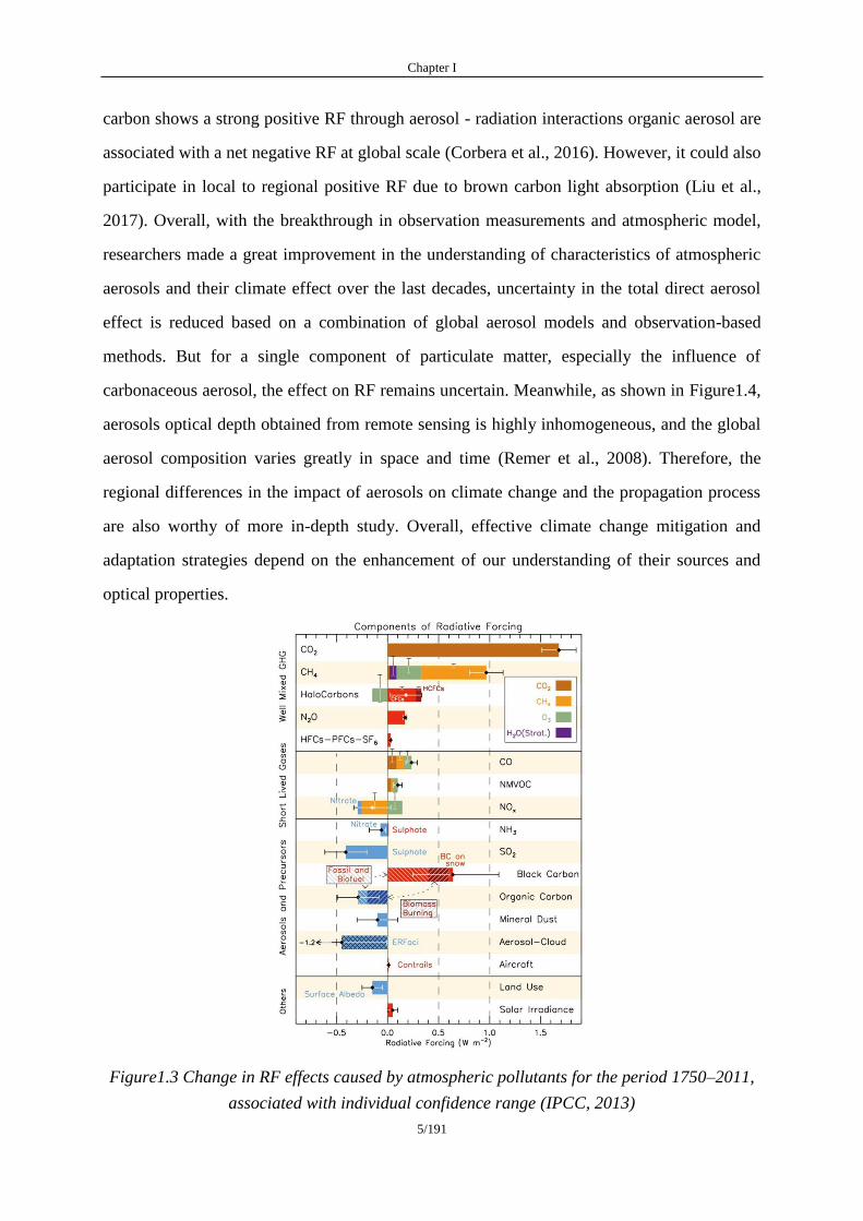
Figure1.3 summarizes the mean net RF estimated for the major air pollutants with uncertainty
levels - as compared to reference conditions prevailing before the industrial age. Gaseous
species globally display an increase of positive RF, uncertainties remains low (Shindell et al.,
2009). In contrast, climate change effects caused by aerosols are strongly associated with their
chemical composition, with opposite influences, as well as much higher uncertainties. For
example, inorganic species like nitrate and sulfate, globally exhibit negative RF, while black
Chapter I
5/191
carbon shows a strong positive RF through aerosol - radiation interactions organic aerosol are
associated with a net negative RF at global scale (Corbera et al., 2016). However, it could also
participate in local to regional positive RF due to brown carbon light absorption (Liu et al.,
2017). Overall, with the breakthrough in observation measurements and atmospheric model,
researchers made a great improvement in the understanding of characteristics of atmospheric
aerosols and their climate effect over the last decades, uncertainty in the total direct aerosol
effect is reduced based on a combination of global aerosol models and observation-based
methods. But for a single component of particulate matter, especially the influence of
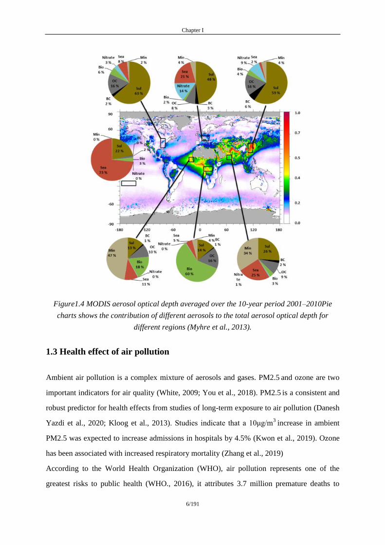
carbonaceous aerosol, the effect on RF remains uncertain. Meanwhile, as shown in Figure1.4,
aerosols optical depth obtained from remote sensing is highly inhomogeneous, and the global
aerosol composition varies greatly in space and time (Remer et al., 2008). Therefore, the
regional differences in the impact of aerosols on climate change and the propagation process
are also worthy of more in-depth study. Overall, effective climate change mitigation and
adaptation strategies depend on the enhancement of our understanding of their sources and
optical properties.
Figure1.3 Change in RF effects caused by atmospheric pollutants for the period 1750–2011,
associated with individual confidence range (IPCC, 2013)
Chapter I
6/191
Figure1.4 MODIS aerosol optical depth averaged over the 10-year period 2001–2010Pie
charts shows the contribution of different aerosols to the total aerosol optical depth for
different regions (Myhre et al., 2013).
1.3 Health effect of air pollution
Ambient air pollution is a complex mixture of aerosols and gases. PM2.5 and ozone are two
important indicators for air quality (White, 2009; You et al., 2018). PM2.5 is a consistent and
robust predictor for health effects from studies of long-term exposure to air pollution (Danesh
Yazdi et al., 2020; Kloog et al., 2013). Studies indicate that a 10μg/m3
increase in ambient
PM2.5 was expected to increase admissions in hospitals by 4.5% (Kwon et al., 2019). Ozone
has been associated with increased respiratory mortality (Zhang et al., 2019)
According to the World Health Organization (WHO), air pollution represents one of the
greatest risks to public health (WHO., 2016), it attributes 3.7 million premature deaths to
Chapter I
7/191
outdoor air pollution and 4.3 million to indoor air pollution. Formation of air pollution
episodes is caused by the harmful emission or excessive quantities of air pollutants combined
with a lack of atmospheric dispersion (Florentina and Io, 2011; Watson et al., 1988a). This
association between air pollution exposure and the risks to human health has been a public
health concern for over 700 years (Yin et al., 2020). Despite this early recognition of the
health risks associated with poor air quality it has only become a global topic over the last 80
years (Manisalidis et al., 2020). Issues related to air quality has emerged in the human
conscious with severe events like such as the Los Angeles smog in 1949, the Great London
fog in 1952, and the Beijing haze in 2013 (Huang, 2018; Li and Svarverud, 2018; McNeill
and Engelke, 2016; Xiao, 2015). Chronic exposure also remaining risks, with air pollution
leading to premature death of about 3 million population per year over the world (Anderson et
al., 2012; Fang et al., 2013). In Europe, aerosols are assessed as the most worrying
atmospheric pollutants along with nitrogen oxides and ozone (―Consolidated Annual Activity
Report 2018 (CAAR) - EEA annual report — European Environment Agency,‖ n.d.). Health
effects include difficulty in breathing, wheezing, coughing, asthma and worsening of existing
respiratory and cardiac conditions (Kim et al., 2013; Levy et al., 2006). These effects result in
increased medication use and premature death (Liu et al., 2018). Some studies are also
showing air pollution impacts on fertility, pregnancy, premature birth, dementia, and/or
obesity (Koman et al., 2018; Olsson et al., 2013).
The various biological mechanisms beyond pollutants health effects still remains uncertainties
(Samet and Krewski, 2007), but it also has been generally recognized that particle size and
chemical composition are major factors determining their health effects (Lighty et al., 2000;
Natusch and Wallace, 1974). Exposure to fine particulate matter has largest health risk (Bell
et al., 2010; Power et al., 2015), since those small particles could join into the deepest regions
of the lungs and transport the toxic compounds into the bloodstream. For instance, Quan et al
(2010) indicated that PM2.5 was responsible for plaque exacerbation, causing vascular
inflammation and atherosclerosis. (Feng et al., 2016) reported that PM2.5 promotes the
initiation and progression of diabetes and driving adverse birth outcomes. Recognizing the
dangers of air pollutants to public health, the European Commission has proposed to fix the
ceiling of the annual average concentration of 25μg/m3 for PM2.5. The European Union
Chapter I
8/191
member states shall comply with this value since 2015 and the is reflecting to adopt more
stringent standards in line with WHO guidelines. Furthermore, some compounds such as
black carbon are suspected to be carcinogenic which have been recently classified in the 2A
(probably carcinogenic to human) and 2B (possibly carcinogenic to human) groups by IARC
(International Agency for Research on Cancer)(Baan, 2007; Lauby-Secretan et al., 2016). Air
pollution is one of the greatest social and environmental problems, with terrible consequences
(Koolen and Rothenberg, 2019a). Therefore, an efficient air quality simulation and forecast
model especially in urban region can be a key tool to assess health risks for humans exposed
to airborne pollutants.
1.4 The development of atmospheric models
Atmospheric models are mathematical representations based on a complete set of dynamic
equations that can generate physical and numerical data of climate and chemical parameters
(Li et al., 2016). Today, an atmospheric model becomes an essential tool in a variety of
atmospheric sciences applications. Early in 1904, the Norwegian scientist Vilhelm Bjerknes
listed seven basic variables (temperature; pressure; air density; humidity; the three
components of wind velocity) and set down a two-step scientific viewpoint for the weather
prediction: (i) the initial state of the atmosphere is determinates by observation giving the
distribution of the variables at different levels in the diagnostic step first, (ii) then the changes
over time calculated using the law of motion in the prognostic step (Lynch, 2008). By about
1922, the British scientist Lewis Fry Richardson presaged the numerical weather prediction
after the advent of electronic computers in his book Weather Prediction by Numerical
Process (Inness and Dorling, 2012; Somerville, 2011). In those days, the weather forecasting
was a haphazard process, the forecaster used rough techniques of extrapolation based on their
knowledge of local climatology and intuition, but the principles of theoretical physics played
little role in practical forecasting, weather forecasting was more an art than a science (Lynch,
2002, 2008). Since the 1960s, with the development of computers and network
communication techniques, the atmospheric model arises at the historic moment (Hersbach et
al., 2015; Paine, 2019). For the past half century, with the rapid development of
Chapter I
9/191
high-performance computers, satellite detection and the continuous in-depth research of
numerical prediction theory, numerical prediction has achieved great success and has become
an important symbol of the atmospheric science and the main methods of weather forecasting
operations (Meng et al., 2019). Although the processes of climate change are of global
proportions, there are significant differences in its specific manifestations between regions
(temperature; precipitation and land-use changes). Thus, atmospheric mesoscale models are
being embedded to provide specific guidance to policy makers at all administrative levels.
The development of mesoscale models goes back to the 1960’s, in which with a grid size of
tens of kilometers to simulate regional weather over a few days (Dudhia, 2014). With the
evolution of dynamics and physical representations and the availability of cheaper computing
resources, high resolution simulation and forecast became possible and various ―local
customized‖ models began to emerge. For example, a mesoscale meteorological model
coupled with a chemical transport model (CTM) is an essential tool to provide the regional
airshed information to help government develop strategies for manage regional air quality. In
the past two decades, those models have been used to provide information for integrated
models like GAINS (Greenhouse gas - Air pollution Interactions and Synergies) for key
negotiations on the air pollution control agreements (Amann et al., 2011). New approaches
based on statistics are in use or under development like the Screening for High Emission
Reduction Potential on Air (SHERPA) tool. In SHERPA (Pisoni et al., 2017; Thunis et al.,
2016a), a different approach is undertaken that reproduces the grid-cell-to-grid-cell approach
but does not require anywhere near as many CTM runs. SHERPA assumes that the unknown
parameters vary on a cell-by-cell basis but are no longer independent of each other.
According to the model design concepts and parameters, the development of CTM is roughly
divided into three generations (Casado, 2013). The first generation of CTM originated in the
1970’s which mainly include the box model based on the law of conservation of mass
(Seinfeld, 1988) such as Empirical Kinetic Modeling Approach (EKMA), the Gaussian
dispersion model based on the statistical theory of turbulence diffusion (Atkinson et al., 1997)
like Industrial Source Complex model (ISC). These models use simple, parameterized linear
mechanisms to describe complex atmospheric physical processes, which are suitable for
simulating the long-term average concentration of inert pollutants (Watson et al., 1988b). In

Chapter I
10/191
the early 1980s, with the study of the turbulence characteristics of the atmospheric boundary
layer, researchers found that the Gaussian model could not answer many questions, which
gradually promoted the development of the second generation. The second generation of
CTM considers nonlinear response mechanism and incorporates the treatment of gas and
aqueous phase chemistry. These models divide the simulated domain into many
three-dimensional grid cells, the cloud, fog and precipitation scavenging processes are
calculated in each cell (Carey Jang et al., 1995; Liu et al., 1984; Stockwell et al., 1990).
Representative models in this category include the Urban Air shed Model (UAM), the
Regional Acid Deposition Model (RADM), etc. The second generation CTM are only
designed to address individual pollutant issues such as ozone and acid deposition, which does
not fully consider the mutual transformation and mutual influence of various pollutants (Reis
et al., 2005). However, the physical and chemical reaction processes among various pollutants
are complex in the real atmosphere. In 1990’s, the US Environmental Protection Agency
(EPA) developed the third-generation air quality simulation platform Models-3 based on the
concept of "one atmosphere" (Byun and Schere, 2006a). At present, the most widely used are
the third-generation comprehensive CTM in clouding WRF-Chem, the Comprehensive
Air-quality Model with extensions (CAMx), Community Multiscale Air Quality Model
(CMAQ), CHIMERE, etc.
The WRF-Chem is a regional atmospheric dynamic-chemical coupling model developed by
the US National Center for Atmospheric Research (NCAR), which is integrated with the
atmospheric chemistry module in the mesoscale Weather Research and Forecast model (WRF)
(Grell et al., 2005). The WRF provides online large airflow fields for CTM, simulating
pollutant transportation, dry and wet deposition, gas phase chemistry, aerosol formation,
radiation, biological radiation, etc. (Lin et al., 2020). The advantage of WRF-Chem is that the
meteorology mode and the chemical transport mode are fully coupled in time and space
resolution to achieve true online feedback. The CAMx model is a comprehensive CTM
developed by ENVIRON on the basis of the UAM model. In addition to the typical features
of the third-generation air quality model, the most famous features of CAMx include:
two-way nesting and flexible nesting, grid plume module, ozone source allocation technology,
particulate source allocation technology(Bove et al., 2014; Pepe et al., 2016). The CMAQ,
Chapter I
11/191
emission inventory processing model (SMOKE), mesoscale meteorological model (MM5 or
WRF.) together constitute the Models-3 platform, of which CMAQ is the core of the entire
system (Hanna, 2008). The CMAQ was originally designed to comprehensively deal with
complex air pollution problems such as tropospheric ozone, acid deposition, and visibility.
For this reason, the design concept of CMAQ can systematically simulate various scales and
various complicated air pollution issues. The CMAQ model has become a quasi-regulatory
model used by the US EPA in environmental planning, management and decision-making.
The characteristics of this model are: simultaneously simulate the behavior of a variety of air
pollutants, including ozone, PM, acid deposition, and visibility and other air quality problems
in different spatial scales; make full use of the latest Computer hardware and software
technologies, such as high-performance computing, modular design, visualization technology,
etc., make air quality simulation technology more efficient and accurate, and the application
fields tend to be diversified. Since CMAQ 5.0, the model has realized the on-line coupling of
meteorological model, absorbing the advantages of WRF-CHEM model (Kong et al., 2015).
CHIMERE is a three-dimensional CTM driven by meteorological drivers like MM5 or WRF.
More than 80 kinds of species more than 300 reactions are described in the model. Processes
include chemistry, transportation, vertical diffusion, photochemistry, dry deposition,
absorption in and below clouds, and SO2 oxidation. Clouds are included in the process model.
It can simulate processes including gas-phase chemistry, vertical diffusion, photochemistry,
aerosol formation, deposition and transport at regional and urban scales (Bessagnet et al.,
2004; Vautard et al., 2005). A new version CHIMERE-V2019 has realized the online
coupling of meteorological model like WRF-Chem and CMAQ (Bessagnet et al., 2020).
Compare to the first and second generation CTM, the third generation CTM has distinct
advances in:
(i) full consideration of various atmospheric physical processes, chemical reactions
between pollutants and gas-solid two-phase transformation process (San José et al.,
2009);
(ii) based on nested grid design, it can be used as a multi-scale atmospheric simulation
and prediction tool (Xue et al., 2001);
Chapter I
12/191
(iii) simultaneously simulate the variety of air pollutants, including ozone, PM, acid
deposition, visibility and other environmental pollution problems;
(iv) make full use of the latest computer technologies, such as high-performance
computing, modular design, visualization technology to make air quality
simulation technology more efficient and accurate (Reis et al., 2005).
Today, around ninety nations run their own mesoscale models until 2016 either for specific
regions or for specific applications such as local air quality, dust transport, agricultural
production, airport weather, solar ultraviolet radiation and hydrology according to World
Meteorological Organization technical progress report
(https://www.wmo.int/pages/prog/www/DPFS/GDPFS-Progress-Reports.html). Despite the
remarkable advances of atmospheric model over the past decades, formidable challenges
remain. The effective coupling between the dynamical processes and physical
parameterizations during the short-term weather changes and extremes is still a significant
challenge. Under the background of global warming, the chaotic nature of the atmosphere
becomes stronger, which puts forward higher requirements for long-term accurate forecasting,
a stronger fusion between model and observations for its data assimilation and bias
corrections are needed. Maybe the next-generation model with a focus on chemical and
physical processes, neural networks, machine learning are the ways in the future model
evolution.
1.5 Urbanization and air quality
In recent decades, air pollution in urban areas, especially megacities, have aroused people's
attention (Baklanov et al., 2016b). With the accelerating process of industrialization and
urbanization, an increasing number of people will be affected by such process especially in
developing regions (Beirle et al., 2011; Fang et al., 2015; Hopke et al., 2008). Urbanization
was positively related to global health in the short term and long term. In the short run, 1%
increase in urbanization was associated with reduced mortality, under-five mortality, and
infant mortality of 0.05%, 0.04%, and 0.04%, respectively, as well as increased life
expectancy of 0.01 year (Wang, 2018). However, the process of urbanization has also made
Chapter I
13/191
important contributions to regional climate changes and has caused a bad effect on ecosystem
and extreme climate significantly increased (Changnon et al., 1996; Semenza et al., 1996).
Since the end of World War II, the world’s population has grown from 2.5 billion to about 7
billion today, the urban pollution has risen from below 30% to 58% in the past seventy years.
Air pollution in cities is exacerbated by increased human activity in urban areas due to
population growth (Miranda et al., 2015). The recent global lockdown events response to
COVID-19 pandemic have reduced the NO2concentrations and particulate matter levels by
about 60% and 31% respectively by using satellite data and a network of more than 10000 air
quality observation stations in 34 countries (Venter et al., 2020), the NO2 and PM2.5
concentration in China was reduced by around 20% and 17% for 30–50 days (Z. Liu et al.,
2020; Zinke, 2020). Using the mesoscale meteorological and chemical transport model,
Menut et al.(2020) noted a decrease of -30% to -50% for NO2 and -5% to -15% for particulate
matter in all western Europe counties during the lockdown events. In general, air pollution is
positively correlated with the initial and acceleration stages of urbanization, with pollution in
major cities tending to increase during the construction phase, passing through a maximum
pollution level and then again decreased at the end of the urbanization process as abatement
strategies are developed (Fenger, 1999). In the industrialized Europe countries, urban air
pollution is in some respects in the last stage with effectively reduced levels of many
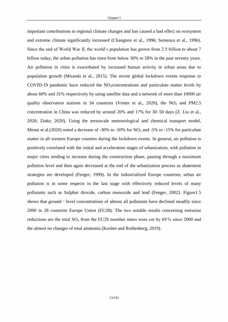
pollutants such as Sulphur dioxide, carbon monoxide and lead (Fenger, 2002). Figure1.5
shows that ground‐level concentrations of almost all pollutants have declined steadily since
2000 in 28 countries Europe Union (EU28). The two notable results concerning emission
reductions are the total SOx from the EU28 member states were cut by 69 % since 2000 and
the almost no changes of total ammonia (Koolen and Rothenberg, 2019).
Chapter I
14/191
Figure1.5 Emission trends in the EU28 on the basis of fuel sold (Koolen and Rothenberg,
2019)
Besides, geographical condition also plays an important role in transportation and dispersion
of pollutants. Pollutants dispersion processes over the valley-basin city are much more
complicated than over flat areas. Therefore, pollution episodes have been frequently
witnessed over complex terrain, especially in wintertime (Chen et al., 2019; Sabatier et al.,
2020). In coastal cities, shipping emissions contribute to air quality degradation. Viana et al.
(2014) found that shipping emissions contribute with 1% to 7% for PM10, with 1% to 20%
for PM2.5, and with 7% to 24% for NO2 annual mean concentrations in European coastal
areas. In addition, continuing urbanization has resulted in cities that are almost always
warmer than the surround, which are known as urban heat island (UHI). A recent research
shows that urban region has higher heat index than rural areas by a difference of about 1.5–
2°C (Bhati and Mohan, 2018). Compared with the natural vegetation canopy, the city has its
unique features: taking buildings as an example, different buildings have different functions,
shapes, heights, orientations, styles, etc. (Wong and Chen, 2008). Figure1.6 shows the
differences in surface temperature between buildings and vegetation canopy. Meanwhile, UHI
can significantly exacerbate building energy consumption (Palme et al., 2017). The growing
cooling energy consumption caused by UHI will increase CO2 emissions by up to five times
in 2050 than in 2000 for buildings in cities (Y. Liu et al., 2020). Besides, there are various
types of artificial surfaces in urban areas, such as asphalt roads, concrete sidewalks, glass
Chapter I
15/191
curtain walls, parking lots, and green spaces which have impact on urban air quality (Wise,
2016). For example, computational fluid dynamics studies indicated that the flow resistance
of tree crowns decreased wind speed and the dispersion of pollutants is limited in the ground
level and the particulate matter concentrations accumulate within the canyon (Gromke and
Blocken, 2015). These diversified types of artificial areas appear alternately, leading to
complex, diverse, and non-uniform urban canopy characteristics, which give more complex
turbulent airflows in urban region, increased the difficulty of air quality simulation and
forecast in cities than in other regions. The urban canopy, urban street canopy and urban
boundary layer consist of the urban micro environment. The boundary layer is the
atmospheric structure closest to the underlying surface. The meteorological conditions within
the boundary layer play an important role in the formation of air pollution (Bianco et al.,
2008). The wind field determines the regional transportation of pollutants. The height of the
atmospheric boundary layer determines the amount of ventilation and the dilution capacity of
pollutants. Heavy pollution episodes are always accompanied by a low boundary layer
height(Quan et al., 2014; Yin et al., 2019). In cities, urbanization causes thermodynamic
perturbations and facilitates the development of the boundary layer (Miao et al., 2019).
Moreover, some aerosols like black carbon can warm the upper PBL which help to stabilize
the boundary layer height and weaken turbulent mixing, resulting in a decrease of the
boundary layer height (BLH), which enhances the accumulation of air pollutants (Ding et al.,
2016; Li et al., 2017).
Overall, cities are highly sensitive to the impact of meteorological disasters. How to be
efficient in extreme climates risk analysis and early warning, firmly keeping the bottom line
of city safe operation and ecological environment protection is a concern of scientists and
politicians. The impact of the accelerated urbanization process on the regional climate and
atmospheric environment mainly includes the following aspects:
(1) The urban underlying surface is defined as the part of the city in direct exchange with
the atmosphere (Y. Li et al., 2020), the changes of the urban underlying surface have
changed the environmental properties of the natural underlying surface;

Chapter I
16/191
(2) The urban canopy has a "shading effect" on solar radiation, which reduces the solar
radiation reaching the surface. At the same time, there is the exchange and storage of
radiation energy between the buildings in the canopy, which affects the surface energy
balance;
(3) Human activities will increase atmospheric pollutants and artificial heat generation. In
short, in addition to bringing economic and social benefits to humanity, urbanization
has also brought many problems to the urban climate and atmospheric environment
Statement.
The climate effect brought by urbanization and its impact on the atmospheric environment is
becoming one of the key issues of the world.
Figure1.6 Urban heat island in cities.
1.6 Objectives and outline of the PhD thesis
The main goal of this PhD work is to improve the air quality simulation and forecast in
France especially in urbanized areas. For its operational requirements, the system requires
continuous improvements, particularly the ability to better predict certain types of episodes
and exceedances of limit values for criteria pollutants. Patterns of urban air pollution are
rather variable and spatially heterogeneous. Turbulence plays an important role on the vertical
mixing of physical parameters and pollutants.. Understanding the impact of multiple
parameterization schemes on air quality simulation can help improve model configuration to
address local areas.
Chapter I
17/191
The third generation of CTM system generally has three basic modules: a meteorological
process module (input information from mesoscale meteorological models), emission
inventory pre-processor and the core air quality simulation module. Studies indicate that the
physics parameterizations play the key role in both meteorological and air quality simulation
particularly in urban areas. The buildings and cement pavement form the urban canopy layers
and surface roughness, therefore change thermal and dynamic characteristics of the surface
layer. These changes will significantly influence the surface heat accumulation that has a
negative effect of the planetary boundary layer (PBL) height and surface wind speed which
affect the transport and dispersion of pollutants. The PBL height is a key factor on the
formation and evolution of pollutants. A low boundary layer height is regarded as a major
meteorological process for haze formation. Thus, a smart selection of physics
parameterizations plays a crucial role in urban air quality prediction.
With the development of computer performances, high resolution meteorological and air
quality simulations become possible. However, studies demonstrate that the higher resolution
does not represent better simulation results, horizontal resolution below 1km is not necessary.
Meanwhile, the building clusters modified surface roughness and zero-plane displacement
height, an overestimated vertical resolution can cause unreasonable wind flows near surface.
The K-theory shows certain advantages in dealing with the dispersion of air pollution at the
mesoscale. It can use the observed wind speed profile data to obtain the concentration
distribution of pollutants without assuming a certain form of distribution. However, high
pollutants concentrations are frequently found under stable and cold weather conditions, such
conditions are characterized by a stratified lower atmosphere and weak turbulent diffusion. In
cities, traffic, residential and local industrial emissions have a major share of the pollutants;
those emissions can accumulate and have longer residence times near the ground level due to
the inefficient transport and mixing. The transient turbulent flow plays an important role on
the transportation and deposition of pollutants, thus, an advanced vertical eddy coefficient
may helpful to provide an accurate prediction of pollution during the short-term episode. It is
noteworthy that meteorological sciences have focused on extreme events to forecast heavy
precipitations, thunderstorms, high wind speed conditions while air quality is mainly driven
Chapter I
18/191
by stable and calm meteorological situations and these latter conditions are difficulty captured
by meteorological models.
Different geographical areas will be investigated in France, especially mainly for short-term
pollution episodes. The ability of models to assess air quality management strategies is also
important, it will be appropriate during this study to perform the diffusion and dispersion of
main pollutants and possibly improve the vertical diffusion coefficient in the selected CTM
(CHIMERE here) (Menut et al., 2013; Mailler et al., 2017).
The objectives of this work are to provide clues and answers to the following questions:
1) Which formulae for computing the vertical diffusion coefficient based on K-theory gives the
best performances on air quality simulation?
2) How well do physics parameterizations impact the urban air quality simulation and
forecast?
3) How does vertical grid resolution and first layer height impact the meteorological and
chemistry transport modelling?
4) Can we improve the vertical mixing through the use of turbulence kinetic energy sub-grid
eddy coefficient?
To tackle these issues, the present work has been breakdown in four main steps detailed in the
various chapters.
Chapter II addresses the results of the one-year air quality simulation that was determined by
three K-theory vertical diffusion coefficient. Inter-annual trends, seasonal and daily variations
of main pollutants concentrations are presented. Here, it has been chosen to focus both on
cities and surroundings over the whole France.
In Chapter III, the impact of physics parameterizations on high-resolution meteorological
and air quality simulations over the urban region will be analyzed, with a focus on a winter
pollution episode in Paris region. Three canopy schemes, three boundary layer schemes, two
land surface schemes will be tested in this part. Benefits as well as drawbacks and specific
issues of the considered approaches are discussed and compared. Finally, the most reasonable
physics parameterizations will be used in the subsequent chapters.
Chapter I
19/191
In Chapter IV, the impact of vertical gird resolution and first layer height on meteorological
and chemistry transport modelling will be analyzed; three vertical resolution configurations
and three first layer height will be applied in a fifteen days winter episode including a
pollution event.
In Chapter V, we use a 1.5-order turbulence kinetic energy-based eddy diffusivity closure
scheme from WRF defined as NED on the urban air quality context to assess consequences of
surface-level pollutants concentrations in Paris, Lyon and Bordeaux regions.
Chapter I
20/191
References
Amann, M., Bertok, I., Borken-Kleefeld, J., Cofala, J., Heyes, C., Höglund-Isaksson, L.,
Klimont, Z., Nguyen, B., Posch, M., Rafaj, P., Sandler, R., Schöpp, W., Wagner, F.,
and Winiwarter, W.: Cost-effective control of air quality and greenhouse gases in
Europe: Modeling and policy applications, Environmental Modelling & Software, 26,
1489–1501, https://doi.org/10.1016/j.envsoft.2011.07.012, 2011.
Anderson, J. O., Thundiyil, J. G., and Stolbach, A.: Clearing the Air: A Review of the Effects
of Particulate Matter Air Pollution on Human Health, J. Med. Toxicol., 8, 166–175,
https://doi.org/10.1007/s13181-011-0203-1, 2012.
Andres, R. J., Boden, T. A., Breon, F.-M., Ciais, P., Davis, S., Erickson, D., Gregg, J. S.,
Jacobson, A., Marland, G., Miller, J., Oda, T., Oliver, J. G. J., Raupach, M. R., Rayner,
P., and Treanton, K.: A synthesis of carbon dioxide emissions from fossil-fuel
combustion, 2012.
Anon: AR5 Climate Change 2013: The Physical Science Basis — IPCC, n.d.
Consolidated Annual Activity Report 2018 (CAAR) - EEA annual report — European
Environment Agency:
https://www.eea.europa.eu/publications/consolidated-annual-activity-report-2018, last
access: 13 January 2021.
WHO | World Malaria Report 2016:
http://www.who.int/malaria/publications/world-malaria-report-2016/report/en/, last
access: 13 January 2021.
Atkinson, D., Bailey, D., Irwin, J., and Touma, J.: Improvements to the EPA Industrial Source
Complex Dispersion Model, Journal of Applied Meteorology - J APPL METEOROL,
36, 1088–1095, https://doi.org/10.1175/1520-0450(1997)036<1088:ITTEIS>2.0.CO;2,
1997.
Baan, R. A.: Carcinogenic Hazards from Inhaled Carbon Black, Titanium Dioxide, and Talc
not Containing Asbestos or Asbestiform Fibers: Recent Evaluations by an IARC
Monographs Working Group, 19, 213–228,
https://doi.org/10.1080/08958370701497903, 2007.
Bai, L., Wang, J., Ma, X., and Lu, H.: Air Pollution Forecasts: An Overview, Int J Environ
Res Public Health, 15, https://doi.org/10.3390/ijerph15040780, 2018.
Baklanov, A., Molina, L. T., and Gauss, M.: Megacities, air quality and climate, Atmospheric
Environment, 126, 235–249, https://doi.org/10.1016/j.atmosenv.2015.11.059, 2016.
Beirle, S., Boersma, K. F., Platt, U., Lawrence, M. G., and Wagner, T.: Megacity Emissions
and Lifetimes of Nitrogen Oxides Probed from Space, 333, 1737–1739,
https://doi.org/10.1126/science.1207824, 2011.
Chapter I
21/191
Bell, M. L., Belanger, K., Ebisu, K., Gent, J. F., Lee, H. J., Koutrakis, P., and Leaderer, B. P.:
Prenatal Exposure to Fine Particulate Matter and Birth Weight, Epidemiology, 21,
884–891, https://doi.org/10.1097/EDE.0b013e3181f2f405, 2010.
Bessagnet, B., Hodzic, A., Vautard, R., Beekmann, M., Cheinet, S., Honoré, C., Liousse, C.,
and Rouil, L.: Aerosol modeling with CHIMERE—preliminary evaluation at the
continental scale, Atmospheric Environment, 38, 2803–2817,
https://doi.org/10.1016/j.atmosenv.2004.02.034, 2004.
Bessagnet, B., Menut, L., Lapere, R., Couvidat, F., Jaffrezo, J.-L., Mailler, S., Favez, O.,
Pennel, R., and Siour, G.: High Resolution Chemistry Transport Modeling with the
On-Line CHIMERE-WRF Model over the French Alps—Analysis of a Feedback of
Surface Particulate Matter Concentrations on Mountain Meteorology, Atmosphere, 11,
565, https://doi.org/10.3390/atmos11060565, 2020.
Bhati, S. and Mohan, M.: WRF-urban canopy model evaluation for the assessment of heat
island and thermal comfort over an urban airshed in India under varying land use/land
cover conditions, Geosci. Lett., 5, 27, https://doi.org/10.1186/s40562-018-0126-7,
2018.
Bond, T. C., Doherty, S. J., Fahey, D. W., Forster, P. M., Berntsen, T., DeAngelo, B. J.,
Flanner, M. G., Ghan, S., Kärcher, B., Koch, D., Kinne, S., Kondo, Y., Quinn, P. K.,
Sarofim, M. C., Schultz, M. G., Schulz, M., Venkataraman, C., Zhang, H., Zhang, S.,
Bellouin, N., Guttikunda, S. K., Hopke, P. K., Jacobson, M. Z., Kaiser, J. W., Klimont,
Z., Lohmann, U., Schwarz, J. P., Shindell, D., Storelvmo, T., Warren, S. G., and
Zender, C. S.: Bounding the role of black carbon in the climate system: A scientific
assessment, 118, 5380–5552, https://doi.org/10.1002/jgrd.50171, 2013.
Bove, M. C., Brotto, P., Cassola, F., Cuccia, E., Massabò, D., Mazzino, A., Piazzalunga, A.,
and Prati, P.: An integrated PM2.5 source apportionment study: Positive Matrix
Factorisation vs. the chemical transport model CAMx, Atmospheric Environment, 94,
274–286, https://doi.org/10.1016/j.atmosenv.2014.05.039, 2014.
Byun, D. and Schere, K. L.: Review of the Governing Equations, Computational Algorithms,
and Other Components of the Models-3 Community Multiscale Air Quality (CMAQ)
Modeling System, Applied Mechanics Reviews, 59, 51–77,
https://doi.org/10.1115/1.2128636, 2006.
Carey Jang, J.-C., Jeffries, H. E., Byun, D., and Pleim, J. E.: Sensitivity of ozone to model
grid resolution—I. Application of high-resolution regional acid deposition model,
Atmospheric Environment, 29, 3085–3100,
https://doi.org/10.1016/1352-2310(95)00118-I, 1995.
Casado, R.: The three generations of Big Data processing, 2013.
Changnon, S. A., Kunkel, K. E., and Reinke, B. C.: Impacts and Responses to the 1995 Heat
Wave: A Call to Action, 77, 1497–1506,
https://doi.org/10.1175/1520-0477(1996)077<1497:IARTTH>2.0.CO;2, 1996.
Chapter I
22/191
Charlson, R. J., Schwartz, S. E., Hales, J. M., Cess, R. D., Coakley, J. A., Hansen, J. E., and
Hofmann, D. J.: Climate Forcing by Anthropogenic Aerosols, 255, 423–430,
https://doi.org/10.1126/science.255.5043.423, 1992.
Chen, Z., Zhuang, Y., Xie, X., Chen, D., Cheng, N., Yang, L., and Li, R.: Understanding
long-term variations of meteorological influences on ground ozone concentrations in
Beijing During 2006–2016, Environmental Pollution, 245, 29–37,
https://doi.org/10.1016/j.envpol.2018.10.117, 2019.
Colbeck, I. and Lazaridis, M.: Aerosols and environmental pollution, Naturwissenschaften, 97,
117–131, https://doi.org/10.1007/s00114-009-0594-x, 2010.
Corbera, E., Calvet-Mir, L., Hughes, H., and Paterson, M.: Patterns of authorship in the IPCC
Working Group III report, 6, 94–99, https://doi.org/10.1038/nclimate2782, 2016.
Danesh Yazdi, M., Kuang, Z., Dimakopoulou, K., Barratt, B., Suel, E., Amini, H., Lyapustin,
A., Katsouyanni, K., and Schwartz, J.: Predicting Fine Particulate Matter (PM2.5) in
the Greater London Area: An Ensemble Approach using Machine Learning Methods,
12, 914, https://doi.org/10.3390/rs12060914, 2020.
Desonie, D.: Atmosphere: Air Pollution and Its Effects, Infobase Publishing, 209 pp., 2007.
Dudhia, J.: A history of mesoscale model development, Asia-Pacific J Atmos Sci, 50, 121–
131, https://doi.org/10.1007/s13143-014-0031-8, 2014.
Fang, C., Liu, H., Li, G., Sun, D., and Miao, Z.: Estimating the Impact of Urbanization on Air
Quality in China Using Spatial Regression Models, 7, 15570–15592,
https://doi.org/10.3390/su71115570, 2015.
Fang, Y., Mauzerall, D. L., Liu, J., Fiore, A. M., and Horowitz, L. W.: Impacts of 21st
century climate change on global air pollution-related premature mortality, Climatic
Change, 121, 239–253, https://doi.org/10.1007/s10584-013-0847-8, 2013.
Feng, S., Gao, D., Liao, F., Zhou, F., and Wang, X.: The health effects of ambient PM2.5 and
potential mechanisms, Ecotoxicology and Environmental Safety, 128, 67–74,
https://doi.org/10.1016/j.ecoenv.2016.01.030, 2016.
Fenger, J.: Urban air quality, Atmospheric Environment, 33, 4877–4900,
https://doi.org/10.1016/S1352-2310(99)00290-3, 1999.
Fenger, J.: Chapter 1 Urban air quality, in: Developments in Environmental Science, vol. 1,
edited by: Austin, J., Brimblecombe, P., and Sturges, W., Elsevier, 1–52,
https://doi.org/10.1016/S1474-8177(02)80004-3, 2002.
Finlayson-Pitts, B. J. and Jr, J. N. P.: Chemistry of the Upper and Lower Atmosphere: Theory,
Experiments, and Applications, Elsevier, 993 pp., 1999.
Fisher, M. R.: 10.1 Atmospheric Pollution, in: Environmental Biology, Open Oregon
Educational Resources, 2017.
Florentina, I. and Io, B.: The Effects of Air Pollutants on Vegetation and the Role of
Vegetation in Reducing Atmospheric Pollution, in: The Impact of Air Pollution on
Chapter I
23/191
Health, Economy, Environment and Agricultural Sources, edited by: Khallaf, M.,
InTech, https://doi.org/10.5772/17660, 2011.
Grell, G., Peckham, S., Schmitz, R., McKeen, S., Frost, G., Skamarock, W., and Eder, B.:
Fully coupled ―online‖ chemistry in the WRF model, Atmospheric Environment, 39,
6957–6975, https://doi.org/10.1016/j.atmosenv.2005.04.027, 2005.
Gromke, C. and Blocken, B.: Influence of avenue-trees on air quality at the urban
neighborhood scale. Part II: Traffic pollutant concentrations at pedestrian level,
Environmental Pollution, 196, 176–184, https://doi.org/10.1016/j.envpol.2014.10.015,
2015.
Hallquist, M., Wenger, J. C., Baltensperger, U., Rudich, Y., Simpson, D., Claeys, M.,
Dommen, J., Donahue, N. M., George, C., Goldstein, A. H., Hamilton, J. F.,
Herrmann, H., Hoffmann, T., Iinuma, Y., Jang, M., Jenkin, M. E., Jimenez, J. L.,
Kiendler-Scharr, A., Maenhaut, W., McFiggans, G., Mentel, T. F., Monod, A., Prévôt,
A. S. H., Seinfeld, J. H., Surratt, J. D., Szmigielski, R., and Wildt, J.: The formation,
properties and impact of secondary organic aerosol: current and emerging issues, 9,
5155–5236, https://doi.org/10.5194/acp-9-5155-2009, 2009.
Hanna, A.: Modelin the Transport and Chemical Evolution of Onshore and Offshore
Emissions and Their Impact on Local and Regional Air Quality Using a
Variable-Grid-Resolution Air Quality Model, Univ. of North Carolina, Chapel Hill,
NC (United States), https://doi.org/10.2172/962694, 2008.
Hansen, J., Sato, M., Ruedy, R., Nazarenko, L., Lacis, A., Schmidt, G. A., Russell, G.,
Aleinov, I., Bauer, M., Bauer, S., Bell, N., Cairns, B., Canuto, V., Chandler, M.,
Cheng, Y., Genio, A. D., Faluvegi, G., Fleming, E., Friend, A., Hall, T., Jackman, C.,
Kelley, M., Kiang, N., Koch, D., Lean, J., Lerner, J., Lo, K., Menon, S., Miller, R.,
Minnis, P., Novakov, T., Oinas, V., Perlwitz, J., Perlwitz, J., Rind, D., Romanou, A.,
Shindell, D., Stone, P., Sun, S., Tausnev, N., Thresher, D., Wielicki, B., Wong, T.,
Yao, M., and Zhang, S.: Efficacy of climate forcings, 110,
https://doi.org/10.1029/2005JD005776, 2005.
Hersbach, H., Peubey, C., Simmons, A., Berrisford, P., Poli, P., and Dee, D.: ERA-20CM: a
twentieth-century atmospheric model ensemble, 141, 2350–2375,
https://doi.org/10.1002/qj.2528, 2015.
Hopke, P. K., Cohen, D. D., Begum, B. A., Biswas, S. K., Ni, B., Pandit, G. G., Santoso, M.,
Chung, Y.-S., Davy, P., Markwitz, A., Waheed, S., Siddique, N., Santos, F. L., Pabroa,
P. C. B., Seneviratne, M. C. S., Wimolwattanapun, W., Bunprapob, S., Vuong, T. B.,
Duy Hien, P., and Markowicz, A.: Urban air quality in the Asian region, Science of
The Total Environment, 404, 103–112, https://doi.org/10.1016/j.scitotenv.2008.05.039,
2008.
Huang, S.: Air pollution and control: Past, present and future, Chin. Sci. Bull., 63, 895–919,
https://doi.org/10.1360/N972017-01271, 2018.
Chapter I
24/191
Inness, P. M. and Dorling, S.: Operational Weather Forecasting, John Wiley & Sons, 211 pp.,
2012.
Jenkin, M. E. and Clemitshaw, K. C.: Ozone and other secondary photochemical pollutants:
chemical processes governing their formation in the planetary boundary layer,
Atmospheric Environment, 34, 2499–2527,
https://doi.org/10.1016/S1352-2310(99)00478-1, 2000.
Kemp, A. C., Horton, B. P., Donnelly, J. P., Mann, M. E., Vermeer, M., and Rahmstorf, S.:
Climate related sea-level variations over the past two millennia, Proceedings of the
National Academy of Sciences, 108, 11017–11022,
https://doi.org/10.1073/pnas.1015619108, 2011.
Kim, K.-H., Jahan, S. A., and Kabir, E.: A review on human health perspective of air
pollution with respect to allergies and asthma, Environment International, 59, 41–52,
https://doi.org/10.1016/j.envint.2013.05.007, 2013.
Kloog, I., Ridgway, B., Koutrakis, P., Coull, B. A., and Schwartz, J. D.: Long- and
Short-Term Exposure to PM2.5 and Mortality, Epidemiology, 24, 555–561,
https://doi.org/10.1097/EDE.0b013e318294beaa, 2013.
Kok, J. F.: A scaling theory for the size distribution of emitted dust aerosols suggests climate
models underestimate the size of the global dust cycle, PNAS, 108, 1016–1021,
https://doi.org/10.1073/pnas.1014798108, 2011.
Koman, P. D., Hogan, K. A., Sampson, N., Mandell, R., Coombe, C. M., Tetteh, M. M.,
Hill-Ashford, Y. R., Wilkins, D., Zlatnik, M. G., Loch-Caruso, R., Schulz, A. J., and
Woodruff, T. J.: Examining Joint Effects of Air Pollution Exposure and Social
Determinants of Health in Defining ―At-Risk‖ Populations Under the Clean Air Act:
Susceptibility of Pregnant Women to Hypertensive Disorders of Pregnancy, World
Med Health Policy, 10, 7–54, https://doi.org/10.1002/wmh3.257, 2018.
Kong, X., Forkel, R., Sokhi, R. S., Suppan, P., Baklanov, A., Gauss, M., Brunner, D., Barò,
R., Balzarini, A., Chemel, C., Curci, G., Jiménez-Guerrero, P., Hirtl, M., Honzak, L.,
Im, U., Pérez, J. L., Pirovano, G., San Jose, R., Schlünzen, K. H., Tsegas, G., Tuccella,
P., Werhahn, J., Ţabkar, R., and Galmarini, S.: Analysis of meteorology–chemistry
interactions during air pollution episodes using online coupled models within AQMEII
phase-2, Atmospheric Environment, 115, 527–540,
https://doi.org/10.1016/j.atmosenv.2014.09.020, 2015.
Koolen, C. D. and Rothenberg, G.: Air Pollution in Europe, 12, 164–172,
https://doi.org/10.1002/cssc.201802292, 2019.
Kwon, O. K., Kim, S.-H., Kang, S.-H., Cho, Y., Oh, I.-Y., Yoon, C.-H., Kim, S.-Y., Kim,
O.-J., Choi, E.-K., Youn, T.-J., and Chae, I.-H.: Association of short- and long-term
exposure to air pollution with atrial fibrillation, Eur J Prev Cardiolog, 26, 1208–1216,
https://doi.org/10.1177/2047487319835984, 2019.
Chapter I
25/191
Lauby-Secretan, B., Loomis, D., Baan, R., El Ghissassi, F., Bouvard, V., Benbrahim-Tallaa,
L., Guha, N., Grosse, Y., and Straif, K.: Use of mechanistic data in the IARC
evaluations of the carcinogenicity of polychlorinated biphenyls and related
compounds, Environ Sci Pollut Res, 23, 2220–2229,
https://doi.org/10.1007/s11356-015-4829-4, 2016.
Levy, M. L., Fletcher, M., Price, D. B., Hausend, T., Halbert, R. J., and Yawn, B. P.:
International Primary Care Respiratory Group (IPCRG) Guidelines: Diagnosis of
respiratory diseases in primary care, 15, 20–34,
https://doi.org/10.1016/j.pcrj.2005.10.004, 2006.
Li, H. and Svarverud, R.: When London Hit the Headlines: Historical Analogy and the
Chinese Media Discourse on Air Pollution, 234, 357–376,
https://doi.org/10.1017/S0305741017001400, 2018.
Li, J., Liu, K., and Huang, Q.: Chapter 17 - Utilizing Cloud Computing to Support Scalable
Atmospheric Modeling: A Case Study of Cloud-Enabled ModelE, in: Cloud
Computing in Ocean and Atmospheric Sciences, edited by: Vance, T. C., Merati, N.,
Yang, C., and Yuan, M., Academic Press, 347–364,
https://doi.org/10.1016/B978-0-12-803192-6.00017-7, 2016.
Li, Y., Zhang, X., Zhu, S., Wang, X., Lu, Y., Du, S., and Shi, X.: Transformation of Urban
Surfaces and Heat Islands in Nanjing during 1984–2018, 12, 6521,
https://doi.org/10.3390/su12166521, 2020.
Lighty, J. S., Veranth, J. M., and Sarofim, A. F.: Combustion Aerosols: Factors Governing
Their Size and Composition and Implications to Human Health, 50, 1565–1618,
https://doi.org/10.1080/10473289.2000.10464197, 2000.
Lin, H., Feng, X., Fu, T.-M., Tian, H., Ma, Y., Zhang, L., Jacob, D. J., Yantosca, R. M.,
Sulprizio, M. P., Lundgren, E. W., Zhuang, J., Zhang, Q., Lu, X., Zhang, L., Shen, L.,
Guo, J., Eastham, S. D., and Keller, C. A.: WRF-GC: online coupling of WRF and
GEOS-Chem for regional atmospheric chemistry modeling, Part 1: description of the
one-way model (v1.0), Climate and Earth System Modeling,
https://doi.org/10.5194/gmd-2019-333, 2020.
Liu, D., Whitehead, J., Alfarra, M. R., Reyes-Villegas, E., Spracklen, D. V., Reddington, C.
L., Kong, S., Williams, P. I., Ting, Y.-C., Haslett, S., Taylor, J. W., Flynn, M. J.,
Morgan, W. T., McFiggans, G., Coe, H., and Allan, J. D.: Black-carbon absorption
enhancement in the atmosphere determined by particle mixing state, 10, 184–188,
https://doi.org/10.1038/ngeo2901, 2017.
Liu, H.-Y., Dunea, D., Iordache, S., and Pohoata, A.: A Review of Airborne Particulate
Matter Effects on Young Children’s Respiratory Symptoms and Diseases, 9, 150,
https://doi.org/10.3390/atmos9040150, 2018.
Chapter I
26/191
Liu, M.-K., Morris, R. E., and Killus, J. P.: Development of a regional oxidant model and
application to the northeastern United States, Atmospheric Environment (1967), 18,
1145–1161, https://doi.org/10.1016/0004-6981(84)90146-X, 1984.
Liu, Y., Li, Q., Yang, L., Mu, K., Zhang, M., and Liu, J.: Urban heat island effects of various
urban morphologies under regional climate conditions, Science of The Total
Environment, 743, 140589, https://doi.org/10.1016/j.scitotenv.2020.140589, 2020a.
Liu, Z., Ciais, P., Deng, Z., Lei, R., Davis, S. J., Feng, S., Zheng, B., Cui, D., Dou, X., He, P.,
Zhu, B., Lu, C., Ke, P., Sun, T., Wang, Y., Yue, X., Wang, Y., Lei, Y., Zhou, H., Cai,
Z., Wu, Y., Guo, R., Han, T., Xue, J., Boucher, O., Boucher, E., Chevallier, F., Wei,
Y., Zhong, H., Kang, C., Zhang, N., Chen, B., Xi, F., Marie, F., Zhang, Q., Guan, D.,
Gong, P., Kammen, D. M., He, K., and Schellnhuber, H. J.: COVID-19 causes record
decline in global CO2 emissions, 2020b.
Lynch, P.: Weather forecasting From woolly art to solid science, in: International Geophysics,
vol. 83, edited by: Pearce, R. P., Academic Press, 106–119,
https://doi.org/10.1016/S0074-6142(02)80160-7, 2002.
Lynch, P.: The origins of computer weather prediction and climate modeling, Journal of
Computational Physics, 227, 3431–3444, https://doi.org/10.1016/j.jcp.2007.02.034,
2008a.
Lynch, P.: The origins of computer weather prediction and climate modeling, Journal of
Computational Physics, 227, 3431–3444, https://doi.org/10.1016/j.jcp.2007.02.034,
2008b.
Mailler, S., Menut, L., Khvorostyanov, D., Valari, M., Couvidat, F., Siour, G., Turquety, S.,
Briant, R., Tuccella, P., Bessagnet, B., Colette, A., Létinois, L., Markakis, K., and
Meleux, F.: CHIMERE-2017: from urban to hemispheric chemistry-transport
modeling, 10, 2397–2423, https://doi.org/10.5194/gmd-10-2397-2017, 2017.
Manisalidis, I., Stavropoulou, E., Stavropoulos, A., and Bezirtzoglou, E.: Environmental and
Health Impacts of Air Pollution: A Review, Front Public Health, 8,
https://doi.org/10.3389/fpubh.2020.00014, 2020.
McNeill, J. R. and Engelke, P.: The Great Acceleration: An Environmental History of the
Anthropocene Since 1945, Harvard University Press, 284 pp., 2016.
Meng, Z., Zhang, F., Luo, D., Tan, Z., Fang, J., Sun, J., Shen, X., Zhang, Y., Wang, S., Han,
W., Zhao, K., Zhu, L., Hu, Y., Xue, H., Ma, Y., Zhang, L., Nie, J., Zhou, R., Li, S.,
Liu, H., and Zhu, Y.: Review of Chinese atmospheric science research over the past
70 years: Synoptic meteorology, Sci. China Earth Sci., 62, 1946–1991,
https://doi.org/10.1007/s11430-019-9534-6, 2019.
Meng, Z. Y., Xu, X. B., Yan, P., Ding, G. A., Tang, J., Lin, W. L., Xu, X. D., and Wang, S. F.:
Characteristics of trace gaseous pollutants at a regional background station in
Northern China, 9, 927–936, https://doi.org/10.5194/acp-9-927-2009, 2009.

Chapter I
27/191
Menut, L., Bessagnet, B., Khvorostyanov, D., Beekmann, M., Blond, N., Colette, A., Coll, I.,
Curci, G., Foret, G., Hodzic, A., Mailler, S., Meleux, F., Monge, J.-L., Pison, I., Siour,
G., Turquety, S., Valari, M., Vautard, R., and Vivanco, M. G.: CHIMERE 2013: a
model for regional atmospheric composition modelling, Geosci. Model Dev., 6, 981–
1028, https://doi.org/10.5194/gmd-6-981-2013, 2013.
Menut, L., Bessagnet, B., Siour, G., Mailler, S., Pennel, R., and Cholakian, A.: Impact of
lockdown measures to combat Covid-19 on air quality over western Europe, Science
of The Total Environment, 741, 140426,
https://doi.org/10.1016/j.scitotenv.2020.140426, 2020.
Miranda, A., Silveira, C., Ferreira, J., Monteiro, A., Lopes, D., Relvas, H., Borrego, C., and
Roebeling, P.: Current air quality plans in Europe designed to support air quality
management policies, Atmospheric Pollution Research, 6, 434–443,
https://doi.org/10.5094/APR.2015.048, 2015.
Mohanakumar, K.: Stratosphere Troposphere Interactions: An Introduction, Springer Science
& Business Media, 424 pp., 2008.
Myhre, G., Lund Myhre, C., Samset, B. H., and Storelvmo, T.: Aerosols and their Relation to
Global Climate and Climate Sensitivity, Nature Education Knowledge, 4, 7, 2013.
Najjar, Y.: Gaseous Pollutants Formation and Their Harmful Effects on Health and
Environment, Ashdin Publishing Innovative Energy Policies, 1,
https://doi.org/10.4303/iep/E101203, 2011.
Natusch, D. F. S. and Wallace, J. R.: Urban Aerosol Toxicity: The Influence of Particle Size,
186, 695–699, https://doi.org/10.1126/science.186.4165.695, 1974.
Nazaroff, W. W. and Weschler, C. J.: Cleaning products and air fresheners: exposure to
primary and secondary air pollutants, Atmospheric Environment, 38, 2841–2865,
https://doi.org/10.1016/j.atmosenv.2004.02.040, 2004.
Olsson, D., Mogren, I., and Forsberg, B.: Air pollution exposure in early pregnancy and
adverse pregnancy outcomes: a register-based cohort study, 3, e001955,
https://doi.org/10.1136/bmjopen-2012-001955, 2013.
Organization, W. H.: Air Quality Guidelines: Global Update 2005 : Particulate Matter, Ozone,
Nitrogen Dioxide, and Sulfur Dioxide, World Health Organization, 497 pp., 2006.
Paine, S.: The am atmospheric model, https://doi.org/10.5281/zenodo.3406483, n.d.
Palme, M., Inostroza, L., Villacreses, G., Lobato-Cordero, A., and Carrasco, C.: From urban
climate to energy consumption. Enhancing building performance simulation by
including the urban heat island effect, Energy and Buildings, 145, 107–120,
https://doi.org/10.1016/j.enbuild.2017.03.069, 2017.
Pepe, N., Pirovano, G., Lonati, G., Balzarini, A., Toppetti, A., Riva, G. M., and Bedogni, M.:
Development and application of a high resolution hybrid modelling system for the
evaluation of urban air quality, Atmospheric Environment, 141, 297–311,
https://doi.org/10.1016/j.atmosenv.2016.06.071, 2016.
Chapter I
28/191
Pisoni, E., Clappier, A., Degraeuwe, B., and Thunis, P.: Adding spatial flexibility to
source-receptor relationships for air quality modeling, Environmental Modelling &
Software, 90, 68–77, https://doi.org/10.1016/j.envsoft.2017.01.001, 2017.
Power, M. C., Kioumourtzoglou, M.-A., Hart, J. E., Okereke, O. I., Laden, F., and Weisskopf,
M. G.: The relation between past exposure to fine particulate air pollution and
prevalent anxiety: observational cohort study, BMJ, 350, h1111,
https://doi.org/10.1136/bmj.h1111, 2015.
Prather, K. A.: Our Current Understanding of the Impact of Aerosols on Climate Change, 2,
377–379, https://doi.org/10.1002/cssc.200900037, 2009.
Quan, C., Sun, Q., Lippmann, M., and Chen, L.-C.: Comparative effects of inhaled diesel
exhaust and ambient fine particles on inflammation, atherosclerosis, and vascular
dysfunction, 22, 738–753, https://doi.org/10.3109/08958371003728057, 2010.
Reis, S., Nitter, S., and Friedrich, R.: Innovative approaches in integrated assessment
modelling of European air pollution control strategies – Implications of dealing with
multi-pollutant multi-effect problems, Environmental Modelling & Software, 20,
1524–1531, https://doi.org/10.1016/j.envsoft.2004.07.019, 2005.
Remer, L. A., Kleidman, R. G., Levy, R. C., Kaufman, Y. J., Tanré, D., Mattoo, S., Martins, J.
V., Ichoku, C., Koren, I., Yu, H., and Holben, B. N.: Global aerosol climatology from
the MODIS satellite sensors, 113, https://doi.org/10.1029/2007JD009661, 2008.
Sabatier, T., Paci, A., Lac, C., Canut, G., Largeron, Y., and Masson, V.: Semi-idealized
simulations of wintertime flows and pollutant transport in an Alpine valley: Origins of
local circulations (Part I), 146, 807–826, https://doi.org/10.1002/qj.3727, 2020.
Samet, J. and Krewski, D.: Health Effects Associated With Exposure to Ambient Air
Pollution, 70, 227–242, https://doi.org/10.1080/15287390600884644, 2007.
San José, R., Pérez, J. L., Morant, J. L., and González Barras, R. M.: The Use of Modern
Third-Generation Air Quality Models (MM5-EMIMO-CMAQ) for Real-Time
Operational Air Quality Impact Assessment of Industrial Plants, Water Air Soil Pollut:
Focus, 9, 27–37, https://doi.org/10.1007/s11267-008-9196-4, 2009.
Scott, C. E., Arnold, S. R., Monks, S. A., Asmi, A., Paasonen, P., and Spracklen, D. V.:
Substantial large-scale feedbacks between natural aerosols and climate, 11, 44–48,
https://doi.org/10.1038/s41561-017-0020-5, 2018.
Seinfeld, J. H.: Ozone Air Quality Models, JAPCA, 38, 616–645,
https://doi.org/10.1080/08940630.1988.10466404, 1988.
Seinfeld, J. H. and Pandis, S. N.: Atmospheric Chemistry and Physics: From Air Pollution to
Climate Change, John Wiley & Sons, 1146 pp., 2016.
Semenza, J. C., Rubin, C. H., Falter, K. H., Selanikio, J. D., Flanders, W. D., Howe, H. L.,
and Wilhelm, J. L.: Heat-Related Deaths during the July 1995 Heat Wave in Chicago,
N Engl J Med, 335, 84–90, https://doi.org/10.1056/NEJM199607113350203, 1996.
Chapter I
29/191
Shindell, D. T., Faluvegi, G., Koch, D. M., Schmidt, G. A., Unger, N., and Bauer, S. E.:
Improved Attribution of Climate Forcing to Emissions, 326, 716–718,
https://doi.org/10.1126/science.1174760, 2009.
Somerville, R.: The Development of Atmospheric General Circulation Models: Complexity,
Synthesis and Computation, Cambridge University Press, 289 pp., 2011.
Stockwell, W. R., Middleton, P., Chang, J. S., and Tang, X.: The second generation regional
acid deposition model chemical mechanism for regional air quality modeling, 95,
16343–16367, https://doi.org/10.1029/JD095iD10p16343, 1990.
Thunis, P., Degraeuwe, B., Pisoni, E., Ferrari, F., and Clappier, A.: On the design and
assessment of regional air quality plans: The SHERPA approach, Journal of
Environmental Management, 183, 952–958,
https://doi.org/10.1016/j.jenvman.2016.09.049, 2016.
Vautard, R., Bessagnet, B., Chin, M., and Menut, L.: On the contribution of natural Aeolian
sources to particulate matter concentrations in Europe: Testing hypotheses with a
modelling approach, Atmospheric Environment, 39, 3291–3303,
https://doi.org/10.1016/j.atmosenv.2005.01.051, 2005.
Venter, Z. S., Aunan, K., Chowdhury, S., and Lelieveld, J.: COVID-19 lockdowns cause
global air pollution declines with implications for public health risk,
2020.04.10.20060673, https://doi.org/10.1101/2020.04.10.20060673, 2020.
Viana, M., Hammingh, P., Colette, A., Querol, X., Degraeuwe, B., Vlieger, I. de, and van
Aardenne, J.: Impact of maritime transport emissions on coastal air quality in Europe,
Atmospheric Environment, 90, 96–105,
https://doi.org/10.1016/j.atmosenv.2014.03.046, 2014.
WANG, Q.: Urbanization and Global Health: The Role of Air Pollution, Iran J Public Health,
47, 1644–1652, 2018.
Watson, A. Y., Bates, R. R., and Kennedy, D.: Atmospheric Transport and Dispersion of Air
Pollutants Associated with Vehicular Emissions, National Academies Press (US),
1988a.
Watson, A. Y., Bates, R. R., and Kennedy, D.: Mathematical Modeling of the Effect of
Emission Sources on Atmospheric Pollutant Concentrations, National Academies
Press (US), 1988b.
White, W. H.: Considerations in the use of ozone and PM2.5 data for exposure assessment,
Air Qual Atmos Health, 2, 223–230, https://doi.org/10.1007/s11869-009-0056-9,
2009.
Williams, C. R. and Avery, S. K.: Analysis of long-period waves using the
mesosphere-stratosphere-troposphere radar at Poker Flat, Alaska, 97, 20855–20861,
https://doi.org/10.1029/92JD02052, 1992.
Chapter I
30/191
Wise, D. K. A. G. and D. S.: ICIE 2016 Proceedings of the 4th International Conference on
Innovation and Entrepreneurship: ICIE2016, Academic Conferences and publishing
limited, 439 pp., 2016.
Wong, N. H. and Chen, Y.: Tropical Urban Heat Islands: Climate, Buildings and Greenery,
Routledge, 276 pp., 2008.
Xiao, Y.: The Experience to Abate Air Pollution : What Lessons can Beijing, China Draw
from Developed Countries When Trying to Reduce Emissions?, 2015.
Xu, M., Yu, D., Yao, H., Liu, X., and Qiao, Y.: Coal combustion-generated aerosols:
Formation and properties, Proceedings of the Combustion Institute, 33, 1681–1697,
https://doi.org/10.1016/j.proci.2010.09.014, 2011.
Xue, M., Droegemeier, K. K., Wong, V., Shapiro, A., Brewster, K., Carr, F., Weber, D., Liu,
Y., and Wang, D.: The Advanced Regional Prediction System (ARPS) – A multi-scale
nonhydrostatic atmospheric simulation and prediction tool. Part II: Model physics and
applications, Meteorol Atmos Phys, 76, 143–165,
https://doi.org/10.1007/s007030170027, 2001.
Yin, P., Brauer, M., Cohen, A. J., Wang, H., Li, J., Burnett, R. T., Stanaway, J. D., Causey, K.,
Larson, S., Godwin, W., Frostad, J., Marks, A., Wang, L., Zhou, M., and Murray, C. J.
L.: The effect of air pollution on deaths, disease burden, and life expectancy across
China and its provinces, 1990–2017: an analysis for the Global Burden of Disease
Study 2017, 4, 13, 2020.
You, C., Lin, D. K. J., and Young, S. S.: PM 2.5 and ozone, indicators of air quality, and
acute deaths in California, 2004–2007, Regulatory Toxicology and Pharmacology, 96,
190–196, https://doi.org/10.1016/j.yrtph.2018.05.012, 2018.
Zhang, J. (Jim), Wei, Y., and Fang, Z.: Ozone Pollution: A Major Health Hazard Worldwide,
Front Immunol, 10, https://doi.org/10.3389/fimmu.2019.02518, 2019.
Zinke, L.: Air quality during COVID-19, 1, 386–386,
https://doi.org/10.1038/s43017-020-0087-1, 2020.

Chapter II
31/191
Chapter II: Meteorology and atmospheric dispersion in
the urban canopy– One-year air quality simulations in
France using IFS/CHIMERE modeling system
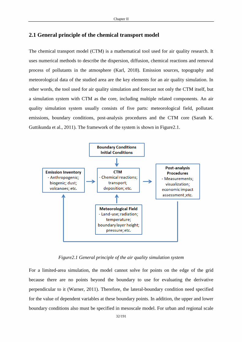
Chapter II
32/191
2.1 General principle of the chemical transport model
The chemical transport model (CTM) is a mathematical tool used for air quality research. It
uses numerical methods to describe the dispersion, diffusion, chemical reactions and removal
process of pollutants in the atmosphere (Karl, 2018). Emission sources, topography and
meteorological data of the studied area are the key elements for an air quality simulation. In
other words, the tool used for air quality simulation and forecast not only the CTM itself, but
a simulation system with CTM as the core, including multiple related components. An air
quality simulation system usually consists of five parts: meteorological field, pollutant
emissions, boundary conditions, post-analysis procedures and the CTM core (Sarath K.
Guttikunda et al., 2011). The framework of the system is shown in Figure2.1.
Figure2.1 General principle of the air quality simulation system
For a limited-area simulation, the model cannot solve for points on the edge of the grid
because there are no points beyond the boundary to use for evaluating the derivative
perpendicular to it (Warner, 2011). Therefore, the lateral-boundary condition need specified
for the value of dependent variables at these boundary points. In addition, the upper and lower
boundary conditions also must be specified in mesoscale model. For urban and regional scale

Chapter II
33/191
numerical simulations, the usual method for determining boundary conditions is to use the
results of larger-scale regional models or global-scale models as boundary conditions. The
meteorological field provides the meteorological data with a certain temporal and spatial
resolution, such as wind field, temperature, mixed layer height, radiation, vertical diffusion
coefficient, cloud characteristics, etc. (Rao et al., 2003). Usually, in air quality models, the
atmospheric motion control equation is independent of the pollutant chemical dynamics
equation. Thus, the formation of pollutants in the atmosphere will not significantly change the
meteorological conditions and the simulation of meteorological field is independent of air
quality simulation, this case is called as offline approach (Baklanov et al., 2016a; Seo et al.,
2018). However, changes of pollutants concentrations have a non-negligible impact on
meteorological conditions in some cases, in this case online approach is required. Study on
the coupling of mesoscale meteorological models and CTM have shown that changes in
pollutant concentration have slight impact on meteorological conditions (Bessagnet et al.,
2020; Jacobson, 1997). Therefore, most air quality simulation systems use offline approach.
Also, an identified drawback regarding the boundary conditions is a possible inconsistency of
the model species and chemical regimes between the large-scale model and the nested
regional model if they are different.
Accurate emission inventories play a crucial role in the simulation results. The list of species
should satisfy the chemical reaction mechanism and temporal and spatial resolution of the
model. For Eulerian models, gridded hourly emission data is usually required. The main
pollutants include CO; NOx; SO2; NH3; PM; VOCs; etc (Crippa et al., 2018). For practical
applications to support decisions and policy making, the purpose of air quality modeling is to
grasp the characteristics and laws of pollution, explore its causes, and finally provide
scientific control countermeasures (Zhang and Na, 2018). The post-analysis program uses the
observational data of the ground observation stations to analyze the simulation results which
provide information toassess the impact on the environment and the economy and formulate
corresponding control plans. In general, the principle of CTM should following those steps: (i)
understand and determine the physical processes are needed for the simulation; (ii) choose a
sufficiently small horizontal grid increment to resolve all the processes to be simulated on the

Chapter II
34/191
grid, numerically a finer resolution is supposed to be better; (iii) select the most suitable
projection map for the range of the model grid, (iv) ensure the vertical resolution is
reasonably compatible with the horizontal resolution, and can accurately define important
vertical structures (Warner, 2011).
2.2 Urban meteorology
In the past centuries, humans are increasingly gathering in large settlements, as well as the
urban population exceeded the rural (Morais et al., 2018). The population is concentrated in
less than 3% of the Earth’s land area (Baklanov et al., 2018). It is expected that two-thirds of
the world’s population will live in cities by 2050 (WUP 2014), therefore general knowledge
of climatic characteristics of typical cities and differences with rural areas are becoming more
and more crucial (Karlický et al., 2020).
Urbanization has a major impact on urban meteorology. It can change the atmospheric
diffusion capacity thereby affecting the concentration of pollutants (Liu et al., 2015), weather
and climate at local, regional and global scales (Baklanov et al., 2007). First, the urban
surface are mostly characterized by buildings, roads and permeable natural surfaces, where
various physical processes such as radiation trapping, atmospheric flow, turbulent heat
exchange, and underground heat conduction occur, resulting in a unique local meteorology
(Kim et al., 2020; Uehara et al., 2000). Second, changes in chemical emissions and feedbacks
of atmospheric pollutants affect the weather and climate both locally and further afield
(Reinmuth-Selzle et al., 2017). The main examples includes: (i) the distribution of rough
elements which can affect the turbulence state, speed and flow direction; (ii) the extensive use
of impervious materials which generally reduces vegetation coverage in urban areas thereby
affecting the hydrological and meteorological conditions and the deposition of pollutants; (iii)
the urban canopy affecting the flow and heat exchange between different land covers; (iv) the
release and diffusion of pollutants can affects radiation transmission and the formation of
clouds and precipitation (Baklanov et al., 2018). The most well-known urban meteorology is
the so-called urban heat island (UHI), which was first described by Oke and Maxwell (Oke
and Maxwell, 1975) in the year 1975 and has been extensively studied in the following

Chapter II
35/191
decades (Baklanov et al., 2016c; Karlický et al., 2020; KIM, 1992; Oke, 1982; Zhang et al.,
2017). In short, it can be described as urban temperature is higher than in the countryside.
UHI not only affects the microscale and mesoscale circulation to a large extent, but also cause
the formation of convection (Dixon et al., 2003;). Several studies have demonstrated that the
increase in the number of convection phenomena in cities were related to the increase in the
convergence of the lower-level over urban areas (Fujibe, 2003). Theeuwes et al. (2019) found
the cloud cover enhancement over urban region of Paris and London during summer because
of increased convection caused by UHI. With the rapid improvement of computer capabilities
and the widespread application of remote sensing technology in meteorology, geographic
information on urban surfaces can be obtained with higher precision, which makes it possible
to develop and apply high-resolution urban boundary layer models. Some studies indicate that
meteorological variables are significantly affected by the urban canopy. For example, the
impact of urban boundary layer structure causes changes in dispersion conditions (Karlický et
al., 2018), which have considerable consequences for primary or secondary pollutant
concentrations (Huszar et al., 2020; Li et al., 2019). Manola et al. (2020) found the overall
precipitation increased in the urban areas of Amsterdam in comparison to rural surroundings.
In general, the relationship between meteorology and city is mutual: meteorology affects how
urban space is used such as the different concerns between coastal cities and landlocked cities
(Pelling and Blackburn, 2013) or tropical cities and boreal cities. In turn, the city has changed
the regional meteorology conditions, resulting in differences in cloud cover, solar radiation,
temperature and wind speed between the city and its surrounding areas thereby resulting the
transport, diffusion, and chemical transformation of particulates and gases. Figure2.2
summarized the main linkages between cities, air quality and climate. Specifically: (i)
non-linear interaction and its feedback between emissions, land use, reaction and meteorology;
(ii) complex spatial scales from local to global and time scales from minutes to centuries; (iii)
mixing of pollutants from multiple pollution sources; (iv) interaction between city
characteristics and emissions (Baklanov et al., 2010).
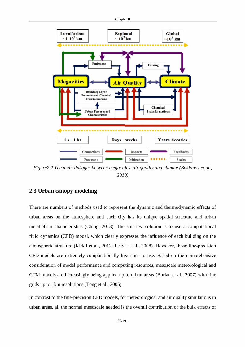
Chapter II
36/191
Figure2.2 The main linkages between megacities, air quality and climate (Baklanov et al.,
2010)
2.3 Urban canopy modeling
There are numbers of methods used to represent the dynamic and thermodynamic effects of
urban areas on the atmosphere and each city has its unique spatial structure and urban
metabolism characteristics (Ching, 2013). The smartest solution is to use a computational
fluid dynamics (CFD) model, which clearly expresses the influence of each building on the
atmospheric structure (Kirkil et al., 2012; Letzel et al., 2008). However, those fine-precision
CFD models are extremely computationally luxurious to use. Based on the comprehensive
consideration of model performance and computing resources, mesoscale meteorological and
CTM models are increasingly being applied up to urban areas (Burian et al., 2007) with fine
grids up to 1km resolutions (Tong et al., 2005).
In contrast to the fine-precision CFD models, for meteorological and air quality simulations in
urban areas, all the normal mesoscale needed is the overall contribution of the bulk effects of

Chapter II
37/191
built-up areas on the mesoscale processes. The mesoscale model defines surface properties
through adjusting parameter attributes associated with land use and other surface covers
datasets to represent the altered morphological, reflective, and anthropogenic heating aspects
so that they approximate the artificial surface conditions in cities (Beltran-Przekurat et al.,
2012). For example, the roughness length can be used to indicate the resistance of the
building. The albedo can be reduced to account for the existence of dark roofs and shortwave
radiation capture in street canyons. The heat capacity and thermal conductivity of the
substrate can be increased to solve the problem of heat storage in the walls of buildings;
reduce the water capacity of the substrate to reflect the universality of impervious surfaces
(Liu et al., 2006). The six key physical parameters of land-use categories are albedo,
emissivity, surface thermal inertia, roughness length, soil moisture availability and soil heat
capacity, respectively (H. Li et al., 2020). However, given the complexity of the urban system,
those similarity frameworks may encounter problems when applied in the urban context (Roth,
2007), some other schemes are needed to represent more complex processes related to the
presence of buildings and non-natural substrates. Oke (1988) provided a concept of the
atmospheric regimes overlying urban areas for the first time. Since the flow convection and
atmospheric processes respond to the heterogeneity of the urban surface, the boundary layer
structure over urban areas are necessarily multi-scale (Klein et al., 2007). The varying
buildings heights, distribution densities and varying street widths create a mean condition in
the urban canopy. The layers above urban canopy is continuously adjusted by the vertical flux
caused by the horizontal changes and gradients of the underlying land use and canopy
structure. This situation produces countless internal boundary layers, and the turbulence
generated in each boundary layer is balanced by dissipation. Urban canopy parameterizations
with varying complexities were developed and coupled with the model to improve its skills in
capturing fine-scale urban processes and in assessing the environmental issues (Kondo et al.,
2005; Kusaka et al., 2001; Kusaka and Kimura, 2004; Liao et al., 2014). The single layer
urban canopy scheme (UCM) parameterizes the aggregate effects of the urban morphology,
but does not explicitly represent the effects of individual buildings and street canyons
(Kusaka et al., 2001). The UCM considered radiation capture and wind shear in urban canopy
affected by the geometry of buildings and roads (Huang et al., 2019). However, the UCM is a
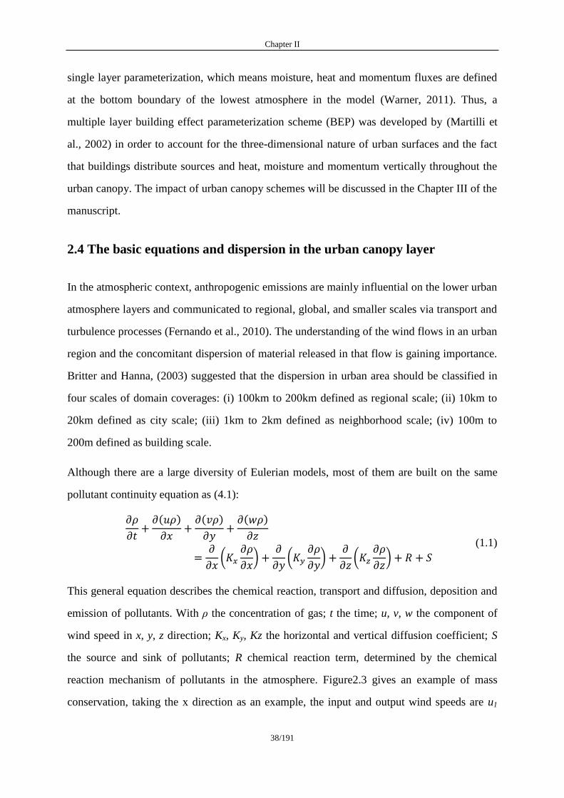
Chapter II
38/191
single layer parameterization, which means moisture, heat and momentum fluxes are defined
at the bottom boundary of the lowest atmosphere in the model (Warner, 2011). Thus, a
multiple layer building effect parameterization scheme (BEP) was developed by (Martilli et
al., 2002) in order to account for the three-dimensional nature of urban surfaces and the fact
that buildings distribute sources and heat, moisture and momentum vertically throughout the
urban canopy. The impact of urban canopy schemes will be discussed in the Chapter III of the
manuscript.
2.4 The basic equations and dispersion in the urban canopy layer
In the atmospheric context, anthropogenic emissions are mainly influential on the lower urban
atmosphere layers and communicated to regional, global, and smaller scales via transport and
turbulence processes (Fernando et al., 2010). The understanding of the wind flows in an urban
region and the concomitant dispersion of material released in that flow is gaining importance.
Britter and Hanna, (2003) suggested that the dispersion in urban area should be classified in
four scales of domain coverages: (i) 100km to 200km defined as regional scale; (ii) 10km to
20km defined as city scale; (iii) 1km to 2km defined as neighborhood scale; (iv) 100m to
200m defined as building scale.
Although there are a large diversity of Eulerian models, most of them are built on the same
pollutant continuity equation as (4.1):
( )
( )
( )
(
)
(
)
(
)
(1.1)
This general equation describes the chemical reaction, transport and diffusion, deposition and
emission of pollutants. With ρ the concentration of gas; t the time; u, v, w the component of
wind speed in x, y, z direction; Kx, Ky, Kz the horizontal and vertical diffusion coefficient; S
the source and sink of pollutants; R chemical reaction term, determined by the chemical
reaction mechanism of pollutants in the atmosphere. Figure2.3 gives an example of mass
conservation, taking the x direction as an example, the input and output wind speeds are u1
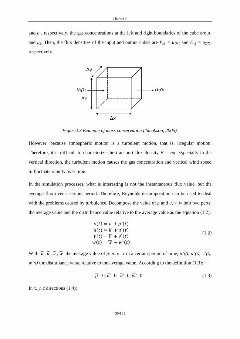
Chapter II
39/191
and u2, respectively, the gas concentrations at the left and right boundaries of the cube are ρ1
and ρ2. Then, the flux densities of the input and output cubes are Fx1 = u1ρ1 and Fx2 = u2ρ2,
respectively.
Figure2.3 Example of mass conservation (Jacobson, 2005).
However, because atmospheric motion is a turbulent motion, that is, irregular motion.
Therefore, it is difficult to characterize the transport flux density F = uρ. Especially in the
vertical direction, the turbulent motion causes the gas concentration and vertical wind speed
to fluctuate rapidly over time.
In the simulation processes, what is interesting is not the instantaneous flux value, but the
average flux over a certain period. Therefore, Reynolds decomposition can be used to deal
with the problems caused by turbulence. Decompose the value of ρ and u, v, w into two parts:
the average value and the disturbance value relative to the average value as the equation (1.2):
( ) ’( )
( ) ’( )
( ) ’( )
( ) ’( )
(1.2)
With , , , the average value of ρ, u, v, w in a certain period of time; ρ’(t), u’(t), v’(t),
w’(t) the disturbance value relative to the average value. According to the definition (1.3):
’ 0, ’ 0 , ’ 0, ’ 0 (1.3)
In x, y, z directions (1.4):
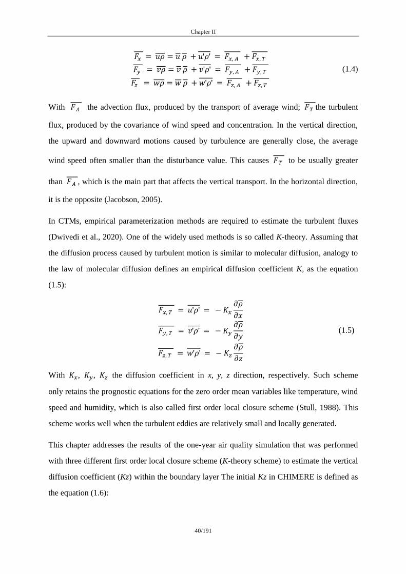
Chapter II
40/191
' '
' '
' '
(1.4)
With the advection flux, produced by the transport of average wind; the turbulent
flux, produced by the covariance of wind speed and concentration. In the vertical direction,
the upward and downward motions caused by turbulence are generally close, the average
wind speed often smaller than the disturbance value. This causes to be usually greater
than , which is the main part that affects the vertical transport. In the horizontal direction,
it is the opposite (Jacobson, 2005).
In CTMs, empirical parameterization methods are required to estimate the turbulent fluxes
(Dwivedi et al., 2020). One of the widely used methods is so called K-theory. Assuming that
the diffusion process caused by turbulent motion is similar to molecular diffusion, analogy to
the law of molecular diffusion defines an empirical diffusion coefficient K, as the equation
(1.5):
' '
' '
' '
(1.5)
With , , the diffusion coefficient in x, y, z direction, respectively. Such scheme
only retains the prognostic equations for the zero order mean variables like temperature, wind
speed and humidity, which is also called first order local closure scheme (Stull, 1988). This
scheme works well when the turbulent eddies are relatively small and locally generated.
This chapter addresses the results of the one-year air quality simulation that was performed
with three different first order local closure scheme (K-theory scheme) to estimate the vertical
diffusion coefficient (Kz) within the boundary layer The initial Kz in CHIMERE is defined as
the equation (1.6):
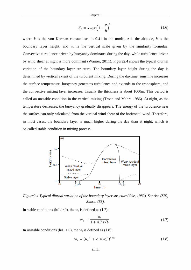
Chapter II
41/191
(
)
(1.6)
where k is the von Karman constant set to 0.41 in the model, z is the altitude, h is the
boundary layer height, and ws is the vertical scale given by the similarity formulae.
Convective turbulence driven by buoyancy dominates during the day, while turbulence driven
by wind shear at night is more dominant (Warner, 2011). Figure2.4 shows the typical diurnal
variation of the boundary layer structure. The boundary layer height during the day is
determined by vertical extent of the turbulent mixing. During the daytime, sunshine increases
the surface temperature, buoyancy generates turbulence and extends to the troposphere, and
the convective mixing layer increases. Usually the thickness is about 1000m. This period is
called an unstable condition in the vertical mixing (Troen and Mahrt, 1986). At night, as the
temperature decreases, the buoyancy gradually disappears. The energy of the turbulence near
the surface can only calculated from the vertical wind shear of the horizontal wind. Therefore,
in most cases, the boundary layer is much higher during the day than at night, which is
so-called stable condition in mixing process.
Figure2.4 Typical diurnal variation of the boundary layer structure(Oke, 1982). Sunrise (SR),
Sunset (SS).
In stable conditions (h/L ≥ 0), the ws is defined as (1.7):
⁄ (1.7)
In unstable conditions (h/L < 0), the ws is defined as (1.8):
(
) (1.8)
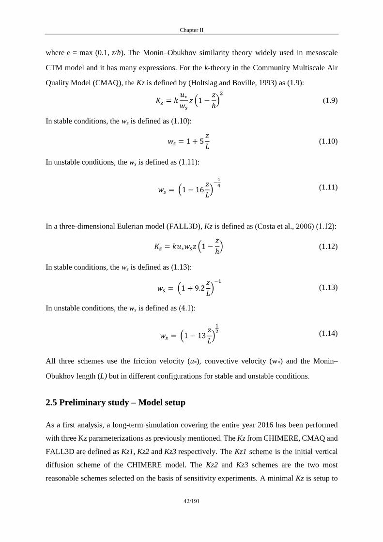
Chapter II
42/191
where e = max (0.1, z/h). The Monin–Obukhov similarity theory widely used in mesoscale
CTM model and it has many expressions. For the k-theory in the Community Multiscale Air
Quality Model (CMAQ), the Kz is defined by (Holtslag and Boville, 1993) as (1.9):
(
)
(1.9)
In stable conditions, the ws is defined as (1.10):
(1.10)
In unstable conditions, the ws is defined as (1.11):
(
)
(1.11)
In a three-dimensional Eulerian model (FALL3D), Kz is defined as (Costa et al., 2006) (1.12):
(
)
(1.12)
In stable conditions, the ws is defined as (1.13):
(
)
(1.13)
In unstable conditions, the ws is defined as (4.1):
(
)
(1.14)
All three schemes use the friction velocity (u*), convective velocity (w*) and the Monin–
Obukhov length (L) but in different configurations for stable and unstable conditions.
2.5 Preliminary study – Model setup
As a first analysis, a long-term simulation covering the entire year 2016 has been performed
with three Kz parameterizations as previously mentioned. The Kz from CHIMERE, CMAQ and
FALL3D are defined as Kz1, Kz2 and Kz3 respectively. The Kz1 scheme is the initial vertical
diffusion scheme of the CHIMERE model. The Kz2 and Kz3 schemes are the two most
reasonable schemes selected on the basis of sensitivity experiments. A minimal Kz is setup to
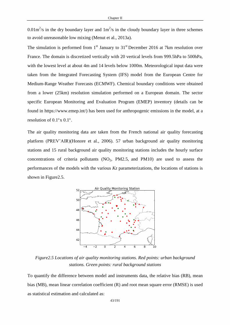
Chapter II
43/191
0.01m2/s in the dry boundary layer and 1m
2/s in the cloudy boundary layer in three schemes
to avoid unreasonable low mixing (Menut et al., 2013a).
The simulation is performed from 1st January to 31
st December 2016 at 7km resolution over
France. The domain is discretized vertically with 20 vertical levels from 999.5hPa to 500hPa,
with the lowest level at about 4m and 14 levels below 1000m. Meteorological input data were
taken from the Integrated Forecasting System (IFS) model from the European Centre for
Medium-Range Weather Forecasts (ECMWF). Chemical boundary conditions were obtained
from a lower (25km) resolution simulation performed on a European domain. The sector
specific European Monitoring and Evaluation Program (EMEP) inventory (details can be
found in https://www.emep.int/) has been used for anthropogenic emissions in the model, at a
resolution of 0.1x 0.1.
The air quality monitoring data are taken from the French national air quality forecasting
platform (PREV’AIR)(Honore et al., 2006). 57 urban background air quality monitoring
stations and 15 rural background air quality monitoring stations includes the hourly surface
concentrations of criteria pollutants (NO2, PM2.5, and PM10) are used to assess the
performances of the models with the various Kz parameterizations, the locations of stations is
shown in Figure2.5.
Figure2.5 Locations of air quality monitoring stations. Red points: urban background
stations. Green points: rural background stations
To quantify the difference between model and instruments data, the relative bias (RB), mean
bias (MB), mean linear correlation coefficient (R) and root mean square error (RMSE) is used
as statistical estimation and calculated as:
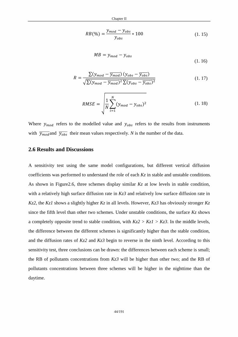
Chapter II
44/191
( )
(1. 15)
(1. 16)
∑( ) ( )
√∑( ) ∑( ) (1. 17)
√
∑( )
(1. 18)
Where refers to the modelled value and refers to the results from instruments
with and their mean values respectively. N is the number of the data.
2.6 Results and Discussions
A sensitivity test using the same model configurations, but different vertical diffusion
coefficients was performed to understand the role of each Kz in stable and unstable conditions.
As shown in Figure2.6, three schemes display similar Kz at low levels in stable condition,
with a relatively high surface diffusion rate in Kz3 and relatively low surface diffusion rate in
Kz2, the Kz1 shows a slightly higher Kz in all levels. However, Kz3 has obviously stronger Kz
since the fifth level than other two schemes. Under unstable conditions, the surface Kz shows
a completely opposite trend to stable condition, with Kz2 > Kz1 > Kz3. In the middle levels,
the difference between the different schemes is significantly higher than the stable condition,
and the diffusion rates of Kz2 and Kz3 begin to reverse in the ninth level. According to this
sensitivity test, three conclusions can be drawn: the differences between each scheme is small;
the RB of pollutants concentrations from Kz3 will be higher than other two; and the RB of
pollutants concentrations between three schemes will be higher in the nighttime than the
daytime.
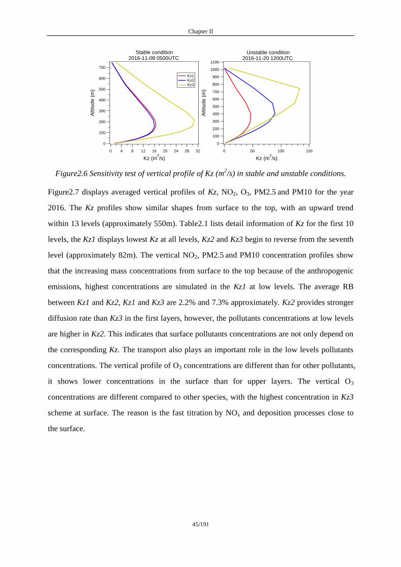
Chapter II
45/191
Figure2.6 Sensitivity test of vertical profile of Kz (m2/s) in stable and unstable conditions.
Figure2.7 displays averaged vertical profiles of Kz, NO2, O3, PM2.5 and PM10 for the year
2016. The Kz profiles show similar shapes from surface to the top, with an upward trend
within 13 levels (approximately 550m). Table2.1 lists detail information of Kz for the first 10
levels, the Kz1 displays lowest Kz at all levels, Kz2 and Kz3 begin to reverse from the seventh
level (approximately 82m). The vertical NO2, PM2.5 and PM10 concentration profiles show
that the increasing mass concentrations from surface to the top because of the anthropogenic
emissions, highest concentrations are simulated in the Kz1 at low levels. The average RB
between Kz1 and Kz2, Kz1 and Kz3 are 2.2% and 7.3% approximately. Kz2 provides stronger
diffusion rate than Kz3 in the first layers, however, the pollutants concentrations at low levels
are higher in Kz2. This indicates that surface pollutants concentrations are not only depend on
the corresponding Kz. The transport also plays an important role in the low levels pollutants
concentrations. The vertical profile of O3 concentrations are different than for other pollutants,
it shows lower concentrations in the surface than for upper layers. The vertical O3
concentrations are different compared to other species, with the highest concentration in Kz3
scheme at surface. The reason is the fast titration by NOx and deposition processes close to
the surface.
700
600
500
400
300
200
100
0
Altitu
de
(m
)
322824201612840
Kz (m2/s)
Kz1 Kz2 Kz3
Stable condition2016-11-08 0500UTC
1100
1000
900
800
700
600
500
400
300
200
100
0
Altitu
de
(m
)
150100500
Kz (m2/s)
Unstable condition2016-11-20 1200UTC

Chapter II
46/191
Figure2.7 Vertical profiles of Kz (m2/s); NO2 (µg/m
3); O3 (µg/m
3) PM2.5 (µg/m
3) and PM10
(µg/m3) over the France domain. The profiles are averaged from January 1
st to December 31
st,
2016.
Table2.1 The Kz (m2/s) values for the 10 levels.
Level 1 2 3 4 5 6 7 8 9 10
Kz1 0.76 1.35 2.09 2.94 3.86 4.78 5.61 6.29 6.93 7.97
Kz2 0.79 1.48 2.41 3.59 5.04 6.71 8.52 10.23 11.66 12.87
Kz3 0.77 1.41 2.27 3.37 4.75 6.45 8.53 10.95 13.63 16.55
Figure2.8 displays the seasonal mean first layer Kz over France domain. Results show that the
regional patterns are similar for three schemes. The Kz1 shows a slightly higher surface Kz
than Kz3 at the Alps and the Pyrenees. However, Kz3 gives a relative higher surface Kz than
Kz1 over mainland France in autumn and winter. In general, Kz2 scheme has slightly higher
vertical diffusion rate than other two schemes, the three schemes give the trend of spring >
summer > autumn > winter of surface Kz in the France domain, and coastal areas are
generally display higher Kz than inland areas, due to the sea breezes which enhance the
dispersion of pollutants (Reid and Steyn, 1997). The seasonal profiles of surface NO2, PM2.5
and PM10 concentrations between observation and simulation are illustrated in Figure 2.9.
Model underestimated NO2 concentrations whatever the season, but particularly during
wintertime. The negative biases are -6.05µg/m3, -6.16µg/m
3 and -7.09µg/m
3 for Kz1, Kz2 and
20
18
16
14
12
10
8
6
4
2
Le
ve
l
1086420
NO2 (µg/m3)
20
18
16
14
12
10
8
6
4
2
Le
ve
l
1086420
PM2.5 (µg/m3)
20
18
16
14
12
10
8
6
4
2
Le
ve
l
1007550
O3 (µg/m3)
20
18
16
14
12
10
8
6
4
2
Le
ve
l
1086420
PM10 (µg/m3)
20
18
16
14
12
10
8
6
4
2
Le
ve
l
201612840
Kz (m2/s)
Kz1 Kz2 Kz3
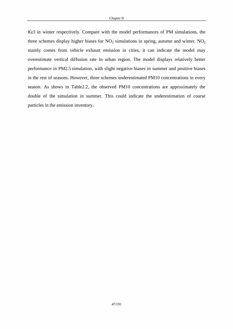
Chapter II
47/191
Kz3 in winter respectively. Compare with the model performances of PM simulations, the
three schemes display higher biases for NO2 simulations in spring, autumn and winter. NO2
mainly comes from vehicle exhaust emission in cities, it can indicate the model may
overestimate vertical diffusion rate in urban region. The model displays relatively better
performance in PM2.5 simulation, with slight negative biases in summer and positive biases
in the rest of seasons. However, three schemes underestimated PM10 concentrations in every
season. As shows in Table2.2, the observed PM10 concentrations are approximately the
double of the simulation in summer. This could indicate the underestimation of coarse
particles in the emission inventory.
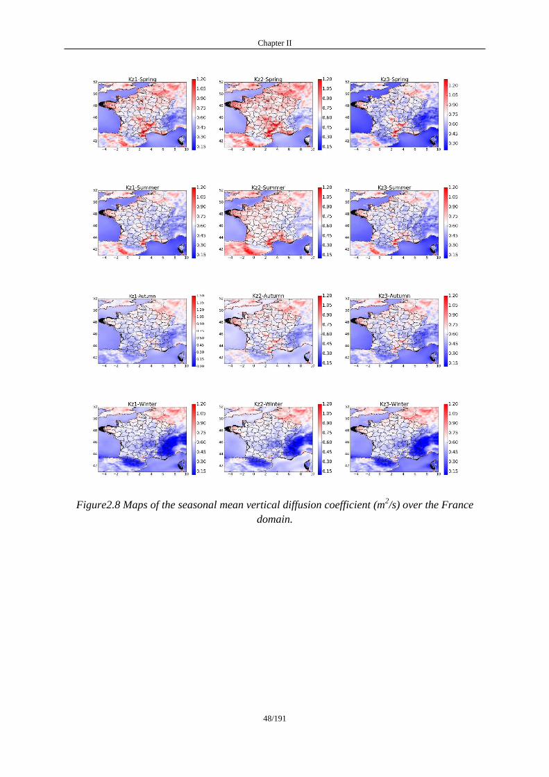
Chapter II
48/191
Figure2.8 Maps of the seasonal mean vertical diffusion coefficient (m2/s) over the France
domain.
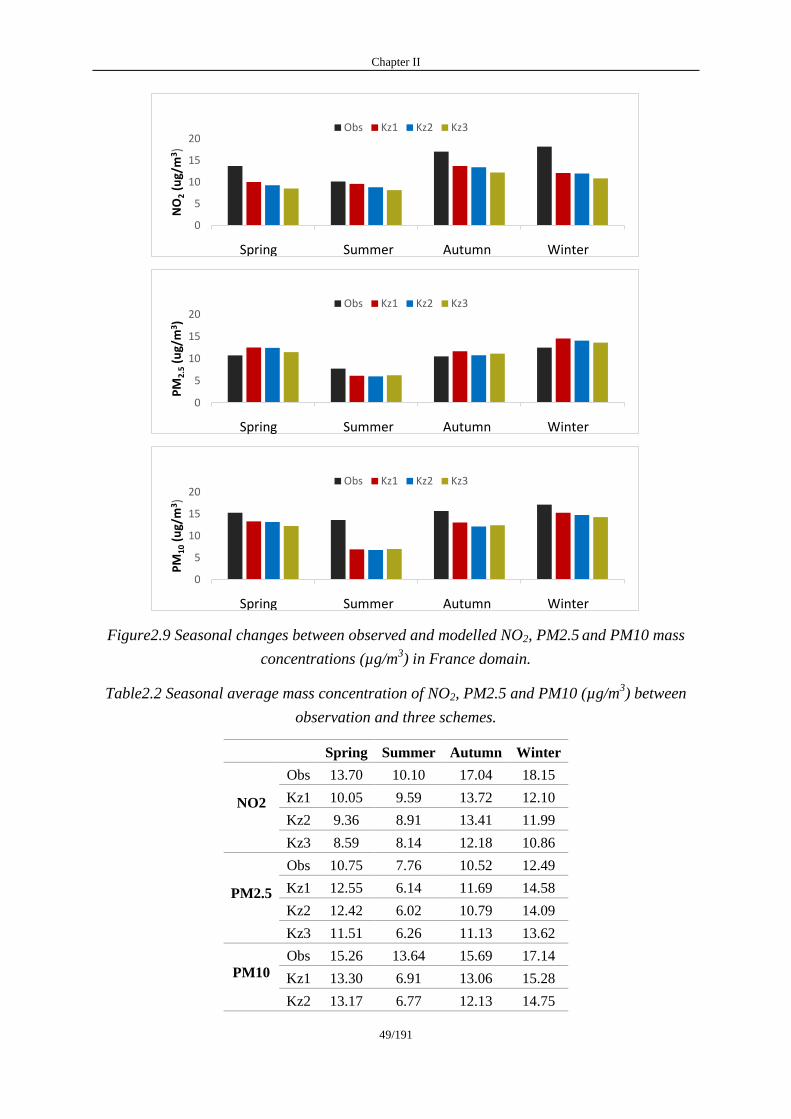
Chapter II
49/191
Figure2.9 Seasonal changes between observed and modelled NO2, PM2.5 and PM10 mass
concentrations (µg/m3) in France domain.
Table2.2 Seasonal average mass concentration of NO2, PM2.5 and PM10 (µg/m3) between
observation and three schemes.
Spring Summer Autumn Winter
NO2
Obs 13.70 10.10 17.04 18.15
Kz1 10.05 9.59 13.72 12.10
Kz2 9.36 8.91 13.41 11.99
Kz3 8.59 8.14 12.18 10.86
PM2.5
Obs 10.75 7.76 10.52 12.49
Kz1 12.55 6.14 11.69 14.58
Kz2 12.42 6.02 10.79 14.09
Kz3 11.51 6.26 11.13 13.62
PM10
Obs 15.26 13.64 15.69 17.14
Kz1 13.30 6.91 13.06 15.28
Kz2 13.17 6.77 12.13 14.75
0
5
10
15
20
NO
2 (u
g/m
3 )
Obs Kz1 Kz2 Kz3
Spring Summer Autumn Winter
0
5
10
15
20
PM
2.5 (
ug/
m3 )
Obs Kz1 Kz2 Kz3
Spring Summer Autumn Winter
0
5
10
15
20
PM
10
(ug/
m3)
Obs Kz1 Kz2 Kz3
Spring Summer Autumn Winter

Chapter II
50/191
Kz3 12.25 6.99 12.41 14.29
In order to better evaluate the impact of vertical diffusion coefficients on the air quality
predictions, modelled time series of the pollutants concentrations compared with the
observations for urban and rural region are displayed in Figure2.10. In urban areas, the
models capture the time variability quite well for NO2, PM2.5 and PM10 simulations,
particularly for the PM2.5, model almost perfectly reproduced the seasonal variability.
However, the model tends to underestimate the NO2 and PM10 concentrations of PM10in
urban areas especially during wintertime for NO2 and summertime for PM10. Comparing the
model performance of PM2.5 and PM10 simulations, the model displays a slight negative bias
of PM10 concentration than PM2.5 for the whole period. The yearly average surface mass
concentrations of PM2.5 and PM10 are 10.37µg/m3 and 15.41µg/m
3 from the observation
over the France domain. PM2.5 comprised 67.30% of total PM10. In the cases of simulations,
PM2.5 surface concentrations are 10.79µg/m3, 11.21µg/m
3, 10.60µg/m
3 and PM10 surface
concentrations are 11.66µg/m3, 12.10µg/m
3, 11.45µg/m
3 from Kz1, Kz2 and Kz3, respectively.
The ratios of PM2.5/PM10 are almost the same which is approximately 92.5% for three
schemes, the bias is approximately 25.3%. This result indicates the models could have a large
overestimation of fine mode emissions or that coarse emissions are lacking. All three schemes
in rural areas display a quite good reproduction of the evolution of pollutant concentrations
and better capture the fluctuations of pollutants in the wintertime than urban areas. The model
underestimate PM10 concentration particularly in summertime. Table2.3 provides an overall
evaluation of three schemes in urban and rural areas including R, MB and RMSE. In general,
the models present a better performance in rural than the model performances in urban areas.
Concentrations of NO2 and PM10 are stronger underestimated in urban areas than for rural
areas. This indicates the three schemes tend to overestimate the local vertical diffusivity in
urban region compared to the rural areas. The value of exponent p is considered as 2 (the
―square‖ in the equation) in equation (1.6) and (1.9). The range of this value has been
considered from 1 to 3 by Troen and Mahrt (Troen and Mahrt, 1986), the vertical mixing
varies considerably correspond to the range of p from 1 to 3 (Hu et al., 2010). Therefore, the
results show that setting p value to 2 is applicable in rural areas, but the p value is
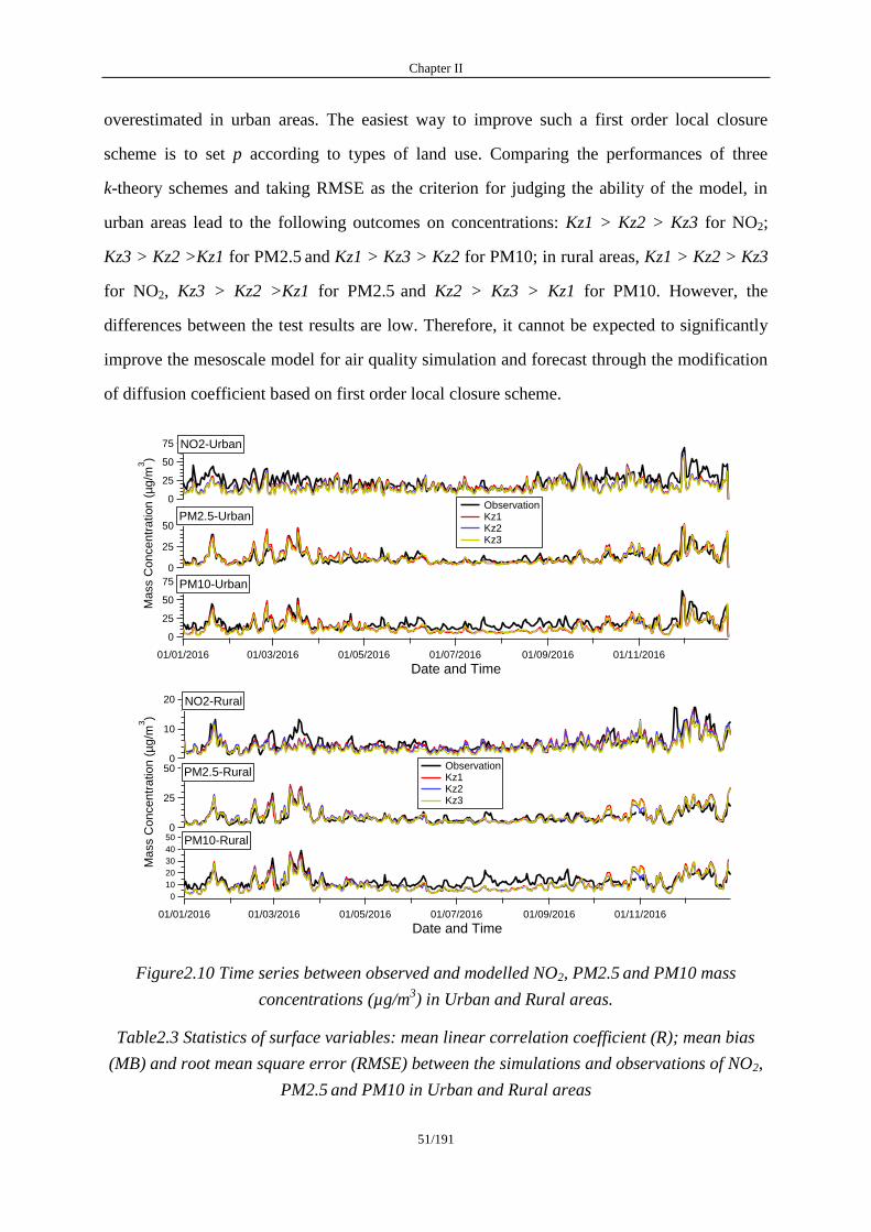
Chapter II
51/191
overestimated in urban areas. The easiest way to improve such a first order local closure
scheme is to set p according to types of land use. Comparing the performances of three
k-theory schemes and taking RMSE as the criterion for judging the ability of the model, in
urban areas lead to the following outcomes on concentrations: Kz1 > Kz2 > Kz3 for NO2;
Kz3 > Kz2 >Kz1 for PM2.5 and Kz1 > Kz3 > Kz2 for PM10; in rural areas, Kz1 > Kz2 > Kz3
for NO2, Kz3 > Kz2 >Kz1 for PM2.5 and Kz2 > Kz3 > Kz1 for PM10. However, the
differences between the test results are low. Therefore, it cannot be expected to significantly
improve the mesoscale model for air quality simulation and forecast through the modification
of diffusion coefficient based on first order local closure scheme.
Figure2.10 Time series between observed and modelled NO2, PM2.5 and PM10 mass
concentrations (µg/m3) in Urban and Rural areas.
Table2.3 Statistics of surface variables: mean linear correlation coefficient (R); mean bias
(MB) and root mean square error (RMSE) between the simulations and observations of NO2,
PM2.5 and PM10 in Urban and Rural areas
75
50
25
0
01/01/2016 01/03/2016 01/05/2016 01/07/2016 01/09/2016 01/11/2016
Date and Time
50
25
0
M
ass C
on
ce
ntr
atio
n (
µg
/m3)
75
50
25
0
NO2-Urban
PM2.5-Urban
PM10-Urban
Observation Kz1 Kz2 Kz3
20
10
0
01/01/2016 01/03/2016 01/05/2016 01/07/2016 01/09/2016 01/11/2016
Date and Time
50
25
0
M
ass C
on
ce
ntr
atio
n (
µg
/m3)
50
40
30
20
10
0
NO2-Rural
PM2.5-Rural
PM10-Rural
Observation Kz1 Kz2 Kz3
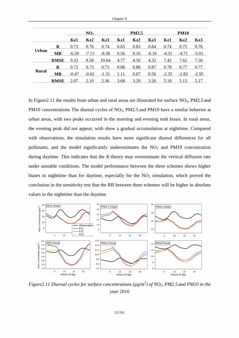
Chapter II
52/191
NO2 PM2.5 PM10
Kz1 Kz2 Kz3 Kz1 Kz2 Kz3 Kz1 Kz2 Kz3
Urban R 0.73 0.76 0.74 0.83 0.83 0.84 0.74 0.75 0.76
MB -6.39 -7.13 -8.38 0.56 0.16 -0.10 -4.31 -4.71 -5.01
RMSE 9.32 9.58 10.64 4.77 4.50 4.32 7.42 7.62 7.50
Rural R 0.72 0.73 0.73 0.88 0.88 0.87 0.78 0.77 0.77
MB -0.47 -0.62 -1.31 1.11 0.67 0.56 -2.35 -2.83 -2.95
RMSE 2.07 2.10 2.36 3.68 3.29 3.26 5.18 5.13 5.17
In Figure2.11 the results from urban and rural areas are illustrated for surface NO2, PM2.5 and
PM10 concentrations. The diurnal cycles of NO2, PM2.5 and PM10 have a similar behavior at
urban areas, with two peaks occurred in the morning and evening rush hours. In rural areas,
the evening peak did not appear, with show a gradual accumulation at nighttime. Compared
with observations, the simulation results have more significant diurnal differences for all
pollutants, and the model significantly underestimates the NO2 and PM10 concentration
during daytime. This indicates that the K-theory may overestimate the vertical diffusion rate
under unstable conditions. The model performance between the three schemes shows higher
biases in nighttime than for daytime, especially for the NO2 simulation, which proved the
conclusion in the sensitivity test that the RB between three schemes will be higher in absolute
values in the nighttime than the daytime.
Figure2.11 Diurnal cycles for surface concentrations (µg/m3) of NO2, PM2.5 and PM10 in the
year 2016
8.0
7.0
6.0
5.0
4.0
3.0
2.0
1.0Ma
ss C
on
ce
ntr
atio
n (
µg
/m3)
2015105
Hours of day
NO2 Rural
40
30
20
10
0
Ma
ss C
on
ce
ntr
atio
n (
µg
/m3)
2015105
Observation Kz1 Kz2 Kz3
NO2 Urban18
16
14
12
10
8
2015105
PM2.5 Urban
13.0
12.0
11.0
10.0
9.0
8.0
7.0
2015105
Hours of day
PM2.5 Rural
25
20
15
10
2015105
PM10 Urban
14
12
10
8
6
2015105
Hours of day
PM10 Rural
Chapter II
53/191
2.7 Conclusions
The micro meteorology over built-up areas differs from the non-urban landscape in many
aspects: wind-flows, radiation, humidity, precipitation and air quality. The dispersion of
pollutants in urban areas is an actual topic and the modelling approaches depend on the
involved atmospheric processes. Initially we focused on the dispersion of pollutants in the
urban canopy, three vertical diffusion coefficients based on first order local closure scheme
have been investigated in a one-year simulation over France. Comparing the model
performances of three scheme in urban and rural areas, it is found that the three schemes
perform better in rural than in urban areas. The vertical mixing is relatively overestimated in
urban areas. One idea is to decrease the p value (the ―square‖ in the Kz equation) on urban
land use. The results also indicate such simplest scheme is an effective way to reproduce the
dispersion of pollutants both in urban canopy and surroundings in mesoscale chemistry
transport model, but it cannot be expected to significantly improve the mesoscale model by
this simple modification based on the first-order local closure Reynolds decomposition
scheme. Further improvements should start with a more accurate turbulence process. Another
problem to be solved is the ratio of PM2.5 / PM10 that exceeds 90% in all seasons in the
models, while the ratio is usually around 70% in the observations, the emission inventory
requires notable improvements with probably a lack of coarse particles anthropogenic or
biogenic in origins.
This first screening of usual K-theory diffusion parameterizations over a long-term simulation
was a first step to identify limitations and possible improvements. The next chapter focuses at
urban scale on pollution event in November-December 2016.
Chapter II
54/191
References
Augustus, N. and Augustus, N.: Development and assessment of the second-generation
National Building Statistics Database, Seventh Conference on Coastal Atmospheric
and Oceanic Prediction and Processes joint with the Seventh Symposium on the Urban
Environment (10-13 September 2007), 2007.
Baklanov, A., Lawrence, M., Pandis, S., Mahura, A., Finardi, S., Moussiopoulos, N.,
Beekmann, M., Laj, P., Gomes, L., Jaffrezo, J.-L., Borbon, A., Coll, I., Gros, V.,
Sciare, J., Kukkonen, J., Galmarini, S., Giorgi, F., Grimmond, S., Esau, I., Stohl, A.,
Denby, B., Wagner, T., Butler, T., Baltensperger, U., Builtjes, P., van den Hout, D.,
van der Gon, H. D., Collins, B., Schluenzen, H., Kulmala, M., Zilitinkevich, S., Sokhi,
R., Friedrich, R., Theloke, J., Kummer, U., Jalkinen, L., Halenka, T., Wiedensholer,
A., Pyle, J., and Rossow, W. B.: MEGAPOLI: concept of multi-scale modelling of
megacity impact on air quality and climate, in: Advances in Science and Research, 9th
EMS Annual Meeting and 9th European Conference on Applications of Meteorology
2009 -, 115–120, https://doi.org/10.5194/asr-4-115-2010, 2010.
Baklanov, A., Baldasano, J., Bouchet, V., Brunner, D., Ekman, A., Galmarini, S., Carmichael,
G., Grell, G., Flemming, J., Forkel, R., Freitas, S., Gauss, M., Hegglin, M., Hov, Ø.,
Joffre, S., Makar, P., Mathur, R., Miranda, A., Moussiopoulos, N., and Zhang, Y.:
Coupled Chemistry-Meteorology/ Climate Modelling (CCMM): status and relevance
for numerical weather prediction, atmospheric pollution and climate research,
https://doi.org/10.13140/RG.2.1.4937.8169, 2016a.
Baklanov, A., Molina, L. T., and Gauss, M.: Megacities, air quality and climate, Atmospheric
Environment, 126, 235–249, https://doi.org/10.1016/j.atmosenv.2015.11.059, 2016b.
Baklanov, A., Grimmond, C. S. B., Carlson, D., Terblanche, D., Tang, X., Bouchet, V., Lee,
B., Langendijk, G., Kolli, R. K., and Hovsepyan, A.: From urban meteorology, climate
and environment research to integrated city services, Urban Climate, 23, 330–341,
https://doi.org/10.1016/j.uclim.2017.05.004, 2018.
Bessagnet, B., Menut, L., Lapere, R., Couvidat, F., Jaffrezo, J.-L., Mailler, S., Favez, O.,
Pennel, R., and Siour, G.: High Resolution Chemistry Transport Modeling with the
On-Line CHIMERE-WRF Model over the French Alps—Analysis of a Feedback of
Surface Particulate Matter Concentrations on Mountain Meteorology, Atmosphere, 11,
565, https://doi.org/10.3390/atmos11060565, 2020.
Britter, R. E. and Hanna, S. R.: Flow and dispersion in urban areas, Annu. Rev. Fluid Mech.,
35, 469–496, https://doi.org/10.1146/annurev.fluid.35.101101.161147, 2003.
Ching, J. K. S.: A perspective on urban canopy layer modeling for weather, climate and air
quality applications, Urban Climate, 3, 13–39,
https://doi.org/10.1016/j.uclim.2013.02.001, 2013.
Chapter II
55/191
Costa, A., Macedonio, G., and Folch, A.: A three-dimensional Eulerian model for transport
and deposition of volcanic ashes, Earth and Planetary Science Letters, 241, 634–647,
https://doi.org/10.1016/j.epsl.2005.11.019, 2006.
Crippa, M., Guizzardi, D., Muntean, M., Schaaf, E., Dentener, F., van Aardenne, J. A., Monni,
S., Doering, U., Olivier, J. G. J., Pagliari, V., and Janssens-Maenhout, G.: Gridded
emissions of air pollutants for the period 1970–2012 within EDGAR v4.3.2, Earth
Syst. Sci. Data, 10, 1987–2013, https://doi.org/10.5194/essd-10-1987-2018, 2018.
Dwivedi, Y. D., Nukala, V. B., Maddula, S. P., and Nair, K.: Prediction of Atmospheric
Turbulence Characteristics for Surface Boundary Layer using Empirical Spectral
Methods, Rev. bras. meteorol., https://doi.org/10.1590/0102-77863540083, 2020.
Fernando, H. J. S., Zajic, D., Di Sabatino, S., Dimitrova, R., Hedquist, B., and Dallman, A.:
Flow, turbulence, and pollutant dispersion in urban atmospheres, Physics of Fluids, 22,
051301, https://doi.org/10.1063/1.3407662, 2010.
Fujibe, F.: Long-term Surface Wind Changes in the Tokyo Metropolitan Area in the
Afternoon of Sunny Days in the Warm Season., JMSJ, 81, 141–149,
https://doi.org/10.2151/jmsj.81.141, 2003.
Holtslag, B. and Boville, B.: Local Versus Nonlocal Boundary-Layer Diffusion in a Global
Climate Model, Journal of Climate, 6, 1825–1842,
https://doi.org/10.1175/1520-0442(1993)006<1825: LVNBLD>2.0.CO;2, 1993.
Honore, C., Menut, L., Bessagnet, B., Meleux, F., Rouil, L., Vautard, R., Beekmann, M.,
Poisson, N., and Peuch, V.-H.: PREV’AIR, a platform for air quality monitoring and
forecasting, AGU Fall Meeting 2006, 2006.
Hu, X.-M., Nielsen-Gammon, J. W., and Zhang, F.: Evaluation of Three Planetary Boundary
Layer Schemes in the WRF Model, 49, 1831–1844,
https://doi.org/10.1175/2010JAMC2432.1, 2010.
Huang, M., Gao, Z., Miao, S., and Chen, F.: Sensitivity of urban boundary layer simulation to
urban canopy models and PBL schemes in Beijing, Meteorol Atmos Phys, 131, 1235–
1248, https://doi.org/10.1007/s00703-018-0634-1, 2019.
Huszar, P., Karlický, J., Ďoubalová, J., Nováková, T., Šindelářová, K., Švábik, F., Belda, M.,
Halenka, T., and Ţák, M.: The impact of urban land-surface on extreme air pollution
over central Europe, Atmos. Chem. Phys., 20, 11655–11681,
https://doi.org/10.5194/acp-20-11655-2020, 2020.
Jacobson, M. Z.: Development and application of a new air pollution modeling system—II.
Aerosol module structure and design, Atmospheric Environment, 31, 131–144,
https://doi.org/10.1016/1352-2310(96)00202-6, 1997.
Jacobson, M. Z.: Fundamentals of Atmospheric Modeling, 2nd ed., Cambridge University
Press, Cambridge, https://doi.org/10.1017/CBO9781139165389, 2005.
Chapter II
56/191
Karl, M.: Development of the city-scale chemistry transport model CityChem-EPISODE and
its application to the city of Hamburg, 1–60, https://doi.org/10.5194/gmd-2018-8,
2018.
Karlický, J., Huszár, P., Halenka, T., Belda, M., Ţák, M., Pišoft, P., and Mikšovský, J.:
Multi-model comparison of urban heat island modelling approaches, Atmos. Chem.
Phys., 18, 10655–10674, https://doi.org/10.5194/acp-18-10655-2018, 2018.
Karlický, J., Huszár, P., Nováková, T., Belda, M., Švábik, F., Ďoubalová, J., and Halenka, T.:
The ―urban meteorology island‖: a multi-model ensemble analysis, 20, 15061–15077,
https://doi.org/10.5194/acp-20-15061-2020, 2020.
Kim, D.-J., Lee, D.-I., Kim, J.-J., Park, M.-S., and Lee, S.-H.: Development of a
Building-Scale Meteorological Prediction System Including a Realistic Surface
Heating, 11, 67, https://doi.org/10.3390/atmos11010067, 2020.
KIM, H. H.: Urban heat island, 13, 2319–2336, https://doi.org/10.1080/01431169208904271,
1992.
Kirkil, G., Mirocha, J., Bou-Zeid, E., Chow, F. K., and Kosović, B.: Implementation and
Evaluation of Dynamic Subfilter-Scale Stress Models for Large-Eddy Simulation
Using WRF*, 140, 266–284, https://doi.org/10.1175/MWR-D-11-00037.1, 2012.
Klein, P., Leitl, B., and Schatzmann, M.: Driving physical mechanisms of flow and dispersion
in urban canopies, 27, 1887–1907, https://doi.org/10.1002/joc.1581, 2007.
Kondo, H., Genchi, Y., Kikegawa, Y., Ohashi, Y., Yoshikado, H., and Komiyama, H.:
Development of a Multi-Layer Urban Canopy Model for the Analysis of Energy
Consumption in a Big City: Structure of the Urban Canopy Model and its Basic
Performance, Boundary-Layer Meteorol, 116, 395–421,
https://doi.org/10.1007/s10546-005-0905-5, 2005.
Kusaka, H. and Kimura, F.: Coupling a Single-Layer Urban Canopy Model with a Simple
Atmospheric Model: Impact on Urban Heat Island Simulation for an Idealized Case,
82, 67–80, https://doi.org/10.2151/jmsj.82.67, 2004.
Kusaka, H., Kondo, H., Kikegawa, Y., and Kimura, F.: A Simple Single-Layer Urban Canopy
Model For Atmospheric Models: Comparison With Multi-Layer And Slab Models,
Boundary-Layer Meteorology, 101, 329–358,
https://doi.org/10.1023/A:1019207923078, 2001.
Letzel, M. O., Krane, M., and Raasch, S.: High resolution urban large-eddy simulation studies
from street canyon to neighbourhood scale, Atmospheric Environment, 42, 8770–8784,
https://doi.org/10.1016/j.atmosenv.2008.08.001, 2008.
Li, H., Zhang, H., Mamtimin, A., Fan, S., and Ju, C.: A New Land-Use Dataset for the
Weather Research and Forecasting (WRF) Model, 11, 350,
https://doi.org/10.3390/atmos11040350, 2020.
Li, X., Hu, X.-M., Ma, Y., Wang, Y., Li, L., and Zhao, Z.: Impact of planetary boundary layer
structure on the formation and evolution of air-pollution episodes in Shenyang,
Chapter II
57/191
Northeast China, Atmospheric Environment, 214, 116850,
https://doi.org/10.1016/j.atmosenv.2019.116850, 2019.
Liao, J., Wang, T., Wang, X., Xie, M., Jiang, Z., Huang, X., and Zhu, J.: Impacts of different
urban canopy schemes in WRF/Chem on regional climate and air quality in Yangtze
River Delta, China, Atmospheric Research, 145–146, 226–243,
https://doi.org/10.1016/j.atmosres.2014.04.005, 2014.
Liu, H., Ma, W., Qian, J., Cai, J., Ye, X., Li, J., and Wang, X.: Effect of urbanization on the
urban meteorology and air pollution in Hangzhou, J Meteorol Res, 29, 950–965,
https://doi.org/10.1007/s13351-015-5013-y, 2015.
Manola, I., Steeneveld, G., Uijlenhoet, R., and Holtslag, A. A. M.: Analysis of urban rainfall
from hourly to seasonal scales using high‐resolution radar observations in the
Netherlands, Int J Climatol, 40, 822–840, https://doi.org/10.1002/joc.6241, 2020.
Martilli, A., Clappier, A., and Rotach, M. W.: An Urban Surface Exchange Parameterisation
for Mesoscale Models, Boundary-Layer Meteorology, 104, 261–304,
https://doi.org/10.1023/A:1016099921195, 2002.
Menut, L., Bessagnet, B., Colette, A., and Khvorostiyanov, D.: On the impact of the vertical
resolution on chemistry-transport modelling, Atmospheric Environment, 67, 370–384,
https://doi.org/10.1016/j.atmosenv.2012.11.026, 2013.
Morais, M. V. B. de, Freitas, E. D. de, Marciotto, E. R., Urbina Guerrero, V. V., Martins, L.
D., and Martins, J. A.: Implementation of Observed Sky-View Factor in a Mesoscale
Model for Sensitivity Studies of the Urban Meteorology, 10, 2183,
https://doi.org/10.3390/su10072183, 2018.
Oke, T. R.: The energetic basis of the urban heat island, Q.J Royal Met. Soc., 108, 1–24,
https://doi.org/10.1002/qj.49710845502, 1982.
Oke, T. R. and Maxwell, G. B.: Urban heat island dynamics in Montreal and Vancouver,
Atmospheric Environment (1967), 9, 191–200,
https://doi.org/10.1016/0004-6981(75)90067-0, 1975.
Pelling, M. and Blackburn, S. (Eds.): Megacities and the coast: risk, resilience and
transformation, Routledge, London, 245 pp., 2013.
Rao, S. T., Ku, J. Y., Berman, S., Zhang, K., and Mao, H.: Summertime Characteristics of the
Atmospheric Boundary Layer and Relationships to Ozone Levels over the Eastern
United States, Pure and Applied Geophysics, 160, 21–55,
https://doi.org/10.1007/s00024-003-8764-9, 2003.
Reid, K. H. and Steyn, D. G.: Diurnal variations of boundary-layer carbon dioxide in a coastal
city—Observations and comparison with model results, Atmospheric Environment, 31,
3101–3114, https://doi.org/10.1016/S1352-2310(97)00050-2, 1997.
Reinmuth-Selzle, K., Kampf, C. J., Lucas, K., Lang-Yona, N., Fröhlich-Nowoisky, J.,
Shiraiwa, M., Lakey, P. S. J., Lai, S., Liu, F., Kunert, A. T., Ziegler, K., Shen, F.,
Sgarbanti, R., Weber, B., Bellinghausen, I., Saloga, J., Weller, M. G., Duschl, A.,

Chapter II
58/191
Schuppan, D., and Pöschl, U.: Air Pollution and Climate Change Effects on Allergies
in the Anthropocene: Abundance, Interaction, and Modification of Allergens and
Adjuvants, Environ. Sci. Technol., 51, 4119–4141,
https://doi.org/10.1021/acs.est.6b04908, 2017.
Roth, M.: Review of atmospheric turbulence over cities, Q.J.R. Meteorol. Soc., 126, 941–990,
https://doi.org/10.1002/qj.49712656409, 2007.
Sarath K. Guttikunda, Calori, G., Lasry, F., and Ngo, R.: Air Quality Forecasting System for
Cities: Modeling Architecture for Delhi, https://doi.org/10.13140/RG.2.2.20285.92648,
2011.
Seo, J., Park, D.-S. R., Kim, J. Y., Youn, D., Lim, Y. B., and Kim, Y.: Effects of meteorology
and emissions on urban air quality: a quantitative statistical approach to long-term
records (1999–2016) in Seoul, South Korea, 18, 16121–16137,
https://doi.org/10.5194/acp-18-16121-2018, 2018.
Stull, R. B.: Turbulence Kinetic Energy, Stability and Scaling, in: An Introduction to
Boundary Layer Meteorology, edited by: Stull, R. B., Springer Netherlands, Dordrecht,
151–195, https://doi.org/10.1007/978-94-009-3027-8_5, 1988.
Theeuwes, N. E., Barlow, J. F., Teuling, A. J., Grimmond, C. S. B., and Kotthaus, S.:
Persistent cloud cover over mega-cities linked to surface heat release, npj Clim Atmos
Sci, 2, 15, https://doi.org/10.1038/s41612-019-0072-x, 2019.
Tong, H., Walton, A., Sang, J., and Chan, J. C. L.: Numerical simulation of the urban
boundary layer over the complex terrain of Hong Kong, Atmospheric Environment, 39,
3549–3563, https://doi.org/10.1016/j.atmosenv.2005.02.045, 2005.
Troen, I. B. and Mahrt, L.: A simple model of the atmospheric boundary layer; sensitivity to
surface evaporation, Boundary-Layer Meteorol, 37, 129–148,
https://doi.org/10.1007/BF00122760, 1986.
Uehara, K., Murakami, S., Oikawa, S., and Wakamatsu, S.: Wind tunnel experiments on how
thermal stratification affects flow in and above urban street canyons, Atmospheric
Environment, 34, 1553–1562, https://doi.org/10.1016/S1352-2310(99)00410-0, 2000.
Warner, T. T.: Numerical weather and climate prediction, Cambridge Univ. Press, Cambridge,
526 pp., 2011.
Zhang, Y. and Na, S.: Research on the Topological Properties of Air Quality Index Based on
a Complex Network, Sustainability, 10, 1073, https://doi.org/10.3390/su10041073,
2018.
Zhang, Y., Miao, S., Dai, Y., and Bornstein, R.: Numerical simulation of urban land surface
effects on summer convective rainfall under different UHI intensity in Beijing, 122,
7851–7868, https://doi.org/10.1002/2017JD026614, 2017.
Chapter III
59/191
Chapter III: Impact of physics parameterizations on
high-resolution air quality simulations over urban
region
Publication accepted and published in Atmosphere
Jiang, L.; Bessagnet, B.; Meleux, F.; Tognet, F.; Couvidat, F. Impact of Physics Parameterizations on
High-Resolution Air Quality Simulations over the Paris Region. Atmosphere 2020, 11, 618.
https://doi.org/10.3390/atmos11060618
Supplementary material for the publication is provided in Annex A
Chapter III
60/191
Impact of physics parameterizations on high-resolution
air quality simulations over the urban region
Lei Jiang1,2,
, Bertrand Bessagnet1, Frederik Meleux
1, Frederic Tognet
1, Florian
Couvidat1
1 INERIS, National Institute for Industrial Environment and Risks, Parc Technologique
ALATA, 60550 Verneuil-en-Halatte, France; 2 Sorbonne University, UPMC Univ Paris 06, ED129, 75005 Paris, France
Abstract
The accurate simulation of meteorological conditions, especially within the planetary
boundary layer (PBL), is of major importance for air quality modeling. In the present work,
we have used the Weather Research and Forecast (WRF) model coupled with the chemistry
transport model (CTM) CHIMERE to understand the impact of physics parameterizations on
air quality simulation during a short-term pollution episode on the Paris region. A lower first
model layer with a 4m surface layer could better reproduce the transport and diffusion of
pollutants in a real urban environment. Three canopy models could better reproduce a 2m
temperature (T2) in the daytime but present a positive bias from 1°C to 5°C during the
nighttime; the multi-urban canopy scheme ―building effect parameterization‖ (BEP)
underestimates the 10m windspeed (W10) around 1.2m/s for the whole episode, indicating the
city cluster plays an important role in the diffusion rate in urban areas. For the simulation of
pollutant concentrations, large differences were found between three canopy schemes, but
with an overall overestimation during the pollution episode, especially for NO2 simulation,
the average mean biases of NO2 prediction during the pollution episode were 40.9 µg/m3, 62.2
µg/m3, and 29.7µg/m
3 for the Bulk, urban canopy model (UCM), and BEP schemes,
respectively. Meanwhile, the vertical profile of the diffusion coefficients and pollutants
indicated an important impact of the canopy model on the vertical diffusion. The PBL scheme
sensitivity tests displayed an underestimation of the height of the PBL when compared with
observations issued from the Lidar. The YonSei University scheme (YSU) and Boulac PBL
schemes improved the PBL prediction compared with the Mellor–Yamada–Janjic (MYJ)
scheme. All the sensitivity tests, except the Boulac–BEP, could not fairly reproduce the PBL
height during the pollution episode. The Boulac–BEP scheme had significantly better
performances than the other schemes for the simulation of both the PBL height and pollutants,
Chapter III
61/191
especially for the NO2 and PM2.5 (particulate matter 2.5 micrometers or less in diameter)
simulations. The mean bias of the NO2, PM2.5, and PM10 (particulate matter 10 micrometers
or less in diameter) prediction were −5.1µg/m3, 1.2µg/m
3, and −8.6µg/m
3, respectively,
indicating that both the canopy schemes and PBL schemes have a critical effect on air quality
prediction in the urban region. The air quality simulation and forecast in urban region mainly
influenced by the urban canopy, boundary layer and diffusion conditions, land surface model
had a slight impact for both meteorological and air quality simulation.
Résumé
La simulation précise des conditions météorologiques, en particulier dans la couche limite
planétaire (PBL), est d'une importance majeure pour la modélisation de la qualité de l'air.
Dans le présent travail, nous avons utilisé le modèle Weather Research and Forecast (WRF)
couplé au modèle de transport de la chimie (CTM) CHIMERE pour comprendre l'impact des
paramétrages de la physique sur la simulation de la qualité de l'air pendant un épisode de
pollution de court terme sur la région parisienne. Un premier niveau vertical du modèle a 4m
permettrait de mieux reproduire le transport et la diffusion des polluants dans un
environnement urbain. Trois modèles de canopée pourraient mieux reproduire une
température de 2m (T2) dans la journée mais présentent un biais positif de 1°C à 5°C pendant
la nuit ; le schéma de canopée multi-urbain "building effect parameterization" (BEP)
sous-estime la vitesse du vent à 10m (W10) d'environ 1.2m/s pour l'ensemble de l'épisode,
indiquant que le cluster de la ville joue un rôle important dans la diffusion des polluants en
zones urbaines. Pour la simulation des concentrations de polluants, de grandes différences ont
été constatées entre les trois schémas de canopée, mais avec une surestimation globale
pendant l'épisode de pollution, en particulier pour la simulation du NO2, les biais moyens de
la prédiction du NO2 pendant l'épisode de pollution étaient de 40,9µg/m3, 62,2µg/m
3 et
29,7µg/m3 pour les schémas Bulk, urban canopy model (UCM) et BEP, respectivement.
Parallèlement, le profil vertical des coefficients de diffusion et des polluants indique un
impact important du modèle de canopée sur la diffusion verticale. Les tests de sensibilité du
schéma PBL ont montré une sous-estimation de la hauteur de la PBL par rapport aux
observations fournies par le Lidar. Les schémas PBL de l'Université YonSei (YSU) et Boulac
ont amélioré la prédiction de la PBL par rapport au schéma Mellor-Yamada-Janjic (MYJ).
Tous les tests de sensibilité, à l'exception du Boulac-BEP, n'ont pas pu reproduire fidèlement
la hauteur de la PBL pendant l'épisode de pollution. Le schéma Boulac-BEP a eu des
Chapter III
62/191
performances significativement meilleures que les autres schémas pour la simulation de la
hauteur de la CLP et des polluants, en particulier pour les simulations de NO2 et PM2.5
(particules de 2,5 micromètres de diamètre ou moins). Le biais moyen des simulations de NO2,
PM2.5 et PM10 (particules de 10 micromètres ou moins de diamètre) était de -5,1µg/m3,
1,2µg/m3 et -8,6µg/m
3, respectivement, ce qui indique que les schémas de canopée urbaine et
de PBL ont un effet critique sur la prévision de la qualité de l'air dans la région urbaine. La
simulation et la prévision de la qualité de l'air dans la région urbaine sont principalement
influencées par la canopée urbaine, la couche limite et les conditions de diffusion, le modèle
de surface terrestre ayant un plus léger impact sur la simulation météorologique et la qualité
de l'air.
Keywords: modeling; high resolution; air quality; urban canopy; surface layer
3.1 Introduction
Nowadays, around 55% of the world’s population lives in urban areas, and this number is
expected to increase by 68% by 2050. The European Environment Agency annual report has
pointed out around 25% of the European urban population are exposed to air quality
exceeding the European Union air quality standards (EEA, 2018), and air pollution is the
leading preventable risk factors for premature death in Europe, being responsible for 400,000
deaths per year directly or indirectly. In addition, built-up surfaces that are mainly composed
of artificial buildings and cement pavement which are clearly distinguished from natural
surfaces favor heat accumulation (Sarrat et al., 2006; Coseo et al., 2015). Recent research
shows that in urban regions, Urban Heat Island (UHI) can be observed by a difference of
about 1.5–2°C compared to rural area temperatures, and about 2.0–2.5°C difference can be
observed over densely built-up areas (Falasca et al., 2018). The UHI has a negative effect on
the planetary boundary layer (PBL) height (Lin et al., 2008a) and surface wind speed, which
affects the transport and dispersion of pollutants. Overall, the UHI changes the local
atmospheric dynamic (Falasca et al., 2016), significantly influences local air pollution,
reduces visibility, increases water usage, and enhances heat-related morbidity (Gedzelman et
al., 2003; Lai et al., 2009). In modeling studies, detailed information on urban parameters is
critical for the simulation of the UHI effect. Studies conducted in Taiwan have found that the
urban canopy model can improve the prediction of UHI intensity, boundary layer
development, land–sea breeze (Lin et al., 2008b), and precipitation (Lin et al., 2008a). Air
pollution prediction is crucial in order to inform a large fraction of the population and take
Chapter III
63/191
adequate short- and long-term measures to improve air quality. The use of air quality
modelling tools at high resolution is now common but remains a challenge, because buildings
create local modifications in air flows and modify surface energy budgets and roughness,
leading to very complex processes which make air quality simulation particularly difficult in
the near-ground layers (Best et al., 2005; Liu et al., 2006; Bessagnet et al., 2014; Barlage et al.,
2016). Chemical transport models usually require numerical weather prediction (NWP)
models, which provide meteorological input data (Molteni et al., 1996; Tuccella et al., 2012).
High-resolution urban canopy parameters databases are becoming more and more available
for cities (Salamanca et al., 2009a; Salamanca et al., 2009b). NWP models with different
physics parameterizations have been widely used in recent decades to simulate air quality
over urban regions, especially the widely used community mesoscale Advanced Research
Weather Research and Forecasting (ARW-WRF) model. Studies show that physics
parameterizations play a critical role both in meteorological and air quality simulation or
forecast (Miao et al., 2010; Fan et al., 2008; Liu et al., 2014; Valari et al., 2014; Markakis et
al.,2016). For example, the Planetary Boundary Layer (PBL) height is determined by the heat
and momentum exchanges between the PBL and the surface. In meteorological models, the
PBL height is calculated by the PBL scheme. Therefore, the PBL scheme is a crucial factor in
simulating the formation and evolution of air pollution (He et al., 2015; Wang et al., 2014;
Wang et al., 2019). Studies on different PBL parameterization schemes have shown that an
accurate description of the meteorological conditions within the PBL via an appropriate
parameterization scheme is important for air pollution modeling (Hu et al., 2010). Some
studies have presented the influences of meteorological models on pollutant concentrations;
they estimate that uncertainties of PBL heights from the different models are one of the major
sources of the differences in Particulate Matter (PM) concentrations (Hariprasad et al., 2014;
Tyagi et al., 2018). Kleczek et al. compared three non-TKE (Turbulent Kinetic Energy)
schemes and four TKE closures schemes; they found that non-TKE schemes tend to produce
higher temperatures and wind speeds than in TKE schemes, especially during nighttime.
Barlage et al. also had a similar result between TKE and non-TKE schemes at night and found
that PBL schemes have little effect on model performances in urban locations during daytime.
Some other studies indicate that most PBL schemes slightly overestimate near-ground wind
speed (Borrego et al., 2013); a possible reason could be the omission of the effect of
unresolved topographic features on the momentum flux (Anderson et al., 2010).

Chapter III
64/191
For the first time, the chemistry transport model CHIMERE model has been used with a very
low first layer of about 4m to simulate the air quality. In order to understand the impact of
physics parameterizations and improve high-resolution air quality simulation, various WRF
configurations have been tested over the Paris region during a critical pollution episode
occurring from 27th
November to 4th December 2016. In this study, we examine three
different PBL schemes: (1) the Mellor–Yamada–Janjic scheme (MYJ), (2) the YonSei
University scheme (YSU), and (3) the Bougeault and Lacarrere scheme (Boulac); and three
canopy schemes, (1) a reference scheme (Bulk) which does not consider urban canopy
parameters, (2) a single urban canopy model (UCM) which simply defines the urban
geometry as two-dimensional street canyons but considers the three-dimensional nature of
urban morphologies, and (3) a multilayer urban canopy model considering building effect
parameterization (BEP). BEP was developed by Martilli et al (2002). and allows the direct
interaction between buildings and low atmospheric layers and therefore is more realistic in
reproducing urban effects (Salamanca et al., 2009a). This work will inform the air quality
community on our ability to assess and understand the atmospheric transport of air pollutants
over cities for operational forecast with air quality models.
3.2 Model Description and Experiment Design
3.2.1 WRF Model Description
Several studies (Flaounas et al., 2010; Patricola et al., 2012; Vigaud et al., 2009) demonstrate
the importance of physics parameterizations in driving air quality modelling outputs. As the
first step of this work, the WRF model (Version 3.9.1) is used to simulate the meteorological
conditions. The WRF model provides several options for the parameterizations (details can be
found in the WRF user manual) of physical processes, including multiple longwave and
shortwave radiation schemes, surface layer schemes, land surface schemes, urban canopy
schemes, and boundary layer schemes. The initial and boundary conditions are issued from
the Global Forecasting System (GFS) analysis data from the National Centers for
Environmental Prediction (NCEP), available at a 0.25° × 0.25° resolution at six-hourly time
steps. The spectral nudging in WRF simulation is a way to constrain large-scale circulation
and constrain the model to be more consistent with observations (Bowden et al., 2012).
However, strong nudging may filter out extreme episodes, since nudging pushes the model
toward a relatively smooth state (Glisan et al., 2013). Therefore, a weak spectral nudging
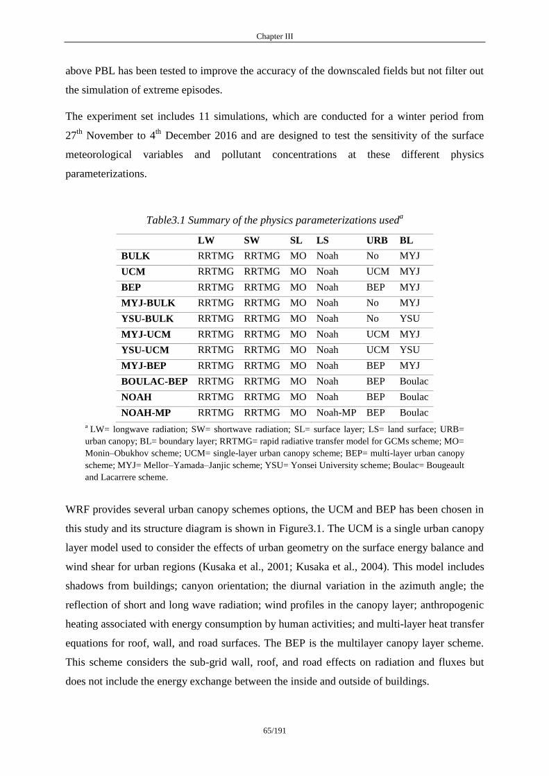
Chapter III
65/191
above PBL has been tested to improve the accuracy of the downscaled fields but not filter out
the simulation of extreme episodes.
The experiment set includes 11 simulations, which are conducted for a winter period from
27th
November to 4th
December 2016 and are designed to test the sensitivity of the surface
meteorological variables and pollutant concentrations at these different physics
parameterizations.
Table3.1 Summary of the physics parameterizations useda
LW SW SL LS URB BL
BULK RRTMG RRTMG MO Noah No MYJ
UCM RRTMG RRTMG MO Noah UCM MYJ
BEP RRTMG RRTMG MO Noah BEP MYJ
MYJ-BULK RRTMG RRTMG MO Noah No MYJ
YSU-BULK RRTMG RRTMG MO Noah No YSU
MYJ-UCM RRTMG RRTMG MO Noah UCM MYJ
YSU-UCM RRTMG RRTMG MO Noah UCM YSU
MYJ-BEP RRTMG RRTMG MO Noah BEP MYJ
BOULAC-BEP RRTMG RRTMG MO Noah BEP Boulac
NOAH RRTMG RRTMG MO Noah BEP Boulac
NOAH-MP RRTMG RRTMG MO Noah-MP BEP Boulac
a LW= longwave radiation; SW= shortwave radiation; SL= surface layer; LS= land surface; URB=
urban canopy; BL= boundary layer; RRTMG= rapid radiative transfer model for GCMs scheme; MO=
Monin–Obukhov scheme; UCM= single-layer urban canopy scheme; BEP= multi-layer urban canopy
scheme; MYJ= Mellor–Yamada–Janjic scheme; YSU= Yonsei University scheme; Boulac= Bougeault
and Lacarrere scheme.
WRF provides several urban canopy schemes options, the UCM and BEP has been chosen in
this study and its structure diagram is shown in Figure3.1. The UCM is a single urban canopy
layer model used to consider the effects of urban geometry on the surface energy balance and
wind shear for urban regions (Kusaka et al., 2001; Kusaka et al., 2004). This model includes
shadows from buildings; canyon orientation; the diurnal variation in the azimuth angle; the
reflection of short and long wave radiation; wind profiles in the canopy layer; anthropogenic
heating associated with energy consumption by human activities; and multi-layer heat transfer
equations for roof, wall, and road surfaces. The BEP is the multilayer canopy layer scheme.
This scheme considers the sub-grid wall, roof, and road effects on radiation and fluxes but
does not include the energy exchange between the inside and outside of buildings.
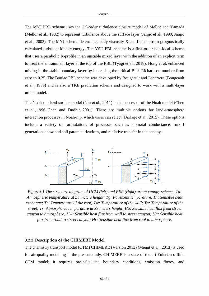
Chapter III
66/191
The MYJ PBL scheme uses the 1.5-order turbulence closure model of Mellor and Yamada
(Mellor et al., 1982) to represent turbulence above the surface layer (Janjic et al., 1990; Janjic
et al., 2002). The MYJ scheme determines eddy viscosity K-coefficients from prognostically
calculated turbulent kinetic energy. The YSU PBL scheme is a first-order non-local scheme
that uses a parabolic K-profile in an unstable mixed layer with the addition of an explicit term
to treat the entrainment layer at the top of the PBL (Tyagi et al., 2018). Hong et al. enhanced
mixing in the stable boundary layer by increasing the critical Bulk Richardson number from
zero to 0.25. The Boulac PBL scheme was developed by Bougeault and Lacarrère (Bougeault
et al., 1989) and is also a TKE prediction scheme and designed to work with a multi-layer
urban model.
The Noah‐mp land surface model (Niu et al., 2011) is the successor of the Noah model (Chen
et al., 1996; Chen and Dudhia, 2001). There are multiple options for land‐atmosphere
interaction processes in Noah‐mp, which users can select (Barlage et al., 2015). These options
include a variety of formulations of processes such as stomatal conductance, runoff
generation, snow and soil parameterizations, and radiative transfer in the canopy.
Figure3.1 The structure diagram of UCM (left) and BEP (right) urban canopy scheme. Ta:
Atmospheric temperature at Za meters height; Tg: Pavement temperature; H : Sensible heat
exchange; Tr: Temperature of the roof; Tw: Temperature of the wall; Tg: Temperature of the
street; Ts: Atmospheric temperature at Zs meters height; Ha: Sensible heat flux from street
canyon to atmosphere; Hw: Sensible heat flux from wall to street canyon; Hg: Sensible heat
fiux from road to street canyon; Hr: Sensible heat fiux from roof to atmosphere.
3.2.2 Description of the CHIMERE Model
The chemistry transport model (CTM) CHIMERE (Version 2013) (Menut et al., 2013) is used
for air quality modeling in the present study. CHIMERE is a state-of-the-art Eulerian offline
CTM model; it requires pre-calculated boundary conditions, emission fluxes, and

Chapter III
67/191
meteorological variables. For the studied period, 27th
November to 4th
December 2016, an
8-day spin-up period is performed for initialization issues. The vertical turbulent mixing in
CHIMERE takes place only within the boundary layer, which is calculated by meteorological
parameters such as surface temperature and the wind speed issued from the WRF simulation.
The first CHIMERE layer is set to 4 m. The vertical dispersion in CHIMERE is mostly
controlled by the PBL height and a turbulent flux modeled by a vertical eddy diffusion
coefficient (Kz). The horizontal diffusion is neglected in CHIMERE. The PBL height is
directly taken from the WRF output and capped at a minimal value of 20m to avoid
unrealistic simulations. In CHIMERE, the Kz is calculated using the parameterization of
Troen and Mahrt (1986) in Equation (3.1):
(
)
#( )
where k is the von Karman constant set to 0.41, z is the altitude, h is the boundary layer height,
and ws is the vertical scale given by the similarity formulae.
The emissions of pollutants include several different gaseous and aerosol species. Those
emissions can be split into four parts: anthropogenic emissions, biogenetic emissions, mineral
dust emissions, and fire emissions. The anthropogenic emissions play a critical role in the
CTM model, since they include all human activities, especially in megacities, and they are the
only source we can reduce. For Europe region studies, anthropogenic emissions of gases and
PM are generated with the French National Spatialized Emission Inventory (INS)
(Hamaoui-Lague et al., 2014), which is updated every six months. Biogenic emissions are
estimated with the Model of Emissions and Gases and Aerosols from Nature (MEGAN).
Mineral dust emissions are parameterized by Menut et al (2013). The resolution INS emission
inventory is approximately 1 × 1 km, and the spatial resolutions of the emission data are
recomputed from the INS emission inventory for each domain. Driven by those input data,
CHIMERE provides the hourly concentrations of tens of species at a regional scale; detailed
descriptions of the model can be found in several previous studies (Bessagnet et al., 2004;
Menut et al., 2012; Bessagnet et al., 2017; Mailler et al., 2017). The aerosol module accounts
for both inorganic and organic species, such as sulfate, nitrate, ammonium, primary organic
matter, element carbon, secondary organic aerosol, sea salt, dust, and water. The aerosol size
is assuming discrete aerosol size sections and that the particles are internally mixed. Nine
diameter bins, from 10nm to 10μm, with 5 bins below 1 μm, are used (Couvidat et al., 2018).
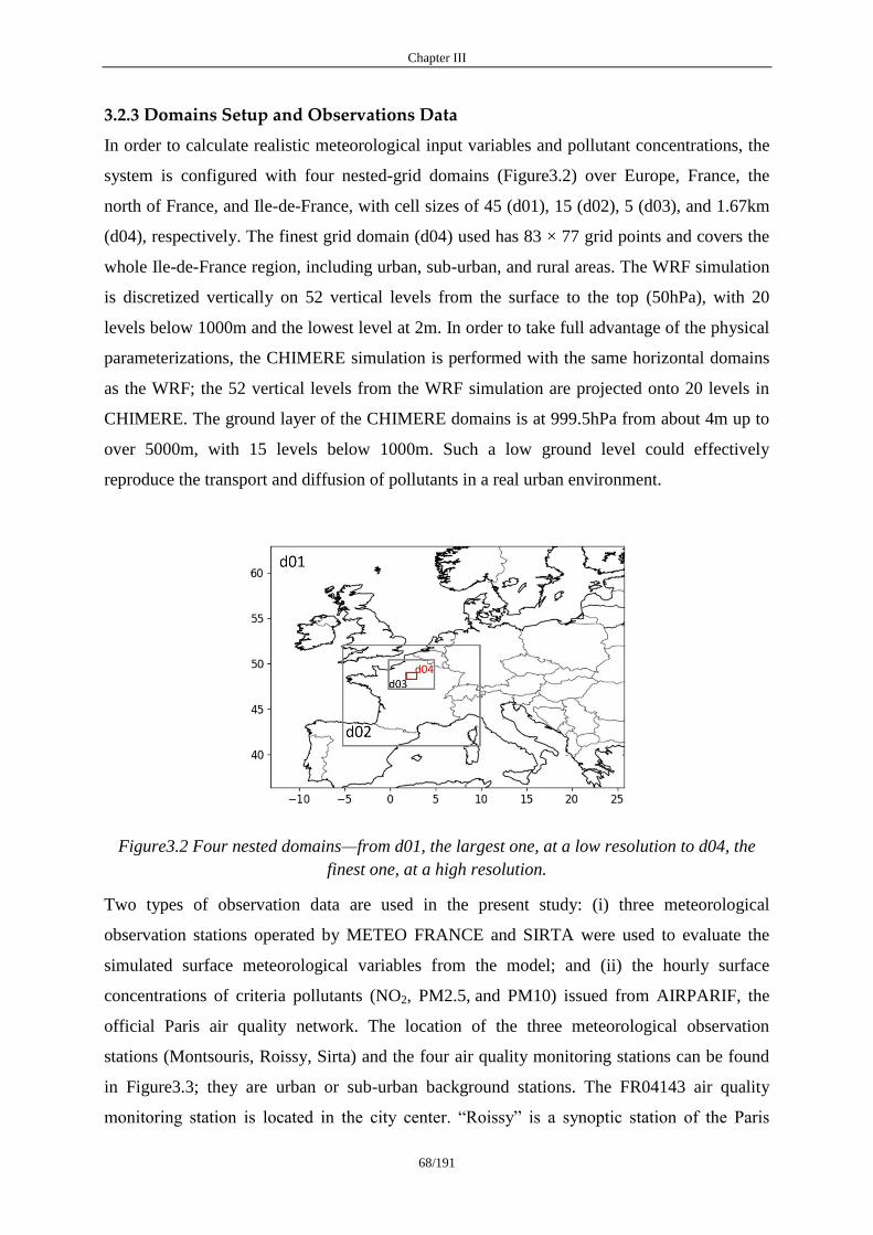
Chapter III
68/191
3.2.3 Domains Setup and Observations Data
In order to calculate realistic meteorological input variables and pollutant concentrations, the
system is configured with four nested-grid domains (Figure3.2) over Europe, France, the
north of France, and Ile-de-France, with cell sizes of 45 (d01), 15 (d02), 5 (d03), and 1.67km
(d04), respectively. The finest grid domain (d04) used has 83 × 77 grid points and covers the
whole Ile-de-France region, including urban, sub-urban, and rural areas. The WRF simulation
is discretized vertically on 52 vertical levels from the surface to the top (50hPa), with 20
levels below 1000m and the lowest level at 2m. In order to take full advantage of the physical
parameterizations, the CHIMERE simulation is performed with the same horizontal domains
as the WRF; the 52 vertical levels from the WRF simulation are projected onto 20 levels in
CHIMERE. The ground layer of the CHIMERE domains is at 999.5hPa from about 4m up to
over 5000m, with 15 levels below 1000m. Such a low ground level could effectively
reproduce the transport and diffusion of pollutants in a real urban environment.
Figure3.2 Four nested domains—from d01, the largest one, at a low resolution to d04, the
finest one, at a high resolution.
Two types of observation data are used in the present study: (i) three meteorological
observation stations operated by METEO FRANCE and SIRTA were used to evaluate the
simulated surface meteorological variables from the model; and (ii) the hourly surface
concentrations of criteria pollutants (NO2, PM2.5, and PM10) issued from AIRPARIF, the
official Paris air quality network. The location of the three meteorological observation
stations (Montsouris, Roissy, Sirta) and the four air quality monitoring stations can be found
in Figure3.3; they are urban or sub-urban background stations. The FR04143 air quality
monitoring station is located in the city center. ―Roissy‖ is a synoptic station of the Paris
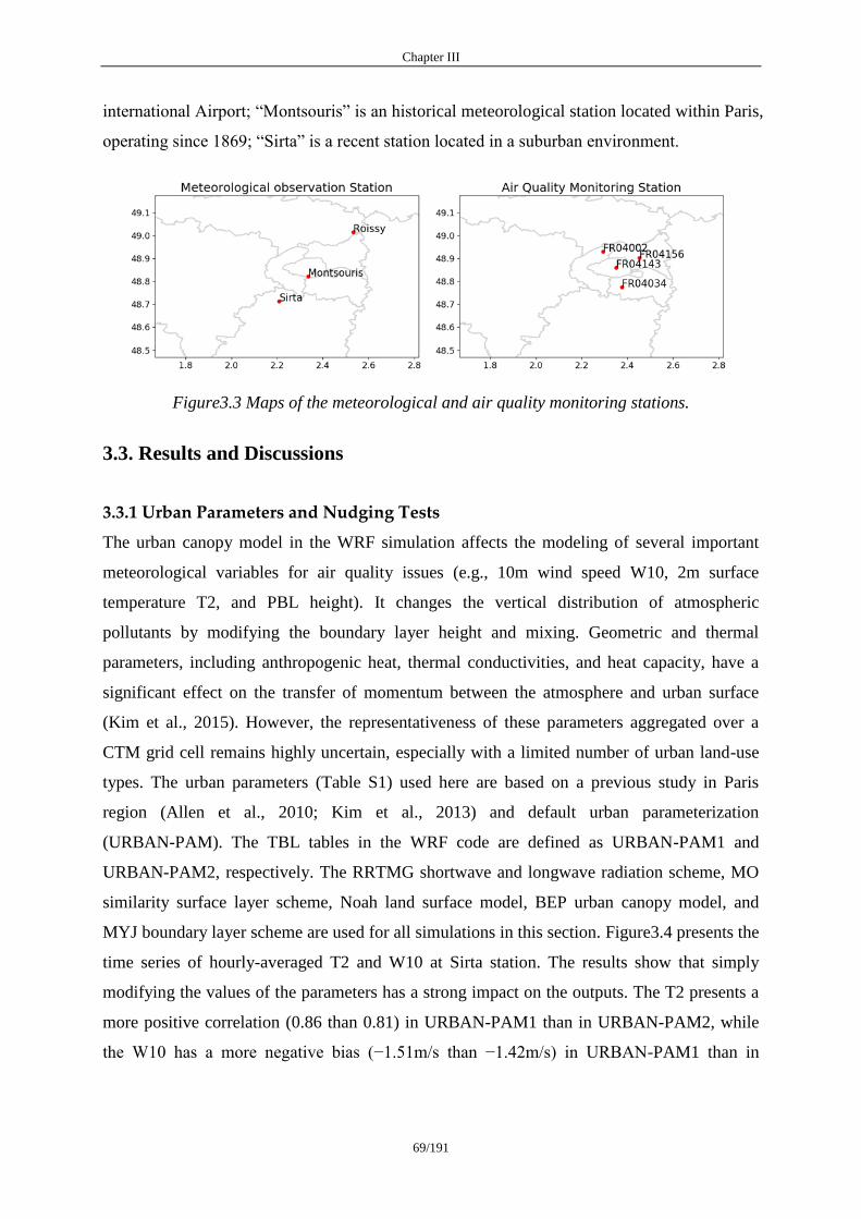
Chapter III
69/191
international Airport; ―Montsouris‖ is an historical meteorological station located within Paris,
operating since 1869; ―Sirta‖ is a recent station located in a suburban environment.
Figure3.3 Maps of the meteorological and air quality monitoring stations.
3.3. Results and Discussions
3.3.1 Urban Parameters and Nudging Tests
The urban canopy model in the WRF simulation affects the modeling of several important
meteorological variables for air quality issues (e.g., 10m wind speed W10, 2m surface
temperature T2, and PBL height). It changes the vertical distribution of atmospheric
pollutants by modifying the boundary layer height and mixing. Geometric and thermal
parameters, including anthropogenic heat, thermal conductivities, and heat capacity, have a
significant effect on the transfer of momentum between the atmosphere and urban surface
(Kim et al., 2015). However, the representativeness of these parameters aggregated over a
CTM grid cell remains highly uncertain, especially with a limited number of urban land-use
types. The urban parameters (Table S1) used here are based on a previous study in Paris
region (Allen et al., 2010; Kim et al., 2013) and default urban parameterization
(URBAN-PAM). The TBL tables in the WRF code are defined as URBAN-PAM1 and
URBAN-PAM2, respectively. The RRTMG shortwave and longwave radiation scheme, MO
similarity surface layer scheme, Noah land surface model, BEP urban canopy model, and
MYJ boundary layer scheme are used for all simulations in this section. Figure3.4 presents the
time series of hourly-averaged T2 and W10 at Sirta station. The results show that simply
modifying the values of the parameters has a strong impact on the outputs. The T2 presents a
more positive correlation (0.86 than 0.81) in URBAN-PAM1 than in URBAN-PAM2, while
the W10 has a more negative bias (−1.51m/s than −1.42m/s) in URBAN-PAM1 than in
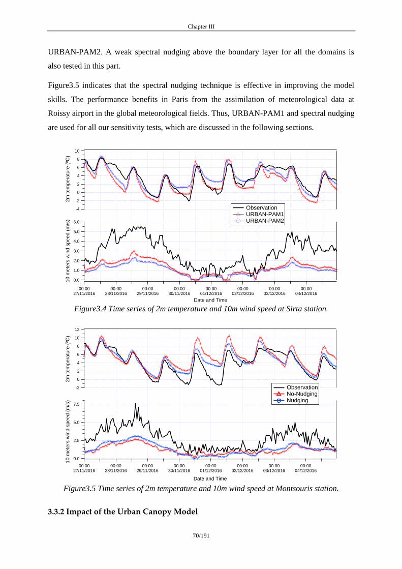
Chapter III
70/191
URBAN-PAM2. A weak spectral nudging above the boundary layer for all the domains is
also tested in this part.
Figure3.5 indicates that the spectral nudging technique is effective in improving the model
skills. The performance benefits in Paris from the assimilation of meteorological data at
Roissy airport in the global meteorological fields. Thus, URBAN-PAM1 and spectral nudging
are used for all our sensitivity tests, which are discussed in the following sections.
Figure3.4 Time series of 2m temperature and 10m wind speed at Sirta station.
Figure3.5 Time series of 2m temperature and 10m wind speed at Montsouris station.
3.3.2 Impact of the Urban Canopy Model
10
8
6
4
2
0
-2
-4
2m
tem
pera
ture
(ºC
)
00:0027/11/2016
00:0028/11/2016
00:0029/11/2016
00:0030/11/2016
00:0001/12/2016
00:0002/12/2016
00:0003/12/2016
00:0004/12/2016
Date and Time
6.0
5.0
4.0
3.0
2.0
1.0
0.010 m
ete
rs w
ind s
peed (
m/s
)
Observation URBAN-PAM1 URBAN-PAM2
12
10
8
6
4
2
0
-2
2m
te
mp
era
ture
(ºC
)
00:0027/11/2016
00:0028/11/2016
00:0029/11/2016
00:0030/11/2016
00:0001/12/2016
00:0002/12/2016
00:0003/12/2016
00:0004/12/2016
Date and Time
7.5
5.0
2.5
0.0
10
me
ters
win
d s
pe
ed
(m
/s)
Observation No-Nudging Nudging
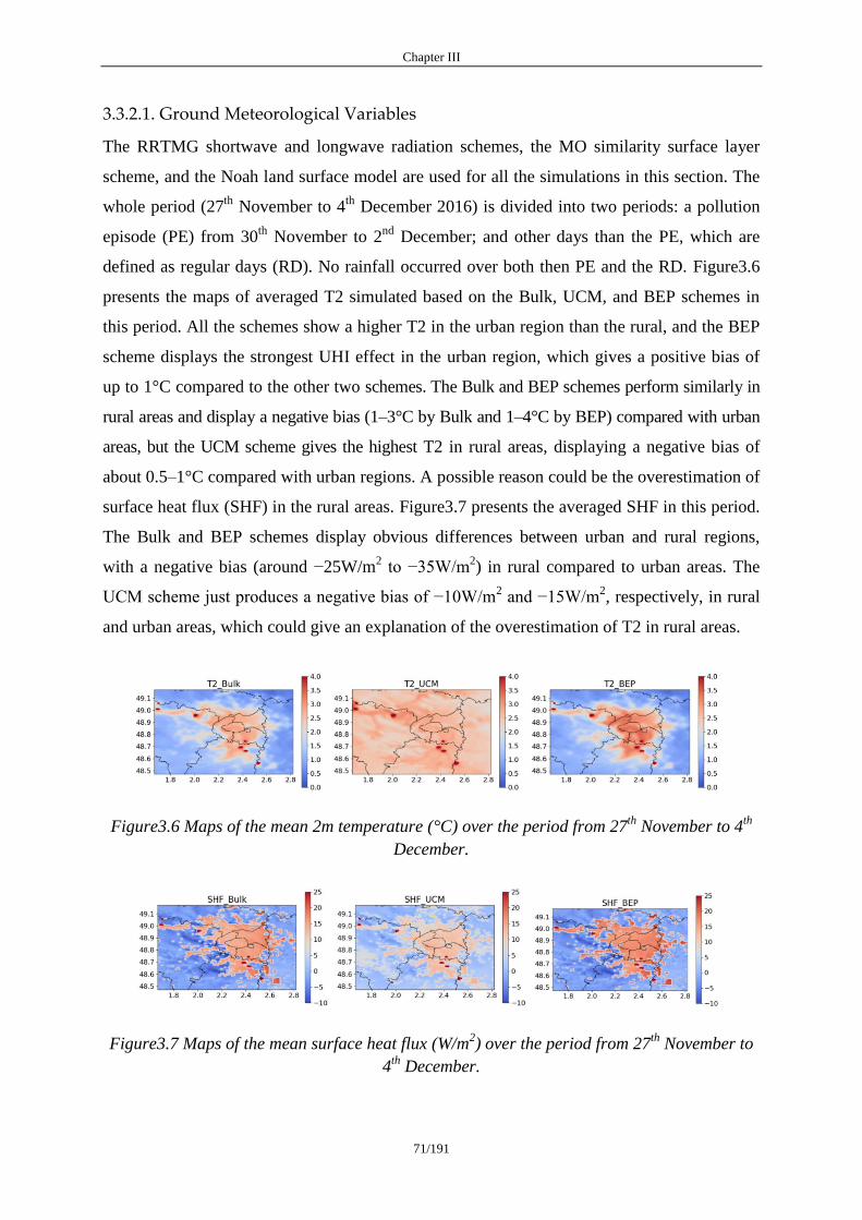
Chapter III
71/191
3.3.2.1. Ground Meteorological Variables
The RRTMG shortwave and longwave radiation schemes, the MO similarity surface layer
scheme, and the Noah land surface model are used for all the simulations in this section. The
whole period (27th
November to 4th
December 2016) is divided into two periods: a pollution
episode (PE) from 30th
November to 2nd
December; and other days than the PE, which are
defined as regular days (RD). No rainfall occurred over both then PE and the RD. Figure3.6
presents the maps of averaged T2 simulated based on the Bulk, UCM, and BEP schemes in
this period. All the schemes show a higher T2 in the urban region than the rural, and the BEP
scheme displays the strongest UHI effect in the urban region, which gives a positive bias of
up to 1°C compared to the other two schemes. The Bulk and BEP schemes perform similarly in
rural areas and display a negative bias (1–3°C by Bulk and 1–4°C by BEP) compared with urban
areas, but the UCM scheme gives the highest T2 in rural areas, displaying a negative bias of
about 0.5–1°C compared with urban regions. A possible reason could be the overestimation of
surface heat flux (SHF) in the rural areas. Figure3.7 presents the averaged SHF in this period.
The Bulk and BEP schemes display obvious differences between urban and rural regions,
with a negative bias (around −25W/m2 to −35W/m
2) in rural compared to urban areas. The
UCM scheme just produces a negative bias of −10W/m2 and −15W/m
2, respectively, in rural
and urban areas, which could give an explanation of the overestimation of T2 in rural areas.
Figure3.6 Maps of the mean 2m temperature (°C) over the period from 27th
November to 4th
December.
Figure3.7 Maps of the mean surface heat flux (W/m2) over the period from 27
th November to
4th
December.
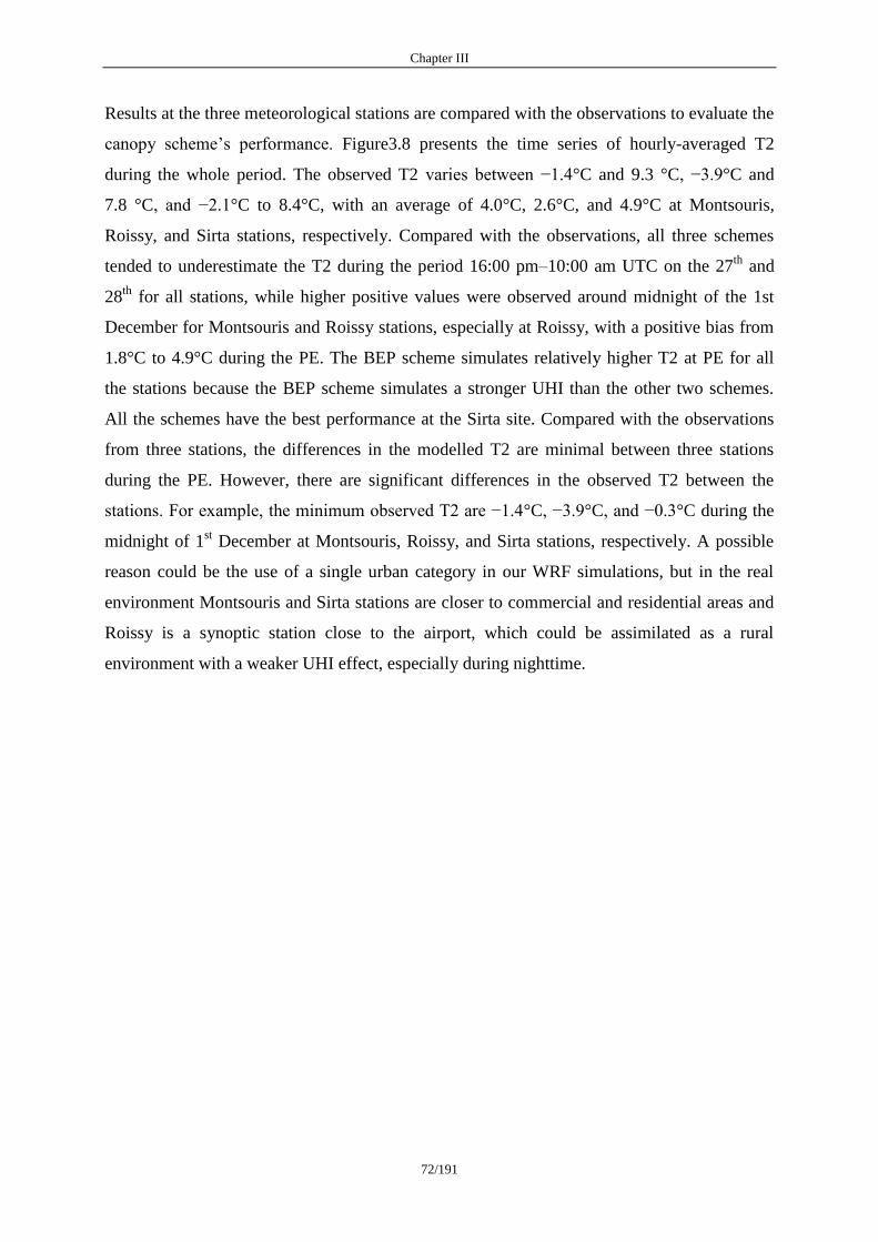
Chapter III
72/191
Results at the three meteorological stations are compared with the observations to evaluate the
canopy scheme’s performance. Figure3.8 presents the time series of hourly-averaged T2
during the whole period. The observed T2 varies between −1.4°C and 9.3 °C, −3.9°C and
7.8 °C, and −2.1°C to 8.4°C, with an average of 4.0°C, 2.6°C, and 4.9°C at Montsouris,
Roissy, and Sirta stations, respectively. Compared with the observations, all three schemes
tended to underestimate the T2 during the period 16:00 pm–10:00 am UTC on the 27th
and
28th
for all stations, while higher positive values were observed around midnight of the 1st
December for Montsouris and Roissy stations, especially at Roissy, with a positive bias from
1.8°C to 4.9°C during the PE. The BEP scheme simulates relatively higher T2 at PE for all
the stations because the BEP scheme simulates a stronger UHI than the other two schemes.
All the schemes have the best performance at the Sirta site. Compared with the observations
from three stations, the differences in the modelled T2 are minimal between three stations
during the PE. However, there are significant differences in the observed T2 between the
stations. For example, the minimum observed T2 are −1.4°C, −3.9°C, and −0.3°C during the
midnight of 1st December at Montsouris, Roissy, and Sirta stations, respectively. A possible
reason could be the use of a single urban category in our WRF simulations, but in the real
environment Montsouris and Sirta stations are closer to commercial and residential areas and
Roissy is a synoptic station close to the airport, which could be assimilated as a rural
environment with a weaker UHI effect, especially during nighttime.
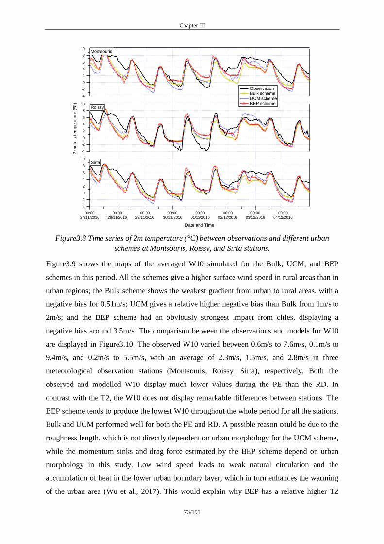
Chapter III
73/191
Figure3.8 Time series of 2m temperature (°C) between observations and different urban
schemes at Montsouris, Roissy, and Sirta stations.
Figure3.9 shows the maps of the averaged W10 simulated for the Bulk, UCM, and BEP
schemes in this period. All the schemes give a higher surface wind speed in rural areas than in
urban regions; the Bulk scheme shows the weakest gradient from urban to rural areas, with a
negative bias for 0.51m/s; UCM gives a relative higher negative bias than Bulk from 1m/s to
2m/s; and the BEP scheme had an obviously strongest impact from cities, displaying a
negative bias around 3.5m/s. The comparison between the observations and models for W10
are displayed in Figure3.10. The observed W10 varied between 0.6m/s to 7.6m/s, 0.1m/s to
9.4m/s, and 0.2m/s to 5.5m/s, with an average of 2.3m/s, 1.5m/s, and 2.8m/s in three
meteorological observation stations (Montsouris, Roissy, Sirta), respectively. Both the
observed and modelled W10 display much lower values during the PE than the RD. In
contrast with the T2, the W10 does not display remarkable differences between stations. The
BEP scheme tends to produce the lowest W10 throughout the whole period for all the stations.
Bulk and UCM performed well for both the PE and RD. A possible reason could be due to the
roughness length, which is not directly dependent on urban morphology for the UCM scheme,
while the momentum sinks and drag force estimated by the BEP scheme depend on urban
morphology in this study. Low wind speed leads to weak natural circulation and the
accumulation of heat in the lower urban boundary layer, which in turn enhances the warming
of the urban area (Wu et al., 2017). This would explain why BEP has a relative higher T2
10
8
6
4
2
0
-2
-4
2 m
ete
rs t
em
pe
ratu
re (
ºC)
00:0027/11/2016
00:0028/11/2016
00:0029/11/2016
00:0030/11/2016
00:0001/12/2016
00:0002/12/2016
00:0003/12/2016
00:0004/12/2016
Date and Time
10
8
6
4
2
0
-2
-4
10
8
6
4
2
0
-2
-4
Observation Bulk scheme UCM scheme BEP scheme
Montsouris
Roissy
Sirta
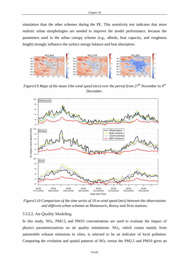
Chapter III
74/191
simulation than the other schemes during the PE. This sensitivity test indicates that more
realistic urban morphologies are needed to improve the model performance, because the
parameters used in the urban canopy scheme (e.g., albedo, heat capacity, and roughness
length) strongly influence the surface energy balance and heat absorption.
Figure3.9 Maps of the mean 10m wind speed (m/s) over the period from 27th
November to 4th
December.
Figure3.10 Comparison of the time series of 10 m wind speed (m/s) between the observations
and different urban schemes at Montsouris, Roissy and Sirta stations.
3.3.2.2. Air Quality Modeling
In this study, NO2, PM2.5, and PM10 concentrations are used to evaluate the impact of
physics parameterizations on air quality simulations. NO2, which comes mainly from
automobile exhaust emissions in cities, is selected to be an indicator of local pollution.
Comparing the evolution and spatial patterns of NO2 versus the PM2.5 and PM10 gives an
10
8
6
4
2
0
10
me
ters
win
d s
pe
ed
(m
/s)
00:0027/11/2016
00:0028/11/2016
00:0029/11/2016
00:0030/11/2016
00:0001/12/2016
00:0002/12/2016
00:0003/12/2016
00:0004/12/2016
Date and Time
10
8
6
4
2
0
10
8
6
4
2
0
Observation Bulk scheme UCM scheme BEP scheme
Montsouris
Roissy
Sirta
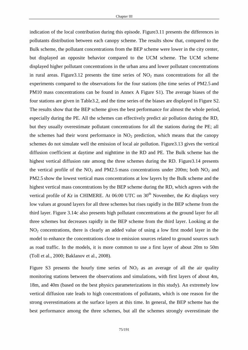
Chapter III
75/191
indication of the local contribution during this episode. Figure3.11 presents the differences in
pollutants distribution between each canopy scheme. The results show that, compared to the
Bulk scheme, the pollutant concentrations from the BEP scheme were lower in the city center,
but displayed an opposite behavior compared to the UCM scheme. The UCM scheme
displayed higher pollutant concentrations in the urban area and lower pollutant concentrations
in rural areas. Figure3.12 presents the time series of NO2 mass concentrations for all the
experiments compared to the observations for the four stations (the time series of PM2.5 and
PM10 mass concentrations can be found in Annex A Figure S1). The average biases of the
four stations are given in Table3.2, and the time series of the biases are displayed in Figure S2.
The results show that the BEP scheme gives the best performance for almost the whole period,
especially during the PE. All the schemes can effectively predict air pollution during the RD,
but they usually overestimate pollutant concentrations for all the stations during the PE; all
the schemes had their worst performance in NO2 prediction, which means that the canopy
schemes do not simulate well the emission of local air pollution. Figure3.13 gives the vertical
diffusion coefficient at daytime and nighttime in the RD and PE. The Bulk scheme has the
highest vertical diffusion rate among the three schemes during the RD. Figure3.14 presents
the vertical profile of the NO2 and PM2.5 mass concentrations under 200m; both NO2 and
PM2.5 show the lowest vertical mass concentrations at low layers by the Bulk scheme and the
highest vertical mass concentrations by the BEP scheme during the RD, which agrees with the
vertical profile of Kz in CHIMERE. At 06:00 UTC on 30th
November, the Kz displays very
low values at ground layers for all three schemes but rises rapidly in the BEP scheme from the
third layer. Figure 3.14c also presents high pollutant concentrations at the ground layer for all
three schemes but decreases rapidly in the BEP scheme from the third layer. Looking at the
NO2 concentrations, there is clearly an added value of using a low first model layer in the
model to enhance the concentrations close to emission sources related to ground sources such
as road traffic. In the models, it is more common to use a first layer of about 20m to 50m
(Toll et al., 2000; Baklanov et al., 2008).
Figure S3 presents the hourly time series of NO2 as an average of all the air quality
monitoring stations between the observations and simulations, with first layers of about 4m,
18m, and 40m (based on the best physics parameterizations in this study). An extremely low
vertical diffusion rate leads to high concentrations of pollutants, which is one reason for the
strong overestimations at the surface layers at this time. In general, the BEP scheme has the
best performance among the three schemes, but all the schemes strongly overestimate the
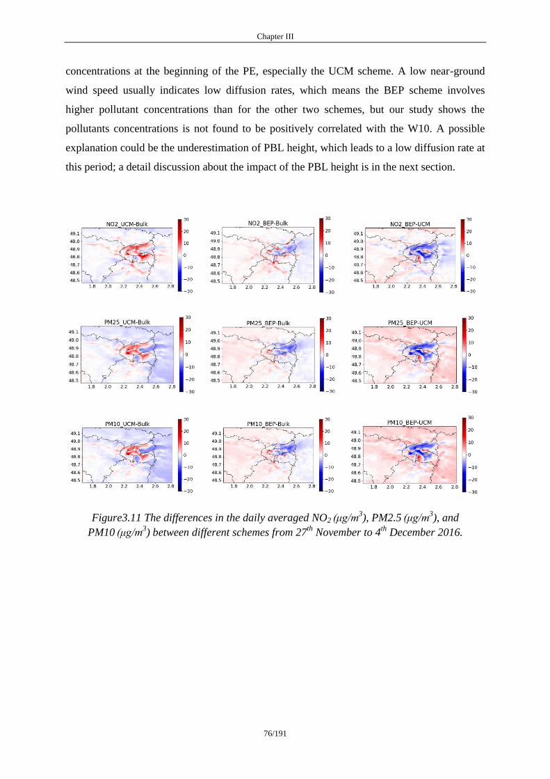
Chapter III
76/191
concentrations at the beginning of the PE, especially the UCM scheme. A low near-ground
wind speed usually indicates low diffusion rates, which means the BEP scheme involves
higher pollutant concentrations than for the other two schemes, but our study shows the
pollutants concentrations is not found to be positively correlated with the W10. A possible
explanation could be the underestimation of PBL height, which leads to a low diffusion rate at
this period; a detail discussion about the impact of the PBL height is in the next section.
Figure3.11 The differences in the daily averaged NO2 (μg/m3), PM2.5 (μg/m
3), and
PM10 (μg/m3) between different schemes from 27
th November to 4
th December 2016.
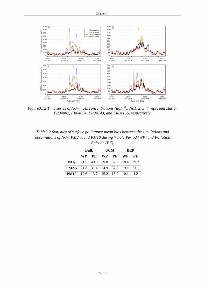
Chapter III
77/191
Figure3.12 Time series of NO2 mass concentrations (µg/m3). No1, 2, 3, 4 represent station
FR04002, FR04034, FR04143, and FR04156, respectively.
Table3.2 Statistics of surface pollutants: mean bias between the simulations and
observations of NO2, PM2.5, and PM10 during Whole Period (WP) and Pollution
Episode (PE).
Bulk UCM BEP
WP PE WP PE WP PE
NO2 21.5 40.9 29.8 62.2 18.4 29.7
PM2.5 21.8 31.4 24.9 37.7 19.1 21.1
PM10 12.6 13.7 15.2 18.9 10.1 4.2
500
450
400
350
300
250
200
150
100
50
0
00:0027/11/2016
12:0029/11/2016
00:0002/12/2016
12:0004/12/2016
Date and Time
4
900
800
700
600
500
400
300
200
100
0
NO
2 M
ass C
on
ce
ntr
atio
n (
µg
/m3)
00:0027/11/2016
12:0029/11/2016
00:0002/12/2016
12:0004/12/2016
1
Observation Bulk scheme UCM scheme BEP scheme
700
600
500
400
300
200
100
0
NO
2 M
ass C
on
ce
ntr
atio
n (
µg
/m3)
00:0027/11/2016
12:0029/11/2016
00:0002/12/2016
12:0004/12/2016
Date and Time
3
400
360
320
280
240
200
160
120
80
40
0
00:0027/11/2016
12:0029/11/2016
00:0002/12/2016
12:0004/12/2016
2
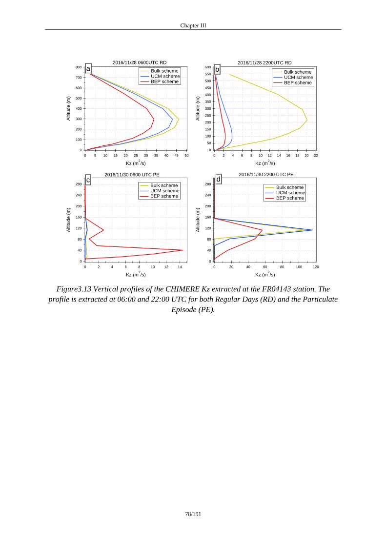
Chapter III
78/191
Figure3.13 Vertical profiles of the CHIMERE Kz extracted at the FR04143 station. The
profile is extracted at 06:00 and 22:00 UTC for both Regular Days (RD) and the Particulate
Episode (PE).
280
240
200
160
120
80
40
0
Altitude (
m)
120100806040200
Kz (m2/s)
2016/11/30 2200 UTC PE
Bulk scheme UCM scheme BEP scheme
d280
240
200
160
120
80
40
0
Altitude (
m)
14121086420
Kz (m2/s)
2016/11/30 0600 UTC PE
Bulk scheme UCM scheme BEP scheme
c
800
700
600
500
400
300
200
100
0
Altitude (
m)
50454035302520151050
Kz (m2/s)
Bulk scheme UCM scheme BEP scheme
a2016/11/28 0600UTC RD
600
550
500
450
400
350
300
250
200
150
100
50
0
Altitude (
m)
2220181614121086420
Kz (m2/s)
Bulk scheme UCM scheme BEP scheme
b2016/11/28 2200UTC RD
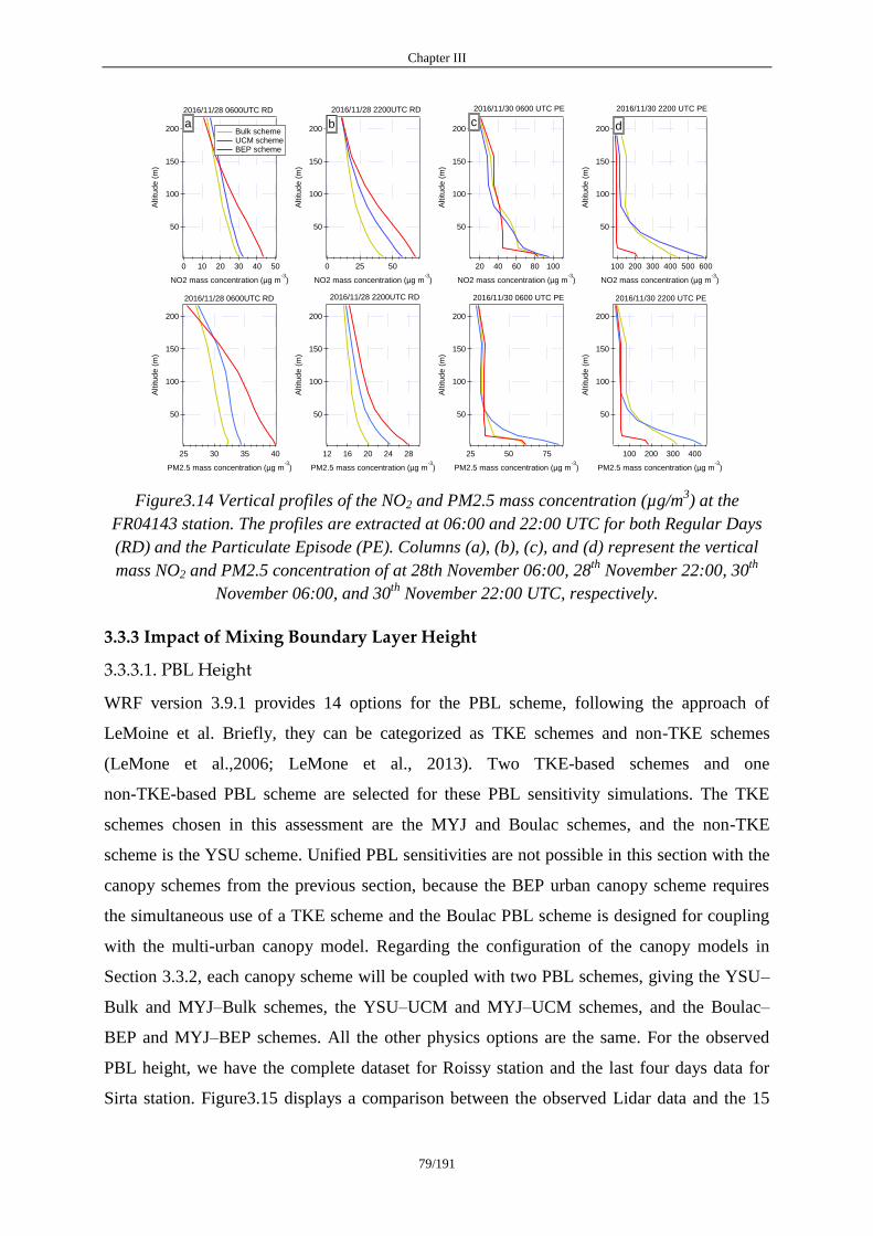
Chapter III
79/191
Figure3.14 Vertical profiles of the NO2 and PM2.5 mass concentration (µg/m3) at the
FR04143 station. The profiles are extracted at 06:00 and 22:00 UTC for both Regular Days
(RD) and the Particulate Episode (PE). Columns (a), (b), (c), and (d) represent the vertical
mass NO2 and PM2.5 concentration of at 28th November 06:00, 28th
November 22:00, 30th
November 06:00, and 30th
November 22:00 UTC, respectively.
3.3.3 Impact of Mixing Boundary Layer Height
3.3.3.1. PBL Height
WRF version 3.9.1 provides 14 options for the PBL scheme, following the approach of
LeMoine et al. Briefly, they can be categorized as TKE schemes and non-TKE schemes
(LeMone et al.,2006; LeMone et al., 2013). Two TKE-based schemes and one
non-TKE-based PBL scheme are selected for these PBL sensitivity simulations. The TKE
schemes chosen in this assessment are the MYJ and Boulac schemes, and the non-TKE
scheme is the YSU scheme. Unified PBL sensitivities are not possible in this section with the
canopy schemes from the previous section, because the BEP urban canopy scheme requires
the simultaneous use of a TKE scheme and the Boulac PBL scheme is designed for coupling
with the multi-urban canopy model. Regarding the configuration of the canopy models in
Section 3.3.2, each canopy scheme will be coupled with two PBL schemes, giving the YSU–
Bulk and MYJ–Bulk schemes, the YSU–UCM and MYJ–UCM schemes, and the Boulac–
BEP and MYJ–BEP schemes. All the other physics options are the same. For the observed
PBL height, we have the complete dataset for Roissy station and the last four days data for
Sirta station. Figure3.15 displays a comparison between the observed Lidar data and the 15
200
150
100
50
Altitu
de
(m
)
2824201612
PM2.5 mass concentration (µg m-3
)
2016/11/28 2200UTC RD
200
150
100
50
Altitu
de
(m
)
400300200100
PM2.5 mass concentration (µg m-3
)
2016/11/30 2200 UTC PE
200
150
100
50
Altitu
de
(m
)
50250
NO2 mass concentration (µg m-3
)
2016/11/28 2200UTC RD
b 200
150
100
50
Altitu
de
(m
)
10080604020
NO2 mass concentration (µg m-3
)
2016/11/30 0600 UTC PE
c200
150
100
50
Altitu
de
(m
)
600500400300200100
NO2 mass concentration (µg m-3
)
2016/11/30 2200 UTC PE
d200
150
100
50
Altitu
de
(m
)
50403020100
NO2 mass concentration (µg m-3
)
2016/11/28 0600UTC RD
Bulk scheme UCM scheme BEP scheme
a
200
150
100
50
Altitu
de
(m
)
755025
PM2.5 mass concentration (µg m-3
)
2016/11/30 0600 UTC PE
200
150
100
50
Altitu
de
(m
)
40353025
PM2.5 mass concentration (µg m-3
)
2016/11/28 0600UTC RD
Chapter III
80/191
min averaged modeled output of PBL height. Generally, all the PBL schemes systematically
underestimate PBL height for the whole time series, especially during the PE and the
beginning of RD (from 27th
November 00:00 UTC). This explains the strong overestimations
of pollutants during the PE in Section 3.3.2 and is consistent with the positive biases of
pollutant concentrations at the beginning of the RD in Figure3.11. If we consider the
simulation of PBL during the PE, the average observed PBL height was around 110m and is
only relatively well reproduced by the Boulac–BEP, scheme even though it still
underestimates the PBL height by around 40m on average. The other PBL schemes reach the
minimum PBL height (set up to 20m in the model) during the whole PE and strongly
underestimate PBL height, especially at night and early in the morning. In general, the
Boulac–BEP scheme gives the best performance, and it is the only option which can
effectively estimate the evolution of the PBL height during the PE in this sensitivity test. For
the other PBL schemes, the agreement between the simulations and observations is poor.
MYJ displays the poorest correlation compared to the observed soundings, regardless of other
parameter settings.
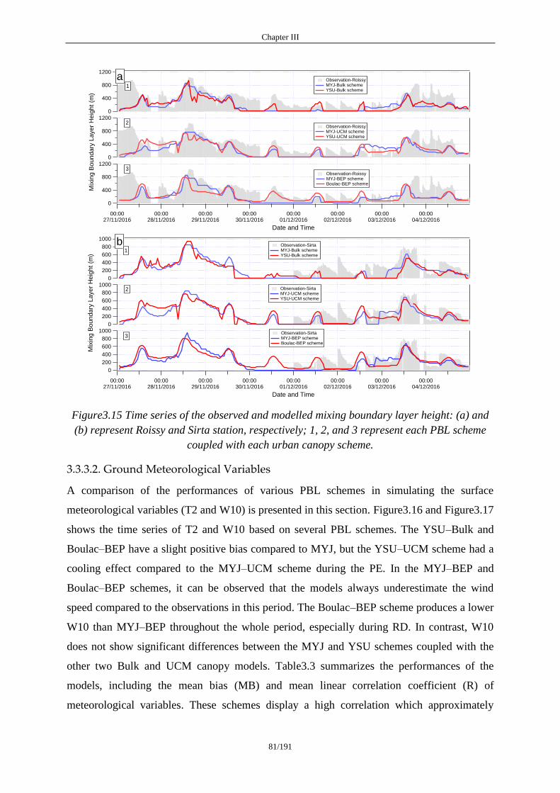
Chapter III
81/191
Figure3.15 Time series of the observed and modelled mixing boundary layer height: (a) and
(b) represent Roissy and Sirta station, respectively; 1, 2, and 3 represent each PBL scheme
coupled with each urban canopy scheme.
3.3.3.2. Ground Meteorological Variables
A comparison of the performances of various PBL schemes in simulating the surface
meteorological variables (T2 and W10) is presented in this section. Figure3.16 and Figure3.17
shows the time series of T2 and W10 based on several PBL schemes. The YSU–Bulk and
Boulac–BEP have a slight positive bias compared to MYJ, but the YSU–UCM scheme had a
cooling effect compared to the MYJ–UCM scheme during the PE. In the MYJ–BEP and
Boulac–BEP schemes, it can be observed that the models always underestimate the wind
speed compared to the observations in this period. The Boulac–BEP scheme produces a lower
W10 than MYJ–BEP throughout the whole period, especially during RD. In contrast, W10
does not show significant differences between the MYJ and YSU schemes coupled with the
other two Bulk and UCM canopy models. Table3.3 summarizes the performances of the
models, including the mean bias (MB) and mean linear correlation coefficient (R) of
meteorological variables. These schemes display a high correlation which approximately
1200
800
400
0
Mix
ing B
oundary
Layer
Heig
ht
(m)
00:0027/11/2016
00:0028/11/2016
00:0029/11/2016
00:0030/11/2016
00:0001/12/2016
00:0002/12/2016
00:0003/12/2016
00:0004/12/2016
Date and Time
1200
800
400
0
1200
800
400
0
Observation-Roissy MYJ-BEP scheme Boulac-BEP scheme
Observation-Roissy MYJ-UCM scheme YSU-UCM scheme
Observation-Roissy MYJ-Bulk scheme YSU-Bulk scheme
a1
2
3
1000
800
600
400
200
0
00:0027/11/2016
00:0028/11/2016
00:0029/11/2016
00:0030/11/2016
00:0001/12/2016
00:0002/12/2016
00:0003/12/2016
00:0004/12/2016
Date and Time
1000
800
600
400
200
0
Mix
ing B
oundary
Layer
Heig
ht
(m)
1000
800
600
400
200
0
Observation-Sirta MYJ-Bulk scheme YSU-Bulk scheme
Observation-Sirta MYJ-UCM scheme YSU-UCM scheme
Observation-Sirta MYJ-BEP scheme Boulac-BEP scheme
b1
2
3
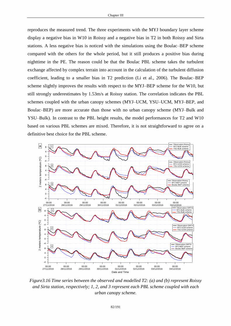
Chapter III
82/191
reproduces the measured trend. The three experiments with the MYJ boundary layer scheme
display a negative bias in W10 in Roissy and a negative bias in T2 in both Roissy and Sirta
stations. A less negative bias is noticed with the simulations using the Boulac–BEP scheme
compared with the others for the whole period, but it still produces a positive bias during
nighttime in the PE. The reason could be that the Boulac PBL scheme takes the turbulent
exchange affected by complex terrain into account in the calculation of the turbulent diffusion
coefficient, leading to a smaller bias in T2 prediction (Li et al., 2006). The Boulac–BEP
scheme slightly improves the results with respect to the MYJ–BEP scheme for the W10, but
still strongly underestimates by 1.53m/s at Roissy station. The correlation indicates the PBL
schemes coupled with the urban canopy schemes (MYJ–UCM, YSU–UCM, MYJ–BEP, and
Boulac–BEP) are more accurate than those with no urban canopy scheme (MYJ–Bulk and
YSU–Bulk). In contrast to the PBL height results, the model performances for T2 and W10
based on various PBL schemes are mixed. Therefore, it is not straightforward to agree on a
definitive best choice for the PBL scheme.
Figure3.16 Time series between the observed and modelled T2: (a) and (b) represent Roissy
and Sirta station, respectively; 1, 2, and 3 represent each PBL scheme coupled with each
urban canopy scheme.
8
4
0
-4
00:0027/11/2016
00:0028/11/2016
00:0029/11/2016
00:0030/11/2016
00:0001/12/2016
00:0002/12/2016
00:0003/12/2016
00:0004/12/2016
Date and Time
8
4
0
-4
8
4
0
-4
2 m
ete
rs t
em
pera
ture
(ºC
)
Observation-Roissy MYJ-Bulk scheme YSU-Bulk scheme
Observation-Roissy MYJ-UCM scheme YSU-UCM scheme
Observation-Roissy MYJ-BEP scheme Boulac-BEP scheme
1
2
3
a
8
4
0
-4
00:0027/11/2016
00:0028/11/2016
00:0029/11/2016
00:0030/11/2016
00:0001/12/2016
00:0002/12/2016
00:0003/12/2016
00:0004/12/2016
Date and Time
8
4
0
-4
2 m
ete
rs t
em
pera
ture
(ºC
)
8
4
0
-4
Observation-SIRTA MYJ-Bulk scheme YSU-Bulk scheme
Observation-SIRTA MYJ-UCM scheme YSU-UCM scheme
Observation-SIRTA MYJ-BEP scheme Boulac-BEP scheme
1
2
3
b
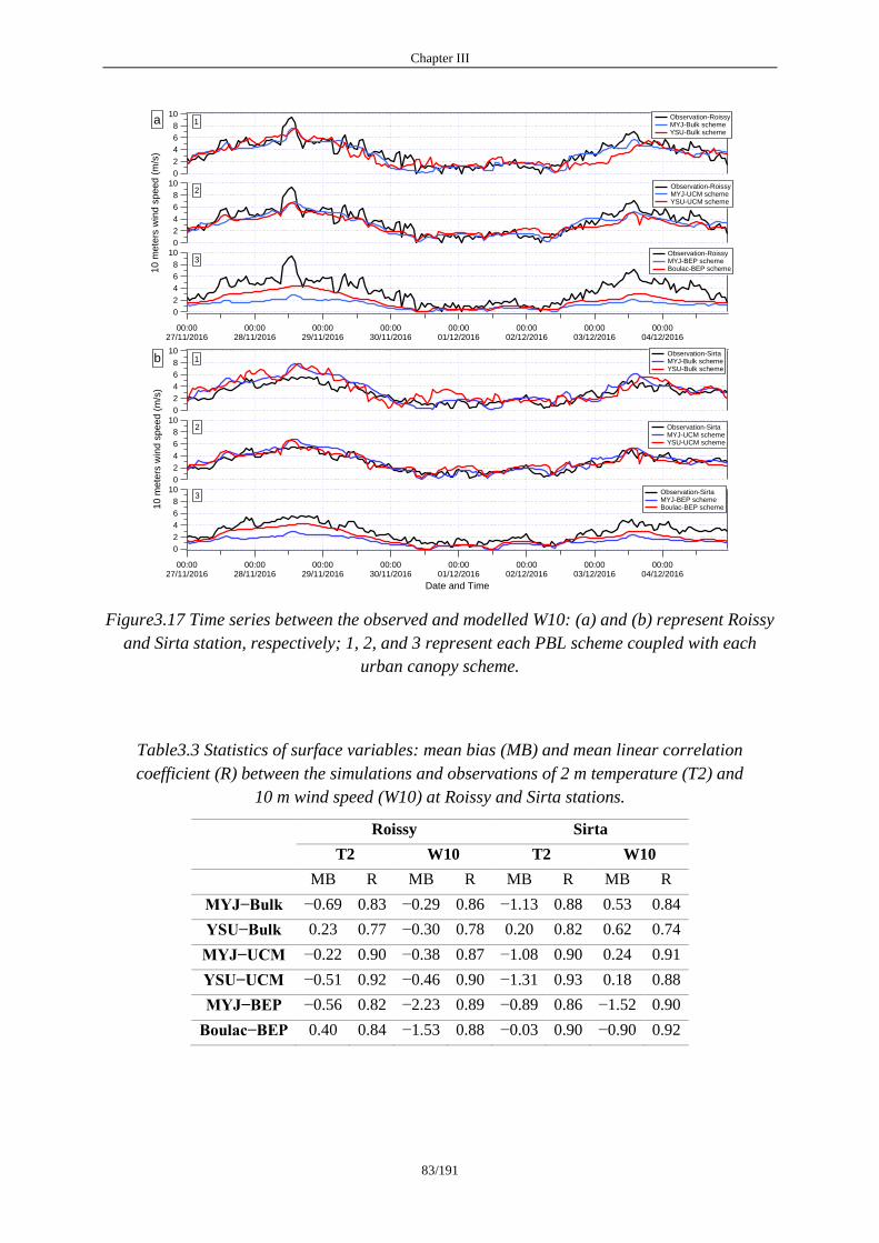
Chapter III
83/191
Figure3.17 Time series between the observed and modelled W10: (a) and (b) represent Roissy
and Sirta station, respectively; 1, 2, and 3 represent each PBL scheme coupled with each
urban canopy scheme.
Table3.3 Statistics of surface variables: mean bias (MB) and mean linear correlation
coefficient (R) between the simulations and observations of 2 m temperature (T2) and
10 m wind speed (W10) at Roissy and Sirta stations.
Roissy Sirta
T2 W10 T2 W10
MB R MB R MB R MB R
MYJ−Bulk −0.69 0.83 −0.29 0.86 −1.13 0.88 0.53 0.84
YSU−Bulk 0.23 0.77 −0.30 0.78 0.20 0.82 0.62 0.74
MYJ−UCM −0.22 0.90 −0.38 0.87 −1.08 0.90 0.24 0.91
YSU−UCM −0.51 0.92 −0.46 0.90 −1.31 0.93 0.18 0.88
MYJ−BEP −0.56 0.82 −2.23 0.89 −0.89 0.86 −1.52 0.90
Boulac−BEP 0.40 0.84 −1.53 0.88 −0.03 0.90 −0.90 0.92
10
8
6
4
2
0
00:0027/11/2016
00:0028/11/2016
00:0029/11/2016
00:0030/11/2016
00:0001/12/2016
00:0002/12/2016
00:0003/12/2016
00:0004/12/2016
Date and Time
10
8
6
4
2
0
10 m
ete
rs w
ind s
peed (
m/s
)
10
8
6
4
2
0
1
2
3
Observation-Roissy MYJ-Bulk scheme YSU-Bulk scheme
Observation-Roissy MYJ-UCM scheme YSU-UCM scheme
Observation-Roissy MYJ-BEP scheme Boulac-BEP scheme
a
10
8
6
4
2
0
00:0027/11/2016
00:0028/11/2016
00:0029/11/2016
00:0030/11/2016
00:0001/12/2016
00:0002/12/2016
00:0003/12/2016
00:0004/12/2016
Date and Time
10
8
6
4
2
0
10
me
ters
win
d s
pe
ed
(m
/s)
10
8
6
4
2
0
1
2
3
Observation-Sirta MYJ-Bulk scheme YSU-Bulk scheme
Observation-Sirta MYJ-UCM scheme YSU-UCM scheme
Observation-Sirta MYJ-BEP scheme Boulac-BEP scheme
b
Chapter III
84/191
3.3.3.3. Air Quality Simulations
The impacts of the PBL schemes on air quality are analyzed in this section. The time series of
the model predictions of the NO2, PM2.5, PM10 concentrations for all the schemes are
compared with the observations (the NO2 can be found in Figure3.18; the PM2.5 and PM10
can be found in Figures S4 and S5). In general, all the schemes have a better performance for
the RD than the PE period, and almost all the schemes strongly overestimate pollutant
concentrations at the beginning of the PE, except the Boulac–BEP scheme. The bias between
the modelled and observed pollutant concentrations can be found in Figures S6, Figure S7,
and Figure S8. All the schemes give a worse performance for NO2 and PM2.5 prediction than
for PM10. The PBL height reaches the minimum value at 18:00 UTC on 29th November,
with the YSU–Bulk scheme corresponding to an underestimation of 500 m; such a difference
creates a large bias in air pollutant concentrations. The same phenomenon occurs for the
MYJ–Bulk, MYJ–UCM, YSU–UCM, and MYJ–BEP schemes at 00:00 UTC on 30th
November. However, the overestimation of pollutant concentrations does not occur at this
time but at 06:00 UTC on 1st December, because this episode is largely influenced by local
sources (road traffic and residential heating). On 1st December 2016 at 06:00 UTC (a
weekday), the morning rush hour leads to a lag effect in the bias, explaining why all the
schemes have their worst performance for the NO2 and PM2.5 predictions. The averaged
statistics for the four air quality monitoring stations are summarized in Table3.4. Figure3.19
gives the scatterplot between the observed and modelled NO2; the scatterplot for the PM2.5
and PM10 can be found in Figure S9. Overall, the MYJ scheme overestimates the mass
concentrations of all pollutants, whatever the selected urban canopy model. The Boulac–BEP
scheme has a significantly better performance than other schemes for all the evaluated
variables. The YSU–Bulk scheme has the lowest mean bias (−1.3 µg/m3) in PM10 prediction,
but its mean linear correlation coefficients of NO2, PM2.5, and PM10 were 0.52, 0.40, and
0.53, respectively. The mean biases for the NO2 and PM2.5 prediction were 17.63µg/m3 and
46.0µg/m3, respectively. The low correlation for all the analyzed variables, positive biases for
NO2 and PM2.5 prediction, and negative bias for PM10 prediction indicate that this scheme
under and over-estimates the concentrations simultaneously, which means that the YSU–Bulk
scheme cannot be performed effectively for the prediction of short-term PE in urban regions.
The Boulac–BEP scheme was better for all the analyzed variables, both in terms of bias and
correlation statistics; its mean biases for NO2, PM2.5, and PM10 prediction were −5.13µg/m3,
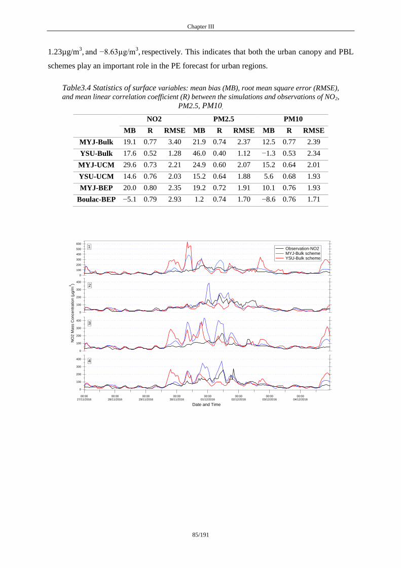
Chapter III
85/191
1.23µg/m3, and −8.63µg/m
3, respectively. This indicates that both the urban canopy and PBL
schemes play an important role in the PE forecast for urban regions.
Table3.4 Statistics of surface variables: mean bias (MB), root mean square error (RMSE),
and mean linear correlation coefficient (R) between the simulations and observations of NO2,
PM2.5, PM10.
NO2 PM2.5 PM10
MB R RMSE MB R RMSE MB R RMSE
MYJ-Bulk 19.1 0.77 3.40 21.9 0.74 2.37 12.5 0.77 2.39
YSU-Bulk 17.6 0.52 1.28 46.0 0.40 1.12 −1.3 0.53 2.34
MYJ-UCM 29.6 0.73 2.21 24.9 0.60 2.07 15.2 0.64 2.01
YSU-UCM 14.6 0.76 2.03 15.2 0.64 1.88 5.6 0.68 1.93
MYJ-BEP 20.0 0.80 2.35 19.2 0.72 1.91 10.1 0.76 1.93
Boulac-BEP −5.1 0.79 2.93 1.2 0.74 1.70 −8.6 0.76 1.71
600
500
400
300
200
100
0
00:0027/11/2016
00:0028/11/2016
00:0029/11/2016
00:0030/11/2016
00:0001/12/2016
00:0002/12/2016
00:0003/12/2016
00:0004/12/2016
Date and Time
400
300
200
100
0
NO
2 M
ass C
on
ce
ntr
atio
n (
µg
/m3)
400
300
200
100
0
400
300
200
100
0
1
2
3
4
Observation-NO2 MYJ-Bulk scheme YSU-Bulk scheme
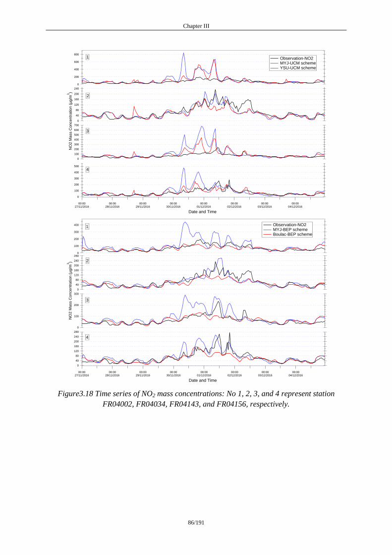
Chapter III
86/191
Figure3.18 Time series of NO2 mass concentrations: No 1, 2, 3, and 4 represent station
FR04002, FR04034, FR04143, and FR04156, respectively.
800
600
400
200
0
00:0027/11/2016
00:0028/11/2016
00:0029/11/2016
00:0030/11/2016
00:0001/12/2016
00:0002/12/2016
00:0003/12/2016
00:0004/12/2016
Date and Time
240
200
160
120
80
40
0
NO
2 M
ass C
on
ce
ntr
atio
n (
µg
/m3)
700
600
500
400
300
200
100
0
500
400
300
200
100
0
1
2
3
4
Observation-NO2 MYJ-UCM scheme YSU-UCM scheme
400
300
200
100
0
00:0027/11/2016
00:0028/11/2016
00:0029/11/2016
00:0030/11/2016
00:0001/12/2016
00:0002/12/2016
00:0003/12/2016
00:0004/12/2016
Date and Time
280
240
200
160
120
80
40
0
NO
2 M
ass C
on
ce
ntr
atio
n (
µg
/m3)
300
200
100
0
280
240
200
160
120
80
40
0
1
2
3
4
Observation-NO2 MYJ-BEP scheme Boulac-BEP scheme
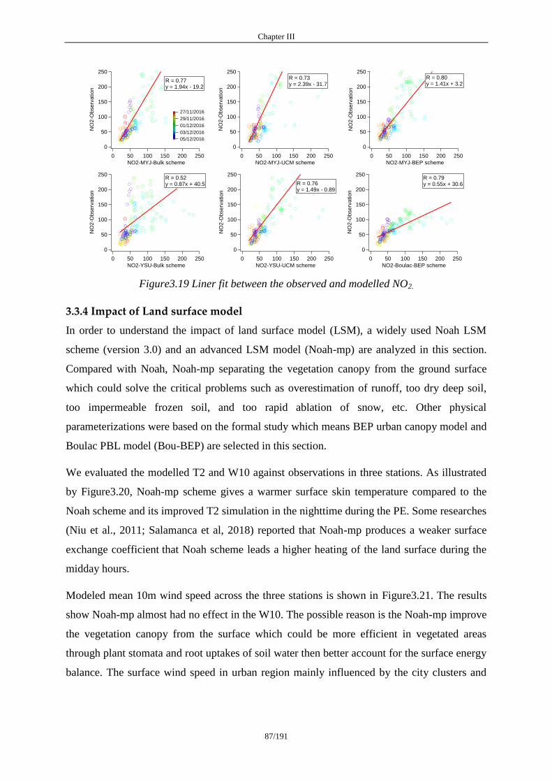
Chapter III
87/191
Figure3.19 Liner fit between the observed and modelled NO2.
3.3.4 Impact of Land surface model
In order to understand the impact of land surface model (LSM), a widely used Noah LSM
scheme (version 3.0) and an advanced LSM model (Noah-mp) are analyzed in this section.
Compared with Noah, Noah-mp separating the vegetation canopy from the ground surface
which could solve the critical problems such as overestimation of runoff, too dry deep soil,
too impermeable frozen soil, and too rapid ablation of snow, etc. Other physical
parameterizations were based on the formal study which means BEP urban canopy model and
Boulac PBL model (Bou-BEP) are selected in this section.
We evaluated the modelled T2 and W10 against observations in three stations. As illustrated
by Figure3.20, Noah-mp scheme gives a warmer surface skin temperature compared to the
Noah scheme and its improved T2 simulation in the nighttime during the PE. Some researches
(Niu et al., 2011; Salamanca et al, 2018) reported that Noah-mp produces a weaker surface
exchange coefficient that Noah scheme leads a higher heating of the land surface during the
midday hours.
Modeled mean 10m wind speed across the three stations is shown in Figure3.21. The results
show Noah-mp almost had no effect in the W10. The possible reason is the Noah-mp improve
the vegetation canopy from the surface which could be more efficient in vegetated areas
through plant stomata and root uptakes of soil water then better account for the surface energy
balance. The surface wind speed in urban region mainly influenced by the city clusters and
250
200
150
100
50
0
NO
2-O
bse
rva
tio
n
250200150100500
NO2-MYJ-BEP scheme
R = 0.80y = 1.41x + 3.2
250
200
150
100
50
0
NO
2-O
bse
rva
tio
n
250200150100500
NO2-MYJ-UCM scheme
R = 0.73y = 2.39x - 31.7
250
200
150
100
50
0
NO
2-O
bse
rva
tio
n
250200150100500
NO2-MYJ-Bulk scheme
05/12/2016
03/12/2016
01/12/2016
29/11/2016
27/11/2016
R = 0.77y = 1.94x - 19.2
250
200
150
100
50
0
NO
2-O
bse
rva
tio
n
250200150100500
NO2-YSU-Bulk scheme
R = 0.52y = 0.87x + 40.5
250
200
150
100
50
0
NO
2-O
bse
rva
tio
n
250200150100500
NO2-YSU-UCM scheme
R = 0.76y = 1.49x - 0.89
250
200
150
100
50
0
NO
2-O
bse
rva
tio
n
250200150100500
NO2-Boulac-BEP scheme
R = 0.79y = 0.55x + 30.6
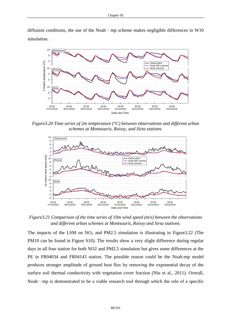
Chapter III
88/191
diffusion conditions, the use of the Noah‐mp scheme makes negligible differences in W10
simulation.
Figure3.20 Time series of 2m temperature (°C) between observations and different urban
schemes at Montsouris, Roissy, and Sirta stations.
Figure3.21 Comparison of the time series of 10m wind speed (m/s) between the observations
and different urban schemes at Montsouris, Roissy and Sirta stations.
The impacts of the LSM on NO2 and PM2.5 simulation is illustrating in Figure3.22 (The
PM10 can be found in Figure S10). The results show a very slight difference during regular
days in all four station for both NO2 and PM2.5 simulation but gives some differences at the
PE in FR04034 and FR04143 station. The possible reason could be the Noah-mp model
produces stronger amplitude of ground heat flux by removing the exponential decay of the
surface soil thermal conductivity with vegetation cover fraction (Niu et al., 2011). Overall,
Noah‐mp is demonstrated to be a viable research tool through which the role of a specific
10
5
0
2 m
ete
rs t
em
pe
ratu
re (
ºC)
00:0027/11/2016
00:0028/11/2016
00:0029/11/2016
00:0030/11/2016
00:0001/12/2016
00:0002/12/2016
00:0003/12/2016
00:0004/12/2016
Date and Time
10
5
0
10
5
0
Observation Noah-MP scheme Noah scheme
Montsouris
Roissy
Sirta
10
8
6
4
2
0
10
me
ters
win
d s
pe
ed
(m
/s)
00:0027/11/2016
00:0028/11/2016
00:0029/11/2016
00:0030/11/2016
00:0001/12/2016
00:0002/12/2016
00:0003/12/2016
00:0004/12/2016
Date and Time
10
8
6
4
2
0
10
8
6
4
2
0
Observation Noah-MP scheme Noah scheme
Montsouris
Roissy
Sirta
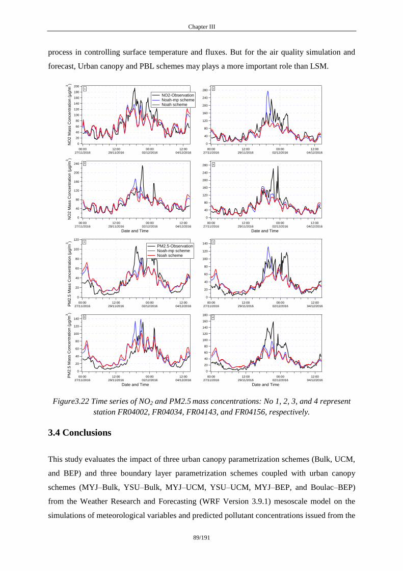
Chapter III
89/191
process in controlling surface temperature and fluxes. But for the air quality simulation and
forecast, Urban canopy and PBL schemes may plays a more important role than LSM.
Figure3.22 Time series of NO2 and PM2.5 mass concentrations: No 1, 2, 3, and 4 represent
station FR04002, FR04034, FR04143, and FR04156, respectively.
3.4 Conclusions
This study evaluates the impact of three urban canopy parametrization schemes (Bulk, UCM,
and BEP) and three boundary layer parametrization schemes coupled with urban canopy
schemes (MYJ–Bulk, YSU–Bulk, MYJ–UCM, YSU–UCM, MYJ–BEP, and Boulac–BEP)
from the Weather Research and Forecasting (WRF Version 3.9.1) mesoscale model on the
simulations of meteorological variables and predicted pollutant concentrations issued from the
280
240
200
160
120
80
40
0
00:0027/11/2016
12:0029/11/2016
00:0002/12/2016
12:0004/12/2016
Date and Time
4
200
180
160
140
120
100
80
60
40
20
0 NO
2 M
ass C
oncentr
atio
n (
µg/m
3)
00:0027/11/2016
12:0029/11/2016
00:0002/12/2016
12:0004/12/2016
1
NO2-Observation Noah-mp scheme Noah scheme
240
200
160
120
80
40
0
NO
2 M
ass C
oncentr
atio
n (
µg/m
3)
00:0027/11/2016
12:0029/11/2016
00:0002/12/2016
12:0004/12/2016
Date and Time
3
280
240
200
160
120
80
40
0
00:0027/11/2016
12:0029/11/2016
00:0002/12/2016
12:0004/12/2016
2
120
100
80
60
40
20
0
PM
2.5
Ma
ss C
on
ce
ntr
atio
n (
µg
/m3)
00:0027/11/2016
12:0029/11/2016
00:0002/12/2016
12:0004/12/2016
1
PM2.5-Observation Noah-mp scheme Noah scheme
140
120
100
80
60
40
20
0
00:0027/11/2016
12:0029/11/2016
00:0002/12/2016
12:0004/12/2016
2
140
120
100
80
60
40
20
0
PM
2.5
Ma
ss C
on
ce
ntr
atio
n (
µg
/m3)
00:0027/11/2016
12:0029/11/2016
00:0002/12/2016
12:0004/12/2016
Date and Time
3180
160
140
120
100
80
60
40
20
0
00:0027/11/2016
12:0029/11/2016
00:0002/12/2016
12:0004/12/2016
Date and Time
4

Chapter III
90/191
CHIMERE chemical transport model. This study aims at understanding those impacts on the
short-term pollution episode in the Paris region, France.
For the first time, chemistry transport models have been used with a first layer at 4m to better
account for physical processes within the suburban layer in relation to ground emissions such
as road traffic. Clearly, the sharp gradient of concentrations shows the added value of using
such a low level in urban areas. This study shows the high sensitivity of air quality simulation
to meteorological model outputs during stable conditions favorable to the occurrence of PM
episodes.
Three urban canopy models could reproduce the T2 effectively in the daytime; the Bulk and
UCM model reproduced the W10 well, but the BEP model underestimates W10 for the whole
episode, indicating an important impact of buildings on the diffusion rate for this scheme. The
UCM scheme overestimates the surface heat index in rural areas, leading to a slight negative
bias for T2 in rural versus urban areas. T2 displays ambiguous results, while all schemes
reproduced results well at Sirta station but overestimated during nighttime at Montsouris and
Roissy during a pollution episode. This could be due to the use of a single urban category in
this study, which leads to a discrepancy that causes more spatial variability in urban
parameters. NO2, PM2.5, and PM10 were selected to evaluate the effect of physics
parameterizations on air quality simulation. Large differences were found in the simulation of
pollutant concentrations, with an overall overestimation during the pollution episode.
The six PBL sensitivity tests display an underestimation of the PBL height when compared
with the observations issued from the Lidar. All the sensitivity tests, except Boulac–BEP,
could not effectively simulate the PBL height during the pollution episode. The two PBL
schemes coupled with the BEP scheme still underestimated the W10 for the whole period, but
the Boulac–BEP scheme improved the simulations compared with the MYJ–BEP scheme.
The Boulac–BEP scheme had a significantly better performance than the other schemes for
the simulation of pollutant concentrations, indicating that both the canopy parametrization and
PBL schemes have a positive effect on air quality simulation in urban regions, especially
during pollution episodes. The Noah-mp land surface scheme has slightly impact for both
meteorological and air quality simulation. An advanced urban category could improve air
quality prediction in urban regions.
Chapter III
91/191
References
Allen, L.; Lindberg, F.; Grimmond, C.S.B. Global to city scale urban anthropogenic heat flux:
Model and variability. Int. J. Clim. 2010, 31, 1990–2005.
Anderson, W.; Meneveau, C. A Large-Eddy Simulation Model for Boundary-Layer Flow
over Surfaces with Horizontally Resolved but Vertically Unresolved Roughness Elements.
Bound. Layer Meteorol. 2010, 137, 397–415.
Baklanov, A.; Mestayer, P.G.; Clappier, A.; Zilitinkevich, S.; Joffre, S.; Mahura, A.; Nielsen,
N.W. Towards improving the simulation of meteorological fields in urban areas through
updated/advanced surface fluxes description. Atmos. Chem. Phys. Discuss. 2008, 8, 523–543.
Barlage, M.; Miao, S.; Chen, F. Impact of physics parameterizations on high‐resolution
weather prediction over two Chinese megacities. J. Geophys. Res. Atmos. 2016, 121, 4487–
4498.
Best, M. Representing urban areas within operational numerical weather prediction models.
Bound. Layer Meteorol. 2005, 114, 91–109.
Bessagnet, B.; Hodzic, A.; Vautard, R.; Beekmann, M.; Cheinet, S.; Honoré, C.; Liousse, C.;
Rouil, L. Aerosol modeling with CHIMERE—preliminary evaluation at the continental scale.
Atmos. Environ. 2004, 38, 2803–2817.
Bessagnet, B.; Beauchamp, M.; Guerreiro, C.; De Leeuw, F.; Tsyro, S.; Colette, A.; Meleux,
F.; Rouïl, L.; Ruyssenaars, P.; Sauter, F.; et al. Can further mitigation of ammonia emissions
reduce exceedances of particulate matter air quality standards? Environ. Sci. Policy 2014, 44,
149–163.
Bessagnet, B.; Menut, L.; Colette, A.; Couvidat, F.; Dan, M.; Mailler, S.; Létinois, L.; Pont,
V.; Rouïl, L. An Evaluation of the CHIMERE Chemistry Transport Model to Simulate Dust
Outbreaks across the Northern Hemisphere in March 2014. Atmosphere 2017, 8, 251.
Borrego, C.; Souto, J.A.; Monteiro, A.; Dios, M.; Rodriguez, A.; Ferreira, J.; Saavedra, S.;
Casares, J.J.; Miranda, A.I. The role of transboundary air pollution over Galicia and North
Portugal area. Environ. Sci. Pollut. Res. 2013, 20, 2924–2936.
Bougeault, P.; Lacarrère. P. Parameterization of orographic induced turbulence in a meso beta
scale model. Mon. Weather Rev. 1989, 117, 1872–1890.
Bowden, J.H.; Otte, T.L.; Nolte, C.G.; Otte, M. Examining Interior Grid Nudging Techniques
Using Two-Way Nesting in the WRF Model for Regional Climate Modeling. J. Clim. 2012,
25, 2805–2823.
Coseo, L. Larsen Cooling the heat island in compact urban environments: The effectiveness of
Chicago’s green alley program. Procedia Eng. 2015, 118, 691–710.
Couvidat, F.; Bessagnet, B.; Garcia-Vivanco, M.; Real, E.; Menut, L.; and Colette, A.
Development of an inorganic and organic aerosol model (Chimere2017b2 v1.0): Seasonal and
spatial evaluation over Europe. Geosci. Model. Dev. 2018, 11, 165–194.
Chapter III
92/191
EEA. Air Quality in Europe—2018 Report; EEA Report No 13/2018; European Environment
Agency: Copenhagen, Denmark, 2018.
Falasca, S.; Catalano, F.; Moroni, M. Numerical Study of the Daytime Planetary Boundary
Layer over an Idealized Urban Area: Influence of Surface Properties, Anthropogenic Heat
Flux, and Geostrophic Wind Intensity. J. Appl. Meteorol. Clim. 2016, 55, 1021–1039.
Falasca, S.; Catalano, F. Impact of Highly Reflective Materials on Meteorology, PM10 and
Ozone in Urban Areas: A Modeling Study with WRF-CHIMERE at High Resolution over Milan
(Italy). Urban Sci. 2018, 2, 18.
Fan, S.; Guo, Y.R.; Chen, M.; Zhong, J.; Chu, Y.; Wang, W.; Huang, X.Y.; Wang, Y.; Guo,
Y.H. Application of WRF 3D Var to a high-resolution model over Beijing area. Plateau
Meteorol. 2008, 27, 1181–1188.
Flaounas, E.; Bastin, S.; Janicot, S. Regional climate modelling of the 2006 West African
monsoon: sensitivity to convection and planetary boundary layer parameterisation using WRF.
Clim. Dyn. 2010, 36, 1083–1105.
Gedzelman, S.D.; Austin, S.; Cermak, R.; Stefano, N.; Partridge, S.; Quesenberry, S.;
Robinson, D.A. Mesoscale aspects of the Urban Heat Island around New York City. Theor.
Appl. Clim. 2003, 75, 29–42.
Glisan, J.M.; Gutowski, W.J.; Cassano, J.J.; Higgins, M.E. Effects of Spectral Nudging in
WRF on Arctic Temperature and Precipitation Simulations. J. Clim. 2013, 26, 3985–3999.
Hamaoui-Laguel, L.; Meleux, F,; Beekmann, M,; Bessagnet, B,; Génermont, S,; Cellier, P,;
Létinois, L. Improving ammonia emissions in air quality modelling for France Atmospheric
Environment, 92 (2014), pp. 584-595
Hariprasad, K.B.R.R.; Srinivas, C.V.; Singh, A.B.; Rao, S.V.B.; Baskaran, R.; Venkatraman, B.
Numerical simulation and inter comparison of boundary layer structure with different PBL
schemes in WRF using experimental observations at a tropical site. Atmos. Res. 2014, 145, 27–
44.
He, Q.; Zhao, X.; Lu, J.; Zhou, G.; Yang, H.; Gao, W.; Yu, W.; Cheng, T. Impacts of
biomass-burning on aerosol properties of a severe haze event over Shanghai. Particuology
2015, 20, 52–60.
Hu, X.-M.; Nielsen-Gammon, J.W.; Zhang, F. Evaluation of Three Planetary Boundary Layer
Schemes in the WRF Model. J. Appl. Meteorol. Clim. 2010, 49, 1831–1844.
Janjic, Z. Nonsingular Implementation of the Mellor-Yamada Level 2.5 Scheme in the NCEP
Meso Model; NCEP Office Note, No. 437; National Centers for Environmental Prediction:
College Park, MD, USA, 2002; p. 61.
Janjić, Z.I. The Step-Mountain Coordinate: Physical Package. Mon. Weather. Rev. 1990, 118,
1429–1443.
Hong, S.-Y.; Noh, Y.; Dudhia, J. A New Vertical Diffusion Package with an Explicit
Treatment of Entrainment Processes. Mon. Weather. Rev. 2006, 134, 2318–2341.
Chapter III
93/191
Kim, Y.; Sartelet, K.; Raut, J.-C.; Chazette, P. Evaluation of the Weather Research and
Forecast/Urban Model Over Greater Paris. Bound. Layer Meteorol. 2013, 149, 105–132,
doi:10.1007/s10546-013-9838-6.
Kim, Y.; Sartelet, K.; Raut, J.-C.; Chazette, P. Influence of an urban canopy model and PBL
schemes on vertical mixing for air quality modeling over Greater Paris. Atmos. Environ. 2015,
107, 289–306.
Kleczek, M.A.; Steeneveld, G.-J.; Holtslag, A. Evaluation of the Weather Research and
Forecasting Mesoscale Model for GABLS3: Impact of Boundary-Layer Schemes, Boundary
Conditions and Spin-Up. Bound. Layer Meteorol. 2014, 152, 213–243.
Kusaka, H.; Kondo, K.; Kikegawa, Y.; Kimura, F. A simple single‐layer urban canopy model
for atmospheric models: Comparison with multi‐layer and slab models. Bound. Layer Meteorol.
2001, 101, 329–358.
Kusaka, H.; Kimura, F. Coupling a Single-Layer Urban Canopy Model with a Simple
Atmospheric Model: Impact on Urban Heat Island Simulation for an Idealized Case. J.
Meteorol. Soc. Jpn. 2004, 82, 67–80.
Lai, L.-W.; Cheng, W.-L. Air quality influenced by urban heat island coupled with synoptic
weather patterns. Sci. Total. Environ. 2009, 407, 2724–2733.
LeMone, M.; Tewari, M.; Chen, F.; Dudhia, J. Objectively‐determined fair‐weather convective
boundary layer depths in the ARW‐WRF NWP model and their comparison to CASES‐97
observations. Mon. Weather Rev. 2013, 141, 30–54.
LeMone, M.; Tewari, M.; Chen, F.; Dudhia, J. Objectively‐determined fair‐weather NBL
features in the ARW‐WRF model and their comparison to CASES‐97 observations. Mon.
Weather Rev. 2014, 142, 2709–2732.
Li, M.; Ma, Y.; Ma, W.; Hu, Z.; Ishikawa, H.; Su, Z.; Sun, F. Analysis of turbulence
characteristics over the northern Tibetan Plateau area. Adv. Atmos. Sci. 2006, 23, 579–585.
Lin, C.-Y.; Chen, F.; Huang, J.-C.; Chen, W.-C.; Liou, Y.-A.; Chen, W.-N.; Liu, S.-C. Urban
heat island effect and its impact on boundary layer development and land–sea circulation over
northern Taiwan. Atmos. Environ. 2008a, 42, 5635–5649.
Lin, C.-Y.; Chen, W.-C.; Liu, S.C.; Liou, Y.A.; Liu, G.; Lin, T. Numerical study of the impact
of urbanization on the precipitation over Taiwan. Atmos. Environ. 2008b, 42, 2934–2947.
Liu, Y.; Chen, F.; Warner, T.; Basara, J.B. Verification of a Mesoscale Data-Assimilation and
Forecasting System for the Oklahoma City Area during the Joint Urban 2003 Field Project. J.
Appl. Meteorol. Clim. 2006, 45, 912–929.
Liu, M.; Chen, M. Evaluation of BJ-RUC system for the forecast quality of planetary boundary
layer in Beijing area. J. Appl. Meteorol. Sci. 2014, 25, 212–221.
Mailler, S.; Menut, L.; Khvorostyanov, D.; Valari, M.; Couvidat, F.; Siour, G.; Turquety, S.;
Briant, R.; Tuccella, P.; Bessagnet, B.; et al. CHIMERE-2017: From urban to hemispheric
chemistry-transport modeling. Geosci. Model Dev. 2017, 10, 2397–2423.
Chapter III
94/191
Markakis, K.; Valari, M.; Engardt, M.; Lacressonniere, G.; Vautard, R.; Andersson, C.
Mid-21st century air quality at the urban scale under the influence of changed climate and
emissions case studies for Paris and Stockholm. Atmos. Chem. Phys. 2016, 16, 1877–1894.
Martilli, A.; Clappier, A.; Rotach, M. An urban surface exchange parameterization for
mesoscale models. Bound. Layer Meteorol. 2002, 104, 261–304.
Mellor, G.L.; Yamada, T. Development of a turbulence closure model for geophysical fluid
problems. Rev. Geophys. 1982, 20, 851–875.
Menut, L.; Goussebaile, A.; Bessagnet, B.; Khvorostiyanov, D.; Ung, A. Impact of realistic
hourly emissions profiles on air pollutants concentrations modelled with CHIMERE. Atmos.
Environ. 2012, 49, 233–244.
Menut, L.; Bessagnet, B.; Khvorostyanov, D.; Beekmann, M.; Blond, N.; Colette, A.; Coll, I.;
Curci, G.; Forêt, G.; Hodzic, A.; et al. CHIMERE 2013: A model for regional atmospheric
composition modelling. Geosci. Model Dev. 2013, 6, 981–1028.
Miao, S.; Chen, F.; Li, Q.; Fan, S. Impacts of urban processes and urbanization on summer
precipitation: A case study of heavy rainfallin Beijing on 1 Aug 2006. J. Appl. Meteorol.
Climatol. 2010, 50, 806–825.
Molteni, F.; Buizza, R.; Palmer, T.N.; Petroliagis, T. The ECMWF ensemble prediction system:
Methodology and validation. Quart. J. R. Meteor. Soc. 1996, 122, 73–119.
Niu, G.‐Y., Yang, Z. L., Mitchell, K. E., Chen, F., Ek, M. B., Barlage, M., et al. The
community Noah land surface model with multiparameterization options (Noah‐MP): 1. Model
description and evaluation with local‐scale measurements. Journal of Geophysical Research.
2011, 116, D12109.
Oke, T. K. Boundary Layer Climates (2nd ed.), Rutledge, New York, 1988. p. 464
Patricola, C.M.; Li, M.; Xu, Z.; Chang, P.; Saravanan, R.; Hsieh, J.-S. An investigation of
tropical Atlantic bias in a high-resolution coupled regional climate model. Clim. Dyn. 2012,
39, 2443–2463.
Salamanca, F.; Krpo, A.; Martilli, A.; Clappier, A. A new building energy model coupled
with an urban canopy parameterization for urban climate simulations—Part I. formulation,
verification, and sensitivity analysis of the model. Theor. Appl. Clim. 2009a, 99, 331–344.
Salamanca, F.; Martilli, A. A new Building Energy Model coupled with an Urban Canopy
Parameterization for urban climate simulations—Part II. Validation with one-dimension
off-line simulations. Theor. Appl. Clim. 2009a, 99, 345–356.
Sarrat, C.; Lemonsu, A.; Masson, V.; Guedalia, D. Impact of urban heat island on regional
atmospheric pollution. Atmos. Environ. 2006, 40, 1743–1758.
Toll, I.; Baldasano, J.M. Modeling of photochemical air pollution in the Barcelona area with
highly disaggregated anthropogenic and biogenic emissions. Atmos. Environ. 2000, 34, 3069–
3084.

Chapter III
95/191
Troen, I.B.; Mahrt, L. A simple model of the atmospheric boundary layer; sensitivity to
surface evaporation. Bound. Layer Meteorol. 1986, 37, 129–148.
Tuccella, P.; Curci, G.; Visconti, G.; Bessagnet, B.; Menut, L.; Park, R.J. Modeling of gas and
aerosol with WRF/Chem over Europe: Evaluation and sensitivity study. J. Geophys. Res.
Space Phys. 2012, 117, D03303.
Tyagi, B.; Magliulo, V.; Finardi, S.; Gasbarra, D.; Carlucci, P.; Toscano, P.; Zaldei, A.;
Riccio, A.; Calori, G.; D’Allura, A.; et al. Performance Analysis of Planetary Boundary Layer
Parameterization Schemes in WRF Modeling Set Up over Southern Italy. Atmosphere 2018, 9,
272.
Valari, M.; Menut, L. Transferring the heterogeneity of surface emissions to variability in
pollutant concentrations over urban areas through a chemistry-transport model. Atmos. Environ.
2014, 44, 3229–3238.
Vigaud, N.; Roucou, P.; Fontaine, B.; Sijikumar, S.; Tyteca, S. WRF/ARPEGE-CLIMAT
simulated climate trends over West Africa. Clim. Dyn. 2009, 36, 925–944.
Wang, L.T.; Wei, Z.; Yang, J.; Zhang, Y.; Zhang, F.F.; Su, J.; Meng, C.C.; Zhang, Q. The
2013 severe haze over southern Hebei, China: model evaluation, source apportionment, and
policy implications. Atmos. Chem. Phys. Discuss. 2014, 14, 3151–3173.
Wang, L.; Liu, J.; Gao, Z.; Li, Y.; Huang, M.; Fan, S.; Zhang, X.; Yang, Y.; Miao, S.; Zou, H.;
et al. Vertical observations of the atmospheric boundary layer structure over Beijing urban
area during air pollution episodes. Atmos. Chem. Phys. Discuss. 2019, 19, 6949–6967,
doi:10.5194/acp-19-6949-2019.
Wu, J.; Zha, J.L.; Zhao, D.M.; Yang, Q.D. Changes in terrestrial near-surface wind speed and
their possible causes: An overview. Clim. Dyn. 2017, 51, 2039–207

Chapter IV
96/191
Chapter IV: On the impact of WRF-CHIMERE
vertical grid resolution and first layer height on
mesoscale meteorological and chemistry transport
modelling
This chapter has been designed to be considered for publication.
Chapter IV
97/191
Chapter IV: On the impact of WRF-CHIMERE vertical
grid resolution and first layer height on mesoscale
meteorological and chemistry transport modelling
Lei Jiang
1,2, *, Bertrand Bessagnet
1,†, Frederik Meleux
1, Frederic Tognet
1, Florian
Couvidat1
1 INERIS, National Institute for Industrial Environment and Risks, Parc Technologique
ALATA, 60550 Verneuil-en-Halatte, France 2 Sorbonne University, UPMC Univ Paris 06, DE129, 75005 Paris, France
† Now at European Commission, Joint Research Centre (JRC), 21027 Ispra, Italy.
Abstract
The mesoscale Weather Research and Forecasting (WRF) and chemistry transport model
(CTM) CHIMERE models were used to evaluate the impact of vertical grid resolution and first
layer height in meteorological and chemistry transport modelling. Three model configuration
(L4, L12 and L40) were investigated: (i) L4: 53 vertical layers in WRF and 20 vertical levels in
CHIMERE are defined, the first layer height is about 4m; (ii) L12: 51 vertical layers in WRF
and 20 vertical levels in CHIMERE, the first layer height approximately at 12m; (iii) L40: 36
vertical layer in WRF and 9 vertical levels in CHIMERE, the first layer height is approximately
at 40m. A fifteen days simulation including a three-day heavy pollution episode (PE) illustrates
the impact of vertical grid resolution. The first layer height has a relatively small impact on
meteorological simulation and the main differences of meteorological variables were observed
at nighttime. However, a consistent improvement in chemistry transport modelling were
displayed with refined vertical resolutions and the first layer height, compared to L12 and L40,
the average improvement from L4 case in terms of RMSE are 23.26% and 25.09% on regular
days (RD) defined as ―without pollution episodes‖ and 62% and 129% during PE respectively.
In general, the ability of the model with low vertical grid resolution to correctly predict air
quality is reasonable on RD or light pollution events, while it fails to predict correctly the
pollutant concentrations for heavy polluted situations. The performances were improved with
refined vertical resolutions particularly with extra fine first layer height at 4m.
Chapter IV
98/191
Résumé
Les modèles à méso-échelle CHIMERE et Weather Research and Forecasting (WRF) ont été
utilisés pour évaluer l'impact de la résolution de la grille verticale et de la hauteur de la
première couche dans la modélisation chimie transport. Trois configurations de modèles (L4,
L12 et L40) ont été étudiées : (i) L4 : 53 couches verticales dans WRF et 20 niveaux verticaux
dans CHIMERE sont définis, la hauteur de la première couche est d'environ 4m ; (ii) L12 : 51
couches verticales dans WRF et 20 niveaux verticaux dans CHIMERE, la hauteur de la
première couche est d'environ 12m ; (iii) L40 : 36 couches verticales dans WRF et 9 niveaux
verticaux dans CHIMERE, la hauteur de la première couche est d'environ 40m. Une
simulation sur quinze jours en hiver incluant un épisode de forte pollution (PE) de trois jours
illustre l'impact de la résolution de la grille verticale. La hauteur de la première couche a un
impact relativement faible sur la simulation météorologique et les principales différences de
variables météorologiques ont été observées la nuit. Cependant, une amélioration significative
de la modélisation du transport des polluants a été constatée avec des résolutions verticales
raffinées et la hauteur de la première couche. Ainsi, l’amélioration moyenne du cas L4 par
rapport à L12 et L40 en termes de RMSE est de 23,26% et 25,09% sur les jours réguliers (RD)
sans épisodes de pollution et 62% et 129% pendant PE respectivement. En général, la capacité
du modèle à faible résolution verticale à reproduire correctement les concentrations de
polluants est raisonnable sur les RD ou les épisodes de pollution légère, alors qu'il ne parvient
pas à reproduire correctement les concentrations de polluants pour les situations de forte
pollution. Les performances ont été améliorées avec une résolution verticale affinée, en
particulier avec une hauteur de première couche très fine.
Keywords: air quality; vertical resolution; first layer height; diffusion; urban
4.1 Introduction
The prevention and control of environmental pollution has become an important task in the
development and construction of the country, and the prevention and control of air pollution
has become the top priority (Lu et al., 2020). Over the past decades, European countries
deepen efforts to decouple air pollution from economic growth and the goal is to build an
ecological civilization society (Ivanova, 2011; Koolen and Rothenberg, 2019b; Nam et al.,
2010). Studies show many air pollutants have decreased substantially since mid-1980’s
(Grennfelt et al., 2020; Lelieveld et al., 2019; Renzi et al., 2017), for example, observation
Chapter IV
99/191
data show that in Europe, the concentration of PM2.5 drops by 2.5μg/m3 per year over the
past decades (Gozzi et al., 2017). However, some reports indicate more than 400,000 people
die prematurely due to air pollution each year in Europe and this number is one million in
1990 (Guerreiro et al., 2015). Air pollution is still one of the biggest threats to the health of
Europeans. In many European cities, the concentration of main pollutants still exceeds the
reference value of European Union (Barsova et al., 2019; Xu et al., 2017) and over the
hemispherical background concentrations (Vautard et al., 2009). Therefore, regional joint
prevention and control play an important role in improving air quality. At region and urban
scale, mesoscale chemistry transport model (CTM) are widely used to assess the efficiency of
such policies in controlling air pollution (Ma et al., 2020). With the continuous improvement
of pollution sources and meteorological knowledge, many studies have proved the important
role of horizontal resolution in improving model capabilities (Jensen et al., 2017; Martins,
2012; Russell et al., 2019; Thunis et al., 2016b). However, there is still a lack of research on
the effect of vertical grid resolution on the chemical transport processes. Accurate simulations
of near-surface parameters particularly the representation of turbulence is difficult but very
important on vertical mixing of meteorological and chemistry transport modelling. A spatial
resolution increase enhances the variability of the concentrations, but also the amplitude of
the errors due to meteorology, vertical resolution, land use or other factors (Aligo et al., 2009;
Vautard et al., 2007). Since human activities are mainly concentrated within 50 meters from
the ground, it is particularly important to improve the model's representation of pollutants in
low boundary height. Research found that adding an extra vertical layer close to the surface is
important for high nocturnal concentrations under stable boundary layers (Menut et al.,
2013b).
In this chapter, an evaluation of three vertical grid resolution configurations and a first layer
height, used to simulate a winter period including a short heavy pollution event in Paris region
is proposed.
4.2 Method
The mesoscale Weather Research and Forecasting (WRF) model in Version3.9.1 and CTM
model CHIMERE in Version2013 are used to simulate the meteorological parameters and
pollutant concentrations over Paris. The horizontal domain setting is same as that of in
Chapter II, with four nested-grid domains over Europe, France, the north of France, and
Ile-de-France, with horizontal resolutions of 45km, 15km, 5km, and 1.67km, respectively.
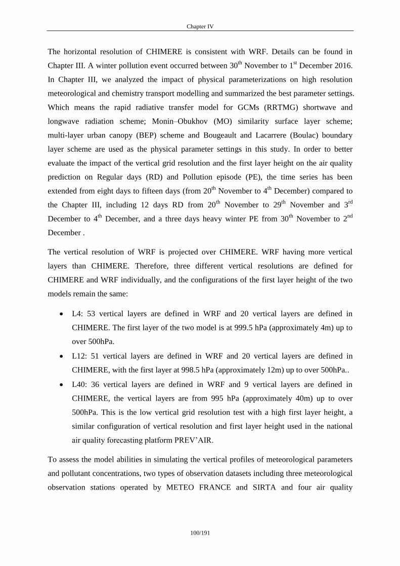
Chapter IV
100/191
The horizontal resolution of CHIMERE is consistent with WRF. Details can be found in
Chapter III. A winter pollution event occurred between 30th
November to 1st December 2016.
In Chapter III, we analyzed the impact of physical parameterizations on high resolution
meteorological and chemistry transport modelling and summarized the best parameter settings.
Which means the rapid radiative transfer model for GCMs (RRTMG) shortwave and
longwave radiation scheme; Monin–Obukhov (MO) similarity surface layer scheme;
multi-layer urban canopy (BEP) scheme and Bougeault and Lacarrere (Boulac) boundary
layer scheme are used as the physical parameter settings in this study. In order to better
evaluate the impact of the vertical grid resolution and the first layer height on the air quality
prediction on Regular days (RD) and Pollution episode (PE), the time series has been
extended from eight days to fifteen days (from 20th
November to 4th
December) compared to
the Chapter III, including 12 days RD from 20th
November to 29th
November and 3rd
December to 4th
December, and a three days heavy winter PE from 30th
November to 2nd
December .
The vertical resolution of WRF is projected over CHIMERE. WRF having more vertical
layers than CHIMERE. Therefore, three different vertical resolutions are defined for
CHIMERE and WRF individually, and the configurations of the first layer height of the two
models remain the same:
L4: 53 vertical layers are defined in WRF and 20 vertical layers are defined in
CHIMERE. The first layer of the two model is at 999.5 hPa (approximately 4m) up to
over 500hPa.
L12: 51 vertical layers are defined in WRF and 20 vertical layers are defined in
CHIMERE, with the first layer at 998.5 hPa (approximately 12m) up to over 500hPa..
L40: 36 vertical layers are defined in WRF and 9 vertical layers are defined in
CHIMERE, the vertical layers are from 995 hPa (approximately 40m) up to over
500hPa. This is the low vertical grid resolution test with a high first layer height, a
similar configuration of vertical resolution and first layer height used in the national
air quality forecasting platform PREV’AIR.
To assess the model abilities in simulating the vertical profiles of meteorological parameters
and pollutant concentrations, two types of observation datasets including three meteorological
observation stations operated by METEO FRANCE and SIRTA and four air quality
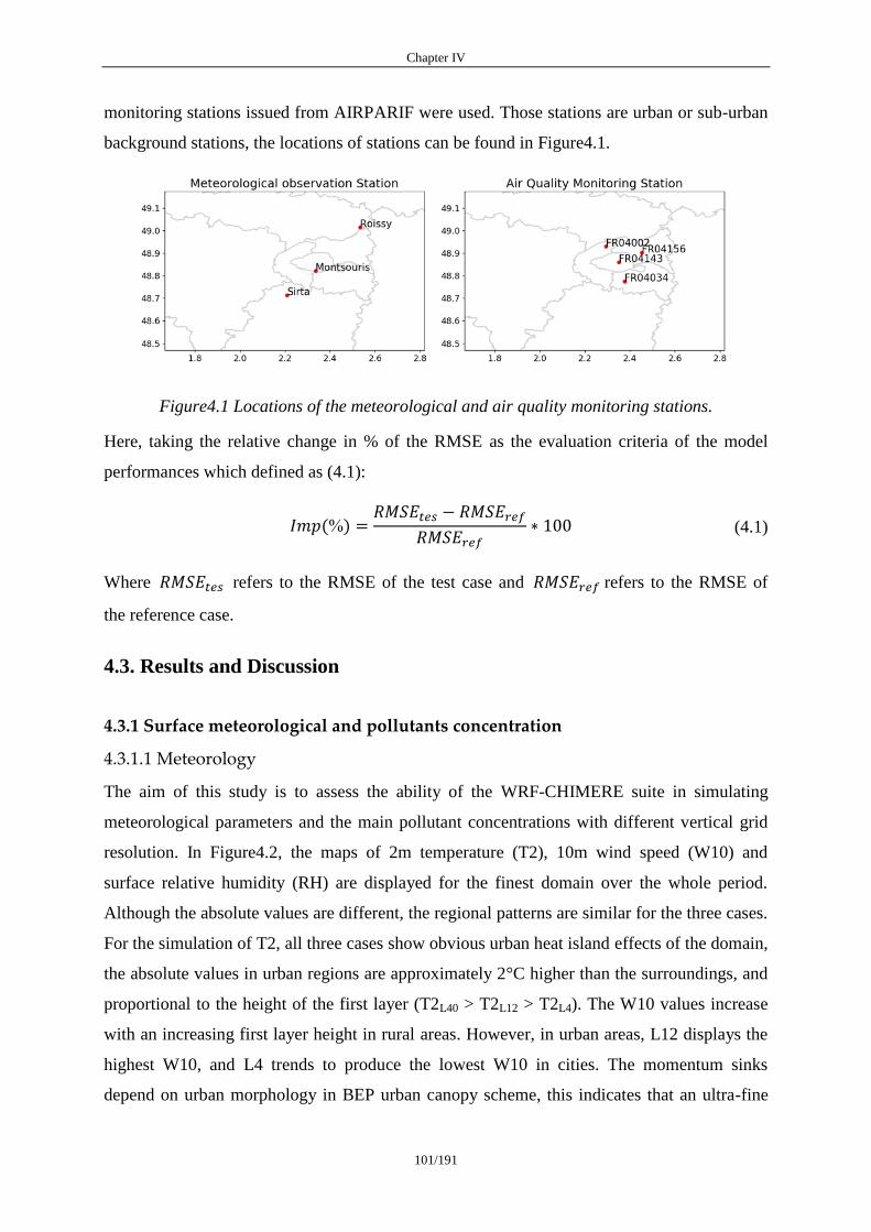
Chapter IV
101/191
monitoring stations issued from AIRPARIF were used. Those stations are urban or sub-urban
background stations, the locations of stations can be found in Figure4.1.
Figure4.1 Locations of the meteorological and air quality monitoring stations.
Here, taking the relative change in % of the RMSE as the evaluation criteria of the model
performances which defined as (4.1):
(%)
(4.1)
Where refers to the RMSE of the test case and refers to the RMSE of
the reference case.
4.3. Results and Discussion
4.3.1 Surface meteorological and pollutants concentration
4.3.1.1 Meteorology
The aim of this study is to assess the ability of the WRF-CHIMERE suite in simulating
meteorological parameters and the main pollutant concentrations with different vertical grid
resolution. In Figure4.2, the maps of 2m temperature (T2), 10m wind speed (W10) and
surface relative humidity (RH) are displayed for the finest domain over the whole period.
Although the absolute values are different, the regional patterns are similar for the three cases.
For the simulation of T2, all three cases show obvious urban heat island effects of the domain,
the absolute values in urban regions are approximately 2°C higher than the surroundings, and
proportional to the height of the first layer (T2L40 > T2L12 > T2L4). The W10 values increase
with an increasing first layer height in rural areas. However, in urban areas, L12 displays the
highest W10, and L4 trends to produce the lowest W10 in cities. The momentum sinks
depend on urban morphology in BEP urban canopy scheme, this indicates that an ultra-fine
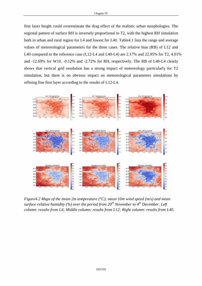
Chapter IV
102/191
first layer height could overestimate the drag effect of the realistic urban morphologies. The
regional pattern of surface RH is inversely proportional to T2, with the highest RH simulation
both in urban and rural region for L4 and lowest for L40. Table4.1 lists the range and average
values of meteorological parameters for the three cases. The relative bias (RB) of L12 and
L40 compared to the reference case (L12-L4 and L40-L4) are 2.17% and 22.95% for T2, 4.01%
and -12.69% for W10, -0.12% and -2.72% for RH, respectively. The RB of L40-L4 clearly
shows that vertical grid resolution has a strong impact of meteorology particularly for T2
simulation, but there is no obvious impact on meteorological parameters simulations by
refining fine first layer according to the results of L12-L4.
Figure4.2 Maps of the mean 2m temperature (°C); mean 10m wind speed (m/s) and mean
surface relative humidity (%) over the period from 20th
November to 4th
December. Left
column: results from L4; Middle column: results from L12; Right column: results from L40.
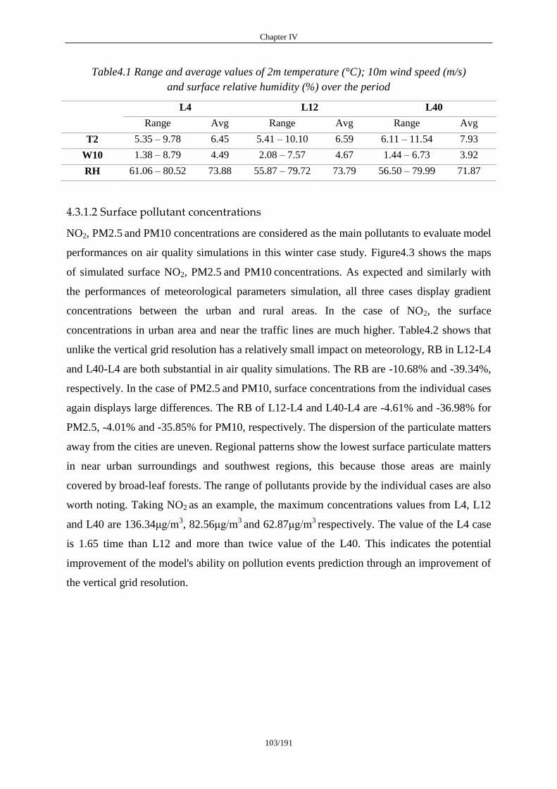
Chapter IV
103/191
Table4.1 Range and average values of 2m temperature (°C); 10m wind speed (m/s)
and surface relative humidity (%) over the period
L4 L12 L40
Range Avg Range Avg Range Avg
T2 5.35 – 9.78 6.45 5.41 – 10.10 6.59 6.11 – 11.54 7.93
W10 1.38 – 8.79 4.49 2.08 – 7.57 4.67 1.44 – 6.73 3.92
RH 61.06 – 80.52 73.88 55.87 – 79.72 73.79 56.50 – 79.99 71.87
4.3.1.2 Surface pollutant concentrations
NO2, PM2.5 and PM10 concentrations are considered as the main pollutants to evaluate model
performances on air quality simulations in this winter case study. Figure4.3 shows the maps
of simulated surface NO2, PM2.5 and PM10 concentrations. As expected and similarly with
the performances of meteorological parameters simulation, all three cases display gradient
concentrations between the urban and rural areas. In the case of NO2, the surface
concentrations in urban area and near the traffic lines are much higher. Table4.2 shows that
unlike the vertical grid resolution has a relatively small impact on meteorology, RB in L12-L4
and L40-L4 are both substantial in air quality simulations. The RB are -10.68% and -39.34%,
respectively. In the case of PM2.5 and PM10, surface concentrations from the individual cases
again displays large differences. The RB of L12-L4 and L40-L4 are -4.61% and -36.98% for
PM2.5, -4.01% and -35.85% for PM10, respectively. The dispersion of the particulate matters
away from the cities are uneven. Regional patterns show the lowest surface particulate matters
in near urban surroundings and southwest regions, this because those areas are mainly
covered by broad-leaf forests. The range of pollutants provide by the individual cases are also
worth noting. Taking NO2 as an example, the maximum concentrations values from L4, L12
and L40 are 136.34μg/m3, 82.56μg/m
3 and 62.87μg/m
3 respectively. The value of the L4 case
is 1.65 time than L12 and more than twice value of the L40. This indicates the potential
improvement of the model's ability on pollution events prediction through an improvement of
the vertical grid resolution.
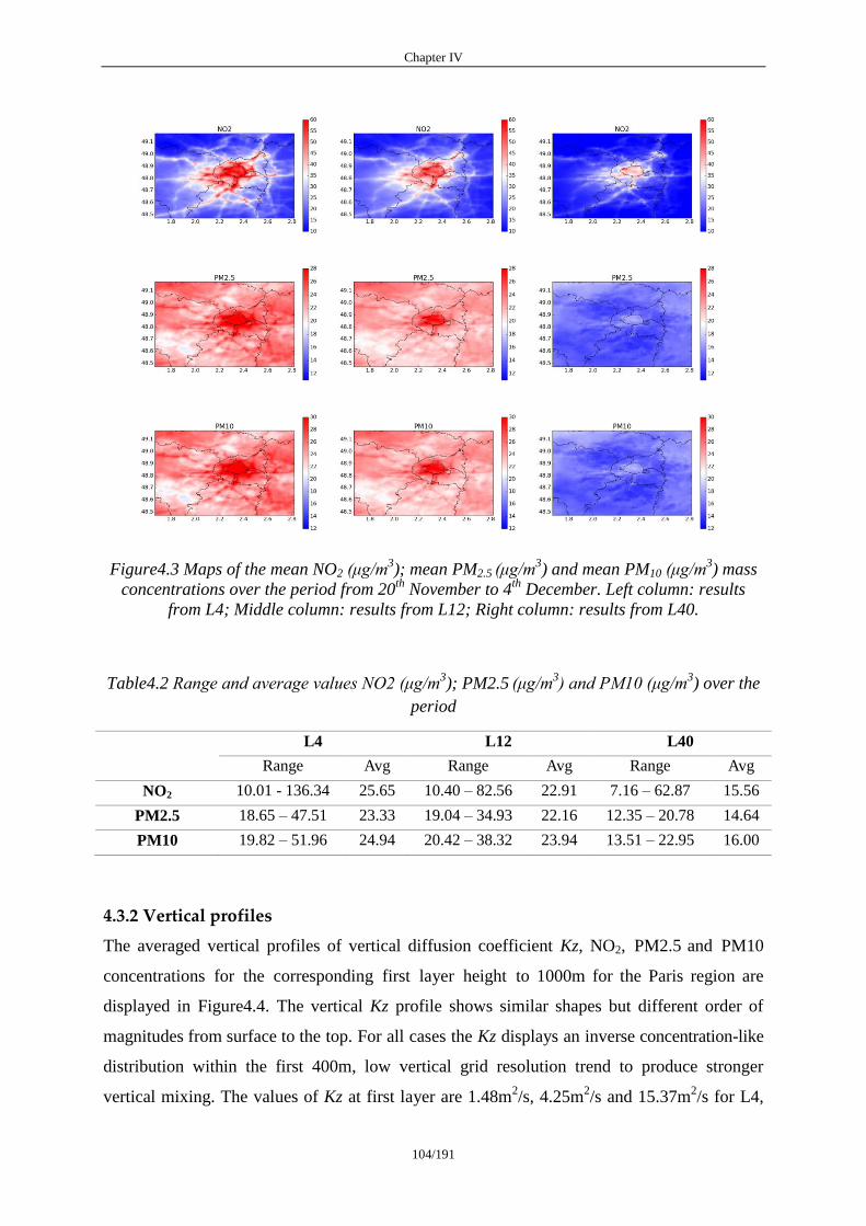
Chapter IV
104/191
Figure4.3 Maps of the mean NO2 (μg/m3); mean PM2.5 (μg/m
3) and mean PM10 (μg/m
3) mass
concentrations over the period from 20th
November to 4th
December. Left column: results
from L4; Middle column: results from L12; Right column: results from L40.
Table4.2 Range and average values NO2 (μg/m3); PM2.5 (μg/m
3) and PM10 (μg/m
3) over the
period
L4 L12 L40
Range Avg Range Avg Range Avg
NO2 10.01 - 136.34 25.65 10.40 – 82.56 22.91 7.16 – 62.87 15.56
PM2.5 18.65 – 47.51 23.33 19.04 – 34.93 22.16 12.35 – 20.78 14.64
PM10 19.82 – 51.96 24.94 20.42 – 38.32 23.94 13.51 – 22.95 16.00
4.3.2 Vertical profiles
The averaged vertical profiles of vertical diffusion coefficient Kz, NO2, PM2.5 and PM10
concentrations for the corresponding first layer height to 1000m for the Paris region are
displayed in Figure4.4. The vertical Kz profile shows similar shapes but different order of
magnitudes from surface to the top. For all cases the Kz displays an inverse concentration-like
distribution within the first 400m, low vertical grid resolution trend to produce stronger
vertical mixing. The values of Kz at first layer are 1.48m2/s, 4.25m
2/s and 15.37m
2/s for L4,
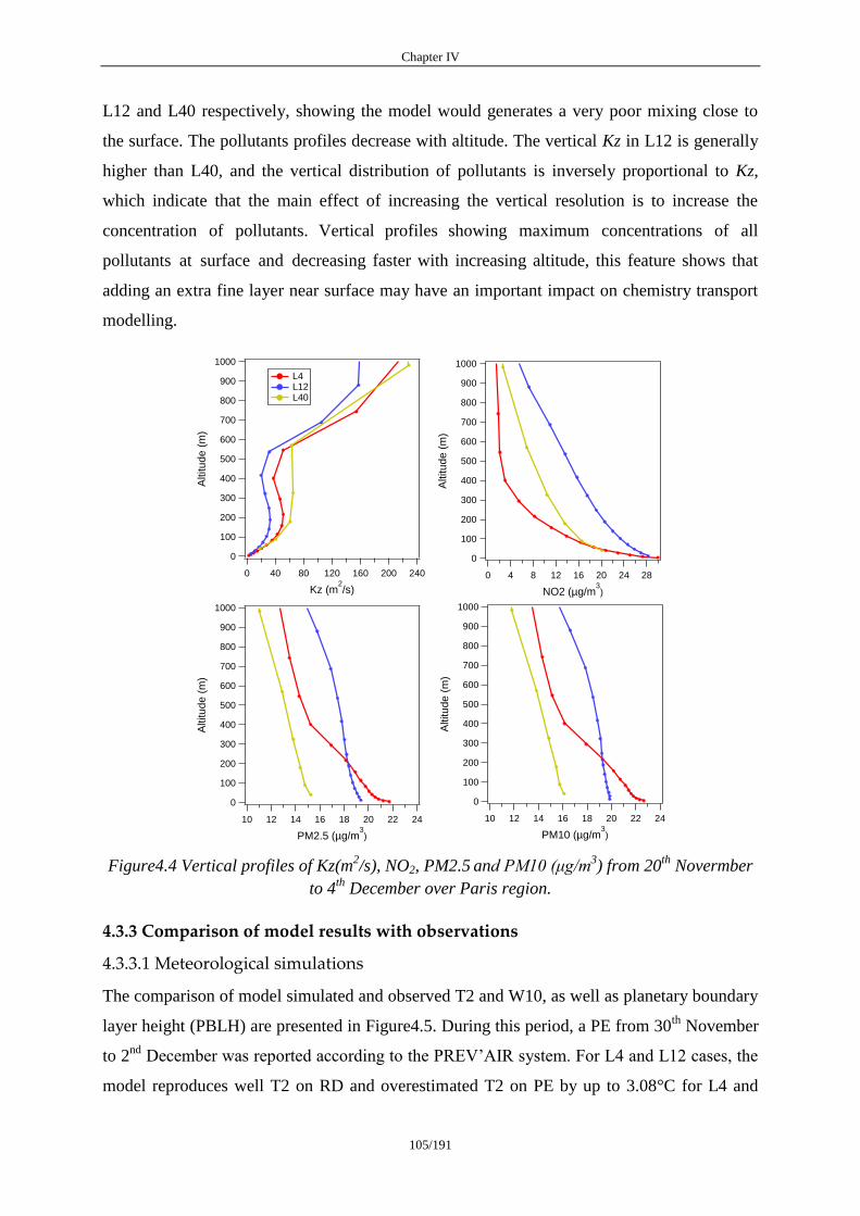
Chapter IV
105/191
L12 and L40 respectively, showing the model would generates a very poor mixing close to
the surface. The pollutants profiles decrease with altitude. The vertical Kz in L12 is generally
higher than L40, and the vertical distribution of pollutants is inversely proportional to Kz,
which indicate that the main effect of increasing the vertical resolution is to increase the
concentration of pollutants. Vertical profiles showing maximum concentrations of all
pollutants at surface and decreasing faster with increasing altitude, this feature shows that
adding an extra fine layer near surface may have an important impact on chemistry transport
modelling.
Figure4.4 Vertical profiles of Kz(m2/s), NO2, PM2.5 and PM10 (μg/m
3) from 20
th Novermber
to 4th
December over Paris region.
4.3.3 Comparison of model results with observations
4.3.3.1 Meteorological simulations
The comparison of model simulated and observed T2 and W10, as well as planetary boundary
layer height (PBLH) are presented in Figure4.5. During this period, a PE from 30th
November
to 2nd
December was reported according to the PREV’AIR system. For L4 and L12 cases, the
model reproduces well T2 on RD and overestimated T2 on PE by up to 3.08°C for L4 and
1000
900
800
700
600
500
400
300
200
100
0
Altitude (
m)
24020016012080400
Kz (m2/s)
L4 L12 L40
1000
900
800
700
600
500
400
300
200
100
0
Altitude (
m)
2422201816141210
PM10 (µg/m3)
1000
900
800
700
600
500
400
300
200
100
0
Altitude (
m)
2422201816141210
PM2.5 (µg/m3)
1000
900
800
700
600
500
400
300
200
100
0
Altitude (
m)
2824201612840
NO2 (µg/m3)
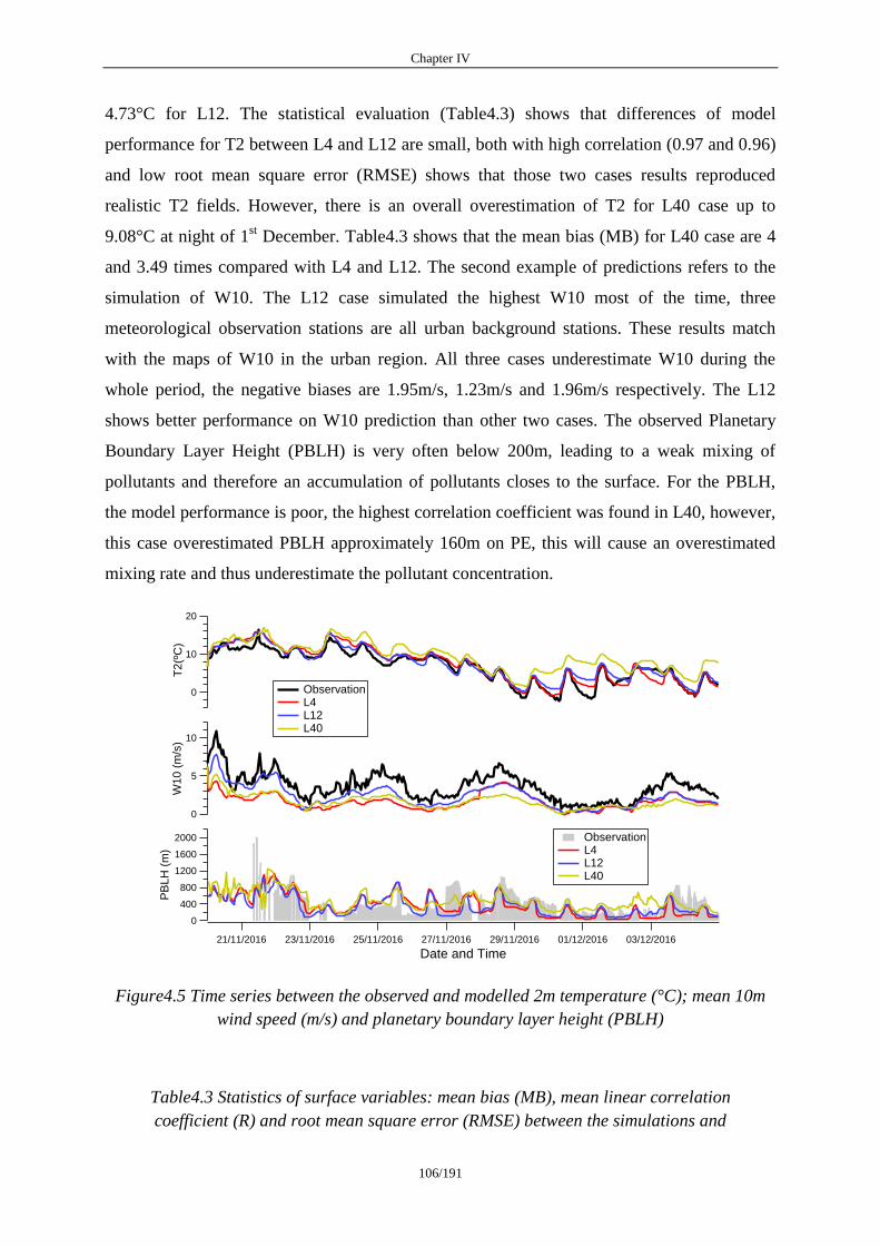
Chapter IV
106/191
4.73°C for L12. The statistical evaluation (Table4.3) shows that differences of model
performance for T2 between L4 and L12 are small, both with high correlation (0.97 and 0.96)
and low root mean square error (RMSE) shows that those two cases results reproduced
realistic T2 fields. However, there is an overall overestimation of T2 for L40 case up to
9.08°C at night of 1st December. Table4.3 shows that the mean bias (MB) for L40 case are 4
and 3.49 times compared with L4 and L12. The second example of predictions refers to the
simulation of W10. The L12 case simulated the highest W10 most of the time, three
meteorological observation stations are all urban background stations. These results match
with the maps of W10 in the urban region. All three cases underestimate W10 during the
whole period, the negative biases are 1.95m/s, 1.23m/s and 1.96m/s respectively. The L12
shows better performance on W10 prediction than other two cases. The observed Planetary
Boundary Layer Height (PBLH) is very often below 200m, leading to a weak mixing of
pollutants and therefore an accumulation of pollutants closes to the surface. For the PBLH,
the model performance is poor, the highest correlation coefficient was found in L40, however,
this case overestimated PBLH approximately 160m on PE, this will cause an overestimated
mixing rate and thus underestimate the pollutant concentration.
Figure4.5 Time series between the observed and modelled 2m temperature (°C); mean 10m
wind speed (m/s) and planetary boundary layer height (PBLH)
Table4.3 Statistics of surface variables: mean bias (MB), mean linear correlation
coefficient (R) and root mean square error (RMSE) between the simulations and
20
10
0
T2
(ºC
)
21/11/2016 23/11/2016 25/11/2016 27/11/2016 29/11/2016 01/12/2016 03/12/2016
Date and Time
10
5
0
W1
0 (
m/s
)
2000
1600
1200
800
400
0
PB
LH
(m
)
Observation L4 L12 L40
Observation L4 L12 L40

Chapter IV
107/191
observations of 2m temperature (°C); mean 10m wind speed (m/s) and planetary
boundary layer height (PBLH)
L4 L12 L40
R MB RMSE R MB RMSE R MB RMSE
T2 0.97 0.68 1.45 0.96 0.78 1.43 0.89 2.72 3.35
W10 0.81 -1.95 2.25 0.92 -1.23 1.42 0.88 -1.96 2.23
PBLH 0.66 -36.17 262.51 0.70 -54.91 238.03 0.77 81.8 213.92
In order to better understand the main differences, diurnal cycles are presented in Figure4.6.
The model tends to overestimate T2 all over the day, usually more overestimated at night
compared to the daytime. The diurnal cycle of W10 is relatively flat and all three cases
strongly underestimate W10. L12 shows good results compare with others regarding the MB
throughout the day. Due to missing part of the observation data, the diurnal cycle of observed
PBLH does not have absolute accuracy. Based on existing data, we can find that L40 tends to
overestimate and L4, L12 tends to underestimate PBLH at night and the diurnal variation of
L40 significantly smaller than the other two cases. The diurnal cycles of meteorological
parameters indicate that the vertical grid resolution is important on meteorology. Refining the
levels thicknesses near the surface mostly affect the wind speed calculation.
Figure4.6 Diurnal cycles for surface 2m temperature (°C); mean 10m wind speed (m/s) and
planetary boundary layer height (PBLH) from 20th
November to 4th
December.
4.3.3.2 Evaluation of main pollutants simulations
10.0
7.5
5.0
T2
(ºC
)
20161284
Hours of day
Observation L4 L12 L40
5.0
4.0
3.0
2.0
1.0
W1
0 (
m/s
)
20161284
Hours of day
700
600
500
400
300
200
PB
LH
(m
)
20161284
Hours of day
Chapter IV
108/191
The time evolution of hourly-averaged NO2, PM2.5 and PM10 between observation and three
cases involved in the inter-comparison is provided in Figure4.7. The results show that all
three cases captured fairly well the day-to-day variability of the surface pollutants
concentrations on RD but generally underestimated the intensity during the PE days. A
relatively small differences between cases can be found from 20th
to 29th
November. While
refining the first layer height has not a very sensitive impact on meteorology, it has a
significant beneficial impact on air quality simulation. As shown in Table4.4, L4 case gives a
clear best performance for of pollutants. The agreement with observations is generally better
than for the other two cases, the correlations are 0.87, 0.90 and 0.91 in the cases of NO2,
PM2.5 and PM10 respectively. Compared to the observations, the peak of pollutants
corresponding to the PE is well modeled in L4 simulation, although it still underestimates
surface concentrations on PE. The changes of pollutants concentrations are small between RD
and PE in L40, which indicates low vertical resolution can hardly predict the PE effectively.
The model comparison in Figure4.8 presents the differences between cases. Positive biases
are found in L12-L4 and negative biases are found in L40-L4 from 20th
to 28th
November. On
reason is the relatively low PBLH of L12 and relatively high PBLH of L40 compare with L4
over this period. Since 29th
November, the surface pollutants concentrations obtained from L4
are mostly higher than other two cases. While the average PM2.5 and PM10 surface
concentrations are 25.64μg/m3 and 36.25μg/m
3 in the observations, in the simulations, the
values are 27.42μg/m3 and 29.67μg/m
3 from L4, 24.45μg/m
3 and 26.69μg/m
3 from L12,
14.82μg/m3 and 16.24μg/m
3 from L40 respectively. This result is consistent with our one-year
simulation over French region in Chapter II, the ratio of PM2.5/PM10 generally over 90% in
the model. The reason could originate from the overestimation of fine mode emissions, as
well as the lack of natural coarse emissions (Im et al., 2010; Vautard et al., 2009). In general,
emission inventory needs improvement.
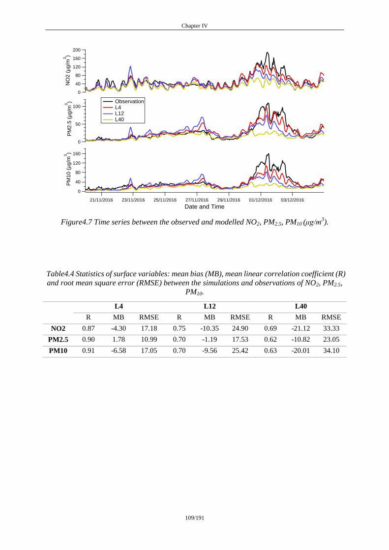
Chapter IV
109/191
Figure4.7 Time series between the observed and modelled NO2, PM2.5, PM10 (μg/m3).
Table4.4 Statistics of surface variables: mean bias (MB), mean linear correlation coefficient (R)
and root mean square error (RMSE) between the simulations and observations of NO2, PM2.5,
PM10.
L4 L12 L40
R MB RMSE R MB RMSE R MB RMSE
NO2 0.87 -4.30 17.18 0.75 -10.35 24.90 0.69 -21.12 33.33
PM2.5 0.90 1.78 10.99 0.70 -1.19 17.53 0.62 -10.82 23.05
PM10 0.91 -6.58 17.05 0.70 -9.56 25.42 0.63 -20.01 34.10
200
160
120
80
40
0
NO
2 (
µg
/m3)
21/11/2016 23/11/2016 25/11/2016 27/11/2016 29/11/2016 01/12/2016 03/12/2016
Date and Time
100
50
0
PM
2.5
(µ
g/m
3)
160
120
80
40
0
PM
10
(µ
g/m
3)
Observation L4 L12 L40
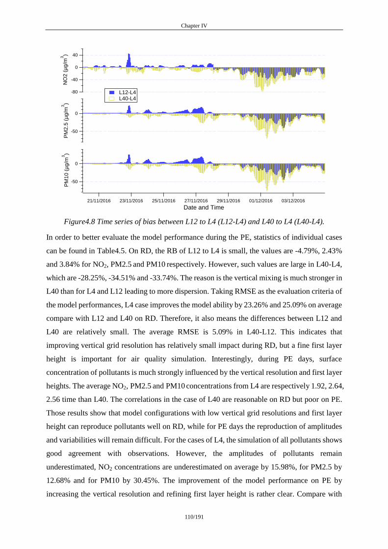
Chapter IV
110/191
Figure4.8 Time series of bias between L12 to L4 (L12-L4) and L40 to L4 (L40-L4).
In order to better evaluate the model performance during the PE, statistics of individual cases
can be found in Table4.5. On RD, the RB of L12 to L4 is small, the values are -4.79%, 2.43%
and 3.84% for NO2, PM2.5 and PM10 respectively. However, such values are large in L40-L4,
which are -28.25%, -34.51% and -33.74%. The reason is the vertical mixing is much stronger in
L40 than for L4 and L12 leading to more dispersion. Taking RMSE as the evaluation criteria of
the model performances, L4 case improves the model ability by 23.26% and 25.09% on average
compare with L12 and L40 on RD. Therefore, it also means the differences between L12 and
L40 are relatively small. The average RMSE is 5.09% in L40-L12. This indicates that
improving vertical grid resolution has relatively small impact during RD, but a fine first layer
height is important for air quality simulation. Interestingly, during PE days, surface
concentration of pollutants is much strongly influenced by the vertical resolution and first layer
heights. The average NO2, PM2.5 and PM10 concentrations from L4 are respectively 1.92, 2.64,
2.56 time than L40. The correlations in the case of L40 are reasonable on RD but poor on PE.
Those results show that model configurations with low vertical grid resolutions and first layer
height can reproduce pollutants well on RD, while for PE days the reproduction of amplitudes
and variabilities will remain difficult. For the cases of L4, the simulation of all pollutants shows
good agreement with observations. However, the amplitudes of pollutants remain
underestimated, NO2 concentrations are underestimated on average by 15.98%, for PM2.5 by
12.68% and for PM10 by 30.45%. The improvement of the model performance on PE by
increasing the vertical resolution and refining first layer height is rather clear. Compare with
-80
-40
0
40
NO
2 (
µg/m
3)
21/11/2016 23/11/2016 25/11/2016 27/11/2016 29/11/2016 01/12/2016 03/12/2016
Date and Time
-50
0
PM
2.5
(µ
g/m
3)
-50
0
PM
10 (
µg/m
3)
L12-L4 L40-L4
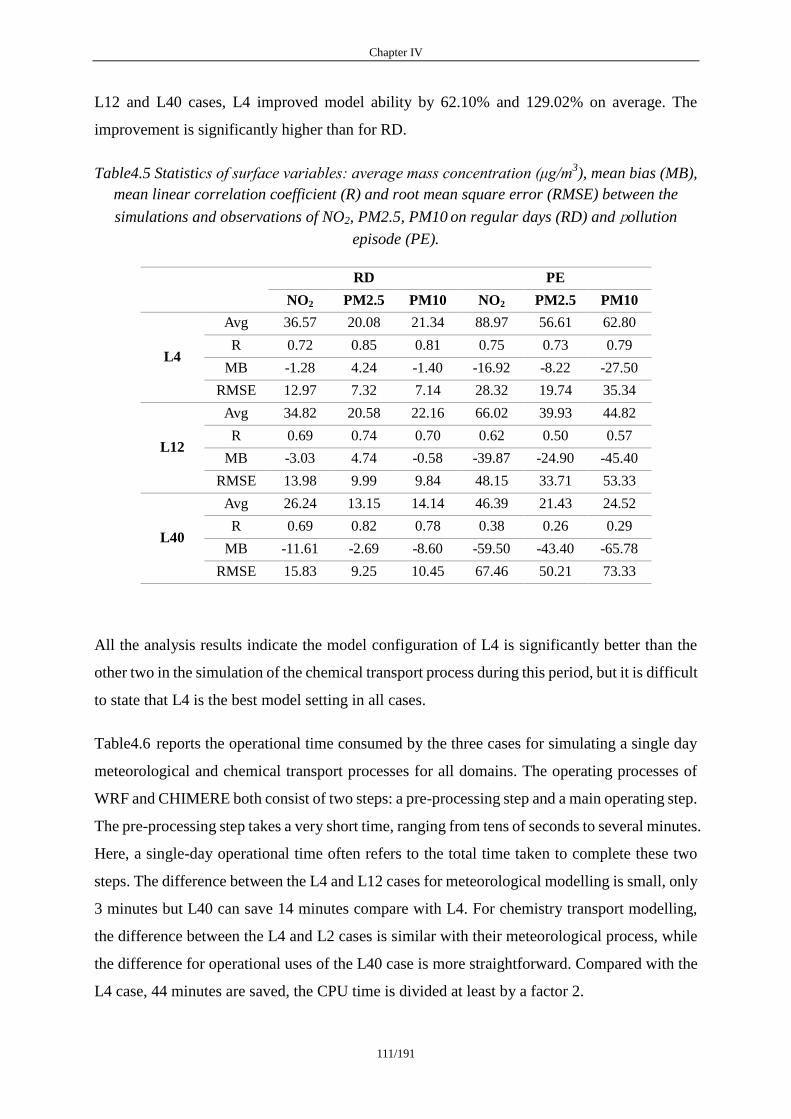
Chapter IV
111/191
L12 and L40 cases, L4 improved model ability by 62.10% and 129.02% on average. The
improvement is significantly higher than for RD.
Table4.5 Statistics of surface variables: average mass concentration (μg/m3), mean bias (MB),
mean linear correlation coefficient (R) and root mean square error (RMSE) between the
simulations and observations of NO2, PM2.5, PM10 on regular days (RD) and pollution
episode (PE).
RD PE
NO2 PM2.5 PM10 NO2 PM2.5 PM10
L4
Avg 36.57 20.08 21.34 88.97 56.61 62.80
R 0.72 0.85 0.81 0.75 0.73 0.79
MB -1.28 4.24 -1.40 -16.92 -8.22 -27.50
RMSE 12.97 7.32 7.14 28.32 19.74 35.34
L12
Avg 34.82 20.58 22.16 66.02 39.93 44.82
R 0.69 0.74 0.70 0.62 0.50 0.57
MB -3.03 4.74 -0.58 -39.87 -24.90 -45.40
RMSE 13.98 9.99 9.84 48.15 33.71 53.33
L40
Avg 26.24 13.15 14.14 46.39 21.43 24.52
R 0.69 0.82 0.78 0.38 0.26 0.29
MB -11.61 -2.69 -8.60 -59.50 -43.40 -65.78
RMSE 15.83 9.25 10.45 67.46 50.21 73.33
All the analysis results indicate the model configuration of L4 is significantly better than the
other two in the simulation of the chemical transport process during this period, but it is difficult
to state that L4 is the best model setting in all cases.
Table4.6 reports the operational time consumed by the three cases for simulating a single day
meteorological and chemical transport processes for all domains. The operating processes of
WRF and CHIMERE both consist of two steps: a pre-processing step and a main operating step.
The pre-processing step takes a very short time, ranging from tens of seconds to several minutes.
Here, a single-day operational time often refers to the total time taken to complete these two
steps. The difference between the L4 and L12 cases for meteorological modelling is small, only
3 minutes but L40 can save 14 minutes compare with L4. For chemistry transport modelling,
the difference between the L4 and L2 cases is similar with their meteorological process, while
the difference for operational uses of the L40 case is more straightforward. Compared with the
L4 case, 44 minutes are saved, the CPU time is divided at least by a factor 2.
Chapter IV
112/191
Results show acceptable model ability at low vertical grid resolution on RD. Therefore, for the
high-resolution small domain cases, it is obvious that high vertical grid resolution is a better
setting. In particular, the reasonable first layer height may greatly improve the simulation
results. For a long-term and large-scale simulation, considering the cost of computing resources,
a low vertical resolution configuration should be a more suitable solution for practical use.
Table4.6 Operational time (minutes) for a single day simulation in meteorological and
chemistry transport modelling
WRF
(min)
CHIMERE
(min)
TOTAL
(min) L4 70 84 154
L12 67 82 149
L40 56 40 96
4.4 Conclusions
This study presents a sensitivity analysis of the impact of vertical grid resolution and the first
layer height in meteorological and chemistry transport modelling during a pollution episode at
urban scale. The simulations are carried out over a fifteen days winter period from 20th
November to 4th
December 2016 including a pollution episode (PE) from 30th
November to 1st
December and the rest of days is defined as regular days (RD).
The maps of meteorological parameters and main pollutants show similar regional patterns for
the three cases. The differences between the different model configurations are relatively
small on meteorological parameters. The relative bias (RB) of L12 and L40 compare with L4
(L12-L4 and L40-L4) are 2.17% and 22.95% for 2m temperature (T2), 4.01% and -12.69%
for 10m wind speed (W10), -0.12% and -2.72% for surface relative humidity (RH),
respectively. The differences between three configurations in chemistry transport modelling
are more obvious. The RB of L12-L4 and L40-L4 are -10.68% and -39.34% for NO2, -4.61%
and -36.98% for PM2.5 and -4.01% and -35.85% for PM10, respectively.
However, for the planetary boundary layer height (PBLH), L40 case reproduces higher PBLH
than others in most of the time of this period and overestimated PBLH about 160m on PE,
leading to a stronger vertical mixing than for L12 and L4 simulations. The differences
between the three configurations in meteorological parameters simulations are larger during
nighttime than that for daytime.
Chapter IV
113/191
The comparisons between observed and modelled surface main pollutants concentrations
were performed. Although the model performances are uneven, all three configurations
demonstrate the ability of chemistry transport modelling on RD. The impact of vertical grid
resolution and first layer height is moderate. Taking the root mean square error as the
evaluation criteria, L4 improves the model ability by 23.26% and 25.09% than L12 and L40
respectively. However, on PE, improving vertical grid resolution and first layer height results
clearly improves the air quality prediction, average improvements are 62.10% and 129.02%
from L12 to L4 and from L40 to L4 respectively.
This study highlights the model ability both in meteorological and chemistry transport
modelling with low vertical resolution on RD, but such a model configuration displays
discrepancies in representing the amplitudes of pollutants concentrations on PE and
increasing the vertical resolution and refining first layer height leads to clear improvement
during pollution episodes.

Chapter IV
114/191
References
Allen, L.; Lindberg, F.; Grimmond, C.S.B. Global to city scale urban anthropogenic heat flux:
Model and variability. Int. J. Clim. 2010, 31, 1990–2005.
Anderson, W.; Meneveau, C. A Large-Eddy Simulation Model for Boundary-Layer Flow
over Surfaces with Horizontally Resolved but Vertically Unresolved Roughness Elements.
Bound. Layer Meteorol. 2010, 137, 397–415.
Baklanov, A.; Mestayer, P.G.; Clappier, A.; Zilitinkevich, S.; Joffre, S.; Mahura, A.; Nielsen,
N.W. Towards improving the simulation of meteorological fields in urban areas through
updated/advanced surface fluxes description. Atmos. Chem. Phys. Discuss. 2008, 8, 523–543.
Barlage, M.; Miao, S.; Chen, F. Impact of physics parameterizations on high‐resolution
weather prediction over two Chinese megacities. J. Geophys. Res. Atmos. 2016, 121, 4487–
4498.
Best, M. Representing urban areas within operational numerical weather prediction models.
Bound. Layer Meteorol. 2005, 114, 91–109.
Bessagnet, B.; Hodzic, A.; Vautard, R.; Beekmann, M.; Cheinet, S.; Honoré, C.; Liousse, C.;
Rouil, L. Aerosol modeling with CHIMERE—preliminary evaluation at the continental scale.
Atmos. Environ. 2004, 38, 2803–2817.
Bessagnet, B.; Beauchamp, M.; Guerreiro, C.; De Leeuw, F.; Tsyro, S.; Colette, A.; Meleux,
F.; Rouïl, L.; Ruyssenaars, P.; Sauter, F.; et al. Can further mitigation of ammonia emissions
reduce exceedances of particulate matter air quality standards? Environ. Sci. Policy 2014, 44,
149–163.
Bessagnet, B.; Menut, L.; Colette, A.; Couvidat, F.; Dan, M.; Mailler, S.; Létinois, L.; Pont,
V.; Rouïl, L. An Evaluation of the CHIMERE Chemistry Transport Model to Simulate Dust
Outbreaks across the Northern Hemisphere in March 2014. Atmosphere 2017, 8, 251.
Borrego, C.; Souto, J.A.; Monteiro, A.; Dios, M.; Rodriguez, A.; Ferreira, J.; Saavedra, S.;
Casares, J.J.; Miranda, A.I. The role of transboundary air pollution over Galicia and North
Portugal area. Environ. Sci. Pollut. Res. 2013, 20, 2924–2936.
Bougeault, P.; Lacarrère. P. Parameterization of orographic induced turbulence in a meso beta
scale model. Mon. Weather Rev. 1989, 117, 1872–1890.
Bowden, J.H.; Otte, T.L.; Nolte, C.G.; Otte, M. Examining Interior Grid Nudging Techniques
Using Two-Way Nesting in the WRF Model for Regional Climate Modeling. J. Clim. 2012,
25, 2805–2823.
Coseo, L. Larsen Cooling the heat island in compact urban environments: The effectiveness of
Chicago’s green alley program. Procedia Eng. 2015, 118, 691–710.
Couvidat, F.; Bessagnet, B.; Garcia-Vivanco, M.; Real, E.; Menut, L.; and Colette, A.
Development of an inorganic and organic aerosol model (Chimere2017b2 v1.0): Seasonal and
spatial evaluation over Europe. Geosci. Model. Dev. 2018, 11, 165–194.

Chapter IV
115/191
EEA. Air Quality in Europe—2018 Report; EEA Report No 13/2018; European Environment
Agency: Copenhagen, Denmark, 2018.
Falasca, S.; Catalano, F.; Moroni, M. Numerical Study of the Daytime Planetary Boundary
Layer over an Idealized Urban Area: Influence of Surface Properties, Anthropogenic Heat
Flux, and Geostrophic Wind Intensity. J. Appl. Meteorol. Clim. 2016, 55, 1021–1039.
Falasca, S.; Catalano, F. Impact of Highly Reflective Materials on Meteorology, PM10 and
Ozone in Urban Areas: A Modeling Study with WRF-CHIMERE at High Resolution over Milan
(Italy). Urban Sci. 2018, 2, 18.
Fan, S.; Guo, Y.R.; Chen, M.; Zhong, J.; Chu, Y.; Wang, W.; Huang, X.Y.; Wang, Y.; Guo,
Y.H. Application of WRF 3D Var to a high-resolution model over Beijing area. Plateau
Meteorol. 2008, 27, 1181–1188.
Flaounas, E.; Bastin, S.; Janicot, S. Regional climate modelling of the 2006 West African
monsoon: sensitivity to convection and planetary boundary layer parameterisation using WRF.
Clim. Dyn. 2010, 36, 1083–1105.
Gedzelman, S.D.; Austin, S.; Cermak, R.; Stefano, N.; Partridge, S.; Quesenberry, S.;
Robinson, D.A. Mesoscale aspects of the Urban Heat Island around New York City. Theor.
Appl. Clim. 2003, 75, 29–42.
Glisan, J.M.; Gutowski, W.J.; Cassano, J.J.; Higgins, M.E. Effects of Spectral Nudging in
WRF on Arctic Temperature and Precipitation Simulations. J. Clim. 2013, 26, 3985–3999.
Hamaoui-Laguel, L.; Meleux, F,; Beekmann, M,; Bessagnet, B,; Génermont, S,; Cellier, P,;
Létinois, L. Improving ammonia emissions in air quality modelling for France Atmospheric
Environment, 92 (2014), pp. 584-595
Hariprasad, K.B.R.R.; Srinivas, C.V.; Singh, A.B.; Rao, S.V.B.; Baskaran, R.; Venkatraman, B.
Numerical simulation and inter comparison of boundary layer structure with different PBL
schemes in WRF using experimental observations at a tropical site. Atmos. Res. 2014, 145, 27–
44.
He, Q.; Zhao, X.; Lu, J.; Zhou, G.; Yang, H.; Gao, W.; Yu, W.; Cheng, T. Impacts of
biomass-burning on aerosol properties of a severe haze event over Shanghai. Particuology
2015, 20, 52–60.
Hu, X.-M.; Nielsen-Gammon, J.W.; Zhang, F. Evaluation of Three Planetary Boundary Layer
Schemes in the WRF Model. J. Appl. Meteorol. Clim. 2010, 49, 1831–1844.
Janjic, Z. Nonsingular Implementation of the Mellor-Yamada Level 2.5 Scheme in the NCEP
Meso Model; NCEP Office Note, No. 437; National Centers for Environmental Prediction:
College Park, MD, USA, 2002; p. 61.
Janjić, Z.I. The Step-Mountain Coordinate: Physical Package. Mon. Weather. Rev. 1990, 118,
1429–1443.
Hong, S.-Y.; Noh, Y.; Dudhia, J. A New Vertical Diffusion Package with an Explicit
Treatment of Entrainment Processes. Mon. Weather. Rev. 2006, 134, 2318–2341.

Chapter IV
116/191
Kim, Y.; Sartelet, K.; Raut, J.-C.; Chazette, P. Evaluation of the Weather Research and
Forecast/Urban Model Over Greater Paris. Bound. Layer Meteorol. 2013, 149, 105–132,
doi:10.1007/s10546-013-9838-6.
Kim, Y.; Sartelet, K.; Raut, J.-C.; Chazette, P. Influence of an urban canopy model and PBL
schemes on vertical mixing for air quality modeling over Greater Paris. Atmos. Environ. 2015,
107, 289–306.
Kleczek, M.A.; Steeneveld, G.-J.; Holtslag, A. Evaluation of the Weather Research and
Forecasting Mesoscale Model for GABLS3: Impact of Boundary-Layer Schemes, Boundary
Conditions and Spin-Up. Bound. Layer Meteorol. 2014, 152, 213–243.
Kusaka, H.; Kondo, K.; Kikegawa, Y.; Kimura, F. A simple single‐layer urban canopy model
for atmospheric models: Comparison with multi‐layer and slab models. Bound. Layer Meteorol.
2001, 101, 329–358.
Kusaka, H.; Kimura, F. Coupling a Single-Layer Urban Canopy Model with a Simple
Atmospheric Model: Impact on Urban Heat Island Simulation for an Idealized Case. J.
Meteorol. Soc. Jpn. 2004, 82, 67–80.
Lai, L.-W.; Cheng, W.-L. Air quality influenced by urban heat island coupled with synoptic
weather patterns. Sci. Total. Environ. 2009, 407, 2724–2733.
LeMone, M.; Tewari, M.; Chen, F.; Dudhia, J. Objectively‐determined fair‐weather convective
boundary layer depths in the ARW‐WRF NWP model and their comparison to CASES‐97
observations. Mon. Weather Rev. 2013, 141, 30–54.
LeMone, M.; Tewari, M.; Chen, F.; Dudhia, J. Objectively‐determined fair‐weather NBL
features in the ARW‐WRF model and their comparison to CASES‐97 observations. Mon.
Weather Rev. 2014, 142, 2709–2732.
Li, M.; Ma, Y.; Ma, W.; Hu, Z.; Ishikawa, H.; Su, Z.; Sun, F. Analysis of turbulence
characteristics over the northern Tibetan Plateau area. Adv. Atmos. Sci. 2006, 23, 579–585.
Lin, C.-Y.; Chen, F.; Huang, J.-C.; Chen, W.-C.; Liou, Y.-A.; Chen, W.-N.; Liu, S.-C. Urban
heat island effect and its impact on boundary layer development and land–sea circulation over
northern Taiwan. Atmos. Environ. 2008a, 42, 5635–5649.
Lin, C.-Y.; Chen, W.-C.; Liu, S.C.; Liou, Y.A.; Liu, G.; Lin, T. Numerical study of the impact
of urbanization on the precipitation over Taiwan. Atmos. Environ. 2008b, 42, 2934–2947.
Liu, Y.; Chen, F.; Warner, T.; Basara, J.B. Verification of a Mesoscale Data-Assimilation and
Forecasting System for the Oklahoma City Area during the Joint Urban 2003 Field Project. J.
Appl. Meteorol. Clim. 2006, 45, 912–929.
Liu, M.; Chen, M. Evaluation of BJ-RUC system for the forecast quality of planetary boundary
layer in Beijing area. J. Appl. Meteorol. Sci. 2014, 25, 212–221.
Mailler, S.; Menut, L.; Khvorostyanov, D.; Valari, M.; Couvidat, F.; Siour, G.; Turquety, S.;
Briant, R.; Tuccella, P.; Bessagnet, B.; et al. CHIMERE-2017: From urban to hemispheric
chemistry-transport modeling. Geosci. Model Dev. 2017, 10, 2397–2423.
Chapter IV
117/191
Markakis, K.; Valari, M.; Engardt, M.; Lacressonniere, G.; Vautard, R.; Andersson, C.
Mid-21st century air quality at the urban scale under the influence of changed climate and
emissions case studies for Paris and Stockholm. Atmos. Chem. Phys. 2016, 16, 1877–1894.
Martilli, A.; Clappier, A.; Rotach, M. An urban surface exchange parameterization for
mesoscale models. Bound. Layer Meteorol. 2002, 104, 261–304.
Mellor, G.L.; Yamada, T. Development of a turbulence closure model for geophysical fluid
problems. Rev. Geophys. 1982, 20, 851–875.
Menut, L.; Goussebaile, A.; Bessagnet, B.; Khvorostiyanov, D.; Ung, A. Impact of realistic
hourly emissions profiles on air pollutants concentrations modelled with CHIMERE. Atmos.
Environ. 2012, 49, 233–244.
Menut, L.; Bessagnet, B.; Khvorostyanov, D.; Beekmann, M.; Blond, N.; Colette, A.; Coll, I.;
Curci, G.; Forêt, G.; Hodzic, A.; et al. CHIMERE 2013: A model for regional atmospheric
composition modelling. Geosci. Model Dev. 2013, 6, 981–1028.
Miao, S.; Chen, F.; Li, Q.; Fan, S. Impacts of urban processes and urbanization on summer
precipitation: A case study of heavy rainfallin Beijing on 1 Aug 2006. J. Appl. Meteorol.
Climatol. 2010, 50, 806–825.
Molteni, F.; Buizza, R.; Palmer, T.N.; Petroliagis, T. The ECMWF ensemble prediction system:
Methodology and validation. Quart. J. R. Meteor. Soc. 1996, 122, 73–119.
Niu, G.‐Y., Yang, Z. L., Mitchell, K. E., Chen, F., Ek, M. B., Barlage, M., et al. The
community Noah land surface model with multiparameterization options (Noah‐MP): 1. Model
description and evaluation with local‐scale measurements. Journal of Geophysical Research.
2011, 116, D12109.
Oke, T. K. Boundary Layer Climates (2nd ed.), Rutledge, New York, 1988. p. 464
Patricola, C.M.; Li, M.; Xu, Z.; Chang, P.; Saravanan, R.; Hsieh, J.-S. An investigation of
tropical Atlantic bias in a high-resolution coupled regional climate model. Clim. Dyn. 2012,
39, 2443–2463.
Salamanca, F.; Krpo, A.; Martilli, A.; Clappier, A. A new building energy model coupled
with an urban canopy parameterization for urban climate simulations—Part I. formulation,
verification, and sensitivity analysis of the model. Theor. Appl. Clim. 2009a, 99, 331–344.
Salamanca, F.; Martilli, A. A new Building Energy Model coupled with an Urban Canopy
Parameterization for urban climate simulations—Part II. Validation with one-dimension
off-line simulations. Theor. Appl. Clim. 2009a, 99, 345–356.
Sarrat, C.; Lemonsu, A.; Masson, V.; Guedalia, D. Impact of urban heat island on regional
atmospheric pollution. Atmos. Environ. 2006, 40, 1743–1758.
Toll, I.; Baldasano, J.M. Modeling of photochemical air pollution in the Barcelona area with
highly disaggregated anthropogenic and biogenic emissions. Atmos. Environ. 2000, 34, 3069–
3084.
Chapter IV
118/191
Troen, I.B.; Mahrt, L. A simple model of the atmospheric boundary layer; sensitivity to
surface evaporation. Bound. Layer Meteorol. 1986, 37, 129–148.
Tuccella, P.; Curci, G.; Visconti, G.; Bessagnet, B.; Menut, L.; Park, R.J. Modeling of gas and
aerosol with WRF/Chem over Europe: Evaluation and sensitivity study. J. Geophys. Res.
Space Phys. 2012, 117, D03303.
Tyagi, B.; Magliulo, V.; Finardi, S.; Gasbarra, D.; Carlucci, P.; Toscano, P.; Zaldei, A.;
Riccio, A.; Calori, G.; D’Allura, A.; et al. Performance Analysis of Planetary Boundary Layer
Parameterization Schemes in WRF Modeling Set Up over Southern Italy. Atmosphere 2018, 9,
272.
Valari, M.; Menut, L. Transferring the heterogeneity of surface emissions to variability in
pollutant concentrations over urban areas through a chemistry-transport model. Atmos. Environ.
2014, 44, 3229–3238.
Vigaud, N.; Roucou, P.; Fontaine, B.; Sijikumar, S.; Tyteca, S. WRF/ARPEGE-CLIMAT
simulated climate trends over West Africa. Clim. Dyn. 2009, 36, 925–944.
Wang, L.T.; Wei, Z.; Yang, J.; Zhang, Y.; Zhang, F.F.; Su, J.; Meng, C.C.; Zhang, Q. The
2013 severe haze over southern Hebei, China: model evaluation, source apportionment, and
policy implications. Atmos. Chem. Phys. Discuss. 2014, 14, 3151–3173.
Wang, L.; Liu, J.; Gao, Z.; Li, Y.; Huang, M.; Fan, S.; Zhang, X.; Yang, Y.; Miao, S.; Zou, H.;
et al. Vertical observations of the atmospheric boundary layer structure over Beijing urban
area during air pollution episodes. Atmos. Chem. Phys. Discuss. 2019, 19, 6949–6967,
doi:10.5194/acp-19-6949-2019.
Wu, J.; Zha, J.L.; Zhao, D.M.; Yang, Q.D. Changes in terrestrial near-surface wind speed and
their possible causes: An overview. Clim. Dyn. 2017, 51, 2039–207

Chapter V
119/191
Chapter V: Improvement of the vertical mixing in
chemistry transport modelling based on a 1.5 order
turbulence kinetic energy-based eddy diffusivity
closure scheme
This chapter has been designed to be considered for publication.

Chapter V
120/191
Improvement of the vertical mixing in chemistry transport
modelling based on a 1.5-order turbulence kinetic
energy-based eddy diffusivity closure scheme
Lei Jiang 1,2, *
, Bertrand Bessagnet 1, †
, Frederik Meleux 1, Frederic Tognet
1, Florian
Couvidat 1
1 INERIS, National Institute for Industrial Environment and Risks, Parc Technologique
ALATA, 60550 Verneuil-en-Halatte, France 2 Sorbonne University, UPMC Univ Paris 06, DE129, 75005 Paris, France
† Now at European Commission, Joint Research Centre (JRC), 21027 Ispra, Italy.
Abstract
In this study, a 1.5-order turbulence kinetic energy-based eddy diffusivity closure scheme
called as the new eddy diffusion (NED) is embedded in the chemical transport model
CHIMERE to describe more realistic diffusion processes near the surface for urban pollution
applications. A 15 days simulation including a winter pollution episode were simulated for
three major French cities with fine horizontal resolution of 1.67km and first layer height 12m
respectively. The NED scheme improved NO2 simulations in every urban site compare with the
initial K diffusion scheme (IKD). Taking the root mean square error as the evaluation criteria,
the average improvements are 18.77%, 24.51% and 9.52% in Paris, Lyon and Bordeaux
respectively for the whole period. PM2.5 and PM10 simulation achieved same results with NO2,
a 13.47% and 19.08% improvement were found in the urban area of Paris respectively.
However, the model performance for Particulate Matter in Lyon and Bordeaux probably
indicate a huge underestimation of biomass burning emissions in wintertime. Sensitivity test
shows that the model results are sensitive to changes of first layer height, over-refined first
layer height will lead to unreasonable TKE simulations. Overall, preliminary outcomes of this
study are encouraging. The simulation with more sophisticated and realistic eddy viscosities are
better than IKD based on K-theory that is widely used in CTMs.

Chapter V
121/191
Résumé
Dans cette étude, un schéma de fermeture d'ordre 1.5 de la diffusion turbulente basé sur
l'énergie cinétique de la turbulence, défini comme la « new eddy diffusion » (NED), est intégré
dans le modèle de transport chimique CHIMERE pour décrire des processus de diffusion plus
réalistes près de la surface pour étudier pollution urbaine. Une simulation de 15 jours incluant
un épisode de pollution hivernale a été réalisée pour trois grandes villes françaises avec une
résolution horizontale fine de 1,67km et une hauteur de première couche de 12m. Le schéma
NED améliore les simulations des concentrations de NO2 pour chaque site urbain par rapport au
schéma de diffusion K initialement implante dans CHIMERE (IKD). En prenant l'erreur
quadratique moyenne comme critère d'évaluation, les améliorations moyennes sont de 18,77%,
24,51% et 9,52% à Paris, Lyon et Bordeaux respectivement pour toute la période. La simulation
des PM2.5 et PM10 a donné les mêmes résultats que celle du NO2, avec une amélioration de
13,47% et 19,08% respectivement dans la zone urbaine de Paris. Cependant, les performances
du modèle pour les particules à Lyon et Bordeaux indiquent probablement une énorme
sous-estimation des émissions de la combustion de la biomasse en hiver. Le test de sensibilité
montre que les résultats du modèle sont sensibles aux changements de la hauteur de la première
couche, une hauteur de première couche trop raffinée conduira à des simulations TKE
déraisonnables. Dans l'ensemble, les résultats préliminaires sont encourageants dans cette étude.
La représentation de schémas de turbulence plus sophistiqués et réalistes semble améliorer les
simulations de chimie transport.
Keywords: turbulence; urban; air quality; vertical diffusion; winter episode
5.1 Introduction
Air pollution is one of the biggest public health hazards worldwide responsible for over 6
million deaths every year ( Forouzanfar et al., 2016; Lim et al., 2012; Valari et al., 2020). In
cities, air quality is a major concern for citizens and city managers (Baklanov et al., 2007).
With the development of computer performance and a better knowledge of the meteorology and
pollution sources, meteorological and air quality modelling has been widely used in the last
Chapter V
122/191
decades, particularly in urbanized and industrialized areas (Mailler et al., 2013). Today, High
resolution mesoscale chemistry–transport models (CTM) such as CMAQ, CAMx or
CHIMERE have achieved sufficient accuracy to be considered for urban air quality predictions
(Byun and Schere, 2006b; Fillingham, 2019; Sokhi et al., 2018; Terrenoire et al., 2015).
However, patterns of urban air pollution are rather variable and spatially heterogeneous (Wolf
et al., 2020), the interactions between urban and the atmosphere remains challenges (Letzel et
al., 2008), especially on modelling airflow and dispersion within the urban canopy (Baker et al.,
2004). Turbulence plays an important role on the vertical mixing of pollutants and other
physical parameters (Laurent Menut et al., 2013a; Pierce et al., 2010), but the representation of
turbulence is difficult to predict particularly close to the ground levels. All CTMs must account
the problem of turbulence, even if turbulent processes are still not fully understood: for example
the statistical approaches of turbulence closure schemes used to solve the Navier-Stokes
equations are not fully mature or are not always relevant for all scales due to the nonlinearity of
these equations (Argyropoulos and Markatos, 2015; Novati et al., 2021). For mesoscale CTM
models, the turbulent diffusion is mainly based on the gradient transport theory (K-theory)
which is a first order turbulence closure. It defines the turbulence fluxes as analogous to
molecular transport, assuming that the turbulence is a fluid cluster, which has the same
properties as the molecular transport model, and a linear relationship between the gradient and
the flux is thus obtained (Huang, 2019; Klimontovich, 1985). This local turbulence closure
approach assumes that turbulence consists of only small eddies, causing diffusion-like
transport. For example, the vertical kinematic flux of a pollutant can be modeled as being
equal to an eddy thermal diffusivity K times the vertical gradient of mean concentrations .
Also, the near-surface flow is complex process to simulate, the nature of turbulent transport is
far from a simple linear relationship, it changes with the spatial scale of the atmospheric
turbulence field and this notion of scale for turbulence is of major importance (He et al., 2019).
In mesoscale model, the grid size Δ is considerably larger than the energy containing turbulence
scale l, the turbulent energy is clearly in the unresolvable sub- scale. Therefore, the turbulence
only needs to be parameterized instead of directly resolved. Currently, the most mainstream
Chapter V
123/191
turbulence parameterization method is based on the first-order local closure scheme. In Chapter
II, three parameterizations were analyzed based on the first-order local closure scheme, and the
results show that this concise method is feasible. However, the high pollutants concentrations
are frequently found under stable atmospheric and cold weather conditions, such conditions are
characterized by a stably stratified lower atmosphere and very low turbulent diffusion
(Wolf-Grosse et al., 2017; Zilitinkevich and Esau, 2005). In cities, traffic and local industrial
emissions have a significant share of the local pollutants, those emissions can accumulate and
have longer residence times near the ground level due to low transport and mixing (Kurppa et
al., 2018) which makes harder to provide an accurate prediction of pollution level and the early
warning of pollution episode (PE). A way to improve the turbulence parameterization is to
increase the order of the closure (Stull, 1988).
In this study we use the eddy diffusion from the 1.5-order closure TKE embedded in the
Weather Research and Forecasting (WRF) model as a new vertical diffusion coefficient (Kz) in
the CTM CHIMERE to describe more realistic diffusion processes near the surface for urban
pollution applications. Two schemes are defined: one as the initial K-theory diffusion scheme in
CHIMERE (IKD) and one as the new eddy diffusion (NED) scheme from WRF respectively. A
high spatial resolution simulation, which is conducted for a winter period from November 20th
to December 4th
, 2016 over three major cities (Paris, Lyon and Bordeaux) in France was
performed with the WRF / CHIMERE suite. Based on our work presented in the previous
chapters, the grid resolution of the models has strong influence on pollutants prediction
(Punger and West, 2013). The first step of the study is to understand the impact of vertical grid
resolution on the NED simulation and find the finest vertical resolution for the following steps.
Second, examples of IKD and NED simulations are investigated for the different urban
environments. The results are presented in terms of model performances between the
configurations for the usual criteria pollutants. The final goal of this study is to propose a more
advanced diffusion scheme to improve air quality simulations and forecast over urban and
peri-urban area especially on the short-term pollution events.
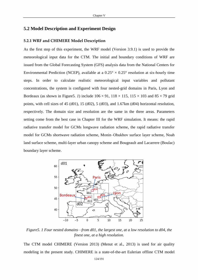
Chapter V
124/191
5.2 Model Description and Experiment Design
5.2.1 WRF and CHIMERE Model Description
As the first step of this experiment, the WRF model (Version 3.9.1) is used to provide the
meteorological input data for the CTM. The initial and boundary conditions of WRF are
issued from the Global Forecasting System (GFS) analysis data from the National Centers for
Environmental Prediction (NCEP), available at a 0.25° × 0.25° resolution at six-hourly time
steps. In order to calculate realistic meteorological input variables and pollutant
concentrations, the system is configured with four nested-grid domains in Paris, Lyon and
Bordeaux (as shown in Figure5. 1) include 106 × 91, 118 × 115, 115 × 103 and 85 × 79 grid
points, with cell sizes of 45 (d01), 15 (d02), 5 (d03), and 1.67km (d04) horizontal resolution,
respectively. The domain size and resolution are the same in the three areas. Parameters
setting come from the best case in Chapter III for the WRF simulation. It means: the rapid
radiative transfer model for GCMs longwave radiation scheme, the rapid radiative transfer
model for GCMs shortwave radiation scheme, Monin–Obukhov surface layer scheme, Noah
land surface scheme, multi-layer urban canopy scheme and Bougeault and Lacarrere (Boulac)
boundary layer scheme.
Figure5. 1 Four nested domains—from d01, the largest one, at a low resolution to d04, the
finest one, at a high resolution.
The CTM model CHIMERE (Version 2013) (Menut et al., 2013) is used for air quality
modeling in the present study. CHIMERE is a state-of-the-art Eulerian offline CTM model
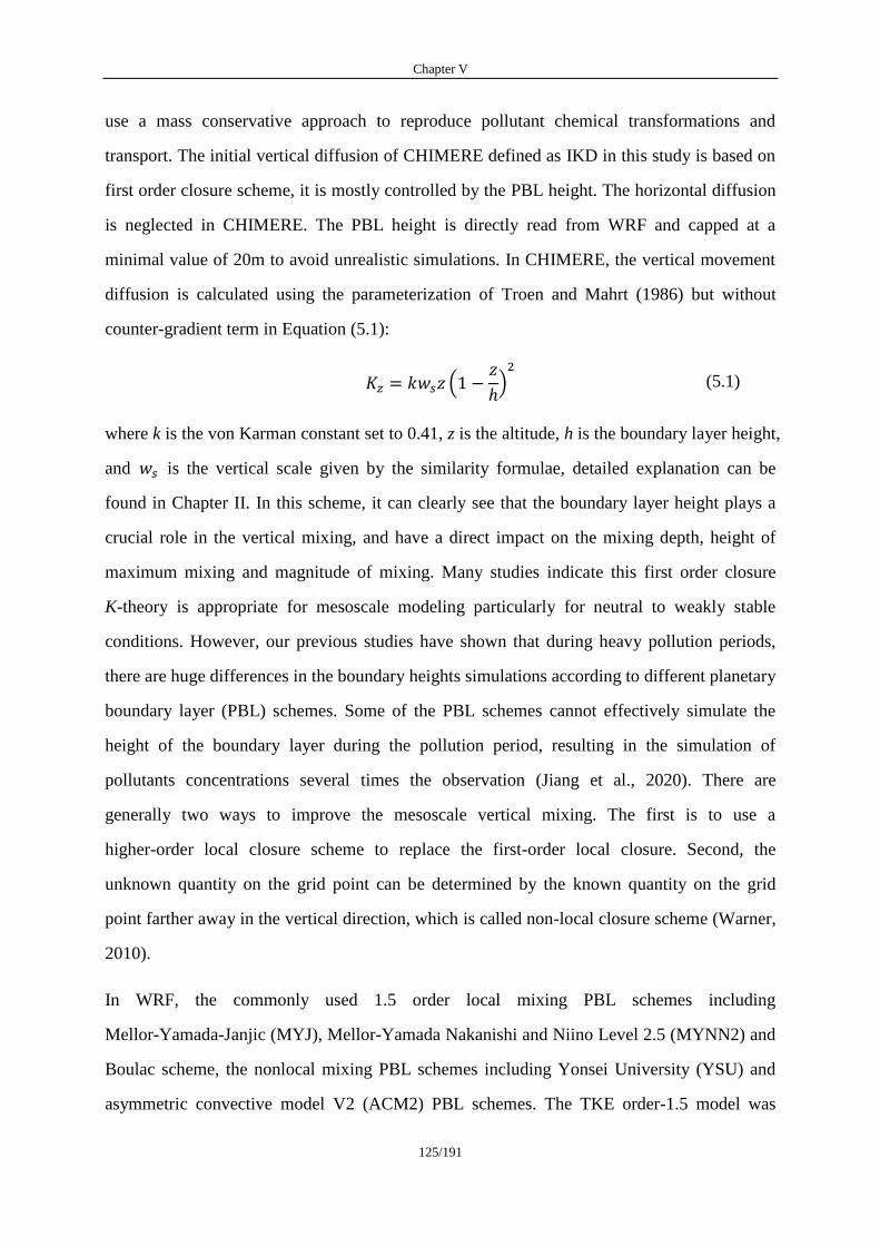
Chapter V
125/191
use a mass conservative approach to reproduce pollutant chemical transformations and
transport. The initial vertical diffusion of CHIMERE defined as IKD in this study is based on
first order closure scheme, it is mostly controlled by the PBL height. The horizontal diffusion
is neglected in CHIMERE. The PBL height is directly read from WRF and capped at a
minimal value of 20m to avoid unrealistic simulations. In CHIMERE, the vertical movement
diffusion is calculated using the parameterization of Troen and Mahrt (1986) but without
counter-gradient term in Equation (5.1):
(
)
(5.1)
where k is the von Karman constant set to 0.41, z is the altitude, h is the boundary layer height,
and is the vertical scale given by the similarity formulae, detailed explanation can be
found in Chapter II. In this scheme, it can clearly see that the boundary layer height plays a
crucial role in the vertical mixing, and have a direct impact on the mixing depth, height of
maximum mixing and magnitude of mixing. Many studies indicate this first order closure
K-theory is appropriate for mesoscale modeling particularly for neutral to weakly stable
conditions. However, our previous studies have shown that during heavy pollution periods,
there are huge differences in the boundary heights simulations according to different planetary
boundary layer (PBL) schemes. Some of the PBL schemes cannot effectively simulate the
height of the boundary layer during the pollution period, resulting in the simulation of
pollutants concentrations several times the observation (Jiang et al., 2020). There are
generally two ways to improve the mesoscale vertical mixing. The first is to use a
higher-order local closure scheme to replace the first-order local closure. Second, the
unknown quantity on the grid point can be determined by the known quantity on the grid
point farther away in the vertical direction, which is called non-local closure scheme (Warner,
2010).
In WRF, the commonly used 1.5 order local mixing PBL schemes including
Mellor-Yamada-Janjic (MYJ), Mellor-Yamada Nakanishi and Niino Level 2.5 (MYNN2) and
Boulac scheme, the nonlocal mixing PBL schemes including Yonsei University (YSU) and
asymmetric convective model V2 (ACM2) PBL schemes. The TKE order-1.5 model was
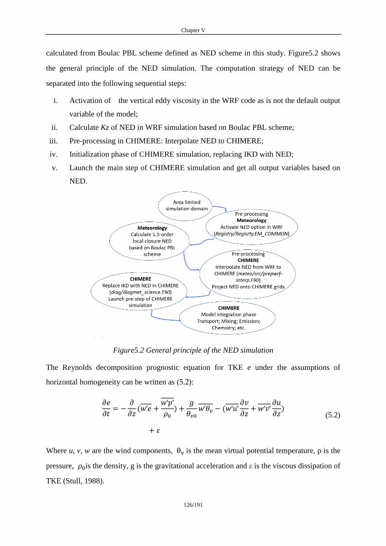
Chapter V
126/191
calculated from Boulac PBL scheme defined as NED scheme in this study. Figure5.2 shows
the general principle of the NED simulation. The computation strategy of NED can be
separated into the following sequential steps:
i. Activation of the vertical eddy viscosity in the WRF code as is not the default output
variable of the model;
ii. Calculate Kz of NED in WRF simulation based on Boulac PBL scheme;
iii. Pre-processing in CHIMERE: Interpolate NED to CHIMERE;
iv. Initialization phase of CHIMERE simulation, replacing IKD with NED;
v. Launch the main step of CHIMERE simulation and get all output variables based on
NED.
Figure5.2 General principle of the NED simulation
The Reynolds decomposition prognostic equation for TKE e under the assumptions of
horizontal homogeneity can be written as (5.2):
( '
' '
)
' ( ' '
' '
)
(5.2)
Where u, v, w are the wind components, is the mean virtual potential temperature, p is the
pressure, is the density, g is the gravitational acceleration and ε is the viscous dissipation of
TKE (Stull, 1988).

Chapter V
127/191
The TKE order-1.5 is also constructed upon the gradient transport theory as (5.3):
(5.3)
The left side represents the Reynolds-average operator, the vertical turbulent flux is
parameterized as the product of local gradient of analytical variable and eddy diffusivity K.
In Boulac scheme, vertical eddy diffusivity defined as (5.4):
√ (5.4)
Where Ck is a constant set up to 0.7, l is the vertical length scale (Deardorff, 1980), and e is
the TKE defined as (5.5):
( ' ' ' ) (5.5)
In the Boulac scheme, it is assumed that at individual level in the atmosphere, the length scale
l may be related to the distance that the parcel originating from the corresponding level and
having the initial kinetic energy equal to the average TKE of the layer which can move up and
down before being prevented by the buoyancy effect. The and is defined as (5.6):
∫ ( ( ) ( ')) ' ( )
∫ ( ( ) ( ')) ' ( )
(5.6)
Thus, the length scale l must be related to some value between and . In Boulac
scheme, the l is written as (5.7):
√ (5.7)
The advantage of this scheme is to allow for remote effects of stable zones to define the
turbulence mixing length scale (Bougeault and Lacarrere, 1989). This scheme solves a
prognostic TKE equation which includes TKE advection and parameterizes sources and sinks
from shear production, buoyancy, mixing and dissipation (Simon et al., 2019). The model
physical parameterizations remain the same as Boulac-BEP scheme detailed in Chapter III,
(see Table3.1 of Chapter III).
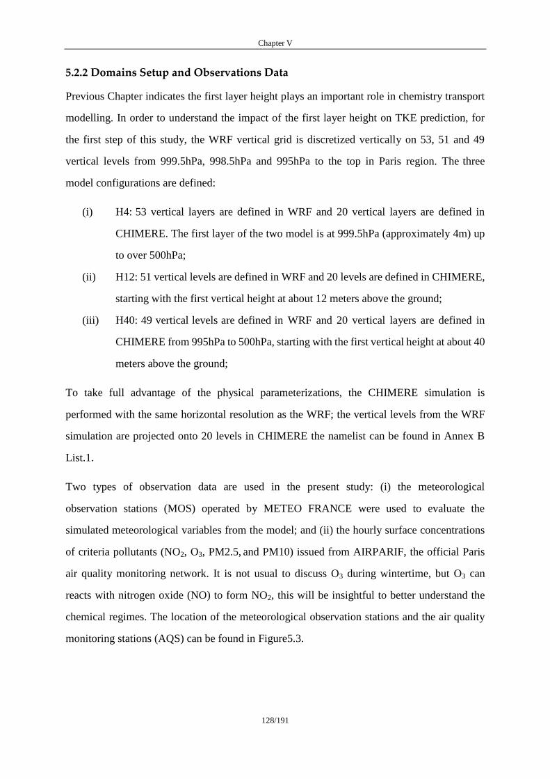
Chapter V
128/191
5.2.2 Domains Setup and Observations Data
Previous Chapter indicates the first layer height plays an important role in chemistry transport
modelling. In order to understand the impact of the first layer height on TKE prediction, for
the first step of this study, the WRF vertical grid is discretized vertically on 53, 51 and 49
vertical levels from 999.5hPa, 998.5hPa and 995hPa to the top in Paris region. The three
model configurations are defined:
(i) H4: 53 vertical layers are defined in WRF and 20 vertical layers are defined in
CHIMERE. The first layer of the two model is at 999.5hPa (approximately 4m) up
to over 500hPa;
(ii) H12: 51 vertical levels are defined in WRF and 20 levels are defined in CHIMERE,
starting with the first vertical height at about 12 meters above the ground;
(iii) H40: 49 vertical levels are defined in WRF and 20 vertical layers are defined in
CHIMERE from 995hPa to 500hPa, starting with the first vertical height at about 40
meters above the ground;
To take full advantage of the physical parameterizations, the CHIMERE simulation is
performed with the same horizontal resolution as the WRF; the vertical levels from the WRF
simulation are projected onto 20 levels in CHIMERE the namelist can be found in Annex B
List.1.
Two types of observation data are used in the present study: (i) the meteorological
observation stations (MOS) operated by METEO FRANCE were used to evaluate the
simulated meteorological variables from the model; and (ii) the hourly surface concentrations
of criteria pollutants (NO2, O3, PM2.5, and PM10) issued from AIRPARIF, the official Paris
air quality monitoring network. It is not usual to discuss O3 during wintertime, but O3 can
reacts with nitrogen oxide (NO) to form NO2, this will be insightful to better understand the
chemical regimes. The location of the meteorological observation stations and the air quality
monitoring stations (AQS) can be found in Figure5.3.
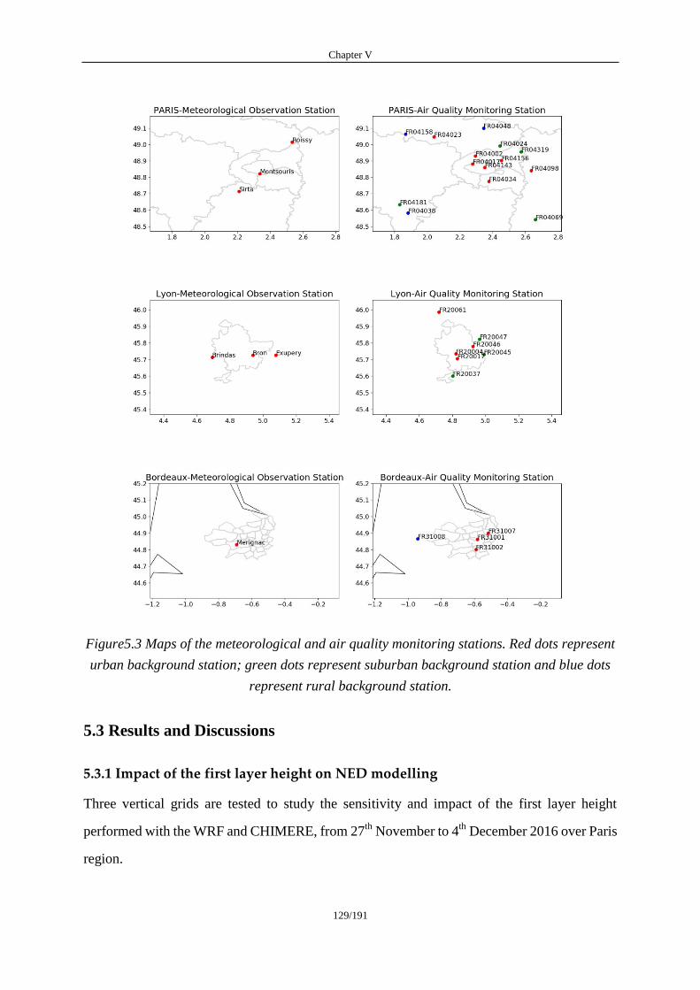
Chapter V
129/191
Figure5.3 Maps of the meteorological and air quality monitoring stations. Red dots represent
urban background station; green dots represent suburban background station and blue dots
represent rural background station.
5.3 Results and Discussions
5.3.1 Impact of the first layer height on NED modelling
Three vertical grids are tested to study the sensitivity and impact of the first layer height
performed with the WRF and CHIMERE, from 27th
November to 4th
December 2016 over Paris
region.
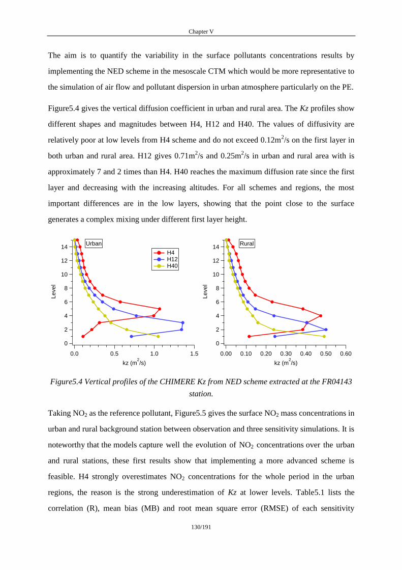
Chapter V
130/191
The aim is to quantify the variability in the surface pollutants concentrations results by
implementing the NED scheme in the mesoscale CTM which would be more representative to
the simulation of air flow and pollutant dispersion in urban atmosphere particularly on the PE.
Figure5.4 gives the vertical diffusion coefficient in urban and rural area. The Kz profiles show
different shapes and magnitudes between H4, H12 and H40. The values of diffusivity are
relatively poor at low levels from H4 scheme and do not exceed 0.12m2/s on the first layer in
both urban and rural area. H12 gives 0.71m2/s and 0.25m
2/s in urban and rural area with is
approximately 7 and 2 times than H4. H40 reaches the maximum diffusion rate since the first
layer and decreasing with the increasing altitudes. For all schemes and regions, the most
important differences are in the low layers, showing that the point close to the surface
generates a complex mixing under different first layer height.
Figure5.4 Vertical profiles of the CHIMERE Kz from NED scheme extracted at the FR04143
station.
Taking NO2 as the reference pollutant, Figure5.5 gives the surface NO2 mass concentrations in
urban and rural background station between observation and three sensitivity simulations. It is
noteworthy that the models capture well the evolution of NO2 concentrations over the urban
and rural stations, these first results show that implementing a more advanced scheme is
feasible. H4 strongly overestimates NO2 concentrations for the whole period in the urban
regions, the reason is the strong underestimation of Kz at lower levels. Table5.1 lists the
correlation (R), mean bias (MB) and root mean square error (RMSE) of each sensitivity
14
12
10
8
6
4
2
0
Level
1.51.00.50.0
kz (m2/s)
Urban
H4 H12 H40
14
12
10
8
6
4
2
0
Level
0.600.500.400.300.200.100.00
kz (m2/s)
Rural
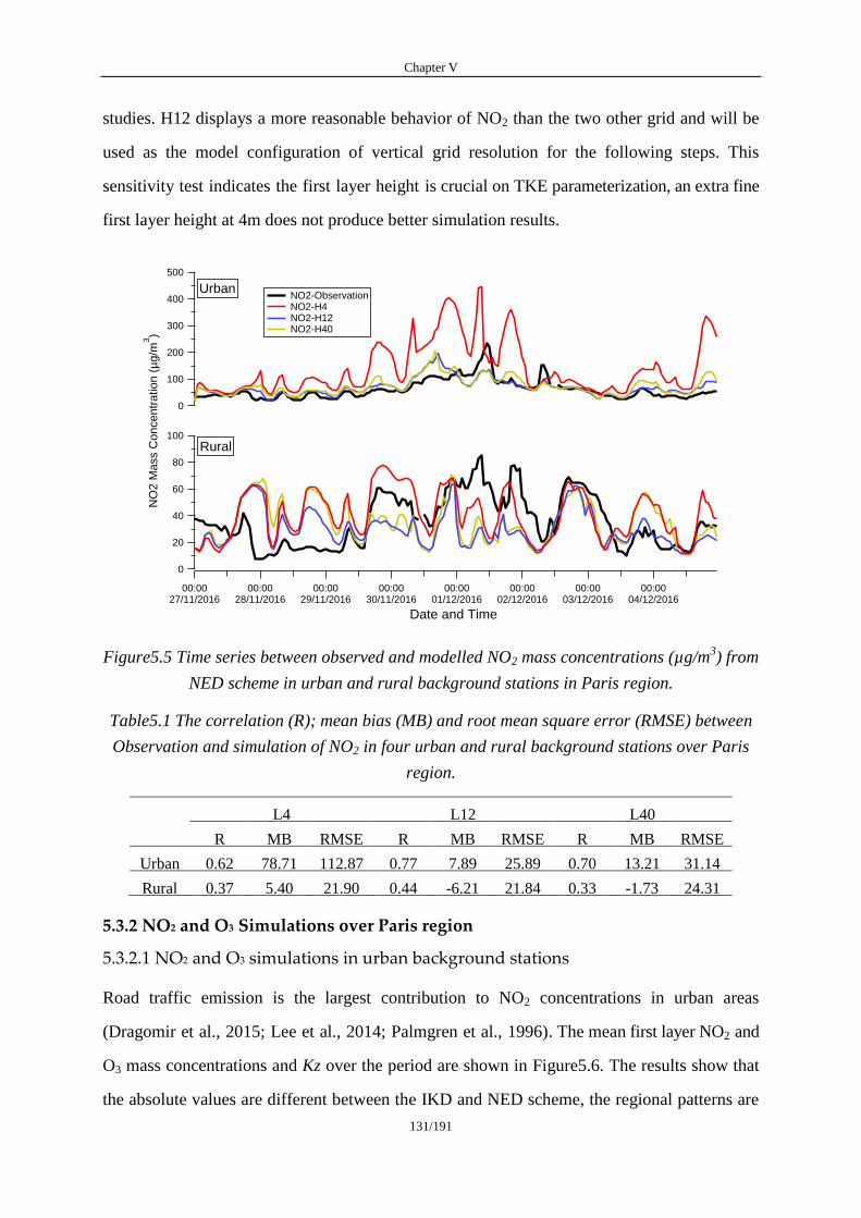
Chapter V
131/191
studies. H12 displays a more reasonable behavior of NO2 than the two other grid and will be
used as the model configuration of vertical grid resolution for the following steps. This
sensitivity test indicates the first layer height is crucial on TKE parameterization, an extra fine
first layer height at 4m does not produce better simulation results.
Figure5.5 Time series between observed and modelled NO2 mass concentrations (µg/m3) from
NED scheme in urban and rural background stations in Paris region.
Table5.1 The correlation (R); mean bias (MB) and root mean square error (RMSE) between
Observation and simulation of NO2 in four urban and rural background stations over Paris
region.
L4 L12 L40
R MB RMSE R MB RMSE R MB RMSE
Urban 0.62 78.71 112.87 0.77 7.89 25.89 0.70 13.21 31.14
Rural 0.37 5.40 21.90 0.44 -6.21 21.84 0.33 -1.73 24.31
5.3.2 NO2 and O3 Simulations over Paris region
5.3.2.1 NO2 and O3 simulations in urban background stations
Road traffic emission is the largest contribution to NO2 concentrations in urban areas
(Dragomir et al., 2015; Lee et al., 2014; Palmgren et al., 1996). The mean first layer NO2 and
O3 mass concentrations and Kz over the period are shown in Figure5.6. The results show that
the absolute values are different between the IKD and NED scheme, the regional patterns are
500
400
300
200
100
0
NO
2 M
ass C
on
ce
ntr
atio
n (
µg
/m3)
00:0027/11/2016
00:0028/11/2016
00:0029/11/2016
00:0030/11/2016
00:0001/12/2016
00:0002/12/2016
00:0003/12/2016
00:0004/12/2016
Date and Time
100
80
60
40
20
0
Urban NO2-Observation NO2-H4 NO2-H12 NO2-H40
Rural
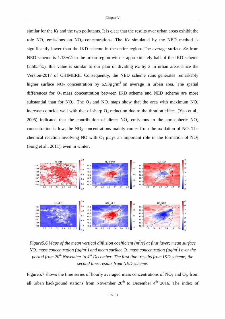
Chapter V
132/191
similar for the Kz and the two pollutants. It is clear that the results over urban areas exhibit the
role NO2 emissions on NO2 concentrations. The Kz simulated by the NED method is
significantly lower than the IKD scheme in the entire region. The average surface Kz from
NED scheme is 1.13m2/s
in the urban region with is approximately half of the IKD scheme
(2.50m2/s), this value is similar to our plan of dividing Kz by 2 in urban areas since the
Version-2017 of CHIMERE. Consequently, the NED scheme runs generates remarkably
higher surface NO2 concentration by 6.93µg/m3
on average in urban area. The spatial
differences for O3 mass concentration between IKD scheme and NED scheme are more
substantial than for NO2. The O3 and NO2 maps show that the area with maximum NO2
increase coincide well with that of sharp O3 reduction due to the titration effect. (Yao et al.,
2005) indicated that the contribution of direct NO2 emissions to the atmospheric NO2
concentration is low, the NO2 concentrations mainly comes from the oxidation of NO. The
chemical reaction involving NO with O3 plays an important role in the formation of NO2
(Song et al., 2011), even in winter.
Figure5.6 Maps of the mean vertical diffusion coefficient (m2/s) at first layer; mean surface
NO2 mass concentration (µg/m3) and mean surface O3 mass concentration (µg/m
3) over the
period from 20th
November to 4th
December. The first line: results from IKD scheme; the
second line: results from NED scheme.
Figure5.7 shows the time series of hourly averaged mass concentrations of NO2 and O3, from
all urban background stations from November 20th
to December 4th
2016. The index of
Chapter V
133/191
agreement between observed and modelled NO2 can be found in Annex B Figure S5.1.
Relatively high NO2 concentrations were observed in all four urban background stations, with a
mean concentration of 53.45 µg/m3; 50.05 µg/m
3; 52.47 µg/m
3; 49.66 µg/m
3 in FR04002;
FR04034; FR04143; FR04156 station, respectively. Table5.2 lists the performances of NO2
simulation for both schemes with their average mass concentration (Avg); correlation (R);
mean bias (MB) and root mean square error (RMSE) at each station. The results show that the
period is well modelled by the IKD scheme with the correlation from 0.62 to 0.74 among
stations. However, this scheme seems underestimated NO2 concentration in all stations, this is
mainly because of the underestimation during the PE. The performance of NED scheme is
very satisfactory and improves NO2 simulations for most of stations. Taking the relative
changes in RMSE as the evaluation criteria, the largest improvements occur for FR04034
station (the improvement is of 19.22%). The averaged time series and statistics for the urban
background stations are summarized in Figure S5.2 and Table S5.1. The two schemes capture
quite well the evolution of NO2 concentration over the urban region, the R and MB are 0.74
and -10.40µg/m3
for IKD scheme and 0.80 and -3.80 µg/m3
for NED scheme with the
improvement is of 18.77% in the urban area. It is noteworthy that both schemes give a better
performance in the city center station (FR40143) than others, it may indicates categories of
urban area are not enough detailed in the model, which might help assessing the urban
categories and roughness length for the model in the urban area. The performances of O3
simulation from IKD and NED schemes are quite different according to their performances of
NO2 simulation. The IKD scheme gives a clearly better performance in the first three days of
the period. Subsequently, both schemes significantly overestimate the O3 concentration at all
urban background stations until 27th
November. Previous researches reported that surface O3
concentrations in wintertime are highly correlated to reduced photochemical activity (Chen et
al., 2020; Peshin et al., 2017). Therefore, the overestimation of O3 may due to
underestimation of cloud thickness in this period. Table5.3 provides an overall evaluation for
IKD and NED schemes for the urban stations. O3 concentrations are on average overestimated
particularly for the IKD scheme. However, the time series shows that the O3 concentration is
strongly overestimated in some days, therefore the MB cannot well represent the simulation
accuracy of two schemes for O3. Unlike the results of NO2 simulation, the IKD scheme gives
Chapter V
134/191
a better correlation and RMSE in all stations than NED scheme. The NED scheme resulted in
4.05%, 9.12%, 1.27% and 13.86% drops in O3 simulation accuracy in four urban stations.
Figure5.7 also shows the ability of the model to locate the pattern of the PE but also a clear
underestimation of NO2 concentrations during the PE for all stations. At most of the sites, the
peak NO2 concentration occurred during the daytime on December 1st, the NO2 exceeded
200µg/m3
in the observations but the model does not effectively capture this moment with
both schemes. The average mean bias in urban background stations for IKD and NED schemes
during the PE are -39.88µg/m3 and -24.16µg/m
3 respectively, showing a better ability of the
NED simulation to reproduce primary pollutant concentrations
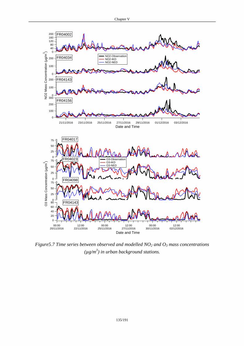
Chapter V
135/191
Figure5.7 Time series between observed and modelled NO2 and O3 mass concentrations
(µg/m3) in urban background stations.
200
100
0
NO
2 M
ass C
oncentr
ation (
µg/m
3)
21/11/2016 23/11/2016 25/11/2016 27/11/2016 29/11/2016 01/12/2016 03/12/2016
Date and Time
200
100
0
200
160
120
80
40
0
300
200
100
0
FR04034
FR04143
NO2-Observation NO2-IKD NO2-NED
FR04002
FR04156
75
50
25
0
O3 M
ass C
oncentr
ation (
µg/m
3)
00:0020/11/2016
12:0022/11/2016
00:0025/11/2016
12:0027/11/2016
00:0030/11/2016
12:0002/12/2016
Date and Time
75
50
25
0
75
50
25
0
80
60
40
20
0
FR04017
FR04023
FR04098
FR04143
O3-Observation O3-IKD O3-NED
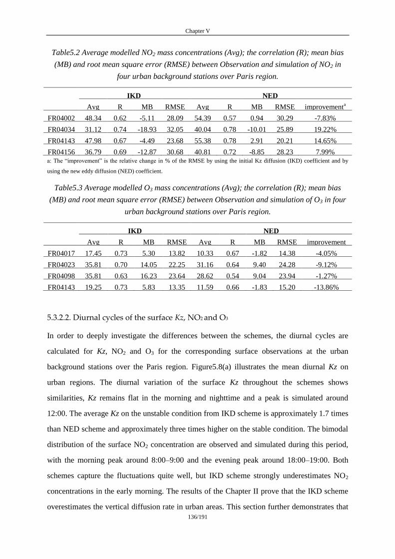
Chapter V
136/191
Table5.2 Average modelled NO2 mass concentrations (Avg); the correlation (R); mean bias
(MB) and root mean square error (RMSE) between Observation and simulation of NO2 in
four urban background stations over Paris region.
IKD NED
Avg R MB RMSE Avg R MB RMSE improvementa
FR04002 48.34 0.62 -5.11 28.09 54.39 0.57 0.94 30.29 -7.83%
FR04034 31.12 0.74 -18.93 32.05 40.04 0.78 -10.01 25.89 19.22%
FR04143 47.98 0.67 -4.49 23.68 55.38 0.78 2.91 20.21 14.65%
FR04156 36.79 0.69 -12.87 30.68 40.81 0.72 -8.85 28.23 7.99% a: The ―improvement‖ is the relative change in % of the RMSE by using the initial Kz diffusion (IKD) coefficient and by
using the new eddy diffusion (NED) coefficient.
Table5.3 Average modelled O3 mass concentrations (Avg); the correlation (R); mean bias
(MB) and root mean square error (RMSE) between Observation and simulation of O3 in four
urban background stations over Paris region.
IKD NED
Avg R MB RMSE Avg R MB RMSE improvement
FR04017 17.45 0.73 5.30 13.82 10.33 0.67 -1.82 14.38 -4.05%
FR04023 35.81 0.70 14.05 22.25 31.16 0.64 9.40 24.28 -9.12%
FR04098 35.81 0.63 16.23 23.64 28.62 0.54 9.04 23.94 -1.27%
FR04143 19.25 0.73 5.83 13.35 11.59 0.66 -1.83 15.20 -13.86%
5.3.2.2. Diurnal cycles of the surface Kz, NO2 and O3
In order to deeply investigate the differences between the schemes, the diurnal cycles are
calculated for Kz, NO2 and O3 for the corresponding surface observations at the urban
background stations over the Paris region. Figure5.8(a) illustrates the mean diurnal Kz on
urban regions. The diurnal variation of the surface Kz throughout the schemes shows
similarities, Kz remains flat in the morning and nighttime and a peak is simulated around
12:00. The average Kz on the unstable condition from IKD scheme is approximately 1.7 times
than NED scheme and approximately three times higher on the stable condition. The bimodal
distribution of the surface NO2 concentration are observed and simulated during this period,
with the morning peak around 8:00–9:00 and the evening peak around 18:00–19:00. Both
schemes capture the fluctuations quite well, but IKD scheme strongly underestimates NO2
concentrations in the early morning. The results of the Chapter II prove that the IKD scheme
overestimates the vertical diffusion rate in urban areas. This section further demonstrates that
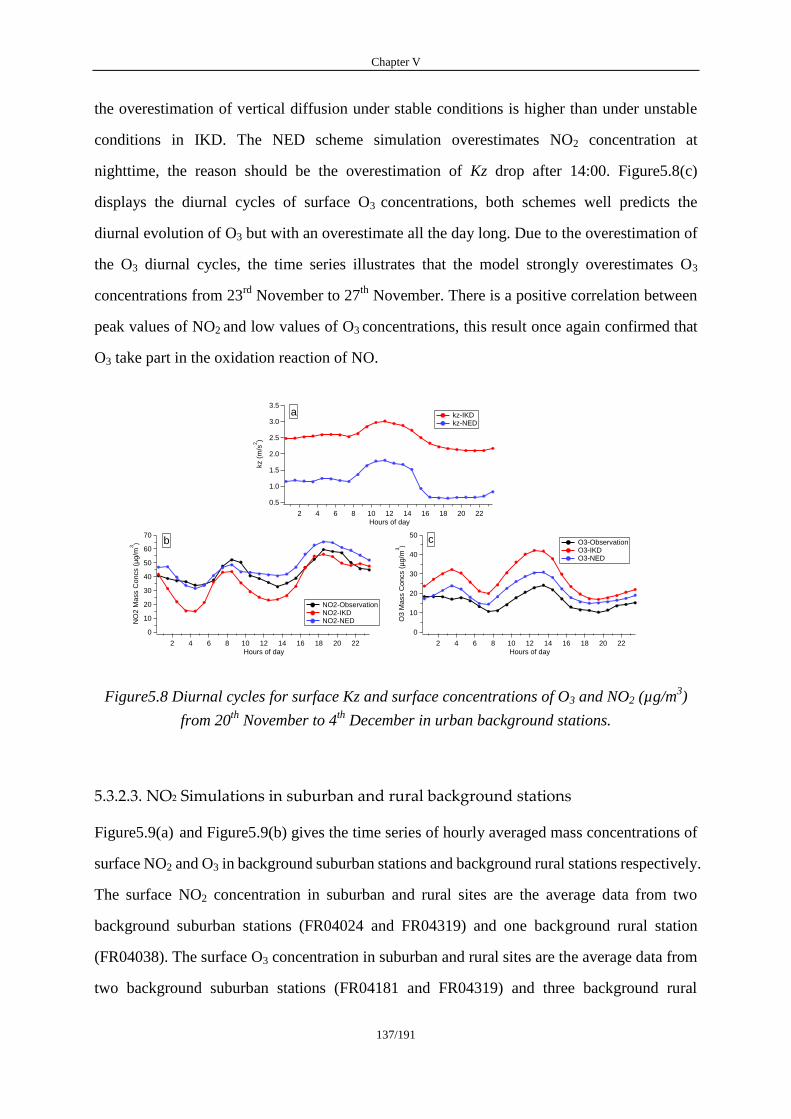
Chapter V
137/191
the overestimation of vertical diffusion under stable conditions is higher than under unstable
conditions in IKD. The NED scheme simulation overestimates NO2 concentration at
nighttime, the reason should be the overestimation of Kz drop after 14:00. Figure5.8(c)
displays the diurnal cycles of surface O3 concentrations, both schemes well predicts the
diurnal evolution of O3 but with an overestimate all the day long. Due to the overestimation of
the O3 diurnal cycles, the time series illustrates that the model strongly overestimates O3
concentrations from 23rd
November to 27th
November. There is a positive correlation between
peak values of NO2 and low values of O3 concentrations, this result once again confirmed that
O3 take part in the oxidation reaction of NO.
Figure5.8 Diurnal cycles for surface Kz and surface concentrations of O3 and NO2 (µg/m3)
from 20th
November to 4th
December in urban background stations.
5.3.2.3. NO2 Simulations in suburban and rural background stations
Figure5.9(a) and Figure5.9(b) gives the time series of hourly averaged mass concentrations of
surface NO2 and O3 in background suburban stations and background rural stations respectively.
The surface NO2 concentration in suburban and rural sites are the average data from two
background suburban stations (FR04024 and FR04319) and one background rural station
(FR04038). The surface O3 concentration in suburban and rural sites are the average data from
two background suburban stations (FR04181 and FR04319) and three background rural
70
60
50
40
30
20
10
0
NO
2 M
ass C
on
cs (
µg
/m3)
222018161412108642
Hours of day
NO2-Observation NO2-IKD NO2-NED
b50
40
30
20
10
0
O3
Ma
ss C
on
cs (
µg
/m3)
222018161412108642
Hours of day
O3-Observation O3-IKD O3-NED
c
3.5
3.0
2.5
2.0
1.5
1.0
0.5
kz (
m/s
2)
222018161412108642
Hours of day
kz-IKD kz-NED
a
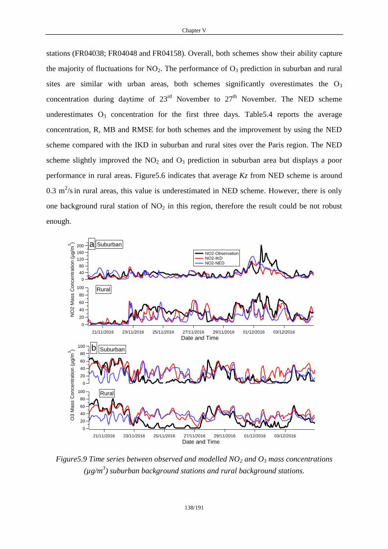
Chapter V
138/191
stations (FR04038; FR04048 and FR04158). Overall, both schemes show their ability capture
the majority of fluctuations for NO2. The performance of O3 prediction in suburban and rural
sites are similar with urban areas, both schemes significantly overestimates the O3
concentration during daytime of 23rd
November to 27th
November. The NED scheme
underestimates O3 concentration for the first three days. Table5.4 reports the average
concentration, R, MB and RMSE for both schemes and the improvement by using the NED
scheme compared with the IKD in suburban and rural sites over the Paris region. The NED
scheme slightly improved the NO2 and O3 prediction in suburban area but displays a poor
performance in rural areas. Figure5.6 indicates that average Kz from NED scheme is around
0.3 m2/s
in rural areas, this value is underestimated in NED scheme. However, there is only
one background rural station of NO2 in this region, therefore the result could be not robust
enough.
Figure5.9 Time series between observed and modelled NO2 and O3 mass concentrations
(µg/m3) suburban background stations and rural background stations.
100
80
60
40
20
0
O3
Ma
ss C
on
ce
ntr
atio
n (
µg
/m3)
21/11/2016 23/11/2016 25/11/2016 27/11/2016 29/11/2016 01/12/2016 03/12/2016
Date and Time
100
80
60
40
20
0
Suburban
Rural
b
100
80
60
40
20
0
NO
2 M
ass C
on
ce
ntr
atio
n (
µg
/m3)
21/11/2016 23/11/2016 25/11/2016 27/11/2016 29/11/2016 01/12/2016 03/12/2016
Date and Time
200
160
120
80
40
0
Suburban
Rural
NO2-Observation NO2-IKD NO2-NED
a
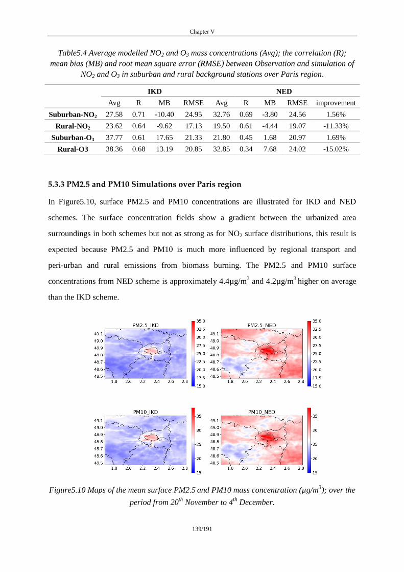
Chapter V
139/191
Table5.4 Average modelled NO2 and O3 mass concentrations (Avg); the correlation (R);
mean bias (MB) and root mean square error (RMSE) between Observation and simulation of
NO2 and O3 in suburban and rural background stations over Paris region.
IKD NED
Avg R MB RMSE Avg R MB RMSE improvement
Suburban-NO2 27.58 0.71 -10.40 24.95 32.76 0.69 -3.80 24.56 1.56%
Rural-NO2 23.62 0.64 -9.62 17.13 19.50 0.61 -4.44 19.07 -11.33%
Suburban-O3 37.77 0.61 17.65 21.33 21.80 0.45 1.68 20.97 1.69%
Rural-O3 38.36 0.68 13.19 20.85 32.85 0.34 7.68 24.02 -15.02%
5.3.3 PM2.5 and PM10 Simulations over Paris region
In Figure5.10, surface PM2.5 and PM10 concentrations are illustrated for IKD and NED
schemes. The surface concentration fields show a gradient between the urbanized area
surroundings in both schemes but not as strong as for NO2 surface distributions, this result is
expected because PM2.5 and PM10 is much more influenced by regional transport and
peri-urban and rural emissions from biomass burning. The PM2.5 and PM10 surface
concentrations from NED scheme is approximately 4.4µg/m3 and 4.2µg/m
3 higher on average
than the IKD scheme.
Figure5.10 Maps of the mean surface PM2.5 and PM10 mass concentration (µg/m
3); over the
period from 20th
November to 4th
December.
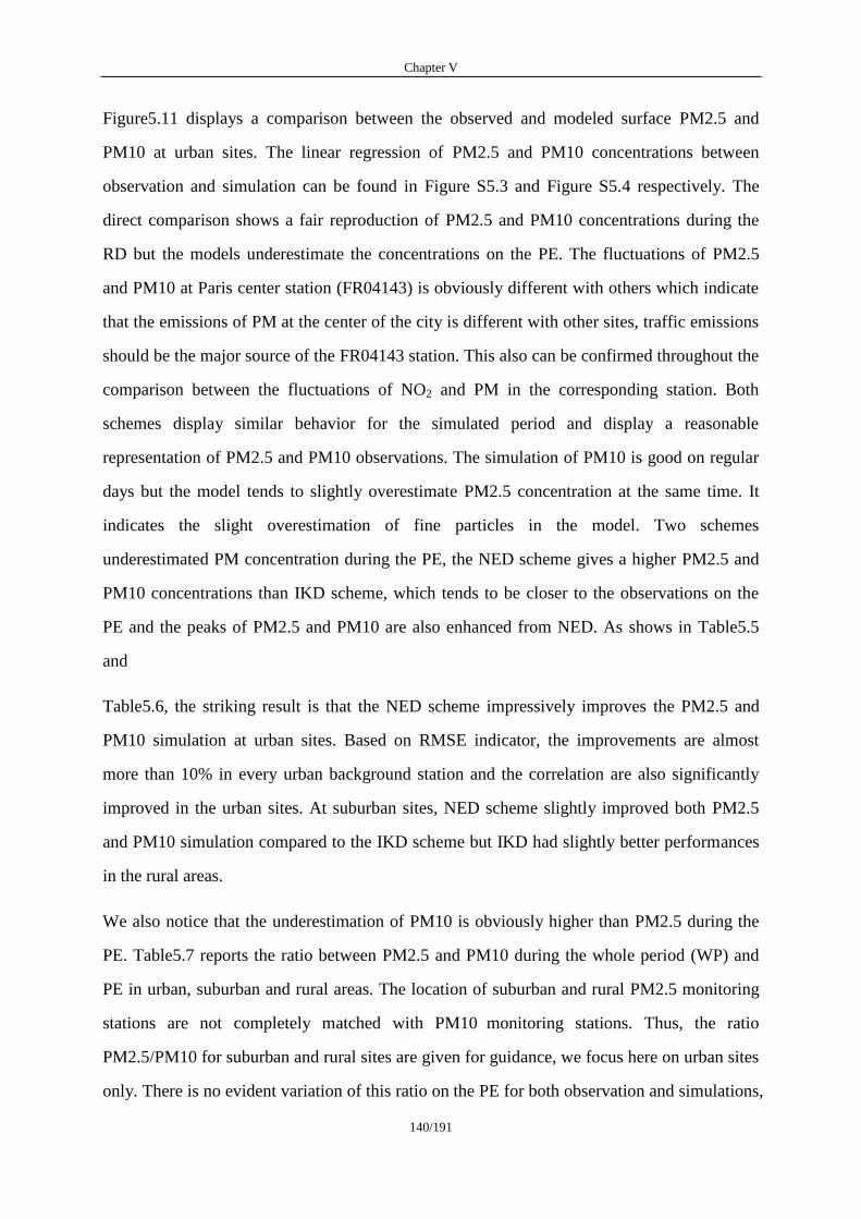
Chapter V
140/191
Figure5.11 displays a comparison between the observed and modeled surface PM2.5 and
PM10 at urban sites. The linear regression of PM2.5 and PM10 concentrations between
observation and simulation can be found in Figure S5.3 and Figure S5.4 respectively. The
direct comparison shows a fair reproduction of PM2.5 and PM10 concentrations during the
RD but the models underestimate the concentrations on the PE. The fluctuations of PM2.5
and PM10 at Paris center station (FR04143) is obviously different with others which indicate
that the emissions of PM at the center of the city is different with other sites, traffic emissions
should be the major source of the FR04143 station. This also can be confirmed throughout the
comparison between the fluctuations of NO2 and PM in the corresponding station. Both
schemes display similar behavior for the simulated period and display a reasonable
representation of PM2.5 and PM10 observations. The simulation of PM10 is good on regular
days but the model tends to slightly overestimate PM2.5 concentration at the same time. It
indicates the slight overestimation of fine particles in the model. Two schemes
underestimated PM concentration during the PE, the NED scheme gives a higher PM2.5 and
PM10 concentrations than IKD scheme, which tends to be closer to the observations on the
PE and the peaks of PM2.5 and PM10 are also enhanced from NED. As shows in Table5.5
and
Table5.6, the striking result is that the NED scheme impressively improves the PM2.5 and
PM10 simulation at urban sites. Based on RMSE indicator, the improvements are almost
more than 10% in every urban background station and the correlation are also significantly
improved in the urban sites. At suburban sites, NED scheme slightly improved both PM2.5
and PM10 simulation compared to the IKD scheme but IKD had slightly better performances
in the rural areas.
We also notice that the underestimation of PM10 is obviously higher than PM2.5 during the
PE. Table5.7 reports the ratio between PM2.5 and PM10 during the whole period (WP) and
PE in urban, suburban and rural areas. The location of suburban and rural PM2.5 monitoring
stations are not completely matched with PM10 monitoring stations. Thus, the ratio
PM2.5/PM10 for suburban and rural sites are given for guidance, we focus here on urban sites
only. There is no evident variation of this ratio on the PE for both observation and simulations,
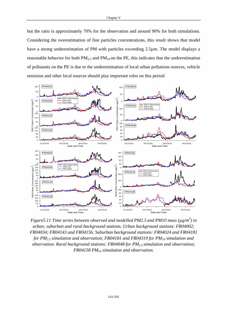
Chapter V
141/191
but the ratio is approximately 70% for the observation and around 90% for both simulations.
Considering the overestimation of fine particles concentrations, this result shows that model
have a strong underestimation of PM with particles exceeding 2.5µm. The model displays a
reasonable behavior for both PM2.5 and PM10 on the PE, this indicates that the underestimation
of pollutants on the PE is due to the underestimation of local urban pollutions sources, vehicle
emission and other local sources should play important roles on this period.
Figure5.11 Time series between observed and modelled PM2.5 and PM10 mass (µg/m3) in
urban; suburban and rural background stations. Urban background stations: FR04002;
FR04034; FR04143 and FR04156. Suburban background stations: FR04024 and FR04181
for PM2.5 simulation and observation; FR04181 and FR04319 for PM10 simulation and
observation. Rural background stations: FR04048 for PM2.5 simulation and observation;
FR04158 PM10 simulation and observation.
150
100
50
0
PM
2.5
Mass C
oncentr
ation (
µg/m
3)
21/11/2016 25/11/2016 29/11/2016 03/12/2016
Date and Time
100
50
0
100
50
0
160
120
80
40
0
FR04002
FR04034
FR04143
FR04156
PM2.5-Observation PM2.5-IKD PM2.5-NED
100
50
0
21/11/2016 25/11/2016 29/11/2016 03/12/2016
Date and Time
100
50
0
PM
2.5
Mass C
oncentr
ation (
µg/m
3)
100
80
60
40
20
0
FR04024
FR04181
FR04048
PM2.5-Observation PM2.5-IKD PM2.5-NED
200
160
120
80
40
0
PM
10 M
ass C
oncentr
ation (
µg/m
3)
21/11/2016 25/11/2016 29/11/2016 03/12/2016
Date and Time
150
100
50
0200
160
120
80
40
0
200
150
100
50
0
FR04002
FR04034
FR04143
FR04156
PM10-Observation PM10-IKD PM10-NED
160
120
80
40
0
21/11/2016 25/11/2016 29/11/2016 03/12/2016
Date and Time
200
100
0
PM
10 M
ass C
oncentr
ation (
µg/m
3)
100
80
60
40
20
0
FR04181
FR04319
FR04158
PM10-Observation PM10-IKD PM10-NED
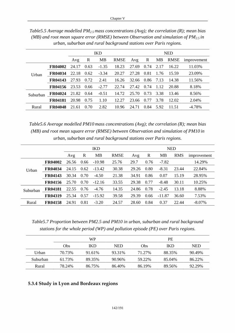
Chapter V
142/191
Table5.5 Average modelled PM2.5 mass concentrations (Avg); the correlation (R); mean bias
(MB) and root mean square error (RMSE) between Observation and simulation of PM2.5 in
urban, suburban and rural background stations over Paris regions.
IKD NED
Avg R MB RMSE Avg R MB RMSE improvement
Urban
FR04002 24.17 0.63 -1.35 18.23 27.69 0.74 2.17 16.22 11.03%
FR04034 22.18 0.62 -3.34 20.27 27.28 0.81 1.76 15.59 23.09%
FR04143 27.93 0.72 2.41 16.26 32.66 0.86 7.13 14.38 11.56%
FR04156 23.53 0.66 -2.77 22.74 27.42 0.74 1.12 20.88 8.18%
Suburban FR04024 21.82 0.64 -0.51 14.72 25.70 0.73 3.38 13.46 8.56%
FR04181 20.98 0.75 1.10 12.27 23.66 0.77 3.78 12.02 2.04%
Rural FR04048 21.61 0.70 2.82 10.96 24.71 0.84 5.92 11.51 -4.78%
Table5.6 Average modelled PM10 mass concentrations (Avg); the correlation (R); mean bias
(MB) and root mean square error (RMSE) between Observation and simulation of PM10 in
urban, suburban and rural background stations over Paris regions.
IKD NED
Avg R MB RMSE Avg R MB RMS
E
improvement
Urban
FR04002 26.56 0.66 -10.98 25.76 29.7
2
0.76 -7.82
22.08
14.29%
FR04034 24.15 0.62 -13.42 30.38 29.26 0.80 -8.31 23.44 22.84%
FR04143 30.34 0.70 -4.50 21.38 34.91 0.86 0.07 15.19 28.95%
FR04156 25.70 0.70 -12.16 33.55 29.38 0.77 -8.48 30.11 10.25%
Suburban FR04181 22.55 0.76 -4.76 14.35 24.86 0.78 -2.45 13.18 8.88%
FR04319 25.34 0.57 -15.92 39.58 29.39 0.66 -11.87 36.60 7.53%
Rural FR04158 24.91 0.81 -3.20 24.57 28.60 0.84 0.37 22.44 -8.07%
Table5.7 Proportion between PM2.5 and PM10 in urban, suburban and rural background
stations for the whole period (WP) and pollution episode (PE) over Paris regions.
WP PE
Obs IKD NED Obs IKD NED
Urban 70.73% 91.61% 93.31% 71.27% 88.35% 90.49%
Suburban 61.73% 89.35% 90.96% 59.22% 85.04% 86.22%
Rural 78.24% 86.75% 86.40% 86.19% 89.56% 92.29%
5.3.4 Study in Lyon and Bordeaux regions

Chapter V
143/191
The IKD and NED schemes are also applied in Bordeaux and Lyon areas in order to
understand whether the NED scheme can be used in other areas. Lyon is in the southeast of
France and is located in the Rhone valley where the wind is meridional and often strong
particularly in winter and is the second largest city in France. Bordeaux is close to the sea that
is often influenced by oceanic flows and located in the southwest part of France. The period
of interest remains the same from 20th
November to 4th
December.
5.3.4.1. Ground Meteorological Variables
Here, we compared observation of 2 meters temperature (T2) and 10 meters wind speed (W10)
from four meteorological observation sites (three in Lyon and one in Bordeaux) to the
simulations from WRF. The comparison is of hourly average values from observation sites
with hourly average values from the nearest of each site location. Figure5.12 presents the
maps of averaged T2 and W10 simulated in Lyon and Bordeaux over the period. Both regions
show a UHI effect in the urban region, which gives positive bias of up to 3°C over the period
in Lyon and 2.5°C in Bordeaux respectively compared to the rural areas. The maps of W10
presents a higher surface wind speed in rural areas than in urban regions with a negative bias for
3.2m/s in Lyon and 3.5m/s in Bordeaux respectively. The City of Lyon is formed by the core
city of Lyon and its 58 suburban municipalities, so the UHI effect is more widespread than
Bordeaux.
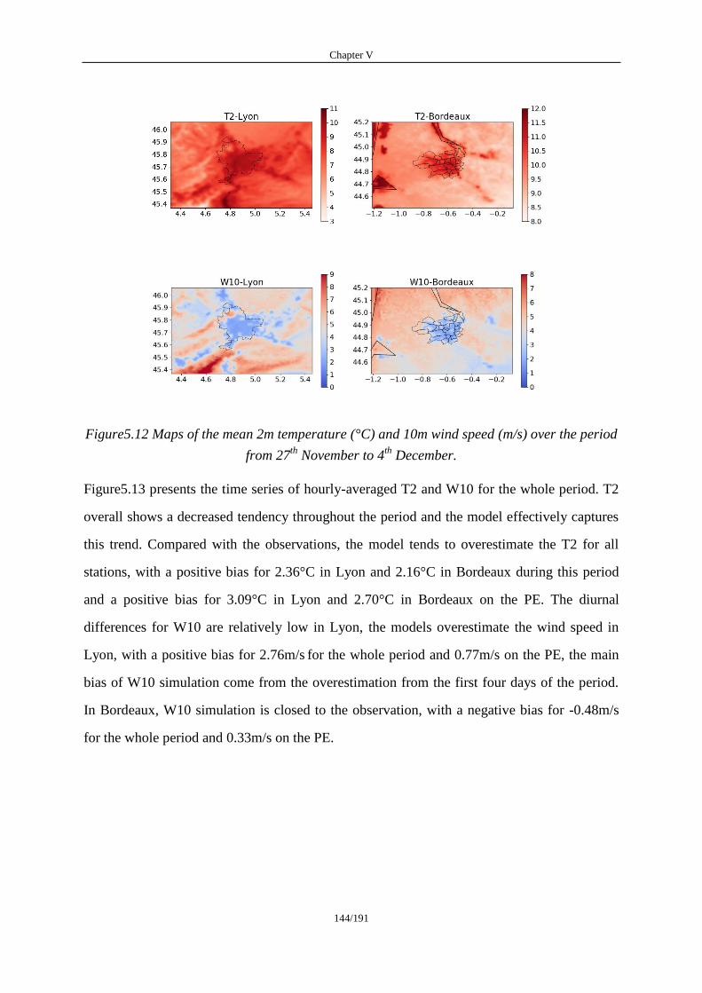
Chapter V
144/191
Figure5.12 Maps of the mean 2m temperature (°C) and 10m wind speed (m/s) over the period
from 27th
November to 4th
December.
Figure5.13 presents the time series of hourly-averaged T2 and W10 for the whole period. T2
overall shows a decreased tendency throughout the period and the model effectively captures
this trend. Compared with the observations, the model tends to overestimate the T2 for all
stations, with a positive bias for 2.36°C in Lyon and 2.16°C in Bordeaux during this period
and a positive bias for 3.09°C in Lyon and 2.70°C in Bordeaux on the PE. The diurnal
differences for W10 are relatively low in Lyon, the models overestimate the wind speed in
Lyon, with a positive bias for 2.76m/s for the whole period and 0.77m/s on the PE, the main
bias of W10 simulation come from the overestimation from the first four days of the period.
In Bordeaux, W10 simulation is closed to the observation, with a negative bias for -0.48m/s
for the whole period and 0.33m/s on the PE.
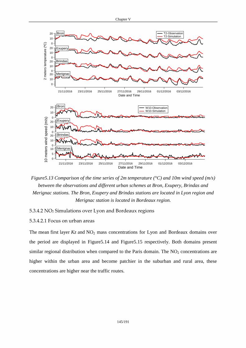
Chapter V
145/191
Figure5.13 Comparison of the time series of 2m temperature (°C) and 10m wind speed (m/s)
between the observations and different urban schemes at Bron, Exupery, Brindas and
Merignac stations. The Bron, Exupery and Brindas stations are located in Lyon region and
Merignac station is located in Bordeaux region.
5.3.4.2 NO2 Simulations over Lyon and Bordeaux regions
5.3.4.2.1 Focus on urban areas
The mean first layer Kz and NO2 mass concentrations for Lyon and Bordeaux domains over
the period are displayed in Figure5.14 and Figure5.15 respectively. Both domains present
similar regional distribution when compared to the Paris domain. The NO2 concentrations are
higher within the urban area and become patchier in the suburban and rural area, these
concentrations are higher near the traffic routes.
10
5
0
21/11/2016 23/11/2016 25/11/2016 27/11/2016 29/11/2016 01/12/2016 03/12/2016
Date and Time
20
10
0
20
10
0
10
me
ters
win
d s
pe
ed
(m
/s)
20
10
0
W10-Observation W10-Simulation
Bron
Exupery
Brindas
Merignac
20
10
0
21/11/2016 23/11/2016 25/11/2016 27/11/2016 29/11/2016 01/12/2016 03/12/2016
Date and Time
20
10
0
20
10
0
2 m
ete
rs t
em
pera
ture
(ºC
)
20
10
0
Bron
Exupery
Brindas
Merignac
T2-Observation T2-Simulation

Chapter V
146/191
Figure5.14 Maps of the mean vertical diffusion coefficient (m2/s); over the period from 20
th
November to 4th
December. The first line: results from Lyon domain; the second line: results
from Bordeaux domain.
Figure5.15 Maps of the mean surface NO2 mass concentration (µg/m3); over the period from
20th
November to 4th
December. The first line: results from Lyon domain; the second line:
results from Bordeaux domain.
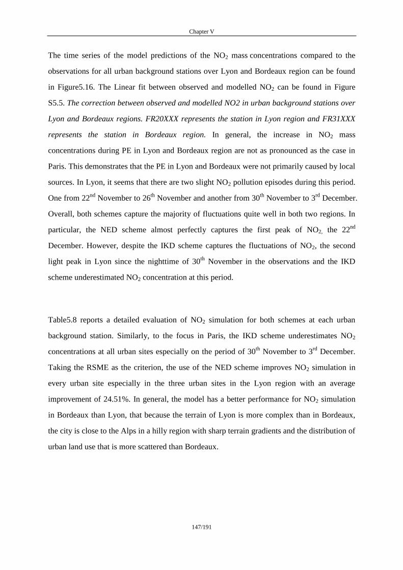
Chapter V
147/191
The time series of the model predictions of the NO2 mass concentrations compared to the
observations for all urban background stations over Lyon and Bordeaux region can be found
in Figure5.16. The Linear fit between observed and modelled NO2 can be found in Figure
S5.5. The correction between observed and modelled NO2 in urban background stations over
Lyon and Bordeaux regions. FR20XXX represents the station in Lyon region and FR31XXX
represents the station in Bordeaux region. In general, the increase in NO2 mass
concentrations during PE in Lyon and Bordeaux region are not as pronounced as the case in
Paris. This demonstrates that the PE in Lyon and Bordeaux were not primarily caused by local
sources. In Lyon, it seems that there are two slight NO2 pollution episodes during this period.
One from 22nd
November to 26th
November and another from 30th
November to 3rd
December.
Overall, both schemes capture the majority of fluctuations quite well in both two regions. In
particular, the NED scheme almost perfectly captures the first peak of NO2, the 22nd
December. However, despite the IKD scheme captures the fluctuations of NO2, the second
light peak in Lyon since the nighttime of 30th
November in the observations and the IKD
scheme underestimated NO2 concentration at this period.
Table5.8 reports a detailed evaluation of NO2 simulation for both schemes at each urban
background station. Similarly, to the focus in Paris, the IKD scheme underestimates NO2
concentrations at all urban sites especially on the period of 30th
November to 3rd
December.
Taking the RSME as the criterion, the use of the NED scheme improves NO2 simulation in
every urban site especially in the three urban sites in the Lyon region with an average
improvement of 24.51%. In general, the model has a better performance for NO2 simulation
in Bordeaux than Lyon, that because the terrain of Lyon is more complex than in Bordeaux,
the city is close to the Alps in a hilly region with sharp terrain gradients and the distribution of
urban land use that is more scattered than Bordeaux.
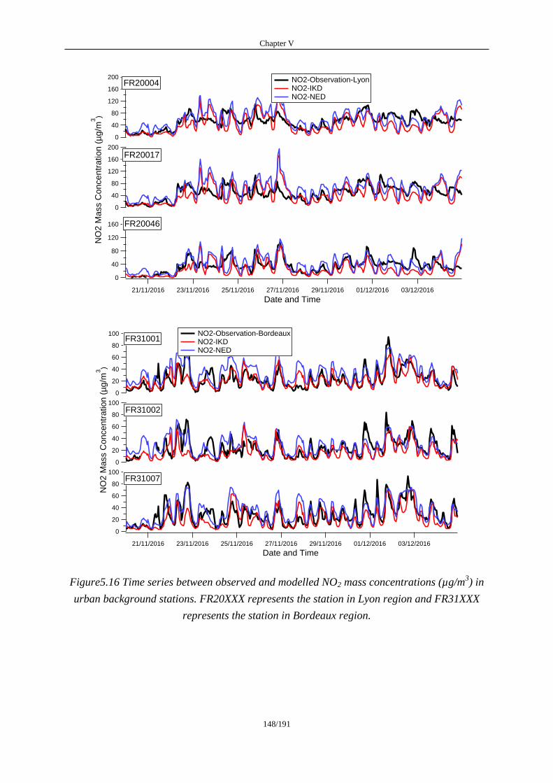
Chapter V
148/191
Figure5.16 Time series between observed and modelled NO2 mass concentrations (µg/m3) in
urban background stations. FR20XXX represents the station in Lyon region and FR31XXX
represents the station in Bordeaux region.
200
160
120
80
40
0
21/11/2016 23/11/2016 25/11/2016 27/11/2016 29/11/2016 01/12/2016 03/12/2016
Date and Time
200
160
120
80
40
0
NO
2 M
ass C
on
ce
ntr
atio
n (
µg
/m3)
160
120
80
40
0
FR20046
FR20017
FR20004 NO2-Observation-Lyon NO2-IKD NO2-NED
100
80
60
40
20
0
21/11/2016 23/11/2016 25/11/2016 27/11/2016 29/11/2016 01/12/2016 03/12/2016
Date and Time
100
80
60
40
20
0
NO
2 M
ass C
oncentr
atio
n (
µg/m
3)
100
80
60
40
20
0
FR31001
FR31002
FR31007
NO2-Observation-Bordeaux NO2-IKD NO2-NED
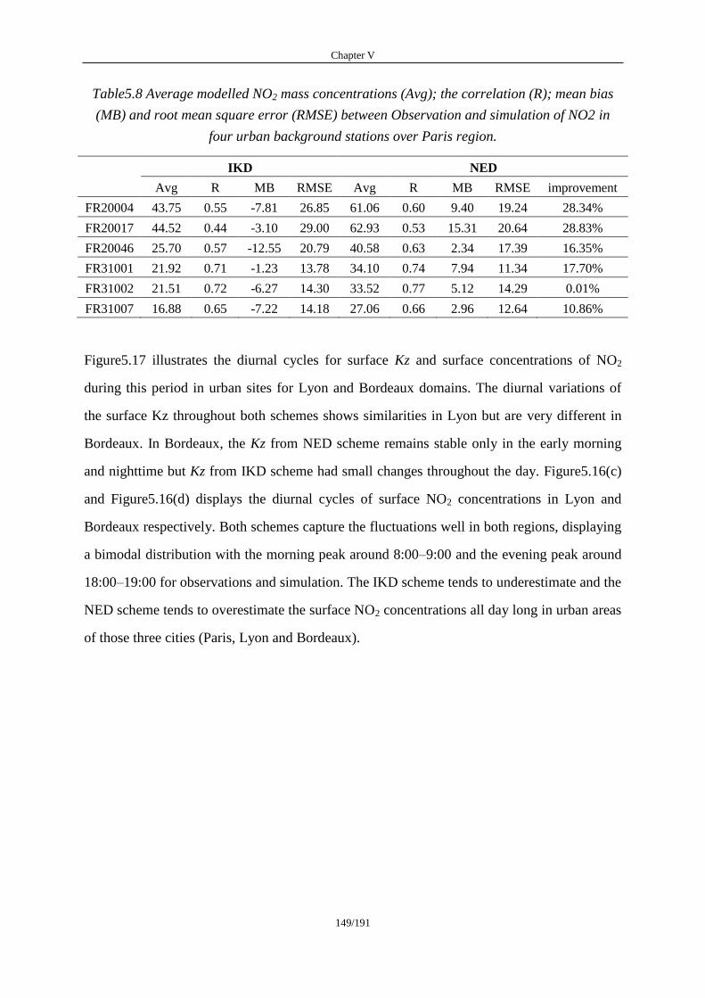
Chapter V
149/191
Table5.8 Average modelled NO2 mass concentrations (Avg); the correlation (R); mean bias
(MB) and root mean square error (RMSE) between Observation and simulation of NO2 in
four urban background stations over Paris region.
IKD NED
Avg R MB RMSE Avg R MB RMSE improvement
FR20004 43.75 0.55 -7.81 26.85 61.06 0.60 9.40 19.24 28.34%
FR20017 44.52 0.44 -3.10 29.00 62.93 0.53 15.31 20.64 28.83%
FR20046 25.70 0.57 -12.55 20.79 40.58 0.63 2.34 17.39 16.35%
FR31001 21.92 0.71 -1.23 13.78 34.10 0.74 7.94 11.34 17.70%
FR31002 21.51 0.72 -6.27 14.30 33.52 0.77 5.12 14.29 0.01%
FR31007 16.88 0.65 -7.22 14.18 27.06 0.66 2.96 12.64 10.86%
Figure5.17 illustrates the diurnal cycles for surface Kz and surface concentrations of NO2
during this period in urban sites for Lyon and Bordeaux domains. The diurnal variations of
the surface Kz throughout both schemes shows similarities in Lyon but are very different in
Bordeaux. In Bordeaux, the Kz from NED scheme remains stable only in the early morning
and nighttime but Kz from IKD scheme had small changes throughout the day. Figure5.16(c)
and Figure5.16(d) displays the diurnal cycles of surface NO2 concentrations in Lyon and
Bordeaux respectively. Both schemes capture the fluctuations well in both regions, displaying
a bimodal distribution with the morning peak around 8:00–9:00 and the evening peak around
18:00–19:00 for observations and simulation. The IKD scheme tends to underestimate and the
NED scheme tends to overestimate the surface NO2 concentrations all day long in urban areas
of those three cities (Paris, Lyon and Bordeaux).
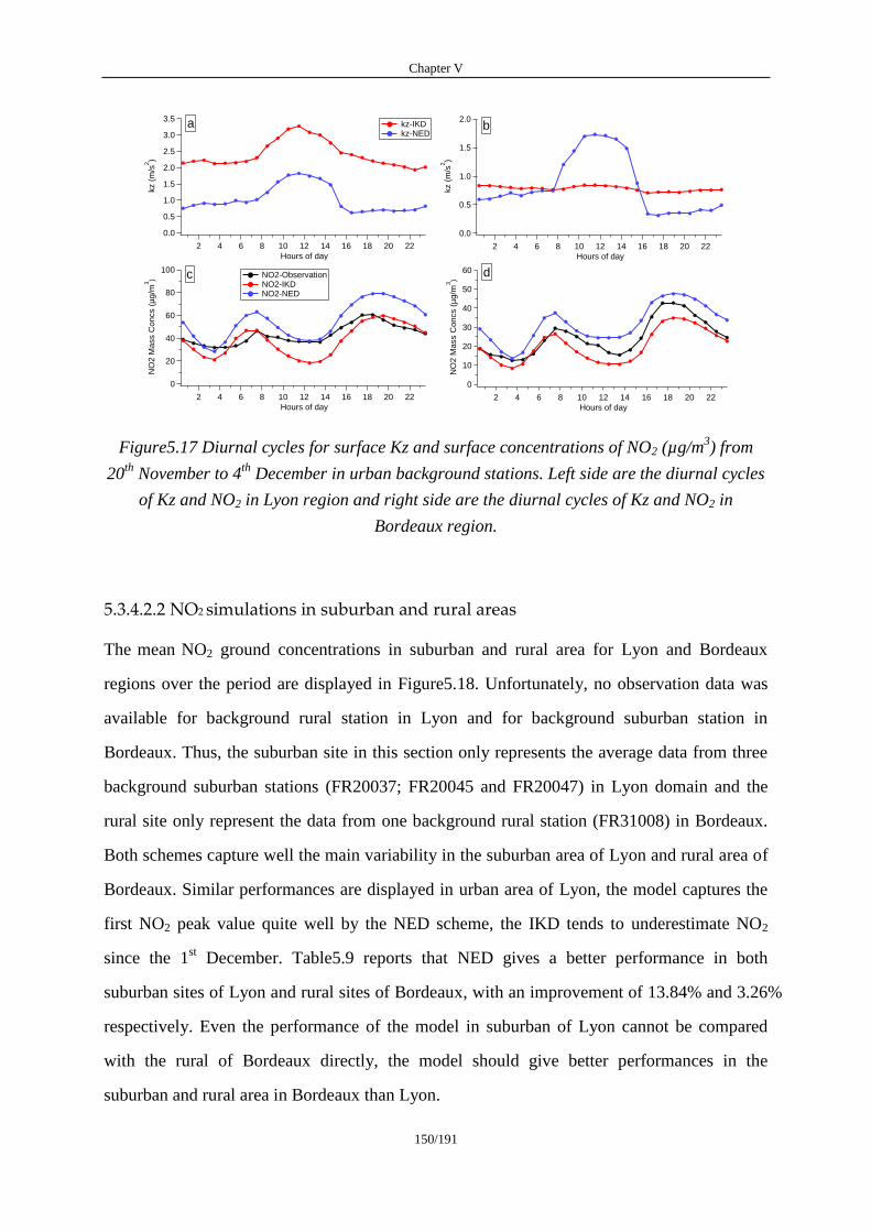
Chapter V
150/191
Figure5.17 Diurnal cycles for surface Kz and surface concentrations of NO2 (µg/m3) from
20th
November to 4th
December in urban background stations. Left side are the diurnal cycles
of Kz and NO2 in Lyon region and right side are the diurnal cycles of Kz and NO2 in
Bordeaux region.
5.3.4.2.2 NO2 simulations in suburban and rural areas
The mean NO2 ground concentrations in suburban and rural area for Lyon and Bordeaux
regions over the period are displayed in Figure5.18. Unfortunately, no observation data was
available for background rural station in Lyon and for background suburban station in
Bordeaux. Thus, the suburban site in this section only represents the average data from three
background suburban stations (FR20037; FR20045 and FR20047) in Lyon domain and the
rural site only represent the data from one background rural station (FR31008) in Bordeaux.
Both schemes capture well the main variability in the suburban area of Lyon and rural area of
Bordeaux. Similar performances are displayed in urban area of Lyon, the model captures the
first NO2 peak value quite well by the NED scheme, the IKD tends to underestimate NO2
since the 1st December. Table5.9 reports that NED gives a better performance in both
suburban sites of Lyon and rural sites of Bordeaux, with an improvement of 13.84% and 3.26%
respectively. Even the performance of the model in suburban of Lyon cannot be compared
with the rural of Bordeaux directly, the model should give better performances in the
suburban and rural area in Bordeaux than Lyon.
3.5
3.0
2.5
2.0
1.5
1.0
0.5
0.0
kz (
m/s
2)
222018161412108642
Hours of day
a kz-IKD kz-NED
60
50
40
30
20
10
0
NO
2 M
ass C
oncs (
µg/m
3)
222018161412108642
Hours of day
d100
80
60
40
20
0
NO
2 M
ass C
oncs (
µg/m
3)
222018161412108642
Hours of day
NO2-Observation NO2-IKD NO2-NED
c
2.0
1.5
1.0
0.5
0.0
kz (
m/s
2)
222018161412108642
Hours of day
b
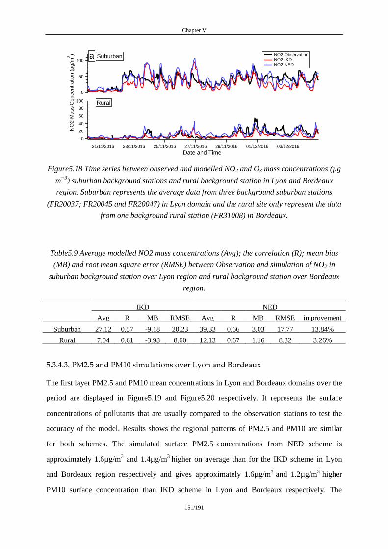
Chapter V
151/191
Figure5.18 Time series between observed and modelled NO2 and O3 mass concentrations (µg
m−3
) suburban background stations and rural background station in Lyon and Bordeaux
region. Suburban represents the average data from three background suburban stations
(FR20037; FR20045 and FR20047) in Lyon domain and the rural site only represent the data
from one background rural station (FR31008) in Bordeaux.
Table5.9 Average modelled NO2 mass concentrations (Avg); the correlation (R); mean bias
(MB) and root mean square error (RMSE) between Observation and simulation of NO2 in
suburban background station over Lyon region and rural background station over Bordeaux
region.
IKD NED
Avg R MB RMSE Avg R MB RMSE improvement
Suburban 27.12 0.57 -9.18 20.23 39.33 0.66 3.03 17.77 13.84%
Rural 7.04 0.61 -3.93 8.60 12.13 0.67 1.16 8.32 3.26%
5.3.4.3. PM2.5 and PM10 simulations over Lyon and Bordeaux
The first layer PM2.5 and PM10 mean concentrations in Lyon and Bordeaux domains over the
period are displayed in Figure5.19 and Figure5.20 respectively. It represents the surface
concentrations of pollutants that are usually compared to the observation stations to test the
accuracy of the model. Results shows the regional patterns of PM2.5 and PM10 are similar
for both schemes. The simulated surface PM2.5 concentrations from NED scheme is
approximately 1.6µg/m3 and 1.4µg/m
3 higher on average than for the IKD scheme in Lyon
and Bordeaux region respectively and gives approximately 1.6µg/m3
and 1.2µg/m3
higher
PM10 surface concentration than IKD scheme in Lyon and Bordeaux respectively. The
100
80
60
40
20
0
NO
2 M
ass C
on
ce
ntr
atio
n (
µg
/m3)
21/11/2016 23/11/2016 25/11/2016 27/11/2016 29/11/2016 01/12/2016 03/12/2016
Date and Time
100
50
0
Suburban
Rural
NO2-Observation NO2-IKD NO2-NED
a
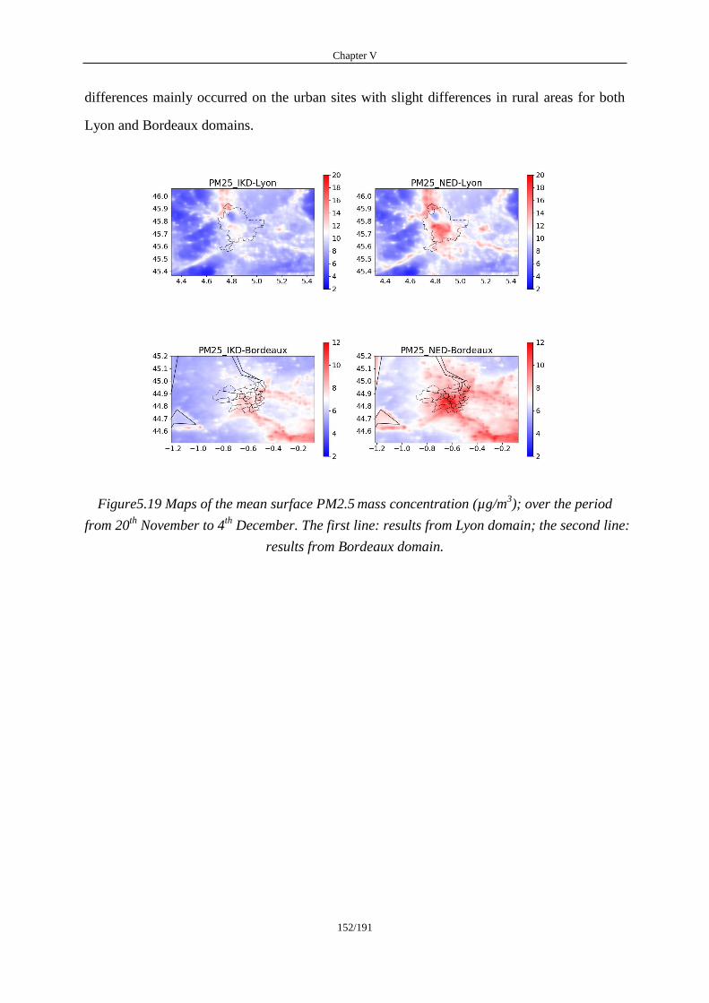
Chapter V
152/191
differences mainly occurred on the urban sites with slight differences in rural areas for both
Lyon and Bordeaux domains.
Figure5.19 Maps of the mean surface PM2.5 mass concentration (µg/m3); over the period
from 20th
November to 4th
December. The first line: results from Lyon domain; the second line:
results from Bordeaux domain.
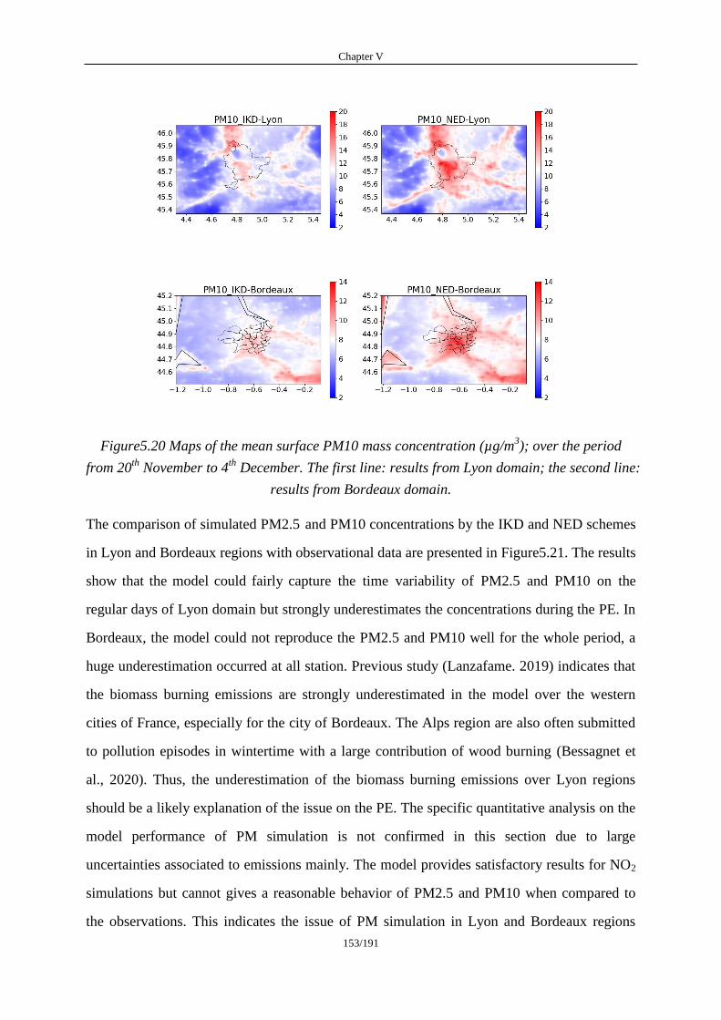
Chapter V
153/191
Figure5.20 Maps of the mean surface PM10 mass concentration (µg/m3); over the period
from 20th
November to 4th
December. The first line: results from Lyon domain; the second line:
results from Bordeaux domain.
The comparison of simulated PM2.5 and PM10 concentrations by the IKD and NED schemes
in Lyon and Bordeaux regions with observational data are presented in Figure5.21. The results
show that the model could fairly capture the time variability of PM2.5 and PM10 on the
regular days of Lyon domain but strongly underestimates the concentrations during the PE. In
Bordeaux, the model could not reproduce the PM2.5 and PM10 well for the whole period, a
huge underestimation occurred at all station. Previous study (Lanzafame. 2019) indicates that
the biomass burning emissions are strongly underestimated in the model over the western
cities of France, especially for the city of Bordeaux. The Alps region are also often submitted
to pollution episodes in wintertime with a large contribution of wood burning (Bessagnet et
al., 2020). Thus, the underestimation of the biomass burning emissions over Lyon regions
should be a likely explanation of the issue on the PE. The specific quantitative analysis on the
model performance of PM simulation is not confirmed in this section due to large
uncertainties associated to emissions mainly. The model provides satisfactory results for NO2
simulations but cannot gives a reasonable behavior of PM2.5 and PM10 when compared to
the observations. This indicates the issue of PM simulation in Lyon and Bordeaux regions
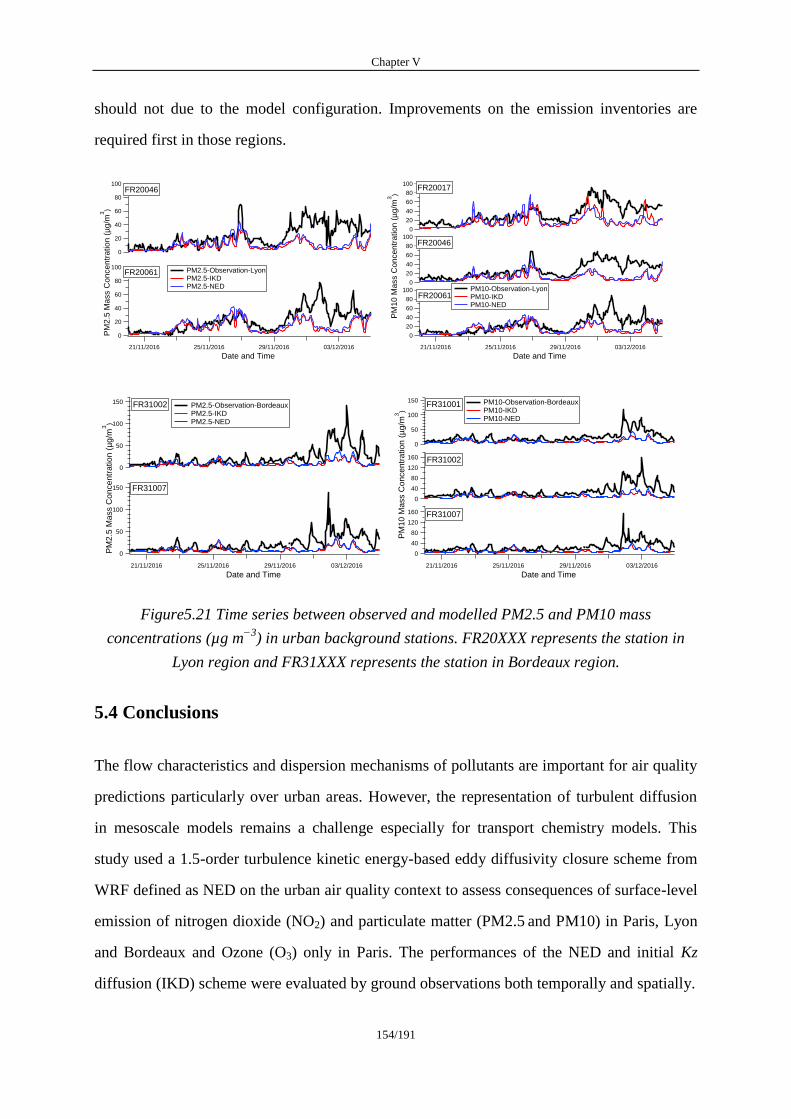
Chapter V
154/191
should not due to the model configuration. Improvements on the emission inventories are
required first in those regions.
Figure5.21 Time series between observed and modelled PM2.5 and PM10 mass
concentrations (µg m−3
) in urban background stations. FR20XXX represents the station in
Lyon region and FR31XXX represents the station in Bordeaux region.
5.4 Conclusions
The flow characteristics and dispersion mechanisms of pollutants are important for air quality
predictions particularly over urban areas. However, the representation of turbulent diffusion
in mesoscale models remains a challenge especially for transport chemistry models. This
study used a 1.5-order turbulence kinetic energy-based eddy diffusivity closure scheme from
WRF defined as NED on the urban air quality context to assess consequences of surface-level
emission of nitrogen dioxide (NO2) and particulate matter (PM2.5 and PM10) in Paris, Lyon
and Bordeaux and Ozone (O3) only in Paris. The performances of the NED and initial Kz
diffusion (IKD) scheme were evaluated by ground observations both temporally and spatially.
100
80
60
40
20
0
21/11/2016 25/11/2016 29/11/2016 03/12/2016
Date and Time
100
80
60
40
20
0
PM
10
Ma
ss C
on
ce
ntr
atio
n (
µg
/m3)
100
80
60
40
20
0
FR20017
FR20046
FR20061 PM10-Observation-Lyon PM10-IKD PM10-NED
100
80
60
40
20
0
21/11/2016 25/11/2016 29/11/2016 03/12/2016
Date and Time
100
80
60
40
20
0 PM
2.5
Ma
ss C
on
ce
ntr
atio
n (
µg
/m3)
PM2.5-Observation-Lyon PM2.5-IKD PM2.5-NED
FR20046
FR20061
160
120
80
40
0
21/11/2016 25/11/2016 29/11/2016 03/12/2016
Date and Time
160
120
80
40
0
PM
10
Ma
ss C
on
ce
ntr
atio
n (
µg
/m3)
150
100
50
0
FR31001
FR31002
FR31007
PM10-Observation-Bordeaux PM10-IKD PM10-NED
150
100
50
0 PM
2.5
Ma
ss C
on
ce
ntr
atio
n (
µg
/m3)
21/11/2016 25/11/2016 29/11/2016 03/12/2016
Date and Time
150
100
50
0
FR31002
FR31007
PM2.5-Observation-Bordeaux PM2.5-IKD PM2.5-NED
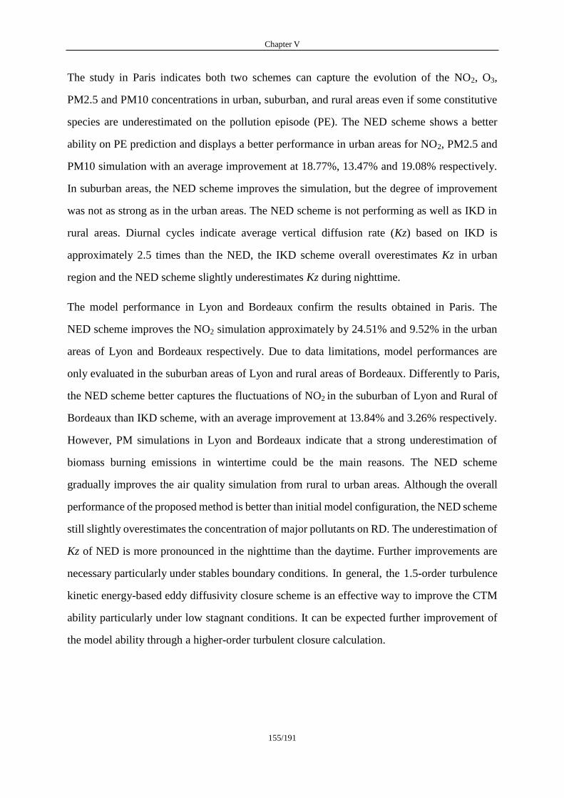
Chapter V
155/191
The study in Paris indicates both two schemes can capture the evolution of the NO2, O3,
PM2.5 and PM10 concentrations in urban, suburban, and rural areas even if some constitutive
species are underestimated on the pollution episode (PE). The NED scheme shows a better
ability on PE prediction and displays a better performance in urban areas for NO2, PM2.5 and
PM10 simulation with an average improvement at 18.77%, 13.47% and 19.08% respectively.
In suburban areas, the NED scheme improves the simulation, but the degree of improvement
was not as strong as in the urban areas. The NED scheme is not performing as well as IKD in
rural areas. Diurnal cycles indicate average vertical diffusion rate (Kz) based on IKD is
approximately 2.5 times than the NED, the IKD scheme overall overestimates Kz in urban
region and the NED scheme slightly underestimates Kz during nighttime.
The model performance in Lyon and Bordeaux confirm the results obtained in Paris. The
NED scheme improves the NO2 simulation approximately by 24.51% and 9.52% in the urban
areas of Lyon and Bordeaux respectively. Due to data limitations, model performances are
only evaluated in the suburban areas of Lyon and rural areas of Bordeaux. Differently to Paris,
the NED scheme better captures the fluctuations of NO2 in the suburban of Lyon and Rural of
Bordeaux than IKD scheme, with an average improvement at 13.84% and 3.26% respectively.
However, PM simulations in Lyon and Bordeaux indicate that a strong underestimation of
biomass burning emissions in wintertime could be the main reasons. The NED scheme
gradually improves the air quality simulation from rural to urban areas. Although the overall
performance of the proposed method is better than initial model configuration, the NED scheme
still slightly overestimates the concentration of major pollutants on RD. The underestimation of
Kz of NED is more pronounced in the nighttime than the daytime. Further improvements are
necessary particularly under stables boundary conditions. In general, the 1.5-order turbulence
kinetic energy-based eddy diffusivity closure scheme is an effective way to improve the CTM
ability particularly under low stagnant conditions. It can be expected further improvement of
the model ability through a higher-order turbulent closure calculation.
Chapter V
156/191
References
Baker, J., Walker, H. L. and Cai, X.: A study of the dispersion and transport of reactive
pollutants in and above street canyons—a large eddy simulation, Atmospheric
Environment, 38(39), 6883–6892, doi:10.1016/j.atmosenv.2004.08.051, 2004.
Baklanov, A., Hänninen, O., Slørdal, L. H., Kukkonen, J., Bjergene, N., Fay, B., Finardi, S.,
Hoe, S. C., Jantunen, M., Karppinen, A., Rasmussen, A., Skouloudis, A., Sokhi, R. S.,
Sørensen, J. H. and Ødegaard, V.: Integrated systems for forecasting urban
meteorology, air pollution and population exposure, Atmospheric Chemistry and
Physics, 7(3), 855–874, doi:https://doi.org/10.5194/acp-7-855-2007, 2007.
Bessagnet, B., Menut, L., Lapere, R., Couvidat, F., Jaffrezo, J.-L., Mailler, S., Favez, O.,
Pennel, R. and Siour, G.: High Resolution Chemistry Transport Modeling with the
On-Line CHIMERE-WRF Model over the French Alps—Analysis of a Feedback of
Surface Particulate Matter Concentrations on Mountain Meteorology, Atmosphere,
11(6), 565, doi:10.3390/atmos11060565, 2020.
Chen, Q., Li, X.-B., Song, R., Wang, H.-W., Li, B., He, H.-D. and Peng, Z.-R.: Development
and utilization of hexacopter unmanned aerial vehicle platform to characterize vertical
distribution of boundary layer ozone in wintertime, Atmospheric Pollution Research,
11(7), 1073–1083, doi:10.1016/j.apr.2020.04.002, 2020.
Deardorff, J. W.: Stratocumulus-capped mixed layers derived from a three-dimensional model,
Boundary-Layer Meteorol, 18(4), 495–527, doi:10.1007/BF00119502, 1980.
Dragomir, C. M., Constantin, D.-E., Voiculescu, M., Georgescu, L. P., Merlaud, A. and
Roozendael, M. V.: Modeling results of atmospheric dispersion of NO 2 in an urban
area using METI–LIS and comparison with coincident mobile DOAS measurements,
Atmospheric Pollution Research, 6(3), 503–510, doi:10.5094/APR.2015.056, 2015.
Forouzanfar, M. H., Afshin, A., Alexander, L. T., Anderson, H. R., Bhutta, Z. A., Biryukov,
S., Brauer, M., Burnett, R., Cercy, K., Charlson, F. J., Cohen, A. J., Dandona, L.,
Estep, K., Ferrari, A. J., Frostad, J. J., Fullman, N., Gething, P. W., Godwin, W. W.,
Griswold, M., Hay, S. I., Kinfu, Y., Kyu, H. H., Larson, H. J., Liang, X., Lim, S. S.,
Liu, P. Y., Lopez, A. D., Lozano, R., Marczak, L., Mensah, G. A., Mokdad, A. H.,
Moradi-Lakeh, M., Naghavi, M., Neal, B., Reitsma, M. B., Roth, G. A., Salomon, J.
A., Sur, P. J., Vos, T., Wagner, J. A., Wang, H., Zhao, Y., Zhou, M., Aasvang, G. M.,
Abajobir, A. A., Abate, K. H., Abbafati, C., Abbas, K. M., Abd-Allah, F., Abdulle, A.
M., Abera, S. F., Abraham, B., Abu-Raddad, L. J., Abyu, G. Y., Adebiyi, A. O.,
Adedeji, I. A., Ademi, Z., Adou, A. K., Adsuar, J. C., Agardh, E. E., Agarwal, A.,
Agrawal, A., Kiadaliri, A. A., Ajala, O. N., Akinyemiju, T. F., Al-Aly, Z., Alam, K.,
Alam, N. K. M., Aldhahri, S. F., Aldridge, R. W., Alemu, Z. A., Ali, R., Alkerwi, A.,
Alla, F., Allebeck, P., Alsharif, U., Altirkawi, K. A., Martin, E. A., Alvis-Guzman, N.,

Chapter V
157/191
Amare, A. T., Amberbir, A., Amegah, A. K., Amini, H., Ammar, W., Amrock, S. M.,
Andersen, H. H., Anderson, B. O., Antonio, C. A. T., Anwari, P., Ärnlöv, J., Artaman,
A., Asayesh, H., Asghar, R. J., Assadi, R., Atique, S., Avokpaho, E. F. G. A., Awasthi,
A., Quintanilla, B. P. A., Azzopardi, P., et al.: Global, regional, and national
comparative risk assessment of 79 behavioural, environmental and occupational, and
metabolic risks or clusters of risks, 1990–2015: a systematic analysis for the Global
Burden of Disease Study 2015, The Lancet, 388(10053), 1659–1724,
doi:10.1016/S0140-6736(16)31679-8, 2016.
Johnson, G. T. and Hunter, L. J.: Urban wind flows: wind tunnel and numerical
simulations—a preliminary comparison, Environmental Modelling & Software, 13(3–
4), 279–286, doi:10.1016/S1364-8152(98)00028-0, 1998.
Kirkil, G., Mirocha, J., Bou-Zeid, E., Chow, F. K. and Kosović, B.: Implementation and
Evaluation of Dynamic Subfilter-Scale Stress Models for Large-Eddy Simulation
Using WRF*, Monthly Weather Review, 140(1), 266–284,
doi:10.1175/MWR-D-11-00037.1, 2012.
Kurppa, M., Hellsten, A., Auvinen, M., Raasch, S., Vesala, T. and Järvi, L.: Ventilation and
Air Quality in City Blocks Using Large-Eddy Simulation—Urban Planning
Perspective, Atmosphere, 9(2), 65, doi:10.3390/atmos9020065, 2018.
Lee, J.-H., Wu, C.-F., Hoek, G., de Hoogh, K., Beelen, R., Brunekreef, B. and Chan, C.-C.:
Land use regression models for estimating individual NOx and NO2 exposures in a
metropolis with a high density of traffic roads and population, Science of The Total
Environment, 472, 1163–1171, doi:10.1016/j.scitotenv.2013.11.064, 2014.
Letzel, M. O., Krane, M. and Raasch, S.: High resolution urban large-eddy simulation studies
from street canyon to neighbourhood scale, Atmospheric Environment, 42(38), 8770–
8784, doi:10.1016/j.atmosenv.2008.08.001, 2008.
Lim, S., Kim, J., Kim, T., Lee, K., Yang, W., Jun, S. and Yu, S.: Personal exposures to PM2.5
and their relationships with microenvironmental concentrations, Atmospheric
Environment, 47, 407–412, doi:10.1016/j.atmosenv.2011.10.043, 2012.
Mailler, S., Khvorostyanov, D. and Menut, L.: Impact of the vertical emission profiles on
background gas-phase pollution simulated from the EMEP emissions over Europe,
Atmos. Chem. Phys., 13(12), 5987–5998, doi:10.5194/acp-13-5987-2013, 2013.
Menut, L., Bessagnet, B., Khvorostyanov, D., Beekmann, M., Blond, N., Colette, A., Coll, I.,
Curci, G., Foret, G., Hodzic, A., Mailler, S., Meleux, F., Monge, J.-L., Pison, I., Siour,
G., Turquety, S., Valari, M., Vautard, R. and Vivanco, M. G.: CHIMERE 2013: a
model for regional atmospheric composition modelling, Geosci. Model Dev., 6(4),
981–1028, doi:10.5194/gmd-6-981-2013, 2013a.
Menut, L., Bessagnet, B., Colette, A. and Khvorostiyanov, D.: On the impact of the vertical
resolution on chemistry-transport modelling, Atmospheric Environment, 67, 370–384,
doi:10.1016/j.atmosenv.2012.11.026, 2013b.
Chapter V
158/191
Palmgren, F., Berkowicz, R., Hertel, O. and Vignati, E.: Effects of reduction of NOx on the
NO2 levels in urban streets, Science of The Total Environment, 189–190, 409–415,
doi:10.1016/0048-9697(96)05238-2, 1996.
Peshin, S. K., Sharma, A., Sharma, S. K., Naja, M. and Mandal, T. K.: Spatio-temporal
variation of air pollutants and the impact of anthropogenic effects on the
photochemical buildup of ozone across Delhi-NCR, Sustainable Cities and Society, 35,
740–751, doi:10.1016/j.scs.2017.09.024, 2017.
Pierce, T., Hogrefe, C., Trivikrama Rao, S., Porter, P. S. and Ku, J.-Y.: Dynamic evaluation
of a regional air quality model: Assessing the emissions-induced weekly ozone cycle,
Atmospheric Environment, 44(29), 3583–3596, doi:10.1016/j.atmosenv.2010.05.046,
2010.
Punger, E. M. and West, J. J.: The effect of grid resolution on estimates of the burden of
ozone and fine particulate matter on premature mortality in the USA, Air Qual Atmos
Health, 6(3), 563–573, doi:10.1007/s11869-013-0197-8, 2013.
Song, F., Young Shin, J., Jusino‐Atresino, R. and Gao, Y.: Relationships among the
springtime ground–level NOx, O3 and NO3 in the vicinity of highways in the US East
Coast, Atmospheric Pollution Research, 2(3), 374–383, doi:10.5094/APR.2011.042,
2011.
Valari, M., Markakis, K., Powaga, E., Collignan, B. and Perrussel, O.: EXPLUME v1.0: a
model for personal exposure to ambient O<sub>3</sub> and
PM<sub>2.5</sub>, Geosci. Model Dev., 13(3), 1075–1094,
doi:10.5194/gmd-13-1075-2020, 2020.
Walton, A. and Cheng, A. Y. S.: Large-eddy simulation of pollution dispersion in an urban
street canyon—Part II: idealised canyon simulation, Atmospheric Environment,
36(22), 3615–3627, doi:10.1016/S1352-2310(02)00260-1, 2002.
Warner, T.T., 2011. Numerical weather and climate prediction. Cambridge Univ. Press,
Cambridge
Wolf, T., Pettersson, L. H. and Esau, I.: A very high-resolution assessment and modelling of
urban air quality, Atmos. Chem. Phys., 20(2), 625–647, doi:10.5194/acp-20-625-2020,
2020.
Wolf-Grosse, T., Esau, I. and Reuder, J.: Sensitivity of local air quality to the interplay
between small- and large-scale circulations: a large-eddy simulation study, Atmos.
Chem. Phys., 17(11), 7261–7276, doi:10.5194/acp-17-7261-2017, 2017.
Wyngaard, J.C., 2004. Toward Numerical Modeling in the ―Terra Incognita.‖ Journal of the
Atmospheric Sciences 61, 1816–1826.
https://doi.org/10.1175/1520-0469(2004)061<1816:TNMITT>2.0.CO;2
Yao, X., Lau, N. T., Chan, C. K. and Fang, M.: The use of tunnel concentration profile data to
determine the ratio of NO<sub>2</sub>/NO<sub>x</sub>

Chapter V
159/191
directly emitted from vehicles, Atmos. Chem. Phys. Discuss., 5(6), 12723–12740,
doi:10.5194/acpd-5-12723-2005, 2005.
Zilitinkevich, S. S. and Esau, I. N.: Resistance and heat-transfer laws for stable and neutral
planetary boundary layers: Old theory advanced and re-evaluated, Q. J. R. Meteorol.
Soc., 131(609), 1863–1892, doi:10.1256/qj.04.143, 2005.

Conclusions and Perspectives
160/191
Conclusions and Perspectives
The first order K-theory is an effective way to reproduce the dispersion of pollutants in
mesoscale chemistry transport model in most of time. However, this method sometimes
lacks the ability to predict vertical mixing under a very low turbulent diffusion.
The urban canopy and boundary layer height plays a crucial role in the mesoscale
chemistry transport modelling simulation, especially for the boundary layer height, it
plays a key role in the early warning of pollution episode.
Geographical condition is also important in regional transport and dispersion of
pollutants. Pollutant's dispersion processes over the valley-basin city are much more
complicated than over flat areas.
Our study indicates the 1.5 order TKE-based eddy diffusivity closure scheme improved
the CTM in every urban site. A way to improve the turbulence parameterization is to
increase the order of the closure.
With an increasing number of humans now living in urban areas, there are needs of
investigating the role of urbanization on air pollution, local meteorology and climate change.
With the increasing computing capacities, numerical tools have become attractive tools for
simulating transport and dispersion of airborne materials in the urban canopy. The present
thesis work uses mesoscale models for meteorological and air quality simulations,
representative of background air quality in urban region and its surroundings. The main goal
of the thesis is to evaluate and improve the ability of models to simulate and forecast air
quality and in France over urban regions.
Initially, three vertical diffusion schemes which have been used in multiple mesoscale
chemical transport models (CTM) were tested over a one-year simulation covering the whole
France. Those schemes are all based on first order local closure scheme, but the expressions
differ. All three schemes present a fair reproduction of pollutant concentrations both in urban
and rural areas, indicating it is an effective way to reproduce the dispersion of pollutants in
chemistry transport modelling. However, the differences between test results are weak.
Conclusions and Perspectives
161/191
Therefore, it cannot be expected to significantly improve the vertical mixing in CTM under
the first order closure scheme.
In the second part of the study, the impact of physical parameterizations was evaluated
through couple the CTM model CHIMERE with the Weather Research and Forecasting
(WRF) mesoscale model. Three canopy schemes, including a single layer urban canopy
scheme (UCM); a multiple layer urban canopy scheme (BEP) and a reference case (Bulk).
Three boundary layer parametrization schemes coupled with urban canopy schemes (MYJ–
Bulk, YSU–Bulk, MYJ–UCM, YSU–UCM, MYJ–BEP, and Boulac–BEP) and two land
surface schemes (Noah and Noah-mp) has been tested in this part. This study aims at
understanding theimpacts on air quality simulation with focus on a short-term pollution
episode (PE) in the Paris region. CTM have been used with a first layer at 4m to better
account for physical processes within the suburban layer in relation to ground emissions. The
results indicate three canopy schemes could reproduce the 2m temperature (T2) effectively in
the daytime; the Bulk and UCM model reproduced the 10m windspeed (W10) well, but the
BEP model underestimates W10 for the whole episode. The UCM scheme overestimates the
surface heat index in rural areas, leading to a slight negative bias for T2 in rural versus urban
areas. NO2, PM2.5, and PM10 were selected to evaluate the effect of physics
parameterizations on air quality simulation. Large differences were found in the simulation of
pollutant concentrations, with an overall overestimation during the pollution episode. The
overall boundary layer schemes display an underestimation of the PBL height practically
during PE. The Boulac–BEP is the only scheme that could relative effectively reproduce the
PBL height during PE. The Boulac–BEP scheme gives a significantly better performance on
air quality simulation than the rest, indicating that both the canopy parameterization and
boundary layer schemes have a significantly positive effect on air quality simulation in urban
regions. The study on the land surface scheme shows it has slightly impact for both
meteorological and air quality simulation. An advanced urban category could improve air
quality prediction in urban regions.
Fifteen days sensitivity tests with multiple vertical grid resolution and first layer height
defined as (i) L4: 53 vertical layers are defined in WRF and 20 vertical layers are defined in
CHIMERE. The first layer of the two model is at 999.5hPa (approximately 4m) up to over
500hPa; (ii) L12: 51 vertical levels are defined in WRF and 20 levels are defined in
CHIMERE, starting with the first vertical height at about 12 meters above the ground; (iii)

Conclusions and Perspectives
162/191
L40: 49 vertical levels are defined in WRF and 20 vertical layers are defined in CHIMERE
from 995hPa to 500hPa, the first layer is about 40m. Results show the impact is relatively
small in meteorological simulations. The relative bias (RB) of L12 and L40 compare with L4
(L12-L4 and L40-L4) are 2.17% and 22.95% for 2m temperature (T2), 4.01% and -12.69%
for 10m wind speed (W10), -0.12% and -2.72% for surface relative humidity (RH),
respectively. On regular days, all three configurations demonstrate the ability of chemistry
transport modelling. L4 improved model ability of 23.26% and 25.09% compare with L12
and L40 respectively. During pollution episodes, refined vertical grid resolution and first layer
height produces a significant improvement in chemistry transport modeling, improvements
are 62.10% and 129.02% in L4 compare with L12 and L40.
The flow characteristics and dispersion mechanisms of pollutants are important for air quality
simulation and forecast. The first part of the study illustrates the difficulties to improve the
ability of the model through the simplest first order local closure schemes.
In the last part of the study, a 1.5-order turbulence-resolve scheme defined as NED has been
applied in the CHIMERE model on the urban air quality context to assess consequences of
low-level emission of pollutants in Paris, Lyon and Bordeaux. The performances of NED and
initial Kz diffusion scheme (IKD) were evaluated against ground observations both
temporally and spatially. The study in Paris shows both two schemes can capture the
evolution of the NO2, O3, PM2.5 and PM10 concentrations in urban, suburban, and rural areas
even if some constitutive species are underestimated on the pollution episode (PE). Taking the
relative change in % of the RMSE as the evaluation criteria, the NED scheme improved the
ability of models to assess air quality with an average improvement at 18.77%, 13.47% and
19.08% of NO2, PM2.5 and PM10 respectively. However, the IKD scheme reproduces the O3
more effectively than NED. In suburban areas, NED scheme improved the simulation, but the
degree of improvement was not as strong as in the urban areas. The NED scheme is not
performing as well as IKD in rural areas. Diurnal cycles between the vertical diffusion
coefficient and pollutants indicate the IKD scheme overall overestimate diffusion rate in
urban region and NED scheme slightly underestimated it during the nighttime. The model
performances in Lyon and Bordeaux are rather good over Paris, NED scheme improved the
Conclusions and Perspectives
163/191
NO2 simulation approximately 24.51% and 9.52% in the urban areas of Lyon and Bordeaux
respectively. However, PM simulation results over those two latter areas could indicate a
huge underestimation of biomass burning emissions in wintertime., Both schemes can capture
the evolution of PM2.5 and PM10, the average concentrations are strongly underestimated
particularly in Bordeaux and on the PE of Lyon. The NED scheme gradually improves the air
quality simulation as it approaches the city center. Sensitivity tests to grid resolution showed
that the model results are sensitive to the vertical resolution and do not tend to improve with
increasing resolution, there configuration of parameters are weak under the displacement
height, the aspect ratio is curial on eddy simulation. Overall, surface turbulent motions were
better preserved by a 1.5-order turbulence kinetic energy-based eddy diffusivity closure
scheme than those with the simplest ones.
Since the 1970s, the CTMs have developed from the initial simple box model to today’s
complex third generation CTM models. The configurations of CTM should be combined with
the characteristics of the research problem, the time and space scale of the simulation, data
availability, technical complexity, software and hardware platform requirements, etc. Not all
simulations have to choose the highest model configuration. Advanced configurations
generally have very strict requirements on basic data, hardware platform, professional
threshold, etc., and the cost will be several times compared with the basic configurations.
Therefore, choosing an appropriate model configuration is the key to achieving the goals with
the lowest cost. From the perspective of air quality model application practice, it is often
difficult for users to accurately grasp the applicable conditions of the model or simplify
complex issues.
With the rapid development of high-performance computers, high resolution numerical
simulation has achieved great success. However, most high-resolution simulations are still at
the research stage, the time span is usually from days to a month. Although computer
resources are not extravagant, long time series high-resolution simulation is still difficult to
achieve. Thus, a technique that could pass the costly high simulation is important. The
uncertainty of the CTM mainly comes from five parts: chemical mechanism; chemical
reaction rate; boundary layer; emission inventory and meteorological data. Take the model
performance of particulate matter as an example, the ratio of PM2.5 to PM10 is above 90% in

Conclusions and Perspectives
164/191
every studies of this research, however, the value is approximately 70% in the real
atmospheric. In coastal cities, the modeled particulate matter concentrations are far from the
observation. The lack of emissions directly leads to the poor performance of models. The
completeness of emission inventories particularly on residential emissions remains
challenging for the air quality community.
Urban-induced atmospheric circulations, though typically small scale, can have a significant
impact on mesoscale dynamics. Many studies indicate that refining urban landuse categories
helps improving the model's ability to simulate the processes in the urban canopy. However, it
could present notable challenges for mesoscale models due to the tremendous horizontal and
vertical variability of the urban landscape and the variety of surface forcing. A lower first
model layer could better reproduce the transport and diffusion of pollutants in a real urban
environment. However, urban canopy is an open canopy, a refined urban category could
increase the displacement height in the cities leads a very weak configuration of parameters at
low level, it requires more studies. Future works should also focus on the comparison of
pollutant concentrations over the vertical within the urban canopy to better evaluate the
performance of models.
In recent years, due to the improvement of computing power, the interdisciplinary field of
machine learning-statistics and computer science has flourished. At present, the application of
Artificial Intelligence (AI) techniques to air quality simulation has been initially applied but is
still in the exploratory stage. For example, use wavelet transform to split the pollutant time
series into more regular sub-sequences, then use the artificial neural network to train
independent models for them to further improve the accuracy. Or using AI techniques could
be used to calculate higher-order turbulent kinetic energy makes it possible to apply direct
numerical simulation to mesoscale models. How to combine CTM and AI techniques for air
quality prediction will be a very active field in the future to allow fast high-resolution
simulations at urban scale to monitor air quality. At last, let us remind that using neural
network is complementary of developing more and more complex physical models with more
layers and accurate urban schemes. They are good instruments to simplify complex models by
developping surrogate associated models for operational uses at high resolution (by catching
the main patterns) and offering the possibility to develop more and more sophisticated
deterministic models representing the "real world".
List of Figures
165/191
List of Figures
Figure1.1 Typical sources, formation, removal pathways and size distributions of atmospheric
aerosol.
Figure1.2 Direct, semi-direct and indirect effects of aerosols on climate.
Figure1.3 Change in RF effects caused by atmospheric pollutants for the period 1750–2011,
associated with individual confidence range.
Figure1.4 MODIS aerosol optical depth averaged over the 10-year period 2001–2010Pie
charts shows the contribution of different aerosols to the total aerosol optical depth for
different regions.
Figure1.5 Emission trends in the EU28 on the basis of fuel sold.
Figure1.6 Urban heat island in cities.
Figure2.1 General principle of the air quality simulation system
Figure2.2 The main linkages between megacities, air quality and climate.
Figure2.3 Example of mass conservation.
Figure2.4 Typical diurnal variation of the boundary layer structure. Sunrise (SR), Sunset (SS).
Figure2.5 Sensitivity test of vertical profile of kz (m2/s) in stable and unstable conditions.
Figure2.6 Vertical profiles of kz (m2/s); NO2 (µg/m
3); O3 (µg/m
3) PM2.5 (µg/m
3) and PM10
(µg/m3) over the France domain. The profiles are averaged from January 1
st to December 31
st,
2016.
Figure2.7 Maps of the seasonal mean vertical diffusion coefficient (m2/s) over the France
domain.
Figure2.7 Seasonal changes between observed and modelled NO2, PM2.5 and PM10 mass
concentrations (µg/m3) in France domain.
Figure2.9 Time series between observed and modelled NO2, PM2.5 and PM10 mass
concentrations (µg/m3) in Urban and Rural areas.
Figure2.10 Diurnal cycles for surface concentrations (µg/m3) of NO2, PM2.5 and PM10 in the
year 2016
Figure3.1 The structure diagram of UCM(left) and BEP(right) urban canopy scheme. Ta:
Atmospheric temperature at Za meters height; Tg: Pavement temperature; H : Sensible heat
exchange; Tr: Temperature of the roof; Tw: Temperature of the wall; Tg: Temperature of the
street; Ts: Atmospheric temperature at Zs meters height; Ha: Sensible heat flux from street

List of Figures
166/191
canyon to atmosphere; Hw: Sensible heat flux from wall to street canyon; Hg: Sensible heat
fiux from road to street canyon; Hr: Sensible heat fiux from roof to atmosphere.
Figure3.2 Four nested domains—from d01, the largest one, at a low resolution to d04, the
finest one, at a high resolution.
Figure3.3 Maps of the meteorological and air quality monitoring stations.
Figure3.4 Time series of 2m temperature and 10m wind speed at Sirta station.
Figure3.5 Time series of 2m temperature and 10m wind speed at Montsouris station.
Figure3.6 Maps of the mean 2m temperature (°C) over the period from 27th
November to 4th
December
Figure3.7 Maps of the mean surface heat flux (W m−2
) over the period from 27th
November to
4th
December.
Figure3.8 Time series of 2m temperature (°C) between observations and different urban
schemes at Montsouris, Roissy, and Sirta stations.
Figure3.9 Maps of the mean 10m wind speed (m s−1
) over the period from 27th
November to
4th
December.
Figure3.10 Comparison of the time series of 10 m wind speed (m s−1
) between the
observations and different urban schemes at Montsouris, Roissy and Sirta stations.
Figure3.11 The differences in the daily averaged NO2 (μg m−3
), PM2.5 (μg m−3
), and PM10
(μg m−3
) between different schemes from 27th
November to 4th
December 2016.
Figure3.12 Time series of NO2 mass concentrations (µg m−3
). No1, 2, 3, 4 represent station
FR04002, FR04034, FR04143, and FR04156, respectively.
Figure3.13 Vertical profiles of the CHIMERE Kz extracted at the FR04143 station. The
profile is extracted at 06:00 and 22:00 UTC for both Regular Days (RD) and the Particulate
Episode (PE).
Figure3.14 Vertical profiles of the NO2 and PM2.5 mass concentration (µg m−3
) at the
FR04143 station. The profiles are extracted at 06:00 and 22:00 UTC for both Regular Days
(RD) and the Particulate Episode (PE). Columns (a), (b), (c), and (d) represent the vertical
mass NO2 and PM2.5 concentration at 28th November 06:00, 28th November 22:00, 30th
November 06:00, and 30th November 22:00 UTC, respectively.
Figure3.15 Time series of the observed and modelled mixing boundary layer height: (a) and
(b) represent Roissy and Sirta station, respectively; 1, 2, and 3 represent each PBL scheme
coupled with each urban canopy scheme.

List of Figures
167/191
Figure3.16 Time series between the observed and modelled T2: (a) and (b) represent Roissy
and Sirta station, respectively; 1, 2, and 3 represent each PBL scheme coupled with each
urban canopy scheme.
Figure3.17 Time series between the observed and modelled W10: (a) and (b) represent Roissy
and Sirta station, respectively; 1, 2, and 3 represent each PBL scheme coupled with each
urban canopy scheme.
Figure3.18 Time series of NO2 mass concentrations: No 1, 2, 3, and 4 represent station
FR04002, FR04034, FR04143, and FR04156, respectively.
Figure3.19 Liner fit between the observed and modelled NO2.
Figure3.20 Time series of 2m temperature (°C) between observations and different urban
schemes at Montsouris, Roissy, and Sirta stations.
Figure3.21 Comparison of the time series of 10m wind speed (m s−1
) between the
observations and different urban schemes at Montsouris, Roissy and Sirta stations.
Figure3.22 Time series of NO2 and PM2.5 mass concentrations: No 1, 2, 3, and 4 represent
station FR04002, FR04034, FR04143, and FR04156, respectively.
Figure4.1 Locations of the meteorological and air quality monitoring stations.
Figure4.2 Maps of the mean 2m temperature (°C); mean 10m wind speed (m/s) and mean
surface relative humidity (%) over the period from 20th
November to 4th
December. Left
column: results from L4; Middle column: results from L12; Right column: results from L40.
Figure4.3 Maps of the mean NO2 (μg/m3); mean PM2.5 (μg/m
3) and mean PM10 (μg/m
3) mass
concentrations over the period from 20th
November to 4th
December. Left column: results
from L4; Middle column: results from L12; Right column: results from L40.
Figure4.4 Vertical profiles of Kz(m2/s), NO2, PM2.5 and PM10 (μg/m
3) from 20
th Novermber to
4th
December over Paris region.
Figure4.5 Time series between the observed and modelled 2m temperature (°C); mean 10m
wind speed (m/s) and planetary boundary layer height (PBLH)
Figure4.6 Diurnal cycles for surface 2m temperature (°C); mean 10m wind speed (m/s) and
planetary boundary layer height (PBLH) from 20th
November to 4th
December.
Figure4.7 Time series between the observed and modelled NO2, PM2.5, PM10 (μg/m3).
Figure4.8 Time series of bias between L12 to L4 (L12-L4) and L40 to L4 (L40-L4).
List of Figures
168/191
Figure5.1 Schematic of a turbulent-energy spectrum. l is the scale of the energy-containing
turbulence, Δ is the horizontal gird size; ɸ is turbulent energy, and λ is wavelength(Warner,
2011).
Figure5.2 Maps of the meteorological and air quality monitoring stations. Red represent urban
background station; green represent suburban background station and blue represent rural
background station.
Figure5.3 Vertical profiles of the CHIMERE Kz extracted at the FR04143 station. The profile
is extracted at 06:00 and 22:00 UTC for both Regular Days (RD) and the Particulate Episode
(PE).
Figure5.4 Time series between observed and modelled NO2 mass concentrations (µg m−3
) in
urban and rural background stations.
Figure5.5 Maps of the mean vertical diffusion coefficient (m s2); mean surface NO2 mass
concentration (µg m−3
) and surface mean O3 mass concentration (µg m−3
) over the period
from 20th
November to 4th
December. The first line: results from IKD scheme; the second line:
results from NED scheme.
Figure5.6 Time series between observed and modelled NO2 and O3 mass concentrations (µg
m−3
) in urban background stations.
Figure5.7 Diurnal cycles for surface kz and surface concentrations of O3 and NO2 (µg m−3
)
from 20th
November to 4th
December in urban background stations.
Figure5.8 Time series between observed and modelled NO2 and O3 mass concentrations (µg
m−3
) suburban background stations and rural background stations.
Figure5.9 Maps of the mean surface PM2.5 and PM10 mass concentration (µg m−3
); over the
period from 20th
November to 4th
December.
Figure5.10 Time series between observed and modelled PM2.5 and PM10 mass concentrations
(µg m−3
) in urban; suburban and rural background stations. Urban background stations:
FR04002; FR04034; FR04143 and FR04156. Suburban background stations: FR04024 and
FR04181 for PM2.5 simulation and observation; FR04181 and FR04319 for PM10 simulation
and observation. Rural background stations: FR04048 for PM2.5 simulation and observation;
FR04158 PM10 simulation and observation.
Figure5.11 Maps of the mean 2m temperature (°C) and 10m wind speed (m s−1
) over the
period from 27th
November to 4th
December.
Figure5.12 Comparison of the time series of 2m temperature (°C) and 10 m wind speed (m s−1
)
between the observations and different urban schemes at Bron, Exupery, Brindas and Merignac
List of Figures
169/191
stations. The Bron, Exupery and Brindas stations are located in Lyon region and Merignac
station is located in Bordeaux region.
Figure5.13 Maps of the mean vertical diffusion coefficient (m2 s
-1); over the period from 20
th
November to 4th
December. The first line: results from Lyon domain; the second line: results
from Bordeaux domain.
Figure5.14 Maps of the mean surface NO2 mass concentration (µg m−3
); over the period from
20th
November to 4th
December. The first line: results from Lyon domain; the second line:
results from Bordeaux domain.
Figure5.15 Time series between observed and modelled NO2 mass concentrations (µg m−3
) in
urban background stations. FR20XXX represents the station in Lyon region and FR31XXX
represents the station in Bordeaux region.
Figure5.16 Diurnal cycles for surface kz and surface concentrations of NO2 (µg m−3
) from
20th
November to 4th
December in urban background stations. Left side are the diurnal cycles
of kz and NO2 in Lyon region and right side are the diurnal cycles of kz and NO2 in Bordeaux
region.
Figure5.17 Time series between observed and modelled NO2 and O3 mass concentrations (µg
m−3
) suburban background stations and rural background station in Lyon and Bordeaux region.
Suburban represents the average data from three background suburban stations (FR20037;
FR20045 and FR20047) in Lyon domain and the rural site only represent the data from one
background rural station (FR31008) in Bordeaux.
Figure5.18 Maps of the mean surface PM2.5 mass concentration (µg m−3
); over the period
from 20th
November to 4th
December. The first line: results from lyon domain; the second line:
results from Bordeaux domain.
Figure5.19 Maps of the mean surface PM10 mass concentration (µg m−3
); over the period from
20th
November to 4th
December. The first line: results from Lyon domain; the second line:
results from Bordeaux domain.
Figure5.20 Time series between observed and modelled PM2.5 and PM10 mass concentrations
(µg m−3
) in urban background stations. FR20XXX represents the station in Lyon region and
FR31XXX represents the station in Bordeaux region.
List of Tables
170/191
List of Tables
Table2.1 The kz (m2/s) values within 10 levels
Table2.2 Seasonal average mass concentration of NO2, PM2.5 and PM10 (µg/m3) between
observation and three schemes.
Table2.3 Statistics of surface variables: mean linear correlation coefficient (R); mean bias
(MB) and root mean square error (RMSE) between the simulations and observations of NO2,
PM2.5 and PM10 in Urban and Rural areas.
Table3.1 Summary of the physics parameterizations used.
Table3.2 Statistics of surface pollutants: mean bias between the simulations and
observations of NO2, PM2.5, and PM10 during Whole Period (WP) and Pollution Episode
(PE).
Table3.3 Statistics of surface variables: mean bias (MB) and mean linear correlation
coefficient (R) between the simulations and observations of 2 m temperature (T2) and 10 m
wind speed (W10) at Roissy and Sirta stations.
Table3.4 Statistics of surface variables: mean bias (MB), root mean square error (RMSE),
and mean linear correlation coefficient (R) between the simulations and observations of
NO2, PM2.5, PM10.
Table4.1 Range and average values of 2m temperature (°C); 10m wind speed (m/s) and
surface relative humidity (%) over the period
Table4.2 Range and average values NO2 (μg/m3); PM2.5 (μg/m
3) and PM10 (μg/m
3) over the
period
Table4.3 Statistics of surface variables: mean bias (MB), mean linear correlation
coefficient (R) and root mean square error (RMSE) between the simulations and
observations of 2m temperature (°C); mean 10m wind speed (m/s) and planetary boundary
layer height (PBLH)
Table4.4 Statistics of surface variables: mean bias (MB), mean linear correlation
coefficient (R) and root mean square error (RMSE) between the simulations and
observations of NO2, PM2.5, PM10.
Table4.5 Statistics of surface variables: average mass concentration (μg/m3), mean bias (MB),
mean linear correlation coefficient (R) and root mean square error (RMSE) between the
simulations and observations of NO2, PM2.5, PM10 on regular days (RD) and pollution episode
(PE).
Table4.6 Operation time (minutes) of single day simulation in meteorological and chemistry
transport modeling
Table5.1 The correlation (R); mean bias (MB) and root mean square error (RMSE) between
Observation and simulation of NO2 in four urban and rural background stations over Paris
region.
List of Tables
171/191
Table5.2 Average modelled NO2 mass concentrations (Avg); the correlation (R); mean bias
(MB) and root mean square error (RMSE) between Observation and simulation of NO2 in four
urban background stations over Paris region.
Table5.3 Average modelled O3 mass concentrations (Avg); the correlation (R); mean bias
(MB) and root mean square error (RMSE) between Observation and simulation of O3 in four
urban background stations over Paris region.
Table5.4 Average modelled NO2 and O3 mass concentrations (Avg); the correlation (R); mean
bias (MB) and root mean square error (RMSE) between Observation and simulation of
NO2 and O3 in suburban and rural background stations over Paris region.
Table5.5 Average modelled PM2.5 mass concentrations (Avg); the correlation (R); mean bias
(MB) and root mean square error (RMSE) between Observation and simulation of PM2.5 in
urban, suburban and rural background stations over Paris regions.
Table5.6 Average modelled PM10 mass concentrations (Avg); the correlation (R); mean bias
(MB) and root mean square error (RMSE) between Observation and simulation of PM10 in
urban, suburban and rural background stations over Paris regions.
Table5.7 Proportion between PM2.5 and PM10 in urban, suburban and rural background
stations for the whole period (WP) and pollution episode (PE) over Paris regions.
Table5.8 Average modelled NO2 mass concentrations (Avg); the correlation (R); mean bias
(MB) and root mean square error (RMSE) between Observation and simulation of NO2 in
four urban background stations over Paris region.
Table5.9 Average modelled NO2 mass concentrations (Avg); the correlation (R); mean bias
(MB) and root mean square error (RMSE) between Observation and simulation of NO2 in
suburban background station over Lyon region and rural background station over Bordeaux
region.
Annex A
172/191
Annex A
Supplementary Material of Chapter III
Impact of Physics Parameterizations on High-Resolution Air
Quality Simulations over the Urban Region
Lei Jiang 1,2, *
, Bertrand Bessagnet 1,†
, Frederik Meleux 1, Frederic Tognet
1, Florian
Couvidat 1
1 INERIS, National Institute for Industrial Environment and Risks, Parc Technologique
ALATA, 60550 Verneuil-en-Halatte, France; [email protected] (B.B.);
[email protected] (F.M.); [email protected] (F.T.);
[email protected] (F.C.) 2 Sorbonne University, UPMC Univ Paris 06, DE129, 75005 Paris, France
† Now at Citepa: Technical Reference Center for Air Pollution and Climate Change, 42, rue
de Paradis, 75010 Paris, France.
LIST OF TABLES AND FIGURES
Table S3.1. The urban parameters for the urban canopy model.
Figure S3.1. Time series of PM2.5, PM10 mass concentrations: No1, 2, 3, 4 represent station
FR04002, FR04034, FR04143, FR04156, respectively.
Figure S3.2. Time series of bias of NO2, PM2.5, PM10 mass concentrations: No1, 2, 3, 4
represent station FR002, FR034, FR143, FR156, respectively.
Figure S3.3. Time series between observed and modelled NO2 with the first height of about 4 m,
18m and 40 m, respectively. Both observation and simulations are the average of Station
FR04002, FR04034, FR04143, FR04156, respectively.
Figure S3.4. Time series between observed and modelled PM2.5: a, b and c represent each PBL
schemes coupled with each urban canopy schemes respectively; 1, 2, 3, and 4 represent Station
FR04002, FR04034, FR04143, FR04156, respectively.

Annex A
173/191
Figure S3.5. Time series between observed and modelled PM10: a, b and c represent each PBL
schemes coupled with each urban canopy schemes respectively; 1, 2, 3, and 4 represent Station
FR04002, FR04034, FR04143, FR04156, respectively.
Figure S3.6. Time series of bias between observed and modelled NO2: a, b and c represent each
PBL schemes coupled with each urban canopy schemes respectively; 1, 2, 3, and 4 represent
Station FR04002, FR04034, FR04143, FR04156, respectively.
Figure S3.7. Time series of bias between observed and modelled PM2.5: a, b and c represent
each PBL schemes coupled with each urban canopy schemes respectively; 1, 2, 3, and 4
represent Station FR04002, FR04034, FR04143, FR04156, respectively.
Figure S3.8. Time series of bias between observed and modelled PM10: a, b and c represent
each PBL schemes coupled with each urban canopy schemes respectively; 1, 2, 3, and 4
represent Station FR04002, FR04034, FR04143, FR04156, respectively.
Figure. S3.9. Liner fit between observed and modelled PM2.5 and PM10.
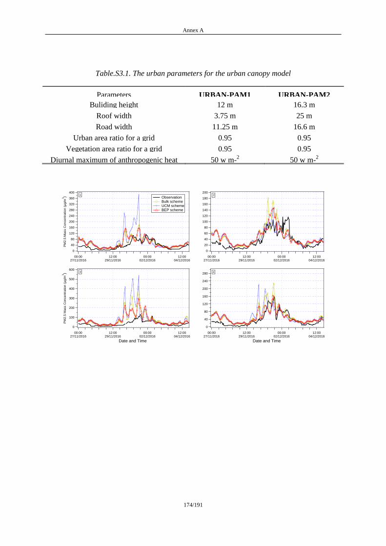
Annex A
174/191
Table.S3.1. The urban parameters for the urban canopy model
Parameters URBAN-PAM1 URBAN-PAM2
Buliding height 12 m 16.3 m
Roof width 3.75 m 25 m
Road width 11.25 m 16.6 m
Urban area ratio for a grid 0.95 0.95
Vegetation area ratio for a grid 0.95 0.95
Diurnal maximum of anthropogenic heat
flux
50 w m-2 50 w m-
2
400
360
320
280
240
200
160
120
80
40
0
PM
2.5
Ma
ss C
on
ce
ntr
atio
n (
µg
/m3)
00:0027/11/2016
12:0029/11/2016
00:0002/12/2016
12:0004/12/2016
1 Observation Bulk scheme UCM scheme BEP scheme
200
180
160
140
120
100
80
60
40
20
0
00:0027/11/2016
12:0029/11/2016
00:0002/12/2016
12:0004/12/2016
2
600
500
400
300
200
100
0
PM
2.5
Ma
ss C
on
ce
ntr
atio
n (
µg
/m3)
00:0027/11/2016
12:0029/11/2016
00:0002/12/2016
12:0004/12/2016
Date and Time
3280
240
200
160
120
80
40
0
00:0027/11/2016
12:0029/11/2016
00:0002/12/2016
12:0004/12/2016
Date and Time
4
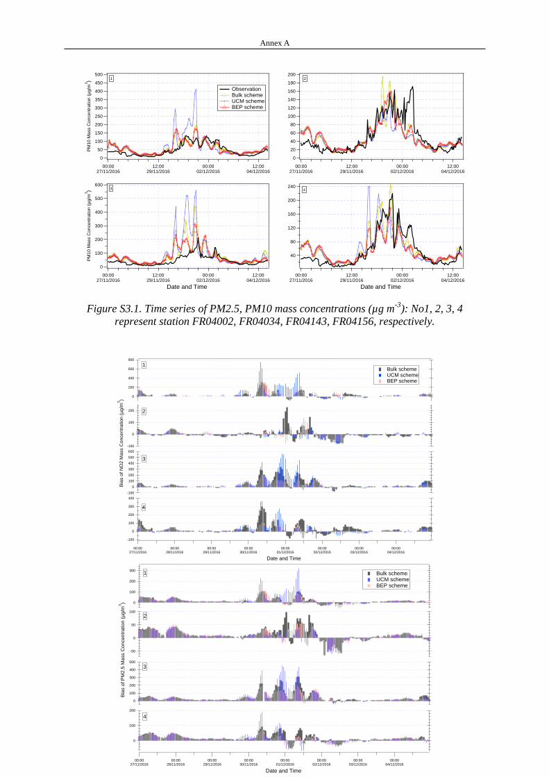
Annex A
175/191
Figure S3.1. Time series of PM2.5, PM10 mass concentrations (µg m-3
): No1, 2, 3, 4
represent station FR04002, FR04034, FR04143, FR04156, respectively.
240
200
160
120
80
40
00:0027/11/2016
12:0029/11/2016
00:0002/12/2016
12:0004/12/2016
Date and Time
4
600
500
400
300
200
100
0
PM
10
Ma
ss C
on
ce
ntr
atio
n (
µg
/m3)
00:0027/11/2016
12:0029/11/2016
00:0002/12/2016
12:0004/12/2016
Date and Time
3
500
450
400
350
300
250
200
150
100
50
0
PM
10
Ma
ss C
on
ce
ntr
atio
n (
µg
/m3)
00:0027/11/2016
12:0029/11/2016
00:0002/12/2016
12:0004/12/2016
1
Observation Bulk scheme UCM scheme BEP scheme
200
180
160
140
120
100
80
60
40
20
0
00:0027/11/2016
12:0029/11/2016
00:0002/12/2016
12:0004/12/2016
2
800
600
400
200
0
00:0027/11/2016
00:0028/11/2016
00:0029/11/2016
00:0030/11/2016
00:0001/12/2016
00:0002/12/2016
00:0003/12/2016
00:0004/12/2016
Date and Time
200
100
0
-100
Bia
s o
f N
O2
Ma
ss C
on
ce
ntr
atio
n (
µg
/m3)
600
500
400
300
200
100
0
-100
400
300
200
100
0
-100
1
2
3
4
Bulk scheme UCM scheme BEP scheme
300
200
100
0
00:0027/11/2016
00:0028/11/2016
00:0029/11/2016
00:0030/11/2016
00:0001/12/2016
00:0002/12/2016
00:0003/12/2016
00:0004/12/2016
Date and Time
100
50
0
-50
Bia
s o
f P
M2
.5 M
ass C
on
ce
ntr
atio
n (
µg
/m3)
500
400
300
200
100
0
200
100
0
1
2
3
4
Bulk scheme UCM scheme BEP scheme
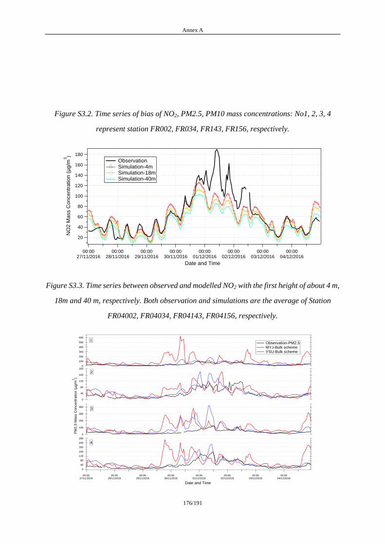
Annex A
176/191
Figure S3.2. Time series of bias of NO2, PM2.5, PM10 mass concentrations: No1, 2, 3, 4
represent station FR002, FR034, FR143, FR156, respectively.
Figure S3.3. Time series between observed and modelled NO2 with the first height of about 4 m,
18m and 40 m, respectively. Both observation and simulations are the average of Station
FR04002, FR04034, FR04143, FR04156, respectively.
180
160
140
120
100
80
60
40
20
NO
2 M
ass C
on
ce
ntr
atio
n (
µg
/m3)
00:0027/11/2016
00:0028/11/2016
00:0029/11/2016
00:0030/11/2016
00:0001/12/2016
00:0002/12/2016
00:0003/12/2016
00:0004/12/2016
Date and Time
Observation Simulation-4m Simulation-18m Simulation-40m
600
500
400
300
200
100
0
00:0027/11/2016
00:0028/11/2016
00:0029/11/2016
00:0030/11/2016
00:0001/12/2016
00:0002/12/2016
00:0003/12/2016
00:0004/12/2016
Date and Time
200
160
120
80
40
0
PM
2.5
Mass C
oncentr
ation (
µg/m
3)
400
300
200
100
0
280
240
200
160
120
80
40
0
1
2
3
4
Observation-PM2.5 MYJ-Bulk scheme YSU-Bulk scheme
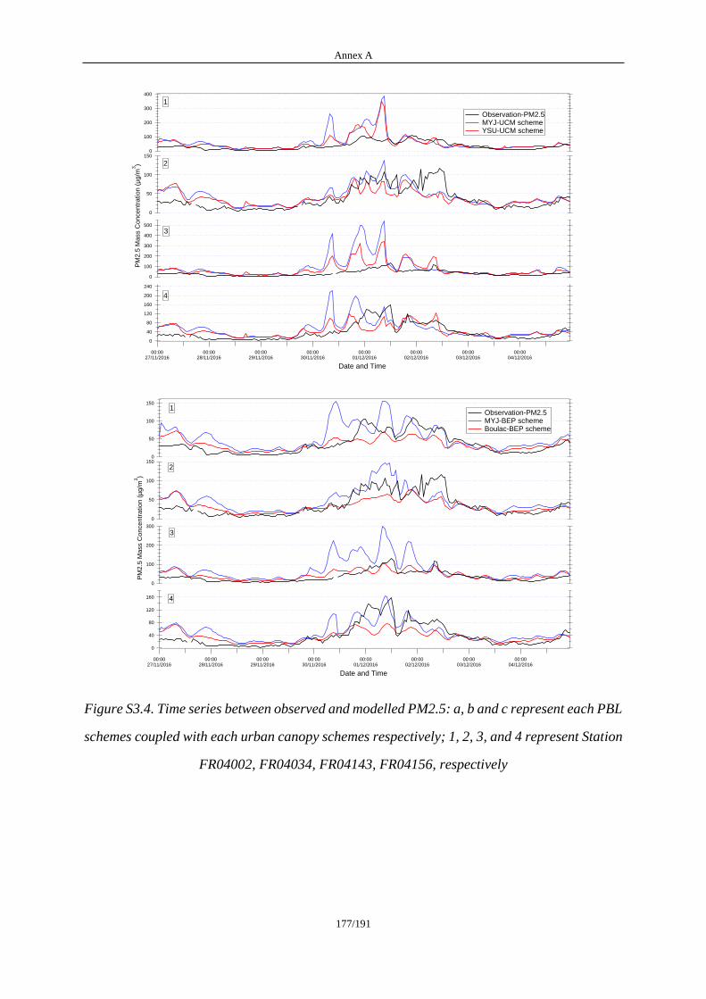
Annex A
177/191
Figure S3.4. Time series between observed and modelled PM2.5: a, b and c represent each PBL
schemes coupled with each urban canopy schemes respectively; 1, 2, 3, and 4 represent Station
FR04002, FR04034, FR04143, FR04156, respectively
400
300
200
100
0
00:0027/11/2016
00:0028/11/2016
00:0029/11/2016
00:0030/11/2016
00:0001/12/2016
00:0002/12/2016
00:0003/12/2016
00:0004/12/2016
Date and Time
150
100
50
0
PM
2.5
Ma
ss C
on
ce
ntr
atio
n (
µg
/m3)
500
400
300
200
100
0
240
200
160
120
80
40
0
1
2
3
4
Observation-PM2.5 MYJ-UCM scheme YSU-UCM scheme
150
100
50
0
00:0027/11/2016
00:0028/11/2016
00:0029/11/2016
00:0030/11/2016
00:0001/12/2016
00:0002/12/2016
00:0003/12/2016
00:0004/12/2016
Date and Time
150
100
50
0
PM
2.5
Ma
ss C
on
ce
ntr
atio
n (
µg
/m3)
300
200
100
0
160
120
80
40
0
1
2
3
4
Observation-PM2.5 MYJ-BEP scheme Boulac-BEP scheme
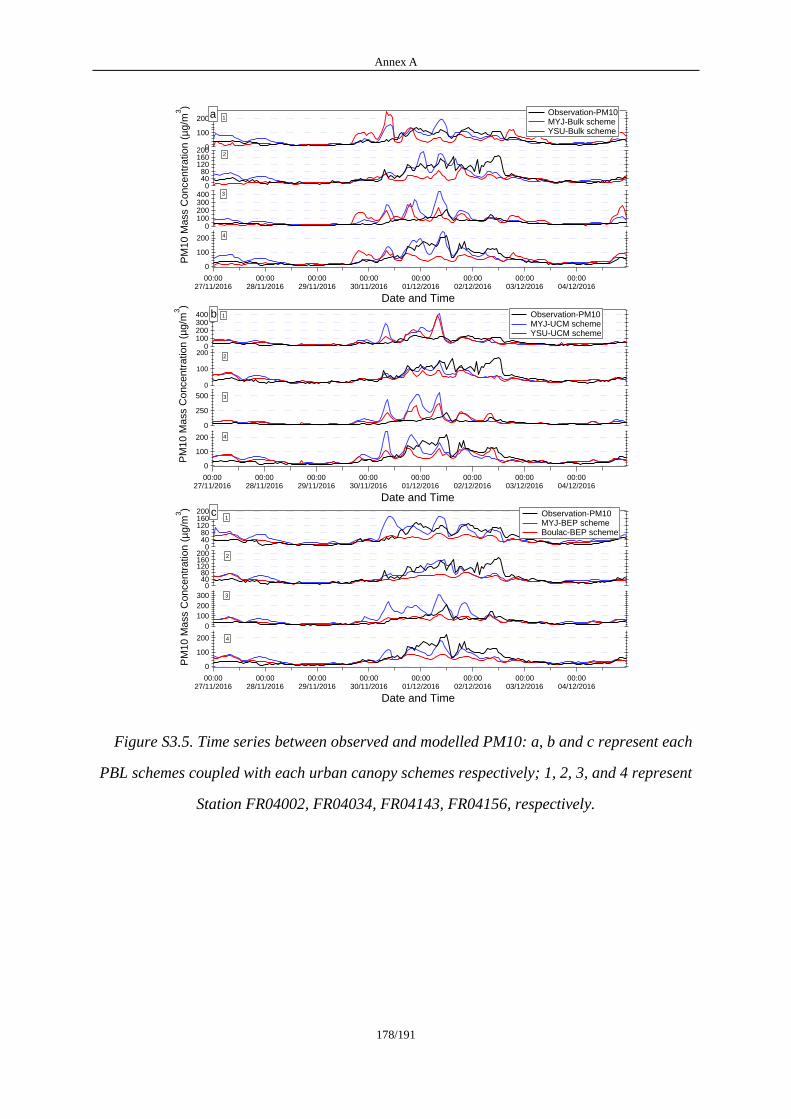
Annex A
178/191
Figure S3.5. Time series between observed and modelled PM10: a, b and c represent each
PBL schemes coupled with each urban canopy schemes respectively; 1, 2, 3, and 4 represent
Station FR04002, FR04034, FR04143, FR04156, respectively.
200160120
80400
00:0027/11/2016
00:0028/11/2016
00:0029/11/2016
00:0030/11/2016
00:0001/12/2016
00:0002/12/2016
00:0003/12/2016
00:0004/12/2016
Date and Time
200160120
8040
0
PM
10 M
ass C
oncentr
ation (
µg/m
3)
300
200
100
0
200
100
0
1
2
3
4
Observation-PM10 MYJ-BEP scheme Boulac-BEP scheme
c
200
100
0
00:0027/11/2016
00:0028/11/2016
00:0029/11/2016
00:0030/11/2016
00:0001/12/2016
00:0002/12/2016
00:0003/12/2016
00:0004/12/2016
Date and Time
200160120
8040
0P
M10 M
ass C
oncentr
ation (
µg/m
3)
400300200100
0
200
100
0
1
2
3
4
Observation-PM10 MYJ-Bulk scheme YSU-Bulk scheme
a
400300200100
0
00:0027/11/2016
00:0028/11/2016
00:0029/11/2016
00:0030/11/2016
00:0001/12/2016
00:0002/12/2016
00:0003/12/2016
00:0004/12/2016
Date and Time
200
100
0
PM
10 M
ass C
oncentr
ation (
µg/m
3)
500
250
0
200
100
0
1
2
3
4
Observation-PM10 MYJ-UCM scheme YSU-UCM scheme
b
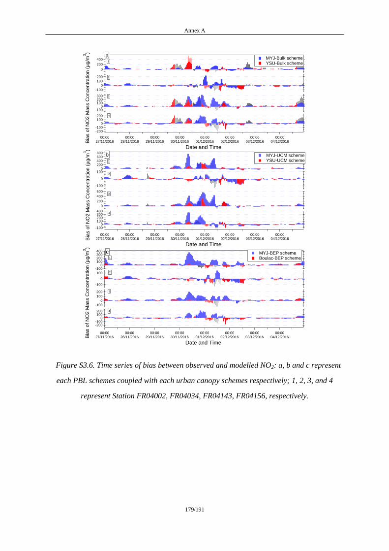
Annex A
179/191
Figure S3.6. Time series of bias between observed and modelled NO2: a, b and c represent
each PBL schemes coupled with each urban canopy schemes respectively; 1, 2, 3, and 4
represent Station FR04002, FR04034, FR04143, FR04156, respectively.
800600400200
0
00:0027/11/2016
00:0028/11/2016
00:0029/11/2016
00:0030/11/2016
00:0001/12/2016
00:0002/12/2016
00:0003/12/2016
00:0004/12/2016
Date and Time
-100
0
100
Bia
s o
f N
O2
Ma
ss C
on
ce
ntr
atio
n (
µg
/m3)
600
400
200
0
400300200100
0-100
1
2
3
4
MYJ-UCM scheme YSU-UCM scheme
b
400300200100
0-100
00:0027/11/2016
00:0028/11/2016
00:0029/11/2016
00:0030/11/2016
00:0001/12/2016
00:0002/12/2016
00:0003/12/2016
00:0004/12/2016
Date and Time
-100
0
100
Bia
s o
f N
O2
Ma
ss C
on
ce
ntr
atio
n (
µg
/m3)
200
100
0
-100
-200-100
0100200
1
2
3
4
MYJ-BEP scheme Boulac-BEP scheme
c
400
200
0
00:0027/11/2016
00:0028/11/2016
00:0029/11/2016
00:0030/11/2016
00:0001/12/2016
00:0002/12/2016
00:0003/12/2016
00:0004/12/2016
Date and Time
200
100
0
-100B
ias o
f N
O2
Ma
ss C
on
ce
ntr
atio
n (
µg
/m3)
300200100
0-100
200100
0-100-200
1
2
3
4
MYJ-Bulk scheme YSU-Bulk scheme
a

Annex A
180/191
Figure S3.7. Time series of bias between observed and modelled PM2.5: a, b and c represent
each PBL schemes coupled with each urban canopy schemes respectively; 1, 2, 3, and 4
represent Station FR04002, FR04034, FR04143, FR04156, respectively.
1208040
0-40-80
00:0027/11/2016
00:0028/11/2016
00:0029/11/2016
00:0030/11/2016
00:0001/12/2016
00:0002/12/2016
00:0003/12/2016
00:0004/12/2016
Date and Time
8040
0-40-80
Bais
of P
M2.5
Mass C
oncentr
ation (
µg/m
3)
200
100
0
1208040
0-40-80
1
2
3
4
MYJ-BEP scheme Boulac-BEP scheme
c
600
400
200
0
00:0027/11/2016
00:0028/11/2016
00:0029/11/2016
00:0030/11/2016
00:0001/12/2016
00:0002/12/2016
00:0003/12/2016
00:0004/12/2016
Date and Time
1208040
0-40-80
Bais
of P
M2.5
Mass C
oncentr
ation (
µg/m
3)
300
200
100
0
200
100
0
-100
1
2
3
4
MYJ-Bulk scheme YSU-Bulk scheme
a
300
200
100
0
00:0027/11/2016
00:0028/11/2016
00:0029/11/2016
00:0030/11/2016
00:0001/12/2016
00:0002/12/2016
00:0003/12/2016
00:0004/12/2016
Date and Time
-80
-40
0
40
Bais
of P
M2.5
Mass C
oncentr
ation (
µg/m
3)
400300200100
0200
100
0
-100
MYJ-UCM scheme YSU-UCM scheme
1
2
3
4
b

Annex A
181/191
Figure S3.8. Time series of bias between observed and modelled PM10: a, b and c represent
each PBL schemes coupled with each urban canopy schemes respectively; 1, 2, 3, and 4
represent Station FR04002, FR04034, FR04143, FR04156, respectively.
300
200
100
0
-100
00:0027/11/2016
00:0028/11/2016
00:0029/11/2016
00:0030/11/2016
00:0001/12/2016
00:0002/12/2016
00:0003/12/2016
00:0004/12/2016
Date and Time
-120-80-40
040
Bia
s o
f P
M1
0 M
ass C
once
ntr
atio
n (
µg
/m3)
400
200
0
200
100
0
-100
1
2
3
4
MYJ-UCM scheme YSU-UCM scheme
b
200
100
0
-100
00:0027/11/2016
00:0028/11/2016
00:0029/11/2016
00:0030/11/2016
00:0001/12/2016
00:0002/12/2016
00:0003/12/2016
00:0004/12/2016
Date and Time
-100
0
100B
ias o
f P
M1
0 M
ass C
on
ce
ntr
atio
n (
µg
/m3)
300200100
0-100
-200
-100
0
100
1
2
3
4
MYJ-Bulk scheme YSU-Bulk scheme
a
100
0
-100
00:0027/11/2016
00:0028/11/2016
00:0029/11/2016
00:0030/11/2016
00:0001/12/2016
00:0002/12/2016
00:0003/12/2016
00:0004/12/2016
Date and Time
-120-80-40
04080
Bia
s o
f P
M1
0 M
ass C
on
ce
ntr
atio
n (
µg
/m3)
200
100
0
-100
-120-80-40
04080
1
2
3
4
MYJ-BEP scheme Boulac-BEP scheme
c
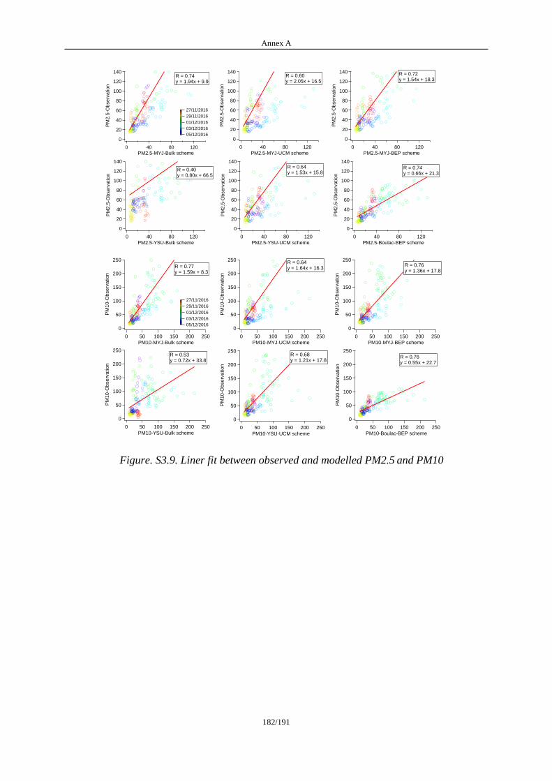
Annex A
182/191
140
120
100
80
60
40
20
0
PM
2.5
-Ob
se
rva
tio
n
12080400
PM2.5-MYJ-BEP scheme
R = 0.72y = 1.54x + 18.3
140
120
100
80
60
40
20
0
PM
2.5
-Ob
se
rva
tio
n
12080400
PM2.5-MYJ-UCM scheme
R = 0.60y = 2.05x + 16.5
140
120
100
80
60
40
20
0
PM
2.5
-Observ
ation
12080400
PM2.5-MYJ-Bulk scheme
05/12/2016
03/12/2016
01/12/2016
29/11/2016
27/11/2016
R = 0.74y = 1.94x + 9.9
140
120
100
80
60
40
20
0
PM
2.5
-Observ
ation
12080400
PM2.5-YSU-Bulk scheme
R = 0.40y = 0.80x + 66.5
140
120
100
80
60
40
20
0
PM
2.5
-Ob
se
rva
tio
n
12080400
PM2.5-YSU-UCM scheme
R = 0.64y = 1.53x + 15.8
140
120
100
80
60
40
20
0
PM
2.5
-Ob
se
rva
tio
n
12080400
PM2.5-Boulac-BEP scheme
R = 0.74y = 0.66x + 21.3
250
200
150
100
50
0
PM
10-O
bserv
ation
250200150100500
PM10-MYJ-UCM scheme
R = 0.64y = 1.64x + 16.3
250
200
150
100
50
0
PM
10-O
bserv
ation
250200150100500
PM10-MYJ-Bulk scheme
05/12/2016
03/12/2016
01/12/2016
29/11/2016
27/11/2016
R = 0.77y = 1.59x + 8.3
250
200
150
100
50
0
PM
10-O
bserv
ation
250200150100500
PM10-MYJ-BEP scheme
R = 0.76y = 1.36x + 17.8
250
200
150
100
50
0
PM
10-O
bserv
ation
250200150100500
PM10-YSU-Bulk scheme
R = 0.53y = 0.72x + 33.8
250
200
150
100
50
0
PM
10-O
bserv
ation
250200150100500
PM10-YSU-UCM scheme
R = 0.68y = 1.21x + 17.8
250
200
150
100
50
0
PM
10-O
bserv
ation
250200150100500
PM10-Boulac-BEP scheme
R = 0.76y = 0.55x + 22.7
Figure. S3.9. Liner fit between observed and modelled PM2.5 and PM10

Annex A
183/191
Figure s3.10. Time series of PM10 mass concentrations: No 1, 2, 3, and 4 represent
station FR04002, FR04034, FR04143, and FR04156, respectively.
240
200
160
120
80
40
0
00:0027/11/2016
12:0029/11/2016
00:0002/12/2016
12:0004/12/2016
Date and Time
4200
160
120
80
40
0
PM
10 M
ass C
oncentr
ation (
µg/m
3)
00:0027/11/2016
12:0029/11/2016
00:0002/12/2016
12:0004/12/2016
Date and Time
3
180
160
140
120
100
80
60
40
20
0
PM
10 M
ass C
oncentr
ation (
µg/m
3)
00:0027/11/2016
12:0029/11/2016
00:0002/12/2016
12:0004/12/2016
1
PM10-Observation Noah-mp scheme Noah scheme
200
180
160
140
120
100
80
60
40
20
0
00:0027/11/2016
12:0029/11/2016
00:0002/12/2016
12:0004/12/2016
2
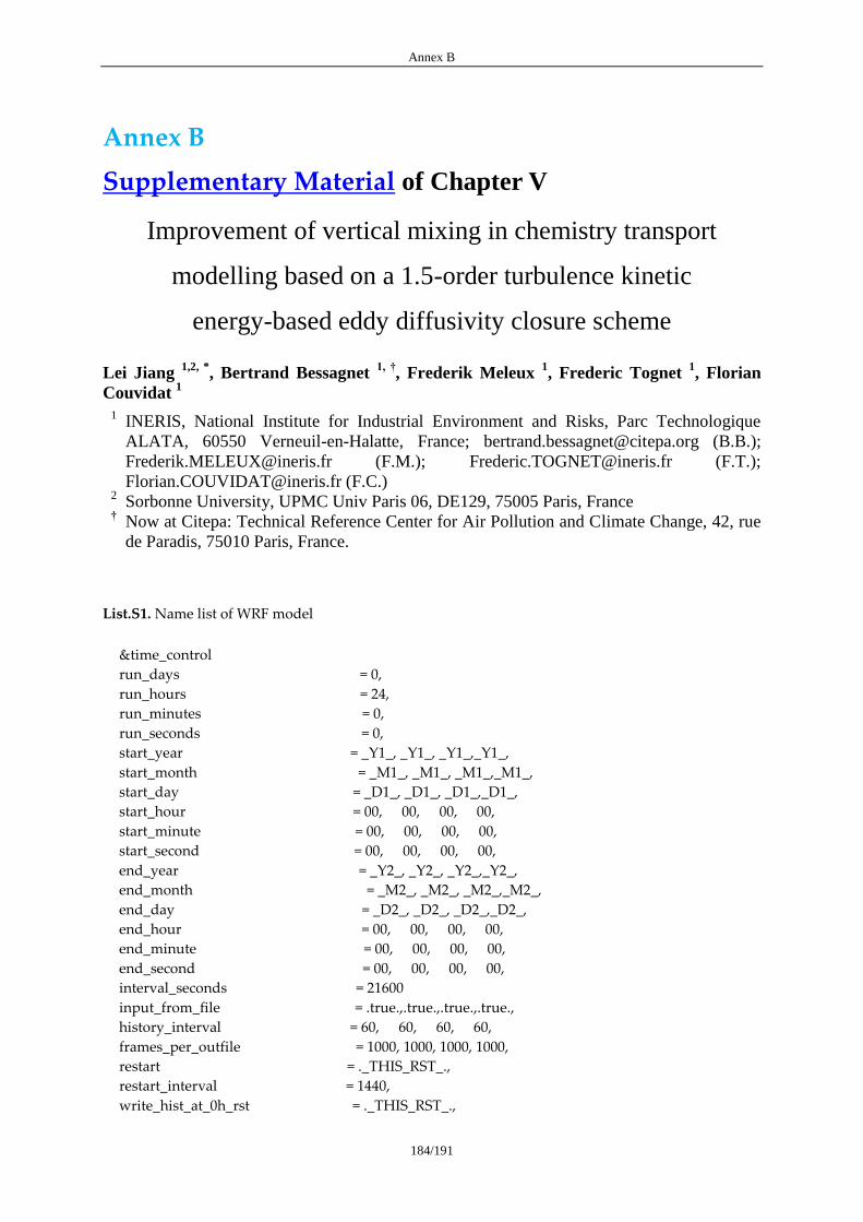
Annex B
184/191
Annex B
Supplementary Material of Chapter V
Improvement of vertical mixing in chemistry transport
modelling based on a 1.5-order turbulence kinetic
energy-based eddy diffusivity closure scheme
Lei Jiang 1,2, *
, Bertrand Bessagnet 1, †
, Frederik Meleux 1, Frederic Tognet
1, Florian
Couvidat 1
1 INERIS, National Institute for Industrial Environment and Risks, Parc Technologique
ALATA, 60550 Verneuil-en-Halatte, France; [email protected] (B.B.);
[email protected] (F.M.); [email protected] (F.T.);
[email protected] (F.C.) 2 Sorbonne University, UPMC Univ Paris 06, DE129, 75005 Paris, France
† Now at Citepa: Technical Reference Center for Air Pollution and Climate Change, 42, rue
de Paradis, 75010 Paris, France.
List.S1. Name list of WRF model
&time_control
run_days = 0,
run_hours = 24,
run_minutes = 0,
run_seconds = 0,
start_year = _Y1_, _Y1_, _Y1_,_Y1_,
start_month = _M1_, _M1_, _M1_,_M1_,
start_day = _D1_, _D1_, _D1_,_D1_,
start_hour = 00, 00, 00, 00,
start_minute = 00, 00, 00, 00,
start_second = 00, 00, 00, 00,
end_year = _Y2_, _Y2_, _Y2_,_Y2_,
end_month = _M2_, _M2_, _M2_,_M2_,
end_day = _D2_, _D2_, _D2_,_D2_,
end_hour = 00, 00, 00, 00,
end_minute = 00, 00, 00, 00,
end_second = 00, 00, 00, 00,
interval_seconds = 21600
input_from_file = .true.,.true.,.true.,.true.,
history_interval = 60, 60, 60, 60,
frames_per_outfile = 1000, 1000, 1000, 1000,
restart = ._THIS_RST_.,
restart_interval = 1440,
write_hist_at_0h_rst = ._THIS_RST_.,
Annex B
185/191
io_form_history = 2
io_form_restart = 102
io_form_input = 2
io_form_boundary = 2
debug_level = 0
use_netcdf_classic = .true.
&domains
time_step = 60,
time_step_fract_num = 0,
time_step_fract_den = 1,
max_dom = 2,
s_we = 1, 1, 1, 1,
e_we = 106, 118, 115, 85,
s_sn = 1, 1, 1, 1,
e_sn = 91, 115, 103, 79,
s_vert = 1, 1, 1, 1,
e_vert = 53, 53, 53, 53,
p_top_requested = 5000,
num_metgrid_levels = 32,
num_metgrid_soil_levels = 4,
dx = 45000, 15000, 5000, 1666.6667,
dy = 45000, 15000, 5000, 1666.6667,
grid_id = 1, 2, 3, 4,
parent_id = 1, 1, 2, 3,
i_parent_start = 1, 24, 39, 44,
j_parent_start = 1, 20, 66, 38,
parent_grid_ratio = 1, 3, 3, 3,
parent_time_step_ratio = 1, 3, 3, 3,
feedback = 1,
smooth_option = 0,
eta_levels for H4 = 1., 0.9995, 0.999, 0.9985, 0.9975,
0.996230185, 0.9949736, 0.993716955, 0.992334723,
0.990814209, 0.989141703, 0.987301886, 0.98527813,
0.983051956, 0.980603218, 0.977909565, 0.974946558,
0.971687257, 0.968101978, 0.964158237, 0.959820092,
0.955048144, 0.949799001, 0.94402492, 0.937673509,
0.930686891, 0.923001587, 0.914547801, 0.905248582,
0.895019472, 0.883767486, 0.871390283, 0.857775331,
0.842798889, 0.826324821, 0.80820334, 0.788269699,
0.7663427, 0.742223024, 0.715691328, 0.68650645,
0.65440315, 0.619089544, 0.580244482, 0.537514985,
0.49051252, 0.438809812, 0.381936818, 0.319376528,
0.250560224, 0.17486228, 0.0915945247, 0.0000,
eta_levels for H12 = 1., 0.9985, 0.9975,
0.996230185, 0.9949736, 0.993716955, 0.992334723,
0.990814209, 0.989141703, 0.987301886, 0.98527813,
0.983051956, 0.980603218, 0.977909565, 0.974946558,
0.971687257, 0.968101978, 0.964158237, 0.959820092,
0.955048144, 0.949799001, 0.94402492, 0.937673509,
Annex B
186/191
0.930686891, 0.923001587, 0.914547801, 0.905248582,
0.895019472, 0.883767486, 0.871390283, 0.857775331,
0.842798889, 0.826324821, 0.80820334, 0.788269699,
0.7663427, 0.742223024, 0.715691328, 0.68650645,
0.65440315, 0.619089544, 0.580244482, 0.537514985,
0.49051252, 0.438809812, 0.381936818, 0.319376528,
0.250560224, 0.17486228, 0.0915945247, 0.0000,
eta_levels for H40 = 1., 0.9949736, 0.993716955, 0.992334723,
0.990814209, 0.989141703, 0.987301886, 0.98527813,
0.983051956, 0.980603218, 0.977909565, 0.974946558,
0.971687257, 0.968101978, 0.964158237, 0.959820092,
0.955048144, 0.949799001, 0.94402492, 0.937673509,
0.930686891, 0.923001587, 0.914547801, 0.905248582,
0.895019472, 0.883767486, 0.871390283, 0.857775331,
0.842798889, 0.826324821, 0.80820334, 0.788269699,
0.7663427, 0.742223024, 0.715691328, 0.68650645,
0.65440315, 0.619089544, 0.580244482, 0.537514985,
0.49051252, 0.438809812, 0.381936818, 0.319376528,
0.250560224, 0.17486228, 0.0915945247, 0.0000,
/
&physics
mp_physics = 6, 6, 6, 6,
ra_lw_physics = 4, 4, 4, 4,
ra_sw_physics = 4, 4, 4, 4,
radt = 30, 30, 30, 30,
bldt = 0, 0, 0, 0,
cu_physics = 1, 1, 1, 0,
cudt = 5, 5, 5, 5,
isfflx = 1,
ifsnow = 1,
icloud = 1,
surface_input_source = 3,
num_soil_layers = 4,
num_land_cat = 21,
maxiens = 1,
maxens = 3,
maxens2 = 3,
maxens3 = 16,
ensdim = 144,
sf_sfclay_physics = 2, 2, 2, 2,
sf_surface_physics = 2, 2, 2, 2,
sf_urban_physics = ( 0 for Bulk; 1 for UCM; 2 for BEP)
bl_pbl_physics = ( 1 for YSU; 2 for MYJ; 8 for Boulac)
num_urban_layers = 6400
/
&fdda
grid_fdda = 1, 1, 0, 0,
gfdda_inname = "wrffdda_d<domain>",

Annex B
187/191
gfdda_end_h = 10000, 10000, 255, 255,
gfdda_interval_m = 360, 360, 360, 360,
io_form_gfdda = 2,
fgdt = 1, 1, 1, 1,
if_no_pbl_nudging_uv = 0, 0, 0, 0,
if_no_pbl_nudging_t = 0, 0, 0, 0,
if_no_pbl_nudging_q = 0, 0, 0, 0,
if_zfac_uv = 1, 1, 1, 1,
k_zfac_uv = 12, 12, 12, 12,
if_zfac_t = 1, 1, 1, 1,
k_zfac_t = 12, 12, 12, 12,
if_zfac_q = 1, 1, 1, 1,
k_zfac_q = 12, 12, 12, 12,
if_zfac_ph = 1, 1, 1, 1,
k_zfac_ph = 12, 12, 12, 12,
guv = 0.0003, 0.0003, 0.0003, 0.0003,
gt = 0.0003, 0.0003, 0.0003, 0.0003,
gq = 0.0003, 0.0003, 0.0003, 0.0003,
gph = 0.0003, 0.0003, 0.0003, 0.0003,
xwavenum = 5, 5, 5, 5,
ywavenum = 5, 5, 5, 5,
if_ramping = 0,
dtramp_min = 60.0,
/
&dynamics
w_damping = 1,
rk_ord = 3,
diff_opt = 1, 1, 1, 2,
km_opt = 4, 4, 4, 2,
diff_6th_opt = 2, 2, 2, 2,
diff_6th_factor = 0.12, 0.12, 0.12, 0.12,
base_temp = 290,
damp_opt = 1,
zdamp = 5000., 5000., 5000., 5000.,
dampcoef = 0.01, 0.01, 0.01, 0.01,
khdif = 0, 0, 0, 0,
kvdif = 0, 0, 0, 0,
smdiv = 0.1, 0.1, 0.1,
emdiv = 0.01, 0.01, 0.01,
epssm = 0.1, 0.1, 0.1,
non_hydrostatic = .true., .true., .true., .true.,
moist_adv_opt = 1, 1, 1, 2,
scalar_adv_opt = 1, 1, 1, 2,
tke_adv_opt = 1, 1, 1, 2,
time_step_sound = 4, 4, 4, 4,
h_mom_adv_order = 5, 5, 5, 5,
v_mom_adv_order = 3, 3, 3, 3,
h_sca_adv_order = 5, 5, 5, 5,
v_sca_adv_order = 3, 3, 3, 3,
/
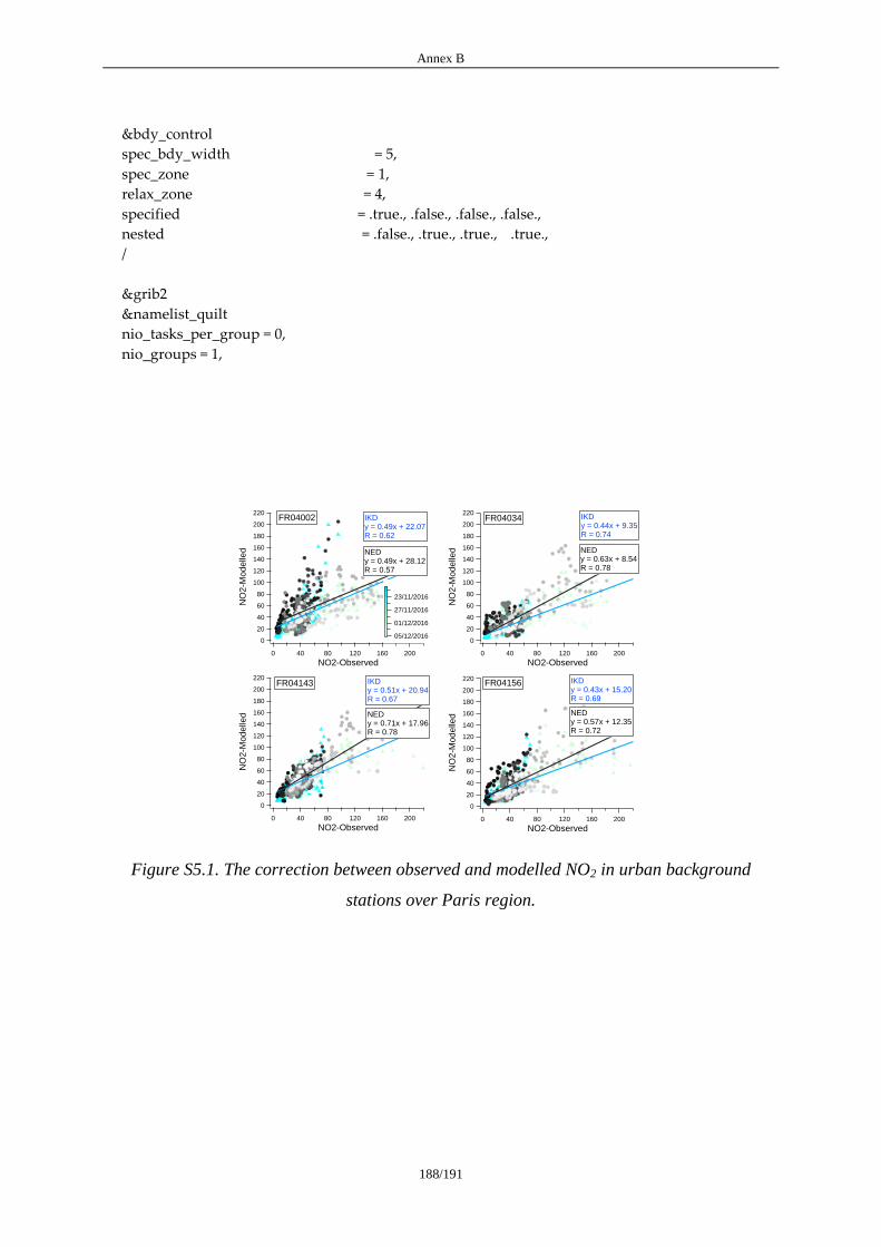
Annex B
188/191
&bdy_control
spec_bdy_width = 5,
spec_zone = 1,
relax_zone = 4,
specified = .true., .false., .false., .false.,
nested = .false., .true., .true., .true.,
/
&grib2
&namelist_quilt
nio_tasks_per_group = 0,
nio_groups = 1,
Figure S5.1. The correction between observed and modelled NO2 in urban background
stations over Paris region.
220
200
180
160
140
120
100
80
60
40
20
0
NO
2-M
odelle
d
20016012080400
NO2-Observed
FR04156 IKDy = 0.43x + 15.20R = 0.69
NEDy = 0.57x + 12.35R = 0.72
220
200
180
160
140
120
100
80
60
40
20
0
NO
2-M
odelle
d
20016012080400
NO2-Observed
IKDy = 0.51x + 20.94R = 0.67
NEDy = 0.71x + 17.96R = 0.78
FR04143
220
200
180
160
140
120
100
80
60
40
20
0
NO
2-M
odelle
d
20016012080400
NO2-Observed
NEDy = 0.63x + 8.54R = 0.78
IKDy = 0.44x + 9.35R = 0.74
FR04034220
200
180
160
140
120
100
80
60
40
20
0
NO
2-M
odelle
d
20016012080400
NO2-Observed
IKDy = 0.49x + 22.07R = 0.62
NEDy = 0.49x + 28.12R = 0.57
FR04002
05/12/2016
01/12/2016
27/11/2016
23/11/2016
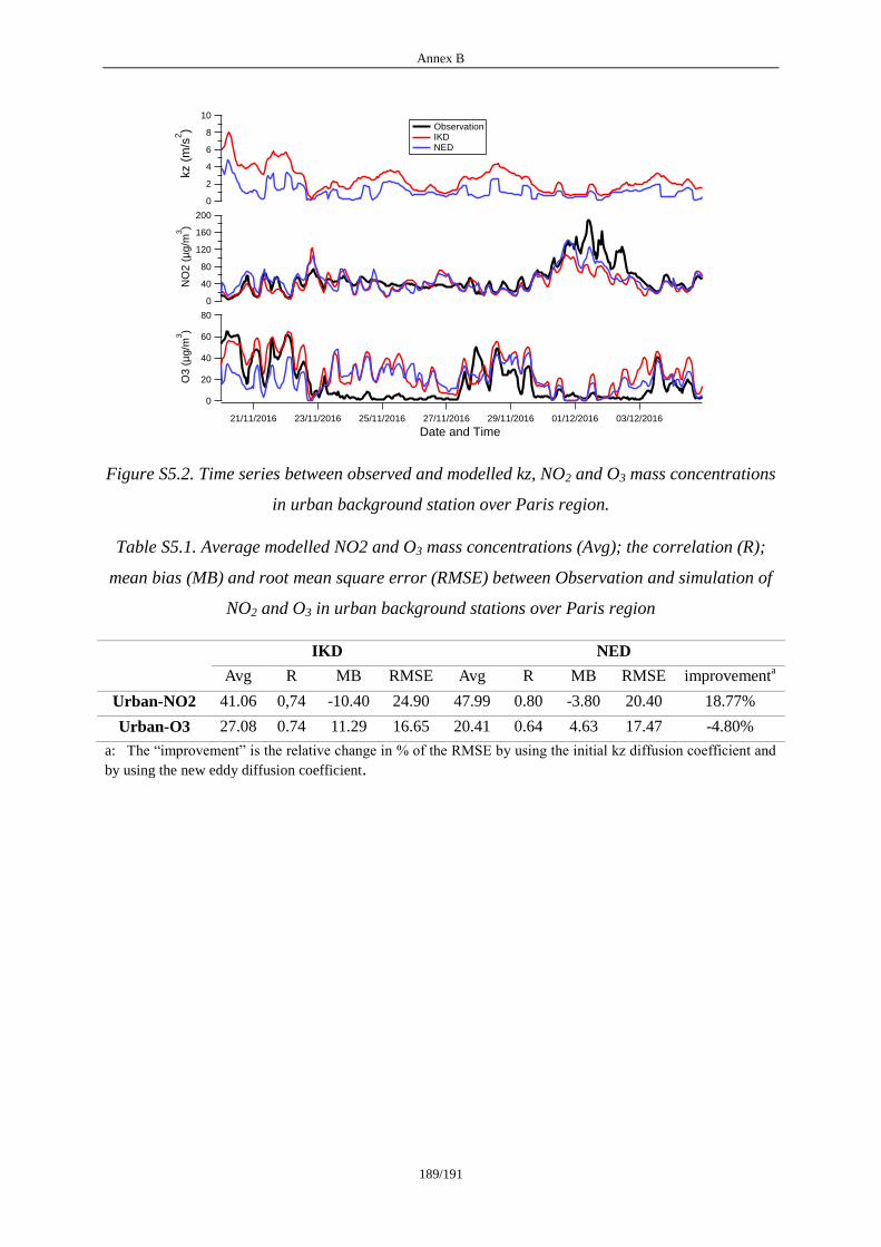
Annex B
189/191
Figure S5.2. Time series between observed and modelled kz, NO2 and O3 mass concentrations
in urban background station over Paris region.
Table S5.1. Average modelled NO2 and O3 mass concentrations (Avg); the correlation (R);
mean bias (MB) and root mean square error (RMSE) between Observation and simulation of
NO2 and O3 in urban background stations over Paris region
IKD NED
Avg R MB RMSE Avg R MB RMSE improvementa
Urban-NO2 41.06 0,74 -10.40 24.90 47.99 0.80 -3.80 20.40 18.77%
Urban-O3 27.08 0.74 11.29 16.65 20.41 0.64 4.63 17.47 -4.80%
a: The ―improvement‖ is the relative change in % of the RMSE by using the initial kz diffusion coefficient and
by using the new eddy diffusion coefficient.
200
160
120
80
40
0
NO
2 (
µg
/m3)
21/11/2016 23/11/2016 25/11/2016 27/11/2016 29/11/2016 01/12/2016 03/12/2016
Date and Time
10
8
6
4
2
0
kz (
m/s
2)
80
60
40
20
0
O3
(µ
g/m
3)
Observation IKD NED
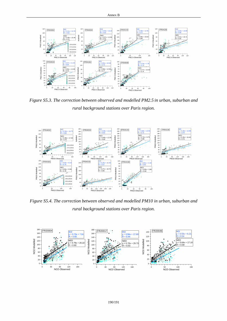
Annex B
190/191
Figure S5.3. The correction between observed and modelled PM2.5 in urban, suburban and
rural background stations over Paris region.
Figure S5.4. The correction between observed and modelled PM10 in urban, suburban and
rural background stations over Paris region.
120
100
80
60
40
20
0
PM
2.5
-Modelle
d
120100806040200
PM2.5-Observed
FR04156 IKDy = 0.34x + 14.69R = 0.66
NEDy = 0.41x + 16.71R = 0.84
120
100
80
60
40
20
0
PM
2.5
-Modelle
d
120100806040200
PM2.5-Observed
FR04034IKDy = 0.35x + 13.23R = 0.62
NEDy = 0.57x + 12.90R = 0.81
140
120
100
80
60
40
20
0
PM
2.5
-Modelle
d
150100500
PM2.5-Observed
FR04143 IKDy = 0.58x + 12.95R = 0.72
NEDy = 0.86x + 10.64R = 0.86
120
100
80
60
40
20
0
PM
2.5
-Modelle
d
120100806040200
PM2.5-Observed
FR04002 IKDy = 0.41x + 13.78R = 0.63
NEDy = 0.48x + 15.46R = 0.74
05/12/2016
01/12/2016
27/11/2016
23/11/2016
100
90
80
70
60
50
40
30
20
10
0
PM
2.5
-Modelle
d
100806040200
PM2.5-Observed
FR04024IKDy = 0.47x + 11.25R = 0.64
NEDy = 0.55x + 13.38R = 0.73
21/11/2016
25/11/2016
29/11/2016
03/12/2016
120
100
80
60
40
20
0
PM
2.5
-Modelle
d
120100806040200
PM2.5-Observed
FR04181 IKDy = 0.55x + 10.38R = 0.75
NEDy = 0.58x + 12.56R = 0.77
100
90
80
70
60
50
40
30
20
10
0
PM
2.5
-Modelle
d
100806040200
PM2.5-Observed
FR04048IKDy = 0.74x + 7.78R = 0.70
NEDy = 0.77x + 10.40R = 0.74
220
200
180
160
140
120
100
80
60
40
20
0P
M1
0-M
od
elle
d20016012080400
PM10-Observed
FR04156 IKDy = 0.28x + 14.98R = 0.70
NEDy = 0.35x + 16.40R = 0.76
200
180
160
140
120
100
80
60
40
20
0
PM
10
-Mo
de
lled
20016012080400
PM10-Observed
FR04034IKDy = 0.29x + 13.41R = 0.62
NEDy = 0.46x + 12.05R = 0.80
220
200
180
160
140
120
100
80
60
40
20
0
PM
10
-Mo
de
lled
20016012080400
PM10-Observed
FR04143 IKDy = 0.48x + 13.55R = 0.70
NEDy = 0.72x + 9.79R = 0.86
140
120
100
80
60
40
20
0
PM
10
-Mo
de
lled
150100500
PM10-Observed
FR04002 IKDy = 0.34x + 14.75R = 0.66
NEDy = 0.39x + 17.30R = 0.76
05/12/2016
01/12/2016
27/11/2016
23/11/2016
160
140
120
100
80
60
40
20
0
PM
10
-Mo
de
lled
150100500
PM10-Observed
FR04181IKDy = 0.53x + 8.14R = 0.76
NEDy = 0.56x + 9.56R = 0.78
21/11/2016
25/11/2016
29/11/2016
03/12/2016
240
200
160
120
80
40
0
PM
10
-Mo
de
lled
24020016012080400
PM10-Observed
FR04319 IKDy = 0.26x + 16.30R = 0.57
NEDy = 0.27x + 18.70R = 0.66
100
90
80
70
60
50
40
30
20
10
0
PM
10
-Mo
de
lled
100806040200
PM10-Observed
FR04158IKDy = 0.81x + 2.34R = 0.81
NEDy = 0.90x + 3.86R = 0.84
140
120
100
80
60
40
20
0
NO
2-M
od
elle
d
150100500
NO2-Observed
IKDy = 0.53x + 6.21R = 0.54
NEDy = 0.64x + 17.10R = 0.59
FR20046180
160
140
120
100
80
60
40
20
0
NO
2-M
od
elle
d
16012080400
NO2-Observed
IKDy = 0.70x + 7.51R = 0.55
NEDy = 0.79x + 20.22R = 0.60
FR20004180
160
140
120
100
80
60
40
20
0
NO
2-M
od
elle
d
16012080400
NO2-Observed
IKDy = 0.56x + 17.69R = 0.44
NEDy = 0.70x + 29.73R = 0.53
FR20017
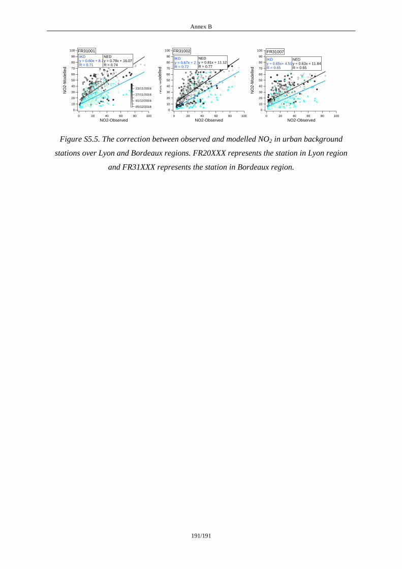
Annex B
191/191
Figure S5.5. The correction between observed and modelled NO2 in urban background
stations over Lyon and Bordeaux regions. FR20XXX represents the station in Lyon region
and FR31XXX represents the station in Bordeaux region.
100
90
80
70
60
50
40
30
20
10
0
NO
2-M
od
elle
d
100806040200
NO2-Observed
FR31002
IKDy = 0.67x + 2.90R = 0.72
NEDy = 0.81x + 11.12R = 0.77
100
90
80
70
60
50
40
30
20
10
0
NO
2-M
od
elle
d
100806040200
NO2-Observed
IKDy = 0.60x + 8.15R = 0.71
NEDy = 0.78x + 16.07R = 0.74
FR31001
05/12/2016
01/12/2016
27/11/2016
23/11/2016
100
90
80
70
60
50
40
30
20
10
0
NO
2-M
od
elle
d
100806040200
NO2-Observed
FR31007
IKDy = 0.65x+ 4.51R = 0.65
NEDy = 0.63x + 11.84R = 0.65