2

Speeding up K-Means Algorithm by GPUs

You Li, Kaiyong Zhao, Xiaowen Chu, and Jiming Liu

Department of Computer Science

Hong Kong Baptist University, Hong Kong

Email: {youli, kyzhao, chxw, jiming}@comp.hkbu.edu.hk

Abstract—Cluster analysis plays a critical role in a wide variety of applications; but it is now facing the computational challenge

due to the continuously increasing data volume. Parallel computing is one of the most promising solutions to overcoming the

computational challenge. In this paper, we target at parallelizing k-Means, which is one of the most popular clustering algorithms,

by using the widely available Graphics Processing Units (GPUs). Different from existing GPU-based k-Means algorithms, we

observe that data dimensionality is an important factor that should be taken into consideration when parallelizing k-Means on

GPUs. In particular, we use two different strategies for low-dimensional data sets and high-dimensional data sets respectively, in

order to make the best use of GPU computing horsepower. For low-dimensional data sets, we design an algorithm that exploits

GPU on-chip registers to significantly decrease the data access latency. For high-dimensional data sets, we design another novel

algorithm that simulates matrix multiplication and exploits GPU on-chip shared memory to achieve high compute-to-memory-

access ratio. Our experimental results show that our GPU-based k-Means algorithms are three to eight times faster than the best

reported GPU-based algorithms.

Keywords - clustering, k-means, GPU computing, CUDA

I. INTRODUCTION

Clustering is a method of unsupervised learning that partitions a set of data objects into clusters, such that intra-cluster

similarity is maximized while inter-cluster similarity is minimized [1, 2]. The k-Means algorithm is one of the most popular

clustering algorithms and is widely used in a variety of fields such as statistical data analysis, pattern recognition, image

analysis and bioinformatics [3, 4]. It has been elected as one of the Top 10 data mining algorithms [5]. The running time of k-

Means algorithm grows with the increase of the size and also the dimensionality of the data set. Hence clustering large-scale

data sets is usually a time-consuming task. Parallelizing k-Means is a promising approach to overcoming the challenge of the

3

huge computational requirement [6-8]. In [6], P-CLUSTER has been designed for a cluster of computers with a client-server

model in which a server process partitions data into blocks and sends the initial centroid list and blocks to each client. It has

been further enhanced by pruning as much computation as possible while preserving the clustering quality [7]. In [8], the k-

Means clustering algorithm has been parallelized by exploiting the inherent data-parallelism and utilizing message passing.

Recently, as a general-purpose and high performance parallel hardware, Graphics Processing Units (GPUs) develop

continuously and provide another promising platform for parallelizing k-Means. GPUs are dedicated hardware for

manipulating computer graphics. Due to the huge computing demand for real-time and high-definition 3D graphics, GPUs

have evolved into highly parallel many-core processors. The advances of computing power and memory bandwidth in GPUs

have driven the development of general-purpose computing on GPUs (GPGPU).

In this paper, we design a parallel k-Means algorithm for GPUs by using a general-purpose parallel programming model,

namely Compute Unified Device Architecture (CUDA) [9, 10]. CUDA has been used for speeding up a large number of

applications [11, 12, 13, 14]. Some clustering algorithms have been implemented on the GPUs, including k-Means. There are

mainly three existing GPU-based k-Means algorithms: GPUMiner [15], UV_k-Means [16], and HP_k-Means [17]. UV_k-

Means achieves a speedup of ten to forty as compared with a four-threaded Minebench [18] running on a dual-core, hyper-

threaded CPU. HP_k-Means claims another speedup of two to four as compared with UV_k-Means and twenty to seventy

speedup as compared with GPUMiner [17]. These existing works have shown the promising high performance advantage of

GPUs. However, the above GPU-based algorithms have not yet fully exploited the computing power of GPUs.

In this paper we conduct systematic research on parallelizing the k-Means using CUDA. Our first contribution is the

observation that the dimensionality of the data set is an important factor to be considered. Our second contribution is the

design, implementation, and evaluation of two different strategies. For low-dimensional data sets, we mainly utilize the GPU

on-chip registers to minimize the memory access latency. Due to the limited size of on-chip registers, this method is not

applicable to data sets with high dimensionality. For high-dimensional data sets, we design a novel and highly efficient

algorithm that treats the most time-consuming part of k-Means as matrix multiplication, and then makes use of GPU on-chip

shared memory together with on-chip registers. Our third contribution is analyzing the strategy for the large data set, which

cannot be processed within a single GPU once. Our experimental results show that our parallel k-Means algorithm performs

much better than existing algorithms, for both low-dimensional data sets and high-dimensional data sets.

4

The rest of this paper is organized as follows. Section II introduces the GPU architecture and existing GPU-based k-Means

algorithms. Section III presents our design of parallel k-Means algorithm on GPUs. Section IV presents our experimental

results, and Section V concludes the paper and presents some future work.

II. RELATED WORK

To the best of our knowledge, there are mainly three existing GPU-based k-Means algorithms, namely UV_k-Means,

GPUMiner, and HP_k-Means. We first briefly introduce the GPU architecture, and then review these three existing GPU-

based k-Means algorithms.

A. The GPU architecture

We take NVIDIA GTX280 as an example to show a typical GPU architecture. GTX 280 has 30 Streaming

Multiprocessors (SMs), and each SM has 8 Scalar Processors (SPs), resulting in a total of 240 processor cores. The SMs have

a Single-Instruction Multiple-Thread (SIMT) architecture: at any given clock cycle, each SP executes the same instruction,

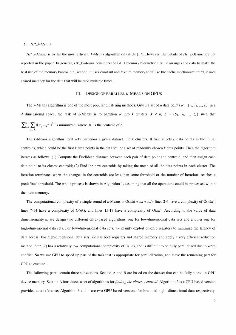
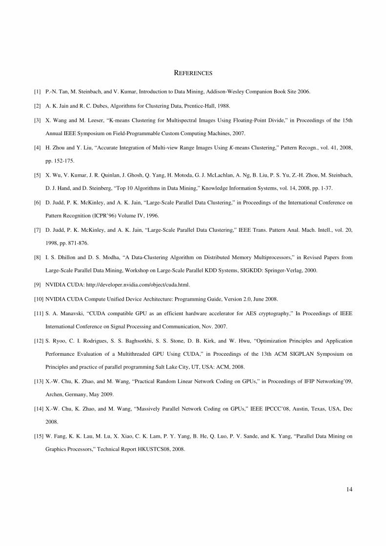
but operates on different data. Each SM has four different types of on-chip memory, namely registers, shared memory,

constant cache, and texture cache, as shown in Fig.1. Constant cache and texture cache are both read-only memories shared

by all SPs. Off-chip memories such as local memory and global memory have relatively long access latency, usually 400 to

600 clock cycles [10]. The properties of the different types of memory have been summarized in [10, 12]. In general, the

scarce registers and shared memory should be carefully utilized to amortize the global memory latency cost.

In CUDA model, GPU is regarded as a coprocessor which is capable of executing a great number of threads in parallel. A

single source program includes host codes running on CPU and also kernel codes running on GPU. Compute-intensive and

data-parallel tasks have to be implemented as kernel codes so as to be executed on GPU. GPU threads are organized into

thread blocks, and each block of threads are executed concurrently on one SM. Threads in a thread block can share data

through the shared memory and can perform barrier synchronization. But there is no native synchronization mechanism for

different thread blocks except by terminating the kernel. Another important concept in CUDA is warp, which is formed by 32

parallel threads and is the scheduling unit of each SM. When a warp stalls, the SM can schedule another warp to execute. A

warp executes one instruction at a time, so full efficiency can only be achieved when all 32 threads in the warp have the same

execution path. There are two consequences: first, if the threads in a warp have different execution paths due to conditional

branch, the warp will serially execute each branch which increases the total time of instructions executed for this warp;

second, if the number of threads in a block is not a multiple of warp size, the remaining instruction cycles will be wasted.

5

Besides, when accessing the memory, half-warp executes as a group, which has 16 threads. If the half-warp threads access

the coalesced data, the data access operation will perform within one instruction cycle. Otherwise, the access operation will

occupy up to 16 instruction cycles.

B. UV_k-Means

In order to avoid the long time latency of global memory access, UV_k-Means copies all the data to the texture memory,

which uses a cache mechanism. Then, it uses constant memory to store the k centroids, which is also more efficient than

using global memory. Each thread is responsible for finding the nearest centroid of a data point; each block has 256 threads,

and the grid has n/256 blocks.

The work flow of UV_k-Means is straightforward. First, each thread calculates the distance from one corresponding data

point to every centroid and finds the minimum distance and corresponding centroid. Second, each block calculates a

temporary centroid set based on a subset of data points, and each thread calculates one dimension of the temp centroid. Third,

the temporal centroid sets are copied from GPU to CPU, and then the final new centroid set is calculated on CPU.

UV_k-Means has achieved a speedup of twenty to forty over the single-thread CPU-based k-Means in our experiment.

This speedup is mainly achieved by assigning each data point to one thread and utilizing the cache mechanism to get a high

reading efficiency. However, the efficiency could be further improved by other memory access mechanisms such as registers

and shared memory.

C. GPUMiner

GPUMiner stores all input data in the global memory, and loads k centroids to the shared memory. Each block has 128

threads, and the grid has n/128 blocks. The main characteristic of GPUMiner is the design of a bitmap. The workflow of

GPUMiner is as follows. First, each thread calculates the distance from one data point to every centroid, and changes the

suitable bit into true in the bit array, which stores the nearest centroid for each data point. Second, each thread is responsible

for one centroid, finds all the corresponding data points from the bitmap and takes the mean of those data points as the new

centroids.

The main problem of GPUMiner is the poor utilization of memory in GPU, since GPUMiner accesses most of the data

(input data point) from global memory directly. As pointed out in [17], bitmap approach is elegant in expressing the problem,

but not a good method for high performance, since bitmap takes more space when k is large and requires more shared

memory.

6

D. HP_k-Means

HP_k-Means is by far the most efficient k-Means algorithm on GPUs [17]. However, the details of HP_k-Means are not

reported in the paper. In general, HP_k-Means considers the GPU memory hierarchy: first, it arranges the data to make the

best use of the memory bandwidth; second, it uses constant and texture memory to utilize the cache mechanism; third, it uses

shared memory for the data that will be read multiple times.

III. DESIGN OF PARALLEL K-MEANS ON GPUS

The k-Means algorithm is one of the most popular clustering methods. Given a set of n data points R = {r1, r2, ..., rn} in a

d dimensional space, the task of k-Means is to partition R into k clusters (k < n) S = {S1, S2, ..., Sk} such that

1

2|| ||

k

ii

x j i

j

S

x µ=

∈

−∑ ∑ is minimized, where i

µ is the centroid of Si.

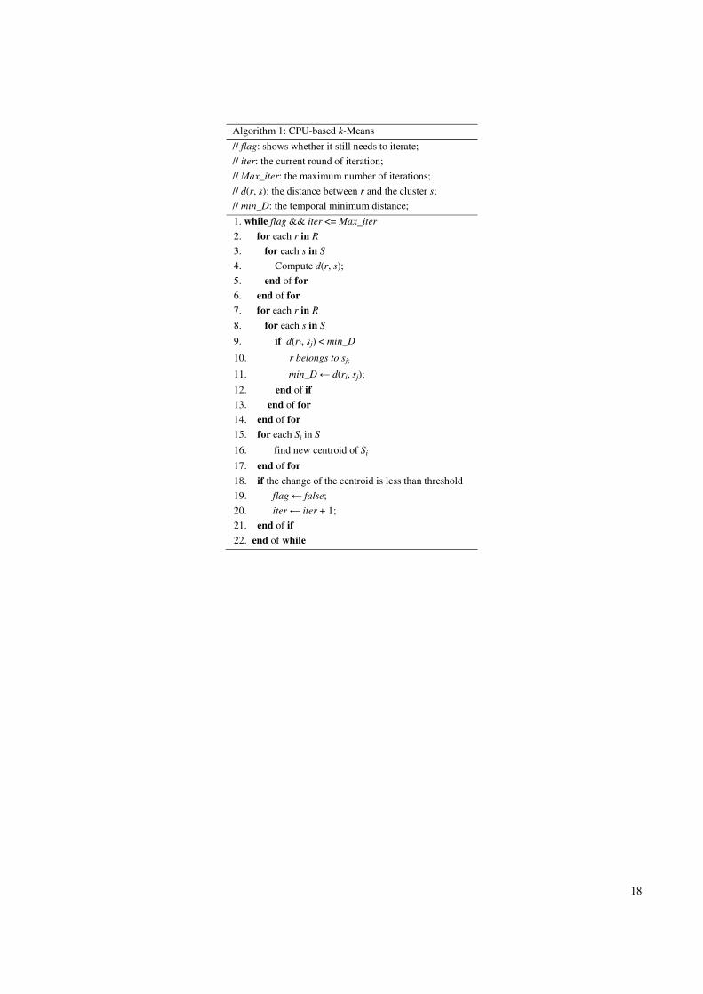
The k-Means algorithm iteratively partitions a given dataset into k clusters. It first selects k data points as the initial

centroids, which could be the first k data points in the data set, or a set of randomly chosen k data points. Then the algorithm

iterates as follows: (1) Compute the Euclidean distance between each pair of data point and centroid, and then assign each

data point to its closest centroid; (2) Find the new centroids by taking the mean of all the data points in each cluster. The

iteration terminates when the changes in the centroids are less than some threshold or the number of iterations reaches a

predefined threshold. The whole process is shown in Algorithm 1, assuming that all the operations could be processed within

the main memory.

The computational complexity of a single round of k-Means is O(nkd + nk + nd): lines 2-6 have a complexity of O(nkd);

lines 7-14 have a complexity of O(nk); and lines 15-17 have a complexity of O(nd). According to the value of data

dimensionality d, we design two different GPU-based algorithms: one for low-dimensional data sets and another one for

high-dimensional data sets. For low-dimensional data sets, we mainly exploit on-chip registers to minimize the latency of

data access. For high-dimensional data sets, we use both registers and shared memory and apply a very efficient reduction

method. Step (2) has a relatively low computational complexity of O(nd), and is difficult to be fully parallelized due to write

conflict. So we use GPU to speed up part of the task that is appropriate for parallelization, and leave the remaining part for

CPU to execute.

The following parts contain three subsections. Section A and B are based on the dataset that can be fully stored in GPU

device memory. Section A introduces a set of algorithms for finding the closest centroid: Algorithm 2 is a CPU-based version

provided as a reference; Algorithm 3 and 4 are two GPU-based versions for low- and high- dimensional data respectively.

7

Section B illustrates the algorithms for computing new centroids: Algorithm 5 is based on CPU provided as a reference, while

Algorithm 6 is the GPU version. Section C discusses the strategies for large datasets that cannot be fully stored in GPU

device memory: Algorithm 7 is a sequential method, which could be implemented on both the CPU and the GPU.

A. Finding closest centroid

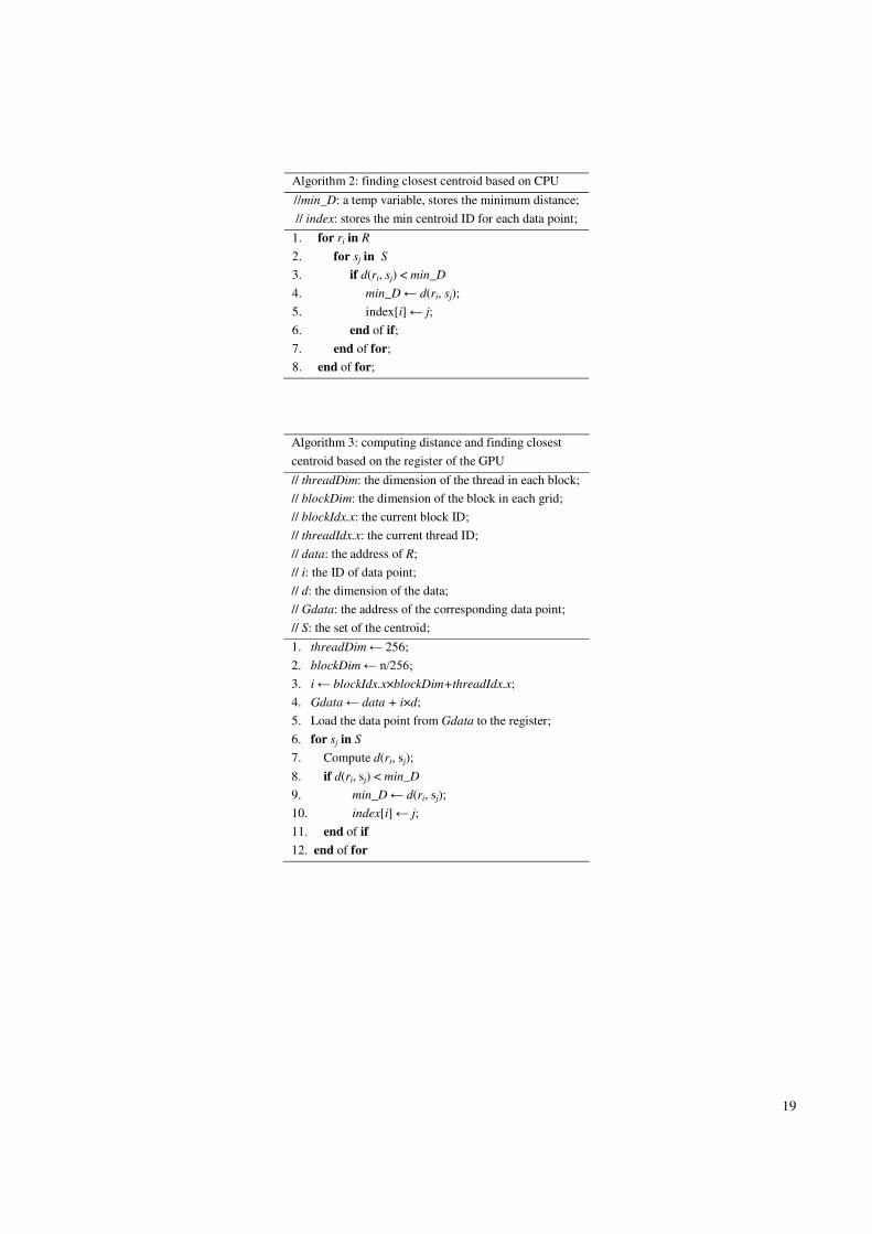
The CPU-based algorithm of finding closest centroid is shown in Algorithm 2. Since the algorithm computes the distance

between each data point and each centroid, our first method to parallelize Algorithm 2 is dispatching one data point to one

thread, and then each thread calculates the distance from one data point to all the centroids, and maintains the minimum

distance and the corresponding centroid, as shown in Algorithm 3. Line 1 and 2 show how the algorithm designs the thread

block and gird. Our experiments show that a block size of 256 results in better performance than block size of 32, 64 and 128.

Line 3 and 4 calculate the position of the corresponding data point for each thread in global memory. Line 5 loads the data

point into the register. Lines 6-12 compute the distance and maintain the minimum one.

Algorithm 3 only has one level of loop instead of two levels in Algorithm 2, because the loop for n data points has been

dispatched to n threads, which decreases the time consumption significantly because many threads are working in parallel. It

is worth pointing out that the key step of achieving high efficiency is loading the data points into the on-chip registers, which

ensures that reading the data point from global memory happens only once when calculating the distances between the data

point and k centroids. Obviously, reading from register is much faster than reading from global memory. Besides, coalesced

access to the global memory also decreases the reading latency. The experimental results in section IV verify the advantage

of Algorithm 3 compared with the best published results. However, the problem of Algorithm 3 is the limited size of the

registers. In fact, users are not able to fully control the registers, and could only utilize registers when the data size is small

enough. When the data points cannot be loaded into the registers as the data dimension grows, they will be stored in local

memory, which will increase the reading latency and decrease the performance significantly.

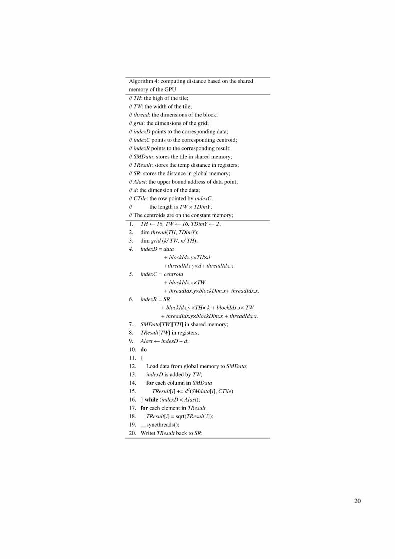
In fact, the input data point and the centroid could be viewed as two matrixes data[n][d] and centroid[d][k]; the result

distance could be denoted as Result[n][k]; and the distance computing process shares the same flow as matrix multiplication.

Based on this observation, we design Algorithm 4 for high-dimensional data sets, by adopting the idea of matrix

multiplication and utilizing registers and the shared memory together.

The main idea of Algorithm 4 is decreasing the global memory access time and latency by loading the data into the shared

memory tile by tile. Thus, Algorithm 4 reads each data point from global memory only once, the same as Algorithm 3. The

key point of Algorithm 4 is how to access the global memory and shared memory efficiently, which is achieved by adopting

8

coalescing reading which accesses sixteen continuous address for the threads in a half warp to avoid the bank conflict. The

details are described as follows.

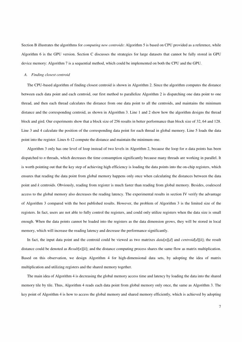
The three matrixes data[n][d], centroid[d][k] and Result[n][k] are partitioned into TH×TW, TW×TH, and TH×TW tiles

respectively. The resource of the GPU is partitioned as follows: the grid has (k/TW)×(n/TH) blocks, the ID of which is noted

by blockIdx.y (by in Fig.2) and blockIdx.x (bx in Fig.2); each block has TH×TDimY threads, the ID of which is noted by

threadIdx.y (ty in Fig.2) and threadIdx.x (tx in Fig.2). The computing task is dispatching as follows: each block calculates

TDimY tiles in the Result, which is noted as SR[TH][TW×TDimY]; each thread computes a column of SR. For each thread,

indexD points to the right position of the data, which contains the following three parts as shown in line 4: data is the

beginning address of the data set; since the height of the data is divided by TH, blockIdx.y×TH×d is the address of the

corresponding block; threadIdx.y×d adding threadIdx.x is the offset address inside the block.

In line 5, indexC points to the right position in centroid, which also has three parts: centroid is the beginning address of

the current centroid; blockIdx.x×TW points to the corresponding block address, since the width of the centroid is divided by

TW; threadIdx.y×blockDim.x adding threadIdx.x points to the address of the current thread inside the block. Obviously, the

threads in one block would access centroid in continuous addresses, which is also called coalesced accessing. indexR is

calculated in the same way as in line 6: the beginning address of the result, the row address, and the offset address inside the

block for the current thread.

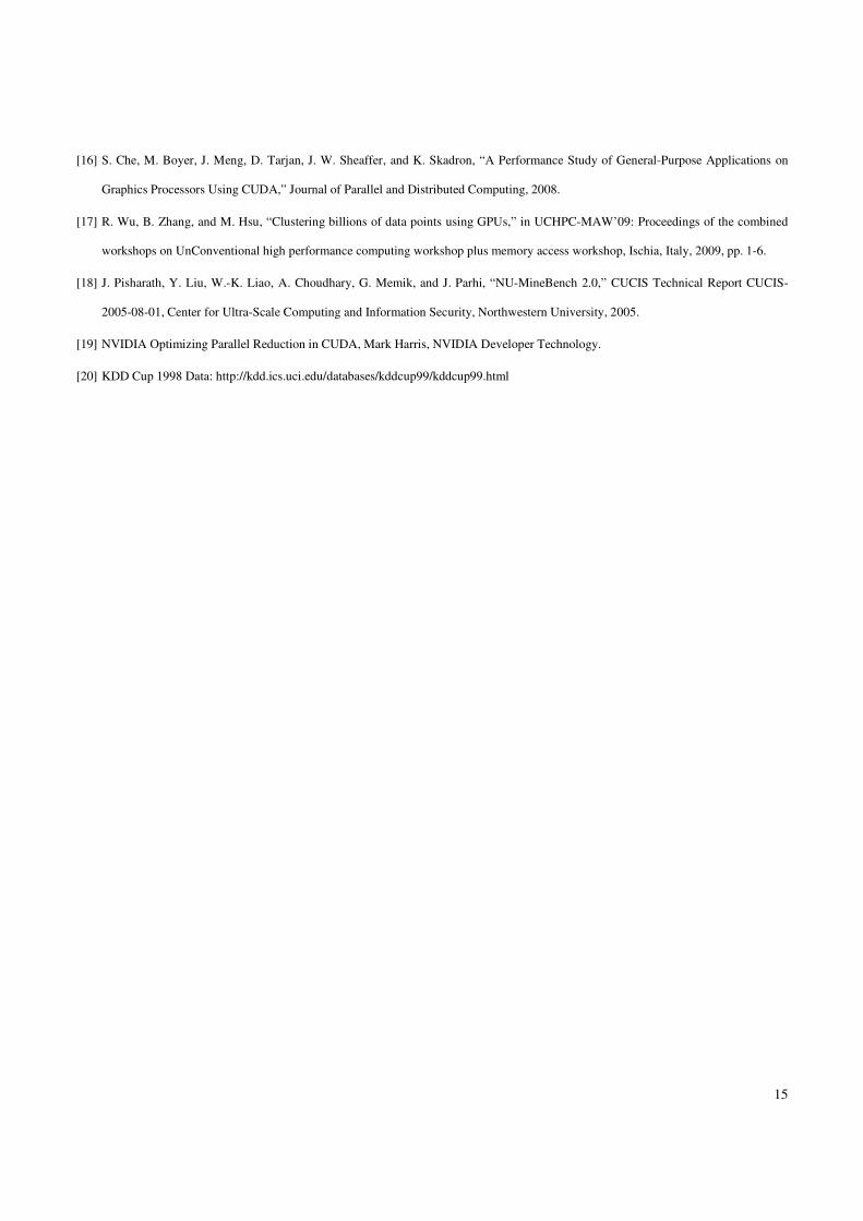
In the loop from line 11 to 16, the algorithm loads a tile of data from global memory to the shared memory, and

computes the temporary distance saved in TResult which are stored in on-chip registers; the loop ends when the whole row

has been calculated. Line 17-18 calculate the distance based on the results of muliplication. Line 19 waits for all the threads

to finish their work. Line 20 writes the distance back from TResult to SR. The details are shown in Fig.2, and take the process

of calculating a SR[TH][TW×TDimY] as an example, which is equal to data[TH][d]×centroid[d][TW×TDimY]: load the first

tile (in blue color) from the data into the shared memory; multiply the blue tile in the data with the blue tile in the Centroid,

which is stored in the constant memory; accumulate the temporary results into TResult, whose initial value is all zero; repeat

loading the next tile (in orange color), multiplying and accumulating, until data[TH][d] and centroid[d][TW×TDimY] have

been all accessed.

After calculating the distances matrix Result[n][k] between the data and the centroid, the next step is find the closest

centroid for each data point. Obviously, based on the CPU, the computational complexity is O(nk). On the GPUs, there are

mainly two methods: firstly, each thread finds the closest centroid for one data point from one row of Result, whose

9

computational complexity is O(k). Secondly, O(k/logk) threads find the closest centroid for one data point from one row of

Result, and each thread deals with O(logk) elements in the row. The computational complexity is O(logk) [19]. In our this

paper, we choose the first strategy because of the following two reasons: first, this step occupies less than 5% time in the

whole process adopting the former strategy; secondly, the latter strategy is clearly more efficient than the former one only if k

is large enough, and they perform nearly the same when k is smaller than 1000 in all the experiment in this paper.

B. Computing new centroids

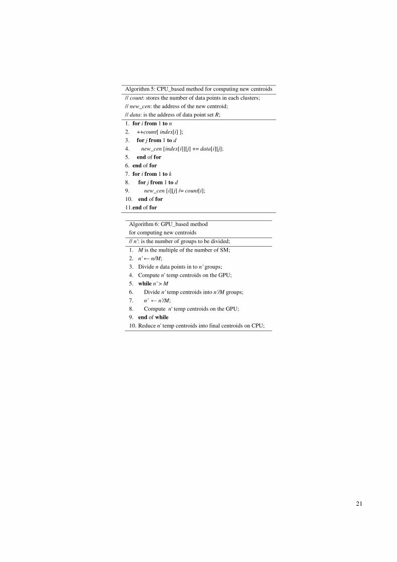
The result of the first step, i.e., finding the closest centroid, is an array index[n] which stores the closest centroid for each

data point. The data points belonging to the same centroid constitute one cluster. Calculating the new centroids is by taking

the mean of all the data points in each cluster. As shown in Algorithm 5, the computational complexity is O(nd+kd), and it is

difficult to be fully parallelized. If we assign each data point to a thread, it will generate write conflict when adding the data

to the shared centroid. On the other hand, if we assign each centroid to a thread, the computing power of the GPU cannot be

fully utilized.

In this paper, we design an algorithm which adopts “divide and conquer” strategy. The main notations of the strategy are

M and n': M is a multiple of stream multiprocessor number in the GPU, and n' is the number of groups, initialized by the

value of n/M, and updated by the value of n'/M. We first divide the data into n' groups, then reduce each group and get

temporary centroids. We then update n', divide the temporary centroids into n' groups and reduce iteratively on the GPU until

n' is smaller than M, indicating the GPU has no advantage than the CPU for further computing. Finally, we calculate the final

centroids on the CPU. The full algorithm is shown in Algorithm 6. By dividing the data into groups, the write conflict

decreases, since each group writes its own temporary centroids and has no influence on other groups. It is necessary to point

out that M in Algorithm 6 line 1 should be a multiple of the number of SM in order to ensure high schedule efficiency on the

GPU.

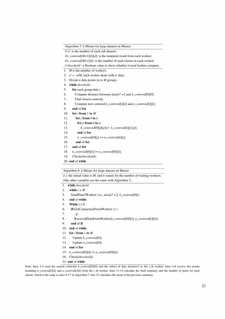
C. Dealing with large dataset

The above algorithms all assume that the dataset can be fully stored in the GPU’s on-board device memory. When the

size of dataset grows larger than a single GPU’s on-board memory, we can adopt a divide-and-merge method as follows: load

the dataset group by group, then compute the temporary results and merge them into the finally results. The details are shown

in Algorithm 7: lines 1-3 divide the whole dataset into M groups, each of which has n' data points and could be loaded into

the GPU's on-board memory; lines 5-9 deal with the ith group of the data, which starts from data[ixn'], compute the distance,

10

find the nearest centroid and compute the new centroids based on the current group of data, until the end of the whole data,

and based on the ith group of data, n_centroid[i][k] stores the number of the points and k_centroid[i][k] stores the summary

of the points without calculating the mean in each cluster, while k_centroid[0][0] stores the current centroids; lines 10-17

calculate the final summary and the number of the points for each cluster based on the whole data set; line 18 calculates the

mean of the previous summary, which is the new centroids currently; line 19 checks the threshold containing the iteration

time and the difference between the current centroids and the previous centroids. In fact, Algorithm 7 could be implemented

on either CPU or GPU. For CPU version, we can adopt Algorithm 2 and 5 for computing distance, finding the closest

centroids and computing new centroids; while for GPU version, we can adopt Algorithm 3 for the low-dimensional data,

Algorithm 4 for the high-dimensional data, and Algorithm 6.

IV. EXPERIMENTS

We have implemented our parallel k-Means algorithm using CUDA version 2.3. Our experiments were conducted on a

PC with an NVIDIA GTX280 GPU and an Intel(R) Core(TM) i5 CPU. GTX 280 has 30 SIMD multi-processors, and each

one contains eight processors and performs at 1.29 GHz. The memory of the GPU is 1GB with the peak bandwidth of 141.7

GB/sec. The CPU has four cores running at 2.67 GHz. The main memory is 8 GB with the peak bandwidth of 5.6 GB/sec.

We calculate the time of the application after the file I/O, in order to show the speedup effect more clearly.

The experiments contain three parts: first, we compare our results with the best published results of HP_k-Means, which

is mainly on low-dimensional data sets. Second, we compare our k-Means with UV_k-Means and GMiner on high-

dimensional data sets. Third, we compare our CPU k-Means and GPU k-Means on the large data set. Each experiment is

repeated ten times and the average results are reported.

A. On low-dimensional data sets

Here we choose exactly the same data sets as HP_k-Means as follows: n has two values, 2x106 and 4x10

6; k has two

values, 100 and 400; d also has two values, 2 and 8. Each dimension is a single-precision floating point number, and

generated randomly. The iteration time is fifty, and the algorithm will stop after fifty rounds, no matter what the change of

the centroid is. Besides, the speeds of HP_k-Means, UV_k-Means and GPUMiner are extracted from [17]. As we use the

same experimental configurations as [17], our comparisons are fair and reasonable.

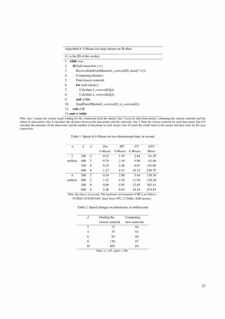
As shown in Table 1, our k-Means is the most efficient one among the four algorithms. It is three to eight times faster

than the best published results from HP_k-Means, ten to twenty faster than UV_k-Means and one hundred to three hundred

11

faster than GPUMiner. Since HP_k-Means only provides some optimization rules without publishing the source code, we

mainly discuss the difference between our k-Means and UV_k-Means.

The workflows of the two algorithms are very similar: each thread finds the minimum centroid for each data point. The

main difference is the memory utilization: UV_k-Means puts the data on the texture and puts the centroids on the constant;

our k-Means firstly loads the data on the register, and reads the data from the register each time when calculating the distance

from each centroid, resulting in a low global memory access times and latency, since reading from register is by far faster

than reading from other memories.

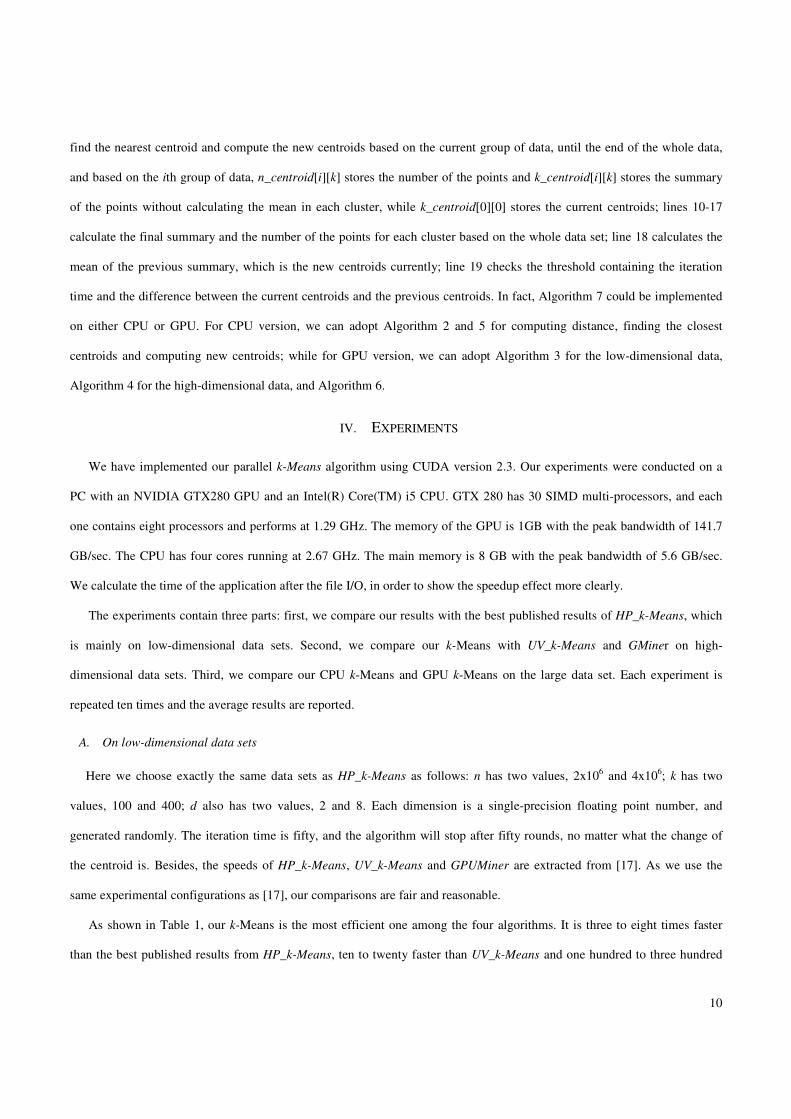
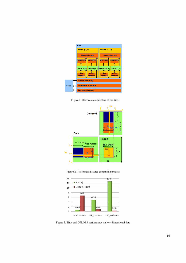
We also analyze the GFLOPS of each algorithm. Since the computational complexity of finding the closest centroid is

O(nkd + nk), which is much larger than O(nd) of computing the new centroid, a reasonable approximation on the total

number of operations can be obtained by:

OP = n×k×(d+d+d-1)×iter (1)

For each data point, the first d in Eq. (1) is the number of subtractions; the second d is the number of multiplications; the

third term d-1 is the number of additions; and iter is the number of iterations. Take the 7th

row of Table 1 as an example (i.e.,

n = 4million, k = 100, d = 8), the number of operations is 4.6×1011

. So the GFLOPS of each algorithm are: 676, 93, 36 and

1.2. The maximum GFLOPS of GTX 280 is around 933, and our algorithm has achieved 72% of the peak GPU computing

power, which could also show the advantage and high efficiency of our algorithm. We visually show the time and GLOPS in

Fig.3, for the setting of the 7th line in Table 1.

As shown in Table 2, we can also observe that our k-Means is insensitive with dimensionality when it is relatively small,

since the time differs a little when the dimensionality varies from 2 to 6. As the dimensionality keeps growing, the time

consumption grows with a higher speed because we are not able to keep a data point in registers, which is the main reason we

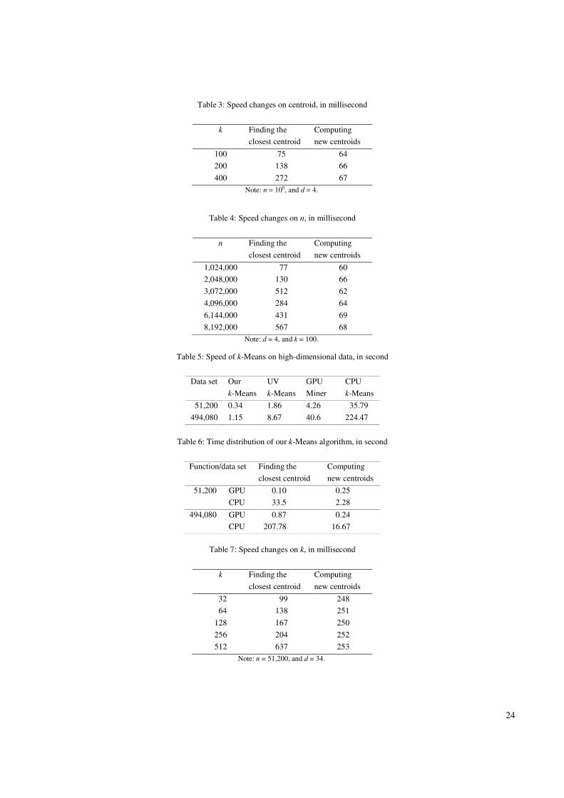
design a new strategy for high-dimensional data sets. As shown in Table 3, when k grows, the algorithm has to access the

global memory more, which is proportional to k, and will spend more time. The computing time also grows with the increase

of n, as shown in Table 4. Besides, we could also observe that the time consumption of “computing new centroids” changes

slightly when the parameters change, due to the low computational complexity and our “divide and conquer” Algorithm 6.

In fact, through our experiment, when the dimensionality is larger than sixteen (assuming single-precision floating point

data), the data point cannot be loaded into the register, and the speed decreases sharply because of accessing the global

memory. So, we use Algorithm 5, shared memory based algorithm to deal with high-dimensional data sets.

12

B. On high-dimensional data sets

For high-dimensional data sets, we use the samples provided by the KDD Cup 1999 [20], and choose two data sets, with

51200 and 494080 data points respectively. Each data point contains 34 features, and each one is a single-precision floating

point number. The default values of k and iteration time are 32 and 100, respectively. Since HP_k-Means does not report any

experimental results on high-dimensional data sets, we can only compare our algorithm with GPUMiner and UV_k-Means.

The comparison results are shown in Table 5. Our k-Means is four to eight times faster than UV_k-Means, ten to forty

times faster than GPUMiner, and one hundred to two hundred times faster than the single thread CPU based k-Means

algorithm developed by us.

When dealing with high-dimensional data, i.e., d is larger than sixteen, our algorithm loads the data tile by tile into the

shared memory. Thus it accesses the global memory only once for each data point. UV_k-Means adopts texture to store the

data point and decreases the global memory reading latency. However, it depends on the cache mechanism, and if the cache

missing grows, the efficiency would decrease. On the other hand, the shared memory could perform more stably.

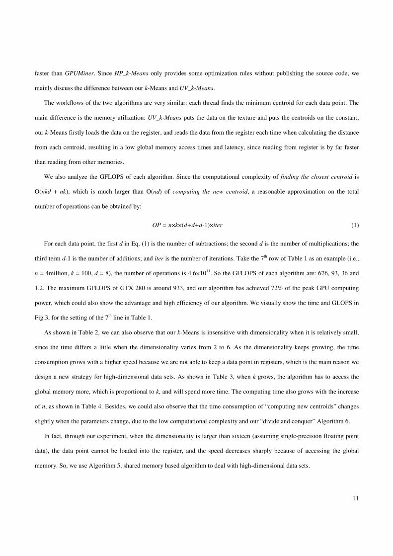
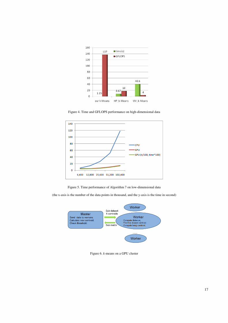
As shown in Table 6, finding the closest centroid achieves a speedup of forty to two hundred compared with our CPU-

based algorithm, while computing new centroid achieves a speedup around ten, which further prove the advantage of our

algorithm. The GFLOPS of the second line in Table 5 are 137, 18, 4 for our k-Means, UV_k-Means and GPUMiner, as shown

in Fig.4. Compared with Fig.3, the GFLOPS of our k-Means decreases, since the time consumption on computing new

centroids occupies relatively more percentage, which does not have a good speedup effect. Besides, we also compare

Algorithm 3 and 4: when n = 1x106 and k = 100, Algorithm 3 needs 1.5 seconds to deal with a 16 dimensional data set, while

Algorithm 4 needs 1.5 seconds to deal with a 32 dimensional data, which proves that it is necessary to design two strategies

for different dimensional data.

As shown in Tables 7 and 8, the time consumption shares the same trend as in Tables 3 and 4, which is appropriately linear

to k and n. Table 9 shows the speed changes on dimensionality, and the time of “finding the closest centroid” is also linear to

d.

C. On large data sets

Here we use the data sets which are larger than the CPU and GPU’s main memory: for the low-dimensional data, we

generate the data randomly; for the high dimensional-data, we generate the data based on the dataset used in section B, by

randomly copying a data point and then randomly choosing half of the dimension and adding them with a random floating

point number. The scale of the dataset is one hundred times larger than the previous data sets used in in Section A and B.

13

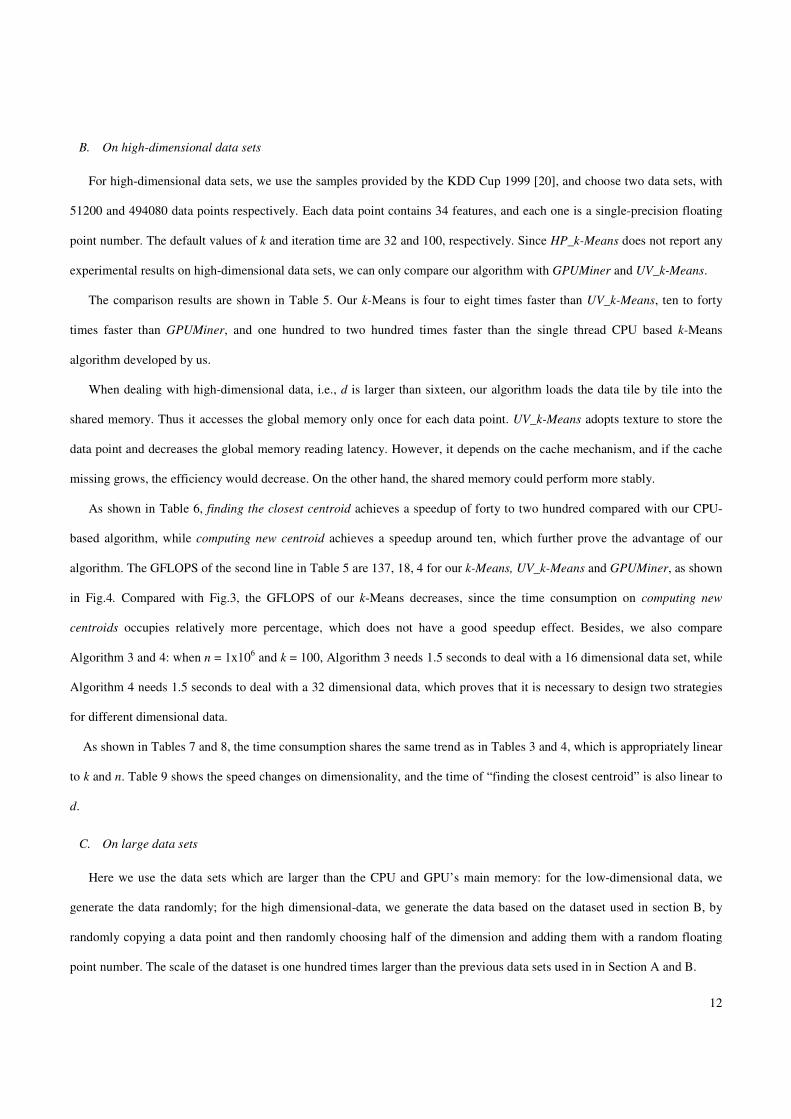
Algorithm 7 runs on the low-dimensional data, and the result is shown in Table 10 and Fig.5. First, the GPU-based

version is more than one hundred times faster than CPU-based version. Second, Fig.5 shows the trend of time consumption

increase with the number of the data point, which is approximately linear. The main reason is that computing the final

centroids has only Mkd operations, which is very small compared with the total operation. For example, merging 51,200

temporary results only takes 0.1 second. In the first row of Table 10, we only need two hundred temporal results, and the time

could be neglected. The green line in Fig. 5 is the time consumption on small dataset: the scale of the dataset is one hundred

times smaller than that of red and blue lines; the time is calculated in ten milliseconds in order to show the figure clearly. The

green line is nearly the same as the red line, which further shows that the merging part occupies a tiny percentage of the total

time and the divide-and-merge strategy is very efficient. Algorithm 7 running on the high-dimensional data sets shows the

similar result, as shown in Table 11.

V. CONCLUSIONS AND FUTURE WORK

In this paper, we proposed a GPU-based parallel k-Means algorithm. It presents mainly two novel ideas: first, based on

the dimensionality of the data set, our k-Means algorithm chooses one from two different strategies. For low-dimensional

data set, our algorithm utilizes GPU registers and achieves a speedup of three to eight over HP_k-Means. For high-

dimensional data, our algorithm firstly observes the similarity between k-Means and matrix multiplication, then adopts shared

memory and registers to avoid multiple accesses of the global memory, and finally achieves a speedup of four to eight as

compared with UV_k-Means. Besides, we also discuss the method for dealing with large data sets based on a single GPU.

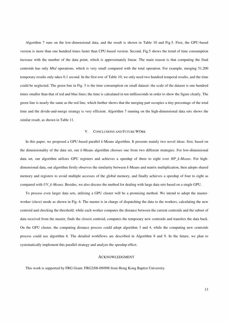
To process even larger data sets, utilizing a GPU cluster will be a promising method. We intend to adopt the master-

worker (slave) mode as shown in Fig. 6. The master is in charge of dispatching the data to the workers, calculating the new

centroid and checking the threshold; while each worker computes the distance between the current centroids and the subset of

data received from the master, finds the closest centroid, computes the temporary new centroids and transfers the data back.

On the GPU cluster, the computing distance process could adopt algorithm 3 and 4, while the computing new centroids

process could use algorithm 6. The detailed workflows are described in Algorithm 8 and 9. In the future, we plan to

systematically implement this parallel strategy and analyze the speedup effect.

ACKNOWLEDGMENT

This work is supported by FRG Grant: FRG2/08-09/098 from Hong Kong Baptist University.

14

REFERENCES

[1] P.-N. Tan, M. Steinbach, and V. Kumar, Introduction to Data Mining, Addison-Wesley Companion Book Site 2006.

[2] A. K. Jain and R. C. Dubes, Algorithms for Clustering Data, Prentice-Hall, 1988.

[3] X. Wang and M. Leeser, “K-means Clustering for Multispectral Images Using Floating-Point Divide,” in Proceedings of the 15th

Annual IEEE Symposium on Field-Programmable Custom Computing Machines, 2007.

[4] H. Zhou and Y. Liu, “Accurate Integration of Multi-view Range Images Using K-means Clustering,” Pattern Recogn., vol. 41, 2008,

pp. 152-175.

[5] X. Wu, V. Kumar, J. R. Quinlan, J. Ghosh, Q. Yang, H. Motoda, G. J. McLachlan, A. Ng, B. Liu, P. S. Yu, Z.-H. Zhou, M. Steinbach,

D. J. Hand, and D. Steinberg, “Top 10 Algorithms in Data Mining,” Knowledge Information Systems, vol. 14, 2008, pp. 1-37.

[6] D. Judd, P. K. McKinley, and A. K. Jain, “Large-Scale Parallel Data Clustering,” in Proceedings of the International Conference on

Pattern Recognition (ICPR’96) Volume IV, 1996.

[7] D. Judd, P. K. McKinley, and A. K. Jain, “Large-Scale Parallel Data Clustering,” IEEE Trans. Pattern Anal. Mach. Intell., vol. 20,

1998, pp. 871-876.

[8] I. S. Dhillon and D. S. Modha, “A Data-Clustering Algorithm on Distributed Memory Multiprocessors,” in Revised Papers from

Large-Scale Parallel Data Mining, Workshop on Large-Scale Parallel KDD Systems, SIGKDD: Springer-Verlag, 2000.

[9] NVIDIA CUDA: http://developer.nvidia.com/object/cuda.html.

[10] NVIDIA CUDA Compute Unified Device Architecture: Programming Guide, Version 2.0, June 2008.

[11] S. A. Manavski, “CUDA compatible GPU as an efficient hardware accelerator for AES cryptography,” In Proceedings of IEEE

International Conference on Signal Processing and Communication, Nov. 2007.

[12] S. Ryoo, C. I. Rodrigues, S. S. Baghsorkhi, S. S. Stone, D. B. Kirk, and W. Hwu, “Optimization Principles and Application

Performance Evaluation of a Multithreaded GPU Using CUDA,” in Proceedings of the 13th ACM SIGPLAN Symposium on

Principles and practice of parallel programming Salt Lake City, UT, USA: ACM, 2008.

[13] X.-W. Chu, K. Zhao, and M. Wang, “Practical Random Linear Network Coding on GPUs,” in Proceedings of IFIP Networking’09,

Archen, Germany, May 2009.

[14] X.-W. Chu, K. Zhao, and M. Wang, “Massively Parallel Network Coding on GPUs,” IEEE IPCCC’08, Austin, Texas, USA, Dec

2008.

[15] W. Fang, K. K. Lau, M. Lu, X. Xiao, C. K. Lam, P. Y. Yang, B. He, Q. Luo, P. V. Sande, and K. Yang, “Parallel Data Mining on

Graphics Processors,” Technical Report HKUSTCS08, 2008.

15

[16] S. Che, M. Boyer, J. Meng, D. Tarjan, J. W. Sheaffer, and K. Skadron, “A Performance Study of General-Purpose Applications on

Graphics Processors Using CUDA,” Journal of Parallel and Distributed Computing, 2008.

[17] R. Wu, B. Zhang, and M. Hsu, “Clustering billions of data points using GPUs,” in UCHPC-MAW’09: Proceedings of the combined

workshops on UnConventional high performance computing workshop plus memory access workshop, Ischia, Italy, 2009, pp. 1-6.

[18] J. Pisharath, Y. Liu, W.-K. Liao, A. Choudhary, G. Memik, and J. Parhi, “NU-MineBench 2.0,” CUCIS Technical Report CUCIS-

2005-08-01, Center for Ultra-Scale Computing and Information Security, Northwestern University, 2005.

[19] NVIDIA Optimizing Parallel Reduction in CUDA, Mark Harris, NVIDIA Developer Technology.

[20] KDD Cup 1998 Data: http://kdd.ics.uci.edu/databases/kddcup99/kddcup99.html

16

Figure 1. Hardware architecture of the GPU

Figure 2. Tile-based distance computing process

Figure 3. Time and GFLOPS performance on low-dimensional data

17

Figure 4. Time and GFLOPS performance on high-dimensional data

Figure 5. Time performance of Algorithm 7 on low-dimensional data

(the x-axis is the number of the data points in thousand, and the y-axis is the time in second)

Figure 6. k-means on a GPU cluster

18

Algorithm 1: CPU-based k-Means

// flag: shows whether it still needs to iterate;

// iter: the current round of iteration;

// Max_iter: the maximum number of iterations;

// d(r, s): the distance between r and the cluster s;

// min_D: the temporal minimum distance;

1. while flag && iter <= Max_iter

2. for each r in R

3. for each s in S

4. Compute d(r, s);

5. end of for

6. end of for

7. for each r in R

8. for each s in S

9. if d(ri, sj) < min_D

10. r belongs to sj;

11. min_D ← d(ri, sj);

12. end of if

13. end of for

14. end of for

15. for each Si in S

16. find new centroid of Si

17. end of for

18. if the change of the centroid is less than threshold

19. flag ← false;

20. iter ← iter + 1;

21. end of if

22. end of while

19

Algorithm 2: finding closest centroid based on CPU

//min_D: a temp variable, stores the minimum distance;

// index: stores the min centroid ID for each data point;

1. for ri in R

2. for sj in S

3. if d(ri, sj) < min_D

4. min_D ← d(ri, sj);

5. index[i] ← j;

6. end of if;

7. end of for;

8. end of for;

Algorithm 3: computing distance and finding closest

centroid based on the register of the GPU

// threadDim: the dimension of the thread in each block;

// blockDim: the dimension of the block in each grid;

// blockIdx.x: the current block ID;

// threadIdx.x: the current thread ID;

// data: the address of R;

// i: the ID of data point;

// d: the dimension of the data;

// Gdata: the address of the corresponding data point;

// S: the set of the centroid;

1. threadDim ← 256;

2. blockDim ← n/256;

3. i ← blockIdx.x×blockDim+threadIdx.x;

4. Gdata ← data + i×d;

5. Load the data point from Gdata to the register;

6. for sj in S

7. Compute d(ri, sj);

8. if d(ri, sj) < min_D

9. min_D ← d(ri, sj);

10. index[i] ← j;

11. end of if

12. end of for

20

Algorithm 4: computing distance based on the shared

memory of the GPU

// TH: the high of the tile;

// TW: the width of the tile;

// thread: the dimensions of the block;

// grid: the dimensions of the grid;

// indexD points to the corresponding data;

// indexC points to the corresponding centroid;

// indexR points to the corresponding result;

// SMData: stores the tile in shared memory;

// TResult: stores the temp distance in registers;

// SR: stores the distance in global memory;

// Alast: the upper bound address of data point;

// d: the dimension of the data;

// CTile: the row pointed by indexC,

// the length is TW × TDimY;

// The centroids are on the constant memory;

1. TH ← 16, TW ← 16, TDimY ← 2;

2. dim thread(TH, TDimY);

3. dim grid (k/ TW, n/ TH);

4. indexD = data

+ blockIdx.y×TH×d

+threadIdx.y×d+ threadIdx.x.

5. indexC = centroid

+ blockIdx.x×TW

+ threadIdx.y×blockDim.x+ threadIdx.x.

6. indexR = SR

+ blockIdx.y ×TH× k + blockIdx.x× TW

+ threadIdx.y×blockDim.x + threadIdx.x.

7. SMData[TW][TH] in shared memory;

8. TResult[TW] in registers;

9. Alast ← indexD + d;

10. do

11. {

12. Load data from global memory to SMData;

13. indexD is added by TW;

14. for each column in SMData

15. TResult[i] += d2(SMdata[i], CTile)

16. } while (indexD < Alast);

17. for each element in TResult

18. TResult[i] = sqrt(TResult[i]);

19. __syncthreads();

20. Writet TResult back to SR;

21

Algorithm 5: CPU_based method for computing new centroids

// count: stores the number of data points in each clusters;

// new_cen: the address of the new centroid;

// data: is the address of data point set R;

1. for i from 1 to n

2. ++count[ index[i] ];

3. for j from 1 to d

4. new_cen [index[i]][j] += data[i][j];

5. end of for

6. end of for

7. for i from 1 to k

8. for j from 1 to d

9. new_cen [i][j] /= count[i];

10. end of for

11. end of for

Algorithm 6: GPU_based method

for computing new centroids

// n': is the number of groups to be divided;

1. M is the multiple of the number of SM;

2. n' ← n/M;

3. Divide n data points in to n' groups;

4. Compute n' temp centroids on the GPU;

5. while n' > M

6. Divide n' temp centroids into n'/M groups;

7. n' ← n'/M;

8. Compute n' temp centroids on the GPU;

9. end of while

10. Reduce n' temp centroids into final centroids on CPU;

22

Algorithm 7: k-Means for large dataset on Master

// n': is the number of each sub dataset;

//k_centroid[M+1][k][d]: is the temporal result from each worker;

//n_centroid[M+1][k]: is the number of each cluster in each worker;

// threshold : a Boolean value to show whether it need further compute;

1. M is the number of workers;

2. n' ← n/M, each worker deals with n' data;

3. Divide n data points in to M groups;

4. while threshold

5. for each group data i

6. Compute distance between data[i* n'] and k_centroid[0][0]

7. Find closest centroid;

8. Compute new centroid k_centroid[i][k] and n_centroid[i][k];

9. end of for

10. for i from 1 to M

11. for j from 0 to k

12. for p from 0 to d

13. k_centroid[0][j][p]+= k_centroid[i][j] [p];

14. end of for

15. n_centroid[0][j] += n_centroid[i][j];

16. end of for

17. end of for

18. k_centroid[0][k] /= n_centroid[0][k];

19. Check(threshold);

20. end of while

Algorithm 8: k-Means for large dataset on Master

// j: the initial value is M, and it stands for the number of waiting workers;

//the other variables are the same with Algorithm 7;

1. while threshold

2. while i < M

3. SendData2Worker( i++, data[i* n'], k_centroid[0]);

4. end of while

5. While j > 0

6. if(GetConnectionFromWorker( i) )

7. --j;

8. ReceivedDataFromWorker(k_centroid[M][i], n_centroid[i][k]);

9. end of if

10. end of while

11. for i from 1 to M

12. Update k_centroid[0];

13. Update n_centroid[0];

14. end of for

15. k_centroid[0][k] /= n_centroid[0][k];

16. Check(threshold);

21. end of while

Note: lines 2-4 send the current centroids k_centroid[0][0] and the subset of data data[ixn'] to the i_th worker; lines 5-8 receive the results

including k_centroid[i][k] and n_centroid[i][k] from the i_th worker; lines 11-14 calculate the final summary and the number of point for each

cluster, which is the same as lines 9-17 in Algorithm 7; line 15 calculates the mean of the previous summary.

23

Algorithm 9: k-Means for large dataset on Worker

//i: is the ID of the worker

1. while true

2. if(GetConnection ( i) )

3. ReceiveDataFromMaster(k_centroid[0], data[i* n']);

4. Computing distance;

5. Find closest centroid;

6. for each cluster j

7. Calculate k_centroid[i][j];

8. Calculate n_centroid[i][j];

9. end of for

10. SendData2Master(k_centroid[i], n_centroid[i]);

11. end of if

12. end of while

Note: line 1 means the worker keeps waiting for the connection from the master; line 3 receives data from master, containing the current centroids and the

subset of data points; line 4 calculates the distance between the data points and the centroids; line 5 finds the closest centroid for each data point; line 6-9

calculate the summary of the data points and the number of the points in each cluster; line 10 sends the results back to the master and then waits for the next

connection.

Table 1: Speed of k-Means on low-dimensional data, in second

n k d Our

k-Means

HP

k-Means

UV

k-Means

GPU

Miner

2

million

100 2 0.22 1.45 2.84 61.39

400 2 0.79 2.16 5.96 63.46

100 8 0.35 2.48 6.07 192.05

400 8 1.23 4.53 16.32 226.79

4

million

100 2 0.34 2.88 5.64 130.36

400 2 1.22 4.38 11.94 126.38

100 8 0.68 4.95 12.85 383.41

400 8 2.26 9.03 34.54 474.83

Note: the time is in second. The hardware environment of HP is as follows:

NVIDIA GTX280 GPU; Intel Xeon CPU, 2.33GHz; 4GB memory.

Table 2: Speed changes on dimension, in millisecond

d Finding the

closest centroid

Computing

new centroids

2 72 64

4 75 63

6 83 64

8 138 67

10 405 64

Note: n = 106, and k = 100.

24

Table 3: Speed changes on centroid, in millisecond

k Finding the

closest centroid

Computing

new centroids

100 75 64

200 138 66

400 272 67

Note: n = 106, and d = 4.

Table 4: Speed changes on n, in millisecond

n Finding the

closest centroid

Computing

new centroids

1,024,000 77 60

2,048,000 130 66

3,072,000 512 62

4,096,000 284 64

6,144,000 431 69

8,192,000 567 68

Note: d = 4, and k = 100.

Table 5: Speed of k-Means on high-dimensional data, in second

Data set Our

k-Means

UV

k-Means

GPU

Miner

CPU

k-Means

51,200 0.34 1.86 4.26 35.79

494,080 1.15 8.67 40.6 224.47

Table 6: Time distribution of our k-Means algorithm, in second

Function/data set Finding the

closest centroid

Computing

new centroids

51,200 GPU

CPU

0.10

33.5

0.25

2.28

494,080 GPU

CPU

0.87

207.78

0.24

16.67

Table 7: Speed changes on k, in millisecond

k Finding the

closest centroid

Computing

new centroids

32 99 248

64 138 251

128 167 250

256 204 252

512 637 253

Note: n = 51,200, and d = 34.