Efficient Tool Path Computation Using Multi-core GPUs

Abstract. Tool path generation is one of the most complex problems in Computer Aided Manufacturing. Although some efficient strategies have been developed, most of them are only useful for standard machining. However, the algorithms used for tool path computation demand a higher computation performance, which makes the implementation on many existing systems very slow or even impractical. Hardware acceleration is an incremental solution that can be cleanly added to these systems while keeping everything else intact. It is completely transparent to the user. The cost is much lower and the development time is much shorter than replacing the computers by faster ones. This paper presents an optimisation that uses a specific graphic hardware approach using the power of multi-core Graphic Processing Units (GPUs) in order to improve the tool path computation. This improvement is applied on a highly accurate and robust tool path generation algorithm. The paper presents, as a case of study, a fully implemented algorithm used for turning lathe machining of shoe lasts. A comparative study will show the gain achieved in terms of total computing time. The execution time is almost two orders of magnitude faster than modern PCs. Keywords. Tool path computing, virtual digitizing, specific hardware architectures, Graphics Processor Unit, CUDA technology.

1 Introduction

In order to machine a surface by means of a cutting tool on a CNC machine tool, a series of 3D or 2D coordinates that define its motion must be supplied. These points are usually referred to as tool centre positions. In this way, the problem can be expressed as obtaining a trajectory of tool centres that defines the desired object to be machined with a given precision, in literature the problem is also known as the tool compensation problem [1].

With a given object and tool, a solution cannot always be found because of the curvature of the surfaces [2]. In these cases, the problem is redefined in order to obtain a trajectory that defines the closest surface that contains the desired object (that is, without collision). Figure 1.a shows the trajectory (tool path) of a circle centre point in order to define a surface. In this case, for the sake of simplicity, the problem is presented in 2D. For 3D surfaces the problem becomes more complex.

Partial solutions to this problem use surface offsets generated by different methods [2-4]. However, these offset-surfaces are restricted to one-radius tools (i.e spherical, cylindrical and conical) and are not valid for more complex tools, such as toroidal ones with two radii. Moreover, in most cases, self-intersection problems arise according to the surface curvature [5] (see figure 1.b). Thus, more sophisticated and higher cost computing techniques are needed to detect and solve these problems. Other solutions, based on ruled surfaces, compute the closest ruled surface to an object, although, once again, they are restricted to one-radius tools and 3-axis isoparametric machining [6].

Fig. 1. a) Tool trajectory for part surface. Machined surface will differ from the original without collision in a; b) Trajectory by means of surface offsetting. Self-intersections in b and discontinuities in c will clash with part surface in shaded regions.

As a case study, we present the efficient implementation of a specific tool path algorithm called Virtual Digitizing [7] (VD). The VD algorithm avoids the problem of tool-surface collision by its own definition. It was inspired by the way mechanical copiers work. These machines touch and move along the reference model’s surface, while a group of arms instantly transmit that movement and distances to the cutting wheels in order to shape the workpiece. Similarly, the virtual digitizing approach “virtually touches” the reference surface with the cutting tool (actually it computes the cutting tool position), and makes sure that the machine does not remove any point within the desired object. Due to the fact that all the machining processes are simulated, this algorithm has no restrictions in tool or machine specifications, so the algorithm can be used both standard (3 or 5 axis machining) and non-standard machining (e.g. in retro-fitting machining where old machines are fitted to be computer controlled).

In recent years some works have dealt with CAD/CAM problems acceleration using GPUs. The key features of the new breed of GPU that are significant for the CAD researcher and commercial developers are outlined in [8]. In [9], cone beam reconstruction is implemented using CUDA (Compute Unified Device Architecture) compatible GPU that accelerate the Feldkamp, Davis, and Kres (FDK) algorithm. In [10] it is proposed a method to evaluate NURBS and compute objects clearance using GPUs. 3D cone-beam CT reconstruction using Simultaneous Algebraic Reconstruction Technique (SART) is presented in [11]. However, there is no evidence of trajectory computation algorithms based on the CUDA technology.

In the paper we present a new parallel version of the VD method that takes advantages of the new and efficient SIMD architectures of programmable graphics cards. Using this approach, complex calculations of VD can be made in real time without replacing the numerical control computer, only a multi-core graphic card would have to be plugged to the system bus.

In section 2, we explain the basic method to obtain a machining trajectory by means of the VD method, including its cost analysis. It is the basis of the parallel algorithm described in section 3 developed onto a multi-core GPU architecture, followed by some real experiments of shoe last machining in section 4. Finally, conclusions and further work are presented in section 5.

2 The Virtual digitizing strategy

This algorithm, initially used for imitating the way traditional copier machines work [12], can be divided into four phases:

a b c

a) b)

1. Definition of the tool motion 2. Obtain a discrete model of the part surface

3. Simulate the tool motion 4. Virtual digitization process

Fig. 2. Example of Virtual the Digitizing process for 2D shapes.

1: t=0 2: while t<=1 do 3: MinDistance= 4: for each surfaceiObject do 5: for each pointj,k surfacei do 6: p’j,k=pointj,kTR4x4(t) 7: d =dv(p’j,k,Tool) 8: if d<MinDistance then MinDistance=d endif 9: endfor 10: endfor 11: EECentre=ComputeCentre(MinDistancie, TR4x4(t)) 12: AddTrajectory(EECentre) 13: Increment(t) 14: endwhile

Table 1. Basic virtual digitizing algorithm

The digitization algorithm becomes simple once the surface and tool motion is

well-defined. Basically, the behaviour can be described as follows: For each point of the trajectory, every part surface is transformed in order to face the cutting tool according to the machining strategy.

Once the part is positioned, the minimum distance from every grid point to the tool is computed in the direction of tool attack axis. This minimum distance determines the tool centre point for this step in the virtual digitization process. Physically, we select the point that touches the tool surface first when the tool is moved along the attack axis. The process is similar to the one used for obtaining z-maps of the tool envelope surface, typically used for 3-axis CNC machining: the inverse offsetting method [13] and the direct cutting simulation [14].

The distance from a point to an object is computed by projection of the grid point on the tool, in the tool attack direction. The distance between the given point and the projected one will be used to compute the tool centre point for that machining position.

As shown in figure 2 (a simple example in 2D in order to obtain a single trajectory point for a circular tool), the minimum distance represents the tool centre distance in order to reach the grid point without colliding with the shape.

On analyzing the algorithm, up to three nested loops can be observed. The innermost one is used to access every grid point on the selected surface, that is, it consists of two loops, one for rows and the other for columns. The outermost loop

Grid points

Tool

Part Surface

Dmin

Tool motion

Winner point

Result

goes through every trajectory position. From experience, in order to obtain a good-quality finish, it is necessary to produce at least as many trajectory points as grid points on the surface.

In the inner loop, a product vector x matrix is computed and stored in a local variable. Let us assume n to be the maximum number of grid points on the surface, and m the number of trajectory positions, then the cost of the algorithm, is:

O(n.m) (1)

The computing cost showed in expression 1 could be high in some machining

scenarios, such as traditional industrial fields, where there are no high-performance computers with a regard to design and manufacture. The use of low-performance computers and standard operating systems is therefore a restriction, since they share both the management tasks and those of the CAD/CAM. As a guide, usual values for both n and m in shoe last machining are about 50,000, that is, a high computer cost for a standard PC.

Algorithm cost

Computational cost is analysed in this section in terms of the problem size for the algorithm introduced in table 1. The operator used to determine an upper limit of the computation cost is “O”.

Analysing this algorithm, it is possible to observe up to three nested loops. One of them, the most internal one, it is used to access to every grid point in the selected surface, that is, it consists into two loops, one for rows and the other for columns in fact.

Every loop iterates on different data. The most external one goes through every trajectory position. In order to obtain a good quality finishing it is necessary produce, at least, as many trajectory points as grid points the surfaces have. The finishing quality also depends on the material to be milled, for example, metallic ones produce best results but need more trajectory points than organic ones (plastics) also more grid points (surface definition).

max( , , )n m s m s DS (2)

Let assume n as the maximum number of grid points (m for u direction, and s for v)

of all the surfaces. The cost of the first loop, and consequently the algorithm cost, is:

1 2 3 42lim ( ) ( )n ct ct n ct ct n

n

(3)

where cti are constant values.

3 The CUDA specific hardware approach

NVIDIA has developed an architecture of parallel computation called CUDA [15, 16], that now is included in the GPUs GeForce, ION, Quadro and Tesla, available in conventional PCs for application developers with low cost. CUDA also makes reference to a set of development tools that facilitates the programming of these devices. The architecture of these devices is based on a lifted number of multiprocessors called Streaming Multiprocessors (SMs) with many cores each calls Streaming Processors (SPs) that lean in a complex system of memory that is distributed in different levels adapted to different functions like the capacity, the speed, the locality or the consistency. In figure 3 the space disposition of the SMs

with its respective SPs can be appreciated, besides the units of memory corresponding to the Fermi architecture that is the last one developed by Nvidia.

Fig. 3. Model of the Fermi architecture composed by 16 SMs with 32 SPs each.

A card of this family can have about 512 SP that are able approximately to reach a capacity of calculation of 1.5 TFlops for single precision.

The computation model that acts on this architecture is based on the model denominated by Nvidia SIMT (Single Instruction Multiple Threads) that is not more than an adaptation of the classic SIMD. When a program is sent to be executed in the GPU this it is duplicated in so many threads as it is indicated and all the threads execute the same code. These threads are grouped logically in thread blocks that can be blocks of until three dimensions where these blocks can be grouped in meshes of up to 2 dimensions. At internal level, the architecture will automatically distribute the blocks on the different multiprocessors. Once we have an amount of threads within each SM, these are distributed in the minimum unit of process, a thread package denominated WARP that normally is compound of 32 threads. Previously, we mentioned that all the threads execute the same code but they are not executed at the same time. Those are the WARPS that exactly execute the same instruction for their corresponding threads. The SM has a control unit that will give each instruction to all the SPs and therefore to all its threads, one per processor at a given time, that will execute the instruction.

Besides, its high capacity of calculation, this architecture owns a powerful hierarchy of memory that can be considered like a hybrid system of shared memory.

The global memory, with most capacity but the slowest one, is located in the memory of the device, common to all the SMs and allocates the input and output data for any CUDA application. As intermediate memory, there is a shared memory located within each SM and faster than the global memory. It is faster and has capacity to share data between threads of the same block. Another important memory are the registries, the fastest memory of the architecture, used to store the intern variables to each thread. Each SM will have a limited number of registries to distribute among the active threads. Other levels of memory like the constant or texture memories complete the system of memory of this architecture. In addition, new development kits facilitate the programming of several cards simultaneously, obtaining therefore a new level of parallelism with the corresponding increase of the available memory. The new Fermi architecture, has improved the memory system including caches for the global memory (L2) and for each processor (L1) achieving better performance. All these characteristics cause that using this type of devices those algorithms with a high level of parallelism can be accelerated remarkably.

Virtual Digitizing parallelization onto GPUs

In this section we propose an alternative to the algorithm introduced in order to improve the average response time. We will show that using this kind of optimisations should reduce the average response time for the machining.

One of the key aspects to consider the implementation of an application or algorithm in CUDA is to analyze the amount of parallelism of the problem. For this reason, we will begin analyzing the parallelism level that can be reached in this application without changing its behaviour.

The algorithm of virtual digitalization has several levels of parallelism, since it would be possible also to be paralleled both internal (lines 4 and 5 of table 1) and external loops (“while” in line 2) because each possible combination does not depend on any data of the rest. This is possible due to the own formulation of the problem, where each point of the trajectory solution it is independently calculated. If we make calculations in sequential form, it can be included certain optimizations since some knowledge about previous steps is available. However, these improvements have not been included in the parallel version of the algorithm although it have been implemented in the sequential CPU versions that later we will use to compare performance in the experimentation section.

The independence between the different points (different values of t) from the trajectory allows parallelizing the algorithm presented in table 2.

1: Initialize GPGPU whith input values 2: In parallel all path points //num points threads 3: t= f(blockIdx.x * blockDim.x + threadIdx.x) //identify my part 4: for each surfacei Object do 5: for each pointj,k surface do 6: pointj,k’=pointj,k(t) 7: d =dv(pj,k’,EE) 8: if d<MinDistance then MinDistance=d; endif 9: endfor 10: endfor 11: EECenter=ComputeCenter(MinDistance,(t)) 12: AddTrajectory(EECenter) 13: endparallel 14: ObtainGPUResults()

Table 2. Paralel version of digitizing algorithm using GPUs

In table 3 we used the variables blockIdx.x, blockDim.x, threadIdx.x, provided by CUDA, to obtain the number of present parallel process that corresponds to a point of the trajectory solution. Theoretically, the computation cost becomes from expression 3 to:

1 2 3 4

/

2lim ( ) ( )

m n p o

m ct ct m ct ct mn

(5)

Where p is the number of stream processors of the GPU and o is the cost associated

to the communication time. The computational cost, without considering communication time, is expressed in

equation 6. In the best case, the total computing time could be reduced by the number of stream processors available. The results of experiments will show the reality of this optimistic prediction.

2

lim 1 2 3 4n nGS GSct ct n ct ct OGSn nproc nprocGS

(6)

4 Case of study: shoe last machining

Once presented the parallel version of the virtual digitalization algorithm, we describe the phase of experimentation where we will use a certain type of models 3D already digitized provided by the Spanish Technological Institute for Footwear Research (INESCOP) that belong to models of women shoe lasts.

The machine selected is a traditional turning lathe for shoe lasts, consisting of three different axes as shown in figure 4. All of them perform a spiral movement around the object to be machined. The tool selected is a 3D torus that simulates the cutting tool in movement.

The surface to be machined consists of a discretization of a free-form NURBS

surface. The more grid points used in each dimension to represent a surface, the finer the spatial resolution of our discretization and the more accurate our trajectory. For an object of 10 x 10 x 200 mm, a grid of approximately 130 x 120 points is used, which implies a distance of 2 mm between points in each surface dimension. Algorithm 1 (from table 1) is slightly transformed for the first lines into: 1: for every_tool_translation_position_x do 2: MinDistance= 3: for every_rotation_step_degree do 4: TR4x4 = Rotation_Matrix_X(x,degree) 5: for each surfaceiObject do 6: for each pointj,k surfacei do 7: p’j,k=pointj,kTR4x4 . .

Table 3. Changes introduced in algorithm 1 for simulating turning lathe movement.

The algorithm showed in table 3 consists of four nested loops, the first and second ones simulate the tool movement around the object. The third and fourth loops analyse every surface point in order to find the nearest one to the tool. The

Fig. 4 Axis implied on a shoe last turning lathe machine

transformation matrix consists of a basic 3D rotation matrix around the X axis. The distance function computes the distance between a 3D point and a 3D torus in the tool attack direction (Y axis) and is expressed in equation 4.

22

22,, zTxrRyTzyxD xy

(4)

Where: Tx, Ty are the x,y coordinates of the torus centre. x,y,z are the 3D point coordinates R, r are the major and minor torus radii

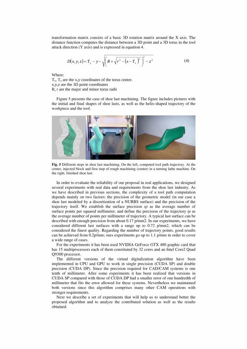
Figure 5 presents the case of shoe last machining. The figure includes pictures with the initial and final shapes of shoe lasts, as well as the helix-shaped trajectory of the workpiece and the tool.

Fig. 5 Different steps in shoe last machining. On the left, computed tool path trajectory. At the center, injected block and first step of rough machining (center) in a turning lathe machine. On the right, finished shoe last.

In order to evaluate the reliability of our proposal in real applications, we designed several experiments with real data and requirements from the shoe last industry. As we have described in previous sections, the complexity of a tool path computation depends mainly on two factors: the precision of the geometric model (in our case a shoe last modeled by a discretization of a NURBS surface) and the precision of the trajectory itself. We establish the surface precision sp as the average number of surface points per squared millimeter, and define the precision of the trajectory tp as the average number of points per millimeter of trajectory. A typical last surface can be described with enough precision from about 0.17 p/mm2. In our experiments, we have considered different last surfaces with a range up to 0.72 p/mm2, which can be considered the finest quality. Regarding the number of trajectory points, good results can be achieved from 0.2p/mm; ours experiments go up to 1.1 p/mm in order to cover a wide range of cases.

For the experiments it has been used NVIDIA GeForce GTX 480 graphic card that has 15 multiprocessors each of them constituted by 32 cores and an Intel Core2 Quad Q9300 processor.

The different versions of the virtual digitalization algorithm have been implemented in CPU and GPU to work in single precision (CUDA SP) and double precision (CUDA DP). Since the precision required for CAD/CAM systems is one tenth of millimeter. After some experiments it has been realized that versions in CUDA SP compared with those of CUDA DP had a smaller error of one hundredth of millimeter that fits the error allowed for these systems. Nevertheless we maintained both versions since this algorithm comprises many other CAM operations with stronger requirements.

Next we describe a set of experiments that will help us to understand better the proposed algorithm and to analyze the contributed solution as well as the results obtained.

4.1 Experiment I

This first experiment compares the improvement of CUDA implementation with respect to the complexity of the algorithm. We will increase the precision of the resulting trajectory tp at the same time as the amount of calculation is greater.

Fig. 6. Computing time versus precision of the trajectory (TP)

Several aspects can be emphasized of figure 6. One of the first conclusions that could be obtained from the data is that the CPU versions have quite similar results. This is due to the present complexity of the CPU that causes that the difference between precisions is imperceptible for this algorithm. In the versions implemented with CUDA, it is possible to appreciated a difference depending on the precision with which they work, since CUDA processors are not as powerful as the CPU and when more complex operations are used (special operations with double precision or functions like sines, cosines, square roots…) performance decreases. But the most appreciable result is the difference between CUDA and CPU versions that is of an order higher.

From the results obtained in this first experiment it could be concluded that the improvement obtained in the version of simple precision is around 70-75x and for the double precision is 35x. In addition, for the tested values of precision, the improvement is indifferent for all the cases.

4.2 Experiment II

In this second experiment we demonstrate how the system performance varies with respect to the complexity of the model to represent. In order to prove this variation we are going to fix the spiral of the path to be calculated, that is to say, we are going to determine the precision of the resulting trajectory using a tp of a 0.72 p/mm. Once determined the resulting precision we will prove models of different complexity (sp) from simplest to most complex.

Fig. 7. Computing time versus complexity of the surface (sp)

As it can be appreciated in figure 7 there are no changes of behavior with respect to the different last models (and therefore to the different complexity of the input data). They are continued respecting the variations between the CUDA and CPU and also among the CUDA versions for different data types.

It can be calculated the improvement ratio in time and they are being maintaining independent of the complexity of the shoe lasts; 35x for the version of double precision and around 70x for single precision.

4.3 Experiment III

In this last experiment we are going to analyze the behavior of CUDA implementation onto different GPU devices. The experiments are the same that in experiment II, using card GTX480 which we have used in the rest of experiments, a GTX465 and a Nvidia Quadro 2000. We present only results for the versions in simple precision for clarity.

Fig. 8. Speed up versus different multi-core GPU types

In figure 8 it can be appreciated differences between the times of both cards. The best ratios are obtained with the GTX480 that is most computationally powerful.

This experiment shows how the algorithm adapts to the capacities of the different devices and therefore, whichever better is the device (with more processors) better performance is obtained from this implementation.

4.4 Quality measurements

In order to check the quality of the trajectories generated, surfaces from a set of nine shoe lasts manufactured using a CNC lathe have been obtained with the aid of

precision digitizers. Subsequently, several fundamental measurements (see figure 9) have been compared. Table 4 shows the results of the comparison.

Fig. 9. Quality measures of the mechanized shoe last models: a) centre line, b) bottom line, c)

cone heel line, d) ball girth

Measure Error found Centre line (190mm) Bottom length (280mm) Cone heel line (300mm) Ball (220mm)

±0.3mm ±0.1mm ±0.6mm ±0.3mm

Table 4. Quality measures of the tested models

5 Conclusions and further work

The idea of integrating trajectory generation into the numerical control itself is now becoming more common. The new ISO standard 14649 (also called STEP-NC) remedies the shortcomings of ISO 6983 by specifying the machining processes rather than machine tool motion by means of machining tasks [17]. In this new environment, the use of specific hardware could be used to facilitate trajectory generation in the control itself. In this way, complex calculations could be made in real time without having to replace the numerical control computer; only new specific processing hardware cards would have to be added.

The specific hardware approach using CUDA technology can be used to solve high cost problems arising from the CAD/CAM. In particular, it can be applied to the computing tool path algorithms.

This approach has been applied to the Virtual Digitizing algorithm, achieving good results in trajectory computing for low performance computers.

Future studies will be aimed at applying specific hardware techniques in order to accelerate other trajectory calculation algorithms in 3 or 5-axis standard manufacturing environments.

b)

c) d)

a)

Acknowledgement

The shoe last of footwear used for the experiments have been provided by the Spanish Technological Institute for Footwear Research (INESCOP). This work have been partially supported by the University of Alicante project GRE-019 and the Valencian Government project GV/2011/034. Experiments were made possible with generous donation of hardware from Nvidia.

References

[1] Farin, G. “Curves and Surfaces for Computer Aided Geometric Design. A Practical Guide”. Academic Press Inc., 1993.

[2] Wang, Y. “Intersection of offsets of parametric surfaces”. Computer Aided Geometric Design, vol. 13, pp.453-465, 1996.

[3] Choi, B. K. “Surface Modeling for CAD/CAM”. Elsevier Science Publishers, pp. 263-272, 1991.

[4] Held, M. “Voronoi Diagrams and Offset Curves of Curvilinear Polygons”. Computer-Aided Design, vol. 30, no. 4, pp. 287-300, 1998.

[5] Wallner, J., Sakkalis, T. “Self-intersections of offset curves and surfaces”. Journal of Shape Modeling, no 7, pp. 1-21, 2001.

[6] Elber, G., Fish, R. “5-Axis Freeform surface milling using piecewise surface approximation”. ASME Journal of Manufacturing Science and Engineering, vol. 119, no. 3, pp. 383-387, 1997.

[7] Jimeno, A.; Maciá, F.; García-Chamizo, J. “Trajectory-based morphological operators: a morphological model for tool path computation”, Proceedings of the international conference on algorithmic mathematics & computer science, AMCS 2004, Las Vegas (USA). 2004.

[8] Ukitxu, Y., Ino, F., Hagihara, K. High-performance cone beam reconstruction using CUDA compatible GPUs. Journal of Parallel Computing, vol. 36, no. 2-3, 2010

[9] Krishnamurthy, A., Khardekar, R. and McMains, C. “Optimized GPU Evaluation of Arbitrary Degree NURBS Curves and Surfaces,” Computer-Aided Design, vol.41, no. 12, pp. 971-980, 2009.

[10] Lu, Y., Wang, W., Chen, S., Xie, Y., Qin, J., Pang, W-M. and Heng, P-A. Accelerating Algebraic Reconstruction Using CUDA-Enabled GPU. In proc. 2009 Sixth International Conference on Computer Graphics, Imaging and Visualization, 2009.

[11] Kurfess, T. R., Tucker, T. M., Aravalli, K. and Meghashyam, P. M. .GPU for CAD.Computer-Aided Design & Applications, vol. 4, no. 6, pp 853-862 2007.

[12] Jimeno A, García J., Salas F. “Shoe lasts machining using Virtual Digitizing”. International Journal of Advanced Manufacturing Technology. vol 17, no. 10, pp.744-750. 2001.

[13] Takeuchi, Y et al. “Development of a personal CAD/CAM system for mold manufacturing’ Annals of CIRP, vol 38, no 1, pp.429-432, 1989.

[14] Jerard, R B, Drysdale, R L and Hauck, K “Geometric simulation of numerically controlled machining” Proc. of ASME Int’l Conf. on Computers in Engineering, ASME, New York, pp.129-136, 1988

[15] Nvidia Corporation, Nvidia CUDA Programming Guide Version 3.2, Nvidia Corporation 2010.

[16] Nvidia Corporation, Nvidia CUDA C Best Practices Guide 3.2, Nvidia Corporation, 2010. [17] X.W. Xu*, Q. He ,“Striving for a total integration of CAD, CAPP, CAM and CNC”,

Robotics and Computer-Integrated Manufacturing, vol. 20 pp. 101–109. 2004