theories of computation
TRANSCRIPT
Theories of Computation
Theodore S. Norvell
Draft Typeset January 22, 2018

ii
Typeset January 22, 2018

Contents
Outline ix
Preface xi
0 Correctness of Computing Systems 1
0 Modelling (Computing) Systems 50.0 Systems and Behavioural specifications . . . . . . . . . . . . . 50.1 Angle bracket notation . . . . . . . . . . . . . . . . . . . . . . 100.2 Uses of Specifications . . . . . . . . . . . . . . . . . . . . . . . 100.3 Refinement . . . . . . . . . . . . . . . . . . . . . . . . . . . . 120.4 Input, Output, Determinism, and Implementability . . . . . . 15
1 Imperative Programming Language 211.0 States . . . . . . . . . . . . . . . . . . . . . . . . . . . . . . . 211.1 A programming language . . . . . . . . . . . . . . . . . . . . . 22
1.1.0 The skip command . . . . . . . . . . . . . . . . . . . . 221.1.1 Assignment commands . . . . . . . . . . . . . . . . . . 221.1.2 Parallel assignments . . . . . . . . . . . . . . . . . . . 231.1.3 Sequential composition . . . . . . . . . . . . . . . . . . 241.1.4 The analogy between imperative specifications and ma-
trices . . . . . . . . . . . . . . . . . . . . . . . . . . . . 271.1.5 Conjunction and Disjunction . . . . . . . . . . . . . . . 291.1.6 Alternation . . . . . . . . . . . . . . . . . . . . . . . . 331.1.7 abort and magic . . . . . . . . . . . . . . . . . . . . . 351.1.8 Iteration . . . . . . . . . . . . . . . . . . . . . . . . . . 35
1.2 Properties of the specification operators . . . . . . . . . . . . . 37
Typeset January 22, 2018

iv CONTENTS
2 Derivation of nonlooping programs 392.0 Strengthening and monotonicity . . . . . . . . . . . . . . . . . 392.1 Programming with skip and assignments . . . . . . . . . . . . 412.2 The substitution laws . . . . . . . . . . . . . . . . . . . . . . . 432.3 Weakest prespecification and weakest postspecification . . . . 462.4 Alternation . . . . . . . . . . . . . . . . . . . . . . . . . . . . 47
2.4.0 Nondeterministic alternation . . . . . . . . . . . . . . . 48
3 Derivation of Loops 493.0 The recursive refinement approach . . . . . . . . . . . . . . . . 49
3.0.0 While law (incomplete version) . . . . . . . . . . . . . 493.0.1 Summation of an array . . . . . . . . . . . . . . . . . . 503.0.2 Greatest Common Denominator . . . . . . . . . . . . . 52
3.1 Loop Termination . . . . . . . . . . . . . . . . . . . . . . . . . 54
4 Loop invariants 594.0 Square root . . . . . . . . . . . . . . . . . . . . . . . . . . . . 594.1 The method of loop invariants . . . . . . . . . . . . . . . . . . 614.2 Examples of using loop invariants . . . . . . . . . . . . . . . . 62
4.2.0 Square Root by Binary Search . . . . . . . . . . . . . . 624.2.1 Searching for a pattern . . . . . . . . . . . . . . . . . . 65
4.3 Finding invariants . . . . . . . . . . . . . . . . . . . . . . . . . 71
5 Data Transformation 735.0 A slightly faster (and smaller) square root . . . . . . . . . . . 73
5.0.0 An Abstract Binary Search algorithm . . . . . . . . . . 75
6 Placeholder 77
1 Formal Languages and Models of Computation 79
7 Strings, Languages, and Regular Expressions 837.0 Strings . . . . . . . . . . . . . . . . . . . . . . . . . . . . . . . 83
7.0.0 Languages . . . . . . . . . . . . . . . . . . . . . . . . . 857.1 Regular language . . . . . . . . . . . . . . . . . . . . . . . . . 867.2 Regular expressions . . . . . . . . . . . . . . . . . . . . . . . . 87
7.2.0 Syntax . . . . . . . . . . . . . . . . . . . . . . . . . . . 877.2.1 Semantics . . . . . . . . . . . . . . . . . . . . . . . . . 89
Typeset January 22, 2018

CONTENTS v
7.2.2 Examples and conventions . . . . . . . . . . . . . . . . 907.3 Matching . . . . . . . . . . . . . . . . . . . . . . . . . . . . . 947.4 Equivalences of regular expressions . . . . . . . . . . . . . . . 957.5 Regular languages and looking forward . . . . . . . . . . . . . 957.6 Reversal . . . . . . . . . . . . . . . . . . . . . . . . . . . . . . 96
8 Finite Recognizers 978.0 Nondeterministic Finite State Recognizers . . . . . . . . . . . 98
8.0.0 Syntax . . . . . . . . . . . . . . . . . . . . . . . . . . . 988.0.1 Semantics . . . . . . . . . . . . . . . . . . . . . . . . . 1008.0.2 Systematic state renaming . . . . . . . . . . . . . . . . 101
8.1 All regular languages are described by NDFRs . . . . . . . . . 1018.1.0 Thompson’s construction . . . . . . . . . . . . . . . . . 1018.1.1 Example of Thompson’s construction . . . . . . . . . . 103
8.2 Recognition algorithms . . . . . . . . . . . . . . . . . . . . . . 1048.2.0 A one-finger algorithm . . . . . . . . . . . . . . . . . . 1048.2.1 Relationship to nondeterminism in programming . . . . 1068.2.2 A many-finger algorithm . . . . . . . . . . . . . . . . . 109
8.3 Deterministic Finite State Recognizers (DFRs) . . . . . 1128.4 From NDFRs to DFRs . . . . . . . . . . . . . . . . . . . . . . 113
8.4.0 Minimal DFRs . . . . . . . . . . . . . . . . . . . . . . 1168.4.1 Recognizing regular expressions with DFRs . . . . . . . 116
8.5 Equivalence of regular expressions and (N)DFRs . . . . . . . . 1178.5.0 From NDFRs to Regular Expressions . . . . . . . . . . 1188.5.1 Example . . . . . . . . . . . . . . . . . . . . . . . . . . 1218.5.2 Summary . . . . . . . . . . . . . . . . . . . . . . . . . 122
8.6 Are all language regular? . . . . . . . . . . . . . . . . . . . . . 1228.7 Regular expressions in practice . . . . . . . . . . . . . . . . . 1248.8 Chapter summary . . . . . . . . . . . . . . . . . . . . . . . . . 124
9 Reactive Systems 1279.0 Reactive Systems . . . . . . . . . . . . . . . . . . . . . . . . . 127
9.0.0 Finite State Transducer . . . . . . . . . . . . . . . . . 1279.0.1 Application to digital circuits . . . . . . . . . . . . . . 128
9.1 System modelling and StateCharts . . . . . . . . . . . . . . . 1289.1.0 Reactive systems . . . . . . . . . . . . . . . . . . . . . 1289.1.1 StateCharts . . . . . . . . . . . . . . . . . . . . . . . . 1299.1.2 Transitions . . . . . . . . . . . . . . . . . . . . . . . . 129
Typeset January 22, 2018

vi CONTENTS
9.1.3 Conditions . . . . . . . . . . . . . . . . . . . . . . . . . 1319.1.4 Time . . . . . . . . . . . . . . . . . . . . . . . . . . . . 1329.1.5 Hierarchy . . . . . . . . . . . . . . . . . . . . . . . . . 1339.1.6 Concurrency. . . . . . . . . . . . . . . . . . . . . . . . 1349.1.7 Communication . . . . . . . . . . . . . . . . . . . . . . 135
9.2 System modelling and StateCharts . . . . . . . . . . . . . . . 1369.2.0 A Microwave oven Example . . . . . . . . . . . . . . . 136
9.3 Using StateCharts to model software classes . . . . . . . . . . 1429.3.0 Relationship to other UML diagrams: . . . . . . . . . . 1439.3.1 An Example . . . . . . . . . . . . . . . . . . . . . . . . 1439.3.2 Another example: . . . . . . . . . . . . . . . . . . . . . 146
9.4 A Case Study – The RunEditor Dialog . . . . . . . . . . . . 1489.4.0 Statechart . . . . . . . . . . . . . . . . . . . . . . . . . 1499.4.1 Implementation . . . . . . . . . . . . . . . . . . . . . . 1539.4.2 Implementation continued . . . . . . . . . . . . . . . . 154
10 Context free grammars and context free parsing. 15510.0 Grammars and Parsing . . . . . . . . . . . . . . . . . . . . . . 155
10.0.0 Unrestricted Grammars . . . . . . . . . . . . . . . . . 15510.0.1 Handier Notation . . . . . . . . . . . . . . . . . . . . . 15810.0.2 Formalizing . . . . . . . . . . . . . . . . . . . . . . . . 16010.0.3 Context Free Grammars . . . . . . . . . . . . . . . . . 162
10.1 Examples Of Context Free Grammars . . . . . . . . . . . . . . 16310.1.0 Programming language examples . . . . . . . . . . . . 16310.1.1 Internet applications . . . . . . . . . . . . . . . . . . . 170
10.2 Recognition and Parsing . . . . . . . . . . . . . . . . . . . . . 17110.3 Derivation Trees and Left-most Derivations . . . . . . . . . . . 172
10.3.0 Ambiguity and expression grammars . . . . . . . . . . 17510.4 Top-Down predictive parsing and recognition. . . . . . . . . . 176
10.4.0 Conceptual view . . . . . . . . . . . . . . . . . . . . . 17610.4.1 Augmenting the grammar . . . . . . . . . . . . . . . . 17710.4.2 States, steps, and stops . . . . . . . . . . . . . . . . . . 17810.4.3 Example . . . . . . . . . . . . . . . . . . . . . . . . . . 18010.4.4 In a more algorithmic form . . . . . . . . . . . . . . . . 18010.4.5 LL(1) Grammars . . . . . . . . . . . . . . . . . . . . . 181
10.5 Recursive Descent Parsing . . . . . . . . . . . . . . . . . . . . 18310.5.0 Recursive Descent parsing of LL(1) grammars . . . . . 18310.5.1 Getting results . . . . . . . . . . . . . . . . . . . . . . 185
Typeset January 22, 2018

CONTENTS vii
10.6 Dealing with non LL(1) grammars . . . . . . . . . . . . . . . . 18810.6.0 Converting to LL(1) . . . . . . . . . . . . . . . . . . . 188
10.7 Bottom-up, Shift-Reduce Parsing . . . . . . . . . . . . . . . . 19010.7.0 State . . . . . . . . . . . . . . . . . . . . . . . . . . . . 19010.7.1 Steps . . . . . . . . . . . . . . . . . . . . . . . . . . . . 19010.7.2 Stops . . . . . . . . . . . . . . . . . . . . . . . . . . . . 19010.7.3 Example using grammar Exp1 . . . . . . . . . . . . . . 19010.7.4 LR(1) grammars and Parser Generators . . . . . . . . 19110.7.5 Deterministic shift-reduce parsing . . . . . . . . . . . . 192
10.8 Extended BNF (EBNF) . . . . . . . . . . . . . . . . . . . . . 19310.8.0 Back to Extended BNF (or extended CFGs) . . . . . . 19310.8.1 EBNF is no more powerful than CFGs . . . . . . . . . 19410.8.2 Recursive Descent Parsing with EBNF . . . . . . . . . 19410.8.3 Syntax diagrams (or railroad diagrams) . . . . . . . . . 195
10.9 Regular languages . . . . . . . . . . . . . . . . . . . . . . . . . 19610.9.0 First way . . . . . . . . . . . . . . . . . . . . . . . . . 19710.9.1 Second way . . . . . . . . . . . . . . . . . . . . . . . . 197
10.10Attribute grammars . . . . . . . . . . . . . . . . . . . . . . . . 19810.11Recognition by “dynamic programming” . . . . . . . . . . . . 198
2 Efficiency 201
11 Computation time 20311.0 The RAM model of computation . . . . . . . . . . . . . . . . 20311.1 Parameterized RAM . . . . . . . . . . . . . . . . . . . . . . . 207
12 A Dialogue concerning P = NP and NP -Completeness 20912.0 First day . . . . . . . . . . . . . . . . . . . . . . . . . . . . . . 20912.1 Second day . . . . . . . . . . . . . . . . . . . . . . . . . . . . 215
3 Reference 225
A Mathematical Background 227A.0 Sets . . . . . . . . . . . . . . . . . . . . . . . . . . . . . . . . 227
A.0.0 Sets, elements, equality and subsets . . . . . . . . . . . 227A.0.1 Operations on sets . . . . . . . . . . . . . . . . . . . . 229
Typeset January 22, 2018

viii CONTENTS
A.0.2 Set builder notation . . . . . . . . . . . . . . . . . . . 230A.0.3 Minimum and maximum . . . . . . . . . . . . . . . . . 233A.0.4 Sets of consecutive integers . . . . . . . . . . . . . . . . 234A.0.5 Pairs, other tuples, and Cartesian products . . . . . . . 234A.0.6 The size of sets . . . . . . . . . . . . . . . . . . . . . . 235A.0.7 Set models of numbers and what isn’t a set . . . . . . . 236
A.1 Relations and functions. . . . . . . . . . . . . . . . . . . . . . 239A.1.0 Binary relations, partial functions, and total functions . 239A.1.1 Domain and Range . . . . . . . . . . . . . . . . . . . . 241A.1.2 Application . . . . . . . . . . . . . . . . . . . . . . . . 241A.1.3 A digression on terminology . . . . . . . . . . . . . . . 241A.1.4 Lambda expressions . . . . . . . . . . . . . . . . . . . 242
A.2 Sequences . . . . . . . . . . . . . . . . . . . . . . . . . . . . . 243A.3 Graphs . . . . . . . . . . . . . . . . . . . . . . . . . . . . . . . 245A.4 Categories . . . . . . . . . . . . . . . . . . . . . . . . . . . . . 246A.5 Propositional logic . . . . . . . . . . . . . . . . . . . . . . . . 247
A.5.0 Implication, follows from, and negation (NOT) . . . . . 247A.5.1 Conjunction (AND) and disjunction (OR) . . . . . . . 248A.5.2 Equivalence and exclusive-or. . . . . . . . . . . . . . . 250A.5.3 Duality . . . . . . . . . . . . . . . . . . . . . . . . . . 250A.5.4 Other notations . . . . . . . . . . . . . . . . . . . . . . 251
A.6 Predicate Logic . . . . . . . . . . . . . . . . . . . . . . . . . . 252A.6.0 Substitution . . . . . . . . . . . . . . . . . . . . . . . . 253A.6.1 The Quantifiers ∀ and ∃ . . . . . . . . . . . . . . . . . 256A.6.2 Laws . . . . . . . . . . . . . . . . . . . . . . . . . . . . 264A.6.3 ‘Universally true’ and ‘Stronger Than’ . . . . . . . . . 265
A.7 Precedence and associativity . . . . . . . . . . . . . . . . . . . 267
Colophon 273
Typeset January 22, 2018

Outline
• Part 0: Correctness of Computing Systems
— General notions of specification and correctness.
— Transformative systems (Hardware and software)
∗ Documentation of software components.
∗ Documentation of hardware components.
— Data structures
— Reactive systems (Hardware and software)
— Data refinement
— Objects
— Hoare logic for sequential systems
— Hoare logic for concurrent systems (POL)
• Part 2: Languages and Machines
— Languages
— Regular expressions
— Finite recognizers
— Context free grammars
— Top-down and bottom-up recognizers
• Part 1: Efficiency of Computing Systems
— Big Oh notation
— Time complexity of algorithms
Typeset January 22, 2018

x OUTLINE
— Efficient data structures
— Efficient algorithms
— Intractable algorithms
— Complexity of problems
— Tractable and intractable problems
— The classes NP and NPC
— Reductions.
• Part 3: Background
— Appendix A: Review of Discrete Mathematics
Typeset January 22, 2018

Preface
Engineering is based on models and these models are usually mathemati-cal. Engineers use mathematics in order to create mathematical models ofthings (systems) and situations (environments). By analyzing the propertiesof their mathematical models, engineers predict properties of real things inreal situations. Even when a full analysis is not done, informal modelling andinformal conclusions about the model guide an engineer’s intuitions about de-sign. For long established engineering disciplines such as Civil Engineering,Mechanical Engineering, and Electrical Engineering, I think that the preced-ing statements are not controversial. This book takes as a premise that thesame applies to much of Computer Engineering, Software Engineering, andComputer Science.
This book is about some of the mathematical modelling techniques thatapply to computing. It focusses particularly on modelling techniques thatcan be used to reason about the correctness and the efficiency of computerprograms and digital hardware designs.
The first part of the book is about theories of correctness. We’ll look ata theory that lets us specify the correct behaviour of a system or program– we will consider computer programs to be certain kind of system. Thistheory is generally known as ‘Predicative Programming’ and it provides anapproach that is very easy to understand but also very general. The theoryalso gives us tools to decide whether a system is correct with respect to itsspecification and, importantly, it gives us methods to derive correct programsfrom their specifications. We also look at the related theories of Hoare-triplesand Proof Outline Logic. The latter is particularly useful for analyzing thecorrectness of parallel programs, which is an important and tricky subject.
The second part of the book deals with sequences. Sets of sequences arecalled languages and we will look at ways of describing languages and waysof writing programs that recognize and analyse sequences (parsers).
Typeset January 22, 2018

xii Preface
The third part of the book deals with efficiency, in particular, asymp-totic time complexity. The key idea is that by being a bit abstract we cancompare the efficiency of algorithms without assuming much about their im-plementations. We do this by considering not the actual time that they takeon particular inputs, but rather the way that the time they take increasesas the size of the input increases. If one algorithm takes time proportionalto the square of the size of its input, while another takes time proportionalto the cube of the size of its input, we can see that the first algorithm willbe quicker, for large enough inputs, regardless of implementation details andthe values of the input. We need to know the details of implementation toknow where the cross-over point will be, but not to see that there will be oneand which algorithm will come out as the faster in the long run. We can usethis approach not only to compare algorithms, but also to compare problems.We can draw the line between easy and hard problems according to whetherthe best algorithm for the problem is ‘fast’ or ‘slow’. By defining ‘fast’ tomean that the time increases as a polynomial function of the input size, weare led to the theory of NP-completeness and one of the major unsolvedproblems of algorithmics, the so-called P = NP problem. Most books thattake the study of computational efficiency as far as NP-completeness do sousing very abstract models of computation, usually Turing Machines. Whilethis approach may be elegant, it is unnecessary and may be off-putting tothe typical student who is used to using programming languages, not TuringMachines. My approach is to use ordinary programming notation and ma-chine models that are closer to common experience to present computationalefficiency and complexity.
Typeset January 22, 2018

Part 0
Correctness of ComputingSystems
Typeset January 22, 2018


3
Letter conventions for this part of the book
I’ll use variables as follows.
e, f, g, h, w Specifications (or boolean valued functions)
A,B, C, I Boolean expressions
E ,F Expressions or sequences of expressions
V,W Names or sequences of names
Σ Signatures
b, i,m, o Behaviours
σ States
n Natural numbers
Note: variables used inside angle brackets, 〈〉, (and certain other places,such as between if and then,between while and do, and before and afterthe := sign) are state variables and do not follow these conventions. Forexample, the variable i is often used as the name of an integer component ofthe state. The V and W, on the other hand, are not names themselves, butmathematical variables that range over names.
Typeset January 22, 2018

4
Typeset January 22, 2018

Chapter 0
Modelling (Computing)Systems
By a model is meant a mathematical construct which, with the addition ofcertain verbal interpretations, describes observed phenomena.
John von Neumann
0.0 Systems and Behavioural specifications
A system is any object or collection of objects that imposes constraints on Systemsome collection of quantities. The collection of quantities is called the systemboundary. For example an amplifier might have as part of its system bound-ary, the voltages on its supply voltage, input wire and output wire, and alsoits temperature and the amount of heat that it radiates. An airplane mighthave as part of its system boundary its shape, size, position, velocity, thrust,and the orientation of its various control surfaces (ailerons, rudder). Systemboundaries must be chosen carefully, as we will often think of a system as a“black box”; that is, we will think only about the system boundary and ig-nore any quantities within the system entirely. For example, while specifyinga system, we will discuss only the quantities at the system boundary.
Any real engineered product will have a very complex system boundaryand an important part of building a system model is to chose a subset ofthe system boundary to model. For example a system model of an airplane,modelling aerodynamic properties, might ignore the shape and size of theairplane and focus on how its position, velocity, thrust, and control surfaces
Typeset January 22, 2018

6 Modelling (Computing) Systems
relate. A system model for an amplifier might ignore the supply voltage, thetemperature and the heat given off.
In Engineering, we use names (variables) to represent actual physicalquantities, things like voltages, currents etc. For example while
V = I ×R
is not necessarily true mathematically (take V = 3, I = 4, and R = 5),it is true physically, provided V represents the voltage across a resistor, Irepresents the current across the same resistor andR represents the resistanceof the resistor, expressed in appropriate units. Often these quantities we givenames to are ones on system boundaries.
Our description of systems and system boundaries, above, is rather vagueand certainly subject to disagreement. To try to be more precise, I’ll definemathematical concepts that reflect the aspects of systems and system bound-aries that are of most interest for the purposes of this book. These conceptsare signatures, behaviours, and behavioural specifications.
A signature is a list of the names for a system boundary together withinformation about the mathematical type for each name.
SignatureDefinition 0 A signature Σ is a partial function from a set of names tosome set of nonempty sets.
VariableDefinition 1 The names in the domain of a signature are variously calledits boundary variables, its state variables, or simply its variables.0
A signature is the mathematical part of a system’s boundary. Considerfor example, an amplifier. Suppose that we choose to ignore such aspects asheat, current drain, temperature, and focus only on how the voltages on theinput and output wires relate. These voltages change over time so each wirecan be mathematically represented as a function of time. We can use thereal numbers to represent time in seconds and also to represent voltage in
0We call these names variables, following computing tradition, although, mathemati-cally, they are values. Even within computing, the word variable is used in at least threesenses: first, for a name that is mapped to a value, second, for a name that is mapped toa memory location, and, third, for a location in a computer’s memory. In this book, weuse the word in the first sense.
Typeset January 22, 2018

0.0 Systems and Behavioural specifications 7
volts, so each of the two wires will be a function from real numbers to realnumbers. If we choose to call the input “x” and the output “x′’”, then thesignature1 will be
{“x” �→
(R
tot→ R), “x′” �→
(R
tot→ R)}
.
There is a lot of information not represented in this signature, informationthat is not mathematical in nature. For example, that we are using voltsrather than say millivolts for voltage, that we are using seconds rather thanminutes or milliseconds to measure time, what ground is used as a referencevoltage and what instant is used for time zero. Even the facts that thevariable “x” represents the input and the variable “x′” represents the outputare not explicitly a part of the signature. So signatures leave out a lot ofuseful information that should be supplied by the engineer, by context, orby convention. Nevertheless, signatures contain the essential mathematicalinformation about a system’s boundary and so they will do for the purposesof this book.
If we observe a system, we can measure the value of each of the quantitieson its boundary. A behaviour consists of a particular value for each variableof a signature.
BehaviourDefinition 2 A behaviour is a partial function from a set of names. Abehaviour b belongs to a signature Σ iff
dom(b) = dom(Σ) ∧ ∀n ∈ dom(Σ) · b(n) ∈ Σ(n) .
I’ll use the notation b : Σ to mean that behaviour b belongs to signature Σ. Belongs to
A behavioural specification is a kind of a system model; it is a descriptionof all possible behaviours of a system, as seen from the system boundary.Because in this book we won’t look at any kinds of specifications that aren’tbehavioural, I’ll just use the word ‘specification’ as a synonymous with ‘be-havioural specification’ from here on.
The purpose of a (behavioural) specification is to first describe a set ofconceivable behaviours and second to divide the conceivable behaviours of a
1I’m only showing the graph of the signature. The source is a set of names; the targetis some set of sets.
Typeset January 22, 2018

8 Modelling (Computing) Systems
system into two categories. Behaviours that the system could actually engagein comprise one category and those that could not comprise the other. We’lluse a boolean function to split the behaviours into categories.
SpecificationDefinition 3 Suppose that Σ is a signature and that f is a boolean valuedfunction, the domain of which includes all behaviours that belong to Σ, thenthe pair (Σ, f) is a specification.
b ∈ dom(f) , for all b : Σ
Notation 4 Generally, I’ll write fΣ instead of (Σ, f) for the pair, and, attimes, I’ll omit the subscript and write f , when the signature is clear fromcontext or doesn’t particularly matter. Furthermore I’ll sometimes write S(b)to mean f(b) where S = fΣ.
Example 5 Let
Σ ={“x” �→
(R
tot→ R), “x′” �→
(R
tot→ R)}
andf(b) = (∀t ∈ R · b(“x′”)(t) = b(“x”)(t)× 2) .
Then (Σ, f) (which we will also write as fΣ or just f) is a specification foran amplifier that outputs twice its input signal, at each point in time.
Example 6 Consider a clocked digital circuit where we measure the voltageson wires at discrete points in time. These points in time are defined by therising edges of the clock. We will take time 0 to be the time when the systemis turned on, time 1 to be the first rising clock edge thereafter and so on.The voltage values don’t matter except in as much as they represent true orfalse values. Let’s consider a one-input, one-output device. An appropriatesignature would be
Σ ={“d” �→
(N
tot→ B), “q′” �→
(N
tot→ B)}
.
If we define
f(b) = (∀t ∈ N · b(“q′”)(t+ 1) = b(“d”)(t)) ,
Typeset January 22, 2018

0.0 Systems and Behavioural specifications 9
then fΣ is a specification for a simple memory device called a D-flip-flop.The output of a D-flip-flop is the same as its input in the previous clockperiod. The output at time 0 is not defined by f , but we can see from Σ thatit will be either true or false. This specification has two properties that theamplifier example does not. First, it exhibits memory, which is to say thatthe the output at each time may depend on earlier input. Second, it exhibitsnondeterminism, which means that the output is not fully determined by theinput.2
Example 7 Suppose that
Σ = {“x” �→ A, “y” �→ A, “x′” �→ A, “y′” �→ A} .
We will interpret x and y as representing the initial values of program vari-ables x and y and x′ and y′ as representing their final values. Let
f(b) = (b(“x′”) = b(“y”) ∧ b(“y′”) = b(“y”)) .
Then fΣ models a command that assigns to x the value of y, in other wordsthe assignment command3 x := y.
Example 8 Let4
Σ = {“in” �→ A∗, “out ′” �→ A∗} ,
where A is some nonempty set, and f be a function
f(b) = (b (“out ′”) = b (“in”) ˆb (“in”)) .
The specification fΣ will describe an “automaton” that reads an input se-quence and writes it out twice. Chapter 9 will deal with automata as modelsof systems.
2At this point our definition of a system model does not distinguish between inputsand outputs and does not require any notion of time, so the properties of having memoryand of being nondeterministic can’t be defined formally. Later this will be rectified.
3In C , C++, or Java, this would be written
x = y;
In this book, following the tradition starting with the Algol language, I use := for theassignment operator and save the semi-colon for a more important purpose.
4For any set A, A∗ is the set of finite sequences with items from A. The concatenationof sequences x and y is written x; y.
Typeset January 22, 2018

10 Modelling (Computing) Systems
0.1 Angle bracket notation
As the examples above show, the notation for specifications is a bit awkward.Let’s use the following convention for boolean functions of behaviours: We’llwrite the function as a boolean expression with the variables from the signa-ture as free variables. We’ll write the boolean expression in angle brackets.The angle brackets are there to remind us that we are dealing with a function,rather than a boolean expression. This convention is perhaps best furtherexplained by example.
Example 9 With this convention the specifications from the above four ex-amples are, respectively
〈∀t ∈ R · x′(t) = x(t)× 2〉Σ ,
〈∀t ∈ N · q′(t+ 1) = d(t)〉Σ ,
〈x′ = y ∧ y′ = y〉Σ , and
〈out ′ = inˆin〉Σ ,
where, in each case, Σ is as given in the corresponding example above.
We’ll call this convention “angle-bracket notation”.Angle-bracket no-tation
0.2 Uses of Specifications
Specifications are useful for a number of purposes
• Documentation: Given a system that exists, or for which we have asufficiently complete understanding, we may wish to describe all theways it may behave. A specification can do that.
• Requirements Specification: A specification can be used to describeall the ways that it is acceptable for a system, which may not yet havebeen built, to behave.
• Testing: Once the system has been built, its actual behaviour can becompared with its intended specification. If the system behaves in away that is not acceptable to the specification, then an error has been
Typeset January 22, 2018

0.2 Uses of Specifications 11
detected. For example, if a behaviour b : Σ is observed, and the systemspecification is gΣ, then ¬g(b) indicates an error.
• Verification: A system meets its specification just if every behaviourthat the system could engage in is acceptable to the specification. Sup-pose specification gΣ describes a system (i.e., it is the documentationof the system) and that fΣ is a requirements specification. The formula
∀b : Σ · g(b) ⇒ f(b)
says that the the system meets the requirements fΣ. So if we prove theabove formula, we have verified that the systemmeets the requirements.If ∀b : Σ · g(b) ⇒ f(b), we say specification gΣ refines specification fΣ.
• Design, derivation, or synthesis: With verification, we start withtwo specifications and try to show refinement. When designing, westart with a specification fΣ and try to find a system design whosespecification gΣ refines fΣ. As we will see later, the process of designcan often by done by a series of small steps, so that we start with aspecification fΣ and then find a series of specifications
fΣ f1Σ f2Σ · · · gΣ
such that each refines the previous and such that the last correspondsto a system we can obviously build. This method is called step-wiserefinement. In practice, each specification in the sequence differs onlyin part from the previous one and we can usually show that it refinesthe previous one looking only at the part that differs. We will lookat this idea more closely when we look at top-down design of softwaresystems in Chapter 2.
• Analysis: Given a design consisting of a set of components, joinedtogether somehow, we might ask what the system as a whole does. Ifwe know specifications of the components and how the components arejoined together, then we can calculate a specification of the whole.
• Equivalence testing: Given two systems, we might ask if they are(behaviourally) equivalent. For example if we replace an expensivepart with a less expensive part, we might wonder if that will change
Typeset January 22, 2018

12 Modelling (Computing) Systems
the overall behaviour of the system. If the specifications are fΣ and gΣwe can ask whether
∀b : Σ · f(b) = g(b) .
If the answer is ‘yes’, then fΣ and gΣ are behaviourally equivalent andwe can be sure that one can be replaced by the other. (If the answeris ‘no’, then further analysis may be needed.)
0.3 Refinement
Suppose that you work for a major operator of vending machines. You needto order 100 coffee dispensing machines for use at various locations. Themachine will dispense about 200 ml of coffee for 1 dollar into a paper cupthat holds about 220 ml. Now if the machine dispenses too much, it costsyou extra money for the ingredients and more effort to replenish supplies;also the cup could overflow, which will make customers unhappy. On theother hand if the machine dispenses too little, customers will be unhappy.It might be nice to specify that the amount dispensed must be exactly 200ml. However, it is unrealistic to expect a manufacturer to produce a machinethat dispenses 200 ml exactly, every time, never a microliter more, never amicroliter less. Thus you specify that the amount should be between 200 and203 ml. Thinking of each cup of coffee as a behaviour, and considering onlythe amount dispensed as the system boundary, we have a signature of
Σ = {“amount ′” �→ R} .
We can write this requirement as a specification
fΣ = 〈200 ≤ amount ′ ≤ 203〉Σ .
Now suppose that the manufacturer delivers machines that actually dis-penses between 201 and 202 ml. The actual machines’ behaviour is describedby
gΣ = 〈201 ≤ amount ′ ≤ 202〉Σ .
Obviously, although the specification of the machines delivered, gΣ, is notexactly the same as your requirement, fΣ, you can have no complaint againstthe manufacturer.
Typeset January 22, 2018

0.3 Refinement 13
Now suppose that the machines delivered were actually described by anyof the following specifications
g1Σ = 〈201 ≤ amount ≤ 204〉Σ ,
g2Σ = 〈199 ≤ amount ≤ 202〉Σ , or
g3Σ = 〈199 ≤ amount ≤ 204〉Σ .
Clearly in each of these cases the delivered product does not meet out spec-ification. There is some relationship � such that
fΣ � gΣ and
fΣ � fΣ
but
fΣ �� g1Σ ,
fΣ �� g2Σ , and
fΣ �� g3Σ .
This relationship is essentially backwards implication, but it is backwardimplication for all possible behaviours. I.e. we have
(∀b : Σ · f(b) ⇐ g(b)) and (obviously)
(∀b : Σ · f(b) ⇐ f(b))
but
¬ (∀b : Σ · f(b) ⇐ g1(b)) ,
¬ (∀b : Σ · f(b) ⇐ g2(b)) , and
¬ (∀b : Σ · f(b) ⇐ g3(b)) .
For example as evidence that
¬ (∀b : Σ · f(b) ⇐ g1(b))
we can considerb = {“amount” �→ 203.5}
We call this relationship between specifications refinement and say that fΣis refined by gΣ.
Typeset January 22, 2018

14 Modelling (Computing) Systems
RefinementDefinition 10 Specification fΣ is refined by specification gΣ iff
∀b : Σ · f(b) ⇐ g(b) .
�Notation 11 We write fΣ � gΣ to mean that fΣ is refined by gΣ. When Σis clear from context, we may write f � g.
Example 12 Suppose that Alice needs a subroutine that computes thesquare root of a positive number to about 4 decimal places. Calling theinput x and the root x′, we can use the following specification
Σ = {“x” �→ R, “x′” �→ R}fΣ =
⟨x > 0 ⇒ x− 0.01 ≤ x′2 ≤ x+ 0.01
⟩Σ
.
This specification deserves a bit more explanation.Why the x > 0 ⇒? WellAlice only cares what the subroutine will do in cases where x is positive, notwhen x is nonpositive. Thus it doesn’t matter to Alice, what the behaviouris when x is nonpositive. To Alice, any behaviour where x is nonpositiveshould acceptable. This is exactly what you can say about a specification ofthe form 〈x > 0 ⇒ P 〉Σ; without even looking at the details of P , you can seethat this boolean expression will evaluate to true (i.e., acceptable), wheneverx ≤ 0. Note that for each input value (i.e., value for x) there are an infinitenumber of values for x′ that will combine with the value for x to make anacceptable behaviour. Now suppose that Alice assigns the job of writing theactual code for the subroutine to Bob. The subroutine he writes is unlikelyto be capable of behaving in all the ways that Alice’s specification deemsacceptable. But that’s ok. All we need is that each behaviour that Bob’ssubroutine can exhibit is acceptable to Alice’s specification. Suppose thatBob creates a subroutine, whose behaviour is described by the following5
gΣ =⟨(x < 0 ⇒ x′ = 0.0) ∧
(x ≥ 0 ⇒ x′ =
⌊+√
�x× 10, 000 ⌋/100)⟩
Σ
Now the question of whether Bob’s subroutine meets Alice’s specificationboils down to the question of whether or not
fΣ � gΣ ,
5The notation �x , for real number x means the largest integer not larger than x.
Typeset January 22, 2018

0.4 Input, Output, Determinism, and Implementability 15
that is whether or not
∀x, x′ ∈ R ·
(x > 0 ⇒ x− 0.01 ≤ x′2 ≤ x+ 0.01)
⇐(
(x < 0 ⇒ x′ = 0.0)
∧(x ≥ 0 ⇒ x′ =
⌊+√
�x× 10, 000 ⌋/100)) .
After a bit of simplification, the question comes down to
∀x ∈ R · x > 0 ⇒ x− 0.01 ≤(⌊
+√
�x× 10, 000 ⌋/100)2
≤ x+ 0.01 ,
which is in fact true.
Example 13 Recall Example 6:
Σ ={“d” �→
(N
tot→ B), “q′” �→
(N
tot→ B)}
fΣ = 〈∀t ∈ N · q′(t+ 1) = d(t)〉Σ .
This specification allows two behaviours where the input, d, is false at alltimes. In one behaviour q′(0) is false and in the other q′(0) is true. Supposethat I put out a contract for devices that behave as fΣ, and suppose that youpromised to deliver 1000 such devices for 100 dollars. After agreeing to theseterms, I pay the money and receive the parts and find that in fact, they aredescribed by the specification
gΣ = 〈q′(0) = false ∧ (∀t ∈ N · q′(t+ 1) = d(t))〉Σ .
Do I have a reason to sue you? All behaviours that the delivered flip-flopsengage in are deemed acceptable by the specification, fΣ. So we have fΣ � gΣand I would not have any claim against you. On the other hand, if I hadrequired a D-flip-flop satisfying gΣ and you delivered flip-flops whose actualrange of behaviour was described by fΣ then I should demand my moneyback. We do not have gΣ � fΣ.
0.4 Input, Output, Determinism, and Implem-
entability
So far we’ve talked about behaviours without reference to which variables arecontrolled by the system and which are controlled from outside the system.
Typeset January 22, 2018

16 Modelling (Computing) Systems
We call the variables controlled by the system its output variables and thosethat are controlled from outside its input variables.
It may seem surprising that we’ve gotten as far as we have without dis-tinguishing inputs from outputs; in particular, the definition of refinementdoes not require inputs and outputs to be distinguished, nor do the notionsof documentation, specification, analysis, design, or equivalence.
The convention used in this book, as you may have noticed, is to writeinput variables without any decoration, like this
x, y, d, q
and output variables with ‘prime marks’ like this
x′, y′, d′, q′ .
Each behaviour belonging to a signature can be divided into two aspects:an input aspect and an output aspect. For example if
b = {“x” �→ 0, “y” �→ 1, “x′” �→ 2, “y′” �→ 3}
is a behaviour, its input aspect is
{“x” �→ 0, “y” �→ 1}
while its output aspect is
{“x” �→ 2, “y” �→ 3}
I’m going to write i † o for the combination of two behaviours i and o.The combined behaviour i † o is a behaviour which has i as its input aspectand o as its output aspect. So for example
{“x” �→ 0, “y” �→ 1} † {“x” �→ 2, “y” �→ 3}
gives the behaviour
{“x” �→ 0, “y” �→ 1, “x′” �→ 2, “y′” �→ 3}
Given a behaviour b, we write←−b for its input aspect and
−→b for its output
aspect so that in general
b =←−b † −→b
Typeset January 22, 2018

0.4 Input, Output, Determinism, and Implementability 17
and we’ll use the same notations for signatures so that
Σ =←−Σ † −→Σ
Now that we can distinguish between input and output, we can makesome important definitions. Suppose we have a system exactly describedby a specification fΣ. For any particular input (stimulus) there is a set ofpossible outputs (responses).
Response setDefinition 14 For a given specification fΣ and an input i :
←−Σ , the response
set is given by
resp(fΣ, i) �{o :
−→Σ | f(i † o)
}
The sizes of the response sets tell us important things about the system’spotential response to particular inputs.
Determined
Underdetermined
Overdetermined
Definition 15 Given a specification fΣ we say
• fΣ is determined, for input i, iff |resp(fΣ, i)| = 1.
• fΣ is underdetermined, for input i, iff |resp(fΣ, i)| > 1.
• fΣ is overdetermined,for input i, iff |resp(fΣ, i)| = 0.
We can also describe two important properties of systems in terms of thesizes of the response sets over all inputs: deterministism and implementabil-ity.
Determininstic
NondetermininsticDefinition 16 We say that fΣ is deterministic, if it is determined for allinputs; that is if
∀i : ←−Σ · |resp(fΣ, i)| = 1
When f is not deterministic it is nondeterministic.
Determinism can also be expressed by
∀i : ←−Σ · ∃!o : −→Σ · f(i † o)
Typeset January 22, 2018

18 Modelling (Computing) Systems
where the notation ∃! means “there exists exactly one”.
While many books on systems, treat only deterministic systems, the the-ory presented here will work equally well for deterministic and nondetermin-istic systems. Allowing nondeterministic systems as well as deterministicones has a number of nice properties.
• We can specify a range of outputs. For example, if it is not importantwhat the exact output is, we can specify a range of acceptable outputs.For example
〈sin x− 0.001 ≤ y′ ≤ sin x+ 0.001〉
• We can avoid specifying the output for input cases we do not careabout. For example
⟨0 ≤ x <
π
2⇒ sin x− 0.001 ≤ y′ ≤ sin x+ 0.001
⟩
• We can omit quantities from the system boundary. For example, con-sider a pseudo random number generator. If we know the seed, we canperfectly predict its output. However if we are not interested in know-ing exactly what the output is, we can omit the seed from the systemboundary and model the generator as 〈y′ ∈ {0, ..100}〉.
• We can freely combine specifications with conjunction, disjunction, im-plication, and negation. If we dealt only with deterministic systems,there would be severe restrictions about using any of these operators.
We won’t usually worry about the sizes of the response sets, as long asthey are not of size zero. Empty response sets mean that the system mustdo something impossible: it must produce an output chosen from an emptyset of choices. We need to be careful about specifications that have one ormore empty response sets. We give these a name: unimplementable.
Implementable
Unimplementable Definition 17 fΣ is implementable if there is at least one acceptable outputfor each possible input; that is
∀i : ←−Σ · |resp(fΣ, i)| > 0
Typeset January 22, 2018

0.4 Input, Output, Determinism, and Implementability 19
In other words fΣ is overdetermined for no inputs. If fΣ is not implementable,we call it unimplementable; which is to say that it is overdetermined for atleast one input
∃i : ←−Σ · resp(fΣ, i) = ∅.
Another way to express implementability that we will often use is
∀i : ←−Σ · ∃o : −→Σ · f(i † o)
Similarly, a specification is unimplementable exactly if
∃i : ←−Σ · ∀o : −→Σ · ¬f(i † o)
Implementability turns out to be tremendously important for the simplereason that all physical devices are implementable. Furthermore an unimple-mentable specification can not be refined by an implementable specificationand hence can not be realized by a physical device. If someone hands youan unimplementable specification and asks you to design an implementationof it, they are asking for something impossible. This is useful to know; youshould turn down the job!
Let’s look at the two claims in the last paragraph more closely. First Iclaimed that physical systems will always be implementable. The reason isthat a physical system will always behave in some way. If I apply a particularinput, there will always be some kind of behaviour and thus some output.6
The second claim is that an unimplementable specification can not be refinedby an implementable one. I’ll leave the proof of this as an exercise.
An unimplementable specification constrains its inputs in some way. Itsays that certain inputs are not possible. An example is
〈x′ < x〉Σ6Later we will face the question of what the output of a program is, if the program goes
into an infinite loop. Some formalisms (such as Z [[ref]], which is otherwise very similar tothe one presented in this book) take the point of view that an infinite loop has no output.This is an intuitively appealing point of view. However, it turns out that that approachrequires a more complicated definition of refinement and more complicated definitions forcertain kinds of system composition. We will take the point of view that all actual systems–even ones that take an infinite amount of time– have an output.
Typeset January 22, 2018

20 Modelling (Computing) Systems
whereΣ = {“x” �→ N, “x′” �→ N} .
Recall that N = {0, 1, 2, · · · } is the set of natural numbers. The specificationsays that the output must be less than the input. When the input is 2, theoutput can be 0 or 1; when the input is 1, the output must be 0; but whenthe input is 0, there is no possible output. The specification says that theinput must not be 0. But it is not up to the system to determine its inputvalues.
Typeset January 22, 2018

Chapter 1
Imperative ProgrammingLanguage
In the next few chapters we will apply the theory of behavioural specifica-tions, as presented in Chapter 0, to imperative programming of noninterac-tive systems. As we do so, new notations and concepts will be introduced. Afew of these are particular to the application, but a great many of these nota-tions and concepts can be applied to other areas such as interactive systemsand hardware development.
The key observation is that a command in a programming language canbe considered to be a specification. The specification relates two states: aninitial state and a final state. This chapter looks at how we can understandprograms from a simple programming language as specifications.
1.0 States
We can think of statements in imperative programs as being transformationson states. A state is simply a mapping from names to values. Assume Σ isa signature that maps only input variables,0 then Σ is called a state space State spaceand any behaviour b : Σ is a state. An imperative specification is then Statea specification with signature Σ † Σ. Throughout this chapter the omittedsubscripts on specifications will be assumed to be Σ † Σ.
0I.e., identifiers without prime marks.
Typeset January 22, 2018

22 Imperative Programming Language
1.1 A programming language
We will consider a simple programming language with commands of thefollowing form
skip SkipV := E Assignmentf ; g Sequential Compositionif A then f else g Alternationwhile A do f Iteration(f) Grouping
The letters in this table are as follows: V a sequence of one or more programvariable names; E is a sequence of expressions; f and g are commands; A isa boolean expression. For now, we won’t worry about how program variablesare declared, instead, we’ll assume that, for each example, there is a fixedset of program variables with known types, as given by Σ. We’ll also assumethat each expression is of an appropriate type.
1.1.0 The skip commandskip
The skip command1 means make no change to the state. Thus we have as adefinition
skip(i † o) � (i = o)
For example, suppose that dom(Σ) = {“x”,“y”,“z”}, then
skip = 〈x′ = x ∧ y′ = y ∧ z′ = z〉
1.1.1 Assignment commandsAssignment
Suppose that dom(Σ) = {“x”,“y”,“z”} and E is an expression involvingthe variables x, y, and z. An assignment x := E means ‘change the valueof x to the initial value of expression E, while leaving the other variablesunchanged’.2 The final value of x (i.e. the value of “x” in the final state) is
1In C, C++, and Java, the skip command can be written as a semicolon not precededby an expression “;”or as an empty pair of braces “{}”.
2In C, C++, and Java assignment commands are written as “x = E;”.
Typeset January 22, 2018

1.1 A programming language 23
the initial value of E. The final values of y and z are the same as their initialvalues. Viewed as a specification, an assignment statement x := E is
〈x′ = E ∧ y′ = y ∧ z′ = z〉
For example x := y + z is
〈x′ = y + z ∧ y′ = y ∧ z′ = z〉
When dom(Σ) is something other than {“x”,“y”,“z”}, the interpretationof the assignment statement changes to match.
If you want a single all-purpose definition, here we go: Suppose Σ is asignature with V in its domain. Suppose g be a function that maps behavioursover Σ to values in Σ(V) according to the expression E ;3 then V := E is aspecification fΣ†Σ where
f(i † o) � (o(V) = g(i) ∧ (∀W ∈ dom(Σ) · W �= V ⇒ o(W) = i(W)))
You can pronounce V := E as “V is assigned E” or as “V becomes E”.4
1.1.2 Parallel assignments
To the left of the assignment operator we can have a finite sequence of vari-ables while to the right we can have a finite sequence of expressions of equallength and corresponding types. For example5
x, y := 1, 2
Assuming that dom(Σ) = {“x”,“y”,“z”} we have
(x, y := 1, 2) = 〈x′ = 1 ∧ y′ = 2 ∧ z′ = z〉3For example if E is x+ y then g(i) = i (“x”) + i (“y”)4Some people make the mistake of saying “V equals E”. I’ve heard people say “x equals
x+1”, which is utter nonsense. This bad habit probably originated because early languagessuch as Fortran used the notation V = E for assignment. (The first version of Fortran,introduced in 1956, had no equality operator.) Unfortunately more recent languages suchas C, C++, and Java have copied this notation. The notation V := E was establishedwith IAL (the International Algebraic Language, also known as Algol58) in 1958.
5In C, C++, and Java, there is no exact equivalent to the parallel assignment. Ingeneral we can write
{T x0=E; y=F ; x=x0 ; }
where T is the type of x.
Typeset January 22, 2018

24 Imperative Programming Language
Note that both expressions are evaluated in the same initial state. From anoperational point-of-view, we can think of the changes to the two variableshappening after both expressions have been evaluated. For example
(x, y := y, x) = 〈x′ = y ∧ y′ = x ∧ z′ = z〉In general
(V,W := E ,F) = (W ,V := F , E)
1.1.3 Sequential composition
We can combine two or more specifications to make a new specification.We can also modify a specification in some way to make a new specifica-tion. Functions that take one or more specifications as inputs and produce aspecification are called composition operators. Composition operators are tospecifications as arithmetic operators, such as +, −, ×, and ÷, are to num-bers. The first kind of composition operator we will consider is sequentialcomposition.
Imperative algorithms are recipes for doing sequences of actions. So farwe’ve seen assignments and skip which are basic actions. Sequential com-position allows us to sequence actions. If f and g are commands then f ; g isa command to do f and then to do g.6 More generally, f and g can be anyspecifications with signatures Σ † Σ; they don’t need to be commands; if fand g are commands, then f ; g is a command, otherwise it is not.
What is the formal meaning of f ; g? Let’s assume, for the moment, thatboth f and g are implementable and that f is deterministic. Starting froma state i the command f with transform the system to the (unique) state msuch that f(i †m). Then the command g will transform the system to somestate o such that g(m † o). So we can say
(f ; g) (i † o) = g(m † o), where m is that state such that f(i †m)
Okay, but what if f is not deterministic? Suppose f is underdeterminedfor i, then m can be any state such that f(i †m). We have
(f ; g) (i † o) = (∃m : Σ · f(i †m) ∧ g (m † o))6In C, C++, and Java, we could write this as {f g}. Note there is a significant difference
between how C, C++, and Java use the semicolon and how it is used in this book: In C,C++, and Java, the semicolon is used to terminate some kinds of commands (expressioncommands, return commands, break, continue, etc.) and declarations. In this book thesemicolon is used as a binary operator on specifications: sequential composition.
Typeset January 22, 2018

1.1 A programming language 25
It turns out that this definition also makes sense in the cases where f and or gare not implementable.7 Thus we will take this as the definition of sequentialcomposition
Sequential compo-sitionDefinition 18 The sequential composition of fΣ†Σ and gΣ†Σ is a specification
hΣ†Σ where
h (i † o) = (∃m : Σ · f(i †m) ∧ g (m † o)) , for all i, o : Σ (0)
Notation 19 We denote the sequential composition of fΣ†Σ and gΣ†Σ byfΣ†Σ; gΣ†Σ.
If the specifications to be composed are given using angle-bracket nota-tion, we can give a simple definition of sequential composition. We’ll assumeΣ = {“x” �→ S, “y” �→ T, “z” �→ U}
〈A〉 ; 〈B〉 = 〈∃x ∈ S, y ∈ T, z ∈ U · A[x′, y′, z′ : x, y, z] ∧ B[x, y, z : x, y, z]〉
(Recall that A[x′, y′, z′ : x, y, z] means the expression A with variables x′, y′,and z′ replaced by variables x, y, and z. See Section A.6.0 in appendix A fordetails.) The expression A[x′, y′, z′ : x, y, z] relates the initial to the middlestate, while the expression B[x, y, z : x, y, z] relates the middle state to thefinal state.
Example 20 For this example, the operand specifications are both deter-ministic. Take Σ = {“x” �→ Z, “y” �→ Z, “z” �→ Z}. Take
f = (x := x+ 1) = 〈x′ = x+ 1 ∧ y′ = y ∧ z′ = z〉
and
g = (y := 2× x) = 〈x′ = x ∧ y′ = 2× x ∧ z′ = z〉7We won’t have much reason to use sequential composition to combine unimple-
mentable specifications, but let’s consider what happens if we do. If resp(f, i) = ∅ thenresp((f ; g) , i) = ∅. The case where resp(g,m) = ∅ is more interesting. In that case m is,in a sense, rejected by g. It is up to the command f to find a middle state m that willnot be rejected by g. This corresponds to “backtracking”, such as is found in the Icon,SNOBOL, and PROLOG programming languages.
Typeset January 22, 2018

26 Imperative Programming Language
1: += xxxy ×= 2:
x
y
z
xx
yy 'y'y
'y
z z 'z'z'z
'x 'x
'x
Figure 1.0: The sequential composition of x := x+ 1 with y := 2× x.
We have
f ; g
=“Definitions of f and g”
x := y + z; y := 2× x
=“Definition of assignment”
〈x′ = y + z ∧ y′ = y ∧ z′ = z〉 ; 〈x′ = x ∧ y′ = 2× x ∧ z′ = z〉=“Definition of sequential composition”⟨
∃x ∈ Z, y ∈ Z, z ∈ Z· (x′ = y + z ∧ y′ = y ∧ z′ = z) [x′, y′, z′ : x, y, z]∧ (x′ = x ∧ y′ = 2× x ∧ z′ = z) [x, y, z : x, y, z]
⟩
=“Making the substitutions”
〈∃x ∈ Z, y ∈ Z, z ∈ Z · x = y + z ∧ y = y ∧ z = z ∧ x′ = x ∧ y′ = 2× x ∧ z′ = z〉=“One point”
〈x′ = y + z ∧ y′ = 2× (y + z) ∧ z′ = z〉=“Definition of assignment”
x, y := y + z, 2× (y + z)
Figure 1.0 illustrates this example.
Typeset January 22, 2018

1.1 A programming language 27
1.1.4 The analogy between imperative specificationsand matrices
We can think of imperative specifications as being very much like squarematrices. Imperative specifications describe transformations on states, whilematrices specify transformations on vectors. Just as matrix multiplicationcomposes transformations represented by matrices, sequential compositioncomposes transformations on states.
Example 21 To illustrate this analogy, let’s consider Example 20 again. Tof and g we can associate matrices
F =
0 1 10 1 00 0 1
G =
1 0 02 0 00 0 1
So that F (x, y, z)T = (y + z, y, z)T and G (x, y, z)T = (x, 2 × x, z)T. Thesequential composition of F and G is given by
GF =
0 1 10 2 20 0 1
so that GF (x, y, z)T = (y+ z, 2× (y+ z), z)T. Note that the (most common)convention for matrices is to work from right to left (the first transformationapplied is on the right) whereas for programming we work from left to right(the first transformation applied is on the left).
We can see that skip is the unit or identity element of sequential compo-sition in the sense that
skip; f = f = f ; skip
So skip is analogous to the identity matrix.
Typeset January 22, 2018

28 Imperative Programming Language
Just as matrix multiplication is associative8, so is sequential composition
(f ; g) ;h = f ; (g;h)
In general f ; g is not the same as g; f , although it may be for certain fand g. For example we have
(x := 0; y := 0) = (y := 0; x := 0)
but(x := y; y := 0) �= (y := 0; x := y)
This is to say that sequential composition is not commutative, in general.The same is true of matrix multiplication.
Just as some matrices (but not all) have inverses, some specifications (butnot all) have inverses. For example, if the type of x is Z and
f = (x := x+ 1)
then f ’s inverse isf = (x := x− 1)
asf ; f = skip = f ; f
Specification inversion is not used much in programming.There are three ways that specifications are more general than matrices:
• Matrices are limited to state spaces that are homogeneous and numer-ical. I.e. each dimension has the same type and that type is a type ofnumber.9
• Matrices are deterministic.
• Matrices specify linear transformations.
8That isA(BC) = (AB)C
9If you know what a “ring” is, then you may recognize that I’m not being entirelytruthful here. Generally matrices contain the elements of rings or even semirings, thatis algebras that have both an “addition” operator and a “multiplication” operator. Theelements of a ring may be numbers, but also might not be.
Typeset January 22, 2018

1.1 A programming language 29
These differences make it hard to carry the analogy very far. For example,while we can add matrices, we can not (in general) add specifications, sincethe underlying data types may not have an addition operation. And thereare operations on specifications that don’t make sense on matrices. Next welook at two such operations.
1.1.5 Conjunction and Disjunction
Before tackling the if-then-else operator, it is useful to consider two simplerways of combining specifications.
Definition 22 Consider two specifications f and g. The disjunction of fand g is the specification f ∨ g where
(f ∨ g) (b) � f(b) ∨ g(b) , for all b
The conjunction of f and g is the specification f ∧ g where
(f ∧ g) (b) � f(b) ∧ g(b) , for all b
These definitions are even simpler using angle-bracket notation
(〈A〉 ∨ 〈B〉) = 〈A ∨ B〉(〈A〉 ∧ 〈B〉) = 〈A ∧ B〉
Similarly we can define implication and negation on specifications:
(〈A〉 ⇒ 〈B〉) = 〈A ⇒ B〉(〈A〉 ⇐ 〈B〉) = 〈A ⇐ B〉
and¬ 〈A〉 = 〈¬A〉
It’s important to remember that, in each case, the result of combiningspecifications with these operators is again a specification. It doesn’t makesense, for example, to say that
〈a ≤ b′〉 ⇒ 〈a < b′〉
Typeset January 22, 2018

30 Imperative Programming Language
is false. It is a specification that is true of some behaviours and false ofothers.
All the usual laws of propositional logic extend to specifications. So, forexample, we have the following distributive law
f ∧ (g ∨ h) = (f ∧ g) ∨ (f ∧ h)
Disjunction is used to indicate that a system can behave in accordancewith either of two specifications..
Example 23 For example, if we have
f =⟨x ≥ 0 ⇒ x′ = +
√x⟩
g =⟨x ≥ 0 ⇒ x′ = −
√x⟩
f specifies that the output should be the positive square root of the input,while g specifies that the output should be the negative root of the input. Ifwe don’t care which root is computed, we can use f ∨ g as the specification.
Conjunction is used to build a specification of a system that must behavesimultaneously according to several specifications. Conjunction is often usedto separately specify different parts of the output.
Example 24 For this example, the signature is
{a �→ Z, b �→ Z, q �→ Z, r �→ Z}
Suppose f specifies the value of q′ to be the integer quotient of two integernumbers
f = 〈b �= 0 ⇒ q′ = �a÷ b 〉while
g = 〈b �= 0 ⇒ r′ = amod b〉specifies r′ to be the remainder of the same two numbers. The conjunctionf ∧ g specifies a system that computes both the quotient and the remainder.After a bit of simplification
f ∧ g = 〈b �= 0 ⇒ q′ = �a÷ b ∧ r′ = amod b〉
Figure 1.1 illustrates this conjunction.
Typeset January 22, 2018

1.1 A programming language 31
a
b
a
b
q'
r'
a
b
q'
r'
baq ÷='
bar mod'=
Figure 1.1: Conjunction of specifications with disjoint outputs.
Conjunction can also be used to combine specifications that constrainoutput under different circumstances.
Example 25 Consider
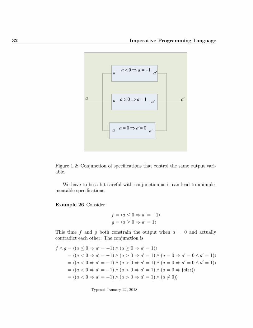
f = 〈a < 0 ⇒ a′ = −1〉g = 〈a > 0 ⇒ a′ = 1〉
Note that f only constrains the output value for inputs with a < 0, whileg only constrains the output value for inputs with a > 0. The conjunctionf ∧ g of the specifications specifies a value for the output in both cases, butnot for the case of a = 0. If
h = 〈a = 0 ⇒ a′ = 0〉then f ∧ g ∧ h is the deterministic specification
〈(a < 0 ⇒ a′ = −1) ∧ (a > 0 ⇒ a′ = 1) ∧ (a = 0 ⇒ a′ = 0)〉Figure 1.2 illustrates this conjunction
Typeset January 22, 2018
32 Imperative Programming Language
1'0 −=⇒< aa
1'0 =⇒> aa
0'0 =⇒= aa
a
a
a
a
'a
'a
'a
'a
Figure 1.2: Conjunction of specifications that control the same output vari-able.
We have to be a bit careful with conjunction as it can lead to unimple-mentable specifications.
Example 26 Consider
f = 〈a ≤ 0 ⇒ a′ = −1〉g = 〈a ≥ 0 ⇒ a′ = 1〉
This time f and g both constrain the output when a = 0 and actuallycontradict each other. The conjunction is
f ∧ g = 〈(a ≤ 0 ⇒ a′ = −1) ∧ (a ≥ 0 ⇒ a′ = 1)〉= 〈(a < 0 ⇒ a′ = −1) ∧ (a > 0 ⇒ a′ = 1) ∧ (a = 0 ⇒ a′ = 0 ∧ a′ = 1)〉= 〈(a < 0 ⇒ a′ = −1) ∧ (a > 0 ⇒ a′ = 1) ∧ (a = 0 ⇒ a′ = 0 ∧ a′ = 1)〉= 〈(a < 0 ⇒ a′ = −1) ∧ (a > 0 ⇒ a′ = 1) ∧ (a = 0 ⇒ false)〉= 〈(a < 0 ⇒ a′ = −1) ∧ (a > 0 ⇒ a′ = 1) ∧ (a �= 0)〉
Typeset January 22, 2018

1.1 A programming language 33
This specification specifies that its input will not be such that a = 0 andhence is an unimplementable specification.
1.1.6 Alternation
Two-way alternation Let A be a boolean expression with free variablesthat are a subset of the variables of Σ. The specification 〈A〉 accepts or rejectsa behaviour depending only on the input aspect of the behaviour. For eachsuch expression, we have a binary operator on specifications if A then _ else _defined by
if A then f else g � (〈A〉 ∧ f) ∨ (¬ 〈A〉 ∧ g)This is called a two-way alternation or a two-way if.
Example 27 Supposing dom(Σ) = {“x”, “y”}, what is if x ≥ 0 then y :=x else y := −x in angle-bracket form
if x ≥ 0 then y := x else y := −x=
(〈x ≥ 0〉 ∧ (y := x) ∨ 〈x < 0〉 ∧ (y := −x))=
(〈x ≥ 0〉 ∧ 〈y′ = x ∧ x′ = x〉 ∨ 〈x < 0〉 ∧ 〈y′ = −x ∧ x′ = x〉)=
〈x ≥ 0 ∧ y′ = x ∧ x′ = x ∨ x < 0 ∧ y′ = −x ∧ x′ = x〉
Exercise 28 Show that
if A then f else g = (〈A〉 ⇒ f) ∧ (¬ 〈A〉 ⇒ g)
Exercise 29 Show that
if A then f else if B then g else h
= (〈A〉 ∧ f) ∨ (¬ 〈A〉 ∧ 〈B〉 ∧ g) ∨ (¬ 〈A〉 ∧ ¬ 〈B〉 ∧ hΣ)
Multiway alternation A generalization of the two-way alternation, thatis sometimes useful, is this: Let A0, A1, ..., A n−1 be n boolean expressions
Typeset January 22, 2018

34 Imperative Programming Language
with free variables that are a subset of the variables of Σ and let f0, f1, ...,fn−1, g be specifications. Now
if A0 then f0� A1 then f1...
......
...� An−1 then fn−1else g
is a specification that is defined to be equal to
(〈A0〉 ∧ f0)∨ (〈A1〉 ∧ f1)...
...∨ (〈An−1〉 ∧ fn−1)∨ (¬ 〈A0〉 ∧ ¬ 〈A1〉 ∧ · · · ∧ ¬ 〈An−1〉 ∧ g)
Note that the order of the expression/specification pairs is not important:I.e. we can switch Ai and fi with Aj and fj for any i, j. Thus
if A then f else if B then g else h
is not (in general) the same as
if A then f � B then g else h
With the former, when A and B are both true of the input, the output isdetermined by f , whereas, with the latter, the output could be determinedby either f or g.
It may be that g can not be reached. This happens when A0 ∨A1 ∨ · · · ∨An−1 is universally true. In such a case, it doesn’t matter what g is, and wecan omit the “else g”.10
10The nondeterministic if-command generalizes Dijkstra’s if-fi command as well as theif-then-else.With Dijkstra’s command, the g is always abort (see section 1.1.7), and isimplicit. (Notationally, the “else g” part is replaced with “fi”, in Dijkstra’s notation.)With the if-then-else construct in languages such as Algol, Pascal, C, C++, and Java,
the “else g” part is optional, with the missing specification assumed to be skip.The question then arises, of whether we should allow the else-clause of the if-construct
to be omitted and, if so, whether the missing else-clause should be assumed to be “elseskip” or “else abort”. For this book, I’m going to come down squarely on the fence: I’lleither include an else-clause or ensure that the missing clause is unreachable. Any otherchoice would create an inconsistency with one or the other established notation.
Typeset January 22, 2018

1.1 A programming language 35
1.1.7 abort and magic
For a given signature Σ we have two specifications at the extremes. We callthese abort and magic.
Definition 30 abort is equivalent to 〈true〉. magic is equivalent to 〈false〉.
abort accepts every possible behaviour; for any input, it allows any out-put. The system that is described by abort is completely unreliable in thatit could produce any output whatsoever. It is easy to implement abort, asall specifications refine it
abort � f , for all f
magic, on the other hand, accepts no behaviours at all. Note that it isoverdetermined for every input and hence (as there is always at least onepossible input) is unimplementable. One curious property of magic is thatit refines any other specification at all.
f � magic, for all f.
magic is not part of the programming language.There is no harm in including abort in a programming language. The
programmer can use abort at points in their code that they expect to beunreachable. The implementer of the language could implement abort tobehave in any way they want; one particularly pragmatic way is to stop theprogram and alert the operating system, the user, and/or the developer. Wecan define a programming construct
assert A to mean if A then skip else abort
1.1.8 Iteration
An important property of iteration is that an iteration is equivalent to itsunrolling: A loopwhile A do h that will iterate 4 times should be equivalentto h;h;h;h. In general we don’t know ahead of time howmany times to unrollthe loop, but we can say a loop w = while A do h should be such that
w = if A then (h;w) else skip
Typeset January 22, 2018

36 Imperative Programming Language
Using this equation, we can unroll the loop as many times as we want. Forexample we can derive that
w = if A then (h; if A then (h; if A then (h;w) else skip) else skip) else skip
Unfortunately, defining while A do h to be that x such that
x = if A then (h; x) else skip (1)
makes a poor definition of the while loop because x occurs on both sides ofthe equation. By analogy, defining φ to be the solution to the equation
x = 1/x+ 1
is a poor definition of the real number φ: there are two solutions. Considerthe case of h = skip and 〈A〉 = 〈true〉. In this case equation (1) simplifies tox = x, which obviously has many solutions (every specification is a solution).
So how do we define the while loop? If w0 and w1 are two differentsolutions to equation (1) with w0 � w1, then w1 is rejecting some behaviourswithout any reason that can be derived from A and h. We’ll take the pointof view while A do h accepts all behaviours accepted by any solution toequation (1). With this definition behaviours are only rejected if there is agood reason.
Definition 31 while A do h is defined to be that specification w such that
• w = if A then (h;w) else skip and
• for any specification x, such that x = if A then (h;x) else skip, wehave w � x.
This definition says that the while loop is the least refined solution toequation (1).11
11You might wonder if this definition is sufficient. Is it the case that for any given Aand h, is there one and only one specification w that fits the definition. It is fairly easy tosee that this is the case. Let X be the set of all x such that
x = if A then (h;x) else skip
The disjunction of any two members of X will also be in x. In fact the disjunction of anyset (even an infinite set) of solutions is also a solution. The disjunction of all membersof X will be a solution and is refined by any other solution. Thus the disjunction of allmembers of X is the unique least-refined solution of (1).
Typeset January 22, 2018

1.2 Properties of the specification operators 37
1.2 Properties of the specification operators
Definition 32
• A unary operator � on specifications is said to preserve implementabil-ity iff for all implementable specifications f , such that �f is welldefined, �f is implementable.
• A binary operator � on specifications is said to preserve implementabil-ity iff for all implementable specifications f and g, such that f �g iswell defined, f � g is implementable.
• In general, an n-ary operator � on specifications is said to preserveimplementability iff for all implementable specifications f0, f1, ..., fn−1,such that � (f0, f1, ..., fn−1) is well defined, � (f0, f1, ..., fn−1) is imple-mentable.
In Example 26 we saw that conjunction does not preserve implementabil-ity.
Exercise 33 Show that disjunction preserves implementability.
Exercise 34 Define that a specification fΣ is independent of a state variablev if f(b0) = f(b1) whenever b0 and b1 agree on all variables other than v.Define that two specifications f and g are output disjoint if, for each outputvariable v′, either f or g is independent of v′. Show that f∧g is implementableif f and g are output disjoint and both f and g are implementable.
Exercise 35 Show that if A then _ else _ preserves implementability.
Exercise 36 Show that sequential composition preserves implementability.
Exercise 37 Show that while A do _ preserves implementability.
With numbers we say that + is monotonic with respect to ≤ since a ≤ bimplies that a+ c ≤ b+ c for all a, b, c.
Typeset January 22, 2018

38 Imperative Programming Language
For specifications, refinement is the key relation and so we define monotonic-ity with respect to refinement.
Definition 38
• A unary operator � is monotonic iff for all f0, f1 such that f0 � f1, wehave �f0 � �f1.
• A binary operator � is monotonic in its left operand iff for all f0, f1, gsuch that f0 � f1, we have f0 � g � f1 � g.
• A binary operator � is monotonic in its right operand iff for all f0, f1, gsuch that f0 � f1, we have g � f0 � g � f1.
• In general, an n-ary operator is monotonic in operand i iff for allf0, f1, g0, g1, ..., gi−1, gi+1, ..., gn−1 such that f0 � f1, we have �(g0, g1,..., gi−1, f0, gi+1, ..., gn−1) � �(g0, g1, ..., gi−1, f1, gi+1, ..., gn−1)
Exercise 39 Show that disjunction and conjunction are both monotonic inboth operands
Exercise 40 Show that if A then _ else _ is monotonic in both operands.
Exercise 41 Show that sequential composition is monotonic in both operands.
Exercise 42 Show that while A do _ is monotonic.
Typeset January 22, 2018

Chapter 2
Derivation of nonloopingprograms
In this chapter we look at techniques for deriving commands from specifica-tions. That is we start with a specification f and derive a command g suchthat f � g. We will develop commands step-by-step so that each step isfairly small and is easily verified. It should be said off the top that this isnot a mechanical process. Far from it. Creativity is required.
The plan of the chapter is this. We’ll look at some of the laws of pro-gramming for each of the programming constructs and how to apply theselaws to deriving programs from specifications.
2.0 Strengthening and monotonicity
We start with some very general laws.
As explained in Section A.6.3, a boolean expression B is stronger than aboolean expressionA exactly if B ⇒ A is universally true (i.e., true regardlessof the values of the variables).
When a specification is in angle-bracket form we can refine by replacingthe expression with a stronger one. I.e. we have
Theorem 43 (Strengthening) 〈A〉 � 〈B〉 exactly if B is stronger than A.
From this we have the following corollaries.
Typeset January 22, 2018

40 Derivation of nonlooping programs
Corollary 44 (Strengthening)
〈A ∨ B〉 � 〈A〉〈B ⇒ A〉 � 〈A〉
〈A〉 � 〈A ∧ B〉
Corollary 45 (Monotonicity) If 〈A〉 � 〈B〉
〈A ∧ C〉 � 〈B ∧ C〉〈A ∨ C〉 � 〈B ∨ C〉〈C ⇒ A〉 � 〈C ⇒ B〉
Corollary 46 (Antimonotonicity) If 〈B〉 � 〈A〉 then
〈¬A〉 � 〈¬B〉〈A ⇒ C〉 � 〈B ⇒ C〉
More generally we have the following monotonicity laws regardless of theform of the specification.
Theorem 47 If f , g, and h are specifications such that f � g, we have
• f ∧ h � g ∧ h
• f ∨ h � g ∨ h
• h⇒ f � h ⇒ g
• f ;h � g;h
• h; f � h; g
• if A then f else h � if A then g else h
• if A then h else f � if A then h else g
• while A do f � while A do g
Typeset January 22, 2018

2.1 Programming with skip and assignments 41
2.1 Programming with skip and assignments
Earlier we saw that skip can refine specifications of the form 〈x′ = x ∧ y′ = y〉.But skip will also refine other specifications, such as 〈k > 0 ⇒ k′ ≥ 0〉; if kis initially greater than 0, then, after not changing, k will still be greaterthan 0 and thus greater or equal to 0. If A is an expression, we’ll write Afor the expression we get by erasing all the prime marks in A. So if A is theexpression k > 0 ⇒ k′ ≥ 0 then A would be the expression k > 0 ⇒ k ≥ 0.This particular expression, k > 0 ⇒ k ≥ 0, has the property that it is truefor all values of its variables. A boolean expression with this property iscalled universally true. In general we have the following law universally true
Theorem 48 (The erasure law for skip) 〈A〉 � skip exactly if A is uni-versally true.
I won’t prove this law in general, but consider the case where the variablesare x and y.
〈A〉 � skip
=“Definitions of refinement and skip”
∀x, y, x′, y′ · x′ = x ∧ y′ = y ⇒ A=“One-point”
∀x, y · A[x′, y′ : x, y]
=“Definition of erasure”
∀x, y · A=“Definition of universally true”
A is universally true
The substitutionnotation is coveredin Section A.6.0.Typeset January 22, 2018

42 Derivation of nonlooping programs
If we take this same line of reasoning and apply it to the assignmentstatement x := E , where E does not contain any primed variables, we get
〈A〉 � x := E=“Definitions of refinement and assignment
∀x, y, x′, y′ · x′ = E ∧ y′ = y ⇒ A=“One-point”
∀x, y · A[x′, y′ : E , y]=“y′ does not occur free in E”
∀x, y · A[x′ : E ][y′ : y]=“x′ does not occur free in A[x′ : E ]
∀x, y · A[x′ : E ][x′, y′ : x, y]=“Definition of erasure”
∀x, y · A[x′ : E ]=“Definition of universally true”
A[x′ : E ] is universally true
which leads us to
Theorem 49 (The erasure law for assignment) 〈A〉 � V := E exactly
if ˜A[V ′ : E ] is universally true.
For example, if k is of type Z, then 〈k′ > k〉 � k := k+42, as (k′ > k) [k′ :k + 42] is k + 42 > k which is universally true.
This law also extends to parallel assignment.
Theorem 50 (The erasure law for parallel assignment) 〈A〉 � V0,V1, ...,Vn :=
E0, E1, ..., En exactly if ˜A[V ′0,V ′1, ...,V ′n : E0, E1, ..., En] is universally true.
For example, let’s work out whether the following refinement holds.
〈x′ = y ∧ y′ = x ∧ z′ ≥ z〉 � x, y := y, x
After making the multiple variable substitution
(x′ = y ∧ y′ = x ∧ z′ ≥ z) [x′, y′ : y, x]
Typeset January 22, 2018

2.2 The substitution laws 43
and erasing the remaining prime, we have y = y ∧ x = x ∧ z ≥ z, which isuniversally true, so the refinement holds.
2.2 The substitution laws
For introducing sequential composition, there is a very useful law
Theorem 51 (The forward substitution law) 〈A[V : E ]〉 = (V := E ; 〈A〉)
I won’t prove this in general, but again, consider the case of a two variablestate space
(x := E ; 〈A〉)=“Definitions of assignment and sequential composition”
〈∃x, y · x = E∧y = y ∧A[x, y : x, y]〉=“One-point”
〈A[x, y : x, y][x, y : E , y]〉=“No dotted variables in A”
〈A[x, y : E , y]〉=“No substitution for y”
〈A[x : E ]〉
The substitution law is very useful for introducing sequential compositioninto programs.
Example 52 Consider the following specification to implement
〈x′ = y ∧ y′ = x〉
We will assume that multiple assignments are not allowed. We’ll also assumethat there is a variable t of appropriate type. Can we derive a sequential
Typeset January 22, 2018

44 Derivation of nonlooping programs
composition of single assignments that does the job?
〈x′ = y ∧ y′ = x〉= Forward substitution law
t := x ; 〈x′ = y ∧ y′ = t〉= Forward substitution law
t := x ; x := y ; 〈x′ = x ∧ y′ = t〉� Erasure law for assignment
t := x ; x := y ; y := t
Note how the last step also uses a monotonicity law. We generally won’t callattention to uses of monotonicity laws. They are used implicit.
There is also a law for introducing an assignment statement at the endof a sequential composition.
Notation 53 Suppose E is an expression with all free variables unprimed.We’ll write E ′ for the same expression, except with primes added to all free
variables, and�
E for the same expression except with a dot added to eachvariable.
Theorem 54 (The backward substitution law) 〈A〉 � (〈A[V ′ : E ′]〉 ;V := E)
Example 55 Consider swapping again. Again, we’ll assume there is a vari-able t that we can use.
〈x′ = y ∧ y′ = x〉�“Backward substitution”
〈x′ = y ∧ t′ = x〉; y := t
�“Backward substitution”
〈y′ = y ∧ t′ = x〉; x := y; y := t
�“Erasure law”t := x; x := y; y := t
Typeset January 22, 2018

2.2 The substitution laws 45
I won’t prove this law in detail, but looking at the case of two variablesshould be convincing
〈A[x′ : E ′]〉 ;x := E=“Definition of assignment”
〈A[x′ : E ′]〉 ; 〈x′ = E ∧ y′ = y〉=“Definition of sequential composition”⟨∃x, y · A[x′ : E ′][x′, y′ : x, y] ∧ x′ =
�
E ∧ y′ = y
⟩
=“Since the primes in E ′ will be replaced with dots”⟨∃x, y · A[x′, y′ :
�
E , y] ∧ x′ =�
E ∧ y′ = y
⟩
=“One point”⟨∃x, y · A[x′, y′ :
�
E , y′] ∧ x′ =�
E⟩
=“It’s safe to assume that x′ =�
E”⟨∃x, y · A[x′, y′ : x′, y′] ∧ x′ =
�
E⟩
=“Null substitution”⟨∃x, y · A ∧ x′ =
�
E⟩
=“Distributivity; no dots in A”
〈A〉 ∧⟨∃x, y · x′ =
�
E⟩
Now since
(〈A〉 ∧
⟨∃x, y · x′ =
�
E⟩)
= (〈A[x′ : E ′]〉 ; x := E ), we have,
by strengthening, the backward substitution law:
〈A〉 � 〈A[x′ : E ′]〉 ; x := ENote that 〈A[x′ : E ′]〉 ;x := E may be a stronger requirement than 〈A〉;
the ‘extra’ bit
⟨∃x, y · x′ =
�
E⟩says that the value of x′ is in the range of the
expression. Consider refining
〈x′ = 4 ∨ x′ = 5〉
Typeset January 22, 2018

46 Derivation of nonlooping programs
using backward substitution and x := 2× x, where x is an integer variable.We have
〈x′ = 4 ∨ x′ = 5〉�“Backward substitution”
〈2× x′ = 4 ∨ 2× x′ = 5〉 ; x := 2× x
=“x is an integer variable”
〈x′ = 2〉 ; x := 2× x
=“Definitions of sequential composition and assignment”
〈x′ = 4〉
You can see that there is a reduction in nondeterminism, the output of x =5 is accepted by 〈x′ = 4 ∨ x′ = 5〉, but is not compatible with the chosenassignment.
This reduction in nondeterminism may mean that the law takes us froman implementable 〈A〉 to an unimplementable 〈A[x′ : E ′]〉.
Consider the specification 〈x′ = 5〉. If we apply backward substitutionwith x := 2× x, we get
〈x′ = 5〉�“backward substitution”
〈2× x′ = 5〉 ; x := 2× x
At this point, the remaining problem, 〈2× x′ = 5〉, is unimplementable.Thus, for practical application, we should be careful how we use back-
ward substitution, so as not to venture into the territory of unimplementablespecifications.
The forward substitution law does not suffer from this problem: If 〈A[V : E ]〉is implementable, then so is 〈A〉.
2.3 Weakest prespecification and weakest post-
specification
This section is optional reading.[[And not yet written!]]
Typeset January 22, 2018

2.4 Alternation 47
2.4 Alternation
Once we have checked a condition, it can become a precondition. This ideais captured in the alternation law
Theorem 56 (alternation law)
f = if A then (〈A〉 ⇒ f) else (¬ 〈A〉 ⇒ f)
The alternation problem allows us to replace a problem f with two newproblems. The trick, of course is to pick an expression A so that both thenew problems are easier to solve than the original.
Example 57 (Finding the minimum) We know that
min(a, b) = a, if a ≤ b (0)
min(a, b) = b, if b ≤ a (1)
Suppose we wish to implement
f = 〈a′ = min(a, b)〉
f
=Alternation law
if a ≤ b then (〈a ≤ b〉 ⇒ f) else (〈a > b〉 ⇒ f)
We can implement the first case as follows
〈a ≤ b〉 ⇒ f
=Defn of f
〈a ≤ b⇒ a′ = min(a, b)〉=By (0)
〈a ≤ b⇒ a′ = a〉�Erasure lawskip
Typeset January 22, 2018

48 Derivation of nonlooping programs
The second case is implemented by
〈a > b〉 ⇒ f
=Defn of f
〈a > b ⇒ a′ = min(a, b)〉�Strengthening⟨a ≥ b⇒ a′ = min(a, b)
⟩
=(1)
〈a ≥ b⇒ a′ = b〉�Erasure lawa := b
Now we have
f
=Alternation law
if a ≤ b then (〈a ≤ b〉 ⇒ f) else (〈a > b〉 ⇒ f)
�Above resultsif a ≤ b then skip else a := b
2.4.0 Nondeterministic alternation
Theorem 58 (alternation law)
f � if A0 then 〈A0〉 ⇒ f� A1 then 〈A1〉 ⇒ f...
......
...� An−1 then 〈An−1〉 ⇒ felse ¬ 〈A0 ∨ A1 ∨ · · · ∨ An−1〉 ⇒ f
Typeset January 22, 2018

Chapter 3
Derivation of Loops
3.0 The recursive refinement approach
3.0.0 While law (incomplete version)
For specifications h and 〈A〉, let tA,h be a function
tA,h(g) = if A then (h; g) else skip
Letw = while A do h
Now w is a fixed point of tA,h, that is
w = if A then (h;w) else skip
A specification g, such that g � if A then (h; g) else skip, will, in manycases, be implemented by w
While law (incomplete version): For any g, h, and A, such that ... if
g � if A then (h; g) else skip
theng � while A do h
Later we will complete this law (fill in the “...”) with extra conditionsthat ensure it is valid for particular g, h, and A.
This gives us an approach to refining a specification g with a while loop.We derive an if command such that its else branch is refined by skip. In
Typeset January 22, 2018

50 Derivation of Loops
refining the then-part, if we come to a point where all that remains to bedone is described by g, we simply stop. Now we have
g � if A then (h; g) else skip
Then (subject to some conditions we will see later), we have g � while A do h.
3.0.1 Summation of an array
For this problem, we calculate the sum of all the elements in an array ofintegers a of size n (a fixed natural number)
f =
⟨s′ =
∑
k∈{0,..n}
a(k)
⟩
It turns out that f is not suitable for directly applying the while law.
The strategy is to find a generalization of the problem g that can serveas the specification of a loop:
f
�Substitution law
i, s := 0, 0 ; g
where
g =
⟨s′ = s+
∑
k∈{i,..n}
a(k)
⟩
Now the problem remaining is to derive a program for g.
In the case where i ≥ n the problem is easy to solve
g
�if i < nthen 〈i < n〉 ⇒ gelse 〈i ≥ n〉 ⇒ g
Typeset January 22, 2018

3.0 The recursive refinement approach 51
Tackling the second problem first we have
⟨i ≥ n ⇒ s′ = s+
∑
k∈{i,..n}
a(k)
⟩
=“If i ≥ n, then {i, ..n} = ∅”⟨i ≥ n ⇒ s′ = s+
(∑
k∈∅
a(k)
)⟩
=The sum over an empty set is 0
〈i ≥ n ⇒ s′ = s + 0〉�“Erasure”skip
In the second case
⟨i < n⇒ s′ = s+
∑
k∈{i,..n}
a(k)
⟩
=“If i < n we can rewrite {i, ..n} as {i} ∪ {i+ 1, ..n} ”⟨i < n⇒ s′ = s+
∑
k∈{i}∪{i+1,..n}
a(k)
⟩
=“Split the summation”⟨i < n⇒ s′ = s+ a(i) +
∑
k∈{i+1,..n}
a(k)
⟩
�“Strengthen”⟨s′ = s+ a(i) +
∑
k∈{i+1,..n}a(k)
⟩
=“Substitution law”
i, s := i+ 1, s+ a(i) ; g
Typeset January 22, 2018

52 Derivation of Loops
Putting these results together (with monotonicity) we get that
g
�if i < nthen 〈i < n〉 ⇒ gelse 〈i ≥ n〉 ⇒ g
�Above calculationsif i < nthen (i, s := i+ 1, s+ a(i); g)else skip
Now we apply the while law
g � while i < n do i, s := i+ 1, s+ a(i)
and thus (by monotonicity)
f � i, s := 0, 0;while i < n do
i, s := i+ 1, s+ a(i)
3.0.2 Greatest Common Denominator
For any natural numbers a and b, we write a | b iff a divides b, i.e. iff thereexists a q ∈ N such that aq = b. Note that
a | 0, for all natural numbers a (0)
The greatest common denominator of two natural numbers a and b is anatural number gcd(a, b) with the following properties.
gcd(a, b) | a, for all natural numbers a, bgcd(a, b) | b, for all natural numbers a, bif c | a and c | b then c | gcd(a, b),
for all natural numbers a, b, c
Typeset January 22, 2018

3.0 The recursive refinement approach 53
From these properties we can derive the following facts (proof left as exercise)
gcd(a, 0) = a, (1)
for all natural numbers a, where a �= 0
gcd(a, b) = gcd(b, amod b), (2)
for all natural numbers a, b where b �= 0
From (0) it is clear that gcd(0, 0) is not defined, since there are an in-finite number of common divisors. Therefore, it makes sense to use as aprecondition that at least one argument is not zero. Let
g = 〈a �= 0 ∨ b �= 0 ⇒ a′ = gcd(a, b)〉
This is ready for implementation as a loop.
g
=Alternation
if b �= 0then 〈b �= 0〉 ⇒ gelse 〈b = 0〉 ⇒ g
In the else part we have (after shunting)
〈b = 0 ∧ (a �= 0 ∨ b �= 0) ⇒ a′ = gcd(a, b)〉= One point and identity law for ∨
〈b = 0 ∧ a �= 0 ⇒ a′ = gcd(a, 0)〉=Fact (1)
〈b = 0 ∧ a �= 0 ⇒ a′ = a〉�Erasureskip
Typeset January 22, 2018

54 Derivation of Loops
In the then part we have (after shunting)
〈b �= 0 ∧ (a �= 0 ∨ b �= 0) ⇒ a′ = gcd(a, b)〉=Domination law for ∨
〈b �= 0 ∧ true⇒ a′ = gcd(a, b)〉=Identity law for ∧
〈b �= 0 ⇒ a′ = gcd(a, b)〉=Fact (2)
〈b �= 0 ⇒ a′ = gcd(b, amod b)〉�Strengthening
〈b �= 0 ∨ amod b �= 0 ⇒ a′ = gcd(b, amod b)〉=Forward substitution
a, b := b, amod b ; g
Now putting the two cases together we get
g
�if b �= 0then a, b := b, amod b ; gelse skip
So by the while loop law we have
g � while b �= 0 do a, b := b, amod b
3.1 Loop Termination
In order to use while loops in programming, we need to be able to provestatements such as
g � while A do h
So we need to know under what conditions this refinement holds. Earlier wesaw an incomplete law
While law (incomplete version): For any g, h, and A, such that ... if
g � if A then (h; g) else skip
Typeset January 22, 2018

3.1 Loop Termination 55
theng � while A do h
But we still need to fill in the “...”It turns out that what is missing is that we must require the loop to
terminate. Consider two loops where x is a natural number program variable
while x > 0 do x := x− 1
andwhile x �= n do x := x+ 1
The first definitely terminates, while the second may not. How can we showthat a loop terminates?
In the case of while x > 0 do x := x − 1, we can find an expression,for example x, such that the number of remaining iterations, never exceedsthat expression. Such an expression is called a bound on the number of re-maining iterations, that is an expression E such that the number of iterationsremaining is no more than E .
In the case of while x �= n do x := x + 1, we can not find any suchexpression. The expression n − x will act as bound in some states (thosewhere n ≥ x), but not in all states.
If we can find a bound for a loop, then it always terminates.
3.1..0 A better iteration law
While law (better version): For any g, h, and A, such that while A do halways terminates, if
g � if A then (h; g) else skip
theng � while A do h
3.1..1 An even better iteration law
In practice, we do not require that loops terminate regardless of the ini-tial state. We only require that they terminate when started in states thatmatter. For example, we would expect that, for an integer i,
〈i ≤ n ⇒ i′ = n〉 � while i �= n do i := i+ 1
Typeset January 22, 2018

56 Derivation of Loops
even though, the loop does not terminate when started with an initial valueof i that is larger than n.
To show this sort of refinement we need an even better law. We will usea program variable τ of type Z to count the number of repetitions of loops.You can think of this variable as representing time. You might expect thatevery operation will take some amount of time and so we should imagine thetime variable increasing with each operation. That would be a more realisticapproach to time, but also a more complicated one. For many purposes, itis sufficient to consider how time
Let us strengthen the example specification to include information aboutthe maximum number of repetitions allowed
g = 〈(i ≤ n ⇒ i′ = n ∧ τ ′ ≤ τ + (n− i))〉Now we show
g � if i �= n then (i := i+ 1; τ := τ + 1; g) else skip
While law (final version): For any g, h, and A, where g is of the form〈B ⇒ C ∧ τ ′ ≤ τ + E〉 and E is a natural number expression, if
g � if A then (h; τ := τ + 1; g) else skip
theng � while A do h
(E is called the bound for the loop.)Practically, what this means is that when A and E > 0 are true initially,
h needs to decrease the value of E by at least 1.
3.1..2 Summation revisited
In the summation problem above we had to refine⟨i ≤ n ⇒ s′ = s+
∑
k∈{i,..n}
a(k)
⟩
with a loop. In that case the bound can be n− i, so we should refine⟨i ≤ n ⇒ s′ = s+
∑
k∈{i,..n}
a(k)
∧ τ ′ ≤ τ + n− i
⟩
by a while loop.
Typeset January 22, 2018

3.1 Loop Termination 57
3.1..3 GCD revisited
In the GCD problem we had to refine
〈a �= 0 ∨ b �= 0 ⇒ a′ = gcd(a, b)〉
in this case we can use b as the bound. We can show that
〈a �= 0 ∨ b �= 0 ⇒ a′ = gcd(a, b) ∧ τ ′ ≤ τ + b〉
is implemented by
while b �= 0 do a, b := b, amod b
since amod b < b.
Typeset January 22, 2018

58 Derivation of Loops
Typeset January 22, 2018

Chapter 4
Loop invariants
4.0 Square root
Suppose x is a natural number. We wish to find the integer part of its squareroot.
f =⟨y′2 ≤ x < (y′ + 1)
2⟩
=⟨y′2 ≤ x ∧ x < (y′ + 1)
2⟩
Our aim is to implement f using a loop. If we have already searched the firsty natural numbers we know y2 ≤ x. Let’s call this expression I.
I is y2 ≤ x
We can generalize f by adding I as an antecedent.
g = (〈I〉 ⇒ f)
We havef � y := 0; g
I is called the loop’s invariant.Note that I is one of the conjuncts of f,except with the primes erased.
Let’s take the other conjunct, negate it, and erase primes; we get (y+1)2 ≤ x;we’ll use this expression as a guard. Applying the alternation law we have
g � if (y + 1)2 ≤ x then g0 else g1
Typeset January 22, 2018

60 Loop invariants
where the else-clause is
g1 =⟨y2 ≤ x < (y + 1)2 ⇒ y′2 ≤ x < (y′ + 1)
2⟩
We have a specification of the form 〈A ⇒ B〉 such that A is the same as B.By the erasure law, such a specification can always be implemented by skip.
For the "then" clause we have:
g0 =⟨I ∧ (y + 1)2 ≤ x⇒ y′2 ≤ x < (y′ + 1)
2⟩
We need to find a specification h so that
g0 � h; g
The following will do
h =⟨I ∧ (y + 1)2 ≤ x⇒ I ′ ∧ x′ = x
⟩
where I ′ is the same as I, but with primes:
I ′ is y′2 ≤ x′
The key point about h is that its job is to preserve the invariant.
h = 〈I ∧ · · · ⇒ I ′ ∧ · · · 〉That is, if h starts in a state where I holds, it must end in a state where Iholds.
Exercise 59 Prove that g0 � h; g using the definition of sequential compo-sition.
Now all that remains is to implement h.
h
= By definition⟨I ∧ (y + 1)2 ≤ x⇒ I ′ ∧ x′ = x
⟩
� Strengthening and assignment laws
y := y + 1
To show that the loop terminates, we can use x− y2 as a bound.
Typeset January 22, 2018

4.1 The method of loop invariants 61
4.1 The method of loop invariants
Let’s try to separate the method used to solve the last problem, from thedetails of the problem.
The general form of the solution is
f � m; g
g � while A do h
The key to the method is the notion of an invariant I, which is a conditionon the initial state.
Suppose f = 〈B〉 and B depends on a list of input variables x. We choosean invariant I and generalize f = 〈B〉 to g = 〈I ⇒ B〉.
The role of the initialization statement m, is to establish the invariant,that is to make I true at the start of the loop. This suggests
〈I ′〉
However, that is not enough, m must not change any of the variables x whoseinitial value is used in B.
m = 〈I ′ ∧ x′ = x〉
Exercise 60 Exercise: Show that f � m; g
Next, we turn our attention to implementing g = 〈I ⇒ B〉withwhile A do h.In the case where A is false, the while loop will do nothing, so the final statewill be the same as the initial state. We can assume that I is true in theinitial state. So we need that ¬A ∧ I implies that B relates the initial stateto itself: I.e. we need that
I ∧ ¬A ⇒ B, is universally true
The role of the loop’s body h is to preserve the invariant ; that is
〈I ⇒ I ′〉
We can assume that A is true to start with, so h needs to implement
〈A ∧ I ⇒ I ′〉
Typeset January 22, 2018

62 Loop invariants
However, h should not change variables whose initial value is used in B. Wehave
h = 〈A ∧ I ⇒ I ′ ∧ x′ = x〉To ensure termination, the loop’s body should also decrease a bound.
Exercise 61 Show that g � 〈A〉 ⇒ (h; g)
4.2 Examples of using loop invariants
4.2.0 Square Root by Binary Search
The floor �a , of a real number a is the largest integer that is not larger thana. We have �a < i iff a < i, for all integers i and real numbers a.
The problem is (again) to find the integer part of the square root of anonnegative real number x: f =
⟨y′2 ≤ x < (y′ + 1)2
⟩. Rewrite f as
f =⟨y′2 ≤ x < (y′ + 1)
2⟩
= Monotonicity of squaring nonnegative reals⟨y′ ≤ √
x < y′ + 1⟩
= Facts about floor⟨y′ ≤⌊√x⌋< y′ + 1
⟩
=⟨y′ =⌊√x⌋⟩
Our plan is to use the method of invariants.
Picking an invariant. The first thing to do is to pick an invariant.We obtain I by replacing the expression y′ + 1 in f with a new variable, z,and erasing all primes.
I : y ≤⌊√x⌋< z
g =⟨I ⇒ y′ =
⌊√x⌋⟩
In terms of sets I = (�√x ∈ {y, ..z}). The invariant says that the answerwe seek is somewhere between y (inclusive) and z (exclusive)
Typeset January 22, 2018

4.2 Examples of using loop invariants 63
0 · · · · · · �√x · · · · · · x+ 1↑ ↑y z
It is a fact that, for all x ∈ N
0 ≤⌊√x⌋< x+ 1
So
f
= Fact just mentioned⟨0 ≤⌊√x⌋< x+ 1 ⇒ y′ =
⌊√x⌋⟩
= Substitution
y, z := 0, x+ 1; g
Picking a Guard When z = y + 1 , according to the invariant, �√x is in the set {y, ..y + 1} = {y}. That is z = y+1 together with the invariantimplies that �√x = y, and so there is nothing left to do:
⟨z = y + 1 ∧ I ⇒ y′ =
⌊√x⌋⟩
� skip
So use z �= y + 1 as the loop guard. Given the invariant, this is the same asz > y + 1. So we have
g
�if z > y + 1 then 〈z > y + 1〉 ⇒ g else 〈z = y + 1〉 ⇒ g
�if z > y + 1 then 〈z > y + 1〉 ⇒ g else skip
Preserving the invariant We need a body that preserves the invariantbut doesn’t change x.
h =⟨⌊√
x⌋∈ {y, ..z} ∧ z > y + 1 ⇒
⌊√x′⌋∈ {y′, ..z′} ∧ x′ = x
⟩
The idea is to consider two parts of the set {y, ..z}. If w ∈ {y, ..z},then {y, ..w} ∪ {w, ..z} = {y, ..z}. Since (according to the invariant) �√x ∈
Typeset January 22, 2018

64 Loop invariants
{y, ..z}, �√x must be in one of the subsets {y, ..w} and {w, ..z}. If we canfigure out which one, we can preserve the invariant by setting y and z to theupper and lower bounds of the appropriate subset. If our bound expressionis z − y, i.e. the size of the set {y, ..z}, we should pick w so that y < w < z.
The fastest way to make progress is to pick w about half way betweeny and z. Since, at the start of the body, z > y + 1, z − y is at least 2,so �(z − y)/2 is at least 1. Let w stand for y + �(z − y) /2 . Note thaty < w < z, as needed. We have {y, ..z} = {y, ..w} ∪ {w, ..z}. From I wehave �√x ∈ {y, ..w} ∨ �√x ∈ {w, ..z}
If w ≤ �√x then �√x ∈ {w, ..z}, and we can set y to w without makingthe invariant false.
0 · · · · · · · · · �√x · · · · · · x+ 1↑ ↑ ↑y w z
If w > �√x then �√x ∈ {y, ..w}, and we can set z to w without makingthe invariant false.
0 · · · · · · �√x · · · · · · · · · x+ 1↑ ↑ ↑y w z
In both cases the bound z − y is decreased by at least one. We have
h
=
〈I ∧ z > y + 1 ⇒ I ′ ∧ x′ = x〉� if w ≤ �√x
then y := welse z := w
But, we can’t use the test w ≤ �√x , as we can’t easily calculate �√x .(If we could easily calculate �√x there wouldn’t be any point designing thisalgorithm.) Can we find an equivalent expression? Yes:
Typeset January 22, 2018

4.2 Examples of using loop invariants 65
w ≤⌊√x⌋
= Since w is an integer
w ≤ √x
= Squaring both sides.
w2 ≤ x
The final algorithm is
f
� y, z := 0, x+ 1;// inv. y ≤ �√x < zwhile z > y + 1do var w := y + �(z − y) /2 ·
if w2 ≤ xthen y := welse z := w
Let’s take a moment to look back at how the algorithm works. Theinvariant says the desired answer is in the set {y, y + 1, ..., z − 1}. We callthis set the “search space”
In each iteration of the loop, we reduce the size of the search space byroughly 2. This technique is called binary search.
Since the size of the search space is roughly halved with each iteration,and the initial size of the search space is x, the number of iterations isroughly log2 x. For large x, log2 x is considerably smaller than
√x. Consider
x = 1012 ∼= 240.√x = 106. log2 x
∼= 40.
4.2.1 Searching for a pattern
In this section we look at a somewhat more difficult problem.Consider the problem of searching for a pattern sequence p within a target
sequence t. For example, if p is “sip" and t is “Mississippi”, then the answeris true. But if the pattern were “ips” the answer would be false. We arelooking to see if there is a place i such that p(0) = t(i) and p(1) = t(i + 1)and so on up to (and including) p(‖p‖−1) = t(i+‖p‖−1). I’ll write t[i, ..i+j]to mean the segment of t that starts at i and that has length max(j, 0); Forexample if t is “abcd”, then t[1, ..3] is “bc”.
Typeset January 22, 2018

66 Loop invariants
4.2.1.0 Formalizing the problem
Let us define match(i, j) to mean that the first j items of p match the j itemsof t starting at position i, where 0 ≤ j ≤ ‖p‖ and 0 ≤ i:
match(i, j) = (i+ j ≤ ‖t‖ ∧ p[0, ..j] = t[i, ..i+ j])
Now we can specify our problem as
f = 〈(b′ = ∃i ∈ {0, .. ‖t‖ − ‖p‖+ 1} ·match(i, ‖p‖)〉
For the rest of this section, I’ll regard t and p as mathematical variablesrather than state variables, and so I won’t explicitly specify that they mustnot be changed by the initialization code and the loop body.
4.2.1.1 Developing an invariant and guard
Note that there are ‖t‖ − ‖p‖ + 1 places that the pattern could be found.Suppose we search from left to right using an index k that ranges from 0 up,and we have established that there is no match in the first k places. Thenwe know I0 ∧ I1 where
I0 is k ≥ 0
I1 is ¬∃i ∈ {0, ..k} ·match(i, ‖p‖)
Suppose we further know that, at position k, the first j items of the patternmatch, i.e. we also know I2 ∧ I3 where
I2 is j ∈ {0, .., ‖p‖}I3 is match(k, j)
All of these invariants are easy to establish by setting k and j to 0.What about a guard? If k > ‖t‖ − ‖p‖, then, by I1, we know that the
pattern exists nowhere in the target and so b should be set to false; the loopcan stop. On the other hand, if j = ‖p‖, then, by I3, there is a match atposition k and so b should be set to true; again the loop can stop. Thissuggests that the guard G be k ≤ ‖t‖ − ‖p‖ ∧ j < ‖p‖.
In summary, so far we have
f � k, j := 0, 0; 〈I ⇒ I ′ ∧ G′〉 ; b := j = ‖p‖
where I is I0 ∧ I1 ∧ I2 ∧ I3.
Typeset January 22, 2018

4.2 Examples of using loop invariants 67
4.2.1.2 Developing a loop body
We can implement 〈I ⇒ I ′ ∧ G′〉 with a loop
while G do h
where h = 〈G ∧ I ⇒ I ′〉, provided we also decrease a bound, so it remainsto implement h while decreasing a bound.
If G ∧ I holds, we have 0 ≤ k ≤ ‖t‖ − ‖p‖ and 0 ≤ j < ‖p‖, so it issafe to compare t(k + j) with p(j); neither subscript is out of bounds. Ift(k + j) = p(j), incrementing j preserves all invariants. If t(k + j) �= p(j),incrementing k preserves all invariants if we also set j to 0. Thus we have
h � if t(k + j) = p(j) then j := j + 1 else k, j := k + 1, 0
The whole algorithm is
k, j := 0, 0;while k < ‖t‖ − ‖p‖+ 1 ∧ j < ‖p‖ do
if t(k + j) = p(j) then j := j + 1 else k, j := k + 1, 0;
b := j = ‖p‖
As a bound we can use (‖t‖ − k) ‖p‖+ ‖p‖ − j.
4.2.1.3 Speed
Is this a good algorithm? Consider for example a pattern “aaaaaaaaab” anda target than is “aa· · · a”. The algorithm behaves quite badly in this case: itmakes 10 comparisons for each value of k ∈ {0, .., ‖t‖ − 10}. In general, thealgorithm makes ‖p‖ × (‖t‖ − ‖p‖+ 1) item comparisons, in the worst case.
4.2.1.4 Improving the algorithm
Is there a better way? When there is a match, it seems hard to improve onadvancing j. When there is a failure and j = 0, the best way to make progressis to increment k, while leaving j at 0. What if there is a failure when j > 0?The algorithm has already made j successful comparisons and that tells alot about the target string that is simply forgotten if k is incremented and jis set to 0. We will look at three examples to figure out a way to use thatinformation
Typeset January 22, 2018

68 Loop invariants
Consider the case where the pattern p is “aaab”. Suppose that, for somet and k, the match fails on the “b” –i.e. we have j = 3 and t(k+3) �= p(3).The algorithm above sets j back to 0 and k to k + 1, so that the nextcomparison will be between t(k + 1) and p(0). We can see that p(0) is “a”by looking at p. We can see that t(k + 1) is “a” by consider I3 which saysthat p[0, ..j] = t[k, ..k + j] and thus that t(k + 1) = p(1). Since both itemsare “a”, there is no need to compare them. Similarly, both p(1) and t(k+2)are “a” and so there is no reason to compare them. We can just set j to 2and k to k + 1.
k k + j↓ ↓
· · · a a a ? · · ·a a a b
↑j
slide by 1
k k + j↓ ↓
· · · a a a ? · · ·a a a b
↑j
Now consider the case where the pattern p is “abcd”. Suppose thatfor some t and k, the match fails on the “d” –i.e., we have j = 3 andt(k + 3) �= p(3). From I3 we know that p[0, ..j] = t[k, ..k + j]. And thust[k, ..k + 3] is “abc”. There is no point trying for a match at position k + 1;we know that t(k + 1) contains a “b”, while p(0) contains an “a”. Similarlythere is no point trying for a match at position k+2, as we know that t(k+2)is a “c”. In this case we can set k to k + 3 and j to 0.
k↓
· · · a b c ? · · ·a b c d
↑j
slide by 3
k↓
· · · a b c ? · · ·a b c d↑j
Finally, consider the case where the pattern p is “ababc” and the matchfails on the “c” when j is 4. This tells us that t[k + 1, ..k + 4] is “bab”. Sothere is no point sliding the pattern 1 place to the right. But if we slide ittwo places to the right, the first two items of p will match. So we should
Typeset January 22, 2018

4.2 Examples of using loop invariants 69
increment k by 2 and set j to 2.
k k + j↓ ↓
· · · a b a b ? · · ·a b a b c
↑j
slide by 2
Note that in all three of these cases, we increment k and decrement j by thesame amount so that j + k remains the same
Given the pattern p, we can work out for each j ∈ {1, .. ‖p‖}, how muchcan we slide the pattern in case the match process fails at point j withoutbreaking any invariants. This will be the smallest number m > 0 such thatp[0, ..j − m] = p[m, ..j]; this m is in {1, .., j}. For each j ∈ {1, .. ‖p‖}, letmj = (minm ∈ {1, .., j} | p[0, ..j −m] = p[m, ..j]). For j ∈ j ∈ {1, .. ‖p‖},we have
I3=
t[k, ..k + j] = p[0, ..j]
⇒t[k +mj , ..k + j] = p[mj, ..j]
⇒ Since p[0, ..j −mj] = p[mj , ..j]
t[k +mj , ..k + j] = p[0, ..j −mj ]
=
I3 [k, j : k +mj , j −mj]
This means we will not violate I3 by assigning k, j := k +mj, j −mj. I1will not be violated by this assignment, since, if it were, we could show thatm is not minimum. The other invariants are trivially not violated.
The new loop body is
h � if t(k+j) = p(j) then j := j+1 else if j = 0 then k := k+1 else k, j := k+mj , j−mj
We can precompute the value of mj, based only on the pattern p.Theimproved algorithm is
Typeset January 22, 2018

70 Loop invariants
var m : {1, .. ‖p‖} tot→ {1, .. ‖p‖} ·for each j ∈ {1, .. ‖p‖}do m(j) := (minm ∈ {1, .., j} | p[0, ..j −m] = p[m, ..j])k, j := 0, 0;while k < ‖t‖ − ‖p‖+ 1 ∧ j < ‖p‖ do
if t(k + j) = p(j) then j := j + 1else if j = 0 then k := k + 1else k, j := k +m(j), j −m(j);
b := j = ‖p‖
Is this really more efficient? Since mj > 0, we can see that each iterationdecreases 2 (‖t‖ − k)+(‖p‖ − j). In total the number of item comparisons isno more than 2 ‖t‖ + ‖p‖. There is also some time required to compute themj values based on p, but this time depends only on ‖p‖, not on ‖t‖. Forlonger patterns this represents a significant improvement in time.
Let’s reflect a bit on what we had to consider and what we didn’t haveto consider in making this improvement. The invariant for the improvedalgorithm is the same as the invariant for the earlier version. So, we couldconfidently make changes to the body of the loop, subject only to the con-straint that it preserves the invariant. In making these changes we did nothave to think about the guard or the initialization or the code after the loop,nor to come up with a different invariant. The only thing we had to thinkabout was how to get from one state where the invariant and the guard bothhold to a state where the invariant holds.
Exercise 62 Show in detail that invariant I1 is preserved by the improvedloop body.
Exercise 63 Describe in detail an algorithm to compute the values of mj
into an array.
Exercise 64 There is still information not used in the improved algorithm.When there is a failure, we not only know that t[k, ..k+ j] = p[0, ..j], but wealso know that t[k+ j] �= p[j]. Can we also make use of this additional fact?
Exercise 65 Suppose that the items can be used to index an array. When
Typeset January 22, 2018

4.3 Finding invariants 71
a match fails, can we use the value of t[j + k] together with the value of jas the indeces to a 2 dimensional array that gives information about how toincrement k and alter j? It should be possible, then, to create an algorithmthat only reads each item of t once.
4.3 Finding invariants
[[To do: Add material from slides 6a]]
Typeset January 22, 2018

72 Loop invariants
Typeset January 22, 2018

Chapter 5
Data Transformation
[[TO DO Rewrite this chapter. Currently it is just my slides.]]
5.0 A slightly faster (and smaller) square root
Consider the square root problem
f =⟨y′2 ≤ x < (y′ + 1)
2⟩
and its solution
Iis y2 ≤ x
g = (〈I〉 ⇒ f)
f � y := 0; g
g � while (y + 1)2 ≤ x do y := y + 1
On many computers, multiplications are slow. In hardware, multipliersare large, slow, or both.
Do we really need to multiply?Introduce a new variable z and redefine the invariant as
I : y2 ≤ x ∧ z = (y + 1)2
As before define
g = (〈I〉 ⇒ f)
Typeset January 22, 2018

74 Data Transformation
Now we must change the two places where the invariant is established.Note that
(y + 2)2 = y2 + 4y + 4 = (y + 1)2 + 2(y + 1) + 1
We get
f � y, z := 0, 1; g
g � while z ≤ xdo y, z := y + 1, z + 2(y + 1) + 1
Although there is still a multiplication by 2, such a multiplication is fastin software and trivial in hardware. (Just shift the binary representation tothe left.)
[Exercise: Do this derivation in detail.]
In both the above solutions we augmented the state space with a variablez and constrained the relationship of z to the other variables by strengtheningthe invariant.
This is an example of a data transformation. In a data transformation,we replace one set of variables with another while specifying an invariantrelationship between the two state spaces.
In both examples we replaced {“x”, “y”} with {“x”, “y”,“z”} the addedrelationships being
z = (y + 1)2
andy ≤⌊√x⌋< z
respectively.
Typeset January 22, 2018

5.0 A slightly faster (and smaller) square root 75
5.0..5 A challenge:
The Square Root by Binary Search algorithm above still has a multiplicationoperation in each iteration. For hardware implementation, this will use upconsiderable time and area, for software implementation, it uses time.
Can you eliminate the multiplication in the Square Root by Binary Search?Hint: Use data transformation.
• Add one or more variables to track quantities that are expensive tocalculate.
• Strengthen the invariant to indicate the relationship between these vari-ables and the quantities they track.
5.0.0 An Abstract Binary Search algorithm
We can abstract away from the particulars of the square root problem toobtain a general search problem. Suppose G is a constant, nonempty, “goalset”. (In our square root application G is {�√x }.)
By constant, I mean that it does not depend on any variables that arechanged.
We wish to find at least one member of the goal set.
f = 〈S ′ ⊆ G ∧ S ′ �= ∅〉
We can abstract away from the particulars of the solution to the squareroot problem to obtain an Abstract Binary Search algorithm. The key isthe invariant, which says that a set variable S always contains at least onemember of the goal set.
I : S ∩G �= ∅g = 〈I ⇒ f〉f � S := some set such that S ∩G �= ∅ ; g
g � while |S| > 1do var S0,S1 | S0 ∪ S1 = S·
if S0 ∩G �= ∅ then S := S0� S1 ∩G �= ∅ then S := S1
The var construct introduces two new variables S0 and S1and initializesthem such that S0 ∪ S1 = S before executing the body of the var command.
Typeset January 22, 2018

76 Data Transformation
Note that either S0 ∩G �= ∅ or S1 ∩G �= ∅ or both since
S0 ∩G �= ∅ ∨ S1 ∩G �= ∅= De Morgan
¬ ((S0 ∩G = ∅) ∧ (S1 ∩G = ∅))= Since A = ∅ ∧B = ∅ iff A ∪B = ∅¬ ((S0 ∩G) ∪ (S1 ∩G) = ∅)= Distributivity
¬ ((S0 ∪ S1) ∩G = ∅)= Since S0 ∪ S1 = S
= ¬ (S ∩G = ∅)Definition of II
The loop bound is the size of S, so we should ensure that both S0 andS1 are smaller than S. For efficiency it is best if S0 and S1 are disjoint(S0 ∩ S1 = ∅) and approximately the same size. In that case the loop williterate Θ(log |S|) times.
5.0.0.0 Applying the general square root algorithm.
Our Square Root by Binary Search algorithm can be obtained from the Ab-stract Binary Search algorithm by the following data transform
G ={⌊√
x⌋}
S = {y, ..z}S0 = {y, ..w}S1 = {w, ..z}
where w = y + �(z − y) /2
Typeset January 22, 2018

Chapter 6
Placeholder
Typeset January 22, 2018

78 Placeholder
Typeset January 22, 2018

Part 1
Formal Languages and Modelsof Computation
Typeset January 22, 2018


81
Letter conventions for this part of the book
I’ll use variables as follows
S an alphabet
a, b, c, d, e ∈ Ss, t, u, v, w ∈ S∗
M,N ⊆ S∗
x, y regular expressions over S
Q a set of states
p, q, r ∈ QR,F ⊆ Q
T a set of transitions
V a set of nonterminal symbols
A,B,C,D,E ∈ V (A is also used for finite state machines)
α, β, γ, δ, η, κ ∈ (V ∪ S)∗
P a set of productions
Typeset January 22, 2018

82
Typeset January 22, 2018
Chapter 7
Strings, Languages, andRegular Expressions
In this chapter, we will be concerned with what are called “formal languages”.Now the word “language” usually means something quite complex with syn-tax, semantics, and pragmatics. However a “formal” language is a fairlysimple thing, simply a set of sequences. We’ll worry about questions suchas: “How can you describe a language?” “How do these ways of describinglanguages relate?” “Are some more powerful than others?” “How can you“recognize” whether a particular sequence is in a language?”
Although the idea of a language is simple –“a set of sequences”–, in-dividual languages can be quite complex. That is they can be difficult todescribe or difficult to recognize. In fact, formal language theory was oneof the first places where ideas about complexity were studied and remainsimportant to understanding complex systems. One particularly intriguingquestion is whether we can describe a language is so complex that recog-nizing members of the language is beyond the capability of any imaginablecomputer.
7.0 Stringsalphabet
symbolDefinition 66 An alphabet set S is simply a nonempty set of things we willcall symbols.
So an alphabet is a set of symbols and a symbol is some member of an
Typeset January 22, 2018

84 Strings, Languages, and Regular Expressions
alphabet. Most of the time, we’ll make use only of finite alphabets, such as{‘0’, ‘1’} of {‘a’, ‘b’, ‘c’}.
A string is finite sequence of symbols.
stringDefinition 67 A string of length n over an alphabet S is a function from
{0, ..n} tot→ S.
We use the notation Sn for the set of all strings of length n over alphabetS. By definition
Sn =({0, ..n} tot→ S
)
If s ∈ Sn we say that its length is n and write ‖s‖ = n.length
Note that there is one element of {0, ..0} tot→ S. This is the function thathas ∅ as its domain, S as its co-domain, and ∅ as its graph. Regardless of Swe’ll write this function as ε.0.empty string
There are |S| elements of S1. For example, if S = {‘a’, ‘b’, ‘c’}, the threeelements of S1 are
({0} , S, {0 �→ ‘a’}) = [‘a’]
({0} , S, {0 �→ ‘b’}) = [‘b’]
({0} , S, {0 �→ ‘c’}) = [‘c’]
We will write these strings as “a”, “b”, and “c”.There are 4 elements of S2,where S = {0, 1}.
{[0, 0] , [0, 1] , [1, 0] , [1, 1]}In general there are |S|n elements of Sn.
The set of all strings over S is
S∗ =⋃n ∈ N·Sn
If S = {‘a’, ‘b’, ‘c’} then S∗ is an infinite set
S = {ε, “a”, “b”, “c”, “aa”, “ab”, “ac”, “ba”, “bb”, “bc”, “ca”, “cb”, “cc”,“aaa”, “aab”, “aac”, “aba”, “abb”, “abc”, “baa”, “bab”, “bac”, · · · }
Note that, while the size of S∗ is infinite, the length of each element of Sis finite.concatenate
0This is the greek letter epsilon. Please don’t confuse it with the set membershipsymbol ∈. Thus we can write that ε ∈ S0.
Typeset January 22, 2018

7.0 Strings 85
We can concatenate two strings s and t to get a string sˆt. Such that
sˆt ∈ S‖s‖+‖t‖ and thus
‖sˆt‖ = ‖s‖+ ‖t‖ . Furthermore(sˆt) (i) = s(i), if 0 ≤ i < ‖s‖ , and
(sˆt) (‖s‖+ i) = t(i), if 0 ≤ i < ‖t‖For example “ab”ˆ“ca” = “abca”.
7.0.0 Languages
A language or formal language over S is any subset of S∗.We can overload the concatenation operation to languages; if M and N
are languages over S.
MˆN = {s ∈M, t ∈ N · sˆt}For example if
M = {“a”, “aa”, “ab”} and N = {ε, “b”} then
MˆN = {“a”, “aa”, “ab”, “aab”, “abb”}For each i ∈ N we can consider M i to be MˆMˆ · · · ˆM where there are
i Ms. A string is in M i exactly if it can be cut into i pieces, each of whichis in M .
For example if
M = {“a”, “aa”, “ab”} then
M1 = {“a”, “aa”, “ab”}M2 = {“aa”, “aaa”, “aab”,“aaaa”, “aaab”,“aba”, “abaa”, “abab”}M3 = {“aaa”, “aaaa”, “aaab”,“aaaaa”, “aaaab”,“aaba”, “aabaa”, “aabab”,
“aaaaaa”, “aaaaab”,“aaaba”, “aaabaa”, “aaabab”,“abaa”, “abaaa”, “abaab”,“abaaaa”, “abaaab”,“ababa”, “ababaa”, “ababab”}
Note that, while the size ofM is 3, the size ofM2 is 8, not 9. This is becausethe string “aaa” is generated in two different ways.
By convention, M0 is {ε}. So we can define M i by
M0 = {ε}M i+1 =MˆM i, for all i ∈ N
Typeset January 22, 2018

86 Strings, Languages, and Regular Expressions
We can define the Kleene closure, M∗, of M as the set of all finite stringsthat can be generated by catenating together strings from M .1 So if M ={“a”,“bb”} then
M∗ = {ε, “a”, “bb”, “aa”, “abb”, “bba”, “bbbb”,“aaa”, “aabb”, “abba”, “abbbb”,“bbaa”, “bbabb”, “bbbba”, “bbbbbb”, · · · }
A string is in M∗ exactly if it can be cut into a finite number of pieces, eachof which is in M .
Formally we can define
M∗ =⋃i ∈ N·M i
Note that ε ∈M∗ regardless of M . For example ∅∗ = {ε}.
7.1 Regular language
Given that M and N are languages over S, consider three ways to makelanguages
• Union: M ∪N – the language that contains all strings either in M orin N
• Concatenation:MˆN – the language of strings s that can be split intotwo parts s = tˆw, where t ∈ M and w ∈ N .
• Kleene closure: M∗– the language of strings s that can be split intosome number (including 0) of parts, each of which is in M .
If we start with one of more finite languages we can build more languagesby applying one or more of the operations above. Here are some examplesuseing the alphabet {0, 1}:
• {[0]} ∪ {[1]} ∪ {ε} = {ε, [0], [1]}
• {[0]} ˆ {[1]} = {[0, 1]}1After the logician Stephen Kleene. “Kleene” is pronounced “cleany”.
Typeset January 22, 2018

7.2 Regular expressions 87
• {[0]}∗ = {ε, [0], [0, 0], [0, 0, 0], . . .}
• {[0]}∗ ∪ {[1]}∗ = {ε, [0], [1], [0, 0], [1, 1], . . .}
• {[0]}∗ ˆ {[1]}∗ = { ε[0], [1],[0, 0], [0, 1], [1, 1],[0, 0, 0], [0, 0, 1], [0, 1, 1], [1, 1, 1], . . .}
A regular language over S is any language that can be formed from thefinite languages over S using the three operations of union, concatenation,and Kleene closure. regular language
Next we look at a nice syntax for describing regular languages.
7.2 Regular expressions
A regular expression over S is a kind of expression that defines a languageover S. Each regular expression itself is simply a string in a language over an regular expressionalphabet that includes S and the seven additional symbols {ε, ∅, |, ;, ∗, (, )}. 2
7.2.0 Syntax
Given a set of symbols S, a regular expression over S is a string formed byfinite application of the following six rules:
• For each a ∈ S, a is a regular expression
• ε is a regular expression.
• ∅ is a regular expression.
• If x and y are regular expressions then
— (ˆxˆ | ˆyˆ) is a regular expression (alternation)
— (ˆxˆ;ˆyˆ) is a regular expression (concatenation)
2For simplicity we’ll assume that S contains none of the seven symbols in{ε, ∅, |, ;, ∗, (, )}. If S is set of characters, we’ll consider, for example the character ‘(’to be distinct from the symbol (.
Typeset January 22, 2018

88 Strings, Languages, and Regular Expressions
— (ˆxˆ∗) is a regular expression (repetition)
Some examples:
• 0 is a regular expression over {0, 1}.
• (0; (((1∗) | (0∗)); 1)) is a regular expression over {0, 1}.
• ((‘(’∗); (‘)’∗)) is a regular expression over {‘(’, ‘)’}.
Underlining:
• I’ve underlined regular expressions to make it clear that that is whatthey are. For example, ε is a regular expression and so is a string oflength 1 in the language of regular expressions, whereas ε is a stringof length 0. I could have written regular expressions in double quotes(e.g. “ε”) to emphasize that regular expressions are strings, but thatleads to some awkwardness.
• Some programming languages use the similar convention of writingregular expressions between slashes. E.g. /(b|(a*))/ is a regular ex-pression in Perl, whereas I’ll write (‘b’| (‘a’∗)).
• When it’s clear that we have a regular expression, the underlining isn’tneeded.
Parentheses:
• Parentheses can be omitted with the understanding that ∗ has higherprecedence than ; and that ; has higher precedence than |. Thus.
(a; (b∗)) can be abbreviated by a; b∗,
whereas(a; b)∗
needs its parentheses. And
((a; b) | (c; d)) can be abbreviated by a; b | c; d,
whereasa; (b | c) ; d
needs its parentheses.
Typeset January 22, 2018

7.2 Regular expressions 89
• We can write x; y; z to mean (x; y); z
• Similarly, we can write x | y | z to mean (x | y) | z.
• Redundant parentheses can be added. E.g. (((‘b’) | ((‘a’)∗))).
(The operators |, ; and ∗ are analogous to +, ×, and exponentiation bothin precedence and in some algebraic properties.)
7.2.1 Semantics
As mentioned above, regular expressions are used to define languages.We can define the “meaning” of regular expressions over an alphabet S
by defining a function L from regular expressions to languages.3
• L(a) = {[a]}, for each a ∈ S.
• L(ε) = {ε}
• L(∅) = ∅
• If x and y are regular expressions then
— L((x;y)) = L(x)ˆL(y)
— L((x | y)) = L(x) ∪ L(y)— L((x∗)) = (L(x))∗
3In mathematics we often gloss over the distinction between expressions and theirmeanings. For example, we might say “(x+ y) (x− y) is x2 − y2” and we might say“x2 − y2 is in sum of products form”, but we would not say “(x+ y) (x− y) is in sum ofproducts form”. In the first case we mean that the meaning of (x+ y) (x− y) is the sameas the meaning of x2 − y2. In the second case we mean that the expression x2 − y2 is insum of products form.When we refer to regular expressions, we really mean the expression itself. The vari-
ables x and y range over expressions, not (as in ordinary mathematics) meanings. Theexpressions (‘a’ | ‘b’) ;‘c’ is not the equal to the exression ‘a’;‘c’|‘b’;‘c’ even though theyhave the same meaning.The reason for carefully distinguishing between expressions and meanings is that we are
interested in various representations of languages. Regular expressions are just one. In thenext chapter we will meet finite recognizers and we will want to be able to clearly expressthat the meaning of a regular expression is the same as the meaning of a finite recognizer.
Typeset January 22, 2018

90 Strings, Languages, and Regular Expressions
If s ∈ L(x) we say that x describes s or that x recognizes s. We also saythat x describes the language L(x). Two regular expression are equivalent ifthey describe the same language.
7.2.2 Examples and conventions
7.2.2.0 Money
Suppose that S = {‘$’,‘0’,‘1’,‘2’,‘3’,‘4’,‘5’,‘6’,‘7’,‘8’,‘9’,‘,’,‘.’,‘-’}We want to define strings representing amounts of money such as
“$0.05”
“$-12,345.67”
We can define a set of strings representing amounts of money as follows.Let x represent the regular expression
(‘0’ | ‘1’ | ‘2’ | ‘3’ | ‘4’ | ‘5’ | ‘6’ | ‘7’ | ‘8’ | ‘9’)
The regular expression
‘$’; (‘−’ | ε); (x;x;x|x;x|x); (‘,’;x;x;x)∗; ‘.’;x;x (0)
describes one convention for writing amounts of money in dollars and cents.
7.2.2.1 Conventions
To make regular expressions easier to use, we can adopt the following nota-tional conventions
• First, when it is clear from context that we are dealing with a regularexpression, we may leave out the underlining.
• Second, by analogy with multiplication, we may leave out the con-catenation operator ˆ. Leaving out the symbol does not affect theprecedence of catenation. So xy∗ means xˆy∗, and both mean xˆ (y∗).
• Third, a concatenation of a regular expression x with itself i times, maybe written xi. For example xxx may be written as x3. Also x1 is justa synonym for x and x0 is just a synonym for ε.
Typeset January 22, 2018

7.2 Regular expressions 91
• Fourth, an alternation (xj | xj+1 | · · · | xi), where j < i, may be writtenas xij. For example, (x | xx | xxx) may be written as x31.
• Fifth, it follows that x10 is an abbreviation for x | ε, which we may alsowrite as x?.
• Sixth xx∗ may be abbreviated by x+.
• Seventh, the catenation of a series of symbols can be written as a string.E.g. ‘a’ˆ‘b’ˆ‘c’ may be written as “abc”.
• Eighth, an alternation of symbols (a | b | · · · | c), where a, b, · · · , c aresuccessive symbols (e.g. in alphabetic order or numerical order), maybe written as [a− c]. E.g.
(‘0’ | ‘1’ | ‘2’ | ‘3’ | ‘4’ | ‘5’ | ‘6’ | ‘7’ | ‘8’ | ‘9’)
may be written as [‘0’−‘9’].
• Ninth, an alternation between all symbols is written as a dot: . .
Summarizing all notations we have
R.E. Describes . . .ε only the empty string.∅ no strings.a just the string with just an a.s just the string s.xˆy any string described by x followed by one described by y.x y same as xˆy.x | y strings described by x or y or both.x∗ any catenation of 0 or more strings, each described by x.x+ any catenation of 1 or more strings, each described by x.xn any catenation of exactly n strings, each described by x.xnm any catenation of from m to n strings, each described by x.x? a string described by x or ε.. any string of length one.[a, b, c] any string of length one using only symbol a, b or c.[ˆa, b, c] any string of length one not using symbols a, b and c.[a− b] any string s of length one such that a ≤ s(0) ≤ b in alphabetical order.
Typeset January 22, 2018

92 Strings, Languages, and Regular Expressions
With these conventions, we can write (0) as
‘$’ ‘-’? [‘0’ − ‘9’]31 (‘,’ [‘0’ − ‘9’]3)∗ ‘.’ [‘0’ − ‘9’]2
(The dot here is in quotes and so means a single dot character, not an alter-nation between all characters.)
The conventions listed above are just abbreviations. Any regular expres-sion using these conventions is easily rewritten as one that does not. Fortheoretical discussions, it is best to stick to the six ways of writing regularexpression that were introduced in Section 7.2.0. In practical use, the con-ventions allow regular expressions that are shorter, easier to write, and ofteneasier to read.
Regular expressions are found in various languages: programming lan-guages such as Perl, JavaScript, Ruby, and awk; editing language such assed and vi; schema languages such as XML’s Document Type Descriptions;parser and lexical analyzer generators such as JavaCC and lex. These var-ious languages have various and conflicting detailed conventions for writingregular expressions. The conventions used here are similar to those used inthe JavaCC lexical analyzer generator.4
7.2.2.2 Identifiers
Suppose that S = {‘_’,‘0’,‘1’,. . . ,‘9’,‘a’,‘b’,. . . ,‘z’,‘A’,‘B’,. . . ,‘Z’}. The regularexpression
([‘a’ − ‘z’] | [‘A’ − ‘Z’] | _)([‘a’ − ‘z’] | [‘A’ − ‘Z’] | [‘0’ − ‘9’] | _)∗
describes C++ identifiers.
7.2.2.3 Parity
Let S = {‘0’, ‘1’}. Here is a regular expression that matches only stringswith an even number of 1s.
(‘0’∗ ‘1’ ‘0’∗ ‘1’)∗ ‘0’∗
4A common abbrevation that we will not use is to allow the quotes around symbols tobe omitted from some symbols. For example, in Perl (0) may written
\$-?[0-9]{1,3}(,[0-9]){3})*\.[0-9]{2}
The $ and the . are ‘quoted’ using the backslash \. For this book, to keep things easierto read, we’ll quote all character symbols.
Typeset January 22, 2018

7.2 Regular expressions 93
7.2.2.4 String search
Let S = {‘_’,‘0’,‘1’,. . . ,‘9’,‘a’,‘b’,. . . ,‘z’,‘A’,‘B’,. . . ,‘Z’}. Let us define a regu-lar expression that matches all strings that contain the substring “regular”.
Recall that “.” represents the choice between all elements of the alphabet.Now the regular expression is
.∗“regular”.∗
7.2.2.5 More string searches
Does a document contain any of the strings “woman”, “women”, “man”, “men”?
.∗ (“woman” | “women” | “man” | “men”) .∗
or, equivalently,
.∗“wo”?‘m’ (‘a’ | ‘e’) ‘n’.∗
Does a document contain the string “John” followed, after 0 or moreintervening characters, by the string “Smith”?
.∗ (“John”) .∗ (“Smith”) .∗
7.2.2.6 C comments
In the C programming language, each comment starts with a ‘/’ followed bya ‘*’ and ends with another ‘*’ followed by another ‘/’. In between there canbe any number of ‘*’s and ‘/’s, but never a ‘*’ immediately followed by a ‘/’.There can also be any number of other characters. Let x be [ˆ‘*’,‘/’] so thatL (x) = S1 − {“*”, “/”}. Let y be [ˆ‘*’], so that L(y) = S1 − {“*”}. Now (Iclaim) the regular expression
“/*” y∗ ‘*’ (x y∗ ‘*’ | ‘*’)∗ ‘/’
will match any C comment.
7.2.2.7 Sums
For this example we will use S = {‘0’, ‘1’}. We’ll represent sums in a waythat is best illustrated by an example. Suppose we want to add 6 to 13. We
Typeset January 22, 2018

94 Strings, Languages, and Regular Expressions
convert to binary to get 110+1101; we pad out the both numbers with zerosto get 00110 + 01101. Adding them up we get
00110+ 01101
10011
Now reading in column major order, we get the string
001 010 110 101 011
Now can we make a regular expression that matches strings such as this, i.e.strings that represent correct binary sums? I propose
(“000” | “101” | “011” | “001” (“010” | “100” | “111”)∗ “110”)+
7.3 Matching
For many regular expressions, it is easy to write a program that determineswhether a string s is in the regular expression. For example, if we have aregular expression “ab”∗;“bab”, we can do as follows: For any symbol c, let
lookahead(c) be ‖s‖ > 0 ∧ s(0) = c, and
consume(c) be if lookahead(c) then s := tail(s) else f := false
where tail(s) is the sequence of length ‖s‖ − 1 such that tail(s)(0) = s(1),tail(s)(1) = s(2), and so on. Now the following algorithmmatches the regularexpression “ab”∗ˆ“bab” in the following sense: The algorithm sets flag f tos ∈ L
(“ab∗; “bab
). I.e. the specification is
⟨f ′ =(s ∈ L(“ab∗; “bab)
)⟩
f := true ;while lookahead(‘a’) do (
consume(‘a’) ;consume(‘b’) ) ;
consume(‘b’) ;consume(‘a’) ;consume(‘b’) ;f := f ∧ ‖s‖ = 0
Typeset January 22, 2018

7.4 Equivalences of regular expressions 95
Note how the structure of the algorithm follows the structure of the reg-ular expression.
However this strategy does not always work, as it is sometimes neces-sary for the algorithm to look many characters ahead in order to determinewhether to take one branch or another. Consider “ab”∗ˆ“ababa”ˆ“ab”∗. Ifwe were to try to write an algorithm analogous to the one we used above,deciding whether to leave the while loop would require looking ahead sixcharacters. In the next chapter we will develop algorithms to determinewhether a string is matched by a regular expression; these algorithms willwork with any regular expression.
Exercise 68 Write an algorithm to recognize C comments.
Exercise 69 Write an algorithm to recognize
(‘a’ | ‘b’)∗ | “ab”∗ ‘c’ “ab”∗
7.4 Equivalences of regular expressions
[[To be written]]
7.5 Regular languages and looking forward
Regular expressions provide a useful notation for describing languages. Theset of languages that can be described using regular expressions over S is setof regular languages over S.
Theorem 70 A language M is a regular language exactly there is a regularexpression x such that L(x) =M .
Exercise 71 Prove this theorem..
As shown by the examples, regular expressions can be a concise andusually clear notation for describing sets of strings. Importantly, regularexpressions give a finite description of (at least some) infinite languages.
Typeset January 22, 2018

96 Strings, Languages, and Regular Expressions
However some problems remain which will be explored in the followingchapter. First, given a regular expression x, how can we write a programthat takes a string as input and determines whether it is in the languagedescribed by x? If we can do that, we can no doubt do even better andproduce a program that takes as input a regular expression x and a string sand determines whether s ∈ L(x). Second, can all languages can be describedby regular expression? I.e., is there a regular expression for each language,or are are there languages that no regular expression can describe? If theanswer is the latter, then are there formalisms that describe the same set oflanguages and are there formalisms that can describe more languages?
7.6 Reversal
Define s� to be the reverse of string s, i.e.∥∥s�∥∥ = ‖s‖ and s�(i) = s(‖s‖ −
1− i), for all i ∈ {0, .. ‖s‖}. Now define the reverse of a language to be thelanguage formed by reversing all its strings
M� ={s ∈M · s�
}
We will prove that ifM is regular then so isM�. Now consider a reversaloperation mapping regular expressions to regular expressions defined by
ε� = ε
∅� = ∅a� = a
((ˆxˆ;ˆyˆ)
)�= (ˆy�ˆ;ˆx�ˆ)
((ˆxˆ|ˆyˆ)
)�= (x�ˆ|ˆy�ˆ)
((ˆxˆ∗)
)�= (ˆx�ˆ∗)
By induction we can prove that L(x�) = (L(x))�. IfM is regular, there mustbe a regular expression x so that L(x) = M . Thus M� = (L(x))� = L(x�)and as x� is a regular expression, M� is a regular language. We say thatregular languages are closed under reversal.
Typeset January 22, 2018

Chapter 8
Finite Recognizers
In this chapter, we will define a simple model of computation called a finiterecognizer. At first, the finite recognizers we will describe are (potentially)nondeterministic (NDFR). This means that, in a sense, they rely on luck towork. Later, we will also look at deterministic finite recognizers (DFR), whichcould be described as not relying on luck. We will see that the set of languagesthat can be described by nondeterministic finite recognizers is exactly thesame as the set of languages that can be described by deterministic finiterecognizers. (I.e. luck is not needed.) Furthermore, this set of languages isalso exactly the set of languages that can be described by regular expressions.We will call this set of languages, the regular languages.
Thus we will answer some of the questions posed at the end of the lastchapter. In particular we will see how to develop algorithms that determinewhether a string is in the language defined by a regular expression. Fur-thermore we will see that not every language can be described by a regularexpression. And we will see some formalisms that are equivalent to that ofregular expressions.
The crucial limitation of finite recognizers is that they have a finite mem-ory. While they can remember the past, their capacity to remember is lim-ited. Any particular automaton can remember only so much and no more.Some languages, it turns out, require machines that can remember an un-bounded amount of information to be accurately recognized.
Here is the plan for the chapter.
• We’ll start by defining nondeterministic finite recognizers (NDFRs).
• Then we’ll see that any regular expression can be translated to an
Typeset January 22, 2018

98 Finite Recognizers
equivalent NDFR. This will show that regular expressions have no moredescriptive power than NDFRs.
• Next we’ll see that given an NDFR, we can create an equivalent de-terministic finite recognizer (DFR). This will show that NDFRs are nomore powerful than DFRs. Since every DFRs is also an NDFR, it istrivial that DFRs are no more powerful than NDFRs. Thus NDFRsand DFRs are equivalent in their descriptive power.
• Finally we will see that, given an NDFR (or DFR), we can constructan equivalent regular expression.
Together these results establish the equivalence of all three formalisms:REs, NDFRs, and DFRs. Any language that can be described by one, canalso be described by the other two. As we saw at the end of the last chapter,these languages are known as the regular languages.
Whether a language is regular or not is an important way of measuringits complexity. A language is regular exactly if there is a device with a fixedamount of memory that can process it (or at least recognize it). Computerchips (for example) have only a fixed amount of storage.0 If a language isnot regular, it can not be used at the input language of a computer chip.
8.0 Nondeterministic Finite State Recogniz-
ers
We will define a kind of finite state automaton for defining languages.
8.0.0 SyntaxNondeterministicFinite State Recog-nizer
NDFR
Definition 72 A Nondeterministic Finite State Recognizer (NDFR) is aquintuple A = (S,Q, qstart, F, T ) consisting of
0The term “finite” is often used instead of “fixed”. You can see this in the term “finiterecognizer”. Since the universe contains a finite amount of mass, it is clear that any digitaldevice will have only a finite amount of memory. What is crucial here is that the amountof memory on a computer chip (and many other digital devices) is finite and fixed. Theamount of memory it has at its disposal can not be increased in response to long inputstrings.
Typeset January 22, 2018

8.0 Nondeterministic Finite State Recognizers 99
• A finite alphabet set S
• A finite set of states Q
• An initial state qstart ∈ Q
• A set of accepting states F ⊆ Q
• A set of labelled transitions T ⊆ Q× (S1 ∪ {ε})×Q
Example 73 As a first example of an NDFR we have A = (S,Q, qstart, F, T )where
• S = {’a’, ’b’, ’c’}
• Q = {0, 1, 2}
• qstart = 0
• F = {2}
• T = {(0, “a”, 1) , (1, “b”, 1) , (1, “c”, 2) , (1, ε, 2)}
At the heart of an NDFR is an edge-labelled directedmultigraph (Q, T,←−,−→, λ).Each transition (q, s, r) is an edge from q to r labelled by s:
←−−−−(q, s, r) = q
−−−−→(q, s, r) = r λ (q, s, r) = s
We can draw a picture of an NDFR by drawing this graph. We draw anarrow with no source to indicate the start state and the members of F drawnas double circles. Figure ?? shows the NDFR from Example 73.
An NDFR
Typeset January 22, 2018

100 Finite Recognizers
8.0.1 Semantics
Each state q ∈ Q of an NDFR A = (S,Q, qstart, F, T ) defines a languageLA(q) ⊆ S∗.
Two rules define the languages described by states:
• If q ∈ F then ε ∈ LA(q).
• If (q, s, r) ∈ T then {s}ˆLA(r) ⊆ LA(q)
Meta-rule: A string is in the language associated with a state iff it can beshown to be by a finite number of applications of the above rules.
Example 74 In the NDFR of Example 73, we have (by the first rule)ε ∈ LA(2). By the second rule we have “c” ∈ LA(1) and ε ∈ LA(1). Byfurther application of the second rule using the transition (1, “b”, 1) we have“bc” ∈ LA(1) and “b” ∈ LA(1) and then “bbc” ∈ LA(1) and “bb” ∈ LA(1)and so on. We can see that L(‘b’∗; ‘c’?) ⊆ LA(1). Now by the second rule we
have L(‘a; ‘b’∗; ‘c’?) ⊆ LA(0). There are no other facts we can derive from the
two rules and so, by the meta-rule, we have LA(2) = {ε}, LA(1) = L(‘b’∗‘c’?),and LA(0) = L(‘a’; ‘b’∗; ‘c’?).
There is another, equivalent, way to define the language associated witheach state. We can define that w ∈ LA(q) iff there is a path from q to somestate in F such that w is the catenation of labels along the path. Formallyw ∈ L(q) exactly if, for some n ∈ N, there are
• n strings w0, w1, . . . , wn−1, such that w0ˆw1ˆ . . . ˆwn−1 = w, and
• n + 1 states q0, q1, ..., qn, such that q0 = q, qn ∈ F , and such that, foreach i ∈ {0, ..n}, (qi, wi, qi+1) ∈ T .
Example 75 We can see that “abb” ∈ LA(0) for the NDFR of Example 73by observing the path
(0, “a”, 1) (1, “b”, 1) (1, “b”, 1) (1, ε, 2)
The language defined by the automaton is the language of its start state:L(A) = LA(qstart).
Typeset January 22, 2018

8.1 All regular languages are described by NDFRs 101
8.0.2 Systematic state renaming
The states don’t really matter.
We can systematically replace any set of states with any other set of thesame size.
Let A be an NDFR A = (S,Q, qstart, F, T ), Q be any set such that∣∣∣Q∣∣∣ ≥
|Q|, and f be a one-one total function from Q to Q. Then L(A) = L(A),where A = (S, Q, qstart, F , T ) is derived from A as follows:
• q0 = f(qstart)
• F = {q ∈ F · f(q)}
• T = {(q, a, r) ∈ T · (f(q), a, f(r))}
8.1 All regular languages are described by
NDFRs
8.1.0 Thompson’s construction
Next we will see that every language described by a regular expressioncan also be described by an NDFR. To do this we will show how an ar-bitrary regular expression x can be translated into an NDFR A(x) such thatL(x) = L(A(x)). This translation is called Thompson’s construction.1 EachNDFR constructed by Thompson’s construction will have a start state, thathas no incoming transitions, and one accepting state, that has no outgoingtransitions. Thompson’s con-
structionWe only need to consider regular expressions made without any of theabbreviations introduced in the last chapter. If a regular expression has ab-breviations, we can first rewrite it as an equivalent regular expression withoutabbreviations.
• For regular expressions ∅, ε, and a, we can construct automata:
1Thompson’s construction is named for Ken Thompson, who is perhaps better knownas the co-creator of the Unix operating system, the Plan-9 operating system, and the Goprogramming language.
Typeset January 22, 2018

102 Finite Recognizers
• For regular expression x;y, we first construct A(x) and A(y), usingThompson’s construction. If necessary, the states are renamed so thatthe two automata have disjoint state sets. Finally, we combine themas follows to get A(x;y).
• For regular expression (x|y), we first construct A(x) and A(y), usingThompson’s construction. If necessary, the states are renamed so thatthe two automata have disjoint state sets. Finally, we combine themand add two new states and four new transitions, as follows to getA((x|y)).
• For regular expression (x∗), we first construct A(x), using Thompson’sconstruction. Finally, we add two new states and two new transitions
Typeset January 22, 2018

8.1 All regular languages are described by NDFRs 103
as follows to get A((x∗)).
The existence of Thompson’s algorithm, shows that every regular lan-guage (i.e. every language described by a regular expression) is also describedby an NDFR. This shows that the class of all regular languages is a subsetof the class of all NDFR languages.
8.1.1 Example of Thompson’s construction
Let’s consider the regular expression “a”; “b”∗; (“c” | ε). We start by build-ing NDFRs for all the primitive regular expressions. To simplify things later,I’ve made sure the state sets are disjoint.
Next we create an NDFR for “b”∗ and another for (“c” | ε)
Finally, we can deal with the catenations by catenating the automata for“a”, “b”∗ , and (“c” | ε); we get:
Typeset January 22, 2018

104 Finite Recognizers
Algorithm 1 The one-finger NDFR recognition algorithm
0: Start by putting your finger on the start state. Whatever state yourfinger is on is called “the current state”.
1: If there are no ε-transitions out of the current state, skip to step 4.Otherwise either go to step 4 or to step 2.
2: Pick one ε-transition out of the current state and move your finger tothe other end of that transition.
3: Go back to step 1.4: If there are no more input symbols and your finger is on a state in F ,you have succeeded. Stop.
5: If there are no more input symbols and your finger is not on an acceptingstate, you have failed. Stop.
6: If there is no transition out of the current state labelled by the nextinput symbol, you have failed. Stop.
7: If you get to this step, there must be at least one transition out of thecurrent state that is labelled with the next input symbol. Pick one suchtransition. Move your finger to the other end of the transition. Cross-offthe input symbol.
8: Go back to step 1.
8.2 Recognition algorithms
Recall that it did not appear easy to directly create an algorithm to deter-mine whether a string is or is not in the language described by a regularexpression. However, now that we can translate regular expressions to ND-FRs, we have a new approach. Given a regular expression, we can translateit to an equivalent NDFR and then determine whether the string is in thelanguage described by the NDFR. So we need an algorithm to determinewhether a string is in such a language. The idea is to find a path from thestart state to an accepting state with a sequence of labels that, catenated,make the string.
8.2.0 A one-finger algorithm
We could imagine recognizing a string, written on a piece of paper, using adiagram of an NDFR, as described in Algorithm 1.
Typeset January 22, 2018

8.2 Recognition algorithms 105
Figure 8.0: An NDFR.
Example 76 Consider the NDFR in Figure 8.0. Suppose we want to recog-nize a string “abbc”. We start with our finger on the start state, state 0. Wecan run the algorithm as follows successfully recognize the string as follows:
• Move finger to state 1 and cross off the first item of input. Remaininginput is now “bbc”.
• Move finger to state 2 and cross off the first remaining item of input.Remaining input is now “bc”.
• Move finger to state 1, using the ε transition.
• Move finger to state 2 and cross off the first remaining item of input.Remaining input is now “c”.
• Move finger to state 3 and cross off the final item of input. Remaininginput is now ε.
At this point we the algorithm finishes successfully.However, if we take different choices we may finish unsuccessfully. As
before we start with our finger on state 0 and remaining input of “abbc”
• Move finger from state 0 to state 4, crossing of the “a”. Remaininginput is now “bbc”.
At this point the algorithm can stop or move on to state 5 and possiblystate 3, but there is no way that more symbols can be crossed off the inputand so the algorithm can only stop with failure.
The problem with this method is that there are a number of places whereyou have to make choices with no guidance.
Typeset January 22, 2018

106 Finite Recognizers
• In step 1, if there are any epsilon transitions out of the current state,you must choose whether to go on to step 4 or to follow an ε-transition.
• In step 2, if there is more than one ε-transition out of the current state,you must pick which one to follow.
• In step 7, if there is more than one transition out of the current statelabelled with the next symbol, you must choose which one to follow.
This is why we say the algorithm is nondeterministic.If you are sufficiently lucky or prescient, you can always use this algorithm
to show that a string is in the language described by the NDFR. However,if luck is not with you, you may find the algorithm fails even if it couldhave succeeded. Furthermore, the algorithm could loop forever by followinga cycle of epsilon transitions in steps 1, 2, and 3.
The best we can say for the algorithm is that if it succeeds then the stringis in the language.
Imagine though that you have a magical lucky coin. Whenever you haveto make a choice, you flip the magic coin. The magic coin has the followingproperty. Whenever tossed, it comes down heads or tails so as to allow youto succeed. If the answer doesn’t matter, the result of the coin is arbitrary.But if the result does matter, that is, one choice leads to possible successand the other to certain failure, the coin comes up heads or tails in a waythat keeps the possibility of success alive. The one-finger algorithm used inconjunction with the magical lucky coin will succeed, if the string is in thelanguage, and will either fail or loop forever if the string is not.
8.2.1 Relationship to nondeterminism in programming
This section is optional reading.In Part 0, we looked at nondeterministic specification.The one finger algorithm is equivalent to a specification of
h =⟨a′ ⇒ w ∈ L(A)
⟩
where a indicates success. This is a nondeterministic specification. If a istrue at the end, then the string w is in the language of the automaton.
Consider a programming construct
try f else g
Typeset January 22, 2018

8.2 Recognition algorithms 107
with the following meaning
(try f else g) (i†o) = if (∃o · f(i†o)) then f(i†o) else g(i†o)
In other words the output of try f else g is determined by f if possible.However, if f can not deliver any result, then the result is determined by g.Note that try f else g is the same as f if f is implementable. It is only an in-teresting construct if f is not implementable. If g is implementable, then so istry f else g, regardless of whether f is implementable. We can use try else
as a mechanism to turn an unimplentable task f into an implementable onetry f else g; if using algorithm f turns out to be infeasible, then algorithmg is used as a back-up plan. This is a bit like exception handling, but it ismore like backtracking in languages such as Prolog and Icon.
In contrast to most programming constructs, try f else g is not monotonicin its first argument.
Another useful construct to use in combination with try else is
force A
where A is a boolean expression in the initial state. We define force by
force A = 〈A〉 ∧ skip
The force command ensures that the expression is true, but it does so inan unimplementable way: it forces the expression to already be true in theinput state.
Now we can combine the one-finger algorithm with forcing the result wewant
h; force a
where, as before h =⟨a′ ⇒ w ∈ L(A)
⟩. This forces the one-finger algorithm
to find a way to succeed if possible
(h; force a) = 〈a ∧ s ∈ L(A)〉
Of course, this is unimplementable. We can make an implementable specifi-cation by
try (h; force a) else a := false
which refines the specification that we really want
〈a′ = (s ∈ L(A))〉
Typeset January 22, 2018

108 Finite Recognizers
Algorithm 2 The NDFR recognition algorithm
var r := qstart·var b := true·while w �= ε ∧ b do (
(var q | (r, ε, q) ∈ T · r := q)∨
(var q | (r, [w(0)], q) ∈ T · r := q;w := tail(w))∨
(b := false))
a := w �= ε ∧ r ∈ F
Aside: In terms of implementation, we can actually implement an algo-rithm of the form
try (f ; force A) else g
where f is an a nondeterministic algorithm written in terms of ordinaryprogramming constructs and nondeterministic choices of the form m0∨m1∨m2 ∨ · · · . Every time we come to a nondeterministic choice within f , werecord the values of all variables and where we are; then we take one branchof the choice, remembering which. If we get to the force, if A is true, we aredone. However if we get to the force and find that A is false, we go back to anearlier choice and take the another branch. (This is called backtracking.) Ifwe exhaust all choices, then we must conclude that f can never make A true,and we then backtrack all the way to the initial program state and executeg. The choice operator ∨ provides the coin. The force and try constructsprovide the magic. End of Aside.
Now what remains is to implement h =⟨a′ ⇒ w ∈ L(A)
⟩.
Let A = (S,Q, qstart, F, T )
The var command (var q | E · f) introduces a new variable q, choosesan arbitrary value for it satisfying the expression E, and then executes thecommand f . The tail function computes a sequence that is just like itsargument, but without the first item.
This algorithm nondeterministicly sets a to true or false, but it can onlyset a to true when w ∈ L(A).
Typeset January 22, 2018

8.2 Recognition algorithms 109
8.2.2 A many-finger algorithm
Next we look at an algorithm that does not rely on luck, magic coins, orbacktracking. You can think of it as being similar to the one-finger algorithmabove, except that we use many fingers. We place one finger on each statethat could be the current state of the one-finger algorithm.
Before getting to the algorithm, it is useful to make a few definitions.Let A = (S,Q, qstart, F, T ) be an NDFR.
• For any r ∈ Q, define ε-closure(r), to be the set of states reachablefrom r using zero or more transitions labelled with ε. That is
r ∈ ε-closure(r) andif p ∈ ε-closure(r) and (p, ε, q) ∈ T then q ∈ ε-closure(r)
• For any R ⊆ Q, define ε-closure(R) to be the set of states reachablefrom any r ∈ R using only zero or more transitions labelled with ε.
ε-closure(R) =⋃
r∈R
ε-closure(r)
Note that R ⊆ ε-closure(R).
• For any r ∈ Q and a ∈ S, define δ(r, a) to be the set of states reachablefrom r by a single transition labelled a.
δ(r, a) = {q ∈ Q | (r, “a”, q) ∈ T}
• For any R ⊆ Q and a ∈ S, define δ(R, a) to be the set of statesreachable from any r ∈ R using a single transition labelled a.
δ(R, a) =⋃
r∈R
δ(r, a)
Suppose we have a string “abc”. If you follow the one-finger algorithm,what states could be the current state after reading this string? I.e., whatstates could your finger be on?
• You start with qstart as the current state but, even before reading the‘a’, you can follow ε transitions, and so, after reading zero symbols, thecurrent state can change to any of the states in ε-closure(qstart). Let R0be this set.
Typeset January 22, 2018

110 Finite Recognizers
• After reading the ‘a’, the current state can become any state connectedto an ε-closure(qstart) by a transition labelled a, thus
δ(R0, ‘a’)
but you can then follow ε transitions to reach other states. Thus afterreading the ‘a’ the current state could be any state in
R1 = ε-closure(δ(R0, ‘a’))
• Similarly after reading “ab”, the current state can be any of the states
R2 = ε-closure(δ(R1, ‘b’))
• Finally after reading “abc”, the current state can be any of the statesin
R3 = ε-closure(δ(R2,‘c’))
Thus “abc” is in the language iff any of these states are accepting, i.e.,if
R3 ∩ F �= ∅
This is how the recognition algorithm works.We can construct an algorithm for recognizing a string w0 with an NDFR
〈 f ′ = (w0 ∈ L(A))〉
We use variables w ∈ S∗ and R ⊆ Q. The invariant is that
(w0 ∈ LA(qstart)) iff (∃r ∈ R · w ∈ LA(r))
and that R is closed under ε transitions: R = ε-closure(R). The resultingalgorithm is Algorithm 3.
Example 77 Let’s consider the behaviour of the algorithm on the NDFRin Figure 8.0 and with input string “abbc”. We start with the start state 0,but even before reading the first input there could be a transition to state 1;the initial value of R is thus {0, 1}.
Typeset January 22, 2018

8.2 Recognition algorithms 111
Algorithm 3 The NDFR recognition algorithm
var w := w0·var R := ε-closure(qstart)·// inv: (w0 ∈ LA(qstart)) = (∃r ∈ R · w ∈ LA(r))// inv: R = ε-closure(R)while w �= ε ∧ R �= ∅ do (
let a, s | w = ([a];s) ·R := ε-closure(δ(R, a)) ;w := s ) ;
f := (R ∩ F �= ∅)
• Now we consider the ‘a’. State 0 has and “a” transition to state 1 (δ (0, ‘a’) = {1, 4}). State 1 has no “a” transitions ( δ (1, ‘a’) = ∅). Afterthe first iteration, we have δ (R, ‘a’) = {1, 4}. ε closure adds states 5and 3. So after the first iteration, we have R = {1, 3, 4, 5}.
• Next we consider the first b. Considering b transitions, we can get tostate 2 from state 1; from states 3, 4, and 5, we get nowhere. We haveδ (R, ‘b’) = {2} and then considering ε transitions we can also get tostate 1. After the second iteration we have R = {1, 2}.
• Next we consider the second b. Considering b transitions, we can getto state 2 from state 1; from state 2 we get nowhere. Again we haveδ (R, ‘b’) = {1} and so at the end of the third iteration we have R ={1, 2}.
• Next consider the c. Considering c transitions, we can get to state 3from state 2. From state 1 we get nowhere. We have δ (R, ‘c’) = {3}.ε closure adds no more states, so we end the iteration with R = {3}.
At this point the loop is done and there is an accepting state in R and sothe algorithm ends successfully.
This gives us a way of recognizing regular expressions: Convert the reg-ular expression to an NDFR using Thompson’s construction (or some othermethod) and then run Algorithm 3.
Typeset January 22, 2018

112 Finite Recognizers
8.2.2.0 Speed
Although the number of iterations equals the length of the string. Eachiteration can take time proportional to the size of R with can be roughly asbig as Q. So overall the algorithm takes no more than time proportional to|Q| × ‖w0‖.
8.3 Deterministic Finite State Recognizers (DFRs)DeterministicFinite StateRecognizer
DFR
Definition 78 A Deterministic Finite State Recognizer (DFR) is an NDFRsuch that
• There are no transitions labeled by ε
Thus ε-closure(q) = {q} for all q ∈ Q.
• For each state-symbol pair (q, a), there is exactly one r such that(q,“a”, r) ∈ T
I.e. |δ(q, a)| = 1, for all q ∈ Q and a ∈ S.
Thus for a DFR, the size of R in the recognition algorithm always 1.If we have a DFR, we can represent variable R ⊆ Q by variable r ∈ Q:
R = {r}
This is a data refinement.The NDFR recognition algorithm specialized to a DFR is given as Algo-
rithm 4.By using numbers for states and symbols, we can represent δ as a 2-
dimensional array. Then this algorithm is linear time in the length of w0.[[Example needed]]This gives us another approach to recognizing regular expressions, which
is potentially very efficient.
• Convert the RE to an NDFR using Thompson’s construction, or someother construction that accomplishes the same thing.
• Convert the NDFR to an equivalent DFR.
Typeset January 22, 2018

8.4 From NDFRs to DFRs 113
Algorithm 4 The DFR recognition algorithm
var w := w0var r := qstart// inv: w0 ∈ L(qstart) ⇔ w ∈ L(r)while w �= ε do (
let a, s | w = ([a];s) ·r := the sole element of δ(r, a) ;w := s )
f := r ∈ F
Algorithm 5 The naive subset construction algorithm
Input: An NDFR A = (S,Q, qstart, F, T )Output: A DFR A = (S, Q, qstart, F , T ) that recognizes the same language:L(A) = L(A)
Q := P(Q) , the power set of Q.qstart := ε-closure(qstart)F := {R ⊆ Q | F ∩R �= ∅}T := {a ∈ S,R ⊆ Q · (R, a, ε-closure(δ(R, a)))}
• Match using the DFR recognition algorithm (Algorithm 4).
Next, we look at how to accomplish the second step.
8.4 From NDFRs to DFRs
If you try to design a DFR for a complex language, you may find it is farmore difficult than designing an NDFR for the same language. It seems thatNDFRs may be a more powerful tool for describing languages than are DFRs.However, in at least one sense, this is not true. It turns out that, for anyNDFR A, there is a DFR A such that L(A) = L(A).
Algorithm 5 shows one way to do it. The states of A are the subsets ofthe states of A.
Typeset January 22, 2018

114 Finite Recognizers
Figure 8.1: The result of a naive subset construction.
Example 79 Consider the following automaton
There are 3 states and so the DFR has 23 = 8 states: {∅, {1} , {2} , {3} ,{0, 1} , {0, 2} , {1, 2} , {0, 1, 2}}. The full automaton is shown in Figure 8.1.
The problem with this algorithm is that it always generates a large num-
ber of states:∣∣∣Q∣∣∣ = 2|Q|. Many of these states will not be reachable from the
start state, and hence contribute nothing. We can obtain some reduction, byincluding only ε-closed sets as states. However this algorithm still potentiallygenerates many states that are not reachable by from the initial state.
The states that are reachable from the start state are exactly the valuesthat the R variable can take on in the NDFR recognition algorithm (Algo-rithm 3).
A better algorithm is shown as Algorithm 6. It only generates DFR statesthat are reachable from the start DFR state. Essentially what we do is tocompute the set of all sets R that might arise in the recognition algorithm.
• W is a set of DFR states that have been discovered, but not explored.
• Q is the set of states that have been discovered and explored.
When we explore a state, we find all its out-going transitions and all thestates they go to.
Typeset January 22, 2018

8.4 From NDFRs to DFRs 115
Algorithm 6 The subset construction algorithm
Input: An NDFR A = (S,Q, qstart, F, T )Output: A DFR A = (S, Q, qstart, F , T ) that recognizes the same language:L(A) = L(A)
qstart := ε-closure(qstart) ;var W := {qstart}·Q := ∅ ;T := ∅ ;F := ∅ ;while W �= ∅ do (
// Pick any state that has been discovered, but not exploredlet q | q ∈W ·// Explore state qW := W − {q} ;Q := Q ∪ {q} ;if q ∩ F �= ∅ then F := F ∪ {q} else skip ;for each a ∈ S do (
let r = ε-closure(δ(q, a))·T := T ∪ {(q,“a”, r)} ;// If r has not been discovered already, add it to W .if r �∈ Q then W := W ∪ {r} else skip ) )
After running the subset construction algorithm, we can systematicallyrename the states in Q with natural numbers so that T can be efficientlyrepresented with an array.
Example 80 Looking at the NDFR from Example 79, and applying thesubset construction algorithm (Algorithm 6), we start with the state qstart =ε-closure(0) = {0, 1}. The algorithm proceeds as shown in Table 8.0. Theresulting DFR (before renaming) is
Typeset January 22, 2018

116 Finite Recognizers
W q a r new transition Q
{{0, 1}} {0, 1} ∅‘a’ {1} ({0, 1} , ‘a’, {1})‘b’ {1, 2} ({0, 1} , ‘b’, {1, 2})
{{1}, {1, 2}} {1} {{0, 1}}‘a’ ∅ ({1} , ‘a’, ∅)‘b’ {1, 2} ({1} , ‘b’, {1, 2})
{{1, 2} , ∅} {1, 2} {{0, 1} , {1}}‘a’ ∅ ({1, 2} , ‘a’, ∅)‘b’ {1, 2} ({1, 2} , ‘b’, {1, 2})
{∅} ∅ {{0, 1} , {1}, {1, 2}}‘a’ ∅ (∅, ‘a’, ∅)‘b’ ∅ (∅, ‘b’, ∅)
∅ {{0, 1} , {1}, {1, 2}, ∅}
Table 8.0: Table Caption
Note that this automaton includes only ε-closed (with respect to the NDFR)sets as states, but it does not include all ε-closed sets.
8.4.0 Minimal DFRs
[[Section to be completed]]
8.4.1 Recognizing regular expressions with DFRs
Now we can ‘efficiently’ recognize regular expressions
• Translate the RE to an NDFR
Typeset January 22, 2018

8.5 Equivalence of regular expressions and (N)DFRs 117
• Translate the NDFR to a DFR
• Replace subsets with numbers
• Optionally minimize the number of states in the DFR.
• Execute the specialized recognition algorithm
Note that the NDFR will be about the same size as the regular expression,but the number of states in the DFR can be exponential in the number ofstates of the NDFR.
An alternative approach, which may be more space efficient, is
• Translate the RE to an NDFR
• Execute the recognition algorithm
The first approach may be best if the regular expression is not too largeand you intend to execute the recognition algorithm many times for the sameregular expression, or on a large complex text. The Unix program grep usesthis approach, as does the lexical analyzer generator lex.
The second approach may be best if the regular expression is so largethat exponential blow-up is worrying or if speed of constructing the machineis more important than speed of executing it. The Unix program fgrep usesthe second approach, as does the lexical analyzer generator in JavaCC.
8.5 Equivalence of regular expressions and (N)DFRs
We have already defined that
• A regular language is a language described by some regular expres-sion
Let’s make the following (temporary) definitions.
• An NDFR language is a language described by some NDFR
• A DFR language is a language described by some DFR
Typeset January 22, 2018

118 Finite Recognizers
We have shown that any regular expression can be translated to an equiv-alent NDFR and any NDFR to an equivalent DFR and so we know
the regular languages ⊆ the NDFR languages ⊆ the DFR languages
Furthermore any DFR is an NDFR and so every DFR language must also bean NDFR language:
the regular languages ⊆ the NDFR languages = the DFR languages
In the next section, we will see that any NDFR can be translated into aregular expression and so
the regular languages = the NDFR languages = the DFR languages
Once we have done that, we no longer need the terms “NDFR language” and“DFR language,” we just use the term “regular language.”
8.5.0 From NDFRs to Regular Expressions
Definition 81 A Regular Expression Finite Recognizer (REFR) is just likean NDFR, except that the transitions are labeled with regular expressionsover S.
The language described by each state q of an REFRA = (S,Q, qstart, F, T )is defined by two rules
• If q ∈ F then ε ∈ LA(q)
• If (q, x, r) ∈ T then L(x)ˆLA(r) ⊆ LA(q)
Meta-rule: A string w is in L(q) only if it can be proved so by finiteapplication of the above 2 rules.
Equivalently, we can define that w ∈ LA(q) iff there is a finite path fromq to some state in F such that w is in the language of the catenation of labelsalong the path.
I.e., w ∈ LA(q) iff, for some n ≥ 0, there are
• n strings w0, w1, . . . , wn−1, such that w0ˆw1ˆ . . . ˆwn = w,
Typeset January 22, 2018

8.5 Equivalence of regular expressions and (N)DFRs 119
• n+ 1 states q0, q1, ..., qn, such that, q0 = q and qn ∈ F , and
• n regular expressions x0, x1, ..., xn−1,such that, for each i ∈ {0, ..n},(qi, xi, qi+1) ∈ T and wi ∈ L(xi).
The language defined by the automaton is the language of its start state:L(A) = LA(qstart).
Any NDFR can be trivially translated to an REFR by replacing eachlabel with the corresponding regular expression.
Any regular expression x over S can be trivially represented by an REFR
(S, {0, 1}, 0, {1}, {(0, x, 1)})
We will look at an algorithm for translating an arbitrary NDFR into aregular expression.
The state removal algorithm
input: An NDFR A0 = (S0, Q0, qstart0 , F0, T0)
output: An RE x
specification: 〈L(x′) = L(A0)〉We start by making an REFR copy, A = (S,Q, qstart, F, T ), of A0
A := convertNDFRtoREFR (A0)
As the algorithm modifies A, we maintain, as an invariant, L(A) = L(A0).
The rest of the algorithm consists of four steps that can calculate a regularexpression from any REFR.
• Step 0. Ensure that there is one accepting state and that there are notransitions into the initial state or out of the accepting state.
• Step 1. Make sure each pair of nodes has no more than one transitionbetween them.
• Step 2. Eliminate all nodes that are not initial or accepting.
• Step 3. Output the remaining regular expression.
Typeset January 22, 2018

120 Finite Recognizers
8.5.0.0 Step 0
In this step we ensure that the REFR has
• no edges into its initial state qstart,
• exactly one accepting state F = {qfinal} with qfinal �= qstart
• no edges out of its accepting state.
This step is easily accomplished by adding a new initial state, a newaccepting state, and ε-labeled transitions as needed.
8.5.0.1 Step 1
In this step we ensure that each pair of states has at most one transitionbetween them
for all pairs of states q and r in Q
coalesceTransitions( q, r )
where coalesceTransitions is defined by
procedure coalesceTransitions( q, r ) is
if there is more than one transition from q to r then
let x0, x1, ...xn be the labels on those transitionsremove all transitions from q to r from Tadd (q, (x0) | (x1) |...| (xn), r) to T
8.5.0.2 Step 2
In this step we reduce the number of states in the automaton to 2.We eliminate states one at a time.
while there are more than two states do
let q be any state that is not initial nor accepting ·eliminate( q )
The loop invariant for this repetition is that the REFR has
Typeset January 22, 2018

8.5 Equivalence of regular expressions and (N)DFRs 121
• a single accepting state, qfinal, with qfinal �= qstart
• no transitions to its initial state nor from its accepting state
• at most one transition between any two states, and
• L(A) = L(A0)
The procedure for eliminating state q is as follows:
procedure eliminate( q ) is
for all p and r in Q such that p �= q and r �= q andthere are transitions from p to q and from q to r·
let x be such that (p, x, q) ∈ T ·let z be such that (q, z, r) ∈ T ·if there is a transition from q to q then (
let y be such that (q, y, q) ∈ T ·add (p, (x); (y)∗; (z), r) to T )
else
add (p, (x); (z), r) to T ;
coalesceTransitions(p, r) ;
remove from T all transitions either to or from q ;remove q from Q
8.5.0.3 Step 3
At this point we have two states, qstart and qfinal, and at most one transitionbetween them
• If there is a transition (qstart, x, qfinal) output x
• Otherwise output ∅.
8.5.1 Example
NOTE TO SELF A simpler example is to find an RE for the set of allstrings in {a, b, c}∗ in which a c never immediately follows an a. The NDFAneeds only two states.
Comments in C follow a syntax as follows
Typeset January 22, 2018

122 Finite Recognizers
• They start with a “/*”.
• They end with a “*/”.
• Between the initial “/*” and the final “*/”, there can be any sequenceof characters that does not include a “*” immediately followed by a“/”.
Examples are “/**/” (the shortest comment), “/*abc/*def*/, and “/*****/”.We will use the algorithm just presented to compute a regular expression
for the language of C comments.For an alphabet, we will use {a, s, x} representing respectively asterisks,
slashes, and all other characters.[[Example to be completed.]]
8.5.2 Summary
We’ve now seen that any DFR or NDFR can be converted to an equivalentregular expression by converting it first to a REFR and then reducing thatto a regular expression.
In summary: We can translate any regular expression to an equivalentNDFR (Thompson’s construction). We can translate any NDFR to an equiv-alent DFR (subset construction); and we can translate any DFR to a regularexpression (state removal).
This completes the proof that
the regular languages = the NDFR languages = the DFR languages
8.6 Are all language regular?
At this point, we have three ways to show that a language is regular: wecan find a regular expression for it; we can find a DFR for it; we can find anNDFR for it.
To show that a language is not regular, we only need to show that one ofthe above methods is doomed to failure.
We will answer the question at the head of this section by presenting alanguage and arguing that there can be no DFR for it. The language is
{ε, “01”, “0011”, “000111”, · · · }
Typeset January 22, 2018

8.6 Are all language regular? 123
Suppose A is a DFA for this language. Further, suppose that after reading m‘0’s the state is q, and after reading n ‘0’s the state is r. If m �= n, then q andr must be different because, if we start the machine in state q and read m‘1’s, the resulting state must be accepting, whereas, if we start the machinein state r and read m ‘1’s, the resulting state must be non-accepting. Themachine must be in a distinct state, for each number of ‘0s’ read. But thismeans there can not be a finite number of states. A DFR for this languagecan not exists. Thus the language is not regular.
We can think of the state of a DFR as summarizing the past input.Suppose after reading string s, a DFR A is in state q, then sˆt ∈ L(A) exactlyif t ∈ LA(q), so all that the machine ‘remembers’ about s is summarized instate q. If there are only a finite set of categories of input that need to beremembered, then a DFR can be used and hence the language is regular. Ifthere are an infinite number of categories of input that need to be remember,then there can be no DFR and so the language is not regular.
For example, consider a language that consists of even length strings of‘0’s and ‘1’s, such that there are never two ‘0’s in a row. We want to knowif sˆt is in this language, but we’ve forgotton what s is. If we can remembersomething about s we may still be able to determine the answer using onlythat something and t. In particular, if we can remember whether the lengthof s was odd or even and whether it ended in a ‘0’ or a ‘1’, then we can stilldetermine whether sˆt is in the language, knowing t and nothing else abouts. There are only 4 possibilities (even-0, even-1, odd-0, odd-1), so it shouldbe possible to construct a DFR (with four states) for the language.
Here is another example: Consider the language of strings representingsums in decimal notation in row-major form. E.g. a sum
0456
0789
1245
is represented by “001472584695”. We need to remember whether the numberof preceeding characters divided by 3 leaves a remainder of 0, 1, or 2. Weneed to remember whether a carry is expected from the next place. (E.g.,after reading “001”, we would expect the next two digits add to more than 9).And may we need to remember the last digit or two, or at least their sum.2
Finally, we need to remember whether any errors have already been found.
2Specifically: when the the length of the input read so far divided by 3 is 0, we don’t
Typeset January 22, 2018

124 Finite Recognizers
If all that is known, we can forget about every other detail of the inputread so far. Thus the language is regular. Now let’s consider a languageformed from sums in column-major form –e.g., “045607891245” is in thislangauge– we will have to remember all of the first number before readingthe second number, so, unless the size of the input is limited, there can beno DFR for this language and thus it is not regular.
8.7 Regular expressions in practice
[[Section to be done. Discussion of grep, lex, etc.]]
8.8 Chapter summary
• Regular expressions, DFRs, NDFRs, and REFRs are formalisms thatall can express the same set of languages: the regular languages.
• All have the same limitation: Fixed, finite memory. Thus this theoryis very important for hardware designers as well as software designers.
• DFRs are efficient for recognition.
• For a given language, the smallest NDFR or regular expression can befar smaller than the smallest DFR.
• Thus converting an NDFR or RE or REFR to a DFR may entail an‘explosion’ in the number of states. The DFR may be unacceptablybig.
• Regular expressions, being textual, are easy to integrate into user-dialogs (e.g., search dialogs on websites, in Eclipse, UltraEdit, andvi) programming languages (e.g. Perl, JavaScript, sed, lex, JavaCC),and libraries (e.g., java.util.regexp, regex.h).
• Regular expressions are very convenient for expressing many languages,while NDFRs occasionally give elegant solutions to problems whereregular expressions do not. REFRs give the best of both worlds. (Forexample, C/Java style comments.)
need to remember any previous digits; when that remainder is 1, we must remember thelast digit; when that remainder is 2, we must remember the sum of the last two digits.
Typeset January 22, 2018

8.8 Chapter summary 125
— Example: JavaCC’s lexical analyzer generator uses a variant ofREFRs for input and NDFRs for implementation.
Typeset January 22, 2018

126 Finite Recognizers
Typeset January 22, 2018

Chapter 9
Reactive Systems
9.0 Reactive Systems
A finite state transducer is similar to a finite state recognizer, but may includeoutput as well as input.
9.0.0 Finite State Transducer
Consider a machine A = (S,O,Q, q0, T ) where
• S is an input alphabet
• O is an output alphabet
• Q is a finite set of states
• q0 is the initial state
• T is a set of transitions from Q× (S ∪ {ε})× (O ∪ {ε})×Q
We assume S ∩ O = ∅.Such a machine defines a set of strings L(A) ⊆ (S ∪O)∗:If there is a path from q0 to some state in Q and
• s is the catenation of input and output labels on that path,
• then s ∈ L(A).
Typeset January 22, 2018

128 Reactive Systems
9.0.1 Application to digital circuits
If the machine is free of εs on both inputs or outputs, then each input isfollowed by a corresponding output. This gives a good model for synchronousdigital systems.
Example: Let S = {00, 01, 10, 11} and O = {0, 1}
0 1
11 / 0
00 / 1
01 / 1
00 / 0
01 / 0
11 / 1
10 / 1 10 / 0
Now we have a serial adder. If we feed in two numbers, least-significantbit first, the machine produces the sum. E.g. we have
[10/1, 00/0, 11/0, 01/0, 10/0, 00/1, 11/0, 01/0, 10/0, 00/1]
corresponding to the sum.01010101010011001100
1000100001
9.1 System modelling and StateCharts
9.1.0 Reactive systems
Reactive systems are systems that must react to events.
• A Calculator must react to the keypresses
• A Microwave oven must react to keypresses and also to the passage oftime.
• An internet router must react to the arrival of packets
• A synchronous hardware circuit must react to the clock ticks.
• Most systems can be viewed as reactive.
We can specify and/or model a reactive system using state machines.
Typeset January 22, 2018

9.1 System modelling and StateCharts 129
9.1.1 StateCharts
StateCharts is a diagrammatic language for modelling finite state systems.
There are various flavours of StateCharts.
I’ll be using UML StateCharts.
9.1.2 Transitions
Our terminal alphabet now consist of a set of events.
Each transition from state to state is labelled
trigger [condition] / reaction
where
• the trigger is an event that triggers the transition
• the condition is a boolean expression
• the reaction is either
— an event that is generated,
— or a change to the system’s state variables
9.1.2.0 Example: A Clap-light.
Typeset January 22, 2018

130 Reactive Systems
Data Dictionary:
Entity Kind DescriptionClap Event Occurs when a single clapping sound is de-
tected.level System variable The amount of power sent to the lights.
Here there are 3 states. One event: Clap and reactions that change thesystem’s state variable level.
If the system is in state Off and a Clap event occurs, then
• immediately and simultaneously
• level is set to 60W and the system state changes of Dim.
9.1.2.1 Transitions in detail
Transitions are labeled as:
(trigger)? ([condition])?( / reaction )?
• If the trigger event is omitted,
Typeset January 22, 2018

9.1 System modelling and StateCharts 131
— the transition is taken as soon as the condition is true.
• If the condition part is omitted,
— the condition is true
• If the reaction is omitted
— there is no reaction, only a state change.
9.1.3 Conditions
Conditions can be used to inhibit transitions:
Notice the event is parameterized.Conditions can also be used to choose between transitions:
Typeset January 22, 2018

132 Reactive Systems
We could also illustrate this as: (The diamond is not a state.)
9.1.4 Time
It is important to realize:
Time passes in the states.
Thus transitions are essentially instantaneous.
9.1.4.0 What if you want a delay?
For real-time systems the passage of time is an important kind of event.
• after: 1 second is an event that happens 1 second after the source statewas entered.
• when( 11:59 AM ) is an event that takes place at 11:59 AM.
Typeset January 22, 2018

9.1 System modelling and StateCharts 133
9.1.5 Hierarchy
Time passes within states.
During that time the system need not be idle.
We can divide states into substates
Typeset January 22, 2018

134 Reactive Systems
When this system is in state Impulse it will be in exactly one of thesubstates Half Impulse or Full Impulse.
When it is in state Warp it will be in exactly one of its 3 substates.At system start the system is in both states Impulse and Half Impulse.If the system is in state Impulse and a ToWarp event happens, the system
will transition to both states Warp and Warp 1.States like Impulse and Warp are called “or” states, since when the system
is in an “or” state, it is also in exactly one of the “or” state’s substates.States with no substates are called “basic” states.The term “state” is being abused here since a system should really be in
exactly one state at a time. The set of Statechart states the system is inconstitutes its “true” state.
Some people prefer to call “or states” “modes”.
9.1.6 Concurrency.
When the system is in an “and” state, it is also in all of the and state’ssubstates.
The substates of an “and” state are always “or” states.
Typeset January 22, 2018

9.1 System modelling and StateCharts 135
An example (transitions omitted)
Wheels is an “and” state.Its substates are Left and Right which are both “or” states.The system could be in states Wheels, Left, Right, LReverse, and RLocked
all at the same time.
9.1.7 Communication
You can use events to coordinate actions of concurrent state machines.If a transition has an event as its reaction,
• That event can trigger a transition out of any state the system is in.
Typeset January 22, 2018

136 Reactive Systems
Example:
If the system is in bothWaiting and Preparing then a codeEntered event causesa disarm event and the new states will include Disarmed and Idle.
9.2 System modelling and StateCharts
9.2.0 A Microwave oven Example
Typeset January 22, 2018

9.2 System modelling and StateCharts 137
Transmitter0
1 2 3
4 5 6
7 8 9
Time
Power
Start
Stop Controller
1:10:55
DoorSensor Beeper
9.2.0.0 Inputs
Entity Type DescriptiontimeButton Event The time button is pressedpowerButton Event The power button is pressedstartButton Event The start button is pressedstopButton Event The stop button is presseddigitButton( d:0..9 ) Event A button 0 to 9 is presseddoor Variable Can be in states open or closed.
9.2.0.1 Outputs
Entity Type Descriptiontransmitter Variable The power level of the transmitter {0,1,..,10}display Variable An alpha-numeric display with 6 characters.beep Event Initiate a beeping sound
Typeset January 22, 2018

138 Reactive Systems
9.2.0.2 Local entities
Entity Type Descriptiontime Variable A natural number. In units of secondspower Variable A natural number {1,..,10}
Typeset January 22, 2018

9.2 System modelling and StateCharts 139
9.2.0.3 Overall behavior
Note
• “entry” actions are performed whenever the state is entered.
• “do” actions are performed continuously when the state is active
• “exit” actions are performed whenever the state is executed.
Typeset January 22, 2018

140 Reactive Systems
9.2.0.4 A closer look at the UpdateTime state
We add more detail by adding a transition for digitButton events in theUpdateTime state.
9.2.0.5 The UpdatePower
DigitButton events in the UpdatePower state.
Typeset January 22, 2018

9.2 System modelling and StateCharts 141
9.2.0.6 The Cook state
Note that ^beep means a beep event occurs as a reaction.
I claim that “the door is open implies transmitter = 0” is a global invari-ant.
Typeset January 22, 2018

142 Reactive Systems
9.3 Using StateCharts to model software classes
Reactive Systems and objects have a lot in common.
• Reactive systems react to events
• Classes react to method invocations.
• Reactive systems have states on which behaviour depends
• Classes have states on which behaviour depends.
Input Events:
• Method calls to this object
Input variables:
• Variables and objects known to the class
Output events
• Calls to objects known to the class
Output variables
• Variables and objects changeable by this object.
Typeset January 22, 2018

9.3 Using StateCharts to model software classes 143
9.3.0 Relationship to other UML diagrams:
• Class diagrams describe the “static” relationships between classes.
• Sequence and collaboration diagrams show examples of behaviour.
• StateCharts describe behaviour.
9.3.1 An Example
A savings account.Account can not be debited once overdrawn:
Typeset January 22, 2018

144 Reactive Systems
The behaviour as a state chart:
Typeset January 22, 2018

9.3 Using StateCharts to model software classes 145
In C++
class Account {
public: Account() { balance = 0 ; }public: withdraw( int amt ) {
if( balance >= 0 ) balance -= amt ;else throw Reject ; }
public: deposit( int amt ) {
balance += amt ; }
} ;
In this case the state diagram is not simpler than the implementationitself.
This is because the class is very simple.
Typeset January 22, 2018

146 Reactive Systems
9.3.2 Another example:
This is class represents a source of network messages.
• It must be initialized before being used and should be shutdown afteruse.
• It observes a network channel. Thus the network channel is an inputvariable.
• The client of this class may use it to get lines.
Typeset January 22, 2018

9.3 Using StateCharts to model software classes 147
State diagram for Client_network_layer:
Notice that the state can change in response to changes in the observedvariable.
The actual implementation of this class is quite a bit more complex thanthe state machine, since the implementation must attempt to determinewhich state the object is in by querying the network connection.
Typeset January 22, 2018

148 Reactive Systems
9.4 A Case Study – The RunEditor Dialog
The RunEditor is a GUI class that controls the running of a series of tests onstudent assignments. The user can pick one or more students and select go.The actual running of the tests is done by a separate worker thread, whichtakes some time to stop.
The dialog includes 5 buttons, a progress bar, and a list of students.
Buttons are: Go, Dismiss, Stop, Select-All, Select-None
Typeset January 22, 2018

9.4 A Case Study – The RunEditor Dialog 149
9.4.0 Statechart
The class has 3 major states
• Waiting. The user: can select students from list, initiate run (if studentsare selected), dismiss the dialog.
• Running. The user: can initiate a stop.
• Stop. The user must wait until the stop is complete.
Note the Statechart on the next slide is a simplification as it omits thestate of the selection buttons, the list, and the progress bar, as well as stateinherited from JDialog.
Note that the state of the buttons is properly a part of the state of theRunEditor. This is because the relationship between these classes is one ofAggregation.
Typeset January 22, 2018

150 Reactive Systems
Data Dictionary:
External Entity Kind In/Out DescriptionclickOnGo event in User clicks on go buttonclickOnStop event in User clicks on stop buttonclickOnDismiss event in User clicks on dismiss buttoncreate worker task event out A worker thread is created.request task stops event out Request thread to stop.worker task finished event in A worker thread completes.
All other signals on the diagram are internal.
Typeset January 22, 2018

9.4 A Case Study – The RunEditor Dialog 151
entry/disableStop,enableDismiss,enableGo,enableSelectNone,enableSelectAll
Waiting
entry/enableStop,disableDismiss,disableGo,disableSelectAll,disableSelectNone
Running
entry/disableStop,disableDismiss,disableSelectAll,disableSelectNone,disableGo
Stopping
go / create worker task
stop / request task stops
worker task finished
goButtonDisabled goButtonEnabled
enableGo [anySelected]
disableGo
clickOnGo / go
stopButtonDisabled stopButtonEnabled
enableStop
disableStop
clickOnStop / stop
dismiss
dismissButtonDisabled dismissButtonEnabled
enableDismiss
disableDismiss
clickOnDismiss / dismiss
[anySelected]
RunEditor
[ not anySelected]
Typeset January 22, 2018

152 Reactive Systems
Typeset January 22, 2018

9.4 A Case Study – The RunEditor Dialog 153
9.4.1 Implementation
JButtons ‘know’ if the are enabled. We represent the state with fields
private final int WAITING = 0, RUNNING = 1, STOPPING = 2 , INIT= 3 ;
private int state = INIT ;JButton goButton = new JButton();JButton dismissButton = new JButton();JButton stopButton = new JButton();... // and more
(The INIT ‘state’ is used only during construction)
The abstraction relation relates the states in the chart (left) to those inthe code (right)
(in Waiting iff state=WAITING)and (in Running iff state=RUNNING)and (in Stopping iff state=STOPPING)and (in goButtonEnabled iff goButton.isEnabled())and (in goButtonDisabled iff not goButton.isEnabled())and (in stopButtonEnabled iff stopButton.isEnabled())and (in stopButtonDisabled iff not stopButtonIsEnabled())and (in dismissButtonEnabled iff dismissButton.isEnabled())and (in dismissButtonDisabled iff not dismissButton.isEnabled())
... and more
Typeset January 22, 2018

154 Reactive Systems
9.4.2 Implementation continued
It is useful to centralize the state switching code in one subroutine
private void changeState( int newState ) {
if( newState == WAITING ) {
if( studentList.getModel().getSize() != 0 )
listLabel.setText("Select students...");
else listLabel.setText("No students ...") ;removeProgressBar() ;goButton.getModel().setEnabled(anySlctd() );dismissButton.getModel().setEnabled( true );stopButton.getModel().setEnabled( false );allButton.getModel().setEnabled( true );noneButton.getModel().setEnabled( true ); }
else if( newState == RUNNING ) {
... code to enter Running state... }
else if( newState == STOPPING ) {
...code to enter Stopping State... }
state = newState ;
}
Typeset January 22, 2018

Chapter 10
Context free grammars andcontext free parsing.
10.0 Grammars and Parsing
A formal language is simply a set of sequences. Usually we restrict our selvesto possibly infinite sets of finite sequences over a finite set S. Formal lan-guage theory considers finite descriptions of languages. We are particularlyinterested in description methods that are
• easy to understand and use
• lead to algorithms for analyzing sequences
• suitable for automated processing
Finite recognizers meet these criteria, but there are many important lan-guages that can not be described by finite recognizers because they (thelanguages) require more than a fixed amount of memory.
10.0.0 Unrestricted Grammars
10.0.0.0 Puzzle 0
Suppose we have an unlimited supply of puzzle pieces of each of 3 shapes.
Typeset January 22, 2018

156 Context free grammars and context free parsing.
1 +
+ 1 + =
1
We’ll call this supply, the pool of pieces. We can think of the pool as beinga program. The puzzle starts with a sequence of pieces we’ll call the input.
1 1 + 1 1 =
The goal is to close all the circles. In each step we can add one piece fromour infinite pool. We can stretch the pieces, but can not alter the sequenceof symbols along their top’s or bottom’s and can not rotate the pieces. Wealso can not cross lines. A solution to this puzzle is.
1 1 + 1 1
1 +
+ 1
1 +
+
1
=
+
=
1
1
11
Now looking at the sequence of closed circles (with no lines at the bottom),we get:
Typeset January 22, 2018

10.0 Grammars and Parsing 157
1111
Thus our pool describes an algorithm (of sorts) for computing addition intally notation.
In general, a set of puzzle pieces defines a relation from finite sequencesto finite sequences.
Proposition 82 Any function from strings to strings that can be computedby an algorithm can be turned into a puzzle like this.
We call such a function a “computable function”.
Exercise 83 Find a pool that will add numbers presented in binary nota-tion. E.g. with input
1100 + 111 =
the output will be 10011.
Exercise 84 Find a pool for multiplyng in tally notation: An input of 111×11 = should result in an output of 111111.
10.0.0.1 Puzzle 1
For this puzzle we start always start with a symbol S and the 7 piece kindsare
( S
S
)
)
(
[ S
S
]
S []
We can make a tree
Typeset January 22, 2018

158 Context free grammars and context free parsing.
S
[
S
S
](
S
S
)S
[ ]( )
The final sequence is [()] other sequences we can reach are [[[(([]))]]] andthe empty sequence.
This puzzle defines an infinite set of finite sequences over the alphabet{‘(’, ‘)’, ‘[’, ‘]’}.
Proposition 85 Any language that can be generated by an algorithm canbe defined by a pool like this. (I.e., the algorithm produces a possibly infinitelist containing each member of the language.)
We call set a language a “recursively enumerable language”.
10.0.1 Handier Notation
To save space, we will use a more compact notation.
10.0.1.0 Puzzle 0 again
• We define a finite set of “terminal symbols” S = {1}.
Typeset January 22, 2018

10.0 Grammars and Parsing 159
• We define a finite set of “nonterminal symbols” (a.k.a. “variables”)V = {‘+’,‘=’}.
• We define a finite set of “production rules”
P = { ‘+ ’ = −→ ε,‘+ ’ ‘1’ −→ ‘1’ ‘+ ’ }
The above comprise a “grammar”.
We solve the puzzle by starting with a sequence, say 11+111=, and re-placing any occurrence of the right hand side of a production with its lefthand side, stopping when only terminals remain
11+111=
=⇒ 111+11=
=⇒ 1111+1=
=⇒ 11111+=
=⇒ 11111
10.0.1.1 Puzzle 1 again
• We define a finite set of “terminal symbols” or “alphabet symbols”S = {‘(’,‘)’,‘[’,‘]’}.
• We define a finite set of “nonterminal symbols” V = {Start}.
• We define a finite set of “productions”
P = { Start −→ ε,Start −→ ‘(’ Start ‘)’,Start −→ ‘[’ Start ‘]’ }
• We define a starting nonterminal Start.
Typeset January 22, 2018

160 Context free grammars and context free parsing.
We solve the puzzle by starting with the starting nonterminal and replac-ing left hand sides with right hand sides until we only have terminals
Start
=⇒ (Start)
=⇒ ((Start))
=⇒ (([Start]))
=⇒ (([]))
Unlike puzzle 0, we are faced with some choices.
10.0.2 Formalizing
10.0.2.0 Grammars
Definition: A “grammar” is a tuple G = (V, S, P, Astart) or G = (V, S, P )where
• V is a finite set of nonterminal symbols
• S is a finite set of terminal symbols (disjoint from V )
• P is a finite set of production rules of the form α −→ β, where α andβ are finite strings over V ∪ S with at least one nonterminal in α.
• Astart is a member of V called the “start symbol”
10.0.2.1 Productions
If we have a production rule α −→ β, we say a string γαδ “can produce” astring γβδ.
Definition: More formally, given a grammar G = (V, S, P, Astart) we saythat η “can produce” κ exactly if there exist
• a production rule (α −→ β) ∈ P
• and strings γ and δ over V ∪ S such that η = γαδ and κ = γβδ.
We write η =⇒ κ to mean η “can produce” κ
Typeset January 22, 2018

10.0 Grammars and Parsing 161
10.0.2.2 Derivation
Definition: If there exists a finite sequence of strings α0, α1, ... , αn suchthat
α = α0 =⇒ α1 =⇒ ... =⇒ αn = β
then we say that α “derives” β. In notation:
α∗
=⇒ β
And we say that [α, α1, ..., β] is a “derivation”.
10.0.2.3 The function defined by a grammar
Each grammar G = (V, S, P ) or G = (V, S, P,Astart) defines a relation rG ∈(V ∪ S)∗ ↔ S∗ so that if α
∗=⇒ w ∈ S∗ then
(α,w) ∈ graph(rG)
For some grammars, this relation is a function.
Every computable function is expressible as a grammar.
10.0.2.4 The language generated by a grammar
Definition: For a grammar G = (V, S, P,Astart) with a start symbol Astart,the language generated by the grammar is
L(G) = {w ∈ S∗ | Astart ∗=⇒ w}
Note that L(G) ⊆ S∗. For example for G from puzzle 0 we have
L(G) = {ε, (), [], (()), ([]), [()], [[]], . . .}
Every language that can be recognized by some sort of digital computercan be expressed by a grammar.
Typeset January 22, 2018

162 Context free grammars and context free parsing.
10.0.3 Context Free Grammars
Puzzle 0 and Puzzle 1 have a significant difference. Puzzle 0 only producestrees. This is because each puzzle piece has only one semicircle in its toprow. We call such a grammar “context free”.
10.0.3.0 Definitions
Definition: A “context free grammar” is a grammar where each productionrule is of the form
A −→ β
for some A ∈ V .Definition: A “context free language” is a language generated by some
context free grammar.
10.0.3.1 Significance
Con: There are (computable) languages that are not context free.Pro: context free grammars:
• Are easy to use and understand
• Given a grammar, there is always an algorithm to determine whetheror not a string is in the language generated by the grammar: O(N3)
— For common special cases there are fast algorithms: O(N).
• Many useful and important languages are context free.
— Example: The language of syntactically correct Java classes
— Example: Well-formed XML documents.
— Example: Valid XML documents.
— Example: Correct usages of many communication protocols.
• For languages that are not context free, we can often start by defininga context free language and then restricting that language
— Example: The language of compile-time error free Java classes.
Typeset January 22, 2018

10.1 Examples Of Context Free Grammars 163
10.1 Examples Of Context Free Grammars
10.1.0 Programming language examples
Typical compiler phase structure
source file → Preprocess → Lexical Analysis
↓object file ← Final Output Syntax Analysis
↑ ↓Optimization Semantic Analysis
↑ ↓Code Generation ← Optimization
Phase goals
• Preprocessing: character sequence to character sequence.
• Lexical analysis: character sequence to sequence of tokens
• Syntax analysis (aka parsing): token sequence to “abstract syntax tree”
• Semantic analysis: build symbol table and find errors
• Code Generation: Select instruction sequences
• Optimization: various time and space improvements
• Final output: output machine code (or assembly code).
10.1.0.0 Role of grammars: Grammars are used in
• Preprocessing to parse macro definitions & uses, includes, conditionalcompilation etc.
• Lexical analysis uses a grammar to describe how to break a sequenceof characters into a sequence of “tokens”
— spaces, newlines, and comments not output
Typeset January 22, 2018

164 Context free grammars and context free parsing.
— Example input to lexical analysis:
// Read two numbers
var i : float read i
var j : float read j
// find the average, and print it
var k k := (i+j)/2 print k
— Example Output:
var, (id, i), :, float, ..., /, (num, 2), print (id k)
• Syntax Analysis (parsing) determines if the sequence of tokens issyntactically in the language and (typically) builds a tree representa-tion.
• Code generationGrammars are sometimes used to describe sequencesof operations that correspond to machine instructions.
10.1.0.1 A handy abbreviation:
We abbreviate multiple productions with the same left-hand side by writing
A −→ α | β
to mean that both A −→ α and A −→ β are productions.
10.1.0.2 Floating point numbers in C/C++ (lexical phase).
Terminals are characters written in typewriter font.
Typeset January 22, 2018

10.1 Examples Of Context Free Grammars 165
floatNum −→ fract optExp optFloatSufix
| digits exp optFloatSufix
fract −→ optDigits . digits | digits .digits −→ digit | digit digitsexp −→ E sign digits
exp −→ e sign digits
optExp −→ ε | expoptDigits −→ ε | digits
optFloatSufix −→ ε | f | l | F | Ldigit −→ 0 | 1 | 2 | 3 | 4
| 5 | 6 | 7 | 8 | 9sign −→ ε | + | −
Example strings in the language:
123.456 .456E+789 123E798
Not in the language:
123$456
.456.789
123
123E0.1
Typeset January 22, 2018

166 Context free grammars and context free parsing.
An example derivation:
floatNum =⇒ fract optExp optFloatSufix
=⇒ fract optExp
=⇒ fract
=⇒ optDigits . digits
=⇒ digits . digits
=⇒ digit . digits
=⇒ digit . digit digits
=⇒ digit . digit digit
=⇒ 1 . digit digit
=⇒ 1 . 2 digit
=⇒ 1 . 2 3
10.1.0.3 A simple programming language (lexical level, partialgrammar)
Terminals are all ASCII characters
Typeset January 22, 2018

10.1 Examples Of Context Free Grammars 167
token −→ spaces tk
tk −→ keyword | id | num | punc | op | EOF
spaces −→ ε | space spaces
space −→ spacechar | newlinechar
| tabchar | comment
comment −→ / / nonnewlines newlinechar
nonnewlines −→ ε | nonnewline nonnewlines
nonnewline −→ alpha | digit | ( | ) | + | − | / | ∗ | · · ·keyword −→ p r i n t
| r e a d
| ...id −→ alpha alphasOrDigits
num −→ digit | digit numalphasOrDigits −→ ε | alphaOrDigit alphasOrDigits
alphaOrDigit −→ alpha | digitalpha −→ a | b | · · · | z | A | B | · · · | Zdigit −→ 0 | 1 | · · · | 9punc −→ ( | )
op −→ + | − | / | ∗ | = | ! =
Typeset January 22, 2018

168 Context free grammars and context free parsing.
10.1.0.4 Expressions for a programming language (syntactic level)
Terminals are (, ), num, id, +, -, /, *, =, and !=. Starting nonterminal isexp
exp −→ num
| id| exp bop exp
| uop exp
| ( exp )bop −→ + | - | * | / | = | !=uop −→ + | -
Example string in the language:
( num + num ) / - id = id / num / id
Not in the language:
( num + ( id * id ) ) )
- num ( num * * id )
Typeset January 22, 2018

10.1 Examples Of Context Free Grammars 169
10.1.0.5 A simple programming language (syntactic level)
Terminals are as in the previous example plus print, read, var, if, else,end, while, int, float, bool, eof
prog −→ stat eof
stat −→ print exp
| read v| var v : type
| v := exp
| if exp stat else stat end
| while exp stat end
| stat statv −→ id
type −→ int | float | boolexp −→ as in previous example
Strings in the language:
var id : int read id print num + id eof
if num id := num else id := id end eof
Note that there may still be “semantic” errors.
Strings not in the language:
var id read num print num + eof
if num id := num else id := id eof
Typeset January 22, 2018
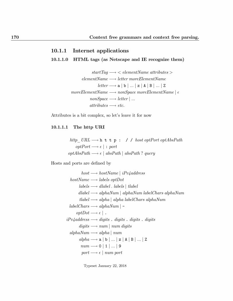
170 Context free grammars and context free parsing.
10.1.1 Internet applications
10.1.1.0 HTML tags (as Netscape and IE recognize them)
startTag −→ < elementName attributes >
elementName −→ letter moreElementName
letter −→ a | b | ... | z | A | B | ... | ZmoreElementName −→ nonSpace moreElementName | ε
nonSpace −→ letter | ...attributes −→ etc.
Attributes is a bit complex, so let’s leave it for now
10.1.1.1 The http URI
http_URL −→ h t t p : / / host optPort optAbsPath
optPort −→ ε | : port
optAbsPath −→ ε | absPath | absPath ? query
Hosts and ports are defined by
host −→ hostName | iPv4addresshostName −→ labels optDot
labels −→ dlabel . labels | tlabeldlabel −→ alphaNum | alphaNum labelChars alphaNum
tlabel −→ alpha | alpha labelChars alphaNum
labelChars −→ alphaNum | -optDot −→ ε | .
iPv4address −→ digits . digits . digits . digits
digits −→ num | num digits
alphaNum −→ alpha | numalpha −→ a | b | ... | z | A | B | ... | Znum −→ 0 | 1 | ... | 9port −→ ε | num port
Typeset January 22, 2018

10.2 Recognition and Parsing 171
Paths
absPath −→ / segments
segments −→ segment | segment / segments
segment −→ etc
query −→ etc
I won’t go into all the details, but just comment that a segment is asequence of almost any characters, as is a query.
10.1.1.2 Protocols
In this case the tokens are requests and replies. Requests go from client toserver and replies from server to client.
This is a greatly simplified FTP (File Transfer Protocol).
session −→ greetingRequest greetingReply moreSesn
moreSesn −→ quitRequest quitReply
| sendFileRequest sendFileReply moreSesn
| sendFileRequest errorReply moreSesn
| getFileRequest getFileReply moreSesn
| getFileRequest errorReply moreSesn
The syntax of the various requests and replies can also be specified in termsof sequences of bytes, just as tokens are specified in compilers.
10.2 Recognition and Parsing
Given a grammar G, the recognition problem is thisInput: A string w of terminal symbols.Output: Whether or not w is in L(G)Parsing problems are similar, but the output also includes a useful data
structure when w ∈ L(G).For example:
• In a compiler: we might output an abstract syntax tree.
Typeset January 22, 2018

172 Context free grammars and context free parsing.
• In a calculator: we might output the numerical value of an expression.
• We might output machine code or a reverse polish notation (RPN)representation of the input.
10.3 Derivation Trees and Left-most Deriva-
tions
Definition 86 A left-most derivation is one where, at each step, the left-most nonterminal is replaced. We write α =⇒lm β
More formally, have α =⇒lm β iff there are A, s, γ, and δ such thatα = sAγ and A −→ δ and β = sδγ. (Recall that s ∈ S∗).
We write α∗
=⇒lm β to indicate that there is a derivation of β from α in0 or more left-most production steps.
Given a grammar G and a string s in L(G) we can consider a tree thatillustrates the proof that the tree is in the language. Any derivation corre-sponds to a “derivation tree”.
Example
exp −→ num | id | exp bop exp | uop exp | ( exp )bop −→ + | - | / | * | = | !=uop −→ + | -
Consider the input 2*i+j, which as a string of terminals is: num * id +id. One derivation is
exp =⇒ exp bop exp
=⇒ exp bop id
=⇒ exp bop exp bop id
=⇒ exp bop id bop id
=⇒ exp ∗ id bop id=⇒ num ∗ id bop id=⇒ num ∗ id + id
Typeset January 22, 2018

10.3 Derivation Trees and Left-most Derivations 173
from which we can build the following “derivation tree”.
exp
expexpbop
exp expbop
idnum id* +
We can build a “left-most derivation” by traversing the tree depth-first andleft to right, expanding the nonterminal that we encounter
exp =⇒lmexp bop exp
=⇒lmexp bop exp bop exp
=⇒lmnum bop exp bop exp
=⇒lmnum * exp bop exp
=⇒lmnum * id bop exp
=⇒lmnum * id + exp
=⇒lmnum * id + exp
But with the same grammar and the same string, we can build a differenttree.
exp
exp
expbop
expexp
bop
idnum id* +
Typeset January 22, 2018

174 Context free grammars and context free parsing.
The corresponding left-most derivation
exp =⇒lmexp bop exp
=⇒lmnum bop exp
=⇒lmnum * exp
=⇒lmnum * exp bop exp
=⇒lmnum * id bop exp
=⇒lmnum * id + exp
=⇒lmnum * id + id
10.3..3 Ambiguity
Definition: We say that a grammar is ambiguous iff for some string thereexist two or more derivation trees.
Equivalently: a grammar is ambiguous iff some string has two or moreleft-most derivations.
For many applications, we should avoid ambiguous grammars since
• other matters (semantics) are generally described in terms of the gram-mar and we don’t want ambiguous semantics.
• it is hard to build an efficient parser for ambiguous grammars.
For other applications: e.g. natural language understanding, ambiguityis useful.
Consider
• “I saw a bird with a telescope”
• “I saw a man with a hat”
• “I saw a man with a telescope”
All 3 sentences fit the pattern
pronoun verb det noun prep det noun
but, in the first, the prepositional phrase attaches to the verb, whereas inthe second the prepositional phrase attaches to the object. This means wewant multiple derivation trees for the same sequence of word forms.
Typeset January 22, 2018

10.3 Derivation Trees and Left-most Derivations 175
10.3.0 Ambiguity and expression grammars
Here is a grammar for expressions Exp0
E −→ n | ( E ) | E + E | E - E | E * E | E / E
This grammar is highly ambiguous.
How many derivation trees are there for n - n / n / n - n ?14? In a sense only 1 reflects the correct precedence and associativity of
the operators.To ‘enforce’ ‘correct’ parsing of expressions we can write a new grammar,
Exp1
E −→ T | E + T | E - T
T −→ F | T * F | T / F
F −→ n | ( E )
This grammar is unambiguous.
10.3.0.0 Left-recursion
A nonterminal A is said to be left-recursive if there is a derivation
A∗
=⇒ Aβ
with at least one step (for some β).A grammar is left-recursive iff it has at least one left-recursive nontermi-
nal.Clearly both Exp0 and Exp1 are left recursive. Here is an unambiguous
grammar for the same language as Exp0 and Exp1 that is not left-recursive.Exp2:
E −→ T E1
E1 −→ + T E1 | - T E1 | εT −→ F T1
T1 −→ * F T1 | / F T1 | εF −→ n | ( E )
Typeset January 22, 2018

176 Context free grammars and context free parsing.
10.4 Top-Down predictive parsing and recog-
nition.
A top-down predictive parser works by trying to build the derivation treefrom the top down.
For example here is a derivation tree that is partially built.
Consumedinput
Input yet to beconsumed
if id = id id := id else print id end
stat
exp stat statif
expexp bop
else
id =
The leaves of the tree are if id = exp stat else statThis tree is a proof that
stat∗
=⇒ if id = exp stat else stat
10.4.0 Conceptual view
The idea is to walk the derivation tree in a depth-first manner, while (con-ceptually) building the tree and consuming the input. Circled nodes are notyet visited. The left to right sequence of circled nodes is called the prediction.
Typeset January 22, 2018

10.4 Top-Down predictive parsing and recognition. 177
10.4.1 Augmenting the grammar
It will simplify things later if we augment the grammar with
• a new terminal: $
• a new starting nonterminal A′start and
Typeset January 22, 2018

178 Context free grammars and context free parsing.
• a new production rule A′start −→ Astart $, where Astart was the originalstarting nonterminal.
We will also add a $ to the end of each input string.
(Typically $ represents the end of the file.)
10.4.2 States, steps, and stops
We will process one terminal at a time.
10.4.2.0 States
A top-down predictive parser’s state consists of
• the input processed so far s
• and the current prediction α
• and the remaining input sequence, t
Let’s write this as
s�α, t
(Note: we don’t represent the partially built tree, but only the sequenceof unvisited nodes α).
As a loop invariant we’ll have that
A′start∗
=⇒lm sα
and that st = w$ where w is the original input.
As an initial state we’ll start with
ε�A′start, w$
where w is the input string.
Typeset January 22, 2018

10.4 Top-Down predictive parsing and recognition. 179
10.4.2.1 Steps
We use two rules to step from one state to another
• Shift: (Read one terminal from the input)
s�aβ, au 4 sa�β, u
• Produce: (Expand the left most nonterminal)
s�Aβ, t 4 s�γβ, t
where A −→ γ is a production rule.
Theorem: Astart∗
=⇒ w iff there is a sequence of steps that goes
ε�A′start, w$ 4 ... 4 w$�ε, ε
10.4.2.2 Stopping
• Successful stop: We stop when the state is s�ε, ε, in which case (fromthe invariant) the input w is in the original grammar.
• Error stop 0: We also stop when the predicted input does not matchthe actual input, i.e. the state is s�aβ, bu where a �= b.
• Error stop 1: We also stop when the state is s�Aβ, t and there is noappropriate production rule.
If we come to a “Successful stop” then
• the input was in the language. Astart∗
=⇒ w
If we come to an “Error stop” then either
• the input was not in the language,
• or we made a bad choice in a ‘produce’ step.
Later we’ll see how to avoid bad choices.
Typeset January 22, 2018

180 Context free grammars and context free parsing.
10.4.3 Example
Here is a trace of the algorithm for grammar Exp2 (augmented) and an inputof n * n
s�α, t Actionε�E
′, n * n $ Produce E′ −→ E$4 ε�E $, n * n $ Produce E −→ T E14 ε�T E1 $, n * n $ Produce T −→ F T14 ε�F T1 E1 $, n * n $ Produce F −→ n4 ε�n T1 E1 $, n * n $ Shift4 n�T1 E1 $, * n $ Produce T1 −→ * F T14 n�* F T1 E1 $, * n $ Shift4 n * � F T1 E1 $, n $ Produce F −→ n4 n * �n T1 E1 $, n $ Shift4 n * n �T1 E1 $, $ Produce T1 −→ ε4 n * n �E1 $, $ Produce E1 −→ ε4 n * n �$, $ Shift4 n * n $�ε, ε Success
So the string is in the language.
10.4.4 In a more algorithmic form
Note that s is not really needed in the state unless we use it to help pick theproduction rule, which we will not do.
Algorithm: Top down predictive parsingInput: A string wOutput: ‘success’ or ‘error’. If the output is ‘success’ then w ∈ L(G). If
the output is ‘error’, then either w /∈ L(G) or a bad choice was made.
var t := w$ // where w is the input stringvar α := A′start // Note: α behaves as a stack.while α �= ε do
if α(0) ∈ S then
if α(0) = t(0) then (
// Shift stept := tail(t)
Typeset January 22, 2018

10.4 Top-Down predictive parsing and recognition. 181
α := tail(α) )
else // α(0) �= t(0)
error
else /* α(0) ∈ V */ (
try to pick a suitable production rule α(0) → γif a suitable production rule exists
// Produce stepα := (γˆtail(α))
else // no suitable production rule exists
error ) )
if t = $ then success else error
(tail(s) is the string [s(1), s(2), ..., s(‖s‖ − 1)]. error means stop withoutput ‘error’. success means stop with output ‘success’)
Assuming the grammar is not left-recursive, the top-down predictive pars-ing algorithm must terminate and is O(N) time, where N is the length ofthe input.
To be done: We still haven’t said how to pick a suitable production rulewhen a nonterminal comes to the top of the α stack.
10.4.5 LL(1) Grammars
Definition: An augmented grammar is called an ‘LL(1) grammar’ when thesuitable production rule can always be chosen on the basis of the next inputitem t(0) and the left-most nonterminal α(0).
Left-recursive grammars can never be LL(1). (Why?)For each production rule A −→ γ we compute the set of terminals which
t(0)might equal whenA −→ γ is chosen as the production rule in a successfulrun of the TDPP algorithm.
This set is called the selector set of the algorithm.So let’s consider Exp2 augmented
E′ −→ E$ {n, (} T1 −→ * F T1 {*}E −→ T E1 {n, (} T1 −→ / F T1 {/}E1 −→ + T E1 {+} T1 −→ ε {$, ),+, -}E1 −→ - T E1 {-} F −→ n {n}E1 −→ ε {$, )} F −→ ( E ) {(}T −→ F T1 {n, (}
Typeset January 22, 2018

182 Context free grammars and context free parsing.
On the right we have a selector set for each production rule.We implement the picking part of the algorithm
/*do pick a suitable production rule α(0) → γ by*/
if there is a production rule α(0) → γwith t(0) in its selector set then
pick that production rule
else
there is no suitable production rule
A grammar is LL(1) iff for each nonterminal A and for each pair of pro-ductions for A, the selectors sets of the two productions are disjoint.
I.e. a grammar is LL(1) iff, for all A, α, β, such that A −→ α andA −→ β are distinct productions,
(SelectorSet (A −→ α)
∩ SelectorSet (A −→ β)
)= ∅
10.4.5.0 Computing the selector sets.
Consider the selector set for a production rule A −→ αLook at E1 −→ + E. It is clear that this production rule should only
be picked if the next terminal is a + sign.From the example it is clear that if α
∗=⇒ bβ then b should be in the
selector set of A −→ α.But there is more to it then that when α
∗=⇒ ε.
Consider E1 → ε the next item in the input should be one that couldlegitimately follow an E1 in a successful derivation. Only items that couldfollow E qualify and these are $ and ).
Suppose A′start∗
=⇒ βAbγ =⇒ βαbγ∗
=⇒ βbγ then b should be in theselector set of A −→ α.
(Note that A′start∗
=⇒ βA =⇒ βα∗
=⇒ β is not possible!)Define functions First and Follow for an augmented grammar by
• b ∈ First(α) iff α∗
=⇒ bβ, for some β and
• b ∈ Follow(A) iff A′start∗
=⇒ βAbγ, for some β and γ.
Typeset January 22, 2018
10.5 Recursive Descent Parsing 183
The selector set for A −→ α is
First(α), when α∗
�=⇒ ε
and isFirst(α) ∪ Follow(A), when α
∗=⇒ ε
10.5 Recursive Descent Parsing
Recursive descent parsing works on the same principle as our state basedparser, but uses the call-return stack rather than an explicit stack.
To write a recursive descent parser, we create a subroutine for each non-terminal.
Let t be the input stream (a global variable)The subroutine for nonterminal A has as its specification.
if(∃u, v · t = uv ∧ A ∗
=⇒ u)
then t := some v such that(∃u · t = uv ∧ A ∗
=⇒ u)
else error
I.e., each subroutine is responsible for recognizing a string u produced by itsnonterminal in the input and removing that string from the remaining input.
Furthermore, each subroutine is responsible for reporting an error if theremaining input does not start with a string that can be derived from A.
10.5.0 Recursive Descent parsing of LL(1) grammars
If the grammar is LL(1) then creating an R.D. parser for it is a mechanicalprocess.
Let’s look at an example. We can write a recursive descent recognizer forExp2 as follows
global var t ·
procedure main is
t := w ‘$’ ; // Where w is the inputSPrime
Typeset January 22, 2018

184 Context free grammars and context free parsing.
procedure consume is
t := tail(t)
procedure expect( a ) is
if t(0) = a then consumeelse error
procedure SPrime is
E ;expect( ‘$’ )
procedure E is
if t(0) ∈ {‘n’,‘(’} then (
T ;E1 )
else
error
procedure E1 is
if t(0) = ‘+’ then (
consume ;T ;E1 )
else if t(0) = ‘-’ then (
consume ;T ;E1 )
else if t(0) /∈ {‘$’,‘)’} then
error
... T and T1 are similar to E and E1 ...
procedure F is
Typeset January 22, 2018

10.5 Recursive Descent Parsing 185
if t(0) = ‘n’ then
consume
else if t(0) = ‘(’ then (
consume ;E ;expect( ‘)’ ) )
else error
10.5.1 Getting results
Often we not only want to recognize the input but also process the input tocreate an output in the case where the input is recognized.
We can do this by augmenting the recursive decent parser with extracode.
As an example, we will produce numbers.
global var t ·
procedure main is
t := w ‘$’ ; // Where w is the inputoutput SPrime
procedure SPrime is
var p := E ·expect( ‘$’ )return p
Typeset January 22, 2018

186 Context free grammars and context free parsing.
procedure E is
if t(0) ∈ {‘n’,‘-’} then (
var p := T ·return E1(p))
else
error
procedure E1( p ) is
if t(0) = ‘+’ then (
t := tail(t) ;var q := T ·return E1( p + q ) )
else if t(0) = ‘-’ then (
t := tail(t) ;var q := T ·return E1( p− q ) )
else if t(0) /∈ {‘$’,‘)’} then
error
else
return p
... T and T1 are similar to E and E1 ...
procedure F is
if t(0) = ‘n’ then (
var p:= the value associated with t(0)·t := tail(t) ;return p )
else if t(0) = ‘(’ then (
t := tail(t)var p:= E then (expect( ‘)’ ) )return p
else error
Typeset January 22, 2018

10.5 Recursive Descent Parsing 187
Consider parsing the sequence: 10-2*3-1 As a string of terminals wehave n-n*n-n.
We have the following call tree which reflects the parse tree. Returnvalues are shown after the colon.
Sprime
E : 3
T : 10
F : 10 E1(4) : 3T1(10) : 10
10
- T : 6
E1(10) : 3
-T : 1
E1(3) : 3F : 2 T1(2) : 6
2 * F : 3 T1(6) : 6
31
F : 1 T1(1) : 1
$
10 - 2 * 3 - 1 $
Parsing 10-2*3-1 with the parameter values and the return values shown.
ε
εε
ε
Questions to consider:
• Can you modify the recursive descent parser above to produce an ab-stract syntax tree for an expression?
Typeset January 22, 2018

188 Context free grammars and context free parsing.
• Can you modify the recursive descent parser above to produce RPN?
• How could you alter the top-down predictive recognizer to compute re-sults rather than to just recognize? Hint: consider adding “commands”to the productions and executing the commands when they come to thetop of the stack. See the ‘Command’ pattern in Gamma et al.
• Can you modify the grammar Exp2 with added commands so that itcomputes the right result (hint use an extra stack to hold intermediateresults).
• Add unary operators to the grammar Exp2 so that you get a LL(1)grammar. Can you parse 12/− 2 ?
10.6 Dealing with non LL(1) grammars
10.6.0 Converting to LL(1)
In many cases we can convert an non-LL(1) grammar to an LL(1) grammar.
10.6.0.0 Factoring
When two productions for a nonterminal start the same way, the nonterminalwill not be LL(1).
Example
Stat −→ if Exp then Stat end
Stat −→ if Exp then Stat else Stat end
The terminal if will be in the selector sets of the first to productions.We can factor out the common left parts to get:
Stat −→ if Exp then Stat MoreIf
Stat −→ other
MoreIf −→ else Stat end
MoreIf −→ end
Typeset January 22, 2018
10.6 Dealing with non LL(1) grammars 189
10.6.0.1 Eliminating left recursion
Consider a sequence of one or more items separated by commas
List −→ List , item
List −→ item
We can replace these rules with equivalent productions
List −→ item List′
List′ −→ , item List′ | εIn general you can eliminate direct left-recursion by replacing rules
A −→ Aα0 | Aα1 | β0 | β1with rules
A −→ β0A′ | β1A′
A′ −→ α0A′ | α1A′ | ε
There exist methods for eliminating indirect left-recursion, e.g.:
A −→ Bα | β B −→ Aγ | δ
10.6.0.2 Is that all there is to it?
The above methods will convert many grammars to LL(1) form.But not all.In fact there exist languages for which there exists no LL(1) grammar.Consider if statements in C/C++/Java/Pascal
Stat −→ if ( E ) Stat MoreIf | . . .MoreIf −→ else Stat | ε
E −→ ...
(This is not LL(1) since else is in Follow(Stat) )You can still use recursive decent or top-down predictive parsing, in this
case, but you have to use a means other than the selector set to pick theproduction rule.
For example in the “ambiguous else” example, the parser should pick thefirst production rule for MoreIf when the next terminal is else.
Typeset January 22, 2018

190 Context free grammars and context free parsing.
10.7 Bottom-up, Shift-Reduce Parsing
We don’t need (or use) augmented grammars for this.
10.7.0 State
In this parsing method the state is α∧t where
• α is a stack (top is at right) representing consumed input and
• t is the remaining input
We initialize the state to ε∧w$, where w is the original input, where w isthe original input and $ is a symbol not in S
Invariant: αt∗
=⇒ w$ I.e. there is a derivation from αt to w$.
10.7.1 Steps
There are two kinds of steps
• Shift steps: α∧au 4bu αa∧u
• Reduce steps: βγ∧t 4bu βA∧t
where A −→ γ is a production rule
10.7.2 Stops
• State Astart∧$ means success
• If neither a shift nor a reduce can lead to a successful parse, then anerror is declared.
10.7.3 Example using grammar Exp1
E −→ T | E + T | E - T
T −→ F | T * F | T / F
F −→ n | ( E )
Typeset January 22, 2018

10.7 Bottom-up, Shift-Reduce Parsing 191
α∧t$ Actionε∧n - n * n - n $ Shift
4bu n ∧ - n * n - n $ Reduce F −→ n
4bu F ∧ - n * n - n $ Reduce T −→ F4bu T ∧ - n * n - n $ Reduce E −→ T4bu E ∧ - n * n - n $ Shift4bu E - ∧ n * n - n$ Shift4bu E - n ∧ * n - n$ Reduce F −→ n
4bu E - F ∧ * n - n $ Reduce T −→ F4bu E - T ∧ * n - n $ Shift4bu E - T * ∧ n - n$ Shift4bu E - T * n ∧ - n $ Reduce F −→ n
4bu E - T * F ∧ - n $ Reduce T −→ T * F4bu E - T ∧ - n $ Reduce E −→ E - T4bu E ∧ - n $ Shift4bu E - ∧ n$ Shift4bu E - n ∧$ Reduce F −→ n
4bu E - F ∧$ Reduce T −→ F4bu E - T ∧$ Reduce E −→ E - T4bu E∧$
Notice how this traces out a (right-most) derivation in reverse.
10.7.4 LR(1) grammars and Parser Generators
Definition: If you can always pick the correct step on the basis of
• the current stack, and
• the first terminal in the remaining input
then the grammar is said to be LR(1)Theorem (Knuth): This decision can be made by running a deterministic
finite state machine on the stack and then basing the decision on the finalstate of that machine and the next terminal.
Theorem (Knuth): LR(1) grammars can be parsed in O(N) timeProof idea: Represent the stack of symbols with a stack of finite machine
states (this is a data refinement). Then only the top state on this stack andthe next input symbol need to be consulted, not the whole stack.
Typeset January 22, 2018

192 Context free grammars and context free parsing.
Theorem: All LL(1) grammars are LR(1).Why: LL(1) parsers must decide the production rule for A on the basis
of the first symbol after the start of A. An LR(1) parser must decide theproduction rule for A on the basis of the first symbol after the end of A.Thus an LR(1) parser has at least as much information on which to base adecision.
Implementing an LR(1) parser by hand is not easy for nontrivial gram-mars.
The “yacc” and “bison” parser generators use shift-reduce parsing andcan handle almost all LR(1) grammars.
yacc and bison produce parsers written in C.
10.7.5 Deterministic shift-reduce parsing
Algorithm: Deterministic shift-reduce parsingInput: a string wOutput: ‘error’ or ‘success’
var t := w$· // where w is the input stringvar α := ε· // Note: α behaves as a stack.while α �= Astart ∨ t �= [$] do (
var q := decide what to do ·if q = shift then (
α := (α ˆt(0)) ;t := tail(t) )
else if q = reduce(A → γ) then
let β be such that α = βγ·α := βA
else /* q = error */
error )
success
The tricky bit is deciding what to do next: There are three possibilities
Typeset January 22, 2018

10.8 Extended BNF (EBNF) 193
• shift
• reduce( A → γ ) where A → γ is a production and γ is the top of thestack.
• error
10.8 Extended BNF (EBNF)
Terminological aside: Context Free Grammars were invented by NoamChomsky in 1957 in the study of natural languages.
John Backus invented an equivalent formalism for describing program-ming languages.
Peter Naur used Backus’s notation in the description of Algol-60.Thus CFG notation is often called BNF for “Backus-Naur Form”
10.8.0 Back to Extended BNF (or extended CFGs)
We extend CFG notation with convenience notations.These do not extend range of languages we can describe.Each production rule now has the form
A −→ x
where A is a nonterminal and x is a regular expression over S ∪ V .For example we can write Exp3 (equivalent to Exp0, Exp1, Exp2) as
E −→ E; ((‘+’ | ‘-’ | ‘*’ | ‘/’); E)∗ | ‘(’;E; ‘)’ | ‘n’Revisiting the C++ Floating Number grammar. We can now be more
concise.
floatNum −→ fract exp?; (‘f ’ | ‘l’ | ‘F’ | ‘L’)?
| [‘0’− ‘9’]+; exp; (‘f ’ | ‘l’ | ‘F’ | ‘L’)?
fract −→ [‘0’− ‘9’]∗; ‘.’; [‘0’− ‘9’]+ | [‘0’− ‘9’]+; ‘.’
exp −→ (‘e’ | ‘E’); (‘+’ | ‘−’ | ε); [‘0’− ‘9’]+
Typeset January 22, 2018

194 Context free grammars and context free parsing.
10.8.1 EBNF is no more powerful than CFGs
Given an EBNF grammar, we can rewrite its productions to obtain a CFGfor the same language:
Algorithm: Apply the following replacements until the grammar is aCFG..
A→ (P ) replace with A → PA→ P ∗ replace with A → A′
A′ → ε | P A′A→ P ;Q replace with A → A1A2
A1 → PA2 → Q
A→ P | Q replace with A → A1 | A2A1 → PA2 → Q
where A1 and A2 are brand-new nonterminals.
10.8.2 Recursive Descent Parsing with EBNF
We can implement repetition with a while loop and choice with and if.Consider this augmented grammar for expressions Exp4
E′ −→ E $
E −→ T ((‘+’ | ‘-’) T )∗T −→ F ((‘*’ | ‘/’) F )∗F −→ ‘n’ | ‘(’ E ‘)’
The choices implicit in the repetitions can be made on the basis of the nexttoken since:
• neither + nor - are in the Follow set of E
• neither * nor / are in the Follow set of T
We can implement E with a subroutine
procedure E is
Typeset January 22, 2018

10.8 Extended BNF (EBNF) 195
var p:= T ·while t(0) ∈ {‘+’,‘-’} do
if t(0) = ‘+’ then (
t:= tail(t) ;var q := T ·p:= p+ q )
else (
t := tail(t) ;var q:= T ·p := p− q )
return p
Note that I didn’t bother to check that t(0) is ‘)’ or $ prior to returning,since the caller of E will presumably make that check and can provide abetter error message.
Parser Generation: The JavaCC parser generator accepts Extended BNFgrammars and produces parsers written in Java. (https://javacc.dev.java.net/)
10.8.3 Syntax diagrams (or railroad diagrams)
Syntax diagrams are similar to EBNF except, instead of using regular expres-sions, we use NDFRs. These NDFRs are conventionally drawn with networksof lines representing the states and boxes representing the transitions. Forexample:
Typeset January 22, 2018

196 Context free grammars and context free parsing.
10.9 Regular languages
Parsing with LL(1) and LR(1) grammars takes
• O(N) time and (worst case)
• O(N) space. (N is the length of the input)
Regular languages are those that take O(1) space.We can define regular languages in terms of grammars one of several
equivalent ways
Typeset January 22, 2018

10.9 Regular languages 197
10.9.0 First way
A regular language is one that can be described by an EBNF grammar withno recursion (direct or indirect) between the nonterminals
For example the syntax of floating point numbers in C++.Example:
M −→ $DD?D?(,DDD)∗.DD
D −→ 0 | 1 | 2 | 3 | 4 | 5 | 6 | 7 | 8 | 9
Counter-example:
E −→ (n ((+ | - | * | /) n)∗) | ‘(’ E ‘)’
has recursion.
10.9.1 Second way
A production rule is right linear if it is of the form
A −→ sB
or of the formA −→ s
(recall that s contains no nonterminal).A regular language is one that can described by a CFG containing only
right-linear productions.Example
A −→ $B
B −→ dC
C −→ D | dDD −→ E | dEE −→ , dddE|.dd
Counter-example:E −→ n | ‘(’ E ‘)’
Recursion of E is not at the very right of the production rule
Typeset January 22, 2018

198 Context free grammars and context free parsing.
10.10 Attribute grammars
Attribute grammars augment terminals and nonterminals with attributes.Each production has an boolean expression that must be satisfied at each
node in the derivation tree.
10.11 Recognition by “dynamic programming”
Input: A string w and a grammar G = (V, S, P,Astart) such that every pro-duction is in one of the following forms
A −→ a
A −→ B C
(Exercise. Show that any grammar such that ε /∈ L(G) can be trans-formed to an equivalent grammar that satisfies this constraint.)
Let n be the length of w.
var m : array {0, .., n} × {0, ..n} of P(V )// Each element of m is a set of nonterminalsfor (i, j) ∈ {0, .., n} × {0, ..n} do m(i, j) := ∅
The idea is to put into each elementm(i, j) all nonterminals that describethe substring w[i, .., j] where i < j.
for i ∈ {0, ..n} do m(i, i+ 1) := {A | A −→ w(i) ∈ P}
So far we have succeeded for substrings of length 1.We can ‘multiply’ two sets of nonterminals U and V as follows: if B ∈ U
and C ∈ V and A −→ B C is a production then A ∈ U ⊗ V . I.e.
U ⊗ V = {A,B,C | (A −→ B C) ∈ P ∧B ∈ U ∧ C ∈ V · A}
If s and t are strings and U contains all nonterminals B such that B∗
=⇒ sand V contains all nonterminals C such that C
∗=⇒ t, then U ⊗ V contains
all nonterminals A such that A∗
=⇒ sˆt.The rest of the algogithm fills in the table for segments of increasing
length.
for k from 2 to n do
Typeset January 22, 2018

10.11 Recognition by “dynamic programming” 199
for i ∈ {0, .., n− k} dolet j := i+ k·for ? ∈ {i+ 1, .., j − 1} dom(i, j) := m(i, j) ∪ (m(i, ?)⊗m(?, j))
Upon completion, the string is in the language iff Astart ∈ m(0, n).
Typeset January 22, 2018

200 Context free grammars and context free parsing.
Typeset January 22, 2018

Part 2
Efficiency
Typeset January 22, 2018


Chapter 11
Computation time
11.0 The RAM model of computation
If we are going to consider how long programs take to run, a natural questionis, “On what machine?” We could pick some particular current model ofcomputer. I’m writing this on an HP dv-4040ca, so why not that? Butthen our results would be very specific. Would they carry over to othercurrent computers or to future computers? In this part of the book, insteadof considering the time taken to run programs on particular computers, wewill try to draw conclusions about running time that will hold true over allcomputers – or at least a broad class of computers.
We will consider an idealized computer defined by the following statespace.
{“m” �→
(Ztot→ Z), “c” �→ N, “p” �→
(N
tot→ I), “A” �→ F(Z), “status” �→ {running, stopped}
}
where I is a set of instructions to be defined shortly. m is the data memory.c is the program counter, p is the program memory, A is the set of allocatedmemory locations, and s is a status flag used to indicate that the machine isdone. The notation F(Z) means the set of all finite subsets of integers. Wewill call this computer a Random Access Machine, or RAM for short.0
0The abbreviation RAM is a bit unfortunate, as the same three letters often stand for“Random Access Memory”. In both cases the word “random” doesn’t mean random atall, but rather that memory locations can be accessed in an arbitrary order, rather thansequentially, as with a tape.
Typeset January 22, 2018

204 Computation time
Compared to the state of a real computer, this is very simple. Real com-puters use many levels of storage, registers, cache, main memory. Multiplelevels exist for reasons of efficiency, we will abstract away from such detailsand so we don’t need to consider multiple levels of memory. Another simpli-fication is that we keep the program separate from the main memory. Thisis called a Harvard architecture, as opposed to the Princeton architecture,which puts the program in the main memory. A Princeton architecture al-lows self-modifying code, which we won’t need, and is very useful if you arewriting an operating system, which we won’t be doing.
You should note that m consists of an infinite number of cells. This isone reason that we call this an idealized computer; it never runs out of mem-ory. Designers of real computers attempt to approximate this idealizationby having very large physical memories and by using virtual memory. Youshould also note that each cell of m can hold any integer. This is anotheridealization. On typical real computers, each cell is limited to some smallnumber of bits, e.g. 8, 16, 32, 48, 64. It is then up to the software designers(and/or compiler writers) to lump together enough adjacent cells to holdwhatever number is desired. (And to deal with the consequences when theyhaven’t used enough cells to hold the result of a computation, i.e. to dealwith overflow.)
There are a few reasons for considering a computer with an infinite num-ber of cells. The first is that we want to consider the time required by aprogram to execute as a function of input size; and we want to consider whathappens as the input size goes to infinity. If we put any limit on the sizeof the memory, that will impose a limit on the size of the input and we’llbe stuck. The second reason is that the infinite memory model is close towhat programming languages try to provide. For example the new operatorin Java or C++ provides new cells without any a priori limit. As program-mers, we work with the abstraction of infinite memory, although if we aregood programmers, we also plan for the case where the abstraction fails, e.g.when the new operator throws an exception because memory has run out.It’s a bit like the physicist who works with an infinite and flat 3D space; weknow the real universe is finite, curved and expanding, but, most of the time,the abstraction is “good enough” and considerably simpler.
Now given that we have an infinite number of cells, is there a good reasonthat each cell should be able to hold any integer? Perhaps for the sake ofrealism, we should make each cell some fixed width w bits. E.g. w = 8is quite common in the real world. This simplification is sometimes made.
Typeset January 22, 2018

11.0 The RAM model of computation 205
Theoretical computer scientists often pick w = 1, as any other number islarger than absolutely necessary. However, fixed sized cells make programsmore complicated, as we have to deal with grouping cells together to obtainenough space to hold data. Even worse, as the size of the input heads towardinfinity, we might have to change the number of cells we lump together. Forexample, suppose we represent a graph by a list of edges; if w = 8 andthe number of nodes is less than 257, we can represent each edge with twomemory cells. However for graphs with 257 through 65, 536 nodes, we needfour cells per edge, and then for larger graphs, more cells. A second reasonfor not using fixed sized cells is that sometimes we want to store the addressof one cell in another cell, since addresses are integers, so are cell contents.
Now we need an instruction set I for the machine. I propose the followingset.
bpos(i, j) if m(j) > 0 then c := i else c := c+ 1call(i, j) m(j) := c+ 1; c := ireturn(i) c := m(i)halt() status := stoppedadd(i, j, k) m(i) := m(j) +m(k); c := c+ 1mult(i, j, k) m(i) := m(j)×m(k); c := c+ 1negate(i, j) m(i) := −m(j); c := c+ 1odd(i, j) if m(j) is odd then m(i) := 1 else m(i) := 0shift(i, j) m(i) := �m(j)/2 ; c := c+ 1fetch(i, j) m(i) := m(m(j)); c := c+ 1store(i, j) m(m(i)) := m(j); c := c+ 1load(i, j) m(i) := j; c := c+ 1
Why this set? Well, I admit that some of the choices are arbitrary, but I amguided by the following aims:
• I want to make sure that the machine is capable of any computing anyfunction that any other computer can compute. This property is calleduniversality.
• On the other hand, I want to keep the set of instructions small andsimple.
• A program that runs on the RAM should be easily translatable to onethat runs on a physical processor.
Typeset January 22, 2018

206 Computation time
• Finally I want to ensure that the number of steps taken by the machineto compute a function is similar to the number of steps taken by atypical physical central processor.
The first requirement, universality, turns out to be impossible to prove,at least in a mathematical sense. We can certainly prove that one model ofcomputation is as expressive as another, but it is hard to show that no onewill ever devise a more expressive model. Neverthelesss we can say that ourRAM is as expressive as any other “realistic” model of computation that hasbeen devised yet.
Thw final requirement involves a few subtleties. For example our RAMcan add any two integers in a single step, whereas a typical physical processor,having fixed width registers, would take several steps to, for example, add two100 digit numbers. On the other hand, most (but not all) physical processorshave an instruction that will divide two (fixed width) integers. On our RAM,division requires several instructions. Whether we have satisfied the finalrequirement depends on what we mean by “similar”.
Here is an example that shows that computation times on a RAM canbe misleading, if we are not careful. If m(0) is initially n, with n > 0, thisprogram computes 2(2
n) into m(1) in only 3n+ 3 steps.
0 : load(1, 2)
1 : load(−1,−1)
2 : mult(1, 1, 1)
3 : add(0, 0,−1)
4 : bpos(2, 0)
5 : halt()
For very very small n this is a realistic result. As soon as n = 5, we will findthat the program will not run on a 32 bit machine without using multiplememory locations to represent m(1). Furthermore, every time n inreasesby one the memory requirements of a real computer double and the timerequirement will surely at least double. The point of this example is to showthat we need to be careful about when to use the RAM model and aboutinterpreting results obtained with the RAM model.
Typeset January 22, 2018

11.1 Parameterized RAM 207
11.1 Parameterized RAM
A RAMw,s is a model of computation much like a RAM, but whose memoryconsists of s words that are each w bits wide; here s and w are integersgreater than 1 or are infinite. Define
words(w) =
{{−2w−1, ..2w−1} if w ∈ NZ if w = ∞
addresses(s) =
{{⌈−s2
⌉, ..⌈s2
⌉} if s ∈ N
Z if s = ∞
The type of the memory for a RAMw,s is addresses(s)tot→ words(w). Thus m
has type
• Z tot→ Z if w = ∞ and s = ∞
• Z tot→ {−2w−1, ..2w−1} if w ∈ N and s = ∞
• {⌈−s2
⌉, ..⌈s2
⌉} tot→ Z if w = ∞ and s ∈ N
• {⌈−s2
⌉, ..⌈s2
⌉} tot→ {−2w−1, ..2w−1} if s, w ∈ N.
For example, in a RAM8,99, the address space is {−49, ..50} and each memoryword holds a value in the range {−128, ..128}.
We also change the type of status to {running, stopped, crashed}.We redefine the instructions for the RAM of section 11.0 so that the
machine crashes rather than storing into a nonexistent location or storing avalue that is too big or too small. For example:
call(i, j) if j ∈ addresses(s) ∧ c+ 1 ∈ words(w) then (m(j) := c+ 1; c := i) else status := crasadd(i, j, k) if i, j, k ∈ addresses(s) ∧m(j) +m(k) ∈ words(w) then (m(i) := m(j) +m(k); c := c
Since a RAM∞,∞ never crashes, it is essentially the same as the RAM ofsection 11.0.
Our program for computing 2(2n) still takes linear time, but requires at
least a RAM2n+1,3.
Typeset January 22, 2018

208 Computation time
Typeset January 22, 2018

Chapter 12
A Dialogue concerning P = NPand NP -Completeness
Dramatis personae (with apologies to Galileo Galilei)
• Salviatus: A scholar who is well informed and perhaps a bit of a know-it-all.
• Sagredus: A willing and apt pupil.
• Simplicius: Another willing pupil, but one who is perhaps not as quickon the uptake as Sagredus
12.0 First day
S������: Salviati, good friend, we have heard that the question of whetherP = NP or not is considered by many to be the most important openquestion in computing science, but I have to confess that I’ve never reallyunderstood it. Perhaps, like much of mathematics, it is simply beyond whatI can fathom.S���� �: I seriously doubt that. The concepts aren’t hard. Like the
4-colour theorem, or Fermat’s last theorem, the proof that P = NP or thatP �= NP , if we ever have one, will no doubt be hard to follow, but thestatement of the question is easy to understand.S�������: Isn’t it just that NP means hard problems and P means
easy problems, so the P?= NP question just asks whether all hard problems
are easy. It seems a rather dumb question.
Typeset January 22, 2018

210 A Dialogue concerning P = NP and NP -Completeness
Figure 12.0: Can you colour the nodes of this graph with three colours sothat nodes connected by an edges are coloured differently?
S���.: No, NP is a set of problems whose affirmative answers can bequickly checked, given some evidence. NP includes both problems that wecan solve quickly (easy problems) and problems that we don’t know how tosolve quickly (apparently hard problems).
S���.: Can you give us an example?
S���.: If I claim that a number n is composite, this claim can be quicklychecked if I back it up with evidence. In this case the evidence would be twofactors p and q. You can quickly check the evidence by multiplying p byq and comparing the result to n. So the question of whether a number iscomposite or not is in NP .
S���.: Can you give us another example?
S���.: Consider the question of whether a graph can be 3-coloured.
S���.: Meaning?
S���.: A graph is 3-coloured iff each node of the graph is assigned oneof 3 colours such that each edge connects nodes of different colours. [SeeFigure 12.0] If a graph can be 3-coloured, there is a way to quickly convincesomeone that it can; here’s how: you simply write out a list of nodes andwrite a colour beside each, red, green, or blue. This list is the evidence.Anyone can quickly check that each edge connects nodes of different colours.[See Figure 12.1]
S���.: You keep using the word ‘quickly’, but what do you mean bythat?
Typeset January 22, 2018

12.0 First day 211
Figure 12.1: Evidence that the graph of Figure 12.0 can be 3-coloured.
S���.: That is a good question. I mean in polynomial time. That is,the checking problem can be solved in polynomial time with respect to thesize of the original input.
S���.: So in the example of determining whether a number n is com-posite, would the size be n?
S���.: When an input is an integer, it is usual to use the number ofbits required to represent the number; so for this problem, the input size is7log2 n8.S���.: And for the graph colouring example.
S���.: In that case, the number of nodes plus the number of edges willdo fine.
S���.: What about ‘no’ answers? Should there also be a quick way ofdemonstrating that the answer is ‘no’?
S���.: That is not needed for a problem to be in NP . If there is a quickway of showing that an answer is ‘no’, we say that the problem is in co-NP .(“co” stands for “complementary”.) It is quite possible for a problem to bein both NP and co-NP .
S���.: This all makes sense for problems that have ‘yes’ or ‘no’ as theiranswers, that is problems that ask one to determine whether its input is ina particular set or not.
S���.: That is true. The set NP contains only decision problems, whichsimply means problems with either ‘yes’ or ‘no’ as answer. We do that fortwo reasons. First it makes it simpler to translate between problems, we only
Typeset January 22, 2018

212 A Dialogue concerning P = NP and NP -Completeness
need to translate the inputs, the outputs need no translation. The secondreason is that it allows us to treat the ‘yes’ outputs differently from the ‘no’outputs, which is what we do in the definition of NP .S���.: So NP is the set of decision problems such that evidence for
affirmative answers can be checked in time that is polynomial with respectto the size of the original input.S���.: Exactly.S���.: I had thought thatNP problems were all hard, but this definition
seems to put no restriction on how easy a problem is, but rather on how hard.So no problem is too easy to be in NP .S���.: That’s right. Consider determining whether the shortest path
between two points in a graph is less than a given number. This problemcan be solved in polynomial time –use Dijkstra’s algorithm to calculate theactual size of the shortest path and then simply compare with the givennumber. We can use the actual shortest path as the evidence. It fits thedefinition of NP .S���.: You could also use as evidence, the input to the problem, that is
the graph, the two nodes, and the length. Then the checker can use Dijkstra’salgorithm.S���.: In fact any decision problem that can be solved in polynomial
time is in NP since all the evidence that is needed is the input to the problemitself.S���.: But I thought NP stood for ‘nonpolynomial.’S���.: Actually it stands for nondeterministic polynomial time. This
means that the problem is solvable in polynomial time on a kind of nonde-terministic computer. This special kind of computer has all the conventionalinstructions plus one special instruction called a “nondeterministic branch”.Whenever the nondeterministic branch is encountered, the machine takes thebranch or doesn’t as follows:
• If both choices inevitably lead to a ‘no’ output, then the choice betweenbranching and not branching is arbitrary.
• If both choices can lead to a ‘yes’ output, then the choice betweenbranching and not branching is again arbitrary.
• But, if only one choice can possibly lead to a ‘yes’ output, then thatchoice is taken.
Typeset January 22, 2018

12.0 First day 213
Here is a nondeterministic algorithm for determining whether a graph canbe 3-coloured.
read a graph (V,E)for each node v ∈ V
paint v rednondeterministic branch to Arepaint v greennondeterministic branch to Arepaint v blueA:
for each edge e ∈ Elet u and v be the endpoints of eif u and v are painted the same colour, output ‘no’ and stop
output ’yes’ and stop
Please understand that this kind of machine is simply used for thoughtexperiments. It’s not something we can really implement.
S���.: You could implement the nondeterministic branch by bracktrack-ing. I read a paper on this by Floyd [[citation needed]].
S���.: Yes, but that would take too long. We assume each nondeter-ministic branch takes constant time, just like a conventional instruction.
S���.: Could you implement a nondeterministic branch with paral-lelism? Every time a nondeterministic branch is encountered, create a newprocess. The new process takes the branch and the old one doesn’t. Onceall processes are done, ‘or’ the results computed by all the processes.
S���.: Yes. Unfortunately this is not efficient, as it takes a lot of hard-ware or a lot of time. In the 3-colouring example the number of processesneeded is 3N where N is the number of nodes in the input graph. If eachprocess runs on its own processor, this takes too much hardware – that is,more than a polynomial amount of hardware. If we time-share a polyno-mial number of processors, then it takes too long – that is, more than apolynomial amount of time. In general a nondeterministic polynomial timealgorithm can take an exponential amount of time, if we execute it on a con-ventional processor, and can take either an exponential amount of time oran exponential number of processors if executed on a multiprocessor madefrom conventional processors.
Typeset January 22, 2018

214 A Dialogue concerning P = NP and NP -Completeness
S���.: So when we talk about ‘time’ complexity, we really mean work,i.e. the time it takes to do something multiplied by the number of processorswe have.S���.: So now we have two definitions of NP . The first is based on
quickly checking evidence. The second is that NP problems are decisionproblems that can be solved with a nondeterministic machine in polynomialtime. Let’s call these two sets NP0 and NP1 respectively. I think I see whythese sets are the same.
Suppose a problem is in NP0. This means there is some evidence for‘yes’ answers that can be checked in polynomial time. Then we can write anondeterministic polynomial time algorithm for it as follows. The first part ofthe algorithm uses the nondeterministic branch instruction to construct theevidence. Since the size of the evidence must be polynomial in the size of theinput, this part will take only polynomial time. The second part uses onlyconventional instructions to check the evidence in polynomial time. (This isthe nature of the program you showed as an example.) The existence of thisalgorithm pattern shows that the problem is also in NP1. In conclusion anyproblem in NP0 is in NP1.
Now suppose that a problem is in NP1. We have a nondeterministic al-gorithm that runs in polynomial time. For ‘yes’ answers, a trace of thisalgorithm will serve as evidence that the answer is ‘yes’. In fact the only ev-idence we need is list of bits telling us whether or not each nondeterministicbranch is taken or not. (Say 0 for not taken, and 1 for taken.) In the graphcolouring example, 10100... would mean that the first three nodes are tobe painted red, green, and blue respectively. We can check the evidence bysimulating the execution of the algorithm, consulting the evidence each timewe need to know whether a branch is to be taken or not. Since the nonde-terministic algorithm takes polynomial time, so does the checking procedure.In conclusion any problem in NP1 is also in NP0. We now know that bothdefinitions for NP define the same set.S���.: Well done my friend.S���.: I’d read that NP is often defined using something called a Turing
Machine.S���.: Yes. Often the definition uses a mathematical model for comput-
ers called Turing Machines. Turing Machines are rather different from con-ventional computers, but for our purposes they amount to the same thing.The reason is that, while Turing Machines generally take more time to do thesame thing, compared to a conventional computer, they are only slower by a
Typeset January 22, 2018

12.1 Second day 215
factor that is polynomial in the size of the input. So when we ask whetheran algorithm takes polynomial time, it doesn’t matter whether we plan toexecute it on a conventional computer or a Turing Machine.
S���.: Getting back to P?= NP , we now know what NP is, so what is
P?S���.: P is thankfully much simpler. P is the set of decision problems
that can be solved in polynomial time on a regular computer.S���.: And since the same algorithm can be run on a nondeterministic
computer, we have that P ⊆ NP .S���.: Exactly.
S���.: So P?= NP asks whether these fictitious nondeterministic
branch instructions would really be that helpful. If P ⊂ NP , there is atleast one problem that can be solved quickly on the nondeterministic ma-chine, but not on a conventional machine. On the other hand if P = NP ,every problem in NP can be solved quickly on a conventional computer.S���.: Quite right.S���.: Well it’s a nice theory, but why is it important.S���.: A lot of practical problems are known to be in NP but are not
known to be in P –we don’t have fast algorithms for them. If P = NP,thenall these problems will have polynomial time algorithms. Furthermore, ifP = NP , that would imply that a number of problems that are not decisionproblems also have polynomial time solutions. Not so obvious is the dualto that. If P ⊂ NP , then this implies there are many problems (bothdecision and optimization) that can not be solved quickly. Knowing whetherP = NP or not would decide the difficulty of a large number of reallypractical problems that come up every day.S���.: How can that be? I can see that if P ⊂ NP , there is at least
one problem in NP that is difficult, but not that there are many. PerhapsP ⊂ NP but there is only one problem in NP that is difficult and that thatis a problem that no one happens to care about. Isn’t that possible?S���.: As I said, it is not so obvious that this is not the case. Let us
leave this question for another day.
12.1 Second day
S���.: Yesterday you told us that if P ⊂ NP , there is more than oneproblem in NP that can not be solved quickly.
Typeset January 22, 2018

216 A Dialogue concerning P = NP and NP -Completeness
S���.: Yes, that’s right. The key to this is to show that certain problemsare among the most difficult in NP .S���.: Most difficult in what sense, since it seems we don’t know how
difficult the most difficult problems in NP are?S���.: Suppose we have a problem Q in NP and we know that if any
problem in NP is difficult then Q is difficult. ...S���.: And by difficult, you mean that there is no polynomial time
algorithm for it.S���.: Yes, exactly. So in that case, we can say that Q is one of the
most difficult problems in NP . Any problem that is among the most difficultin NP in this sense is called NP -complete.S���.: So how can you show that a problem is NP -complete?S���.: Well suppose that Q and R are two problems in NP and that
we have a polynomial-time algorithm f that implements a function F suchthat Q(F (x)) = R(x), for all x. That is, f translates each input to R into aninput to Q. We say f is a polynomial-time reduction from R to Q. Now if Qis in P , then so is R since we can use a polynomial time algorithm for Q, incombination with our polynomial time algorithm for F , to get a polynomialtime algorithm for R. If Q is easy, so is R. Equivalently: if R is difficult, sois Q.S���.: Can you give an example?S���.: Sure. Let’s take PSAT and 3-Colouring and find a reduction
from 3-Colouing to PSAT, which is the problem of determining whether apropositional formula is satisfiable. ...S���.: Refresh my memory ...S���.: A propositional formula is just a formula that uses ands, ors, nots,
xors, equivalences, parentheses, and variables. A formula φ is satisfiable ifthere is a way to set each variable to true or false so that the whole formulais true.S���.: So that there is a line in its truth table where it’s true.S���.: Exactly.S���.: I can see that this could be useful in checking whether an acyclic
digital circuit meets its specification. Suppose ψ is the formula for a circuitwith inputs u and outputs v and φ is the specification for that circuit withinputs x and outputs y, then we could check a formula
(x0 = u0) ∧ (x1 = u1) ∧ · · · ∧ ψ ∧ φ ∧ ((v0 �= y0) ∨ (v1 �= y1) ∨ · · · )If it’s not satisfiable then, the circuit and its specification are equivalent.
Typeset January 22, 2018

12.1 Second day 217
S���.: Just so. And that’s just one application, there are plenty ofothers. You can see that PSAT is a useful problem on its own. Now we cansee that if 3-Colouring is hard, then so is PSAT ...S���.: So we need to transform each graph that might be input into
3-Colouring into a formula so that the graph has a 3-Colouring exactly if theformula can be satisfied.S���.: And the formula must be produced in polynomial time with
respect to the size of the graph.S���.: Exactly. Given any graph G = (V,E) we can produce a formula
with 3× |V | variables. For each node u ∈ V we have variables Ru, Gu, andBu. The idea is that Ru = true represents vertex v being coloured red. Weneed to say that each vertex is given one and only one colour, so for eachvertex u we need
(Ru ∨Gu ∨ Bu) ∧ ¬ (Ru ∧Gu) ∧ ¬ (Gu ∧ Bu) ∧ ¬ (Bu ∧Ru)
and we conjoin (and-together) the formulas for all the vertices. Then foreach edge {u, v} ∈ E we need a conjunct
¬(Ru ∧Rv) ∧ ¬(Gu ∧Gv) ∧ ¬(Bu ∧ Bv).
For example for a completely connected graph with three nodes ({0, 1, 2} , {{0, 1} , {1, 2} , {0, 2}})we would have
(R0 ∨G0 ∨B0) ∧ ¬ (R0 ∧G0) ∧ ¬ (G0 ∧B0) ∧ ¬ (B0 ∧R0)∧ (R1 ∨G1 ∨B1) ∧ ¬ (R1 ∧G1) ∧ ¬ (G1 ∧B1) ∧ ¬ (B1 ∧R1)∧ (R2 ∨G2 ∨B2) ∧ ¬ (R2 ∧G2) ∧ ¬ (G2 ∧B2) ∧ ¬ (B2 ∧R2)∧¬(R0 ∧R1) ∧ ¬(G0 ∧G1) ∧ ¬(B0 ∧ B1)∧¬(R1 ∧R2) ∧ ¬(G1 ∧G2) ∧ ¬(B1 ∧ B2)∧¬(R2 ∧R0) ∧ ¬(G2 ∧G0) ∧ ¬(B2 ∧ B0)
This algorithm for producing formulas from graphs is a polynomial-time re-duction from 3-Colouring to PSAT.
3COL −→ PSAT
Now if we have a quick (polynomial time) algorithm for PSAT, we havea quick algorithm for 3-Colouring. So that shows that if 3-coloring is hard,so is PSAT.
Typeset January 22, 2018

218 A Dialogue concerning P = NP and NP -Completeness
S���.: So back to NP -completeness, to show that a problem Q is NP -complete, we need to show that for every problem R in NP , there is apolynomial-time reduction from R to Q.S���.: This seems a difficult thing to prove. Are there any problems
known to be NP -complete?S���.: Yes there are. In fact there are many. It turns out that once
you know one problem is NP -complete, you can build on that knowledge toshow that other problems are NP -complete without having to worry aboutreductions from every problem in NP .S���.: I think I see why. Suppose we know that S is NP -complete and
we are wondering whether a problem Q, that is known to be in NP , is alsoNP -complete. Since S is NP -complete, we know that , for any problem Rin NP , there is a polynomial-time reduction f from R to S. Suppose wecan find a polynomial time reduction g from S to Q; then, for every problemR in NP , there is also a polynomial-time reduction from R to Q formed bycomposing f with g; thus Q is NP -complete.
Rf−→ S
g−→ Q and so Rf ;g−→ S
S���.: I see, because executing one polynomial-time algorithm and thenanother is still polynomial-time.S���.: Exactly. And the more problems we learn to be NP -complete,
the easier it becomes to show that yet others are as well, because we thenhave more choices of problems to reduce from, that is a wider choice forSagredus’s S.S���.: So if you think of NP-completeness as a disease, then a polynomial
time reduction from S to Q allows the disease to spread. If S is NP-complete,then Q must be too.S���.: OK. But don’t you need a patient zero? You need to start by
showing that some particular problem is NP-Complete, and that means youhave to find an infinite number of reductions, one for each of the other prob-lems in NP . That seems an impossible task.S���.: Nevertheless, that’s exactly what was done by Stephen Cook in
1971. He found that any problem in NP can be reduced to PSAT.S���.: and how did he do that?S���.: Suppose you have a problem R in NP . We need to be able to
transform any input x toR represented as a sequence of bits [x0, x1, · · · , xn−1],to a formula φx that is satisfiable exactly if R(x).
Typeset January 22, 2018

12.1 Second day 219
Since R is in NP , there is a nondeterministic program r for R that runsin polynomial time, say no more than p(n) steps on a particular computer,for each input of size n, where p is some polynomial function.S���.: A computer with a nondeterministic branch instruction.S���.: Right, a computer with a nondeterministic branch instruction. A
deterministic program defines a function that maps the state of the computerin one time cycle to the state of the computer in the next time cycle. (You canarrange that when the algorithm is done, the function acts as the identityfunction.) A nondeterministic program defines a relation that maps eachstate of the computer to one or more states in the next time cycle. Since rimplements a decision algorithm, we can assume that one particular bit ofmemory is used to represent the output, say bit o. For each input size n wecan workout the maximum number of additional bits of memory the programneeds, say q(n). Of course q(n) must be polynomial, since the algorithm onlyhas a polynomial amount of time to read or write the bits. We’ll call thesebits b0, b1, ... , bq(n)−1. We can also assume that some of these bits initiallyhold the input at the start of the computation, say bits b0 to bn−1. Now foreach input x of size n, you can create a formula φ as follows: You use a bunchof boolean variables to represent the state of the memory and registers attime 0 (say o0, b0,0 b1,0, and so on up to bq(n)−1) and a bunch of other variablesto represent the state of the memory at time 1 (say o1, b0,1 b1,1, and so on upto bq(n)−1,1); and you can use a formula ψ0 to represent the relation betweenthese two states defined by r. Then you use a bunch more boolean variablesto represent the state at cycle 2 and make a formula ψ1 to represent therelation between the state in cycle 1 and the state in cycle 2. And so onfor all p(n) steps. Finally you conjoin (‘and’ together) all these one-stepformulas
ψ = ψ0 ∧ ψ1 ∧ · · · ∧ ψp(n)−1We can throw in a formula that forces the variable representing the outputbit at cycle p(n) to be true and formulas that force the states of the bitsrepresenting the input to represent x in cycle 0. Now we have a big formula
φx = ψ ∧ op(n) ∧ (b0,0 = x0) ∧ · · · ∧ (bn−1,0 = xn−1)
Now if R(x) is true, then there is a computation of r that starts with theinput bits set to [x0, x1, · · · , xn−1] and ends with the output bit being trueafter p(n) cycles, thus there is a way to set all the propositional variablesof φ that satisfies φ. On the other hand, if R(x) is false, there can be no
Typeset January 22, 2018

220 A Dialogue concerning P = NP and NP -Completeness
computation of the program r with input x and the output being ‘yes’; andso, in this case, φ is not satisfiable.S���.: That’s a big formula.S���.: Yes, but since the algorithm takes a polynomial amount of time,
it can’t use more than a polynomial number of bits, so the whole computationcan be represented by a polynomial number of boolean variables. The size ofthe whole formula is still only a polynomial function of n and the time takento produce it is also polynomial.S���.: So for any problem R in NP , we can make a transformation,
based on a nondeterministic program r for R and a polynomial time boundp, that turns any input x to R into a formula that is satisfiable exactlyif R(x). Furthermore, it only takes polynomial time to do so. Let’s callthis transformation compiler,p. Now if the satisfiability problem PSAT canbe solved in polynomial time, by a regular algorithm sat, we can solve anyproblem R in NP in polynomial time by first running compiler,p on the inputand then running sat on the resulting formula.S���.: Exactly.S���.: So if PSAT can be solved in polynomial time, all problems in NP
can be solved in polynomial time, meaning P = NP.S���.: And if PSAT can’t be solved in polynomial time, it is not in P ,
but still in NP and so P �= NP .So the question of whether P = NP or not is the same as the question
of whether PSAT can be solved in polynomial time or not.S���.: Exactly.S���.: But that’s still just one problem.S���.: Lots of other problems are in the same boat. There are lots
of NP -complete problems. For example the 3-colouring problem that wetalked about yesterday. It turns out that any propositional formula φ canbe translated into a graph so that the formula is satisfiable exactly if thethe graph can be 3-coloured. Furthermore the graph is polynomial in sizewith respect to the size of φ and takes only a polynomial amount of time tocompute. So for all problems R in NP we have:
R −→ PSAT −→ 3COL
so a quick solution for 3COL implies a quick solution for all problems in NP ,i.e., 3COL is NP -complete.S���.: Can you show us how.
Typeset January 22, 2018

12.1 Second day 221
S���.: Sure. Start by rewriting φ as an equivalent formula ψ, that usesonly conjunction (and) and negation (not). Now draw a digital circuit equiv-alent to ψ. The circuit is a tree consisting of and gates, not gates, and wires.Now we make a graph as follows. Start with three nodes connected withthree edges like this.
We’ll call these nodes R, G, and B. Obviously in any colouring they have tobe coloured differently from each other. We can assume that in any colouringB is coloured blue, R is coloured red and G is coloured green. Now for each‘not’ gate in the circuit, add two more nodes and three more edges like this.
S���.: So, Y is coloured blue if X is coloured red, and Y is coloured redif X is coloured blue, and neither can be coloured green.S���.: Exactly. So, if we represent “true” with colour blue and “false”
with colour red, it represents a ‘not’ gate. Next, for each ‘and’ gate, add 7nodes and 14 edges as follows.
Typeset January 22, 2018

222 A Dialogue concerning P = NP and NP -Completeness
S���.: Clearly X, Y, and Z can only be coloured red or blue; Since youare using it to represent and ‘and’-gate, and said that red represents falsewhile blue represents true, I’d guess
• that, when X and Y are both coloured blue, Z can and must be colouredblue; and
• that, when one or both of X and Y are coloured red, Z can and mustbe coloured blue.
S���.: Try it your self.[At this point Sagredus and Simplicius start making copies of the graph
and colouring the graph, and you, dear Reader, should do the same; trycolouring X and Y with all 4 combinations of colours red and blue and seewhat colour options are left for Z. Do they agree with Sagredus’s guess?]S���.: And to represent wires from the output of one gate to an input
to another, we just need to merge the two nodes in the sense that all edgesto one are redirected to the other and then the first node can be deleted.S���.: Right. And if two ports represent the same input variable we
merge them as well. Finally we merge the output of the root gate with theB node. Here is an example. Consider a φ which is
(a ⇒ b) ∧ (b⇒ c) ∧ (c ⇒ ¬a)
we get for ψ¬(a ∧ ¬b) ∧ ¬(b ∧ ¬c) ∧ ¬(c ∧ a)
The circuit is this
and a drawing of the final graph is this
Typeset January 22, 2018

12.1 Second day 223
In this drawing of the graph, the ‘two nodes’ labelled a are in fact two draw-ings of the same node and likewise for the nodes labeled b and c; furthermorenodes R, G, and B have been drawn repeatedly as have several edges –e.g.,the edge between a and G is drawn twice and the edge between B and G isdrawn 11 times.
Now for any φ, the corresponding graph can be three coloured if andonly if φ can be satisfied. (i) Suppose that φ can be satisfied. Then there isan assignment to its variables that make it true and thus a way to set theinputs to the circuit to make it result in true. Start by colouring nodes R,G, and B red, green, and blue; For each node representing a variable, colourit blue if the corresponding variable is true in the assignment and red if thecorresponding variable is false in the assignment. Now you can colour each‘gate’ in the graph and of course the final root output port will be have tobe coloured blue, which it is, so every thing works out. (ii) Now supposethe graph can be three coloured; then there must be a three colouring inwhich R is red, G is green, and B is blue; starting with such a colouring, wecan construct an assignment that satisfies φ: For each variable node, if it iscoloured blue, then the corresponding variable is true in the assignment, andif it is coloured red then the corresponding variable is false in the assignment.S���.: And that means that any problem Q in NP can be reduced to
3-colouring. Suppose we have an input x to Q and want to know whetherQ(x) is true. Start with nondeterministic polynomial time algorithm q forQ. Using Cook’s method, turn q and x into a formula φ and then turn φ
Typeset January 22, 2018

224 A Dialogue concerning P = NP and NP -Completeness
into a graph. Note all this takes polynomial time and produces a graph thatis polynomial in size with respect to the size of x. Now Q(x) is true iff thegraph can be three coloured. If we had a fast way to three-colour graphs, wewould have a fast way to calculate Q(x).S���.: And that means that the question of whether or not P = NP
is also equivalent to the question of whether 3-colouring can be done inpolynomial time or not.S���.: Now you’re getting it; and there are many other problems that
can also be seen to have efficient solutions if and only if P = NP .
Typeset January 22, 2018

Part 3
Reference
Typeset January 22, 2018


Appendix A
Mathematical Background
This appendix summarizes the mathematical notations and term used inthe rest of the book. Most of the notations and terms presented here arestandard. Where there is a single common notation or term, I’ve used that.In some cases there are several common notations; this is especially true in thecase of propositional and predicate logic; in these cases, I’ve picked one. Ina few cases there are no common notations; an example is sets of contiguousintegers which I’ve written as {i, ..j}. Certain terms such as ‘domain’ and‘range’ are used with various meanings by various people. I’ve picked onemeaning and used other terms for other meanings, in this case ‘source’ and‘target’.
A.0 Sets
A.0.0 Sets, elements, equality and subsetsset
A set is a collection of mathematical objects. If S is a set and x is a mathe-matical object, then x is either an element of the set S or it is not. We writex ∈ S and say ‘x is an element of S’, ‘x is a member of S’, or ‘S contains x’.We write x �∈ S and say ‘x is not an element of S’, ‘x is not a member ofS’, or ‘S does not contain x’. ∅
Some sets are:
• ∅ is the empty set . It contains no objects.0
0Although the symbol is similar, it should not be confused with the number 0.
Typeset January 22, 2018

228 Mathematical Background
• {1} is the set containing only the number 1.
• {2, 3, 5, 7} is the set containing only the numbers 2, 3, 5, and 7.
Sets are themselves mathematical objects and so we can have sets thatcontain sets.
• {∅, {1} , {1, 2}} a set containing 3 objects, each of which is a set.
All the sets we‘ve seen so far are finite sets meaning that they each containa finite number of elements. Other sets are infinite meaning that they containan infinite number of elements.
Some infinite sets are:
• N the set of all natural numbers: 0, 1, 2, 3, etc.
• Z the set of all integers: 0, −1, 1, −2, 2, −3, 3, etc.
• Q the set of all rational numbers.
• R the set of all real numbers.=
Two sets are considered equal (S = T ) exactly if they contain exactly thesame objects. So for example:
• ∅ = ∅
• {1, 2, 3} = {2, 3, 1}
• {1, 1, 2} = {1, 2, 2}
• {∅} = {∅}
Two sets are considered unequal (S �= T ) exactly if one contains an objectthat the other does not. For example:
• {0, 1} �= {0}. The first contains 1 and the second does not.
• ∅ �= {∅}. The first does not contain ∅ and the second does.
⊆A set S is considered a subset of a set T exactly if every element of S is
an element of T . We write S ⊆ T . For example:
Typeset January 22, 2018

A.0 Sets 229
• {2, 3, 5, 7} ⊆ {0, 1, 2, 3, 4, 5, 6, 7, 8, 9}
• ∅ ⊆ S for any set S.
• N ⊆ Z
• Z ⊆ R
• S ⊆ S for any set S
A.0.1 Operations on sets∪
If we have two sets S and T then their union (written S ∪ T ) is the setcontaining all objects contained in either S or in T . Thus:
• {1, 3, 5} ∪ {2, 3, 5} = {1, 2, 3, 5},
• ∅ ∪ S = S for any set S,
• S ∪ S = S for any set S, and
• S ∪ T = T exactly if S ⊆ T , for any sets S and T .
∩The intersection of two sets S and T (written S∩T ) is the set containing
all objects contained in both S and in T . Thus
• {0, 2, 4, 6, 8, 10, 12} ∩ {2, 3, 5, 7, 11} = {2},
• ∅ ∩ S = ∅ for any set S.
• S ∩ S = S for any set S, and
• S ∩ T = S exactly if S ⊆ T , for any sets S and T .
−The difference of sets S and T (written S−T ) is the subset of S containing
only objects that are not in T . Thus
• {0, 1, 2, 3, 4, 5, 6, 7, 8, 9} − {2, 3, 5, 7, 11} = {0, 1, 4, 6, 8, 9}
• S − ∅ = S for any set S
• S − S = ∅ for any set S
Typeset January 22, 2018

230 Mathematical Background
• (S − T ) ∪ (S ∩ T ) = S for any sets S and T
• (S − T ) ∩ T = ∅ for any sets S and T .
We can also take the union or intersection of a set of sets. If S is a setand E is a set valued expression,
⋃x ∈ S · E
is the set of objects in any set E obtained by substituting an element of Sfor the variable x in the expression E. For example
•⋃x ∈ N·{3x+1, 3x+2} is the set of natural numbers not divisible by
3.
• For any particular p,⋃q ∈ N · {p× q} is the set of all multiples of p:
{0, p, 2p, 3p, · · · }
• And so⋃p ∈ N ·
⋃q ∈ N · {(p+ 2)× (q + 2)} is the set of all positive
composite numbers {4, 6, 8, 9, 10, 12, · · · }.
The power set of a set S is the set of all subsets of S. We write P(S) forthe power set of S. So for example
• P({1, 2, 3}) = {∅, {1}, {2}, {3}, {1, 2}, {1, 3}, {2, 3}, {1, 2, 3}}
• T ∈ P(S) exactly if T ⊆ S, for any set S and object T .
A.0.2 Set builder notationset builder nota-tion A very useful notation for sets is set builder notation.
A.0.2.0 Filtering
If V is a variable, S is a set and A is some boolean expression describingvariable V then
{V ∈ S | A}represents the subset of S that contains exactly elements that fit the descrip-tion A. For example:
Typeset January 22, 2018

A.0 Sets 231
• {x ∈ R | x > 0} is the set of positive real numbers
• {y ∈ N | y/3 ∈ N} is the set of natural number that are multiples of 3.
The boolean expression acts as a filter. You can think of S as a lightsource and A as some sort of filter that casts a shadow.
We can pronounce {V ∈ S | A} as “the set of all V in S such that A”.
A.0.2.1 Mapping
We write
{V ∈ S · E}where V is a variable, S is a set, and E is an expression, for the set of allvalues of E where V is replaced by a member of S. For example
• {n ∈ Z · n2} is the set of all squares of integers
• {n ∈ N · 2n} is the set of even natural numbers
• {m ∈ N· {n ∈ N | n < m}} is the set of all downward closed sets ofnatural numbers, i.e.
{∅, {0}, {0, 1}, {0, 1, 2}, · · · }
You can think of S as a source of light and E as a lens that alters theimage projected from S.
We can pronounce {V ∈ S · E} as “the set of all E, where V is in S” or“the set over V in S of E”
When we use this mapping notation, there is no need to restrict ourselvesto one variable and one set. For example
{i ∈ R, j ∈ R · f(i, j)}
gives the set of all values that a function f results in. We might also writethis as
{i, j ∈ R · f(i, j)}
Typeset January 22, 2018

232 Mathematical Background
A.0.2.2 Filtering and Mapping Combined
The full set builder notation combines filtering with mapping. First we filter,then we map. The set
{V ∈ S | A · E}is the set of all values of E where V is replaced by value of S that A describes.For example
• {n ∈ N |n is prime · n2} is the set of all squares of primes {4, 9, 25, 49, · · · }
• {n,m ∈ N | neither n nor m equals 1 ·m× n} is the set of composite(natural) numbers, i.e. natural numbers that aren’t prime and aren’t1.
When there is only one variable, the expression {V ∈ S | A · E} can beregarded as an abbreviation for
{V ∈ T · E} , where T = {V ∈ S | A}
On the other hand, we can regard the filtering and mapping notation asabbreviations for the full set builder notation:
{x ∈ S | A} abbreviates {x ∈ S | A · x}
{x ∈ S · E} abbreviates {x ∈ S | true · E}
We can pronounce {V ∈ S | A · E} as “the set, over all V in S, such thatA, of E”. For example
{m,n ∈ N | m and n are both prime ·m+ n}
is “the set, over all natural numbers m and n, such that m and n are bothprime, of m+ n”, i.e. the set of all numbers that the sum of two primes.1
1The mapping notation and the combined notation are not widely used. Most authorswould write {2x | x ∈ N} rather than {x ∈ N · 2x} for the set of even natural numbers.I prefer the notation presented in this book, as it makes the scope of each variable clear.Furthermore, the mapping and filtering notations introduced here will be echoed in othernotations that introduce local variables.
Typeset January 22, 2018

A.0 Sets 233
A.0.3 Minimum and maximum
We can pick the maximum or minimum values from a set of real numbersusing the max and min functions. These functions won’t be defined when theset is empty.2 For infinite sets they might also not be defined. For examplemax(N) is not defined, although min(N) = 0. Set builder notation is veryuseful for describing maxima and minima. The idea is that we first builda nonempty set of numbers and then take the maximum or minimum valuefrom the set. For example suppose that I is some nonempty set, and that fis a function from I to R. There are several distinct questions about minimarelating to a function like f that we might ask:
• What is the smallest value of f?
• What is the smallest value i in I such that f(i) has some particularproperty?
• What are the values of I where f has the smallest value.
The answer to the first question –what is the smallest value of f?– isanswered by
min {i ∈ I · f(i)}It is a number in R. Often this is written as
mini∈I
f(i)
On the other hand,
min {i ∈ I | f(i) > 0}
is the smallest value of i such that the function is positive; it is a member ofI. Note that
min {i ∈ I | f(i) > 0}is undefined, if there is no i in I such that f(i) > 0. You might see such anexpression written also as
mini∈I|f(i)>0
i
2For some applications, it may be useful to define min(∅) = ∞ and max(∅) = −∞,where ∞ and −∞ are objects such that ∞ > x and −∞ < x, for all x ∈ R.
Typeset January 22, 2018

234 Mathematical Background
Sometimes we want to denote those arguments that give a function itsminimum value. Of course there could be more than one such argument, sowe have a set {
i ∈ I | f(i) = mini∈I
f(i)
}
This expression is sometimes abbreviated as
argmin i∈If(i)
and of course there is an analogous argmax. Note that argmini∈I f(i) (andargmax i∈If(i)) is, in general, a set, although, if we know a priori that thereis only one member, we might use these notations to denote the sole memberof the set.
If f counts the number of times something occurs in a population I,argmax i∈If(i) is called the set of modes of f .
A.0.4 Sets of consecutive integers
Sets of integers. We use special notations for finite sets of consecutive integers
• {i, .., k} = {j ∈ Z | i ≤ j ≤ k}
• {i, ..k} = {j ∈ Z | i ≤ j < k}
Note that {i, ..i} = ∅, while {i, .., i} = {i}.The set of the first n natural numbers is {0, ..n}. The set of the first n
positive integers is {1, .., n}.
A.0.5 Pairs, other tuples, and Cartesian productspair
A pair of objects x and y is written (x, y). A pair is an ordered collection ofobjects so, for example, the pair (1, 2) is not the same as the pair (2, 1). Simi-larly we have triples (x, y, z), quadruples (w, x, y, z), quintuples (v, w, x, y, z),and in general n-tuples for any n ≥ 2. In general we can use the word tuplefor all these.�−→
An alternative notation for a pair is x �→ y. This is often used when thepair helps define a function or binary relation as discussed in Section A.1.
The Cartesian product of two sets S and T is the set of all pairs (x, y)such that x ∈ S and y ∈ T . For example:
Typeset January 22, 2018

A.0 Sets 235
• {0, 1, 2} × {3, 5} = {(0, 3) , (0, 5) , (1, 3) , (1, 5) , (2, 3) , (2, 5)}
We can extend the set builder notations to allow multiple variables whenforming a set of pairs. For example
•
{(x, y) ∈ N× N | x < y}= {x, y ∈ N | x < y · (x, y)}= {(0, 1) , (0, 2), (1, 2), (0, 3), (1, 3), (2, 3), (0, 4), (1, 4), (2, 4), (3, 4), · · · }
• {(x, y) ∈ R×R | x2 + y2 = 1.0} is a circle of radius 1.
• {(a, b, c) ∈ N×N× N | a2 + b2 = c2} is the set of Pythagorean triples.
A.0.6 The size of sets |S|We write |S| for the size or cardinality of a set. Obviously some sets havesizes in N; we call these finite sets. Thus
• |∅| = 0
• |{13}| = 1
• |{2, 3, 5, 7, 11, 13, 17}| = 7
• if i ≤ j then |{i, ..j}| = j − i.
Some sets, such as N, Z, and R have sizes that are not in N; not sur-prisingly we call these infinite sets. The size of N is written as ℵ0 (alephnull); you can think of this as just a symbol that represents the size of aninfinite set. We say that two sets are the same size when we can arrangetheir members as pairs. Consider a set of horses and a set of saddles. If wecan put a saddle on each horse with no saddles or horses left over, then thesizes of the sets are the same. The beauty of this definition is that we don’tneed to count the saddles or horses. For example we can pair-off the set ofnatural numbers and the set of squares of the natural numbers thus
(0, 0) (1, 1) (2, 4) (3, 9) (4, 16) · · ·
Typeset January 22, 2018

236 Mathematical Background
You can see that there will be no left over squares or naturals in this processand so ∣∣{n ∈ N · n2
}∣∣ = |N| = ℵ0(This example is due to Galileo Galilei.)
Interestingly, according to generally accepted theory, not all infinite setsare the same size. For example it is generally accepted that |P(S)| �= |S|and so |P(N)| �= ℵ0, that is, you can not pair-off the natural numbers withsubsets of the natural numbers in such a way that there are no subsets leftover. This is an interesting idea. The number of descriptions of sets in anygiven language is surely the same as the number of natural numbers.3 So thismeans that there are somehow subsets of N that we can not describe. Does itmake sense that mathematics should contain objects that are too complex tobe clearly described? Furthermore (according to generally accepted theory),|R| �= ℵ0, so there are real numbers that can not be described. What arethey and are they of any use? Whether and in what sense there really areinfinities of different sizes is a fascinating question which is, for better orworse, not of relevance to this book, and so we will not discuss the matterfurther.
A.0.7 Set models of numbers and what isn’t a set
Sets, as we will see, are very useful for modelling things. In the late 19th andearly 20th centuries, philosophers and mathematicians considered whethermathematical objects, such as numbers, could be modelled with sets. Whywould they ask that question? Well, they wanted to show that mathematicsis purely a matter of definition; all objects of mathematics are defined interms of something else and all conclusions of mathematics are simply thelogical consequences of these definitions. In a way, this would mean thatnumbers don’t really exist at all, they are just mental constructions definedin terms of the simple concept of sets. This was in contrast to Plato’s idea
3To be formal about this, we could take the set of descriptions to be the programs insome simple programming language. For example
var x : N := 0 ·while true do (print x;x := x+ 2)
describes the set of even numbers. Each program is a finite sequence of characters; wecan order the set of all programs primarily by length and secondarily alphabetically; eachprogram corresponds to a natural number according to its position in the order.
Typeset January 22, 2018
A.0 Sets 237
that the objects of mathematics have some sort of existence independent ofthe mind.
I’m going to take a detour to look at how numbers and pairs can bemodelled as sets. The models in the rest of this subsection won’t be usedelsewhere in this book, but it is informative to take a look at them.
Each natural number can be modelled as the set of all (models of) smallernatural numbers so:
0 is modeled by ∅1 is modeled by {∅}2 is modeled by {∅, {∅}}3 is modeled by {∅, {∅} , {∅, {∅}}}
Operations such an addition and multiplication can be modeled as operationson sets. For example, the operation of adding one is modelled by
X ∪ {X}
The set of all (models of) natural numbers is an interesting set in that it notonly has an infinite number of members, but is infinitely deep!
A pair (x, y) can be modelled by {{X} , {X, Y }} where X and Y are setsthat model objects x and y. Thus
(0, 1) is modeled by {{∅} , {∅, {∅}}}
and(1, 0) is modeled by {{{∅}} , {∅, {∅}}} .
Now each integer can be modelled by (a model of) a pair in which the firstmember indicates whether the integer is nonnegative (∅) or negative ({∅})and the second member models the magnitude of the integer. So
0 as an integer is modeled by {{∅}}1 as an integer is modeled by {{∅}, {∅, {∅}}}−1 as an integer is modeled by {{{∅}}}2 as an integer is modeled by {{∅} , {∅, {∅, {∅}}}}−2 as an integer is modeled by {{{∅}} , {{∅} , {∅, {∅}}}}
You can see that we have a different model of the number 1 depending onwhether we are talking about natural numbers or integers. This isn’t a
Typeset January 22, 2018

238 Mathematical Background
problem as long as we are clear about what kinds of things we are talkingabout.
Rational numbers can be represented by pairs consisting of an integernumerator and a nonzero, natural denominator, where the numerator anddenominator have no common factors larger than 1. Thus 1
2is represented by
{{N} , {N,D}} whereN is the model of 1 as an integer (N = {{∅}, {∅, {∅}}})and D is the model of 2 as a natural number (D = {∅, {∅}}).
One way to represent a real number is by the set of all rational numbersthat are not greater than it. So, for example, the set representing π contains31, 3110, 227, 314100
, and 31411000
, but does not contain 41, 3210, 315100
, and 31421000
. If we usethe set representations of rational numbers, we have a representation of thereal numbers that is entirely based on sets. This representation was proposedand investigated by Richard Dedekind in the late 19th century.
Each complex number can be represented as a pair of real numbers. Oftenmathematicians deliberately ignore that this is a model and simply considerthe set of complex numbers and the set of pairs of real numbers to be thesame thing.
It is certainly useful to know that all this can be done. For example theproperties of complex numbers were considered very mysterious until Gausspointed out that they can be represented by pairs of real numbers. Likewise,it was a huge advance when René Descartes modelled the points on a planewith pairs of real numbers. Furthermore, the concept of a real number wasnot well understood until it could be modelled in terms of simpler things,namely the rational numbers.4 From the point of view of the philosophy ofmathematics, it is satisfying to know that numbers and arithmetic can bebased on the seemingly simple concept of sets.
However, for the purposes of this book, we will consider that each numberis a mathematical object that is not a set and that each tuple is an objectthat is not a set or a number. Thus, for the purposes of this book, it makes nosense to write, for example 1 ∈ 2 or 3 ∈ (3, 5). We won’t consider statementslike this to be true or false, but rather to be meaningless or ill-formed, i.e.type errors.
On the other hand, we will use sets and tuples to model concepts such
4If we understand real numbers as lengths of lines, the idea of modelling real numberswith rational numbers is very old. The ancient Greeks believed that rational numbersand geometric lengths were the same thing. When one of the Pythagorean brotherhooddiscovered that
√2 is not rational they tried to keep this discovery a secret and are said
to have gone as far as to have murdered the discoverer.
Typeset January 22, 2018

A.1 Relations and functions. 239
as relations, functions, sequences and undirected graphs that may be lessfamiliar to you than are numbers. And, like the mathematicians who considerthat a complex number is a pair of real numbers, we will consider that afunction is a certain kind of triple, ignoring the fact that there exist otherways of expressing the concept of a function. The next section looks at howto define the concept of ‘function’ using sets and tuples.
A.1 Relations and functions.
A.1.0 Binary relations, partial functions, and total func-tions
binary relationsourcetarget
graph
A binary relation is any triple (S, T,G) where S and T are sets and G ⊆S × T . We call S the source, T the target , and G the graph of the binaryrelation.
For example the following is a binary relation5
R0 = ({1, 2, 3} , {1, 2, 3} , {1 �→ 2, 1 �→ 3, 2 �→ 3})
where the source and target are both the same set {1, 2, 3}. If (x �→ y) ∈ Gwe say that the relation maps x to y. S ↔ T
S ↔ T is the set of all binary relations with source S and target T . partial functionA partial function (S, T,G) is a binary relation in which, for each x ∈ S,
there is at most one y such that (x �→ y) ∈ G.You can see that R0 is not apartial function because it maps 1 to both 2 and 3. On the other hand
P0 = ({1, 2, 3} , {1, 2, 3} , {1 �→ 2, 2 �→ 3})
is a partial function. Spar→ T
Spar→ T is the set of all partial functions with source S and target T . total function
A total function (S, T,G) is a relation in which, for each x ∈ S, thereis exactly one y such that (x, y) ∈ G.You can see that P0 is not a totalfunction, as 3 maps to no element of the target set. On the other hand
T0 = ({1, 2, 3} , {1, 2, 3} , {1 �→ 2, 2 �→ 3, 3 �→ 3})
is a total function as well as a partial function and a binary relation. Notethat each total function is also a partial function. S
tot→ T
5Recall that 1 �→ 2 is just another notation for the pair (1, 2).
Typeset January 22, 2018

240 Mathematical Background
Stot→ T is the set of all total functions with source S and target T .
Some examples
• Consider (S, S,G) where S = {0, 1, 2, 3} and
G = {0 �→ 0, 0 �→ 1, 1 �→ 1, 1 �→ 2, 2 �→ 2, 2 �→ 3, 3 �→ 3, �→ 0}
This is a relation. It is not a partial function and not a total function.
• Consider (S, S,H) where S = {0, 1, 2, 3} and
H = {(0, 1), (1, 2), (2, 3), (3, 3)}
It is a total function and also a partial function and a relation.
• Consider (Z,Z, J) and
J = {(a �→ b) ∈ Z× Z | b = a× a}
This is a total function.
• Consider (R,R, K) where
K = {(x �→ y) ∈ R× R | x× y = 1}
This is a partial function. It is not total since there is no (x �→ y) pairwith x = 0.
• Consider (R,R, L) where
L = {(x �→ y) ∈ R× R | y × y = x}
This is not a partial function (nor a total function) since we have 4 �→ 2and 4 �→ −2.
Exercise 87 List all functions in the following sets
• ∅ tot→ {9}
• {1} tot→ {9}
• {1, 2} tot→ {8, 9}
Typeset January 22, 2018

A.1 Relations and functions. 241
• {1, 2} par→ {8, 9}
Exercise 88 Suppose that S and T are finite. How many relations are inS ↔ T? Of these, how many are total functions? How many are partialfunctions?
A.1.1 Domain and Rangedefined for
A binary relation R, with source S, target T , and graph G, is defined for anitem x in S if there is a y in T such that (x, y) is in G. domain
The domain of a relation R = (S, T,G) is the set of elements for whichit is defined
dom(R) = {x ∈ S | R is defined for x}= {x ∈ S | there is a y ∈ T such that (x, y) ∈ G}
For a total function f : Stot→ T , the domain is the same as the source S
dom(f) = S
rangeThe range of a relation R = (S, T,G) is the set of elements that appear
as the right component of a pair in the graph
rng(R) = {y ∈ T | there is an x ∈ S such that (x, y) ∈ G}
A.1.2 Applicationapplication
defined
f(x)
If f = (S, T,G) is a partial function defined for x ∈ S, we write f(x) to mean‘that y ∈ T such that (x, y) ∈ G’. We call f(x) the application of f to x.We say the expression f(x) is defined iff f is defined for x. If f is a totalfunction, then f(x) is sure to be defined, provided x ∈ S.
A.1.3 A digression on terminology
The words “relation’, function’ and ‘partial function’ are defined differentlyby different people. Some people define ‘function’ to mean (what I’ve called)‘total function’. Some people define ‘function’ to mean (what I’ve called)
Typeset January 22, 2018

242 Mathematical Background
‘partial function’. Some people use the words ‘partial function’ only for(what I’ve called) partial functions that are not total.6
Furthermore, some people aren’t particularly consistent. For example,both the Mathworld and the Wikipedia web-sites’ entries on ‘function’ man-age to contradict themselves. (At least at the time I am writing this.) Youshould be aware that different authors will use these words somewhat differ-ently. To avoid confusion, I will try to avoid using the word ‘function’ byitself, except when it is either obvious or unimportant whether I mean a totalor partial function.
The word’s ‘domain’ and ‘range’ are often used for what I’m calling the‘source’ and ‘target’.
A.1.4 Lambda expressions
[This section may be safely skipped.]lambda expression
λ A useful notation is that of lambda expressions. We write
(λx ∈ S · E)
to denote a partial function whose source is S and whose value, when appliedto x, is the value of E . In other words it is
(S, T, {(x �→ y) ∈ S × T | y = E})
for some T . Clearly this notation is vague about what the target set is, butthat information is often either clear from context or irrelevant.
For example (λx ∈ Z · x2
)
is a function that squares its argument
(λx ∈ Z · x2
)(5) = 25
6This is consistent with the normal English use of the words ‘partial’ and ‘total’. InEnglish ‘partial’ almost always means ‘not total’. A total solar eclipse is not a variety ofpartial solar eclipse, as throughout a partial eclipse only a ‘fraction’ of the sun is covered.Mathematicians, however, recognize that 1
1is a fraction.
In mathematical usage the word ‘partial’ is often used to in a way that allows thepossibility of ‘totality’, i.e., the way I am using it: A partial order may also be a totalorder. A partially correct algorithm may also be totally correct.
Typeset January 22, 2018

A.2 Sequences 243
And ifg =(λf ∈ Z tot→ Z · (λx ∈ Z · f(f(x))
)
then g is a function so that
g(λx ∈ Z · x2
)(5) = 225
whileg (λx ∈ Z · 2x+ 5) (3) = 27
Aside on the Lambda Calculus. The way that I’ve defined lambdaexpressions is ‘extensional ’, i.e. in terms of a set of pairs. This way oflooking at a function means that we look at functions as ‘completed’ or‘actual’ infinities. Originally, lambda expressions were employed as a kindof programming language in which one can write a ‘rule’ for calculatingthe value of a function. In this case the lambda expression expresses theintention of the person who wrote it. The lambda expression is regarded,then, as ‘intentional ’. In this view, the lambda expression is finite (it takesa finite number of symbols to express it) and the calculation of a value ofan application from a lambda expression and an argument is either finiteor no value is computed. When using lambda expressions this way, we areusing a ‘lambda calculus’. Lambda calculus is historically and practicallyimportant, but I won’t be discussing it further in this book. The lambdaexpression notation, however, is useful when one wants to use a function,but not to give it a name. End of Aside.
A.2 Sequencesfinite sequence
A finite sequence over a set S is a total function in {0, ..n} tot→ S, where n issome natural number. (Recall that {0, ..n} is the set of the first n naturalnumbers.) Finite sequences are also called strings, when the set S is a set ofsymbols. See Chapter 7 for more about strings.
For each n ∈ N, the set of finite sequences of length n over S is
Sn =({0, ..n} tot→ S
)
length
‖s‖If s ∈ Sn, we say that its length is n and write ‖s‖ = n. Considering thecase of n = 0, we find there is (for each S), one sequence (∅, S, ∅) which hasan empty domain. This is called the empty sequence. S∗
Typeset January 22, 2018

244 Mathematical Background
The set of all finite sequences over S is
S∗ =⋃n ∈ N · Sn
Note that while the size of the set S∗ is infinite (even for finite S), the lengthof each element of S is finite.concatenate
sˆt We can concatenate two finite sequences s and t to get a string sˆt. Ifu = sˆt then,
‖u‖ = ‖s‖+ ‖t‖u(i) = s(i), for all i such that 0 ≤ i < ‖s‖
u(‖s‖+ i) = t(i), for all i such that 0 ≤ i < ‖t‖one-way infinite se-quence One-way infinite sequences are functions from N
tot→ S. The set of one-wayinfinite sequences may be written as S∞. If s ∈ S∞ then ‖s‖ = ∞.
The definition of catenation can be extended to include one-way infinitesequences as follows. If s ∈ S∞, t ∈ S∗ ∪ S∞, and u = sˆt then u = s;furthermore, if s ∈ S∗, t ∈ S∞, and u = sˆt, then
u ∈ S∞u(i) = s(i), for all i such that 0 ≤ i < ‖s‖
u(‖s‖+ i) = t(i), for all i ∈ N
We use two notations for explicitly listing the elements of a finite sequence.
• In the first notation, the elements are listed in square brackets so that
— [ ] is the empty string.
— [a] is a string of length 1 with [a](0) = a
— [a, b, c, a, b] is a string of length 5 with [a, b, c, a, b](0) = a =[a, b, c, a, b](3), [a, b, c, a, b](1) = b = [a, b, c, a, b](4), and [a, b, c, a, b](2) =c.
• The second notation is commonly used in formal language theory:
— The empty string ε is the sole function from S0 =(∅ tot→ S
).
— We write strings of length 1 or more by listing the elements indouble quotes. E.g. “abcab” .
Typeset January 22, 2018

A.3 Graphs 245
By analogy with set builder notation (of Section A.0.2), we can invent asequence builder notation. For example,
[n ← [0, ..]|n is prime · n2
]
is the one-way infinite sequence of squares of primes. [4, 9, 25, . . .]. Notationssimilar to this are common in many programming languages (ML, Haskell,and Python, for example), but not commonly used in mathematics.
A.3 Graphs
Consider a social networking website such as facebook. There is a set ofaccounts and any two accounts either are or are not ‘friends’. We have aset of accounts and a set of friendships. We can consider each friendship tobe represented by a set of two accounts. Such a network is an example of agraph. Graphs describe how things connect to other things. Because we canlook at connections in greater or lesser detail, there are a number of kinds ofmathematical objects that share the name ‘graph.’ undirected graph
vertex
edge
An undirected, simple graph with loops is a pair G = (V,E) where V isa set, called the set of vertices, and E is set, called the set of edges, of setsof vertices of size 1 or 2. I.e.
E ⊆ {(a, b) ∈ V × V · {a, b}}
An edge of size 1 is called a loop. (A loop connects a vertex to itself.) Ifwe disallow loops, then we have a undirected simple graph without loops. Ofcourse the phrase ‘with loops’ doesn’t mean there are necessarily loops in thegraph, just that they are possible. Our example a social networking websiteis an example of an undirected simple graph without loops.
Consider a network of computers. We wish to describe how they areconnected. As a first cut we might describe which computers are connectedto which others. An undirected simple graph is sufficient for this. But whatif some of the communication links are one-way? Maybe HAL can sendinformation directly to TRON, but not the other way around. In this casewe need a tool that is slightly sharper. directed graph
A directed, simple graph with loops is a pair G = (V,E) where V is aset, called the set of vertices, and E is set, called the set of edges, of pairs ofvertices I.e.
E ⊆ V × V
Typeset January 22, 2018

246 Mathematical Background
In this case, an edge (a, a) is called a loop. If we disallow loops, then we havea directed, simple graph without loops.
Consider our computer network again. Suppose that we wish to show thatif two links are cut, all computers can still communicate with each other. Inthis case we need to consider how many communication links there are ineach direction between each pair of computers. We need an even sharpertool.multigraph
The definitions above do not allow multiple edges between the same pairof vertices – except that there might be distinct directed edges in oppo-site directions (a, b) and (b, a). Multigraphs solve this problem. A directedmultigraph with loops is tuple
(V,E,←−,−→)
where V is a set, called the set of vertices, E is a set called the set of edges,
and ←− and −→ are functions from Etot→ V , called respectively the source and
target functions. Consider our computer network again. Suppose each linkis given a unique number; the numbers can serve as edges. If there are twocommunication links from HAL to TRON, numbered m and n then we have←−m = ←−n = HAL and −→m = −→n = TRON.
If ←−e = −→e , e is called a loop. If we disallow loops, of course, we have adirected multigraph without loops.
Thus graphs come in eight flavours according to 3 dichotomies: simple ormulti-, directed or undirected, with or without loops. I haven’t bothered todefine undirected multigraphs, as they aren’t often used. Authors often usethe term graph by itself to mean any of these various possibilities and aresometimes vague about which one they intend.
Graphs are often accompanied by labelling functions that map from eitherthe vertices or the edges to some set. For example an edge-labelled directedmultigraph is a tuple (V,E,←−,−→, λ) where (V,E,←−,−→) is a directed multi-
graph, and λ : Etot→ R for some set R.
A.4 Categoriescategory
[[To be deleted if categories are never used.]] A category is a 6-tuple (V,E,←−,−→, id , ; )where V is a set, called the objects, E is a set, called the arrows, (V,E,←−,−→)is a directed multigraph with loops, id is a total function from objects to ar-rows, and ; is a partial function, called composition, mapping pairs of arrows
Typeset January 22, 2018

A.5 Propositional logic 247
to arrows.7 Furthermore following must be true, for all arrows e, f and g,and objects a:
• id(a) is a loop on a, i.e.,←−−−id(a) = a =
−−−→id(a), for all a ∈ V
• e; f is defined exactly if −→e =←−f ,
• ←−e; f = ←−e and
−→e; f =
−→f if e; f is defined,
• id(←−e ); e = e = e; id(−→e ), and
• (e; f); g = e; (f ; g) if all compositions are defined (i.e., if −→e =←−f and−→
f = ←−g ).
A.5 Propositional logicboolean value
BWe assume a set B of size 2. B = {true, false}. You can think of true andfalse as being primitive mathematical objects like numbers. Like numbers,they are not sets. The set B is called the set of boolean values.
A.5.0 Implication, follows from, and negation (NOT)
A.5.0.0 Implicationimplication⇒Define a function (⇒) ∈ B× B tot→ B so that
(false⇒ q) = true, for all q ∈ B(true⇒ q) = q, for all q ∈ B
In table form
p q p ⇒ qfalse false true
false true true
true false false
true true true
7Strictly speaking this definition defines a ‘small category’. In general, there may beso many objects or arrows that we can’t define a set that holds them all. For example,we might want every set to be an object, but then V would need to be a set of all sets,something that is known to cause trouble and thus is generally avoided. There is a categoryof sets, but it is not a small category and so doesn’t fit our definition.
Typeset January 22, 2018

248 Mathematical Background
The function ⇒ is called implication. Its left operand is called the an-tecedent and its right operand is called the consequent. For p ⇒ q, wegenerally say p implies q or if p then q.
if (p ⇒ q) = true and (q ⇒ r) = true then (p ⇒ r) = true Transitivity
A.5.0.1 Follows fromfollows from⇐ We can define a function (⇐) ∈ B×B tot→ B which is the similar to implication,
but with the operands switched. The defining equation is
(p ⇐ q) = (q ⇒ p) , for all p, q ∈ BWe say p follows from q or p if q or p is implied by p.
A.5.0.2 Negationnot¬ Define (¬) ∈ B tot→ B such that
¬p = (p ⇒ false) , for all p ∈ BIn table form
p ¬pfalse true
true false
We usually say not p for ¬p.We can observe some algebraic laws about negation and implication. The
reader should check that these are true for all boolean values of p and q.
¬¬p = p Involution
(p⇒ q) = (¬q ⇒ ¬p) Contrapositive
A.5.1 Conjunction (AND) and disjunction (OR)disjunction
∨ Define disjunction (OR) by
(∨) ∈ B× B tot→ B
(p ∨ q) = ¬p⇒ q
Typeset January 22, 2018

A.5 Propositional logic 249
and conjunction (AND) by conjunction
∧(∧) ∈ B× B tot→ B
(p ∧ q) = ¬ (p⇒ ¬q)
In table form we have
p q p ∨ q p ∧ qfalse false false false
false true true false
true false true false
true true true true
The operands of ∧ are called conjuncts and The operands of ∨ are calleddisjuncts.
Here are some laws involving conjunction and disjunction
(true ∧ p) = p(false ∨ p) = p
}Identity
(false ∧ p) = false(true ∨ p) = true
}Domination
(p ∧ p) = p(p ∨ p) = p
}Idempotence
(p ∧ q) = (q ∧ p)(p ∨ q) = (q ∨ p)
}Commutativity
((p ∧ q) ∧ r) = (p ∧ (q ∧ r))((p ∨ q) ∨ r) = (p ∨ (q ∨ r))
}Associativity
(p ∧ (q ∨ r)) = ((p ∧ q) ∨ (p ∧ r))(p ∨ (q ∧ r)) = ((p ∨ q) ∧ (p ∨ r))
}Distributivity
(p ∧ ¬p) = false(p ∨ ¬p) = true
}{law of contradictionlaw of excluded middle
¬(p ∧ q) = (¬p ∨ ¬q)¬(p ∨ q) = (¬p ∧ ¬q)
}De Morgan’s laws
Typeset January 22, 2018

250 Mathematical Background
(p⇒ q) = (¬p ∨ q) Material implication
(p⇒ q) = (¬q ⇒ ¬p) Contrapositive law
(p ∧ q ⇒ r) = (p ⇒ (q ⇒ r)) Shunting
(p ∧ q ⇒ r) = ((p ⇒ r) ∨ (q ⇒ r)) Distributivity
(p ∨ q ⇒ r) = ((p ⇒ r) ∧ (q ⇒ r)) Distributivity
(p⇒ q ∧ r) = ((p ⇒ q) ∧ (p ⇒ r)) Distributivity
(p⇒ q ∨ r) = ((p ⇒ q) ∨ (p ⇒ r)) Distributivity
if p ⇒ q and q ⇒ r then p ⇒ r Transitivity
A.5.2 Equivalence and exclusive-or.equivalence≡ Define
(p⇔ q) = (p⇒ q) ∧ (q ⇒ p)
(p� q) = ¬(p ⇔ q)
These three operators are respectively the equivalence, exclusive-or.Note that for boolean p and q, p⇔ q is just the same as p = q.
A.5.3 Duality
As can be seen, laws about conjunction and disjunction come in pairs. Ingeneral if you have a law
E = Finvolving only propositional variables, boolean values, and propositional op-erators, there is an equivalent law
E ′ = F ′
where E ′ and F ′ are obtained from E and F (respectively) by replacing eachoperator with its dual according to the following table
∧ ∨¬ ¬⇔ ⇔� �⇒
where(p q) = ¬ (p⇐ q) = (¬p ∧ q)
Typeset January 22, 2018

A.5 Propositional logic 251
A.5.4 Other notations
There is a diversity of notations used for propositional logic.Many text books, especially those concerned with digital circuits, use
+ for disjunction and · or nothing at all for conjunction. For example thedistributivity of conjunction over disjunction is expressed by
p (q + r) = pq + pr
Clearly prior experience with the algebra of numbers helps one remembersuch a law. On the other hand, the distributivity of disjunction over con-junction is expressed as
p+ qr = (p+ q) (p + zr)
As this example shows, prior experience with the algebra of numbers may alsobe a bit of a psychological roadblock. The same textbooks generally also use 1for true and 0 for false. This notation was introduced to engineering by Shan-non [[ref]] in one of the earliest works on computer engineering. Shannon wasfollowing Whitehead [[ref]] who was following Boole [[ref]]. Whitehead andBoole both wanted to explore the relationships propositional logic has withother algebras, so using the same notation for propositional logic, arithmetic,linear algebra, etc. made sense. However: when dealing with both numbersand boolean values, as we do in this book, the overloading of notation getsconfusing: is 1 + 1 equal to 1 or to 2?8
Programming languages have generally used notations that need only alimited character set. Pascal and several other languages use the key wordsand and or. Fortran uses .AND. and .OR., while C, C++, and Java use thenotations && and ||.9
8To add confusion, some works, especially those in cryptography, use + for exclusive-or,giving 1 + 1 = 0.Boole himself was careful to avoid this particular question. For example to express
inclusive-or (∨) he would write p + q(1 − p) and to express exclusive-or he would writep(1 − q) + q(1− p). (Boole used 1 − p for ¬p. Later writers would simplify the notationas p.) Thus Boole avoided ever adding two 1s. Boole would not have agreed with
p+ qr = (p+ q) (p+ r)
Nor did he accept p + p = p, even though he did accept pp = p. For Boole the laws oflogic were a subset of the laws of ordinary arithmetic.
9When the 95 printing characters for the ASCII character set were being chosen in the
Typeset January 22, 2018

252 Mathematical Background
In this book, we will follow the notation that is standard in much of theliterature of mathematics, logic, computer science, and computer engineering,which is to use ∧ for conjunction and ∨ for disjunction. The use of ∨ fordisjunction was popularized by Russell and Whitehead in their PrincipiaMathematica [[ref]], the use of ∧ for conjunction followed later. This notationemphasizes the relationships with set theory and lattice theory.
ThisBook
DigitalLogic
C/C++/Java
C/C++/Javabitwise
Other
⇒ ⊃,→∧ · && &∨ + || |⇔ == ↔� ⊕ != ^ +¬ ! ~ ∼
A.6 Predicate Logic
In natural language, one often wants to express facts such as
• All flavours of ice-cream are good.
• Some people like peanut butter.
• The Q output is always equal to the D input of the previous time cycle.
• The system will be in the initial state within 5 seconds of the resetbutton being depressed.
To treat such sentences mathematically, we extend our logic with two“quantifiers”
• ∀, pronounced “for all”, and
early 1960s the inclusion of the backward slash character was justified by its usefulness inwriting ‘and’ and ‘or’ as /\ and \/. It seems that one of the leading forces in the defnitionof ASCII was an fan of the Algol language, which included the characters ∧ and ∨ inits official definition, but left undefined how to represent them in actual computer code.Nevertheless, no other major programming languages adopted this notation, probablybecause few computers used ASCII representation internally until the 1980s.[[Ref http://www.trailing-edge.com/˜bobbemer/BACSLASH.HTM ]]
Typeset January 22, 2018

A.6 Predicate Logic 253
• ∃, pronounced “exists”.
You can say that ∀ and ∃ have the same relationship to ∧ and ∨ (respec-tively) as
∑has to +.
We will extend our 2-valued propositional logic to deal with the quanti-fiers.
A.6.0 Substitution
A.6.0.0 Free and bound occurrences of variables
In Engineering, we often use variables to represent quantities in the real-world and boolean expressions containing variables to represent constraintson those quantities, imposed by nature or by an engineered system. Forexample, we might write
0 ≤ x < 1
to express that the x coordinate of the position of something (say a robot’shand) is constrained within certain limits. A constraint
0 ≤ y < 1
means something quite different. So we can conclude that the names matter.We call such occurrences of a variable “free”.
Now consider the following pairs of expressions
• z =∑N
i=0 f(i) and z =∑N
j=0 f(j)
• z <∫∞0f(u) du and z <
∫∞0f(v) dv
• {(x, y) ∈ R×R | x2 + y2 ≤ 1.0} and {(a, b) ∈ R× R | a2 + b2 ≤ 1.0}
In each case, the two parts of the pairs express the same constraint: theyare equivalent. So in these cases the choice of variables i, j , u, v, x, y, a,and b doesn’t matter. Such occurrences of variables are called “bound”.
An analogous situation comes up in software. The two subroutines
void f() { ++i ; }
andvoid f() { ++j ; }
Typeset January 22, 2018

254 Mathematical Background
are not equivalent, whereas the two subroutines
int g(int i) { return i+1 ; }
and
int g(int j) { return j+1 ; }
are equivalent.
A.6.0.1 Single variable substitutionsubstitution
Suppose that E is an expression and that V is a variable. We’ll write E [V : F ]for the expression obtained by replacing every free occurrence of x in E with(F).
Examples
• (x/y)[x : y + z] is (y + z)/y
• (0 ≤ i < N ∧ A[i] = 0)[i : i+ 1] is (0 ≤ (i+ 1) < N ∧A[(i+ 1)] = 0)
When the parentheses would be redundant we can replace E with F .
Example
• (0 ≤ i < N ∧ A[i] = 0)[i : i+ 1] is (0 ≤ i+ 1 < N ∧A[i+ 1] = 0)
A.6.0.2 Multiple variable substitution
We sometimes need to replace a number of variables at once.
We’ll write E [V0,V1, · · · ,Vn−1 : F0,F1, · · · ,Fn−1] to mean the simultane-ous replacement of n distinct variables by n expressions.
Example
• (x/y)[x, y : y, x] is (y/x)
• whereas ((x/y)[x : y])[y : x] is (x/x)
Typeset January 22, 2018

A.6 Predicate Logic 255
A.6.0.3 Substitution and bound variables
We would like that making the same substitution in two equivalent expres-sions will give two equivalent expressions.
Thus we have to be a bit careful about exactly how substitution is defined.In making substitutions we do not substitute for bound occurrences of
variables. For example in the expression
N−1∑
i=0
f(i)
the variable i is bound, so we don’t substitute for it. Thus
(N−1∑
i=0
f(i)
)[f, i : g, j + 1] is
N−1∑
i=0
g(i)
Furthermore, it may be necessary to rename bound variables in order to avoidvariables in F from being “captured”. For example
(N−1∑
i=0
(k × i)
)[k : i+ 1] is
(N−1∑
j=0
(k × j)
)[k : i+ 1]
which isN−1∑
j=0
((i+ 1)× j)
Note that I had to rename i to j to avoid conflict with the i in the replacementexpression.
A.6.0.4 Notations
Different authors use different notations for substitution.
• In Hoare’s Axiomatic basis paper [[ref]], he doesn’t use any notation atall.
• In Hehner’s practical theory paper [[ref]], he writes
(substitute F for V in E)
• Some writers write E(V/F) while others write E(F/V) or (V/F)E
Typeset January 22, 2018

256 Mathematical Background
• A common notation is EVF .
• I use E [V : F ] because it is short, hard to mistake for anything else,and does not involve subscripts or superscripts
A.6.0.5 One-point laws
The substitution notation lets usto express some useful laws called “one-pointlaws”.
Consider an expression (V = F) ⇒ A, where A is a boolean expression,F is an expression„ and V is a variable. When V �= F then the value ofA doesn’t matter, the implication will be true regardless of the value of A.In the case of V = F , we need only worry about the value of A underthe assumption that V = F . Similar reasoning applies to an expression(V = F) ∧A.
The one point laws can be expressed as:
((V = F) ⇒ A) = ((V = F) ⇒ A[V : F ])
and((V = F) ∧ A) = ((V = F) ∧ A[V : F ])
For example we can simplify i = 0 ∧ s =∑
k∈{0,..i} f(k) to i = 0 ∧ s =∑k∈∅ f(k) and then to i = 0 ∧ s = 0.The more general principle is that if C implies A = B then (C ∧ A) =
(C ∧ B) and (C ⇒ A) = (C ⇒ B).
A.6.1 The Quantifiers ∀ and ∃for all
∀ Suppose that S is the finite set {0, 1, 2, 3} and A is a boolean expression. Wewrite
∀x ∈ S · Ato mean
A[x : 0] ∧ A[x : 1] ∧ A[x : 2] ∧ A[x : 3] ,
and we writeexists
∃ ∃x ∈ S · Ato mean
A[x : 0] ∨ A[x : 1] ∨ A[x : 2] ∨ A[x : 3] ,
Typeset January 22, 2018

A.6 Predicate Logic 257
just as we would write3∑
x=0
E
to meanE [x : 0] + E [x : 1] + E [x : 2] + E [x : 3]
where E is some numerical expression.10 quantifier
universal quantifier
existential quanti-fier
The symbols ∀ and ∃ are called quantifiers. The ∀ is the universal quan-tifier, and the ∃ is the existential quantifier. ∀x ∈ S · A may be pronounced“for all x in S it is the case that A”. ∃x ∈ S · A may be pronounced “thereexists an x in S for which A”.
As long as the set S is finite, ∀ and ∃ are convenient notations, but notvery interesting, as they don’t allow us to do any thing new. However, if weallow S to be an infinite set, then we have something really interesting. Forexample consider the set N = {0, 1, 2, ...} then
(∀x ∈ N · A) = A[x : 0] ∧ A[x : 1] ∧ A[x : 2] ∧ · · ·
and(∃x ∈ N · A) = A[x : 0] ∨ A[x : 1] ∨ A[x : 2] ∨ · · ·
In general
• ∀V ∈ S · A is true if A[V : y] is true for every value y ∈ S, otherwise itis false.
• ∃V ∈ S · A is true if A[V : y] is true for at least one value y ∈ S,otherwise it is false.
A.6.1.0 Some examples:
• All flavours of ice-cream are good:
∀f ∈ F · good(iceCream(f))
where F is the set of all flavours of ice-cream, iceCream is a functionmapping a flavour to a variety of ice-cream, and good is a “predicate”(boolean function) indicating a variety is good.
10To be more consistent with the other notations in this book, we might write∑x ∈
{0, ..4} · E.
Typeset January 22, 2018

258 Mathematical Background
• Some people like peanut butter:
∃p ∈ P · like(p, peanutButter)
where P is the set of all people and like is a predicate indicating thatits first argument likes its second argument.
• The Q output is always equal to the D input of the previous time cycle:
∀t ∈ N ·Q(t+ 1) = D(t)
where Q and D indicate the values of Q and D in a given cycle. Weuse N as a time domain, as is appropriate for discrete time systems.
• The system will be in the initial state within 5 seconds of the resetbutton being depressed:
∀t ∈ R+ · reset(t) ⇒ (∃u ∈ R+ · t ≤ u ≤ t+ 5 ∧ initial(u))
where reset is a predicate indicating the reset button is depressed andinitial indicates that the system is in its initial state. Here I have usedR+ = {x ∈ R | x ≥ 0} to model time, as is appropriate for real-timesystems. Implicitly the unit for time is seconds.
In the last example, it should be noted how ⇒ is used with ∀ to indicatethat we are only interested in certain time. I.e. ∀t ∈ R+ · reset(t) ⇒ E saysthat property E holds for all times t where reset(t) is true. Similarly ∧ is tofocus ∃ on certain times. I.e., ∃u ∈ R+ · t ≤ u ≤ t+ 5 ∧ E means that thereis a u such that t ≤ u ≤ t+ 5 where E is also true.
A.6.1.1 Relationship to set theory
Recall: The notation {x ∈ S | A} means the subset of S with elements xsuch that A is true.
We can understand ∀ and ∃ in terms of set notation:
(∀x ∈ S · A) = ({x ∈ S | A} = S)
(∃x ∈ S · A) = ({x ∈ S | A} �= ∅)
I find that looking at quantifications this way sometimes helps make themeasier to understand. For example, one thing that puzzles some students is
Typeset January 22, 2018

A.6 Predicate Logic 259
the behaviour of quantifiers when S is empty. Suppose that U is the set ofall unicorns, and that black and white are boolean functions indicating thatsomething is, respectively, black or white. Could it be that
∀u ∈ U · black(u)and that
∀u ∈ U · white(u)are both true? I.e. that all unicorns are black and also that all unicorns arewhite? Well if U = ∅ then we have
∀u ∈ U · black(u)= ({u ∈ U | black(u)} = U)
= ({u ∈ ∅ | black(u)} = ∅)= (∅ = ∅)=true
and of course a similar argument shows (∀u ∈ U · white(u)) is true. Somepeople find this surprising. Another way to look at it is this: Count thenumber of unicorns that are black. If there are the same number of blackunicorns as the number of unicorns, then it makes sense that all unicorns areblack.
Above we used the filtering notation for sets. We can also understand thequantifiers in terms of the mapping notation:
(∀x ∈ S · A) = (false /∈{x ∈ S · A})(∃x ∈ S · A) = (true ∈ {x ∈ S · A})
In English when we say something like “all unicorns are black” we often reallyintend something like
{true} = {u ∈ U · black(u)}In took logicians in the nineteenth century a while to realize that the defini-tion
(∀x ∈ S · A) = (false /∈{x ∈ S · A})is ‘simpler’ than the alternative, subtly different, and –from our point ofview— incorrect definition
(∀x ∈ S · A) = ({true} = {x ∈ S · A})
Typeset January 22, 2018

260 Mathematical Background
And it often takes students a while to get used to this too. Indeed it mayseem pointless to worry about the case when S is empty, since no one sensiblewould bother to write a quantification over an empty set. However, sensibleexamples do come up when the set is dependant on some variable. Considerthis definition that a sequence a is a ‘prefix’ of a sequence b
‖a‖ ≤ ‖b‖ ∧ (∀i ∈ {0, .. ‖a‖} · a(i) = b(i))
When a is the empty sequence, its length is 0 and {0, .. ‖a‖} = ∅. The defin-ition correctly implies that an empty sequence is a prefix of every sequence.
The definition of the quantifiers in terms of set builder notation suggestsa generalization of the notation:
(∀x ∈ S | P · A) = (false /∈{x ∈ S | P · A})(∃x ∈ S | P · A) = (true ∈ {x ∈ S | P · A})
This generalization isn’t really needed, as we can always write
(∀x ∈ S | P · A) as (∀x ∈ S · P ⇒ A)
and
(∃x ∈ S | P · A) as (∃x ∈ S · P ∧A) .
A.6.1.2 Nested quantifiers
Quantifiers can be nested. You have to be careful about how you nest quan-tifiers. Let’s look at an example. Suppose that S is a set of students and Cis a set of courses.
• It is the same to say ∀s ∈ S · ∀c ∈ C · takes(s, c) as it is to say∀c ∈ C · ∀s ∈ S · takes(s, c). The first says ‘every student takes everycourse’, while the second says ‘every course is taken by every student’:the meanings are the same.
• It is the same to say ∃s ∈ S · ∃c ∈ C · takes(s, c) as it is to say∃c ∈ C · ∃s ∈ S · takes(s, c). The first says ‘some student takes somecourse’, while the second says ‘some course is taken by some student’:again the meanings are the same.
Typeset January 22, 2018

A.6 Predicate Logic 261
• But consider ∃s ∈ S · ∀c ∈ C · takes(s, c). This means that some ‘thereis some student who is taking all of the courses’. On the other hand∀c ∈ C · ∃s ∈ S · takes(s, c) means that ‘for each course there is somestudent who is taking it’, i.e. no course has an enrollment of 0. Themeanings are quite different.
Exercise 89 Write as clearly as possible, in English, the meanings of ∀s ∈S · ∃c ∈ C · takes(s, c) and ∃c ∈ C · ∀s ∈ S · takes(s, c). Do these twoexpressions have the same meaning? Do they mean the same as any earlierexpression?
For another example, suppose f : Rtot→ R and that a ∈ R. We can express
that f approaches a in the limit by
∀e ∈ R · e ≥ 0 ⇒ (∃x ∈ R · ∀y ∈ R · y > x⇒ |f(y)− a| ≤ e)
If words: f approaches a in the limit exactly if, for any positive quantity e,no matter how small, there is a number x such that to the right of x thevalue of f is within e of a.
A.6.1.3 Negated quantifications
What does it mean to combine negation with quantification? Is it the sameto say ∀s ∈ S · ¬P as to say ¬∀s ∈ S ·P? Let’s look at an example. Supposethat S is the set of students taking Prof. Einstein’s course in quantum theory
and that likes : Stot→ B is a function so that likes(s) is true if student s likes
Prof. Einstein’s course and false otherwise. What does ∀s ∈ S · ¬likes(s)mean? It means that every student does not like the course. To put itanother way: it is not the case that there is a student who likes the course.And we can write that formally as ¬∃s ∈ S · likes(s). So we have
(∀s ∈ S · ¬likes(s)) = (¬∃s ∈ S · likes(s))
How about ¬∀s ∈ S · likes(s). What does that mean? It means that it isnot the case that all students like the course. To put it another way: Thereis at least one student who does not like the course. We can write this as∃s ∈ S · ¬likes(s). So we have
(¬∀s ∈ S · likes(s)) = (∃s ∈ S · ¬likes(s))
Typeset January 22, 2018

262 Mathematical Background
If you consider the case where there are just two students in the course,say Alice and Bob, then these example boil down to De Morgan’s laws.Consider
(∀s ∈ S · ¬likes(s))=
¬likes(Alice) ∧ ¬likes(Bob)= De Morgan
¬ (likes(Alice) ∨ likes(Bob))=
(¬∃s ∈ S · likes(s))Thus we also call the following identities De Morgan’s laws.
(∀s ∈ S · ¬A) = (¬∃s ∈ S · A)
¬ (∀s ∈ S · A) = (∃s ∈ S · ¬A)
Exercise 90 Use the definitions of the quantifiers given in Section A.6.1.1to prove these laws.
A.6.1.4 Restricting variables
The set S in ∃x ∈ S ·A restricts our interest to the members of S; whether Ais true or false outside of this set doesn’t matter in trying to figure of whether∃x ∈ S · A is true. Consider x ∈ S ∧A. If x is not in S, then the expressionis false, and the value whether A is true or false in this case doesn’t matterin trying to figure out whether x ∈ S ∧A is true. Suppose S ⊆ T . Then thefollowing expressions are equivalent:
(∃x ∈ S · A) and (∃x ∈ T · x ∈ S ∧A)
For example, suppose that prime : Ntot→ B is a function indicating that a
number is prime. We can define a set Prime = {n ∈ N | prime(n)}. Nowyou can see that the following expressions are equivalent
∀x ∈ N · ∃y ∈ Prime · y > x ∧ prime(y + 2)
and∀x ∈ N · ∃y ∈ N · prime(y) ∧ y > x ∧ prime(y + 2)
Typeset January 22, 2018

A.6 Predicate Logic 263
Similarly we can use implication to restrict variables introduced by ∀. Ingeneral, if S ⊆ T ,
∀x ∈ S · Ais equivalent to
∀x ∈ T · x ∈ S ⇒ AFor example
∀x ∈ Prime · x = 2 ∨ odd(x)can also be written
∀x ∈ N · prime(x) ⇒ x = 2 ∨ odd(x)
Why does this work? Well consider the cases where x is not prime. In thesecases the body of the quantification simplifies to
false⇒ x = 2 ∨ odd(x)
which simplifies to true.
A.6.1.5 Alternative notations
It is quite common to leave out the ∈ S part when the domain of the variableis understood by some other means.
Many writers also leave out the · or replace it by some other symbol.There is a wide variety of conventions for using parentheses. You are likelyto see any of the following in other works.
∀x · A∀xA∀x(A)
∀x,A[∀x ∈ S, A]
∀x[A]
(x)A
Typeset January 22, 2018

264 Mathematical Background
A.6.2 Laws
There are a number of laws of predicate calculus. Some useful ones aresummarized in this section.
Identity laws:
(∀x ∈ S · true) = true(∃x ∈ S · false) = false(∀x ∈ S · false) = (S = ∅)(∃x ∈ S · true) = (S �= ∅)
(∀x ∈ ∅ · A) = true
(∃x ∈ ∅ · A) = false
Change of variable: Provided y does not occur free in A,
(∀x ∈ N · A) = (∀y ∈ N · A[x : y])
(∃x ∈ N · A) = (∃y ∈ N · A[x : y])
De Morgan’s laws
(∀x ∈ S · A) = ¬(∃x ∈ S · ¬A)
(∃x ∈ S · A) = ¬(∀x ∈ S · ¬A)
Domain splitting
(∀x ∈ S ∪ T · A) = (∀x ∈ S · A) ∧ (∀x ∈ T · A)
(∃x ∈ S ∪ T · A) = (∃x ∈ S · A) ∨ (∃x ∈ T · A)
Splitting
(∀x ∈ S · A ∧ B) = (∀x ∈ S · A) ∧ (∀x ∈ S · B)(∃x ∈ S · A ∨ B) = (∃x ∈ S · A) ∨ (∃x ∈ S · B)
Trading
(∀x ∈ S · A ⇒ B) = (∀x ∈ {x ∈ S | A} · B)(∃x ∈ S · A ∧ B) = (∃x ∈ {x ∈ S | A} · B)
Typeset January 22, 2018

A.6 Predicate Logic 265
One-point laws: Provided x does not appear free in F and that F ∈ S,
(∀x ∈ S · (x = F) ⇒ A) = A[x : F ]
(∃x ∈ S · (x = F) ∧ A) = A[x : F ]
Commutative: Provided x is not free in T and y is not free in S,
(∀x ∈ S · ∀y ∈ T · A) = (∀y ∈ T · ∀x ∈ S · A)
(∃x ∈ S · ∃y ∈ T · A) = (∃y ∈ T · ∃x ∈ S · A)
Distributive laws: Provided x is not free in A
A∧ (∃x ∈ S · B) = (∃x ∈ S · A ∧ B)A∨ (∀x ∈ S · B) = (∀x ∈ S · A ∨ B)
A ⇒ (∀x ∈ S · B) = (∀x ∈ S · A ⇒ B)
Distributive laws: Provided S �= ∅ and x is not free in A
A∧ (∀x ∈ S · B) = (∀x ∈ S · A ∧ B)A∨ (∃x ∈ S · B) = (∃x ∈ S · A ∨ B)
A ⇒ (∃x ∈ S · B) = (∃x ∈ S · A ⇒ B)
A.6.3 ‘Universally true’ and ‘Stronger Than’universally true
If a boolean expression A is true regardless of the values of its free variables,it is said to be universally true.
If x, y, and z are integer variables, and p and q are boolean variables,each of the following expressions is universally true.
true
x ≥ x
x+ 42 > x
x ∈ {x, y, z}p ∧ q ⇒ p
stronger thanA boolean expression B is considered to be stronger than a boolean ex-
pression A ifB ⇒ A, is universally true
Typeset January 22, 2018

266 Mathematical Background
For example0 < x < y is stronger than 0 ≤ x < y,
0 < x < y is stronger than 0 < x ≤ y
and furthermore all three of these expressions are stronger than
0 ≤ x ≤ yweaker than
If B is stronger than A, we also say that A is weaker than B.It is possible that given two expressions, neither is stronger than the
other. For example
0 ≤ x < y is not stronger than 0 < x ≤ y, and
0 < x ≤ y is not stronger than 0 ≤ x < y.
Note that every expression is stronger than itself! Perhaps a better ex-pression would be ‘stronger than or just as strong as’, but that would bequite long-winded.equivalent
Two expressions that are equivalently strong (i.e. A is stronger than Band B is stronger than A) are said to be equivalent expressions, they expressthe same thing about their free variables.
Here are some general laws about how the boolean operators interact withthe relation of being stronger than.
A is stronger than A ∨ BA is stronger than B ⇒ AA ∧ B is stronger than A
Monotonicity properties: If B is stronger than A then
B ∧ C is stronger than A ∧ CB ∨ C is stronger than A ∨ CC ⇒ B is stronger than C ⇒ A
Anti-monotonicity properties: If B is stronger than A then
¬A is stronger than ¬BA ⇒ C is stronger than B ⇒ C
Typeset January 22, 2018

A.7 Precedence and associativity 267
A.7 Precedence and associativity
As you know, mathematics uses “precedence conventions” to reduce the needfor parentheses. For example we all know that
w × x+ y × z
means
(w × x) + (y × z)
rather than
w × (x+ y)× z
as × has “higher” precedence than +.
Furthermore we know that
a− b+ c means (a− b) + c
rather than a− (b+ c) as − and + are “left associative”.
Some operators are associative meaning it doesn’t matter how we addparentheses. E.g.
((a ∧ b) ∧ c) = (a ∧ b ∧ c) = (a ∧ (b ∧ c))
On the other hand
a ≤ b < c means (a ≤ b) ∧ (b < c)
and we say that ≤, <, =, etc are “chaining”The following table shows many of the operators used in the book in order
Typeset January 22, 2018

268 Mathematical Background
of precedence (highest to lowest)
x(y) LA−x ¬xx× y x/y LAx+ y x− y LA∩ A∪ Ax = y x ≤ y x < y x ∈ y Chx ∧ y Ax ∨ y Ax⇒ y NA x⇔ y x� y Ax : y NAif B then x else y while B do xx; y Ax � y Ch∀v ∈ S · x ∃v ∈ S · x
whereLA Left associativeRA Right associativeA AssociativeNA NonassociativeCh Chaining
The low precedence of the quantifiers basically means that the scope of aquantified variable extends to the right to the end of the formula, unless thereis explicit parenthesization or punctuation to stop it. I recommend puttingquantifications in parentheses except when there is no possible confusion.
That ∧ has higher precedence than ∨ is conventional, but I recommendusing extra parentheses, e.g. to write
p ∧ q ∨ r as (p ∧ q) ∨ r
Typeset January 22, 2018

Index
( , ), 234−
applied to sets, 229:
in substitution, 254:=, 22;, see sequential composition[ ], 244⇐, 248⇒, 247∩, 229∪, 229∅, 227ε, 244∃, 253, 256∀, 252, 256∈, 227λ, 242‖‖, 243〈〉, 10||
set, 235↔, 239¬, 248�−→, 234/∈, 227par→, 239tot→, 240�, 14⊆, 228
∨, 248applied to specifications, 29
∧, 249applied to specifications, 29
{i, .., j}, 234{i, ..j}, 234∗
of a set, 244
abort, 35alphabet, 83alternation
multiway, 33two-way, 33
AND, 249angle-bracket notation, 10antecedant, 248application, 241argmax, 234argmin, 234assert, 35assignment, 22
parallel, 23
behaviour, 7behavioural specification, 7belongs to, 7binary relation, 239boolean values, 247
cardinality, 235
Typeset January 22, 2018

270 INDEX
category, 246composition
sequential, 25concatenate, 84concatenation
of finite sequences, 244conjunction, 249
of specifications, 29consequent, 248contains, 227
D-flip-flop, 9defined
of a function, 241defined for, 241determined, 17deterministic, 17Deterministic Finite State Recognizer,
112DFR, 112DFR recognition algorithm, 112difference, 229directed graph, 245, 246disjunction, 248
of specifications, 29dom, 241domain, 241
element of, 227empty set, 227empty string, 84ε, 84equivalent, 266existential quantifier, 257exists, 253, 256
finite sequence, 243finite set, 228follows from, 248
for all, 252, 256function
application, 241partial, 239total, 239
graphdirected multi-, 246directed simple, 245of a relation or function, 239undirected simple, 245
if, 248if
multiway, 33two-way, 33
implementabilitypreservation of, 37
implementable, 18, 19implication, 247infinite sequence
one-way, 244infinite set, 228input variables, 16intersection, 229iteration, 35
lambda expression, 242length
of a sequence, 243of a string, 84
loopof a graph, 245, 246
magic, 35maps to, 239matrices, 27max, 233member, 227
Typeset January 22, 2018

INDEX 271
min, 233monotonic, 38multigraph, 246
N, 228NDFR, 98NDFR recognition algorithm, 110nondeterministic, 17Nondeterministic Finite State Recog-
nizer, 98not, 248
One-finger recognition algorithm, 104OR, 248output variables, 16overdetermined, 17
pair, 234partial function, 239preserve implementability, 37
Q, 228quantifier, 257quantifiers, 252
R, 228range, 241refinement, 13refines, 11Regular expression, 87Regular language, 87, 95relation
binary, 239rng, 241
sequence, 243finite, 243
sequential composition, 25set, 227
builder notation, 230
cardinality, 235contains, 227difference, 229element of, 227empty set, 227finite, 228infinite, 228intersection, 229member of, 227size, 235subset, 228union, 229
set builder notation, 230signature, 6size
of a set, 235skip, 22source
of a relation or function, 239specification, 7, 8state, 21state space, 21stepwise refinement, 11stonger than, 265string, 84
concatenate, 84empty, 84length, 84
subset, 228substitution, 254symbol, 83system, 5
targetof a relation or function, 239
Thompson’s construction, 101total function, 239tuple, 234
Typeset January 22, 2018

272 INDEX
underdetermined, 17undirected graph, 245unimplementable, 18, 19union, 229universal quantifier, 257universally true, 41, 265
variable, 6
weaker than, 266while, 35
Z, 228
Typeset January 22, 2018

Colophon
This book was prepared with Scientific Workplace in the LATEX2e languageand uses the Computer Modern fonts.
Typeset January 22, 2018