speeding up architectural simulations for high-performance processors
TRANSCRIPT

Speeding Up Architectural Simulations for High Performance Processors
Lieven Eeckhout Koen De BosschereDepartment of Electronics and Information Systems (ELIS), Ghent University
Sint-Pietersnieuwstraat 41, B-9000 Gent, BelgiumE-mail:
�leeckhou,kdb � @elis.rug.ac.be
Abstract
Designing a high performance microprocessor is ex-tremely time-consuming taking at least several years. Animportant part of this design flow are the architectural sim-ulations which define the microarchitecture or the internalorganization of the microprocessor. The reason why thesesimulations are so time-consuming is fourfold: (i) the ar-chitectural design space is huge, (ii) the number of bench-marks the microarchitecture needs to be evaluated with, islarge, (iii) the number of instructions that need to be sim-ulated per benchmark is huge as well, and (iv) simulatorsare becoming relatively slower due to the increasingly com-plex designs of current high performance microprocessors.In this paper, we extensively discuss these issues and foreach of them, we propose a solution. As such, we presenta new simulation methodology for designing high perfor-mance microprocessors. This is done by combining sev-eral recently proposed techniques, such as statistical simu-lation, representative workload design, trace sampling andreduced input sets. The major contribution of this paper isto present a holistic view on speeding up the architecturaldesign phase in which the above mentioned techniques areintegrated in one single architectural design framework. Inthis methodology, we first identify a region of interest in thehuge design space through statistical simulation. Subse-quently, this region is further explored using detailed simu-lations. Fortunately, these slow simulations can be sped up:(i) by selecting a limited but representative workload, (ii)by applying trace sampling and reduced input sets to limitthe simulation time per benchmark, and (iii) by optimizingthe architectural simulators. As such, we can conclude thatthis methodology can reduce the total simulation time con-siderably. In addition to presenting this new architecturalmodeling and simulation approach, we present a survey ofrelated work of this important and fast growing researchfield.
Keywords: computer architecture, architectural design,statistical simulation, trace sampling, reduced input sets
1 Introduction
An important phenomenon that can be observed nowa-days is the ever increasing complexity of computer applica-tions. This trend is primarily caused by the ever increasingperformance of modern computer systems (Moore’s law)and by the ever increasing demands of end users. The in-creasing performance of computer systems is made possi-ble by a number of factors. First, today’s chip technolo-gies can integrate several hundreds of millions of transis-tors on a single die. In addition, these transistors can beclocked at ever increasing frequencies. Second, computerarchitects develop advanced microarchitectural techniquesto take advantage of these huge numbers of transistors. Assuch, they push the performance of microprocessors evenfurther. Third, current compilers as well as dynamicallyoptimizing environments are capable of generating highlyoptimized code.
These observations definitely have their repercussionson the design methodologies of current and near futuremicroprocessors. Nowadays it is impossible to design ahigh performance microprocessor based on intuition, expe-rience and rules of thumb. Detailed performance evalua-tions through simulations are required to characterize theperformance of a given microarchitecture for a large num-ber of applications. As such, the total design time of a com-plex microprocessor can take up to seven long years [60].During this design process we can identify several designsteps [9, 10, 71]:
1. the selection of a workload or choosing a number ofrepresentative benchmarks with suitable inputs.
2. design space exploration or bounding the space of po-tential designs by using rough estimates of perfor-mance, power consumption, total chip area, chip pack-aging cost, pin count, etc.
3. architectural simulations which define the microarchi-tecture or the internal organization of the micropro-cessor, for example, the number of arithmetic-logical
units (ALUs), the size of the caches, the degree of par-allelism in the processor, etc.
4. register transfer level (RTL) simulations modeling themicroprocessor at a lower abstraction level whichincorporates full function as well as latch-accuratepipeline flow timing.
5. logic and gate level simulations in which the function-ing of the microarchitecture is modeled at the level ofNAND gates and latches.
6. circuit level simulations which model the microproces-sor at the chip layout level.
7. and finally, verification [6].
In this paper, we will limit ourselves to the first three designsteps. Note that although these design steps are done at ahigh level, they are still extremely time-consuming, espe-cially step 3, the architectural simulations.
There are four reasons why architectural simulations areso time-consuming. First, the microprocessor design spaceis huge but needs to be explored in order to find the op-timal design. Second, the workload space, i.e., the num-ber of computer programs to be simulated, is large as well.Third, the number of instructions that need to be simulatedper computer program is enormeous. Evaluating the per-formance of complex applications requires the simulationof huge numbers of instructions—nowadays, tens or evenhundreds of billions of instructions are simulated per ap-plication. Fourth, the simulators themselves are slow sincethey need to model complex microarchitectures.
In this paper, we present a new simulation methodol-ogy that considerably reduces the total architectural sim-ulation time by addressing all these issues. This is doneby first exploring the entire design space and selecting aregion with interesting properties in terms of performanceand/or power consumption. Statistical simulation, whichis a fast and quite accurate simulation technique, is wellsuited for performing this first design step. Subsequently,simulations need to be run on detailed and thus slow simu-lators to identify the optimal design within this region of in-terest. These slow microarchitecture-level simulations canbe sped up (i) by selecting a limited set of representativebenchmarks, (ii) by applying trace sampling and by usingreduced input sets to limit the number of instructions perbenchmark and (iii) by optimizing the architectural simula-tors to increase their instruction throughput. As such, usingthis simulation methodology the architectural design phasecan be sped up considerably without losing accuracy, i.e.,the same optimal design is identified as would have beenthe case through common practice architectural simulationruns.
This paper is organized as follows. In section 2, we dis-cuss why architectural simulations are so extremely time-consuming. In section 3, we present our new simulationmethodology which reduces the total architectural simu-lation time by addressing four issues: the huge designspace, the large workload space, the number of instructionsper benchmark and the simulator slowdown factor. Eachof these issues are discusses in the following sections: 4through 7. With each of these, we extensively discuss re-lated work. Finally, we conclude in section 8.
2 Architectural simulation
This section discusses why architectural simulations areso time-consuming.
2.1 Design space
Designing a microprocessor with optimal characteristicscan be viewed as evaluating all possible configurations andselecting the most optimal one. As such, the total simulationtime � is proportional to the number of processor configu-rations � that need to be evaluated: ����� . It is interestingto note that the most optimal microprocessor configurationcan be different depending on the design criteria. For ex-ample, in a workstation, performance will obviously be themajor concern. In a mobile device on the other hand, energyconsumption will be the key design issue.
Irrespective of the primary design concern, the designspace is obviously huge since there are typically severaldozens or even over one hundred architectural parametersthat need to be tuned. Some examples of architectural pa-rameters are: the number of ALUs, the types of the ALUs,the latencies of the ALUs, the number of instructions exe-cuted per cycle, the number of memory ports, the configura-tion of the memory hierarchy, etc. And since every architec-tural parameter can take several numbers—e.g., the numberof ALUs can be varied from 2 up to 8—the total number ofprocessor configurations that need to be evaluated is expo-nential in the number of architectural parameters. For ex-ample, if we assume there are 100 architectural parameterseach possibly taking 4 values, the total number of processorconfigurations that need to be evaluated is �������� �� ��� ������ .As such, it is obvious that we need better methods than enu-meration to reduce the total number of processor configura-tions that need to be evaluated.
2.2 Workload space
Evaluating the performance of a microprocessor configu-ration is done by executing a computer program or a bench-mark with a suitable input. In current practice, this is done
2
through simulation. Later on we will detail on the simula-tion process itself. In this section, we will concentrate onthe collection of computer programs, also called the work-load, that are used during this evaluation process.
The composition of a workload requires that benchmarkswith suitable inputs are selected that are representative forthe target domain of operation of the microprocessor [37].For example, a representative workload for a microproces-sor that is targeted for the desktop market will typically con-sist of a number of desktop applications such as a word pro-cessor, a spreadsheet, etc. For a workstation aimed at scien-tific research on the other hand, a representative workloadshould consist of a number of applications that are compu-tation intensive, e.g., weather prediction, solving partial dif-ferential equations, etc. Embedded microprocessors shouldbe designed with a workload consisting of digital signal pro-cessing (DSP) and multimedia applications. Note that com-posing a workload consists of two issues: (i) which bench-marks need to be chosen and (ii) which input data sets needto be selected. It is important to realize that the compositionof a workload is extremely crucial since the complete designprocess will be based on this workload. If the workload isbadly composed, the microprocessor will be optimized fora workload that is not representative for the real workload.As such, the microprocessor might attain non-optimal per-formance in its target domain of operation.
If � is the size of the workload, i.e., the total numberof program-input pairs in the workload, we can state thatthe total simulation time � is proportional to � , or in otherwords � ��� . Since we have to evaluate the performancefor each processor configuration � , see previous section,and for each program-input pair in the workload, the totalsimulation time becomes proportional to the product of �and � : � � � ��� .
2.3 Length of program runs
A simulator of a microprocessor needs to simulate everyindividual instruction of a program run. As a result, thetotal simulation time is proportional to the average numberof instructions in a single program run � . Consequently, thetotal simulation time is proportional to � � � ��� ��� .
The number of instructions in a single program run isconstantly increasing over the years. The reason for thisphenomenon is the increasing complexity of todays ap-plications. Indeed, huge numbers of instructions need tobe simulated in order to have a workload that is repre-sentative for real applications. For example, the Stan-dard Performance Evaluation Corporation (SPEC) releasedthe CPU2000 benchmark suite [38] which replaces theCPU95 benchmark suite. The dynamic instruction count ofCPU2000 is much higher than CPU95 which is beneficialfor real hardware evaluations but infeasible for architectural
simulations. For example, the dynamic instruction count ofthe SPEC2000 benchmark parser with reference input isabout 500 billion instructions.
Another way of looking at the same problem, is as fol-lows. Consider for example one second of a 2 GHz ma-chine. If we assume that the number of instructions exe-cuted per clock cycle (IPC) varies between 1 or 2 on currentmicroprocessors, then we can conclude that one second ofa real machine corresponds to 2 to 4 billion instructions.In other words, simulating a representative time window inthe order of minutes or hours, requires the simulation ofhundreds or even thousands of billions of instructions. Ob-viously, simulating these huge numbers of instructions for asingle program-input pair run is impractical, if not impossi-ble.
2.4 Simulator speed
Architectural simulations, although they model a mi-croarchitecture at a high level, they are quite slow. Bose [7]reports a simulation speed for the IBM simulation tools of50,000 instructions per cycle. Austin et al. [1] report asimulation speed of 300,000 instructions per cycle for Sim-pleScalar’s most detailed architectural simulator. If we as-sume an instruction throughput per cycle (IPC) of 1, we ob-serve that simulation is a factor 50,000 to 300,000 timesslower than real hardware simulation. There is one promi-nent reason for this phenomenon, namely the ever increas-ing complexity of current microprocessor designs. Indeed,computer architects are designing more and more complexmicroarchitectures in order to get the highest possible per-formance in a given chip technology. A number of im-portant microarchitectural features have been added to in-crease performance: branch prediction, speculative execu-tion, memory disambiguation, prefetching, cache line pre-diction, trace caches, etc. All these enhancements obviouslymake the simulator run slower, or in other words, more(simulator) instructions need to be executed per simulatedinstruction.
If we denote the simulation slowdown factor of a simu-lator � , then the total simulation time � becomes propor-tional to the following product: ��� ����� ��� ��� . In otherwords, the total simulation time is the result of the size ofthe microprocessor design space � , the size of the work-load space � , the average number of instructions � in eachprogram-input pair in the workload space, and the simulatorslowdown factor � .
3 Reducing the total simulation time
Obviously, if we want to reduce the total simulation time,there are four possible options, namely reducing � , � , �and � . In this paper, we discuss how we can reduce all four.
3
As such, we propose the following simulation methodology.First, we identify an interesting region in the microproces-sor design space through statistical simulation. Statisticalsimulation is a fast simulation technique that yields quiteaccurate power/performance predictions. As such, an inter-esting region can be selected efficiently. Second, once wehave defined this region, we can run detailed, and thus slowarchitectural simulations. Fortunately, we can reduce the to-tal simulation time by the following four techniques: (i) wepropose to reduce the total number of program-input pairsin the workload, (ii) we propose to use reduced input sets,i.e., inputs that result in smaller dynamic instruction countsbut similar program behavior, (iii) we propose to apply tracesampling, or the selection of representative slices from along program run, and (iv) we propose to speed up the ar-chitectural simulator by applying various optimizations. Assuch, we have reduced all four factors:
� the size of the microprocessor design space � by se-lecting a region of interest through statistical simula-tion before proceeding to detailed architectural simu-lations,
� the size of the workload space � by choosing a limitedbut representative set of program-input pairs,
� the length of a program run, or the dynamic instructioncount � of a program run by considering reduced inputsets and trace sampling,
� the slowdown factor of the architectural simulator �by optimizing simulators.
The result of this simulation methodology is that the totalarchitectural simulation time can be reduced compared tocurrent practice with several orders of magnitude. Thesefour simulation reduction approaches will be described anddiscussed in sections 4, 5, 6 and 7, respectively.
4 Reducing the design space
As stated in section 2.1, the design space that needs tobe explored is huge. Design space explorations throughenumeration, i.e., by evaluating the performance of eachindividual design point, is obviously infeasible. As such,we need methods computer architects can use to guide theirdesign process. These methods should be able to quicklyidentify a region in the design space with interesting char-acteristics. This smaller region can then be further evaluatedusing more detailed, and thus slower, architectural simula-tions.
In the following subsection, we extensively detail a re-cently introduced technique, namely statistical simulation.Section 4.2 discusses analytical modeling techniques. Insection 4.3, we enumerated a number of other approaches.
real trace
program statistics
synthetic trace
synthetic trace generator
branch statistics cache statistics
trace-driven simulator
power/performance characteristics
microarchitecture-dependentprofiling tool
microarchitecture-INdependentprofiling tool
statisticalprofile
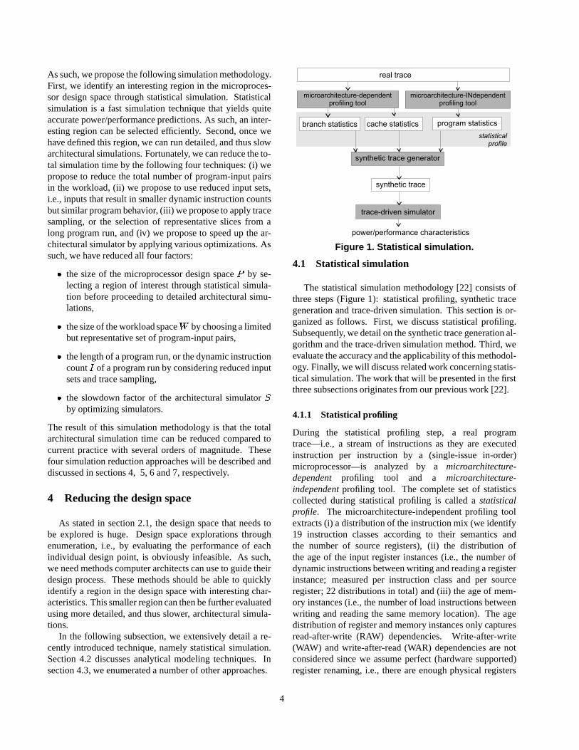
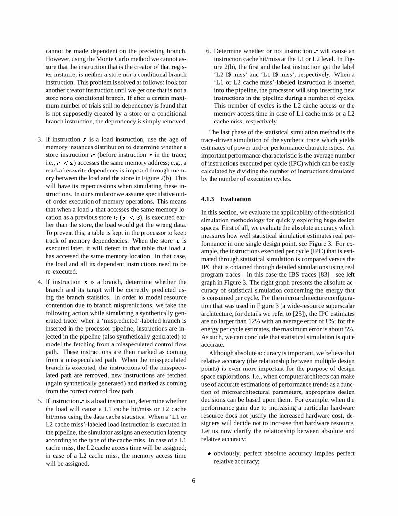
Figure 1. Statistical simulation.
4.1 Statistical simulation
The statistical simulation methodology [22] consists ofthree steps (Figure 1): statistical profiling, synthetic tracegeneration and trace-driven simulation. This section is or-ganized as follows. First, we discuss statistical profiling.Subsequently, we detail on the synthetic trace generation al-gorithm and the trace-driven simulation method. Third, weevaluate the accuracy and the applicability of this methodol-ogy. Finally, we will discuss related work concerning statis-tical simulation. The work that will be presented in the firstthree subsections originates from our previous work [22].
4.1.1 Statistical profiling
During the statistical profiling step, a real programtrace—i.e., a stream of instructions as they are executedinstruction per instruction by a (single-issue in-order)microprocessor—is analyzed by a microarchitecture-dependent profiling tool and a microarchitecture-independent profiling tool. The complete set of statisticscollected during statistical profiling is called a statisticalprofile. The microarchitecture-independent profiling toolextracts (i) a distribution of the instruction mix (we identify19 instruction classes according to their semantics andthe number of source registers), (ii) the distribution ofthe age of the input register instances (i.e., the number ofdynamic instructions between writing and reading a registerinstance; measured per instruction class and per sourceregister; 22 distributions in total) and (iii) the age of mem-ory instances (i.e., the number of load instructions betweenwriting and reading the same memory location). The agedistribution of register and memory instances only capturesread-after-write (RAW) dependencies. Write-after-write(WAW) and write-after-read (WAR) dependencies are notconsidered since we assume perfect (hardware supported)register renaming, i.e., there are enough physical registers
4
to remove all WAW and WAR dependencies dynamically.Note that this is not unrealistic since it is implementedin the Alpha 21264 [45]. If measuring performance asa function of the number of physical registers would beneeded, the methodology presented in this paper can beeasily extended for this purpose by modeling WAR andWAW dependencies as well.
The microarchitecture-dependent profiling tool only ex-tracts statistics concerning the branch and cache behaviorof the program trace for a specific branch predictor and aspecific cache organization. The branch statistics consist ofseven probabilities: (i) the conditional branch target predic-tion accuracy, (ii) the conditional branch (taken/not-taken)prediction accuracy, (iii) the relative branch target predic-tion accuracy, (iv) the relative call target prediction accu-racy, (v) the indirect jump target prediction accuracy, (vi)the indirect call target prediction accuracy and (vii) the re-turn target prediction accuracy. The reason to distinguishbetween these seven probabilities is that the prediction ac-curacies greatly vary among the various branch classes. Inaddition, the penalties introduced by these are completelydifferent [37]. A misprediction in cases (i), (iii) and (iv)only introduces a single-cycle bubble in the pipeline. Cases(ii), (v), (vi) and (vii) on the other hand, will cause the en-tire processor pipeline to be flushed and to be refilled whenthe mispredicted branch is executed.
The cache statistics include two sets of distributions: thedata cache and the instruction cache statistics. The datacache statistics contain two probabilities for a load opera-tion, namely (i) the probability that a load needs to accessthe level-2 (L2) cache—as a result of a level-1 (L1) cachemiss—and (ii) the probability that main memory—as a re-sult of a level-2 (L2) cache miss—needs to be accessed toget its data; idem for the instruction cache statistics.
A statistical profile can be computed from an actual tracebut it is more convenient to compute it on-the-fly from ei-ther an instrumented functional simulator, or from an instru-mented version of the benchmark program running on a realsystem which eliminates the need to store huge traces. Asecond note is that although computing a statistical profilemight take a long time, it should be done only once for eachbenchmark with a given input. And since statistical simula-tion is a fast analysis technique, computing a statistical pro-file will be worthwhile. A third important note is that mea-suring microarchitecture-dependent characteristics such asbranch prediction accuracy and cache miss rates, impliesthat statistical simulation cannot be used to efficiently studybranch predictors or cache organizations. Other microar-chitectural parameters however, can be varied freely. Webelieve this is not a major limitation since, e.g., cache missrates for various cache sizes can be computed simultane-ously using the cheetah simulator [82].
1
program characteristic
random
num
ber
(a)
(b)
add
store
branch
load
add
L1 I$ miss
L2 I$ miss
L1 D$ miss
mispredicted
synth
etic instr
uction tra
ce
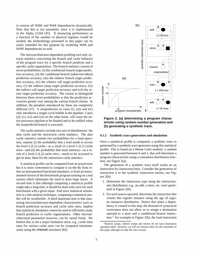
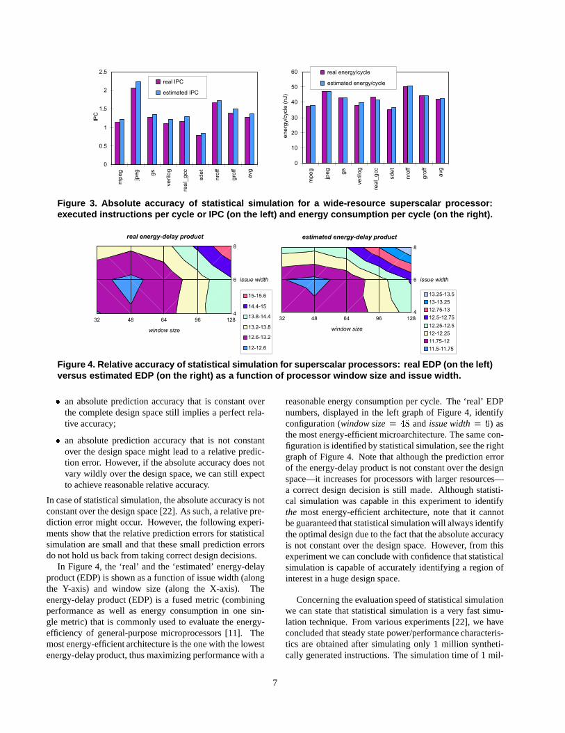
Figure 2. (a) determining a program charac-teristic using random number generation and(b) generating a synthetic trace.
4.1.2 Synthetic trace generation and simulation
Once a statistical profile is computed, a synthetic trace isgenerated by a synthetic trace generator using this statisticalprofile. This is based on a Monte Carlo method: a randomnumber is generated between 0 and 1, that will determine aprogram characteristic using a cumulative distribution func-tion, see Figure 2(a).
The generation of a synthetic trace itself works on aninstruction-by-instruction basis. Consider the generation ofinstruction � in the synthetic instruction stream, see Fig-ure 2(b):
1. Determine the instruction type using the instruction-mix distribution; e.g., an add, a store, etc. were gener-ated in Figure 2(b).
2. For each source operand, determine the instruction thatcreates this register instance using the age of regis-ter instances distribution. Notice that when a depen-dency is created in this step, the demand of syntacticalcorrectness does not allow us to assign a destinationoperand to a store and a conditional branch instruc-tion.1 For example in Figure 2(b), the load instruction
1Relative jumps, indirect jumps and returns do not have destinationoperands either. However, we will not mention them for the remainder ofthis paper although we take this into account.
5
cannot be made dependent on the preceding branch.However, using the Monte Carlo method we cannot as-sure that the instruction that is the creator of that regis-ter instance, is neither a store nor a conditional branchinstruction. This problem is solved as follows: look foranother creator instruction until we get one that is not astore nor a conditional branch. If after a certain maxi-mum number of trials still no dependency is found thatis not supposedly created by a store or a conditionalbranch instruction, the dependency is simply removed.
3. If instruction � is a load instruction, use the age ofmemory instances distribution to determine whether astore instruction � (before instruction � in the trace;i.e., ��� � ) accesses the same memory address; e.g., aread-after-write dependency is imposed through mem-ory between the load and the store in Figure 2(b). Thiswill have its repercussions when simulating these in-structions. In our simulator we assume speculative out-of-order execution of memory operations. This meansthat when a load � that accesses the same memory lo-cation as a previous store � ( ��� � ), is executed ear-lier than the store, the load would get the wrong data.To prevent this, a table is kept in the processor to keeptrack of memory dependencies. When the store � isexecuted later, it will detect in that table that load �
has accessed the same memory location. In that case,the load and all its dependent instructions need to bere-executed.
4. If instruction � is a branch, determine whether thebranch and its target will be correctly predicted us-ing the branch statistics. In order to model resourcecontention due to branch mispredictions, we take thefollowing action while simulating a synthetically gen-erated trace: when a ‘mispredicted’-labeled branch isinserted in the processor pipeline, instructions are in-jected in the pipeline (also synthetically generated) tomodel the fetching from a misspeculated control flowpath. These instructions are then marked as comingfrom a misspeculated path. When the misspeculatedbranch is executed, the instructions of the misspecu-lated path are removed, new instructions are fetched(again synthetically generated) and marked as comingfrom the correct control flow path.
5. If instruction � is a load instruction, determine whetherthe load will cause a L1 cache hit/miss or L2 cachehit/miss using the data cache statistics. When a ‘L1 orL2 cache miss’-labeled load instruction is executed inthe pipeline, the simulator assigns an execution latencyaccording to the type of the cache miss. In case of a L1cache miss, the L2 cache access time will be assigned;in case of a L2 cache miss, the memory access timewill be assigned.
6. Determine whether or not instruction � will cause aninstruction cache hit/miss at the L1 or L2 level. In Fig-ure 2(b), the first and the last instruction get the label‘L2 I$ miss’ and ‘L1 I$ miss’, respectively. When a‘L1 or L2 cache miss’-labeled instruction is insertedinto the pipeline, the processor will stop inserting newinstructions in the pipeline during a number of cycles.This number of cycles is the L2 cache access or thememory access time in case of L1 cache miss or a L2cache miss, respectively.
The last phase of the statistical simulation method is thetrace-driven simulation of the synthetic trace which yieldsestimates of power and/or performance characteristics. Animportant performance characteristic is the average numberof instructions executed per cycle (IPC) which can be easilycalculated by dividing the number of instructions simulatedby the number of execution cycles.
4.1.3 Evaluation
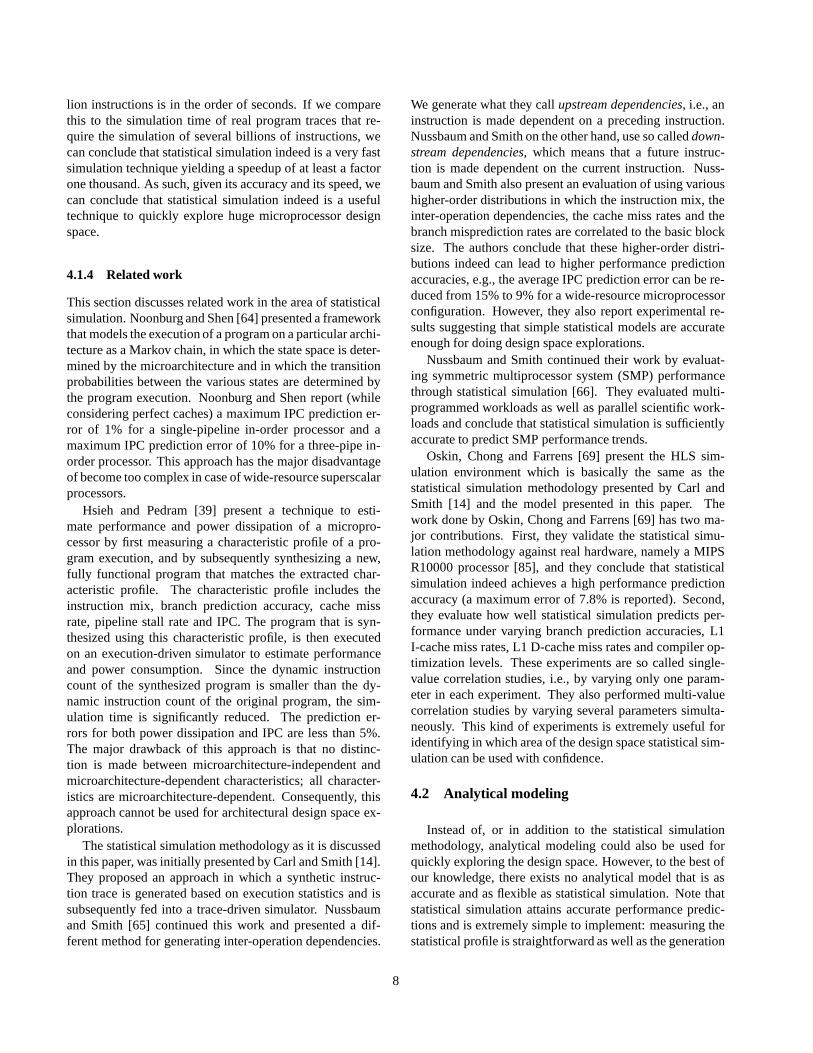
In this section, we evaluate the applicability of the statisticalsimulation methodology for quickly exploring huge designspaces. First of all, we evaluate the absolute accuracy whichmeasures how well statistical simulation estimates real per-formance in one single design point, see Figure 3. For ex-ample, the instructions executed per cycle (IPC) that is esti-mated through statistical simulation is compared versus theIPC that is obtained through detailed simulations using realprogram traces—in this case the IBS traces [83]—see leftgraph in Figure 3. The right graph presents the absolute ac-curacy of statistical simulation concerning the energy thatis consumed per cycle. For the microarchitecture configura-tion that was used in Figure 3 (a wide-resource superscalararchitecture, for details we refer to [25]), the IPC estimatesare no larger than 12% with an average error of 8%; for theenergy per cycle estimates, the maximum error is about 5%.As such, we can conclude that statistical simulation is quiteaccurate.
Although absolute accuracy is important, we believe thatrelative accuracy (the relationship between multiple designpoints) is even more important for the purpose of designspace explorations. I.e., when computer architects can makeuse of accurate estimations of performance trends as a func-tion of microarchitectural parameters, appropriate designdecisions can be based upon them. For example, when theperformance gain due to increasing a particular hardwareresource does not justify the increased hardware cost, de-signers will decide not to increase that hardware resource.Let us now clarify the relationship between absolute andrelative accuracy:
� obviously, perfect absolute accuracy implies perfectrelative accuracy;
6
0
0.5
1
1.5
2
2.5
mp
eg
jpe
g
gs
ve
rilo
g
rea
l_g
cc
sd
et
nro
ff
gro
ff
avg
IPC
real IPC
estimated IPC
0
10
20
30
40
50
60
mp
eg
jpe
g
gs
ve
rilo
g
rea
l_g
cc
sd
et
nro
ff
gro
ff
avg
en
erg
y/c
ycle
(nJ)
real energy/cycle
estimated energy/cycle
Figure 3. Absolute accuracy of statistical simulation for a wide-resource superscalar processor:executed instructions per cycle or IPC (on the left) and energy consumption per cycle (on the right).
32 48 64 96 128
4
6
8
window size
issue width
real energy-delay product
15-15.6
14.4-15
13.8-14.4
13.2-13.8
12.6-13.2
12-12.6
32 48 64 96 128
4
6
8
window size
issue width
estimated energy-delay product
13.25-13.5
13-13.25
12.75-13
12.5-12.75
12.25-12.5
12-12.25
11.75-12
11.5-11.75
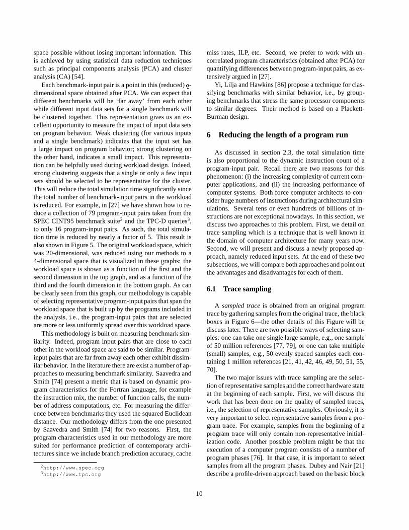
Figure 4. Relative accuracy of statistical simulation for superscalar processors: real EDP (on the left)versus estimated EDP (on the right) as a function of processor window size and issue width.
� an absolute prediction accuracy that is constant overthe complete design space still implies a perfect rela-tive accuracy;
� an absolute prediction accuracy that is not constantover the design space might lead to a relative predic-tion error. However, if the absolute accuracy does notvary wildly over the design space, we can still expectto achieve reasonable relative accuracy.
In case of statistical simulation, the absolute accuracy is notconstant over the design space [22]. As such, a relative pre-diction error might occur. However, the following experi-ments show that the relative prediction errors for statisticalsimulation are small and that these small prediction errorsdo not hold us back from taking correct design decisions.
In Figure 4, the ‘real’ and the ‘estimated’ energy-delayproduct (EDP) is shown as a function of issue width (alongthe Y-axis) and window size (along the X-axis). Theenergy-delay product (EDP) is a fused metric (combiningperformance as well as energy consumption in one sin-gle metric) that is commonly used to evaluate the energy-efficiency of general-purpose microprocessors [11]. Themost energy-efficient architecture is the one with the lowestenergy-delay product, thus maximizing performance with a
reasonable energy consumption per cycle. The ‘real’ EDPnumbers, displayed in the left graph of Figure 4, identifyconfiguration (window size � � �
and issue width � � ) asthe most energy-efficient microarchitecture. The same con-figuration is identified by statistical simulation, see the rightgraph of Figure 4. Note that although the prediction errorof the energy-delay product is not constant over the designspace—it increases for processors with larger resources—a correct design decision is still made. Although statisti-cal simulation was capable in this experiment to identifythe most energy-efficient architecture, note that it cannotbe guaranteed that statistical simulation will always identifythe optimal design due to the fact that the absolute accuracyis not constant over the design space. However, from thisexperiment we can conclude with confidence that statisticalsimulation is capable of accurately identifying a region ofinterest in a huge design space.
Concerning the evaluation speed of statistical simulationwe can state that statistical simulation is a very fast simu-lation technique. From various experiments [22], we haveconcluded that steady state power/performance characteris-tics are obtained after simulating only 1 million syntheti-cally generated instructions. The simulation time of 1 mil-
7
lion instructions is in the order of seconds. If we comparethis to the simulation time of real program traces that re-quire the simulation of several billions of instructions, wecan conclude that statistical simulation indeed is a very fastsimulation technique yielding a speedup of at least a factorone thousand. As such, given its accuracy and its speed, wecan conclude that statistical simulation indeed is a usefultechnique to quickly explore huge microprocessor designspace.
4.1.4 Related work
This section discusses related work in the area of statisticalsimulation. Noonburg and Shen [64] presented a frameworkthat models the execution of a program on a particular archi-tecture as a Markov chain, in which the state space is deter-mined by the microarchitecture and in which the transitionprobabilities between the various states are determined bythe program execution. Noonburg and Shen report (whileconsidering perfect caches) a maximum IPC prediction er-ror of 1% for a single-pipeline in-order processor and amaximum IPC prediction error of 10% for a three-pipe in-order processor. This approach has the major disadvantageof become too complex in case of wide-resource superscalarprocessors.
Hsieh and Pedram [39] present a technique to esti-mate performance and power dissipation of a micropro-cessor by first measuring a characteristic profile of a pro-gram execution, and by subsequently synthesizing a new,fully functional program that matches the extracted char-acteristic profile. The characteristic profile includes theinstruction mix, branch prediction accuracy, cache missrate, pipeline stall rate and IPC. The program that is syn-thesized using this characteristic profile, is then executedon an execution-driven simulator to estimate performanceand power consumption. Since the dynamic instructioncount of the synthesized program is smaller than the dy-namic instruction count of the original program, the sim-ulation time is significantly reduced. The prediction er-rors for both power dissipation and IPC are less than 5%.The major drawback of this approach is that no distinc-tion is made between microarchitecture-independent andmicroarchitecture-dependent characteristics; all character-istics are microarchitecture-dependent. Consequently, thisapproach cannot be used for architectural design space ex-plorations.
The statistical simulation methodology as it is discussedin this paper, was initially presented by Carl and Smith [14].They proposed an approach in which a synthetic instruc-tion trace is generated based on execution statistics and issubsequently fed into a trace-driven simulator. Nussbaumand Smith [65] continued this work and presented a dif-ferent method for generating inter-operation dependencies.
We generate what they call upstream dependencies, i.e., aninstruction is made dependent on a preceding instruction.Nussbaum and Smith on the other hand, use so called down-stream dependencies, which means that a future instruc-tion is made dependent on the current instruction. Nuss-baum and Smith also present an evaluation of using varioushigher-order distributions in which the instruction mix, theinter-operation dependencies, the cache miss rates and thebranch misprediction rates are correlated to the basic blocksize. The authors conclude that these higher-order distri-butions indeed can lead to higher performance predictionaccuracies, e.g., the average IPC prediction error can be re-duced from 15% to 9% for a wide-resource microprocessorconfiguration. However, they also report experimental re-sults suggesting that simple statistical models are accurateenough for doing design space explorations.
Nussbaum and Smith continued their work by evaluat-ing symmetric multiprocessor system (SMP) performancethrough statistical simulation [66]. They evaluated multi-programmed workloads as well as parallel scientific work-loads and conclude that statistical simulation is sufficientlyaccurate to predict SMP performance trends.
Oskin, Chong and Farrens [69] present the HLS sim-ulation environment which is basically the same as thestatistical simulation methodology presented by Carl andSmith [14] and the model presented in this paper. Thework done by Oskin, Chong and Farrens [69] has two ma-jor contributions. First, they validate the statistical simu-lation methodology against real hardware, namely a MIPSR10000 processor [85], and they conclude that statisticalsimulation indeed achieves a high performance predictionaccuracy (a maximum error of 7.8% is reported). Second,they evaluate how well statistical simulation predicts per-formance under varying branch prediction accuracies, L1I-cache miss rates, L1 D-cache miss rates and compiler op-timization levels. These experiments are so called single-value correlation studies, i.e., by varying only one param-eter in each experiment. They also performed multi-valuecorrelation studies by varying several parameters simulta-neously. This kind of experiments is extremely useful foridentifying in which area of the design space statistical sim-ulation can be used with confidence.
4.2 Analytical modeling
Instead of, or in addition to the statistical simulationmethodology, analytical modeling could also be used forquickly exploring the design space. However, to the best ofour knowledge, there exists no analytical model that is asaccurate and as flexible as statistical simulation. Note thatstatistical simulation attains accurate performance predic-tions and is extremely simple to implement: measuring thestatistical profile is straightforward as well as the generation
8

of a synthetic trace, and the simulator that is used to simu-late the synthetic trace is very simple since only a limitedfunctionality of the microarchitecture needs to be modeled.An analytical model on the other hand, is harder to developbecause of the complex behavior of contemporary microar-chitectures. As such, analytical models typically assumeseveral assumptions to be true, such as unit execution laten-cies of instructions, unlimited number of functional units oronly one functional unit, memory dependencies not beingmodeled, etc. In statistical simulation on the other hand,these assumptions do not need to be fulfilled.
Noonburg and Shen [63] present an analytical model ofthe interaction between program parallelism and machineparallelism. This is done by combining component func-tions concerning the program (data and control parallelism)as well as the machine (branch, fetch and issue parallelism).The program characteristics are measured only once foreach benchmark as it is the case for statistical simulation.The machine characteristics are obtained by analyzing themicroarchitecture. This analytical model attains quite accu-rate performance predictions. Unfortunately, unit instruc-tion execution latencies are assumed and memory depen-dencies are not modeled.
Dubey, Adams and Flynn [20] propose an analytical per-formance model on the basis of two parameters that are ex-tracted from a program trace. The first parameter, the condi-tional independence probability ��� , is defined as the prob-ability that an instruction � is independent of instruction
����� given that � is independent of all instructions in thetrace between � and ����� . The second parameter � is de-fined as the probability that an instruction is scheduled withan instruction from � basic blocks earlier in the programtrace. The main disadvantages of this analytical model arethat only one dependency is considered per instruction andthat no differentation is made between various instructionclasses for �� , which will lead to inaccurate performanceestimates. In [43], Kamin et al. propose to approximate theconditional independence probability ��� using an exponen-tial distribution. In [23], Eeckhout and De Bosschere showthat a power law is a better approximation than the expo-nential distribution.
Squillante, Kaeli and Sinha [81] propose analyticalmodels to capture the workload behavior and to estimatepipeline performance. Their technique was evaluated for asingle-issue pipelined processor.
Sorin et al. [80] present a performance analysis method-ology for shared-memory systems that combines analyticaltechniques with traditional simulations to speed up the de-sign process.
Although current analytical models are not flexibleenough or accurate enough for performing design space ex-plorations of contemporary superscalar processors, they canbe extremely useful to investigate particular parts of a mi-
croarchitecture. As such, simple analytical models are of-ten used to get insight in the impact of microarchitecturalparameters on performance [30, 31, 33, 57, 61].
4.3 Other approaches
Conte, in his PhD thesis [16], presents an approach thatautomatically searches near-optimal processor configura-tions in a huge design space. His technique is based onsimulated annealing. The architectural parameters that arevaried in his experiments are the number of functional units,their types and their execution latencies.
Brooks, Martonosi and Bose [12] evaluate the popularabstraction via separable components method [30] whichconsiders performance as the summation of a base perfor-mance level (idealized base cycles per instruction or CPIwhile assuming perfect caches, perfect branch prediction,etc.) plus additional stall factors due to conflicts, hazards,cache misses, mispredictions, etc. A simulation speedupis obtained with this technique since the base performancelevel and the stall factors can be computed using simplesimulators instead of fully-detailed and thus slower simula-tors. They conclude that for modeling out-of-order architec-tures, this methodology attains, in spite of its poor absoluteaccuracy, a reasonable relative accuracy.
5 Reducing the workload
In section 2.2, we argued that the selection of a repre-sentative workload is extremely important throughout theentire microprocessor design flow. A representative work-load consists of a selected number of benchmarks with wellchosen inputs that are representative for the target domain ofoperation of the microprocessor currently under design. Anaive approach to the workload composition problem wouldbe to select a huge number of benchmarks and for eachbenchmark a large number of inputs. Since the total sim-ulation time is proportional to the number of program-inputpairs in the workload, this approach is infeasible. As such,we propose to chose a selected number of program-inputpairs that span the workload space [28].
Conceptually, the complete workload design space canbe viewed as a � -dimensional space with � the num-ber of important program characteristics that affect perfor-mance, e.g., branch prediction accuracy, cache miss rates,instruction-level parallelism (ILP), etc. Obviously, � willbe too large to display the workload design space under-standably. In addition, correlation exists between these vari-ables which reduces the ability to understand what programcharacteristics are fundamental to make the diversity in theworkload space. In this paper, we reduce the � -dimensionalworkload space to a -dimensional space with ���� ( ���to ��� typically) making the visualisation of the workload
9
space possible without losing important information. Thisis achieved by using statistical data reduction techniquessuch as principal components analysis (PCA) and clusteranalysis (CA) [54].
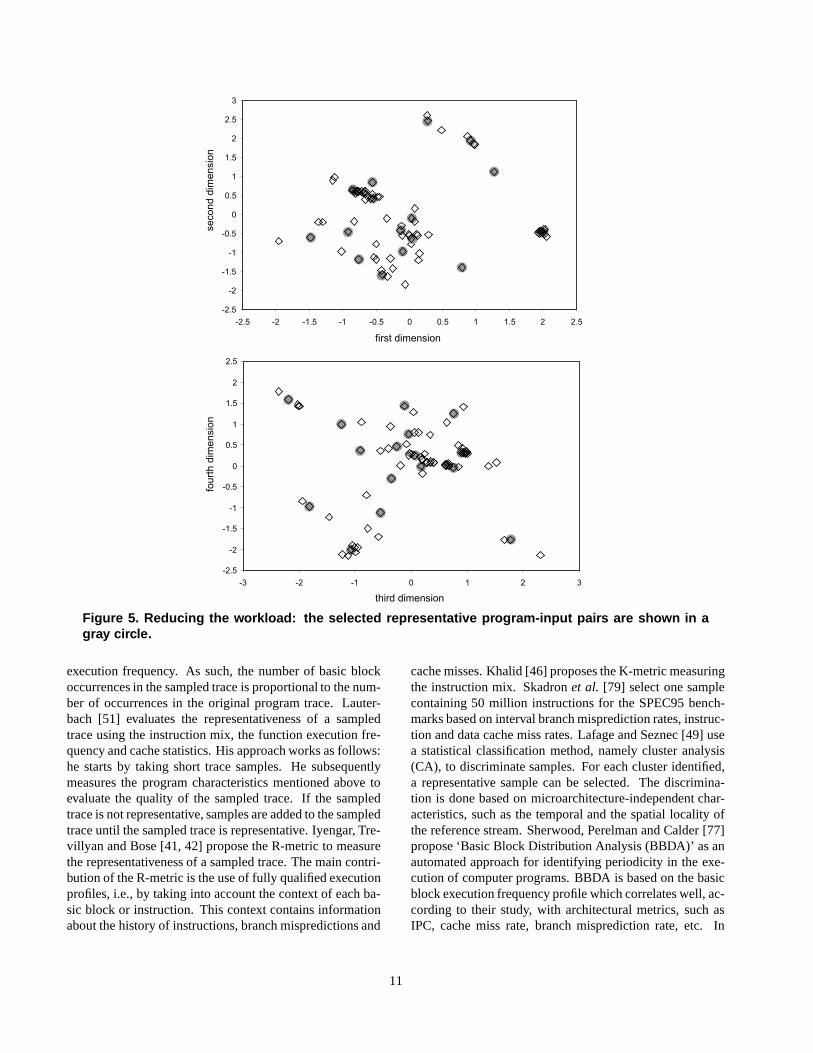
Each benchmark-input pair is a point in this (reduced) -dimensional space obtained after PCA. We can expect thatdifferent benchmarks will be ‘far away’ from each otherwhile different input data sets for a single benchmark willbe clustered together. This representation gives us an ex-cellent opportunity to measure the impact of input data setson program behavior. Weak clustering (for various inputsand a single benchmark) indicates that the input set hasa large impact on program behavior; strong clustering onthe other hand, indicates a small impact. This representa-tion can be helpfully used during workload design. Indeed,strong clustering suggests that a single or only a few inputsets should be selected to be representative for the cluster.This will reduce the total simulation time significantly sincethe total number of benchmark-input pairs in the workloadis reduced. For example, in [27] we have shown how to re-duce a collection of 79 program-input pairs taken from theSPEC CINT95 benchmark suite2 and the TPC-D queries3,to only 16 program-input pairs. As such, the total simula-tion time is reduced by nearly a factor of 5. This result isalso shown in Figure 5. The original workload space, whichwas 20-dimensional, was reduced using our methods to a4-dimensional space that is visualized in these graphs: theworkload space is shown as a function of the first and thesecond dimension in the top graph, and as a function of thethird and the fourth dimension in the bottom graph. As canbe clearly seen from this graph, our methodology is capableof selecting representative program-input pairs that span theworkload space that is built up by the programs included inthe analysis, i.e., the program-input pairs that are selectedare more or less uniformly spread over this workload space.
This methodology is built on measuring benchmark sim-ilarity. Indeed, program-input pairs that are close to eachother in the workload space are said to be similar. Program-input pairs that are far from away each other exhibit dissim-ilar behavior. In the literature there are exist a number of ap-proaches to measuring benchmark similarity. Saavedra andSmith [74] present a metric that is based on dynamic pro-gram characteristics for the Fortran language, for examplethe instruction mix, the number of function calls, the num-ber of address computations, etc. For measuring the differ-ence between benchmarks they used the squared Euclideandistance. Our methodology differs from the one presentedby Saavedra and Smith [74] for two reasons. First, theprogram characteristics used in our methodology are moresuited for performance prediction of contemporary archi-tectures since we include branch prediction accuracy, cache
2http://www.spec.org3http://www.tpc.org
miss rates, ILP, etc. Second, we prefer to work with un-correlated program characteristics (obtained after PCA) forquantifying differences between program-input pairs, as ex-tensively argued in [27].
Yi, Lilja and Hawkins [86] propose a technique for clas-sifying benchmarks with similar behavior, i.e., by group-ing benchmarks that stress the same processor componentsto similar degrees. Their method is based on a Plackett-Burman design.
6 Reducing the length of a program run
As discussed in section 2.3, the total simulation timeis also proportional to the dynamic instruction count of aprogram-input pair. Recall there are two reasons for thisphenomenon: (i) the increasing complexity of current com-puter applications, and (ii) the increasing performance ofcomputer systems. Both force computer architects to con-sider huge numbers of instructions during architectural sim-ulations. Several tens or even hundreds of billions of in-structions are not exceptional nowadays. In this section, wediscuss two approaches to this problem. First, we detail ontrace sampling which is a technique that is well known inthe domain of computer architecture for many years now.Second, we will present and discuss a newly proposed ap-proach, namely reduced input sets. At the end of these twosubsections, we will compare both approaches and point outthe advantages and disadvantages for each of them.
6.1 Trace sampling
A sampled trace is obtained from an original programtrace by gathering samples from the original trace, the blackboxes in Figure 6—the other details of this Figure will bediscuss later. There are two possible ways of selecting sam-ples: one can take one single large sample, e.g., one sampleof 50 million references [77, 79], or one can take multiple(small) samples, e.g., 50 evenly spaced samples each con-taining 1 million references [21, 41, 42, 46, 49, 50, 51, 55,70].
The two major issues with trace sampling are the selec-tion of representative samples and the correct hardware stateat the beginning of each sample. First, we will discuss thework that has been done on the quality of sampled traces,i.e., the selection of representative samples. Obviously, it isvery important to select representative samples from a pro-gram trace. For example, samples from the beginning of aprogram trace will only contain non-representative initial-ization code. Another possible problem might be that theexecution of a computer program consists of a number ofprogram phases [76]. In that case, it is important to selectsamples from all the program phases. Dubey and Nair [21]describe a profile-driven approach based on the basic block
10
-2.5
-2
-1.5
-1
-0.5
0
0.5
1
1.5
2
2.5
3
-2.5 -2 -1.5 -1 -0.5 0 0.5 1 1.5 2 2.5
-2.5
-2
-1.5
-1
-0.5
0
0.5
1
1.5
2
2.5
-3 -2 -1 0 1 2 3
first dimension
third dimension
fou
rth
dim
en
sio
nse
co
nd
dim
en
sio
n
Figure 5. Reducing the workload: the selected representative program-input pairs are shown in agray circle.
execution frequency. As such, the number of basic blockoccurrences in the sampled trace is proportional to the num-ber of occurrences in the original program trace. Lauter-bach [51] evaluates the representativeness of a sampledtrace using the instruction mix, the function execution fre-quency and cache statistics. His approach works as follows:he starts by taking short trace samples. He subsequentlymeasures the program characteristics mentioned above toevaluate the quality of the sampled trace. If the sampledtrace is not representative, samples are added to the sampledtrace until the sampled trace is representative. Iyengar, Tre-villyan and Bose [41, 42] propose the R-metric to measurethe representativeness of a sampled trace. The main contri-bution of the R-metric is the use of fully qualified executionprofiles, i.e., by taking into account the context of each ba-sic block or instruction. This context contains informationabout the history of instructions, branch mispredictions and
cache misses. Khalid [46] proposes the K-metric measuringthe instruction mix. Skadron et al. [79] select one samplecontaining 50 million instructions for the SPEC95 bench-marks based on interval branch misprediction rates, instruc-tion and data cache miss rates. Lafage and Seznec [49] usea statistical classification method, namely cluster analysis(CA), to discriminate samples. For each cluster identified,a representative sample can be selected. The discrimina-tion is done based on microarchitecture-independent char-acteristics, such as the temporal and the spatial locality ofthe reference stream. Sherwood, Perelman and Calder [77]propose ‘Basic Block Distribution Analysis (BBDA)’ as anautomated approach for identifying periodicity in the exe-cution of computer programs. BBDA is based on the basicblock execution frequency profile which correlates well, ac-cording to their study, with architectural metrics, such asIPC, cache miss rate, branch misprediction rate, etc. In
11
samplewarm-up
ho
t
wa
rm
co
ld
ho
t
wa
rm
co
ld
ho
t
wa
rm
co
ld
original trace
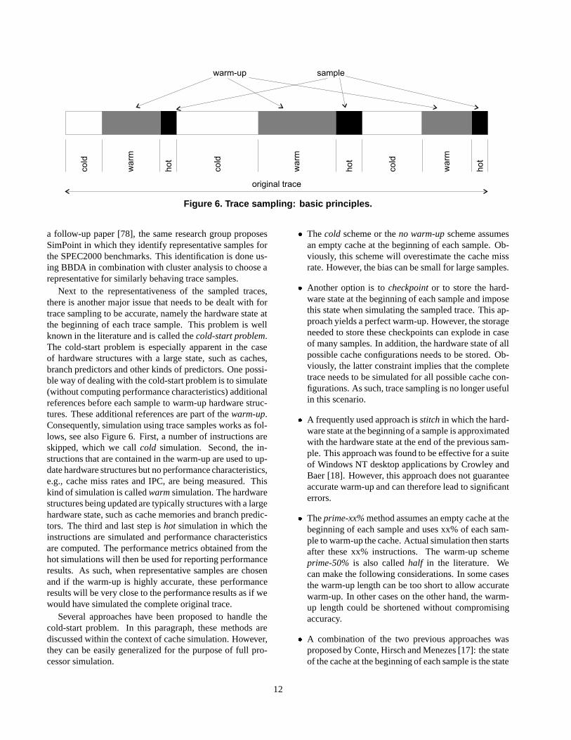
Figure 6. Trace sampling: basic principles.
a follow-up paper [78], the same research group proposesSimPoint in which they identify representative samples forthe SPEC2000 benchmarks. This identification is done us-ing BBDA in combination with cluster analysis to choose arepresentative for similarly behaving trace samples.
Next to the representativeness of the sampled traces,there is another major issue that needs to be dealt with fortrace sampling to be accurate, namely the hardware state atthe beginning of each trace sample. This problem is wellknown in the literature and is called the cold-start problem.The cold-start problem is especially apparent in the caseof hardware structures with a large state, such as caches,branch predictors and other kinds of predictors. One possi-ble way of dealing with the cold-start problem is to simulate(without computing performance characteristics) additionalreferences before each sample to warm-up hardware struc-tures. These additional references are part of the warm-up.Consequently, simulation using trace samples works as fol-lows, see also Figure 6. First, a number of instructions areskipped, which we call cold simulation. Second, the in-structions that are contained in the warm-up are used to up-date hardware structures but no performance characteristics,e.g., cache miss rates and IPC, are being measured. Thiskind of simulation is called warm simulation. The hardwarestructures being updated are typically structures with a largehardware state, such as cache memories and branch predic-tors. The third and last step is hot simulation in which theinstructions are simulated and performance characteristicsare computed. The performance metrics obtained from thehot simulations will then be used for reporting performanceresults. As such, when representative samples are chosenand if the warm-up is highly accurate, these performanceresults will be very close to the performance results as if wewould have simulated the complete original trace.
Several approaches have been proposed to handle thecold-start problem. In this paragraph, these methods arediscussed within the context of cache simulation. However,they can be easily generalized for the purpose of full pro-cessor simulation.
� The cold scheme or the no warm-up scheme assumesan empty cache at the beginning of each sample. Ob-viously, this scheme will overestimate the cache missrate. However, the bias can be small for large samples.
� Another option is to checkpoint or to store the hard-ware state at the beginning of each sample and imposethis state when simulating the sampled trace. This ap-proach yields a perfect warm-up. However, the storageneeded to store these checkpoints can explode in caseof many samples. In addition, the hardware state of allpossible cache configurations needs to be stored. Ob-viously, the latter constraint implies that the completetrace needs to be simulated for all possible cache con-figurations. As such, trace sampling is no longer usefulin this scenario.
� A frequently used approach is stitch in which the hard-ware state at the beginning of a sample is approximatedwith the hardware state at the end of the previous sam-ple. This approach was found to be effective for a suiteof Windows NT desktop applications by Crowley andBaer [18]. However, this approach does not guaranteeaccurate warm-up and can therefore lead to significanterrors.
� The prime-xx% method assumes an empty cache at thebeginning of each sample and uses xx% of each sam-ple to warm-up the cache. Actual simulation then startsafter these xx% instructions. The warm-up schemeprime-50% is also called half in the literature. Wecan make the following considerations. In some casesthe warm-up length can be too short to allow accuratewarm-up. In other cases on the other hand, the warm-up length could be shortened without compromisingaccuracy.
� A combination of the two previous approaches wasproposed by Conte, Hirsch and Menezes [17]: the stateof the cache at the beginning of each sample is the state
12
at the end of the previous sample plus warming-up us-ing a fraction of the sample.
� Another approach proposed by Kessler, Hill andWood [44, 84] is to assume an empty cache at the be-ginning of each sample and to estimate which cold-start misses would have missed if the cache state at thebeginning of the sample was known.
� Nguyen et al. [62] use � instructions to warm-up thecache which is calculated as follows:
� �
������ ����
with�
the cache size,�
the line size, � the cachemiss rate and � the memory reference ratio, or in otherwords the percentage loads and stores in case of a datacache evaluation. The problem with this approach isthat the cache miss rate � is unknown; this is exactlywhat we are trying to approximate through trace sam-pling. A possible solution is to use the cache miss rateunder the no-warmup scheme. However, this mightlead to a warm-up length that is too short because themiss rate under the no-warmup scenario is generallyan overestimation.
� Minimal Subset Evaluation (MSE) proposed by Hask-ins and Skadron [34] determines a minimally suffi-cient warm-up period. The technique works as fol-lows. First, the user specifies the probability that thecache state at the beginning of the sample after warm-up equals the cache state at the beginning of the sam-ple in case of full trace simulation and thus perfectwarm-up. Second, the MSE formulas are used to deter-mine how many unique references are required duringwarm-up. Third, using a benchmark profile it is calcu-lated where exactly the warm-up should be started inorder to generate these unique references.
� Haskins and Skadron continued this research projectand proposed Memory Reference Reuse Latency(MRRL) [35] as a refinement of MSE, i.e., by reduc-ing the total warm-up length without sacrifying accu-racy. In this approach, a histogram of the MRRL, orthe number of memory references between two refer-ences to the same memory location, is used to deter-mine when to start the warm simulation.
� Very recently, Eeckhout et al. [24] proposed yet an-other warm-up technique that is similar to the two pre-vious techniques, MSE and MRRL, in the vision that areliable indication should be given beforehand whetherthe hardware state will be accurately approximated atthe beginning of a sample. However, the mechanismto achieve this is quite different from the ones em-ployed in MSE and MRRL. Whereas MSE looks at
the references in the pre-sample, and MRRL looks atthe references in the pre-sample and the sample, theapproach presented by Eeckhout et al. is based on thereferences in the sample solely. The rationale behindtheir approach is that the cache memories need only tobe warmed-up with memory addresses that are refer-enced within the sample.
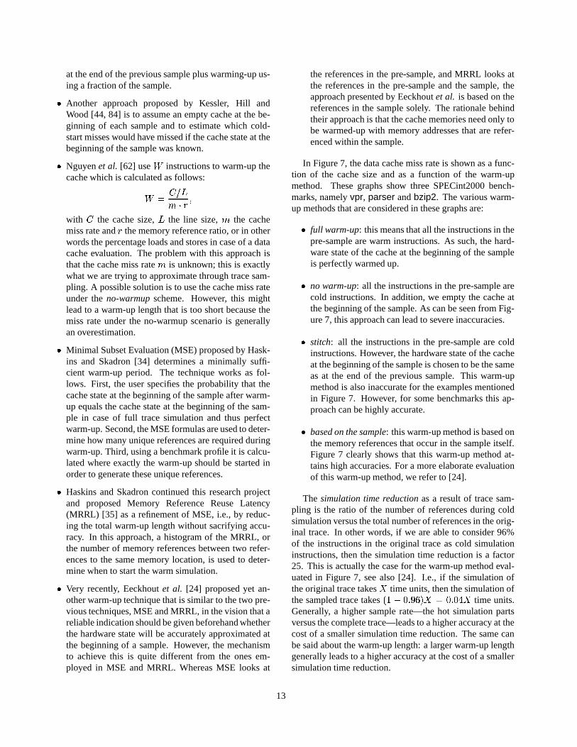
In Figure 7, the data cache miss rate is shown as a func-tion of the cache size and as a function of the warm-upmethod. These graphs show three SPECint2000 bench-marks, namely vpr, parser and bzip2. The various warm-up methods that are considered in these graphs are:
� full warm-up: this means that all the instructions in thepre-sample are warm instructions. As such, the hard-ware state of the cache at the beginning of the sampleis perfectly warmed up.
� no warm-up: all the instructions in the pre-sample arecold instructions. In addition, we empty the cache atthe beginning of the sample. As can be seen from Fig-ure 7, this approach can lead to severe inaccuracies.
� stitch: all the instructions in the pre-sample are coldinstructions. However, the hardware state of the cacheat the beginning of the sample is chosen to be the sameas at the end of the previous sample. This warm-upmethod is also inaccurate for the examples mentionedin Figure 7. However, for some benchmarks this ap-proach can be highly accurate.
� based on the sample: this warm-up method is based onthe memory references that occur in the sample itself.Figure 7 clearly shows that this warm-up method at-tains high accuracies. For a more elaborate evaluationof this warm-up method, we refer to [24].
The simulation time reduction as a result of trace sam-pling is the ratio of the number of references during coldsimulation versus the total number of references in the orig-inal trace. In other words, if we are able to consider 96%of the instructions in the original trace as cold simulationinstructions, then the simulation time reduction is a factor25. This is actually the case for the warm-up method eval-uated in Figure 7, see also [24]. I.e., if the simulation ofthe original trace takes time units, then the simulation ofthe sampled trace takes � � � � ���� � � ��� � �� time units.Generally, a higher sample rate—the hot simulation partsversus the complete trace—leads to a higher accuracy at thecost of a smaller simulation time reduction. The same canbe said about the warm-up length: a larger warm-up lengthgenerally leads to a higher accuracy at the cost of a smallersimulation time reduction.
13
vpr
2.5%
3.0%
3.5%
4.0%
4.5%
5.0%
5.5%
64KB 128KB 256KB 512KB 1MB
mis
sra
te
full warm-up
no warm-up
stitch
based on the sample
parser
1.5%
2.0%
2.5%
3.0%
3.5%
4.0%
4.5%
64KB 128KB 256KB 512KB 1MB
mis
sra
te
bzip2
2.1%
2.2%
2.3%
2.4%
2.5%
2.6%
2.7%
2.8%
2.9%
3.0%
3.1%
64KB 128KB 256KB 512KB 1MB
mis
sra
te
Figure 7. Dealing with the cold-start problem:(i) full warm-up (no cold instructions), (ii) nowarm-up (no warm instructions and emptycache at beginning of each sample), (iii) stitch(no warm instructions and stale cache state atbeginning of each sample), and (iv) the warm-up method proposed by Eeckhout et al. [24]that is based on the references in the sample.
6.2 Reduced input sets
Recall that section 6 deals with reducing the length of aprogram run. Recently, another approach to this problem
was proposed, namely reduced input sets. KleinOsowskiet al. [47, 48] propose to reduce the simulation time of theSPEC 2000 benchmark suite4 by using reduced input datasets, called MinneSPEC. Instead of using the reference in-put data sets provided by SPEC, which result in unreason-ably long simulation times, they propose to use reducedinput data sets that result in smaller dynamic instructioncounts and yet accurately reflect the behavior of the fullreference input sets. These reduced input sets are derivedfrom the reference inputs by a number of techniques: mod-ifying inputs (for example, reducing the number of itera-tions), truncating inputs, etc. They propose three reducedinputs: smred for short simulations (100 million instruc-tions), mdred for medium length simulations (500 millioninstructions) and lgred for full length, reportable simula-tions (1 billion instructions). For determining whether twoinput sets result in more or less the same behavior, they usedthe chi-squared statistic based on the function-level execu-tion profiles for each input set. A function-level profile isnothing more than a distribution that measures what frac-tion of the time is spent in each function during the execu-tion of the program. Note however that a resemblance offunction-level execution profiles does not necessarily im-ply a resemblance of other workload characteristics that areprobably more closely related to performance, such as in-struction mix, cache behavior, branch predictability, etc.For example, consider the case that we would scale downthe number of times a function is executed by a factor S.Obviously, this will result in the same function-level exe-cution profile. However, a similar function-level executionprofile does not guarantee a similar behavior concerning forexample the data memory. Indeed, reducing the input setoften reduces the size of the data the program is workingon while leaving the function-level execution profile un-touched. And this might lead to a significantly differentdata cache behavior. KleinOsowski et al. also recognizedthat this is a potential problem.
In [26], Eeckhout et al. validated the program behaviorsimilarity of MinneSPEC versus the reference SPEC bench-mark suite. This was done using the methodology describedin section 5. Recall that this methodology transforms ahighly correlated, high dimensional workload space into anon-correlated, low dimensional workload space. In thisunderstandable workload space, program-input pairs thatare close to each other exhibit similar behavior; program-input pairs far away from each other reflect dissimilar be-havior. As such, this methodology can be used to validatereduced input sets. Indeed, if a reduced input is situatedclose to its reference counterpart we conclude that the re-duced input results in similar behavior. From this analy-sis, Eeckhout et al. concluded that although validating re-duced inputs based on function-level execution profiles, as
4http://www.spec.org
14
is done by KleinOsowski and Lilja [48], is accurate in mostcases, there are a number of cases where this approach fails.In conclusion, we have to be careful when comparing re-duced input sets based on the function-level execution pro-files only.
6.3 Comparing trace sampling versus reduced in-put sets
Haskins et al. [36] and Eeckhout et al. [27] comparedtrace sampling and reduced input sets. Their results showthat for some benchmarks trace sampling is more accuratethan reduced input sets; for other benchmarks on the otherhand, the opposite is true. The simulation time reductionis comparable in both cases: a factor 20 to 100. Both ap-proaches come with their own benefits. Reduced inputs al-low the execution of a program from the beginning to theend; trace sampling allows flexibility by varying the sam-ple rate, the sample length, the number of samples, etc. Assuch, we can conclude that both approaches are useful toreduce the length of a program run.
7 Increasing the simulation speed
The fourth and last aspect that contributes to the time-consuming behavior of architectural simulations is theslowdown of the simulator itself. Architectural simulationsare done at a high level using an architectural simulator thatis written in a high level programming language such as C,C++ or Java. Usually, companies have their own simulationinfrastructure, such as Asim [29, 72] used by the Compaqdesign team now with Intel, and MET [58, 59] used by IBM.Virtutech released Simics [53], a platform for full systemsimulation. The SimpleScalar Tool Set [1, 13] is an archi-tectural simulator that is widely used in the academia andthe industry for evaluating uniprocessors at the architecturallevel. Other examples of architectural simulators devel-oped by the academia are Rsim [40] at Rice University (forsimulating shared-memory multiprocessors), SimOS [73] atStanford University (for full system simulation of shared-memory multiprocessors), fMW [2] at Carnegie MellonUniversity (quite similar to SimpleScalar), and TFsim [56]at the University of Wisconsin–Madison (a full system mul-tiprocessor simulator). Note that these simulators do modelmicroarchitectures at a high abstraction level which mightintroduce inaccuracies in the performance results whencompared to real hardware [5, 19, 32]. It is also interestingto note that there exist two types of architectural simulators:trace-driven and execution-driven. The basic difference be-tween both is that an execution-driven simulator actuallyexecutes the executable as it would be executed on a realsystem—this involves interpreting the individual instruc-tions. A trace-driven simulator on the other hand, only im-
poses dependencies between instructions since the instruc-tions do not need to be re-executed—the exact sequence ofinstructions is already available in the trace. This gives a po-tential speed advantage for the trace-driven simulator. In ad-dition, a trace-driven simulator is generally more portable,more simple and more flexible than execution-driven sim-ulators. Unfortunately, there are two important disadvan-tages associated with trace-driven simulators. First, unlessspecial care is being taken, not simulating instructions alongmisspeculated paths can lead to significant errors [3, 4, 15].Second, the traces need to be stored on a hard drive, whichmight be impractical in case of long traces.
As stated in section 2.4, the slowdown factor of an ar-chitectural simulator is typically 50,000 to 300,000. Ob-viously, there is only one solution to this problem, namelyto optimize the simulator. However, there are two possibleconstraints: (i) without sacrifying accuracy, and (ii) withsacrifying (little) accuracy.
The first approach we discuss does not sacrify accuracy.Schnarr and Larus [75] show how to speed up an architec-tural simulator using memoization. Traditionally, memo-ization refers to caching function return values in functionalprogramming languages. These cached values can then bereturned when available during execution avoiding expen-sive computations. Schnarr and Larus present a similartechnique that caches microarchitecture states and the re-sulting simulation actions. When a cached state is encoun-tered during simulation, the simulation is then fast-forwardby replaying the associated simulation actions at high speeduntil a previously unseen state is reached. They achieve an 8to 15 times speedup over SimpleScalar’s out-of-order sim-ulator [13] while producing exactly the same result.
The following three approaches sacrify little accuracy,i.e., these approaches model a microarchitecture at aslightly higher abstraction level which obviously introduceadditional modeling errors. Bose [8] proposes to pre-process a program trace, e.g., by tagging loads and storeswith hit/miss information, or by tagging branches with pre-diction information (wrong or correct prediction). Thistagged program trace can then be executed on a simulatorthat imposes an appropriate penalty in the simulator. Thesimulator speedup comes from the fact that several hard-ware structures do not need to be modeled.
Loh [52] presents a time-stamping algorithm thatachieves an average prediction error of 7.5% with a 2.42Xsimulation speedup for wide-issue superscalar architec-tures. This approach is built on the idea that it is suffi-cient to know when events—such as the end of an instruc-tion execution or the availability of a resource—occur. Bytime-stamping the resources associated with these events,the IPC can be computed by dividing the number of instruc-tions simulated by the highest time stamp. The inaccuracycomes from making assumptions in the time-stamping al-
15
gorithm which make it impossible to accurately model thebehavior of a complex out-of-order architecture such as out-of-order cache accesses, wrong path cache accesses, etc.
Ofelt and Hennessy [68] present a profile-based perfor-mance prediction technique that is an extension of a wellknown approach consisting of two phases. The first (instru-mentation) phase counts the number of times a basic blockis executed. The second phase then simulates each basicblock while measuring the amount of IPC. This estimatedIPC number is multiplied by the number of times the ba-sic block is executed during a real program execution. Thesum over all basic blocks then gives an estimate of the IPCof program. The approach presented by Ofelt and Hen-nessy [68] extends this simple method to enable the mod-eling of out-of-order architectures, e.g., by modeling paral-lelism between instructions from various basic blocks. Thisapproach achieves a high accuracy (errors of only a few per-cent are reported) while assuming perfect branch predictionand perfect caches. However, when a realistic branch predi-cor and realistic caches are included in the evaluation, theaccuracy falls short [67].
8 Conclusion
The architectural simulations that need to be done dur-ing the design of a microprocessor are extremely time-consuming for a number of reasons. First, the microar-chitectural design space that needs to be explored is huge.Second, the workload space or the number of benchmarks(with suitable inputs) is large as well. Third, the numberof instructions that need to be simulated per benchmark ishuge. Fourth, due to the ever increasing complexity of cur-rent high performance microprocessors, simulators are run-ning relatively slower (more simulator instructions per sim-ulated instruction). As such, computer architects need tech-niques that could speed up their design flow. In this paper,we presented such an architectural design framework. First,a region of interest is identified in the huge design space.This is done through statistical simulation which is a fastand quite accurate simulation technique. Subsequently, thisregion is further evaluated using detailed architectural sim-ulations. Fortunately, the duration of these slow simulationruns can be reduced: (i) by selecting a limited but represen-tative workload using statistical data analysis techniques,such as principal components analysis and cluster analysis,(ii) by limiting the number of instructions that need to besimulated per benchmark in the workload; this can be donethrough trace sampling or through the use of reduced in-put sets, and (iii) by optimizing the architectural simulationsso that the simulator’s instruction throughput increases. Assuch, we conclude that this architectural simulation method-ology can reduce the total design time of a microprocessorconsiderably.
References
[1] T. Austin, E. Larson, and D. Ernst. SimpleScalar: An infras-tructure for computer system modeling. IEEE Computer,35(2):59–67, Feb. 2002.
[2] C. Bechem, J. Combs, N. Utamaphetai, B. Black, R. D. S.Blanton, and J. P. Shen. An integrated functional per-formance simulator. IEEE Micro, 19(3):26–35, May/June1999.
[3] R. Bhargava, L. K. John, and F. Matus. Accurately modelingspeculative instruction fetching in trace-driven simulation.In Proceedings of the IEEE Performance, Computers, andCommunications Conference (IPCCC-1999), pages 65–71,Feb. 1999.
[4] B. Black, A. S. Huang, M. H. Lipasti, and J. P. Shen. Cantrace-driven simulators accurately predict superscalar per-formance? In Proceedings of the 1996 International Con-ference on Computer Design (ICCD-96), Oct. 1996.
[5] B. Black and J. P. Shen. Calibration of microprocessor per-formance models. IEEE Computer, 31(5):59–65, May 1998.
[6] P. Bose. Performance test case generation for microproces-sors. In Proceedings of the 16th IEEE VLSI Test Symposium,pages 50–58, Apr. 1998.
[7] P. Bose. Performance evaluation and validation of micro-processors. In Proceedings of the International Conferenceon Measurement and Modeling of Computer Systems (SIG-METRICS’99), pages 226–227, May 1999.
[8] P. Bose. Performance evaluation of processor operation us-ing trace pre-processing. US Patent 6,059,835, May 2000.
[9] P. Bose and T. M. Conte. Performance analysis and its im-pact on design. IEEE Computer, 31(5):41–49, May 1998.
[10] P. Bose, T. M. Conte, and T. M. Austin. Challenges in pro-cessor modeling and validation. IEEE Micro, 19(3):9–14,May 1999.
[11] D. Brooks, P. Bose, S. E. Schuster, H. Jacobson, P. N.Kudva, A. Buyuktosunoglu, J.-D. Wellman, V. Zyuban,M. Gupta, and P. W. Cook. Power-aware microarchitecture:Design and modeling challenges for next-generation micro-processors. IEEE Micro, 20(6):26–44, November/December2000.
[12] D. Brooks, M. Martonosi, and P. Bose. Abstraction via sep-arable components: An empirical study of absolute and rela-tive accuracy in processor performance modeling. TechnicalReport RC 21909, IBM Research Division, T. J. Watson Re-search Center, Dec. 2000.
[13] D. C. Burger and T. M. Austin. The SimpleScalar ToolSet. Computer Architecture News, 1997. See alsohttp://www.simplescalar.com for more informa-tion.
[14] R. Carl and J. E. Smith. Modeling superscalar processors viastatistical simulation. In Workshop on Performance Analysisand its Impact on Design (PAID-98), held in conjunctionwith the 25th Annual International Symposium on ComputerArchitecture (ISCA-25), June 1998.
[15] J. Combs, C. B. Combs, and J. P. Shen. Mispredicted pathcache effects. In Proceedings of the 1999 Euro-Par Confer-ence, pages 1322–1331, Aug. 1999.
16
[16] T. M. Conte. Systematic Computer Architecture Prototyp-ing. PhD thesis, University of Illinois at Urbana-Champaign,1992.
[17] T. M. Conte, M. A. Hirsch, and K. N. Menezes. Reducingstate loss for effective trace sampling of superscalar proces-sors. In Proceedings of the 1996 International Conferenceon Computer Design (ICCD-96), pages 468–477, Oct. 1996.
[18] P. Crowley and J.-L. Baer. Trace sampling for desktop appli-cations on windows NT. In Proceedings of the First Work-shop on Workload Characterization (WWC-1998) held inconjunction with the 31st ACM/IEEE Annual InternationalSymposium on Microarchitecture (MICRO-31), Nov. 1998.
[19] R. Desikan, D. Burger, and S. W. Keckler. Measuring exper-imental error in microprocessor simulation. In Proceedingsof the 28th Annual International Symposium on ComputerArchitecture (ISCA-28), pages 266–277, July 2001.
[20] P. K. Dubey, G. B. Adams III, and M. J. Flynn. Instructionwindow size trade-offs and characterization of program par-allelism. IEEE Transactions on Computers, 43(4):431–442,Apr. 1994.
[21] P. K. Dubey and R. Nair. Profile-driven sampled trace gener-ation. Technical Report RC 20041, IBM Research Division,T. J. Watson Research Center, Apr. 1995.
[22] L. Eeckhout. Accurate Statistical Workload Modeling. PhDthesis, Ghent University, Belgium, Dec. 2002.
[23] L. Eeckhout and K. De Bosschere. Hybrid analytical-statistical modeling for efficiently exploring architecture andworkload design spaces. In Proceedings of the 2001 Inter-national Conference on Parallel Architectures and Compi-lation Techniques (PACT-2001), pages 25–34, Sept. 2001.
[24] L. Eeckhout, S. Eyerman, B. Callens, and K. De Bosschere.Accurately warmed-up trace samples for the evaluation ofcache memories. In High Performance Computing Sympo-sium (HPC-2003), Apr. 2003. Accepted for publication.
[25] L. Eeckhout, D. Stroobandt, and K. De Bosschere. Effi-cient microprocessor design space exploration through sta-tistical simulation. In 36th Annual Simulation Symposium,Apr. 2003. Accepted for publication.
[26] L. Eeckhout, H. Vandierendonck, and K. D. Bosschere. De-signing workloads for computer architecture research. IEEEComputer, 36(2):65–71, Feb. 2003.
[27] L. Eeckhout, H. Vandierendonck, and K. D. Bosschere.Quantifying the impact of input data sets on program behav-ior and its applications. Journal of Instruction-Level Par-allelism, 2003. http://www.jilp.org. Accepted forpublication.
[28] L. Eeckhout, H. Vandierendonck, and K. De Bosschere.Workload design: Selecting representative program-inputpairs. In Proceedings of the 2002 International Confer-ence on Parallel Architectures and Compilation Techniques(PACT-2002), pages 83–94, Sept. 2002.
[29] J. Emer, P. Ahuja, E. Borch, A. Klauser, C.-K. Luk,S. Manne, S. S. Mukherjee, H. Patil, S. Wallace, N. Binkert,R. Espasa, and T. Juan. Asim: A performance model frame-work. IEEE Computer, 35(2):68–76, Feb. 2002.
[30] P. G. Emma. Understanding some simple processor-performance limits. IBM Journal of Research and Devel-opment, 41(3):215–232, May 1997.
[31] M. J. Flynn, P. Hung, and K. W. Rudd. Deep-submicronmicroprocessor design issues. IEEE Micro, 19(4):11–22,July/August 1999.
[32] J. Gibson, R. Kunz, D. Ofelt, M. Horowitz, J. Hennessy,and M. Heinrich. FLASH vs. (simulated) FLASH: Closingthe simulation loop. In Proceedings of the 9th InternationalConference on Architectural Support for Programming Lan-guages and Operating Systems (ASPLOS-IX), pages 49–58,Nov. 2000.
[33] A. Hartstein and T. R. Puzak. The optimal pipeline depthfor a microprocessor. In Proceedings of the 29th AnnualInternational Symposium on Computer Architecture (ISCA-29), pages 7–13, May 2002.
[34] J. W. Haskins Jr. and K. Skadron. Minimal subset evalua-tion: Rapid warm-up for simulated hardware state. In Pro-ceedings of the 2001 International Conference on ComputerDesign (ICCD-2001), pages 32–39, Sept. 2001.
[35] J. W. Haskins Jr. and K. Skadron. Memory reference reuselatency: Accelerated sampled microarchitecture simulation.Technical Report CS-2002-19, Department of ComputerScience, University of Virginia, July 2002.
[36] J. W. Haskins Jr., K. Skadron, A. J. KleinOsowski, and D. J.Lilja. Techniques for accurate, accelerated processor simu-lation: An analysis of reduced inputs and sampling. Tech-nical Report CS-2002-01, University of Virginia—Dept. ofComputer Science, Jan. 2002.
[37] J. L. Hennessy and D. A. Patterson. Computer Architecture:A Quantitative Approach. Morgan Kaufmann Publishers,third edition, 2003.
[38] J. L. Henning. SPEC CPU2000: Measuring CPU perfor-mance in the new millennium. IEEE Computer, 33(7):28–35, July 2000.
[39] C. Hsieh and M. Pedram. Micro-processor power estimationusing profile-driven program synthesis. IEEE Transactionson Computer-Aided Design of Integrated Circuits and Sys-tems, 17(11):1080–1089, Nov. 1998.
[40] C. J. Hughes, V. S. Pai, P. Ranganathan, and S. V. Adve.Rsim: Simulating shared-memory multiprocessors with ILPprocessors. IEEE Computer, 35(2):40–49, Feb. 2002.
[41] V. S. Iyengar and L. H. Trevillyan. Evaluation and gener-ation of reduced traces for benchmarks. Technical ReportRC 20610, IBM Research Division, T. J. Watson ResearchCenter, Oct. 1996.
[42] V. S. Iyengar, L. H. Trevillyan, and P. Bose. Representa-tive traces for processor models with infinite cache. In Pro-ceedings of the Second International Symposium on High-Performance Computer Architecture (HPCA-2), pages 62–73, Feb. 1996.
[43] R. A. Kamin III, G. B. Adams III, and P. K. Dubey. Dy-namic trace analysis for analytic modeling of superscalarperformance. Performance Evaluation, 19(2-3):259–276,Mar. 1994.
[44] R. E. Kessler, M. D. Hill, and D. A. Wood. A comparison oftrace-sampling techniques for multi-megabyte caches. IEEETransactions on Computers, 43(6):664–675, June 1994.
[45] R. E. Kessler, E. J. McLellan, and D. A. Webb. The Alpha21264 microprocessor architecture. In Proceedings of the1998 International Conference on Computer Design (ICCD-98), pages 90–95, Oct. 1998.
17

[46] H. Khalid. Validating trace-driven microarchitectural sim-ulations. IEEE Micro, 20(6):76–82, November/December2000.
[47] A. J. KleinOsowski, J. Flynn, N. Meares, and D. J. Lilja.Adapting the SPEC 2000 benchmark suite for simulation-based computer architecture research. In Workload Charac-terization of Emerging Computer Applications, Proceedingsof the IEEE 3rd Annual Workshop on Workload Character-ization (WWC-2000) held in conjunction with the Interna-tional Conference on Computer Design (ICCD-2000), pages83–100, Sept. 2000.
[48] A. J. KleinOsowski and D. J. Lilja. MinneSPEC: A newSPEC benchmark workload for simulation-based computerarchitecture research. Computer Architecture Letters, June2002.
[49] T. Lafage and A. Seznec. Choosing representative slices ofprogram execution for microarchitecture simulations: A pre-liminary application to the data stream. In IEEE 3rd AnnualWorkshop on Workload Characterization (WWC-2000) heldin conjunction with the International Conference on Com-puter Design (ICCD-2000), Sept. 2000.
[50] S. Laha, J. H. Patel, and R. K. Iyer. Accurate low-cost meth-ods for performance evaluation of cache memory systems.IEEE Transactions on Computers, 37(11):1325–1336, Nov.1988.
[51] G. Lauterbach. Accelerating architectural simulation by par-allel execution of trace samples. Technical Report SMLITR-93-22, Sun Microsystems Laboratories Inc., Dec. 1993.
[52] G. Loh. A time-stamping algorithm for efficient perfor-mance estimation of superscalar processors. In Proceedingsof the International Conference on Measurement and Mod-eling of Computer Systems (SIGMETRICS-2001), pages 72–81, May 2001.
[53] P. S. Magnusson, M. Christensson, J. Eskilson, D. Fors-gren, G. Hallberg, J. H. nad F. Larsson, A. Moestedt, andB. Werner. Simics: A full system simulation platform. IEEEComputer, 35(2):50–58, Feb. 2002.
[54] B. F. J. Manly. Multivariate Statistical Methods: A primer.Chapman & Hall, second edition, 1994.
[55] M. Martonosi, A. Gupta, and T. Anderson. Effectiveness oftrace sampling for performance debugging tools. In Pro-ceedings of the 1993 ACM SIGMETRICS Conference onMeasurement and Modeling of Computer Systems, pages248–259, May 1993.
[56] C. J. Mauer, M. D. Hill, and D. A. Wood. Full-systemtiming-first simulation. In Proceedings of the 2002 ACMSIGMETRICS Conference on Measurement and Modelingof Computer Systems, pages 108–116, June 2002.
[57] P. Michaud, A. Seznec, and S. Jourdan. Exploringinstruction-fetch bandwidth requirement in wide-issue su-perscalar processors. In Proceedings of the 1999 Interna-tional Conference on Parallel Architectures and Compila-tion Techniques (PACT-1999), pages 2–10, Oct. 1999.
[58] M. Moudgill. Techniques for implementing fast processorsimulators. In Proceedings of the 31st Annual SimulationSymposium, pages 83–90, Apr. 1998.
[59] M. Moudgill, J.-D. Wellman, and J. H. Moreno. Environ-ment for PowerPC microarchitecture exploration. IEEE Mi-cro, 19(3):15–25, May/June 1999.
[60] S. S. Mukherjee, S. V. Adve, T. Austin, J. Emer, and P. S.Magnusson. Performance simulation tools: Guest editors’introduction. IEEE Computer, Special Issue on High Perfor-mance Simulators, 35(2):38–39, Feb. 2002.
[61] H. Neefs, H. Vandierendonck, and K. De Bosschere. Atechnique for high bandwidth and deterministic low la-tency load/store accesses to multiple cache banks. In Pro-ceedings of the Sixth International Symposium on High-Performance Computer Architecture (HPCA-6), pages 313–324, Jan. 2000.
[62] A.-T. Nguyen, P. Bose, K. Ekanadham, A. Nanda, andM. Michael. Accuracy and speed-up of parallel trace-drivenarchitectural simulation. In Proceedings of the 11th Inter-national Parallel Processing Symposium (IPPS’97), pages39–44, Apr. 1997.
[63] D. B. Noonburg and J. P. Shen. Theoretical modeling ofsuperscalar processor performance. In Proceedings of the27th Annual International Symposium on Microarchitecture(MICRO-27), pages 52–62, Nov. 1994.
[64] D. B. Noonburg and J. P. Shen. A framework for statis-tical modeling of superscalar processor performance. InProceedings of the third International Symposium on High-Performance Computer Architecture (HPCA-3), pages 298–309, Feb. 1997.
[65] S. Nussbaum and J. E. Smith. Modeling superscalar proces-sors via statistical simulation. In Proceedings of the 2001 In-ternational Conference on Parallel Architectures and Com-pilation Techniques (PACT-2001), pages 15–24, Sept. 2001.
[66] S. Nussbaum and J. E. Smith. Statistical simulation ofsymmetric multiprocessor systems. In Proceedings of the35th Annual Simulation Symposium 2002, pages 89–97, Apr.2002.
[67] D. J. Ofelt. Efficient Performance Prediction for Modern Mi-croprocessors. PhD thesis, Stanford University, Aug. 1999.
[68] D. J. Ofelt and J. L. Hennessy. Efficient performance pre-diction for modern microprocessors. In Proceedings of theInternational Conference on Measurement and Modeling ofComputer Systems (SIGMETRICS-2000), pages 229–239,June 2000.
[69] M. Oskin, F. T. Chong, and M. Farrens. HLS: Combiningstatistical and symbolic simulation to guide microprocessordesign. In Proceedings of the 27th Annual InternationalSymposium on Computer Architecture (ISCA-27), pages 71–82, June 2000.
[70] A. Poursepanj. The PowerPC performance modelingmethodology. Communications of the ACM, 37(6):47–55,June 1994.
[71] M. Reilly. Designing an Alpha microprocessor. IEEE Com-puter, 32(7):27–34, July 1999.
[72] M. Reilly and J. Edmondson. Performance simulation of anAlpha microprocessor. IEEE Computer, 31(5):50–58, May1998.
[73] M. Rosenblum, E. Bugnion, S. Devine, and S. A. Herrod.Using the SimOS machine simulator to study complex com-puter systems. ACM Transactions on Modeling and Com-puter Simulation (TOMACS), 7(1):78–103, Jan. 1997.
[74] R. H. Saavedra and A. J. Smith. Analysis of bench-mark characteristics and benchmark performance predic-tion. ACM Transactions on Computer Systems, 14(4):344–384, Nov. 1996.
18
[75] E. Schnarr and J. R. Larus. Fast out-of-order processor sim-ulation using memoization. In Proceedings of the EighthInternational Conference on Architectural Support for Pro-gramming Languages and Operating Systems (ASPLOS-VIII), pages 283–294, Oct. 1998.
[76] T. Sherwood and B. Calder. Time varying behavior of pro-grams. Technical Report UCSD CS99-630, Department ofComputer Science and Engineering, University of Califor-nia, San Diego, Aug. 1999.
[77] T. Sherwood, E. Perelman, and B. Calder. Basic block dis-tribution analysis to find periodic behavior and simulationpoints in applications. In Proceedings of the 2001 Interna-tional Conference on Parallel Architectures and Compila-tion Techniques (PACT-2001), pages 3–14, Sept. 2001.
[78] T. Sherwood, E. Perelman, G. Hamerly, and B. Calder. Au-tomatically characterizing large scale program behavior. InProceedings of the Tenth International Conference on Archi-tectural Support for Programming Languages and Operat-ing Systems (ASPLOS-X), pages 45–57, Oct. 2002.
[79] K. Skadron, P. S. Ahuja, M. Martonosi, and D. W. Clark.Branch prediction, instruction-window size, and cache size:Performance tradeoffs and simulation techniques. IEEETransactions on Computers, 48(11):1260–1281, Nov. 1999.
[80] D. J. Sorin, V. S. Pai, S. V. Adve, M. K. Vernon, and D. A.Wood. Analytic evaluation of shared-memory systems withILP processors. In Proceedings of the 25th Annual Inter-national Symposium on Computer Architecture (ISCA-25),pages 380–391, June 1998.
[81] M. S. Squillante, D. R. Kaeli, and H. Sinha. Analytic mod-els of workload behavior and pipeline performance. In Pro-ceedings of the IEEE International Symposium on Modeling,Analysis, and Simulation of Computer and Telecommunica-tions Systems (MASCOTTS-1997), pages 91–96, Jan. 1997.
[82] R. A. Sugumar and S. G. Abraham. Efficient simulation ofcaches under optimal replacement with applications to misscharacterization. In Proceedings of the 1993 ACM Confer-ence on Measurement and Modeling of Computer Systems(SIGMETRICS’93), pages 24–35, 1993.
[83] R. Uhlig, D. Nagle, T. Mudge, S. Sechrest, and J. Emer. In-struction fetching: Coping with code bloat. In Proceedingsof the 22nd Annual International Symposium on ComputerArchitecture (ISCA-22), pages 345–356, June 1995.
[84] D. A. Wood, M. D. Hill, and R. E. Kessler. A model for esti-mating trace-sample miss ratios. In Proceedings of the 1991SIGMETRICS Conference on Measurement and Modeling ofComputer Systems, pages 79–89, May 1991.
[85] K. C. Yeager. MIPS R10000 superscalar microprocessor.IEEE Micro, 16(2), Apr. 1996.
[86] J. J. Yi, D. L. Lilja, and D. M. Hawkins. A statistically rig-orous approach for improving simulation methodology. InProceedings of the Ninth International Symposium on HighPerformance Computer Architecture (HPCA-9), Feb. 2003.
19