a model order reduction technique for speeding up computational homogenisation

A model order reduction technique forspeeding up computational homogenisation

Olivier Goury, Pierre Kerfriden, Wing Kam Liu, StéphaneBordas

Cardiff University

Outline

IntroductionHeterogeneous materialsComputational Homogenisation

Model order reduction in Computational HomogenisationProper Orthogonal Decomposition (POD)Optimal snapshot selectionSystem approximationResults

Conclusion

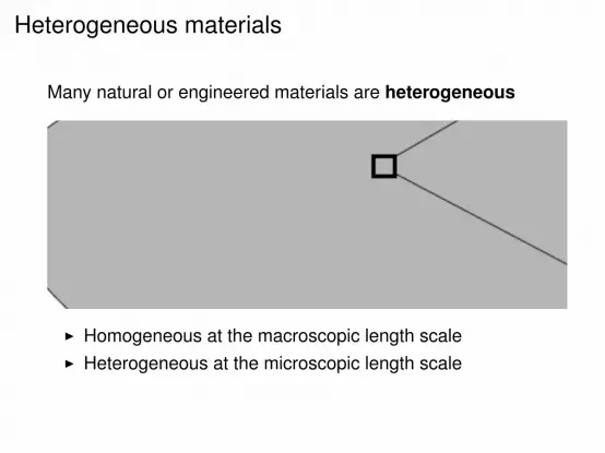
Heterogeneous materials

Many natural or engineered materials are heterogeneous

I Homogeneous at the macroscopic length scaleI Heterogeneous at the microscopic length scale

Heterogeneous materials

Need to model the macro-structure while taking themicro-structures into account

=⇒ better understanding of material behaviour, design, etc..

Two choices:I Direct numerical simulation: brute force!I Multiscale methods: when modelling a non-linear materials

=⇒ Computational Homogenisation

Outline



Conclusion

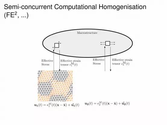
Semi-concurrent Computational Homogenisation(FE2, ...)

Effective strain

tensor

Macrostructure

Effective strain

tensorEffective

Stress

Effective

Stress

Problem

I For non-linear materials: Have to solve a RVE boundaryvalue problem at each point of the macro-mesh where it isneeded. Still expensive!

I Need parallel programming

Outline



Conclusion

Strategy

I Use model order reduction to make the solving of the RVEboundary value problems computationally achievable

I Linear displacement:

εM(t) =

(εxx (t) εxy (t)εxy (t) εyy (t)

)u(t) = εM(t)(x− x) + u with u|Γ = 0

Fluctuation u approximated by: u ≈∑

i φiαi

Projection-based model order reduction

The RVE problem can be written:

Fint(u(εM(t)), εM(t))︸︷︷︸Non-linear

+ Fext(εM(t)) = 0 (1)

We are interested in the solution u(εM) for many differentvalues of εM(t ∈ [0,T ]) ≡ εxx , εxy , εyy .

Projection-based model order reduction assumption:

Solutions u(εM) for different parameters εM are contained in aspace of small dimension span((φi)i∈J1,nK)

RVE boundary value problem

Matrix

Inclusions

Proper Orthogonal Decomposition (POD)

How to choose the basis [φ1,φ2, . . .] = Φ ?

I “Offline“ Stage ≡ Learning stage : Solve the RVE problemfor a certain number of chosen values of εM

I We obtain a base of solutions (the snapshot):(u1,u2, ...,unS ) = S

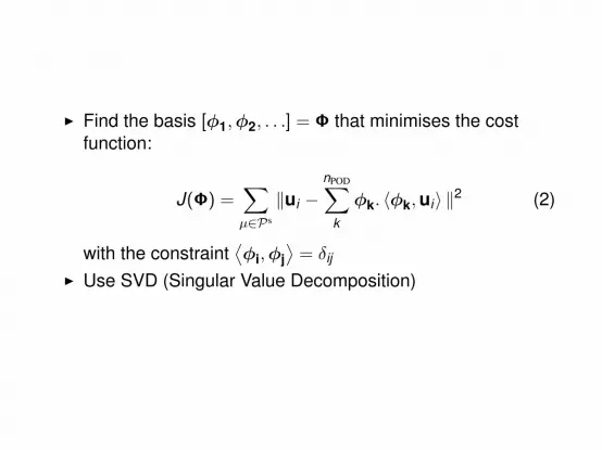
I Find the basis [φ1,φ2, . . .] = Φ that minimises the costfunction:

J(Φ) =∑µ∈Ps

‖ui −nPOD∑

k

φk. 〈φk,ui〉 ‖2 (2)

with the constraint⟨φi,φj

⟩= δij

I Use SVD (Singular Value Decomposition)

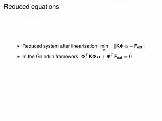
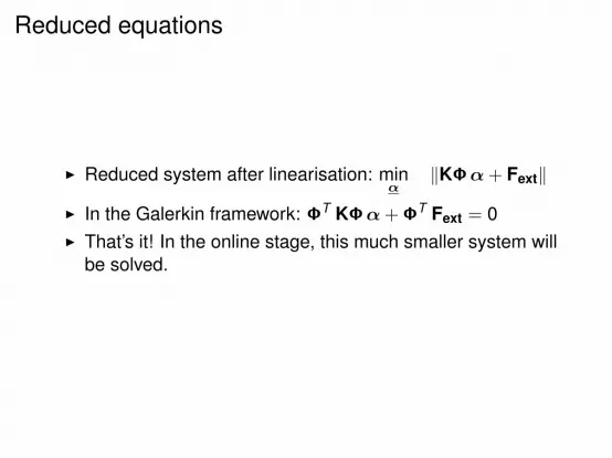
Reduced equations

I Reduced system after linearisation: minα

‖KΦα + Fext‖

I In the Galerkin framework: ΦT KΦα + ΦT Fext = 0I That’s it! In the online stage, this much smaller system will

be solved.

Reduced equations


‖KΦα + Fext‖

I In the Galerkin framework: ΦT KΦα + ΦT Fext = 0

I That’s it! In the online stage, this much smaller system willbe solved.

Reduced equations


‖KΦα + Fext‖

I In the Galerkin framework: ΦT KΦα + ΦT Fext = 0I That’s it! In the online stage, this much smaller system will

be solved.

Outline



Conclusion

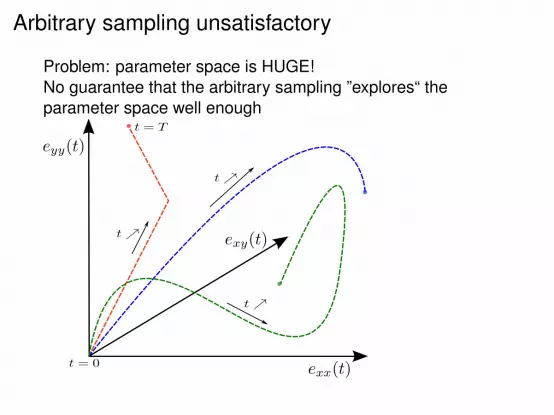
Arbitrary sampling unsatisfactory

Problem: parameter space is HUGE!No guarantee that the arbitrary sampling ”explores“ theparameter space well enough

Load of worst prediction

Rather than an arbitrary sampling, iteratively add the path ofworst prediction:

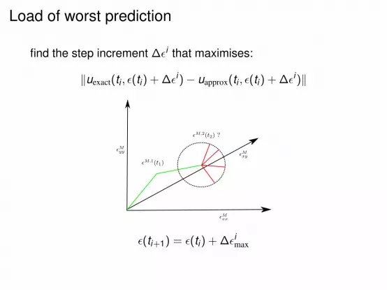
Load of worst prediction

find the step increment ∆εi that maximises:

‖uexact(ti , ε(ti) + ∆εi)− uapprox(ti , ε(ti) + ∆εi)‖

ε(ti+1) = ε(ti) + ∆εimax

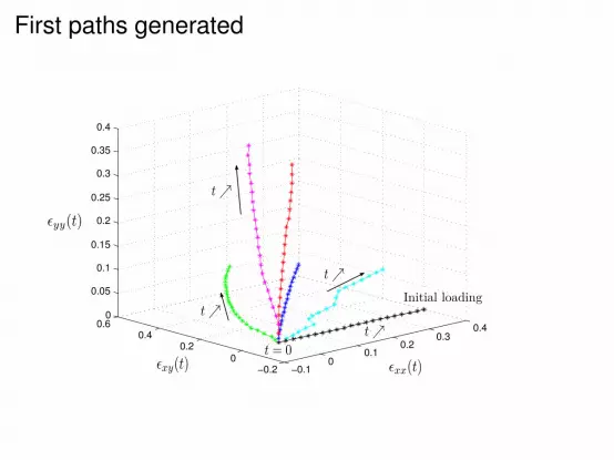
First paths generated

−0.10

0.10.2

0.30.4

−0.20

0.20.4

0.60

0.05

0.1

0.15

0.2

0.25

0.3

0.35

0.4

Initial loading

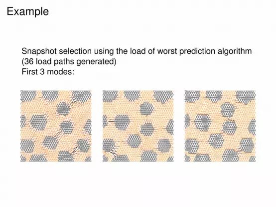
Example

Snapshot selection using the load of worst prediction algorithm(36 load paths generated)First 3 modes:

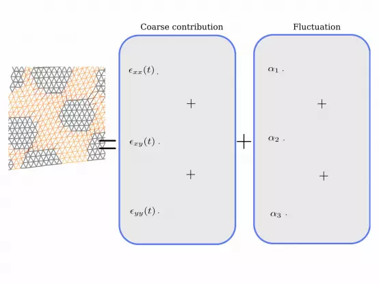
FluctuationCoarse contribution

+

+

+

+

=

.

.

.

.

.

.

+

Is that good enough?

I Speed-up actually poorI Equation “ΦT KΦα + ΦT Fext = 0“ quicker to solve but

ΦT KΦ still expensive to evaluateI Need to do something more =⇒ system approximation

Outline



Conclusion

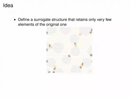
Idea

I Define a surrogate structure that retains only very fewelements of the original one

I Reconstruct the operators using a second POD basisrepresenting the internal forces

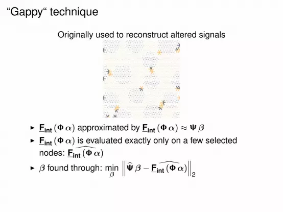
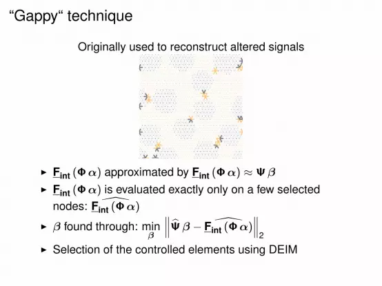
“Gappy“ technique

Originally used to reconstruct altered signals

I Fint (Φα) approximated by Fint (Φα) ≈ Ψβ

I Fint (Φα) is evaluated exactly only on a few selectednodes: Fint (Φα)

I β found through: minβ

∥∥∥Ψβ − Fint (Φα)∥∥∥

2

I Selection of the controlled elements using DEIM

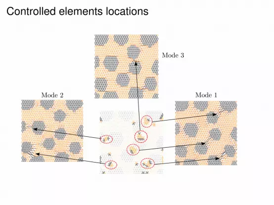
Controlled elements locations

Mode 1Mode 2

Mode 3

Outline



Conclusion

Error

0 2 4 6 8 10 12 14 16 18 200

20

40

60

80

100

120

0.001

0.003

0.01

0.03

0.1

0.3

1

Number of displacement basis vectors

Num

ber

of s

tatic

bas

is ve

ctor

s Relative error in energy norm

Speedup

4 6 8 10 12 14 16 18 20

20

30

40

50

60

70

80

90

100

110

120

1

2

3

4

5

6

7

8

9

10

11

12

Number of displacement basis vectors

Num

ber

of s

tatic

bas

is ve

ctor

sSpeedup

8 10 12 14 16 18 200

0.005

0.01

0.015

0.02

0.025

0.03

0.035

Number of basis vectors increases

Speedup

Rel

ativ

e er

ror

in e

nerg

y no

rm

Outline



Conclusion

Conclusion

I Model order reduction can be used to solved the RVEproblem faster and with a reasonable accuracy

I An efficient snapshot selection algorithm can be developedwhen dealing with time-dependent parameters

I The controlled elements generated by the DEIM algorithmlie where damage is high

I Can be thought of as a bridge between analytical andcomputational homogenisation:the reduced bases are pseudo-analytical solutions of theRVE problem that is still computationally solved at veryreduced cost

Thank you for your attention!

a model order reduction technique for speeding up computational homogenisation

Documents