pg day 2009 - hkbu comp
TRANSCRIPT

PROCEEDINGS
The 10th HKBU-CSD Postgraduate Research Symposium
PG Day 2009
Department of Computer Science Hong Kong Baptist University
August 31 & September 1, 2009

The 10th HKBU-CSD Postgraduate Research Symposium (PG Day) Program
August 31 Monday, 2009
Time Sessions 09:00-09:20 On-site Registration (LT1) 09:20-09:30 Welcome: Prof. Clement LEUNG (LT1) 09:30-10:30 Keynote Talk: Ms. Jenny Li
IBM Master Inventor, Chief Technology Officer for the Energy and Utility Industry, IBM System and Technology Group in Poughkeepsie, NY (LT1) (Chair: Dr. Xiaowen CHU) You Can Build a Smarter Planet
10:30-10:45 Tea Break (LMC511) 10:45-12:45
Session I: (Chair: Benyun SHI) (LMC511) • An Automatic Lip-reading Method Based On Polynomial Fitting
Meng LI • Image Analysis based on the Local Features of 2D Intrinsic Mode Functions
Dan ZHANG • Discriminability and Reliability Indexes: Two New Measures to Enhance
Multi-image Face Recognition Weiwen ZOU
• A Dynamic Trust Network for Autonomy-Oriented Partner Finding Hongjun QIU
12:45-13:00 Noon Break (LMC511) 13:00-15:00 Session II: (Chair: Shang XIA) (LMC511)
• Control Behavior of 3D Humanoid Animation Object Using Reinforcement Learning Yuesheng HE
• Optimize Write Performance for DBMS on Solid State Drive Yu LI
• Cooperative Stochastic Differential Game in P2P Content Distribution Network Xiaowei CHEN
• Social Knowledge Dynamics: A Case Study on Modeling Wikipedia Benyun SHI
15:00-15:10 Tea Break (LMC511) 15:10-17:10 Session III: (Chair: Dan ZHANG) (LMC511)
• Edge Detection Combining Wavelet Transform and Canny Operator Based on Fusion Rules Jian Jia PAN

• Modeling and Simulating Human Vaccinating Behaviors on a Disease Diffusion Network Shang XIA
• Extracting Discriminating Binary Template for Face Template Protection Yi Cheng FENG
• Incorporating Concept Ontology into Multi-level Image Indexing Chun Fan WONG
17:10-17:20 Tea Break (LMC511) 17:20-19:20 Session IV: (Chair: Xiaowei CHEN) (LMC511)
• Hiding Emerging Pattern with Local Recoding Generalization Wai Kit CHENG
• Estimation of the Number of Relevant Images in Infinite Databases Xiaoling WANG
• Patient Journey Optimization Using A Multi-Agent Approach Chung Ho CHOI
• Commentary-based Video Categorization and Concept Discovery Kwan Wai LEUNG
September 1 Tuesday, 2009
Time Sessions 09:20-10:20 Session V: (Chair: Weiwen ZOU) (RRS905)
• Implementation of Multiple-precision Modular Multiplication on GPU Kaiyong ZHAO
• L-BFGS and Delayed Dynamical Systems Approach for Unconstrained Optimization Xiaohui XIE
10:30-11:30 Distinguished Lecture: David Lorge Parnas Pioneer in Software Engineering, Professor Emeritus, University of Limerick & McMaster University (LT1) (Chair: Prof. Jiming LIU, Head of Department of Computer, HKBU) How Precise Documentation Allows Information Hiding to Reduce Software Complexity and Increase its Agility
11:30-14:00 Noon Break 14:00-15:00 Dialogue with Prof. David Lorge Parnas (RRS905)
(Chair: Weiwen ZOU) 16:30 Awards Ceremony: Best Paper & Best Presentation Awards (RRS905)
(Chair: Prof. Jiming LIU) All students and faculty are invited


Table of Contents An Automatic Lip-reading Method Based On Polynomial Fitting …………………………………1
Image Analysis based on the Local Features of 2D Intrinsic Mode Functions…………………………7
Discriminability and Reliability Indexes: Two New Measures to Enhance Multi-image Face
Recognition ………………………………………………………………………………………….13
A Dynamic Trust Network for Autonomy-Oriented Partner Finding ……………………......…….24
Control Behavior of 3D Humanoid Animation Object Using Reinforcement Learning ……………32
Optimize Write Performance for DBMS on Solid State Drive ……………………………......…….42
Cooperative Stochastic Differential Game in P2P Content Distribution Network …………………48
Social Knowledge Dynamics: A Case Study on Modeling Wikipedia ………......………………….54
Edge Detection Combining Wavelet Transform and Canny Operator Based on Fusion Rules
…………………………………………………………….........…………………………….60
Agent-based Epidemic Control Strategies: Modeling and Simulation of Dual-network Dynamics
…………………………………………............…………………………………………….65
Extracting Discriminating Binary Template for Face Template Protection …………………………72
Incorporating Concept Ontology into Multi-level Image Indexing …………..……….………….81
Hiding Emerging Pattern with Local Recoding Generalization …………………………......……….88
Estimation of the Number of Relevant Images in Infinite Databases …………...………………….98
Patient Journey Optimization Using A Multi-Agent Approach ……………………...……...125
Commentary-based Video Categorization and Concept Discovery ……………………………...133
Implementation of Multiple-precision Modular Multiplication on GPU …………………………143
L-BFGS and Delayed Dynamical Systems Approach for Unconstrained Optimization ……………149
An Automatic Lip-reading Method Based on Polynomial Fitting
Meng Li
Abstract
This paper addresses the problem of speaker-dependentisolate digits recognition using sole visual information. Weemploy intensity transformation and spatial filter to esti-mate the minimum enclosing rectangle of mouth in eachframe. Thus, for each utterance, we can obtain two vectorscomposed of width and height of mouth, respectively. Then,we propose an approach to recognize the speech based onpolynomial fitting. Firstly, both width and height vectorsare normalized into the constant length via interpolation.Secondly, least square method is utilized to produce two 3-order polynomials that can represent the main trend of thetwo vectors, respectively, and reduce the noise caused bythe estimate error. Lastly, positions of three crucial points(i.e. maximum, minimum and right boundary point) in each3-order polynomial curve are recorded as a feature vector.For each utterance, we calculate the average of all vectorsof training sample to make a template, and using Euclideandistance between the template and testing data to performthe classification. Experiments show the promising resultsof the proposed approach.
1 Introduction
Lip reading is to understand speech by visually interpretthe lip movement of speakers [7]. This technique has po-tential attractive applications in speech recognition, humanidentification, and so forth [4, 9, 13].
So far, two kinds of features are widely used in lip read-ing system, namely image-based and model-based. In theimage-based approach, the pixels of lip region are trans-formed by PCA, DWT or DCT, to become a feature vec-tor [2, 5, 6]. Under the ideal environment, the accuracy ofimage-based approach is considerable high, but the perfor-mance will be degraded seriously in real environment. Onemain reason is that the approach is restricted by the illu-mination, mouth rotation and some other conditions. Thus,from the practical view point, the image-based approach isnot the appropriate choice for automatic lip reading sys-tem. In the model based approach, shape and position oflip contours, tongue, teeth or some other features like width
and height of mouth are modeled, and controlled by a setof parameters(e.g. Snake, ASM and AAM) [3, 8, 10, 12].Model-based approach can invariant to the effects of scal-ing, rotation, translation and illumination. Hereby, with re-gard to the feature extraction, many researchers resort to themodal-based approach.
In this paper, we propose a lip reading approach undersimple modal – the width and height of mouth. We em-ploy intensity transformation and spatial filter to the imageof ROI(Range Of Interesting) in gray scale space to local-ize the minimum enclosing rectangle of lip automatically.Then, give a video clip for an utterance, we can obtain twovectors composed of the width and hight of mouth fromeach frame, respectively. Based on the least square method,two 3-order polynomials are built to fit the width and heightvector. The positions of three crucial points (i.e. maximum,minimum, and right boundary point) in each 3-order poly-nomial curve are recorded as a feature vector. For each ut-terance, we calculate the average of all vectors of trainingdata to make a template, and use Euclidean distance be-tween the template and testing data to perform the classi-fication.
The remainder of this paper is organized as follows. Sec-tion 2 describes the visual feature, namely the minimumenclosing rectangle of mouth, extraction method. Section3 presents our new approach for lip-reading recognition. InSection 4, we will conduct the experiment to compare ourapproaches with the existing methods. Finally, Section 5draws a conclusion.
2 Lip localization and feature extraction
Before showing the details, a pre-processing is needed.The images captured by camera are comprised of RGB val-ues. We heuristically project these RGB values into thegray-level space based on the following equation:
I = 0.299R + 0.587G + 0.114B. (1)
In order to enhance the contrast between lip and sur-rounding skip region, we adjust the histogram of the imageand make it equalized for the first step. Then we make an
1 of 162
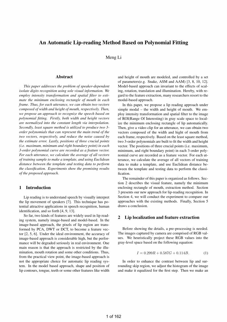
accumulation of gray level value for each row of the im-age. The slopes of the curve contain the information aboutthe boundaries between the lips and the surrounding skinregion. The minimum value on the curve retained as therow position of mouth corner points or the nearby position,the row can be named as horizontal midline of mouth. Themidline is shown in Figure 1.
Figure 1. Accumulation curve of gray levelvalue for each row. The vertical crossing linerepresents the relation between the horizon-tal midline of mouth and the minimum valueof the accumulation curve.
The curve of gray level values along with the horizon-tal midline is saved in vector G. Building a sub-vector Gs
by a segment of G which between the first maximum fromleft and the first maximum from right. Using the followingequations to make the curve smooth and save it into a newvector which named C.
C(i)l =
G(i)s (C(i−1)
l > G(i)s )
C(i−1)l (C(i−1)
l ≤ G(i)s )
i = 1, 2, . . . , n (2)
C(i)r =
G(i)s (C(i+1)
r > G(i)s )
C(i+1)r (C(i+1)
l ≤ G(i)s )
i = n− 1, n− 2, . . . , 1
(3)
C = Cl + Cr (4)
where Cl and Cr are assistant vectors, C(i)l is the ith ele-
ment in vector Cl, n is the dimension of the vector G. Theinitial values of the two vectors are shown in equation 5.
C(1)l = G(1)
C(n)r = G(n)
(5)
Set the minimum of the most left and most right valuein C as threshold. Elements in C less than the thresholdbuild a new vector C ′ . Accordingly, the average can becalculated by the equation 6.
cavg =∑m
i=1 C′(i)
m(6)
The equation 7 is employed to adjust the contrast of im-age.
Iout =
255 (1.5cavg < Iin < 1)
500cavg
− 500 (0 < Iin ≤ 1.5cavg)(7)
where Iin is the input gray level value, and the Iout is theoutput.
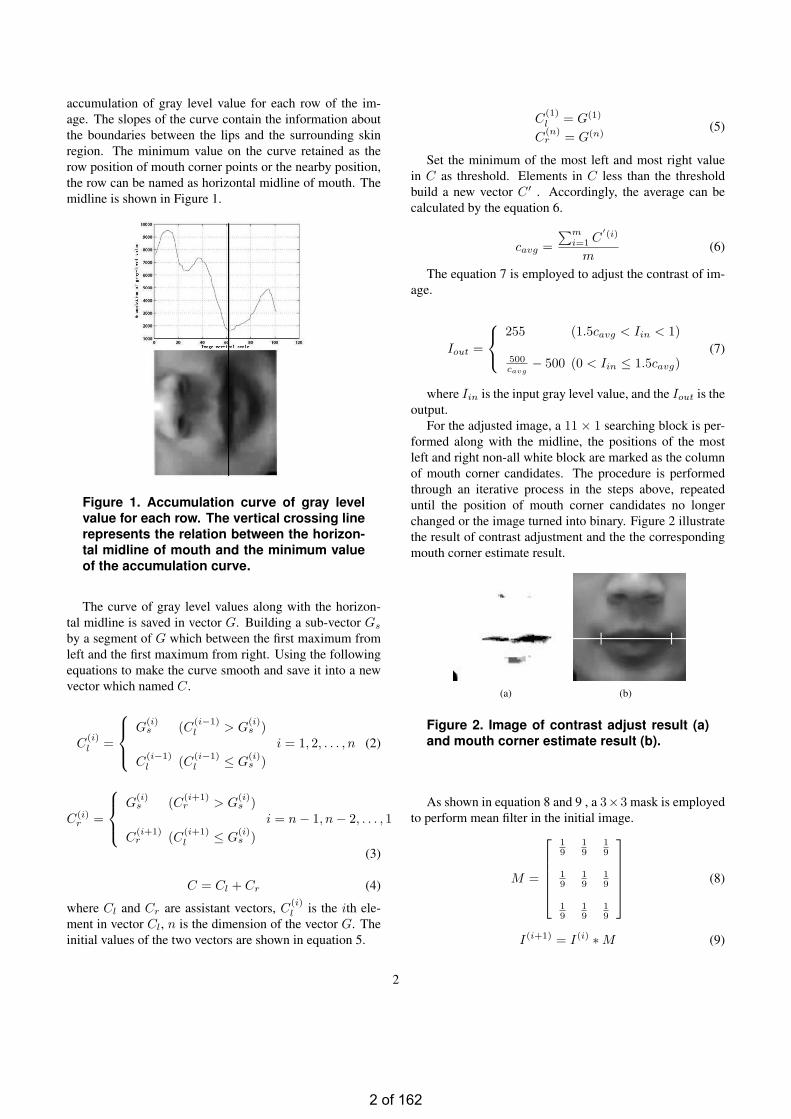
For the adjusted image, a 11 × 1 searching block is per-formed along with the midline, the positions of the mostleft and right non-all white block are marked as the columnof mouth corner candidates. The procedure is performedthrough an iterative process in the steps above, repeateduntil the position of mouth corner candidates no longerchanged or the image turned into binary. Figure 2 illustratethe result of contrast adjustment and the the correspondingmouth corner estimate result.
(a) (b)
Figure 2. Image of contrast adjust result (a)and mouth corner estimate result (b).
As shown in equation 8 and 9 , a 3×3 mask is employedto perform mean filter in the initial image.
M =
19
19
19
19
19
19
19
19
19
(8)
I(i+1) = I(i) ∗M (9)
2
2 of 162
where the I(i) is the result of ith time filter. The timesfilter performed is determined by the equation 10.
δi = dist(I(i+1), I(i)) (10)
where δi is the Euclidean distance between I(i) andI(i+1). The procedure should be ceased once δi less thana given threshold, and the I(i+1) can be marked as If .
Due to the position of left and right mouth corners havebeen estimated in section 2.1, we can utilize them to calcu-late the center of mouth easily. For each I(i), a gray valuevector G
(i)mu is built by the segment from the center point
to the top of image along with the normal direction respec-tively. Then the vector ∆Gacc is calculated by the equation11.
∆Gacc =n∑
i=1
(|G(0)mu −G(i)
mu|) (11)
The point correspond to extreme value of maximum(except boundary value) is retained as the row position ofupper bound of mouth.
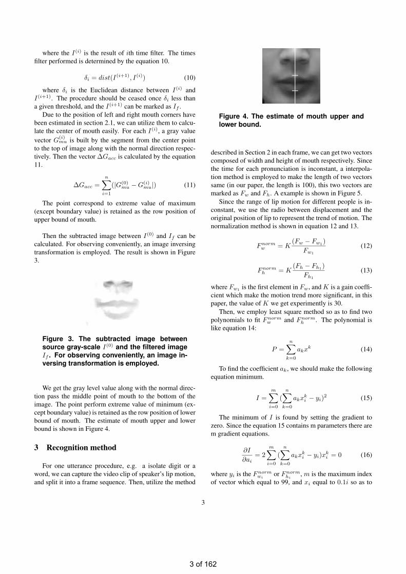
Then the subtracted image between I(0) and If can becalculated. For observing conveniently, an image inversingtransformation is employed. The result is shown in Figure3.
Figure 3. The subtracted image betweensource gray-scale I(0) and the filtered imageIf . For observing conveniently, an image in-versing transformation is employed.
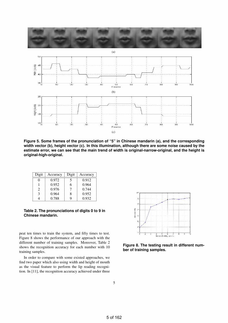
We get the gray level value along with the normal direc-tion pass the middle point of mouth to the bottom of theimage. The point perform extreme value of minimum (ex-cept boundary value) is retained as the row position of lowerbound of mouth. The estimate of mouth upper and lowerbound is shown in Figure 4.
3 Recognition method
For one utterance procedure, e.g. a isolate digit or aword, we can capture the video clip of speaker’s lip motion,and split it into a frame sequence. Then, utilize the method
Figure 4. The estimate of mouth upper andlower bound.
described in Section 2 in each frame, we can get two vectorscomposed of width and height of mouth respectively. Sincethe time for each pronunciation is inconstant, a interpola-tion method is employed to make the length of two vectorssame (in our paper, the length is 100), this two vectors aremarked as Fw and Fh. A example is shown in Figure 5.
Since the range of lip motion for different people is in-constant, we use the radio between displacement and theoriginal position of lip to represent the trend of motion. Thenormalization method is shown in equation 12 and 13.
Fnormw = K
(Fw − Fw1)Fw1
(12)
Fnormh = K
(Fh − Fh1)Fh1
(13)
where Fw1 is the first element in Fw, and K is a gain coeffi-cient which make the motion trend more significant, in thispaper, the value of K we get experimently is 30.
Then, we employ least square method so as to find twopolynomials to fit Fnorm
w and Fnormh . The polynomial is
like equation 14:
P =n∑
k=0
akxk (14)
To find the coefficient ak, we should make the followingequation minimum.
I =m∑
i=0
(n∑
k=0
akxki − yi)2 (15)
The minimum of I is found by setting the gradient tozero. Since the equation 15 contains m parameters there arem gradient equations.
∂I
∂ai= 2
m∑
i=0
(n∑
k=0
akxki − yi)xk
i = 0 (16)
where yi is the Fnormwi
or Fnormhi
, m is the maximum indexof vector which equal to 99, and xi equal to 0.1i so as to
3
3 of 162

avoid the conditioned in coefficient matrix. Moreover, ow-ing to the characteristic of human speech, n is chosen by 3.Thus, we can get the solution Aw = [aw0, aw1, aw2, aw3]T
and Ah = [ah0, ah1, ah2, ah3]T . A example of polynomialfitting result is shown in Figure 6.
The polynomial shapes for the same utterance areconstrained to have similar expression. Thus, we canget the global maximum and minimum in the twopolynomial marked as (xwmin
, ywmin), (xhmin
, yhmin),
(xwmax, ywmax
) and (xhmax, ywmax
) to build the featurevectors which shown below:
Fw = [xwmin , ywmin , xwmax , ywmax , ywbound]T (17)
Fh = [xhmin, yhmin
, xhmax, yhmax
, yhbound]T (18)
where the ybound is the most right value of polynomial whenx ∈ [0, 9.9] (e.g. x = x99).
(a)
(b)
Figure 6. The curve of polynomial which fitto the width vector (a) and height vector (b)shown in Figure 5.
Moreover, for the feature vectors, if xmin 6∈ [0, 9.9],both xmin and ymin are set to zero. In a similarway, we can determine the value of xmax and ymax.For example, as shown in Figure 6, the feature vectorsare Fw = [4.1558,−2.3476, 0, 0, 0.9460]T and Fh =[0, 0, 4.1266, 12.9164, 1.2969]T .
For each utterance, we calculate the average of all vec-tors of training data to make a template by following equa-tions.
T i+1w =
T iw + Fw
2(19)
T i+1h =
T ih + Fh
2(20)
Digit Phonetic Symbol Digit Phonetic Symbol0 [li6] 5 [u:]1 [jau] 6 [liou]2 [7Þ] 7 [tC’]3 [san] 8 [ba:]4 [s1] 9 [tCiou]
Table 1. The pronunciations of number 0 to 9in Chinese mandarin.
where Ti is the template after i times trains employed, Fis the new training data. For each classification, there is atemplate which involve two vectors.
When testing, we calculate the distance between eachtemplate and testing data via the following equation.
d = ||Fw − Tw|| · ||Fh − Th|| (21)
that is, the input testing data is classified into the categorywhich corresponding into the minimum d.
4 Experiment result
We conduct an experiment to demonstrate the perfor-mance of the proposed approach. The experiment environ-ment is shown in Figure 7. The illumination source is a 18wfluorescent lamp which placed in front of speaker.The res-olution of camera is 320 × 240, and the FPS(Frames PerSecond) is 30.
Figure 7. The illustration of experiment envi-ronment.
Our task is to recognize 10 isolate digits(0 to 9) in Chi-nese mandarin, which pronunciations are shown in Table 1.
There are 5 speakers(4 males and 1 female) take part intothe experiment. For each digit, speakers were asked to re-
4
4 of 162
(a)
(b)
(c)
Figure 5. Some frames of the pronunciation of “5” in Chinese mandarin (a), and the correspondingwidth vector (b), height vector (c). In this illumination, although there are some noise caused by theestimate error, we can see that the main trend of width is original-narrow-original, and the height isoriginal-high-original.
Digit Accuracy Digit Accuracy0 0.972 5 0.9121 0.952 6 0.9642 0.976 7 0.7443 0.964 8 0.9524 0.788 9 0.932
Table 2. The pronunciations of digits 0 to 9 inChinese mandarin.
peat ten times to train the system, and fifty times to test.Figure 8 shows the performance of our approach with thedifferent number of training samples. Moreover, Table 2shows the recognition accuracy for each number with 10training samples.
In order to compare with some existed approaches, wefind two paper which also using width and height of mouthas the visual feature to perform the lip reading recogni-tion. In [11], the recognition accuracy achieved under three
Figure 8. The testing result in different num-ber of training samples.
5
5 of 162
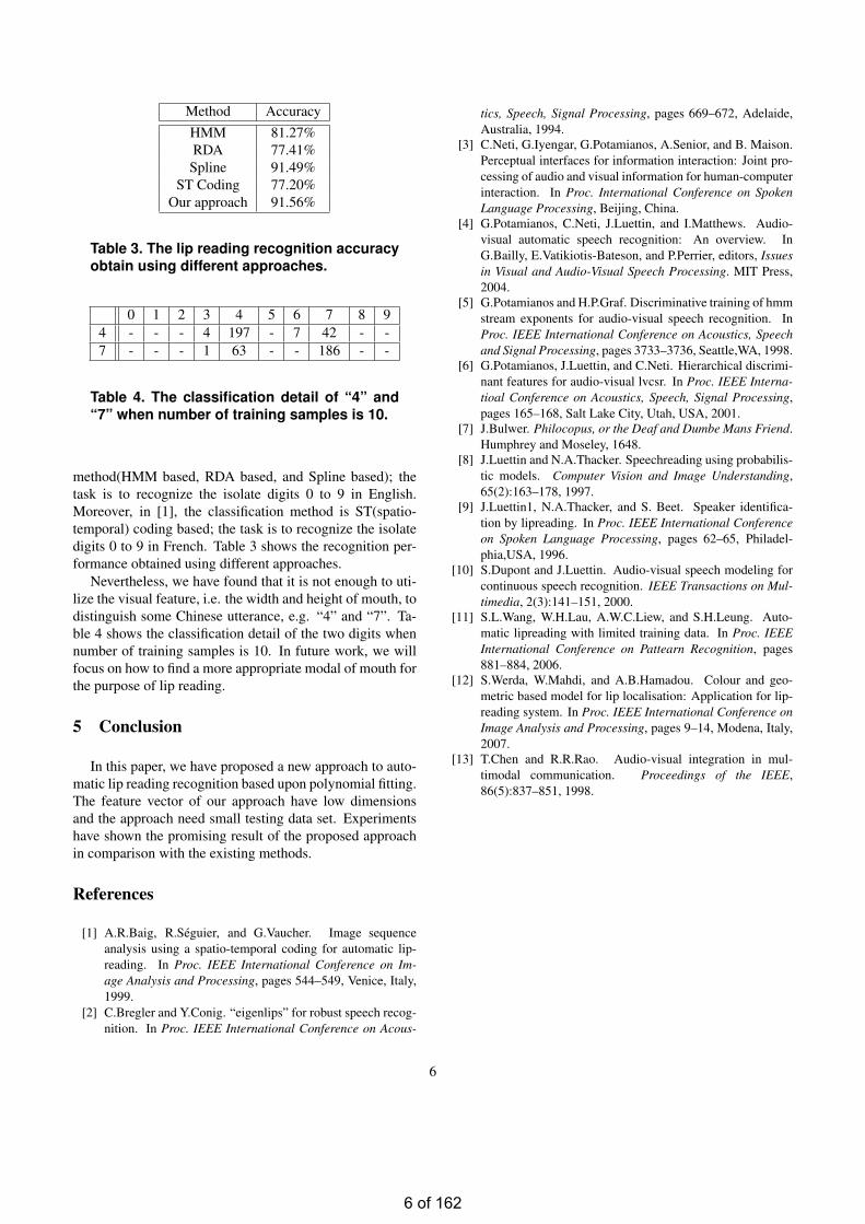
Method AccuracyHMM 81.27%RDA 77.41%Spline 91.49%
ST Coding 77.20%Our approach 91.56%
Table 3. The lip reading recognition accuracyobtain using different approaches.
0 1 2 3 4 5 6 7 8 94 - - - 4 197 - 7 42 - -7 - - - 1 63 - - 186 - -
Table 4. The classification detail of “4” and“7” when number of training samples is 10.
method(HMM based, RDA based, and Spline based); thetask is to recognize the isolate digits 0 to 9 in English.Moreover, in [1], the classification method is ST(spatio-temporal) coding based; the task is to recognize the isolatedigits 0 to 9 in French. Table 3 shows the recognition per-formance obtained using different approaches.
Nevertheless, we have found that it is not enough to uti-lize the visual feature, i.e. the width and height of mouth, todistinguish some Chinese utterance, e.g. “4” and “7”. Ta-ble 4 shows the classification detail of the two digits whennumber of training samples is 10. In future work, we willfocus on how to find a more appropriate modal of mouth forthe purpose of lip reading.
5 Conclusion
In this paper, we have proposed a new approach to auto-matic lip reading recognition based upon polynomial fitting.The feature vector of our approach have low dimensionsand the approach need small testing data set. Experimentshave shown the promising result of the proposed approachin comparison with the existing methods.
References
[1] A.R.Baig, R.Seguier, and G.Vaucher. Image sequenceanalysis using a spatio-temporal coding for automatic lip-reading. In Proc. IEEE International Conference on Im-age Analysis and Processing, pages 544–549, Venice, Italy,1999.
[2] C.Bregler and Y.Conig. “eigenlips” for robust speech recog-nition. In Proc. IEEE International Conference on Acous-
tics, Speech, Signal Processing, pages 669–672, Adelaide,Australia, 1994.
[3] C.Neti, G.Iyengar, G.Potamianos, A.Senior, and B. Maison.Perceptual interfaces for information interaction: Joint pro-cessing of audio and visual information for human-computerinteraction. In Proc. International Conference on SpokenLanguage Processing, Beijing, China.
[4] G.Potamianos, C.Neti, J.Luettin, and I.Matthews. Audio-visual automatic speech recognition: An overview. InG.Bailly, E.Vatikiotis-Bateson, and P.Perrier, editors, Issuesin Visual and Audio-Visual Speech Processing. MIT Press,2004.
[5] G.Potamianos and H.P.Graf. Discriminative training of hmmstream exponents for audio-visual speech recognition. InProc. IEEE International Conference on Acoustics, Speechand Signal Processing, pages 3733–3736, Seattle,WA, 1998.
[6] G.Potamianos, J.Luettin, and C.Neti. Hierarchical discrimi-nant features for audio-visual lvcsr. In Proc. IEEE Interna-tioal Conference on Acoustics, Speech, Signal Processing,pages 165–168, Salt Lake City, Utah, USA, 2001.
[7] J.Bulwer. Philocopus, or the Deaf and Dumbe Mans Friend.Humphrey and Moseley, 1648.
[8] J.Luettin and N.A.Thacker. Speechreading using probabilis-tic models. Computer Vision and Image Understanding,65(2):163–178, 1997.
[9] J.Luettin1, N.A.Thacker, and S. Beet. Speaker identifica-tion by lipreading. In Proc. IEEE International Conferenceon Spoken Language Processing, pages 62–65, Philadel-phia,USA, 1996.
[10] S.Dupont and J.Luettin. Audio-visual speech modeling forcontinuous speech recognition. IEEE Transactions on Mul-timedia, 2(3):141–151, 2000.
[11] S.L.Wang, W.H.Lau, A.W.C.Liew, and S.H.Leung. Auto-matic lipreading with limited training data. In Proc. IEEEInternational Conference on Pattearn Recognition, pages881–884, 2006.
[12] S.Werda, W.Mahdi, and A.B.Hamadou. Colour and geo-metric based model for lip localisation: Application for lip-reading system. In Proc. IEEE International Conference onImage Analysis and Processing, pages 9–14, Modena, Italy,2007.
[13] T.Chen and R.R.Rao. Audio-visual integration in mul-timodal communication. Proceedings of the IEEE,86(5):837–851, 1998.
6
6 of 162
Image Analysis Based on the Local Features of 2D Intrinsic Mode Functions
Dan Zhang
Abstract
The Hilbert-Huang transform (HHT) is a novel sig-nal processing method which can efficiently handle non-stationary and nonlinear signals. It firstly decomposes sig-nals into a series of Intrinsic Mode Functions (IMFs) adap-tively by the Empirical Mode Decomposition (EMD), thenapplies the Hilbert transform on the IMFs afterward. Basedon the analytical signals obtained, the local analysis of theIMFs are conducted. This paper contains two main works.First, we proposed a new two-dimensional EMD (2DEMD)method, which is faster, better-performed than the current2DEMD methods. Second, the Riesz transform are utilizedon the 2DIMFs to get the 2D analytical signals. The lo-cal features (amplitude, phase orientation, phase angle, etc)are evaluated. The performances are demonstrated on bothtexture images and natural images.
1 Introduction
Texture [1] is ubiquitous and provides powerful charac-teristics for many image analysis applications such as seg-mentation, edge detection, and image retrieval. Amongvarious texture analysis methods, signal processing meth-ods are promising, which include Gabor filters [2], wavelettransforms [3], Wigner distributions and so forth. Theycharacterize textures through filter responses directly.
Hilbert-Huang transform is a new signal processingmethod proposed by Huang et al [8, 10, 9]. It contains twokernel parts: Empirical Mode Decomposition (EMD) andHilbert transform. First, it decomposes signals into a se-ries of Intrinsic Mode Functions (IMFs) adaptively by theEmpirical Mode Decomposition (EMD), then applies theHilbert transform on the IMFs afterward. Based on the an-alytical signals obtained, the local analysis of the IMFs areconducted. Though Fourier spectral analysis and wavelettransform have provided some general methods for analyz-ing signals and data, they are still weak at non-stationaryand nonlinear data processing. However, due to the fullydata-driven process, the HHT is more efficient in this situa-tion. It provides an efficient way for the local analysis.
As the kernel part of HHT, EMD works as a filter bank.It has a wide application in signal analysis including oceanwaves, rogue water waves, sound analysis, earthquake timerecords as well as image analysis [19, 18, 16, 21, 20, 22, 23].The EMD has been extended to 2DEMD. However, it coun-tered a lot of difficulties such as inaccuracy of surface in-terpolation, high computational complexity and so forth[27, 29, 25, 26, 28, 31]. Finding a powerful 2DEMD isstill a challenge. In this paper, we implemented a modi-fied 2DEMD and study the local properties of the 2DIMFsby Riesz transform [4, 5]. The image after its Riesz trans-form, we can get the 2D analytical signal. The estimationof the local features is crucial in image processing. Gener-ally, structures such as lines and edges can be distinguisedby the local phase, the local amplitude can be used for edgedetection.
This paper is organized as follows: Section 2 presents anintroduction to HHT. In Section 3, the details of the modi-fied 2DEMD are shown firstly, then we reviewed the Riesztransform. The simulation results are demonstrated in Sec-tion 4. Finally, the conclusions are given.
2 Hilbert-Huang transform
Hilbert-Huang transform was proposed by N.E.Huang in1998. It contains two parts in terms of Empirical ModeDecomposition (EMD) and Hilbert transform. The signalsare decomposed into a series of Intrinsic Mode Functions(IMFs), then Hilbert transform are applied on these IMFs toget analytic signals. Since this method is local, data-driven,it is capable of handling nonlinear and non-stationary sig-nals.
EMD captures information about local trends in the sig-nal by measuring oscillations, which can be quantized by alocal high frequency or a local low frequency, correspond-ing to finest detail and coarsest content. Here we brieflyreview the sifting process of EMD. Four main steps are con-tained, S1, S2, S3 and S4 are abbreviation for Step 1 to Step4. Given a signal x(t),
S1. Identify all the local minima and maxima of the inputsignals x(t);
7 of 162

S2. Interpolate between all minima and maxima to yieldtwo corresponding envelopes Emax(t) and Emin(t).Calculate the mean envelope m(t) = (Emax(t) +Emin(t))/2;
S3. Compute the residue h(t) = x(t) −m(t). If it is lessthan the threshold predefined then it becomes the firstIMF, go to Step 4. Otherwise, repeat Step 1 and Step 2 usingthe residue h(t), until the latest residue meets the thresholdand turns to be an IMF;
S4. Input the residue r(t) to the loop from Step 1 to Step 3 toget the next remained IMFs until it can not be decomposedfurther.
The analytical signal provides a way to compute the 1Dsignal’s local amplitude and phase, which is obtained by theHilbert transform on a real signal. The Hilbert transformfH(x) of a real 1D signal f is given by:
fH(x) = f(x) ∗ 1πx
,
where ∗ is convolution. fH(x) is the imaginary part of thesignal. The analytical signal can be written as
fA = f(x) + ifH(x) = a(t)eiθ(t),
in which, a(t) is the amplitude, θ(t) is the phase.Applying Hilbert transform on each IMF can evaluate
the local properties such as amplitude and phase.
3 Local Analysis of 2DIMFs
3.1 The improved 2DEMD
Here we propose an alternative algorithm for EMD. In-stead of using the envelopes generated by splines we use alow pass filter to generate a “moving average” to replace themean of the envelopes. The essence of the sifting algorithmremains.
The moving average is the most common filter in dig-ital signal processing. It operates by averaging a numberof points from the input signal to produce each point in theoutput signal, it is written:
y[i] =1M
M−1∑
j=0
x[i + j],
where x[] is the input signal, y[] is the output signal, andM is the number of points used in the moving average. It isactually a convolution using a simple filter [ai]Mi=1, ai = 1
M ,and [Ai,j ]
M,Ni=1,j=1, Ai,j = 1
M×N for the 2-dimensional case.Detection of local extrema means finding the local max-
ima and minima points from the given data. No matter for
1D signal or 2D array, neighboring window method is em-ployed to find local maxima and local minima points. Thedata point/pixel is considered as a local maximum (mini-mum) if its value is strictly higher (lower) than all of itsneighbors.
We illustrated 1-dimensional case and 2-dimensionalcase separately.
• 1-dimensional case:For each extrema map, the distance between the twoneighborhood local maxima (minima, extrema, zero-crossing) has been calculated called as adjacent max-ima (minima, extrema, zero-crossing) distance vectorAdj max (Adj min,Adj ext,Adj zer). Four typesof window size:
– Window-size I: max(Adj max);
– Window-size II: max(Adj min);
– Window-size III: max(Adj zer);
– Window-size IV: max(Adj ext).
• 2-dimensional case:The window size for average filters is determinedbased on the maxima and minima maps obtained froma source image. For each local maximum (minimum)point, the Euclidean distance to the nearest local max-imum (minimum) point is calculated, denoted as ad-jacent maxima (minimum) distance array Adj max(Adj min).
– Window-size I: max(Adj max);
– Window-size II: max(Adj min);
3.2 Monogenic signal
The analytic signal is the basis for all kinds of ap-proaches which makes use of the local phase. The combi-nation of a 1D signal and its Hilbert transform is called theanalytic signal. Similarly, the combination of a image andits Riesz transform, which is the generalization of Hilberttransform, is called the monogenic signal [4, 5].
The monogenic signal is often identified as a local quan-titative or qualitative measure of an image. Different ap-proaches to an nD analytic or complex signal have beenproposed in the past:
• Total Hilbert Transform, The Hilbert transform is per-formed with respect to both axes:
HT (−→v ) = jsign(v1)sign(v2)
This transform is not a valid generalization of theHilbert transform since it does not perform a phaseshift of π/2.It can’t meet orthogonality.
8 of 162
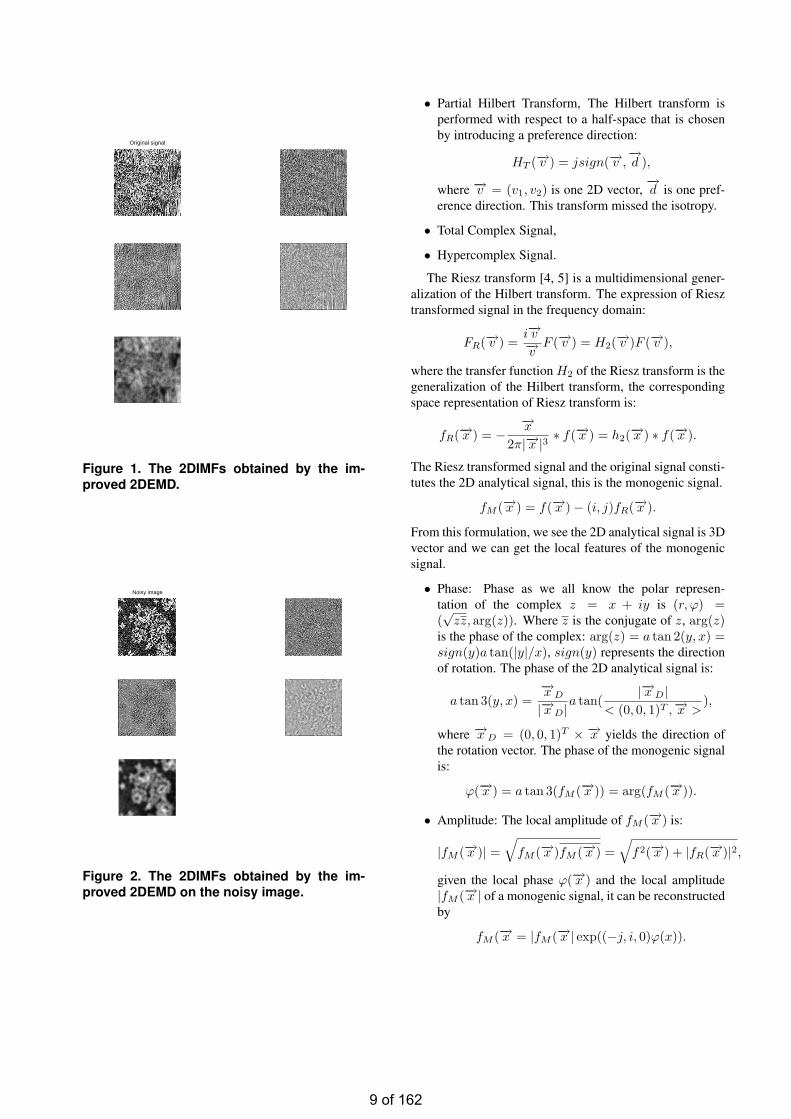
Original signal
Figure 1. The 2DIMFs obtained by the im-proved 2DEMD.
Noisy image
Figure 2. The 2DIMFs obtained by the im-proved 2DEMD on the noisy image.
• Partial Hilbert Transform, The Hilbert transform isperformed with respect to a half-space that is chosenby introducing a preference direction:
HT (−→v ) = jsign(−→v ,−→d ),
where −→v = (v1, v2) is one 2D vector,−→d is one pref-
erence direction. This transform missed the isotropy.
• Total Complex Signal,
• Hypercomplex Signal.
The Riesz transform [4, 5] is a multidimensional gener-alization of the Hilbert transform. The expression of Riesztransformed signal in the frequency domain:
FR(−→v ) =i−→v−→v F (−→v ) = H2(−→v )F (−→v ),
where the transfer function H2 of the Riesz transform is thegeneralization of the Hilbert transform, the correspondingspace representation of Riesz transform is:
fR(−→x ) = −−→x
2π|−→x |3 ∗ f(−→x ) = h2(−→x ) ∗ f(−→x ).
The Riesz transformed signal and the original signal consti-tutes the 2D analytical signal, this is the monogenic signal.
fM (−→x ) = f(−→x )− (i, j)fR(−→x ).
From this formulation, we see the 2D analytical signal is 3Dvector and we can get the local features of the monogenicsignal.
• Phase: Phase as we all know the polar represen-tation of the complex z = x + iy is (r, ϕ) =(√
zz, arg(z)). Where z is the conjugate of z, arg(z)is the phase of the complex: arg(z) = a tan 2(y, x) =sign(y)a tan(|y|/x), sign(y) represents the directionof rotation. The phase of the 2D analytical signal is:
a tan 3(y, x) =−→x D
|−→x D|a tan(|−→x D|
< (0, 0, 1)T ,−→x >),
where −→x D = (0, 0, 1)T × −→x yields the direction ofthe rotation vector. The phase of the monogenic signalis:
ϕ(−→x ) = a tan 3(fM (−→x )) = arg(fM (−→x )).
• Amplitude: The local amplitude of fM (−→x ) is:
|fM (−→x )| =√
fM (−→x )fM (−→x ) =√
f2(−→x ) + |fR(−→x )|2,given the local phase ϕ(−→x ) and the local amplitude|fM (−→x | of a monogenic signal, it can be reconstructedby
fM (−→x = |fM (−→x | exp((−j, i, 0)ϕ(x)).
9 of 162
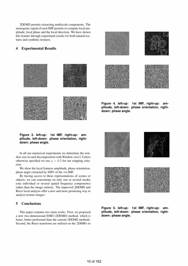
2DEMD permits extracting multiscale components. Themonogenic signal of each IMF permits to compute local am-plitude, local phase and the local direction. We have shownthis feature through experiment results for both natural tex-tures and synthetic textures.
4 Experimental Results
Figure 3. left-up: 1st IMF, right-up: am-plitude, left-down: phase orientation, right-down: phase angle.
In all our numerical experiments we determine the win-dow size in each decomposition with Window-size I. Unlessotherwise specified we use α = 0.5 for our stopping crite-rion.
We show the local features amplitude, phase orientation,phase angle extracted by SMV of the 1st IMF.
By having access to these representations of scenes orobjects, we can concentrate on only one or several modes(one individual or several spatial frequency components)rather than the image entirety. The improved 2DEMD andRiesz local analysis offer a new and more promising way toanalyze texture images.
5 Conclusions
This paper contains two main works. First, we proposeda new two-dimensional EMD (2DEMD) method, which isfaster, better-performed than the current 2DEMD methods.Second, the Riesz transform are utilized on the 2DIMFs to
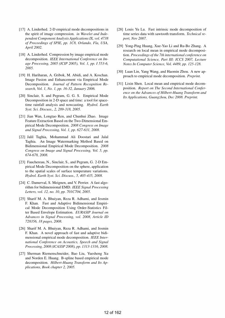
Figure 4. left-up: 1st IMF, right-up: am-plitude, left-down: phase orientation, right-down: phase angle.
Figure 5. left-up: 1st IMF, right-up: am-plitude, left-down: phase orientation, right-down: phase angle.
10 of 162
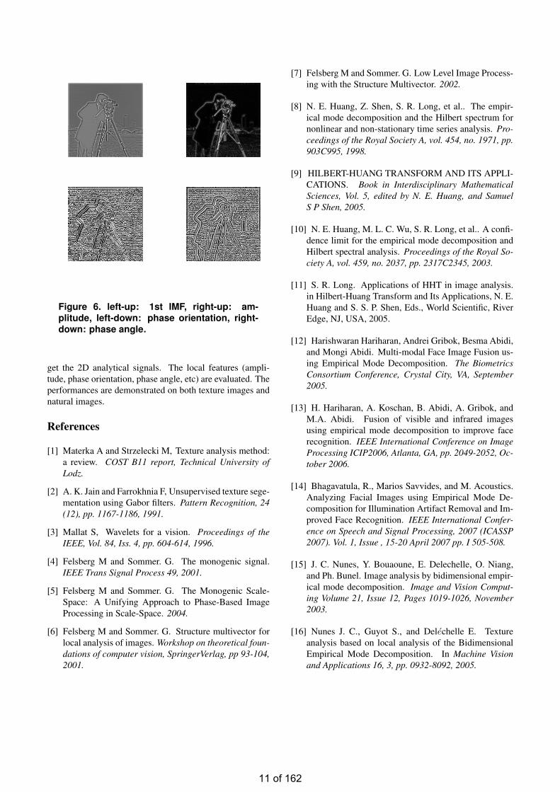
Figure 6. left-up: 1st IMF, right-up: am-plitude, left-down: phase orientation, right-down: phase angle.
get the 2D analytical signals. The local features (ampli-tude, phase orientation, phase angle, etc) are evaluated. Theperformances are demonstrated on both texture images andnatural images.
References
[1] Materka A and Strzelecki M, Texture analysis method:a review. COST B11 report, Technical University ofLodz.
[2] A. K. Jain and Farrokhnia F, Unsupervised texture sege-mentation using Gabor filters. Pattern Recognition, 24(12), pp. 1167-1186, 1991.
[3] Mallat S, Wavelets for a vision. Proceedings of theIEEE, Vol. 84, Iss. 4, pp. 604-614, 1996.
[4] Felsberg M and Sommer. G. The monogenic signal.IEEE Trans Signal Process 49, 2001.
[5] Felsberg M and Sommer. G. The Monogenic Scale-Space: A Unifying Approach to Phase-Based ImageProcessing in Scale-Space. 2004.
[6] Felsberg M and Sommer. G. Structure multivector forlocal analysis of images. Workshop on theoretical foun-dations of computer vision, SpringerVerlag, pp 93-104,2001.
[7] Felsberg M and Sommer. G. Low Level Image Process-ing with the Structure Multivector. 2002.
[8] N. E. Huang, Z. Shen, S. R. Long, et al.. The empir-ical mode decomposition and the Hilbert spectrum fornonlinear and non-stationary time series analysis. Pro-ceedings of the Royal Society A, vol. 454, no. 1971, pp.903C995, 1998.
[9] HILBERT-HUANG TRANSFORM AND ITS APPLI-CATIONS. Book in Interdisciplinary MathematicalSciences, Vol. 5, edited by N. E. Huang, and SamuelS P Shen, 2005.
[10] N. E. Huang, M. L. C. Wu, S. R. Long, et al.. A confi-dence limit for the empirical mode decomposition andHilbert spectral analysis. Proceedings of the Royal So-ciety A, vol. 459, no. 2037, pp. 2317C2345, 2003.
[11] S. R. Long. Applications of HHT in image analysis.in Hilbert-Huang Transform and Its Applications, N. E.Huang and S. S. P. Shen, Eds., World Scientific, RiverEdge, NJ, USA, 2005.
[12] Harishwaran Hariharan, Andrei Gribok, Besma Abidi,and Mongi Abidi. Multi-modal Face Image Fusion us-ing Empirical Mode Decomposition. The BiometricsConsortium Conference, Crystal City, VA, September2005.
[13] H. Hariharan, A. Koschan, B. Abidi, A. Gribok, andM.A. Abidi. Fusion of visible and infrared imagesusing empirical mode decomposition to improve facerecognition. IEEE International Conference on ImageProcessing ICIP2006, Atlanta, GA, pp. 2049-2052, Oc-tober 2006.
[14] Bhagavatula, R., Marios Savvides, and M. Acoustics.Analyzing Facial Images using Empirical Mode De-composition for Illumination Artifact Removal and Im-proved Face Recognition. IEEE International Confer-ence on Speech and Signal Processing, 2007 (ICASSP2007). Vol. 1, Issue , 15-20 April 2007 pp. I 505-508.
[15] J. C. Nunes, Y. Bouaoune, E. Delechelle, O. Niang,and Ph. Bunel. Image analysis by bidimensional empir-ical mode decomposition. Image and Vision Comput-ing Volume 21, Issue 12, Pages 1019-1026, November2003.
[16] Nunes J. C., Guyot S., and Delechelle E. Textureanalysis based on local analysis of the BidimensionalEmpirical Mode Decomposition. In Machine Visionand Applications 16, 3, pp. 0932-8092, 2005.
11 of 162
[17] A. Linderhed. 2-D empirical mode decompositions inthe spirit of image compression. in Wavelet and Inde-pendent Component Analysis Applications IX, vol. 4738of Proceedings of SPIE, pp. 1C8, Orlando, Fla, USA,April 2002.
[18] A. Linderhed. Compression by image empirical modedecomposition. IEEE International Conference on Im-age Processing, 2005 (ICIP 2005), Vol. 1, pp. I 553-6,2005.
[19] H. Hariharan, A. Gribok, M. Abidi, and A. Koschan.Image Fusion and Enhancement via Empirical ModeDecomposition. Journal of Pattern Recognition Re-search, Vol. 1, No. 1, pp. 16-32, January 2006.
[20] Sinclair, S. and Pegram, G. G. S. Empirical ModeDecomposition in 2-D space and time: a tool for space-time rainfall analysis and nowcasting. Hydrol. EarthSyst. Sci. Discuss., 2, 289-318, 2005.
[21] Jian Wan, Longtao Ren, and Chunhui Zhao. ImageFeature Extraction Based on the Two-Dimensional Em-pirical Mode Decomposition. 2008 Congress on Imageand Signal Processing, Vol. 1, pp. 627-631, 2008.
[22] Jalil Taghia, Mohammad Ali Doostari and JalalTaghia. An Image Watermarking Method Based onBidimensional Empirical Mode Decomposition. 2008Congress on Image and Signal Processing, Vol. 5, pp.674-678, 2008.
[23] Fauchereau, N., Sinclair, S., and Pegram, G. 2-D Em-pirical Mode Decomposition on the sphere, applicationto the spatial scales of surface temperature variations.Hydrol. Earth Syst. Sci. Discuss., 5, 405-435, 2008.
[24] C. Damerval, S. Meignen, and V. Perrier. A fast algo-rithm for bidimensional EMD. IEEE Signal ProcessingLetters, vol. 12, no. 10, pp. 701C704, 2005.
[25] Sharif M. A. Bhuiyan, Reza R. Adhami, and JesminF. Khan. Fast and Adaptive Bidimensional Empiri-cal Mode Decomposition Using Order-Statistics Fil-ter Based Envelope Estimation. EURASIP Journal onAdvances in Signal Processing, vol. 2008, Article ID728356, 18 pages, 2008.
[26] Sharif M. A. Bhuiyan, Reza R. Adhami, and JesminF. Khan. A novel approach of fast and adaptive bidi-mensional empirical mode decomposition. IEEE Inter-national Conference on Acoustics, Speech and SignalProcessing, 2008 (ICASSP 2008), pp. 1313-1316, 2008.
[27] Sherman Riemenschneider, Bao Liu, Yuesheng Xuand Norden E. Huang. B-spline based empirical modedecomposition. Hilbert-Huang Transform and Its Ap-plications, Book chapter 2, 2005.
[28] Louis Yu Lu. Fast intrinsic mode decomposition oftime series data with sawtooth transform. Technical re-port, Nov 2007.
[29] Yong-Ping Huang, Xue-Yao Li and Ru-Bo Zhang. Aresearch on local mean in empirical mode decomposi-tion. Proceedings of the 7th international conference onComputational Science, Part III: ICCS 2007, LectureNotes In Computer Science, Vol. 4489, pp. 125-128.
[30] Luan Lin, Yang Wang, and Haomin Zhou. A new ap-proach to empirical mode decomposition. Preprint.
[31] Lixin Shen. Local mean and empirical mode decom-position. Report on The Second International Confer-ence on the Advances of Hilbert-Huang Transform andIts Applications, Guangzhou, Dec 2008. Preprint.
12 of 162
Discriminability and Reliability Indexes: Two New Measures to EnhanceMulti-image Face Recognition
Weiwen Zou
Abstract
In order to handle complex face image variationsin face recognition, multi-image face recognition hasbeen proposed, instead of using a single still-image-based approach. In many practical scenarios, multi-ple images can be easily obtained in enrollment andquery stages, for example, using video. By accessingthese images, a good ”quality” image(s) will be usedfor recognition using conventional still-image-basedrecognition algorithms so that the recognition per-formance can be improved. However, existing meth-ods do not fully utilize all images information. Inthis paper, two new measurements, namely discrim-inability index (DI) and reliability index (RI), are pro-posed to evaluate the enrolled and query images re-spectively. By considering the distribution of enrolledimages from individuals, the discriminability index ofeach image is calculated and a weight is assigned. Fortesting images, a reliability index is calculated basedon matching quality between the testing image andenrolled images. If the reliability index of a testingimage is small, the testing image will be discardedas it may degrade the recognition performance. Toevaluate and demonstrate the use of DI and RI, weadopt the recognition algorithm using combining clas-sifiers with eigenface representations in input and ker-nel spaces. CMU-PIE , YaleB and FRGC databasesare used for experiments. Experimental results showthat the recognition performance, with three popu-lar combination rules, can be increased by more than10% on average with the use of DI and RI.
1 Introduction and Related Works
Research on face recognition has been performed formore than three decades and a number of encouraging re-sults have been reported [18, 23]. However, some hard
This paper has been submitted to Pattern Recognition, Jun 2009
problems, such as outdoor illumination, still remain un-solved [12, 20, 23].
To overcome the remaining problems, a natural move isto change from single-frame image-based face recognitionto multi-image-based recognition [3, 4, 5, 10, 21] as mul-tiples frames in both enrollment and query phases provideadditional information and can be easily obtained, for ex-ample, using video. In turn, multi-image face recognitionhas been proposed for solving the image variations problem.The common practice in multi-image recognition is to selecta good visual quality frontal-view face image for recog-nition. While experimental results show that the recogni-tion performance can be improved [16], non-frontal viewgood quality images, which can also be used to enhance therecognition performance, are discarded. That means, theavailable useful information are not fully utilized. To makeuse of multiple information, multi-image-based recognitionmethods were proposed.
Kruger et al. [15] proposed a new method to selectframes from video. By applying an online-clustering algo-rithm on video, exemplar (representative frame) from eachcluster is used to represent the cluster and used it as ref-erence image in recognition system. Based on the clustersize, a weight (importance) is assigned to each representa-tive frame. Hadid et al. [10] selected the representative im-ages from video for recognition. They minimized distancebetween original images and the images to be selected asrepresentative images, so that the most representative im-ages are selected for recognition. However, representativeimages/exemplars do not guarantee they have high discrim-inability power.
Zhang et al. [22] assigned weights to testing imagesby evaluating similarity between the testing images andreference images based on the pose and facial expression.Thomas et al.[21] used a measurement called Faceness toassess the quality of the images. Based on Faceness, theimages were selected in several selecting strategies, includ-ing N highest Faceness (NHF) and N evenly spaced from Mhighest faceness (NEHF). Experimental results showed thatusing the N highest faceness images did not get the best per-formance. Instead, using multi-images with ensuring face-
13 of 162

ness diversity got the best result. Therefore, evaluating andselecting enrolled and testing images is an important taskfor multiple images face recognition system.
To overcome the existing problems in evaluating the en-rolled and testing images, two new measurements are pro-posed in this paper. First, a discriminability index (DI) isproposed to measure the discriminative power of enrolledimages in each individual. Second, a reliability index (RI)is proposed to measure the matching quality which reflectshow good a face image can be used for face recognition.It is important to point out that both DI and RI are genericand can be integrated into most of the existing image-basedalgorithms.
The rest of this paper is organized as follows. Section2 reports the proposed method in calculating the discrim-inability index for enrolled image and reliability index fortesting image. Experimental evaluation on the two proposedindexes are given in Section 3. Finally, Section 4 gives theconclusions.
2 Proposed method
Consider the case that there are multiple images in probe(P) and multiple images in gallery (G). This paper proposestwo new image measurements to evaluate how good the im-ages are. A weight is then assigned to each image in probeand gallery set. The weight for both reference and testingimages can be taken into account in the recognition process.It is important to note that there may have different ways tomake use of DI and RI. In the experimental result section,we will demonstrate one of the ways of using DI and RI toimprove the performance of multi-image face recognitionsystem.
For multiple images in gallery set, discriminability index(DI) is developed to measure how discriminative an refer-ence image is. A high discriminative (i.e. high DI) ref-erence image means that such image is relatively far awayfrom the classes boundary and has a relatively high toler-ance to the intra-class variations. Then, a larger weightwill be assigned to those reference images with high DI.Similarly, if a reference image is very close to the imagesin other classes, it will be easily affected by the intra-classvariations. In turn, a smaller weight will be assigned.
For multiple images in probe set (testing set), reliabilityindex (RI) is developed to measure how reliable the imageis. A testing image with higher RI means that we have ahigher confidence to treat the result is correct. Unlike exist-ing schemes [15, 10, 21] selecting the representative imagesbased on the face appearance, our proposed method calcu-lates the RI by considering the matching quality of the im-age. This paper considers the distances between the testingimage and the images in each class, as well as the distribu-tions of the reference images in each class. The basic idea
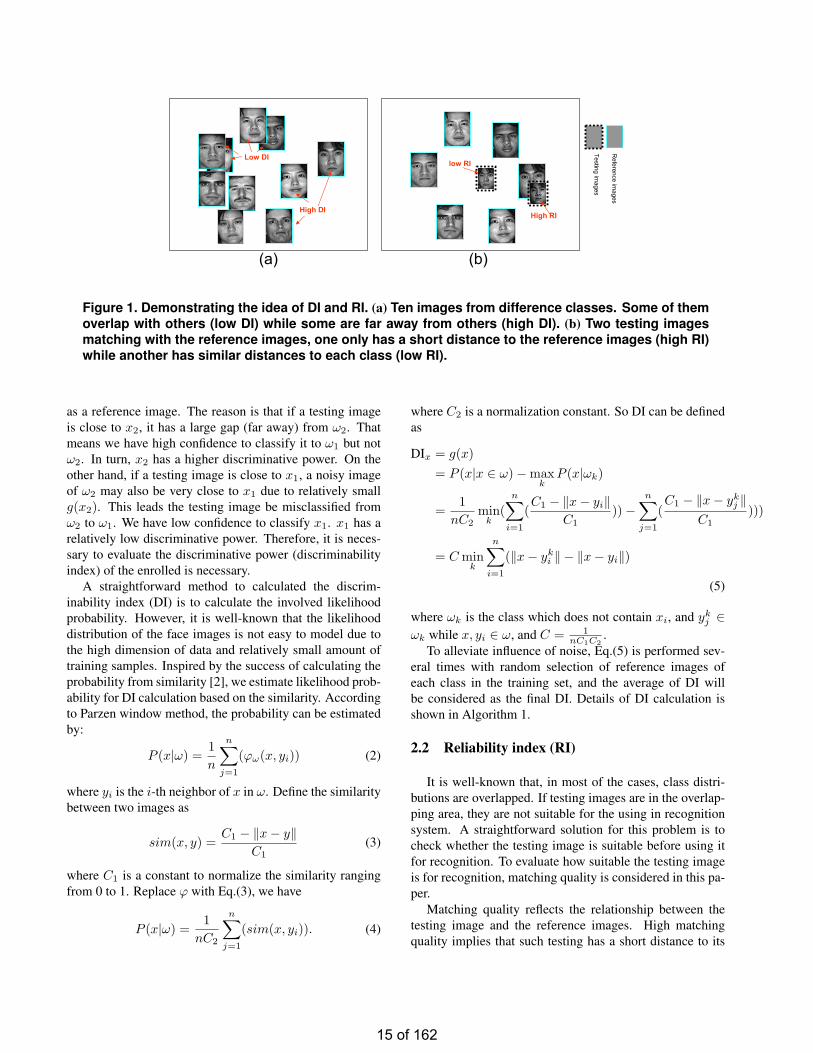
Likelihood distribution of class and class
!2
!1
!2!1
Figure 2. The distribution of ω1 and ω2. x1 andx2 are two reference image in ω1.
of DI and RI is shown in Figure 1. Details in calculating DIand RI are given as follows.
Some useful notations are used in this paper: P repre-sents the probe set while G represents the gallery set (refer-ence images), T represents the training set; the small lettersx, y, z represent still images; ωi represents i-th class of thedatabase.
2.1 Discriminability index (DI)
Discriminability index (DI) measures how much dis-criminative power of a reference image has. Since thereis no generic definition of discriminative power of an im-age, this paper defines the discriminative power as the abil-ity of an image distinguishing from images from otherclasses. Therefore, an image which is far away from theclasses’ boundary will have a high discriminative power.This discriminative power depends on two factors, namelythe margin between a reference image and images fromother classes, and the tolerance to intra-class variants whichare caused by pose, illuminance, expression etc.
To clearly present and illustrate our idea on DI, we con-sider a two-class problem. As shown in Figure 2, x1 and x2
are two reference images which belong to the same class,ω1. The distributions of ω1 and ω2 are overlapped. Inpractice, the classes distribution is always overlapped witheach other due to intra-class variations, such as pose, illu-minance, expression, occlusion. So the reference imageswill have different discriminative powers. Consider theprobability likelihood P (x1|ω1), P (x1|ω2), P (x2|ω1) andP (x2|ω2), according to the discriminant function [7]
g(x) = P (x|ω1)− P (x|ω2) (1)
we get g(x2) > g(x1). This implies that x2 is better than x1
14 of 162
High DI
Low DI
Reference im
ages
Testing images
High RI
low RI
(a) (b)
Figure 1. Demonstrating the idea of DI and RI. (a) Ten images from difference classes. Some of themoverlap with others (low DI) while some are far away from others (high DI). (b) Two testing imagesmatching with the reference images, one only has a short distance to the reference images (high RI)while another has similar distances to each class (low RI).
as a reference image. The reason is that if a testing imageis close to x2, it has a large gap (far away) from ω2. Thatmeans we have high confidence to classify it to ω1 but notω2. In turn, x2 has a higher discriminative power. On theother hand, if a testing image is close to x1, a noisy imageof ω2 may also be very close to x1 due to relatively smallg(x2). This leads the testing image be misclassified fromω2 to ω1. We have low confidence to classify x1. x1 has arelatively low discriminative power. Therefore, it is neces-sary to evaluate the discriminative power (discriminabilityindex) of the enrolled is necessary.
A straightforward method to calculated the discrim-inability index (DI) is to calculate the involved likelihoodprobability. However, it is well-known that the likelihooddistribution of the face images is not easy to model due tothe high dimension of data and relatively small amount oftraining samples. Inspired by the success of calculating theprobability from similarity [2], we estimate likelihood prob-ability for DI calculation based on the similarity. Accordingto Parzen window method, the probability can be estimatedby:
P (x|ω) =1n
n∑j=1
(ϕω(x, yi)) (2)
where yi is the i-th neighbor of x in ω. Define the similaritybetween two images as
sim(x, y) =C1 − ‖x− y‖
C1(3)
where C1 is a constant to normalize the similarity rangingfrom 0 to 1. Replace ϕ with Eq.(3), we have
P (x|ω) =1nC2
n∑j=1
(sim(x, yi)). (4)
where C2 is a normalization constant. So DI can be definedas
DIx = g(x)= P (x|x ∈ ω)−max
kP (x|ωk)
=1nC2
mink
(n∑
i=1
(C1 − ‖x− yi‖
C1))−
n∑j=1
(C1 − ‖x− yk
j ‖C1
)))
= Cmink
n∑i=1
(‖x− yki ‖ − ‖x− yi‖)
(5)
where ωk is the class which does not contain xi, and ykj ∈
ωk while x, yi ∈ ω, and C = 1nC1C2
.To alleviate influence of noise, Eq.(5) is performed sev-
eral times with random selection of reference images ofeach class in the training set, and the average of DI willbe considered as the final DI. Details of DI calculation isshown in Algorithm 1.
2.2 Reliability index (RI)
It is well-known that, in most of the cases, class distri-butions are overlapped. If testing images are in the overlap-ping area, they are not suitable for the using in recognitionsystem. A straightforward solution for this problem is tocheck whether the testing image is suitable before using itfor recognition. To evaluate how suitable the testing imageis for recognition, matching quality is considered in this pa-per.
Matching quality reflects the relationship between thetesting image and the reference images. High matchingquality implies that such testing has a short distance to its
15 of 162
Algorithm 1 DI CalculationInput: Reference images G = xij, threshold for termi-nation th, number of neighbors n, number of images to beselected NOutput: DI of each image in GInitial: DIij ← 0, DI′ij ← 0, DI∗ij ← φ;
repeatDI′ij ←DIijfor each xij do
randomly select N reference images from eachclass, denote as ω′ksearch the n-nearest neighbors in each ω′k, denote asN k
xij
DIij ← DI∗ij⋃ 1
n mink
∑nj=1(‖xij − yi
j‖−‖xij −yk
j ‖)end forDIij ← avg(DI∗ij)
until |DI′ij−DIij | < thOutput DIij
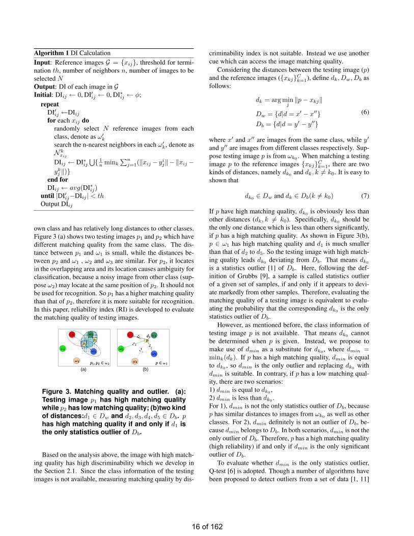
own class and has relatively long distances to other classes.Figure 3 (a) shows two testing images p1 and p2 which havedifferent matching quality from the same class. The dis-tance between p1 and ω1 is small, while the distances be-tween p2 and ω1 , ω2 and ω3 are similar. For p2, it locatesin the overlapping area and its location causes ambiguity forclassification, because a noisy image from other class (sup-pose ω2) may locate at the same position of p2. It should notbe used for recognition. So p1 has a higher matching qualitythan that of p2, therefore it is more suitable for recognition.In this paper, reliability index (RI) is developed to evaluatethe matching quality of testing images.
(a) (b)
!1!1
!2!2
!3!3
!4!4
!5!5
p1p1
p2p2
!1!1
!2!2
!3!3
!4!4
!5!5
d1d1
pp
p1; p2 2 !1p1; p2 2 !1 p 2 !1p 2 !1
Figure 3. Matching quality and outlier. (a):Testing image p1 has high matching qualitywhile p2 has low matching quality; (b)two kindof distances:d1 ∈ Dw and d2, d3, d4, d5 ∈ Db. phas high matching quality if and only if d1 isthe only statistics outlier of Db.
Based on the analysis above, the image with high match-ing quality has high discriminability which we develop inthe Section 2.1. Since the class information of the testingimages is not available, measuring matching quality by dis-
criminability index is not suitable. Instead we use anothercue which can access the image matching quality.
Considering the distances between the testing image (p)and the reference images (xkjCk=1), define dk, Dw, Db asfollows:
dk = arg minj‖p− xkj‖
Dw = d|d = x′ − x′′Db = d|d = y′ − y′′
(6)
where x′ and x′′ are images from the same class, while y′
and y′′ are images from different classes respectively. Sup-pose testing image p is from ωk0 . When matching a testingimage p to the reference images xkjCk=1, there are twokinds of distances, namely dk0 and dk, k 6= k0. It is easy toshown that
dk0 ∈ Dw and dk ∈ Db(k 6= k0) (7)
If p have high matching quality, dk0 is obviously less thanother distances (dk, k 6= k0). Specifically, dk0 should bethe only one distance which is less than others significantly,if p has a high matching quality. As shown in Figure 3(b),p ∈ ω1 has high matching quality and d1 is much smallerthan that of d2 to d5. So the testing image with high match-ing quality leads dk0 deviating from Db. That means dk0
is a statistics outlier [1] of Db. Here, following the def-inition of Grubbs [9], a sample is called statistics outlierof a given set of samples, if and only if it appears to devi-ate markedly from other samples. Therefore, evaluating thematching quality of a testing image is equivalent to evalu-ating the probability that the corresponding dk0 is the onlystatistics outlier of Db.
However, as mentioned before, the class information oftesting image p is not available. That means dk0 cannotbe determined when p is given. Instead, we propose tomake use of dmin as a substitute for dk0 , where dmin =mink(dk). If p has a high matching quality, dmin is equalto dk0 , so dmin is the only outlier and replacing dk0 withdmin is suitable. In contrary, if p has a low matching qual-ity, there are two scenarios:1) dmin is equal to dk0 ,2) dmin is less than dk0 .For 1), dmin is not the only statistics outlier of Db, becausep has similar distances to images from ωk0 as well as otherclasses. For 2), dmin definitely is not an outlier of Db, be-cause dmin belongs toDb. In both scenarios, dmin is not theonly outlier ofDb. Therefore, p has a high matching quality(high reliability) if and only if dmin is the only significantoutlier of Db.
To evaluate whether dmin is the only statistics outlier,Q-test [6] is adopted. Though a number of algorithms havebeen proposed to detect outliers from a set of data [1, 11]
16 of 162
, Q-test is simpler and more suitable. That is because Q-test can handle scenario with only one outlier existing moreeffectively, while other existing methods, such as Grubb test[9] and t-test [13], consider the extrema as well as othersamples as the candidate outliers. Moreover, Q-test is easyto implement and computationally efficient, as it dose notrequire calculation of the mean and standard deviation inadvance.
In this paper, RI of p is defined as the Q-value [6] of theextreme (dmin) in Q-test, as follows:
RI = Q-value(dmin)
=Gap
Range
=dmin −mink(dk \ dmin)
min dk −max dk
(8)
Detailed calculation of RI is shown in Algorithm 2.
Algorithm 2 RI CalculationInput: Reference images xkjCk=1, testing image yi
Output: RIifor each class k dodk ← ‖yi − xkj‖
end forCalculate the Q-value Q← by Eq.[8]output RIi = Q-value
3 Experimental Results
This section demonstrates and evaluates the use of DIand/or RI with three public domain face databases. The re-sults are presented into four parts. First, evaluation method-ology of the comparative experiments are shown. Second,the use of DI and RI is reported. Third, three databasesused in the experiments and the corresponding settings arediscussed. Finally the experimental results are given. Theresults show that the proposed DI/RI can help the recogni-tion system improving the performance.
3.1 Evaluation methodology
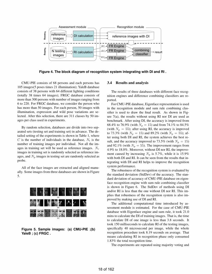
To evaluate the effectiveness of DI and RI, comparativeexperiments are performed based on the existing face recog-nition system integrating with and without DI and/or RI. Asshown in Figure 4, the system consists of two independent
modules, namely assessment module and recognition mod-ule.
In the assessment module, training images (xkjCk=1)are assessed with proposed DI by Algorithm 1, while test-ing images (pi
Np
i=1) are assessed with RI by Algorithm 2.After these two assessments, DI of reference images and RIof testing images are obtain and then integrated with the ex-isting face recognition in the way as mentioned in Section3.2.
In the recognition module, two popular existing facerecognition engines (namely Eigenface, and Kernel PCA)with combining classifiers are used to construct the recog-nition module. The face recognition engines match pi tothe reference images (xkj), and output the similarity sik
which is calculated by Eq.(9):
sik = maxj
(S(pi, xkj)) (9)
where S(pi, xkj) is the similarity calculated by the facerecognition engine. Combining classifiers is used to drawthe final result with multiple testing images. In this paper,three typical combining classifiers [14] are used, namelysum rule (SUM), product rule (PROD) and majority vot-ing (MV). We do not make use of max/min rule, becausemax/min rule actually combine the results based on onemaximal/minimal data rather than making use of all data.
3.2 Usage of DI and/or RI
This paper suggests one way to make use of DI and/orRI for face recognition. It is important to mention that theremay have other better way to adopt DI/RI.
Based on determined DI/RI of each image, weights areassigned to reference images and testing images. For DI,a reference image xkj is assigned with a weight which isdefined as:
wkj = (1 + DIkj
2) (10)
So wkj is normalized to [0 1]. For RI, the testing imageswith low RI are discarded by assigning a weight of 0, whilethe ones with high RI are kept by assigning a weight of 1:
w′i =
1 if RIi > th,0 othervise. (11)
where th is a threshold determined by the Quotient Criti-cal Value [6] of Q-test. In our experiments, we accept thetesting images with 90% confidence level as an outlier.
3.3 Databases and experiment settings
Three public domain face databases, namely CMU-PIE[19], YaleB [8] and FRGC [17], are selected for experi-ments in this paper.
17 of 162
referenceimages
N testingimages
DI calculation
RI calculation FR Engine combiningclassifier
reference images with DI
TrainingTesting result
Assessment module Recognition module
FR Engine
FR Engine
…
Figure 4. The block diagram of recognition system integrating with DI and RI .
CMU-PIE consists of 68 persons and each persons has105 images(5 poses times 21 illumination); YaleB databaseconsists of 38 persons with 64 different lighting conditions(totally 38 times 64 images); FRGC database consists ofmore than 300 persons with number of images ranging from6 to 220. For FRGC database, we consider the person whohas more than 50 images. For each person, 50 images withillumination, expression and wild pose variations are se-lected. After this selection, there are 311 classes by 50 im-ages per class used in experiments.
By random selection, databases are divide into two sep-arated sets (testing set and training set) in advance. The de-tailed setting of the experiments is shown in Table 1, whereC is the number of individuals in the database, Nt is thenumber of training images per individual. Not all the im-ages in training set will be used as reference images. Nr
images in training set is randomly selected as reference im-ages, and Np images in testing set are randomly selected asprobe.
All of the face images are extracted and aligned manu-ally. Some images from three databases are shown in Figure5.
(a)
(b)
(c)
Figure 5. Sample images: (a) CMU-PIE ;(b)YaleB ; (c) FRGC .
3.4 Results and analysis
The results of three databases with different face recog-nition engines and difference combining classifiers are re-ported.
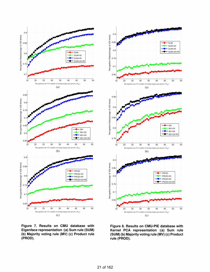
For CMU-PIE database, Eigenface representation is usedin the recognition module and sum rule combining clas-sifier is used to draw the final result. As shown in Fig-ure 7(a), the results without using RI nor DI are used asbenchmark. After using DI, the accuracy is improved from68.4% to 76.9% (with Np = 15) and from 74.1% to 84.5%(with Np = 55); after using RI, the accuracy is improvedto 73.3% (with Np = 15) and 89.2% (with Np = 55); af-ter using both DI and RI, the system achieves the best re-sult, and the accuracy improved to 73.5% (with Np = 15)and 92.1% (with Np = 55). The improvement ranges from4.9% to 18.0%. Moreover, without DI nor RI, the improve-ment caused by increasing Np is 5.7%, while it is 15.9%with both DI and RI. It can be seen from the results that in-tegrating with DI and RI helps to improve the recognitionsystem performance.
The robustness of the recognition system is evaluated bythe standard deviation (StdDev) of the accuracy. The stan-dard deviation of accuracy of CMU-PIE database on eigen-face recognition engine with sum rule combining classifieris shown in Figure 6. The StdDev of methods using DIand/or RI is less than the one without DI nor RI. This im-plies that robustness of the recognition system is also im-proved by making use of DI and RI.
The additional computational time introduced by as-sessment module is estimated. For the case of CMU-PIEdatabase with Eigenface engine and sum rule, it took 21.0mins to calculate the DI of training images. That is, the timeto calculate DI of one image is less than 3.8 seconds. Ittook 150 milliseconds to calculate RI of the testing images,specifically 40 microsecond per image, while the wholerecognition procedure took 8.19 seconds on average. Thatmeans calculating RI in recognition phase only consumed1.83% the total recognition time.
The experiments are repeated using majority voting and
18 of 162
Table 1. Experiment settingsdatabase C Nt Nr Np variations
CMU-PIE 68 50 10 15∼55 pose, illuminationYaleB 38 32 4 15∼32 illuminationFRGC 311 20 4 15∼30 illumination, expression, mild pose
C is the number of individuals; Nt is the number of training images; Nr is the number of reference images; Np is thenumber of testing images. (per individual)
15 20 25 30 35 40 45 50 55
0.08
0.1
0.12
0.14
0.16
0.18
0.2
0.22
Sta
ndar
d D
evia
tion
SUMSUM+DISUM+RISUM+DI+RI
Figure 6. The standard deviation of resultsamount 100 times on CMU PIE with eigenfacerepresentation and sum rule.
product rule. Similar patterns are obtained, shown in Figure7 (b) and (c), respectively. Moreover, replacing Eigenfacerepresentation with Kernel PCA representation, the experi-ments are repeated. The results are shown in Figure 8. Itcan be observed that the performances are improved afterintegrating DI and/or RI with the recognition system.
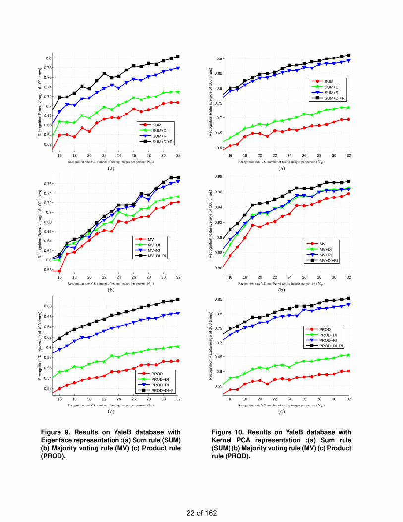
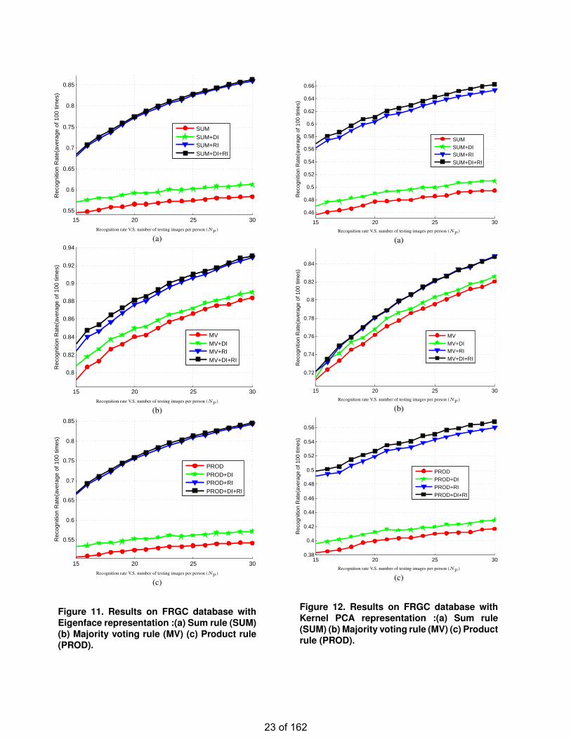
For YaleB database and FRGC database, the same exper-iments are conducted and the results are shown from Figure9-12. It can be seen that same conclusions as that on CMU-PIE are drawn.
4 Conclusions
In this paper, two new measurements, discriminabilityindex (DI) and reliability index (RI), are introduced. Differ-ing from the existing image assessment methods, the pro-posed method is based on the discriminative power and thematching quality. These two new measurements help themultiple image based face recognition systems improvingtheir performance. The experimental results show that afteradopting the proposed DI and RI to the existing recognitionalgorithm, the recognition accuracy and the robustness ofthe performance are improved. The improvement of accu-
racy ranging from 4% to 30%.AcknowledgementThis project was partially supported by Research Grant
Council and Faculty Research Grant of Hong Kong Bap-tist University. The authors would like to thank CMU forproviding the CMU-PIE database, Yale University for pro-viding the YaleB database and University of Notre Damefor providing the FRGC database.
References
[1] V. Barnett and T. Lewis. Outliers in Statistical Data.John Wiley & Sons New York, 1994.
[2] S. Blok, D. Medin, D. Osherson Probability from sim-ilarity AAAI Conference on Commonsense Reasoning. AAAI Press: Stanford, CA, 2002
[3] K. Bowyer, K. Chang, P. Flynn, and C. X. Face Recog-nition Using 2-D, 3-D, and Infrared: Is MultimodalBetter Than Multisample? . Proceedings of the IEEE,94(11), 2006.
[4] S. Canavan, M. Kozak, Y. Zhang, J. Sullins,M. Shreve, and D. Goldgof. Face Recognition byMulti-Frame Fusion of Rotating Heads in Videos. InIEEE International Conference on Biometrics: The-ory, Applications, and Systems, pages 1–6, 2007.
[5] K. Chang, K. Bowyer, and P. Flynn. An evaluationof multimodal 2D+ 3D face biometrics. IEEE Trans-actions on Pattern Analysis and Machine Intelligence,27(4):619–624, 2005.
[6] W. Dixon. Analysis of extreme values. The Annals ofMathematical Statistics, pages 488–506, 1950.
[7] R.O. Duda, P.E. Hart and D.G. Stork Pattern Classifi-cation. Wiley New York, 2001
[8] A. Georghiades, P. Belhumeur, and D. Kriegman.From few to many: Illumination cone models for facerecognition under variable lighting and pose. IEEETransactions on Pattern Analysis and Machine Intelli-gence, 23(6): 643–660, 2001.
19 of 162
[9] F.E. Grubbs. Procedures for Detecting Outlying Ob-servations in Samples Technometrics, 11(1): 1–21,1969.
[10] A. Hadid and M. Pietikainen. From still image tovideo-based face recognition: an experimental analy-sis. In Proceedings of IEEE International Conferenceon Automatic Face and Gesture Recognition, pages813–818, 2004.
[11] V. Hodge and J. Austin. A survey of outlier detec-tion methodologies. Artificial Intelligence Review,22(2):85–126, 2004.
[12] A.K. Jain, S. Pankanti, S. Prabhakar, L. Hong,A. Ross, J.L. Wayman Biometrics: A Grand Chal-lenge In Proceedings of IEEE International Confer-ence on Pattern Recognition (CVPR). IEEE ComputerSociety, 2004
[13] A. John. Mathematical Statistics and Data Analysis.Wadsworth & Brooks/Cole, 1988.
[14] J. Kittler, M. Hatef, R. P. W. Duin, and J. Matas.On combining classifiers. IEEE Transactions on Pat-tern Analysis and Machine Intelligence, 20:226–239,1998.
[15] V. Kruger and S. Zhou. Exemplar-based face recogni-tion from video In Proceedings of IEEE InternationalConference on Automatic Face and Gesture Recogni-tion, pages 175 – 180, 2002.
[16] X. Liu, J. Rittscher and T. Chen. Optimal Pose forFace Recognition. Proceedings of IEEE InternationalConference on Pattern Recognition (CVPR).IEEEComputer Society, vol(2), pp:1439-1446, 2006.
[17] P.J. Phillips, P.J. Flynn, T. Scruggs, K.W. Bowyer,etal.. Overview of the face recognition grand challengeIn Proceedings of IEEE International Conference onPattern Recognition (CVPR).IEEE Computer Society,vol(1), pp:947-954, 2005.
[18] P.J. Phillips, W.T. Scruggs, A.J. O’Toole,et al.. FRVT2006 and ICE 2006 Large-Scale Experimental ResultsIEEE Transactions on Pattern Analysis and MachineIntelligence, IEEE Computer Society, in press, 2009.
[19] T. Sim, S. Baker, and M. Bsat. The CMU pose, il-lumination, and expression database. IEEE Transac-tions on Pattern Analysis and Machine Intelligence,25(12):1615–1618, 2003.
[20] X. Tan, S. Chen, Z. Zhou, and F. Zhang. Face recogni-tion from a single image per person: A survey. PatternRecognition, 39(9):1725–1745, 2006.
[21] D. Thomas, K. W. Bowyer, and P. J. Flynn. Multi-frame approaches to improve face recognition. InProceedings of IEEE Workshop on Motion and VideoComputing, pages 19–19, 2007.
[22] Y. Zhang and A. Martınez. A weighted probabilis-tic approach to face recognition from multiple imagesand video sequences. Image and Vision Computing,24(6):626–638, 2006.
[23] W. Zhao, R. Chellappa, P. Phillips, and A. Rosenfeld.Face recognition: A literature survey. ACM Comput-ing Surveys, 35(4):399–458, 2003.
20 of 162
15 20 25 30 35 40 45 50 55
0.7
0.75
0.8
0.85
0.9
Rec
ogni
tion
Rat
e(av
erag
e of
100
tim
es)
SUMSUM+DISUM+RISUM+DI+RI
Recognition rate V.S. number of testing images per person (Np)
(a)
15 20 25 30 35 40 45 50 55
0.55
0.6
0.65
0.7
0.75
0.8
0.85
Rec
ogni
tion
Rat
e(av
erag
e of
100
tim
es)
MVMV+DIMV+RIMV+DI+RI
Recognition rate V.S. number of testing images per person (Np)
(b)
15 20 25 30 35 40 45 50 55
0.65
0.7
0.75
0.8
0.85
0.9
Rec
ogni
tion
Rat
e(av
erag
e of
100
tim
es)
PRODPROD+DIPROD+RIPROD+DI+RI
Recognition rate V.S. number of testing images per person (Np)
(c)
Figure 7. Results on CMU database withEigenface representation :(a) Sum rule (SUM)(b) Majority voting rule (MV) (c) Product rule(PROD).
15 20 25 30 35 40 45 50 55
0.65
0.7
0.75
0.8
0.85
0.9
Rec
ogni
tion
Rat
e(av
erag
e of
100
tim
es)
SUMSUM+DISUM+RISUM+DI+RI
Recognition rate V.S. number of testing images per person (Np)
(a)
15 20 25 30 35 40 45 50 55
0.75
0.8
0.85
0.9
0.95
Rec
ogni
tion
Rat
e(av
erag
e of
100
tim
es)
MVMV+DIMV+RIMV+DI+RI
Recognition rate V.S. number of testing images per person (Np)
(b)
15 20 25 30 35 40 45 50 55
0.65
0.7
0.75
0.8
0.85
0.9
Rec
ogni
tion
Rat
e(av
erag
e of
100
tim
es)
PRODPROD+DIPROD+RIPROD+DI+RI
Recognition rate V.S. number of testing images per person (Np)
(c)
Figure 8. Results on CMU-PIE database withKernel PCA representation :(a) Sum rule(SUM) (b) Majority voting rule (MV) (c) Productrule (PROD).
21 of 162
16 18 20 22 24 26 28 30 32
0.62
0.64
0.66
0.68
0.7
0.72
0.74
0.76
0.78
0.8
Rec
ogni
tion
Rat
e(av
erag
e of
100
tim
es)
SUMSUM+DISUM+RISUM+DI+RI
Recognition rate V.S. number of testing images per person (Np)
(a)
16 18 20 22 24 26 28 30 32
0.58
0.6
0.62
0.64
0.66
0.68
0.7
0.72
0.74
0.76
Rec
ogni
tion
Rat
e(av
erag
e of
100
tim
es)
MVMV+DIMV+RIMV+DI+RI
Recognition rate V.S. number of testing images per person (Np)
(b)
16 18 20 22 24 26 28 30 32
0.52
0.54
0.56
0.58
0.6
0.62
0.64
0.66
0.68
Rec
ogni
tion
Rat
e(av
erag
e of
100
tim
es)
PRODPROD+DIPROD+RIPROD+DI+RI
Recognition rate V.S. number of testing images per person (Np)
(c)
Figure 9. Results on YaleB database withEigenface representation :(a) Sum rule (SUM)(b) Majority voting rule (MV) (c) Product rule(PROD).
16 18 20 22 24 26 28 30 32
0.6
0.65
0.7
0.75
0.8
0.85
0.9
Rec
ogni
tion
Rat
e(av
erag
e of
100
tim
es)
SUMSUM+DISUM+RISUM+DI+RI
Recognition rate V.S. number of testing images per person (Np)
(a)
16 18 20 22 24 26 28 30 32
0.86
0.88
0.9
0.92
0.94
0.96
0.98
Rec
ogni
tion
Rat
e(av
erag
e of
100
tim
es)
MVMV+DIMV+RIMV+DI+RI
Recognition rate V.S. number of testing images per person (Np)
(b)
16 18 20 22 24 26 28 30 32
0.55
0.6
0.65
0.7
0.75
0.8
0.85
Rec
ogni
tion
Rat
e(av
erag
e of
100
tim
es)
PRODPROD+DIPROD+RIPROD+DI+RI
Recognition rate V.S. number of testing images per person (Np)
(c)
Figure 10. Results on YaleB database withKernel PCA representation :(a) Sum rule(SUM) (b) Majority voting rule (MV) (c) Productrule (PROD).
22 of 162
15 20 25 30
0.55
0.6
0.65
0.7
0.75
0.8
0.85
Rec
ogni
tion
Rat
e(av
erag
e of
100
tim
es)
SUMSUM+DISUM+RISUM+DI+RI
Recognition rate V.S. number of testing images per person (Np)
(a)
15 20 25 30
0.8
0.82
0.84
0.86
0.88
0.9
0.92
0.94
Rec
ogni
tion
Rat
e(av
erag
e of
100
tim
es)
MVMV+DIMV+RIMV+DI+RI
Recognition rate V.S. number of testing images per person (Np)
(b)
15 20 25 30
0.55
0.6
0.65
0.7
0.75
0.8
0.85
Rec
ogni
tion
Rat
e(av
erag
e of
100
tim
es)
PRODPROD+DIPROD+RIPROD+DI+RI
Recognition rate V.S. number of testing images per person (Np)
(c)
Figure 11. Results on FRGC database withEigenface representation :(a) Sum rule (SUM)(b) Majority voting rule (MV) (c) Product rule(PROD).
15 20 25 30
0.46
0.48
0.5
0.52
0.54
0.56
0.58
0.6
0.62
0.64
0.66
Rec
ogni
tion
Rat
e(av
erag
e of
100
tim
es)
SUMSUM+DISUM+RISUM+DI+RI
Recognition rate V.S. number of testing images per person (Np)
(a)
15 20 25 30
0.72
0.74
0.76
0.78
0.8
0.82
0.84
Rec
ogni
tion
Rat
e(av
erag
e of
100
tim
es)
MVMV+DIMV+RIMV+DI+RI
Recognition rate V.S. number of testing images per person (Np)
(b)
15 20 25 300.38
0.4
0.42
0.44
0.46
0.48
0.5
0.52
0.54
0.56
Rec
ogni
tion
Rat
e(av
erag
e of
100
tim
es)
PRODPROD+DIPROD+RIPROD+DI+RI
Recognition rate V.S. number of testing images per person (Np)
(c)
Figure 12. Results on FRGC database withKernel PCA representation :(a) Sum rule(SUM) (b) Majority voting rule (MV) (c) Productrule (PROD).
23 of 162
A Dynamic Trust Network for Autonomy-Oriented Partner Finding
Hongjun Qiu∗
Abstract
The problem of partner finding is to identify which en-tities (agents) can provide requested services from a groupof entities. It can be found in open and distributed environ-ments for such tasks as file sharing and resource allocation.Previous studies have shown that entities can refine anddetermine partners through measuring trust relationships,i.e., the beliefs of entities that others will accomplish a re-quest for assigned services at hand. Entities dynamicallychange their beliefs through recalling their past experiencesto quickly identify partners for new requests. This paperaims to observe whether those changes can enable entitiesefficiently find partners and hence provide services. We pro-pose a dynamic network, which contains trust relationshipsas links among entities (nodes). Then, we investigate itsstructure and efficiency in the moments with different trustrelationships. Autonomy-Oriented Computing (AOC) is ap-plied to observe how the network dynamics emerge fromlocal behaviors. A notion of autonomy is embodied in defin-ing how entities activate their partner finding behaviors,whereas self-organization is realized to update the strengthof trust relationships. Experimental results explicitly dis-play a dynamic process of this network, changing from con-taining no link to having some stable links. Specially, in thisprocess, the efficiency gradually gets enhanced.
1 Introduction
In a multi-entity network, entities (e.g., companies) usu-ally look for some others (i.e., finding partners) to provideservices beyond their own limited abilities. The problem ofpartner finding appears widely in real-world applications.Here, we take cloud computing as an example. In cloudcomputing, vendors (e.g., Google, Amazon and Microsoft)deploy numerous servers over the Internet, to store data orrun programs in real time as requested by users [3]. Theservers work together to deal with such requests from hun-dreds or thousands of users per second [4]. Hence, it is quiteimportant for servers to immediately identify who can work
∗Prof. Jiming Liu is her corresponding supervisor
together to accomplish requests.Currently, researchers have introduced a notion of trust
relationship as a measurement for identifying partners, tosolve real-world problems in open, distributed and dynamicenvironments [2]. Trust relationships refer to entities’ be-liefs that others will provide services as needed [11]. Inmost cases, entities are inclined to choose partners from theones in which their beliefs are relatively strong. Entitiesweaken their beliefs if the found partners cannot provideservices. Otherwise, they strengthen their beliefs. They dy-namically change the strength values of their beliefs withmore and more such experiences. Thus, they can quicklyidentify partners at any time.
Many studies have been done in applying trust relation-ships to find partners. Golbeck [2] argues that trust relation-ships can be used to identify who can produce trustworthyonline information. Sen et al. [1] compare three schemes ofcomputing trust relationships in reducing the cost of findingpartners from a small group of entities. Specially, they in-troduce a nearest neighbor algorithm as a scheme throughrecalling a fixed number of latest experiences of findingpartners. To get rid of malicious entities from the groupof potential partners, Kamvar et al. [6] build a matrix ofweighted trust relationships through aggregating and nor-malizing based on a history of uploading files. They com-pute the left principal eigenvector of this matrix as theirmetric. More related work can be found in [5, 12, 13]. Insuch work, entities either measure the probabilities that oth-ers have successfully provided services before, or ask pastpartners for their beliefs about third-party ones.
However, it remains to clarify why and how trust rela-tionships can make entities efficiently find partners in dy-namic, distributed, real-world networks. This paper aims tosolve this problem through proposing a dynamic trust net-work based on the bottom-up methodology of Autonomy-Oriented Computing (AOC). AOC can help us charac-terize how network dynamics emerge from local interac-tions through utilizing the ideas of autonomy and self-organization [7, 9, 8]. Here, network dynamics refers tothe dynamics of network structure, network performancesin providing services and so forth. Zhang et al. [14] havesuccessfully characterized such dynamics of a distributednetwork, in which entities work together to provide various
24 of 162
services. Their work shows the feasibility and rationalityfor the work in this paper.
In this study, the autonomy is embodied for entities(nodes) to find partners while a process of self-organizationis realized to update trust relationships (links). Entities de-cide to activate which behaviors for partner search or se-lection through measuring their abilities and beliefs. Theyalso immediately update their beliefs, once they receive thefeedback from their latest partners. Specially, a positivefeedback mechanism is emphasized, i.e., the strong beliefsbecome stronger while the weak become weaker. Experi-mental results show that our network quickly converges tobe scale-free. With such a structure, entities quickly findpartners for any request. These results explain why dynamictrust relationships are helpful for entities to find partners.
The reminder of this paper is organized as follows: Sec-tion 2 gives a detailed problem statement. Section 3 formu-lates a network on the basis of AOC. The network containsautonomous entities as nodes and self-organized trust rela-tionships as links. In Section 4, we observe the structuralemergence of this network and the dynamics of trust rela-tionships. The efficiency in finding partners is also mea-sured. Finally, the paper is concluded in Section 5.
2 Problem Statement
As mentioned above, the goal of this study is to examinethe effects of dynamic trust relationships on finding partnersin open, dynamic, and distributed networks, such as the In-ternet. It requires us to answer the following questions:
• How do entities update their trust relationships? Whatwill they do if they never interact with their newly-found partners before? Will entities memorize the in-formation about all of their past partners?
• What are the mechanisms for entities search and selectpartners? How do entities refine partners based on up-dated beliefs? How do entities identify their partnersfrom their refinement results?
• Which parameters can we introduce to characterize thechange of trust relationships, besides the variation oftheir strength? Is it enough to count the number ofentities’ trustees, associated by their beliefs?
• What is the efficiency in finding partners based ondynamically-changing trust relationships?
Previous studies have confirmed two preliminary phe-nomena. One is that entities prefer to interact with theirtrustees rather than strangers. The other is that entitiesstrengthen their beliefs about another entity once it accom-plishes a service request and vice versa. Based on the two
phenomena, we attempt to answer the above questions inthe following scenario.
Here, we assume that there exists a virtual network,which contains trust relationships as links and entities asnodes. In this network, entities are assigned with fixed abil-ities of providing certain services. Each of them can finda partner to satisfy a whole service request, which cannotbe finished by itself. The request has a cost limit, i.e., themaximum number of times for finding partners. The partnerwill honestly inform whether it can finish this request. Thenthe finder can decide to strength or weaken its belief aboutthis partner. If this partner cannot finish, it will transfer therequest to the third entity, which is discovered as its partner.In other words, this request propagates among entities untilit is accomplished or the number of finding times reachesthe given cost limit.
Accordingly, the above questions can be translated intothe following tasks:
1. Modeling a virtual network, in which distributed enti-ties can find partners and update their beliefs.
2. Measuring structural characteristics at different mo-ments to display the dynamics of the links amongentities. The characteristics include network inde-gree (outdegree), the clustering coefficient and the har-monic mean of average path length (APL−1).
3. Examining the efficiency in finding partners with twoparameters, i.e.,
• Accomplishment ratio: the ratio of the numberof accomplished requests to the total number ofrequests;
• Average propagation step: the average times thatentities find partners for finishing requests.
3 Modeling a Dynamic Trust Network
3.1 Basic ideas
In this section, we will model a virtual network of dis-tributed entities, i.e., a dynamic trust network. Then, wecan characterize the structural dynamics of this network, asa reflection of dynamic trust relationships.
To meet the distributed, dynamic needs, we will de-fine the network based on the methodology of AOC. AOCaims to characterize complex networks (e.g., large-scale,dynamic and distributed networks), through deploying a setof autonomy-oriented entities and defining their behavioralrules of self-organization [7, 10]. These entities activate dif-ferent behaviors to finish a certain task or else, according totheir different states, e.g., the number of entities they inter-acted before. Moreover, entities self-organize their coupling
25 of 162
relationships based on their received feedbacks, such as thestate of other entities.
In this work, entities continually find partners in an au-tonomous manner, as well as self-organize trust relation-ships based on the feedback from partners.
For finding partners, entities activate one of well-definedsearch or selection behaviors in a probabilistic manner. Theprobability of activating each behavior is adaptive to newrequests and entities’ states (e.g., their beliefs).
A process of self-organization is realized to update trustrelationships. At first, there is no trust relationship in thenetwork. After a period of continually finding partners, en-tities maintain several trust relationships. The realizationof this process lies in two aspects. On one side, entities’behaviors are defined to be exploratory or even stochastic.They may find strangers as their partners and create theirbeliefs about the newly-found partners. However, with pos-itive feedback mechanisms, the newly-created beliefs maybe weakened or even eliminated later. Therefore, only a partof generated relationships can remain. The remaining rela-tionships can help entities effectively find partners to finishnew requests. So, any request can be accomplished with ahigher probability.
The network, entities and service requests are defined asfollows:
Definition 1 Let G′(t)=< E,L
′(t) > denote a dynamic
network of trust-based entities on the basis of AOC. Forbrevity, we call it a dynamic trust network. E =e1, · · · , eNe
denotes the set of entities and Ne is the num-ber of entities in the network. L
′(t) = l′ij(t)|ei, ej ∈ E
is the set of trust relationships at time t.
Definition 2 Let ei =< ID, ability, rules > denote anentity where ID is its identifier, i.e., ei.ID = i, i ∈ [1, Ne].It can provide some services with different performances,i.e., ei.ability =< cw1, · · · , cwNservice
>, where cwj de-notes the performance on the jth type of service tj . Nservice
is the number of service types. The rules define when andhow entities activate their behaviors.
Definition 3 A request can be formulated as rm=<rw1, · · · , rwNservice , Tmax > where rwj denotes the per-formance requirement of the type of service tj . Tmax is themaximum number of times that entities are allowed to findpartners.
The two ideas from AOC are illustrated through describingthe process of finding partners for finishing a request, whichis specified in Section 3.5. Once a new request rm is sub-mitted to an entity ei, this entity will perform the following:
1. Evaluating. Firstly, the entity will determine whetherit can solely accomplish the new request by means of
matching its ability with this request using a cosine-based similarity function ei.simRE(rm). The requestcan be considered as accomplished once the value ofei.simRE(rm) is larger than a threshold. The evalua-tion functions are specified in Section 3.4.
2. Partner Search and Selection. If the request cannotbe accomplished and its Tmax is not reached, the en-tity ei will start finding partners. Firstly, it will searchsome candidates by means of activating one of searchbehaviors in a probabilistic manner. Then, it will se-lect a candidate as its partner through activating oneof selection behaviors also probabilistically. The prob-abilities are adaptive to the request and the states ofthe entity, e.g., its trust relationships. So, trust rela-tionships will explicitly affect entities’ partner finding.The detailed behaviors are given in Section 3.2.
3. Updating. The entity ei will change its states oncea partner is found. Firstly, it will deliver the wholerequest to its partner. Then, the partner ej will hon-estly feedback its evaluating results ej .simRE(rm).Finally, this entity will generate the trust relationshipl′ij if l
′ij(t) is not in the network. Otherwise, it will
strengthen the relationship if the ability of this partneris relatively closer to this request, or weaken the trustrelationship if not. The mechanisms of trust relation-ships are specified in Section 3.3.
3.2 The Local Autonomy of Entities
Three search behaviors and two selection behaviors aredefined in this section. They will be probabilistically acti-vated to realize the autonomy of entities. The probabilityof activating each behavior is determined with the degreeof similarity between requests and entities’ abilities, i.e.,ei.simRE(rm). When the degree is high, entities’ neigh-bors will be discovered as partners with a high probability.Stochastic behaviors are given for entities to avoid beingtrapped in local-optima and for newcomers to join this net-work.
The detailed operations of search and selection behaviorsare specified in below:
• Neighbor-based search neighborSearch(). An en-tity ei will find some neighbors, which are not in-volved in the current request rm, with the probabilityof ei.simRE(rm). The probability will be adaptive torequests accordingly. Neighbors refer to its trustees.i.e., there are trust relationships from this entity tothem.
• Recommendation-based search recommendSear−ch(). An entity ei will discover candidates withina distance maxD around itself with a probability of
26 of 162
1 − ei.simRE(rm) when the receiving request is rel-atively near the entity’s ability. That is, the entity willenlarge its search area from its neighbors to the areawithin a given distance. This behavior is inspired bytwo observations: 1) besides direct experiences, in-direct experiences are also important for entities tomake decisions; 2) communities have been discoveredin many real-world networks, i.e., agents with similarinterests cluster together. Here, the request far beyondthe ability of an entity is likely out of its neighbors’abilities.
• Random search randomSearch(). An entity ei willsearch in the whole network when it is a newcomer orits neighbors are all involved in the current request.
• Trust-based select trustSelect(). The entity ei willselect an entity ej with the maximal degree of trust,ei.trust(ej , t), from its candidates as its partner witha probability of ei.simRE(rm). Entities are supposedto be more confident in selecting partners for requestswhich are relatively closer to its abilities.
• Random select randomSelect(). The entity ei willstochastically select an entity from the candidate setei.cand(rm) as its partner with a probability of 1 −ei.simRE(rm).
3.3 The Mechanisms of Trust Relationships
We have introduced how trust relationships are applied inactivating entities’ behaviors for finding partners in the pre-vious section. Now, we will introduce how they are changedbased on the feedback from partners. Trust relationships aredefined as follows:
Definition 4 A link l′ij=< ei, ej , ei.succ(ej , t),
ei.fail(ej , t), ei.latestT ime(ej), ei.trust(ej , t) >|1 ≤i, j ≤ Ne reflects a trust relationship from ei to ej where
• ei.succ(ej , t) and ei.fail(ej , t) denote the numbers ofsuccessful and failed interactions, respectively;
• ei.latestT ime(ej) is the time of their latest interac-tion;
• ei.trust(ej , t) is the degree of trust at time t, quanti-fying the belief that ej will accomplish a new requestfrom ei. It is a numeric value in [ε, 1.0], where thethreshold ε will be described below.
Once an entity ei receives the feedback of its partnerej .simRE(rm), a new relationship lij(t) will be generatedif it is not in the network. Otherwise, the existing relation-ship will be updated. The parameters of this relationshipwill be assigned as introduced below.
Firstly, the time of their latest interaction is set as thecurrent time. Then, ei will evaluate whether the partner ismore suitable for the current request with Eq. 1 where λ isa threshold, λ ∈ (0, 1).
ei.QoI(ej , rm) =
true
ej .simRE(rm)ei.simRE(rm) > (1 + λ);
false otherwise
(1)Other parameters will be assigned according to the resultof ei.QoI(ej). When the partner is more suitable for thisrequest, i.e., ei.QoI(ej , rm) = true, this interaction is re-garded as successful and the number of their successful in-teractions increases. Otherwise, the number of failed inter-actions increases. Then, the degree of trust ei.trust(ej , t)can be set with updated ei.succ(ej , t) and ei.fail(ej , t) asfollows:
ei.trust(ej , t) =ei.succ(ej , t)
ei.succ(ej , t) + ei.fail(ej , t)(2)
Trust relationships may be removed since the degree oftrust is supposed to decay over time as follows:
ei.trust(ej , t) = ei.trust(ej , ei.latestT ime(ej))− η ∗ (t− ei.latestT ime(ej)) (3)
where η is the decay factor, η ∈ (0.0, 1.0). Once the de-gree of trust is less than a small negative numeric value ε,i.e., ei.trust(ej , t) < ε, the neighbor is interpreted as beingno longer able to accomplish new requests from this entity,and the corresponding relationship will be eliminated. Thethreshold ε is empirically set, ε ∈ (−0.05, 0).
In addition, entities will derive new trust relationshipsfrom the relationships already in the network. If the short-est distance from entity ei to entity ej is larger than a giventhreshold maxD, i.e., ei.shortestDis(ej , t) > maxD, ei
has no idea about the ability of ej and the degree of trustei.trust(ej , t) is set as 0. Otherwise, the following func-tions can be used to compute the degree of trust for the de-rived relationships:
ei.trust(ej , t) =
nij(t)∑k=1
eki .trustPath(ej , t)
nij(t)
eki .trustPath(ej , t) =
∑
l′mj
(t)∈L′ (t)
(eki .trustPath(em, t)
×em.trust(ej , t)) (4)
where nij(t) is the number of the shortest paths from ei toej and the function ek
i .trustPath(ej , t) denotes the degreeof trust derived from the kth shortest path. If ej is a neigh-bor of ei, ek
i .trustPath(ej , t) will be computed with Eq. 3.
27 of 162
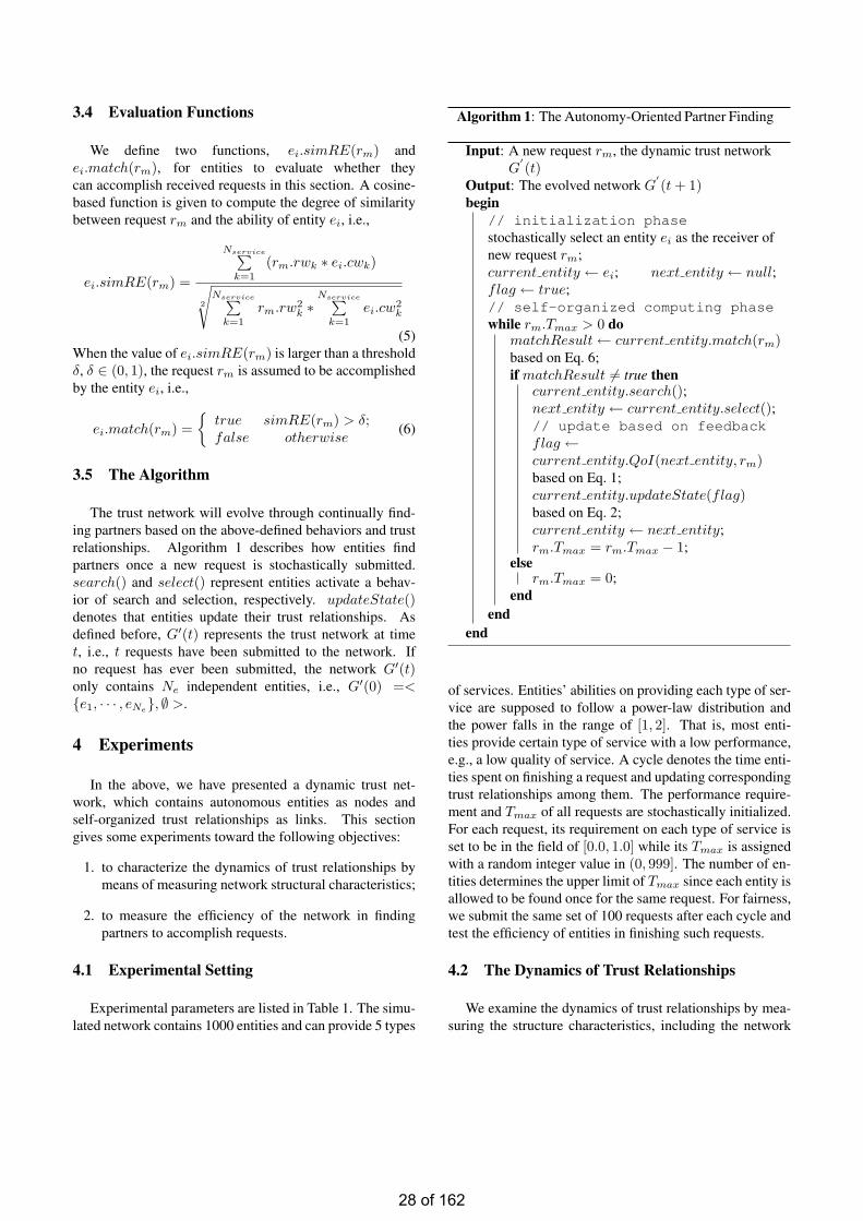
3.4 Evaluation Functions
We define two functions, ei.simRE(rm) andei.match(rm), for entities to evaluate whether theycan accomplish received requests in this section. A cosine-based function is given to compute the degree of similaritybetween request rm and the ability of entity ei, i.e.,
ei.simRE(rm) =
Nservice∑k=1
(rm.rwk ∗ ei.cwk)
2
√Nservice∑
k=1
rm.rw2k ∗
Nservice∑k=1
ei.cw2k
(5)When the value of ei.simRE(rm) is larger than a thresholdδ, δ ∈ (0, 1), the request rm is assumed to be accomplishedby the entity ei, i.e.,
ei.match(rm) =
true simRE(rm) > δ;false otherwise
(6)
3.5 The Algorithm
The trust network will evolve through continually find-ing partners based on the above-defined behaviors and trustrelationships. Algorithm 1 describes how entities findpartners once a new request is stochastically submitted.search() and select() represent entities activate a behav-ior of search and selection, respectively. updateState()denotes that entities update their trust relationships. Asdefined before, G′(t) represents the trust network at timet, i.e., t requests have been submitted to the network. Ifno request has ever been submitted, the network G′(t)only contains Ne independent entities, i.e., G′(0) =<e1, · · · , eNe, ∅ >.
4 Experiments
In the above, we have presented a dynamic trust net-work, which contains autonomous entities as nodes andself-organized trust relationships as links. This sectiongives some experiments toward the following objectives:
1. to characterize the dynamics of trust relationships bymeans of measuring network structural characteristics;
2. to measure the efficiency of the network in findingpartners to accomplish requests.
4.1 Experimental Setting
Experimental parameters are listed in Table 1. The simu-lated network contains 1000 entities and can provide 5 types
Algorithm 1: The Autonomy-Oriented Partner Finding
Input: A new request rm, the dynamic trust networkG′(t)
Output: The evolved network G′(t + 1)
begin// initialization phasestochastically select an entity ei as the receiver ofnew request rm;current entity ← ei; next entity ← null;flag ← true;// self-organized computing phasewhile rm.Tmax > 0 do
matchResult ← current entity.match(rm)based on Eq. 6;if matchResult 6= true then
current entity.search();next entity ← current entity.select();// update based on feedbackflag ←current entity.QoI(next entity, rm)based on Eq. 1;current entity.updateState(flag)based on Eq. 2;current entity ← next entity;rm.Tmax = rm.Tmax − 1;
elserm.Tmax = 0;
endend
end
of services. Entities’ abilities on providing each type of ser-vice are supposed to follow a power-law distribution andthe power falls in the range of [1, 2]. That is, most enti-ties provide certain type of service with a low performance,e.g., a low quality of service. A cycle denotes the time enti-ties spent on finishing a request and updating correspondingtrust relationships among them. The performance require-ment and Tmax of all requests are stochastically initialized.For each request, its requirement on each type of service isset to be in the field of [0.0, 1.0] while its Tmax is assignedwith a random integer value in (0, 999]. The number of en-tities determines the upper limit of Tmax since each entity isallowed to be found once for the same request. For fairness,we submit the same set of 100 requests after each cycle andtest the efficiency of entities in finishing such requests.
4.2 The Dynamics of Trust Relationships
We examine the dynamics of trust relationships by mea-suring the structure characteristics, including the network
28 of 162
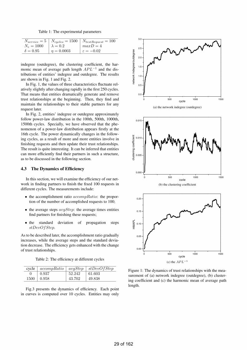
Table 1: The experimental parameters
Nservice = 5 Ncycles = 1500 NtestRequest = 100Ne = 1000 λ = 0.2 maxD = 4δ = 0.95 η = 0.0003 ε = −0.02
indegree (outdegree), the clustering coefficient, the har-monic mean of average path length APL−1 and the dis-tributions of entities’ indegree and outdegree. The resultsare shown in Fig. 1 and Fig. 2.
In Fig. 1, the values of three characteristics fluctuate rel-atively slightly after changing rapidly in the first 250 cycles.That means that entities dramatically generate and removetrust relationships at the beginning. Then, they find andmaintain the relationships to their stable partners for anyrequest later.
In Fig. 2, entities’ indegree or outdegree approximatelyfollow power-law distribution in the 100th, 500th, 1000th,1500th cycles. Specially, we have observed that the phe-nomenon of a power-law distribution appears firstly at the16th cycle. The power dynamically changes in the follow-ing cycles, as a result of more and more entities involve infinishing requests and then update their trust relationships.The result is quite interesting. It can be inferred that entitiescan more efficiently find their partners in such a structure,as to be discussed in the following section.
4.3 The Dynamics of Efficiency
In this section, we will examine the efficiency of our net-work in finding partners to finish the fixed 100 requests indifferent cycles. The measurements include:
• the accomplishment ratio accompRatio: the propor-tion of the number of accomplished requests to 100;
• the average steps avgStep: the average times entitiesfind partners for finishing these requests;
• the standard deviation of propagation stepsstDevOfStep.
As to be described later, the accomplishment ratio graduallyincreases, while the average steps and the standard devia-tion decrease. The efficiency gets enhanced with the changeof trust relationships.
Table 2: The efficiency at different cycles
cycle accompRatio avgStep stDevOfStep0 0.937 52.242 61.603
1500 0.958 43.702 49.838
Fig.3 presents the dynamics of efficiency. Each pointin curves is computed over 10 cycles. Entities may only
0 500 1000 1500
0.0
0.5
1.0
1.5
2.0
2.5
3.0
ne
two
rk in
de
gre
e/o
utd
eg
ree
cycle
(a) the network indegree (outdegree)
0 500 1000 1500
0.000
0.005
0.010
0.015
clu
ste
rin
g c
oe
ffic
ien
t
cycle
(b) the clustering coefficient
0 500 1000 1500
0.00
0.05
0.10
0.15
0.20
HM
AP
L
cycle
(c) the APL−1
Figure 1: The dynamics of trust relationships with the mea-surement of (a) network indegree (outdegree), (b) cluster-ing coefficient and (c) the harmonic mean of average pathlength.
29 of 162
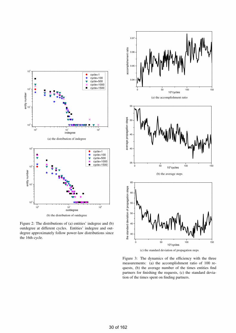
100
101
102
100
101
102
103
cycle=1
cycle=100
cycle=500
cycle=1000
cycle=1500
en
tity
nu
mb
er
indegree
(a) the distribution of indegree
100
101
102
100
101
102
103
cycle=1
cycle=100
cycle=500
cycle=1000
cycle=1500
en
tity
nu
mb
er
outdegree
(b) the distribution of outdegree
Figure 2: The distributions of (a) entities’ indegree and (b)outdegree at different cycles. Entities’ indegree and out-degree approximately follow power-law distributions sincethe 16th cycle.
0 50 100 150
0.94
0.95
0.96
0.97
acco
mp
lish
em
en
t ra
tio
10*cycles
(a) the accomplishment ratio
0 50 100 150
35
40
45
50
55
ave
rag
e p
rop
ag
atio
n s
tep
s
10*cycles
(b) the average steps
0 50 100 150
40
45
50
55
60
65
the
sta
nd
ard
de
via
tio
n o
f p
rop
ag
atio
n s
tep
s
10*cycles
(c) the standard deviation of propagation steps
Figure 3: The dynamics of the efficiency with the threemeasurements: (a) the accomplishment ratio of 100 re-quests, (b) the average number of the times entities findpartners for finishing the requests, (c) the standard devia-tion of the times spent on finding partners.
30 of 162
update 2 or 3 relationships in a cycle of updating, whichhardly affects the efficiency. We can find that the upwardor downward tendency in each sub-graph is quite clear. Ta-ble 2 gives the efficiency at the beginning cycle and endingcycle. The average steps decrease about 17.653%. It po-tently shows that the change of trust relationships leads tothe high efficiency of finding partners.
5 Concluding Remarks
In this study, we are interested in characterizingdynamically-changing trust relationships in real-world ap-plications. We attempt to understand why trust relationshipscan enable distributed entities quickly find partners to pro-vide their requested services.
Specifically, we have proposed a dynamic trust net-work by means of utilizing the ideas of autonomy andself-organization from AOC. These ideas can help us un-derstand how network-level phenomena emerge from enti-ties’ local behaviors. In this study, the notion of autonomymeans that distributed entities (nodes) activate different be-haviors based on their abilities and trust relationships. Self-organization refers to the process that entities change theirrelationships (links) with positive feedback mechanisms,according to the feedback from their partners.
Experimental results have shown that the networkquickly converges to be scale-free. In other words, parts ofdynamically-generated trust relationships remain relativelystable while others are eliminated. That is, the process ofself-organization makes trust relationships emerge quickly.Meanwhile, the accomplishment ratio gradually rises whilethe average steps and the standard deviation of propagationsteps gradually decrease. It can be inferred that, the con-vergence process of this network is accomplished with theenhancement of its efficiency in successfully finding part-ners.
References
[1] L. Erete, E. Ferguson, and S. Sen. Learning task-specifictrust decisions. In Proceedings of the 7th International JointConference on Autonomous Agents and Multi-Agent Sys-tems, 1477–1480, 2008.
[2] J. Golbeck. Weaving a web of trust. Science,321(5896):1640–1641, 2008.
[3] M. Greeger. CTO roundtable: Cloud computing. Communi-cations of the ACM, 52(8):50–56, 2009.
[4] B. Hayes. Cloud computing. Communications of the ACM,51(7):9–11, 2008.
[5] A. Jøsang, R. Ismail, and C. Boyd. A survey of trust andreputation systems for online service provision. DecisionSupport Systems, 43:618–644, 2007.
[6] S. D. Kamvar, M. T. Schlosser, and H. Garcia-Molina. Theeigentrust algorithm for reputation management in P2P net-works. In Proceedings of the 12th International World WideWeb Conference, 640–651, 2003.
[7] J. Liu. Autonomy-oriented computing (AOC): The natureand implications of a paradigm for self-organized computing(keynote talk). In Proceedings of the 4th International Con-ference on Natural Computation and the 5th InternationalConference on Fuzzy Systems and Knowledge Discovery, 3–11, 2008.
[8] J. Liu, X. Jin, and K. C. Tsui. Autonomy-oriented com-puting (AOC): Formulating computational systems withautonomous components. IEEE Transactions on Sys-tems, Man, and Cybernetics-Part A: Systems and Humans,35(6):879–902, 2005.
[9] J. Liu, X. Jin, and K. C. Tsui. Autonomy Oriented Comput-ing: From Problem Solving to Complex Systems Modeling.Springer, 2005.
[10] J. Liu and K. Tsui. Toward nature-inspired computing. Com-munications of the ACM, 49(10):59–64, 2006.
[11] S. P. Marsh. Formalising Trust as a Computational Concept.PhD thesis, University of Stirling, 1994.
[12] S. D. Ramchurn, T. D. Huynh, and N. R. Jennings. Trust inmulti-agent systems. The Knowledge Engineering Review,19(1):1–25, 2004.
[13] J. Sabater and C. Sierra. Review on computational trust andreputation models. Artificial Intelligence Review, 24:33–60,2005.
[14] S. Zhang and J. Liu. Autonomy-oriented social networksmodeling: Discovering the dynamics of emergent structureand performance. International Journal of Pattern Recogni-tion and Artificial Intelligence, 21(4):611–638, 2007.
31 of 162
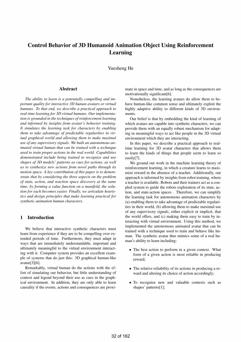
Control Behavior of 3D Humanoid Animation Object Using ReinforcementLearning
Yuesheng He
Abstract
The ability to learn is a potentially compelling and im-portant quality for interactive 3D human avatars or virtualhumans. To that end, we describe a practical approach toreal-time learning for 3D virtual humans. Our implementa-tion is grounded in the techniques of reinforcement learningand informed by insights from avatar’s behavior training.It simulates the learning task for characters by enablingthem to take advantage of predictable regularities in vir-tual graphical world and allowing them to make maximaluse of any supervisory signals. We built an autonomous an-imated virtual human that can be trained with a techniqueused to train proper actions in the real world. Capabilitiesdemonstrated include being trained to recognize and useshapes of 3D models’ patterns as cues for actions, as wellas to synthesize new actions from novel paths through itsmotion space. A key contribution of this paper is to demon-strate that by considering the three aspects on the problemof state, action, and reaction space discovery at the sametime, by forming a value function on a manifold, the solu-tion for each becomes easier. Finally, we articulate heuris-tics and design principles that make learning practical forsynthetic animation human characters.
1 Introduction
We believe that interactive synthetic characters mustlearn from experience if they are to be compelling over ex-tended periods of time. Furthermore, they must adapt inways that are immediately understandable, important andultimately meaningful to the virtual environment interact-ing with it. Computer system provides an excellent exam-ple of systems that do just this: 3D graphical human-likeavatar[3][6].
Remarkably, virtual human do the actions with the ef-fort of simulating our behavior, but little understanding ofcontext and legend beyond their use as cues in the graph-ical environment. In addition, they are only able to learncausality if the events, actions and consequences are proxi-
mate in space and time, and as long as the consequences aremotivationally significant[6].
Nonetheless, the learning avatars do allow them to be-have human-like common sense and ultimately exploit thehighly adaptive ability to different kinds of 3D environ-ments.
Our belief is that by embedding the kind of learning ofwhich avatars are capable into synthetic characters, we canprovide them with an equally robust mechanism for adapt-ing in meaningful ways to act like people in the 3D virtualenvironment which they are interacting.
In this paper, we describe a practical approach to real-time learning for 3D avatar characters that allows themto learn the kinds of things that people seem to learn soeasily[7].
We ground our work in the machine learning theory ofreinforcement learning, in which a creature learns to maxi-mize reward in the absence of a teacher. Additionally, ourapproach is informed by insights from robot training, wherea teacher is available. Robots and their trainers act as a cou-pled system to guide the robots exploration of its state, ac-tion, and state-action spaces . Therefore, we can simplifythe learning task for autonomous animation characters by(a) enabling them to take advantage of predictable regulari-ties in their world, (b) allowing them to make maximal useof any supervisory signals, either explicit or implicit, thatthe world offers, and (c) making them easy to train by in-teracting with virtual environment. Using this method, weimplemented the autonomous animated avatar that can betrained with a technique used to train and behave like hu-man. The synthetic avatar thus mimics some of a real hu-man’s ability to learn including:
• The best action to perform in a given context. Whatform of a given action is most reliable in producingreward;
• The relative reliability of its actions in producing a re-ward and altering its choice of action accordingly;
• To recognize new and valuable contexts such asshapes’ patterns[1];
32 of 162
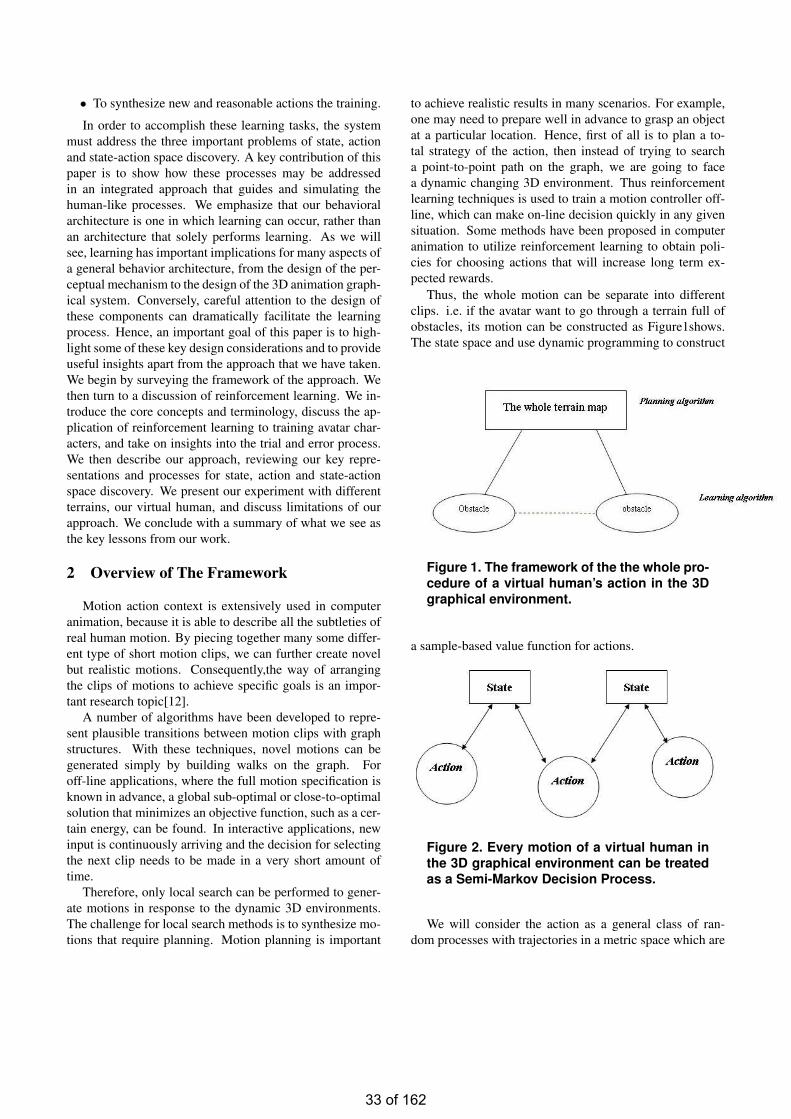
• To synthesize new and reasonable actions the training.
In order to accomplish these learning tasks, the systemmust address the three important problems of state, actionand state-action space discovery. A key contribution of thispaper is to show how these processes may be addressedin an integrated approach that guides and simulating thehuman-like processes. We emphasize that our behavioralarchitecture is one in which learning can occur, rather thanan architecture that solely performs learning. As we willsee, learning has important implications for many aspects ofa general behavior architecture, from the design of the per-ceptual mechanism to the design of the 3D animation graph-ical system. Conversely, careful attention to the design ofthese components can dramatically facilitate the learningprocess. Hence, an important goal of this paper is to high-light some of these key design considerations and to provideuseful insights apart from the approach that we have taken.We begin by surveying the framework of the approach. Wethen turn to a discussion of reinforcement learning. We in-troduce the core concepts and terminology, discuss the ap-plication of reinforcement learning to training avatar char-acters, and take on insights into the trial and error process.We then describe our approach, reviewing our key repre-sentations and processes for state, action and state-actionspace discovery. We present our experiment with differentterrains, our virtual human, and discuss limitations of ourapproach. We conclude with a summary of what we see asthe key lessons from our work.
2 Overview of The Framework
Motion action context is extensively used in computeranimation, because it is able to describe all the subtleties ofreal human motion. By piecing together many some differ-ent type of short motion clips, we can further create novelbut realistic motions. Consequently,the way of arrangingthe clips of motions to achieve specific goals is an impor-tant research topic[12].
A number of algorithms have been developed to repre-sent plausible transitions between motion clips with graphstructures. With these techniques, novel motions can begenerated simply by building walks on the graph. Foroff-line applications, where the full motion specification isknown in advance, a global sub-optimal or close-to-optimalsolution that minimizes an objective function, such as a cer-tain energy, can be found. In interactive applications, newinput is continuously arriving and the decision for selectingthe next clip needs to be made in a very short amount oftime.
Therefore, only local search can be performed to gener-ate motions in response to the dynamic 3D environments.The challenge for local search methods is to synthesize mo-tions that require planning. Motion planning is important
to achieve realistic results in many scenarios. For example,one may need to prepare well in advance to grasp an objectat a particular location. Hence, first of all is to plan a to-tal strategy of the action, then instead of trying to searcha point-to-point path on the graph, we are going to facea dynamic changing 3D environment. Thus reinforcementlearning techniques is used to train a motion controller off-line, which can make on-line decision quickly in any givensituation. Some methods have been proposed in computeranimation to utilize reinforcement learning to obtain poli-cies for choosing actions that will increase long term ex-pected rewards.
Thus, the whole motion can be separate into differentclips. i.e. if the avatar want to go through a terrain full ofobstacles, its motion can be constructed as Figure1shows.The state space and use dynamic programming to construct
Figure 1. The framework of the the whole pro-cedure of a virtual human’s action in the 3Dgraphical environment.
a sample-based value function for actions.
Figure 2. Every motion of a virtual human inthe 3D graphical environment can be treatedas a Semi-Markov Decision Process.
We will consider the action as a general class of ran-dom processes with trajectories in a metric space which are
33 of 162
DynamicProgramAlgorithm1 Q.Insert(Gx) and mark Gx as visited2 while Q not empty do3 x ← Q.GetFirst() //Get the priori queue4 return SUCCESS5 forall u-1 ∈ U-1(x)6 x ← f-1(x’, u-1)7 if x not visited8 Mark x as visited9 Q.Insert(x)10 else11 Resolve duplicate x12 return FAILURE
Table 1. The dynamic programming algorithmto update the value of action’s policy.
continuous from the right and have limits from the left atany point of the half-line. These processes were continuoussemi-Markov processes in according to the property of theirfirst exit streams. The structure of the these processes of ac-tions are showed on Figure 2 Thus, it is necessary to developmethods or to modernize traditional methods of investiga-tion, which do not use the simple Markov property[12].
We can support value functions with to evaluate the ac-tions’ policy. Moreover, the above methods suffer from thelimitation that the space of available motions is discrete.The parametric space is an abstract space defined by kine-matic or physical attributes of motions. By parameterizingall motion samples in the space, and by blending amongmultiple motions, motion interpolation can create novel mo-tions that have specific kinematic or physical attributes. Webuild a continuous parameterized motion space for similarmotions that provide efficient control for interpolation.
To improve the action’s policy π episode by episode, weadopt a value function Q and dynamic programm algorithmto achieve the goal Table 1[21].
To improve motion interpolation with the use of geomet-ric statistics, treating interpolation as statistical predictionof missing data in the parametric space. We analyze inter-polated human motions for physical correctness and showthat the interpolated results are close to the physically cor-rect motions. Cooper et al. proposed active learning toadaptively sample the parametric space so that the spacecan be well sampled with a reduced number of clips . Re-cently, researchers have also combined motion graphs withparametric synthesis to form richer, more complete motionspaces. In order to provide proper control, we present away to learn parametric motion controllers, which can com-pute near-optimal parameters for motion synthesis for the3D graphical environment in real-time.
3 Learning Algorithm on Manifold
In this section we describe a reinforcement learningframework to obtain motion controllers for interactive char-acter animation. Using a database of atomic motion clips,our goal is to generate natural character motion as a se-quence of clips. At each time step, the motion controllerdecides which motion clip best follows the user input andrespects constraints imposed by the environment. This de-cision must be made quickly, since time lags are not allowedin interactive environments. The controller should also beable to achieve user objectives that require planning aheadof time. In addition, both user input and the environmentshould be represented using continuous parameters to allowfor proper control.
We begin to introduce the Markov decision process(MDP) model for the control of the virtual human’s action,and describe methods for approximately solving MDPs.This section is principally about choosing a basis for ap-proximation of real-valued functions called value functions,which are central to solving Markov decision processes[13]. For in the most cases, previous work has modeledvalue functions as vectors in a Euclidean space to evaluatethe action’s policy π. One of the novel ideas is the approachto treat value functions as elements of a vector space on agraph or manifold [12]. This approach enables construct-ing basis functions that capture the large-scale (irregular)topology of the graph, and approximating (value) functionson these graphs by projecting them onto the space spannedby these bases.
A discrete Markov decision process (MDP) M =(S,A, P a
s,s′ , Ras,s′) is defined by a finite set of discrete states
S, a finite set of actions A, a transition model P as,s′ specify-
ing the distribution over future states s′ when an action ais performed in state s, and a corresponding reward modelRa
s,s′ specifying a scalar cost or reward [13].Any optimal policy π defines the same unique optimal
value function V which satisfies the nonlinear constraints:
V (s) = maxa
(Ras,s′ + γ
∑
s′∈S
P as,s′V (s′))
where Rsa =∑
s′∈S P as,s′R
as,s′ is the expected immediate
reward.The Bellman operator Tπ on the space of value function
which is used to evaluate the policy π can be written as
Tπ(V ) = Rsπ(s) + γ∑
s′P
π(s)ss′ V (s′)
Thus, the value function Vp associated with following a(deterministic) policy p can be defined as
V π(s) = T (V π(s)) = Rsπ(s) + γ∑
s′∈S
Pπ(s)ss′ V π(s′).
34 of 162
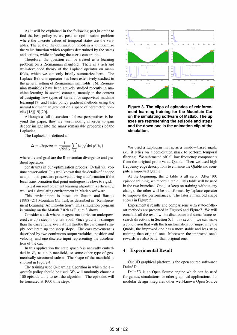
As it will be explained in the following part,in order tofind the best policy π, we pose an optimization problemwhere the discrete values of temporal states are the vari-ables. The goal of the optimization problem is to maximizethe value function which requires determined by the statesand actions, while enforcing the user’s constraints.
Therefore, the question can be treated as a learningproblem on a Riemannian manifold. There is a rich andwell-developed theory of the Laplace operator on mani-folds, which we can only briefly summarize here. TheLaplace-Beltrami operator has been extensively studied inthe general setting of Riemannian manifolds [16]. Rieman-nian manifolds have been actively studied recently in ma-chine learning in several contexts, namely in the contextof designing new types of kernels for supervised machinelearning[17] and faster policy gradient methods using thenatural Riemannian gradient on a space of parametric poli-cies [18][19][20].
Although a full discussion of these perspectives is be-yond this paper, they are worth noting in order to gaindeeper insight into the many remarkable properties of theLaplacian.
The Laplacian is defined as
∆ = divgrad =1√
det g
∑
i,j
∂i(√
det gij∂j)
where div and grad are the Riemannian divergence and gra-dient operators.
constraints in our optimization process. Detail vs. vol-ume preservation. It is well known that the details of a shapeat a point in space are preserved during a deformation if thelocal transformation that point undergoes is close to rigid.
To test our reinforcement learning algorithm’s efficiency,we used a simulating environment in Matlab software.
This environment is based on Sutton and Barto’s(1998)[21] Mountain Car Task as described in ”Reinforce-ment Learning: An Introduction”. This simulation programis running on the Matlab 7.02b as Figure 3 shows.
Consider a task where an agent must drive an underpow-ered car up a steep mountain road. Since gravity is strongerthan the cars engine, even at full throttle the car cannot sim-ply accelerate up the steep slope. The cars movement isdescribed by two continuous output variables, position andvelocity, and one discrete input representing the accelera-tion of the car.
In this application the state space S is naturally embed-ded in Rd as a sub-manifold, or some other type of geo-metrically structured subset. The shape of the manifold isshowed in Figure 4.
The training used Q-learning algorithm in which the ε−greedy policy should be used. We will randomly choose a100 episode table to test the algorithm. The episodes willbe truncated at 1000 time steps.
0 50 100 150 200 250 3000
200
400
600
800
1000Episode: 300 epsilon: 0.00049041
−1.5 −1 −0.5 0 0.5−1
−0.5
0
0.5
1
1.5Step:152
0 50 100 150 200 250 300 350 4000
200
400
600
800
1000Episode: 400 epsilon: 0.00017951
−1.5 −1 −0.5 0 0.5−1
−0.5
0
0.5
1
1.5Step:152
0 100 200 300 400 500 6000
200
400
600
800
1000Episode: 550 epsilon: 3.9752e−005
−1.5 −1 −0.5 0 0.5−1
−0.5
0
0.5
1
1.5Step:284
0 100 200 300 400 500 600 7000
200
400
600
800
1000Episode: 700 epsilon: 8.8031e−006
−1.5 −1 −0.5 0 0.5−1
−0.5
0
0.5
1
1.5Step:284
Figure 3. The clips of episodes of reinforce-ment learning training for the Mountain Caron the simulating software of Matlab. The upaxes are representing the episode and stepsand the down one is the animation clip of thesimulation.
We used a Laplacian matrix as a window-based mask,ı.e. it relies on a convolution mask to perform temporalfiltering. We subtracted off all low frequency componentsfrom the original proto-value Qtable. Then we used highfrequency edge descriptions to enhance the Qtable and com-pute a improved Qtable.
At the beginning, the Q table is all zero. After 100episode training, we record a table. This table will be usedin the two branches. One just keep on training without anychange, the other will be transformed by laplace operatorto improve the performances. The later’s manifold shapeshows in Figure 5.
Experimental results and comparisons with state-of-the-art methods are presented in Figure6 and Figure7. We willconclude all the result with a discussion and some future re-search directions in Section 5. In this section, we can makea conclusion that with the transformation for improving theQtable, the improved one has a more stable and less stepstraining than original one. Moreover, the improved one’srewards are also better than original one.
4 Experimental Result
Our 3D graphical platform is the open source software :Delta3D.
Delta3D is an Open Source engine which can be usedfor games, simulations, or other graphical applications. Itsmodular design integrates other well-known Open Source
35 of 162
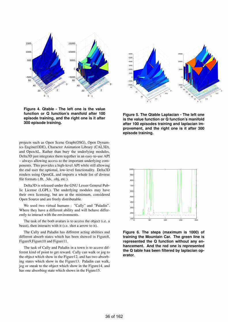
1
2
3
0
20
40
60−500
0
500
1000
1500
1
2
3
0
20
40
60−5000
0
5000
10000
15000
Figure 4. Qtable - The left one is the valuefunction or Q function’s manifold after 100episode training, and the right one is it after300 episode training.
projects such as Open Scene Graph(OSG), Open Dynam-ics Engine(ODE), Character Animation Library (CAL3D),and OpenAL. Rather than bury the underlying modules,Delta3D just integrates them together in an easy-to-use API– always allowing access to the important underlying com-ponents. This provides a high-level API while still allowingthe end user the optional, low-level functionality. Delta3Drenders using OpenGL and imports a whole list of diversefile formats (.flt, .3ds, .obj, etc.).
Delta3D is released under the GNU Lesser General Pub-lic License (LGPL). The underlying modules may havetheir own licensing, but are at the minimum, consideredOpen Source and are freely distributable.
We used two virtual humans : ”Cally” and ”Paladin”.Where they have a different ability and will behave differ-ently to interact with the environments.
The task of the both avatars is to access the object (ı.e. abeast), then interacts with it (ı.e. shot a arrow to it).
The Cally and Paladin has different acting abilities anddifferent absorb states which has been showed in Figure8,Figure9,Figure10 and Figure11.
The task of Cally and Paladin in a town is to access dif-ferent kind of point to get reward. Cally can walk or jog tothe object which show in the Figure12, and has two absorb-ing states which show in the Figure13. Paladin can walk,jog or sneak to the object which show in the Figure14, andhas one absorbing state which shows in the Figure15.
1
1.5
2
2.5
3
0
20
40
60−2000
−1000
0
1000
2000
3000
4000
5000
6000
1
1.5
2
2.5
3
0
10
20
30
40
50
60−5000
0
5000
10000
15000
Figure 5. The Qtable Laplacian - The left oneis the value function or Q function’s manifoldafter 100 episodes training and laplacian im-provement, and the right one is it after 300episode training.
0 50 100 150 200100
200
300
400
500
600
700
800
900
1000
Figure 6. The steps (maximum is 1000) oftraining the Mountain Car. The green line isrepresented the Q function without any en-hancement. And the red one is representedthe Q table has been filtered by laplacian op-erator.
36 of 162
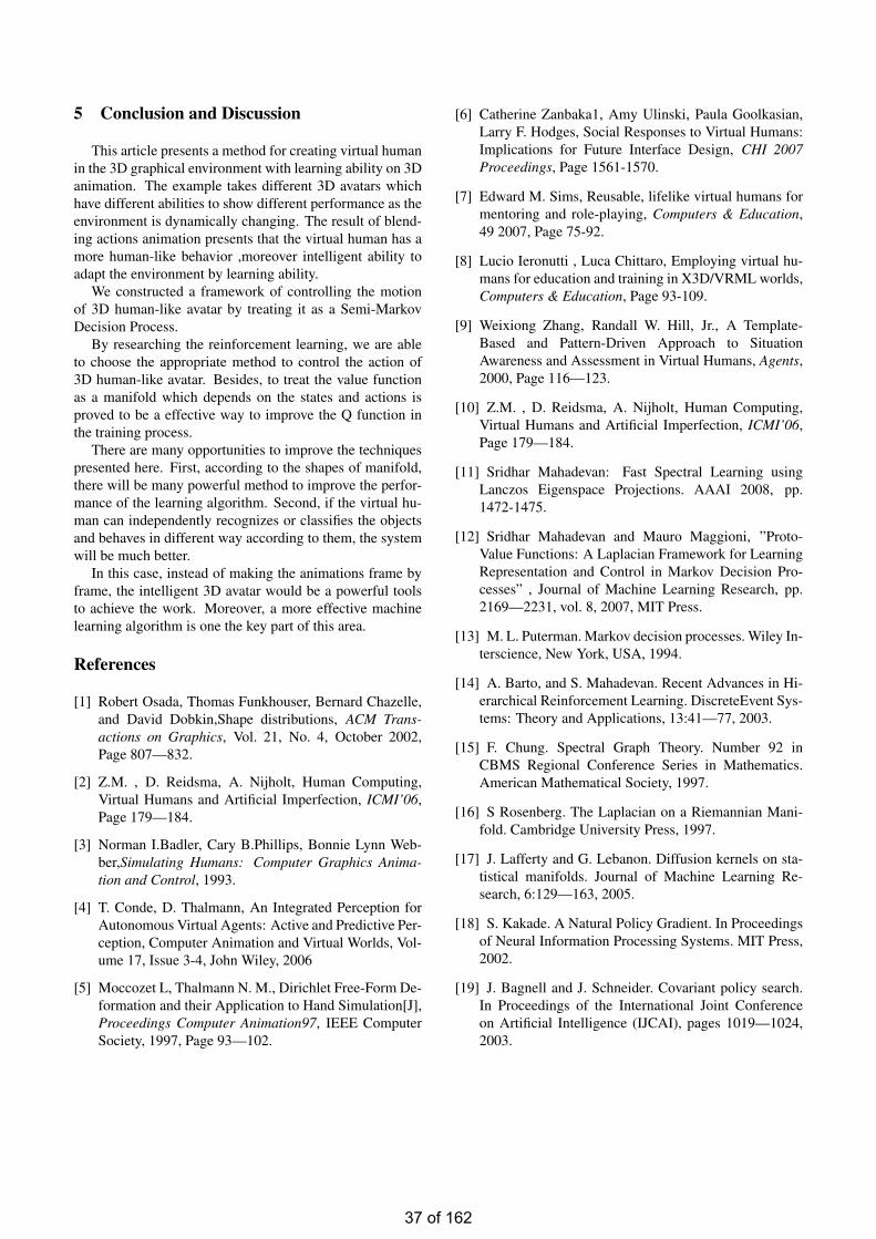
5 Conclusion and Discussion
This article presents a method for creating virtual humanin the 3D graphical environment with learning ability on 3Danimation. The example takes different 3D avatars whichhave different abilities to show different performance as theenvironment is dynamically changing. The result of blend-ing actions animation presents that the virtual human has amore human-like behavior ,moreover intelligent ability toadapt the environment by learning ability.
We constructed a framework of controlling the motionof 3D human-like avatar by treating it as a Semi-MarkovDecision Process.
By researching the reinforcement learning, we are ableto choose the appropriate method to control the action of3D human-like avatar. Besides, to treat the value functionas a manifold which depends on the states and actions isproved to be a effective way to improve the Q function inthe training process.
There are many opportunities to improve the techniquespresented here. First, according to the shapes of manifold,there will be many powerful method to improve the perfor-mance of the learning algorithm. Second, if the virtual hu-man can independently recognizes or classifies the objectsand behaves in different way according to them, the systemwill be much better.
In this case, instead of making the animations frame byframe, the intelligent 3D avatar would be a powerful toolsto achieve the work. Moreover, a more effective machinelearning algorithm is one the key part of this area.
References
[1] Robert Osada, Thomas Funkhouser, Bernard Chazelle,and David Dobkin,Shape distributions, ACM Trans-actions on Graphics, Vol. 21, No. 4, October 2002,Page 807—832.
[2] Z.M. , D. Reidsma, A. Nijholt, Human Computing,Virtual Humans and Artificial Imperfection, ICMI’06,Page 179—184.
[3] Norman I.Badler, Cary B.Phillips, Bonnie Lynn Web-ber,Simulating Humans: Computer Graphics Anima-tion and Control, 1993.
[4] T. Conde, D. Thalmann, An Integrated Perception forAutonomous Virtual Agents: Active and Predictive Per-ception, Computer Animation and Virtual Worlds, Vol-ume 17, Issue 3-4, John Wiley, 2006
[5] Moccozet L, Thalmann N. M., Dirichlet Free-Form De-formation and their Application to Hand Simulation[J],Proceedings Computer Animation97, IEEE ComputerSociety, 1997, Page 93—102.
[6] Catherine Zanbaka1, Amy Ulinski, Paula Goolkasian,Larry F. Hodges, Social Responses to Virtual Humans:Implications for Future Interface Design, CHI 2007Proceedings, Page 1561-1570.
[7] Edward M. Sims, Reusable, lifelike virtual humans formentoring and role-playing, Computers & Education,49 2007, Page 75-92.
[8] Lucio Ieronutti , Luca Chittaro, Employing virtual hu-mans for education and training in X3D/VRML worlds,Computers & Education, Page 93-109.
[9] Weixiong Zhang, Randall W. Hill, Jr., A Template-Based and Pattern-Driven Approach to SituationAwareness and Assessment in Virtual Humans, Agents,2000, Page 116—123.
[10] Z.M. , D. Reidsma, A. Nijholt, Human Computing,Virtual Humans and Artificial Imperfection, ICMI’06,Page 179—184.
[11] Sridhar Mahadevan: Fast Spectral Learning usingLanczos Eigenspace Projections. AAAI 2008, pp.1472-1475.
[12] Sridhar Mahadevan and Mauro Maggioni, ”Proto-Value Functions: A Laplacian Framework for LearningRepresentation and Control in Markov Decision Pro-cesses” , Journal of Machine Learning Research, pp.2169—2231, vol. 8, 2007, MIT Press.
[13] M. L. Puterman. Markov decision processes. Wiley In-terscience, New York, USA, 1994.
[14] A. Barto, and S. Mahadevan. Recent Advances in Hi-erarchical Reinforcement Learning. DiscreteEvent Sys-tems: Theory and Applications, 13:41—77, 2003.
[15] F. Chung. Spectral Graph Theory. Number 92 inCBMS Regional Conference Series in Mathematics.American Mathematical Society, 1997.
[16] S Rosenberg. The Laplacian on a Riemannian Mani-fold. Cambridge University Press, 1997.
[17] J. Lafferty and G. Lebanon. Diffusion kernels on sta-tistical manifolds. Journal of Machine Learning Re-search, 6:129—163, 2005.
[18] S. Kakade. A Natural Policy Gradient. In Proceedingsof Neural Information Processing Systems. MIT Press,2002.
[19] J. Bagnell and J. Schneider. Covariant policy search.In Proceedings of the International Joint Conferenceon Artificial Intelligence (IJCAI), pages 1019—1024,2003.
37 of 162
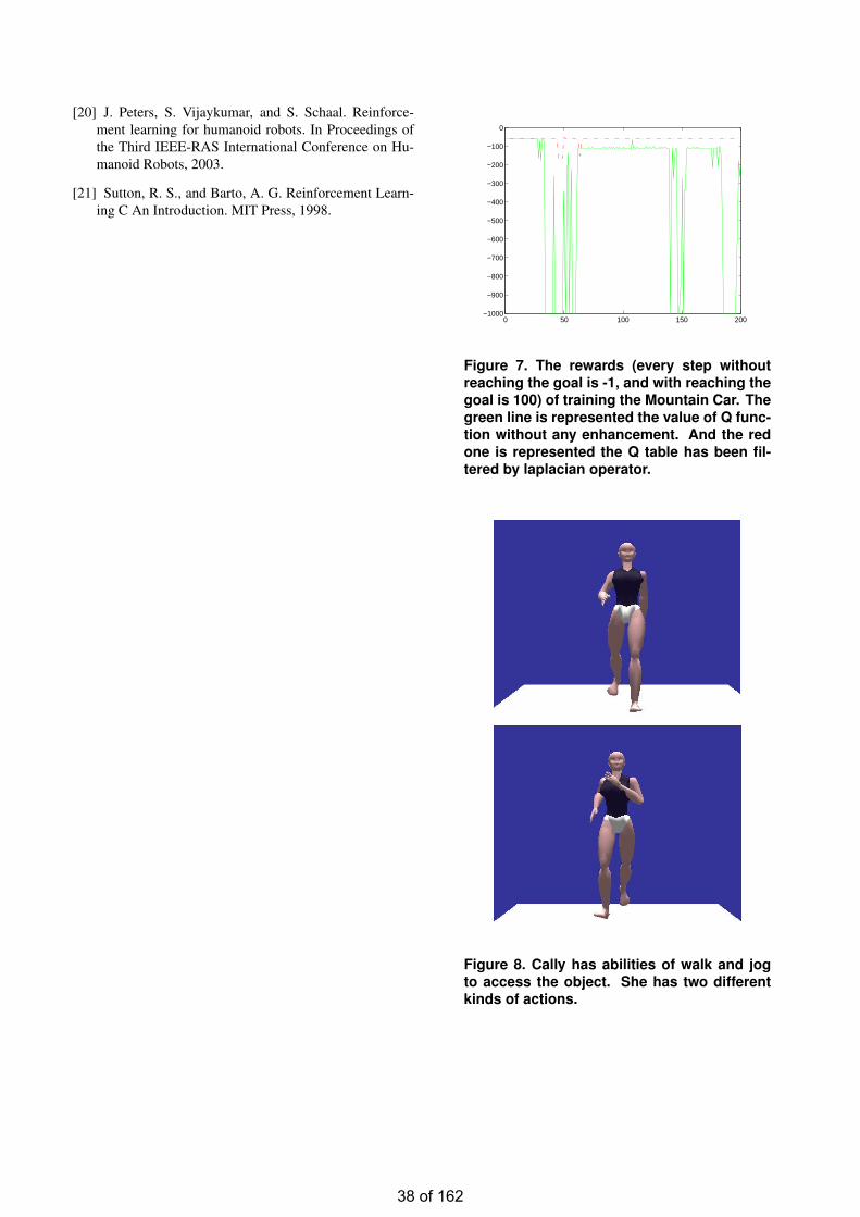
[20] J. Peters, S. Vijaykumar, and S. Schaal. Reinforce-ment learning for humanoid robots. In Proceedings ofthe Third IEEE-RAS International Conference on Hu-manoid Robots, 2003.
[21] Sutton, R. S., and Barto, A. G. Reinforcement Learn-ing C An Introduction. MIT Press, 1998.
0 50 100 150 200−1000
−900
−800
−700
−600
−500
−400
−300
−200
−100
0
Figure 7. The rewards (every step withoutreaching the goal is -1, and with reaching thegoal is 100) of training the Mountain Car. Thegreen line is represented the value of Q func-tion without any enhancement. And the redone is represented the Q table has been fil-tered by laplacian operator.
Figure 8. Cally has abilities of walk and jogto access the object. She has two differentkinds of actions.
38 of 162
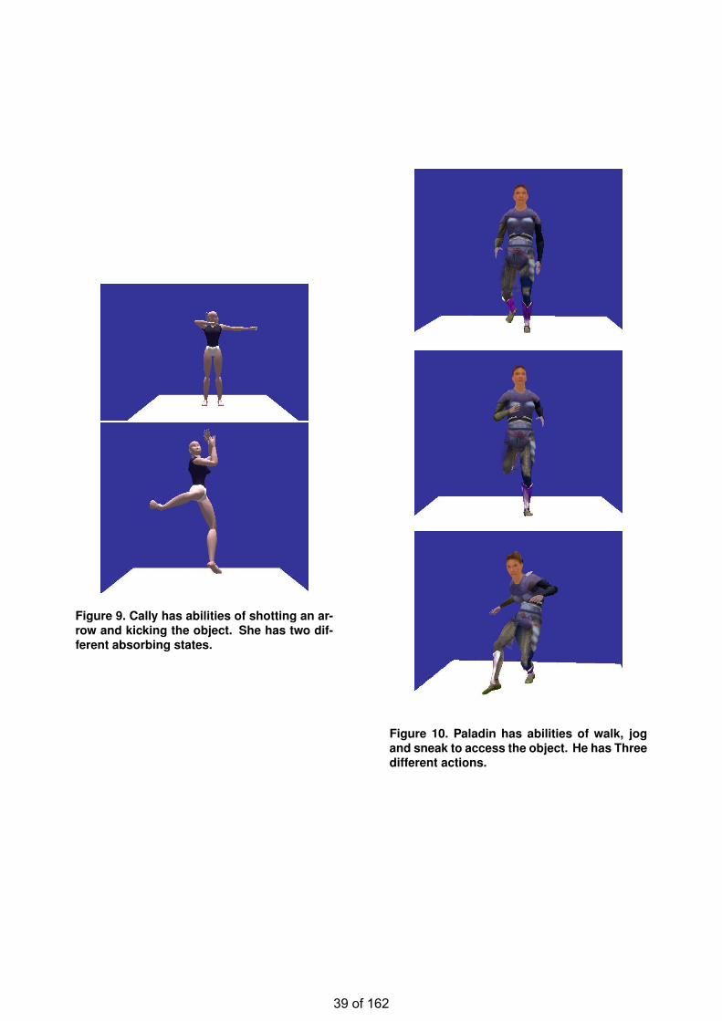
Figure 9. Cally has abilities of shotting an ar-row and kicking the object. She has two dif-ferent absorbing states.
Figure 10. Paladin has abilities of walk, jogand sneak to access the object. He has Threedifferent actions.
39 of 162
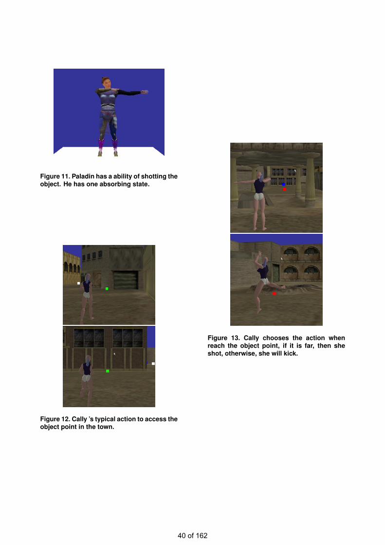
Figure 11. Paladin has a ability of shotting theobject. He has one absorbing state.
Figure 12. Cally ’s typical action to access theobject point in the town.
Figure 13. Cally chooses the action whenreach the object point, if it is far, then sheshot, otherwise, she will kick.
40 of 162
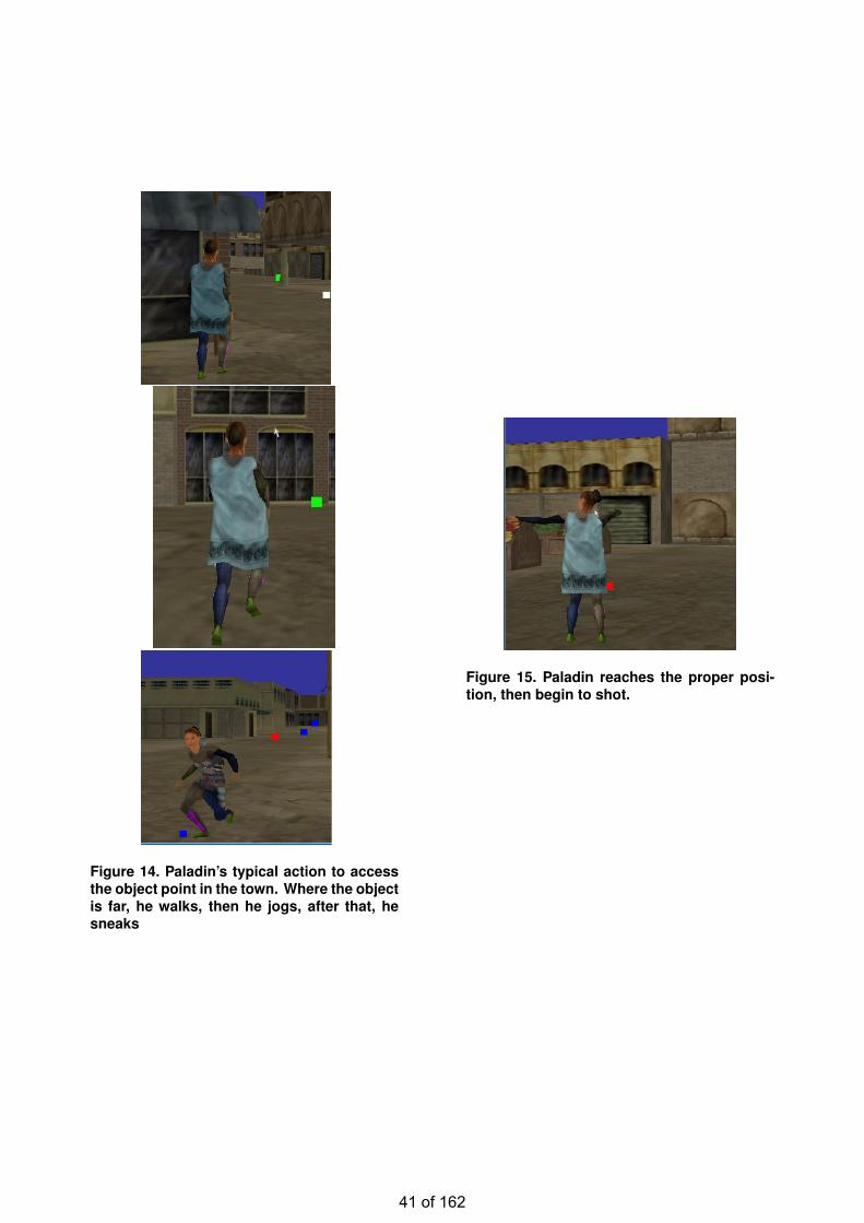
Figure 14. Paladin’s typical action to accessthe object point in the town. Where the objectis far, he walks, then he jogs, after that, hesneaks
Figure 15. Paladin reaches the proper posi-tion, then begin to shot.
41 of 162
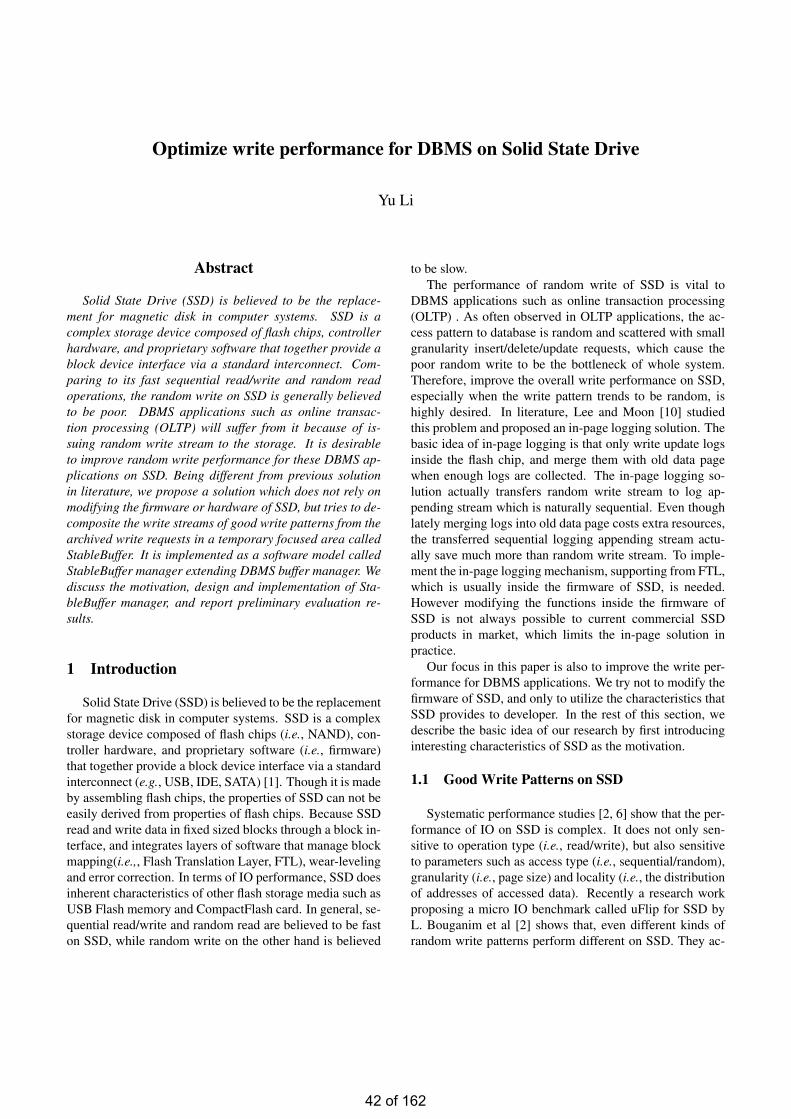
Optimize write performance for DBMS on Solid State Drive
Yu Li
Abstract
Solid State Drive (SSD) is believed to be the replace-ment for magnetic disk in computer systems. SSD is acomplex storage device composed of flash chips, controllerhardware, and proprietary software that together provide ablock device interface via a standard interconnect. Com-paring to its fast sequential read/write and random readoperations, the random write on SSD is generally believedto be poor. DBMS applications such as online transac-tion processing (OLTP) will suffer from it because of is-suing random write stream to the storage. It is desirableto improve random write performance for these DBMS ap-plications on SSD. Being different from previous solutionin literature, we propose a solution which does not rely onmodifying the firmware or hardware of SSD, but tries to de-composite the write streams of good write patterns from thearchived write requests in a temporary focused area calledStableBuffer. It is implemented as a software model calledStableBuffer manager extending DBMS buffer manager. Wediscuss the motivation, design and implementation of Sta-bleBuffer manager, and report preliminary evaluation re-sults.
1 Introduction
Solid State Drive (SSD) is believed to be the replacementfor magnetic disk in computer systems. SSD is a complexstorage device composed of flash chips (i.e., NAND), con-troller hardware, and proprietary software (i.e., firmware)that together provide a block device interface via a standardinterconnect (e.g., USB, IDE, SATA) [1]. Though it is madeby assembling flash chips, the properties of SSD can not beeasily derived from properties of flash chips. Because SSDread and write data in fixed sized blocks through a block in-terface, and integrates layers of software that manage blockmapping(i.e.,, Flash Translation Layer, FTL), wear-levelingand error correction. In terms of IO performance, SSD doesinherent characteristics of other flash storage media such asUSB Flash memory and CompactFlash card. In general, se-quential read/write and random read are believed to be faston SSD, while random write on the other hand is believed
to be slow.The performance of random write of SSD is vital to
DBMS applications such as online transaction processing(OLTP) . As often observed in OLTP applications, the ac-cess pattern to database is random and scattered with smallgranularity insert/delete/update requests, which cause thepoor random write to be the bottleneck of whole system.Therefore, improve the overall write performance on SSD,especially when the write pattern trends to be random, ishighly desired. In literature, Lee and Moon [10] studiedthis problem and proposed an in-page logging solution. Thebasic idea of in-page logging is that only write update logsinside the flash chip, and merge them with old data pagewhen enough logs are collected. The in-page logging so-lution actually transfers random write stream to log ap-pending stream which is naturally sequential. Even thoughlately merging logs into old data page costs extra resources,the transferred sequential logging appending stream actu-ally save much more than random write stream. To imple-ment the in-page logging mechanism, supporting from FTL,which is usually inside the firmware of SSD, is needed.However modifying the functions inside the firmware ofSSD is not always possible to current commercial SSDproducts in market, which limits the in-page solution inpractice.
Our focus in this paper is also to improve the write per-formance for DBMS applications. We try not to modify thefirmware of SSD, and only to utilize the characteristics thatSSD provides to developer. In the rest of this section, wedescribe the basic idea of our research by first introducinginteresting characteristics of SSD as the motivation.
1.1 Good Write Patterns on SSD
Systematic performance studies [2, 6] show that the per-formance of IO on SSD is complex. It does not only sen-sitive to operation type (i.e., read/write), but also sensitiveto parameters such as access type (i.e., sequential/random),granularity (i.e., page size) and locality (i.e., the distributionof addresses of accessed data). Recently a research workproposing a micro IO benchmark called uFlip for SSD byL. Bouganim et al [2] shows that, even different kinds ofrandom write patterns perform different on SSD. They ac-
42 of 162
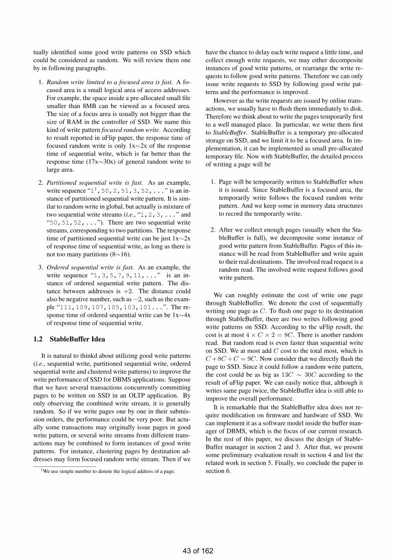
tually identified some good write patterns on SSD whichcould be considered as random. We will review them oneby in following paragraphs.
1. Random write limited to a focused area is fast. A fo-cused area is a small logical area of access addresses.For example, the space inside a pre-allocated small filesmaller than 8MB can be viewed as a focused area.The size of a focus area is usually not bigger than thesize of RAM in the controller of SSD. We name thiskind of write pattern focused random write. Accordingto result reported in uFlip paper, the response time offocused random write is only 1x∼2x of the responsetime of sequential write, which is far better than theresponse time (17x∼30x) of general random write tolarge area.
2. Partitioned sequential write is fast. As an example,write sequence “11,50,2,51,3,52,...” is an in-stance of partitioned sequential write pattern. It is sim-ilar to random write in global, but actually is mixture oftwo sequential write streams (i.e., “1,2,3,...” and“50,51,52,...”). There are two sequential writestreams, corresponding to two partitions. The responsetime of partitioned sequential write can be just 1x∼2xof response time of sequential write, as long as there isnot too many partitions (8∼16).
3. Ordered sequential write is fast. As an example, thewrite sequence “1,3,5,7,9,11,...” is an in-stance of ordered sequential write pattern. The dis-tance between addresses is +2. The distance couldalso be negative number, such as−2, such as the exam-ple “111,109,107,105,103,101...”. The re-sponse time of ordered sequential write can be 1x∼4xof response time of sequential write.
1.2 StableBuffer Idea
It is natural to thinkd about utilizing good write patterns(i.e., sequential write, partitioned sequential write, orderedsequential write and clustered write patterns) to improve thewrite performance of SSD for DBMS applications. Supposethat we have several transactions concurrently committingpages to be written on SSD in an OLTP application. Byonly observing the combined write stream, it is generallyrandom. So if we write pages one by one in their submis-sion orders, the performance could be very poor. But actu-ally some transactions may originally issue pages in goodwrite pattern, or several write streams from different trans-actions may be combined to form instances of good writepatterns. For instance, clustering pages by destination ad-dresses may form focused random write stream. Then if we
1We use simple number to denote the logical address of a page.
have the chance to delay each write request a little time, andcollect enough write requests, we may either decompositeinstances of good write patterns, or rearrange the write re-quests to follow good write patterns. Therefore we can onlyissue write requests to SSD by following good write pat-terns and the performance is improved.
However as the write requests are issued by online trans-actions, we usually have to flush them immediately to disk.Therefore we think about to write the pages temporarily firstto a well managed place. In particular, we write them firstto StableBuffer. StableBuffer is a temporary pre-allocatedstorage on SSD, and we limit it to be a focused area. In im-plementation, it can be implemented as small pre-allocatedtemporary file. Now with StableBuffer, the detailed processof writing a page will be
1. Page will be temporarily written to StableBuffer whenit is issued. Since StableBuffer is a focused area, thetemporarily write follows the focused random writepattern. And we keep some in memory data structuresto record the temporarily write.
2. After we collect enough pages (usually when the Sta-bleBuffer is full), we decomposite some instance ofgood write pattern from StableBuffer. Pages of this in-stance will be read from StableBuffer and write againto their real destinations. The involved read request is arandom read. The involved write request follows goodwrite pattern.
We can roughly estimate the cost of write one pagethrough StableBuffer. We denote the cost of sequentiallywriting one page as C. To flush one page to its destinationthrough StableBuffer, there are two writes following goodwrite patterns on SSD. According to the uFlip result, thecost is at most 4 × C × 2 = 8C. There is another randomread. But random read is even faster than sequential writeon SSD. We at most add C cost to the total most, which isC +8C +C = 9C. Now consider that we directly flush thepage to SSD. Since it could follow a random write pattern,the cost could be as big as 13C ∼ 30C according to theresult of uFlip paper. We can easily notice that, although itwrites same page twice, the StableBuffer idea is still able toimprove the overall performance.
It is remarkable that the StableBuffer idea does not re-quire modification on firmware and hardware of SSD. Wecan implement it as a software model inside the buffer man-ager of DBMS, which is the focus of our current research.In the rest of this paper, we discuss the design of Stable-Buffer manager in section 2 and 3. After that, we presentsome preliminary evaluation result in section 4 and list therelated work in section 5. Finally, we conclude the paper insection 6.
43 of 162
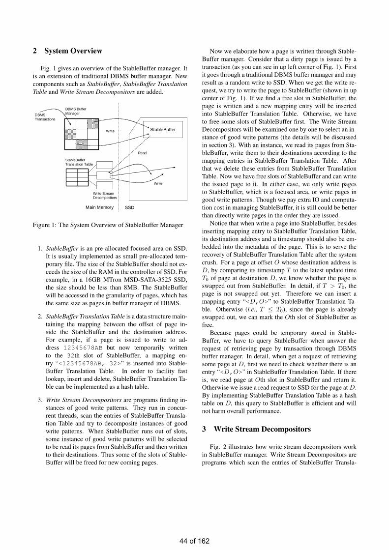
2 System Overview
Fig. 1 gives an overview of the StableBuffer manager. Itis an extension of traditional DBMS buffer manager. Newcomponents such as StableBuffer, StableBuffer TranslationTable and Write Stream Decompositors are added.
StableBuffer
DBMS Buffer ManagerDBMS
Transactions
StableBufferTranslation Table
Write
Write Stream Decompositors
Main Memory SSD
Write
Read
Figure 1: The System Overview of StableBuffer Manager
1. StableBuffer is an pre-allocated focused area on SSD.It is usually implemented as small pre-allocated tem-porary file. The size of the StableBuffer should not ex-ceeds the size of the RAM in the controller of SSD. Forexample, in a 16GB MTron MSD-SATA-3525 SSD,the size should be less than 8MB. The StableBufferwill be accessed in the granularity of pages, which hasthe same size as pages in buffer manager of DBMS.
2. StableBuffer Translation Table is a data structure main-taining the mapping between the offset of page in-side the StableBuffer and the destination address.For example, if a page is issued to write to ad-dress 12345678AB but now temporarily writtento the 32th slot of StableBuffer, a mapping en-try “<12345678AB, 32>” is inserted into Stable-Buffer Translation Table. In order to facility fastlookup, insert and delete, StableBuffer Translation Ta-ble can be implemented as a hash table.
3. Write Stream Decompositors are programs finding in-stances of good write patterns. They run in concur-rent threads, scan the entries of StableBuffer Transla-tion Table and try to decomposite instances of goodwrite patterns. When StableBuffer runs out of slots,some instance of good write patterns will be selectedto be read its pages from StableBuffer and then writtento their destinations. Thus some of the slots of Stable-Buffer will be freed for new coming pages.
Now we elaborate how a page is written through Stable-Buffer manager. Consider that a dirty page is issued by atransaction (as you can see in up left corner of Fig. 1). Firstit goes through a traditional DBMS buffer manager and mayresult as a random write to SSD. When we get the write re-quest, we try to write the page to StableBuffer (shown in upcenter of Fig. 1). If we find a free slot in StableBuffer, thepage is written and a new mapping entry will be insertedinto StableBuffer Translation Table. Otherwise, we haveto free some slots of StableBuffer first. The Write StreamDecompositors will be examined one by one to select an in-stance of good write patterns (the details will be discussedin section 3). With an instance, we read its pages from Sta-bleBuffer, write them to their destinations according to themapping entries in StableBuffer Translation Table. Afterthat we delete these entries from StableBuffer TranslationTable. Now we have free slots of StableBuffer and can writethe issued page to it. In either case, we only write pagesto StableBuffer, which is a focused area, or write pages ingood write patterns. Though we pay extra IO and computa-tion cost in managing StableBuffer, it is still could be betterthan directly write pages in the order they are issued.
Notice that when write a page into StableBuffer, besidesinserting mapping entry to StableBuffer Translation Table,its destination address and a timestamp should also be em-bedded into the metadata of the page. This is to serve therecovery of StableBuffer Translation Table after the systemcrush. For a page at offset O whose destination address isD, by comparing its timestamp T to the latest update timeT0 of page at destination D, we know whether the page isswapped out from StableBuffer. In detail, if T > T0, thepage is not swapped out yet. Therefore we can insert amapping entry “<D,O>” to StableBuffer Translation Ta-ble. Otherwise (i.e., T ≤ T0), since the page is alreadyswapped out, we can mark the Oth slot of StableBuffer asfree.
Because pages could be temporary stored in Stable-Buffer, we have to query StableBuffer when answer therequest of retrieving page by transaction through DBMSbuffer manager. In detail, when get a request of retrievingsome page at D, first we need to check whether there is anentry “<D,O>” in StableBuffer Translation Table. If thereis, we read page at Oth slot in StableBuffer and return it.Otherwise we issue a read request to SSD for the page at D.By implementing StableBuffer Translation Table as a hashtable on D, this query to StableBuffer is efficient and willnot harm overall performance.
3 Write Stream Decompositors
Fig. 2 illustrates how write stream decompositors workin StableBuffer manager. Write Stream Decompositors areprograms which scan the entries of StableBuffer Transla-
44 of 162
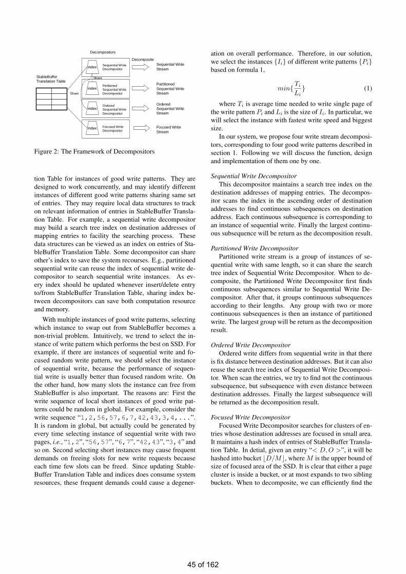
index
Sequential Write Stream
Partitioned Sequential Write Stream
Focused Write Stream
StableBufferTranslation Table
DecompositeSequential Write Decompositor
Petitioned Sequential Write Decompositor
Focused Write Decompositor
Decompositors
Share
Ordered Sequential Write Stream
Ordered Sequential Write Decompositor
Share
index
index
index
Figure 2: The Framework of Decompositors
tion Table for instances of good write patterns. They aredesigned to work concurrently, and may identify differentinstances of different good write patterns sharing same setof entries. They may require local data structures to trackon relevant information of entries in StableBuffer Transla-tion Table. For example, a sequential write decompositormay build a search tree index on destination addresses ofmapping entries to facility the searching process. Thesedata structures can be viewed as an index on entries of Sta-bleBuffer Translation Table. Some decompositor can shareother’s index to save the system recourses. E.g., partitionedsequential write can reuse the index of sequential write de-compositor to search sequential write instances. As ev-ery index should be updated whenever insert/delete entryto/from StableBuffer Translation Table, sharing index be-tween decompositors can save both computation resourceand memory.
With multiple instances of good write patterns, selectingwhich instance to swap out from StableBuffer becomes anon-trivial problem. Intuitively, we trend to select the in-stance of write pattern which performs the best on SSD. Forexample, if there are instances of sequential write and fo-cused random write pattern, we should select the instanceof sequential write, because the performance of sequen-tial write is usually better than focused random write. Onthe other hand, how many slots the instance can free fromStableBuffer is also important. The reasons are: First thewrite sequence of local short instances of good write pat-terns could be random in global. For example, consider thewrite sequence “1,2,56,57,6,7,42,43,3,4,...”.It is random in global, but actually could be generated byevery time selecting instance of sequential write with twopages, i.e., “1,2”, “56,57”, “6,7”, “42,43”, “3,4” andso on. Second selecting short instances may cause frequentdemands on freeing slots for new write requests becauseeach time few slots can be freed. Since updating Stable-Buffer Translation Table and indices does consume systemresources, these frequent demands could cause a degener-
ation on overall performance. Therefore, in our solution,we select the instances Ii of different write patterns Pibased on formula 1,
minTi
Li (1)
where Ti is average time needed to write single page ofthe write pattern Pi and Li is the size of Ii. In particular, wewill select the instance with fastest write speed and biggestsize.
In our system, we propose four write stream decomposi-tors, corresponding to four good write patterns described insection 1. Following we will discuss the function, designand implementation of them one by one.
Sequential Write DecompositorThis decompositor maintains a search tree index on the
destination addresses of mapping entries. The decompos-itor scans the index in the ascending order of destinationaddresses to find continuous subsequences on destinationaddress. Each continuous subsequence is corresponding toan instance of sequential write. Finally the largest continu-ous subsequence will be return as the decomposition result.
Partitioned Write DecompositorPartitioned write stream is a group of instances of se-
quential write with same length, so it can share the searchtree index of Sequential Write Decompositor. When to de-composite, the Partitioned Write Decompositor first findscontinuous subsequences similar to Sequential Write De-compositor. After that, it groups continuous subsequencesaccording to their lengths. Any group with two or morecontinuous subsequences is then an instance of partitionedwrite. The largest group will be return as the decompositionresult.
Ordered Write DecompositorOrdered write differs from sequential write in that there
is fix distance between destination addresses. But it can alsoreuse the search tree index of Sequential Write Decomposi-tor. When scan the entries, we try to find not the continuoussubsequence, but subsequence with even distance betweendestination addresses. Finally the largest subsequence willbe returned as the decomposition result.
Focused Write DecompositorFocused Write Decompositor searches for clusters of en-
tries whose destination addresses are focused in small area.It maintains a hash index of entries of StableBuffer Transla-tion Table. In detial, given an entry “< D, O >”, it will behashed into bucket bD/Mc, where M is the upper bound ofsize of focused area of the SSD. It is clear that either a pagecluster is inside a bucket, or at most expands to two siblingbuckets. When to decomposite, we can efficiently find the
45 of 162
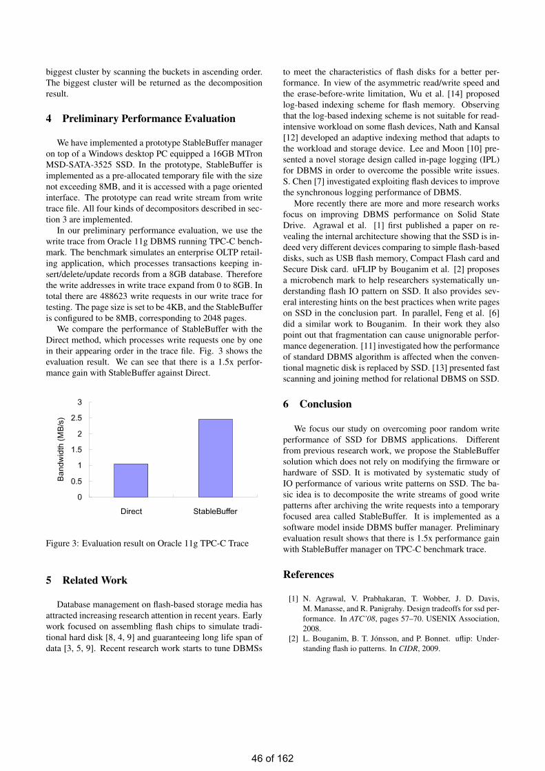
biggest cluster by scanning the buckets in ascending order.The biggest cluster will be returned as the decompositionresult.
4 Preliminary Performance Evaluation
We have implemented a prototype StableBuffer manageron top of a Windows desktop PC equipped a 16GB MTronMSD-SATA-3525 SSD. In the prototype, StableBuffer isimplemented as a pre-allocated temporary file with the sizenot exceeding 8MB, and it is accessed with a page orientedinterface. The prototype can read write stream from writetrace file. All four kinds of decompositors described in sec-tion 3 are implemented.
In our preliminary performance evaluation, we use thewrite trace from Oracle 11g DBMS running TPC-C bench-mark. The benchmark simulates an enterprise OLTP retail-ing application, which processes transactions keeping in-sert/delete/update records from a 8GB database. Thereforethe write addresses in write trace expand from 0 to 8GB. Intotal there are 488623 write requests in our write trace fortesting. The page size is set to be 4KB, and the StableBufferis configured to be 8MB, corresponding to 2048 pages.
We compare the performance of StableBuffer with theDirect method, which processes write requests one by onein their appearing order in the trace file. Fig. 3 shows theevaluation result. We can see that there is a 1.5x perfor-mance gain with StableBuffer against Direct.
0
0.5
1
1.5
2
2.5
3
Direct StableBuffer
Band
width
(MB/s
)
Figure 3: Evaluation result on Oracle 11g TPC-C Trace
5 Related Work
Database management on flash-based storage media hasattracted increasing research attention in recent years. Earlywork focused on assembling flash chips to simulate tradi-tional hard disk [8, 4, 9] and guaranteeing long life span ofdata [3, 5, 9]. Recent research work starts to tune DBMSs
to meet the characteristics of flash disks for a better per-formance. In view of the asymmetric read/write speed andthe erase-before-write limitation, Wu et al. [14] proposedlog-based indexing scheme for flash memory. Observingthat the log-based indexing scheme is not suitable for read-intensive workload on some flash devices, Nath and Kansal[12] developed an adaptive indexing method that adapts tothe workload and storage device. Lee and Moon [10] pre-sented a novel storage design called in-page logging (IPL)for DBMS in order to overcome the possible write issues.S. Chen [7] investigated exploiting flash devices to improvethe synchronous logging performance of DBMS.
More recently there are more and more research worksfocus on improving DBMS performance on Solid StateDrive. Agrawal et al. [1] first published a paper on re-vealing the internal architecture showing that the SSD is in-deed very different devices comparing to simple flash-baseddisks, such as USB flash memory, Compact Flash card andSecure Disk card. uFLIP by Bouganim et al. [2] proposesa microbench mark to help researchers systematically un-derstanding flash IO pattern on SSD. It also provides sev-eral interesting hints on the best practices when write pageson SSD in the conclusion part. In parallel, Feng et al. [6]did a similar work to Bouganim. In their work they alsopoint out that fragmentation can cause unignorable perfor-mance degeneration. [11] investigated how the performanceof standard DBMS algorithm is affected when the conven-tional magnetic disk is replaced by SSD. [13] presented fastscanning and joining method for relational DBMS on SSD.
6 Conclusion
We focus our study on overcoming poor random writeperformance of SSD for DBMS applications. Differentfrom previous research work, we propose the StableBuffersolution which does not rely on modifying the firmware orhardware of SSD. It is motivated by systematic study ofIO performance of various write patterns on SSD. The ba-sic idea is to decomposite the write streams of good writepatterns after archiving the write requests into a temporaryfocused area called StableBuffer. It is implemented as asoftware model inside DBMS buffer manager. Preliminaryevaluation result shows that there is 1.5x performance gainwith StableBuffer manager on TPC-C benchmark trace.
References
[1] N. Agrawal, V. Prabhakaran, T. Wobber, J. D. Davis,M. Manasse, and R. Panigrahy. Design tradeoffs for ssd per-formance. In ATC’08, pages 57–70. USENIX Association,2008.
[2] L. Bouganim, B. T. Jonsson, and P. Bonnet. uflip: Under-standing flash io patterns. In CIDR, 2009.
46 of 162
[3] L. Chang. On efficient wear leveling for large-scale flash-memory storage systems. In SAC’07, pages 1126–1130,2007.
[4] L. Chang, T. Kuo, and S. Lo. Real-time garbage collectionfor flash-memory storage systems of real-time embeddedsystems. Trans. on Embedded Computing Sys., 3(4):837–863, 2004.
[5] Y. Chang, J. Hsieh, and T. Kuo. Endurance enhancementof flash-memory storage systems: an efficient static wearleveling design. In DAC’07, pages 212–217, 2007.
[6] F. Chen, D. A. Koufaty, and X. Zhang. Understanding intrin-sic characteristics and system implications of flash memorybased solid state drives. In SIGMETRICS ’09, pages 181–192. ACM, 2009.
[7] S. Chen. Flashlogging: exploiting flash devices for syn-chronous logging performance. In SIGMOD ’09, pages 73–86. ACM, 2009.
[8] A. Kawaguchi, S. Nishioka, and H. Motoda. A flash-memory based file system. In USENIX Winter, pages 155–164, 1995.
[9] H. Kim and S. Lee. A new flash memory management forflash storage system. In COMPSAC’99, page 284, 1999.
[10] S. Lee and B. Moon. Design of flash-based dbms: an in-pagelogging approach. In SIGMOD ’07, pages 55–66, 2007.
[11] S.-W. Lee, B. Moon, C. Park, J.-M. Kim, and S.-W. Kim.A case for flash memory ssd in enterprise database applica-tions. In SIGMOD, pages 1075–1086, 2008.
[12] S. Nath and A. Kansal. Flashdb: Dynamic self-tuningdatabase for nand flash. Technical Report MSR-TR-2006-168, Microsoft Research, 2006.
[13] D. Tsirogiannis, S. Harizopoulos, M. A. Shah, J. L. Wiener,and G. Graefe. Query processing techniques for solid statedrives. In SIGMOD ’09, pages 59–72. ACM, 2009.
[14] C. Wu, T. Kuo, and L. P. Chang. An efficient b-tree layerimplementation for flash-memory storage systems. Trans.on Embedded Computing Sys., 6(3):19, 2007.
47 of 162
Cooperative Stochastic Differential Game in P2P Content Distribution Networks
Xiaowei Chen
Abstract Pareto-optimal resource allocation is one of the major goals in game-theoretic solutions for peer-to-peer content distribution network. These solutions have been designed that force the participants to behave more cooperatively to reach the overall efficiency as well as individual efficiency of a distributed system. But there exist many issues when these solutions are applied in stochastic differential environment which is more realistic. In this paper, we propose an incentive framework based on cooperative stochastic differential game. In this framework, peers can cooperate with each other and get Pareto-optimal bandwidth allocation without any binding agreements. We prove the payoff distribution procedure can achieve dynamic Shapley value by using equilibrating transitory compensation during peers' cooperation and make peers follow the original optimality principle and cooperative state trajectory path. Our incentive framework is more flexible and realistic than previous game-theoretic solutions. It can build cooperation relationship in stochastic dynamic peer-to-peer network without the limitation of time consistency. 1. Introduction
The Peer-to-Peer (P2P) paradigm offers obvious
advantages for the fast distribution of large content in the Internet. As reported in an ipoque report [1] in 2009, P2P generates most traffic in all regions. Just as in previous years, and BitTorrent is the dominating P2P protocol followed by HTTP in all regions but South America (There is another P2P protocol which leads the pack before BitTorrent and eDonkey in South America).
Though the swarming principle supports P2P content distribution protocol in a non-cooperative environment and exploits the two-way interest of peers in different blocks which the other one provides, the cooperation of peers is not a matter of course. Most of the peers behave selfishly and are interested in maximizing their own download rates, the mutual interest results in peers, which bargain for bandwidth with each other. P2P faces the problem of free-riding [2] where peers consume resources solely without contributing anything to the network. Therefore, reputation systems and/or incentive mechanisms are implemented in P2P applications frequently.
A very popular example is the BitTorrent protocol [3] where a peer uploads to others from which it receives the highest download rates. This strategy is inspired by the tit-for-tat principle that is well known from game theory. Here, a player adopts the strategy, which his opponent used in the previous round. By cooperating in the first step the tit-for-tat
strategy proved very effective in the repeated prisoner’s dilemma [4].
Unfortunately, simulation-based studies for BitTorrent reveal a high variability in the download rates [5] and unfairness in terms of the ratio of uploaded to downloaded data [6]. Tit-for-tat strategy may look beneficial from a local perspective, but from a more global perspective, they are not effective. Piatek [7] shows that increased upload contribution only marginally improves download rates, and peers have no reason to contribute once they have satisfied their immediate demands.
These results lead to two questions. Firstly, from the user perspective: Does another strategy exist which outperforms BitTorrent’s tit-for-tat strategy? This means with such kind of strategy a user can fairly increase its download performance according to it upload performance. Secondly, from the angle of a protocol designer: Does a strategy exist which ensures fairness between peers although peers behave selfishly?
Users in a P2P social network are strategic and rational, and they are likely to manipulate any incentive systems to maximize their own payoff. They will even cheat if they believe it could help maximize their payoff. Hence, game theory is a proper tool to model the interaction among peers, and to analyze the optimal and cheat-proof cooperation strategies. But there exist many issues when the proposed solutions are applied in stochastic differential environment which is more realistic.
Our work tries to answer the above two questions based on game theory. We design an incentive framework based on cooperative stochastic differential game to achieve Pareto-optimal bandwidth allocation fairly without any binding agreements. Our contributions are: We analyze the root issue of BitTorrent tit-for-tat
strategy from game theory prospective and reveal the reason that why this strategy cannot achieve its original goal.
We clearly define the basic elements of game theory from P2P content distribution network’s prospective, which lay a solid foundation to help us explore the essence of incentive framework based on game theory in P2P content distribution network.
We present a general incentive framework based on cooperative stochastic differential game. It adopts an analytically tractable “payoff distribution procedure” which would lead to subgame-consistent solutions. We prove the payoff distribution procedure can achieve dynamic Shapley value by using equilibrating transitory compensation during peers' cooperation and make peers follow the original optimality principle and cooperative state trajectory path.
48 of 162
1.1 Related work
We now briefly present some related work. Micro-payment [8] is probably the earliest work on designing incentive protocol for P2P networks. It relies on a centralized server and uses virtual currency to provide incentive for resource sharing. Since then, much efforts are focused on incentive mechanisms for P2P systems [9] and wireless networks [10]. Vishnumurthy [11] shows that shared history based incentives can overcome the scalability problem of private history based mechanisms and one can use DHT to implement the shared history incentive mechanism. One shared history based incentive is the reciprocative strategy [12]. It makes decisions according to the reputation of requesters and is studied via simulation only.
There are some existing works on designing a particular incentive mechanism. Feldman [13] assumes that each peer has a fixed strategy with a certain distribution while we assume peers can adapt their strategies. In [14], authors show that a proportional strategy can lead to market equilibria but the result does not generalize to multiple strategies.
Pareto-optimal resource allocation is one of the major goals in game-theoretic solutions for peer-to-peer content distribution network. The above solutions have been designed that force the participants to behave more cooperatively to reach the overall efficiency as well as individual efficiency of a distributed system. But there exist many issues when these solutions are applied in stochastic differential environment which is more realistic. Our paper focuses on the incentive mechanism design in cooperative stochastic differential environment in P2P content distribution systems.
1.2 Paper organization
The balance of the paper is organized as follows. In section
2, we analyze the root issue of tit-for-tat strategy and reveal the reason that why this strategy cannot achieve its original goal. In section 3, we clearly define the basic elements and their properties of game theory from P2P content distribution network’s view. In section 4, we present a general incentive framework based on cooperative stochastic differential game and prove its effectiveness. Finally, section 5 concludes this paper.
2. Analysis of Tit-for-Tat Strategy
From section 1, we know that the swarming principle
supports P2P content distribution protocol in a non-cooperative environment. But under non-cooperative environment, the profit of each peer and whole system will be far away from Pareto-optimality, even hurting each other. The result must be “solitary, poor, nasty, brutish and shot” [15]. The difficulty of cooperation is rooted from free-riding problem in many situations. As a matter of fact, the reason is the temporary profit of each peer exits conflicts.
Based on this analysis, many researchers induct game theory as tool to solve this problem. Because static non-cooperative game often leads to lose-lose situation, so the static cooperative game which can build Pareto-optimality is applied in P2P systems. But there is an assumption in static cooperative game that peers can meet a binding agreement. Actually, whether there is a binding agreement is the watershed between non-cooperative game and cooperative game. The Shapley value in cooperative game is a very important solution which can create a unique fairly profit distribution which can achieve Pareto-optimality. Unfortunately, binding agreement has not one hundred percent sanction in real P2P systems. There always exist conflicts between individual rationality and group rationality.
Under this circumstance, strategic conflict resolution becomes a way of building cooperation in non-cooperative P2P environment. We realize that repeated game still can bring on Tragedy of Common, but there can exist cooperation in infinite repeated game. The most used strategy is tit-for-tat which is implemented in BitTorrent protocol. Here we should be noted that infinite repeated game is a very special game model which often does not exist in real P2P systems. That is why the tit-for-tat strategy often cannot achieve fairness bandwidth allocation.
On one hand, since peers interact in time and decisions generally lead to effects over time, it is only a slight exaggeration to claim that “P2P content distribution is a dynamic game”. Dynamic or differential game investigates interactive decision making over time. On the other hand, the dynamic cooperation among pees often changes stochastically. For example, there are unstable network bandwidth and unexpected lost connection among peers, etc. Yeung [16] introduced the paradigm of randomly-furcating stochastic differential games to make it possible to study stochastic elements via branching payoffs under the format of differential games.
Cooperative games hold out the promise of socially optimal and group efficient solutions to problems involving strategic actions. Formulation of optimal peer behavior is a fundamental element. In dynamic cooperative games, a stringent condition on cooperation and agreement is required: In the solution, the optimality principle must remain optimal throughout the game, at any instant of time along the optimal state trajectory determined at the outset. This condition is known as dynamic stability or time consistency. In other words, dynamic stability of solutions to any cooperative differential game involved the property that, as the game proceeds along an optimal trajectory, players are guided by the same optimality principle at each instant of time, and hence do not possess incentives to deviate from the previously adopted optimal behavior throughout the game.
In the presence of stochastic elements, a more stringent condition, subgame consistency, is required for a credible cooperative solution. In particular, a cooperative solution is subgame-consistent if an extension of the solution policy to a situation with a later starting time and any feasible state brought about by prior optimal behavior would remain optimal. Along with Yeung and Petrosyan’s significant breakthrough in
49 of 162
the study of cooperative stochastic differential games [17], we propose an incentive framework based on their contributions and apply it in P2P content distribution networks.
Before we introduce our incentive framework, we need to define the basic elements of game theory from P2P content distribution network’s prospective to lay a solid foundation and help us explore the essence of incentive framework based on game theory.
3. Basic Elements of Game Theory
In P2P content distribution environment, we need provide
clear definition of the following basic elements in game theory: player, action, information, strategy, payoff, rationality, objective, order of play, outcome and equilibrium.
Definition 1. Player is peer which can make decisions in P2P content distribution.
Player must have more than one action to be selected. Normally, there are at least two peers in P2P content distribution. Except player, there can exist pseudo-player, namely, nature. Nature is a player or mechanism without objective. It will randomly choose action as pre-defined probability.
In general, player is assumed as rational. Definition 2: Action is decision variable of player in a
specific time point. We use ai∈Ai denotes a specific action of i-th player. Ai denotes the action sets that the player can select.
The action of player can be discrete or continuous. In P2P content distribution networks, we can view it as the bandwidth that a peer wants to upload.
Definition 3: Information is knowledge of peer in P2P content distribution game. We use information set to describe information. In game theory, an information set is a set that, for a particular player, establishes all the possible moves that could have taken place in the game so far, given what that player has observed so far.
If the game has perfect information, every information set contains only one member, namely the point actually reached at that stage of the game. Otherwise, it is imperfect information that some players cannot be sure exactly what has taken place so far in the game and what their position is.
An item of information in a game is common knowledge if all of the players know it (it is mutual knowledge) and all of the players know that all other players know it and all other players know that all other players know that all other players know it, and so on.
Complete information requires that every player know the strategies and payoffs of the other players but not necessarily the actions. If and only if the type, strategy space and payoff function of each peer are all common knowledge, we call the game has complete information, otherwise, it has incomplete information. We assume the information in a game is complete. If not, we can use Harsanyi Transformation which adds nature as a player in the game to make an incomplete information game transform as a complete but imperfect information game, or Bayesian game.
Definition 4: A player's strategy in a game is a complete plan of action for whatever situation might arise; this fully determines the player's behavior. A player's strategy will determine the action the player will take at any stage of the game, for every possible history of play up to that stage.
There are two kinds of strategies: pure strategy and mixed strategy. A pure strategy provides a complete definition of how a player will play a game. A mixed strategy is an assignment of a probability to each pure strategy. This allows for a player to randomly select a pure strategy.
We use si∈Si denotes a specific strategy of i-th player. Si denotes the strategy set or strategy space. Definition 5: Payoffs are numbers which represent the motivations of players. Payoffs may represent profit, quantity, "utility," or other continuous measures, or may simply rank the desirability of outcomes. In P2P content distribution networks, payoff of a peer is the download bandwidth of a peer. We use ui denotes payoff of i-th player.
Definition 6: Rationality implies that every player is motivated by maximizing his own payoff. In a stricter sense, it implies that every player always maximizes his utility, thus being able to perfectly calculate the probabilistic result of every action. Rationality can be classified as individual rationality and group rationality.
Definition 7: If each player’s preference can be represented as expected payoff function, then player has a clear and definite objective that optimizes its payoff function by strategy or choosing actions.
Definition 8: In game theory, each player has time point to select action. These time points are called decision nodes. Decision nodes can have sequence which is called as order of play. In differential game, players can take actions simultaneously or with sequential order.
Definition 9: Outcome is a set of moves or strategies taken by the players, or their payoffs resulting from the actions or strategies taken by all players.
Definition 10: Equilibrium is the combination of optimal strategies among all players. In an equilibrium, each player of the game has adopted a strategy that they are unlikely to change. We use *
is denotes optimal strategy of i-th player. 4. Cooperative Stochastic Differential Game
4.1 Incentive Framework
The balance of the According to Yeung [16] and [17], we
know that the dynamic stability of a solution of a cooperative differential game is the property that, when the game proceeds along an optimal trajectory, at each instant of time the players are guided by the same optimality principles, and hence do not have any ground for deviation from the previously adopted “optimal” behavior throughout the game.
In the presence of stochastic elements, a more stringent condition, subgame consistency, is required for a credible cooperative solution. A cooperative solution is subgame consistent if an extension of the solution policy to a situation
50 of 162
with a later starting time and any feasible state brought about by prior optimal behaviors would remain optimal.
Consider the cooperative game 0 0( , )c x T tΓ − in which the
players agree to act to maximize their joint payoff and adopt a certain mechanism governing the sharing of the players’ payoffs. t0 and x0 are start time and start state. To achieve group rationality, the players adopt the cooperative controls
0 0( )* ( )*1 2[ ( , ), ( , )]t tt x t xψ ψ . A set of controls 0 0( )* ( )*
1 2[ ( , ), ( , )]t tt x t xψ ψ provides an optimal solution to the stochastic control problem
0 0( , )x T tΨ − . The optimal cooperative state trajectory follows the stochastic path
0
* ( )Ts tx s =
.
At time t0, with the state being x0, the term 0( )0 0( , )t i t xξ
denotes the expected share/imputation of total cooperative payoff (received over the time interval [t0, T]) to player i guided by the agreed-upon optimality principle.
Now, consider the cooperative game *( , )c x Tτ τΓ − in which the game starts at time τ ∈ [t0, T] with initial state * *x Xτ τ∈ , and the same agreed-upon optimality principle as above is adopted. Let ( ) *( , )i xτ
τξ τ denote the expected share/imputation of total cooperative payoff given to player i over the time interval [τ, T].
Following Yeung and Petrosyan [17], we formulate a payoff distribution over time so that the agreed imputations can be realized. Let the vectors 1 2( ) [ ( ), ( )]B s B s B sτ τ τ= denote the instantaneous payoff of the cooperative game at time s ∈ [τ, T] for the cooperative game *( , )c x Tτ τΓ − . In other words, player i, for i ∈ 1, 2, obtains a payoff equaling ( )iB sτ at time instant s. A terminal value of *( ( ))iq x T is received by player i at time T.
In particular, ( )iB sτ and *( ( ))iq x T constitute a Payoff Distribution Procedure (PDP) for the game *( , )c x Tτ τΓ − .
( )iB sτ is equilibrating transitory compensation, *( ( ))iq x T is optimal terminal value. Subgame consistency guarantees that the solution imputations throughout the game interval in the sense that the extension of the solution policy to a situation with a later starting time and any feasible state brought about by prior optimal behaviors would remain optimal. Equilibrating transitory compensation is developed for the implementation of subgame consistency cooperation scheme.
In stochastic environment, the compensation ( )iB τ player i receives at time τ given the state * *x Xτ τ∈ is the sum of
(i) Player i’s agreed upon marginal share of total expected cooperative profit,
(ii) Player i’s agreed upon marginal share of his own expected non-cooperative profit plus the instantaneous effect on his non-cooperative expected payoff when the change in the state variable *xτ follows the cooperative trajectory instead of the non-cooperative path, and
(iii) Player i’s agreed upon marginal share of Player j’s non-cooperative profit plus the instantaneous effect on Player j’s non-cooperative payoff when the change in the state variable x follows the optimal trajectory instead of the non-cooperative path.
In P2P content distribution networks, consider the scenario in which n peers, and peer i’s objective is:
00 0
0
[ , ( ), ( )]exp[ ( ) ]
exp[ ( ) ] ( ( ))
T sit i it t
s iit
E g s x s u s r y dy ds
r y dy q x T
−
+ −
∫ ∫
∫ (1)
for for [ ]1,2, , i n N∈ … ≡ , ( ) 0, ( ) 0i ig q≥ ≥
where xi(s) ∈Xi denotes the current bandwidth of peer i, ui ∈ Ui is the control vector of peer i, denotes the upload bandwidth of peer i can provide,
0
exp[ ( ) ]s
tr y dy−∫ is discount
factor which can be viewed as a peer’s opportunity cost, and ( ( ))i
iq x T is the terminal payoff which can be viewed as the future potential current value (bandwidth) in terminal time.
[ , ( ), ( )]ii ig s x s u s denotes the instantaneous bandwidth that peer
i can get. In particular, [ , ( ), ( )]ii ig s x s u s and ( )i
iq x are positively related to xi.
The state dynamics of the game is characterized by the set of vector-valued stochastic differential equations:
0
0
( ) [ , ( ), ( )] [ , ( )] ( ),
( )
ii i i i i
i i
dx s f s x s u s ds s x s dz s
x t x
σ= +
= (2)
where [ , ( )]is x sσ is a i im ×Θ matrix, and ( )iz s is a iΘ -dimensional Wiener process and the initial state 0
ix is given. Let [ , ( )] [ , ( )] [ , ( )]T
i i i is x s s x s s x sσ σΩ = denote the covariance matrix with its element in row h and column ζ denoted by
[ , ( )]hi is x sζΩ . For i ≠j, i jx x∩ =∅ , and zi(s) and zj(s) are
independent Wiener processes. Trough the above processes, we import stochastic environment factors in dynamic cooperation joined by multiple peers. We also used xN(s) to denote the vector [x1(s), x2(s), . . . , xn(s)] and 0
Nx denotes the vector [ 01x ,
02x , …, 0
nx ]. Consider a coalition of a subset of peers K ⊆ N. There are k
peers in the subset K. The participating peers can gain more bandwidth that would be difficult for them to obtain on their own, and hence the state dynamics of peer i in the coalition K becomes
0
0
( ) [ , ( ), ( )] [ , ( )] ( ),
( )
ii K i i i
i i
dx s f s x s u s ds s x s dz s
x t x
σ= +
=, (3)
for i ∈ K where xK(s) is the concatenation of the vectors xj(s) for j∈K. In particular, [ , , ] / 0K
i K i jf s x u x∂ ∂ ≥ , for j ≠ i. Thus positive effects on the state of peer i could be derived from the other peers within the coalition. Without much loss of generalization, the effect of xj on [ , , ]K
i K if s x u remains the same for all possible coalitions K containing peers i and j. 4.2 The Dynamic Shapley Value Imputation
51 of 162
Consider the above cooperation involving n peers. The member peers would maximize their joint profit and share their cooperative profits according to the Shapley value. The Shapley value is one of the most commonly used sharing mechanism in static cooperation games with transferable payoffs. Besides being individually rational and group rational, the Shapley value is also unique. The uniqueness property makes a more desirable cooperative solution relative to other solutions like the Core or the Stable Set. Specifically, the Shapley value gives an imputation rule for sharing the cooperative profit among the members in a coalition as:
( 1)!( )!( ) ( ( ) ( \ ))!
i
K N
k n kv v K v K in
ϕ⊆
− −= −∑ (4)
for i ∈ N where K\i is the relative complement of i in K, v(K) is the profit of coalition K, and [v(K) − i(K\i)] is the marginal contribution of peer i to the coalition K. Given the assumption that v(K) is super-additive, the Shapley value yields the desirable properties of individual rationality and group optimality. Though the Shapley value is used as the profit allocation mechanism, there exist two features that do not conform with the standard Shapley value analysis. The first is that the present analysis is dynamic so that instead of a one-time allocation of the Shapley value, we have to consider the maintenance of the Shapley value imputation over the cooperation horizon. The second is that the profit v(K) is the maximized profit to coalition K, and is not a characteristic function (from the game in which coalition K is playing a zero-sum game against coalition N\K). To maximize the cooperation’s profits the peers would adopt the control vector 0
0
( ) * * ( , )t N t TN N t tt xψ =
over the time [t0, T] interval, and the corresponding optimal state trajectory
0
* ( )t TN t tx t =
would result. At time t0 with state 0tNx , the peers
agree that peer i’s share of profits be:
00 0,
0 0
( ) ( )
( ) ( ) \0 00 0 \
( 1)!( )![ ( , ) ( , )]!
Nt i t x
t K t K iK K i
K N
vk n k W t x W t x
n⊆
=− −
−∑ (5)
for i ∈ N However, the Shapley value has to be maintained throughout the cooperation horizon [t0, T]. In particular, at time τ ∈ [t0, T] with the state being *
Nxτ , the following imputation principle has to be maintained: Condition 1. At time τ, peer i’s share of profits be:
*( ) ( , )
( ) * ( ) \ *\
( 1)!( )![ ( , ) ( , )]!
Ni x
K K iK K i
K N
vk n k W x W x
n
ττ τ
τ τ τ ττ τ⊆
=− −
−∑ (6)
for i ∈ N and τ ∈ [t0, T] Condition 1 satisfies the property of Pareto optimality throughout the game interval and guarantees individual rationality throughout the game interval. Pareto optimality and individual rationality are essential properties of imputation vectors. Moreover, if Condition 1 can be maintained, the solution optimality principle – sharing profits according to the
Shapley value – is in effect at any instant of time throughout the game along the optimal state trajectory chosen at the outset. Hence time consistency is satisfied and no peers would have any incentive to depart the cooperation. Therefore a dynamic imputation principle leading to formula (6) is dynamically stable or time consistent. Crucial to the analysis is the formulation of a profit distribution mechanism that would lead to the realization of Condition 1. This will be done in the next section. 4.3 The Dynamic Shapley Value Imputation
In this section, a profit distribution mechanism will be
developed to compensate transitory changes so that the Shapley value principle could be maintained throughout the venture horizon. From Yeung [16] and [17], we can get the following theorem.
Theorem 1. A payment to peer i ∈ N at time τ ∈ [t0, T] equaling
* *
( ) * ( ) \ *\
( ) * ( ) \ *\
* ( ) *
( )( 1)!( )![ ( , ) ] [ ( , ) ]
!
([ ( , ) ] [ ( , ) ])
[ , , ( , )]N N
i
K K it K t t K i t
K N
K K iK t K i tx x
N NN N N
Bk n k W x W x
nW t x W x
f x x
τ τ
τ τ τ ττ τ
τ τ τ ττ τ
τ τ τ
τ
τ τ
τ
τ ψ τ
= =⊆
= =
=− −
− −
+ −
×
∑ (7)
will lead to the realization of the Condition 1. Since the partial derivative of ( ) *( , )K
KW xτ ττ with respect to xj, where j ∉K, will vanish, a more concise form of Theorem 1 can be obtained as:
Theorem 2. A payment to peer i ∈ N at time τ ∈ [t0, T] leading to the realization of the Condition 1 can be expressed as:
*
*
( ) * ( ) \ *\
( ) * * ( ) *
( ) \ * * ( ) *\
\
( )( 1)!( )![ ( , ) ] [ ( , ) ]
!
[ ( , ) ] [ , , ( , )]
[ ( , ) ] [ , , ( , )]
( 1)!( )![!
j
h
i
K K it K t t K i t
K N
K N NK t j N N Nx
j K
K i N NK i t h N h Nx
h K i
Bk n k W x W x
nW t x f x x
W x f x x
k n k Wn
τ
τ
τ τ τ ττ τ
τ τ τ τ ττ
τ τ τ τ ττ
τ
τ τ
τ ψ τ
τ τ ψ τ
= =⊆
=∈
=∈
=
− −− −
+
− =
− −
∑
∑
∑
*
*\
( ) * ( ) \ *\
( ) * * ( ) *
( ) \ * * ( ) *\ \ \
( , ) ] [ ( , ) ]
[ ( , ) ] [ , , ( , )]
[ ( , ) ] [ , , ( , )]N
K i
K K it K t t K i t
K N
K N NK t K N K Nx
K i N NK i t K i N K i Nx
x W x
W t x f x x
W t x f x x
τ
τ
τ τ τ ττ τ
τ τ τ τ ττ
τ τ τ τ ττ
τ τ
τ ψ τ
τ ψ τ
= =⊆
=
=
−
+
−
∑
,
where * ( ) *[ , , ( , )]N NK N K Nf x xτ τ ττ ψ τ is a column vector containing * ( ) *[ , , ( , )]N N
i N i Nf x xτ τ ττ ψ τ for i ∈ K. The vector B(τ) serves as a form equilibrating transitory
compensation that guarantees the realization of the Shapley value imputation throughout the game horizon. Note that the instantaneous profit Bi(τ) offered to peer i at time τ is conditional upon the current state *
Nxτ and current time τ. One can elect to express Bi(τ) as *( , )i NB xττ . Hence an instantaneous
52 of 162
payment *( , )i NB xττ to player i ∈ N yields a dynamically stable solution to the cooperation. 5. Conclusion
In this paper, we analyze the root of issues derived from
BitTorrent tit-for-tat strategy, reveal that the cooperative stochastic differential environment is more realistic than the current proposed mechanism. Based on the clear definition of basic game theory elements from P2P content distribution prospective, we propose an incentive framework which peers can cooperate with each other and get Pareto-optimal bandwidth allocation without any binding agreements. We prove the payoff distribution procedure can achieve dynamic Shapley value by using equilibrating transitory compensation during peers' cooperation and make peers follow the original optimality principle and cooperative state trajectory path. Our incentive framework is more flexible and realistic than previous game-theoretic solutions. It can build cooperation relationship in stochastic dynamic peer-to-peer network without the limitation of time consistency. References [1] IPOQUE Report. Internet Study 2008-2009,
http://portal.ipoque.com/downloads/index/get/?id=265, 2009. [2] E. Adar and B. A. Huberman. Free riding on Gnutella. First
Monday, 5(10), Oct. 2000. [3] B. Cohen. Incentives build robustness in BitTorrent. In Proc. 1st
Workshop on Economics of Peer-to-Peer Systems, Berkeley, June 2003.
[4] M. J. Osborne. An Introduction to Game Theory. Oxford University Press, 2004.
[5] M. Izal, G. Urvoy-Keller, E. W. Biersack, P. Felber, A. A. Hamra, and L. Garc´es-Erice. Dissecting BitTorrent: Five months in a torrent’s lifetime. In Passive and ActiveMesurements, pages 1–11, April 2004.
[6] A. R. Bharambe, C. Herley, and V. N. Padmanabhan. Analyzing and improving BitTorrent performance. Technical Report MSR-TR-2005-03, Microsoft Research, 2005.
[7] M. Piatek, T. Isdal, A. Krishnamurthy, T. Anderson, One hop reputations for peer to peer file sharing workloads, in NSDI08, pp. 1-14.
[8] P. Golle, K. Leyton-Brown, and I. Mironov. Incentives for sharing in P2P networks. In 3rd ACM Conf. on Electronic Commerce, 2001.
[9] T. B. Ma, C. M. Lee, J. C. S. Lui, and K. Y. Yau. Incentive and Service Differentiation in P2P Networks: A Game Theoretic Approach. IEEE/ACM Trans. on Networking, 14(5), 2006.
[10] S. Zhong, J. Chen, and Y. Yang. Sprite: a simple, cheat-proof, creditbased system for mobile ad-hoc networks. In INFOCOM, IEEE, 2003.
[11] V. Vishnumurthy, S. Chandrakumar, and E. Sirer. Karma: A secure economic framework for peer-to-peer resource sharing. In Workshop on Economics of Peer-to-Peer Networks, 2003.
[12] M. Feldman, K. Lai, I. Stoica, and J. Chuang. Robust incentive techniques for peer-to-peer networks. In ACM EC’04, 2004.
[13] M. Feldman, C. Papadimitriou, J. Chuang, and I. Stoica. Free-riding and whitewashing in peer-to-peer systems. In Workshop on Practice & theory of incentives in networked systems, 2004.
[14] F. Wu and L. Zhang. Proportional response dynamics leads to market equilibrium. In ACM STOC, 2007.
[15] Thomas Hobbes. Leviathan. 1651. http://publicliterature.org/books/leviathan/xaa.php
[16] Yeung, D.W.K.: Infinite horizon stochastic differential games with branching payoffs. Journal of Optimization Theory and Applications, 111, No. 2, 445–460, 2001.
[17] Yeung, D.W.K., Petrosyan, L.: Subgame consistent cooperative solutions in stochastic differential games. Journal of Optimization Theory and Applications, 120, No.3, 651–666, 2004.
53 of 162
Social Knowledge Dynamics: A Case Study on Modeling Wikipedia
Benyun Shi
Abstract
We show the current research progresses and focuseson Wikipedia to try to understand principles behind socialknowledge dynamics. Wikipedia is a popular web-based en-cyclopedia, which can be edited freely and collaborativelyby its users. This kind of truly collaborative and social plat-form provides a good opportunity for sociologist, physicists,computer scientists, and other researchers on traditionalsocial knowledge dynamics to better understand the evo-lution of social cognition - that is, the ability of a group ofpeople to remember, think, and reason. We survey recentresearch work on how to characterize global features ofWikipedia and how to model the growth of Wikipedia. Whileprevious work mainly focus on statistical analysis of a massof date from Wikipedia, it is extremely hard to understandthe nature behind the Wikipedia phenomena. In this work,we try to study how to build bottom-up models based onautonomy-oriented computing (AOC) to better understandthe nature and fundamental principles of social knowledgedynamics through a case study of Wikipedia.
1 Introduction
Wikipedia is a freely available online encyclopedia, thatanyone can create, edit, as well as delete articles. Theunique character of the free editing policy and the largenumber of participants make the success of Wikipedia.Each article of Wikipedia can be treated as a collectiveknowledge of a group of users who have made updateson it. Sociologists define knowledge as follows. “Knowl-edge is embodied in people gathered in communities andnetworks. The road to knowledge is via people, conversa-tions, connections and relationships. Knowledge surfacesthrough dialog, all knowledge is socially mediated and ac-cess to knowledge is by connecting to people that know orknow who to contact.” In terms of this definition, the evolu-tion of Wikipedia can be treated as a type of social knowl-edge dynamics for the following reasons: i) the formationof each article of Wikipedia is contributed by a collectiveof users that gathered together on the page of the article,ii) users on the article page can exchange their knowledge
through “talk” page (i.e., user interaction), iii) users withsimilar opinions or users who act frequently on a specificarticle may form community on the article, and iv) the un-derlying structure of some articles may inversely influenceuses’ knowledge on some other articles. In this case, find-ing principles behind about the evolution of Wikipedia mayhelp to have a better understanding about social knowledgedynamics.
Social knowledge dynamic is a research branch of socialdynamics. Social dynamics mainly focuses on the study of asociety of individuals to react to inner and/or outer changesand tries to find ways to explain some social phenomena.Researches [7] on social dynamics have shown that inter-esting global patterns, such as phase transition and critical-ity in culture dynamics [8], can emerge from even a groupof simple individuals (in term of their behavior rules and/orrelationships). Understanding the driven force behind suchemergence is the first step for us to realize the complex realworld. Previous studies show that individual’s social be-haviors play important roles in this process. For example,Surowiecki’s “The Wisdom of Crowds” [20] discusses thequestion about why the many are smarter than the few andhow collective wisdom shapes business, economies, soci-eties and nations.
The physics community [7] has long aimed at the dis-covery of fundamental principles behind emergent proper-ties, such as phase transition, of the social systems by localdynamic models, for example, the simple sand pile model[6]. However, for any investigation of local dynamic mod-els of social dynamics, there are two levels of difficulty:i) the definition of sensible and realistic microscopic mod-els, and ii) the usual problem of inferring the macroscopicphenomenology out of the microscopic dynamics of suchmodels. However, without intact data of social activities, itis extremely hard i) to build a realistic microscopic model,and ii) to observe explicit macroscopic phenomena. Witha millions of articles, hundreds of thousands of contribu-tors, and tens of millions of fully recorded article revisions,Wikipedia’s freely available database [2] made it possibleto study how human knowledge is recorded and organizedthrough an open collaborative process.
In this work, we survey recent research work on howto characterize microscopic features of Wikipedia and how
54 of 162
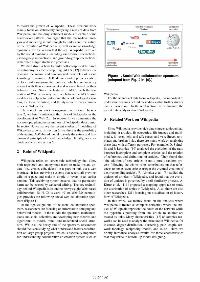
to model the growth of Wikipedia. These previous workmainly focus on statistically analyzing a mass of data fromWikipedia, and building statistical models to explain somemacro-level patterns. We argue that the macro-level anal-ysis and modeling is not enough to understand the natureof the evolution of Wikipedia, as well as social knowledgedynamics, for the reason that the real Wikipedia is drivenby the social dynamics, including user-to-user interactions,use-to-group interactions, and group-to-group interactions,rather than simple stochastic processes.
We then discuss how to build bottom-up models basedon autonomy-oriented computing (AOC) [12] to better un-derstand the nature and fundamental principles of socialknowledge dynamics. AOC defines and deploys a systemof local autonomy-oriented entities, which spontaneouslyinteract with their environment and operate based on theirbehavior rules. Since the features of AOC match the for-mation of Wikipedia very well, we believe the AOC-basedmodels can help us to understand the whole Wikipedia sys-tem, the topic evolution, and the dynamic of user commu-nities on Wikipedia.
The rest of this work is organized as follows. In sec-tion 2, we briefly introduce the roles of Wikipedia in thedevelopment of Web 2.0. In section 3, we summarize themicroscopic phenomena analysis of Wikipedia data dump.In section 4, we survey the recent studies of modeling ofWikipedia growth. In section 5, we discuss the possibilityof designing AOC-based model to study the nature and fun-damental principle of social knowledge. Finally, we con-clude our work in section 6.
2 Roles of Wikipedia
Wikipedia relies on server-side technology that allowboth registered and anonymous users to make instant up-date (i.e., create, edit, delete) to a page or link via a webinterface. It has archiving systems that record all previousedits of a page and make it simple to revert to an earlierversion. This archiving system ensures that no permanentharm can be caused by cankered editing. The key technol-ogy behind Wikipedia is its online heavyweight Web-basedcollaboration. Ed H. Chi’s work [9] on Web 2.0 technolo-gies provides the following social web collaboration spec-trum (Figure 1).
At the lightweight end of the social collaboration spec-trum, researchers are focusing on information-foraging andbehavioral models. In the middle the spectrum, mathemati-cians and social scientists are developing new theories andalgorithms to model, mine, and understand social struc-ture. While at the heavy end of the spectrum, researchersshould focus on studying what hinders and fosters coordina-tion on large group projects, which is especially importantfor understanding collaborative co-creation system such as
Figure 1. Social Web collaboration spectrum.(adopted from Fig. 2 in [9].)
Wikipedia.For the richness of data from Wikipedia, it is important to
understand features behind these data so that further studiescan be carried out. In the next section, we summarize therecent data analysis about Wikipedia.
3 Related Work on Wikipedia
Since Wikipedia provides rich data sources to download,including i) articles, ii) categories, iii) images and multi-media, iv) user, help, and talk pages, and v) redirects, tem-plates and broken links, there are many work on analyzingthese data with different purposes. For example, D. Spinel-lis and P. Louridas [19] analyzed the evolution of the ratiobetween incomplete and complete articles, and the relationof references and definitions of articles. They found that“the addition of new articles in not a purely random pro-cess following the whims of its contributors but that refer-ences to nonexistent articles trigger the eventual creation ofa corresponding article”. R. Almeida et al. [3] studied theupdates of articles in Wikipedia, and found that the evolu-tion of updates is governed by a self-similarity process. A.Kittur et al. [11] proposed a mapping approach to studythe distribution of topics in Wikipedia. Also, there are alsoother researches [21] focusing on visualization of historyflow of Wikipedia.
In this work, we mainly focus on the analysis whereWikipedia is treated as complex networks, where the arti-cles of Wikipedia represent the nodes of the network whilethe hyperlinks pointing from one article to another aretreated as links. Many characteristics [17] of complex net-works can be used to analyze the structure of Wikipedia, forinstance, degree distribution, clustering, path length, net-work topology, reciprocity, motifs, and so on. Here, webriefly introduce analysis results for three characteristicsthat may relate to bottom-up model designing.
55 of 162
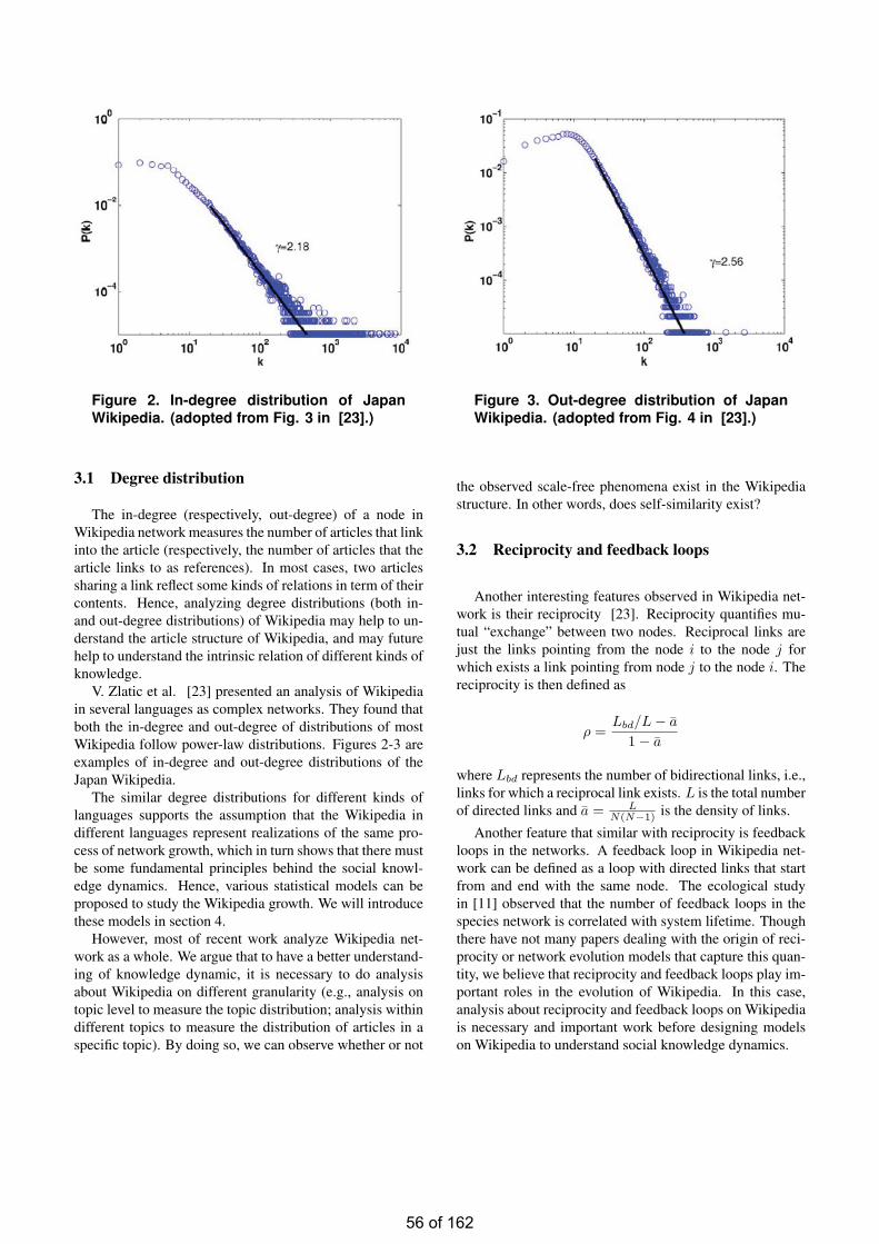
Figure 2. In-degree distribution of JapanWikipedia. (adopted from Fig. 3 in [23].)
3.1 Degree distribution
The in-degree (respectively, out-degree) of a node inWikipedia network measures the number of articles that linkinto the article (respectively, the number of articles that thearticle links to as references). In most cases, two articlessharing a link reflect some kinds of relations in term of theircontents. Hence, analyzing degree distributions (both in-and out-degree distributions) of Wikipedia may help to un-derstand the article structure of Wikipedia, and may futurehelp to understand the intrinsic relation of different kinds ofknowledge.
V. Zlatic et al. [23] presented an analysis of Wikipediain several languages as complex networks. They found thatboth the in-degree and out-degree of distributions of mostWikipedia follow power-law distributions. Figures 2-3 areexamples of in-degree and out-degree distributions of theJapan Wikipedia.
The similar degree distributions for different kinds oflanguages supports the assumption that the Wikipedia indifferent languages represent realizations of the same pro-cess of network growth, which in turn shows that there mustbe some fundamental principles behind the social knowl-edge dynamics. Hence, various statistical models can beproposed to study the Wikipedia growth. We will introducethese models in section 4.
However, most of recent work analyze Wikipedia net-work as a whole. We argue that to have a better understand-ing of knowledge dynamic, it is necessary to do analysisabout Wikipedia on different granularity (e.g., analysis ontopic level to measure the topic distribution; analysis withindifferent topics to measure the distribution of articles in aspecific topic). By doing so, we can observe whether or not
Figure 3. Out-degree distribution of JapanWikipedia. (adopted from Fig. 4 in [23].)
the observed scale-free phenomena exist in the Wikipediastructure. In other words, does self-similarity exist?
3.2 Reciprocity and feedback loops
Another interesting features observed in Wikipedia net-work is their reciprocity [23]. Reciprocity quantifies mu-tual “exchange” between two nodes. Reciprocal links arejust the links pointing from the node i to the node j forwhich exists a link pointing from node j to the node i. Thereciprocity is then defined as
ρ =Lbd/L− a
1− a
where Lbd represents the number of bidirectional links, i.e.,links for which a reciprocal link exists. L is the total numberof directed links and a = L
N(N−1) is the density of links.
Another feature that similar with reciprocity is feedbackloops in the networks. A feedback loop in Wikipedia net-work can be defined as a loop with directed links that startfrom and end with the same node. The ecological studyin [11] observed that the number of feedback loops in thespecies network is correlated with system lifetime. Thoughthere have not many papers dealing with the origin of reci-procity or network evolution models that capture this quan-tity, we believe that reciprocity and feedback loops play im-portant roles in the evolution of Wikipedia. In this case,analysis about reciprocity and feedback loops on Wikipediais necessary and important work before designing modelson Wikipedia to understand social knowledge dynamics.
56 of 162
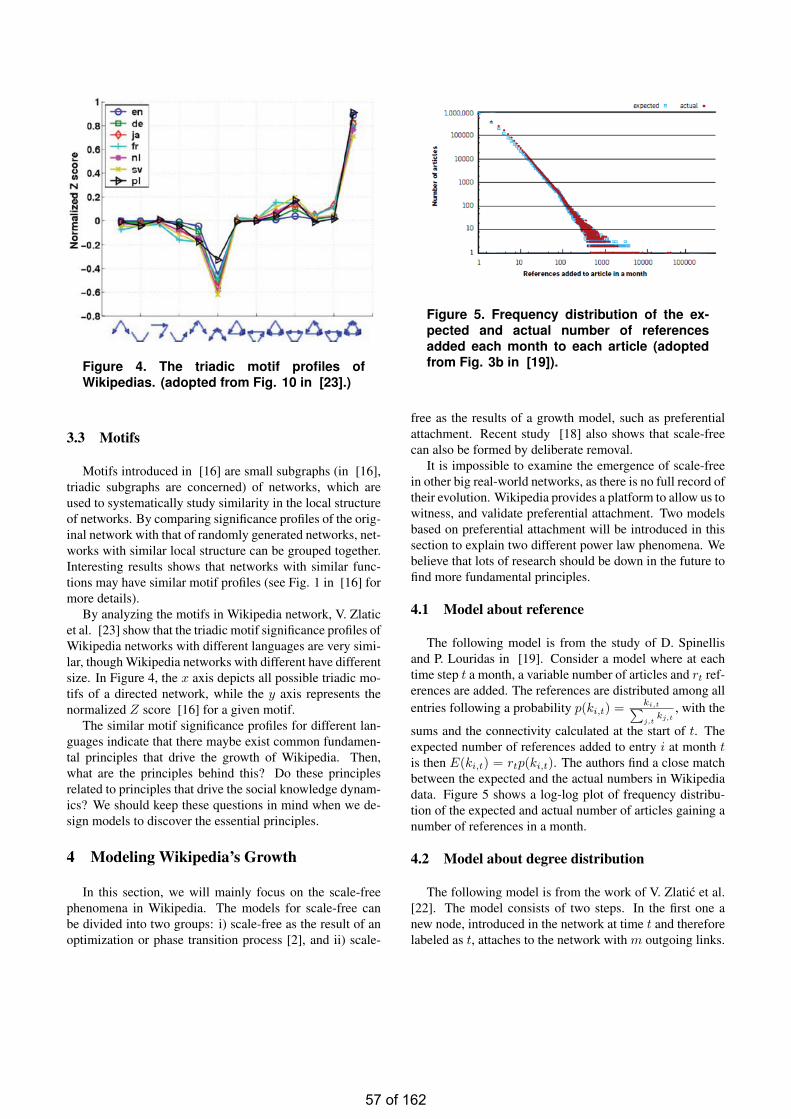
Figure 4. The triadic motif profiles ofWikipedias. (adopted from Fig. 10 in [23].)
3.3 Motifs
Motifs introduced in [16] are small subgraphs (in [16],triadic subgraphs are concerned) of networks, which areused to systematically study similarity in the local structureof networks. By comparing significance profiles of the orig-inal network with that of randomly generated networks, net-works with similar local structure can be grouped together.Interesting results shows that networks with similar func-tions may have similar motif profiles (see Fig. 1 in [16] formore details).
By analyzing the motifs in Wikipedia network, V. Zlaticet al. [23] show that the triadic motif significance profiles ofWikipedia networks with different languages are very simi-lar, though Wikipedia networks with different have differentsize. In Figure 4, the x axis depicts all possible triadic mo-tifs of a directed network, while the y axis represents thenormalized Z score [16] for a given motif.
The similar motif significance profiles for different lan-guages indicate that there maybe exist common fundamen-tal principles that drive the growth of Wikipedia. Then,what are the principles behind this? Do these principlesrelated to principles that drive the social knowledge dynam-ics? We should keep these questions in mind when we de-sign models to discover the essential principles.
4 Modeling Wikipedia’s Growth
In this section, we will mainly focus on the scale-freephenomena in Wikipedia. The models for scale-free canbe divided into two groups: i) scale-free as the result of anoptimization or phase transition process [2], and ii) scale-
Figure 5. Frequency distribution of the ex-pected and actual number of referencesadded each month to each article (adoptedfrom Fig. 3b in [19]).
free as the results of a growth model, such as preferentialattachment. Recent study [18] also shows that scale-freecan also be formed by deliberate removal.
It is impossible to examine the emergence of scale-freein other big real-world networks, as there is no full record oftheir evolution. Wikipedia provides a platform to allow us towitness, and validate preferential attachment. Two modelsbased on preferential attachment will be introduced in thissection to explain two different power law phenomena. Webelieve that lots of research should be down in the future tofind more fundamental principles.
4.1 Model about reference
The following model is from the study of D. Spinellisand P. Louridas in [19]. Consider a model where at eachtime step t a month, a variable number of articles and rt ref-erences are added. The references are distributed among allentries following a probability p(ki,t) = ki,t∑
j,tkj,t
, with the
sums and the connectivity calculated at the start of t. Theexpected number of references added to entry i at month tis then E(ki,t) = rtp(ki,t). The authors find a close matchbetween the expected and the actual numbers in Wikipediadata. Figure 5 shows a log-log plot of frequency distribu-tion of the expected and actual number of articles gaining anumber of references in a month.
4.2 Model about degree distribution
The following model is from the work of V. Zlatic et al.[22]. The model consists of two steps. In the first one anew node, introduced in the network at time t and thereforelabeled as t, attaches to the network with m outgoing links.
57 of 162
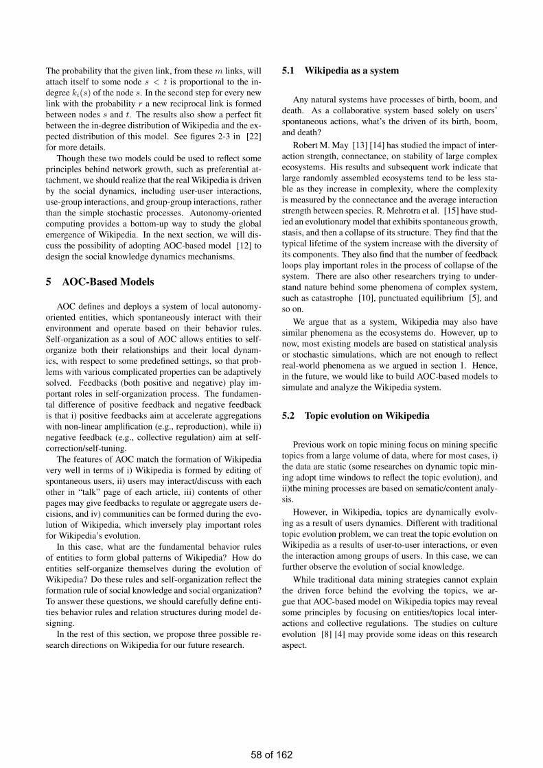
The probability that the given link, from these m links, willattach itself to some node s < t is proportional to the in-degree ki(s) of the node s. In the second step for every newlink with the probability r a new reciprocal link is formedbetween nodes s and t. The results also show a perfect fitbetween the in-degree distribution of Wikipedia and the ex-pected distribution of this model. See figures 2-3 in [22]for more details.
Though these two models could be used to reflect someprinciples behind network growth, such as preferential at-tachment, we should realize that the real Wikipedia is drivenby the social dynamics, including user-user interactions,use-group interactions, and group-group interactions, ratherthan the simple stochastic processes. Autonomy-orientedcomputing provides a bottom-up way to study the globalemergence of Wikipedia. In the next section, we will dis-cuss the possibility of adopting AOC-based model [12] todesign the social knowledge dynamics mechanisms.
5 AOC-Based Models
AOC defines and deploys a system of local autonomy-oriented entities, which spontaneously interact with theirenvironment and operate based on their behavior rules.Self-organization as a soul of AOC allows entities to self-organize both their relationships and their local dynam-ics, with respect to some predefined settings, so that prob-lems with various complicated properties can be adaptivelysolved. Feedbacks (both positive and negative) play im-portant roles in self-organization process. The fundamen-tal difference of positive feedback and negative feedbackis that i) positive feedbacks aim at accelerate aggregationswith non-linear amplification (e.g., reproduction), while ii)negative feedback (e.g., collective regulation) aim at self-correction/self-tuning.
The features of AOC match the formation of Wikipediavery well in terms of i) Wikipedia is formed by editing ofspontaneous users, ii) users may interact/discuss with eachother in “talk” page of each article, iii) contents of otherpages may give feedbacks to regulate or aggregate users de-cisions, and iv) communities can be formed during the evo-lution of Wikipedia, which inversely play important rolesfor Wikipedia’s evolution.
In this case, what are the fundamental behavior rulesof entities to form global patterns of Wikipedia? How doentities self-organize themselves during the evolution ofWikipedia? Do these rules and self-organization reflect theformation rule of social knowledge and social organization?To answer these questions, we should carefully define enti-ties behavior rules and relation structures during model de-signing.
In the rest of this section, we propose three possible re-search directions on Wikipedia for our future research.
5.1 Wikipedia as a system
Any natural systems have processes of birth, boom, anddeath. As a collaborative system based solely on users’spontaneous actions, what’s the driven of its birth, boom,and death?
Robert M. May [13] [14] has studied the impact of inter-action strength, connectance, on stability of large complexecosystems. His results and subsequent work indicate thatlarge randomly assembled ecosystems tend to be less sta-ble as they increase in complexity, where the complexityis measured by the connectance and the average interactionstrength between species. R. Mehrotra et al. [15] have stud-ied an evolutionary model that exhibits spontaneous growth,stasis, and then a collapse of its structure. They find that thetypical lifetime of the system increase with the diversity ofits components. They also find that the number of feedbackloops play important roles in the process of collapse of thesystem. There are also other researchers trying to under-stand nature behind some phenomena of complex system,such as catastrophe [10], punctuated equilibrium [5], andso on.
We argue that as a system, Wikipedia may also havesimilar phenomena as the ecosystems do. However, up tonow, most existing models are based on statistical analysisor stochastic simulations, which are not enough to reflectreal-world phenomena as we argued in section 1. Hence,in the future, we would like to build AOC-based models tosimulate and analyze the Wikipedia system.
5.2 Topic evolution on Wikipedia
Previous work on topic mining focus on mining specifictopics from a large volume of data, where for most cases, i)the data are static (some researches on dynamic topic min-ing adopt time windows to reflect the topic evolution), andii)the mining processes are based on sematic/content analy-sis.
However, in Wikipedia, topics are dynamically evolv-ing as a result of users dynamics. Different with traditionaltopic evolution problem, we can treat the topic evolution onWikipedia as a results of user-to-user interactions, or eventhe interaction among groups of users. In this case, we canfurther observe the evolution of social knowledge.
While traditional data mining strategies cannot explainthe driven force behind the evolving the topics, we ar-gue that AOC-based model on Wikipedia topics may revealsome principles by focusing on entities/topics local inter-actions and collective regulations. The studies on cultureevolution [8] [4] may provide some ideas on this researchaspect.
58 of 162
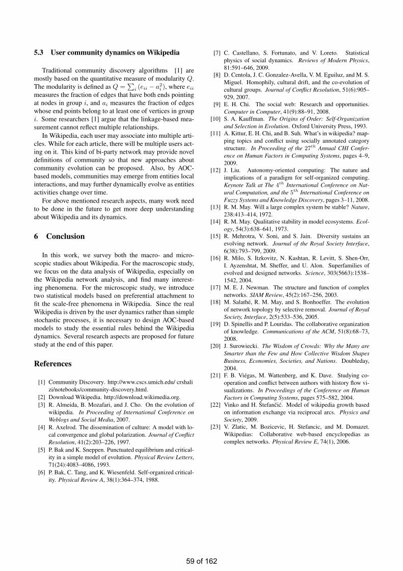
5.3 User community dynamics on Wikipedia
Traditional community discovery algorithms [1] aremostly based on the quantitative measure of modularity Q.The modularity is defined as Q =
∑i (eii − a2
i ), where eii
measures the fraction of edges that have both ends pointingat nodes in group i, and ai measures the fraction of edgeswhose end points belong to at least one of vertices in groupi. Some researchers [1] argue that the linkage-based mea-surement cannot reflect multiple relationships.
In Wikipedia, each user may associate into multiple arti-cles. While for each article, there will be multiple users act-ing on it. This kind of bi-party network may provide noveldefinitions of community so that new approaches aboutcommunity evolution can be proposed. Also, by AOC-based models, communities may emerge from entities localinteractions, and may further dynamically evolve as entitiesactivities change over time.
For above mentioned research aspects, many work needto be done in the future to get more deep understandingabout Wikipedia and its dynamics.
6 Conclusion
In this work, we survey both the macro- and micro-scopic studies about Wikipedia. For the macroscopic study,we focus on the data analysis of Wikipedia, especially onthe Wikipedia network analysis, and find many interest-ing phenomena. For the microscopic study, we introducetwo statistical models based on preferential attachment tofit the scale-free phenomena in Wikipedia. Since the realWikipedia is driven by the user dynamics rather than simplestochastic processes, it is necessary to design AOC-basedmodels to study the essential rules behind the Wikipediadynamics. Several research aspects are proposed for futurestudy at the end of this paper.
References
[1] Community Discovery. http://www.cscs.umich.edu/ crshalizi/notebooks/community-discovery.html.
[2] Download Wikipedia. http://download.wikimedia.org.[3] R. Almeida, B. Mozafari, and J. Cho. On the evolution of
wikipedia. In Proceeding of International Conference onWeblogs and Social Media, 2007.
[4] R. Axelrod. The dissemination of culture: A model with lo-cal convergence and global polarization. Journal of ConflictResolution, 41(2):203–226, 1997.
[5] P. Bak and K. Sneppen. Punctuated equilibrium and critical-ity in a simple model of evolution. Physical Review Letters,71(24):4083–4086, 1993.
[6] P. Bak, C. Tang, and K. Wiesenfeld. Self-organized critical-ity. Physical Review A, 38(1):364–374, 1988.
[7] C. Castellano, S. Fortunato, and V. Loreto. Statisticalphysics of social dynamics. Reviews of Modern Physics,81:591–646, 2009.
[8] D. Centola, J. C. Gonzalez-Avella, V. M. Eguiluz, and M. S.Miguel. Homophily, cultural drift, and the co-evolution ofcultural groups. Journal of Conflict Resolution, 51(6):905–929, 2007.
[9] E. H. Chi. The social web: Research and opportunities.Computer in Computer, 41(9):88–91, 2008.
[10] S. A. Kauffman. The Origins of Order: Self-Organizationand Selection in Evolution. Oxford University Press, 1993.
[11] A. Kittur, E. H. Chi, and B. Suh. What’s in wikipedia? map-ping topics and conflict using socially annotated categorystructure. In Proceeding of the 27th Annual CHI Confer-ence on Human Factors in Computing Systems, pages 4–9,2009.
[12] J. Liu. Autonomy-oriented computing: The nature andimplications of a paradigm for self-organized computing.Keynote Talk at The 4th International Conference on Nat-ural Computation, and the 5th International Conference onFuzzy Systems and Knowledge Discovery, pages 3–11, 2008.
[13] R. M. May. Will a large complex system be stable? Nature,238:413–414, 1972.
[14] R. M. May. Qualitative stability in model ecosystems. Ecol-ogy, 54(3):638–641, 1973.
[15] R. Mehrotra, V. Soni, and S. Jain. Diversity sustains anevolving network. Journal of the Royal Society Interface,6(38):793–799, 2009.
[16] R. Milo, S. Itzkovitz, N. Kashtan, R. Levitt, S. Shen-Orr,I. Ayzenshtat, M. Sheffer, and U. Alon. Superfamilies ofevolved and designed networks. Science, 303(5663):1538–1542, 2004.
[17] M. E. J. Newman. The structure and function of complexnetworks. SIAM Review, 45(2):167–256, 2003.
[18] M. Salathe, R. M. May, and S. Bonhoeffer. The evolutionof network topology by selective removal. Journal of RoyalSociety, Interface, 2(5):533–536, 2005.
[19] D. Spinellis and P. Louridas. The collaborative organizationof knowledge. Communications of the ACM, 51(8):68–73,2008.
[20] J. Surowiecki. The Wisdom of Crowds: Why the Many areSmarter than the Few and How Collective Wisdom ShapesBusiness, Economies, Societies, and Nations. Doubleday,2004.
[21] F. B. Viegas, M. Wattenberg, and K. Dave. Studying co-operation and conflict between authors with history flow vi-sualizations. In Proceedings of the Conference on HumanFactors in Computing Systems, pages 575–582, 2004.
[22] Vinko and H. Stefancic. Model of wikipedia growth basedon information exchange via reciprocal arcs. Physics andSociety, 2009.
[23] V. Zlatic, M. Bozicevic, H. Stefancic, and M. Domazet.Wikipedias: Collaborative web-based encyclopedias ascomplex networks. Physical Review E, 74(1), 2006.
59 of 162
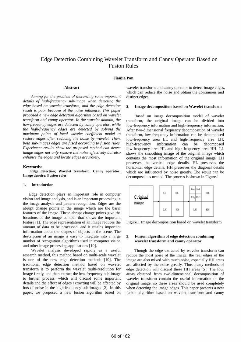
Edge Detection Combining Wavelet Transform and Canny Operator Based on Fusion Rules
Jianjia Pan
Abstract Aiming for the problem of discarding some important
details of high-frequency sub-image when detecting the edge based on wavelet transform, and the edge detection result is poor because of the noise influence. This paper proposed a new edge detection algorithm based on wavelet transform and canny operator. In the wavelet domain, the low-frequency edges are detected by canny operator, while the high-frequency edges are detected by solving the maximum points of local wavelet coefficient model to restore edges after reducing the noise by wavelet. Then, both sub-images edges are fused according to fusion rules. Experiment results show the proposed method can detect image edges not only remove the noise effectively but also enhance the edges and locate edges accurately.
Keywords: Edge detection; Wavelet transform; Canny operator;
Image denoise; Fusion rules;
1. Introduction
Edge detection plays an important role in computer vision and image analysis, and is an important processing in the image analysis and pattern recognition. Edges are the abrupt change points in the image which are the basic features of the image. These abrupt change points give the locations of the image contour that shows the important feature [1]. The edge representation of an image reduces the amount of data to be processed, and it retains important information about the shapes of objects in the scene. The description of an image is easy to integrate into a large number of recognition algorithms used in computer vision and other image processing applications [10].
Wavelet analysis developed rapidly as a useful research method, this method based on multi-scale wavelet is one of the new edge detection methods [10]. The traditional edge detection method based on wavelet transform is to perform the wavelet multi-resolution for image firstly, and then extract the low-frequency sub-image to further process, which will discard some important details and the effect of edges extracting will be affected by lots of noise in the high-frequency sub-images [2]. In this paper, we proposed a new fusion algorithm based on
wavelet transform and canny operator to detect image edges, which can reduce the noise and obtain the continuous and distinct edges.
2. Image decomposition based on Wavelet transform
Based on image decomposition model of wavelet transform, the original image can be divided into low-frequency information and high-frequency information. After two-dimensional frequency decomposition of wavelet transform, low-frequency information can be decomposed low-frequency area LL and high-frequency area LH, high-frequency information can be decomposed low-frequency area HL and high-frequency area HH. LL shows the smoothing image of the original image which contains the most information of the original image. LH preserves the vertical edge details. HL preserves the horizontal edge details. HH preserves the diagonal details which are influenced by noise greatly. The result can be decomposed as needed. The process is shown in Figure.1
Figure.1 Image decomposition based on wavelet transform
3. Fusion algorithm of edge detection combining wavelet transform and canny operator
Though the edge extracted by wavelet transform can reduce the most noise of the image, the real edges of the image are also mixed with much noise, especially HH areas are affected by the noise greatly. Thus many methods of edge detection will discard these HH areas [5]. The four areas obtained from two-dimensional decomposition of wavelet transform contain the useful information of the original image, so these areas should be used completely when detecting the image edges. This paper presents a new fusion algorithm based on wavelet transform and canny
60 of 162
operator to detect image edges, which can reduce the noise and obtain the continuous and distinct edges.
3.1. Low-frequency sub-image edge detecting based on canny operator
The LL area shows the smoothing image of the original image which contains the most information of the original image. Canny operator is a edge detecting operator based on an optimal algorithm, which has the most stringent criterions of edge detecting. The good effect will be obtained adopted canny operator when processing the image contaminated by additive white Gaussian noise. So canny operator [3,9] are adopted to detect the edges of the low-frequency sub-image. The realization process is as follows.
(1) Smoothing image. Gaussian function is used to smooth the image; the method use 5×5 Gaussian template and the original image to weight neighborhood [4]. Denote any point (x, y) of the image as the center when processing and extracting 5×5 neighborhood, the weighting neighborhood can be indicated as follows:
∑∑−= −=
++×++×
=2
2
2
2)2,2(),(
551),(*
i jjiMjyixIyxI
x=1,2,…,m; y=1,2,…,n (1) Where the pixel value of the low-frequency
sub-image is I(x, y), M is Gaussian template, the pixel value of the smoothed image is I*(x, y).
(2) Computing gradient direction and amplitude. Computing gradient direction and amplitude of smoothed image I*(x,y) adopting first order partial finite difference of 2×2 neighborhood.
),(),(),( 22 yxgyxgyxM yx += (2)
)],(),,(arctan[),( yxgyxgyxQ yx= (3)
−−
=2/12/1
xf
2/12/1
[ 2/1=yf ]2/1 (4)
Where xg and yg are the results of the original
image filtered along rows and lines. (3) Gradient image with non-maximum suppression. If
the gradient amplitude of the pixel is no less than the gradient amplitude between two adjacent pixels in the gradient direction, the point can be judged as the edge point possibly.
(4) Dual threshold method of detecting and connecting the edges. Select two thresholds, Hth and Lth. Hth denotes the high threshold and Lth denotes the low threshold to process the gradient image. Where Hth=Lth*h,
h=1.5 ~ 2. There will be two detecting results, one resulted from high threshold detecting, and the other resulted from low threshold detecting. Connecting the edge contour from the former and finding weak edge points from the latter to recoup the former edge gaps when connecting to the endpoint.
Through adopting canny operator to detect the low-frequency sub-image can obtain clear edge image which will miss some real edges and exist some sham edges. Thus the edges of the high-frequency sub-images should be fused.
3.2. High-frequency sub-image edges detecting based on wavelet transform
After two-dimensional frequency decomposition of wavelet transform, there will be three high-frequency sub-images LH、HL and HH where contain the noise and the details of the image. When extracting the edges from the high-frequency sub-images, the result will be affected because of much noise. Thus, this paper presents that the noise should be reduced before extracting the edges from the high-frequency sub-images. The algorithm can not only keep the important details of the high-frequency sub-images but also restrain the noise.
3.3. Denoising algorithm of the high-frequency sub-images based on wavelet transform
Among the wavelet coefficients of the high-frequency sub-image, the wavelet coefficients which have smaller amplitude present the most noise part, and the wavelet coefficients which have larger amplitude present the details of the image [2]. Based on the characteristic of the high-frequency sub-images, we proposed a method based on wavelet transform to reduce the noise in the high-frequency sub-images. The wavelet coefficients are multiplied by a denoising factor which is relative to their own coefficients’ value. This denoising factor is less than 1 and will decrease if the absolute value of the wavelet coefficients increases. This algorithm considers energy distribution property of the wavelet decomposition of the image globally, and obtains a better denoising result, which support the foundation for extracting the edge of the high-frequency sub-images. The process function is as follows.
×=
kyxw
yxwyxF
),(0
),(),(
else
averyxw
yxw
≤
≥
),(
3),( σ
(5)
61 of 162
Where ),( yxw denotes the high-frequency coefficient, ),( yxF denotes the high-frequency coefficient gained after denoising; σ 、 aver indicate the variance and the mean value of the high-frequency coefficient in different wavelet decomposition levels. On the basis of the statistic property of the wavelet coefficients, k is a function which is relative to the coefficient:
1),( −= +− byxawek (6) When ),( yxw is greater than σ3 , ),( yxw can
be considered as consisting of the signal completely. So k=1, it will be:
11)3( =−+− bae σ (7) When ),( yxw is smaller than aver , ),( yxw will
approaches 0, it will be: 01 =−+×− baverae (8)
It can be obtained from the two upper equations:
avera
−−
=σ3
2ln averab ×= (9)
Denoising factor k will be obtained when a and b substituted into the equation (6).
132ln),(
32ln
−=×
−−
+×−
− averaver
yxwaverek σσ (10)
Denoising algorithm will be computed when k substituted into equation (5). This algorithm is aiming for the wavelet coefficients multiplied by different denoising factors from different wavelet decomposition levels and different high-frequency sub-image, which can reduce the image noise and keep useful details.
3.4. Edge detecting of denoising high-frequency sub-image based on wavelet transform
After eliminating noise of the high-frequency sub-image, the edges of the high-frequency sub-image can be detected using wavelet modulus maxima algorithm [7]. The wavelet modulus maxima algorithm is obtained from an irregular sampling based on multiscale wavelet transform which can describe mechanism singularity of the signal. The wavelet modulus maxima algorithm can describe multiscale edges of the target in the image which has translation, scale and rotation-invariant performance. Thus the wavelet modulus maxima algorithm is an effective algorithm to detect the edges. The realization process is as follows:
),( yxθ denotes Gaussian smoothing function, supposing:
=
sy
sx
syxs ,1),( 2 θθ (11)
Calculating the partial derivative of the smoothing function ),( yxθ , the wavelet function will be:
=
∂∂
=sy
sx
sxyxyxs ,1),(),( 1
21 φθφ (12)
=
∂∂
=sy
sx
syyxyxs ,1),(),( 2
22 φθφ (13)
Convolution of ),( yxf will obtain two components of two dimensional wavelet transform in scale s:
( )yxfyxfW ss ,),( 11 φ∗= (14)
),(),( 22 yxfyxfW ss φ∗= (15) The gradient module in scale s is:
2221 ),(),(),( yxfWyxfWyxfM sss += (16)
The angel in scale s is:
=
),(),(
arctan),( 1
2
yxfWyxfW
yxfAs
ss (17)
Detecting the edges of the high-frequency sub-images LH、HL and HH using wavelet modulus maxima algorithm. Computing the local modulus maxima of three sub-images after wavelet transform using equation (16) and (17), then their edge images LHG , HLG and HHG will be obtained. Those high-frequency sub-images contain the details of the original image, so we proposed that the wavelet coefficients of three edge images should be computed with weighting fusion rules. Computing formula [13] is described as follows:
),(*),(*),(*),( jiDrjiDrjiDrjiD HHHHHLHLLHLHH ++= (18)
Where ),(),(),( jiDjiDjiD HHHLLH 、、 indicate the wavelet coefficients corresponding to the edge images LHG 、 HLG and HHG . ),( jiDH denotes the
wavelet coefficient after fusion. LHr 、 HLr and HHr indicate the corresponding weights, the sum of the three weights is 1.
After these processes, we can get the edges of the low-frequency sub-image and the weighting edges of the high-frequency sub-images. The final edge images are obtained through wavelet composition from the fusion edge sub-images [13].
62 of 162
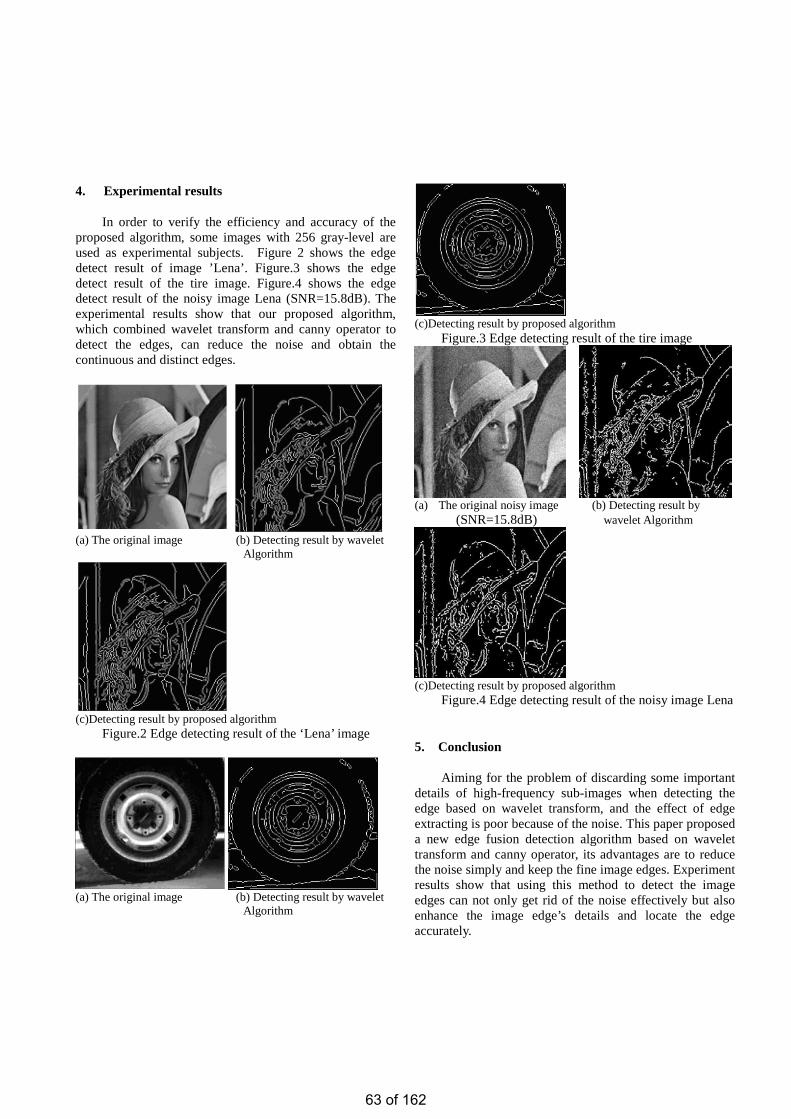
4. Experimental results
In order to verify the efficiency and accuracy of the proposed algorithm, some images with 256 gray-level are used as experimental subjects. Figure 2 shows the edge detect result of image ’Lena’. Figure.3 shows the edge detect result of the tire image. Figure.4 shows the edge detect result of the noisy image Lena (SNR=15.8dB). The experimental results show that our proposed algorithm, which combined wavelet transform and canny operator to detect the edges, can reduce the noise and obtain the continuous and distinct edges.
(a) The original image (b) Detecting result by wavelet Algorithm
(c)Detecting result by proposed algorithm
Figure.2 Edge detecting result of the ‘Lena’ image
(a) The original image (b) Detecting result by wavelet Algorithm
(c)Detecting result by proposed algorithm
Figure.3 Edge detecting result of the tire image
(a) The original noisy image (b) Detecting result by
(SNR=15.8dB) wavelet Algorithm
(c)Detecting result by proposed algorithm
Figure.4 Edge detecting result of the noisy image Lena
5. Conclusion
Aiming for the problem of discarding some important details of high-frequency sub-images when detecting the edge based on wavelet transform, and the effect of edge extracting is poor because of the noise. This paper proposed a new edge fusion detection algorithm based on wavelet transform and canny operator, its advantages are to reduce the noise simply and keep the fine image edges. Experiment results show that using this method to detect the image edges can not only get rid of the noise effectively but also enhance the image edge’s details and locate the edge accurately.
63 of 162
References:
[1] MALLAT S, HW ANG W L. “Singularity Detection and Processing with Wavelets”. IEEE Trans 2002, IT-38(2):617-643.
[2] MALLAT S. “Multi-frequency Channel Decomposition of Images and Wavelet Models”. IEEE Trans 1998, AS-SP-37(12) :2091-2110.
[3] Yanlong-Chen, Chenghu-Zhu. “Improved Edge Detection Algorithm Based on Canny Operator”. Computer Applications and Software. 2008, vol.25(8):51-53.
[4] Wenyao-Liu. “Photoelectric Image Processing”. Publishing house of electronics industry, 2002, vol.11:106-107
[5] Musheng-Chen. “A New Method of Image Denoising Based on Wavelet Transform”. Optical Technique, 2006, vol.32(5):796-798.
[6] Zhang L, Bao P. “Edge Detection by Scale Multiplication in Wavelet Domain”. Pattern Recognition Letters, 2002, vol. 23(14):1771-1784
[7] Zhu-lihua, Ji-xiaoping. “The application of wavelet modulus maxima algorithm in the image retrieval”. SCI-tech information development and economy. 2007, vol.17(3): 169-170
[8] Wen-Ge, Liqun-Gao. “Fusion Based Algorithm of Edge Detection Combining Wavelet Transform with Morphology”. Journal of Northeastern University. 2008, vol.29(4):477-479
[9] J.F. Canny, “A computational approach to edge detection,” IEEE Transactions on Pattern Analysis and Machine Intelligence, 1986 ,vol.8, pp.679-698
[10] Mitra Basu, “Gaussian-Based Edge-Detection Methods—A Survey”, IEEE Transactions on Systems, Man, and Cybernetics, Part C, 2002, Vol.32(3), pp. 252-260
[11] A. L. Yuille and T. A. Poggio, “Scaling theorems for zero-crossings,” IEEE Transactions on Pattern Analysis and Machine Intelligence, vol.8, pp.15–25, 1986.
[12] P. Bao and L. Zhang, “Noise Reduction for Magnetic Resonance Image via Adaptive Multiscale Products Thresholding,” IEEE Transactions on Medical Imaging, vol.22, pp. 1089-1099, 2003.
[13] Pajares G . "A wavelet-based image fusion tutorial".Pattern Recognition,2004,vol.37(9):1855—1872.
64 of 162
Modeling and Simulating Human Vaccinating Behaviors
On a Disease Diffusion Network
Shang Xia
Abstract
As human is the host of disease infection, its social interactions and vaccinating behaviors influence the dynamics of disease spreading. Previous disease diffusion models are mainly based on the homogeneous mixing assumption, which assumes that individuals in population are identical to each other in terms of disease infection. This assumption ignores inherent heterogeneities in both human contact patterns and individuals’ possible behavioral choices. By comparison, we design a disease diffusion model, in which a SIV disease model transmits on a social contact network with scale free topology. We assume that each individual in population will make their self-interest decisions, vaccinating or not, according to the perceived payoff of different choice. Under the AOC modeling framework we incorporate human decision making features, e.g. self-interest choice, following neighbors, panic irrationality, etc, into individual’s behavioral sets, and observe how the individual-level decision making behaviors can directly determinate the global-level disease diffusion dynamics and inversely how the disease spreading influence individuals’ vaccinating choices.
1. Introduction
In recent years, several serious epidemic outbreaks show that disease diffusion is no longer confined within a local region but involved every corner of the world. These epidemic outbreaks share some common complex characteristics, such as quick spreading through continents, intense outbreak in a certain population communities, unexpected lower new infection case or even sudden disappearance [1][2]. How to characterize or even predict these complex disease diffusion patterns is critical important and urgent, for we do not know when and where a new epidemic attack will happen.
However, even armed with the most progressive biochemistry theories and brilliant innovations of modern biotechnology, it is still hard to trace the expansion of disease spreading.
Based on the analysis of epidemic spreading datas, these complexities should be blamed to the combination of disease infections and human social contact behaviors. Human long range travels facilitate the disease spreading cross nations or even continents; individuals’ vaccination attitude or self-interest behaviors will greatly influence the potential disease diffusion. Interactions between individuals are both the infection mediums and the information exchange channel. Hence, the problems of epidemic spreading are involved both the macro disease diffusion dynamics and micro human behavioral patterns.
How to understand the relationship between heterogeneities of human social interactions and disease diffusion dynamics is one of the most prominent challenges in epidemic spreading research. The previous analysis of disease diffusion is mainly based on statistical model and differential equations, e.g. homogenous mixing assumption, assuming that individuals in a population have the same probability to contact with each other and thus have the equal chance to be infected by infectious ones [3][4]. These assumptions failed to reveal the complexity in both diffusion dynamics and individual behavioral heterogeneities and thus obscure the veiled correlation between local human individual behaviors and global epidemic spreading dynamics, which we can call it local-global relationship for short.
To analyze the local-global relationship, a
methodology called Autonomy-Oriented Computing (AOC) provides a fundamental framework to investigate the emergent complex patterns in epidemic spreading system. AOC emphasize the modeling of autonomy in the entity of a complex system and designing the self-organization mechanism of them to achieve a global level emergent dynamics. In this study, we will build a multi-agent system model following the modeling framework of AOC. In our model, we present the disease infection system as an autonomy agent system which is located on a social contact network with a scale free topology. For the artificial behavior construction, we specify the individuals’ vaccinating decision making mechanisms and individual interaction rules. Thus, based on the performance measurement, we can investigate the
65 of 162
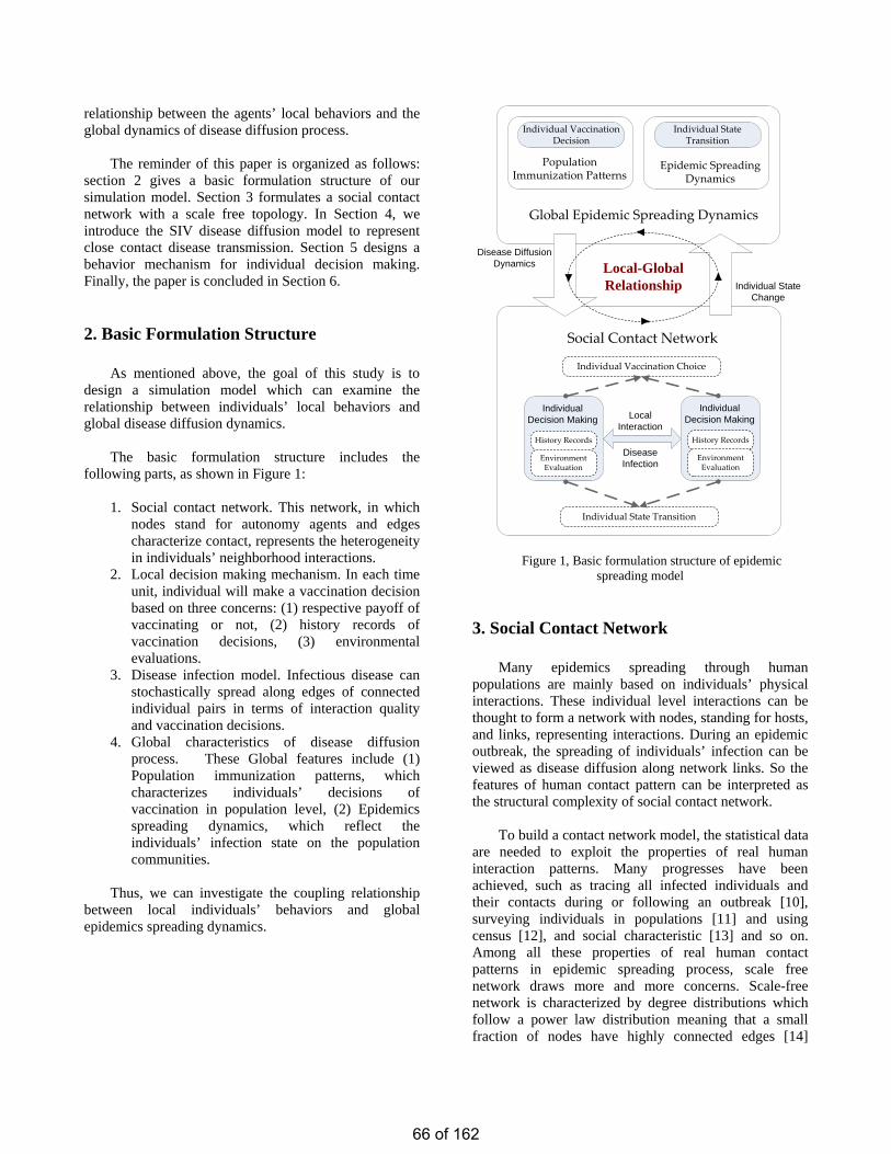
relationship between the agents’ local behaviors and the global dynamics of disease diffusion process.
The reminder of this paper is organized as follows:
section 2 gives a basic formulation structure of our simulation model. Section 3 formulates a social contact network with a scale free topology. In Section 4, we introduce the SIV disease diffusion model to represent close contact disease transmission. Section 5 designs a behavior mechanism for individual decision making. Finally, the paper is concluded in Section 6.
2. Basic Formulation Structure
As mentioned above, the goal of this study is to design a simulation model which can examine the relationship between individuals’ local behaviors and global disease diffusion dynamics.
The basic formulation structure includes the
following parts, as shown in Figure 1: 1. Social contact network. This network, in which
nodes stand for autonomy agents and edges characterize contact, represents the heterogeneity in individuals’ neighborhood interactions.
2. Local decision making mechanism. In each time unit, individual will make a vaccination decision based on three concerns: (1) respective payoff of vaccinating or not, (2) history records of vaccination decisions, (3) environmental evaluations.
3. Disease infection model. Infectious disease can stochastically spread along edges of connected individual pairs in terms of interaction quality and vaccination decisions.
4. Global characteristics of disease diffusion process. These Global features include (1) Population immunization patterns, which characterizes individuals’ decisions of vaccination in population level, (2) Epidemics spreading dynamics, which reflect the individuals’ infection state on the population communities.
Thus, we can investigate the coupling relationship
between local individuals’ behaviors and global epidemics spreading dynamics.
Individual State Change
Global Epidemic Spreading Dynamics
Disease Diffusion Dynamics
Individual Vaccination Decision
Individual State Transition
Population Immunization Patterns
Epidemic Spreading Dynamics
Local-Global Relationship
Local Interaction
Individual Decision Making
History Records
Environment Evaluation
Individual Decision Making
History Records
Environment Evaluation
Social Contact Network
Individual Vaccination Choice
Disease Infection
Individual State Transition
Figure 1, Basic formulation structure of epidemic spreading model
3. Social Contact Network
Many epidemics spreading through human populations are mainly based on individuals’ physical interactions. These individual level interactions can be thought to form a network with nodes, standing for hosts, and links, representing interactions. During an epidemic outbreak, the spreading of individuals’ infection can be viewed as disease diffusion along network links. So the features of human contact pattern can be interpreted as the structural complexity of social contact network.
To build a contact network model, the statistical data are needed to exploit the properties of real human interaction patterns. Many progresses have been achieved, such as tracing all infected individuals and their contacts during or following an outbreak [10], surveying individuals in populations [11] and using census [12], and social characteristic [13] and so on. Among all these properties of real human contact patterns in epidemic spreading process, scale free network draws more and more concerns. Scale-free network is characterized by degree distributions which follow a power law distribution meaning that a small fraction of nodes have highly connected edges [14]
66 of 162
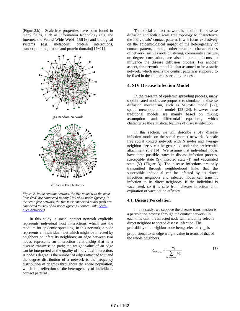
(Figure2.b). Scale-free properties have been found in many fields, such as information technology (e.g. the Internet, the World Wide Web) [15][16] and biological systems (e.g. metabolic, protein interactions, transcription regulation and protein domain)[17~21].
(a) Random Network
(b) Scale Free Network Figure 2, In the random network, the five nodes with the most links (red) are connected to only 27% of all nodes (green). In the scale-free network, the five most connected nodes (red) are connected to 60% of all nodes (green). (Source Link: Scale-Free Networks)
In this study, a social contact network explicitly represents individual host interactions which are the medium for epidemic spreading. In this network, a node represents an individual host which might be infected by neighbors or infect its neighbors; an edge between two nodes represents an interaction relationship that is a disease transmission path; the weight value of an edge can be interpreted as the quality of individual interaction. A node’s degree is the number of edges attached to it and the degree distribution of a network is the frequency distribution of degrees throughout the entire population, which is a reflection of the heterogeneity of individuals contact patterns.
This social contact network is medium for disease diffusion and with a scale free topology to characterize the individuals’ contact pattern. It will focus exclusively on the epidemiological impact of the heterogeneity of contact pattern, although other structural characteristics of network, such as node clustering, community structure, or degree correlation, are also important factors to influence the disease diffusion process. For another aspect, the network model is also assumed to be a static network, which means the contact pattern is supposed to be fixed in the epidemic spreading process.
4. SIV Disease Infection Model
In the research of epidemic spreading process, many sophisticated models are proposed to simulate the disease diffusion mechanism, such as SIS/SIR model [22], spatial metapopulation models [23][24]. However these traditional models are mainly based on mixing assumption and differential equations, which characterize the statistical features of disease infection.
In this section, we will describe a SIV disease infection model on the social contact network. A scale free social contact network with N nodes and average neighbor size v can be generated under the preferential attachment rule [14]. We assume that individual nodes have three possible states in disease infection process, susceptible state (S), infected state (I) and vaccinated state (V) (Figure 3). The disease infections are only transmitted through neighborhood links that the susceptible individual can be infected by its direct infectious neighbors and infected nodes can transmit infection to its direct neighbors. If the individual is vaccinated, so it is safe from disease infection until expiration of vaccination efficacy. 4.1. Disease Percolation
In this study, we suppose the disease transmission is a percolation process through the contact network. In each time unit, the infected node will randomly select a direct neighbor to spread disease infection. The probability of a neighbor node being selected is proportional to its edge weight value in terms of that of the whole neighbors.
TransP
( , )ij
Trans i jik
k neighbor
wP
w∈
=∑
(1)
67 of 162
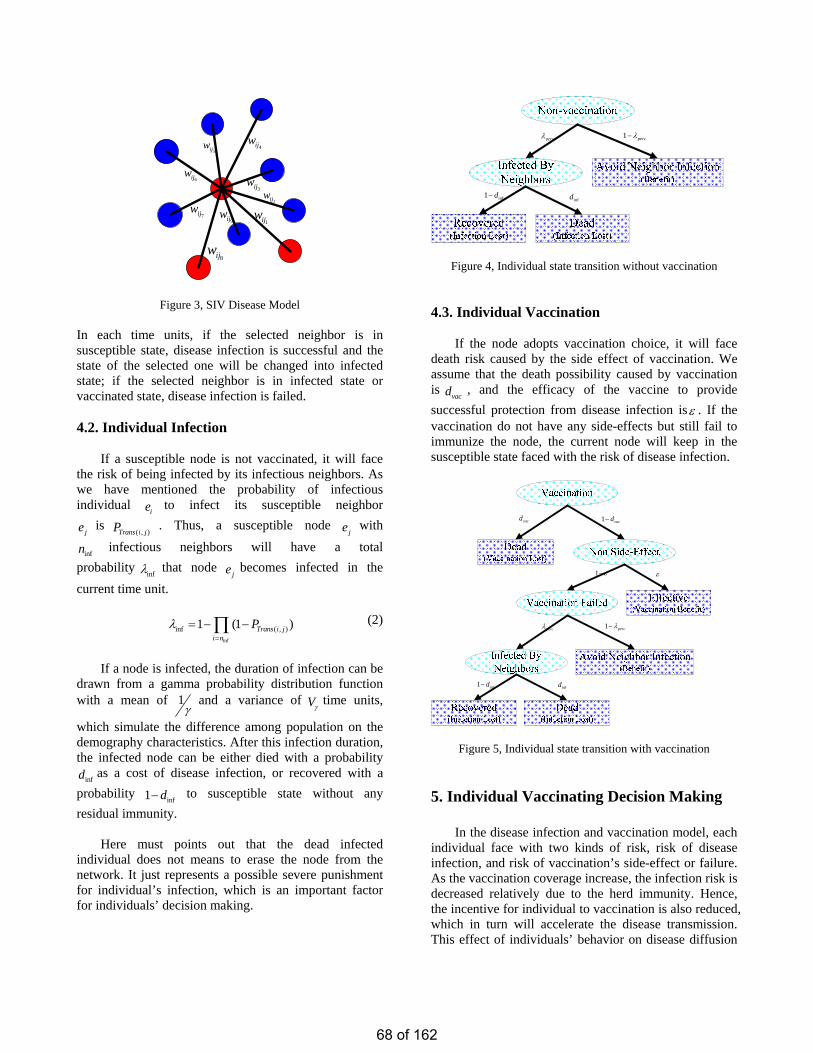
1ijw
4ijw
9ijw
3ijw2ijw
7ijw
8ijw
6ijw
5ijw
Figure 3, SIV Disease Model In each time units, if the selected neighbor is in susceptible state, disease infection is successful and the state of the selected one will be changed into infected state; if the selected neighbor is in infected state or vaccinated state, disease infection is failed. 4.2. Individual Infection
If a susceptible node is not vaccinated, it will face the risk of being infected by its infectious neighbors. As we have mentioned the probability of infectious individual to infect its susceptible neighbor
is . Thus, a susceptible node with infectious neighbors will have a total
probability
ie
( , )i j
inf
je
infnTransP je
λ that node becomes infected in the current time unit.
je
inf
inf ( , )1 (1 Trans i ji n
Pλ=
= − −∏ ) (2)
If a node is infected, the duration of infection can be
drawn from a gamma probability distribution function with a mean of 1
γ and a variance of Vγ
time units,
which simulate the difference among population on the demography characteristics. After this infection duration, the infected node can be either died with a probability
as a cost of disease infection, or recovered with a probability to susceptible state without any residual immunity.
infd
inf1 d−
Here must points out that the dead infected
individual does not means to erase the node from the network. It just represents a possible severe punishment for individual’s infection, which is an important factor for individuals’ decision making.
percλ 1 percλ−
infdinf1 d−
Figure 4, Individual state transition without vaccination
4.3. Individual Vaccination
If the node adopts vaccination choice, it will face death risk caused by the side effect of vaccination. We assume that the death possibility caused by vaccination is , and the efficacy of the vaccine to provide successful protection from disease infection is
vacdε . If the
vaccination do not have any side-effects but still fail to immunize the node, the current node will keep in the susceptible state faced with the risk of disease infection.
vacd 1 vacd−
1 ε− ε
percλ 1 percλ−
infdinf1 d−
Figure 5, Individual state transition with vaccination
5. Individual Vaccinating Decision Making
In the disease infection and vaccination model, each individual face with two kinds of risk, risk of disease infection, and risk of vaccination’s side-effect or failure. As the vaccination coverage increase, the infection risk is decreased relatively due to the herd immunity. Hence, the incentive for individual to vaccination is also reduced, which in turn will accelerate the disease transmission. This effect of individuals’ behavior on disease diffusion
68 of 162
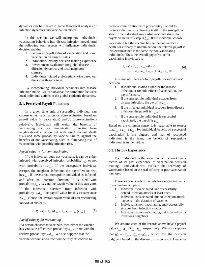
dynamics can be treated in game theoretical analyses of infection dynamics and vaccination choice.
In this section, we will incorporate individuals’ vaccinating behaviors into disease infection model. And the following four aspects will influence individuals’ decision making:
1. Perceived payoff value of vaccination and non-vaccination on current status.
2. Individuals’ history decision making experience. 3. Environment Evaluation for global disease
diffusion dynamics and local neighbors’ statuses.
4. Individuals’ biased preferential choice based on the above three criteria.
By incorporating individual behaviors into disease
infection model, we can observe the correlation between local individual actions to the global epidemic dynamics. 5.1. Perceived Payoff Functions
In a given time unit, a susceptible individual can choose either vaccination or non-vaccination based on payoff value (vaccination) and (non-vaccination) relatively. Individuals will weigh the benefits of vaccinating, such as immunization protection from neighborhood infection but with small vaccine death risks and some probability vaccine failure, against the benefits of non-vaccinating, such as eliminating risk of vaccine but with possibly infection risk.
vP NP
Payoff value for non-vaccinating
NPIf the individual does not vaccinate, it can be either
infected with perceived infection probability infλ or not
with probabilityinf1 λ− . If the susceptible individual
escapes the neighbor infections the payoff value will be
susL . If the current susceptible individual is infected, and after its infection duration it is died with probability , leaving the payoff value in this step zero. If the individual survives from infection with probability , the payoff value for this circumstance is
infd
1 d− inf
infL . Hence, the overall payoff value of non-vaccinating individual choice is
inf inf inf inf(1 ) [(1 ) ]N susP L d Lλ λ= − + −i i i
(3)
Payoff value for vaccinating vP
If a person chooses to vaccinate, then either the vaccine has vital side-effect with probability , or not with the relative probability1 . We also suppose that the vaccine without side-effect will be truly efficacious to
provide immunization with probability
vacd
vacd−
ε , or fail to protect individuals just leaving it still in the susceptible state. If the individual successful vaccinate itself, the payoff value in this step is
vacL . If the individual choose vaccination but the vaccine has neither side-effect to death nor efficacy to immunization, the relative payoff in this circumstance is the same the non-vaccinating individuals. Thus, the overall payoff value for vaccinating individuals is
inf nf inf
(1 ) )(1 ) [(1 ]
V vacP dL d Li
(1vac
sus
L
inf )ε ε
λ λ= − +
− +−
i i i i− (4)
In summary, there are four payoffs for individuals’
decision. 1. If individual is died either for the disease
infection or for side-effect of vaccination, the payoff is zero.
2. If the susceptible individual escapes from disease infection, the payoff is susL ,
3. If the infected individual recovers from disease infection, the payoff is
infL , 4. If the susceptible individual is successful
vaccinated, the payoff isvacL .
Based on the common sense, it is reasonable to expect that inf sus vacL L L< < , for individual benefit of successful vaccination is the biggest, and that of recovered individual is the least, the benefit of susceptible individual is in the middle. 5.2. History Experience
Each individual in the social contact network has a record of its past experience of vaccination decision making. Individual will evaluate the necessary of vaccination based on the real efficacy of past vaccination memory.
There are four kinds of records for each individual’s to vaccination adoption.
1. Individual is vaccinated, and successfully defend infection attacks at least once.
2. Individual is vaccinated, but no infection attack happens in the duration of vaccine.
3. Individual is non-vaccinating, and successfully escapes from infection attacks.
4. Individual is non-vaccinating, but infected by its infectious neighbors.
We assume each of the records above have a payoff
value vach+ ,vach− ,
nonh+ ,nonh− respectively. We also suppose
thatvac vach h+ −= − ,
non nonhh+ −= − , which are the decision judgment based on the disease diffusion result. Hence, in
69 of 162

time unit k the historical evaluation of vaccinating behaviors ( )vacH k (vaccination history) and ( )nonH k
( )
(non vaccination history) can be updated as following:
( ) ( 1)decay vac vacvacH k H kλ= −i h k+
( )
(5) ( ) ( 1)decay non nonnonH k H kλ= −i h k+ (6)
decayλ is decay ratio, meaning that the most recent records
have a bigger influence on individuals’ decision making.
5.3. Environment Evaluation
We assume that each individual has a full ability to communicate with its direct neighbors, but a confined global information achievement. For local interaction, the individual can detect its neighbor’s state and vaccination choice of last time. For global information, we suppose that individuals can get the global infection rate as a severity estimation criterion. Thus these environment evaluation parameters will influence individuals’ vaccination decision making process.
vacr is the proportion of the vaccinated neighbors to all neighbors.
vacvac
neigb
nrn
= (7)
infr is the proportion of the infected neighbors to all neighbors.
inf
vac
neigb
irn
= (8)
infR is the infection rate in the global network.
infIRN
= (9)
5.4. Individual Biased Preference Rules
In each time unit, individuals’ vaccination decision making is based on three parts (Figure 5): (1) Payoff function and ; VP NP(2) History records
vacH andnonH ;
(3) Environment estimation , and . vacr infr infR
Environment Evaluation
VaccinationChoice
Non-vaccinationChoice
Pv>Pn ? History Experience
Individual Biased Preference Rules
Y N
W3W2W1
Figure 6, Individual Biased Preference Rules We assume some biased preference rules to simulate human’s irrational decision making behaviors.
Individuals are more incline to rely on their history experience.
Individuals are likely to simulate its neighbor’s behaviors.
Pandemic scare is based on individuals’ irrational estimation.
Thus, based on the above biased preference assumptions, we can design the decision making functions as following:
1
2inf
( ) ( ) ( )
[ ( ) ( )]2 2
vac V i vac
i vac
E k P k H k
tg r tg R
ξπ πξ
= +
+ +
i
i i i
(10)
1
2inf
( ) ( ) ( )
[ ( (1 )) ( (1 ))]2 2
non N i non
i vac
E k P k H k
tg r tg R
ζπ πζ
= +
+ − + −
i
i i i
(11)
If ( ) ( )vac nonE k E k> , the current individual will adopt
the vaccination choice, or vice versa. 1iξ
1iζ are
parameters to modify the influence of history experience for vaccination and non-vaccination. 2
iξ2iζ are variables
to control the impact of environment estimations.
Function (2 vactg r )πi
is designed to simulate
individual’s neighbor following feature. If the proportion of vaccinated neighbors is increased the current will more inclined to adopt vaccination. Function
inf(2
tg R )πi
tries to describe the potential epidemic scare.
If the global infection rate is near 100%, each individual will irrationally adopt vaccination instead of balancing payoff gains.
70 of 162
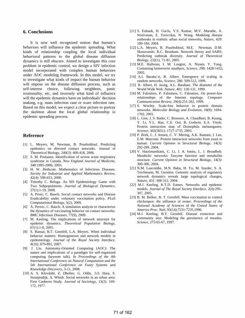
6. Conclusions It is now well recognized notion that human’s
behaviors will influence the epidemic spreading. What kinds of relationship coupling the local individual behavioral patterns to the global disease diffusion dynamics is still obscure. Aimed to investigate this core problem in epidemic control, we design a SIV infection model incorporated with complex human behaviors under AOC modeling framework. In this model, we try to investigate what kinds of impact the human behavior will impose on the disease diffusion process, such as self-interest choice, following neighbors, panic irrationality, etc, and inversely what kind of influence will the epidemic dynamics have on individuals’ decision making, e.g. mass infection case or scare infection rate. Based on this model, we expect a clear picture to portray the skeleton about the local global relationship in epidemic spreading process. Reference [1] L. Meyers, M. Newman, B. Pourbohloul. Predicting
epidemics on directed contact networks. Journal of Theoretical Biology, 240(3): 400-418, 2006.
[2] S. M. Poutanen. Identification of severe acute respiratory syndrome in Canada. New England Journal of Medicine, 348:1995-2006, 2003.
[3] H. W. Hethcote. Mathematics of Infectious Diseases. Society for Industrial and Applied Mathematics Review, 42(4): 599-653, 2000.
[4] Timothy C. Reluga. An SIS Epidemiology Game with Two Subpopulations. Journal of Biological Dynamics, 27(1):1-19, 2008.
[5] A. Prisic, C. Bauch. Social contact networks and Disease Eradicability under voluntary vaccination policy. PLoS Computational Biology, 5(2), 2009.
[6] A. Perisic, C. Bauch. A simulation analysis to characterize the dynamics of vaccinating behavior on contact networks. BMC Infectious Diseases, 77(9), 2009.
[7] M. Keeling. The implications of network structure for epidemic dynamics. Theoretical Population Biology, 67(1):1-8, 2005.
[8] S. Bansal, B.T. Grenfell, L.A. Meyers. When individual behavior matters: Homogeneous and network models in epidemiology. Journal of the Royal Society Interface, 4(16): 879-891, 2007.
[9] J. Liu. Autonomy-Oriented Computing (AOC): The nature and implications of a paradigm for self-organized computing (keynote talk). In Proceedings of the 4th International Conference on Natural Computation and the 5th International Conference on Fuzzy Systems and Knowledge Discovery, 3-11, 2008.
[10] A. S. Klovdahl, Z. Dhofier, G. Oddy, J.O. Hara, S. Stoutjesdijk, A. Whish. Social networks in an urban area: First Canberra Study. Journal of Sociology, 13(2): 169-172, 1977.
[11] S. Eubank, H. Guclu, V.S. Kumar, M.V. Marathe, A. Srinivasan, Z. Toroczkai, N. Wang. Modeling disease outbreaks in realistic urban social networks, Nature, 429: 180-184, 2004.
[12] L.A. Meyers, B. Pourbohloul, M.E. Newman, D.M. Skowronski, R.C. Brunham. Network theory and SARS: Predicting outbreak diversity. Journal of Theoretical Biology, 232(1), 71-81, 2005.
[13] M.E. Halloran, I. M. Longini, A. Nizam, Y. Yang. Containing bioterrorist smallpox, Science, 298: 1428-1432, 2002.
[14] A.L Baraba´si, R. Albert. Emergence of scaling in random networks, Science, 286: 509-512, 1999.
[15] R. Albert, H. Jeong, A.L. Barabasi. The diameter of the World Wide Web. Nature, 401: 130-131, 1999.
[16] M. Faloutsos, P. Faloutsos, C. Faloutsos. On power-law relationships of the Internet topology. Computer Communication Review, 29(4):251-262, 1999.
[17] S. Wuchty. Scale-free behavior in protein domain networks. Molecular Biology and Evolution, 18(9): 1694-1702, 2001.
[18] L. Giot, J. S. Bader, C. Brouwer, A. Chaudhuri, B. Kuang, Y. Li, Y.L. Hao, C.E. Ooi, B. Godwin, E.A. Vitols. Protein interaction map of Drosophila melanogaster, Science, 302(5651): 1727-1735, 2003.
[19] P. Bork, L. J. Jensen, C. V. Mering, A.K. Ramani, I. Lee, E.M. Marcotte. Protein interaction networks from yeast to human. Current Opinion in Structural Biology, 14(3): 292-299, 2004.
[20] V. Hatzimanikatis, C. Li, J. A. Ionita, L. J. Broadbelt. Metabolic networks: Enzyme function and metabolite structure. Current Opinion in Structural Biology, 14(3): 300-306, 2004.
[21] N.M. Luscombe, M.N. Babu, H. Yu, M. Snyder, S. A. Teichmann, M. Gerstein. Genomic analysis of regulatory network dynamics reveals large topological changes, Nature, 431: 308-312, 2004.
[22] M.J. Keeling, K.T.D. Eames. Networks and epidemic models. Journal of The Royal Society Interface, 2(4):295–307, 2005.
[23] B. M. Bolker, B. T. Grenfell. Mass vaccination to control chickenpox: the influence of zoster. Proceedings of the National Academy of Sciences of the United States of America Proc. Natl, 93(14):7231-7235,1996.
[24] M.J. Keeling, B.T. Grenfell. Disease extinction and community size: Modeling the persistence of measles. Science, 275:65-67, 1997.
71 of 162
Extracting Discriminative Binary Template for Face Template Protection
Yicheng Feng
Abstract
This paper addresses the security issues of the face bio-metric templates stored in a database. In order to improvethe security level of the stored face templates, cryptographictechniques are commonly employed. Since most of suchtechniques require a binary input, thresholding is usuallyemployed to binarize the real valued face features. Whilebinary templates are obtained, the discriminability of theoriginal templates may be affected and so is the recognitionperformance. In order to overcome this limitation, this pa-per proposes a new approach to discriminative extract bi-nary templates from original face templates. A projectionis applied before thresholding such that the thresholdingcan fit the projected data distribution better, which makesthe extracted binary templates more discriminative. A dis-criminability index is constructed to measure the discrim-inability of the extracted binary templates and the projec-tion matrix is optimized. The proposed method is evaluatedon three public domain databases, namely FERET, CMU-PIE and FRGC. Experimental results show that, in compar-ison to the existing thresholding-based methods, the pro-posed method improves the GAR by around11% − 13% ata FAR of 1%.
1 Introduction
Biometrics is a reliable, robust and convenient way forperson authentication [9, 10, 6]. With the success of thebiometrics research in the last two decades, several largescale recognition systems have been successfully deployed.With the growing use of biometrics, there is a rising con-cern about the security and privacy of the stored biometrictemplates (which refer to a set of features extracted fromraw biometric data) stored in a database or a smartcard. Re-cent studies [11] show that simple attacks on a biometricsystem, such as hill climbing, are able to recover the rawbiometric data from a stolen biometric template. Moreover,the attacker may be able to make use of the stolen templateto access the system or cross-match across databases. Acomprehensive analysis of eight types of attacks [6] on abiometric system has been reported. Therefore, biometric
template security [9, 10, 6, 18] has been an important issuein deploying a biometric system.
In order to overcome the security and privacy prob-lems [6, 7, 9], a number of biometric template protec-tion algorithms have been reported in the last few years.These methods can be broadly categorized into two ap-proaches, namely biometric cryptosystem approach andtransformation-based approach. The basic idea of both theapproaches is that instead of storing the original biometrictemplate, the transformed/encrypted template is stored. Incase the transformed/encrypted biometric template is stolenor lost, it is computationally hard to reconstruct the bio-metric template and the original raw biometric data fromthe transformed/encrypted template. Generally speaking,the transform-based approach suffer from a trade-off be-tween dicriminability and security of the transformed tem-plates while biometric cryptosystems may provide both en-hanced security and acceptable discriminability. Crypto-graphic technique is employed in the last step in the cryp-tosystems approach to enhance the security of the tem-plates. Error-correcting schemes are applied to deal withthe intra-class variance thus the discriminability of the en-crypted templates will not degrade too much. However,most of the protection algorithms in biometric cryptosystemapproach require a binary template or integer data (most forthe fuzzy vault scheme [5]) for encryption. That means,the input template has to be converted into a binary or in-teger template before encryption. The fuzzy vault schemeis mostly applied to fingerprint. The minutiae of fingerprintare unordered set of points, which the fuzzy vault schemeis just able to encrypt. For face recognition algorithms likePCA or LDA schemes, the situation is much different be-cause the extracted templates are ordered real value vec-tors with large range, which causes a problem to apply thefuzzy vault scheme. On the other hand, there are schemesto transform the original face templates into binary stringsfor protection. In order to satisfy the input requirements,thresholding is a typically employed in existing algorithms[12, 13, 14, 15, 16, 17]. While the binary template can beobtained, some useful and discriminative information in theoriginal (real valued) template may be lost after threshold-ing leading to degraded matching accuracy (discriminabil-ity) [12, 13]. And existing approaches lack of discriminabil-
72 of 162
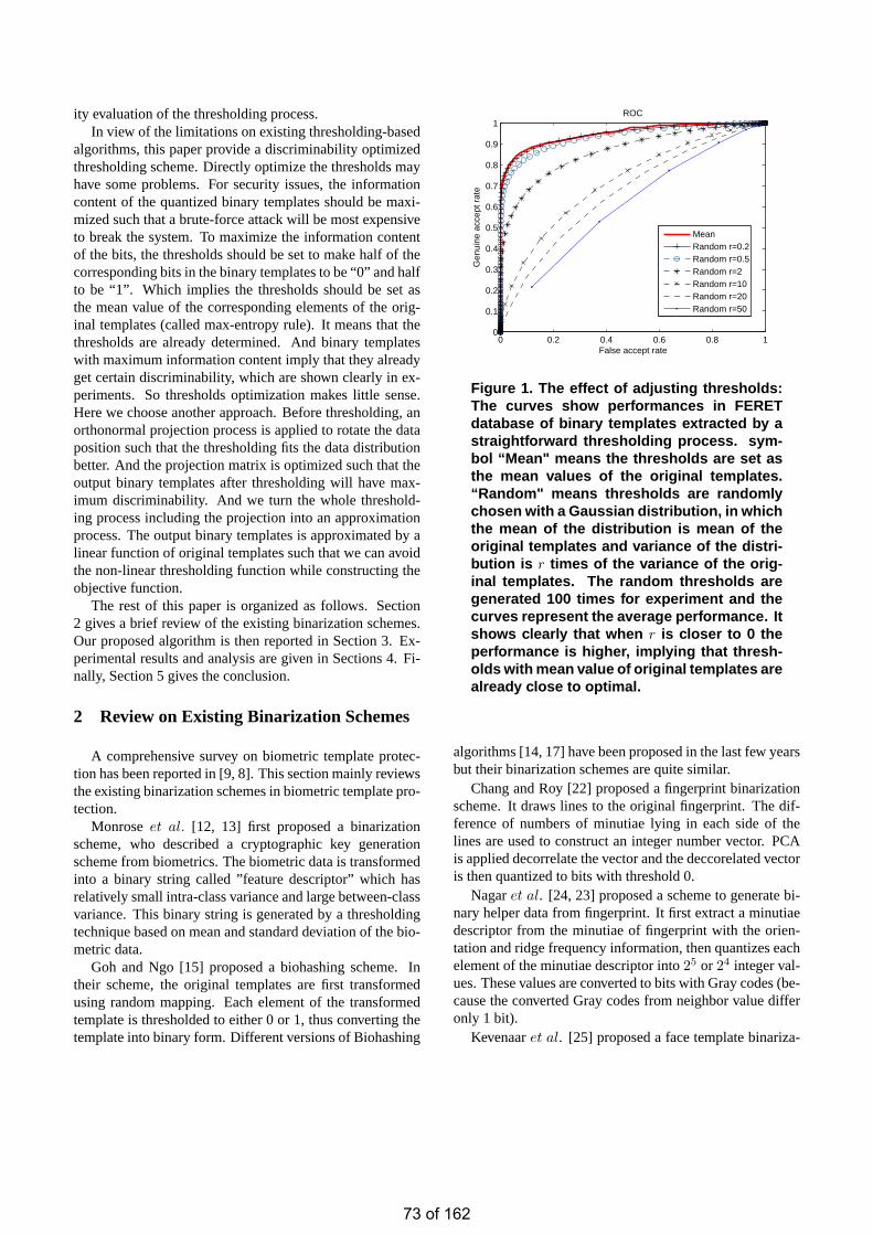
ity evaluation of the thresholding process.In view of the limitations on existing thresholding-based
algorithms, this paper provide a discriminability optimizedthresholding scheme. Directly optimize the thresholds mayhave some problems. For security issues, the informationcontent of the quantized binary templates should be maxi-mized such that a brute-force attack will be most expensiveto break the system. To maximize the information contentof the bits, the thresholds should be set to make half of thecorresponding bits in the binary templates to be “0” and halfto be “1”. Which implies the thresholds should be set asthe mean value of the corresponding elements of the orig-inal templates (called max-entropy rule). It means that thethresholds are already determined. And binary templateswith maximum information content imply that they alreadyget certain discriminability, which are shown clearly in ex-periments. So thresholds optimization makes little sense.Here we choose another approach. Before thresholding, anorthonormal projection process is applied to rotate the dataposition such that the thresholding fits the data distributionbetter. And the projection matrix is optimized such that theoutput binary templates after thresholding will have max-imum discriminability. And we turn the whole threshold-ing process including the projection into an approximationprocess. The output binary templates is approximated by alinear function of original templates such that we can avoidthe non-linear thresholding function while constructing theobjective function.
The rest of this paper is organized as follows. Section2 gives a brief review of the existing binarization schemes.Our proposed algorithm is then reported in Section 3. Ex-perimental results and analysis are given in Sections 4. Fi-nally, Section 5 gives the conclusion.
2 Review on Existing Binarization Schemes
A comprehensive survey on biometric template protec-tion has been reported in [9, 8]. This section mainly reviewsthe existing binarization schemes in biometric template pro-tection.
Monroseet al. [12, 13] first proposed a binarizationscheme, who described a cryptographic key generationscheme from biometrics. The biometric data is transformedinto a binary string called ”feature descriptor” which hasrelatively small intra-class variance and large between-classvariance. This binary string is generated by a thresholdingtechnique based on mean and standard deviation of the bio-metric data.
Goh and Ngo [15] proposed a biohashing scheme. Intheir scheme, the original templates are first transformedusing random mapping. Each element of the transformedtemplate is thresholded to either 0 or 1, thus converting thetemplate into binary form. Different versions of Biohashing
0 0.2 0.4 0.6 0.8 10
0.1
0.2
0.3
0.4
0.5
0.6
0.7
0.8
0.9
1ROC
False accept rate
Gen
uine
acc
ept r
ate
MeanRandom r=0.2Random r=0.5Random r=2Random r=10Random r=20Random r=50
Figure 1. The effect of adjusting thresholds:The curves show performances in FERETdatabase of binary templates extracted by astraightforward thresholding process. sym-bol “Mean" means the thresholds are set asthe mean values of the original templates.“Random" means thresholds are randomlychosen with a Gaussian distribution, in whichthe mean of the distribution is mean of theoriginal templates and variance of the distri-bution is r times of the variance of the orig-inal templates. The random thresholds aregenerated 100 times for experiment and thecurves represent the average performance. Itshows clearly that when r is closer to 0 theperformance is higher, implying that thresh-olds with mean value of original templates arealready close to optimal.
algorithms [14, 17] have been proposed in the last few yearsbut their binarization schemes are quite similar.
Chang and Roy [22] proposed a fingerprint binarizationscheme. It draws lines to the original fingerprint. The dif-ference of numbers of minutiae lying in each side of thelines are used to construct an integer number vector. PCAis applied decorrelate the vector and the deccorelated vectoris then quantized to bits with threshold 0.
Nagaret al. [24, 23] proposed a scheme to generate bi-nary helper data from fingerprint. It first extract a minutiaedescriptor from the minutiae of fingerprint with the orien-tation and ridge frequency information, then quantizes eachelement of the minutiae descriptor into25 or 24 integer val-ues. These values are converted to bits with Gray codes (be-cause the converted Gray codes from neighbor value differonly 1 bit).
Kevenaaret al. [25] proposed a face template binariza-
73 of 162
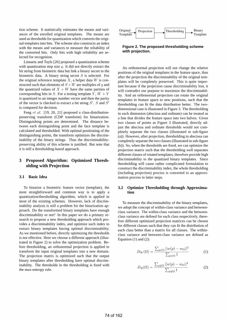
tion scheme. It statistically estimates the means and vari-ances of the enrolled original templates. The means areused as thresholds for quantization which converts the origi-nal templates into bits. The scheme also constructs an indexwith the means and variances to measure the reliability ofthe converted bits. Only bits with high reliability are se-lected for recognition.
Linnartz and Tuyls [26] proposed a quantization schemewith quantization step sizeq. It did not directly extract thebit string from biometric data but link a binary secret to thebiometric data. A binary string secretS is selected. Forthe original reference templateX, a helper dataW is con-structed such that elements ofS +W are multiples ofq andthe quantized values ofX + W have the same parities ofcorresponding bits inS. For a testing templateY , W + Yis quantized to an integer number vector and then the parityof the vector is checked to extract a bit stringS′. S andS′
is compared for decision.Fenget al. [19, 20, 21] proposed a class-distribution-
preserving transform (CDP transform) for binarization.Distinguishing points are determined. The distance be-tween each distinguishing point and the face template iscalculated and thresholded. With optimal positioning of thedistinguishing points, the transform optimizes the discrim-inability of the binary strings. Thus the discriminability-preserving ability of this scheme is justified. But note thatit is still a thresholding-based approach.
3 Proposed Algorithm: Optimized Thresh-olding with Projection
3.1 Basic Idea
To binarize a biometric feature vector (template), themost straightforward and common way is to apply aquantization/thresholding algorithm, which is applied inmost of the existing schemes. However, lack of discrim-inability analysis is still a problem for the binarization ap-proach. Do the transformed binary templates have enoughdiscriminability or not? In this paper we do a primary re-search to propose a new thresholding approach which pro-vides a discriminability index, and optimize such index toextract binary templates having optimal discriminability.As we mentioned before, directly optimizing the thresholdsis not effective. Here we choose a different approach (illus-trated in Figure 2) to solve the optimization problem. Be-fore thresholding, an orthonormal projection is applied totransform the input original templates into a new domain.The projection matrix is optimized such that the outputbinary templates after thresholding have optimal discrim-inability. The thresholds in the thresholding is fixed withthe max-entropy rule.
Projection ThresholdingOriginal
Template
Binary
Template
Figure 2. The proposed thresholding schemewith projection.
An orthonormal projection will not change the relativepositions of the original templates in the feature space, thusafter the projection the discriminability of the original tem-plates will be completely preserved. This is quite impor-tant because if the projection cause discriminability lost, itwill contradict our purpose to maximize the discriminabil-ity. And an orthonormal projection can rotate the originaltemplates in feature space to new positions, such that thethresholding can fit the data distribution better. The two-dimensional case is illustrated in Figure 3. The thresholdingin each dimension (abscissa and ordinate) can be treated asa line that divides the feature space into two halves. Giventwo classes of points as Figure 3 illustrated, directly ad-just the abscissa and ordinate thresholds would not com-pletely separate the two classes (illustrated in sub-figure(a)). However, after projection, thresholding in abscissa cancompletely separate the two classes (illustrated in sub-figure(b)). So, when the thresholds are fixed, we can optimize theprojection matrix such that the thresholding well separatesdifferent classes of rotated templates, therefore provide highdiscriminability to the quantized binary templates. Sincethresholding will cause rather complicated formulation toconstruct the discriminability index, the whole thresholding(including projection) process is converted to an approxi-mation process in latter steps.
3.2 Optimize Thresholding through Approxima-tion
To measure the discriminability of the binary templates,we adopt the concept of within-class variance and between-class variance. The within-class variance and the between-class variance are defined for each class respectively, there-fore different optimized projection matrices can be chosenfor different classes such that they can fit the distribution ofeach class better than a matrix for all classes. The within-class variance and between-class variance are defined asEquation (1) and (2):
DW (Ω) =
∑p∈Ω ||w(p)− wΩ||2∑
p∈Ω 1(1)
DB(Ω) =
∑p6∈Ω ||w(p)− wΩ||2∑
p6∈Ω 1(2)
74 of 162
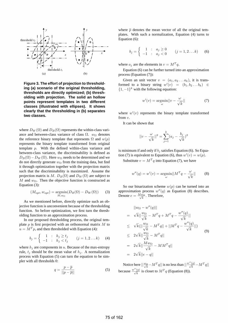
x
y
(a)
y
x0
(b)
0
threshold t2
threshold t1
Figure 3. The effort of projection to threshold-ing (a) scenario of the original thresholding,thresholds are directly optimized; (b) thresh-olding with projection. The solid an hollowpoints represent templates in two differentclasses (illustrated with ellipses). It showsclearly that the thresholding in (b) separatestwo classes.
whereDW (Ω) andDB(Ω) represents the within-class vari-ance and between-class variance of classΩ. wΩ denotesthe reference binary template that representsΩ and w(p)represents the binary template transformed from originaltemplatep. With the defined within-class variance andbetween-class variance, the discriminability is defined asDB(Ω)−DW (Ω). HerewΩ needs to be determined and wedo not directly generatewΩ from the training data, but findit through optimization together with the projection matrixsuch that the discriminability is maximized. Assume theprojection matrix isM . DB(Ω) andDW (Ω) are subject toM andwΩ. Then the objective function is constructed asEquation (3):
(Mopt, wopt) = argminM,wΩ
(DB(Ω)−DW (Ω)) (3)
As we mentioned before, directly optimize such an ob-jective function is unconvenient because of the thresholdingfunction. So before optimization, we first turn the thresh-olding function to an approximation process.
In our proposed thresholding process, the original tem-platep is first projected with an orthonormal matrixM tou = MT p, and then thresholded with Equation (4):
bj =
1 : hj ≥ tj−1 : hj < tj
(j = 1, 2 . . . k) (4)
wherehj are components inu. Because of the max-entropyrule, tj should be the mean value ofhj . A normalizationprocess with Equation (5) can turn the equation to be sim-pler with all thresholds 0:
q =p− p
||p− p|| (5)
wherep denotesthe mean vector of all the original tem-plates. With such a normalization, Equation (4) turns toEquation (6):
bj =
1 : aj ≥ 0−1 : aj < 0 (j = 1, 2 . . . k) (6)
whereaj are the elements inv = MT q.
Equation (6) can be further turned into an approximationprocess (Equation (7)):
Given an unit vectorv = (a1, a2 . . . ak), it is trans-formed to a binary stringw′(v) = (b1, b2 . . . bk) ∈1,−1k with the following equation:
w′(v) = argminω
||v − ω√k|| (7)
where w′(v) representsthe binary template transformedfrom v.
It can be shown that
||v − ω√k||2 =
k∑
j=1
(aj − bj√k
)2
isminimum if and only ifbj satisfies Equation (6). So Equa-tion (7) is equivalent to Equation (6), thusw′(v) = w(p).
Substitutev = MT q into Equation (7), we have
w′′(q) = w′(v) = argminω
||MT q − ω√k|| (8)
So our binarization schemew(p) can be turned into anapproximation processw′′(q) as Equation (8) describes.Denotee = MwΩ√
k. Therefore,
||wΩ − w′′(q)||=
√k||wΩ√
k−MT q + MT q − w′′(q)√
k||
≤√
k(||wΩ√k−MT q||+ ||MT q − w′′(q)√
k||)
≤ 2√
k||wΩ√k−MT q||
= 2√
k||MwΩ√k
−MMT q||
= 2√
k||e− q||
(9)
Noticehere||wΩ√k−MT q|| isno less than||w′′(q)√
k−MT q||
becausew′′(q)√
kis closet toMT q (Equation (8)).
75 of 162
Onthe other side,
||wΩ − w′′(q)||=
√k||wΩ√
k−MT q + MT q − w′′(q)√
k||
≤√
k||wΩ√k−MT q||+
√k||MT q − w′′(q)√
k||
=√
k||q − e||+√
k||MT q − w′′(q)√k||
implies
|(||wΩ − w′′(q)|| −√
k||q − e||)|≤
√k||MT q − w′′(q)√
k|| (10)
Here||MT q− w′′(q)√k|| is minimized with optimalw′′(q).
To let the approximation error as small as possible, Equa-tion (5) makesMT q an unit vector and scalar
√k is used
such thatw′′(q)√
kis a normalized vector too. Without
√k,
||MT q − w′′(q)|| ≥ ||w′′(q)|| − ||MT q|| =√
k − 1
causinglarge approximation error. With√
k, w′′(q)√k
is a unit
vector thus the norms ofMT q and w′′(q)√k
provide no con-tribution to the approximation error, resulting in small ap-proximation error. Then Equation (10) implies that
||wΩ − w′′(q)|| ≈√
k||wΩ√k−MT q|| (11)
Denotem =∑
p6∈Ω 1 and n =∑
p∈Ω 1. SubstituteEquation (9) into Equation (1) and (11) into (2). Sincew′′(q) = w′(v) = w(p), we have
DW (Ω) =
∑p∈Ω
||w(p)− wΩ||2
n≤ 4k
∑q∈Ω
||q − e||2
n(12)
and
DB(Ω) =
∑p6∈Ω
||w(p)− wΩ||2
m≈ k
∑q 6∈Ω
||q − e||2
m(13)
Equation(13) implies that a largeD′B(Ω) leads to large
DB(Ω). Equation (12) indicates that a smallD′W (Ω) leads
to a smallDW (Ω). So the objective function is changed to
(Mopt, wopt) = argminM,wΩ
(D′B(Ω)−D′
W (Ω)) (14)
where
D′B(Ω) =
∑q 6∈Ω
||q − e||2
m
and
D′W (Ω) =
∑q∈Ω
||q − e||2
n.
From Equation (14) we can see that with the approxi-mation process, the terms including binary templates in theobjective functions are replaced by terms with original tem-plates. Therefore, there is no need to consider the correla-tion between bits and the thresholding process, thus solvesthe problems mentioned before. In Equation (14)M andwΩ are only related toe. So we can first optimizee andthen chooseM andwΩ to fit the optimizede:
eopt = argmaxe
(
∑q 6∈Ω
||q − e||2
m−
∑q∈Ω
||q − e||2
n) (15)
with constraint||e|| = 1 (16)
.The constraint is becausee = M wΩ√
kis an unit vector.
After eopt is found,wopt is randomly generated andMopt isconstructed such thatMoptwopt√
k= eopt.
However, we should notice that the objective functioncan only ensureD′
B(Ω) is large, but can not ensure thatD′
W (Ω) is small. So the following constraint
e · qΩ ≥ θ (17)
is required. HereqΩ is the normalized mean vector ofΩ andθ is a threshold smaller than 1. This constraint ensure thatD′
W (Ω) is relatively small.
3.3 Solve the Objective Function
The objective function is first expanded as follows:∑
q 6∈Ω
(||q − e||2)/m−∑
q∈Ω
(||q − e||2)/n
= (∑
q 6∈Ω
||q||2 − 2∑
q 6∈Ω
q · e)/m + ||e||2
−(∑
q∈Ω
||q||2 − 2∑
q∈Ω
q · e)/n− ||e||2
= (∑
q 6∈Ω
||q||2/m−∑
q∈Ω
||q||2/n)
+2(∑
q∈Ω
q/n−∑
q 6∈Ω
q/m) · e
where· denotes inner product. Assumer is the normalizedvector of
∑q∈Ω q/n−∑
q 6∈Ω q/m. According to the aboveequation, to maximize the objective function is equivalentto maximizer · e.
76 of 162

Apply the Gram-Schmidt algorithm to randomly gener-ate an orthonormal basiss1, s2 . . . sk wheres1 = qΩ.DenoteQ to be the orthonormal matrix usings1, s2 . . . sk
as columns. Then From Equation (17), we have
eT QQT qΩ ≥ θ (18)
Denotez = QT e = (x1, x2 . . . xk). According to Equation(16), z is an unit vector. Because of the construction ofQ, QT qΩ = (1, 0, . . . 0). Substitute these two terms intoEquation (18), we have
x1 ≥ θ (19)
Denotel = QT r = (y1, y2 . . . yk). Sincer is an unit vector,l is an unit vector. Therefore,
r · e = rT QQT e = lT z =k∑
j=1
xjyj
And
k∑
j=1
xjyj = x1y1 +k∑
j=2
xjyj
≤ x1y1 + (k∑
j=2
x2j ·
k∑
j=2
y2j )
12
= x1y1 +√
1− x21
√1− y2
1
∑kj=1 xjyj will achieve its maximum if and only if
xj =
√1− x2
1√1− y2
1
yj j = 2 . . . k
Denoteφ = arccos x1, ϕ = arccos y1. Then,
k∑
j=1
xjyj = x1y1 +√
1− x21
√1− y2
1
= cos φ cos ϕ + sinφ sinϕ
= cos(ϕ− φ)
From Equation (19), we have the restriction forφ:
0 ≤ φ ≤ arccos θ
If ϕ ≤ arccos θ (that is, y1 ≥ θ), setφ = ϕ, r · e canachieve the maximum value 1. Ifϕ > arccos θ, Then0 <ϕ − φ < π. cos(ϕ − φ) will be maximum whenϕ − φis minimum. Soφ should bearccos θ. That is,r · e willachieve its maximum when
x1 =
y1 : y1 ≥ θθ : y1 < θ
and
xj =
√1− x2
1√1− y2
1
yj j = 2 . . . k.
Then,eopt = Qz = Q[x1, x2 . . . xk]T .After eopt is found,wΩ is randomly generated andMopt
is constructed such thatMoptwΩ/√
k = eopt.
3.4 Algorithm Implementation
In enrollment,
• Normalize the original feature vectors with Equation(5).
• ConstructM andwΩ for classΩ.
• wΩ is used as the reference template and encryptedwith the fuzzy commitment scheme for protection.
• The encryptedwΩ andM are stored in database.
In authentication,
• when input a queryp, the correspondingM is released.
• Normalizep to q with Equation (5). And thenq isprojected tov = MT q.
• Thresholdq to w′′(q) = (b1, b2 . . . bk) with Equation(6).
• Comparew(p) with wΩ to make a decision.
4 Experimental Results
In the experiments, three public databases namely CMUPIE, FERET and FRGC are applied to evaluate the perfor-mance of our proposed thresholding with orthonormnal pro-jection (TOP) algorithm. The Fisherface [1] scheme is usedfor feature extraction. The detailed parameters settings areshown in Table 1, wherenc is the number of individualsin the database,np denotes the total number of images fromeach individual,nt is the number of images used for trainingfrom each individual. In our TOP algorithm, the paramterθis chosen 0.8.
Table 1. The experiment settingsDatabase nc np nt
CMU PIE 68 105 10FERET 250 4 2FRGC 350 40 5
Our proposed TOP algorithm is also compared withthe recent developed Random Multi-space Quantization
77 of 162

0 0.1 0.2 0.3 0.40.5
0.6
0.7
0.8
0.9
1ROC
False accept rate
Gen
uine
acc
ept r
ate
OriginalRMQTOP
Figure 4. Experimental results on the CMU PIEdatabase.
Table 2. The GARs(%) of the experiments withfixed FAR=0.01
Database Original RMQ TOPCMU PIE 59.26 73.53 85.99FERET 45.47 74.01 85.09FRGC 26.28 67.40 78.35
(RMQ) algorithm. The RMQ algorithm, as a binarizationscheme, is also used for face recognition and has similarprocedure with our scheme. It also does a projection beforethresholding, though the purpose of the projection is muchdifferent from ours. For fair comparison, we use a randomlygenerated orthonormal matrix in the projection step of theRMQ algorithm, therefore the projection step does not re-duce the dimension of the face template and will not causeinformation lost. So it will get higher performance than anormal RMQ algorithm.
The experimental results are shown in Figure 4-6. Sym-bol “Original” represents the original Fisherface algorithmwithout protection. The figures show clearly that our al-gorithm outperforms the RMQ algorithm. Following thepopular setting, we fix the FAR at 0.01 and compare theGAR. The results are shown in Table 2. We also measurethe equal error rate (EER) and the results are shown in Ta-ble 3. In all three databases, our proposed method gives thehighest GAR and lowest EER.
The security of the proposed scheme depends on thesecurity of the extracted binary templates, which are pro-tected by cryptosystems scheme like the fuzzy commitmentscheme. Since this part is not our main concern, we as-
0 0.1 0.2 0.3 0.40.4
0.5
0.6
0.7
0.8
0.9
1ROC
False accept rate
Gen
uine
acc
ept r
ate
OriginalRMQTOP
Figure 5. Experimental results on the FERETdatabase.
Table 3. The EERs(%) of the experimentsDatabase Original RMQ TOPCMU PIE 17.32 10.37 6.30FERET 21.66 11.29 7.44FRGC 31.75 13.38 10.05
sumethe protecting scheme provides enough security thusit is very computationally expensive for attackers to extractthe binary templates from the protected data. Then attackerswould have to guess the binary template with what they got.It should be mentioned that the projection matrixMopt isunprotected and may be exposed to attackers. However, thiswould not help the attackers because the only relationshipbetweenMopt and wΩ is equationMoptwΩ/
√k = eopt,
whereeopt is kept secret to attackers. And as we know,wΩ
is randomly generated. So the entropy ofwΩ is the lengthof it, that is,k bits. And this is also the security level of ourproposed algorithm.
5 Conclusions
This paper has proposed a new method to generate a bi-nary face template from a real valued face template. Theoriginal face templates are first projected with an orthonor-mal matrix, and then thresholded to binary templates. Theorthonormal matrix is optimized such that the extracted bi-nary templates can get highest discriminability. Three pub-lic domain available face databases have been used to eval-uate the proposed method. The experimental results showthat the proposed method has good performance and outper-forms the RMQ algorithm for comparison. The security of
78 of 162

0 0.1 0.2 0.3 0.40.3
0.4
0.5
0.6
0.7
0.8
0.9
1ROC
False accept rate
Gen
uine
acc
ept r
ate
OriginalRMQTOP
Figure 6. Experimental results on the FRGCdatabase.
the proposed algorithm is just the lengthk of the extractedbinary template, which is quite sufficient whenk is large(say 40).
References
[1] P N Belhumeur, J P Hespanha and D J Kriegman,“Eigenfaces vs. fisherfaces: Recognition using classspecific linear projection”, IEEE Trans. on PAMI,19(7), pp. 711-720, 1997.
[2] S Z Li, “Face Recognition Based on Nearest LinearCombinations,”Computer Vision and Pattern Recogni-tion, pp. 839-844,1998.
[3] R L Rivest, “The MD5 Message-Digest Algorithm,”RFC1321, Network Working Group, MIT Laboratoryfor Computer Science and RSA Data Security, Inc.,1992.
[4] J Daugman, “The Importance of Being Random: Sta-tistical Principles of Iris Recognition,”Pattern Recog-nition, Vol. 36, No. 2, pp. 279-291, 2003.
[5] A Juels and M Sudan. “A Fuzzy Vault Scheme”,IEEEInternational Symposium on Information Theory,2002.
[6] N Ratha, J Connell and R Bolle, “Enhancing securityand privacy in biometric-based authentication systems,”IBM Systems Journal,Vol. 40. No. 3, pp. 614 - 634,2001.
[7] S Prabhakar, S Pankanti and A K Jain, “BiometricRecognition: Security and Privacy Concerns,”IEEESecurity and Privacy Magazine, Vol. 1, No. 2, pp. 33-42, March-April 2003.
[8] A K Jain, K Nandakumar and A Nagar, “Biometrictemplate security,”EURASIP Journal on Advances inSignal Processing, Vol. 8, 2008.
[9] U Uludag, S Pankanti, S Prabhakar and A K Jain, “Bio-metric cryptosystems: issues and challenges,”Proceed-ings of the IEEE,vol. 92, no. 6, pp. 948-960, 2004.
[10] A K Jain, A Ross and S Pankanti, “Biometrics: ATool for Information Security”,IEEE Transactions onInformation Forensics and Security,Vol. 1, No. 2, pp.125-143, 2006.
[11] A Alder, “Images can be regenerated from quantizedbiometric match score data”,Proceedings of Cana-dian conference of Electrical and Computer Engineer-ing, pp. 469-472, 2004.
[12] F Monrose, M K Reiter and S Wetzel, “PasswordHardening Based on Key Stroke Dynamics,”Proc.ACM Conf. Computer and Comm. Security, pp. 73-82,1999.
[13] F Monrose, M Reiter, Q Li and S Wetzel, “Crypto-graphic Key Generation from Voice,”Proc. IEEE Symp.Security and Privacy, pp.202-213, May 2001.
[14] A Teoh, D Ngo and A Goh, “Biohashing: Two Fac-tor Authentication Featuring Fingerprint Data and To-kenised Random Number,”Pattern Recognition, vol.37, no. 11, pp. 2245-2255, Nov. 2004.
[15] A Goh and D C L Ngo, “Computation of crypto-graphic keys from face biometrics”,in Proc. 7th IFIPTC6/TC11 Conf. Commun. Multimedia Security,vol.22, pp. 1-13, 2003.
[16] D Ngo, A Teoh and A Goh, “Biometric Hash: High-Confidence Face Recognition”,IEEE transactions oncircuits and systems for video technology,vol. 16, no.6, 2006.
[17] A Teoh, A Goh and D. Ngo, “Random MultispaceQuantization as an Analytic Mechanism for BioHash-ing of Biometric and Random Identity Inputs,”IEEETransactions on Pattern Analysis and Machine Intelli-gence, vol. 28, no. 12, pp. 1892-1901, Dec. 2006.
[18] N Ratha, S Chikkerur, J Connell and R Bolle, “Gener-ating Cancelable Fingerprint Templates”,IEEE Trans-actions on Pattern Analysis and Machine Intelligence,vol.29, no.4, pp. 561-572, 2007.
[19] Y C Feng, P C Yuen and A K Jain, “A Hybrid Ap-proach for Face Template Protection,”Proceedings ofSPIE Defense and Security Symposium, 2008.
[20] Y C Feng and P C Yuen, “Class-Distribution Preserv-ing Transform for Face Biometric Data Security,”Pro-ceedings of IEEE International Conference on Acous-tics, Speech, and Signal Processing (ICASSP),pp. 141-144, 2007.
79 of 162

[21] Y C Feng and P C Yuen, “Selection of DistinguishPoints for Class Distribution Preserving Transform forBiometric Template Protection,”Proceedings of IEEEInternational Conference on Biometrics (ICB),pp. 636-645, 2007.
[22] E C Chang and S Roy, “Robust extraction of secret bitsfrom minutiae,” in Proceedings of 2nd InternationalConference on Biometrics,pp. 750C759, 2007.
[23] A Nagar, K Nandakumar and A K Jain, “A Hy-brid Biometric Cryptosystem for Securing FingerprintMinutiae Templates,” Pattern Recognition Letters,2009.
[24] A Nagar, K Nandakumar and A K Jain, “Securing fin-gerprint template: Fuzzy vault with minutiae descrip-tors,” International Conference on Pattern Recognition,pp. 1-4, 2008.
[25] T A M Kevenaar, G J Schrijen, M Veen, A H M Akker-mans, “Face recognition with renewable and privacypreserving binary templates,”IEEE Workshop on Auto-matic Identification Advanced Technologies,pp. 21-26,2005.
[26] J P Linnartz, P Tuyls, “New Shielding Functions toEnhance Privacy and Prevent Misuse of Biometric Tem-plates,” Audio and Video-Based Biometric Person Au-thentication,2003.
80 of 162
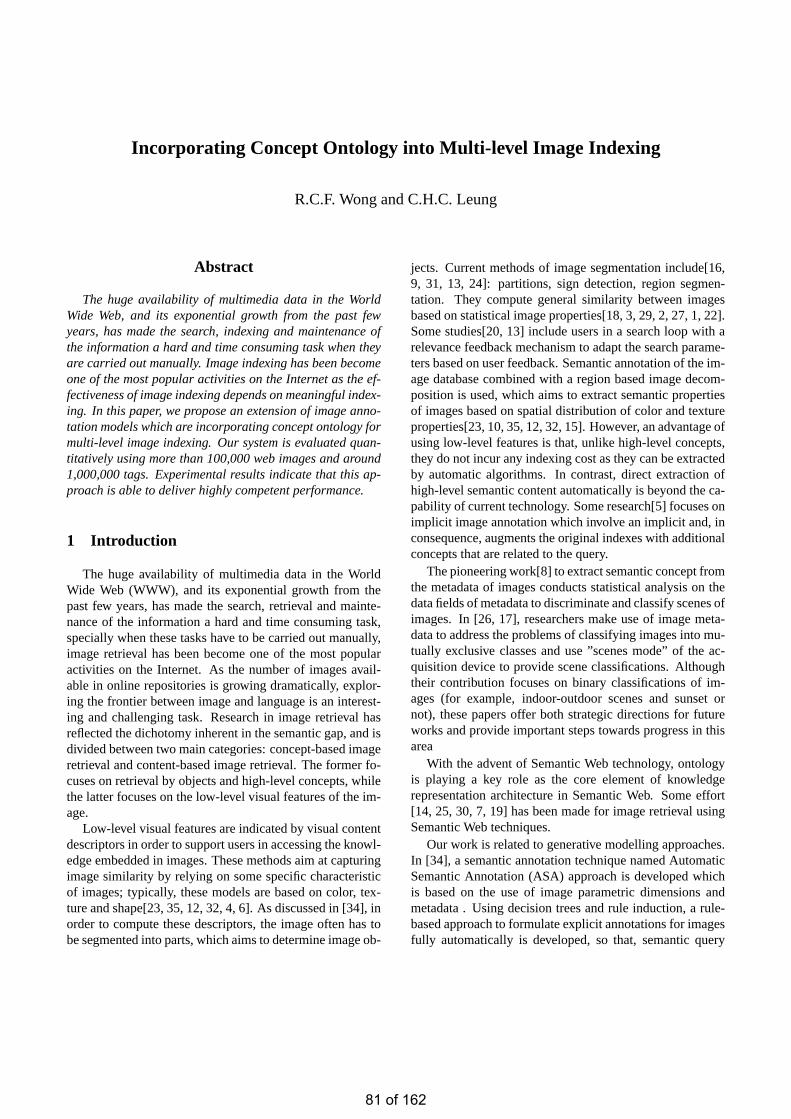
Incorporating Concept Ontology into Multi-level Image Indexing
R.C.F. Wong and C.H.C. Leung
Abstract
The huge availability of multimedia data in the WorldWide Web, and its exponential growth from the past fewyears, has made the search, indexing and maintenance ofthe information a hard and time consuming task when theyare carried out manually. Image indexing has been becomeone of the most popular activities on the Internet as the ef-fectiveness of image indexing depends on meaningful index-ing. In this paper, we propose an extension of image anno-tation models which are incorporating concept ontology formulti-level image indexing. Our system is evaluated quan-titatively using more than 100,000 web images and around1,000,000 tags. Experimental results indicate that this ap-proach is able to deliver highly competent performance.
1 Introduction
The huge availability of multimedia data in the WorldWide Web (WWW), and its exponential growth from thepast few years, has made the search, retrieval and mainte-nance of the information a hard and time consuming task,specially when these tasks have to be carried out manually,image retrieval has been become one of the most popularactivities on the Internet. As the number of images avail-able in online repositories is growing dramatically, explor-ing the frontier between image and language is an interest-ing and challenging task. Research in image retrieval hasreflected the dichotomy inherent in the semantic gap, and isdivided between two main categories: concept-based imageretrieval and content-based image retrieval. The former fo-cuses on retrieval by objects and high-level concepts, whilethe latter focuses on the low-level visual features of the im-age.
Low-level visual features are indicated by visual contentdescriptors in order to support users in accessing the knowl-edge embedded in images. These methods aim at capturingimage similarity by relying on some specific characteristicof images; typically, these models are based on color, tex-ture and shape[23, 35, 12, 32, 4, 6]. As discussed in [34], inorder to compute these descriptors, the image often has tobe segmented into parts, which aims to determine image ob-
jects. Current methods of image segmentation include[16,9, 31, 13, 24]: partitions, sign detection, region segmen-tation. They compute general similarity between imagesbased on statistical image properties[18, 3, 29, 2, 27, 1, 22].Some studies[20, 13] include users in a search loop with arelevance feedback mechanism to adapt the search parame-ters based on user feedback. Semantic annotation of the im-age database combined with a region based image decom-position is used, which aims to extract semantic propertiesof images based on spatial distribution of color and textureproperties[23, 10, 35, 12, 32, 15]. However, an advantage ofusing low-level features is that, unlike high-level concepts,they do not incur any indexing cost as they can be extractedby automatic algorithms. In contrast, direct extraction ofhigh-level semantic content automatically is beyond the ca-pability of current technology. Some research[5] focuses onimplicit image annotation which involve an implicit and, inconsequence, augments the original indexes with additionalconcepts that are related to the query.
The pioneering work[8] to extract semantic concept fromthe metadata of images conducts statistical analysis on thedata fields of metadata to discriminate and classify scenes ofimages. In [26, 17], researchers make use of image meta-data to address the problems of classifying images into mu-tually exclusive classes and use ”scenes mode” of the ac-quisition device to provide scene classifications. Althoughtheir contribution focuses on binary classifications of im-ages (for example, indoor-outdoor scenes and sunset ornot), these papers offer both strategic directions for futureworks and provide important steps towards progress in thisarea
With the advent of Semantic Web technology, ontologyis playing a key role as the core element of knowledgerepresentation architecture in Semantic Web. Some effort[14, 25, 30, 7, 19] has been made for image retrieval usingSemantic Web techniques.
Our work is related to generative modelling approaches.In [34], a semantic annotation technique named AutomaticSemantic Annotation (ASA) approach is developed whichis based on the use of image parametric dimensions andmetadata . Using decision trees and rule induction, a rule-based approach to formulate explicit annotations for imagesfully automatically is developed, so that, semantic query
81 of 162
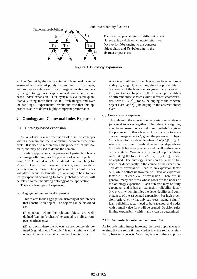
T1
T11 T12 ... T1k
Sub-tree reliability factor = rTraversal probabilities
t1kt11
t1kj
The traversal probabilities of different object
classes exhibit different characteristics, with
tij > t’mn for tij belonging to the concrete
object class, and t’mn belonging to the
abstract object class.
Figure 1. Ontology expansion
such as ”sunset by the sea in autumn in New York” can beanswered and indexed purely by machine. In this paper,we propose an extension of such image annotation modelsby using ontology-based expansion and contextual feature-based index expansion. Our system is evaluated quan-titatively using more than 100,000 web images and over990,000 tags. Experimental results indicate that this ap-proach is able to deliver highly competent performance.
2 Ontology and Contextual Index Expansion
2.1 Ontology-based expansion
An ontology is a representation of a set of conceptswithin a domain and the relationships between those con-cepts. It is used to reason about the properties of that do-main, and may be used to define the domain.
In certain applications, the presence of particular objectsin an image often implies the presence of other objects. IftermU ⇒ V , and if onlyU is indexed, then searching forV will not return the image in the result, even thoughVis present in the image. The application of such inferenceswill allow the index elementsTi of an image to be automat-ically expanded according to some probability which willbe related to the underlying ontology of the application.
There are two types of expansion:
(a) Aggregation hierarchical expansion
This relates to the aggregation hierarchy of sub-objectsthat constitute an object. The objects can be classifiedas:
(i) concrete, where the relevant objects are well-defined (e.g. an ”orchestra” expanded to violins, trum-pets, clarinets etc.)
(ii) abstract, where the objects are not concretely de-fined (e.g. although ”conflict” is not a definite visualobject, it contains certain common characteristics).
Associated with each branch is a tree traversal prob-ability tij (Fig. 1) which signifies the probability ofoccurrence of the branch index given the existence ofthe parent index. In general, the traversal probabilitiesof different object classes exhibit different characteris-tics, with tij > t′mn for tij belonging to the concreteobject class, andt′mn belonging to the abstract objectclass.
(b) Co-occurrence expansion
This relates to the expectation that certain semantic ob-jects tend to occur together. The relevant weightingmay be expressed as a conditional probability giventhe presence of other objects. An expansion to asso-ciate an image objectOj given the presence of objectOi is taken to be indexable whenProb[Oj |Oi] ≥ h,where h is a preset threshold value that depends onthe tradeoff between precision and recall performanceof the system. More generally, complex probabilisticrules taking the formProb[Oj |O1, ..., On] ≥ h willbe applied. The ontology expansion tree may be tra-versed bi-directionally in the course of the expansion.Top-down traversal will lead to an expansion factor> 1, while bottom-up traversal will have an expansionfactor < 1 at each level of expansion. There are, ingeneral, many sub-trees whose roots are the nodes ofthe ontology expansion. Each sub-tree may be fullyexpanded, and it has an expansion reliability factor0 < r < 1, which signifies the dependability and com-pleteness of the associated expansion. For high preci-sion retrieval (π ≈ 1), only sub-trees having a signif-icant reliability factor need to be traversed, and nodeswith a small value forr will be pruned. Decision ruleslinking expansibility withπ andr can be determined.
2.1.1 Semantic Knowledge from WordNet
As for redefining image indexing, the most popular way isto simplify the semantic knowledge into the semantic sim-ilarity between concepts, WordNet, is one of these applica-
82 of 162
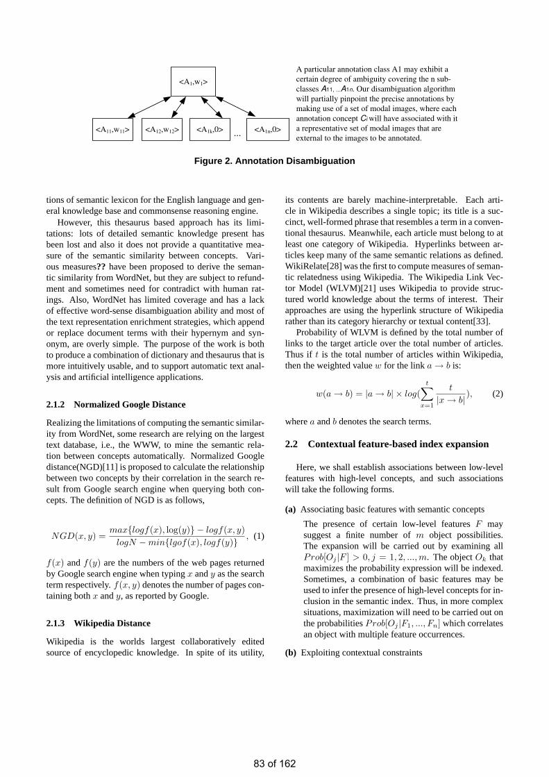
...
<A1,w1>
<A11,w11> <A12,w12> <A1n,0><A1k,0>
A particular annotation class A1 may exhibit a
certain degree of ambiguity covering the n sub-
classes A11, ...A1n. Our disambiguation algorithm
will partially pinpoint the precise annotations by
making use of a set of modal images, where each
annotation concept Ci will have associated with it
a representative set of modal images that are
external to the images to be annotated.
Figure 2. Annotation Disambiguation
tions of semantic lexicon for the English language and gen-eral knowledge base and commonsense reasoning engine.
However, this thesaurus based approach has its limi-tations: lots of detailed semantic knowledge present hasbeen lost and also it does not provide a quantitative mea-sure of the semantic similarity between concepts. Vari-ous measures??have been proposed to derive the seman-tic similarity from WordNet, but they are subject to refund-ment and sometimes need for contradict with human rat-ings. Also, WordNet has limited coverage and has a lackof effective word-sense disambiguation ability and most ofthe text representation enrichment strategies, which appendor replace document terms with their hypernym and syn-onym, are overly simple. The purpose of the work is bothto produce a combination of dictionary and thesaurus that ismore intuitively usable, and to support automatic text anal-ysis and artificial intelligence applications.
2.1.2 Normalized Google Distance
Realizing the limitations of computing the semantic similar-ity from WordNet, some research are relying on the largesttext database, i.e., the WWW, to mine the semantic rela-tion between concepts automatically. Normalized Googledistance(NGD)[11] is proposed to calculate the relationshipbetween two concepts by their correlation in the search re-sult from Google search engine when querying both con-cepts. The definition of NGD is as follows,
NGD(x, y) =maxlogf(x), log(y) − logf(x, y)
logN −minlgof(x), logf(y) , (1)
f(x) andf(y) are the numbers of the web pages returnedby Google search engine when typingx andy as the searchterm respectively.f(x, y) denotes the number of pages con-taining bothx andy, as reported by Google.
2.1.3 Wikipedia Distance
Wikipedia is the worlds largest collaboratively editedsource of encyclopedic knowledge. In spite of its utility,
its contents are barely machine-interpretable. Each arti-cle in Wikipedia describes a single topic; its title is a suc-cinct, well-formed phrase that resembles a term in a conven-tional thesaurus. Meanwhile, each article must belong to atleast one category of Wikipedia. Hyperlinks between ar-ticles keep many of the same semantic relations as defined.WikiRelate[28] was the first to compute measures of seman-tic relatedness using Wikipedia. The Wikipedia Link Vec-tor Model (WLVM)[21] uses Wikipedia to provide struc-tured world knowledge about the terms of interest. Theirapproaches are using the hyperlink structure of Wikipediarather than its category hierarchy or textual content[33].
Probability of WLVM is defined by the total number oflinks to the target article over the total number of articles.Thus if t is the total number of articles within Wikipedia,then the weighted valuew for the linka → b is:
w(a → b) = |a → b| × log(t∑
x=1
t
|x → b| ), (2)
wherea andb denotesthe search terms.
2.2 Contextual feature-based index expansion
Here, we shall establish associations between low-levelfeatures with high-level concepts, and such associationswill take the following forms.
(a) Associating basic features with semantic concepts
The presence of certain low-level featuresF maysuggest a finite number ofm object possibilities.The expansion will be carried out by examining allProb[Oj |F ] > 0, j = 1, 2, ..., m. The objectOk thatmaximizes the probability expression will be indexed.Sometimes, a combination of basic features may beused to infer the presence of high-level concepts for in-clusion in the semantic index. Thus, in more complexsituations, maximization will need to be carried out onthe probabilitiesProb[Oj |F1, ..., Fn] which correlatesan object with multiple feature occurrences.
(b) Exploiting contextual constraints
83 of 162
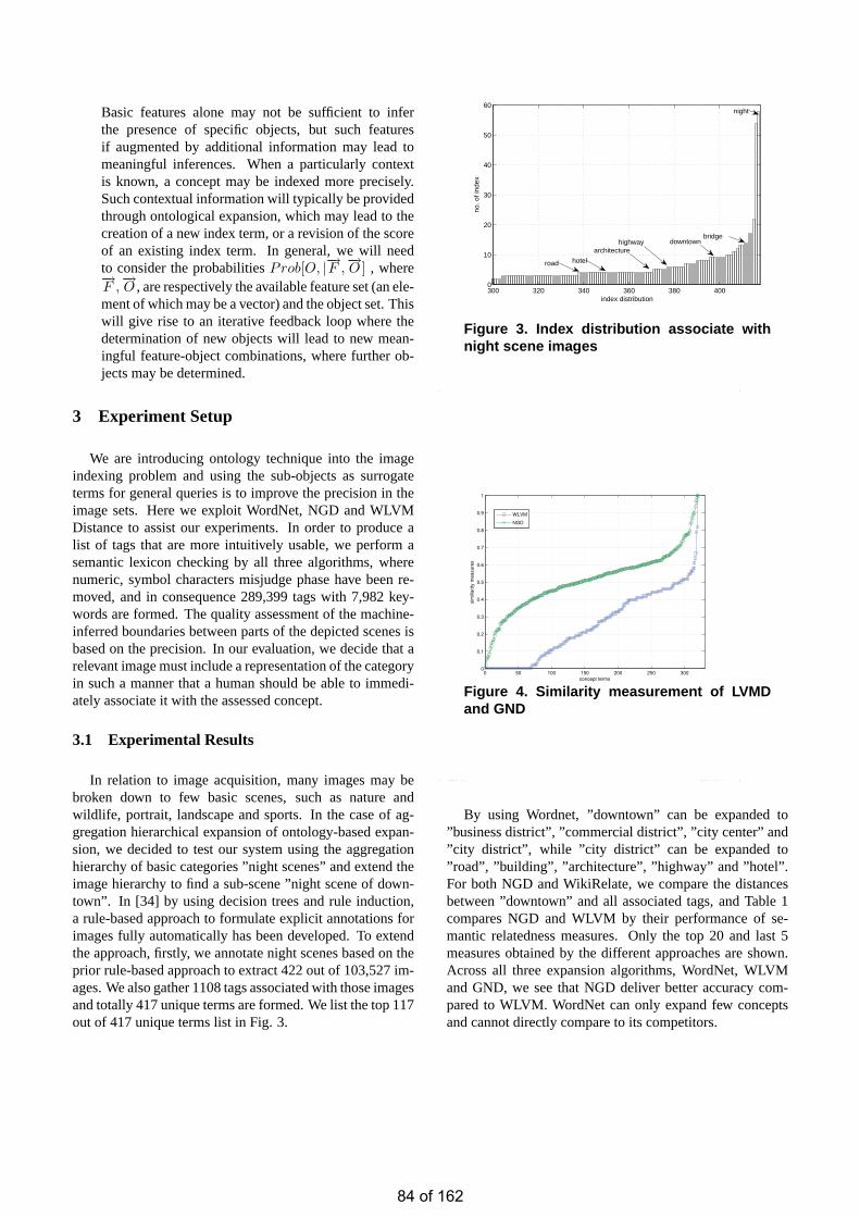
Basic features alone may not be sufficient to inferthe presence of specific objects, but such featuresif augmented by additional information may lead tomeaningful inferences. When a particularly contextis known, a concept may be indexed more precisely.Such contextual information will typically be providedthrough ontological expansion, which may lead to thecreation of a new index term, or a revision of the scoreof an existing index term. In general, we will needto consider the probabilitiesProb[O, |−→F ,
−→O ] , where−→
F ,−→O , are respectively the available feature set (an ele-
ment of which may be a vector) and the object set. Thiswill give rise to an iterative feedback loop where thedetermination of new objects will lead to new mean-ingful feature-object combinations, where further ob-jects may be determined.
3 Experiment Setup
We are introducing ontology technique into the imageindexing problem and using the sub-objects as surrogateterms for general queries is to improve the precision in theimage sets. Here we exploit WordNet, NGD and WLVMDistance to assist our experiments. In order to produce alist of tags that are more intuitively usable, we perform asemantic lexicon checking by all three algorithms, wherenumeric, symbol characters misjudge phase have been re-moved, and in consequence 289,399 tags with 7,982 key-words are formed. The quality assessment of the machine-inferred boundaries between parts of the depicted scenes isbased on the precision. In our evaluation, we decide that arelevant image must include a representation of the categoryin such a manner that a human should be able to immedi-ately associate it with the assessed concept.
3.1 Experimental Results
In relation to image acquisition, many images may bebroken down to few basic scenes, such as nature andwildlife, portrait, landscape and sports. In the case of ag-gregation hierarchical expansion of ontology-based expan-sion, we decided to test our system using the aggregationhierarchy of basic categories ”night scenes” and extend theimage hierarchy to find a sub-scene ”night scene of down-town”. In [34] by using decision trees and rule induction,a rule-based approach to formulate explicit annotations forimages fully automatically has been developed. To extendthe approach, firstly, we annotate night scenes based on theprior rule-based approach to extract 422 out of 103,527 im-ages. We also gather 1108 tags associated with those imagesand totally 417 unique terms are formed. We list the top 117out of 417 unique terms list in Fig. 3.
300 320 340 360 380 4000
10
20
30
40
50
60
index distribution
no. o
f ind
ex
night
bridgedowntownhighway
architecture
hotelroad
Figure 3. Index distribution associate withnight scene images
0 50 100 150 200 250 3000
0.1
0.2
0.3
0.4
0.5
0.6
0.7
0.8
0.9
1
concept terms
sim
iliarity
measure
s
WLVM
NGD
Figure 4. Similarity measurement of LVMDand GND
By using Wordnet, ”downtown” can be expanded to”business district”, ”commercial district”, ”city center” and”city district”, while ”city district” can be expanded to”road”, ”building”, ”architecture”, ”highway” and ”hotel”.For both NGD and WikiRelate, we compare the distancesbetween ”downtown” and all associated tags, and Table 1compares NGD and WLVM by their performance of se-mantic relatedness measures. Only the top 20 and last 5measures obtained by the different approaches are shown.Across all three expansion algorithms, WordNet, WLVMand GND, we see that NGD deliver better accuracy com-pared to WLVM. WordNet can only expand few conceptsand cannot directly compare to its competitors.
84 of 162
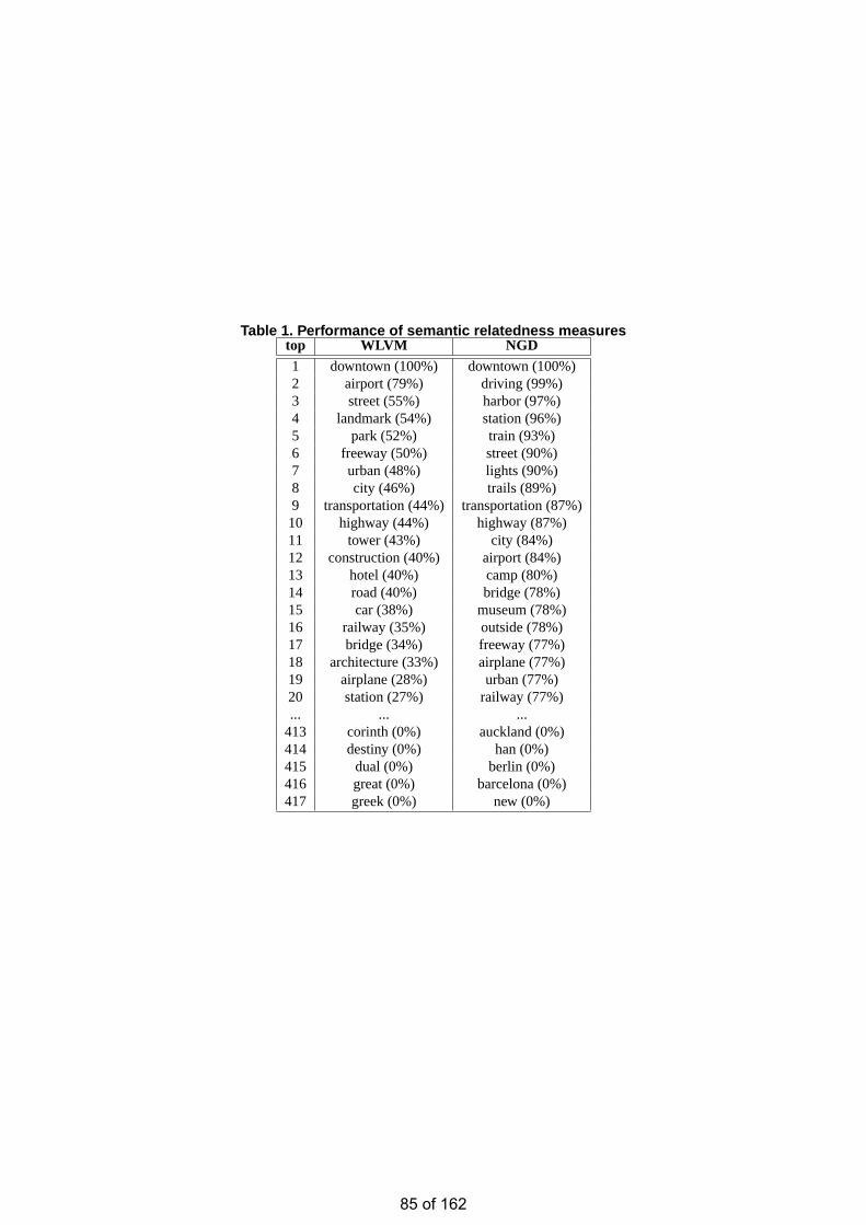
Table 1. Performance of semantic relatedness measurestop WLVM NGD1 downtown (100%) downtown (100%)2 airport(79%) driving (99%)3 street(55%) harbor(97%)4 landmark(54%) station(96%)5 park(52%) train (93%)6 freeway (50%) street(90%)7 urban(48%) lights (90%)8 city (46%) trails (89%)9 transportation(44%) transportation(87%)10 highway (44%) highway (87%)11 tower (43%) city (84%)12 construction(40%) airport(84%)13 hotel(40%) camp(80%)14 road(40%) bridge(78%)15 car(38%) museum(78%)16 railway (35%) outside(78%)17 bridge(34%) freeway (77%)18 architecture(33%) airplane(77%)19 airplane(28%) urban(77%)20 station(27%) railway (77%)... ... ...
413 corinth(0%) auckland(0%)414 destiny (0%) han(0%)415 dual(0%) berlin (0%)416 great(0%) barcelona(0%)417 greek(0%) new (0%)
85 of 162
4 Conclusion
In this paper, we propose an extension of image indexingmodels which uses ontology-based expansion with Word-Net, WLVM and NGD. Our system is evaluated quantita-tively, and experimental results indicate that this approachis able to deliver highly competent performance. Our ap-proach, not only demonstrates the applicability of ontologyto the image annotation problem, but also using the sub-objects as surrogate terms for general queries is to improvethe precision in the image sets.
[1] G. Amato and C. Meghini. Combining features forimage retrieval by concept lattice querying and navi-gation. International Conference on Image Analysisand Processing Workshops, 0:107–112, 2007.
[2] J. Amores, N. Sebe, and P. Radeva. Context-basedobject-class recognition and retrieval by generalisedcorrelograms.IEEE Transactions on Pattern Analysisand Machine Intelligence, 29(10):1818–1833, Octo-ber 2007.
[3] V. Athitsos, J. Alon, S. Sclaroff, and G. Kollios.Boostmap: A method for efficient approximate sim-ilarity rankings. IEEE Computer Society Conferenceon Computer Vision and Pattern Recognition, 02:268–275, 2004.
[4] I. Azzam, A. G. Charlapally, C. H. C. Leung, and J. F.Horwood. Content-based image indexing and retrievalwith xml representations.Proceedings of the Inter-national Symposium on Intelligent Multimedia, Videoand Speech Processing, Hong Kong, pages 181–185,2004.
[5] I. A. Azzam, C. H. C. Leung, and J. F. Horwood.Implicit concept-based image indexing and retrieval.In Proceedings of the IEEE International Conferenceon Multi-media Modeling, pages 354–359, Brisbane,Australia, January 2004.
[6] I. A. Azzam, C. H. C. Leung, and J. F. Horwood. Afuzzy expert system for concept-based image indexingand retrieval.International Conference on MultimediaModeling Conference, 0:452–457, 2005.
[7] K. Barnard, P. Duygulu, N. de Freitas, D. Forsyth,D. Blei, and M. Jordan. Matching words and pictures.Journal of Machine Learning Research, 3:1107–1135,2003.
[8] M. Boutell and J. Luo. Photo classification by inte-grating image content and camera metadata. InICPR’04: Proceedings of the Pattern Recognition, 17th In-ternational Conference on (ICPR’04) Volume 4, pages901–904, Washington, DC, USA, 2004. IEEE Com-puter Society.
[9] Y. Chen, J. Z. Wang, and R. Krovetz. Content-basedimage retrieval by clustering. InMIR’03: Proceed-ings of the 5th ACM SIGMM international workshopon Multimedia information retrieval, pages 193–200,New York, NY, USA, 2003. ACM.
[10] J. S. Cho and J. Choi. Contour-based partial objectrecognition using symmetry in image databases. InSAC’05: Proceedings of the 2005 ACM symposium onApplied computing, pages 1190–1194, New York, NY,USA, 2005. ACM Press.
[11] R. L. Cilibrasi and P. M. Vitanyi. The google similaritydistance.IEEE Transactions on Knowledge and DataEngineering, 19(3):370–383, 2007.
[12] D. Cremers, M. Rousson, and R. Deriche. A review ofstatistical approaches to level set segmentation: Inte-grating color, texture, motion and shape.InternationalJournal of Computer Vision, 72(2):195–215, 2007.
[13] R. Datta, J. Li, and J. Z. Wang. Content-based im-age retrieval: approaches and trends of the new age.In MIR’05: Proceedings of the 7th ACM SIGMM in-ternational workshop on Multimedia information re-trieval, pages 253–262, New York, NY, USA, 2005.ACM.
[14] L. Fan and B. Li. A hybrid model of image retrievalbased on ontology technology and probabilistic rank-ing. Web Intelligence, 0:477–480, 2006.
[15] K. Hornsby. Retrieving event-based semantics fromimages.International Symposium on Multimedia Soft-ware Engineering, 00:529–536, 2004.
[16] R. Krishnapuram, S. Medasani, S. H. Jung, Y. S. Choi,and R. Balasubramaniam. Content-based image re-trieval based on a fuzzy approach.IEEE Transactionson Knowledge and Data Engineering, 16(10):1185–1199, 2004.
[17] W. Ku, M. S. Kankanhalli, and J. H. Lim. Usingcamera settings templates (”scene modes”) for im-age scene classification of photographs taken on man-ual/expert settings. InThe Pacific-Rim Conference onMultimedia, pages 10–17, 2007.
[18] J. Li and J. Z. Wang. Automatic linguistic indexingof pictures by a statistical modeling approach.IEEE
86 of 162
Transactions on Pattern Analysis and Machine Intelli-gence, 25(9):1075–1088, 2003.
[19] H. Lieberman and H. Liu. Adaptive linking betweentext and photos using common sense reasoning.Adap-tive Hypermedia and Adaptive Web-Based Systems,Second International Conference, AH 2002, Malaga,Spain, pages 2–11, May 2002.
[20] D. Liu and T. Chen. Content-free image retrieval usingbayesian product rule.IEEE International Conferenceon Multimedia and Expo, 0:89–92, 2006.
[21] D. Milne and I. H. Witten. An effective, low-cost measure of semantic relatedness obtained fromwikipedia links. InWIKIAI’08: first AAAI Workshopon Wikipedia and Artificial Intelligence.
[22] A. P. Natsev, A. Haubold, J. Tesic, L. Xie, andR. Yan. Semantic concept-based query expansionand re-ranking for multimedia retrieval. InInterna-tional conference on Multimedia, pages 991–1000,New York, NY, USA, 2007. ACM.
[23] R. Pawlicki, I. Kokai, J. Finger, R. Smith, and T. Vet-ter. Navigating in a shape space of registered mod-els. IEEE Transactions on Visualization and Com-puter Graphics, 13(6):1552–1559, 2007.
[24] A. Perina, M. Cristani, and V. Murino. Natural scenescategorization by hierarchical extraction of typicalitypatterns.International Conference on Image Analysisand Processing, pages 801–806, 2007.
[25] A. Popescu, G. Grefenstette, and P. A. Moellic. Usingsemantic commonsense resources in image retrieval.In International Workshop on Semantic Media Adap-tation and Personalization, pages 31–36, Washington,DC, USA, 2006. IEEE Computer Society.
[26] P. Sinha and R. Jain. Classification and annotation ofdigital photos using optical context data. InThe In-ternational Conference on Image and Video Retrieval,pages 309–318, 2008.
[27] K. Stevenson and C. H. C. Leung. Comparative eval-uation of web image search engines for multimediaapplications.IEEE International Conference on Mul-timedia and Expo, 0:4 pp., 2005.
[28] M. Strube and S. P. Ponzetto. Wikirelate! computingsemantic relatedness using wikipedia. July 2006.
[29] Y. Sun, S. Shimada, and M. Morimoto. Visual patterndiscovery using web images.MIR’06: Proceedings ofthe 8th ACM international workshop on Multimediainformation retrieval, pages 127–136, 2006.
[30] A. M. Tam and C. H. C. Leung. Semantic content re-trieval and structured annotation: Beyond keywords.ISO/IEC JTC1/SC29/WG11 MPEG00/M5738, Noord-wijkerhout, Netherlands, March 2000.
[31] N. Vasconcelos. From pixels to semantic spaces: Ad-vances in content-based image retrieval.IEEE Com-puter, 40(7):20–26, 2007.
[32] J. Vogel, A. Schwaninger, C. Wallraven, and H. H.Bulthoff. Categorization of natural scenes: Local ver-sus global information and the role of color.ACMTransactions on Applied Perception, 4(3):19, 2007.
[33] M. Volkel, M. Krotzsch, D. Vrandecic, H. Haller,and R. Studer. Semantic wikipedia. InWWW ’06:Proceedings of the 15th international conference onWorld Wide Web, pages 585–594, New York, NY,USA, 2006. ACM.
[34] R. C. F. Wong and C. H. C. Leung. Automatic seman-tic annotation of real-world web images.IEEE Trans-actions on Pattern Analysis and Machine Intelligence,30(11):1933–1944, November 2008.
[35] T. Zoller and J. M. Buhmann. Robust image segmen-tation using resampling and shape constraints.IEEETransactions on Pattern Analysis and Machine Intelli-gence, 29(7):1147–1164, July 2007.
87 of 162
Hiding Emerging Pattern with Local Recoding Generalization
Michael Wai-Kit Cheng
Abstract
When data is published to public, it is vastly preferableto publish meaningful data and yet protect embedded sensi-tive patterns. This process is often referred to as privacypreserving data publishing (PPDP). In this paper, we in-vestigate PPDP in the context of frequent itemsets mining –one of the fundamental data-mining concepts – and emerg-ing patterns (EPs) – patterns that have a high classificationpower. More specifically, we want to hide all EPs embeddedin data while publishing the data with a minimal distortionon its frequent itemsets. We propose a novel heuristic solu-tion that captures the unique properties of hidding EPs andincorporates with local recoding generalization. To guidea bottom-up recoding generalization, a metric is derivedbased on (i) frequent-itemset distortion that quantifies thequality of published data and (ii) the degree of reduction inemerging patterns in each recoding generalization. We haveimplemented our proposed solution and experimentally ver-ified its effectiveness using two benchmark datasets.
1 Introduction
Organizations often publish or share their data to supportsubsequent data analysis for various reasons, for instance,advancing medical research [27] or raising customer satis-faction level [32]. In many cases, data may involve personalinformation or company’s secrets which are not supposed tobe disclosed in normal circumstances. Protecting the pub-lished data against privacy breaching is often of top priority.Nonetheless, people may still choose to relinquish certainprivacy for a greater good, but only when they can be as-sured that the published data will be properly sanitized.
Studies on data sanitization can be dated back to theearlier work on statistical disclosure control [1]. For in-stance, it is a common requirement to remove personal iden-tifiers from published data using mechanisms like masking(e.g., ID=“123456(7)” → ID=“123***(*)”) and substitu-tion (e.g., name=“Donald” → name=“YxfG1L”) to ensureanonymization. However, the privacy-breaching challengegoes beyond that. It has been clear that combinations ofquasi-identifiers, e.g., the demographic attributes, can al-
low sensitive information such as personal identity, facts, orforbidden patterns to be inferred, and thus disclosed [34].Given that data publishing is still a must in many situations,there has been a stream of work called privacy-preservingdata publishing (PPDP), emerged in recent years to flightagainst the privacy-breaching challenge [13]. The partic-ular type of PPDP considered in this paper tries to sanitizethe data to be published so that some specified sensitive pat-terns could not be discovered and meanwhile, certain statis-tical properties of the published data are preserved as far aspossible to support subsequent analysis.
In this paper, we argue that emerging patterns embeddedin data can carry important intelligence (e.g., newly emerg-ing sales opportunities revealed in sales records) that dataowners may want to hide before they publish them for fur-ther analysis. In particular, emerging patterns has knownto have a high classification power where EP-based classi-fiers can often be more accurate than classifiers with C5.0,naive Bayes and CAEP. At the meantime, frequent itemsetmining is a classical data mining technique and has alreadybeen well-supported by commercial data mining software.Published data may be evidently subjected to such an anal-ysis. Therefore, we study a novel form of PPDP where thesensitive information to be protected is emerging patterns indatasets and the data analysis is frequent itemset mining.
More specifically, given two transactional datasets D1
and D2, a threshold of growth rate ρ and a threshold ofsupport σ, we want to determine a sanitization operationG on both D1 and D2 such that the emerging patterns witha growth rate higher than ρ are eliminated and the distor-tion of σ-frequent itemsets is minimized. (The details ofthe problem formulation shall be given in Section 3.)Example 1.1: Let us consider an example from a demo-graphic dataset [36], which contains some census informa-tion of the United States. We divide the dataset into two:(i) people who earned more than $50/year and (ii) peoplewho do not. When we set ρ to be 35, we find that thereare 8 emerging patterns. One emerging pattern in (ii) is(never-married, own-child). In other words, in [36],there are at least 35 times more people who have never mar-ried and have their own child in (ii) than (i). We remark that(never-married, own-child) is not a frequent itemset ofthe entire dataset when σ = 0.4.
88 of 162
The example shows that emerging patterns may revealcertain sensitive information from data. For applicationslike publishing census reports, sanitizing data might not belegitimate. But for applications related to business intelli-gence, protecting customer data and cooperations’ interestsbecome a necessity. We speculate that in many other sce-narios, one may prefer to sanitize such sensitive informationembedded in data before publishing.
Different data sanitization approaches have been pro-posed in the literature for PPDP [12] (as well as other pri-vacy preservation related fields), which could be roughlycategorized into recoding generalization [20, 5, 15, 19, 34,28, 40, 35, 31] and perturbation [2, 8, 10, 18]. In thispaper, recoding generalization is adopted. Recoding gen-eralization has been extensively used in the context of k-anonymization which was originally proposed in [34]. Re-coding generalization is (intuitively) a value-grouping pro-cess according to a given attribute generalization hierarchy.Since the attribute hierarchy is always published with thedata, data recipients can correctly interpret every general-ized values that appear in the sanitized data. Therefore, thesanitized data can be “blurred” but is not lost. This workfocuses on exploring the possibilities of adopting recodinggeneralization in the context of hiding emerging patterns.
A sanitization is obviously unacceptable if a data min-ing technique would either (i) reveal sensitive informationor (ii) produce a highly distorted result from the sanitizeddata. These two competing objectives make the problemtechnically intriguing.
We remark that hiding emerging patterns is more tech-nically challenging than some related works on hiding fre-quent itemsets [30, 2]. The reason is that the apriori anti-monotone property of frequent itemsets does not hold foremerging patterns. Thus, the search space of emerging pat-terns cannot be pruned as effectively as that of frequentitemsets. Furthermore, recoding generalization may hidean emerging pattern as well as generating new emergingpatterns. To the best of our knowledge, there has notbeen work on adopting recoding generalization techniquesto hide emerging patterns.
The paper is organized as follows. In Section 2, we give abrief summary on the research on PPDP. In Section 3, wepresent the background and notations used and give the for-mal problem statement of this paper. In Section 4, we dis-cuss the recoding generalization technique adopted to solvethis problem. Section 5 gives an overview of our algorithm.Section 6 derives the heuristics that quantifies the qualityof a recoding generalization. Section 7 discusses a numberof optimizations related to solving this PPDP problem. InSection 8, we present an experimental evaluation that veri-fies the effectiveness of our proposed algorithm. Section 9concludes this work and discusses future works.
2 Related Work
There have been recent research efforts on various as-pects of PPDP. In this section, we highlight some relevant,admittedly non-exhaustive PPDP techniques.
Anonymity measure and recoding generalization. In ananalysis of a demographic dataset with external informa-tion [35], it has been shown that personal identity can be re-covered from a published dataset, even the identifiers havebeen removed. The notion of k-anonymity [35] was thusintroduced. A published data is said to be k-anonymized ifat least k individuals are linked with a particular record inthe published data even if the data may be cross-referencedwith external information. Each group of items with indis-tinguishable attribute values is called an equivalence class.To further improve k-anonymity, `-diversity [25] was pro-posed to require also each sensitive value in each equiva-lence class to appear at most 1/` times.
Given a particular measure, recoding generalization [34,40, 23] is commonly adopted to achieve anonymization.Recoding generalization has two advantages over the per-turbation approach for data sanitization,. First, the datasetsanitized by recoding generalization is still semanticallyconsistent with the original one. The information conveyedby a generalized dataset always contains the truth, eventhough it is “blurred”. In contrast, perturbation techniquesmay generate fake information. These may not be accept-able in many real applications, e.g., a database with pa-tient information. Second, since the attribute hierarchy isoften published with the dataset, the generalized values inthe published dataset can be always interpreted. We adoptrecoding generalization, to protect emerging patterns.
The notion of information preservation. There has beena stream of work on k-anonymity which also makes anattempt to preserve as much information of the originaldataset as possible [5, 16, 14]. For example, [5, 16] con-siders the preservation of classification accuracy during thesanitization process. [14] investigates the preservation ofcluster structures of the data. In addition, there has beensome recent work studying the trade-off effect between pri-vacy and utility [24] in the context of PPDP. However, theyare not designed to tackle some particular patterns.
Frequent itemset hiding. There has been previous work[30, 33, 29] on hiding frequent itemsets for PPDP. In par-ticular, users specify a subset of frequent itemsets, namelysensitive frequent itemsets, that are not supposed to be dis-closed to public. The main objective of this related workis to sanitize the data such that the sensitive frequent item-sets are removed from the sanitized data while non-sensitivefrequent itemsets are retained as many as possible. In ourstudy, we focus on hiding emerging patterns, which makesa different contribution to PPDP.
89 of 162
We remark that the previous work on frequent-itemsethiding used techniques like removing sensitive data, intro-ducing random and unknown data. Recoding generalizationhas not been adopted in this stream of work.
Emerging patterns. Intuitively, EPs are some distinctivefeatures from one class to the others. Much previous effort[17, 38, 11, 7] has been spent on using EPs for building clas-sifiers. The results of these efforts have shown that the accu-racy of EP-based classifiers can often be higher than those oftraditional classifiers, such as, C5.0 and naive Bayes. Dueto the high classification power, EP-based classifiers havebeen used for predicting the likelihood of diseases such asacute lymphoblastic leukemia [21] and discovering knowl-edge in gene expression data [22].
Although EPs have been found useful in classification,there have not been studies on EPs with PPDP. Previouswork on EPs focuses on the mining efficiency. Mining EPshas been technically intriguing. First, the total number ofEPs in large datasets can be huge. In the worst case, thetotal number of EPs is exponential to the total number ofattributes in transactions. Second, there has not been a cor-responding notion of the apriori anti-monotone property offrequent itemsets in EPs. As such, the search space pruningstrategies of frequent-itemset mining cannot be adopted toEP mining. There have been a border-based approach [4],constraint-based approach [41] and jumping emerging pat-terns [3] to improve the efficiency of EP mining.
3 Background and Problem Statement
In the following, we present the definitions, notationsused and the problem statement of the paper.
Let D be a transactional dataset and I := i1, i2, ..., inbe a finite set of distinct items in D. A transaction tmay have a set of nominal attributes A and each attributetakes values from a set Vi ⊆ I , where the domain D isV1 × V2 × ... × V|A|. We make two simple remarks aboutthese notations. (i) While we assume transactional datawith nominal attributes, data of a continuous domain canbe casted into nominal data, e.g., by defining ranges. (ii)One may consider a relation as a set of transactions of afixed arity.
SuppD(X) denotes the support of an itemset X ⊆ I
in a dataset D, which can be computed as |t | X∈t∧t∈D||D| .
Given a support threshold σ, X is said to be a σ-frequentitemset if SuppD(X) ≥ σ. The growth rate of an itemset isthe ratio of its support in one dataset to that in the other.
Definition 3.1: [6] Given two datasets, namely D1 and D2,the growth rate of an itemset X , denoted as GR(X , D1,
D2), from D1 to D2 is defined as GR(X , D1, D2) =
0 , if SuppD1 = 0 and SuppD2 = 0
∞ , if SuppD1 = 0 and SuppD2 > 0SuppD2 (X)
SuppD1 (X), otherwise.
Intuitively, given two datasets, emerging patterns(EPs) [6] are the itemsets whose support increases signifi-cantly from one dataset to another. The formal definition ofEPs can be given as follows.
Definition 3.2: [6] Given a growth rate threshold ρ and twodatasets D1and D2, an itemset X is said to be a ρ-emergingpattern (ρ-EP) from D1 to D2 if GR(X , D1, D2) ≥ ρ .
An emerging pattern with a growth rate ∞ (i.e. item-set that appears in one dataset but not the other) is called ajumping emerging pattern.
For ease of presentation, we may skip σ, ρ, D1 and D2
of EPs when they are not essential to our discussions.Example 3.1: Table 1 shows a hypothetical dataset D ofAdult dataset [36]. More description of the dataset can befound in Section 8. We opt to present some nominal at-tributes of Adult for discussions. Each record (or transac-tion) represents a person. Let us consider two subsets of D:D1 contains the people who are married and D2 containsthe people who never marry before. From Table 1, we findthe following patterns, among many others.• The pattern (MSE, manager) has a support 75% in D1
and 20% in D2. Therefore, the growth rate of (MSE,manager) from D1 to D2 is 3.75. When we set ρ to3, (MSE, manager) is a ρ-emerging pattern in D2. Ob-viously, when we set ρ to 4, (MSE, manager) is not aρ-emerging pattern.
• High-school graduate (HS) has a support 0% in D1 but20% in D2. Hence, its grwoth rate from D2 to D1 isinfinite. (HS) is a jumping emerging pattern in D1.
• Suppose that the threshold support for frequent itemsetσ is set to 50%. Neither (MSE, manager) nor (HS) is aσ-frequent itemset of D. In comparison, (manager) isa σ-frequent itemset, whose support is 77.8%.
Using the above notations, we state the formal problemstatement of this paper below (visualized in Figure 3).Problem statement. Given two datasets (D1, D2), σ and ρ,we want to sanitize (D1, D2) to (D′
1, D′2) such that no ρ-EPs
can be mined from (D′1, D′
2) while the distortion betweenσ-frequent itemsets of (D1, D2) and those of (D′
1, D′2) is
minimized.
4 Global vs Local Recoding Generalization
Our proposed algorithm for hiding emerging pattern isderived from local recoding generalization. In this section,
90 of 162
Table 1. A hypothetical subset of AdultID Edu. Martial Occup. Rel. Race Sex
1 BA married executive wife black F2 MSE married manager husband black M3 MSE married manager wife white F4 MSE married manager husband black M5 BA never manager NA white M6 MSE never manager NA white F7 HS never repair NA black M8 BA never manager NA white M9 BA never manager NA black F
Figure 1. The problem statement illustration
we give a brief overview on global and local recoding gen-eralization, or recoding for simplicity, and its variations.Recoding. In privacy-preserving data mining, recoding hasbeen a popular technique for sanitizing datasets in orderto achieve anonymization. The key idea of recoding is tomodify a value into a more general value such that more tu-ples will share the same values and cannot be distinguishedindividually. Thus, anonymization can be achieved. Inthis work, we recode emerging patterns with some non-emerging values. As a result, the corresponding patternsbecome less emerging after recoding. Such a recoding pro-cess is repeated until the desired anonymization is reached.Variations of recoding. In the following, we describe thethere types of recoding. In this work, we adopt the last re-coding technique.
1. Single-dimensional global recoding. Single-dimensionalglobal recoding has been studied in [5, 15, 19, 34]. It per-forms recoding on the domain of an attribute in a dataset.It recodes a value of the domain to another (generalized)value. That is, if a particular value is recoded, the at-tribute of all the tuples containing that particular value willbe recoded. It is evident that datasets are very often over-generalized by this recoding.
2. Multidimensional global recoding. Multidimensionalglobal recoding was first proposed in [20]. It generalizesdata at “cell” level. This recoding relies on the notion ofequivalence classes. An equivalence class of attributes Ais a set of tuples T where πA(T ) is a singleton. That is,the tuples in T has the same value in attributes A. In mul-tidimensional global recoding, the tuples in an equivalenceclass (of a set of attributes) are generalized together. By do-
ing so, both original and generalized values may exist in therecoded dataset. When compared to the previous global re-coding, multidimensional global recoding generalizes datain a finer granularity. Hence, this recoding over-generalizesdata less often.
Example 4.1: Let us revisit the dataset in Table 1 and theemerging pattern (MSE, manager). The pattern is related tothe attributes of education background (Edu.) and occupa-tion (Occup.). Regarding (Edu., Occup.), the equivalenceclasses in D2 are 5, 8, 9, 6, 7, where the numbersare the IDs. In multidimensional global recoding, we mayrecode the Edu. attribute of 2, 3, 4 and 5, 8, 9. For in-stance, we may recode BA and MSE into degree holder Deg.After such a recoding, all BA, MSE and Deg. appear in therecoded dataset. We remark that (Deg., manager) is not anemerging pattern since its growth rate is 75%/60% = 1.25.
3. Multidimensional local recoding. Local recoding hasbeen studied in [9, 28, 40, 23] in the context of k-anonymity.It performs generalization at cell level as well. It also relieson equivalence classes. Its difference between the multidi-mensional global recoding is that it does not require the en-tire equivalence class to be recoded, as long as anonymityhas been achieved. For instance, we may recode 8, 9,as opposed to 5, 8, 9, with 2, 3, 4 in Example 4.1.The growth rate of (Deg., manager) in the recoded datasetis 75%/40% = 1.875. Hence, (Deg., manager) is not ρ-emerging when ρ = 3.
In this paper, we focus on this recoding. In the subsequentdiscussions, we use the term local recoding to refer to mul-tidimensional local recoding.
5 Overview on hiding emerging patterns
In this section, we present an overall algorithmhide-eps (shown in Figure 2) to hide emerging patternswith a minimal distortion in frequent itemsets. Its detailsshall be discussed shortly. Then, we provide some detailsof the heuristics in hide-epse in Section 6.Overall algorithm. We give the main ideas of Figure 2.First, we find the frequent itemsets to be preserved (Line 03)and the emerging patterns to be hidden (Line 04). InLine 05, we select an emerging pattern to hide. Next, wecarry out a local recoding local-recoding (Line 06).This process is repeated until there is no more emergingpattern to hide (Lines 07-08).
The main tasks of the local recoding local-recoding
are to compute (i) the equivalence classes of an emergingpattern e to generalize (Line 03) and (ii) the correspondingutility gain (details in Section 6) to guide us to choose anequivalence class for local recoding (Line 06). To avoid be-
91 of 162
Procedure hide-epsInput: two datasets, Di and Dj , the threshold of
the growth rate and frequent itemsets ρ and σ,the heuristic parameters p and q,a temperature t0 and the cooling parameter α
Output: transformed datasets (Di, Dj)
01 initialize a hashtable H to optimizecomputing equiv. classes; t = t0
02 do03 F := mine-fis(Di ∪Dj , σ)04 E := mine-eps(Di, Dj , ρ)05 e := next-overlapping-ep(E)06 if e is not null
(Di, Dj) := local-recoding(Di, Dj , e, F , t, α)07 if t > 0.01 then t = α × t08 while E 6= ∅09 return (Di, Dj)
Procedure local-recodingInput: two datasets, Di and Dj , an emerging pattern ea frequent itemset F , a temperature t0
Output: transformed datasets (Di, Dj)
01 let Di be the dataset where e has a higher support02 t := t0; u = 0 //initialization03 compute equiv. classes C of Dj of the attr. of e04 //compute the heuristic function of local recoding05 denote ce be the equiv. class of e in Di
06 for each ck in CH[ce][ck] := util gain(G(ce,ck), E) //heap
r[ck] = expH[ce][ck]
t
sum = sum + r[ck]07 find k s.t. r[ck]/sum < rand(1)< r[ck+1]/sum
Di := recode(Di, ce, ck)Dj := recode(Dj , ce, ck)
08 return (Di, Dj)
Figure 2. Overall algorithm
ing trapped at some local sub-optima, we present our algo-rithm in a simulated-annealing style search (Lines 06-08).
Next, we provide the details of the overall algorithm.The effect of local recoding on frequent itemsets. Wefirst remark that global recoding may only merge some fre-quent itemsets, shown in Figure 3 (a). Hence, the change infrequent itemsets due to global recoding can be determinedeasily. However, local recoding may lead to a non-trivialchange in frequent itemsets, shown in Figure 3 (b). Thereason is that by the definition of local recoding, two tuples,even in the same equivalence class, are not always recodedtogether. This leads to a few possible effects on the frequentitemsets. First, since some of the values of the attributes Ahave been recoded to a generalized value, a frequent itemsetmay not be frequent after a local recoding. Second, multi-ple frequent itemsets may be recoded into one generalizedfrequent itemset. Third, a frequent itemset may not be af-fected by a local recoding. The first case is only possible
Figure 3. The relationship between F and F ′
in (a) global recoding (b) local recoding
with local recoding whereas the second and third cases mayappear correspondingly in global recoding as well.
The above complication leads to Line 04 of hide-eps,which mines the current frequent itemsets in each iterationof local recoding.The selection of emerging patterns for hiding. In theworst case, there are O(|E| × (|D1| + |D2|) × D × H)possible local recodings on a set of emerging patterns E,where D is the total size of the domains of the attributesof E and H is the total height of the hierarchy of the at-tributes of E. In the worst case, local recoding allowstuple-wise recoding, which leads to the term |D1| + |D2|.While there may be search algorithms to explore an opti-mal local recoding on E, we employ a simple and efficientsolution to avoid exploring a large search space – we hidean emerging pattern, one-at-a-time (Line 05 of hide-eps,next-overlapping-ep), based on equivalence classes.
The pseudocode of next-overlapping-ep has beenomitted, since it is straightforward but tedious. Here, wepresent its intuitions. Given a set of emerging patterns E,next-overlapping-ep determines the emerging patterne in E such that it overlaps with the remaining emergingpatterns the most. The intuition is that reducing the growthrate of e may indirectly reduce the growth rate of the over-lapping emerging patterns as well. We verify this with somepreliminary experiments that this approach consistently out-performs generalizing the most independent, the longest orthe shortest emerging patterns first.The search algorithm. The algorithm is presented in a sim-ulated anneanling style in Figure 2. We have implementeda deterministic search to analyze our heuristics (Section 6).
6 Heuristics for Guiding Local Recoding
In this section, we present the formulation of the utilitygain (util gain) adopted to guide the local recoding pro-cess local-recoding, discussed in Figure 2. The mainidea is that we consider a local recoding perferrable if it re-sults in a small distortion in the frequent itemsets and at thesame time it reduces the growth rate of an emerging patternsignificantly. In the following two subsections 6.1 and 6.2,we present the details of the metrics for measuring (i) thedistortion of frequent itemsets and (ii) the reduction in thegrowth rate of emerging patterns, respectively.
92 of 162
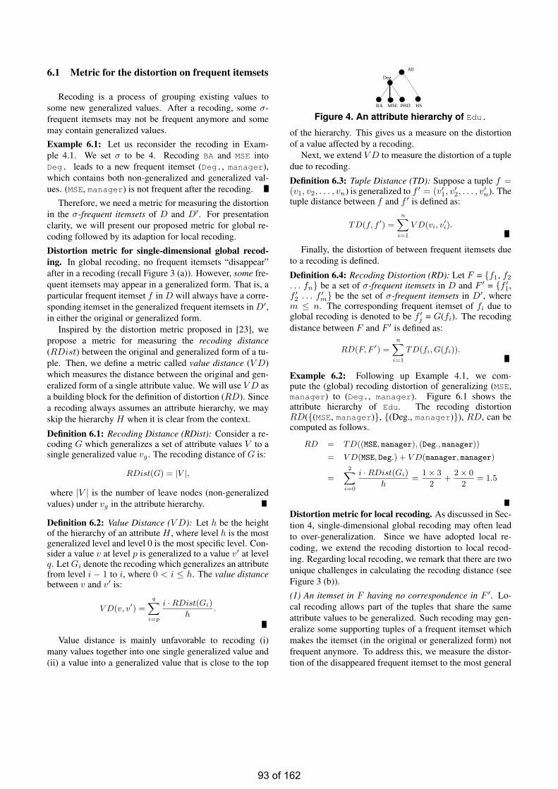
6.1 Metric for the distortion on frequent itemsets
Recoding is a process of grouping existing values tosome new generalized values. After a recoding, some σ-frequent itemsets may not be frequent anymore and somemay contain generalized values.Example 6.1: Let us reconsider the recoding in Exam-ple 4.1. We set σ to be 4. Recoding BA and MSE intoDeg. leads to a new frequent itemset (Deg., manager),which contains both non-generalized and generalized val-ues. (MSE, manager) is not frequent after the recoding.
Therefore, we need a metric for measuring the distortionin the σ-frequent itemsets of D and D′. For presentationclarity, we will present our proposed metric for global re-coding followed by its adaption for local recoding.
Distortion metric for single-dimensional global recod-ing. In global recoding, no frequent itemsets “disappear”after in a recoding (recall Figure 3 (a)). However, some fre-quent itemsets may appear in a generalized form. That is, aparticular frequent itemset f in D will always have a corre-sponding itemset in the generalized frequent itemsets in D′,in either the original or generalized form.
Inspired by the distortion metric proposed in [23], wepropose a metric for measuring the recoding distance(RDist) between the original and generalized form of a tu-ple. Then, we define a metric called value distance (V D)which measures the distance between the original and gen-eralized form of a single attribute value. We will use V D asa building block for the definition of distortion (RD). Sincea recoding always assumes an attribute hierarchy, we mayskip the hierarchy H when it is clear from the context.
Definition 6.1: Recoding Distance (RDist): Consider a re-coding G which generalizes a set of attribute values V to asingle generalized value vg . The recoding distance of G is:
RDist(G) = |V |,
where |V | is the number of leave nodes (non-generalizedvalues) under vg in the attribute hierarchy.
Definition 6.2: Value Distance (V D): Let h be the heightof the hierarchy of an attribute H , where level h is the mostgeneralized level and level 0 is the most specific level. Con-sider a value v at level p is generalized to a value v′ at levelq. Let Gi denote the recoding which generalizes an attributefrom level i− 1 to i, where 0 < i ≤ h. The value distancebetween v and v′ is:
V D(v, v′) =
q∑i=p
i ·RDist(Gi)
h.
Value distance is mainly unfavorable to recoding (i)many values together into one single generalized value and(ii) a value into a generalized value that is close to the top
All
Deg
BA MSE PHD HS
Figure 4. An attribute hierarchy of Edu.
of the hierarchy. This gives us a measure on the distortionof a value affected by a recoding.
Next, we extend V D to measure the distortion of a tupledue to recoding.
Definition 6.3: Tuple Distance (TD): Suppose a tuple f =(v1, v2, . . . , vn) is generalized to f ′ = (v′1, v
′2, . . . , v
′n). The
tuple distance between f and f ′ is defined as:
TD(f, f ′) =
n∑i=1
V D(vi, v′i).
Finally, the distortion of between frequent itemsets dueto a recoding is defined.
Definition 6.4: Recoding Distortion (RD): Let F = f1, f2
. . . fn be a set of σ-frequent itemsets in D and F ′ = f ′1,f ′2 . . . f ′m be the set of σ-frequent itemsets in D′, wherem ≤ n. The corresponding frequent itemset of fi due toglobal recoding is denoted to be f ′j = G(fi). The recodingdistance between F and F ′ is defined as:
RD(F, F ′) =
n∑i=1
TD(fi, G(fi)).
Example 6.2: Following up Example 4.1, we com-pute the (global) recoding distortion of generalizing (MSE,manager) to (Deg., manager). Figure 6.1 shows theattribute hierarchy of Edu. The recoding distortionRD((MSE, manager), (Deg., manager)), RD, can becomputed as follows.
RD = TD((MSE, manager), (Deg., manager))
= V D(MSE, Deg.) + V D(manager, manager)
=
2∑i=0
i ·RDist(Gi)
h=
1× 3
2+
2× 0
2= 1.5
Distortion metric for local recoding. As discussed in Sec-tion 4, single-dimensional global recoding may often leadto over-generalization. Since we have adopted local re-coding, we extend the recoding distortion to local recod-ing. Regarding local recoding, we remark that there are twounique challenges in calculating the recoding distance (seeFigure 3 (b)).(1) An itemset in F having no correspondence in F ′. Lo-cal recoding allows part of the tuples that share the sameattribute values to be generalized. Such recoding may gen-eralize some supporting tuples of a frequent itemset whichmakes the itemset (in the original or generalized form) notfrequent anymore. To address this, we measure the distor-tion of the disappeared frequent itemset to the most general
93 of 162
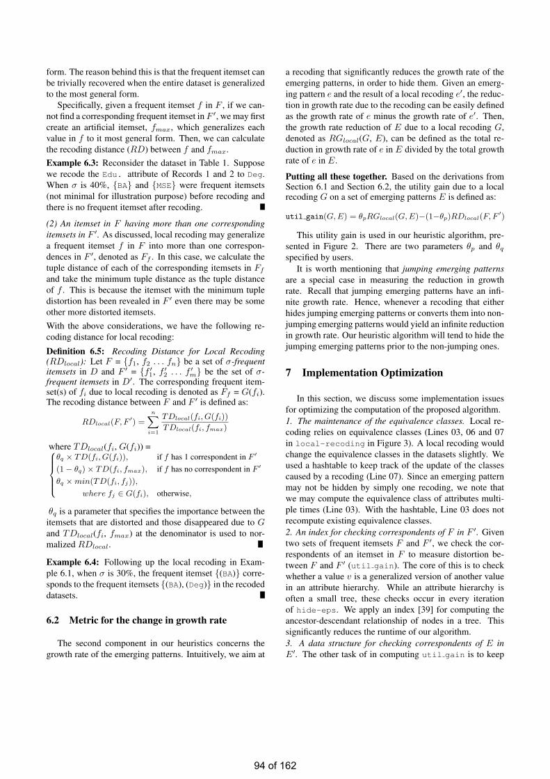
form. The reason behind this is that the frequent itemset canbe trivially recovered when the entire dataset is generalizedto the most general form.
Specifically, given a frequent itemset f in F , if we can-not find a corresponding frequent itemset in F ′, we may firstcreate an artificial itemset, fmax, which generalizes eachvalue in f to it most general form. Then, we can calculatethe recoding distance (RD) between f and fmax.Example 6.3: Reconsider the dataset in Table 1. Supposewe recode the Edu. attribute of Records 1 and 2 to Deg.When σ is 40%, BA and MSE were frequent itemsets(not minimal for illustration purpose) before recoding andthere is no frequent itemset after recoding.
(2) An itemset in F having more than one correspondingitemsets in F ′. As discussed, local recoding may generalizea frequent itemset f in F into more than one correspon-dences in F ′, denoted as Ff . In this case, we calculate thetuple distance of each of the corresponding itemsets in Ff
and take the minimum tuple distance as the tuple distanceof f . This is because the itemset with the minimum tupledistortion has been revealed in F ′ even there may be someother more distorted itemsets.With the above considerations, we have the following re-coding distance for local recoding:
Definition 6.5: Recoding Distance for Local Recoding(RDlocal): Let F = f1, f2 . . . fn be a set of σ-frequentitemsets in D and F ′ = f ′1, f ′2 . . . f ′m be the set of σ-frequent itemsets in D′. The corresponding frequent item-set(s) of fi due to local recoding is denoted as Ff = G(fi).The recoding distance between F and F ′ is defined as:
RDlocal(F, F ′) =
n∑i=1
TDlocal(fi, G(fi))
TDlocal(fi, fmax)
where TDlocal(fi, G(fi)) =
θq × TD(fi, G(fi)), if f has 1 correspondent in F ′
(1− θq)× TD(fi, fmax), if f has no correspondent in F ′
θq ×min(TD(fi, fj)),
where fj ∈ G(fi), otherwise,
θq is a parameter that specifies the importance between theitemsets that are distorted and those disappeared due to Gand TDlocal(fi, fmax) at the denominator is used to nor-malized RDlocal.
Example 6.4: Following up the local recoding in Exam-ple 6.1, when σ is 30%, the frequent itemset (BA) corre-sponds to the frequent itemsets (BA), (Deg) in the recodeddatasets.
6.2 Metric for the change in growth rate
The second component in our heuristics concerns thegrowth rate of the emerging patterns. Intuitively, we aim at
a recoding that significantly reduces the growth rate of theemerging patterns, in order to hide them. Given an emerg-ing pattern e and the result of a local recoding e′, the reduc-tion in growth rate due to the recoding can be easily definedas the growth rate of e minus the growth rate of e′. Then,the growth rate reduction of E due to a local recoding G,denoted as RGlocal(G, E), can be defined as the total re-duction in growth rate of e in E divided by the total growthrate of e in E.
Putting all these together. Based on the derivations fromSection 6.1 and Section 6.2, the utility gain due to a localrecoding G on a set of emerging patterns E is defined as:
util gain(G, E) = θpRGlocal(G, E)−(1−θp)RDlocal(F, F ′)
This utility gain is used in our heuristic algorithm, pre-sented in Figure 2. There are two parameters θp and θq
specified by users.It is worth mentioning that jumping emerging patterns
are a special case in measuring the reduction in growthrate. Recall that jumping emerging patterns have an infi-nite growth rate. Hence, whenever a recoding that eitherhides jumping emerging patterns or converts them into non-jumping emerging patterns would yield an infinite reductionin growth rate. Our heuristic algorithm will tend to hide thejumping emerging patterns prior to the non-jumping ones.
7 Implementation Optimization
In this section, we discuss some implementation issuesfor optimizing the computation of the proposed algorithm.1. The maintenance of the equivalence classes. Local re-coding relies on equivalence classes (Lines 03, 06 and 07in local-recoding in Figure 3). A local recoding wouldchange the equivalence classes in the datasets slightly. Weused a hashtable to keep track of the update of the classescaused by a recoding (Line 07). Since an emerging patternmay not be hidden by simply one recoding, we note thatwe may compute the equivalence class of attributes multi-ple times (Line 03). With the hashtable, Line 03 does notrecompute existing equivalence classes.2. An index for checking correspondents of F in F ′. Giventwo sets of frequent itemsets F and F ′, we check the cor-respondents of an itemset in F to measure distortion be-tween F and F ′ (util gain). The core of this is to checkwhether a value v is a generalized version of another valuein an attribute hierarchy. While an attribute hierarchy isoften a small tree, these checks occur in every iterationof hide-eps. We apply an index [39] for computing theancestor-descendant relationship of nodes in a tree. Thissignificantly reduces the runtime of our algorithm.3. A data structure for checking correspondents of E inE′. The other task of in computing util gain is to keep
94 of 162
track of the change of emerging patterns during local recod-ing, which is neccessary to measure the reduction in growthrate. Hence, we associate an emerging pattern of e to itsrecords. By comparing the records of e and e′, we obtainthe correspondence between e and e′.
8 Experimental Evaluation
To verify the effectiveness of our proposed algorithms,we have conducted an experimental study of our algorithmon two benchmark datasets.
We have implemented both our algorithm in simulatedannealing style in Figure 2 and a greedy-search version ofthis algorithm, denoted as SA and Greedy, respectively.The implementation is written in JAVA SDK 1.6. We haverun our experiment on a desktop PC with a Quad CPU at2.4GHz and 3.25GB RAM. The desktop PC runs a WindowsXP operating system. We have used system calls to in-voke the implementations from [41] and [26] to determineemerging patterns and frequent itemsets, respectively.
We have applied our implementation on two datasets,namely Adult [36] and Mushroom [37]. Adult is a cen-sus dataset which is used to predict whether a person’s in-come exceeds $50k/year. Each record in Adult containseight attributes. We removed the records that contain miss-ing values. Adult has two classes of people – people whoearn more than $50k/year (7508 records) and people whodo not (22654 records). We used the attribute hierarchypresented in [15] for local recoding. Mushroom describesphysical characteristics, classification and poisonous/edibleproperties of mushrooms. Our discussions will mainly fo-cus on Adult as its results demonstrate the properties of ourproposed algorithm better.The effect of the parameters θp and θq. We performed aset of experiments to verify the effects on the parameters θp
and θq on the heuristic algorithm. The performance met-ric used was given in distortion on the frequent itemsets /the number of missing frequent itemsets, unless otherwisespecified. We used the Adult dataset and Greedy in thisexperiment. σ and ρ were set to 40% and 5, respectively.The frequent itemsets are:
(Husband, Married-civ-spouse, Male)(Married-civ-spouse, White)(Married-civ-spouse, United-States)(Male, Private, White)(Male, Private, United-States)(Male, White, United-States)
(Private, White, United-States).
When we recode all attributes to All in the frequentitemsets, we obtain the maximum distortion of the frequentitemsets of Adult 623.1.
To illustrate the possible recoding in the frequent item-sets, we list the frequent itemsets after applying Greedy,where θp and θq were both set to 0.8:
Table 2. The effect of the parameters inutil gain on Greedy’s performance on Adultθp\θq 0.0 0.2 0.4 0.6 0.8 1.0
0 0/0 50/1 50/1 50/1 50/1 NA0.2 46.7/1 73.3/1 21.5/1 21.5/1 21.5/1 7.5/30.4 46.7/1 73.3/1 21.5/1 21.5/1 21.5/1 7.5/30.6 46.7/1 73.3/1 42.5/1 42.5/1 21.5/1 7.5/30.8 46.7/1 73.3/1 21.5/1 42.5/1 42.5/1 7.5/41.0 7.5/4 7.5/4 7.5/4 7.5/4 7.5/4 7.5/4
(Relationship, United-States)(Married, White, United-States)(Male, Private, White)(Male, Private, United-States)(Male, White, United-States)
(Private, White, United-States).
The distortion obtained is 21.5 (out of 623.1).Next, we varied θp and θq and measured the distortion of
frequent itemsets and runtime of our algorithm. The resultsare shown in Table 2 and Table 3.
We make a few observations from Table 2 and Table 3.Firstly, when θp is set to 0, the algorithm only concerns dis-tortion (regardless of the corresponding reduction in growthrate) during local recodings. In such a case, the distortionin frequent itemsets of various θq’s is in general large. Wenote that the corresponding runtime in Table 3 is also rela-tively high. We used DNF to denote “did not finish in 360mins”. The reason is that when θp is 0, the heuristics do noteffectively reduce the growth rate and the search takes morerecodings that are not relevant to hiding emerging patterns.This results in a relatively large distortion and runtime.
Secondly, when θp is 1, util gain concerns only thereduction in growth rate. Table 3 shows that util gain fin-ished quickly. However, four frequent itemsets disappeared.
Thirdly, when we set θq to 1 and varied θp, we do notconsider the frequent itemsets that disappear. Hence, suchrecodings lose relatively more frequent itemsets. Similarly,when we set θq to 0, we consider only the distortion of thosethat do not disappear. Since there is in fact one frequentitemset that disappears during recodings, overlooking thisfrequent itemset would lead to more distortion.
Fourthly, we obtained no distortion with no missing fre-quent itemset when θp was 1 and θq was 0. We speculatethat this is an outlier (although a good outlier), as we bench-marked our the algorithm with a real dataset.
In all, we found that on the Adult dataset, Greedy mayyield frequent itemsets with a distortion of 21.5 (out of623.1) and one (out of seven) missing frequent itemset whenθp is moderate (0.2 - 0.6) and θq is large (0.8).Simulated annealing search. After verifying the effectof the parameters θp and θq on Greedy, we applied SA toAdult. We set the temperature of SA to be low with a highcooling rate (T = 10 and α = 0.4). Hence, SA initially hassome chance to avoid local sub-optimas and then convergesto Greedy quickly. SA is allowed to restart five times and
95 of 162
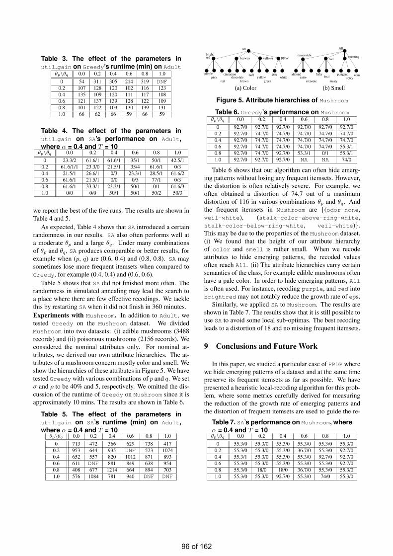
Table 3. The effect of the parameters inutil gain on Greedy’s runtime (min) on Adult
θp\θq 0.0 0.2 0.4 0.6 0.8 1.00 54 311 305 214 319 DNF
0.2 107 128 120 102 116 1230.4 135 109 120 111 117 1080.6 121 137 139 128 122 1090.8 101 122 103 130 139 1311.0 66 62 66 59 66 59
Table 4. The effect of the parameters inutil gain on SA’s performance on Adult,where α = 0.4 and T = 10
θp\θq 0.0 0.2 0.4 0.6 0.8 1.00 23.3/2 61.6/1 61.6/1 35/1 50/1 42.5/1
0.2 61.6/1/1 23.3/0 21.5/1 35/4 61.6/1 0/30.4 21.5/1 26.6/1 0/3 23.3/1 28.5/1 61.6/20.6 61.6/1 21.5/1 0/0 0/3 77/1 0/30.8 61.6/1 33.3/1 23.3/1 50/1 0/1 61.6/31.0 0/0 0/0 50/1 50/1 50/2 50/3
we report the best of the five runs. The results are shown inTable 4 and 5.
As expected, Table 4 shows that SA introduced a certainrandomness in our results. SA also often performs well ata moderate θp and a large θq. Under many combinationsof θp and θq, SA produces comparable or better results, forexample when (p, q) are (0.6, 0.4) and (0.8, 0.8). SA maysometimes lose more frequent itemsets when compared toGreedy, for example (0.4, 0.4) and (0.6, 0.6).
Table 5 shows that SA did not finished more often. Therandomness in simulated annealing may lead the search toa place where there are few effective recodings. We tacklethis by restarting SA when it did not finish in 360 minutes.Experiments with Mushroom. In addition to Adult, wetested Greedy on the Mushroom dataset. We dividedMushroom into two datasets: (i) edible mushrooms (3488records) and (ii) poisonous mushrooms (2156 records). Weconsidered the nominal attributes only. For nominal at-tributes, we derived our own attribute hierarchies. The at-tributes of a mushroom concern mostly color and smell. Weshow the hierarchies of these attributes in Figure 5. We havetested Greedy with various combinations of p and q. We setσ and ρ to be 40% and 5, respectively. We omitted the dis-cussion of the runtime of Greedy on Mushroom since it isapproximately 10 mins. The results are shown in Table 6.
Table 5. The effect of the parameters inutil gain on SA’s runtime (min) on Adult,where α = 0.4 and T = 10
θp\θq 0.0 0.2 0.4 0.6 0.8 1.00 713 472 366 629 738 417
0.2 953 644 935 DNF 523 10740.4 652 557 820 1012 871 8930.6 611 DNF 881 849 638 9540.8 408 677 1214 664 894 7031.0 576 1084 781 940 DNF DNF
purpleyellow
cinnamonchocolatepink
brownred
buff
green
graywhite
browny yellowy B&Wbrightred
All
almondanise
creosote
fishyfoul
musty
pungentspicy
none
irritating
All
badreasonable
(b) Smell(a) Color
Figure 5. Attribute hierarchies of Mushroom
Table 6. Greedy’s performance on Mushroomθp\θq 0.0 0.2 0.4 0.6 0.8 1.0
0 92.7/0 92.7/0 92.7/0 92.7/0 92.7/0 92.7/00.2 92.7/0 74.7/0 74.7/0 74.7/0 74.7/0 74.7/00.4 92.7/0 74.7/0 74.7/0 74.7/0 74.7/0 74.7/00.6 92.7/0 74.7/0 74.7/0 74.7/0 74.7/0 55.3/10.8 92.7/0 74.7/0 92.7/0 53.3/1 0/1 55.3/11.0 92.7/0 92.7/0 92.7/0 NA NA 74/0
Table 6 shows that our algorithm can often hide emerg-ing patterns without losing any frequent itemsets. However,the distortion is often relatively severe. For example, weoften obtained a distortion of 74.7 out of a maximumdistortion of 116 in various combinations θp and θq. Andthe frequent itemsets in Mushroom are (odor-none,veil-white), (stalk-color-above-ring-white,stalk-color-below-ring-white, veil-white).This may be due to the properties of the Mushroom dataset.(i) We found that the height of our attribute hierarchyof color and smell is rather small. When we recodeattributes to hide emerging patterns, the recoded valuesoften reach All. (ii) The attribute hierarchies carry certainsemantics of the class, for example edible mushrooms oftenhave a pale color. In order to hide emerging patterns, Allis often used. For instance, recoding purple, and red intobrightred may not notably reduce the growth rate of eps.
Similarly, we applied SA to Mushroom. The results areshown in Table 7. The results show that it is still possible touse SA to avoid some local sub-optimas. The best recodingleads to a distortion of 18 and no missing frequent itemsets.
9 Conclusions and Future Work
In this paper, we studied a particular case of PPDP wherewe hide emerging patterns of a dataset and at the same timepreserve its frequent itemsets as far as possible. We havepresented a heuristic local-recoding algorithm for this prob-lem, where some metrics carefully derived for measuringthe reduction of the growth rate of emerging patterns andthe distortion of frequent itemsets are used to guide the re-
Table 7. SA’s performance on Mushroom, whereα = 0.4 and T = 10θp\θq 0.0 0.2 0.4 0.6 0.8 1.0
0 55.3/0 55.3/0 55.3/0 55.3/0 55.3/0 55.3/00.2 55.3/0 55.3/0 55.3/0 36.7/0 55.3/0 92.7/00.4 55.3/1 55.3/0 55.3/0 55.3/0 92.7/0 92.7/00.6 55.3/0 55.3/0 55.3/0 55.3/0 55.3/0 92.7/00.8 55.3/0 18/0 18/0 36.7/0 55.3/0 55.3/01.0 55.3/0 55.3/0 92.7/0 55.3/0 74/0 55.3/0
96 of 162
coding process. We have implemented the proposed algo-rithm and tested it with two benchmark datasets. Our exper-imental results show that the algorithm is effective in hid-ing emerging patterns while minimizing the distortion onthe frequent itemsets. To the best of our knowledge, this isthe first work on hiding emerging patterns in a transactionaldataset using recoding generalization.Future work. While the proposed algorithm has shownto be effective in emerging pattern hiding, there remains anumber of open research issues worth future research effort.Firstly, the heuristic algorithm hides emerging patterns in agreedy manner and one by one (next-overlapping-ep).It will be interesting to investigate if more advanced searchstrategies could be adopted to explore more effectively thegeneralization space to further minimize the frequent item-set distortion. Possible ideas include hiding a group ofemerging patterns instead of hiding them one-at-a-time,and guiding the recoding process to avoid generating newemerging patterns as far as possible. Secondly, our algo-rithm invokes some existing implementations of frequentitemset and emerging pattern mining. It may be possibleto further optimize our algorithm by incorporating our al-gorithm into the native implementations of those data min-ing techniques. Thirdly, since recoding approaches requireattribute hierarchies, the frequent itemset distortion couldbe better measured by considering multilevel frequent item-sets. The corresponding change will be replacing Line 03in hide-eps. The computational complexity for multilevelfrequent itemset mining is high though.
References
[1] N. R. Adam and J. C. Worthmann. Security-control methods forstatistical databases: A comparative study. ACM Computing Surveys,21(4):515–556, 1989.
[2] D. Agrawal and C. Aggarwal. On the design and quantification ofprivacy preserving data mining algorithms. In Proc. of PODS, 2001.
[3] J. Bailey, T. Manoukian, and K. Ramamohanarao. Fast algorithmsfor mining emerging patterns. In Proc. of ECML/PKDD, 2002.
[4] J. R. Bayardo. Efficiently mining long patterns from databases. InProc. of SIGMOD, pages 85–93, 1998.
[5] R. Bayardo and R. Agrawal. Data privacy through optimal k-anonymization. In Proc. of ICDE, pages 217–228, 2005.
[6] G. Dong and J. Li. Efficient mining of emerging patterns: Discover-ing trends and differences. In Proc. of SIGKDD, pages 43–52, 1999.
[7] G. Dong, X. Zhang, and L. Wong. CAEP: Classification by aggre-gating emerging patterns. In Proc. of DS’99, pages 30–42, 1999.
[8] W. Du and Z. Zhan. Using randomized response techniques forprivacy-preserving data mining. In Proc. of SIGKDD, 2003.
[9] Y. Du, T. Xia, Y. Tao, D. Zhang, and F. Zhu. On multidimensionalk-anonymity with local recoding generalization. In Proc. of ICDE,pages 1422–1424, 2007.
[10] A. Evfimievski, R. Strikant, R. Agrawal, and J. Gehrke. Privacypreserving mining of association rules. In Proc. of SIGKDD, 2002.
[11] H. Fan and K. Ramamohanarao. A Bayesian approach to use emerg-ing patterns for classification. In Proc. of ADC, pages 39–48, 2003.
[12] B. Fung, K. Wang, R. Chen, and P. Yu. Privacy-preserving data pub-lishing: A survey on recent developments. ACM Computing Surveys,in press.
[13] B. Fung, K. Wang, A. Fu, and P. Yu. Privacy-Preserving Data Pub-lishing: Concepts and Techniques. Chapman & Hall/CRC, 2010.
[14] B. Fung, K. Wang, L. Wang, and M. Debbabi. A framework forprivacy-preserving cluster analysis. In Proc. of ISI, page 4651, 2008.
[15] B. Fung, K. Wang, and P. Yu. Top-down specialization for infor-mation and privacy preservation. In Proc. of ICDE, pages 205–216,2005.
[16] B. Fung, K. Wang, and P. Yu. Anonymizing classification data forprivacy preservation. TKDE, 10(5):711–725, 2007.
[17] H. F. K. Ramamohanarao. Pattern based classifiers. In Proc. ofWWW, pages 71–83, 2007.
[18] H. Kargupta, S. Datta, Q. Wang, and K. Sivakumar. Random-dataperturbation techniques and privacy-preserving data mining. KAIS,7(4):387–414, 2005.
[19] K. LeFevre, D. Dewitt, and R. Ramakrishnan. Incognito: Efficientfull-domain k-anonymity. In Proc. of SIGMOD, pages 49–60, 2005.
[20] K. LeFevre, D. Dewitt, and R. Ramakrishnan. Mondrian multidi-mensional k-anonymity. In Proc. of ICDE, page 25, 2006.
[21] J. Li, H. Liu, J. Downing, A.-J. Yeoh, and L. Wong. Simple rulesunderlying gene expression profiles of more than six subtypes ofacute lymphoblastic leukemia (all) patients. In Bioinformatics, vol-ume 19(1), pages 71–78, 2003.
[22] J. Li, H. Liu, S.-k. Ng, and L. Wong. Discovery of significant rulesfor classifying cancer ddiagnosis data. In Bioinformatics, volume19(Suppl. 2), pages ii93–ii102, 2003.
[23] J. Li, R. Wong, A. Fu, and J. Pei. Anonymization by local recodingin data with attribute hierarchical taxonomies. TKDE, 20(9):1181–1194, 2008.
[24] T. Li and N. Li. On the tradeoff between privacy and utility in datapublishing. In Proc. of SIGKDD, 2009.
[25] A. Machanavajjhala, D. Kifer, J. Gehrke, andM. Venkitasubramaniam. L-diversity: Privacy beyond k-anonymity.TKDD, 1(1):3, 2007.
[26] MAFIA. Mining Maximal Frequent Itemsets.http://himalaya-tools.sourceforge.net/Mafia/.
[27] K. Mandl, P. Szolovits, and I. Kohane. Public standards and patients’control: How to keep electronic medical records accessible but pri-vate. British Medical Journal, 322(7281):283–287, 2001.
[28] A. Meyerson and R. Williams. On the complexity of optimal k-anonymity. In Proc. of PODS, pages 223–228, 2004.
[29] G. Moustakides and V. Verykios. A maxmin approach for hidingfrequent itemsets. DKE, 65(1):75–79, 2008.
[30] S. Oliveira and O.R.Zaiane. Privacy preserving frequent itemset min-ing. In Proc. of ICDM Workshop on Privacy, Security and Data Min-ing, volume 14, pages 43–54, 2002.
[31] Y. Saygin, V. Verykios, and C. Clifton. Using unknowns to preventdiscovery of association rules. SIGMOD Record, 30(4):45–54, 2001.
[32] T. Server. Sharing real-time market research data to increase cus-tomer satisfaction. Information Management Magazine, July 2008.
[33] X. Sun and P. Yu. A border-based approach for hiding sensitive fre-quent itemsets. In Proc. of ICDM, pages 426–433, 2005.
[34] L. Sweeney. Achieving k-anonymity privacy protection using gener-alization and suppression. IJUFKS, 10(5):571–588, 2002.
[35] L. Sweeney. k-anonymity: A model for protecting privacy. InIJUFKS, pages 557–570, 2002.
[36] UCI Machine Learning Repository. Adult Data Set.http://archive.ics.uci.edu/ml/datasets/Adult.
[37] UCI Machine Learning Repository. Mushroom Data Set.http://archive.ics.uci.edu/ml/datasets/Mushroom.
[38] Z. Wang, H. Fan, and K. Ramamohanarao. Exploiting maximalemerging patterns for classification. In Proc. of AUS-AI, pages 1062–1068, 2004.
[39] X. Wu, M. L. Lee, and W. Hsu. A prime number labeling scheme fordynamic ordered xml trees. In Proc. of ICDE, pages 66–78, 2004.
[40] J. Xu, W. Wang, J. Pei, X. Wang, B. Shi, and A. Fu. Utility-basedanonymization using local recoding. In Proc. of SIGKDD, pages785–790, 2006.
[41] X. Zhang, G. Dong, and K. Ramamohanarao. Exploring constraintsto efficiently mine emerging patterns from large high-dimensionaldatasets. In Proc. of SIGKDD, pages 310–314, 2000.
97 of 162

Estimation of the Number of Relevant Images in Infinite Databases Xiaoling Wang
Abstract
In image retrieval the most commonly used performance measures are precision and recall. However, to determine the number of relevant images in an infinite database presents a significant challenge as the relevant parameters are not directly observable. In our research, we use internet as a vehicle to investigate this problem, and evaluate search results from major image search engines. We also investigate whether the cumulative relevance of images in different results pages follows particular stochastic behaviors, such as the Independent Model or the Markov Chain Distribution. From such models, we shall estimate the total number of relevant images for major image search engines. 1. Introduction and Related Works
Due to the increased importance of the Internet, the use of image search engines such as Google, Yahoo, and Msn is becoming increasingly widespread. However, for many image search engines, it is difficult for users to make a decision as to which image search engine should be selected. It is obvious that the more effective the system is, the more it will offer satisfaction to the user. Therefore, retrieval effectiveness becomes one of the most important parameters to measure the performance of image retrieval systems [18, 19, 20]. As we know, the most commonly used performance measures are the precision P and recall R[1, 2, 3, 13, 14 ], but to compute recall R is rather difficult as the total number of relevant images is not directly observable in such a potentially infinite database. Many researchers have conducted studies to evaluate the retrieval effectiveness of image search engines. Ece Çakır et al. [4] described the retrieval effectiveness of image search engines based on various query topics. Fuat Uluç et al. [10] described the impact of the number
of query words on image search engines. However, none of these studies describe how to estimate the total number of relevant images for the image search engines. All of them only view the first two page results. In the study by Sprink and Jansen [20], data collected from Dogpile was analyzed and one of the findings was that the percentages of the users that viewed only the first page and those that viewed only the first two pages of document search results were about 71.9% and 15.8%, respectively. Although many works used recall as the measure to evaluate the image search engine, not many papers work on the estimation of the number of relevant images in infinite databases. An algorithm called sample-resample is presented in by Si and Callan [6]; in environments containing resource descriptions already created by query-based sampling, the sample-resample method uses several additional queries to provide an estimate of the database size. Therefore, if the database size has been known, then the distribution of relevant images can be estimated. In our paper, we model the probabilistic behavior of the distribution of relevant images among the returned results by evaluating the performance of some widespread image search engines. 2. Basic Models and Empirical Evaluation 2.1 Independent Distribution
The cumulative relevance of images in different results pages may follow the independent distribution. We let Pk denote the probability that the cumulative relevance of all the images in Page k. In general, it is normally true that, for search engines, the first pages provide a larger probability, so that P1 ≥ P2 ≥ … ≥ Pk ≥ Pk+1 ≥ … And in practice, we may take that after a certain number of retrieved results, the inequalities in the above will become strict ones. Since the relevant outcomes of different ranked images are not mutually exclusive
98 of 162

events and that the search results do not feasibly
terminate, we have in general 11
>>∑∞
=kkP and
that 0→kP , as ∞→k . We shall model such
probability sequence by independent distribution laws which conform to the above characterization and validate these experimentally. We shall also investigate the usefulness of the quadratic formula: Pk = β1k2 +β2k +α, where k=1, 2, 3… in representing results relevance over the different pages. Therefore, after determining the parameters using the least square method, we can use the non-linear model to estimate the number of relevant images page by page. Therefore, from this model we can estimate the total number of relevant images for the major image search engines.
2.2 Markov Chain Model
Since in internet image search, results are returned in units of pages, we shall focus on the integer-valued stochastic process X1, X2,…, where XJ represents the aggregate relevance of all the images in page J, which
may be estimated by ∑∈
=Ji
JiJ YX , where YJi=1 if the
ith image on page J is relevant, and YJi =0 if the ith image on page J is not relevant. For this stochastic modeling of cumulative page image relevance, we shall investigate in particular the Markov Chain Model. Here, we model the sequence X=X1, X2 ,… by a Markov Chain [11, 16, 17]. That is, we assume that the number of relevant images XJ in a page J only depends on XJ-1 and not on the cumulative number of relevant images returned in X1, X2 ,…XJ-2. We take the conditional probability of the number of relevant images in XJ given the number of relevant images in XJ-1 to be the transition probability p(J-1),J. From this, we construct the transition probability matrix.
=
nnnnn
n
n
pppp
pppppp
P
210
11110
00100
..................
,
Where n is the number of images contained in a page. We can effectively estimate the initial probabilities if the sample is reasonably large. The probabilities are placed in a vector of state probabilities: π (J) = vector of state probabilities for page J = (π0, π1, π2, π3, … , πn) Where πk is the probability of having k relevant images Therefore, from this model, we can estimate the number of relevant images by pages by using the formula in page J: π(J) = π(J-1)*P, J=1, 2, 3, …, n 2.3 Queries Selection
We shall evaluate the top image search engines, namely, Google [7], Yahoo [8], and Msn [9], whose market shares are 64%, 16.3%, and 9.9%, respectively [10].By using 72 example queries. The queries consist of one-word, two-word and more than three-word queries, which range from simple words like apple to more specific query like apple computers and finally progressing to rather specific search. In the table below I only list part of queries.
Categories Sample Queries
One-word query
Apple Dolphin Octopus Facebook Roxy Wildlife Skiing Alleyway Maldives Puppy
Two-word query
Apple Computer Plane Crash Octopus Card Outer Space
99 of 162

Night Scene Daisy Flower Street-Art Baby Cry Afghan Child Twin Towers
More than Three-word
query
Man Wearing Hat Macro Fly Eyes Sunrise and Sunset Jordan Basketball Nike Black and White Portrait HongKong Night Scene Flowing in the Wind Michael Schumacher Ferrari Chinese Opera Mask Victoria Harbour Hong Kong
Table 1. Part of Sample Query list
Categories Test Queries One-word query Volcano Two-word query Tibetan Girl
Three-word query Desert Camel Shadow
Table 2. Test Query list 2.4 Test Image Search Engines
The Test Image Search Engines we have selected are listed as follows. Google(www.google.com) Yahoo(www.yahoo.com) Msn(www.msn.com) Each query is run on the selected image search engines separately. Based on Spink and Jansen’s study [12], evaluating the images in first two pages is enough. Such a finding seems useful for the users who only want to find less than forty images, but not so useful for users who need a lot of images. Therefore, we will model the independent model or the Markov Chain Model to help us to estimate the number of relevant images per page while we have the initial probability and transition probability matrix in a specific ISE, and it will also guide us as to when we should stop viewing. 3. Experimental Results
The search results for every query in Google, Yahoo
and Msn are shown in Appendix 1, Appendix 2 and Appendix 3 respectively. In Appendix 1, the search results show that Google performs quite well except for the query “apple”. The ISE Yahoo also shows us that it performs well except for the queries “apple”, “roxy”, “plane crash”, “octopus card”, and “outer space” in Appendix 2. Appendix 3 shows that the Msn Search Engine also performs well except for the queries “Apple”, “octopus card”, “outer space”, “black and white portrait” and “HK night scene”. 3.1 Independent Distribution
If the cumulative relevance of images in different results pages is independent, we try to create a formula to estimate the number relevant images in pages. In this experiment, we search 69 queries, and we totally review page by page to calculate the number of relevant images. The data are shown in Appendix 1. We can obtain a mean number of relevant images for each pages based on the data we collected. We plot the results for Google, Yahoo and Msn as follows.
8
10
12
14
16
18
20
1 2 3 4 5 6 7 8 9 10
No. of Page
Number of Relevant Images Per Page
MSN
Yahoo
Figure 1. The Mean of the Number of Relevant
Images for All the ISEs The figure below shows the formula that we can use to estimate the number of relevant image page by page.
100 of 162
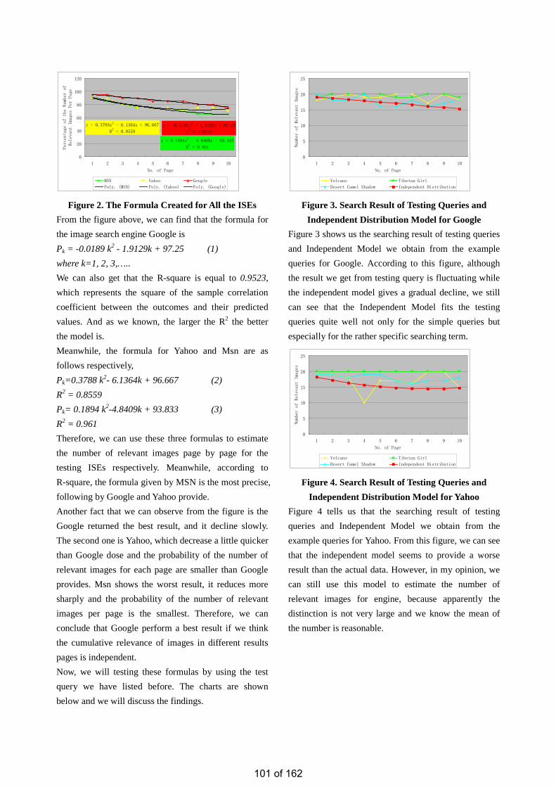
y = 0.1894x2 - 4.8409x + 93.833
R2 = 0.961
y = 0.3788x2 - 6.1364x + 96.667
R2 = 0.8559
y = -0.0189x2 - 1.9129x + 97.25
R2 = 0.9523
0
20
40
60
80
100
120
1 2 3 4 5 6 7 8 9 10
No. of Page
Percentage of the Number of
Relevant Images Per Page
MSN Yahoo Google
Poly. (MSN) Poly. (Yahoo) Poly. (Google) Figure 2. The Formula Created for All the ISEs
From the figure above, we can find that the formula for the image search engine Google is Pk = -0.0189 k2 - 1.9129k + 97.25 (1) where k=1, 2, 3,….. We can also get that the R-square is equal to 0.9523, which represents the square of the sample correlation coefficient between the outcomes and their predicted values. And as we known, the larger the R2 the better the model is. Meanwhile, the formula for Yahoo and Msn are as follows respectively, Pk=0.3788 k2- 6.1364k + 96.667 (2) R2 = 0.8559 Pk= 0.1894 k2-4.8409k + 93.833 (3) R2 = 0.961 Therefore, we can use these three formulas to estimate the number of relevant images page by page for the testing ISEs respectively. Meanwhile, according to R-square, the formula given by MSN is the most precise, following by Google and Yahoo provide. Another fact that we can observe from the figure is the Google returned the best result, and it decline slowly. The second one is Yahoo, which decrease a little quicker than Google dose and the probability of the number of relevant images for each page are smaller than Google provides. Msn shows the worst result, it reduces more sharply and the probability of the number of relevant images per page is the smallest. Therefore, we can conclude that Google perform a best result if we think the cumulative relevance of images in different results pages is independent. Now, we will testing these formulas by using the test query we have listed before. The charts are shown below and we will discuss the findings.
0
5
10
15
20
25
1 2 3 4 5 6 7 8 9 10
No. of Page
Number of Relevant Images
Volcano Tibetan Girl
Desert Camel Shadow Independent Distribution Figure 3. Search Result of Testing Queries and
Independent Distribution Model for Google Figure 3 shows us the searching result of testing queries and Independent Model we obtain from the example queries for Google. According to this figure, although the result we get from testing query is fluctuating while the independent model gives a gradual decline, we still can see that the Independent Model fits the testing queries quite well not only for the simple queries but especially for the rather specific searching term.
0
5
10
15
20
25
1 2 3 4 5 6 7 8 9 10
No. of Page
Number of Relevant Images
Volcano Tibetan Girl
Desert Camel Shadow Independent Distribution Figure 4. Search Result of Testing Queries and
Independent Distribution Model for Yahoo Figure 4 tells us that the searching result of testing queries and Independent Model we obtain from the example queries for Yahoo. From this figure, we can see that the independent model seems to provide a worse result than the actual data. However, in my opinion, we can still use this model to estimate the number of relevant images for engine, because apparently the distinction is not very large and we know the mean of the number is reasonable.
101 of 162
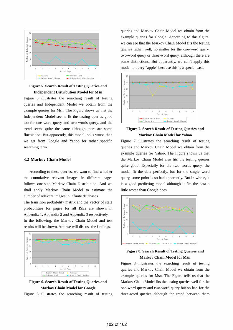
0
5
10
15
20
25
1 2 3 4 5 6 7 8 9 10
No. of Page
Number of Relevant Images
Volcano Tibetan Girl
Desert Camel Shadow Independent Distribution Figure 5. Search Result of Testing Queries and
Independent Distribution Model for Msn Figure 5 illustrates the searching result of testing queries and Independent Model we obtain from the example queries for Msn. The Figure shows us that the Independent Model seems fit the testing queries good too for one word query and two words query, and the trend seems quite the same although there are some fluctuation. But apparently, this model looks worse than we get from Google and Yahoo for rather specific searching term. 3.2 Markov Chain Model
According to these queries, we want to find whether the cumulative relevant images in different pages follows one-step Markov Chain Distribution. And we shall apply Markov Chain Model to estimate the number of relevant images in infinite databases. The transition probability matrix and the vector of state probabilities for pages for all ISEs are shown in Appendix 1, Appendix 2 and Appendix 3 respectively. In the following, the Markov Chain Model and test results will be shown. And we will discuss the findings.
0
5
10
15
20
25
1 2 3 4 5 6 7 8 9 10
No. of Page
Number of Relevant Images
Markov Chain Model Volcano
Tibetan Girl Desert Camel Shadow Figure 6. Search Result of Testing Queries and
Markov Chain Model for Google Figure 6 illustrates the searching result of testing
queries and Markov Chain Model we obtain from the example queries for Google. According to this figure, we can see that the Markov Chain Model fits the testing queries rather well, no matter for the one-word query, two-word query or three-word query, although there are some distinctions. But apparently, we can’t apply this model to query “apple” because this is a special case.
0
5
10
15
20
25
1 2 3 4 5 6 7 8 9 10
No. of Page
Number of Relevant Images
Markov Chain Model Volcano
Tibetan Girl Desert Camel Shadow Figure 7. Search Result of Testing Queries and
Markov Chain Model for Yahoo Figure 7 illustrates the searching result of testing queries and Markov Chain Model we obtain from the example queries for Yahoo. The Figure shows us that the Markov Chain Model also fits the testing queries quite good. Especially for the two words query, the model fit the data perfectly, but for the single word query, some point is so bad apparently. But in whole, it is a good predicting model although it fits the data a little worse than Google does.
0
5
10
15
20
25
1 2 3 4 5 6 7 8 9 10
No. of Page
Number of Relevant Image
Markov Chain Model Volcano Tibetan Girl Desert Camel Shadow Figure 8. Search Result of Testing Queries and
Markov Chain Model for Msn Figure 8 illustrates the searching result of testing queries and Markov Chain Model we obtain from the example queries for Msn. The Figure tells us that the Markov Chain Model fits the testing queries well for the one-word query and two-word query but so bad for the three-word queries although the trend between them
102 of 162
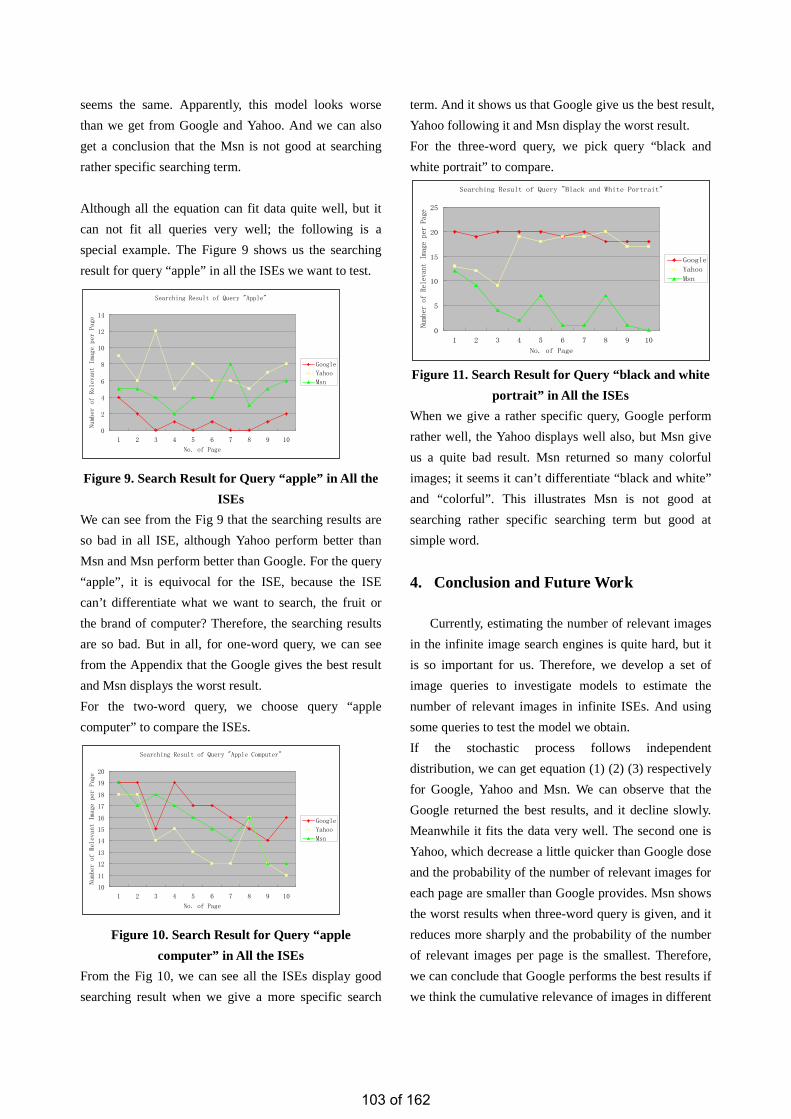
seems the same. Apparently, this model looks worse than we get from Google and Yahoo. And we can also get a conclusion that the Msn is not good at searching rather specific searching term. Although all the equation can fit data quite well, but it can not fit all queries very well; the following is a special example. The Figure 9 shows us the searching result for query “apple” in all the ISEs we want to test.
Searching Result of Query "Apple"
0
2
4
6
8
10
12
14
1 2 3 4 5 6 7 8 9 10
No. of Page
Number of Relevant Image per Page
Yahoo
Msn
Figure 9. Search Result for Query “apple” in All the
ISEs We can see from the Fig 9 that the searching results are so bad in all ISE, although Yahoo perform better than Msn and Msn perform better than Google. For the query “apple”, it is equivocal for the ISE, because the ISE can’t differentiate what we want to search, the fruit or the brand of computer? Therefore, the searching results are so bad. But in all, for one-word query, we can see from the Appendix that the Google gives the best result and Msn displays the worst result. For the two-word query, we choose query “apple computer” to compare the ISEs.
Searching Result of Query "Apple Computer"
10
11
12
13
14
15
16
17
18
19
20
1 2 3 4 5 6 7 8 9 10
No. of Page
Number of Relevant Image per Page
Yahoo
Msn
Figure 10. Search Result for Query “apple
computer” in All the ISEs From the Fig 10, we can see all the ISEs display good searching result when we give a more specific search
term. And it shows us that Google give us the best result, Yahoo following it and Msn display the worst result. For the three-word query, we pick query “black and white portrait” to compare.
Searching Result of Query "Black and White Portrait"
0
5
10
15
20
25
1 2 3 4 5 6 7 8 9 10
No. of Page
Numb
er o
f Re
leva
nt I
mage
per
Pag
e
Yahoo
Msn
Figure 11. Search Result for Query “black and white
portrait” in All the ISEs When we give a rather specific query, Google perform rather well, the Yahoo displays well also, but Msn give us a quite bad result. Msn returned so many colorful images; it seems it can’t differentiate “black and white” and “colorful”. This illustrates Msn is not good at searching rather specific searching term but good at simple word. 4. Conclusion and Future Work
Currently, estimating the number of relevant images in the infinite image search engines is quite hard, but it is so important for us. Therefore, we develop a set of image queries to investigate models to estimate the number of relevant images in infinite ISEs. And using some queries to test the model we obtain. If the stochastic process follows independent distribution, we can get equation (1) (2) (3) respectively for Google, Yahoo and Msn. We can observe that the Google returned the best results, and it decline slowly. Meanwhile it fits the data very well. The second one is Yahoo, which decrease a little quicker than Google dose and the probability of the number of relevant images for each page are smaller than Google provides. Msn shows the worst results when three-word query is given, and it reduces more sharply and the probability of the number of relevant images per page is the smallest. Therefore, we can conclude that Google performs the best results if we think the cumulative relevance of images in different
103 of 162
results pages is independent. And the most important thing is that we can use these formulas to estimate the number of relevant images for ISEs. If the stochastic process follows Markov Chain Distribution, we can find that the Markov Chain Model we obtain for Google is the best, because it fits the data quite well, especially for the quite specific queries. Yahoo comes in 2nd. The model fits the specific query quite well, but for the special specific query, the result is a little worse than Google have done. Msn seems the worst among these three ISEs when a rather specific query is given. But it fits easy word and specific query quite good. In a word, according to our experiment, we can use Independent Model and Markov Chain Model to estimate the total number of relevant images in infinite image search engines. But apparently, the equivocal character of the query “apple” made all the Independent Model and Markov Chain Model incapable of estimating. For infinite image repositories, it is generally impractical to step through the interminable set of search results presented. Therefore, our future work is to find an optimal stopping rule. According to what we have done above, it seems using Markov Chain could provide us a good stopping rule.
5. Reference [1] K. Stevenson and C. Leung, “Comparative Evaluation of Web Image Search Engines for Multimedia Applications”, In Proceedings of IEEE International Conference on Multimedia and Expo, July 2005 [2] Ishioka, T. 2003, “Evaluation of Criteria for Information Retrieval”, In Proceedings of the 2003 IEEE/WIC International Conference on Web Intelligence (October 13 - 17, 2003). Web Intelligence IEEE Computer Society, Washington, DC, 425 [3]Raquel Kolitski Stasiu, Carlos A. Heuser, and Roberto da Silva, “Estimating Recall and Precision for Vague Queries in Databases”, In Proceedings of Springer-Verlag Berlin Heidelberg, CAiSE 2005, LNCS 3520, pp. 187-200, 2005 [4] Ece Çakır, Hüseyin Bahçeci, Yıltan Bitirim, "An
Evaluation of Major Image Search Engines on Various Query Topics," icimp, pp.161-165, 2008. In Proceedings of the Third International Conference on Internet Monitoring and Protection, 2008 [5] F. Uluç, E. Emirzade and Y. Bitirim, “The Impact of Number of Query Words on Image Search Engines”, In Proceedings of Second International Conference on Internet and Web Applications and Services (ICIW), pp. 50, 2007 [6] Si, L. and Callan, J. 2003, “Relevant document distribution estimation method for resource selection”, In Proceedings of the 26th Annual international ACM SIGIR Conference on Research and Development in informaion Retrieval Toronto, Canada, July 28 - August 01, 2003. SIGIR '03. ACM, New York, NY, 298-305 [7] Google Search Engine www.google.com [8] Yahoo Search Engine www.yahoo.com [9] Msn Search Engine www.msn.com [10] Nielsen//NetRatings, “Goole accounts for more than half of all web searches, while Yahoo and Msn combined account more than one fourth, according to Nielson//Netrating”, April 2009. http://www.polepositionmarketing.com/emp/april-2009-search-engine-2/ [11] Render, R., R. M. Stair Jr., and M. E. Hanna. “Quantitative Analysis for Management-Chapter 16”, 10th Edition, Prentice Hall, 2009 [12] A.Sprink and B.J.Jansen, “Searching Multimedia Federated Content Web Collections”, Online Information Review, Vol.30, No.5, pp. 485-495,2006 [13] Jin, X. and French, J. C. 2003. Improving image retrieval effectiveness via multiple queries. In Proceedings of the 1st ACM international Workshop on Multimedia Databases (New Orleans, LA, USA, November 07 - 07, 2003). MMDB '03. ACM, New York, NY, 86-93. DOI= http://doi.acm.org/10.1145/951676.951692 [14] Nottelmann, H. and Fuhr, N. 2003. Evaluating different methods of estimating retrieval quality for resource selection. In Proceedings of the 26th Annual international ACM SIGIR Conference on Research and Development in informaion Retrieval (Toronto, Canada, July 28 - August 01, 2003). SIGIR '03. ACM, New York, NY, 290-297. DOI=
104 of 162

http://doi.acm.org/10.1145/860435.860489 [15] Thomas W. Miller, Data and Text Mining: A Business Applications Approach. Upper Saddle River, N.J. : Pearson Prentice Hall, c2005 [16]W.S. Kendall, F. Liang, J.-S. Wang, Markov chain Monte Carlo : innovations and applications, Singapore ; Hackensack, NJ : World Scientific, c2005 [17]Dani Gamerman, Markov chain Monte Carlo : stochastic simulation for Bayesian inference, London ; New York : Chapman & Hall, 1997 [18] Shirahatti, N. V. and Barnard, K. 2005. Evaluating Image Retrieval. In Proceedings of the 2005 IEEE Computer Society Conference on Computer Vision and Pattern Recognition (Cvpr'05) - Volume 1 - Volume 01 (June 20 - 26, 2005). CVPR. IEEE Computer Society, Washington, DC, 955-961. DOI=
http://dx.doi.org/10.1109/CVPR.2005.147 [19] Black Jr, J. A., Fahmy, G., and Panchanathan, S. 2002. A Method for Evaluating the Performance of Content-Based Image Retrieval Systems. In Proceedings of the Fifth IEEE Southwest Symposium on Image Analysis and interpretation (April 07 - 09, 2002). SSIAI. IEEE Computer Society, Washington, DC, 96. [20] Münevver Tugçe Elagöz , Mehtap Mendeli , Remziye Zeden Manioglulari , Yiltan Bitirim, "An Empirical Evaluation on Meta-Image Search Engines," ICDT, pp.135-139, 2008. In Proceedings of the Third International Conference on Digital Telecommunications (ICDT 2008), 2008
105 of 162
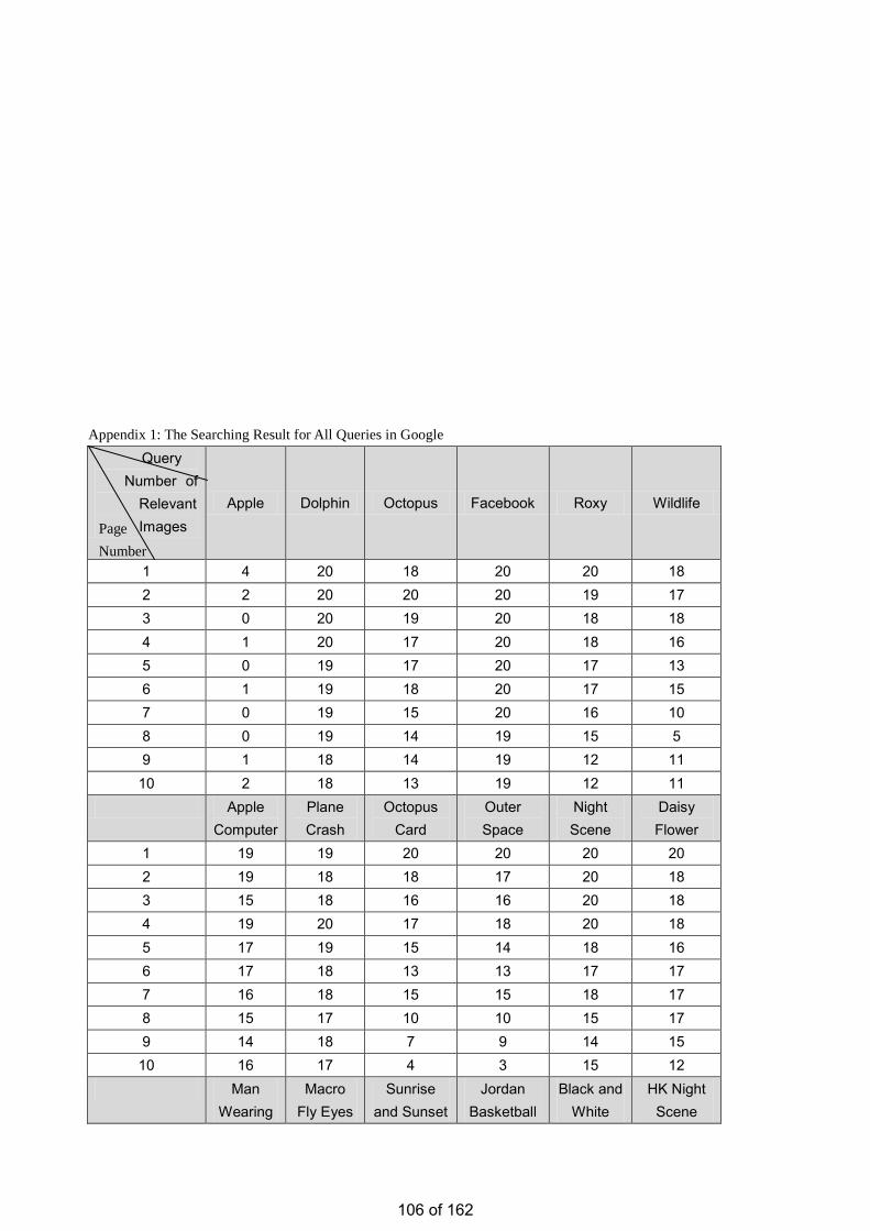
Appendix 1: The Searching Result for All Queries in Google
Query Number of
Relevant Images
Apple Dolphin Octopus Facebook Roxy Wildlife
1 4 20 18 20 20 18 2 2 20 20 20 19 17 3 0 20 19 20 18 18 4 1 20 17 20 18 16 5 0 19 17 20 17 13 6 1 19 18 20 17 15 7 0 19 15 20 16 10 8 0 19 14 19 15 5 9 1 18 14 19 12 11 10 2 18 13 19 12 11 Apple
Computer Plane Crash
Octopus Card
Outer Space
Night Scene
Daisy Flower
1 19 19 20 20 20 20 2 19 18 18 17 20 18 3 15 18 16 16 20 18 4 19 20 17 18 20 18 5 17 19 15 14 18 16 6 17 18 13 13 17 17 7 16 18 15 15 18 17 8 15 17 10 10 15 17 9 14 18 7 9 14 15 10 16 17 4 3 15 12 Man
Wearing Macro
Fly Eyes Sunrise
and Sunset Jordan
Basketball Black and
White HK Night
Scene
Page Number
106 of 162
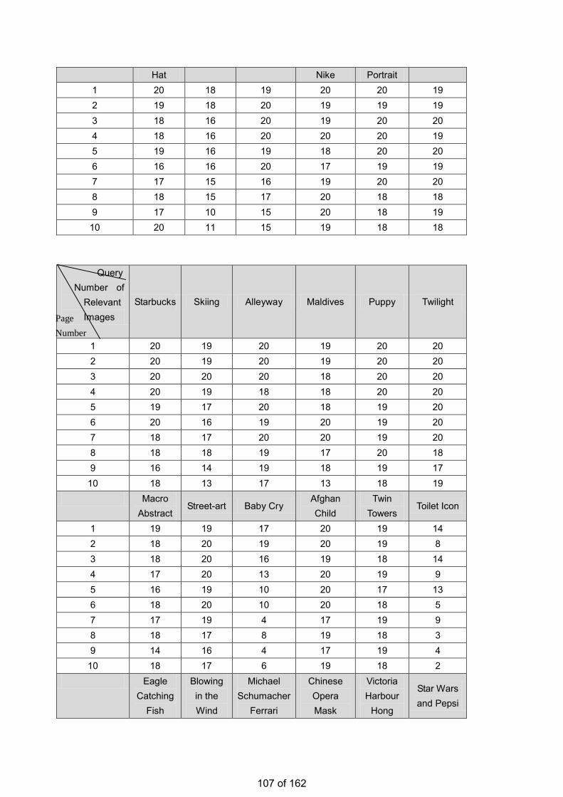
Hat Nike Portrait 1 20 18 19 20 20 19 2 19 18 20 19 19 19 3 18 16 20 19 20 20 4 18 16 20 20 20 19 5 19 16 19 18 20 20 6 16 16 20 17 19 19 7 17 15 16 19 20 20 8 18 15 17 20 18 18 9 17 10 15 20 18 19 10 20 11 15 19 18 18
Query Number of
Relevant Images
Starbucks Skiing Alleyway Maldives Puppy Twilight
1 20 19 20 19 20 20 2 20 19 20 19 20 20 3 20 20 20 18 20 20 4 20 19 18 18 20 20 5 19 17 20 18 19 20 6 20 16 19 20 19 20 7 18 17 20 20 19 20 8 18 18 19 17 20 18 9 16 14 19 18 19 17
10 18 13 17 13 18 19 Macro
Abstract Street-art Baby Cry
Afghan Child
Twin Towers
Toilet Icon
1 19 19 17 20 19 14 2 18 20 19 20 19 8 3 18 20 16 19 18 14 4 17 20 13 20 19 9 5 16 19 10 20 17 13 6 18 20 10 20 18 5 7 17 19 4 17 19 9 8 18 17 8 19 18 3 9 14 16 4 17 19 4
10 18 17 6 19 18 2 Eagle
Catching Fish
Blowing in the Wind
Michael Schumacher
Ferrari
Chinese Opera Mask
Victoria Harbour
Hong
Star Wars and Pepsi
Page Number
107 of 162
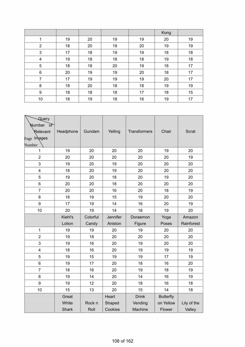
Kong 1 19 20 19 19 20 19 2 18 20 19 20 19 19 3 17 18 19 19 18 18 4 19 18 18 18 19 18 5 18 18 20 19 18 17 6 20 19 19 20 18 17 7 17 19 19 19 20 17 8 18 20 18 18 19 19 9 18 18 18 17 18 15
10 18 19 18 16 19 17
Query Number of
Relevant Images
Headphone Gundam Yelling Transformers Chair Scrat
1 19 20 20 20 19 20 2 20 20 20 20 20 19 3 19 20 19 20 20 20 4 18 20 19 20 20 20 5 19 20 18 20 19 20 6 20 20 18 20 20 20 7 20 20 16 20 18 19 8 18 19 15 19 20 20 9 17 19 14 16 20 19
10 20 19 14 18 19 20 Kiehl's
Lotion Colorful Candy
Jennifer Aniston
Doraemon Figure
Yoga Poses
Amazon Rainforest
1 19 19 20 19 20 20 2 19 18 20 20 20 20 3 19 16 20 19 20 20 4 18 16 20 19 19 19 5 19 15 19 19 17 19 6 19 17 20 18 16 20 7 18 16 20 19 18 19 8 19 14 20 14 16 19 9 19 12 20 18 16 18
10 15 13 20 15 14 18 Great
White Shark
Rock n Roll
Heart Shaped Cookies
Drink Vending Machine
Butterfly on Yellow
Flower Lily of the
Valley
Page Number
108 of 162
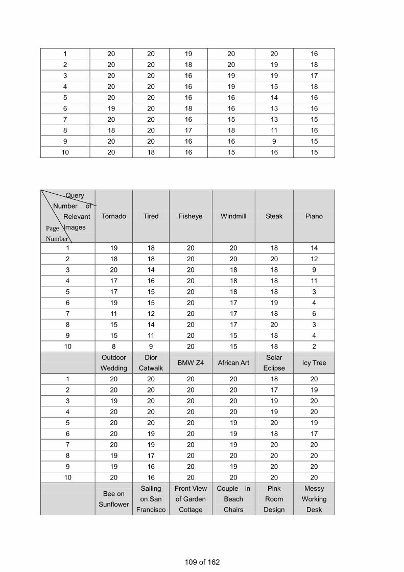
1 20 20 19 20 20 16 2 20 20 18 20 19 18 3 20 20 16 19 19 17 4 20 20 16 19 15 18 5 20 20 16 16 14 16 6 19 20 18 16 13 16 7 20 20 16 15 13 15 8 18 20 17 18 11 16 9 20 20 16 16 9 15
10 20 18 16 15 16 15
Query Number of
Relevant Images
Tornado Tired Fisheye Windmill Steak Piano
1 19 18 20 20 18 14 2 18 18 20 20 20 12 3 20 14 20 18 18 9 4 17 16 20 18 18 11 5 17 15 20 18 18 3 6 19 15 20 17 19 4 7 11 12 20 17 18 6 8 15 14 20 17 20 3 9 15 11 20 15 18 4 10 8 9 20 15 18 2 Outdoor
Wedding Dior
Catwalk BMW Z4 African Art
Solar Eclipse
Icy Tree
1 20 20 20 20 18 20 2 20 20 20 20 17 19 3 19 20 20 20 19 20 4 20 20 20 20 19 20 5 20 20 20 19 20 19 6 20 19 20 19 18 17 7 20 19 20 19 20 20 8 19 17 20 20 20 20 9 19 16 20 19 20 20 10 20 16 20 20 20 20
Bee on Sunflower
Sailing on San
Francisco
Front View of Garden Cottage
Couple in Beach Chairs
Pink Room Design
Messy Working
Desk
Page Number
109 of 162

Bay 1 20 19 17 16 20 16 2 20 19 16 15 19 13 3 20 17 14 15 19 14 4 17 19 15 17 14 12 5 16 17 14 17 15 15 6 18 16 17 15 15 15 7 16 15 13 12 15 14 8 16 17 12 10 14 13 9 18 19 14 11 11 13 10 18 20 15 7 10 14
Appendix 1: Google Transition Probability Matrix
110 of 162

111 of 162
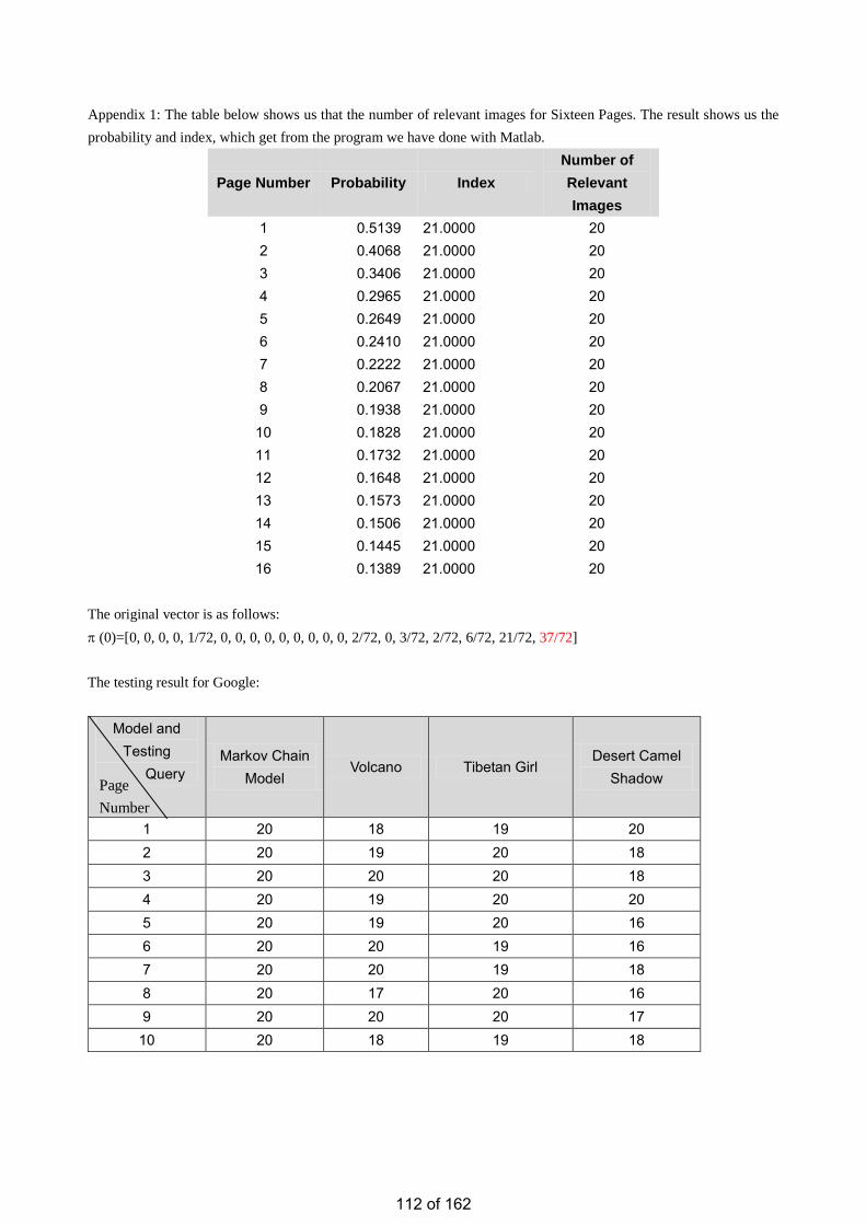
Appendix 1: The table below shows us that the number of relevant images for Sixteen Pages. The result shows us the probability and index, which get from the program we have done with Matlab.
Page Number Probability Index Number of Relevant Images
1 0.5139 21.0000 20 2 0.4068 21.0000 20 3 0.3406 21.0000 20 4 0.2965 21.0000 20 5 0.2649 21.0000 20 6 0.2410 21.0000 20 7 0.2222 21.0000 20 8 0.2067 21.0000 20 9 0.1938 21.0000 20
10 0.1828 21.0000 20 11 0.1732 21.0000 20 12 0.1648 21.0000 20 13 0.1573 21.0000 20 14 0.1506 21.0000 20 15 0.1445 21.0000 20 16 0.1389 21.0000 20
The original vector is as follows: π (0)=[0, 0, 0, 0, 1/72, 0, 0, 0, 0, 0, 0, 0, 0, 0, 2/72, 0, 3/72, 2/72, 6/72, 21/72, 37/72] The testing result for Google:
Model and Testing
Query Markov Chain
Model Volcano Tibetan Girl
Desert Camel Shadow
1 20 18 19 20 2 20 19 20 18 3 20 20 20 18 4 20 19 20 20 5 20 19 20 16 6 20 20 19 16 7 20 20 19 18 8 20 17 20 16 9 20 20 20 17 10 20 18 19 18
Page Number
112 of 162

Appendix 2: The Searching Result for All Queries in Yahoo Query Number of Relevant
Images Apple Dolphin Octopus Facebook Roxy Wildlife
1 9 19 19 19 20 15 2 6 19 19 17 20 16 3 12 20 18 9 15 17 4 5 15 13 5 5 13 5 8 15 16 6 10 13 6 6 13 11 7 12 14 7 6 16 14 5 14 15 8 5 16 9 5 6 12 9 7 11 8 6 9 13 10 8 16 14 4 4 10 Apple
Computer Plane Crash
Octopus Card
Outer Space
Night Scene
Daisy Flower
1 18 18 13 19 20 19 2 18 18 3 17 19 20 3 14 16 8 4 19 18 4 15 4 2 1 20 19 5 13 11 5 1 18 19 6 12 9 8 3 19 16 7 12 8 7 0 20 18 8 16 7 6 1 19 18 9 12 7 4 0 19 17 10 11 7 8 0 18 15 Man
Wearing Hat
Macro Fly Eyes
Sunrise and Sunset
Jordan Basketball
Nike
Black and White
Portrait
HK Night Scene
1 19 20 18 19 13 20 2 17 19 16 20 12 20 3 15 19 17 20 9 20 4 17 19 15 20 19 20 5 18 20 19 20 18 19 6 18 20 19 20 19 18 7 19 18 18 18 19 20 8 17 19 19 20 20 20 9 18 19 19 19 17 19 10 18 19 19 19 17 19
Page Number
113 of 162
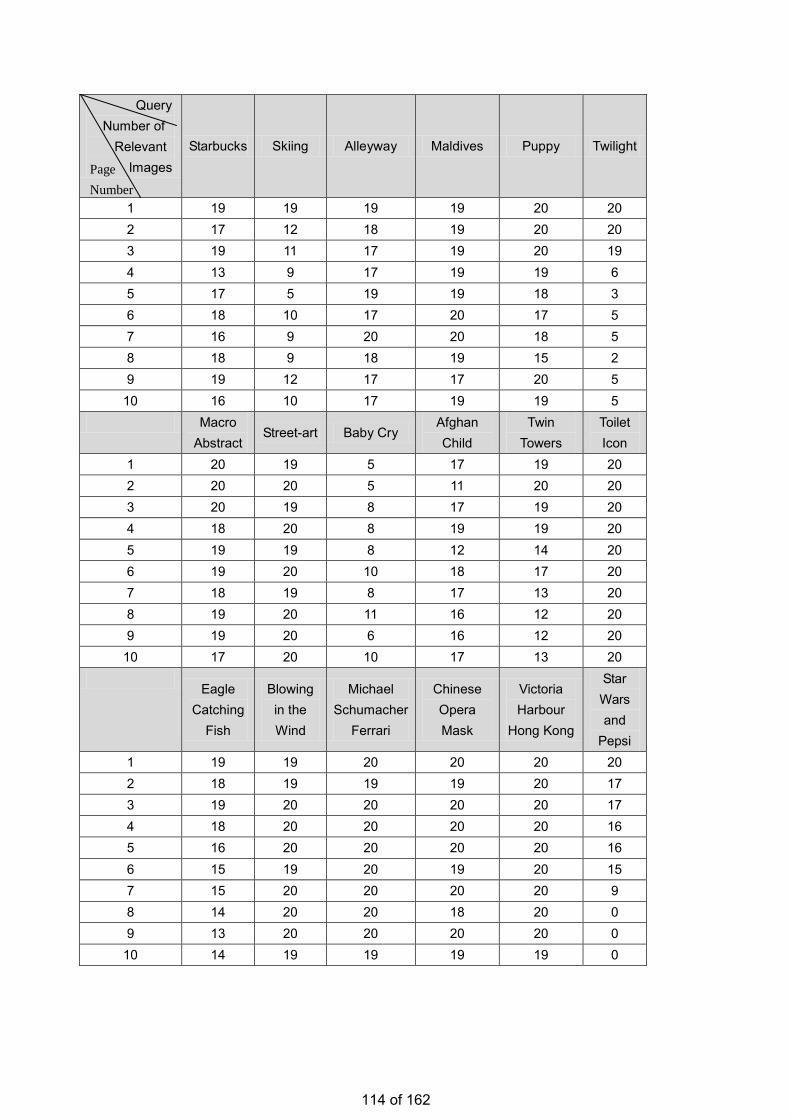
Query Number of Relevant
Images Starbucks Skiing Alleyway Maldives Puppy Twilight
1 19 19 19 19 20 20 2 17 12 18 19 20 20 3 19 11 17 19 20 19 4 13 9 17 19 19 6 5 17 5 19 19 18 3 6 18 10 17 20 17 5 7 16 9 20 20 18 5 8 18 9 18 19 15 2 9 19 12 17 17 20 5
10 16 10 17 19 19 5 Macro
Abstract Street-art Baby Cry
Afghan Child
Twin Towers
Toilet Icon
1 20 19 5 17 19 20 2 20 20 5 11 20 20 3 20 19 8 17 19 20 4 18 20 8 19 19 20 5 19 19 8 12 14 20 6 19 20 10 18 17 20 7 18 19 8 17 13 20 8 19 20 11 16 12 20 9 19 20 6 16 12 20
10 17 20 10 17 13 20
Eagle Catching
Fish
Blowing in the Wind
Michael Schumacher
Ferrari
Chinese Opera Mask
Victoria Harbour
Hong Kong
Star Wars and
Pepsi 1 19 19 20 20 20 20 2 18 19 19 19 20 17 3 19 20 20 20 20 17 4 18 20 20 20 20 16 5 16 20 20 20 20 16 6 15 19 20 19 20 15 7 15 20 20 20 20 9 8 14 20 20 18 20 0 9 13 20 20 20 20 0
10 14 19 19 19 19 0
Page Number
114 of 162

Query Number of
Relevant Images
Headphone Gundam Yelling Transformers Chair Scrat
1 19 9 18 20 20 20 2 12 17 18 20 20 20 3 7 8 17 18 20 14 4 6 0 17 18 20 12 5 7 1 16 18 19 7 6 7 4 14 18 18 6 7 9 8 13 17 19 8 8 9 15 13 18 19 8 9 12 20 6 20 19 10
10 11 17 7 18 20 5 Kiehl's
Lotion Colorful Candy
Jennifer Aniston
Doraemon Figure
Yoga Poses
Amazon Rainforest
1 6 17 20 19 20 20 2 19 20 20 20 16 17 3 19 19 20 18 14 20 4 18 16 20 13 20 20 5 19 19 18 11 19 17 6 12 19 20 8 17 15 7 14 20 20 7 18 15 8 13 18 20 0 17 17 9 13 17 20 0 18 17
10 14 17 20 0 17 20 Great
White Shark
Rock n Roll
Heart Shaped Cookies
Drink Vending Machine
Butterfly on Yellow
Flower
Lily of the Valley
1 20 20 20 19 20 16 2 20 19 20 20 17 16 3 20 14 20 19 15 17 4 19 18 20 19 11 20 5 19 20 19 19 13 17 6 20 20 19 18 14 15 7 18 7 18 19 12 11 8 18 10 16 18 15 16 9 19 18 16 20 13 20
10 19 20 17 19 11 18
Page Number
115 of 162

Query Number of Relevant
Images Tornado Tired Fisheye Windmill Steak Piano
1 18 18 20 20 20 17 2 19 17 20 18 16 18 3 11 17 20 18 17 16 4 8 17 20 16 18 13 5 8 16 20 19 18 15 6 11 17 20 18 17 11 7 6 16 20 16 17 9 8 5 18 20 16 17 13 9 7 16 20 18 17 11 10 6 18 20 16 16 12 Outdoor
Wedding Dior
Catwalk BMW Z4 African Art
Solar Eclipse
Icy Tree
1 19 20 20 20 17 20 2 19 19 20 20 20 20 3 19 20 20 18 17 20 4 20 20 20 18 11 20 5 19 19 20 20 17 19 6 18 12 20 20 20 20 7 18 17 20 19 16 20 8 17 19 20 20 17 20 9 19 19 19 20 17 20 10 19 19 19 20 14 20
Bee on Sunflower
Sailing on San
Francisco Bay
Front View of Garden Cottage
Couple in Beach Chairs
Pink Room Design
Messy Working
Desk
1 20 19 11 11 16 18 2 18 19 15 9 17 16 3 18 19 12 3 12 16 4 18 18 12 5 11 15 5 20 19 11 4 10 16 6 20 20 12 5 4 16 7 20 19 13 0 6 15 8 18 19 12 2 14 15 9 19 18 8 2 6 14 10 20 17 9 0 11 13
Page Number
116 of 162

Appendix 2: Yahoo Transition Probability Matrix
117 of 162

Appendix 2: The table below shows us that the number of relevant images for Sixteen Pages. The result shows us the probability and index, which get from the program we have done with Matlab.
Page Number Probability Index Number of Relevant
Images 1 0.4028 21.0000 20 2 0.3282 21.0000 20 3 0.2809 21.0000 20 4 0.2498 21.0000 20 5 0.2278 21.0000 20 6 0.2112 21.0000 20 7 0.1980 21.0000 20 8 0.1872 21.0000 20 9 0.1781 21.0000 20
10 0.1703 21.0000 20 11 0.1636 21.0000 20 12 0.1577 21.0000 20 13 0.1525 21.0000 20 14 0.1479 21.0000 20 15 0.1438 21.0000 20 16 0.1402 21.0000 20
The original vector: π (0)= [0,0,0,0,0,1/72,1/72,0,0,2/72,0,2/72,0,2/72,0,1/72,2/72,4/72,7/72,21/72,29/72] The Testing Result for Yahoo:
Model and Testing
Query
Markov Chain Model
Volcano Tibetan Girl Desert Camel
Shadow
1 20 19 20 19 2 20 19 20 19 3 20 18 20 18 4 20 10 20 19 5 20 17 20 19 6 20 17 20 17 7 20 16 20 16 8 20 20 20 17 9 20 20 20 17 10 20 15 20 18
Page Number
118 of 162

Appendix 3: The Searching Result for All Queries in Msn Query Number of Relevant
Images Apple Dolphin Octopus Facebook Roxy Wildlife
1 5 20 19 18 20 20 2 5 17 19 17 18 19 3 4 18 18 18 18 19 4 2 16 17 17 17 18 5 4 14 18 17 18 16 6 4 11 16 15 17 15 7 8 10 16 18 16 13 8 3 8 15 18 14 15 9 5 7 15 18 14 15 10 6 11 13 17 14 14 Apple
Computer Plane Crash
Octopus Card
Outer Space
Night Scene
Daisy Flower
1 19 17 18 16 19 17 2 17 17 14 13 16 16 3 18 17 6 11 17 15 4 17 16 11 8 16 16 5 16 16 9 11 15 13 6 15 15 6 5 16 13 7 14 17 8 4 16 12 8 16 12 8 1 12 10 9 12 18 6 7 14 9 10 12 16 5 7 15 9 Man
Wearing Hat
Macro Fly Eyes
Sunrise and Sunset
Jordan Basketball
Nike
Black and White
Portrait
HK Night Scene
1 18 15 19 12 18 18 2 17 12 19 9 14 17 3 16 14 16 4 13 16 4 14 13 19 2 10 14 5 15 16 16 7 4 15 6 15 15 16 1 7 15 7 13 11 17 1 7 13 8 11 14 17 7 0 11 9 6 11 19 1 0 6 10 10 12 20 0 0 10
Page Number
119 of 162
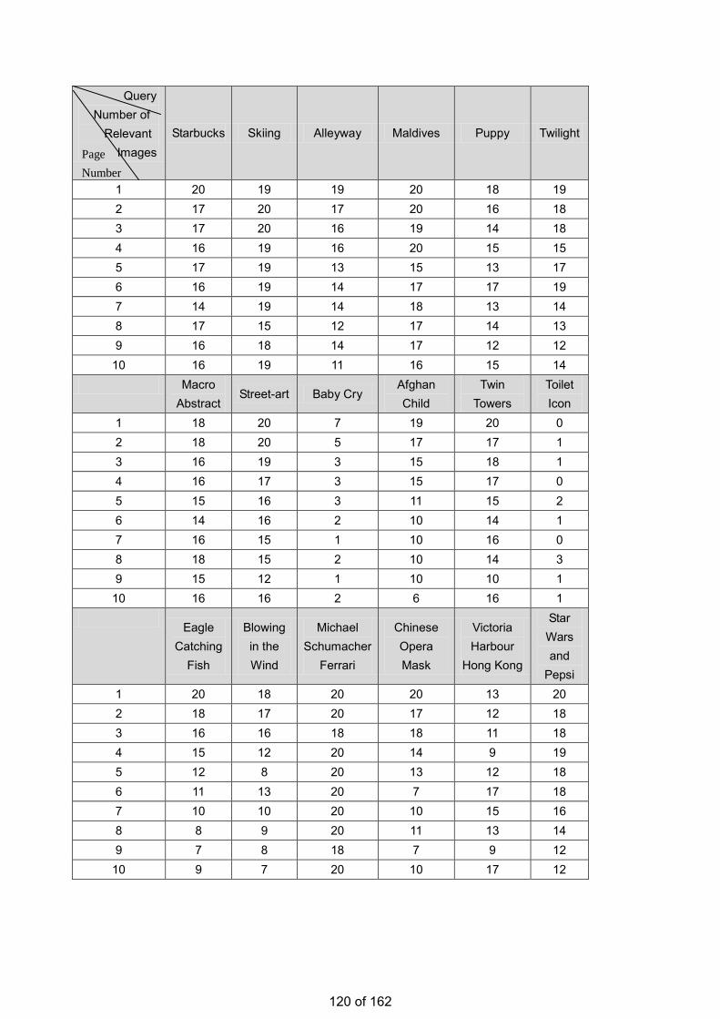
Query Number of Relevant
Images Starbucks Skiing Alleyway Maldives Puppy Twilight
1 20 19 19 20 18 19 2 17 20 17 20 16 18 3 17 20 16 19 14 18 4 16 19 16 20 15 15 5 17 19 13 15 13 17 6 16 19 14 17 17 19 7 14 19 14 18 13 14 8 17 15 12 17 14 13 9 16 18 14 17 12 12
10 16 19 11 16 15 14 Macro
Abstract Street-art Baby Cry
Afghan Child
Twin Towers
Toilet Icon
1 18 20 7 19 20 0 2 18 20 5 17 17 1 3 16 19 3 15 18 1 4 16 17 3 15 17 0 5 15 16 3 11 15 2 6 14 16 2 10 14 1 7 16 15 1 10 16 0 8 18 15 2 10 14 3 9 15 12 1 10 10 1
10 16 16 2 6 16 1
Eagle Catching
Fish
Blowing in the Wind
Michael Schumacher
Ferrari
Chinese Opera Mask
Victoria Harbour
Hong Kong
Star Wars and
Pepsi 1 20 18 20 20 13 20 2 18 17 20 17 12 18 3 16 16 18 18 11 18 4 15 12 20 14 9 19 5 12 8 20 13 12 18 6 11 13 20 7 17 18 7 10 10 20 10 15 16 8 8 9 20 11 13 14 9 7 8 18 7 9 12
10 9 7 20 10 17 12
Page Number
120 of 162
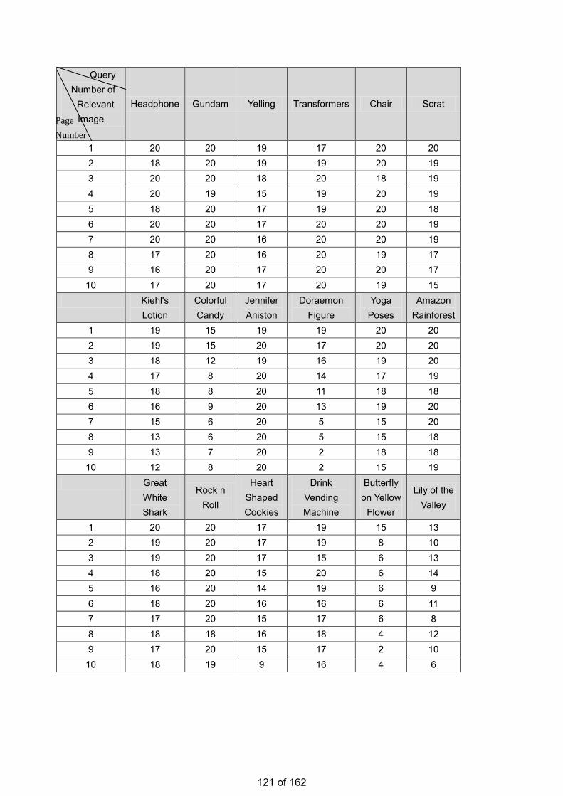
Query Number of Relevant
Image Headphone Gundam Yelling Transformers Chair Scrat
1 20 20 19 17 20 20 2 18 20 19 19 20 19 3 20 20 18 20 18 19 4 20 19 15 19 20 19 5 18 20 17 19 20 18 6 20 20 17 20 20 19 7 20 20 16 20 20 19 8 17 20 16 20 19 17 9 16 20 17 20 20 17
10 17 20 17 20 19 15 Kiehl's
Lotion Colorful Candy
Jennifer Aniston
Doraemon Figure
Yoga Poses
Amazon Rainforest
1 19 15 19 19 20 20 2 19 15 20 17 20 20 3 18 12 19 16 19 20 4 17 8 20 14 17 19 5 18 8 20 11 18 18 6 16 9 20 13 19 20 7 15 6 20 5 15 20 8 13 6 20 5 15 18 9 13 7 20 2 18 18
10 12 8 20 2 15 19 Great
White Shark
Rock n Roll
Heart Shaped Cookies
Drink Vending Machine
Butterfly on Yellow
Flower
Lily of the Valley
1 20 20 17 19 15 13 2 19 20 17 19 8 10 3 19 20 17 15 6 13 4 18 20 15 20 6 14 5 16 20 14 19 6 9 6 18 20 16 16 6 11 7 17 20 15 17 6 8 8 18 18 16 18 4 12 9 17 20 15 17 2 10
10 18 19 9 16 4 6
Page Number
121 of 162

Query Number of Relevant
Images Tornado Tired Fisheye Windmill Steak Piano
1 18 19 20 18 19 17 2 18 17 20 18 20 17 3 14 17 19 18 20 17 4 12 16 19 18 16 17 5 13 17 19 18 19 14 6 13 17 20 18 18 17 7 10 17 19 16 18 17 8 13 15 17 16 17 15 9 13 16 18 16 18 17 10 10 15 18 20 16 15 Outdoor
Wedding Dior
Catwalk BMW Z4 African Art
Solar Eclipse
Icy Tree
1 19 17 20 20 16 19 2 18 19 20 20 12 18 3 19 16 20 19 15 16 4 20 18 20 19 14 14 5 18 19 20 20 13 17 6 18 19 20 19 10 16 7 18 18 20 20 11 18 8 15 15 19 17 8 17 9 17 17 20 19 12 17 10 13 14 20 20 11 12
Bee on Sunflower
Sailing on San
Francisco Bay
Front View of Garden Cottage
Couple in Beach Chairs
Pink Room Design
Messy Working
Desk
1 20 17 16 9 11 20 2 19 15 16 6 10 18 3 20 16 15 5 8 17 4 17 17 14 3 9 10 5 16 19 16 4 3 13 6 17 17 15 4 4 12 7 16 17 12 2 2 9 8 18 18 14 1 4 8 9 16 15 14 1 6 8 10 13 17 12 2 3 5
Page Number
122 of 162

Appendix 3: Msn Transition Probability Matrix
123 of 162

Appendix 3: The table below shows us that the number of relevant images for Sixteen Pages. The result shows us the probability and index, which get from the program we have done with Matlab.
Page Number Probability Index Number of Relevant
Images 1 0.3194 21.0000 20 2 0.2500 21.0000 20 3 0.1927 21.0000 20 4 0.1527 21.0000 20 5 0.1304 18.0000 18 6 0.1245 18.0000 18 7 0.1179 18.0000 18 8 0.1114 18.0000 18 9 0.1051 18.0000 18
10 0.0992 18.0000 18 11 0.0937 18.0000 18 12 0.0886 18.0000 18 13 0.0839 18.0000 18 14 0.0796 18.0000 18 15 0.0757 18.0000 18 16 0.0720 18.0000 18
The Original Vector: π (0)= [1/72,0,0,0,0,1/72,0,1/72,0,1/72,0,1/72,1/72,2/72,0,3/72,3/72,7/72,9/72,18/72,23/72] The Testing Result for Msn:
Model and Testing
Query
Markov Chain Model
Volcano Tibetan Girl Desert Camel
Shadow
1 20 20 19 8 2 20 18 16 3 3 20 18 20 2 4 20 17 19 7 5 18 18 16 3 6 18 19 16 2 7 18 18 17 1 8 18 17 16 5 9 18 16 19 0
10 18 15 15 0
Page Number
124 of 162
Patient Journey Optimization Using A Multi-Agent Approach
Chung Ho CHOI
Abstract
With the increasing expectation from patients and theregulations enacted by the government, exploring ways toshorten patient journey has caught increasing attention. Pa-tient journey optimization typically involves treatment op-eration scheduling at multiple medical units. The decen-tralized nature of the problem makes conventional central-ized operation research methods inapplicable in generaland motivates the use of the multi-agent approach. In thispaper, we focus on cancer patient treatment. We model pa-tients and medical units as autonomous agents which inter-act locally via a bidding process and a coordination pro-cess for patient journey optimization. With reference to adataset containing more than five thousand different cancerpatient journeys, the effectiveness of the proposed algorithmunder different settings of implementation has been experi-mentally evaluated via experimental simulations.
1 Introduction
Shortening the length of patient journey is always an ex-pectation of patients. Also, it is one of the vital key perfor-mance indicators for evaluating the effectiveness of health-care service providers. In order to best utilize the existingresources to raise healthcare service level, careful applica-tion of scheduling algorithms is crucial [7]. While conven-tional operations research methods have been found effec-tive for scheduling related problems found in different med-ical units [8, 9, 4], most of them take the centralized ap-proach and are not designed to be applied to decentralizedsituations where multiple resources at multiple hospitals areto be coordinated [5, 7, 2].
The multi-agent approach is characterized by emphasiz-ing on local interaction and self-organization of differententities being modeled. These properties make it especiallysuitable for tackling complex tasks with a lot of stakehold-ers [11, 1]. Multi-agent methods have found applicationsin a variety of problem domains, such as airport resourcescheduling [3], load allocation in transportation logistics[6], supply chain management [10], etc. Recently, it hasalso been applied to patient scheduling in [5, 7] with some
initial success demonstrated. And yet, there are limitations.Paulussen et al., in [5], assume that a quantified health statecan be accurately derived as a utility measure for guidingthe scheduling process. In [7], Vermeulen et al. did notconsider the temporal constraints between the treatment op-erations during the scheduling process.
In this paper, we focus on the problem of improving thehealthcare experience of cancer patients by optimizing theirpatient journeys. It is common that many developed citieshave established a number of cancer centers to pool up re-sources for best utilization and yet to ensure that the centersare properly located to cater for the needs in different re-gions of the cities. However, the geographical distributionof the patient demand is dynamic in general and hard to beaccurately predicted at different time points. The objectiveof this study is to explore the extent to which patient journeycan be improved by better coordinating and mobilizing re-sources distributed at different cancer centers. In particular,we formulate the problem based on the healthcare systemfor cancer treatment in Hong Kong. We propose the use ofa multi-agent approach where each patient and each unit ofresources are modeled as autonomous agents which can in-teract with others to arrive an effective overall schedule withreduced amount of patient waiting times. To evaluate the ef-fectiveness of the proposed approach, we made use of a pa-tient identity anonymized data set collected by Hospital Au-thority in Hong Kong which contains 5819 cancer patientswith an admission period spanning over 6 months, and havecarried out simulations with the proposed approach givendifferent settings of the environment.
The rest of the paper is organized as follows. The patientscheduling problem formulation is described in Section 2.Section 3 and Section 4 present the details of the proposedagent-based scheduling algorithm. Section 5 presents somepreliminary experimental results and Section 6 concludesthe paper.
2 PROBLEM FORMULATION
In this section, we first briefly describe the establishmentof the cancer centers in Hong Kong. Then, we formulatethe patient scheduling problem for cancer treatment as anoptimization problem and explain how a particular multi-
125 of 162
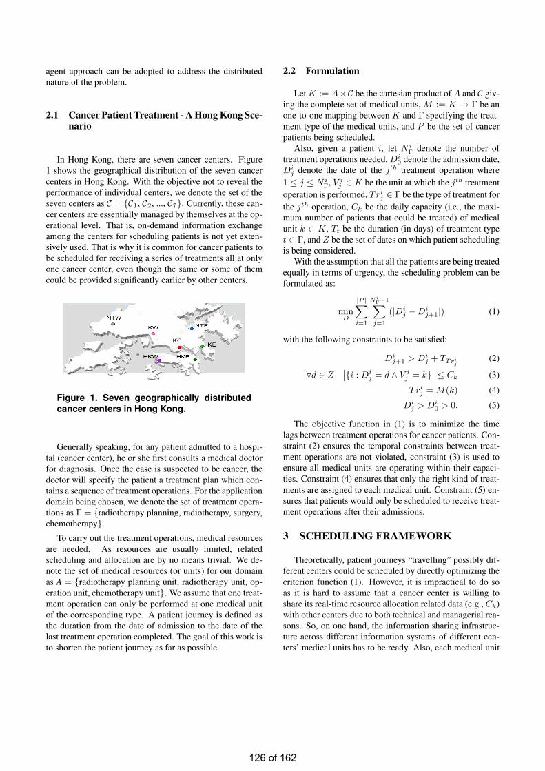
agent approach can be adopted to address the distributednature of the problem.
2.1 Cancer Patient Treatment - A Hong Kong Sce-nario
In Hong Kong, there are seven cancer centers. Figure1 shows the geographical distribution of the seven cancercenters in Hong Kong. With the objective not to reveal theperformance of individual centers, we denote the set of theseven centers as C = C1, C2, ..., C7. Currently, these can-cer centers are essentially managed by themselves at the op-erational level. That is, on-demand information exchangeamong the centers for scheduling patients is not yet exten-sively used. That is why it is common for cancer patients tobe scheduled for receiving a series of treatments all at onlyone cancer center, even though the same or some of themcould be provided significantly earlier by other centers.
Figure 1. Seven geographically distributedcancer centers in Hong Kong.
Generally speaking, for any patient admitted to a hospi-tal (cancer center), he or she first consults a medical doctorfor diagnosis. Once the case is suspected to be cancer, thedoctor will specify the patient a treatment plan which con-tains a sequence of treatment operations. For the applicationdomain being chosen, we denote the set of treatment opera-tions as Γ = radiotherapy planning, radiotherapy, surgery,chemotherapy.
To carry out the treatment operations, medical resourcesare needed. As resources are usually limited, relatedscheduling and allocation are by no means trivial. We de-note the set of medical resources (or units) for our domainas A = radiotherapy planning unit, radiotherapy unit, op-eration unit, chemotherapy unit. We assume that one treat-ment operation can only be performed at one medical unitof the corresponding type. A patient journey is defined asthe duration from the date of admission to the date of thelast treatment operation completed. The goal of this work isto shorten the patient journey as far as possible.
2.2 Formulation
Let K := A×C be the cartesian product of A and C giv-ing the complete set of medical units, M := K → Γ be anone-to-one mapping between K and Γ specifying the treat-ment type of the medical units, and P be the set of cancerpatients being scheduled.
Also, given a patient i, let N iΓ denote the number of
treatment operations needed, Di0 denote the admission date,
Dij denote the date of the jth treatment operation where
1 ≤ j ≤ N iΓ, V i
j ∈ K be the unit at which the jth treatmentoperation is performed, Tri
j ∈ Γ be the type of treatment forthe jth operation, Ck be the daily capacity (i.e., the maxi-mum number of patients that could be treated) of medicalunit k ∈ K, Tt be the duration (in days) of treatment typet ∈ Γ, and Z be the set of dates on which patient schedulingis being considered.
With the assumption that all the patients are being treatedequally in terms of urgency, the scheduling problem can beformulated as:
minD
|P |∑
i=1
NiΓ−1∑
j=1
(|Dij −Di
j+1|) (1)
with the following constraints to be satisfied:
Dij+1 > Di
j + TTrij
(2)
∀d ∈ Z∣∣i : Di
j = d ∧ V ij = k
∣∣ ≤ Ck (3)
Trij = M(k) (4)
Dij > Di
0 > 0. (5)
The objective function in (1) is to minimize the timelags between treatment operations for cancer patients. Con-straint (2) ensures the temporal constraints between treat-ment operations are not violated, constraint (3) is used toensure all medical units are operating within their capaci-ties. Constraint (4) ensures that only the right kind of treat-ments are assigned to each medical unit. Constraint (5) en-sures that patients would only be scheduled to receive treat-ment operations after their admissions.
3 SCHEDULING FRAMEWORK
Theoretically, patient journeys “travelling” possibly dif-ferent centers could be scheduled by directly optimizing thecriterion function (1). However, it is impractical to do soas it is hard to assume that a cancer center is willing toshare its real-time resource allocation related data (e.g., Ck)with other centers due to both technical and managerial rea-sons. So, on one hand, the information sharing infrastruc-ture across different information systems of different cen-ters’ medical units has to be ready. Also, each medical unit
126 of 162
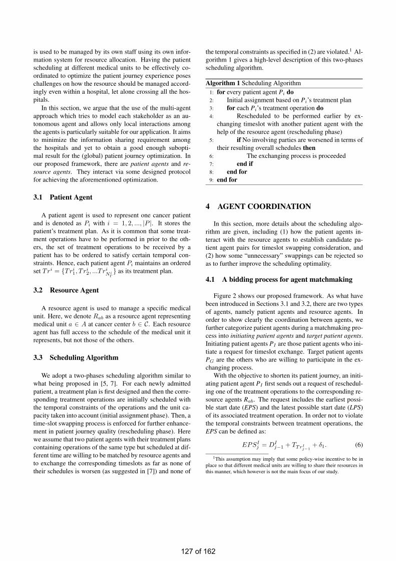
is used to be managed by its own staff using its own infor-mation system for resource allocation. Having the patientscheduling at different medical units to be effectively co-ordinated to optimize the patient journey experience poseschallenges on how the resource should be managed accord-ingly even within a hospital, let alone crossing all the hos-pitals.
In this section, we argue that the use of the multi-agentapproach which tries to model each stakeholder as an au-tonomous agent and allows only local interactions amongthe agents is particularly suitable for our application. It aimsto minimize the information sharing requirement amongthe hospitals and yet to obtain a good enough subopti-mal result for the (global) patient journey optimization. Inour proposed framework, there are patient agents and re-source agents. They interact via some designed protocolfor achieving the aforementioned optimization.
3.1 Patient Agent
A patient agent is used to represent one cancer patientand is denoted as Pi with i = 1, 2, ..., |P |. It stores thepatient’s treatment plan. As it is common that some treat-ment operations have to be performed in prior to the oth-ers, the set of treatment operations to be received by apatient has to be ordered to satisfy certain temporal con-straints. Hence, each patient agent Pi maintains an orderedset Tri = Tri
1, T ri2, ...T ri
NiΓ as its treatment plan.
3.2 Resource Agent
A resource agent is used to manage a specific medicalunit. Here, we denote Rab as a resource agent representingmedical unit a ∈ A at cancer center b ∈ C. Each resourceagent has full access to the schedule of the medical unit itrepresents, but not those of the others.
3.3 Scheduling Algorithm
We adopt a two-phases scheduling algorithm similar towhat being proposed in [5, 7]. For each newly admittedpatient, a treatment plan is first designed and then the corre-sponding treatment operations are initially scheduled withthe temporal constraints of the operations and the unit ca-pacity taken into account (initial assignment phase). Then, atime-slot swapping process is enforced for further enhance-ment in patient journey quality (rescheduling phase). Herewe assume that two patient agents with their treatment planscontaining operations of the same type but scheduled at dif-ferent time are willing to be matched by resource agents andto exchange the corresponding timeslots as far as none oftheir schedules is worsen (as suggested in [7]) and none of
the temporal constraints as specified in (2) are violated.1 Al-gorithm 1 gives a high-level description of this two-phasesscheduling algorithm.
Algorithm 1 Scheduling Algorithm1: for every patient agent Pi do2: Initial assignment based on Pi’s treatment plan3: for each Pi’s treatment operation do4: Rescheduled to be performed earlier by ex-
changing timeslot with another patient agent with thehelp of the resource agent (rescheduling phase)
5: if No involving parties are worsened in terms oftheir resulting overall schedules then
6: The exchanging process is proceeded7: end if8: end for9: end for
4 AGENT COORDINATION
In this section, more details about the scheduling algo-rithm are given, including (1) how the patient agents in-teract with the resource agents to establish candidate pa-tient agent pairs for timeslot swapping consideration, and(2) how some “unnecessary” swappings can be rejected soas to further improve the scheduling optimality.
4.1 A bidding process for agent matchmaking
Figure 2 shows our proposed framework. As what havebeen introduced in Sections 3.1 and 3.2, there are two typesof agents, namely patient agents and resource agents. Inorder to show clearly the coordination between agents, wefurther categorize patient agents during a matchmaking pro-cess into initiating patient agents and target patient agents.Initiating patient agents PI are those patient agents who ini-tiate a request for timeslot exchange. Target patient agentsPG are the others who are willing to participate in the ex-changing process.
With the objective to shorten its patient journey, an initi-ating patient agent PI first sends out a request of reschedul-ing one of the treatment operations to the corresponding re-source agents Rab. The request includes the earliest possi-ble start date (EPS) and the latest possible start date (LPS)of its associated treatment operation. In order not to violatethe temporal constraints between treatment operations, theEPS can be defined as:
EPSIj = DI
j−1 + TTrIj−1
+ δ1. (6)
1This assumption may imply that some policy-wise incentive to be inplace so that different medical units are willing to share their resources inthis manner, which however is not the main focus of our study.
127 of 162
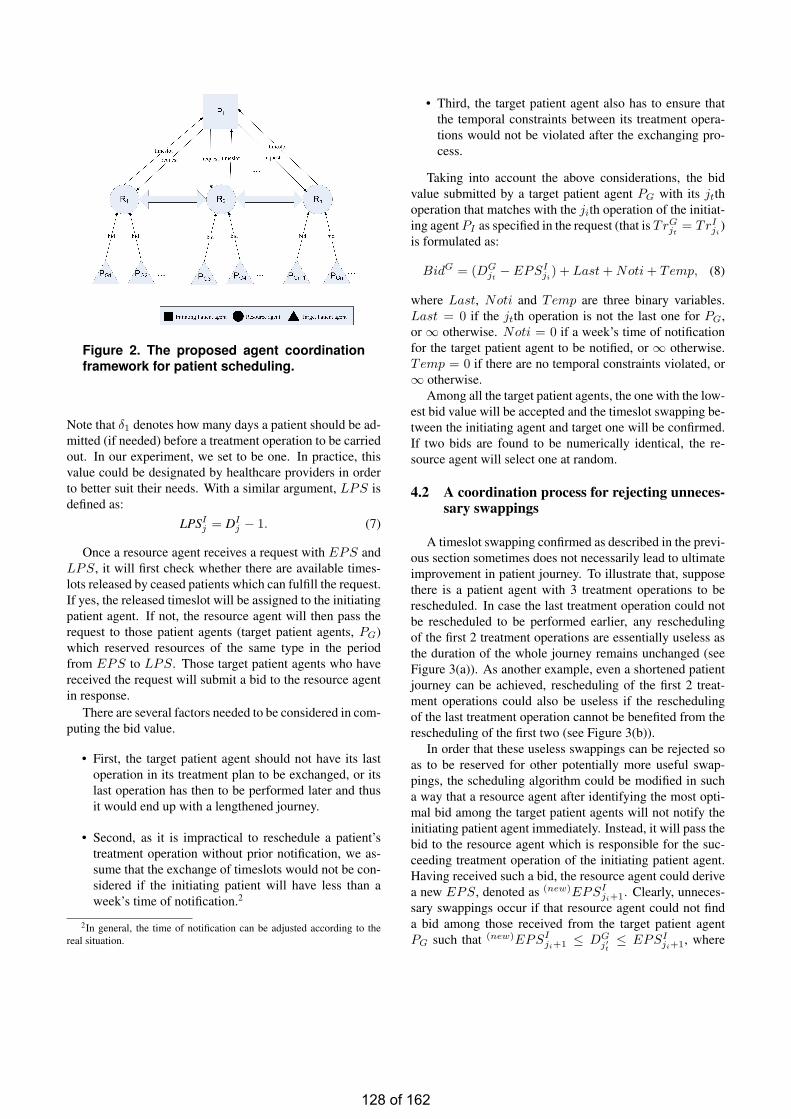
Figure 2. The proposed agent coordinationframework for patient scheduling.
Note that δ1 denotes how many days a patient should be ad-mitted (if needed) before a treatment operation to be carriedout. In our experiment, we set to be one. In practice, thisvalue could be designated by healthcare providers in orderto better suit their needs. With a similar argument, LPS isdefined as:
LPSIj = DI
j − 1. (7)
Once a resource agent receives a request with EPS andLPS, it will first check whether there are available times-lots released by ceased patients which can fulfill the request.If yes, the released timeslot will be assigned to the initiatingpatient agent. If not, the resource agent will then pass therequest to those patient agents (target patient agents, PG)which reserved resources of the same type in the periodfrom EPS to LPS. Those target patient agents who havereceived the request will submit a bid to the resource agentin response.
There are several factors needed to be considered in com-puting the bid value.
• First, the target patient agent should not have its lastoperation in its treatment plan to be exchanged, or itslast operation has then to be performed later and thusit would end up with a lengthened journey.
• Second, as it is impractical to reschedule a patient’streatment operation without prior notification, we as-sume that the exchange of timeslots would not be con-sidered if the initiating patient will have less than aweek’s time of notification.2
2In general, the time of notification can be adjusted according to thereal situation.
• Third, the target patient agent also has to ensure thatthe temporal constraints between its treatment opera-tions would not be violated after the exchanging pro-cess.
Taking into account the above considerations, the bidvalue submitted by a target patient agent PG with its jtthoperation that matches with the jith operation of the initiat-ing agent PI as specified in the request (that is TrG
jt= TrI
ji)
is formulated as:
BidG = (DGjt− EPSI
ji) + Last + Noti + Temp, (8)
where Last, Noti and Temp are three binary variables.Last = 0 if the jtth operation is not the last one for PG,or ∞ otherwise. Noti = 0 if a week’s time of notificationfor the target patient agent to be notified, or ∞ otherwise.Temp = 0 if there are no temporal constraints violated, or∞ otherwise.
Among all the target patient agents, the one with the low-est bid value will be accepted and the timeslot swapping be-tween the initiating agent and target one will be confirmed.If two bids are found to be numerically identical, the re-source agent will select one at random.
4.2 A coordination process for rejecting unneces-sary swappings
A timeslot swapping confirmed as described in the previ-ous section sometimes does not necessarily lead to ultimateimprovement in patient journey. To illustrate that, supposethere is a patient agent with 3 treatment operations to berescheduled. In case the last treatment operation could notbe rescheduled to be performed earlier, any reschedulingof the first 2 treatment operations are essentially useless asthe duration of the whole journey remains unchanged (seeFigure 3(a)). As another example, even a shortened patientjourney can be achieved, rescheduling of the first 2 treat-ment operations could also be useless if the reschedulingof the last treatment operation cannot be benefited from therescheduling of the first two (see Figure 3(b)).
In order that these useless swappings can be rejected soas to be reserved for other potentially more useful swap-pings, the scheduling algorithm could be modified in sucha way that a resource agent after identifying the most opti-mal bid among the target patient agents will not notify theinitiating patient agent immediately. Instead, it will pass thebid to the resource agent which is responsible for the suc-ceeding treatment operation of the initiating patient agent.Having received such a bid, the resource agent could derivea new EPS, denoted as (new)EPSI
ji+1. Clearly, unneces-sary swappings occur if that resource agent could not finda bid among those received from the target patient agentPG such that (new)EPSI
ji+1 ≤ DGj′t≤ EPSI
ji+1, where
128 of 162
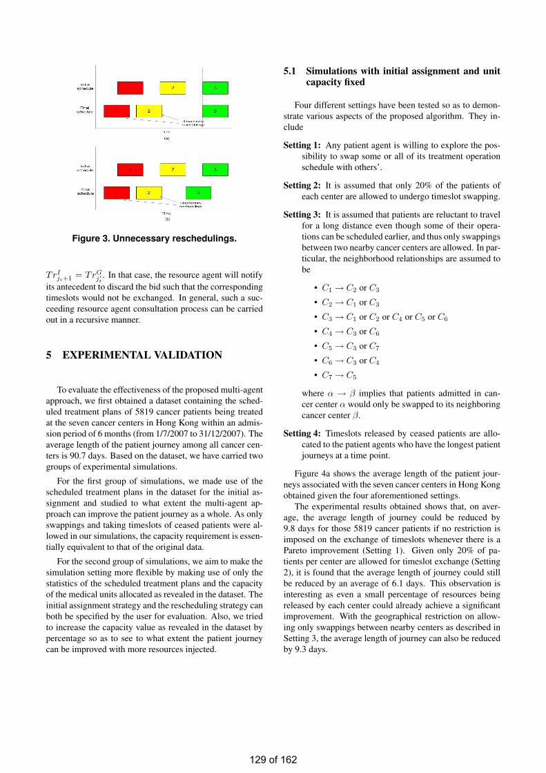
Figure 3. Unnecessary reschedulings.
TrIji+1 = TrG
j′t. In that case, the resource agent will notify
its antecedent to discard the bid such that the correspondingtimeslots would not be exchanged. In general, such a suc-ceeding resource agent consultation process can be carriedout in a recursive manner.
5 EXPERIMENTAL VALIDATION
To evaluate the effectiveness of the proposed multi-agentapproach, we first obtained a dataset containing the sched-uled treatment plans of 5819 cancer patients being treatedat the seven cancer centers in Hong Kong within an admis-sion period of 6 months (from 1/7/2007 to 31/12/2007). Theaverage length of the patient journey among all cancer cen-ters is 90.7 days. Based on the dataset, we have carried twogroups of experimental simulations.
For the first group of simulations, we made use of thescheduled treatment plans in the dataset for the initial as-signment and studied to what extent the multi-agent ap-proach can improve the patient journey as a whole. As onlyswappings and taking timeslots of ceased patients were al-lowed in our simulations, the capacity requirement is essen-tially equivalent to that of the original data.
For the second group of simulations, we aim to make thesimulation setting more flexible by making use of only thestatistics of the scheduled treatment plans and the capacityof the medical units allocated as revealed in the dataset. Theinitial assignment strategy and the rescheduling strategy canboth be specified by the user for evaluation. Also, we triedto increase the capacity value as revealed in the dataset bypercentage so as to see to what extent the patient journeycan be improved with more resources injected.
5.1 Simulations with initial assignment and unitcapacity fixed
Four different settings have been tested so as to demon-strate various aspects of the proposed algorithm. They in-clude
Setting 1: Any patient agent is willing to explore the pos-sibility to swap some or all of its treatment operationschedule with others’.
Setting 2: It is assumed that only 20% of the patients ofeach center are allowed to undergo timeslot swapping.
Setting 3: It is assumed that patients are reluctant to travelfor a long distance even though some of their opera-tions can be scheduled earlier, and thus only swappingsbetween two nearby cancer centers are allowed. In par-ticular, the neighborhood relationships are assumed tobe
• C1 → C2 or C3
• C2 → C1 or C3
• C3 → C1 or C2 or C4 or C5 or C6
• C4 → C3 or C6
• C5 → C3 or C7
• C6 → C3 or C4
• C7 → C5
where α → β implies that patients admitted in can-cer center α would only be swapped to its neighboringcancer center β.
Setting 4: Timeslots released by ceased patients are allo-cated to the patient agents who have the longest patientjourneys at a time point.
Figure 4a shows the average length of the patient jour-neys associated with the seven cancer centers in Hong Kongobtained given the four aforementioned settings.
The experimental results obtained shows that, on aver-age, the average length of journey could be reduced by9.8 days for those 5819 cancer patients if no restriction isimposed on the exchange of timeslots whenever there is aPareto improvement (Setting 1). Given only 20% of pa-tients per center are allowed for timeslot exchange (Setting2), it is found that the average length of journey could stillbe reduced by an average of 6.1 days. This observation isinteresting as even a small percentage of resources beingreleased by each center could already achieve a significantimprovement. With the geographical restriction on allow-ing only swappings between nearby centers as described inSetting 3, the average length of journey can also be reducedby 9.3 days.
129 of 162
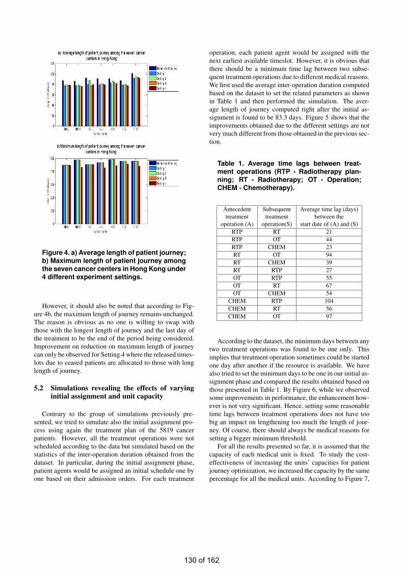
Figure 4. a) Average length of patient journey;b) Maximum length of patient journey amongthe seven cancer centers in Hong Kong under4 different experiment settings.
However, it should also be noted that according to Fig-ure 4b, the maximum length of journey remains unchanged.The reason is obvious as no one is willing to swap withthose with the longest length of journey and the last day ofthe treatment to be the end of the period being considered.Improvement on reduction on maximum length of journeycan only be observed for Setting 4 where the released times-lots due to ceased patients are allocated to those with longlength of journey.
5.2 Simulations revealing the effects of varyinginitial assignment and unit capacity
Contrary to the group of simulations previously pre-sented, we tried to simulate also the initial assignment pro-cess using again the treatment plan of the 5819 cancerpatients. However, all the treatment operations were notscheduled according to the data but simulated based on thestatistics of the inter-operation duration obtained from thedataset. In particular, during the initial assignment phase,patient agents would be assigned an initial schedule one byone based on their admission orders. For each treatment
operation, each patient agent would be assigned with thenext earliest available timeslot. However, it is obvious thatthere should be a minimum time lag between two subse-quent treatment operations due to different medical reasons.We first used the average inter-operation duration computedbased on the dataset to set the related parameters as shownin Table 1 and then performed the simulation. The aver-age length of journey computed right after the initial as-signment is found to be 83.3 days. Figure 5 shows that theimprovements obtained due to the different settings are notvery much different from those obtained in the previous sec-tion.
Table 1. Average time lags between treat-ment operations (RTP - Radiotherapy plan-ning; RT - Radiotherapy; OT - Operation;CHEM - Chemotherapy).
Antecedent Subsequent Average time lag (days)treatment treatment between the
operation (A) operation(S) start date of (A) and (S)RTP RT 21RTP OT 44RTP CHEM 23RT OT 94RT CHEM 39RT RTP 27OT RTP 55OT RT 67OT CHEM 54
CHEM RTP 104CHEM RT 56CHEM OT 97
According to the dataset, the minimum days between anytwo treatment operations was found to be one only. Thisimplies that treatment operation sometimes could be startedone day after another if the resource is available. We havealso tried to set the minimum days to be one in our initial as-signment phase and compared the results obtained based onthose presented in Table 1. By Figure 6, while we observedsome improvements in performance, the enhancement how-ever is not very significant. Hence, setting some reasonabletime lags between treatment operations does not have toobig an impact on lengthening too much the length of jour-ney. Of course, there should always be medical reasons forsetting a bigger minimum threshold.
For all the results presented so far, it is assumed that thecapacity of each medical unit is fixed. To study the cost-effectiveness of increasing the units’ capacities for patientjourney optimization, we increased the capacity by the samepercentage for all the medical units. According to Figure 7,
130 of 162
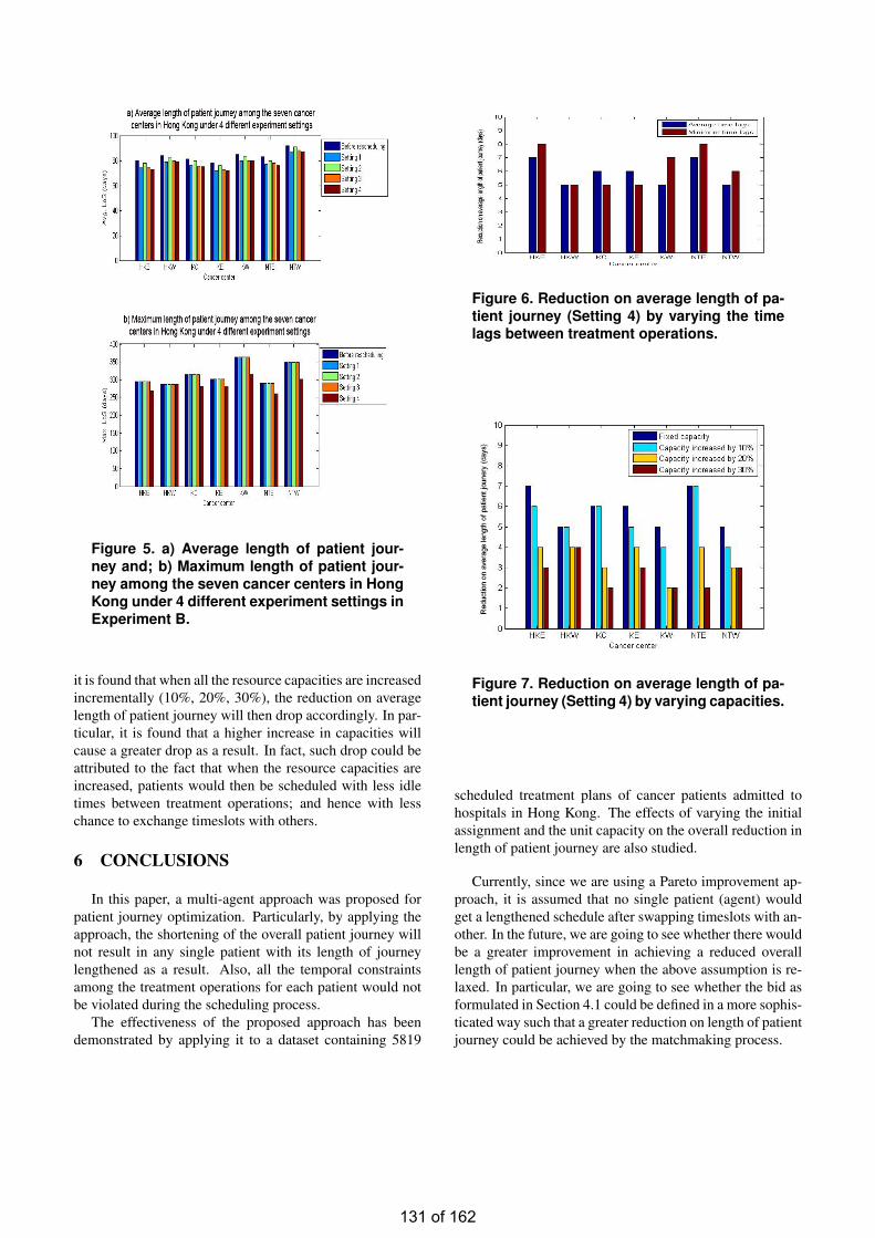
Figure 5. a) Average length of patient jour-ney and; b) Maximum length of patient jour-ney among the seven cancer centers in HongKong under 4 different experiment settings inExperiment B.
it is found that when all the resource capacities are increasedincrementally (10%, 20%, 30%), the reduction on averagelength of patient journey will then drop accordingly. In par-ticular, it is found that a higher increase in capacities willcause a greater drop as a result. In fact, such drop could beattributed to the fact that when the resource capacities areincreased, patients would then be scheduled with less idletimes between treatment operations; and hence with lesschance to exchange timeslots with others.
6 CONCLUSIONS
In this paper, a multi-agent approach was proposed forpatient journey optimization. Particularly, by applying theapproach, the shortening of the overall patient journey willnot result in any single patient with its length of journeylengthened as a result. Also, all the temporal constraintsamong the treatment operations for each patient would notbe violated during the scheduling process.
The effectiveness of the proposed approach has beendemonstrated by applying it to a dataset containing 5819
Figure 6. Reduction on average length of pa-tient journey (Setting 4) by varying the timelags between treatment operations.
Figure 7. Reduction on average length of pa-tient journey (Setting 4) by varying capacities.
scheduled treatment plans of cancer patients admitted tohospitals in Hong Kong. The effects of varying the initialassignment and the unit capacity on the overall reduction inlength of patient journey are also studied.
Currently, since we are using a Pareto improvement ap-proach, it is assumed that no single patient (agent) wouldget a lengthened schedule after swapping timeslots with an-other. In the future, we are going to see whether there wouldbe a greater improvement in achieving a reduced overalllength of patient journey when the above assumption is re-laxed. In particular, we are going to see whether the bid asformulated in Section 4.1 could be defined in a more sophis-ticated way such that a greater reduction on length of patientjourney could be achieved by the matchmaking process.
131 of 162
ACKNOWLEDGEMENT
This is to acknowledge Hong Kong Hospital Authorityfor providing the patient journey dataset to support this re-search study.
References
[1] H. Czap and M. Becker. Multi-agent systems and microe-conomic theory: A negotiation approach to solve schedul-ing problems in high dynamic environments. In HICSS ’03:Proceedings of the 36th Annual Hawaii International Con-ference on System Sciences (HICSS’03) - Track 3, page 83.2,Washington, DC, USA, 2003. IEEE Computer Society.
[2] K. Decker, J. Li, and Y. Demazeau. Coordinating mutuallyexclusive resources using gpgp. Autonomous Agents andMulti-Agent Systems, 3:200–0, 2000.
[3] X. Mao, A. Mors, N. Roos, and C. Witteveen. Coordinatingcompetitive agents in dynamic airport resource scheduling.In MATES ’07: Proceedings of the 5th German conferenceon Multiagent System Technologies, pages 133–144, Berlin,Heidelberg, 2007. Springer-Verlag.
[4] J. Patrick and M. Puterman. Reducing wait times throughoperations research: optimizing the use of surge capacity.Healthc Q, 11(3):77–83, 2008.
[5] T. O. Paulussen, I. S. Dept, K. S. Decker, A. Heinzl, andN. R. Jennings. Distributed patient scheduling in hospitals.In Coordination and Agent Technology in Value Networks.GITO, pages 1224–1232. Morgan Kaufmann, 2003.
[6] V. Robu, H. Noot, H. La Poutre, and W.-J. van Schijndel.An interactive platform for auction-based allocation of loadsin transportation logistics. In AAMAS ’08: Proceedings ofthe 7th international joint conference on Autonomous agentsand multiagent systems, pages 3–10, Richland, SC, 2008.International Foundation for Autonomous Agents and Mul-tiagent Systems.
[7] I. Vermeulen, S. Bohte, K. Somefun, and H. La Poutre. Im-proving patient activity schedules by multi-agent pareto ap-pointment exchanging. In CEC-EEE ’06: Proceedings ofthe The 8th IEEE International Conference on E-CommerceTechnology and The 3rd IEEE International Conferenceon Enterprise Computing, E-Commerce, and E-Services,page 9, Washington, DC, USA, 2006. IEEE Computer Soci-ety.
[8] J. Vissers and R. Beech. Health operations management: patient flow logistics in health care. Routledge, 2 ParkSquare, Milton Park, Abingdon, Oxon OX14 4RN, 2005.
[9] J. Vissers, J. Bekkers, and I. Adan. Patient mix optimiza-tion in tactical cardiothoracic surgery planning: a case study.IMA Journal of Management Mathematics, 16, 2005.
[10] M. Wang, J. Liu, H. Wang, W. K. Cheung, and X. Xie.On-demand e-supply chain integration: A multi-agentconstraint-based approach. Expert Systems with Applica-tions, 34(4):2683 – 2692, 2008.
[11] G. Weiss. Multiagent systems : a modern approach to dis-tributed artificial intelligence. Cambridge, Mass. : MITPress, 1999.
132 of 162
Commentary-based Video Categorization and Concept Discovery
Janice Kwan-Wai Leung
Abstract
Social network contents are not limited to text but alsomultimedia. Dailymotion, YouTube, and MySpace are ex-amples of successful sites which allow users to share videosamong themselves. Due to the huge amount of videos,grouping videos with similar contents together can helpusers to search videos more efficiently. Unlike the tradi-tional approach to group videos into some predefined cat-egories, we propose a novel comment-based matrix factor-ization technique to categorize videos and generate conceptwords to facilitate searching and indexing. Since the cate-gorization is learnt from users feedback, it can accuratelyrepresent the user sentiment on the videos. Experimentsconducted by using empirical data collected from YouTubeshows the effectiveness of our proposed methodologies.
1 Introduction
Starting from last decade, World Wide Web is developedinto the second generation Web 2.0. Thanks to this newestdevelopment, people can control over the data in the Inter-net instead of just retrieve data. Furthermore, it led to theevolution of web-based communities. Social networks suchas forums, blogs, video sharing sites are examples of appli-cations.
Recent years online video sharing systems are burgeon-ing. In video sharing sites, users are allowed to upload andshare videos with other users. YouTube is one of the mostsuccessful and fast-growing systems. In YouTube, users canshare their videos in various categories. Among these videocategories, music is the most popular one and the num-ber of music videos overly excess that of other categories[1, 7]. Users are not only allowed to upload videos but tagvideos and leave comments on them as well. With morethan 65,000 new videos being uploaded every day and 100million video views daily, YouTube becomes a representa-tive community among video sharing sites.
Due to the incredible growth of video sharing sites, videosearching is no longer a easy task and more effort shouldbe paid by users to search their desire videos from the en-tire video collection. To address this problem, grouping
videos with similar contents together is necessary. Cur-rently, videos on YouTube are only coarsely grouped intosome predefined high level categories (e.g. music, enter-tainment, sports, etc). Videos in a single category still spanthrough a wide range of varieties. For example, in the musiccategory, we may find music from various countries or withdifferent musical styles. Though some other video sharingsites, such as DailyMotion and MySpace, have a lower levelof category for music videos, the categorizes just follow thebasic music genre. However, people interests on music arenot limited to these simple genre. Furthermore, the prede-fined categories maybe too subjective to capture the real in-terest of the majority of users since they are only defined bya small group of people. Finally, the current categories onYouTube are fixed and it is hard to add/remove categoriestoo often. As time goes by, some categories may becomeobsolete and some new topics may be missing from the cat-egories.
These observations motivate us to explore a new wayof video categorization. In this work, we propose a novelcomment-based clustering technique by utilizing user com-ments for achieving this goal. Unlike the traditional ap-proaches of predefining some categories by human, our cat-egorization is learnt from the user comment. The advantageof our proposed approach is three-fold. First, our approachcan capture user interests more accurately and fairly thanthat of the predefined categories approach. The reason isthat we have taken the user opinions into consideration. Inother words, the resulting categories are contributed by pub-lic users rather than a small group of people; Second, sinceuser interest can be changed from time to time, the cate-gories of our method can be changed dynamically accordingto the recent comments by users; Finally, as users commentsare in the form of natural language, users can describe theiropinions in detailed. Therefore, by comment-based clus-tering, we can obtain clusters which represent fine-grainedlevel ideas.
In the literature, various clustering techniques have beenproposed for video categorization [5, 12]. However, thistype of techniques did not take user opinion into consid-eration and thus the clustering results do not capture userinterests. On the other hand, researchers have proposed touse the user tags on videos for clustering [6, 4]. Though
133 of 162
user tags can somehow reflect user feelings on videos, tagsare, in many cases, too brief to represent the complex ideasof users and thus the resulting clusters may only carry high-level concepts. Another stream of works which use com-monly fetched objects of users for clustering [2] also suffersimilar shortcomings as tag-based clustering. In [11], theyproposed to adopt a multi-modal approach for video catego-rization. However, their work required lots of human effortsto first identified different categories from a large amount ofvideos.
We want to remark that although comment-based cluster-ing can theoretically obtain more fine-grained level clusters,it is much more technically challenging than that of tag-based clustering. The reason is that user comments are usu-ally in the form of natural language and thus pre-processingis necessary for us to clean up the noisy data before usingthem for clustering.
The rest of the paper is organized as follows. Section2 discusses previous works in the context of social networkmining. Section 3 explains our proposed approach for videocategorization in video sharing sites. Section 4 briefly in-troduces our web crawler. Section 5 presents the details ofpre-processing of the raw data grabbed by our crawler. Sec-tion 6 describes our video clustering algorithm. Section 7presents and discusses our experimental results. Section 8concludes the paper.
2 Related Works
Since the late eighties, data mining has became a hot re-search field. Due to the advancing development of technolo-gies, there is an increasing number of applications involv-ing large amount of multimedia. For this reason, researchesin the field of data mining are not limited to text miningbut multimedia mining. Qsmar R. Zaine et al. [12] de-veloped a multimedia data mining system prototype, Mulit-MediaMiner, for analyzing multimedia data. They proposedmodules to classify and cluster images and videos basedon the multimedia features, Internet domain of pares ref-erencing the image of video, and HTML tags in the webpages. The multimedia features used include size of im-age or videos, width and height of frams, date on which theimage or video was created, etc. S. Kotsiantis et al. [5] pre-sented a work to discover relationships between multimediaobjects based on the features of a multimedia document. Intheir work, features of videos such as color or grayscale his-tograms, pixel information, are used for mining the contentof videos.
Motivated by the bloom of social networks, plenty ofworks have been done involving the study or analysis of on-line social networks. Different approaches are proposed todiscover user interests and communities in social networks.Tag-based approach is one of the invented methods. In [6],
Xin Li et al. developed a system to found common userinterests, and clustered users and their saved URLs by dif-ferent interest topics. They used the dataset from a URLsbookmarking and sharing site, del.icio.us. User interestsdiscovery, and user and URLs clustering were done by us-ing the tags users used to annotate the content of URLs.Another approach introduced to study user interests is user-centric which detects user interests based on the social con-nection among users. M. F. Schwartz et al. [8] discoverpeople’s interests and expertise by analyzing the social con-nections between people. A system, Vizster [3], was de-signed and developed to visualize online social networks.The job of clustering networks into communities was in-cluded in the system. For this task, Jeffrey and Danah iden-tified group structures based on linkage. Except the use ofsole tag-based or user-centric approaches, there are worksdone with a hybrid approach by combing the two methods.In [4], user interests in del.icio.us are modeled using thehybrid approach. Users are able to make friends with otherusers to form social ties in the URLs sharing network. Ju-lia Stoyanovich et al. examined user interests by utilizingboth the social ties and tags users used to annotate con-tent of URLs. Some researchers proposed the object-centricapproach for social interests detection. In this approach,user interests are determined with the analysis of commonlyfetched objects in social communities. Figuring out com-mon interests is also a useful task in peer-to-peer networkssince shared interests facilitate the content locating of desireobjects. Guo et al. [2] and K. Sripanidkulchai [9] presentedin their works the algorithms of examining shared interestsbased on the common objects users requested and fetchedin peer-to-peer systems.
3 Interest-based Video Categorization forVideo Searching
With the ceaseless growth of media content, it is in-creasingly a tense problem for video searching. It is usualthat users hardly find their desire videos from the immenseamount of videos. There are two main directions to ease theprocess of video searching, one is enhancing the text-basedsearch engine whilst the other one is designing a better di-rectory. In this paper, we focus on the former approach.
Though many video sharing sites allowed tagging func-tion for users to use tag to annotate videos during the uploadprocess, it is very common for user to tag videos by somehigh level wordings. As such, tags are usually too brieffor other users to locate the videos by using the text-basedsearch engine. In our method, as user comments usuallydescribe the video in details, we can use them for videoclustering to obtain fine-grained categories. By identifyingthe concept words for each categories, we can use them aslatent tags for the corresponding categories in order to facil-
134 of 162
itate the video searching process.In music domain, music videos in sharing systems are al-
ways categorized according to their types of musical sounds(e.g. pop, metal, country, etc.) under the music genre. How-ever, except music styles, people may have many differentattitudes and preferences (e.g. appearance of singers, eventof performance, age of songs, etc) towards music in differ-ent regions. Therefore, to categorize music based on peopleinterests, music genre is not a good categorical construct forvideo searching.
Our aim is to find a categorization where videos in eachvideo group are representing a popular topic of interest. Inour algorithm, interests are modeled by clustering videosinto groups with the utilization of user-left comments. Pre-viously, computer scientists have tried many ways to finduser interests. Tags are very popular to help in this context[6]. However, two disadvantages would be raised in thismanner. First, tags on a video are manually given by theone who uploads the video, thus the tags are just expressinga single user’s feeling about the video. Therefore, tags ona video would have a strong bias and are not fair enough toexactly describe what the video is actually about. Further-more, single-user given tags are definitely not representativeof public feelings about the video. Second, videos are of-ten tagged with a small number of words. As such, oftenfails to give enough description on the video. Therefore,tags are insufficient to provide detailed information aboutvideos. Since comments can be given by any users on anyvideos as feedbacks, they express different users thoughtsabout a video. Thus, containing more in-depth informationabout the videos. Also, allowing every user to leave feed-backs, the number of comments on a video are usually muchmore than that of tags. Hence, utilizing comments to findout interests instead of tags can solve the above difficulties.
Beside tag-based, some researchers proposed thecontent-based approach to categorize videos. Using videocontent as categorizing materials can group similar videostogether according to their actual content. Nevertheless,video content itself only provide information about thevideos but nothing about users’ idea. Consequently, thisapproach fails to group videos according to user interests.In contrast, user-left comments include users’ view aboutthe videos. Therefore, comments can, undoubtedly, be usedto categorize videos based on popular user interests.
Video features can also be used to achieve the goal ofcluster videos [5]. Video features, however, are hard to beextracted automatically. Due to the limitation of human re-sources, automatic information retrieval from mass amountof data is preferred. Also, using video features to clustervideos suffers the same shortcomings of content-based aswell. Because of information retrieval dealing with text ismuch easier than video features extraction, and comments,in addition to video content, provide users’ views on videos,
user-left comments are significant for clustering videos.
4 Data set collection
YouTube is a video sharing platform which users can up-load their own videos for sharing purpose. Along with eachvideo, a short description can be entered by the uploadinguser and also comments can be given by other registeredusers. In this paper, we focused on the user comments ofmusic videos of Hong Kong singers in YouTube.
We first defined a set of 102 Hong Kong singer/groupnames. Given the set of singer/group names, we developeda crawler to firstly visit the YouTube web site and auto-matically searches from the site the related videos basedon video titles and video descriptions. From the resultingvideos, the crawler saves the URL of each videos for fur-ther process. For the convenience of gathering user com-ments, the crawler transforms the fetched URLs to linkswhich link to the pages of ”all comments” mode of cor-responding videos. With all the transformed video URLs,for each link, the crawler is able to scrape the video webpage and grab the video title, all the user comments anduser name of who left comments on the video.
In the data set acquired by our crawler, there are 19305videos, 102 singers and 7271 users in total.
5 Data Pre-processing
To ease the process of video searching by discoveringthe user interest and categorizing videos, larger amount ofdata is required from video sharing sites. However, just thelarge-sized collection of text-formatted raw data is not ap-plicable for further processing. Large-sized dataset alwaysneed to undergo data pre-processing in the field of data min-ing. Here is no exception in our algorithm. After crawlingYouTube, the mass data need to be pre-processed beforeperforming video clustering.
Here are two steps of data pre-processing involved in ourintroduced algorithm,
1) Data Cleaning2) Text Matrix Generation
5.1 Data Cleaning
As the comments left on YouTube videos are writtenin natural languages which consist lots of non-informativewords, such as ”thank” , ”you”, etc, text processing withsuch materials must be caution. To avoid resulting a poorclustering,data cleaning is necessary for handling the noisywords.
In natural languages, there are many words that are notinformative for clustering. These words would make the
135 of 162
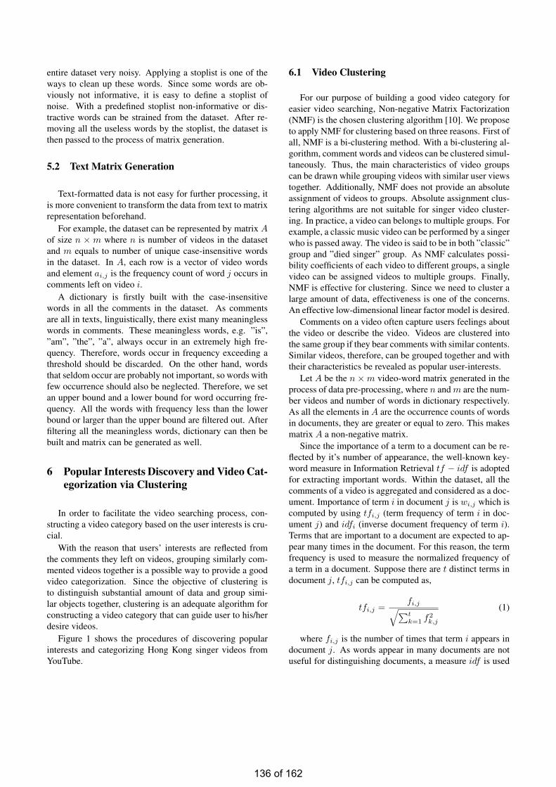
entire dataset very noisy. Applying a stoplist is one of theways to clean up these words. Since some words are ob-viously not informative, it is easy to define a stoplist ofnoise. With a predefined stoplist non-informative or dis-tractive words can be strained from the dataset. After re-moving all the useless words by the stoplist, the dataset isthen passed to the process of matrix generation.
5.2 Text Matrix Generation
Text-formatted data is not easy for further processing, itis more convenient to transform the data from text to matrixrepresentation beforehand.
For example, the dataset can be represented by matrix Aof size n × m where n is number of videos in the datasetand m equals to number of unique case-insensitive wordsin the dataset. In A, each row is a vector of video wordsand element ai,j is the frequency count of word j occurs incomments left on video i.
A dictionary is firstly built with the case-insensitivewords in all the comments in the dataset. As commentsare all in texts, linguistically, there exist many meaninglesswords in comments. These meaningless words, e.g. ”is”,”am”, ”the”, ”a”, always occur in an extremely high fre-quency. Therefore, words occur in frequency exceeding athreshold should be discarded. On the other hand, wordsthat seldom occur are probably not important, so words withfew occurrence should also be neglected. Therefore, we setan upper bound and a lower bound for word occurring fre-quency. All the words with frequency less than the lowerbound or larger than the upper bound are filtered out. Afterfiltering all the meaningless words, dictionary can then bebuilt and matrix can be generated as well.
6 Popular Interests Discovery and Video Cat-egorization via Clustering
In order to facilitate the video searching process, con-structing a video category based on the user interests is cru-cial.
With the reason that users’ interests are reflected fromthe comments they left on videos, grouping similarly com-mented videos together is a possible way to provide a goodvideo categorization. Since the objective of clustering isto distinguish substantial amount of data and group simi-lar objects together, clustering is an adequate algorithm forconstructing a video category that can guide user to his/herdesire videos.
Figure 1 shows the procedures of discovering popularinterests and categorizing Hong Kong singer videos fromYouTube.
6.1 Video Clustering
For our purpose of building a good video category foreasier video searching, Non-negative Matrix Factorization(NMF) is the chosen clustering algorithm [10]. We proposeto apply NMF for clustering based on three reasons. First ofall, NMF is a bi-clustering method. With a bi-clustering al-gorithm, comment words and videos can be clustered simul-taneously. Thus, the main characteristics of video groupscan be drawn while grouping videos with similar user viewstogether. Additionally, NMF does not provide an absoluteassignment of videos to groups. Absolute assignment clus-tering algorithms are not suitable for singer video cluster-ing. In practice, a video can belongs to multiple groups. Forexample, a classic music video can be performed by a singerwho is passed away. The video is said to be in both ”classic”group and ”died singer” group. As NMF calculates possi-bility coefficients of each video to different groups, a singlevideo can be assigned videos to multiple groups. Finally,NMF is effective for clustering. Since we need to cluster alarge amount of data, effectiveness is one of the concerns.An effective low-dimensional linear factor model is desired.
Comments on a video often capture users feelings aboutthe video or describe the video. Videos are clustered intothe same group if they bear comments with similar contents.Similar videos, therefore, can be grouped together and withtheir characteristics be revealed as popular user-interests.
Let A be the n ×m video-word matrix generated in theprocess of data pre-processing, where n and m are the num-ber videos and number of words in dictionary respectively.As all the elements in A are the occurrence counts of wordsin documents, they are greater or equal to zero. This makesmatrix A a non-negative matrix.
Since the importance of a term to a document can be re-flected by it’s number of appearance, the well-known key-word measure in Information Retrieval tf − idf is adoptedfor extracting important words. Within the dataset, all thecomments of a video is aggregated and considered as a doc-ument. Importance of term i in document j is wi,j which iscomputed by using tfi,j (term frequency of term i in doc-ument j) and idfi (inverse document frequency of term i).Terms that are important to a document are expected to ap-pear many times in the document. For this reason, the termfrequency is used to measure the normalized frequency ofa term in a document. Suppose there are t distinct terms indocument j, tfi,j can be computed as,
tfi,j =fi,j√∑tk=1 f2
k,j
(1)
where fi,j is the number of times that term i appears indocument j. As words appear in many documents are notuseful for distinguishing documents, a measure idf is used
136 of 162
Figure 1. Popular interests discovery and video categorization of Hong Kong singer videos in YouTube.
to scale down the importance of these widely-used terms.The inverse document frequency of term i is defined as,
idfi = logN
ni(2)
where N is the total number documents in the dataset,and ni is number of documents that containing term i.
After computing the term frequency and inverse docu-ment frequency, the importance weight of a term i in docu-ment j is defined as the combination of tfi,j and idfi,
wi,j = tfi,j × idfi (3)
The greater the weighting, the more the important is theterm to the respecting document.
From matrix A, a non-negative matrix X can be pro-duced by calculating the importance weights. Each elementin X is defined as,
xi,j = wi,j =ai,j√∑tk=1 a2
k,j
× logN
ni(4)
By fitting a k-factor model to matrix X , where k equalsto number of groups to be obtained, X is decomposed totwo non-negative matrices W and H , such that X = WH+U . After matrix decomposition, W is in size of n × k andH is in size of k ×m.
Our objective is to find W and H such that X ≈ WH .By iteratively updating W and H , we can obtain W and Hby minimizing the following function,
F (W,H) = ||X −WH||2 (5)
with respect to W and H and subject to constraints thatW,H ≥ 0.
Figure 2 shows the decomposition of video dataset ma-trix. From the resulting matrices, relationships betweenwords videos and clusters are revealed. Matrix W shows the
relationships between videos and different clusters, whilstH clarifies the relationships between words and clusters.In W , value held in wn,k is the coefficient indicated howlikely video n belongs to cluster k. To fit the purpose ofour research, we have refined the method of group assign-ing in NMF. The original NMF algorithm assigns an objectto a group in a maximum coefficient approach. However,in our method, a video n is treated to be in group k if wn,k
has the a value greater than a threshold βk within vector nin W , where the value of threshold βk is data dependent.The threshold should be chosen in a coefficient distributiondepend manner. Videos can then be grouped into clustersbased on their similarities. We define the set of cluster forvideo Vn that it belongs to as,
Cn = k ∈ K | ∀ Wn,k > βk (6)
where K is set of all clusters.Matrix H provides the information about the character-
istics of the video groups. Concept words of a cluster canbe found with H as hk,m is the coefficient of the term mbelongs to cluster k. For each cluster, the top 10 words,with respect to the term-cluster coefficient, are consideredto be the concept words for the cluster. Hence, stating theproperties of a group of videos.
7 Experimental Evaluation
A proof-of-concept experiment was done to study theHong Kong social culture in regional music domain. AnIntel(R) Core(TM)2 Quad 2.40GHz PC with 4GB RAMwas used to conduct our experiment. Our web crawler wasimplemented in VC++ and the core algorithm was imple-mented in Matlab.
137 of 162
Figure 2. NMF decomposition for video clus-tering.
7.1 Empirical Setting
As the videos were grabbed by searching from theYouTube site with predefined list of singer names, there arepossibilities that some videos are grabbed more than onetime. For those videos preformed by more than one singer,as long as there are more than one singer names annotatedin the video title, the video will be collected in times equalsto the number of hits the predefined singer name hits thevideo title. To achieve a more accurate clustering result,duplicated videos are removed form the dataset.
In comments, users are used to mention the singer nameswhen they are commenting on him/her. This will make thesinger names dominate in every group of concept words.However, it is not conspicuous enough to reveal interests bysingers. Therefore, in our experiment, we add singer namesto the stoplist as well.
Furthermore, some videos are less popular or just beenuploaded for a short time that only have a few comments.These videos which have relatively few words are informa-tiveless for video clustering. Videos which have less than30 valid words are eliminated.
The videos are clustered into k groups with the cluster-ing algorithm discussed in section 7, where k is experimen-tally set as 20. The experiment was done twice, once withthreshold βi regarding cluster i to be mean coefficient of allvideos,
βi = meanCoefi =
∑nj=1 wj,i
n(7)
To compensate the poor performance caused by the ex-tremely uneven distribution of coefficient, we chose thethreshold to be mean coefficient plus standard deviation ofall videos for the second experiment. βi regarding cluster iis defined as,
Group Concept Words1 beautiful lyrics melody2 female makeup dress3 cute pretty handsome4 sex photos scandal5 funny hilarious laughing6 rap raps hip7 movie film story8 cantonese mandarin language9 commercial pepsi coke
10 piano piece ear grade11 japanese japan korean12 china olympic games13 old classic memories14 dance dancer moves15 guitar band rock16 award tvb gold17 english chinese accent18 sad legend died19 together couple two20 voice pretty talent
Table 1. Latent video categories discoveredin Hong Kong music video domain fromYouTube
βi = meanSdCoefi =
√√√√ 1n
n∑
j=1
(wj,i −meanCoefi)2
(8)where n is total number of videos being clustered.
7.2 Video Categorization
Since video clustering is a complete clustering analysis,music categories and trends in Hong Kong can be found byclustering the videos. We deployed NMF as our cluster-ing method. Applied the clustering algorithm to the videodataset in the way discussed in Section 5.2, with the ex-perimentally chosen number of cluster of 18, videos wereclustered into groups based on the words in their comments.The mean coefficient of videos to a cluster is set as the crit-ical point. Videos with coefficient higher than the criticalpoint of a cluster are said to be in that cluster. Under thisstrategy, videos can belong to several clusters as they mayhave multiple characteristics. Table 1 shows the discoveredcategories from our dataset.
Unlike the generic music video categorization of somefamous video sharing sites, such as DailyMotion dividesmusic videos into eight classes (Pop, Rock, Rap, R&B,
138 of 162
Figure 3. Singer video distribution inYouTube.
Precision
Group Concept Words Mean asThreshold
Mean + SDas Thresh-old
A sex photos scandal 21.64% 81.58%B old classic memories 61.04% 78.16%C sad legend died 35.86% 60.34%D together couple two 64.44% 79.82%
Average 45.75% 74.96%
Table 2. Precision of objective clusters
Jazz, Metal, Covers, and Electros), we categorized videosof local singers into twenty classes which are far more spe-cific.
From our clustering result, we noticed that videos ofsingers are not only limited to general music videos, butalso funny clips, award presentations, commercial adver-tisements as well as event promotion clips. Looking atthe music videos alone, by clustering users’ comments, wefound that people’s attitude towards Hong Kong music arenot only target on the music styles. There are also other fea-tures of music people are interested at, like languages, ageof music, music instruments, type of singers, singer’s voice,composition goodness, etc.
Furthermore, categorize singer videos with the proposedclustering algorithm, people can identify dance-orientedvideos (Group 14), cross-culture produced music (Group11) or even movie theme songs (Group 7) easily. Otherthan simply categorizing singer video clips, some up-to-date news in the local music circle, like scandals (Group4), can also be found.
Figure 3 illustrates the distribution of Hong Kong singervideos in YouTube according to the proposed algorithm us-ing mean and mean + sd as thresholds. From the figure,we can see that the distribution of videos diverse over dif-ferent threshold values. With the mean coefficient as thethreshold, compared to the video groups resulted from the
algorithm with mean + SD coefficient as threshold, largergroups of videos can be obtained. In the other words, algo-rithm associated with a smaller group assigning thresholdwould result heavier overlapped video groups.
The video clustering results are evaluated by human ex-perts. To make the evaluation less controvertible, we onlyshow the precisions of objective video groups in Table 2where groups A, B, C, D are cluster 4, 13, 18, 19 in ourclustering. In the table, we noticed that assigning videosto groups with a smaller threshold may sometimes lowerthe precision. This will be caused in the groups which arevery distinct to others. As a video group is too specific, thevideo-group coefficients to the group hold the extreme val-ues. Also, closely related videos to the distinct group is al-ways much fewer than videos which do not. Hence, videosare condense at the lower extreme side. As a result, low-ered the mean coefficient and caused the poor precision. Onthe other hand, we can see that the algorithm which assignsvideos into groups with a larger threshold yields far betterprecisions. The average precision of the larger-thresholdclustering groups in the table is 74.96% whilst that of thelower-threshold clustering is just 45.75%. The differencebetween the precisions resulted from clustering with the twodifferent thresholds reflects the degree of extraordinary ofthe video group. The larger the difference, the more thespecial the group is. For example, in group 4, the two preci-sions differ from each other by a large percentage at about60%, and from the concept words we can know that thisgroup is about scandal of singers involving their sex photos.This is obviously an extremely distinct group.
7.3 User Comments vs User Tags
As tags are believed to be an accurate description of anobject and have been widely used for finding user interestsand grouping objects, it is necessary to examine the virtuesof user comments over tags before utilizing comments tocapture popular interests and categorize videos to facilitatethe video search in video sharing sites. One important ob-servation from our experimental results is that user com-ments usually contains more in-depth information than thatof user tags. Table 3 shows both the top 10 concept wordsfound from user comments and the top 10 user tags of fourclustered groups. From the concept words in the user com-ments, we can make a reasonable prediction that cluster Iis about some music videos of some old songs. From theuser tags, however, we can only find some singer names orsome high-level descriptions (e.g. music, mv, mtv). Sameas cluster II, from the concept words, this cluster is probablytalking about some superstars who are already died. Nev-ertheless, the most frequent tags are only names of thosedead superstars which do not reveal the low-level descrip-tion of the group. Cluster III is the similar case as the above
139 of 162
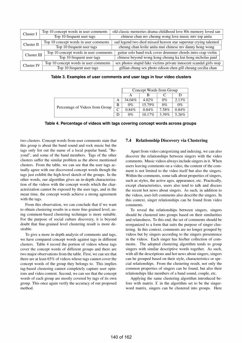
Cluster I Top 10 concept words in user comments old classic memories drama childhood love 80s memory loved sanTop 10 frequent user tags chinese chan mv cheung wong love music mtv top anita
Cluster II Top 10 concept words in user comments sad legend two died missed heaven star superstar crying talentedTop 10 frequent user tags cheung chan leslie anita mui chinese mv danny hong wong
Cluster III Top 10 concept words in user comments guitar solo band rock cover drummer chords intro crap violinTop 10 frequent user tags chinese beyond wong kong cheung ka kui hong nicholas paul
Cluster IV Top 10 concept words in user comments sex photos stupid fake victims private innocent scandal girls stopTop 10 frequent user tags gillian chung sex photo edison chen gill cheung cecilia chan
Table 3. Examples of user comments and user tags in four video clusters
Concept Words from GroupA B C D
Percentage of Videos from Group
A 34.04% 4.02% 0% 2.13%B 0% 15.79% 0% 0%C 0.84% 0.84% 7.58% 0.84%D 0% 10.17% 3.39% 5.26%
Table 4. Percentage of videos with tags covering concept words across groups
two clusters. Concept words from user comments state thatthis group is about the band sound and rock music but thetags only list out the name of a local popular band, ”Be-yond”, and some of the band members. Tags of the otherclusters suffer the similar problem as the above mentionedclusters. From the table, we can see that the user tags ac-tually agree with our discovered concept words though thetags just exhibit the high-level sketch of the groups. In theother words, our algorithm gives an in-depth characteriza-tion of the videos with the concept words which the char-acterization cannot be exposed by the user tags, and in themean time, the concept words achieve a strong agreementwith the tags.
From this observation, we can conclude that if we wantto obtain clustering results in a more fine-grained level, us-ing comment-based clustering technique is more suitable.For the purpose of social culture discovery, it is beyonddoubt that fine-grained level clustering result is more de-sirable.
To give a more in-depth analysis of comments and tags,we have compared concept words against tags in differentclusters. Table 4 record the portion of videos whose tagscover the concept words of different groups and there aretwo major observations from the table. First, we can see thatthere are at least 65% of videos whose tags cannot cover theconcept words of the group they belongs to. This impliestag-based clustering cannot completely capture user opin-ions and video content. Second, we can see that the conceptwords of each group are mostly covered by tags of its owngroup. This once again verify the accuracy of our proposedmethod.
7.4 Relationship Discovery via Clustering
Apart from video categorizing and indexing, we can alsodiscover the relationships between singers with the videocomments. Music videos always include singers in it. Whenusers leaving comments on a video, the content of the com-ment is not limited to the video itself but also the singers.Within the comments, some talk about properties of singers,such as styles, the active ages, appearance, etc. Practically,except characteristics, users also tend to talk and discussthe recent hot news about singers. As such, in addition tothe videos, user-left comments also describe the singers. Inthis context, singer relationships can be found from videocomments.
To reveal the relationships between singers, singersshould be clustered into groups based on their similaritiesand relatedness. To this end, the set of comments should bereorganized to a form that suits the purpose of singer clus-tering. In this context, comments are no longer grouped byvideos but by singers according to the singers presentencein the videos. Each singer has his/her collection of com-ments. The adopted clustering algorithm tends to groupsingers with similar descriptive words together. As such,with all the descriptions and hot news about singers, singerscan be grouped based on their style, characteristics or spe-cial relationships. From the clustering result, not only thecommon properties of singers can be found, but also theirrelationships like members of a band sound, couple, etc.
Applying the same clustering algorithm introduced be-fore with matrix X in the algorithm set to be the singer-word matrix, singers can be clustered into groups. Here
140 of 162
Figure 4. Singer Relationship.
we visualize the relationships between singers in a singernetwork based on their similarities reflected from the com-ments. With a visualized singer network, not only the re-lationships between singers can be shown but also the hid-den phenomenon. Due to the paper size, Figure 4 illustrateonly partial of the singer network. In this graph, the singersare relatively closely connected to each others than to othersingers and thus form a subnetwork. In this subnetwork,all the nodes are active singers in 80s, this is one of theirrelationships. The network is a directed graph which thesinger being pointed to is highly referenced by the singerwho points to him/her. Grasshopper, at the top left cor-ner is pointing to Anita Mui at the bottom as the membersof Grasshopper are students of Anita Mui. Leslie Cheung,Danny Chan and Anita Mui are famous singers and manyother singers have used their songs for performance. Thiscan be reflected in the graph: many other singers points tothese three singers.
8 Conclusion and Future Work
In this paper, we have proposed a comment-based videocategorization approach by using NMF. Experimental re-sults showed that our comment-based clustering yields bet-ter performance than that of tag-based approach which wasproposed previously in the literature. On the other hand,we have successfully discovered some non-trivial categoriesamong the videos of Hong Kong singers. Since our catego-rization is learnt from user feedbacks, it can provide an easyway for users to reach their desire videos via our list of cate-gories. Additionally, our comment-based clustering can re-veal relationships among singers within the social networkwhich can help in the context of social culture study.
In our future work, we plan to extend the comment-based
technique from video and singer clustering to user clus-tering. After we have obtained the three types of cluster,we can acquire the relationships among different videos,singers and users by analyzing the inter-cluster similarity.As such, social culture can be studied by combining and an-alyzing the discovered relationships. With the video-video,singer-singer, user-singer, and user-user relationships foundby clustering, we can know the changes in music styles andsinger styles over the ages, the trend of music, the wayspeople appreciate music, and even the special relationshipsof singers reflected by news, and more. Relationships ob-served by clustering are not only useful for social scientiststo study social culture, but also beneficial for businesses,entertainment companies, fans clubs, social network sys-tems and system users. With the help of examined user-user relationships, businesses can be profited from reduc-ing advertising costs by advertise only to the potential cus-tomer groups. User-signer relationships define user-idolgroups, entertainment companies can effectively promoteto the target groups. Determining the user-singer relation-ships, in addition to profits for entertainment companies,fans groups can easily be managed. Other than the advan-tages for some specific parties, general users are also bene-fited. Well-clustered groups of videos and singers equippedwith a batch of indicative words leads to a effort savingvideo searching for users. Also, social network systems areable to detect and refine incorrect tags with the indicativewords resulted from clustering. As a result, introductions tovideos are more precise and thus improves the video search-ing function.
141 of 162
References
[1] X. Cheng, C. Dale, and J. Liu. Understanding the char-acteristics of internet short video sharing: Youtube asa case study. In CoRR abs, Jul 2007.
[2] L. Guo, S. Jiang, L. Xiao, and X. Zhang. Fast and low-cost search schemes by exploiting localities in p2pnetworks. J. Parallel Distrib. Comput., 65(6):729–742, 2005.
[3] J. Heer and D. Boyd. Vizster: Visualizing online socialnetworks. IEEE Symposium on Information Visualiza-tion, 2005.
[4] C. M. C. Y. Julia Stoyanovich, Sihem Amer-Yahia. Leveraging tagging to model user interests indel.icio.us. In AAAI ’08: Proceedings of the 2008AAAI Social Information Spring Symposium. AAAI,2008.
[5] P. P. Kotsiantis S., Kanellopoulos D. Multimedia min-ing. In WSEAS Transactions on Systems, Issue 10,Volume 3, pages 3263–3268, December 2004.
[6] X. Li, L. Guo, and Y. E. Zhao. Tag-based social inter-est discovery. In WWW ’08: Proceeding of the 17thinternational conference on World Wide Web, pages675–684, New York, NY, USA, 2008. ACM.
[7] C. G. R. A. A. F. L. Rodrygo L. T. Santos, Bruno P.S. Rocha. Characterizing the youtube video-sharingcommunity. 2007.
[8] M. F. Schwartz and D. C. M. Wood. Discoveringshared interests using graph analysis. Commun. ACM,36(8):78–89, 1993.
[9] K. Sripanidkulchai, B. Maggs, and H. Zhang. Effi-cient content location using interest-based locality inpeer-to-peer systems. In INFOCOM 2003. Twenty-Second Annual Joint Conference of the IEEE Com-puter and Communications Societies. IEEE, volume 3,pages 2166–2176 vol.3, 2003.
[10] W. Xu, X. Liu, and Y. Gong. Document clusteringbased on non-negative matrix factorization. In SI-GIR ’03: Proceedings of the 26th annual internationalACM SIGIR conference on Research and developmentin informaion retrieval, pages 267–273, New York,NY, USA, 2003. ACM.
[11] L. Yang, J. Liu, X. Yang, and X.-S. Hua. Multi-modality web video categorization. In MIR ’07: Pro-ceedings of the international workshop on Workshopon multimedia information retrieval, pages 265–274,New York, NY, USA, 2007. ACM.
[12] O. R. Zaıane, J. Han, Z.-N. Li, S. H. Chee, and J. Y.Chiang. Multimediaminer: a system prototype formultimedia data mining. In SIGMOD ’98: Proceed-ings of the 1998 ACM SIGMOD international confer-ence on Management of data, pages 581–583, NewYork, NY, USA, 1998. ACM.
142 of 162
Implementation of Multiple-precision Modular Multiplication on GPU
Kaiyong Zhao
Abstract Multiple-precision modular multiplications are the key
components in security applications, like public-key cryptography for encrypting and signing digital data. But unfortunately they are computationally expensive for contemporary CPUs. By exploiting the computing power of the many-core GPUs, we implemented a multiple-precision integer library with CUDA. In this paper, we will investigate the implementation of two approaches of multiple-precision modular multiplications on GPU. We will analyze the detail of the instructions of multiple-precision modular multiplication on the GPU and find the hit issues, and then we propose to use the inline ASM to improve the implementation of this function. Our experimental results show that the performance of multiple-precision modular multiplication has been improved by 20%.
Keywords GPU computing, CUDA, Multiple-precision Modular Multiplication, Karatsuba multiplication, Montgomery modular multiplication
1. Introduction
In recent years, peer-to-peer (P2P) content distribution applications such as BitTorrent and ppLive, have become the most popular Internet applications due to their scalability and robustness. Network coding has been proposed as an effective mechanism to improve the performance of such P2P applications [14]. However, P2P applications with network coding suffer from the notorious pollution attacks: a malicious node can send out bogus packets which will be merged into other genuine packets and propagated into the whole network at an exponential speed. To resolve this problem, homomorphic hash functions have to be applied such that the hash of any encoded packet can be effectively derived from the hashes of the original packets, which enables the detection of bogus packets before a peer encodes it with other packets [12]. Unfortunately homomorphic hash functions rely on multiple-precision modular operations and are computationally expensive [10] [12].
Recent advances in Graphics Processing Units (GPUs) open a new era of GPU computing [20]. For example, commodity GPUs like NVIDIA’s GTX 280 has 240
processing cores and can achieve 933 GFLOPS of computational horsepower. More importantly, the NVIDIA CUDA programming model makes it easier for developers to develop non-graphic applications using GPU [1] [4]. In CUDA, the GPU becomes a dedicated coprocessor to the host CPU, which works in the principle of Single-Program Multiple Data (SPMD) where multiple threads based on the same code can run simultaneously.
In this paper, we present our study of using GPUs for multiple-precision modular multiplication, which is the key component of not only the homomorphic hashing, but also a number of security applications that make use of public-key cryptography. We implement two methods of multiple-precision modular multiplications on NVIDIA GPUs using CUDA. One is Coarsely Integrated Operand Scanning (CIOS) Montgomery method; the second one is Karatsuba multiplication with Montgomery. In order to achieve the highest performance, we analyze the ptx code (i.e., the assembly code for NVIDIA GPUs) of the implementation. As the CUDA PTX standard is not open to the public, we rely on the decuda tool to disassemble the compiled binary cubin file and search for the bottleneck for an improvement.
The contribution of this work is twofold: • First, we designed and implemented two approaches of
multiple-precision modular multiplication on the CUDA architecture.
• Second, we analyze the implementation of the directive instructions, and use inline ASM to optimize the Montgomery algorithm.
The rest of the paper is organized as follows. Section 2 provides background information on Karatsuba Mulitiplication, Montgomery algorithm, GPU architecture, and CUDA programming model. Section 3 presents the design of multiple-precision modular arithmetic on GPU. Section 4 presents the decuda analysis, and then presents our inline ASM implementation of the 32-bit integer multiplication. Experimental results are presented in Section 5, and we conclude the paper in Section 6.
2. Background and Related Work
In this section, we provide the required background knowledge of Karatsuba multiplication, Montgomery multiplication algorithm, GPU architecture, and CUDA programming model.
143 of 162
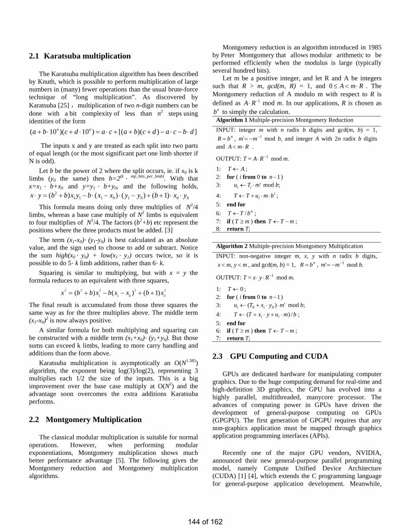
2.1 Karatsuba multiplication
The Karatsuba multiplication algorithm has been described by Knuth, which is possible to perform multiplication of large numbers in (many) fewer operations than the usual brute-force technique of “long multiplication”. As discovered by Karatsuba [25] ,multiplication of two n-digit numbers can be done with a bit complexity of less than n2 steps using identities of the form ( 10 )( 10 ) [( )( ) ]n na b c d a c a b c d a c b d+ ⋅ + ⋅ = ⋅ + + + − ⋅ − ⋅
The inputs x and y are treated as each split into two parts of equal length (or the most significant part one limb shorter if N is odd).
Let b be the power of 2 where the split occurs, ie. if x0 is k limbs (y0 the same) then b=2(k mp_bits_per_limb). With that x=x1 b+x0 and y=y1 b+y0, and the following holds,
⋅
1) (⋅ ⋅
12
1 1 0 0 0 0( ) ( ) ( 1)x y b b x y b x x y b x y+ − − ⋅ − + + ⋅ ⋅y⋅ = ⋅
This formula means doing only three multiplies of N2/4 limbs, whereas a base case multiply of N2 limbs is equivalent to four multiplies of N2/4. The factors (b2+b) etc represent the positions where the three products must be added. [3]
The term (x1-x0) ⋅ (y1-y0) is best calculated as an absolute value, and the sign used to choose to add or subtract. Notice the sum high(x0 y0) + low(x1 y1) occurs twice, so it is possible to do 5 ⋅ k limb additions, rather than 6 ⋅ k.
⋅ ⋅
Squaring is similar to multiplying, but with x = y the formula reduces to an equivalent with three squares,
2 2 2 2
1 1 0( ) ( ) ( 1) 2
0x b b x b x x b x= + − − + +
The final result is accumulated from those three squares the same way as for the three multiplies above. The middle term (x1-x0)2 is now always positive.
A similar formula for both multiplying and squaring can be constructed with a middle term (x1+x0) (y1+y0). But those sums can exceed k limbs, leading to more carry handling and additions than the form above.
⋅
Karatsuba multiplication is asymptotically an O(N1.585) algorithm, the exponent being log(3)/log(2), representing 3 multiplies each 1/2 the size of the inputs. This is a big improvement over the base case multiply at O(N2) and the advantage soon overcomes the extra additions Karatsuba performs.
2.2 Montgomery Multiplication
The classical modular multiplication is suitable for normal operations. However, when performing modular exponentiations, Montgomery multiplication shows much better performance advantage [5]. The following gives the Montgomery reduction and Montgomery multiplication algorithms.
Montgomery reduction is an algorithm introduced in 1985 by Peter Montgomery that allows modular arithmetic to be performed efficiently when the modulus is large (typically several hundred bits).
Let m be a positive integer, and let R and A be integers such that R > m, gcd(m, R) = 1, and 0 A m R≤ < ⋅ . The Montgomery reduction of A modulo m with respect to R is defined as 1A R−⋅ mod m. In our applications, R is chosen as
to simply the calculation. nbAlgorithm 1 Multiple-precision Montgomery Reduction
INPUT: integer m with n radix b digits and gcd(m, b) = 1, , mod b, and integer A with 2n radix b digits
and
nbR =A
1' −−= mmRm ⋅< .
OUTPUT: T = mod m. 1−⋅RA
1: AT ← ; 2: for ( i from 0 to 1−n ) 3: mod b; 'mTu ii ⋅←
4: ; ii bmuTT ⋅⋅+←
5: end for 6: ; nbTT /←7: if ( ) then mT ≥ mTT −← ; 8: return T;
Algorithm 2 Multiple-precision Montgomery Multiplication
INPUT: non-negative integer m, x, y with n radix b digits, mymx << , , and gcd(m, b) = 1, , mod b. nbR = 1' −−= mm
OUTPUT: T = mod m. 1−⋅⋅ Ryx
1: 0←T ; 2: for ( i from 0 to 1−n ) 3: mod b; ')( 00 myxTu ii ⋅⋅+←
4: bmuyxTT ii /)( ⋅+⋅+← ; 5: end for 6: if ( ) then mT ≥ mTT −← ; 7: return T;
2.3 In GPU Computing and CUDA
GPUs are dedicated hardware for manipulating computer graphics. Due to the huge computing demand for real-time and high-definition 3D graphics, the GPU has evolved into a highly parallel, multithreaded, manycore processor. The advances of computing power in GPUs have driven the development of general-purpose computing on GPUs (GPGPU). The first generation of GPGPU requires that any non-graphics application must be mapped through graphics application programming interfaces (APIs).
Recently one of the major GPU vendors, NVIDIA, announced their new general-purpose parallel programming model, namely Compute Unified Device Architecture (CUDA) [1] [4], which extends the C programming language for general-purpose application development. Meanwhile,
144 of 162
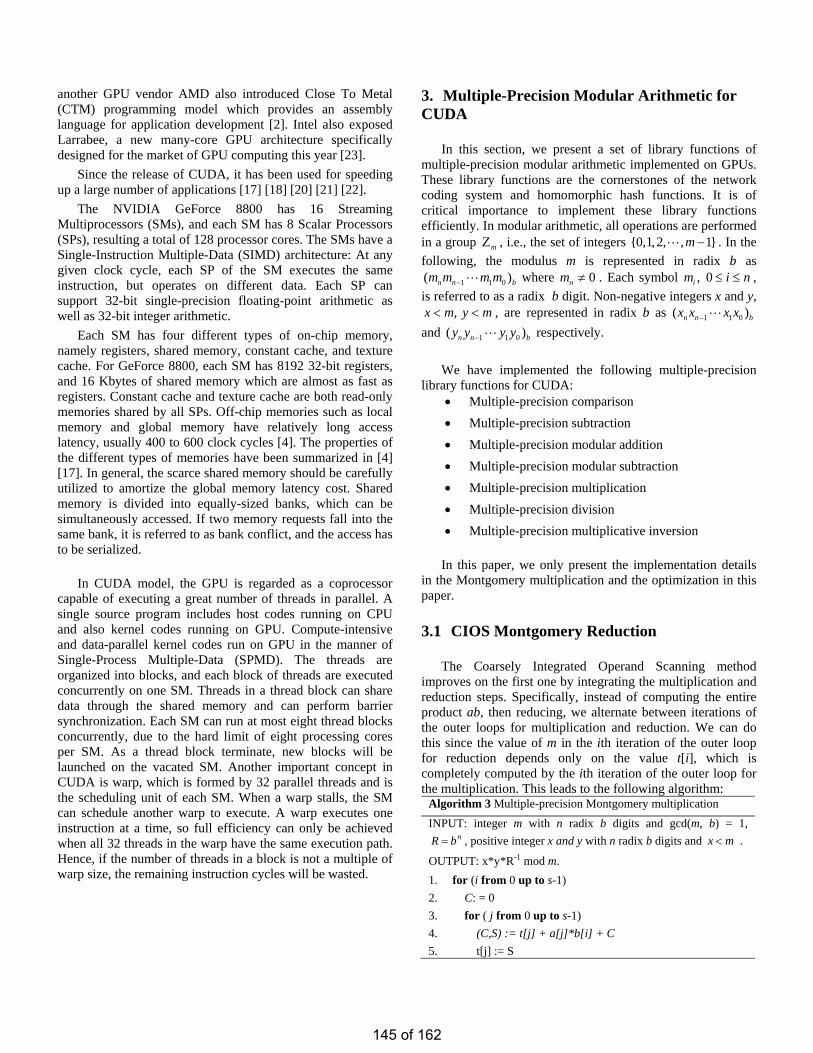
another GPU vendor AMD also introduced Close To Metal (CTM) programming model which provides an assembly language for application development [2]. Intel also exposed Larrabee, a new many-core GPU architecture specifically designed for the market of GPU computing this year [23].
Since the release of CUDA, it has been used for speeding up a large number of applications [17] [18] [20] [21] [22].
The NVIDIA GeForce 8800 has 16 Streaming Multiprocessors (SMs), and each SM has 8 Scalar Processors (SPs), resulting a total of 128 processor cores. The SMs have a Single-Instruction Multiple-Data (SIMD) architecture: At any given clock cycle, each SP of the SM executes the same instruction, but operates on different data. Each SP can support 32-bit single-precision floating-point arithmetic as well as 32-bit integer arithmetic.
Each SM has four different types of on-chip memory, namely registers, shared memory, constant cache, and texture cache. For GeForce 8800, each SM has 8192 32-bit registers, and 16 Kbytes of shared memory which are almost as fast as registers. Constant cache and texture cache are both read-only memories shared by all SPs. Off-chip memories such as local memory and global memory have relatively long access latency, usually 400 to 600 clock cycles [4]. The properties of the different types of memories have been summarized in [4] [17]. In general, the scarce shared memory should be carefully utilized to amortize the global memory latency cost. Shared memory is divided into equally-sized banks, which can be simultaneously accessed. If two memory requests fall into the same bank, it is referred to as bank conflict, and the access has to be serialized.
In CUDA model, the GPU is regarded as a coprocessor capable of executing a great number of threads in parallel. A single source program includes host codes running on CPU and also kernel codes running on GPU. Compute-intensive and data-parallel kernel codes run on GPU in the manner of Single-Process Multiple-Data (SPMD). The threads are organized into blocks, and each block of threads are executed concurrently on one SM. Threads in a thread block can share data through the shared memory and can perform barrier synchronization. Each SM can run at most eight thread blocks concurrently, due to the hard limit of eight processing cores per SM. As a thread block terminate, new blocks will be launched on the vacated SM. Another important concept in CUDA is warp, which is formed by 32 parallel threads and is the scheduling unit of each SM. When a warp stalls, the SM can schedule another warp to execute. A warp executes one instruction at a time, so full efficiency can only be achieved when all 32 threads in the warp have the same execution path. Hence, if the number of threads in a block is not a multiple of warp size, the remaining instruction cycles will be wasted.
3. Multiple-Precision Modular Arithmetic for CUDA
In this section, we present a set of library functions of multiple-precision modular arithmetic implemented on GPUs. These library functions are the cornerstones of the network coding system and homomorphic hash functions. It is of critical importance to implement these library functions efficiently. In modular arithmetic, all operations are performed in a group mΖ , i.e., the set of integers 0,1,2, , 1m −L
, 0im
. In the following, the modulus m is represented in radix b as
where . Each symbol 1 1m m0( )n n bm m − L 0nm ≠ i n≤ ≤ , is referred to as a radix b digit. Non-negative integers x and y,
, x m y m< < , are represented in radix b as 1 1 0( )bn nx x x x− L and respectively. 1 1n ny y y y0 b( − L )
We have implemented the following multiple-precision library functions for CUDA:
• Multiple-precision comparison • Multiple-precision subtraction • Multiple-precision modular addition • Multiple-precision modular subtraction • Multiple-precision multiplication • Multiple-precision division • Multiple-precision multiplicative inversion
In this paper, we only present the implementation details in the Montgomery multiplication and the optimization in this paper.
3.1 CIOS Montgomery Reduction
The Coarsely Integrated Operand Scanning method improves on the first one by integrating the multiplication and reduction steps. Specifically, instead of computing the entire product ab, then reducing, we alternate between iterations of the outer loops for multiplication and reduction. We can do this since the value of m in the ith iteration of the outer loop for reduction depends only on the value t[i], which is completely computed by the ith iteration of the outer loop for the multiplication. This leads to the following algorithm:
Algorithm 3 Multiple-precision Montgomery multiplication
INPUT: integer m with n radix b digits and gcd(m, b) = 1, , positive integer x and y with n radix b digits and nbR = mx < .
OUTPUT: x*y*R-1 mod m. 1. for (i from 0 up to s-1) 2. C: = 0 3. for ( j from 0 up to s-1) 4. (C,S) := t[j] + a[j]*b[i] + C 5. t[j] := S
145 of 162

6. end for 7. (C,S) := t[s] + C 8. t[s] := S 9. t[s+1] := C 10. C := 0 11. m := t[0]*n'[0] mod W 12. for (j from 0 up to s-1) 13. (C,S) := t[j] + m*n[j] + C 14. t[j] := S 15. end for 16. (C,S) := t[s] + C 17. t[s] := S 18. t[s+1] := t[s+1] + C 19. for (j from 0 up to s) 20. t[j] := t[j+1] 21. end for 22. end for
Note that the array t is assumed to be set to 0 initially. The last j-loop is used to shift the result one word to the right (i.e., division by 2w), hence the references to t[j] and t[0] instead of t[i+j] and t[i]. A slight improvement is to integrate the shifting into the reduction as follows:
m := t[0]*n'[0] mod W (C,S) := t[0] + m*n[0] for (j from 1 up to s-1) (C,S) := t[j] + m*n[j] + C t[j-1] := S end for (C,S) := t[s] + C t[s-1] := S t[s] := t[s+1] + C The auxiliary array t uses only s + 2 words. This is due to
the fact that the shifting is performed one word at a time, rather than s words at once, saving s - 1 words. The final result is in the first s+1 words of array t. A related method, without the shifting of the array (and hence with a larger memory requirement), is described in [2].
The CIOS method (with the slight improvement above) requires 2s2+s multiplications, 4s2+4s+2 additions, 6s2+7s+2 reads, and 2s2+5s+1 writes, including the final multi-precision subtraction, and uses s+3 words of memory space. The memory reduction is a significant improvement over the SOS method.
We say that the integration in this method is "coarse" because it alternates between iterations of the outer loop. In the next method, we will alternate between iterations of the inner loop [24].
3.2 Karatsuba Montgomery Reduction
Modular multiplication can be spared into two parts, one is multiplication and one is modular reduction. In this method, we choose the Karatsuba multiplication to implement the multiplication, and then perform Montgomery reduction.
Algorithm 4 Multiple-precision Karatsuba and Montgomery Multiplication
INPUT: integer m with n radix b digits and gcd(m, b) = 1, , positive integer x and y with n radix b digits and nbR = mx < .
OUTPUT: x*y*R-1 mod m. 1. Karatsuba(x,y) 2. for (i from 0 up to s-1) 3. C := 0 4. m := t[i]*n'[0] mod W 5. for (j from 0 up to s-1) 6. (C,S) := t[i+j] + m*n[j] + C 7. t[i+j] := S 8. end for 9. ADD (t[i+s],C) 10. end for 11. for (j from 0 up to s) 12. u[j] := t[j+s] 13. end for 14. B := 0 15. for (i from 0 up to s-1) 16. (B,D) := u[i] - n[i] - B 17. t[i] := D 18. end for 19. (B,D) := u[s] - B 20. t[s] := D 21. if B=0 then return t[0], t[1], ... , t[s-1] 22. else return u[0], u[1], ... , u[s-1]
4. Improving the Montgomery Multiplication
To achieve a high performance, we analyze the implementation of the instructions of the Montgomery Multiplication. We use the decuda tool to disassemble the cubin file of the CUDA binary codes. We will tell the details as below.
4.1 ASM of Integer Multiplication
When we use the decuda tool disassemble the cubin. We get that the 32bit multiplication 32bit integer is not only using one instruction but using ten to twenty instructions.
We can see the MULT64X64LO need more than 20 instructions, but the MULT32X32WIDE only need 10 instructions. So, we use inline ASM to limit the compiler
146 of 162
compile the 32bit multiplication 32bit work with the 10 instructions. eg.:
Algorithm 5 32bit integer multiplication
INPUT: 32bit integer A multiplicative with 32bit integer B. OUTPUT: A*B. 1. static inline __device__ unsigned __int64
mul_32x32(unsigned A, unsigned B) 2. unsigned __int64 out; 3. asm("mul.wide.u32 %0, %1, %2;" : "=l"(out) : "r"(A),
"r"(B)); 4. return out; 5.
5. Implementation and Experimental Results
We tested these implementations on T61 NVIDIA Quadro NVS140M graphic card which contains an NVIDIA Quadro G86M GPU. The G86M GPU uses the G80 architecture with 16 processing cores working at 0.8 GHz. The implementation of modular multiplication is in 1024-bit integer. All the implementation is 1024-bit multiplied by 1024-bit modular 1024-bit.
5.1 Comparing Karatsuba Method and CIOS Method
In Fig. 1, the X-coordinate represents the number of threads. As Fig. 1 shows, the karatsuba Montgomery multiplication is slow than the CIOS method of Montgomery multiplication. The karatsuba Montgomery multiplication method needs 60 registers and 5132 local memories. But the CIOS method only needs 14 register and no local memory at all. The blue block shows the CIOS method of the Montgomery Multiplication. The red block shows the method with K-MM (Karatsuba Montgomery Multiplication). The K-MM method needs more variables in the implementation, because that can’t use callback function in the CUDA model recently, so the 1024bit integer multiplication will be translate into 2 256bit integer function, and 256bit to 128bit, and so on. So the K-MM method is slow than the CIOS method on the recently GPU model.
The CIOS method only needs 14 registers and using unrolling method unroll the loop.
Figure 1. Throughput of Montgomery multiplication and karatsuba Montgomery multiplication on GPU using Algorithm 3&4, with different number of threads.
5.2 Montgomery Multiplication with inline ASM
We use the inline ASM to limit the instruction work with the Short instruction. The experimental results are shown in Fig. 2. The performance has been improved by 20% as compared with the one without using our inline ASM code.
The blue and red block all use the CIOS method. But the red one, as the Fig. 2 shows is 20% faster than blue one. Because the inside ASM function used to solve the 32bit multiplicative 32bit integer. In the decuda code we can see that each loop the CIOS-ASM method is 11 instructions little than the CIOS method.
Figure 2. Throughput of inline ASM in CIOS on GPU, with different number of threads
6. Conclusions
Multiple-precision modular multiplication is an important component in public-key cryptography for encrypting and signing digital data. In this paper, we describe the design, implementation and optimization of multiple-precision modular multiplication using GPU and CUDA. Although Karasuba multiplication is theoretically advantageous, we
147 of 162

found that it is not practical for the current GPU platform due to the high cost of comparing large integers. Nevertheless, we improved the performance of the CIOS method by developing an inline ASM implementation of 32-bit integer multiplication.
7. References
[1] NVIDIA CUDA. http://developer.nvidia.com/object/cuda.html [2] AMD CTM Guide: Technical Reference Manual.
2006. http://ati.amd.com/companyinfo/researcher/documents/ATI_CTM_Guide.pdf
[3] GNU MP Arithmetic Library. http://gmplib.org/ [4] NVIDIA CUDA Compute Unified Device Architecture:
Programming Guide, Version 2.0beta2, Jun. 2008. [5] Montgomery, P., 1985. Multiplication without trial division,
Math. Computation, vol. 44, 1985, 519-521. [6] Menezes, A., van Oorshot, P., and Vanstone S., 1996. Handbook
of applied cryptography. CRC Press, 1996. [7] Ahlswede, R., Cai, N., Li S. R., and Yeung, R. W. 2000.
Network information flow. IEEE Transactions on Information Theory, 46(4), July 2000, 1204-1216.
[8] Ho, T., Koetter. R., Médard, M., Karger, D.R. and Effros, M. 2003. The benefits of coding over routing in a randomized setting. In Proceedings of IEEE ISIT, 2003.
[9] Li, S.-Y.R., Yueng, R.W., and Cai, N. 2003. Linear network coding. IEEE Transactions on Information Theory, vol. 49, 2003. 371-381.
[10] Krohn, M., FreedMan, M., and Mazieres, D. 2004. On-the-fly verification of rateless erasure codes for efficient content distribution. In Proceedings of IEEE Symposium on Security and Privacy, Berkeley, CA, 2004.
[11] Gkantsidis, C. and Rodriguez, P. 2005. Network coding for large scale content distribution. In Proceedings of IEEE INFOCOM 2005.
[12] Gkantsidis, C. and Rodriguez, P. 2006. Cooperative security for network coding file distribution. In Proceedings of IEEE INFOCOM’06, 2006.
[13] Li, Q., Chiu, D.-M., and Lui, J. C.S. 2006. On the practical and security issues of batch content distribution via network coding. In Proceedings of IEEE ICNP’06, 2006, 158-167.
[14] Chou, P. A. and Wu, Y. 2007. Network coding for the Internet and wireless networks. Technical Report. MSR-TR-2007-70, Microsoft Research.
[15] Wang, M. and Li, B. 2007. Lava: a reality check of network coding in peer-to-peer live streaming. In Proceedings of IEEE INFOCOM’07, 2007.
[16] Wang, M. and Li, B. 2007. R2: random push with random network coding in live peer-to-peer streaming. In IEEE Journal on Selected Areas in Communications, Dec. 2007, 1655-1666.
[17] Ryoo, S., Rodrigues, C. I., Baghsorkhi, S. S., Stone, S. S., Kirk, D. B., and Hwu, W. 2008. Optimization principles and application performance evaluation of a multithreaded GPU using CUDA. In Proceedings of ACM PPoPP’08, Feb. 2008.
[18] Falcao, G., Sousa, L., and Silva, V. 2008. Massiv parallel LDPC decoding in GPU. In Proceedings of ACM PPoPP’08, Feb. 2008.
[19] Yu, Z., Wei, Y., Ramkumar, B., and Guan, Y. 2008. An efficient signature-based scheme for securing network coding against pollution attacks. In Proceedings of IEEE INFOCOM’08, Apr. 2008.
[20] Owens, J. D., Houston, M., Luebke, D., Green, S., Stone, J. E., and Phillips, J. C. 2008. GPU computing. IEEE Proceedings, May 2008, 879-899.
[21] Al-Kiswany, S., Gharaibeh, A., Santos-Neto, E., Yuan, G., and Ripeanu, M. 2008. StoreGPU: exploiting graphics processing units to accelerate distributed storage systems. In Proceedings of IEEE Symposium on High Performance Distributed Computing (HPDC), Jun. 2008.
[22] Silberstein, M., Geiger, D., Schuster, A., Patney, A., Owens, J. D. 2008. Efficient computation of sum-products on GPUs through software-managed cache. In Proceedings of the 22nd ACM International Conference on Supercomputing, Jun. 2008.
[23] Seiler, L., et. al., 2008. Larrabee: a many-core x86 architecture for visual computing. ACM Transactions on Graphics, 27(3), Aug. 2008.
[24] CCetin Kaya Koc and Tolga Acar,Burton S. Kaliski Jr,Analyzing and Comparing Montgomery Multiplication Algorithms, IEEE Micro, 16(3):26-33, June 1996
[25] A. Karatsuba and Yu. Ofman (1962). "Multiplication of Many-Digital Numbers by Automatic Computers". In Proceedings of the USSR Academy of Sciences 145: 293–294.
148 of 162
L-BFGS and Delayed Dynamical Systems Approach for
Unconstrained Optimization
Xiaohui XIE
Abstract
The dynamical (or ode) systems approach for optimization
problems has existed for two decades. The main feature of this
approach is that a continuous path starting from the initial point
can be generated and eventually the path will converge to the so-
lution. This approach is quite different from conventional opti-
mization methods where a sequence of points, or a discrete path,
is generated. An advantage of the dynamical systems approach
is that it is more suitable for large scale problems. Common ex-
amples of this approach are ode’s based on the steepest descent
direction or the Newton’s direction. In this research we apply
the L-BFGS scheme to the ode model, hopefully to improve on
the rate of convergence over the steepest descent direction, but
not to suffer from the large amount of computational work in
the Newton’s direction.
1 Problem background and in-troduction
This paper studies computational methods for alocal or the global minimizer of an unconstrained op-timization problem. Optimization problems are clas-sified into:(a) Unconstrained Problem:
minx∈Rn
f(x) f : Rn → R1 (UP )
(b) Equality Constrained Problem:
minx∈Rn
f(x)
h(x) = 0 h : Rn → Rp
(c) Inequality Constrained Problem:
minx∈Rn
f(x)
g(x) ≤ 0 h : Rn → Rp
(d) General Constrained Problem:
minx∈Rn
f(x)
g(x) ≤ 0h(x) = 0
The motivation of unconstrained methods is togenerate a sequence of points xk (x0 given) suchthat (1) f(xk) > f(xk+1);(2) xk is convergent, and(3) the limit point of the sequence is a stationarypoint of (UP). Different methods advance from xk
to xk+1 differently. Well-known methods includethe steepest descent method, Newton’s method andquasi-Newton method. A common theme behind allthese methods is to find a direction p ∈ Rn so thatthere exists an ε > 0 such that
f(x + εp) < f(x) ∀ε ∈ (0, ε)
This direction is called a descent direction of f(x)at x. Once we have found a descent direction, we maygo along this direction to approach one more step to-ward the optimum solution.
The following paragraphs summarize the advan-tages and disadvantages of these methods.
1.1 Steepest descent method
Using directional derivative in multivariable calcu-lus, it is clear that for (UP), p is a descent direction
149 of 162
at x⇔ ∇f(x)T p < 0. Hence p = −∇f(x), or equiva-lently, p = −∇f(x)/‖∇f(x)‖2 is obviously a descentdirection for f(x). This direction is called the steep-est descent direction.Method of Steepest Descent: At each iteration k:find the lowest point of f in the direction −∇f(xk)from xk, i.e., find λk that solves
minλ>0
f(xk − λ∇f(xk))
Then xk+1 = xk − λ∇f(xk).Unfortunately, the steepest descent method con-
verges only linearly, and sometimes very slowly lin-early. In fact, if xk, which is generated by thesteepest descent method, converges to a local min-imizer x∗ where ∇2f(x∗) is positive definite (p.d.),and λmax and λmin are the largest and smallest eigen-values of ∇2f(x∗), then one can show that xk sat-isfies
limk→∞
sup‖xk+1 − x∗‖‖xk − x∗‖
≤ c, c =λmax − λmin
λmax + λmin,
in a particular weighted l2 norm, and the bound onc is tight for some starting x0. This property indi-cates that the steepest descent method is q-linearlyconvergent. When λmax and λmin are far apart, thenc is close to 1, and the convergence will be slow.
1.2 Newton’s method
At point xk, if ∇2f(xk) is p.d., the function f(x)can be approximated by a quadratic function basedon the Taylor expansion:
f(x) ∼= f(xk) +∇f(xk)T (x− xk)
+12(x− xk)T∇2f(xk)(x− xk) (1)
Then the minimizer of (1) is given by
∇f(x) = 0⇒ ∇f(xk) +∇2f(xk)(x− xk) = 0⇒ x = xk − [∇2f(xk)]−1∇f(xk),
where −[∇2f(xk)]−1∇f(xk), is called the Newton’sdirection. Then we define
xk+1 = xk − [∇2f(xk)]−1∇f(xk),
and the resulting method of computing xk is calledthe Newton’s method.Newton’s methodGiven x0, compute
xk+1 = xk − [∇2f(xk)]−1∇f(xk), k ← k + 1.
A key requirement for Newton’s method is the p.d.of ∇2f(xk). Descent directions guarantee thatf(x) can be further reduced and therefore theyform the basis of some global methods. However,in some real applications, if the starting point isfar away from the optimal solution, or the Hessianis not positive definite, Newton’s direction is notadopted. Although Newton’s method convergesvery fast (xk converges to x∗ q-quadratically),the Hessian matrix is difficult to compute. So wewould like to find more feasible methods with (A) nosecond-order information, i.e., no Hessian; and (B)fast convergence. A rule of thumb is that first-orderinformation normally gives slow (linear) convergence,while second-order information normally gives fast(quadratic) convergence. Let us discuss severalpractical considerations. In general, the convergenceis quadratic: the error is essentially squared at eachstep (that is, the number of accurate digits doublesin each step). There are some caveats, however.Firstly, Newton’s method requires that the derivativebe calculated directly. (If the derivative is approxi-mated by the slope of a line through two points onthe function, the secant method results; this canbe more efficient depending on how one measurescomputational effort.) Secondly, if the initial valueis too far from the true zero, Newton’s method canfail to converge. Because of this, most practicalimplementations of Newton’s method put an upperlimit on the number of iterations and perhaps on thesize of the iterates. Thirdly, if the root being soughthas multiplicity greater than one, the convergencerate is merely linear (errors reduced by a constantfactor at each step) unless special procedures aretaken. Finding the inverse of the Hessian is anexpensive operation. Therefore the descent direction−[∇2f(x)]−1∇f(x) is often solved approximately(but to great accuracy) using methods such as theconjugate gradient method. There also exist variousquasi-Newton methods, where an approximation for
150 of 162
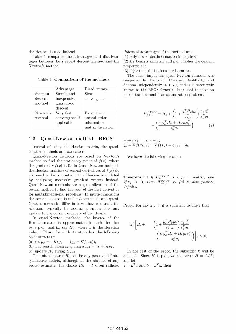
the Hessian is used instead.Table 1 compares the advantages and disadvan-
tages between the steepest descent method and theNewton’s method.
Table 1: Comparison of the methods
Advantage DisadvantageSteepest Simple and Slowdescent inexpensive, convergencemethod guarantees
descentNewton’s Very fast Expensive,method convergence if second-order
applicable informationmatrix inversion
1.3 Quasi-Newton method—BFGS
Instead of using the Hessian matrix, the quasi-Newton methods approximate it.
Quasi-Newton methods are based on Newton’smethod to find the stationary point of f(x), wherethe gradient ∇f(x) is 0. In Quasi-Newton methodsthe Hessian matrices of second derivatives of f(x) donot need to be computed. The Hessian is updatedby analyzing successive gradient vectors instead.Quasi-Newton methods are a generalization of thesecant method to find the root of the first derivativefor multidimensional problems. In multi-dimensionsthe secant equation is under-determined, and quasi-Newton methods differ in how they constrain thesolution, typically by adding a simple low-rankupdate to the current estimate of the Hessian.
In quasi-Newton methods, the inverse of theHessian matrix is approximated in each iterationby a p.d. matrix, say Hk, where k is the iterationindex. Thus, the k th iteration has the followingbasic structure:(a) set pk = −Hkgk, (gk = ∇f(xk)),(b) line search along pk giving xk+1 = xk + λkpk,(c) update Hk giving Hk+1.
The initial matrix H0 can be any positive definitesymmetric matrix, although in the absence of anybetter estimate, the choice H0 = I often suffices.
Potential advantages of the method are:(1) only first-order information is required;(2) Hk being symmetric and p.d. implies the descentproperty; and(3) O(n2) multiplications per iteration.
The most important quasi-Newton formula wassuggested by Broyden, Fletcher, Goldfarb, andShanno independently in 1970, and is subsequentlyknown as the BFGS formula. It is used to solve anunconstrained nonlinear optimization problem.
HBFGSk+1 = Hk +
(1 +
yTk Hkyk
sTk yk
)sksT
k
sTk yk
−(
skyTk Hk + HkyksT
k
sTk yk
)(2)
where sk = xk+1 − xk,yk = ∇f(xk+1)−∇f(xk) = gk+1 − gk.
We have the following theorem.
Theorem 1.1 If HBFGSk is a p.d. matrix, and
sTk yk > 0, then HBFGS
k+1 in (2) is also positivedefinite.
Proof: For any z 6= 0, it is sufficient to prove that
zT
[Hk+
(1 +
yTk Hkyk
sTk yk
)sksT
k
sTk yk
−(
skyTk Hk + HkyksT
k
sTk yk
)]z > 0,
In the rest of the proof, the subscript k will beomitted. Since H is p.d., we can write H = LLT ,and leta = LT z and b = LT y, then
151 of 162
zT Hk+1z = zT
[Hk +
(1 +
yTk Hkyk
sTk yk
)sksT
k
sTk yk
−(
skyTk Hk + HkyksT
k
sTk yk
)]z
= zT
[H +
(1 +
yT Hy
sT y
)ssT
sT y−
(syT H + HysT
sT y
)]z
= aT a +zT bT bssT z
(sT y)2+
(zT s)2
sT y− zT sbT a
sT y− aT bsT z
sT y
=(
a− zT sb
sT y
)T (a− zT sb
sT y
)+
(zT s)2
sT y
=∥∥∥∥a− zT sb
sT y
∥∥∥∥2
+(zT s)2
sT y
≥ 0
If the norm above equals zero, i.e.,∥∥∥∥a− zT sb
sT y
∥∥∥∥ = 0,
then we have
a =zT sb
sT y, or LT z =
zT sLT y
sT y,
which means that y ∝ z.However, since sT y > 0,
(zT s)2
sT y> 0,
as y ∝ z. Thus the theorem is proved. 2
1.4 Limited-Memory Quasi-NewtonMethods—L-BFGS
Limited-memory quasi-Newton methods are usefulfor solving large problems whose Hessian matricescannot be computed at a reasonable cost or are notsparse. These methods maintain simple and com-pact approximations of Hessian matrices: insteadof storing fully dense n × n approximations, theysave only a few vectors of length n that representthe approximations implicitly. Despite these modest
storage requirements, they often yield an accept-able rate of convergence. Various limited-memorymethods have been proposed; we focus mainly onan algorithm known as L-BFGS, which, as its namesuggests, is based on the BFGS updating formula.The main idea of this method is to use curvatureinformation from only the most recent iterations toconstruct the Hessian approximation. Curvatureinformation from earlier iterations, which is lesslikely to be relevant to the actual behavior of theHessian at the current iteration, is discarded in theinterest of saving storage.
As we have discussed in section 1.3, each step ofthe BFGS method has the form
xk+1 = xk − αkHk∇fk,
where αk is the step length and Hk is updated atevery iteration by means of the formula
Hk+1 = V Tk HkVk + ρksksT
k , (3)
where
ρk =1
yTk sk
, Vk = I − ρkyksTk , (4)
and
sk = xk+1 − xk, yk = ∇fk+1 −∇fk. (5)
Since the inverse Hessian approximation Hk willgenerally be dense, the cost of storing and manipu-lating it is prohibitive when the number of variables islarge. To circumvent this problem, we store a mod-ified version of Hk implicitly, by storing a certainnumber (say, m) of the vector pairs si, yi used inthe formulas (3)-(5). The product Hk∇fk can be ob-tained by performing a sequence of inner productsand vector summations involving ∇fk and the pairssi, yi. After the new iterate is computed, the oldestvector pair in the set of pairs si, yi is replaced bythe new pair sk, yk obtained from the current step(5).
We now describe the updating process in a littlemore detail. At iteration k, the current iterate is xk
and the set of vector pairs is given by si, yi fori = k − m, . . . , k − 1. We first choose some initial
152 of 162

Hessian approximation H0 (in contrast to the stan-dard BFGS iteration, this initial approximation is al-lowed to vary from iteration to iteration) and findby repeated application of the formula (3) that theL-BFGS approximation Hk+1 satisfies the followingformula [12]:
In general, we have for k + 1 ≤ m the usual BFGSupdated
Hk+1 = V Tk V T
k−1 · · ·V T0 H0V0 · · ·Vk−1Vk
+V Tk · · ·V T
1 ρ0s0sT0 V1 · · ·Vk
...+V T
k V Tk−1ρk−2sk−2s
Tk−2Vk−1vk (6)
+Vkρk−1sk−1sTk−1Vk
+ρksksTk .
For k + 1 > m we have the update
Hk+1 = V Tk V T
k−1 · · ·V Tk−m+1H0Vk−m+1 · · ·Vk−1Vk
+V Tk · · ·V T
k−m+2ρk−m+1sk−m+1sTk−m+1
·Vk−m+2 · · ·Vk
... (7)+V T
k V Tk−1ρk−2sk−2s
Tk−2Vk−1Vk
+Vkρk−1sk−1sTk−1Vk
+ρksksTk .
A method for choosing H0 that has proved effectivein practice is to set H0 = γkI, where
γk =sT
k−1yk−1
yTk−1yk−1
.
The strategy of keeping the m most recent cor-rection pairs si, yi works well in practice; indeedno other strategy has yet proved to be consistentlybetter. However, the main weakness of the L-BFGSmethod is that it converges slowly on ill-conditionedproblems —– specifically, on problems where the Hes-sian matrix contains a wide distribution of eigenval-ues. On certain applications, the nonlinear conjugatemethods are competitive with limited-memory quasi-Newton methods.Algorithm (L-BFGS)
Choose starting point x0, integer m > 0;k ← 0;repeat
Choose H0
Compute pk ← −Hk∇fk
Compute xk+1 ← xk + αkpk where αk is chosento satisfy the Wolfe conditions;
if k > mDiscard the vector pair sk−m, yk−m from
storage;Compute and save
sk ← xk+1 − xk, yk = ∇fk+1 −∇fk;k ← k + 1;
until convergence.
2 Analysis for dynamical sys-tems with time delay
2.1 Introduction of dynamical sys-tems
For the easiness of reading, the (UP) problem isreproduced here:
minx∈Rn
f(x) f : Rn → R1 (8)
It is very important that the optimization problem(8) itself is posted in the continuous form, i.e., xcan be changed continuously. In the literature,the necessary and sufficient conditions of a localoptimum are also presented in the continuous form.Furthermore, almost all the theoretical study forproblem (8) is in the continuous form. However,it is very interesting to say that when it comesdown to the numerical solution of (8), most ofthe conventional methods, such as the gradient/steepest descent method, Newton’s method andquasi-Newton’s method, are all addressed in thediscrete form. This interesting situation is mainlydue to the fact that the computer’s computationcan be only done discretely. However, is it possibleto study both the optimization problem and thesolution methods in its original form, i.e., continuousform? In this sense, we may use the dynamicalsystem approach or neural network approach to
153 of 162
solve the original optimization problem.• Dynamical system approach. The essence of thisapproach is to convert problem (8) into a dynamicalsystem or an ordinary differential equation (ode) sothat the solution of problem (8) corresponds to astable equilibrium point of this dynamical system.• Neural network approach. The mathematicalrepresentation of neural network is an ordinarydifferential equation which is asymptotically stableat any isolated solution point. A companion ofthis neural network is an energy function whichis a Lyapunov function. And as time evolves, thesolution of the ode will converge to the optimum,and in this whole process, the energy function willdecrease monotonically in time.
The following discussion reviews the researchresults in the dynamical system approach, andidentifies the merits of this approach.
Consider the following simple dynamical systemor ordinary differential equation
dx(t)dt
= p(x). (9)
We first state some classical result on the existenceand uniqueness of the solution, and some stabilitydefinitions for the dynamical system (9) [21,24].
Theorem 2.1 [24] Assume that p(x) is a continuousfunction from Rn to Rn. Then for arbitrary t0 ≥ 0and x0 ∈ Rn there exists a local solution x(t) satis-fying x(t0) = x0, t ∈ [t0, τ) to (9) for some τ > t0.If furthermore p(x) is locally Lipschitz continuous atx0, then the solution is unique, and if p(x) is Lips-chitz continuous in Rn then τ can be extended to ∞.
Definition 2.2 (Equilibrium point) A point x∗ ∈ Rn
is called an equilibrium point of (9) if p(x∗) = 0.
Definition 2.3 (Stablility in the sense of Lyapunov)Let x(t) be the solution of (9). An isolated equilibriumpoint x∗ is Lyapunov stable if for any x0 = x(t0) andany scalar ε > 0, there exists a δ > 0 such that if‖x(t0)− x∗‖ < δ, then ‖x(t)− x∗‖ < ε for t ≥ t0.
Definition 2.4 (Convergence) Let x(t) be the solu-tion of (9). An isolated equilibrium point x∗ is con-vergent if there exists a δ > 0 such that if ‖x(t0) −x∗‖ < δ, x(t)→ x∗ as t→∞.
A dynamical system or ode (9) arising from an opti-mization problem needs to have p(x) being a descentdirection for the objective function f(x). Some well-known versions are:
Dynamical system based on the steepest descentdirection:
dx(t)dt
= −∇f(x(t))
Dynamical system based on the Newton direction:
dx(t)dt
= −[∇2f(x(t))]−1∇f(x(t)) (10)
As in the discrete optimization methods in the pre-vious chapter, the steepest descent direction has aslow convergence rate - meaning that it takes a very”large” value of t to approach the equilibrium point.The Newton direction has a much faster convergencerate, but the amount of work in evaluating the Jaco-bian is much greater.
Some other dynamical systems in the literature are:
dx(t)dt
= s(t) · p(x(t)), (11)
a(t) · d2x(t)dt2
+ b(t) ·B(x(t)) · dx(t)dt
= p (x(t)) , (12)
where p(x)is a descent direction for f(x),B(x) ∈ Rn×n is a positive definite matrix, a(t)and b(t) are scalar functions in t, and s(t) is apositive scalar function in t and bounded above.
A major advantage of the dynamical systemsapproach is that very large problems can be solved[13]. No matter whether we use any of (9)-(12),existing ode methods are quite mature to tackle theseproblems. Solving systems with tens or hundredsof thousands of unknowns poses no problem to odesolvers. The problem size handled can be muchlarger than traditional methods described in Chapter1, which are of order of magnitude in the thousands.The research in the ode approach is to find a ”good”p(x) in (9) that balances the convergence rate andthe amount of work.
The dynamical systems approach normally con-sists of the following three steps:
(a) to establish an ode system;
154 of 162
(b) to study the convergence of the solution x(t)of the ode as t→∞; and
(c) to solve the ode system numerically.The convergence study of x(t) as t → ∞ and the
stability of the corresponding dynamical system havemostly been addressed on a case by case base. Nostandard theory and/or methodology are given. Thisphenomenon certainly limits the systematic study ofthe dynamical system approach and its applicationpotential as well. Two papers are worth mentioning,one by Tanabe [18] which used the stability theoryof the dynamical system to study the ode system,and the other one by Yamashita [24] which employedLyapunov’s direct method to study the ode system.
Even though the solutions of ode systems are con-tinuous, yet the actual computation has to be donediscretely. In all the dynamical systems (10)-(12),the numerical solutions were mainly solved by eitherdiscrete optimization methods or finite differencemethods.
In summary, the main attractiveness of this ap-proach is its simplicity and its originality in pursuingthe continuous form. Furthermore, there is not anyrestriction on the form of the objective function f(x)in (8).
2.2 Delayed dynamical systems ap-proach
As stated above, the steepest descent direction andthe Newton direction of the dynamical systems ap-proach both have their weakness. The main idea inthis paper is to apply the theme of the L-BFGS al-gorithm in Chapter 1 to the dynamical systems ap-proach, making it a bridge between the steepest de-scent direction and the Newton direction. The result-ing dynamical system is a delayed ode, thus we callit the delayed dynamical systems approach.
The delayed dynamical systems approach solvesthe delayed ode:
dx(t)dt
= −H(x(t), x(t− τ1(t), . . . , x(t− τm(t))))
·∇f(x(t)), (13)
where H and t− τ1(t), . . . , t− τm(t) are to be definedbelow.
As the delayed ode (13) is numerically solved, wecompute approximations x0, x1, . . . , xk, xk+1, . . . tox(t) at time points t0, t1, . . . , tk, tk+1, . . . . We defineH = Hk to be a different function in the interval(tk−1, tk] iteratively by:
Given t0, x(t0) = x0, and an initial H0, for t0 ≤ t,we define
H(x(t), x(t0)) := H1(x(t), x(t0)):= V0(t)T H0V0(t) + ρ0(t)s0(t)s0(t)T ,
wheres0(t) = x(t)− x0,
y0(t) = ∇f(x(t))−∇f(x0),
ρ0(t) = 1/y0(t)T s0(t),
V0(t) = I − ρ0(t)y0(t)s0(t)T ,
in the R.H.S. of (13) and determine a stepsize h1 =(t1 − t0) to compute, using some numerical odemethod, an approximation x1 to x(t1) at t1. Thenfor t1 ≤ t, we define
H(x(t), x(t1), x(t0)):= H2(x(t), x(t1), x(t0)):= V1(t)T V0(t1)T H0V0(t1)V1(t)
+V1(t)T ρ0(t1)s0(t1)s0(t1)T V1(t)+ρ1(t)s1(t)s1(t)T
where
s1(t) = x(t)− x(t1),
y1(t) = ∇f(x(t))−∇f(x(t1)),
ρ1(t) = 1/y1(t)T s1(t),
V1(t) = I − ρ1(t)y1(t)s1(t)T ,
in the R.H.S. of (13) and determine a stepsize h2 =(t2 − t1) to compute, using some numerical odemethod, an approximation x2 to x(t2) at t2. Ofcourse, computationally x1 is used instead of x(t1).
155 of 162

This process is repeated until we have accepted xm−1
at tm−1. Then for tm−1 ≤ t, we use
H(x(t), x(tm−1), . . . , x(t1), x(t0)):= Hm(x(t), x(tm−1), . . . , x(t1), x(t0)):= Vm−1(t)T Vm−2(tm−1)T . . . V1(t2)T V0(t1)T
·H0V0(t1)V1(t2) . . . Vm−2(tm−1)Vm−1(t)+Vm−1(t)T Vm−2(tm−1)T . . . V1(t2)T
·ρ0(t1)s0(t1)s0(t1)T V1(t2) . . . Vm−2(tm−1)·Vm−1(t)
+ . . .
+Vm−1(t)T ρm−2(tm−1)sm−2(tm−1)·sm−2(tm−1)T Vm−1(t)
+ρm−1(t)sm−1(t)sm−1(t)T (13A)
where
sm−1(t) = x(t)− x(tm−1),
ym−1(t) = ∇f(x(t))−∇f(x(tm−1)),
ρm−1(t) = 1/ym−1(t)T sm−1(t),
Vm−1(t) = I − ρm−1(t)ym−1(t)sm−1(t)T .
to compute xm at tm. Beyond this point we save onlym previous values of x. The definition of H is now,for m ≤ k,for tk ≤ t,
H(x(t), x(tk), . . . , x(tk−m+2), x(tk−m+1)):= Hk+1(x(t), x(tk), . . . , x(tk−m+2), x(tk−m+1)):= Vk(t)T Vk−1(tk)T . . . Vk−m+2(tk−m+3)T
·Vk−m+1(tk−m+2)T H0Vk−m+1(tk−m+2)·Vk−m+2(tk−m+3) . . . Vk−1(tk)Vk(t)
+Vk(t)T Vk−1(tk)T . . . Vk−m+2(tk−m+3)T
·ρk−m+1(tk−m+2)sk−m+1(tk−m+2)·sk−m+1(tk−m+2)T Vk−m+2(tk−m+3) . . .
·Vk−1(tk)Vk(t)+ . . .
+Vk(t)T ρk−1(tk)sk−1(tk)·sk−1(tk)T Vk(t)
+ρk(t)sk(t)sk(t)T (13B)
where
sk(t) = x(t)− x(tk),
yk(t) = ∇f(x(t))−∇f(x(tk)),
ρk(t) = 1/yk(t)T sk(t),
Vk(t) = I − ρk(t)yk(t)sk(t)T .
It is obvious that the delayed ode (13) is a contin-uous version of the L-BFGS scheme. The H = Hk in(13) attempts to approximate the inverse of the Jaco-bian in the Newton method. It is worth mentioningthat the matrix Hk is never computed explicitly. Weonly need to compute the R.H.S. of (13), i.e., theproduct of Hk and a vector.
2.3 Uniqueness property of dynamicalsystems
The positive definite property of the dynamicalsystem (13) is proved in Appendix I, hence weconclude that the solution exists. The next step is toshow the Lipschitz continuity of this system, whichimplies that the solution is also unique.
2.3.1 Definition of Lipschitz continuity
Let F : Rn → Rm be a function, we say thatF is Lipschitz continuous with Lipschitz con-stant L if there is a nonnegative constant L such that
‖F (x1)− F (x2)‖ ≤ L‖x1 − x2‖
for all x1 and x2 in Rm.
2.3.2 Lipschitz continuity of method (13)
By Theorem 2.1, the solution of our new uncon-strained optimization method (13) is unique if theright-handed-side of (13) is Lipschitz continuous. Wefirstly rewrite (13) as
dx(t)dt
= −H(x(t), x(t− τ))∇f(x(t)) .
Let u = x(t) and w = x(t− τ), then our aim is toprove that −H(u, w)∇f(u) is Lipschitz continuous
156 of 162

with respect to u and w. In other words, we want toprove that
‖H(u, w)∇f(u)−H(u, w)∇f(u)‖ ≤ L1‖u−u‖, (14)
‖H(u, w)∇f(u)−H(u, w)∇f(u)‖ ≤ L2‖w − w‖.(15)
This problem is a difficult one and the followingtheorem may give some hint to our goal:
Theorem 2.5 (Kurdyka, subanalytic, semi-algebraic) Let F : X ⊂ Rn → R be a definableC1-function such that∣∣∂F/∂xi
∣∣ < M
for some M and each i.Then there exist a finite partition of X and C > 0such that on each piece, the restriction of F to thispiece is C-Lipschitz.Moreover, this finite partition only depends on X andnot on F . (And C only depends on M and n.)
It is obvious that H(u, w)∇f(u) is a column vector.In order to transform a vector into a scalar we canuse eT
i H(u, w)∇f(u) and problem (14) and (15) canbe converted to∣∣ ∂
∂u[eT
i H(u, w)∇f(u)]∣∣ < M1,
∣∣ ∂
∂w[eT
i H(u, w)∇f(u)]∣∣ < M2
Equation (13B) shows that H(u, w) depends in acomplicated way on
y(u, w) = ∇f(u)−∇f(w) ,
s(u, w) = u− w .
The resulting partial derivatives ∂∂w [eT
i H∇f(u)] con-tain so many fractions whose denominators all haveterms yT s that the bound must be controlled prop-erly because the denominators tend to 0. The mainproblem is therefore to make the numerators and de-nominators have the same order so that they canceledout each other.
The following lemma seems to play a critical rolein this cancellation:
Lemma 2.6 Let F : Rn → Rm be continuously dif-ferentiable in the open convex set D ⊂ Rn, x ∈ D,and let J = ∂F
∂x be Lipschitz continuous at x in theneighborhood D, using a vector norm and the inducedmatrix operator norm and the Liptschitz constant γ.Then, for any x + p ∈ D,
‖F (x + p)− F (x)− J(x)p‖ ≤ γ
2‖p‖2.
If we define x = w, p = u − w = s, F (x) = ∇f(x),then the lemma converts to
‖∇f(u)−∇f(w)−∇2f(w)(u− w)‖ ≤ γ
2‖u− w‖
Substituting y and s into the above inequality yields
‖y −∇2f(w)s‖ ≤ γ
2‖s‖.
3 Numerical testing
Based on the analysis in the previous sections, wehope to conclude that the continuous-time LimitedMemory BFGS method has a better performancethan other traditional methods. In this sectionwe will show the computational results of severalexamples.
3.1 The test problems
We have tested method (13) on the following un-constrained optimization problems:Problem 1: Extended Rosenbrock function
f(x) =n∑
i=1
[100(x2i − x22i−1)
2 + (1− x2i−1)2],
[x0]2i−1 = −1.2, [x0]2i = 1, [x∗]i = 1, f(x∗) = 0.
Problem 2: Penalty function I
f(x) =n∑
i=1
10−5(xi − 1)2 + [(n∑
i=1
x2i )−
14]2,
[x0]i = i.
157 of 162
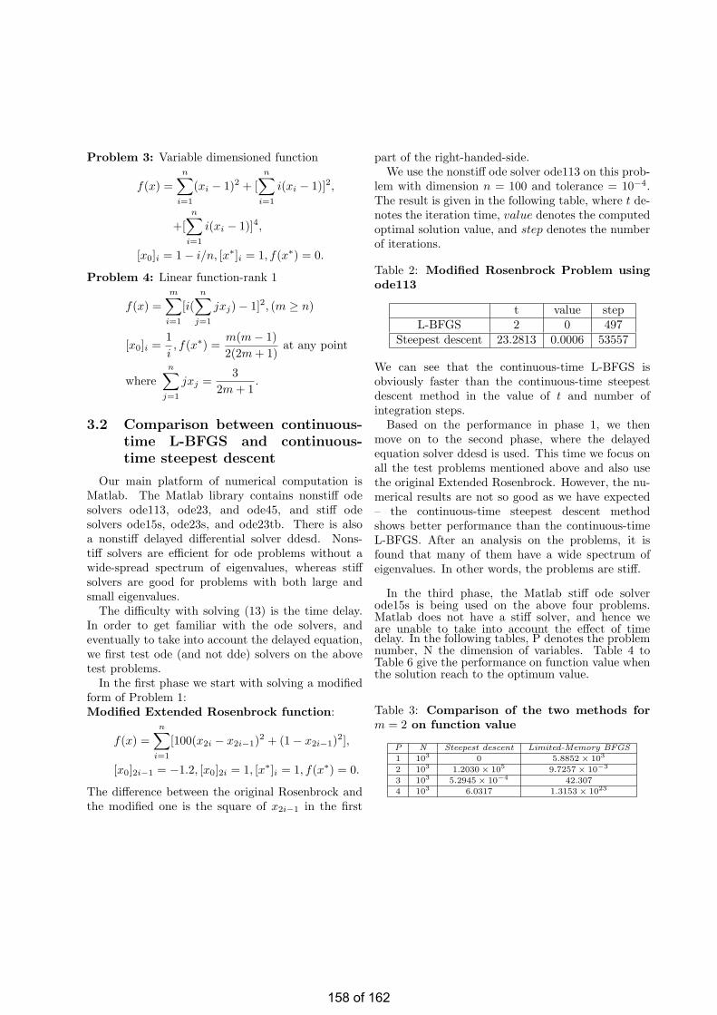
Problem 3: Variable dimensioned function
f(x) =n∑
i=1
(xi − 1)2 + [n∑
i=1
i(xi − 1)]2,
+[n∑
i=1
i(xi − 1)]4,
[x0]i = 1− i/n, [x∗]i = 1, f(x∗) = 0.
Problem 4: Linear function-rank 1
f(x) =m∑
i=1
[i(n∑
j=1
jxj)− 1]2, (m ≥ n)
[x0]i =1i, f(x∗) =
m(m− 1)2(2m + 1)
at any point
wheren∑
j=1
jxj =3
2m + 1.
3.2 Comparison between continuous-time L-BFGS and continuous-time steepest descent
Our main platform of numerical computation isMatlab. The Matlab library contains nonstiff odesolvers ode113, ode23, and ode45, and stiff odesolvers ode15s, ode23s, and ode23tb. There is alsoa nonstiff delayed differential solver ddesd. Nons-tiff solvers are efficient for ode problems without awide-spread spectrum of eigenvalues, whereas stiffsolvers are good for problems with both large andsmall eigenvalues.
The difficulty with solving (13) is the time delay.In order to get familiar with the ode solvers, andeventually to take into account the delayed equation,we first test ode (and not dde) solvers on the abovetest problems.
In the first phase we start with solving a modifiedform of Problem 1:Modified Extended Rosenbrock function:
f(x) =n∑
i=1
[100(x2i − x2i−1)2 + (1− x2i−1)2],
[x0]2i−1 = −1.2, [x0]2i = 1, [x∗]i = 1, f(x∗) = 0.
The difference between the original Rosenbrock andthe modified one is the square of x2i−1 in the first
part of the right-handed-side.We use the nonstiff ode solver ode113 on this prob-
lem with dimension n = 100 and tolerance = 10−4.The result is given in the following table, where t de-notes the iteration time, value denotes the computedoptimal solution value, and step denotes the numberof iterations.
Table 2: Modified Rosenbrock Problem usingode113
t value stepL-BFGS 2 0 497
Steepest descent 23.2813 0.0006 53557
We can see that the continuous-time L-BFGS isobviously faster than the continuous-time steepestdescent method in the value of t and number ofintegration steps.
Based on the performance in phase 1, we thenmove on to the second phase, where the delayedequation solver ddesd is used. This time we focus onall the test problems mentioned above and also usethe original Extended Rosenbrock. However, the nu-merical results are not so good as we have expected– the continuous-time steepest descent methodshows better performance than the continuous-timeL-BFGS. After an analysis on the problems, it isfound that many of them have a wide spectrum ofeigenvalues. In other words, the problems are stiff.
In the third phase, the Matlab stiff ode solverode15s is being used on the above four problems.Matlab does not have a stiff solver, and hence weare unable to take into account the effect of timedelay. In the following tables, P denotes the problemnumber, N the dimension of variables. Table 4 toTable 6 give the performance on function value whenthe solution reach to the optimum value.
Table 3: Comparison of the two methods form = 2 on function value
P N Steepest descent Limited-Memory BFGS
1 103 0 5.8852× 10³
2 103 1.2030× 10⁵ 9.7257× 10⁻³
3 103 5.2945× 10⁻⁴ 42.307
4 103 6.0317 1.3153× 10²³
158 of 162

Table 4: Comparison of the two methods form = 4 on function value
P N Steepest descent Limited-Memory BFGS
1 103 0 4.2692× 10³
2 103 1.5114× 10⁵ 9.7304× 10³
3 103 0 2.9868× 10⁻¹
4 103 6.0317 32.595
Table 5: Comparison of the two methods form = 6 on function value
P N Steepest descent Limited-Memory BFGS
1 103 0 1.1273× 10³
2 103 1.5068× 10⁵ 9.7296× 10⁻³
3 103 7.1928× 10⁻⁸ 1.0795× 10⁻⁵
4 103 6.0317 6.0317
Table 7 to Table 9 focus on the comparison for thenorm of gradient as solution tends to the optimumvalue.
Table 6: Comparison of the norm of gradientof the two methods for m = 2
P N Steepest descent Limited-Memory BFGS1 1000 0 57.060
2 1000 1.4146× 10³ 6.9366× 10⁻⁵
3 1000 4.6056× 10 3.1173
4 1000 8.5570× 10⁻⁷ 2.8544× 10¹⁵
Table 7: Comparison of the norm of gradientof the two methods for m = 4
P N Steepest descent Limited-Memory BFGS1 1000 0 6.5250
2 1000 1.6787× 10³ 1.8992× 10⁻⁴
3 1000 0 8.1280× 10
4 1000 2.1221× 10⁻⁷ 1.9531× 10²
Table 8: Comparison of the norm of gradientof the two methods for m = 6
P N Steepest descent Limited-Memory BFGS1 1000 0 3.1648
2 1000 1.6749× 10³ 1.7542× 10⁻⁴
3 1000 5.3639× 10⁻¹ 1.5238
4 1000 3.7336× 10⁻⁷ 3.7253× 10⁻⁵
By comparing these tables one may find that thecontinuous-time L-BFGS performs better in Problem2, while the continuous-time steepest descent methodperforms better in Problem 4. In Problems 1 and 3,
there is not much difference.In order to show the full potential of the
continuous-time L-BFGS, it is our next goal to use astiff dde solver, which will be performed in the nextphase of this research.
3.3 A new code using Radar5
For stiff problems, including differential-algebraicand neutral delay equations with constant or state-dependent (eventually vanishing) delays, the codeRADAR5 written by Ernest Hairer is more appro-priate. This code uses collocation methods based onRadau nodes and solves dde’s of the type
My′(t) = f (t, y(t), y(t− α1(t, y(t))), . . . , y(t− αm(t, y(t))))
y(t0) = y0, y(t) = g(t) for t < t0,
where M is a constant d×d matrix and αi(t, y(t)) < tfor all t ≥ t0 and for all i. The value g(t0) maybe different from y0, allowing for a discontinuity att0. (Collocation methods have been proved to haveexcellent stability properties for delay equations.)
The code RADAR5 is written in ANSI Fortran-90and is made up of several routines. Because our maintest programs are written in MATLAB, we need tocall FORTRAN from MATLAB. This is not an easytask and will be tackled in the next phase of ourresearch.
4 Main stages of this research
(A) Prove that the function H in (13) is positivedefinite. (Done and shown in Appendix I).
(B) Prove that H is Lipschitz continuous. (Stillongoing)
(C) Show that the solution to (13) is asymptoti-cally stable. (A simple consequence of (B).)
(D) Show that (13) has a better rate of con-vergence than the dynamical system basedon the steepest descent direction.
(E) Perform numerical testing.(F) Apply this new optimization method to pr-
actical problems.
159 of 162
APPENDIX I: To show that H in (13) ispositive definite.
Without loss of ambiguity, in the subsequentproof, we drop the t, t0, t1, . . . , tk, tk+1, ect. insk(t), yk(t), Vk(t), and so on below.Property 1 If H0 is positive definite, the matrixH defined by (13) is positive definite (provided thatyT
i si > 0 for all i).Proof: We prove the result by induction. From theabove discussion we know that (13), the continuousanalog of the L-BFGS formula, has two cases. Henceour proof needs to cater for each of them.
For the first case k+1 > m, note that when m = 1
Hk+1 = V Tk H0Vk + ρksksT
k
= H0 −H0yksT
k
yTk sk
− skyTk H0
yTk sk
+skyT
k H0yksTk
(yTk sk)2
+sksT
k
yTk sk
It is obvious that the proof of p.d. of this matrix isthe same as that of Theorem 1 in section 1.3. There-fore, Hk+1 is p.d. when m = 1.
Now suppose they are true for m = l, we show thatthey are true for m = l + 1.
When m = l, we have (denoting Hk+1 by H lk+1 to
emphasize m = l)
H lk+1 = V T
k V Tk−1 · · ·V T
k−l+1H0Vk−l+1 · · ·Vk−1Vk
+V Tk · · ·V T
k−l+2ρk−l+1sk−l+1sTk−l+1
·Vk−l+2 · · ·Vk
+V Tk · · ·V T
k−l+3ρk−l+2sk−l+2sTk−l+2
·Vk−l+3 · · ·Vk
...+V T
k V Tk−1ρk−2sk−2s
Tk−2Vk−1Vk
+Vkρk−1sk−1sTk−1Vk
+ρksksTk .
being positive definite. (There are l + 1 terms inH l
k+1)If m = l + 1, from (13B)
H l+1k+1 = V T
k V Tk−1 · · ·V T
k−lH0Vk−l · · ·Vk−1Vk
+V Tk · · ·V T
k−l+1ρk−lsk−lsTk−l
·Vk−l+1 · · ·Vk
+V Tk · · ·V T
k−l+2ρk−l+1sk−l+1sTk−l+1
·Vk−l+2 · · ·Vk
+V Tk · · ·V T
k−l+3ρk−l+2sk−l+2sTk−l+2
·Vk−l+3 · · ·Vk
...+V T
k V Tk−1ρk−2sk−2s
Tk−2Vk−1Vk
+Vkρk−1sk−1sTk−1Vk
+ρksksTk .
(There are l + 2 terms in H l+1k+1.)
Comparing these two equations we find that theterms in curly braces are the same, and let
(∗) = V Tk · · ·V T
k−l+2ρk−l+1sk−l+1sTk−l+1
·Vk−l+2 · · ·Vk
+V Tk · · ·V T
k−l+3ρk−l+2sk−l+2sTk−l+2
·Vk−l+3 · · ·Vk
...+V T
k V Tk−1ρk−2sk−2s
Tk−2Vk−1Vk
+Vkρk−1sk−1sTk−1Vk
+ρksksTk
Thus,
H lk+1 = V T
k V Tk−1 · · ·V T
k−l+1H0Vk−l+1 · · ·Vk−1Vk
+(∗)
H l+1k+1 = V T
k V Tk−1 · · ·V T
k−lH0Vk−l · · ·Vk−1Vk
+V Tk · · ·V T
k−l+1ρk−lsk−lsTk−l
·Vk−l+1 · · ·Vk + (∗)= V T
k V Tk−1 · · ·V T
k−l+1(VTk−lH0Vk−l + ρk−l
·sk−lsTk−l)Vk−l+1 · · ·Vk−1Vk + (∗)
Since we have assumed that H lk+1 is p.d., if we try
to prove that H l+1k+1 is also p.d., we should prove that
160 of 162
V Tk−lH0Vk−l + ρk−lsk−ls
Tk−l and H0 have the same
property, i.e., V Tk−lH0Vk−l +ρk−lsk−ls
Tk−l is also p.d..
Now we move forward to prove that V Tk−lH0Vk−l +
ρk−lsk−lsTk−l is p.d..
From the proof before, we have the following con-clusion:
Consider the formula
B = V Tk AVk + ρksksT
k k = 0, 1, · · ·
(The definition of Vk, ρk, sk are the same as in theL-BFGS formula.) If we know A is a p.d. matrix,then B is also p.d..
In this sense, it is easy to know that V Tk−lH0Vk−l +
ρk−lsk−lsTk−l is p.d.. As we have assumed that H l
k+1
is p.d. when H0 is p.d., we conclude that H l+1k+1 is
p.d..For the second case k + 1 ≤ m,
Hk+1 = V Tk V T
k−1 · · ·V T0 H0V0 · · ·Vk−1Vk
+V Tk · · ·V T
1 ρ0s0sT0 V1 · · ·Vk
...+V T
k V Tk−1ρk−2sk−2s
Tk−2Vk−1vk
+Vkρk−1sk−1sTk−1Vk
+ρksksTk .
We also use induction to prove Hk+1 is p.d..Firstly, H1 = V T
0 H0V0 + ρ0s0sT0 from above, so it
is clearly that H1 is p.d..Secondly, assumed that Hk is p.d.. We are going
to prove that Hk+1 is also p.d.. We have assumed
Hk = V Tk−1V
Tk−2 · · ·V T
0 H0V0 · · ·Vk−2Vk−1
+V Tk−1 · · ·V T
1 ρ0s0sT0 V1 · · ·Vk−1
+V Tk−1 · · ·V T
2 ρ1s1sT1 V2 · · ·Vk−1
...+Vk−1ρk−2sk−2s
Tk−2Vk−1
+ρk−1sk−1sTk−1.
is p.d.. Hence,
Hk+1 = V Tk V T
k−1 · · ·V T0 H0V0 · · ·Vk−1Vk
+V Tk · · ·V T
1 ρ0s0sT0 V1 · · ·Vk
...+V T
k V Tk−1ρk−2sk−2s
Tk−2Vk−1vk
+Vkρk−1sk−1sTk−1Vk
+ρksksTk
= V Tk (V T
k−1VTk−2 · · ·V T
0 H0V0 · · ·Vk−2Vk−1
+V Tk−1 · · ·V T
1 ρ0s0sT0 V1 · · ·Vk−1
+V Tk−1 · · ·V T
2 ρ1s1sT1 V2 · · ·Vk−1
+ · · ·+ Vk−1ρk−2sk−2sTk−2Vk−1
+ρk−1sk−1sTk−1)Vk + ρksksT
k
= V Tk HkVk + ρksksT
k .
Therefore, we have proved that Hk+1 is p.d. whenk + 1 ≤ m.
So we have proved the property for both casesk + 1 ≤ m and k + 1 > m. 2
The proof of the property above is part of ourwork on the delayed dynamical systems approachfor unconstrained optimization. The requirementthat yT
i si > 0 for all i in Property 1 is not a majorissue, because we work with a continuous ode andthe numerical method can always be restarted.
References
[1] Aluffi-Pentini, F., Parisi, V. and Zirilli, F. Al-gorithm 617 DAFNE: A differential equationsalgorithm for nonlinear equations, ACM Trans.on Math. Software, 10 (3), 1984, 317-324.
[2] Boggs, P. T., The solution of nonlinear systemsof equations by A-stable integration techniques,SIAM J. Numer. Anal. 8 (4), 1971, 767-785.
[3] Botsaris, C. A. and Jacobson, D. H., A Newton-type curvilinear search method for optimiza-tion, JMAA, 54, 1976, 217-229.
161 of 162

[4] Brown, A. A. and Bartholomew-Biggs, M. C.,ODE versus SQP methods for constrained op-timization, JOTA 62 (3), 1989, 371-386.
[5] Chen, Y. H. and Fang, S. C., Solving convexprogramming problem with equality constraintsby neural networks, Computers Math. Appl. 36,1998, 41-68.
[6] Chu, M. T., On the continuous realization ofiterative processes, SIAM Review 30 (3), 1988,375-387.
[7] Han, Q., Liao, L.-Z., Qi, H. and Qi, L., Stabilityanalysis of gradient-based neural networks foroptimization problems, J. Global Optim. 19 (4),1962, 363-381.
[8] Hassan, N. and Rzymowski, W., An ordinarydifferential equation in nonlinear programming.Nonlinear Analysis, Theory, Method & Appli-cations 15 (7), 1990, 597-599.
[9] aykin, S. S., Neural Networks: A Compre-hensive Foundation, Prentice-Hall, EnglewoodCliffs, NJ, 1994.
[10] He, B. S., Inexact implicit methods for mono-tone general variational inequalities, Mathe-matical Programming, 86 (1), 1999, 199-217.
[11] Incerti, S., Parisi, V. and Zirilli, F., Anew method for solving nonlinear simultaneousequations, SIAM J. Numer. Anal. 16, 1979, 779-789.
[12] Jorge Nocedal, Updating Quasi-Newton Ma-trices With Limited Storage, Mathematics ofComputation, Vol 35, No 151, July 1980, pp.773-782.
[13] Liao, L.-Z. and Qi, H., A neural network for thelinear complementarity problem, Math. Com-put. Modelling 29 (3), 1999, 9-18.
[14] L.Z. Liao, L.Q. Qi, and H.W. Tam, A gradient-based continuous method for large-scale op-timization problems, Journal of Global Opti-mization, Vol 31 , Apr 2005, pp. 271-286.
[15] Liao, L.-Z., Qi, H. and Qi, L., Solving non-linear complementarity problems with neuralnetworks: a reformulation method approach,JCAM 131 (12), 2001, 343-359.
[16] LI-ZHI LIAO, HOUDUO QI and LIQUN QI,(2004), Neurodynamical Optimization, Journalof Global Optimization 28: 175-195.
[17] Novakovi?c, Z. R., Solving systems of non-linearequations using the Lyapunov direct method,Computers Math. Applic. 20 (12), 1990, 19-23.
[18] Tanabe, K., A geometric method in nonlinearprogramming, JOTA 30 (2), 1980, 181-210.
[19] Tank, D. W. and Hopfield, J. J., Simple neuraloptimization networks: An A/D convert, signaldecision circuit, and a linear programming cir-cuit, IEEE Trans. Circuits Syst. 33, 1986, 533-541.
[20] Wilde, N. G., A note on a differential equationapproach to nonlinear programming, Manage-ment Science 15 (11), 1969, 739-739.
[21] Williems, J. L., Stability Theory of DynamicalSystems, Nelson, 1970.
[22] Wu, X., Xia, Y., Li, J. and Chen, W. K., A highperformance neural network for solving linearand quadratic programming problems, IEEETrans. Neural Networks, 7, 1996, 643-651.
[23] Xia, Y., A new neural network for solving lin-ear programming problems and its applications,IEEE Trans. Neural Networks 7, 1996, 525-529.
[24] Yamashita, H., A differential equation ap-proach to nonlinear programming, Math. Prog.18,1980, 155-168.
[25] Zabcayk, J ., Mathematical Control Theory:An Introduction, Birkhauser, Boston, 1992.
162 of 162