sparse frequency transmit and receive waveform design

Sparse Frequency Transmit andReceive Waveform Design

MICHAEL J. LINDENFELDScience Applications International Corp.

A computationally efficient algorithm derives complex digital

transmit and receive ultra-wideband radar and communication

waveforms with excellent arbitrary frequency band suppression

and range sidelobe minimization. The transmit waveform

minimizes a scalar function penalizing weighted spectral energy

in arbitrary frequency bands. Near constant power results from

another penalty function for deviations from constant power, or

constant power is enforced by a phase-only formulation. Next,

a least squares solution for the receive waveform minimizes a

weighted sum of suppressed band spectral energy and range

sidelobes (for pulse and continuous wave operation), with a

mainlobe response constraint. Both waveforms are calculated by

iterative algorithms whose updates require only linear order in

memory and computation, permitting quick calculation of long

pulses with thousands of samples.

Manuscript received December 2, 2002; revised November 10,2003; released for publication April 19, 2004.

IEEE Log No. T-AES/40/3/835883.

Refereeing of this contribution was handled by E. S. Chornoboy.

This work was sponsored by DARPA under ContractSTO/STC00-01.

Author’s address: Science Applications International Corporation,10260 Campus Point Dr., M/S C-4, San Diego, CA 92121.

0018-9251/04/$17.00 c° 2004 IEEE

I. INTRODUCTION

Ultra-wide bandwidth (UWB) synthetic apertureradars (SARs) applied to foliage penetration (FOPEN)operate usually in the VHF and UHF bands toreduce attenuation due to vegetation [1]. This RFregion contains numerous assigned bands withstrong emitters. Also, there are bands that cannot beradiated into, such as those dedicated for navigation.Frequency filtering of either the transmit or receivewaveform or both leads to increased range sidelobes.Previous investigations have concentrated

on interference suppression in the receiver. Fornarrowband interference, frequency, amplitude,and phase of multiple pure tones are estimated andsubtracted [2—6]. Receive-only processing duringevery other pulse may be used to estimate noise tosubtract on the succeeding pulse when the transmitteris operating [6], although the pulse repetitionfrequency (PRF) is reduced. However, for widebandinterference, correlation times may be comparableto the pulse repetition interval. Also, some pure toneestimation algorithms are iterative [2, 4, 5] and manytens of tones or more may require subtraction. A leastmean square (LMS) algorithm estimates incominginterference for subtraction [7—9].Another algorithm approach is notch filtering,

which does not depend on accurate interferencecoherent waveform estimates. A nonadaptivetechnique [10] estimates interference spectral energyand derives a filter by inverse Fourier transforminga binary function which is one where interference isbelow a threshold and zero elsewhere. However, thesefilters do not always have good performance betweenFourier frequency bin centers. The frequency notchfilter is usually combined into the range compressionfilter. However, range sidelobes may increase unlessspecial attention is paid to their minimization. Theminimization algorithm [11] uses a least squaressolution for a receive waveform correlated with arandom noise transmit waveform to reproduce thedesired range response. Range sidelobes have beenreduced by a combination of median and apodizationfiltering [12].Another approach employs a Burg predictive

algorithm to fill in frequency bands contaminatedby interference [13]. Also, adaptive transmit andreceive waveforms are derived to maximize outputsignal-to-interference plus noise ratio (SINR) in thepresence of signal-dependent interference [14].The constrained least squares receive waveform

algorithm used here has a close analog in theproblem of generating beamforming coefficientsin the presence of interference. For beamforming,complex weighting coefficients are applied tominimize mainlobe angular beamwidth while notchingout response in directions towards interference.These angular regions could be enlarged to account

IEEE TRANSACTIONS ON AEROSPACE AND ELECTRONIC SYSTEMS VOL. 40, NO. 3 JULY 2004 851

for interference sources of finite extent, such asterrain-scattered interference [15, 16]. An additionalconstraint of zero slope in angular response energy atthe target direction ensures a maximum there [17].Novel algorithms are introduced here for

calculation of transmit and receive waveforms. Onedesirable property is frequency notching in thetransmit band. Operational systems must avoid certainbands used by critical systems, such as navigationaids, and must not interfere with other radios andradars. Also, bands with interference will not beuseful to the receiver and any power radiated in themis wasted. The transmit waveform is designed by aniterative algorithm to minimize a weighted sum of oneor two penalty functions. The first penalty functionis a weighted integral of spectral energy in arbitrarybands. In addition, since transmitters are often peakpower limited, the second penalty function weightspower that deviates from a constant. A variation ofthe algorithm generates a phase-only waveform, withconstant power, and the second penalty function isnot necessary. A similar algorithm has been applied tophase-only beamforming [18]. Since the minimizationfunctional is quartic in waveform samples for thepower penalty function and transcendental for thephase-only penalty function, an iterative solutionmethod is necessary. A beneficial property of thetransmit waveform is that spectral energy is almostevenly distributed among the allowed bands for alltimes during the pulse. This noise-like nature of thetransmit waveform reduces probability of intercept.The receive waveform is the solution of a

constrained least squares minimization of twopenalty functions. The first penalty function similarlyminimizes spectral energy in a set of bands and thesecond minimizes range sidelobes. Minimizationproblems require some additional condition to avoidthe zero solution. For the transmit waveform, it isuniform power, and for the receive waveform, it isthe constraint that range response at the mainlobesample is assigned a given value. An additionalconstraint of zero slope in range response energycould be applied to the receive waveform algorithmto guarantee that the range mainlobe has a peak at thedesired location [17], but this has not been necessary.An iterative conjugate gradient solution method isemployed. Taking advantage of the ability to weighteach stopband differently, enough suppression canbe realized (» 50 dB) in some receive bands to beeffective as an antijamming countermeasure.An important contribution here is that for both

calculations the computational effort and memoryrequirements for each iteration update are linearin the number of samples. This is a major issueas, for example, a 100 ¹s pulse over a 200 MHzbandwidth requires 20,000 digital samples. The keyto linear computational and memory order updates isthat weighting matrices are Toeplitz. The conjugate

gradient receive waveform algorithm achievesadequate convergence in much less time required bythe exact (quadratic order) Levinson solution.Section II introduces the algorithms for the

calculation of both waveforms. Section III showsresults for a baseline set of parameters. The allowedbands are determined from a set of allowed and radiofrequency interference (RFI) bands [13]. Spectralenergy suppression and range sidelobes are quantified.The baseline algorithm uses the phase-only transmitwaveform. Section IV shows effects due to algorithmvariations, such as soft power penalty for the transmitwaveform, modifications for CW operation, andphase-only transmit waveform quantization. Finally,Section V has a conclusion.

II. ALGORITHM

A. Transmit Waveform

The first step is to calculate the transmitwaveform; the receive waveform calculation follows.A set of Nt transmit waveform samples hn, n=1, : : : ,Nt, has the Fourier transform

h(f) =NtXn=1

hn exp[¡2¼if(n¡ 1)¢t] (1)

where ¢t is the sampling interval and i=p¡1. If

the fast-time frequency f is bounded between f1 andf2, the baseband complex waveform is assumed tobe relative to the central frequency fc = (f1 +f2)=2.Therefore, the sample spacing must be less thanor equal to 1=(f2¡f1). When spectral functionsare plotted, frequencies are shifted by the centralfrequency.A minimization (penalty) function is constructed to

penalize the transmit waveform in certain “forbidden”or stop frequencies. A set of Nb frequency bands toavoid is identified, where the kth band is between fk1and fk2, with a corresponding weight wk > 0, and thepenalty function is

JT1 =NbXk=1

wk

Z fk2

fk1

dfjh(f)j2

= h†R(2)h

R(2)mn =NbXk=1

wk

8>><>>:exp[2¼i(m¡ n)fk2¢t]¡ exp[2¼i(m¡ n)fk1¢t]

2¼i(m¡ n)¢t ,

m6= n(fk2¡fk1), m= n

(2)

where the dagger superscript denotes the Hermitianconjugate and (1) has been used. The nthelement of the column vector h is hn. Use of afrequency-dependent weighting function inside the

852 IEEE TRANSACTIONS ON AEROSPACE AND ELECTRONIC SYSTEMS VOL. 40, NO. 3 JULY 2004

frequency integral could be considered if the integralis analytic, but multiple, contiguous, constant weightbands would work as well. The band weights wkmay be adjusted arbitrarily in accordance with theimportance of notching out particular bands. The R(2)

matrix is Hermitian Toeplitz.Penalizing spectral energy at a set of discrete

frequencies was attempted in an earlier version ofthe algorithm. However, in order to avoid sharpspikes, the set of frequencies must be oversampledby about a factor of 4 over the fast Fourier transform(FFT) frequency spacing 1=Nt¢t. For this reason, andbecause of the additional computation complexity andarbitrariness in the choice of discrete frequencies, thepenalty function with a continuous frequency integralin the stopbands is preferred.Some additional condition is required to prevent

all transmit samples collapsing to zero when thefrequency penalty is minimized. Another earlieralgorithm did not use penalty functions but insteadcalculated a complex Remez filter with the samestopbands and passbands. The specified non-zeropassband magnitude prevents a zero solution. TheRemez filter least squares solution allows differentialweighting among stopbands and passbands. However,waveform time samples have far too much dynamicrange (about 30 dB between peak and average powerfor 1,000 samples). Since transmitters are generallypeak power limited, this 30 dB loss of average poweris unacceptable and a condition of equal (or almostequal) time sample power is necessary.1) Soft Power Constraint: Two methods of

ensuring equal or almost equal power are investigatedhere. The first method adds to JT1 in (2) a penaltyfunction for deviation of transmit power from unity,or

JT = ±h†(R(2) +¸TI)h+(1¡ ±)

NtXn=1

(jhnj2¡1)2(3)

where I is the identity matrix. The additional powerpenalty term is the second term. The real constant±, 0< ± < 1, controls relative weighting of the twopenalty functions. The constraint is soft as waveformsamples will have magnitude near, but not exactly,a constant (here one). Before this weighting, theR(2) matrix is normalized by dividing by its constantdiagonal value.The diagonal loading coefficient ¸T penalizes the

sum of absolute squares of the waveform samples.Diagonal loading is commonly employed [23, p. 565]to regularize nearly singular matrices. Numericalexperiments showed that the R(2) matrix could havesmall negative eigenvalues. Diagonal loading ensuresthat the quadratic coefficient matrix in (3) is positivedefinite. In the remainder of this subsection, thediagonal loading term is incorporated into the R(2)

matrix.

Since the additional penalty term is quartic in thesamples, the minimum is found using an iterativesteepest descent method,

h(p+1)n = h(p)n ¡ 2¹[±(R(2)h(p))n+2(1¡ ±)(jh(p)n j2¡ 1)h(p)n ]´ h(p)n ¡ 2¹dn (4)

where h(p)

n is the pth iteration of the nth transmitwaveform sample and the nth element of the columnvector h(p) is h

(p)

n . The nth component of the gradientvector d is dn and is given by the quantity in thesquare brackets in (4). Initial values are independent,random, complex numbers. The correctness of thisiteration for complex functions and Hermitian penaltymatrices has been verified [19—21]. The value of¹, the distance along the negative gradient, can beoptimized by substituting the right hand side of (4)into (3), yielding a penalty function JT(¹) =

P4q=0 aq¹

q

of fourth degree polynomial in ¹. The coefficients are

a0 = JT(¹= 0) = ±h†R(2)h+(1¡ ±)

Xn

(jhnj2¡ 1)2

a1 = 2±Re(d†R(2)h) +4(1¡ ±)

Xn

(jhnj2¡ 1)Re(d¤nhn)

a2 = ±(d†R(2)d) +2(1¡ ±)

Xn

(5)£f2[Re(d¤nhn)]2 + (jhnj2¡ 1)jdnj2g

a3 = 4(1¡ ±)Xn

Re(d¤nhn)jdnj2

a4 = (1¡ ±)Xn

jdnj4

where asterisks denote the complex conjugate.Differentiating JT with respect to ¹ and solving theresulting cubic equation yields in practice always twoconjugate complex roots and a single real positiveroot. The real positive root is chosen.2) Phase-Only Transmit Design: The other

method of regulating transmit power constrains itexactly by writing hn = bn exp(iÁn), where bn, n=1, : : : ,Nt is a set of fixed real amplitudes, which aregenerally unity but may have some tapering at theedges, and Án, n= 1, : : : ,Nt are phases. The powerpenalty function and diagonal loading terms are notneeded now and the total transmit penalty function is

JT = h†R(2)h=

Xm,n

bmR(2)mnbn exp[i(Án¡Ám)]: (6)

An iterative solution is generated as

Á(p+1)n = Á(p)n ¡¹ @JT@Á(p)n

@JT@Án

= 2Im

(bn exp(¡iÁn)

Xm

R(2)nmbm exp(iÁm)

):

(7)

LINDENFELD: SPARSE FREQUENCY TRANSMIT AND RECEIVE WAVEFORM DESIGN 853

The pth iteration of the nth phase sample is Á(p)n .Initial phases are random values between 0 and 2¼.A similar solution has been derived for adaptivephase-only beamforming [18]. The optimal valuefor ¹ requires solution of a transcendental equation.However, an arbitrary value for ¹ of 0.1 givesadequate convergence. Line search algorithms [22]could possibly speed up convergence.The key to fast computation and feasible memory

requirements is that iteration updates for both methodsdepend only on the product of a Toeplitz matrix anda vector. This can be accomplished by operations andmemory requirements of only linear order.

B. Receive Waveform

The receive waveform is now calculated as thesolution that minimizes a weighted sum of penaltyfunctions that depend on frequency stopband powerand range sidelobes. Receive samples are defined as

gn, n= 1, : : : ,Nr (8)

where Nr is the number of receive samples. Thecolumn vector g has the nth element gn. For pulsedsystems, the number of receive samples may bedifferent from the number of transmit samples. Areceive waveform penalty function for stopbands,g†R(2)g, may use different frequency bands than thoseof the transmit waveform, but has a form identical tothat of (2).The second penalty function minimizes range

sidelobes. Pulsed system range response is theconvolution

rn =min(Nr ,n)X

k=max(1,n¡Nt+1)hn¡k+1gk, n= 1, : : : ,Nc

Nc ´Nr+Nt¡1(9)

which can be written as a matrix multiplication

r=Hg

H=

0BBBBBBBBBBB@

h1 0 ¢ ¢ ¢ 0

h2 h1 ¢ ¢ ¢ 0

......

......

hNt hNt¡1 ¢ ¢ ¢ h1

......

......

0 0 0 hNt

1CCCCCCCCCCCA(10)

where the matrix H is Nc£Nr and the nth element ofthe vector r is rn.A natural strategy is to minimize range sidelobes

avoiding a region of width 2¢n+1, ¢n= 0,1, : : :samples around the mainlobe at sample N0 by

minimizing24N0¡¢n¡1Xn=1

+NcX

n=N0+¢n+1

35 jrnj2 = Nc¡2¢n¡1Xn=1

jrnj2 = g†R(1)g(11)

R(1) = H†H, r= Hg

where the H matrix is the H matrix with theappropriate rows excised out, and the samples ofr around the mainlobe are missing. The receivewaveform that results from this approach is g.The R(1) matrix is Nr£Nr. If zero-mean additivesystem noise is included in (11), after an expectationvalue, an additional term involving the noise timecorrelation function is obtained. However, this termis independent of the receive waveform and may beignored. The mainlobe sample is in the center of therange response (N0 = (Nc+1)=2 for Nc odd), but ingeneral could be anywhere.The total penalty function is a weighted sum of

the penalty functions for frequency bands, rangesidelobes, and a small diagonal loading term thatpenalizes sample magnitudes

R= ¯R(1) + (1¡¯)R(2) +¸RI: (12)

The constraint is that the mainlobe sample rangeresponse is unity. This is a linear constraint from(10). In general, the minimum of g†Rg, where g isan unknown Nr£ 1 vector and R is a known Nr£Nrmatrix, subject to Ne arbitrary known linear constraintsC†g= v, where C is Nr£Ne and v is Ne£1, is givenby [23, p. 566]

g= R¡1C(C†R¡1C)¡1v: (13)

The solution (13) requires the inverse of R, orsolution of simultaneous linear equations with it.The problem is that the R matrix is not Toeplitz.This leads to unacceptable memory requirements andcomputation times, which are cubic in the number ofsamples.The solution is to include all range samples into

the range sidelobe penalty function, including those inthe constraint. Therefore, the range sidelobe penaltyterm is proportional to

NcXn=1

jrnj2 = g†R(1)g, R(1) =H†H (14)

and R(1) is Toeplitz as it is the product of twotriangular Toeplitz matrices.The motivation to include all range samples is

the expectation that including additional equationsto be minimized which are constrained should haveno effect on the solution. To make this rigorous,it may be shown that both the non-Toeplitz andToeplitz penalty matrices have the same constrained


minimization solution for the case where all theexcised range samples are constrained. The differencein these matrices is then R= R+¯CC†. The twosolutions are

g= R¡1C(C†R¡1C)¡1v

g= (R+¯CC†)¡1CfC†(R+¯CC†)¡1Cg¡1v:(15)

The Sherman-Morrison-Woodbury matrix inversionlemma [23, p. 51] implies

(R+¯CC†)¡1 = R¡1¡¯R¡1C(I+¯C†R¡1C)¡1C†R¡1

(16)

which when substituted into (15), and after somealgebra, yields g= g.This identity is valid only when all the excised

samples are constrained. Therefore, for example, onecannot excise three samples centered on the mainlobefrom the penalty function and constrain only thesingle mainlobe sample. In practice, poor results wereobtained when more than one constraint sample wasattempted. This was probably due to having no goodchoice for the complex range samples around themainlobe. Thus, only the mainlobe constraint of unityis enforced. As mentioned before, the condition thatthe range response energy have zero slope at mainlobecan be enforced by additional constraints [17]. Thisensures that the mainlobe is a maximum, but thiswas not necessary. Unequal range response powerweighting does permit reduction of high sidelobesand minimization of integrated sidelobe levels, butthe resulting penalty matrices are not Toeplitz.The constrained minimization in (13) requires

solution to the Toeplitz equations with coefficientmatrix R in

g=R¡1C(C†R¡1C)¡1v: (17)

The Levinson algorithm is quadratic order incomputation operations and takes much too long. Amore efficient method for quadratic minimizationis conjugate gradient [24, 25]. Basically, a locationalong the gradient is found where the next gradientis orthogonal. There is a standard conjugate gradientmethod and a slightly modified one [24] that hasthe additional property that residuals decrease ateach iteration. Both methods work about as well,but the second method is adopted because of itsslightly faster convergence. Initial receive waveformvalues are random complex numbers. However, ifa new interference source is suddenly turned onand a solution has to be modified, then the existingwaveform would be used as the initial condition.

III. BASELINE RESULTS

A baseline set of parameters is based upona hypothetical UWB SAR system. The system

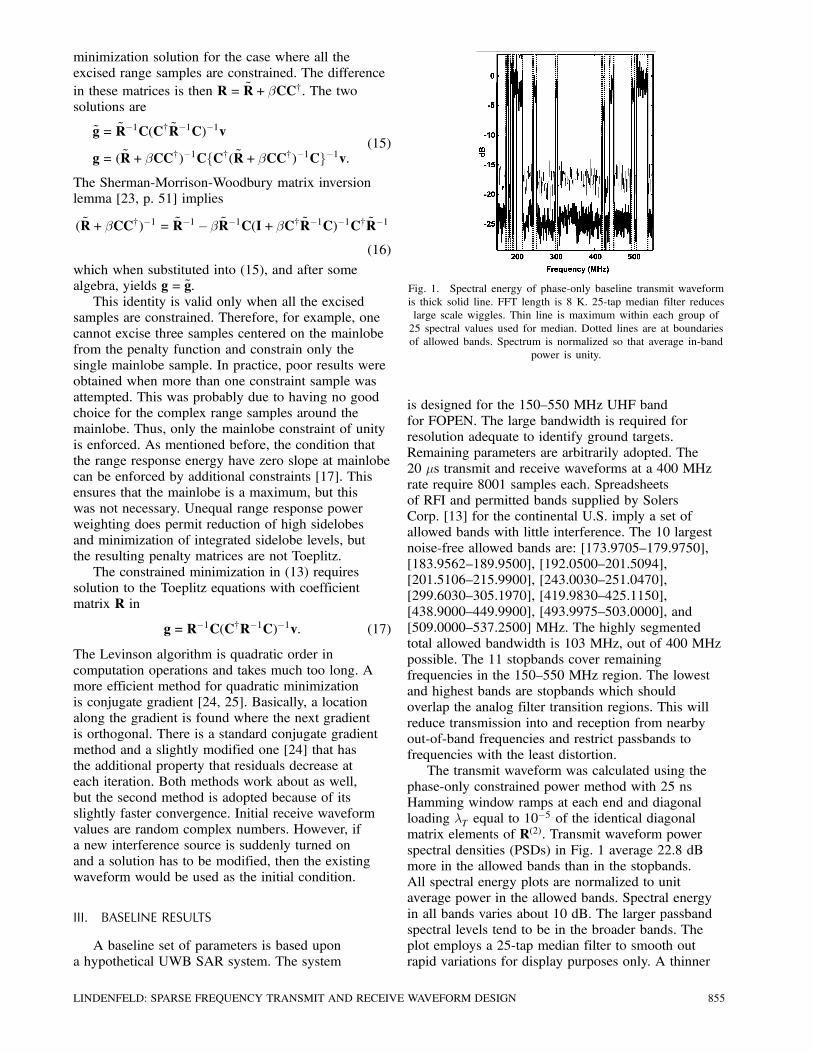
Fig. 1. Spectral energy of phase-only baseline transmit waveformis thick solid line. FFT length is 8 K. 25-tap median filter reduceslarge scale wiggles. Thin line is maximum within each group of25 spectral values used for median. Dotted lines are at boundariesof allowed bands. Spectrum is normalized so that average in-band

power is unity.

is designed for the 150—550 MHz UHF bandfor FOPEN. The large bandwidth is required forresolution adequate to identify ground targets.Remaining parameters are arbitrarily adopted. The20 ¹s transmit and receive waveforms at a 400 MHzrate require 8001 samples each. Spreadsheetsof RFI and permitted bands supplied by SolersCorp. [13] for the continental U.S. imply a set ofallowed bands with little interference. The 10 largestnoise-free allowed bands are: [173.9705—179.9750],[183.9562—189.9500], [192.0500—201.5094],[201.5106—215.9900], [243.0030—251.0470],[299.6030—305.1970], [419.9830—425.1150],[438.9000—449.9900], [493.9975—503.0000], and[509.0000—537.2500] MHz. The highly segmentedtotal allowed bandwidth is 103 MHz, out of 400 MHzpossible. The 11 stopbands cover remainingfrequencies in the 150—550 MHz region. The lowestand highest bands are stopbands which shouldoverlap the analog filter transition regions. This willreduce transmission into and reception from nearbyout-of-band frequencies and restrict passbands tofrequencies with the least distortion.The transmit waveform was calculated using the

phase-only constrained power method with 25 nsHamming window ramps at each end and diagonalloading ¸T equal to 10

¡5 of the identical diagonalmatrix elements of R(2). Transmit waveform powerspectral densities (PSDs) in Fig. 1 average 22.8 dBmore in the allowed bands than in the stopbands.All spectral energy plots are normalized to unitaverage power in the allowed bands. Spectral energyin all bands varies about 10 dB. The larger passbandspectral levels tend to be in the broader bands. Theplot employs a 25-tap median filter to smooth outrapid variations for display purposes only. A thinner


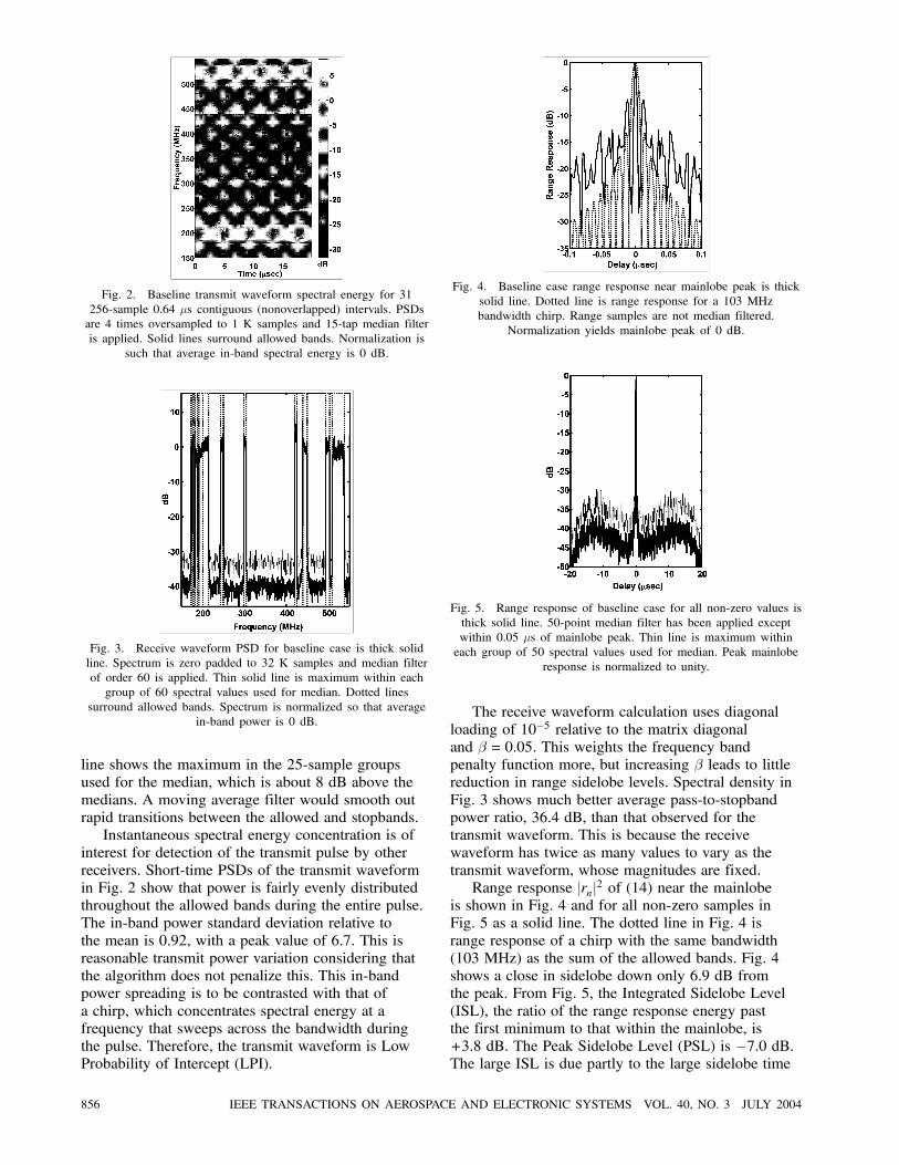
Fig. 2. Baseline transmit waveform spectral energy for 31256-sample 0:64 ¹s contiguous (nonoverlapped) intervals. PSDsare 4 times oversampled to 1 K samples and 15-tap median filteris applied. Solid lines surround allowed bands. Normalization is

such that average in-band spectral energy is 0 dB.

Fig. 3. Receive waveform PSD for baseline case is thick solidline. Spectrum is zero padded to 32 K samples and median filterof order 60 is applied. Thin solid line is maximum within eachgroup of 60 spectral values used for median. Dotted lines

surround allowed bands. Spectrum is normalized so that averagein-band power is 0 dB.

line shows the maximum in the 25-sample groupsused for the median, which is about 8 dB above themedians. A moving average filter would smooth outrapid transitions between the allowed and stopbands.Instantaneous spectral energy concentration is of

interest for detection of the transmit pulse by otherreceivers. Short-time PSDs of the transmit waveformin Fig. 2 show that power is fairly evenly distributedthroughout the allowed bands during the entire pulse.The in-band power standard deviation relative tothe mean is 0.92, with a peak value of 6.7. This isreasonable transmit power variation considering thatthe algorithm does not penalize this. This in-bandpower spreading is to be contrasted with that ofa chirp, which concentrates spectral energy at afrequency that sweeps across the bandwidth duringthe pulse. Therefore, the transmit waveform is LowProbability of Intercept (LPI).

Fig. 4. Baseline case range response near mainlobe peak is thicksolid line. Dotted line is range response for a 103 MHzbandwidth chirp. Range samples are not median filtered.

Normalization yields mainlobe peak of 0 dB.

Fig. 5. Range response of baseline case for all non-zero values isthick solid line. 50-point median filter has been applied exceptwithin 0:05 ¹s of mainlobe peak. Thin line is maximum withineach group of 50 spectral values used for median. Peak mainlobe

response is normalized to unity.

The receive waveform calculation uses diagonalloading of 10¡5 relative to the matrix diagonaland ¯ = 0:05. This weights the frequency bandpenalty function more, but increasing ¯ leads to littlereduction in range sidelobe levels. Spectral density inFig. 3 shows much better average pass-to-stopbandpower ratio, 36.4 dB, than that observed for thetransmit waveform. This is because the receivewaveform has twice as many values to vary as thetransmit waveform, whose magnitudes are fixed.Range response jrnj2 of (14) near the mainlobe

is shown in Fig. 4 and for all non-zero samples inFig. 5 as a solid line. The dotted line in Fig. 4 isrange response of a chirp with the same bandwidth(103 MHz) as the sum of the allowed bands. Fig. 4shows a close in sidelobe down only 6.9 dB fromthe peak. From Fig. 5, the Integrated Sidelobe Level(ISL), the ratio of the range response energy pastthe first minimum to that within the mainlobe, is+3:8 dB. The Peak Sidelobe Level (PSL) is ¡7:0 dB.The large ISL is due partly to the large sidelobe time


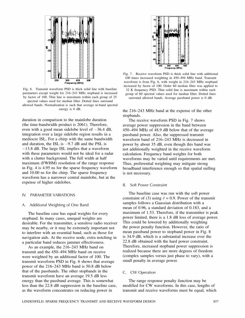
Fig. 6. Transmit waveform PSD is thick solid line with baselineparameters except weight for 216—243 MHz stopband is increasedby factor of 100. Thin line is maximum within each group of 25spectral values used for median filter. Dotted lines surround

allowed bands. Normalization is such that average in-band spectralenergy is 0 dB.

duration in comparison to the mainlobe duration(the time-bandwidth product is 2061). Therefore,even with a good mean sidelobe level of ¡36:4 dB,integration over a large sidelobe region results in amediocre ISL. For a chirp with the same bandwidthand duration, the ISL is ¡9:7 dB and the PSL is¡13:8 dB. The large ISL implies that a waveformwith these parameters would not be ideal for a radarwith a clutter background. The full width at halfmaximum (FWHM) resolution of the range responsein Fig. 4 is 4.95 ns for the sparse frequency waveformand 10.00 ns for the chirp. The sparse frequencywaveform has a narrower central mainlobe, but at theexpense of higher sidelobes.

IV. PARAMETER VARIATIONS

A. Additional Weighting of One Band

The baseline case has equal weights for everystopband. In many cases, unequal weights aredesirable. For the transmitter, a sensitive radio receivermay be nearby, or it may be extremely important notto interfere with an essential band, such as those fornavigation aids. At the receive node, extra notching ina particular band reduces jammer effectiveness.As an example, the 216—243 MHz band on

transmit and the 450—494 MHz band on receivewere weighted by an additional factor of 100. Thetransmit waveform PSD in Fig. 6 shows that averagepower of the 216—243 MHz band is 50.8 dB belowthat of the passbands. The other stopbands in thetransmit waveform have an average 19.5 dB lessenergy than the passband average. This is somewhatless than the 22.8 dB suppression in the baseline case,as the waveform concentrates on reducing power in

Fig. 7. Receive waveform PSD is thick solid line with additional100 times increased weighting in 450—494 MHz band. Transmitwaveform is from Fig. 6, with weight in 216—243 MHz stopbandincreased by factor of 100. Order 60 median filter was applied to32 K frequency PSD. Thin solid line is maximum within eachgroup of 60 spectral values used for median filter. Dotted linessurround allowed bands. Average passband power is 0 dB.

the 216—243 MHz band at the expense of the otherstopbands.The receive waveform PSD in Fig. 7 shows

average power suppression in the band between450—494 MHz of 48.9 dB below that of the averagepassband power. Also, the suppressed transmitwaveform band of 216—243 MHz is decreased inpower by about 35 dB, even though this band wasnot additionally weighted in the receive waveformcalculation. Frequency band weights for bothwaveforms may be varied until requirements are met.Thus, preferential weighting may mitigate strongbroadband interference enough so that spatial nullingis not necessary.

B. Soft Power Constraint

The baseline case was run with the soft powerconstraint of (3) using ± = 0:9. Power of the transmitsamples follows a Gaussian distribution with amean of 0.96, a standard deviation of 0.183, and amaximum of 1.53. Therefore, if the transmitter is peakpower limited, there is a 1.8 dB loss of average power.This could be lowered by additionally weightingthe power penalty function. However, the ratio ofmean passband power to stopband power in Fig. 8is 34.9 dB, which is a substantial increase over the22.8 dB obtained with the hard power constraint.Therefore, increased stopband power suppression isrealized because there are more degrees of freedom(complex samples versus just phase to vary), with asmall penalty in average power.

C. CW Operation

The range response penalty function may bemodified for CW waveforms. In this case, lengths oftransmit and receive waveforms must be equal, which


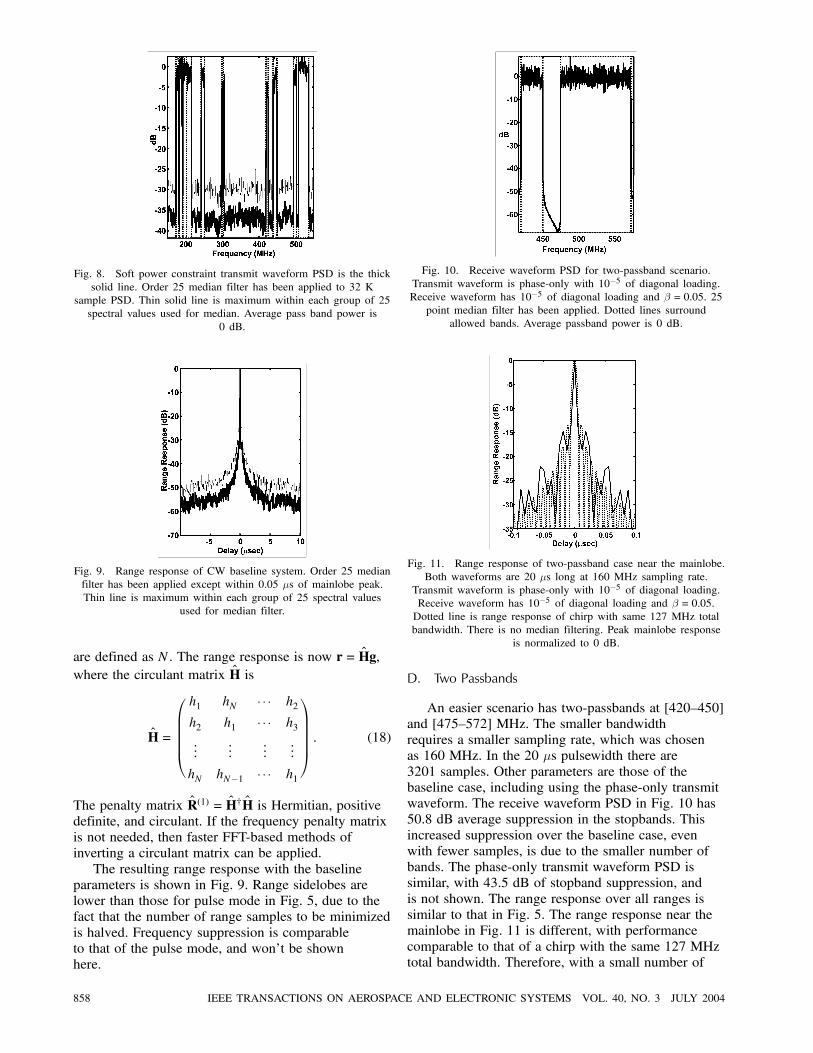
Fig. 8. Soft power constraint transmit waveform PSD is the thicksolid line. Order 25 median filter has been applied to 32 K

sample PSD. Thin solid line is maximum within each group of 25spectral values used for median. Average pass band power is

0 dB.

Fig. 9. Range response of CW baseline system. Order 25 medianfilter has been applied except within 0:05 ¹s of mainlobe peak.Thin line is maximum within each group of 25 spectral values

used for median filter.

are defined as N. The range response is now r= Hg,where the circulant matrix H is

H=

0BBBB@h1 hN ¢ ¢ ¢ h2

h2 h1 ¢ ¢ ¢ h3...

......

...

hN hN¡1 ¢ ¢ ¢ h1

1CCCCA : (18)

The penalty matrix R(1) = H†H is Hermitian, positivedefinite, and circulant. If the frequency penalty matrixis not needed, then faster FFT-based methods ofinverting a circulant matrix can be applied.The resulting range response with the baseline

parameters is shown in Fig. 9. Range sidelobes arelower than those for pulse mode in Fig. 5, due to thefact that the number of range samples to be minimizedis halved. Frequency suppression is comparableto that of the pulse mode, and won’t be shownhere.

Fig. 10. Receive waveform PSD for two-passband scenario.Transmit waveform is phase-only with 10¡5 of diagonal loading.Receive waveform has 10¡5 of diagonal loading and ¯ = 0:05. 25

point median filter has been applied. Dotted lines surroundallowed bands. Average passband power is 0 dB.

Fig. 11. Range response of two-passband case near the mainlobe.Both waveforms are 20 ¹s long at 160 MHz sampling rate.

Transmit waveform is phase-only with 10¡5 of diagonal loading.Receive waveform has 10¡5 of diagonal loading and ¯ = 0:05.Dotted line is range response of chirp with same 127 MHz totalbandwidth. There is no median filtering. Peak mainlobe response

is normalized to 0 dB.

D. Two Passbands

An easier scenario has two-passbands at [420—450]and [475—572] MHz. The smaller bandwidthrequires a smaller sampling rate, which was chosenas 160 MHz. In the 20 ¹s pulsewidth there are3201 samples. Other parameters are those of thebaseline case, including using the phase-only transmitwaveform. The receive waveform PSD in Fig. 10 has50.8 dB average suppression in the stopbands. Thisincreased suppression over the baseline case, evenwith fewer samples, is due to the smaller number ofbands. The phase-only transmit waveform PSD issimilar, with 43.5 dB of stopband suppression, andis not shown. The range response over all ranges issimilar to that in Fig. 5. The range response near themainlobe in Fig. 11 is different, with performancecomparable to that of a chirp with the same 127 MHztotal bandwidth. Therefore, with a small number of


stopbands, even wide ones, there is increased stopbandspectral suppression and lower range sidelobe levels.

E. Quantization

For the constant power phase-only transmitwaveform, hardware can be simplified by restrictingphase angles to a set of discrete values. This is donesimply in the simulation by rounding the phase of thecalculated transmit waveform to the nearest angle bin.This may not be the optimal discrete phase solution,but should have comparable performance. For thebaseline case, for 2, 4, 8, 16, 32, and (essentially)infinite number of discrete phases, ratios of averagepassband power to average stopband power are 7.0,12.0, 14.3, 19.8, 22.2, and 22.8 dB, respectively.The suppression loss is only 3.0 dB for 16 discretephases, but unacceptable for a biphase waveform.Comparable receive waveform PSD levels andrange sidelobes to those of the baseline case areobserved. This is consistent with the serial natureof the calculation–the receive waveform does thebest it can with almost any input transmit waveform.For the bands defined in the two-passband case, theaverage power ratios are 2.5, 7.7, 10.8, 18.0, 25.0,36.5, and 43.5 dB for 2, 4, 8, 16, 32, 256, and infinitenumber of discrete phases. There is comparablesuppression for 16 phases, implying that increasedband suppression requires more resolution.

V. CONCLUSIONS

A powerful algorithm has been presented forcalculation of long, wideband, sparse frequencytransmit, and receive digital waveforms. Whilesome aspects of the algorithm have been presentedelsewhere, this algorithm has novel features. Themost important advantage is that computational andmemory requirements are both linear in the numberof samples. A proof has been presented that all rangesidelobes can be included in the receive waveformminimization calculation, even those in the constraint,without affecting the solution, resulting in a Toeplitzmatrix. Both transmit and receive waveforms involveToeplitz matrices, which are required for linear updateorder. As a result, waveforms of thousands of samplesare rapidly calculated, permitting real-time adaptationto dynamic RFI environments. Only incoherentRFI estimates are required, which can occur duringreceive-only processing.Another advantage is the flexibility in stopband

specifications. The frequency penalty functionis generated by an integral over stopbands andtherefore is of arbitrary width. Particular bands withadditional weighting achieve increased attenuation. Ifsuppression levels in certain stopbands are not met,then weighting in that band can be increased, thepenalty matrix updated, and the iterative calculation

resumed. Similarly, if an RFI source appears, thepenalty matrix is updated with the additional bandand the iteration is continued. Increased stopbandweighting results in significant additional suppressionin that band, so that transmitters can radiate nearcritical bands and receivers can notch out jammers.Receive waveforms tend to have band suppressionbetter than that of the corresponding transmitwaveforms.Superior transmit band suppression is obtained

by the soft power penalty function method, asopposed to the phase-only algorithm, due to theadditional degrees of freedom of sample magnitudes.Tradeoffs between degree of band suppression and theadvantages of phase-only waveforms determine whichalgorithm should be adopted.A third advantage is the constant or near-constant

transmit sample power. Transmit waveform samplescan be phase-only, or almost equal power, resulting innegligible performance loss for peak power limitedtransmitters. If polyphase codes are adopted, atleast 16 bits should be employed for about 20 dBof stopband suppression, and more bits if moresuppression is possible. Transmit waveforms havepower uniformly spread throughout the allowed bandsfor all short time segments. Thus, they are noise-likeand LPI.Potential applications are in radar (monostatic

and bistatic) and communications. The algorithm iseasily modified for CW operation. For communicationradios and bistatic radar, the transmit waveform wouldhave to be communicated to the receiver. This couldbe accomplished by transmitting the waveform, orparameters needed for its calculation. Depending onthe computational power of the hardware, transmit andreceive waveforms could be calculated both on thetransmitter, both on the receiver, or one on each.

ACKNOWLEDGMENT

The DARPA program manager was Mr. LeeMoyer. The author acknowledges many informativediscussions with Drs. Jonathan Bar-On, GeraldGerace, and Amir Sarajedini.

REFERENCES

[1] Taylor, J. D. (Ed.) (2001)Ultra-Wideband Radar Technology.New York: CRC Press, 2001.

[2] Miller, T., Potter, L., and McCorkle, J. (1997)RFI suppression for ultra wideband radar.IEEE Transactions on Aerospace and Electronic Systems,33 (1997), 1142—1156.

[3] Juhel, B., Vezzosi, G., and Le Goff, M. (1999)Radio frequency interferences suppression for noisy ultrawide band SAR measurements.In J. Shiloh, B. Mandelbaum, E. Heyman (Eds.),Ultra-Wideband, Short-Pulse Electromagnetics 4, NewYork: Kluwer Academic, 1999, 387—393.


[4] Huang, X., and Liang, D. (1999)Gradual RELAX algorithm for RFI suppression inUWB-SAR.Electronics Letters, 35 (1999), 1916—1917.

[5] Golden, A., Jr., Werness, S. A., et al. (1995)Radio frequency interference removal in a VHF/UHFderamp SAR.In D. A. Giglio (Ed.), Algorithms for Synthetic ApertureRadar Imagery II, SPIE Conference Proceedings, Vol. 2487,1995, 84—95.

[6] Ferrell, B. H. (1995)Interference suppression in UHF synthetic-aperture radar.In D. A. Giglio (Ed.), Algorithms for Synthetic ApertureRadar Imagery II, SPIE Conference Proceedings. Vol. 2487,1995, 96—106.

[7] Lord, R. T., and Inggs, M. R. (1998)Approaches to RF interference suppression for VHF/UHFsynthetic aperture radar.In Proceedings of the 1998 IEEE South African Symposiumon Communications and Signal Processing, 1998, 95—100.

[8] Lord, R. T., and Inggs, M. R. (1999)Efficient RFI suppression in SAR using LMS adaptivefilter integrated with range/Doppler algorithm.Electronics Letters, 35 (1999), 629—630.

[9] Luo, X., Ulander, L. M. H., et al. (2001)RFI suppression in ultra-wideband SAR systems usingLMS filters in frequency domain.Electronics Letters, 37 (2001), 241—243.

[10] Stephens, J. P., Sr., and Parks, R. S. (2000)Interference avoiding transform domain basedcommunication systems.In Proceedings of International Microwave Symposium,Boston, MA, 2000, 1—7.

[11] Koutsoudis, T., and Lovas, L. (1995)RF interference suppression in ultra wideband radarreceivers.In D. A. Giglio (Ed.), Algorithms for Synthetic ApertureRadar Imagery II, SPIE Conference Proceedings, Vol. 2487,1995, 107—118.

[12] Xu, X., and Narayanan, R. M. (2001)Range sidelobe suppression technique for coherent ultrawide-band random noise radar imaging.IEEE Transactions on Antennas Propagation, 49 (2001),1836—1842.

[13] Salzman, J., Akamine, D., and Lefevre, R. (2001)Optimal waveforms and processing for sparse frequencyUWB operation.In Proceedings of 2001 IEEE Radar Conference, 105—110.

[14] Pillai, S. U., Oh, H. S., Youla, D. C., and Guerci, J. R.(2000)Optimum transmit-receiver design in the presence ofsignal-dependent interference and channel noise.IEEE Transactions on Information Theory, 46, 2 (2000),577—584.

[15] Tseng, C. Y., and Griffiths, L. J. (1992)A simple algorithm to achieve desired patterns forarbitrary arrays.IEEE Transactions on Signal Processing, 40 (1992),2737—2746.

[16] Tseng, C. Y., and Griffiths, L. J. (1992)A unified approach to the design of linear constraints inminimum variance adaptive beamformers.IEEE Transactions on Antennas Propagation, 40 (1992),1533—1542.

[17] Tseng, C. Y. (1992)Minimum variance beamforming with phase-independentderivative constraints.IEEE Transactions on Antennas Propagation, 40 (1992),285—294.

[18] Smith, S. T. (1999)Optimum phase-only adaptive nulling.IEEE Transactions on Signal Processing, 47 (1999),1835—1843.

[19] Jaffer, A. G., and Jones, W. E. (1995)Weighted least-squares design and characterization ofcomplex FIR filters.IEEE Transactions on Signal Processing, 43 (1995),2398—2401.

[20] Brandwood, D. H. (1983)A complex gradient operator and its application inadaptive array theory.IEE Proceedings, 130, Pt. F and H (1983), 11—16.

[21] van den Bos, A. (1994)Complex gradient and Hessian.IEE Proceedings in Visual Image Signal Processing, 141(1994), 380—382.

[22] Luenberger, D. G. (1984)Linear and Nonlinear Programming (2nd ed.).Reading, MA: Addison-Wesley, 1984, sect. 7.5.

[23] Golub, G. H., and Van Loan, C. F. (1996)Matrix Computations (3rd ed.).Baltimore, MD: The Johns Hopkins University Press,1996.

[24] Hestenes, M. R., and Stiefel, E. (1952)Methods of conjugate gradients for solving linearsystems.Journal of Res. National Bureau of Standards, 49 (1952),409—436.

[25] Chan, R. H., and Ng, M. K. (1996)Conjugate gradient methods for Toeplitz systems.SIAM Review, 38 (1996), 427—482.


Michael Lindenfeld received a B.S. degree from the California Institute ofTechnology, Pasadena, in 1970 and a Ph.D. degree from Brandeis University,Waltham, MA, in 1976, both in physics. His thesis and later postdoctoral researchat the University of Florida, Gainesville, and the University of British Columbia,Vancouver, were in classical kinetic theory, nonlinear transport in fluids, neutrontransport, upper atmosphere physics, and nonequilibrium atmospheric chemicalreaction rates.He is currently a senior research scientist at Science Applications International

Corp. He has worked on performance prediction for detection systems includingphysics of the target, background, and sensor. For visible and optical systems,he has investigated performance gains due to multiple frames and spectralchannels. He has also designed and analyzed data from innovative radar andsonar systems. In electromagnetics he has worked in radar propagation andmagnetohydrodynamic fields generated by seawater motion through Earth’smagnetic field.


sparse frequency transmit and receive waveform design

Documents