transmit and receive signal processing for mimo terrestrial
TRANSCRIPT
Ph.D. Dissertation
Transmit and Receive SignalProcessing for MIMO Terrestrial
Broadcast Systems
Universitat Politecnica de Valencia
Departamento de Comunicaciones
Author
David E. Vargas Paredero
Advisor
Dr. David Gomez-Barquero
Tutor
Prof. Narcıs Cardona Marcet
Valencia, May 2016

Supervisors
Dr. David Gomez-BarqueroInstitute of Telecommunications and Multimedia ApplicationsUniversitat Politecnica de Valencia, Spain
Professor Narcıs Cardona MarcetCommunications DepartmentUniversitat Politecnica de Valencia, Spain
Reviewers
Associate Professor Camilla HollantiDepartment of Mathematics and Systems AnalysisAalto University, Finland
Associate Professor Jeongchang KimDivision of Electronics and Electrical Information EngineeringKorea Maritime and Ocean University, South Korea
Assistant Professor Youssef NasserFaculty of Engineering and ArchitectureAmerican University of Beirut, Lebanon
Opponents
Professor Alberto Gonzalez SalvadorCommunications DepartmentUniversitat Politecnica de Valencia, Spain
Dr. Mikel Mendicute ErrastiDepartment of Electronics and Computer ScienceMondragon Unibertsitatea, Spain
Dr. Belkacem MouhoucheSamsung Electronics Research Institute, United Kingdom
iii

iv
Abstract
Multiple-Input Multiple-Output (MIMO) technology in Digital Terrestrial Tele-vision (DTT) networks has the potential to increase the spectral efficiency andimprove network coverage to cope with the competition of limited spectrum use(e.g., assignment of digital dividend and spectrum demands of mobile broad-band), the appearance of new high data rate services (e.g., ultra-high definitionTV - UHDTV), and the ubiquity of the content (e.g., fixed, portable, and mo-bile). It is widely recognised that MIMO can provide multiple benefits suchas additional receive power due to array gain, higher resilience against signaloutages due to spatial diversity, and higher data rates due to the spatial mul-tiplexing gain of the MIMO channel. These benefits can be achieved withoutadditional transmit power nor additional bandwidth, but normally come at theexpense of a higher system complexity at the transmitter and receiver ends.The final system performance gains due to the use of MIMO directly depend onphysical characteristics of the propagation environment such as spatial correla-tion, antenna orientation, and/or power imbalances experienced at the trans-mit aerials. Additionally, due to complexity constraints and finite-precisionarithmetic at the receivers, it is crucial for the overall system performance tocarefully design specific signal processing algorithms.
This dissertation focuses on transmit and received signal processing for DTTsystems using MIMO-BICM (Bit-Interleaved Coded Modulation) without feed-back channel to the transmitter from the receiver terminals. At the transmitterside, this thesis presents investigations on MIMO precoding in DTT systemsto overcome system degradations due to different channel conditions. At thereceiver side, the focus is given on design and evaluation of practical MIMO-BICM receivers based on quantized information and its impact in both thein-chip memory size and system performance. These investigations are carriedwithin the standardization process of DVB-NGH (Digital Video Broadcasting- Next Generation Handheld) the handheld evolution of DVB-T2 (Terrestrial- Second Generation), and ATSC 3.0 (Advanced Television Systems Commit-tee - Third Generation), which incorporate MIMO-BICM as key technology toovercome the Shannon limit of single antenna communications. Nonetheless,
v
ABSTRACT
this dissertation employs a generic approach in the design, analysis and evalu-ations, hence, the results and ideas can be applied to other wireless broadcastcommunication systems using MIMO-BICM.
The first part of the thesis analyses the performance and structure of MIMOprecoders based on rotation matrices for 2×2 MIMO and focus on the case ofcross-polar antennas, which is the preferred configuration in DTT systems inthe UHF band. Analysis and evaluation with the information-theoretic limitsof BICM systems and bit-error-rate simulations including channel coding showthe interesting results that the performance of the precoder depends on theselected code-rate. While rotation can provide significant improvements whenconnected with high code-rates, the performance improvement diminishes withlower code-rates. The results obtained in this part of the dissertation pro-vide new insights on the performance of these type precoders in typical DTTscenarios and the dependences with channel characteristics and system param-eters. Furthermore, a channel-precoder is proposed that exploits statisticalinformation of the MIMO channel. The performance of the channel-precoderis evaluated in a wide set of channel scenarios and mismatched channel con-ditions, a typical situation in the broadcast set-up. Capacity results showperformance improvements in the case of strong line-of-sight scenarios withcorrelated antenna components and resilience against mismatched condition.Finally, bit-error-rate simulation results compare the performance of single-input single-output, 2×2 and 4×2 MIMO systems and the proposed MIMOchannel-precoder.
The second part of the thesis is devoted to investigations of memory andperformance trade-offs of soft-quantized information in MIMO receivers. DTTsystems rely on time-interleaving techniques to overcome signal fluctuationsand improve the system performance. Yet, time-interleaving imposes the high-est in-chip memory requirements which depend on the quantization resolu-tion and algorithms employed at the receiver terminal. Since on-chip memoryaccounts for a large fraction of the chip area, it is desirable to have smallword length with reduced performance loss. Two types of quantized receiversare investigated: quantization of In-phase and Quadrature (I&Q) samples andquantization of log-likelihood ratios. The implications on the in-chip memoryand the possibility of implementing MIMO-BICM with iterative decoding arepresented and discussed. The performance of uniform quantization and non-uniform quantization is evaluated showing potential benefits for non-uniformquantization adapted to the signal statistics. The results obtained in this chap-ter provide new insights on the important trade-off between in-chip memoryand system performance for receiver architectures with quantized information.
vi
Resumen
La tecnologıa de multiples entradas y multiples salidas (MIMO) en redes deTelevision Digital Terrestre (TDT) tiene el potencial de incrementar la eficien-cia espectral y mejorar la cobertura de red para afrontar las demandas de usodel escaso espectro electromagnetico (e.g., designacion del dividendo digital yla demanda de espectro por parte de las redes de comunicaciones moviles), laaparicion de nuevos contenidos de alta tasa de datos (e.g., ultra-high definitionTV - UHDTV) y la ubicuidad del contenido (e.g., fijo, portable y movil). Esampliamente reconocido que MIMO puede proporcionar multiples beneficioscomo: potencia recibida adicional gracias a las ganancias de array, mayor ro-bustez contra desvanecimientos de la senal gracias a la diversidad espacial ymayores tasas de transmision gracias a la ganancia por multiplexado del canalMIMO. Estos beneficios se pueden conseguir sin incrementar la potencia trans-mitida ni el ancho de banda, pero normalmente se obtienen a expensas deuna mayor complejidad del sistema tanto en el transmisor como en el recep-tor. Las ganancias de rendimiento finales debido al uso de MIMO dependendirectamente de las caracterısticas fısicas del entorno de propagacion como: lacorrelacion entre los canales espaciales, la orientacion de las antenas y/o losdesbalances de potencia sufridos en las antenas transmisoras. Adicionalmente,debido a restricciones en la complejidad y aritmetica de precision finita en losreceptores, es fundamental para el rendimiento global del sistema un disenocuidadoso de algoritmos especıficos de procesado de senal.
Esta tesis doctoral se centra en el procesado de senal, tanto en el trans-misor como en el receptor, para sistemas TDT que implementan MIMO-BICM(Bit-Interleaved Coded Modulation) sin canal de retorno hacia el transmisordesde los receptores. En el transmisor esta tesis presenta investigaciones enprecoding MIMO en sistemas TDT para superar las degradaciones del sistemadebidas a diferentes condiciones del canal. En el receptor se presta especialatencion al diseno y evaluacion de receptores practicos MIMO-BICM basadosen informacion cuantificada y a su impacto tanto en la memoria del chip comoen el rendimiento del sistema. Estas investigaciones se llevan a cabo en elcontexto de estandarizacion de DVB-NGH (Digital Video Broadcasting - Next
vii
RESUMEN
Generation Handheld), la evolucion portatil de DVB-T2 (Second GenerationTerrestrial), y ATSC 3.0 (Advanced Television Systems Commitee - Third Gen-eration) que incorporan MIMO-BICM como clave tecnologica para superar ellımite de Shannon para comunicaciones con una unica antena. No obstante,esta tesis doctoral emplea un metodo generico tanto para el diseno, analisisy evaluacion, por lo que los resultados e ideas pueden ser aplicados a otrossistemas de comunicacion inalambricos que empleen MIMO-BICM.
La primera parte de la tesis analiza el rendimiento y la estructura de losprecoders MIMO basados en matrices de rotacion para MIMO 2×2 y se centraen el caso de antenas crospolarizadas que es la configuracion preferida de lossistemas TDT en la banda UHF. El analisis y la evaluacion con los lımites deteorıa de la informacion de los sistemas BICM y las simulaciones de bit-error-rate (BER) incluyendo codificacion de canal, demuestran que el rendimiento delprecoder depende del code-rate seleccionado. Mientras que la rotacion puedeproporcionar mejoras significativas con el uso de code-rates altos, la mejorade rendimiento se reduce utilizando code-rates bajos. Ademas, se propone unprecoder de canal que explota la informacion estadıstica del canal MIMO. Elrendimiento del precoder de canal se evalua en una amplia variedad de escenar-ios de canal y en condiciones de mismatch (i.e., difieren los estadısticos usadospor el precoder y los estadısticos del canal), una situacion tıpica en los sistemasde difusion. Los resultados de capacidad demuestran mejoras de rendimientoen casos de una fuerte componente de vision directa con el transmisor junto acanales espaciales correlados, y robustez en condiciones de mismatch. Final-mente, se comparan el rendimiento mediante resultados de simulacion de BERde sistemas de una antenna, 2×2 y 4×2 MIMO y el precoder de canal MIMO.
La segunda parte de la tesis investiga los trade-off entre la memoria y elrendimiento de receptores MIMO con informacion soft cuantificada. Los sis-temas TDT utilizan tecnicas de entrelazado temporal para superar las fluc-tuaciones de la senal y mejorar el rendimiento del sistema. Sin embargo, elentrelazado temporal impone los requisitos mas altos de memoria de chip quedependen de la resolucion de cuantificacion y de los algoritmos en los recep-tores. Debido a que la memoria de chip conlleva una gran parte del area delchip, es deseable tener representaciones de palabra reducidas con una perdidade rendimiento limitada. Dos tipos de receptores cuantificados son investi-gados: cuantificacion de muestras In-phase y Quadrature (I&Q) y de log-likelihood ratios. Las implicaciones en la memoria de chip y la posibilidadde implementar MIMO-BICM con decodificacion iterativa se presentan y dis-cuten. El rendimiento de cuantificacion uniforme y no-uniforme es evaluadodemostrando beneficios potenciales para cuantificacion no-uniforme adaptadaa los estadısticos de la senal. Los resultados obtenidos en este capıtulo mejo-ran el conocimiento sobre el importante trade-off entre memoria de chip y elrendimiento para arquitecturas de recepcion con informacion cuantificada.
viii
Resum
La tecnologia de multiples entrades i multiples eixides (MIMO) en xarxes deTelevisio Digital Terrestre (TDT) te el potencial d’incrementar l’eficiencia es-pectral i millorar la cobertura de xarxa per a afrontar les demandes d’us del’escas espectre electromagnetic (e.g., designacio del dividend digital i la de-manda d’espectre per part de les xarxes de comunicacions mobils), l’aparicio denous continguts d’alta taxa de dades (e.g., ultra-high deffinition TV - UHDTV)i la ubiquitat del contingut (e.g., fix, portatil i mobil). Es ampliament re-conegut que MIMO pot proporcionar multiples beneficis com: potencia rebudaaddicional gracies als guanys de array, major robustesa contra esvaments delsenyal gracies a la diversitat espacial i majors taxes de transmissio gracies alguany per multiplexat del canal MIMO. Aquests beneficis es poden aconseguirsense incrementar la potencia transmesa ni l’ample de banda, pero normalments’obtenen a costa d’una major complexitat del sistema tant en el transmissorcom en el receptor. Els guanys de rendiment finals a causa de l’us de MIMOdepenen directament de les caracterıstiques fısiques de l’entorn de propagaciocom: la correlacio entre els canals espacials, l’orientacio de les antenes, i/o elsdesequilibris de potencia patits en les antenes transmissores. Addicionalment,a causa de restriccions en la complexitat i aritmetica de precisio finita en elsreceptors, es fonamental per al rendiment global del sistema un disseny acuratd’algorismes especıfics de processament de senyal.
Aquesta tesi doctoral se centra en el processament de senyal tant en el trans-missor com en el receptor per a sistemes TDT que implementen MIMO-BICM(Bit-Interleaved Coded Modulation) sense canal de tornada cap al transmis-sor des dels receptors. En el transmissor aquesta tesi presenta recerques enprecoding MIMO en sistemes TDT per a superar les degradacions del sistemadegudes a diferents condicions del canal. En el receptor es presta especialatencio al disseny i avaluacio de receptors practics MIMO-BICM basats eninformacio quantificada i al seu impacte tant en la memoria del xip com enel rendiment del sistema. Aquestes recerques es duen a terme en el contextd’estandarditzacio de DVB-NGH (Digital Video Broadcasting - Next Genera-tion Handheld), l’evolucio portatil de DVB-T2 (Second Generation Terrestrial),
ix
RESUM
i ATSC 3.0 (Advanced Television Systems Commitee - Third Generation) queincorporen MIMO-BICM com a clau tecnologica per a superar el lımit de Shan-non per a comunicacions amb una unica antena. No obstant aco, aquesta tesidoctoral empra un metode generic tant per al disseny, analisi i avaluacio, per laqual cosa els resultats i idees poden ser aplicats a altres sistemes de comunicaciosense fils que empren MIMO-BICM.
La primera part de la tesi analitza el rendiment i l’estructura dels pre-coders MIMO basats en matrius de rotacio per a MIMO 2×2 i se centra enel cas d’antenes amb polaritzacio croada que es la configuracio preferida delssistemes TDT en la banda UHF. L’analisi i l’avaluacio amb els lımits de teoriade la informacio dels sistemes BICM i les simulacions de bit-error-rate incloentcodificacio de canal, demostren els interessants resultats que el rendiment delprecoder depen del code-rate seleccionat. Mentre que la rotacio pot propor-cionar millores significatives mitjancant l’us de code-rates alts, la millora derendiment es redueix utilitzant code-rates mes baixos. A mes, es proposa unprecoder de canal que explota la informacio estadıstica del canal MIMO. Elrendiment del precoder de canal s’avalua en una amplia varietat d’escenaris decanal i en condicions de mismatch (i.e., difereixen els estadıstics usats pel pre-coder i els estadıstics del canal), una situacio tıpica en els sistemes de difusio.Els resultats de capacitat demostren millores de rendiment en casos d’una fortacomponent de visio directa amb el transmissor al costat de canals espacialscorrelats, i robustesa en condicions de mismatch. Finalment, es comparen elrendiment amb resultats de simulacio de bit-error-rate de sistemes single-inputsingle-output, 2×2 i 4×2 MIMO i el precoder de canal MIMO proposat.
La segona part de la tesi es dedica a recerques dels trade-off entre la memoriai el rendiment de receptors MIMO amb informacio soft quantificada. Els sis-temes TDT depenen de les tecniques d’entrellacat temporal per a superar lesfluctuacions del senyal i millorar el rendiment del sistema. No obstant aco,l’entrellacat temporal imposa els requisits mes alts de memoria de xip que de-penen de la resolucio de quantificacio i dels algorismes emprats en els receptors.A causa que la memoria de xip comporta una gran part de l’area del xip, es de-sitjable tenir representacions de paraula redudes amb una perdua de rendimentlimitada. Dos tipus de receptors quantificats son investigats: quantificacio demostres In-phase i Quadrature (I&Q) i quantificacio de log-likelihood ratios.Les implicacions en la memoria de xip i la possibilitat d’implementar MIMO-BICM amb descodificacio iterativa es presenten i discuteixen. El rendimentde quantificacio uniforme i no-uniforme es avaluat demostrant beneficis poten-cials per a quantificacio no-uniforme adaptada als estadıstics del senyal. Elsresultats obtinguts en aquest capıtol milloren el coneixement sobre l’importanttrade-off entre memoria de xip i el rendiment de sistema per a arquitectures derecepcio amb informacio quantificada.
x
Acknowledgements
The realization of this Ph.D. dissertation has been a very fulfilling and reward-ing experience. I would like to take this opportunity to thank all the exceptionalpeople I have encountered through this exciting journey.
Foremost, I would like to express gratitude to my thesis advisers. Dr.David Gomez-Barquero for his excellent supervision, guidance, and constantadvice over the last years, which have been very important for my professionaldevelopment. Prof. Narcıs Cardona Marcet for all his support during thecourse of this dissertation and for giving me the opportunity to pursuit myPh.D. within his research group.
I am also very grateful to Prof. Camilla Hollanti from Aalto University,Prof. Jeongchang Kim from Korea Maritime and Ocean University, and Prof.Youssef Nasser from American University of Beirut, for acting as reviewers ofthis dissertation and for providing useful comments and suggestions. I wouldalso like extend my gratitude to the thesis examiners, Prof. Alberto GonzalezSalvador from Universitat Politecnica de Valencia, Dr. Mikel Mendicute Errastifrom Mondragon Unibertsitatea and Dr. Belkacem Mouhouche from SamsungElectronics Research Institute, for taking the time to review this thesis.
During the course of this Ph.D. I had the pleasure to visit other researchcentres and cooperate with very talented researchers. These appointments havebeen a source of inspiration, learning, and personal growth.
I would like to thank Prof. Gerald Matz from the Vienna University ofTechnology for inviting me to his research group. His research group is a veryexciting place to conduct research. A special mention goes to Dr. AndreasWinkelbauer for his excellent technical suggestions, advice and discussions fromwhich I have learnt a lot. I would also like to thank him for providing his imple-mentation of the Information-Bottleneck and Lloyd-Max algorithms. Duringmy second visit, I extend my gratitude to Michael Meidlinger for his coopera-tion and technical suggestions.
I thank Prof. Jan Bajcsy from McGill University for hosting me at hisresearch group. I also thank him for allowing me attend one of his courses
xi
ACKNOWLEDGEMENTS
from which I obtained a deeper understanding of the theoretical aspects ofcommunication systems. During this visit I am very grateful to Prof. YongJin Daniel Kim for all the very interesting discussions, cooperation and for histechnical advice.
I owe my deepest gratitude to Peter Moss formerly of BBC Research andDevelopment for his supervision during my internship at BBC Research andDevelopment. Discussing different technical topics with Peter has been a priv-ilege and I feel very lucky to have collaborated with such a talented researcherwith extraordinary motivation, great intuition, and great technical insight. Hisadvice has not only been important for certain parts of this thesis but also formy professional development. Thank you Peter! I would also like to thankChris Nokes for allowing me to conduct my internship within his section.
I am very grateful to all the members of the Mobile Communications Group(MCG) of the Instituto de Comunicaciones y Aplicaciones Multimedia (iTEAM)for providing such a pleasant environment: Jordi Joan Gimenez, Carlos Her-ranz, Gerardo Martinez, Conchi Garcıa, Josetxo Monserrat, Jorge Cabrejas,Sonia Gimenez, Tere Pardo, Juanan Dıaz, Irene Alepuz, Alicia Abad, CarlosBarjau, Dani Calabuig, Sandra Roger, David Garcıa, David Martın-Sacristan,Edu Garro, Manuel Fuentes, Jefferson Ribadeneira, former members of thegroup David Gozalvez, Jaime Lopez, Jordi Calabuig and may others.
Last, but not least, I would like to thank my beloved parents, Marıa Teresaand Segundo, my sister Cusi and my brother Segundo for all their uncondi-tional love, support and encouragement through all the years. My most sinceregratitude goes to Soraya, for all her love and support during the course of thisdissertation. Her endless patient during my multiple research stays and en-couragement along all these years have been vital for the completion of thisthesis. Thank you.
David E. Vargas ParederoMay 2016
xii
Contents
Acronyms . . . . . . . . . . . . . . . . . . . . . . . . . . . . . . . . . 1
1 Introduction 5
1.1 State-of-the-Art of MIMO Signal Processing in DTT Systems . 11
1.2 Motivation and Problem Statement . . . . . . . . . . . . . . . . 15
1.3 Objectives and Thesis Scope . . . . . . . . . . . . . . . . . . . . 17
1.4 Research Approach and Methodology . . . . . . . . . . . . . . . 17
1.5 Thesis Outline . . . . . . . . . . . . . . . . . . . . . . . . . . . 19
1.6 Research Contributions . . . . . . . . . . . . . . . . . . . . . . 21
1.7 List of Publications . . . . . . . . . . . . . . . . . . . . . . . . . 24
2 Preliminaries 27
2.1 System Model Overview . . . . . . . . . . . . . . . . . . . . . . 28
2.2 MIMO Channel: Signal model, Gains and Capacity . . . . . . . 30
2.2.1 AWGN channel . . . . . . . . . . . . . . . . . . . . . . . 30
2.2.2 Fading . . . . . . . . . . . . . . . . . . . . . . . . . . . . 30
2.2.3 Multiple Antenna Channel . . . . . . . . . . . . . . . . 31
2.2.4 MIMO Channel Capacity . . . . . . . . . . . . . . . . . 34
2.3 A Fundamental Trade-Off and Transmission Approaches . . . . 37
2.3.1 Multiplexing-Diversity Trade-Off . . . . . . . . . . . . . 37
2.3.2 Space-Frequency Block codes . . . . . . . . . . . . . . . 38
2.3.3 Spatial Multiplexing Techniques . . . . . . . . . . . . . 40
2.4 MIMO-BICM: Components and Mutual Information . . . . . . 44
2.4.1 Forward Error Correction . . . . . . . . . . . . . . . . . 44
2.4.2 Bit-Interleaver . . . . . . . . . . . . . . . . . . . . . . . 45
2.4.3 Mapping from Bits to Constellation Symbols . . . . . . 46
2.4.4 MIMO Demodulation and Iterative Decoding . . . . . . 48
2.4.5 Mutual Information of MIMO-BICM systems . . . . . . 53
2.5 Quantization . . . . . . . . . . . . . . . . . . . . . . . . . . . . 55
xiii
CONTENTS
3 MIMO Precoding for Terrestrial Broadcast Systems 593.1 Introduction and Scope . . . . . . . . . . . . . . . . . . . . . . 603.2 Precoding Based on Rotation Matrices . . . . . . . . . . . . . . 62
3.2.1 BICM Capacity Analysis . . . . . . . . . . . . . . . . . 643.2.2 System Performance . . . . . . . . . . . . . . . . . . . . 753.2.3 MIMO Precoding in DVB-NGH and ATSC 3.0 . . . . . 87
3.3 Precoding Based on Maximum Ergodic Capacity . . . . . . . . 923.3.1 Design of MIMO-Channel-Precoders . . . . . . . . . . . 973.3.2 Capacity Analysis . . . . . . . . . . . . . . . . . . . . . 993.3.3 System Performance . . . . . . . . . . . . . . . . . . . . 104
3.4 Summary and Conclusions . . . . . . . . . . . . . . . . . . . . . 113
4 Receiver Memory and Performance Trade-Off of Soft-QuantizedInformation 1154.1 Quantized receiver Architectures . . . . . . . . . . . . . . . . . 1164.2 Quantization Algorithms . . . . . . . . . . . . . . . . . . . . . . 120
4.2.1 Quantization of I&Q Signal Components . . . . . . . . . 1204.2.2 Quantization of Log-likelihood Ratios . . . . . . . . . . 121
4.3 Performance Evaluation of Quantized Architectures . . . . . . . 1264.4 Memory vs. Performance Trade-Off . . . . . . . . . . . . . . . . 1314.5 Summary and Conclusions . . . . . . . . . . . . . . . . . . . . . 138
5 Conclusions and Outlook 1415.1 Conclusions . . . . . . . . . . . . . . . . . . . . . . . . . . . . . 1435.2 Outlook . . . . . . . . . . . . . . . . . . . . . . . . . . . . . . . 148
A MIMO Channels in Terrestrial Broadcasting: Models and Ca-pacity 153A.1 Channel Models . . . . . . . . . . . . . . . . . . . . . . . . . . . 154
A.1.1 Basic Models . . . . . . . . . . . . . . . . . . . . . . . . 154A.1.2 Modified Guilford Rooftop Model . . . . . . . . . . . . . 156A.1.3 Next Generation Handheld Models . . . . . . . . . . . . 158A.1.4 Extension to Four Transmit Antennas . . . . . . . . . . 161
A.2 Ergodic Capacity with Asymptotic SNR . . . . . . . . . . . . . 162A.3 Performance Evaluation . . . . . . . . . . . . . . . . . . . . . . 163
A.3.1 Performance evaluation in basic channels . . . . . . . . 163A.3.2 Performance evaluation in Terrestrial broadcast channels 169
B DVB-NGH and ATSC 3.0 MIMO Physical Layers 177B.1 Generic Transmit MIMO DVB-NGH & ATSC 3.0 Physical layer 178B.2 Overview of DVB-NGH and ATSC 3.0 Transmitting blocks . . 178
References 185
xiv
ACRONYMS
Acronyms
1D-NUC One-dimensional Non-Uniform Constellation
2D-NUC Two-dimensional Non-Uniform Constellation
3GPP Third Generation Partnership Project
ADC Analog-to-Digital Converters
ATSC Advanced Television Systems Committee
ATSC-M/H ATSC – Mobile/Handheld
ATSC 3.0 ATSC – Terrestrial Third Generation
AWGN Additive White Gaussian Noise
BCH Bose-Chaudhuri-Hocquenghem
BER Bit Error Rate
bpc bits per channel use
BICM Bit Interleaved Coded Modulation
cdf Cumulative Density Function
CM Coded Modulation
CMMB China Mobile Multimedia Broadcasting
CNR Carrier to Noise Ratio
CRSI Channel Receive State Information
CSI Channel State Information
CTSI Channel Transmit State Information
DMT Diversity-Multiplexing Tradeoff
DTMB Digital Terrestrial Multimedia Broadcast
DTT Digital Terrestrial TV
DVB Digital Video Broadcasting
DVB-C2 DVB – Cable 2nd Generation
DVB-H DVB – Handheld
1
ACRONYMS
DVB-NGH DVB – Next Generation Handheld
DVB-SH DVB – Satellite services to Handheld devices
DVB-T DVB – Terrestrial
DVB-T2 DVB – Terrestrial 2nd Generation
E-MBMS Enhanced Multimedia Broadcast and Multicast Service
eSFN enhanced Single Frequency Network
eSM-PH Enhanced Spatial Multiplexing with Phase Hopping
FEC Forward Error Correction
FER Frame Error Rate
FOBTV Future of Broadcast Television
HDTV High Definition TV
HEVC High Efficiency Video Coding
IB Information Bottleneck
ISDB-T Integrated Services Digital Broadcasting – Terrestrial
ISDB-T2 ISDB – Terrestrial 2nd Generation
ITU International Telecommunication Union
LDPC Low Density Parity Check
LLR Log-Likelihood Ratio
LoS Line Of Sight
LTE Long Term Evolution
MAP Maximum a Posteriori
MFN Multi Frequency Network
MGM Modified Guilford Model
MIMO Multiple-Input Multiple-Output
MIMO-BICM MIMO - Bit Interleaved Coded Modulation
MIMO-BICM-ID MIMO-BICM with Iterative Decoding
2
ACRONYMS
MISO Multiple-Input Single-Output
MMSE Minimum Mean Square Error
MSB Most Significant Bit
MSE Mean Squared Error
NLoS Non Line Of Sight
OFDM Orthogonal Frequency Division Multiplexing
PAM Pulse Amplitude Modulation
pdf Probability Density Function
PI Power Imbalance
QoS Quality of Service
RF Radio Frequency
SDTV Standard Definition TV
SFBC Space Frequency Block Coding
SFN Single Frequency Network
SHV Super Hi-Vision
SIMO Single-Input Multiple-Output
SISO Single-Input Single-Output
SM Spatial Multiplexing
SNR Signal to Noise Ratio
STBC Space Time Block Code
TDCFS Transmit Diversity Code Filter Sets
TDI Time de-Interleaving
T-DMB Terrestrial - Digital Multimedia Broadcasting
TI Time Interleaving
TV Television
UHDTV Ultra-High Definition TV
3
ACRONYMS
UHF Ultra High Frequency
WiMAX Worldwide Interoperability for Microwave Access
WRC World Radiocommunication Conference
XPD Cross Polarization Discrimination
4
Chapter 1
Introduction
Terrestrial broadcasting systems are facing a new era in which the spec-trum efficiency is forced to be significantly enhanced due to increasing
demands of the scarce frequency resource in the Ultra High Frequency (UHF)band. Since the 1950s, Television (TV) was the most widespread and populartelecommunication system. The introduction of TV produced social changes,where the entire family and friends stopped daily activities to gather aroundthis new technology device to watch the news, historic events, or entertainmentTV. The switch from analogue to digital processing in the 1990s brought var-ious benefits, such better use of the frequency spectrum, noise-free reception,High Definition TV (HDTV), flexible network parameter configurations (e.g.,trade-off service area, quality reception, transmission power, data capacity andspectrum) and the introduction of multimedia or interactivity amongst others.
The utilization of broadcasting systems for the delivery of Digital Terres-trial TV (DTT) has grown very strongly during the last decade, and DTTnetworks are already in place in many countries all over the world. Severalfirst generation broadcasting technologies are available today for the provisionof DTT services: Advanced Television Systems Committee (ATSC) in NorthAmerica, Integrated Services Digital Broadcasting – Terrestrial (ISDB-T) inJapan, Terrestrial - Digital Multimedia Broadcasting (T-DMB) in Korea, Digi-tal Terrestrial Multimedia Broadcast (DTMB) in China, and the Digital VideoBroadcasting (DVB) forum in Europe developed DVB – Terrestrial (DVB-T).Also, already deployed a second generation DTT system, DVB – Terrestrial 2ndGeneration (DVB-T2) standard [1], which provides a 50% increase of spectralefficiency over its predecessor [2], and motivated by technological advances incommunications and the appearance of new digital content such as HDTV.
5
CHAPTER 1. INTRODUCTION
Pressure on DTT spectrum
The better utilization of the DTT spectrum has lead to the so-called digitaldividend, defined as the amount of spectrum made available by the transitionof terrestrial TV broadcasting from analogue to digital [3]. Part of releasedspectrum can be used by broadcasting services to accommodate more programsor with higher quality, or on the other hand it can be assigned to other servicessuch mobile broadband. With the strong penetration of mobile terminals, suchsmart-phones and tablet computers, there is an exploding demand for mobiledata traffic, which is estimated to increase nearly eightfold between 2015 and2020, and video content will reach a significant percentage of this traffic [4].
It is obvious that mobile broadband networks need more resources to fulfilthe current mobile data-tsunami in the form of new infrastructure or new spec-trum bands. This served as motivation to the International TelecommunicationUnion (ITU) to allocate to mobile broadband the upper part of the 800 MHzUHF band (i.e., from 790 to 862 MHz) in ITU region 11, and the 700 MHzband (698-806 MHz) in ITU regions 2 and 3. At the World Radiocommuni-cation Conference (WRC) 2012 (WRC-12), the 700 MHz band (694-790 MHz)in Region 1 was already assigned to broadcasting and mobile broadband on aco-primary basis. Recently, in the WRC-15 it has been decided to release the700 MHz band (also known as the second digital dividend) in ITU region 1,but it has also been decided that there would be no change to the allocationin the 470-694 MHz band either now, or at WRC19. However, there will bea review of the spectrum use in the entire UHF band (470-960 MHz) at theWRC in 2023.
Equally important in the pressure on DTT spectrum is the higher datarates required for the delivery of HDTV, new content such as Ultra-High Defi-nition TV (UHDTV), and the pressure for all Standard Definition TV (SDTV)services to be converted to HDTV.
It is obvious that in this time of competitiveness, DTT networks have to sig-nificantly increase their spectrum efficiency to cope with the limited spectrumuse, appearance of new content, and the ubiquity of the content (e.g., fixed,portable, mobile). To cope with these demands currently various internationaltechnical forums are envisaging new DTT technologies: ATSC – TerrestrialThird Generation (ATSC 3.0) in North America and ISDB – Terrestrial 2ndGeneration (ISDB-T2) in Japan. At the same time, motivated by the highfragmentation of terrestrial broadcasting systems around the world, and thenecessity to benefit from economies of scale, in November 2011 the Future of
1For the purpose of global radio spectrum management, the world is divided in three ITUregions. The first is formed by Europe, Africa, the Middle East west of the Persian Gulfincluding Iraq, the former Soviet Union and Mongolia. The second includes the Americas,Greenland and some of the eastern Pacific Islands. The third covers most of non-former-Soviet-Union Asia, east of and including Iran, and most of Oceania.
6
Broadcast Television (FOBTV) initiative was launched. FOBTV aims to createnext generation single world-wide terrestrial broadcast system [5].
DTT Systems for the Delivery of Mobile Broadcast
The transmission of mobile video is one of the most popular multimedia con-tent currently conveyed through the networks, and since it requires higherdata-rate that other multimedia contents (e.g., such audio or text), it absorbsnotable part of the network’s bandwidth. Estimations allocate around three-fourths of the world’s mobile data traffic will be video by 2020 [4]. DTTspecifications for the provision of mobile services in handheld devices havebeen deployed by the main broadcasting organizations such as: ATSC – Mo-bile/Handheld (ATSC-M/H) [6], ISDB-T one-segment [7], or China MobileMultimedia Broadcasting (CMMB) [8]. In Europe, the DVB forum specifiedDVB – Next Generation Handheld (DVB-NGH) [9] for the provision of mobileservices to handheld devices outperforming in coverage and capacity previousmobile broadcasting standards such as DVB – Handheld (DVB-H) and DVB –Satellite services to Handheld devices (DVB-SH).
Technology Advancements for DTT Systems
Higher spectral efficiencies are enabled by the utilization of new technologicaladvancements. More sophisticated modulation and coding schemes can in-crease the system capacity or equivalently reduce the required Signal to NoiseRatio (SNR) for a service to be decodable. The use of advanced channel cod-ing like turbo or Low Density Parity Check (LDPC) codes [10, 11] achieve aperformance that is close to the theoretical limits in Additive White GaussianNoise (AWGN) channel and reduces the gap with capacity in mobile chan-nels. For instance, the switch from convolutional to LDPC codes brought 50%capacity increase from DVB-T to DVB-T2 [1]. Also, the progress in videocompression schemes allows for significant bit rate reductions as for the HighEfficiency Video Coding (HEVC) which can reduce by 50% the video bit ratecompared with the previous H.264/AVC codec version [12].
However, the spectral efficiencies reached even with combining state of theart DTT system with performance close to capacity (e.g., DVB-T2) and latestvideo compression schemes (e.g., HEVC) may not to suffice to face presentand future DTT spectrum demands. A significant increase in DTT spectralefficiency can be achieved is by multi-antenna technology, i.e., Multiple-In-put Multiple-Output (MIMO). MIMO allows overcoming the capacity limit ofsingle antenna wireless communications in a given channel bandwidth withoutany increase in the total transmission power [13]. The spectral efficienciesachieved with MIMO and new video compression schemes have the potentialto cope with present demands of DTT spectral efficiency.
7
CHAPTER 1. INTRODUCTION
MIMO can be a key technology for future broadcasting systems, which in-creases the system capacity and the signal resilience without any additionalbandwidth or increased transmission power. However these gains come atexpense of additional hardware and more sophisticated signal processing atboth sides of the transmission link. Because of its potential, MIMO hasbecome part of wireless standards such as: IEEE 802.11n for wireless localarea networks, Worldwide Interoperability for Microwave Access (WiMAX) forbroadband wireless access area systems, and Third Generation PartnershipProject (3GPP)s Long Term Evolution (LTE) for cellular networks amongstothers.
Multiple-Input Multiple Output (MIMO) for DTT Systems
In DTT broadcasting world, DVB-NGH and ATSC 3.0 incorporate multi-antenna technology exploiting the benefits of the MIMO channel [14, 15]. Sim-ilarly, ISDB-T2 [16], FOBTV, and DVB with a potential extension to DVB-T2are also considering MIMO. MIMO has proved the potential of 80% capac-ity increase over Single-Input Single-Output (SISO) in mobile scenarios [14],and higher capacity gains are expected in rooftop reception due to higher sig-nal strength levels where figures of 25 dB of Carrier to Noise Ratio (CNR)are practical [17]. An important difference between DTT and cellular systemsis the lack of a return channel from the receivers to the transmitters, whichprevents link adaptation and/or beamforming techniques in DTT systems.
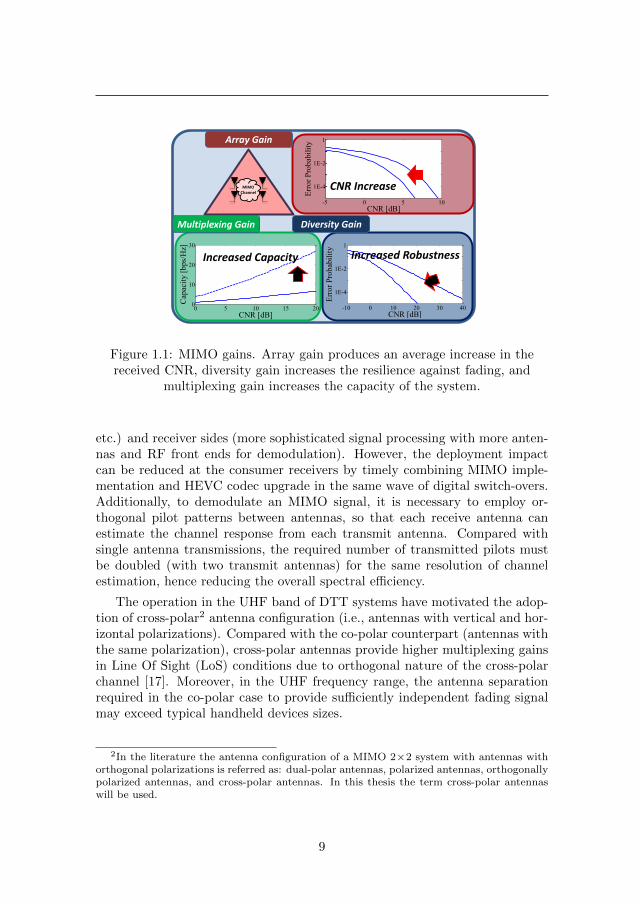
Multi antenna techniques provide three important gains, i.e. array gain,diversity gain, and multiplexing gain [18], and illustrated in Fig. 1.1. Arraygain increases the received CNR with coherent combination at the receive side(signal co-phasing and weighting for constructive addition). Here, informationabout channel state information is required, and it is commonly obtained bytracking the channel variations with the transmission of pilot signals. Diversitygain improves the reliability of the transmission by sending the same informa-tion through independently faded spatial branches to reduce the probabilitythat all channels are in a deep fade. In addition to array and diversity gains,the MIMO channel can increase the system capacity by transmitting indepen-dent data streams across the transmit antennas through spatial multiplexing.MIMO techniques can be used to improve the robustness of the transmittedsignal by exploiting the spatial diversity of the MIMO channel, but also toachieve increased data rates through spatial multiplexing especially at highCNR values [13], e.g., outdoor medium/high signal use cases such as vehicularreception or fixed rooftop reception.
The main drawback for implementing MIMO is that existing DTT networkinfrastructure needs to be upgraded at both transmitter (e.g., additional trans-mit antennas, Radio Frequency (RF) feedings, power combiners and amplifiers,
8
0 5 10 15 200
10
20
30
CNR [dB]
Cap
acity
[bps
/Hz]
-5 0 5 10
1
1E-2
1E-4
CNR [dB]
Erro
r Pro
babi
lity
MIMO
Channel
Diversity Gain Multiplexing Gain
Array Gain
Increased Capacity
CNR Increase
-10 0 10 20 30 40
1
1E-2
1E-4
CNR [dB]
Erro
r Pro
babi
lity
Increased Robustness
Figure 1.1: MIMO gains. Array gain produces an average increase in thereceived CNR, diversity gain increases the resilience against fading, and
multiplexing gain increases the capacity of the system.
etc.) and receiver sides (more sophisticated signal processing with more anten-nas and RF front ends for demodulation). However, the deployment impactcan be reduced at the consumer receivers by timely combining MIMO imple-mentation and HEVC codec upgrade in the same wave of digital switch-overs.Additionally, to demodulate an MIMO signal, it is necessary to employ or-thogonal pilot patterns between antennas, so that each receive antenna canestimate the channel response from each transmit antenna. Compared withsingle antenna transmissions, the required number of transmitted pilots mustbe doubled (with two transmit antennas) for the same resolution of channelestimation, hence reducing the overall spectral efficiency.
The operation in the UHF band of DTT systems have motivated the adop-tion of cross-polar2 antenna configuration (i.e., antennas with vertical and hor-izontal polarizations). Compared with the co-polar counterpart (antennas withthe same polarization), cross-polar antennas provide higher multiplexing gainsin Line Of Sight (LoS) conditions due to orthogonal nature of the cross-polarchannel [17]. Moreover, in the UHF frequency range, the antenna separationrequired in the co-polar case to provide sufficiently independent fading signalmay exceed typical handheld devices sizes.
2In the literature the antenna configuration of a MIMO 2×2 system with antennas withorthogonal polarizations is referred as: dual-polar antennas, polarized antennas, orthogonallypolarized antennas, and cross-polar antennas. In this thesis the term cross-polar antennaswill be used.
9
CHAPTER 1. INTRODUCTION
MIMO Broadcast Field Trials
The potentials of MIMO for DTT with cross-polar transmission were recognizedin early work of Monnier et al. in [19] in 1992. Latter in 2006, the publicbroadcaster BBC (UK) performed initial tests of MIMO broadcast with cross-polar antennas in laboratory and small scale field measurements [20], whichlead to a high-power field trial in Guildford (UK) [21]. This field test showedthe potential of doubling the system bit-rate obtained with DVB-T in the same8 MHz channel with similar coverage area. In addition, this field test allowedthe creation of a channel model representative of fixed reception at rooftoplevel with cross-polar antennas [22].
During the standardization process of DVB-NGH, a channel sounding cam-paign took place in July 2010 in Helsinki, Finland, focussing on cross-polarUHF transmission and reception in order to compare candidate schemes insimulation with a realistic measurement-based channel model [17]. The trialsincluded a number of practical designs for antennas suitable for a handheld ter-minal. From the measurements, the following channel models were developed:an outdoor mobile model, an outdoor portable model and an indoor portablemodel. For the mobile case, a user velocity of 350 km/h or 60 km/h are con-sidered, whereas for the portable case, user velocities of 3 km/h or 0 km/h areconsidered.
The Japanese public broadcaster (NHK) has performed various field trialsand research experiments of cross-polar MIMO under the development of theSuper Hi-Vision (SHV) video system for fixed and mobile reception. In 2012,a transmission was achieved with cross-polar MIMO with LDPC codes and aconstellation order of 4096QAM [23]. Such a high spectral efficiency is requiredto support the very high data rates of the SHV video system. The performancein mobile environments using Space Frequency Block Coding (SFBC) was eval-uated by simulations and field experiments [24]. Results in [16, 25] present fieldtrials with two transmitter sites in a in Single Frequency Network (SFN) con-figuration, forming a 4×2 MIMO system. In this trial the use of Space TimeBlock Code (STBC) provides enhanced performance over conventional SFNtransmitting the same signal at each site.
Although MIMO in DTT systems has already been included in DVB-NGHand ATSC 3.0, and multiple field trials have been performed, there are cur-rently no commercial deployments of DTT systems using MIMO with multipleantennas at the transmitters and the receivers.
DVB-T2 specification did not include cross-polar MIMO because the com-mercial requirements mandated the reuse of existing domestic receiving an-tenna installations and of existing transmitter infrastructures. For this reasonDVB-T2 adopted a Multiple-Input Single-Output (MISO) scheme based on asite distributed configuration with SFBC reusing the transmitter infrastruc-
10
1.1 State-of-the-Art of MIMO Signal Processing in DTT Systems
ture. The SFBC scheme adopted in DVB-T2 is based on Alamouti coding [26]defined to exploit only diversity gain. The Alamouti code is designed for achiev-ing full diversity with reduced (linear) complexity at the receiver side with twotransmit antennas. By using the Alamouti code in a distributed manner itis possible to improve the performance in SFN transmission. The arrival ofsimilar-strength signals from different transmitters in LoS scenarios can causedeep notches in the frequency response of the channel degrading the perfor-mance in an important manner. The Alamouti code requires orthogonal pilotpatterns between antennas which imposes doubling the number of transmit-ted pilots to achieve the same resolution of channel estimation as with singleantenna transmissions. Despite the potential improvements shown in theoryby the distributed MISO scheme in SFN scenarions, results from simulationin [27] and field measurements carried out in Germany in portable and mobilescenarios do not recommend the use of MISO [28] based on Alamouti coding.
1.1 State-of-the-Art of MIMO Signal Process-ing in DTT Systems
Transmit MIMO Signal Processing
DVB-NGH is the first broadcast system to employ MIMO (i.e., with spatialmultiplexing gains) as key technology exploiting the benefits of the MIMOchannel (cf. Fig. 1.1). In DVB-NGH two types of MIMO schemes are specifiedwhich are detailed next.
The first type of techniques is known in DVB-NGH as MIMO rate 1 codes,which exploit the spatial diversity of the MIMO channel without the need ofmultiple antennas at the receiver side. They can be applied across the trans-mitter sites of SFNs to reuse the existing network infrastructure (i.e. DVB-Tand DVB-T2), as well as to an individual multiple-antenna transmitter site.These codes are specified as part of the base (sheer-terrestrial) profile and in-clude the Alamouti code, already featured in DVB-T2, together with a schemeknown as enhanced Single Frequency Network (eSFN). The main idea of eSFNis to apply a linear pre-distortion function to each antenna in such a way thatit does not impact the channel estimation. This technique increases the fre-quency diversity of the channel without the need of specific pilot patterns orsignal processing to demodulate the signal. eSFN is also well suited for itsutilization in a distributed manner, as the randomization performed in eachtransmitter can avoid the negative effects cause by LoS components in thiskind of networks [29].
The second type of techniques is known in DVB-NGH as MIMO rate 2codes, which exploit the diversity and multiplexing capabilities of the MIMO
11
CHAPTER 1. INTRODUCTION
channel. In this category DVB-NGH has adopted a novel scheme known as En-hanced Spatial Multiplexing with Phase Hopping (eSM-PH). The most simpleway of increasing the multiplexing rate of information consists on dividingthe information symbols between the transmit antennas, this is referred to asMIMO Spatial Multiplexing (SM). However, the presence of correlation inthe MIMO channel due to LoS channel condition, which frequency happensin terrestrial broadcast transmissions, is especially detrimental for MIMO SM.eSM-PH was designed to overcome this situation retaining the multiplexing ca-pabilities of MIMO SM, and at the same time, increasing the robustness againstspatial correlation. With eSM-PH the information symbols are weighted andcombined before their transmission across the antennas according to a speci-fied rotation angle. This rotation angle has been tuned for every combinationof constellation order and deliberated transmit power imbalance. To ease dualpolar operation, MIMO rate 2 codes can be transmitted with deliberated powerimbalance between the transmit antennas with values of 0 dB, 3 dB and 6 dB.In addition, eSM-PH includes a periodical phase hopping term to the secondantenna in order to randomize the code structure and avoid the negative effectof certain channel realizations. It is important to note that the implementationof eSM-PH scheme requires additional investment at both sides of the trans-mission link. For this reason, these codes are specified as an optional profile toallow for a progressive deployment of MIMO networks depending on the mar-ket demands. In addition to demodulate an eSM-PH signal it is necessary toemploy orthogonal pilot patterns (as for the Alamouti code) between antennas.
MIMO for DVB-NGH targets mobile terminals operating in the low-to-medium spectral efficiency range. High data rate services operating in the highspectral efficiency range for rooftop reception are addressed by the developmentof ATSC 3.0. ATSC 3.0 includes a wider range of spectral efficiencies thanDVB-NGH and in addition it uses non-uniform constellations to provide addi-tional shaping gains [15]. The MIMO precoding scheme adopted in ATSC 3.0 iscomposed of a rotation matrix (as in DVB-NGH), an In-phase and Quadrature(I&Q) polarization interleaver and a phase hopping blocks [15]. Each of thethree sub-blocks of the MIMO precoder can be optionally selected. The phasehopping block adopted in ATSC 3.0 is the same as in DVB-NGH. The I&Qpolarization interleaver is simply a switching interleaving operation, such thatthe output cells consist of the real (In-phase) component of one input sym-bol and the imaginary (Quadrature) component of the other input symbol. Amore sophisticated inter-polarization spreading techniques is proposed in [30],to improve the performance under high correlated channels or reception withone antenna.
The use of MIMO in SFN networks has been studied by the hybrid terrestrial-satellite profile of DVB-NGH. The terrestrial and satellite transmitters canform a SFN network where either the terrestrial site or the satellite can have
12
1.1 State-of-the-Art of MIMO Signal Processing in DTT Systems
multiple transmit antennas. During the DVB-NGH standardization multiplerate 1 and rate 2 SFBCs were proposed to optimize the performance in the dis-tributed scenario [31, 32]. Other codes have been proposed for DTT systemsto optimize the performance in SFN scenarios as in [33] with high decodingcomplexity and similarly in [34] with a code design to significantly reduce thereceiving computational complexity. A good survey of MIMO SFBCs in DTTscenarios can be found in [35].
Feature Comparison with Long Term Evolution (LTE) Multi-AntennaTechniques
LTE/LTE-Advanced is a wireless standard for cellular networks with multi-antenna technology [36]. The main physical difference with broadcasting sys-tems is the feedback channel from the receiver to the transmitter that allows forlink adaptation techniques in LTE/LTE-Advanced. Link adaptation techniquesimprove the communication from the transmitter to the receiver by dynamicallyadapting key transmission parameters (e.g. modulation, coding rate, antennaweight vector for transmit beamforming) to the channel variations occurred intime, frequency and/or space.
Note that LTE/LTE-Advanced does not include MIMO for its multicastbroadcast extension known as Enhanced Multimedia Broadcast and MulticastService (E-MBMS). However, the MIMO schemes adopted for DVB-NGH andATSC 3.0 share similar technologies with LTE/LTE-Advanced open loop singleuser downlink schemes as the way to exploit the benefits of the MIMO channel.Regarding the number of transmitting elements, MIMO DTT systems definea maximum of two transmit antennas, while for LTE the maximum numberis four, and eight for LTE-Advanced. Increasing the number of transmit an-tennas generally improves the system performance at expense of higher systemcomplexity.
Receive MIMO Signal Processing
Bit Interleaved Coded Modulation (BICM) [37, 38] is a pragmatic approach tocoded Coded Modulation (CM) [39] where a bit-wise interleaver permits theindependent design of modulation and coding. Design flexibility and robust-ness against fading have motivated rapid extensions to MIMO systems andits combination with Orthogonal Frequency Division Multiplexing (OFDM)modulation. MIMO - Bit Interleaved Coded Modulation (MIMO-BICM) is akey technology for modern wireless communications systems, such the speci-fied DVB-NGH and ATSC 3.0. Although BICM with single antenna systemscan provide performance close to capacity [40], there is still a substantial gapbetween MIMO-BICM and the multi-antenna system capacity. MIMO-BICM
13
CHAPTER 1. INTRODUCTION
with Iterative Decoding (MIMO-BICM-ID), where MIMO demodulator andthe channel decoder exchange extrinsic information in an iterative fashion, hasthe potential to reduce the gap to the CM bound. However, the performanceimprovements of iterative decoding the MIMO-BICM system come at expenseof higher computational complexity, making it less suited for mobile devices. Toreduce the computational complexity, numerous suboptimal MIMO receivershave been proposed, e.g., sphere decoding implementation [41, 42] and Mini-mum Mean Square Error (MMSE) receivers [43].
The performance of MIMO-BICM-ID was evaluated during the standard-ization of the MIMO profile of DVB-NGH due to the introduction of a bit-interleaver, which exhibits low complexity, low latency, and fully parallel de-sign that ease the implementation of iterative structures. The bit-interleavingis based on permutation sequences that have been optimized for the differ-ent combinations of constellation and code-rate and transmit power imbal-ance. Furthermore, these selected permutations optimize the gain achieved byMIMO-BICM-ID receivers. The evaluations of MIMO-BICM-ID showed anincreasing iterative decoding gain at increasing code-rate [14, 44].
During the standardization of new communication systems the initial de-sign accounts for perfect reception conditions, e.g., optimal demodulators, per-fect Channel State Information (CSI), perfect noise power estimation, andinfinite-precision number representations. For instance, that was the approachto design DVB-T2, DVB-NGH and ATSC 3.0. However, due to complexityconstraints and finite-precision arithmetic, it is crucial for the overall systemperformance to carefully design receiver algorithms. In addition since on-chipmemory accounts for a large fraction of the chip area, it is desirable to havesmall word length with reduced performance loss.
DTT systems such as DVB-T2, DVB-NGH and ATSC 3.0 rely on TimeInterleaving (TI) techniques to overcome signal fluctuations and improve thesystem performance. Yet, TI imposes the highest in-chip memory require-ments [45], which depend on the quantization resolution and algorithms em-ployed at the receiver terminal. DVB-T2 defines the same TI memory in num-ber of cells (which represent a modulated OFDM carrier) irrespectively of themodulation and coding configured [46]. Using a constant number of cells irre-spective of the modulation and coding leads to an important reduction in themaximum data rate and maximum TI depth duration for low order constel-lations [46]. It is important to note that the final amount of memory in bitsrequired for the time-deinterleaving block directly depends on the resolution ofthe quantization algorithms. Since low order constellations, such as QPSK, cantolerate higher quantization noise levels, DVB-NGH introduced the concept ofadaptive cell quantization [47]. Adaptive cell quantization permits, for a giventime-deinterleaving memory size in bits, increasing the number of cells of theTI block for low order constellations while maintaining the interleaving depth
14
1.2 Motivation and Problem Statement
for higher order constellations. Numerical evaluations for different quantiza-tion resolutions for the I&Q components showed that the number of cells ofthe TI block can be doubled for QPSK and 16QAM compared to 64QAM and256QAM for similar performance degradation [47]. Similarly, ATSC 3.0 hasalso introduced adaptive cell quantization scheme in its specification.
1.2 Motivation and Problem Statement
MIMO in DTT networks has the potential to increase the spectral efficiencyand improve network coverage to cope with the competition of limited spectrumuse, the appearance of new high data rate services, and the ubiquity of thecontent. The MIMO benefits can be achieved without additional transmitpower nor additional bandwidth, but normally come at the expense of a highersystem complexity at the transmitter and receiver ends. However, the finalgains due to the use of MIMO directly depend on physical characteristics ofthe propagation environment such as spatial correlation, antenna orientation,and/or power imbalances experienced at the transmit aerials. Additionally,due to complexity constraints and finite-precision arithmetic at the receivers,it is crucial for the overall system performance to carefully design specific signalprocessing algorithms.
DVB-NGH and ATSC 3.0, the DTT systems with the most advanced terres-trial broadcast transmission technologies, have adopted MIMO as key technol-ogy to overcome the Shannon limit of single antenna communications. DVB-NGH targeting mobile and portable reception, and ATSC 3.0 targeting mobile,portable and fixed reception, implement similar MIMO precoding solutionsbased on rotation matrices for 2×2 MIMO. Hence, the performance analysis ofMIMO precoding techniques for DTT systems in realistic cross-polar MIMOchannels in the UHF band targeting mobile, portable, and fixed rooftop re-ception is an important research topic. Additionally, a characterization of theprecoder performance against typical characteristics of the MIMO cross-polarchannel in the UHF band (such as antenna correlation and/or transmit powerimbalance) and/or transmission parameters (such as the transmit constellationorder and/or the channel code-rate) is of significant research interest.
Other interesting topic of research is precoding which can exploit statisti-cal information of the MIMO channel. Previous works in the literature suchas in references [48, 49, 50, 51] have studied MIMO precoding schemes whentransmitters have only available statistical information of the channel due weakfeedback information of high mobility channels, for instance. However, it hasnot been applied to the MIMO terrestrial broadcast set-up. Additionally, thedesign of precoders for 4×2 MIMO is an interesting topic due to initial consid-
15
CHAPTER 1. INTRODUCTION
erations of 4×2 MIMO set-ups in the MIMO study mission of the DVB forafor a potential extension of DVB-T2 specification.
So far, receiver hardware design has taken into account finite-precision num-ber representations only in a straightforward manner via simulations, com-pletely neglecting non-uniform quantizers adjusted to the signal properties. Inaddition since on-chip memory accounts for a large fraction of the chip area, itis desirable to have small word length with reduced performance loss. DTT sys-tems, such as DVB-NGH, rely on TI techniques to overcome signal fluctuationsand improve the system performance by time-diversity gain. Yet, long TI im-poses the highest in-chip memory requirements at the receiver, which dependson the quantization resolution and specific algorithms. With the introductionof adaptive cell quantization [47] during the standardization of DVB-NGH (andrecently in ATSC 3.0), uniform quantization of I&Q signal component has beenconsidered and evaluated. However, neither quantization of Log-LikelihoodRatio (LLR)s nor non-uniform quantizers adapted to the signal statistics havebeen considered during the development of DVB-NGH or ATSC 3.0. On theother hand, [52] proposes non-uniform quantization of LLRs to reduce the timede-interleaving memory for a DVB – Cable 2nd Generation (DVB-C2) system.However, quantization of I&Q signal component was not considered in thiswork and the algorithms were applied to a SISO system. Hence, investigationson the topic of quantized MIMO-BICM receivers in DTT systems comparingI&Q signal components and LLR quantization is an important research topic.
16
1.3 Objectives and Thesis Scope
1.3 Objectives and Thesis Scope
The main research topic of this dissertation is the design, characterization andevaluation of transmit and receive signal processing for DTT systems employingMIMO-BICM. In particular, the following specific objectives are defined:
Transmit MIMO Signal Processing
• To analyse the structure of the precoding based on rotation matrices forMIMO 2×2 systems as the one proposed in DVB-NGH and ATSC 3.0.
• To characterize the performance of the MIMO 2×2 precoding based onrotation matrices against important channel parameters in DTT systemsin the UHF band, and different transmission parameters.
• To compare the results and conclusions obtained in the research of MIMO2×2 precoding based on rotation matrices with the solutions adopted inDVB-NGH and ATSC 3.0.
• To develop new precoding schemes for DTT systems which exploit statis-tical information of the MIMO channel for 2×2 and 4×2 MIMO systems.
Receive MIMO Signal Processing
• To investigate the performance of uniform and non-uniform quantizationof I&Q signal components and LLRs in MIMO-BICM receivers with it-erative decoding.
• To investigate the impact on the in-chip memory and receiving architec-ture of quantization of I&Q signal components and quantization of LLRs.
• To study the performance and in-chip memory trade-off of quantizedMIMO-BICM receiver with iterative decoding.
1.4 Research Approach and Methodology
This thesis includes design of communication algorithms (e.g., MIMO precod-ing techniques and practical iterative MIMO receivers based on quantized in-formation) and system performance evaluation (e.g., evaluation of DVB andATSC terrestrial standards). It is noted that despite the focus is primarilyunder the scope of DTT standards, the investigations will embrace a more gen-eral scope as design of communication techniques for future wireless broadcastcommunication systems using MIMO-BICM.
17
CHAPTER 1. INTRODUCTION
The evaluation processes will be mostly driven by numerical simulations.In practice, the performance evaluation of a new communication system can beaddressed by formula-based calculations, waveform-level simulation, or throughhardware prototyping and measurements [53], and not mutually exclusive. Infirst stages of a system design simulation-based approach provides with a costand flexible tool where different system/component configurations and trade-off can be efficiently tested. Simulators can model with desired level of detailthe information flow along the consequent blocks. However, the computa-tional complexity of current algorithms, such MIMO demodulation or channeldecoding, is significantly increasing and the simulation time to reach accept-able low error rate criteria can be extremely time demanding. On the otherhand, formula-based techniques are mathematical expressions for different per-formance measures (Bit Error Rate (BER), Frame Error Rate (FER), etc.)dependent of the system parameters. They require very low computationalcomplexity but are, in general, very complex to obtain or various assumptionshave to be integrated in the model which in turns reduces the accuracy ofthe predictions. This thesis aims to design and evaluate DTT communica-tion systems in various environments (e.g., fixed, portable, and mobile) withmost of its components (e.g., channel encoders, modulators, interleavers, etc)and with practical channel models extracted from measurement campaigns;therefore, exact closed-form expression are extremely complex to obtain. Nat-urally, hardware implementations provide massive computational time gainsin addition to accurate and realistic results. Still, it usually involves longerdevelopment time, lower flexibility and higher expenses in equipment. Due tothese reasons, hardware implementations are not commonly used at the earlystages of design cycle when high flexibility is required. In this thesis the designand evaluation methodology will be mainly based of a combination of systemnumerical simulations and derivation of mathematical expressions due to therequirement of flexibility on design and feasible mathematical tractability.
The performance evaluation of the different signal processing algorithms inthis thesis will be carried in the context of the DTT systems. To this enda simulation platform supporting the MIMO profiles of the DVB-NGH andATSC 3.0 physical layers is developed. This development includes the MIMOcross-polar channel models in the UHF band for mobile/portable reception (i.e.,NGH channel models), for fixed rooftop reception (MGM channel mode), andother basic channels detailed in the Appendix A. These platforms have beencalibrated during the standardization of DVB-NGH and ATSC 3.0 with thesimulation platform of other entities showing good alignment.
The numerical evaluations will average enough channel realizations to pro-vide statistically reliable results. To this end a number of minimum numberof simulated frames and a minimum number or erroneous detected frames isdefined. The error criteria for the evaluations is selected in each case as a
18
1.5 Thesis Outline
trade-off between simulation accuracy and simulation time and common valuesused in this dissertation are BER 10−4 and 10−5. Specific simulation stoppingconditions and error rate criteria will be provided in each section prior theevaluation results.
Transmit MIMO signal processing: In this part of the thesis, the MIMOchannel precoders based on rotation matrices and the proposed channel pre-coder will be evaluated with information theoretic measures, and with systemBER. Information theoretic measures allow us to study the performance of theprecoders in ideal transmit and receive conditions, providing upper limits forthe maximum achievable rate of a practical implementation. For the perfor-mance characterization of the MIMO precoding based on rotation matrices,the mutual information of the BICM and CM systems will be used. For theperformance characterization of MIMO-Channel-precoder based on statisticalinformation the channel capacity will be used. On the other hand system BERevaluations provide us with a performance closer to a practical implementationwith specific of transmit and receiving algorithms. In this case both type ofprecoders will use the BER criteria to characterize the minimum CNR at agiven error-rate criteria. For the evaluations of the 4×2 MIMO schemes, theDVB-NGH physical layer simulation platform will be extended to support fourantennas and information streams.
Receive MIMO signal processing: Specifically to this work, the simula-tion platform has been extended to include MIMO-BICM iterative decodingand the uniform/non-uniform quantizers of I&Q signal components and LLRs.The performance of the unquantized MIMO-BICM receiver with iterative de-coding was also calibrated during the standardization process of DVB-NGHsince the bit-interleaving of the MIMO profile was optimized to improve theiterative decoding gain. In this part of the thesis the goal is to evaluate theperformance of practical receivers, hence, the comparisons will be carried usingsystem BER.
1.5 Thesis Outline
This thesis is divided in five chapters and two appendices which are outlinednext.
Chapter 2 presents fundamental concepts on wireless communicationsneeded for the rest of the thesis. First it presents the fundamentals of MIMOchannels and the fundamental trade-off in MIMO communication which allowsto introduce two important transmission approaches the so-called SFBC andspatial multiplexing schemes. Then it provides a description of the different
19
CHAPTER 1. INTRODUCTION
components and their interactions of MIMO-BICM systems and presents itsinformation theoretic limits. Finally, this chapter concludes introducing theconcept of iterative demapping and quantization of the received informationwhich permits signal processing with finite resolution. The theoretical andpractical description of the communication components used in this thesis willallow to present more in-depth the contributions for this thesis work.
Chapter 3 first studies the performance and structure of MIMO precodersbased on rotation matrices for 2×2 MIMO and focus on the case of cross-polarantennas, which is the preferred configuration in DTT systems in the UHFband. Interesting insights are obtained by analysis and evaluation with theinformation-theoretic limits of BICM systems and bit-error-rate simulationsincluding channel coding. Then, a channel-precoder is proposed that exploitsstatistical information of the MIMO channel. The performance of the channel-precoder is evaluated in a wide set of channel scenarios and mismatched channelconditions, a typical situation in the broadcast set-up. Capacity and systemperformance simulations study the benefits and drawbacks of the proposedMIMO-channel-precoder.
Chapter 4 investigates memory and performance trade-offs of soft-quantizedinformation in MIMO-BICM receivers. Two types of quantized receivers areinvestigated: quantization of I&Q samples and quantization of LLRs. The im-plications on the in-chip memory and the possibility of implementing MIMO-BICM with iterative decoding are presented and discussed. Additionally, theperformance degradations of uniform quantization and non-uniform quanti-zation algorithms is evaluated showing significant potential benefits for non-uniform quantization adapted to the signal statistics. The results obtainedin this chapter highlight the important trade-off between in-chip memory andperformance for quantized receiver architectures.
Chapter 5 summarizes the main contributions of this thesis and suggestsfurther topics of research beyond the results of this work.
Appendix A presents the potential gains of multi-antenna techniques interms of ergodic and outage capacities for representative channel models interrestrial broadcast TV systems. It first starts with the evaluation with somebasic channels widely used within literature and then proceed with the anal-ysis with channel models extracted from channel measurement campaigns inthe UHF band. The potential gains over the single antenna transmitter andreceivers, which is the most representative case of the current DTT deploy-ment worldwide, are given. Here, the performance evaluation considers thecase where the information of the channel state is available only at the receiver(CRSI) and when is also available at the transmitter (CTSI).
20
1.6 Research Contributions
Appendix B describes the MIMO physical layers adopted for DVB-NGHand ATSC 3.0 specifications. Both specifications share similar architecture forthe implementation of MIMO.
1.6 Research Contributions
Precoding for MIMO 2×2 based in Rotation Matrices
• Performance characterization of the MIMO 2×2 precoding based on ro-tation matrices against: typical channel characteristics of the MIMOcross-polar channel in the UHF band, and transmit constellation orderand channel code-rate. Results based on Monte-Carlo simulations of theinformation theoretical limits of MIMO-BICM systems and system bit-error-rate with practical channel codes show the interesting result that ingeneral the optimal rotation angle depends on the system code-rate. Inparticular, the rotation gain increases for increasing code-rate, i.e., at lowcode-rates it is optimal not to rotate, and at mid and high code-rates it isoptimal to rotate. It has been found that the gain achieved with rotation,on the other hand, decreases with increasing constellation orders. Thestudy of the effect of power imbalance between transmit antennas, whichis an important scenario in the broadcast-set-up, shows that the rotationperformance has the same behaviour as with equal power between trans-mit antennas. However, in this case the rotation gains are even higher,increasing for increasing power imbalance factor.
• Performance characterization of the stream-power-allocation matrix withconstellations of different cardinality in each transmit antenna. The eval-uation in the case of cross-polar antennas shows that allocation of morepower to the constellation with higher cardinality can improve the per-formance from mid to high code-rates. This can be achieved by eitherintentional transmit power imbalance between antennas or stream-powerallocation. The rotation matrix in this case allows for a flexible config-uration of the desired power allocation to the asymmetric informationstreams.
• Analysis and comparison of the precoding solutions adopted in DVB-NGHand ATSC 3.0. A comparison with the results and conclusions obtainedin this thesis show that the adopted parameters for the precoding inDVB-NGH can be suboptimal for some transmission configurations dueto the use of the same rotation angle at all transmitted code-rates. ForATSC 3.0 case, a per code-rate rotation angle optimization allows optimalrotation performance at each transmitted spectral efficiency.
21
CHAPTER 1. INTRODUCTION
MIMO Precoding based on Channel Statistical Information
• A MIMO channel-precoder that exploits statistical information of theMIMO channel for the terrestrial broadcasting setting. This precoder hasthe potential to further increase the channel capacity when compared toequivalent unprecoded MIMO set-up. The performance of the proposedchannel-precoder is evaluated for fixed and portable channels and variousreception conditions. A mismatched analysis allows to evaluate the per-formance of the precoder when the channel statistics do not match theprecoder, a typical situation in the broadcast set-up. Capacity resultspresent performance enhancements in scenarios with strong LoS corre-lated antenna component, and resilience in mismatched condition for theconsidered 4×2 MIMO systems but no enhacement for 2×2 MIMO sys-tems. BER simulation results with the DVB-NGH MIMO physical layershow that for low code rates, performance improvements can be achievedin the case of strong LoS correlation and resilience against mismatchedcondition with the channel statistics.
Receiver Memory and Performance Trade-Off of Soft-Quantized In-formation
• Performance comparison of uniform and non-uniform quantizers for I&Qsignal components and LLRs. The numerical evaluations show that non-uniform quantizer design adapted to the signal statistics provide signif-icant improvements in terms of system performance or alternatively in-chip memory savings. This has been verified for both quantized archi-tectures, quantized I&Q components and quantized LLRs, but showinghigher enhancement for the latter.
• Impact of the type of quantization in the receiving architecture. An anal-ysis of the receiving architectures with quantized I&Q signal componentsand quantized LLRs unveils than the latter is not tailored to performMIMO-BICM with iterative decoding. This is due to the exchange ofdemapping and time de-interleaving processing blocks. A receiving ar-chitecture with quantized I&Q signal components does not have such arestriction since all the necessary signals for demapping with prior infor-mation are quantized and stored into memory.
• Impact of the type of quantization in the in-chip receiving memory. Dueto the highest in-chip memory requirements are imposed by the time de-interleaving memory in DTT systems, this processing block is taken asreference for memory size calculations. An further study of the in-chipmemory requirements shows lower memory requirements for a receivingarchitecture with quantized LLRs than for a receiving architecture with
22
1.6 Research Contributions
quantized I&Q signal components. From the results it can be concludedthat for similar quantization performance degradation, LLR quantizationrequires around half the memory compared to the in-chip memory withI&Q quantization (assuming non-uniform quantizers).
• In-chip memory vs. performance trade-off of MIMO-BICM receivers withquantized soft-information. Due to the interrelationships between type ofquantization architecture, MIMO-BICM with iterative decoding and in-chip memory, this thesis presents the in-chip memory vs. performancetrade-off to characterize MIMO-BICM receivers with quantized informa-tion. Quantization type selection guidelines are provided depending onthe complexity and in-chip memory restrictions imposed at the receiver.
23
CHAPTER 1. INTRODUCTION
1.7 List of Publications
International journals
[J1] D. Gozalvez, D. Gomez-Barquero, D. Vargas, and N. Cardona, “TimeDiversity in Mobile DVB-T2 Systems,” IEEE Transactions on Broadcast-ing, vol. 57, no. 3, pp. 617-628, September 2011.
[J2] D. Vargas, D. Gozalvez, D. Gomez-Barquero and N. Cardona, “MIMOfor DVB-NGH, The Next Genaration Mobile TV Broadcasting,” IEEECommunications Magazine, vol. 51, no. 7, pp. 130-137, July 2013.
[J3] D. Gozalvez, D. Gomez-Barquero D. Vargas and N. Cardona, “Com-bined Time, Frequency and Space Diversity in DVB-NGH,” IEEE Trans-actions on Broadcasting, vol.59, no. 4, pp. 674-684, December 2013.
[J4] D. Vargas , Y. J. D. Kim, J. Bajcsy, D. Gomez-Barquero, and N. Car-dona, “A MIMO-Channel-Precoding Scheme for Next Generation Terres-trial Broadcast TV Systems,” IEEE Transactions on Broadcasting, vol.61, no. 3, pp. 445-456, September 2015.
[J5] M. Fuentes, D. Vargas, and D. Gomez-Barquero, “Low-ComplexityDemapping Algorithm for Two-Dimensional Non-Uniform Constellations,”IEEE Transactions on Broadcasting, 2016.
[J6] S. LoPresto, R. Citta, D. Vargas, and David Gomez-Barquero, “Trans-mit Diversity Code Filter Sets (TDCFS), a MISO Antenna FrequencyPre-Distortion Scheme for ATSC 3.0,” IEEE Transactions on Broadcast-ing, vol. 62, no. 1, pp. 271-280, March 2016.
[J7] D. Gomez-Barquero, D. Vargas, M. Fuentes, P. Klenner, S. Moon, J.-Y.Choi, D. Schneider, and K. Murayama, “MIMO for ATSC 3.0,” IEEETransactions on Broadcasting, vol. 62, no. 1, pp. 298-305, March 2016.
National journals
[NJ1] D. Vargas, D. Gozalvez, D. Gomez-Barquero, and N. Cardona, “MultiAntenna Techniques for Digital Video Broadcasting (DVB) Systems,”Waves, year 4, pp. 79-88, 2012.
Book chapters
[B1] D. Vargas, S. Moon, W.-S. Ko, and D. Gomez-Barquero. “EnhancedMIMO Spatial Multiplexing with Phase Hopping for DVB-NGH,” in NextGeneration Mobile Broadcasting , D. Gomez-Barquero Ed. Boca Raton,FL, USA: CRC Press, 2013, pp. 609-634.
24
1.7 List of Publications
Papers in conference proceedings (international and na-tional)
[C1] D. Gozalvez, D. Vargas, D. Gomez-Barquero, and N. Cardona, “Per-formance evaluation of DVB-T2 time interleaving in mobile environ-ments,” Proc. IEEE Vehicular Technology Conference (VTC) Fall, Ot-tawa, Canada, September 2010.
[C2] D. Gomez-Barquero, D. Vargas, P. Gomez, J. Llorca, C. Romero, J.Puig, J. Gimenez, J. Lopez, D. Gozalvez, N. Cardona, “DVB-NGH, LaNueva Generacion de Television Digital Movil,” Jornadas Telecom I+D,Santander, Spain, 2011.
[C3] D. Vargas, A. Winkelbauer, G. Matz, D. Gomez-Barquero and N. Car-dona, “Low Complexity Iterative MIMO Receivers for DVB-NGH UsingSoft MMSE Demapping and Quantized Log-Likelihood Ratios,” 3rd MCand Scientific Meeting, European COST IC1004 action, Barcelona, Spain,February 2012.
[C4] S. Moon, W. Ko, D. Vargas, D. Gozalvez, M.D. Nisar, V. Pauli, “En-hanced Spatial Multiplexing for Rate-2 MIMO of DVB-NGH System,”Proc. IEEE 19th International Conference on Telecommunications (ITC),Jounieh, Lebanon, April 2012.
Contributions to standardization activities
[S1] 9 contributions to the MIMO task force in the standardization process ofDVB-NGH.
Contributions to the performance evaluation and validation of physicallayer candidate technologies:
– MIMO precoding techniques based on rotation matrices in NGHmobile/portable channels,
– Performance evaluation of MIMO precoding techniques based on ro-tation matrices with real channel estimation in NGH mobile/portablechannels,
– Performance evaluation of MIMO-BICM with iterative decoding andnew parallel bit-interleaving permutations,
– Performance evaluation of MIMO-BICM with iterative decoding andMMSE demapping with prior information.
25
CHAPTER 1. INTRODUCTION
[S2] 2 contributions to the DVB Technical Module MIMO Study Mission.
– Contributions to the capacity evaluation of multi-antenna schemesin fixed rooftop channel models for DTT systems. In particular,evaluation with the MIMO MGM channel model with log-normalfading.
[S3] 7 contributions to the TG3/S32-2 Ad-hoc Group on Modulation and Cod-ing in the standardization process of ATSC 3.0.
Contributions for the performance evaluation and validation of physicallayer candidate technologies:
– Bit-interleaving coded modulation components: LDPC codes, par-allel bit-interleaving permutations and non-uniform constellations,
– Transmit diversity techniques for Multiple-Input Single-Output sys-tems in SFN networks,
– Performance evaluation and optimization of MIMO precoding basedon rotation matrices.
Other journals not directly related to this thesis
[OJ1] Y. J. D. Kim, J. Bajcsy, and D. Vargas, “Faster-Than-Nyquist Broad-casting in Gaussian Channels: Achievable Rate Regions and Coding,”IEEE Transactions on Communications, vol. 64, no. 3, pp. 1016-1030,March 2016.
26
Chapter 2
Preliminaries
This chapter describes fundamental concepts on wireless communicationsneeded for the rest of the thesis. First, a system overview of main com-
munication components is provided. The fundamentals of MIMO communica-tions taking a look at the channel matrix representation, types of fading, gainsprovided by MIMO and information theoretic limits are presented. The fun-damental trade-off in MIMO communication between spatial multiplexing (toincrease the data rate) and signal diversity (to increase the signal resilienceagainst channel fading) is presented. This fundamental trade-off serves asintroduction to review two important transmission approaches, the so-calledspace-frequency/time-block codes (to extract diversity) and spatial multiplex-ing schemes (to extract the multiplexing gain). The focus is then given to prac-tical systems based on bit-interleaved coded modulation that aim at extractingthe various benefits of the MIMO channel. Followed by a description of thedifferent components and their interactions, the information theoretic limits ofMIMO-BICM systems are presented. The last part of this chapter is devotedto the receiver side. First it introduces the concept of iterative demappingthat can provide significant system performance gains at the cost of higherreceiver complexity. Additionally, an important aspect on practical receiverimplementation is the quantization of the received information which permitssignal processing with finite resolution. This chapter describes quantizationconcepts and design challenges. The theoretical and practical description ofthe communication components detailed in this chapter will allow to introducewith more in-depth the contributions of this thesis work.
27
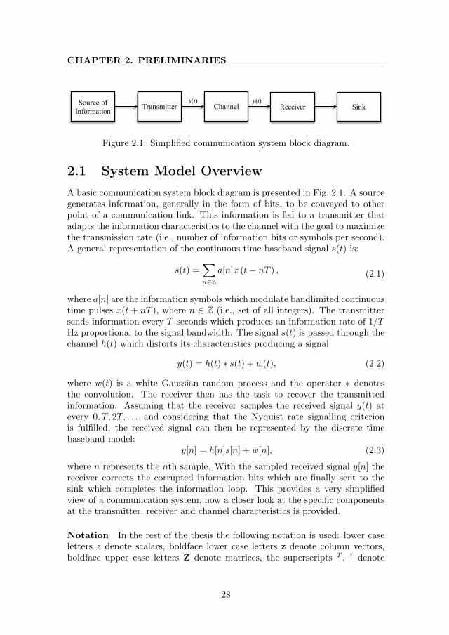
CHAPTER 2. PRELIMINARIES
Source of Information Transmitter Channel Receiver Sink
s(t) y(t)
Figure 2.1: Simplified communication system block diagram.
2.1 System Model Overview
A basic communication system block diagram is presented in Fig. 2.1. A sourcegenerates information, generally in the form of bits, to be conveyed to otherpoint of a communication link. This information is fed to a transmitter thatadapts the information characteristics to the channel with the goal to maximizethe transmission rate (i.e., number of information bits or symbols per second).A general representation of the continuous time baseband signal s(t) is:
s(t) =∑n∈Z
a[n]x (t− nT ) , (2.1)
where a[n] are the information symbols which modulate bandlimited continuoustime pulses x(t + nT ), where n ∈ Z (i.e., set of all integers). The transmittersends information every T seconds which produces an information rate of 1/THz proportional to the signal bandwidth. The signal s(t) is passed through thechannel h(t) which distorts its characteristics producing a signal:
y(t) = h(t) ∗ s(t) + w(t), (2.2)
where w(t) is a white Gaussian random process and the operator ∗ denotesthe convolution. The receiver then has the task to recover the transmittedinformation. Assuming that the receiver samples the received signal y(t) atevery 0, T, 2T, . . . and considering that the Nyquist rate signalling criterionis fulfilled, the received signal can then be represented by the discrete timebaseband model:
y[n] = h[n]s[n] + w[n], (2.3)
where n represents the nth sample. With the sampled received signal y[n] thereceiver corrects the corrupted information bits which are finally sent to thesink which completes the information loop. This provides a very simplifiedview of a communication system, now a closer look at the specific componentsat the transmitter, receiver and channel characteristics is provided.
Notation In the rest of the thesis the following notation is used: lower caseletters z denote scalars, boldface lower case letters z denote column vectors,boldface upper case letters Z denote matrices, the superscripts T , † denote
28
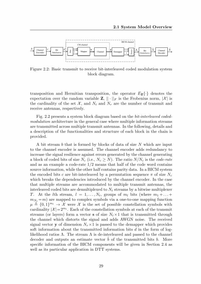
2.1 System Model Overview
BICM channelCM channel
ChannelEnconder
b Bit Interleaver Mapper
c sdChannel Demapper
y BitDeinterleaver
ChannelDecoder
bΛ Λ~
Mux
Dem
ux
Figure 2.2: Basic transmit to receive bit-interleaved coded modulation systemblock diagram.
transposition and Hermitian transposition, the operator EZ· denotes theexpectation over the random variable Z, || · ||F is the Frobenius norm, |X | isthe cardinality of the set X , and Nt and Nr are the number of transmit andreceive antennas, respectively.
Fig. 2.2 presents a system block diagram based on the bit-interleaved coded-modulation architecture in the general case where multiple information streamsare transmitted across multiple transmit antennas. In the following, details anda description of the functionalities and structure of each block in the chain isprovided.
A bit stream b that is formed by blocks of data of size N which are inputto the channel encoder is assumed. The channel encoder adds redundancy toincrease the signal resilience against errors generated by the channel generatinga block of coded bits of size Nc (i.e., Nc ≥ N). The ratio N/Nc is the code-rateand as an example a code-rate 1/2 means that half of the code word containssource information, while the other half contains parity data. In a BICM systemthe encoded bits c are bit-interleaved by a permutation sequence π of size Ncwhich breaks the dependencies introduced by the channel encoder. In the casethat multiple streams are accommodated to multiple transmit antennas, theinterleaved coded bits are demultiplexed to Nt streams by a bitwise multiplexerT . At the lth stream, l = 1, . . . , Nt, groups of ml bits (where m1 + . . .+mNt
=m) are mapped to complex symbols via a one-to-one mapping functionµ , 0, 1ml → X were X is the set of possible constellation symbols withcardinality |X |=2ml . Each of the constellation symbols at each of the transmitstreams (or layers) form a vector s of size Nt×1 that is transmitted throughthe channel which distorts the signal and adds AWGN noise. The receivedsignal vector y of dimension Nr×1 is passed to the demapper which providessoft information about the transmitted information bits d in the form of log-likelihood ratios Λ. The stream Λ is de-interleaved and passed to the channeldecoder and outputs an estimate vector b of the transmitted bits b. Morespecific information of the BICM components will be given in Section 2.4 aswell as its particular application in DTT systems.
29
CHAPTER 2. PRELIMINARIES
2.2 MIMO Channel: Signal model, Gains andCapacity
2.2.1 AWGN channel
Given the discrete complex base-band representation of (2.3), a received signaly distorted by AWGN noise at the nth sample is:
y[n] = s[n] + w[n] , (2.4)
where s[n] is the transmitted symbol and w[n] ∼ CN (0, σ2) is additive cir-cularly symmetric complex Gaussian noise where σ2 is the noise power. Thischannel, although simple, provides with an accurate model for a wide set ofcommunication channels. Shannon in his path-breaking paper [54] showed thatthe maximum rate at which information can be communicated across noisychannel with arbitrary reliability is:
Cawgn = log2 (1 + SNR) bits/s/Hz, (2.5)
where SNR is the signal-to-noise ratio P/σ2 where P = ‖s‖2 is the varianceof the transmitted signal. As the transmission duration tends to infinity theprobability of error asymptotically approaches zero as long as the rate of infor-mation R < Cawgn.
2.2.2 Fading
In the scenario with one transmit and one receive antennas where a transmittedsignal s is distorted due to the transmission through a wireless environmentwith multiple obstacles and signal reflections the discrete complex base-bandmodel can be mathematically expressed as:
y[n] = h[n] s[n] + w[n] , (2.6)
where h ∼ CN (0, 1) is the fading coefficient at sample n. The amplitude |h| isRayleigh distributed and it models the arrival of a large number of rays at asinge receive antenna. At the receiver the value of h can be estimated (undercertain channel variability constrains) for coherent detection by tracking thechannel with pilot information sent multiplexed with the data. In the case thatthe information of the channel estate h is absent at the receiver this is knownas blind or non-coherent detection. In this thesis it is always assumed that thereceiver estimates the channel for coherent detection.
30
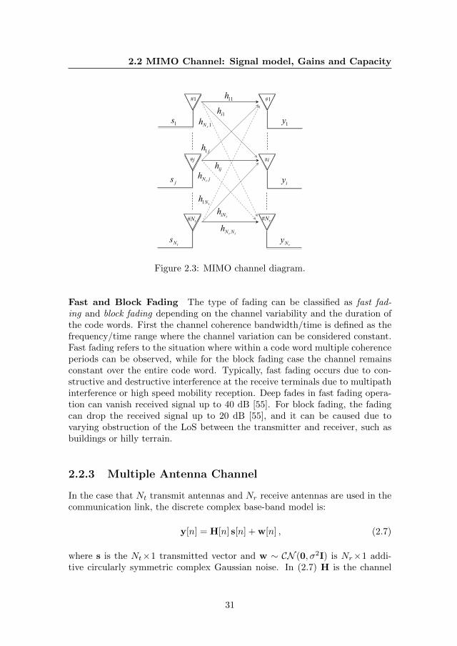
2.2 MIMO Channel: Signal model, Gains and Capacity
1rNh
tNh1
tiNh
trNNh
ijh
jh1
jNrh
1ih11h#1
#Nt
#j
tNs
js
1s
#1
#i
#Nr
rNy
iy
1y
Figure 2.3: MIMO channel diagram.
Fast and Block Fading The type of fading can be classified as fast fad-ing and block fading depending on the channel variability and the duration ofthe code words. First the channel coherence bandwidth/time is defined as thefrequency/time range where the channel variation can be considered constant.Fast fading refers to the situation where within a code word multiple coherenceperiods can be observed, while for the block fading case the channel remainsconstant over the entire code word. Typically, fast fading occurs due to con-structive and destructive interference at the receive terminals due to multipathinterference or high speed mobility reception. Deep fades in fast fading opera-tion can vanish received signal up to 40 dB [55]. For block fading, the fadingcan drop the received signal up to 20 dB [55], and it can be caused due tovarying obstruction of the LoS between the transmitter and receiver, such asbuildings or hilly terrain.
2.2.3 Multiple Antenna Channel
In the case that Nt transmit antennas and Nr receive antennas are used in thecommunication link, the discrete complex base-band model is:
y[n] = H[n] s[n] + w[n] , (2.7)
where s is the Nt×1 transmitted vector and w ∼ CN (0, σ2I) is Nr×1 addi-tive circularly symmetric complex Gaussian noise. In (2.7) H is the channel
31
CHAPTER 2. PRELIMINARIES
represented by a matrix of dimension Nr×Nt:
H =
h11 . . . h1j . . . h1Nt
.... . .
.... . .
...hi1 . . . hij . . . hiNt
.... . .
.... . .
...hNr1 . . . hNrj . . . hNrNt
(2.8)
where hij is the channel coefficient between the ith receive antenna and thejth transmit antenna and distributed -in the general case- as CN (0, 1). Theindex n is omitted for simplicity in the rest of the subsection. Fig. 2.3 showsa representation of a MIMO channel. Different antenna configurations aredefined depending on the number of transmit (Nt) and receive (Nr) antennas.SISO refers to the case when a single antenna is used at both sides of thecommunication link, Single-Input Multiple-Output (SIMO) when only multipleantennas are employed at the receiver, MISO when only multiple antennas areused at the transmitter, and the general case when both the transmitter andthe receiver have multiple antennas is called MIMO.
Channel normalization In this thesis the channel power is defined as thesquared Frobenius matrix norm:
||H||2F =
Nr,Nt∑i,j
|hij |2, (2.9)
and additionally we force∑Nr
i |hij |2 =1. As an example for a system with Nr=2 and Nt=1 the channel power in (2.9) is equal to 1 and for a MIMO systemwith Nr =2 and Nt=2 the channel power in (2.9) is equal to 2. This channelnormalization is valid for the antenna schemes considered in this dissertationwith up to two receive antennas, and it will be useful when comparing MIMOchannels with different structure (e.g., co-polar and cross-polar) for the samenumber of transmit and receive antennas.
SNR definition In the literature multiple definitions are used for the SNR.In this thesis the SNR is defined as SNR = P/σ2, where P is the total trans-mitted power across all the transmit antennas. For a fair comparison betweenMIMO schemes with different number of transmit antennas, the following powerconstrain:
∑Nt
i Pi=1 is set.
CNR definition In a OFDM system the SNR can be defined with respect tothe CNR. In a practical OFDM signal some of the outer end carriers are unused
32
2.2 MIMO Channel: Signal model, Gains and Capacity
(guard carriers) to reduce the potential interfere to adjacent RF channels dueto the spectrum roll-off. The number of guard carriers depend on the FFT size,the larger the FFT-size the quicker the spectrum roll-off and therefore morecarriers can be used to convey information data [45]. In the CNR definitionused in this thesis the carrier power refers to information carrier power. Sincethe noise added at the receiver (in time domain) affects all the carriers (i.e.,information and guard carriers) the signal to noise ratio at the input of theOFDM demodulator (SNR) and the output of the OFDM demodulator (CNR)has the following relationship in dB:
SNR = CNR− 10 · log10
(FFTsize
NInfo−carriers
). (2.10)
Multi-antenna self interference At the ith receive antenna the signal is:
yi =
Nt∑j
hijsj + wi, i=1, 2 . . . , Nr, (2.11)
as we can see the received signal at the ith antenna is the combination of all thesignals from all the transmit antennas plus the AWGN noise. Let us consider atthe jth receive antenna the symbol from the ith transmit antenna when i=j asthe desired message and the other transmit symbols (i.e., i 6=j) as interference.Then expression (2.11) can be decomposed as:
yi = hiisi +
Nt∑j 6=i
hijsj︸ ︷︷ ︸interfence term
+wi, i=1, 2 . . . , Nr.(2.12)
Here, we can clearly observe the inter-antenna interference created in a MIMOchannel. Optimal detection of the received vector y with the inter-antennainterference term increases the search space of the received signal to |X |Nt .The full space search increases exponentially with the number of the transmitantennas which can impose significant limitations on the system complexityfor typical constellation sizes and number of transmit antennas. More detailedexplanation of MIMO demodulation and complexity issues will be discussed insubsection 2.4.4.
MIMO Gains The implementation of MIMO provides array gain, diversitygain and multiplexing gains which are described next. Array gain increases thereceived SNR with multiple transmit and/or receive antennas. When channelstate information is available at the receiver, the signal received from multi-ple receive antennas can be added coherently. In a transmitter with multiple
33
CHAPTER 2. PRELIMINARIES
transmit antennas and channel state information, the information at each ofthe transmit antennas can pre-processed so the signals add coherently at thereceiver side. This is also known as beamforming, however, information aboutthe channel state at the transmitter is absent in DTT systems. Diversity gainimproves the reliability of the transmission by sending the same informationthrough independently faded spatial branches to reduce the probability that allchannels are in a deep fade. The simultaneous utilization of multiple antennasat the transmitter and receiver side permits the opening of multiple spatialpipes across the wireless channel providing multiplexing gain.
2.2.4 MIMO Channel Capacity
Fixed channel For a fixed matrixH, the channel capacity derived by Telatar [56]with information about the channel coefficients only available at the receiveris:
C = log2 det
(INr +
SNR
NtHH†
), (2.13)
where SNR is the received SNR at each receive antenna.An alternative formulation for the channel capacity comes from the singular
value decomposition of a matrix [57]
H = UΣV†, (2.14)
where U and V are Nr×Nr and Nt×Nt, respectively, unitary matrices and Σof size Nr×Nt is a rectangular matrix with non-negative real numbers on thediagonal. Substituting (2.14) in (2.7) and defining [13]:
x := V†x
y := U†y
w := U†w
(2.15)
expressions (2.7) can be reformulated as:
y = Σx + w. (2.16)
Using the fact that w is the equally distributed1 as w, (2.13) is expressed as afunction of the singular values of the channel matrix H:
C =
nmin∑i=1
log2
(1 +
SNR
Ntλ2i
), (2.17)
where λi is the ith diagonal entry of Σ.
1Uw ∼ w if w ∼ CN (0, I) and U is unitary matrix, i.e., U†U = I.
34
2.2 MIMO Channel: Signal model, Gains and Capacity
The above expression shows that the MIMO channel can be decomposedinto a parallel channel where the gain of each channel is given by the singularvalues of the matrix H. The value nmin is the number of non-zero singularvalues which depend on the rank of the matrix channel H. The higher the valuenmin the higher the number of parallel channels in which information can betransmitted through. The maximum capacity in a MIMO channel is achievedwhen the matrix H is full rank, i.e., columns are linearly independent (whenNr > Nt) or rows are linearly independent (when Nt > Nr). Full rank matricesare achieved in environments with many scatters with sufficient separationbetween antennas, or in MIMO systems that use different polarizations. Inthe extreme case that the MIMO components are fully correlated, the channelmatrix H becomes singular, with only one non-zero singular value, which hasthe same capacity as a SISO communication link. The impact of correlation inMIMO capacity will be studied in more detail in Chapter 3 and Appendix A.
Fast fading channel If the channel matrix H is a Rayleigh random variablei.i.d. from sample to sample (i.e., fast fading) the long-term rate of reliablecommunication is:
C = EHlog2 det
(INr +
SNR
NtHH†
). (2.18)
This channel capacity commonly known as ergodic-capacity is achieved for sys-tems where coding is performed over multiple channel realizations. This isthe case as in mobile channels where the information can be interleaved overdifferent channel realizations due to the varying nature of the mobile channel.Although the ergodic capacity is achieved for infinite long code-words, prac-tical systems have sufficiently long coding and interleaving which makes theergodic-capacity a valuable metric. The capacity in (2.18) is for the case wherethe receiver perfectly tracks the channel states but no knowledge is availableat the transmitter site. In this channel the optimal transmission strategy isto isotropically transmit among the transmit antennas. The case with channelstate information at the transmitter is discussed in a latter section.
Block fading channel In the situation of slow fading, where a channel real-ization does not vary within a code-word, the capacity limit as the maximumachievable rate with arbitrary reliability is no longer useful. In this case, sincethere is no average (or interleaving) over multiple channel realizations, theprobability that a specific channel realization is
log2 det
(INr +
SNR
NtHH†
)< R (2.19)
35
CHAPTER 2. PRELIMINARIES
is no longer zero. In this case it is said that the channel is in outage and isuseful to compute the probability of outage given the channel distribution:
pout = Plog2 det
(INr +
SNR
NtHH†
)< R. (2.20)
With the outage probability pout, one can define the ε-outage-capacity Cεwhich is the largest rate of transmission R such pout is less than ε. It can beexpressed mathematically as:
Cε = supR|pout < ε (2.21)
Channel state information at the transmitter side In the case that thetransmitter has also knowledge of the information about the channel state, thetransmission can be adapted to optimize the system performance. This case isreferred as Channel Transmit State Information (CTSI).
Similarly to the case with CSI only at the receiver (i.e., Channel ReceiveState Information (CRSI)), the analysis is started with the simple case whenthe channel matrix H is fixed. In this case, the capacity expression in (2.17)can be rewritten as:
C =
nmin∑i=1
log2
(1 +
P ∗iσ2λ2i
), (2.22)
where P ∗i are the optimized powers with the water-filling algorithm [13] as-signed to each of equivalent MIMO channels which follow the following expres-sion:
P ∗i = maxµ− σ2
λ2i
, 0, (2.23)
and with the common power constrain∑i P∗i = 1.
In the fast fading case, the ergodic capacity is:
C =
nmin∑i=1
E log2
(1 +
P ∗iσ2λ2i
). (2.24)
For the slow-fading case:
pout = Pnmin∑i=1
log2
(1 +
P ∗iσ2λ2i
)< R. (2.25)
It is noted that for the slow-fading case, transmission can only be optimizedin the spatial domain, since the transmitter does not have knowledge of thevariations of the channel in time.
36
2.3 A Fundamental Trade-Off and Transmission Approaches
In the situation that the transmitter wants to optimize the transmissionin a statistical way, one has to find the optimal transmit covariance matrix Qthat maximizes the following problem:
maximizeQ0 s.t.
EHlog2 det
(INr
+ρ
NtHQH†
).
trace(Q)=Nt
(2.26)
This will be further developed in Chapter 3, where a precoder is optimizedbased on the statistics of the channel.
2.3 A Fundamental Trade-Off and TransmissionApproaches
2.3.1 Multiplexing-Diversity Trade-Off
A MIMO system can be used to increase the transmission reliability throughdiversity gain or to increase the system rate through spatial multiplexing gain.There is however, a trade-off between the diversity and multiplexing gain thatmay be achieved in a MIMO channel [13, 58], i.e., one cannot arbitrarily in-crease the diversity and multiplexing gains at the same time.
For a MIMO system with a fixed transmission rate R, the maximum achiev-able diversity gain dmax is given by the negative slope of the probability oferror pe(SNR, R) (which is a function of the rate R and SNR) with asymptoticSNR [59]:
dmax = − limSNR→∞
log2(pe(SNR, R))
log2(SNR). (2.27)
In such a system the probability of error scales as pe(SNR, R) ≈ SNR−dmax . Forinstance, in a MIMO slow fading i.i.d. Rayleigh channel with Nt transmit andNr receive antennas, a capacity achieving system (with optimal transmissionand receiver detection) can achieve a maximum diversity order dmax = Nt ·Nr [13, 59].
Alternatively, the Nr×Nt MIMO system has a maximum multiplexing gainrmax given by the slope of the outage capacity with asymptotic SNR [59]:
rmax = limSNR→∞
Cε(SNR)
log(SNR). (2.28)
In a MIMO slow fading i.i.d. Rayleigh channel and a capacity achieving system(with optimal transmission and receiver detection) the maximum multiplexinggain is rmax = minNt, Nr [59].
37
CHAPTER 2. PRELIMINARIES
Expressions in (2.27) and (2.28) are the two extremes of the so-calledDiversity-Multiplexing Tradeoff (DMT) which describes the relationship be-tween diversity and multiplexing in MIMO systems. A MIMO system cannotincrease both the transmission rate and reliability to the maximum values in(2.27) and (2.28) but needs to trade between them. In a slow fading i.i.d.Rayleigh channel, the optimal DMT is a piecewise linear function:
d(r) = (Nt − r)(Nr − r), (2.29)
where r = 0, . . . , rmax. This trade-off indicates that if the rate is increased asr log2(SNR), then the error probability decreases as SNR−d(r) [13]. The designof MIMO coding schemes with different diversity and multiplexing capabilitieshas been an active area of research in the last two decades.
2.3.2 Space-Frequency Block codes
Coding the information symbols across the signal dimensions, i.e., space, timeand frequency, can bring substantial performance improvements in the link reli-ability and throughput. Space Frequency (or Time) Block Codes (SFBC/STBC)code information data across space and frequency (or time) to get closer to the-oretical performance limits. SFBC/STBC can be designed to increase transmis-sion reliability, to increase the data rate, or both following the DMT principle.In order to exploit the benefits of SFBCs, it is necessary to employ orthogonalpilot patterns between antennas, so that the receiver can estimate the channelresponse from each transmit antenna. This means that to maintain the sameresolution of channel estimation as with single antenna transmissions, the num-ber of pilots required with one transmit antenna shall be doubled/quadrupledwith SFBC across two/four transmit antennas. This additional overhead canimpose significant limits in the final system performance [14].
A very well known STBC is the Alamouti code designed to provide fulldiversity with rate 1 (i.e., one information symbol per channel use) in a MISO2× 1 channel. The encoding matrix of the Alamouti code is:
CAlam =
[c1 −c†2c2 c†1
], (2.30)
where c1 and c2 are constellation symbols. The columns of the matrix corre-spond to different transmit antennas and the rows correspond to different timeor frequency slots. The Alamouti code is optimal in the sense that reachesthe DMT frontier. With two receive antennas (i.e., 2×2 MIMO) the Alamouticode still provides full diversity but it is no longer optimal in terms of the DMTlimit since only one information symbol is transmitted in one channel use.
38
2.3 A Fundamental Trade-Off and Transmission Approaches
Transmit Diversity Techniques in DTT systems
The Alamouti code has been adopted in DTT systems first in DVB-T2 andthen in DVB-NGH. In DVB-T2 it was used to encode information symbols fromdistributed pairs of transmitters to improve reception in SFNs where the signalsfrom multiple transmitters can create destructive interference erasing parts ofthe received signal bandwidth. For optimal performance of SFBCs/STBCswith linear decoding complexity, it is important that channel responses for allthe carriers (or time slots) carrying one block should remain unchanged. Forthis reason, the Alamouti code in DVB-T2 encodes information symbols inspace and OFDM carriers since it was assumed that the channel coefficients inadjacent OFDM carriers have lower variation than in adjacent OFDM symbols.
Alternatively to Alamouti code, the performance in SFNs with single an-tenna receivers can be improved by applying a linear pre-distortion to thecommon waveform of the signals transmitted by the multiple sites increasingthe spatial diversity. DVB-NGH adopted eSFN [60], a linear pre-distortion tothe frequency carriers of the OFDM waveform in a manner that special signalprocessing at the receivers is not necessary, since the frequency pre-distortionis seen by the receivers as part of the channel. Compared to the Alamouticode, there is no additional overhead due to increased pilot density. Similarly,ATSC 3.0 has adopted an antenna scheme to improve the overall performancein SFN, known as Transmit Diversity Code Filter Sets (TDCFS) [61], but withbetter correlation properties than eSFN.
SFBCs can be also designed to provide multiplexing gain, a full-rate full-diversity scheme for 2×2 MIMO channels is the Golden-Code proposed in [62].Its encoding matrix is:
CGC =1√5
[α (c1 + c2θ) α
(c1 + c2θ
)iα(c3 + c4θ
)α (c3 + c4θ)
], (2.31)
where θ =(1 +√
5)/2, θ =
(1−√
5)/2, α = 1 + i (1− θ), α = 1 + i
(1− θ
),
and ci, i = 1, . . . , 4 are constellation symbols. The Golden-Code achieves theDMT limit with an encoding matrix providing nonvanishing determinant withdecoding complexity proportional to O(X 4). The Golden-Code was evaluatedduring the standardization process of DVB-NGH but was discarded in favourof more simple schemes such as plain SM due to the increased decoding com-plexity (decoding complexity of SM proportional to O(X 2)) and performancedegradation when connected with strong channel coding such as the LDPCcodes at low code-rates [29, 63].
Various SFBCs rate 1 and rate 2 codes for MIMO systems in distributedscenarios were also proposed and evaluated during the DVB-NGH standard-ization process for the hybrid terrestrial-satellite MIMO profile with multipleantennas at the terrestrial site and/or the satellite [32, 64, 65, 66, 67]. For rate
39
CHAPTER 2. PRELIMINARIES
1, the codes adopted in the hybrid terrestrial-satellite MIMO profile dependon the number of transmit antennas at the terrestrial site and satellite. Withone transmit antenna at the terrestrial site and the satellite, the adopted codesare based on the Alamouti code and eSFN. With two transmit antennas atthe terrestrial site and one transmit antenna at the satellite, or vice-versa, theadopted codes are based on the Alamouti+QAM code [67] and eSFN. In thecase that the terrestrial site and the satellite have two transmit antennas, theadopted codes are based on the Alamouti code and eSFN. For rate 2, the codesadopted in the hybrid terrestrial-satellite MIMO profile are based on rotationmatrices which will be presented in latter sections.
2.3.3 Spatial Multiplexing Techniques
In the previous subsections, SFBC schemes that increase the multiplexing rateof the communication system have been presented. However, the most simpleway of using spatial multiplexing is by sending independent information acrossthe transmit antennas, i.e., MIMO SM. In a 2×2 MIMO system with SM,one information symbols is transmitted by one antenna and received by twoantennas through two spatial paths. The spatial diversity of MIMO SM canbe increased by applying a rotation matrix R to the data streams:
R =
[cos θ sin θsin θ − cos θ
]. (2.32)
A 2×2 rotation matrix has the form in (2.32) and is a family of matrices thatare characterized as orthonormal matrices, i.e., RRT = I. A rotation matrixwith parameter θ linearly combines independent data streams so each transmitantenna conveys information of all data streams increasing the spatial diversity.The input-output relationship of a processing block based of a rotation matrixis: [
y1
y2
]=
[cos θ sin θsin θ − cos θ
] [x1
x2
]=
[cos θsin θ
]x1 +
[sin θ− cos θ
]x2.
(2.33)It compares with the case where no rotation matrix is applied with input-
output relationship:[y1
y2
]=
[1 00 1
] [x1
x2
]=
[10
]x1 +
[01
]x2. (2.34)
It can be seen that the information vector [x1, x2]T
is transmitted over the
basis vectors [1, 0]T
and [0, 1]T
for the non-rotated case, and [cos θ, sin θ]T
and
[sin θ,− cos θ]T
for the rotated case.
40
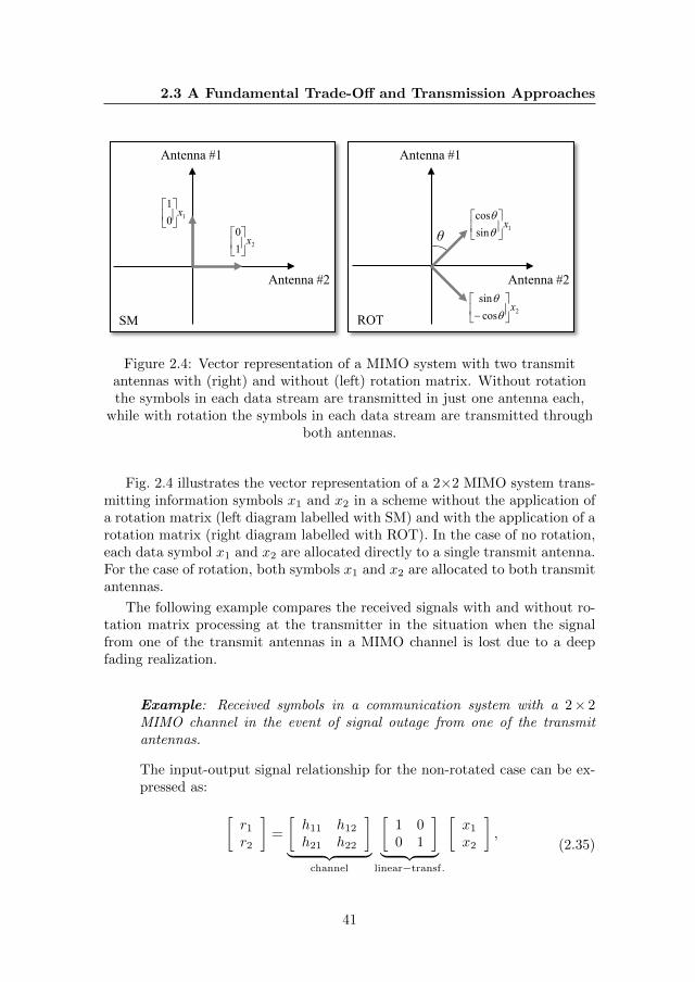
2.3 A Fundamental Trade-Off and Transmission Approaches
Antenna #1
Antenna #2
Antenna #1
Antenna #2
101x
θ21
0x
1sincos
x
θθ
2cossin
x
− θ
θ
SM ROT
Figure 2.4: Vector representation of a MIMO system with two transmitantennas with (right) and without (left) rotation matrix. Without rotationthe symbols in each data stream are transmitted in just one antenna each,
while with rotation the symbols in each data stream are transmitted throughboth antennas.
Fig. 2.4 illustrates the vector representation of a 2×2 MIMO system trans-mitting information symbols x1 and x2 in a scheme without the application ofa rotation matrix (left diagram labelled with SM) and with the application of arotation matrix (right diagram labelled with ROT). In the case of no rotation,each data symbol x1 and x2 are allocated directly to a single transmit antenna.For the case of rotation, both symbols x1 and x2 are allocated to both transmitantennas.
The following example compares the received signals with and without ro-tation matrix processing at the transmitter in the situation when the signalfrom one of the transmit antennas in a MIMO channel is lost due to a deepfading realization.
Example: Received symbols in a communication system with a 2× 2MIMO channel in the event of signal outage from one of the transmitantennas.
The input-output signal relationship for the non-rotated case can be ex-pressed as: [
r1
r2
]=
[h11 h12
h21 h22
]︸ ︷︷ ︸
channel
[1 00 1
]︸ ︷︷ ︸
linear−transf.
[x1
x2
],
(2.35)
41
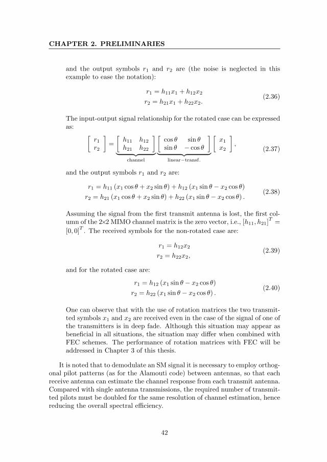
CHAPTER 2. PRELIMINARIES
and the output symbols r1 and r2 are (the noise is neglected in thisexample to ease the notation):
r1 = h11x1 + h12x2
r2 = h21x1 + h22x2.(2.36)
The input-output signal relationship for the rotated case can be expressedas: [
r1
r2
]=
[h11 h12
h21 h22
]︸ ︷︷ ︸
channel
[cos θ sin θsin θ − cos θ
]︸ ︷︷ ︸
linear−transf.
[x1
x2
],
(2.37)
and the output symbols r1 and r2 are:
r1 = h11 (x1 cos θ + x2 sin θ) + h12 (x1 sin θ − x2 cos θ)
r2 = h21 (x1 cos θ + x2 sin θ) + h22 (x1 sin θ − x2 cos θ) .(2.38)
Assuming the signal from the first transmit antenna is lost, the first col-umn of the 2×2 MIMO channel matrix is the zero vector, i.e., [h11, h21]
T=
[0, 0]T
. The received symbols for the non-rotated case are:
r1 = h12x2
r2 = h22x2,(2.39)
and for the rotated case are:
r1 = h12 (x1 sin θ − x2 cos θ)
r2 = h22 (x1 sin θ − x2 cos θ) .(2.40)
One can observe that with the use of rotation matrices the two transmit-ted symbols x1 and x2 are received even in the case of the signal of one ofthe transmitters is in deep fade. Although this situation may appear asbeneficial in all situations, the situation may differ when combined withFEC schemes. The performance of rotation matrices with FEC will beaddressed in Chapter 3 of this thesis.
It is noted that to demodulate an SM signal it is necessary to employ orthog-onal pilot patterns (as for the Alamouti code) between antennas, so that eachreceive antenna can estimate the channel response from each transmit antenna.Compared with single antenna transmissions, the required number of transmit-ted pilots must be doubled for the same resolution of channel estimation, hencereducing the overall spectral efficiency.
42
2.3 A Fundamental Trade-Off and Transmission Approaches
-2 -1 0 1 2-2
-1
0
1
2
Q
I
-2 -1 0 1 2-2
-1
0
1
2
Q
I
t
)(nj te θ
MIMOPrecoding
s1
s2
QAMmod
QAMmod
Splitterbits bits
bits
SM
eSM
eSM-PH
PH
Tx1 (VP)
Tx2 (HP)
x1
x2
-2 -1 0 1 2-2
-1
0
1
2
Q
I
-2 -1 0 1 2-2
-1
0
1
2
Q
I
-2 -1 0 1 2-2
-1
0
1
2
Q
I
-2 -1 0 1 2-2
-1
0
1
2
Q
I
-2 -1 0 1 2-2
-1
0
1
2
Q
I-2 -1 0 1 2-2
-1
0
1
2
Q
I
-2 -1 0 1 2-2
-1
0
1
2
Q
I-2 -1 0 1 2-2
-1
0
1
2
Q
I
Figure 2.5: MIMO precoding scheme adopted in DVB-NGH form by aconcatenation of rotation matrix and phase-hopping term with two transmitantennas with vertical polarization (VP) and horizontal polarization (HP).
Spatial Multiplexing Techniques in DTT systems
DVB-NGH and ATSC 3.0 have adopted a spatial multiplexing techniques basedon rotation matrices and presented in Fig. 2.5. The presence of correlationin the MIMO channel due to LoS channel condition, which frequently hap-pens in fixed terrestrial broadcast environments, is especially detrimental forMIMO SM. MIMO precoding based on rotation matrices overcomes this sit-uation retaining the multiplexing capabilities of MIMO SM, and at the sametime, increasing the robustness against spatial correlation. The informationsymbols are weighted and combined before their transmission across the anten-nas according to a specified rotation angle. This rotation angle can be tunedfor different transmission parameters and channel conditions. In addition, aperiodical phase hopping term is added to the second antenna in order torandomize the code structure and avoid the negative effect of certain channelrealizations. The specific parameters and structure of the MIMO precodinginlcuded in DVB-NGH and ATSC 3.0 is detailed in Chapter 3. The analysisof MIMO precoding based on rotation matrices, with both an information-theoretic point of view and with numerical evaluations using channel coding isalso provided in Chapter 3.
43
CHAPTER 2. PRELIMINARIES
2.4 MIMO-BICM: Components and Mutual In-formation
A coded modulation system jointly designs modulation and coding. Trellis-coded modulation [39] and multilevel codes [40] are popular coded modulationschemes. In bit-interleaved coded modulation system [37, 38], modulation andcoding are separated by a bit-interleaving allowing independent design of eachcomponent. However, the introduction of a bit-interleaver imposes an infor-mation loss due to the elimination of the interdependences of the transmittedcoded bits. Design flexibility and robustness against fading channels have mo-tivated rapid extensions to MIMO systems and its combination with OFDMmodulation. Modern wireless communications systems, such as DVB-NGH andATSC 3.0 include MIMO-BICM as key technology to cope with the increasingdemand for data rate and transmission reliability.
In the next subsection introduces and details the main characteristics ofthe components of a MIMO-BICM system, and provide information-theoreticresults of BICM and CM under fading channels.
2.4.1 Forward Error Correction
Channel coding is a core part of any communication systems which allowsthe correction of channel impairments in the received signal and is generallyreferred as Forward Error Correction (FEC). The information bits act as aninput to the channel encoder which adds redundancy to the information bitsto increase the robustness of the transmitted signal, allowing correction ofcorrupted bits at the receiver with feasible decoding complexity. Shannon in1948 [54] derived the channel capacity as upper bound on the maximum reliableinformation rates achievable over noisy channels, which has become a practicalbenchmark for reliable communications over many practical communicationchannels. It was only with the development of practical error correcting codessuch as the turbo-codes [68] and the LDPC codes [10, 69], that channel codingstarted to perform closely to the capacity limits of practical channels [70].A concatenation of Bose-Chaudhuri-Hocquenghem (BCH) and LDPC codeshas been adopted amongst others in the physical layers of DVB-T2, DVB-NGH and ATSC 3.0. Compared with the FEC scheme used in first-generationDVB systems based on the concatenation of a convolutional and Reed-Solomoncodes, the utilization of BCH and LDPC codes provide gains ranging from 3 dBto more than 5 dB for low and high bit-rate services, respectively, in stationarychannels [71].
Low density parity check codes are linear, binary block codes and are con-structed with sparse parity-check matrices which provide decoding complexity
44
2.4 MIMO-BICM: Components and Mutual Information
only increasing linearly with the size of the code. A sparse (Nc−N)×Nc parity-check matrix H (being N and Nc the size of the input uncoded bits and outputcoded bits, respectively) can be represented by factor graphs [72] consisting onNc variable nodes and Nc − N check nodes (or number of parity-check equa-tions). An entry value of 1 at the ijth position of the matrix connects by anedge the ith check node to the jth variable node. Classical decoding consistson exchange of extrinsic soft information between the variable nodes and thecheck nodes in an iterative fashion until the estimated code-word verifies theparity-check equations (i.e., HxT = 0T ) or a maximum number of iterations isreached. This type of algorithm approximates Maximum a Posteriori (MAP)decoding performance and is termed belief propagation [73]. Although the de-coding performance improves with increasing number of iterations, it comesat the expense of higher computational complexity. Furthermore, reaching acertain number of iterations, the performance improvement saturates and ad-ditional iterations only provide marginal improvement. A common value ofmaximum number of iterations is 50, and is the one assumed for DTT systemssuch as DVB-T2 [45], and is the value used in this dissertation.
DVB-T2 and ATSC 3.0 specify code sizes of 16200 bits (short codes) and64800 bits (long codes). DVB-NGH targeting mobile devices with limited hard-ware requirements specify up to 16200 bits code size. With the objective ofreaching varying reception environments with services requiring different spec-tral efficiencies, modern DTT systems include in its specifications a wide setof code-rates, ranging from very low code-rates (for high robustness) to highcode-rates (for maximum spectral efficiency). The MIMO profile of DVB-NGHdefines 7 code-rates from 5/15 to 11/15 with equal spacing. ATSC 3.0 widensthis set with a total of 13 code-rates from 2/15 to 13/15.
2.4.2 Bit-Interleaver
The output of the channel encoder is bit-interleaved to break the dependencesintroduced by the binary channel code and fed to the mapper. The bit inter-leaver permits an independent design of binary channel encoders and mapper,which can be adapted to the channel and system requirements, greatly sim-plifying the design. Although in the literature the bit-interleaver is generallydefined as a sufficiently long random sequence, practical systems require thedesign of particular permutation sequences known at the transmitter and atthe receiver.
Due to the irregular structure of the LDPC codes included in the DVB-T2specification (and inherit by DVB-NGH) with non-uniform protection alongthe code-word and non-uniform robustness amongst the bits in the label of amultilevel constellation, a concatenation of a bit-interleaver and demux is in-troduced. This concatenation provides equal protection along the code-word
45
CHAPTER 2. PRELIMINARIES
and avoids performance degradation in fading channels. The design of the dif-ferent stages of this type of bit-interleaver is a function of the constellation size,code-rate and channel encoding code-word size. The bit-interleaver part is com-prised of a parity-interleaver followed by a column-twist block interleaver. Theparity-interleaver applies a permutation sequence in such a way that the paritypart of the parity-check matrix has the same structure as the information part.The parity-interleaved bits are serially written into the column-twist interleavercolumn-wise, and serially read out row-wise where the write start position ofeach column is twisted depending on the constellation size. Compared to thistype of bit-interleaver, the MIMO profile of DVB-NGH includes in its specifica-tion a novel parallel bit-interleaver with reduced hardware complexity and lowlatency. The parallel bit-interleaver encourages the use of iterative structuresand it has been optimized for iterative reception. The main novelty of thistype of bit-interleaver is the inclusion of a group-wise interleaver which allowsoptimum combination between code bits and constellation symbols with dif-ferent permutations for each combination of constellation and code-rate. Dueto the additional performance and hardware benefits exhibit by this type ofbit-interleaving, ATSC 3.0 has adopted this architecture as bit-interleaving so-lution.
2.4.3 Mapping from Bits to Constellation Symbols
The mapper takes in a bit-interleaved stream of coded bits in groups of m bitsand produces output complex valued symbol vector from a constellation set Xwith cardinality |X | = 2m. The location of the constellation points has a directimpact in the system performance. Quadrature amplitude modulation (QAM)constellations are widely used in practical systems such as DVB-T, DVB-T2and DVB-NGH. This constellation have uniform distribution of the symbolson the complex I&Q plane with the same distance between any two adjacentpoints and have a squared shape. Fig. 2.6 shows an example of a 16QAM con-stellation. However, this uniform sampling of constellation points is suboptimalfrom the capacity point of view since to approach the Shannon information-theoretic limit the transmitted signal has to be Gaussian distributed. Non-uniform constellations are designed to overcome the performance degradationdue to uniform spaced constellations obtaining more Gaussian-like distributedconstellations sets [74, 75, 76]. This gain is normally referred as shaping gain.Fig. 2.6 shows an example of a non-uniform 16-point constellation. Non-uniform constellations have been adopted in broadcasting standards such asDVB-NGH [77] and ATSC 3.0 [78]. Two types of non-uniform constellationshave been defined: One-dimensional Non-Uniform Constellation (1D-NUC) andTwo-dimensional Non-Uniform Constellation (2D-NUC). 1D-NUCs are formedby two non-uniform Pulse Amplitude Modulation (PAM)s, corresponding to
46
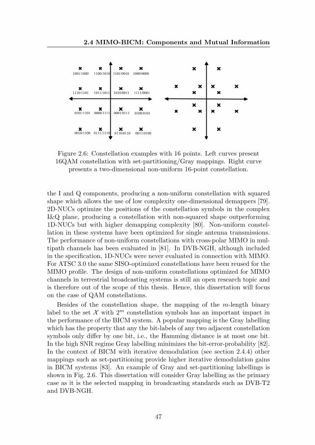
2.4 MIMO-BICM: Components and Mutual Information
1001/1000 1101/0010 1000/0000
1110/1101 1010/0011 1111/0001
0101/1101 0001/0111 0100/0101
0010/1100 0110/0110
1100/1010
1011/1011
0000/1111
0111/1110 0011/0100
Figure 2.6: Constellation examples with 16 points. Left curves present16QAM constellation with set-partitioning/Gray mappings. Right curve
presents a two-dimensional non-uniform 16-point constellation.
the I and Q components, producing a non-uniform constellation with squaredshape which allows the use of low complexity one-dimensional demappers [79].2D-NUCs optimize the positions of the constellation symbols in the complexI&Q plane, producing a constellation with non-squared shape outperforming1D-NUCs but with higher demapping complexity [80]. Non-uniform constel-lation in these systems have been optimized for single antenna transmissions.The performance of non-uniform constellations with cross-polar MIMO in mul-tipath channels has been evaluated in [81]. In DVB-NGH, although includedin the specification, 1D-NUCs were never evaluated in connection with MIMO.For ATSC 3.0 the same SISO-optimized constellations have been reused for theMIMO profile. The design of non-uniform constellations optimized for MIMOchannels in terrestrial broadcasting systems is still an open research topic andis therefore out of the scope of this thesis. Hence, this dissertation will focuson the case of QAM constellations.
Besides of the constellation shape, the mapping of the m-length binarylabel to the set X with 2m constellation symbols has an important impact inthe performance of the BICM system. A popular mapping is the Gray labellingwhich has the property that any the bit-labels of any two adjacent constellationsymbols only differ by one bit, i.e., the Hamming distance is at most one bit.In the high SNR regime Gray labelling minimizes the bit-error-probability [82].In the context of BICM with iterative demodulation (see section 2.4.4) othermappings such as set-partitioning provide higher iterative demodulation gainsin BICM systems [83]. An example of Gray and set-partitioning labellings isshown in Fig. 2.6. This dissertation will consider Gray labelling as the primarycase as it is the selected mapping in broadcasting standards such as DVB-T2and DVB-NGH.
47
CHAPTER 2. PRELIMINARIES
2.4.4 MIMO Demodulation and Iterative Decoding
In a MIMO coded system, joint demodulation and decoding achieves optimalerror-rate performance for CM. Joint demodulation and decoding is able toexploit the bit interdependences introduced by the channel code. However, op-timal performance comes at expense of prohibitively high computational com-plexity. In contrast, in BICM, demodulation and decoding are separated intoindependent processing blocks by using bit-wise interleaving with feasible com-putational complexity. Solving both tasks separately introduces an informationloss because bit interdependences introduced by the channel code are no longerexploited. Although single antenna BICM systems with Gray labeling are ableto perform close to CM capacity on AWGN channel, there is a significant gapbetween MIMO demodulation in a BICM system and joint detection and de-coding.
Alternatively, non-binary LDPC codes [84, 85] based on low density paritycheck matrix where equations are done on a Galois Field of cardinality higherthan 2, work directly with constellation symbols which prevent the mutualinformation loss due to marginalization in the binary case. This performanceadvantage comes at the expense of higher decoding complexity compared to thebinary counterpart. Furthermore, the worldwide efforts in hardware implemen-tation, adoption in practical standards and development of optimal algorithmsof non-binary LDPC codes are still far compared to the binary case.
In a MIMO-BICM system, the performance can be further improved by em-ploying iterative MIMO decoding [86]. Here, MIMO demodulator and channeldecoder exchange extrinsic (new) information in an iterative fashion. IterativeMIMO-BICM decoding is a key technology to approach the coded-modulationbound. Iterative decoding increases the receiver complexity due to the repeatedapplication of the demodulator and channel decoder blocks. Since iterative de-coding only affects the receiver, no modifications are required in standards andtransmitters.
Fig. 2.7 presents the conceptual diagram of a iterative decoding process.The soft-in soft-out demodulator computes a-posteriori information about thetransmitted code bits in the form of LLRs with the received distorted signal,channel estimates, noise power and in the light of the a-priori informationcoming from the channel decoder. At the output of the soft-in soft-out detectorextrinsic (new) information is computed by subtracting the a-priori LLRs fromthe a-posteriori information estimates. Exchange of only new information iscrucial for the convergence of the iterative process. Then, the extrinsic LLRsare bit-wise de-interleaved to become a-priori information input to the LDPCchannel decoder which performs belief propagation iterative message passingalgorithm to compute corrected a-posteriori LLRs. Here, extrinsic informationis again computed by extracting the a-priori information at the input of the
48
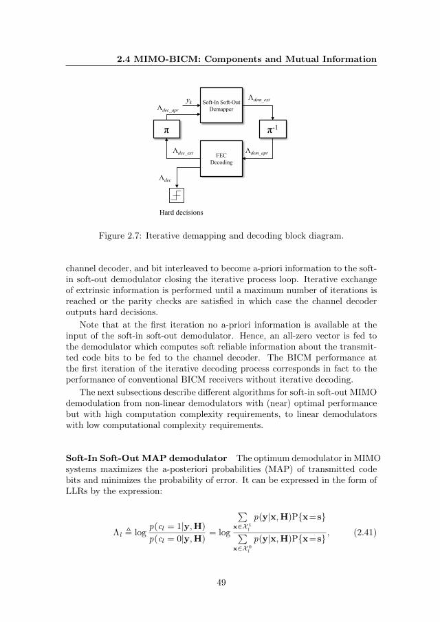
2.4 MIMO-BICM: Components and Mutual Information
Soft-In Soft-OutDemapper
π-1
yk
π
FECDecoding
Λdem_ext
Λdec_ext Λdem_apr
Λdec_apr
Λdec
Hard decisions
Figure 2.7: Iterative demapping and decoding block diagram.
channel decoder, and bit interleaved to become a-priori information to the soft-in soft-out demodulator closing the iterative process loop. Iterative exchangeof extrinsic information is performed until a maximum number of iterations isreached or the parity checks are satisfied in which case the channel decoderoutputs hard decisions.
Note that at the first iteration no a-priori information is available at theinput of the soft-in soft-out demodulator. Hence, an all-zero vector is fed tothe demodulator which computes soft reliable information about the transmit-ted code bits to be fed to the channel decoder. The BICM performance atthe first iteration of the iterative decoding process corresponds in fact to theperformance of conventional BICM receivers without iterative decoding.
The next subsections describe different algorithms for soft-in soft-out MIMOdemodulation from non-linear demodulators with (near) optimal performancebut with high computation complexity requirements, to linear demodulatorswith low computational complexity requirements.
Soft-In Soft-Out MAP demodulator The optimum demodulator in MIMOsystems maximizes the a-posteriori probabilities (MAP) of transmitted codebits and minimizes the probability of error. It can be expressed in the form ofLLRs by the expression:
Λl , logp(cl = 1|y,H)
p(cl = 0|y,H)= log
∑x∈X 1
l
p(y|x,H)Px=s∑x∈X 0
l
p(y|x,H)Px=s, (2.41)
49
CHAPTER 2. PRELIMINARIES
where p(cl|y,H) is the probability mass function of the transmitted coded bitsconditioned to the received vector y and the channel matrix H. X 1
l and X 0l
are the set constellation symbols with the corresponding bit label cl to 1 and 0,respectively, and the conditional Probability Density Function (pdf) p (y|x,H)is given by the expression:
p (y|x,H)=1
(πσ2)Nr
exp
(−‖y −Hx‖2
σ2
). (2.42)
Additionally, Px = s is the transmitted vector probability that can befurther developed as
Px=s =
m∏l=1
Pcl=bl =
m∏l=1
exp(−bl La(cl)
)1 + exp
(−La(cl)
) , (2.43)
where bl ∈ 0, 1 is the bit label of s and La(cl) is the a priori LLR for clwhich is provided by the LDPC decoder. In the case of non-iterative detectiona priori information is not fed back to demodulate the MIMO signal and La isa zero vector.
Using (2.41) and (2.42) and some expression manipulations [45], (2.41) canbe expressed as:
Λl =log
∑x∈X 1
l
exp
(− 1σ2 ‖y −Hx‖2 +
∑j
bjLa(cj )
)∑
x∈X 0l
exp
(− 1σ2 ‖y −Hx‖2 +
∑j
bjLa(cj )
) , (2.44)
where the summation of the a-priori LLRs La spans all the label bits that equal1. Despite the optimal error rate performance of MAP demodulator, for eachdemodulator execution the complexity order is O(|A|Nt) where |A| is the car-dinality of the symbol constellation A (e.g., |A| = 4 for QPSK) and Nt is thenumber of transmit antennas. That is, complexity increases exponentially withthe number of transmit antennas and linearly with the number of demodulationexecutions. The complexity of the MAP demodulator is commonly consideredas too computationally demanding for most of the practical applications there-fore a vast number of suboptimal demodulator with lower complexity have beenproposed in the literature.
Soft-In Soft-Out Max-log demodulator To reduce the computationalcomplexity of MAP detection the max-log approximation
log
(∑i
exp (xi)
)≈ max
ixi (2.45)
50
2.4 MIMO-BICM: Components and Mutual Information
replaces the computation of logarithmic and exponential functions to a min-imum distance problem more suitable for hardware implementation with re-duced performance loss. Applying the max-log approximation to (2.41) andfurther manipulations similar to those in (2.44), the computation of the ap-proximate LLRs has the form [45]
Λl = minx∈X 0
l
1
σ2‖y −Hx‖2 +
∑j
bjLa(cj )
−minx∈X 1
l
1
σ2‖y −Hx‖2 +
∑j
bjLa(cj )
,
(2.46)
where the summation of the a-priori LLRs La spans all the label bits thatequal 1. The complexity for each execution of max-log demodulation has orderO(|A|Nt), hence still scales exponentially with the number of transmit antennasand linearly with the number of demodulation executions.
Soft-In Soft-Out MMSE demodulator Linear demodulators like MMSEare other kind of efficient receivers with very low computational complexity.They apply a linear equalizer to suppress the stream interference to provide anestimate of the transmitted symbols followed by a per-layer detection. There-fore, the joint MIMO detection problem is transformed into independent singletransmit antenna (i.e., one layer) detection problems. The estimates computedby the MMSE equalizer can be improved using the information provided bythe channel decoder. This approach was initially proposed for soft MMSEequalization for communication over intersymbol interference (ISI) channels(cf. [87, 88]) and later to wireless communication systems [43, 89, 44]. Thelinear MMSE receiver for non-iterative schemes is given by [90]:
x = (H†H + σ2I)−1H†y, (2.47)
where y = Hx + w is the noisy receive vector, H is the MIMO channel matrix,x is the transmit vector. The estimated transmit vector is denoted by x and Idenotes the identity matrix.
The expression in (2.47) can be generalized to take a-priori information intoaccount. The modified estimate is given by
x = µx + Cx,yC−1y (y − µy), (2.48)
with (E· denotes the expectation operator)
51
CHAPTER 2. PRELIMINARIES
µx = Ex, µy = Ey = Hµx,
Cx,y = Exy† = CxH†, (2.49)
Cy = Eyy† = HCxH† + σ2I.
Using the expressions in (2.49), the estimate in (2.48) can be expressed interms of µx and Cx, whose elements are given by (note that Cx is a diagonalmatrix)
µxn=∑α∈A
αPxn=α, n = 1, 2, . . . , Nt,
(Cx)n,n =∑α∈A|α|2 Pxn=α − |µxn
|2, (2.50)
where A is the transmit symbol alphabet in one transmit antenna. Let |A|denote the cardinality of the symbol alphabet. Then the symbol probabilitiesin (2.50) can be further developed as
Pxn=α =m∏j=1
Pcn,j=bj =m∏j=1
exp(bjLa(cn,j)
)1 + exp
(La(cn,j)
) ,where bj ∈ 0, 1 (cn,j) is the bit label of α (xn) and La(cn,j) is the a-prioriLLR for cn,j which is provided by the LDPC decoder.
For each execution of the soft-in soft-out MMSE-based demodulator, thecomplexity of such procedure comprises the complexity for the symbol estima-tionO(NrN
2t ) operations plus the complexity to detect all code bitsO(NrNt|A|),
where Nr is the number of receive antennas. As we observe the complexity forthe detection of the independent layers is linear with the number of transmitantennas and linearly with the number of demodulation executions. Hence, asignificant complexity reduction can be achieved compared to optimal demod-ulation.
Fig. 2.8 presents performance results with iterative decoding for two typesof soft-in soft-out demodulators, the max-log and MMSE demodulators in pre-vious subsections. This figure shows the FER vs. CNR for code rates 1/3,8/15, and 11/15 using the MIMO profile of DVB-NGH with eSM-PH. For themax-log demapper, the iterative decoding gain increases with increasing coderate, i.e., 1 dB (1/3), 1.1 dB (8/15), and 1.8 dB (11/15). Furthermore, theresults with MMSE demodulator show that it is able to exploit the benefitsof iterative decoding while keeping computational complexity low [89]. In thiscase, MMSE demodulator gains approximately 0.7 dB (1/3), 0.9 dB (8/15), and
52
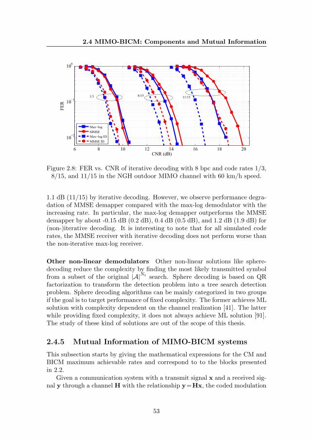
2.4 MIMO-BICM: Components and Mutual Information
6 8 10 12 14 16 18 20
10−2
10−1
100
CNR (dB)
FER
Max−logMMSEMax−log IDMMSE ID
11/158/151/3
Figure 2.8: FER vs. CNR of iterative decoding with 8 bpc and code rates 1/3,8/15, and 11/15 in the NGH outdoor MIMO channel with 60 km/h speed.
1.1 dB (11/15) by iterative decoding. However, we observe performance degra-dation of MMSE demapper compared with the max-log demodulator with theincreasing rate. In particular, the max-log demapper outperforms the MMSEdemapper by about -0.15 dB (0.2 dB), 0.4 dB (0.5 dB), and 1.2 dB (1.9 dB) for(non-)iterative decoding. It is interesting to note that for all simulated coderates, the MMSE receiver with iterative decoding does not perform worse thanthe non-iterative max-log receiver.
Other non-linear demodulators Other non-linear solutions like sphere-decoding reduce the complexity by finding the most likely transmitted symbolfrom a subset of the original |A|Nt search. Sphere decoding is based on QRfactorization to transform the detection problem into a tree search detectionproblem. Sphere decoding algorithms can be mainly categorized in two groupsif the goal is to target performance of fixed complexity. The former achieves MLsolution with complexity dependent on the channel realization [41]. The latterwhile providing fixed complexity, it does not always achieve ML solution [91].The study of these kind of solutions are out of the scope of this thesis.
2.4.5 Mutual Information of MIMO-BICM systems
This subsection starts by giving the mathematical expressions for the CM andBICM maximum achievable rates and correspond to to the blocks presentedin 2.2.
Given a communication system with a transmit signal x and a received sig-nal y through a channel H with the relationship y=Hx, the coded modulation
53
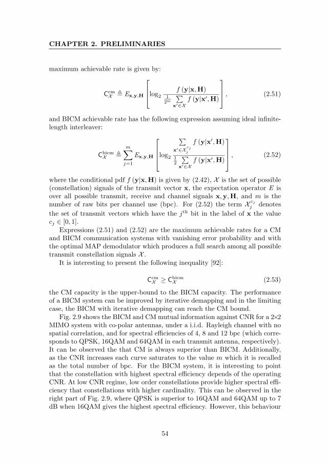
CHAPTER 2. PRELIMINARIES
maximum achievable rate is given by:
CcmX , Ex,y,H
log2
f (y|x,H)1
2m
∑x′∈X
f (y|x′,H)
, (2.51)
and BICM achievable rate has the following expression assuming ideal infinite-length interleaver:
CbicmX ,
m∑j=1
Ex,y,H
log2
∑x′∈X
cjj
f (y|x′,H)
12
∑x′∈X
f (y|x′,H)
, (2.52)
where the conditional pdf f (y|x,H) is given by (2.42), X is the set of possible(constellation) signals of the transmit vector x, the expectation operator E isover all possible transmit, receive and channel signals x,y,H, and m is thenumber of raw bits per channel use (bpc). For (2.52) the term X cjj denotes
the set of transmit vectors which have the jth bit in the label of x the valuecj ∈ [0, 1].
Expressions (2.51) and (2.52) are the maximum achievable rates for a CMand BICM communication systems with vanishing error probability and withthe optimal MAP demodulator which produces a full search among all possibletransmit constellation signals X .
It is interesting to present the following inequality [92]:
CcmX ≥ Cbicm
X (2.53)
the CM capacity is the upper-bound to the BICM capacity. The performanceof a BICM system can be improved by iterative demapping and in the limitingcase, the BICM with iterative demapping can reach the CM bound.
Fig. 2.9 shows the BICM and CM mutual information against CNR for a 2×2MIMO system with co-polar antennas, under a i.i.d. Rayleigh channel with nospatial correlation, and for spectral efficiencies of 4, 8 and 12 bpc (which corre-sponds to QPSK, 16QAM and 64QAM in each transmit antenna, respectively).It can be observed the that CM is always superior than BICM. Additionally,as the CNR increases each curve saturates to the value m which it is recalledas the total number of bpc. For the BICM system, it is interesting to pointthat the constellation with highest spectral efficiency depends of the operatingCNR. At low CNR regime, low order constellations provide higher spectral effi-ciency that constellations with higher cardinality. This can be observed in theright part of Fig. 2.9, where QPSK is superior to 16QAM and 64QAM up to 7dB when 16QAM gives the highest spectral efficiency. However, this behaviour
54
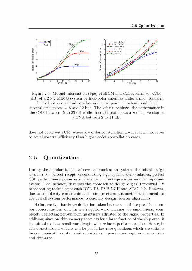
2.5 Quantization
−5 0 5 10 15 20 25 30 350
2
4
6
8
10
12
CNR (dB)
Mut
ual I
nfor
mat
ion
(bpc
)
BICMCM
4 bpc
8 bpc
12 bpc
2 4 6 8 10 12 141
1.5
2
2.5
3
3.5
4
4.5
5
CNR (dB)
Mut
ual I
nfor
mat
ion
(bpc
)
4 bpc − BICM8 bpc − BICM12 bpc − BICM4 bpc − CM8 bpc − CM12 bpc − CM
Figure 2.9: Mutual information (bpc) of BICM and CM systems vs. CNR(dB) of a 2× 2 MIMO system with co-polar antennas under a i.i.d. Rayleigh
channel with no spatial correlation and no power imbalance and threespectral efficiencies: 4, 8 and 12 bpc. The left figure shows the performance inthe CNR between -5 to 35 dB while the right plot shows a zoomed version in
a CNR between 2 to 14 dB.
does not occur with CM, where low order constellation always incur into loweror equal spectral efficiency than higher order constellation cases.
2.5 Quantization
During the standardization of new communication systems the initial designaccounts for perfect reception conditions, e.g., optimal demodulators, perfectCSI, perfect noise power estimation, and infinite-precision number represen-tations. For instance, that was the approach to design digital terrestrial TVbroadcasting technologies such DVB-T2, DVB-NGH and ATSC 3.0. However,due to complexity constraints and finite-precision arithmetic, it is crucial forthe overall system performance to carefully design receiver algorithms.
So far, receiver hardware design has taken into account finite-precision num-ber representations only in a straightforward manner via simulations, com-pletely neglecting non-uniform quantizers adjusted to the signal properties. Inaddition, since on-chip memory accounts for a large fraction of the chip area, itis desirable to have small word length with reduced performance loss. Hence, inthis dissertation the focus will be put in low-rate quantizers which are suitablefor communication systems with constrains in power consumption, memory sizeand chip-area.
55
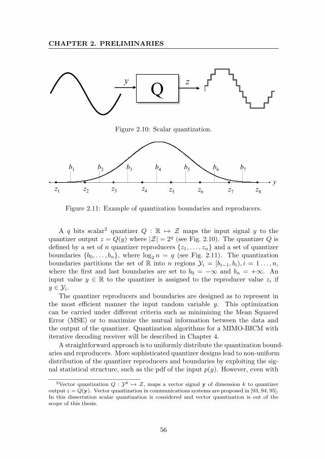
CHAPTER 2. PRELIMINARIES
Qy z
Figure 2.10: Scalar quantization.
y
b1 b2 b3 b4 b5 b6
z1 z2 z3 z4 z5 z6 z7 z8
b7
Figure 2.11: Example of quantization boundaries and reproducers.
A q bits scalar2 quantizer Q : R 7→ Z maps the input signal y to thequantizer output z = Q(y) where |Z| = 2q (see Fig. 2.10). The quantizer Q isdefined by a set of n quantizer reproducers z1, . . . , zn and a set of quantizerboundaries b0, . . . , bn, where log2 n = q (see Fig. 2.11). The quantizationboundaries partitions the set of R into n regions Yi = [bi−1, bi), i = 1 . . . , n,where the first and last boundaries are set to b0 = −∞ and bn = +∞. Aninput value y ∈ R to the quantizer is assigned to the reproducer value zi ify ∈ Yi.
The quantizer reproducers and boundaries are designed as to represent inthe most efficient manner the input random variable y. This optimizationcan be carried under different criteria such as minimizing the Mean SquaredError (MSE) or to maximize the mutual information between the data andthe output of the quantizer. Quantization algorithms for a MIMO-BICM withiterative decoding receiver will be described in Chapter 4.
A straightforward approach is to uniformly distribute the quantization bound-aries and reproducers. More sophisticated quantizer designs lead to non-uniformdistribution of the quantizer reproducers and boundaries by exploiting the sig-nal statistical structure, such as the pdf of the input p(y). However, even with
2Vector quantization Q : Yk 7→ Z, maps a vector signal y of dimension k to quantizeroutput z = Q(y). Vector quantization in communications systems are proposed in [93, 94, 95].In this dissertation scalar quantization is considered and vector quantization is out of thescope of this thesis.
56
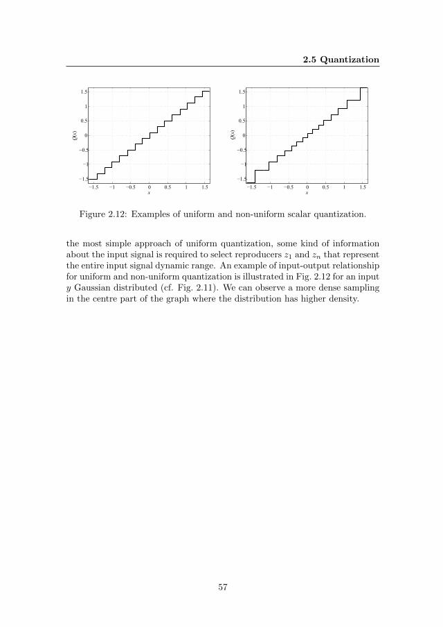
2.5 Quantization
−1.5 −1 −0.5 0 0.5 1 1.5−1.5
−1
−0.5
0
0.5
1
1.5
x
Q(x)
−1.5 −1 −0.5 0 0.5 1 1.5−1.5
−1
−0.5
0
0.5
1
1.5
x
Q(x)
Figure 2.12: Examples of uniform and non-uniform scalar quantization.
the most simple approach of uniform quantization, some kind of informationabout the input signal is required to select reproducers z1 and zn that representthe entire input signal dynamic range. An example of input-output relationshipfor uniform and non-uniform quantization is illustrated in Fig. 2.12 for an inputy Gaussian distributed (cf. Fig. 2.11). We can observe a more dense samplingin the centre part of the graph where the distribution has higher density.
57

CHAPTER 2. PRELIMINARIES
58
Chapter 3
MIMO Precoding forTerrestrial BroadcastSystems
This chapter studies the performance and structure of MIMO precodersbased on rotation matrices for 2×2 MIMO and focus on the case of cross-
polar antennas, which is the preferred configuration in DTT systems in theUHF band. Analysis and evaluation with the information-theoretic limits ofBICM systems and bit-error-rate simulations including channel coding showthe interesting results that the performance of the precoder depends on theselected code-rate. Then, the 2×2 MIMO precoders adopted in DVB-NGHand ATSC 3.0 are analysed and the selected parameters are compared with theresults obtained in this chapter.
Furthermore, a channel-precoder is proposed that exploits statistical in-formation of the MIMO channel. The performance of the channel-precoder isevaluated in a wide set of channel scenarios and mismatched channel conditions,a typical situation in the broadcast set-up. Capacity results show performanceimprovements in the case of strong line-of-sight scenarios with correlated an-tenna components and resilience against mismatched condition for 4×2 MIMOset-up. Finally, bit-error-rate simulation results compare the performance ofsingle-input single-output, 2×2 and 4×2 MIMO systems and the proposedMIMO channel-precoder.
59
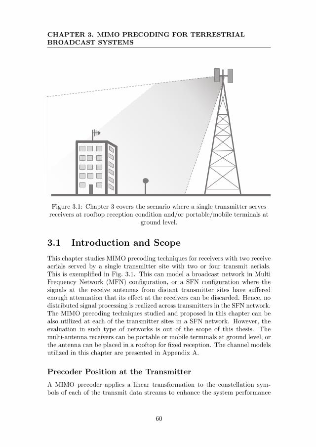
CHAPTER 3. MIMO PRECODING FOR TERRESTRIALBROADCAST SYSTEMS
Figure 3.1: Chapter 3 covers the scenario where a single transmitter servesreceivers at rooftop reception condition and/or portable/mobile terminals at
ground level.
3.1 Introduction and Scope
This chapter studies MIMO precoding techniques for receivers with two receiveaerials served by a single transmitter site with two or four transmit aerials.This is exemplified in Fig. 3.1. This can model a broadcast network in MultiFrequency Network (MFN) configuration, or a SFN configuration where thesignals at the receive antennas from distant transmitter sites have sufferedenough attenuation that its effect at the receivers can be discarded. Hence, nodistributed signal processing is realized across transmitters in the SFN network.The MIMO precoding techniques studied and proposed in this chapter can bealso utilized at each of the transmitter sites in a SFN network. However, theevaluation in such type of networks is out of the scope of this thesis. Themulti-antenna receivers can be portable or mobile terminals at ground level, orthe antenna can be placed in a rooftop for fixed reception. The channel modelsutilized in this chapter are presented in Appendix A.
Precoder Position at the Transmitter
A MIMO precoder applies a linear transformation to the constellation sym-bols of each of the transmit data streams to enhance the system performance
60
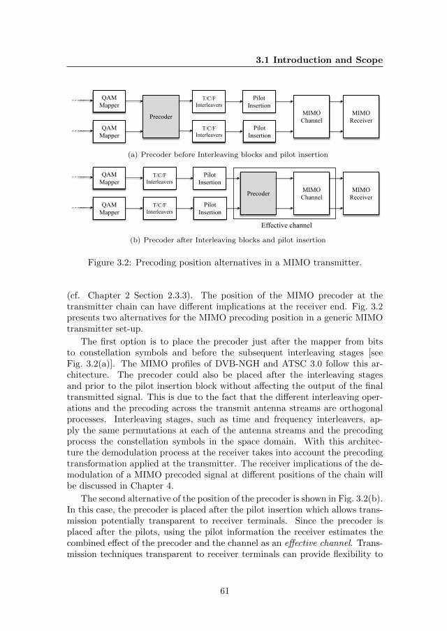
3.1 Introduction and Scope
QAMMapper
QAMMapper
Precoder
T/C/FInterleavers
T/C/FInterleavers
MIMOChannel
MIMOReceiver
PilotInsertion
PilotInsertion
(a) Precoder before Interleaving blocks and pilot insertion
QAMMapper
QAMMapper
Precoder
T/C/FInterleavers
T/C/FInterleavers
MIMOChannel
MIMOReceiver
PilotInsertion
PilotInsertion
Effective channel
(b) Precoder after Interleaving blocks and pilot insertion
Figure 3.2: Precoding position alternatives in a MIMO transmitter.
(cf. Chapter 2 Section 2.3.3). The position of the MIMO precoder at thetransmitter chain can have different implications at the receiver end. Fig. 3.2presents two alternatives for the MIMO precoding position in a generic MIMOtransmitter set-up.
The first option is to place the precoder just after the mapper from bitsto constellation symbols and before the subsequent interleaving stages [seeFig. 3.2(a)]. The MIMO profiles of DVB-NGH and ATSC 3.0 follow this ar-chitecture. The precoder could also be placed after the interleaving stagesand prior to the pilot insertion block without affecting the output of the finaltransmitted signal. This is due to the fact that the different interleaving oper-ations and the precoding across the transmit antenna streams are orthogonalprocesses. Interleaving stages, such as time and frequency interleavers, ap-ply the same permutations at each of the antenna streams and the precodingprocess the constellation symbols in the space domain. With this architec-ture the demodulation process at the receiver takes into account the precodingtransformation applied at the transmitter. The receiver implications of the de-modulation of a MIMO precoded signal at different positions of the chain willbe discussed in Chapter 4.
The second alternative of the position of the precoder is shown in Fig. 3.2(b).In this case, the precoder is placed after the pilot insertion which allows trans-mission potentially transparent to receiver terminals. Since the precoder isplaced after the pilots, using the pilot information the receiver estimates thecombined effect of the precoder and the channel as an effective channel. Trans-mission techniques transparent to receiver terminals can provide flexibility to
61
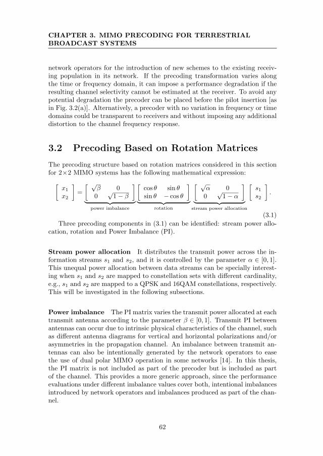
CHAPTER 3. MIMO PRECODING FOR TERRESTRIALBROADCAST SYSTEMS
network operators for the introduction of new schemes to the existing receiv-ing population in its network. If the precoding transformation varies alongthe time or frequency domain, it can impose a performance degradation if theresulting channel selectivity cannot be estimated at the receiver. To avoid anypotential degradation the precoder can be placed before the pilot insertion [asin Fig. 3.2(a)]. Alternatively, a precoder with no variation in frequency or timedomains could be transparent to receivers and without imposing any additionaldistortion to the channel frequency response.
3.2 Precoding Based on Rotation Matrices
The precoding structure based on rotation matrices considered in this sectionfor 2×2 MIMO systems has the following mathematical expression:[
x1
x2
]=
[ √β 0
0√
1− β
]︸ ︷︷ ︸
power imbalance
[cos θ sin θsin θ − cos θ
]︸ ︷︷ ︸
rotation
[ √α 0
0√
1− α
]︸ ︷︷ ︸
stream power allocation
[s1
s2
].
(3.1)
Three precoding components in (3.1) can be identified: stream power allo-cation, rotation and Power Imbalance (PI).
Stream power allocation It distributes the transmit power across the in-formation streams s1 and s2, and it is controlled by the parameter α ∈ [0, 1].This unequal power allocation between data streams can be specially interest-ing when s1 and s2 are mapped to constellation sets with different cardinality,e.g., s1 and s2 are mapped to a QPSK and 16QAM constellations, respectively.This will be investigated in the following subsections.
Power imbalance The PI matrix varies the transmit power allocated at eachtransmit antenna according to the parameter β ∈ [0, 1]. Transmit PI betweenantennas can occur due to intrinsic physical characteristics of the channel, suchas different antenna diagrams for vertical and horizontal polarizations and/orasymmetries in the propagation channel. An imbalance between transmit an-tennas can also be intentionally generated by the network operators to easethe use of dual polar MIMO operation in some networks [14]. In this thesis,the PI matrix is not included as part of the precoder but is included as partof the channel. This provides a more generic approach, since the performanceevaluations under different imbalance values cover both, intentional imbalancesintroduced by network operators and imbalances produced as part of the chan-nel.
62
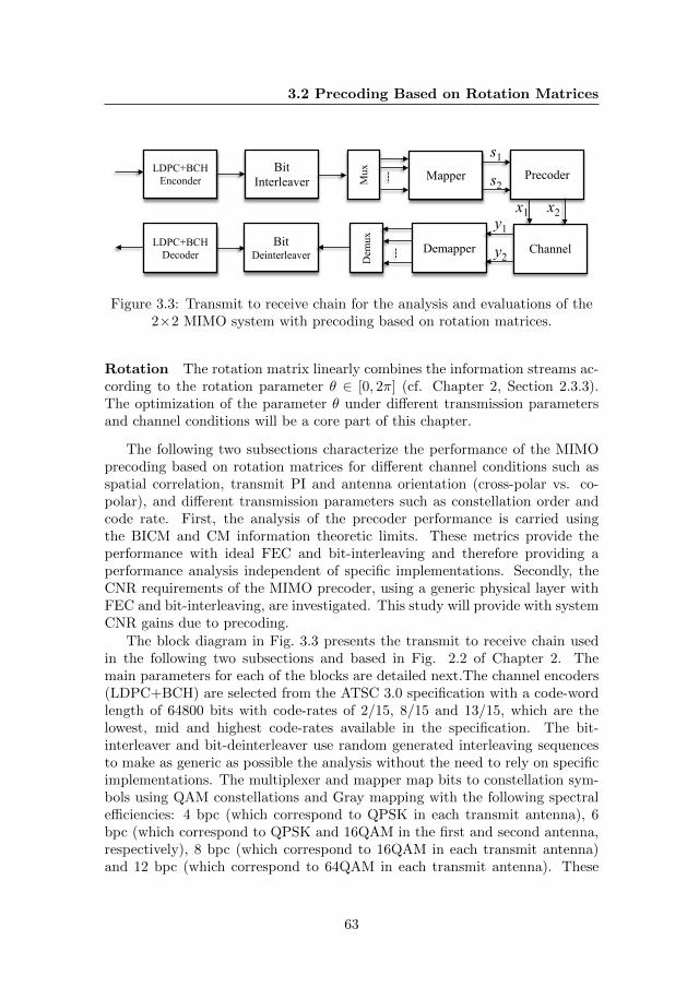
3.2 Precoding Based on Rotation Matrices
LDPC+BCHEnconder
Bit Interleaver Mapper
s1
ChannelDemapperBitDeinterleaver
LDPC+BCHDecoder
Mux
Dem
ux
s2Precoder
x1 x2y1
y2
Figure 3.3: Transmit to receive chain for the analysis and evaluations of the2×2 MIMO system with precoding based on rotation matrices.
Rotation The rotation matrix linearly combines the information streams ac-cording to the rotation parameter θ ∈ [0, 2π] (cf. Chapter 2, Section 2.3.3).The optimization of the parameter θ under different transmission parametersand channel conditions will be a core part of this chapter.
The following two subsections characterize the performance of the MIMOprecoding based on rotation matrices for different channel conditions such asspatial correlation, transmit PI and antenna orientation (cross-polar vs. co-polar), and different transmission parameters such as constellation order andcode rate. First, the analysis of the precoder performance is carried usingthe BICM and CM information theoretic limits. These metrics provide theperformance with ideal FEC and bit-interleaving and therefore providing aperformance analysis independent of specific implementations. Secondly, theCNR requirements of the MIMO precoder, using a generic physical layer withFEC and bit-interleaving, are investigated. This study will provide with systemCNR gains due to precoding.
The block diagram in Fig. 3.3 presents the transmit to receive chain usedin the following two subsections and based in Fig. 2.2 of Chapter 2. Themain parameters for each of the blocks are detailed next.The channel encoders(LDPC+BCH) are selected from the ATSC 3.0 specification with a code-wordlength of 64800 bits with code-rates of 2/15, 8/15 and 13/15, which are thelowest, mid and highest code-rates available in the specification. The bit-interleaver and bit-deinterleaver use random generated interleaving sequencesto make as generic as possible the analysis without the need to rely on specificimplementations. The multiplexer and mapper map bits to constellation sym-bols using QAM constellations and Gray mapping with the following spectralefficiencies: 4 bpc (which correspond to QPSK in each transmit antenna), 6bpc (which correspond to QPSK and 16QAM in the first and second antenna,respectively), 8 bpc (which correspond to 16QAM in each transmit antenna)and 12 bpc (which correspond to 64QAM in each transmit antenna). These
63
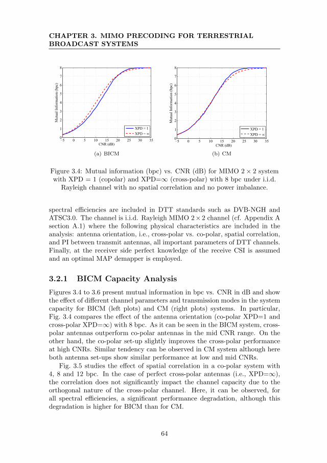
CHAPTER 3. MIMO PRECODING FOR TERRESTRIALBROADCAST SYSTEMS
−5 0 5 10 15 20 25 30 350
1
2
3
4
5
6
7
8
CNR (dB)
Mut
ual I
nfor
mat
ion
(bpc
)
XPD = 1XPD = ∞
(a) BICM
−5 0 5 10 15 20 25 30 350
1
2
3
4
5
6
7
8
CNR (dB)
Mut
ual I
nfor
mat
ion
(bpc
)
XPD = 1XPD = ∞
(b) CM
Figure 3.4: Mutual information (bpc) vs. CNR (dB) for MIMO 2× 2 systemwith XPD = 1 (copolar) and XPD=∞ (cross-polar) with 8 bpc under i.i.d.
Rayleigh channel with no spatial correlation and no power imbalance.
spectral efficiencies are included in DTT standards such as DVB-NGH andATSC3.0. The channel is i.i.d. Rayleigh MIMO 2× 2 channel (cf. Appendix Asection A.1) where the following physical characteristics are included in theanalysis: antenna orientation, i.e., cross-polar vs. co-polar, spatial correlation,and PI between transmit antennas, all important parameters of DTT channels.Finally, at the receiver side perfect knowledge of the receive CSI is assumedand an optimal MAP demapper is employed.
3.2.1 BICM Capacity Analysis
Figures 3.4 to 3.6 present mutual information in bpc vs. CNR in dB and showthe effect of different channel parameters and transmission modes in the systemcapacity for BICM (left plots) and CM (right plots) systems. In particular,Fig. 3.4 compares the effect of the antenna orientation (co-polar XPD=1 andcross-polar XPD=∞) with 8 bpc. As it can be seen in the BICM system, cross-polar antennas outperform co-polar antennas in the mid CNR range. On theother hand, the co-polar set-up slightly improves the cross-polar performanceat high CNRs. Similar tendency can be observed in CM system although hereboth antenna set-ups show similar performance at low and mid CNRs.
Fig. 3.5 studies the effect of spatial correlation in a co-polar system with4, 8 and 12 bpc. In the case of perfect cross-polar antennas (i.e., XPD=∞),the correlation does not significantly impact the channel capacity due to theorthogonal nature of the cross-polar channel. Here, it can be observed, forall spectral efficiencies, a significant performance degradation, although thisdegradation is higher for BICM than for CM.
64
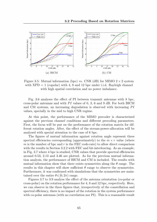
3.2 Precoding Based on Rotation Matrices
−5 0 5 10 15 20 25 30 350
2
4
6
8
10
12
CNR (dB)
Mut
ual I
nfor
mat
ion
(bpc
)
Low corr.High corr.
4 bpc
8 bpc
12 bpc
(a) BICM
−5 0 5 10 15 20 25 30 350
2
4
6
8
10
12
CNR (dB)
Mut
ual I
nfor
mat
ion
(bpc
)
Low corr.High corr.
8 bpc
12 bpc
4 bpc
(b) CM
Figure 3.5: Mutual information (bpc) vs. CNR (dB) for MIMO 2× 2 systemwith XPD = 1 (copolar) with 4, 8 and 12 bpc under i.i.d. Rayleigh channel
with high spatial correlation and no power imbalance.
Fig. 3.6 analyses the effect of PI between transmit antennas with 8 bpc,cross-polar antennas and with PI values of 0, 3, 6 and 9 dB. For both BICMand CM systems, an increasing degradation is observed with increasing PIvalues, specially in the mid to high CNR regime.
At this point, the performance of the MIMO precoder is characterizedagainst the previous channel conditions and different precoding parameters.First, the focus will be put on the performance of the rotation matrix for dif-ferent rotation angles. After, the effect of the stream-power-allocation will beanalysed with special attention to the case of 6 bpc.
The figures of mutual information against rotation angle represent threespectral efficiencies corresponding (approximately) to the m × r value (wherem is the number of bpc and r is the FEC code-rate) to allow direct comparisonwith the results in Section 3.2.2 with FEC and bit-interleaving. As an example,in Fig. 3.7 where 4 bpc is studied, CNR values that provide spectral efficienciesaround 0.53, 2.13 and 3.46 are plotted. As for the previous mutual informa-tion analysis, the performance of BICM and CM is included. The results withmutual information show that there exists symmetries along the θ range. Theresults in this chapter will show sufficient θ range to observe the symmetries.Furthermore, it was confirmed with simulations that the symmetries are main-tained over the entire θ∈ [0, 2π) range.
Figures 3.7 to 3.9 analyse the effect of the antenna orientation (co-polar orcross-polar) on the rotation performance for 4, 8 and 12 bpc, respectively. Here,we can observe in the three figures that, irrespectively of the constellation andspectral efficiency, there is no impact of the rotation in the system performancewith co-polar antennas (with no correlation nor PI). This is a reasonable result
65
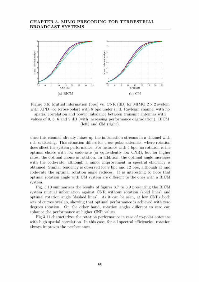
CHAPTER 3. MIMO PRECODING FOR TERRESTRIALBROADCAST SYSTEMS
−5 0 5 10 15 20 25 30 350
1
2
3
4
5
6
7
8
CNR (dB)
Mut
ual I
nfor
mai
ton
(bpc
)
(a) BICM
−5 0 5 10 15 20 25 30 350
1
2
3
4
5
6
7
8
CNR (dB)
Mut
ual I
nfor
mat
ion
(bpc
)
(b) CM
Figure 3.6: Mutual information (bpc) vs. CNR (dB) for MIMO 2× 2 systemwith XPD=∞ (cross-polar) with 8 bpc under i.i.d. Rayleigh channel with no
spatial correlation and power imbalance between transmit antennas withvalues of 0, 3, 6 and 9 dB (with increasing performance degradation). BICM
(left) and CM (right).
since this channel already mixes up the information streams in a channel withrich scattering. This situation differs for cross-polar antennas, where rotationdoes affect the system performance. For instance with 4 bpc, no rotation is theoptimal choice with low code-rate (or equivalently low CNR), but for higherrates, the optimal choice is rotation. In addition, the optimal angle increaseswith the code-rate, although a minor improvement in spectral efficiency isobtained. Similar tendency is observed for 8 bpc and 12 bpc, although at midcode-rate the optimal rotation angle reduces. It is interesting to note thatoptimal rotation angle with CM system are different to the ones with a BICMsystem.
Fig. 3.10 summarizes the results of figures 3.7 to 3.9 presenting the BICMsystem mutual information against CNR without rotation (solid lines) andoptimal rotation angle (dashed lines). As it can be seen, at low CNRs bothsets of curves overlap, showing that optimal performance is achieved with zerodegrees rotation. On the other hand, rotation angles different to zero canenhance the performance at higher CNR values.
Fig 3.11 characterizes the rotation performance in case of co-polar antennaswith high spatial correlation. In this case, for all spectral efficiencies, rotationalways improves the performance.
66
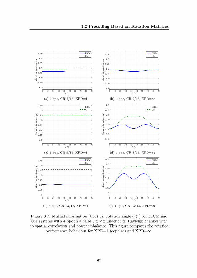
3.2 Precoding Based on Rotation Matrices
0 10 20 30 40 50 60 70 80 90
0.4
0.45
0.5
0.55
0.6
0.65
0.7
0.75
θ (º)
Mut
ual I
nfor
mat
ion
(bpc
)
BICMCM
(a) 4 bpc, CR 2/15, XPD=1
0 10 20 30 40 50 60 70 80 900.4
0.45
0.5
0.55
0.6
0.65
0.7
0.75
θ (º)
Mut
ual I
nfor
mat
ion
(bpc
)
BICMCM
(b) 4 bpc, CR 2/15, XPD=∞
0 10 20 30 40 50 60 70 80 90
2.1
2.15
2.2
2.25
2.3
2.35
2.4
2.45
θ (º)
Mut
ual I
nfor
mai
ton
(bpc
)
BICMCM
(c) 4 bpc, CR 8/15, XPD=1
0 10 20 30 40 50 60 70 80 90
2.15
2.2
2.25
2.3
2.35
2.4
2.45
2.5
θ (º)
Mut
ual I
nfor
mat
ion
(bpc
)
BICMCM
(d) 4 bpc, CR 8/15, XPD=∞
0 10 20 30 40 50 60 70 80 903
3.05
3.1
3.15
3.2
3.25
3.3
3.35
θ (º)
Mut
ual I
nfor
mat
ion
(bpc
)
BICMCM
(e) 4 bpc, CR 13/15, XPD=1
0 10 20 30 40 50 60 70 80 90
3
3.05
3.1
3.15
3.2
3.25
3.3
3.35
θ (º)
Mut
ual I
nfor
mat
ion
(bpc
)
BICMCM
(f) 4 bpc, CR 13/15, XPD=∞
Figure 3.7: Mutual information (bpc) vs. rotation angle θ () for BICM andCM systems with 4 bpc in a MIMO 2× 2 under i.i.d. Rayleigh channel with
no spatial correlation and power imbalance. This figure compares the rotationperformance behaviour for XPD=1 (copolar) and XPD=∞.
67
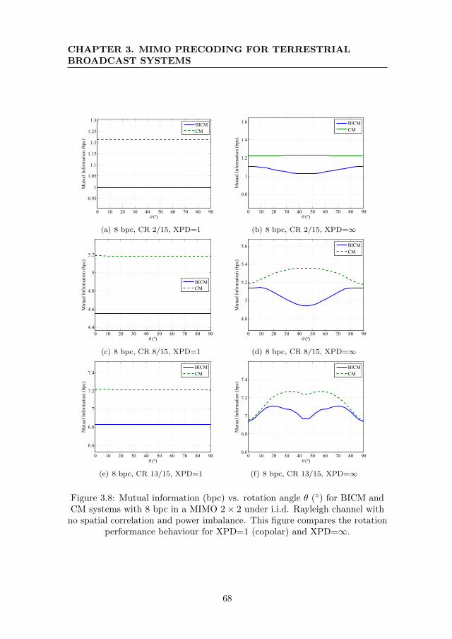
CHAPTER 3. MIMO PRECODING FOR TERRESTRIALBROADCAST SYSTEMS
0 10 20 30 40 50 60 70 80 90
0.95
1
1.05
1.1
1.15
1.2
1.25
1.3
θ (º)
Mut
ual I
nfor
mai
ton
(bpc
)
BICMCM
(a) 8 bpc, CR 2/15, XPD=1
0 10 20 30 40 50 60 70 80 90
0.8
1
1.2
1.4
1.6
θ (º)
Mut
ual I
nfor
mat
ion
(bpc
)
BICMCM
(b) 8 bpc, CR 2/15, XPD=∞
0 10 20 30 40 50 60 70 80 904.4
4.6
4.8
5
5.2
θ (º)
Mut
ual I
nfor
mat
ion
(bpc
)
BICMCM
(c) 8 bpc, CR 8/15, XPD=1
0 10 20 30 40 50 60 70 80 90
4.8
5
5.2
5.4
5.6
θ (º)
Mut
ual I
nfor
mat
ion
(bpc
)
BICMCM
(d) 8 bpc, CR 8/15, XPD=∞
0 10 20 30 40 50 60 70 80 90
6.6
6.8
7
7.2
7.4
θ (º)
Mut
ual I
nfor
mat
ion
(bpc
)
BICMCM
(e) 8 bpc, CR 13/15, XPD=1
0 10 20 30 40 50 60 70 80 906.6
6.8
7
7.2
7.4
θ (º)
Mut
ual I
nfor
mat
ion
(bpc
)
BICMCM
(f) 8 bpc, CR 13/15, XPD=∞
Figure 3.8: Mutual information (bpc) vs. rotation angle θ () for BICM andCM systems with 8 bpc in a MIMO 2× 2 under i.i.d. Rayleigh channel with
no spatial correlation and power imbalance. This figure compares the rotationperformance behaviour for XPD=1 (copolar) and XPD=∞.
68
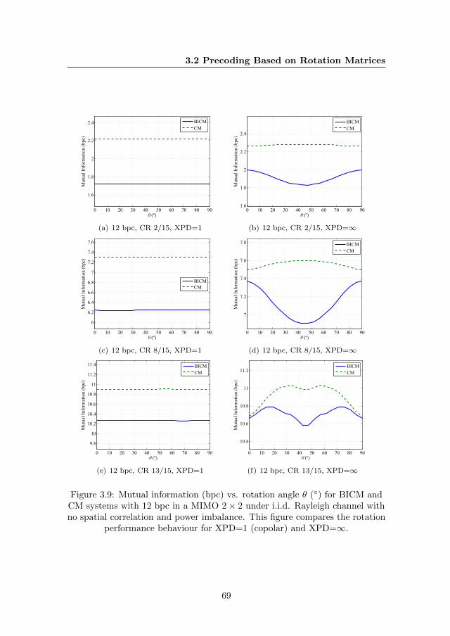
3.2 Precoding Based on Rotation Matrices
0 10 20 30 40 50 60 70 80 90
1.6
1.8
2
2.2
2.4
θ (º)
Mut
ual I
nfor
mat
ion
(bpc
)
BICMCM
(a) 12 bpc, CR 2/15, XPD=1
0 10 20 30 40 50 60 70 80 901.6
1.8
2
2.2
2.4
θ (º)
Mut
ual I
nfor
mat
ion
(bpc
)
BICMCM
(b) 12 bpc, CR 2/15, XPD=∞
0 10 20 30 40 50 60 70 80 90
6
6.2
6.4
6.6
6.8
7
7.2
7.4
7.6
θ (º)
Mut
ual I
nfor
mat
ion
(bpc
)
BICMCM
(c) 12 bpc, CR 8/15, XPD=1
0 10 20 30 40 50 60 70 80 90
7
7.2
7.4
7.6
7.8
θ (º)
Mut
ual I
nfor
mat
ion
(bpc
)
BICMCM
(d) 12 bpc, CR 8/15, XPD=∞
0 10 20 30 40 50 60 70 80 90
9.8
10
10.2
10.4
10.6
10.8
11
11.2
11.4
θ (º)
Mut
ual I
nfor
mat
ion
(bpc
)
BICMCM
(e) 12 bpc, CR 13/15, XPD=1
0 10 20 30 40 50 60 70 80 90
10.4
10.6
10.8
11
11.2
θ (º)
Mut
ual I
nfor
mat
ion
(bpc
)
BICMCM
(f) 12 bpc, CR 13/15, XPD=∞
Figure 3.9: Mutual information (bpc) vs. rotation angle θ () for BICM andCM systems with 12 bpc in a MIMO 2× 2 under i.i.d. Rayleigh channel withno spatial correlation and power imbalance. This figure compares the rotation
performance behaviour for XPD=1 (copolar) and XPD=∞.
69
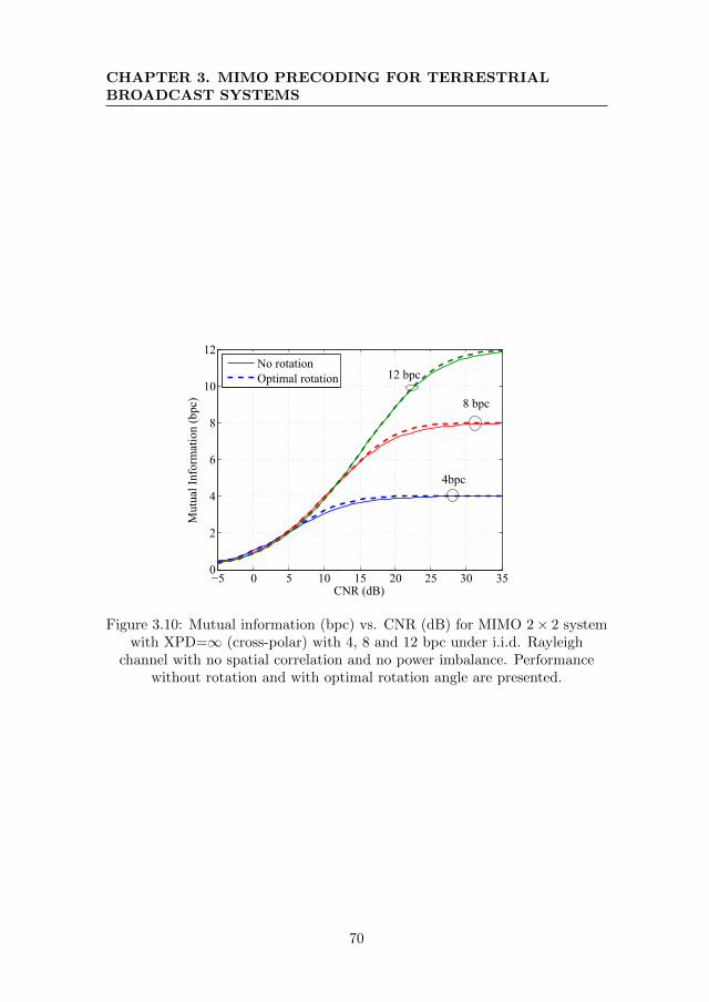
CHAPTER 3. MIMO PRECODING FOR TERRESTRIALBROADCAST SYSTEMS
−5 0 5 10 15 20 25 30 350
2
4
6
8
10
12
CNR (dB)
Mut
ual I
nfor
mat
ion
(bpc
)
No rotationOptimal rotation
8 bpc
12 bpc
4bpc
Figure 3.10: Mutual information (bpc) vs. CNR (dB) for MIMO 2× 2 systemwith XPD=∞ (cross-polar) with 4, 8 and 12 bpc under i.i.d. Rayleigh
channel with no spatial correlation and no power imbalance. Performancewithout rotation and with optimal rotation angle are presented.
70
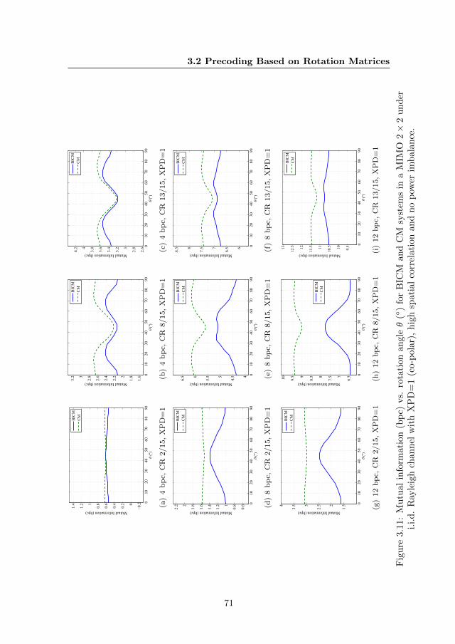
3.2 Precoding Based on Rotation Matrices
010
2030
4050
6070
8090
−0.20
0.2
0.4
0.6
0.81
1.2
1.4
θ (º)
Mutual Information (bpc)
BIC
MC
M
(a)
4b
pc,
CR
2/15,
XP
D=
1
010
2030
4050
6070
8090
1.6
1.82
2.2
2.4
2.6
2.83
3.2
θ (º)
Mutual Information (bpc)
BIC
MC
M
(b)
4b
pc,
CR
8/15,
XP
D=
1
010
2030
4050
6070
8090
2.6
2.83
3.2
3.4
3.6
3.84
4.2
θ (º)
Mutual Information (bpc)
BIC
MC
M
(c)
4b
pc,
CR
13/15,
XP
D=
1
010
2030
4050
6070
8090
0.6
0.81
1.2
1.4
1.6
1.82
2.2
θ (º)
Mutual Information (bpc)
BIC
MC
M
(d)
8b
pc,
CR
2/15,
XP
D=
1
010
2030
4050
6070
8090
4
4.55
5.56
6.5
θ (º)
Mutual Information (bpc)
BIC
MC
M
(e)
8b
pc,
CR
8/15,
XP
D=
1
010
2030
4050
6070
8090
6
6.57
7.58
8.5
θ (º)
Mutual Information (bpc)
BIC
MC
M
(f)
8b
pc,
CR
13/15,
XP
D=
1
010
2030
4050
6070
8090
1.52
2.53
3.54
θ (º)
Mutual Information (bpc)
BIC
MC
M
(g)
12
bp
c,C
R2/15,
XP
D=
1
010
2030
4050
6070
8090
6.57
7.58
8.59
9.510
θ (º)
Mutual Information (bpc)
BIC
MC
M
(h)
12
bp
c,C
R8/15,
XP
D=
1
010
2030
4050
6070
8090
9.510
10.511
11.512
12.513
θ (º)
Mutual Information (bpc)
BIC
MC
M
(i)
12
bp
c,C
R13/15,
XP
D=
1
Fig
ure
3.11
:M
utu
alin
form
atio
n(b
pc)
vs.
rota
tion
angl
eθ
()
for
BIC
Man
dC
Msy
stem
sin
aM
IMO
2×
2u
nd
eri.
i.d
.R
ayle
igh
chan
nel
wit
hX
PD
=1
(co-
pol
ar),
hig
hsp
atia
lco
rrel
atio
nan
dn
op
ower
imb
alan
ce.
71
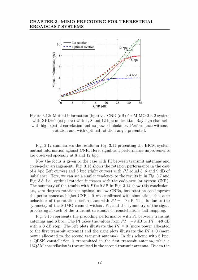
CHAPTER 3. MIMO PRECODING FOR TERRESTRIALBROADCAST SYSTEMS
0 5 10 15 20 25 30 350
2
4
6
8
10
CNR (dB)
Mut
ual I
nfor
mat
ion
(bpc
)
No rotationOptimal rotation 12 bpc
8 bpc
4 bpc
Figure 3.12: Mutual information (bpc) vs. CNR (dB) for MIMO 2× 2 systemwith XPD=1 (co-polar) with 4, 8 and 12 bpc under i.i.d. Rayleigh channelwith high spatial correlation and no power imbalance. Performance without
rotation and with optimal rotation angle presented.
Fig. 3.12 summarizes the results in Fig. 3.11 presenting the BICM systemmutual information against CNR. Here, significant performance improvementsare observed specially at 8 and 12 bpc.
Now the focus is given to the case with PI between transmit antennas andcross-polar arrangement. Fig. 3.13 shows the rotation performance in the caseof 4 bpc (left curves) and 8 bpc (right curves) with PI equal 3, 6 and 9 dB ofimbalance. Here, we can see a similar tendency to the results in in Fig. 3.7 andFig. 3.8, i.e., optimal rotation increases with the code-rate (or system CNR).The summary of the results with PI=9 dB in Fig. 3.14 show this conclusion,i.e., zero degrees rotation is optimal at low CNRs, but rotation can improvethe performance at higher CNRs. It was confirmed with simulations the samebehaviour of the rotation performance with PI = −9 dB. This is due to thesymmetry of the MIMO channel without PI, and the symmetry of the signalprocessing at each of the transmit streams, i.e., constellations and mapping.
Fig. 3.15 represents the precoding performance with PI between transmitantennas and 6 bpc. The PI takes the values from PI=−9 dB to PI=+9 dBwith a 3 dB step. The left plots illustrate the PI ≥ 0 (more power allocatedto the first transmit antenna) and the right plots illustrate the PI ≤ 0 (morepower allocated to the second transmit antenna). In this scheme with 6 bpc,a QPSK constellation is transmitted in the first transmit antenna, while a16QAM constellation is transmitted in the second transmit antenna. Due to the
72
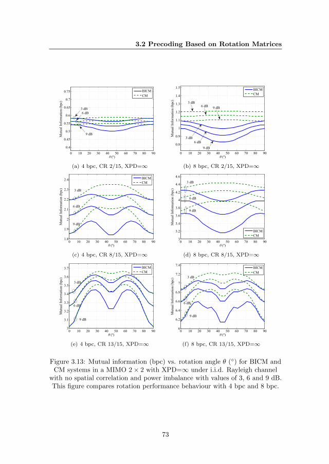
3.2 Precoding Based on Rotation Matrices
0 10 20 30 40 50 60 70 80 90
0.4
0.45
0.5
0.55
0.6
0.65
0.7
0.75
θ (º)
Mut
ual I
nfor
mat
ion
(bpc
)
BICMCM
3 dB6 dB
9 dB
(a) 4 bpc, CR 2/15, XPD=∞
0 10 20 30 40 50 60 70 80 90
0.8
0.9
1
1.1
1.2
1.3
1.4
1.5
θ (º)
Mut
ual I
nfor
mat
ion
(bpc
)
BICMCM
3 dB
3 dB
6 dB
6 dB
9 dB
9 dB
(b) 8 bpc, CR 2/15, XPD=∞
0 10 20 30 40 50 60 70 80 901.8
1.9
2
2.1
2.2
2.3
2.4
θ (º)
Mut
ual I
nfor
mat
ion
(bpc
)
BICMCM
3 dB
6 dB
9 dB
(c) 4 bpc, CR 8/15, XPD=∞
0 10 20 30 40 50 60 70 80 903
3.2
3.4
3.6
3.8
4
4.2
4.4
4.6
θ (º)
Mut
ual I
nfor
mat
ion
(bpc
)
BICMCM
3 dB
6 dB
9 dB
(d) 8 bpc, CR 8/15, XPD=∞
0 10 20 30 40 50 60 70 80 903
3.1
3.2
3.3
3.4
3.5
3.6
3.7
θ (º)
Mut
ual I
nfor
mat
ion
(bpc
)
BICMCM
3 dB
6 dB
9 dB
(e) 4 bpc, CR 13/15, XPD=∞
0 10 20 30 40 50 60 70 80 906
6.2
6.4
6.6
6.8
7
7.2
7.4
θ (º)
Mut
ual I
nfor
mat
ion
(bpc
)
BICMCM
3 dB
6 dB
9 dB
(f) 8 bpc, CR 13/15, XPD=∞
Figure 3.13: Mutual information (bpc) vs. rotation angle θ () for BICM andCM systems in a MIMO 2× 2 with XPD=∞ under i.i.d. Rayleigh channel
with no spatial correlation and power imbalance with values of 3, 6 and 9 dB.This figure compares rotation performance behaviour with 4 bpc and 8 bpc.
73
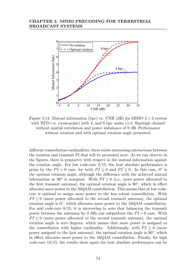
CHAPTER 3. MIMO PRECODING FOR TERRESTRIALBROADCAST SYSTEMS
−5 0 5 10 15 20 25 30 350
1
2
3
4
5
6
7
8
CNR (dB)
Mut
ual I
nfor
mai
ton
(bpc
)
No rotationOptimal rotation 8 bpc
4 bpc
Figure 3.14: Mutual information (bpc) vs. CNR (dB) for MIMO 2× 2 systemwith XPD=∞ (cross-polar) with 4, and 8 bpc under i.i.d. Rayleigh channel
without spatial correlation and power imbalance of 9 dB. Performancewithout rotation and with optimal rotation angle presented.
different constellation cardinalities, there exists interesting interactions betweenthe rotation and transmit PI that will be presented next. As we can observe inthe figures, there is symmetry with respect to the mutual information againstthe rotation angle. For low code-rate 2/15, the best absolute performance isgiven by the PI = 0 case, for both PI ≥ 0 and PI ≤ 0. In this case, 0 isthe optimal rotation angle, although the difference with the achieved mutualinformation at 90 is marginal. With PI ≥ 0 (i.e., more power allocated tothe first transmit antenna), the optimal rotation angle is 90, which in effectallocates more power to the 16QAM constellation. This means that at low code-rate is optimal to assign more power to the less robust constellation. WithPI ≤ 0 (more power allocated to the second transmit antenna), the optimalrotation angle is 0, which allocates more power to the 16QAM constellation.For mid code-rate 8/15, it is interesting to note that balancing the transmitpower between the antennas by 3 dBs can outperform the PI = 0 case. WithPI ≤ 0 (more power allocated to the second transmit antenna), the optimalrotation angle is zero degrees, which means that more power is assigned tothe constellation with higher cardinality. Additionally, with PI ≥ 0 (morepower assigned to the first antenna), the optimal rotation angle is 90, whichin effect allocates more power to the 16QAM constellation. Finally, for highcode-rate 13/15, the results show again the best absolute performance can be
74
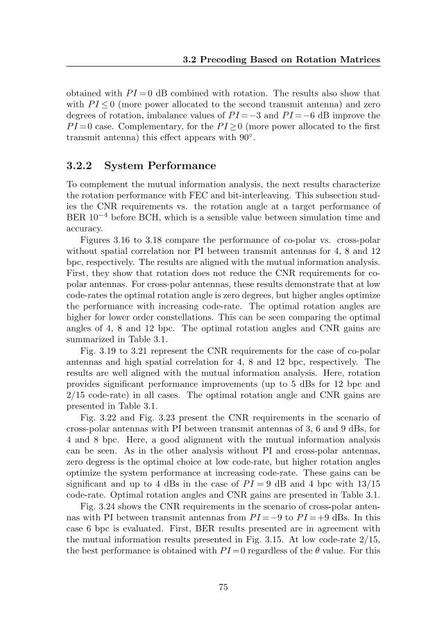
3.2 Precoding Based on Rotation Matrices
obtained with PI = 0 dB combined with rotation. The results also show thatwith PI ≤ 0 (more power allocated to the second transmit antenna) and zerodegrees of rotation, imbalance values of PI=−3 and PI=−6 dB improve thePI=0 case. Complementary, for the PI≥0 (more power allocated to the firsttransmit antenna) this effect appears with 90.
3.2.2 System Performance
To complement the mutual information analysis, the next results characterizethe rotation performance with FEC and bit-interleaving. This subsection stud-ies the CNR requirements vs. the rotation angle at a target performance ofBER 10−4 before BCH, which is a sensible value between simulation time andaccuracy.
Figures 3.16 to 3.18 compare the performance of co-polar vs. cross-polarwithout spatial correlation nor PI between transmit antennas for 4, 8 and 12bpc, respectively. The results are aligned with the mutual information analysis.First, they show that rotation does not reduce the CNR requirements for co-polar antennas. For cross-polar antennas, these results demonstrate that at lowcode-rates the optimal rotation angle is zero degrees, but higher angles optimizethe performance with increasing code-rate. The optimal rotation angles arehigher for lower order constellations. This can be seen comparing the optimalangles of 4, 8 and 12 bpc. The optimal rotation angles and CNR gains aresummarized in Table 3.1.
Fig. 3.19 to 3.21 represent the CNR requirements for the case of co-polarantennas and high spatial correlation for 4, 8 and 12 bpc, respectively. Theresults are well aligned with the mutual information analysis. Here, rotationprovides significant performance improvements (up to 5 dBs for 12 bpc and2/15 code-rate) in all cases. The optimal rotation angle and CNR gains arepresented in Table 3.1.
Fig. 3.22 and Fig. 3.23 present the CNR requirements in the scenario ofcross-polar antennas with PI between transmit antennas of 3, 6 and 9 dBs, for4 and 8 bpc. Here, a good alignment with the mutual information analysiscan be seen. As in the other analysis without PI and cross-polar antennas,zero degress is the optimal choice at low code-rate, but higher rotation anglesoptimize the system performance at increasing code-rate. These gains can besignificant and up to 4 dBs in the case of PI = 9 dB and 4 bpc with 13/15code-rate. Optimal rotation angles and CNR gains are presented in Table 3.1.
Fig. 3.24 shows the CNR requirements in the scenario of cross-polar anten-nas with PI between transmit antennas from PI=−9 to PI=+9 dBs. In thiscase 6 bpc is evaluated. First, BER results presented are in agreement withthe mutual information results presented in Fig. 3.15. At low code-rate 2/15,the best performance is obtained with PI=0 regardless of the θ value. For this
75
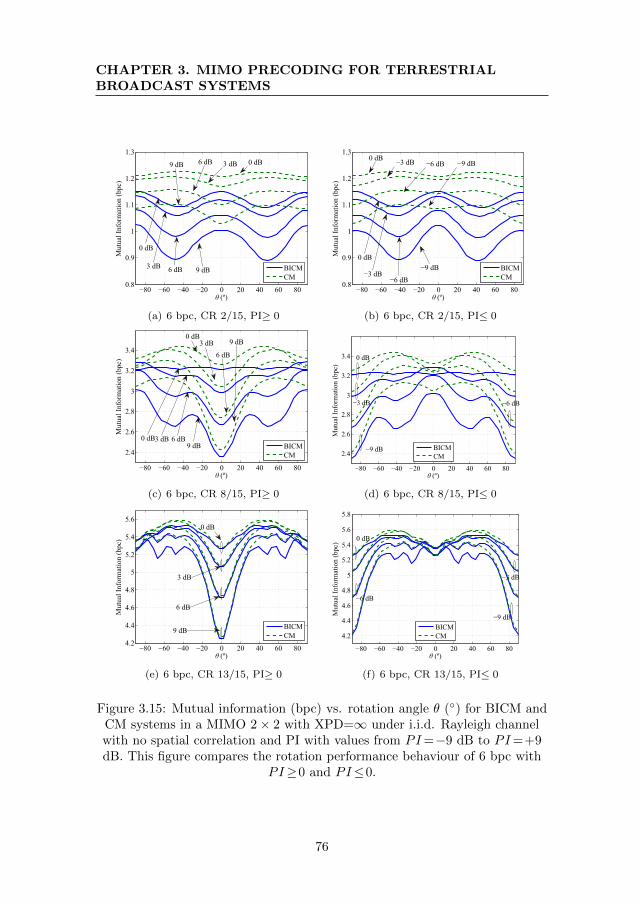
CHAPTER 3. MIMO PRECODING FOR TERRESTRIALBROADCAST SYSTEMS
−80 −60 −40 −20 0 20 40 60 800.8
0.9
1
1.1
1.2
1.3
θ (º)
Mut
ual I
nfor
mat
ion
(bpc
)
BICMCM
0 dB
3 dB 6 dB 9 dB
9 dB 6 dB 3 dB 0 dB
(a) 6 bpc, CR 2/15, PI≥ 0
−80 −60 −40 −20 0 20 40 60 800.8
0.9
1
1.1
1.2
1.3
θ (º)
Mut
ual I
nfor
mat
ion
(bpc
)
BICMCM
0 dB
−3 dB−9 dB
−3 dB0 dB
−6 dB
−6 dB −9 dB
(b) 6 bpc, CR 2/15, PI≤ 0
−80 −60 −40 −20 0 20 40 60 80
2.4
2.6
2.8
3
3.2
3.4
θ (º)
Mut
ual I
nfor
mat
ion
(bpc
)
BICMCM
0 dB3 dB 6 dB9 dB
3 dB0 dB
6 dB
9 dB
(c) 6 bpc, CR 8/15, PI≥ 0
−80 −60 −40 −20 0 20 40 60 80
2.4
2.6
2.8
3
3.2
3.4
θ (º)
Mut
ual I
nfor
mat
ion
(bpc
)
BICMCM
0 dB
−3 dB
−9 dB
−6 dB
(d) 6 bpc, CR 8/15, PI≤ 0
−80 −60 −40 −20 0 20 40 60 804.2
4.4
4.6
4.8
5
5.2
5.4
5.6
θ (º)
Mut
ual I
nfor
mat
ion
(bpc
)
BICMCM
0 dB
3 dB
6 dB
9 dB
(e) 6 bpc, CR 13/15, PI≥ 0
−80 −60 −40 −20 0 20 40 60 80
4.2
4.4
4.6
4.8
5
5.2
5.4
5.6
5.8
θ (º)
Mut
ual I
nfor
mat
ion
(bpc
)
BICMCM
0 dB
−6 dB
−9 dB
−3 dB
(f) 6 bpc, CR 13/15, PI≤ 0
Figure 3.15: Mutual information (bpc) vs. rotation angle θ () for BICM andCM systems in a MIMO 2× 2 with XPD=∞ under i.i.d. Rayleigh channelwith no spatial correlation and PI with values from PI=−9 dB to PI=+9dB. This figure compares the rotation performance behaviour of 6 bpc with
PI≥0 and PI≤0.
76
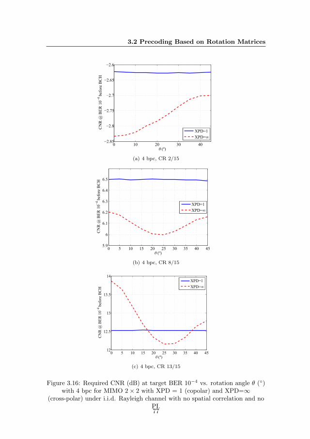
3.2 Precoding Based on Rotation Matrices
0 10 20 30 40−2.85
−2.8
−2.75
−2.7
−2.65
−2.6
θ (º)
CN
R @
BER
10−4
bef
ore
BC
H
XPD=1XPD=∞
(a) 4 bpc, CR 2/15
0 5 10 15 20 25 30 35 40 455.9
6
6.1
6.2
6.3
6.4
6.5
θ (º)
CN
R @
BER
10−4
bef
ore
BC
H
XPD=1XPD=∞
(b) 4 bpc, CR 8/15
0 5 10 15 20 25 30 35 40 4512
12.5
13
13.5
14
θ (º)
CN
R @
BER
10−4
bef
ore
BC
H
XPD=1XPD=∞
(c) 4 bpc, CR 13/15
Figure 3.16: Required CNR (dB) at target BER 10−4 vs. rotation angle θ ()with 4 bpc for MIMO 2× 2 with XPD = 1 (copolar) and XPD=∞
(cross-polar) under i.i.d. Rayleigh channel with no spatial correlation and noPI.77
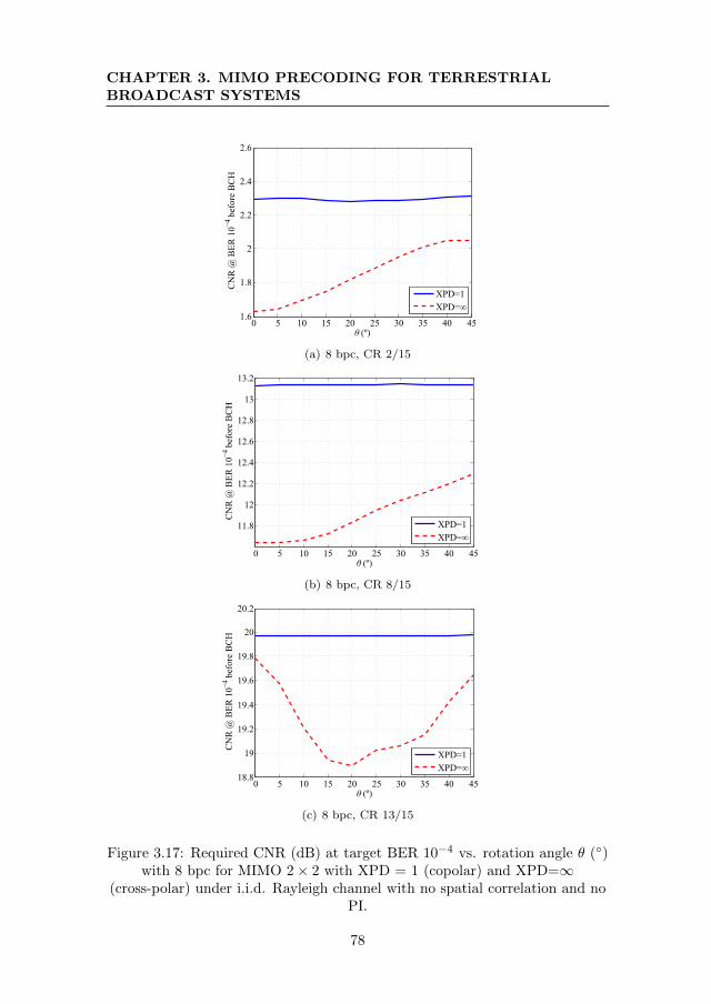
CHAPTER 3. MIMO PRECODING FOR TERRESTRIALBROADCAST SYSTEMS
0 5 10 15 20 25 30 35 40 451.6
1.8
2
2.2
2.4
2.6
θ (º)
CN
R @
BER
10−4
bef
ore
BC
H
XPD=1XPD=∞
(a) 8 bpc, CR 2/15
0 5 10 15 20 25 30 35 40 45
11.8
12
12.2
12.4
12.6
12.8
13
13.2
θ (º)
CN
R @
BER
10−4
bef
ore
BC
H
XPD=1XPD=∞
(b) 8 bpc, CR 8/15
0 5 10 15 20 25 30 35 40 4518.8
19
19.2
19.4
19.6
19.8
20
20.2
θ (º)
CN
R @
BER
10−4
bef
ore
BC
H
XPD=1XPD=∞
(c) 8 bpc, CR 13/15
Figure 3.17: Required CNR (dB) at target BER 10−4 vs. rotation angle θ ()with 8 bpc for MIMO 2× 2 with XPD = 1 (copolar) and XPD=∞
(cross-polar) under i.i.d. Rayleigh channel with no spatial correlation and noPI.
78
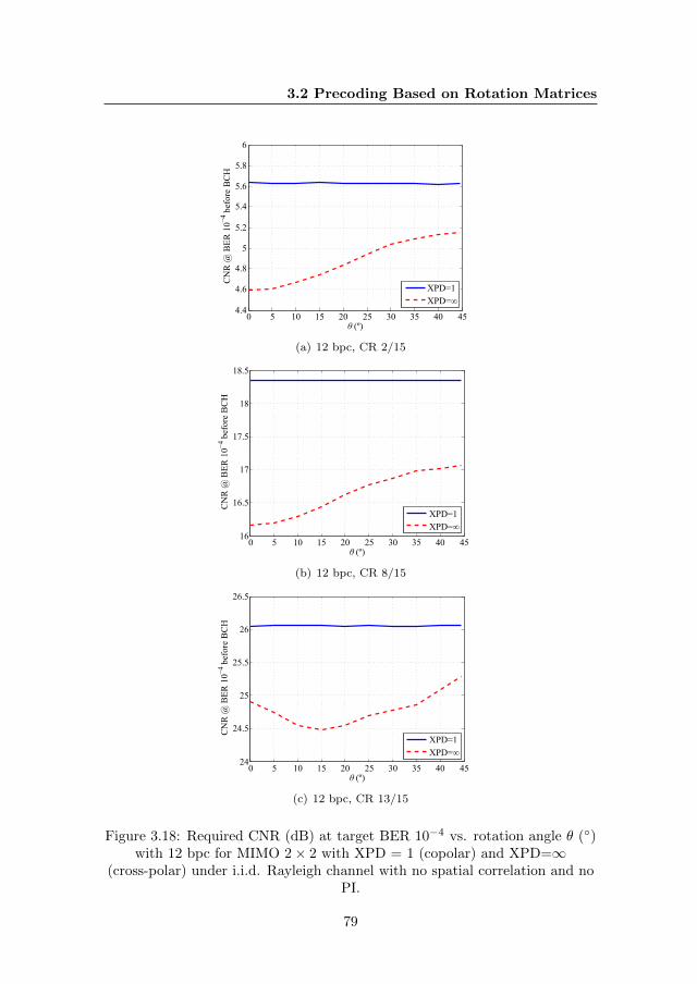
3.2 Precoding Based on Rotation Matrices
0 5 10 15 20 25 30 35 40 454.4
4.6
4.8
5
5.2
5.4
5.6
5.8
6
θ (º)
CN
R @
BER
10−4
bef
ore
BC
H
XPD=1XPD=∞
(a) 12 bpc, CR 2/15
0 5 10 15 20 25 30 35 40 4516
16.5
17
17.5
18
18.5
θ (º)
CN
R @
BER
10−4
bef
ore
BC
H
XPD=1XPD=∞
(b) 12 bpc, CR 8/15
0 5 10 15 20 25 30 35 40 4524
24.5
25
25.5
26
26.5
θ (º)
CN
R @
BER
10−4
bef
ore
BC
H
XPD=1XPD=∞
(c) 12 bpc, CR 13/15
Figure 3.18: Required CNR (dB) at target BER 10−4 vs. rotation angle θ ()with 12 bpc for MIMO 2× 2 with XPD = 1 (copolar) and XPD=∞
(cross-polar) under i.i.d. Rayleigh channel with no spatial correlation and noPI.
79
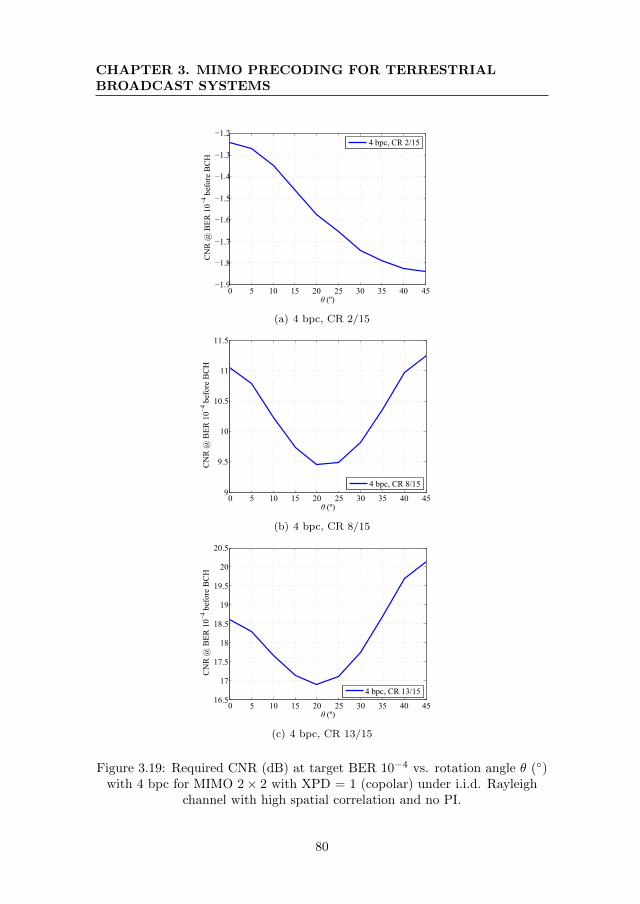
CHAPTER 3. MIMO PRECODING FOR TERRESTRIALBROADCAST SYSTEMS
0 5 10 15 20 25 30 35 40 45−1.9
−1.8
−1.7
−1.6
−1.5
−1.4
−1.3
−1.2
θ (º)
CN
R @
BER
10−4
bef
ore
BC
H
4 bpc, CR 2/15
(a) 4 bpc, CR 2/15
0 5 10 15 20 25 30 35 40 459
9.5
10
10.5
11
11.5
θ (º)
CN
R @
BER
10−4
bef
ore
BC
H
4 bpc, CR 8/15
(b) 4 bpc, CR 8/15
0 5 10 15 20 25 30 35 40 4516.5
17
17.5
18
18.5
19
19.5
20
20.5
θ (º)
CN
R @
BER
10−4
bef
ore
BC
H
4 bpc, CR 13/15
(c) 4 bpc, CR 13/15
Figure 3.19: Required CNR (dB) at target BER 10−4 vs. rotation angle θ ()with 4 bpc for MIMO 2× 2 with XPD = 1 (copolar) under i.i.d. Rayleigh
channel with high spatial correlation and no PI.
80
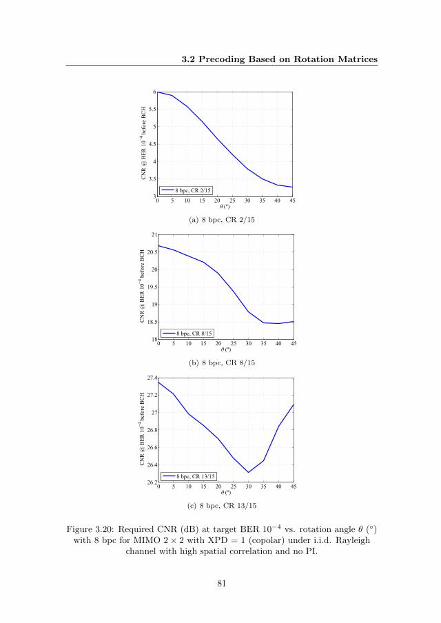
3.2 Precoding Based on Rotation Matrices
0 5 10 15 20 25 30 35 40 453
3.5
4
4.5
5
5.5
6
θ (º)
CN
R @
BER
10−4
bef
ore
BC
H
8 bpc, CR 2/15
(a) 8 bpc, CR 2/15
0 5 10 15 20 25 30 35 40 4518
18.5
19
19.5
20
20.5
21
θ (º)
CN
R @
BER
10−4
bef
ore
BC
H
8 bpc, CR 8/15
(b) 8 bpc, CR 8/15
0 5 10 15 20 25 30 35 40 4526.2
26.4
26.6
26.8
27
27.2
27.4
θ (º)
CN
R @
BER
10−4
bef
ore
BC
H
8 bpc, CR 13/15
(c) 8 bpc, CR 13/15
Figure 3.20: Required CNR (dB) at target BER 10−4 vs. rotation angle θ ()with 8 bpc for MIMO 2× 2 with XPD = 1 (copolar) under i.i.d. Rayleigh
channel with high spatial correlation and no PI.
81
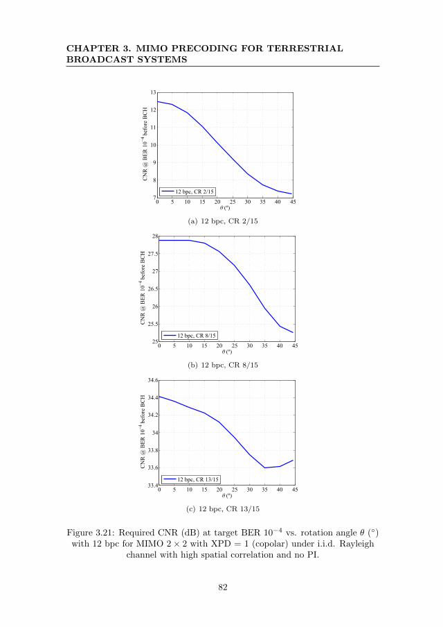
CHAPTER 3. MIMO PRECODING FOR TERRESTRIALBROADCAST SYSTEMS
0 5 10 15 20 25 30 35 40 457
8
9
10
11
12
13
θ (º)
CN
R @
BER
10−4
bef
ore
BC
H
12 bpc, CR 2/15
(a) 12 bpc, CR 2/15
0 5 10 15 20 25 30 35 40 4525
25.5
26
26.5
27
27.5
28
θ (º)
CN
R @
BER
10−4
bef
ore
BC
H
12 bpc, CR 8/15
(b) 12 bpc, CR 8/15
0 5 10 15 20 25 30 35 40 4533.4
33.6
33.8
34
34.2
34.4
34.6
θ (º)
CN
R @
BER
10−4
bef
ore
BC
H
12 bpc, CR 13/15
(c) 12 bpc, CR 13/15
Figure 3.21: Required CNR (dB) at target BER 10−4 vs. rotation angle θ ()with 12 bpc for MIMO 2× 2 with XPD = 1 (copolar) under i.i.d. Rayleigh
channel with high spatial correlation and no PI.
82
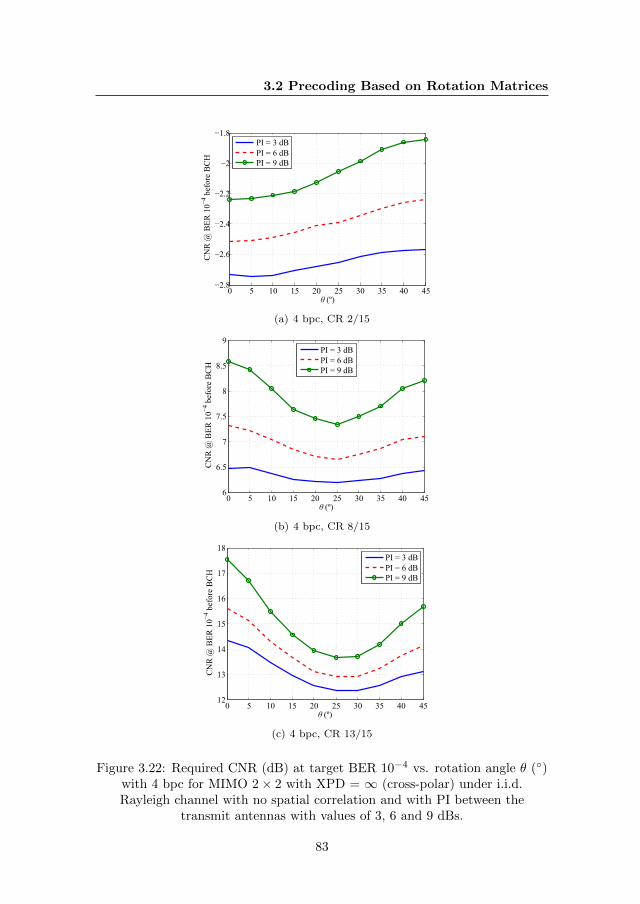
3.2 Precoding Based on Rotation Matrices
0 5 10 15 20 25 30 35 40 45−2.8
−2.6
−2.4
−2.2
−2
−1.8
θ (º)
CN
R @
BER
10−4
bef
ore
BC
H
PI = 3 dBPI = 6 dBPI = 9 dB
(a) 4 bpc, CR 2/15
0 5 10 15 20 25 30 35 40 456
6.5
7
7.5
8
8.5
9
θ (º)
CN
R @
BER
10−4
bef
ore
BC
H
PI = 3 dBPI = 6 dBPI = 9 dB
(b) 4 bpc, CR 8/15
0 5 10 15 20 25 30 35 40 4512
13
14
15
16
17
18
θ (º)
CN
R @
BER
10−4
bef
ore
BC
H
PI = 3 dBPI = 6 dBPI = 9 dB
(c) 4 bpc, CR 13/15
Figure 3.22: Required CNR (dB) at target BER 10−4 vs. rotation angle θ ()with 4 bpc for MIMO 2× 2 with XPD = ∞ (cross-polar) under i.i.d.Rayleigh channel with no spatial correlation and with PI between the
transmit antennas with values of 3, 6 and 9 dBs.
83
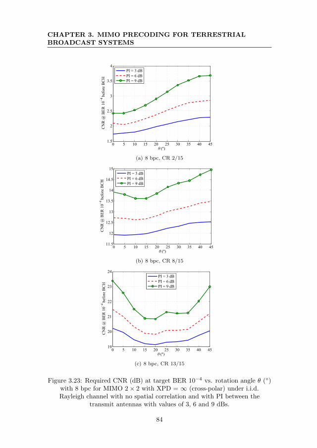
CHAPTER 3. MIMO PRECODING FOR TERRESTRIALBROADCAST SYSTEMS
0 5 10 15 20 25 30 35 40 451.5
2
2.5
3
3.5
4
θ (º)
CN
R @
BER
10−4
bef
ore
BC
H
PI = 3 dBPI = 6 dBPI = 9 dB
(a) 8 bpc, CR 2/15
0 5 10 15 20 25 30 35 40 4511.5
12
12.5
13
13.5
14
14.5
15
θ (º)
CN
R @
BER
10−4
bef
ore
BC
H
PI = 3 dBPI = 6 dBPI = 9 dB
(b) 8 bpc, CR 8/15
0 5 10 15 20 25 30 35 40 4519
20
21
22
23
24
θ (º)
CN
R @
BER
10−4
bef
ore
BC
H
PI = 3 dBPI = 6 dBPI = 9 dB
(c) 8 bpc, CR 13/15
Figure 3.23: Required CNR (dB) at target BER 10−4 vs. rotation angle θ ()with 8 bpc for MIMO 2× 2 with XPD = ∞ (cross-polar) under i.i.d.Rayleigh channel with no spatial correlation and with PI between the
transmit antennas with values of 3, 6 and 9 dBs.
84
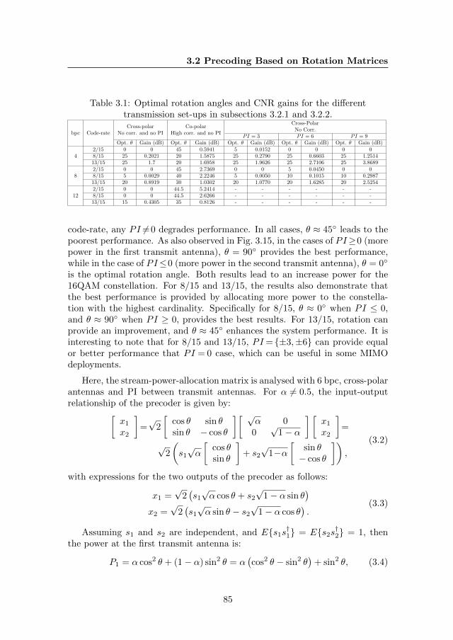
3.2 Precoding Based on Rotation Matrices
Table 3.1: Optimal rotation angles and CNR gains for the differenttransmission set-ups in subsections 3.2.1 and 3.2.2.
bpc Code-rateCross-polar
No corr. and no PICo-polar
High corr. and no PI
Cross-PolarNo Corr.
PI = 3 PI = 6 PI = 9Opt. θ Gain (dB) Opt. θ Gain (dB) Opt. θ Gain (dB) Opt. θ Gain (dB) Opt. θ Gain (dB)
42/15 0 0 45 0.5941 5 0.0152 0 0 0 08/15 25 0.2021 20 1.5875 25 0.2790 25 0.6603 25 1.251413/15 25 1.7 20 1.6958 25 1.9626 25 2.7106 25 3.8689
82/15 0 0 45 2.7369 0 0 5 0.0450 0 08/15 5 0.0029 40 2.2246 5 0.0050 10 0.1015 10 0.298713/15 20 0.8919 30 1.0302 20 1.0770 20 1.6285 20 2.5254
122/15 0 0 44.5 5.2414 - - - - - -8/15 0 0 44.5 2.6266 - - - - - -13/15 15 0.4305 35 0.8126 - - - - - -
code-rate, any PI 6=0 degrades performance. In all cases, θ ≈ 45 leads to thepoorest performance. As also observed in Fig. 3.15, in the cases of PI≥0 (morepower in the first transmit antenna), θ = 90 provides the best performance,while in the case of PI≤0 (more power in the second transmit antenna), θ = 0
is the optimal rotation angle. Both results lead to an increase power for the16QAM constellation. For 8/15 and 13/15, the results also demonstrate thatthe best performance is provided by allocating more power to the constella-tion with the highest cardinality. Specifically for 8/15, θ ≈ 0 when PI ≤ 0,and θ ≈ 90 when PI ≥ 0, provides the best results. For 13/15, rotation canprovide an improvement, and θ ≈ 45 enhances the system performance. It isinteresting to note that for 8/15 and 13/15, PI= ±3,±6 can provide equalor better performance that PI = 0 case, which can be useful in some MIMOdeployments.
Here, the stream-power-allocation matrix is analysed with 6 bpc, cross-polarantennas and PI between transmit antennas. For α 6= 0.5, the input-outputrelationship of the precoder is given by:[
x1
x2
]=√
2
[cos θ sin θsin θ − cos θ
][ √α 0
0√
1− α
] [x1
x2
]=
√2
(s1
√α
[cos θsin θ
]+ s2
√1−α
[sin θ− cos θ
]),
(3.2)
with expressions for the two outputs of the precoder as follows:
x1 =√
2(s1
√α cos θ + s2
√1− α sin θ
)x2 =
√2(s1
√α sin θ − s2
√1− α cos θ
).
(3.3)
Assuming s1 and s2 are independent, and Es1s†1 = Es2s
†2 = 1, then
the power at the first transmit antenna is:
P1 = α cos2 θ + (1− α) sin2 θ = α(cos2 θ − sin2 θ
)+ sin2 θ, (3.4)
85
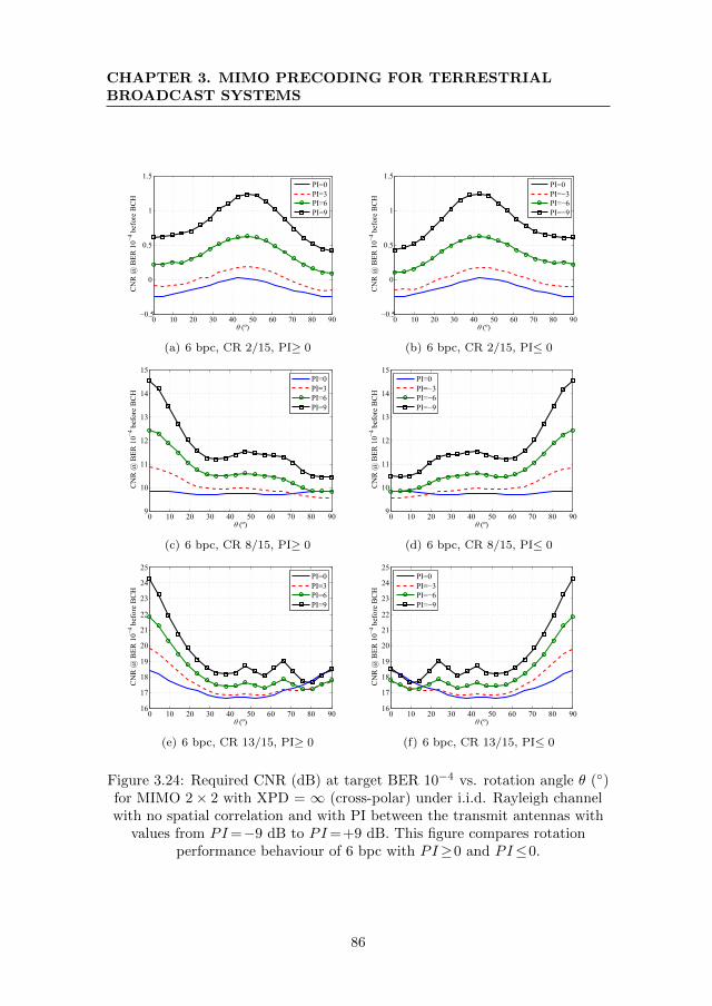
CHAPTER 3. MIMO PRECODING FOR TERRESTRIALBROADCAST SYSTEMS
0 10 20 30 40 50 60 70 80 90−0.5
0
0.5
1
1.5
θ (º)
CN
R @
BER
10−4
bef
ore
BC
H
PI=0PI=3PI=6PI=9
(a) 6 bpc, CR 2/15, PI≥ 0
0 10 20 30 40 50 60 70 80 90−0.5
0
0.5
1
1.5
θ (º)
CN
R @
BER
10−4
bef
ore
BC
H
PI=0PI=−3PI=−6PI=−9
(b) 6 bpc, CR 2/15, PI≤ 0
0 10 20 30 40 50 60 70 80 909
10
11
12
13
14
15
θ (º)
CN
R @
BER
10−4
bef
ore
BC
H
PI=0PI=3PI=6PI=9
(c) 6 bpc, CR 8/15, PI≥ 0
0 10 20 30 40 50 60 70 80 909
10
11
12
13
14
15
θ (º)
CN
R @
BER
10−4
bef
ore
BC
HPI=0PI=−3PI=−6PI=−9
(d) 6 bpc, CR 8/15, PI≤ 0
0 10 20 30 40 50 60 70 80 9016
17
18
19
20
21
22
23
24
25
θ (º)
CN
R @
BER
10−4
bef
ore
BC
H
PI=0PI=3PI=6PI=9
(e) 6 bpc, CR 13/15, PI≥ 0
0 10 20 30 40 50 60 70 80 9016
17
18
19
20
21
22
23
24
25
θ (º)
CN
R @
BER
10−4
bef
ore
BC
H
PI=0PI=−3PI=−6PI=−9
(f) 6 bpc, CR 13/15, PI≤ 0
Figure 3.24: Required CNR (dB) at target BER 10−4 vs. rotation angle θ ()for MIMO 2× 2 with XPD = ∞ (cross-polar) under i.i.d. Rayleigh channelwith no spatial correlation and with PI between the transmit antennas with
values from PI=−9 dB to PI=+9 dB. This figure compares rotationperformance behaviour of 6 bpc with PI≥0 and PI≤0.
86
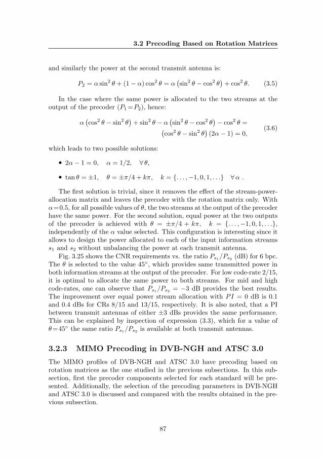
3.2 Precoding Based on Rotation Matrices
and similarly the power at the second transmit antenna is:
P2 = α sin2 θ + (1− α) cos2 θ = α(sin2 θ − cos2 θ
)+ cos2 θ. (3.5)
In the case where the same power is allocated to the two streams at theoutput of the precoder (P1 =P2), hence:
α(cos2 θ − sin2 θ
)+ sin2 θ − α
(sin2 θ − cos2 θ
)− cos2 θ =(
cos2 θ − sin2 θ)
(2α− 1) = 0,(3.6)
which leads to two possible solutions:
• 2α− 1 = 0, α = 1/2, ∀ θ,
• tan θ = ±1, θ = ±π/4 + kπ, k = . . . ,−1, 0, 1, . . . ∀α .
The first solution is trivial, since it removes the effect of the stream-power-allocation matrix and leaves the precoder with the rotation matrix only. Withα=0.5, for all possible values of θ, the two streams at the output of the precoderhave the same power. For the second solution, equal power at the two outputsof the precoder is achieved with θ = ±π/4 + kπ, k = . . . ,−1, 0, 1, . . .,independently of the α value selected. This configuration is interesting since itallows to design the power allocated to each of the input information streamss1 and s2 without unbalancing the power at each transmit antenna.
Fig. 3.25 shows the CNR requirements vs. the ratio Ps1/Ps2 (dB) for 6 bpc.The θ is selected to the value 45, which provides same transmitted power inboth information streams at the output of the precoder. For low code-rate 2/15,it is optimal to allocate the same power to both streams. For mid and highcode-rates, one can observe that Ps1/Ps2 = −3 dB provides the best results.The improvement over equal power stream allocation with PI = 0 dB is 0.1and 0.4 dBs for CRs 8/15 and 13/15, respectively. It is also noted, that a PIbetween transmit antennas of either ±3 dBs provides the same performance.This can be explained by inspection of expression (3.3), which for a value ofθ=45 the same ratio Ps1/Ps2 is available at both transmit antennas.
3.2.3 MIMO Precoding in DVB-NGH and ATSC 3.0
The MIMO profiles of DVB-NGH and ATSC 3.0 have precoding based onrotation matrices as the one studied in the previous subsections. In this sub-section, first the precoder components selected for each standard will be pre-sented. Additionally, the selection of the precoding parameters in DVB-NGHand ATSC 3.0 is discussed and compared with the results obtained in the pre-vious subsection.
87
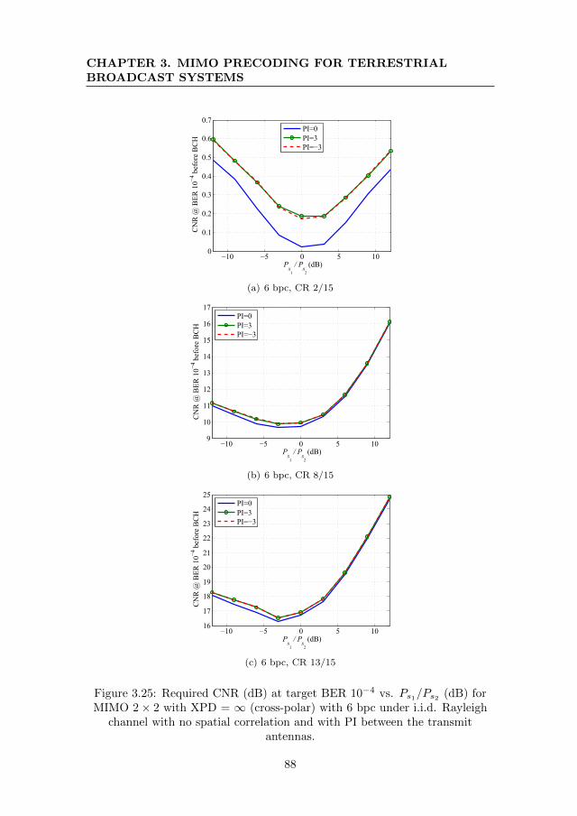
CHAPTER 3. MIMO PRECODING FOR TERRESTRIALBROADCAST SYSTEMS
−10 −5 0 5 100
0.1
0.2
0.3
0.4
0.5
0.6
0.7
Ps1
/ Ps2
(dB)
CN
R @
BER
10−4
bef
ore
BC
H
PI=0PI=3PI=−3
(a) 6 bpc, CR 2/15
−10 −5 0 5 109
10
11
12
13
14
15
16
17
Ps1
/ Ps2
(dB)
CN
R @
BER
10−4
bef
ore
BC
H
PI=0PI=3PI=−3
(b) 6 bpc, CR 8/15
−10 −5 0 5 1016
17
18
19
20
21
22
23
24
25
Ps1
/ Ps2
(dB)
CN
R @
BER
10−4
bef
ore
BC
H
PI=0PI=3PI=−3
(c) 6 bpc, CR 13/15
Figure 3.25: Required CNR (dB) at target BER 10−4 vs. Ps1/Ps2 (dB) forMIMO 2× 2 with XPD = ∞ (cross-polar) with 6 bpc under i.i.d. Rayleigh
channel with no spatial correlation and with PI between the transmitantennas.
88
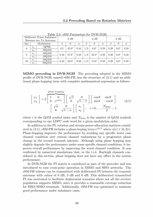
3.2 Precoding Based on Rotation Matrices
Table 3.2: eSM Parameters for DVB-NGHDeliberate Power ImbalanceBetween two Tx Antennas
0 dB 3 dB 6 dB
bpc Modulation β θ α β θ α β θ α
6x1 QPSK
0.5 45.0 0.44 1/3 0.0 0.50 0.20 0.0 0.50x2 16QAM
8x1 16QAM
0.50 57.8 0.50 1/3 25.0 0.50 0.20 0.0 0.50x2 16QAM
10x1 16QAM
0.50 22.0 0.50 1/3 15.0 0.50 0.20 0.0 0.50x2 64QAM
MIMO precoding in DVB-NGH The precoding adopted in the MIMOprofile of DVB-NGH, named eSM-PH, has the structure of (3.1) and an addi-tional phase hopping term with complete mathematical expression as follows:
[x1
x2
]= 2
phase hopping︷ ︸︸ ︷[1 00 ejφ(i)
] [ √β 0
0√
1− β
] [cos θ sin θsin θ − cos θ
]·
·[ √
α 00√
1− α
] [s1
s2
], i=0, . . . ,
Ndata
2− 1.
(3.7)
where i is the QAM symbol index and Ndata is the number of QAM symbolscorresponding to one LDPC code word for a given modulation order.
In addition to the PI, rotation and stream-power-allocation matrices consid-ered in (3.1), eSM-PH includes a phase-hoping term ejφ(i) where φ(i) ∈ [0, 2π).Phase-hopping improves the performance by avoiding any specific worst casechannel condition over various channel realizations by a progressive phasechange at the second transmit antenna. Although using phase hopping mayslightly degrade the performance under some specific channel conditions, it im-proves overall performance by improving the worst channel condition. It wasconfirmed by numerical simulations that, in the i.i.d. Rayleigh channels con-sidered in this section, phase hopping does not have any effect in the systemperformance.
In DVB-NGH the PI matrix is considered as part of the precoder and wasintroduced to ease cross-polar operation in MIMO and SISO networks. TheeSM-PH scheme can be transmitted with deliberated PI between the transmitantennas with values of 0 dB, 3 dB and 6 dB. This deliberated transmittedPI was motivated to facilitate deployment scenarios where not all the receiverpopulation supports MIMO, since it provides a reasonable coverage reductionfor SISO/SIMO terminals. Additionally, eSM-PH was optimized to maintaingood performance under imbalance cases.
89
CHAPTER 3. MIMO PRECODING FOR TERRESTRIALBROADCAST SYSTEMS
The parameters β, θ and α of the eSM precoder are summarized in Table 3.2.Multiple remarks can be made by comparing the parameters selected in DVB-NGH and the results obtained in the previous sections:
• DVB-NGH optimizes β, θ, and α for the three cases of bpc (i.e., 6, 8 and10 bpc) and for the different values of transmit PI. It is important to notethat these parameters are to be used for every code-rate available in theMIMO profile of DVB-NGH. However, as it has been investigated in pre-vious sections, there is a strong dependency of the optimal rotation anglewith the code-rate, which makes the precoding potentially suboptimal forsome transmit configurations.
• The parameter α has for all the combinations of Table 3.2 the value0.5, except for the 6 bpc configuration with PI = 0 in which α = 0.44.The value α= 0.5 transforms the stream-power-allocation matrix to theidentity matrix, which has no effect in the precoder. Interestingly, inthe case α = 0.44, the rotation parameter θ takes the value 45, whichas we saw in subsection 3.2.2 provides equal power at the two transmitantennas (but prior to the PI matrix). Furthermore, the value α= 0.44assigns more power to the data stream mapped to a 16QAM constellationthan the data stream mapped to QPSK constellation, which agrees withthe results of in Fig. 3.25.
• Since α is always 0.5, except for the case discussed in the previous bulletpoint, the parameter β takes the values 0.5, 0.33, and 0.2 to provide PIsbetween transmit antennas of 0, 3 and 6 dBs, respectively.
MIMO precoding in ATSC 3.0 The MIMO precoding scheme adoptedin ATSC 3.0 is composed of a rotation matrix, an I&Q polarization inter-leaver and a phase-hopping blocks [15]. Each of the three sub-blocks of theMIMO precoder can be optionally selected. The phase-hopping block adoptedin ATSC 3.0 is the same as in DVB-NGH and discussed in previous section anddetailed in Appendix B. The I&Q polarization interleaver is simply a switchinginterleaving operation, such that the output cells consist of the real (In-phase)component of one input symbol and the imaginary (Quadrature) component ofthe other input symbol. The I/Q polarization interleaving is described by thefollowing equations:
x1 = Res1+ iIms2x2 = Res2+ iIms1.
(3.8)
The rotation matrix has the same form as the one discussed in detail inthis chapter and also included in DVB-NGH. The value of the rotation an-gle θ is fixed and its value depends on the modulation and code-rate used.
90
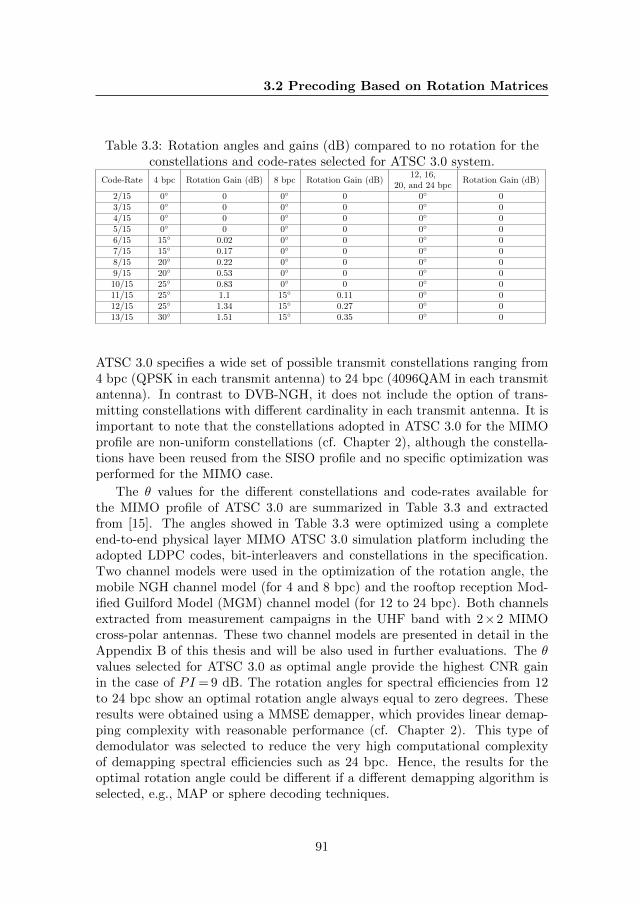
3.2 Precoding Based on Rotation Matrices
Table 3.3: Rotation angles and gains (dB) compared to no rotation for theconstellations and code-rates selected for ATSC 3.0 system.
Code-Rate 4 bpc Rotation Gain (dB) 8 bpc Rotation Gain (dB)12, 16,
20, and 24 bpcRotation Gain (dB)
2/15 0 0 0 0 0 03/15 0 0 0 0 0 04/15 0 0 0 0 0 05/15 0 0 0 0 0 06/15 15 0.02 0 0 0 07/15 15 0.17 0 0 0 08/15 20 0.22 0 0 0 09/15 20 0.53 0 0 0 010/15 25 0.83 0 0 0 011/15 25 1.1 15 0.11 0 012/15 25 1.34 15 0.27 0 013/15 30 1.51 15 0.35 0 0
ATSC 3.0 specifies a wide set of possible transmit constellations ranging from4 bpc (QPSK in each transmit antenna) to 24 bpc (4096QAM in each transmitantenna). In contrast to DVB-NGH, it does not include the option of trans-mitting constellations with different cardinality in each transmit antenna. It isimportant to note that the constellations adopted in ATSC 3.0 for the MIMOprofile are non-uniform constellations (cf. Chapter 2), although the constella-tions have been reused from the SISO profile and no specific optimization wasperformed for the MIMO case.
The θ values for the different constellations and code-rates available forthe MIMO profile of ATSC 3.0 are summarized in Table 3.3 and extractedfrom [15]. The angles showed in Table 3.3 were optimized using a completeend-to-end physical layer MIMO ATSC 3.0 simulation platform including theadopted LDPC codes, bit-interleavers and constellations in the specification.Two channel models were used in the optimization of the rotation angle, themobile NGH channel model (for 4 and 8 bpc) and the rooftop reception Mod-ified Guilford Model (MGM) channel model (for 12 to 24 bpc). Both channelsextracted from measurement campaigns in the UHF band with 2×2 MIMOcross-polar antennas. These two channel models are presented in detail in theAppendix B of this thesis and will be also used in further evaluations. The θvalues selected for ATSC 3.0 as optimal angle provide the highest CNR gainin the case of PI = 9 dB. The rotation angles for spectral efficiencies from 12to 24 bpc show an optimal rotation angle always equal to zero degrees. Theseresults were obtained using a MMSE demapper, which provides linear demap-ping complexity with reasonable performance (cf. Chapter 2). This type ofdemodulator was selected to reduce the very high computational complexityof demapping spectral efficiencies such as 24 bpc. Hence, the results for theoptimal rotation angle could be different if a different demapping algorithm isselected, e.g., MAP or sphere decoding techniques.
91
CHAPTER 3. MIMO PRECODING FOR TERRESTRIALBROADCAST SYSTEMS
Comparing the results in Table 3.3 with the investigations about rotationangle in this thesis the following remarks are provided:
• ATSC 3.0 uses a different rotation angle per code-rate, which has beenshown in this chapter to be optimal due to strong relationship betweenthe rotation performance and the code-rate.
• The results in Table 3.3 show that: (i) the rotation gain increases with thecode-rate, (ii) for low to mid code-rates it is optimal to rotate with zerodegrees angle, and (iii) the gain is higher for lower order constellations.These results are very well aligned with the results shown in section 3.2.1and section 3.2.2 with i.i.d. Rayleigh channel with cross-polar antennas.The mobile NGH channel model is a cross-polar channel with high XPDand low spatial correlation, which makes a similar scenario to the onestudied in this chapter.
• The results in Table 3.3 reinforce the conclusions extracted in this chap-ter since even with different physical layer components, such as bit-interleavers and constellations, and even different channel models, theconclusions still hold.
3.3 Precoding Based on Maximum Ergodic Ca-pacity
Due to the lack of feedback channel from the receiver to the transmitter, anddiffering channel realizations at different locations of the broadcasting network,conventional MIMO-precoding that maximizes capacity of individual MIMOlinks cannot be employed in the broadcasting system. On the contrary, the pre-coding design proposed in this part of the chapter exploits common statisticalstructure found in the overall broadcast network such as statistical distributionof the channel, correlation between antennas, and LoS conditions. This pre-coder design aims to maximize the ergodic capacity of the MIMO broadcastingsystem and depends only on the channel model and the target CNR1.
First, the ergodic capacity of MIMO channel with no information at thetransmitter, perfect CSI at the receiver and zero-mean Gaussian distributedinputs is recalled as [56]:
C = EHlog2 det
(INr
+ρ
NtHH†
), (3.9)
1The main results of this section are covered in [96]. c© 2015 IEEE.
92
3.3 Precoding Based on Maximum Ergodic Capacity
where ρ is the CNR in linear units, INris the identity matrix of size Nr×Nr,
and the statistical expectation operator E is over all possible channel realiza-tions. Equation (3.9) provides with the maximum achievable system rate withdiminishing error probability as the transmission duration tends to infinity (cf.Chapter 2). This definition is convenient for fast fading channels or for longcodeword transmission in which the channel can be assumed to be sufficientlyaveraged.
The previous definition assumed perfect CSI at the receiver with no infor-mation at the transmitter. However, the broadcast network tends to exhibitcommon channel characteristics such as predominant LoS (i.e., high K factor)in rooftop environment, or correlation between antenna paths [17]. Inspiredby [56, 48, 50, 49, 51], a MIMO channel-precoder is designed that attemptsto adapt the transmission signal characteristics to the channel statistics to in-crease the ergodic capacity in MIMO DTT systems. The approach followed inthis chapter of exploiting the channel statistics can provide significant capacityimprovements for users with strong LoS component and/or correlation amongantennas, while preserving similar area coverage for receivers with dominantmultipath environment, i.e., low K factor, and uncorrelated antenna paths.The optimization problem is mathematically defined as:
maximizeQ0 s.t.
EHlog2 det
(INr +
ρ
NtHQH†
)
trace(Q)=Nt
(3.10)
where the statistical expectation is over all realizations of MIMO channel H,and Q is the covariance matrix of the transmitted vector x. While the firstconstraint keeps the positive semi-definite property of the covariance matrix,the second constraint maintains constant sum power for any transmit antennadimension, i.e., trace(Q)/Nt = 1. With strong error correcting codes, suchas LDPC codes used in the considered MIMO system, capacity optimizationcriterion is the preferred metric [50].
Once the capacity maximizing Q is obtained from (3.10), it can be furtherdecomposed into Q = UΛU† by the eigen-decomposition [97], where U is theunitary matrix whose columns are the eigenvectors of Q, and Λ is the diagonalmatrix whose diagonal entries are the corresponding non-negative real eigenval-ues. Consequently, the optimal channel-precoder which maximizes the systemergodic capacity is given by:
Γ = UΛ12 , (3.11)
and the information streams are precoded as:
xp = Γx, (3.12)
93
CHAPTER 3. MIMO PRECODING FOR TERRESTRIALBROADCAST SYSTEMS
where Γ is the channel-precoder matrix, and x and xp are input/output symbolvectors to the channel-precoder.
With the precoding, the power per transmit antenna is given by diag(Expx†p
)where
Expx†p=EΓxx†Γ†=ΓExx†Γ†
=ΓΓ†=UΛ12 Λ
12 U†=Q
(3.13)
because for i.i.d. column vector x, Exx†= INt. Thus, the power allocation
per transmit antenna in this precoded MIMO system is given by diag (Q) /Nt.Consequently, this channel-precoding allocates different power per transmitantenna. However, for all the solutions proposed in this part of the chapter,the maximum power imbalance between any pair of transmit antennas is lowerthan 0.5 dB, that can be considered negligible.
Equation (3.10) describes a convex optimization problem because log-determinantis a concave function over positive semi-definite matrices and expectation is alinear operator. Hence, the optimal value can be calculated numerically byusing standard convex optimization techniques [98]. Direct computation of theoptimization problem, however, is still computationally expensive due to thelarge degrees of freedom in the MIMO-channel matrix H found in the broad-casting systems. Consequently, next a semi-analytical solution is proposedbelow with low computational complexity, to obtain MIMO channel-precodersbased on ergodic capacity2 for a generic MIMO transmission system of dimen-sion Nt×Nr.
The system model employed in this part of the chapter is based on DVB-NGH physical layer standard specification and presented in Fig. 3.26. Thefollowing subsections study two transmitter configurations with two and fourtransmit aerials and receivers with two receive aerials, i.e., MIMO 2×2 andMIMO 4×2 systems, respectively.While the two transmit antennas case is in-cluded in DVB-NGH standard, the four transmit antennas case is an extensionof DVB-NGH physical layer.
2For the case of quasi-static or slow fading, in which one codeword is affected by onechannel realization, the appropriate measure is the ε-outage capacity with the following ex-pression: Cε , supR | PrCH < R < ε where CH is the capacity of a specific channelrealization, and PrCH < R is the probability that CH is lower than rate R. The ε-outagecapacity can be interpreted as the minimum rate Cε that can be achieved at the (1− ε) 100%of the channel realizations (cf. Chapter 2). The optimization of channel-precoders based onoutage capacity requires a different approach to the one proposed in this thesis and is thus be-yond the scope of this dissertation. For the interested reader references [99] and [100] provideresults related to the optimization of transmission techniques based on outage capacity.
94
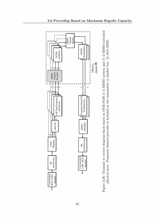
3.3 Precoding Based on Maximum Ergodic Capacity
OFD
Mde
mod
ulat
ion
MIM
O
dem
appe
r
Bit
inte
rleav
ing
Tim
e &
cel
lC
ell/T
ime/
Freq
uenc
yin
terle
aver
s
Freq
uenc
y/Ti
me/
Cel
lde
-inte
rleav
ers
Bit
de-in
terle
avin
g
Con
cate
nate
dB
CH
+LD
PCen
code
rs
Con
cate
nate
dLD
PC+B
CH
deco
ders
MIM
O
Cha
nnel
Mod
els
MIM
OC
hann
elPr
ecod
erO
FDM
mod
ulat
orx 1x 2x 3x 4 y 1 y 2
Effe
ctiv
ech
anne
l H
x p1
x p2
x p3
x p4
eSM
-PH
QA
MM
appi
ngs 1s 2
s p1s p2
s 3s 4
Fig
ure
3.26
:T
ran
smit
tore
ceiv
ed
iagr
amb
lock
bas
edon
DV
B-N
GH
2×
2M
IMO
syst
eman
d4×
2M
IMO
exte
nd
edp
hysi
cal
laye
r.P
rop
osed
chan
nel
-pre
cod
eris
incl
ud
edat
the
tran
smit
ter
insh
aded
box
.c ©
2015
IEE
E.
95
CHAPTER 3. MIMO PRECODING FOR TERRESTRIALBROADCAST SYSTEMS
The incoming bit stream is first encoded by the concatenation of a BCH andLDPC codes and passed through the bit-interleaver that, specifically for DVB-NGH MIMO, it was designed to exploit the quasi-cyclic structure of the LDPCcodes exhibiting low complexity, low latency, and fully parallel design easing theimplementation of iterative structures (cf. Appendix B). The interleaved codebits are then multiplexed into one data stream (layer) per transmit antennafollowing a Gray labelling. Subsequently, in the case of two transmit antennas,the modulated data streams are processed by the eSM-PH processing block (cf.subection 3.2.3). In Fig. 3.26 s1, s2, sp1, and sp2 are the input/output constel-lation symbols to the eSM-PH precoding where both transmit antennas havethe same power, i.e., PI=0. In case of four transmit antennas, the transmitterspatially multiplexes the four modulated data streams s1, s2, s3, s4 which arepassed directly to the cell interleaver operating at codeword level. The cellinterleaver applies a different pseudo-random permutation for every codewordto ensure a uniform distribution of the channel fading realizations. Then, thetime interleaver interlaces symbols from several codewords over various OFDMsymbols to provide protection against selective fading. After time interleaving,the frequency interleaver operates on an OFDM level and its function is two-fold. First it mixes up symbols from various services and secondly, it applies apseudo-random permutation to break the structured nature of the time inter-leaver output. Here, the proposed MIMO channel-precoder gives the option ofcombining the samples among transmit layers according to a specific channel-precoding matrix per OFDM carrier as in (3.12). Finally, before transmissionacross the cross-polarized antennas, the signal is passed from frequency to timedomain by IFFT operation plus guard interval insertion, which composes theOFDM modulator.
The channel models used are the NGH portable outdoor channel modeland the MGM channel model, which represent a portable outdoor and fixedrooftop reception environments. A detailed description of the channel modelsand its extension to four transmit antennas is presented in Appendix A of thisdissertation.
The signal distorted by the channel is received by two cross-polarized an-tennas. Referring to Fig. 3.26, the received streams are first processed by theOFDM demodulator, which essentially discards the guard interval and performsan FFT. In Fig. 3.26, this effective channel H is denoted by the dashed box.In this section perfect knowledge of CSI at the receiver side is also assumed.However, a practical receiver implementation estimates the channel responsefrom each transmit antenna with known orthogonal pilot signals sent multi-plexed with the data [101]. Therefore, the receiver needs to estimate four andeight channel responses for the 2×2 and 4×2 schemes, respectively3. The two
3Compared with SISO, the amount of pilot information has to be doubled and quadrupledfor 2×2 and 4×2 MIMO schemes, respectively. This amount of pilot information reduces
96
3.3 Precoding Based on Maximum Ergodic Capacity
received streams are then frequency, time and cell de-interleaved to undo thetransmitter operations and fed to the MIMO demodulator which provides softinformation about the transmitted code bits. It is noted that in the case of twotransmit antennas with eSM-PH, the MIMO demodulator takes into accounteSM-PH processing. LLRs for the transmitted code bits are calculated usingthe received data streams and CSI. Next, the LLRs are de-interleaved and pro-cessed by the LDPC decoder that runs several iterations of the sum-productalgorithm before outputting its decisions to the BCH decoder.
3.3.1 Design of MIMO-Channel-Precoders
MIMO-Channel-Precoder Based on Mean-Optimality
Now, a channel-precoder is derived with near-optimal performance in the con-sidered broadcast TV channel. This method is based on averaging per-channel-realization optimal covariance matrices. First, slightly abusing terminology, letH be a possible channel realization. For this specific channel realization, thesolution U matrix is given by the eigenvector matrix of H†H and the solutionΛ matrix is given by the following water-filling solution:
λk = max
(µ− σ2
dk, 0
), k=1, 2, . . . , Nt, (3.14)
where λk is the kth diagonal entry of Λ, dk is kth eigenvalue of H†H, σ2 is thenoise power, and the water-filling parameter µ is chosen such that λ1+λ2+. . .+λNt
= Nt. The mean-optimal covariance matrix is then obtained by averagingalong all per-channel optimal covariance matrices:
QMO = EUΛU†, (3.15)
where the statistical expectation is over all possible channel realizations. Theresulting MIMO-channel-precoder for the mean-optimal solution is given by
ΓMO = UMOΛ12
MO, (3.16)
where UMO and ΛMO are the eigenvector and eigenvalue matrices, respectively,of the mean-optimal covariance matrix QMO. The proposed algorithm has lowcomputational complexity and it is a simple tool to optimize the performance of
significantly the available spectral efficiency in mobile scenarios since denser patterns areneeded to sample the time-variant channel, e.g., 8, 3% and 16, 6% of pilots assumed for SISOand MIMO 2× 2 in DVB-NGH, respectively. This situation improves in static/portablereception (as the one studied in this section) where sparser pilot patterns can be supporteddue to time-invariability of the channel e.g.,1% for SISO DVB-T2 UK mode, 2% for 2×2MIMO, and 4% for 4×2 MIMO.
97
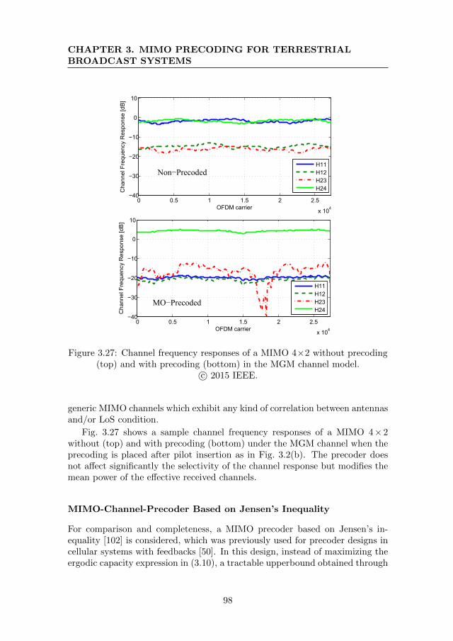
CHAPTER 3. MIMO PRECODING FOR TERRESTRIALBROADCAST SYSTEMS
0 0.5 1 1.5 2 2.5
x 104
−40
−30
−20
−10
0
10
OFDM carrier
Cha
nnel
Fre
quen
cy R
espo
nse
[dB]
H11H12H23H24
0 0.5 1 1.5 2 2.5
x 104
−40
−30
−20
−10
0
10
OFDM carrier
Cha
nnel
Fre
quen
cy R
espo
nse
[dB]
H11H12H23H24
Non−Precoded
MO−Precoded
Figure 3.27: Channel frequency responses of a MIMO 4×2 without precoding(top) and with precoding (bottom) in the MGM channel model.
c© 2015 IEEE.
generic MIMO channels which exhibit any kind of correlation between antennasand/or LoS condition.
Fig. 3.27 shows a sample channel frequency responses of a MIMO 4×2without (top) and with precoding (bottom) under the MGM channel when theprecoding is placed after pilot insertion as in Fig. 3.2(b). The precoder doesnot affect significantly the selectivity of the channel response but modifies themean power of the effective received channels.
MIMO-Channel-Precoder Based on Jensen’s Inequality
For comparison and completeness, a MIMO precoder based on Jensen’s in-equality [102] is considered, which was previously used for precoder designs incellular systems with feedbacks [50]. In this design, instead of maximizing theergodic capacity expression in (3.10), a tractable upperbound obtained through
98
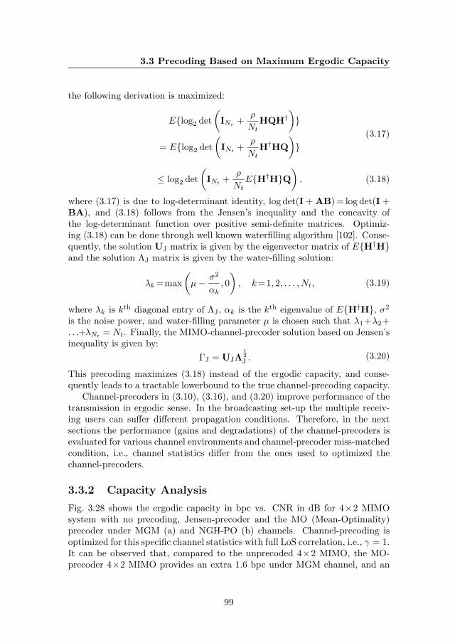
3.3 Precoding Based on Maximum Ergodic Capacity
the following derivation is maximized:
Elog2 det
(INr
+ρ
NtHQH†
)
= Elog2 det
(INt +
ρ
NtH†HQ
)
(3.17)
≤ log2 det
(INt
+ρ
NtEH†HQ
), (3.18)
where (3.17) is due to log-determinant identity, log det(I + AB) = log det(I +BA), and (3.18) follows from the Jensen’s inequality and the concavity ofthe log-determinant function over positive semi-definite matrices. Optimiz-ing (3.18) can be done through well known waterfilling algorithm [102]. Conse-quently, the solution UJ matrix is given by the eigenvector matrix of EH†Hand the solution ΛJ matrix is given by the water-filling solution:
λk=max
(µ− σ2
αk, 0
), k=1, 2, . . . , Nt, (3.19)
where λk is kth diagonal entry of ΛJ, αk is the kth eigenvalue of EH†H, σ2
is the noise power, and water-filling parameter µ is chosen such that λ1+λ2+. . .+λNt
= Nt. Finally, the MIMO-channel-precoder solution based on Jensen’sinequality is given by:
ΓJ = UJΛ12
J . (3.20)
This precoding maximizes (3.18) instead of the ergodic capacity, and conse-quently leads to a tractable lowerbound to the true channel-precoding capacity.
Channel-precoders in (3.10), (3.16), and (3.20) improve performance of thetransmission in ergodic sense. In the broadcasting set-up the multiple receiv-ing users can suffer different propagation conditions. Therefore, in the nextsections the performance (gains and degradations) of the channel-precoders isevaluated for various channel environments and channel-precoder miss-matchedcondition, i.e., channel statistics differ from the ones used to optimized thechannel-precoders.
3.3.2 Capacity Analysis
Fig. 3.28 shows the ergodic capacity in bpc vs. CNR in dB for 4×2 MIMOsystem with no precoding, Jensen-precoder and the MO (Mean-Optimality)precoder under MGM (a) and NGH-PO (b) channels. Channel-precoding isoptimized for this specific channel statistics with full LoS correlation, i.e., γ = 1.It can be observed that, compared to the unprecoded 4×2 MIMO, the MO-precoder 4×2 MIMO provides an extra 1.6 bpc under MGM channel, and an
99
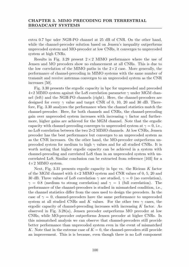
CHAPTER 3. MIMO PRECODING FOR TERRESTRIALBROADCAST SYSTEMS
extra 0.7 bpc uder NGH-PO channel at 25 dB of CNR. On the other hand,while the channel-precoder solution based on Jensen’s inequality outperformsunprecoded system and MO-precoder at low CNRs, it converges to unprecodedsystem at high CNRs.
Results in Fig. 3.29 present 2× 2 MIMO performance where the use ofJensen and MO precoders show no enhancement at all CNRs. This is due tothe low correlation of the MIMO paths in the 2×2 case. More generally, theperformance of channel-precoding in MIMO systems with the same number oftransmit and receive antennas converges to an unprecoded system as the CNRincreases [50].
Fig. 3.30 presents the ergodic capacity in bpc for unprecoded and precoded4×2 MIMO system against the LoS correlation parameter γ under MGM chan-nel (left) and the NGH-PO channels (right). Here, the channel-precoders aredesigned for every γ value and target CNR of 0, 10, 20 and 30 dB. There-fore, Fig. 3.30 analyzes the performance when the channel statistics match thechannel-precoder. Here, for both channels and CNRs, the channel-precodinggain over unprecoded system increases with increasing γ factor and further-more, higher gains are achieved for the MGM channel. Note that the ergodiccapacity with channel-precoding converges to unprecoded system at γ = 0, i.e.,no LoS correlation between the two 2×2 MIMO channels. At low CNRs, Jensenprecoder has the best performance but converges to an unprecoded system asas the CNR increases. On the other hand, the MO-precoder outperforms un-precoded system for medium to high γ values and for all studied CNRs. It isworth noting that higher ergodic capacity can be achieved in a system withchannel-precoding and correlated LoS than in an unprecoded system with un-correlated LoS. Similar conclusion can be extracted from reference [103] for a4×2 MIMO system.
Next, Fig. 3.31 presents ergodic capacity in bpc vs. the Riciean K factorof the MGM channel with 4×2 MIMO system and CNR values of 0, 5, 20 and30 dB. Three values of LoS correlation γ are studied, γ = 0 (no correlation),γ = 0.8 (medium to strong correlation) and γ = 1 (full correlation). Theperformance of the channel-precoders is studied in mismatched condition, i.e.,the channel statistics differ from the ones used to design the precoders. In thecase of γ = 0, channel-precoders have the same performance to unprecodedsystem at all studied CNRs and K values. For the other two γ cases, theergodic capacity of channel-precoding increases with increasing K factor. Asobserved in Fig. 3.28(a), Jensen precoder outperforms MO precoder at lowCNRs, while MO-precoder outperforms Jensen precoder at higher CNRs. Inthis mismatched analysis we can observe that channel-precoders still providebetter performance than unprecoded system even in the event of mismatchedK. Note that in the extreme case of K = 0, the channel-precoders still providean improvement. This is is because, even though there is no LoS component
100
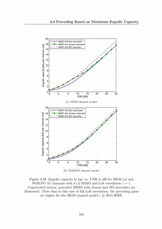
3.3 Precoding Based on Maximum Ergodic Capacity
−5 0 5 10 15 20 25 300
2
4
6
8
10
12
14
16
18
20
CNR [dB]
Ergo
dic
capa
city
[bits
per
cha
nnel
use
]
MIMO 4x2 Non−precodedMIMO 4x2 Jensen−precoderMIMO 4x2 MO−precoder
(a) MGM channel model.
−5 0 5 10 15 20 25 300
2
4
6
8
10
12
14
16
18
CNR [dB]
Ergo
dic
capa
city
[bits
per
cha
nnel
use
]
MIMO 4x2 Non−precodedMIMO 4x2 Jensen−precoderMIMO 4x2 MO−precoder
(b) NGH-PO channel model.
Figure 3.28: Ergodic capacity in bpc vs. CNR in dB for MGM (a) andNGH-PO (b) channels with 4×2 MIMO and LoS correlation γ = 1.
Unprecoded system, precoded MIMO with Jensen and MO precoders areillustrated. (Note that in this case of full LoS correlation, the precoding gains
are higher for the MGM channel model.) c© 2015 IEEE.
101
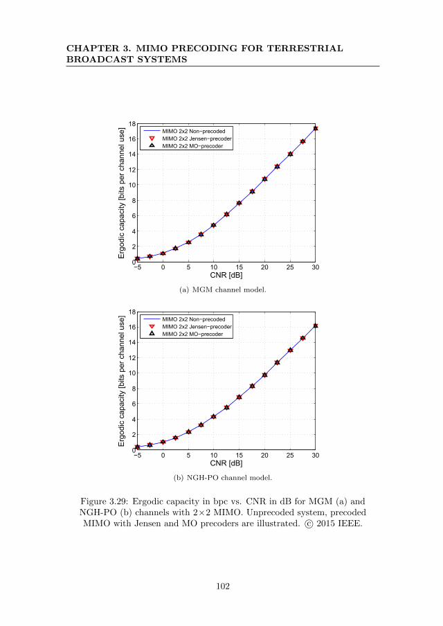
CHAPTER 3. MIMO PRECODING FOR TERRESTRIALBROADCAST SYSTEMS
−5 0 5 10 15 20 25 300
2
4
6
8
10
12
14
16
18
CNR [dB]
Ergo
dic
capa
city
[bits
per
cha
nnel
use
]
MIMO 2x2 Non−precodedMIMO 2x2 Jensen−precoderMIMO 2x2 MO−precoder
(a) MGM channel model.
−5 0 5 10 15 20 25 300
2
4
6
8
10
12
14
16
18
CNR [dB]
Ergo
dic
capa
city
[bits
per
cha
nnel
use
]
MIMO 2x2 Non−precodedMIMO 2x2 Jensen−precoderMIMO 2x2 MO−precoder
(b) NGH-PO channel model.
Figure 3.29: Ergodic capacity in bpc vs. CNR in dB for MGM (a) andNGH-PO (b) channels with 2×2 MIMO. Unprecoded system, precodedMIMO with Jensen and MO precoders are illustrated. c© 2015 IEEE.
102
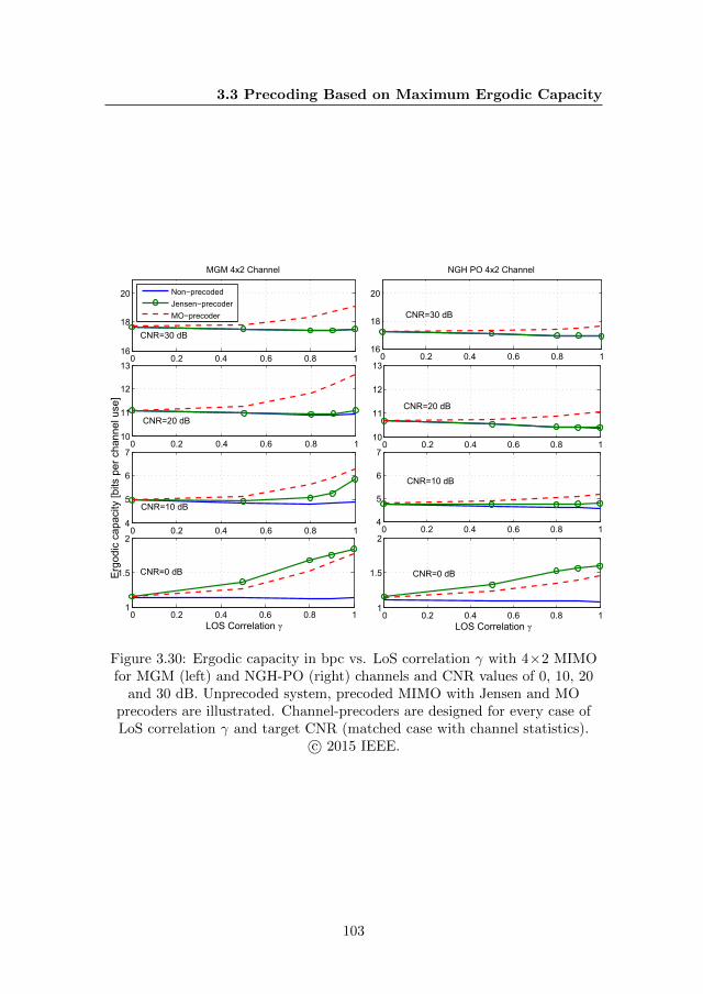
3.3 Precoding Based on Maximum Ergodic Capacity
0 0.2 0.4 0.6 0.8 116
18
20
MGM 4x2 Channel
0 0.2 0.4 0.6 0.8 116
18
20
NGH PO 4x2 Channel
0 0.2 0.4 0.6 0.8 110
11
12
13
0 0.2 0.4 0.6 0.8 110
11
12
13
0 0.2 0.4 0.6 0.8 14
5
6
7
Ergo
dic
capa
city
[bits
per
cha
nnel
use
]
0 0.2 0.4 0.6 0.8 14
5
6
7
0 0.2 0.4 0.6 0.8 11
1.5
2
LOS Correlation γ0 0.2 0.4 0.6 0.8 1
1
1.5
2
LOS Correlation γ
Non−precodedJensen−precoderMO−precoder
CNR=30 dB
CNR=20 dB
CNR=10 dB
CNR=0 dB
CNR=10 dB
CNR=0 dB
CNR=30 dB
CNR=20 dB
Figure 3.30: Ergodic capacity in bpc vs. LoS correlation γ with 4×2 MIMOfor MGM (left) and NGH-PO (right) channels and CNR values of 0, 10, 20
and 30 dB. Unprecoded system, precoded MIMO with Jensen and MOprecoders are illustrated. Channel-precoders are designed for every case ofLoS correlation γ and target CNR (matched case with channel statistics).
c© 2015 IEEE.
103
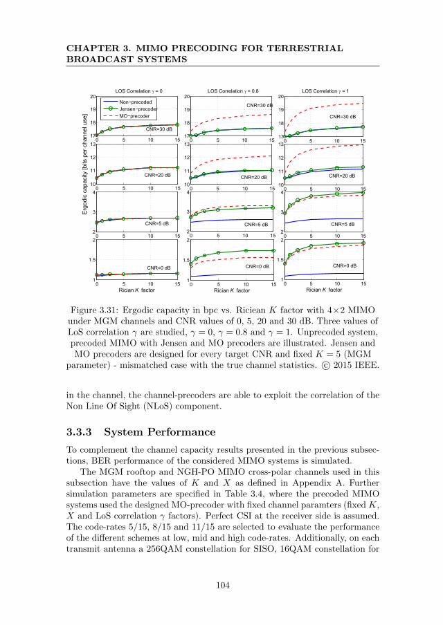
CHAPTER 3. MIMO PRECODING FOR TERRESTRIALBROADCAST SYSTEMS
0 5 10 1517
18
19
20LOS Correlation γ = 0
0 5 10 1517
18
19
20LOS Correlation γ = 0.8
0 5 10 1517
18
19
20LOS Correlation γ = 1
0 5 10 1510
11
12
13
Ergo
dic
capa
city
[bits
per
cha
nnel
use
]
0 5 10 1510
11
12
13
0 5 10 1510
11
12
13
0 5 10 152
3
4
0 5 10 152
3
4
0 5 10 152
3
4
0 5 10 151
1.5
2
Rician K factor0 5 10 15
1
1.5
2
Rician K factor0 5 10 15
1
1.5
2
Rician K factor
Non−precodedJensen−precoderMO−precoder
CNR=20 dBCNR=20 dB
CNR=0 dB CNR=0 dB CNR=0 dB
CNR=30 dB
CNR=30 dB
CNR=30 dB
CNR=20 dB
CNR=5 dB CNR=5 dB CNR=5 dB
Figure 3.31: Ergodic capacity in bpc vs. Riciean K factor with 4×2 MIMOunder MGM channels and CNR values of 0, 5, 20 and 30 dB. Three values ofLoS correlation γ are studied, γ = 0, γ = 0.8 and γ = 1. Unprecoded system,precoded MIMO with Jensen and MO precoders are illustrated. Jensen andMO precoders are designed for every target CNR and fixed K = 5 (MGM
parameter) - mismatched case with the true channel statistics. c© 2015 IEEE.
in the channel, the channel-precoders are able to exploit the correlation of theNon Line Of Sight (NLoS) component.
3.3.3 System Performance
To complement the channel capacity results presented in the previous subsec-tions, BER performance of the considered MIMO systems is simulated.
The MGM rooftop and NGH-PO MIMO cross-polar channels used in thissubsection have the values of K and X as defined in Appendix A. Furthersimulation parameters are specified in Table 3.4, where the precoded MIMOsystems used the designed MO-precoder with fixed channel paramters (fixed K,X and LoS correlation γ factors). Perfect CSI at the receiver side is assumed.The code-rates 5/15, 8/15 and 11/15 are selected to evaluate the performanceof the different schemes at low, mid and high code-rates. Additionally, on eachtransmit antenna a 256QAM constellation for SISO, 16QAM constellation for
104
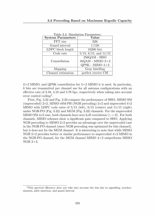
3.3 Precoding Based on Maximum Ergodic Capacity
Table 3.4: Simulation Parameters.System Parameters Value
FFT size 32KGuard interval 1/128
LDPC block length 16200 bitsCode rate 5/15, 8/15, and 11/15
256QAM - SISOConstellation 16QAM - MIMO 2×2
QPSK - MIMO 4×2Mapping Gray labelling
Channel estimation perfect receive CSI
2×2 MIMO, and QPSK constellation for 4×2 MIMO it is used. In particular,8 bits are transmitted per channel use for all antenna configurations with aneffective rate of 2.58, 4.18 and 5.78 bpc, respectively when taking into accounterror control coding4.
First, Fig. 3.32 and Fig. 3.33 compare the performance of SISO, MIMO SM(unprecoded) 2×2, MIMO eSM-PH (NGH precoding) 2×2 and unprecoded 4×2MIMO with LDPC code rates of 5/15 (left), 8/15 (center) and 11/15 (right)under NGH-PO (Fig. 3.32) and MGM (Fig. 3.33) channels. For the unprecodedMIMO SM 4×2 case, both channels have zero LoS correlation (γ = 0). For bothchannels, MIMO schemes show a significant gain compared to SISO. ApplyingNGH precoding to MIMO 2×2 provides an advantage over the unprecoded casein the NGH-PO channel (since NGH precoding was optimized for this channel),but it does not for the MGM channel. It is interesting to note that while MIMONGH 2×2 provides better or similar performance to unprecoded 4×2 MIMO inthe NGH-PO channel, for the MGM channel MIMO 4×2 outperforms MIMONGH 2×2.
4This spectral efficiency does not take into account the loss due to signalling, synchro-nization, pilot insertion, and guard interval.
105
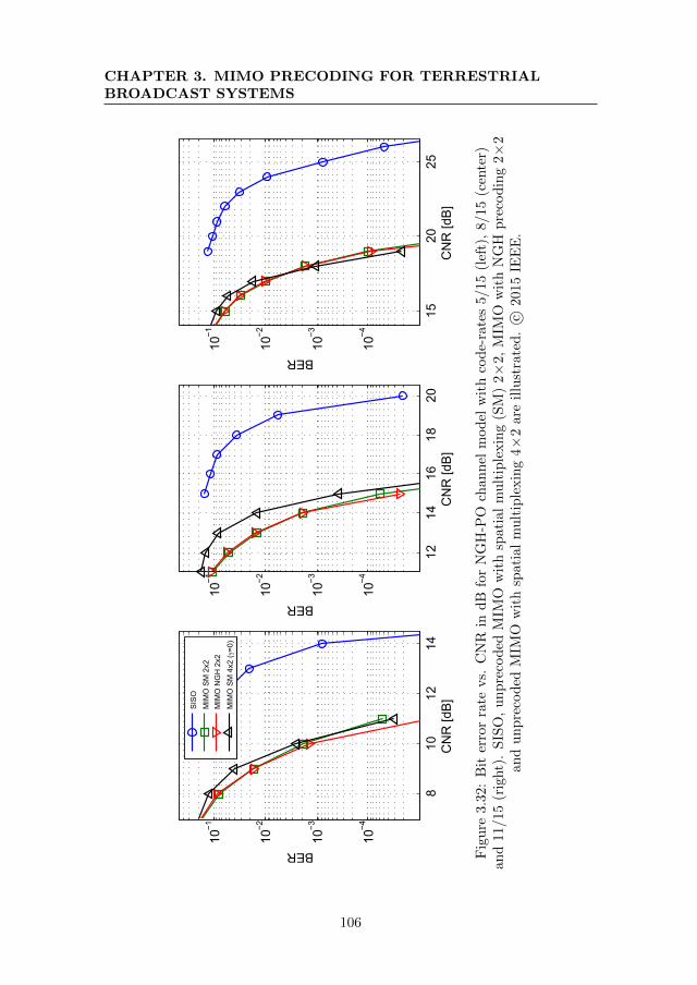
CHAPTER 3. MIMO PRECODING FOR TERRESTRIALBROADCAST SYSTEMS
810
1214
10−4
10−3
10−2
10−1
CN
R [d
B]
BER
1214
1618
20
10−4
10−3
10−2
10−1
CN
R [d
B]
BER
1520
25
10−4
10−3
10−2
10−1
CN
R [d
B]
BER
SISO
MIM
O S
M 2
x2M
IMO
NG
H 2
x2M
IMO
SM
4x2
(γ=0
)
Fig
ure
3.32
:B
iter
ror
rate
vs.
CN
Rin
dB
for
NG
H-P
Och
ann
elm
od
elw
ith
cod
e-ra
tes
5/15
(lef
t),
8/15
(cen
ter)
and
11/1
5(r
ight)
.S
ISO
,u
np
reco
ded
MIM
Ow
ith
spat
ial
mu
ltip
lexin
g(S
M)
2×
2,M
IMO
wit
hN
GH
pre
cod
ing
2×
2an
du
np
reco
ded
MIM
Ow
ith
spat
ial
mu
ltip
lexin
g4×
2ar
eil
lust
rate
d.
c ©20
15IE
EE
.
106
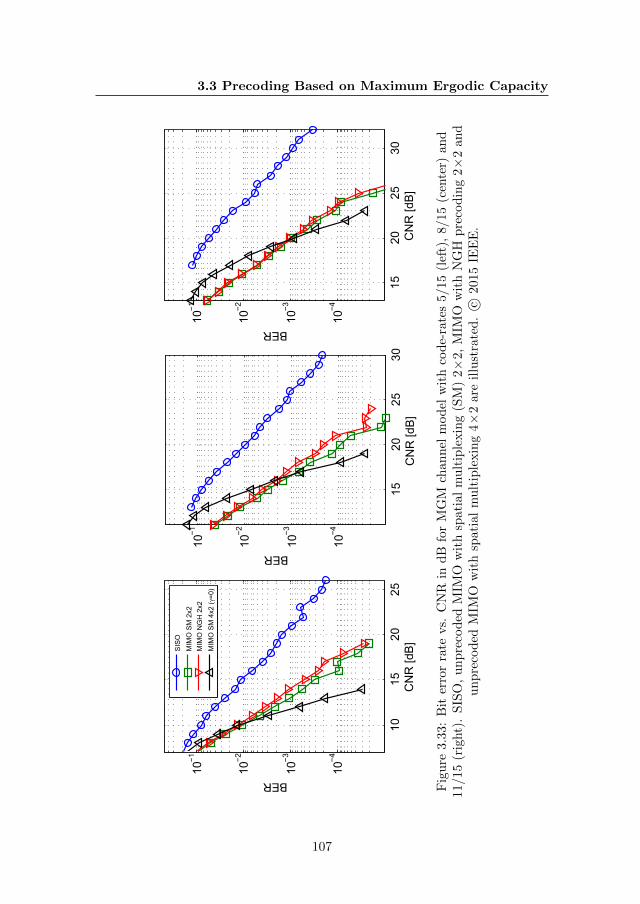
3.3 Precoding Based on Maximum Ergodic Capacity
1015
2025
10−4
10−3
10−2
10−1
CN
R [d
B]
BER
1520
2530
10−4
10−3
10−2
10−1
CN
R [d
B]
BER
1520
2530
10−4
10−3
10−2
10−1
CN
R [d
B]
BER
SISO
MIM
O S
M 2
x2M
IMO
NG
H 2
x2M
IMO
SM
4x2
(γ=0
)
Fig
ure
3.33
:B
iter
ror
rate
vs.
CN
Rin
dB
for
MG
Mch
ann
elm
od
elw
ith
cod
e-ra
tes
5/15
(lef
t),
8/15
(cen
ter)
an
d11
/15
(rig
ht)
.S
ISO
,un
pre
cod
edM
IMO
wit
hsp
atia
lm
ult
iple
xin
g(S
M)
2×
2,M
IMO
wit
hN
GH
pre
cod
ing
2×
2an
du
np
reco
ded
MIM
Ow
ith
spat
ial
mu
ltip
lexin
g4×
2ar
eil
lust
rate
d.
c ©20
15IE
EE
.
107
CHAPTER 3. MIMO PRECODING FOR TERRESTRIALBROADCAST SYSTEMS
Here, Fig. 3.34 investigates the unprecoded 4×2 MIMO performance degra-dation due to LoS correlation under MGM (top) and NGH-PO (bottom) chan-nels . One can observe that the performance degrades with increasing γ factorfor both channels. However, this degradation is higher in the MGM channel.
Fig. 3.35 and Fig. 3.36 compares the performance of 4×2 MIMO with theMO-precoder and the unprecoded case in the NGH-PO and MGM channels,respectively. LoS correlation values γ = 0.8 and γ = 1.0 are included. Inboth channels one can observe that MO-precoding provides improved or similarperformance to unprecoded system at code rate 5/15 but incurs in an increasingperformance degradation with increasing code rate.
To explain the performance dependence with the code rate of the MO-precoding, Fig. 3.37 presents the pdf of the LLR values at the output of theMIMO demodulator for a MIMO 4×2 with and without MO-precoding un-der the MGM channel model with 15 dB (top) and 25 dB (bottom). First,it can be observed that MO-precoding affects the distribution of LLR values.With precoding, the LLRs take, with high probability, either small (i.e., lowbit reliability) or high absolute values (i.e., high bit reliability). Without pre-coding the LLR values are more uniformly distributed. The strong reliabilityfor some of the LLR values with precoding can be connected with the im-proved performance at low code-rates. When channel coding is used, previousworks in [104, 63] have shown that while diversity techniques improve perfor-mance at high code-rates, they can degrade the performance at low code-rates.MO-precoding reduces the diversity of the LLR values in favour of enhancingthe reliability of some of the transmitted bits, which can be exploited by thediversity of the channel code at low code-rates.
Finally, in Fig. 3.38 the performance of MO-precoder 4×2 MIMO is analysedin the case of mismatch condition with a K factor, where the precoder statisticsand true channel statistics differ. This is common situation in the broadcastingset-up, since different users can experience channels with different receptionconditions and therefore different channel statistics. Here, the gain is comparedover unprecoded 4×2 MIMO in the NGH-PO channel with two values of γ equalto 0.8 and 1.0. The performance of code rate 5/15 is studied since higher onesprovided poor performance for channel-precoding. The gain increases for bothvalues of γ with increasing K factor. It is interesting to note that for this lowcode-rate even in the extreme case of K = 0 (where there is no LoS component)the channel-precoder still provides a gain of about 0.5 dB. This is because theprecoder is still able to exploit the covariance matrix of the NLoS componentswhich also has some degree of correlation (cf. Appendix A).
108
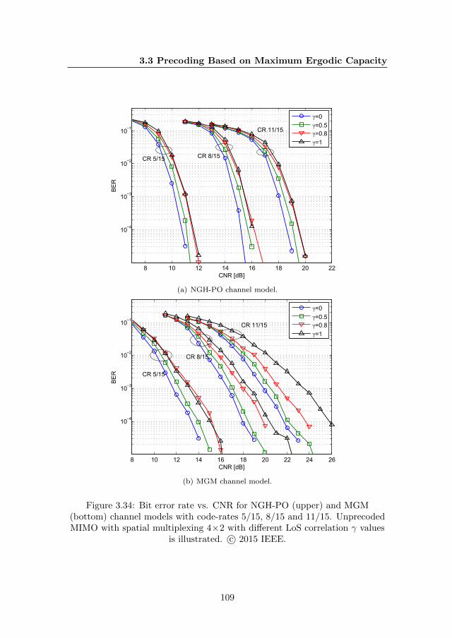
3.3 Precoding Based on Maximum Ergodic Capacity
8 10 12 14 16 18 20 22
10−4
10−3
10−2
10−1
CNR [dB]
BER
γ=0γ=0.5γ=0.8γ=1
CR 11/15
CR 8/15CR 5/15
(a) NGH-PO channel model.
8 10 12 14 16 18 20 22 24 26
10−4
10−3
10−2
10−1
CNR [dB]
BER
γ=0γ=0.5γ=0.8γ=1
CR 5/15
CR 8/15
CR 11/15
(b) MGM channel model.
Figure 3.34: Bit error rate vs. CNR for NGH-PO (upper) and MGM(bottom) channel models with code-rates 5/15, 8/15 and 11/15. UnprecodedMIMO with spatial multiplexing 4×2 with different LoS correlation γ values
is illustrated. c© 2015 IEEE.
109
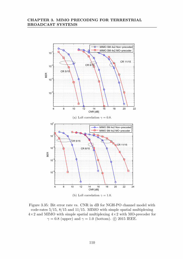
CHAPTER 3. MIMO PRECODING FOR TERRESTRIALBROADCAST SYSTEMS
6 8 10 12 14 16 18 20 22
10−4
10−3
10−2
10−1
CNR [dB]
BER
MIMO SM 4x2 Non−precodedMIMO SM 4x2 MO−precoder
CR 5/15
CR 11/15CR 8/15
(a) LoS correlation γ = 0.8.
6 8 10 12 14 16 18 20 22 24
10−4
10−3
10−2
10−1
100
CNR [dB]
BER
MIMO SM 4x2 Non−precodedMIMO SM 4x2 MO−precoder
CR 11/15CR 8/15
CR 5/15
(b) LoS correlation γ = 1.0.
Figure 3.35: Bit error rate vs. CNR in dB for NGH-PO channel model withcode-rates 5/15, 8/15 and 11/15. MIMO with simple spatial multiplexing
4×2 and MIMO with simple spatial multiplexing 4×2 with MO-precoder forγ = 0.8 (upper) and γ = 1.0 (bottom). c© 2015 IEEE.
110
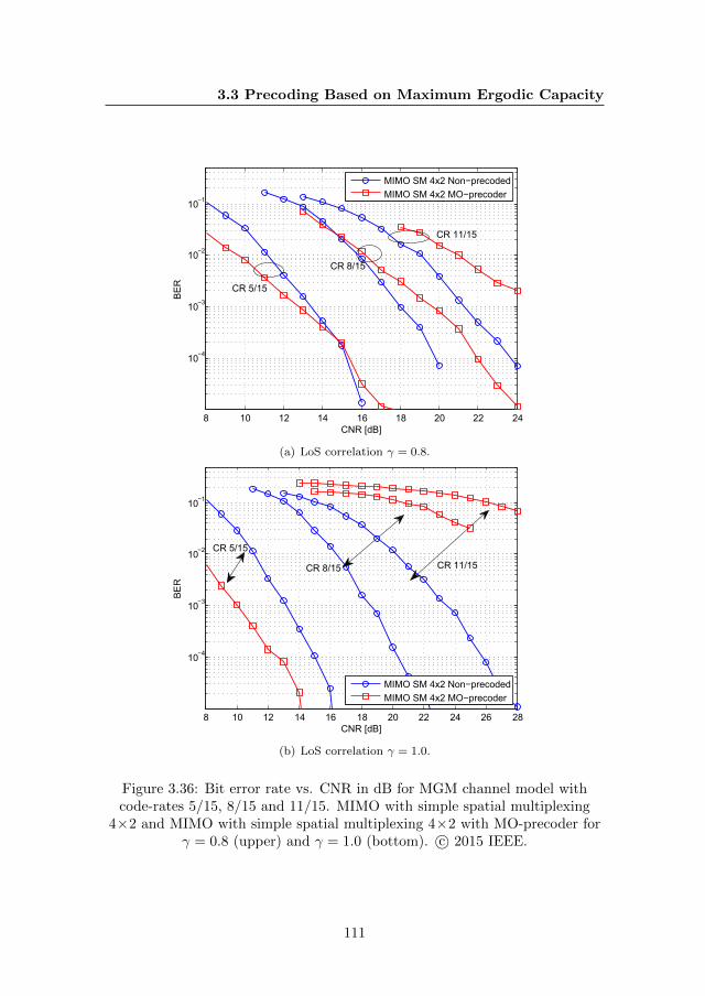
3.3 Precoding Based on Maximum Ergodic Capacity
8 10 12 14 16 18 20 22 24
10−4
10−3
10−2
10−1
CNR [dB]
BER
MIMO SM 4x2 Non−precodedMIMO SM 4x2 MO−precoder
CR 5/15
CR 8/15
CR 11/15
(a) LoS correlation γ = 0.8.
8 10 12 14 16 18 20 22 24 26 28
10−4
10−3
10−2
10−1
CNR [dB]
BER
MIMO SM 4x2 Non−precodedMIMO SM 4x2 MO−precoder
CR 5/15
CR 8/15 CR 11/15
(b) LoS correlation γ = 1.0.
Figure 3.36: Bit error rate vs. CNR in dB for MGM channel model withcode-rates 5/15, 8/15 and 11/15. MIMO with simple spatial multiplexing
4×2 and MIMO with simple spatial multiplexing 4×2 with MO-precoder forγ = 0.8 (upper) and γ = 1.0 (bottom). c© 2015 IEEE.
111
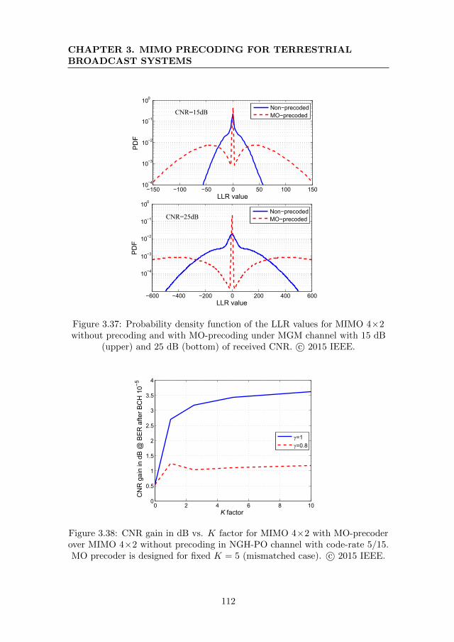
CHAPTER 3. MIMO PRECODING FOR TERRESTRIALBROADCAST SYSTEMS
−150 −100 −50 0 50 100 15010−4
10−3
10−2
10−1
100
LLR value
Non−precodedMO−precoded
−600 −400 −200 0 200 400 600
10−4
10−3
10−2
10−1
100
LLR value
Non−precodedMO−precoded
CNR=15dB
CNR=25dB
Figure 3.37: Probability density function of the LLR values for MIMO 4×2without precoding and with MO-precoding under MGM channel with 15 dB
(upper) and 25 dB (bottom) of received CNR. c© 2015 IEEE.
0 2 4 6 8 100
0.5
1
1.5
2
2.5
3
3.5
4
K factor
CN
R g
ain
in d
B @
BER
afte
r BC
H 1
0−5
γ=1γ=0.8
Figure 3.38: CNR gain in dB vs. K factor for MIMO 4×2 with MO-precoderover MIMO 4×2 without precoding in NGH-PO channel with code-rate 5/15.MO precoder is designed for fixed K = 5 (mismatched case). c© 2015 IEEE.
112
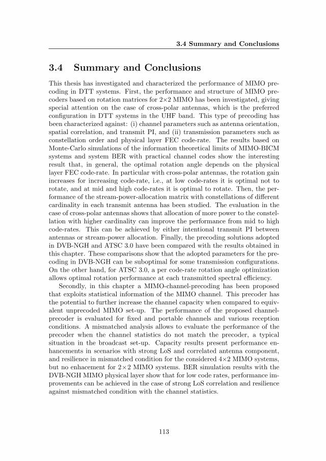
3.4 Summary and Conclusions
3.4 Summary and Conclusions
This thesis has investigated and characterized the performance of MIMO pre-coding in DTT systems. First, the performance and structure of MIMO pre-coders based on rotation matrices for 2×2 MIMO has been investigated, givingspecial attention on the case of cross-polar antennas, which is the preferredconfiguration in DTT systems in the UHF band. This type of precoding hasbeen characterized against: (i) channel parameters such as antenna orientation,spatial correlation, and transmit PI, and (ii) transmission parameters such asconstellation order and physical layer FEC code-rate. The results based onMonte-Carlo simulations of the information theoretical limits of MIMO-BICMsystems and system BER with practical channel codes show the interestingresult that, in general, the optimal rotation angle depends on the physicallayer FEC code-rate. In particular with cross-polar antennas, the rotation gainincreases for increasing code-rate, i.e., at low code-rates it is optimal not torotate, and at mid and high code-rates it is optimal to rotate. Then, the per-formance of the stream-power-allocation matrix with constellations of differentcardinality in each transmit antenna has been studied. The evaluation in thecase of cross-polar antennas shows that allocation of more power to the constel-lation with higher cardinality can improve the performance from mid to highcode-rates. This can be achieved by either intentional transmit PI betweenantennas or stream-power allocation. Finally, the precoding solutions adoptedin DVB-NGH and ATSC 3.0 have been compared with the results obtained inthis chapter. These comparisons show that the adopted parameters for the pre-coding in DVB-NGH can be suboptimal for some transmission configurations.On the other hand, for ATSC 3.0, a per code-rate rotation angle optimizationallows optimal rotation performance at each transmitted spectral efficiency.
Secondly, in this chapter a MIMO-channel-precoding has been proposedthat exploits statistical information of the MIMO channel. This precoder hasthe potential to further increase the channel capacity when compared to equiv-alent unprecoded MIMO set-up. The performance of the proposed channel-precoder is evaluated for fixed and portable channels and various receptionconditions. A mismatched analysis allows to evaluate the performance of theprecoder when the channel statistics do not match the precoder, a typicalsituation in the broadcast set-up. Capacity results present performance en-hancements in scenarios with strong LoS and correlated antenna component,and resilience in mismatched condition for the considered 4×2 MIMO systems,but no enhacement for 2×2 MIMO systems. BER simulation results with theDVB-NGH MIMO physical layer show that for low code rates, performance im-provements can be achieved in the case of strong LoS correlation and resilienceagainst mismatched condition with the channel statistics.
113

CHAPTER 3. MIMO PRECODING FOR TERRESTRIALBROADCAST SYSTEMS
114
Chapter 4
Receiver Memory andPerformance Trade-Off ofSoft-Quantized Information
The previous chapter assumed perfect reception conditions such as op-timal demodulators and infinite-precision number representations. How-
ever, due to complexity constraints and finite-precision arithmetic, it is crucialfor the overall system performance to carefully design receiver algorithms. Thischapter investigates memory and performance trade-offs of soft-quantized in-formation in MIMO-BICM receivers. DTT systems, such as DVB-NGH, relyon TI techniques to overcome signal fluctuations and improve the system per-formance by time-diversity gain. Yet, long TI imposes the highest in-chipmemory requirements at the receiver, which depends on the quantization res-olution and specific algorithms. Two types of quantized receivers are investi-gated: quantization of I&Q samples and quantization of log-likelihood ratios.The implications on the in-chip memory and the possibility of implementingMIMO-BICM with iterative decoding are presented and discussed. Addition-ally, the performance degradations of uniform quantization and non-uniformquantization algorithms is evaluated showing significant potential benefits fornon-uniform quantization adapted to the signal statistics. The results obtainedin this chapter highlight the important trade-off between in-chip memory andperformance for quantized receiver architectures.
115
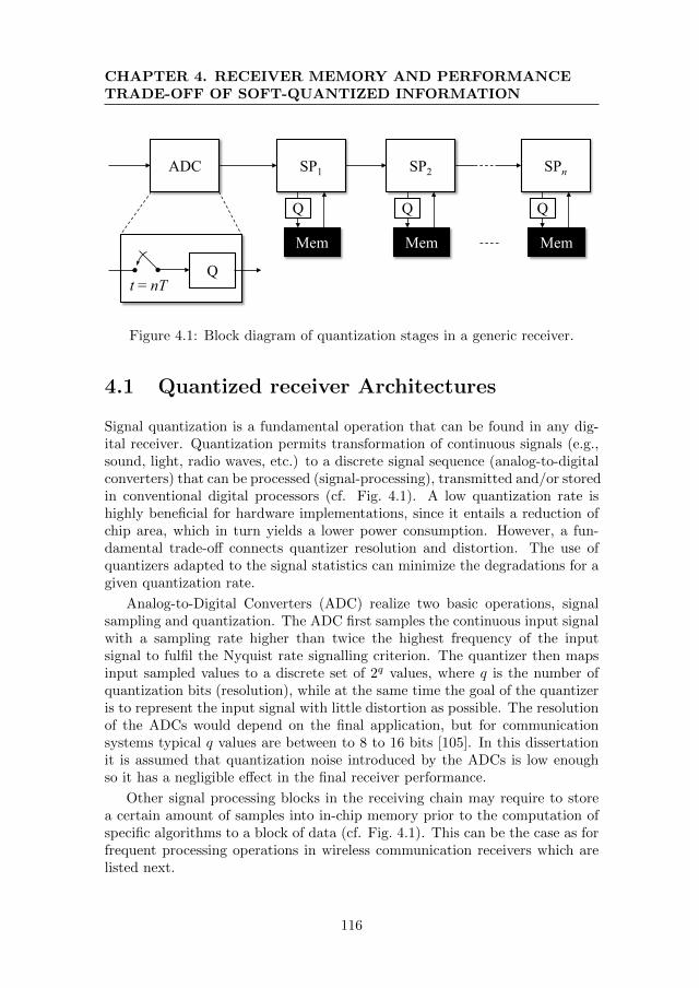
CHAPTER 4. RECEIVER MEMORY AND PERFORMANCETRADE-OFF OF SOFT-QUANTIZED INFORMATION
ADC SP1
Mem
SP2
Mem
SPn
Mem
Qt = nT
Q Q Q
Figure 4.1: Block diagram of quantization stages in a generic receiver.
4.1 Quantized receiver Architectures
Signal quantization is a fundamental operation that can be found in any dig-ital receiver. Quantization permits transformation of continuous signals (e.g.,sound, light, radio waves, etc.) to a discrete signal sequence (analog-to-digitalconverters) that can be processed (signal-processing), transmitted and/or storedin conventional digital processors (cf. Fig. 4.1). A low quantization rate ishighly beneficial for hardware implementations, since it entails a reduction ofchip area, which in turn yields a lower power consumption. However, a fun-damental trade-off connects quantizer resolution and distortion. The use ofquantizers adapted to the signal statistics can minimize the degradations for agiven quantization rate.
Analog-to-Digital Converters (ADC) realize two basic operations, signalsampling and quantization. The ADC first samples the continuous input signalwith a sampling rate higher than twice the highest frequency of the inputsignal to fulfil the Nyquist rate signalling criterion. The quantizer then mapsinput sampled values to a discrete set of 2q values, where q is the number ofquantization bits (resolution), while at the same time the goal of the quantizeris to represent the input signal with little distortion as possible. The resolutionof the ADCs would depend on the final application, but for communicationsystems typical q values are between to 8 to 16 bits [105]. In this dissertationit is assumed that quantization noise introduced by the ADCs is low enoughso it has a negligible effect in the final receiver performance.
Other signal processing blocks in the receiving chain may require to storea certain amount of samples into in-chip memory prior to the computation ofspecific algorithms to a block of data (cf. Fig. 4.1). This can be the case as forfrequent processing operations in wireless communication receivers which arelisted next.
116
4.1 Quantized receiver Architectures
FFT operation The FFT processing requires the storage of N samples priorto the FFT operation. The value of N depends on the application, but for DTTsystems N takes values from 1024 (1K) to 32768 (32K) samples.
Channel estimation Prior to the estimation of the CSI in the data carriers,the receiver requires the storage of pilot information in frequency and timedomain in doubly selective channels. For instance, in DTT systems such asDVB-T2, DVB-NGH and ATSC 3.0, pilot signals are sent multiplexed withthe data in a comb-type pilot arrangement. In particular, [45] recommends,for a DVB-T2 system, the storage of two and four OFDM symbols to performtemporal interpolation for FFT sizes of 32K and 16K, respectively.
Interleaving stages Frequency, cell, time and bit de-interleaving stages alsorequire the storage of sampled data before the permutation to the block ofreceived data can be applied. Taking as an use case the receiving chain ofDVB-NGH, the storage requirements for the different de-interleaving stagesare:
• Frequency de-interleaving : one OFDM symbol where the number of sam-ples depend on the FFT size.
• Cell de-interleaving : one FEC code-word, where the number of samplesdepend on the FEC block size (e.g., 16200 or 64800 bits) and the cardinal-ity of the constellation, e.g., 4050 samples with 16200 bits FEC code-wordsize and 4 bpc.
• Bit de-interleaving : one FEC code-word, where the number of samplesdepend on the FEC block size, e.g., 16200 or 64800 bits.
• Time de-interleaving : multiple FEC code-words where the number ofsamples depend on the TI depth at the transmitter and the antennaconfiguration. For instance, in the SISO profile of DVB-NGH the numberof cells to be stored at the receiver are 524288 cells (for the data andCSI paths). Furthermore, the memory requirements can increase for theMIMO case as it will be discussed in this chapter.
It is important to note that the final amount of memory in bits requiredto store the samples of the previous processing blocks directly depends on theresolution of the quantization algorithms. From the previous requirements, itcan be clearly seen that Time de-Interleaving (TDI) in DTT systems is thestage with the highest memory requirements [45]. Hence, the study of in-chip memory and performance trade-off of practical receiver architectures withquantized signals is highly motivated.
117
CHAPTER 4. RECEIVER MEMORY AND PERFORMANCETRADE-OFF OF SOFT-QUANTIZED INFORMATION
Figures 4.2 and 4.3 present simplified transmit to receive communicationchains where the receivers implement, at different parts of the receiving chain,signal quantization to store received information at the TDI memory. At thetransmitter, first the information bits are encoded by the LDPC and BCHcodes. Then, the encoded bits are bit-interleaved (cl) and fed to the con-stellation mapper, which outputs constellation symbols. Finally, the outputconstellation symbols are time-interleaved and transmitted through the chan-nel.
The architecture in Fig. 4.2 first needs to store the received (distorted) con-stellation symbols and the channel estimates in order to perform TDI. Beforestoring into the TDI memory, the in-phase (I) and quadrature (Q) componentsof the received signals y and the channel estimates H are quantized. Thequantizer uses the algorithms described in section 4.2.1. Prior to the TDI op-eration, the quantized symbols are stored until the entire TDI memory is filled.Then, the demapper can use the quantized symbols yq and quantized chan-nel estimates Hq to produce LLRs. (In this chapter the MAP demapper withthe max-log approximation is employed cf. Chapter 2.) The output LLRs arebit de-interleaved and passed to the LDPC decoder which performs multipleoperations of the max-sum algorithm. With iterative MIMO demapping, thesoft-ouput information of the LDPC decoder is passed back to the demapperthrough a bit-interleaving to output refined soft-decisions.
The architecture in Fig. 4.3 realizes the quantization in a different point ofthe receiver chain. With this architecture the demapping and TDI positionsare exchanged, i.e., demapper is executed before the TDI. If the TDI block de-interleaves groups of LLRs corresponding to the received symbols and channelestimates, there is no effect in the performance [52]. It is assumed that thedemapper operates with full resolution. This assumption is reasonable sinceonly the received symbols from each antenna (i.e., y1 and y2) and channelestimates (h11, h12, h21 and h22) from a single channel realization need to bestored with full resolution. The ouput LLRs (Λl) at the demapper are quantized(dl) prior to storage to the TDI. This approach is also described in [52]. Oncethe TDI is filled, the groups of LLRs are de-interleaved and passed to the bit de-interleaving which are finally fed to the LDPC decoder. With this architecture,iterative decoding of the MIMO-BICM receiving chain is not possible. This isbecause for performing iterative decoding of the MIMO-BICM, the receiverneeds access to previous instances of y and H, which are not available withthis structure.
118
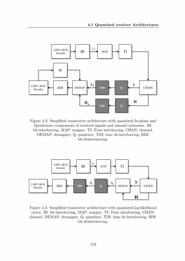
4.1 Quantized receiver Architectures
LDPC+BCHEncoder BI MAP TI
CHANBDI DEMAP TDILDPC+BCHDecoder Q
QTDI
y
H
yq
Hq
BI
cl
Figure 4.2: Simplified transceiver architecture with quantized In-phase andQuadrature components of received signals and channel estimates. BI:bit-interleaving, MAP: mapper, TI: Time interleaving, CHAN: channel,
DEMAP: demapper, Q: quantizer, TDI: time de-interleaving, BDI:bit-deinterleaving.
LDPC+BCHEncoder BI MAP TI
CHANBDI TDILDPC+BCHDecoder Q DEMAP
y
H
Λl
cl
dl
Figure 4.3: Simplified transceiver architecture with quantized log-likelihoodratios. BI: bit-interleaving, MAP: mapper, TI: Time interleaving, CHAN:
channel, DEMAP: demapper, Q: quantizer, TDI: time de-interleaving, BDI:bit-deinterleaving.
119
CHAPTER 4. RECEIVER MEMORY AND PERFORMANCETRADE-OFF OF SOFT-QUANTIZED INFORMATION
4.2 Quantization Algorithms
4.2.1 Quantization of I&Q Signal Components
For the receiver structure in Fig. 4.2 the signal components y and H need tobe quantized. This chapter considers only scalar quantization, hence, the I andQ components of each of the elements of the vector y (i.e., y1 and y2) and thematrix H (i.e., h11, h12, h21 and h22) are quantized independently.
Uniform quantization
With uniform quantization of I&Q components it is assumed that the receivercan adapt the maximum quantization range to the received signal. In particularthis is done in this chapter by measuring the maximum range of the signal forevery received frame. This is clearly an idealization since in a practical receiverdesign, the signal dynamic range should be decided beforehand to computea static set of quantizer reproducers and boundaries. This assumption willprovide optimistic results for the uniform quantization of I&Q components.The information of the maximum signal range could be limited in practiceby the dynamic range of the ADC which could be used for the design of theuniform quantizer.
Non-Uniform quantization: Lloyd-Max Algorithm
For non-uniform quantization of I&Q components, the Lloyd-Max algorithm [106,107] is selected and the main steps of the algorithm are presented next.
The Lloyd-Max algorithm finds the quantizer reproducers and boundariesthat minimizes the MSE between the input y and the quantized output z, i.e.,E(y − z)2. The MSE associated with the quantizer Q can be expressed as:
MSE = E(y − z)2 =
∫Y
(y −Q(y))2p(y) dy, (4.1)
which can expressed with respect to the quantization regions (cf. Chapter 2)as:
MSE =n∑i=1
∫Yi
(y − zi)2p(y) dy, (4.2)
where log2 n = q.
For the optimization of the quantizer boundaries and reproducers with theLloyd-Max algorithm, two necessary conditions are defined (assuming n repro-ducer values and known p(y):
120
4.2 Quantization Algorithms
1. For fixed reproducer values, the quantizer boundary bi between regionsYi and Yi+1 that minimizes the MSE is the point equidistant to thequantization reproducers zi and zi+1, i.e.,
bi =zi + zi+1
2, i = 1, . . . , n− 1. (4.3)
2. For fixed quantizer boundaries, the optimal reproducers are the centroidsat each quantization region:
zi =
∫ bi
bi−1
yp(y) dy∫ bi
bi−1
p(y) dy
, i = 1, . . . , n. (4.4)
The Lloyd-Max algorithm starts with an arbitrary initial set of n quantizerreproducers and then executes equations (4.3) and (4.4) until the additionalimprovement over the MSE minimization is lower than a predefined threshold,or the a maximum number of iterations has been reached.
Figure 4.4 shows the pdf of the I component of the received symbol at thefirst received antenna for a received CNR of 11.25 dB. This figure also showsthe quantizer reproducers and boundaries with non-uniform distribution usingthe Lloyd-Max algorithm. As we can observe, a more dense sampling is doneat the center of the pdf where it has the highest density. It is interesting tonote that the resulting pdf has Gaussian like distribution. It was confirmedwith simulations that very similar performance is obtained by using either themeasured pdf or a Gaussian approximation for the design of the quantizer withthe Lloyd-Max algorithm. In the following evaluations, the measured pdfs inthe selected environments are used for the design of the quantizers with theLloyd-Max algorithm.
4.2.2 Quantization of Log-likelihood Ratios
Here, scalar n-level quantizers Ql : R 7→ Nl, l = 1, 2, . . . ,m are considered,where |Nl| = n = 2q. It is noted that depending on the mapping, the quan-tizers will in general depend on the code bit position l. Specific fixed-pointalgorithms for the demodulator and the channel decoder are not used. Hence,for a given demodulator the results in this chapter constitute an upper boundon the performance achievable by any implementation under quantized soft-output demodulation. From a system level perspective it would be desirableto have demodulators which directly produce quantized LLRs, instead of com-puting them at full resolution before quantization. For a specific variant of
121
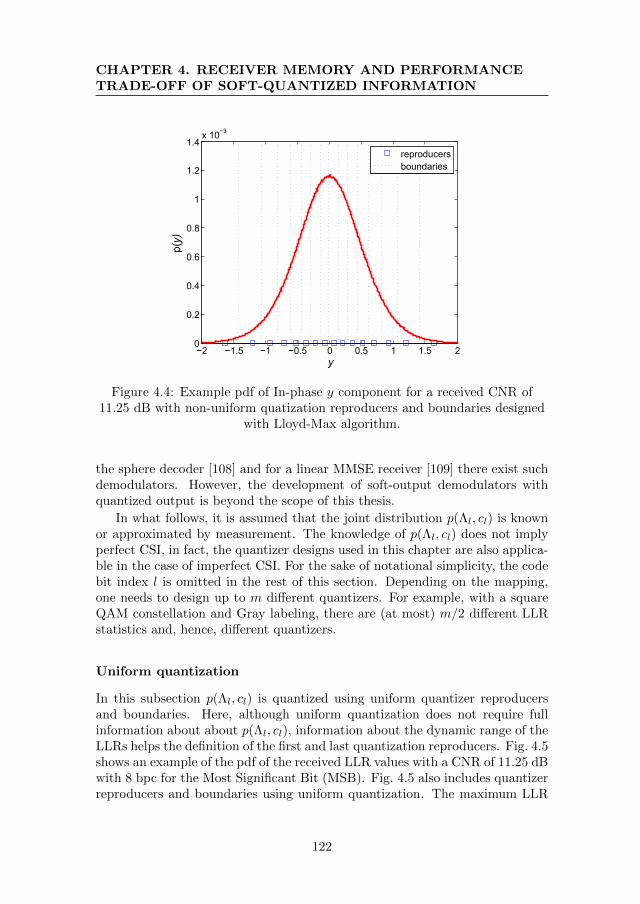
CHAPTER 4. RECEIVER MEMORY AND PERFORMANCETRADE-OFF OF SOFT-QUANTIZED INFORMATION
−2 −1.5 −1 −0.5 0 0.5 1 1.5 20
0.2
0.4
0.6
0.8
1
1.2
1.4x 10⁻³
y
p(y)
reproducersboundaries
Figure 4.4: Example pdf of In-phase y component for a received CNR of11.25 dB with non-uniform quatization reproducers and boundaries designed
with Lloyd-Max algorithm.
the sphere decoder [108] and for a linear MMSE receiver [109] there exist suchdemodulators. However, the development of soft-output demodulators withquantized output is beyond the scope of this thesis.
In what follows, it is assumed that the joint distribution p(Λl, cl) is knownor approximated by measurement. The knowledge of p(Λl, cl) does not implyperfect CSI, in fact, the quantizer designs used in this chapter are also applica-ble in the case of imperfect CSI. For the sake of notational simplicity, the codebit index l is omitted in the rest of this section. Depending on the mapping,one needs to design up to m different quantizers. For example, with a squareQAM constellation and Gray labeling, there are (at most) m/2 different LLRstatistics and, hence, different quantizers.
Uniform quantization
In this subsection p(Λl, cl) is quantized using uniform quantizer reproducersand boundaries. Here, although uniform quantization does not require fullinformation about about p(Λl, cl), information about the dynamic range of theLLRs helps the definition of the first and last quantization reproducers. Fig. 4.5shows an example of the pdf of the received LLR values with a CNR of 11.25 dBwith 8 bpc for the Most Significant Bit (MSB). Fig. 4.5 also includes quantizerreproducers and boundaries using uniform quantization. The maximum LLR
122
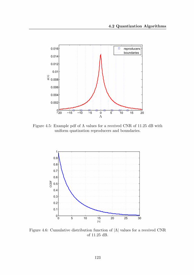
4.2 Quantization Algorithms
−20 −15 −10 −5 0 5 10 15 200
0.002
0.004
0.006
0.008
0.01
0.012
0.014
0.016
Λ
p(Λ
)
reproducersboundaries
Figure 4.5: Example pdf of Λ values for a received CNR of 11.25 dB withuniform quatization reproducers and boundaries.
0 5 10 15 20 25 300
0.1
0.2
0.3
0.4
0.5
0.6
0.7
0.8
0.9
1
|Λ|
CCDF
Figure 4.6: Cumulative distribution function of |Λ| values for a received CNRof 11.25 dB.
123
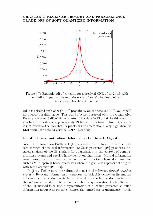
CHAPTER 4. RECEIVER MEMORY AND PERFORMANCETRADE-OFF OF SOFT-QUANTIZED INFORMATION
−20 −15 −10 −5 0 5 10 15 200
0.002
0.004
0.006
0.008
0.01
0.012
0.014
0.016
Λ
p(Λ
)
reproducersboundaries
Figure 4.7: Example pdf of Λ values for a received CNR of 11.25 dB withnon-uniform quatization reproducers and boundaries designed with
information bottleneck method.
value is selected such as with 10% probability all the received LLR values willhave lower absolute value. This can be better observed with the CumulativeDensity Function (cdf) of the absolute LLR values in Fig. 4.6. In this case, anabsolute LLR value of approximately 13 fulfils this criteria. This 10% criteriais motivated by the fact that, in practical implementations, very high absoluteLLR values are clipped prior to LDPC decoding.
Non-Uniform quantization: Information Bottleneck Algorithm
Next, the Information Bottleneck (IB) algorithm, used to maximize the datarate through the mutual-information I(c; d), is presented. [95] provides a de-tailed analysis of the IB method for quantization in the context of commu-nication systems and specific implementation algorithms. Mutual-informationbased design for LLR quantization can outperform other classical approaches,such as MSE-optimal based quantizers where the goal is to represent the signalwith low distortion [95, 110].
In [111], Tishby et al. introduced the notion of relevance through anothervariable. Relevant information in a random variable Λ is defined as the mutualinformation this random variable provides about another random variable c,the relevance variable. For a fixed number of quantization levels, the aimof the IB method is to find a representation of Λ, which preserves as muchinformation about c as possible. Hence, the limited set of quantization levels
124
4.2 Quantization Algorithms
constitutes a “bottleneck” through which we squeeze the information that Λprovides about c. Since closed-form expressions for p(c,Λ) are rarely available,p(c,Λ) is approximated by measurement. Λ is regarded as a discrete randomvariable in what follows.
The IB problem is given by
p?(d|Λ) = arg minp(d|Λ)
I(Λ; d)− βI(c; d), (4.5)
where β is the Lagrange multiplier of the relevant information I(c; d). In [111]it is shown that the optimal p(d|Λ) is
p(d|Λ) ∝ p(d) exp [−β D(p(c|Λ)‖p(c|d))] , (4.6)
where D(· ‖ ·) denotes relative entropy. It must be emphasized that (4.6) isonly a formal solution since p(d) and p(c|d) are defined implicitly in terms ofp(d|Λ). Then
p(d) =∑Λ
p(d|Λ)p(Λ), (4.7)
p(c|d) =1
p(d)
∑Λ
p(c,Λ)p(d|Λ). (4.8)
The iterative IB algorithm consists of converging alternating iterations between(4.6)-(4.8), where β allows to tradeoff quantization rate and relevant informa-tion. The IB algorithm converges to a locally optimal point. For β 1deterministic quantizer can be obtained. However, large values of β can lead tonumerical problems in the iterative IB algorithm. Therefore, this chapter usesthe algorithm first proposed in [112] where a modified algorithm maximizes therelevant information for a given number of quantization levels and to take intoaccount that the optimal quantizer is deterministic. A deterministic quantizeris returned upon convergence to a relative accuracy of ε or otherwise after apredetermined number of iterations. The algorithm is executed with different,randomized initializations in order to obtain a good quantizer.
The relevant information I(c; d) does not depend on the values of d. There-fore the reproducer values need to be computed in a separate step after thequantizer design is completed:
λk = logp(c = 1|Λ ∈ Ik)
p(c = 0|Λ ∈ Ik), k = 1, 2, . . . , n, (4.9)
where Ik, k = 1, 2, . . . , n are the quantization regions defined by the designedboundaries. (4.9) ensures that the quantized LLRs are consistent.
125
CHAPTER 4. RECEIVER MEMORY AND PERFORMANCETRADE-OFF OF SOFT-QUANTIZED INFORMATION
Fig. 4.7 shows the pdfs of the received LLR values with a CNR of 11.25 dBwith 8 bpc for the MSB. Fig. 4.7 also includes non-uniform quantizer reproduc-ers and boundaries designed with the IB algorithm described above. We canobserve how the non-uniform quantizer gathers the reproducers closely aroundthe absolute value zero, where the pdf has higher probability.
4.3 Performance Evaluation of Quantized Ar-chitectures
This section provides physical layer simulation results to illustrate the perfor-mance improvements by iterative detection and the performance degradationintroduced by LLR and I&Q quantization with different word lengths and algo-rithms. A summary of the simulation parameters is presented in Table 4.1. Thesimulated scenario is NGH vehicular MIMO 2 × 2 cross-polar channel modelwith 60 km/h (cf. Appendix A). The simulations include inner LDPC codeswith a word length size of 16200 bits with a code-rate 1/3 and outer BCH. Thesimulated system uses 4096 subcarriers and an 1/8 guard interval, to trade-offnetwork cell area and resilience against Doppler spread in an 8 MHz bandwidth.For the performance evaluation, TI blocks with 48 LDPC codewords are trans-mitted and decoded. These values have been selected as a trade-off betweensimulation time and performance accuracy. It was confirmed with simulationsthat using more LDPC codewords within the TI block did not have a signifi-cant impact in the final performance. To analyse the effect of the quantizationwith the constellation order three spectral efficiencies are evaluated, which arespecified in DVB-NGH, i.e., 6 bpc (with QPSK and 16QAM constellations inthe first and second transmit antennas, respectively), 8 bpc (with 16QAM con-stellation in both transmit antennas), and 10 bpc (with 16QAM and 64QAMin the first and second transmit antennas, respectively). As specified in DVB-NGH, Gray labelling is used and perfect CSI at the receiver side it is assumed.To provide reliable results, the performance under different channel realiza-tions at each CNR is evaluated, i.e., different seeds for the (pseudo) randomgenerators at each CNRs. On the other hand, for a given CNR all the receiverconfigurations were simulated under the same set of channel realizations, i.e.,same seed for the (pseudo) random generator for a given CNR. Regarding thestopping criteria, for each CNR a maximum number of 20 ·103 and a minimumnumber of 2 · 103 TI blocks are simulated. The simulation is stopped when 200erroneous TI Blocks have been detected. A TI Block is considered erroneouswhen a erroneous bit is detected in the entire TI block. Finally, the selectedQuality of Service (QoS) for the comparisons is a BER of 10−5 before BCHdecoding. This error criteria was selected as a compromise between simulationtime and error criteria in mobile channels.
126
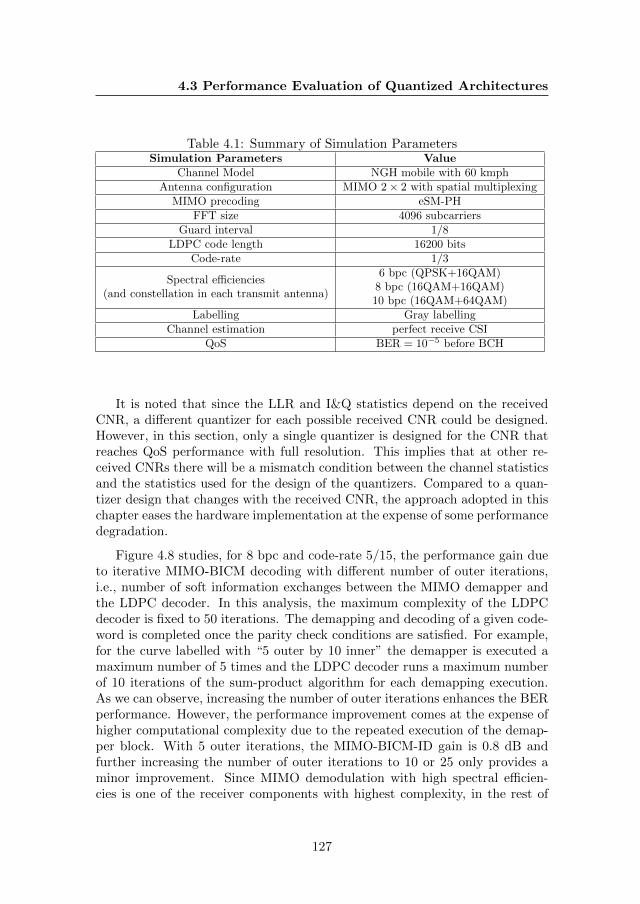
4.3 Performance Evaluation of Quantized Architectures
Table 4.1: Summary of Simulation ParametersSimulation Parameters Value
Channel Model NGH mobile with 60 kmphAntenna configuration MIMO 2× 2 with spatial multiplexing
MIMO precoding eSM-PHFFT size 4096 subcarriers
Guard interval 1/8LDPC code length 16200 bits
Code-rate 1/3
Spectral efficiencies(and constellation in each transmit antenna)
6 bpc (QPSK+16QAM)8 bpc (16QAM+16QAM)10 bpc (16QAM+64QAM)
Labelling Gray labellingChannel estimation perfect receive CSI
QoS BER = 10−5 before BCH
It is noted that since the LLR and I&Q statistics depend on the receivedCNR, a different quantizer for each possible received CNR could be designed.However, in this section, only a single quantizer is designed for the CNR thatreaches QoS performance with full resolution. This implies that at other re-ceived CNRs there will be a mismatch condition between the channel statisticsand the statistics used for the design of the quantizers. Compared to a quan-tizer design that changes with the received CNR, the approach adopted in thischapter eases the hardware implementation at the expense of some performancedegradation.
Figure 4.8 studies, for 8 bpc and code-rate 5/15, the performance gain dueto iterative MIMO-BICM decoding with different number of outer iterations,i.e., number of soft information exchanges between the MIMO demapper andthe LDPC decoder. In this analysis, the maximum complexity of the LDPCdecoder is fixed to 50 iterations. The demapping and decoding of a given code-word is completed once the parity check conditions are satisfied. For example,for the curve labelled with “5 outer by 10 inner” the demapper is executed amaximum number of 5 times and the LDPC decoder runs a maximum numberof 10 iterations of the sum-product algorithm for each demapping execution.As we can observe, increasing the number of outer iterations enhances the BERperformance. However, the performance improvement comes at the expense ofhigher computational complexity due to the repeated execution of the demap-per block. With 5 outer iterations, the MIMO-BICM-ID gain is 0.8 dB andfurther increasing the number of outer iterations to 10 or 25 only provides aminor improvement. Since MIMO demodulation with high spectral efficien-cies is one of the receiver components with highest complexity, in the rest of
127
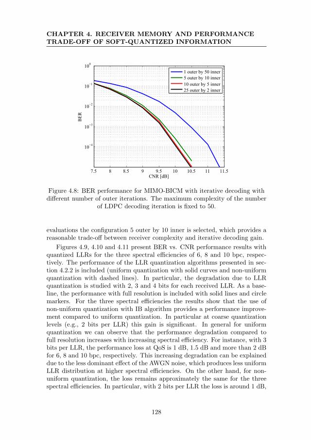
CHAPTER 4. RECEIVER MEMORY AND PERFORMANCETRADE-OFF OF SOFT-QUANTIZED INFORMATION
7.5 8 8.5 9 9.5 10 10.5 11 11.5
10−4
10−3
10−2
10−1
100
CNR [dB]
BER
1 outer by 50 inner5 outer by 10 inner10 outer by 5 inner25 outer by 2 inner
Figure 4.8: BER performance for MIMO-BICM with iterative decoding withdifferent number of outer iterations. The maximum complexity of the number
of LDPC decoding iteration is fixed to 50.
evaluations the configuration 5 outer by 10 inner is selected, which provides areasonable trade-off between receiver complexity and iterative decoding gain.
Figures 4.9, 4.10 and 4.11 present BER vs. CNR performance results withquantized LLRs for the three spectral efficiencies of 6, 8 and 10 bpc, respec-tively. The performance of the LLR quantization algorithms presented in sec-tion 4.2.2 is included (uniform quantization with solid curves and non-uniformquantization with dashed lines). In particular, the degradation due to LLRquantization is studied with 2, 3 and 4 bits for each received LLR. As a base-line, the performance with full resolution is included with solid lines and circlemarkers. For the three spectral efficiencies the results show that the use ofnon-uniform quantization with IB algorithm provides a performance improve-ment compared to uniform quantization. In particular at coarse quantizationlevels (e.g., 2 bits per LLR) this gain is significant. In general for uniformquantization we can observe that the performance degradation compared tofull resolution increases with increasing spectral efficiency. For instance, with 3bits per LLR, the performance loss at QoS is 1 dB, 1.5 dB and more than 2 dBfor 6, 8 and 10 bpc, respectively. This increasing degradation can be explaineddue to the less dominant effect of the AWGN noise, which produces less uniformLLR distribution at higher spectral efficiencies. On the other hand, for non-uniform quantization, the loss remains approximately the same for the threespectral efficiencies. In particular, with 2 bits per LLR the loss is around 1 dB,
128
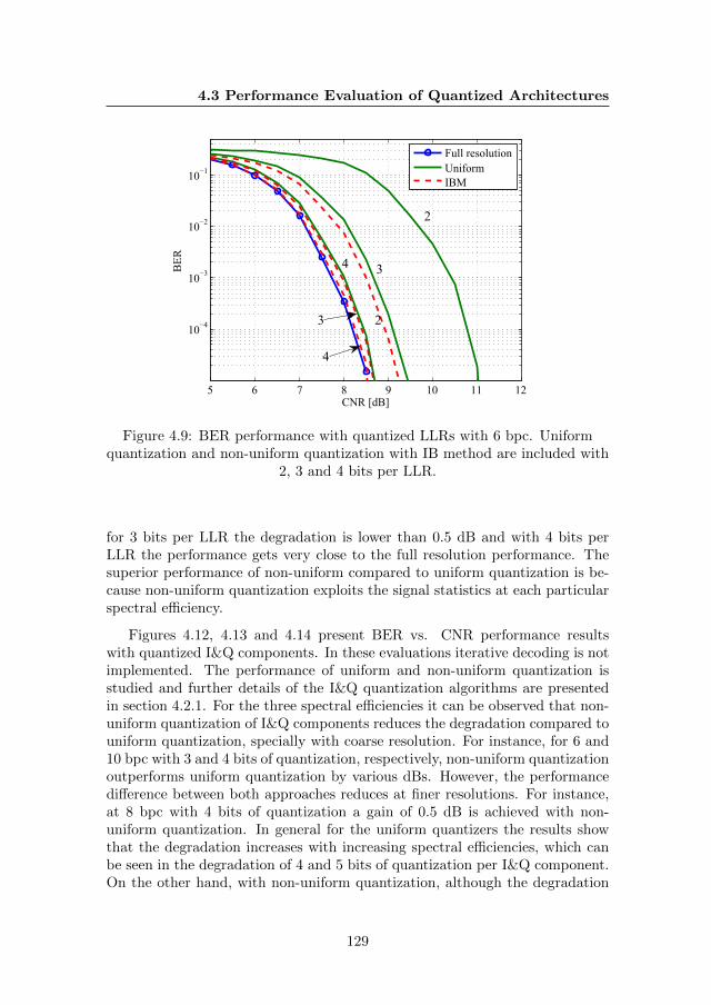
4.3 Performance Evaluation of Quantized Architectures
5 6 7 8 9 10 11 12
10−4
10−3
10−2
10−1
CNR [dB]
BER
Full resolutionUniformIBM
4
2
4
3
3
2
Figure 4.9: BER performance with quantized LLRs with 6 bpc. Uniformquantization and non-uniform quantization with IB method are included with
2, 3 and 4 bits per LLR.
for 3 bits per LLR the degradation is lower than 0.5 dB and with 4 bits perLLR the performance gets very close to the full resolution performance. Thesuperior performance of non-uniform compared to uniform quantization is be-cause non-uniform quantization exploits the signal statistics at each particularspectral efficiency.
Figures 4.12, 4.13 and 4.14 present BER vs. CNR performance resultswith quantized I&Q components. In these evaluations iterative decoding is notimplemented. The performance of uniform and non-uniform quantization isstudied and further details of the I&Q quantization algorithms are presentedin section 4.2.1. For the three spectral efficiencies it can be observed that non-uniform quantization of I&Q components reduces the degradation compared touniform quantization, specially with coarse resolution. For instance, for 6 and10 bpc with 3 and 4 bits of quantization, respectively, non-uniform quantizationoutperforms uniform quantization by various dBs. However, the performancedifference between both approaches reduces at finer resolutions. For instance,at 8 bpc with 4 bits of quantization a gain of 0.5 dB is achieved with non-uniform quantization. In general for the uniform quantizers the results showthat the degradation increases with increasing spectral efficiencies, which canbe seen in the degradation of 4 and 5 bits of quantization per I&Q component.On the other hand, with non-uniform quantization, although the degradation
129
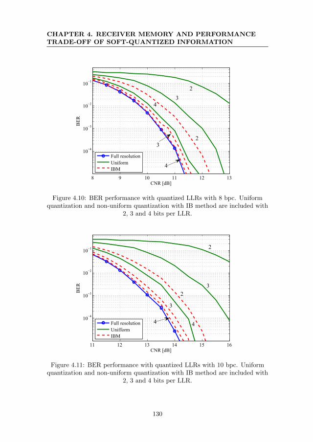
CHAPTER 4. RECEIVER MEMORY AND PERFORMANCETRADE-OFF OF SOFT-QUANTIZED INFORMATION
8 9 10 11 12 13
10−4
10−3
10−2
10−1
CNR [dB]
BER
Full resolutionUniformIBM
23
4
23
4
Figure 4.10: BER performance with quantized LLRs with 8 bpc. Uniformquantization and non-uniform quantization with IB method are included with
2, 3 and 4 bits per LLR.
11 12 13 14 15 16
10−4
10−3
10−2
10−1
CNR [dB]
BER
Full resolutionUnifformIBM
4
2
23
3
4
Figure 4.11: BER performance with quantized LLRs with 10 bpc. Uniformquantization and non-uniform quantization with IB method are included with
2, 3 and 4 bits per LLR.
130
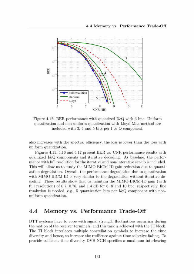
4.4 Memory vs. Performance Trade-Off
5 6 7 8 9 10 11
10−4
10−3
10−2
10−1
CNR [dB]
BER
Full resolutionUniformLloyd
33
4
5
Figure 4.12: BER performance with quantized I&Q with 6 bpc. Uniformquantization and non-uniform quantization with Lloyd-Max method are
included with 3, 4 and 5 bits per I or Q component.
also increases with the spectral efficiency, the loss is lower than the loss withuniform quantization.
Figures 4.15, 4.16 and 4.17 present BER vs. CNR performance results withquantized I&Q components and iterative decoding. As baseline, the perfor-mance with full resolution for the iterative and non-interative set-up is included.This will allow us to study the MIMO-BICM-ID gain reduction due to quanti-zation degradation. Overall, the performance degradation due to quantizationwith MIMO-BICM-ID is very similar to the degradation without iterative de-coding. These results show that to maintain the MIMO-BICM-ID gain (withfull resolution) of 0.7, 0.76, and 1.4 dB for 6, 8 and 10 bpc, respectively, fineresolution is needed, e.g., 5 quantization bits per I&Q component with non-uniform quantization.
4.4 Memory vs. Performance Trade-Off
DTT systems have to cope with signal strength fluctuations occurring duringthe motion of the receiver terminals, and this task is achieved with the TI block.The TI block interlaces multiple constellation symbols to increase the timediversity and hence, to increase the resilience against time selective fading. Toprovide sufficient time diversity DVB-NGH specifies a maximum interleaving
131
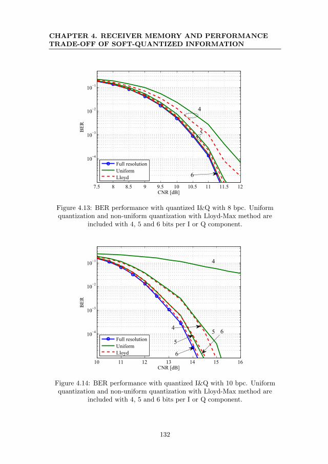
CHAPTER 4. RECEIVER MEMORY AND PERFORMANCETRADE-OFF OF SOFT-QUANTIZED INFORMATION
7.5 8 8.5 9 9.5 10 10.5 11 11.5 12
10−4
10−3
10−2
10−1
CNR [dB]
BER
Full resolutionUniformLloyd
4
6
5
Figure 4.13: BER performance with quantized I&Q with 8 bpc. Uniformquantization and non-uniform quantization with Lloyd-Max method are
included with 4, 5 and 6 bits per I or Q component.
10 11 12 13 14 15 16
10−4
10−3
10−2
10−1
CNR [dB]
BER
Full resolutionUniformLloyd
4
5 64
5
6
Figure 4.14: BER performance with quantized I&Q with 10 bpc. Uniformquantization and non-uniform quantization with Lloyd-Max method are
included with 4, 5 and 6 bits per I or Q component.
132
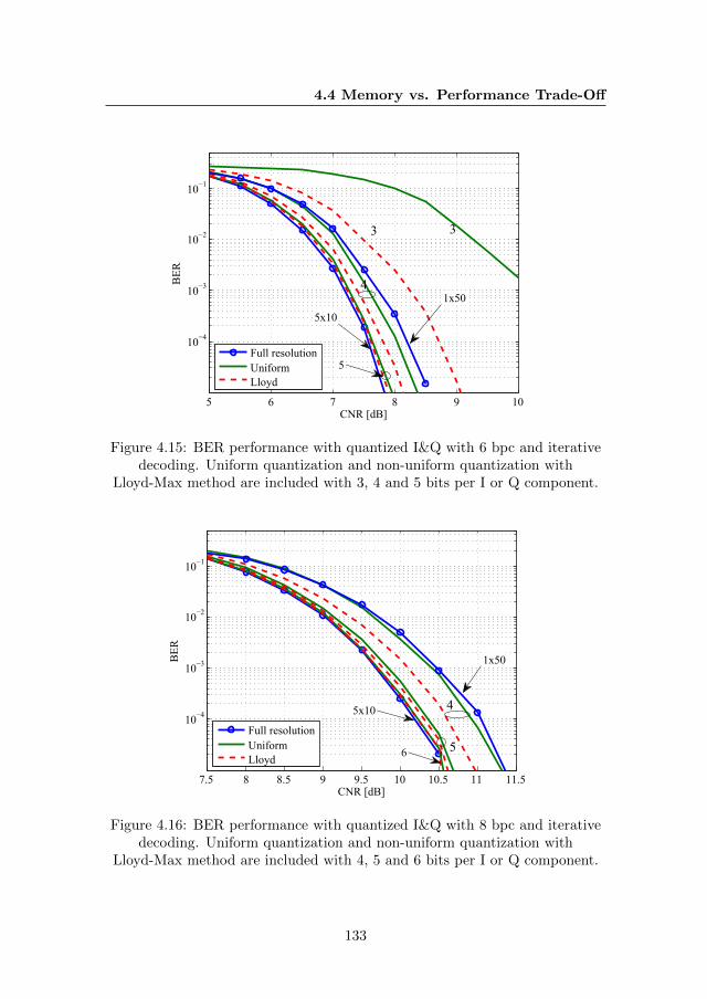
4.4 Memory vs. Performance Trade-Off
5 6 7 8 9 10
10−4
10−3
10−2
10−1
CNR [dB]
BER
Full resolutionUniformLloyd
1x50
33
4
5x10
5
Figure 4.15: BER performance with quantized I&Q with 6 bpc and iterativedecoding. Uniform quantization and non-uniform quantization with
Lloyd-Max method are included with 3, 4 and 5 bits per I or Q component.
7.5 8 8.5 9 9.5 10 10.5 11 11.5
10−4
10−3
10−2
10−1
CNR [dB]
BER
Full resolutionUniformLloyd
1x50
4
5
5x10
6
Figure 4.16: BER performance with quantized I&Q with 8 bpc and iterativedecoding. Uniform quantization and non-uniform quantization with
Lloyd-Max method are included with 4, 5 and 6 bits per I or Q component.
133
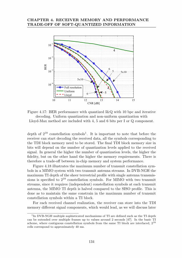
CHAPTER 4. RECEIVER MEMORY AND PERFORMANCETRADE-OFF OF SOFT-QUANTIZED INFORMATION
10 11 12 13 14 15
10−4
10−3
10−2
10−1
CNR [dB]
BER
Full resolutionUniformLloyd
5x1056
4
5x10
6 54
Figure 4.17: BER performance with quantized I&Q with 10 bpc and iterativedecoding. Uniform quantization and non-uniform quantization with
Lloyd-Max method are included with 4, 5 and 6 bits per I or Q component.
depth of 218 constellation symbols1. It is important to note that before thereceiver can start decoding the received data, all the symbols corresponding tothe TDI block memory need to be stored. The final TDI block memory size inbits will depend on the number of quantization levels applied to the receivedsignal. In general the higher the number of quantization levels, the higher thefidelity, but on the other hand the higher the memory requirements. There istherefore a trade-off between in-chip memory and system performance.
Figure 4.18 illustrates the maximum number of transmit constellation sym-bols in a MIMO system with two transmit antenna streams. In DVB-NGH themaximum TI depth of the sheer terrestrial profile with single antenna transmis-sions is specified to 218 constellation symbols. For MIMO with two transmitstreams, since it requires (independent) constellation symbols at each transmitantenna, the MIMO TI depth is halved compared to the SISO profile. This isdone as to maintain the same constrain in the maximum number of transmitconstellation symbols within a TI block.
For each received channel realization, the receiver can store into the TDImemory different signal components, which would lead, as we will discuss later
1In DVB-NGH multiple sophisticated mechanisms of TI are defined such as the TI depthcan be extended over multiple frames up to values around 2 seconds [47]. In the basic TIscheme, where contiguous constellation symbols from the same TI block are interlaced, 218
cells correspond to approximately 40 ms.
134
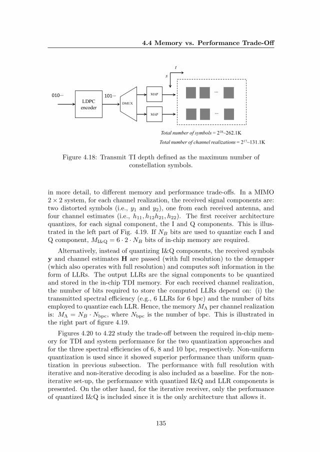
4.4 Memory vs. Performance Trade-Off
LDPCencoder
010··· 101···DMUX
MAP
MAP
···
···
t
Total number of symbols = 218~262.1K
Total number of channel realizations = 217~131.1K
s
Figure 4.18: Transmit TI depth defined as the maximum number ofconstellation symbols.
in more detail, to different memory and performance trade-offs. In a MIMO2× 2 system, for each channel realization, the received signal components are:two distorted symbols (i.e., y1 and y2), one from each received antenna, andfour channel estimates (i.e., h11, h12h21, h22). The first receiver architecturequantizes, for each signal component, the I and Q components. This is illus-trated in the left part of Fig. 4.19. If NB bits are used to quantize each I andQ component, MI&Q = 6 · 2 ·NB bits of in-chip memory are required.
Alternatively, instead of quantizing I&Q components, the received symbolsy and channel estimates H are passed (with full resolution) to the demapper(which also operates with full resolution) and computes soft information in theform of LLRs. The output LLRs are the signal components to be quantizedand stored in the in-chip TDI memory. For each received channel realization,the number of bits required to store the computed LLRs depend on: (i) thetransmitted spectral efficiency (e.g., 6 LLRs for 6 bpc) and the number of bitsemployed to quantize each LLR. Hence, the memory MΛ per channel realizationis: MΛ = NB · Nbpc, where Nbpc is the number of bpc. This is illustrated inthe right part of figure 4.19.
Figures 4.20 to 4.22 study the trade-off between the required in-chip mem-ory for TDI and system performance for the two quantization approaches andfor the three spectral efficiencies of 6, 8 and 10 bpc, respectively. Non-uniformquantization is used since it showed superior performance than uniform quan-tization in previous subsection. The performance with full resolution withiterative and non-iterative decoding is also included as a baseline. For the non-iterative set-up, the performance with quantized I&Q and LLR components ispresented. On the other hand, for the iterative receiver, only the performanceof quantized I&Q is included since it is the only architecture that allows it.
135
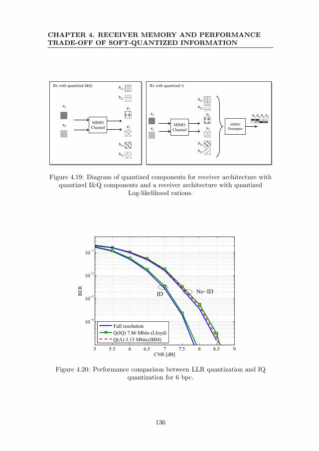
CHAPTER 4. RECEIVER MEMORY AND PERFORMANCETRADE-OFF OF SOFT-QUANTIZED INFORMATION
x1
x2MIMOChannel
y1
y2
h11
h12
h21
h22
x1
x2MIMOChannel
y1
y2
h11
h12
h21
h22
MIMODemapper
Λ1 Λ2 Λ3 Λ4
Rx with quantized I&Q Rx with quantized Λ
Figure 4.19: Diagram of quantized components for receiver architecture withquantized I&Q components and a receiver architecture with quantized
Log-likelihood rations.
5 5.5 6 6.5 7 7.5 8 8.5 9
10−4
10−3
10−2
10−1
CNR [dB]
BER
Full resolutionQ(IQ) 7.86 Mbits (Lloyd)Q(Λ) 3.15 Mbits (IBM)
ID No−ID
Figure 4.20: Performance comparison between LLR quantization and IQquantization for 6 bpc.
136
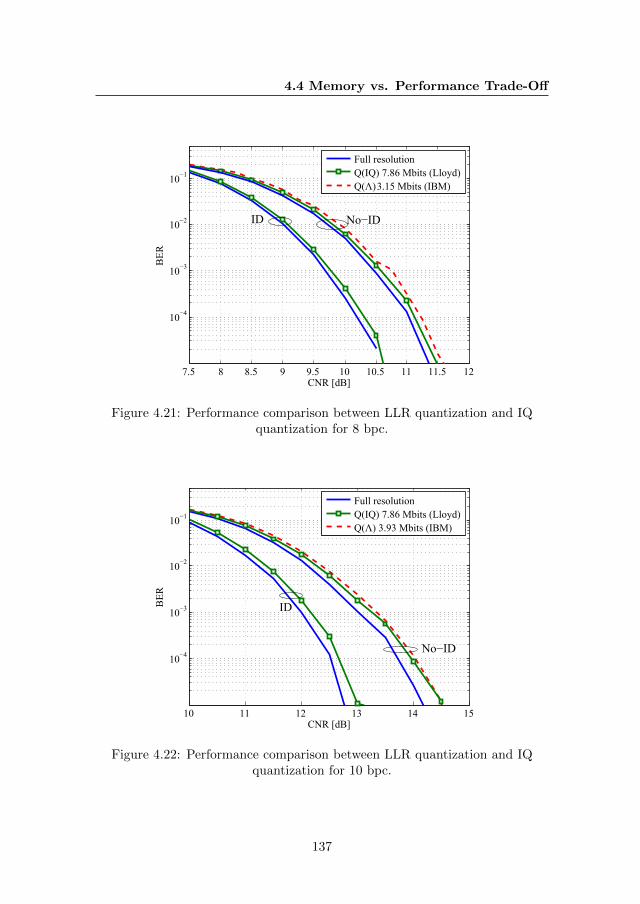
4.4 Memory vs. Performance Trade-Off
7.5 8 8.5 9 9.5 10 10.5 11 11.5 12
10−4
10−3
10−2
10−1
CNR [dB]
BER
Full resolutionQ(IQ) 7.86 Mbits (Lloyd)Q(Λ) 3.15 Mbits (IBM)
No−IDID
Figure 4.21: Performance comparison between LLR quantization and IQquantization for 8 bpc.
10 11 12 13 14 15
10−4
10−3
10−2
10−1
CNR [dB]
BER
Full resolutionQ(IQ) 7.86 Mbits (Lloyd)Q(Λ) 3.93 Mbits (IBM)
ID
No−ID
Figure 4.22: Performance comparison between LLR quantization and IQquantization for 10 bpc.
137
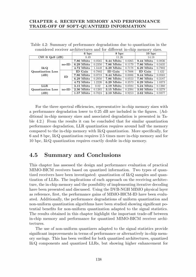
CHAPTER 4. RECEIVER MEMORY AND PERFORMANCETRADE-OFF OF SOFT-QUANTIZED INFORMATION
Table 4.2: Summary of performance degradations due to quantization in theconsidered receiver architectures and for different in-chip memory sizes.
6 bpc 8 bpc 10 bpcCNR @ QoS (dB) 8.49 11.26 14.18
I&QQuantization Loss
(dB)
no-ID7.86 Mbits 0.0565 9.44 Mbits 0.0265 9.44 Mbits 0.08366.29 Mbits 0.2350 7.86 Mbits 0.1179 7.86 Mbits 0.34354.72 Mbits 1.3448 6.29 Mbits 0.7178 6.29 Mbits 0.7902
ID
ID Gain 0.7002 ID Gain 0.7606 ID Gain 1.4227.86 Mbits 0.0718 9.44 Mbits 0.0086 9.44 Mbits 0.05656.29 Mbits 0.2950 7.86 Mbits 0.0553 7.86 Mbits 0.31874.72 Mbits 1.2226 6.29 Mbits 0.3573 6.29 Mbits 1.0373
LLRQuantization Loss
(dB)no-ID
3.15 Mbits 0.02 4.19 Mbits 0.0594 5.24 Mbits 0.13602.36 Mbits 0.1265 3.15 Mbits 0.2394 3.93 Mbits 0.32791.57 Mbits 0.7024 2.10 Mbits 0.9213 2.62 Mbits 0.9377
For the three spectral efficiencies, representative in-chip memory sizes witha performance degradation lower to 0.25 dB are included in the figures. (Ad-ditional in-chip memory sizes and associated degradation is presented in Ta-ble 4.2.) From the results it can be concluded that for similar quantizationperformance degradation, LLR quantization requires around half the memorycompared to the in-chip memory with I&Q quantization. More specifically, for6 and 8 bpc, I&Q quantization requires 2.5 times more in-chip memory and for10 bpc, I&Q quantization requires exactly double in-chip memory.
4.5 Summary and Conclusions
This chapter has assessed the design and performance evaluation of practicalMIMO-BICM receivers based on quantized information. Two types of quan-tized receivers have been investigated: quantization of I&Q samples and quan-tization of LLRs. The implications of each approach on the receiving architec-ture, the in-chip memory and the possibility of implementing iterative decodinghave been presented and discussed. Using the DVB-NGH MIMO physical layeras reference, first, the performance gains of MIMO-BICM-ID have been evalu-ated. Additionally, the performance degradations of uniform quantization andnon-uniform quantization algorithms have been studied showing significant po-tential benefits for non-uniform quantization adapted to the signal statistics.The results obtained in this chapter highlight the important trade-off betweenin-chip memory and performance for quantized MIMO-BICM receiver archi-tectures.
The use of non-uniform quantizers adapted to the signal statistics providesignificant improvements in terms of performance or alternatively in-chip mem-ory savings. This has been verified for both quantized architectures, quantizedI&Q components and quantized LLRs, but showing higher enhancement for
138
4.5 Summary and Conclusions
the latter. The higher memory requirements required by I&Q quantization al-low, on the other hand, to exploit the benefits of MIMO-BICM with iterativedecoding. As shown in Table 4.2, the MIMO-BICM-ID gain is retained withquantization (and with sufficient resolution), which increases with increasingspectral efficiency (0.7, 0.8 and 1.4 dB of gain for 6, 8, and 10 bpc, respec-tively). These additional gains not only come at the expense of additionalin-chip memory, but also at the expense of additional demapping complexity.
In a receiver design constrained by in-chip memory, the best option is toquantized LLRs, since it entails the lowest memory requirements, althoughiterative decoding is not possible any more. In a receiver design constrained bydemodulation complexity, the preferred option may also be quantized LLRs,since it would also provide additional in-chip memory savings. On the otherhand, this chapter has only considered max-log demapper, which has highdemodulation complexity. Other MIMO-BICM-ID demodulation algorithmsare available in the literature, such as soft-in soft-out single-tree-search [41] orMMSE with priors (cf. Chapter 2 and [89, 44]), which can significantly reducethe demapper complexity. The evaluation of the complexity of such demappersis out of the scope of this thesis. In a receiver design not constrained byeither on in-chip memory or demodulation complexity, the preferred receiverarchitecture is to quantize I&Q components since it also allows MIMO-BICM-ID, which can provide significant performance improvements. This type orreceiver could be classified as an advanced receiver providing best performancewith higher receiver complexity.
139

CHAPTER 4. RECEIVER MEMORY AND PERFORMANCETRADE-OFF OF SOFT-QUANTIZED INFORMATION
140
Chapter 5
Conclusions and Outlook
This dissertation has focused on transmit and receive signal processing fordigital terrestrial TV (DTT) systems with multiple-input multiple-output
(MIMO) and bit-interleaved coded modulation (BICM) technologies, withouta return channel from the receivers to the transmitters. MIMO offers multiplebenefits such as additional received power thanks to the array gain, additionalsystem resilience against signal fluctuations due to diversity gain and higherdata rates through spatial multiplexing gain. These benefits can be achievedwith the same transmit power and bandwidth requirements as in single antennacommunications. However, these enhancements usually imply a higher systemcomplexity at the transmitter and receiver sides. Due to the potential benefits,MIMO has been included for the first time as part of the DTT specificationsDVB-NGH and ATSC 3.0 to overcome the Shannon limit of single antennacommunications. These two specifications have adopted a MIMO configura-tion with two antennas at transmit and receiver ends (i.e., 2×2 MIMO) ableto transmit two independent data streams into the same time and frequencyresources, i.e., spatial multiplexing gain of two. The operation in the UHFband of theses systems have motivated the adoption of cross-polar antennaconfiguration (i.e., antennas with vertical and horizontal polarizations). Cross-polar antennas can improve the performance under spatial correlated fadingdue to the orthogonal nature of the cross-polar channel, and also it can providesmaller handset device sizes compared to the co-polar configuration (i.e., an-tennas with the same polarization) which rely on antenna separation to provideindependent fading signals.
The final MIMO gains directly depend on the intrinsic physical character-istics of the MIMO channel such as correlation among the spatial paths andtransmit power imbalance between transmit antennas. To overcome the poten-tial degradations, DVB-NGH and ATSC 3.0 have adopted precoding solutions
141
CHAPTER 5. CONCLUSIONS AND OUTLOOK
based on rotation matrices which apply a linear transformation to the indepen-dent information streams to improve the performance. The three main compo-nents of these type of precoders are rotation matrix, stream-power-allocation,and power imbalance matrix (which can be considered as part of the precoderor as part of the channel). Additionally, since the broadcast network tendsto exhibit common channel characteristics such as predominant line-of-sight(LOS) in rooftop environment, antenna correlation, or cross-polarization dis-crimination (XPD) factors, these characteristics could be used by a precoderto exploit such information statistics.
On the other hand, even in ideal channel conditions, MIMO-BICM receiversneed sophisticated signal processing to extract the potential benefits of theMIMO channel. It is common practice during the standardization of new com-munication schemes to evaluate candidate transmission technologies with op-timal receiving conditions such as optimal demodulation or infinite precisionarithmetic. However, it is crucial for a good final system performance to care-fully design specific receiving algorithms, which provide suitable performancewhile meeting complexity restrictions.
Signal quantization is a fundamental operation that can be found in any dig-ital receiver, which permits transformation of continuous signals to a discretesignal sequence that can be processed, transmitted and/or stored in conven-tional digital processors. A fundamental trade-off connects quantizer resolutionand distortion, hence, the quantization algorithms used at the receiver have adirect impact on the final performance and in-chip memory. Other importantfactor in MIMO-BICM receivers is that the performance can be significantlyenhanced by iterative decoding algorithms, which exchange soft informationbetween the demapper and the channel decoder in a iterative fashion. Apartfrom the additional computational complexity, this type of processing requiresspecific receiving architectures which can also have an impact on the in-chipmemory.
At the transmitter side, the goal of this thesis has been to investigate andcharacterize the performance of MIMO precoding in DTT systems. First, thisthesis has provided a performance characterization of the 2×2 MIMO precod-ing based on rotation matrices against: (i) channel parameters such as antennaorientation, spatial correlation, and transmit power imbalance, and (ii) trans-mission parameters such as constellation order and physical layer forward errorcorrection (FEC) code-rate. Secondly, a MIMO-channel-precoding has beenproposed that exploits statistical information of the MIMO channel. In thispart of the thesis the DTT MIMO systems have been extended to support fourindependent information streams and its performance in DTT channels hasbeen evaluated. The performance of the MIMO-channel-precoder is evaluatedin a wide set of channel scenarios and mismatched channel conditions, (i.e.,
142
5.1 Conclusions
channel statistics and the statistics used for the design of the precoder differ),a typical situation in the broadcast set-up.
At the receiver side, the goal of this thesis has been to design and eval-uate the performance of practical MIMO-BICM receivers based on quantizedinformation. Two types of quantized receivers have been investigated: quan-tization of In-phase and Quadrature (I&Q) samples and quantization of log-likelihood ratios (LLRs). The implications on the receiving architecture, thein-chip memory and the possibility of implementing iterative decoding havebeen investigated. Here, using the DVB-NGH MIMO physical layer as refer-ence, first, the performance gains of MIMO-BICM with iterative decoding havebeen evaluated. Then, the performance of uniform and non-uniform quantiza-tion has been analysed showing potential benefits for non-uniform quantizationadapted to the signal statistics. Finally, the in-chip memory size and systemperformance trade-off of quantized MIMO-BICM receivers has been presentedand investigated.
This concluding chapter summarizes the main contributions of this disser-tation and suggests further topics of research beyond the results of this work.
5.1 Conclusions
MIMO Precoding for Terrestrial Broadcast Systems
The research results obtained in this thesis, with the information-theoreticlimits of BICM systems and BER simulations including channel coding, for2×2 MIMO-BICM with Gray mapping and precoders based on rotation matricesshow the following conclusions:
• In the case of co-polar antennas under i.i.d. fast fading Rayleigh channel,rotation does not have any effect in the final system performance. Thischannel model emulates a environment with co-polar antennas and richscattering which already mixes the transmits information streams and afurther linear transformation does not have a significant effect. Althoughthis type of channel with co-polar antennas is not very representative forDTT systems, which relay in cross-polar antennas, it can provide insightsfor cross-polar channels with low XPD values (i.e., high coupling betweenpolarizations). In the case that correlation between spatial paths exists,the results in this dissertation show that with high correlation condition,rotation can provide a significant improvements at all code-rates.
• In MIMO systems with cross-polar antennas under i.i.d. fast fadingRayleigh channel, rotation has an impact in the system performance.This type of channel is the most representative for DTT systems. As
143
CHAPTER 5. CONCLUSIONS AND OUTLOOK
presented in Appendix A, mobile and fixed rooftop reception channelshave high XPD values (i.e., low coupling between polarizations) with lowspatial correlation.
In general, the optimal rotation angle depends on the FEC code-rate. Inparticular, the gain due to rotation increases as the code-rate increases,i.e., at low code-rates it is optimal not to rotate, and at mid and highcode-rates it is optimal to rotate. The gain achieved with rotation, onthe other hand, decreases with increasing constellation orders. The effectof power imbalance between transmit antennas shows that the rotationperformance has the same behaviour as with equal power between trans-mit antennas. But in this case a higher rotation gain is achieved, whichincreases with the power imbalance between transmit antennas. This re-sult suggests that the optimal rotation patterns obtained in this thesiscan be resilient in the event of mismatch channel condition. The con-clusions obtained for the optimal rotation tendency with both, mutualinformation analysis and numerical evaluations of system performanceincluding bit-interleaving and FEC, presented a good alignment.
• This performance behaviour of the optimal rotation angles can be con-nected to other works in the literature. Previous works in [63, 104] haveshown that while diversity techniques in MIMO systems with strong FECcodes improve performance at high code-rates, they can degrade the per-formance at low code-rates. And not only in MIMO systems, same be-haviour in SISO systems with rotated constellations [80] has been re-ported. When the channel code has enough redundancy, additional di-versity does not enhance the performance. On the contrary, when thesystem is configured with high code-rates (low redundancy levels), relay-ing on diversity techniques helps improving the performance. It is worthnoting that the selection of constellation order and code-rate will dependon the requirements of the targeted services, i.e., improved robustness orhigh spectral efficiency.
• Additionally, results obtained during the standardization of the MIMOprofile of ATSC 3.0 show same rotation behaviour as the one presentedin this thesis. With 4 bits per channel use (bpc) (QPSK constellation atboth transmit streams) and 8 bpc (16QAM constellation at both trans-mit antennas), the optimized rotation angles in ATSC 3.0 under portableoutdoor channels show the same tendency as the results reported in thisthesis. Even with more sophisticated channel models and different trans-mit components, such as practical bit-interleaving implementations andnon-uniform constellations, the conclusions still hold.
144
5.1 Conclusions
• Stream-power-allocation connected to rotation has been investigated inthe set-up of cross-polar antennas, i.i.d. fast fading Rayleigh channel andwith transmit constellations in each antenna with different cardinality. Inthis scenario, the allocation of more power to the constellation with highercardinality can improve the performance from mid to high code-rates.This can be achieved by transmit power imbalance or by stream-powerallocation. The rotation in this case, allows for a flexible configuration ofthe desired power allocation to the information streams.
• The following remarks are given after a comparison of the precodingparameters adopted in DVB-NGH and ATSC 3.0 with the results ob-tained in this dissertation. The adopted parameters for the precodingin DVB-NGH can be suboptimal for some transmission configurations,since the same rotation angle has to be used for all system code-rates.For ATSC 3.0, since for each code-rate a different optimized rotation an-gle has been specified, it performs better providing optimal performancefor each case. Although not included as basic part of the precoder in thisdissertation, DVB-NGH and ATSC 3.0 include a phase-hopping (PH)term which applies a progressive change in the phase of the signal at thesecond transmit antenna. This PH has shown to be useful to improvethe performance by avoiding any specific worst case channel conditionover various channel realizations [44, 15]. In the MIMO i.i.d. Rayleighchannels considered in this dissertation, it was confirmed with simula-tions that the introduction of the PH term did not have a significanteffect in the final performance. Additionally, ATSC 3.0 included a newprecoding component, the I/Q polarization interleaver, which is simplya switching interleaving operation between the real (In-phase) and imag-inary (Quadrature) components of the two output symbols. Althoughincluded in the specification, no performance evaluation was done in con-nection to other precoder components.
• Furthermore, it is interesting to note that the rotation performance anal-ysis with mutual information showed that the optimal rotation anglesare different if the CM limit is computed. This means for a MIMO-BICM receiver employing iterative decoding, the optimal rotation anglecan change with the iterations as the performance approaches the CMbound.
The investigations regarding the proposed MIMO-channel-precoder that ex-ploits statistical information of the MIMO channel for the terrestrial broadcast-ing setting show the following conclusions:
• This precoder has the potential to further increase the channel capac-ity when compared to the equivalent unprecoded MIMO set-up. The
145
CHAPTER 5. CONCLUSIONS AND OUTLOOK
performance of the proposed channel-precoder is evaluated for fixed andportable channels and various reception conditions. A mismatched anal-ysis allows the evaluation of the precoder performance when the channelstatistics do not match the precoder statistics, a typical situation in thebroadcast set-up. Capacity results present performance enhancements inscenarios with strong line-of-sight and correlated antenna component, andresilience against mismatched condition for the considered 4×2 MIMOsystems. However, the MIMO-channel-precoder with 2×2 MIMO systemsshowed no performance enhancement.
• BER simulation results show, for the proposed MIMO-channel-precodersystem, that for low code rates, enhancements can be achieved in the caseof strong LOS correlation and resilience against mismatched conditionwith the channel statistics, a typical situation in the broadcast set-up.
Receiver Memory and Performance Trade-Off of Soft-Quantized In-formation
• The evaluations in this chapter have shown that the use of non-uniformquantizers adapted to the signal statistics provide significant improve-ments in terms of system performance or alternatively in-chip memorysavings. This has been verified for both quantized architectures, quan-tized I&Q components and quantized LLRs, but showing higher enhance-ment for the latter.
• An analysis of the receiving architectures with quantized I&Q signal com-ponents and quantized LLRs unveils than the latter is not tailored to per-form MIMO-BICM with iterative decoding. This is due to the exchangeof demapping and time de-interleaving processing blocks. A receivingarchitecture with quantized I&Q signal components does not have such arestriction since all the necessary signals (i.e., y and , H) for demappingwith prior information are quantized and stored into memory.
• Since the highest in-chip memory requirements are imposed by the timede-interleaving memory in DTT systems, this processing block is takenas reference for the memory size calculations. A further study of thein-chip memory requirements shows lower memory requirements for areceiving architecture with quantized LLRs than for a receiving architec-ture with quantized I&Q signal components. Furthermore, the in-chipmemory requirements with quantized LLRs depend only on the numberof bits employed to quantize each LLR, and the number of bpc (e.g.,6 bpc for QPSK+16QAM, 8 bpc for 16QAM+16QAM, or 10 bpc for16QAM+64QAM for DVB-NGH). Since there is no dependence on the
146
5.1 Conclusions
number of spatial paths, this architecture provides similar memory re-quirements to a SISO receiver. On the other hand, with quantized I&Qsignal components, the in-chip memory size does depend on the numberof spatial paths. Due to the interrelationships between type of quan-tization architecture, MIMO-BICM with iterative decoding and in-chipmemory, this thesis presents the in-chip memory vs. performance trade-off to characterize MIMO-BICM receivers with quantized information.
• A receiver architecture with quantized I&Q signal components has highermemory requirements than an receiver architecture with quantized LLRs.From the results it can be concluded that, for similar quantization perfor-mance degradation, LLR quantization requires around half the memorycompared to the in-chip memory with I&Q quantization. More specifi-cally, for 6 and 8 bpc, I&Q quantization requires 2.5 times more in-chipmemory, and for 10 bpc, I&Q quantization requires exactly double in-chipmemory. On the other hand it is important to note that quantization ofI&Q signal components allows to exploit the benefits of MIMO-BICMwith iterative demapping.
As shown in Table 4.2 (with sufficient resolution) the MIMO-BICM iter-ative decoding gain is maintained with quantization. This gain increaseswith increasing spectral efficiency: 0.7, 0.8 and 1.4 dB of gain for 6, 8,and 10 bpc, respectively, at BER 10−5. (These gains were obtained undera NGH mobile channel with 60 kmph.) However, these additional gainsnot only come at the expense of additional in-chip memory, but also atthe expense of additional demapping complexity. Decreasing the quanti-zation resolution can provide in-chip memory savings at the expense of aloss in the iterative decoding gain.
• If the receiver design is constrained by in-chip memory and/or demappingcomplexity, a receiver architecture with quantized LLRs is the preferredoption. To reduce the demapping complexity, the receiver would notimplement MIMO-BICM with iterative decoding, and in this case, LLRquantization provides with the lowest memory requirements.
• If the target is best receiving performance, a receiver architecture withquantized I&Q signal components is the preferred option. Although thisarchitecture has the highest in-chip memory requirements with the high-est demodulation complexity, it also allows MIMO-BICM with iterativedecoding which can provide significant performance improvements on topof the MIMO gain.
147
CHAPTER 5. CONCLUSIONS AND OUTLOOK
5.2 Outlook
Transmit Signal Processing for Terrestrial Broadcast Systems
• In this dissertation, the investigated MIMO precoders have been opti-mized by maximizing the ergodic BICM mutual information for the pre-coders based on rotation matrices and by maximizing the ergodic capacityfor the MIMO-channel-precoders. The ergodic criteria is the most appro-priate measure for fast fading channels where within a code word multiplecoherence periods of the channel occur. In static and portable channels,where the channel remains constant for the entire code word, the outageprobability and the outage capacity are better measures, which are alsocommonly used in network planning [113].
The design of MIMO precoders with outage probability and outage ca-pacity as design criteria is an interesting research topic. As studied inthis dissertation, the optimization can take into account, amongst oth-ers, important channel parameters such as: transmit power imbalance,transmit asymmetric constellations, constellation cardinalities and FECcode-rate. Although, the results presented in this dissertation have shownperformance improvements by precoding in static and portable channels,additional enhancements with system performance closer to the theoret-ical limits could be achieved with a precoder design based on outagecriteria.
• The optimal rotation angles based on mutual information for a CM sys-tem have been shown to differ to the optimal angles for a BICM system.This implies that the rotation performance for a MIMO-BICM receiverimplementing iterative decoding could change with the iterations. It thusseems very interesting to investigate the impact of the iterative MIMOdecoding process in the MIMO rotation performance.
• The constellations used in this thesis are multilevel QAM with an uni-form distance between constellation points. However, uniform constella-tions are suboptimal from the information theoretic point of view since toreach the channel capacity limit a Gaussian like distributed transmittedsignal is required. Non-uniform constellations are designed to overcomethis limitation and have been recently adopted for ATSC 3.0. MIMOprecoding based on rotation matrices combined with non-uniform con-stellations has been adopted in ATSC 3.0 and reported in [15]. However,the non-uniform constellations adopted for the MIMO profile in ATSC 3.0are reused from the SISO profile for which the non-uniform constellationhave been optimized. Results in [15] show very similar rotation per-formance to the results presented in this thesis for QAM constellations.
148
5.2 Outlook
However, it would be interesting to study the relationship between theMIMO precoder based on rotation matrices and non-uniform constel-lations designed for the MIMO channel. Alternatively, a joint design ofnon-uniform constellations and precoding in terrestrial broadcast systemsis an open research topic.
• Layer division multiplex (LDM) is a physical layer transmission techniqueto multiplex multiple services with different robustness and throughputsin the same time and frequency resource [114, 115] outperforming orthog-onal time and frequency division multiplex. LDM has been included asa SISO baseline technology in ATSC 3.0 with two layers, one targetingmobile services (upper layer) and one targeting high data rate services(lower layer). The upper layer is configured with a robust modulationand code-rate to be able to operate in mobile environments and in thepresence of interference. The lower layer can be configured with higherorder modulation and code-rate to deliver higher throughput. A mo-bile receiver can decode its intended signal treating the lower layer asinterference. A receiver targeting the lower layer, first needs to decodethe upper layer, then use the decoded upper layer to remove it from themain received signal and then decode the lower layer signal. A naturalextension of LDM and a important research topic is to include MIMOtechnology. Some initial investigations are reported in [116]. MIMO canbe used in a LDM system to improve the resilience of the upper layerand/or to increase the data rate of the lower layer. There are systemcomplexity implications such as the inclusion of additional transmit andreceive antennas and additional demapping complexity which needs tobe considered for a MIMO LDM system. Additionally, transmit signaldesign targeting layers with different optimization criteria, e.g., ergodicmeasures for mobile reception and outage probability for portable andstatic reception, is and interesting research problem.
Receive Signal Processing for Terrestrial Broadcast Systems
• This work has focused on quantization of I&Q signal components andLLRs for MIMO systems with uniform constellations and due to the re-cent adoption of non-uniform constellations in broadcasting standardsis interesting to extend this work to non-uniform constellations. Non-uniform constellations are designed per code-rate basis due to the differentCNR thresholds which lead to different constellation diagrams. Hence, adifferent quantizer needs to be designed for each of the possible definedconstellations. Additionally, constellations designed with robust code-rates tend to condensate some of the constellation points which leads toa predominant contribution of the MSBs and marginal contribution of
149
CHAPTER 5. CONCLUSIONS AND OUTLOOK
the LSBs to the average mutual information [80, 117]. This propertycan be used to reduce the MIMO demapping complexity by avoiding thecalculation of distances for condensed constellation points (as a MIMOextension to the work reported in [80]). Additionally, this property canalso be used to be exploited by the quantizer design by reducing the num-ber of quantization levels for the LSBs and hence reduce the final in-chipmemory.
• The evaluation of the gains achieved by MIMO-BICM with iterative de-coding with non-uniform constellations is a straightforward evaluation,which can provide interesting results. An interesting analysis is the in-vestigation on how the shaping gain behaves in a MIMO-BICM receiverwith iterative decoding due to the different significance of the bits at thelabel with non-uniform constellations, which in turn also depend on theselected code-rate.
• From a system level perspective it would be desirable to have demodula-tors which directly produce quantized LLRs, instead of computing themat full resolution before quantization. For a specific variant of the spheredecoder [108, 118] and for a linear MMSE receiver [109] there exist suchdemodulators. However, the development of soft-output demodulatorswith quantized output is an interesting research topic.
• In Chapter 4, it has only been considered the max-log demapper whichhas demodulation complexity which increases exponentially with the num-ber of transmit antennas. Other soft-in soft-out demodulation algorithmsare available in the literature such as soft-in soft-out single-tree-search [41]or MMSE with priors (cf. Chapter 2 and [89, 44]) which can significantlyreduce the demapper complexity. A performance vs. complexity trade-offof soft-in soft-out demappers is provided in [119] and an extension includ-ing the in-chip memory due to soft-quantized information is an interestingresearch work.
• The demapper used in Chaper 4 is the soft-in soft-out max-log demod-ulator (cf. Section 2.4.4), which assumes that the input y is Gaussiandistributed (2.42). However, in a practical receiver with quantized I&Qsignal components, the input of the demodulator is yq, a quantized ver-sion of y. Since yq is no longer Gaussian distributed, this produces amismatched demapper. A further improvement to the results in Chap-ter 4 requires the computation/estimation of p(yq|x,H) so the demappertakes into account the distribution of the quantized variable yq. Althoughthe performance difference between the mismatched demapper and themodified demapper could reduce with the number of quantization levels,
150
5.2 Outlook
using this modified demapper can provide performance improvements atcoarse quantization levels.
• The non-uniform quantizer design for I&Q signal components in Chapter4 has been based on the Lloyd-Max algorithm which minimizes the mean-squared-error (MSE). An interesting variant to this solution is to applythe same approach as for the quantization of LLRs by maximizing theend-to-end rate through the mutual information of the quantized I&Qchannel outputs. The method in [120] or an a solution based on theinformation bottleneck method are promising ways to extend this work.
151

CHAPTER 5. CONCLUSIONS AND OUTLOOK
152
Appendix A
MIMO Channels inTerrestrial Broadcasting:Models and Capacity
This appendix presents the potential gains of multi-antenna techniques interms of ergodic and outage capacities for representative channel models
in terrestrial broadcast TV systems. First, it provides an evaluation with somebasic channels widely used within literature and then proceeds with the analysiswith channel models extracted from channel measurement campaigns in theUHF band. The focus is given on the potential gains over the single antennatransmitter and receivers, which is the most representative case in the currentDTT deployment worldwide. The performance evaluation considers the casewhere the information of the channel state is available only at the receiver(CRSI) and when it is also available at the transmitter (CTSI).
153
APPENDIX A. MIMO CHANNELS IN TERRESTRIALBROADCASTING: MODELS AND CAPACITY
A.1 Channel Models
A.1.1 Basic Models
Correlated Co-polar MIMO Channel Using the model in (2.7) a gen-eral model for the complex baseband received signal is y = Hs + w, whereH is the channel matrix with Nt transmit by Nr receive antennas, s is theNt × 1 transmitted vector, and w ∼ CN (0, σ2I) is Nr × 1 additive circu-larly symmetric complex Gaussian noise, where σ2 is the noise power. Asdescribed in Chapter 2, when the MIMO system has antennas sufficiently sep-arated, equally polarized and with many scatters the elements of the matrixH can be modelled with i.i.d. zero-mean complex Gaussian components, i.e.,hij ∼ CN (0, 1/2), i = 1 . . . Nr, j = 1 . . . Nr. Fading components with suchcharacteristics are commonly known as Rayleigh distributed and it will de-noted with the following matrix notation: Hw.
In the case of co-polarized antennas, reaching independent fading dependson the coherence distance of the channel. This is defined as the maximumspatial separation over which the channel can be assumed constant, and ischaracterized by the angular spread, which in turn depends on the local scat-tering environment and the carrier frequency. In order to ensure independentfading across antennas, it is necessary that the separation between antennasis larger than the coherence distance. For a mobile which is near the groundwith many scatterers around, the channel decorrelates over shorter space dis-tances, and typical antenna separations of half to one carrier wavelength aresufficient. For transmit towers, larger antenna separations of several to tensof wavelengths may be required as a result of the longer distance between thescatterers and the antennas [26].
In the situation that the transmit and receive antennas are not sufficientlyseparated, and receiver and/or many scattered components come from the samedirection, the channel components hij are correlated. The correlation effect canbe included by the following operation to the matrix Hw:
vec(H) = R1/2vec(Hw), (A.1)
where R is the NtNr×NtNr covariance matrix which describes the correlationbetween the channel paths. The operator vec(·) is the linear transformationwhich converts the Nr×Nt matrix into a NrNt×1 column vector obtained byplacing the columns of the matrix on top of one another. The term R1/2 is theCholesky decomposition of the covariance matrix. In the case of uncorrelatedchannel components the matrix R=I.
Correlated Cross-polar MIMO channel The matrix H models the caseof correlated fading with co-polar antennas either horizontal or vertical. An
154
A.1 Channel Models
alternative configuration is to use antennas with different polarization, i.e.,one transmit/receive antenna with vertical polarization and the other trans-mit/receive antenna with horizontal polarization and vice-versa. A change tocross-polar configuration can be made through a matrix X:
X =
x11 . . . x1Nt
.... . .
...xNr1 . . . xNrNt
, (A.2)
where xij = |hij |/|href |. Here |href | is the amplitude of the reference channelthat in this thesis is chosen as href = h11. In the particular case of a 2×2cross-polarized MIMO system the matrix X is [121]:
X =
[|h11|/|h11| |h12|/|h11||h21|/|h11| |h22|/|h11|
]. (A.3)
Next the Cross Polarization Discrimination (XPD) factor is defined as the av-erage power ration of the co-polar channel component and the cross-polarizedchannel component. In particular for the 2× 2 cross-polarized MIMO caseXPD = 1/X = |h11|2/|h21|2 = |h11|2/|h12|2. High/low XPD values representlow/high coupling between polarizations, e.g., XPD = 1 full coupling (pureco-polar) and XPD =∞ no coupling (two parallel channels without interfer-ence). The cross-polar matrix H× with correlated antennas can be expressedas H× = X H, where operator represents the Hadamard of element-wisemultiplication.
Low fading correlation with cross-polarized antennas relays on the fact thatthe fading experimented by each polarization path possesses a low degree ofcorrelation.
Line-of-Sight component The previous models represent the scenario wherethere is NLoS between the transmitter and the receiver. In the case that thisLoS component exists, the previous models can be extended:
H =
exp(iθ11) . . . exp(iθ1Nt)...
. . ....
exp(iθNr1) . . . exp(iθNrNt)
, (A.4)
where θij is a fixed random phase uniformly distributed between [0, 2π). Simi-larly to the NLoS component, one can obtain a LoS component for cross-polarantennas through the matrix X as H×= X H. Finally, the channel matrixH is i.i.d. Rice distributed and can be further expressed as [121]:
H =
√K
1 +KH× +
√1
1 +KH×, (A.5)
155

APPENDIX A. MIMO CHANNELS IN TERRESTRIALBROADCASTING: MODELS AND CAPACITY
where K factor describes the power ratio between the LoS and NLoS compo-nents.
A.1.2 Modified Guilford Rooftop Model
This channel characterizes a rooftop reception environment, based on the modelin [22] and extracted from a channel sounding campaign in Guildford, UK [21]of a MIMO 2×2 channel with cross-polar antennas arrangement. The MGM(Modified Guilford Channel) in [122] is made up of 8 taps with different valuesof delay and power gain. While the first tap is Rice distributed with K factor,the rest are Rayleigh distributed. Each tap has a specific X factor (cross-polarpower ratio) describing the energy coupling between cross-polarized paths. Thetransmit antennas are co-located in a single transmitter site which cause atthe receiver locations impinging signals with same strengths, arriving at thesame time, and with no frequency offsets due to a common transmit localoscillator [45].
Power delay profile Specific values of the power delay profile and X factorsextracted from [123] and are presented in Table A.1.
Table A.1: Power delay profile of the MGM channel model, extractedfrom [123]
Tap numper, p Excess delay, τp(µs)Co-polar power gainσ2
11(τp)=σ222(τp) dB
Cross-polar power gainσ2
12(τp)=σ221(τp) dB
Xj
1 LoS 0 -0.943 -16.13 0.03031 NLoS 0 -8.110 -20.54 0.05722 NLoS 0.2632 -22.97 -32.24 0.1183 NLoS 0.5264 -32.27 -39.1 0.2084 NLoS 0.7896 -35.59 -41.48 0.2575 NLoS 1.448 -37.0 -42.64 0.2726 NLoS 2.501 -38.5 -44.09 0.2777 NLoS 3.554 -40.88 -46.27 0.2888 NLoS 4.607 -43.94 -49.0 0.313
Spatial correlation The model also exhibits spatial correlation between theantennas represented with a covariance matrix per tap:
Rp =
1 0.125
√Xp 0 0.15
0.125√Xp Xp 0 0
0 0 Xp 0.125√Xp
0.15 0 0.125√Xp 1
. (A.6)
156
A.1 Channel Models
The MGM is characterized by a prominent LoS component with low X values,i.e., low coupling between vertical an horizontal components. The overall valuesfor the K and X factors are 5 and 0.03, respectively.
Signal model The time domain channel model for 2×2 MIMO is expressedin matrix form as:
H(t , τ) =
[h11(t , τ) h12(t , τ)h21(t , τ) h22(t , τ)
], (A.7)
where hij (t , τ) is the impulse response between the j th transmit antenna andthe i th receive antenna, t is the time index, and τ a delay time. Furthermore,the channel can be decomposed into a LoS and NLoS components in vectorform as follows [123], [22]:
vec(HT (t, τ)) = hδ(t) +
8∑p=1
R1/2p hw,pδ(t− τp), (A.8)
where h is the vectorized LoS term, and the summation over the eight tapscorresponds to the vectorized NLoS term. For the pth tap, the NtNr×NtNrcovariance matrix Rp describes the correlation between the channel paths, hw,pis i.i.d complex Gaussian random vector of size Nt×1, and τp is its time positiondefined in Table A.1.
Log-normal fading Additionally, the MGM model includes a 5.5 dB stan-dard deviation log-normal distributed fading contribution into the LoS compo-nent to represent various network locations providing into a single model localand regional variations of the fading. The term h is:
h =1√2.23
λ1σ11(τ1) exp(iθ11)λ2σ12(τ1) exp(iθ12)λ3σ21(τ1) exp(iθ21)λ4σ22(τ1) exp(iθ22)
, (A.9)
where
• λk=10uk/20, k=1, . . . , 4,
• u= W1/2q,
• q=[q1, q2, q3, q4]T is i.i.d. Gaussian elements with standard deviation of5.5 dB, and
157
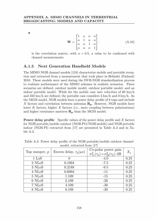
APPENDIX A. MIMO CHANNELS IN TERRESTRIALBROADCASTING: MODELS AND CAPACITY
•
W =
1 α α αα 1 α αα α 1 αα α α 1
. (A.10)
is the correlation matrix, with α = 0.5, a value to be confirmed withchannel measurements.
A.1.3 Next Generation Handheld Models
The MIMO NGH channel models [124] characterize mobile and portable recep-tion and extracted from a measurement that took place in Helsinki (Finland)2010. These models were used during the DVB-NGH standardization processto evaluate performance of the MIMO schemes in realistic scenarios. Threescenarios are defined, outdoor mobile model, outdoor portable model, and anindoor portable model. While for the mobile case user velocities of 60 km/hand 350 km/h are defined, the portable case considers 3 km/h and 0 km/h. Asthe MGM model, NGH models have a power delay profile of 8 taps and includeX factors and correlation between antennas Rp. However, NGH models havelower K factors, higher X factors (i.e., more coupling between polarizations)and higher covariance matrices Rp than the MGM model.
Power delay profile Specific values of the power delay profile and X factorsfor NGH portable/mobile outdoor (NGH-PO/NGH-mobile) and NGH portableindoor (NGH-PI) extracted from [17] are presented in Table A.2 and in Ta-ble A.3.
Table A.2: Power delay profile of the NGH portable/mobile outdoor channelmodel, extracted from [17]
Tap numper, p Excess delay, τp(µs)Co-polar power gainσ2
11(τp)=σ222(τp) dB
Xj
1 LoS 0 -4.0 0.252 NLoS 0.1094 -7.5 0.253 NLoS 0.2188 -9.5 0.254 NLoS 0.6094 -11 0.255 NLoS 1.109 -15 0.256 NLoS 2.109 -26 0.257 NLoS 4.109 -30 0.258 NLoS 8.109 -30 0.25
158
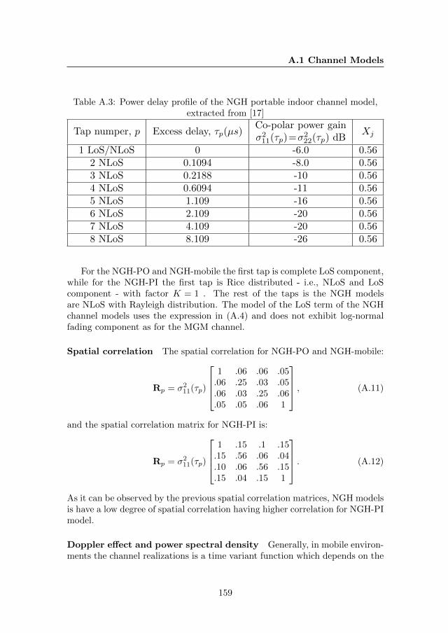
A.1 Channel Models
Table A.3: Power delay profile of the NGH portable indoor channel model,extracted from [17]
Tap numper, p Excess delay, τp(µs)Co-polar power gainσ2
11(τp)=σ222(τp) dB
Xj
1 LoS/NLoS 0 -6.0 0.562 NLoS 0.1094 -8.0 0.563 NLoS 0.2188 -10 0.564 NLoS 0.6094 -11 0.565 NLoS 1.109 -16 0.566 NLoS 2.109 -20 0.567 NLoS 4.109 -20 0.568 NLoS 8.109 -26 0.56
For the NGH-PO and NGH-mobile the first tap is complete LoS component,while for the NGH-PI the first tap is Rice distributed - i.e., NLoS and LoScomponent - with factor K = 1 . The rest of the taps is the NGH modelsare NLoS with Rayleigh distribution. The model of the LoS term of the NGHchannel models uses the expression in (A.4) and does not exhibit log-normalfading component as for the MGM channel.
Spatial correlation The spatial correlation for NGH-PO and NGH-mobile:
Rp = σ211(τp)
1 .06 .06 .05.06 .25 .03 .05.06 .03 .25 .06.05 .05 .06 1
, (A.11)
and the spatial correlation matrix for NGH-PI is:
Rp = σ211(τp)
1 .15 .1 .15.15 .56 .06 .04.10 .06 .56 .15.15 .04 .15 1
. (A.12)
As it can be observed by the previous spatial correlation matrices, NGH modelsis have a low degree of spatial correlation having higher correlation for NGH-PImodel.
Doppler effect and power spectral density Generally, in mobile environ-ments the channel realizations is a time variant function which depends on the
159
APPENDIX A. MIMO CHANNELS IN TERRESTRIALBROADCASTING: MODELS AND CAPACITY
relative speed of the transmit and receive pair. The time dependent variation ofthe channel realizations produce frequency shifts in the received signal knownas Doppler effect. The maximum frequency shift fD in the received signal dueto the Doppler effect is:
fD =v
cfc cosα, (A.13)
where v is the receiver velocity1 c is the speed of light, fc is the carrier frequencyof the signal, and α is the angle between directions of the receiver velocity andthe arriving signal.
The pdf for Doppler frequency shifts depends on maximum Doppler fre-quency and the angular probability distribution of the received components.Under certain assumption such as signals propagate between the transmitterand the receiver in horizontal plane, the angles of arrival at the receive antennaare uniformly distributed, and a circular symmetric radiation pattern for thereceive antenna, the power spectral distribution follows so-called Jakes powerspectral density or the Clarke power spectral density. The Jakes power spectraldensity has the following expression:
S(f, fd) =
1
πfd√
1−(f/fD)2∀f ∈]− fD, fD[
0 elsewhere(A.14)
where the frequency shift components are distributed between −fD, and fD.A tap with Jakes power spectral density can be obtained by method of exactDoppler spread (MEDS) [125].
The tap spectral characteristic for the NGH-PO and NGH-mobile are:S(f − 3fD/4, fD/4) for p = 2, 3S(f + 3fD/4, fD/4) for p = 4, 5, 6, 7, 8
(A.15)
where the tap p = 1 is LoS with no Doppler shift and the tap spectral charac-teristics for the NGH-PI model are: S(f, fD) for p = 1
S(f − 3fD/4, fD/4) for p = 2, 3S(f + 3fD/4, fD/4) for p = 4, 5, 6, 7, 8
(A.16)
where for tap p = 1 the Doppler shifts are applied to the NLoS of the tap.
1The velocity v corresponds to the relative velocity between the transmitter and receiverpair, where the transmitter and/or receiver can be in motion. The Doppler effect can bealso observed in the received signal components from reflected objects that are in motion. InDTT systems the transmitters are normally static, therefore we assume in this thesis Dopplereffect caused by mobile receivers.
160
A.1 Channel Models
Rotation and imbalance matrices Additional matrices in the NGH mod-els includes the effects of antenna alignment mismatch and transmit powerimbalance in the NGH models.
The mismatch antenna matrix typically occurs in handset receivers wherethe orientation of the receive antenna depends on how the user holds the ter-minal. This mismatch is reduced in the case of rooftop reception since a pro-fessional installer aligns the receive antenna to the direction of the receivedsignal. The mismatch matrix has the form of a rotation matrix:
W =
[cos Ω − sin Ωsin Ω cos Ω
], (A.17)
where Ω is the rotation angle and takes the values from the set −45, 0,+45.The imbalance matrix models the case where there exists a power imbalance
between the two transmit vertical and horizontal polarizations. This situationis modelled with the diagonal matrix:
Γ =
[Γ11 00 Γ22
], (A.18)
where Γ11 and Γ22 can take the following values: [Γ11 = 1.1074,Γ22 = 0.8796],[Γ11 = 1,Γ22 = 1] and [Γ11 = 0.8796,Γ22 = 1.1074]. This transmit power imbal-ance model could also be included in the MGM channel model although it isnot initially defined in the reference documents.
Signal model The basic signal model (without matrices Ω and W) for theNGH channels follow the expressions (A.7) and (A.8), but for the NGH-POand NGH-mobile models the summation excludes the tap p= 1 since the firsttap is only LoS for those channels. When the matrices Ω and W are included,expression (A.7) is replaced by:
WH(t , τ)Γ =
[cos Ω − sin Ωsin Ω cos Ω
] [h11(t , τ) h12(t , τ)h21(t , τ) h22(t , τ)
] [Γ11 00 Γ22
]. (A.19)
Due to the more static nature of the rotation and power imbalance matrices,they may affect multiple frames. The reinitialization of these variables mayoccur after various seconds, e.g., reference documents recommend five seconds.
A.1.4 Extension to Four Transmit Antennas
MIMO 4×2 channel models considered in thesis are composed at the transmitterside of 4 transmit cross-polar antennas (two horizontal and two vertical) andtwo cross-polar antennas at the receiver side. The case where the transmitantennas are co-located in the site is considered. The extension to 4 transmit
161
APPENDIX A. MIMO CHANNELS IN TERRESTRIALBROADCASTING: MODELS AND CAPACITY
antennas is achieved with two correlated independent instances of 2×2 MIMOchannels previously described. For the second 2×2 MIMO NLoS and LoScomponents, the terms Hw and Hw are replaced with Hw and Hw where
vec(Hw) = βvec(Hw) +√
1− β2vec(Hw),
vec(Hw) = γvec(Hw) +√
1− γ2vec(Hw)(A.20)
where Hw and Hw are independent instances of i.i.d zero-mean complex Gaus-sian random matrices. The MGM model in [123] suggests a β = 0.5 value forthe NLOS. Chapter 3 of this thesis studies different correlation values γ for theLOS in the [0, 1] range. Although the correlation between channel componentsfrom different polarizations is low [121], higher correlation values are observedbetween channel components with the same polarization [126]. Furthermore,strong LOS scenarios produces high correlated channels components [127, 128].Specific values need to be confirmed with data extracted from measurementcampaigns of cross-polar 4×2 MIMO in the UHF band.
A.2 Ergodic Capacity with Asymptotic SNR
For the performance analysis of the MIMO gains over SISO it will be conve-nient to use approximate ergodic capacity expressions in the high and low SNRregime.
Low SNR regime At low SNR values the ergodic capacity expression canapproximated by [13]:
C = Elog det
(INr +
SNR
NtHH†
) = E
nmin∑i=1
log
(SNR
Ntλ2i
)
≈ Enmin∑i=1
SNR
Ntλ2i log(e) =
SNR
Ntlog(e)
nmin∑i=1
Eλ2i
=SNR
Ntlog(e)E||H||2F =
SNR
Ntlog(e)E
Nr,Nt∑i,j
|hij |2.
(A.21)
where nmin is the minimum number of Nt transmit and Nr receive antennasin a i.i.d. Rayleigh channel with no spatial correlation and using the followingapproximation: log(1 + x) ≈ x log(e) when x→ 0.
162
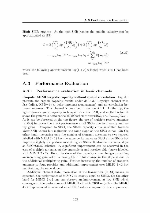
A.3 Performance Evaluation
High SNR regime At the high SNR regime the ergodic capacity can beapproximated as [13]:
C = Enmin∑i=1
log
(SNR
Ntλ2i
) ≈ E
nmin∑i=1
logSNR
Ntλ2i
= nmin log SNR− nmin logNt +
nmin∑i=1
Elog λ2i
≈ nmin log SNR
(A.22)
where the following approximation: log(1 + x)≈ log(x) when x 1 has beenused.
A.3 Performance Evaluation
A.3.1 Performance evaluation in basic channels
Co-polar MIMO ergodic capacity without spatial correlation Fig. A.1presents the ergodic capacity results under de i.i.d. Rayleigh channel withfast fading, XPD=1 (co-polar antennas arrangement) and no correlation be-tween antennas. This channel is described in section A.1.1. At the top, thefigure shows ergodic capacity in bits/s/Hz vs. the SNR, and at the bottom itshows the gain ratio between the MIMO schemes over SISO, i.e., CMIMO/CSISO.As it can be observed at the top figure, the use of multiple receive antennas(SIMO) improves the SISO performance at all SNRs due to diversity and ar-ray gains. Compared to SISO, the SIMO capacity curve is shifted towardslower SNR values but maintains the same slope as the SISO curve. On theother hand, increasing only the number of transmit antennas to two (curvedlabelled with MISO 2×1) has the same performance as SISO at low SNRs butimproves slightly the performance at higher SNRs. It also has the same slopeas SISO/SIMO schemes. A significant improvement can be observed in thecase of multiple antennas at the transmitter and receiver side (curve labelledwith MIMO 2×2). Here, the slope of the capacity curve changes providingan increasing gain with increasing SNR. This change in the slope is due tothe additional multiplexing gain. Further increasing the number of transmitantennas to four, provides and additional improvement over MIMO 2×2 butmaintaining the same slope.
Additional channel state information at the transmitter (CTSI) makes, asexpected, the performance of MISO 2×1 exactly equal to SIMO. On the otherhand for MIMO 2× 2 one can observe an improvement at low SNR whichconverges to the performance of MIMO 2×2 with CRSI only. For the MIMO4×2 improvement is achieved at all SNR values compared to the unprecoded
163
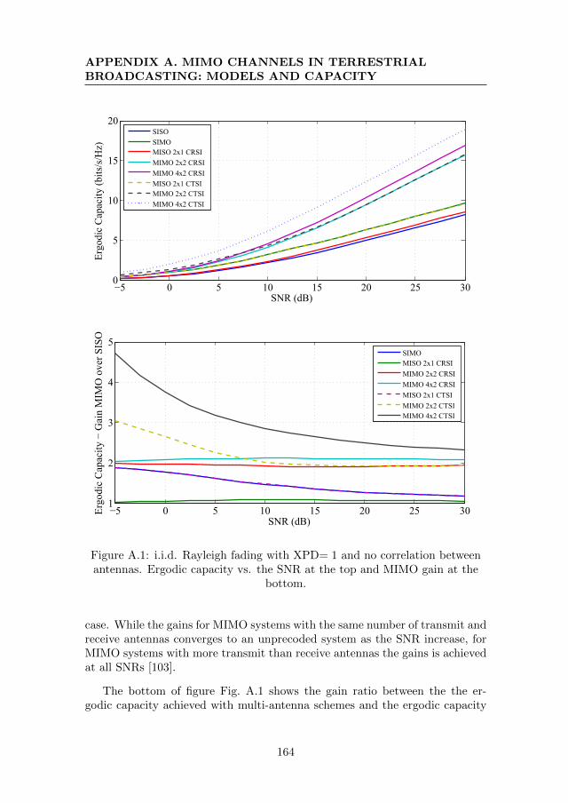
APPENDIX A. MIMO CHANNELS IN TERRESTRIALBROADCASTING: MODELS AND CAPACITY
−5 0 5 10 15 20 25 300
5
10
15
20
SNR (dB)
Ergo
dic
Cap
acity
(bits
/s/H
z)
SISO SIMOMISO 2x1 CRSIMIMO 2x2 CRSIMIMO 4x2 CRSIMISO 2x1 CTSIMIMO 2x2 CTSIMIMO 4x2 CTSI
−5 0 5 10 15 20 25 301
2
3
4
5
SNR (dB)
Ergo
dic
Cap
acity
− G
ain
MIM
O o
ver S
ISO
SIMOMISO 2x1 CRSIMIMO 2x2 CRSIMIMO 4x2 CRSIMISO 2x1 CTSIMIMO 2x2 CTSIMIMO 4x2 CTSI
Figure A.1: i.i.d. Rayleigh fading with XPD= 1 and no correlation betweenantennas. Ergodic capacity vs. the SNR at the top and MIMO gain at the
bottom.
case. While the gains for MIMO systems with the same number of transmit andreceive antennas converges to an unprecoded system as the SNR increase, forMIMO systems with more transmit than receive antennas the gains is achievedat all SNRs [103].
The bottom of figure Fig. A.1 shows the gain ratio between the the er-godic capacity achieved with multi-antenna schemes and the ergodic capacity
164
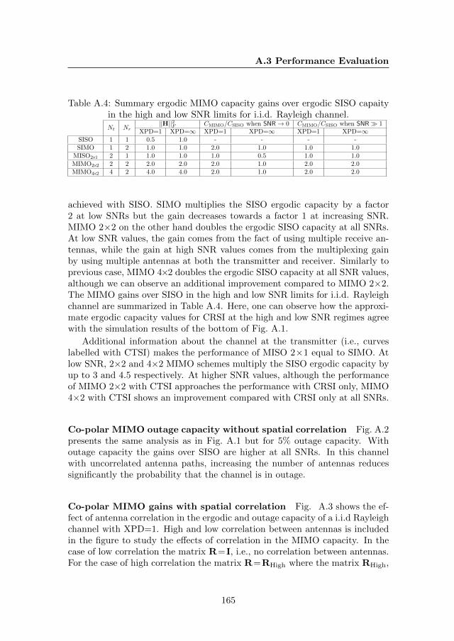
A.3 Performance Evaluation
Table A.4: Summary ergodic MIMO capacity gains over ergodic SISO capaityin the high and low SNR limits for i.i.d. Rayleigh channel.
Nt Nr||H||2F CMIMO/CSISO when SNR→ 0 CMIMO/CSISO when SNR 1
XPD=1 XPD=∞ XPD=1 XPD=∞ XPD=1 XPD=∞SISO 1 1 0.5 1.0 - - - -SIMO 1 2 1.0 1.0 2.0 1.0 1.0 1.0
MISO2×1 2 1 1.0 1.0 1.0 0.5 1.0 1.0MIMO2×2 2 2 2.0 2.0 2.0 1.0 2.0 2.0MIMO4×2 4 2 4.0 4.0 2.0 1.0 2.0 2.0
achieved with SISO. SIMO multiplies the SISO ergodic capacity by a factor2 at low SNRs but the gain decreases towards a factor 1 at increasing SNR.MIMO 2×2 on the other hand doubles the ergodic SISO capacity at all SNRs.At low SNR values, the gain comes from the fact of using multiple receive an-tennas, while the gain at high SNR values comes from the multiplexing gainby using multiple antennas at both the transmitter and receiver. Similarly toprevious case, MIMO 4×2 doubles the ergodic SISO capacity at all SNR values,although we can observe an additional improvement compared to MIMO 2×2.The MIMO gains over SISO in the high and low SNR limits for i.i.d. Rayleighchannel are summarized in Table A.4. Here, one can observe how the approxi-mate ergodic capacity values for CRSI at the high and low SNR regimes agreewith the simulation results of the bottom of Fig. A.1.
Additional information about the channel at the transmitter (i.e., curveslabelled with CTSI) makes the performance of MISO 2×1 equal to SIMO. Atlow SNR, 2×2 and 4×2 MIMO schemes multiply the SISO ergodic capacity byup to 3 and 4.5 respectively. At higher SNR values, although the performanceof MIMO 2×2 with CTSI approaches the performance with CRSI only, MIMO4×2 with CTSI shows an improvement compared with CRSI only at all SNRs.
Co-polar MIMO outage capacity without spatial correlation Fig. A.2presents the same analysis as in Fig. A.1 but for 5% outage capacity. Withoutage capacity the gains over SISO are higher at all SNRs. In this channelwith uncorrelated antenna paths, increasing the number of antennas reducessignificantly the probability that the channel is in outage.
Co-polar MIMO gains with spatial correlation Fig. A.3 shows the ef-fect of antenna correlation in the ergodic and outage capacity of a i.i.d Rayleighchannel with XPD=1. High and low correlation between antennas is includedin the figure to study the effects of correlation in the MIMO capacity. In thecase of low correlation the matrix R=I, i.e., no correlation between antennas.For the case of high correlation the matrix R=RHigh where the matrix RHigh,
165
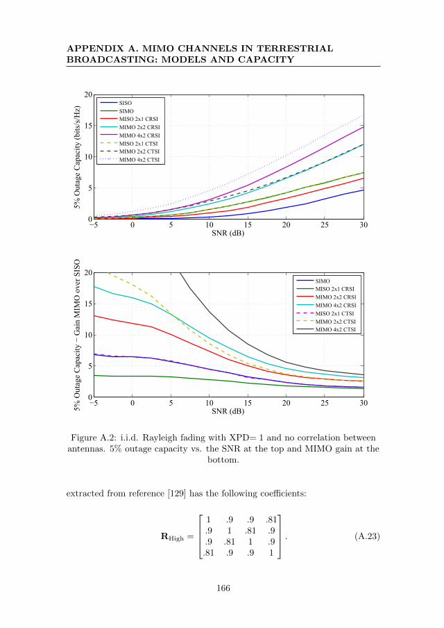
APPENDIX A. MIMO CHANNELS IN TERRESTRIALBROADCASTING: MODELS AND CAPACITY
−5 0 5 10 15 20 25 300
5
10
15
20
SNR (dB)
5% O
utag
e C
apac
ity (b
its/s
/Hz)
SISOSIMOMISO 2x1 CRSIMIMO 2x2 CRSIMIMO 4x2 CRSIMISO 2x1 CTSIMIMO 2x2 CTSIMIMO 4x2 CTSI
−5 0 5 10 15 20 25 300
5
10
15
20
SNR (dB)5% O
utag
e C
apac
ity −
Gai
n M
IMO
ove
r SIS
O
SIMOMISO 2x1 CRSIMIMO 2x2 CRSIMIMO 4x2 CRSIMISO 2x1 CTSIMIMO 2x2 CTSIMIMO 4x2 CTSI
Figure A.2: i.i.d. Rayleigh fading with XPD= 1 and no correlation betweenantennas. 5% outage capacity vs. the SNR at the top and MIMO gain at the
bottom.
extracted from reference [129] has the following coefficients:
RHigh =
1 .9 .9 .81.9 1 .81 .9.9 .81 1 .9.81 .9 .9 1
. (A.23)
166
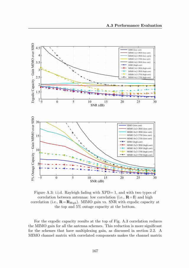
A.3 Performance Evaluation
−5 0 5 10 15 20 25 301
1.5
2
2.5
3
3.5
4
4.5
SNR (dB)
Ergo
dic
Cap
acity
− G
ain
MIM
O o
ver S
ISO
SIMO (low corr)MIMO 2x2 CRSI (low corr)MIMO 4x2 CRSI (low corr))MIMO 2x2 CTSI (low corr)MIMO 4x2 CRSI (low corr)SIMO (high corr)MIMO 2x2 CRSI (high corr)MIMO 4x2 CRSI (high corr)MIMO 2x2 CTSI (high corr)MIMO 4x2 CTSI (high corr)
−5 0 5 10 15 20 25 30
5
10
15
20
SNR (dB)5% O
utag
e C
apac
ity −
Gai
n M
IMO
ove
r SIS
O
SIMO (low corr)MIMO 2x2 CRSI (low corr)MIMO 4x2 CRSI (low corr)MIMO 2x2 CTSI (low corr)MIMO 4x2 CTSI (low corr)SIMO (high corr)MIMO 2x2 CRSI (high corr)MIMO 4x2 CRSI (high corr)MIMO 2x2 CTSI (high corr)MIMO 4x2 CTSI (high corr)
Figure A.3: i.i.d. Rayleigh fading with XPD= 1, and with two types ofcorrelation between antennas: low correlation (i.e., R=I) and high
correlation (i.e., R=RHigh). MIMO gain vs. SNR with ergodic capacity atthe top and 5% outage capacity at the bottom.
For the ergodic capacity results at the top of Fig. A.3 correlation reducesthe MIMO gain for all the antenna schemes. This reduction is more significantfor the schemes that have multiplexing gain, as discussed in section 2.2. AMIMO channel matrix with correlated components makes the channel matrix
167
APPENDIX A. MIMO CHANNELS IN TERRESTRIALBROADCASTING: MODELS AND CAPACITY
singular which decreases the multiplexing gain. For SIMO, only a marginalreduction is observed since the power gain is retained and only the diversitygain is lost due to correlated fading. With CTSI, same performance loss isobserved at high SNRs. However, at low SNRs, higher ergodic capacity can beachieved with correlated antennas than with un-correlated antennas. Similarresults is observed in references [103, 96].
For the 5% outage capacity results at the bottom of Fig. A.3 presents similarbehaviour to the ergodic capacity plot, i.e., the MIMO gain reduces due tocorrelated antennas. However, with CTSI also reduces the available gain atthe low SNR regime. Here, the loss of SIMO is also significant, specially at lowSNRs. With correlated antennas the probability that all channel paths are inoutages increases, reducing the outage capacity.
Co-polar vs. Cross-polar MIMO with spatial correlation Fig. A.4shows the same results as in Fig. A.3 but for high spatial correlation and twotypes XPD values, XPD= 1 (full inter-antenna interference - co-polar antennas)and XPD= ∞ (no inter-antenna interference - perfect cross-polar antennas).First the ergodic capacity results at the top of Fig. A.4 for the MIMO schemeswith XPD =∞ are studied. With cross-polar antennas, SIMO provides thesame performance than SISO at all SNRs, and MISO 2×1 provides a perfor-mance loss compared to SISO at low SNRs (towards a 0.5 ratio) but this lossis reduced with increasing SNR towards a value of 1. On the other hand, thegains of 2×2 and 4×2 MIMO schemes tend to 1 at low SNRs, but increase withincreasing SNR asymptotically to a gain of 2. These gains can also be predictedby expressions (A.21) and (A.22) and summarized in Table A.4. The perfor-mance of MIMO schemes with XPD =∞ compares with the case of XPD = 1in the following way. For SIMO, the gains achieved with XPD = 1 are higherthan XPD=∞ at all SNRs. The same comparison can be done for MISO 2×1,but here XPD=∞ always performs worse than SISO, that discourages its use.In the case of 2× 2 and 4× 2 MIMO, although XPD =∞ does not provide abenefit compared to XPD = 1 at low SNRs, it can overcome the performancedegradation due to spatial correlation at high SNRs.
In terms of outage capacity results at the bottom of Fig. A.4 for all theschemes, XPD=∞ always provides lower or equal performance than XPD=1at all SNRs. This performance difference is specially significant at low SNRvalues. It is interesting to note that for 2× 2 and 4× 2 MIMO with eitherXPD=1 or XPD=∞ reach the same value at high SNRs. This is not the casefor SIMO and MISO 2× 1 with XPD = 1 which still obtain higher gain thanXPD=∞ at high SNR values.
168
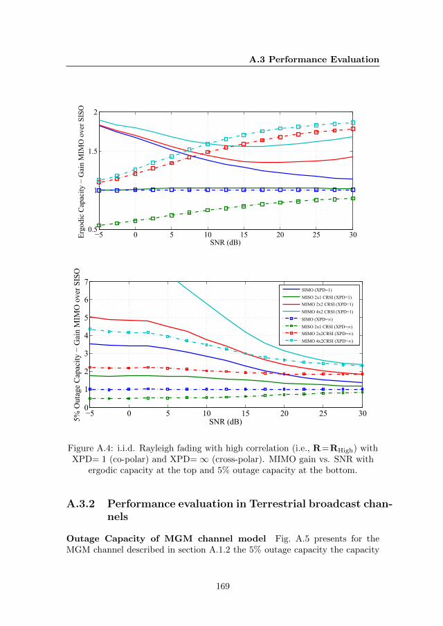
A.3 Performance Evaluation
−5 0 5 10 15 20 25 300.5
1
1.5
2
SNR (dB)
Ergo
dic
Cap
acity
− G
ain
MIM
O o
ver S
ISO
−5 0 5 10 15 20 25 300
1
2
3
4
5
6
7
SNR (dB)5% O
utag
e C
apac
ity −
Gai
n M
IMO
ove
r SIS
O
SIMO (XPD=1)MISO 2x1 CRSI (XPD=1)MIMO 2x2 CRSI (XPD=1)MIMO 4x2 CRSI (XPD=1)SIMO (XPD=∞)MISO 2x1 CRSI (XPD=∞)MIMO 2x2 CRSI (XPD=∞)MIMO 4x2 CRSI (XPD=∞)
Figure A.4: i.i.d. Rayleigh fading with high correlation (i.e., R=RHigh) withXPD= 1 (co-polar) and XPD=∞ (cross-polar). MIMO gain vs. SNR with
ergodic capacity at the top and 5% outage capacity at the bottom.
A.3.2 Performance evaluation in Terrestrial broadcast chan-nels
Outage Capacity of MGM channel model Fig. A.5 presents for theMGM channel described in section A.1.2 the 5% outage capacity the capacity
169
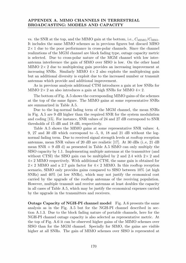
APPENDIX A. MIMO CHANNELS IN TERRESTRIALBROADCASTING: MODELS AND CAPACITY
vs. the SNR at the top, and the MIMO gain at the bottom, i.e., CMIMO/CSISO.It includes the same MIMO schemes as in previous figures but discard MISO2× 1 due to the poor performance in cross-polar channels. Since the channelrealizations of the MGM channel are block fading type, outage capacity metricis selected. Due to cross-polar nature of the MGM channel with low inter-antenna interference the gain of SIMO over SISO is low. On the other handMIMO 2× 2 due to multiplexing gain provides an increasing improvement atincreasing SNRs. Similarly MIMO 4× 2 also exploits the multiplexing gainbut an additional diversity is exploit due to the increased number or transmitantennas which provide and additional improvement.
As in previous analysis additional CTSI introduces a gain at low SNRs forMIMO 2× 2 an also introduces a gain at high SNRs for MIMO 4× 2.
The bottom of Fig. A.5 shows the corresponding MIMO gains of the schemesat the top of the same figure. The MIMO gains at some representative SNRsare summarized in Table A.5.
Due to the log-normal fading term of the MGM channel, the mean SNRsin Fig. A.5 are 9 dB higher than the required SNR for the system modulationand coding [15]. For instance, SNR values of 24 and 27 dB correspond to SNRthresholds of 15 dB and 18 dB, respectively.
Table A.5 shows the MIMO gains at some representative SNR values: 4,9, 27 and 30 dB which correspond to -5, 0, 18 and 21 dB without the log-normal fading term. Due to received signal strength levels at rooftop receptionantennas, mean SNR values of 20 dB are realistic [17]. At 30 dBs (i..e, 21 dBmean SNR + 9 dB d) as presented in Table A.5 SIMO can only multiply theSISO capacity by 1.1. Implementing multiple antennas at the transmitter (andwithout CTSI) the SISO gain can be multiplied by 2 and 2.4 with 2× 2 and4× 2 MIMO respectively. With additional CTSI, the same gain is obtained for2× 2 MIMO and a 2.7 gain factor for 4× 2 MIMO. In this rooftop receptionscenario, SIMO only provides gains compared to SISO between 10% (at highSNRs) and 40% (at low SNRs), which may not justify the economical costcarried by the upgrade of the rooftop antennas of the receiving population.However, multiple transmit and receive antennas at least doubles the capacityin all cases of Table A.5, which may be justify the economical expenses carriedby the upgrade in the transmitters and receivers.
Outage Capacity of NGH-PI channel model Fig. A.6 presents the sameanalysis as in the Fig. A.5 but for the NGH-PI channel described in sec-tion A.1.3. Due to the block fading nature of portable channels, here for theNGH-PI channel outage capacity is also selected as representative metric. Atthe top of Fig. A.6 it can be observed higher gains of the MIMO schemes overSISO than for the MGM channel. Specially for SIMO, the gains are visiblehigher at all SNRs. The gain of MIMO schemes over SISO is represented at
170
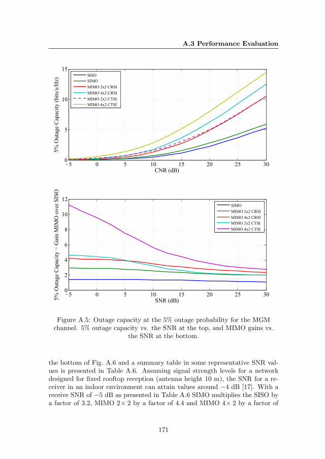
A.3 Performance Evaluation
−5 0 5 10 15 20 25 300
5
10
15
CNR (dB)
5% O
utag
e C
apac
ity (b
its/s
/Hz)
SISOSIMOMIMO 2x2 CRSIMIMO 4x2 CRSIMIMO 2x2 CTSIMIMO 4x2 CTSI
−5 0 5 10 15 20 25 300
2
4
6
8
10
12
SNR (dB)5% O
utag
e C
apac
ity −
Gai
n M
IMO
ove
r SIS
O
SIMOMIMO 2x2 CRSIMIMO 4x2 CRSIMIMO 2x2 CTSIMIMO 4x2 CTSI
Figure A.5: Outage capacity at the 5% outage probability for the MGMchannel. 5% outage capacity vs. the SNR at the top, and MIMO gains vs.
the SNR at the bottom.
the bottom of Fig. A.6 and a summary table in some representative SNR val-ues is presented in Table A.6. Assuming signal strength levels for a networkdesigned for fixed rooftop reception (antenna height 10 m), the SNR for a re-ceiver in an indoor environment can attain values around −4 dB [17]. With areceive SNR of −5 dB as presented in Table A.6 SIMO multiplies the SISO bya factor of 3.2, MIMO 2× 2 by a factor of 4.4 and MIMO 4× 2 by a factor of
171
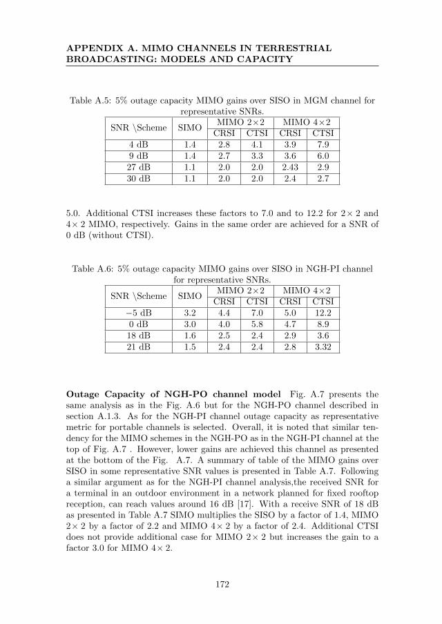
APPENDIX A. MIMO CHANNELS IN TERRESTRIALBROADCASTING: MODELS AND CAPACITY
Table A.5: 5% outage capacity MIMO gains over SISO in MGM channel forrepresentative SNRs.
SNR \Scheme SIMOMIMO 2×2 MIMO 4×2
CRSI CTSI CRSI CTSI4 dB 1.4 2.8 4.1 3.9 7.99 dB 1.4 2.7 3.3 3.6 6.027 dB 1.1 2.0 2.0 2.43 2.930 dB 1.1 2.0 2.0 2.4 2.7
5.0. Additional CTSI increases these factors to 7.0 and to 12.2 for 2× 2 and4× 2 MIMO, respectively. Gains in the same order are achieved for a SNR of0 dB (without CTSI).
Table A.6: 5% outage capacity MIMO gains over SISO in NGH-PI channelfor representative SNRs.
SNR \Scheme SIMOMIMO 2×2 MIMO 4×2
CRSI CTSI CRSI CTSI−5 dB 3.2 4.4 7.0 5.0 12.20 dB 3.0 4.0 5.8 4.7 8.918 dB 1.6 2.5 2.4 2.9 3.621 dB 1.5 2.4 2.4 2.8 3.32
Outage Capacity of NGH-PO channel model Fig. A.7 presents thesame analysis as in the Fig. A.6 but for the NGH-PO channel described insection A.1.3. As for the NGH-PI channel outage capacity as representativemetric for portable channels is selected. Overall, it is noted that similar ten-dency for the MIMO schemes in the NGH-PO as in the NGH-PI channel at thetop of Fig. A.7 . However, lower gains are achieved this channel as presentedat the bottom of the Fig. A.7. A summary of table of the MIMO gains overSISO in some representative SNR values is presented in Table A.7. Followinga similar argument as for the NGH-PI channel analysis,the received SNR fora terminal in an outdoor environment in a network planned for fixed rooftopreception, can reach values around 16 dB [17]. With a receive SNR of 18 dBas presented in Table A.7 SIMO multiplies the SISO by a factor of 1.4, MIMO2× 2 by a factor of 2.2 and MIMO 4× 2 by a factor of 2.4. Additional CTSIdoes not provide additional case for MIMO 2× 2 but increases the gain to afactor 3.0 for MIMO 4× 2.
172
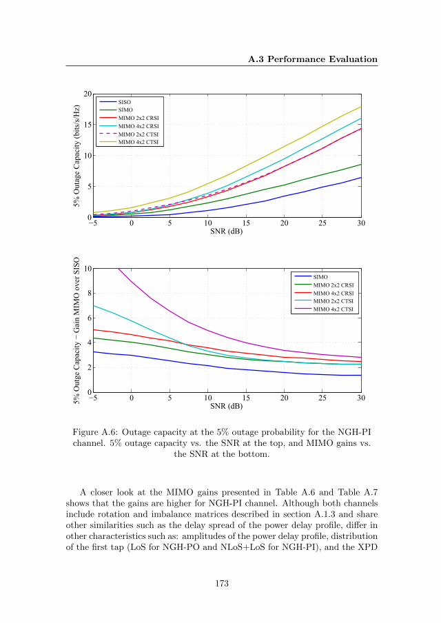
A.3 Performance Evaluation
−5 0 5 10 15 20 25 300
5
10
15
20
SNR (dB)
5% O
utag
e C
apac
ity (b
its/s
/Hz)
SISOSIMOMIMO 2x2 CRSIMIMO 4x2 CRSIMIMO 2x2 CTSIMIMO 4x2 CTSI
−5 0 5 10 15 20 25 300
2
4
6
8
10
SNR (dB)5% O
utge
Cap
acity
− G
ain
MIM
O o
ver S
ISO
SIMOMIMO 2x2 CRSIMIMO 4x2 CRSIMIMO 2x2 CTSIMIMO 4x2 CTSI
Figure A.6: Outage capacity at the 5% outage probability for the NGH-PIchannel. 5% outage capacity vs. the SNR at the top, and MIMO gains vs.
the SNR at the bottom.
A closer look at the MIMO gains presented in Table A.6 and Table A.7shows that the gains are higher for NGH-PI channel. Although both channelsinclude rotation and imbalance matrices described in section A.1.3 and shareother similarities such as the delay spread of the power delay profile, differ inother characteristics such as: amplitudes of the power delay profile, distributionof the first tap (LoS for NGH-PO and NLoS+LoS for NGH-PI), and the XPD
173
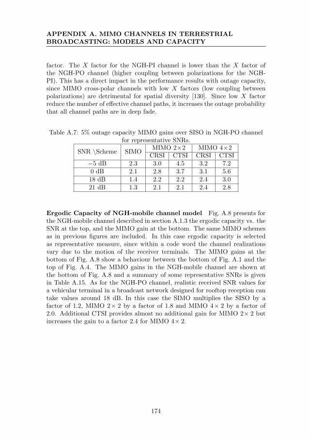
APPENDIX A. MIMO CHANNELS IN TERRESTRIALBROADCASTING: MODELS AND CAPACITY
factor. The X factor for the NGH-PI channel is lower than the X factor ofthe NGH-PO channel (higher coupling between polarizations for the NGH-PI). This has a direct impact in the performance results with outage capacity,since MIMO cross-polar channels with low X factors (low coupling betweenpolarizations) are detrimental for spatial diversity [130]. Since low X factorreduce the number of effective channel paths, it increases the outage probabilitythat all channel paths are in deep fade.
Table A.7: 5% outage capacity MIMO gains over SISO in NGH-PO channelfor representative SNRs.
SNR \Scheme SIMOMIMO 2×2 MIMO 4×2
CRSI CTSI CRSI CTSI−5 dB 2.3 3.0 4.5 3.2 7.20 dB 2.1 2.8 3.7 3.1 5.618 dB 1.4 2.2 2.2 2.4 3.021 dB 1.3 2.1 2.1 2.4 2.8
Ergodic Capacity of NGH-mobile channel model Fig. A.8 presents forthe NGH-mobile channel described in section A.1.3 the ergodic capacity vs. theSNR at the top, and the MIMO gain at the bottom. The same MIMO schemesas in previous figures are included. In this case ergodic capacity is selectedas representative measure, since within a code word the channel realizationsvary due to the motion of the receiver terminals. The MIMO gains at thebottom of Fig. A.8 show a behaviour between the bottom of Fig. A.1 and thetop of Fig. A.4. The MIMO gains in the NGH-mobile channel are shown atthe bottom of Fig. A.8 and a summary of some representative SNRs is givenin Table A.15. As for the NGH-PO channel, realistic received SNR values fora vehicular terminal in a broadcast network designed for rooftop reception cantake values around 18 dB. In this case the SIMO multiplies the SISO by afactor of 1.2, MIMO 2× 2 by a factor of 1.8 and MIMO 4× 2 by a factor of2.0. Additional CTSI provides almost no additional gain for MIMO 2× 2 butincreases the gain to a factor 2.4 for MIMO 4× 2.
174
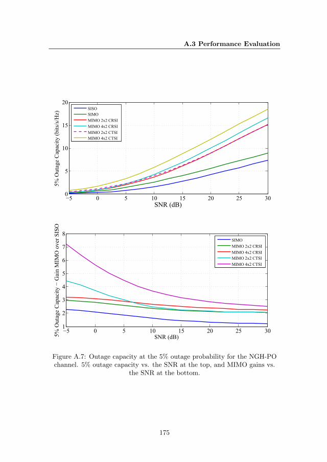
A.3 Performance Evaluation
−5 0 5 10 15 20 25 300
5
10
15
20
SNR (dB)
5% O
utag
e C
apac
ity (b
its/s
/Hz)
SISOSIMOMIMO 2x2 CRSIMIMO 4x2 CRSIMIMO 2x2 CTSIMIMO 4x2 CTSI
−5 0 5 10 15 20 25 301
2
3
4
5
6
7
8
SNR (dB)5% O
utag
e C
apac
ity −
Gai
n M
IMO
ove
r SIS
O
SIMOMIMO 2x2 CRSIMIMO 4x2 CRSIMIMO 2x2 CTSIMIMO 4x2 CTSI
Figure A.7: Outage capacity at the 5% outage probability for the NGH-POchannel. 5% outage capacity vs. the SNR at the top, and MIMO gains vs.
the SNR at the bottom.
175
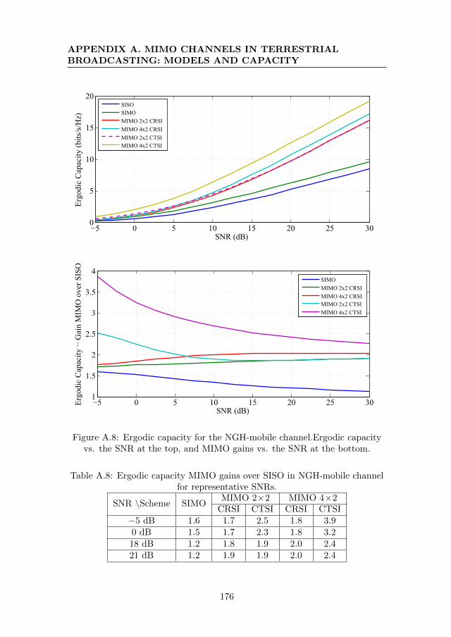
APPENDIX A. MIMO CHANNELS IN TERRESTRIALBROADCASTING: MODELS AND CAPACITY
−5 0 5 10 15 20 25 300
5
10
15
20
SNR (dB)
Ergo
dic
Cap
acity
(bits
/s/H
z)
SISOSIMOMIMO 2x2 CRSIMIMO 4x2 CRSIMIMO 2x2 CTSIMIMO 4x2 CTSI
−5 0 5 10 15 20 25 301
1.5
2
2.5
3
3.5
4
SNR (dB)
Ergo
dic
Cap
acity
− G
ain
MIM
O o
ver S
ISO
SIMOMIMO 2x2 CRSIMIMO 4x2 CRSIMIMO 2x2 CTSIMIMO 4x2 CTSI
Figure A.8: Ergodic capacity for the NGH-mobile channel.Ergodic capacityvs. the SNR at the top, and MIMO gains vs. the SNR at the bottom.
Table A.8: Ergodic capacity MIMO gains over SISO in NGH-mobile channelfor representative SNRs.
SNR \Scheme SIMOMIMO 2×2 MIMO 4×2
CRSI CTSI CRSI CTSI−5 dB 1.6 1.7 2.5 1.8 3.90 dB 1.5 1.7 2.3 1.8 3.218 dB 1.2 1.8 1.9 2.0 2.421 dB 1.2 1.9 1.9 2.0 2.4
176
Appendix B
DVB-NGH and ATSC 3.0MIMO Physical Layers
This appendix presents the MIMO physical layers adopted for DVB-NGHand ATSC 3.0 specifications. Both specifications share similar architecture
for the implementation of MIMO. First, a common transmit block diagram forthe two specifications is presented. Then, specific differences and commonalitiesfor each of the transmitting blocks are detailed.
177
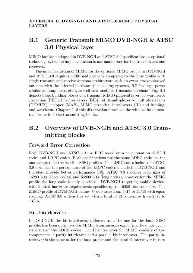
APPENDIX B. DVB-NGH AND ATSC 3.0 MIMO PHYSICALLAYERS
B.1 Generic Transmit MIMO DVB-NGH & ATSC3.0 Physical layer
MIMO has been adopted in DVB-NGH and ATSC 3.0 specifications as optionaltechnologies, i.e., its implementation is not mandatory for the transmitters andreceivers.
The implementation of MIMO for the optional MIMO profile in DVB-NGHand ATSC 3.0 requires additional elements compared to the base profile withsingle transmit and receive antenna architecture such an extra cross-polarizedantenna with the inferred hardware (i.e. cooling systems, RF feedings, powercombiners, amplifiers, etc.), as well as a modified transmission chain. Fig. B.1depicts basic building blocks of a transmit MIMO physical layer: forward errorcorrection (FEC), bit-interleavers (BIL), bit demultiplexer to multiple streams(DEMUX), mapper (MAP), MIMO precoder, interleavers (IL) and framing,and waveform. Chapter 2 of this dissertation describes the wireless fundamen-tals for each of the transmitting blocks.
B.2 Overview of DVB-NGH and ATSC 3.0 Trans-mitting blocks
Forward Error Correction
Both DVB-NGH and ATSC 3.0 use FEC based on a concatenation of BCHcodes and LDPC codes. Both specifications use the same LDPC codes as theones adopted for the baseline SISO profiles. The LDPC codes included in ATSC3.0 optimize the performance of the LDPC codes included in DVB-NGH andtherefore provide better performance [78]. ATSC 3.0 specifies code sizes of16200 bits (short codes) and 64800 bits (long codes), however for the MIMOprofile the long code is only specified. DVB-NGH targeting mobile deviceswith limited hardware requirements specifies up to 16200 bits code size. TheMIMO profile of DVB-NGH defines 7 code-rates from 5/15 to 11/15 with equalspacing. ATSC 3.0 widens this set with a total of 13 code-rates from 2/15 to13/15.
Bit-Interleavers
In DVB-NGH the bit-interleaver, different from the one for the basic SISOprofile, has been optimized for MIMO transmissions exploiting the quasi-cyclicstructure of the LDPC codes. The bit-interleaver for MIMO consists of twocomponents: a parity interleaver and a parallel bit interleaver. The parity in-terleaver is the same as for the base profile and the parallel interleaver in turn
178
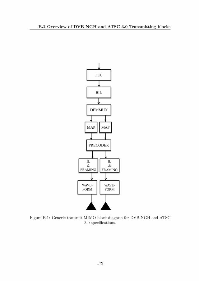
B.2 Overview of DVB-NGH and ATSC 3.0 Transmitting blocks
FEC
BIL
DEMMUX
MAPMAP
PRECODER
IL&
FRAMING
IL&
FRAMING
WAVE-FORM
WAVE-FORM
Figure B.1: Generic transmit MIMO block diagram for DVB-NGH and ATSC3.0 specifications.
179
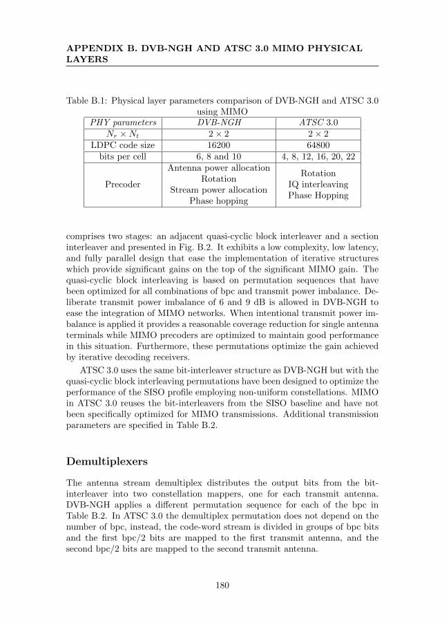
APPENDIX B. DVB-NGH AND ATSC 3.0 MIMO PHYSICALLAYERS
Table B.1: Physical layer parameters comparison of DVB-NGH and ATSC 3.0using MIMO
PHY parameters DVB-NGH ATSC 3.0Nr ×Nt 2× 2 2× 2
LDPC code size 16200 64800bits per cell 6, 8 and 10 4, 8, 12, 16, 20, 22
Precoder
Antenna power allocationRotation
Stream power allocationPhase hopping
RotationIQ interleavingPhase Hopping
comprises two stages: an adjacent quasi-cyclic block interleaver and a sectioninterleaver and presented in Fig. B.2. It exhibits a low complexity, low latency,and fully parallel design that ease the implementation of iterative structureswhich provide significant gains on the top of the significant MIMO gain. Thequasi-cyclic block interleaving is based on permutation sequences that havebeen optimized for all combinations of bpc and transmit power imbalance. De-liberate transmit power imbalance of 6 and 9 dB is allowed in DVB-NGH toease the integration of MIMO networks. When intentional transmit power im-balance is applied it provides a reasonable coverage reduction for single antennaterminals while MIMO precoders are optimized to maintain good performancein this situation. Furthermore, these permutations optimize the gain achievedby iterative decoding receivers.
ATSC 3.0 uses the same bit-interleaver structure as DVB-NGH but with thequasi-cyclic block interleaving permutations have been designed to optimize theperformance of the SISO profile employing non-uniform constellations. MIMOin ATSC 3.0 reuses the bit-interleavers from the SISO baseline and have notbeen specifically optimized for MIMO transmissions. Additional transmissionparameters are specified in Table B.2.
Demultiplexers
The antenna stream demultiplex distributes the output bits from the bit-interleaver into two constellation mappers, one for each transmit antenna.DVB-NGH applies a different permutation sequence for each of the bpc inTable B.2. In ATSC 3.0 the demultiplex permutation does not depend on thenumber of bpc, instead, the code-word stream is divided in groups of bpc bitsand the first bpc/2 bits are mapped to the first transmit antenna, and thesecond bpc/2 bits are mapped to the second transmit antenna.
180
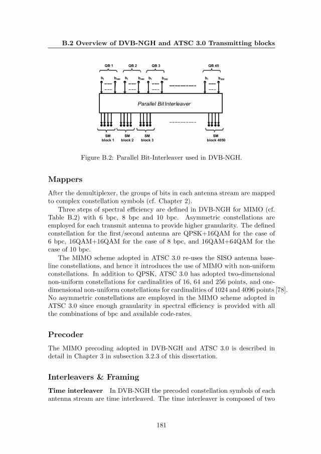
B.2 Overview of DVB-NGH and ATSC 3.0 Transmitting blocks
Parallel Bit Interleaver
b1 b360 b1 b360 b1 b360 b1 b360
QB 1 QB 2 QB 3 QB 45
SM block 1
SM block 2
SM block 3
SM block 4050
Figure B.2: Parallel Bit-Interleaver used in DVB-NGH.
Mappers
After the demultiplexer, the groups of bits in each antenna stream are mappedto complex constellation symbols (cf. Chapter 2).
Three steps of spectral efficiency are defined in DVB-NGH for MIMO (cf.Table B.2) with 6 bpc, 8 bpc and 10 bpc. Asymmetric constellations areemployed for each transmit antenna to provide higher granularity. The definedconstellation for the first/second antenna are QPSK+16QAM for the case of6 bpc, 16QAM+16QAM for the case of 8 bpc, and 16QAM+64QAM for thecase of 10 bpc.
The MIMO scheme adopted in ATSC 3.0 re-uses the SISO antenna base-line constellations, and hence it introduces the use of MIMO with non-uniformconstellations. In addition to QPSK, ATSC 3.0 has adopted two-dimensionalnon-uniform constellations for cardinalities of 16, 64 and 256 points, and one-dimensional non-uniform constellations for cardinalities of 1024 and 4096 points [78].No asymmetric constellations are employed in the MIMO scheme adopted inATSC 3.0 since enough granularity in spectral efficiency is provided with allthe combinations of bpc and available code-rates.
Precoder
The MIMO precoding adopted in DVB-NGH and ATSC 3.0 is described indetail in Chapter 3 in subsection 3.2.3 of this dissertation.
Interleavers & Framing
Time interleaver In DVB-NGH the precoded constellation symbols of eachantenna stream are time interleaved. The time interleaver is composed of two
181
APPENDIX B. DVB-NGH AND ATSC 3.0 MIMO PHYSICALLAYERS
stages, i.e. inter-frame convolutional interleaver and intra-frame block inter-leaver [47]. However, for MIMO the time interleaver process is implemented toeach transmit layer. Due to the same memory constrains apply for all DVB-NGH transmission schemes, i.e. MIMO and non-MIMO, the time interleavingdepth for MIMO is halved compared to non-MIMO transmissions [44].
In ATSC 3.0 for single physical layer pipe mode a sheer convolutional timeinterleaving is used, whereas for the multiple physical layer pipe mode a hybridtime interleaving composed of cell interleaver, twisted block interleaver, and aconvolutional delay-line is used. Optionally, the convolutional time interleavingand the hybrid time interleaving can be used in conjunction with extended timeinterleaving and a cell interleaver (only for hybrid time interleaving) to furtherimprove robustness over long burst error lengths at the expense of latency [131].
Frequency interleaver For MIMO scheme, both MIMO branches, i.e. thesignal generation for both transmit antennas, shall use the same frequency in-terleaver configuration. In addition, since MIMO services can be multiplexedwith MISO services into one NGH frame, pair-wise interleaving scheme is nec-essary. As described in [44], this latter condition comes from the use of Alam-outi encoding for MISO in NGH system as Alamouti-encoded output pair cellsshould experience similar channel realizations to avoid the loss of the codeorthogonality. In OFDM system, the cells are mapped to frequency carriers,hence, to output of the Alamouti code is mapped to adjacent carriers to maxi-mize the probability of similar channel realizations. For simplicity, NGH systemre-uses the frequency interleaving scheme already adopted for SISO transmis-sion. That is, the frequency interleaver in a given FFT mode only generateshalf of the interleaver addresses compared to the addresses generated in SISOtransmissions. The cells pair always shares the address and interleaved togetherinto adjacent carrier positions.
The frequency interleaver adopted in ATSC 3.0 has similar structure to theDVB-NGH frequency interleaver and is described in [132].
Pilot Paterns For MIMO orthogonal pilot patterns among the transmit an-tennas allow at the receiver estimation of the channel response from each trans-mit antenna. DVB-NGH inherits the pilot patten scheme from MISO DVB-T2which is based on the Walsh-Hadamard encoding algorithm [17, 133]. WithWalsh-Hadamard MIMO pilot encoding, the pilots from the second transmitantenna are inverted compared to the first transmit antenna on alternate scat-tered pilot bearing carriers. Both antennas shall transmit in all pilot positions.In the case of intentional transmit power imbalance between transmit anten-nas, the power of the pilots has to be modified accordingly to have the samepower imbalance as the data. This is because the transmit power imbalance
182
B.2 Overview of DVB-NGH and ATSC 3.0 Transmitting blocks
is included as part of the precoder (cf. Section 3.2.3) affecting only the datacarriers.
ATSC 3.0 in addition to the Walsh-Hadamard encoding algorithm, it alsoincludes null pilots encoding algorithm. However only one pilot algorithm maybe used in a given frame. With MIMO null pilot encoding, in opposition toWalsh-Hadamard encoding, two orthogonal pilot patterns are defined whereeach pattern does not share common pilot carrier positions with the other.Here, the pilots in each transmit antenna have 3 dB increased transmit powerto compensate for the null pilots not transmitted in the other group.
The null pilots encoding might be more suited for static channel conditions(e.g., for fixed roof-top reception) while the Walsh-Hadamard pilot encodingmight be more suited for mobile channels. The reason is that the pilot spac-ing in time direction is higher for the null pilots encoding compared to a pilotspacing of the Walsh-Hadamard pilot encoding. For fast varying channel con-ditions, it is more challenging for the channel estimation to follow these channelvariations if the pilot spacing in time direction is increased.
Waveform
The OFDM modulator is the same as for the SISO profile, i.e. IFFT operationplus guard interval insertion. For the MIMO rate-2 profile it is duplicatedto process the information of each transmit layer. The same IFFT operationprocess is applied for DVB-NGH and ATSC 3.0.
183

APPENDIX B. DVB-NGH AND ATSC 3.0 MIMO PHYSICALLAYERS
184
References
[1] Frame structure channel coding and modulation for a second generationdigital terrestrial television broadcasting system (DVB-T2), ETSI Std.EN 302 755, Rev. 1.2.1, 2011.
[2] “DVB-T2 - 2nd Generation Terrestrial Broadcasting,” DVB Fact Sheet,2015.
[3] J. Doeven, P. Walop, E. Zilles, J.-J. Guitot, and S. Ripley, “Digital Div-idend: Insights for Spectrum Decisions,” ITU Technical Report, 2012.
[4] “Cisco Visual Networking Index: Global Mobile Data Traffic ForecastUpdate, 2015–2020,” White Paper, CISCO, 2016.
[5] W. Zhang, Y. Wu, N. Hur, T. Ikeda, and P. Xia, “FOBTV: Worldwide Ef-forts in Developing Next-Generation Broadcasting System,” IEEE Trans-actions on Broadcasting, vol. 60, no. 2, pp. 154–159, June 2014.
[6] M. Simon and M. A. Aitken, “An Overview of the North American ATSCM/H Mobile Broadcasting System and Its Next-Generation ATSC 3.0,”in Next Generation Mobile Broadcasting, D. Gomez-Barquero, Ed. BocaRaton, FL, USA: CRC Press, 2013, pp. 91–122.
[7] T. Masayuki et al., “An Overview of the ISDB-T One-Seg Broadcasting,ISDB-TSB and ISDB-Tmm,” in Next Generation Mobile Broadcasting,D. Gomez-Barquero, Ed. Boca Raton, FL, USA: CRC Press, 2013, pp.31–68.
[8] Y. Zhang, W. Guan and D. He, “Overview of the Chinese Digital Ter-restrial Multimedia Broadcasting System,” in Next Generation MobileBroadcasting, D. Gomez-Barquero, Ed. Boca Raton, FL, USA: CRCPress, 2013, pp. 123–150.
185
REFERENCES
[9] D. Gomez-Barquero, “An Overview of the Next-Generation Mobile Dig-ital Video Broadcasting Standard DVB-NGH,” in Next Generation Mo-bile Broadcasting, D. Gomez-Barquero, Ed. Boca Raton, FL, USA: CRCPress, 2013, pp. 186–219.
[10] R. Gallager, “Low-density parity-check codes,” IRE Transactions on In-formation Theory, vol. 8, no. 1, pp. 21–28, Jan. 1962.
[11] K. J. Kim et al., “Low-Density Parity-Check Codes for ATSC 3.0,” IEEETransactions on Broadcasting, vol. 62, no. 1, pp. 189–196, March 2016.
[12] B. Bross, “Overview of the HEVC Video Coding Standard,” in NextGeneration Mobile Broadcasting, D. Gomez-Barquero, Ed. Boca Raton,FL, USA: CRC Press, 2013, pp. 713–748.
[13] D. Tse and P. Viswanath, Fundamentals of Wireless Communications.Cambridge University Press, 2005.
[14] D. Vargas, D. Gozalvez, D. Gomez-Barquero, and N. Cardona, “MIMOfor DVB-NGH, the Next Generation Mobile TV Broadcasting,” IEEECommunications Magazine, vol. 51, no. 7, pp. 130–137, July 2013.
[15] D. Gomez-Barquero, D. Vargas, M. Fuentes, P. Klenner, S. Moon, J. Y.Choi, S. Schneider, and K. Murayama, “MIMO for ATSC 3.0,” IEEETransactions on Broadcasting, vol. 62, no. 1, pp. 298–305, March 2016.
[16] S. Saito et al., “8K Terrestrial Transmission Field Tests Using Dual-Polarized MIMO and Higher-Order Modulation OFDM,” IEEE Trans-actions on Broadcasting, vol. 62, no. 1, pp. 306–315, March 2016.
[17] P. Moss and T. Y. Poon, “Overview of the Multiple-Input Multiple-Output Terrestrial Profile of DVB-NGH,” in Next Generation MobileBroadcasting, D. Gomez-Barquero, Ed. Boca Raton, FL, USA: CRCPress, 2013, pp. 549–580.
[18] A. J. Paulraj, D. A. Gore, R. U. Nabar, and H. Bolcskei, “An overviewof MIMO communications - a key to gigabit wireless,” Proceedings of theIEEE, vol. 92, no. 2, pp. 198–218, Feb. 2004.
[19] R. Monnier, J. Rault, and T. De Couasnon, “Digital Television Broad-casting with High Spectral Efficiency,” in International BroadcastingConvention, IBC, July 1992, pp. 380–384.
[20] J. Mitchell, P. Moss, and M. Thorp, “A dual polarisation MIMO broad-cast TV System,” White Paper, British Broadcasting Corporation, 2006.
186
REFERENCES
[21] J. Boyer, P. G. Brown, K. Hayler, M. L. Garcia, J. D. Mitchell, P. N.Moss, and M. J. Thorp, “MIMO for Broadcast-Results from a High-PowerUK Trial,” White Paper, British Broadcasting Corporation, 2007.
[22] P. Moss, “2-by-2 MIMO Fixed Reception Channel Model for Dual-PolarTerrestrial Transmission,” White Paper, British Broadcasting Corpora-tion, 2008.
[23] T. Shitomi, K. Murayama, M. Taguchi, S. Asakura, and K. Shibuya,“Technology for next-generation digital terrestrial broadcasting - Fieldexperiments of dual-polarized MIMO-OFDM transmission using LDPCcodes,” in IEEE International Symposium on Broadband Multimedia Sys-tems and Broadcasting (BMSB), June 2012, pp. 1–6.
[24] Y. Narikiyo, M. Nakamura, H. Sanei, and M. Takada, “Mobile receptionperformance of sfbc-mimo transmission system with walsh code scatteredpilot - computer simulation and field test results,” in IEEE Interna-tional Symposium on Broadband Multimedia Systems and Broadcasting(BMSB), June 2013, pp. 1–5.
[25] T. Shitomi, K. Murayama, S. Asakura, and K. Shibuya, “A study onadvanced single frequency network technology using STC-SDM transmis-sion,” in IEEE International Symposium onBroadband Multimedia Sys-tems and Broadcasting (BMSB), June 2013, pp. 1–5.
[26] S. M. Alamouti, “A simple transmit diversity technique for wireless com-munications,” IEEE J. Sel. Areas Comm., vol. 16, no. 10, pp. 1451–1458,Oct. 1998.
[27] J. Robert, “Terrestrial TV Broadcast Using Multi-Antenna Systems,”Ph.D. dissertation, Technical University Braunschweig, 2013.
[28] M. Slimani, J. Robert, P. Schlegel, U. Reimers, R. Burow, F. Kattanek,R. Pfeffer, and L. Stadelmeier, “Results of the DVB-T2 Field Trial inGermany,” IEEE Transactions on Broadcasting, vol. 61, no. 2, pp. 177–194, June 2015.
[29] D. Gozalvez, “Combined Time, Frequency and Space Diversity in Mul-timedia Mobile Broadcasting Systems,” Ph.D. dissertation, UniversitatPolitecnica de Valencia, 2012.
[30] H. Miyasaka et al., “A study on MIMO OFDM transmissions using inter-polarization spreading,” in Broadband Multimedia Systems and Broad-casting (BMSB), 2015 IEEE International Symposium on, June 2015,pp. 1–4.
187
REFERENCES
[31] T. Jokela, C. Hollanti, J. Lahtonen, R. Vehkalahti, and J. Paavola, “Per-formance Evaluation of 4x2 MIMO Schemes for Mobile Broadcasting,” inIEEE International Symposium on Broadband Multimedia Systems andBroadcasting (BMSB), June 2011, pp. 1–6.
[32] T. Jokela, P.-D. Arapoglou, C. Hollanti, M. Bhavani Shankar, andV. Tapio, “Hybrid SatelliteTerrestrial MIMO for Mobile Digital Broad-casting,” in Next Generation Mobile Broadcasting, D. Gomez-Barquero,Ed. Boca Raton, FL, USA: CRC Press, 2013, pp. 713–748.
[33] Y. Nasser, J.-F. Helard, and M. Crussiere, “3D MIMO Scheme for Broad-casting Future Digital TV in Single-Frequency Networks,” ElectronicsLetters, vol. 44, no. 13, pp. 829–830, June 2008.
[34] M. Liu, M. Helard, M. Crussiere, and J.-F. Helard, “Distributed MIMOcoding Scheme with Low Decoding Complexity for Future Mobile TVBroadcasting,” Electronics Letters, vol. 48, no. 17, pp. 1079–1081, Aug.2012.
[35] M. Liu, J.-F. Helard, M. Helard, and M. Crussiere, “Towards theNext Generation Video Broadcasting: Improved Performance Using Dis-tributed MIMO,” Wireless Personal Communications, May 2015.
[36] S. Sesia, I. Toufik, and M. Baker, LTE - The UMTS Long Term Evolution:From Theory to Practice, 2nd ed. Chichester, UK: John Wiley and Sons,Ltd., 2011.
[37] G. Caire, G. Taricco, and E. Biglieri, “Bit-interleaved coded modulation,”IEEE Transactions on Information Theory, vol. 44, no. 3, pp. 927–946,May 1998.
[38] A. Guillen i Fabregas, A. Martinez, and G. Caire, “Bit-interleaved codedmodulation,” Foundations and Trends in Communications and Informa-tion Theory, vol. 5, no. 1-2, pp. 1–153, 2008.
[39] G. Ungerboeck, “Channel coding with multilevel/phase signals,” IEEETransactions on Information Theory, vol. 28, no. 1, pp. 55–67, Jan. 1982.
[40] U. Wachsmann, R. Fischer, and J. Huber, “Multilevel codes: theoreticalconcepts and practical design rules,” IEEE Transactions on InformationTheory, vol. 45, no. 5, pp. 1361–1391, July 1999.
[41] C. Studer and H. Bolcskei, “Soft Input Soft Output Single Tree-SearchSphere Decoding,” IEEE Transactions on Information Theory, vol. 56,no. 10, pp. 4827–4842, Oct. 2010.
188
REFERENCES
[42] I. Sobron, “Detection and Decoding Algorithms of Multi-Antenna Diver-sity Techniques for Terrestrial DVB Systems,” Ph.D. dissertation, Mon-dragon Unibertsitatea, 2010.
[43] M. Witzke, S. Baro, F. Schreckenbach, and J. Hagenauer, “Iterative de-tection of MIMO signals with linear detectors,” in Thirty-Sixth AsilomarConference on Signals, Systems and Computers, vol. 1, Nov. 2002, pp.289–293.
[44] D. Vargas, S. Moon, W.-S. Ko, and D. Gomez-Barquero, “EnhancedMIMO Spatial Multiplexing with Phase Hopping for DVB-NGH,” in NextGeneration Mobile Broadcasting, D. Gomez-Barquero, Ed. Boca Raton,FL, USA: CRC Press, 2013, pp. 609–634.
[45] Implementation guidelines for a second generation digital terrestrial tele-vision broadcasting system (DVB-T2), ETSI Std. TR 102 831, Rev.0.10.4, 2010.
[46] D. Gozalvez, D. Gomez-Barquero, D. Vargas, and N. Cardona, “TimeDiversity in Mobile DVB-T2 Systems,” IEEE Transactions on Broad-casting, vol. 57, no. 3, pp. 617–628, Sept. 2011.
[47] P. Gomez, D. Gomez-Barquero, D. Gozalvez, A. Anorga, and M. Breiling,“Time Interleaving in DVB-NGH,” in Next Generation Mobile Broadcast-ing, D. Gomez-Barquero, Ed. Boca Raton, FL, USA: CRC Press, 2013,pp. 609–634.
[48] H. Sampath and A. Paulraj, “Linear Precoding for Space-Time CodedSystems with Known Fading Correlations,” IEEE Communications Let-ters, vol. 6, no. 6, pp. 239–241, June 2002.
[49] S. Zhou and G. Giannakis, “Optimal Transmitter Eigen-Beamformingand Space-Time Block Coding Based on Channel Mean Feedback,” IEEETransactions on Signal Processing, vol. 50, no. 10, pp. 2599–2613, Oct.2002.
[50] M. Vu and A. Paulraj, “MIMO Wireless Linear Precoding,” IEEE SignalProcessing Magazine, vol. 24, no. 5, pp. 86–105, Oct. 2007.
[51] D. Love, R. Heath, V. K. N. Lau, D. Gesbert, B. Rao, and M. An-drews, “An Overview of Limited Feedback in Wireless CommunicationSystems,” IEEE Journal on Selected Areas in Communications, vol. 26,no. 8, pp. 1341–1365, Oct. 2008.
[52] S. Rosati, S. Tomasin, M. Butussi, and B. Rimoldi, “LLR Compressionfor BICM Systems Using Large Constellations,” IEEE Transactions onCommunications, vol. 61, no. 7, pp. 2864–2875, July 2013.
189
REFERENCES
[53] M. C. Jeruchim, P. Balaban, and K. S. Shanmugan, Simulation of Com-munication Systems, Modeling, Methodology, and Techniques. SpringerUS, 2002.
[54] C. E. Shannon, “A mathematical theory of communication,” Bell Syst.Tech. J, vol. 27, pp. 379–423, 1948.
[55] S. R. Saunders and A. Aragon-Zavala, Antennas and Propagation forWireless Communication Systems, 2nd ed., J. . S. Ltd, Ed., 2007.
[56] E. Telatar, “Capacity of multi-antenna Gaussian channels,” EuropeanTrans. Telecomm., vol. 10, no. 6, pp. 585–596, Nov. 1999.
[57] G. Strang, Introduction to Linear Algebra, 4th ed. Wellesley-CambridgePress, 2009.
[58] L. Zheng and D. Tse, “Diversity and Multiplexing: a Fundamental Trade-off in Multiple-Antenna Channels,” IEEE Transactions on InformationTheory, vol. 49, no. 5, pp. 1073–1096, May 2003.
[59] E. Biglieri, R. Calderbank, A. Constantinides, A. Goldsmith, A. Paulraj,and P. H. V., Eds., MIMO Wireless Communications. Cambridge Uni-versity Press, 2007.
[60] J. Robert and J. Zoellner, “Multiple-Input Single-Output AntennaSchemes for DVB-NGH,” in Next Generation Mobile Broadcasting,D. Gomez-Barquero, Ed. Boca Raton, FL, USA: CRC Press, 2013,pp. 581–608.
[61] S. LoPresto, R. Citta, D. Vargas, and D. Gomez-Barquero, “TransmitDiversity Code Filter Sets (TDCFS), a MISO Antenna Frequency Pre-Distortion Scheme for ATSC 3.0,” IEEE Transactions on Broadcasting,vol. 62, no. 1, pp. 271–280, March 2016.
[62] J.-C. Belfiore, G. Rekaya, and E. Viterbo, “The golden code: a 2 ×2 Full-Rate Space-Time Code with Nonvanishing Determinants,” IEEETransactions on Information Theory, vol. 51, no. 4, pp. 1432–1436, April2005.
[63] S. Moon, W.-S. Ko, D. Vargas, D. Gozalvez, M. Nisar, and V. Pauli, “En-hanced Spatial Multiplexing for Rate-2 MIMO of DVB-NGH System,”in Proccedings of 19th International Conference on Telecommunications(ICT), 2012, April 2012, pp. 1–5.
[64] H. Jafarkhani, “A Quasi-Orthogonal Space-Time Block Code,” IEEETransactions on Communications, vol. 49, no. 1, pp. 1–4, Jan. 2001.
190
REFERENCES
[65] C. Hollanti, J. Lahtonen, and H. feng L., “Maximal Orders in the Designof Dense Space-Time Lattice Codes,” IEEE Transactions on InformationTheory, vol. 54, no. 10, pp. 4493–4510, Oct. 2008.
[66] R. Vehkalahti and C. Hollanti, “Reducing Complexity with Less ThanMinimum Delay Space-Time Lattice Codes,” in IEEE Information The-ory Workshop, Oct. 2011, pp. 130–134.
[67] C. Hollanti, R. Vehkalahti, and Y. Nasser, “Algebraic Hybrid Satellite-Terrestrial Space-Time Codes for Digital Broadcasting in SFN,” in IEEEWorkshop on Signal Processing Systems (SiPS), Oct. 2011, pp. 234–238.
[68] C. Berrou, A. Glavieux, and P. Thitimajshima, “Near Shannon limiterror-correcting coding and decoding: Turbo-codes,” in IEEE Interna-tional Conference on Communications, vol. 2, Geneva, Switzerland, May1993, pp. 1064–1070.
[69] D. MacKay, “Good error-correcting codes based on very sparse matrices,”IEEE Transactions on Information Theory, vol. 45, no. 2, pp. 399–431,March 1999.
[70] D. Costello Jr. and G. Forney Jr., “Channel coding: The road to channelcapacity,” Proceedings of the IEEE, vol. 95, no. 6, pp. 1150–1177, June2007.
[71] D. Gomez-Barquero, Next Generation Mobile Broadcasting. CRC Press,2013.
[72] F. Kschischang, B. Frey, and H.-A. Loeliger, “Factor graphs and the sum-product algorithm,” IEEE Transactions on Information Theory, vol. 47,no. 2, pp. 498–519, Feb. 2001.
[73] T. Richardson and R. Urbanke, “The capacity of low-density parity-checkcodes under message-passing decoding,” IEEE Transactions on Informa-tion Theory, vol. 47, no. 2, pp. 599–618, Feb. 2001.
[74] G. Foschini, R. Gitlin, and S. Weinstein, “Optimization of two-dimensional signal constellations in the presence of gaussian noise,” IEEETransactions on Communications, vol. 22, no. 1, pp. 28–38, Jan. 1974.
[75] J. Stott, “CM and BICM limits for rectangular constellations,” WhitePaper, British Broadcasting Corporation, August 2013.
[76] J. Zoellner and N. Loghin, “Optimization of high-order non-uniform qamconstellations,” in IEEE International Symposium on Broadband Multi-media Systems and Broadcasting (BMSB), June 2013, pp. 1–6.
191
REFERENCES
[77] D. Gomez-Barquero, C. Douillard, P. Moss, and V. Mignone, “DVB-NGH: The Next Generation of Digital Broadcast Services to HandheldDevices,” IEEE Transactions on Broadcasting, vol. 60, no. 2, pp. 246–257,June 2014.
[78] L. Michael and D. Gomez-Barquero, “Bit-Interleaved Coded Modulation(BICM) for ATSC 3.0,” IEEE Transactions on Broadcasting, vol. 62,no. 1, pp. 181–188, March 2016.
[79] P. Xue, K. Bae, K. Kim, and H. Yang, “M-best candidates based soft-demapper for rotated M-QAM constellation,” in IEEE 11th ConsumerCommunications and Networking Conference (CCNC), Jan. 2014, pp.623–628.
[80] M. Fuentes, D. Vargas, and D. Gomez-Barquero, “Low-ComplexityDemapping Algorithm for Two-Dimensional Non-Uniform Constella-tions,” IEEE Transactions on Broadcasting, pp. 1–9, 2016.
[81] T. Shitomi, S. Asakura, S. Saito, T. Saito, and K. Shibuya, “Study oncircularly arranged non-uniform constellations in dual-polarized MIMO-OFDM transmission,” in IEEE International Symposium on BroadbandMultimedia Systems and Broadcasting (BMSB), June 2014, pp. 1–4.
[82] L. Szczecinski and A. Alvarado, Bit-Interleaved Coded Modulation: Fun-damentals, Analysis and Design. Wiley, Feb. 2015.
[83] A. Chindapol and J. Ritcey, “Design, analysis, and performance evalu-ation for BICM-ID with square QAM constellations in Rayleigh fadingchannels,” IEEE Journal on Selected Areas in Communications, vol. 19,no. 5, pp. 944–957, May 2001.
[84] M. Davey and D. MacKay, “Low-density parity check codes over GF(q),”IEEE Communications Letters, vol. 2, no. 6, pp. 165–167, June 1998.
[85] E. Boutillon, L. Conde-Canencia, and A. Al Ghouwayel, “Design of aGF(64)-LDPC Decoder Based on the EMS Algorithm,” IEEE Transac-tions on Circuits and Systems I: Regular Papers, vol. 60, no. 10, pp.2644–2656, Oct. 2013.
[86] B. Hochwald and S. ten Brink, “Achieving near-capacity on a multiple-antenna channel,” IEEE Transactions on Communications, vol. 51, no. 3,pp. 389–399, March 2003.
[87] C. Douillard, C. B. Michel Jezequel, A. Picart, P. Didier, and A. Glavieux,“Iterative correction of intersymbol interference: Turbo-equalisation,”European Trans. Telecomm., vol. 6, no. 5, pp. 507–511, Sept./Oct. 1995.
192
REFERENCES
[88] R. Koetter, A. Singer, and M. Tuchler, “Turbo equalization,” IEEE Sig-nal Processing Magazine, vol. 21, no. 1, pp. 67–80, Jan. 2004.
[89] D. Vargas, A. Winkelbauer, G. Matz, D. Gomez-Barquero, and N. Car-dona, “Low complexity iterative MIMO receivers for DVB-NGH usingsoft MMSE demapping and quantized log-likelihood ratios,” in Proceed-ings of the COST IC1004, Barcelona, Spain, Feb. 2012.
[90] D. Seethaler, G. Matz, and F. Hlawatsch, “An efficient MMSE-based de-modulator for MIMO bit-interleaved coded modulation,” in IEEE GlobalTelecommunications Conference, vol. 4, Nov. 2004, pp. 2455–2459.
[91] L. Barbero and J. Thompson, “Extending a fixed-complexity sphere de-coder to obtain likelihood information for turbo-MIMO systems,” IEEETransactions on Vehicular Technology, vol. 57, no. 5, pp. 2804–2814, Sept.2008.
[92] P. Fertl, J. Jalden, and G. Matz, “Performance assessment of MIMO-BICM demodulators based on mutual information,” IEEE Transactionson Signal Processing, vol. 60, no. 3, pp. 1366–1382, March 2012.
[93] M. Danieli, S. Forchhammer, J. Andersen, L. Christensen, and S. Chris-tensen, “Maximum mutual information vector quantization of log-likelihood ratios for memory efficient HARQ implementations,” in Proc.Data Compression Conference (DCC 2010), March 2010, pp. 30–39.
[94] A. Winkelbauer, G. Matz, and A. Burg, “Channel-optimized vector quan-tization with mutual information as fidelity criterion,” in Asilomar Con-ference on Signals, Systems and Computers, Nov. 2013, pp. 851–855.
[95] A. Winkelbauer, “Blind Performance Estimation and Quantizer Designwith Applications to Relay Networks,” Ph.D. dissertation, Institute ofTelecommunications, Vienna University of Technology, 2014.
[96] D. Vargas, Y. J. D. Kim, J. Bajcsy, D. Gomez-Barquero, and N. Cardona,“A MIMO-Channel-Precoding Scheme for Next Generation BroadcastTV Systems,” IEEE Transactions on Broadcasting, vol. 61, no. 3, pp.445–456, Sept. 2015.
[97] G. H. Golub and C. F. Van Loan, Matrix Computations, 3rd ed. Balti-more: Johns Hopkins University Press, 1996.
[98] S. P. Boyd and L. Vandenberghe, Convex Optimization. CambridgeUniversity Press, 2004.
193
REFERENCES
[99] E. Jorswieck and H. Boche, “Behavior of outage probability in MISOsystems with no channel state information at the transmitter,” in Pro-ceedings IEEE Information Theory Workshop, March 2003, pp. 353–356.
[100] B. Varadarajan and J. Barry, “The outage capacity of linear space-timecodes,” IEEE Transactions on Wireless Communications, vol. 4, no. 6,pp. 2642–2648, Nov. 2005.
[101] J.-S. Baek and J.-S. Seo, “Efficient Pilot Patterns and Channel Estima-tions for MIMO-OFDM Systems,” IEEE Transactions on Broadcasting,vol. 58, no. 4, pp. 648–653, Dec. 2012.
[102] T. M. Cover and J. A. Thomas, Elements of Information Theory. NewYork: Wiley, 1991.
[103] M. Vu and A. Paulraj, “On the capacity of MIMO Wireless Channels withDynamic CSIT,” IEEE Journal on Selected Areas in Communications,vol. 25, no. 7, pp. 1269–1283, Sept. 2007.
[104] R. Kobeissi, S. Sezginer, and F. Buda, “Downlink Performance Analysisof Full-Rate STCs in 2x2 MIMO WiMAX Systems,” in Proceedings IEEEVehicular Technology Conference (VTC), April 2009, pp. 1–5.
[105] B. Roslind Jose, “Design Techniques For Sigma-Delta Based ADC ForWireless Applications,” Ph.D. dissertation, Cochin University Of ScienceAnd Technology, 2010.
[106] J. Max, “Quantizing for minimum distortion,” IRE Transactions on In-formation Theory, vol. 6, no. 1, pp. 7–12, March 1960.
[107] S. Lloyd, “Least squares quantization in PCM,” IEEE Transactions onInformation Theory, vol. 28, no. 2, pp. 129–137, March 1982.
[108] S. Roger, A. Gonzalez, V. Almenar, and G. Matz, “An Efficient Fixed-Complexity Sphere Decoder with Quantized Soft Outputs,” IEEE Com-munications Letters, vol. 16, no. 11, pp. 1828–1831, Nov. 2012.
[109] C. Novak, “Design of multiuser and multi-antenna communication sys-tems based on graphical models and soft information,” Ph.D. disserta-tion, Institute of Telecommunications, Vienna University of Technology,2010.
[110] A. Winkelbauer and G. Matz, “On quantization of log-likelihood ratiosfor maximum mutual information,” in IEEE 16th International Workshopon Signal Processing Advances in Wireless Communications (SPAWC),June 2015, pp. 316–320.
194
REFERENCES
[111] N. Tishby, F. Pereira, and W. Bialek, “The information bottleneckmethod,” in Proc. 37th Allerton Conf. on Communication, Control, andComputing, Sept. 1999, pp. 368–377.
[112] A. Winkelbauer and G. Matz, “Joint network-channel coding for theasymmetric multiple-access relay channel,” in Proc. IEEE ICC 2012,June 2012.
[113] J. J. Gimenez, “Improved Spectrum Usage with Multi-RF Channel Ag-gregation Technologies for the Next-Generation Terrestrial Broadcast-ing,” Ph.D. dissertation, Universitat Politecnica de Valencia, 2015.
[114] J. Montalban, “Solutions for new terrestrial broadcasting systems offer-ing simultaneously stationary and mobile services,” Ph.D. dissertation,Universidad del Pas Vasco/Euskal Herriko Unibertsitatea, 2014.
[115] L. Zhang et al., “Layered-Division-Multiplexing: Theory and Practice,”IEEE Transactions on Broadcasting, vol. 62, no. 1, pp. 216–232, March2016.
[116] S. Jeon, J. Han, R. Shrestha, S. Park, H. Mok, H. Kim, and J. Seo,“MIMO Cloud Transmission Based on BICM-ID for High Data RateLocal Contents Delivery,” IEEE Transactions on Broadcasting, vol. 61,no. 4, pp. 580–589, Dec. 2015.
[117] N. Loghin, J. Zoellner, B. Mouhouche, D. Ansorregui, J. Kim, andS. Park, “Non-Uniform Constellations for ATSC 3.0,” IEEE Transac-tions on Broadcasting, vol. 62, no. 1, pp. 197–203, March 2016.
[118] S. Roger, “Design and Implementation of Efficient Algorithms for Wire-less MIMO Communication Systems,” Ph.D. dissertation, Universitat Po-litecnica de Valencia, 2012.
[119] C. Studer, “Iterative MIMO Decoding: Algorithms and VLSI Implemen-tation Aspects,” Ph.D. dissertation, ETH Zurich, 2009.
[120] B. M. Kurkoski and H. Yagi, “Quantization of Binary-Input DiscreteMemoryless Channels,” IEEE Transactions on Information Theory,vol. 60, no. 8, pp. 4544–4552, Aug. 2014.
[121] F. Quitin, “Channel modeling for polarized MIMO systems,” Ph.D. dis-sertation, Universite Libre de Bruxelles/Universite catholique de Lou-vain, 2011.
[122] P. Moss, “MIMO Technology in Broadcasting - and an Application inProgramme-Making,” in 2nd IEEE Broadcast Technology Society GoldWorkshop on Next Generation Broadcasting, Cagliari, March 2013.
195
REFERENCES
[123] ——, “SM-MIMO Channel Models,” DVB Document TM-MIMO0051,2013.
[124] P. Moss, T. Y. Poon, and J. Boyer, “A simple model of the UHF cross-polar terrestrial channel for DVB-NGH,” White Paper, British Broad-casting Corporation, 2011.
[125] M. Patzold, U. Killat, F. Laue, and Y. Li, “On the statistical propertiesof deterministic simulation models for mobile fading channels,” IEEETransactions on Vehicular Technology, vol. 47, no. 1, pp. 254–269, Feb.1998.
[126] X. Zhang and X. Zhou, LTE-Advanced Air Interface Technology. CRCPress, 2012.
[127] N. Czink, “The random-cluster model - a stochastic MIMO channel modelfor broadband communication systems of the 3rd generation and be-yond,” Ph.D. dissertation, Institut fur Nachrichtentechnik und Hochfre-quenztechnik, Vienna University of Technology, 2007.
[128] L. Jiang, V. Jungnickel, S. Jaeckel, L. Thiele, and A. Brylka, “Correlationanalysis of multiple-input multiple-output channels with cross-polarizedantennas,” in 14th Asia-Pacific Conference on Communications, 2008.APCC 2008, Oct. 2008, pp. 1–5.
[129] LTE; Evolved Universal Terrestrial Radio Access (E-UTRA); Base Sta-tion (BS) radio transmission and reception, ETSI Std. TS 136 104, Rev.0.11.0, 2013.
[130] R. Nabar, H. Bolcskei, V. Erceg, D. Gesbert, and A. Paulraj, “Perfor-mance of Multiantenna Signaling Techniques in the Presence of Polariza-tion Diversity,” IEEE Transactions on Signal Processing, vol. 50, no. 10,pp. 2553–2562, Oct. 2002.
[131] P. Klenner, J. S. Baek, N. S. Loghin, D. Gomez-Barquero, and W. S.Ko, “Physical Layer Time Interleaving for the ATSC 3.0 System,” IEEETransactions on Broadcasting, vol. 62, no. 1, pp. 253–262, March 2016.
[132] M. Earnshaw, K. Shelby, H. Lee, Y. Oh, and M. Simon, “Physical LayerFraming for ATSC 3.0,” IEEE Transactions on Broadcasting, vol. 62,no. 1, pp. 263–270, March 2016.
[133] J. Morgade, P. Angueira, A. Arrinda, R. Pfeffer, V. Steinmann, J. Frank,and R. Brugger, “SFN-SISO and SFN-MISO Gain Performance Analysisfor DVB-T2 Network Planning,” IEEE Transactions on Broadcasting,vol. 60, no. 2, pp. 272–286, June 2014.
196