diversity analysis of distributed space-time codes in relay networks with multiple transmit/receive...

Hindawi Publishing CorporationEURASIP Journal on Advances in Signal ProcessingVolume 2008, Article ID 254573, 17 pagesdoi:10.1155/2008/254573

Research ArticleDiversity Analysis of Distributed Space-Time Codes in RelayNetworks with Multiple Transmit/Receive Antennas

Yindi Jing1 and Babak Hassibi2

1 Department of Electrical Engineering and Computer Science, University of California, Irvine, CA 92697, USA2 Department of Electrical Engineering, California Institute of Technology, Pasadena, CA 91125, USA

Correspondence should be addressed to Yindi Jing, [email protected]

Received 1 May 2007; Revised 13 September 2007; Accepted 28 November 2007

Recommended by M. Chakraborty

The idea of space-time coding devised for multiple-antenna systems is applied to the problem of communication over a wirelessrelay network, a strategy called distributed space-time coding, to achieve the cooperative diversity provided by antennas of the relaynodes. In this paper, we extend the idea of distributed space-time coding to wireless relay networks with multiple-antenna nodesand fading channels. We show that for a wireless relay network with M antennas at the transmit node, N antennas at the receivenode, and a total of R antennas at all the relay nodes, provided that the coherence interval is long enough, the high SNR pairwise

error probability (PEP) behaves as (1/P)min {M,N}R if M /=N and (log 1/MP/P)MR

if M = N , where P is the total power consumedby the network. Therefore, for the case of M /=N , distributed space-time coding achieves the maximal diversity. For the case ofM = N , the penalty is a factor of log 1/MP which, compared to P, becomes negligible when P is very high.

Copyright © 2008 Y. Jing and B. Hassibi. This is an open access article distributed under the Creative Commons AttributionLicense, which permits unrestricted use, distribution, and reproduction in any medium, provided the original work is properlycited.

1. INTRODUCTION

It is known that multiple antennas can greatly increase thecapacity and reliability of a wireless communication link in afading environment using space-time coding [1–4]. Recently,with the increasing interestin ad hoc networks, researchershave been looking for methods to exploit spatial diversityusing the antennas of different users in the network [5–24]. Many cooperative strategies are proposed, for example,amplify-and-forward (AF) [11, 13, 14, 16, 21, 23], decode-and-forward (DF) [9, 10, 14, 16, 22], and coded cooperation[15]. In [7], the authors proposed the use of space-time codesbased on Hurwitz-Radon matrices in wireless relay networks.

This work follows the strategy of [5], where the ideaof space-time coding devised for multiple-antennasystemsis applied to the problem of communication over a wire-less relay network. (Though having the same name, thedistributed space-time coding idea in [5] is different fromthat in [14]. Similar ideas for networks with one and tworelays have appeared in [6, 11].) In [5], the authors considerwireless relay networks in which every node has a singleantenna and the channels are fading, and use a cooperativestrategy called distributed space-time coding by applying a

linear dispersion space-time code [25] among the relays.It is proved that without any channel knowledge at therelays, a diversity of R(1 − log logP/ logP) can be achieved,where R is the number of relays and P is the total powerconsumed in the whole network. This result is based on theassumption that the receiver has full knowledge of the fadingchannels. Therefore, when the total transmit power P is highenough, the wireless relay network achieves the diversity ofa multiple-antenna system with R transmit antennas andone receive antenna, asymptotically. That is, antennas of therelays work as antennas of the transmitter although theycannot fully cooperate and do not have full knowledge of thetransmit signal. After the appearance of [5], code designs fordistributed space-time coding have been proposed in [26–31] and the differential use of distributed space-time codinghas been introduced in [32–35]. The references [36, 37] ana-lyze the diversity-multiplexing tradeoff of distributed space-time coding. Distributed space-time coding in asynchronousnetworks is discussed in [38–43]. Other related papers can befound in [44–46].

This paper has two main contributions. First, we extendthe idea of distributed space-time coding to wireless relaynetworks whose nodes have multiple antennas. Second and

mailto:[email protected]

2 EURASIP Journal on Advances in Signal Processing

more importantly, based on the pairwise error probability(PEP) analysis, we prove lower bounds on the diversity ofthis scheme. We use the same two-step transmission methodin [5], where in one step the transmitter sends signals tothe relays and in the other the relays encode their receivedsignals into a linear dispersion space-time code and transmitto the receiver. For a wireless relay network with M antennasat the transmitter, N antennas at the receiver, and a totalof R antennas at all the relay nodes, our work shows thatwhen the coherence interval is long enough, a diversity ofmin{M,N}R ifM /=N andMR(1−(1/M)(log logP/ logP))if M = N can be achieved, where P is the total power used inthe network. With this two-step protocol, it is easy to see thatthe errorprobability is determined by the worse of the twosteps: the transmission from the transmitter to the relays andthe transmission from the relays to the receiver. Therefore,when M /=N , distributed space-time coding is optimal sincethe diversity of the first stage cannot be larger than MR,the diversity of a multiple-antenna system with M transmitantennas and R receive antennas, and the diversity of thesecond stage cannot be larger than NR. When M = N ,the penalty on the diversity, because the relays cannot fullycooperate and do not have full knowledge of the signal,is R(log logP/ logP). When P is very high, it is negligible.Therefore, with distributed space-time coding, wireless relaynetworks achieve the same diversity of multiple-antennasystems, asymptotically.

The paper is organized as follows. In the followingsection, the network model and the generalized distributedspace-time coding are explained in detail. A training schemeis also proposed. The PEP is first analyzed in Section 3.In Section 4, the diversity for the network with an infinitenumber of relays is discussed. Then, the diversity for thegeneral case is obtained in Section 5. Section 6 containsthe conclusion. Proofs of some of the technical theoremsare given in Appendices A–D. In Appendix E, we discussheterogeneous networks.

2. WIRELESS RELAY NETWORK

2.1. Network model and distributed space-time coding

We first introduce some notation. For a complex matrix A,A, At , and A∗ denote the conjugate, the transpose, and theHermitian of A, respectively. detA, rank A, and trA indicate

the determinant, rank, and trace of A, respectively. �A denotesthe vectorization of A formed by stacking the columns of Xinto a single column vector. In denotes the n × n identitymatrix and 0m,n is the m × n matrix with all zero entries.We often omit the subscripts when there is no confusion. logindicates the natural logarithm. ‖ · ‖ indicates the Frobeniusnorm. P and E indicate the probability and the expectedvalue. g(x) = O( f (x)) means that limx→∞(g(x)/ f (x)) is aconstant. h(x) = o( f (x)) means that limx→∞(h(x)/ f (x)) =0. �a� is the minimal integer that is not less than a.

Consider a wireless network with R + 2 nodes whichare placed randomly and independently according to somedistribution. As shown in Figure 1, there are one transmitnode and one receive node. All the other R nodes work

Transmitter Receiver

Relaysf11

f1R

fM1

fMR

g11

g1N

......

......

...

r1t1

rRtR

gR1

gRN

Step 1: time 1 to T Step 2: time T + 1 to 2T

Figure 1: Wireless relay network with multiple-antenna nodes.

as relays. The transmitter has M transmit antennas, thereceiver has N receive antennas, and the ith relay has Riantennas. Since the transmit and received signals at differentantennas of the same relay can be processed and designedindependently, the network can be transformed to a networkwith R = ∑R

i=1Ri single-antenna relays by designing thetransmit signal at every antenna of every relay according tothe received signal at that antenna only. This is one possiblescheme. In general, the signal sent by one antenna of a relaycan be designed using received signals at all antennas of therelay. However, as will be seen later, this simpler schemeachieves the optimal diversity asymptotically although ageneral design may improve the coding gain of the network.Therefore, to highlight the diversity results by simplifyingnotation and formulas, in the following, we assume thatevery relay has a single antenna. Denote the channel vectorfrom the M antennas of the transmitter to the ith relay as

fi = [ f1i · · · fMi]t, and the channels from the ith relay

to the N antennas at the receiver as gi = [gi1 · · · giN ].We use the block-fading model [2] by assuming a coherenceinterval T . From the two-step protocol that will be discussedin the following, we can see that we only need fi to keepconstant for the first step of the transmission and gi to keepconstant for the second step. It is thus good enough to chooseT as the minimum of the coherence intervals of fi and gi.Also, perfect symbol-level synchronization is assumed in thisnetwork model. For asynchronized networks, please refer to[38–43].

The information bits are encoded into T × M matricess, whose mth column is the signal sent by the mth transmitantenna. For the power analysis, s is normalized as

E tr s∗s =M. (1)

To send s to the receiver, the same two-step strategy in [5] isused, as shown in Figure 1. In step one, the transmitter sends√P1T/Ms. The average total power used at the transmitter for

theT transmissions is P1T . The received signal vector and thenoise vector at the ith relay are denoted as ri and vi. In steptwo, the ith relay sends ti. The received signal and noise at thereceiver are denoted as X and w. The noises are assumed tobe i.i.d. CN (0, 1). Clearly,

ri =√P1T/Msfi + vi,

X =[

t1 · · · tR]G + w,

(2)

where G = [gt1 · · · gtR]t.

Y. Jing and B. Hassibi 3

We use distributed space-time coding proposed in [5] bydesigning the transmit signal at relay i as a linear function ofits received signal:

ti =√

P2

P1 + 1Airi, (3)

where Ai is a predetermined T × T unitary matrix known toboth the ith relay and the receiver. It is fixed during trainingand data transmissions. For various methods on how todesign the Ai, see [26–31]. P2 can be proved to be the averagetransmit power for one transmission at every relay. Aftersome calculation, the system equation can be written as

X =√

P1P2T

M(P1 + 1

)SH +W , (4)

where

S =[A1s · · · ARs

], H =

[(f1g1

)t · · · (fRgR

)t]t

,

(5)

W =√

P2

P1 + 1

⎡

⎣R∑

i=1

gi1Aivi · · ·R∑

i=1

giNAivi

⎤

⎦ + w. (6)

The received signal matrix, X , is T ×N . S, which is T ×MR,is the linear distributed space-time code. Since fi isM×1 andgi is 1×N , the equivalent channel matrix H is RM ×N . W ,which is T ×N , is the equivalent noise matrix.

Define

RW = I +P2

1 + P1G∗G. (7)

The covariance matrix of the equivalent noise matrix canbe proved to be RW . The diversity analysis in this paper ismuch more difficult than that in [5] because in networkswith single-antenna nodes, the covariance matrix of theequivalent noise is a multiple of the identity matrix. Here,for the diversity result, we need to analyze the eigenvalues ofRW or find bounds on them.

2.2. Assumptions and training

In this paper, we assume that fmi and gin have independentRayleigh distributions; that is, fmi and gin are independentcirculant complex Gaussian random variables with zeromean. For simplicity, we also assume that fmi and gin havethe same variance, which is 1. The heterogeneous case, inwhich every channel has a different variance, is discussed inAppendix E. The same diversity results can be obtained inheterogeneous networks. We make the practical assumptionthat the relays have no channel information. However, we doassume that the receiver has enough channel information todo coherent detection. Thus, a training process is needed.

For coherence ML decoding at the receiver, the receiverneeds to know H and RW , or equivalently, H and G. Wepropose a training process that contains two steps and takesMp + 2Np symbol periods (other training methods can alsobe envisioned, and the one proposed here is one possibility).

Each step mimics the training process of a multiple-antennasystem [47] as its system equation has the same structure.

First, we estimate G, which takes Mp symbol periods. LetUp be a predesigned full-rank Mp × R pilot matrix. The ithrelay sends the ith column ofUp simultaneously. The receivergets

Yp =√QpMp

RUpG + wp, (8)

where Qp is the power used at every relay and wp isthe Mp × N noise matrix. Since there are RN unknowns(corresponding to the components of G) and min{Mp,R}Nindependent equations, we need Mp ≥ R. We could estimateG from Up using ML, MMSE, or other criteria.

Then, we estimateH using distributed space-time codingdiscussed in Section 2.1. This takes 2Np symbol periods. Thetransmitter sends a full-rank Np ×M pilot signal matrix spand the relays perform distributed space-time coding. From(4), the received signal can be written as

Xp =√√√√ P1,pP2,pNp

M(P1,p + 1)SpH +Wp, (9)

where P1,p and P2,p are the powers used at the transmitterand every relay and

Sp =[A1sp · · · ARsp

](10)

is the carefully designedNp×MR pilot space-time codeword.Now, let us discuss the number of training symbols neededin this step. Note that G is known from the first training step.Define

f =[

f t1 · · · f tR]t. (11)

By stacking the columns of X into one single column vector,we can rewrite (9) as

�Xp =√√√√ P1,pP2,pNp

M(P1,p + 1

)

⎡

⎢⎢⎢⎢⎣

Spdiag{g11IM , . . . , gR1IM

}

...

Spdiag{g1NIM , . . . , gRNIM

}

⎤

⎥⎥⎥⎥⎦

f + �Wp

=√√√√ P1,pP2,pNp

M(P1,p + 1

)

⎡

⎢⎢⎢⎢⎣

g11A1sp · · · gR1ARsp...

. . ....

g1NA1sp · · · gRNARsp

⎤

⎥⎥⎥⎥⎦

f + �Wp

=√√√√ P1,pP2,pNp

M(P1,p + 1

)

⎡

⎢⎢⎢⎢⎣

g11INp · · · gR1INp

.... . .

...

g1NINp · · · gRNINp

⎤

⎥⎥⎥⎥⎦

× diag{A1sp, . . . ,ARsp

}f + �Wp.

(12)


Denote

Hp =

⎡

⎢⎢⎣

g11INp · · · gR1INp

.... . .

...g1NINp · · · gRNINp

⎤

⎥⎥⎦diag

{A1sp, . . . ,ARsp

}.

(13)

The number of independent equations in (9) equals the rankof Hp, which is min{NpN ,NpR,MR}. Since there are MRunknowns (corresponding to the components of f), we needmin{NpN ,NpR,MR} ≥MR, which is equivalent to

Np ≥ max{�MR/N�,M}

. (14)

While this condition is satisfied, we could estimate f fromXp using ML, MMSE, or other criteria. The overall trainingprocess takes at least R+2 max{�MR/N�,M} symbol periods.The optimal designs of Up, Qp, Sp (or sp), and P1,p, P2,p areinteresting issues. However, they are beyond the scope of thispaper.

3. PAIRWISE ERROR PROBABILITY ANDOPTIMAL POWER ALLOCATION

To analyze the PEP, we have to determine the maximum-likelihood (ML) decoding rule. This requires the conditionalprobability density function (PDF) P(X | s k), where s k ∈ Sand S is the set of all possible transmit signal matrices.

Theorem 1. Given that s k is transmitted, define

Sk =[A1s k A2s k · · · ARs k

]. (15)

Then conditioned on s k, the rows of X are independentlyGaussian distributed with the same variance RW . The tth rowof X has mean

√P1P2T/M(P1 + 1)[Sk]tH with [Sk]t being the

tth row of Sk. Also,

P(X | s k

)

= (πN detRW

)−T

× e−tr(X−√

P1P2T/M(P1+1

)SkH)R−1

W (X−√

P1P2T/M(P1+1

)SkH)∗ .

(16)

Proof. See Appendix A.

In view of Theorem 1, we should emphasize that for awireless relay network with multiple antennas at the receiver,the columns of X are not independent although the rows ofX are. (The covariance matrix of each row RW is not diagonalin general.) That is, the received signals at different antennasare not independent, whereas the received signals at differenttimes are. This is the main reason that the PEP analysis in thenew model is much more difficult than that of the networkin [5], where X had only a single column.

With P(X | s k) in hand, we can obtain the ML decodingand thereby analyze the PEP. The result follows.

Theorem 2 (ML decoding and the PEP Chernoff bound).The ML decoding of the relay network is

arg mins k

tr

(

X −√

P1P2T

M(P1 + 1

)SkH

)

× R−1W

(

X −√

P1P2T

M(P1 + 1

)SkH

)∗.

(17)

With this decoding, the PEP of mistaking s k by s l, averaged overthe channel realization, has the following upper bound:

P(

s k −→ s l) ≤ E

fmi,gine−(P1P2T/4M(1+P1)) tr (Sk−Sl)∗(Sk−Sl)HR−1

W H∗.

(18)

Proof. The proof is omitted since it is the same as the proofof Theorem 1 in [5].

As both H and RW are known at the receiver, spheredecoding can be used to perform the ML decoding in (17).

The main purpose of this work is to analyze how the PEPdecays with the total transmit power. The total power used inthe whole network is P = P1 + RP2. One natural question ishow to allocate power between the transmitter and the relaysif P is fixed. Notice that when R → ∞, according to the lawof large numbers, the off-diagonal entries of (1/R)G∗G go tozero while the diagonal entries approach 1 with probability1. It is thus reasonable to assume (1/R)G∗G ≈ IN for largeR. With this approximation, minimizing the PEP is nowequivalent to maximizing P1P2T/4M(1 + P1 + RP2). This isexactly the same power allocation problem in [5]. Therefore,we can conclude that the optimum solution is to set

P1 = P

2, P2 = P

2R. (19)

That is, the optimum power allocation is such that thetransmitter uses half the total power and the relays sharethe other half. As discussed in Section 2.1, for the generalnetwork where the ith relay has Ri antennas, the antennasare treated as Ri different relays. Therefore, in general, theoptimum power allocation is such that the transmitter useshalf the total power as before, but every relay uses a powerthat is proportional to its number of antennas, that is, P1 =P/2 and the power used at the ith relay is RiP/2R.

4. DIVERSITY ANALYSIS FOR R→∞

4.1. Basic results

As mentioned earlier, to obtain the diversity, we have tocompute the expectations over fmi and gin in (18). We will dothis rigorously in Section 5. However, since the calculationis detailed and gives little insight, in this section, we give asimple asymptotic derivation for the case where the numberof relay nodes approaches infinity, that is, R → ∞. Asdiscussed in the previous section, when R is large, we canmake the approximation RW ≈ (1 +P2R/(P1 + 1))IN . Denotethe nth column of H as hn. From (5), hn = Gnf , where we


have defined Gn = diag{g1nIM , . . . , gRnIM}. Therefore, from(18) and using the optimal power allocation in (19),

P(

s k −→ s l)

� Efmi,gin

e−(PT/16MR)trH∗(Sk−Sl)∗(Sk−Sl)H

= Efmi,gin

e−(PT/16MR)∑Nn=1h∗n

(Sk−Sl

)∗(Sk−Sl)hn

= Efmi,gin

e−(PT/16MR)f∗[∑Nn=1 G∗n

(Sk−Sl

)∗(Sk−Sl)Gn]f .

(20)

Since f is white Gaussian with mean zero and variance IRM ,

P(s k −→ s l)

� Egin

det−1

⎡

⎣IRM +PT

16MR

N∑

n=1

G∗n (Sk − Sl)∗(Sk − Sl)Gn

⎤

⎦ .

(21)

Similar to the multiple-antenna case [4, 48] and the caseof wireless relay networks with single-antenna nodes [5], toachieve full diversity, Sk − Sl must be full rank. Since thedistributed space-time codes Sk and Sl are T × MR, in thefollowing, we will assume T ≥ MR and the code is fullydiverse.

Denote the minimum singular value of (Sk − Sl)∗(Sk −Sl) by σ2

min. From the full diversity of the code, σ2min >

0. Therefore, the right side of (21) can be further upperbounded as

P(

s k −→ s l)

� Egin

det−1

⎡

⎣IRM +PTσ2

min

16MR

N∑

n=1

G∗nGn

⎤

⎦

= Egin

R∏

i=1

⎛

⎝1 +PTσ2

min

16MR

N∑

n=1

∣∣gin

∣∣2

⎞

⎠

−M

.

(22)

Since gin are i.i.d. CN (0, 1),∑N

n=1|gin|2 are i.i.d. gamma

distributed with PDF (1/(N − 1)!)gN−1i e−gi . Therefore,

P(

s k −→ s l)

� 1

(N − 1)!R

⎡

⎣∫∞

0

(

1 +PTσ2

min

16MRx

)−MxN−1e−xdx

⎤

⎦

R

.

(23)

By defining y = 1 + (PTσ2min/16MR)x, we have

P(

s k −→ s l)

� 1

(N − 1)!R

(16MR

PTσ2min

)NR

e16MR2/PTσ2min

×[∫∞

1

(y − 1)N−1

yMe−(16MR/PTσ2

min)ydy

]R

� 1

(N − 1)!R

(16MR

PTσ2min

)NR

×⎡

⎣N−1∑

l=0

(N − 1

l

)∫∞

1yl−Me−(16MR/PTσ2

min)ydy

⎤

⎦

R

.

(24)

The following theorem can be obtained by calculating theintegral.

Theorem 3 (diversity for R → ∞). Assume that R → ∞,T ≥ MR, and the distributed space-time code is full diverse.For large total transmit power P, by looking at only the highest-order term of P, the PEP of mistaking s k by s l has the followingupper bound:

P(

s k −→ s l)

� 1

(N − 1)!R

(16MR

Tσ2min

)min{M,N}R

×

⎧⎪⎪⎪⎪⎪⎪⎪⎪⎪⎪⎨

⎪⎪⎪⎪⎪⎪⎪⎪⎪⎪⎩

(2N−1

M −N

)R

P−NR if M > N ,

(log1/MP

P

)MR

if M = N ,

(N −M − 1)!RP−MR if M < N.

(25)

Therefore, the diversity of the wireless relay network is

d =

⎧⎪⎪⎪⎪⎨

⎪⎪⎪⎪⎩

min{M,N}R ifM /=N ,

MR

(

1− 1M

log logPlogP

)

ifM = N.

(26)

Proof. See Appendix B.

4.2. Discussion

With the two-step protocol, it is easy to see that regardlessof the cooperative strategy used at the relay nodes, theerror probability is determined by the worse of the twotransmission stages: the transmission from the transmitter tothe relays and the transmission from the relays to the receiver.The PEP of the first stage cannot be better than the PEP ofa multiple-antenna system with M transmit antennas and Rreceive antennas, whose optimal diversity is MR, while thePEP of the second stage can have diversity not larger thanNR. Therefore, when M /=N , according to the decay rateof the PEP, distributed space-time coding is optimal. Forthe case of M = N , the penalty on the decay rate is justR(log logP/ logP), which is negligible when P is high.

If we can use the diversity definition in [49], sincelimP→∞(log logP/ logP) = 0, diversity min{M,N}R can beobtained.

The results in Theorem 6 are obtained by consideringonly the highest-order term of P in the PEP formula. In brief,we call the rth highest-order term of P in the PEP formula


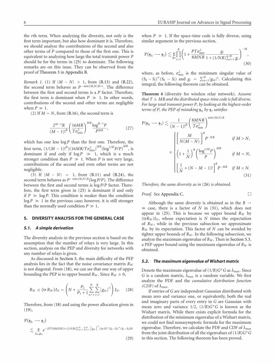
the rth term. When analyzing the diversity, not only is thefirst term important, but also how dominant it is. Therefore,we should analyze the contributions of the second and alsoother terms of P compared to those of the first one. This isequivalent to analyzing how large the total transmit power Pshould be for the terms in (25) to dominate. The followingremarks are on this issue. They can be observed from theproof of Theorem 3 in Appendix B.

Remark 1. (1) If |M − N| > 1, from (B.13) and (B.22),the second term behaves as P−min{M,N}R+1. The differencebetween the first and second terms is a P factor. Therefore,the first term is dominant when P � 1. In other words,contributions of the second and other terms are negligiblewhen P� 1.

(2) If M = N , from (B.16), the second term is

2M−1R

(M − 1)!R

(16MR

Tσ2min

)MRlogR−1P

PMR, (27)

which has one less logP than the first one. Therefore, the

first term, (1/(M − 1)!R)(16MR/Tσ2min)

MR(log1/MP/P)

MR, is

dominant if and only if logP � 1, which is a muchstronger condition than P � 1. When P is not very large,contributions of the second and even other terms are notnegligible.

(3) If |M − N| = 1, from (B.11) and (B.24), thesecond term behaves as P−min{M,N}R(logP/P). The differencebetween the first and second terms is logP/P factor. There-fore, the first term given in (25) is dominant if and onlyif P � logP. This condition is weaker than the conditionlogP � 1 in the previous case; however, it is still strongerthan the normally used condition P� 1.

5. DIVERSITY ANALYSIS FOR THE GENERAL CASE

5.1. A simple derivation

The diversity analysis in the previous section is based on theassumption that the number of relays is very large. In thissection, analysis on the PEP and diversity for networks withany number of relays is given.

As discussed in Section 3, the main difficulty of the PEPanalysis lies in the fact that the noise covariance matrix RWis not diagonal. From (18), we can see that one way of upperbounding the PEP is to upper bound RW . Since RW ≥ 0,

RW ≤ (trRW

)IN =

⎛

⎝N +P2

P1 + 1

N∑

n=1

R∑

i=1

∣∣gin

∣∣2

⎞

⎠ IN . (28)

Therefore, from (18) and using the power allocation given in(19),

P(

s k −→ s l)

� Efmi,gin

e−(PT/8MNR(1+(1/NR)∑Nn=1

∑Ri=1

∣∣gin

∣∣2

))trH∗(Sk−Sl)∗(Sk−Sl)H

(29)

when P � 1. If the space-time code is fully diverse, usingsimilar argument in the previous section,

P(

s k −→ s l)

� Egin

R∏

i=1

(

1 +PTσ2

min

8MNR

gi

1 + (1/NR)∑R

i=1 gi

)−M,

(30)

where, as before, σ2min is the minimum singular value of

(Sk − Sl)∗(Sk − Sl) and gi =∑N

n=1|gin|2. Calculating thisintegral, the following theorem can be obtained.

Theorem 4 (diversity for wireless relay network). AssumethatT ≥MR and the distributed space-time code is full diverse.For large total transmit power P, by looking at the highest-orderterms of P, the PEP of mistaking s k by s l satisfies

P(s k −→ s l) � 1

(N − 1)!R

(8MNR

Tσ2min

)min{M,N}R

×

⎧⎪⎪⎪⎪⎪⎪⎪⎪⎪⎪⎪⎪⎨

⎪⎪⎪⎪⎪⎪⎪⎪⎪⎪⎪⎪⎩

[M

N(M −N)

]R

P−NR if M > N ,

(

1 +1N

)R(

log1/MP

P

)MR

if M = N ,

[1N

+ (N −M − 1)!]RP−MR if M < N.

(31)

Therefore, the same diversity as in (26) is obtained.

Proof. See Appendix C.

Although the same diversity is obtained as in the R →∞ case, there is a factor of N in (31), which does notappear in (25). This is because we upper bound RW by(trRW )IN , whose expectation is N times the expectationof RW , while in the previous subsection we approximateRW by its expectation. This factor of N can be avoided bytighter upper bounds of RW . In the following subsection, weanalyze the maximum eigenvalue of RW . Then in Section 5.3,a PEP upper bound using the maximum eigenvalue of RW isobtained.

5.2. The maximum eigenvalue of Wishart matrix

Denote the maximum eigenvalue of (1/R)G∗G as λmax. SinceG is a random matrix, λmax is a random variable. We firstanalyze the PDF and the cumulative distribution function(CDF) of λmax.

If entries of G are independent Gaussian distributed withmean zero and variance one, or equivalently, both the realand imaginary parts of every entry in G are Gaussian withmean zero and variance 1/2, (1/R)G∗G is known as theWishart matrix. While there exists explicit formula for thedistribution of the minimum eigenvalue of a Wishart matrix,we could not find nonasymptotic formula for the maximumeigenvalue. Therefore, we calculate the PDF and CDF of λmax

from the joint distribution of all the eigenvalues of (1/R)G∗Gin this section. The following theorem has been proved.


0

0.5

1

1.5

2

2.5

3

Pr

(λm

ax=λ)

0 1 2 3 4 5

λ

R = 10 N = 2R = 10 N = 3R = 10 N = 4

R = 40 N = 2R = 40 N = 3R = 40 N = 4

PDF of λmax of Wishart matrix

Figure 2: PDF of the maximum eigenvalue of (1/R)G∗G.

Theorem 5. Assume that R ≥ N and G is an R × N matrixwhose entries are i.i.d. CN (0, 1).

(1) The PDF of the maximum eigenvalue of (1/R)G∗G is

pλmax (λ) = RRNλR−Ne−Rλ∏N

n=1Γ(R− n + 1)Γ(n)detF, (32)

where F is an (N − 1) × (N − 1) Hankel matrix whose(i, j)th entry equals fi j =

∫ λ0 (λ− t)2tR−N+i+ j−2e−Rtdt.

(2) The CDF of the maximum eigenvalue of (1/R)G∗G is

P(λmax ≤ λ

) = RRN∏N

n=1Γ(R− n + 1)Γ(n)detF′, (33)

where F′ is anN×N Hankel matrix whose (i, j)th entry

equals f ′i j =∫ λ0 t

R−N+i+ j−2e−Rtdt.

Proof. See Appendix D.

A theoretical analysis of the PDF and CDF from (32)and (33) appears to be quite difficult. To understand λmax,we plot the two functions in Figures 2 and 3 for different Rand N . Figure 2 shows that the PDF has a peak at a value abit larger than 1. As R increases, the peak becomes sharper.An increase in N shifts the peak right. However, the effect issmaller for larger R. From Figure 3, the CDF of λmax growsrapidly around λ = 1 and becomes very close to 1 soon after.The larger R is, the faster the CDF grows. Similar to the PDF,an increase in N results in a right shift of the CDF. However,as R grows, the effect diminishes. This verifies the validity ofthe approximation G∗G ≈ RIN in Section 4 for large R.

In the following corollary, we give an upper bound onthe PDF. This result is used to derive the diversity result forgeneral R in the next subsection.

0

0.2

0.4

0.6

0.8

1

Pr

(λm

ax<λ)

0 1 2 3 4 5

λ

R = 10 N = 2R = 10 N = 3R = 10 N = 4

R = 40 N = 2R = 40 N = 3R = 40 N = 4

CDF of λmax of Wishart matrix

Figure 3: CDF of the maximum eigenvalue of (1/R)G∗G.

Corollary 1. When R ≥ N , the PDF of the maximumeigenvalue of (1/R)G∗G can be upper bounded as

pλmax (λ) ≤ C1λRN−1e−Rλ, (34)

where

C1= 1∏N

n=1Γ(R− n + 1)Γ(n)

× 2N−1RRN∏N−1

n=1 (R−N + 2n− 1)(R−N + 2n)(R−N + 2n + 1)(35)

is a constant that depends only on R and N .

Proof. From the proof of Theorem 5, F is a positive semidef-inite matrix. Therefore, detF ≤∏N−1

n=1 fnn. From (32), fnn canbe upper bounded as

fnn ≤∫ λ

0(λ− t)2tR−N+2n−2dt

= 2(R−N + 2n− 1)(R−N + 2n)(R−N + 2n + 1)

× λR−N+2n+1,(36)

then we have

detF

≤ 2N−1

∏N−1n=1 (R−N + 2n− 1)(R−N + 2n)(R−N + 2n + 1)

× λRN−R+N−1.(37)

Thus, (34) is obtained.


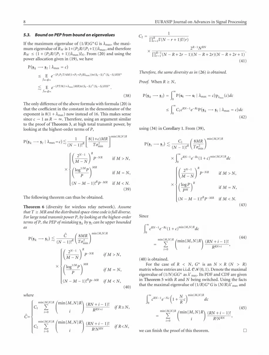
5.3. Bound on PEP from bound on eigenvalues

If the maximum eigenvalue of (1/R)G∗G is λmax, the maxi-mum eigenvalue ofRW is 1+(P2R/(P1+1))λmax, and thereforeRW ≤ (1 + (P2R/(P1 + 1))λmax)IN . From (20) and using thepower allocation given in (19), we have

P(

s k −→ s l | λmax = c)

≤ Efmr ,grn

e−(P1P2T/4M(1+P1+P2Rλmax))tr(Sk−Sl)∗(Sk−Sl)HH∗

� Efmr ,grn

e−(PT/8(1+λmax)MR)tr(Sk−Sl)∗(Sk−Sl)HH∗.

(38)

The only difference of the above formula with formula (20) isthat the coefficient in the constant in the denominator of theexponent is 8(1 + λmax) now instead of 16. This makes sensesince c → 1 as R → ∞. Therefore, using an argument similarto the proof of Theorem 3, at high total transmit power, bylooking at the highest-order terms of P,

P(

s k −→ s l | λmax=c)� 1

(N − 1)!R

[8(1+c)MR

Tσ2min

]min{M,N}R

×

⎧⎪⎪⎪⎪⎪⎪⎪⎪⎪⎨

⎪⎪⎪⎪⎪⎪⎪⎪⎪⎩

(2N−1

M −N

)R

P−NR if M > N ,

(log1/MP

P

)MR

if M = N ,

(N −M − 1)!RP−MR if M < N.

(39)

The following theorem can thus be obtained.

Theorem 6 (diversity for wireless relay network). AssumethatT ≥MR and the distributed space-time code is full diverse.For large total transmit power P, by looking at the highest-orderterms of P, the PEP of mistaking s k by s l can be upper boundedas

P(

s k −→ s l)

� C

(N − 1)!R

(8MR

Tσ2min

)min{M,N}R

×

⎧⎪⎪⎪⎪⎪⎪⎪⎪⎪⎪⎨

⎪⎪⎪⎪⎪⎪⎪⎪⎪⎪⎩

(2N−1

M −N

)R

P−NR if M > N ,

(log1/MP

P

)MR

if M = N ,

(N −M − 1)!RP−MR if M < N ,(40)

where

C=

⎧⎪⎪⎪⎪⎪⎪⎪⎪⎪⎨

⎪⎪⎪⎪⎪⎪⎪⎪⎪⎩

C1

min{M,N}R∑

i=0

⎛

⎝min{M,N}R

i

⎞

⎠ (RN + i− 1)!RRN+i

if R≥N ,

C2

min{M,N}R∑

i=0

⎛

⎝min{M,N}R

i

⎞

⎠ (RN + i− 1)!RiNRN

if R<N ,

C2 = 1∏R

r=1Γ(N − r + 1)Γ(r)

× 2R−1NRN

∏R−1r=1 (N − R + 2r − 1)(N − R + 2r)(N − R + 2r + 1)

.

(41)

Therefore, the same diversity as in (26) is obtained.

Proof. When R ≥ N ,

P(

s k −→ s l) =

∫∞

0P(

sk −→ sl | λmax = c)pλmax

(c)dc

≤∫∞

0C1c

RN−1e−RcP(

s k −→ s l | λmax = c)dc

(42)

using (34) in Corollary 1. From (39),

P(

s i −→ s i)

� C1

(N − 1)!R

(8MR

Tσ2min

)min{M,N}R

×∫∞

0cRN−1e−Rc(1 + c)min{M,N}Rdc

×

⎧⎪⎪⎪⎪⎪⎪⎪⎪⎪⎪⎨

⎪⎪⎪⎪⎪⎪⎪⎪⎪⎪⎩

(2N−1

M −N

)R

P−NR if M > N ,

(logPPM

)R

if M = N ,

(N −M − 1)!RP−MR if M < N.

(43)

Since

∫∞

0cRN−1e−Rc(1 + c)min{M,N}Rdc

=min{M,N}R∑

i=0

(min{M,N}R

i

)(RN + i− 1)!

RRN+i,

(44)

(40) is obtained.For the case of R < N , G∗ is an N × R (N > R)

matrix whose entries are i.i.d. CN (0, 1). Denote the maximaleigenvalue of (1/N)GG∗ as λ′max. Its PDF and CDF are givenin Theorem 5 with R and N being switched. Using the factsthat the maximal eigenvalue of (1/R)G∗G is (N/R)λ′max and

∫∞

0cRN−1e−Nc

(

1 +N

Rc)min{M,N}R

dc

=min{M,N}R∑

i=0

(min{M,N}R

i

)(RN + i− 1)!

RiNRN,

(45)

we can finish the proof of this theorem.


6. SIMULATION RESULTS

In this section, we show simulated block error rates ofthree networks with multiple transmit/receive antennas andcompare them with the three PEP bounds we derived in(25), (31), and (40). These bounds are also addressed as PEPbound 1, PEP bound 2, and PEP bound 3 for the sake ofpresentation. The main purpose of this section is to verifythe diversity results in (26). The optimal code design is notan issue. In the simulations, we use the power allocation in(19) and the ML decoding in (17). It is known that with MLmetric, a factor of 1/2 can be applied to Chernoff boundson the two-signal error rate, which is the block error ratewhen there are two possible transmit signals. Thus, the PEPbounds shown in Figures 4–6 are calculated from (25), (31),and (40) with a factor of 1/2. In all figures, the horizontalaxis indicates P, the total transmit power used in the wholenetwork.

Our first example, whose performance is shown inFigure 4, is a network with one transmit antenna, two relayantennas, and two receive antennas, that is, M = 1, R = 2,N = 2. We set T = MR = 2. The transmit signal is designedas

s =[s1 s2

]t, (46)

where s1 and s2 are chosen as BPSK signals (normalizedaccording to (1)). The matrices used at relays are designedas

A1 = I2, A2 =[

0 −11 0

]

. (47)

The distributed space-time codeword formed at the receiverS is thus a 2 × 2 real orthogonal design [50]. Then, we showperformance of a network with M = 2, R = 2, N = 1 inFigure 5. We set T =MR = 4. The transmit signal is deignedas

s =

⎡

⎢⎢⎢⎣

s1 −s2s2 s1s3 −s4s4 s3

⎤

⎥⎥⎥⎦

, (48)

where s1, s2, s3, s4 are also BPSK signals (normalizedaccording to (1)). The matrices used at relays are designedas

A1 = I4, A2 =

⎡

⎢⎢⎢⎣

0 0 −1 00 0 0 11 0 0 00 1 0 0

⎤

⎥⎥⎥⎦. (49)

The distributed space-time codeword formed at the receiverS is thus a 4 × 4 real orthogonal design [50]. Finally, inFigure 6, we show performance of a network with M = 2,R = 1, N = 2. We set T = MR = 2. The transmit signal is

10−5

10−4

10−3

10−2

10−1

100

Blo

cker

ror

rate

10 12 14 16 18 20 22 24 26 28 30

P (dB)

2-signal error rateBlock error ratePEP bound 1

PEP bound 2PEP bound 3

Figure 4: M = 1, R = 2, N = 2, T = 2.

10−5

10−4

10−3

10−2

10−1

100

Blo

cker

ror

rate

10 12 14 16 18 20 22 24 26 28 30

P (dB)



Figure 5: M = 2, R = 2, N = 1, T = 4.

designed as

s =[s1 −s2s2 s1

]

, (50)

where s1 and s2 are BPSK signals (normalized according to(1)). The matrices used at the relay are set to be I2. Thedistributed space-time codeword formed at the receiver S isagain a 2 × 2 real orthogonal design [50]. The transmissionrate of all three networks can be calculated to be 1/2. Forcomparison, we also show the 2-signal error rates of the threenetworks by fixing s2, . . . , sT .


10−5

10−4

10−3

10−2

10−1

100

Blo

cker

ror

rate

10 12 14 16 18 20 22 24 26 28 30

P (dB)



Figure 6: M = 2, R = 1, N = 2, T = 2.

Figures 4–6 indicate that when the transmit power ishigh, all three networks achieve the diversities shown by thePEP bounds. This verifies our diversity result in (26). PEPbound 1 is the tightest of the three. This is because PEPbound 1 is obtained by approximating RW by its asymptotic(R → ∞) limit, which is also its mean; however, strict lowerbounds on RW are used in the calculations of bound 2 andbound 3. In Figure 5, the three bounds are very close to eachother and, actually, bounds 1 and 2 are the same.

7. CONCLUSIONS

In this paper, we generalize the idea of distributed space-timecoding to wireless relay networks whose transmitter, receiver,and/or relays can have multiple antennas. We assume that thechannel information is only available at the receiver. The MLdecoding at the receiver and PEP of the network are analyzed.We have shown that for a wireless relay network with Mantennas at the transmitter,N antennas at the receiver, a totalof R antennas at all the relay nodes, and a coherence intervalnot less than MR, an achievable diversity is min{M,N}Rif M /=N and MR(1 − (1/M)(log logP/ logP)) if M = N ,where P is the total power used in the whole network.This result shows the optimality of distributed space-timecoding according to the diversity gain. Simulation results areexhibited to justify our diversity analysis.

APPENDICES

A. PROOF OF THEOREM 1

Proof. It is obvious that sinceH is known andW is Gaussian,the rows of X are Gaussian. We only need to show thatthe rows of X are uncorrelated and that the mean andvariance of the tth row are

√(P1P2T/(P1 + 1)M)[Sk]tH and

RW , respectively.

The (t,n)th entry of X can be written as

xtn =√

P1P2T

M(P1 + 1)

R∑

i=1

M∑

m=1

T∑

τ=1

fmiginai,tτ sk,τm

+

√P2

P1 + 1

R∑

i=1

T∑

τ=1

ginai,tτviτ +wtn,

(A.1)

where ai,tτ is the (t, τ)th entry of Ai and sk,τm is the (τ,m)thentry of s k. With full channel information at the receiver,

Extn =√

P1P2T

M(P1 + 1

)R∑

i=1

M∑

m=1

T∑

τ=1

fmiginai,tτ sk,τm. (A.2)

Therefore, the mean of the tth row is then represented by√(P1P2T/M(P1 + 1))[Sk]tH . Since vi, wn, and s k are inde-

pendent,

Cov(xt1n1 , xt2n2

)

= E(xt1n1 − Ext1n1

)(xt2n2 − Ext2n2

)

= P2

P1 + 1

R∑

i1=1

T∑

τ1=1

R∑

i2=1

T∑

τ2=1

× Egi1n1ai1,t1τ1vr1τ1gi2n2ai2,t2τ2vi2τ2 + Ewt1n1wt2n2

= P2

P1 + 1

R∑

i=1

T∑

τ=1

ai,t1τai,t2τgin1gin2+ δn1n2δt1t2

= δt1t2

⎛

⎝ P2

P1 + 1

R∑

r=1

gin1gin2+ δn1n2

⎞

⎠

= δt1t2

⎛

⎜⎜⎜⎜⎝

P2

P1 + 1

[g1n1 · · · gRn1

]

⎛

⎜⎜⎜⎜⎝

g1n2

...

gRn2

⎞

⎟⎟⎟⎟⎠

+ δn1n2

⎞

⎟⎟⎟⎟⎠.

(A.3)

The fourth equality is true sinceAi are unitary. Therefore, therows of X are independent since the covariance of xt1n1 andxt2n2 is zero when t1 /= t2. It is also easy to see that the variancematrix of each row is IN +(P2/(P1 +1))GtG, which equals RW .Therefore,

P([X]t | s k

)

=(πN detRW

)−T

× e−tr[X−√

(P1P2T/M(P1+1))SkH]t R−1W [X−

√(P1P2T/M(P1+1))SkH]

t

t

=(πN detRW

)−T

× e−tr[X−√

(P1P2T/M(P1+1))SkH]tR−1W [X−

√(P1P2T/M(P1+1))SkH]

∗t .

(A.4)

Since P(X | s k) = ∏Tt=1P([X]t | s k), (16) can be obtained.


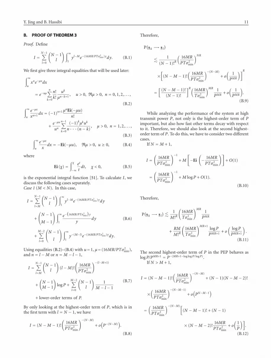
B. PROOF OF THEOREM 3

Proof. Define

I =N−1∑

l=0

(N − 1l

)∫∞


min)ydy. (B.1)

We first give three integral equalities that will be used later:∫∞

uxne−μxdx

= e−uμn∑

k=0

n!k!

uk

μn−k+1, u > 0, Rμ > 0, n = 0, 1, 2, . . . ,

(B.2)∫∞

u

e−μx

xn+1dx = (−1)n+1 μ

nEi(−μu)n!

+e−μu

un

n−1∑

k=0

(−1)kμkuk

n · · · (n− k), μ > 0, n = 1, 2, . . . ,

(B.3)∫∞

u

e−μx

xdx = −Ei(−μu), Rμ > 0, u ≥ 0, (B.4)

where

Ei (χ) =∫ χ

−∞

et

tdt, χ < 0, (B.5)

is the exponential integral function [51]. To calculate I , wediscuss the following cases separately.Case 1 (M < N). In this case,

I =N−1∑

l=M

(N − 1l

)∫∞


min)ydy

+

⎛

⎝N − 1

M − 1

⎞

⎠∫∞

1

e−(

16MR/PTσ2min

)y

ydy

+M−2∑

l=0

⎛

⎝N − 1

l

⎞

⎠∫∞

1y−(M−l)e−(16MR/PTσ2

min)ydy.

(B.6)

Using equalities (B.2)–(B.4) with u=1, μ= (16MR/PTσ2min),

and n = l −M or n =M − l − 1,

I =N−1∑

l=M

(N − 1l

)

(l −M)!

(16MR

PTσ2min

)−(l−M+1)

+

(N − 1M − 1

)

logP +M−2∑

l=0

(N − 1l

)1

M − l − 1

+ lower-order terms of P.

(B.7)

By only looking at the highest-order term of P, which is inthe first term with l = N − 1, we have

I = (N −M − 1)!

(16MR

PTσ2min

)−(N−M)

+ o(P−(N−M)

).

(B.8)

Therefore,

P(

s k −→ s l)

� 1

(N − 1)!R

(16MR

PTσ2min

)NR

×[

(N −M − 1)!(

16MR

PTσ2min

)−(N−M)

+ o(

1PMR

)]R

=[

(N −M − 1)!(N − 1)!

]R(16MR

Tσ2min

)MR 1PMR

+ o(

1PMR

)

.

(B.9)

While analyzing the performance of the system at hightransmit power P, not only is the highest-order term of Pimportant, but also how fast other terms decay with respectto it. Therefore, we should also look at the second highest-order term of P. To do this, we have to consider two differentcases.

If N =M + 1,

I =(

16MR

PTσ2min

)−1

+M

[

−Ei

(

− 16MR

PTσ2min

)]

+O(1)

=(

16MR

PTσ2min

)−1

+M logP +O(1).

(B.10)

Therefore,

P(

s k −→ s l)

� 1

M!R

(16MR

Tσ2min

)MR1

PMR

+RM

M!R

(16MR

Tσ2min

)MR+1logPPMR+1

+ o(

logPPMR+1

)

.

(B.11)

The second highest-order term of P in the PEP behaves aslogP/PMR+1 = P−(MR+1−log logP/ logP).

If N > M + 1,

I = (N −M − 1)!(

16MR

PTσ2min

)−(N−M)

+ (N − 1)(N −M − 2)!

×(

16MR

PTσ2min

)−(N−M−1)

+ o(PN−M−1

)

=(

16MR

PTσ2min

)−(N−M)[

(N −M − 1)! + (N − 1)

× (N −M − 2)!16MR

PTσ2min

+ o(

1P

)]

.

(B.12)


Therefore,

P(

s k −→ s l)

� (N −M − 1)!R

(N − 1)!R

(16MR

Tσ2min

)MR 1PMR

+(N − 1)(N −M − 2)(N −M − 1)!R−1

(N − 1)!R

×(

16MR

Tσ2min

)MR+1 1PMR+1

+ o(

1PMR+1

)

.

(B.13)

Case 2 (M = N). In this case,

I =∫∞

1

e−(

16MR/PTσ2min

)y

ydy

+N−2∑

l=0

(N − 1l

)∫∞


min)ydy.

(B.14)

Using (B.4) with μ = 16MR/PTσ2min and u = 1, and (B.3)

with u = 1 and n =M − l − 1, we have

I = logP +N−2∑

l=0

(N − 1l

)1

M − l − 1

+ lower-order terms of P

< logP + 2N−1 + lower-order terms of P.

(B.15)

Therefore,

P(

s k −→ s l)

� 1

(M − 1)!R

(16MR

Tσ2min

)MR logRPPMR

+2N−1R

(M − 1)!R

(16MR

Tσ2min

)MR logR−1P

PMR

+ o(

logR−1P

PMR

)

.

(B.16)

Also, the second highest-order term of P in the PEP behavesas logR−1P/PRM and the next term has one logP less and soon.Case 3 (M > N). In this case,

I =M−2∑

l=0

(N − 1l

)∫∞


min)ydy. (B.17)

Using (B.3) with u = 1, μ = 16MR/PTσ2min, and n =M−l−1,

I =N−1∑

l=0

(N − 1l

)1

M − l − 1+ lower-order terms of P.

(B.18)

Thus,

P(

s k −→ s l)

� 1

(N − 1)R

(16MR

PTσ2min

)NR

×[N−1∑

l=0

(N − 1

l

)1

M − l − 1+ o(1)

]R

=[

1(N − 1)!

N−1∑

l=0

(N − 1

l

)1

M − l − 1

]R

×(

16MR

Tσ2min

)NRP−NR + o

(P−NR

).

(B.19)

We can further upper bound the PEP to get a simplerformula. Notice that 1/(M − l − 1) ≤ 1/(M −N). Thus,

P(

s k −→ s l)

�[

1(M −N)(N − 1)!

N−1∑

l=0

(N − 1

l

)]R

×(

16MR

Tσ2min

)NRP−NR

≤[

2N−1

(M −N)(N − 1)!

]R(16MR

Tσ2min

)NRP−NR.

(B.20)

As discussed before, we also want to see how dominantthe highest-order term of P given in the above formula is. IfM > N + 1, M− l− 2 > N + 1− (N − 1)− 2 = 0. From (B.3),

I <2N−1

M −N − 2N−1

(M −N)(M −N − 1)16MR

PTσ2min

+ o(

1P

)

.

(B.21)

Therefore,

P(

s k −→ s l)

�[

2N−1

(M −N)(N − 1)!

]R(16MR

Tσ2min

)NR

×[

1PNR

+R

M −N − 1

(16MR

Tσ2min

)1

PNR+1

]

+ o(

1PNR+1

)

.

(B.22)

The second highest-order term in the PEP behaves as1/(PNR+1). If M = N + 1,

I< 2N−1 +16MR

Tσ2min

logPP

+O(

1P

)

. (B.23)

Therefore,

P(

s k −→ s l)

� 2R(N−1)

(N − 1)!R

(16MR

Tσ2min

)NR 1PNR

+2(R−1)(N−1)R

(N − 1)!R

(16MR

Tσ2min

)NR+1 logPPNR+1

+ o(

logPPNR+1

)

,

(B.24)


which indicates that the second highest-order term in thePEP behaves as logP/PNR+1 = R−(NR+1−log logP/ logP).

C. PROOF OF THEOREM 4

Proof. Since gi have PDF p(gi) = (1/(N − 1)!)gN−1i e−gi ,

P(

s k −→ s l) ≤

R∑

r=0

∑

1≤i1<···<ir≤RTi1,...,ir , (C.1)

where

Ti1,...,ir =1

(N − 1)!R

∫

· · ·∫

the i1,...,ir th integrals are from x to ∞,

others are from 0 to x

×R∏

i=1

(

1 +PTσ2

min

8MNR

gi

1 + (1/NR)∑R

i=1gi

)−M

× gN−1i e−gidg1 · · ·dgR

(C.2)

and x is any positive real number. Let us calculate T1,...,r first:

T1,...,r = 1

(N − 1)!R

∫∞

x. . .∫∞

x︸︷︷︸r

∫ x

0. . .∫ x

0︸︷︷︸R−r

R∏

i=1

×(

1 +PTσ2

min

8MNR

gi

1 + (1/NR)∑R

i=1 gi

)−M

× gN−1i e−gidg1 · · ·dgR

<1

(N − 1)!R

∫∞

x· · ·

∫∞

x

r∏

i=1

×(PTσ2

min

8MNR

gi1 + ((R− r)/NR)x + (1/NR)

∑ri=1 gi

)−M

× gN−1i e−gidg1 · · ·dgr

×∫ x

0· · ·

∫ x

0

R∏

i=r+1

gN−1i e−gidgr+1 · · ·dgR

= 1

(N − 1)!R

(PTσ2

min

8MNR

)−rMγR−r(N , x)

×∫∞

x· · ·

∫∞

x

⎛

⎝1 +R− rNR

x +1NR

r∑

i=1

gi

⎞

⎠

rM

×r∏

i=1

e−gi

gM−N+1i

dg1 · · ·dgr ,

(C.3)

where γ(n, x) is the incomplete gamma function [51]. Weshould choose x so that the diversity is maximized. Definex = βPα, where β is a positive constant and α is any real

constant. The value of β does not affect the diversity. Here, tohave the PEP result consistent with formula (25) in Section 6,we set β = (Tσ2

min/8MNR)α. Therefore, choosing the optimal

(in the sense of maximizing the diversity) x is equivalent tochoosing the optimal α. If α > 0, the r = 0 term in the PEPupper bound is

1

(N − 1)!RγR(N ,Pα) = 1 + o(1). (C.4)

Therefore, having α positive is not optimal according todiversity. Similarly, if α = 0, x = 1. The r = 0 term in the PEPupper bound, (1/(N−1)!R)γR(N , 1), is a constant. Therefore,α should be negative. Thus,

γ(N , x) = 1NxN + o

(xN) = 1

NβNPαN + o

(PαN

)(C.5)

We are only interested in the highest-order term of P. WhenP is large, ((R − r)/NR)x is negligible compared with 1.Therefore,

T1,...,r � 1

(N − 1)!RNR−r

(Tσ2

min

8MNR

)−rM+αN(R−r)

× P−rM+αN(R−r)Λ,

(C.6)

where we have defined

Λ =∫∞

x· · ·

∫∞

x

⎛

⎝1 +1NR

r∑

i=1

gi

⎞

⎠

rMr∏

i=1

e−gi

gM−N+1i

dg1 · · ·dgr .

(C.7)

We consider the expansion of (A +∑k

i=1λi)a

into monomialterms:(

1 +1NR

r∑

i=1

gi

)a

=a∑

j=0

(∑

1≤l1<···<lj≤k

∑

i1,...,i j≥1∑im≤a

C(i1, . . . , i j

)

× 1

(NR)i1+···+i j gi1l1gi2l2 · · · g

ijl j

)

,

(C.8)

where j denotes how many gi are present, l1, . . . , l j are thesubscripts of the gi that appear, im ≥ 1 indicates that glm istaken to the imth power, and finally

C(i1, . . . , i j

) =(ki1

)(k − i1i2

)

· · ·(k − i1 − · · · − i j−1

i j

)

(C.9)

counts how many times the term gi1l1 gi2l2· · · gijl j appears in the

expansion. Thus,

Λ =r∑

j=0

∑

1≤l1<···<lj≤r

∑

i1,...,i j≥1∑im≤r

× C(i1, . . . , i j)Λ(j; l1, . . . , l j ; i1, . . . , i j

),

(C.10)


where

Λ(j; l1, . . . , l j ; i1, . . . , i j

)

= 1

(NR)i1+···+i j

( j∏

m=1

∫∞

x

e−glm

gM−N+1−imlm

dglm

)

×∏

i /=i1,...,i j

∫∞

x

e−gi

gM−N+1i

dgi.

(C.11)

From (B.2)–(B.4), while P →∞, α < 0, and n > 0,∫∞

xλne−λdλ = n! + o(1),

∫∞

x

e−λ

λdλ = (−α) logP + o(logP),

∫∞

x

e−λ

λn+1dλ = 1

nβ−nP−αn + o

(P−αn

).

(C.12)

Therefore, the highest-order term of P in Λ is the j = 0 term.If we only keep the highest-order term of P in Λ,

Λ =r∏

i=1

∫∞

x

e−gi

gM−N+1i

dgi

≈

⎧⎪⎪⎪⎪⎪⎪⎪⎨

⎪⎪⎪⎪⎪⎪⎪⎩

1(M −N)r

β−r(M−N)P−rα(M−N) if M > N ,

(−α)r logrP if M = N ,

(N −M − 1)!r if M < N.

(C.13)

From the symmetry of g1, . . . , gR, we have Ti1,...,ir = T1,...,r .Therefore,

P(

s k −→ s l)

≤R∑

r=0

(Rr

)

T1,...,r

� 1

(N − 1)!R

R∑

r=0

(R

r

)1

NR−r

×(Tσ2

min

8MNR

)−rM+αN(R−r)P−rM+αN(R−r)

×

⎧⎪⎪⎪⎪⎪⎪⎪⎨

⎪⎪⎪⎪⎪⎪⎪⎩

1(M −N)r

(Tσ2

min

8MNR

)−rα(M−N)

P−rα(M−N) if M > N ,

(−α)r logrP if M = N ,

(N −M − 1)!r if M < N.

(C.14)

We should choose a negative α such that the exponent of thehighest-order term of P in the above formula is minimized.In other words, if we denote the exponent of the rth term asf (r), choose an α < 0 such that maxr f (r) is minimized.

If M > N , f (r) = −rM + αN(R − r) − rα(M − N) =αNR − rM(1 + α). If α ≤ −1, f (r) is an increasing function

of r. Thus, maxr f (r) = f (R) = −α(M − N)R −MR, whichis minimized when α equals its maximum −1. If α ≥ −1,f (r) is a decreasing function of r. Thus, maxr f (r) = f (0) =αNR, which is minimized when α equals its minimum −1.Therefore, we should set α = −1, and

P(

s k −→ s l)

�(1/N + 1/(M −N)

)R

(N − 1)!R

(8MNR

Tσ2min

)NRP−NR

=[

M/N

(M −N)(N − 1)!

]R(8MNR

Tσ2min

)NRP−NR.

(C.15)

If M < N , f (r) = αNR − rN(α + M/N). By similarargument, we should set α = −M/N . Thus,

P(

s k −→ s l)

�(1/N + (N −M − 1)!

)R

(N − 1)!R

(8MNR

Tσ2min

)−MR

P−MR.

(C.16)

If M = N , f (r) = αNR − rN(α + 1 − (1/N)(log logP/logP)). Using similar argument, the optimal choice of α is1− (1/N)(log logP/ logP). Therefore,

P(

s k −→ s l)

� 1

(N − 1)!R

[(8MNR

Tσ2min

)log logP/ logP 1N

+(

1− 1N

log logPlogP

)]R

×(

8MNR

Tσ2min

)−MR( log1/MP

P

)−MR

≈ (1/N + 1)R

(N − 1)!R

(8MNR

Tσ2min

)−MR( log1/MP

P

)−MR

.

(C.17)

D. PROOF OF THEOREM 5

Proof. We first give a theorem that will be needed later.

Theorem 7. Define Λ = (λ1, . . . , λN ). For any functions f , g,and h,

∫

dΛN∏

i=1

f(λi)

detVg(Λ) detVh(Λ) = N ! detFgh,

Vg(Λ) =

⎡

⎢⎢⎢⎣

g0(λ1) · · · g0

(λN)

.... . .

...

gN−1(λ1) · · · gN−1

(λN)

⎤

⎥⎥⎥⎦

,

Vh(Λ) =

⎡

⎢⎢⎢⎣

h0(λ1) · · · h0

(λN)

.... . .

...

hN−1(λ1) · · · hN−1

(λN)

⎤

⎥⎥⎥⎦

,

Fgh =∫

f (t)

⎡

⎢⎢⎣

g0(t)...

gN−1(t)

⎤

⎥⎥⎦

[h0(t) · · · hN−1(t)

]dt.

(D.1)


Define G′ as a complex Gaussian matrix whose entries’real and imaginary parts have mean zero and variance one.Denote the ordered eigenvalues of G′G′∗ as λ′1 ≥ λ′2 · · · ≥λ′N . It is well known that the eigenvalues have the followingjoint distribution [52]:

P(λ′1, . . . , λ′N

) = CN∏

i=1

λ′R−Ni e−λ′i /2

∏

1≤i< j≤N

(λ′i − λ′j

)2, (D.2)

where C = 2−RN/∏N

n=1Γ(R−n+ 1)Γ(n) is a constant. Denotethe ordered eigenvalues of (1/R)GG∗ as λ1 ≥ λ2 · · · ≥ λN .Therefore, λ′i = 2Rλi. The joint distribution of λ1, . . . , λN istherefore

P(λ1, . . . , λN

)

= P(λ′1, . . . , λ′N

)dλ′1 · · ·dλ′Ndλ1 · · ·dλN

= det[diag{2R, . . . , 2R}](2Rλ1, . . . , 2RλN

)

= (2R)NCN∏

i=1

(2Rλi

)R−Ne−Rλi

∏

1≤i< j≤N

[2R(λi − λj

)]2

= C(2R)RNN∏

i=1

λR−Ni e−Rλi∏

1≤i< j≤N

(λi − λj

)2.

(D.3)

To get the PDF of λ1, we have to do the integral overλ2, . . . , λN . Define f (x) = (λ − x)2xR−Ne−Rx and gi(x) =hi(x) = xi−1. Thus,

P(λmax = λ

)

= P(λ1 = λ

)

=∫

λ≥λ2≥···λNP(λ, λ2, . . . , λN

)dλ2 · · ·dλN

= 1(N − 1)!

∫ λ

0· · ·

∫ λ

0P(λ, λ2, . . . , λN

)dλ2 · · ·dλN

= C(2R)RN

(N − 1)!λR−Ne−Rλ

∫ λ

0· · ·

∫ λ

0

N∏

i=2

(λ− λi

)2λR−Ni e−Rλi

×∏

2≤i< j≤N

(λi − λj

)2dλ2 · · ·dλN

= C(2R)RN

(N − 1)!λR−Ne−Rλ

∫ λ

0· · ·

∫ λ

0

N∏

i=2

f (λi)

× detVg(λ2, . . . , λN

)detVh

(λ2, . . . , λN

)λ1 · · · λN

= C(2R)RN

(N − 1)!λR−Ne−Rλ(N − 1)! detF,

(D.4)

where in the second equality we have changed the integralspace from ordered λi to unordered one. From the symmetry

of λi, we only need to divide the new value by (N − 1)!. FromTheorem 7,

F =∫ λ

0g(t)

⎡

⎢⎢⎢⎢⎣

1t...

tN−2

⎤

⎥⎥⎥⎥⎦

[1 t · · · tN−2

]dt, (D.5)

whose (i, j)th entry is fi j =∫ λ0 (λ− t)2tR−N+i+ j−2e−Rtdt. The

CDF of λ1 can be obtained similarly.

E. DISCUSSION ON HETEROGENEOUS NETWORKS

In Section 2.2, it is assumed that fmi and gin have the samevariance. Physically, this means that the distances betweenthe transmitter/receiver and all relays are about the same,which may not be a practical assumption for networks withscattered nodes. In this appendix, we extend our diversityanalysis to heterogeneous networks whose channels havedifferent variances. We assume that the distributions of fmiand gin are CN (0, σ2

fmi) and CN (0, σ2

gin), respectively. Byfollowing the derivation in Section 4, compared with (21),the PEP for the heterogeneous case can be upper bounded by

P(

s k −→ s l)

� Egin

det−1

[

Σf +PT

16MR

N∑

n=1

G∗n(Sk − Sl)∗

(Sk − Sl

)Gn

]

,

(E.1)

where Σf = diag{σ2f 11, . . . , σ2

f m1, . . . , σ21R, . . . , σ2

f mR} is the

covariance matrix of f . Denote σ2fi = minMm=1{σ2

fmi} and σ2

gi =minMm=1{σ2

gin}. We have from (E.1) that

P(

s k −→ s l)

� Egin

R∏

i=1

(

σ2fi +

σ2giPTσ

2min

16MR

∑N

n=1

∣∣gin

∣∣2

σ2gin

)−M

.

(E.2)

Since |gin|2/σ2gin has the exponential distribution with mean 1

and gin’s are independent,∑N

n=1|gin|2/σ2gin has the i.i.d.

gamma distribution (1/(N − 1)!)gN−1i e−gi . Thus, following

the derivations in Section 4 and Appendix B, we can showthat the PEP of heterogeneous networks has the followingupper bound:

P(

s k −→ s l)

� 1

(N − 1)!R

( R∏

i=1

σ2fi

)−min{M,N}(16MR

Tσ2min

)min{M,N}R

×

⎧⎪⎪⎪⎪⎪⎪⎪⎪⎪⎪⎨

⎪⎪⎪⎪⎪⎪⎪⎪⎪⎪⎩

( R∏

i=1

σ2gi

)−(N−M)(2N−1

M −N)R

P−NR if M > N ,

(log1/MP

P

)MR

if M = N ,

(N −M − 1)!RP−MR if M < N.

(E.3)


Thus, the same diversity results as in (26) can be obtained.Similarly, the rigorous analysis in Section 5 also applies tothis heterogeneous case.

ACKNOWLEDGMENTS

This work is supported in part by the National ScienceFoundation under Grants nos. CCR-0133818 and CCR-0326554, by the David and Lucille Packard Foundation,and by Caltech’s Lee Center for Advanced Networking. Apreliminary version of this paper and the related results firstappeared in the Proceeding of the 2005 IEEE InternationalSymposium on Information Theory [53].

REFERENCES

[1] I. E. Telatar, “Capacity of multi-antenna Gaussian channels,”European Transactions on Telecommunications, vol. 10, no. 6,pp. 585–595, 1999.

[2] T. L. Marzetta and B. M. Hochwald, “Capacity of a mobilemultiple-antenna communication link in rayleigh flat fading,”IEEE Transactions on Information Theory, vol. 45, no. 1, pp.139–157, 1999.

[3] G. J. Foschini, “Layered space-time architecture for wirelesscommunication in a fading environment when using multi-element antennas,” Bell Labs Technical Journal, vol. 1, no. 2,pp. 41–59, 1996.

[4] V. Tarokh, N. Seshadri, and A. R. Calderbank, “Space-timecodes for high data rate wireless communication: performancecriterion and code construction,” IEEE Transactions on Infor-mation Theory, vol. 44, no. 2, pp. 744–765, 1998.

[5] Y. Jing and B. Hassibi, “Distributed space-time coding inwireless relay networks,” IEEE Transactions on Wireless Com-munications, vol. 5, no. 12, pp. 3524–3536, 2006.

[6] Y. Chang and Y. Hua, “Application of space-time linear blockcodes to parallel wireless relays in mobile ad hoc networks,” inProceedings of the 36th Asilomar Conference on Signals, Systemsand Computers (ACSSC ’02), vol. 1, pp. 1002–1006, PacificGrove, Calif, USA, November 2003.

[7] Y. Hua, Y. Mei, and Y. Chang, “Wireless antennas-makingwireless communications perform like wireline communica-tions,” in Proceedings of IEEE Topical Conference on WirelessCommunication Technology, Honolulu, Hawaii, USA, October2003.

[8] Y. Tang and M. C. Valenti, “Coded transmit macrodiversity:block space-time codes over distributed antennas,” in Proceed-ings of IEEE Vehicular Technology Conference (VTC ’01), vol. 2,pp. 1435–1438, Atlantic City, NJ, USA, May 2001.

[9] A. Sendonaris, E. Erkip, and B. Aazhang, “User cooperationdiversity—part I: system description,” IEEE Transactions onCommunications, vol. 51, no. 11, pp. 1927–1938, 2003.

[10] A. Sendonaris, E. Erkip, and B. Aazhang, “User cooperationdiversity-part II: implementation aspects and performanceanalysis,” IEEE Transactions on Communications, vol. 51,no. 11, pp. 1939–1948, 2003.

[11] R. U. Nabar, H. Bolcskei, and F. W. Kneubuhler, “Fading relaychannels: performance limits and space-time signal design,”IEEE Journal on Selected Areas in Communications, vol. 22,no. 6, pp. 1099–1109, 2004.

[12] H. Bolcskei, R. U. Nabar, O. Oyman, and A. J. Paulraj,“Capacity scaling laws in MIMO relay networks,” IEEETransactions on Wireless Communications, vol. 5, no. 6, pp.1433–1444, 2006.

[13] A. F. Dana and B. Hassibi, “On the power efficiency ofsensory and ad-hoc wireless networks,” IEEE Transactions onInformation Theory, vol. 52, no. 7, pp. 2890–2914, 2006.

[14] J. N. Laneman and G. W. Wornell, “Distributed space-time-coded protocols for exploiting cooperative diversity in wirelessnetworks,” IEEE Transactions on Information Theory, vol. 49,no. 10, pp. 2415–2425, 2003.

[15] M. Janani, A. Hedayat, T. E. Hunter, and A. Nosratinia,“Coded cooperation in wireless communications: space-timetransmission and iterative decoding,” IEEE Transactions onSignal Processing, vol. 52, no. 2, pp. 362–371, 2006.

[16] K. Azarian, H. El Gamal, and P. Schniter, “On the achievablediversity-multiplexing tradeoff in half-duplex cooperativechannels,” IEEE Transactions on Information Theory, vol. 51,no. 12, pp. 4152–4172, 2005.

[17] J. N. Laneman, D. N. C. Tse, and G. W. Wornell, “Cooperativediversity in wireless networks: efficient protocols and outagebehavior,” IEEE Transactions on Information Theory, vol. 50,no. 12, pp. 3062–3080, 2004.

[18] M. Katz and S. Shamai, “Transmitting to colocated users inwireless ad hoc and sensor networks,” IEEE Transactions onInformation Theory, vol. 51, no. 10, pp. 3540–3563, 2005.

[19] T. E. Hunter, S. Sanayei, and A. Nosratinia, “Outage analysis ofcoded cooperation,” IEEE Transactions on Information Theory,vol. 52, no. 2, pp. 375–391, 2006.

[20] N. Devroye, P. Mitran, and V. Tarokh, “Achievable rates incognitive radio channels,” IEEE Transactions on InformationTheory, vol. 52, no. 5, pp. 1813–1827, 2006.

[21] Q. Zhao and H. Li, “Performance of differential modulationwith wireless relays in rayleigh fading channels,” IEEE Com-munications Letters, vol. 9, no. 4, pp. 343–345, 2005.

[22] S. Yiu, R. Schober, and L. Lampe, “Differential distributedspace-time block coding,” in Proceedings of the IEEE PacificRim Conference on Communications, Computers and SignalProcessing (PACRIM ’05), pp. 53–56, Vancouver, BC, Canada,August 2005.

[23] M. Gastpar and M. Vetterli, “On the capacity of wirelessnetworks: the relay case,” in Proceedings of the 21st AnnualJoint Conference of the IEEE Computer and CommunicationsSocieties (INFOCOM ’02), vol. 3, pp. 1577–1586, New York,NY, USA, June 2002.

[24] A. Ribeiro, X. Cai, and G. B. Giannakis, “Symbol errorprobabilities for general cooperative links,” IEEE Transactionson Wireless Communications, vol. 4, no. 3, pp. 1264–1273,2005.

[25] B. Hassibi and B. M. Hochwald, “High-rate codes that arelinear in space and time,” IEEE Transactions on InformationTheory, vol. 48, no. 7, pp. 1804–1824, 2002.

[26] Y. Jing and H. Jafarkhani, “Using orthogonal and quasi-orthogonal designs in wireless relay networks,” IEEE Transac-tions on Information Theory, vol. 53, pp. 4106–4118, Novem-ber 2007.

[27] F. Oggier and B. Hassibi, “An algebraic family of distributedspace-time codes for wireless relay networks,” in Proceedingsof the IEEE International Symposium on Information Theory(ISIT ’06), Seattle, Wash, USA, July 2006.

[28] F. Oggier and B. Hassibi, “An algebraic coding schemefor wireless relay networks with multipleantenna nodes,” toappear in IEEE Transactions on Signal Processing.

[29] T. Kiran and B. S. Rajan, “Distributed space-time codes withreduced decoding complexity,” in Proceedings of the IEEEInternational Symposium on Information Theory (ISIT ’06),Seattle, Wash, USA, July 2006.


[30] G. S. Rajan and B. S. Rajan, “Algebraic distributed space-time codes with low ML decoding complexity,” in Proceedingsof the IEEE International Symposium on Information Theory(ISIT ’07), Nice, France, June 2007.

[31] G. S. Rajan, A. Tandon, and B. S. Rajan, “On four-group MLdecodable distributed space time codes for cooperative com-munication,” submitted to IEEE Transactions on InformationTheory, http://arxiv.org/abs/cs.IT/0701067v1.

[32] Y. Jing and H. Jafarkhani, “Distributed differential space-time coding in wireless relay networks,” to appear in IEEETransactions on Communications.

[33] F. Oggier and B. Hassibi, “Cyclic distributed space-timecodes for wireless networks with no channel information,”Submitted.

[34] T. Kiran and B. S. Rajan, “Partially-coherent distributedspace-time codes with differential encoder and decoder,” IEEEJournal on Selected Areas in Communications, vol. 25, no. 2, pp.426–433, 2007.

[35] G. S. Rajan and B. S. Rajan, “Noncoherent low-decoding-complexity space-time codes for wireless relay networks,” inProceedings of the IEEE International Symposium on Informa-tion Theory (ISIT ’07), Nice, France, June 2007.

[36] P. V. Kumar, K. Vinodh, M. Anand, and P. Elia, “Diversity-multiplexing gain tradeoff and DMT-optimal distributedspace-time codes for certain cooperative communicationprotocols: overview and recent results,” in Proceedings ofInformation Theory and Applications Workshop, San Diego,Calif, USA, January 2007.

[37] P. Elia and P. V. Kumar, “Approximately universal schemes forcooperative diversity in wireless networks,” submitted to IEEETransactions on Information Theory.

[38] X. Guo and X.-G Xia, “A distributed space-time coding inasynchronous wireless relay networks,” to appear in IEEETransactions on Wireless Communications.

[39] Y. Li, W. Zhang, and X.-G Xia, “Distributive high-rate space-frequency codes achieving full cooperative and multipathdiversities for asynchronous cooperative communications,” toappear in IEEE Transactions on Vehicular Technology.

[40] Z. Li and X.-G Xia, “A simple Alamouti space-time trans-mission scheme for asynchronous cooperative systems,” IEEESignal Processing Letters, vol. 14, pp. 804–807, November 2007.

[41] Y. Li and X.-G. Xia, “A family of distributed space-timetrellis codes with asynchronous cooperative diversity,” IEEETransactions on Communications, vol. 55, no. 4, pp. 790–800,2007.

[42] P. Elia, S. Kittipiyakul, and T. Javidi, “Cooperative diversityschemes for asynchronous wireless networks,” Wireless Per-sonal Communications, vol. 43, no. 1, pp. 3–12, 2007.

[43] P. Elia and P. V. Kumar, “Constructions of cooperative diversityschemes for asynchronous wireless networks,” in Proceedingsof the IEEE International Symposium on Information Theory(ISIT ’06), pp. 2724–2728, Seattle, Wash, USA, July 2006.

[44] G. S. Rajan and B. S. Rajan, “Distributed space-time codesfor cooperative networks with partial CSI,” submitted toIEEE Transactions on Information Theory, http://arxiv.org/abs/cs/0701068v1.

[45] G. S. Rajan and B. S. Rajan, “A non-orthogonal distributedspace-time coded protocol part I: signal model and designcriteria,” submitted to IEEE Transactions on InformationTheory, http://arxiv.org/abs/cs/0610161v1.

[46] G. S. Rajan and B. S. Rajan, “A non-orthogonal distributedspace-time coded protocol part II: code construction and DM-G tradeoff,” submitted to IEEE Transactions on InformationTheory, http://arxiv.org/abs/cs/0610160.

[47] B. Hassibi and B. M. Hochwald, “How much training isneeded in multiple-antenna wireless links?” IEEE Transactionson Information Theory, vol. 49, no. 4, pp. 951–963, 2003.

[48] B. M. Hochwald and T. L. Marzetta, “Unitary space-timemodulation for multiple-antenna communications in rayleighflat fading,” IEEE Transactions on Information Theory, vol. 46,no. 2, pp. 543–564, 2000.

[49] L. Zheng and D. N. C. Tse, “Diversity and multiplexing:a fundamental tradeoff in multiple-antenna channels,” IEEETransactions on Information Theory, vol. 49, no. 5, pp. 1073–1096, 2003.

[50] V. Tarokh, H. Jafarkhani, and A. R. Calderbank, “Space-timeblock codes from orthogonal designs,” IEEE Transactions onInformation Theory, vol. 45, no. 5, pp. 1456–1467, 1999.

[51] I. S. Gradshteyn and I. M. Ryzhik, Table of Integrals, Series andProducts, Academic Press, New York, NY, USA, 6th edition,2000.

[52] A. Edelman, Eigenvalues and Condition Numbers of RandomMatrices, Ph.D. thesis, Massachusetts Institute of Technology(MIT), Department of Mathematics, Cambridge, Mass, USA,1989.

[53] Y. Jing and B. Hassibi, “Cooperative diversity in wireless relaynetworks with multiple-antenna nodes,” in Proceedings of theInternational Symposium on Information Theory (ISIT ’05), pp.815–819, Adelaide, South Australia, September 2005.

http://arxiv.org/abs/cs.IT/0701067v1

http://arxiv.org/abs/cs/0701068v1



http://arxiv.org/abs/cs/0610160

Photograph © Turisme de Barcelona / J. Trullàs

Preliminary call for papers

The 2011 European Signal Processing Conference (EUSIPCO 2011) is thenineteenth in a series of conferences promoted by the European Association forSignal Processing (EURASIP, www.eurasip.org). This year edition will take placein Barcelona, capital city of Catalonia (Spain), and will be jointly organized by theCentre Tecnològic de Telecomunicacions de Catalunya (CTTC) and theUniversitat Politècnica de Catalunya (UPC).EUSIPCO 2011 will focus on key aspects of signal processing theory and

li ti li t d b l A t f b i i ill b b d lit

Organizing Committee

Honorary ChairMiguel A. Lagunas (CTTC)

General ChairAna I. Pérez Neira (UPC)

General Vice ChairCarles Antón Haro (CTTC)

Technical Program ChairXavier Mestre (CTTC)

Technical Program Co Chairsapplications as listed below. Acceptance of submissions will be based on quality,relevance and originality. Accepted papers will be published in the EUSIPCOproceedings and presented during the conference. Paper submissions, proposalsfor tutorials and proposals for special sessions are invited in, but not limited to,the following areas of interest.

Areas of Interest

• Audio and electro acoustics.• Design, implementation, and applications of signal processing systems.

l d l d d

Technical Program Co ChairsJavier Hernando (UPC)Montserrat Pardàs (UPC)

Plenary TalksFerran Marqués (UPC)Yonina Eldar (Technion)

Special SessionsIgnacio Santamaría (Unversidadde Cantabria)Mats Bengtsson (KTH)

FinancesMontserrat Nájar (UPC)• Multimedia signal processing and coding.

• Image and multidimensional signal processing.• Signal detection and estimation.• Sensor array and multi channel signal processing.• Sensor fusion in networked systems.• Signal processing for communications.• Medical imaging and image analysis.• Non stationary, non linear and non Gaussian signal processing.

Submissions

Montserrat Nájar (UPC)

TutorialsDaniel P. Palomar(Hong Kong UST)Beatrice Pesquet Popescu (ENST)

PublicityStephan Pfletschinger (CTTC)Mònica Navarro (CTTC)

PublicationsAntonio Pascual (UPC)Carles Fernández (CTTC)

I d i l Li i & E hibiSubmissions

Procedures to submit a paper and proposals for special sessions and tutorials willbe detailed at www.eusipco2011.org. Submitted papers must be camera ready, nomore than 5 pages long, and conforming to the standard specified on theEUSIPCO 2011 web site. First authors who are registered students can participatein the best student paper competition.

Important Deadlines:

P l f i l i 15 D 2010

Industrial Liaison & ExhibitsAngeliki Alexiou(University of Piraeus)Albert Sitjà (CTTC)

International LiaisonJu Liu (Shandong University China)Jinhong Yuan (UNSW Australia)Tamas Sziranyi (SZTAKI Hungary)Rich Stern (CMU USA)Ricardo L. de Queiroz (UNB Brazil)

Webpage: www.eusipco2011.org

Proposals for special sessions 15 Dec 2010Proposals for tutorials 18 Feb 2011Electronic submission of full papers 21 Feb 2011Notification of acceptance 23 May 2011Submission of camera ready papers 6 Jun 2011

diversity analysis of distributed space-time codes in relay networks with multiple transmit/receive...

Documents