Progress in Oceanography xxx (2014) xxx–xxx

Contents lists available at ScienceDirect

Progress in Oceanography

journal homepage: www.elsevier .com/ locate /pocean

Review

Subsurface and deeper ocean remote sensing from satellites:An overview and new results

0079-6611/$ - see front matter � 2013 Elsevier Ltd. All rights reserved.http://dx.doi.org/10.1016/j.pocean.2013.11.010

⇑ Corresponding author. Tel.: +1 3028318256.E-mail address: klemas@udel.edu (V. Klemas).

Please cite this article in press as: Klemas, V., Yan, X.-H. Subsurface and deeper ocean remote sensing from satellites: An overview and new resultOceanogr. (2014), http://dx.doi.org/10.1016/j.pocean.2013.11.010

Victor Klemas a,⇑, Xiao-Hai Yan a,b

a School of Marine Science and Policy, University of Delaware, Newark, DE 91716, United States of Americab University of Delaware/Xiamen University, Joint Institute of Coastal Research and Management, Xiamen, China

a r t i c l e i n f o a b s t r a c t

Article history:Received 6 September 2013Received in revised form 23 October 2013Accepted 11 November 2013Available online xxxx

Satellite remote sensors cannot see far beneath the surface layers of the ocean. Yet many important oceanprocesses and features are located well below the surface and at considerable depths. Examples includeMediterranean Eddies (meddies), mixed layer depth, internal waves, and bottom topography. Deeperocean remote sensing is becoming even more important because recent data seem to indicate that thedeeper ocean is responding to climate variability and change. Many of these subsurface phenomena havesurface manifestations which can be interpreted with the help of models to derive key parameters of dee-per ocean processes. The objective of this paper is to provide an overview of satellite remote sensing andmodeling techniques which enable scientists to characterize subsurface and deeper ocean processes andfeatures and to present some new results.

� 2013 Elsevier Ltd. All rights reserved.

Contents

1. Introduction . . . . . . . . . . . . . . . . . . . . . . . . . . . . . . . . . . . . . . . . . . . . . . . . . . . . . . . . . . . . . . . . . . . . . . . . . . . . . . . . . . . . . . . . . . . . . . . . . . . . . . . . . . 002. Ocean thermal structure . . . . . . . . . . . . . . . . . . . . . . . . . . . . . . . . . . . . . . . . . . . . . . . . . . . . . . . . . . . . . . . . . . . . . . . . . . . . . . . . . . . . . . . . . . . . . . . . 003. Mixed layer depth . . . . . . . . . . . . . . . . . . . . . . . . . . . . . . . . . . . . . . . . . . . . . . . . . . . . . . . . . . . . . . . . . . . . . . . . . . . . . . . . . . . . . . . . . . . . . . . . . . . . . 004. Meddies and subsurface outflow. . . . . . . . . . . . . . . . . . . . . . . . . . . . . . . . . . . . . . . . . . . . . . . . . . . . . . . . . . . . . . . . . . . . . . . . . . . . . . . . . . . . . . . . . . 005. Ocean internal waves. . . . . . . . . . . . . . . . . . . . . . . . . . . . . . . . . . . . . . . . . . . . . . . . . . . . . . . . . . . . . . . . . . . . . . . . . . . . . . . . . . . . . . . . . . . . . . . . . . . 006. Seabottom topography from satellite altimetry and SAR imagery . . . . . . . . . . . . . . . . . . . . . . . . . . . . . . . . . . . . . . . . . . . . . . . . . . . . . . . . . . . . . . . 007. Summary and conclusions . . . . . . . . . . . . . . . . . . . . . . . . . . . . . . . . . . . . . . . . . . . . . . . . . . . . . . . . . . . . . . . . . . . . . . . . . . . . . . . . . . . . . . . . . . . . . . . 00

Acknowledgments . . . . . . . . . . . . . . . . . . . . . . . . . . . . . . . . . . . . . . . . . . . . . . . . . . . . . . . . . . . . . . . . . . . . . . . . . . . . . . . . . . . . . . . . . . . . . . . . . . . . . 00References . . . . . . . . . . . . . . . . . . . . . . . . . . . . . . . . . . . . . . . . . . . . . . . . . . . . . . . . . . . . . . . . . . . . . . . . . . . . . . . . . . . . . . . . . . . . . . . . . . . . . . . . . . . 00

1. Introduction

For several decades satellite sensors have been providing seasurface observations at various spatial and temporal scales. For in-stance, thermal infrared sensors are mapping sea surface tempera-tures, microwave radiometers are measuring sea surface salinity,radar imagers are mapping surface wave fields and oil slicks andradar scatterometers are measuring sea surface winds. However,many important processes and structures are located below thesurface or at greater depths. Examples may include deep-oceanthermal and haline structure variations, Mediterranean eddies(meddies), internal waves and bottom topography. Because theycannot be directly observed from satellites, most of the research

on ocean interior characteristics has traditionally relied on modelsand in situ measurements that are not able to provide suitablywide coverage in near-real time. While there are many directand indirect applications of satellite measurements of oceandynamics at the sea surface, there are few studies of subsurfacethermal and haline structures using satellite measurements on aglobal scale.

Global sea surface changes have been mapped with satellitealtimetry over the last two decades, and water mass changes andsubsurface density fields with Gravity Recovery and Climate Exper-iment (GRACE) measurements and Argo floats over several years.The missing information between sea surface height changes,water mass, and density field changes is ocean interior variability.The estimation of the 3-D global thermohaline and densitystructures can be critically important not only to physical oceanog-raphers, but also to biological and chemical oceanographers,

s. Prog.

2 V. Klemas, X.-H. Yan / Progress in Oceanography xxx (2014) xxx–xxx

because they can estimate subsurface flow fields, allowing them tocompute horizontal and vertical advection in the ocean interior(Wilson and Coles, 2005). This is becoming especially important,because there are indications that the deeper ocean is respondingto global warming, climate variability and change.

Improvements are needed in the accuracy of large-scale subsur-face thermal structure in near-real time assimilation models. As analternative to obtaining subsurface information from assimilationmodels, satellite measurements can be used if special algorithms/techniques are developed. Recently, new algorithms are beingdeveloped to estimate ocean interior thermal and thermohalinestructures and subsurface flow fields using satellite and in situmeasurements and to improve the spatial resolution of these phys-ical properties. The algorithm development is based on the hypoth-esis that thermocline depth changes can quantify the variability ofair–sea interactions in the upper layer and mass changes in thelower layer (Jo and Yan, 2013). The objective of this paper is to pro-vide an overview of satellite remote sensing and modeling tech-niques which enable oceanographers to characterize subsurfaceand deeper ocean processes.

2. Ocean thermal structure

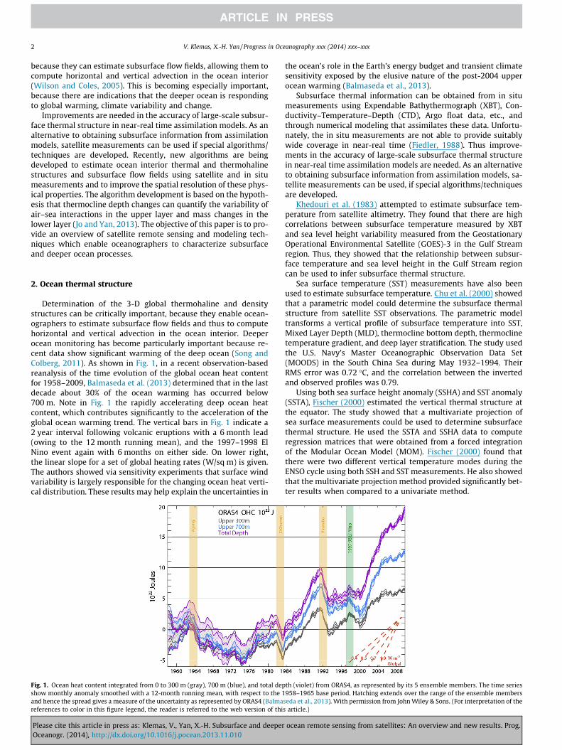
Determination of the 3-D global thermohaline and densitystructures can be critically important, because they enable ocean-ographers to estimate subsurface flow fields and thus to computehorizontal and vertical advection in the ocean interior. Deeperocean monitoring has become particularly important because re-cent data show significant warming of the deep ocean (Song andColberg, 2011). As shown in Fig. 1, in a recent observation-basedreanalysis of the time evolution of the global ocean heat contentfor 1958–2009, Balmaseda et al. (2013) determined that in the lastdecade about 30% of the ocean warming has occurred below700 m. Note in Fig. 1 the rapidly accelerating deep ocean heatcontent, which contributes significantly to the acceleration of theglobal ocean warming trend. The vertical bars in Fig. 1 indicate a2 year interval following volcanic eruptions with a 6 month lead(owing to the 12 month running mean), and the 1997–1998 ElNino event again with 6 months on either side. On lower right,the linear slope for a set of global heating rates (W/sq m) is given.The authors showed via sensitivity experiments that surface windvariability is largely responsible for the changing ocean heat verti-cal distribution. These results may help explain the uncertainties in

Fig. 1. Ocean heat content integrated from 0 to 300 m (gray), 700 m (blue), and total depshow monthly anomaly smoothed with a 12-month running mean, with respect to the 1and hence the spread gives a measure of the uncertainty as represented by ORAS4 (Balmareferences to color in this figure legend, the reader is referred to the web version of thi

Please cite this article in press as: Klemas, V., Yan, X.-H. Subsurface and deeperOceanogr. (2014), http://dx.doi.org/10.1016/j.pocean.2013.11.010

the ocean’s role in the Earth’s energy budget and transient climatesensitivity exposed by the elusive nature of the post-2004 upperocean warming (Balmaseda et al., 2013).

Subsurface thermal information can be obtained from in situmeasurements using Expendable Bathythermograph (XBT), Con-ductivity–Temperature–Depth (CTD), Argo float data, etc., andthrough numerical modeling that assimilates these data. Unfortu-nately, the in situ measurements are not able to provide suitablywide coverage in near-real time (Fiedler, 1988). Thus improve-ments in the accuracy of large-scale subsurface thermal structurein near-real time assimilation models are needed. As an alternativeto obtaining subsurface information from assimilation models, sa-tellite measurements can be used, if special algorithms/techniquesare developed.

Khedouri et al. (1983) attempted to estimate subsurface tem-perature from satellite altimetry. They found that there are highcorrelations between subsurface temperature measured by XBTand sea level height variability measured from the GeostationaryOperational Environmental Satellite (GOES)-3 in the Gulf Streamregion. Thus, they showed that the relationship between subsur-face temperature and sea level height in the Gulf Stream regioncan be used to infer subsurface thermal structure.

Sea surface temperature (SST) measurements have also beenused to estimate subsurface temperature. Chu et al. (2000) showedthat a parametric model could determine the subsurface thermalstructure from satellite SST observations. The parametric modeltransforms a vertical profile of subsurface temperature into SST,Mixed Layer Depth (MLD), thermocline bottom depth, thermoclinetemperature gradient, and deep layer stratification. The study usedthe U.S. Navy’s Master Oceanographic Observation Data Set(MOODS) in the South China Sea during May 1932–1994. TheirRMS error was 0.72 �C, and the correlation between the invertedand observed profiles was 0.79.

Using both sea surface height anomaly (SSHA) and SST anomaly(SSTA), Fischer (2000) estimated the vertical thermal structure atthe equator. The study showed that a multivariate projection ofsea surface measurements could be used to determine subsurfacethermal structure. He used the SSTA and SSHA data to computeregression matrices that were obtained from a forced integrationof the Modular Ocean Model (MOM). Fischer (2000) found thatthere were two different vertical temperature modes during theENSO cycle using both SSH and SST measurements. He also showedthat the multivariate projection method provided significantly bet-ter results when compared to a univariate method.

th (violet) from ORAS4, as represented by its 5 ensemble members. The time series958–1965 base period. Hatching extends over the range of the ensemble members

seda et al., 2013). With permission from John Wiley & Sons. (For interpretation of thes article.)

ocean remote sensing from satellites: An overview and new results. Prog.

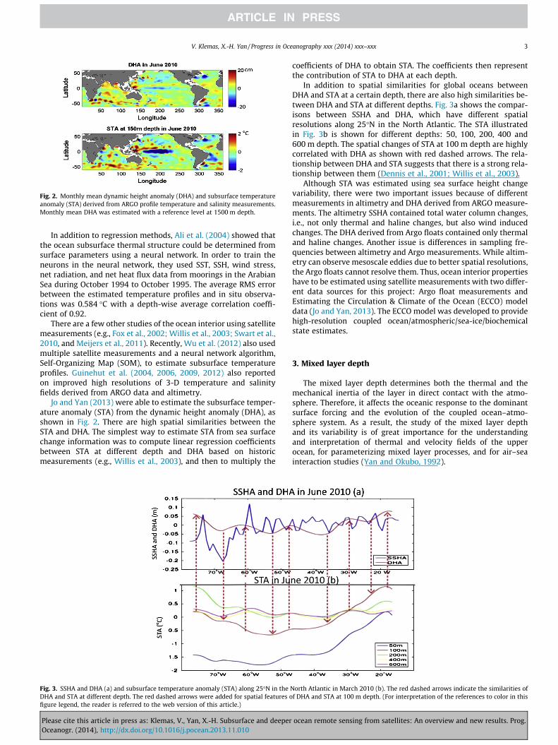
Fig. 2. Monthly mean dynamic height anomaly (DHA) and subsurface temperatureanomaly (STA) derived from ARGO profile temperature and salinity measurements.Monthly mean DHA was estimated with a reference level at 1500 m depth.

V. Klemas, X.-H. Yan / Progress in Oceanography xxx (2014) xxx–xxx 3

In addition to regression methods, Ali et al. (2004) showed thatthe ocean subsurface thermal structure could be determined fromsurface parameters using a neural network. In order to train theneurons in the neural network, they used SST, SSH, wind stress,net radiation, and net heat flux data from moorings in the ArabianSea during October 1994 to October 1995. The average RMS errorbetween the estimated temperature profiles and in situ observa-tions was 0.584 �C with a depth-wise average correlation coeffi-cient of 0.92.

There are a few other studies of the ocean interior using satellitemeasurements (e.g., Fox et al., 2002; Willis et al., 2003; Swart et al.,2010, and Meijers et al., 2011). Recently, Wu et al. (2012) also usedmultiple satellite measurements and a neural network algorithm,Self-Organizing Map (SOM), to estimate subsurface temperatureprofiles. Guinehut et al. (2004, 2006, 2009, 2012) also reportedon improved high resolutions of 3-D temperature and salinityfields derived from ARGO data and altimetry.

Jo and Yan (2013) were able to estimate the subsurface temper-ature anomaly (STA) from the dynamic height anomaly (DHA), asshown in Fig. 2. There are high spatial similarities between theSTA and DHA. The simplest way to estimate STA from sea surfacechange information was to compute linear regression coefficientsbetween STA at different depth and DHA based on historicmeasurements (e.g., Willis et al., 2003), and then to multiply the

Fig. 3. SSHA and DHA (a) and subsurface temperature anomaly (STA) along 25�N in theDHA and STA at different depth. The red dashed arrows were added for spatial features ofigure legend, the reader is referred to the web version of this article.)

Please cite this article in press as: Klemas, V., Yan, X.-H. Subsurface and deeperOceanogr. (2014), http://dx.doi.org/10.1016/j.pocean.2013.11.010

coefficients of DHA to obtain STA. The coefficients then representthe contribution of STA to DHA at each depth.

In addition to spatial similarities for global oceans betweenDHA and STA at a certain depth, there are also high similarities be-tween DHA and STA at different depths. Fig. 3a shows the compar-isons between SSHA and DHA, which have different spatialresolutions along 25�N in the North Atlantic. The STA illustratedin Fig. 3b is shown for different depths: 50, 100, 200, 400 and600 m depth. The spatial changes of STA at 100 m depth are highlycorrelated with DHA as shown with red dashed arrows. The rela-tionship between DHA and STA suggests that there is a strong rela-tionship between them (Dennis et al., 2001; Willis et al., 2003).

Although STA was estimated using sea surface height changevariability, there were two important issues because of differentmeasurements in altimetry and DHA derived from ARGO measure-ments. The altimetry SSHA contained total water column changes,i.e., not only thermal and haline changes, but also wind inducedchanges. The DHA derived from Argo floats contained only thermaland haline changes. Another issue is differences in sampling fre-quencies between altimetry and Argo measurements. While altim-etry can observe mesoscale eddies due to better spatial resolutions,the Argo floats cannot resolve them. Thus, ocean interior propertieshave to be estimated using satellite measurements with two differ-ent data sources for this project: Argo float measurements andEstimating the Circulation & Climate of the Ocean (ECCO) modeldata (Jo and Yan, 2013). The ECCO model was developed to providehigh-resolution coupled ocean/atmospheric/sea-ice/biochemicalstate estimates.

3. Mixed layer depth

The mixed layer depth determines both the thermal and themechanical inertia of the layer in direct contact with the atmo-sphere. Therefore, it affects the oceanic response to the dominantsurface forcing and the evolution of the coupled ocean–atmo-sphere system. As a result, the study of the mixed layer depthand its variability is of great importance for the understandingand interpretation of thermal and velocity fields of the upperocean, for parameterizing mixed layer processes, and for air–seainteraction studies (Yan and Okubo, 1992).

North Atlantic in March 2010 (b). The red dashed arrows indicate the similarities off DHA and STA at 100 m depth. (For interpretation of the references to color in this

ocean remote sensing from satellites: An overview and new results. Prog.

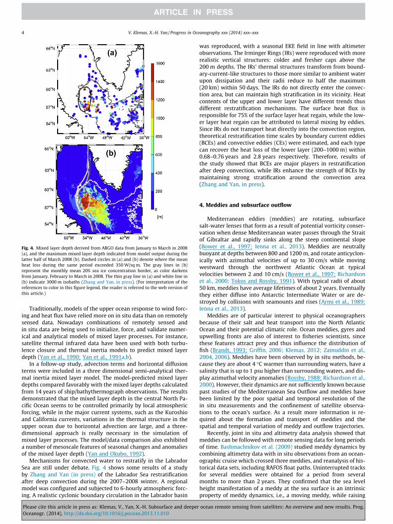
Fig. 4. Mixed layer depth derived from ARGO data from January to March in 2008(a), and the maximum mixed layer depth indicated from model output during thelatter half of March 2008 (b). Dashed circles in (a) and (b) denote where the meanheat loss during the same period exceeded 350 W/sq m. The gray lines in (b)represent the monthly mean 20% sea ice concentration border, as color darkensfrom January, February to March in 2008. The thin gray line in (a) and white line in(b) indicate 3000 m isobaths (Zhang and Yan, in press). (For interpretation of thereferences to color in this figure legend, the reader is referred to the web version ofthis article.)

4 V. Klemas, X.-H. Yan / Progress in Oceanography xxx (2014) xxx–xxx

Traditionally, models of the upper ocean response to wind forc-ing and heat flux have relied more on in situ data than on remotelysensed data. Nowadays combinations of remotely sensed andin situ data are being used to initialize, force, and validate numer-ical and analytical models of mixed layer processes. For instance,satellite thermal infrared data have been used with both turbu-lence closure and thermal inertia models to predict mixed layerdepth (Yan et al., 1990; Yan et al., 1991a,b).

In a follow-up study, advection terms and horizontal diffusionterms were included in a three dimensional semi-analytical ther-mal inertia mixed layer model. The model-predicted mixed layerdepths compared favorably with the mixed layer depths calculatedfrom 14 years of ship/bathythermograph observations. The resultsdemonstrated that the mixed layer depth in the central North Pa-cific Ocean seems to be controlled primarily by local atmosphericforcing, while in the major current systems, such as the Kuroshioand California currents, variations in the thermal structure in theupper ocean due to horizontal advection are large, and a three-dimensional approach is really necessary in the simulation ofmixed layer processes. The model/data comparison also exhibiteda number of mesoscale features of seasonal changes and anomaliesof the mixed layer depth (Yan and Okubo, 1992).

Mechanisms for convected water to restratify in the LabradorSea are still under debate. Fig. 4 shows some results of a studyby Zhang and Yan (in press) of the Labrador Sea restratificationafter deep convection during the 2007–2008 winter. A regionalmodel was configured and subjected to 6-hourly atmospheric forc-ing. A realistic cyclonic boundary circulation in the Labrador basin

Please cite this article in press as: Klemas, V., Yan, X.-H. Subsurface and deeperOceanogr. (2014), http://dx.doi.org/10.1016/j.pocean.2013.11.010

was reproduced, with a seasonal EKE field in line with altimeterobservations. The Irminger Rings (IRs) were reproduced with morerealistic vertical structures: colder and fresher caps above the200 m depths. The IRs’ thermal structures transform from bound-ary-current-like structures to those more similar to ambient waterupon dissipation and their radii reduce to half the maximum(20 km) within 50 days. The IRs do not directly enter the convec-tion area, but can maintain high stratification in its vicinity. Heatcontents of the upper and lower layer have different trends thusdifferent restratification mechanisms. The surface heat flux isresponsible for 75% of the surface layer heat regain, while the low-er layer heat regain can be attributed to lateral mixing by eddies.Since IRs do not transport heat directly into the convection region,theoretical restratification time scales by boundary current eddies(BCEs) and convective eddies (CEs) were estimated, and each typecan recover the heat loss of the lower layer (200–1000 m) within0.68–0.76 years and 2.8 years respectively. Therefore, results ofthe study showed that BCEs are major players in restratificationafter deep convection, while IRs enhance the strength of BCEs bymaintaining strong stratification around the convection area(Zhang and Yan, in press).

4. Meddies and subsurface outflow

Mediterranean eddies (meddies) are rotating, subsurfacesalt-water lenses that form as a result of potential vorticity conser-vation when dense Mediterranean water passes through the Straitof Gibraltar and rapidly sinks along the steep continental slope(Bower et al., 1997; Ienna et al., 2013). Meddies are neutrallybuoyant at depths between 800 and 1200 m, and rotate anticyclon-ically with azimuthal velocities of up to 30 cm/s while movingwestward through the northwest Atlantic Ocean at typicalvelocities between 2 and 10 cm/s (Bower et al., 1997; Richardsonet al., 2000; Tokos and Rossby, 1991). With typical radii of about50 km, meddies have average lifetimes of about 2 years. Eventuallythey either diffuse into Antarctic Intermediate Water or are de-stroyed by collisions with seamounts and rises (Armi et al., 1989;Ienna et al., 2013).

Meddies are of particular interest to physical oceanographersbecause of their salt and heat transport into the North AtlanticOcean and their potential climatic role. Ocean meddies, gyres andupwelling fronts are also of interest to fisheries scientists, sincethese features attract prey and thus influence the distribution offish (Brandt, 1993; Griffin, 2006; Klemas, 2012; Zainuddin et al.,2004, 2006). Meddies have been observed by in situ methods, be-cause they are about 4 �C warmer than surrounding waters, have asalinity that is up to 1 psu higher than surrounding waters, and dis-play azimuthal velocity anomalies (Rossby, 1988; Richardson et al.,2000). However, their dynamics are not sufficiently known becausepast studies of the Mediterranean Sea Outflow and meddies havebeen limited by the poor spatial and temporal resolution of thein situ measurements and the confinement of satellite observa-tions to the ocean’s surface. As a result more information is re-quired about the formation and transport of meddies and thespatial and temporal variation of meddy and outflow trajectories.

Recently, joint in situ and altimetry data analysis showed thatmeddies can be followed with remote sensing data for long periodsof time. Bashmachnikov et al. (2009) studied meddy dynamics bycombining altimetry data with in situ observations from an ocean-ographic cruise which crossed three meddies, and reanalysis of his-torical data sets, including RAFOS float paths. Uninterrupted tracksfor several meddies were obtained for a period from severalmonths to more than 2 years. They confirmed that the sea levelheight manifestation of a meddy at the sea surface is an intrinsicproperty of meddy dynamics, i.e., a moving meddy, while raising

ocean remote sensing from satellites: An overview and new results. Prog.

V. Klemas, X.-H. Yan / Progress in Oceanography xxx (2014) xxx–xxx 5

isopycnals, also compresses the vorticity tubes above. Both pro-cesses act to generate anticyclonic vorticity in the upper layer. Rel-ative movement appeared to be an important condition for ameddy to have a clear surface signature. Enhancement of meddysurface signature was usually observed during periods of steadypropagation. During periods of stagnation the associated surfacesignals seemed to become weak and intermittent. Results suggestthe possibility of long-term routine meddy tracking, once an altim-etry anomaly is linked to a meddy (Bashmachnikov et al., 2009).

New remote sensing methods have been developed to observeand study meddies by means of unique approaches in the analysisof integrated multisensor data from satellites. Yan et al. (2006)used satellite altimeter, scatterometer, infrared satellite imagery,and XBT data to detect and calculate the trajectories and the rela-tive transport of the Mediterranean outflow and meddies. XBTtemperature measurements were used to validate their approach,showing that monthly mean features derived from floats and XBTsfor multiple meddies significantly correlated with remote sensingresults. The singular value decomposition method was used to

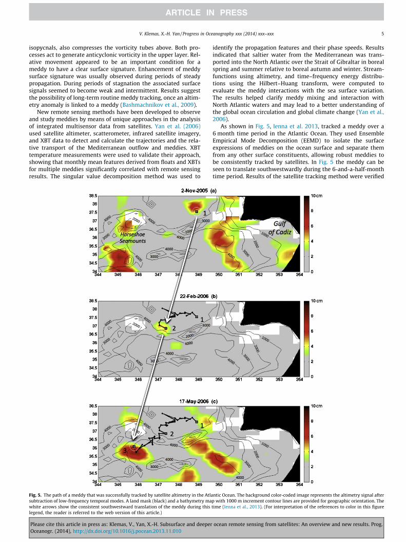
Fig. 5. The path of a meddy that was successfully tracked by satellite altimetry in the Atlasubtraction of low-frequency temporal modes. A land mask (black) and a bathymetry mawhite arrows show the consistent southwestward translation of the meddy during thislegend, the reader is referred to the web version of this article.)

Please cite this article in press as: Klemas, V., Yan, X.-H. Subsurface and deeperOceanogr. (2014), http://dx.doi.org/10.1016/j.pocean.2013.11.010

identify the propagation features and their phase speeds. Resultsindicated that saltier water from the Mediterranean was trans-ported into the North Atlantic over the Strait of Gibraltar in borealspring and summer relative to boreal autumn and winter. Stream-functions using altimetry, and time–frequency energy distribu-tions using the Hilbert–Huang transform, were computed toevaluate the meddy interactions with the sea surface variation.The results helped clarify meddy mixing and interaction withNorth Atlantic waters and may lead to a better understanding ofthe global ocean circulation and global climate change (Yan et al.,2006).

As shown in Fig. 5, Ienna et al. 2013, tracked a meddy over a6 month time period in the Atlantic Ocean. They used EnsembleEmpirical Mode Decomposition (EEMD) to isolate the surfaceexpressions of meddies on the ocean surface and separate themfrom any other surface constituents, allowing robust meddies tobe consistently tracked by satellites. In Fig. 5 the meddy can beseen to translate southwestwardly during the 6-and-a-half-monthtime period. Results of the satellite tracking method were verified

ntic Ocean. The background color-coded image represents the altimetry signal afterp with 1000 m increment contour lines are provided for geographic orientation. Thetime (Ienna et al., 2013). (For interpretation of the references to color in this figure

ocean remote sensing from satellites: An overview and new results. Prog.

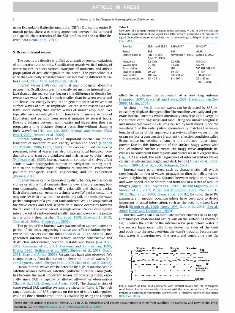
Table 1Overview of Synthetic Aperture Radar (SAR) satellites. V and H are vertical andhorizontal polarizations of SAR signal. First letter denotes polarization of transmittedsignal. Second letter represents polarization of received signal. Adapted from Susantoet al. (2005).

6 V. Klemas, X.-H. Yan / Progress in Oceanography xxx (2014) xxx–xxx

using Expendable Bathythermographs (XBTs). During the entire 6-month period there was strong agreement between the temporaland spatial characteristics of the XBT profiles and the satellite-de-rived data (Ienna et al., 2013).

Satellite ERS-1 and ERS-2 RADARSAT ENVISAT

Sensor SAR SAR ASARLaunch dates (s) July 17, 1991 November 4, 1995 March 1, 2002

April 20, 1995Frequency 5.3 GHz 5.3 GHz 5.3 GHzWavelength 5.6 cm 5.6 cm 5.6 cmPolarization VV HH VV, HH, VH, HVIncidence angle 20–26� 10–59� 15–45�Swat width 100 km 50–500 km 100–405 kmGround resolution 25 � 25 m 8 � 100 m 25 � 25 m

150 � 150 m

Fig. 6. Sketch of flow field associated with internal waves and the consequentmodulation of surface waves which interact with the radar pulses. Here ‘‘c’’ denotesregions of horizontally convergent currents and ‘‘d’’ denotes regions of divergence(Robinson, 2004).

5. Ocean internal waves

The oceans are density stratified as a result of vertical variationsof temperature and salinity. Stratification retards vertical mixing ofwater masses, reduces vertical transport of nutrients, and affectspropagation of acoustic signals in the ocean. The pycnocline is azone that vertically separates water masses having different densi-ties (Pinet, 2009; Mirie and Pennell, 1989).

Internal waves (IWs) can form at and propagate along thepycnocline. Oscillations are more easily set up at an internal inter-face than at the sea-surface, because the difference in density be-tween two water layers is much smaller than between water andair. Hence, less energy is required to generate internal waves thansurface waves of similar amplitude. For the same reason IWs alsotravel more slowly than surface waves of similar amplitude. IWstypically have wavelengths from hundreds of meters to tens ofkilometers and periods from several minutes to several hours.Due to a balance between nonlinearity and dispersion, they canpropagate a long distance along a pycnocline without changingtheir waveform (Hsu and Liu, 2000; Klymak and Moum, 2003;Pinkel, 2000; Susanto et al., 2005).

Internal solitary waves are an important mechanism for thetransport of momentum and energy within the ocean (Helfrichand Melville, 1986; Lamb, 1994). In the context of vertical mixingprocesses, internal waves can also influence local biological pro-ductivity and transport plankton and fish larvae to other areas(Holligan et al., 1985). Internal waves on continental shelves affectacoustic wave propagation; submarine navigation; mixing nutri-ents to the euphotic zone; sediment re-suspension; cross-shorepollutant transport; coastal engineering and oil exploration(Klemas, 2012).

Internal waves can be generated by disturbances, such as oceanstorms or strong tidal currents flowing over sharply varying bot-tom topography, including shelf breaks, sills and shallow banks.Each disturbance can generate a single-wave IW packet containingonly one IW with or without an oscillating tail, or a multiple-wavepacket composed of a group of rank-ordered IWs. The amplitude ofthe wave crests and their separation distance decreases towardsthe tail end of the wave packet. A single-wave ISW can disintegrateinto a packet of rank-ordered smaller internal waves while propa-gating onto a shoaling shelf (Liu et al., 1998; Zhao and Li, 2012;Zhao et al., 2004a; Zheng et al., 2001a).

The period of the internal wave packets often approximates theperiod of the tides, suggesting a cause-and-effect relationship be-tween the packets and the tides (Zhao et al., 2012, 2004b). Oncegenerated, internal waves can refract, undergo constructive anddestructive interference, become unstable and break (Cai et al.,2002; Cummins et al., 2003; Gerkema and Zimmerman, 1995;Hibiya, 1990; Holloway et al., 1997; Shroyer et al., 2011; Small,2001; Zhao and Alford, 2006). Researchers have also observed IWschange polarity from depression to elevation internal waves (Orrand Mignerey, 2003; Shroyer et al., 2007; Zhao et al., 2003, 2004a).

Ocean internal waves can be detected by high-resolution visiblesatellite sensors, however, satellite Synthetic Aperture Radar (SAR)has become the most important sensor for observing them, espe-cially since SAR is capable of all-day, all-weather observations(Zhao et al., 2003; Zheng and Alpers, 2004). The characteristics ofsome typical SAR satellite systems are shown in Table 1. The highrange resolution of SAR depends on the use of short radar pulses,while its fine azimuth resolution is attained by using the Doppler

Please cite this article in press as: Klemas, V., Yan, X.-H. Subsurface and deeperOceanogr. (2014), http://dx.doi.org/10.1016/j.pocean.2013.11.010

effect to synthesize the equivalent of a very long antenna(Campbell, 2007; Cracknell and Hayes, 2007; Elachi and van Ziel,2006; Martin, 2004).

As shown in Fig. 6, internal waves can be detected by SAR be-cause they displace the pycnocline/thermocline vertically and gen-erate internal currents which alternately converge and diverge onthe surface, capturing slicks and modulating sea surface roughnessand small-scale waves (1–10 cm), caused by local winds. Since thewavelength of the radar pulses geometrically matches the wave-lengths of some of the small-scale gravity-capillary waves on theocean surface, a constructive (resonant) reflection condition calledBragg scattering results, enhancing the returned radar signalpower. Due to this interaction of the surface Bragg waves withthe IW-induced surface currents, the Bragg wave amplitude in-creases in convergent flow regions and decreases in divergent flow(Fig. 3). As a result, the radar signatures of internal solitary wavesconsist of alternating bright and dark bands (Alpers et al., 2008;Jackson, 2004; Li et al., 2000; Robinson, 2004).

Internal wave parameters, such as characteristic half width,crest length, number of waves, propagation direction, distance be-tween neighboring packets, distance between neighboring waves,and wave speed, can be determined from one or a series of satelliteimages (Alpers, 1985; Alpers et al., 2008; Orr and Mignerey, 2003;Shroyer et al., 2007; Porter and Thompson, 1999; Zhao and Li,2012; Zhao et al., 2003; Zheng et al., 2001b). By using these IWparameters in models, oceanographers have been able to deriveimportant physical information, such as the oceanic mixed layerdepth (Brandt et al., 1996; Jones, 1995; Kara et al., 2003; Li et al.,2000; Porter and Thompson, 1999).

Internal waves can also modulate surface currents so as to cap-ture biological material and natural oils on the surface. As shown inFig. 6, when the crests of the internal wave pass below, water inthe surface layer essentially flows down the sides of the crestand pools into the area overlying the wave’s troughs. Because sur-face water is diverging over the crests and converging over the

ocean remote sensing from satellites: An overview and new results. Prog.

V. Klemas, X.-H. Yan / Progress in Oceanography xxx (2014) xxx–xxx 7

troughs, biological material and natural oils on the surface are alsoalternately dispersed and concentrated in a similar wave pattern.These natural ‘‘slicks’’ calm the water surface and change how it re-flects the radar waves, thus revealing the presence of the underly-ing internal waves (Alpers, 1985; Apel, 2003; Robinson, 2004).

6. Seabottom topography from satellite altimetry and SARimagery

Satellite altimeter data is being used to fill gaps in our knowl-edge of ocean depths between ship tracks. Satellite altimetry is alsoused to interpolate between acoustic echo sounder measurements.Altimeters profile the shape of the ocean surface, and its shape isvery similar to the shape of the sea-floor. Excess mass at the sea-floor, like a seamount, increases local gravity because the mass ofthe seamount is larger than the mass of water it displaces. The ex-cess mass increases local gravity, which attracts water toward theseamount. This changes the shape of the sea surface accordingly(Stewart, 2007).

The level surface corresponding to the surface of the ocean atrest is called the geoid. To a first approximation, the geoid is anellipsoid that corresponds to the surface of a rotating, homoge-neous fluid in solid-body rotation, meaning that the fluid has nointernal flow. To a second approximation, the geoid differs fromthe ellipsoid because of local variations in gravity, called undula-tions, which have a maximum amplitude of about ±60 m. For in-stance, because it is more dense than seawater, a 2 km highseamount would produce an upward bulge of about 10 m.Trenches have a deficiency of mass and produce a downwarddeflection of the geoid. As a result, the geoid is closely related tosea-floor topography (Calmant et al., 2002; Stewart, 2007).

To a third approximation, the sea surface deviates from thegeoid because the ocean is not at rest. The deviation of the sea levelfrom the geoid is defined as the sea surface topography which iscaused by tides, heat content of the water, and ocean surface cur-rents. Because the maximum amplitude of the sea surface topogra-phy is about ±1 m, it is small compared to the geoid undulations(Stewart, 2007).

Satellite altimetry has been used to map the seafloor on a globalscale. Calmant et al. (2002) prepared a worldwide map of seafloortopography computed from an iterative inversion combiningaltimetry measurements of the marine geoid and shipboard echosoundings from the National Geophysical Data Center (NGDC)database. The input geoid data for their computation were derivedfrom altimetry measurements of the sea-surface height from theERS-1 Geodetic Mission, and the GEOSAT, ERS-1 and Topex-Posei-don Exact Repeat Mission. To calculate the seafloor topographyfrom sea surface height measurements, the authors took the regio-nal isostatic compensation of the topographic load into account byusing a model of elastic flexure of the oceanic lithosphere in whichthe elastic plate thickness increases with crustal age. With thissolution, they were able to provide an uncertainty map that re-flects the uneven distribution of and errors in the data, and uncer-tainties in the model parameters, as well as the increase of thegeopotential error with the deepening of the seafloor. Comparingthe bathymetric solution with Smith and Sandwell’s (1994) solu-tion, the RMS difference between the two amounted to 350 m.Other examples of global ocean bathymetry derived from satellitealtimetry are presented by Ramillien and Cazenave (1997) andSmith and Sandwell (2008).

In coastal and offshore waters, seabed topography is importantfor many applications, such as erosion studies and the constructionof coastal defenses. In these shallow coastal waters, subsurfacebottom topographic features become visible on radar images ofthe sea surface when there is a current (usually tidal) that flows

Please cite this article in press as: Klemas, V., Yan, X.-H. Subsurface and deeperOceanogr. (2014), http://dx.doi.org/10.1016/j.pocean.2013.11.010

over these features. This causes local perturbations to the currentwhich in turn modulates the sea surface roughness. Since SAR isa very sensitive roughness sensor, it can be used to map the rough-ness pattern induced by (tidal) flow over bottom topography.Using series of SAR images and hydrodynamic analysis, scientistshave developed various methods for obtaining information oncoastal seabottom features (Hennings, 1998; Hesselmans et al.,2013; Yang et al., 2010; Yuan et al., 2009). Sometimes shallowwater bottom features can also be observed by ocean color sensors(Shi et al., 2011).

Most of the approaches for mapping seabottom topographywith SAR consist of three ocean interaction modeling steps, includ-ing the modulation of the current by the underwater features;modulation of the sea surface waves by the variable surface cur-rent; and the interaction of the microwaves with the surfacewaves. The interaction between (tidal) flow and bottom topogra-phy can be described by several models of increasing complexity:continuity equation, shallow water equations, and the NavierStokes equations. Modulations of surface flow velocity are modeledusing the action balance equation, including a relaxation sourceterm to simulate the restoring forces of wind input and wavebreaking. To compute the backscatter modulation caused by sur-face waves, a simple Bragg model can be used (Hesselmans et al.,2013; Vogelzang et al., 1992, 1997; Wensink and Campbell,1997; Zhao et al., 2012).

SAR techniques have also been applied to deeper waters, whichcan be vertically stratified. Zheng et al. (2006) used SAR images tostudy wave-like patterns of ocean bottom topographic features atthe southern outlet of the Taiwan Strait, which is vertically strati-fied. Most previous SAR imaging models had been developed forhomogeneous waters and were unable to characterize bottom fea-tures in stratified water bodies. In order to determine the quantita-tive relationship between the SAR imagery and bottom features,Zheng et al. (2006) developed a two-dimensional, three-layerocean model with sinusoidal bottom topographic features. Resultsindicate that the topographic waves on the SAR images have thesame wavelength of bottom topographic corrugation, and theimagery brightness peaks are either inphase or antiphase with re-spect to the topographic corrugation, depending on the sign of acoupling factor. The results of this study provide a physical basisfor quantitative interpretation of SAR images of bottom topo-graphic waves in a stratified ocean (Zheng et al., 2006).

7. Summary and conclusions

Satellite sensors cannot directly observe subsurface and deeperocean processes and features, such as ocean thermal and halinestructures. Traditionally these have been studied with modelsand in situ sensors deployed from research vessels or attached tomoorings or drifter buoys. In situ measurements have been fairlyaccurate, yet unable to provide suitably wide coverage in near-realtime. Because this information is important to physical, biochemi-cal and geological studies of the oceans, new models and algo-rithms are being developed that will enable scientists to usesatellite data to determine mixed layer depths, monitor meddies,characterize internal waves, map deep ocean bathymetry, andstudy other deep ocean processes. Deeper ocean remote sensingand modeling are becoming particularly important, because thereare clear indications that the deeper ocean is responding to globalwarming, climate variability and change.

Since most research on ocean interior structure still relies onin situ measurements and numerical models, there is a need to de-velop algorithms that provide subsurface thermohaline densitystructure and subsurface current fields based on multiple satellitemeasurements on a global scale to allow subsurface phenomena to

ocean remote sensing from satellites: An overview and new results. Prog.

8 V. Klemas, X.-H. Yan / Progress in Oceanography xxx (2014) xxx–xxx

be further explored. The ocean interior variability is still the miss-ing information between surface height changes, water mass, anddensity field changes. The estimation of the 3-D thermohalineand density structures is critically important to oceanographersbecause with that information they can estimate subsurface flowfields and compute horizontal and vertical advection in the oceaninterior.

Acknowledgments

This study has been partially supported by the NASA PhysicalOceanography Program, NASA EPSCoR Program, NASA Space Grant,and NOAA Sea Grant Program at the University of Delaware.

References

Ali, M.M., Swain, D., Weller, R.A., 2004. Estimation of ocean subsurface thermalstructure from surface parameters, a neural network approach. GeophysicalResearch Letters 31, L20308, 10.1029.

Alpers, W., 1985. Theory of radar imaging of internal waves. Nature 314, 245–247.Alpers, W., Brandt, P., Rubino, A., 2008. Internal waves generated in the Strait of

Gibraltar and Messina: observations from space. In: Barale, V., Gade, M. (Eds.),Remote Sensing of the European Seas. Springer, Dordrecht, The Netherlands, pp.319–330.

Apel, J.R., 2003. A new analytical model for ISWs in the ocean. Journal of PhysicalOceanography 33, 2247–2269.

Armi, L., Hebert, D., Price, J., Richardson, P., Rossby, T., Ruddick, B., 1989. Two yearsin the life of a Mediterranean salt lens. Journal of Physical Oceanography 19,354–370.

Balmaseda, M.A., Trendberth, K.E., Kallen, E., 2013. Distinctive climate signals inreanalysis of global ocean heat content. Geophysical Research Letters 40, 1–6.

Bashmachnikov, I., Machin, F., Mendonca, A., Martins, A., 2009. In situ and remotesensing signature of meddies east of the mid-Atlantic ridge. Journal ofGeophysical Research 114 (C05018), 2009, 10.1029/2008JC005032.

Bower, A.S., Armi, L., Ambar, I., 1997. Lagrangian observations of eddy formationduring a Mediterranean undercurrent seeding experiment. Journal of PhysicalOceanography 27, 2545–2575.

Brandt, S.B., 1993. The effect of thermal fronts on fish growth: a bioenergeticsevaluation of food and temperature. Estuaries 16, 142–159.

Brandt, P., Alpers, W., Backhaus, J.O., 1996. Study of the generation and propagationof internal waves in the Strait of Gibraltar using a numerical model andsynthetic aperture radar images of the European ERS-1 satellite. Journal ofGeophysical Research 101, 14237–14252.

Cai, S., Long, X., Gan, Z., 2002. A numerical study of the generation and propagationof internal solitary waves in the Luzon Strait. Oceanologica Acta 25, 51–60.

Calmant, S., Berge-Nguyen, M., Cazenave, A., 2002. Global seafloor topography froma least-squares inversion of altimetry-based high-resolution mean sea surfaceand shipboard soundings. Geophysical Journal International, 151795–151808.

Campbell, J.B., 2007. Introduction to Remote Sensing. The Guilford Press, New York.Chu, P.C., Fan, C., Liu, W.T., 2000. Determination of vertical thermal structure from

sea surface temperature. Journal of Atmospheric and Oceanic Technology 17,971–979.

Cracknell, A.P., Hayes, L., 2007. Introduction to Remote Sensing, fifth ed. CRC Press,Boca Raton, Florida.

Cummins, P.F., Vagle, S., Armi, L., Farmer, D., 2003. Stratified flow over topography:upstream influence and generation of nonlinear internal waves. Proceedings ofthe Royal Society of London A459, 1467–1487.

Dennis, A.M., Molinari, R.L., Baringer, M.O., Goni, G., 2001. Transition regions andtheir role in the relationship between sea surface height and subsurfacetemperature structure in the Atlantic Ocean. Geophysical Research Letters 28,3943–3946.

Elachi, C., van Ziel, Z., 2006. Introduction to the Physics and Techniques of RemoteSensing, second ed. John Wiley and Sons, Hoboken, New Jersey.

Fiedler, P.C., 1988. Surface manifestations of subsurface thermal structure in theCalifornia Current. Journal of Geophysical Research 93, 4975–4983.

Fischer, M., 2000. Multivariate projection of ocean surface data onto subsurfacesections. Geophysical Research Letters 27, 755–757.

Fox, D.N., Teague, W.J., Barron, C.N., Carnes, M.R., Lee, C.M., 2002. The Modula OceanData Assimilation System (MODAS). Journal of Atmospheric and OceanicTechnology 19, 240–252.

Gerkema, T., Zimmerman, J.T.F., 1995. Generation of non-linear internal tides andsolitary waves. Journal of Physical Oceanography 25, 1081–1094.

Griffin, R.B., 2006. Sperm whale distributions and community ecology associatedwith a warm-core ring off Georges Bank. Marine Mammal Science 15, 33–51.

Guinehut, S., Le Traon, P.-Y., Larnicol, G., Philipps, S., 2004. Combining Argo andremote-sensing data to estimate the ocean three dimensional temperaturefields – a first approach based on simulated observations. Journal of MarineSystems 46, 85–98.

Guinehut, S., Le Traon, P.-Y., Larnicol, G., 2006. What can we learn from globalaltimetry/hydrography comparisons? Geophysical Research Letters 33, L10604,10.1029/2005GL025551.

Please cite this article in press as: Klemas, V., Yan, X.-H. Subsurface and deeperOceanogr. (2014), http://dx.doi.org/10.1016/j.pocean.2013.11.010

Guinehut, S., Coatanoan, C., Dhomps, A.-L., Le Traon, P.-Y., Larnicol, G., 2009. On theuse of satellite altimeter data in Argo quality control. Journal of Atmosphericand Oceanic Technology 26, 395–402.

Guinehut, S., Dhomps, A.-L., Larnicol, G., LeTraon, P.-Y., 2012. High resolution 3-Dtemperature and salinity fields derived from in situ and satellite observations.Ocean Science 8, 845–857.

Helfrich, K.R., Melville, W.K., 1986. On long non-linear internal waves over slopeshelf topography. Journal of Fluid Mechanics 167, 285–308.

Hennings, I., 1998. An historical overview of radar imagery of seabottomtopography. International Journal of Remote Sensing 19, 1447–1454.

Hesselmans, G., Calkoen, C., Wensink, H., 2013. Mapping of Seabed Topography toand from Synthetic Aperture Radar. ESA Earthnet Online (accessed 05.08.13).

Hibiya, T., 1990. Generation mechanism of internal waves by a vertically shearedtidal flow over a sill. Journal of Geophysical Research 95, 1757–1764.

Holligan, P.M., Pingree, R.D., Mardell, G.T., 1985. Oceanic solitons, nutrient pulseand phytoplankton growth. Nature 314, 348–350.

Holloway, P.E., Pelinovsky, E., Talipova, T., Barnes, B., 1997. A nonlinear model ofinternal tide transformation on the Australian North West Shelf. Journal ofPhysical Oceanography 27, 871–893.

Hsu, M.-K., Liu, A.K., 2000. Nonlinear internal waves in the South China Sea.Canadian Journal of Remote Sensing 26, 72–81.

Ienna, F., Jo, Y-H., Yan, X-H., 2013. A new method for tracking Meddies by satellitealtimetry. Journal of Atmospheric and Oceanic Technology. http://dx.doi.org/10.1175/JTECH-D-13-00080.1.

Jackson, C.R., 2004. An Atlas of Internal Solitary Waves and their Properties, seconded. GlobalOceanAssociates, Alexandria, VA, http://www.internalwaveatlas.com.

Jo, Y., Yan, X-H., 2013. Personal Communication.Jones, R.M., 1995. On using ambient internal waves to monitor Brunt-Väisälä

frequency. Journal of Geophysical Research 100, 11005–11011.Kara, A.B., Rochford, P.A., Hurlburt, H.E., 2003. Mixed layer depth variability over the

global ocean. Journal of Geophysical Research 108 (C3), 3079. http://dx.doi.org/10.1029/2000JC000736.

Khedouri, E., Szczechowski, C., Cheney, R.E., 1983. Potential oceanographicapplications of satellite altimetery for inferring subsurface thermal structure.Oceans 15, 274–280.

Klemas, V., 2012. Remote sensing of ocean internal waves: an overview. Journal ofCoastal Research 28, 540–546.

Klymak, J.M., Moum, J.N., 2003. Internal solitary waves of elevation advancing on ashoaling shelf. Geophysical Research Letters 30, 2045.

Lamb, K.G., 1994. Numerical experiments of internal wave generation by strongtidal flow across a finite amplitude bank edge. Journal of Geophysical Research99, 843–864.

Li, X., Clemente-Colon, P., Friedman, K.S., 2000. Estimating oceanic mixed layerdepth from internal wave evolution observed from RADARSAT-1 SAR. JohnsHopkins APL Technical Digest 21, 130–135.

Liu, A.K., Chang, S.Y., Hsu, M.K., Liang, N.K., 1998. Evolution of nonlinear internalwaves in East and South China Seas. Journal of Geophysical Research 103, 7995–8008.

Martin, S., 2004. An Introduction to Remote Sensing. Cambridge University Press,Cambridge, UK.

Meijers, A.J.S., Bindoff, N.L., Rintoul, S.R., 2011. Estimating the four-dimensionalstructure of the southern ocean using satellite altimetry. Journal of Atmosphericand Oceanic Technology 28, 548–568. http://dx.doi.org/10.1175/2010JTECHO790.1.

Mirie, R.M., Pennell, S.A., 1989. Internal solitary waves in a two-fluid system.Physics of Fluids. A. Fluid Dynamics I (6), 986–991.

Orr, M.H., Mignerey, P.C., 2003. Nonlinear internal waves in the South China Sea:observation of the conversion of depression internal waves to elevation internalwaves. Journal of Geophysical Research 108 (C3), 3064, doi: 10.1029/2001JC001163.

Pinet, P.R., 2009. Invitation to Oceanography. Jones and Bartlett Publishers,Sudbury, MA.

Pinkel, R., 2000. Internal solitary waves in the warm pool of the western equatorialPacific. Journal of Physical Oceanography 30, 2906–2926.

Porter, D.J., Thompson, D.R., 1999. Continental shelf parameters inferred from SARinternal wave observations. Journal of Atmospheric and Oceanic Technology 16,475–487.

Ramillien, G., Cazenave, A., 1997. Global bathymetry derived from altimeter data ofthe ERS-1 geodetic mission. Journal of Geodynamics 23, 129–149.

Richardson, P.L., Bower, A.S., Zenk, W., 2000. A census of eddies tracked by fronts.Progress in Oceanography 45, 209–250, Pergamon.

Robinson, I.S., 2004. Measuring the Oceans from Space: The Principles and Methodsof Satellite Oceanography. Springer-Praxis Publishing Ltd., Chichester, UK.

Rossby, T., 1988. Five drifters in a Mediterranean salt lens. Deep Sea Research Part A.Oceanographic Research Papers 35, 1653–1663, Elsevier, Waltham, MA.

Shi, W., Wang, M., Li, X., Pichel, W.G., 2011. Ocean sand ridge signatures in the BohaiSea observed by satellite ocean color and synthetic aperture radarmeasurements. Remote Sensing of Environment 115, 1926–1934.

Shroyer, E.L., Moum, J.N., Nash, J.D., 2007. Observations of polarity reversal inshoaling nonlinear internal waves. Journal of Physical Oceanography 39, 691–701.

Shroyer, E.L., Moum, J.N., Nash, J.D., 2011. Nonlinear internal waves over NewJersey’s continental shelf. Journal of Geophysical Research 116, C03022. http://dx.doi.org/10.1029/2010JC006332.

Small, J., 2001. Refraction and shoaling of nonlinear internal waves at the Malinshelf break. Journal of Physical Oceanography 33, 2657–2674.

ocean remote sensing from satellites: An overview and new results. Prog.

V. Klemas, X.-H. Yan / Progress in Oceanography xxx (2014) xxx–xxx 9

Smith, W.H.F., Sandwell, D.T., 1994. Bathymetric prediction from dense satellitealtimetry and sparse shipboard bathymetry. Journal of Geophysical Research 99(B11), 21803–21824.

Smith, W.H.F., Sandwell, D.T., 2008. Bathymetric prediction from dense satellitealtimetry and sparse shipboard bathymetry. Journal of Geophysical Research 99(B11), 21803–21824. http://dx.doi.org/10.1029/94JB00988.

Song, Y.T., Colberg, F., 2011. Deep ocean warming assessed from altimeters, gravityrecovery and climate experiment, in situ measurements, and a non-Boussinesqocean general circulation model. Journal of Geophysical Research 116 (C02020),1–16.

Stewart, R.H., 2007. Introduction to Physical Oceanography. On-line Textbook:HTML or PDF Version. Texas A & M University.

Susanto, R.D., Mitnik, L., Zheng, Q., 2005. Ocean internal waves observed in theLombok Strait. Oceanography 18, 80–87.

Swart, S., Speich, S., Ansorge, I.J., Lutjeharms, J.R.E., 2010. An altimetry-based gravestempirical mode south of Africa: 1. Development and validation. Journal ofGeophysical Research 115, C03002. http://dx.doi.org/10.1029/2009JC005299.

Tokos, K.S., Rossby, T., 1991. Kinematics and dynamics of a Mediterranean salt lens.Journal of Physical Oceanography 21, 879–892.

Vogelzang, J., Wensink, G.J., de Loor, G.P., Peters, H.C., Pouwels, H., 1992. Seabottomtopography with X-band SLAR: the relation between radar imagery andbathymetry. International Journal of Remote Sensing 13, 1943–1958.

Vogelzang, J., Wensink, G.J., Calkoen, C.J., van der Kooij, M.W.A., 1997. Mappingsubmarine sand waves with multiband imaging radar, 2. Experimental resultsand model comparison. Journal of Geophysical Research 102, 1183–1192.

Wensink, H., Campbell, G., 1997. Bathymetric map production using ERS SAR.Backscatter 8, 17–22.

Willis, J.K., Roemmich, D., Cornuelle, B., 2003. Combining altimetric height withbroadscale profile data to estimate steric height, heat storage, subsurfacetemperature, and sea-surface temperature variability. Journal of GeophysicalResearch 108 (C9), 3292.

Wilson, C., Coles, V.J., 2005. Global climatological relationships between satellitebiological and physical observations and upper ocean properties. Journal ofGeophysical Research 110, c10001. http://dx.doi.org/10.1029/2004JC002724.

Wu, X., Yan, X.-H., Jo, Y.-H., Liu, W.T., 2012. Estimation of subsurface temperatureanomaly in the north Atlantic using a self-organizing map neural network.Journal of Atmospheric and Oceanic Technology, http://dx.doi.org/10.1175/JTECH-D-12-00013.1.

Yan, X.-H., Okubo, A., 1992. Three-dimensional analytical model for the mixed layerdepth. Journal of Geophysical Research 97 (C12), 20201–20226.

Yan, X.-H., Schubel, J.R., Pritchard, D.W., 1990. Oceanic upper mixed layer depthdetermination by the use of satellite data. Remote Sensing of Environment 32,55–74.

Yan, X.-H., Okubo, A., Shubel, J.R., Pritchard, D.W., 1991a. An analytical mixed layerremote sensing model. Deep-Sea Research 38, 267–287.

Yan, X.-H., Niller, P.P., Stewart, R.H., 1991b. Construction and accuracy analysis ofimages of the daily–mean mixed layer depth. International Journal of RemoteSensing 12, 2573–2584.

Please cite this article in press as: Klemas, V., Yan, X.-H. Subsurface and deeperOceanogr. (2014), http://dx.doi.org/10.1016/j.pocean.2013.11.010

Yan, X.-H., Jo, Y.-H., Liu, W.T., He, M.-X., 2006. A new study of the Mediterraneanoutflow, air–sea interactions, and meddies using multisensory data. Journal ofPhysical Oceanography 36, 691–710.

Yang, J., Zhang, J., Meng, J., 2010. A detection model of underwater topography witha series of SAR images acquired at different times. Acta Oceanologica Sinica 29,28–37.

Yuan, Y., Jin, M., Song, P., Zhang, J., 2009. Empiric and dynamic detection of theseabottom topography from synthetic aperture radar images. Advances inAdaptive Data Analysis 01, 243. http://dx.doi.org/10.1142/S1793536909000126.

Zainuddin, M., Saitoh, K., Saitoh, S., 2004. Detection of potential fishing ground foralbacore tuna using synoptic measurements of ocean color and thermal remotesensing in the northwestern North Pacific. Geophysical Research Letters 31(L20311), 1029, 10/2004GL021000.

Zainuddin, M., Kiyofuji, H., Saitoh, K., Saitoh, S.-I., 2006. Using multi-sensor satelliteremote sensing and catch data to detect ocean hot spots for albacore (Thunnusalalalunga) in the northwestern North Pacific. Deep-Sea Research 53, 419–431.

Zhang, W., Yan, X-H., in press. Lateral heat exchange after deep convection in theLabrador Sea. Journal of Physical Oceanography

Zhao, Z., Alford, M.H., 2006. Source and propagation of internal solitary waves in theSouth China Sea. Journal of Geophysical Research 111 (C11), C11012.

Zhao, Z., Li, X., 2012. Internal solitary waves in the China seas observed usingsatellite remote sensing techniques: A review and perspectives. InternationalJournal of Remote Sensing, 1–18.

Zhao, Z., Klemas, V., Zheng, Q., Yan, X.-H., 2003. Satellite observation of internalsolitary waves converting polarity. Geophysical Research Letters 30 (19), 1988.http://dx.doi.org/10.1029/2003GL018286.

Zhao, Z., Klemas, V., Yan, X.-H., Zheng, Q., 2004a. Remote sensing evidence forbaroclinic tide origin of internal solitary waves in the northeastern South ChinaSea. Geophysical Research Letters 31, L60302. http://dx.doi.org/10.1029/2003GL019077.

Zhao, Z., Klemas, V., Zheng, Q., Li, X., Yan, X.-H., 2004b. Estimating parameters of atwo-layer stratified ocean from polarity conversion of internal solitary wavesobserved in satellite SAR images. Remote Sensing of Environment 92, 276–287.

Zhao, Z., Alford, M.H., Girton, J.B., 2012. Mapping low-mode internal tides frommultisatellite altimetry. Oceanography 25, 42–51.

Zheng, K., Alpers, W., 2004. Generation of internal solitary waves in the Sulu Sea andtheir refraction by bottom topography studied by ERS SAR imagery and anumerical model. International Journal of Remote Sensing 25, 1277–1281.

Zheng, Q., Klemas, V., Yan, X.-H., Pan, J., 2001a. Nonlinear evolution of ocean ISWspropagating along an inhomogeneous thermocline. Journal of GeophysicalResearch 106, 14083–14094.

Zheng, Q., Yuan, Y., Klemas, V., Yan, X.-H., 2001b. Theoretical expression for anocean internal soliton synthetic aperture radar image and determination of thesoliton characteristic half width. Journal of Geophysical Research 106, 31415–31423.

Zheng, Q., Li, L., Guo, X., GE, Y., Zhu, D., Li, C., 2006. SAR imaging and hydrodynamicanalysis of ocean bottom topographic waves. Journal of Geophysical Research111, 1–16. http://dx.doi.org/10.1029/2006JC003586.

ocean remote sensing from satellites: An overview and new results. Prog.