station report on the goddard space flight center (gsfc) 1.2 meter telescope facility
TRANSCRIPT

Conference Publication 3214
in
nternat,onalp on Laser
nstrumentat,on
ternationai Workshop
Annapolis, MarylandMay 18-22,1992
N94-15552- !
LA3ER --THRU--
(NASA) N94-15625
Unc|as
(NASA-CP-3214) EIGHTH
INTERNATIONAL WORKSHOP ON
RANGING INSTRUMENTATION
741 p
HI/19 0171410
=
ir
_rTq_[1,;..................... !!'! i ii = i _i
;,-,, ......... = _,= ;_-: :: iiiiii'_ , ...... , ............... =l_r --- ;_

NASA Conference Publication 3214
Eighth InternationalWorkshop on Laser
Ranging Instrumentation
Compiled and Edited by
John J. Degnan
Goddard Space Flight Center
Greenbelt, Maryland
National Aeronauticsand Space Administration
Goddard Space Flight CenterGreenbelt, Maryland 20771
1993


Proceedings of the Eighth International Workshop
on Laser Ranging Instrumentation
Annapolis, Maryland, USA
May 18-22, 1992
TABLE OF CONTENTS
Page No.
Foreward ...................... • . vii
,.,
List of Participants ......................................... vm
Workshop Agenda .......................................... xv
Scientific Applications and Measurements Requirements
Laser Tracking for Vertical Control, P. Dunn et al., Hughes STX ............. 1-1
Laser Ranging NetwOrk Performance and Routine Orbit
Determination at D-PAF, F.-H. Massman et al., DGFI ................. 1-19
Laser Ranging Application to Time Transfer Using Geodetic
Satellite and to Other Japanese Space Programs, H. Kunimori et al., CRL ..... 1-34
Applications ofSLR, B. E. Schutz, Center for Space Research, .............. 1-43
University of Texas
Timely Issues
Satellite Signatures in SLR Observations, G.M. Appleby, Royal Greenwich Obs ..... 2-1
Work at Graz on Satellite Signatures, G. Kirchner, SLR Graz ............... 2-15
The Precision of Today's Satellite Laser Ranging Systems, P.J. Dunn et al.,
Hughes STX ........................................... 2-23
SLR Data Screening," Location of Peak of Data Distribution, A.T. Sinclair,
Royal Greenwich Observatory ................................ 2-34
Adaptive Median Filtering for Preprocessing of Time Series Measurements,
M. Paunonen, Finnish Geodetic Institute .......................... 2-44
SATCOP Mission Planning Software Package, S. Bucey, BFEC .............. 2-51
Laser Technology
Nd: YLF Laser for Airborne/Spaceborne Laser Ranging, J.L. Dallas et al.,NASA/GSFC ............................................ 3-1
Alternative Wavelengths for Laser Ranging, K. Hamal, Czech Technical Univ ...... 3-7
New Methods of Generation of Ultrashort Laser Pulses for Ranging, H. Jelinkova
et al., Czech Technical University ............................... 3-9
Simultaneously Compression of the Passively Mode-Locked Pulsewidth and Pulse
Train, Yang Xiangchun et al., Shanghai Institute of Optics and Fine Mechanics . . 3-15
An Improved Light Source for Laser Ranging, K. Hamal et al, Czech Technical
University ............................................. 3-19
iiiPI_CEI:]_flG PAGE BLANK NOT FILMED

Epoch and Event Timing
Preliminary Results from the Portable Standard Satellite Laser Ranging
lntercomparison with MOBLAS-7, M. Seldon et al., BFEC ................ 4-1
Detector Technology
Performance Optimization of Detector Electronics for Millimeter Laser Ranging,S. Cova et al., Politecnico di Milano ............................. 5-1
Tracking Capabilities of SPADs for Laser Ranging, F. Zappa et al.,Politecnico di Milano ...................................... 5-19
How to Squeeze High Quantum Efficiency and High Time Resolution out of a SPAD,
A. Lacaita et al., Politecnico di Milano ........................... 5-25
The Solid State Detector Technology for Picosecond Laser Ranging, I. Prochazka,
Czech Technical University .................................. 5-31
Streak Camera Based SLR Receiver for Two Color Atmospheric Measurements,
T. Varghese et al., BFEC ................................... 5-36
The First Satellite Laser Echoes Recorded on the Streak Camera, K. Hamal et al.,
Czech Technical University .................................. 5-47
Calibration Techniques/Targets
Experience and Results of the 1991 MTLRS#1 USSR Campaign, P. Sperber et al.,IfAG ................................................. 6-1
ETALON-1, -2 Center of Mass Correction and Array Reflectivity, N.T. Mironov
et al., Main Astron. Obs. of the Academy of Sciences .................. 6-9
Test Results from LAGEOS-2 Optical Characterization Using Pulsed Lasers,
T. Varghese et al., BFEC ................................... 6-33
Analysis of TOPEX Laser Retroreflector Array Characteristics, T. Varghese, BFEC 6-47
Historical MOBLAS Syst6m Characterization, V. Husson, BFEC . . . .......... 6-59
Multiwavelength Ranging/Streak Cameras
Optimum Wavelengths for Two Color Ranging, J. Degnan, NASA/GSFC ......... 7-1
TWo Color Satellite Laser Ranging Upgrades at Goddard's 1.2m Telescope Facility,
T. Zagwodzki et al., NASA/GSFC ............................. 7-15
Measuring Atmospheric Dispersion with WLRS in Multiple Wavelength Mode,
U. Schreiber et al., Fundamentalstation Wettzell ..................... 7-28
Millimeter Accuracy Satellites for Two Color Ranging, J. Degnan, NASA/GSFC . . . 7-36
TWo Wavelength Satellite Laser Ranging Using SPAD, I. Prochazka et al., Czech
Technical University ...................................... 7-52
New Perspectives for High Accuracy SLR with Second Generation Geodesic Satellites,
G. Lund, AEROSPATIALE .................................. 7-56
SLR Data Analysis/Model Errors
State-of-the-Art Satellite Laser Range Modeling for Geodetic and Oceanographic
Applications, S.M. Klosko et al., Hughes STX ....................... 8-1
Geometric Analysis of Satellite Laser Ranging Data, B. Conklin et al., BFEC ..... 8-15
Improvement of SLR Accuracy, A Possible New Step, M. Kasser, ESGT ......... 8-23
iv
Operational Software Developments
On the Accuracy of ERS-1 Orbit Predictions, R. Koenig etal., DGFI ........... 9-1
Compensation for the Distortion in Satellite Laser Range Predictions Due to Varying
Pulse Travel Times, M. Paunonen, Finnish Geodetic Institute .............. 9-9
Timebias Corrections to Predictions, R. Wood etal., Satellite Laser Ranger Group,
Herstmonceux Castle ...................................... 9-13
Formation of On-Site Normal Points, G.M. Appleby et al., Royal Greenwich Obs... 9-19
Poisson Filtering of Laser Ranging Data, R.L. Ricldefs etal., McDonald Obs ..... 9-26
Computer Networking at SLR Stations, A. Novotny, Czech Technical Univ ....... 9-33
Upgrading NASA�DOSE Laser Ranging System Control Computers, R.L. Ricldefs
etal., McDonald Observatory ........... ..................... 9-43
HP Upgrade Operational Streamlining, D. Edge etal., BFEC ............... 9-49
Application of the Robust Estimate in SLR Data Preprocessing, T. Detong etal.,
Shanghai Observatory ..................................... 9-57
Lunar Laser Ranging
A Computer-Controlled x-y Offset Guiding Stage for the MLRS, P.J. Shelus et al.,
McDonald Observatory ..................................... 10-1
Lunar Laser Ranging Data Processing in a Unix/X Windows Environment,
R.L. Ricldefs etal., McDonald Observatory ........................ 10-6
LLR-Activities in Wettzell, U. Schreiber et al., Fundamentalstation Wettzell ....... 10-14
Fixed Station Upgrades/Developments
Matera Laser Ranging Observatory (MLRO); An Overview, T. Varghese et al.,BFEC ............................................... 11-1
Performance of the Upgraded Orroral Laser Ranging System, J. Mck. Luck,
Orroral Geodetic Observatory ................................. 11-6
SUB-CM Ranging and Other Improvements in Graz, G. Kirchner etal., SLR Graz . . 11-31
Upgrading of the Borowiec Laser Station, S. Schillak et al., Space Research
Center of Polish Academy of Sciences ........................... 11-37
Development of Shanghai Satellite Laser Ranging Station, F.M. Yang et al.,
Shanghai Observatory ..................................... 11-44
Status-Report on WLRS, R. Dassing et al., IfAG ....................... 11-51
Ground Based Laser Ranging for Satellite Location, G.C. Gilbreath etal., Naval
Research Laboratory ...................................... 11-54
New Progress of Ranging Technology at Wuhan Satellite Laser Ranging Station,
Xia Zhizhong et al., Institute of Seismology ........................ 11-60
Mobile Syslem Upgrades/Developments
TLRS-3 System Upgrades, R. Eichinger et al., BFEC .................... 12-1
Results of the MTLRS-1 Upgrade, P. Sperber et al., IfAG ................. 12-17
The new MTLRS#1 Receiving System, P. Sperber et al., IfAG ............... 12-26
The new MTLRS Transmitting System, P. Sperber et al., IfAG ............... 12-33
Transputer Based Control System for MTLRS, E. Vermaat et al., Kootwijk
Observatory for Satellite Geodesy .............................. 12-40
V

Airborne and Spaceborne Systems
Airborne 2 Color Ranging Experiment, P.S. Millar et al., NASA/GSFC ......... 13-1
GLRS 2-Colour Retroreflector Target Design and Predicted Performance, G. Lurid,
AEROSPATIALE ........................................ 13-17
Effects of Turbulence on the Geodynamic Laser Ranging System, J.H. Chumside,
NOAA Wave Propagation Laboratory ............................ 13-33
Development of the Mars Observer Laser Altimeter (MOLA), B.L. Johnson Jr. et al.,
NASA/GSFC ..... . ...................................... 13-49
Bench Checkout Equipment for Spaceborne Laser Altimeter Systems, J.C. Smith
et al., NASA/GSFC ...................................... 13-52
Mars Laser Altimeter Based on a Single Photon Ranging Technique, I. Prochazka
et al., Czech Technical University .............................. 13-74
Multi-Beam Laser Altimeter, J.L. Burton, NASA/GSFC ................... 13-78
Poster Presentations
Satellite Laser Station Helwan Status 1992, M. Cech et al., Czech Technical
University ............................................. 14-1
Optical Attenuation Mechanism Upgrades, MOBLAS and TLRS Systems,
R. Eichinger et al., BFEC ................................... 14-2
The Third Generation SLR Station Potsdam No. 7836, H. Fischer et al.,
GeoForschungsZentrum Potsdam ............................... 14-14
Performance Comparison of High Speed Microchannel Plate Photomultiplier Tubes,
T. Varghese et al., BFEC ................................... 14-20
Station Report on the Goddard Space Flight Center (GSFC) 1.2 Meter Telescope
Facility, J.F. McGarry et al., NASA/GSFC ........................ 14-29
Session Summaries ......................................... 15-1
Scientific Applications and Measurements Requirements ................... 15-2
Timely Issues ............................................. 15-5
Laser Technology .......................................... 15-6
Epoch and Event Timing ...................................... 15-7
Detector Technology ........................................ 15-8
Calibration Techniques/Targets .................................. 15-9
Multiwavelength Ranging/Streak Cameras ........................... 15-10
SLR Data Analysis/Model Errors ................................ 15-11
Operational Software Developments ............................... 15-12
Lunar Laser Ranging ........................................ 15-13
Fixed Station Upgrades/Developments .............................. 15-14
Mobile System Upgrades/Developments ............................ 15-15
Conference Sununary/Resolutions ................................ 16-1
Business Meeting/Next Workshop ............................... 17-1
vi

FOREWORD
At long last, the Proceedings of the Eighth International Workshop are "ready" for publication.
As Chairman, I tried very hard to obtain 100 percent of the presentations in printed form so that
they could be distributed in these proceedings. In spite of the fact that the original submission
deadline of 1 August 1992 was extended twice into early 1993 and numerous personal contacts
were made, there are still several fine papers missing. Nevertheless, this volume contains the
vast majority of the presentations, and I felt I could not delay publication any longer. Besides,
I desperately wanted to avoid the embarrassment of distributing these proceedings at the 1994
workshop in Australia. Thank you to all who contributed.
One does not take on the job of chairing a major international meeting without a lot of help, and
I wish to take this opportunity to thank a number of people who made the Annapolis meeting
a success.
A special thank you goes to Miriam Baltuck and Joe Engeln at NASA Headquarters who
provided funding support for the meeting. Not only did this contribute substantially to the
overall success of the workshop, but it permitted greater participation from many of our foreign
colleagues.
I alse wish to express my thanks to Karel Hamal of the Technical University of Prague, who
kindly offered his laboratory as a meeting site for the Program Committee in January 1992, and
to Ivan Prochazka for serving as unofficial recording secretary during our deliberations. Thanks
also to Program Committee members Christian Veillet and Ben Greene for taking time from
their busy schedules and coming to Prague to help plan the workshop.
I am grateful also for the support of the session chairmen who were responsible for soliciting
papers and for organizing and summarizing the material presented in their sessions. These
include Bob Schutz, Andrew Sinclair, Helena Jelinkova, Ben Greene, Tom Varghese, Jean
Gaignebet, Karel Hamal, Ron Kolenkiewicz, Georg Kirchner, Christian Veillet, Erik Vermaat,
Jim Abshire, Mike Pearlman, Carroll Alley, and Richard Eanes (for standing in on occasion).
Thanks also to Sarah Wager and Deborah Williams of Westover Consultants for their assistance
in selecting the site for the meeting, helping with hotel and travel arrangements for the meeting,
and general coordinating activities.
Last, but certainly not least, I want to thank my secretary, Mrs. Diana Elben, for her wonderful
support during the entire effort - from mailing the initial circulars, through supporting the
meeting itself (in countless ways), through the preparation of the proceedings for publication
through their final distribution. I couldn't have done it without her.
John I. Degnan
Chairman
Eighth International Workshop on Laser Ranging Instrumentation
vii

8TH INTERNATIONAL WORKSHOP ON LASERRANGING INSTRUMENTATION
MAY 18 - 22, 1992
LIST OF PARTICIPANTS
James Abshire
NASA/Goddard Space Flight Cntr.Code 924
Greenbelt, MD 20771USA
Phone: 301-286-2611
Robert Afzal
NASA/Goddard Space Flight Cntr.Code 924
Greenbelt, MD 20771USA
Fahad AI-Hussain
428-2 Ridge RoadGreenbelt, MD 20770USA
Phone: 301-474-4787
Carroll Alley
Department of Physics
University of Maryland
College Park, MD 20742USA
Phone: 301-405-6098
Fax: 30!-699-9195
G.M. Appleby
Royal Greenwich Observatory
Madingley Road
Cambridge, CB30EZENGLAND
Phone: 44-223-37437
Fax: 44-223-374700
Miriam Baltuck
NASA HeadquartersCode SEP-05
Washington, D.C. 20541
Aldo Banni
Via Ospedale 72
Cagliari, 09124ITALY
Phone: 39-70-72-5246
Wiard Beek
Kootwijk ObservatoryP.O. Box 581
Apeldoorn, 7300 ANNETHERLANDS
Phone: 31-5769-8212
Fax: 31-5769-1344
Tammy Bertram
NASA/Goddard Space Flight Cntr.Code 726.1
Greenbelt, MD 20771USA
Phone: 301-286-8119
Fax: 301-286-2429
Giuseppe Bianco
Centro di Geodesia SpazialeP.O. Box 11
Matera, 75100ITALY
Phone: 39-835-377209
Fax: 39-835-339005
John Bosworth
NASA/Goddard Space Flight Cntr.Code 901
Greenbelt, MD 20771USA
Phone: 301-286-7052
Fax: 301-286-4943
Steven BuceyBFEC
10210 Greenbelt Rd/Suite 700
Seabrook, MD 20706USA
Phone: 301-794-3466
Fax: 301-794-3524
Jack L. Bufton
NASA/Goddard Space Flight Cntr.Code 920
Greenbelt, MD 20771USA
Phone: 301-286-8591
Fax: 301-286-9200
Alberto Cenci
via Tiburtina,
Rome, 965ITALY
Phone: 39-640693861
Fax: 39-640693638
Jean Eugene Chabaudie
Ave. CopernicGrasse, F06130FRANCE
Phone: 33-93-365869
Fax: 33-93-368963
Jack Cheek
4400 Forbes Boulevard
Lanham, MD 20782USA
Phone: 301-286-4076
Fax: 301-286-1620
Jim Churnside
NOAA - Wave Propagation
R/E/WP1,325 BroadwayBoulder, CO 80303USA
Phone: 303-497-6744
Fax: 303-497-6978
Brion ConklinBFEC
10210 Greenbelt Rd/Suite 700
Seabrook, MD 20706USA
Phone: 301-794-3510
Fax: 301-794-3524
Sergio Cova
p.z.a. Leonardo da Vinci 32Politecnico di Milano
Milano, 20133ITALY
Phone: 39-2-23996103
Fax: 39-2-2367604
.°,
Vlll

WilliamCrawfordBFEC10210 Greenbelt Rd/Suite 700
Seabrook, MD 20706USA
Phone: 301-794-3495
Fax: 301-794-3524
Don Cresswell
BFEC10210 Greenbelt Rd/Suite 700
Seabrook, MD 20706USA
Phone: 301-794-3493
Fax: 301-794-3524
Henry A. Crooks
BFEC
10210 Greenbelt Rd/Suite 700
Seabrook, MD 20706
USA
Phone: 301-794-3500Fax: 301-794-3524
E. Cuot
Avenue Nicolas Copemic
Grasse 06130,FRANCE
Phone: 33-93-126270
Fax: 33-93-092615
Joseph DallasNASA/Goddard Space Flight Cntr.Code 726.1
Greenbelt, MD 20771USA
Phone: 301-286-6041
Reiner DassingFundamental Station Wettzell
Koetzting, 8493GERMANY
Phone: 49-9941-603112
Fax: 49-9941-603222
Winfield M. Decker
BFEC10210 Greenbelt Rd/Suite 700
Seabrook, MD 20706
USAPhone: 301-794-3474
Fax: 301-794-3524
John J. Degnan
NASA/Goddard Space Flight Cntr.Code 901
Greenbelt, MD 20771
USAPhone: 301-286-8470
Fax: 301-286-4943
Domenico Del Rosso
Centro Spaziale Di MateraITALYPhone: 39-835-334951
Fax: 39-835-3771
Howard Donovan
BFEC
10210 Greenbelt Rd/Suite 700
Seabrook, MD 20706USA
Phone: 301-794-3491
Fax: 301-794-3524
Peter Dunn
Hughes STX4400 Forbes Blvd.
Lanham, MD 20905
Phone: 301-796-5036
Fax: 301-306-1010
Richard Eanes
Cntr. for Space Research
University of Texas - AustinAustin, TX 78712-1085
USAPhone: 512-471-5573
Fax: 512-471-3570
David R. EdgeBFEC
10210 Greenbelt Rd/Suite 700
Seabrook, MD 20706USA
Phone: 301-794-3474
Fax: 301-794-3524
Richard EichingerBFEC
10210 Greenbelt Rd/Suite 700
Seabrook, MD 20706USA
Phone: 301-794-3508
Fax: 301-794-3524
Kenneth S. Emenheiser
BFEC
10210 Greenbelt Rd/Suite 700
Seabrook, MD 20706USA
Phone: 301-794-3495
Fax: 301-794-3524
Joe Engeln
NASA HeadquartersCode SEP-05
Washington, D.C. 20541Phone: 202-453-1725
Fax: 202-755-2552
Dominique FeraudyCERGA
Ave. CopemieGrasse, F06130
FRANCE
Phone: 33-93-365849
Fax: 33-93-092613
Thomas Fischetti
2609 Village Lane
Silver Spring, MD 20906USA
Phone: 301-871-2425
Fax: 301-871-0269
J.C. GaignebetGRGS/CERGAIOCA
Av CopernicGrasse, F06130
FRANCE
Phone: 33-93-365899Fax: 33-93-368963
Virgil F. Gardner
NASA/Goddard Space Flight Cntr.Code 901
Greenbelt, MD 20771USA
Phone: 301-286-8437
Fax: 301-286-4943
Luciano Garramone
Centro Spaziale Di MateraITALY
Phone: 39-835-334951
Fax: 39-835-3771
ix

G.C.GilbreathCode 8133
4555 Overlook Avenue, S.W.
Washington, DC 20375USA
Phone: 202-767-2828
Fax: 202-767-1317
Carl Gliniak
EER Systems Corporation
10289 Aerospace RoadSeabrook, MD 20706USA
Phone: 301-306-7840
Fax: 301-577-7493
Ben Greene
Electro Optic Systems Pty. Ltd.55A Monaro Street
Queanbeyan, NSW 2820AUSTRALIA
Phone: 61-6-2992470
Fax: 61-6-2992477
Ludwig Grunwaldt
Telegrafenberg A 17Potsdam, 0-1561GERMANY
Phone: 37-331-0325
Fax: 37-332-2824
Paci Guido
ESA/ESRIN
via G. Galilei
Frascati, 00044ITALY
Phone: 49-6-94180386
Fax: 49-6-94180361
Karel Hamal
Technical University of PragueBrehova 7
115 19 Prague ICZECHOSLOVAKIA
Phone: 42-2-84-8840Fax: 42-2-84-8840
William Hanrahan III
BFEC
10210 Greenbelt Rd/Suite 700
Seabrook, MD 20706USA
Phone: 301-794-3495
Jean Louis Hatat
GRGS/CERGA/OCA
Avenue Nicolas CopernicGrasse 06130,FRANCE
Phone: 33-93-126270
Fax: 33-93-092615
J. Michael HeinickBFEC
10210 Greenbelt Rd/Suite 700
Seabrook, MD 20706USA
Phone: 301-794-3469
Fax: 301-794-3524
Feng Hesheng
Chinese Academy of Sciences
P.O. Box 110, KunmingYunnan Province,PEOPLE'S REP. OF CHINA
Phone: 86-0871-72946
Fax: 86-0871-71845
Van S. Husson
BFEC
10210 Greenbelt Rd/Suite 700
Seabrook, MD 20706USA
Phone: 301-794-3470
Fax: 301-794-3524
Helena Jelinkova
Technical University of PragueBrehova 7
115 19 Prague 1CZECHOSLOVAKIA
Phone: 42-2-84-8840
Fax: 42-2-84-8840
Lawrence S. Jessie
NASA/Goddard Space Flight Cntr.Code 901
Greenbelt, MD 20771USA
Phone: 301-286-2052
Bert Johnson
NASA/Goddard Space Flight Cntr.Code 924
Greenbelt, MD 20771USA
Phone: 301-286-6179
Michel Kasser
18 Allee Jean Rostand
Evry Cedex, 91025FRANCE
Phone: 33-160780042
Fax: 33-160779699
Waldemar Kielek
Warsaw University of TechnologyFaculty of ElectronicsWarsaw, 00667POLAND
Fax: 48-22255248
Georg KirchnerLustbuhelstr 46
Graz, A-8042AUSTRIA
Phone: 43-316-472231
Fax: 43-316-462678
Steve Klosko
Hughes STX4400 Forbes Blvd.
Lanham, MD 20706
Phone: 301-794-5284Fax: 301-306-1010
Rol f KoenigDGFI
Marstallplatz 8800 Munich 22
GERMANY
Phone: 49-8153-281353
Fax: 49-8153-281207
Yuri Kokurin
Lebedev Physical Institute
Russian Academy of Sciences
Leninski ProspectMoscow, 53117924RUSSIA
Phone: 7-95-132-7147
Ronald Kolenkiewicz
NASA/Goddard Space Flight Cntr.Code 926
Greenbelt, MD 20771USA
Phone: 301-286-5372Fax: 301-286-9200

DannyKrebsNASAIGoddardSpaceFlightCntr.Code726.1Greenbelt,MD 20771USAPhone:301-286-7714
HirooKunimori4-2-1Nukui-Kita-MachiKoganeiTokyo,184JAPANPhone:81-423-27-7560Fax:81-423-21-9899
MauriceLaplancheCERGA/OCA
Ave. Copernic
Grasse, F06130FRANCE
Phone: 33-93-426270
Fax: 33-93-092613
Dr. Kasimir Lapushka
Riga SLR Station
University of Riga
RigaLATVIA
John Luck
AUSLIG, P.O. Box 2
Belconnen, ACT 2616AUSTRALIA
Phone: 61-6-2357285
Fax: 61-6-2575883
Glenn Lund
Aerospatiale CA/TO/I
100 Blvd, du Midi06322 Cannes La Bocca
FRANCE
Phone: 33-9292-7856
Fax: 33-9292-7190
Jan McGarry
NASA/Goddard Space Flight Cntr.Code 901
Greenbelt, MD 20771
USAPhone: 301-286-5020
Fax: 301-286-4943
Michael Maberry
Institute for AstronomyP.O. Box 209
Kula, HI 96790USA
Phone: 808-878-1215
Fax: 808-878-2862
Paul Malitson
BFEC
10210 Greenbelt Rd/Suite 700
Seabrook, MD 20706USA
Phone: 301-794-3505
Fax: 301-794-3524
Jean Francois ManginCERGA/OCA
Ave. Copernic
Grasse, F06130FRANCE
Phone: 33-93-365849
Fax: 33-93-092613
Franz-Heinrich Massmann
Pfarrangerweg 4Petershalisen, D-8037
GERMANYPhone: 49-8137-5965
Fax: 49-8153-28-1207
Timothy May
Electro Optic Systems Pty. Ltd.55A Monaro Street
Queanbeyan, NSW 2820AUSTRALIA
Phone: 61-6-2992470
Fax: 61-6-2992477
Pamela Millar
NASA/Goddard Space Flight Cntr.Code 924
Greenbelt, MD 20771USA
Phone: 301-286-3793
Fax: 301-286-2717
Joseph Miller1130 Freeland Road
Freeland, MD 21053Phone: 410-357-5818
Grant Moule
Electro Optic Systems Pty. Ltd.55A Monaro Street
Queanbeyan, NSWAUSTRALIA
Phone: 61-6-2992470
Fax: 61-6-2992477
Alan Murdoch
BFEC
10210 Greenbelt Rd/Suite 700
Seabrook, MD 20706USA
Phone: 301-794-3497
Fax: 301-794-3524
Reinhart Neubert
Telegrafenberg A 17
Potsdam, 0-1561GERMANY
Phone: 37-331-0325
Fax: 37-332-2824
Carey Noli
NASA/Goddard Space Flight Cntr.Code 935
Greenbelt, MD 20771USA
Phone: 301-286-9283
Fax: 301-286-4952
Antonin Novotny
Technical University of Prague
Brehova 7
115 19 Prague 1CZECHOSLOVAKIA
Phone: 42-2-84-8840
Fax: 42-2-84-8840
Jacek Offierski
P.O. Box 581
7300 An ApeldoornNETHERLANDS
Phone: 31-5769-8211
Fax: 31-5769-1344
Thomas Oldham
BFEC
10210 Greenbelt Rd/Suite 700
Seabrook, MD 20706USA
Phone: 301-794-3499
Fax: 301-794-3524
xi

Klaus Otten
P.O. Box 581
7300 An ApeldoomNETHERLANDSPhone: 31-5769-8211
Fax: 31-5769-1344
Linda Pacini
NASA/Goddard Space Flight Cntr.Code 726
Greenbelt, MD 20771USA
Phone: 301-286-4685
Jocelyn ParisCERGA
Avenue Nicolas Copemic
Grasse, 06130FRANCE
Phone: 33-93-126270
Fax: 33-93-092615
Kamoun Paul
Le Rocazur, Rue Cntr.so
Nice, 06100FRANCE
Phone: 33-92-92-7517
Fax: 33-92-92-7620
Matti Paunonen
Ilmalankatu IA
Helsinki, 00240FINLAND
Phone: 353-0-264994Fax: 353-0-264995
Michael R. Pearlman
SAO
60 Garden Street
Cambridge, MA 02138USA
Phone: 617-495-7481
Fax: 617-495-7105
Peter Pendlebury
MOBLAS-5 Tracking StationP.O. Box 137
Dongara, 6525AUSTRALIA
Phone: 61-99-291011
Fax: 61-99-291060
Francis Pierron
OCA/CERGA
Ave N. Copemic
Grasse, F06130FRANCEPhone: 33-93-365849
Fax: 33-93-092613
James Pirozzoli
Naval Research Laboratory4555 Overlook Ave.
Washington, D.C. 20375-5000USA
Phone: 202-767-2828Fax: 202-767-1317
E. PopSidlerstr. 5
Bern, 3012PEOPLE'S REP. OF CHINA
Phone: 4131658591
Fax: 4131653869
Ivan Prochazka
Technical University of PragueBrehova 7
115 19 Prague 1CZECHOSLOVAKIA
Phone: 42-2-84-8840
Fax: 42-2-84-8840
U.K. Rao
BFEC10210 Greenbelt Rd/Suite 700
Seabrook, MD 20706
USA
Phone: 301-794-3478
Fax: 301-794-3524
Randall Ricklefs
McDonald Observatory
University of TexasAustin, TX 78712-1083
USA
Phone: 512-471-1342
Fax: 512-471-6016
Giancarlo Ripamonti
p.z.a. Leonardo da Vinci 32Politecnico di Milano
Milano, 20133ITALY
Phone: 39-2-23996103
Gary D. RobinsonBFEC%CDSLR, Suite 75010210 Greenbelt Road
Seabrook, MD 20706USA
Phone: 301-794-3467
Fax: 301-794-3524
Norris J. Roessler
5844 Five Oaks PkwySt. Louis, MO 63128Phone: 314-233-0421
Fax: 314-232-3393
Stanislaw Schillak
Astronomical Latitude Observ.
Borowiec 91
Komik, 62-035POLAND
Phone: 48-61-170187
Fax: 48-61-170219
Ulrich Schreiber
Fundamental Station Wettzell
Kotzting, Munich, 8493GERMANY
Phone: 49-9941603113
Fax: 49-9941-60322
Bob E. Schutz
Cntr. for Space Research
University of TexasAustin, TX 78712USA
Phone: 512-471-4267
Fax: 512-471-3570
Bernard Seery
NASA/Goddard Space Flight Cntr.Code 726
Greenbelt, MD 20771USA
Phone: 301-286-8943
Paul J. SeeryBFEC
10210 Greenbelt Rd/Suite 700
Seabrook, MD 20706USA
Phone: 301-794-3494
Fax: 301-794-3524
xii

Michael Selden
BFEC10210 Greenbelt Rd/Suite 700
Seabrook, MD 20706USA
Phone: 301-794-3499
Fax: 301-794-3524
Mark Selker
NASA/Goddard Space Flight Cntr.Code 726.1
Greenbelt, MD 20771USA
Phone: 301-286-1013
Victor ShargorodskyScience Research Institute for
Precision Device Engineering
53, Aviamotornaya StreetMoscow, 111024
RUSSIA
Phone: 7-95-273-47-19
Fax: 7-95-273-19-37
Peter Shelus
University of Texas at Austin
Austin, TX 78712USA
Phone: 512-471-3339
Fax: 512-471-6016
Andrew T. Sinclair
Royal Greenwich Observatory
Madingley Road
Cambridge, CB30EZENGLAND
Phone: 44-223-374741
Fax: 44-223-374700
David E. Smith
NASAIGoddard Space Flight Cntr.
Code 920
Greenbelt, MD 20771USA
Phone: 301-286-8671
Fax: 301-286-9200
Jay SmithNASA/Goddard Space Flight Cntr.Code 924
Greenbelt, MD 20771USA
Phone: 301-286-8525
Peter SperberFundamental Station Wettzeil
Koetzting, 8493GERMANY
Phone: 49-9941-603205
Fax: 49-9961-603222
Charles A. SteggerdaBFEC10210 Greenbelt Rd/Suite 700
Seabrook, MD 20706
USA
Phone: 301-794-3489Fax: 301-794-3524
Mark Torrence
STX4400 Forbes Boulevard
Lanham, MD 20706
USAPhone: 301-794-5213
Fax: 301-794-1010
J. UtzingerSidlerstr. 5
Berm, 3012PEOPLE'S REP. OF CHINA
Phone: 4131658591
Fax: 4131653869
M.R. van der Kraan
P.O. Box 155
2600 AD Delft,
NETHERLANDS
Phone: 31-15-692269
Fax: 31-15-692111
Carolus Vanes
P.O. Box 581
7300 An ApeldoornNETHERLANDS
Phone: 31-5769-8211
Fax: 31-5769-1344
Christian Veillet
CERGA
Ave. Copernic
Grasse, F06130FRANCE
Phone: 33-93-365869
Fax: 33-93-368963
,°o
Xlll
Erik Vermaat
Kootwijk ObservatoryP.O. Box 581
7300 An ApeldoomNETHERLANDS
Phone: 31-5769-8211
Fax: 31-5769-1344
Huib Visser
P.O. Box 155
2600 AD Delft,
NETHERLANDSPhone: 31-15-692160
Fax: 31-15-692111
Thomas VargheseBFEC
10210 Greenbelt Rd/Suite 700
Seabrook, MD 20706
USAPhone: 301-794-3498
Fax: 301-794-3524
Scott Wetzel
BFEC
10210 Greenbelt Rd/Suite 700
Seabrook, MD 20706
USA
Phone: 301-794-3492
Fax: 301-794-3524
Roger Wood
Satellite Laser Ranging GroupHerstmonceux Castle
Hailsham, East Sussex BN271RP
ENGLAND
Phone: 44-323-833888
Fax: 44-223-374700
Yao Xingdia
Changchun,PEOPLE'S REP. OF CHINA
Phone: 0431-42859
Fu-Min Yang
Shanghai Observatory80NanDan Road
Shanghai, 200030PEOPLE'S REP. OF CHINA
Phone: 86-21-4386191
Fax: 86-21-4384618

WenweiYeWuhanSLRStationXiaoHongshan430071PEOPLE'SREP.OFCHINA
Lu Yu-Lin
Changchun,PEOPLE'S REP. OF CHINA
Phone: 0431-42859
Xia ZhizhongWuhan SLR Station
Xiao Hongshan 430071PEOPLE'S REP. OF CHINA
Phone: 86-027-81342
Fax: 86-027-712989
Thomas Zagwodzki
NASA/Goddard Space Flight Cntr.Code 715
Greenbelt, MD 20771USA
Phone: 301-286-5199
Ronald Zane
University of HawaiiP.O. Box 209
Kula, HI 96790USA
Phone: 808-878-1215
Fax: 808-878-2862
Barbara ZukowskiSTX
4400 Forbes Boulevard
Lanham, MD 20706
USA
Phone: 301-286-2779
Fax: 301-286-2929
xiv

WORKSHOP AGENDA
EIGHTH INTERNATIONAL WORKSHOP
ON
LASER RANGING INSTRUMENTATION
Sunday Evening, May 17
6:00-10:00pm
8:00-10:00pm
Registration/Orientation (Governor Calvert Inn)
Session Chairman Meeting (Calvert Chamber, Governor Calvert
House)
Monday Morning, May 18
8:30-10:00am Registration (Joint Senate Hearing Room Lobby)
10:00-11:30am Welcome/Orientation - John Degnan
Welcome/Introductions- J. Degnan, Program Chairman
Welcoming Address - M. Baltuck, Head, Geodynamics Branch, NASA
Headquarters
Welcoming Address - J. Bosworth, Manager, NASA Crustal Dynamics
Project
Orientation - John Degnan
Last Minute Agenda
Poster Papers
Submission Schedule for Proceedings - August 1, 1992
Conference Rooms/Splinter Meetings
Facilities (A-V equipment, xerox, etc.)
Local Phone Number for Workshop Participants
GGAO Tour/Cruise
Restaurants/Local Attractions
XV

Monday Afternoon, May 18
l:00-3:30pm Scientific Applications & Measurements Requirements - Bob Schutz
Applications ofSLR, B. E. Schutz, Center for Space Research, Univ. of
Texas
SLR Tracking of Lageos and Etalon: Past Results and Future Trends,
Richard J. Fanes, et al., Center for Space Research, Univ. of Texas
Applications of SLR to Gravity Field Modeling and Sea Surface
Topography Determination, D. E. Smith et al., NASA/GSFC
Laser Tracking for Vertical Control, P. Dunn et al., Hughes STX
ESA's Intentions for Laser Tracking of Future European Earth
Observation Satellites, Dr. Paci, ESA
ERS-I : Laser Ranging Network Performance and Routine Orbit
Determination at the D-PAF, Ch. Reigber et al., DGFI
LASSO Experiments, Christian Veillet, OCA/CERGA
Laser Ranging Application to Time Transfer Using Geodetic Satellite
and Other Japanese Space Programs, Hiroo Kunimori et al., CRL
Laser Ranging Support for TV Time Transfer, John McK. Luck, On'oral
Geodetic Observatory
4:00-6:00pm Timely Issues - Andrew Sinclair
Satellite Signatures in SLR Data, G. M. Appleby et al., Royal
Greenwich Observatory
Work at Graz on Satellite Signatures, G. Kirschner, ObservatoryLustbuhel
SLR Data Qualify Control, P. Dunn et al., Hughes STX
SLR Data Screening for Normal Points, A. T. Sinclair, Royal
Greenwich Observatory
Adaptive Median Filtering for Preprocessing of Time Series
Measurements, M. Paunonen, Finnish Geodetic Institute
SATCOP Mission Planning Software Package, S. Bucey, BFEC
xvi

TuesdayMorning, May 19
8:30-10:30am Laser Technology - Helena Jelinkova
Nd: YLF Laser for Airborne/Spaceborne Laser Ranging, J. L. Dallas et
al., NASA/GSFC
Picosecond Laser Transmitter, J. Ferrario, QUANTA Systems
Alternative Wavelengths for Laser Ranging, K. Hamal, Faculty of Nuc.
Sci. and Physical Engineering
Laser for Two Color Laser Ranging, J. Gaignebet, OCA/CERGA
New Methods of Generation of Ultrashort Laser Pulses for Ranging, H.
Jelinkova, Faculty of Nuc. Sci. and Physical Engineering
Multi-Pulse Ranging to the Moon and Meteosat3 at OCA LLR Station,
C. Veillet, OCA/CERGA
Recent Analyses and Laser Oscillator Breadboard Test Results for the
Geoscience Laser Ranging System (GLRS), J. Gaignebet et al.,
OCA/CERGA
Simultaneous Compression of Passive Mode-locked Pulsewidth and
Pulse Train, Yang Fu Min, Shanghai Observatory
11:00am- 12:00pm Epoch and Event Timing - Ben Greene
Results of Accurate Timing Tests at Graz, G. Kirchner, Observatory
Lustbuhel
Streak Camera Timing Resolution, J. Gaignebet, OCA/CERGA
Preliminary Results from the Portable Standard Satellite Laser Ranging
Intercomparison with MOBLAS-7, M. Seldon et al., BFEC
xvii

Tuesday Afternoon,
1:30-3:30pm
4:00-6:00pm
6:30pm
7:00-10:00pm
10:30pm
May 19
Detector Technology - Thomas Varghese
Performance Optimization of Detector Electronics for Millimeter
Ranging, S. Cova et al., Politecnico di Milano (Invited Talk)
Tracking Capabilities of SPADs for Laser Ranging, F. Zappa et at.,Politecnico di Milano
How to Squeeze High Quantum Efficiency and High Temporal
Resolution out ofa SPAD, A. Lacaita et al., Politecnico di Milano
Solid State Detector Technology for Picosecond Laser Ranging, I.
Prochazka, Faculty of Nuc. Sci. and Physical Engineering
Streak Camera Based SLR Receive System for High Accuracy
Multiwavelength Atmospheric Differential Delay Measurements, T. K.
Varghese et al., BFEC
Temporal Analysis of Picosecond Laser Pulses Reflected from Satellites,
K. Hamal, Faculty of Nuc. Sci. and Physical Engineering
Calibration Techniques/Targets - Jean Gaignebet
Experiences and Results of the MLTRS#1 USSR Collocation Campaign
1991, P. Sperber et al., IfAG
ETALON 1, 2 Center of Mass Correction and Array Reflectivity,
Nikolai Mironov et al., Main Astron. Obs. of the Ukrainian Acad. of
Science (presented by B. Schutz)
Test Results from LAGEOS-2 Optical Characterization Using Pulsed
Lasers, T. Varghese et al., BFEC
Historical System Characterization of the NASA SLR Network of the
NASA SLR Network Using Collocation and Special Analysis Techniques,
V. Husson, BFEC
New Target Concept Based on Fizeau Effect, V. Shargorodsky
Buses leave for GGAO tour
Barbecue/tour of the Goddard Geophysical and Astronomical
Observatory (GGAO)Buses return to hotel
,°,
XVII1

Wednesday Morning, May 20
8:30-10:30am Multiwavelength Ranging/Streak Cameras - Karel Hamal
Two Color Laser Ranging: Potential and New Developments, J.
Gaignebet, OCA/CERGA
Optimum Wavelengths for Two Color Ranging, J. Degnan,NASA/GSFC
Two Color Satellite Laser Ranging Upgrades at Goddard's 1.2m
Telescope Facility, T. Zagwodzki et al., NASA/GSFC
Two Color Ranging at Wettzell, U. Schreiber, WLRS
Two Wavelengths Satellite Laser Ranging Using SPAD, I. Prochazka et
al., Faculty of Nuc. Sci. and Physical Engineering
Millimeter Accuracy Satellites for Two Color Ranging, J. Degnan,
NASA/GSFC
Low Pulse Spread Laser Retroreflector Array, I. Prochazka et al.,
Faculty of Nuc. Sci. and Physical Engineering
New Possibilities for High Precision 2 Color Ranging to Geodesic
Satellites, G. Lund
ll:00am-12:00pm SLR Data Analysis/Model Errors - Ronald Kolenkiewicz
State of the Art SLR Data Analysis at GSFC, S. Klosko, Hughes STX
SLR Modelling Errors, R. Eanes, Center for Space Research, Univ. of
Texas
Geometric Analysis of Satellite Laser Ranging Data, J. Degnan et al.,
NASA/GSFC
Improvement of SLR Accuracy: A Possible New Step, M. Kasser,ESGT
xix

Wednesday Afternoon, May 20
1:30-4:00pm Operational Software Developments - Georg Kirchner
On the Accuracy of ERS-1 Orbit Predictions, R. Koenig et al., DGFI
Compensation for the Distortion in Satellite Laser Range Predictions
Due to Varying Pulse Travel Times, M. Paunonen, Finnish GeodeticInstitute
Timebias Corrections to Predictions, Roger Wood, Satellite Laser
Ranger, Herstmonceux
The Formation of On-Site Normal Points, G. Appleby, Royal
Greenwich Obs.
Poisson Filtering of Laser Ranging Data, Randall L. Ricklefs et al.,
McDonald Obs., Univ. of Texas
Computer Networking at SLR Stations, Antonin Novotny, CzechTechnical Univ.
Upgrading NASA�DOSE Laser Ranging System Control Computers,
R.L. Ricklefs et al., McDonald Obs., University of Texas
HP Upgrade Operational Streamlining, D. Edge et al., BFEC
Application of the Robust Estimate in SLR Data Preprocessing, T.
Detong, Shanghai Observatory
4:30-6:00pm Lunar Laser Ranging - Christian Veillet
A Computer-Controlled X-Y Offset Guiding Stage for the MLRS, P.J.
Shelus et al., McDonald Obs., University of Texas
Lunar Laser Ranging Data Processing in a Unix/X Windows
Environment, R.L. Ricklefs et al., McDonald Obs., University of Texas
LLR Activities in Wettzell, U. Schreiber et al., Wettzell Laser RangingStation
Multi-Wavelength Ranging to the Moon and METEOSAT 3 at OCA
LLR, J.F. Mangin, OCA/CERGA
Orroral LLR Activities, J. McK. Luck, Orroral Geodetic Obs.
XX

Wednesday Evening, May 20
7:30-10:30pm WEGENER/CSTG Splinter Meetings
Thursday Morning, May 21
8:30-10:30am Fixed Station Upgrades/Developments - John Degnan
Design Principles of Fully Automated Ranging Systems, B. Greene et
al., EOS Systems Inc.
Status of the Matera Laser Ranging Observatory, G. Bianco et al.,
ASI/CGS (presented by T. Varghese)
Performance of the Upgraded Orroral Laser Ranging System, J. McK.
Luck, Orroral Geodetic Obs.
Sub-CM Ranging and Other Improvements in Graz, G. Kirchner et al.,
Laser Station Graz
Upgrading of the Borowiec Laser Station, S. Schillak et al., Space
Research Center of Polish Academy of Sciences
New Progress in the Work of the Yunnan Laser Ranging Station, Feng
Hesheng, Yunnan Observatory
Development of Shanghai SLR Station, Yang Fu Min, Shanghai
Observatory
WLRS Status Report, R. Dassing and U. Schreiber, WLRS
NRL SLR Activities, C. Gilbreath, NRL
Status of Tokyo Station, Hiroo Kunimori, CRL
ll:00am-12:00pm Mobile System Upgrades/Developments - Erik Vermaat
TLRS-3 System Upgrades, R. Eichinger, BFEC
Results of the MTLRS-1 Upgrade, P. Sperber et al., IfAG
A Transputer Based Control @stem for MTLRS, E. Vermaat et al.,
Delft Uni_,. of Technology
Presentation of the Highly Mobile French SLR Station, F. P[erron et
al., ESGT
xxi

Thursday Afternoon, May 21
l:30-4:00pm
4:00-6:00pm
6:15pm
6:30-9:30pm
9:30pm
Airborne and Spaceborne Systems - James Abshire
Airborne Laser/GPS Mapping of the Greenland Ice Sheet, W. B.
Krabill et al., NASA/GSFC
Airborne 2 Color Ranging Experiment, P.S. Millar et al., NASA/GSFC
GLRS Phase B Extension Studies, K. Anderson, GE/ASD
GLRS-R 2 Color Retroreflector Target Design and Predicted
Performance, G. Lund
Turbulence Effects on the Geodynamic Laser Ranging System, J.H.Churnside
Development of the Mars Observer Laser Altimeter, B.L. Johnson et
al., NASA/GSFC
Bench Checkout Equipment for Spaceborne Laser Altimeter Systems, J.
C. Smith
Single Photon Ranging Systems for Mars Altimetry and Atmospheric
Studies, I. Prochazka et al., Faculty of Nuc. Sci. and Physical
Engineering
Small Spacecraft Laser Altimeter Instrument Concepts for Topography
Measurement from Low Earth Orbit, J.L. Bufton, NASA/GSFC
Satellite to Satellite Laser Ranging System for Lunar Gravity
Measurements, J. Abshire et al., NASA/GSFC
Operational Software Splinter Meeting/Joint Hearing Room
LASSO Splinter Meeting/Arundel Room/Maryland InnPoster Session/Governor Calvert Inn/Calvert Chamber
Boarding time for Conference Dinner Cruise (Annapolis Harbor)
Conference Dinner Cruise
Return to Annapolis Harbor
Friday Morning, May 22
8:30-10:00am
10:30am-12:00pm
12:00pm
Conference Summary/Resolutions - Michael Pearlman
Business Meeting/Next Workshop - Carroll Alley
Adjourn
xxii

POSTER PRESENTATIONS
Satellite Laser Station Helwan, NRIAG, Helwan, Egypt, and Czech Tech. Univ., Prague,
Czechoslovakia
1.2 Meter Telescope Facility, Goddard Space Flight Center, Greenbelt, Md., T. W.
Zagwodzki et al., NASA/GSFC
Ranging Data Quality Improvement from High Speed Detection Using 6m Core Microchannel
Plate Photomultiplier Tube, T. Varghese et al., BFEC
The Optical Attenuation Mechanism, R. Eichinger, BFEC
,,°
XXIII


Scientific Applications
and
Measurements Requirements


N94-15553
LASER TRACKING FOR VERTICAL CONTROL
Peter Dunn and Mark Torrence, Hughes STX Corp.,Lanham,MD
Erricos Pavlis, Univ. of Maryland,College Park,MDRon Kolenklewiez and David Smith, GSFC LTP,Greenbelt,MD
ABSTRACT
The Global Laser Tracking Network has provided LAGEOS ranglng data of high accuracy
since the first MERIT campaign in late 1983 and we can now resolve centimeter-level three
dimensional positlons of participating observatories at monthly intervals. In this analysis, the
station height estimates have been considered separately from the horizontal components, and
can be determined by the strongest stations with a formal standard error of 2 ram. using eight
years of continuous observations. The rate of change in the vertical can be resolved to a few
mm./year, which is at the expected level of several geophysical effects. In comparing the behavior
of the stations to that predicted by recent models of post-glacial rebound, we find no correlation
in this very small effect. Particular attention must be applied to data and survey quality control
when measuring the vertical component, and the survey observatlons are critical components of
the geodynamle results. Seasonal patterns are observed in the heights of most stations, and the
possibility of secular motion at the level of several millimeters per year cannot be excluded. Any
such motion must be considered in the interpretation of horizontal inter-slte measurements, and
can help to identify mechanisms which can cause variations which occur linearly with time,
seasonally or abruptly.
INTRODUCTION
LAGEOS laser ranging measurements have added significantly to our knowledge of
horizontal motion at the observing stations and have helped to improve models of tectonic
processes and regional deformation at plate boundaries (Frey and Bosworth,1988). The tectonic
movements are as large as 17 cm/year between fast moving stations such as Huahine and Easter
Island which lie astride the Paciflc/Nacza plate boundary. The SLR data have demonstrated their
ability to measure centimeter per year motions to a few mm/year, but geodesic lengths have
usually been used in this work because they directly provide horizontal rates and are
independent of vertical variations. The time grain of the horizontal measurements has
progressed from annual values (Chrlstodoulldls et al., 1985) to quarterly averages (Smith et
al., 1990) as the network has grown and observation and force models have improved.
Accurate vertical control can assist the horizontal positioning in monitoring tectonic
processes and the detection of pre- or post-selsmlc events. Accurate height determination also
allows the measurement of post-glaclal rebound and the investigation of atmospheric pressure
loading at the stations. The scale of an Earth-centered reference system can be defined in a
network of SLR stations to establish a global vertical datum. The systems can also be employed
to calibrate altimeter instruments by determining the radial component of the orbit of the
altimeter mission.
I-I
Degnan(1985)hasdescribedthevarioustechnicalmethodsof accuraterange m_surement
which include careful calibration for electronic path delays and atmospheric refraction, as well
as accurate surveys of the distance between a system's electro-optical center and a ground
bench-mark. Any systematic errors in the original observations will be preserved in the normal
points which we employ in our analysis, and will affect the final position estimates for the
stations. Characteristics of each instrument's laser transmitter and detection system must be
monitored to ensure that the distribution of satellite returns is normally distributed. Any
skewness in the range pattern would bias the normal points, and would usually be causecl by
errors which would delay the detection of the return, yielding normal points with a longer range
value than that from a Gausslan distribution, although this system characteristic will vary with
the detection scheme. The magnitude of the signature of the satellite retro-reflector array on the
range measurement will also depend on the instrument. We have adopted a value of 251 ram.
(Fitzmaurice et al., 1977) for the correction for the offset between the satellite's center-of-mass
and its reflecting surface, which would be expected from the multiple photon, leading edge
detection MOBLAS systems. Lower power transmitters with alternative detection methods may
require corrections differing by a few millimeters.
Errors in station time-keeping can degrade the resolution of the horizontal component of
station position, although modern systems using GPS time transfer for epoch time are
synchronized to the microsecond, which is an insignificant error at the level of positioning
accuracy currently dominated by errors in the satellite perturbation model. Systematic errors in
the round-trip time measurement for range are more difficult to control. They will tend to cancel
out in the horizontal position measurements of stations with adequate sky coverage, but will
directly affect their height estimates. In this treatment we have restricted our analysis to the best
calibrated observatories in the network, and have subjected their observations to particularly
strict quality control standards. The locations of these stations are shown on the world map of
Figure 1, and their positions listed in Table 1, with particular emphasis on the vertical
component. The observations from these strong stations now allow us to reduce the interval for
determination of 3-dimensional positions from a quarter of a year to a month, and thus provide
improved resolution of the rate of any station movement.
DATA ANALYSIS METHOD
In our analysis, each SLR measurement constrains the solution of a numerically integrated
satellite trajectory. A system of equations which satisfies all of the range Information in a least
squares sense is developed (Putney, 1990) for orbits independently computed with an accurate
perturbation model over time spans of approximately a month. The resulting linear system is
subsequently solved to yield monthly three-dimenslonal coordinates of the tracking station
positions, together with other geodetic parameters estimated at various tlme Intervals. The
motion of the satellite is computed in a reference frame which Includes the effect of general
relativity about the Earth with an adopted value of 398600.4415 km3/sec2 for GM, the product
of mass and gravitational constant (Ries et ai.,1992). The GEM-T3 geopotentlal model (Lerch et
al., 1992) with expanded ocean tides to Include significant LAGEOS perturbations was
supplemented by third body perturbations from the sun and the moon, together with the planets
Mercury through Neptune.
The effects of thermal drag on the satellite were represented by a model of the Earth
Yarkovsky effect (Rublncam, 1990) with an initial satellite spin axis orientation of 22 degrees,
I-2
decreasing by 50% every 6 years. To satisfy remaining unmodelled orbit effects, a secular along-
track acceleration was adjusted every 15 days, as well as the phase and amplitude of an along-
track component acting once per revolution of the orbit. This once per revolution adjustment
parameter is related to the eccentricity excitation vector described by Yoder et al.(1983) and hasbeen found to accommodate variations in the behavior of LAGEOS which have not yet been
adequately described (cf. Eanes et al., 1991). The values of secular along-track acceleration
determined by the full network over the experimental period is shown in Figure 2. This is a well-
determined parameter with a formal uncertainty of about. 1 plcometer/scc2, and the regularly
repeating patterns in the early part of the signature have been modelled by several workers
(Anselmo et al., 1983; Afonso et al., 1989; Scharoo et al., 1991) using theories based on both
Earth-reflected and direct solar heating. The unusual behavior of the along-track signature
commencing in 1990 is not very well predicted by these models.
Figure 3 shows the orthogonal components of the once-per revolution acceleration
estimates, which are more weakly determined than the direct effect, and have formal errors of
about the same size as a typical value. The cosine function of orbital angle from equator crossing
measures unmodelled perturbations in the equatorial plane, particularly those associated with
solar position and radiation pressure. The unusual variation in it's amplitude indicates a
change in the satellite's behavior in 1989 and again in 1991, and recent observations have shown
that the irregular behavior continues in 1992. Bertotti and Iess(1991) have suggested that
torques on the spacecraR due to eddy currents and gravity gradient would lead to chaotic spin
dynamics in 1991 or 1992, and this could help explain these results. The once per revolution
perturbations affect monthly orbital fits to the ranging observations by as much as ten
centimeters, but when modelled according to the values of Figure 3, the root mean square fit of
each month's data remains below five centimeters, and with this precision it is possible to
resolve the vertical components of the selected stations at the centimeter level each month.
Ocean loading at appropriate locations was applied (IERS Standards: McCarthy, 1991),
although this semi-diurnal effect would be very small when averaged over the monthly positionestimates of stations with adequate sky coverage, but would have an effect on stations which
track at favored times of the day (or night). Earth rotation and orientation parameters (EOP)
were taken from a global solution in which they were adjusted daily in the J2000 reference
system with the effects of dynamic polar motion included, and in which the UT1 time published
by the International Earth Rotation Service was fixed for one day of each month to establish a
longitude frame. In the global solution the station position for each site was estimated, but its
motion was modelled according to Smith et al.(1990), resulting in a consistent reference frame
throughout the eight year experimental period. In both the global solution for EOP and the
monthly analysis which yielded the height values presented here, the stations' reference system
was set by fixing the horizontal position components of Greenbelt (latitude and longitudes) and
Maul (latitude). The results for monthly values of station height are reported only if coverage for
both of the flducial stations at Greenbelt and Maul reached a minimum of nine LAGEOS passes,
and if there were adequate data from each individual station. A nutatlon series according to
Wahr(1981) was adopted and the effect of solid Earth tides at the stations was also computed
according to Wahr( 1981)
LASER DATA QUALITY CONTROL
Each of the observatories whose vertical motion was monitored In this analysis contains a
well calibrated system that has been in operation since late 1983. During the lifetime of each
1-3

station, continuous improvements are made to the system through up-grades in hardware and
software. Any disturbance at an instrument is monitored with accurate resurveys of the system's
eccentricity (optical center with respect to an associated ground marker) as well as of any change
in the surveyed distance of the calibration tower used for system delay correction. The
eccentricity offsets for the various MOBLAS instruments fielded by the Goddard Space Flight
Center are listed in Table 2. They have been retrieved from the Crustal Dynamics Data
Information System (CDDIS) in December 1991 and their correctness will directly affect the
estimated heights given in Table 1, as well as any measure of vertical motion. The remaining
observatories in the network were assumed stationary during the eight year period and their
positions refer to the optical axis of each telescope, which is the estimated parameter in our data
reduction. Any improved information on eccentricity surveys can be used to efficiently up-date
the marker positions, and it is not necessary to repeat the full data reduction process. On the
other hand, techniques for direct estimation of station velocity will require accurate eccentricity
values at the outset of the analysis to connect the positions of each occupation at a site.
Information concerning calibration characteristics of each system is accessible through the
CDDIS, although it is has already been used in the processing of the raw range measurements
and is thus embedded in the normal points. As corrections to the calibration procedures are
uncovered by subsequent analysis, it is necessary to compensate for any effects that retro-actlve
improvements might exert on station position. Subtle engineering problems in the detection
system must be remedied in a pre-processlng stage using the original time-of-flight observations,
but many of the data corrections can be represented by pass-by-pass or longer term range or
timing bias parameters, and the design of our analysis facilitates the incorporation of historical
updates using linear shiRs based on the partial derivatives of range or clock bias computed in
the initial time-consuming computation of normal equations. Several corrections to the released
data were required. In particular, range corrections to Arequlpa observations were applied: 4
cm to each measurement up to March 1986 to allow for the improved survey of the calibration
tower noted in the CDDIS description of this station, as well as another 3 cm until July 1988 at
which time improved system delay calibration procedures Indicated this offset (Husson, 1988).
Range errors of this magnitude would significantly affect any estimates of vertical motion
occurring at the rate of a few ram/year, and the possibility of similar anomalies at other locations
is closely monitored. The most compelling indication of engineering effects in station position is
an abrupt change in station height to a subsequently maintained level: this was clearly seen
when earlier, uncorrected Arequipa data was used in quarterly solutions shown in the lower
frame of Figure 4. When the height of the station was held fixed at a value estimated over the 13
year data span, the monthly estimates of range bias shown in Figure 4 indicate error in the
earlier observations of the correct magnitude.
ANALYSIS OF VERTICAL MEASUREMENTS
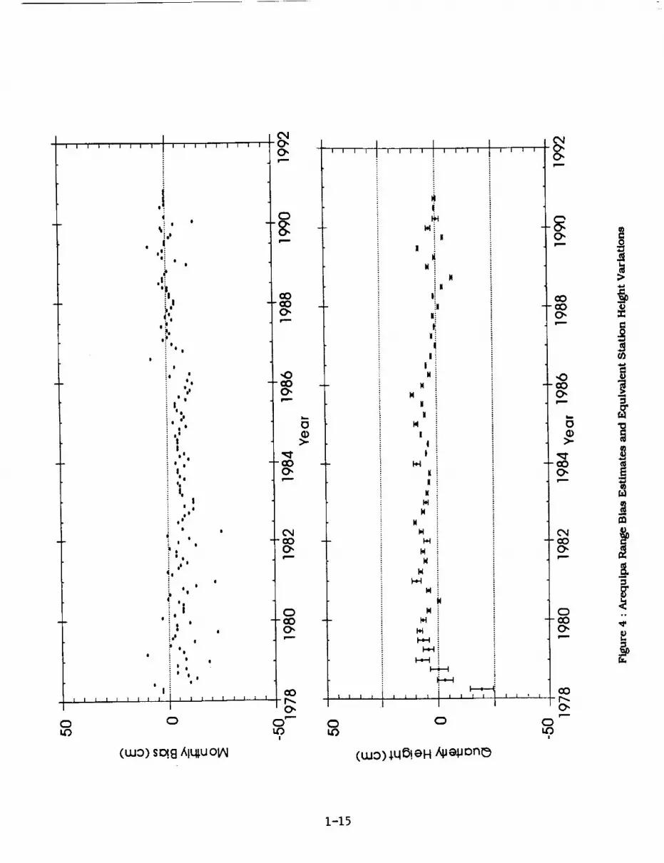
The independent monthly values of height at the three stations with the lowest month-to
month variation seen In our analysis are given in Figures 5a,b and c. The least significant figures
in millimeters of the distance from an average Earth semi-major axis of 6378136.3 m. appear on
the vertical scale and the measurements are qualified by error estimates of twice their formal
standard deviation based on the final fit of the range observations to each orbital arc. Although
the ranges themselves are formally accurate to better than a centimeter, systematic residual
signatures of several centimeters In amplitude are observed due to uncompensated errors In
force, measurement and Earth orientation models. The effect of atmospheric refraction on the
laser ranges is modelled according to Marini and Murray (1973) who assumed a spherically
1-4
stratified atmosphere based on surface pressure measurements. Herring (1988) has shown that
range corrections due the refractivity formula, the zenith range correction and the elevation
dependence of the range correction formula should only be a few millimeters at 20 degree
elevation angle, which is the lower limit for most of the systems. However, any long termvariations in station barometer accuracy or in the effects of lateral gradients in the atmosphere
(see Abshire and Gardner, 1985) will directly affect the vertical estimates. The SLR systems could
thus be used to monitor aberrations in the dry component of atmospheric refraction which
would not be separable from the wet component in nearby microwave instruments.
The possibility of errors in the adopted eccentricities must also be considered, particularly
for stations which have undergone changes of system occupation, such as Greenbelt, Quincy and
Huahine (see Table 2). The system changes at the North American sites coincided with
collocation tests which cross-calibrated each instrument's ranging machine as well as its
eccentricity. The transportable systems are periodically returned to Greenbelt for up-grades and
collocation calibration against MOBLAS-7, but do not usually undergo a collocation test at their
working location. The Huahine position shows more variation than the other sites but, becauseTLRS-2 eccentricity errors are minimized by employing a precise reposltionlng technique, this
behavior is more likely to be due to the influence of the early, less accurate MOBLAS-1
measurements.
Considerable deviation from uniform motion can be noted in the height variation for some
stations, and most of the estimated height rates shown in Table 3 are not significant compared
to their quoted uncertainties, which are twice the formal standard error based on the fit of the
individual values to a straight line. The measures of scatter of the height values about the mean
listed in Table 1 are only reduced by a millimeter or two when a linear fit is substituted. The
height statistic has been used as a quality control factor in earlier work measuring the horizontal
component of motion (see, for example Table 3 of Smith et al., 1990). Considering the scatter of a
station's height about a mean (or uniformly moving) value as a measure of the 'quality' of the
station's performance, we see that it depends as much on system stability and careful calibration
as upon the precision of the observations, and the lower values of height scatter at Greenbelt,
Yarragadee and Arequipa testify to the reliability of these instruments.
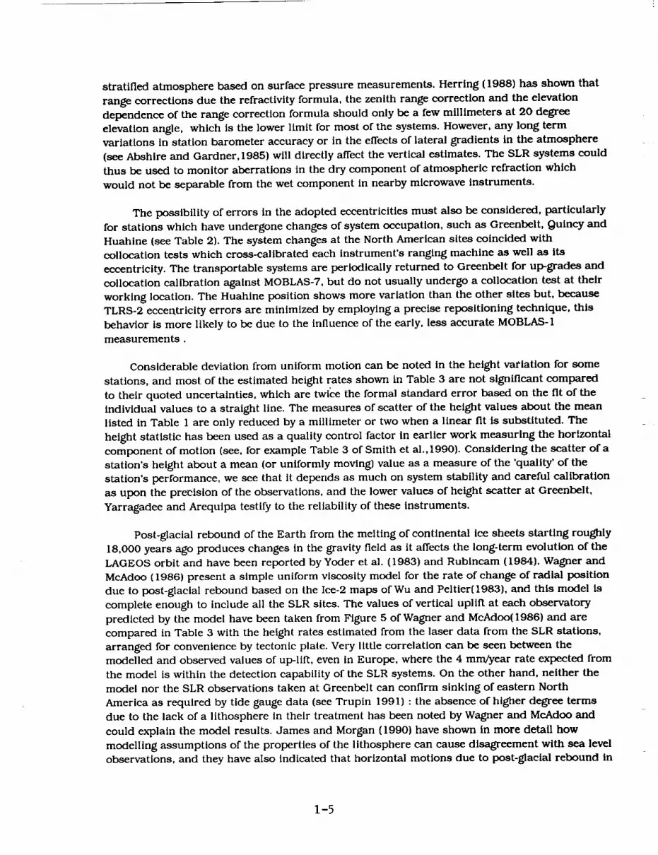
Post-glacial rebound of the Earth from the melting of continental ice sheets starting roughly
18,000 years ago produces changes in the gravity field as it affects the long-term evolution of the
LAGEOS orbit and have been reported by Yoder et al. (1983) and Rubincam (1984). Wagner and
McAdoo (1986) present a simple uniform viscosity model for the rate of change of radial position
due to post-glacial rebound based on the Ice-2 maps of Wu and Peltier(1983), and this model is
complete enough to include all the SLR sites. The values of vertical uplift at each observatory
predicted by the model have been taken from Figure 5 of Wagner and McAdoo(1986) and are
compared in Table 3 with the height rates estimated from the laser data from the SLR stations,
arranged for convenience by tectonic plate. Very little correlation can be seen between the
modelled and observed values of up-lift, even in Europe, where the 4 mm/year rate expected from
the model is within the detection capability of the SLR systems. On the other hand, neither the
model nor the SLR observations taken at Greenbelt can confirm sinking of eastern North
America as required by tide gauge data (see Trupin 1991) : the absence of higher degree terms
due to the lack of a lithosphere in their treatment has been noted by Wagner and McAdoo and
could explain the model results. James and Morgan (1990) have shown in more detail how
modelling assumptions of the properties of the lithosphere can cause disagreement with sea level
observations, and they have also indicated that horizontal motions due to post-glacial rebound in
1-5

North America and Fennoscandia can amount to 4 mm/year from plausible models. This
movement is predicted in the Hudson Bay region where vertical movement can amount to over
10 ram/year, and both components are clearly within the resolution capability of a modern SLR
system occupying this region in an extended campaign.
It is possible that further investigation of the SLR observations will uncover a source of
instrument error which would alias into the vertical component of station tx_sition. However, the
apparent rate, of 4 mm/year observed at Arequipa Is large enough that no SLR analysis should
assume a stationary vertical component and expect accurate baseline measurements to distant
stations. Only explicit separation from the vertical component by considering geodesic lengthswill allow the definition of accurate horizontal motion.
CONCLUSIONS
The stability of the radial component of position at the strongest SLR observatories in an
eight year time span suggests that vertical motion Is bounded by 2 or 3 ram/year and this
analysis does not confirm variations suggested by models of post-glacial rebound. Periodic
signatures apparent in the height results may represent seasonal variations of a geophysical
nature, but do not produce significant long term trends. These accurate estimates of station
height can help in the calibration of satellite altimeters as well as to establish scale for
positioning tech'niques which degrade as a function of distance on a global scale, such as GPS
campaigns in close proximity to the SLR Observatories. The data quality control which must be
exercised to retain the full scaling accuracy of the laser ranges is not so stringent in the analysis
of GPS networks as they benefit from strong orbital geometry when multiple satellites are
simultaneously tracked. On the other hand, accurate relative position measurements of each
instrument's reception center from a ground marker is critical in both space techniques and
must be carefully monitored. The capability with which the Global Laser Tracking Network can
control vertical scale will grow with the increased number of retro-reflector-carrylng satellites
expected to be in high Earth orbit in the next few years. As observations from LAGEOS 2 are
supplemented by concentrated tracking of the currently orbiting ETALON spacecraft, time
resolution of any subtle vertical motion should also be improved.
1-6

REFERENCES
Abshire,J.B. and C.S.Gardner,"Atmospherlc Refractivity Corrections in Satellite Laser Ranging",IEEE Trans. on Geose. and Rem. Sense. GE-23, 1985
Afonso, G,F.Barlier,M.Carplno,P.Farlnella,F.Mignard,M.Milanl and A.M..Nobill," Orbital Effects of
LAGEOS Seasons and Eclipses", Ann.Geophys.A 7(5),501-514,1989
Anselmo,L.,B.Bertotti,P.Farinella,A.Milani and A.M.Noblli,'Orbital Perturbations due to Radiation
Pressure for a Spacecraft of Complex Shape", Celest. Mech. 29,27,1983
Bertotti,B.,and L.less,"The Rotation of LAGEOS", J.Geophys.Res., 96,2431-2440, 1991
Chrlstodoulidis,D.C., D.E.Smith, R.Kolenkiewicz, S.M.Klosko, M.H.Torrence and
P.J.Dunn,"Observing Tectonic Plate Motions and Deformations from Satellite Laser Ranging",J.Geophys.Res., 90(B 1 I),9249-9263,1985
Degnan,J.J.,"Satellite Laser Ranging: Current Status and Future Prospects", IEEE Trans. onGeose. and Rem. Sense. GE-23, 1985
Eanes,R.J. and M.M. Watkins,"Temporal Variability of Earth's Gravitational Field from Satellite
Laser Ranging Observations", XX Gen. Ass. IUGG Syrup. No.3,Vlenna, 1991
Fltzmaurice,M.W.,P.O.Minott,J.B.Abshire and H.E.Rowe,"Prelaunch Testing of the Laser
Geodynamic Satellite (LAGEOS)", NASA Tech. Paper 1062,1977
Frey H.V. and J.M.Bosworth,"Measurlng Contemporary Crustal Motions: NASA's Crustal
Dynamics Project", Earthqu. and Volc. 20(3), 1988
Husson,V.S.,"First Six Month Data Processing Report",BFEC Report, October 1988
James,T.S.,and W.J.Morgan,'Horizontal Motions due to Post-Glacial Rebound", Geo. R.Lett. 17(7)1990
Lerch,F.J," Geopotential Models of the Earth from Satellite Tracking, Altimeter and SurfaceGravity Observations: GEM-T3 and GEM-T3S", NASA TM 104555, 1992
McCarthy D.D.(ed.), IERS Standards(1989), IERS Tech. Note 3, Central Bureau of IERS,Observatoire de Paris, 1989
Putney,B.,R.Kolenkiewlcz,D.Smith,P.Dunn and M.H.Torrence,"Preclslon Orbit Determination at
the NASA Goddard Space Flight Center", Adv. Space Res., I0(3), 197-203, 1990
Ries,J.C.,R.J.Eanes,C.K.Shum and M.M.Watkins,"Progress in the Determination of the
Gravitational Coefficient of the Earth", in press, 1992
i-7

Rubincam,D.P.,"Postglacial Rebound Observed by LAGEOS and the Effective Viscosity of the
Lower Mantle", J.Geophys.Res., 89(B2), 1077-1087, 1984
Rublncam D.P.,"Drag on the LAGEOS Satellite",J. Geophys.Res., 95,4881-4886,1990
Scharoo,R.,K.F.Wakker,B.A.C.Ambroslus and R.Noomen,"On the Along-track Acceleration of the
LAGEOS Satellite", J.Geophys.Res., 96,729-740, 1991
Smith,D.E.,R.Kolenkiewicz,P.J.Dunn,J.W.Robbins,M.H.Torrence,S.M.Klosko and
R.G.Williamson,"Tectonic Motion and Deformation from Satellite Laser Ranging to LAGEOS",
J.Geophys.Res., 95(B 13),22013-22041, 1990
Trupin A.S.," The Effect of Global Change and Long Period Tides on the Earth's Rotation and
Gravitational Potential", U. Col. Ph.D. Thesis, 1991
Wagner,C.A. and McAdoo,D.C.,"Time Variation In the Earth's Gravity Field Detectable With GRM
Intersatellite Traeking_,J.Geophys.Re s. 91(B8), July, 1986
Wahr,J.M.,"The Forced Nutatlons of an Ellipsoidal Rotating, Elastic and Oceanless Earth",
Geophys.J.R.Astron.Soc.64, 1981
Wu, P.,and Peltier,W.P.," Glacial Isostatic Adjustment and the Free Air Gravity Anomaly as a
Constraint on Deep Mantle Viscosity", Geophys. J. R. Astron. Soc.74, 1983
Yoder,C.F.,J.G.Williams,J.O.Dickey,B.E.Schutz,R.J.Eanes and B.D.Tapley,"Secular Variation of
Earth's Gravitational J2 Coefficient from LAGEOS and Non-tidal Acceleration of Earth Rotation",
Nature 303, 1983
I-8

TABLE 1 :
GREENBELT 7105
QUINCY 7109
MON.PEAK 7110
YARAGADEE 7090
HUAHINE 7123
AREQUIPA 7907
MATERA 7939
WETZEL 7834
GRAZ 7839
RGO 7840
SIMOSAT0 7838
STATION POSITIONS
LATITUDE
DEG MNSEC
39 114
39 58 30
32 53 30
-29 2 47
-16 44 l
-16 27 57
40 38 56
49 8 42
4742
50 52 3
33 34 40
LONGITUDE
DEG MNSEC
283 i0 20
239 3 19
243 34 39
115 20 48
208 57 32
288 30 25
16 42 17
12 52 41
15 29 36
20 I0
135 56 13
HEIGHT ST.ERR. ST.DEV NO.
METERS MILLIMETERS MONTHS
19.931 2 16 69
1107.119 2 18 67
1839.746 2 20 73
242.080 2 16 69
46.110 5 23 22
2492.945 2 17 52
536.551 2 19 60
661.842 4 24 45
540.125 3 20 55
76.114 3 21 69
100.175 4 25 51
I-9

TABLE 2 : ECCENTRICITY OFFSETS
START
GREENBELT 7105 MOBLAS-7
STOP N(mm)E(mm) UP(mm)
84 1 1 84 3 22 16 -26 3169
84 3 22 85 7 29 17 -32 3169
85 7 29 89 10 12 17 -31 3168
89 10 12 90 7 25 35 -40 3162
90 7 25 91 12 31 -14 -33 3153
7918 TLRS-4 90 4 6 90 7 23 -7 -5 2613
QUINCY 7109 MOBLAS-8 84 I l 86 9 18 -29 11 3124
86 9 26 91 3 17 -27 12 3138
TLRS-4 91 3 19 91 8 19 -5 0 2651
MOBLAS-8 91 l l 18 91 12 II -19 5 3184
91 12 12 91 12 31 -35 -3 3184
MON.PEAK 71 I0 MOBLAS-4 841 1
88 4 30
YARAGADEE 7090 MOBLAS-5
HUAHINE 7121 MOBLAS- I
7123 TLRS-2
88 4 30 -33 -15 3210
91 12 31 -33 -16 3213
GROUND MARKER DISTANCES
87 8 13
91 12 31
3 11 3185
3 10 3177
84 1 1
87 813
84 l 1 86 3 13 8 I 3662
87 7 14 87 10 8 0 0 1453
88 3 16 88 9 I 0 0 1437
89 424 89 9 3 0 0 1482
90 3 15 90 8 20 -I 3 1459
91 4 5 91 9 4 -2 4 1482
X(mm) Y(mm) Z(mm)
7105 TO 7918 -14419 5137 9457
7121 TO 7123 1458 807 501
i-I0
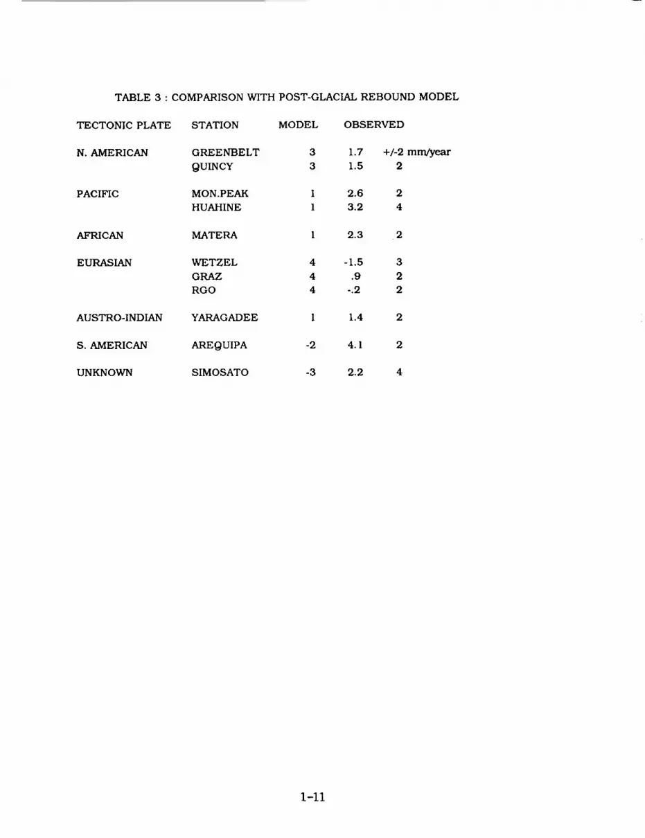
TABLE 3 : COMPARISON WITH POST-GLACIAL REBOUND MODEL
TECTONIC PLATE STATION MODEL
N. AMERICAN GREENBELT 3 1.7
QUINCY 3 1.5
PACIFIC MON.PEAK I 2.6
HUAHINE I 3.2
AFRICAN MATERA I 2.3
EURASIAN WETZEL 4 - 1.5
GRAZ 4 .9
RGO 4 -.2
AUSTRO-INDIAN YARAGADEE I 1.4
S. AMERICAN AREQUIPA -2 4. l
UNKNOWN SIMOSATO -3 2.2
OBSERVED
+b2 mm/year
2
2
4
2
3
2
2
2
2
4
I-II

0
0
0
"I"
.Qr-
E
P
Q.
O"
<
"I-
>.
_o
®O.
_=e.
o.
1-12

0
4,'O
4,tA
4,
4'
$
4,
• 4,
-- v
o 4,
,_41,
4,44, 4,
04_
4, 4,
$.
,it.4,
4, • "
4,4, •
4, 4, 4,:'e'
• 04,_ 4,
4,
4, 4_4k
4'4,
14'4' _qk • •
-¢J 4,
% .
:.''
0
I
4_4' 4_
!4_4'
4'
0
0k=,
O0 lO
CO @
CO
r_cO
CO
OcO
I
4_
t...,0
=
z:)eslw z__OI.
1-13

N
+m
I
iwql m
500.0
250.0
0.0
-250.0
-500.084
SINE(_+M )TERM
+ ii ii
e'_le f • 6•+,.+o,%..+•11t, l .1,_.+•+, 1_•,,, _ • •o++.+_t'
.-.+,,..1.- ••*:1.." "o1.1.-o "11o -•0 .-..'-.1- ....
i
I Il
85 86 87 88year
89 90 91 92
%
iNm
I
500.0
250.0
0.0
-250.0
-500.084
l I
I
t
L'.,_'*. - ._o.41_ j, .... % ,t
..,.,..---- ..,.-.:,.-i
+
COSINE@+M) TERM
+"%..:,..;'"
_•l_o 4Dh.
r
l
r
I
r.?,. ,%
# 1,.. I
I
85 86 87 88 89 90
year
tI
91 92
Figure 3 : Semi-monthly values of the once-per revolution acceleration
1-14
0U")
I | I I i I I i I
! i I I I I I I
Illilllil
e
I
Oe
i
li
, e
e e° l
I
e
:i il
ell
| e
II I
t I
I | I
i |
88
$|1e
e
Iel I
e e
I,I
0 i
e e
e e
I
e e
|°01 0
i
e I
i'
,i't
|
I i Ii
: e
i,',: e
O _ e
'iI
lllllllll
(:D
(LUO) S_B AInU OIAI
1("4IO"
O"
CO'COO"
,40COO-
'OOO"e,,,,-,
("4COO"
C)'COO-
COr--O-
O"-
O
(b>- >-
cOO-R
>
1-15
.............................................. + ............ _.._ .............................................
I
MH
J l
/'_zl
0 0 0 0 0 00 0 0 0 0 0
(s,e),Om!ll!m)),q6!eH
1-16
0
In
I=.
m
C
I_
0
0
0
i
0
o.
L

OU)
C_O_
_IHH
HHi
' i
O_
_lm' CO
........................................................._ CO"".............................................CO 4)
>,
h4_
...............................................................,.._._.............................................r,,,
!
a_
2 .jI
: CO
0 0 0 0 0
(_1 T- O O_ CO
k.
0
.C
0
O
sJe),eu_!ll!U_
1-17

m_!
! I
I
i Ji
iI
iI
.............................................t.........._ .........+......................._......................
!
....... "I".................................... i"_ ..................................................
, _t H._
ItIN
I !
5 'I
[
0 0 0 0 0 00 0 0 0 0 0
sJa),eUJ!ll!m
(MO_
Ii
01
0O_
O_CO
O0¢0
GO
(DGO
InGO
O0
Im
mG)>,
t
E_m
0
{J.c:
0
J=_a
0
L.
1-18

N94-15554L
Laser Ranging Network Performance andRoutine Orbit Determination at D-PAF
F.-H. Massmann, Ch. Reigber, H. Li, R. Ktinig,
J.C. Raimondo, C. Rajasenan, M. Vei
Deutsches Geod_itisches Forschungsinstitut (DGFI), Abt. I, and
German Processing and Archiving Facility (D-PAF)MiJnchner Str. 20
D-8031 Oberpfaffenhofen
Germany
Summary
ERS-1 is now about 8 months in orbit and has been tracked by the global laser network from
the very beginning of the mission. The German processing and archiving facility for ERS-1
(D-PAF) is coordinating and supporting the network and performing the different routine orbitdetermination tasks.
This paper presents details about the global network status, the communication to D-PAF and
the tracking data and orbit processing system at D-PAF. The quality of the preliminary and
precise orbits are shown and some problem areas are identified.
1. Background
On July 17, 1991, the first European (ESA) Remote Sensing Satellite (ERS-1) was successful-
ly launched from Kourou, French Guayana. The satellite is equipped with a number of active
microwave instruments for the monitoring of the Earth's environment (see figure 1). In order
to make full use of the measurements the ERS-1 orbit has to be known very precisely. For
this purpose ERS-1 is carrying a laser retro-reflector and, as an experiment, the Prare system
(Precise Range and Range Rate Equipment). After the failure of the Prare system due to a ra-
diation damage the satellite laser ranging (SLR) measurements are the basis for the precise or-bit determination.
ERS-1 is flying in a sun-synchronous circular orbit (quasi-polar) at a mean altitude of 785 km
and an inclination of 98.5 degrees with different ground repeat cycles (see table 1). TheKepler period is about 100.5 min.
To keep the satellite ground tracks within +-1 km deadband (first 6 months +- 2 km) so called
maintenance manoeuvres have to be executed, which take place usually every two to four
weeks depending mainly on the solar activity.
1-19

Figure 1: ERS- 1 Satellite
Wind
1DHT Antenna
Table 1: ERS- 1 Orbit Characteristics
Revolutions per cycleRevs per day
Mean Semi-Major Axis [km]Mean Inclination [Degrees]Mean EccentricityMean Argument of PerigeeMean local solar time of
descending node
Longitudinal phase(ascending node) [degrees]
(1) Venice (2) ICE Orbit
Duration
3 days43 revs14 + 1/37153.13898.5161.165 xl0 -3
90.0 deg
10h 30min
24.36 EastO)128.2 West _)
26/07/91-12/12/91 ¢1_'23/12/91-30/03/92 (2)16/12/93-01/04/94 (2)
Repeat Cycle
35 days1.501 revs
14 + 11/357159.4'965
98.54291.165 xl0 -3
90.0 deg
10h 30rain
20.9605 East
2/4/92-15/12/93
I 176 days2521 revs14 + 57/1767156.3098.51141.165 xl0 -3
90.0 deg
10h 30min
not decided
8/4/94-...
1-20

2. ERS-1 Laser Tracking Network
The ERS-1 satellite is tracked by a network of globally distributed stations which were funded
by many different institutes. In table 2 the stations are listed along with their ERS-1 trackingperiods.
In figures 2 to 4 the geographical distribution of the stations is plotted for the first three orbit
phases (see table 1). As can be seen, most of the tracking stations are located in Europe and
North America. The southern hemisphere is covered only by up to four SLR stations and none
of them is located in the south African region. The plots show also the actual tracked ERS-1
orbital passes.
Figure 2: SLR Tracking Coverage within the Commissioning Phase (Venice Orbit)
9O
6O
5O
- 120 -60 50 120 180
1-21

Table 2:ERS-1 Tracking Network Stations
ID Name Location System Tracking Periods
q181186318641873
1884
18931953
70467080
70907097710571097110
72107236
74037512754278107811
7824
7831
783578377838783978407843
78827883
79077918
79398834
PotsdamMaidanakMaidanakSimeiz
Riga
KatzivelySantiago de Cuba
Bear LakeFort Davis
YarragadeeEaster IslandGreenbeltQuincyMonument Peak
HaleakalaWuhan
ArequipaKattaviaMonte VendaZimmerwaldBorowiec
San Femando
Helwan
Orasse
ShanghaiSimosatoGraz
HerstmonceuxOrroral
Cabo San LucasEnsenada
ArequipaGreenbelt
MateraWettzen
Germany, Europe fix 910720 ..Russia, fix 910724 ..Russia, fix 920421 ..Russia, Europe fix 910723 .. 910829
920501 ..Latvia, Europe fix 910731 .. 911028
920225 .. 920226920401 ..
Russia, Europe fix 920422 .. 920515Cuba, Carribean fix 910808 .. 910922
911127 ..USA, North America TLRS-4 910906 .. 911015USA, North America fix 910822 .. 910822
911121 .. 920124920318 ..
Australia MOBLAS-5 910731 ..Chile, Pacific TLRS-2 911018 .. 920311USA, North America MOBLAS-7 910802 ..USA, North America MOBLAS-8 911211 ..USA, North America MOBLAS-4 910725 .. 920306
920504 ..
Hawaii, USA fix 910731 ..China, Asia fix 910929 .. 920222
920404 ..
Chile, South America TLRS-3 910731 .. 911010Greece, Europe MTLRS-1 920328 .. 920426Italy, Europe MTLRS-2 910729 .. 910917Switzerland, Europe fix 910719 ..Poland, Europe fix 910807 .. 910818
911002 .. 911006920107 .. 920121
Spain, Europe fix 911029 .. 920327920505 ..
Egypt, North Africa fix 910803 .. 911131920226 ..
France, Europe fix 910717 ..China, Asia fix 910816 ..Japan, Asia fix 910720 ..Austria, Europe fix 910722 ..Great Britain, Europe fix 910719 ..Australia fix 910725 .. 910729
911117 .. 911117920119 .. 920127920414 ..
Mexico TLRS-4 920319 ..Mexico TLRS-4 911113 .. 911126
920109 .. 920208Chile, South America fix 911129 .. 911129USA, North America TLRS-3 920107 .. 920115
920404 ..
Italy, Europe fix 910724 ..Germany, Europe fix 910918 .. 910918
920305 ..
MOBLASMTLRSTLRS
mobile laser systemmodular transportable laser systemtransportable laser system
1-22

Figure 3: SLR Tracking Coverage within the First Ice Phase (Ice Orbit)
90
6O
3O
-_0
-60
-90-180
.. ,_ k./---_ , ,
.--. _., V_ " .W'/"(L . _i _ _ I _ /
-- _........ -7_--,_-.. • _-._. .-_.,._: ....
_._l_. 'V ) _" I _-/ _ '_ _"_.;'_k-'-_ -_,
I
, I
-120 -60 0 60 120 180
Figure 4: SLR Tracking Coverage within the first Month of the Multidisciplinary Phase
i
120-180 -120 -60 0 60180
1-23

!
3. Data Flow to D-PAF Systems
Soon after the tracking of a satellite pass the SLR data is preprocessed at the station:
a first data screening is performed by most of the stations;
then from each pass about 50 data points were selected (quick-look (Q/L) data) or
the measurements were compressed into onsite normal points (ONP).
This Q/L or ONP data is then transmitted to the Data Analysis Center at D-PAF. There are
two centers collecting and forwarding the data: the data from the CDSLR stations is transmit-
ted via existing internal links to the CDSLR headquarters and then forwarded to CDDIS; the
second center is at the European Data Center (EDC) at DGFI. EDC is collecting all data from
the European systems (EUROLAS) and also from stations in Russia, Cuba and China. From
these two data centers D-PAF is retrieving the collected data files on a daily basis and merges
them with data from those stations which have sent their data directly to D-PAF.
The data transmission is performed by using all currently available communication links:
telex, Span, Bitnet, Intemet, GE/MARK III and ftp.
After having applied all necessary corrections the full tracking data set (full-rate (FR)) is
transmitted to the two centers, usually by CCT or Span. Again D-PAF retrieves the FR data
sets from CDDIS and EDC and merges them with the directly received files.
It has to be noted, that all three parties exchange their data to have the full information avail-
able for all partners. In the beginning of the mission when EDC was not established D-PAF
performed the EDC activities too.
According to the work distribution between the four European processing and archiving facili-
ties (PAF) D-PAF is responsible for the generation of operational precision orbital products
and for a processing of SAR data. In order to fulfill these tasks D-PAF has set up a number
of processing systems. Used for the orbit generation are:
the telecommunication system (TCS)
the data management system (DMS)
the trackfng and orbit determination system (TOS), which consists of the following
subsystems:
preprocessing subsystem: preprocessing of incoming data, generation of normal pointsfrom laser and altimeter data
orbit determination subsystem: differential orbit correction by numerical integration
methods, quality control, generation of numerical and graphical products
orbit prediction subsystem: orbit extrapolation, generation of orbit prediction sets in
different formats, generation of time bias functions, quality control
earth gravity modelling subsystem: processing of surface gravity data, reduction and
solution of normal equation systems, quality control
1-24

4. Station Performance
At D-PAF all incoming data is checked for quality and statistics are generated. On
a weekly basis Q/L reports are generated presenting incoming data statistics and
data quality check information. This paragraphs will present some of the statistical
information.
As already seen in figures 2 to 4 only a small part of the ERS-1 orbital path is ob-
served by the ground stations and this is mainly located north of the equator.
Especially over South America the situation became worse from the first to the
second phase and in the first month of the multidisciplinary phase there is no
tracking in that part of the world.
From the figures it is also visible that mainly the ascending arcs were observed by
the stations, while only a few descending arcs were tracked. The reason probably
is that the descending passes can be tracked only during daylight.
Figure 7 presents the variation in the number of stations observing ERS-1 per day.
It ranges from 0 to 13 and shows clearly a decrease for the months October 91 to
March 92, when ERS-1 was not in sunlight for many of the stations. A
corresponding trend is visible in figure 9 which depicts the number of passes per
week. For an arc of 7 days about 30 to 60 passes are available.
Figure 7:ERS-1 SLR Stations per Day
14
,tLil o
00 100 150 200
elapse time [days] o=,,3OO
1-25
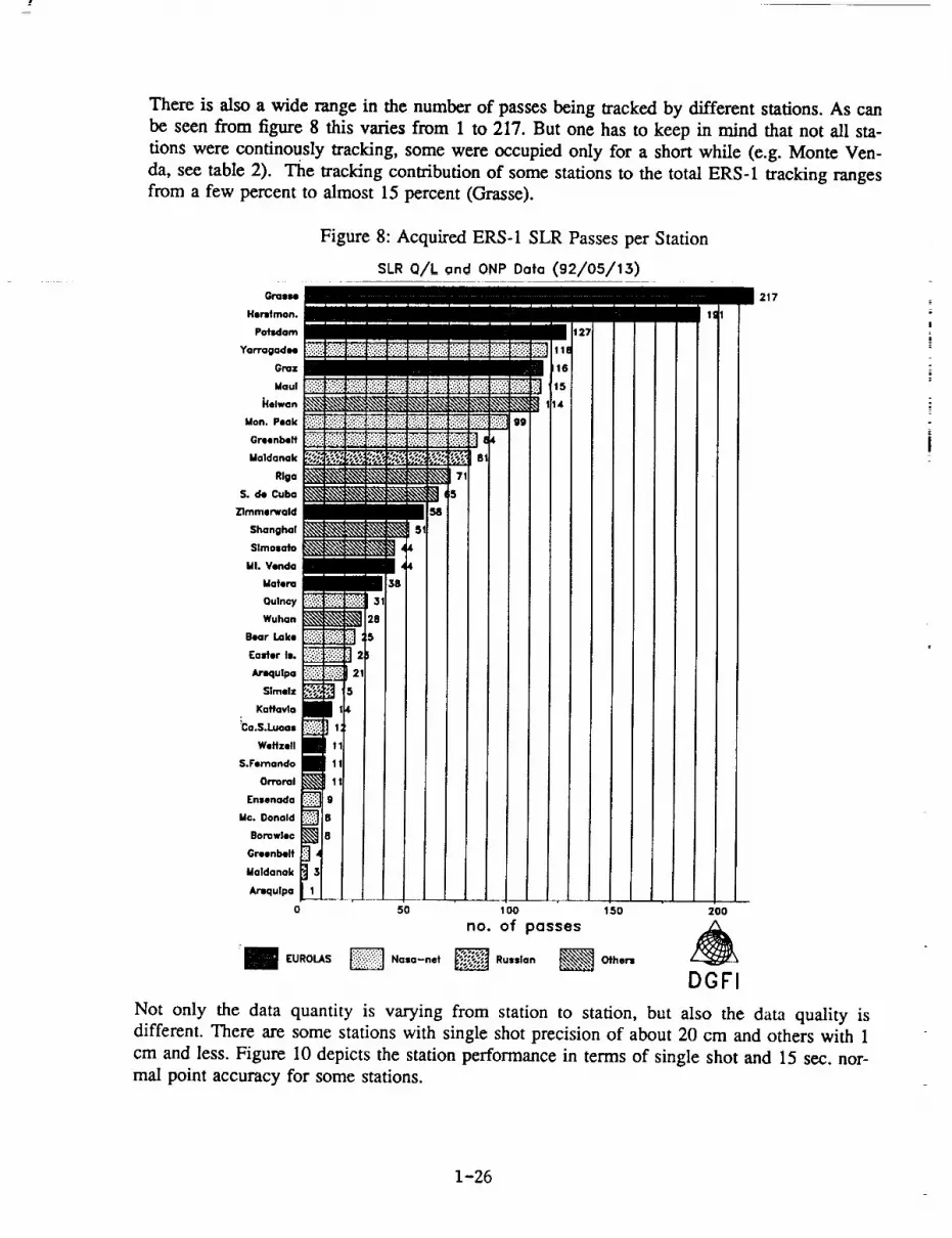
There is also a wide range in the number of passes being tracked by different stations. As can
be seen from figure 8 this varies from 1 to 217. But one has to keep in mind that not all sta-
tions were continously tracking, some were occupied only for a short while (e.g. Monte Ven-
da, see table 2). The tracking contribution of some stations to the total ERS-1 tracking rangesfrom a few percent to almost 15 percent (Grasse).
Gralllle
Herstrnon.
Potsdam
Yarragadee
Gmz
Maul
J4elwan
Mon. Peak
Greenbelt
Maldanak
Riga
S. de Cuba
Zlmmerwald
Shanghai
Slmasato
Mh Venda
Matera
Qulnoy
Wuhan
Bear Lake
Easter Iw.
Adrmqulpa
Slmelz
Kattavla
_a.S.Luoas
WeHzell
S.Femando
Orrorol
rnsenada
Mc. Donald
Borowte©
Greenbelt
Maldanak
Arwquipa
o
Figure 8: Acquired ERS-1 SLR Passes per Station
st.R 0/t. o.d ONP Data (92/0S/13)
III
I
[]
[][]3
28
$
;
II[]
I
I33
IIIIII
II
5
L
IIIII I IIiiii [][]mmmmm •i:-::i!!/.(.Fi_::_i_:__i-.-_:!ii-.::!_immmIl ,,
ii:,.'-:"_ :..;.:_'!__!_::'_ g9
:);i-.:_i?1_4
71
N
miII
50 100 150
no. of passes
:I_uROt_S _Na,o-net _Ru,,;*. _O,h.,-.
IIIIIII ,,
200
DGFI
m m 217
I
Not only the data quantity is varying from station to station, but also the data quality isdifferent. There are some stations with single shot precision of about 20 cm and others with 1
cm and less. Figure 10 depicts the station performance in terms of single shot and 15 sec. nor-mal point accuracy for some stations.
1-26

8O
Figure 9: Acquired ERS-1 SLR Passes per We_k
70
O
10.
DGFI
[¢m]
Figure 10:ERS-1 Tracking Precision per Station (cm)
26
dam type
/ 15 soe._ormnl truant
stad(mnarn8
1-27

5. Orbit Determination at D-PAF
In order to provide ERS-1 precision orbits the following ERS-1 orbital products are routinelygenerated and distributed:
orbit predictions and time bias functions
preliminary orbits
precise orbits
The latter two proctucts are official ESA products, while the first one is an internal one. More
details about the ERS-1 orbit predictions can be found in Kt_nig et.al. (1992). A detailled
description of all radar altimeter and tracking data products is presented in Bosch et.al.
(1990).
The overall data flow for the orbit determination processes is explained in figure 11.
Figure 11: Orbit Determination Data Flow
Int. Organis. ESA Stations SLR Stations
Data Reception
Dlstrtb. of Orbit Predictions
Reformatting RAFD
Screening
Orbit Prediction Generation
Plausibility Check
Merging, ScreeningNormal Point Generation
Orbit AdjustmentQuality Control
Comp. with MMCC Orbits
Archiving of Orbits
1-28
Submission of Orbits

The processing schemes are outlined in figure 12 for manoeuvre free periods.
Figure 12: Processing Scheme
(for manoeuvre free periods)
F S S M
orbit I I3--4 days
orbit 2
D M D F S S M D
I I I I I I I I I
, I0 days
, _ _'///ii/II/ilIA.---10 days
->
PRL _-_I I@
7 day orbits I
7 day overlap arcs I
I I I I I I I I I I I I I I I@ @
@ @
I I
PRC _i@
5-7 day orbits _--
5-7 day overlap arcs I
I I I I I I I I I I I I I I I I
@ @
(3 @ ®
I I
5.1 Preliminary Orbit Determination
Preliminary orbits are computed on a weekly basis by using Q/L laser and radar altimeter fast
delivery (RA-FD) data and are usually available within two weeks. Both data sets are
compressed into normal points (15 sec. bins for SLR, 10 sec. bins for RA-FD) after first qual-
ity checks. As can be seen from figure 14, the use of RA-FD data improves the global cover-
age especially for arc with only a few SLR passes.
In manoeuvre free periods weekly arcs are computed plus another 7-day arc which is overlap-
ping by 3-4 days and is used for quality assessment (see figure 12). The models for the orbitdetermination are described in Zhu and Reigber (1991) and Massmann et.al. (1992). Solve-for
parameters are the six orbital elements at epoch, one solar radiation coefficient, daily/half-
daily drag coefficients, altimeter range bias (if RA-FD data is used) and station coordinates
(for new stations only).
The resulting orbital fits are usually around 50-80 cm, in case of bad data coverage up to 130
cm. Figure 13 presents the quality control results from overlapping arcs for 1991 and 1992.
The large values in November 91 are resulting from a period with no useful RA-FD data and
only a very few laser passes. The same hold for the end of December 91.
1-29

Figure 13: PRL Precision Assessment by Overlapping Arc Comparison
PRL Radial RMS Differences
Ioo
IPRL Cross-track RMS Differences
40(
_x
2ix
loc
PRL Cress-treck RILLS Differences
1-30

Figure 14: Input Example for the Preliminary Orbit Determination
(January 20-27, 1992)
• .go !
6O
3O
\
i iI
-go 12o 18(-1BO -120 -60 0 60
5.2 Precise Orbit Determination
The precise orbits are based up to now only on laser data which have been compressed into
15 sec. normal points. The orbits are computed with a delay of 3-6 months depending on the
availability of all FR laser data at D-PAF. The arc length is choosen to fit as good as possiblein between two manoeuvres and is usually in the range of 5-7 days. The quality control is
also performed by overlapping arc comparison. Models and solve-for parameters are the same
as for the preliminary orbits, except the earth rotation parameters, the geomagnetic indices and
the solar flux data, which are now the official final values instead of predicted or preliminary
ones.
Figure 15 presents the resulting rms orbital fit values for the precise orbit arcs generated up to
now while figure 16 shows the quality estimates from the overlapping arc comparison. When
comparing figure 13 and 16 one has to be careful, because the arcs are not the same. But gen-
erally one can say that the PRC results are more homogeneous and do not show large spikes
due to better input data and a more intensive data handling. The most interesting radial com-
ponent of the orbit seems to be accurate to 50 to 60 cm.
1-31

Figure 15: PRC Orbital Fits
(_)
i i +FI
! i .....200 210 220 230 240 250 260 270 280
DlyI In 1991 q,_w_,_m._ ,_e_,
Figure 16: PRC Precision Assessment by Overlapping Arc Comparison
PRC Radial RMS Differences
m)
r/
, : _ I i
|I _!
220 230 240 250 260 270
18(
16( -----
14(
12:
10( ---
IR--
2OO 210
II
PRC Cross-Track RMS Differences _ PRO Along-Track RMS Differences200 (°m) SOo_orn)
1_. .
O_m In111_ _ 270
1-32

6. Conclusion
Soon after the ERS-1 launch DGFI/D-PAF has started the orbit computations and demonstrat-
ed its capability to generate good quality orbits on an operational basis. On the other hand theSLR stations have demonstrated their capability to track ERS-1 and provide high quality
tracking data.
Nevertheless there are a few things that could be improved: The accuracy of the generated
preliminary and precise orbits is very much limited by the spatial and temporal coverage of
the SLR data.
Up to now there are only a few stations in the southern hemisphere of which only one has a
good tracking record. On the African continent only one tracking station can be found andthat is located in North Africa (Helwan). On the northern hemisphere some gaps can be
identified over Russia.
The temporal coverage suffers from the fact that mostly the ascending ERS-1 arcs (night
passes) were tracked by the stations. A reason for that is partly the missing daylight tracking
capability of the station, partly tracking restrictions and partly man power problems.
Due to the data coverage it is difficult to model large ERS-1 drag perturbation, especially dur-
ing periods with high solar activity. Tests are initiated to improve this by using either drag
information derived from Spot2 Doris data or by using crossover altimeter data.
References
Bosch, W., Flechtner, F.,K_Snig, R., Massmann, F.-H., Reigber, Ch., Schwintzer, P. and
Wilmes, H., 1990. The German PAF for ERS-I: RAT Product Specification Docu-
ment. D-PAF/DGFI, Document ERS-D-PSD-30000, Issue 1.1, Miinchen.
K_Snig, R., Li, H., Massmann, F.-H., Raimondo, J.C. and Reigber, Ch., 1992. On the Accu-
racy of ERS-1 Orbit Predictions, this proceedings
Massmann, F.-H., Reigber, Ch., Raimondo, J.C. and Rajasenan, C., 1992. Operational ERS-1 Orbit Determination at D-PAF, Proceedings of the Sixth International Geodetic
Symposium on Satellite Positioning, Columbus, Ohio r.-
Zhu, S.Y. and Reigber, Ch., 1991. The German PAF for ERS-I: ERS-I Standards used at
D-PAF. D-PAF/DGFI, Document ERS-D-STD-31101, Miinchen.
1-33

N94-15555
Laser ranging application to time transfer using geodetic satellite
and to other Japanese space programs
Hiroo KUNIMORI*, Fujinobu TAKAHASHI*, Toshikazu ITABE*
and Atsushi YAMAMOTO**
" Commumcations Research Laboratory, 4-2-1 Nukui-kita, Koganei-shi,
Tokyo 184 Japan
""Maritime Safety Academy, Wakaba-Cho 5-1 Kure-shi, Hiroshima 737 Japan
ABSTRACT
Communications Research Laboratory (CRL) has been developing a laser time transfer
system using a satellite laser ranging (SLR) system. We propose Japanese geodetic satellite
'AJISAI', launched in 1986 as a target satellite. The surface is covered not only with comercube reflectors but also with mirrors. The mirrors are originally designed for observation of
flushing solar light _'eflected by the separate mirrors while the satellite is 'spinning. In the
experiment, synchronized laser pulses are transferred via specified mirror from one station to
another during the satellite is up on the horizon to both stations. The system is based on the
epoch timing ranging system with 40 ps ranging precision, connected together with UTC(CRL).Simulation study indicates that two stations at thousands of km distance from each other can be
linked with signal strength of more than 10 photons and the distributed images of laser beam
from AJISAI mirrors give many chances to two stations to link each other during a singleAJISAI pass.
In other topics on the application to Japanese space programs, Retro-reflector In Spacefor Advanced Earth Observation Satellite (ADEOS) and RendDezVous docking mission ofExperimental Technology Satellite-VII (ETS-VII) are briefly presented.
1. Laser Time Transfer via Geodetic Satellite AJISAI
1.1 Introduction
Users of time and frequency standards have been able to take a variety of time
comparison techniques even if they pursue the highest accuracy. The precision of GPS common
view observation, for example, have got to several few nano seconds and 1 ns or higherprecision have been attained by radio techniques such as two way time transfer via satellite
(Ref.1). The requirement of such an extremely high precision may exist in deep space navigation,space geodesy, relativity physics and astronomy which always demand extreme precision and
accuracy in their measurements. In addition to the radio techniques, time transfer using opticalpulses has recently been suggested as one of potential for giving precision of sub-nano or
picosecond time transfer to overcome the maximum bandwidth of radio waves (Ref.2).
Satellite laser ranging (SLR) have progressed as one of space geodetic techniques in the
field of global geodesy and geophysics. Some SLR stations measure the range to as precise as 30
ps or higher (Refs. 3,4). Since the SLR system is essentially a highly precise epoch recorder
transmitting and receiving of optical pulses, a combination of two or more SLR systems haspotential as a highly precise time comparison and transfer system.
1-34

Illlqdlll_
m
¢_cit
(a) (b)
Fig.1 Configuration of Laser time transfer
(a) One way uplink (LASSO) (b) Two way
There are two configurations considered for ground-based-laser time transfer system
using a satellite (See Fig.l). The first is called the one-way up-link configuration. Both SLRstations transmit a laser pulse to the time interval unit (TIU) on the satellite and the TIU
measures the interval between their arrival times. Such an optical time comparison has been
performed in Europe in the LASSO experiment (Refs. 5,6). In the LASSO experiment of
European phase, laser echoes were successfully received at Grasse, France and at other
European laser ranging sites. The second is the two-way configuration. Each station transmits a
laser pulse to the other station via a satellite with mirror reflectors. The satellite also has comercube reflectors for conventional SLR, and they are used to determine the distance from each
station to the satellite'to give support to the time transfer solution. In this paper, we examines
the two-way configuration using the Japanese SLR satellite AJISAI, including time transfer
concept, calibration methods, signal strength and spatial distribution of the reflected beam. The
system performance is based on the CRL SLR system (Refs. 7,8), including additions to be made
for two-way time transfer.
1.2 Target satellite AJISAI
Table 1 • Major specifications of AJISAI
Launch Date: August, 1986
Configuration: Polyhedron inscribed in sphere of diameter 2.15 m
Weight: 685kg
Comer cubes: 1436 pieces,
Number of mirrors :318 pieces,
Reflective efficiency: 0.85,
Duration of a flash :. 5 msec,
Spin rate: 40 rpmLaunch orbit:
Effective area :91.2 cm 2
Curvature of mirrors :8.4-9 m
Brightness : 1.5-3.5 star mag.
Rate of flashing : 2 Hz
Altitude 1500 km,
Inclination 50 deg, Eccentricity 0.001
1-35

z
• •
Vlau_ sp_'.
, w_h mirror1
Fig.2 Arrangement of mirrors on AJISAIParts of an 8.5m radius virtual sphere (mirror) isplaced on the surface of the i-m radius AJISAImaintaining their latitude angles.
AJISAI is the Japanese geodetic satellite launched in 1986 by the National SpaceDevelopment Agency (NASDA). The major specifications of AJISAI are listed in Table 1. The
satellite is a hollow sphere 2:15 m in diameter and weighs 685 kg. The surface is covered with
mirrors as well as corner cube reflectors. The orbit is a circular with an inclination of 50 degrees
and an altitude of 1500 km (Ref.9). The mirrors were originally designed for observing flashingsolar light reflected by separate mirrors while the satellite is spinning at about 40 rpm. Eachmirror is a piece of a surface with a radius of curvature of 8.5 m. Three elements from the same
latitude of the 8.5-m sphere at longitudes of 0, 120 and 240 degrees areput on thesurface Of a
1-m radius satellite retaining the phase angle of the original sphere (See Fig.2). The latitudes
from which every set of three is taken are uniformly selected from the original surface so that a
distant observer can observe the light reflected from the front surface flashing three times perrotation.
1.3 Two way time transfer
The equation for two-way time transfer via laser pulse is in principle the same as those
being developed in radio frequency band (Ref. 1). The time difference d_2 (: positive when clock
1 is ahead of clock 2) between the clocks of stations 1 and 2 is given by:
dt2= (tertle+tl-t2)/2 + (RIe-R21)/2c (1),
where
t,.• (t;j =1, 2),Epoch of pulse departure at station i measured by station clock i,
(i .NE.j_ Epoch of station i's pulse reflected by a satellite mirror arriving atstation j measured by station clock j,
=
=
1-36

Re : (i .NEd') One-way distance of a laser pulse to travel from station i to stationjvia the satellite, and
c: speed of light.
The last term (Rlz-Rzt)/2c is expected to be nearly zero because of the good symmetry of
travelling paths, but not negligible due to the effect on motions of both satellite and stations. Itis related to the difference between the satellite position at the times the two laser pulses arrive.
It approaches zero if the two pulses arrive at nearly the same time on the satellite. This is doneby controlling the firing timing at both stations. Timing control within the precision of 1-ms is
necessary to obtain a station to station link by a mirror of AJISAI with 20cm x 20cm size
spinning at 40 rpm. If the laser fire timing is controllable to l_s, (RIz-Rz)/2c is down to a few
ps on the assumption that both the predicted position of the satellite and the clock
synchronization are known with the accuracy of less than 1 _ (300 m in distance) before the
experiment. The Its firing control can be performed by a fully active mode-locked laser
operation. In this observation mode, we can apply the geometric method rather than dynamicalone to the orbit solution using SLR range data (Ref. 10).
1.4 Laser ranging system
We use an active-passive mode-locked Nd:YAG laser to generate 532 nm wavelength
optical pulses 100 ps wide. The passive mode-locking is performed by saturable dye. The
energy is 100 mJ per pulse and the nominal repetition rate is 10 pulses per second. The
repetition rate can be controlled from 7 to 14 pps by real-time software. If the passive
mode-locking by a saturable dye is replaced with an active component, the synchronization of
firing timing can be controlled on nanosecond level (Ref.11).The receiving telescope aperture has diameter of 1.5 m. A micro-channel plate photo
multiplier (MCP-PMT) is used for detector. It has a 300-ps rise time, 8% quantum efficiency
and the transit time jitter of less than 30 ps with a constant fraction discriminator. The MCP
detector can be also gated temporarily by the prediction of photons arrival in 20-ns time steps.
The timing system consists of a high performance disciplined quartz oscillator, a GPS
receiver, and a time interval unit (TIU). Either a GPS timing receiver or cesium clock of UTC
(CRL) can keep the reference to UTC. Timing epoch is measured for up to 4 stop events with
a resolution of 40-ps.
1.5. Calibration systemIn the actual experiment, we must consider that the reference signal of the atomic clock
is transmitted to the SLR system via cables and electronics. Furthermore, the laser transmitting
and receiving point is not at the telescope reference point.
The cables and electronics delay between the atomic clock and the TIU is monitored by
an independent measurement system. Figure 3 is a block diagram of the monitoring system used
in the experiment. The combined 5-MHz+l-pps signal from the cesium clock room is transmitted
via a 500-m optical fiber. Output signal (50 MHz) of the quartz oscillator is phase-locked by the
5-MHz and used as the reference frequency in TIU. The 1 pps signal is used for the epoch
reference of UTC. The 5-MHz and 1-pps signals are combined again at SLR site and are sent
back to the clock room. Then delay and phase difference with respect to the original signals are
continuously monitored at the clock room. It has been installed to get the characteristics of the
long-term stability of the system.
1-37

5_z
s
Optics[ Fiber
(50O I)
i 5 _z _ I PPS
great tiniag
Telescope _._zt.ro[
[J_ER flrs ti_ial
$r.ar tIP_ T I C
> Stop
[-'-ITIC: T[ae Interval Co,rater [ '
cs: Cesim Standard
MONITOR
Fig.3 Reference signal monitoring system
The epoch latch point at each laser pulse start and stop must be treated as if these events
occurred at the telescope reference point ( intersection of two rotation axes). The calibration
target is put on the telescope moving axis, as it takes partial reflection of transmitting beam and
its physical distance from reference point must be measured precisely.
The time difference between clocks including calibration term (d';2) is given by:
d;2 =(te;-tle+t;-t 2 )/2 + (R,e-R21)/2C
+ { (tla-tlj,)-(t2_-tza,)+(tz._+t2.r)-(tL_+tx. r) }/2 (2),
ti. b "
tL_
ti.y "
: (i=1,2), in addition to the parameter defined in Eq. 1,
Optical path delay from firing (laser input) point to telescope reference point atstation i,
Optical path delay from telescope reference point to receiver point at station i,
Electronic delay from firing point to start-epoch latch gate at station i, and
Electronic delay from receiver point to stop-epoch latch gate at station i.
In order to calibrate the time difference between clock 1 and 2, each value of parameter
in { } in the Eq.2 must be evaluated. The optical delay can be measured by a distance meter or
by scales, and it will be stable in time unless optical design is changed. To cancel out the
electronic delay, the common portable receiver can be collocated at two stations. This
measurement wotald still have errors coming from the dependence on signal strength andtemperature.
1.6 Link budget
In the laser time transfer experiment, the number of photons (Np) detected at the remoteground station are calculated according to the following equation:
Np=(E)Jhc)(Grer f ,2)'(16Ae4 JnZR,2ReZq,2q,2) (3)
where E" Energy in a pulse, _ • Laser wavelength,
h • Planck's constant, c • Velocity of light,
!"1 • Transmission beam efficiency, re • Receiving beam efficiency,
E
1-38
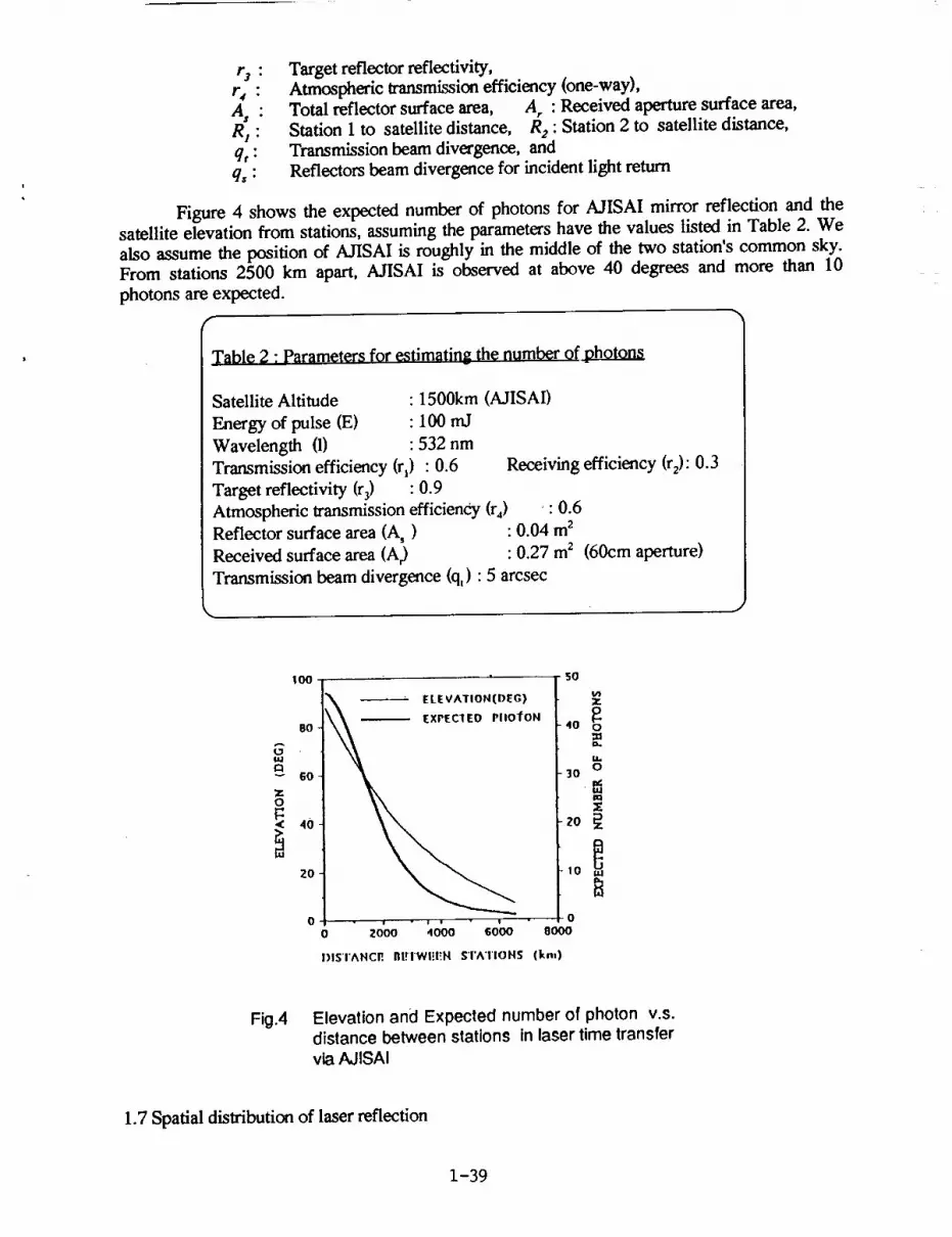
1"3:
r,:A, :
R1 :
qt :
q, :
Target reflector reflectivity,Atmospheric transmission efficiency (one-way),Total reflector surface area, A r : Received aperture surface area,
Station 1 to satellite distance, R2 : Station 2 to satellite distance,Transmission beam divergence, andReflectors beam divergence for incident fight return
Figure 4 shows the expected number of photons for AJISAI mirror reflection and thesatellite elevation from stations, assuming the parameters have the values listed in Table 2. Wealso assume the position of AJISAI is roughly in the middle of the two station's common sky.From stations 2500 km apart, AJISAI is observed at above 40 degrees and more than 10
photons are expected.
Table 2 • Parameters for estimating the number of ohotons
Satellite Altitude : 1500km (AJISAI)
Energy of pulse (E) : 100 mJ
Wavelength (1) : 532 nm
Transmission efficiency (r_) : 0.6 Receiving efficiency (r2): 0.3
Target reflectivity (r3) : 0.9
Atmospheric transmission efficiency (r4) ,: 0.6
Reflector surface area (A,) : 0.04 m 2
Received surface area (A) : 0.27 m 2 (60cm aperture)
Transmission beam divergence (q,) : 5 arcsec
10o
B0
G
v 60
O
ZO
N _ = ELEVATION(DEG)
fON
• w - ! i /
0 2000 4000 gO00
5O
Z
,o=
o30
ZO
10
o
8OO0
DISTANCE BI!I'WEI'.'H S'I'ATIOHS (kin)
im
ttl
Fig .4 Elevation and Expected number of photon v.s.distance between stations in laser time transfer
via AJISAI
1.7 Spatial distribution of laser reflection
1-39
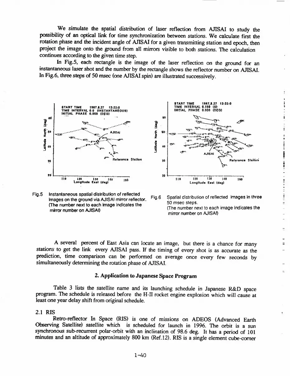
We simulate the spatial distribution of laser reflection from AJISAI to study the
possibility of an optical link for time synchronization between stations. We calculate first the
rotation phase and the incident angle of AJ'ISAI for a given transmitting station and epoch, then
project the image onto the ground from all mirrors visible to both stations. The calculation
continues according to the given time step.
In Fig.5, each rectangle is the image of the laser reflection on the ground for an
instantaneous laser shot and the number by the rectangle shows the reflector number on AJISAI.
In Fig.6, three steps of 50 msec (one AJISAI spin) are illustrated successively.
ad
Z
J:t 4o
10
Fig.5
START TIME 1987.8.27 12:22:0TIME INTERVAL 0.0 (INSTANTANEOUS)INITIAL PHASE 0.000 (DIEG)
- IIo
"''" °'"° " w"¢_m
114 '''" In''"...'_1_ -_ . .--'""" ""- AJISAI _ EO-
",_l.I.o "_
.. ¢,,...dt, "'41,,.
,dl' f'" "1"- ,. 40
#" Reference Slsllon 90
z0I10 110 1.10 140 II;0
Longitude Essl (dog)
Instantaneous spatial distribution of reflectedimages on the ground via AJISAI mirror reflector.(The number next to each image indicates themirror number on AJISAI)
Fig.6
8TART TIME tgR7.11.27 12:22:0TIME INTERVAL 0.IS0 (S)INITIAL PHASE 0.000 (O8(31
,_,. '_"_.-,,.,_ ,_.__._._. ___-_.L_,_..__ ,t,,. o_lt...,,0t:" ---......._,,.
,¢_j,.__-4xIl.,i...._l,, , • _'ll,:_..,.4j_.
,s,. " .... :IIL_/_',_ -"_';_" _'_".;
°_ ,°i._'. "N
neference St|il()r_
_pv.
IiO Jzo i_ _4o t_oLongitude El'It (deg}
Spatial distribution of reflected images in three50 msec steps.(The number next to each image indicates themirror number on AJISAI)
A several percent of East Asia can locate an image, but there is a chance for many
stations' to get the link every AJISAI pass. If the timing of every shot is as accurate as the
prediction, time comparison can be performed on average once every few seconds bysimultaneously determining the rotation phase of AJISAI.
2. Application to Japanese Space Program
Table 3 lists the satellite name and its launching schedule in Japanese R&D spaceprogram. The schedule is released before the H-II rocket engine explosion which will cause atleast one year delay shift from original schedule.
2.1 RIS
Retro-reflector In Space (RIS) is one of missions on ADEOS (Advanced EarthObserving Satellite) satellite which is scheduled for launch in 1996. The orbit is a sun
synchronous sub-recurrent polar-orbit with an inclination of 98.6 deg. It has a period of 101
minutes and an altitude of approximately 800 km (Ref.12). RIS is a single element cube-corner
1-40

Table 3 R&D Satellite Launching
Schedule (1992- 2001),
released by NASDA in April 1992
Fiscal year/Satellite name........... n .......................
1992 JERS-1,FMPT
1993 ETS-VI, SFU
1994 IML-2,SFU
1995 ADEOS
1996 cOMETS
1997 TRMM,
1998 JEM-1,2, ADEOS-II
1999 JEM-n
2001 HOPE
Curved surface
/_.,. __.. _lat_urface
X: Direction of satellitemovement
Z: Nadir
Fig.7 Structure of RIS( Effective diameter" 50cm )
retro-reflector with a diameter of 0.5 m designed for earth-satellite-earth laser long-path
absorption experiments. RIS is proposed by the National Institute for Environmental Studiescollaborated with CRL.
In the experiment, laser beam transmitted from a ground station is reflected by RIS and
received at the ground station. The absorption of the intervening atmosphere is measured in the
round-trip optical path. Figure 7 shows the structure of RIS. We use a slightly curved mirrorsurface for one of three mirrors forming the retro-reflector, which diverges the reflected beam to
overcome the velocity aberration caused by the satellite movement.We have proposed a simple spectroscopic method which utilizes the Doppler shift of the
reflected beam resulting from the satellite movement for measuring the high resolution
transmission spectrum of the atmosphere. The wider laser beam is used for illuminating satellite
and for autonomous tracking the satellite by guiding camera.
2.2 ETS-VIINASDA will schedule to launch the Experimental Technology Satellite (ETS-VII) in
1998 whose objectives are development of space robotics and rendezvous control. It consists of
two satellites, the chaser and the target, each has GPS receiver for orbit control of chaser.Tentative altitude is 550kin and communication to the ground will utilize the data relay satellite.
We have proposed that each satellite should be loaded with corner cube reflector set, oneof which is two-color sensitive and be monitored the rendezvous process from the ground. We
will track the satellites with switching or simultaneously mode depending on two satellites being
within one beam or not.
3. CONCLUSION
We have studied the feasibility of the sub-nanosecond precision laser time
synchronization system with a target satellite of AJISAI based on CRL laser ranging system,
whose timing system is connected with UTC(CRL).
1-41

Simulation study indicates that two stations at thousands of km distance from each other
can be linked by laser beam with signal strength of more than 10 photons. The images of laser
beam from AJISAI mirrors is uniformly distributed on the ground and two stations have many
chances to link each other during a single AJISAI pass. It requires the lasec control of laser fire
timing, however, it bring on the precise information of the orbit as well by using the self-returnedsatellite range data.
The system has been operating in geodetic mode since CRL started the SLR observations
to the major geodetic satellites from 1990. While global position of the SLR station has been
determined with the precision of several centimeters, we are re-designing our system so that
current system has also for time synchronization mode operation as well as adapting forJapanese space program in future.
REFERENCES
,
2.
.
4.
5.
6.
7.
8.
9.
10.
11.12.
Kirchner D.,1991, Two-way Time Transfer via communication satellites, _..Qg,_.L_,Vol.79, No.7, pp.983-990
Leschiutta S.,1991, Time synchronization using laser techniques, _, Vol.79,No.7, pp. 1001-1008.
Degnan JJ., 1985, Satellite Laser Ranging : Current Status and Future Prospects, IEEETrans. Geosci. Remote Sensing. GE-23, 4, pp.398-4 13.
Pearlman M., & al. 1989 , Ground-based laser ranging measurement techniques andtechnology, _g.09.13...QLC,,J_-COOLFONT, section2.1, pp. 1-26.
Serene B. and Albertinoli P. 1979, The LASSO Experiment, Proc.PTI'I 1 lth conference,pp.145-167.
Veillet C. 1989, LASSO - the European Phase Aug.88-Sept.89, Proc.7th InternationalWorkshop on Laser Ranging Instrumentation, Matera 2-6.
Kunimori H. & al. 1991, "Satellite Laser ranging system", Journal of CRL. Vol.38, No.2,pp.303-317.
Greene B.A. 1984, Epoch timing for laser ranging, Proc. 5th International Workshop onLaser Ranging Inswumentation (Herstmoncex), pp.247-250.
Sasaki M.and Hashimoto H. 1987, Launch and observation program of the experimentalgeodetic satellite of Japan, IEEE Trans.Geo.Rem., GE-25, 5, pp.526-533.
Yang F.M. 1986, The proposal of strictly simultaneous satellite laser ranging, The 6-th
international workshop on laser ranging instrumentation, France, pp.549-557.Electro Optic Systems 1991, EOS-V1 Active/Active Laser Characterization.
Sugirnoto,A., Minato A. and Sasano Y.,19_1, Retro-reflector in space for the ADEOSsatellite, CREO'91 Baltimore,.
Dl[i
Z
1-42
APPLICATIONS OF SLR
B.E. Schutz
Center For Space Research
The University of Texas at Austin
Austin, TX 78712, USA
N94-15556
INTRODUCTION
Satellite Laser Ranging (SLR) has a rich history of development which began in the 1960s with
10 meter-level first generation systems. These systems evolved with order of magnitude improve-
ments to the systems that now produce several millimeter single shot range precisions. What
began, in part, as an interesting application of the new laser technology has become an essential
component of modem, precision space geodesy, which in turn enables contributions to a variety of
science areas.
Modem space geodesy is the beneficiary of technological developments which have enabled pre-
cision geodetic measurements. Aside fro SLR and its closely related technique, Lunar Laser
Ranging (LLR), Very Long Baseline Interferometry (VLBI) has made prominent science contri-
butions also. In recent years, the Global Positioning System (GPS) has demonstrated a rapidly
growing popularity as the result of demonstrated low cost with high precision instrumentation.
Other modem techniques such as DORIS have demonstrated the ability to make significant sci-
ence contributions; furthermore, PRARE can be expected to contribute in its own right.
An appropriate question is "why should several techniques be financially supported"? While thereare several answers, I offer the opinion that, in consideration of the broad science areas that are
the benefactors of space geodesy, no single technique can meet all the requirements and/or expec-
tations of the science areas in which space geodesy contributes or has the potential for contribut-
ing. The more well-known science areas include plate tectonics, earthquake processes, Earth
rotation/orientation, gravity (static and temporal), ocean circulation, land and ice topography, to
name a few applications.
It is unfortunate that the modem space geodesy techniques are often viewed as competitive, but
this view is usually encouraged by funding competition, especially in an era of growing needs but
diminishing budgets. The techniques are, for the most part, complementary and the ability to
reduce the data to geodetic parameters from several techniques promotes confidence in the geo-
physical interpretations.
In the following sections, the current SLR applications are reviewed in the context of the other
techniques. The strengths and limitations of SLR are reviewed and speculation about the future
prospects are offered.
SLR Summary
Satellite Laser Ranging measures the round-trip time-of-flight for a laser pulse to travel from a
transmitter to a target and back. Current and near-term satellite targets include Starlette (1000 km
1-43

altitude), Ajisai (1500 km), ERS-1 (800 kin), Lageos (59000 km) and Etalon-1 and -2 (25000
km). Future satellites include TOPEX/POSEIDON (August 1992 launch) and Lageos-2 (October
1992 launch). The geodetic satellites (Starlette, Ajisai, Lageos and Etalon) have a long orbital
lifetime measured in thousands of years to millions of years for the high altitude satellites, thereby
offering a distinct advantage that the satellite will be available at no cost for a very long period of
time. Only the ground segment requires operation and maintenance support. By contrast, all other
satellite techniques (GPS, DORIS, PRARE) rely on an active space segment with a lifetime deter-
mined by the on-board power system, usually several years. VLBI, on the other hand, uses
extragalactic radio sources which will, presumably, be available for a very long time.
Precision Orbit Determination/Gravity
The traditional strength of SLR has been in the ability to determine the orbits of target satellite
with high accuracy. In the case of TOPEX/POSEIDON, SLR is the primary means of precisely
determining the orbit to the required 13 cm in the radial component in support of radar altimeter
analyses. SLR tracking of NASA altimeter satellites has been an important element in the accom-
plishment of the respective mission goals, SLR, however, has a distinct disadvantage Created by
dependency on atmospheric transparency. Radiometric systems, such as GPS and DORIS, are
potentially able to provide essentially continuous tracking. Since TOPEX/POSEIDON includes
SLR, GPS and DORIS, it will provide a unique opportunity tO evaluate the performance of all sys-
tems. The focus of tracking systems on future satellites may be GPS with SLR as a backup. Nev-
ertheless, it is important to note that the passive nature of SLR provides an extremely reliable
space segment--it simply will not fail except under catastrophic circumstances. A cautionary note
for the future is in order. The risk of regarding SLR as a backup system encourages the reduction
in operating systems for budgetary reasons, but as systems close, it becomes more difficult to
reactivate them in the event that the backup mode must be initiated.
Improvements in the gravity field, including the gravitational parameter GM, are other areas
where SLR has made very significant contributions. The development of new models in prepara-tion for TOPEX/POSEIDON have benefitted from the SLR data base that has been accumulated
over the years, some of which has been used in previous fields and some has not. Gravity fields
used for GPS applications, such as the Department of Defense WGS-84, have used SLR data from
Lageos and Starlette which have particularly contributed to determination of low degree and order
gravity coefficients. Current GPS applications use GEM-T3 or other, more recent fields, which
have relied on SLR data. Furthermore, the Etalon satellites can be used to study gravitational
effects that will be somewhat similar to those influencing the GPS satellites, except for the partic-ular GPS effect of deep gravitational resonance.
SLR has made unique contributions to the study of temporal variations in the gravity field, both
tidal and non-tidal variations. These studies have, in part, been made possible by the nature of low
area-to-mass ratio satellites (Lageos and Starlette), which diminish the nongravitationai forces.
This diminishment enhances the opportunity to identify the spectral content of gravitational
effects. Furthermore, the study of temporal changes in gravity has been enhanced by the ability toinvestigate the orbit evolution over long periods of time, spanning in some cases more than 15years.
1-44
i
|
E
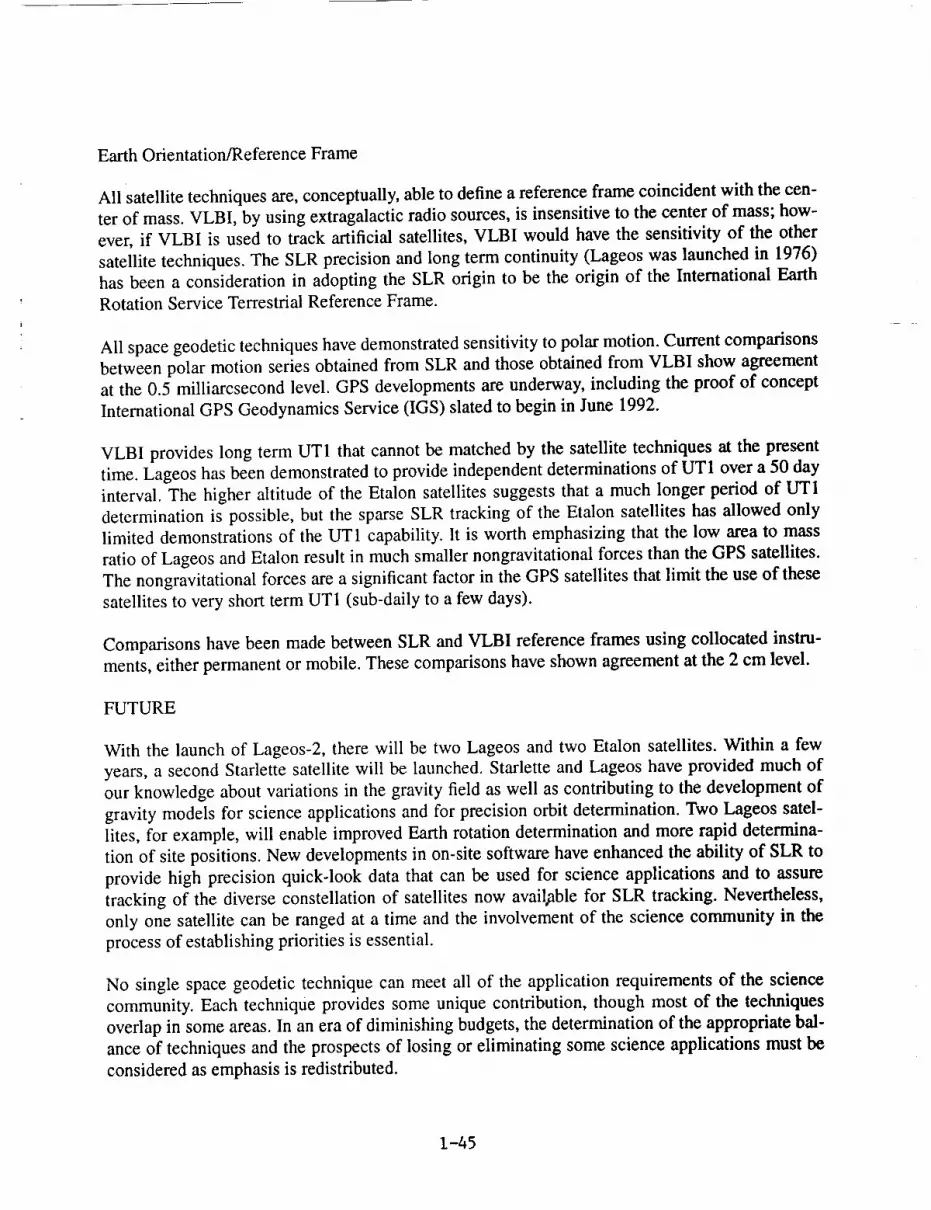
Earth Orientation/Reference Frame
All satellite techniques are, conceptually, able to define a reference frame coincident with the cen-
ter of mass. VLBI, by using extragalactic radio sources, is insensitive to the center of mass; how-
ever, if VLBI is used to track artificial satellites, VLBI would have the sensitivity of the other
satellite techniques. The SLR precision and long term continuity (Lageos was launched in 1976)has been a consideration in adopting the SLR origin to be the origin of the International Earth
Rotation Service Terrestrial Reference Frame.
All space geodetic techniques have demonstrated sensitivity to polar motion. Current comparisons
between polar motion series obtained from SLR and those obtained from VLBI show agreementat the 0.5 milliarcsecond level. GPS developments are underway, including the proof of concept
International GPS Geodynamics Service (IGS) slated to begin in June 1992.
VLBI provides long term UT1 that cannot be matched by the satellite techniques at the present
time. Lageos has been demonstrated to provide independent determinations of UT1 over a 50 day
interval. The higher altitude of the Etalon satellites suggests that a much longer period of UTI
determination is possible, but the sparse SLR tracking of the Etalon satellites has allowed only
limited demonstrations of the UT1 capability. It is worth emphasizing that the low area to mass
ratio of Lageos and Etalon result in much smaller nongravitational forces than the GPS satellites.
The nongravitational forces are a significant factor in the GPS satellites that limit the use of these
satellites to very short term UT1 (sub-daily to a few days).
Comparisons have been made between SLR and VLBI reference frames using collocated instru-
ments, either permanent or mobile. These comparisons have shown agreement at the 2 cm level.
FUTURE
With the launch of Lageos-2, there will be two Lageos and two Etalon satellites. Within a few
years, a second Starlette satellite will be launched. Starlette and Lageos have provided much of
our knowledge about variations in the gravity field as well as contributing to the development of
gravity models for science applications and for precision orbit determination. Two Lageos satel-
lites, for example, will enable improved Earth rotation determination and more rapid determina-
tion of site positions. New developments in on-site software have enhanced the ability of SLR to
provide high precision quick-look data that can be used for science applications and to assure
tracking of the diverse constellation of satellites now avail,able for SLR tracking. Nevertheless,
only one satellite can be ranged at a time and the involvement of the science community in the
process of establishing priorities is essential.
No single space geodetic technique can meet all of the application requirements of the science
community. Each technique provides some unique contribution, though most of the techniques
overlap in some areas. In an era of diminishing budgets, the determination of the appropriate bal-
ance of techniques and the prospects of losing or eliminating some science applications must be
considered as emphasis is redistributed.
1-45

The international collaboration in the SLR community has been outstanding. The promotion of
further collaboration will enhance the prospects for long term availability of a global SLR net-
work, thereby assuring the continued collection of data for the purpose of gaining better scientificunderstanding of our planet.
1-46

Timely Issues

E
R_B
zl
m
m_
E

N94- 15557Satellite Signatures in SLR Observations
G.M. Appleby
Royal Greenwich Observatory
Madingley Road
Cambridge CB3 0EZ, UK
Abstract.
We examine the evidence for the detection of satellite-dependent s,ignatures in the laser range
observations obtained by the UK single-photon SLR system. Models of the expected obser-
vation distributions from Ajisai and Lageos are developed from the published satellite spread
functions and from the characteristics of the SLR system, and compared with the observa-
tions. The effects of vamfing return strengths are discused using the models and by experi-
mental observations of Ajisai, during which a range of return, levels from single to multiple-
photons is achieved. The implications of these results for system-dependent centre of mass
corrections are discussed.
1. Introduction.
The UK SLR system sited at Herstmonceux, and run by the Royal Greenwich Observatory,
routinely observes the primary tax'gets ERS-1, Lageos, Etalon-1 and -2, Starlette and Aji-
sai. The single-shot precision achieved by calibration ranging is close to 1 cm (1-sigma).
Tile detection and timing hardware has recently been upgraded to include a Single Photon
Avalanche Photodio(le (SPAD, Procha.zk_t ctal, 1990), and an HP 5370 time interred counter.
Epoch is derived at present from a Maryland 4-stop event timer, which is also used to make
rangc measurements simultaneously and independently of the HP counter. Pass-averaged
return rates are in general fairly low, varying from a few percent from the Etalon satellites,
through about 20% fl'om Lageos to up to 50% from Ajisai. Returns from the calibration
targets are deliberately kept to similarly low levels (about 10-15%) using neutral density fil-
ters in the laser path. Under such conditions we can describe the system as a single photorl
return, single photon detection system. A detailed study of the system error budget was
carried out following the upgrade of the detector from a PMT. During this investigation it
becaxne clear that the observational precision of in particular Lageos and Ajisai was consis-
tently worse than that of the calibration targets. It was considered likely that the spacial
distribution of the retroreflector arrays on the satellites would modify the distribution of the
range residuals, when compared with those from the fiat calibration targets. In this paper weexamine the evidence for detection of satellite signatures in our range observations, compare
the observations with models of the expected distributions from a selection of those satel-
lites regularly observed, and discuss the implications in terms of the appropriate corrections
required to reduce the observations to the centres of mass of the satellites
2. Observations.
This investigation is based upon the pass-by-pass range residuals that are formed during
2-1
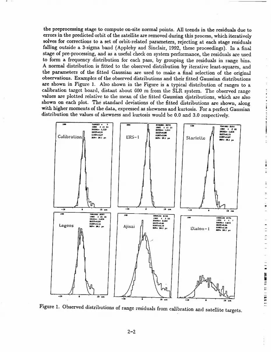
the preprocessingstageto compute on-site normal points. All trends in the residuals due to
errors in the predicted orbit of the satellite are removed during this process, which iteratively
solves for corrections to a set of orbit-related parameters, rejecting at each stage residuals
falling outside a 3-sigma band (Appleby and Sinclair, 1992, these proceedings). In a final
stage of pre-processing, and as a useful che¢& on system performance, the residuals are used
to form a frequency distribution for each pass, by grouping the residuals in range bins.
A normal distribution is fitted to the observed distribution by iterative least-squares, and
the parameters of the fitted Gaussian are used to make a final selection of the origin',.1observations. Examples of the observed distributions and their fitted Gaussian distributions
are shown in Figure 1. Also shown in the Figure is a typical distribution of ranges to a
cMibration target board, distant about 600 m from the SLR system. The observed range
values are plotted relative to the mean of the fitted Gaussian distributions, which are also
shown on each plot. The standard deviations of the fitted distributions are shown, along
with higher moments of the data, expressed as skewness and kurtosis. For a perfect Gaussian
distribution the values of skewness and kurtosis would be 0.0 and 3.0 respectively.
IINI TaJICI[T * I,
II)@Z 4 11 =l
_lGllAi i. I "*_1
•53.13'a @ .34
C lib Li x,,,._,ia ra oil • .
-I0 • I@ em
Lageos
-i@ g
•rao:igo j _l?
lul 4 IS l@
.58r.NA = ldt._l
_lCVndl,f.4l
I_UIITI_43
IKNi [email protected] p*
•- :,%,..,,=.II Zl
11¢111| l..II|
JIUIIIF=3.00
I_RS- 1 ,_n- ,., ,.
i@e _|@1 li|_
I_IGNAm 3..@ liT.
I;l;1¢ If ..e j..r.
Aj isa i tu=r.=.jwJill r
_10 • I| tm
13@ ?'.A) INI ]Ill 114
IIIg_ 4 8 ZZ
li_-.tU. = 1.1_6
lai[lr=41. I S
qla, I,_ k'@rl_m,l.e7
•t - - :-- ' " i
-I@ g Ig rm
r,l_ lIA m d_lll
KInlT*3.S4
_Lolon- l _. _,., p,
-I@ • IO em
Figure 1. Observed distributions of range residuals from calibration and satellite targets.
m
E_
k
2-2

2.1 Discussion.
From the distributions shown in Figure 1, we make the following observations. The distri-
butions of the calibration ranges and those fl-om Starlette and ERS-1 are clearly symmetric
and well-fitted by the Gaussian distributions, but all have a significant 'tail' of observations
outside the fitted curves. Skewness values for these 3 targets are between 0.05 and 0.1. The
Lageos distribution is much less symmetric, and is less well fit by the Gaussian distribution.
A chi-square goodness of fit test indicates significant departure, at a 5% level of significance,from the best-fit distribution shown in the plot. The results from Ajisai and Etalon 1 show
large asymmetry, and are not at all well fit by the Gaussian distributions. Of particular
significance to this investigation, are the 'widths' of the distributions, characterized by thestandard deviations of the fitted distributions. Mean values of these standard deviations for
a number of observations made during November and December 1991 arc given in the Table
below. These mean values of standard deviations confirm the impression given in Figure 1,
that the calibration ranges have the smallest scatter, and those of Ajisai and Etalon-1 the
largest, the range of standard deviations being from 1.1 cm to 4.8 cm.
Target allll-n
Calib 11
ERS-1 12
Starlette 16
LAGEOS 18
Ajisai 32Etalon 48
Before proceeding to investigate the hypothesis that satellite signatures arc present in our
observations, we first consider the possible causes of the 'tail' in the distributions, particularly
evident in the calibration and Starlette data. We remark here that the existence of this tail
does not constitute the thrust of our argument that we are detecting satellite signatures in
our observations, since the tail is also present in the calibration ranges from a flat target
board. We must therefore rule out such a target-induced effect and consider as probable
cause the SPAD or the laser. In an experiment primarily designed to quantify the system
time-walk under a large range of return signal strengths, calibration ranging was carried out
using neutral density filters to vary the average number of photons reaching the detector.
In this way the average number of photons was varied from about 0.5 to 50 photons per
shot, as deduced fl'om the observed return rates. A selection of the results is given in
Figure 2, where the results are displayed in histogram form as before. The plots show, as
expected, a reduction in the standard deviations of the distributions with increasing signal
strength, since for a given laser pulse-width we would expect the contribution of the laser
to the observational jitter to decrease with increasing number of photons in the return
train, as the single-event detector increasingly receives photons originating nearer to the
leading edge of the transmitted pulse. The plots also demonstrate that the extent of thetail in the distributions decreases with signal strength, suggesting an origin within the laser.
However Prochazka (1992, private communication), points out that correct optical alignment
2-3
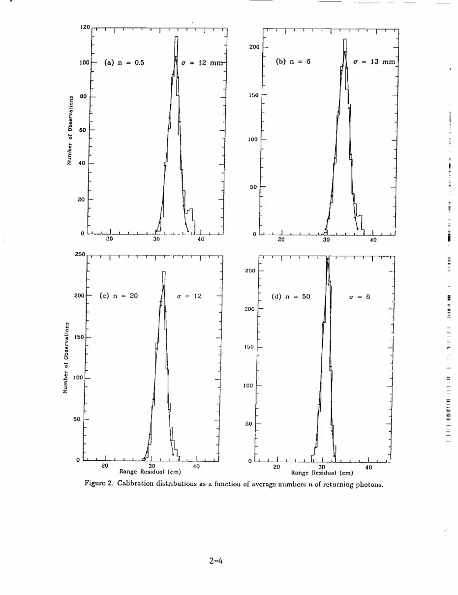
120
IOO
0
o 60
Ez 40
20
' ' I ' ' ' ' I ' '
(a) n = 0.5 = 12
I I [ I | I L___-_.A_ _ __ __l____d--k__L__.L
20 30 d0
200
150
100
50
(b)n = 6
I I Illll
20 30 40
a= 13mm
250
200
0
i 150
o
._ 100
5o
0
20 30 40
Range Residual (cm)
200 -- t[ Z]
it JI00 - _ ] --
20 30 40Range Residual (cm)
Figure 2. Calibration distributions as a function of average numbers u of returning photons.
2-4

of the SPAD detector is essential to avoid possible effects of non-uniformity within the chip.
Resolution of this problem awaits further experimentation.
3. Satellite Signature Models.
We now take as our standard, single-photon system-signature the calibration distribution
shown in Figure 1, and develop from it models of expected satellite return signatures, by
convolution with the spread functions of Lageos and Ajisai. For Lageos, we take the model
of cross-section para_neters based upon row-by-row far-field diffraction pattern tests in polar
orientation, presented in Fitzmaurice et al (1977). The parameters give, for the particular
orientation, the lidar cross-section and number of corner cubes, in rows, contributing to the
strength of returning signal. Also given is the optical distance of each row of reflectors fl'om
the spacecraft centre of gravity. We use the effective cross section of the cubes in their
rings, of known distances from the centre of the satellite, to caxry out a convolution of our
system signature with that of Lageos. In this estimate of the shape of the returning pulse
we ignore the effects of changing polarisation, which mainly affects the amplitude of the
convolved pulse, and not its shape (Fitzmanrice et al 1977.) To model the return signatures
from Ajisa_ we use the results of a computer simulation carried out by Sasald and Hashimoto
(1987). They find that the number of retroreflector sets contributing to the return signal froma given single laser pulse can only be 1, 2 or 3.5, and give the computed pulse shape in each ofthese 3 cases. The laser used in their simulation is gaussian in profile, of standard deviation
33 ps. From the published profiles, we can infer the spread distributions, consisting of lidarcross-section's and dista.nccs from spa.cecrMt ccntrc of grltvity. We now have the informa.tion
required to ca.rry out a convolution with our system signature, in the same way as for Lagcos.Wc assume that the rapid spin rate of Ajisai, of 40 rpm (Sasaki and H,'Lshimoto, 1987) will
ensure that for cvcry pass all 3 possible orientations of the slitellite will be sampled. Wc thus
convolve our system signature with each of the spread distributions, and sum the resulting
3 distributions.
The results of the simulations for Lageos and Ajisai are shown in histogram form in Figures
3(a) and (b), where the quoted standard deviations are those of the fitted Gaussian distri-
butions, also shown on the plots. For completeness wc also present in Figure 3 the result of
convolving our system scpaz'ately with each of the 3 orientations of Ajisai.
_' ' I ' ' ' ' I ' ' ' ' I 'o 60 --
- o" = 17 mrn 1
-©
40 --
0
0
20 --,_a
_.
--
0 __L_ .__ I I -
Figure 3. (a) SimulaLcd L_gcos rangc residual distributions.
2-5

of the SPAD detector is essential to avoid possible effects of non-uniformity within the chip.Resolution of this problem awaits further experimentation.
3. Satellite Signature Models.
We now take as our standard, single-photon system-signature the calibration distribution
shown in Figure 1, and develop from it models of expected satellite return signatures, by
convolution with the spread functions of Lageos and Ajisai. For Lageos, we take the model
of cross-section paa'aaneters based upon row-by-row fax-field diffraction pattern tests in polar
orientation, presented in Fitzmaurice et al (1977). The parameters give, for the particula_
orientation, the lidar cross-section and number of corner cubes, in rows, contributing to thestrength of returning signal. Also given is the opticM distance of each row of reflectors from
the spacecraft-centre of gravity. We use the effective cross section of the cubes in their
rings, of known distances from the centre of the satellite, to cazry out a convolution of our
system signature with that of Lageos. In this estimate of the shape of the returning pulse
we ignore the effects of changing polarisation, which mainly affects the amplitude of the
convolved pulse, and not its shape (Fitzmaurice et al 1977.) To model the return signaturesfrom Ajisai we use the results of a computer simulation carried out by Sasaki and Hashimoto
(1987). They find that the number of retroreflector sets contributing to the return signal from
a given single laser pulse can only be 1, 2 or "1.5, and give the computed pulse shape in each of
these 3 cases. The laser used in their simulation is gaussian in profile, of standard deviation
33 ps. From the published profiles, we Call infer the spread distributions, consisting of lidar
cross-sections and distances from spacecraft centre of gravity, gTe now have the information
required to carry out a convolution with our system signature, in the same way as for Lageos.
We assume that the rapid spin rate of Ajisai, of 40 rpm (Sasaki and Hashimoto, 1987) will
ensurc that for every pass all 3 possible orientations of the satellite will be sampled. Wc thus
convolve our system signature with each of the spread distributions, and sum the resulting3 distributions.
The results of the simulations for Lageos mad Ajisai axe shown in histogram form in Figures3(a) and (b), where the quoted standard deviations are those of the fitted Gaussian distri-
butions, also shown on the plots. For completeness we also present in Figure 3 the result of
convolving our system separately with each of the 3 orientations of Ajisai.
01
o 60
l>0
o
0
I.-,
,.o
X;
4O
20
0
a = 17 mm
-_ I I ] I I
Figurc 3. (a) Simulated Lagcos r,'mgc rcsidu'al distribution
z
2-6

_, 4o
.o
,>
o 30
,,D
E
6o
(_)
5O
lO
5O
40
.2
30
0 '
"5
,-, 20E
1o
II I
(c)
= 23 mm
20 30 dO
I ' ' ' ' I ' ' ' ' I '
_r _ 33
20 30 40
Range Residual (cm)
5O
(b)
40
30
2O
10
140
120
I00
O0
GO
'u = 30
20 30 40
' ' I ' ' ' ' I .... 1 '
(a+b+c) cr = 20
,10
2O
20 30 40Range Residual (cm)
Figure 3. (b) Simulated Ajisai range residual distributions.
2-7

3.1 Discussion.
The standard deviation of the simulated Lageos data (1.7 cm) is close to our observational
mean of 1.8 cm, and the appearance of the simulated and observed histograms is similar.
The underestimate of the observed scatter by our model may be attributed to various causes;
neglect of atmospheric turbulence (Gardner, 197G); neglect of coherency fading induced by
the satellite, and the single satellite orientation chosen for the model. The models of the
Ajisai return signatures give standard deviations of between 2.3 and 3.3 cm, which compare
well with the observational results. There is some evidence in the Ajisai observations of
variations of signature with pass circumstances, which may be due to the dominance of a
particular satellite orientation or orientations for a given ground track.
4. Multi-photon Returns.
The foregoing discussion is based upon return energies at the single photon level; the detected
photon is considered to be a random event taken from a population formed by the convolution
of the laser pulse distribution with that of the satellite response. We now consider the effects
of a larger number of photons reaching the single-photon detector, in order to quantify the
subsequent systematic effects caused by a signal-strength-dependent variation of the meanreflection distance to the satellite.
4.1 Observations and reduction.
Experiments were carried out using Ajisai since it is relatively easy to obtain a large variation
in received encrgy from the large target. The variation from single photon to multiple photon
levels was achieved during the expcrimental passes by altering the divergence of the laser
beam and hence the energy density at the satellite. The observations wcre filtered in the
standard way, by using them to solve for corrections to the predicted orbit. However, it was
found that this process did not remove all trcnds from the range residuals, indicating the
presence of systematic range biases which varied during the passes. We found that it was
necessary to divide each pass into a number (G) of segments, and use the processing software
to filter the observations in each segment separately. The resulting scatter plot for one of
the experimental passes is shown in Figure 4. The residuals from each of the six segments
are shown in histogram form in Figure 5, along with the standard deviations of the fittedGaussian distributions.
We calculate the average percentage return rates at intervals of 30 seconds throughout the
passes by counting the numbers of satcllite returns and the numbcrs of pre-rct_rn noise
detections. Given that the laser fires 10 shots per second, the true percentage return rate ineach 30-second interval is then
(number of true range measurements*100)/(30*10 - number of noise events)
On the assumption that the quantum efficiency of the SPAD is 20%, we calculate from these
corrected return rates the average numbers of photons in each return. However we found
that in several of the 30-second intervals the calculated return rate was nearly 100%. At
such return levels we cannot reliably estimate the mean number of returning photons, which
may be fax in excess of the 16 estimated for a near 100% rate. Where possible, we have
used these 30-second mean values to estimate the mean numbers of photons contributing to
the observations in our 6 segments, and these averages are shown in Figure 5. For those 2
2-8

m
r1 I
(cuo) l_np!so_l a+u+_I
2-9

140
120
I00
• N
,o
_ 4o
0-1_
.... I'' ''1''''1 .... ]'' ''1'''
n = 6 o" = 20 mm
, , , , I , .- , , [_
-I0 -5 0
,I,,,,1
lO 15
I00
OO
6O
40
2O
F
L20 n = 0 ; o = 20 mm
m _
0 __Ji--L-L_/_[_L • , , , J , i I I
-15 -lO -5 0 ,5 I0 15
140
P'O
I00
z 40
2O
0-15
.... I ' ' ' ' I r'T-m_]_ .... I .... I ' ' °
n _'[_ ll_ 1 (r = IG
J
"-..- 10 -5 0 fi, 10 15
14Q
120
I00
O0 F--
''''l .... I .... I .... I .... I'''
Jl /%IG a = 13
60 I-- _Lj_j_I"
2O
o JJ-J-J_ J--LLLL LLLL_
-15 -10 -to 0 b lO 15
140f_120
100
w
o "
N GO
_ 4o
2O
0
-lg
' ' ' I ' ' * ' I ' ' ' ' I'"_ ' ' ' I ' ' ' ' I ' ' 'In = 15 it= 16
,,,,1,,,, ,1,
-iO -5 0 ( cn5 0Range Residual
.... I,,,,i
iO 15
14OL_
120L
lO01--
00'
60
4O
20
0
-15
° ' ' I .... I * ' ' ' I ' ' ' ' i ' ' ' ' t ' ' ' "T
,]
o" = 18 --_1_ = fJ
-IO -5 0 5 10Raw8© Residual (el,0
15
Figurc 5. Distribution of reazgc rcsiduMs from Ajisai pass as ,_ functioll of avcragc numbers n of x','-turning photons.
_=
2-10
segments where the average return rates were near 100%, we have asigned the numbers of
photons as >16, but remark that the true numbers could be several times as large.
4.2 Model and Discussion.
There is a clear variation of histogram shape and single-shot precision with change of signal
strength. At low return rates equivalent to single photon returns, the distribution of residualsis similar to the 'standard' Ajisa.i distribution (Figure 1). For the high return rates little
of the satellite signature remains in the distributions, and the histograms qualitatively and
quantitatively resemble those from Starlette or ERS-1 (Figure 1).
These results cannot be used to detect a systematic variation of satellite mean reflection dis-
ta_uce during the passes, because the method of reducing the observations absorbs any such
corrections. However we can use models to predict both the increase of precision and this
change of mean reflection distance as a function of numbers of photons in each return. Wemodel the time-distribution of the returning photons, from which we may sample a variable
number, by convolution of the Ajisai spread distributions with a Gaussian distribution of
FWHM 50 ps, to represent the laser. To model the effect of n photons reaching the detector,we use a random number generator to pick one 'photon' from our time-distribution of pho-
tons, then reco1"d its time-location within the distribution, and repeat the process n times.We then sort this sequence of n relative event times into chronological order of arrival at the
detector. We model the 20% efficiency of the detector by stepping through the n events in
time order, at each step generating an integer ran(lore number in the range 1-5. If the ran-
dom number is 1, the event is accepted (detected). If the random number is not 1, the next
event is 'tested'. In this way wc generate a large number of event times each resulting from
the selection of a single photon from a series of returns containing an average of n photons.
The mean and standard deviation of these event times arc computed and converted to range
in cm. The standard deviation values are added quadratically to the estimated system jitter
(0.8 cm) to fully model the observations. The results of simulations of range precision andbiases from Ajisai for values of n between 1 and 50 arc shown in Figures 6a and 6b, where
the results hnye bccn joined by continuous lines. The 30-second aver_Lge observed values
of precision, where they can be reliably cstimated (see section 4.1) from our experimental
Ajisai passes, are shown as dots on the graph and agree well with those predicted. The
predicted range bias curve in Figure 6b expresses the expected change of mean reflectiondistance from the satellite centre of mass as a result of increasing the number of photons
reaching the detector in each laser return. Most of the bias, which contains a contribution
from the finite pulse length of the laser (FWHM 50ps), is seen to take effect between signal
strengths at the single photon level up to an average of about 40 photons per return. Little
change is predicted with increasing numbers of photons beyond that point.
4.3 Lageos Centre-of-mass correction.
We can use the above techniques to estim_Lte the magnitude of a systematic range-bias for
Lageos, in the context of worldwide SLR systems working at different return-signal levels.
Figure 6 shows the results of a computation of the rmlgc bias as a function of avcragc
number of photons reaching the detector, for 2 modelled laser pulse-lengths. The magnitude
of the change of the effective reflection distaalce from the satellite centre of mass is about1.3 cm for a variation of return level fl'om single-photons to the 40 photon level. This result
2-11
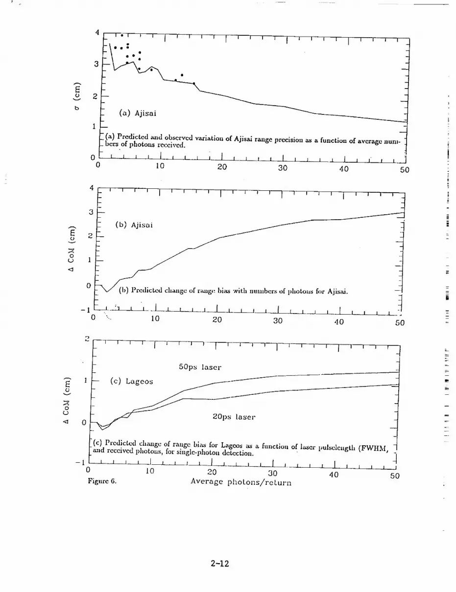
Bo
v
Bo
v
o¢.)
<1
zl_'-'l--*l I l I I I l I l i i i i i I i i i i i i i i
I I _I I
3 •
++b a) Ajisai
i
_(a) Prcdictcd lind obscrvcd variation of Ajisai range prccision as a function of avcragc num-
bcrs of photons rcccivcd.| l ' J I ] ] | l0 J , ] , ....J , , t , , i J I .J , J__.a__
0 I0 20 30 40 50
o(.9
4
2
- (b) Ajisni
- )_eeith munbcrs of photons for Ajis+d.
-1 , ', , , J I f , , I , j , ,___] , ,, j 1 , , , L+0 "-+. I0 20 30 40 50
0
2
I
0
-l0
Figure 6.
- 50ps laser
(c) aageos
---_ 20ps laser
(c) Predicted ch_mgc of ra,lgc bias for Lagcos as a function of ]a.scr l,ulsclcagth (FWHM, !
aa_d received photons, for single-photon dctcction. ._I I I I l l__ I l J+.I ' ' I '_., , , I _ ' , J l
10 20 30 40 50Average photons/return
£
2-12

implies that an SLR system receiving and detecting single photons, and using a laser with
a pulsewidth (FWHM) of 50 ps, is on average effectively observing a distance 1.3 cm closerto the satellite centre of mass than a single-photon detection system receiving more than
about 40 photons per shot. Removing from this figure the effect of the length (FWHM) of
the laser pulse, the satellite-induced range bias amounts to about 0.6 cm. The recommendedcentre-of-mass correction for Lageos is 25.1 cm for leading-edge, half-maximum detection of
a large return pulse, and 24.9 for peak detection (Fitzmaurice et al, 1977). We assume thatthe electronic detection of the peak of a large return pulse is equivalent, in terms of distance
from cenre of mass, to the formation of the me,_n of a set of range residuals arising from
the detection of single photons. For the Herstmonceux system working at the level of single
photon returns, the appropriate centre-of-mass correction should therefore be the same as
for the large-pulse, peak-detection systems, ie 24.9 cm. However, for single-photon systems
departing from the single photon regime, the implic_Ltions of this investigation are that thecentre of mass correction should be increased from the 24.9 cm by an amount as given in
Figure 6, depending upon the laser pulse-length and the number of photons reaching the
detector.
5. Conclusion
Using observations fi'om the UK single-photon SLR system, we have demonstrated that theobservational scatter contains a satellite-dependent signature, and that this signature varies
as expected with the number of photons reaching the detector. The implications of this
variation upon the corrections required to relate range observations to the centres-of-ma_s
of the satellites is modelled and discussed. The magnitude of the cffect is system-dependent
since it depends both on the number of photons reaching the detector, _ld hence on laser
energy level and local atmospheric conditions, and upon the laser pulse length. A graph is
presented giving a calculated, energy and pulse-length dependent, center of mass correction
for Lageos range data obtained using single-photon detection, which varies by 1.3 cm over
the range of the parameters considered.
6. Acknowledgements
All of the observations reported here were carried out by the SLR team at Herstmonceux,
East Sussex, UK, under the direction of the station manager Dr. Roger Wood. The team's
interest in carrying out the non-standard observations is appreciated. I thank Dr. Andrew
Sinclair, Head of the RGO Space Geodesy Group, for his comments throughout the work on
this project.
7. References
Fitzmaurice, M.W., P.O. Minott, J.B. Abshire and H.E. Rowe. 1977. Nasa Technical Paper
1062.
Gardner, C.S. 1976. Effects of random pat, h fluctuations on tile accuracy of laser ranging
systems. App. Optics, VoI 15, No. 10.
Prochazka, I., K. Hamal and B. Sopko, 1990. Photodiode Based Detector Package for
Centimeter Satellite Ranging, Proc. 7th Int.. Workshop on Laser Ranging Instrumentation,
Matera, Italy, 1989.
2-13

Sasaki, M and H. Hashimoto. 1987. Launch and Observational Programme of the Experi-
mental Geodetic Satellite of Japan. IEEE Trans. on Geoscience and Remote Sensing, VolGE-25, No. 5.
L:
L
2-14

N94-15558
Work at Graz on
Satellite Signatures
Georg KIRCHNER, Franz KOIDL
SLR Graz / Institute for Space Research
Austrian Academy of Sciences
Observatory Lustbfihel, Lustb_helstr. 46
A-8042 GRAZ, AUSTRIA
Tel.: +43-316-472231; Fax: +43-316-462678
E-Mail: [email protected]
Abstract
The size and shape of the satellites retroreflector arrays
have a major impact on the distribution and scatter of the return
signal; this can be seen clearly when reaching sub-cm ranging
accuracies and when using Single-Photon Detectors with single- or
multi-photon returns; for other receiver systems (using MCP's) it
should be checked also. As a consequence, the necessary center-
of-mass correction for some satellites will different, depending
on the receiver systems.
While this effect is not yet visible on small satellites or
small retro-reflector arrays (like STARLETTE, ERSl), it can be in
the order of centimeters on AJISAI or ETALON.
1.0 Introduction
The SLR station Graz uses, since some years, Single Photon
Avalanche Diodes (SPAD) to detect return signals from satellites;
these diodes can detect single photons - which is used for
ranging to ETALON, or, in worse atmospheric conditions, also for
lower satellites -, but usually we use multiphoton returns to get
maximum return fates; this results in better accuracies when
using Normal-Point-Methods, and helps to avoid part of the
2-15

satellite signaturesdescribed later.
in the return signal distribution, as
2.0 Ranging tests to the calibration target
Standard calibration to our target (distance about 400 m)
gives an RMS of 6 to 7 mm for the routine SLR setup (with HP5370A
counter, SPAD at I0 V above break, cooled to -27"C; 2.5a limits);
an example is shown in fig. i, upper histogram; the distribution
shows nice symmetry, with an RMS of 5.8 mm at 2.5a ; there is no
significant change of the mean value when using different sigma
criteria, also indicating a proper distribution.
To check influences of the ranging system itself on the
distribution of the return signals, different tests with various
misadjustments of the involved devices were made; a worst-case
example is shown in fig. i, lower histogram: A similar calibra-
tion as before, but with misaligned SPAD, lower voltage above
break, no cooling, and non-optimum start puls detection; this
results in a non-symmetric distribution, higher RMS, and measu-
rable shift of the mean value for varying sigma criteria.
After verifying the maximum contribution of the system itself,
the distribution of returns from different satellites were
analyzed.
3. ERSI and STARLETTE
Due to their small size of the retroreflector arrays there is
no significant satellite signature visible in ERSI and STARLETTE
data; the average RMS is between 8 and 9 mm, close to the values
obtained from the calibration target.
The distribution of the data (fig. 2, upper histogram) is more
or less symmetric, with small irregularities due to lower number
of returns; the 3 mm bin width for all these histograms was
chosen in coincidence with the 20 ps resolution of the HP 5370A
counter.
2-16

4.0 AJISAI
As a contrast to the previous satellites, AJISAI shows quite
significant signatures; these are very dependant of the return
signal strength (fig. 3).With strong (multiphoton) return signals, AJISAI shows low RMS
(11.8 mm, upper histogram), and only slightly non-symmetricdistribution; when reducing the return signal level to mostly
single photon-electrons (by switching off the last laser
amplifier, and opening divergence; the return signal level ischecked in real time by watching the return signal rate and/or
the number of semi-train returns on a graphic screen), the RMS
increases to 22 mm (lower histogram), while the distribution now
follows the shape of the satellite.Both histograms in fig. 3 are shown with editing criteria of
2.5 a, which is used for our routine ranging procedures; usingother a values (4 a, 3 o, 2 a), the mean value of the histogram
will move - in the worst cases - between 1 and almost 2 cm.
5.0 LAGEOS
As expected from size and shape of LAGEOS, the satellite
signature is much less visible than with AJISAI, but is still
present (fig. 2); it is the main contribution to the increase of
the RMS, from 6 to 7 mm from the target, to ii to 14 mm from the
satellite (again, this is valid for our single-photon detection
system, using single photon and/or multi-photon return
signals!!), with lower signal levels resulting in higher RMS.
When using different editing criteria again, the non-symmetric
distribution causes a shift of the mean value of about 1 to 2 mm,
only in extreme cases up to 4 mm.
6.0 ETALON
To complete the satellite's list, we show also the signature
coming from ETALON ranging data, this time using a different way
2-17

of demonstrating the non-symmetric distribution. While fig. 4
shows the residuals of an ETALON-2 pass (demonstrating also the
advantage of using the semitrain!), in fig. 5 the residuals are
plotted after "folding", polynomial fitting and 2.Sa-editing. Due
to the low return signal level from these satellites (most of the
returns are single photons: We are ranging with 5 to i0 mJ
Semitrain - this is about 2 or 3 mJ for the first pulse! - and 50
cm receiver to the ETALONS, still getting return rates of up to
i000 returns per hour), we see the full satellite's size and
shape in the data, with an RMS of 3.5 to 4 cm
7.0 Conclusion
To keep systematic errors due to the influence of the
satellite's shape as low as possible, we
- keep calibration and satellite return signals in the same level
- use the same editing criteria (2.5 a) for calibration and for
satellite data;
- try to minimize any contributions of the system itself to non-
symmetric distributions.
As far as we know, in all analyzing calculations the
satellites are treated as a "flat" reflecting surface, with a
fixed center-of-mass correction, which was determined before
launch using the detectors, techniques and accuracies available
at that time. However, with the improvements in accuracy, we can
see now the shape of the satellites in our data, which in turn
can influence the values of the center-of-mass corrections; so it
seems necessary to determine the center-of-mass correction with
respect to different receiver systems, and using different values
for the analysis.
2-18

TARGET 1 CALIB. 1500 Rets
i...........!fill!!!!!iiiii!!i!ii!!!!!iiiiiiiilliiiiiiiiiiii i-........_"_M_ -Io.0 ,,,,,i U ,-, mmiiiiiiiill........................................
iiiiiiiiiiiiiiiiiiiiiiiiiiiiiiiiiiiiii ii iiii! iiiiii!iiii!I I i[ll Ii
i ¢ ; i; , i t i t ; i I , il_i, i i | I I i ¢ i i
Bin Width: 3 [ram]
1992-05=08
TARGET 1 CALIB 1500 RetsWe_ SFAD ALI_,NMENT / 5 V_b / _']5°C
Mezn RM8 _ 1
......, _ ; _!a_'t! _:t _" _:9 '_ ........................_ ....... " t_l.a • $1GMk 7.4 mm 9._1 _ [I L |
_,,. S,QM,_ 7.o.,. e.e _ Ill2.0 • SIGMA: (1,1 mm 0.5 nun Jl ] ............................................
.....................................................................
_io Iiiitl i*l*Igii;]illli'i IIit I [I
Bin Width: 3 [ram]
I RMS: 8.6 mm
l .........................................................
l ................................................
ii _il I]I ill i It Ill i
1992-05-08
Figure I: Histograms of calibration ranging to the target
2-19
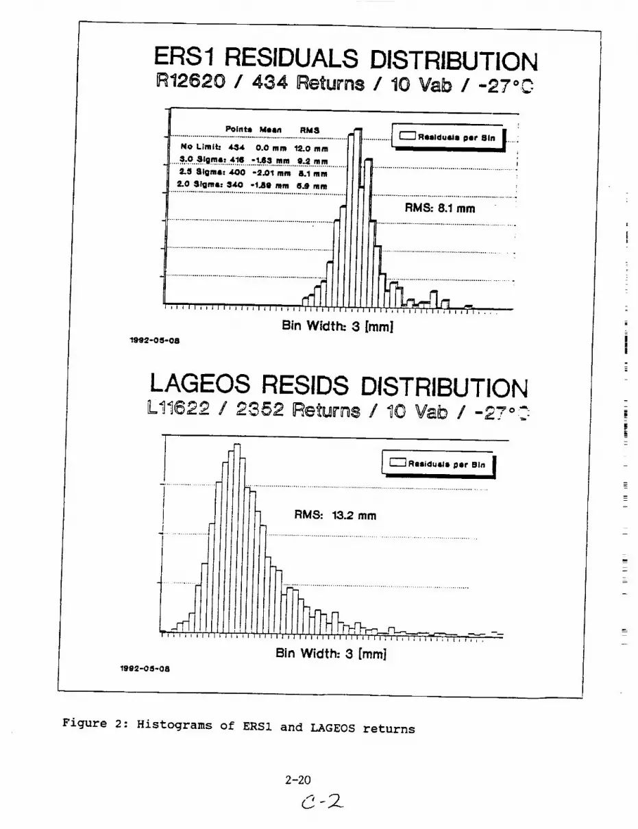
ERS1 RESIDUALS DISTRIBUTIONR12620 / 4,34 Returns / 10 Vab / -27 °r"
I_inta Mean RM8 _ Realduala pap Bin ....
No Llmlh ,184 0.0 mm 12.0 mr. i$.0 81gin4- 416 -1.68 mm 9.2 mm
2.5 Sigma, 4.00 -2.01 mm &l ram
2-0 Stgms: 840 -1.a9 mm 8J mm
Bin Width: 3 [mm]1992-05-08
LAGEOS RESIDS DISTRIBUTIONLt1622 t 2552 F_e_urn8 / 10 Vab / -27o?
i.......................l_r_'_...........................................................L3;'iiiil;iiii,'nl
I lIttilttl RMS: 13.2 mm
Bin Width: 3 [mini1992-05-08
Figure 2: Histograms of ERSI and LAGEOS returns

AJISAI RESIDS DISTRIBUTIONJOT000 / "i]3_0 IRetums / 10 Vab / -27 °
Strong Return Signal ,-_ Small Influence of Satellite Shape
........:...................'[[ ......................RiWsTiY.8_m....................................................
................................................_t l l l l ! ! l _1 ................................................................t r_.°...=.., s,. ii..............................................................
[ I i I I I t 1 d I t I I I I i I i i I I I I t i I I I I tlllltllll III11111 11 IIIII I
Bin Width: 3 [ram]
lgg2-QS-lS
AJISA! RESIDS DISTRIBUTIONJ_0_18 i _2 _el_u_n8 t t]0 V_b I-27°C
! Weak Return Signal --, Large Influence of Satellite Shape1
Ii
I
J ...................
I
I, ' : . . .
I i i I I i i i i'l-
f .....................................................................................................................RMS: 22.0 mm
t ....... ....Bin Width: 3 [ram]
1992-05-13
Figure 3: Histograms of AJISAI returns
2-21

_o. oo
M.1
t_¢ 8.00
4.00
P. O0
O. O0
-Z. O0
-4.00
-B, 00
-g. oo
-tO. O0
F34616 lg_1-12-f2 START 16 57 O. 6005 POINTS
• ". . , • ,
• • o" "" i'.: • . ... %.:. "- _: ".', .: •. " . . . • ." ;: 8.... "
._. ; ..-'_ -... • .... .. ":"....o"'."'... "• lr, ,I •• •% • • .% , .• •• • "% i" w"
• • , *• % "_ • ;• e t• .• " -Pj'_" ." .' •" . r • ', .• • ,{" -': .._, ; • ._, _:
".-. :'. :'.'...-• " . .... . ...- .:.•: ... : -':..:..., ... • . ::, ...,• -., • . .* -.''/.. . ..•--" . • . • . "
•. • _°• . • J- • •
e_,v.. :21 " .. :1 : .;..'. " .,•.e .,,._ "" • •'. ; "'_ • I-- " " ." " ;.*:"'•'_', .'--_" "l.'i-.-a-; ._--,_.--_," ":-
"'4,_.T_/ "-. : •" • '" ".": _'.." • "" _...'.':*:. " ""•-' _7_ .--'_._.'S,,;,,_ ".'r"_J" _" " "" " ""
¢ • .o o • . . • • [-_
,; ".:.;, :... ... .-'.
..... ":';'_'f'" " _'" "_ " ", "n'_":,,:-"., F:"• • •. . . ." • . % ". .
• • • . W" • . .....:.. •.e: . #" .t "_." °"
. o" -'qee . ".
• .. i • .. ,.
• -. • ' .....e.
• _ , . _ "
:_O " CO. : go 120 1500 180 210
62.7 ° ELEV^TION
H[HUTES/i, FTER START
240 270 300
Figure 4: Residuals of ETALON-2, showing semitrain returns
oi
.m
0c
F3-'5'.S ;gg_.-i2--L2 STAR" 18 57 O 5;52 POI:;TS S_7 o ELF/.C':I')•IT
| _.HS ---3. gC_ c,'n ,_.::TER 5"IpGL'{-F[TI TIHE ._[AS, -e8. O ms, P.^,_JGE BIAS, .'. g
• 20 -
.I0
-. CO
-._.C
"30". ___
t
-.30 i
0
Figure 5 :
- :. * ;-w. .. • ,¢" • "- .., ., _, .- . ._.
' "._#.:e_i;_4,_._O _'_7÷ _._ ,,
fi
I l I l
30 8C gC
Same ETALON-2,
:20
with
M.'::UTES .._-'-£;_ ST._R,
; 50 Z80 210 240 2"0 3CG
non-symmetric distribution
2-22
N94-15559
THE PRECISION OF TODAY'S SATELLITE LASER RANGING SYSTEMS
P.J.Dunn and M.H.Torrence, Hughes STX Corp., Lanham,MD
V.Hussen, Bendix Field Engineering Corporation, Greenbelt,MD
M.Peariman, Smlthsonian Astrophysical Observatory, Cambridge,Mass
Introduction
Recent improvements in the accuracy of modern SLR systems are strengthened by the new
capability of many instruments to track an increasing number of geodetic satellite targets without
significant scheduling conflict. This will allow the refinement of some geophysical parameters, suchas solid Earth tidal effects and GM, and the improved temporal resolution of others, such as Earth
orientation and station position. Better time resolution for the locations of fixed observatories will
allow us to monitor more subtle motions at the stations, and transportable systems will be able to
provide indicators of long term trends with shorter occupations. If we are to take advantage of these
improvements, care must be taken to preserve the essential accuracy of an increasing volume of
range observations at each stage of the data reduction process.
The Range Measurement
The SLR measurement is computed as one half of the product of an adopted value of the
speed of light and the observed interval between the transmit time of the pulse and the time of adetected return. The essential simplicity of this process is tempered by the need for careful
calibration for system delay and atmospheric refraction, as well as for an accurate survey of mount
eccentricity and other important local coordinates to match the millimeter accuracy of the best
current systems. The influence of satellite signature and detector time-walk must also be considered
at this high accuracy level, and we consider here the particular need to preserve any details of these
effects which may be lost in the current normal point compression process.
Normal Point Generation
The loss of detail at each stage of the process to reduce engineering data to normal points
is illustrated in Table 1, which shows the information content of each of the parameters measured
by most instruments for a typical satellite pass or pass sequence. Information on receive energy level
is not necessary if all time-walk characteristics of the detector system have been eliminated or
corrected before data compression. Neither will the absence of calibration details matter if the
distribution of returns is identical to that from the satellite and the same algorithm is applied to
reduce each observation. The accuracy of the satellite observations will be preserved aa long as the
return distribution is normal (or Gaussian) about the mean range.
Shape Factors
Two measures of the deviation of a distribution from normal are illustrated in Figure 1. Any
skewness in the pattern of range residuals about the mean would bias normal points if we assume
that the peak of the distribution is a better measure of the range. Skewness is computed from the
third moment of the residual distribution, just as the standard deviation is based on the second
moment: it is positive for a distribution with a tail towards long ranges, and negative (a rare
2-23

occurrence) when the noise is short. Another shape factor can be simply obtained as a combination
ofthlrd and fourth moments: kurtosls gives an Indication of flatness (low values) or peaklnesa (high
values). A resldual histogram with low kurtosis values can be produced by using a lower value of
the sigma multipller than three for data editing (clipping); high kurtosls values are obtained when
a larger sigma multiplier than three is employed, and the return signal appears as a spike in thebackground noise.
Interpretative Aids
The utility of these shape factors can be demonstrated with examples from several different
systems. To illustrate the mechanism used to build the basic contour picture which we have adopted
for data quality assurance we refer to Figure 2, which is a three-dimensional accumulation of a
number of pass histograms for LAGEOS ranges taken at the Grasse Observatory during a three
month interval. The vertical scale shows the percentage of range measurements which lie within ten
millimeter bins distributed about the mean value. An imaginative reader will observe a progression
from a nearly symmetrical distribution in December 1990 to a significantly skewed pattern in
February 1991: the front profile on 91-02-27 demonstrates the characteristic of long noise. Thecoarse grain caused by the centimeter bin width is softened in the contour of the same data which
is shown in Figure 3. The grey band of the contour scale shows a shift in the distribution in early
January 1991 and the lighter peaks also suggest a change in character at this time: the darker
contour levels emphasize the asymmetrical tail towards long ranges in January and February 1991.
Quantifying the residual behavior
Numerical descriptors for the changing residual pattern are shown in the scatter plot to the
left of the contour frame. The crosses depict a normalized skew factor which jumps from a low
(moderately skewed) to a high value at the same time that a low (flat peak) kurtosis measure returns
to a nominal level as shown by the open circles. The change in the pattern was caused by a
relaxation of the tight data editing criterion applied to the earlier observations which clipped the
distribution and muted the intrinsic asymmetry exposed with more liberal editing, The standard
deviation of the" full-rate data is recorded with the normal points in the currently adopted
compression scheme, so this event would be flagged as an increase in noise level, but the skew and
kurtosls shape factors provide improved diagnostics at a relatively low computational cost.
The cause of any data asymmetry can be lsolated by inspecting the distribution of the calibration
measurements: if the asymmetry is restricted to the satellite returns, the shift in the effective range
measurement due to the editing change would amount to over a centimeter and would cause an even
larger change In the apparent height or a station position determined from these observations. On
the other hand, similar levels of asDnmetry in the ground target returns would suggest a source in
the detector rather than the satellite, and if the same editing scheme was used for each data type,there would be no bias in the satellite measurements.
Satellite and Calibration Target Data
We have considered the shape of distributions from calibration and satellite targets in an
analysis of observations from six GSFC systems collected in early 1992. Figure 4 shows a collage
of residual histogram contours from the systems tracking several different satellites: ERS-I{E),
Starlette(S), LAGEOS(L), Ajisai(A), ETALON-I(E 1), and ETALON-2(E2). This broad representation
shows at a glance the higher noise level of the ETALON satellite returns, as well as the tight
2-24

precision of data from lower-orbiting satellites like ERS-1, which amounts to about 5 millimetersfor MOBLAS-7. The same ten millimeter bin scale is used to describe the characterlsties of these
instruments as for the data from Grasse in the earlier example.
The patterns for the appropriate calibration passes are given In Figure 5: they show less variation
than the satellite data, and allow us to discriminate satellite-dependent variations from detector
characteristics. None of the systems depicted here shows a systematic bias of more than a
millimeter, but subtle effects in the distribution for an individual system can be detected and
quantified by the skew and kurtosis shape factors plotted in the Figures provided for a couple of
the instruments. The satellite returns for Moblas-7 show no consistent kurtosts but a hint of the
positive skew typical of all systems' observations of the ETALON satellites (at the bottom of the plot);
the MOBLAS-7 calibration returns are slightly clipped (low kurtosis). On the other hand, TLRS-4's
satellite returns show no significant skew, but indicate a hint of clipping; this instrument's
calibration data possesses the rare property of slight negative skewness.
Summary
The effects of these idiosyncrasies in residual pattern for the GSFC systems is well below the
accuracy threshold for any currently employed application of the data, but they could be used to
characterize subtle changes in system characteristics. We have attempted to demonstrate in the
above examples tl_e enhanced ability to monitor data quality for any SLR system with some simple
shape factors which can be computed economlctilly in the normal point compression stage. Regular
inspection of these parameters can flag changes In data characteristics which affect range accuracy,
and also provide reassurance that our most advanced systems do indeed attain the millimeter
accuracy of which they are capable.
2-25

n
LUn
<a
LU>LU
LUt--
(9 <Z n" CO
LU ...I ZLU D _Z LL 13.-- 121 ._1_ ixl <Z m _w CO rr"N "' oO< Zrr" O
rr-
2-26
-_O@
4-1 0
_ O
_ _._
-,.4
_-,.4
®NO
o=_
°o .I..I -,'4r-t Ul 4J
-,-t
=|
i
=
z

2-27

2-28
_QJO_
0
Ul m
0
0_I
t/l
_ -,-.I
o_
r..I -r.t
=
_0
_J
_0
0
QI
0
011)_

J_
@
2-29

f
2-30
I I I I I I
I I ! I I I I I
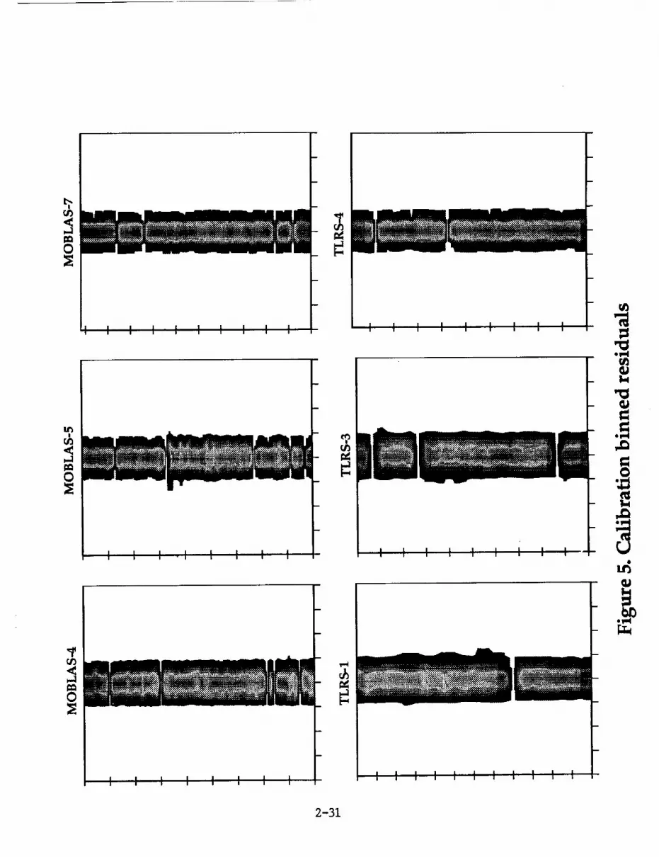
!
O
I
l L I ,I I I I I
I
I I I I I I I I
I I
I I I I I I I I I
Iu
2-31

OL
I I i t ! oL-, ' T' • . ....
!
<
0
0
m
,I-,4
_J
QJ
_J
m
-OLo
__ ___._o o_go__ _ _o __. _ ___. . =x 0
.... -o t l :1-- I-- T......... l--° o g." l ! I i i I 0_-
2'32

I I L I ! I , I I _ ! I I ! t I I ! I
rj_
E-
_n
oMI_n
,.0
,,MI
r,j
,.l-)eM.I
,,k.l
_D
QJ
oMl
l
2-33
I f= I.:__
0
OL
5
0
Or-

N94-15560SLR Data Screening; location of peak of data distribution
A.T. Sinclair
Royal Greenwich Observatory, Madingley Road, Cambridge CB3 0EZ, England
1. Introduction
At the 5th Laser Ranging Instrumentation Workshop held at Herstmonceux in 1984 consider-
ation was given to the formation of on-site normal points by laser stations, and an algorithmwas formulated. The algorithm included a recommendation that an iterated 3.0 x rms re-
jection criterion should be used to screen the data, and that arithmetic means should be
formed within the normal point bins of the retained data. From 1990 September onwards
this algoritm and screening criterion have been brought into effect by various laser stations
for forming on-site normal points, and small variants of the algorithm are used by most
analysis centres for forming normal points from full-rate data, although the data screeningcriterion they use ranges from about 2.5 to 3.0 x rms. At the CSTG SLR Subcommission _
working group was set up in 1991 March to review the recommended screening procedure
The working group consists of A.T. Sinclair (chairman), G.M. Appleby, R.J. Eanes, P.J.
Dunn and T.K. Varghese. This paper has been influenced by the discussions of this workinggroup, although the views expressed are primarily those of this author.
The main thrust of this paper is that, particularly for single photon systems, a more im-
portant issue than data screening is the determination of the peak of a data distributioll.
and hence the determination of the bias of the peak from the mean. Several methods of
determining the peak are discussed.
2. The effect of skew data
The first stage of forming normal points (described by Appleby in these proceedings) is to
fit a trend-function to the raw ranges or to their residuals from a predicted orbit so that all
signature from the orblt is removed, _d then the distr_but:ion of the trend-removed data
can be examined. Some level of screening is needed in the]terative process of fitting a trend-
function, but this is not critical; 3.0 x rms or perhaps even tighter should be fine, and finallya wider band of trend-removed data, say 5:0 x rms, should =_e:retained for examination of the
distribution and then final screening, if these :data have a symmetrical distribution about
the peak then the criterion used for final screening is not critical, and a 3.0 × rms screeningand use of the arithmetic mean should be fine. However if the data have a skew distribution
then the arithmetic mean will be biased away from the peak, and the amount of bias will
probably be dependent on the level of final screening used.
Analysis of the raw data from numerous stations shows that stations operating at a multi-
photon return level per shot tend to have a fairly symmetrical distribution of data, wherea_
those operating at a single photon return level frequently show a significant skewness in the
distribution of the data, usually skewed towards long ranges. As is described in papers b:_
w
_=
z[]
2-34 z

Appleby and by Kirchner in these proceedings, some satellites (particulary Ajisai) impose
their own signature on the laser data and can cause skewness as has been detected by some
single-photon systems. However it is probable that some of the skewness is caused by the
laser systems themselves, and it is certainly not the intention to explain away features of
the system as being due the satellite. However if the skewness is due to the satellite thena means must be found in software of handling it. If it is due to the system then one view
is that it is an engineering problem and that the hardware should be adjusted, but another
view is that hardware will never be perfectly adjusted, and that one should accept some
level of real-adjustment and calibrate the effect out with software. Also it is possible that
some detectors such as avalanche photo-diodes have an inherent skewness which would be
very difficult to remove by adjustment of the hardware.
Systems which operate at a multi-photon return level and use pulse-level detection are in
effect using hardware to form a mean of the individual photon returns obtained each shot,
and so will see little effect from the distribution structure of the individual returns. Systems
which operate at multi-photon level and detect the first photon received will primarily see
the leading part of the distribution and will see little effect of any skew tail. Hence these
system use a hardware method to eliminate any effects of satellite signature, and must ensurethat the hardware is set up so as not to cause any biases. The objective of this paper is to
devise an equivalent software scheme for systems operating at single photon return levels.
3. Choice of reference point of data distribution
The current recommendation is that the reference point of a data distribution should be the
arithmetic mean of the' data retained after a 3.0 x rms screening. This may not be ideal for
a skew distribution of data.
If a skew data distribution is entirely caused by the laser ranging system, and if the ranges
to the terrestrial calibration target have the same skew distribution as the satellite ranges.
then it probably does not matter what screening criterion is used, provided the same is
used for both calibration and satellite ranging, and it will probably be satisfactory to take
the arithmetic mean of the data, even though this does not give the peak of a skew data
distribution. However if the satellite is adding a significant contribution to the distribution,
or if for some other reason the distributions of calibration and satellite data are different,
then it is probably best that some means of processing the data should be devised such that
the peak can be located. This is because, in the complicated coxivolution of the signatures of
the system and the satellite, the range represented by the peak corresponds to the distance
travelled by a photon from the peak of the laser pulse to the peak reflection point of the
satellite (and so the centre of mass correction for the satellite should be that corresponding
to peak reflection as determined in pre-launch testing).
Note that for a satellite pass it is not the peak of the trend-removed data for the whole pass
that is required, but the peak of the distribution of the data within each normal point bin.
This is a problem as there may not be sufficient points within a bin to give a reasonable indi-cation of the distribution. The solution we recommend is that both the peak and arithmetic
mean of the whole pass should be determined, and the difference, or bias, of the mean from
the peak shouM thus be determined for the whole pass. Then within each normal point bin
2-35
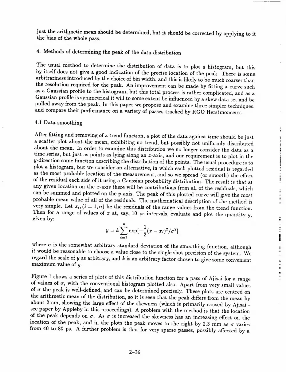
just the arithmetic mean should be determined, but it should be corrected by applying to itthe bias of the whole pass.
4. Methods of determining the peak of the data distribution
The usual method to determine the distribution of data is to plot a histogram, but this
by itself does not give a good indication of the precise location of the peak. There is some
arbitrariness introduced by the choice of bin width, and this is likely to be much coarser than
the resolution required for the peak. An improvement can be made by fitting a curve such
as a Gaussian profile to the histogram, but this total process is rather complicated, and as a
Gaussian profile is symmetrical it will to some extent be influenced by a skew data set and be
pulled away from the peak. In this paper we propose and examine three simpler techniques,
and compare their performance on a variety of passes tracked by RGO Herstmonceux.
4.1 Data smoothing
After fitting and removing of a trend flmction, a plot of the data against time should be just
a scatter plot about the mean, exhibiting no trend, but possibly not uniformly distributed
about the mean. In order to examine this distribution we no longer consider the data as a
time series, but just as points as lying along an x-axis, and our requirement is to plot in the
y-direction some function describing the distribution of the points. The usual procedure is to
plot a histogram, but we consider an alternative, in which each plotted residual is regard(.d
as the most probable location of the measurement, and so we spread (or smooth) the eff(,cr,
of the residual each side of it using a Gaussian probability distribution. The result is that at
any given location on the x-axis there will be contributions from all of the residuals, which
can be summed and plotted on the y-axis. The peak of this plotted curve will give the most
probable mean value of all of the residuals. The mathematical description of the method is
very simple. Let xi, (i = 1,n) be the residuals of the range values from the trend function.
Then for a range of values of x at, say, 10 ps intervals, evaluate and plot the quantity y,given by:
n
y=k Z :-Ix-I
i=l
where a is the somewhat arbitrary standard deviation of the smoothing function, although
it would be reasonable to choose a value close to the single shot precision of the system. We
regard the scale of y as arbitrary, and k is an arbitrary factor chosen to give some convenientmaximum value of y.
Figure 1 shows a series of plots of this distribution function for a pass of Ajisai for a range
of values of a, with the conventional histogram plotted also. Apart fi'om very small values
of a the peak is well-defined, and can be determined precisely. These plots are centred on
the arithmetic mean of the distribution, so it is seen that the peak differs fi'om the mean by
about 2 cm, showing the large effect of the skewness (which is primarily caused by Ajisai -see paper by Appleby in this proceedings). A problem with the method is that the location
of the peak depends on a. As a is increased the skewness has an increasing effect on the
location of the peak, and in the plots the peak moves to the right by 2.3 mm as a varies
from 40 to 80 ps. A further problem is that for very sparse passes, possibly affected by a
=
_!
z
2-36

significant amount of noise, the method fails to give a single main peak, or requires a large
value of a in order to do so.
4.2 Tight rejection criterion
The arithmetic mean of a set of data will be biased away from the peak due to any skewness of
the data, but the amount of bias will be reduced if a tighter rejection level is used in forming
the mean. We look at the effect of using various rejection levels, expressed as multiples
of the root mean square difference from the mean (rms). However the rms of the retained
data varies and usually gets smaller as the rejection limit is reduced, so for clarity we first
determine the mean and rms using a 3.0 × rms iterated rejection level. Then subsequent
rejection levels are expressed as multiples of this fixed rms. It also aids convergence with a
tight rejection level if the rejection level itself does not vary as the iterations proceed. The
table below gives the results of using various rejection levels on the Ajisai pass shown in
Figure 1, with the various determinations of the mean given relative to the mean obtained
using 3.0 x rms rejection.
Rej. Mean(era) No.Pts.
3.0 x rms 0.00 1104
2.5 x rms 0.19 1081
2.0 x rms 0.58 1030
1.5 x rms 1.18 936
1.0 × rms 1.72 799
0.5 × rms 2.13 501
The peak of the distribution, as given by the smoothing method, is about 2 cm from the
initial mean, and it is seen that the successive estimates of the mean move closer to the peak
as the rejection level is reduced. For the rejection level of 0.5 × rms a large number of points
have been rejected, and also in tests on various passes some difficulty was experienced ill
obtaining convergence. So for subsequent tests we have adopted a level of 1.0 × rms.
Objections that are frequently raised to using a tight rejection level are that too much data
is being discarded, and that the data are being made to look better than they really are.
However what we are proposing is that this tight rejection level is used only for the purpose
of obtaining an estimate of the peak of the pass distribution, so that the bias of the peakfrom the 3.0 × rms mean can be determined. The means in the normal point bins and the
value of the rms of the whole pass will be calculated from the data that remain after making
a 3.0 × rms rejection.
4.3 Pearson curves
A distribution of n points xi with mean 2 is characterised to a large extent by its moments
#2, #3, #4 where
• n
= - zi - x')J#J n
2-37

The second moment is the square of the standard deviation. The following quantities arealso defined:
Skewness 2 3= /%/g2 indicates deviation from symmetry, = 0 for symmetry about
Kurtosis =/z4/_t_ 2 indicates degree of peakiness, = 3 for Gaussian distribution.
These quantities are dimensionless and of restrained magnitude, and so are in some appli-cations more convenient than the 3rd and 4th moments. This conventional definition of
skewness has the disadvantage that the sign of the 3rd moment is lost, and it is this which
describes the direction of the skewness. (It may be better to define skewness as _3/_/2.)In the plots in this paper we attach the sign of the 3rd moment to the skewness.
There is a method in statistics of deriving a distribution function from values of these three
moments obtained from a set of data. These are the Pearson distributions (see description by
M.G. Kendall, The Advanced Theory of Statistics, Vol 1, 1947). The distribution function
f of the quantity :r is defined by a differential equation
df (x-a)f
dx bo + bl x + b2x 2
where
a = -I,3(1t4 + 3#_)/A
bo = -#2(41,21t4 - 3#])/A
bl = -t'3(/0 + 3#22)/A
b2 = -(2tt2P4 - 31t32 - 6tz32)/A
.4 = 10#4#2 - 18#,_ - 12#2
and where the origin of x is now at its mean value. The peak of the distribution curve is atx=a.
This differential equation has several forms of analytical solution depending on the values of
the moments. For values likely to be met in practice its solution is of the form
f = k(1 + _-] )"'(1 - x---) TMa2
but for the precise values of the moments corresponding to a Gaussian distribution this
solution becomes singular, and it has an alternative solution which is in fact the Gaussian
distribution. So unfortunately the analytical solution is close to a singularity in the region
likely to be met in practice, and so is not a very useful way of deriving the shape of the
curve. However it is easy to solve the differential equation by numerical integration starting
from the peak, although there can be problems as the singularity on the x axis is approached
2-38

which require a little fudging. Some solution curves are shown in Figure 2 for a range of
values of skewness and kurtosis. No attempt has been made to normalise the area under
the curves; they are all plotted with the same height at the peak. It is seen that the shapes
of the curves are close to a Gaussian curve until fairly extreme values of the parameters
axe reached, eg., skewness of 0.6 or kurtosis of 2.2, and then the shapes are not particulary
typical of what is seen in some SLR data, and so it can be expected that this method will
give a good estimate of the peak for distributions close to Gaussian, but not be so useful in
more extreme cases.
This discussion of how to plot the Pearson curves is given here for completeness, but it is
not proposed that this should be a normal procedure for SLR data handling. However the
method provides a simple estimator of the location of the peak of a. distribution of data.
Expressed in terms of the standard deviation _r, the skewness s, and the kurtosis k, with
consideration given to the sign of the 3rd moment, the displacement of the peak from the
mean is
-sl/2a(k + 3) x sign(It3)
lOk - 18 - 12s
5. Comparison of methods of peak determination
Figure 3 shows the results of applying these various methods of peak determination to a
number of passes tracked by RGO Herstmonceux. The passes were selected to provide a
good test of the methods, and are not necessary typical passes from the station. The figures
give the following information:
• the conventional histogram, using a bin of 40 ps (= 6 mm)
• the smoothing-method distribution function plotted as a solid curve
• the Pearson distribution function plotted as a dashed curve
• the 3 × rms-rejection mean shown as a solid vertical line from the top
• the 1 × rms-rejection mean shown as a dashed vertical line from the top.
The two distribution curves are plotted with slightly different peak heights for clarity, and
the peak height of the histogram is limited if necesssary to be slightly below these two curves.
The information 'given in the captions includes:
• Smoothing parameter cr in ps (multiply by 0.15 to get mm)
• Bias(l): difference of smoothing-method peak from 3 × rms mean
• Bias(2): difference of 1 × rms mean fi'om 3 × rms mean
• Bias(3): difference of Pearson peak from 3 × rms mean.
Figures 3(a) and 3(b) show passes with insignificant skewness, in which all methods of
determining the peak and mean agree well.
2-39

Figures 3(c), 3(d) and 3(e) show passes with significant skewness, in which smoothing,
Pearson and 1 x rms agree well, but axe significantly different from the 3 x rms mean.
Figures 3(f) and 3(g) show passes in which smoothing and 1 x rms agree well, but the Pearson
peak stands off, and all differ from the 3 x rms mean.
Figures 3(h) and 3(i) show passes in which the Pearson peak and 1 x rms agree fairly well,
but the smoothing peak stands off.
From these and tests on numerous other passes we conclude that:
• for a single-photon station there is often a significant difference of the peak from the
3 x rms-rejection mean
• the 1 x rms-rejection mean usually agrees with one or other of the smoothing peak
and Pearson peak, and often with both.
6. Recommendations
In conclusion we recommend the following:
a) the ranges to a calibration target or the trend-removed data from a whole satellite pass
should be screened at an iterated 3 × rms level, and in the process determine rms and mean
of the retained data
b) the skewness and kurtosis of the retained data should be determined
c) using this fixed value of rms a second determination of the mean should be made using
an iterated 1 × rms rejection. This provides an estimate of peak. Then the bias of the
calibration or pass is bias = peak - mean
d) for a calibration run, use the value of peak as the calibration value
e) for a satellite pass, form normal points from the screened data within each bin in the
usual way, but add the correction bias to the normal point.
2-/40
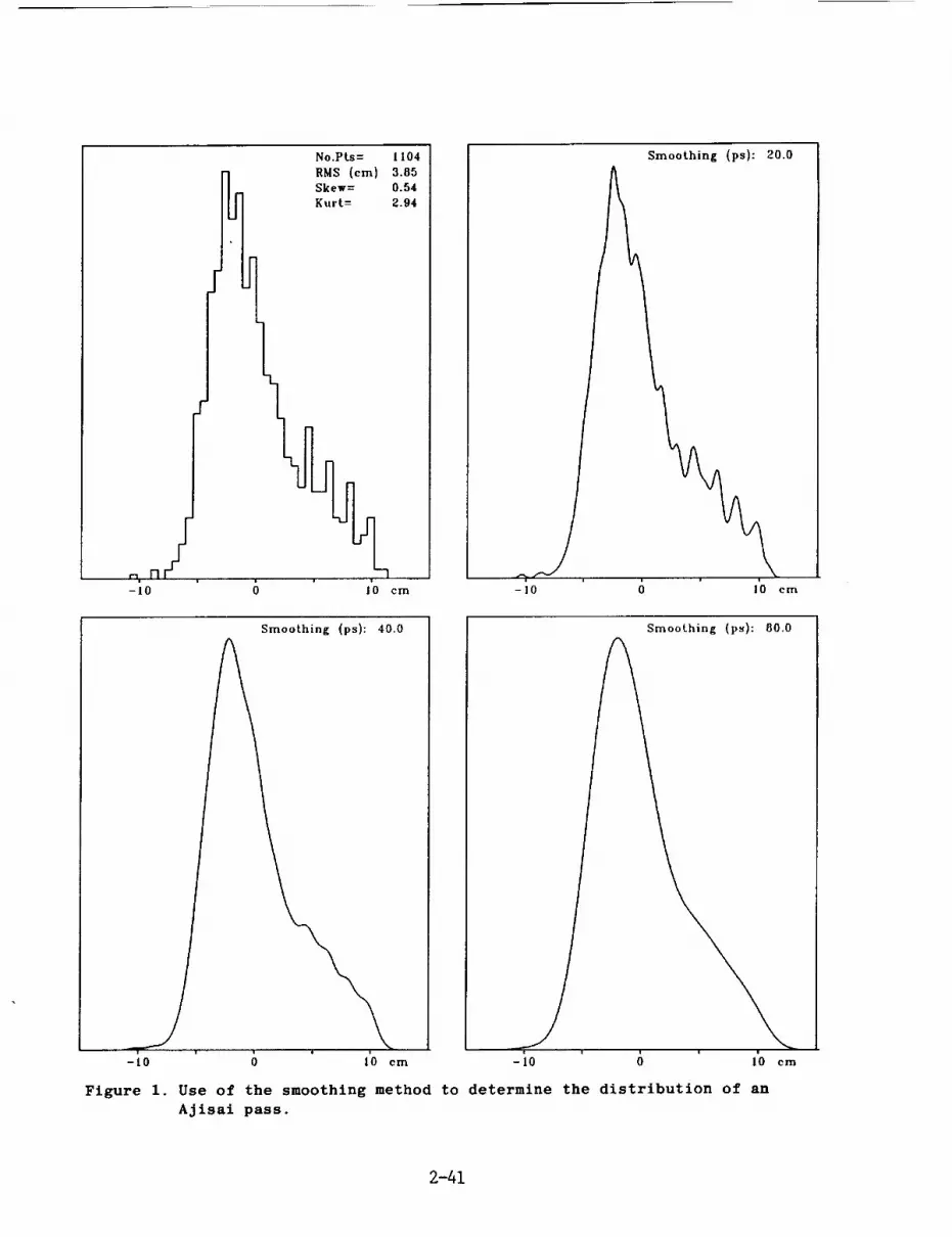
No.Pts= 1104
RMS (cm) 3.85
Skew= 0.54
Kurt= 2.94
I0 cm
Smoothing (ps): 40.0
Smoothing (ps): 20.0
-10 0 I0 em
Smoothing (ps): 00.0
-tO 0 10 cm -10 0 10 em
Figure 1. Use of the smoothing method to determine the distribution of an
Ajisai pass.
2-41

/-lO
RMS (era) 3.00
Skew':- 0.00
Kurt= 3.00
RMS (era) 3.00
Skew_ O. i 0
• ,00
-10 0 10 cm
-I0
RMS (era) 3.00
Skew= 0.40
urt= 3,00
210 ©m
RMS (era) 3.00
Skew= 0.80
= 3,00
-iO 0 I0 cm -iO
RMS (era) 3.00
// Skews- 0.00
Kurt: 2.60
-lO
RMS (©m) 3,00
i _ 0.00
3.40
0 I'0 cm
Figure 2. A range of Pearson distribution curves.
-|0
I_S (cm) 3.0o
Skew: 0.20
urt= 3,00
RMS (era) 3.00
_;kew= 0.00
: 2.20
/ ,0 I0 cm
RMS (¢m) 3.00
Skew= 0.00
= ,Bo
0 lO cm
2-42

Pare 105
0105001
(-)
palm 219
7BO3gOI
(d)
Pare 122
0105001
(b)
I'0 cm
SmoothlnC (ps): 80.0No.Pts_ 4i0 i
IUdS (era) 2.36
Skew- 0.54
Kurt= 3.66
Bi.s(1)= -l.03
Bias(2): -l.Oi
Bias(3)= -I.17
t
i
Ill _
10 em
TPau s'16 iB60_lOI
IPass 218 i6606101
(f) / \.
!lo em
Smoothing (p_): 80.0
No,PtJ= 1104
Rids (era) 3.B5
Skevw 0.54
Kurt= 2,94
Blam(l)z -2.01
Btas(Z)s -I.72
_ss{3)_ -3.74
10 em
Figure 3. Comparison of methods of peak determination.
2-43

N94-15561
ADAPTIVE MEDIAN FILTERING FOR PREPROCESSING
OF TIME SERIES MEASUREMENTS
Matti Paunonen
Finnish Geodetic Institute
Ilmalankatu IA
SF-00240 Helsinki, Finland
Telefax:358-0-264995
ABSTRACT.
A median (Ll-norm) filtering program using polynomials was
developed. This program was used in automatic recycling
data screening. Additionally a special adaptive program
to work with asymmetric distributions was developed.
Examples of adaptive median filtering of satellite laser
range observations and TV satellite time measurements are
given. The program proved out versatile and time saving
in data screening of time series measurements.
i. INTRODUCTION
The advantages of data screening of satellite laser range
measurements using median (or Ll-norm) instead of least
squares were shown earlier (Paunonen 1989). The median is
known to be insensitive'to outlying observations, which is
a useful property in preliminary data screening of anytime series measurements. Asymmetric distributions often
arise for various reasons; saturation of the laser detector
and the receiver electronics, laser prepulses etc. This
cannot be easily treated with least squares methods.
In response to multiple needs, a median program permitting
use of a higher order polynomial of up to ten was developed.
A second version used automatic recycling of the fitting loop
until a specified fit was obtained and a special program to
work with unsymmetric distributions was devised. Examplesof screening satellite laser range observations and TV
satellite time measurements are given.
2-44

2.1 MEDIAN PROGRAM
The median program was constructed with the Fortran-
procedure published by Barrodale and Roberts (1974),
modified for polynomial use. The function to be minimized
in the overdetermined case is
M
_"lYil - a - a x - a2 x2 N Io 1 i i - "'" - aNxi(1)
where Yi are the observations, xi the observing times (here),
M the number of observations and N the degree of the
polynomial to be fitted to the observations, and aj (j=0...N)the coefficients of the polynomial.
2.2 AUTOMATIC MEDIAN FILTER PROGRAM
A versatile data screening program should be able to run
automatically, without any manual interface. The median is
good basis for a filtering program, because it selects reliably
the densest part of the measurements as a reference. This means
that any erratic points, that is out[iers, are of true size, and
not evened out as in the least squares method. Operation of the
sequential median filtering program is started by forming the
residuals of all the observations and calculating their average.
Observations below a certain rejection limit are selected
for the next cycle only. The problem is to find a suitablelimit which is neither too inclusive nor too exclusive. Good
operation was obtained by using the rejection level, R,
R = 3.5 * AVR , (2)
where AVR is the average of the residuals in the earlier
round. For a Gaussian-shaped distribution the width between
the zero and the point corresponding to one standard
deviation is 1.46 times the width corresponding to the
average. Thus the limit used is roughly equivalent to 2.4
times the standard deviation used in the least squares
method. The repeated rounds are limited to four, but the
final selection is generally ready after three rounds.°:
2.3 ADAPTIVE AUTOMATIC MEDIAN FILTER PROGRAM
In practice, the distribution of the data may be asymmetric
and may include separated peaks. In satellite laser ranging,
a distribution as shown in Fig.l can easily arise with mode-
locked lasers. The transmitted pulse may contain a small
prepulse if selection of a single laser pulse from a train
of mode-locked laser pulses is incomplete. Even if the
parasitic pulse is small, it causes stops in the photon
counting mode. This poses difficulties for normal
screening methods using least squares. Use of only
2-45
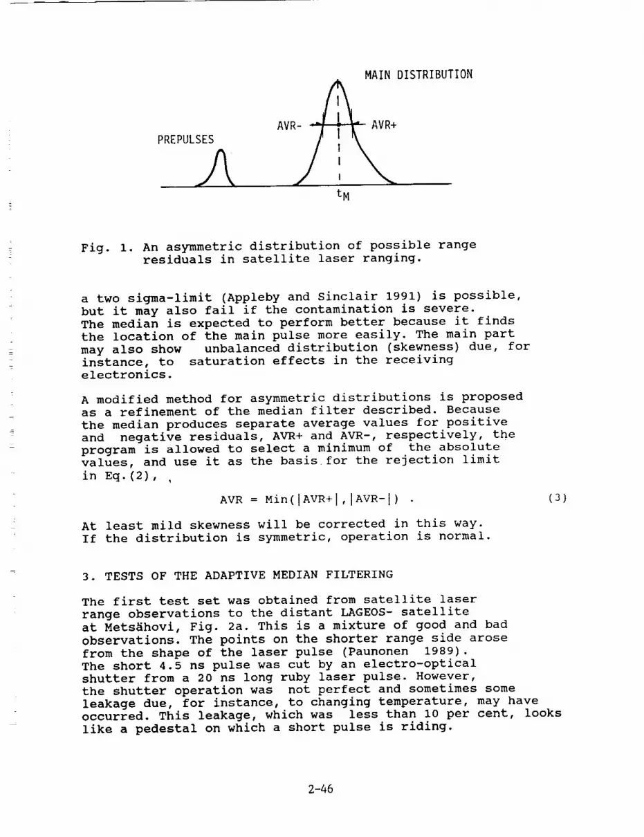
PREPULSES
MAIN DISTRIBUTION
AVR- _ AVR+
/,,\tM
Fig. i. An asymmetric distribution of possible rangeresiduals in satellite laser ranging.
a two sigma-limit (Appleby and Sinclair 1991) is possible,
but it may also fail if the contamination is severe.
The median is expected to perform better because it finds
the location of the main pulse more easily. The main part
may also show unbalanced distribution (skewness) due, for
instance, to saturation effects in the receiving
electronics.
A modified method for asymmetric distributions is proposed
as a refinement of the median filter described. Because
the median produces separate average values for positive
and negative residuals, AVR+ and AVR-, respectively, the
program is allowed to select a minimum of the absolute
values, and use it as the basis for the rejection limit
in Eq.(2), ,
AVR = Min(IAVR+I,IAVR- I)
At least mild skewness will be corrected in this way.
If the distribution is symmetric, operation is normal.
(3)
3. TESTS OF THE ADAPTIVE MEDIAN FILTERING
The first test set was obtained from satellite laser
range observations to the distant LAGEOS- satellite
at Mets_hovi, Fig. 2a. This is a mixture of good and bad
observations. The points on the shorter range side arose
from the shape of the laser pulse (Paunonen 1989).
The short 4.5 ns pulse was cut by an electro-optical
shutter from a 20 ns long ruby laser pulse. However,
the shutter operation was not perfect and sometimes some
leakage due, for instance, to changing temperature, may have
occurred. This leakage, which was less than i0 per cent, looks
like a pedestal on which a short pulse is riding.
2-46
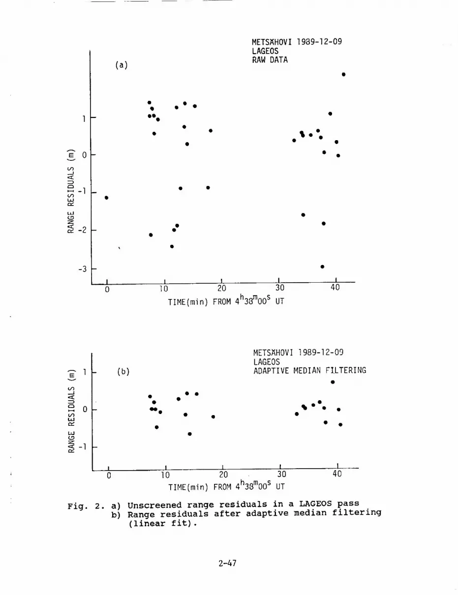
,== 0v
r..,r).._i,,cI::::D
'--' -lc/')wr_
w
z,,=I:c_-2
-3
(a)
METSAHOVl 1989-12-09
LAGEOSRAW DATA
I I I I I0 I0 20 30 40
TIME(min) FROM 4h38mo0 s UT
"-" 1I=
v
c,r}.._I
D,r-.,,-., 0or)w
z,,==:-]rY-
(b)
METS_HOVI 1989-12-09LAGEOSADAPTIVE MEDIAN FILTERING
qD• • •4We
I I 1 I I
0 10 20 30 40
TIME(min) FROM 4h38mo0 s UT
Fig. 2. a) Unscreened range residuals in a LAGEOS passb) Range residuals after adaptive median filtering
(linear fit).
2-47

_O00_O000_QO00_O000_ 0 • O_ 0 0 00000 _ 0_00_
11920
11915
I,I
l-- 11910
11905
(a)
0
0
o
0
0
0
0
o0
0 0 0
0 0 0
0
0
0 00
o
0
0 0
0
0
0
0
0
0 0
1 I I J j j j0 2 4 6 8 10 12
TIME (min) FROM ohomo s, DAY 267, 1991
o
.--I
::)
(/)
r_"
20
10
0
-10
-20
(b)
0 0
_0_-- 0 O0 0 0
- oo4O0ooooO Oo.0
00
0 0 o0 0 0
0 0 0
00 0
o o
] I I0 2 4 6 _ I_ It2
TIME (min) FROM ohomo s, DAY 267, 1991
Fig. 3. a) Unscreened time measurements from a TV satellite
b) Time residuals after adaptive median filtering(parabolic fit).
2-48

The energy ahead of the main pulse may stop the time interval
counter. The adaptive median filter selected 22 observations
from the 33 available ones (Fig. 2b). The initial data set is
not random, because similar results were also obtained at the
calibration line. The result is also plausible, because its
width corresponds to the laser pulse width. The earlier
method for testing one observation at a time (Paunonen 1982)
would be of little value, without knowing what to seek.
Another test set originated from recent TV satellite time
measurements (Fig. 3a). Here the second tick from the station
clock started the time interval counter and the horizontal
syncronization pulse from a satellite TV receiving system
(50 Hz rate) stopped it. The large number of badly timed
pulses propably originated from the encrypting method
the TV transmission (program RAIUNO on the EUTELSAT I-F5
satellite) is using. This set was also cleared well with the
adaptive median filter (Fig. 3b). The r.m.s, value of theresiduals was Ii ns.
4. DISCUSSION AND CONCLUSIONS
The adaptive median filter has proved to be versatile and
to save time. It can safely remove several outliers, how-
ever large they are. This is a big advantage over the least
squares method, in which all large outliers must be removed
before any useful operations can be obtained. Polynomials
should be used with care also in median filtering.
End points in particular may behave peculiarly.
The median program sets the value of some residuals at zero
(this number is same as the degree of the polynomial),
which is artificial. The asymptotic estimation efficiency
of median is also usually worse than that of the
mean (Eadie, et.al.,1971). It seems therefore best to use
the median in the data screening phase and to use the normal
least squares method for final extraction of the results.
Use of the least squares is then well justified, because
the distribution of the screened data is nearly normal.
REFERENCES
Appleby, G.M. and A.T. Sinclair (1991). Formation of on-site
normal points. Satellite Laser Ranging Newsletter, SLR Sub-
commission of the CSTG (International Coordination of
Space Techniques for Geodesy and Geodynamics), April 1991,
pp. 25-28.
Barrodale, I. and F.D.K. Roberts (1974). Solution of an over-
determined system of equations in the ii norm.
Communications of the ACM, Vol. 17, No. 6, pp. 319-320.
2-49

Eadie, W.T., D. Dryard, F.E. James, M. Roos, B. Sadoulet(1971). Statistical Methods in Experimental Physics.North-Holland Publishing Company, Amsterdam 1971,
296 pp.
Paunonen, M. (1982). Studies on the Mets_hovi satellite
laser ranging system. Reports of the Finnish Geodetic
Institute, 1982:2, Helsinki 1982, 47 pp.
Paunonen, M. (1989). Use of the Ll-norm in screening laser
range observations to satellites. Proc. of the 18th
INTERKOSMOS Symposium on the Use of Artificial Satellite
Observations for Geodesy and Geophysics, June 12-17,
1989, Cracow, Poland, (Ed. WL. Goral, Polish Academy of
sciences, Observations of Artificial Satellites of the
Earth, No 27, Warsaw 1990), pp. 359-362.
2-50

N94-15562
SATCOP MISSION PLANNING SOFTWARE PACKAGE
S. BUCEY
Bendix Field Engineering Corp.
Seabrook, MD
New laser ranging capabilities, additional satellites, and changing
priorities are making it more difficult to determine the most efficient
method of operations for NASA's CDSLR Network. A software package called
SATCOP (Satellite Ranging Coordination Programs) has been developed to
assist in mission support and planning operations. Its uses range from
planning daily station operations to conducting pre-launch satellite
visibility studies. SATCOP provides a listing and graphics output of
satellite visibility for a given occupation site for any time period.
SATCOP may also be used to determine the optimum ranging scenario for a
station, taking into account satellite ranging priorities and station
operational requirements. Finally, SATCOP may be used to illustrate
simultaneous satellite visibility for multiple stations.
Introduction
As the CDSLR Network grows into the 1990's it is undergoing many
changes in both its capabilities and requirements. On the one hand great
progress has been made in terms of increasing the SLR systems'
performance. Upgrades to the onsite computer and improved laser ranging
hardware have greatly increased the number of satellite passes which can
be acquired during an operating shift by reducing the amount of time
needed for operations other than actual ranging. On the other hand, more
requirements have been placed on the systems. Many more satellites have
become available, with more scheduled for launch, thus increasing the
likelihood of simultaneous satellite visibility. In addition, the
possible scenarios required for ranging these many satellites are changing
frequently, with conflicting priorities and needs.
It became apparent that some tools needed to be developed to assist
the planners in determining Network ranging priorities. Such tools have
been developed at Bendix under the direction of NASA's Dynamics of the
Solid Earth Project (DOSE) for both long range planning and routine
operations to maximize the amount of data collected. This paper will
review some of these tools and describe their uses.
2-51

The SATCOP software package has several parts which are used for both
routine operations and pre-launch scheduling. The use of such software
helps determine pre-mission requirements such as ground track
determination, forecasted station performance, predictions of optimum
system locations, and predicted satellite visibility. SATCOP also
produces graphs of ground tracks of acquired passes; determines
availability of simultaneous ranging opportunities; schedules operating
hours for maximum visibility; and produces automated single station
scheduling for daily station activities.
Figure 1 is a time plot of satellite visibility for a given station.
This figure demonstrates that even with just 6 satellites considered the
opportunities for laser ranging are abundant. Such plots, and others like
it, are used for operational scheduling of station activities and for the
determination of operational requirements for future missions or
locations. Typically such a plot is done for a 7 day period, but the
number of satellites and number of days is user determined. The plot
consists of a time scale in hours GMT across the top, and a day scale down
the left. A subscale of each day is present, dividing each day into a
line for each satellite. _Fofeach satellite, atw_ietter satellite
identiffer indicates the h0rizontal line across which the satellite could
be visible (refer to Figure 8 to identify the satellite associated with
each two letter identifier). Across the plot a solid line indicates when
a satellite is visible, and a total number of minutes for that day is
printed on the right. On the last day of the plot a column on the right
also indicates the total number of minutes visible during the time periodof the plot.
Figure 2 illustrates the number of possible sightings of two
satellites over a four day period at 5 locations. Such graphs are used
when extended time periods are considered, and can be used to compare
satellite visibility at several stations simultaneously. Such graphs are
useful for determining the best of several possible station locations and
the expected visibility at a given location, and can include several
satellites. Often it is also desired to know the number of possible
simultaneous sightings of a satellite for several locations. Figures 3
and 4 demonstrate the tools used for determining this number. Figure 3 is
a matrix showing the number of mutual sightings possible at several
locations. The number of such sightings for a given pair of stations is
found by cross indexing between the two desired stations to find the
result within the matrix; as an example for MOBLAS 4 (7110) and MOBLAS 8
(7109) the number of such sightings is found to be 130. Figure 4 is a
listing of all possible subsets of the desired stations which can range,
along with the times of mutual availability. The user can determine the
minimum number of stations desired for simultaneous ranging, and the time
period for consideration.
The SATCOP software package has been developed to provide support for
other purposes as well. Figure 5 is a plot which shows the distribution
of acquired LAGEOS passes reported as quicklook data for the time period
May 2 to May 14, 1992. This type of plot allows the user to quickly
2-52

determine the geographic distribution of data reported during the
indicated time period. Figure 6 is used to compare sightings for two or
more stations over a 24 hour period, and is read similarly to Figure 1.
Such a graph is convenient for quickly determining the opportunities for
coordinated activities between two or more locations with one or more
satellites.
A major use for the SATCOP package is single station scheduling for
daily activities. The purpose of such scheduling is to assist the station
crew in conducting laser operations by considering as many of the
requirements and opportunities presented to the station as possible, and
then producing a schedule which is a possible 'optimum' solution for the
day's activities.
To perform such scheduling many parameters are considered. A major
requirement is to resolve ranging opportunities when two or more
satellites are visible simultaneously. SATCOP considers satellite
priority, ranging limitations such as a maximum time limit on a satellite
pass, and day or night ranging restrictions. If two satellites of the
same priority are available then the software ensures that ranging is as
evenly distributed between the two during the day as possible, based on
available minutes of data. Activities which may exclude laser activities
are taken into account, such as data preprossessing and calibration time.
If the system has the multi-satellite calibration capability then the
software determines a best sequence for calibration and ranging.
As an example a schedule generated for MOBLAS 4 at Monument Peak will
be considered, using the time period covered by Figure 1. Some of the
parameters used for generating the schedule are illustrated in Figures 7
and 8. As an aid to readability only two days will be scheduled, but
normally a regular workweek is considered. The hours of operation were
determined previously using other methods described earlier. From this
information the schedule sent to the station is graphically shown in
Figure 9. Looking at the plot for each day there is a line corresponding
to each satellite plus an additional line showing laser.calibration,
denoted by 'C1'. Since this system is using the multi-satellite
calibration capability data may be acquired on several satellites between
calibrations. Also, since the overhead time has been greatly reduced by
this, and other, upgrades true interleaving of passes is possible when a
high priority short pass occurs at the same time as a low priority long
pass. The thick line represents the time that the station is actually
ranging (or calibrating), while the thin line represents the time the
satellite is actually visible (the thick line corresponding to the ranging
of a given pass is located above the thin line).
Conclusion
In the future the requirements for SLR activities will only become
greater. New satellites, new ranging scenarios, and new station abilities
will require changes to be made to the methods used to schedule
operations. Recent examples are the ETALON campaign and the multi-
2-53

satellite upgrade. Of course, many possible parameters have yet to be
considered. Obviously it is impossible to account for poor weather
conditions deterring laser activities on a given day, but plans are being
considered to include long term weather effects as a statistical
modification of the predicted station performance. And it would be
similarly difficult to account for system down time due to component
failure. But the use of this package, and its continued improvement, has
allowed Bendix to more efficiently coordinate the NASA CDSLR network
activities.
2-54

"_IH "IY&O&
o
a,
m.-1'
}--"4
r/] ,,--I
I,---,i
q ¢x]R'3.-4
ff'1
CO
i
I t
¢X]
II
j o !
w _
1_. _ i_ _
i
',0
_ ,-4if')
_\\\\\\\\\\\\\\\'_ _\'_\\\\\\\\\\\\\\\'__'_\\\\\\\\\\\\\\\\'_ _\\\\\\\\\\__'_
°_\_ _\\\\__\\\\\\_\__\\\_\\\\\\_"_\_\_\\_\,__\\\\,_,__\\\_\_\_\\\\\'_
_.x\\\ _\\\\x\\\ \\\\\\\\x_\\\\_\\\_\\\' \\\\\\\\@
i
,,.-4
2-55 o
¢0I
n_
o
@
MId
@
u
0
iIU
4i

OJ
111n"
COm
U.
Iii
O0az<I::
O0
0
>-co
LLI _O0o0
,!.,. Ill
m
-) Y-< ©
m
m
") 0
.J _-
.._ oo
CO
.J _-
CO
m
m
-) 0
CO
"( co.J _-
m
"_ co<oo_o
m
CO< o
2-56
E
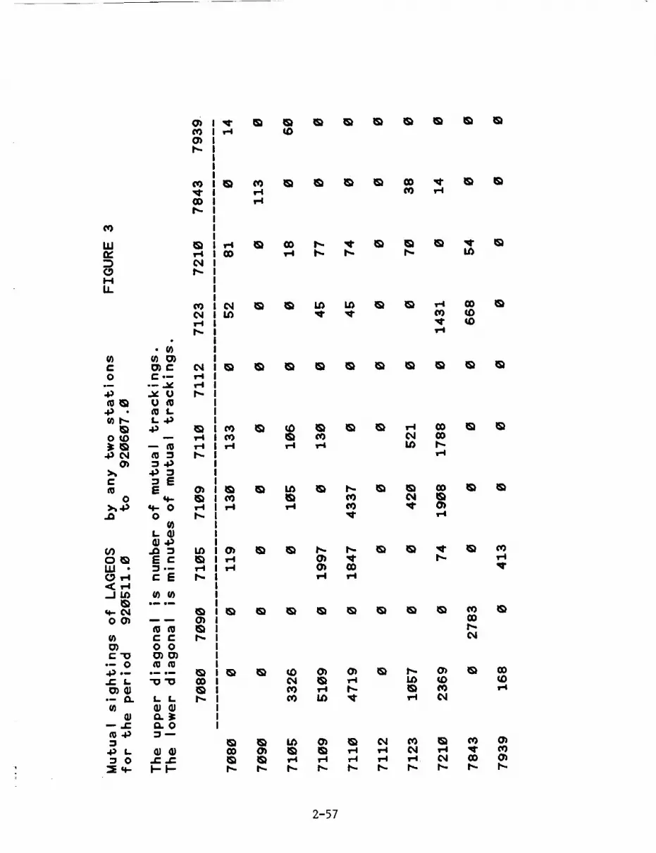
LU
C_
LL
t-O
u_
.
OtO
O_
C
O
r_
U_
LLI •
_JLO
OO_
ol O
-- c-
DL
D O
_C
UL
L._.P
DD_
D=EE
q- OO
L
.43 DEC
r- E
w
r- r_O O
L L
_.OD--
o_
O_
_D
C_I-..I
E_
_D
O_
OD
rq
E_ E_ E_ E_
E_
E_
eO _D
E_
E_
OD
E_
E_
E_
t_
r_
_D
r_
LDE_
r_ _D(3O
OD
O_
_r_
E_
O_O_
_D
t_
E_
E_
OD
O_
r_L_
O_ O_LD _D
E_
r_
E_
_D_D
i_. p_. i_. i_. _. I_. I_ I_. _- _-
2-57
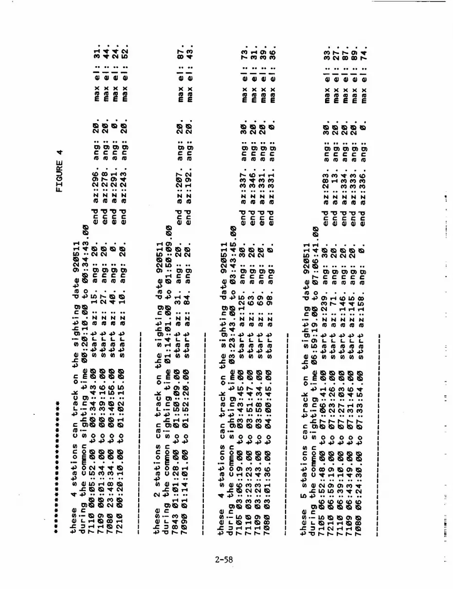
cO ,q" tN
oe ou le
o_
mo
Q)
,q.
I.Ury
i-Ii.L
x x x xm _ _ eoEEEE
c<o_ o4
C C C C_ m m _
• _ ee ue um
N N N N
"0 "0 "0 "Or- r- r- C:QJ (11W (_
LD "" C_i C_I 04
04 _ ........O_ -. O_ O_ O) O)
_ C C C r"
O ....
v-0 0,1 _" _-I
,,"_ ........--- • N N N N
r'_.l
---_LLLL
: _;_: _ooo: _ _
:: o _._• _ oo_,;,_
mu___ ........
_.-___L__
_O_l"
• e ee
m m
x x
EE
t- r-m m
_0_C_l ,-a
N N
"ID "IDr. ,-
QD .. 04 O_l
I.O ....
_.1 t- _-
0 -•"0 4._ _-I _1_
"-- • M M
•--'q" L I.
• . -I-_ ._
U _ 0 0
_" 0_
.o_._UOJ_
0_43 ....
_.- e0 _
XXXX
EEEE
CCCC
ee
NNNN
CC_
It) .. t_ C_I C_I
O_ _r" ........O_ -. o) O) o) o)
£::I_ ........*-- • N N N N
O_ -, .¢._.oa._ .la,-_ L L L L
,.__
_).E_ _ _ _
,_ xl" ,q" t_ ,q"U _ ........
._4._ ........
U'_) 0 0 0 0
(_ r. "_ 4"_"_ "1_
.o | _ _._._.
4-_ "0 I'-- r-- I,,. h-
2-58
XXXXX
EEEEE
C C C C C
N N N N N
_D "ID "O "ID "_D£:: r- t- C t-_J _J _J • W
IQIQ
_-_ '_" _Q eQ eQ _Q eQ
i_. t- ,- r t- /-
0 .....
•-- • N N N N N
•-0_ L L L L L
• .._ -_ 4-_ ._ ._
4-_._ ..........
U'_ 0 0 0 0 0
U_ r" "_ "_ 4"_"_ "_
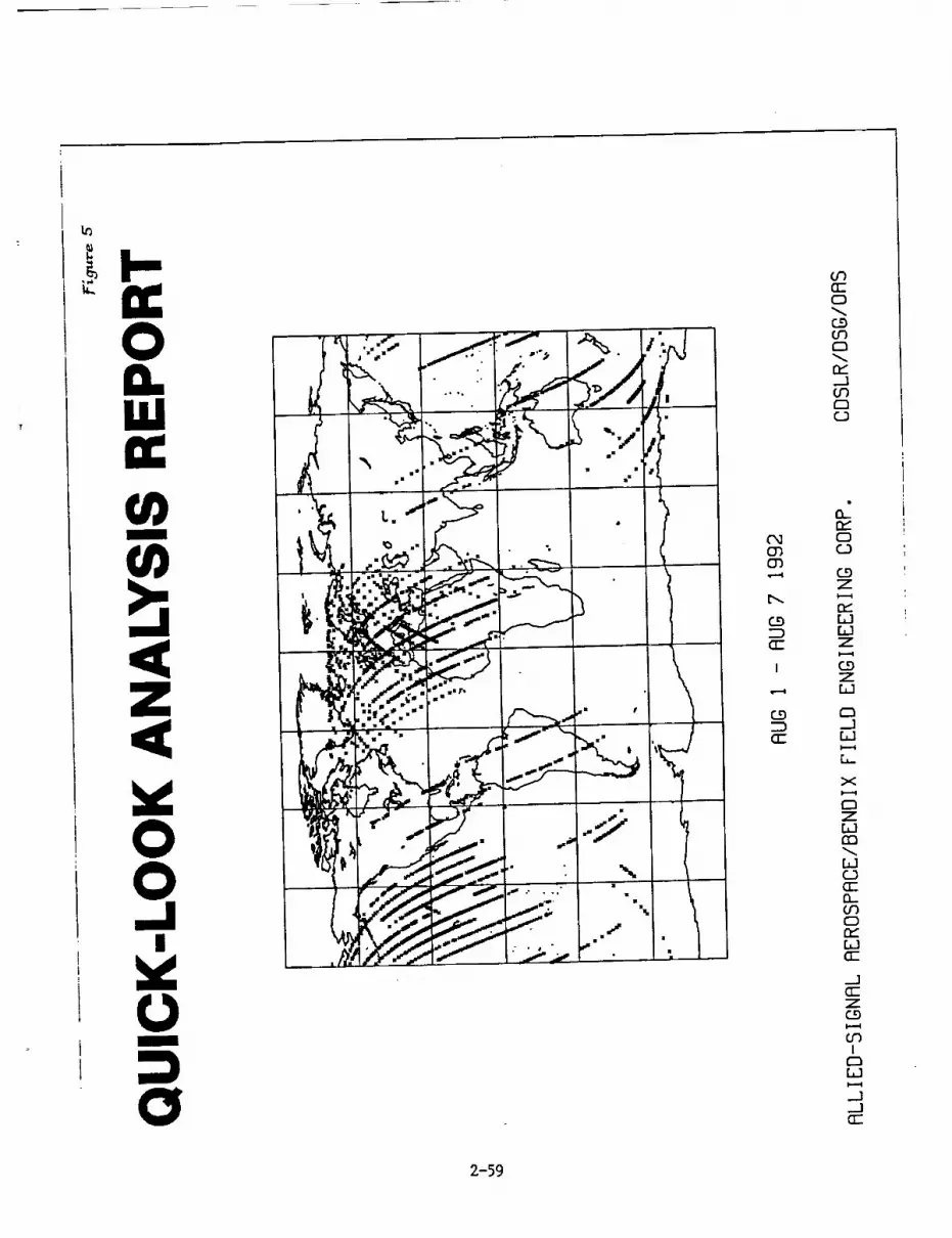
0n_u,ir_
m
0
0
n 0
,bI
I
I
\I
/
(3")0"),e--i
C__
cl-
I
C_q
0
0
r__]
00
0
Z
Z
ZW
O._]
X
0Zb.)03
0
0n_6_]rm
Z
I
._]
n-
2-59

(o
{3
E_
>
I--.I
(k]
,--I
i
•< .<
I Ii-i
(_
E_
,_ •"_ m )-m _
-(
_-_ _\\\\\\\\\\\\\\\\\_
i,_ _\_\\\_\\\ _,. _\\\%\\\\\\\\\\\\_
,. _\\\%\\\\\\\\\\\\\__\\\\\\\_
Q
NOI.I-V.tS
i I

Wrr
m
U.n"
,o
<n
cO
2-61

CO
wr¥"
m
or)n-'LLII--
0
I-ZILl
01.1.1
ILlI--
Z
wr_
__oo
_ N _ 4
2-62
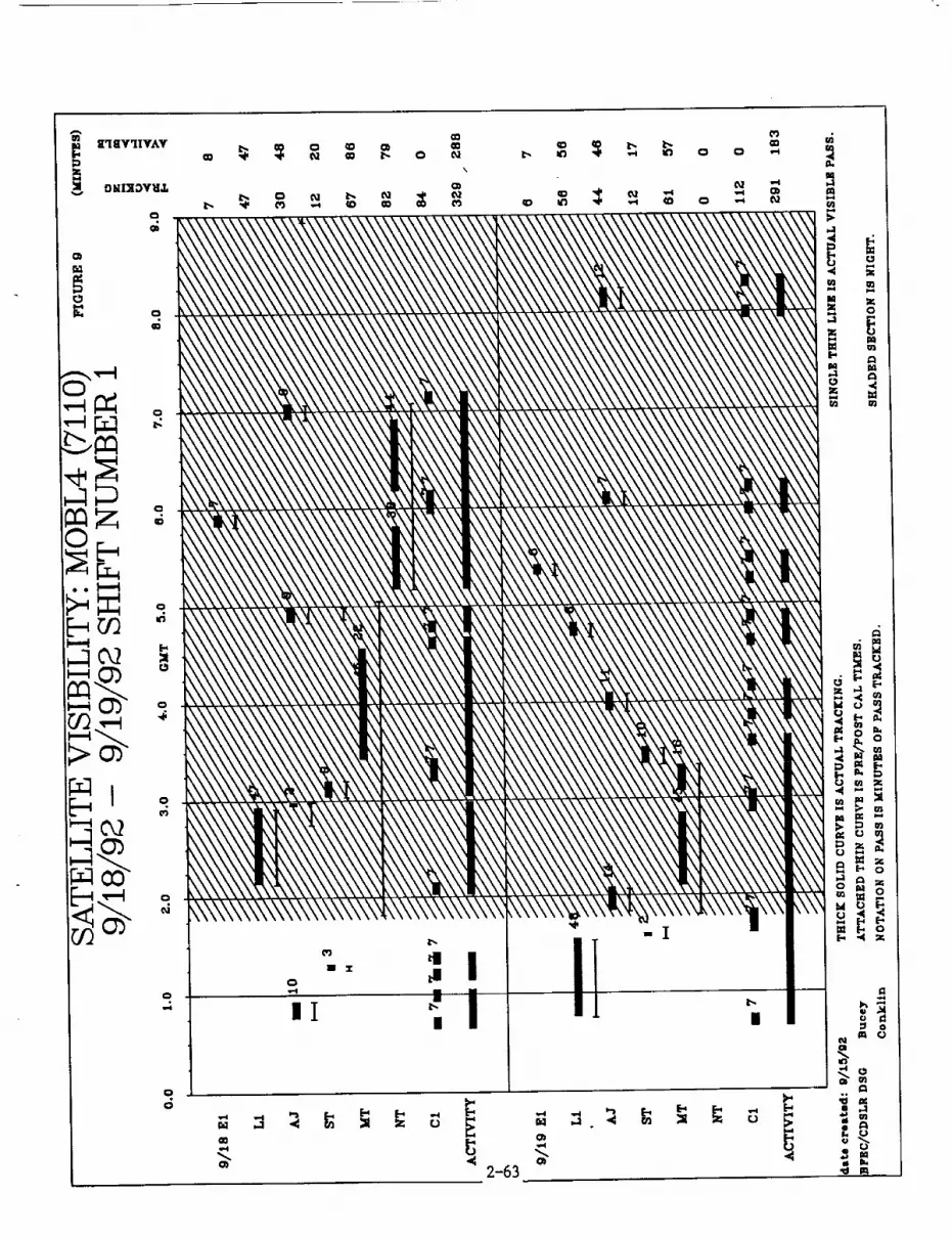
0
0
m 0


Laser Technology


N94-15563
Nd:YLF Laser for Airborne/Spaceborne Laser Ranging
J.L. Dallas, M.D. Selker
NASA - Goddard Space Flight Center
Abstract - In order to meet the need for light weight, long lifetime, efficient, short pulse
lasers a diode-pumped, Nd:YLF oscillator and regenerative amplifier is being developed.
The anticipated output is 20 mJ per 10 picosecond pulse, running at a repetition rate of 40
Hz. The fundamental wavelength is at 1047 nm. The oscillator is pumped by a single laser
diode bar and modelocked using an electro-optic, intra-cavity phase modulator. The
output from the oscillator is injected as a seed into the regenerative amplifier. The
regenerative amplifier laser crystal is optically pumped by two 60W quasl-cw laser diode
bars. Each diode is collimated using a custom designed micro-lens bar. The injected 10 ps
pulse from the oscillator is kept circulating within the regenerative amplifier until this
nanojoule level seed pulse is amplified to 2-3 millUoules. At this point the pulse is ejected
and sent on to a more standard single pass amplifier where the energy is boosted to 20 mJ.
The footprint of the entire laser (oscillator - regenerative amplifier - amplifier) will fit on a
3' by 4' optical pallet.
I. INTRODUCTION
There are a number of programs at NASA's Goddard Space Flight Center which are driving the
need for compact, efficient, diode-pumped lasers. These programs fall within the headings of
Ranging, Altimetry, Metrology, LIDAR, and Communications. One of the primary leaders in
this technology push has been the Geodynamic Laser Ranging System (GLRS) which proposed
to perform both sub-centimeter ranging to retro-reflectors placed at geodynamically interesting
regions as well as sub-decameter altimetry to the Earth's surface, ice sheets, cloud tops, etc. t
The original requirements were for a spaceborne, 5 year lifetime, diode-pumped, Nd:YAG laser
having an output of 200 mJ in 100 ps at the fundamental wavelength (1064 nm). This light was
then frequency doubled and tripled to produce a resultant 100 mJ at 1064 nm (IR), 60 mJ at 532
nm (green) and 40 mJ at 355 nm (UV). The green and UV light were to be used for 2-color
ranging in an attempt to back out atmospheric refraction effects. The IR radiation was for
altimetry operations. Due to the complexity of the GLRS instrument and the still unresolved
technological challenges, it was decided to divide the instrument into 2 separate instruments.
The ranger is now called GLRS-R and the altimeter, GLRS-A. The work being described in this
paper deals with the development of a laser source for an aircraft instrument to proceed and be a
"stepping-stone" to the GLRS-R instrument. The requirements for this mission were derived and
scaled down from the GLRS requirements and are meant to push the technology to produce a
proof-of-concept breadboard for the GLRS-R instrument. This GLRS breadboard laser is
required to be: diode pumped, compact (fitting on 3' x 4' palette), greater than 6% efficient, low
maintenance, long lived (10 s shots), low cost, and flyable.
3-1

II. BREADBOARD DESIGN
The overall design for the breadboard laser is shown in Fig.l. The laser consists of 3
sub-sections: the oscillator, the regenerative amplifier, and a final power amplifier, with the
doubling and tripling left as future tasks. The oscillator produces low energy, short pulses
which are used to seed the regenerative amplifier, where their energy is amplified 6 orders of
magnitude. The output of the regenerative amplifier is sent to a standard amplifier where the
pulse energy is increased by a factor of 20. The required output is an energy of 20 raJ per I0 pspulse occurring at a repetition rate of 40 Hz. Each of the 3 sub-sections are now described in
greater detail. The oscillator is a diode pumped, FM mode-locked laser (Fig.2) 2. The Nd:YLF
laser crystal (the choice of Nd:YLF over Nd:YAG will be described later) is end-pumped by a
CW SDL-2482 3 Watt laser diode operating at 796 nra. The highly diverging light from the 500
x I pm emitting aperture is collimated and focused using a high NA Fujinon F35B compound
lens array and a 12.0 ram cylindrical lens. A spot size of less than 500 Ixm can be maintained for
4 tara leading to efficient end-puraping of the Nd:YLF rod since the cavity mode size at the rod
is also 500 _ra. The Nd:YLF rod is 12 rata long with a 6.35 tara diameter. The one end is cut
flat and anti-reflection coated for the pump wavelength of 796 nra and high-reflection coated for
the [asing wavelength of 1047 nm. The opposite end of the rod is Brewcster cut. The onlyintracavity element is an electro-optic phase modulator which FM raodc-]ocks the laser. In order
to keep the laser output stable, a feed-back loop has been designed which keeps the RF
modulation frequency (200 MHz) of the phase modulator equal to the cavity mode frequency
(c/2L). In a previous experiment performed at NASA/GSFC using a Nd:YAG crystal, stable 15
ps pulses were obtained at a modulation frequency of 344 MHz. An output energy of 5 nJ perpulse is expected for the Nd:YLF oscillator.
Fig. 1. Breadboard Design
3-2

Fig. 2. FM Mode-Locked Laser and Feed-Back Loop
The regenerative amplifier is essentially a Q-switched, cavity dumped oscillator with an injected
seed pulse. The seed pulse is trapped electro-optically in the cavity and circulates through the
gain medium until the energy of the pulse has been amplified to the desired level. The regen
designed for this breadboard (Fig. 3) uses laser diode side-pumped Nd:YLF as the gain medium
and a combination of polarizers and a very fast rise-time Pockels cell (3-4ns) to switch the seed
pulse into and out of the regen. The laser diodes used to pump the Nd:YLF crystal are Spectra
Diode Labs model 3230 which have an output energy of 60mJ within a 500 pts pulse and a
repetition rate of 40 Hz at 796 nm. The 10 x 0.001 mm aperture of the diode leads to a
divergence of the emitting light of 10 ° by 40 °. In order to collimate this highly diverging light, a
unique lens has been utilized that was created at Lawrence Livermore Labs. 3 First the
theoretically perfect lens for collimation of the fast axis is created in bulk form. As with optical
fibers, this bulk lens is then pulled down to a 200 om diameter microlens while still retaining the
original hyperbolic shape of the bulk lens. Slices of these microlenses are attached to the output
facet of the laser diode giving a collimated output of 500 _m at 3 cm. The output from two
collimated diodes is delivered through the top of the 2 x 5 x 15 mm Nd:YLF slab (Fig. 4.). The
lenses are -80% efficient leading to -50 mJ being delivered to the surface of the crystal.
As previously mentioned, control of the number of round trips the seed pulse makes within
the regen is accomplished by a very fast electro-optic switch made by Medox Electro-Optics.
By rotating the polarization of the traveling pulse through the Pockels cell, the light will either
see the Thin Film Polarizer (TFP) as a mirror or a window. After a sufficient number of round
trips within the regen, the energy of the seed pulse will have been amplified from 5 nJ to 2mJ.
For our design, optical damage puts the ultimate limit on the number of round trips and
therefore the gain of the regenerative amplifier.The third sub-section is a standard single pass diode side-pumped Nd:YLF amplifier which
will increase the energy per pulse from 2 mJ to 20 mJ (Fig. 1.).
3-3

Thin Film Polarizer
DPockels
Cell
! I
Mirror
l_./4 Plate
Nd:YI_F
Mirror
Fig. 3. Regenerative Amplifier
Laser Diodes _'_ ./_ Microlens
0 0
Nd:YLF Slab
5 mm
Brewester Faces
Fig. 4. Diode Collimation and Pump Scheme
III. Nd:YLF vs Nd:YAG
Since the absolute ranging accuracy is increased as the laser pulse width is decreased, the design
of this breadboard encompasses the use of Nd:YLF versus Nd:YAG (the crystal of choice in the
original GLRS design). From the equation for the pulse width achievable from an electro-opticphase modulated mode-locked laser4;
3-4

1/2
where f_ is the modulation frequency, Af is the bandwidth of the lasing medium, go is the gain
and 8o is the effective single-pass phase retardation, it is apparent why it is desirable to useNd:YLF with a bandwidth of 420 GHz instead of Nd:YAG with a 120 GHz bandwidth for short
pulse generation.
Lasing Wavelength
Stimulated Cross Section
Upper State Lifetime
Bandwidth
Nd:YLF
1.047 vtm
3.0 x 10 19 cm 2
480 lxs
420 GHz
Nd:YAG
1.064 _m
6.5 x 10 t9 cm 2
240 las
120 GHz
Table.1 Nd:YLF vs Nd:YAG
In addition, Nd:YLF has the advantage of having an upper state lifetime approximately 2.5 times
greater than Nd:YAG allowing for approximately 2.5 times the energy storage, hence a larger
gain as well. YLF is also naturally birefringent making it resistant to thermally induced
birefringence and the concomitant undesired polarization dependent losses. Other advantagesinclude less thermal lensing, and a nonlinear index less than three times that of YAG. Although
thermally induced stress fracture has been reported in Nd:YLF, we have not encountered this
problem.
IV. SUMMARY
The design for a compact, efficient, diode pumped Nd:YLF laser has been shown. The expected
output is 20 mJ per 10 ps pulse at a repetition rate of 40 Hz. The size, weight and power
consumption makes this design ideal for aircraft ranging. Some of the areas to be investigated
so that this technology may successfully make the transition to a spacecraft instrument include:
the reduction of pulse width and its implications to optical damage, shot lifetime of laser diodes,
efficient and stable collimation of laser diodes, high voltage Pockels cell driver and mode locker
lifetimes, and overall system efficiency.
[1] S.C. Cohen, J.J. Degnan, J.L. Bufton, J.B. Garvin, and J.B. Abshire, "The Geoscience Laser
Altimetry/Ranging System," IEEE Trans. Geosci. Rem. Sens., vol GE-25, 581, 1987.
[2] G.T. Maker and A.I. Ferguson, "Frequency-Modulation Mode Locking of a Diode-Pumped
Nd:YAG Laser," Optics Letters, vol. 14, 15, 1989.
3-5

[3] J.J. Snyder, P. Reichert, and T.M. Baer, "Fast Diffraction-Limited Cylindrical Microlenses,"Applied Optics, vol. 30, 19, 1991.
[4] D.J. Kuizenga and A.E. Siegman, "FM and AM Mode Locking of the Homogenous
Laser-Part I: Theory," IEEE J. Quantum Electron., vol. 6, 11, 1970.
3-6

N94-1556' = •
ALTERNATIVE WAVELENGTHS FOR LASER RANGING
K. Hamal
Faculty of Nuclear Science and Physical Engineering, Czech Technical University
Brehova 7, 115 19 Prague, 1 Czechoslovakia
phone / fax +42 2 848840,tlx 121254 fjfi c,E-mail tjcan_:searn.bitnet
To accomplish multicolor laser ranging we should consider :
* the nature of the atmospheric dispersion and absorption,
* the Satellite/Lunar/Ground retro array characteristics,
* Ground/Satellite ranging machine performance.
The existing atmospheric dispersion models [1,2] are perhaps valid up to 1 cm
accuracy. It is evident, the higher time interval difference of a chosen pair, the requirements on
the ground / satellite instrument are less stringent. The energy balance and jitter budget have to
be considered, as well.
The existing Satellite / Lunar retro
arrays show serious limitation to accomplish
a multicolor experiment [3].
The fieldable picosecond lasers,
considered up to now, have the origin on the
NdYAG transition (1.06um) and its
harmonics (0.53 um, 0.35um), Raman Stokes
transition (0.68 um) of 0.53 um in Hydrogen
[4,5], Titanium Sapphire (0.8 / 0.4 um) and
Alexandrite. We do propose the Raman
Stokes / Raman Anti Stokes pair of 0.53 um
(0.68 um/0.43 urn) and Cr:LiSAF (0.8/0.4
am).
The streak detector experiments
carried out in Prague on a ground target
(0.53/0.35 um), (0.53/0.68 um) [4],
(0.53/1.06 um) and in Graz [5] on Ajisai and
Starlette satellites proved the expectancy,
INd YAG, 35 psec, 10 Hz l_,[-_ &5._3
single I s ernitr aln
,*,o,,I _ Heam expanaer 1= ].
_" 'Raman H2 20 bars I.,....-.-4F• 0.43 I ' ' i n53-
0.530.68
AVAILABLE WAVELENGTHS
0.35 urn 3 nkl I pulse0.43um 2 rnJ I pulse0.53 urn 5 mJ I pulse0.6B urn 3 md I pulse1.06 um > 10 mJ ! pulse
Figure 1 Multiple wavelength laser transmitter
The 3HG may replace the Raman tube
however, indicated the complexity. On the other hand, the solid state detector technology offers
a remarkable simplicity and compactness with the access to the near infrared. The experiment
(0.53/0.68 um) accomplished in Graz [6] indicates a chance, if data averaging requirements willbe fulfilled.
Since several years ago, Alexandrite based Fundamental / SHG lasers do not show to
much progress. Using the Titanium Sapphire based laser, the scheme is becoming quite complex
because of short relaxation time (3 useconds) of the metastable level of the active medium.
The new material Li:SAF [7] tunable around 800 nm, having 66 usec relaxation
3-7

time,lookspromising related to the spectral response of existing vacuum and solid state detectors
and the atmospheric propagation and dispersion, as well.
At the conclusion : the existing Satellite / Lunar retroreflectors seem to be not adequate
for the future experiments. The Raman Stokes/Anti Stokes (0.68/0.43um) plus solid state
detector look as a promising instrumentation satisfying the Ground/Satellite and Satellite/Ground
ranging machine requirements on the precision, compactness and data processing.
WAVELENGTHS PAIRS SELECTIONG[az SLR, 2.5 echolseclw., 45 deg.elev.
wavelengths prec.req, aver.time
0.35'/ 0,53 um 5,3 psec 0.8 rrtnute
0.4 / 0.8 um 4.1psec 1.6 minute
0,43 I 0,68 um 3.3 psec 2,6 minules
0.53 I 0,68 um t.6 psec 10 minutes
0.53 I 1,015um 2,9 psec 5,2 minutes
t energy budgetproblems at this wavelengthPro ch.HztmaLdel, Kit ch,IColdI,Annspolls 1992
Figure 2 The wavelength pair selection. The two wavelength ranging setup using SPAD is
expected, the mean elevation 45 degrees is expected, the SPAD jitter dependence versus
wavelength is taken into account.
References:
i°
2.
3.
4.
=
6.
7.
Marrini J.K., Murray C.W., report GSFC X-591-73-351
Abshire J., Applied Optics, Vol.19, 1980
Prochazka I., in this Proceedings
Gaignebet J. et al, Hamal K. et at, Proceedings of the 6th International Workshop on
Laser Ranging Instrumentation, Antibes, 1986, p565-577
Hamal K et al,to be published at IQEC'92, Vienna, June 1992
Kirchner G. et al, to be published at IQEC'92, Vienna, June 1992
Hamal K, Richardson M., in this Proceedings
3-8

N94-15565 "
NEW METHODS OF GENERATION OF ULTRASHORT LASER
PULSES FOR RANGING
H.Jelinkova,K.Hamal,V.Kube_ek,I.Prochazka
Czech Technical University,Faculty of Nuclear Science and Physical Engineering
Brehova 7, 11519 Prague 1,Czechoslovakia
ph/fax +42 2 848840,tlx 121254 fjfi c,bitnet [email protected]
INTRODUCTION
To reach the millimeter satellite laser ranging accuracy, the goal for nineties, new
laser ranging techniques have to be applied. To increase the laser ranging precision, the
application of the ultrashort laser pulses in connection with the new signal detection and
processing techniques, is inevitable. The two wavelength laser ranging is one of the ways to
measure the atmospheric dispersion to improve the existing atmospheric correction models
and hence to increase the overall system ranging accuracy to the desired value.
We are presenting a review of several nonstandard techniques of ultrashort laser
pulses generation, which may be utilized for laser ranging:
* Compression of the nanosecond pulses using stimulated Brillouin and Raman backscattering
* Compression of the mode-locked pulses using Raman backscattering
* Passive mode-locking technique with nonlinear mirror
* Passive mode-locking technique with the negative feedback
BRILLOUIN AND RAMAN BACKWARD SCATTERING
The idea of obtaining a single subnanosecond light pulse by temporal compression of
a nanosecond laser pulse was suggested in [1] and the compression cascade by backward
stimulated scattering of
passively Q-switched
Nd:YAG laser pulses was
experimentally demonstrated
in [2]. We had been investi-
gated the generation of
monopulse from Q-switched
Nd:YAP oscillator [3]. The
experimental setup is in
Fig.1. The resonator was
formed by the concave mir-
ror M1 and the plane output
mirror M2 deposited on the
front surface of the Nd:YAP
laser rod (Nd:YAP1). The b-
axis of the crystal Nd:YAP
yields linearly polarized light
l_l _ D 4 nm.l.OBum POL]YP tJ I_
[1 I Lr_2"_'_1 . _ r-'AIj_!U I ]al vl_, Na:Y_ 2 L2 1
._0 pn,O.O4 'u,m290 pe,l.08
3-9

mirror MI andtheplane output mirror M2 depositedon the front surface of the Nd:YAP laser rod
(Nd:YAP1). The b-axis of the crystal Nd:YAP
yields linearly polarized light output at ),_ = 1.0795
_m. Q-switching was performed by the plastic BDN
foil QS. The length of the resonator was 20 cm and
together with low initial transmission of the Q-
switch enable generation of pulses with duration r=
= 4 ns (Fig.2a). The pulse energy in TEM= mode
was 7.5 nO. This setup of short resonator gives most
stable output pulses [4].The oscillator radiation
passing a cube dielectric polarizer POL and a
quarter wave plate WP, was focused by lens LI into
SBS compressor - a 70 cm long cell BC filled with
CC14. When the necessary condition for SBS was
fulfilled, the backward Stokes pulse was generated.
The compressed Stokes pulse passing prism P1 and
a negative lens L2 is amplified by the single pass
Nd:YAP amplifier (Nd:YAP2) to the energy 30 nO.
The diverging beam is recollimated by the concave
mirror M3. After frequency doubling in a SHG
crystal, the pulse (X2 = 0.54 _m) has an energy of
10 nO. The radiation at different wavelengths is
spatially separated by the dispersion prism P2. The0.54 #m pulse is then focussed with lens L3 into the
second compressor consisting of the Raman cell RCfilled with methane at 18 bars.
Temporal characteristcs of the pulses in
subnanosecond range were measured by the streak
camera Imacon 500 with readout system consisting
of SIT television camera, single frame memory and
computer. The temporal resolution of the whole
system was better than 2 ps [5]. Fig.2b shows the
pulse after the first stage compression and the
frequency doubling (X2 = 0.54 _um). The mean pulse
duration was r2 = 160 ps. Streak camera record of
the backward Stokes pulse (X3 = 0.64 #m) from the
Pump 0.54ta. pulse
J8O0 1600
lime (psl
160 ps FWHA
2¢00
2
ol_0
tOO I_ ETALON
8ps FWHA
IBO Z20 260 300
time [ ps I
2,80
/.33 p_V/ch
_.J{,20
FJguFe 2 A records of compressed pulses
Raman cell is on Fig.2c. The mean value of the pulse duration r3 for given focussing optics
depends on pump energy. The minimum length of pulse r3=9 ps was obtained for pumppulse energy 3-5 mJ.
The advantage of this compression technique in comparison to the used mode-locked
picosecond lasers, are the absence of the active and/or passive mode lockers used to generate
a train of picosecond pulses, and the absence of a fast electrooptical shutter used to select a
single pulse from a train of pulses.
3-10

RAMAN BACKSCATI'ERING PULSE COMPRESSION
The generation of single picosecond pulses through backward Raman scattering can
start directly from the pulse train generated from a mode-locked laser. The experimental
setup composes a passively mode-locked modified SFUR [6] loaded with 1/4"x4" Nd:YAG
rod, delivering 30 mJ in a train of 4-5 pulses (FWHM) at h_ = 1.064 #m and with r_ =24
ps timewidth and an amplitude fluctuation of the highest pulse in the train of 13%. Theradiation is then converted to the second harmonic in a KDP crystal using type 1I
configuration, giving 10 mJ and
r2=17 ps timewidth, with a 20%
amplitude fluctuation. The output
train is then fed into the Raman cell,
focussing it with a 160 mm focal
length lens. The Raman cell was
filled with 20 bars methane gas. On
each shot, signals from fundamental,
second harmonic k2=0.532 /_m and
Raman Stokes Backscattering at _,3 =
0.68/_m were detected and stored for
later processing. The Raman signal
was checked to be the phase conjugat-
ed of the input second harmonic
signal. Its energy was measured to be _ _J N m3 mJ, giving an average green-to-red tm
conversion efficiency of 30%. Time
duration of the Raman pulses was m
1-3=7.4 ps with a 2.3 compression A ,factor with respect to second harmon- aa ]_ /_ r, I
ic pulses. On Fig.4a is oscilloscope
record of the rest of mode-locked
train pulses (positive trace) and a /
single generated Raman pulse (nega- aa |
five trace). Fig.4b shows streak 1camera records of the overlap of 100 _,._.__,___, .... • .... , .... , ....second harmonic pulses (positive , u .... ta m _a
trace) and Raman Stokes pulses (neg- m:
ative trace). The second harmonic Figure 3 h records of the generated pulses
radiation and Raman output pulses
were detected by the independent
photodiodes, one of the photodiode output was inverted and both signals have been added on
the oscilloscope input.
This technique gives possibility to generate one ultrashort pulse without expensive optical
and electronic part as they are Pockels cell, polarizers, high voltage pulse forming circuitry,
optostart, high voltage power supply,etc, which are obviously needed to select single
picosecond pulse from mode-locked train.
3-11

GENERATION.OF MODE-LOCKING PULSES USING A FREQUENCY-DOUBLING
NONLINEAR MIRROR
The mode-locking technique based on intracavity frequency doubling offers new
capabilities for generation of ultrashort laser pulses. A frequency doubler inside the cavity,
together with an
NONLINEAR MIRROR output mirror with
M1 M2 high reflectivity at
D SHG the second harmonicSH F forms a nonlinear
mirror, whose
reflectivity at thefundamental wave-
length can either in-crease or decrease
FUNDAMENTAL: SECOND HARMONIC, when the input light
TOTAL REFLECTOR TOTAL REFLECTOR intensity increases.
Figure 4 Experimental scheme When the phasecondition facilitate
increasing
reflectivity, the device can be used as a passive mode-locker. First experiment with the
nonlinear mirror was performed by K.Stankov [8]. With the Nd:YAG laser active medium
he got 20 ps length of pulses. We investigated the attractive potential of the second harmonic
nonlinear mirror to mode-lock lasers at quite different wavelengths. The laser cavity was
formed by the dielectric mirrors. In all cases the rear mirror was a total reflector at the
fundamental, the output mirror was dichroic and it was total reflector at the second harmonic
and had 20-24% reflectivity at the fundamental wavelength (Fig.4). Using a single 30°-cut
LiIO3 frequency doubler (20 mm long), mode locking at the 1.08/_m and 1.34/_m transitions
of pulsed Nd:YAP laser was achieved [9]. Pulses as short as 40 ps and 15 ps at the
corresponding wavelength were obtained. Mode-locking was achieved also in Er:YAP laser
at 1.66 #m wavelength with pulse duration of 450 ps [10] and in Ti:Sapphire laser at 0.7/_m
wavelength with pulse duration of 100-130 ps [11]. A comparative wavelength indicates that
the minimum pulse duration is determined by the limited number of round trips only.
This experiment showed that non-
linear mirror technique allows to mode lock
a number of solid state lasers ranging in
wavelength 0.8 #m (Ti:Sapphire laser) up
to 1.66 #m (Er:YAP laser). When the
optimalization will be done and shorter
pulses will be generated, the advantages of
short pulse immediately with the generation
of first and second harmonic radiation will
be evident.
Figure 5 The mode locked Ti:Sapphire laser (10 ns/div)
3-12
d

PASSIVE MODE-LOCKING TECHNIQUE WITH THE NEGATIVE FEEDBACK
The solid state lasers with negative feedback through an electro-optic loss that limits
the maximum intensity inside the cavity and prevents the rapid growth of the laser pulse,
were successfully used for the generation of shorter reproducible pulses [12,13]. The
possibility of using a passive two-photon absorption element instead of the active loss control,
was also suggested and demonstrated [14,15,16]. Two-photon absorber (GaAs or CdSe) actsinside the
_. OUTPUT
T
M 1 POL NFE D
DC
AOML
Nd:YAP M 2
Figure 6 The experimental setup
resonator as a
passive negative
feedback element
(NFE). Thescheme of ex-
periment withNd:YAG or
Nd:YAP laser is
similar and it is
schematically
shown in Fig.6.
The Fabry-Perot cavity is formed by concave mir-
rors M1 and M2(R=10m) having a reflectivity of99.8%. The mirror M2 is in contact with a 0.5 mm
thick dye cell (DC) containing flowing Eastman
Kodak 9860 dye in 1,2-dichloroethane (T0=30% at
1.08 #m). The output coupling of the resonator is
achieved by means of a dielectric polarizer (POL),
which, in combination with the quarter-wave plate
keeps the output coupling at 50%. The active medi-
um was Nd:YAG or Nd:YAP. The cavity round trip
time was synchronized to the modulation period of
the acoustooptic mode locker. With the Nd:YAG
laser long trains of steady-state pulses was
generated, with a single pulse time duration of 10 ns
and an energy of 10 #J,with cw comparable
stability. The minimum of pulse duration was
obtained for Nd:YAP laser with CdSe working as a
negative feedback element. In this case, the pulses
with 5 ps length was generated with an energy of 1
mJ.The example of the generated pulse trains for
different negative feedback elements are in Fig.7.
CdSe
GaAs I
GaAs II
Hdiv
Figure 7 The records of the generated pulses
3-13

CONCLUSION
This review article shows some possibilities for generation of short and ultrashort
laser applicable in laser ranging.
References
[1] M.Maier,W.Kaiser,J.A.Giordmaine: Phys.Rev.Lett. 17 (1966) 1275
[2] R.R.Buzelis,A.S.Dement'ev,E.K.Kosenko: Sov.Joum.Quant.Electron. 12 (1985) 2024
(in russian)
[3] V.Kubecek,K.Hamal,I.Prochazka, P.Valach,R.Buzelis,A.Dement'ev: Optics
Commun.,vol.73,3 (1989) 251
[4] H.Jelinkova,K.Hamal,M.Vrbova:High Brightness Nd:YAG Oscillator, Preprint SeriesFJFI No.77/4
[5] l.Prochazka,K.Hamal,H.Jelinkova:Technical Digest Conference on Lasers and Electro-
optics (Optical Society of America, Baltimore, MD) (1989) pap.THK42
[6] H.Jelinkova,J.Marek,P.Valach,K.Hamal,G.C.Reali,G.Gabeta:Optics Communications
Vol.75,No.5,6,March 1990,p.447
[7] K.Hamal,H.Jelinkova,I.Prochazka,G.C.Reali:Czech Journal Phys.(will be published)
[8] K.A.Stankov:Appl.Phys.B45 (1988) 191
[9] K.A. S tankov, V. K ubex3ek, K. Hamal: IEEE Journal of Quan t. Electron., vol. 27, No. 9 ( 1991)2135
[10] K.A.Stankov,V.Kubecek,K.Hamal,H.Jelinkova,I.Prochazka:Proceedings of the
EQEC,Edinburg,UK,(1991)
[11] K.Hamal,K.A.Stankov,H.Jelinkova,I.Prochazka, M.Koselja:Proceedings of the VIIth
Int.Symp. on Ultrafast Proc. in Spect.,Bayreuth,Germany,(1991),TU3-3
[12] K.P.Komarov,A.S.Kuchyanov,V.D.Ugozhayev:Opt.Commun.57,279 (1986)
[13] P.Heinz,W.Kriegleder,A.Lauberau: Appl.Phys.A,43,209 (1987)
[14] K.P.Komarov,V.D.Ugozhyaev: Opt.Spectrosc. 55,564 (1983)
[ 15] A.V.Babushkin,in Proceedings of Ultrashort Phenomena in Spectroscopy '89,
Springer-Verlag,Berlin (1989), PTh20
[ 16] A. Del Corno, G, Gabetta, G. C. Reali, V. Kubecek,J. Marek: Optics Letters, vol. 15,
No. 13 (1990) July 1,734
3-14
N94-15566
Simultaneously Compression of the Passively Mode-Locked
Pulsewidth and Pulse Train
Yan£ Xianschun, Zhu Xiaolei, _u Zhaoqing and Sun Zhan'ao
(Shanshai Institute of Optics and Pine Mechanics, Academia Sinica,
Lab. of I_ser Technology, Shanghai, _01800, P.R. Chi_)
Yen& Fumin, Tan 1)etong, Xiao chihun, Chen Wanzhen and Lu Vfenhu
(Shanghai ObJervtory, Academia 8inica, P.R. China)
Abstract
Simultaneously compression of the passively mode-locked pulsewidth and pulse
train have achieved by using a piano-convex unstable resonator hybrided by a nonlinear
Sagnac ring interferometer. The _30mJ single pulse energy of alone oscillator and
_10ps pulsewidth have obtained. Using this system, the LAGEO8 and ETALON satellites
laser ranging have been performed successfully.
Key words: Nonlinear Sagnac ring interfereometer,
Simultaneously compression of M-L pulsewidth and train
1. Introduction
]n a variety of scientific research and technical applications, laser ranging
included, the single mode-locked pulse is necessary. For this reason, the single pulse
selector has to be need, and perhaps needs several stages amplifiers in order that
achieving necessary energy. Moreover, in outfield applications, not only need smaller
and lighter equipments, but need that, the equipment insensitive to mechanical and
thermal perturbations, maintaining good alignment over days of operation. Recently
years, our group in base on investigations of antirseonant ring hybrided unstable
resonator, deeply into investigated the conditions and paramaters of simultaneously
compression using an unstable resonator hybrided by nonlinear ring interferometer, and
following results have been obtained:
the pulse train compressed to two cavity periods, the mode-locked pulsewidth
3-15
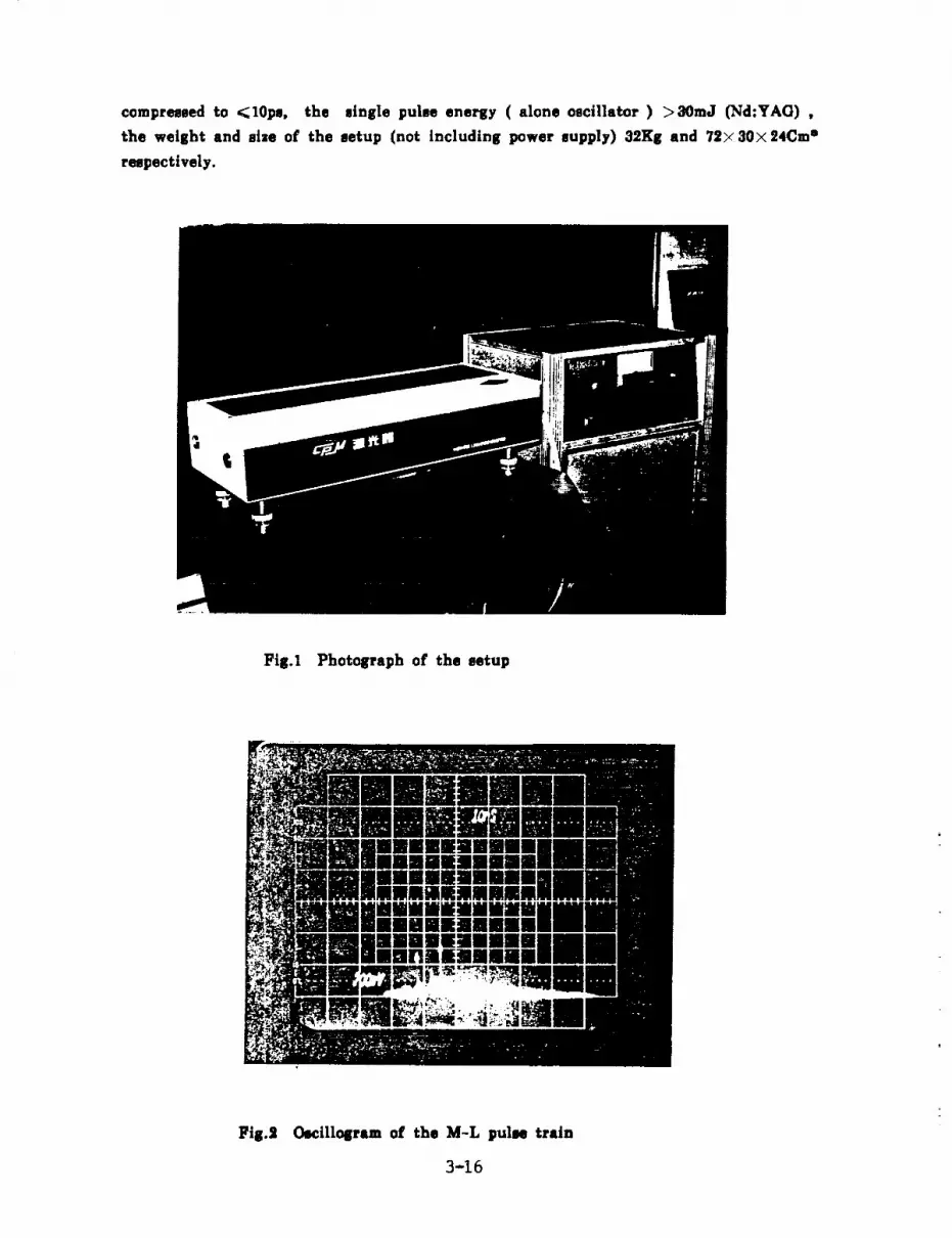
compressed to _10ps, the single pulse energy ( alone oscillator ) _30mJ (Nd:YAG) ,
the weight and size of the setup (not including power supply) 32KS and 72× 30x 24Cm s
respectively.
Fig.1 Photograph of the setup
Fig.2 0scillqram of the M-L pulse train
3-16
2. Theroy
Our experiment results exhibit that the mode-locked pulse train and pulse width
have achieved compression simultaneously. This cantt been explained fully by previous
passively mode-locked theroytXi'tmi. Our study believe that true reasons for
simultaneously compression should be altributed to the collision interference of the
nonlinear ring interferometer, which formed a temporally modulated grating and
stationary in space. Therefore, this grating is free from the deleterious atomic
motionally induced or frequency-induced *washout n effect. Then, counterpropagation two
beams, suffer strongly saturable absorption modulation, and at splitter mirror, again
interference, resulting beams, which through a high inversion gain medium, the pulse
signal obtain enhanced and compressed by cross-phase modulation. The necessary
conditions of the doubly compression by using nonlinear ring interferometer, are YI
parameter enough large, as that has to be at least one order of magnitude larger than
R of [I]. Y1 _ i In6 Q I is the initial amplitude of the stimulated emission, 6 Q is
solid angle, in which the laser radiation are concentrated. In according to [3], we
deduced
8 n TV (Xl+ _.)¥I= (_)"
n 2_
here _ is the relative excess pump power above the threshold for a closed shutter,
(6 n/n) is the relative excess inversion population, T, cavity period time for mode-
locked operation, (XI+ IX,), XI is the linear losses per unit optical path, tl, is
absorption coefficient of the mode-locking dye. t_- must be enough large, as that has
to be at least one order of magnitude larger than corresponding value of optimum
transmittance of [2]. In proper conditions, sufficient large YI can be depleted the
8 n, and initiated the nonlinear ring interferometer, an overshoot pulse after
switching[4], return to a high inversion gain medium, then the pulse signal enhanced
and compressed by cross-phase modulation, simultaneously compression of the mode-
locked pulses achieved quickly, and a single pint pulse is obtained.
3. Experiment setup
Experiment setup used in this work is different to [4] slightly. The main
difference are addition of interferometer*e function.
The nonlinear ring interferometer is composed of a P-polarisation 50/60 splitter
1, two totally reflective turning mirrors 2 and 3, and a dye cell 4, which located at
the colliding center, fulling pentamethine cyanine dissolve in 1,2-dichloroethane. Two
polarizers 6 and 10 used for enhance the polarization purity of the gain medium
Nd:YAG, 6, 90mm in length and 6.0ram in diameter, the ends of the rod were angled
at 87.6 ° to the normal of the rod axis. The rear reflector, 11 is a convex mirror,
turning mirrors 7 and 8, an aperture 9, output coupled mirror li and recollimated
lens 13.
3-17

7
Fig.3
C__3 6 ..'5'.2
i /
Optical layout of a nonlinear Sagnac ring lnterferometer.
Since the distance from the splitter mirror to colliding center is equal optical path,
for all longitudinal modes _ o_+ m A _, that into oscillated, can be formed interference
fringes, stabiised in space, and thess fringes are inMnjitive to mechanical and thermal
perturbation. Due to the high angle selectivity of this system, me that it may be
maintaining good aligenement over days of operation. In this syltem do not need single
pulse selector and A-O modulator, without any amplify, the output energy of oscillator
can he achieved _30mJ, pulsewldth _10ps. Theme performances are sufficient f_r many
applications. For as LAGEOS and ETALON ( 20,000KM ) utellite laser ranging, only
need addition to one amplifier and a frequency doupler. More recently, the facts of
successful laser ranging of LAGEOS and ETALON in Shanghai Oblervatory, have
showed this point.
4. Conclusions
We have reported the results of a nonlinear Sagnac ring interferometer hybried
unstable resonator. The results demonstate that the multiple interference effect
quicken the mode-locking process, and the simultaneously compre_ion of the mode-
locked pulsewidth and pulse train have been achieved, and a GW level single pul_ wu
obtained. This system have many advantages as that lighter weight, Imaller size and
insensitive to mechanical and thermal perturbationl, particularly applied to outfield
utilizations, such as mobile utellite laser ranging, and have great potentialities
for heighten precision and distance of lamer satellite ranging.
The damage problem of the optical components and improvement of the ratio of the
first-second peak of the mode-locked train are currently in the progr_s.
Reference
[1] G.H.C. New, PIEEE, V01.67, No.3, PP.380-396, Mar. (1979)
[2] A.L. Max, etal, IEEE JQE., Vol.QE-19, No.4, PP.662-r_66, Apr. (1983)
[3] A.M. Rather "Spectral, Spatial and Temporal Properties of Luers"
PP.]90-191, Plenum Press, New York-London, (1972)
[4] T. Bischifberger and Y.R. Shen, Physical Review A, Vol.]9, No.3,
PP.]169-1176, (]979)
[6] Sun Zhan'ao, etal, "Chinese Journal of Lasers', Vo].16, No.5, PP.302-304, (1989)
3-18

N94-15567
An improved light source for laser ranging
Karel Hamal
Technical UniversityPrague, Czechoslovakia
Tel 422 46 23 97Fax 422 847688
and
Martin RichardsonCREOL
University of Central Florida:Orlando, USA
Tel 407 658 6819Fax 407 658 6880
Summary
The development of a new laser material, Cr-doped LiSAF makes possible the
development of a laser source for satellite ranging systems that is superior in performancecapabilities than current Nd:YAG-based laser sources. This new material offers thepotential of shorter pulses and more preferrable wavelengths (850nm and 425nm) thanmulti-wavelength Nd:YAG systems, leading to superior ranging resolution and greater
detection sensitivity.
We are embarking on a feasibility study of a two-wavelength, mode-locked laser
system based on Cr:LiSAF, providing shorter pulses for improved ranging resolution.
Background
Current satellite multi-wavelength laser-ranging systems operating with Nd:YAGbased systems are capable of resolving earth-satellite distances to within a centimeter.The latter limitation is primary set by the minimum pulse-duration available from currentfield-usable mode-locked Nd:YAG laser systems having diffraction-limited beamdivergence. Recent developments in ultrashort laser pulse technology with a new lasermaterial perfected at CREOL in the last two years, now offers the possibility of animproved multi-wavelength laser-ranging system. The principal advantages this newmaterial will offer is in shorter laser pulse durations, down to a few picoseconds, thereby
improving ranging accuracy to the millimeter level, and in the use of shorter laserwavelengths permitting detection in a region of higher photocathode sensitivity, thereby
improving overall sensitivity.
The new laser material Cr-doped LiSAF 1 has already been extensively studied 2,3, and
reliable mode-locked operation has been demonstrated 4. At the present time most of the
technology of Cr-doped LiSAF is resident at CREOL. This has occured as consequenceof it's crystal growth development at CREOL, and in a concerted effort being made byCREOL scientists to determine it's optical and physical properties. As a consequence,
many laboratories are examining potential applications of this exciting new laser material.
3-19

Technical Details
We wish to take advantage of the possibilities offered by Cr:LiSAF in developinga fieldable laser for satellite ranging providing the general properties referred to above. Amodelocked Cr:LiSAF laser can be built under this program that would have the principalcomponents shown in fig. 1.
Harmonic I _ Activegenerator mode
locker 11F"sh"m'1 I !Pcu F IPo' r'zor tch
DiodeLed [
[ inlect°r ]
Fig. 1. Schematic of an actively modelocked multifrequency Cr:LiSAF laser for satelliteranging
A cw single mode diode laser operating at ~845nm can be used to seed theCr:LiSAF laser with a specific frequency. This will both control the frequency of thelaser, and it's harmonic, and ensure that the modelocked laser has single mode outputitself, ensuring diffraction-limited beam divergence. Short pulses wouldbe formed withinthe laser with the aid of conventional modelocking and Q-switching techniques. With thelaser locked to a specific output frequency, efficient, stable, phase-matched secondharmonic conversion will be guaranteed. The output performance of the laser will havethe following parametersEnergy per pulse-train 500mJ Wavelength 850nmNumber of pulses 10 Energy per pulse 50mJPulse-duration 30ps Pulse separation 10nsSecond Harmonic Conv. Eft. 25% En. @ 425nm 12.5mJ
References
.
2.
3.
.
S.A. Payne, L.L. Chase, L.K. Smith, W.L. Kway, and H.W. Newkirk, "Laser
performance of LiSrA1F6:Cr3+, '' J. Appl. Phys. 66, 1051, 1989.
P. Beaud, Y-F. _hen, B. Chal, and M. Richardson, "Small-signal gain propertiesof LiSrA1F6:Cr3+", submitted to Optics Letters.Y. F. Chen, P. Beaud, B. H. T. Chai& M. Richardson, "Small signal gainmeasurements of Cr-doped LiSAF and LiCAF" Proc. Conf. on Advanced SolidState Lasers Santa Fe (Optical Society of America 1992) to be published.P. Beaud, E. Miesak, Y-F. Chen, B. H. T. Chen and M. Richardson, "A flashlamp-pumped Cr:LiSAF regenerative amplifier" Proc. Conf. on Advanced Solid StateLasers Santa Fe (Optical Society of America 1992) to be published.
3-20
Epoch and Event Timing


N94- 155t t
Preliminary Results from the Portable StandardSatellite Laser Ranging Intercomparison with MOBLAS-7
Michael Selden, Thomas Varghese, Michael Heinick, Thomas OldhamAllied Signal Aerospace Company,
BFEC/CDSLR10210 Greenbelt RoadSeabrook, MD 20706
USA
AbstractConventional Satellite Laser Ranging (SLR) instrumentation has been configured and successfully used toprovide high-accuracy laboratory measurements on the LAGEOS-2 and TOPEX cube-corner arrays. Theinstrumentation, refered to as the Portable Standard, has also been used for field measurements of satelliteranges in tandem with MOBLAS-7. Preliminary results of the SLR measurements suggest that improvedrange accuracy can be achieved using this system. Results are discussed.
1 IntroductionThe portable standard (PS) is a collection ofranging instrumentation which was originallybroughttogether as a calibration mechanism forthe CDSLR network. The system was designedto take parallel measurements with field stationswhile sharing the existing telescope/mount,system shelter, power, and laser. It is a methodto tie and intercompare the worldwide networkto a single standard which periodically travelsfrom system to systemto maintain the caliber ofthe satellite laser ranging measurements. Asecond role for the PS is as a test bed for newinstrumentation and SLR techniques. As aconstantly improving system, it provides ameans of proving new technology prior toimplementing changes to the network. A thirduse of the portable system has been as atroubleshooting mechanism to resolve conflictsduring collocation.
LABORATORY
TEST BED FOR
EMERGINGI_CHNOLOCy
I TRANSPORTABLE 1
STANDARD FOR
NETWORKCAIJBRAT[ON t
Tmubk-shooU_ Tool 1
for Sy_m ProblemRuolutlon
Figure 1 Portable Standard Functions
4-1
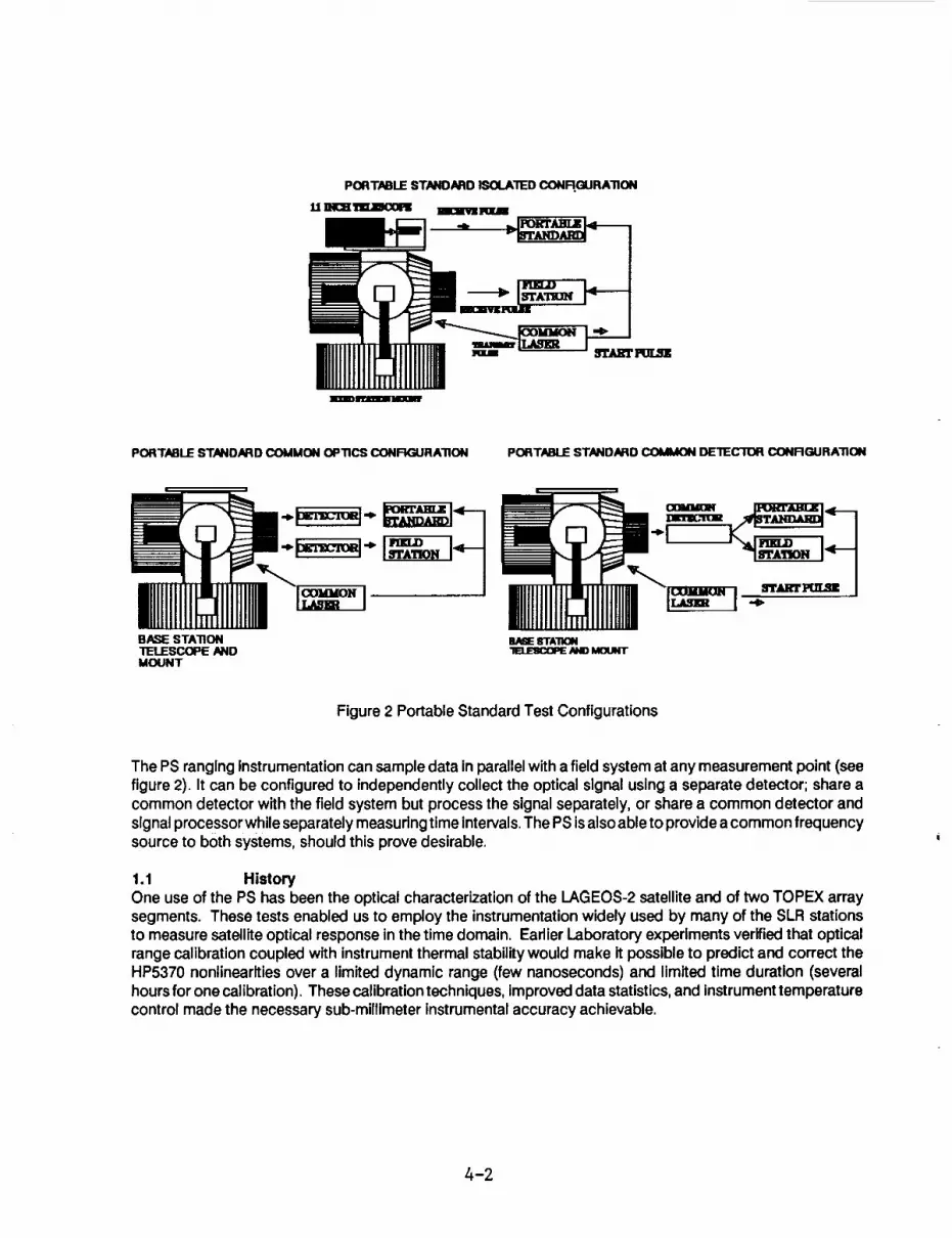
PORTABLE STANDARD ISOLATED CONRGURA'nON
tt II_E I_,_O01_ ilC_tmlqLm
B//
PORTABLE STANDARD COMMON OPTICS CONRGURATION PORTABLE STANDARD COMMON DETECTOR CONRGURA'nON
• • . .
IIIlllllllll llllllllll Illlllllllll llllllll!BASE STA_ON _ rrA'.ON"I1ELESCOPE AND "_LE'SCOPE N_) M(xJwrMOUNT
Figure 2 Portable Standard Test Configurations
The PS ranging instrumentation can sample data in parallelwith a field system at any measurement point (seefigure 2). It can be configured to independently collect the optical signal uslng a separate detector; share acommon detector with the field system but process the signal separately, or share a common detector andsignalprocessor while separately measuring time intervals.The PS is alsoable to provide a common frequencysource to both systems, should this prove desirable.
1.1 HistoryOne use of the PS has been the optical characterization of the LAGEOS-2 satellite and of two TOPEX arraysegments. These tests enabled us to employ the instrumentation widely used by many of the SLR stationsto measure satellite optical response inthe time domain. Earlier Laboratory experiments verified that opticalrange calibration coupled with instrument thermal stabilitywould make it possible to predict and correct theHP5370 nonlinearities over a limited dynamic range (few nanoseconds) and limited time duration (severalhours for one calibration). These calibration techniques, improved data statistics,and instrument temperaturecontrol made the necessary sub-millimeter instrumental accuracy achievable.
4-2
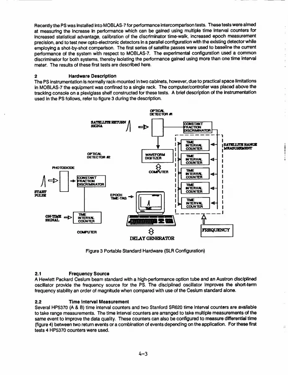
Recently the PS was Installed into MOBLAS-7 for performance Intercomparison tests. These testswere aimedat measuring the increase in performance which can be gained using multiple time Interval counters forincreased statistical advantage, calibration of the discriminator time-walk, Increased epoch measurementprecision, and to test new opto-electronlc detectors in a parallel configuration with the existing detector whileemploying a shot-by-shot comparison. The first series of satellite passes were used to baseline the currentperformance of the system with respect to MOBLAS-7. The experimental configuration used a commondiscriminator for both systems, thereby isolating the performance gained using more than one time intervalmeter. The results of these first tests are described here.
2 Hardware DescriptionThe PS instrumentation is normally rack-mounted intwo cabinets, however, due to practical space limitationsin MOBLAS-7 the equipment was confined to a single rack. The computer�controller was placed above thetracking console on a plexiglass shelf constructed for these tests. A brief description of the instrumentationused in the PS follows, refer to figure 3 during the description.
OP11_ I WAVEFORMDE'IECl13R #2 DIGITIZER
PHOTOOIODE
==)> .-_ IFnAC'nONpISCRIMINATOR
I°" I_. ==):> ,NmnV._.COUNTER
COMPUIER
EPOO4"lIME-TAG =P"
OP'IIC_.OEIECTOR
ICONS.I.,_NTpISCRIBN/_.lrl_.i__._
;-nAc'nON I
COUN'n_ I I
COI_IER
14
4% 4
DELAY GENERATOR
m'IERVN. ,_-COUN'IER
INTERVAL _[--COUNllER
IN'IERVN. ,_-COUN'IER
IN1ERVN. _-COUN'IER
Figure 3 Portable Standard Hardware (SLR Configuration)
2.1 Frequency SourceA Hewlett Packard Cesium beam standard with a high-performance option tube and an Austron disciplinedoscillator provide the frequency source for the PS. The disciplined oscillator improves the short-termfrequency stability an order of magnitude when compared with use of the Cesium standard alone.
2.2 Time Interval MeasurementSeveral HP5370 (A & B) time interval counters and two Stanford SR620 time Interval counters are availableto take range measurements. The time interval counters are arranged to take multiple measurements of thesame event to Improve the data quality. These counters can also be configured to measure differential time(figure 4) between two return events or a combination of events depending on the application. For these firsttests 4 HP5370 counters were used.
4-3

I,ll]ql _ULEH(_II4 !
J l LMI_ WAt_JE_alH #1
<[=,=]>VARIABLE
OPTICALDE'lECTOR #2
PHOTODIODE
,=I> IFRACTION I[DISCRIMINATORJ
PRIMARYSTARTPULSE
EPOCHTIME-TAG -dl>
r
WAVELENGTHSEPARATOR
I
OPTICALDEIECTOR #1
L It°"DIGITIZER IN'IERVALcouN11ERI
I_ACNSTANT I"nON I
CRIMINA'TOR]_ I
"nuE IL. IIN'IERVAL I
COUN R il I
I TIME
IN'IERVALICONSTANT I COUNIERIFRACTION IIDISCRIMINATOR j IDIFFERENTIAL TIME
IRANGE AND PULSE INTERVAL'AMPUTUDEIMEASUREMENT COUNTER
I INTERVALI COUNTER
]M]EASA_ ]lL,M_,ze
Figure 4 Differential Range Configuration (Two Color etc)
2.3 Signal Processing
A Tennelec constant fraction discriminator (TC-454) is used to process the MCP-PMT detector output. The
discriminator is calibrated to remove systematic amplitude-dependent errors (time-walk). For these first tests
the MOBLAS-7 discriminator was used and no amplitude measurement was made using the PS.
2.4 Optical Detection
The PS features a detector package which can accommodate several detectors. These may be directly
coupled to the optics, or indirectly using fiber-optics. During two-color ranging experiments two MCP-PMT's
may be used to separate the wavelenths for differential time measurement. Other types of detectors (PMT,
APD, Photodiode) can be used depending on the application, or simultaneously for detection
Intercomparison. During the first series of passes the MOBLAS-7 MCP-PMT detector was used.
2.5 Amplitude/Waveform Measurement
The output of the MCP-PMT may be digitized using a Tektronix 7912HB (1 GHz bandwidth) digitizer from
which amplitude information is extracted. This information can be applied to the range measurements to
correct for discriminator time-walk. The digitizer can also be configured to measure the differential time
between two pulses while the entire waveform record of each shot is stored on disk. During the TOPEX
measurements, a 4.5 GHz bandwidth digitizer coupled to a 60 GHz bandwidth photodiode was substituted
for the normal digitizer to map the optical response of the TOPEX array segments.
4-4

2.6 Environmental InstrumentationThe thermal environment of the PS instrumentation is monitored and stabilized using microprocessorcontrolled fans. Thermal sensors are arranged to measure the temperature of the air discharged by theinstruments. Thermal stability can be maintained better than 1 degree Centigrade depending on theairconditioning system available. Thermal stability is essential to maintain high data quality.
2.7 CalibrationOptical calibration provides a means to model Time Interval Meter non-linearities for limited dynamic rangemeasurements such as satellite laboratory characterization and two-color differential time intervalmeasurement. The optical calibration mechanism (figure 5) consists of a diode laser, optics and acomputer-controlled microposltioner with ~ 2 _m precision. A pulse emitted by the diode laser is split intotwo pulses, one pulse travels a fixed distance while the second pulse traverses a known but variable range.The two pulses are each detected by a common detector and the signal processed using a commondiscrlmlnator. The calibration mechanism may be used two ways. For discriminator (amplitude-dependenterror) calibration the separation between the pulses is held constant, while the amplitude of one of the pulsesisvaried using a neutral density filter wheel. A real-time histogram of the varied pulse height is displayed onthe computer CRT assuring that a good distribution of data is collected to determine the CFD time-walk curve.For range-dependent error, the amplitude of each pulse is maintained at a constant value, while the pulse-pairseparation iSvaried. A number of data values are collected at each range Interval. The variation in separationstep size and number of points per position is selectable and Is dependent on the desired accuracy. ForLAGEOS-2 measurements 0.25 mm instrumental accuracy was desired so an appropriate step size and datavolume (500 measurements/position) were used.
LASER PULSE
CUBECORNER
<3
CO_-CON_OLT__ MICROPOSI_O_
BEAM S]_FFI'_R
DIODE LASER
DIODE LASERPULSE PAIR
A A
MIRROR
Figure 5 Optical Calibration Mechanism
4-5

2.9 Range Gate GeneratorA Stanford model DG535 delay generator is used to generate range gates and to perform range simulationfordiagnostic purposes. The delay generator may be usedto simulate the various ranges encountered duringexperimental operations. In this mode it is useful for diagnosing Internal problems and for softwaredevelopment. The DG-535 uses an external frequency source for enhanced performance.
2.9 ControllerVirtually all Instrument control and data acquisition is done using the IEEE-488 interface standard. Thecontroller is a Hewlett Packard model 380 computer which operates using the HP Basic-UX programdevelopment environment.
3 Experiment DescriptionThe intercomparison with MOBLAS-7 is a multi-stage experiment. The first stage has been in a commondiscriminator configuration. One of the output ports of the constant fraction discriminator was divided andfed to four HP 5370 time intervalcounters. This configuration Isthe least invasivetest and did not affect normalstation performance. For this test, no measurement of amplitude was performed, thus, no time-walkcorrection has been applied to the data. There are two differences to the measurements made by the PS andMOBLAS-7. The PS used its own frequency source (withenhanced short-term stability), and four time Intervalmeters for each event. The choir effect of the counters provides an improvement to the time Intervalmeasurement component of the ranging error.
4 Results and DiscussionThe resulting satellitedata (see table 1) shows significant improvement over MOBLAS-7 data on a shot-by-shotbasis. The low-orbit satellite (stadette, ERS-1) trend (see figure 6) shows a somewhat less pronouncedImprovement when compared .to the LAGEOS data. It should be noted that during the period of theintercomparison, MOBLAS-7 was not delivering the level of performance which it is capable of achieving.Historically, MOBLAS-7 has routinely delivered data of 7 - 9 mm single shot rms, whereas, dudng these testsitstypical performance was inthe9 - 11 mm neighborhood. Ground target residuals forthe PSvaried between2.5 mm rms (best) and 4.5 mm rms (worst), typically is was in the 3 - 3.5 mm range. There is a consistentbias between the MOBLAS-7 time interval counter and the average of the 4 PS time interval counters. Theaverage Ofthe biaswas 3.8 mm with a standard deviation of 1.3 mm. Applying a 3 sigma criteria to the resultswould eliminate one satellite pass resulting in a mean difference of 3.54 mm with a standard deviation of 0.86mm. This bias can be largely attributed to the MOBLAS-7 time intervalcounter. The bias is at a level consistentwith HP-5370 counters: agreement better than 1 cm and typically better than 5 mm.
4--6
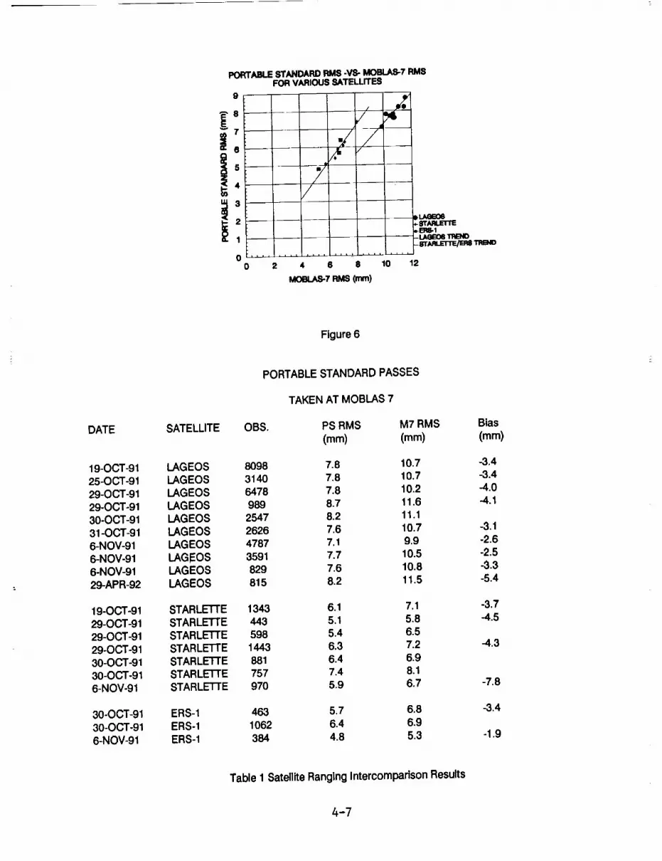
PORTABLE STANDARD RMS -VS- MOBLA8-7 RMSFOR VARIOUS SATELLITES
e
87
O
l 54
I'21
/_STk"_'T'_ TnSNO
0 ....... ' ' .......
0 2 4 6 8 10 12
MOB.AS-7RMS(nln)
DATE
19-0CT-9125-0CT-9129-0CT-9129-0CTo9130-0CT-9131 -OCT-916-NOV-916-NOV-916-NOV-9129-APR-92
19-OCT-9129-OCT-9129-OCT-9129-OCT-9130-OCT-9130-OCT-916-NOV-91
SATELLITE
Figure 6
PORTABLE STANDARD PASSES
TAKEN AT MOBLAS 7
OBS. PS RMS M7 RMS Bias(mm) (mm) (mm)
LAGEOS 8098 7.8 10.7 -3.4LAGEOS 3140 7.8 10.7 -3.4LAGEOS 6478 7.8 10.2 -4.0LAGEOS 989 8.7 11.6 -4.1LAGEOS 2547 8.2 11.1LAGEOS 2626 7.6 10.7 -3,1LAGEOS 4787 7.1 9.9 -2.6LAGEOS 3591 7.7 10.5 -2.5LAGEOS 829 7.6 10.8 -3.3LAGEOS 815 8.2 11.5 -5.4
STARLETTE 1343 6.1 7.1STARLETTE 443 5.1 5.8STARLETTE 598 5.4 6.5STARLETI'E 1443 6.3 7.2STARLETrE 881 6.4 6.9STARLETTE 757 7.4 8.1STARLET'rE 970 5.9 6.7
30-OCT-91 ERS-1 463 5.7 6.830-OCT-91 ERS-1 1062 6.4 6.96-NOV-91 ERS-1 384 4.8 5.3
-3.7-4.5
-4.3
-7.8
-3.4
-1.9
Table 1 Satellite Ranging Intercomparison Results
4-7

5 Future Plans
As noted, MOBLAS-7 is notachieving itsbest performance at thistime. For the second stage ofthe experimentwe plan to perform adjustments and fine-tuning of the MOBLAS-7 instrumentation to regain its typicalperformance, then make the intercomparlson again. During the the next serles of passes amplitudemeasurements will also be taken to apply the discriminator time-walk correction to the data. For the thirdstage of the experiment, we will installa second detector inthe MOBLAS-7 receive package for dual-detectiontests. The new detector exhibits enhanced bandwidth and jitter characteristics ("Performance Comparisonof Microchannel Plate PMTs", Varghese, Selden and Oldham, These Proceedings). We also plan to obtainan APD detection system to perform direct intercomparison measurements between APD and MCP-PMTs atboth the multi-photoelectron and single photoelectron level.
Stanford time interval counters will also be used for range measurement. In the past, We have tested theperformance of Stanford counters in the laboratory with varying results. Of the five counters tested, twoexhibited large and un-predictable ( 100 ps) jumps in range while the remaining three counters behavednormally and were comparable to the HP-5370 in performance. At least one Stanford SR620 counter whichperforms well inthe laboratory will be used for a shot-by shot comparison with the other time Interval meters.
Other plans have begun to perform in-orbit satellite characterization experiments using TOPEX. For thesetests the PS will be used in optical isolation mode; a celestron C-11 telescope will be "piggy-backed" on theMOBLAS-7 Contraves telescope for parallel measurement. The test will also provide a comparison betweenlarge and small aperture systemson other satellites. Recently, a study ofthe relative effect of thermal-loadingonthe two telescopes was done to determine their focal-length stability for smalldetector (APD) applications.
6 Conclusions
The portable standard, developed and proven through laboratory experiments, has shown Improved satelliterange residuals through the use of multiple time interval counters over data acquired by MOBLAS-7. Use ofits full capabilities should provide even more Improvement and test the accuracy limitations imposed bycurrent ranging Instrumentation. Sequential testing and replacement of measurement components (detector,signal processor, time interval/event meter, etc.) will offer a controlled measurement baseline and increaseour understanding of $LR error sources.
4-8

Detector Technology


N94-15569
Performance optimization of detectorelectronics for millimeter laser ranging
S. Cova +, A Lacaita + and G Pdpamonti _
+ Politecnico di Milano, Dipartimento di Elettronica e Informazione and CEQSE-CNR,
Piazza L. da Vinci 32 - 20133 Milano (Italy)
*Universita' degli Studi di Milano, Dipartimento di Fisica
Via Celoria 16 - 20133 Milano (Italy)
(invited paper)
ABSTRACT
The front-end electronic circuitry plays a fundamental role in determining the performance
actually obtained from uitrafast and highly sensitive photodetectors. We deal here with
electronic problems met working with Microchannel Plate photomultipliers (MCP-PMTs)
and Single Photon Avalanche Diodes (SPADs) for detecting single optical photons and
measuring their arrival time with picosecond resolution. The performance of available fast
circuits is critically analyzed. Criteria for selecting the most suitable electronics are derived
and solutions for exploiting at best the detector performance are presented and discussed
I. INTRODUCTION
Laser ranging applications with millimeter resolution require to measure the time
of flight of single photons with precision better than 30ps root mean square (rms), that
is, with better than 70ps full-width at half maximum (FWHM) of the resolution curve.
Two photodetector types can attain single photon sensitivity and picosecond resolution:
proximity-focused Microchannel Plates (MCPs) [1-31 and Single Photon Avalanche
Diodes (SPADs) [4-7]. In both cases the front-end electronics associated to the detector
plays a fundamental role. In order to take full advantage of the detector timing
performance, the electronic pulse processing should be carefully optimized.
In set ups where MCPs are employed, the fast preamplifier and the constant
fraction trigger circuit (CFT) are by far the most critical electronic components. In this
paper we discuss criteria for optimum selection of the preamplifier, taking into account
the noise and bandwidth characteristics. We show that preamplifiers with very large
bandwidth (3GHz or more) are not to be employed, since they impair the timing
performance 18]. We analyze problems met by constant fraction triggers working with
5-1

subnanosecondpulsesfrom MCPs. We discusshow the performanceof available CVI's
can be improved by simple modifications that provide a better adjustment of the relevant
CFI" parameters and/or by suitable pre-filtering of the MCP pulses [9,10].
SPADs are avalanche photodiodes that operate biased above the breakdown voltage
in the so-called Geiger-mode 14-7,11 l. Their operation is fundamentally different from
that of photomultiplier tubes (PMTs) and of ordinary avalanche photodiodes (APDs).
The device does not have a linear internal gain, that is, it does not amplify linearly the
primary photocurrent. It instead exploits the avalanche process to behave in a way
similar to that of a trigger circuit, rather than an amplifier. When one or more photons
are detected at a given time, a fast-rising current pulse is generated, with standard
amplitude and shape, independent of the number of photons. The leading edge of this
pulse marks with very high precision, down to 20ps FWHM, the time of arrival of the
photon that has triggered the avalanche 151.
We analyze limitations met working with SPADs in the simple biasing
arrangements that employ a ballast resistor to quench the avalanche, called Passive
Quenching Circuits (PQCs) I6,7,11 ]. In order to fully exploit the ultimate SPAD timing
performance, the device should be operated with an Active Quenching Circuit (AQC)
112,13]. We introduce a new AQC model, capable of driving the detector in remote
position, connected by a coaxial cable [13]. Special care has been devoted to the design
of the-input stage, in order to minimize the circuit noise and thus reduce to less than 3ps
rms the internal time jitter of the circuit, making negligible its contribution to the overall
time resolution.
II. SELECTION OF THE OPTIMUM PREAMPLIFIER FOR MCPs
Since the gain of the MCP is limited to 5 10 s, a fast preamplifier with gain higher
than 10 must be used between the MCP output and the pulse-timing trigger circuit. This
gain makes the noise of the following circuits negligible, in comparison to that of the
amplifier. In order to avoid reflections and ringing in the pulse shape, the MCP output
must be terminated on a 50 Ohm resistor R s , as outlined in the equivalent circuit of
Fig. 1.
MCP Amplifier
i',i.............._ i i [ H( ) Triggeri,', ...................................................W circuit 1f i
P rd I
":_ _:! : i _Rs=5OOhmv,''' ",:" i
Fig. 1 Equivalent circuit for analyzing the effect of the amplifier noise and bandwidth
on the pul_ time-jitter.
5-2

An accurate analysis of the time-jitter contribution arising from the electronic noise
has been carried out [81 and we report here the main results. The action of the amplifier
on the MCP pulses is described (see Fig. 1) by two blocks: a transfer function in the
frequency f domain HA(f), normalized to unity dc gain, followed by a constant gain G.
The time-domain impulse response of the amplifier is hA(t) = F-l [HA(f)] (where F-I
denotes the inverse Fourier transform and hA(t ) is normalized to unit area). S i is the
spectral density of the equivalent input noise generator of the amplifier, assumed to be
gaussian. As sketched in Fig.2, the noise causes a random shift of the actual crossing
time of the trigger threshold.
Vn FWHM Noise ," ,,,'
_J.res.,," ,1 \
Tn Time jitter ,-5,, '
Fig.2 Effect of the electronic noise on the triggering time.
Let us denote by v, the rms value and by V n the FWHM of the amplitude
distribution of the noise, and by r the slope of the ideal, noise-free pulse at the triggering
threshold. The FWHM T, of the additional time jitter is given by
V n v n
T n - - 2.36-- (1)r r
This time jitter at the comparator threshold (point 3 in Fig. 1) is equivalently evaluated at
the input of the gain stage G (point 2 in Fig. 1).
In first instance, the noisespectrum can be considered white, that is, with constant
spectral amplitude Si = a2. Let us denote by B, the noise bandwidth, proportional to the
signal bandwidth B A (3dB down bandwidth)
B. = K n B A
with constant K. depending on the shape of the frequency response HA(f). We have
Vn = a-k//-_, = a_
(2)
(3)
5-3

The sloper also increaseswith BA , and it canbeeasily seenthat thereis a minimum inthe plot of T. versusB^. Let us first considerthe high bandwidth side, where the B^valuesarehigh enoughto haverisetimepracticallyequal to that of the MCP pulse. Onthat side,T. goesup as"kf_A, sincethe sloper is unaffectedand the noisevn increases
as "_A- Let USnow consider the low bandwidthside, wherethe pulse-risetimeTr isfully dominatedby BA, namely,Tr is about 1/(3 BA).On this side,T. goesdown asB^-
3/2 when BA is increased, since the slope r increases as BA2 and noise increases as "_A.
A minimum of T, will therefore be found at an intermediate value of B A , at which the
relative rate of increase of the pulse slope r will be equal to that of the noise V.. More
accurate quantitative results can be obtained by considering the actual voltage waveform.
Let us denote by VD(t) the voltage pulse at the 50 Ohm output of the MCP detector
VD(t ) = Q ho(t ) (4)
where Q denotes the area of VD(t ) and ho(t ) is normalized to unit area. The actual
voltage waveform V(t) at the input of the gain stage G (point 2 in Fig. I), results from
the convolution product of the detector pulse VD(t ) and of the amplifier impulse response
hA(t)
V(t) - Q ht:,(t ) * hA(t ) (5)
t'--
.tnO
z
-./-
t.a_
10-3
10-4
10-5
10-6
10-7
10-8
10-9
106
! I I ITTTT] I | I II1|1] I I I I IIII t _1 I I I |
_10
10
I I lilll[ I I I Illll[ J ,I l llllll l l I Illlll i I I till 10
107 108 109 1010 1011
Amplifier bendwidth (Hz)
-1
-210 _"
c-
-2 "-
._Q
t0 -4Ex
-510
-G
Fig.3 Maximum slope, r, of the amplified pulse and FWHM Vn of the noise
amplitude distribution at point 2 in Fig. 1 vs amplifier bandwidth BA. Pulses of
a 12/,tm channel MCP (Hamamatsu RI564U); amplifier having frequency
resl'_mse with two real poles, white input noise generator with rms density
a= 2nV Hz -ts-'. Results of detailed computations of the pulse waveform (full line)
are compared with the approximation discussed in Ref. 18l (dotted line).
5-4
The shapeof V(t) and the correspondingmaximum slope r can be obtainedbynumericalcomputations,accuratelytaking into accountthecharacteristicsof the detectorpulseand of the amplifier impulse response[8]. A simple approximation earl also be
employed to obtain a sufficiently good estimate of r. Essentially, it consists in computing
the slope r as result of a weighted average of the corresponding slopes of the detector
pulse and of the amplifier impulse response [8]. Fig.3 reports the computed behavior of r
and V n versus amplifier bandwidth for a typical case. Fig.4 illustrates for another case
the detailed behavior of the time jitter versus amplifier bandwidth. A broad minimum is
found in all cases considered, centered at an optimum bandwidth value BAot,t , which in
all cases is well below 2GHz and mostly is around IGHz.
The analysis carried out with a white noise spectrum leads to definite conclusions.
Selecting the amplifier for very high bandwidth and paying minor attention to the noise
is not only useless, but even disadvantageous. The noise has primary importance, since
the time jitter is proportional to the root-mean square spectral density a. The optimum
bandwidth value BAopt is markedly lower than that suggested by the criterion of keeping
the risetime of the amplified pulse very near to the original risetime of the detector pulse.
Even for the fastest available MCP detector, BA,,p t does not exceed I.TGHz. Satisfactory
results can be obtained with bandwidth values remarkably lower than BA_ I, even by a
factor of two. On the basis of these results, it was concluded that amplifiers employing
fast bipolar transistors (BJTs) provide better performance than amplifiers based on
ultrafast metal-semiconductor field-effect transistors (MESFETs). in fact, the higher
bandwidth of MESFETs is not required and, working with a 50 Ohm source, the lower
input current noise is not important. Furthermore, MESFETs may have higher
components in the low-frequency noise spectrum. However, it must be taken into
account that the input noise spectrum of BJTs also contains a high frequency component
proportional to f2. A detailed analysis 18] shows that the f2_noise component causes a
steeper increase of V, for rising BA, thereby shifting to lower B A value the minimum of
Tn and making much steeper the rise of T, on the high B A side. Fig.5 illustrates a typical
case. It is worth stressing that the effect is more marked and the shift of the minimum is
greater for transistors having lower white noise component (that is, lower value of a).
These results further support and enhance the conclusions drawn in the white noise
analysis. The presence of a f2 component in the noise spectrum of BJTs i) shifts to even
lower value the optimum amplifier bandwidth BAopt ; ii) makes remarkably more severe
the penalty for working with amplifier bandwidths higher than the optimum one ; iii)
has almost negligible influence on the results obtained with amplifier bandwidth lower
than BAopr
In conclusion, the quantitative analysis demonstrates that, by using available low-
noise high-frequency bipolar transistors in rationally selected operating conditions, the
additional time jitter due to the circuit noise can be kept below 5 ps FWHM. In any case
of interest, the behavior of the jitter versus the amplifier bandwidth can be fairly simply
analyzed by using the approximate approach introduced in Ref.8. This approach just
requires the knowledge of a few numerical parameters characterizing the pulse shapes
involved, which can be obtained by analytical representation or by measurements of the
waveforms.
5-5
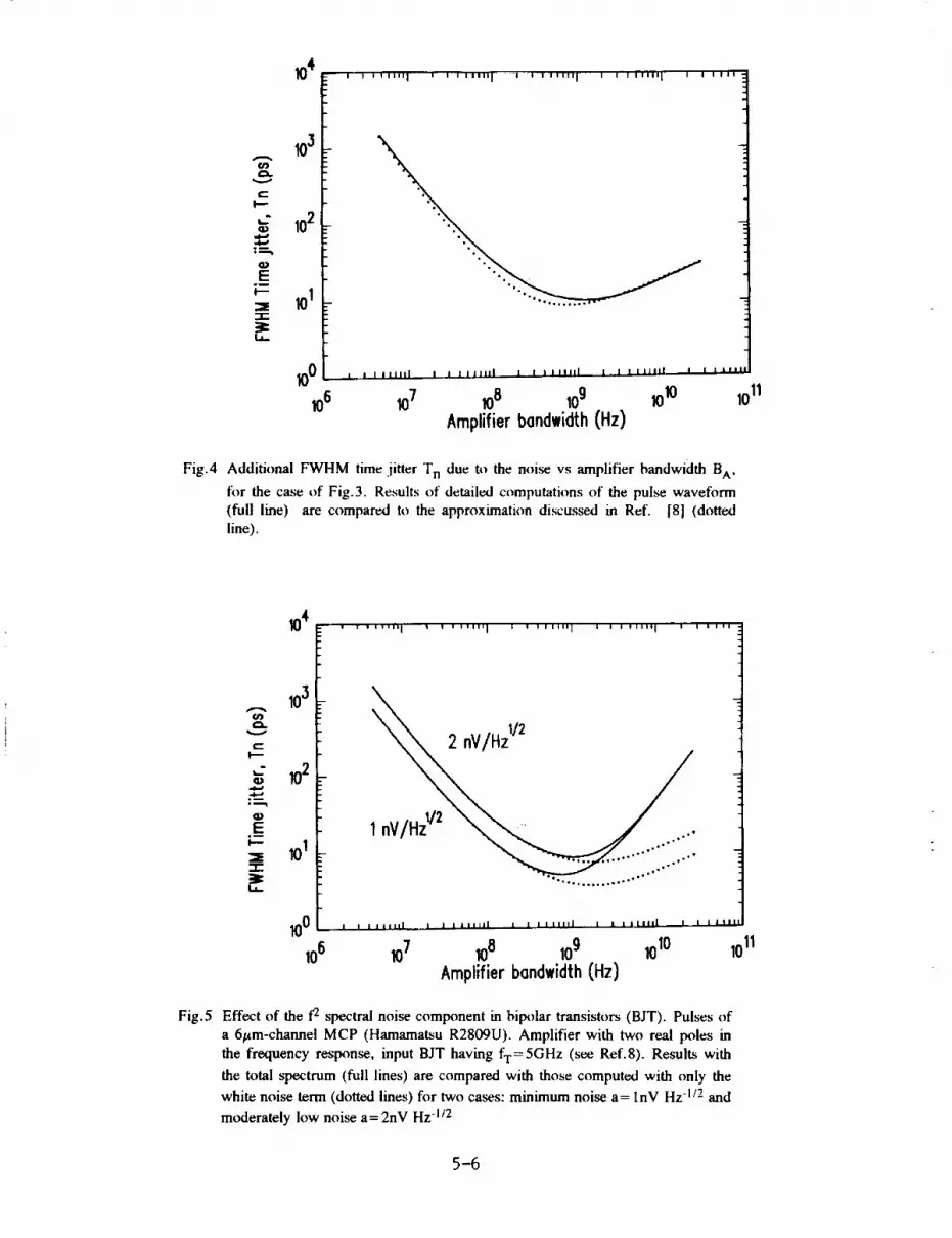
104' _ , , t t,,,u I , I , ,,,,q t , I i,,H I a i t s,,i, I I i li,1 .
¢..=
I--"
,.7
.n
E
--I-
3:t.l-
103
102
101
00 ± I I IIIItl I J 1Jllill l I I IIIIII I I I Iit111 I I I IlIa
106 107 108 109 1010 1011
Amplifier bondwidth (Hz)
Fig.4 Additional FWHM time jitter T n due to the noise vs amplifier bandwidth BA,
for the case of Fig.3. Results of detailed computations of the pulse waveform
(full line) are compared to the approximation discussed in Ref. 18] (dottedline).
i03
_" _ 2 nV/H"" zl/2e"-"
ols
ID
E
101
" F_ *°'°"*o°.**"***°
00 ! I lilLtL l I [llilll I I i lillll I I llllli I I I I TMi
106 107 108 109 1010Amplifier bandwidth (Hz)
1011
Fig.5 Effect of the f2 spectral noise component m bipolar transistors (BJT). Pulses of
a 6#m-channel MCP (Hamamatsu R2809U). Amplifier with two real poles in
the frequency response, input BJT having fT=5GHz (see Ref.8). Results with
the total spectrum (full lines) are compared with those computed with only the
white noise term (dotted lines) for two cases: minimum noise a= InV Hz -1/2 and
moderately low noise a= 2nV Hz -1/2
5-6

III. CONSTANT FRACTION TRIGGERS WITH MCPs
Since single-photon pulses of photomultiplier tubes (PMTs) have statistically
fluctuating amplitude, constant-fraction trigger circuits (CFT) are normally employed for
accurate timing [14]. However, with the subnanosecond signals of MCPs non-ideal CFT
behavior is observed. A residual amplitude-dependent time-walk sets the ultimate
resolution in photon timing. A quantitative analysis of the problem has been carried out
and will be here summarized 110].
Fig. 6 illustrates the basic structure and the principle of operation of a CFT circuit.
The triggering point of the fast comparator is determined by the crossing of two replicas
of the amplified MCP pulse, the first attenuated by a factor k, the second one delayed by
a time T o.
1.0
0.8
2E" 0.6
0.4
o.2
0.0 . i-1 0 1 2
Time [A.U.]
Fig.6 Working principle of Constant Faction Triggers (CFTs) b''ased on a fast
comparator with differential input. Block diagram (inset) and pulse waveforms
at the comparator inputs (norma!ized to unit peak amplitude) are depicted in
simplified form.
Crossing occurs when the delayed pulse reaches a given percentage of the peak.
The time-walk effect is eliminated, since the triggering time is independent of the actual
pulse amplitude A. This is strictly true only if the two waveforms have the same baseline
level. However, setting both inputs at the same bias voltage level is unacceptable, since
it causes the comparator to oscillate. A small dc voltage offset b is necessary; in practice,
about 10 mV with modern fast comparators. This constant offset b causes a deviation
from the ideal CFT operation, since it causes the crossing time to walk as A is varied.
The slower is the rise of the delayed waveform, the larger is the walk. The problem is
quantitatively analyzed making reference to the pulse waveform g(t) normalized at unit
peak amplitude and to the correspondingly normalized baseline offset x. The pulse-
amplitude distribution, with probability density p(A), is transformed in a distribution of
5-7
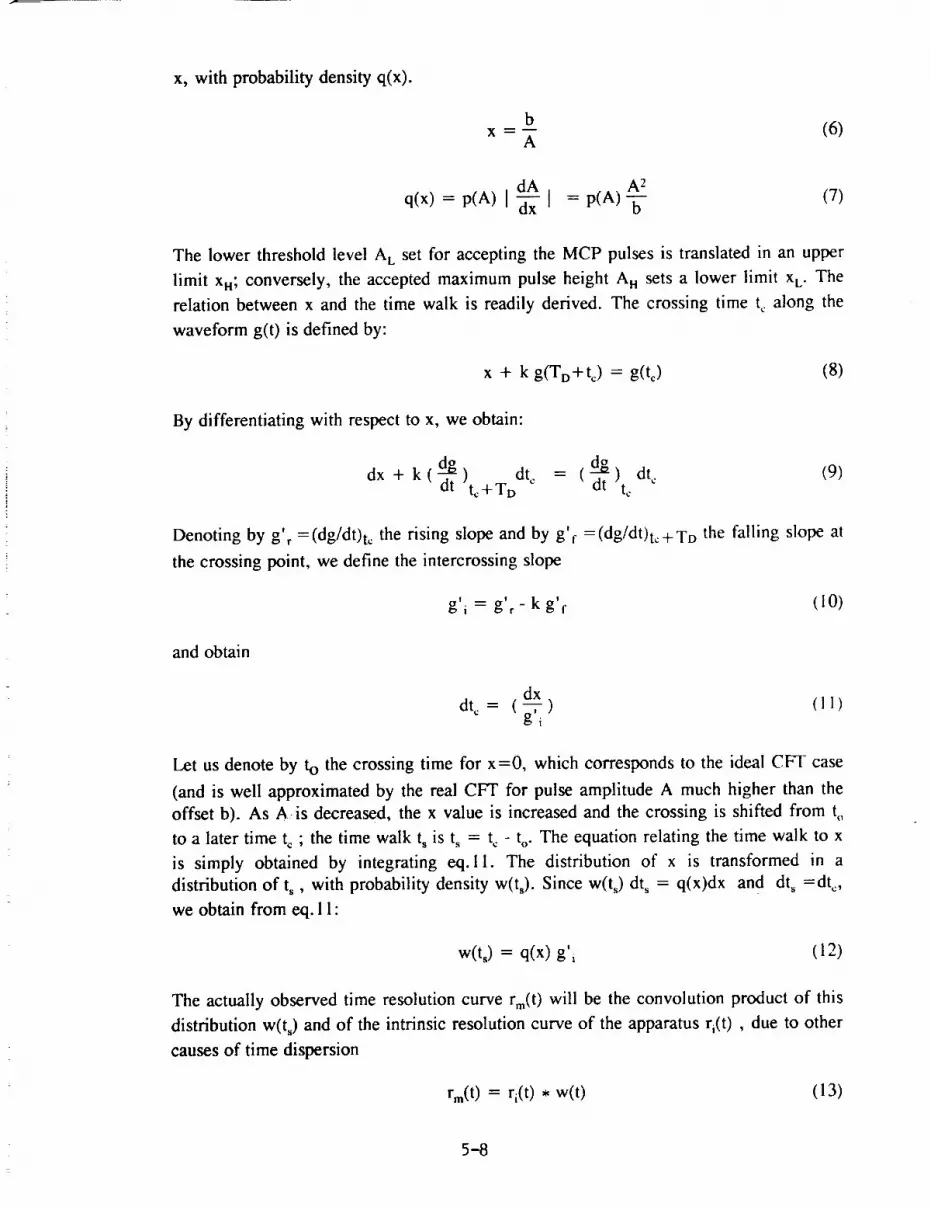
x, with probability densityq(x).
bx = -- (6)
A
dA A2
q(x) = p(A) [ -d-_x I = p(A)-_ (7)
The lower threshold level A L set for accepting the MCP pulses is translated in an upper
limit x,; conversely, the accepted maximum pulse height A H sets a lower limit x L. The
relation between x and the time walk is readily derived. The crossing time t_ along the
waveform g(t) is defined by:
x + k g(TD+t¢) = g(t¢) (8)
By differentiating with respect to x, we obtain:
dx + k( dgdt )t_+To dt_
= (d___) dL (9)dt t_
Denoting by g'r =(dg/dt)t_ the rising slope and by g'f =(dg/dt)t_+TD the falling slope at
the crossing point, we define the intercrossing slope
g'i = g'r - k g'f (I0)
and obtain
d___xdt_ = (g,i) (11)
Let us denote by to the crossing time for x=0, which corresponds to the ideal CFF case
(and is well approximated by the real CFT for pulse amplitude A much higher than the
offset b). As A is decreased, the x value is increased and the crossing is shifted from t,,
to a later time tc ; the time walk ts is t._ = t_ - t o. The equation relating the time walk to x
is simply obtained by integrating eq. ll. The distribution of x is transformed in a
distribution of t_, with probability density w(t_). Since w(ts) dt_ = q(x)dx and dt_ =d L,
we obtain from eq. 11:
w(t_) = q(x) g'l (12)
The actually observed time resolution curve rm(t) will be the convolution product of this
distribution w(t_) and of the intrinsic resolution curve of the apparatus q(t) , due to other
causes of time dispersion
rm(t ) = ri(t ) • w(t) (13)
5-8
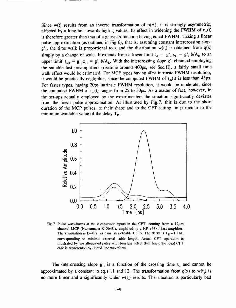
Since w(t) results from an inverse transformation of p(A), it is strongly asymmetric,
affected by a long tail towards high t s values. Its effect in widening the FWHM of rm(t)
is therefore greater than that of a gaussian function having equal FWHM. Taking a linear
pulse approximation (as outlined in Fig.6), that is, assuming constant intercrossing slope
g'i, the time walk is proportional to x and the distribution w(ts) is obtained from q(x)
simply by a change of scale. It extends from a lower limit tsL = g'i XL = g'i b/AH to an
upper limit tsH = g'i xrl = g'i b/AL" With the intercrossing slope g'i obtained employing
the suitable fast preamplifiers (risetime around 400ps, see Sec.II), a fairly small time
walk effect would be estimated. For MCP types having 40ps intrinsic FWHM resolution,
it would be practically negligible, since the computed VWHM of rm(t) is less than 45ps.
For faster types, having 20ps intrinsic FWHM resolution, it would be moderate, since
the computed FWHM of rm(t) ranges from 25 to 30ps. As a matter of fact, however, in
the set-ups actually employed by the experimenters the situation significantly deviates
from the linear pulse approximation. As illustrated by Fig.7, this is due to the short
duration of the MCP pulses, to their shape and to the CFT setting, in particular to the
minimum available value of the delay TD.
1.0
0.8
0.6t'_
E
0.4
0.2
0.5 1.0 1.5 2.0 2.5 3.0 3.5 4.0Time [ns]
Fig.7 Pulse wavefl_rms at the comparator inputs in the CFT, coming from a 12#m
channel MCP (Hamamatsu RI564U), amplified by a HP 8447F fast amplifier.
The attenuation is k=0.2, as usual in available CFTs. The delay is To= l.lns,
corresponding to minimal external cable length. Actual CFT operation isillustrated by the attenuated pulse with baseline offset (full line); the ideal CFT
case is represented by dotted-line wavefonn.
The intercrossing slope ,:,o'.. is a function of the crossing time tc and cannot be
approximated by a constant in eq.s 11 and 12. The transformation from q(x) to w(t_) is
no more linear and a significantly wider w(t_) results. The situation is particularly bad
5-9
when the crossing occurs at the onset of the delayed pulse leading edge, where the rise is
slower and the intercrossing slope is correspondingly low. Such a situation can be
avoided by making the delay T D shorter than the duration of the input pulse. In
commercial CFr circuits, T D is mainly determined by the propagation time in a coaxial
cable, externally connected to the circuit module and selected by the user. The least
obtainable value of TD is about 1. Ins or slightly less [15], determined by the connectors,
the circuit layout and the minimal length possible for the external cable. This was
adequate for the pulses of ordinary PMTs, lasting a few nanoseconds, but it is no more
sufficient for the subnanosecond pulses of ultrafast MCPs. As illustrated in Fig.7, with
TD= 1. l ns the crossing occurs just in the low slope zone of the rising waveform. The
operation only roughly approximates the ideal CFT; in fact, it is intermediate between a
CFT and a leading edge trigger with small, constant threshold.
Such a situation can be avoided by a suitable selection of parameters in the
experiment. The analysis points out the basic criteria for m_nimizing the time walkeffect:
i) the preamplifier gain should be high enough to keep low the value of the upper limit
x H in all cases, even when a small value of the lower threshold A L is selected for
accepting almost all pulses, e.g. 90%of the amplitude distribution p(A).
ii) the delay TD and attenuation k should be selected for maximizing the intercrossing
slope.
The latter criterion is usually not satisfied by industrially produced CFT models. Beside
having too long minimum delay, they are normally set to low constant fraction values,
around 0.2, which are optimal for timing signals from scintillation detectors of ionizing
radiations, but not for timing single photons 110,141. This is due to historical reasons,
since CFTs were originally developed for working with ionizing radiation detectors
A detailed quantitative analysis of the CFT time-walk effect in the conditions of
actual experiments can be carried out by means of computer simulation, taking
accurately into account the actual shape of the signal waveform processed by the
amplifier.' It is worth noting that the rosult of the computation of the crossing time t¢
versus normalized baseline offset x can be easily foreseen, by linearly shifting upwards
the attenuated waveform in figures like Fig.7 and directly observing the walk of the
crossing point. In the following, in order to set in evidence the effects on the time
resolution, all the time distribution curves are drawn aligned at the peak value. All
FWHM values reported are measured on the complete computed curve rm(t). In fact,
since the shape of the distribution w(ts) is asymmetrical and far from gaussian, the
FWHM value of rm(t) would be remarkably underestimated by a quadratic composition
of the FWHM values of w(ts) and ri(t).
Previously published experimental results were analyzed and improvements
obtainable by modifying the CFT parameters and/or the pulse shape were evaluated [10l.
We first considered cases where a 12micron channel MCP Hamamatsu R1564U is
employed with a fast amplifier model HP8447F. The amplitude distribution and signal
waveform are reported from Yamazaki et al. 11] and from the manufacturer data sheets
5-10

and technical notes [16]. On the basis of published results [1-3] the intrinsic time
distribution ri(t), due to the detector is assumed to be gaussian with 40ps FWHM.
We studied the effect of a filtering stage with a Ins integrating time constant,
interposed between fast amplifier and CFI" as proposed and experimented in our
laboratory 191. The wider pulse obtained by filtering makes possible to obtain a higher
intercrossing slope with the minimum delay of 1.3ns available in our set up. The
computer analysis gives results in perfect agreement with the experiment, confirming that
the improvement of the FWHM from 75ps to 55ps was obtained thanks to the reduction
of the time walk effect.
1.0
0.8
f""-I
:5 0.6
= 0.4o0
0.2
0.00 50
elolul,oI100 150 200 250
Time [psi
Fig. 8 Computed time resolution curve for measurement with low selecting threshold
level (accepting almost all pulses), compared to the intrinsic time resolution
curve (dotted curve) of a 12 #m channel MCP (Harnamatsu R1564U). The
computed FWHM is 61ps; the experimental value in Ref. 1 is 63ps.
We analyzed then the experiments reported by Yamazaki et al. 11|, where the
resolution was measured with two different levels of the auxiliary lower threshold A L of
the CFT, which selects pulses accepted for the time measurement. With low threshold,
accepting almost all pulses, they measured 63ps FWHM; the computed value for
TD= 1. Ins and k=0.2 was 61ps, as illustrated in Fig.8. The computation also confirmed
that with high, threshold, accepting only 15% of the pulses, the FWHM suffers negligible
degradation with respect to the intrinsic value. For the experiments with low threshold
level, we also evaluated the improvement obtainable by reducing the pulse delay T D
and/or the attenuation ratio k, in order to increase the intercrossing slope. It is not
difficult to reduce the delay T D in existing CFTs, without needing to redesign and
fabricate new CFT models. The available models can be modified by cutting lines in the
printed circuit board and making new internal connections for a shorter delay path, that
avoids the external delay cable. By modifying the resistor network that attenuates the
prompt waveform (see Fig.6), one can also change the k to higher values. In order to
attain k= 1, however, major modifications or complete redesigning of the CFT circuit
5-11
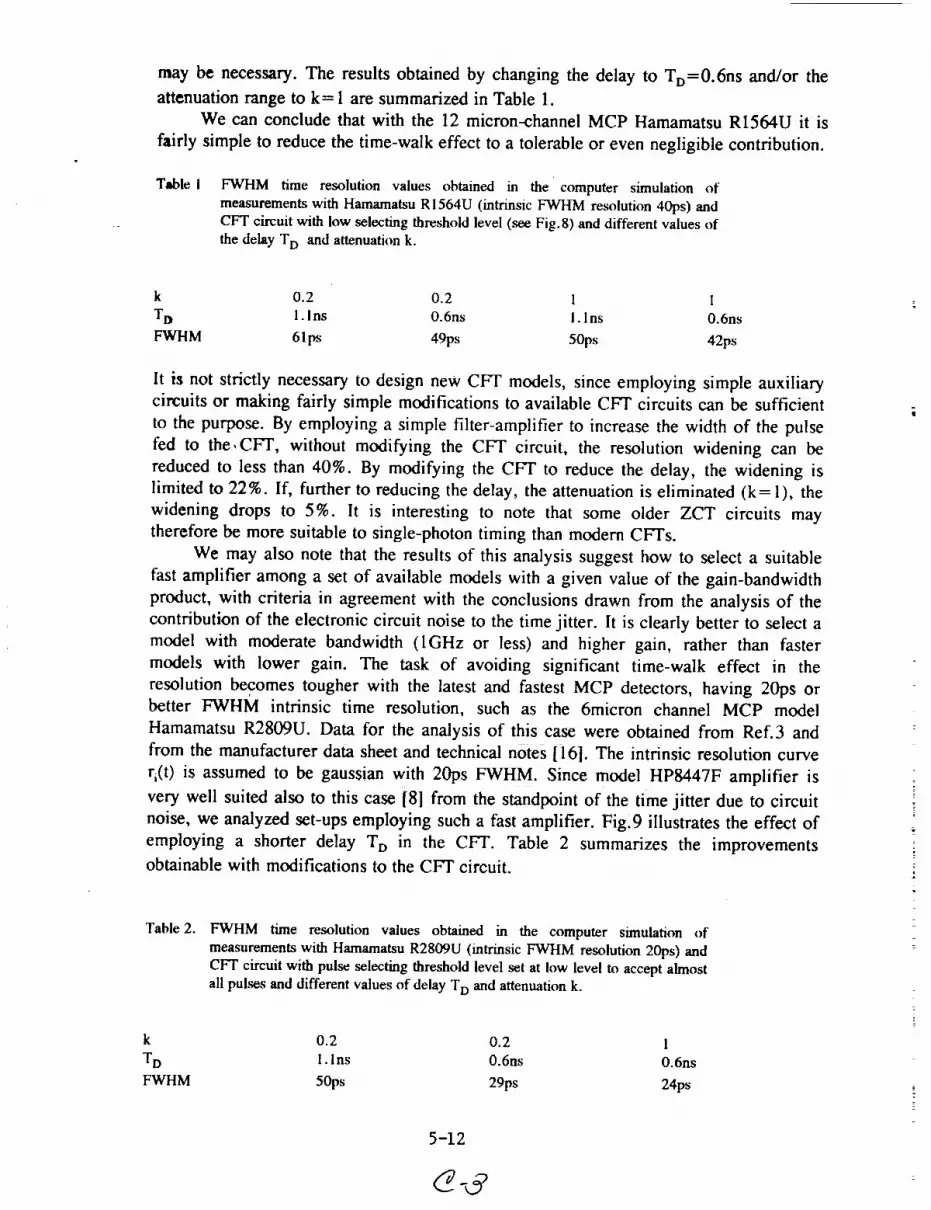
may be necessary. The results obtained by changing the delay to TD=0.6ns and/or the
attenuation range to k= 1 are summarized in Table 1.
We can conclude that with the 12 micron-channel MCP Hamamatsu RI564U it is
fairly simple to reduce the time-walk effect to a tolerable or even negligible contribution.
Table i FWHM time resolution values obtained in the computer simulation of
measurements with Hamamatsu R 1564U (intrinsic FWHM resolution 40ps) andCFT circuit with low selecting threshold level (see Fig.8) and different values of
the delay T o and attenuation k.
k 0.2 0.2 I I
T D 1. Ins 0.6ns I. Ins 0.6ns
FWHM 61 ps 49ps 50ps 42ps
It is not strictly necessary to design new CPT models, since employing simple auxiliary
circuits or making fairly simple modifications to available CFT circuits can be sufficient
to the purpose. By employing a simple filter-amplifier to increase the width of the pulse
fed to the,CFT, without modifying the CFT circuit, the resolution widening can be
reduced to less than 40%. By modifying the CFT to reduce the delay, the widening is
limited to 22%. If, further to reducing the delay, the attenuation is eliminated (k= 1), the
widening drops to 5%. It is interesting to note that some older ZCT circuits may
therefore be more suitable to single-photon timing than modern CFTs.
We may also note that the results of this analysis suggest how to select a suitable
fast amplifier among a set of available models with a given value of the gain-bandwidth
product, with criteria in agreement with the conclusions drawn from the analysis of the
contribution of the electronic circuit noise to the time jitter. It is clearly better to select a
model with moderate bandwidth (1GHz or less) and higher gain, rather than faster
models with lower gain. The task of avoiding significant time-walk effect in the
resolution becomes tougher with the latest and fastest MCP detectors, having 20ps orbetter FwHM intrinsic time resolution, such as the 6micron channel MCP model
Hamamatsu R2809U. Data for the analysis of this case were obtained from Ref.3 and
from the manufacturer data sheet and technical notes [16]. The intrinsic resolution curve
ri(t) is assumed to be gaussian with 20ps FWHM. Since model HP8447F amplifier is
very well suited also to this case [8] from the standpoint of the time jitter due to circuit
noise, we analyzed set-ups employing such a fast amplifier. Fig.9 illustrates the effect of
employing a shorter delay T o in the CFT. Table 2 summarizes the improvements
obtainable with modifications to the CFT circuit.
Table 2. FWHM time resolution values obtained in the computer simulation of
measurements with Hamamatsu R2809U (intrinsic FWHM resolution 20ps) andCFT circuit with pulse selecting threshold level set at low level to accept almost
all pulses and different values of delay T D and attenuation k.
k 0.2 0.2 1
T D 1. Ins 0.6ns 0.6ns
FWHM 50ps 29ps 24ps
5-12

::5
I......,.I
t-
OL.)
1.0
0.8
0.6
0.4
0.2
0.0 i
0
a) 20ps FWHM(intr. res.)
! _1\ b) 29ps FWHM(To=O.6ns)
_ _Ops FWHMCTD=1.lns)
50 100 150 200 250Time [ps]
Fig.9 Computed time resolution curves, including effects of amplitude dependent timewalk in CFT, for measurement set-ups with MCP model R2809U, fast amplifier
HP8447F, CFT pulse selecting threshold set at low level to accept almost all
pulses. The dotted curve is the assumed intrinsic resolution curve, having 20psFWHM. Two cases are reported: a) CFT with the usual attenuation k=0.2 and
delay corresponding to minimal external cable T,= I. Ins (wider curve, 50ps
FWHM); b) CFT with k=0.2, but with shorter delay To=O.6ns (narrower
curve, 29ps FWHM).
It is interesting to compare these results to the corresponding ones for the case of
the 12micron channel model R1564U. Essentially, the time walk in the corresponding
situations is quite similar in the two cases, but its relative effect on the obtainable
performance becomes greater as the intrinsic detector is improved. For the R2809U the
actual resolution with the short delay of 0.6ns is remarkable, but 45% wider than the
intrinsic one. With delay 0.6ns and no attenuation (k= 1) the obtainable resolution is still
20% wider than the intrinsic. Some experimental results point out that the detector
intrinsic resolution may be even better than 20ps, possibly 10ps or better.The time walk
effect should therefore be considered a major limitation to the ultimate obtainable
resolution.
We conclude that there is considerable margin for further improvement. Greater
care should be therefore devoted to the electronic pulse processing, in order to take full
advantage of the detector intrinsic resolution. It is advisable to work with CFT having
k= 1 and even shorter delay, possibly with specially studied filter-amplifier input stage.
Designing new CFT circuits specially devised for photon counting may be rewarding.
5-13

IV. ACTIVE-QUENCHING CIRCUITS FOR SPADs
In early studies on SPADs, the bias arrangement used for the device operation was
the so-called passive quenching circuit (PQC) [4,5,11]. This circuit employs a high load
resistor (in the 100k range) in order to force the diode voltage V to drop down near to
the breakdown voltage V B after each avalanche triggering. This quenches the avalanche.
The diode voltage is then slowly restored to the bias voltage, since the diode capacitance
is recharged by the small current flowing through the high value resistor. The voltage
recovery takes at least some microseconds. A photon can arrive during the recovery from
a previous avalanche pulse and trigger the avalanche when the SPAD voltage is at some
intermediate level, randomly placed between the breakdown voltage and the correct bias
voltage. This'has a twofold detrimental effect on the timing performance. First, the
intrinsic time resolution of SPADs is strongly reduced as the excess bias voltage V-V B
actually applied to the diode is reduced. Second, at lower excess bias voltage the
avalanche current pulse not only has smaller amplitude, but also slower risetime. This
causes a walk of the triggering time of the following timing circuit, which is not properly
corrected even employing a CFT (CFTs require constant pulse shape to work properly).
The intrinsic performance of SPADs can be exploited working with PQCs only in cases
where the probability of such events (photons arriving during a recovery from a previous
avalanche pulse) is very low, that is, where the rate of repetition of pulses is very low, at
best a few kHz. Note that this limitation applies to the total rate of pulses, that is, to the
sum of the dark count rate of the SPAD plus the detected photon rate, including
unwanted background light.
A partial remedy to such limitations is to apply a pulsed bias voltage to simple
passive circuit arrangements, for obtaining a gated operation of SPADs. The additional
voltage pulse can be superimposed to the dc bias either by ac coupling or by dc coupling.
The ac coupling is very simply implemented, by connecting the junction between SPAD
and load resistor to a low-impedance fast pulse generator through a suitable capacitor.
The dc coupled gate is obtained by employing a smaller load resistor, typically l kOhm
or less, and applying directly to it the sum of the dc bias voltage plus a pulsed additional
voltage. The detailed analysis [ 18] of such circuit arrangements, however, points out that
i) it is possible to detect not more than one photon in the gate interval ii) other specific
limitations are associated to each circuit arrangement. With ac coupling, the repetition
rate of gating pulses must be low. With dc coupling, the power dissipated in the SPAD
may become excessive. In summary, it can be concluded that pulsed-bias passive circuits
are of practical interest only for working with gate intervals having short duration,
typically below lOOns, and low or moderate repetition rate.
In the early stage of development of SPADs, it became therefore clear that more
sophisticated circuits were necessary, in order to fully exploit the device performance.
Active quenching circuits (AQCs) were thus conceived and developed in our laboratory
[6,12,13]. Essentially, the AQC performs the following operations.
i) It senses the onset of the avalanche current.
ii) It generates an output pulse, synchronous with the avalanche, with the least
possible jitter.
iii) It forces the bias voltage of the diode to drop as swiftly as possible below the
breakdown voltage. It must therefore have a low-impedance output driver, capable
of driving efficiently the capacitance associated to SPADs and connections.
5-14
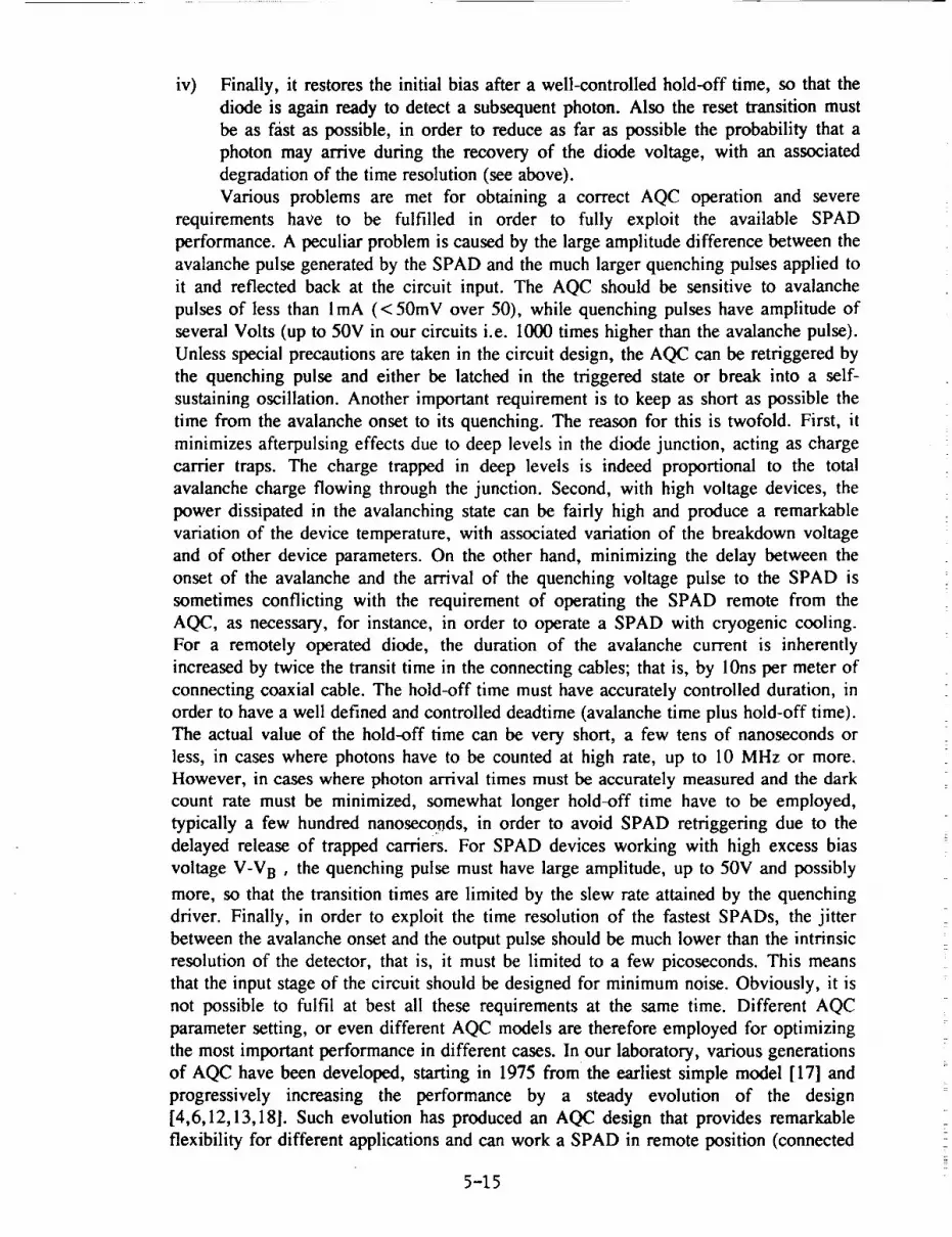
iv) Finally, it restoresthe initial bias after a well-controlled hold-off time, so that the
diode is again ready to detect a subsequent photon. Also the reset transition must
be as fist as possible, in order to reduce as far as possible the probability that a
photon may arrive during the recovery of the diode voltage, with an associated
degradation of the time resolution (see above).
Various problems are met for obtaining a correct AQC operation and severe
requirements have to be fulfilled in order to fully exploit the available SPAD
performance. A peculiar problem is caused by the large amplitude difference between the
avalanche pulse generated by the SPAD and the much larger quenching pulses applied to
it and reflected back at the circuit input. The AQC should be sensitive to avalanche
pulses of less than lmA (<50mV over 50), while quenching pulses have amplitude of
several Volts (up to 50V in our circuits i.e. 1000 times higher than the avalanche pulse).
Unless special precautions are taken in the circuit design, the AQC can be retriggered by
the quenching pulse and either be latched in the triggered state or break into a self-
sustaining oscillation. Another important requirement is to keep as short as possible the
time from the avalanche onset to its quenching. The reason for this is twofold. First, it
minimizes afterpulsing effects due to deep levels in the diode junction, acting as charge
carrier traps. The charge trapped in deep levels is indeed proportional to the total
avalanche charge flowing through the junction. Second, with high voltage devices, the
power dissipated in the avalanching state can be fairly high and produce a remarkable
variation of the device temperature, with associated variation of the breakdown voltage
and of other device parameters. On the other hand, minimizing the delay between the
onset of the avalanche and the arrival of the quenching voltage pulse to the SPAD is
sometimes conflicting with the requirement of operating the SPAD remote from the
AQC, as necessary, for instance, in order to operate a SPAD with cryogenic cooling.
For a remotely operated diode, the duration of the avalanche current is inherently
increased by twice the transit time in the connecting cables; that is, by 10ns per meter of
connecting coaxial cable. The hold-off time must have accurately controlled duration, in
order to have a well defined and controlled deadtime (avalanche time plus hold-off time).
The actual value of the hold-off time can be very short, a few tens of nanoseconds or
less, in cases where photons have to be counted at high rate, up to 10 MHz or more.
However, in cases where photon arrival times must be accurately measured and the dark
count rate must be minimized, somewhat longer hold-off time have to be employed,
typically a few hundred nanoseconds, in order to avoid SPAD retriggering due to the
delayed release of trapped carriers. For SPAD devices working with high excess bias
voltage V-V B , the quenching pulse must have large amplitude, up to 50V and possibly
more, so that the transition times are limited by the slew rate attained by the quenching
driver. Finally, in order to exploit the time resolution of the fastest SPADs, the jitter
between the avalanche onset and the output pulse should be much lower than the intrinsic
resolution of the detector, that is, it must be limited to a few picoseconds. This means
that the input stage of the circuit should be designed for minimum noise. Obviously, it is
not possible to fulfil at best all these requirements at the same time. Different AQC
parameter setting, or even different AQC models are therefore employed for optimizing
the most important performance in different cases. In our laboratory, various generations
of AQC have been developed, starting in 1975 from the earliest simple model [17] and
progressively increasing the performance by a steady evolution of the design
[4,6,12,13,18]. Such evolution has produced an AQC design that provides remarkable
flexibility for different applications and can work a SPAD in remote position (connected
5-15

by a coaxial cable) exploiting at best the device performance. With a minimum-noise
input stage, the circuit has intrinsic timing jitter well below I0ps FWHM; it can work at
more than 10MHz repetition rate and, with suitably designed output quenching driver, it
can provide a 50V quenching pulse.
OUTI I0 OS M
Fig. 10 Simplified block diagram of the most recent AQC generation, described in thetext. Note the _mmetry of the circuit.
The circuit design approach, covered by international patents [13], will be
here illustrated making reference to the simplified circuit diagram in Fig.7. The
figure illustrates the high degree of symmetry of the circuit. Thanks to this
symmetry, the fast comparator can have a low threshold level, as requ!red to sense
the avalanche pulse, and at the same time be insensitive to the quenching pulse,
avoiding spurious retriggering (see above). The avalanche pulse is applied
asymmetrically (only to the non-inverting terminal of the comparator): it is
therefore a differential-mode signal that triggers the comparator. The quenching
voltage pulse is symmetrically applied (to both input terminals of the comparator),
so that it is a common mode signal and does not trigger the comparator. In order to
obtain this, the symmetry should be maintained also in the voltage transients,
including reflections, overshoots or ringing caused by the load connected to each
circuit input. It is therefore necessary to connect to the non-inverting input of the
AQC a passive load, in order to match that given by the SPAD, connected to the
other input. This normally means a simple capacitor C, with capacitance value
equal to that of the SPAD (a trimmer capacitor of a few pF is normally employed).
In case of. remote SPAD operation, care must be taken of maintaining the
5-16

symmetry by connecting with coaxial cables (CC1 and CC2) having equal lengththe SPAD and the matched load. The cables are terminated at the circuit inputs
through the resistors R01 and R02. The avalanche signal flows through the diode
DI and the common-base transistor TI, reaching the comparator input. The role of
TI is twofold. First it establishes a low impedance input, to which the cable-
matching resistor R01 is connected. Second, it provides amplification of the
voltage signal fed to the comparator, which is important for minimizing the
intrinsic time-jitter of the circuit, due to its electronic noise. In stationary
conditions, diodes DI (and D2) is conducting, diodes D3 (and D4) is instead not
conducting. When an avalanche is triggered, the current is sensed by the
comparator, whose output changes state. This signal triggers a monostable
multivibrator, M, that sets the duration of the quenching pulse. In order to obtain
the desired amplitude of the quenching signal, a suitable voltage driver stage, DR,
is employed. When the quenching voltage pulse is applied by DR, the voltage
through D3 becomes direct, the diode conducts and the quenching pulse reaches the
photodiode. At the same time the diode D1 is driven to reverse bias condition and
prevents the high voltage pulse (up to 50V) from reaching T1. If diode DI were
not present, the entire quenching pulse would be applied to the base-emitter
junction of TI, causing it to break down. Another important effect of the two
diodes is to break the positive feedback loop of the circuit, thus reducing the risk
of oscillations. The AQC output pulse is derived from the comparator, through an
output stage OS.
By employing this kind of AQCs, the timing performance of SPADs has
been verified down to 20ps FWHM 151. The flexibility and performance of the
circuit have been extensively tested in many different experiments, carried out in a
wide variety of conditions, with SPAD working either embedded in the circuit or
remote from it and operating in different ambients over a wide range of device
temperatures, including cryogenic cooling.
ACKNOWLEDGMENTS
Work supported in part by ASI (Italian Space Agency), CNR (Italian
National Research Council) and MURST (Italian Ministry of University and
Research). The author wish to thank N.Carbone and S.Masci for their technical
support in the development of Active Quenching Circuits.
Rrl RENCES
I l.Yamazaki, M.Tamai, H.Kume, H.Tsuchiya and K.Oba, Rev. Sci. Instrum 56, 1187 (1985).
2 D.Bebelaar, Rev.Sci.lnstrum. 57, 1116 (1986).
3 H.Ktime, K.Koyama, K.Nakatsugawa, S.Suzuki, and D.Fatlowitz, Appl. Opt. 27, 1170 (1988).
4 S.Cova, G.Ripamonti and A.Lacaita, Nucl. instrum. Methods A253, 482 (1987).
5 S.Cova, A.Lacaita, M.Ghioni, G.Ripamonti, T.A.Louis, Rev. Sci. Instrum. 60, 1104 (1989).
5-17

6 S.Cova, A.Longoni, and A.Andreoni, Rev. Sci. lnstrum. 52, 408 (1981).
7 A.Lacaita, S.Cova, M.Ghioni, Rev. Sci. Instrum. 59, I 115 (1988).
8 S.Cova, M.Ghioni, and F.Zappa, Rev. Sci. Instrum. 62, 2596 (1991).
9 S.Cova and G.Ripamonti, Rev. Sci. Instrum. 61, 1072 (1990).
10 S.Cova, M.Ghioni, F.Zappa, and A.Lacaita, Rev. Sci. Instrum. to be published.
I I R.H.Haitz, J. Appl. Phys. 35, 1370 (1964); 36, 3123 (1965).
12 S.Cova, A.Longoni, and G.Ripamonti, IEEE Trans. Nucl. Sci. NS-29, 599 (1982).
13 S.Cova, US.Patent #4,963,727, Italian patent 22367A/88. Industrial licence to SILENA S.p.A.Milano (Italy).
14 P.W.Nicholson, Nuclear Electronics p. 259 (J.Wiley, NewYork, 1974).
15 See e.g. Instruction Manual of ORTEC Mod.583 or Tennelec Mod.454.
16 Hamamatsu Photonics K.K., Hamamatsu City, Japan, and Hamamatsu Corp., Bridgewater, N.J.U.S.A., MCP-PMTs data sheets and Technical lnformations No. ET-03/Oct. 1987.
17 P.Antognetti, S.Cova and A.Longoni, Proc. Ispra Nucl. Electron. Syrup. 1975, EuratomPublication EUR 537e, 453 (1975)
18 S.Cova et al. Rev. Sci. lnstrum, to be published
5-18
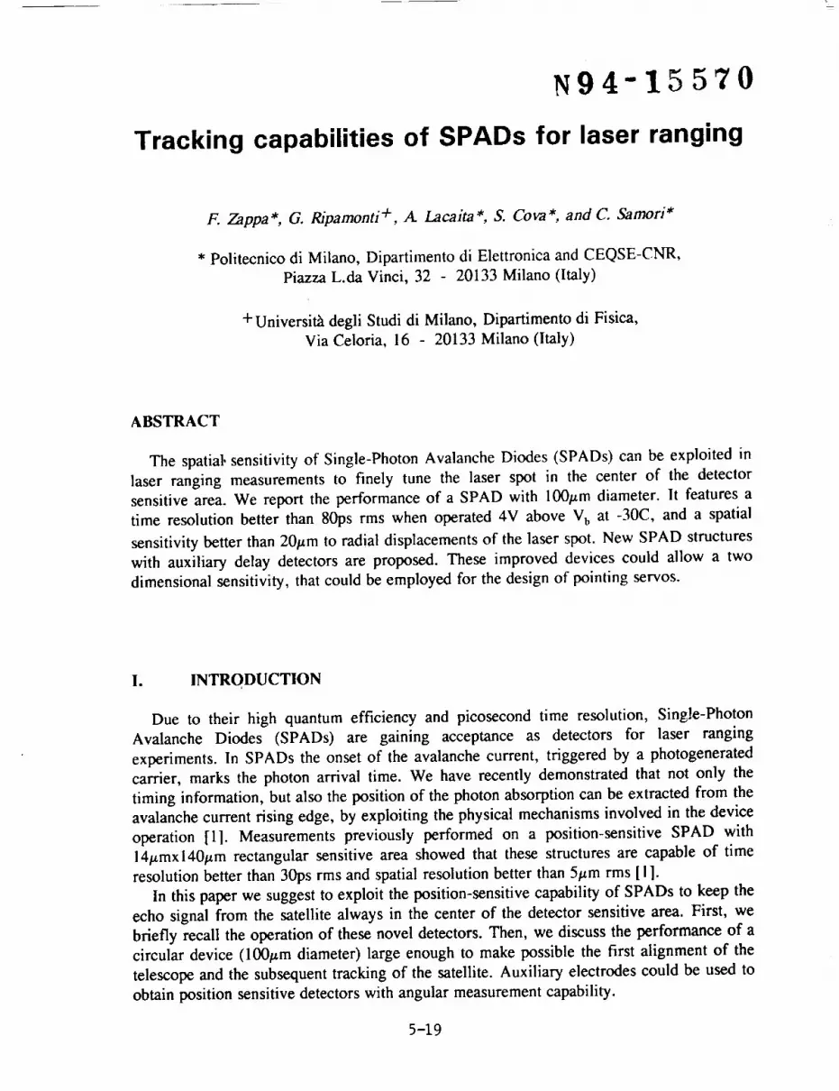
N94-15570
Tracking capabilities of SPADs for laser ranging
F. Zappa*, G. Pdpamonti +, A Lacaita*, S. Cova*, and C Samori*
* Politecnico di Milano, Dipartilnento di Elettronica and CEQSE-CNR,
Piazza L.da Vinci, 32 - 20133 Milano (Italy)
+ Universith degli Studi di Milano, Dipartimento di Fisica,
Via Celoria, 16 - 20133 Milano (Italy)
ABSTRACT
The spatial, sensitivity of Single-Photon Avalanche Diodes (SPADs) can be exploited in
laser ranging measurements to finely tune the laser spot in the center of the detector
sensitive area. We report the performance of a SPAD with 100/zm diameter. It features a
time resolution better than 80ps rms when operated 4V above V b at -30C, and a spatial
sensitivity better than 20#m to radial displacements of the laser spot. New SPAD structures
with auxiliary delay detectors are proposed. These improved devices could allow a two
dimensional sensitivity, that could be employed for the design of pointing servos.
To INTRODUCTION
Due to their high quantum efficiency and picosecond time resolution, Single-Photon
Avalanche Diodes (SPADs) are gaining acceptance as detectors for laser ranging
experiments. In SPADs the onset of the avalanche current, triggered by a photogenerated
carrier, marks the photon arrival time. We have recently demonstrated that not only the
timing information, but also the position of the photon absorption can be extracted from the
avalanche current rising edge, by exploiting the physical mechanisms involved in the device
operation [ll. Measurements previously performed on a position-sensitive SPAD with
14/zmxl40#m rectangular sensitive area showed that these structures are capable of time
resolution better than 30ps rms and spatial resolution better than 5#m rms [1].
In this paper we suggest to exploit the position-sensitive capability of SPADs to keep the
echo signal from the satellite always in the center of the detector sensitive area. First, we
briefly recall the operation of these novel detectors. Then, we discuss the performance of a
circular device (100#m diameter) large enough to make possible the first alignment of the
telescope and the subsequent tracking of the satellite. Auxiliary electrodes could be used to
obtain position sensitive detectors with angular measurement capability.
5-19

H. OPERATION OF SPAD POSITION SENSITIVE DETECTORS
Recently, the avalanche dynamics in silicon SPADs has been investigated; high
performance detectors have been designed and fabricated [2-4]. To the purpose of our
discussion, here we briefly recall the basic operation of SPADs with a depletion layer only
a few microns thick [5]. The avalanche photodiode is operated biased above the breakdown
voltage, Vb, but no current flows until the first carrier triggers the avalanche in a seed
point. Then, the free carrier concentration swiftly rises by impact ionization around the
seed point and, in a few tens of picoseconds, the free carrier space charge lowers the local
multiplicatioti rate to a self-sustaining level. The carrier density around the seed point
cannot increase further, unless the avalanche is triggered in the surroundings by lateral
diffusion of avalanching carriers. As the activated area increases, the diode current rises.
At the end, when the multiplication process occurs over the whole active area, the
avalanche current reaches the final steady state value given by the ratio of the excess bias
above V b and the diode series resistance.
lower threshold
her threshold
i I
Time
Fig. 1 Avalanche dynamics in a circular device: the curves qualitatively show the
dependence of the current rise on the point where the avalanche is
triggered. The circle schematically represents the sensitive area of the
detector with spreading avalanches. The delay between the crossing times
of the tin9 thresholds is proportional to the current rise-time.
The pulse crossing of a discriminator threshold gives the timing information. However,
this pecuHm'-dynamics causes the avalanche pulse leading edge to depend on the position
where the avalanche is triggered. Fig. 1 schematically shows the rise of the diode current in
a circular device. The closer is the seed point to the center, the faster is the activation of
the whole sensitive area. Therefore, the current leading edge becomes steeper as the seed
point moves from the periphery to the detector center. This effect sets a limit to the timing
performance of the detector 12,31, but it can also be exploited to get the position
5-20

information: the shape of the avalanche leading edge carries the spatial information on thepoint where the photon was absorbed [1].
HI. EXPERIMENTAL DATA
Fig.2 shows the cross section of the tested devices. The avalanching region is the n+p +
junction: the depleted region is about l#m thick. The electric field at the edge is tailored by
the n+p junction with the epilayer. A complete discussion of the structure is carried out in
Ref.6. The detector has a 100#m diameter and a V b of 14.3V.
The rise time of the avalanche current pulses was accurately measured by an Active
Quenching (AQ) circuit [7] with two discriminators having different thresholds. The
purposes of the AQ circuit are: i) to sense the onset of the avalanche current; ii) to lower
the bias of the photodiode below the breakdown voltage, thus quenching the avalanche; and
iii) to rapidly restore the bias after a suitable dead time to enable the detection of another
photon. The first discriminator is set to sense the avalanche when the current is still low
(0.4mA), while the second is triggered when the avalanche is almost saturated. The delay
between the output pulses of the discriminators gives the rise time of the avalanche pulse.
A K
Fig.2 Cross section of the double epitaxial devices tested in the experiments.
The active n+p + junction is built in a 10 flcm p epistrate. ?he buriedp+epilayer is 0. 3 _cm.
In order to reduce the dark count rate, the detector was cooled by a Peltier stage at -30C
and operated in gated mode: in stand-by the diode was reverse biased below V h, and a
waveform generator provided pulses at 10 kHz, raising the bias 4V above V h for 500ns. A
850nm laser diode synchronously emitted a 20ps rms optical pulse, focused to a 10#m spot
with a microscope. A Time to Pulse Height Converter measured the delay between the
triggering times of the two discriminators. A histogram of the measurements was collected
with a MultiChannel Analyzer.
We carried out various measurements by changing the radial position of the light spot.
Fig.3 shows the histograms of the delay between the threshold crossing times. The peak
shifts 130ps when the laser spot moves from the center to the edge of the detector. The
5-21

inset of Fig.3 shows the complete dependence of the peak shift on the spot position. As the
laser spot shifts more than 20#m from the device center, the histogram peak moves
considerably and a suitable feedback system can react to restore the original centered
position.The time resolution of the device was measured just by recording the delay between the
laser shot and the crossing time of the low threshold discriminator. The observed resolution
changed somewhat with focusing and with the position of the spot. With the light focused
to a 10#m spot size in the center of the sensitive area, the time resolution was 80ps rms.
10
8
"-" 6
4¢.-
O
Peak shift =
041,
q _°° • _ "__
.- ] ; 2
• ee • •e
• • • • 0
• • 0 I_ _ _ 40 50
,j_ _ R°diot displacement [tJm]I =
0 100 200 300 400 500 600
"rime [ps]
Fig.3 Avalanche pulse rise-time, measured as the delay between the crossing
times of the low and the high thresholds of Fig. 1. The two histograms
correspond to the measurements performed by focusing the laser spot in
the center (Srst histogram to the le#) and at the edge of the detector of
Fig.2 (histogram to the righO. The peak shills I30ps when the laser spot
moves to the periphery of the detector. The inset shows the complete
dependence of the peak shit_ on the spot position.
It is worth noting that photons absorbed at the same distance from the device center
generate avalanche pulses with the same risetime. Therefore, these devices cannot give the
information on how to operate in order to position the light spot in the detector center, in a
single measurement. A trial and error method should be adopted to keep centered the echo
light signal.
Fig.4 describes a possible improvement of the technique in order to achie'ce a complete
angular sensitivity. Four SPAD sensors are placed along two perpendicular axes of the
main detector, close enough to its boundary to be triggered when the avalanche reaches the
corresponding edge. Since the avalanche spreads evenly from the seed point, by measuring
the time delay between the current pulses of the sensors one can get the position of the laser
5-22

spot over the main sensitive area. Pointing servos could be implemented to correct for
misalignement, thus keeping the laser spot always in the center of the main photodetector.
It is worth noting that the design of such a device is expected to be critical in the coupling
between the delay detectors and the central SPAD. Projects are under way in our
laboratories to study suitable stuctures and the most effective coupling arrangements.
Propagatingavalanche
Sensors
\
SensorsMain detector
Fig.4 Proposed improvement of the position sensitive detector in order to
achieve a complete angular sensitivity. Four SPADs can sense when the
avalanche reaches the edge of the central device. By measuring the time
delay between the current pulses of the sensors, one can obtain the
position of the laser spot over the main sensitive area.
IV. CONCLUSIONS
A position-sensitive single-photon detector with 100#m diameter has been demonstrated.
It features a time resolution better than 80ps rms when operated 4V above V b at -30C, and
a spatial sensitivity better than 20#m to radial displacements of the laser spot. The detector
provides a continuous sensitive area, free from dead zones, and can be exploited in laser
ranging measurements to keep the laser signal always centered into the sensitive area. We
have also proposed a more complex SPAD structure, where the introduction of auxiliary
delay detectors could allow a complete angular sensitivity of the device. These structures
are investigated to overcome the trial and errors method used in pointing with simple
position-sensitive SPADs.
5-23

ACKNOWLEDGEMENTS
Work supported in part by ASI (Italian Space Agency), CNR (Italian National Research
Council) and MURST (Italian Ministry of University and Research). The authors wish to
thank ST-Microelectronics for the fabrication of the samples, and S. Masci for his technical
support.
REFERENCES
1. G. Ripamonti, M. Ghioni, S. Cova, and M. Mastrapasqua, IEEE Electron Device Left. EDL-13, 35(1992).
A. Lacaita, M. Mastrapasqua, M. Ghioni, and S. Vanoli, Appl. Phys. Left. 57, 489 (1990).
A. Lacaita and M. Mastrapasqua, Electron. Left. 26, 2053 (1990).
A. Lacaita, F. Zappa, S. Cova, G. Ripamonti, and A. Spmelli,:Sth International _rkshop on LaserRaaginglastrumentation. Annapolis, MD, May 18-22, 1992
S. Cova, A. Lacaita, M. Ghioni, G. Ripamonti, and T.A. LouLs, Rev. Svi. lnstrum 60, 1104 (1989).
A. Lacaita, M. Ghiom, and S. Cova, Eiectroo. Lett. 25, 841 (1989).
S. Cova, A. Longoni, and G. Ripamonti, IEEE Trans. NucL S,'i. NS-29, 599 (1982).
,
3.
4.
.
6.
7.
5-24
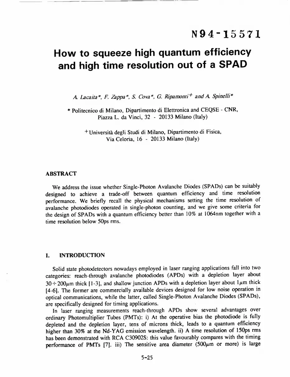
N94-15571
How to squeeze high quantum efficiency
and high time resolution out of a SPAD
A Lacaita*, 1=. Zappa*, S. Cova*, G. Ripamonti + and A Spinelli*
* Politecnico di Milano, Dipartimento di Elettronica and CEQSE - CNR,
Piazza L. da Vinci, 32 - 20133 Milano (Italy)
+Universit_ degli Studi di Milano, Dipartimento di Fisica,
Via Celoria, 16 - 20133 Milano (Italy)
ABSTRACT
We address the issue whether Single-Photon Avalanche Diodes (SPADs) can be suitably
designed to achieve a trade-off between quantum efficiency and time resolution
performance. We briefly recall the physical mechanisms setting the time resolution of
avalanche photodiodes operated in single-photon counting, and we give some criteria for
the design of SPADs with a quantum efficiency better than 10% at 1064nm together with a
time resolution below 50ps rms.
I. INTRODUCTION
Solid state photodetectors nowadays employed in laser ranging applications fall into two
categories: reach-through avalanche photodiodes (APDs) with a depletion layer about
30+ 200/zm thick I1-31, and shallow junction APDs with a depletion layer about l#m thick
[4-61. The former are commercially available devices designed for low noise operation in
optical communications, while the latter, called Single-Photon Avalanche Diodes (SPADs),
are specifically designed for timing applications.
In laser ranging measurements reach-through APDs show several advantages over
ordinary Photomultiplier Tubes (PMTs): i) At the operative bias the photodiode is fully
depleted and the depletion layer, tens of microns thick, leads to a quantum efficiency
higher than 30% at the Nd-YAG emission wavelength, ii) A time resolution of 150ps rms
has been demonstrated with RCA C30902S: this value favourably compares with the timing
performance of PMTs [71. iii) The sensitive area diameter (500#m or more) is large
5-25
enoughto makepossiblethe alignmentof the telescope and the subsequent tracking of thesatellite.
Indeed, high performance SPADs can attain much better time resolution (8ps rms) [4].
However, these devices have a quantum efficiency lower than 1% at 1064nm and their
small active area (5#m diameter) makes impossible their use in laser rangingmeasurements.
In this paper we address the issue whether a silicon SPAD can be suitably designed to
achieve a trade-off between quantum efficiency and time resolution performance. We
briefly recall the physical mechanisms setting the time resolution of APDs operated in
single-photon counting. We discuss how the performance depends on the device geometry
and the junction electric field profile. We give some criteria for the design of SPADs with
a quantum efficiency higher than 10% at 1064nm and a time resolution below 50ps rms.
This combination of performance cannot be achieved with any commercially available
single photon detector, both solid state and vacuum tube.
II. AVALANCHE PHYSICS AND TIME RESOLUTION
Single photon sensitivity is achieved with APDs operated biased above the junction
breakdown voltage, V b. At this bias a single photogenerated carder can trigger a diverging
avalanche process. The leading edge of the avalanche current marks the photon arrival time
[1-61. Any jitter in the delay between photon absorption and the crossing time of the
discriminator threshold, impairs the precision in timing measurements I4-6].
The ultimate limit to the timing resolution of a SPAD comes from the thickness of the
depletion layer. In fact, the distance between the point where the photon is absorbed and
the junction leads to a statistical delay between the photon absorption time and the
avalanche triggering. As a rule of thumb, if the photon absorption length, La, is longer than
the depletion layer thickness, W, and carriers drift at the saturated velocity (v,= 10ps/#m)
almost everywhere in the depleted region, the ultimate rms time jitter will be of the order
of W/(3.5v_)=2.9ps rms per each depleted micron. Since in silicon the absorption length,
L a, of a photon at 1064nm is 83#m, the choice of a 10#m depletion layer thickness
guarantees a quantum efficiency higher than 10%, with an ultimate time resolution less
than 30ps rms. Unfortunately, other mechanisms do not allow to reach this limit.
In the device operation the avalanche is triggered by photon absorption in a seed point,
then it progressively spreads over the whole detector area. The leading edge of the diode
current is affected by the spreading process. In SPADs, with thin depletion layer and small
active volume, the avalanche spreads evenly from the seed point to the remaining detector
area by transverse diffusion of avalanching carders [5,61. This mechanism makes the
avalanche propagating with a transverse velocity given by [5]:
v0=2_ (1)
where D is the average transverse diffusion coefficient of the carriers and 7" is the time
constant of the avalanche build-up, which increases by increasing the device bias.
Fig.1 helps in understanding how the avalanche spreading impairs the timing
performance. In fact, the closer the seed point is to the center of the junction area, the
faster is the activation of the whole device. Therefore, in the circular device shown in
5-26

Fig. 1, thecurrent leadingedge becomes steeper as the seed point moves from the periphery
to the center. Since a photon can be absorbed everywhere on the detector area, this effect
causes a randomness in the pulse crossing of the timing threshold. It follows that the
achievable time resolution is related to the difference, A, between the crossing times of the
fastest and the slowest current pulses. This difference increases by increasing the sensitive
area and/or decreasing vp (i.e. the bias).
0LI
I I I
Iimo
Fig. 1 Avalanche dynamics in a circular device: the shil_ A between the crossing
times of the fastest and the slowest leading edges sets the limit to the time
resolution of the detector. The inset schematically shows the sensitive area
of the detector ruth concentric circles representing the spreadingavalanche.
As the detector volume increases, another phenomenon can play a role in the avalanche
propagation. Secondary photons, emitted by hot carriers radiative relaxation processes in
the avalanching region, can be absorbed in other regions, thus triggering the avalanche
even there. Phot.ons with absorption length of a few hundred microns are the most effective
in sowing the avalanche. This latter process is dominant in APDs with large sensitive area
and thick depletion layer [31.
We have developed a computer simulation of the avalanche dynamics. Fig.2 shows a
comparison between the current leading edge of a RCA C30902S APD biased 40V above
V b at room temperature and the result of the computer program. It is worth noting that, due
to the intrinsic randomness of the photon-assisted process, the timing performance of the
device (170ps rms) is considerably worst than the ultimate limit set by the 30#m thick
depletion layer. Moreover, the time dispersion increases by increasing the level of thetiming threshold.
In order to reach a reasonable trade-off between quantum efficiency and time resolution,
the impairing effects of the photon-assisted spreading have to be overcome. In principle
this goal can be achieved in two ways: i) by adopting a timing threshold low enough to
sense the avalanche current soon after the avalanche triggering and before the emission of
5-27

the first secondary photon; ii) by designing the detector structure so that the lateral carrier
diffusion becomes the steering mechanism of the avalanche spreading. The design of fast
and sensitive detector circuits is under way in our laboratories. In the next section, we will
give some guide-lines on the design of high quantum efficiency SPADs with the avalanche
propagation steered by transverse carrier diffusion.
.... i
5)Omr
.w
Fig.2 Comparison between the current leading edge of a RCA C30902S APD
biased 40V above Vb at room temperature (le#) and the result of the
computer simulation of the avalanche dynamics (right).
HI. DESIGN CRITERIA
In order to make it clear some fundamental design rules, let us compare the expected
performance of two devices with 10% quantum efficiency at 1064nm. Therefore, both
devices are supposed to have a 10#m depletion layer thickness. The inset of Fig.3 shows
the electric field profile of the first device (D#1) at 169V, that is 34V above the estimated
Vb=135V. The peak electric field is 3.3xl05V/cm. The high field region is about 3#m
thick and, in the remaining part of the depletion layer, the electric field (6xl04V/cm)
makes the carders drifting at saturated velocity. The second device (D#2) has a similar
electric field profile (inset of Fig.3) but a high field region only 0.3/.tin thick and an
estimated V b of 63V. Since the two devices have different V b, we will compare their
performance at the same relative excess bias (V0-Vt,)/V h. Thus D#2 will be operated at 79V
and the peak electric field will be 6xlOSV/cm.
Fig.3 shows the dependence on the device radius of both diffusion and photon assisted
spreading velocities, as obtained from a computer simulation of the avalanche dynamics.
The diffusion velocity was estimated from Eq.(l), while the photon assisted contribution
was estimated by switching off the diffusion process in the simulation, and then computing
the resulting ratio between the device radius and the current risetime. As expected, the role
of the photon-assisted process increases by increasing the sensitive area radius; it becomes
5-28

eventually dominant in D#1 for a radius greater than 80#m. D#2 has a diffusion velocity
more than three times larger and a photon assisted process less effective than in D#1.
_=2OO
E
_ 160
_o 120
.9 80
" 40O
n
0
'-"6E
,2
--'00
0 50 100 150 250Oevice radius [pm]
Ot_2
2 ¢ 6 8 10_Depth [urn]
l i
200
Fig.3 Dependence of the diffusion and the photon assisted spreading velocities
on the de14ce radius, as obtained from a computer simulation of the
a valanche dynamics in two de_4ces with a 10#m thick depletion layer. The
inset shows the electric 5eM profiles assumed in the calculations.
The higher diffusion velocity is due to the steeper electric field profile of D#2. In fact,
the avalanche time constant, 7", is proportional to the carrier transit time in the high field
region and is inversely proportional to the loop gain of the avalanche feedback process (i.e.
the average number of impact ionization events experienced by a carrier crossing the
junction). It can be shown that two junctions with similar electric field profile have the
same avalanche loop gain when biased at the same relative excess bias. Therefore, in the
present comparison, the devices are operated at the same loop gain, and the thinner high
field region of D#2 results in a correspondingly shorter multiplication time constant, 7".
From Eq.(1) it follows that D#2 is expected to have a faster diffusion-assisted avalanche
propagation.
With regard to the difference in the photon-assisted process, it should be noted that D#2
is supposed to work at only 16V above V b, while D#1 is operated at 34V excess voltage.
Both of them have the same depletion layer thickness and therefore the same series
resistance. It follows that, at the supposed operating conditions, the current flowing
through D#2 is less than that of D#1. Since the photon emission rate is proportional to the
current, the photon assisted propagation is less effective in D#2.
These results highlight that, by adopting a suitable steep electric field profile, the
diffusion-assisted avalanche propagation can overcome the noisy photon-assisted process
even in large area SPADs. We estimated the time resolution of a SPAD detector with
100#m diameter and the electric field profile of D#2 as follows. We computed the leading
5-29

edge of the avalanche pulses triggered at the center and at the edge of the detector,
assuming that the avalanching area spreads evenly with a radial velocity of 75#m/ns. The
time resolution is expected to be proportional to the difference, A, between the crossing
times of the fastest and the slowest avalanche pulses. By using a timing threshold at
0.3mA, we forecast A=87ps. Therefore the time resolution of such a device, defined as
the rms value of the timing curve, should be better than 50ps.
IV. CONCLUSIONS
We have discussed the physical mechanisms setting the timing resolution of Single-
Photon APDs. In present devices, the timing resolution is limited by the mechanisms
involved in the avalanche spreading from the seed point to the entire sensitive area. The
best time resolution is obtained when the steering mechanism is the multiplication-assisted
diffusion. We have shown that, with a proper design of the electric field profile, the
diffusion-assisted process can overcome the photon-assisted spreading also in APDs with a
large sensitive area. Therefore, SPAD devices with time resolution better than 50ps rms
and a quantum efficiency better than 10% at 1064nm could be obtained. In such devices,
the timing resolution would be ultimately limited by the transit time in the thick depleted
region.
ACKNOWLEDGEMENTS
Work supported in part by ASI (Italian Space Agency), CNR (Italian National
Research Council) and MURST (Italian Ministry of University and Research). The authors
wish to thank ST-Microelectronics for the fabrication of the SPADs; EG&G
Optoelectronics for providing the reach-through APDs; and S. Masci for his technical
support.
REFERENCES
I.
2.
3.
4.
5.
6.
7.
P.P. Webb, R.J .Mclntyre, and J. Conradi, RCA Rev. 35, 234 (1974).
A. Lacaita, S. Cova, and M. Ghioni, Rev. Sci. lastrum. 59, 1115 (1988).
M. Ghioni and G. Ripamonti, Rev. Sci. lnstrum. 62, 163 (1991).
S. Cova, A. Lacaita, M. Ghioni, and G. Ripamonti, Rev. Sci. Iustrum 60, 1104 (1989).
A. Lacaita, M. Mastrapasqua, M. Ghioni, and S. Vanoli, Appl. Phys. Lett. 57, 489 (1990).
A. Lacaita and M. Mastrapasqua, El_'tron. Lett. 26, 2053 (1990).
D. Bebelaar, Rev. Sci. lnstrum. 57, 1116 (1986).
5-30

N94-15572
THE SOLID STATE DETECTOR TECHNOLOGYFOR PICOSECOND LASER RANGING
I.Prochftzka
Faculty of Nuclear Science and Physical Engineering,Czech Technical University
Brehova 7, 115 19 Prague, 1 Czechoslovakia
phone/fax +42 2 848840, telex 121254 fjfi c, E-mail [email protected]
GENERAL
The millimeter accuracy, multiple wavelength laser ranging to the satellite and long
ground baseline is a goal for nineties. Assuming the laser, optics and electronics technology
currently available, the optical detectors represent the principal contributions to the ranging error
budget in the laser ranging chain. In our group we developed an all solid state laser ranging
detector technology [1,2,3], which makes the goal of millimeter accuracy achievable. Our design
and construction philosophy is to combine the techniques of : single photon ranging, ultrashort
laser pulses and fast fixed threshold discrimination while avoiding any analog signal processing
within the laser ranging chain.
The all solid state laser ranging detector package consists of the START detector and the
STOP solid state photon counting module. Both the detectors are working in an optically
triggered avalanche switching regime. The optical signal is triggering an avalanche current
buildup which results in the generation of an uniform, fast risetime output pulse. The fixed
threshold discrimination represents no drawback for our application. In connection with the
ultrashort laser pulses (35 picoseconds or less), this detection technique introduces the timing
jitter of a few picoseconds on the multi photon signal level and less than 15 picoseconds on a
single photon signal level. Omitting the fast analog signal processing is simplifying the ranging
system and simultaneously increasing its temporal stability.
START DETECTOR PACKAGE
It detects a small portion of the laser output and triggers the time interval unit. The
detection structure on silicon is used. The detector is operating in an avalanche switching
regime, it is acting as a fixed threshold opto switch generating on its output an uniform current
pulse. Its amplitude is typically 8 Volts, length 5 nanoseconds, the risetime is bellow 400
picoseconds. Thanks to the output pulse shape and its uniformity, no additional pulse
amplification and discrimination is needed. As no analog signals are propagating along the
cables, the detector output is uniform and its amplitude is high, the whole setup is highly
resistant to the radio frequency interference and electrical noise problems. This fact is becoming
significant in the vicinity of a laser system generating a lot of electrical noise. The detector is
capable of operation in three modes :
1. In linear mode it may be used as a laser output pulse monitor with the bandwidth of 1 GHz.
5-31

In this mode, the optical alignment of the detector may be optimized.
2. The opto switching mode described above is used for ranging.
3. In the self oscillation mode the detector generates on its output the sequence of uniform
output pulses with the repetition rate of about 1 kHz. This mode is and attractive feature for test
purpose.
The detector jitter contribution to the overall jitter budget was not measured
independently. When it has been used to trigger the streak camera, the overall trigger jitter
(detector + streak camera) of 8-16 picoseconds has been observed using the passively mode
locked lasers with pulse length 3 - 100 psec FWHM. Thus, the trigger jitter contribution of the
START detector itself is well bellow 15 picoseconds for these pulse lengths. Generally, in
connection with the active-passive mode locked lasers with pulse lengths bellow 100 psec and
the fast response time interval unit input, the jitter contribution of the START detector may be
neglected.
SOLID STATE PHOTON COUNTING MODULE
It is used to detect the laser ranging echo signals. The Module is a self consistent detector
package, which detects single photons of light over the wavelength range from 0.35 to 1.1
microns. The Module utilizes a unique silicon Single Photon Avalanche Diode (SPAD) [4,2],
which is connected in the active quenching and gating circuit and pulse biased above the break.
Biasing the diode above the break, the extreme gain of order of I. 109 is achieved. This high gain
obtained within the semiconductor chip permits to avoid any further amplification of the detector
output and the constant fraction discrimination, as well. Simple fixed threshold discrimination
technique is used to recognize the detector output and to generate the uniform output NIM pulse.
The detector may be gated using the TI'L signal, the 'gate on' delay is bellow 25 nanoseconds.
The detection diode together with the active quenching circuit, the gating logic, the
discriminator, output pulse forming circuit and the light collecting optics in enclosed in one
package. It is a cylinder, 120 millimeters long,
40 millimeters in diameter. The optics has an
effective focal length 10 millimeters and is
optimized for the beam diameter of 8-10
millimeters. Due to the diode relatively small
sensitive area (20, 40 or 100 micrometers), the
resulting receiver field of view is limited.
Using the 100 micrometer diameter diode and
the final collecting optics f/D = 1, the resultingfield of view is 40 arc seconds when installed
in the 0.5 meter input aperture telescope.
Using the same diode in connection with the 1
meter aperture telescope, the 20 arc seconds
field of view is achieved. The 40 um detection
chip has been successfully used for SLR at
Helwan and Graz, however, the field of view
has been to narrow for routine operation. Due
to the detection and avalanche buildup
mechanisms inside the SPAD chip, the minimal
0.11
::::t|.Or
0.3
SPAD spectral response20urn chlp,0.3V etbove breal:, conl.mode
uanturnellicienc_/[arb.units]I
:::::::::l:::::_i ...... :::::::::::::::::::::::::::::::::::::::::::::::::::!!!!!!::::!!!!!!!!:._!!.:::::.::!!!!!!!!!_!!!!!.x.!!_!::::!ii::i!!!!!!!!!!_!!!!!!!!!!_!!!!!!!!!::::::: ::::::::::::::::::::::::::::::::::::::::::::::::::::::::::::::::::::::::::::::::::
:! i ! .i i N..................:::::: :::::::::::::::::::::::::::::::::::::::::::::::::::::::::::::::: ::::::::
...... ÷......... ÷......... • ................... _.......... _.........................
....... _ ......... • ......... _ ......... e ......... !.......... !.......... q................
_ : : : : :
"T.........r .........t...................!..........!.....................ktI 1 I I I I I |
0.4 0.5 0.6 0,1 0,1 0.9 I tl 1.2
wavelength lrnicronslL.R*LI.ProcktzI:a,J une 26,1991
Figure 1 The SPAD relative photon detection
probability, 0.3V above the break, + 25"C
5-32

detection jitter is achievable when the input photons are focussed on a small spot near to the
diode's center. Thus, the good quality light collecting and beam focussing optics together with
a careful optical alignment is essential for minimal jitter.
The photon detection probability and its dependence on the wavelength has been
measured using the 20 um diameter diode operating in the continuous counting mode. The diode
was biased 0.3 Volt above the break. The results are plotted on Figure 1. The detection
probability depends on the diode biasing, it increases with the increase of the bias up to 3 Volts
above the break. For higher biases, the photon detection probability is not increasing more. The
absolute figures of the quantum efficiency have been estimated by comparison to the calibrated
photocathode to be 20 % at 0.53 um wavelength and bias 3 Volts above the break. Using the
calibrated light source and filters, the quantum efficiency exceeding 20 % at 0.8 um wavelength
and biased only 1V above the break has been observed [5].
DETECTORS PERFORMANCE
Since the last Workshop presentation [6], the detectors overall performance has been
improved. The SPAD manufacturing technology has been tuned to get lower dark count rates.
This is permitting to apply higher voltages above the break and hence to get lower jitter, lower
time walk and higher photon detection probability, as well. The active quenching and gating
logic has been modified (Prochazka, Kirchner) for this purpose. Cooling the diode using the
Peltiere elements down to -25 Centigrades [7] the reduction of the dark count rate is achieved.
This proved to be useful for ranging to low satellites suffering of the poor range prediction. Both
the detectors are routinely used at the Satellite Laser Station in Graz, Austria since 1989. Most
of the application results are based on the data acquired at this site.
The SPAD detector timing jitter and its
dependence on the diode biasing is plotted on
Figure 2. The jitter values have been computed
on the basis of the ground target ranging at the
0.53 um wavelength. At the same figure, the
effective dark count rate at the temperatures
+25 and -10 Centigrades is plotted. The jitter
is depending on the wavelength, it is slightly
increasing toward longer wavelengths and
reaches 60-70 picoseconds at the 1.06 umwhen the SPAD is biased 2.5V above the
break. The detector package time walk, the
detection delay dependence on the signal
strength is plotted on Figure 3. The data have
been acquired biasing the diode 2.5 Volts
above the break and using the semiconductor
laser pulser 32 psec FWHM. On Figure 4 there
JITTER Ipsecl DARK COUNT [kHzl
_JITTER
20 l-........................ _ ............................ "":'"_".............. -------I 200
........... IoO 02i l I._ 2 2.5 3 3.$ 4 4.5 $
VOLTS ABOVE BREAK
Figure 2 SPAD detector package jitter andeffective dark count rate at +25_2 and -10t
is a plot of evolution of the ranging system single shot precision using the all solid state detector
technology together with the list of main upgrades. The ranging system temporal stability is
demonstrated on Figure 5, where is a plot of the mean values of ground target calibration runs.
It is worth to mention, that this test has been made at the time, when the system single shot
precision was 8-9 millimeters. The drift of the 5 picoseconds per hour may be attributed to the
5-33

SPAD deteclor package2.5V above break,32pseclaser
time walk IpsecI
O
-20
-4D
-60
-800
i | ! , I
20 40 60 80 I00
relurn rate J%]
Figure 3 SPAD time walk test,2.5V above break,32 psec laser
GROUND TARGET RANGINGPRECISIONAll solid state detector package
cent_melers
::::::::::::::::::::::::::::::::::::::::::::::::::::::::::::::::::::::::::::::::::::::::::::::::::::::::::::::::::::::::::::::::::::::As n..................................................
_::v::: ! ........:::::::::::::::::::::::::::::::::::::::::::::::::::::::::::::::1-. _ _............J,.............I ..............! ......AO .mo.de.tQ_:ker..........I "ii_.._ v / I I 5R 620^ _. "_._ I I I
_],r.om.sale._l.,e ..................................................................................
_lq..um.c_._.p.......EH;!O..O.umch!p.:................................_,_...........HelwanSLR Graz SLR, '.>
I i • I i I
'84 '86 '89 '90 '91 Jan'92 May'92
Figure 4 Ground target ranging precision increase
.... SYSTEM TEMPORAL STABILITYAll Solid State Delector Package
Optoswitch ._SPAD * HP5370
syslem inle_nal delay InseclGround largel calibralion,300 echoes each
_9D.ss7 .....................................................................................................55 psecl 8.2 mm RMS single shot
t9D.550 .....................................................................................................
190.543 ............................. t ........................................................ .t .........
190.537 __
190.530 .....................................................................................................
190.523 .....................................................................................................slope 5 psecl 0.75 mm per hour
t9o.517 .....................................................................................................
t9o.51o _ _ _ ' ' i i _ _ J , , ,o Io 20 30 ,4o so so 70 eo 90 too ,m _o
time [mlnulesl
Figure 5 System temporal stability, vert.scale lmm / div
5-34

temperature changes within the control & electronics room and its influence on the ranging
counter.
SATELLITE RANGING RESULTS
The all solid state detector package has been used for routine satellite laser ranging since
early 1989. Since that time, the ranging precision has been improved from original 2 centimetersto subcentimeter level in 1992.
The satellite signature - its contribution to the echo signal time spread is becoming
dominant in the ranging error budget when using the 35 psec laser pulse and single photon
detection. On a single photon echo signal level, the ranging precision is limited to 1.5 cm when
ranging to Starlette, to 2 cm for Lageos and to 4-5 cm when ranging to Etalon satellites. The
effect of the "satellite depth" may be reduced by the use of multiphoton (1-10) return signal
strength. In this case, the return photon(s) reflected from the first corner cube is detected. As
the detector response time is bellow 20 picoseconds, the photons reflected by the more distant
corner cubes are not contributing and are not affecting the detection and discrimination process.
Due to this effect, the satellites may be ranged with the return rate exceeding 95% without a
detectable time walk and the satellite signature effect on the ranging jitter reduced.
The typical ranging precision obtained in Graz is 8 millimeters for Starlette and ERS-1
satellites, 10 millimeters for Lageos and 12-15 millimeters for Ajisai satellites.
CONCLUSION
The field use of the solid state detector package for satellite laser ranging at various sites
over the world : Graz Austria, RGO Great Britain, Shanghai China, MTLRS-1 Germany proved
the top performance of the solid state detector technology. The extremely simple, compact and
rugged design, the absence of the analog signal processing and the resulting subcentimeter
ranging capability and submillimeter temporal stability are the most attractive features. The
optical alignment of the SPAD is a difficult task, but it may be solved once the receiver optics
is properly designed. The satellite signature and its influence on both the random and systematic
error budget is becoming significant from the point of view of millimeter ranging goal.
REFERENCES
[1] I.Prochazka,proc.of 6th lnt.Work.on Laser Ranging Instrumentation, Antibes, Sept. 1986
[2] K. Hamal, I. Prochftzka, B. S opko, G. Kirch ner, proc. of Con ference on Lasers and Electro Optics,
CLEO'90, Anaheim, CA, May 1990
[3] I.Proch_ka et al,proc.VIIth International Symposium on Ultrafast Processes in Spectroscopy,
Bayreuth, Germany, October 1991
[4] S.Cova et al,JQE, Vol. 19,630 (1983)'w •
[5] J. Rl_ka, M.Hoebel, private communication, (1992)
[6] I.Prochazka,K.Hamal,B.Sopko,proc.7th Int.Workshop on Laser Ranging Instrumentation,
Matera, Italy, Oct. 1989
[7] G.Kirchner, private communication (1991)
5-35
N94-15573 "
STREAK CAMERA BASED SLR RECEIVERFOR TWO COLOR ATMOSPHERIC MEASUREMENTS
Thomas Varghese, Christopher Clarke, Thomas Oldham, Michael SeldenAllied Signal Aerospace Company,
BFEC/CDSLR10210 Greenbelt Road
Seabrook, MD 20706 USA
Abstract.
To realize accurate two-color differential measurements, an image digitizingsystem with variable spatial resolution was designed, built and integrated to aphoton-counting picosecond streak camera, yielding a temporal scanresolution better than 300 femtosecond/pixel. The streak camera is
configured to operate with 3 spatial channels; two of these support green(532 nm) and uv (355 nm) while the third accommodates reference pulses(764 nm) for real-time calibration. Critical parameters affecting differentialtiming accuracy such as pulse width and shape, number of received photons,streak camera/imaging system nonlinearities, dynamic range, and noisecharacteristics were investigated to optimize the system for accuratedifferential delay measurements.
The streak camera output image consists of three image fields, each field is1024 pixels along the time axis and 16 pixels across the spatial axis. Each ofthe image fields may be independently positioned across the spatial axis. Twoof the image fields are used for the two wavelengths used in the experiment,the third window measures the temporal separation of a pair of diode laserpulses which verify the streak camera sweep speed for each data frame. The
sum of the 16 pixel intensities across each of the 1024 temporal positions forthe three data windows is used to extract the three waveforms. The waveform
data is processed using an iterative three-point running average filter (10 to 30iterations are used) to remove high-frequency structure. The pulse pairseparations are determined using the half-max and centroid type analysis.Rigorous experimental verification has demonstrated that this simplifiedprocess provides the best measurement accuracy. To calibrate the receiver
system sweep, two laser pulses with precisely known temporal separation arescanned along the full length of the sweep axis. The experimentalmeasurements are then modelled using polynomial regression to obtain a
best fit to the data. Data aggregation using normal point approach hasprovided accurate data fitting techniques and is found to be much more
convenient than using the full rate .single shot data. The systematic errorsfrom this model has been found to be less than 3 ps for normal points.
5-36

Objectives:
TWO COLOR ATMOSPHERIC MEASUREMENTS
Measure atmospheric velocity dispersion differencebetween 532 and 355 nm using short (<:30 ps) pulses,
very accurately (2-3 ps).
Compute atmospheric refraction correction (RC)
directly from the differential range.
Compare this correction with the theoretical oneobtained from surface meteorological measurements
for agreement/refinement.
Issues of Importance:
Is there true hydrostatic equilibrium
troposphere on a local scale ?
What are the diurnal and seasonal effects ?
in the
What effect does the local/global temperature
gradient have on RC ?
STREAK CAMERA SLR RECEIVER SYSTEM
Desirable Features:
High Temporal Resolution (ps).Good temporal sweep stability.
High quantum efficiency (> 10%)Single photoelectron sensitivity.
High resolution spatial imaging (< _1ps/pixel).
Repetition Rate _ 10 Hz.
Optical calibration source with temporal
amplitude stability.Spectral filtering and wavelength isolation.
and
5-37
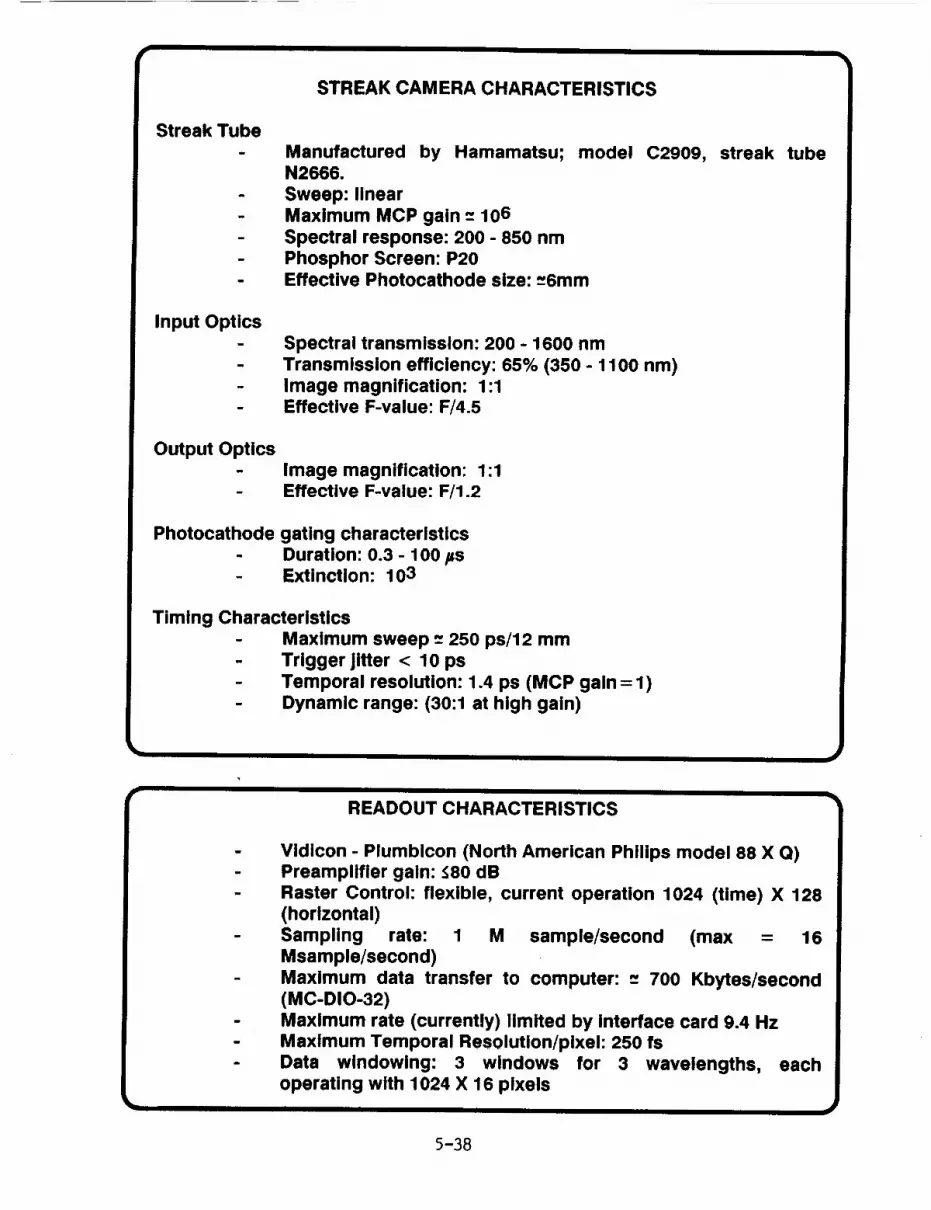
STREAK CAMERA CHARACTERISTICS
Streak Tubem Manufactured by Hamamatsu;
N2666.
Sweep: linearMaximum MCP gain -- 106
Spectral response: 200 - 850 nm
Phosphor Screen: P20Effective Photocathode size: --6mm
model C2909,
Input Optics
m
m
Spectral transmission: 200 - 1600 nm
Transmission efficiency: 65% (350 - 1100 nm)Image magnification: 1:1Effective F-value: F/4.5
Output Opticsm Image magnification: 1:1
Effective F-value: F/1.2
Photocathode gating characteristics
- Duration: 0.3 - 100/_s- Extinction: 103
Timing Characteristics
- Maximum sweep -- 250 ps/12 mm
- Trigger Jitter < 10 ps
- Temporal resolution: 1.4 ps (MCP gain=l)
- Dynamic range: (30:1 at high gain)
streak tube
READOUT CHARACTERISTICS
Vidicon - Plumbicon (North American Philips model 88 X Q)Preamplifier gain: _;80 dB
Raster Control: flexible, current operation 1024 (time) X 128(horizontal)
Sampling rate: 1 M sample/second (max = 16
Msample/second)
Maximum data transfer to computer: -- 700 Kbytes/second(MC-DIO-32)
Maximum rate (currently) limited by Interface card 9.4 HzMaximum Temporal Resolution/pixel: 250 fs
Data windowing: 3 windows for 3 wavelengths, eachoperating with 1024 X 16 pixels
5-38

TWO COLOR DIFFERENTIAL MEASUREMENT
THEORETICAL AND EXPERIMENTAL LIMITS OF ACCURACY
RO = R(),I) - _ f (X2)-f (X1)
O-R(X1)+ Ob-T(X1,)_2) (2)f (>,2)-f (Xl)Where
5T(X1,X2) -_T(X2)-T(X1)
°o'-r0,_,>,2)=
2
i=1
AT (X i)nph(Xi) • T/qE(), i ) " A sweep
(3)
RO =R(X) =
f(X) =
TO =
T(X) =
s(x) =r/ph =_QE =
A =
5T =
(7 =
AT(X) =
Absolute range to the satellite
Measured range at wavelength ),
Dispersion factor
Absolute time of flight
Increase in time of flight through atmosphere
at wavelength ),
Pulse profile factorNumber of photonsPhotocathode quantum efficiency
Microchannel coupling factor
Differential time of flightStandard deviation
Pulse width at X
5-39

DATA ANALYSIS TECHNIQUES
SMOOTHING (3 POINT) ALGORITHM
( a<Ip-1 >(m-l)+ b<Ip>(m-1)+ ¢<Ip+l>(m-1) )
<Ip>(m-=) ( a + b + c )(4)
<Io >(m) =I b<I1022>(m-1)+ c<Ii>(m-1)l
(b+c)(s)
<I1023> (m) =I a<I1022 >(m-l) . b<i1023>(m-1) )
(a+b)(6)
<lp>m
a,b,c
Mean intensity of the pixel at location p after"m" iterations
Weighting coefficients
DETECTION:
Peak
Half Maximum (Mean Value)Centroid
5-40
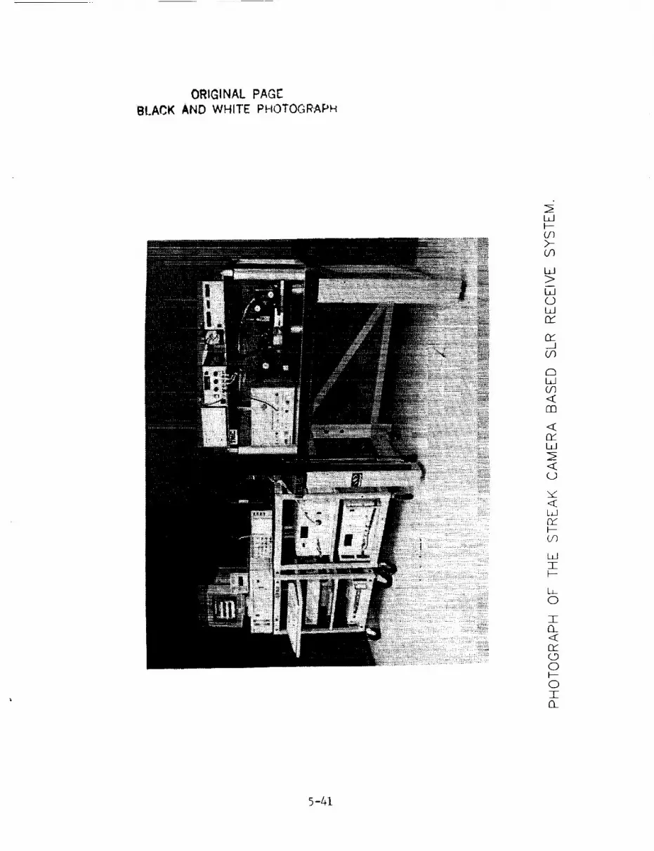
ORIGINAL PAGE
BLACK AND WHITE PHOTOGRAPH
LLII--"Cf)>--U3
LLI>
LL](._)LLI(3£
rY_JCO
CDLL]U3
CIJ
<(3£L_J
<C(_.)
<[LJ
F-CA
LdI
Li_0
I
Cr(._90
0I
5-41

nm
0
5-42
v--Zw
Wr_
($)<w
f_0--J
o{J
0
I--
£EoLL
W
>-/
ZWfYZE
0
03>-
r_
W
Wn-uj
13_
n," (__WO')_w,_.J
oN
rY wI---m_
0LhO_
w
w_
(.)Z
w__1
0
i_. I--o_

5-43
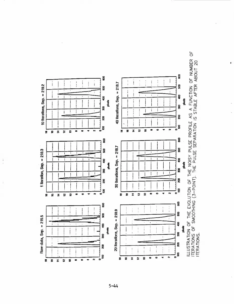
l,o
rYi__jo_o,J
D_
5-44

C
+++++I.,x+Oo_.
m_
+go o
i i' i :
('13XId/Sd) a33dCj d3"-JMS
:m--+++,+,_,_+,_
("FIXId/Sd)a:13clScl33MS
|
0
5-45
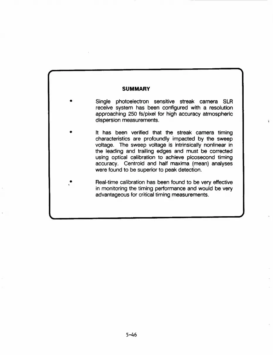
SUMMARY
Single photoelectron sensitive streak camera SLRreceive system has been configured with a resolutionapproaching 250 fs/pixel for high accuracy atmosphericdispersion measurements.
It has been verified that the streak camera timingcharacteristics are profoundly impacted by the sweepvoltage. The sweep voltage is intrinsically nonlinear inthe leading and trailing edges and must be correctedusing optical calibration to achieve picosecond timingaccuracy, centroid and half maxima (mean) analyseswere found to be superior to peak detection.
Real-time calibration has been found to be very effectivein monitoring the timing performance and would be veryadvantageous for critical timing measurements.
5-46

N94-15574
THE FIRST SATELLITE LASER ECHOES
RECORDED ON THE STREAK CAMERA
K.Hamal, I.Proch_ka
Faculty of Nuclear Science and Physical Engineering, Czech Technical University
Brehova 7,115 19 Prague l,Czechoslovakia,
Phone/fax +42 2 848840, telex 121254 fjfi c, E-mail [email protected]
G.Kirchner, F.Koidl
Austrian Academy of Sciences,Lustbuenel Observatory
A-8042 Graz, Austria, Phone +43 316 472231
ABSTRACT
The application of the streak camera with the circular sweep for the satellite laser ranging
is described. The Modular Streak Camera system employing the circular sweep option was
integrated into the conventional Satellite Laser System. The experimental satellite tracking and
ranging has been performed. The first satellite laser echo streak camera records are present-ed.
GENERAL
The laser ranging of the artificial Earth satellites, the Moon and the long ground baselines
is an attractive and rapidly developing technique. The laser ranging precision and accuracy
is gradually increasing, it reaches one centimeter level at present. The goal for nineties,
requested by the data users, is the satellite laser ranging to artificial satellites with millimeter
accuracy. The existing pulsed laser ranging systems are using short pulse lasers of 20-200
picoseconds at 532 nanometers as a transmitter, the fast microchannel plate photomultiplier
tube along with an appropriate electric discriminator or an avalanche photodiode as a return
signal detector reaching fi time interval resolution of 30 picoseconds. An electronic time
interval unit having a resolution of 20-35 picoseconds is used to determine the interval
between the laser pulse transmittion and echo signal detection _.
The limiting factor for the current systems accuracy improvement from centimeter to
millimeter level are the currently used detectors and discriminators, time interval meters and
the contribution of the target itself. The main contributors to the systematic error and hence
limiting the final accuracy is the atmosphere. The existing atmospheric models based on
meteorological data permit to predict the atmospheric optical delay with centimeter accuracy.
It is expected, that ranging simultaneously on two wavelength and determining the two
wavelength propagation time difference, the existing atmospheric models will be improved
to millimeter accuracy. However, to obtain the valuable data for atmospheric model
improvement, the two wavelength delay must be measured with picosecond accuracy 2 .
The goals of the implementation of a streak camera into a laser ranging system :
The first : the replacement of the existing detectors and discriminators by the streak camera
5--47

with and appropriate readout and data processing system. This will increase the time intervalresolution of the radar detection chain several times, the echo pulses distortion by the target
geometry may be monitored and compensated. The second : the streak camera will be usedfor two wavelength laser ranging echo signals detection, the two wavelength range delay may
be determined with the picosecond accuracy. The third : along with the detector, the streak
camera may be integrated into the time interval unit. The picosecond time resolution and a
high overall timing accuracy is expected I.
THE STREAI_ CAMERA CONSTRUCTION
Designing the streak camera for satellite laser ranging purpose several key problemshave to be solved:
- the energy budget of the ranging chain, closely connected to the photocathode and sweep
speed used,
- the camera configuration, the type of deflection, input optics configuration,
- the readout system and the output data processing.Completing the series of indoor and ground target ranging experiments, we have
chosen the $25 photocathode, the circular sweep camera setup and a two dimensional TV
readout system with a full frame image processing. "l'be linear sweep tube setup reacheshigher limiting temporal resolution. However, the necessity of a trigger signal appearing 10-
30 nanoseconds prior to the photons to be detected with a subnanosecond jitter and the angu-
lar/temporal relation may cause serious difficulties when ranging to satellites. Using the
circular sweep tube setup, the trigger signal requirements are moderate : the trigger signal
must appear 10-20 microseconds before the optical signal, the jitter of several microseconds
is acceptable. The temporal/angular dependence may be monitored, software modelled and
compensated.The PV-006 streak tube having the $25 photocathode and the microchannel plate
image intensifier fiber optically coupled together have been used. The streak tube is equipped
with two pairs of deflecting plates acting in the mutually perpendicular direction. Applying
the RF signal phase shifted to both deflection plate pairs, the circular sweep may be obtained.
The 320 MHz signal, 13 Watts of pulsed RF power is used. The maximal RF power ap-
plicable on the deflection system is limited by the internal ionization inside the tube. The
diameter of the circle was about 6 mm resulting in 155 psec/mm sweep speed. Due to the
imperfect impedance matching of the RF driving circuit to the tube deflection system, the
deflection is not perfectly circular. Nevertheless, the complex streak image processing andcalibration package is able to compensate for these effects. The temporal resolution of 30-35
psec and the range difference jitter 6 psec have been achieved.
The application of the streak camera for ranging purposes is accomplished by the timingand gating circuitry. The deflection signal is ON for only few microseconds before laser
transmittion and again few microseconds before expected arrival of the satellite echo. All the
remaining time the camera is working in the static image mode and may be used for guiding
/ alignment purposes, as well. The 320MHz deflection signal is produced by multiplication
of the 5 MHz sine wave output of the station Cs beam frequency standard, which is simul-
taneously acting as an master oscillator for all the station timing electronics. This way, the
precise phase synchronism of the radar electronics and the camera circular deflection ismaintained. In fact, the camera may be used as a vernier to the time interval unit, rough time
interval is derived from the integer number of periods from Start to Stop event, the fraction
of the period may be determined from the phase difference of the Start and Stop even_.
The microchannel plate intensifier gain is controlled in three steps. During the laser
5-48

transmittion, the gain is set to minimum to avoid the blinding of the system by the
atmospheric backscattered light. Optionally, the mechanical shutter in front of the input
photocathode is used. Most of the time the microchannel plate gain is set to 100, a com-
promise between the static image mode gain and the background noise contribution. At the
expected echo arrival time, the gain is set to maximum of 10,000 for 300 microseconds to
achieve maximum detection sensitivity.
To readout the tube screen image we use the Silicon Intensified Target (SIT) tube
made by Haimann. The output signal was fed to the Visionetics Frame Grabber card (512x51-
2x8bits) inserted in the IBM PC. To solve the problem of a deflection nonsymetry, the
software package 3 allows the full frame image processing and accomplishes the software
modelling of the image distortion, the sweep nonlinearity, the gain nonuniformity etc. On the
end of the image processing procedure the temporal curve consisting of 1000 channels, 8 bits
each is generated. Once the center of the deflection circle is identified, for example using the
satellite image in the static mode, the temporal/angular effecP may be software compensated.
The compact design of the camera, its rugged construction along with its low mass
permitted to install it directly on the moving part of the tracking telescope.
SATELLITE LASER RANGING SYSTEM
The streak camera has been integrated to the Satellite Ranging System of the
Lustbuehel Observatory, Graz, Austria. The ranging system consists of a modified Quantel
laser, passively mode locked NdYAG with the second harmonic generator, delivering pulses
of 10 milliJoules, 35 picoseconds in green. Alternatively the semitrain of 5 - 7 such pulses
containing totally 60 milliJoules may be transmitted. The telescope is a Contraves laser
tracking type. The laser output is transmitted by a 10 cm diameter Galileo telescope, the 0.5
meter diameter Cassegrain optics is used for both return photons collection and visual
guiding. The streak camera replaced an original ISIT camera attached to the telescope and
dedicated for faint objects visual tracking. The dielectric mirror is directing 99% of the
returned photons on the streak photocathode the remaining photons enter the standard detector
package based on a single photon avalanche photodiode. All the rest of the satellite laser
ranging hard/software remained unchanged. Thanks to the photodiode single photon response
capability, the satellite routine ranging capability has been preserved, although with reduced
return rate. The streak camera system timing and gating logic has been added.
The streak tube, the image intensifier and the readout have been kept at the
temperature + 5 C what resulted in significant dark noise reduction.
RESULTS
The retroreflectors equipped satellites at the distances of 1,000 to 2,300 kilometers
have been ranged. The first satellite laser ranging echoes recorded by a streak camera have
been obtained January 18,1991 at 21:37 UT from the AJISAI satellite at the distance 2000
km, see Figure 1. In this stage, the semitrain of pulses separated by 8.557 nanoseconds has
been transmitted. On the image the time interval of 40 milliseconds covering the laser pulse
transmittion to echo detection is integrated. The transmitted laser beam backscattered light
image is near the center of the pattern displayed in the static image. At this moment the
satellite was not illuminated by the Sun. On Figure 2 there is a streak camera record of the
AJISAI satellite echo obtained transmitting single picosecond pulse containing 10 mJ of
energy. The temporal profile of the firs part of the trace is included. Please, note the streak
camera receiver system saturation by the strong echo signal coming from the first rows of the
5-49
corner reflectors. The satellite is a sphere of diameter exceeding two meters covered with
retroreflectors. According to numerical simulations, the returned pulse should be spread over
the time interval about one nanosecond depending on the satellite orientation. The separate
echoes coming from various retroreflectors may be clearly distinguished. The sweep speed
nonlinearity has not been compensated on this display. The central spot is an static image of
the satellite illuminated by the Sun, thus marking the center of the sweep. The atmospheric
backscattered light has been blocked out by the mechanical shutter. The STARLE-TFE
satellite echo record is on Figure 3. Single picosecond pulse has been transmitted. The
satellite is a sphere covered with retroreflectors of the diameter of about 25 centimeters at a
distance about 1,000 kilometers. The echo signal time spread is significantly smaller in
comparison to the AJISAI satellite. The temporal profile of the echo is included, as well. The
detector saturation may be seen. The system temporal resolution may be demonstrated on the
not saturated response from a single corner reflector resulting in a pulse width of 25-30
picoseconds.
CONCLUSION
The first satellite laser echoes have been recorded on the streak camera to our knowledge
for the first time. The applicability of a Modular Streak Camera system employing the
circular sweep for satellite laser ranging has been demonstrated. The sensitivity of the streak
camera has been confirmed to be satisfactory for the purpose : for standard geodetic satellite
ranging employing available laser ranging technology.
REFERENCES
1. J.J.Degnan, "Satellite Laser Ranging: Current Status and Future Prospects', IEEE
Trans.on Geoscience and Remote Sensing, Vol. GE-23,pp.398-413,July 1985
2. J.Abshire, Applied Optics, Vol. 19, No 20,pp.3436-3440, 1980
3. P.Valach," Streak Camera Full Frame Image Processing", proc.of the Seventh
International Workshop on Laser Ranging Instrumentation,Matera, Oct.1989, edited by
C.Veilet,CERGA,France
4. I.Prochazka, K.Hamal, "Streak Camera as a Laser Radar Receiver, its Performance and
Limitations", proc. of the Sixth International Workshop on Laser Ranging Instrumentation,
Antibes, Sept. 1986, edited by J.Gaignebet,Cerga,France, 1987
5. K.Hamal, I.Prochazka, M.Schelev, V.Lozovoi, V.Postovalov, " Modular Streak Camera
for Ranging", presented at the 19th International Congress on High Speed Photography and
Photonies, Cambridge, UK,Sept. 17-21,1991, published in SPIE 1358-55
5-50

SATELLITE LASER RANGINGFIRST STREAK RECORDS
O
AJISAI satellite, diameter 2., meters
range 1 500 kmJanuary 19, 1991 , UT 21:37
0 v
C=
%an dk
sweep period 3.125 nsec, displayed part 1 nsec
Fig. 1
5-51

...... • IN
r "_ q • " • Qq, lb
i88
?5
58
25
8
fiJI_lI satellite picosecondlaser pulse response on streak
t 1 !
68 128fine [ 5 psec/pixel : 1,5 nsec/screen ]
188 24B
5-52 Fig. 2

SATELLITE L,_ SER RANGINGFIRST STREAK RECORDS
STARLETTE satellite, diameter 0.3 meter
range 1 000 kmJanuary 24, 1991 , UT 21:59
t -_.J n --
100 psec
15 mm range
•-41. r_ _ _ .,11...,113__ ,.r-,..,n_r_ .IL,qn_ .,S'Cnr'__
echo signal temporal profile 8 psec / pixel
Fig. 3
5-53


Calibration
Techniques/Targets


N94-15575
Experience and Results of the 1991 MTLRS_I USSR Campaign
P. SPERBER
INSTITUT FUR ANGEWANDTE GEODASIE
FUNDAMENTALSTATION WETTZELL
DER FORSCHUNGSGRUPPE SATELLITENGEOD,_SIE
D-8493 K()TZTING
H. HAUCK
INSTITUT FUR ANGEANDTE GEODASIE
RICHARD-STRAUSS ALLEE II
D-6000 FRANKFURT/MAIN 70
Abstract. In the fall 1991 the Modular, Transportable Laser Ranging System MTLRS#I was operatingin the USSR for collocation of the SLR systems in Riga, Simeiz and Kazivelli. In this paper we willsummarize the results of the collocation experiments and we will show our (positive and negative)
experiences, we got during this campaign in the USSR).
1. Introduction
The year 1991 was a special year for the mobile laser ranging systems. Due to the scheduled
upgrades of the Modular Transportable Laser Ranging Systems MTLRS#1 (operated by the IfAG,
Germany) and MTLRS#2 (operated by the OSG Kootwijk, Netherlands) neither a WEGENER-
MEDLAS nor a Crustal Dynamics Project campaign was carried out in 1991.
After the successful upgrade of MTLRS#I in the first half of 1991 (P. Sperber et al.) the system
departed from Wettzell in August to make maesurements at two sites in the USSR.
In Riga/Latvia we operated close to the fixed SLR system, in Simeiz/Ucrainea the place for
MTLRS#1 pad was choosen to collocate the two fixed SLR station in Simeiz (300 m distance to
MTLRS#I) and Kasivelli (about 3 km distance).
2. Results
An overview about the number and quality of the MTLRS#1 passes is shown in Fig. 1 and Fig.
2.
The system arrived in Riga during week 32. Because the crew was not yet familiar with some
new parts of the system, which were installed during the upgrade, it took some days, before the
first data were collected successfully.
In week 34 we were faced with a problem, we never had before: In moscow parts of the soviet
army putsched against gorbatchov. Due to the unclear and dangereous political and military
situation we had to stop our observations again for nearly one week.
During the rest of measurements in Riga we were faced with extremely bad weather conditions.
All this problems are showing in an unusual poor performance of MTLRS# 1 in Riga. Neither
the quantity (number of passes per week) nor the quality (number of normalpoints per pass) was
completely satisfying.
After 43 Lageos passes we stopped the observations in Riga on October 3 rd and moved the
sytem to Simeiz.
Typeset by .AA,t-q-TEX
6-1

Here the system was able to show its habitual performance. After 53 Lageos passes with more
than eleven normalpoints per pass in average the campaign was finished on November 23 rd.
The computation of the collocation was performed by the computing center of the IfAG in
Frankfurt/Main. The results are summarized in Fig. 3 - Fig. 5.
Fig. 3 shows the results of the Riga collocation. We got 16 simuitaneos Lageos passes with a
R.M.S. of 20 cm at the Riga system and 1 cm or 2 cm at MTLBS#I depending whether a PMT
or a single photon avalanche diode (I. Prochaska et al., P. Sperber et al.) was used as receiver.
Out of this 16 passes six passes with good residual overlap (for example: Fig. 4) were selected
to calculate the range and epoch bias of the Riga SLR system. There is a small negative tendencyin both biases, but compared to the error values and the R.M.S. of the Riga system we can't finda significant bias.
Fig. 5 summarizes the results of the collocation in Simeiz. Because of problems, the fixed
stations only were able to observe few passes during the collocation, but all of the passes weresimultaneous with MTLRS# 1.
The data of the fixed stations are not yet delivered to the network, so until now a computationwas not possible.
3. Experience
In this chapter we will summarize our experience during the on-site operartion and the transportof a dedicated geodetic system in the USSR.
2.2. Operation on stations
From the operational point of view there were no problems as long as the system was working
near stations. All our requirements concerning electrical power, safety, infrastructure, etc. were
fullfilled. In Riga also the supply of fuel and the hotel accomodation were satisfying.
On all stations an independent communication facility like Inmarsat is necessary. The only localdata channnel is a very unreliable telex line.
In Simeiz, the hotel, food and fuelsituation is very inconvenient:
• A hotel near the station is far under western standard, an acceptable one is more than 40km away.
• For fuel a big spare tank is necessary, because fuel is not always available.
• As there are no restaurants near the station, facalities are needed to prepare own food
Additionally most of the people only speak russian language.
In spite of this problems, the operation of a sir system near fixed stations is always possible, ifsome preparations are made to facilitate the life of the crew members.
2.2. Transport between stations
During the transport of a system from one station to the other the situation becomes very badcompared to the operation on stations.
• Communication channels to foreign countries are not available in short time
• Hotels only exist in big cities. Sleeping facilities for all persons in cars (caravans) are stronglyrecommended because most of the hotels are full without reservation four weeks in advance.
6-2
• Food is only available in hotels, so there are facilities necessary to cook in the cars.
• Security is a big problem, day and night guards are absolutely necessary.
• Fuel is not always availble, therefor big fuel tanks are needed in the ears.
• Car repair is possible, but takes a lot of time and you should have all spare parts with you.
The poeple only speak russian (or sometimes german), but are very friendly and will always try
to help if there are problems.
3. Summary
In the second half of 1991 the MTLRS#I was operating successfully in Riga and Simeiz to
collocate the fixed laser ranging stations on this places.The results of the collocation shows no significant problem at the Riga fixed slr station. The
collocation in Simeiz is not yet computed.
To operate and transport a dedicated geodetic system like MTLRS#I in in the underdeveloped
regions of the USSR big efforts and preparations are necessary to become as independent as possible
from the local infrastructure.
6-3

REFERENCES
P. Sperber, L. Amberg, L. Beyer, G. Blenski, U. Hessels, 11. Motz, in this Proceedings, Remlhj ol the MTLR5#1
Upgrscle, 199t.
I. Prochazka, K. Kamal, B. Sopko, Proceedings of the seventh international Workshop on Laser Ranging
Instrument&tion S. 219, PAotodiode Bazed Detector PackaEe ]or CentimeLer Satellite Ranglug , 1989.
P. Sperber, U. Hessels, R. Motz in this Proceedings, The new MTLRS#1 Receiver Pscka#e 199t.
6-4

NUMBER OF TRACKED PASSES
14 IILIGHT !_ NIGHT _ ALL II
II II
12 i-i ....n-m .... mm-- - _ ]
_1 410
8
6
J
1 30 32 34 36 38 40 42 44 46 48
WEEK IN 1991
Fig. 1 Number of Lageos Passes in Riga and Simeiz
NORMALPOINTS PER PASS
I E_J NIGHT ii ALL ]15 LIGHT
10
oii
0 I i t _ _ -7-
1 30 32 34 36 38 40 42 44 46 48
WEEK IN 1991
Fig. 2 Number of Normalpoints per Lageos passin Riga and Simeiz
6-5
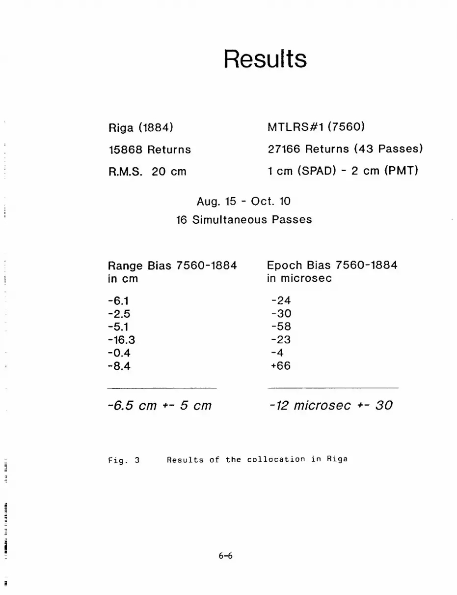
Results
Riga (1884)
15868 Returns
R.M.S. 20 cm
MTLRS#1 (7560)
27166 Returns (43 Passes)
1 cm (SPAD) - 2 cm (PMT)
Aug. 15 - Oct. 10
16 Simultaneous Passes
Range Biasin cm
-6.1-2.5-5.1
-16.3-0.4-8.4
7560-1884 Epoch Biasin microsec
-24-30
-58-23
-4+66
7560-1884
-6.5 cm +- 5 cm -12 microsec +- 30
Fig. 3 Results of the collocation in Riga
6-6
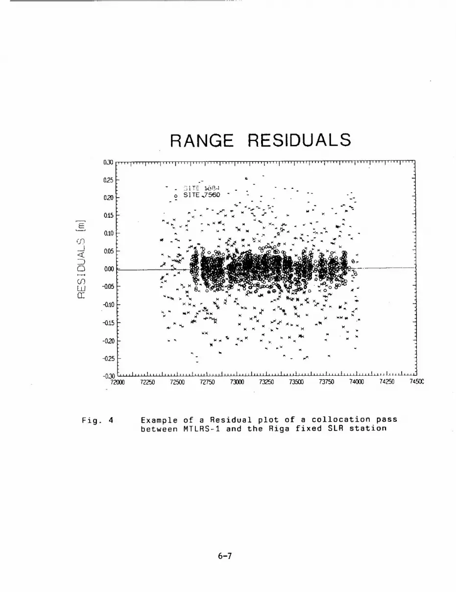
__]<£
a:---,I
LLJ05.
RANGE RESIDUALS030
025
020
0.15
&10
0.05
0.00
-0.05
-0.10
-O.'15
-020
-025
-03072OOO
.'"'1 .... I .... I""1""1'"'1''"I'"'1 .... I .... 1'"'1 .... I .... I .... I'"'1 .... t'"'1 .... t .... I .... -
r.
!!;,t T= t<-.*,q-i - -o S I TE .,,7560 °- -
11l i" _ __'.
Y,. i,,i
,,,I .... t .... I,_a_LtJJ.a_l_LLt!!J_Jl .... I .... I .... I .... t .... I .... I .... I .... I,,,,I,,,,t_._t_J_l,,_
72250 72500 72750 73000 73250 73,..'..'..'..'._073750 74000 74250 74543C
Fig. 4 Example of a Residual plot of a collocation passbetween MTLRS-I and the Riga fixed SLR station
6-7

Results
Simeiz (1873 )
R.M.S. 10 cm
10 Passes
Kazivelli (1893)
10 cm
20 Passes
MTLRS#1 (7561)
1 cm - 2 cm
53 Passes
Oct. 14 - Nov. 23
Data not yet processed
Fig. 5 Results of the collocation in Simeiz
6-8

ETALON-15-2 CENTER OF MASS CORRECTION
AND ARRAY REFLECTIVITY
N94-15576
N.T.Mironov, A.I.Emetz
Main Astronomical Observatory of the Academy of Sciences
Ukraine_ 2521275 Kiev, Goloseevo
A.N.Zaharov, V.E.Tchebotarev
United Space Device Corporation
Russia, 111024, Moscow, Aviamotornaya st.,53
ABSTRACT. Center of mass correction to be applied to measu-
red ranges to the ETALON-1,-2 satellites are considered. Numeri-
cal values of the correction and reflectivity from retroreflector
array are computed. The variations of these values with satellite
orientation are investigated.
i. INTRODUCTION
In 1989 two identical passive satellites, ETALON-I,-2, deve-
loped for precise laser ranging measurements were launched in the
Soviet Union into nearly circular high orbits ( about 20,000 km ).
It was reported that the distance between the center of mass and
the plane of probable reflection is 558 mm ,Tatevian,1989.
To evaluate the ETALON-I,-2 satellites for Earth rotation ap-
plications5 the International Earth Rotation Service (IERS) Direc-
ting Board has announced an SLR campaign for the tracking of these
satellites. The campaign took place for three months period from
September 1, 1990 to December I_ 1990.
To discuss the various aspects of analysis of the ETALON-15-2
laser ranging data carried out at the number of scientific center_
the Institute of Astronomy of the USSR Academy of Sciences and the
Soviet Mission Control Center organized the International symposi-
um "ETALON-91" which took place in Moscow during June 3-9, 1991.
Recognizing the requirement for precise information characteriz-
ing the ETALON-I,-2 satellites, the participants of the Internati-
onal Symposium meeting in Moscow recommended
1) that complete design and orbit insertion information on
the ETALON-1,-2 satellites be released to the analyst participat-
6-9

ing in the international programs,
2) that the international community undertake experiments to
measure ETALON satellite characteristics, such as spin rate and
direction_ photometry, calorimetry and other.
We undertook the study of the center of mass correction and
array reflectivity of the ETALON satellites in order to ensure
their accuracy.
2. OPTICAL CUBE-CORNER SPECIFICATIONS
The optical cube corners on ETALON-I,-2 satellites have hexa-
gonal entrance faces, each with a width of 27.0 mm across flats.
The length from vertex to face is H=Ig.I mm. The optical cube-cor-
ners are made of fused silica and the reflecting faces are alumi-
nium coated The index of refraction of the fused silica is n =
1.455442 at _1=0.6943 Hm and n2=1.460915 at _i=0.5320 Hm.
The dihedral angles between the back faces have offsets in
order to compensate for velocity aberration. The divergence of the
cube corner is about 32 prad for half-maximum level.
3. GEOMETRY OF THE ARRAY
The ETALON satellite is a sphere 1294 mm in diameter with
2146 retroreflectors distributed over the surface (Figure I). Six
of the cube corners are made of germanium for infrared wavelength
and the others 2140 are made of fused silica for use at visible
wavelength.
The optical cube corners are arranged in 30b lattice frame
with 7 cube corners in each one. The lattice frame are mounted
over 14 separated zones. Their orientation is shown in Figure 2.
The distribution of the lattice frames and cube corners over the
zone is illustrated in Figure 3. Table I lists such distribution
for each zone.
The cube corners are recessed below the surface of the sphere
by 5.5 mm. This recession_ together with the fact that the front
face of a cube corner is flat_ places the center of the front face
of the cube corner closer to the center of the satellite than
647.0 mm radius of the satellite.
6-10

Table i Oistribution of the cube corners through zones
( +:Yes; O:No )
System of
cube
Zones
corners A I A 2 A 3 A 4 A 5 A 6 B I B 2 B 3 B 4 B i B 2 B 3 B4
0 + 0 + 0 + + + + + + ÷ + ÷ +
O. 1-0.6 + + + + + + + + + + + + + +
1.-3. + + + + + + + + + + + + + +
4.1-4.3 0 0 0 0 0 0 + + + + + + + +
4.4; 4.5 0 0 0 0 0 0 + + + + + + + +
4.6 0 0 0 0 0 0 + + + + + + + +
Number of
cube 133 132 133 132 133 133 175 175 175 175 161 161 161 161
corners
4. OPTICAL CUBE CORNER REFLECTIVITY
The reflectivity E of the ETALON-I_-2 optical cube corners is
given below as a function of incidence angle. The angle • is mea-
A Isured from the normal N to the front face_ and the angle is the
angle to the projection of the incident beam onto the front face;
both these angles are shown in Figure 4_5. The variations of the
cutoff angles for reflection • (and refracted angle ) with theC c
azimuth A I are illustrated in Table 2 and Figure 6. These varia-
tions repeat every 6n ° in A I and the values • for 30°-A I are- C
equal to those for 30°+A I.
Table 2. Cutoff angles for reflectionC
of azimuth A I
as a function
A_ deg _ deg c' degcl _ _c2,deg _1
0 66.965 67.479 39.220
10 61.031 61.421 36.949
20 58.064 58.410 35.667
30 57.147 57.482 35.253
6-11

In computing the reflectivity E it was assumed that the cube
corners had perfect-metal reflecting faces and no dihedral-angleoffset. In Figure 7 each curve is the calculated total reflecti-
vity and is proportional to the active reflecting area. The curves
include reflection losses at the front face in entering and leav-ing the cube corner by laser beam. All curves are normalized to
unity at normal incidence. The active reflecting area at normalincidence is &31.33 mm2 for a hexagonal cube corner whose width
W=27.0 mm across flats. The active reflecting area and the reflec-tivity repeat every 60 ° in A i In additional_ the values E for
30°-A i are equal to those for 30°+A I. The curves for the two dif-
ferent wavelengths are fairly similar. The results were used to
calculate the center of mass correction and array reflectivity.
5. ARRAY COORDINATE SYSTEM
The coordinate system used to describe the geometry of the
array is as follows (Figure 8).As a rule the position and orienta-
tion of each cube corner in the array are given by the six num-
bers: x, y, z B_L_A. The origin of the x-y-z coordinate system is
in the center of satellite. X_Y and Z are in the directions of the
and A zones respectively. The angles B and L arecenters AI_ A_ I 12given in an x -y -z coordinate system_ which is parallel to the
x-y-z system and the origin ks in the center of front face of each
cube corner. The azimuth angles A are given in _-_-_ coordinate
system. Its origin ks at the center of the front face_ its _ axis
normal to the front face_ _ in the direction of increasing B_ and
in the direction of increasing L. The orientation angle A ks me-
asured counterclockwise from _ axis to the projection of one of
the back edges of the cube corner onto front face_ as shown in Fi-
gure 8.
The direction of the incident beam V in the array coordinate
system is given by the angles _ and _: both these angles are shown
in Figure 8. To compute the incidence angles • and A i on the cube
corner_ the vector V must be expressed in the _-_-_ coordinate
system (Figure 8). The conversion between the coordinate systems
of the array and incident beam is accomplished by rotating the co-
ordinate system of V first about the z-axis by the angle L unti-
6-12

clockwise and then about new y-axis by the angle B clockwise.
For the ETALON-I_-2 cube corners the angles A are unknown but
the cube corners have been installed so as to give a uniform dif-
fraction divergence independent of satellite orientation. The di-
vergence of the retroreflector array is about 42 Hrad for half -
maximum level. Taking into account these aspects and the total re-
flectivity of the ETALON-1,-2 optical cube corners and their rece-
ssions_the active reflecting area of each retroreflectors has beenaveraged for AI=O°, I°,...,30 °.
&.METHODOF COMPUTINGTHE CENTEROF MASS CORRECTION
The center of mass correction to be applied to measured ran-
ges is the distance of the centroid of the computed total energy
of the return from the center of gravity of the satellite. Compu-
tation of the range correction includes a correction for the opti-cal path length of the ray within the cube corner. The correction
listed is the one-way correction
N N
/k=l k=t
where Pk is the distance of the apparent reflection point for the
k-th retroreflector from the plane through the center of mass of
the satellite perpendicular to the incident beam. Constant E k gi-
ving the intensity of the reflection from the k-th cube corner is
proportional to the active reflecting area. N is the number of the
cube corners contributing to the reflected signal.
The apparent reflection point as a function of the angle
between the incident beam and the normal to the front face of the
cube corner is given by the expression
.-
z z_Pk = rcos_ k - H n -sin k
where r=distance from the center of the satellite to the front fa-
ce of the cube corner (641.7 mm)_ _k=the incidence angle on the
k-th cube corner, H=the length of the cube corner (19.1 mm), n=the
index of refraction.
In computing the center of mass correction p and array refle-
ctivity E(=_ Ek), the cube corners have been modeled as isothermal,
geometrically perfect reflectors with perfect reflecting coatings
6-13

on the back faces. The reflection losses at the front face as the
laser beam enters and leaves the cube corners are taken into
account.
7. APPARENTREFLECTION POINT AND SPREADIN RANGE
The cube corners contributing to the reflected signal are
contained in a spherical cap whose angular radius (half angle) is
the cutoff angle of the cube corner. The earliest possible refle-
ction would come from a reflector directly facing the incident
beam, and the latest, from a cube corner near the cutoff angle.
Apparent spread in range is the difference between the apparent
reflection points for these two cases along the direction of il-
lumination.
Since the cube corners are nonuniformly distributed over the
sphere of the ETA_ON-I,-2 and recessed below the satellite sur-
face there are variations of the earliest and latest reflection
points. Table 3 lists the apparent reflection points along the
line of sight measured from the center of satellite for various
cases: i) the earliest possible reflection point (a cube corner
whose face is normal to the incident beam]_ 2) the earliest point
where an incident beam in the center of A 2 zone could be up to
about 4 ° from nearest cube corner (replacing an optical cube
with an germanium cube]; 3) the earliest point where an incident
beam could be up to about 8 ° from the nearest cube corner (re-
placing two lattice frame of 14 cube corners with the supporting
holder); 4) the last possible reflection point where the active
reflecting area goes to zero; 5) the last possible reflection
point where there is a sharp decrease in reflectivity because of
the recession of the cube curners.
Replacing an optical cube corner in zones A 2 and A 4 with a
germanium cubes, which is opaque to visible light, reduces the
distance of apparent reflection point by about 1.5 mm. The maxi-
mum variation of the earliest reflection point is about 5.9 mm in
replacing 14 cube corners with supporting holders in BI, B2, B 3
and B 4 zones. The total range spread without taking into account
the recession of the reflectors is about 400 mm. The recession
reduces the range spread approximately by 2 times. Figure 9 illu-
6-14
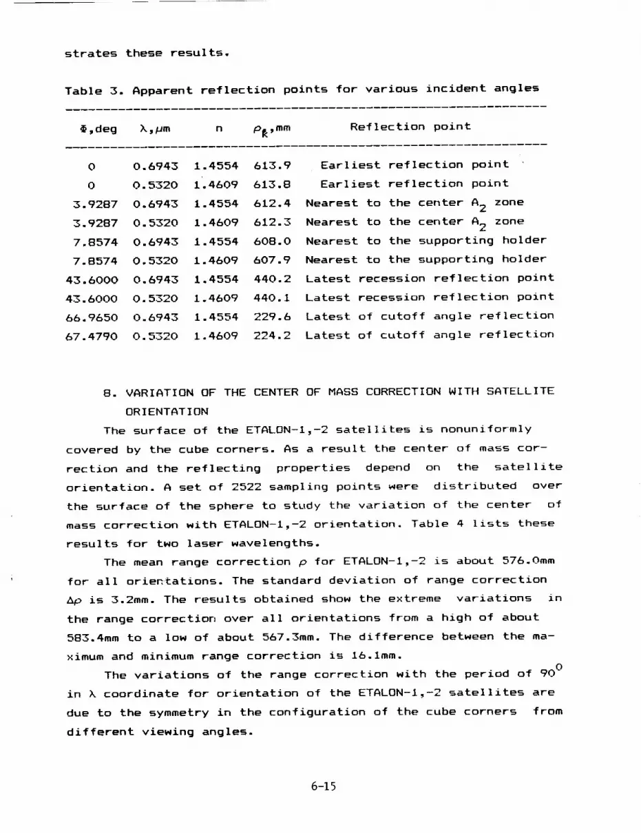
strates these results.
Table 3. Apparent reflection points for various incident angles
• ,deg X,pm n p_,mm Reflection point
0 0.6943 1.4554 6i3.90 0.5320 I'.4609 613.8
3.9287 0.6943 1.4554 6i2.43.9287 0.5320 1.4609 612.3
7.8574 0.6943 1.4554 608.0
7.8574 0.5320 1.4609 607.943.6000 0.6943 1.4554 440.2
43.6000 0.5320 1.4609 440.i
66.9650 0.6943 1.4554 229.6
67.4790 0.5320 1.4609 224.2
Earliest reflection point
Earliest reflection point
Nearest to the center A 2 zone
Nearest to the center A 2 zone
Nearest to the supporting holder
Nearest to the supporting holder
Latest recession reflection point
Latest recession reflection point
Latest of cutoff angle reflection
Latest of cutoff angle reflection
8. VARIATION OF THE CENTER OF MASS CORRECTION WITH SATELLITE
ORIENTATION
The surface of the ETALON-I,-2 satellites is nonuniformly
covered by the cube corners. As a result the center of mass cor-
rection and the reflecting properties depend on the satellite
orientation. A set of 2522 sampling points were distributed over
the surface of the sphere to study the variation of the center of
mass correction with ETALON-I,-2 orientation. Table 4 lists these
results for two laser wavelengths.
The mean range correction p for ETALON-I,-2 is about 576.0mm
for all orientations. The standard deviation of range correction
Ap is 3.2mm. The results obtained show the extreme variations in
the range correction over all orientations from a high of about
583.4mm to a low of about 567.3mm. The difference between the ma-
ximum and minimum range correction is 16.1mm.
The variations of the range correction with the period of 90 °
in k coordinate for orientation of the ETALON-I,-2 satellites are
due to the symmetry in the configuration of the cube corners from
different viewing angles.
6-15
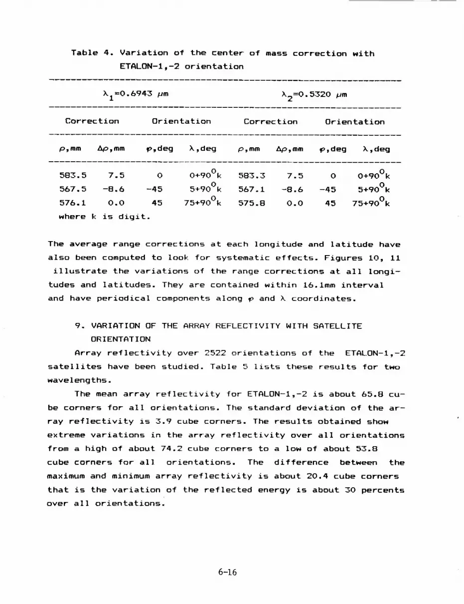
Table 4. Variation of the center of mass correction with
ETALON-1,-2 orientation
XI=0.6943 pm X2=0.5320 Hm
Correction Orientation Correction Orientation
p,mm _Ip,mm _,deg %,deg p,mm Ap,mm _,deg _,deg
583.5 7.5 0 O+900k 583.3 7.5 0 O+900k
567.5 -8.6 -45 5+900k 567.1 -8.6 -45 5+900k
576.1 0.0 45 75+900k 575.8 0.0 45 75+900k
where k is digit.
The average range corrections at each longitude and latitude have
also been computed to look for systematic effects. Figures I0, II
illustrate the variations of the range corrections at all longi-
tudes and latitudes. They are contained within 16.1mm interval
and have periodical components along _ and X coordinates.
9. VARIATION OF THE ARRAY REFLECTIVITY WITH SATELLITE
ORIENTATION
Array reflectivity over 2522 orientations of the ETALON-I,-2
satellites have been studied. Table 5 lists these results for two
wavelengths.
The mean array reflectivity for ETALON-I,-2 is about 65.8 cu-
be corners for all orientations. The standard deviation of the ar-
ray reflectivity is 3.9 cube corners. The results obtained show
extreme variations in the array reflectivity over all orientations
from a high of about 74.2 cube corners to a low of about 53.8
cube corners for all orientations. The difference between the
maximum and minimum array reflectivity is about 20.4 cube corners
that is the variation of the reflected energy is about 30 percents
over all orientations.
6-16

Table 5. Variation of the array reflectivity with
ETALON-I,-2 orientation
_i=0.6943 Hm X2=0.5320 Hm
Reflectivity Orientation Reflectivity Orientation
E_c.c. E_c.c. _deg X,deg E,c.c. E,c.c. _,deg X,deg
74.1 8.6 35 45+900k 74.4 8.6 35 45+900k
53.6 -12.0 -45 5+900k 53.9 -12.0 -45 5+900k
65.6 0.0 0 25+900k 65.9 0.0 0 25+900k
where k is digit.
The variations of the array reflectivity with the period of
90 degrees in k coordinate for orientation of the ETALON-I,-2 sa-
tellites are due to the symmetry in the configuration of the cube
corners from different viewing angles.
For the purpose of illustrating more detailed studies of the
ref!ectivity properties, the sampling points have been looked at
individually to find one whose properties are close to the averagefor all orientations. The point at _=45°, _=75 ° has nearly the
average range correction and reflectivity, so it has been used for
above purpose. Figures 12 are histograms of the contribution to
the reflected signal from each l-cm interval along the line of
sight starting from the earliest reflection point. The origin ofthe distance scale is the center of satellite. These histogramsare for a direction of illumination given by _=45 ° and _=75 °. For
this direction the total effective reflecting area is 66.8 times
the area of Qne cube corner, and the mean apparent reflection
point is 576.0mm from the center of the satellite. The cube corner
shown on the histogram is the closest possible position to the
observer.(None of the cube corner points exactly at the observer
for this particular direction of illumination. The earliest and
latest apparent reflection points for this case are 613.5mm and
440.7mm, respectively). Table 6 lists the data used to plot the
histogram: the equivalent number of cube corners at normal inci-
6-17

dence_ the percentage of the total return
percentage in each l-cm interval_starting
reflection point.
and the cumulative
from the earliest
Table 6. Total return in each l-cm interval starting from
the earliest apparent reflection point
Interval Equivalent numberof cube corners
% of total return Cumulative %
X1 X2 _I X2 _I _2
i 16.62 17.24 25.00 25.68 25.00 25.68
2 9.38 7.90 14.11 11.77 39.11 37.45
3 9.22 8.16 13 87 12.16 52.98 49.61
4 5.38 8.87 8.09 13.21 61.07 62 825 4.51 5.53 6.78 8.23 67.85 71.05
6 5.20 4.17 7.87 6.22 75.72 77.27
7 3.99 3.58 6.00 5.33 81.72 82.60
8 3.46 3.31 5.21 4.93 86.93 87.53
9 2.78 2.79 4.18 4.16 91.11 91.69
10 2.41 I. 98 3.62 2.94 94.73 94.63
ii 1.26 1.38 1.89 2.06 96.62 96.69
12 1.21 0.97 1.82 1.45 98.44 98.14
13 0.56 0.77 0.85 i. 14 99.29 99.28
14 0.28 0.24 0.42 0.35 99.70 99.63
15 0.12 0.16 O. 18 0.25 99.88 99.88
16 0.07 0.06 O. I0 0.09 99.98 99.97
17 0.02 0.02 0.02 0.03 100.00 100.00
A quarter of the return energy comes from the first l-cm in-
terval, over half the return energy comes from the first 3-cm in-
terval_ and over 90% comes from the first 9-cm interval. The cen-
ter of mass correction is at 576.0mm, which is 37.5mm in back of
the first reflection point.
The average array reflectivity at each latitude and longitude
have also been computed to look for systematic effects. The
6-18

variations of the average array reflectivity at all latitudes and
longitudes are contained within 21 cube corners and have periodi-
cal components. Figures 13 and 14 illustrate these regularities.These variations are similar to ones in the range correction of
ETALON-I,-2 satellites.F
The effects of the recession of cube corners in concentrating
the energy and computing the range correction have been studied.
The center of mass correction and array reflectivity_ if the cube
corners were not recessed_ would be 540.7mm and 126.53 cube
corners respectively.
lO. CONCLUSION
The ETALON-I_-2 center of mass correction is about 576.0mm
for both laser wavelengths. This value is 18mm more than value
which was published by Tatevian_1989. The range correction has pe-
riodical peak-to peak variations of about 2 cm with satellite
orientation. These peculiarities give the possibility to derive
for ETALON-I_-2 spin rate and direction using the precise laser
ranging measurements to the satellites with SLR systems of 3-rd
generation.
The mean array reflectivity for ETALON-I_-2 satellites is
about 66 cube corners. Difference between the maximum and minimum
array reflectivity is about 21 cube corners or 30% over all
satellite orientations.
Such regularities in ETALON-I_-2 center of mass correction and
array reflectivity are due to the symmetry with respect to the
X-axis in the dissemination of the cube corners over the satellite
surface.
REFERENCES
Tatevian S.K.Satellite report: ETALON. Satellite laser ranging
newsletter.1989,June,p.5.
Pochukaev V.N., Schutz 8.E., Tatevian S.K. International symposium
on ETALON satellites. Satellite laser ranging newsletter. 1991,Ap-
ril,p.22.
6-19

FiG.t. ETALON-1,-2SATeLLII'E
6-20

;i
t-
o/
>--I-
0
\
\
//
.a3
_PULI
4_
b,(:)
Q_4D_
u.I
IF-
Z9C
(:3I'-r,.ll
I.u,,ml
uill
Q_InILl
ILl"7"I"
LI.0
U.IZC_
N
L.,,;
U.
ot
I
__-2J...

270 ° @
@
® @
o i®,®
.® _ @ ®®
o _ogO °
FIG.3. D[s'reisuTioN OF THE LATTICE FRAME ANDReTRORe_LECTORS OVER A ZONE
6-22

/
W
]
Fief.4. DiRSCTiONOF iNCiDSN'r BEAU
. m
O !
o/Fiq.5. AcTiVE REFLECTING AREA: SEPARATION OF iNPuT
AND OUTPUT APERTURES
6-23
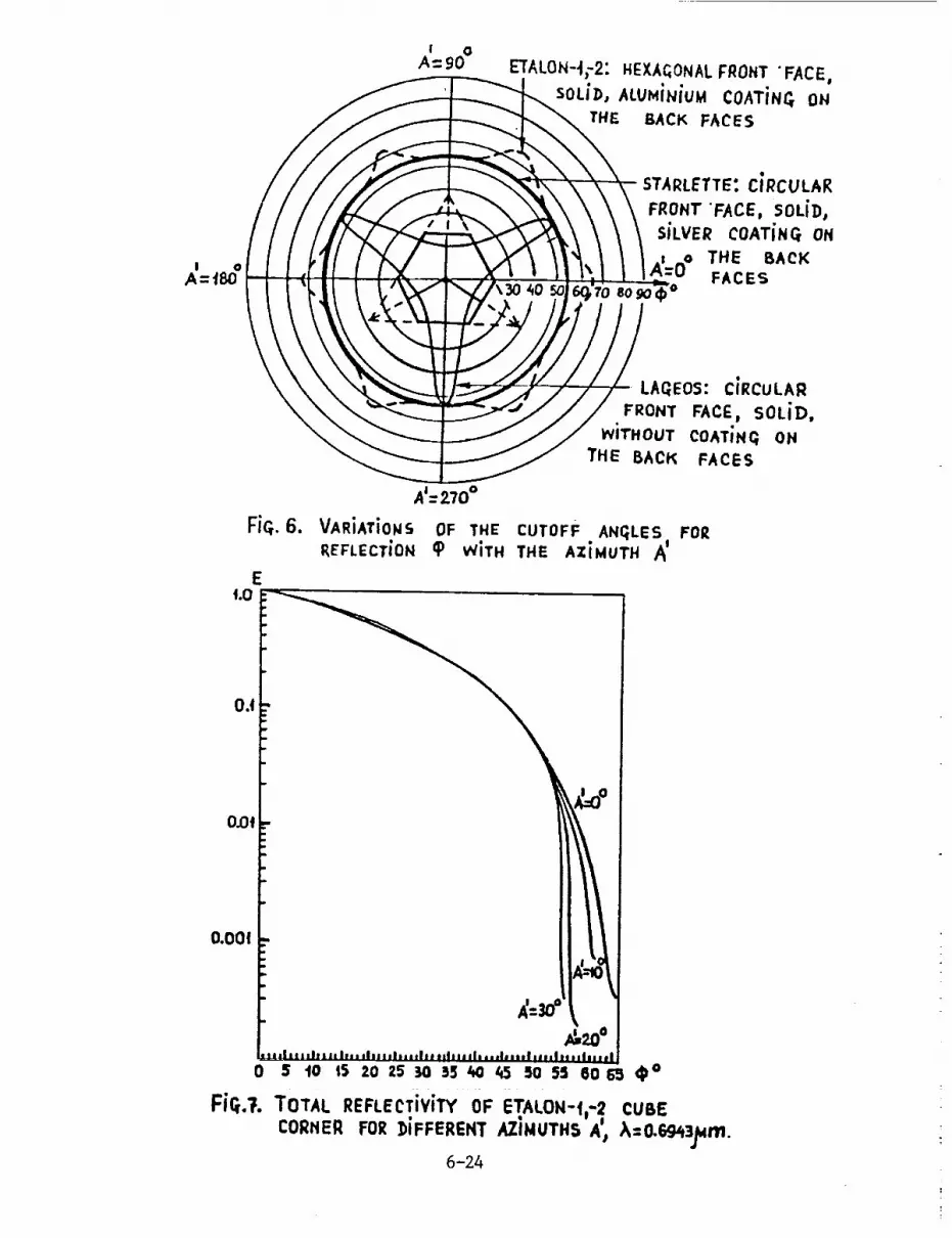
A_=P.70°
Fi(;.6. VARiATiO_ISOF THE CUTOFF ANqLES FOR
REFLECTION <P WiTH THE AZIMUTH Aj
OJ3!
0.001
6-24

COOR1)iNATESYSTEMSFORRETROREFLECTORPOSiTiONI_ND ORiEN'_ATiON
A
N
Fiq.9. APPARENT REFLECTION POINTS
AN]) SPREAD iN RANGE
6-25

/
::t o_o :,oot__ ! | I I I ! I J I ! I ! I ... ! I ! I
90 80 70 60 50 _0 30 20 t0 0 -_0-20-J0-40-50-50-70-80-90
6-26
Fi_.fO. VARiATiON OF ETALON-f;'2 CENTER OF MAr-'_ CORRECTION
AT EACH LONGJTUOE

o_o90
80
70
6o
30 40 50 60 70
/ \/
.¢........\./
M t:0.t
0.0
0.0
0.0
-f.O
;I,4)
"0.0
Z_.O
Fret. ffCL. VARiATiON OF ETALON-|,-2 CENTER OF HASS
CORRECT'ION )iT EACH UITiTU])E
6-27
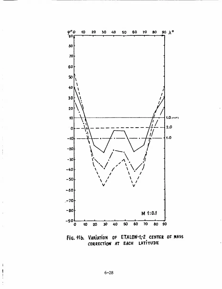
8O
70
60
50
]0
2O
fO
0
-dO
-20
-30
-40
-50
-60
.--70
-80
-900
40 20 _0 _0 SO 60 70 SO 90 _o
" " 7-
,).,/.- ,,'\./)\ / X /
/ X /X / x/
V v
M t:O.fI | • | | J • •
t0 20 30 40 50 60 70 80 90
_.0
Fic;.Hb, VaRiATiONOF ETALON-1,--2CENTEROF_AssCORRECTIONAT EACH LATiTU])E
6-28

E_
t/t
uJz
o 44¢.#
U4= t2(.3
40
el
>==8I-- =o
_ 6
.=1
.>- 2
.it
576A m m
II
_. CENTER OFSATELLITE
1 I i i I I I | | | i J I | ! I It I I ! I
8 .12 _6 20 £Zt 28 32 56 40DISTANCE FROg
Ir.=
o.
| I°.
!!II
II_ 46 52 56
CENTER OF SATELLITE (CM)
Fi_.t2ct. RI_FLECTiViTY Hib-roC;RAXOF ETALON-1,-2;_=o.6_3j_m
;o
;
itr
octM2= 46
u t2
_.u.I- o
• - t0
:_u 8 _ CENTER Fw SATELLIT_1 2u. 6
_2
,_ e , i I I a l. I l !
0 _ 8
575.8mm _1
e
Fi_.t2b.
m,i i |= .
.t2 46 =0 24 =8 32 36 40 _ _8 5:l 56 60])ISTA_ICE FROM CENTER OF SATELLITE (CM)
REFLECTiViTY HISTOqRAt4 OF ETALON-|,-2; _=O.53ZOjqm
6-29
1IL

4
3
2
t
....,_=0 °
_ _ _,7,,=40°
,...,_., ._=20 °
e
\ \,v \.
90 60 70 60 50 _0 30 _0 |0 0 -40-20-30-/t0-_-60-70-60-90
Fi_..13. VAeiA'rioNOF ETALON-f;2 REFLECTiVJTY AT EACH tOl_T_e
6-30

90,
80
70
6O
50
,40
30
20
tO
0
/
e_ D
-3O
-SO
-60
-?0 _-
-gO
g
e,@e o
• • t • • • • • • •
/x," \
j
/ \
/
M 4:t
\
o 10
Fi .
90 30 _ 50 60
VAR}AT_ON OF ET/[LON-t,-2
AT EACH LATITU3E
6-31
-CL5
• • . . -3.0
-5.0
-4.0
-).0
_.4\\
3.2r
70 80 9O
IZEFLECTTIVITY
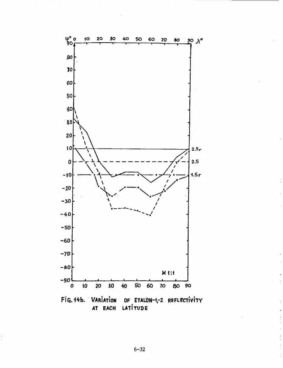
(_)o to 2o SO _o 50 60 ?0 so 90 _o
_0
30
_0
5.o
_o
io
20
I0
0
-I0
-20
-30
-40
-50
-60
-70
-80
-\I
•,,, /--.__ .:/
-90 ' • '
M _:t
| • • •
0 10 20 30 _ 50 60 70 _0 90
2.5r
2.5
t.5r
FiG.tttb. ' VARiAT;ON OF ETAL(]N-'I,-2 REFLECTiVh'YAT EACH LATITUDE
6-32

N94-15577
Test Results from LAGEOS-2 Optical
Characterization Using Pulsed Lasers
Thomas Varghese, Michael Selden,Thomas Oldham,Christopher ClarkeAllied Signal Aerospace Company,
BFEC/CDSLR
10210 Greenbelt Road
Seabrook, MD 20706USA
Thomas ZagwodzkiPhotonics Branch
NASA Goddard Space Flight CenterGreenbelt
Maryland, 20770U.S.A
Abstract
Laser Geodynamic Satellite (LAGEOS-2) has undergone extensive optical testing atNASA Goddard Space Flight Center during 1989. The techniques included
measuring the far field diffraction pattern using cw and pulsed lasers. In the pulsedmeasurement technique, response of the satellite was studied by measuring the
FFDP as a function of pulsewidth, wavelength, polarization, position in the FFDP,
detector/processing techniques, and satellite orientation. The purpose of the pulsed
laser testing was two-fold: (1) Characterize the satellite optical response with the
detector and signal processing electronics currently used in most SLR stations usingthe Portable laser ranging standard, and (2) to characterize the satellite response for
various conditions using the highest bandwidth optical detector (streak camera)
available for the next generation of SLR technology. The portable ranging standard
employed multiple measurement devices and an optical calibration scheme to
eliminate range-dependent and amplitude-dependent systematics. These
precautions were taken to eliminate/minimize instrumental errors and providemaximum accuracy. For LAGEOS orbit (6000 Km) ground stations are located 34 to
38/_-radians off the axis of the return signal from the satellite; therefore an opticalmask was used to restrict the field of view (FOV) of detection to this annular region of
the far-field diffraction pattern (FFDP). The two measurement techniques were
implemented using an aperture sharing scheme and complemented each other by
providing mutual verification.
6-33

The results indicate a variation of range correction as a function of satellite orientation
and location within the far-field diffraction pattern. Range correction as a function of
wavelength shows a maximum at 532 nm. For other wavelengths, the FFDP of
normal-incidence cube-corners is detuned, providing a greater contribution to the
integrated response from cube-corners farther away from the observer. Constant-
fraction processing of the detected pulse provided more consistent results than peak
and leading-edge. Changes in the orientation of the E-vector of the linearly polarized
light showed a systematic variation of _ 2mm in the polar regions of the satellite. A
consistent difference in RC of _,z2 mm between linearly polarized light and circularly
polarized light was also observed. The test results showed that a range correction of
-' 251 mm is applicable to the third-generation SLR systems operating at the multi-
photoelectron (MPE) level. The use of short (---15 ps) laser pulses and streak
cameras would provide time resolved signature of the satellite allowing improved(lmm accuracy) range correction.
6-34

" BACKGROUND
- LAGEOS-1 launched on May 4, 1976; 5900km orbit; 110 ° inclination.
- Prior to launch, the satellite was optically tested (532nm, 60ps) atGSFC.
- Remarkable progress in SLR technology over 15 years and theprojections for the future required understanding of LAGEOS-2 LRAbetter than LAGEOS-1.
- Major emphasis to accurately (submillimeter) determine the rangeoffset to satellite CM from the effective reflection point.
- Elaborate experimental schemes with state of the art Instrumentation
and expanded parameteric study than LAGEOS-1.
- Satellite manufactured by Aeritalia for ASI.
- LAGEOS-2 scheduled for deployment Oct. 15, 1992; 5900km orbit52 ° Inclination.
SATELLITE FEATURES:
MECHANICAL• Spherical satellite with a DIAMETER of 599.87mm.
• Two hemispherical shells with outer skin made of aluminum.
• Core of the satellite has brass to Improve mass..
• Cylindrical core for preferred spin axis (N-S).
• Total mass 405.38 kgm.
• Hemispherical shells and the brass core held together bya steel shaft.
• 426 cube corner cavities.
• Center of gravity and center of geometry are nearly coin-ciden ( 0.078mm)..
6-35

SATELLITE FEATURES:
OPTICAL
• 426 cube corners; fused silica (422), germanium (4).
• UV-near IR supported by FS; Ge for Infrared ranging..
• FS cubes distributed with symmetry about the polar axis;Ge cubes distributed as a tetrahedron.
• Special grade of FS (Suprasil 1, Special T19) for material homogenityand isotropy..
• Clear aperture 38.1 mm; face to apex depth 27.84mm..
• Dihedral offset of 1.5 arc sec for FS cubes; no dihedral offset for Gecubes.
• No metallic coating; only TIR to enhance reflection from CCs closeto the incoming laser beam.
• TIR cubes are sensitive to polarization affecting FFDP and thereforerange correction.
OPTICAL CHARACTERIZATIONPURPOSE
• Range correction to center of mass from effectivereflection point.
• Target spread function.
• Lidar cross section.
APPROACH
• Measure the temporal response of the satelliteusing mode-locked lasers and fast detectors(streak camera, photodiode, MCP-PMT) as afunction of wavelength, pulsewidth, polar-ization, position in the FFDP, satellite orien-tation, detection bandwidth and, type of signalprocessing; Compute and deduce the satellitecharacteristics.
6-36

MEASUREMENT PARAMETERS
LASER• Wavelength: Pulsed 1064, 532, 355nm• Polarization: Linear (horizontal, vertical), circular• Pulsewidth: 60ps (1064nm); 140ps, 45ps, 25ps (532nm), 30ps
(355nm)DETECTOR
• Temporal Resolution: 2.5ps (streak camera); 100ps (photo-diode) 500 ps (MCP-PMT)
• Photoelectron Level: 10-100 (MCP-PMT); 1000-10000 (SC);100000 - (Photodiode)
SIGNAL PROCESSING• Peak• Half Max.• Centroid• Constant Fraction
SATELLITE ORIENTATION• Polar• Equatorial• Others
Velocity Aberration: Various positions in the annular(34-38 microradlan) region of the FFDP.
EXPERIMENTAL APPROACH
PULSE MEASUREMENT• Mode-locked laser for illumination.
• Temporal detectors in the focal plane.• Detection limited to useful region in the FFDP.
ADVANTAGES
• Net effect of coherent/incoherent superpositionof FFDPs directly measured.
• More direct than cw case since instrumentatiion used is
similar to those currently used for SLR; easy to verifyspaceborne performance.
• Computationally simple.• Less sensitive to air currents, vibration, etc.
DISADVANTAGES
• Experimental measurement is complex.• Allows only discrete measurement of the FFDP.
I
6-37
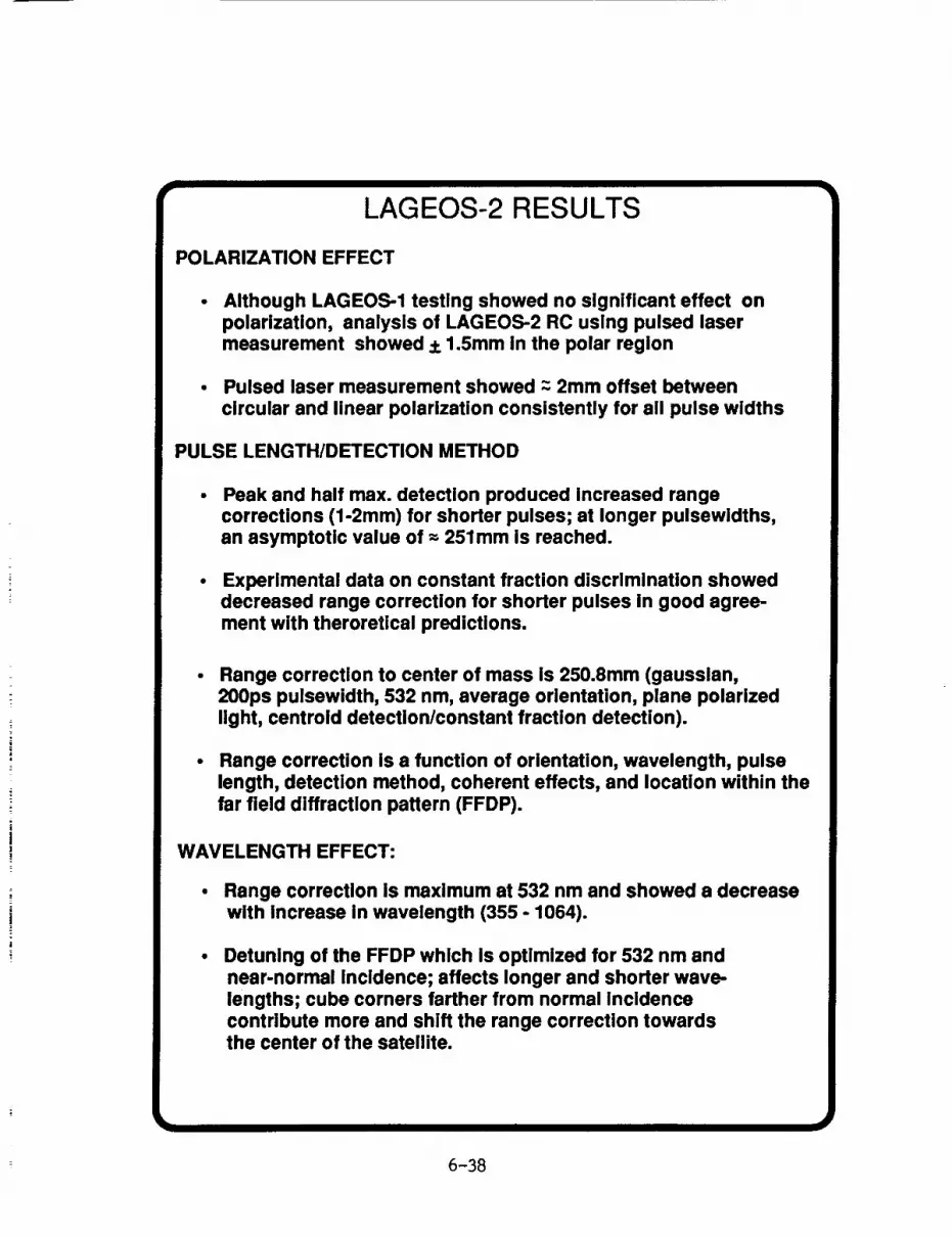
LAGEOS-2 RESULTS
POLARIZATION EFFECT
• Although LAGEOS-1 testing showed no significant effect onpolarization, analysis of LAGEOS-2 RC using pulsed lasermeasurement showed + 1.5mm in the polar region
• Pulsed laser measurement showed z 2mm offset between
circular and linear polarization consistently for all pulse widths
PULSE LENGTH/DETECTION METHOD
• Peak and half max. detection produced Increased rangecorrections (l-2mm) for shorter pulses; at longer pulsewldths,an asymptotlc value of -=251mm Is reached.
• Experimental data on constant fraction discrimination showeddecreased range correction for shorter pulses in good agree-ment with theroretical predictions.
• Range correction to center of mass is 250.8mm (gausslan,200ps pulsewidth, 532 nm, average orientation, plane polarizedlight, centroid detection/constant fraction detection).
Range correction is a function of orientation, wavelength, pulselength, detection method, coherent effects, and location within thefar field diffraction pattern (FFDP).
WAVELENGTH EFFECT:
• Range correction is maximum at 532 nm and showed a decreasewith Increase in wavelength (355 - 1064).
• Detuning of the FFDP which is optimized for 532 nm andnear-normal Incidence; affects longer and shorter wave-lengths; cube corners farther from normal Incidencecontribute more and shift the range correction towardsthe center of the satellite.
6-38

SUMMARY
• Detailed investigation of LAGEOS-2 optical characteristicshas been completed, algorithms for RC to CM of the satel-lite have been derived to apply any SLR scenario.
• The small departure of LAGEOS-2 results from LAGEOS-1is currently believed to be due to calibration/instrumen-
tation errors in LAGEOS-1 measurement.
• Current estimates of the satellite-limited ranging accuracyis estimated to be < 3mm for the best multi-photoelectron(MPE) SLR station; accuracy approaching lmm can beobtained with shorter pulses (<15ps) and streak cameras.
6-39

I BroilI I T
4,
0
6-40

7,_t t t t t,_
II : I I I! ll,_8, i I I _JI I I ,J II I I _
li I i ; i I ,,
-Y' _ I i _, _
_'_11_,_ _ I_
6-41
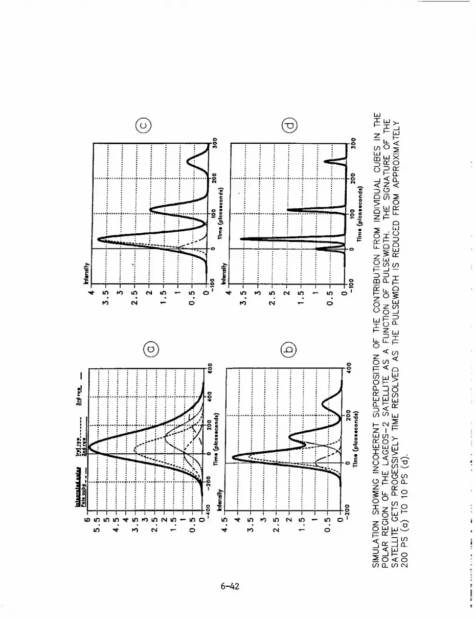
@
; : ; : ,,.0.
: ; ; : "E
Iv3" ¢'q" _" C_
I
@o
, ,.... ° 0 , • ....., . , . ,'.
: : : , : : : : : : ;
EI °
•, d""i"'i"'""i'":i r">" _ .o_|B , . • • . , ". , m
.... -.,:,..°: : :
l I l I l I l I l I I l I
_ U3 U3 U3 "_" U3 _3 L'3 ¢_IU3 _-- UF) 0 _
©; ; ; : : ; ;
i I I I I I I
U_ _ U3 C',l U3 _ U3
,4 d ,- o
©
i.
W" U') _ _ _1 _ -- t._ 0 j
W
_ _b _
_°0.oo _
o I--"
o b-_Ozwcr)n__'_w
o° Dnn 13__ i_-r
0--' o0_Z ObZ ._IW(,#'_
W-l- 0(_) _)n
l--Z w
h0
Zoo3<
o iz<n
_o,,,-_<=__,,_o,
_z eql_
_"'wo°_z
_°-I-0_zO_)_Ob-(_91_-_i°-__0"--__0°
o___. _
__o I_<±-_oo°-U) n (_ Cq
6-42
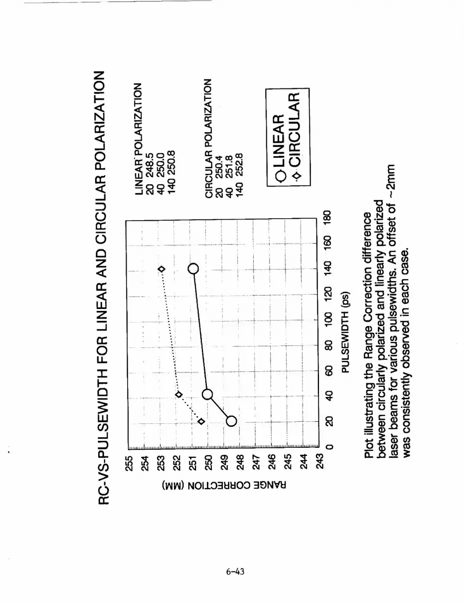
Z
o _
_0 o _ o
0"_. (D
i!!
u_ I::1.'_ .£_o :i iili.........................._ o>.oo
n.........i.........,.........i.........i.........i.........i.........i.........i.........i.........i.........i,, o _ +" _ _O_mm
cs/ (_i C_l csl C_l
>' (ININ) NOllO3hl_lO0 :IDNVI::I
0n"
6-43

Z0
_q r,._
_o_8_ zoo
Will
O0
"1-'1-
O0OgZ
O°
(Ihl_) N01103_I_00 :=I£)N'_I
6-44
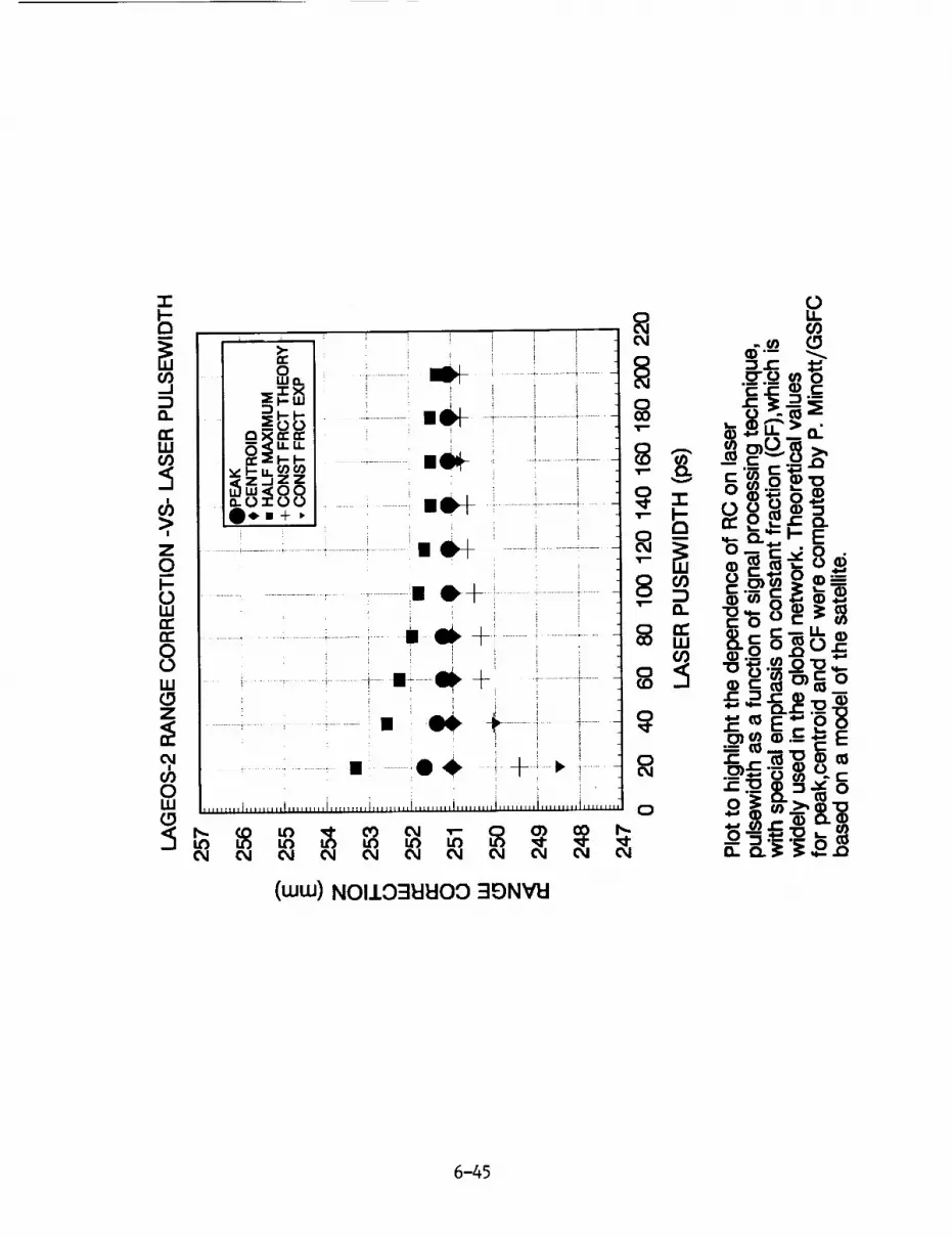
_1 _ _ ! ! t_ _.,,,_0"0_0"_'_ _c
_,i ,,1,,,_z_zz _ , _ -_ g ___I _o 88 ;..............u-,-_ _................!.........................._.....4 ,, "" _o_I O*.+, : ' " I "" '""-"®=
g , ........._ .....,............... ,+ ...............:i........... _,_o-.--®'mg_®$
l i...........................l.!i i 11 -_®
° I !....................._...............i......"............."÷ i.................!...........] _ _ ;___/ -t i] "----
.---- u _ .,.r"e- "0 (D '-s ",e" 0_, .........,.........,..................,..................;,,,,,,,,,,,,,,,,,,,,,,,,,,,i,,,,,,,,,,o .__-o__°
(ww) N011031:II:I00 3_NVI:I
6-45

"0
_I:113_17"IIIaI - NOIIO:IEII:IO0 :IONVI:I
6-46

N94-15575
ANALYSIS OF TOPEX LASER RETROREFLECTOR ARRAY
CHARACTERISTICS
Thomas Varghese
Allied-Signal Aerospace CompanyBendix/CDSLR Network
Seabrook, Maryland 20706U.S.A.
Abstract:
The joint U.S./French TOPEX/POSEIDON mission was successfully launched
on August 10, 1992 for the study of ocean height variation using
microwave altimetry. Accurate determination of the satellite orbit is
paramount to the determination of the above phenomenon. To accomplish
this, using laser ranging, the satellite is equipped with a laser retroreflector
array (LRA) around the altimeter antennae. The goal of laser ranging is to
obtain precision orbits with a radial accuracy of 13 cm to the Center of
Mass of the Satellite. This requires the laser range correction to the LRA
reference be known at the sub-cm level and is quite a challenge considering
the geometry of the LRA. Detailed studies were initiated by the TOPE×
project office (Christensen) under the auspices of the CDP/DOSE project
(Degnan) at Goddard Space Flight Center.
The studies included the following:
(1) Theoretical Modelling of the LRA using FFDP data and computationof Centroid tables: P. Minott/GSFC; D. Arnold/SAO
(2) Experimental measurement of the LRA trays using CW techniques:
P. Minott/GSFC; Carl Gliniak/EER
(3) Pulsed experimental measurement and modelling:T. Varghese/Bendix
(4) Range Correction tables for Global SLR Tracking Configurations:
T. Varghese/Bendix
(5) Data Compression using Fourier Analysis and Satellite RangeCorrection: A. Marshall/GSFC
This paper provides an overview of items (3) and (4).
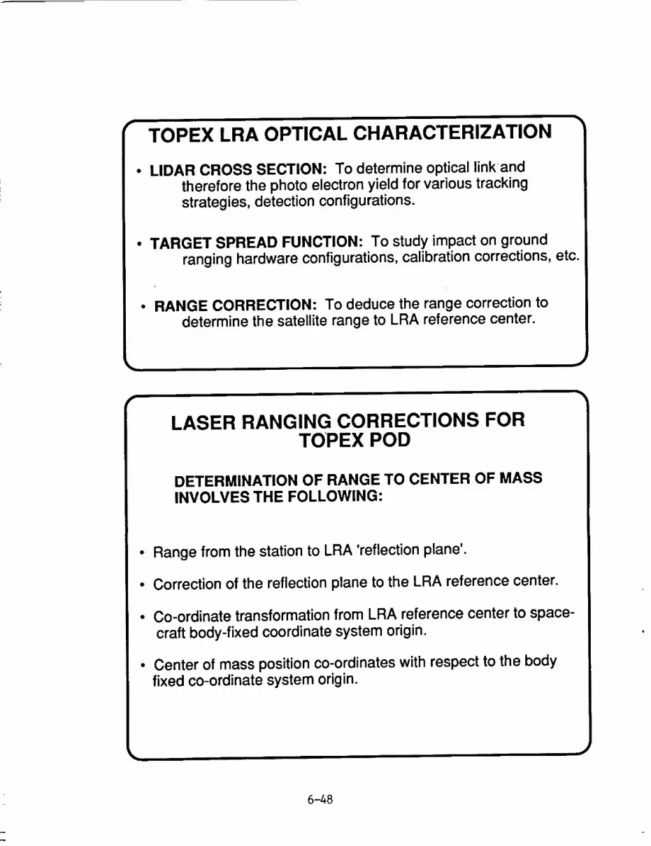
TOPEX LRA OPTICAL CHARACTERIZATION
LIDAR CROSS SECTION: To determine optical linkandtherefore the photo electron yield for various trackingstrategies, detection configurations.
• TARGET SPREAD FUNCTION: To study impact on groundranging hardware configurations, calibration corrections, etc.
• RANGE CORRECTION" To deduce the range correction todetermine the satellite range to LRA reference center.
LASER RANGING CORRECTIONS FORTOPEX POD
DETERMINATION OF RANGE TO CENTER OF MASSINVOLVES THE FOLLOWING:
Range from the station to LRA 'reflection plane'.
Correction of the reflection plane to the LRA reference center.
Co-ordinate transformation from LRA reference center to space-craft body-fixed coordinate system origin.
Center of mass position co-ordinates with respect to the bodyfixed co-ordinate system origin.
6-48

r
LASER RANGING CORRECTIONS FORTOPEX POD
FACTORS AFFECTING LASER RANGING CORRECTION
• Satellite elevation angle with respect to the ranging station
• Satellite velocity normal to the line of sight and therefore the locationwithin the FFDP.
• Ranging hardware configuration
a) Laser wavelength and pulsewidth
b) Type of detection (peak, leading edge, centroid, CFD)
c) Detector bandwidth and skewd) Detection threshold (spe, mpe, low/high threshold)
Very accurate determination of each of these parameters is required
to obtain a laser ranging correction to 0.5cm (1 sigma).
I
TOPEX CHARACTERISTICS PERTINENTTO LASER RANGING
• Circular orbit of 1336 km
• Maximum Range ~ 2700 KM (20° Elevation)
• Minimum Range ~ 1336 KM (90 ° Elevation)
• Range of velocity aberration 28-481_r
• Nadir pointing LRA - orientation of the array changes as a function of elevation angle
• LRA consist of 192 hexagonal cubes in a conical ring configuration with 128 cubesin the lower row and 64 cubes in the upper row. There are 16 trays each with 12 cubes
• Lower row diameter - 826.3mm
• Upper row diameter - 852.9mm
• Height of lower row from reference center - 88.6mm
• Height of upper row from reference center - 66.3mm
• Center of mass is away from the LRA reference center by a known distance and varies as afunction of expended fuel
6-49

TOPEX CUBE CHARACTERISTICS
EACH HEXAGONAL CUBE HAS THE FOLLOWING FEATURES:
• Material -Corning fused silica #7958
• Aperture - 38mm
• Depth - 27.25mm
• Dihedral Offset - 1.75 + 0.25 arc secu
• Refractive Index- 1.4606
• Antireflection coating (Mg F2) for the entrance face
_. • Protected silver coating for all other sides; total transmission 82% •
• PULSED LASER MEASUREMENT• OBJECTIVE: MEASURE FFDP IN THE ANNUAL REGION USING
LINEARLY POLARIZED 60ps LASER PULSES AT 532 nm
• MEASUREMENT TECHNIQUES:
• Range measurements using portable standard similar to LAGEOS-2
• Temporal mapping using"
(a) High speed photodiode (<10ps rise time) and a 4.5 GHz Oscillo-scope
(b) MCP-PMT and 4.5 GHz Oscilloscope
• Spatial intensity mapping using a CCD Camera and a Frame Grabber
• MEASUREMENT CONFIGURATION:
• Single trays and individual cubes
• ORIENTATIONS:
• Elevation from 0 ° to 40 ° in steps of 20 °
• Azimuth from 0 ° to 45 ° in steps of 11.25 °
The elevation and azimuth here refer strictly to the laboratory setup for
mounting the,,tray _,,
6-50

TARGET SPREAD FUNCTION
Although the leading edge is fairly sharp, the trailing edge is skewedand very long.
The pulse shape is a function of elevation angle, and the positionin the FFDP annulus.
The presence of two rows of cubes arranged in the form of a conicsection produces a skewed return pulse; for the leading edge theskew diminishes monotonically until the elevation reaches 40 ° atwhich time the trailing edge picks up the contribution from the
upper row of cubes.
Simulations show that if the predicted contribution from eachcube is altered by a process such as thermal gradient, theresulting pulse can have significantly different temporalcharacteristics.
The temporal envelope of the pulse affects the range accuracy.
SUMMARY
Optical characterization of the LRA has been completed and amodel has been established to derive the LRA optical parameters
such as a Lidar Cross Section, target spread function and rangecorrection to the LRA reference center.
Range correction is profoundly impacted by type of detection. It is also afunction of the input pulse width and the number of photo electrons used
for signal definition.
Since the range varies considerably (3-6cm) within the FFDP, the rangecorrection has to be applied to the satellite data with the knowledge of the
satellite velocity and orientation.
Current efforts to incorporate velocity aberration and ranginginstrumentation features into the data correction algorithms should
provide data accuracy better than 1 cm.
6-51
Acknowledgements
The author acknowledges his deep appreciation to the following colleagues
for technical assistance during the course of this project. In strictly
alphabetical order, they are Steve Bucey, Christopher Clarke, Brion Conklin,
Tony Mann, Tom Oldham, and Mike Selden. He is also indebted to John
Degnan for various technical discussions and P. Minott for providing the farfield diffraction data of the individual cubes for various orientation of the
LRA.
6-52

[]
W_J
bJ Q_tv
ty
W
rv rv _--
tv[]
(Jw_J
13tv_-
tyWI-
(;_>-,,-4(,,i
>z
rv
bJ_JLgZH
z<E
<[tv.J
XbJa_DF-
i,[3
ZDH
<[0dH-(/)
_]_J
b_
6-53

JLOz
rv
A<[Z
i,O
ZDH
H-
Z
b_
ZD
F--ZW
AtD
rv.J
OJ
6_
6-54

or)
X
<_
(Y
n
.<Z
.<rr._J
{.D E)
II ItII II _
e_ _ x xX X _ O0
II II II II
.z: r- rY IY
IIII
II
tl
Ir"
W
_i O
DO
IX)
Z
5 O..-I
W"'mC)
w
-FI--
O
(.J
LL
I.---ZOrYI,
w"l"I--
w WI
0 0I-- l--
w w
D(D
Z
oF
oFWO_
a_ d d_-_ Z Z
w n-- Og
El rF [K
0 n
w 0 a_T __.1 DI--.- W W
u_ _ T
w _ L0 0 0
b_ w wm m
Z 0 00n_ W WU.. -1- -r
I--- I---w
_ ,, u_0 0
_ _ m W
0 0 0 C)_C
rY rY _ b_
F- _-- I--Z Z Z Z
W 0 0W (D
w Z w Z
T< ,,,-J I I
oZ v v
W W
I W D D
rnee1" I rY Pr"
II < II _ II II_ I'Y (NI /'Y _y c_l.C _1 _El I::E
mDO>-bO
Wt--<Z
rl
n-O0(__
W
(PZWn/wLLWrY
.<r,"_1
XWn0I--
I0
d_LL
6-55
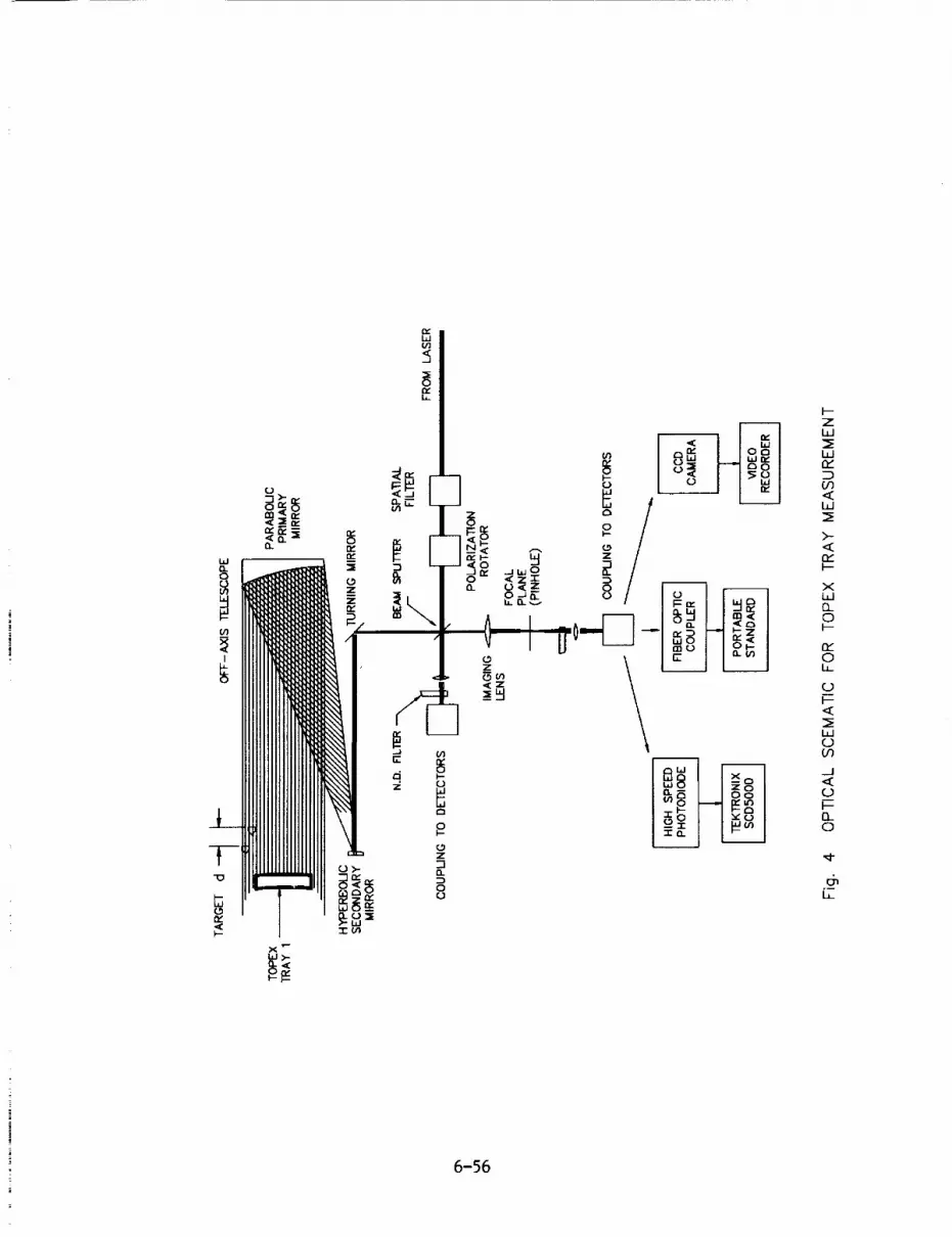
I
o
,,5o
z
____1
I---Zl.,ul
Wn,"
GO,<
>.-,<n,,"l--
Xl.ul0..OI---
0i,
(J
I--<
I.M(DOr)
_J,<(D
I--O_O
6,i,
6-56

o Q 0
"_ II
o cE oo _o I _ /
'-' t_n
P,
__ ot'M
0 ___ 11
c0
J
0
Ite.-o
>i1)
w
<
XW
Q_
0F-
W
t.l_
0
IZI
Z0
<l--
Z
W
n,"
0
n_0
L
OqF-
ZW
m
C/3
m
>tY
0
<0_0co<
U'3
6,L
6-57

11111 III111111
6-58

N94-15579
HISTORICAL MOBLAS
SYSTEM CHARACTERIZA ON
Van S. Husson
Abstract - This paper is written as a direct response to the published NASA LAser GEOdynamic Satellite (LAGEOS)
orbital solution SL7.1 [Smith et al., 1991], in order to close the data information loop with an emphasis on the NASA
MOBile LAser Ranging System's (MOBLAS 4,5,6,7,8) LAGEOS fullrate data since November 1, 1983. A
preliminary analysis of the supporting information (i.e. satellite laser ranging system eccentricities and system
dependent range and time bias corrections) contained in SL7.1 indicated CentiMeter (cm) level discrepancies. In
addition, a preliminary analysis of the computed monthly MOBLAS range biases from SL7.1 appear to show cm
level systematic trends, some of which appear to be "real", particularly in the 1984 to 1987 time period. This paper
is intended to be a reference document for known MOBLAS systematic errors (magnitude and direction) and for
supporting MOBLAS information (eccentricities, hardware configurations, and potential data problem periods).
Therefore, this report is different than your typical system characterization report [Pearlman, 1984], but will be
more valuable to the user. The MOBLAS error models and supporting information contained in this paper will be
easily accessible from the Crustal Dynamics Data Information System (CDDIS).
1. INTRODUCTION
In the late 1970's, NASA developed five, second generation mobile laser ranging systems in support of
the SEa Altimeter SATellite (SEASAT) mission. The goal of the SEASAT mission was to map the surface
of the oceans using the onboard satellite altimeter. Satellite Laser Ranging (SLR) data was used to
calibrate the SEASAT altimeter. During the 1980's, the MOBLAS systems underwent an extensive
upgrade program that improved the data accuracy and precision an order of magnitude, from the
100 MilliMeter (mm) to the 10 mm level. Since the mid-1980's, LAGEOS data has been compressed into 2
minute bins (normal points), which statistically reduces the single shot precision level [Smith et al., 1985].
MOBLAS LAGEOS normal point precision levels have been at the 1-2 mm level since the late-1980's.
During the 1980's, cm level systematic biases were discovered through special and collocation analysis
techniques developed by Bendix in support of the Goddard Laser Tracking Network (GLTN) and the
Crustal Dynamics Satellite Laser Ranging (CDSLR) mission contracts. When centim_er level systematic
errors were discovered in NASA SLR data, the NASA management philosophy was to identify the source
of the bias; to eliminate or model the bias; and to document the nature of the bias. Due to cost
considerations, historical NASA SLR data were not repaired (in most cases) to remove known on level
systematics. In addition, the documentation of these bias problems was not maintained in a central
database and had a limited distribution. The intent of this paper is to provide one reference source for
known uncorrected MOBLAS (LAGEOS) systematic errors that will be available from the CDDIS.
6-59
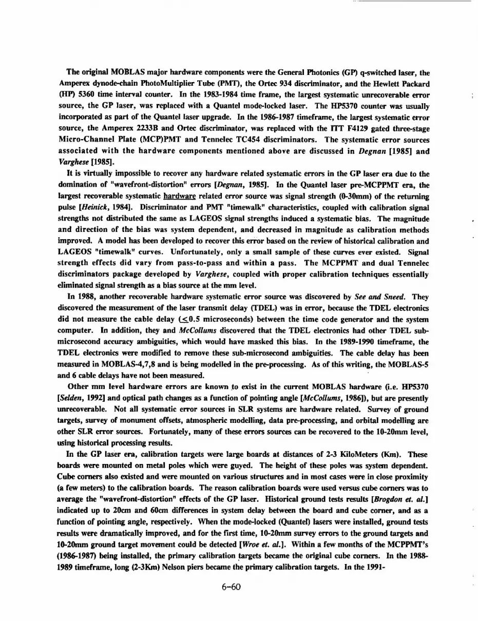
The original MOBLAS major hardware components were the General Photonics (GP) q-switched laser, the
Amperex dynode-chain PhotoMultiplier Tube (PMT), the Ortec 934 discriminator, and the Hewlett Packard
(HI') 5360 time interval counter. In the 1983-1984 time frame, the largest systematic unrecoverable error
source, the GP laser, was replaced with a Qnantel mode-locked laser. The HP5370 counter was usually
incorporated as part of the Quantei laser upgrade. In the 1986-1987 timeframe, the largest systematic error
source, the Amperex 2233B and Ortec discriminator, was replaced with the ITT F4129 gated three-stage
Micro-Channel Plate (MCP)PMT and Tennelec TC454 discriminators. The systematic error sources
associated with the hardware components mentioned above are discussed in Degnan [1985] and
Varghese [1985].
It is virtually impossible to recover any hardware related systematic errors in the GP laser era due to the
domination of "wavefront-distortion" errors [Degnan, 1985]. In the Quantel laser pre-MCPPMT era, the
largest recoverable systematic hardw;_rf related error source was signal strength (0-30mm) of the returning
pulse [Heinick, 1984]. Discriminator and PMT "timewalk" characteristics, coupled with calibration signal
strengths not distributed the same as LAGEOS signal strengths induced a systematic bias. The magnitude
and direction of the bias was system dependent, and decreased in magnitude as calibration methods
improved. A model has been developed to recover this error based on the review of historical calibration and
LAGEOS "timewalk" curves. Unfortunately, only a small sample of these curves ever existed. Signal
strength effects did vary from pass-to-pass and within a pass. The MCPPMT and dual Tennelec
discriminators package developed by Varghese, coupled with proper calibration techniques essentially
eliminated signal strength as a bias source at the mm level.
In 1988, another recoverable hardware systematic error source was discovered by See and Sneed. They
discovered the measurement of the laser transmit delay (TDEL) was in error, because the TDEL electronics
did not measure the cable delay (__0.5 microseconds) between the time code generator and the system
computer. In addition, they and McCollums discovered that the TDEL electronics had other TDEL sub-
microsecond accuracy ambiguities, which would have masked this bias. In the 1989-1990 timeframe, the
TDEL electronics were modified to remove these sub-microsecond ambiguities. The cable delay has been
measured in MOBLAS-4,7,8 and is being modelled in the pre-processing. As of this writing, the MOBLAS-5
and 6 cable delays have not been measured.
Other mm level hardware errors are known to exist in the current MOBLAS hardware (i.e. HP5370
[Selden, 1992] and optical path changes as a function of pointing angle [McCollurns, 1986]), but are presently
unrecoverable. Not all systematic error sources in SLR systems are hardware related. Survey of ground
targets, survey of monument offsets, atmospheric modelling, data pre-processing, and orbital modelling are
other SLR error sources. Fortunately, many of these errors sources can be recovered to the 10-20mm level,
using historical processing results.
In the GP laser era, calibration targets were large boards at distances of 2-3 KiloMeters (Km). These
boards were mounted on metal poles which were guyed. The height of these poles was system dependent.
Cube corners also existed and were mounted on various structures and in most cases were in close proximity
(a few meters) to the calibration boards. The reason calibration boards were used versus cube corners was to
average the "wavefront-distortion" effects of the GP laser. Historical ground tests results [Brogdon et. al.]
indicated up to 20era and 60era differences in system delay between the board and cube corner, and as a
function of pointing angle, respectively. When the mode-locked (Quantel) lasers were installed, ground tests
results were dramatically improved, and for the first time, 10-20mm survey errors to the ground targets and
10-20mm ground target movement could be detected [Wroe et. a/.]. Within a few months of the MCPPMT's
(1986-1987) being installed, the primary calibration targets became the original cube corners. In the 1988-
1989 timeframe, long (2-3Km) Nelson piers became the primary calibration targets. In the 1991-
6-60

1992 timeframe, the primary targets became short (100-200 meters) Nelson piers with the advent of the
translator and the short target ranging dectronics [Eichinger et. aL, 1990].
In the early to mid 1980's, cm level movement of the original targets, coupled with survey uncertainties and
infrequent surveys, severely limited the absolute accuracy of MOBLAS data. "Average" target movement
and survey uncertainties, in most cases, is recoverable to the 10-20ram level using historical ground test
results. In the mid-1980's, surveying equipment and frequency of surveying was improved, but the problem
still existed with unstable targets. In the late-1980's, the target stability problem was minimized to the
millimeter level, when the current day target calibration structure, the Nelson pier, were used as the primary
calibration target.
The MOBLAS eccentricity measurement techniques were improved in the mid-1980's [Nelson, 1986]. The
infrequency of eccentricity surveys was a mm level systematic error source, because long term temporal
changes in the eccentricity data were at this level. Some of these errors are traceable based on MOBLAS log
records or special analysis techniques.
Neutral Density (ND) filters have always been used during calibration to attenuate the signal. During
satellite ranging the filters were removed, thus inducing a difference in the "effective" calibration and satellite
optical paths [Crawford, 1985]. This difference was not modelled, but is recoverable to the lmm level. In
1991-1992 the Optical Attenuation Mechanisms (OAM) [Silva et. al., 1991] were installed in the MOBLAS,
which minimizes the use of ND filters. The ND filter bias is currently being modelled in the pre-processing.
Prior to January 1, 1988, the tropospheric range correction applied to the fullrate data was computed
based on the MOBLAS elevation encoder measurements. These measurements could be in error by a few
millidegrecs and would thus induce a systematic error in the tropospheric refraction correction [Husson et.
a/., 1987]. This correction could be in error up to 20ram. The error was system and satellite dependent, but
is fully recoverable to the sub-mm level. To remove this error in pre-1988 MOBLAS data, the applied
tropospheric refraction must be removed and reapplied using the computed elevation angle. All MOBLAS
data taken after January 1, 1988, were pre-processed using the computed elevation angle from a short arc fit
to the ranges.
LAGEOS orbital modelling errors have improved significantly over the last 12 years along with the quality
of SLR data [Smith et. al., 1991]. Orbital modelling is limited by the quality and distribution of the global
SLR dataset, but in some instances, is the only hope for recovering the "net" historical SLR biases.
In the remainder of this article, each MOBLAS system is addressed individually. Each system's
eccentricities and recoverable bias sources are discussed and summarized in tables, which are contained at the
end of this article. The bias model tables include the major system configuration changes 0aser, PMT,
discriminators, counter) and important pre-processing information (i.e. calibration target and calibration
range). The tables and this article will be available from the CDDIS.
2. MOBLAS-4
2.1 MOBLAS-4 EccentricitiesSince August 15, 1983, MOBLAS-4 has only occupied one monument/marker (7110). Prior to August
1983, 7110 was occupied by MOBLAS-3. There exists 5 sets of MOBLAS-4 eccentricities and 10 MOBLAS-4
Site Occupation Designators (SOD's) at 7110. SOD's 71100402, 71100403, and 71100410, each have two sets
of eccentricities.
6-61

The 3mm change in the Up ecc., between the 1985 and 1988, surveys could be caused by settlement of the
pad and monument [Nelson, 1988]. There were no measurements of the eccentricities between 1985 and
1988. The MOBLAS-4 mount was releveled twice in 1988 (June 16 and December 13), but apparently there
was no change in eccentricities, based on the April 1988 and November 1989 surveys. In February 1992, the
eccentricities were remeasured prior to the removal of the mount. There was a 2mm unexplained change in
the North ecc. In March 1992, the MOBLAS-4 mount was removed from system to be refurbished, and in
April 1992, the refurbished mount was re-installed and the ecc. were remeasured. Table I contains the
recommended set of MOBLAS-4 eccentricities with their corresponding SOD(s) and effective starting dates.
2.2 MOBLAS-4 LAGEOS Biases
The net MOBLAS-4 recoverable biases (range and time) are presented in Table 2. To correct MOBLAS-4
LAGEOS data, the known range and time biases (in Table 2) should be subtracted from the LAGEOS range
and timetags, respectively. Any time there is the Potential for a change in the bias(es), even though the
bias(es) did not change, a new entry has been added. A component breakdown of the biases is presented,
followed by a section describing known problem data, and followed by a section describing potential problem
data.
2.2.1 MOBLAS-4 ND filters
MOBLAS-4 LAGEOS data was biased short by 3mm + 1 and lmm + 0mm from August 15, 1983 through
January 17, 1992, and from January 18 through May 31, 1992, respectively, due to ND filters. On January
18, 1992, the OAM was installed in MOBLAS-4 reducing the ND filter bias. After June 1, 1992, this bias has
been removed through modelling.
2.2.2 MOBLAS-4 signal strength
MOBLAS-4 LAGEOS data was biased long by 20mm + 10, 10mm + 5, 6mm + 3, and 4mm + 2 from
August 15, 1983 through June 30, 1984; July 1, 1984 through August 31, 1984; September 1, 1984 through
July 31, 1985; and August 1, 1985 through November 19, 1986; respectively, due to signal strength. This
bias would vary from pass-to-pass and would have a slight elevation dependence. Low elevation data would
be biased longer by several mm than high elevation data. Signal strength effects were reduced as the
MOBLAS-4 calibration techniques improved, and were eliminated when the MCPPMT package was installed
on November 20, 1986.
2.2.3 MOBLAS-4 elevation angles
Prior to January 1, 1988, the tropospheric range correction applied to the fullrate data was computed
based on the MOBLAS-4 encoder measurements. To remove this error in pre-1988 MOBLAS-4 data, the
applied tropospheric refraction must be removed and reapplied using the computed elevation angle.
2.2.4 MOBLAS-4 calibration targets/distances
MOBLAS-4 has used 4 different calibration targets (1 board and 3 cube corners) at marker 7110. From
August 15, 1983 through December 31, 1987; from January 1, 1987 through January 28, 1988; from January
29 through April 29, 1988; from April 29, 1988 through December 5, 1991; and from December 6, 1991 to
the present; the MOBLAS-4 primary calibration targets were the 2Km board, the 2Km cube corner, the 2Km
board, the 2Kin Nelson pier, and the 200m Nelson pier, respectively.
6-62

MOBLAS-4 has been surveyed 5 times (1983, 1985, 1988, and twice in 1992) at marker 7110. Sometime
between the 1983 and the 1985 surveys, vandals removed the bracing support of the MOBLAS-4 calibration
board tower [Nelson, 1985], which could explain the 13mm difference between the 1983 and 1985 calibration
board distances. When the new calibration board values were used in data processing, there would be an
automatically induced 13mm discontinuity in the MOBLAS-4 range bias. The new board values were used
with all data taken after June 20, 1985. Data just prior to June 20, 1985 would have been biased longer by
13mm than data after June 20, 1985 (This 13mm change does not appear in the range bias model, because
the exact date of the change is unknown). The cube corner became the operational target in January 1987
(The exact day is unknown at this time).
The distance (2Km) and the design/stability of the original MOBLAS-4 targets (a calibration board
mounted on a tower and a cube corner mounted on wooden posts) were limiting factors to surveying accuracy
and MOBLAS-4 data accuracy. The survey accuracy of these original targets was at the 10-15ram level
[Nelson]. Historical ground test results indicate up to 20mm differences in "apparent" system delays between
the MOBLAS-4 calibration board and the cube corner, which indicates both targets could move at least
10mm in either direction from month-to-month and from day-to-day. LAGEOS orbital analysis appears to
be the only viable means for recovering the "true" average MOBLAS-4 monthly target distance to better than
20mm in the October 1983 to April 1988 timeframe.
Between November 1, 1987 and January 28, 1988, the MOBLAS-4 operational calibration target, cube
corner, was very unstable, which caused unusual changes (up to 90mm) in the "apparent" system delay.
Individual MOBLAS-4 LAGEOS passes could be biased long (up to 90mm) during this period. Eanes [1987]
originally discovered this data problem. The bias could change (up to 30mm) from pass-to-pass and from
day-to-day. The problem was eliminated when the previous calibration target (board) was used starting
January 29, 1988. On April 30, 1988, the MOBLAS-4 calibration target became the 2Km Nelson pier.
2.2.5 MOBLAS-4 TDEL
All MOBLAS-4 data between January 5, 1990 and May 31, 1992 contains a time bias of -0.4 microseconds.
To correct this time bias, add +0.4 microseconds to each observation's timetag. This correction is only valid
after January 5, 1990, because on this date, the MOBLAS-4 TDEL electronics were modified to eliminate
other TDEL sub-microsecond accuracy ambiguities, which would have masked this bias. This bias has been
eliminated through modelling, effective June 1, 1992.
2.2.6 MOBLAS-4 known problem data
Between April 12, 1984 and May 24, 1984, individual MOBLAS-4 passes contained discontinuities (100mm
up to 600mm) due to the range gate window being changed during the pass. The magnitude of the
discontinuities depends upon where the return occurred in the range gate window [Varghese, 1985]; therefore,
data during this period should not be used. This problem was originally detected by Eanes [1985] and was
resolved when the system adhered to standard tracking procedures.
2.2.7 MOBLAS-4 potential problem data
Between December 29, 1988 and January 27, 1989, MOBLAS-4 LAGEOS data is questionable due to a bad
time interval unit (HP5370). The RMS scatter of this data was cyclic and dependent upon the LAGEOS
range [Heinick et. al., 1989]. The data is believed to be unbiased and just systematically noisy. This problem
was resolved by replacing the HP5370.
6-63

3. MOBLAS-5
3.1 Eccentricities
Since July 1, 1979_ MOBLAS-5 has only occupied one monument/marker (7090). There exists only 3
unique sets of MOBLAS-5 eccentricities and 12 MOBLAS-5 SOD's at 7090. SOD 70900508 has 2 sets of
eccentricities.
The MOBLAS-5 mount was releveled on September 5, 1985. No survey was performed after the releveling
til 1987. The 8mm change in the Up ecc., between the 1979 and 1987 surveys, remains unexplained. It is not
known how far back the 1987 Up ecc. can be backdated. The MOBLAS-5 mount was also releveled on
August 5, 1989, but the eccentricities were not remeasured. In January 1992, the mount was re-installed and
the eccentricities were remeasured. Table 3 contains the recommended set of MOBLAS-5 eccentricities with
their corresponding SOD(s) and effective starting dates.
3.2 MOBLAS 5 LAGEOS BiasesThe net MOBLAS-5 recoverable biases (range and time) are presented in Table 4. To correct MOBLAS-5
LAGEOS data, the known range and time biases (in Table 4) should be subtracted from the LAGEOS range
and timetags, respectively. Any time there is the potential for a change in the bias(es), even though the
bias(es) did not change, a new entry has been added. A component breakdown of the biases is presented,
followed by a section describing known problem data, and followed by a section describing potential problem
data.
3.2.1 MOBLAS-5 ND filters
Prior to June 1, 1992, MOBLAS-5 LAGEOS data was biased short by 3mm + 1 due to ND filters. After
June 1, 1992, this bias has been removed through modelling.
3.2.2 MOBLAS-5 signal strength
MOBLAS-5 LAGEOS data was biased short by 3mm + 2 from July 27, 1983 through April 22, 1987, due
to signal strength. This bias would be fairly constant from pass-to-pass. This bias was eliminated when the
MCPPMT package was installed in MOBLAS-5 on April 23, 1987.
3.2.3 MOBLAS-5 elevation angles
Prior to January 1, 1988, the tropospheric range correction applied to the fullrate data was computed
based on the MOBLAS-5 encoder measurements. To remove this error in pre-1988 MOBLAS-5 data, the
applied tropospheric refraction must be removed and reapplied using the computed elevation angle.
3.2.4 MOBLAS-5 calibration targets/distances
MOBLAS-5 has used 4 different calibration targets (2 boards and 2 cube corners) at marker 7090. From
August 1, 1979 through June 7, 1980; from June 8, 1980 through May 31, 1987; from June 1 through July
31, 1987; from August 1 through August 25, 1987; and from August 26, 1987 through June 30, 1992; the
MOBLAS-5 primary calibration targets were the 2Kin calibration board, the 3Kin calibration board, the
IKm cube corner, the 3Kin calibration board, and the 3Kin Nelson pier, respectively.
6-64

MOBLAS-5 has been surveyed only 3 times in 13 years (1979/80, 1987, & 1992) at marker 7090. Between
the 1979/80 and 1987 surveys, the lion cube corner and the 3Kin board ranges changed by +30ram and
-9ram, respectively. The 2Km board was never resurveyed and the 3Kin board blew away in August 1987.
In early January 1992, the mount was replaced and a new survey was performed.
The system delay differences obtained from the 1Kin cube corner and the 3Km board in historical minico
tests since June 1985 were 39ram 4- 5 and 0ram 4- 5 [Husson and Wroe, 1987] using the 1980 and 1987
surveys, respectively. Therefore, the 1987 survey values can be backdated to at least June 1985, which means
MOBLAS-5 data between June 1985 through May 31, 1987 (all board calibrated data) was biased long by
9ram +_.5ram. All data since June 1, 1987, until the mount replacement in 1992, was processed with the 1987
surveyed ranges and should be bias free. Research into minico results prior to June 1985 still needs to be
performed.
3.2.5 MOBLAS-5 TDEL
The MOBLAS-5 cable delay causing this bias has not been measured as of this writing. On January 30,
1990, the MOBLAS-5 TDEL electronics were modified to eliminate other TDEL sub-microsecond
ambiguities.
3.2.6 MOBLAS-5 PMT Gating
Prior to June 8, 1980, MOBLAS-5 LAGEOS data was biased short by 20mm+5 due to calibration data
falling in a non-linear region of the Amperex 2233B PMT gate. This bias was characterized by Varghese
[1985]. This bias was eliminated, effective June 8, 1980, when a longer calibration board (> 3Kin) was used.
3.2.7 MOBLAS-5 known problem data
Between December 19, 1991 and January 3, 1992, MOBLAS-5 data quality was degraded due to a stuck
bit. The bit was stuck low (100 picosec.) for LAGEOS. It does not appear that this data is recoverable,
because of it's unknown effect on calibration data.
3.2.8 MOBLAS-5 potential problem data
Between August 12, 1988 and January 31, 1989, MOBLAS-5 system ddays and pre-to-post calibration
shifts were erratic [Heinick et al., 1989]. Therefore, the uncertainty in the system delay is increased during
this period; however, this should be a random error than should average over several passes. This problem
disappeared during February 1989.
4. MOBLAS-6
4.1 MOBLAS-6 Eccentricities
Since March 3, 1983, MOBLAS-6 has only occupied one monmnent\marker (7122). There exists 4 sets of
MOBLAS-6 eccentricities and 9 MOBLAS-6 SOD's at 7122. SOD 71220604 has two sets of eccentricities.
The May 1988 survey sheet had the wron2 si2n for the East ecc. It should be negative, not positive. Based
on the 1991 survey, there was no apparent change in the eccentricities when the MOBLAS-6 mount was
releveled on August 5, 1989. Table 5 contains the recommended set of MOBLAS-6 eccentricities with their
corresponding SOD(s) and effective starting dates.
6-65

4.2 MOBLAS-6 LAGEOS Biases
The net MOBLAS-6 recoverable biases (range and time) are presented in Table 6. To correct MOBLAS-6
LAGEOS data, the known range and time biases (in Table 6) should be subtracted from the LAGEOS range
and timetags, respectively. Any time there is the potential for a change in the bias(es), even though the
bias(es) did not change, a new entry has been added. A component breakdown of the biases is presented,
followed by a section describing known problem data, and followed by a section describing potential problem
data.
4.2.1 MOBLAS-6 ND filters
All MOBLAS-6 LAGEOS data was biased short by 3mm + 1 due to ND filters.
4.2.2 MOBLAS-6 signal strength
MOBLAS-6 LAGEOS data was biased long by 12mm + 4, 10mm + 3, and 4ram + 2 from May 1, 1984
through March 31, 1986; from April 1 through August 31, 1986; and September 1, 1986 through January 27,
1987; respectively, due to signal strength. This bias would vary slightly (several ram) from pass-to-pass and
would have a slight elevation dependence. Low elevation data would be biased longer than high elevation
data. Signal strength effects were reduced as system calibration techniques improved, and were eliminated
when the MCPPMT package was installed in MOBLAS-6 on January 28, 1987.
4.2.3 MOBLAS-6 elevation angles
Prior to January 1, 1988, the tropospheric range correction applied to the fullrate data was computed
based on the MOBLAS-6 encoder measurements. To remove this error in pre-1988 MOBLAS-6 data, the
applied tropospheric refraction must be removed and reapplied using the computed elevation angle.
4.2.4 MOBLAS-6 calibration targets/distances
MOBLAS-6 has used 4 different calibration targets (1 board and 3 cube corners) at marker 7122. From
May 1, 1983 through March 26, 1987; from March 27, 1987 through August 16, 1988; from August 17, 1988
through October 3, 1989; and from October 4, 1989 through April 30, 1991; the MOBLAS-6 primary
calibration targets were the 2Kin calibration board, the 2Km cube corner, the first 2Kin Nelson pier, and the
second 2Km Nelson pier, respectively.
MOBLAS-6 was surveyed 4 times in 8 years (1983, 1988, 1989, & 1991) at marker 7122. In October 1983,
several months after the first survey, a hurricane passed through the site. Between the 1983 and 1988
surveys, the ranges to the 2Km cube corner and the 2Km board changed by + 6ram and -17mm, respectively.
The system delay differences obtained from the these two targets in historical minico tests, since the Quantel
laser installation (July 1984), were 33mm + 15 and 10mm + 15 [Husson and Wetzel, 1987] using the 1983
and 1988 surveyS, respectively. The 1988 surveyed target ranges for the cube corner and the board are only
accurate to the 10mm level. The 10mm difference which remains in the historical minico results can be
attributed to survey. Making this assumption and distributing the 10mm difference equally to both targets,
the 1988 survey (with adjustment) can be backdated to the hurricane (October 1983). This means
MOBLAS-6 data from October 1, 1983 through March 26, 1987; from March 27, 1987 through May 2, 1988;
and from May 3 through August 16, 1988; is biased long by 22mm + 10, short by llmm + 10, and short by
5mm + 10, respectively.
6-66

In 1988, the first Nelson pier was built; however, the pier foundation was not built to specifications. The
pier moved 14mm between 1988 and 1989 due to a poor foundation and being on a steep slope [Nelson,
1989]. Nelson believes this movement would have been linear over the 13 months between the 1988 and 1989
surveys. MOBLAS-6 data between August 17, 1989 and June 23, 1989, was biased long by 4mm +
lmm/month. On October 4, 1989, the primary MOBLAS-6 calibration target became the second Nelson
pier, which eliminated target movement as a MOBLAS-6 systematic bias source.
4.2.5 MOBLAS-6 TDEL
The MOBLAS-6 cable delay causing this bias has not been measured as of this writing. On January 11,
1990, the MOBLAS-6 TDEL electronics were modified to eliminate other TDEL sub-microsecond
ambiguities.
4.2.6 MOBLAS-6 known problem data
All MOBLAS-6 satellite RMS's between February 1 and March 1, 1984, were high caused by a bad
distribution amplifier [Oldham]. Data during this period should not be used. On March 2, 1984, the
distribution amplifier was replaced which eliminated the problem.
4.2.7 MOBLAS-6 potential problem data
All MOBLAS-6 data between February 8 and May 12, 1989, was affected by a bad Setra barometer. Setra
barometric data was in error by up to 30 millibars. All MOBLAS-6 data during this interval was corrected
and believed to be accurate to at least 3 millibars.
All MOBLAS-6 calibration data between April 1 and September 26, 1990, was unusually noisy (twice the
normal RMS). The LAGEOS data during this period is suspected to be bias free. The calibration data
returned to normal when some adjustments were performed on the HP5370 in late September [MOBLAS-6,
19901.
5. MOBLAS-7
5.1 MOBLAS-7 Eccentricities
Since January 1, 1981, MOBLAS-7 has only occupied one monument/marker (7105); however, two other
laser systems (TLRS-2, 71051206, and MOBLAS-2, 71050207) have been referenced to marker 7105. There
exists 14 sets of MOBLAS-7 eccentricities and 21 MOBLAS-7 SOD's at 7105.
The reason for the 5mm change in the east ecc. between the 1981 and 1984 survey is assumed to be caused
by movement of the survey monument to the East or by movement of the MOBLAS support pad to the West
[Nelson, 1984].
During the 1985 pre-collocation survey of MTLRS-1 and MOBLAS-7, a 2 em discrepancy was found in the
7105 Up eccentricity [Nelson, 1985]. The original determination of the Up eccentricity is suspected to be in
error [Nelson, private communication]; and therefore, the 1985 Up eccentricity can be backdated to
Jan 1, 1981.
Prior to the TLRS-I and MOBLAS-7 collocation in 1986 [Nelson, 1986], MOBLAS-7 eccentricities were
measured on three different occasions, once in December 1985 and twice in January 1986 (before and after
the MOBLAS-7 mount was releveled on January 18, 1986). There were millimeter level changes between
these surveys. This would give SOD 71050709 five unique sets of eccentricities.
6-67
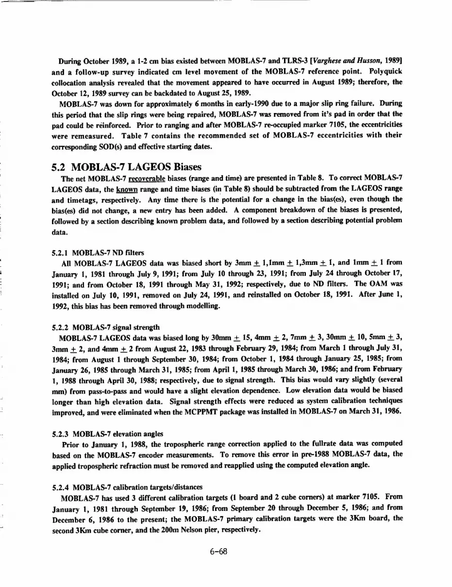
During October 1989, a 1-2 cm bias existed between MOBLAS-7 and TLRS-3 [Varghese and Husson, 1989]
and a follow-up survey indicated cm level movement of the MOBLAS-7 reference point. Polyquick
collocation analysis revealed that the movement appeared to have occurred in August 1989; therefore, the
October 12, 1989 survey can be backdated to August 25, 1989.
MOBLAS-7 was down for approximately 6 months in early-1990 due to a major slip ring failure. During
this period that the slip rings were being repaired, MOBLAS-7 was removed from it's pad in order that the
pad could be reinforced. Prior to ranging and after MOBLAS-7 re-occupied marker 7105, the eccentricities
were remeasured. Table 7 contains the recommended set of MOBLAS-7 eccentricities with their
corresponding SOD(s) and effective starting dates.
5.2 MOBLAS-7 LAGEOS BiasesThe net MOBLAS-7 recoverable biases (range and time) are presented in Table 8. To correct MOBLAS-7
LAGEOS data, the known range and time biases (in Table 8) should be subtracted from the LAGEOS range
and timetags, respectively. Any time there is the potential for a change in the bias(es), even though the
bias(es) did not change, a new entry has been added. A component breakdown of the biases is presented,
followed by a section describing known problem data, and followed by a section describing potential problem
data.
5.2.1 MOBLAS-7 ND filters
All MOBLAS-7 LAGEOS data was biased short by 3mm +__1,1mm + 1,3mm + 1, and lmm + 1 from
January 1, 1981 through July 9, 1991; from July 10 through 23, 1991; from July 24 through October 17,
1991; and from October 18, 1991 through May 31, 1992; respectively, due to ND filters. The OAM was
installed on July 10, 1991, removed on July 24, 1991, and reinstalled on October 18, 1991. After June 1,
1992, this bias has been removed through modelling.
5.2.2 MOBLAS-7 signal strength
MOBLAS-7 LAGEOS data was biased long by 30mm + 15, 4mm + 2, 7mm + 3, 30ram + 10, 5mm + 3,
3mm + 2, and 4mm + 2 from August 22, 1983 through February 29, 1984; from March 1 through July 31,
1984; from August 1 through September 30, 1984; from October 1, 1984 through January 25, 1985; from
January 26, 1985 through March 31, 1985; from April 1, 1985 through March 30, 1986; and from February
1, 1988 through April 30, 1988; respectively, due to signal strength. This bias would vary slightly (several
ram) from pass-to-pass and would have a slight elevation dependence. Low elevation data would be biased
longer than high elevation data. Signal strength effects were reduced as system calibration techniques
improved, and were eliminated when the MCPPMT package was installed in MOBLAS-7 on March 31, 1986.
5.2.3 MOBLAS-7 elevation angles
Prior to January 1, 1988, the tropospheric range correction applied to the fullrate data was computed
based on the MOBLAS-7 encoder measurements. To remove this error in pre-1988 MOBLAS-7 data, the
applied tropospheric refraction must be removed and reapplied using the computed elevation angle.
5.2.4 MOBLAS-7 calibration targets/distances
MOBLAS-7 has used 3 different calibration targets (1 board and 2 cube corners) at marker 7105. From
January 1, 1981 through September 19, 1986; from September 20 through December 5, 1986; and from
December 6, 1986 to the present; the MOBLAS-7 primary calibration targets were the 3Km board, the
second 3Km cube corner, and the 200m Nelson pier, respectively.

MOBLAS-7hasbeensurveyedatleastonce per year since January 1984. The February 1981 and the June
1981 surveyed board ranges were incorrect, causing all MOBLAS-7 data from March 1 through
June 30, 1981 and from July 1 through December 31, 1981 to be biased long by 49mm + 20 and
22mm +_. 20, respectively.
Between the 1984 and 1985 surveys, the board range changed by 17mm, however; historical minico results
support the 1984 survey value [Heinick, 1985] for the board range (not the 1985 value). On
February 7, 1986, the guy wires were tensioned on the calibration board before the board was resurveyed
(12mm change); however, the new surveyed calibration board range was not used until March 2, 1986.
Therefore, all MOBLAS-7 LAGEOS passes from August 1, 1985 through February 6, 1986, and from
February 7 through March 1, 1986, is biased long by 17mm +__20 and short by 12mm + 20, respectively,
for the LAGEOS passes in Table 9. Occasionally due to ground fog conditions, the board could not be
ranged, so the secondary calibration target, the 3km cube corner, was used. All passes in Table 9 were
calibrated using the original 3Km cube corner and are believed to have the correct calibration distance.
Between the January and October 1989 surveys, the Nelson pier target range changed by 15mm due to
movement of the MOBLAS-7 reference point. Apparently, the MOBLAS-7 reference point moved around
August 25, 1989 based upon intercomparison with TLRS-3 [Varghese and Husson, 1989]. All MOBLAS-7
data from August 25 through October 11, 1989 is biased short by 15mm.
5.2.5 MOBLAS-7 TDEL
All MOBLAS-7 data from July 13, 1989 through September 27, 1990, and from September 28, 1990
through May 31, 1992 contains a time bias -0.5 and -0.3 microseconds, respectively. This correction is only
valid after July 13, 1989, because on this date, the MOBLAS-7 TDEL electronics were modified to eliminate
other TDEL sub-microsecond accuracy ambiguities, which would have masked this bias. On September 28,
1990, the cable length causing this bias was shortened, which caused a decrease in the magnitude of the bias.
This bias has been eliminated through modelling, effective June 1, 1992.
5.2.6 MOBLAS-7 known problem data
All MOBLAS-7 data between January 13 through January 17, 1986, has a reference frequency problem
and should not be used. The HP5370 frequency was on internal frequency during this period of time.
5.2.7 MOBLAS-7 potential problem data
All MOBLAS-7 LAGEOS data between June 7 and June 13, 1984 was noisy (100-130mm) and should be
used with caution. The cause of the high noise is unknown.
All MOBLAS-7 LAGEOS data between September 25 and October 5, 1984 was noisy (80-120mm) and
should be used with caution. The cause of the high noise is unknown.
6. MOBLAS-8
6.1 MOBLAS-8 Eccentricities
Since October 1, 1981, MOBLAS-8 has only occupied one monument/marker (7109). In July 1982, the
MOBLAS-4 and MOBLAS-8 morns vans were switched. There exists 9 sets of MOBLAS-8 eccentricities, and
15 MOBLAS-8 SOD's at 7109.
6-69

On August 4, 1982 the system was releveled, but there was not a follow-up survey until 1984, which
indicated a 17ram change in the Up ecc. Nelson [1984] recommends that the 1984 survey be backdated to
1982. There was a 4ram change in the Up ecc between 1985 and 1988, possibly due to settlement of the laser
support slab [Nelson ,1985]. Table 10 contains the recommended set of MOBLAS-8 eccentricities with their
corresponding SOD(s) and effective starting dates.
6.2 MOBLAS-8 LAGEOS Biases
The net MOBLAS-8 recoverable biases (range and time) are presented in Table 11. To correct
MOBLAS-8 LAGEOS data, the known range and time biases (in Table 11) should be subtracted from the
LAGEOS range and timetags, respectively. Any time there is the potential for a change in the bias(es), even
though the bias(es) did not change, a new entry has been added. A component breakdown of the biases is
presented and followed by a section describing known problem data.
6.2.1 MOBLAS-8 ND filters
All MOBLAS-8 LAGEOS data was biased short by 3mm + 1 and lmm + 1 from September 1, 1981
through April 7, 1992, and from April 8, 1992 through May 31, 1992, respectively, due to ND filters. On
April 7, 1992, the OAM was installed in MOBLAS-8 reducing the N-D filter bias. After June 1, 1992, this
bias has been removed through modelling.
6.2.2 MOBLAS-8 signal strength
MOBLAS-8 LAGEOS data was biased long by 5mm + 3, 10ram + 5, 6mm + 3, and 3ram + 2 from
August 4, 1982 through December 31, 1983; from January 1 through March 31, 1984; April 1 through July
31, 1984; and from August 1, 1984 through September 25, 1986; respectively, due to signal strength. This
bias would vary slightly (several mm) from pass-to-pass and would have a slight elevation dependence. Low
elevation data would be biased longer than high elevation data. Signal strength effects were reduced as
system calibration techniques improved, and were eliminated when the MCPPMT package was installed in
MOBLAS-8 on September 26, 1986.
6.2.3 MOBLAS-8 elevation angles
Prior to January 1, 1988, the tropospheric range correction applied to the fullrate data was computed
based on the MOBLAS-8 encoder measurements. To remove this error in pre-1988 MOBLAS-8 data, the
applied tropospheric refraction must be removed and re.applied using the computed elevation angle.
6.2.4 MOBLAS-8 calibration targets/distances
MOBLAS-8 has used 5 different calibration targets (2 boards and 3 cube corners) at marker 7109. From
September 1, 1981 through August 19, 1985; from August 20, 1985 through December 31, 1986; from
January 1, 1987 through March 22, 1989; from March 23, 1989 through April 7, 1992; and from April 8,
1992 to the present; MOBLAS-8 primary calibration targets were the original 2Km board, the second 2Km
board, the second 2Km cube corner, the 2Km Nelson pier, and the 200m Nelson pier, respectively.
6-70
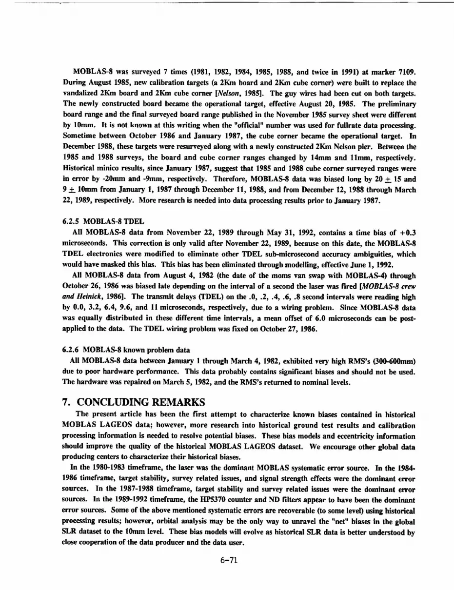
MOBLAS-8 was surveyed 7 times (1981, 1982, 1984, 1985, 1988, and twice in 1991) at marker 7109.
During August 1985, new calibration targets (a 2Km board and 2Kin cube corner) were built to replace the
vandalized 2Km board and 2Km cube corner [Nelson, 1985]. The guy wires had been cut on both targets.
The newly constructed board became the operational target, effective August 20, 1985. The preliminary
board range and the final surveyed board range published in the November 1985 survey sheet were different
by 10mm. It is not known at this writing when the "official" number was used for fullrate data processing.
Sometime between October 1986 and January 1987, the cube corner became the operational target. In
December 1988, these targets were resurveyed along with a newly constructed 2Km Nelson pier. Between the
1985 and 1988 surveys, the board and cube corner ranges changed by 14mm and llmm, respectively.
Historical minico results, since January 1987, suggest that 1985 and 1988 cube corner surveyed ranges were
in error by -20ram and -9mm, respectively. Therefore, MOBLAS-8 data was biased long by 20 + 15 and
9 + 10ram from January 1, 1987 through December 11, 1988, and from December 12, 1988 through March
22, 1989, respectively. More research is needed into data processing results prior to January 1987.
6.2.5 MOBLAS-8 TDEL
All MOBLAS-8 data from November 22, 1989 through May 31, 1992, contains a time bias of +0.3
microseconds. This correction is only valid after November 22, 1989, because on this date, the MOBLAS-8
TDEL electronics were modified to eliminate other TDEL sub-microsecond accuracy ambiguities, which
would have masked this bias. This bias has been eliminated through modelling, effective June 1, 1992.
All MOBLAS-8 data from August 4, 1982 (the date of the moms van swap with MOBLAS-4) through
October 26, 1986 was biased late depending on the interval of a second the laser was fired [MOBLAS-8 crew
and Heinick, 1986]. The transmit delays (FDEL) on the .0, .2, .4, .6, .8 second intervals were reading high
by 0.0, 3.2, 6.4, 9.6, and 11 microseconds, respectively, due to a wiring problem. Since MOBLAS-8 data
was equally distributed in these different time intervals, a mean offset of 6.0 microseconds can be post-
applied to the data. The TDEL wiring problem was fixed on October 27, 1986.
6.2.6 MOBLAS-8 known problem data
All MOBLAS-8 data between January 1 through March 4, 1982, exhibited very high RMS's (300-600mm)
due to poor hardware performance. This data probably contains significant biases and should not be used.
The hardware was repaired on March 5, 1982, and the RMS's returned to nominal levels.
7. CONCLUDING REMARKS
The present article has been the first attempt to characterize known biases contained in historical
MOBLAS LAGEOS data; however, more research into historical ground test results and calibration
processing information is needed to resolve potential biases. These bias models and eccentricity information
should improve the quality of the historical MOBLAS LAGEOS dataset. We encourage other global data
producing centers to characterize their historical biases.
In the 1980-1983 timeframe, the laser was the dominant MOBLAS systematic error source. In the 1984-
1986 timeframe, target stability, survey related issues, and signal strength effects were the dominant error
sources. In the 1987-1988 timeframe, target stability and survey related issues were the dominant error
sources. In the 1989-1992 timeframe, the HP5370 counter and ND filters appear to have been the dominant
error sources. Some of the above mentioned systematic errors are recoverable (to some level) using historical
processing results; however, orbital analysis may be the only way to unravel the "net" biases in the global
SLR dataset to the 10mm level. These bias models will evolve as historical SLR data is better understood by
close cooperation of the data producer and the data user.
6-71

8. ACKNOWLEDGEMENTSThe material in this article has been amassed through years of close interaction with a highly talented
group of colleagues at the Bendix Field Engineering Corporation in Greenbelt and Columbia, Md; at the
NASA Goddard Space Flight Center in Greenbelt, Md; and at the Center for Space Research in Austin,
Texas, and much of their work is referenced here.
6-72

REFERENCES
Brogdon O. L., Heinick J. M., MOBLAS Ground Test Results, Bendix Field Engineering Corporation
internal reports, 1980-1983.
Crawford W. F., LTN Data, Bendix Field Engineering Corporation internal report, Nov. 1985.
Degnan J. J., Satellite Laser Ranging: Current Status and Future Prospects, IEEE Trans. Geosci. Remote
Sensing, Vol GE-23 Number 4, pp 398-413, Jul. 1985.
Eichinger R. A., Oldham T. J., MOBLAS 4, 6, 7, 8 AntiparaIlax Optical Path Differences, Bendix Field
Engineering Corporation internal reports, 1990-1992.
Heinick J. M., Receive Energy Dependence and Correction at MOBLAS 4, 5, 7, and 8, Bendix Field
Engineering Corporation, presented at the spring 1984 AGU, Feb. 1984.
Heinick J. M, Husson V. S., Wroe S. A., Brogdon O. L., Wetzel S. L., Clarke C. B., Six Month Data
Processing Report, Bendix Field Engineering Corporation internal report, Nov. 1989.
Heinick J. M., MOBLAS-7's calibrations using the corner cube and the most recently published calibration
board range, Bendix Field Engineering Corporation internal report, Oct. 1985.
Husson V. S., Wroe S. A., MOBLAS-5 Processing Dilemma Update, Bendix Field Engineering
Corporation, presented at the weekly CDPSLR meeting, Oct. 1987.
Husson V. S., Wetzel S. L., MOBLAS-6 Processing Dilemma Update, Bendix Field Engineering
Corporation, presented at the weekly CDPSLR meeting, Oct. 1987.
Husson V. S., Wroe S. A., Wetzel S. L., TLRS-I/MOBLAS-7 Collocation Analysis Report, Bendix Field
Engineering Corporation internal report, 1987.
McCollums D. L., private communication, Bendix Field Engineering Corporation.
McCollums D. L., Varghese T. K., MOBLAS-7 System Characterization Reports, Bendix Field
Engineering Corporation, 1986-1988.
MOBLAS-8 Crew, Heinick J. M., MOBLAS-8 Transmit Delay Investigation, Bendix Field Engineering
Corporation internal report, Oct. 1986.
Murphy B., Nelson V. E., MOBLAS 5 Survey Reports, Australian Division of National Mapping, Bendix
Field Engineering Corporation, 1979/80, 1987, 1992.
Nelson V. E., MOBLAS 4 Survey Reports, Bendix Field Engineering Corporation, 1983, 1985, 1988, 1992.
Nelson V. E., MOBLAS 6 Survey Reports, Bendix Field Engineering Corporation, 1983, 1988, 1989, 1991.
Nelson V. E., MOBLAS 7 Survey Reports, Bendix Field Engineering Corporation, 1981, 1982, 1984, 1985,
1986, 1987, 1988, 1889, 1990, 1991, 1992.
Nelson V. E., MOBLAS 8 Survey Reports, Bendix Field Engineering Corporation, 1981, 1982, 1984, 1985,1988, 1989, 1991.
Nelson V. E., private communication, Bendix Field Engineering Corporation.
6-73

Nelson V. E., System Eccentricity Measurement Procedures for MOBLAS Systems, Bendix Field
Engineering Corporation internal report, 1986.
Oldham T. J., private communication, Bendix Field Engineering Corporation.
Pearlman M. R., Laser System Characterization, Smithsonian Institution Astrophysical Observatory,
Proc. 5th Int. Workshop on Laser Ranging Instrumentation, Sep. 1984.
Selden M. D., Varghese T. K., Heinick J. M., Oldham T. J., Preliminary Results from the Portable
Standard Satellite Ranging Intercomparison with MOBLAS-7, Proc. 8th Int. Workshop on Laser Ranging
Instrumentation, May 1992.
See D., Sneed R. S., Suggestions for new or improved LRC logic, Bendix Field Engineering Corporation
internal report, Oct. 1988.
Silva T. D, Malitson P. H. Eichinger R. E., Optical Attenuation Mechanism, Bendix Field Engineering
Corporation internal report, Feb. 1991.
Smith D. E., Kolenkiewicz R., Dunn, P. D., Klosko S. M., Robbins J. W., Torrence M. H., Williamson R.
G., Pavlis E. C, Douglas N. B, Fricke S. K., LAGEOS Geodetic Analysis--SL7.1, NASA Technical
Memorandum 104549, Sep. 1991.
Varghese T. K., Heinick J. M., Sub-cm Multiphotoelectron Satellite Laser Ranging, Bendix Field
Engineering Corporation, Proc. of 6th Int. Workshop on Laser Ranging Instrumentation, 1986.
Varghese T. K., Husson V. S., TLRS-3: Engineering Upgrades and Performance Evaluation through
Intercomparison with MOBLAS-7 from Oct. 88 - Nov. 89., Bendix Field Engineering Corporation internal
report, Nov. 1989.
Wroe S. A., Heinick J. M., Brogdon O. L., Wetzel S. L., Clarke C. B, Cheng G. S., Horvath J. E.,
MOBLAS Ground Test Results, Bendix Field Engineering Corporation internal reports, 1984-1992.
6-74
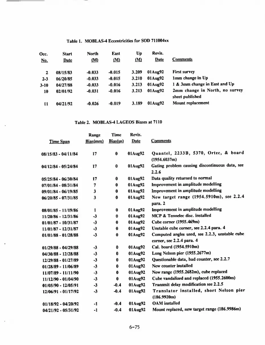
Table 1. MOBLAS-4 Eccentricities for SOD 711004xx
Occ. Start North East Up Revis.
No. Dat___g (M) _ (M) Dat___ge
2 08/15/83 -0.033 -0.015 3.209 01Aug92
2-3 06/2,0/85 -0.033 -0.015 3.210 01Aug92
3-10 04/27/88 -0.033 -0.016 3.213 01Aug92
10 02/01/92 -0.031 -0.016 3.213 01Aug92
11 04/21/92 -0.026 -0.019 3.189 01Aug92
Comments
First survey
lmm change in Up
1 & 3mm change in East and Up
2mm change in North, no survey
sheet published
Mount replacement
Table 2. MOBLAS-4 LAGEOS Biases at 7110
Range Time Revis.
Time Span Bias(mm) Bi_(us) Date Comments
08/15/83 - 04/11/84 17 0 01Aug92
04/12/84 - 05/24/84 17 0 01Aug92
05/25/84 - 06/30/84 17 0 01Aug92
07/01/84 - 08/31/84 7 0 01Aug92
09/01/84 - 06/19/85 3 0 01Aug92
06/20/85 - 07/31/85 3 0 01Aug92
08/01/85 - 11/19/86 1 0 01Aug92
11/20/86- 12/31/86 -3 0 01Aug92
01/01/87- 10/31/87 -3 0 01Aug92
11/01/87- 12131/87 -3 0 01Aug92
01101188 - 01/28/88 -3 0 01Aug92
01/29/88 - 04/29/88 -3 0 01Aug92
04/30/88- 12/28/88 -3 0 01Aug92
12/29/88 - 01/27/89 -3 0 01Aug92
01/28/89- 11/06/89 -3 0 01Aug92
11/07/89- 11/11/90 -3 0 01Aug92
11/12/90 - 01/04/90 -3 0 01Aug92
01/05/90 - 12/05/91 -3 -0.4 01Aug92
12/06/91 - 01/17/92 -3 -0.4 01Aug92
01/18/92 - 04/20/92 -1 -0.4 01Aug92
04/21/92 - 05/31/92 -1 -0.4 01Aug92
Quantel, 2233B, 5370, Ortec, & board
(1954.6037m)
Gating problem causing discontinuous data, see
2.2.6
Data quality returned to normal
Improvement in amplitude modelling
Improvement in amplitude modelling
New target range (1954.5910m), see 2.2.4
para. 2
Improvement in amplitude modelling
MCP & Tennelec disc. installed
Cube corner (1955.469m)
Unstable cube corner, see 2.2.4 para. 4
Computed angles used, see 2.2.3, unstable cube
corner, see 2.2.4 para. 4
Cal. board (1954.5910m)
Long Nelson pier (1955.2677m)
Questionable data, bad counter, see 2.2.7
New counter installed
New range (1955.2682m), cube replaced
Cube vandalized and replaced (1955.2600m)
Transmit delay modification see 2.2.5
Translator installed, short Nelson pier
(186.9920m)
OAM installed
Mount replaced, new target range (186.9986m)
6-75
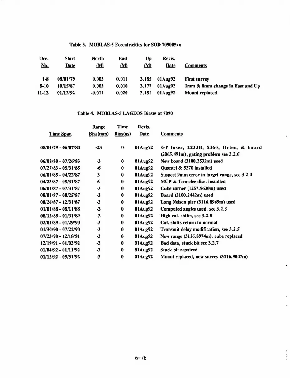
Table 3. MOBLAS-5 Eccentricities for SOD 709005xx
Occ. Start North East Up Revis.
No___. Date (M) (M) fM) l)at_
1-8
8-10
11-12
08/01/79 0.003 0.011 3.185 01Aug92
10/15/87 0.003 0.010 3.177 01Aug92
01/12/92 -0.011 0.020 3.181 01Aug92
Comments
First survey
lmm & 8mm change in East and Up
Mount replaced
Time
08/01/79
06/08/80
07/27/83
06/01/85
04/23/87
06/01/87
08/01/87
08126/87
01101/88
08/12/88
02/01/89
01130/90
07123190
12/19/91
01/04/92
01/12/92
Table 4. MOBLAS-5 LAGEOS Biases at 7090
Range Time Revis.
Span Bias(mm) _ Date Comments
- 06/07/80 -23 0 01 Aug92
- 07/26/83 -3 0 01Aug92
- 05/31/85 -6 0 01Aug92
- 04/22/87 3 0 01Aug92
- 05/31/87 6 0 01Aug92
- 07/31/87 -3 0 01Aug92
- 08/25/87 -3 0 01Aug92
- 12/31/87 -3 0 01Aug92
- 08/11/88 -3 0 01Aug92
- 01/31/89 -3 0 01Aug92
- 01/29/90 -3 0 01Aug92
- 07/22/90 -3 0 01Aug92
- 12/18/91 -3 0 01Aug92
- 01/03/92 -3 0 01Aug92
- 01/11/92 -3 0 01Aug92
- 05/31/92 -3 0 01Aug92
GP laser, 2233B, 5360, Ortec, & board
(2065.491m), gating problem see 3.2.6
New board (3100.2532m) used
Quantel & 5370 installed
Suspect 9mm error in target range, see 3.2.4
MCP & Tennelec disc. installed
Cube corner (1257.9630m) used
Board (3100.2442m) used
Long Nelson pier (3116.8969m) used
Computed angles used, see 3.2.3
High cal. shifts, see 3.2.8
Cal. shifts return to normal
Transmit delay modification, see 3.2.5
New range (3116.8974m), cube replaced
Bad data, stuck bit see 3.2.7
Stuck bit repaired
Mount replaced, new survey (3116.9047m)
6-76

Table 5. MOBLAS-6 Eccentricities for SOD 712206xx
Occ. Start North East Up Rev.
No. Dat____e (M_ (M) /M) Dat.___ge Comments
1-4 05/01/83 0.001 -0.007 3.182 01Aug92
4-7 05/03/88 0.002 -0.006 3.181 01Aug92
8-9 06/23/89 0.002 -0.006 3.181 01Ang92
9 04/30/91 0.002 -0.006 3.181 01Aug92
First survey
lmm change in all eccs., see 4.1
No change
No change, final survey
Table 6. MOBLAS-6 LAGEOS Biases at 7122
Range Time Revis.
Time Span Bias(mm) _ Date Comments
05/01/83 - 09/30/83 -3 0 01Aug92
10/01/83 - 01/31/84 19 0 01Aug92
02/01/84 - 03/01/84 19 0 01Aug92
03/02/84 - 04/30/84 19 0 01Aug92
05/01/84 - 03/31/86 31 0 01Aug92
04/01/86 - 08/31/86 29 0 01Aug92
09/01/86 - 01/27/87 23 0 01Aug92
01/28/87 - 03/26/87 19 0 01Aug92
03/27/87- 12/31/88 -14 0 01Aug92
01/01/88 - 05/02/88 -14 0 01Aug92
05/03/88 - 08/16/88 -8 0 01Aug92
08/17/88 - 08/31/88 1 0 01Aug92
09/01/88 - 09/30/88 2 0 01Aug92
10/01/88- 10/31/88 3 0 01Aug88
11/01/88- 11/30/88 4 0 01Aug92
12/01/88- 12/31/88 5 0 01Aug92
01/01/89 - 01/31/89 6 0 01Aug92
02/01/89 - 02/28/89 7 0 01Aug92
03/01/89 - 03/31/89 8 0 01Aug92
04/01/89 - 04/30/89 9 0 01Aug92
05/01/89 - 05/12/89 10 0 01Aug92
05/13/89 - 05/31/89 10 0 01Aug92
06/01/89 - 06/22/89 11 0 01Aug92
06/23/89 - 11/16/89 -3 0 01Aug92
11/17/89 - 01/10/90 -3 0 01Aug92
01/11/90 - 03/31/90 -3 0 01Aug92
04/01/90 - 09/26/90 -3 0 01Aug92
09/27/90 - 04/30/91 -3 0 01Aug92
GP laser, 2233B, 5360, Ortec, & Board
(2229.1998m)
Hurricane, suspect target movement, see 4.2.4,
para 2
Bad distribution amplifier, see 4.2.6
Distribution amplifier replaced
Quantel laser and HP5370 installed
Improvement in amplitude modelling
Improvement in amplitude modelling
MCP and Tennelec installed
Cube corner used (2229.4086m)
Computed angles used, see 4.2.3
New cube corner range used (2229.4150m)
First Nelson pier used (2229.2215m)
Nelson pier movement, see 4.2.4 para 3
Nelson pier movement
Nelson pier movement
Nelson pier movement
Nelson pier movement
Nelson pier movement, bad barometric data
Nelson pier movement, bad barometric data
Nelson pier movement, bad barometric data
Nelson pier movement, bad barometric data
Barometer repaired
Nelson pier movement
Second Nelson pier used (2232.7419m)
New range (2232.7447m), cube replaced
Transmit delay modification
Calibration RMS's are high
Calibration RMS's return to normal levels
6-77
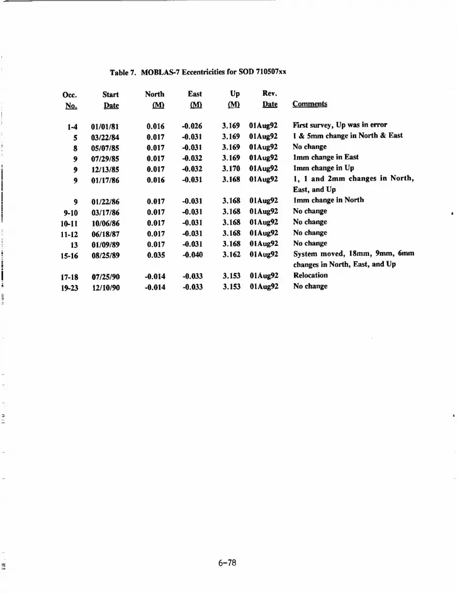
Table 7. MOBLAS-7 Eccentricities for SOD 710507xx
Occ. Start North East Up Rev.
No. Dat....ee (M) (M) (M) Date
1-4 01/01/81 0.016 -0.026 3.169 01Aug92
5 03/22/84 0.017 -0.031 3.169 01Aug92
8 05/07/85 0.017 -0.031 3.169 01Aug92
9 07/29/85 0.017 -0.032 3.169 01Aug92
9 12/13/85 0.017 -0.032 3.170 01Aug92
9 01/17/86 0.016 -0.031 3.168 01Aug92
01/22/86 0.017 -0.031 3.168 01Aug92
03/17/86 0.017 -0.031 3.168 01Aug92
10/06/86 0.017 -0.031 3.168 01Aug92
06/18/87 0.017 -0.031 3.168 01Aug92
01/09/89 0.017 -0.031 3.168 01Aug92
08/25/89 0.035 -0.040 3.162 01Aug92
9
9-10
10-11
11-12
13
15-16
17-18 07/25/90 -0.014 -0.033 3.153 01Aug92
19-23 12/10/90 -0.014 -0.033 3.153 01Aug92
Comments
First survey, Up was in error
1 & 5mm change in North & East
No change
lmm change in East
lmm change in Up
1, 1 and 2mm changes in North,
East, and Up
lmm change in North
No change
No change
No change
No change
System moved, 18mm, 9mm, 6mm
changes in North, East, and Up
Relocation
No change
6-78
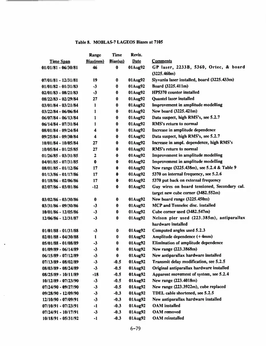
Table 8. MOBLAS-7 LAGEOS Biases at 7105
Time Span
01/01/81 - 06/30/81
07101181 - 12/31/81
01/01/82 - 01/31/83
02101183 - 08121/83
08/22/83 - 02/29/84
03/01/84 - 03/21/84
03/22/84 - 06/06/84
06/07/84 - 06/13/84
06/14/84 - 07/31/84
08/01/84 - 09/24/84
09/25/84 - 09/30/84
10/01/84- 10/05/84
10/05/84 - 01/25/85
01/26/85 - 03/31/85
04/01/85 - 07/31/85
08/01/85 - 01/12/86
01/13/86 - 01/17/86
01/18/86 - 02/06/86
02/07/86 - 03/01/86
03/02/86 - 03/30/86
03/31/86 - 09/30/86
10/01/86 - 12/05/86
12/06/86 - 12/31/87
01/01/88 - 01/31/88
02/01/88 - 04/30/88
05/01/88 - 01/08/89
01/09/89 - 06/14/89
06/15/89 - 07/12/89
07/13/89 - 08/02/89
08/03/89 - 08/24/89
08/25/89- 10/11/89
10/12/89 - 07/23/90
07/24/90 - 09/27/90
09/28/90 - 12/09/90
12/10/90 - 07/09/91
07/10/91 - 07/23/91
07/24/91 - 10/17/91
10/18/91 - 05/31/92
Range Time Revis.
Bias(ram) _ Date
46 0 01Aug92
19 0 01Aug92
-3 0 01Aug92
-3 0 01Aug92
27 0 01Aug92
1 0 01Aug92
1 0 01Aug92
1 0 01Aug92
1 0 01Aug92
4 0 01Aug92
4 0 01Aug92
27 0 01Aug92
27 0 01Aug92
2 0 01Aug92
0 0 01Aug92
17 0 01Aug92
17 0 01Aug92
17 0 01Aug92
-12 0 01Aug92
0 0 01Aug92
-3 0 01Aug92
-3 0 01Aug92
-3 0 01Aug92
-3 0 01Aug92
1 0 01Aug92
-3 0 01Aug92
-3 0 01Aug92
-3 0 01Aug92
-3 -0.5 01Aug92
-3 -0.5 01Aug92
-18 -0.5 01Aug92
-3 -0.5 01Aug92
-3 -0.5 01Aug92
-3 -0.3 01Aug92
-3 -0.3 01Aug92
-1 -0.3 01Aug92
-3 -0.3 01Aug92
-1 -0.3 01Aug92
Comments
GP laser, 2233B, 5360, Ortec, & board
(3225.460m)
Slyvania laser installed, board (3225.433m)
Board (3225.411m)
HP5370 counter installed
Quantel laser installed
Improvement in amplitude modelling
New board (3225.421m)
Data suspect, high RMS's, see 5.2.7
RMS's return to normal
Increase in amplitude dependence
Data suspect, high RMS's, see 5.2.7
Increase in ampl. dependence, high RMS's
RMS's return to normal
Improvement in amplitude modelling
Improvement in amplitude modelling
New range (3225.438m), see 5.2.4 & Table 9
5370 on internal frequency, see 5.2.6
5370 put back on external frequency
Guy wires on board tensioned, Secondary cal.
target new cube corner (3482.552m)
New board range (3225.450m)
MCP and Tennelec disc. installed
Cube corner used (3482.547m)
Nelson pier used (223.385m), antiparallax
hardware installed
Computed angles used 5.2.3
Amplitude dependence (+ 4ram)
Elimination of amplitude dependence
New range (223.3868m)
New antiparallax hardware installed
Transmit delay modification, see 5.2.5
Original antiparallax hardware installed
Apparent movement of system, see 5.2.4
New range (223.4018m)
New range (223.3922m), cube replaced
TDEL cable shortened, see 5.2.5
New antiparallax hardware installed
OAM installed
OAM removed
OAM reinstalled
6-79

Table 9. MOBLAS-7 Cube Corner Calibrated LAGEOS Passes
(The range biases for these passes would be 0)
Date Time
08/09/85 5:20
08/09/85 8:51
08/14/85 5:51
08/28/85 4:11
08/29/85 6:16
08/29/85 9:42
08/30/85 8:30
08/31/85 7:08
09/04/85 5:10
09/04/85 8:36
09/06/85 5:55
09/06/85 9:22
09/07/85 4:35
09/07185 8:03
09/10/85 3:59
09/10/85 7:31
09/11/85 2:52
09/11/85 6:15
09/11185 9:37
09/17/85 5:04
09/18/85 10:38
09/20/85 8:01
09/21/85 9:59
10/01/85 10:22
10/07/85 12:49
10/08/85 11:24
10/16/85 11:34
10/17/85 13:22
12/03/85 21:32
12/04/85 0:59
02/13/86 22:07
6-80

Table 10. MOBLAS-8 Eccentricities for SOD 710908xx
Occ. Start North East Up Rev.
No_..._. Date 0Vl) (M) ¢M3 Date Comments
1 09/01/81 0.012 0.011 3.225 01Aug92
1 07/22/82 -0.029 0.011 3.124 01Aug92
1-2 08/04/82 -0.029 0.011 3.141 01Aug92
2-3 09/24/84 -0.029 0.011 3.141 01Aug92
3-5 08/20/85 -0.029 0.011 3.142 01Aug92
6-11 12/12/88 -0.027 0.012 3.138 01Aug92
12 12/01/91 -0.019 0.005 3.184 01Aug92
13-15 12/12/91 -0.035 -0.003 3.184 01Aug92
First Survey
M8 & M4 mom's van swap
System releveled, 17mm change in
Up, based on 84 survey
No survey sheet
lmm change in Up
2, 1, & 4mm change in North, East,
and Up
Mount replacement
System releveled, 16 & 8mm change
in North and East
Table 11. MOBLAS-8 LAGEOS Biases at 7109
Range Time Revis.
Time Span Bias(mm) _ Date Comments
09/01/81 - 12/31/81 -3 0 01Aug92
01/01/82 - 03/04/82 -3 0 01Aug92
03/05/82 - 08/03/82 -3 0 01Aug92
08/04/82 - 12/31/83 2 + 6.0 01Aug92
01/01/84 - 03/31/84 7 +6.0 01Aug92
04/01/84 - 07/31/84 3 + 6.0 01Aug92
08/01/84 - 08/19/85 0 + 6.0 01Aug92
08/20/85 - 09/25/86 0 + 6.0 01Aug92
09/26/86- 10/26/86 -3 +6.0 01Aug92
10/27/86- 12/31/86 -3 0 01Aug92
01/01/87- 12/31/87 17 0 01Aug92
01/01/88- 12/11/88 17 0 01Aug92
12/12/88 - 03/22/89 6 0 01Aug92
03/23/89- 11/06/89 -3 0 01Aug92
11/07/89- 11/21/89 -3 0 01Aug92
11/22/89- 11/30/91 -3 -0.3 01Aug92
12/01/91 - 12/11/91 -3 -0.3 01Aug92
12/12/91 - 04/06/92 -3 -0.3 01Aug92
04/07/92 - 05/31/92 -1 -0.3 01Aug92
GP laser, 2233B, 5360, Ortec, & board
(2394.087m)
Very high RMS's (300-600mm), see 6.2.6
Hardware repaired, data nominal
M4/M8 van switch, Quantel, HP5370, transmit
delay problem see 6.2.5, board (2394.120m)
Increase in amplitude dependence
Improvement in amplitude modelling
Improvement in amplitude modelling
New board used (2389.506 or 2389.496m), see
6.2.4
MCP & Tennelec disc. installed
Transmit delay wire connected, see 6.2.5
Cube corner used (2389.519m), see 6.2.4
Computed angles, see 6.2.3
New cube corner range (2389.508m)
Nelson pier used (2401.1450m)
New range (2401.1458m), cube replaced
Transmit delay modification, see 6.2.5
Mount re-installed, Nelson pier (2401.1392m)
Mount releveled, Nelson pier (2401.1576m)
Short range Nelson pier used (207.4742m), OAM
installed
6-81


Multiwavelength
Ranging/Streak Cameras


N94-15580
OPTIMUM WAVELENGTHS FOR TWO COLOR RANGING
John J. Degnan
Code 901/ Crustal Dynamics Project
NASA Goddard Space Flight Center
Greenbelt, MD 20771
ABSTRACT
The range uncertainties associated with the refractive atmosphere
can be mitigated by the technique of two color, or dual wave-
length, ranging. The precision of the differential time of flight
(DTOF) measurement depends on the atmospheric dispersion between
the two wavelengths, the received pulsewidths and photoelectron
counts, and on the amount of temporal averaging. In general, the
transmitted wavelengths are not independently chosen but instead
are generated via nonlinear optics techniques (harmonic crystals,
Raman scattering, etc.) which also determine their relative pul-
sewidths. The mean received photoelectrons at each wavelength are
calculated via the familiar radar link equation which contains
several wavelength dependent parameters. By collecting the vari-
ous wavelength dependent terms, one can define a wavelength fig-
ure of merit for a two color laser ranging system.
In this paper, we apply the wavelength figure of merit to the
case of an extremely clear atmosphere and draw several conclu-
sions regarding the relative merits of fundamental-second har-
monic, fundamental-third harmonic, second-third harmonic, and
Raman two color systems. We find that, in spite of the larger
dispersion between wavelengths, fundamental-third harmonic sys-
tems have the lowest figure of merit due to a combination of poor
detector performance at the fundamental and poor atmospheric
transmission at the third harmonic. Fundamental-second harmonic
(-700 nm and 350 nm) have the highest figure of merit, but
second-third harmonic systems, using fundamental transmitters
near i000 nm, are a close second. Raman-shifted transmitters
appear to offer no advantage over harmonic systems because of (i)
the relatively small wavelength separation that can be achieved
in light gases such as hydrogen and (2) the lack of good ultra-
short pulse transmitters with an optimum fundamental wavelength
near 400 nm.
7-1

1 INTRODUCTION
With the subcentimeter precisions available from modern satellite
laser ranging (SLR) hardware [Degnan, 1985], atmospheric refrac-tion is a dominant error source in the absolute determination of
the geometric range from the station to the satellite. While
atmospheric modelling is believed to reduce the systematic errors
to roughly one centimeter or less, future progress toward milli-meter absolute accuracy ranging will rely on the technique of two
color, or dual wavelength, ranging.
In the present paper, we attempt to define optimum wavelengths
for two color ranging. In order to accomplish this, we must takeinto account all of the wavelength dependent parameters which
influence our ability to make an accurate differential time of
flight (DTOF) measurement. As we will see in the ensuing sec-
tions, a proper accounting of wavelength dependent terms will
include atmospheric dispersion, atmospheric transmission as a
function of sea level visibility, transmit antenna and target
gains, detector responsivities, transmitter availability and pul-
sewidth, and the detailed characteristics of the available non-
linear optics techniques for achieving the necessary optical
frequency translations.
2 ATMOSPHERIC REFRACTION: THE MARINI-MURRAY MODEL
In the Marini-Murray model of atmospheric refraction [Marini and
Murray, 1973], radial variability in the meteorological parame-
ters (i.e. with altitude) is assumed to be governed by the equa-
tions for hydrostatic equilibrium, the law of partial pressures,
and the perfect gas law. This leads to the following equations
for the spherical range correction, SCMM:
f(k) A(Pu,eu)+ B(¢,Tu,Pu)' B(,.r.,e.) (2.1)
SC uu ( X, E, P u T u, e u ) = F ( _, H ) si n ( E ) + ,(,,..,1.,(,. r.. ,,)lin £*,01
where
/(k)=.9650+ -.0164 .000228
+
k 2 A.4
F(¢.H)=l-.OO26cos2¢-.OOO31H
(2.2ct)
(2.2b)
A(Pt-z,eH) = .002357Pu + .000141e u (2.2c)
B(},Tu,PH) = 1.084x]O-SPuTuK(_,Tu,Pu)+4.734x]O -SPzuT,3
21
K(t,Ts.P . )
and
(2.2d)
K(#,T u,PH) = 1.163-.O0968cos2¢-,OOlO4T u + .00001435P u (2.2e)
7-2

where k is the laser wavelength in microns, E is the true eleva-
tion angle of the satellite in degrees, _ is the station lati-
tude, H is the station height above mean sea level, and PH, TH
and e H are the surface pressure, temperature, and water vapor
pressure at the station. The water vapor pressure e H is related
to the surface percent relative humidity R H and surface tempera-
ture T H by the equation
( T,273,5R n 7.s
eH(RH,TH)=._6.11xl 0 237.3.(T.-273.,S)) (2.3)
The wavelength dependence of the range correction is contained in
the dispersion term /(k) which is plotted in Figure i. It was
arbitrarily chosen by Marini and Murray to have a value of unity
at the ruby laser wavelength of .6943 microns.
_.2I I I I I I I - I -].....
1.1
_(,,,)
1.0
0.9 .............. l .I.3 .6 .9 1.2
_,(_)
Figure i. Atmospheric dispersion in a standard atmosphere as a
function of wavelength from the near ultraviolet to the nearinfrared.
3 TWO-COLOR LASER RANGING
By measuring the pulse times-of-flight at two colors and multi-
plying the results by the velocity of light in vacuum, c, we
obtain a measure of the optical path lengths through the
atmosphere at the two wavelengths. Thus, the atmospheric refrac-
tion correction is given by
7-3
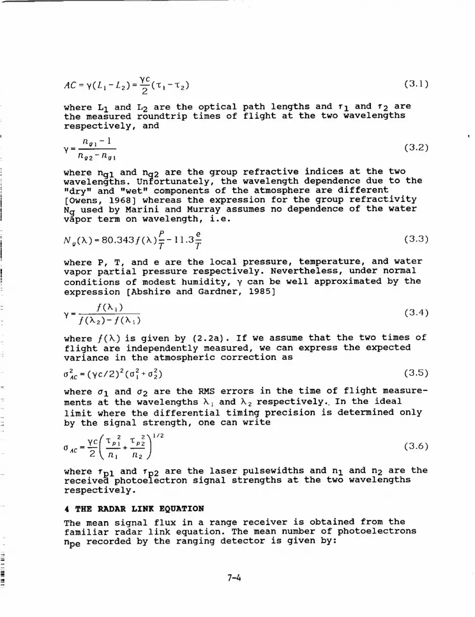
yc --%2)AC = y( L1- L2) = -_('_! (3.])
where L1 and L 2 are the optical path lengths and rI and r2 arethe measured roundtrip times of flight at the two wavelengths
respectively, and
_ol - 1¥ = (3.2)
_g2--_gl
where nal and nq2 are the group refractive indices at the twowavelengths. Unfortunately, the wavelength dependence due to the
"dry" and "wet" components of the atmosphere are different
[Owens, 1968] whereas the expression for the group refractivity
Ng used by Marini and Murray assumes no dependence of the watervapor term on wavelength, i.e.
P 3£No(k ) = 80.343j(k) - ] 1. T (3.3)
where P, T, and e are the local pressure, temperature, and water
vapor partial pressure respectively. Nevertheless, under normal
conditions of modest humidity, ¥ can be well approximated by the
expression [Abshire and Gardner, 1985]
f(x )7= (3.4)
f(x2)-f(x,)
where /(k) is given by (2.2a). If we assume that the two times of
flight are independently measured, we can express the expectedvariance in the atmospheric correction as
oAcz =(yc/2)2(o21 +°§) (3.5)
where aI and a 2 are the RMS errors in the time of flight measure-
ments at the wavelengths k I and k z respectively. In the ideal
limit where the differential timing precision is determined only
by the signal strength, one can write
_( 2 211/2+ (3.6)
OAC= _1 n2
where fpl and rp2 are the laser pulsewidths and n I and n2 are thereceivea photoelectron signal strengths at the two wavelengths
respectively.
4 THE RADAR LINK EQUATION
The mean signal flux in a range receiver is obtained from the
familiar radar link equation. The mean number of photoelectrons
npe recorded by the ranging detector is given by:
7-4
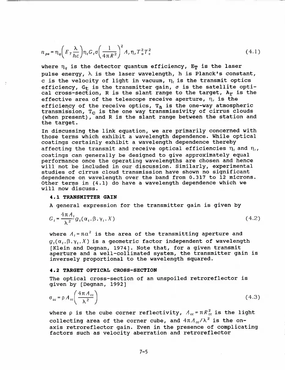
(i)2np_=1-1,7 Er qtG,o 4TtR z A_rI_T]T_(4.1)
where q_ is the detector quantum efficiency, ET is the laser
pulse energy, k is the laser wavelength, h is Planck's constant,
c is the velocity of light in vacuum, _e is the transmit optics
efficiency, Gt is the transmitter gain, a is the satellite opti-cal cross-section, R is the slant range to the target, A r is the
effective area of the telescope receive aperture, _r is the
efficiency of the receive optics, Ta is the one-way atmospheric
transmission, Tc is the one way transmissivity of cirrus clouds
(when present), and R is the slant range between the station and
the target.
In discussing the link equation, we are primarily concerned with
those terms which exhibit a wavelength dependence. While optical
coatings certainly exhibit a wavelength dependence thereby
affecting the transmit and receive optical efficiencies _e and Ur,
coatings can generally be designed to give approximately equal
performance once the operating wavelengths are chosen and hence
will not be included in our discussion. Similarly, experimentalstudies of cirrus cloud transmission have shown no significant
dependence on wavelength over the band from 0.317 to 12 microns.
Other terms in (4.1) do have a wavelength dependence which wewill now discuss.
4.1 TRANSMITTER GAIN
A general expression for the transmitter gain is given by
4_At
G t- k z gt(_,,_,¥t,X) (4.2)
where At = na 2 is the area of the transmitting aperture and
gt(_t,_,¥t,X) is a geometric factor independent of wavelength
[Klein and Degnan, 1974]. Note that, for a given transmit
aperture and a well-collimated system, the transmitter gain is
inversely proportional to the wavelength squared.
4.2 TARGET OPTICAL CROSS-SECTION
The optical cross-section of an unspoiled retroreflector is
given by [Degnan, 1992]
(4_Acc_ (4.3)oc_=pAc_ kz j
where p is the cube corner reflectivity, Acc= nR_c is the light
collecting area of the corner cube, and 4KAcc/k z is the on-
axis retroreflector gain. Even in the presence of complicating
factors such as velocity aberration and retroreflector
7-5

spoiling, an array of retroreflectors designed to operate atboth wavelengthswould be expected to retain the same inverse
square law dependence on wavelength exhibited by (4.3).
4.3 ATMOSPHERIC ATTENUATION
In the near-ultraviolet to visible spectral band between 0.3
and 0.7 _, atmospheric attenuation is dominated by aerosol
(Mie) scattering but molecular (Rayleigh) and ozone absorption
also play a role [RCA, 1968]. In the near infrared beyond0.7_, the plot of atmospheric transmission versus wavelength
(see Figure 2) is modulated by strong absorption features ofvarious molecular constituents in the atmosphere, notably
water vapor, oxygen, and carbon dioxide.
1.0
0.8
d 0.6.
0.4
0.2
I///I I I / I I I I
.3 .4 .5 .6 .7 .8 .9 1.0 1.1
Figure 2. Atmospheric transmission as a function of wavelength
under extremely clear conditions with 2 cm of precipitable
water vapor at zenith angles of 0, 50, and 70 ° (corresponding
to I, 2, and 3 air masses) respectively.
The transmission curve presented in Figure 2 corresponds to
excellent "seeing" conditions (80 Km visibility) and 2 cm of
precipitable water vapor. It should be noted that atmospheric
seeing conditions vary widely from day to day and from site tosite and are usually characterized by "sea level visibility"
expressed in kilometers. Plots of the sea level attenuationcoefficient versus wavelength (from 0.4 to 4 _) as a function
of sea level visibility can be found in the RCA Electro-Optics
7-6

Handbook [RCA, 1968]. For the purpose of this analysis, how-
ever, we will consider only the extremely clear atmosphere
depicted in Figure 2.
4.4 OPTICAL DETECTORS
Finally, the availability of high quantum efficiency optical
detectors at the two laser wavelengths is important. If a com-
mon photocathode is to be used, such as in most streak camera
schemes for performing differential timing, the photocathode
must be sensitive at both wavelengths. However, since the
images of the two return pulses can be spatially separated in
the entrance slit of the streak camera, one can conceive of
specially constructed streak tubes containing more than one
photocathode material to obtain the highest sensitivity at
both wavelengths. It may also be possible, at some future
date, to do the necessary timing via electronic means, such as
high speed GaAs technology, without resorting to streak camera
technology although this capability has not yet been demon-strated.
80
70
60
A) "BEST" PHOTOEMISSIVE DETECTOR RESPONSIVITIES
WAVELENGTH {t-,-)
50
40 --
30 --
20 --
10 --
0.3
.3
.35
.40
.45
.50
.55
.60
.65
.70
.75
.B0
.B5
.90
.gB
1.02
1.1
RESPON SIVtTV
5O
60
80
70
63
64
65
67
6S
69
70
58
13
9
.8
.2
PHOTOCATHODE (+ WINDOW)MATERIAL
S20
K-C_Sb - (UME GLASS)
K-C_Sb - (UME GLASS)
K-C_Sb -- (UME GLASS)
K-CIPSb ÷ (LIME GLASS)
GaAS (_ 9741 GLASS)
GI_Jz (- 9741 GLASS)
GBAs (- 9741 GLASS)
GaAs (- 9741 GLASS)
OaAs (._ 9741 GLASS)
Ga/M_ (+ 9741 GLASS)
GmAs (+ 9741 GLASS)
Gi_DI%B( _- 9741 GLASS)
Ga.tnA._ (+ 9741 GRASS)
GalnAs (+ 9741 GLASS)
Sl
B) COMPOSITE GRAPH OF PHOTOEMISSIVEDETECTOR RESPONSIVITY
I .L I , , I.4 .S .e .7 .8 .9 1.0
), (_.)1.1
Figure 3. Summary of "best" photoemissive detector responsivi-ties from the near ultraviolet to the near infrared.
7-7
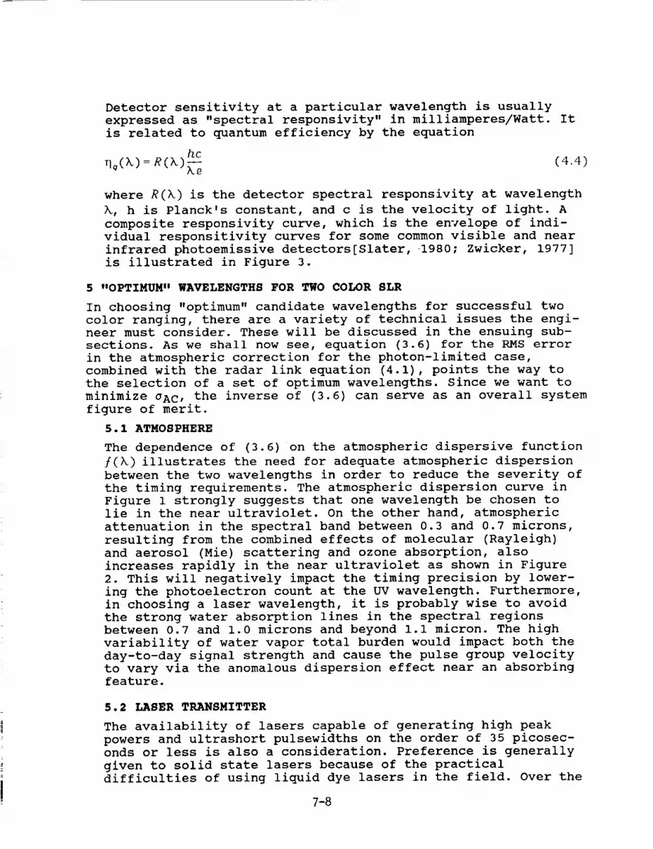
Detector sensitivity at a particular wavelength is usually
expressed as "spectral responsivity" in milliamperes/Watt. It
is related to quantum efficiency by the equation
where R(k) is the detector spectral responsivity at wavelength
k, h is Planck's constant, and c is the velocity of light. A
composite responsivity curve, which is the envelope of indi-
vidual responsitivity curves for some common visible and near
infrared photoemissive detectors[Slater, 1980; Zwicker, 1977]
is illustrated in Figure 3.
5 "OPTIMUM" WAVELENGTHS FOR TWO COLOR SLR
In choosing "optimum" candidate wavelengths for successful two
color ranging, there are a variety of technical issues the engi-
neer must consider. These will be discussed in the ensuing sub-
sections. As we shall now see, equation (3.6) for the RMS error
in the atmospheric correction for the photon-limited case,
combined with the radar link equation (4.1), points the way to
the selection of a set of optimum wavelengths. Since we want to
minimize aAC, the inverse of (3.6) can serve as an overall system
figure of merit.
5.1 ATMOSPHERE
The dependence of (3.6) on the atmospheric dispersive function
/(k) illustrates the need for adequate atmospheric dispersion
between the two wavelengths in order to reduce the severity of
the timing requirements. The atmospheric dispersion curve in
Figure 1 strongly suggests that one wavelength be chosen to
lie in the near ultraviolet. On the other hand, atmospheric
attenuation in the spectral band between 0.3 and 0.7 microns,
resulting from the combined effects of molecular (Rayleigh)
and aerosol (Mie) scattering and ozone absorption, also
increases rapidly in the near ultraviolet as shown in Figure
2. This will negatively impact the timing precision by lower-
ing the photoelectron count at the UV wavelength. Furthermore,
in choosing a laser wavelength, it is probably wise to avoid
the strong water absorption lines in the spectral regions
between 0.7 and 1.0 microns and beyond i.i micron. The high
variability of water vapor total burden would impact both the
day-to-day signal strength and cause the pulse group velocity
to vary via the anomalous dispersion effect near an absorbing
feature.
5.2 LASER TRANSMITTER
The availability of lasers capable of generating high peak
powers and ultrashort pulsewidths on the order of 35 picosec-
onds or less is also a consideration. Preference is generally
given to solid state lasers because of the practical
difficulties of using liquid dye lasers in the field. Over the
7-8

past decade, much progress has been made in the development ofhighly tunable solid state lasers such as Alexandrite (700 to
810 nm) and Titanium-doped sapphire (600 to 900 nm). The widebandwidths of these new materials are capable of supporting
subpicosecond pulsewidths whereas today's workhorse, Nd:YAG,
is limited to about I0 picoseconds by it's relatively narrow
linewidth (120 GHz). However, high bandwidth comes at a price
- i.e. lower gain - making the construction of high peak power
Ti:Sapphire and Alexandrite devices more difficult.
Generally, the wavelengths in two color systems are generated
from the fundamental wavelength k I via nonlinear optical tech-
niques such as harmonic generation in crystals or Raman shift-
ing in gases. This assures simultaneity of emission and
eliminates (thankfully) the need to synchronize the firings of
two separate lasers with picosecond precisions. However,
reliance on nonlinear teqhniques implies that the two wave-
lengths cannot be chosen independently of each other. In the
case of harmonic generation, the second and third harmonic
wavelengths are given by
respectively.
In Raman shifting, a portion of the incident radiation at
input frequency, v o is shifted by some fixed amount v s (the
"Stokes shift") toward longer wavelengths relative to the fun-
damental. One also obtains frequencies at longer ("Stokes")
and shorter ("Anti-Stokes") wavelengths, but these are
generally too weak to supply sufficient energy for satellite
ranging. Large Stokes frequency shifts, and hence high disper-sion between wavelengths, are obtained by Raman shifting in
light gases. Hydrogen produces the largest shift of 4155 cm -I,
and photon conversion efficiencies as high as 80% have been
reported. For example, one proposed two color SLR system usesthe second harmonic of Nd:YAG (532 nm) in hydrogen to obtain a
second wavelength output at 680 nm [Gaignebet et al, 1986].
A second consequence of harmonic or Raman generation is that
the pulsewidth of the secondary wavelength is generally
shorter than the pulsewidth of the fundamental. From the
theory of harmonic generation [Degnan, 1979], the harmonic
pulsewidths are approximately given by
TI T 1
for low to moderate energy conversion efficiencies (< 50% -the usual case). Raman generation depends on third order non-
linear processes, and the pulsewidth dependence is identical
to that of third harmonic generation.
7-9

5.3 WAVELENGTH FIGURE OF MERIT
In order to treat all potential system configurations on an
equal basis, some assumptions are in order. We will assume
that the fundamental laser, from which all other wavelengths
are derived, is characterized by an energy E and a pulsewidth
7p which is constant for all wavelengths. Thus, Equation (3.6)becomes
_/ 1 1 (5.3)
where 81 and 82 are pulsewidth scale factors which depend on
the nonlinear process used to generate them as in (5.2). In
addition, we recognize that wavelengths derived via nonlinear
processes are obtained with some typical energy efficiency
which we will denote by q_ and q2 respectively. If the funda-
mental wavelength is used as one of the two wavelengths, we
will assign values of _f = 1 and U/= I. For second and third
harmonic generation in the ultrashort pulse regime, typical
conversion efficiencies are _sh = .5 and qth =.2 respectively.
In order to derive a wavelength figure of merit, we must now
bring together all of the wavelength dependent terms in equa-
tions (4.1) and (3.5). We obtain for the figure of merit
!
(5.4)
where /(k) is the wavelength dispersion term in the Marini-
Murray atmospheric correction formula, q_ and _z and 81 and _2
are the energy conversion efficiencies and pulsewidth
reduction factors respectively for the relevant nonlinear pro-
cess, R(A) is the spectral responsivity, and Ta(k.E) is the
one way atmospheric transmission as a function of wavelength
and elevation angle. The factor of k 4 comes from the combined
inverse square law dependence of the transmitter and target
(retroreflector) gains on wavelength. The additional factor of
k associated with converting detector quantum efficiency to
spectral responsivity cancels with a similar factor in (4.1)
which converts transmitter laser energy to the number of
transmitter photons. In plotting (5.4), we will use the enve-
lope of the individual photoemitter responsivity curves in
Figure 3 so that we present each wavelength in its most
favorable light.
7-10

6 CONCLUSIONS
Figure 4 provides plots of the wavelength figure of merit as a
function of the fundamental (laser) wavelength and elevation
angle for the extremely clear atmosphere depicted in Figure 2.
Parts (a), (b), and (c) correspond to elevation angles of 90, 45,
and 20 degrees respectively. The three curves within each plot
compare systems which use: (1) the fundamental and second har-
monic wavelengths; (2) the fundamental and third harmonic wave-
lengths; and (3) the second and third harmonic wavelengths.
In spite of their greater dispersion, fundamental-third harmonic
systems have the lowest figure of merit at all elevation angles
due to a combination of poor detector performance at the funda-
mental and poor atmospheric transmission at the third harmonic.
The performance of these systems peaks at a fundamental
wavelength of about .97 microns independent of elevation angle.
At zenith, fundamental-second harmonic systems, operating at
wavelengths of 670 and 335 nm, have the highest figure of merit
(F = 1.75) but second-third harmonic systems, operating at wave-
lengths of 525 and 350 nm (fundamental = 1050 nm), are almost as
good (F = 1.6). As one progresses to smaller elevation angles,
atmospheric attenuation in the ultraviolet begins to dominate and
the optimum fundamental wavelength is shifted toward longer wave-
lengths with a corresponding reduction in the wavelength figure
of merit. Thus, the Nd:YAG laser, with a fundamental wavelength
of 1064 nm and a very mature technology, is a near-optimum choice
for a second-third harmonic system. However, a fundamental-second
harmonic system which utilizes a Ti:Sapphire laser operating inthe near infrared beyond 670 nm is a possible alternative.
Figure 5 suggests that a fundamental wavelength of about 400 nm
is optimum for a hydrogen Raman-shifted laser and that these sys-
tems offer no real advantage over harmonic systems because of
their lower wavelength figure of merit. Thls conclusion is
further supported by the fact that there are no high power solid
state lasers operating in the near ultraviolet. The principle
short wavelength devices are excimer ("excited dimer") gas dis-
charge lasers. At present, excimers cannot achieve ultrashort
pulsewidths on the order of picoseconds, typically operate in the
high atmospheric attenuation region of the spectrum below 360 nm,
and are operationally less desirable than high power solid state
lasers. Doubling or tripling solid state lasers to achieve a near
ultraviolet wavelength prior to Raman shifting only decreases the
overall wavelength figure of merit further by reducing the values
for the energy efficiency factors _i and _2- However, this effect
is partially offset by the slight reduction in pulsewidth (in-
creased _ values) resulting from nonlinear generation.
7-11

(A) E = 90 _2
0.6 .7 .8 .9 1.0 1.1 1.2
FUNDAMENTAL WAVELENGTH. X. (i¢)(B) E = 45 °
2
0,6 .7 .8 .9 1.0 1.1 1.2
FUNDAMENTAL WAVELENGTH. X. (p,)
(C) E = 20"
2t_ - ] I ] I I I I I ! I I
& I--- FUND-2ND __1
0.6 .7 .8 .9 1.0 1.1 1.2
FUNDAMENTAL WAVELENGTH. X (p,)
Figure 4. Two color wavelength figure of merit for fundamental-second harmonic, fundamental-third harmonic, and second-third
harmonic systems operating in an extremely clear atmosphere at
elevation angles of (a) 90 ° , (b) 45 ° and (c) 20 ° respectively.
7-12

1.0
0.8
0.6
--- 0.4U_
0.2
I I I I I I I I
/., RAMAN
.3 .4 ,5 .6 .7
FUNDAMENTAL WAVELENGTH, X(_)
m
.8
Figure 5. Two color wavelength figure of merit for Raman systems
operating in an extremely clear atmosphere at elevation angles of
90 ° , 45 ° and 20 ° .
7 REFERENCES
Abshire, J. B. and C.S. Gardner, "Atmospheric refractivity cor-rections in satellite laser ranging", IEEE Trans. on Geoscience
and Remote Sensing, GE-23, pp. 414-425, 1985.
Degnan, J. J., "Physical processes affecting the performance of
high-power, frequency-doubled short pulse laser systems: analy-sis, simulation, and experiment", Ph.D. Dissertation, University
of Maryland, College Park, MD, May 1979.
Degnan, J. J., "Satellite Laser Ranging: Current Status andFuture Prospects", IEEE Trans. on Geoscience and Remote Sensing,
GE-23, pp. 398-413, 1985.
Degnan, J. J., "Millimeter Accuracy Satellites for Two Color
Ranging", these proceedings (1992).
Gaignebet, J., F. Baumont, J. L. Hatat, K. Hamal, H. Jelinkova,
and I. Prochazka, "Two wavelength ranging on ground target using
Nd:YAG 2HG and Raman 0.68 _m pulses", Proceedings of the Sixth
International Workshop on Laser Ranging Instrumentation, Antibes-
Juan Les Pins, France, September 22-26, 1986.
Klein B. J., and J. J. Degnan, "Optical antenna gain. 1. Trans-
mitting antennas", Applied Optics, 13, pp. 2134-2140, 1974.
7-13
Marini, J. W. and C. W. Murray, "Correction of laser range track-
ing data for atmospheric refraction at elevations above i0
degrees", NASA Report X-591-73-351, Goddard Space Flight Center,
1973.
Owens, J. C., "Optical refractive index of air: Dependence on
pressure, temperature, and composition", Applied Optics, 6,51-58,
1967.
RCA Electro-optics Handbook, Technical Series EOH-10, RCA Commer-
cial Engineering, Harrison, NJ, 1968.
Slater, P. N., Remote Sensing: Optics and Optical Systems, Chap-
ter 13, Addison-Wesley Publishing Co., Reading, Massachusetts,
1980.
Zwicker, H. R., "Photoemissive Detectors", in Optical and
Infrared Detectors, Ed. R. J. Keyes, Springer Verlag, New York,
1977.
7-14

N94-15581
Two Color Satellite Laser Ranging Upgrades
At Goddard's 1.2m Telescope Facility
Thomas W. ZagwodzkiJan F. McGarryJohn J. Degnan
NASA/Goddard Space Flight CenterGreenbelt, Maryland 20771
Thomas K. Varghese
Bendix Field Engineering CorporationSeabrook, Maryland 20706
Abstract
The ranging laboratory at Goddard°s 1.2m telescope trackingfacility has recently been upgraded to include a singlephotoelectron sensitive Hamamatsu streak camera-based rangereceiver which uses doubled and tripled Nd:YAG frequencies forsatellite laser ranging. Other ranging system upgrades include anew Continuum laser, which will deliver up to 30 millijoules (mJ)at both 532 and 355 nm at a pulsewidth of 30 picoseconds(FWHM), and replacement of both ranging and tracking computerswith COMPAQ 386 based systems. Preliminary results using aphotomultiplier tube based receiver and waveform digitizerindicate agreement within the accuracy of the measurement withthe theoretical Marini and Murray model for atmospheric refraction.Two color streak camera measurements will be used to further
analyze the accuracy of these and other atmospheric refractionmodels.
7-15

INTRODUCTION
Satellite laser ranging efforts at the 1.2m tracking telescope at
Goddard's Geophysical and Astronomical Observatory (GGAO) have
evolved over the past few years in response to the demand for more
accurate SLR data. This includes a frequency-tripled Nd:YAG laser
system and a streak camera based range receiver. The laboratorywhich houses the Experimental Satellite Laser Ranging System
(ESLRS) adjoins a azimuth-elevation mount multi-user facilitydesigned to support the scientific community at the Goddard Space
Flight Center. Two of six facility experimenter port locations arededicated to the laser transmitter and the streak camera based
receiver for ranging applications. The ESLRS is a ranging laboratory
where new instrumentation, hardware and software are investigated
and characterized for planning and developing next generation
systems. The SLR data gathered by the ESLRS is considered
engineering data and is not archived as is other NASA laser trackingnetwork data. The end users of the ESLRS data are the
experimenters and their goal is to use this information to better
understand system problems and to help transition laboratory
systems more efficiently to field SLR operations. Other system
upgrades include a new 386 based tracking computer, a new 386
based ranging computer, and physical plant upgrades at the facility.
The ESLRS has been operational since 1983 except for periods in
which high priority flight programs within the Instrument Electro-
Optics Branch left the facility without crew support. The initial
SLR system [McGarry et al, 1986] included a Quantel YG 402 DP
frequency-doubled Nd:YAG laser, a two stage ITT F4128
microchannel plate photomultiplier tube (MCP-PMT), Ortec 934 andlater Tennelec TC 453 constant fraction discriminators (CFD's), and
a developmental time interval unit (TIU) built by Lawrence Berkeley
Laboratory. This system operated at a 5 hertz rate at the doubled
YAG wavelength (532nm) and yielded data at the 1 to 2 centimeter
level on LAGEOS with a very high return-to-fire ratio.
7-16

PROGRAMGOALS
Goddard Laser Tracking Network (GLTN) systems currently operatingat or below the 1 cm level RMS must still rely on models ofatmospheric range correction which assume certain altitude profilesfor temperature, pressure, and possible gradient effects. Knowledgeof atmospheric range correction on a shot-to-shot basis is thereforeuncertain, and must be addressed to eliminate atmospheric concerns.
The best way of accounting for the atmospheric range correction isto measure it on a shot-to-Shot basis. The time of flight
measurement is made in the conventional manner with a MCP based
receiver using the 532nm pulse, while a differential time of flightbetween the 532nm and 355nm pulses is made with a streak camera
based receiver. In making a streak camera differential measurement
accurate at the few picosecond level, the atmospheric rangecorrection can be recovered at the few millimeter level. Work in
improving ground-based SLR accuracies closely parallel work on
planned next generation space-based laser ranging systems. Efforts
in the ranging laboratory at the 1.2m facility have been
concentrating on both programs in this parallel effort.
SYSTEM UPGRADES
The extension from single color to two color operation at the 1.2m
facility required significant system upgrades, one being an
improvement in low mirror reflectivities in the UV. Recoating of all
telescope mirror surfaces was required since previous coatingsrevealed mirror reflectivities in the UV of typically 50 to 60% andone as low as 40%. For a 6 mirror coude focus system used in
common optics configuration, UV operation was prohibitive. Newaluminum mirror coatings with an SiOx overcoating (peaked at
355nm) improved surface reflectivities to typically 92% at 355nmand 88% at 532nm while maintaining broadband characteristics
required by other experimenters at the facility.
Return signal levels from LAGEOS are not adequate for two colorstreak camera-based operation with the present system. Therefore
we have opted to use low earth orbiting satellites such asSTARLETTE, AJISAI, and ERS-1 for two color data collection. As an
acquisition aid for sunlit passes, two TV camera systems have beenadded to the mount, and a third low light level RCA silicon
intensified target (SIT) camera has been used in the system primefocus.
7-17

Facility upgrades include the replacement of the PDP 11/24 tracking
computer with a COMPAQ 386/20 based system, and new
meteorological instruments including air pressure, temperature, and
relative humidity. The ranging computer, a LSI 11/23 (MINC), was
also replaced with a COMPAQ 386/20 system.
Ranging instrumentation upgrades include both laser transmitter andreceiver. The laser available for use at the 1.2m facility for ranging
from 1983 to March of 1992 was a Quantel passively mode locked
Nd:YAG system model number YG402 DP. This laser system generated
up to 60 mJ of doubled YAG at 532nm and about 15 mJ of tripled YAG
at 355 nm in a 140 picosecond pulse (FWHM). To make differential
measurements accurate at the picosecond level laser pulsewidths
must be narrowed considerably, and target satellites with low pulse
spreading must be used. The Quantel laser was replaced with aContinuum model PY-62 YAG with doubling and tripling capability.
The new Continuum laser outputs 30 picosecond pulses with about
30 mJ of energy at both 532nm and 355nm. The laser fire rate is
currently 4 hertz, with work underway to increase it to 10 hertz.
The laser is housed in a clean room approximately 10 meters fromthe base of the mount. The output beam is coupled into the telescope
system with a negative lens (negative focal length matching the F28
ray bundle of the 1.2m system) and a 45 degree aperture sharing
'holey' mirror just inside the system focal plane. The outgoing laserbeam is translated approximately 1.25 cm from the optical axis of
the telescope to avoid the shadowing by the central obscuration
(secondary mirror) in the telescope. The output beam is
approximately .4m in diameter, exits the system cleanly between
the primary and secondary mirror, and travels around that annulus as
the system tracks in azimuth. This configuration results in theleast amount of loss in the outgoing beam. In the common optics
mode the return path at the 45 degree mirror is folded across an NRC
table top to another mirror, splitter, and receiver package. In the
prime focus of the system is a field stop, to limit the receiver field
of view, and a high speed shutter.
The receive signal is split between a two stage ITT model F4128MCP PMT and a Hamamatsu streak camera. Shown in Figure 1 is a
simplified block diagram of the system that was used for bothaircraft and Relay Mirror experiments as well as current SLR
activities. The streak camera in use up until the Spring of 1992 was
7-18

7-19

a 2 picosecond resolution Hamamatsu model 1370. This unit was
integrated into the system in support of two color experimentswhich included both aircraft and the NASA/Air Force Relay Mirror
Experiment (RME) programs. The signal threshold for the Hamamatsu1370 streak camera is estimated at several thousand photoelectrons
and could be used only for ground work, aircraft, and the RME
program where signal levels were extremely high. The Hamamatsu1370 streak camera has since been replaced with a newer
Hamamatsu model 2909 which has an additional internal
microchannel plate intensifier giving the unit single photoelectron
sensitivity. A summary of upgraded system parameters is given inTable 1.
Table 1. Laser Ranging
Laser
EnergyPulsewidth
Beamwidth
Telescope
Trans/Rec Sw
System transDetector
Discriminator
Time Interval Unit
Streak Camera
Minicomputers
System Parameters and Instrumentation
Continuum PY-62, active/passive
mode-locked
30 mJ@532nm, 30 mJ @355nm
30 picoseconds (FWHM)
.0057 degree (FWHM)1.2 meter diam., f/28 Cassegrain
Common optics configuration
Aperture shared60%
ITT F4128 MCP PMTTennelec TC 454
HP5370, 20 ps resolutionHamamatsu model 2909
COMPAQ 386/20: Tracking
COMPAQ 386/20: Ranging
PS/2 model 60: Streak camera
In the ranging mode a small fraction of the return signal is detectedwith the MCP PMT, discriminated with a CFD, and triggers the streak
camera sweep. Both streak cameras require a pretrigger of 25 to 40nanoseconds dependent on the sweep speed selected. Sweep speeds
available in both cameras are .3, 1, 2, 5, and 10 nanoseconds full
scale. The pretrigger is accomplished by delaying the optical return
by one of two means. The streak camera input signal is delayed witheither a white cell optical delay, or a spot to slit 10m multimode
fiber optic bundle. Each technique has it's own advantages and
7-20

disadvantages. The fiber optic bundle is easy to align and has the
largest field of view, but introduces pulse spreading, while thewhite cell has the best throughput, no pulse spreading, but is
difficult to align. To maintain the best differential timing
capability at the receive end an artificial delay on the 532nm pulseis introduced at the laser transmitter. This delay is a dogleg optical
path into a total internal reflection (TIR) cube corner on a
Compumotor linear motor stage. The linear translation stage
provides the differential delay control from -.5 to 10 nanoseconds
additional optical path length for the 532nm pulse so that both
return pulses can be maintained within the 1 nanosecond sweep
window. The linear motor stage under computer control uses the
differential delay predicted by differencing the Marini & Murray
model delays at 355nm and 532nm The optical delay is adjusted so
that the two spatially separated pulses are incident in the streak
camera slit at approximately the same time. This minimizes
nonlinearity problems in the streak camera sweep. To resolve
simultaneous pulses in the PMT based receiver using the waveform
digitizer two PMT'S must be used.
PRELIMINARY RESULTS
The NASA/Air Force two color RME experiment mentioned earlier
generated the first streak camera returns for the ESLRS [Zagwodzki
et al, 1992]. The RME satellite was very attractive for several
reasons. The RME satellite represented an active, single cube corner
response target with an extremely high lidar cross section (~6x10⁹
m2). With a short pulse laser transmitter and streak camera based
receiver, the individual cube corners on the satellite, separated by
41.2 mm, could be resolved in time. In the Fall of 1991 the only
streak camera available at the 1.2m facility for the RME programwas the Hamamatsu model 1370. The high threshold of several
thousand photoelectrons for this streak camera made the RME the
only viable satellite target. Shown in Figure 2 are streak camerareturn waveforms from the RME satellite at 532nm only. Three cube
corners on the satellite could clearly be resolved in time (separation
of 41.2mm). The horizontal sweep speed was 1.2 nanoseconds in
time and the laser pulsewidth was 140 picoseconds. Unfortunately
satellite control problems ended the experiment prematurely before
UV operation began.
7-21
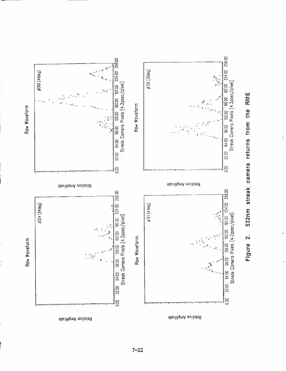
EL0
O
3:=
D
c_
0
o ..o
. -
* ._ o
,<.::'.
" °-,....
.°;°"
-..0..-.-
!o.
E
0C_
apn1!IdwV aA!IDla_l
°s " * "
.,.-
°.
c_
- c,,,J
]8
-_r_,J
'_0 r.,."lI_C_ CL
8 _._,r_
_o
o
8
o__
C_)
cn
c_-Q.
:N
E
0
o
orY
o
8
o
- .'._; :" :"i8
-c,.,;
a."
°.° ,.|
o ° %...- o
; :." ioo
. :".: , -.
"_... oo
0o
I
I-1
apn1!IdwV aA!IDla_
o
_J
..,
"°a,":_-o o
o"-;-".
.
°'- ..,.
' ..... iN
_r . i, .. i I .... i .... i,.,. I .... _. i I .... i .... i . .
o
L
u_.)
os,_
o
I.I.I
n-
i-
EoI,--
"4--
r-I....
I,-
E
o
0_
"4'--'
E
c_
11.-
IJ.
apn1!IdwV aA!IDla_l apnl!ldwV aA[IOla_l
7-22

The loss of the RME as a target meant satellite streak camera workhad to wait for the installation of the more sensitive Hamamatsu
2909 unit. In the interim, two color efforts have continued at the
1.2m facility using the MCP PMT based receiver with a 1 Ghzbandwidth Tektronix model 7912 waveform digitizer. The ranging
system can be configured with two PMT's (one each for 532nm and
355nm) or a single PMT (usually the 355nm). For night time
operation, when no bandpass filters are required, a single PMT isused. Since the UV link is the weakest, the PMT with peaked
quantum efficiency at 355nm is used. To resolve two distinct
pulses with the single UV PMT the differential delay at thetransmitter is set to allow at least two nanoseconds offset between
the peaks of the two pulses. This assures adequate separation of
return pulses at the receiver, but reduces the temporal resolution of
the differential time-of-flight measurement.
Figure 3 shows a comparison plot of the theoretical differential
delay versus the measured delay calculated from the two color
returns as seen by the Tektronix 7912. The theoretical differential
delay was calculated by differencing the 355nm and 532nm delays
computed using the Marini and Murray model. The Marini and Murraycalculations used the weather conditions from the log file taken
during the pass. This weather information was taken in real-time,
so the actual temperature and pressure were not constant. The
pressure changed minimally (1006.27 to 1006.31 millibars) as did
the temperature (14.24 to 14.48 C). The gaps (thinner lines) in the
Marini and Murray curve represent times that no weatherinformation was available, and so the data had to be interpolated for
those regions.
For this pass the linear translator was fixed at 6 nanoseconds. This
necessitated a slow sweep setting on the 7912 waveform digitizer
in order to capture both frequency's return waveforms during the
entire pass. Setting the green delay at 6 nanoseconds always placedthe 355nm return ahead of the 532nm return and caused the UV
pulses to move toward the green as the elevation decreased.
The measured differential delay was computed by taking the
inverted raw 7912 waveforms (no smoothing) and computing the
pixel locations of the highest two peaks. The location of these two
pixels was differenced, converted to nanoseconds, and subtracted
from the fixed 6 nanosecond green delay. This was a "quick-look" atthe data so no interpolation was performed between pixels, and
7-23

X
XX
XxXx
X
X
X
X
X
X
X
X
[_asu] IV7-:1(]
00
c:__0:3
0
0
0
"7_
Eo_
c_
oI_
_- 0
"I0 (n
0--
O0O--
c6
0L=.
w--
i,
7-24
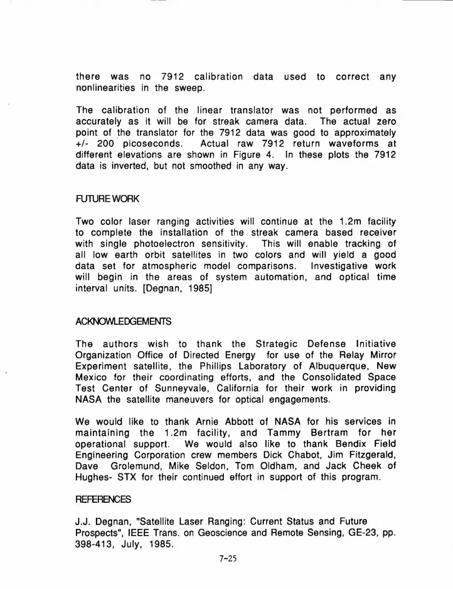
there was no 7912 calibration data used to
nonlinearities in the sweep.correct any
The calibration of the linear translator was not performed as
accurately as it will be for streak camera data. The actual zero
point of the translator for the 7912 data was good to approximately+/- 200 picoseconds. Actual raw 7912 return waveforms at
different elevations are shown in Figure 4. In these plots the 7912
data is inverted, but not smoothed in any way.
FUTURE WORK
Two color laser ranging activities will continue at the 1.2m facility
to complete the installation of the streak camera based receiver
with single photoelectron sensitivity. This will enable tracking of
all low earth orbit satellites in two colors and will yield a good
data set for atmospheric model comparisons. Investigative work
will begin in the areas of system automation, and optical time
interval units. [Degnan, 1985]
ACKNOWLEDGEMENTS
The authors wish to thank the Strategic Defense Initiative
Organization Office of Directed Energy for use of the Relay Mirror
Experiment satellite, the Phillips Laboratory of Albuquerque, NewMexico for their coordinating efforts, and the Consolidated Space
Test Center of Sunneyvale, California for their work in providing
NASA the satellite maneuvers for optical engagements.
We would like to thank Arnie Abbott of NASA for his services in
maintaining the 1.2m facility, and Tammy Bertram for her
operational support. We would also like to thank Bendix Field
Engineering Corporation crew members Dick Chabot, Jim Fitzgerald,Dave Grolemund, Mike Seldon, Tom Oldham, and Jack Cheek of
Hughes- STX for their continued effort in support of this program.
REFERENCES
J.J. Degnan, "Satellite Laser Ranging: Current Status and Future
Prospects", IEEE Trans. on Geoscience and Remote Sensing, GE-23, pp.
398-413, July, 1985.
7-25

250.0
220.0
0
_o_o
_- 160.0
130.0
100.0
250.0-
220.0
LJO
-_ IgO.O0_
_- 160.0
Woveform #A1G2[levotion: 233 dog
532nmA
.355nm
A '" :%
' ' ' _.6' ' i2_.b' ' b_.6' ' _5g.b'' i2b.b' 'g'4.b' 'i4'a.b' ' _lkOPIXELS [39psec/pixel]
20nsec full scole
130.0
Woveform#C054[levotion: 52.4deg
355nm 532nm
_loo.o0.0'' ' _.6' ' i213.b'' b_.6' ' _5'6.b'' g2bb' '_8'4.b'' 4_.b' 'g_.o
PIXELS[39psec/pixel]20nsec full scole
250.0-
2200
LJCb
IgOO
_- 1G0.0
LJQE
130.0
532nm
._
WoveformNB406[levotion: 73.4 deg
355nm :
A ":. : :
,; ._.v..j V 'x/A_,k, _
PIXELS [39psec/pixel]20nsec full stole
250.0
220.0
_oo
w
150.0.<
bJ
1300
Woveform#C216Elevotion:43.2 deg
532nm355nm w,
,_, :-• _ ." :
- : :- :_ ; _ _ ,.!--
_.6' ' bt_.b'' b_.o' ' _5'o.b'' _2b._;'' ]8_.b' '_.b' ' _100.00.0
PIXELS[39psec/pixel]20nsec full scole
!.0
Figure 4. Two color return waveforms from AJISAI
pass of June 27, 1992.
7-26

J. L. McGarry, T. W. Zagwodzki, J. J. Degnan, "Large aperture high
accuracy satellite laser tracking," in Proc. of S.P.I.E. Acquisition,
Tracking, and Pointing, Orlando, Florida, April, 1986.
T.W. Zagwodzki, J.F. McGarry, A. Abbott, J.W. Cheek, R.S. Chabot, J.D.
Fitzgerald, D.A. Grolemund, "Laser Ranging to the Relay Mirror
Experiment (RME) Satellite from Goddard Space Flight Center's 1.2m
Telescope Facility", to be published in the Journal of GeophysicalResearch.
7-27

N94-15582
Measuring Atmospheric Dispersion With WLRS
In Multiple Wavelength Mode
U. Sehreiber 1
Forschungseinricht ung SatelhtengeodaesieFundamentalstation Wettzell
D - 8493 Koetzting
K. H. Haufe R. Dassing,
Institut fuer Angewandte GeodaesieFundamentalstation Wettzell
D - 8493 Koetzting
Abstract
The WLRS (Wettzell Laser Ranging System) allows the simultaneous tracking ofsatellites on two different wavelengths. These are the fundamental frequency of Nd :YAGat 1.064 pm and the second harmonic at 532 nm. Range measurements to the satelliteLAGEOS were carried out with different experimental set- ups, after developing a de-tector unit based on a silicon avalanche photodiode in Geiger mode, which is sufficientlysensitive in the infrared domain. An approach towards a quantitative interpretation of
the data is suggested and discussed briefly.
1 The effect of atmospheric dispersion on satellite ranges
The varying index of refraction of the atmosphere can be considered one of the most impor-
tant contributions to the error sources for satellite ranges. Following a model of Marini and
Murray [1], the additional time for the laser pulse passing through the atmosphere under an
elevation angle of 90 degrees is as much as 8 as. This model assumes rotational symmetric
atmospheric layers with respect to the geocenter and has been established with the help
of ballon experiments. Inputs to to this model are atmospheric pressure, temperature and
humidity, which are measured around the ranging station. In general it can be said that
the calculated corrections are very precise, so that the requirements for an experimental im-
provement are extremly high [2]. However, orbit fitting procedures on the basis of complex
programs often show a small systematic error, depending on the pointing elevation of the
ranging station. Therefore a better determination of the atmospheric influence is desirable.
2 The experimental set- up
2.1 The ttwo-' detector experiment
When the WLRS telescope was designed [3], care had been taken to optimise the signal path
for the fundamental (1.064/_m) and second harmonic (532 nm) wavelength of the Nd:YAG
1Techn. Universitaet Muenchen, Arcisstr. 21 D - 8000 Muenchen 2
7-28
laser. The remaining optical components of the ranging equipment were replaced to allow
transmission and reception of these 2 frequencies. In the beginning it was not known if
the second harmonic generating crystal (KD*P) would laterally displace the pulses of the
2 frequencies so far, that there would not be a sufficient overlap of the two signals at
the location of the satellite. During the experiments a weak dependance of the return
rate of each detector with respect to the pointing was noticed. However, the overlap was
found to be acceptable. The WLRS- system uses the same telescope for transmitting and
receiving, therefore the photodetector was placed behind the transmit/receive- switch inside
the thermocontrolled laboratory. This gives the advantage of high signal stability and an
easily accessible working enviroment. Figure 1 outlines the experimental set- up. The receive
signal is split into its two different frequency components at a dichrolc mirror. The signs2
with a wavelength of 532 nm is reflected towards a microchannel plate (MCP), while the
infrared part of the satellite echo is focused onto the active area of an avalanche photodiode
(APD: SPll4) placed in Geiger mode. In its present state, the WLRS is capable of recording
one stop event per outgoing laser pulse only. This causes the detection of either an event
from the MCP or the APD. To achieve a high number of echos from both channels, a constant
delay- line of 44.9 ns was added to the MCP output, before recombining both signal lines at
an impedance matched T - junction and feeding them to the eventtimer. There are two stops
for each measured roundtrip possible, only one of them will be recorded, as the electronics
gets disactivated after processing one event. The delayline places the less favourable signal
channel to be detected first. When the measured return residuals axe plotted versus time
one can see two signal tracks (fig. 2) separated in range by the delay of the additional
cable. This can be noticed during tracking and indicates, if there are enough recordings for
both laser frequencies. The contribution to each wavelength has to be separated during the
analysis, as all the range information goes to one datafile.
2.2 The 'one-' detector experiment
A slowly varying instability (i.e. drift) in the detector characteristics would be indicated
during the ranging run, as a shot by shot calibration to a fixed target is carried out. To
exclude such effects generally, the experiment was altered to use just one detector. The
dichroic mirror (ref. fig. 1) was removed and the APD recorded both frequencies. The
sensitivity of the diode is higher on 532 nm than on 1.064 #m but, because of the dispersion
of the atmosphere, the infrared signal reaches the detector first. Therefore, a sufficient
amount of data for both signal frequencies can be obtained. For the present this kind
of experiment is restricted to the night hours, as there are no suitable spectral filters for
this application. During tracking, the operator notices the formation of one track only, as
both satellite tracks axe separated by their differential atmospheric dispersion delay only,
which contributes as much as 0.6 to 1.8 ns. In figure 3 there is a residual plot for such
a measurement. In the analysis the two tracks also have to be seperated. To calibrate
this measurement a circuit has been developed, which detects the starting oscillation in the
laser after the fire command and forms a trigger signal to gate the APD into the Geiger
mode before the calibration return hits the diode. This process is extremly time critical.
Measurements to the local ground target demonstrate the proper operation of this set- up.
7-29

3 Analysing the satellite data
In this approach the question of wether the simultaneous use of different laser frequencies
would result in the same satellite range information and, under the condition that a large
amount of ranges have been measured, whether the measurements would Mlow for a correc-
tion of the employed atmospheric model were of interest. Therefore the analysis is limited
to the differences in the range residuals of the two spectral components. In the following,
the measurements obtained at a wavelength of 532 nm are taken as a reference to correct for
other satellite ranging side effects; a non linear least squares fitting procedure is employed
to fit a polynomial up to the order of 12 to the reference data. In the second step, the range
residuals of the measurement in the infrared spectral domain are analysed. It was assumed
that this data can be represented by the same polynomial when the additional contribution
by the atmospheric dispersion and, if applicable, the extra cable delay is taken into account.Under the condition that the model of Marini and Murray gives a good representation of
the atmospheric influence, so that there can be a minor modification to it only, it is:
= - -
where _4 represents the contribution of the difference of the atmospheric dispersion of
the two used laser frequencies depending on the elevation angle w. _ is a dimensionsless
scaling factor around the value of 1 and/_ yields the constant value of the introduced extra
delay. The measured range depending on the epoch is given by r. A curve fitting result of
= l gives the exact representation of the Marini- Murray model. It is a known i'act that a
possible range correction for this pair of frequencies contributes with a value of only a few
ps to the difference between the two used laser frequencies at a given pointing elevation (i.e.
a fixed pathlength through the dispersive medium). This can not be taken from the rangeresidual distribution. However, the characteristic elevation dependence of the difference of
the ranges of the two laser frequencies places a constraint on the model, such that it might
allow an interpretation of the ranging results, especially when a wide range of elevation
angles has been spanned by the measurements. At low elevation angles, the separation
of the two frequency components is largest, so it is desirable to range down to very low
elevation angles. The model has been tested by creating a data set, introducing _ = 1.05
to an arbitrarily chosen data set of ranges artificially. After running through the evaluation
procedure a = 1.05002 was obtained as a result. This shows, that a small additionally
introduced effect could be well extracted by this procedure. However, this can not be taken
as sufficient proof for the applicability of the suggested model modification.
4 The experimental results
Up to now there are two series of measurements, one for each experimental set- up. In
figures 4 and 5 the obtained range residuals are plotted versus the angle of elevation. Inthe lower part of each diagram the fitted data of the reference wavelength (A = 532 nm) is
displayed, while the upper half shows the satellite returns taken at the other laser frequency.
In all cases a satisfying residual distribution around the fitted curve was obtained. As a side
effect, figure 5 shows a higher sensitivity of the photodiode in the infrared spectral range.
This was unexpected because the system is at least one order of magnitude more sensitivearound 532 nm. The results are summarized in table 1:

Date: Type4. Oct. 91 MCP/APD8. March92 APD
0.92 44.89
1.02 -0.027
Table 1: The results of the parameter fitting procedure of the 2 LAGEOS passages
In both cases a good representation of the expected contribution of the second laserpulse
with a different wavelength was obtained. The passage of LAGEOS, measured in Oct.
1991, shows a small offset from the Marini- Murray formula, but , it is beyond the point
of interpretation within the frame of this work. More experience with this measurement
technique and much more data are necessary to judge the applicability of this approach.
A higher resolution in the measurement of the satellite ranges is also desirable. Therefore,
a modification of this experiment using a streak camera is in preparation. The goal is a
higher precision in measuring the time difference in the roundtrip between the two spectral
components simultaneously. Furthermore, the measurements will be extended to lower
elevation angles and the search for APD's with less jitter and noise will also be continued.
Summarizing the present state of the simultaneous ranging on two different laser pulse
frequencies, one can say that the obtained ranges under normal atmospheric conditions do
not depend on the wavelength of the employed laser.
References
[1] Marini, J. W.; Murray, C. W.; Correction of Laser Range Tracking Data for Atmo-
spheric Refraction at Elevations above I0 Degrees NASA X- Document 591-73-351
(Nov. 1973)
[2] Abshire J. Pulsed multiwavelength laser ranging system for measuring atmospheric delay
Aplied Optics / Vol. 19, No. 20 / 15 October 1980
[3] Schlueter, W.; Hauck, H.; Dassing, R.; Schreiber, U.; Mueller, J.; Egger, D.; Wettzell
Laser Ranging System (WLRS) -- First Tracking Results to Satellites and to the Moon,
paper presented at the Crustal Dynamics Project Meeting, held in Pasadena, spring
1991.
7-31

lescope
,_ T/R- Switch
\
Eventtimer
' !
II
:£,64 ".,'_ j
.......... n-- t ............. J
I
APD
I
MCP
Delay
Figure l: Block diagram for the two detector set- up
7-32

130
t-
"O
(Dtr
OCDt-
12:
90
5O
10
-3O
MCP (532 nm)
- APD (1064 nm] _,
%,
US 5/92-70 1 1 1
80700 81180 81660 82140 82620 83100
Epoch [s]
Figure 2: Residual plot of the measured LAGEOS pass from Oct. 4th 1991 after the
screening process. The lower track was recorded using the Avalanche photodiode SPII4,
while'the upper track was obtained using a microchannel plate ITT: F 4129 f
532 nmell • •co • •• •
_, , •_'r''e'ql r'-•II_
CcO
(:l:_2l_4nm
US 3/92-4 1 I I I64200 64560 64920 65280 65640 66000
Epoch[s]
Figure 3: Residual plot of the measured LAGEOS pass from March 8th 1992 after the screen-
ing process. Both frequency components were recorded, using the Avalanche photodiode
SPll4
7-33

1,5
._ 1064 nm
1.oL .'. i..,_;_i,'._.,.:;,t.'.._-_: :"<, - . II ¢- .'. _'_.J'f;_,'---""" _- '-" .... " • " •. • --, J
I --: • F" _ "_rt*,s _-_,%- ,' .... "%: J II • • ,_ •..?.,- _ ,.,1,,.11_1,.o_.._v -% i,--,,- ...... • .......... • .," ._"S. I
_ 0,5rr 5.32 n
_ .i *4*
gn,-
0,0 f'_ " "' _
-0,5 i l 1 i US 4/92
30 40 50 60 70 80 90
Angle of Elevation [Degrees]
Figure 4: The range residuals of the two different frequency components plotted versus the
angle of elevation (satellite: LAGEOS Oct. 4th 1991)
7-34

Or)c"
--_ 1,00
I3
(I)rr"
13)a} 0,50c
rr
2,00 1 "-;." _ .° ".. 1064 nm
r-_-_:. :%4. ,_. I• • • • • •1,5ol- _" ." ..:, • . ,. • .
l 532 am "" '_' _'"___:'_'_:_
",'2" ;;" "
• • . .o; %• • • •o • • • •eP _o e•
I I I .° " _ " [ " " I US4192
0,00
-0,5025 30 35 40 45 50 55 60
Angle of Elevation [Degrees]
Figure 5: The range residuals of the two different frequency components plotted versus the
angle of elevation (satellite: LAGEOS Mar. 8th 1992)
7-35

N94-1558
MILLIMETER ACCURACY SATELLITES FOR TWO COLOR RANGING
John J. Degnan
Code 901
NASA Goddard Space Flight Center
Greenbelt, MD 20771 USA
ABSTRACT
The principal technical challenge in designing a millimeter accu-
racy satellite to support two color observations at high alti-
tudes is to provide high optical cross-section simultaneously
with minimal pulse spreading. In order to address this issue, we
provide, in this paper, a brief review of some fundamental prop-
erties of optical retroreflectors when used in spacecraft target
arrays, develop a simple model for a spherical geodetic
satellite, and use the model to determine some basic design cri-
teria for a new generation of geodetic satellites capable of sup-
porting millimeter accuracy two color laser ranging. We find that
increasing the satellite diameter provides: (i) a larger surface
area for.additional cube mounting thereby leading to higher
cross-sections; and (2) makes the satellite surface a better
match for the incoming planar phasefront of the laser beam.
Restricting the retroreflector field of view (e.g. by recessing
it in its holder) limits the target response to the fraction of
the satellite surface which best matches the optical phasefront
thereby controlling the amount of pulse spreading. In surveying
the arrays carried by existing satellites, we find that European
STARLETTE and ERS-I satellites appear to be the best candidates
for supporting near term two color experiments in space.
7-36

1 INTRODUCTION
A companion article in these proceedings [Degnan, 1992] demon-strates the benefits of utilizing and maintaining ultrashort pul-
sewidths in performing two color ranging measurements tosatellites. Unfortunately, even if one starts with a very short
pulsewidth (e.g. 35 psec), most of the existing satellites willbroaden the pulse significantly thereby degrading the precision
of the differential time-of-flight measurement. This is espe-
cially true for the high altitude satellites, such as LAGEOS and
ETALON, which are the primary targets for space geodesy
applications. The principal technical challenge in designing amillimeter accuracy satellite to support two color observations
at high altitudes is to provide high optical cross-section simul-
taneously with minimal pulse spreading. In order to address this
issue, we provide, in this paper, a brief review of some
fundamental properties of optical retroreflectors when used in
spacecraft target arrays, develop a simple analytical model for
spherical geodetic satellites, and use the model to determine
some basic design criteria for a new generation of geodetic sat-
ellites capable of supporting millimeter accuracy two color laser
ranging.
2 RETROREFLECTOR CHARACTERISTICS
For normally incident light, a single unspoiled retroreflector
has a peak (on-axis) optical cross-section Ucc defined by
f4nAcc)oct--=p (2.1)
where P is the cube corner reflectivity, A_=nR 2_ is the light
collecting area of the corner cube, and 4nA_/k 2 is the on-axis
retroreflector gain. For a circular entrance aperture, the far
field diffraction pattern (FFDP) of the reflected wave is the
familiar Airy function given by [Born and Wolf, 1975]
o(x) =_ (2.2a)
where
x = kR¢_sin(O l) (2.2b)
The Airy pattern consists of a main central lobe surrounded byweak rings. The angular half-width from the beam center to the
first null is given by the first nonzero root of the Bessel func-
tion Jl which, with (2.2b), yields the formula
= 1.22--k (2.3)O"'tt Dec
where k is the wavelength and Dcc = 2 Rcc is the diameter of the
retroreflector.
7-37

At arbitrary incidence angle, the area in (2.1) is reduced by the
factor [Minott, 1974]
2 -l t-_l_ tan er,t) cos e,._rl(O,._)=_(sin p- (2.4)
where Oi.c is the incident angle and Orof is the refracted angle
determined by Snell's law, i.e.
Or_j=sin -1 sin (2.5)n
where n is the cube index of refraction. The quantity B is given
by the formula
_= _l-2tane0r_! (2.6)
Thus the peak optical cross-section in the center of thereflected lobe falls off as
o_t t (0_._) = .q2(0,._) o _ (2.7)
1.0
t',t"
£0I..IJ_Zu-oOV-rr oI- I..1..ILUe 0.5n-
rncOm 0N_rr_.1<O
0Z
FUSEDSILICA
HOLLOW CUBE
0 .... I0 10 20 30 40 50 60
INCIDENCEANGLE, DEGREES
Figure i: Normalized peak optical cross-section as a function of
incidence angle for an unspoiled retroreflector.
7-38
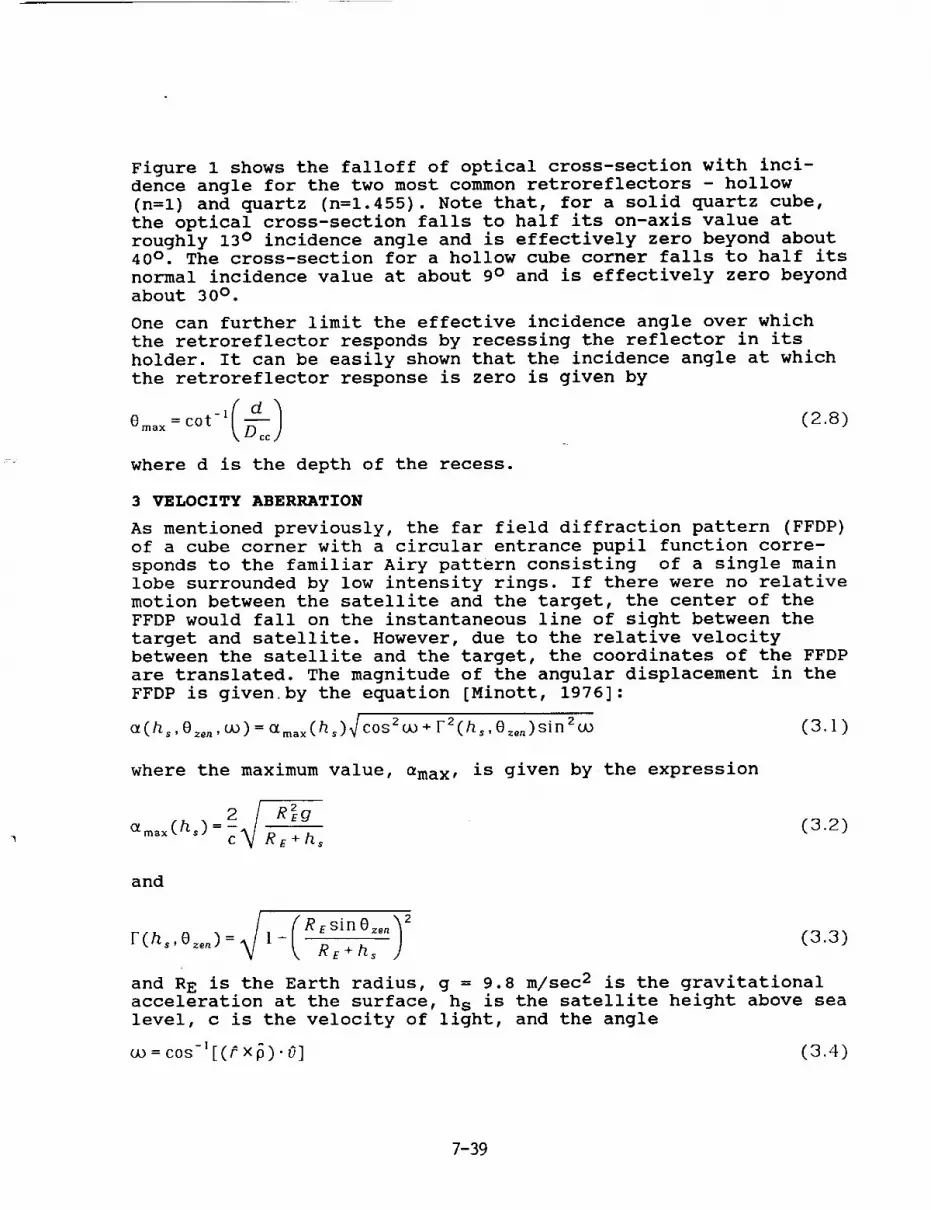
Figure 1 shows the falloff of optical cross-section with inci-
dence angle for the two most common retroreflectors - hollow
(n=l) and quartz (n=1.455). Note that, for a solid quartz cube,
the optical cross-section falls to half its on-axis value at
roughly 13 ° incidence angle and is effectively zero beyond about40 ° . The cross-section for a hollow cube corner falls to half its
normal incidence value at about 9° and is effectively zero beyond
about 30 ° .
One can further limit the effective incidence angle over which
the retroreflector responds by recessing the reflector in its
holder. It can be easily shown that the incidence angle at which
the retroreflector response is zero is given by
Omax=COt-l(D_c ) (2.8)
where d is the depth of the recess.
3 VELOCITY ABERRATION
AS mentioned previously, the far field diffraction pattern (FFDP)
of a cube corner with a circular entrance pupil function corre-
sponds to the familiar Airy pattern consisting of a single main
lobe surrounded by low intensity rings. If there were no relative
motion between the satellite and the target, the center of the
FFDP would fall on the instantaneous line of sight between the
target and satellite. However, due to the relative velocity
between the satellite and the target, the coordinates of the FFDP
are translated. The magnitude of the angular displacement in the
FFDP is given by the equation [Minott, 1976]:
_(hs,e_.,co)= ama×(h_)_cosZco+Fz(hs,e_.)sin2co (3.1)
where the maximum value, amax, is given by the expression
I R_gamax( h,) =_2,1
C %/ RE+h_(3.2)
and
R Esin Oz_,
F(h_, O=_.) = 1 - RE+hs(3.3)
and R E is the Earth radius, g = 9.8 m/sec 2 is the gravitational
acceleration at the surface, hs is the satellite height above sea
level, c is the velocity of light, and the angle
co = cos-' [(r* Xl_ )" 0] (3.4)
7-39

where P, p, and u are all unity length vectors corresponding to
the satellite position vector (relative to the Earth center), the
line-of-sight vector between station and satellite, and the sat-
ellite velocity vector respectively. Since F(hs.8_,) is always
less than unity, equation (3.1) has an effective "minimum" value
for a given 8z_n, when _ = n/2. Thus,
Ot rain ( h s, 0 zo,_) = Ot max (_h s) 1F (h s, 0 zo,_) (3.5)
The maximum and minimum angular displacements of the FFDP are
plotted as a function of satellite height in Figure 2 assuming a
maximum 0ze. of 70 ° . It should be noted from the figure that the
angular displacement decreases with altitude and that the maximumand minimum values converge for high satellites. At ETALON alti-
tudes (19,000 Km), for example, the angular displacement is
roughly constant at about 26 _rad.
6O
5O
40
ot(_.rad)30
20
I' t I I I I''1 I I
C[ma X
F;| 0_11
I I ! I6, 8 10 12
h, (103kin)
10
0 I I2 4
,,,i14 16 18 20
Figure 2: Maximum and minimum angular displacements in the retro-reflector far field diffraction pattern caused by the velocityaberration effect as a function of satellite altitude above the
Earth's surface.
If the target FFDP is angularly narrow relative to the size of
the velocity aberration displacement, the receiver will lie on
the low signal edge of the FFDP or even lie outside the FFDP
entirely. For example, consider a moving retroreflector whoseface is normal to the ranging system line-of-sight. The cross-
section is given by (2.2a) with x=kRccSin(_)-kRcca where alpha is
the instantaneous angular displacement caused by velocity
7-40

aberration. If a << a,u m the reduction in cross-section is negli-
gible. However, if a is large, the reflected beam will "miss" the
receiver and low or nonexistent signal levels will result. For
non-normal incidence angles, the reflected FFDP is no longer cir-
cularly symmetric since the collecting (and transmitting) aper-
ture of the retroreflector appears as an ellipse to the range
receiver. The FFDP peak is again along the instantaneous receiver
line-of-sight, but the FFDP is now given by the two-dimensional
Fourier transform of the elliptic entrance aperture of the corner
cube. The velocity aberration causes the retroreflector response
to be reduced relative to the peak value given by (2.7). This
reduction is greater for velocity vectors which are parallel to
the long axis of the ellipse because of the faster falloff of the
FFDP with angle in this direction.
4 RETROREFLECTOR "SPOILING"
TO reduce the effects of velocity aberration in large retrore-
flectors, the retroreflector is often "spoiled". The goal of
"spoiling" is to concentrate more reflected energy into the
annular region bordered by ama X and ami .. Ideally, one would like
to uniformly spread the energy within the annular ring yielding
an optimum cross-section given by
max -- _ m|n
where the quantity in parentheses is the effective target gain
and _cc is the solid angle subtended by the annular ring of
interest. However, conventional spoiling techniques generally
result in average optical cross-sections which agree only within
an order of magnitude with the ideal limit described by (4.1).
Spoiling is usually accomplished by introducing slight variations
into the cube corner dihedral angles (typically less than two
arcseconds). This creates a complicated FFDP which, for an inci-
dent beam normal to the cube face, breaks the initial single main
Airy lobe into 2N lobes (where N = 1 to 3 is the number of
spoiled dihedral angles) distributed within an angular annulus.
The mean angular radius of the annulus increases linearly with
the dihedral offset angle from a perfect cube and, from diffrac-
tion theory [see (2.3)], one expects the effective width of the
various lobes to depend inversely on cube diameter.
Each of the 2N lobes originates from a different sector of the
retroreflector entrance aperture. In fact, the FFDP of each lobe
is determined by the two-dimensional Fourier transform of the
projection of the 180°/2N sector of the (assumed) circular retro-
reflector entrance aperture into a plane perpendicular to the
line-of-sight between the satellite and the station. The
distribution of energy within this "annulus" is therefore highly
nonuniform. Furthermore, the effective area for each lobe isreduced to:
7-41
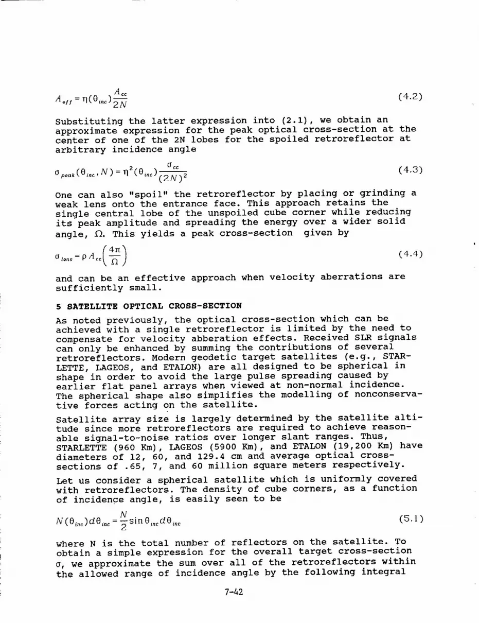
Ace (4.2)d.H=_(O_.c)2N
Substituting the latter expression into (2.1), we obtain an
approximate expression for the peak optical cross-section at thecenter of one of the 2N lobes for the spoiled retroreflector at
arbitrary incidence angle
oc_ (4.3)Opeak(Oi.c.N)=qZ(O_.c)i2N)Z
One can also "spoil" the retroreflector by placing or grinding aweak lens onto the entrance face. This approach retains the
single central lobe of the unspoiled cube corner while reducing
its peak amplitude and spreading the energy over a wider solid
angle, _. This yields a peak cross-section given by
o_. _pAcc _ (4.4)
and can be an effective approach when velocity aberrations are
sufficiently small.
5 SATELLITE OPTICAL CROSS-SECTION
As noted previously, the optical cross-section which can be
achieved with a single retroreflector is limited by the need to
compensate for velocity abberation effects. Received SLR signalscan only be enhanced by summing the contributions of several
retroreflectors. Modern geodetic target satellites (e.g., STAR-
LETTE, LAGEOS, and ETALON) are all designed to be spherical in
shape in order to avoid the large pulse spreading caused byearlier flat panel arrays when viewed at non-normal incidence.
The spherical shape also simplifies the modelling of nonconserva-
tive forces acting on the satellite.
Satellite array size is largely determined by the satellite alti-tude since more retroreflectors are required to achieve reason-
able signal-to-noise ratios over longer slant ranges. Thus,
STARLETTE (960 Km), LAGEOS (5900 Km), and ETALON (19,200 Km) have
diameters of 12, 60, and 129.4 cm and average optical cross-
sections of .65, 7, and 60 million square meters respectively.
Let us consider a spherical satellite which is uniformly coveredwith retroreflectors. The density of cube corners, as a function
of incidence angle, is easily seen to be
N(Oi,_)d0i, =_sin0_,_d0,n_ (5.1)2
where N is the total number of reflectors on the satellite. To
obtain a simple expression for the overall target cross-section
_, we approximate the sum over all of the retroreflectors within
the allowed range of incidence angle by the following integral
7-42

R
(s.2)
where we have used (2.7). If the retroreflectors are not recessed
in their holders, q(Stnc) is given by (2.4). If their angular
response is limited by the recess, the variation can be well-
approximated by the expression
Otnc
q(O_._) = 1--- (5.3)rflaX
where Omax is given by (2.8). Actually, (5.3) is an excellent
approximation to (2.4) as well provided we choose ema × equal to
.54 rad (31 ° ) for hollow cubes or .75 rad (43 ° ) for solid cubes
respectively (see Figure i). Substituting (5.2) and (5.3) into
(5.2) and evaluating the resulting integrals yields
occN 1
V=-'_ (___) 2 (S.4)
Let us now examine the validity of (5.4) by substituting LAGEOS
values. The LAGEOS Satellite has a radius R = 29.8 cm and is
imbedded with 426 retroreflectors (422 fused quartz and 4 germa-
nium) with a clear aperture diameter Dcc of 3.81 cm. Ignoring the
fact that four cubes are germanium, we choose N = 426 and a value
of ema × = .75 rad for solid quartz cubes. We now use a value _cc =
2.834 x 10⁶ in agreement with the input values to the RETRO com-
puter program as determined during LAGEOS testing and evaluation
[Fitzmaurice et al, 1977]. Substituting the latter values into
(5.4) yields
OtAcEos = 9.8Vcc=2.78xlOZm 2 (5.5)
This is roughly equal to the peak value computed by the much more
detailed RETRO program which showed a range of values between .54
and 2.7 x 10⁷ m 2. Equation (5.4) tends to overestimate the actual
cross-section because it includes only geometric, and not veloc-
ity aberration, effects. Equation (5.5) also implies that the
LAGEOS array cross-section is roughly 9.8 times that of a single
cube corner at normal incidence.
7-43
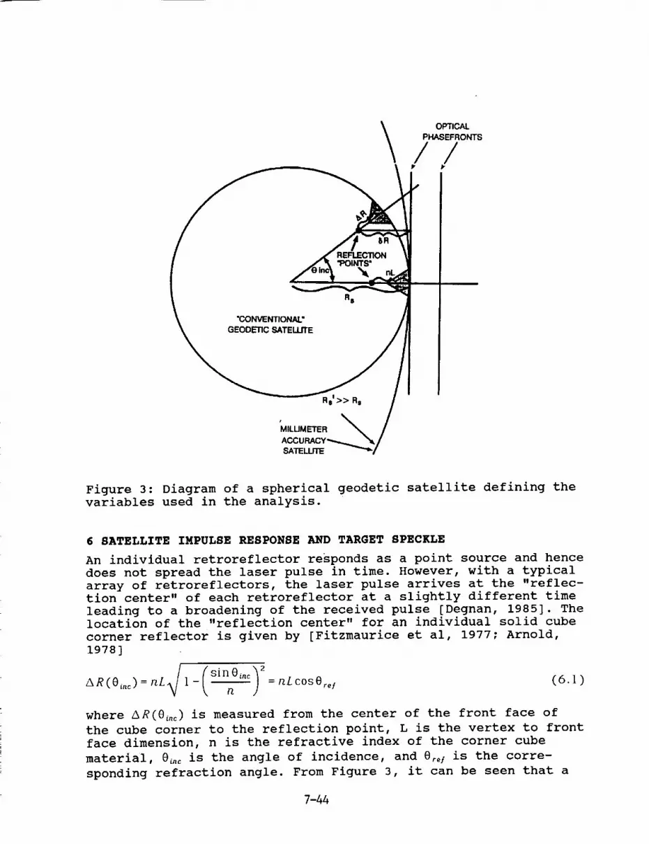
OPTICAL
PHASEFRONTS
//
REFLECTION"POINTS"
"CONVENTIONAL"
GEODETIC SATELLrrE
Rs=>> Ra
MILLIMETER
SATELLITE
Figure 3: Diagram of a spherical geodetic satellite defining the
variables used in the analysis.
6 SATELLITE IMPULSE RESPONSE AND TARGET SPECKLE
An individual retroreflector responds as a point source and hence
does not spread the laser pulse in time. However, with a typical
array of retroreflectors, the laser pulse arrives at the "reflec-tion center" of each retroreflector at a slightly different time
leading to a broadening of the received pulse [Degnan, 1985]. Thelocation of the "reflection center" for an individual solid cube
corner reflector is given by [Fitzmaurice et al, 1977; Arnold,
1978]
si _,cAR(Oi.c)= nL 1 - = nLcosOre/ (6.1)
where AR(0i,c) is measured from the center of the front face of
the cube corner to the reflection point, L is the vertex to front
face dimension, n is the refractive index of the corner cube
material, 0_.c is the angle of incidence, and 0re/ is the corre-
sponding refraction angle. From Figure 3, it can be seen that a
7-44
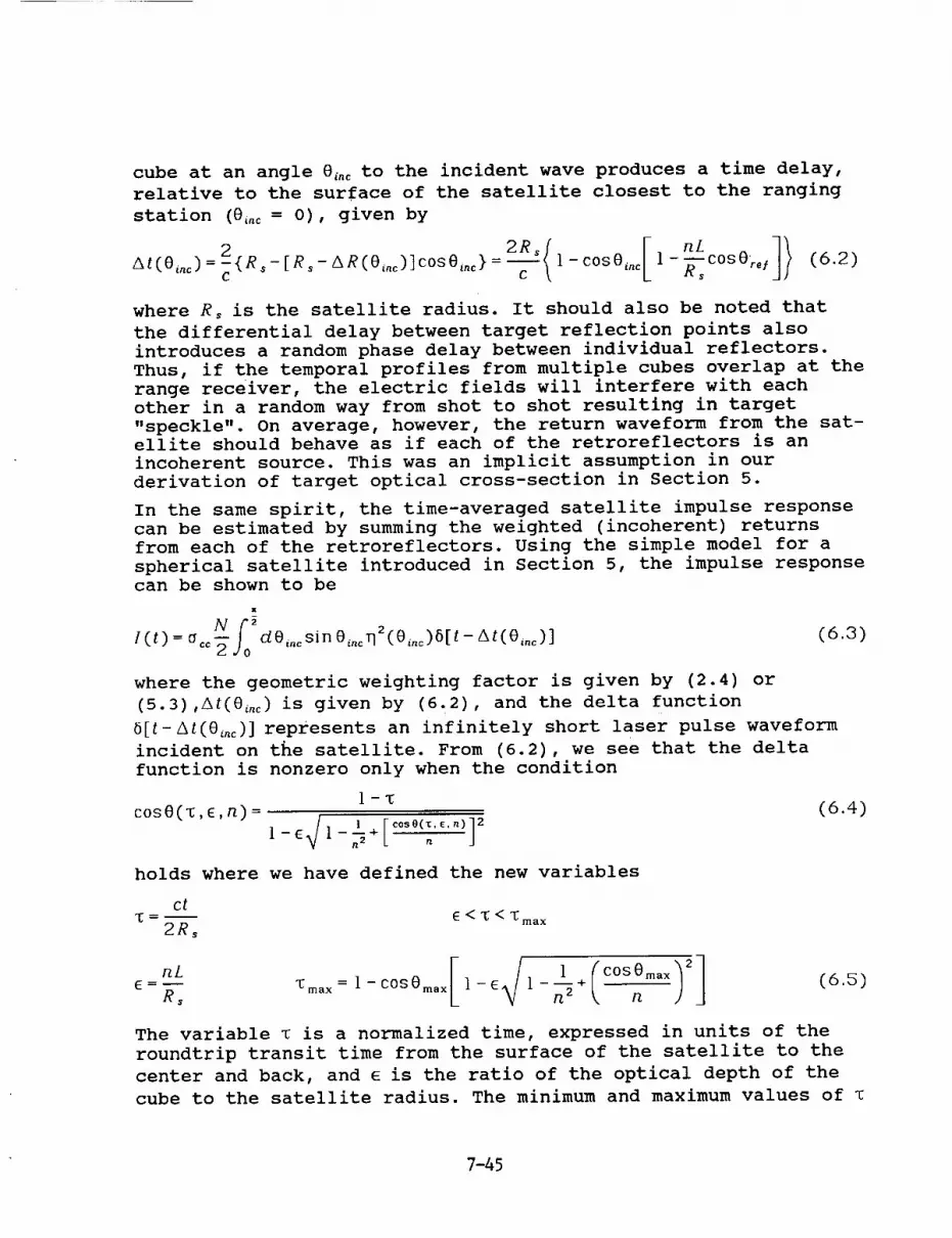
cube at an angle 0i,c to the incident wave produces a time delay,
relative to the surface of the satellite closest to the ranging
station (0inc = 0), given by
At(0inc)=_{R-[Rs-_R(Oinc)]cosOinc}= l--c0s0in e l--EC0S0re I (6.2)C s
where Rs is the satellite radius. It should also be noted that
the differential delay between target reflection points also
introduces a random phase delay between individual reflectors.
Thus, if the temporal profiles from multiple cubes overlap at the
range receiver, the electric fields will interfere with each
other in a random way from shot to shot resulting in target
"speckle". On average, however, the return waveform from the sat-ellite should behave as if each of the retroreflectors is an
incoherent source. This was an implicit assumption in our
derivation of target optical cross-section in Section 5.
In the same spirit, the time-averaged satellite impulse response
can be estimated by summing the weighted (incoherent) returns
from each of the retroreflectors. Using the simple model for a
spherical satellite introduced in Section 5, the impulse responsecan be shown to be
dO,._ sin O,..q2 (O,._)6[t - At(O,._)] (6 3)
where the geometric weighting factor is given by (2.4) or
(5.3),A/(0_,c) is given by (6.2), and the delta function
5[t-_/(0Lnc) ] represents an infinitely short laser pulse waveform
incident on the satellite. From (6.2), we see that the delta
function is nonzero only when the condition
I-TcosO( , ,n) =
, [co,oc c,°,]21 -6 1 -_+ .
(6.4)
holds where we have defined the new variables
ctT -- 6 < T < T max
2Rs
nL 1 + COS max (6.5)6 -- R s T max = I- C0S0ma x i-6 I -_
The variable • is a normalized time, expressed in units of the
roundtrip transit time from the surface of the satellite to the
center and back, and e is the ratio of the optical depth of the
cube to the satellite radius. The minimum and maximum values of
7-45

are determined by setting 8 equal to zero and 8ma × respectively in
(6.4) and solving for _. The total pulse duration, measured at
the baseline, is given by At=tmax-6.
From (5.3) and (6.3), the satellite impulse response can now be
expressed as a function of the variables _, e, n, and @max, i.e.
N [ 0('_, 6,n)72
l('_'6'n'Oma×)=°cc-2sinO(_'6'n)L 1 0--m_x J (6.6)
where 8(T.6.n) is defined by (6.4). In the limit of large satel-
lite diameters (6 _ 0), (6.4) reduces to the simple forml
O(_,O,n)=cos-l(1-_) (6.7)
and (6.6) becomes
2'(T,0,/'_,0max) = 0ceNt/2(1 -_)[ 1 - cos-'(1-,)] 2Omax (6.8)
The quantity'e is typically small and, for nonzero values of e,
(6.4) can be easily solved by iteration using (6.7) as a starting
point, i.e.
I-T
[COS0(T'6'/_)]i÷I = ]-6_ l-nzl--+[[c°se(x'E'n)]J]2--n
(6.9)
until it converges.
As an illustration, let us use (6.6) to estimate the impulse
response of the LAGEOS satellite. Substituting n = 1.455 (fused
silica), L = 1.905 cm, and R s = 29.8 cm into (6.5b), we obtain a
value 6 = .093. We recall that, for solid cube corners, we can
use a value 0ma x = .75 rad. Now, using (6.6) and (6.9), we obtain
the plot of the LAGEOS impulse response shown in Figure 4(a). The
profile shows the characteristic fast rise and long tail of the
LAGEOS response. Furthermore, if we compute a center-of-mass cor-
rection from the centroid of this impulse response profile, we
obtain a value of 250.2 mm which is in excellent agreement with
the accepted LAGEOS value of 249 ± 1.7 mm [Fitzmaurice et al,
1977].
The impulse response in the large satellite limit, given by
(6.8), is shown in figure 4(b) for the case of solid quartz and
hollow cubes. Note that both the temporal width of the reflected
pulse and the target optical crossection is smaller for the hol-
low cubes than for the solid cubes because of their smaller field
of view.
7-46
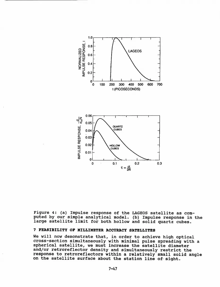
1.0 I
08
N_ 06
0.4
0.2
0 J0 100
I I I _
L I I I _d_--_
200 300 400 500 600 700
t (PICOSECONDS)
0.06
uJo9z 0.04OO..o9 0.03W
nr"w 0.02o9....I
0.01O..
-- 0
0
i I i I i
_OUAR_cuBE_
i I_l I
0.1 0.2
Z=_2R
0.3
Figure 4: (a) Impulse response of the LAGEOS satellite as com-
puted by our simple analytical model. (b) Impulse response in thelarge satellite limit for both hollow and solid quartz cubes.
7 FEASIBILITY OF MILLIMETER ACCURACY SATELLITES
We will now demonstrate that, in order to achieve high optical
cross-section simultaneously with minimal pulse spreading with aspherical satellite, we must increase the satellite diameter
and/or retroreflector density and simultaneously restrict the
response to retroreflectors within a relatively small solid angle
on the satellite surface about the station line o5 sight.
7-47

The total time duration of the reflected pulse (0% to 0% inten-
sity points) can be determined from (6.5), i. e.
At = --('_max- E)=C _ t2sin --+62 COS Omax 1 n2 1 (7 .1)
which, in the limit of small maximum incidence angles, reduces to
-R'0 [- e(l+
In the same limit, Eq.section reduces to
(7.2)
(5.4) for the satellite optical cross-
0"co N
o'- -_- O_,,, (7.3)
As mentioned earlier, the angular response can be restricted by
recessing the retroreflectors in their holders. Substituting
(7.2) into (7.3) yields
OccN CAtmax0 = (7.4)
24 R,[1-"_(I+_)]
We can now express the total number of retroreflectors as
8 2
N=4p_ (7.5)
where _ is a "packing density" ( = .435 for LAGEOS) which repre-sents the fraction of total surface area occupied by the cube
faces. Substituting (7.5) into (7.4) yields our final result
0_ [3R_cAt(7.6)
6Ri
The product _RscAt in (7.6) quantifies our earlier statement
that, if we wish to reduce the amount of pulse-spreading At by
some factor (via reduction of the retroreflector field-of-view),we must increase the retroreflector packing density -satellite
radius product (_Rs) by the same factor to retain a similar tar-
get cross-section.
8 CONCLUSION
As mentioned previously, the principal technical challenge in
designing a millimeter accuracy satellite to support two color
observations at high altitudes is to provide high optical cross-
section simultaneously with minimal pulse spreading. Increasing
the satellite diameter provides: (i) a larger surface area for
additional cube mounting thereby leading to higher cross-
sections; and (2) makes the satellite surface a better match for
7-48

the incoming planar phasefront of the laser beam as in Figure 3.
Simultaneously restricting the retroreflector field of view (e.g.
by recessing it in its holder) limits the target response to the
fraction of the satellite surface which best matches the optical
phasefront thereby reducing the amount of pulse spreading.
For near term experiments, the small radius of STARLETTE makes it
an attractive target for testing and.evaluating two color systems
or for testing atmospheric models. Furthermore, its low altitude
(960 Km) and moderate target cross section results in relatively
high received signal levels. AJISAI, also in a relatively low
1375 Km orbit, consists of small clusters of retroreflectors sep-
arated by large reflecting panels and has comparable signal
strength to STARLETTE. Unfortunately, the satellite is quite
large and simultaneous returns from several retro clusters
results in a complicated satellite signature [Prochazka et al,
1991]. From Figure 4, LAGEOS spreading is in excess of 150 pico-
seconds FWHM in agreement with [Fitzmaurice et al, 1977]
although, with sufficiently short laser pulses (<50 psec),
individual retro rings should be resolvable via streak cameras at
certain satellite orientations. (Note that the simple satellite
model presented here gives an average response over the full
range of satellite orientations and shows none of the structure
expected from a particular orientation). The LAGEOS pulse spread-
ing combined with relatively low signal returns, measured at the
few to several tens of photoelectron level for most systems,
would make the necessary differential timing very difficult [Deg-
nan, 1992].
Another useful target for two-color system evaluation is the
recently launched European Earth Remote Sensing satellite, ERS-I.
It flies at a relatively low altitude (<800 Km) and has a small
compact target consisting of one nadir-viewing retroreflector
surrounded by a uniformly spaced ring of eight identical cube
corners at a nadir angle of 50 ° . Approximate modelling of this
satellite by the author indicates that sharp returns consisting
of one or two peaks (well separated) can be obtained from most
viewing angles as illustrated in Figure 5. At nadir angles
between 0 ° and 15 ° , the nadir viewing cube is dominant whereas,
for nadir angles between 30 ° and 70 ° , the ring provides a sharp
return at virtually all azimuthal angles. At nadir angles between
about 15 ° and 30 ° , there is some overlapping of returns and pulse
distortion.
7-49

ir
ERS-1TEMPORALRESPONSE(50psecPULSE)AZIMUTHANGLE
0o 20' 41_I I I I I I I I 't I I i I I
I I i I I I I I I I I''1 1
i°2,,
t I , J o I o
5r
40tlml
I I
11 _I
200 -_0 im .ran Z
1 I I I I I I I I I I
0
Ilw,_
I . I
Figure 5: Approximate (geometric) response of the ERS-I satellite
to a 50 picosecond pulse as a function of nadir and azimuthal
angle.
9 REFERENCES
Arnold, D. A., "Optical and infrared transfer function of the
LAGEOS retroreflector array", Final Report NASA Grant NGR
09-015-002, Smithsonian Institution Astrophysical Observatory,
May 1978.
Born M. and E. Wolf, "Principles of Optics", Chapter 8, Pergamon
Press, New York, 1975.
Degnan, J. J., "Satellite laser ranging: current status and
future prospects", IEEE Trans. on Geoscience and Remote Sensing,
GE-23, pp. 398-413, 1985.
7-50

Degnan, J. J., "Optimum wavelengths for two color ranging", these
proceedings, May 1992.
Fitzmaurice, M. W., P. O. Minott, J. B. Abshire, and H. E. Rowe,
"Prelaunch testing of the Laser Geodynamic Satellite (LAGEOS)",
NASA Technical Paper 1062, October 1977.
Minott, P. O., "Design of retrodirector arrays for laser ranging
of satellites", NASA TM-X-723-74-122, Goddard Space Flight Cen-
ter, March, 1974.
Minott, P. O., "Reader's Guide to the RETRO Program Output", NASA
TM-X-722-76-267, Goddard Space Flight Center, September, 1976.
Prochazka, I., K. Hamal, G. Kirchner, M. Schelev, and V. Postova-
lov, "Circular streak camera application for satellite laser
ranging", presented at SPIE Conference on Electronic Imaging, SanJose, California, Feb. 24-27, 1991.
7-51

TWO WAVELENGTH SATELLITE LASER RANGING USING SPAD
M94-15584I.Prochazka, K.Hamal, H.Jelinkova
Faculty of Nuclear Science and Physical Engineering,Czech Technical University
Brehova 7, 115 19 Prague 1, Czechoslovakia
phone/fax +42 2 848840, tlx 121254, bitnet [email protected]
G.Kirchner, F.Koidl
Lustbuehel Observatory,Lustbuehel str. 46,A-8042 Graz, Austria
phone +43 316 472231, fax +43 316 462678
GENERAL
When ranging to satellites with lasers, there are several principal contributions
to the error budget : from the laser ranging system on the ground, from the satellite retro
array geometry and from the atmosphere. Using a single wavelength we have been routinely
achieved a ranging precision of 8 millimeters when ranging to the ERS-1 and Starlette
satellites. The systematic error of the atmosphere, assuming the existing dispersion models,
is expected to be of the order of 1 cm. Multiple wavelengths ranging might contribute to the
refinement of the existing models. Taking into account the energy balance, the existing
picosecond lasers and the existing receiver and detection technology, several pairs or multiple
wavelengths may be considered. To be able to improve the atmospheric models to the
subcentimeter accuracy level, the Differential Time Interval (DTI) has to be determined
within a few picoseconds depending on the selected wavelength pair [1].
There exist several projects, based on picosecond lasers as transmitters and on two
types of detection techniques : one is based on a photo detectors like photomultipliers or
photodiodes connected to the time interval meters [5]. Another technique is based on the use
of a streak camera as a echo signal detector,temporal analyzer and time interval vernier. The
temporal analysis at a single wavelength using the streak camera showed the complexity of
the problem [2].
EXPERIMENT SETUP
We are reporting on the novel concept of ranging to satellites at two wavelengths
using a single solid state photon counter. The block scheme is plotted on Figure 1. The
receiver package is based on the Silicon avalanche photodiode [4] capable of single photon
detection. The receiver and detector is common for both wavelengths, the different color
returns are separated in time due to the atmospheric dispersion. In principle, the use of
common detector for both Wavelengths results in system simplicity, stability and accuracy,
as well. Most of the DTI measurement error contributions cancel out by averaging. The
system calibration is simple and straightforward.
The experiment has been accomplished at the Satellite Laser Ranging Station Graz,
Austria, employing the 0.5 meter aperture Contraves tracking telescope. Considering the
available laser technology, the satellite laser telescope transmitter and receiver optics, namely
7-52

the Coude path dielectric coatings, and the detector sensitivity, we have chosen the
wavelength pair of 0.532 #m and 0.683_,m proposed by J.Galgnebet [3]. The laser
transmitter consists of the passively mode locked Quantel Nd:AG laser including the second
harmonic generator, modified by inserting a Raman cell filled by Hydrogen at 25 Bars,
delivering 15 mJ/35 psec at 0.532/_m and 5 ml/25 psec at the 0.683/tin Stokes waves.
Additionally, the anti Stokes radiation at 0.45 _,m having the energy of 1-3 rnJ is generated.
TELESCOPE COUDE PATH TW LASER
iSTARTI
isPADi_. l co! JNTERiFILTER
RECEIVERi
Figure 1 Two wavelengths laser ranging system setup using SPAD
RESULTS
Ranging to several ground targets we obtained a ranging precision of 42 picoseeonds
at 0.532 ttm and 56 picoseconds at 0.683_m. The detector quantum efficiency at both these
wavelengths reaches 20 %. The 6 kilometer distant ground target ranging results is shown
on Figure 2. The first peak corresponds to 0.683 _tm echoes, the second one to the 0.532/_m
echoes. The measured DTI was 303.3 picoseconds. Taking into account the data of the
atmosphere at this time, the calculated value is 299.4 picoseconds. The precision estimate
of our DTI measurement is 4 picoseconds, if 400 returns per color are accumulated.
The first results of two wavelength laser ranging to the Ajisai satellite is on Figure
3, where the range residuals to the fitted orbit are plotted.The lower trace corresponds to the
0.683/_m echoes, the upper one to the 0.532/zm echoes. The DTI value variation along the
pass is caused by changes in the satellite elevation and hence the atmospheric path difference.
Up to now the satellites Lageos, ERS-1 and Ajisai have been ranged with two wavelengths.
Typically a few hundreds of returns per pass and per wavelength have been collected when
the system has been operating at 2.5 Hz. Averaging the two wavelengths data over the whole
pass, the two wavelengths differential time interval has been determined with the precision
typically 7 picoseconds.
7-53

2-COLOR RANGING TO TARGETIRESnDUAL$ of 532/883 nm Pulses
[-6'83 nm: RMS 8.4 mm
I ........
0
1991-12-12
Meas. Dispersion: 45.5 mm I
Calc. Dispersion: 44.9 mmI
(both: 1-Way)
532 nm: RMS 7.9 mm
45 90
Range Residuals, 1-Way [ram]
I
hi
......... | ............... It ...............
135 180 225
Fig. 2
Satellite AJISAI2-Colorr IRanging: 532 and 683 nm
2-Way Dispersion Ins]1.6
0.5
0
-0.5
-1
-1.5
Calc. and Measured Refraction; 532 and 683 nm
............................................................................................................................................................................................................................................................
532 nm Echoes Calc. Refraction 532 nm
....i::i ............i'_ ..........7:::-:::::i:::::_ .................:.......................................:i............... , ." " ".. : .".':: • ;",_:_'i":../ . ' - -." ." :.''". :":. :..::.::.:""::J::..:i:!':':.; _-::.. ..- . ."".... ;+ ........, <,:_-__ .............................................................
683 nm Echoes Calc. Refraction 683 nl_ ÷
2O 67 20I I I I I I I I I I ! I I I I I I I I I I I I I I I I I i I I I
Elevation Angle [Degrees]
1991-12-12
F i9 . 3
7-54

The energy budget, the number of returns per wavelength and hence the differential
time interval precision has been limited by the system ranging repetition rate of 2.5 Hz,
which is determined by the station ranging electronics. Additional limitation is the chromatic
aberration of the transmitter refracting telescope, which limits the minimal divergence
achievable simultaneously on both wavelengths. These two limitations are expected to be
resolved within 1992.
CONCLUSION
Taking into account the energy budget when ranging to a satellite, assuming the data
rate requested for two minute burst averaging and the ground target ranging results, one may
conclude, that the picosecond accuracy of the two wavelength time difference interval is
achievable using this technique. Comparing to the other two wavelengths ranging techniques,
the simplicity, stability and the simple calibration is obvious. Some other wavelengths pairs,
namely the Raman Stokes and anti Stokes, resulting in a considerably higher value of DTI
may be considered. However, the telescope transmitter beam delivering optics has to be
reconstructed.
References
1. J.B. Abshire, Applied Optics, Vol. 19,No.20,1980, p34-36
2. I. Prochazka,K.Hamal,G. Kirchner, M. Schelev, V. Lozovoi,V. Postovalov, SPIE 1449-40
3. J.Gaignebet et al, Technical Digest of the Conference on Lasers and Electro Optics,
CLEO 89, Baltimore, MD, 1989
4. I.Prochazka et al, technical Digest of the Conference on Lasers and Electro Optics, CLEO
90, Anaheim, CA, May 1990
5. B.Greene,proc.of the 6th International Workshop on Laser Ranging Instrumentation,
Antibes,France, 1986
7-55
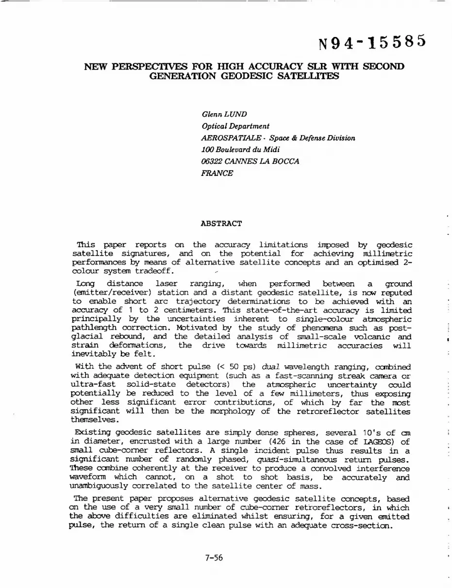
N94-15585
NEW PERSPECTIVES FOR HIGH ACCURACY SLIt WITH SECONDGENERATION GEODESIC SATELLITES
Glenn LUND
Optical Department
AEROSPATIALE - Space & Defense Division
100 Boulevard du Midi
06322 CANNES LA BOCCA
FRANCE
ABSTRACT
This paper reports on the accuracy limitations imposed by geodesic
satellite signatures, and on the potential for achieving millimetric
performances by means of alternative satellite concepts and an optimised 2-
colour system tradeoff. .
Long distance laser ranging, when performed between a ground
(emitter/receiver) station and a distant geodesic satellite, is now reputed
to enable short arc trajectory determinations to be achieved with an
accuracy of I to 2 centimeters. This state-of-the-art accuracy is limited
principally by the uncertainties inherent to single-colour atmospheric
pathlength correction. MDtivated by the study of phencmena such as post-
glacial rebound, and the detailed analysis of small-scale volcanic and
strain deformations, the drive towards millimetric accuracies will
inevitably be felt.
With the advent of short pulse (< 50 ps) dual wavelength ranging, cc_bined
with adequate detection equipment (such as a fast-scanning streak camera or
ultra-fast solid-state detectors) the atmospheric uncertainty could
potentially be reduced to the level of a few millimeters, thus exposing
other less significant error contributions, of which by far the most
significant will then be the morphology of the retroreflector satellitesthemselves.
Existing geodesic satellites are simply dense spheres, several I0' s of cm
in diameter, encrusted with a large number (426 in the case of LAGEOS) of
small cube-corner reflectors. A single incident pulse thus results in a
significant number of randomly phased, quasi-simultaneous return pulses.
These _ine coherently at the receiver to produce a convolved interference
waveform which cannot, on a shot to shot basis, be accurately and
unambiguously correlated to the satellite center of mass.
The present paper proposes alternative geodesic satellite concepts, based
on the use of a very small number of cube-corner retroreflectors, in which
the above difficulties are eliminated whilst ensuring, for a given emitted
pulse, the return of a single clean pulse with an adequate cross-section.
7-56

I RECENT AND IMMINENT ADVANCES IN SLR ACCURACY
Many SLR groups have reported, during the course of the present workshop,
considerable progress in their laser station equipment, as well as in the
performance of data reduction and orbital modeling.
Laser technology has made considerable progress since the days of the first
ruby lasers, and most stations are now equipped with a doubled Nd:YAG. Pulse
widths down to 50 ps, with an output power of - 30 mJ and a repeat rate of -
10 Hz are now being reported and can be expected to become routine
performances in many stations. The temporal width of such pulses is now
responsible for much less of the return signal duration than th.e optical
depth of the satellite itself.
The technology of ultra-fast SPAD (Silicon Photo Avalanche Diode) detectors
would seem very promising for picosecond event timing. Streak cameras,
despite the considerable expense involved in their exploitation, are
recognised not only for their single picosecond capacity but also for their
ability to record single or multiple waveforms (eg. for 2-colour
differential flight time measurements). K. Hamal has reported streak camera
satellite signature recordings from AJISAI and STARLEITE.
The accuracy of atmospheric models, used to correct for the delay in pulse
flight time, is considered to be limited by the small amount of
meteorological data exploited and frc_ which the entire atmospheric profile
is implicitly defined. Although single-colour SLR makes use of a single /n
situ measurement of temperature pressure and water vapour pressure, 2-colour
ranging is expected to enable a considerable improvement to be achieved by
virtue of differential flight time correction. The residual error with this
technique lies in the range of 2 to 3 n_n.
Although several authors have reported improvements in the modeling used to
take into account both gravitational and non-gravitational (radiation,
thermal, drag) orbital influences, the residual bias in the determination of
LAGEOS' orbit is estimated as 2 to 3 cm for I month of data and I cm for a
year of data (R. Eanes). Many sophiticated data reduction and collation
procedures have been elaborated, but the limit in rms baseline accuracy
nevertheless appears to saturate at the level of I cm.
2 RETURN SIGNAL CONVOLUTION BY MULTIPLE ECHOS
The time domain behaviour of a round-trip SLR pulse can be thought of as an
initially narrow Gaussian pulse which is convolved successively by the
atmospheric transfer function (due to refractive index dispersion -
typically - 10 ps), the "forest" of Diracs corresponding to each of thesatellite reflectors "visible" at the ranging instant, the atmospheric
transfer function for a second time, and finally the detector transfer
function. Whereas the emission, detection and atmospheric functions could
well provide a global received pulse FWHM of - 50 ps (7.5 n_n), the satellite
signature, determined by the overlapping reflector echos within its apparent
optical depth, is typically an order of magnitude greater in duration.
The practically indeterminant and undeconvoluable nature of the resulting
signature imposes a practical lim/t in residual range uncertainty varying
between I and 5 cm (depending on the size and characteristics of the ranged
satellite), even after several months of data accumulation. This uncertainty
is represented by _2sat (- > 100 ps) in expression (I) of _3.
7-57

In an effort to eliminate the drawbacks of such complex signatures, a novelgeodesic satellite concept is proposed in which a very small number ofretroreflectors, exhibiting very little or no local FOVoverlap, is arranged
in such a way as to ensure the unicity (or at least unambiguous
identifiability) of the detected return waveforms. Ideally, the apexes of
each retroreflecting cube corner would be mutually co-located at the
satellite's centre of mass. In practice, this requirement cannot be exactly
met, implying either sane form of attitude stabilisation and/or
deterministic correction between measured and true (centre of mass) ranges.
The residual uncertainty in range correction should be no more than I or 2
_I.
Velocity aberration is a parameter of considerable importance, and the
means used to achieve appropriate correction would depend on the
implementation (or not) of attitude stabilisation.
Finally, an adequate systems approach to high accuracy SLR would require acareful tradeoff to be made between the mean satellite reflector cross-
section (i.e. related to the cube corner size, mean incidence angle and
diffraction lobe pattern) and station parameters such as (dual colour) laser
wavelength choice, pulse energy and width, and receiving telescope size. The
latter considerations are adressed on the following section.
3 LINK BUDGET REQUIREMENTS AND SYSTEM CONSIDERATIONS
The parameters which exert an influence on range accuracy include not only
the retroreflector characteristics, but also the laser station design. Range
accuracy and link budget analyses are thus needed in order to ascertain an
optimal approach to the specification of high accuracy SLR satellites and 2-
colour ranging stations, as set out below. The uncertainty in the absolute
value of a 2-colour corrected normal point can be expressed as;
a2 - I ap%lse apulsea 2 = K 1 a2at 4 nois.__et_A2 O2c + 1 +
norm.pt. Nshot Nsho t [Nd_t(_l ) Nd_t(_2) )jj
a)
where ;
• O2sa t is the unaccountable satellite center-of-mass bias,
• a2noise is the cumulated randc_n'variance of the timing system,
• Nshot is the number of shots used to establish a normal point,
• K; is a conversion factor frQm ps to mm,
• (T2sc is the unaccountable Streak Camera bias (typically I to 2 ps),
• _2puds e defines the received pulse width ((_ = 0.425 FWHM),
• A is the 2-colour correction sensitivity (related to )%1 and )%2), and
• Ndet (A) is the number of detected photons at wavelength I.
The expected number of detected photons at a given wavelength is derived
from the link budget analysis as follows :
®Ndet=K2{2_.R--_(z).l-_.(,-Si/40).T2tm(Z).QE(2_)} Semit'tel "_2cx [ Q2
7-58

where ;
• K2 is a constant including geometrical factors optical efficiencies,
• R is the station to satellite range,
• _0 is the emitted beam divergeance,
• @ is the local incidence angle of the rangi_ beam relative to the
reflector normal. (1- 8/40) gives a close approximation to the cube-
corner cross-section falloff as a function of incidence angle),
• Tat m is the l-way atmospheric transmission, depending on range angle Z,
• QE l is the receiver detector quantum efficiency at wavelength _,
• Eemit is the emitted pulse energy,
• _te/ is the station receiving telescope diameter,
• _oc is the retroreflector diameter, and
• _2 is the equivalent angular diameter of the retroreflector diffraction
pattern.
Expression (2) has been grouped into two parts of which the first includes
non-system or typically invariant parameters, whereas the second contains
those variables which depend on the station (laser, telescope) and satellite
(retroreflector size, diffraction pattern) designs.
The term _x/se in (I) is also considered as a system parameter, and has
been combined with the second group of variables in (2) to form the quantity
Xsyst :
_2 _2
Emit" tel" cc Ij.m4.rad-2.s-21Xyst: o,E, eo,_,eo _,S2 = _2. o2
(3)•, t
pulse
Tradeoff analysis of the satellite and laser station characteristics can be
made on the basis of the numerical evaluation of this quantity. Although the
factor A is also a system-related parameter, its numerical value happens to
be very similar for the 2 cases treated below and is there-fore not included
in the above expression. In the following, it is assumed that _ is not
dependant on Zcc, but rather on an engineered diffraction lobe pattern; a
conservatively large value of _ is taken, corresponding to diffraction into
a uniform ring 2.5 arcsecs in width, at a mean distance of 9 arcsecs from
the incoming beam direction.
Figures (I) and (2) thus illustrate the computed variation of the 10-shot
ranging accuracy (_Norm.Pt. (exp. I) as a function of Xsyst., for a 800 km
circular orbit and negligeable center-of-mass bias (_sat), at four values
of zenith ranging angle : 0°, 20°, 40 ° & 60 ° (assuming 10 km Standard
Atmosphere visibility), and for two different cases of dual wavelength laser
configuration :
Fig.1 Doubled & tripled Nd:YAG,
Fig.2 Fundamental & doubled (eg. Ti-Sapphire) wavelengths @ 800 & 400 nm.
7-59
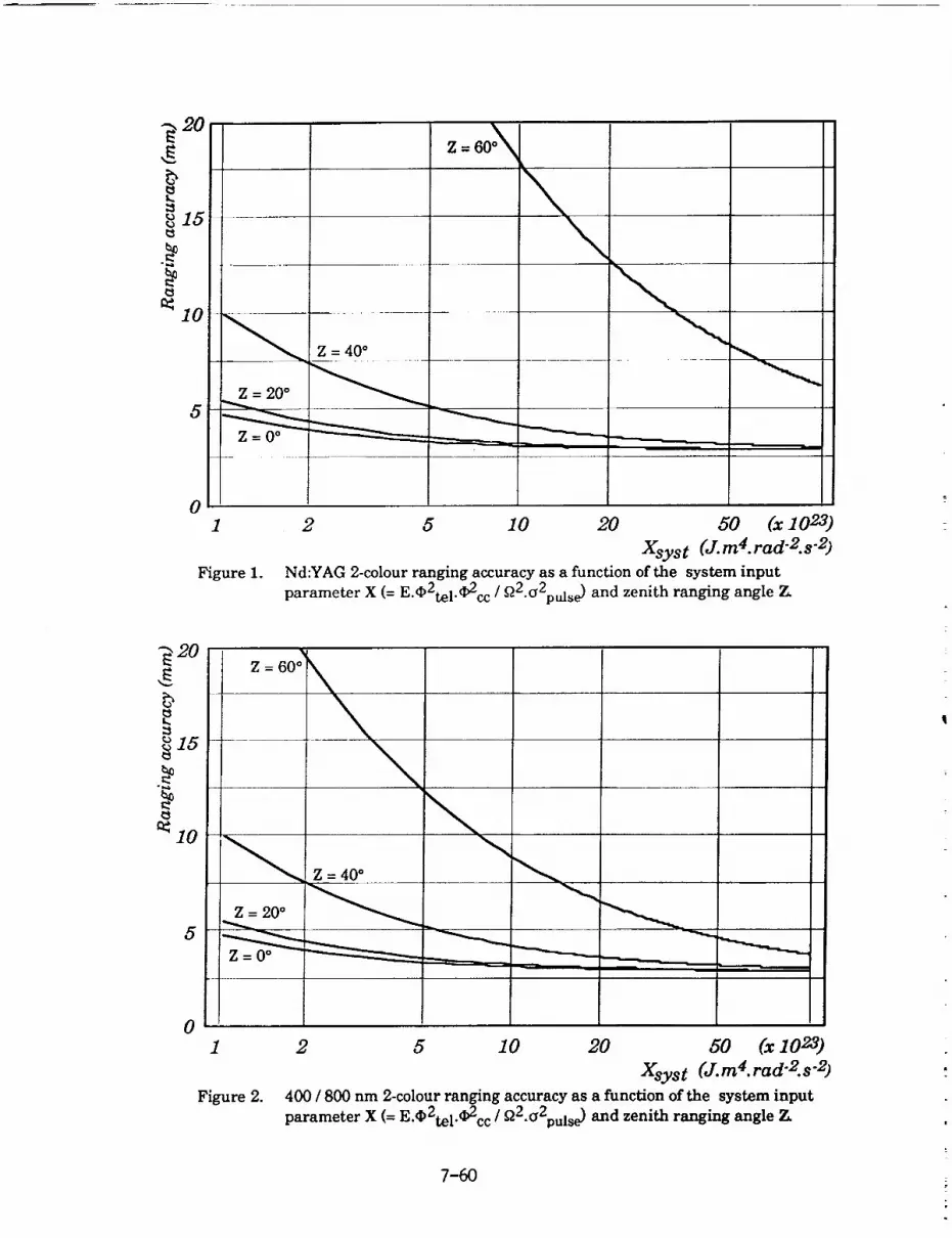
9 20
k.
15
10
g = 40°
Z = 20 ° _
I
01
Figure 1.
2 5 10 20 50 (x 1 023)
Xsyst (J.m4.rad'2.s "2)
Nd:YAG 2-colour ranging accuracy as a function of the system input
parameter X (= E.O2tel.O2cc / fl2.a2puls e) and zenith ranging angle 7_
920Z = 60 ° \
\
_15
_ 10 .......
01
Figure 2.
2 5 10 20 50 (x 1023)
Xsyst (J.m4.rad'2.s "2)
400 / 800 nm 2-colour ranging accuracy as a function of the system input
parameter X (= E.O2tel.¢2cc / _2.g2puls e) and zenith ranging angle Z,
7-60

The resulting curves show (for example) that if sub-centimetric ranging
accuracies are to be achieved with 2-colour systems up to zenith angles of
60 ° , cne could accept a value of Xsyst. >- 7-1023 from the fundamental/doubled
system, whereas a factor of - 8 improvement would be needed for oomparable
performance from a Nd:YAG station.
The above example supposes normal incidence at the retroreflector, and
could be provided by the following numerical values for a 800 / 400 nm
system and a single cube-corner retroreflector :
• = 40 mJ
" _te/ = 30 cm
• _cc = 4ore
• G_dse = 43 ps (FWHM_dse = 100 ps)
By shortening the emitted pulse FWHM to - 50 ps, one could achieve the same
performance at local retroreflector incidences up to 300. An additional
factor of - 3 improvement in telescope or reflector diameter would be
required to achieve the same result with a Nd:YAG laser (assuming 40 mJ and
50 ps FWHM to be near to the practical limits for the emitted pulse power).
Further improvements could be achieved with still shorter pulses (in the
case of a broad bandwidth amplification medium), or a larger number of
pulses per normal-point. At the satellite level, larger retroreflectors, or
more ccnfined diffraction lobe patterns could be considered, without having
to resort to the classical multiple reflector solution.
The strong link budget dependance on orbital height (_ R-4) w_Id probably
render single-reflector satellites unsatisfactory for orbits higher than a
few 1000 km, if sub-centimetric accuracies were to be expected at high
zenith angles and with. a small number of pulses per normal point.
These considerations are encouraging, as they suggest that millimetric
center-of-mass determinations could well be achieved with dual-colour SLR,
provided appropriate consideration is given to the design of future geodesic
satellites.
4 SECOND GENERATION REFLECTOR SATELLITE CONFIGURATIONS
It has been pointed out at the beginning of th/s paper that in the
interests of a clean return signature and unambiguous center-of-mass
determinations, the "ideal" geodesic satellite should exhibit non-
overlapping reflector FOVs in order to inhibit multiple ecb_ returns,
whereas the link budget calculations given in § 3 show that a single
retroreflector of reasonable dimensions could provide adequate return signal
strength for millimetric range determination accuracies.
A parameter of considerable importance in the retroreflector design is that
of velocity aberration correction, in which an appropriate trade-off is
needed between link budget considerations (influenced by the value of _) and
stabilisation of the reflector orientation relative to the orbital plane.
Two fundamentally different approaches could thus be used, according to the
choice between ultimate satellite simplicity and optimal link budget
performance, as set out in the examples below :
7-61
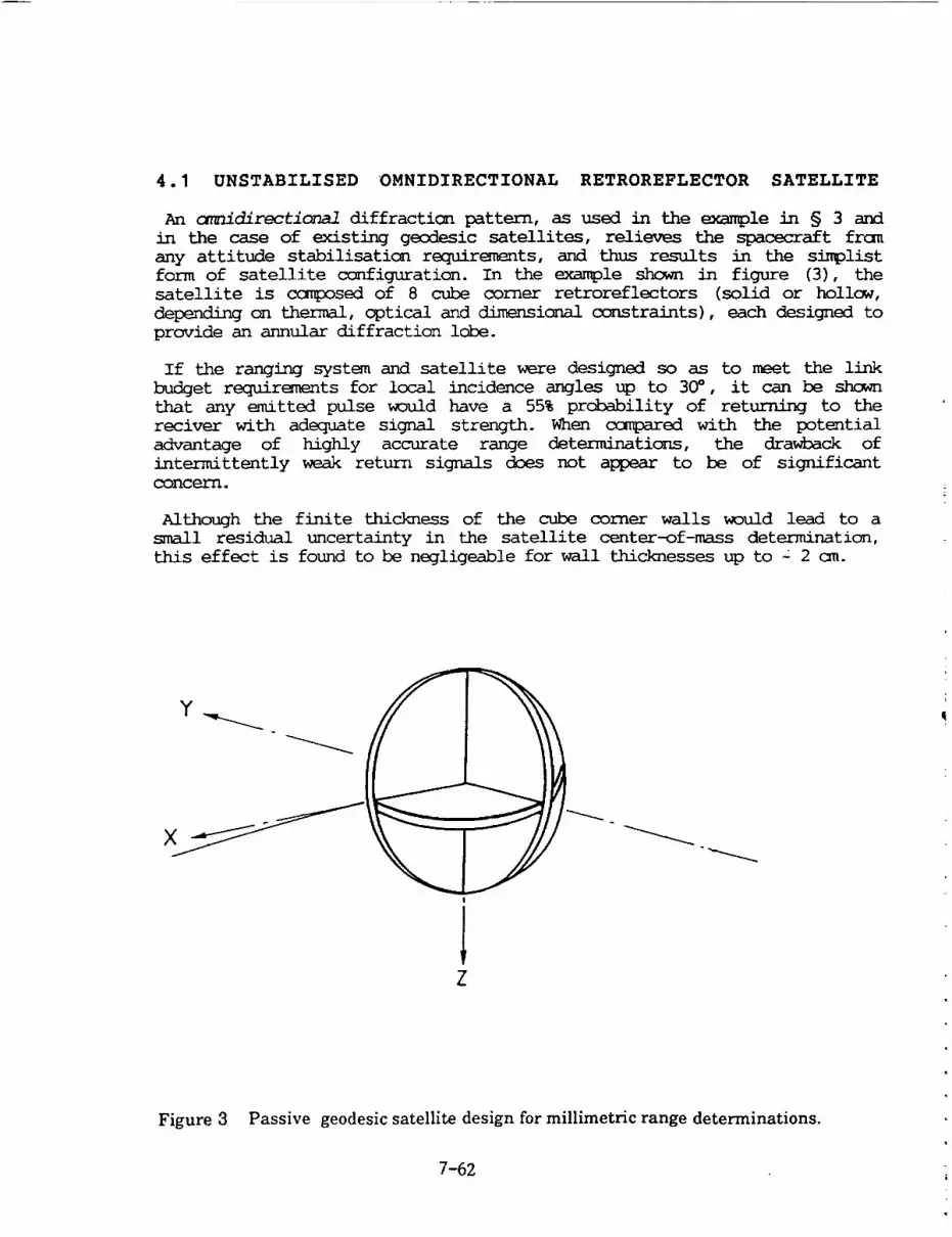
4.1 UNSTABILISED OMNIDIRECTIONAL RETROREFLECTOR SATELLITE
An cmnidirectional diffracticn pattern, as used in the example in § 3 and
in the case of existing geodesic satellites, relieves the spacecraft from
any attitude stabilisaticn requirements, and thus results in the simplist
form of satellite configuration. In the example shown in figure (3), the
satellite is crmp0sed of 8 cube corner retroreflectors (solid or hollow,
depending on thermal, optical and dimensional ccrastraints), each designed to
provide an annular diffraction lobe.
If the ranging system and satellite were designed so as to meet the link
budget requirements for local incidence angles up to 30° , it can be shown
that any emitted pulse _ould have a 55% prchability of returning to the
reciver with adequate signal strength. When cc_pared with the potential
advantage of highly accurate range determinations, the drawback of
intermittently weak return signals does not appear to be of significant
concern.
Although the finite thickness of the cube corner walls would lead to a
small residual uncertainty in the satellite center-of-mass determination,
this effect is found to be negligeable for wall thicknesses up to = 2 cm.
Z
Figure 3 Passive geodesic satellite design for millimetric range determinations.
7-62

4.2 STABILISED DIRECTIONAL RETROREFLECTOR SATELLITE
The link budget performance of the previous design could be ccnsiderably
improved by concentrating the diffracted energy into 2 small lobes (i.e. by
reducing _), as is the case with the proposed GLRS-R ground target design
(reported elsewhere in these proceedings). This approach could only be
impl_nented if the direction of the diffraction lobes were appropriatelymaintained in alignment with the direction of relative movement between
emitter and reflector.
In Figure (4), such a satellite design is shown, in which spin stabilisedattitude control is used to maintain one of each of the cube corner dihedral
angles in a direction perpindicular to the orbital plane. These dihedral
angles would be slightly spoiled from perpindicularity so as to generate two
small diffraction lobes in opposite directicns, of sufficient amplitude to
correct for the velocity aberration. A gain of - 10 or more in return signal
strength, cc_pared with the annular diffraction lobe design, could be
expected.
Although a sp/n stabilisation is shown here, 3-axis stabilisation could
also be envisaged - thus requiring a smaller number of cube corners. In both
cases the attitude control _uld not have to be very precise (typically -
+ 5° should be adequate), and could be achieved using virtually passive
systems such as magnetic torquers. A further possibility would be to use a
completely passive 3-axis stabilisation system based on gravity masts.
| i
V
Figure 4 Spin-stabilised geodesic satellite design for millimetric range determinations.
7-63

5 CONCLUSIONS
It has been shown from link budget analyses that, when coupled with an
appropriate satellite configuration, realistic single retroreflectordimensions could enable millimetric absolute accuracies to be achieved with
future 2-colour SLR, through the removal of center-of-mass uncertainties in
the range determination.
The engineering of retroreflector velocity aberration corrections is an
important factor in the design of a geodesic satellite and in the link
budget performance to be expected from the _lete ranging system.
Two approaches to the design of second generation geodesic satellites have
been suggested. Although these might imply the use of non-spherical orbiting
bodies, with ccrLsequently higher atmospheric drag and solar radiation
pressure imbalances than for existing satellites, they could nevertheless
enable excellent geometric mode (short arc) range determinations to be
achieved, and could be expected to provide very good long arc performance
for high altitude orbits.
7-64

SLR Data
Analysis/Model Errors


N94-15586
STATE-OF-THE-ART SATELLITE LASER RANGE MODELINGFOR GEODETIC AND OCEANOGRAPHIC APPLICATIONS
S.M. Klosko
Hughes ST Systems Corporation Lanham, MD 20706
D.E. Smith
NASA/GSFC, Greenbelt, MD 20771
Abstract
Significant improvements have been made in the modeling and accuracy of Satellite LaserRange (SLR) data since the launch of LAGEOS in 1976. Some of these include; improvedmodels of the static geopotential, solid-Earth and ocean tides, more advanced
atmospheric drag models, and the adoption of the J2000 reference system with improvednutation and precession. Site positioning using SLR systems currently yield -2 cm staticand 5 mm/y kinematic descriptions of the geocentric location of these sites.Incorporation of a large set of observations from advanced Satellite Laser Ranging (SLR)tracking systems have directly made major contributions to the gravitational fields and inadvancing the state-of-the-art in precision orbit determination. SLR is the baselinetracking system for the altimeter bearing TOPEX/Poseidon and ERS-1 satellites and thuslywill play an important role in providing the Conventional Terrestrial Reference Frame forinstantaneously locating the geocentric position of the ocean surface over time, inproviding an unchanging range standard for altimeter range calibration and for improvingthe geoid models to separate gravitational from ocean circulation signals seen in the seasurface. Nevertheless, despite the unprecedented improvements in the accuracy of themodels used to support orbit reduction of laser observations, there still remain systematicunmodeled effects which limit the full exploitation of modern SLR data.
1. INTRODUCTION
The analysis of Satellite Laser Ranging (SLR) data requires precise dynamic modeling ofa rapidly moving near-Earth orbiting target. Through the application of the theory ofmotion for an orbiting object, both the satellite position and the SLR observing sites canbe located in a common reference frame through the accurate determination of thesatellite ephemerides. The principal model needed for the computation of a satellite's
trajectory is that of the gravitational field which accurately reflects the inhomogeneousdistribution of the Earth's mass, and the temporal changes in the field due to tidal and
presently unmodeled climatological sources. Depending on the orbit of interest and thearea-to-mass ratio of the satellite, non-gravitational forces arising from the effects of
8-1

atmospheric drag and solar radiation are also important. Ground tracking systemsprovide an accurate means of sensing the perturbed motion of satellites. The primaryadvance in SLR geophysical applications comes through improvements in gravitationalfield modeling. By modeling the SLR measurements within global orbit solutions frommany satellites, the broad features of the gravity field have been unambiguouslydetermined. When combined with other less accurate forms of satellite tracking, satellite
altimetry and surface gravimetry, the gravity field is sensed over an extensive spatialbandwidth. Using all these measurements has yielded comprehensive models of theEarth's gravity field in the form of spherical harmonic coefficients. These solutionsdescribe the complex shape of the geoid as well as the resulting variation in thegravitational potential at altitude which perturbs the orbits of near-Earth artificial satellites.
SLR-based geodesy has benefitted from three achievements over the last 15 years.The first and certainly the most important is the advancement in laser tracking hardware.Since the launch of LAGEOS in 1976, laser systems have improved from 50 cm tocentimeter level accuracies. With this rapid change in technology and an expanding
global network, the laser data themselves were able to directly contribute to geophysicalmodeling. However, although great advances have been made, the SLR methodologyhas always been and continues to be geophysical and measurement model limited.
Laser systems are currently the most accurate and advanced means of precisionsatellite tracking. These ranging systems have substantially evolved, undergoing nearlya threefold improvement in system precision every five years during the last 15 years.The evolution of laser systems in monitoring the motion of near-Earth satellites has in turnresulted in much more stringent demands for geophysical models being used forrepresenting the data to the sub-centimeter level.
Today the precision of existing SLR measurements is less than a cm for the bestInstruments. The process of forming laser normal points, a type of compressed data,effectively eliminates spurious observational noise of the current measurements. For allthe laser data, there are systematic errors which are not eliminated in the normal pointcomputation process. The effects of atmospheric propagation, especially horizontalgradients in the atmosphere which are not detectable by the surface meteorologicalmeasurements made at the laser sites, are the largest source of systematic error.Estimates of these errors are in the 0.5 to 2 cm range (Abshire and Gardner, 1985).
Electronic errors, non-linearities in the tracking electronics as a function of signal strength,errors in the distance to the calibration targets, together with remaining spurious effectsall result in a range system capable of 1-2 cm absolute accuracy for the current SLR data(Degnan, 1985) with further improvements in tracking hardware in progress.
2. IMPROVED GEOPOTENTIAL MODELING
Since the launch of LAGEOS, the gravity model has been improved through the
analysis of millions of laser ranges acquired on satellites which span a wide range oforbital Inclinations. Knowledge of the geopotential field has improved in accuracy by anorder of magnitude or more, especially for the longest wavelength portion of the field.
8-2

Closelycoupled"withthe improvementin thegravityfieldwasthe developmentof ancillaryforce, environmental, and measurement models which enabled the exploitation of thesedata closer to their precision. Advanced solid Earth and ocean tidal models, descriptionsof site motion due to various sources of loading, and improved realization of a
geocentrically referenced Conventional Terrestrial Reference System all played animportant role in the more accurate representation of SLR data in the orbit determinationprocess. The very significant impact of the precise SLR data on the gravity solution wasdemonstrated when LAGEOS observations first were included in the GEM-L2 solution.
This solution used 2.5 years of measurements acquired by third generation laser systemsfrom 20 globally distributed stations. Given the stability of the LAGEOS orbit against theinfluences of solar radiation pressure and atmospheric drag, a well isolated gravitational
signal was available for geopotential modeling. While complex non-conservative orbitaleffects are seen on the LAGEOS orbit leading to numerous important studies (e.g.
Rubincam et al., [1987]; Rubincam, [1988,1990]; Afonso et al., [1985]; Scharroo et al.,
[1991]), these effects are far smaller and much better modeled than are the non-conservative effects on less stable lower orbiting satellites. For example, Starlette, likeLAGEOS, is a small dense sphere. However, this satellite at its 800-1200 km altitude, it
is subjected to atmospheric drag perturbations of several m/day 2 in the along trackdirection depending on atmospheric conditions whereas the along track "drag" (includingthermal, neutral density and charged particle) on LAGEOS is approximately 2 cm/day 2.The GEM-L2 solution contained 630,000 laser measurements, about 70% of which were
the high quality ranges to LAGEOS. During the time interval of 1979-1981 where theLAGEOS data used in GEM-L2 were taken, the best systems operated at single shot
precision levels of approximately 5-cm. The LAGEOS range measurements were by farthe most precise satellite observations used in GEM-l_2 and the significant improvementseen in this model is directly attributable to LAGEOS' contribution.
In the mid-1980's, preparation for orbit determination support for the TOPEX]PoseidonMission began in earnest with the goal being to achieve 10 cm RMS radial orbit modeling.This necessitated a complete reiteration of the GEM solutions requiring recomputation ofall of the normal equations in order to benefit from modern constants and models. It wasalso essential to significantly increase the size of the gravity field to realize the full benefitof better modeling available at this time. Further improvements in laser tracking
technologies (e.g. single photon tracking using more sensitive detection technologies withmulti-channel plates), required consideration of force and measurement modelsaddressing effects at the cm level. New models were introduced to meet advancing lasertracking precision. The recent GEM-T2 solution (Marsh et al., 1990) is an example of thenew series of GEM solutions. It contained over two million observations from 1130 arcs
spanning 31 satellite orbits. There was also a significant improvement in the laser dataincluded in the GEM-T2 solution. Third generation SLR observations from Starlette, Ajisai,
LAGEOS, BE-C, GEOS-1 and GEOS-3 were included. Second generation data setsincluded SEASAT and GEOS-2. Early laser data taken on BE-B, D1-C, D1-D and PEOLEwere also used. GEM-T2 effectively exploited the available historical satellite trackingdatabase available for geopotential recovery. GEM-T2 extended the truncation limits ofthe satellite solution for certain resonance and zonal orders to degree 50. The GEM-T3
solution (Lerch et al., [1992]), which combines satellite models with surface gravimetry
8-3
and satellitealtimetryfrom GEOS-3, SEASAT and GEOSAT, represents the most robusttreatment of these diverse data sets within the GEM models.
2.1 IMPROVEMENTS IN SUPPORTING GEOPHYSICAL MODELS
Additional model improvements have significantly contributed to improved representationof the SLR data within orbital solutions. These improvements fall mutually into two
categories. The first entails improvement of the other geophysical models effecting orbitdetermination and the time-dependent positioning of the observer within a well definedConventional Terrestrial Reference System (CTRS). The second category concerns model
optimization, and the ability to extract the best signal from the diverse observational dataset available for geopotential recovery. The first category will be reviewed below.
SLR-geodesy is based on the exploitation of the functional relationships between veryprecise observations and the underlying model parameters. These parameters are eitherpart of a model used to environmentally correct the data or are part of the physicalmodels which describe the perturbations acting on a satellite and observer-to-satellitepositioning. Model parameters are classified in two groups; arc parameters which areorbit-specific including the initial satellite state-vector, atmospheric drag coefficients, solarradiation modelling parameters, measurement related parameters such as measurementbiases etc.; and common parameters which are satellite-invariant including tracking stationpositions and their motions (tectonic and environmental), reference frame parametersincluding polar motion and Earth rotation, nutation and planetary ephemerides, and thegeophysical force models representing the static and time-dependent gravitational field.
Improved modeling of satellite tracking data over the years has progressivelycontributed to the accuracy of SLR solutions. Table 1 shows that recent GEM modelshave significantly increased the number and complexity of the models used to computeorbital motion due to temporal gravitational effects and those used to position an Earth-fixed observer. This development parallels that used at GSFC in the overall analysis ofSLR. These models are required to support cm-ievel geodesy which has resulted in large
increases in the size of various models. By increasing the number of harmoniccoefficients in both the static and tidal gravity models, the truncation effect on low orbitingsatellites is reduced. For example, based on the evaluation of the TOPEX orbit byCasotto (1989), the ocean tide model required for TOPEX to reduce omission effectsbelow the one cm RMS radial error has required us to develop and employ ocean tidemodels containing more than 7000 terms spanning 96 discrete tidal lines. Along withimproved and more complete models of tidal changes in the geopotential fields, relianceon space-based determinations of Earth orientation parameters, creation of SLR normalpoints, and improved accommodation of non-conservative force model effects have allmade significant contributions to recent solutions.
These supporting models were not available for earlier studies or for the supportingsite positioning and Earth orientation recovery. The attendant model error created
systematic errors in both the orbits and the recovered parameters over a large range ofspatial and temporal scales. To reduce these errors, temporal averaging was extensivelyapplied. For example, early GSFC site positioning solutions focused on annual solutions
8-4

(Christodoulidiset al., 1985). Earthorientationparameterswere recovered using 5-dayaveraging. With the current level of supporting models, less averaging is needed. RecentGSFC solutions (Robbins et al., 1992) now yield monthly station positions and dailyvalues of Earth pole and length of day variations. Also, the improved stability of the longperiod reference frame has permitted direct recovery of horizontal site velocities which aremuch less distorted by the former neglect of some important long period force modelingeffects which cause a drift in the orbital frame with respect to Conventional TerrestrialReference Frame.
The importance of these models are quantified by mapping them into the space of thelaser observations on Starlette and LAGEOS (Table 2). The contribution to the variance
of the range residuals of numerous models which have been introduced into the analysisof the SLR observations are tabulated. The level of modeling has been systematicallystepped back to that which was used to develop GEM-L2. Simulated laser ranging froma global network was generated using all of the current TOPEX standard models (Wakker,1991). These models were then eliminated to demonstrate the sensitivity of the satelliteranging to each model in turn. These two satellites are at widely separated altitudeslargely spanning the geodetic orbits currently available. While cm-level modeling is stilla goal, Table 2 demonstrates that a great many effects must be considered when thislevel of modeling is required. Since many of these effects are similar to the signal arisingfrom the static gravitational field, some aliasing will occur within geopotential solutionsdue to the limitation and/or neglect of these and other supporting models. Developingmodels which support mm level ranging will require further advances in the understandingof the geophysical response of the Earth. For example, Figure 1 presents a comparisonof the laser site motion due to ocean loading using two independent models (Ray andSanchez, 1989 vs IERS Standards, 1990) for the largest M2 constituent at the Maui,Hawaii site. While these models are suitable to support cm level geodesy, mm level dataprecision is rapidly approaching and will require extensive (especially environmental)modeling improvements.
The current gravity models cannot be expected to yield orbit errors at the overallaccuracy level of the laser data themselves. The projections from solution covariancesreflect instead, our overall ability to fit these data a posteriori as reviewed in Table 3.This limitation in our ability to model the laser ranges is a vexing problem for there aremany unmodeled error sources which contribute to the post-solution data fits. Amonglikely candidates, we have some evidence that the error attributable to the static or tidalgravitational field is no longer the major contributing factor to the observation residuals.This conclusion is reached by taking individual satellite data sets like the laser dataacquired on Ajisai and giving these data extremely high weight in test solutions. Whensuch solutions are then tested, there is little improvement in the Ajisai orbital fit. Thisindicates that other effects are playing a significant role. Yet this inability to fit the dataat their noise levels has important consequences.
It has long been observed that precise SLR observation residuals from orbit solutionsexhibit systematic behavior within each pass, even after adjustment of the gravity field.An analysis of 600 passes of Starlette SLR data reveal that over 90% had apparent biases
of 3 cm or more. This residual characterization is dominated by orbit modeling rather
8-5

thanobservationshortcomings. As a resultof large (as compared to SLR nominal data
accuracy) unmodeled effects in the residuals, their variance is much higher than that ofa random effect. Thus, not all of the geodetic information can be extracted from these
precise data. For example, gravitational signals which would otherwise be detectable atthe cm level are obscured. If these data could be fully modeled with their gravity signalexhausted, there would be a considerable improvement in the accuracy of the SLR
geodetic products produced using these data.
From the previous discussion, gravitational and orbit positioning solutions based uponnear-continuous inter-satellite tracking have certain advantages. They largely eliminatethe need to make complex media corrections to the observations since they are madeabove the atmosphere. Of course, force modeling errors effecting the orbit arising fromsolar radiation pressure and atmospheric drag still require further improvement. However,a word of caution is warranted. While continuous high precision tracking above the
atmosphere like GPS tracking of TOPEX will eliminate many sources of systematicmodeling error, the basic parameterization of the gravity field as a static and tidallyvarying physical system may itself have significant shortcomings. Only now are wecoming to realize that there are a great number of environmental sources of massredistribution arising from meteorological sources, such as variations of the atmospheric
pressure field (Chao and Au, 1991) and continental water storage (Chao and O'Connor,1988) which require much more attention in current orbit determination processes. Thesemeteorological fluctuations, although having strong seasonality, are rather erratic in natureon shorter time scales. A recent report by Nerem et al., (1992) shows significant changesin the LAGEOS sensed zonal harmonics of the gravitational field related to atmosphericmass redistribution within monthly solutions. Evidence is mounting that these sourcesof unaccommodated signal are being sensed well above the noise level exhibited bymodern SLR/GPS tracking systems. Treatment of these effects will require extensiveevaluation of in situ data sources many of which are currently insufficient for the modern
needs of precision orbit modeling. Neglect of these effects can limit the detection of
signals of great general interest, such as the changes in the geopotential field due topost-glacial rebound, tectonic movement, and core activities.
3. SLR SUPPORT OF OCEAN APPLICATIONS
Satellite Laser Ranging will be used to support oceanographic science through thetracking support provided on recent satellite altimeter missions. Both TOPEX]Poseidon(launched in August 1992) and ERS-1 (launched in July 1991) are heavily dependent onSLR data for precise orbit determination. The accuracy of the orbital reference providedby SLR directly impacts the ability of these missions to geocentrically monitor the oceansurface over time needed for studying global ocean circulation.
From the analysis of the climatological models, the sea surface is known to depart
significantly (==70 cm) from the geoid, and is offset in its center of figure with respect tothe earth's center of gravity by as much as 25 cm. The absence of perfect symmetry of
the dynamic height field with respect to the geocenter gives rise to non-zero degree oneterms in the spherical harmonic expansion of the ocean topographic field (see Figure 2).
The degree one terms in the absolute ocean height models are essential for
8-6

understandinglong term changesin thecharacterof the dynamicheightfield. C,S(1,1)describetheeast-to-westslopeof theoceantopographyacrossthe majoroceanbasins.The C(1,0)has implicationsfor understandingthe seasonalthermal expansion of theoceans. Eachof these termshas an importantphysicalbasis. Thevaluesfor the firstdegreetermsfromclimatologyImplythat onaverageoverthepast70years,the southernoceansaremoredensethan their northerncounterparts,andthat the westernportionofthe majorgyresaremoreenergeticthan that of the east;eachof theseobservationsareseen in the in situ data record. It is thereforeimportantto verify that these terms areaccuratelydeterminedwithin the satelliteanalyses. Theseterms areof specialconcernfor they are of the 1 CPR spatial scale of the dominant orbit error.
The orbital motion of a an altimeter satellite exhibits an integrated response to the
forces generated by the inhomogeneous mass distribution on and within the Earth, thedensity of the atmospheric medium it traverses, by the size and orientation of the satellitesurfaces exposed to the Sun and Earth and the response of these surfaces to thisincident radiation. There are many additional, although less significant, forces acting on
the satellite which require consideration. It is important to characterize the likely errorsin these models, and their effect on the radial position over time of an orbiting altimetersatellite. Through this assessment, significant insight can be gained into the role of highlyaccurate SLR tracking in the recovery of satellite's orbital ephemerides and by inference,in the recovery of the ocean's dynamic height.
Much of the orbit error signal is at or near to 1 Cycle Per Revolution (CPR). At longer
periods, principally errors in the odd zonal geopotential harmonics and errors in modelingsatellite surface forces are capable of producing a modulation of the 1 CPR error over theorbital arc length. This is the so called "bow-tie" error effect. Moreover, there areimportant ocean topographic signals on the spatial scale of the 1 CPR orbit errors. Theonly hope for separating these signals from those of the 1 CPR orbit errors, is throughthe dense, global distribution of highly accurate tracking data which allows parametersin the orbit determination process to eliminate these errors. Again, TOPEX]Poseidon, withsimultaneous tracking provided by satellite laser ranging and DORIS, offers the promisethat this separation of signals can effectively be accomplished. The complete spatialcorrelation of the orbit and oceanographic effects at 1 CPR and the existence of weaktracking data sets supporting previous altimeter missions has limited the understandingof the change in ocean topography on this spatial scale to date.
Secondly, the best "standard" in existence for precise ranging is provided by SLR.Both of these altimeter satellites will overfly ocean/sea oil platforms allowing simultaneoustracking from the SLR and altimeter systems. The SLR ranges will be used to position thesatellite with respect to the platform location (using GPS ties). Through tide gauges onthe platform, the satellite altimeter is accurately located with respect to the instantaneous
ocean surface based on the absolute scale provided by SLR. The altimeter range iscalibrated through this method. In this way, the altimeter measurements can be assessedand monitored over the course of these missions to prevent instrument drift beingconfused with long period sea level changes.
8-7
4. SUMMARY
Since the launch of LAGEOS, our ability to model the range data to this and othersatellites has improved by more than an order of magnitude. The accuracy and precisionof the existing SLR systems has made an enormous contribution to the modeling of thestatic and tidal geopotential fields. Primarily, through the employment of millions of laserranges, great progress was seen in the modeling of the gravity field at GSFC as well asat UT/CSR and DGFI/GRGS. These data are capable of detecting the gravity and tidal
signals to unprecedented accuracy levels. However, with data of this precision, thefurther need for supporting geophysical and environmental models of improved accuracyis evident. These underlying models are themselves of considerable scientific interest.
Currently, given a posteriori data fits which are inferior to the accuracy of SLR, theaccuracy of SLR systems are yet to be fully exploited in current solutions, and geodetic
signals otherwise detectable at the cm-level, are being obscured by these modelingshortcomings. With improvement, SLR data will be better able to detect temporalchanges in many physical systems, like that of the geopotential field. This is importantfor example, for monitoring mean eustatic conditions apart from postglacial crustalrebounding.
Focus on improving underlying geophysical models, improving data treatment andincorporation of in situ data bases to describe short-term and erratic meteorologicalsources of mass transport are required objectives for future SLR geodetic investigations.
The SLR observations are also playing an increasingly important role in supportingsatellite-based oceanography. Through the tracking support being provided to ERS-1and TOPEX/Poseidon, these data and their supporting models, will be the basis for
defining the absolute geocentric location of the instantaneous ocean surface to betterunderstand the Earth's climatological system and ocean circulation. The SLR data willalso be invaluable in the continuous calibration of the altimeter instruments over thelifetime of these and other altimeter missions.
REFERENCES
Abshtre, J.B., S. Gardner, Atmospheric Refractivity Corrections in Satellite Laser Ranging,
IEEE Trans. on Geoscience and Remote Sensing, GE-23, 4, 414-425, 1985.
Afonso, G., F. Barlier, C. Berger, F. Mignard, and J.J. Waleh, "Reassessment of the Charge
and Neutral Drag of LAGEOS and its Geophysical Implications", J. Geophys. Res., 90.9381-9398, 1985.
Barlier, F., Berger, C., Falin, J., Kockarts, G. and Thuillier, G, "A Thermospheric Model
Based on Satellite Drag Data", AERONOMICA ACTA, A-No. 185, 1987.Casotto, S., Ocean Tide Models for TOPEX Precise Orbit Determination, PhD Thesis,
University of Texas, Austin, Texas, 1989.Chao, B.F., W.P. O'Connor, Global Surface-Water-Induced Seasonal Variations in the Earth's
Rotation and Gravitational Field, Geophys. J., 94, 263-270, 1988.
8-8

Chao, B.F., A.Y. Au, Temporal Variation of the Earth's Low-degree Gravitational Field Caused
by Atmospheric Mass Redistribution: 1980-1988, J. Geophys. Res., 96, B4, 6569-6575,
1991.
Christodoulidis, D.C., D.E. Smith, R.G. Williamson, and S.M. Klosko, Observed Tidal
Braking in the Earth/Moon/Sun System, J. Geophys. Res., 93, B6, pp. 6216-6236, 1988.
Degnan, J.J., Satellite Laser Ranging: Current Status and Future Prospects, IEEE Trans. on
Geoselence and Remote Sensing, GE-23, 4, 398-413,1985.
Engelis, T., Global Circulation from Seasat Altimeter Data, Mar. Geodesy, 9, I, 1985.Jacchla, L.G., "Revised Static Model of the Thermosphere and Exosphere with Empirical
Temperature Profiles", Special Report 332, SAO, Cambridge, MA, 1971.
Lerch, F.J., S.M. Klosko, R.E. Laubscher, C.A. Wagner, Gravity Model Improvement Using
GEOS-3 (GEM-9 and I0), J. Geophys. Res., 84, 3897-3915, 1979.
Lerch, F.J., S.M. Klosko, and G.B. Patel, Gravity Model Development From Lageos, Geophys.
Res. Letters, 9, (11), pp. 1263-1266, 1982.
Lerch, F.J. et al., Geopotential Models of the Earth from Satellite Tracking, Altimeter and
Surface Gravity Observations: GEM-T3 and GEM-T3S, NASA Tech. Mem. 104555,
January, 1992a.Marsh, J.G., et al._ n, New Gravitational Model for the Earth From Satellite Tracking Data:
GEM-T1, J. Geophys, Res., Vol. 93, No. B6, pp. 6169-6215, 1988.
Marsh, J.G., Lerch, F.J., Putney, G.H., Felsentreger, T.L., Sanchez, B.V., Klosko, S.M., Patel,
G.B., Robbins, J.R., Williamson, R.G., Engelis, T.E., Eddy, W.F., Chandler, N.L., Chinn,
D.S., Kapoor, S., Raehlin, K.E., Braatz, L.E., and Pavlis, E.C., The GEM-TR Gravitational
Model, J. Geophys. Res., 95, B 13, 22043-22070, 1990.
Nerem, R.S., B.F. Chao, A.Y. Au, J.C. Chan, S.M. Klosko, N.K. Pavlis, R.G. Williamson,
"Temporal Variations of the Earth's Gravitational Field from Satellite Laser Ranging to
LAGEOS.", Geophys. Res. Let., in press, 1992.
Ray, R.D. and B.V. Sanchez, Radial Deformation of the Earth by Oceanic Tidal Ixmding,
NASA Tech. Mem. 100743, July, 1989.
Robbins, J.W., P.J. Dunn, M.H. Torrence, R. Kolenkiewicz, D.E. Smith, "Direct Estimation
of Horlzontal Velocities of Satellite Laser Tracking Sites from the SL8 LAGEOS Analysis",
presented at the 1992 European Geophysical Society Meeting, Edinburgh, Scotland,
1992.
Rubincam, D.P., "Yarkovsky Thermal Drag on LAGEOS", J. Geophys. Res., 93, 13,805-
13,810, 1988.
Rubincam, D.P., "Drag on the LAGEOS Satellite", J. Geophys. Res., 95, 4881-4886, 1990.
Rubincam, D.P., P. Knocke, V.R. Taylor, and S. Blackwell, "Earth Anisotropic Reflection and
the Orbit of LAGEOS", J. Geophy. Res., 92, 11,662-11,668, 1987.
Scharroo, R., K.F. Wakker, B.A.C. Ambrosius, and R. Noomen, "On the Along-Track
Acceleration of the LAGEOS Satellite", J. Geophys. Res., 96, 729-740, 1987.
Smith, D.E., Kolenkiewiez, R., Dunn, P.J., Robbins, J.W., Torrence, M.H., Klosko, S.M.,
Williamson, R.G., Pavlis, E.C., Douglas, N.B., Pricke, S.K., Tectonic Motion and
Deformation from Satellite Laser Ranging to LAGEOS, J Geophys Res, 95, BI3, 22013-
22041, 1990.
Wakker, K.F., "Report by the Subcommittee on Intercomparison and Merging of Geodetic
Data .for the TOPEX/Poseldon Science Working Team", Technical University of Delft,
Report LR-638, May, 1990.
8-9

Table I. Chronological parameterization of GEM models
NAME {DATE')/
NO. OF SATS
FIELD MOST RECENT F_EF SYS/ SOUD OCEAN
SLR DATA:" NUTATIONS TIDES TIDES
CTRS DRAG
GEM-9/10(1977)
/30
GEM-L2(1983)
/3O
GEM-T1 (1987)
/17
GEM-T2 (199O)
/31
GEM-T3(1991 )
/31 T3S
Pre-Launch
TOPE)( Model
(1992)I34
20x20 76S 1950/Wollard None None
no relativity
20x20 81L,S L k2=0,29 None
e2=2.018 °
h2=0.60
12=0.075
36x36 84L,S J20(X)/Wahr k2=.30 32 line=
no relativity e2=o 0 (600 coo0
h2=.609
12= ,0852
Frequency
dependence
36x36 87L,S.A L A A
50x50 89L,S,A A 1 t
70x70 90L,S,A J20001 _ 96 lines
91 E,R 1,R 2 Wahr (6000+coo0
w/relativity
CIO J71
w/24 hr Ap
L !
'zero-
mesn"
+ DTM
w/3 hr kp
l L
lEFtS + MSIS
with w/3 hr kp
dynamic
polar motion
* L LAGEOS
S Starlette
A Ajisai
E ERS-1
FI1, R2: Etalon (USSR) -1 and-2
Key for CTRS: CIO - mean figure axis referenced to the Conventional lnternaUonal Origin; "zero-mean" - mean figure
ax_ referenc_ obtained from the LAOEOS polar motion series: [ERS - new International standard deflnlUon of the
Convenuonai Terrestrial Reference System (McCarthy, 1989}.
Key for Drag: [YI'M - Baffler et al.. ( 1987); MSIS - Hedln ( 1986}: J71 - Jacchia ( 1971 ); 3 hr kp - model uses 3 hour
values of the I¢_ magnetic index; 24 hr Ap - model uses daily values o£ the Ap magnetic index.
8-i0
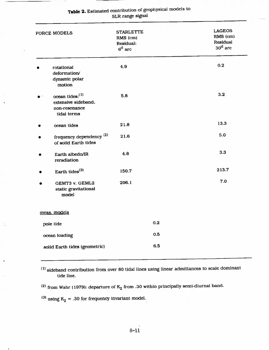
Table 2, Estimated contribution of geophysical models to
SLR range signal
FORCE MODELS STARLETTE LAGEOS
RMS (cm) RMS (cm)
Residual: Residual
6 d arc 30 d arc
rotational
deformation/
dynamic polarmotion
ocean tides: (I)
extensive sideband,
non-resonance
tidal terms
ocean tides
frequency dependency t2)
of solid Earth tides
Earth albedo/IR
reradiatlon
Earth tides (3)
GEMT3 v. GEML2
staticgravitational
model
4.9
5.8
0.2
3.2
21.8 13.3
21.6 5.0
4.8 3.3
150.7 213.7
206. I 7.0
mess. models
pole tide 0.2
ocean loading 0.5
solid Earth tides (geometric) 6.5
Cl} sideband contribution from over 80 tidal lines using linear admittances to scale dominant
tide line.
(2) from Wahr ( 1979): departure of K 2 from .30 within principally semi-diurnal band.
(3} using K2 = .30 for frequency invariant model.
8-11

Table 3. Typical satellite laser ranging orbital fitsin cm from various GEM solutions
Gravity model Lageos Ajisai Starlette
GEM-9 33.3 95.1 116.0
GEM-L2 19.9 79.7 100.0GEM-TI 5.5 12.3 21.2
GEM-T2 5.3 9.4 13.3
GEM-T3 5.2 9.0 11.8
Overall laser
ranging precision 3.8
8-12

EE
v
4=/oE
¢)
W
12-
lO-
B-
6-
¢-
2-
0 _
--2 -
-B
at times of La_eo_ Ob$,
!:i
, t, II !
I I I i I I | I I i I
6 B 10 12 1¢ 16 IB 20
days _lnce July l, 1989[] IER5 Standards + Roy & 5anchez
22 24.
Figare 1. Comparison of models for ocean loading correctionfor the M2 tide at Maui, Hawaii
8-13

-1-
0
I--
LO.,-I
I].)LCO
0
_D
0
O0
I::::1
0L._
C_
O0
I---
LLI.._1
!%0
8-14
0
r,o
ooI'.O
o
c,.I
.c>co
o
o
o
I'Oo
oLO
0
0
0
0L.O
0I
00
4.
I
.,:-ICO
!
..-..
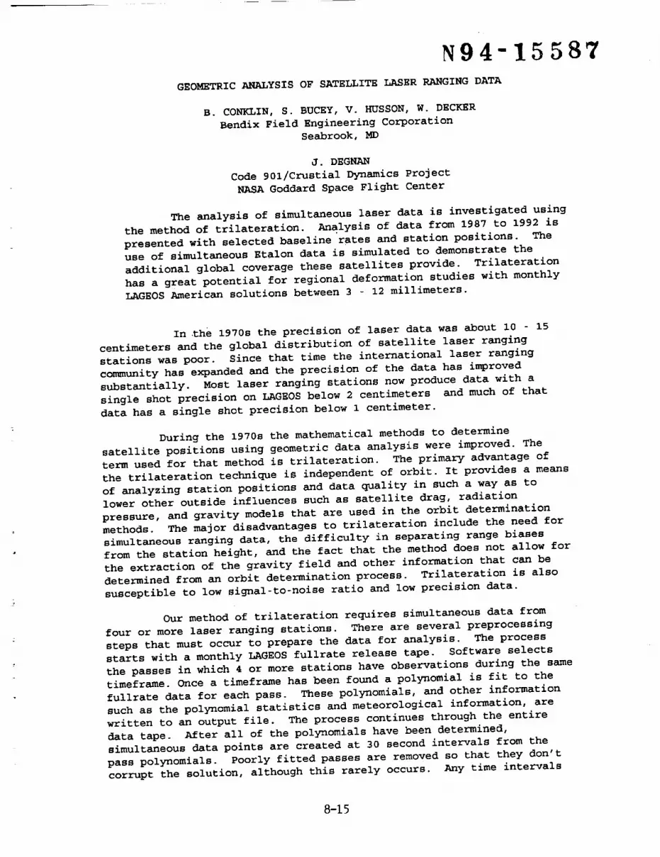
N94-15587
GEOMETRIC ANALYSIS OF SATELLITE LASER RANGING DATA
B. CONKLIN, S. BUCEY, V. HUSSON, W. DECKER
Bendix Field Engineering Corporation
Seabrook, MD
J. DEGNAN
Code 901/Crustial Dynamics Project
NASA Goddard Space Flight Center
The analysis of simultaneous laser data is investigated using
the method of trilateration. Analysis of data from 1987 to 1992 is
presented with selected baseline rates and station positions. The
use of simultaneous Etalon data is simulated to demonstrate the
additional global coverage these satellites provide. Trilateration
has a great potential for regional deformation studies with monthly
LAGEOS American solutions between 3 - 12 millimeters.
In _he 1970s the precision of laser data was about 10 - 15
centimeters and the global distribution of satellite laser ranging
stations was poor. Since that time the international laser ranging
community has expanded and the precision of the data has improved
substantially. Most laser ranging stations now produce data with a
single shot precision on LAGEOS below 2 centimeters and much of that
data has a single shot precision below 1 centimeter.
During the 1970s the mathematical methods to determine
satellite positions using geometric data analysis were improved. The
term used for that method is trilateration. The primary advantage of
the trilateration technique is independent of orbit. It provides a means
of analyzing station positions and data quality in such a way as to
lower other outside influences such as satellite drag, radiation
pressure, and gravity models that are used in the orbit determination
methods. The major disadvantages to trilateration include the need for
simultaneous ranging data, the difficulty in separating range biases
from the station height, and the fact that the method does not allow for
the extraction of the gravity field and other information that can be
determined from an orbit determination process. Trilateration is also
susceptible to low signal-to-noise ratio and low precision data.
Our method of trilateration requires simultaneous data from
four or more laser ranging stations. There are several preprocessing
steps that must occur to prepare the data for analysis. The process
starts with a monthly LAGEOS fullrate release tape. Software selects
the passes in which 4 or more stations have observations during the same
timeframe. Once a timeframe has been found a polynomial is fit to the
fullrate data for each pass. These polynomials, and other information
such as the polynomial statistics and meteorological information, are
written to an output file. The process continues through the entire
data tape. After all of the polynomials have been determined,
simultaneous data points are created at 30 second intervals from the
pass polynomials. Poorly fitted passes are removed so that they don't
corrupt the solution, although this rarely occurs. Any time intervals
8-15

within the selected passes that have fewer than 4 stations are deleted.
A summary output of the available stations and data yield is also
produced at this step. Finally, the remaining LAGEOS tracking data is
separated into two sections. One section is for Europe, North Africa,
Commonwealth of Independent States. The other section is for the
Americas, Easter Island, and Huahine.
To analyze the data geometrically, each section of LAGEOS
ranging data is read in by the software. Apriori station positions and
station velocities are used to compute each stations position at the
middle of the month. The satellite position is determined for each
observation so that angle dependent corrections are computed and applied
to the data. Once all the data has been corrected an iterative process
is started. The observed minus computed values (O-Cs) from each
satellite position are determined for each epoch along with an average
satelllte position. The O-Cs are then edited using a 6-sigma editing
criterion and the average satellite position is recomputed. A summary
of each stations mean and rms are written to the run summary file along
with the total number of observations per station and the number of
edits. A sensitivity matrix is then generated. This is done by
applying small offsets to each of the station position vector elements
and determining what effect each offset has on the O-Cs for all of the
epochs. This procedure is performed for each coordinate (ie. 12 times
for 4 stations). A P transpose P matrix is generated and then inverted,
where P is the matrix of partial derivatives of the O-Cs with respect to
the adjusted station position. The O-Cs are then multiplied by the
resulting partials and a matrix is then computed. These corrections are
applied to the station positions and a new set of average satellite
positions are computed and new O-Cs determined. Again these O-Cs are
multiplied by the P matrix and reiterated. This iterative process is
repeated until the delta rms of the O-Cs between consecutive iterations
is less than one percent, or six iterations have been reached. The
total change of the station position is determined for both x,y,z and
latitude, longitude and height. The baseline lengths are determined for
only the stations involved in the solution and saved in a database.
This database also contains the month and the number of simultaneous
observations between the two stations. A sample summary for a one month
period for a European solution is shown in Figure 1. A by-product of
the solution is the point distribution plot, a sample of which is shown
in Figure 2. Baseline rates are generated from the baselines and a
least-squares linear fit of each of the station combinations is computed
by weighting the monthly baseline with the number of observations during
that month. Some sample baseline rates are illustrated in Figures 3-5.
The method of trilateration also lends itself to doing long
term solutions. In this method both the initial stationposition and
the station velocities are determined. This method of analysis is stillunder development.
The requirement for simultaneous ranging data from 4 stations
requires geographic coverage over a broad area, which in turn requires
high altitude satellites. The Etalon satellites offer great potential
because of their high altitude and visibility to a larger number of
stations at one time. However, the Etalon satellites have had a low
8-16

global ranging priority so they are rarely ranged by more than two
stations at any one time. An intense Etalon campaign was performed
during May and June of 1992 to determine how well these satellites can
be used for Crustal Dynamics research and geometric data analysis.
Unfortunately, because of the low Etalon priorities, the'campaign
yielded no simultaneous ranging data sets from 4 stations and only 1
data set where 3 station ranged simultaneously. LAGEOS 2, scheduled for
launch in October 1992, offers the next best opportunity to obtain a
large simultaneous ranging data set. In addition, at an inclination of
about 65 degrees, there will be an opportunity to obtain simultaneous
trans-atlantic data sets on a high priority SLR satellite.
In the future, we expect that simultaneous geometric analysis
of data from LAGEOS, LAGEOS2, and Etalonl and Etalon 2, spread over a
period of a few days, will accurately determine baselines and
velocities. Future modifications to the geometric analysis software are
expected to include the additional determination of range and time
biases from individual data sets.
8-17
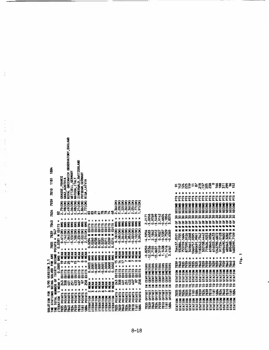
II II tl II II II II II
UUUUUUUU
8-18
@@
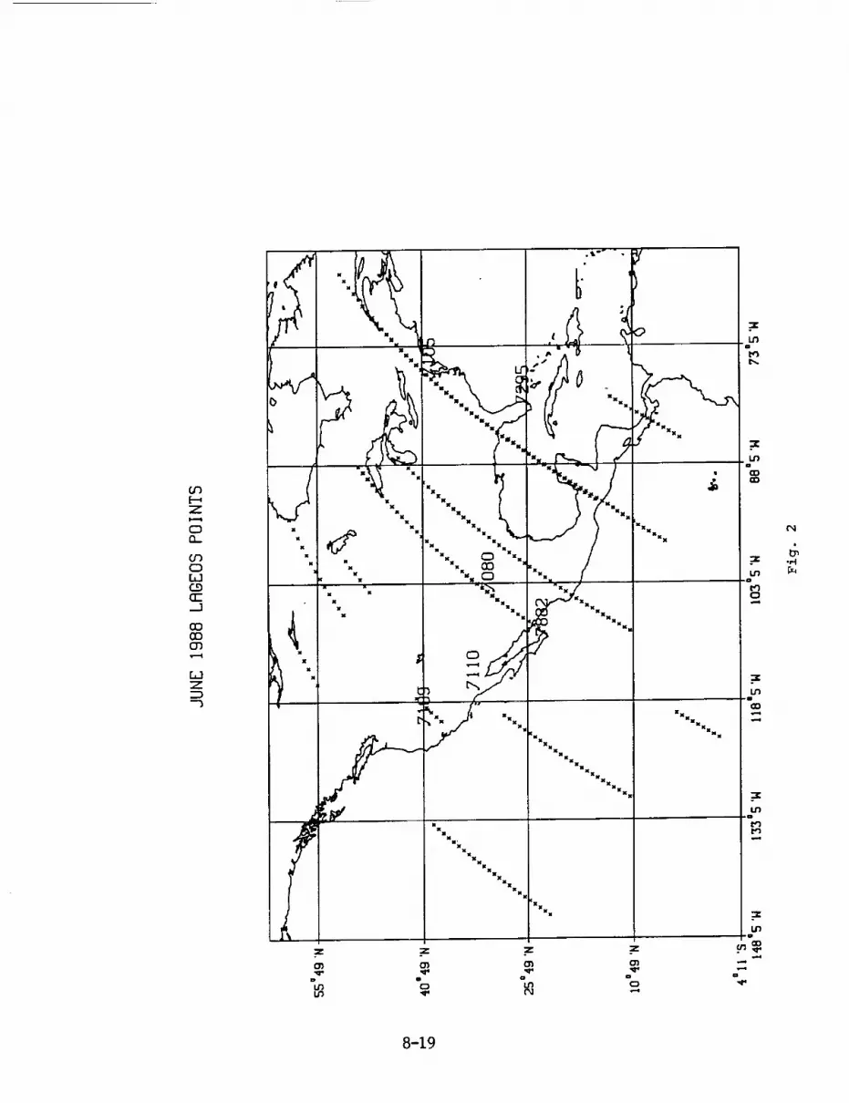
Z
0._
(.00[.J
(]Z
GOGO
[J
fI
I
x x I MXXUxX
xu I xxx
'_
xxxu
mini
NxWx
U wX w
X NX w
X xx M
UXMW
X N
IXXxzxxx
_zx z
• -:r
t._
CO
C_ O) "*_r q
o
% "_*-'4
.,-I
8-19

II
iX
\
#
X
X
0 0
0
0
CWW)
8-20
XX
X
x><
• /\
x
0
X
0
Lt_
8
Lt_
QLt_
a--
"'Z
r.1
0
0
0
d
3NIq_S_8
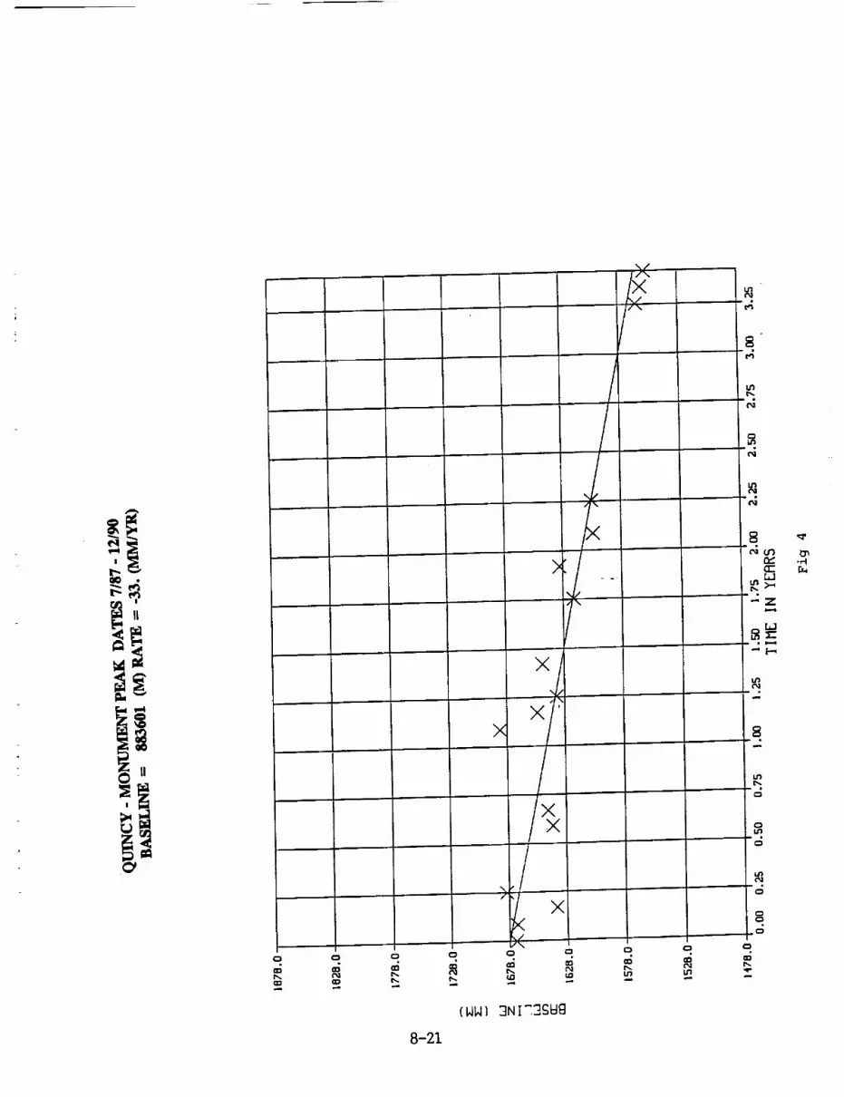
|II
0
I
• t
"(._
UI
(NNI _NI_SUg
n_
"'Z
8-21
B
0
. °0
0

8-22
8 th International Workshop on SLR Instrumentation
Session: Mobile System Upgrades / Developments
N94-15588
IMPROVEMENT OF SLR ACCURACY, A POSSIBLE NEW STEP
M. KASSER, ESGT, 18 All6e J. Rostand, BP 77, 91 002 EVRY France
Abstract
The SLR technology experienced a large number of technical improvementss ..... I..... i,, 1970 les, leading now to a millimetric instrumental accuracy.
Presently it apl_ears as useless to increase these instrumental performances as longas the atmospheric propagation delay suffers its actual imprecision. It has been
proposed since many years to work in multiwavelength mode. but up to now theconsiderable technological difficulties of subptcosecond timing have seriously
delayed such an approach.
Then a new possibility is proposed, using a device which is not optimized
now for SLR but has already given good results in the lower troposphere for wind
measurement: the association of a radar mad a sodar. While waiting for the 2-k
methodology, this one could provide an atmospheric propagation delay at the
millimetre level during a few years with only little technological investment.
I/ INTRODUCTION
It has been pointed out since a long time that all space geodesy techniques
have to deal with the same general problem, i. e. the crossing of the atmosphere to
reach either an artificial satellite, or the moon, or a star, or a quasar, etc...
Nevertheless, if it is the same atmosphere for every techniques, the effect is
known to be quite different for radiowave and for optical methodologies, the first
ones suffering more than the other ones from the crossing of ionosphere (but thisis corrected classically by two-frequencies methods) and from the troposphere
transit (because of the atmospheric water vapor content which is quite
unpredictable and has a strong impact on propagation of radio waves and not on
optical ones). Considering these aspects, the general advantages of radio techniques
compared with optical ones in geodesy are their aU-weather capabilities, and theirdrawbacks are linked with their poor tropospheric correction quality.
As long as the instrumental accuracies were at a few centimeters level, this
meteorological aspects were of secondary concern. This is no longer the case since
many years with VLBI, who had to use costly water vapor radiometers to upgrade
the tropospheric correction to an excellent level (and since this period, VLBI has gotthe best positioning precision among all space geodesy techniques). Since a few
years too it is no longer the case with satellite laser ranging, which is able of an
8-23

internal instrumental precision of a few millimeters, to be compared with the final!
positioning accuracy of 2-3 cm. Of course the tropospheric corrections are not the
only problems biasing the results (consider for example the poor world coverage ofSLR stations), but significant improvements of this parameter must be researched.
Many teams have pointed out that multiwavelength methodology could p_vlde thisrequired amelioration. Anyway it is quite clear that this will ask for a tremendous
technological effort and will probably not be operational since some years. For that
reason we have looked for a new solution, able to give better tropospheric correctionwith up-to-date' techniques, even if probably not as efficient as 2-colour method,but immediately available.
II/THE ATMOSPHERIC CORRECTION FOR SLR
If n is the Index of refraction, n = c o / c (c o is the light celerity In vacuumand c in the atmosphere).
Classically we define the co-index of refraction as
N= (n- 1).10 6
and for optical wavelengths, using for example Essen's formula:
N=A_(P. /T).{ I ÷ (a-b.t).P.}-B x(Pv /T)
where P. is the atmospheric pressure, Pv is the water vapor pressure. T is the
absolute temperature and t is the centigrade temperature. Ax and B x are _.-
dependant parameters, and a and b are constants. With a I0 -7 precision it isacceptable to use the simplified formulation:
N=A'_tP. /T)-B_(p_ / T)
We define also the geometric length of the optical ray Lg, the optical path Lo,
and the geometric distance L between two points s o and s t being one at the groundlevel and the other beyond the atmosphere, at the satellite level:
$1 $1
,, = fa, L. = f,(,).d,so so
If we call AL = Lo - L. it is a function of tile angle a between the vertical andthe direction of the satellite. We notice that:
AL= tL o-Lg) + (L z-L)L ± _2± i: : ::
As the Curvature of the ray pa{i_ ]glow. and as this curvature IS experienced
only on a small range (a few tens of kilometersL the difference Lg - L IS generallyconsidered as negligible. On another hand. AL can be expressed as:
AL = f(a) . AL,,_tl_ t
8-24

And the function f(a) may be found in (Berrada-Baby et al., 1987 orAkhundov et Stoskii, 1992). We have now to deal with AL for _ = 0. h o being the
elevation of the SLR station above "sea level",
w
AL = f N(h).dh
ko
Considering the very low dependance of the result regarding the water vapor
for these optical wavelengths, we will focus on the "dry" part of this expression AI d :
m
AL,: f A P--'.dhT
ho
And. p(h) being the air density. T(h) the absolute temperature, P(h) theatmospheric pressure and g(h) the acceleration of the pesanteur at the elevation
h. with R = 287 J.kg/°K
* P. = p(h). R. T(h)
* d P(h) = p(h). g(h). dh
so that.
AL d = f dP(h).A.Rho g(h)
At this level we may have different assumptions:
I 't hyp. g(h) = go = constant. Then AId = A'R'Po / go
2" hyp. g(h) - go / ( 1 + 2.h/r o ) closer to the reality. We find then:
aLd-A.R.P o
8o
I +
]ro -p- (go ÷ R. - 2.go"to
( _ is the gradient of T ). For Po = I000 mbar, we find ALd -_ 2,3 meters
And the difference between these two models is below I cm : various studies
show (Berrada-Baby. 1987) that this discrepancy is around 5 mm. and is quite
stable and thus easy to model. On another hand, the differences between thesecond model and real data deduced from (Cira 1965) campaigns are quite small
(I mm typically).
8-25

So we conclude that it is extremely important to measure I% with an
excellent precision (1 mbar of error induces 2.3 mm on the atmospheric correction).And one must take into account the fact that the function f(a) (that is the air-mass
number) will multiply these values by numbers up to 2.5 in operationnal SLRmeasurements.
If the temperature is measured in the first 5 kilometers, looking at fig. 1 and
fig. 2, we observe that half the total correction is already acquired (fig. I), and that
the upper layers are quite well defined by the profile in the troposphere. If we
compare these facts with the abovementionned value of 5 mm. whose noise isaround 1-2 mm, multiplied by the air-mass value (I to 2.5), i. e. less than 5 mm,,
it is clear that any temperature profile of good precision acquired in the tropospherewill leave a residual error on the atmospheric correction at the millimeter level.
1.0C
3.gc
3.8C
).7C
3.6C
3.50
3.40
).30
).20
3'.10
).00
/
/
J
J
Jf
ff
0 10000 20000 300005000 15000 25000
Fig. I: Fraction (Y-axls) of the total atmospheric correction for a vertical transitof a laser pulse, from the ground level up to a given altitude (X-axis, in
meters). Computed from an observed radio-profile in Greece, 1990.
8-26
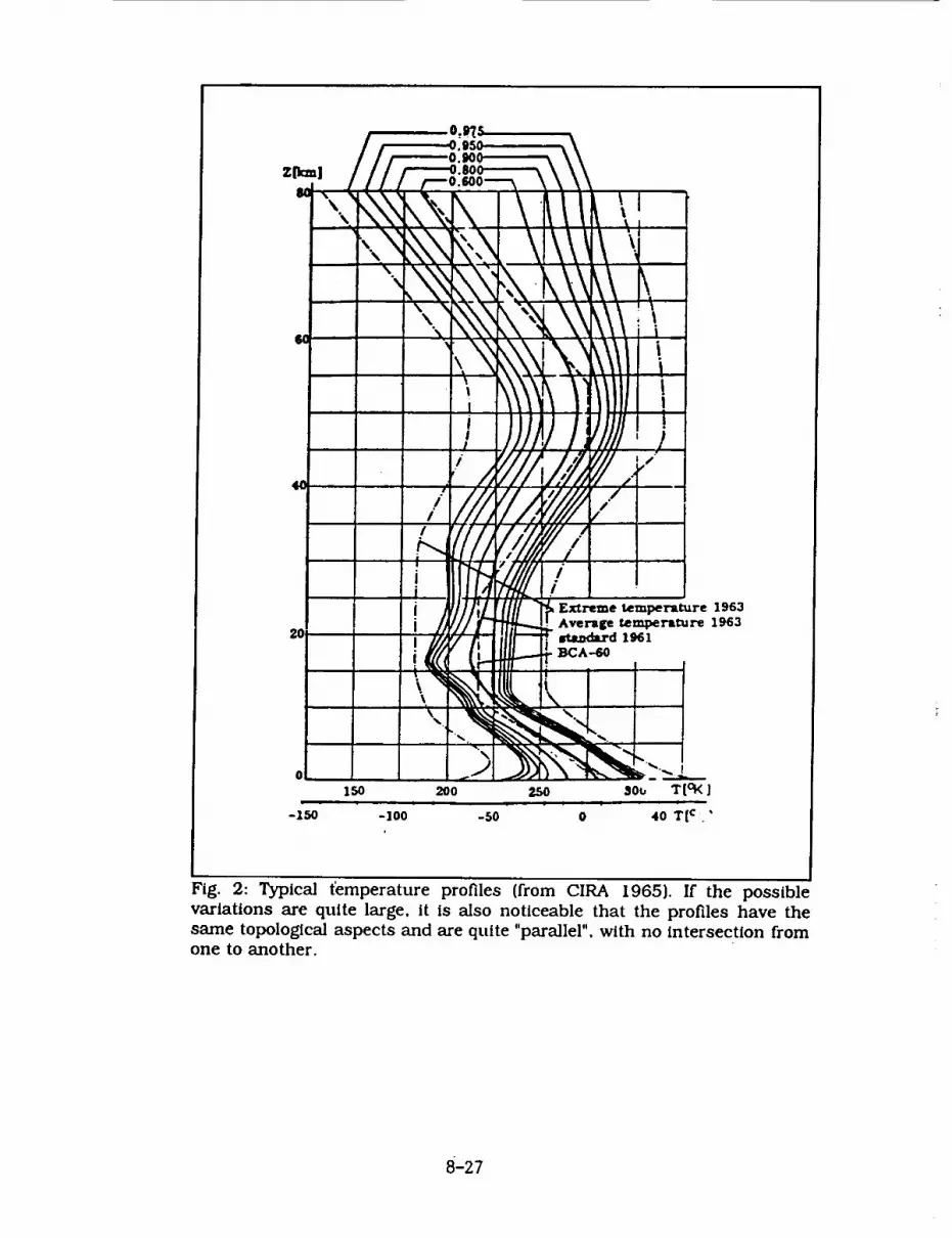
Z[_a!J
\_\
6C
20 ¸
//
III
II II
\
//
temperature 1963
Avenge _emperat'ure 1963standard 1961
BCA-60
! iI
0
15o 2o0 250 3or, T[CK ]
-150 -]00 -50 0 40 T[ c '
Fig. 2: Typical temperature profiles (from CIRA 1965)• If the possible
variations are quite large, it is also noticeable that the profiles have thesame topological aspects and are quite "parallel", with no intersection fromone to another.
8-27

HI/PROPOSITIONS
The first one is obviously to measure Po quite carefully. It is necessary tocalibrate often the barometers employed, to measure preferably the pressure close
to the level of the axes intersection of the telescope (it is generally the case). It must
be posslble to measure the pressure with an absolute precision < 0.2 mbar.
Considering the efficiency ofbarometric levelling, whose precision may reacll
one meter, we observe that it means that constant pressure surfaces are quite
horizontal, so that it is useless to measure the horizontal gradient of Po in order to
correct its effect in the direction of the sight, provided the weather is reasonably
quiet.
Anyway, it seems mostly advisable to improve the correction by a good
measurement of T(h) in the direction of the satellite, at the O. I°C level, up to anelevation' of 3 to 10 km.
In these conditions, one may be sure to get an atmospheric correction better
than 1 mm. It is easy to notice that such a precision with 2-wavelength SLR will
require a 20 times better precision on the differential time-of-flight measurementbetween the two colors (i. e. 0.5 picosecond), which is quite uneasy to reach.
The solution we propose for an easy measurement of the temperature profile
along the llne of sight is a SODAR (Acoustic LIDAR) associated with a RADAR, theacoustic and the radio wave having the same wavelength. The radar is used to trackthe acoustic wave, so it allows to measure the speed of the sound in the
atmosphere, which in turn provides an excellent temperature profile (at the 0. I °C
level). Such instruments (e. g. Remtech) are now used close to airports, in order tomeasure winds and wind shears, and this technology is already available. The
common ranges are 3 to 5 km, but large instruments may reach I0 km.
8-28

IV/ CONCLUSIONS
We propose that an experiment be carried with a radar/sodar equipment
close to an up-to-date SLR station in order to check the possible improvementsthat such data could provide to the laser data. This solution is probably an
excellent alternative allowing to wait for the 2-wavelength generation of SLR
stations.
On another hand. we insist on the necessity to check quite carefully the
barometric equipments used in SLR stations, as the P, parameter is by far the most
important to perform a good atmospheric correction.
BIBLIOGRAPHY
H. BERRADA-BABY. P. GOLE & J. LAVERGNAT
Effets de la troposphere sur les mesures de distance Terre-Satelllte.
Application au proJet DORIS.CRPE/158 Technical note. June 1987
RPE/ETP, 38-40 rue du G6ndral LECLERC. 92 131 ISSY-LES-MOULINEAUX,France
CIRA 1965
North-Holland Publishing Company. Amsterdam Edition, 1965
T. A. AKHUNDOV, A. A. STOTSKII
Zenith angle dependance of path length through the troposphere
Proceedings of the symposium "Refraction of transatmospheric signals in geodesy".
Den Haag, 19-22 May 1992, pp 37-41
REMTECH Company, technical papers on acoustic wind profilers.
Remtech Inc., 1,040 Townley Circle, Long_ont, CO 80 50 I, USA
8-29


Operational Software
Developments


N94-15589
On the Accuracy of ERS-1 Orbit Predictions
presented at
8th International Workshop on Laser Ranging Instrumentation
Annapolis, MD USA
May 18-22, 1992
by
R. Kt_nig, H. Li, F.-H. Massmann, J.C. Raimondo, C. Rajasenan, Ch. Reigber
Deutsches Geodiitisches Forschungsinstitut, Abt.I (DGFI) and
German Processing and Archiving Facility (D-PAl)MiJnchner Str. 20
D-8031 Oberpfaffenhofen
Germany
Summary
Since the launch of ERS-1 (first European Remote Sensing Satellite) the D-PAF (German Pro-
cessing and Archiving Facility) provides regularly orbit predictions for the worldwide SLR
(Satellite Laser Ranging) tracking network. The weekly distributed orbital elements are so-
called tuned IRVs and tuned SAO-elements. The tuning procedure, designed to improve the
accuracy of the recovery of the orbit at the stations, is discussed based on numerical results.
This shows that tuning of elements is essential for ERS-1 with the currently applied tracking
procedures.
The orbital elements are updated by daily distributed iime bias functions. The generation of
the time bias function is explained. Problems and numerical results are presented. The time
bias function increases the prediction accuracy considerably.
Finally the quality assessment of ERS-1 orbit predictions is described. The accuracy is com-
piled for about 250 days since launch. The average accuracy lies in the range of 50-100 ms
and has considerably improved.
9-1

1. Background and Introduction
Since the very first days when ERS-1 began his mission in space, the D-PAF is sending orbit
predictions to the SLR community. The orbit predictions are produced in form of the well es-
tablished IRVs and SAO-elements. The procedure is given in chapter 2. Though these orbital
elements are very compressed forms of complicated orbit trajectories, they optimally represent
the orbit. The trick to achieve this is called tuning of elements. In chapter 3 the problem is il-
luminated from the numerical point of view.
Very soon after launch it became clear that the ERS-1 trajectory is extremely affected by solar
and geomagnetic activities. The orbit predictions lost accuracy mainly in along-track direction.
The D-PAF therefore introduced the time bias function which is generated and disseminated
daily. Meanwhile the time bias function has become an accepted tool in the SLR community.
Some features of the time bias function and related topics are explained in chapter 4.
The extremly high solar activity in the first months of the mission brought extraordinary
events such as a geomagnetic storm of nearly singular type. Though SLR tracking was almost
lost for two days, the D-PAF orbit prediction system (and the SLR community in turn) gained
at the end. The software system got more backup solutions and the quality checks were large-
ly extended. Chapter 5 tells more about quality assessment and quality checks.
Finally the orbit prediction system has developed to a reliable system in SLR tracking. This.
becomes obvious from the course of the average accuracy of the orbit predictions shown in
the more detailed analysis in chapter 5.
2. Generation of Orbit Predictions
In a first step the orbital parameters are estimated by differential orbit correction with the
DOGS-OC (DGFI Orbit and Geodetic parameter estimation System - Orbit Computation)
software. Laser ranges are mainly used as observations for the least squares procedure and in
few cases also RA FD data (Radar Altimeter Fast Delivery) ( Massmann, F.-H. et.al., 1992 ).
The use of PRARE data (Precise Range And Range rate Equipment) was also planned prior to
launch.
Orbit perturbation models used are state of the art ones. The gravitational forces are mainly
represented by the GRIM4-S2 gravity field model ( Schwintzer, P. et.al., 1992 ). The major
non-gravitational perturbations of the low altitude orbit stemm from surface forces. DOGS-
OC adopts!a macro modell of the surface of ERS-1 for albedo, direct solar radiation and drag.
Earth's high atmosphere is represented by the CIRA'86 model where solar and geomagnetic
activity is needed as input.
In a second step the orbit is integrated forward by the DOGS-OC software with the parame-
ters derived before. Adopted are the same perturbation models but now solar and geomagnetic
activity are predicted for the respectiv time period. And this indeed is the major error source
that degrades the accuracy of ERS-1 orbit predictions. Also the ERPs (Earth rotation parame-
ters) are predicted for the time period of the forward integration. The accuracy of ERP predic-
tions is quite good for the lifetime of ERS-1 orbit predictions, the effect can therefore be
neglected.
9-2
In the third step DOGS-PD (PD for Predictions) compresses the orbit to dedicated forms and
formats of orbital elements which can easily be disseminated worldwide via various telecom-
munication channels. In addition these elements are tuned so that the user will recover the or-
bit in an optimal way. So-called tuned IRVs (Inter-Range Vectors) and tuned SAO-elements
(Smithsonian Astrophysical Observatory) are delivered to the SLR community, PRARE-
elements to the PRARE system.
3. Tuning
The orbit is recovered at the SLR sites by simple programs intended for use on low capacity
computers. These programs adopt low degree and order gravity fields and do not consider
nongravitational forces as drag. The IRVINT integrator written at the university of Texas
starts from the IRVs. The ancient AIMLASER program applies analytical orbit theory to re-cover the orbit from the SAO-elements.
Because of these severe neglections, D-PAF tunes IRVs and SAO-elements. This means that
despite of simple perturbation modelling onsite the orbit is recovered in an optimal way. The
optimum is a minimum difference in the least squares sense of the recovered orbit to the full
perturbation model orbit or reference orbit. The IRVINT and AIMLASER programs have to
run then in a defined mode. D-PAF assumes for IRVINT a 60s integration step size and the
GEM10N gravity field coefficients up to degree and order 18. The AIMLASER program
should run in the RGO version (Royal Greenwich Obse_atory) with dedicated GEM10B.coefficients.
Fig. 1 shows the along-track error if an un-tuned IRV is integrated by IRVINT. The example
holds in general. Due to the missing drag forces modelling the error grows during the day to
ca. 1400m ;in along-track position or ca. 200ms in time bias which would prevent tracking ofthe satellite.
Fig. 2 displays the error after tuning. Maxima are now ca. 20ms around midnight and around
noon. The remaining along-track errors are similar day by day, the maxima are dependent on
the solar activity. They could be accounted for by a function giving the error for 24 hours of
a day. The more proper way of course would be to model drag in the integrator. Anyway the
remaining errors are in a range that can be accepted for tracking.
9-3

[ m ] ALONG-TRACK ERROR
1200
1oo0
800
6O0
400
200
DGFI
2 4 6 8 10 12 " '14 " 1.8 1.8 20 22 [h]
Figure 1 Along-track error from un-tuned IRVs
[m]
150
1oo
5O
-5O
-lO0
o
ALONG-TRACK ERROR J
-DGFI
2' 4 6 8 I0 12 14 1"6 18 20 2"2 [h]
Figure 2 Along-track error from tuned IRVs
9-4

The accuracy of tuning, that is the difference of the recovered orbit to the reference orbit, can
be seen in Table I where the typical differences are given as RMS-values in meters for both
types of prediction elements. Again the values are largely dependent on the solar activity.
radial
across-track
along-track
IRYs
ld
3-5
3
20-60
SAO-elements
lOd
10-20
10
20-100
Table 1: Tuning accuracy (in m)
The SAO-elements show less accurate recovery because they represent the whole prediction
period (normally 10d) whereas the IRVs are given each day. All values are within a range
thatcan be accepted for tracking.
4
4. Time Bias
D-PAF generates and disseminates weekly prediction sets containing IRVs and SAO-elements.
Due to the sensitivity of ERS-1 to variations of the high atmosphere the predictions loose ac-
curacy mainly in along-track direction. This is also known to the stations as so-called time
bias i.e. the satellite rises too late or the satellite rises too early. The determination of the time
bias provides a quick and simple update of the orbit predictions.
Therefore D-PAF generates and disseminates daily a time bias function from new Q/L (Quick
Look) Laser ranges. For every pass over all stations having observed ERS-1, a time bias is
computed relative to the last prediction set. A third order function in time is fitted by LS
(Least Squares) to these time bias values. In the LS procedure the time bias values are
checked for outliers and the parameters are checked for significance ,leading all in all to a best
approximating function. The function fits to the time bias values within 1ms for up to four
days.
A typical example of time bias values is given in Fig.3. Fig.4 shows the fitted function after
removing the outliers and after the significance check of the parameters.
The time bias function represents the time bias values of the last few days. More important it
is capable of predicting the along-track error.
The EDC (European Data Center) provides another important tool to handle the time bias
problem. Stations can store the observed time bias immediately after the pass in the data base.
Currently Graz, Potsdam, RGO, Santiago de Cuba and WettzeU do so. This time bias is nearly
in real-time available to other stations. The stations can then compare the results with their
own computations and with the D-PAF time bias function. This all this together should yield
to more confidence in the time bias that is going to be used for the next upcoming pass.
9-5

[ms]
.0
-5O
-100
-150
Time Bias
DGFI
0.0 0,5 1.0 1.5 2.0 2.5 3.0 3.5
Figure 3 Time bias values
4.o[_]
[ms]
-50
-IOO
-150
-200
0.0
Time Bias
0.5 1.0 1.5 2.0 2.5 3.0 3.5 4.0[ d]
Figure 4 Time bias function
9-6
5. Quality
The quality of the ERS-1 prediction products is indicated to the users by a quality flag. Incase of orbit predictions the quality flag is computed from the fit of observations in the orbitanalysis (step 1 in chapter 2), from the comparison of overlapping arcs and from the tuningaccuracy. The quality of the time bias function is assessed from the approximation error of thefunction and the dam coverage.
Of course the quality flag gives only an idea on how the quality of the products can be. Bynature predictions go into the future and nobody can determine what will be. Particularly theaccuracy of ERS-1 orbit predictions is heavily influenced by unpredictable solar activity. Any-
way the quality flag shows the current knowledge of the quality. It convinces the generatorthat he did a good job and it gives a first indication to the user in case he has problems.
All prediction products are subject to permanent quality checks. Dally the time bias of newlyincoming Q/L Laser passes are determined relative to the actual prediction orbit which leadsto the time bias function. The prediction orbit is also compared to the MMCC orbit (Missionand Management Control Center). The MMCC orbit is generated by an independent group inESOC (European Space Operation Center), Darmstadt, from S-band observations and radar al-timeter fast delivery ranges. The comparison with such a completely external source providesmore confidence in the results.
On a weekly basis when new orbit predictions are generated the new prediction orbit is com-pared to the old one. The differences in along-track direction should exactly reflect the oldtime bias function. The differences in radial and across-track direction normally stay within afew meters.
The internal quality checks proceed in a closed loop from prediction set to prediction set. Theexternal checks give an independent judgement. So the reliability of the orbit prediction sys-tem has reached a quite high level.
Fig.5 displays the along-track errors of ERS-1 orbit predictions since launch. The first 100dare clearly affected by large solar activities. In addition a manoeuvre was missed. Meanwhile
these cases are taken care of. In the right half of Fig.5 it can be seen that the mean accuracysteadily improves, but is clearly degraded by the frequent manoeuvres.
9-7
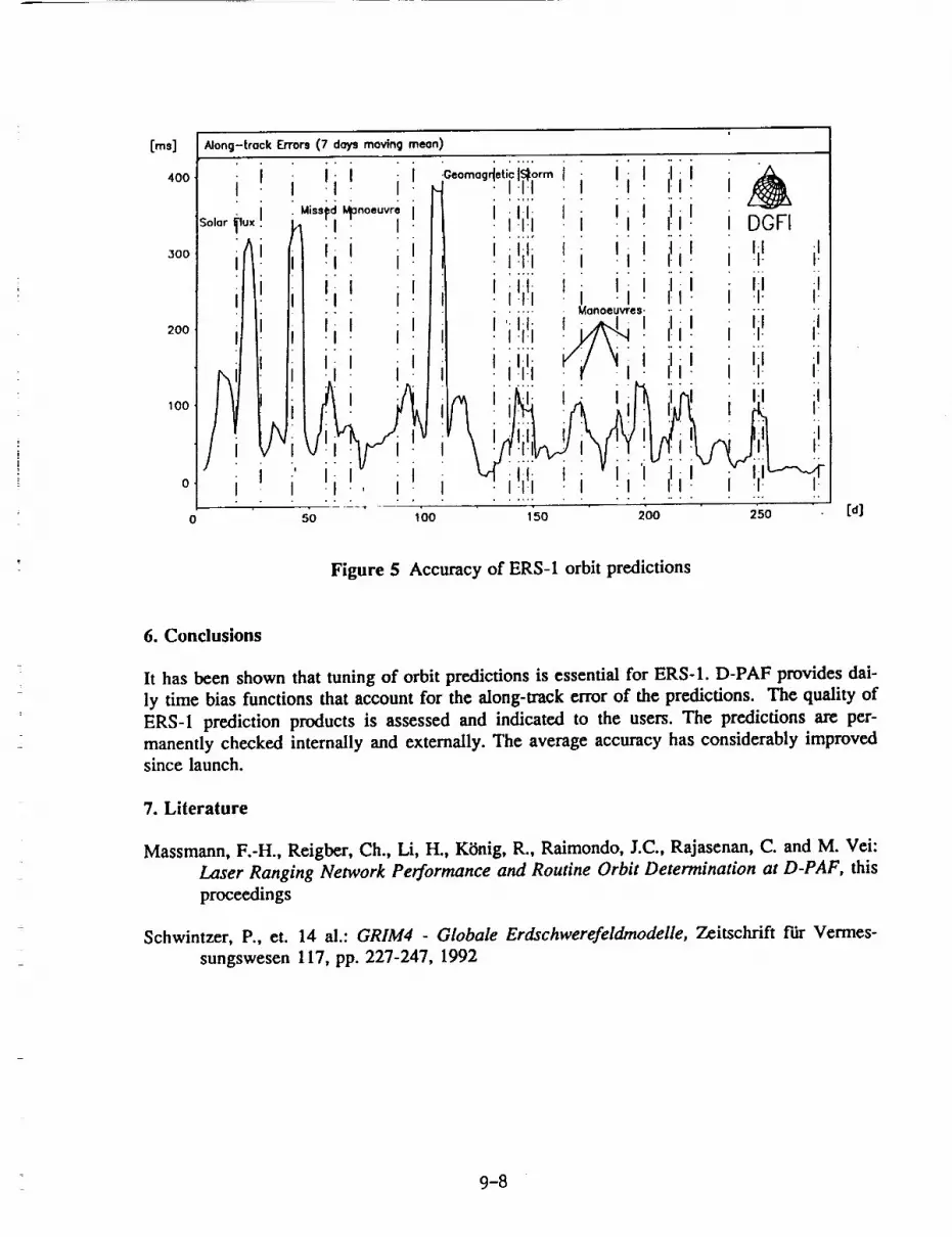
[ms]
4OO
.3OO
200
100
0
0
Along-track Errors (7 days moving mean)
so,or_u_ii
i
i
ii
!t! i!",i n°'uvi
ii! i'
• .
ii! _iiii iil
! i!i!i !! i!i!i
! i!i!i
i !i!i !i!
• °
i, ii!
i• ° .
i!• °
i!!
i
i
i
i DOFI
i !i! i!
i !i! i!
i !i! i!
,!;i ;!
i_ i!
50 100 150 200 250[d]
Figure 5 Accuracy of ERS-1 orbit predictions
6. Conclusions
It has been shown that tuning of orbit predictions is essential for ERS-1. D-PAF provides dai-
ly time bias functions that account for the along-track error of the predictions. The quality of
ERS-1 prediction products is assessed and indicated to the users. The predictions are per-
manently checked internally and externally. The average accuracy has considerably improved
since launch.
7. Literature
Massmann, F.-H., Reigber, Ch., Li, H., Ktinig, R., Raimondo, J.C., Rajasenan, C. and M. Vei:
Laser Ranging Network Performance and Routine Orbit Determination at D-PAF, this
proceedings
Schwintzer, P., et. 14 al.: GRIM4 - Globale Erdschwerefeldmodelle, Zeitschrift £dr Vermes-
sungswesen 117, pp. 227-247, 1992
9-8
N94-15590
COMPENSATION FOR THE DISTORTION IN SATELLITE LASER RANGE
PRED%CTIONS DUE TO VARYING PULSE TRAVEL TIMES
Matti Paunonen
Finnish Geodetic Institute
Ilmalankatu IA
SF-00240 Helsinki, Finland
Telefax:358-0-264995
ABSTRACT
A method for compensating for the effect of the varying
travel time of a transmitted laser pulse to a satellite
is described. The "observed minus predicted" range differ-
ences then appear to be linear, which makes data screening
or use in range gating more effective.
I. INTRODUCTION
Accurate range predictions are necessary in satellite
laser range measurements when the operation takes place in
daylight. Then the range gate, where the return pulse
detector is active, can be set very narrow to effectively
discriminate against noise. Data screening of the
observations is often done using ',observed minus predicted"
(O-C) range differences. The predicted satellite times are
generally equally spaced, as are the transmit times.
But the true hitting times are not equally spaced because
of the varying pulse travel times. This leads to distortion
of the O-C differences which can be as high as 10-20 m. A
polynomial of suitable degree is used in screening. It is well
known that the polynomial should be of low degree so as to
avoid an artificially good fit or end effects. If the travel
time distortion is removed, the O-C deviations are nearly
constant with time for high quality orbit predictions.
This paper describes and tests a simple correction method.
9-9

2. METHOD OF RANGE CORRECTION
The range from the laser station to the satellite varies
approximately parabolically with time, Fig. i. When thesatellite is passing the closest point, a small time change
does not affect the range much. At the far end of the pass
the range changes several kilometers per second.
\
\\
%\
P
/
A Ri/_'
TRUE POSITION
Rmin Ri_/ Ri o CALCULATED ....
/_/ LASER STATION
Fig.l Conceptual scheme for the origin ot the traveltime distortion in ranges.
This rate , v i , can be calculated together with theranges, or it can be approximated from the change between
the successive predicted ranges Ri_ ] and R i
v i = ( R i - Ri_] ) / T ,
where T is the time step (often 1 s).
The travel time difference between the Minimum range
Rmi n , and the instantaneous range _ is
Zit i = (Ri - Rmi n ) / c ,
where c is the speed of light. Then the travel time cor-
rection _R i to be added to the predicted range is
AR i = v i * At i •
(1)
(2)
(3)
9-10
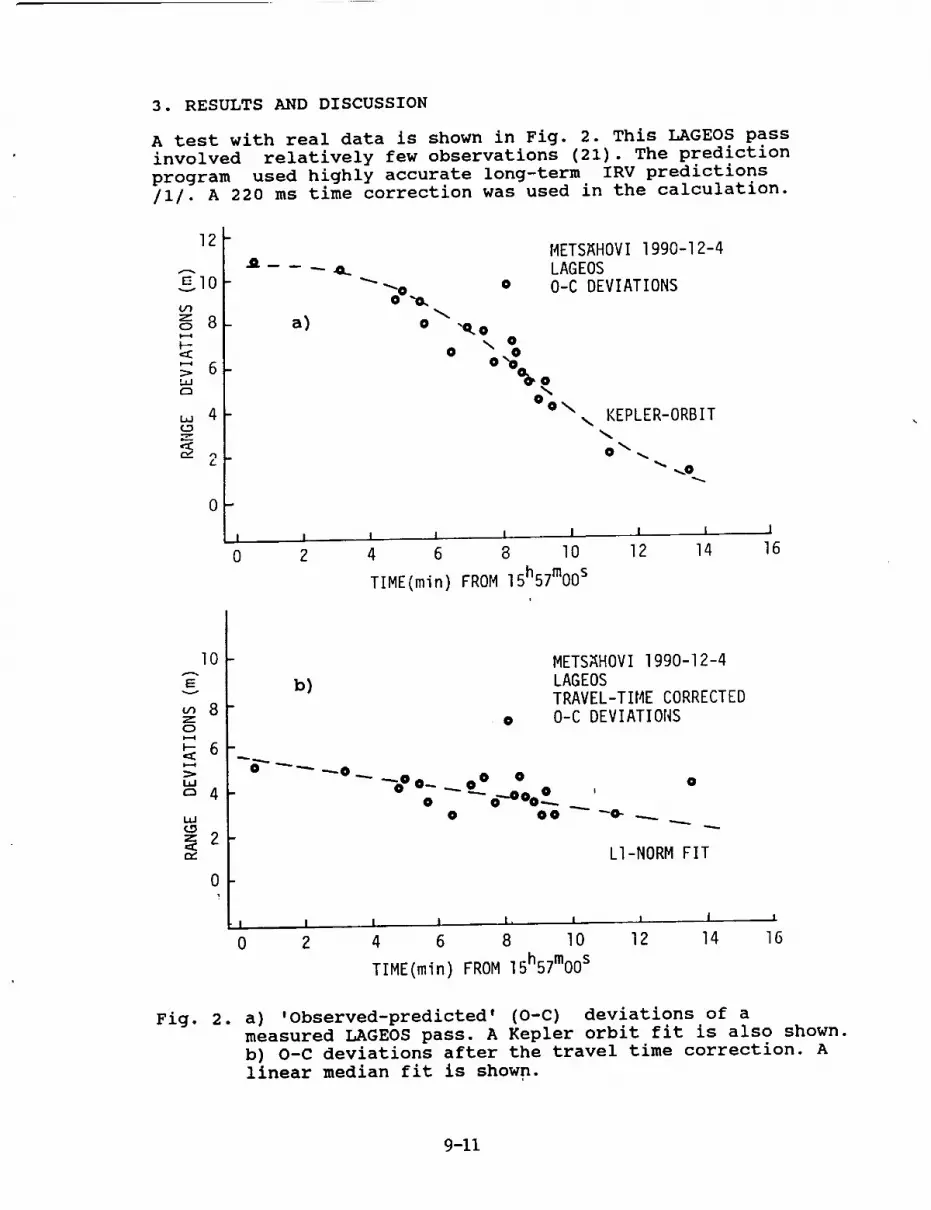
3. RESULTS AND DISCUSSION
A test with real data is shown in Fig. 2. This LAGEOS pass
involved relatively few observations (21). The prediction
program used highly accurate long-term IRV predictions
/i/. A 220 ms time correction was used in the calculation.
12
EIO
z 8
F--
_ 6,.ul
,,, 4
"_ 2
0
METSAHOVI 1990-12-4
_.. LAGEOSo O-C DEVIATIONS
"_°.o.
a) o
o
-o. o\ @
° oo
o\,_ KEPLER-ORBIT
0 _
! I | I | I I i I
0 2 4 6 8 10 12 14 16
TIME(min) FROM 15h57mo0 s
lO
Ev
8zo
_- 6
>
'-' 4
(D
b)
o
METS_HOVI 1990-12-4
LAGEOSTRAVEL-TIME CORRECTED
O-C DEVIATIONS
°--o __._°oo- °'-°°° oo OO
!0
LI-NORM FIT
I I i I I I I I
0 2 4 6 8 lO 12 14 16
TIME(min) FROM 15h57mo0 s
Fig. 2. a) 'Observed-predicted' (O-C) deviations of ameasured LAGEOS pass. A Kepler orbit fit is also shown.
b) O-C deviations after the travel time correction. A
linear median fit is shown.
9-11

The time error varies slowly with time, and is normally
known from earlier observations. The O-C deviations are
shown in Fig. 2a. A simple Kepler orbit /2/ fits the obser-
vations quite well, and only one outlier is indicated.
In polynomial fitting determination of the order is not
easy. The first point would be rejected in a linear fit.
The situation becomes considerably clearer after application
of the travel time correction method described (Fig.2b). The
fit using the linear Ll-norm /3/ eliminated the last point as
well as the known outlier. Because the model is now linear,
it is not necessary to use higher order polynomials.
This example shows that a very narrow range window is
possible in ranging to LAGEOS. A 50 ns window corresponds
to 7.5 m of range. This would help considerably in
implementing daylight satellite laser range-finding.
As has been seen, the method can also help resolve difficult
data screening tasks. Good orbit elements and a good orbitare essential for this method.
Note that recalculation of the orbit after the pass, using
the satellite hit times, produces approximately the sameO-C deviations as the method described.
REFERENCES
. The Texas University, long term IRV- predictions for
LAGEOS satellite; a satellite prediction program ORBIT
developed at the Royal Greenwich Observatory,
Herstmonceaux, England.
. J_ Kakkuri, O. Ojanen, M. Paunonen, Ranging precision
of the Finnish satellite laser range finder.
Reports of the Finnish Geodetic Institute 78:8,
Helsinki 1978, ii p.
. M. Paunonen, Use of the Ll-norm in screening laser
range observations to satellites. Proc. 18th Inter-
cosmos Symposium on the Use of Artificial Satellite
Observations for Geodesy and Geophysics, June 12-17,
1989, Cracow, Poland (Ed. WI. Goral, Observations
of Artificial satellites of the Earth, No 27, 1989,
Polish Academy of Sciences, Warsaw 1990),pp.359-362.
9-12

94-15591
Timebias corrections to predictions
Roger Wood and Philip Gibbs
Satellite Laser IL_nger Group
Herstmonceux Castle, Ha_lsham
East Sussex, BN27 IILP, UK
Abstract This talk aims to highlight the importance to an SLR
observer of an accurate knowledge of the timebias "corrections to
predicted orbits, especially for low satellites. Sources of timebias
values and the optimum strategy for extrapolation are discussed
from the viewpoint of the observer wishing to maximise the chances
of getting returns from the next pass. What is said may be seen
as a commercial encouraging wider and speedier use of existing
data centres for mutually beneficial exchange of timebias data.
Introduction
The real behaviour of low satellites is never in exact agreement with even the best predictions.The principal reasons axe that modelling the effect of atmospheric drag is difficult, and the pertur-
bations due to solar radiation pressure are not predictable in advance. EI'tS-1 is much larger andsomewhat lower than either Staxlctte or Ajisai and consequently presents the biggest headaches in
making_predictions. Dcspitc the problcms, dctailed elscwhcre in these proceedings, the prediction
teams do an excellent job in providing orbits and thereby give observing stations the best possiblechance of tracking the satellites succcssfully. Fortunately, most of the deviation from the predicted
orbit appears as an along-track crror and can be corrected by applying a suitable timebias to the
predictions (as has been done 'very successfully for Lageos for many years now). For a particular
set of predictions observing stations can, for each satellite, model the history of the behaviour of
the timebias with time and extrapolate to predict the timebias at the time of observation of the
next pass.
At Herstmonceux we have been working to improve the accuracy of our extrapolation of timebias
values. This talk outlines our findings, indicates the benefits to be gained from increased use of the
data centres and shows how helpful good timebiases can be if you have English weather and are
trying to keep us with Grasse!
Why do we need accurate timebiases?
We see three distinct advantages:
Ease of satellite acquisition. This is always important, at whatever stage of the pass the
satellite is first acquired. But it is especially important at the very beginning of a pass, necessarily
at low elevation_ whcn accurate pointing helps to minimise the time spent in searching for
returns. Ease of acquisition is also importaz_t when there has been a break of a few days in
the scquencc of observations, because of cloud or technical downtime, where accurate knowledge
of the timebias correction can lead to immediate recovery of the satellite. This second point
emphasises the usefullness of having access to continuous records of timebias data in order to
base any extrapolation on the best available data set.
9-13

Improved telescope tracking. If an incorrect timebias is used to compute the telescope
position during a pass, the offsets from the reference position on the detector will depend ontime and the observer will have to insert ever-changing manual corrections in order to keep the
satellite image. By contrast a correct timebias results i_ [|ttle or no guiding, provided that the
pointing model for the telescope is weU-determined.
Better noise elimination. When the timebias is exactly right the returns from the satellite
always appear at the same place in the range window. This means that the window can be made
very small and so the amount of noise reaching the detector can be drastically reduced. This
improvement in the ratio of signal to noise is particularly valuable for daylight ranging.
The second and third advantages can still be gained (even in cases where an accurate timebias is
not available beforehand) if the first few good returns from the satellite are used in real time to
convert a range offset into a timebias correction. This technique is routinely applied for multi-
photon detection systems where the identity of true returns is not in doubt. But for single photon
detection in daylight, or using an intrinsically noisy detector such as a SPAD, it is not always easy
for the software to pick out the track, and some form of manual intervention may be required.
Where can we get timebiases?
Originally we used only our own history of passes to make extrapolations to current behaviour: Tl_is
was quite satisfactory during periods of continuous good weather, but was often very frustrating
when trying to recover satellites _ter a break of two or three days due to cloud or instrumental
problems.Then, for Ajisai and Starlette, we tried using Bendix's timebias data from many stations in
addition to our own. We immediately found a great improvement in the quality of our extrapolation
and could use narrower range windows right at the start of the pass. We also found that the change
from using elements to using IRVs gave better consistency in the timebias histories.When EILS-1 was launched we, like everyone else, had mixed success in finding it. When we
had a reasonable history and the solar activity was not too wild, we got good passes. But at other
times, once we had failed to get passes for a day or two, it became increasingly difficult to recover
the satellite. We were very pleased when DGFI _reed to use the pass data that they receive from
many stations to produce timebias functions for EILS-1. This gave, and continues to give, valuable
additional weight to timebias trends,
v
[-.
8-7g_
oo
I I i i i
48720
,il,001
0
I ! I i I _
48722 48724 48728Julian Date
[] RGO
x Potsdam
• Santiago de Cuba
Graz
Figure 1: ERS-I timebiasesfrom EDC for IRV setA920,_07 and symbol key
9-14

Since then, following the establishment of the European Data Centre (EDC), a small number of
stations have begun to make regular deposits of their timebias data for ERS-1 soon after theobservations. We often get EDC data from Graz and Potsdam--and occasionally from %Vettzell
and Santiago de Cuba. Figure 1 shows a plot of the data deposited for IR.V set A920407 at thebeginning of 1992 April. The interagreement between the values from different stations is striking
and gives great confidence that all timebiases have been reduced to a common system. But, with all
the stations close together in Europe, it is clear that the data are clumped together in time: indeed,
sometimes they are all clouded out simultaneously! The addition of more data points from other
stations at other longitudes around the world would give mucll better "round the clock" coverage.
How can we best use timebias histories?1
EB.S-1 Over the last two or three months we have been investigating how best to predict future
timebias values from whatever timebias history we ha_l available on a particular day. This usually
consisted of a small number of values covering a few days.
First we looked at the timebiases shown in Figure 1 which cover a period of about a week and
are all referred to the same IRV set from DGFI. Our approach was to see, in retrospect, how well
the observed values available up to a certain day could be used as predictors for the points which
followed. The results of our trial fits are shown in Figure 2. First we fitted to data for the first two
days only; next we used data for the first three days; then the first four days and so on. For each
O
O
Ev
O
:S ,
E
O
I
O
7
I
i-r. iO
I
__'-_A.' ' ' I ' ' ' /II' II[I_
, °,-, I , , I, ,, I, _ tXl i48720 48722 48724 48726
Julian Date
r_.l , ' , I ' ' ' I ' ' ' I ' -
'_,. :
,;._. -
-, I , , i I , _ I , I ,48720 48722 48724 48726
Julian Date
O
OO
I
OO
7$7$T
•....
"'- °
, I , , , , , , I ,
48720 48722 48724 48726Julian Date
O
o{W
IOOiv)
I
OO
I
°:,
t _,. -- kxj -48720 48722 48724 48726
Julian Date
Figure 2: Successive fits to ERS-I timcbiases from EDC
9-15

trial we fitted the data with functions of three different orders--linear (represented by a solid line
in Figure 2), quadratic (dotted line) and cubic (dashed line). Only points to the left of the verticalarrow at the bottom of each plot wcre included in the fit. We then looked at the next few points
to the right of the arrow to see how well, or how badly, each of the attempted fits represented thedata which followcd. From this examination we drew a number of preliminary conclusions:
• Use the simplest function wlfich gives a reasonable fit to the data (even if it is not the best
fit)--it will generally be better for extrapolationthan a higher order function;
• Use only linear fits for the first 2 or 3 days--there are too few data points to justify anything
fancy;
• It would be helpful to have quick timebias deposits by all stations and better longitude
coverage. This would:
o fill the gaps in the Europema data;
o add data points to strengthen the fit;
o provide actual timebias values closer to the time of observation than are avMlable now.
More recently we tried a new experiment based on normal point data for EKS-1 passes extractedfrom the CDDIS database and reduced to give timebiases. [We had hoped to use directly the
Bendix values, but there are currently unexplained discrepancies between their derived values of
tlmebias and ours, so we have worked entirely from the normal point data. This effect also appears
to exist in the Bendix timebiases for Ajisai and Starlette, but to a lesser extent which does not
prevent their use in revealing long-term trends]. In this case we took the data set shown in Figure 3which covers a week in early May and is referred to IRV set A920505 from DGFI. It is clear that
OO
t_
Ev
oo
E
O
_---]-_--iiiiiiiII1'""'1111_
B
B
0
48748 48750 48752 48754Julian Date
Pigure 3:ERS-1 timebiases from CDDIS normal points
the longitude coverage is more uniform and the daily density of points is higher. However, there
is a drawback as far as immediacy is concerned in that the turn round time for data input can
be longer than for EDC, so that some of the data are relatively old. We then followed the same
procedure that we used for the EDC data and made trial fits to subsets of the data to see how
well the extrapolated curves acted as predictors for what was subsequently observed. The plots in
Figure 4 again show that the higher order fits are wildly ineffective for the first few days, and only
begin to make more sense later. But around day 48752 the data take a wholly unexpected turn
towards large positive values and the trends evident in the early points are no longer relcvant. This
sudden change of behaviour is probably due to solar activity, andin such circumstances it is wise
to abandon the early points of the data set and start the fit again from part way through.
9-16

E
oo(w
oo
o
-4
-I
I
I
I '_ ' I _ ° ° I ' J ' I'-[]
[]
A
! \
48748 48750 48752 48754
Julian Date
, I, I , , , I , , j II
g 11
' ' I
in
[]
i .
I []o_ I
o
48748 4{]750 48752 48754Ju]ian Date
oO
.--. O3
Ev
E
o
_-' I ' ' ' I ' ' '_/' ' ' I J'[]
_ []
/--
/
/
[] [] //
48748 48750 48752 48754Julian Date
o-_ / 4
.. 13 ./'"
0 ...*''"
48748 48750 48752 48754
Julian Date
Figure 4: Successive fits to ERS-1 timcbiases from CDDIS
Our _:dditional conclusions as a result of this exercise were:
• For El%S-1 it is necessary to examine the data and functions d'aily in order to pick up unex-
pected trends in good time;
• Better longitude coverage is essential for early warning of departures from previous behaviour;
• Access to the raw data is very useful for making value judgements on the quality of the fit ofany functions!
Ajisai and Starlette Generally the prediction of timebiases for these satellites is much more
straightforward than for EllS-1 since they are relatively unaffected by atmospheric drag and solar
radiation pressure. Indeed orbit predictions can run quite satisfactorily for several weeks so that a
long timebias history can be established for one II%V set. Over such an interval timebias corrections
usually behave sensibly and, even when the corrections get quite large, a good history with respect
to one set of IllVs allows meaningful extrapolation to get accurate values.
What can be done to improve?
We think that all stations can share the clear benefits to be gained from the daily examination of
trends in timebiases for EllS-1 by depositing their timebias values with data centres as soon as
possible after the pass has ended. Then, by retrieving a comprehensive set of timebiases obtained
9117 ==

worldwide, and using itas the basisforextrapolation,the "hitrate"can be significantlyimproved.
Alternatively,but probably with greaterdelay,stationscan retrievenormal point data and derive
timebiasesfrom .them.
Itwould be very worthwhile to extend the system to includeAjisaiand Starlette;and tomake
surethat provisionismade forrapid feedbackofTopex/Poseidon data.
Finallythe proper commercial: we think thattimebiasesarejustlikewashing powdcr--use the
rightone and your whole lifeistransformedforthe better!
Figure 5: "Net# improved Timebias _
Acknowledgements
We wish to thank the staffof the predictionand data archivingcentresfor advice and data.
Specialthanks go to Brion Conklin of Bendix forhis speedy and cheerfulresponsesto our many
requests.We greatlyappreciateassistancefrom Rolf Koenig of DGFI and Wolfgang SeemiiUcrof
the European Data Centre.
9-18
N94-15592
Formation of on-site Normal Points
G.M. Appleby and A.T. Sinclair
Royal Greenwich Observatory
Madingley Road
Cambridge CB3 0EZ, UK
Abstract.
We describe our methods of fittin 9 a smoothin 9 function to observational range differences
from a predicted orbit, by deducing corrections to the orbit in the radial and along-track
directions. The method has been used on observations of a variety of satellites, and using
predicted orbits computed both by numerical integration usin 9 [RVs as startin 9 values and
analytically from orbital elements. The along-track corrections to the predicted orbit have
been succesfully used in the form of time biases to improve subsequent predictions, and a sta-
tistical test has been devised to ensure that the range residuals may be used to form unbiased
quicklook normal points.
1. Introduction.
It was recommended at the Fifth International Laser Ranging Instrumentation Workshop
held at Herstmonceux, UK, that laser range normal points should be formed by the stations
shortly after each satellite pass and transmitted as quicklook data (Gaignebet, 1985). The
final version of the quicklook normal point format was agreed by the SLR Subcommission of
the CSTG and published in the April 1990 Satellite Laser Ranging Newsletter (Schutz, 1990).
The process of forming normal points consists of 2 stages; (a) fitting a smoothing function
to the observational range differences from a predicted orbit and subtracting the function in
order to form a flat track of residuals, and (b) rejecting noise and outliers and forming the
mean values of the accepted residuals in bins spread through the pass. The values of the
smoothing function and the predicted orbit at the epoch of an actual observation nearest
the mean epoch of the bin are then added to the mean value of the residuals in the bin. The
resulting normal points are then virtually independent of both the smoothing function and
of the predicted orbit.
In this report we detail the processes adopted to carry out stage (a) of the process; methods
for rejecting noise and forming unbiased normal point bin means are developed by Sinclair
(these proceedings)
2. Development of the Smoothing Function.
During the observation of a satellite pass, differences from the predicted range are computedI
for all events detected within the range gate and displayed in realtime, true satellite returns
appearing as a track of correlated values among the randomly distributed noise events. An
example of such a plot is given in Figure 1, which shows a pass of ERS-1. The rejection of
gross noise events is carried out visually using the plot, and the subsequent set of satellite
9-19 '

range measurements and some noise events are passed to the next stage of processing.
At an early stage of the development of the preprocessing software, the decision was taken
to use the pass-by-pass observations to s61ve for corrections to the predicted orbit, and
in particular to monitor the along-track error, in order to improve subsequent prediction
accuracy. Thus the possible use of an arbitrary polynomial for the smoothing function was
not considered. However, corrections to the predicted orbital elements of the satellite would
be difficult to apply to orbits computed by numerical integration and using IRVs as starting
values, and similarly corrections to the IRVs would not be applicable to orbits computed
analytically. Thus it was decided to express orbital corrections as along-track, across-track
and radial displa_:ements to the predicted position. Such corlections are then readily applied
to the geocentric orbit during the solution iteration process, and the derived along-track
correction can be expressed as an orbital time-bias for improving subsequent predictions.
During the prediction process an orbit in the form of geocentric rectangular satellite co-ordinates and velocities at 1-minute time intervals and in units of Mm and Mm/day, is
computed and stored. For each observational epoch, we use 8th order Lagrangean interpola-
tion to compute the instantaneous position r and velocity v of the satellite. Let r = (x,y,z),
and v = (v,, vu, vz), and let the magnitudes of these vectors be r and v respectively. Thereference frame used is different depending upon the source of the orbit being considered; for
an orbit generated by numerical integration and using IRVs, the coordinates are given with
respect to the true equator and mean equinox at 0hrs UT of the epoch of the IRVs. For an
analytically-derived orbit, the coordinates are given with respect to the mean equator and
equinox of date. At the observational epoch, we compute the coordinates of the observingstation in the same reference frame. Let the station coordinates be s = (zs, y,, z,). Then
the predicted topocentric coordinates of the satellite are
XT = X '--:-Xs, YT = Y - Ys, ZT = z -- Zs ,
and the predicted range is the magnitude of this topocentric vector. We thus form the
difference of the observed from the predicted range, and in order to solve for corrections to
the predicted orbit we require partial derivatives of range with respect to the along-track,
across-track and radial components of the displacement of the predicted orbit.
2.2 Partial Derivatives.
(a) Let the along-track displacement or time-bias be AT.
Then the displaced range R is given by
Then
R 2 = (x + vzAT- xs) 2 + (y + v_AT- ys) 2 + (z + vzAT-- Zs) 2
R.._-_-_ =ORv_(x + v_AT- xs) + v_(y + vyAT- y,) + v_(z + vzAT- z,),
or approximately
9-20

OR
OAT = (V=ZT + vyyT + VzZT)/R
(b) Let the across-track displacement be A Q
The across-track direction is
rXV
= (l,m,n)r-v
, say.
So_
l = (yvz- zv_)/r_
n = (xv v - yvx)/rv
So the displaced range R is given by
So_
n 2 = (x + IAQ - z,) 2 + (y + mZlQ - y,)2 + (z + nAQ - z,) 2
OR
RcOAQ
or approximately
= l(x + lAQ- z,) + m(y + ,nAQ - y,) + n(z + nAQ - z,)),
OR
OAQ - (l XT + m YT A- n ZT)/R
(c) Let the radial displacement be Ar
So the displaced coordinates of the satellite are x + zAr/r, etc.
So the displaced range R is given by
= yArR2 (_ + _____5__ x_)_+ (y + __ _ y,12+ (z + -- -r r
Then as before we calculate the approximate partial derivative
zAr
rz,) 2
OR
o3r = (__r + yyr + z zr)/(_R)
9-21

2.3 Solutions.
In practice it was found that the across-track correction was always highly correlated with
the radial correction, and in many cases the solution was indeterminate. Hence both could
not be solved-for, and so it was decided to suppress the solution for across-track, and solve
for a radial correction only, which would thus absorb the across-track error. It was also
found that simple constant along-track and radial corrections to the predicted orbit did not
in general absorb all the error in the orbits, and that the set of parameters to be determined
for a particular pass should be selected from along-track and radial displacements.and theirtime rates of change and accelerations. We denote these parameters T, T, T, R, R,/_. The
partial derivatives of range with respect to the rates of change and accelerations of these
parameters were formed from those of the constant terms by mutiplication by t and t 2, where
time t is the epoch of each observation relative to the mid-tlme of the pass. Such a definition
for the origin of t is optimum in reducing correlations between the unknowns. It was usually
found necessary to solve for only 4 of the possible six parameters, but occasionally all six
were required to remove all trends from the observational residuals.
Initially a scheme was devised to automatically check for very high (>0.999) correlations
among the 4 unknowns _h, _,/_,/_, and to supress any one or two of them in order to obtain a
determinate solution, consistent with obtaining a flat track of residuals. However experience
showed that the values determined for these 4 parameters were always quite small, of the
order of 0.1 ms/minute for 2h and 1.0 cm/minute for R, and of similar magnitude for the
accelerations. We thus imposed a-priori standard errors of these magnitudes upon the 4
parameters, and allowed the program to solve for all six unknowns.
In order to iterate the solution, at each stage we replace the predicted coordinates of the
satellite by the displaced coordinates as determined from the previous solution. So for
example
x = x + vzAT + IAQ + xAr/r
and similarly for y and z. It was found that 4 or 5 iterations were usually sufficient, where
outliers of magnitude greater than 3 x rms were removed at each stage.
A selection of some plots of observational residuals is given in Figure 2, where it is clear that
all trends have been removed; these residuals are readily used to form normal points using
the Herstmonceux algorithm.
As a final check that the track of residuals is indeed statistically flat, we have introduced
a single-factor analysis of variance test on the residuals. This test checks for significant
differences between the means of residuals grouped into normal point bins; any differences
indicate that not all trends have been removed from the residuals, and a warning is given
that normal points should not be formed until the cause of the problem is traced. It is
anticipated that this test may prove useful for the detection of system calibration changes
during a pass.
9-22

3. Conclusion.
The scheme was found to be determinate for a wide range of satellites and pass durations
and quality of predictions, and has been adopted at Herstmonceux. An earlier version of thesoftware is also in use at several European SLR stations. The deduced values of time bias
are used to good effect for improving subsequent predictions, and additionally the software
has been used to generate time bias values from the quicklook observations from other SLR
stations, as described by Wood and Gibbs (these proceedings).
4. References.
Gaignebet, J. (Ed) 1985. Recommendation 84A, Normal Points, in Proc. 5th Int. Workshop
on Laser Ranging Instrumentation. CERGA, France.
Schutz, B.E. (Ed) 1990, April Satellite Laser Ranging Newsletter, Center for Space Research,
University of Texas at Austin, USA.
9-23

!
0 0 0 00 0 O.
(su) I_?npTsa_ a_ue_ i
- 00
la0°,,q
° •
0
00O_
I
9-24

.4
.2
0
w
"" -.2
-.4
• o o • • o ". ° .° . ... •_° . ° . ° ".• • °* . ° . ° : • o ° °° %. ; ° . • •
o" . o. • . .° . • °. ° °. .° .: • ... ° ; ° .. .o . °o ".. • .... • ::.-...._.-., ... • ....... .-._ .'... • ... :'." . .'_ ., ...; ... . . o.." •
.. - ..... ,..°_ o° o_ .o . • .." .'...._ • .,'._ "t......° -"'.A, t* .:-_ .° • -°.':. .° • D • ' "." " °" 'T"x;": _ '.:. -'°.."..'.°.. .L- ".'" o"._ _ .,_''_." q : "_'.. - "."::°._ ": ."....'" .'...,."t ..... ' "'"• " "." :: • • "' " " ". " • "" '" ." -" %'.-"F" :_ .:" •
' • " • " • • • ..o: ° i "
I I , I I I I I I , , I , , , , 1 i j , _ I I ,._____3550 3600 3650 3'700 3750
Time (secs) ERA 281. (SPAD+HP)
r-4 -
i
7/ 2° ,. , • °o ° • . °° • • * o ,
_, .. • . . o.,:..-'.:.'o:::.-.[...:..¢ . ......-..-r. -.. . • - ;.... • :; _._,.._; • ...I.._...: -..-,.. :..... .".... ..= _ ,'" ". "".-.:_'",'>'.."_"_,(,:. ':,;')!.'.'._",'L_ e"7"" _._ ;'.:.:.
_0 • . ; t " °.. • w,., .,... s, *t:..'_*-.%.:.'e?_._
.,.r.. ,':>_.,-,_,._:._j,-_-.'_.._?; -,__,._.#T_,_._'£_':."",_,_".;:. :."_L: .,".-_,• • .._.::,.""*'-(': .V :"' ":". _:'._-;",,.:;_'. • • '
"2_ | _.o_,.... • • ,,. * .,..' . , s ,.-.o., * • . . ,T • °
-_ __. ., , • ° • • ." _ • " ,r ° .% "
-.4i (b)
:.L_J : i ij i ,_'_4200 4400 4600 4800 5000 5200
Time (s) L-_G 236
' I'' '-]_--_-_-_j
im!
• ° •
I • , t
_%.e**• •• _ •° "_ *" • "° ••". * •. . . • .. • • • ..•.'-";'": :, 4 *." :* "" "..-;_..2.._._. .. ;'_.. . ",._"'" * _l" "%*¢'* ." " _. " " "" ":
;_¢_:.*..o::_,..*-. • _ _.:; ;.,
'.L"..,, _' .'.V:2.• " ". • '• _ *, " l
I
: ,I ; ,. _ i ____1 , _ i ,. ; ; ,_,.__
5400 5600 5800 6000
Figure 2. _ange residuals from a pass of ERS-1 (a) ax/d Lageos (b).
9-25

Poisson Filtering of Laser Ranging Data
by
R. L Ricklefs and P. J. ShelusMcDonald Observatory, University of Texas, Austin, TX 78712
The filtering of data in a high noise, low signal strengthenvironment is a situationencountered routinely in lunar laser ranging (LLR) and, to a lesser extent, in artificialsatellite laser ranging (SLR). The use of Poisson statistics as one of the tools forfilteringLLR data is described first in a historical context. The more recent application ofthis statistical technique to noisy SLR data is also described.
Introduction
Routine LLR operations began at McDonald Observatory in August, 1969 as a part ofthe NASA Apollo Lunar Ranging Experiment (LURE), using the newly-commissioned2.7-m astronomical telescope to range to the retro-reflector array placed upon the lunarsurface by the Apollo 11 astronauts. During the next several years, additional arrays wereleft on the moon during the Apollo 14 and Apollo 15 missions, and by two Sovietunmanned soft landing vehicles. Routine LLR operations continued on the 2.7-m telescopeuntil the mid-1980's when these operations were transferred to.the dedicated 0.76-m
aperture McDonald Laser Ranging Station (MLRS).
It is important to realize that the return signal strength ratio, neglecting all parametersexcept distance, for a near-Earth artificial satellite and the Moon is something like 3 x 10¹².Thus, it is more than a trillion times more difficult to range to the Moon than it is to rangeto, say, Ajisai. In the extremely low signal strength environment of LLR it was (andcontinues to be) necessary to operate largely at the single photon-electron level. However,this means that a very large number of "volunteer" photons from any number ofbackground noise sources may trigger the detection electronics, even though very narrowspatial, spectral and temporal f'flters are routinely employed in the receive package. Since allincoming photons are indistinguishable from one another, identifying the valid returns fromthe moon has been a difficult task. From this experiment's inception, the reliance onstatistical f'fltering methods, in addition to the physical ones, had been always assumed.
The application of Poisson statistics to the LLR data filtering problem provided aneffective tool for dealing with high-noise, low signal data. The technique has now beenexpanded and adapted to handle marginal SLR data as well and has proven to be especiallyeffective when applied to data from single or low-multiple photo-electron systems duringdaylight passes and data from all stations when they are ranging more difficult targets likeEtalon- 1, Etalon-2, and MP-2. Figures 1 and 2 show samples of noisy data, displayed byMLRS onsite software, for which the Poisson technique is required.
Background
Let us consider the mathematical concept of the Poisson distribution, which gives the
probability that a certain integer number, k, of unit rate random events from a population,n, will occur in a given interval of time, x, within some total interval of time. The operativeequation is:
9-26

x[k] e-X
P(k) - [k]!
where [k] is the largest integer less than k. For x large enough, this function has a bellshape comprised of many rectangular steps. Multiplying the computed probability by thenumber of bins in the entire sample time gives the number of bins which contain exactly kevents.
In a descriptivesense,Poisson statisticsstatesthatffone has "n" observationsof some
independent variabledefined over some range of "m" binsof uniform width, and ifthoseobservationsarc random, one can compute, in a statisticalsense,how many of those bins
willcontainexactlyk observations. For example, for some specificexperiment of,say,16 independent observationsof some value,one might compute from theabove equation
that 3 of the binswillbe empty, 4 of them willcontainexactly 1 observation,3 of them
willcontainexactly2 observations,2 of them willcontainexactly3 observations,and nobins willcontain 4 or more observations. Then, ifone looks at the actualhistogram ofmeasurements and findsthatone of the binscontains8 of the 16 observations,one might
safelyassume thatthose observationsare indeed not from a random distributionand that
something systematichas occurred. In the case of LLR or SLR observations,where the
measurement isan (o-c)range residual,itisassumed thatthe bin (or bins)containing astatisticalexcessof observationsarc probably validreturnsfrom the targetor theresultof
some systematiceffectin theranging equipment. As anotherexample, figure3 representsthe statisticsfrom the lunardatainfigureI. The predictionsindicatethatthereshould be
no bins with more than 21 points. One bins has 22 points,which is probably not
significant,but thereisanotherbin with 47 points,which issignificant.That bin containsthe lunardata.
This technique is routinely applied to thc filtering of McDonald Observatory LLR dataand is fully described in "Laser observations of the Moon: Identification and construction
of normal points for 1969-1971 by Abbot, Shclus, Mulholland and Silverberg (Astron. J.,Vol. 78, No. 8, pp 784-793, October, 1973).
Current state of affairs
In the routine application of the Poisson technique to data filterin.g it must be noted that,in order to have the best possible chance of isolating signal from norse, one should use thenarrowest bin width possible, keeping in mind at all times, of course, the quantity beingmeasured. Narrow bins will maximize the signal to noise ratio since, in a narrow-binenvironment, a relatively small number of noise photons will be found in any one bin.Further, it is absolutely required that the data be flattened before a histogram is formed,i.e., trends must be removed from the data as much as is possible, so that signal will not
"spill over" into many adjacent bins and, again, be lost in the "noise". This problem hasbeen addressed in a straightforward way in the current data screening implementation at theMI_S, as shown in figure 4. All bins are scanned sequentially through a predeterminedrange of slopes, the plan being that the signal will appear at a significant peak at a slope thatmatches the inherent slope of the data. This technique is especially important for LLR datawhen signal strength is low and for SLR data when orbits arc not well known. Of course,in altering the slope of the data, one must take care to exclude, or compensate for, thosebins which will be incomplete due to clipping. In its present implementation at the MLRS,the Poisson screening software also allows multiple segments of a pass, or a run, to betreated separately. This handles the natural change in residual slope over an extendedobservation session.
9-27

Although personnel atthe MLRS arc now applying the Poisson filteringtechniqueforboth lunar and artificialsatellitedata,the LLR and SLR screeningsystems are somewhat
different. Both systems provide userinteractionto allow the selectionof the parameters
of the Poisson fit,placement of the time bins,maximum and minimum slopes,and a
maximum 8nd minimum residualfor data to be accepted as "real'_.For lunar data,wc
employ fairlystrictlimitson acceptableslopesand allowableresiduals.Earth rotationand
polar motion are major contributorsto slope and residualfor lunar data, so the earth
orientationpredictionsarekept as freshas possible.Further,thereisconsiderablelatitude
in selectingtime binstoreflecttheobserved clumping of NR,RS LLR data. Ultimately,the
Poisson filterisreliedon to provide the LLR data compression, i.e.,normal pointing,
softwarewith a setof acceptabledata.
For the SLR case, the Poisson algorithms serve as a preliminary filter and suggest tothe polynomial fitting algorithms in the normal pointing packages a set of data with whichto start. The polynomial fit, in its job, can then return previously rejected data back into thefit or remove data suggested to it by the Poisson filter, if either of these tasks arcwarranted. Also, the polynomial fit, working on the entire pass, can pull in data that mightbe missed or misinterpreted when the Poisson filter was working on only shorter segmentsof a pass.
The independent time segments, into which an SLR pass is broken, allow the softwareto follow changes in slope during a pass and minimize the effect of anomalous distributionsof data in short segments. We are examining the desirability of having several softwarechecks that require the slopes and average O-C residuals to be smoothly varying over thepass. However, in the cases where there are breaks in the data and other unusualdistributions, this may not be practical.
Results
In the case of LLR data,the presentlyimplemented Poisson filteringtechniqueworks
well,especiallywith a bitof interactivehelpfrom the user,although,in marginal cases,itwould be preferableto use allruns taken over a lunar pass to aid in the filtering.This
particularextensionisnow being examined. As time permits we arc alsopursuing more
elaboratefilteringtechniques such as jack-knifingand bootstrappingto see ifthey holdmerit.
In the case of SLR, the technique has been used successfully at MLRS for about a yearnow. In that time our experience has been that the combination of the Poisson filter and the
polynomial fit produces good results virtually all of the time. The marginal cases canusually be satisfactorily processed, after the fact, by altering some of the parameter of thePoisson fit or by eliminating from consideration extremely noisy parts of the pass. Ofcourse, most of the anomalies usually occur with weak passes, especially Etalon- 1, Etalon-2 and ERS-1. The Poisson filter algorithms are being upgraded so that each satellite uses a
parameter set tailored to it. Tests indicate that this will allow successful batch processing ofvirtually all passes that previously required special handling. Also, an interactive toolsimilar to the Lunar Data Editor is being developed to help the observing crews to quickly
recover passes that were improperly processed. The Laser Tracking Network operated bythe Bendix Field Engineering Corporation will soon install the MLRS "batch" Poisson code
into their processing software.
9-28

Conclusion
The Poisson filtering technique has proven itself to be an extremely valuable tool forboth LLR and SLR operations at the MLRS. This technique is being optimized for eachranging target, and in the future provision will be made for routine, near-real-timeobserving crew interaction with the filter. In addition, new filtering techniques such asjack-knifing and bootstrapping will be evaluated as to suitability for laser ranging data
filtering.
9-29
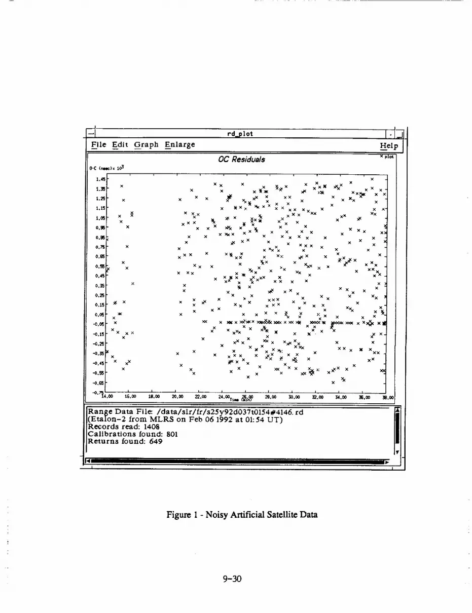
rd.p Iot
File Edit Graph Enlarge Help
O-C (rmc>x 103
1,4_
x1._
1._. x
1.1'.
1.0_ xx
x
xx
x xx
OC Residuals x plot
0._ x
0._
0._ X
0.R
x
0.5_ x
0.4_
0._ x
0.2_
0.15 _x x
0.05 x XK
-0._ x
x
-0.15 x X xx
.-0.25_-0.35 x
-o.45_ x xXX
:L"0. I 1
16.00 18.00
x
xx
>o<
x
Xx
xXx
20.0O 22.0O
x x
x
X X X )4z_xX X
x xXxx x _ _x _< x>_t Xx xi_ x_ xX x xx x XxX X X X X
X T_ x >:_ )4,x x x X X Xx x xx X x x x
XX
_< x _x_ . x x x xx x xx xx
x x x _ x XXx x x
x x x x_x x x _x xX XKX X X X X X X X XX X>
X X X X X X X X XX
x xx x x x x xx x x x x
x xxxXx X X x
xX X X X_x _ x>: xKX X x.X/xXX X X X )'_<X X X X XX
X XX X _ XXxX X >:X XX X X:X X
x xXX xXxx xxx _ X x x xXx X 'x_ x x x X
x x x X x x x xx x xX x x x xxX x xX x
Xx x xX x x
xx x x,xX X X X _< X : X X X
>( X X X "
x _x:.O,>:_xxtt_:._m_xxxxx_ x>oo_ i_oo_x_oo(x Xx_ x_x Xx :dgx XxX xx Xxxx x X x x , _ x-
x XX x x x X x
x x x x xK xXxxX Xx .. X XX X X X
X X..)_: .. X XX
X X X X X X
_x x _. x xxx x x
X x :¢< x x _>: xx X Xx X x _ x
x xxx
t i I 1 ! i I
24.o%,.._oj0 2s.oo 3o.oo m.oo _.0o _.oo _.o0
Range Data Filc Idatalslrlfr/s25y92dO37tO154#4146. rd(Etalon-2 from MLR$ on Feb 06 1992 at 01:54 UT)Records read: 140BCalibrations found: B01Returns found: 649
¢ I II ID-
l |
Figure 1 - Noisy Artificial Satellite Data
9-30
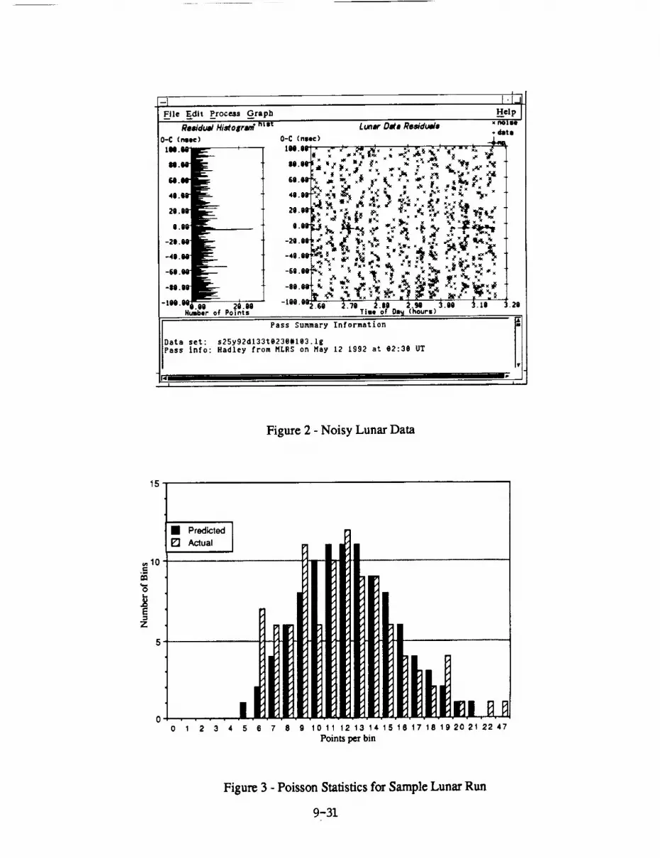
-1 l.i-IFile Edit Proceaa Graph
O-C (neat)
Ill .el
ll.lO _
61.N _
40.U _
20. O0 ___
o.oo _
-20.00
-40,00 F_:
Residual HistoErw." nza_
t
-6O.OO
•lie.x ,.oo .70.ooNumber of taints
LunRrDam Residuals . ,wns,• data
O-C (noDe) l_
x _ x x _" x x 3K x x_ _-Lx
Tile of 00_ (hours).20
Pass Summary Information
Data set: s25y92d133te238#103.1_Pass info: Hadley from HLRS on May 12 1992 at 82:30 OT
I I
Figure 2 - Noisy Lunar Data
15
t • Predicted I I_ I
' t_ot- _'_
i] o il llll l ]
o0 1 2 3 4 5 S 7 8 9 10 11 12 13 14 15 18 17 18 1920 21 22 47
Points per bin
Figure 3 - Poisson Statistics for Sample Lunar Run
9-31

_oo
Bins for Poisson
analysis, slopedto match data.
Histogram resultsfrom 2 bins beingselected at a time
Bins at improperslope, result inno significantbins.
/
/
\/ \
/ \/ time into \
/ pass \\
\
\
.a ,.
la
I
Maximum number
of points expected inbin due to random processes.
L I
1'I ....I
Yi
I• ° °|
Slgnlficarlt
bin(s) _
Figure 4 - Effect of Tilting Bins
9-32
N94"15594
Computer Networking at SLR StationsAntonin Novotn_ 1
Czech Technical University, Prague
Czechoslovakia
Eighth International Workshop on Laser Ranging Instrumentation
Annapolis, MD USA
May 18-22, 1992
Abstract
There are existing several communication methods to deliver data from SLR
station to the SLR data centre and back: telephonmodem, telex and computer
networks. The SLR scientific community has been exploiting mainly INTER, NET,
BIT,NET/EARN and SPAN. 56 countries are connected to INTERNET and the
number of nodes is exponentially gro_ng. The computer networks mentioned above
and others are connected through E-mail protocol.
The scientific progress of SLR requires to increase the communication speed
and amount of the transmitted datda. The TOPEX/POSEIDON test campaign
required to deliver Quick Look data (1.7 kB/pass) from a SLR site to SLR data
centre within 8 hours and Full Rate data (up to 500 kB/pass) within 24 hours.
We developed networking for remote SLIt station in Helwan, Egypt. The reliable
scheme for data delivery consists of: compression of MERIT2 format (up to 89%),
encoding to ASCII file (files); e-mail sending from SLR station -- e-mail receiving,
decoding and decompression at the center.
We do propose to use ZIP method for compression/decompression and UUCODE
method for ASCII encoding/decoding. This method will be useful for stations con-
nected' via telephonemodems or commercial networks.
The electronics delivery could solve the problem of the too late receiving of the
FR data by SLR data center.
_mail: [email protected]@earn. cvut. cs
9-33
The Name of the Game
The computer network backbone has spread all over the world.
Nowadays we may claim three axioms on network data exchange:
Axiom 1.
Axiom 2.
Axiom 3.
network.
All non-local networks are connected to InterNet.
All non-local networks have common protocol 'm mail protocol.
The longer tile is transferred, the longer it takes a byte to get through the
Networking within the SLR Community
The most commonly used non-commercial networks are BITNet, lnterNet, SPAN,
UUCP. All are used on the satellite laser ranging facilities over the World.
The CSTG SLR Subcommission Meeting in Passadena, CA USA, March 12, 1992
agreed that "InterNet will be implemented to all of the SLR and other DOSE relatedstations. This includes the stations in Russia and some of the other Commonwealth
states that participate in the global network."
We will propose the new computer network standard for data handling between SLR
data center and SLR stations. The following two figures schematically show one of the
possible configurations.
9-34

o
1I
9-35
I
I
'0
L_
.J0
Z
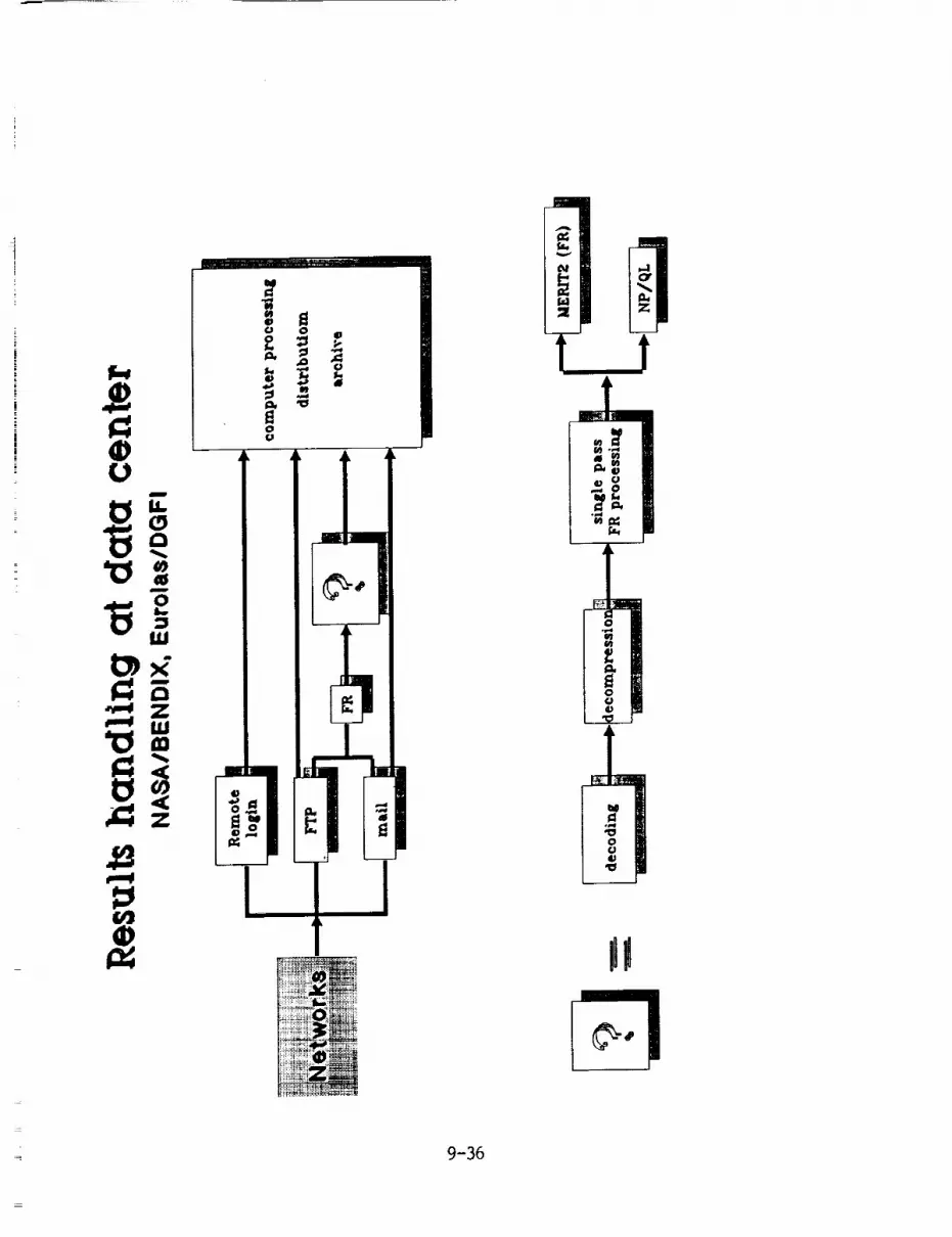
'oorj
'0
9-36

Networks Data Exchange
Mail at other networks
From the other networks, the files are sent to InterNet (and back) as a mail without
any difficulties. The possibility of FTP (File Transfer Protocol)is strongly reduced to the
use of mail servers.
Selection of Large networks 2
applelink
bitnet/earnbix
bmug
compuserveconnect
envoyfax
fidonet
geonet
ieee-compmailinternet
Ill C i
mfenet
nasamail
peacenetsinet
span
sprintmailthenet
usdamail
Apple Computer, Inc.'s in-house networkinternational academic network
Byte Information eXchange: Byte magazine's commercial BBS
Berkeley Macintosh Users Group
commercial time-sharing serviceConnect Professional Information Network
Envoy- 100 (Canadian commercial mail service)Facsimile document transmission
PC-based BBS network
GeoNet Mailbox Systems (commercial)
A DIALCOM system supporting IEEE usersthe Internet
MCI's commercial electronic mail service
Magnetic Fusion Energy NetworkNASA internal electronic mail
non-profit mail service
Schlumberger Information NETwork
Space Physics Analysis Network
Sprint's commercial mail service
Texas Higher Education Network
A DIALCOM system for USDA researchers
The more detailed information on mail network-to-network access see 2.
InterNet data transfer protocols
FTP: (File Transfer Protocol) Allows a user to connect to host computer and with re-
duced set of commands get and/or put files. FTP is essentially inaccessible from
other nets. Getting files from FTP sites may be provided by mail servers (they
retrieve the file and send it as a mail). Putting files by mail servers isn't supported.
FTP is unfortunately slow (approx. 500 bytes/second, for longer files 200
bytes/second), the transfer rate depends on traffic in the network. The terminal
nmst stay on-line while putting/receiving.
Mail: A convenient way for sending a file. A user has no possibility to receieve files via
mail (in sense that somebody must send the file, it can't send itself).
_(g) 1990 John J. Chew, available as EMAILGUI.ZlP at SIMTEL and TRICKLE archives
9-37

The transferrate is a bit slower,but itdoes not keep local terminal busy as FTP
does. Fileslonger than 50000 bytes are regarded as "huge" and sent only when the
network isfree.
Mail isessentially7-bitprotocol,80 charactersper line.Formatted or binary data
can be converted to fit.
TelNet: Allows a remote login. Usefull for remote user access to any computer on the
InterNet. Unusable for sending/retrieving files. User has to know remote computer's
operating system.
Unfortunately, lots of SLR stations are not connected to InterNet and won't be connected
soon. What's more, most stations have to use modems to connect to networks (which
naturally slows down the transmission). That's why we should figure out how to send
shorter files and how to send them from other networks.
What Kind of Data Is Exchanged?
1. From SLR center to SLR stations
• Prediction (IRV or SAO) _ 5 kB
• Whole year IRV- Lageos _ 100 kB
• Conaments on operation _ 2 kB
• Bendix QL analysis _ 1 kB
• Reports < 25 kB
Suz._estion: I would suggest the center to deliver these files to SLR stations as a
regular mail to an automatic list of addressees. FTP makes the server at SLR center
very busy while everybody is trying to receive the files. Due to the network software,
when the network breaks down, it takes the biggest care of mail -- it is almost always
delivered. The FTP data might be easily lost or corrupted during breakdown.
The non-InterNeters have to use mail-servers (for example BITFTP_PUCC) that may
become very busy.
2. From SLR stations to SLR center
Comments on operation _ 2 kB
QL or NP data _ 2 kB/pass
FR data MERIT2 format
130 chars/line, 1 line/point =¢, huge file
up to 500 kB/pass
This file is ahnost undeliverable via mall -- it has more than 80 chars/line and
9-38
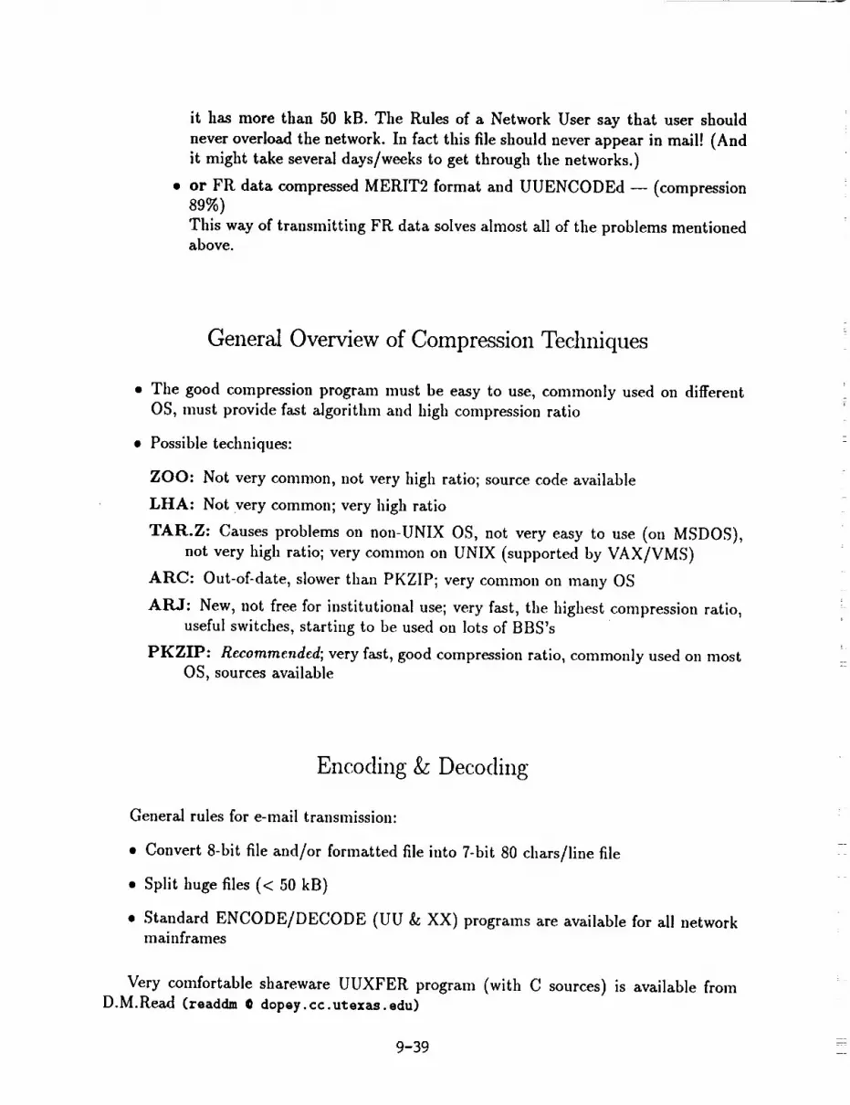
it has more than 50 kB. The Rules of a Network User say that user should
never overload the network. In fact this file should never appear in mail! (And
it might take several days/weeks to get through the networks.)
• or FR data compressed MERIT2 format and UUENCODEd -- (compression
89%)
This way of transnfitting FR data solves ahnost all of tile problems mentionedabove.
Gener'M Overview of Compression Techniques
• Tlle good compression program must be easy to use, commonly used on different
OS, nmst provide fast algorithm and high compression ratio
• Possible techniques:
ZOO: Not very common, not very high ratio; source code available
LHA: Not very common; very high ratio
TAR.Z: Causes problems on non-UNIX OS, not very easy to use (oil MSDOS),
not very high ratio; very common on UNIX (supported by VAX/VMS)
ARC: Out-of-date, slower than PKZIP; very common on many OS
AtLI: New, not free for institutional use; very fast, the highest compression ratio,
useful switches, starting to be used on lots of BBS's
PKZIP: Recommended; very fast, good compression ratio, commonly used on most
OS, sources available
Encoding & Decoding
General rules for e-mail translnission:
• Convert 8-bit file and/or formatted file into 7-bit 80 chars/line file
• Split huge files (< 50 kB)
• Standard ENCODE�DECODE (UU & XX) programs are available for all networkmainframes
Very comfortable shareware UUXFER program (with C sources) is available fromD.M.Read (readdm @ dopey, cc.utexas, edu)
9-39

Featuresof UUXFER:
• Encoding UU, XX, usingexternal table
• DecodingUU, XX (automatically detected)
• Optional splitting of hugefiles to user-definedsize
• Mergefile options
,, Interactive/command-line commands
• User friendly
• Supports most of mainframes
Conclusion
According to tile Monthly Report on ERS-1 FR Laser Tracking Data Preprocessing,
DGFI/D-PAF October 1991 (issued April 1992), it took up to three and half a month to
deliver FR data from Sinmsato, Japan to the SLR Center (on tile magnetic tape), and it
took five (!!) months to deliver data from Maidanak, CICon floppy disks!!! This MUST
BE CHANGED.
The electronic delivery via computer networks is the effective method to avoid the late
delivery results from SLR sites..
Requirements
• All SLR stations can access computer network
• Accepted standard for compression and/or coding
• Files have standard names for automatic processing at data center
• Sufficient operating hours of the involved networks including holidaysr-
• Defined deadline time schedule for FR data delivery (in case QL, NP data would be
sent by spare channel)
Goals of computer networking at SLR world network
• NP/QL/FR data available for processing at SLR centers within less than 24 hours
(hopefully)
• FR data would be transmitted instead of redundant NP and/or QL data
• Increased effectiveness when using data (delivered reliably and in time)
• Much cheaper data exchange
9 -40
Appendix
Network data exchange of huge data files was successfully tested from Helwan and
from Prague during spring 1992
• Helwan -- BITNET/EARN
• Prague -- BITNET/EARN
InterNet (the same mainframe)
• Miinchen -- InterNet
Tile Prague IBM mMnframe was used as data center emulator
1. Helwan -- compression, encoding
2. Helwan-Cairo VAX -- by KERMIT (_ 30 B/s)
3. Cairo-Prague -- BITNET (file transfer)
BITNET-lnterNet (mail)
4. Prague -- decoding, decompression
5. Prague-Mfinchen -- FTP huge file transfer (_ 100-700 B/s)
All FR data from Helwan were delivered to Eurolas/DGFI by e-mail/FTP.
The comlnunication facilities at SLR Helwan are described on the Figure.
Remark: After the workshop, the problem was discussed with Dr. W. Seemfiller. The
Eurolas Data Center is ready to accept FR data as e-mail (compressed using PKZIP,
encoded using UUENCODE/XXENCODE). I expect that all FR data from Helwan SLR
will be delivered to EDC compressed and by e-mail from BITNet network.
9-41
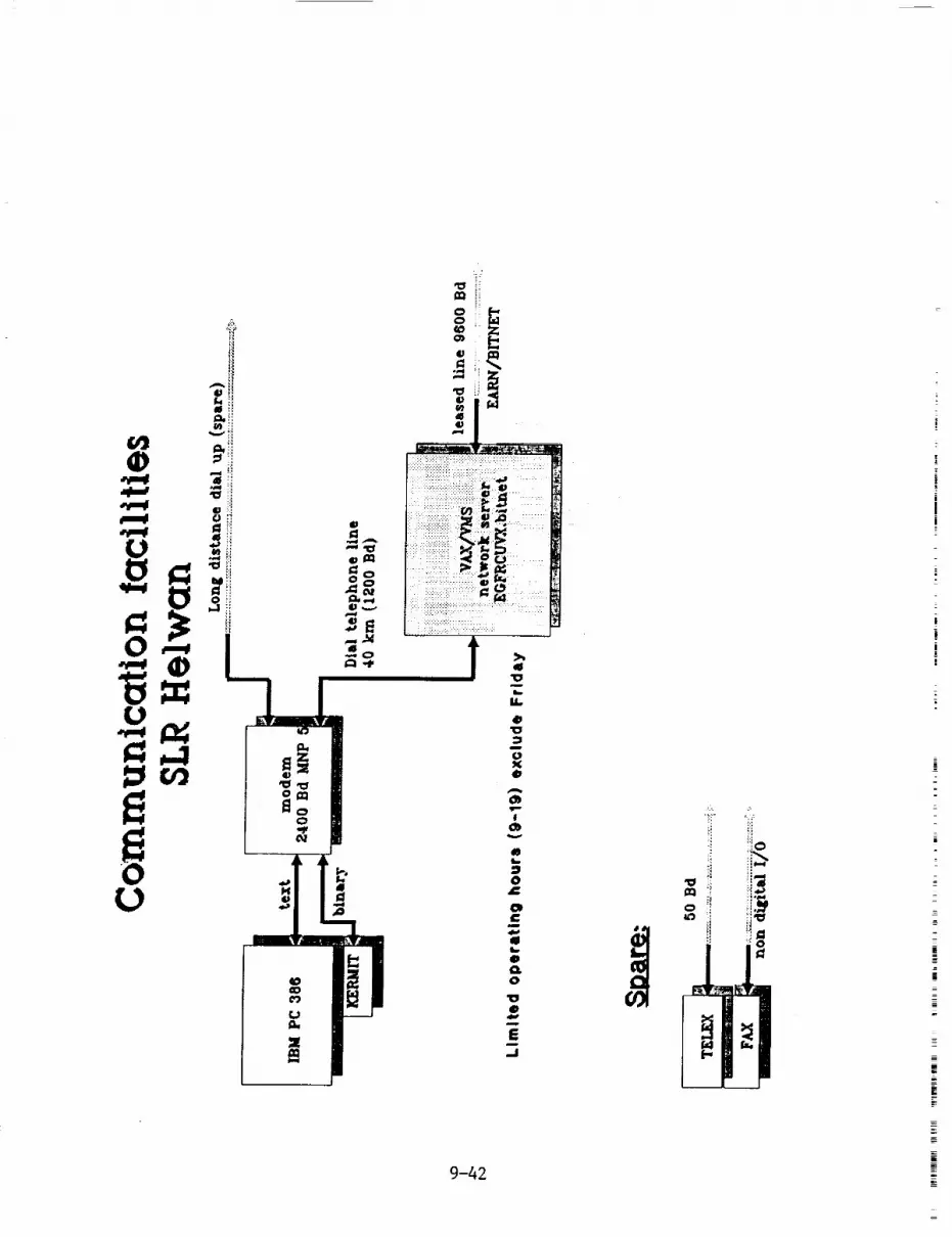
9-42

N94-15595
Upgrading NASA/DOSE Laser Ranging SystemControl Computers
byRandall L. Ricldefs
McDonald Observatory, University of Texas, Austin,Texas 78712
Jack Cheek
Hughes-STX, Lanham, MD 20706
Paul J. Seery, Kenneth Emenheiser,William P. Hanrahan
Bendix Field Engineering Corp., Seabrook, MD 20706
Jan F. McGarryNASA Goddard Space Flight Center, Greenbelt, MD 20771,
Laser ranging systems now managed by the NASA Dynamics of the Solid Earth(DOSE) and operated by the Bendix Field Engineering Corporation, the University ofHawaii, and the University of Texas, have produced a wealth of inter-disciplinaryscientific data over the last three decades. Despite upgrades to the most of the rangingstation subsystems, the control computers remain a mix of 1970s-vintageminicomputers. These encompass a wide range of vendors, operating systems, andlanguages, making hardware and software support increasingly difficult. Currenttechnology allows replacement of controller computers at a relatively low cost whilemaintaining excellent processing power and a friendly operating environment. The newcontroller systems are now being designed using IBM-PC-compatible 81M86-basedmicrocomputers, a reai-time Unix operating system (LynxOS), and X-windows/Motifgraphical user interface. Along with this, a flexible hardware design using CAMAC, GP-I13,and serial interfaces has been chosen. This design supports minimizing short and longterm costs by relying on proven standards for both hardware and software components.Currently, the project is in the design and prototyping stage with the first systemstargeted for production in mid-1993.
Introduction
In the more than two decades of laser ranging, the observational accuracy of theNASA-funded laser stations has dropped from tens of centimeters to a centimeter or better.To achieve this, most parts of the ranging system have been upgraded a number of times.It has long been recognized that the computer subsystems are antiquated and unable to keepup with the requirements for ever-more-precise range measurements and an ever-growinglist of targets. In the last year, a plan of action has been formulated to upgrade thesesystems in such a way as to minimize both short and long term cost by making extensiveuse of standard hardware and system software. The stations involved are the DOSE-
operated GSFC 1.2m telescope, the Bendix Field Engineering Corporation-operatedMOBLAS 4-8 and TLRS 2-4, the University of Hawaii-operated HOLLAS station, and theUniversity of Texas-operated MLRS
9-43
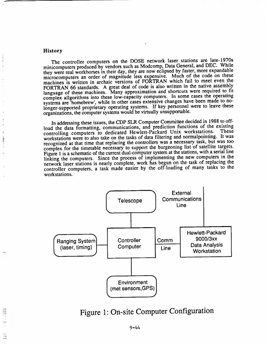
History
The controller computers on the DOSE network laser stations are late-1970sminicomputers produced by vendors such as Modcomp, Data General, and DEC. Whilethey were real workhorses in their day, they are now eclipsed by faster, more expandablemicrocomputers an order of magnitude less expensive. Much of the code on thesemachines is written in archaic versions of FORTRAN which fail to meet even theFORTRAN 66 standards. A great deal of code is also written in the native assembly
language of these machines. Many approximation and shortcuts were required to fitcomplex allgorithms into these low-capacity computers. In some cases the operatingsystems are 'homebrew', while in other cases extensive changes have been made to no-longer-supported proprietary operating systems. If key personnel were to leave theseorganizations, the computer systems would be virtually unsupportable.
In addressing these issues, the CDP SLR Computer Committee decided in 1988 to off-load the data formatting, communications, and prediction functions of the existing
controlling computers to dedicated Hewlett-Packard Unix workstations. Theseworkstations were to also take on the tasks of data filtering and norrnalpointing. It was
recognized at that time that replacing the controllers was a necessary task, but was toocomplex for the timetable necessary to support the burgeoning list of satellite targets.Figure 1 is a schematic of the current dual-computer system at the stations, with a serial linelinking the computers. Since the process of implementing the new computers in thenetwork laser stations is nearly complete, work has begun on the task of replacing the
controller computers, a task made easier by the off-loading of many tasks to theworkstations.
I 1 ExternalTelescope Communications
Line
IRanging System_l Controller
(laser, timing)_-_ Computer
L_me?n_ir°onme_ps_
Comm
Line
Hewlett-Packard
9000/3xx
Data AnalysisWorkstation
Figure 1" On-site Computer Configuration
9-44

Hardware Environment
The new controller system must accommodate many of the vagaries of 7 or so laser
systems' designs and philosophies and must be flexible enough to permit expansion ofthese systems in various ways. For instance, most of the Bendix-operated systems and theUniversity of Hawaii system fire their lasers at 5 or 8 Hz, use external pre- and post-calibrations, and use Hewlett-Packard 5370 counters as time interval units. MLRS on theother hand, fires at 10 I-Iz, uses internal calibrations and uses a TD811 time digitizer as the
finest part of its 3-tiered epoch timing system. The MOBLAS and transportable systemsare limited to satellites up to the orbits of the Etalons. The GSFC 1.2m research systemaccommodates many experimenters, and ranges to aircraft as well as to satellites. MLRS
ranges all currently targeted CDP satellites as well as MP-2 (in geostationary orbit) andreflectors on the moon. Some systems use CAMAC interfaces, while others use a
proprietary bus interface standard. Some incorporate GP-IB (IEEE-488), and most use
serials ports for various devices.
To replace the current controller computers, a new computer must be identified that cantalk with each of the existing interfaces and that is likely to be supportable for theforeseeable future. It must support one or more real-time operating systems, and must be
fast enough to meet all near term needs. Proprietary architecture and all the danger thatimplies must be avoided. In addition, the new system must be inexpensive. The obviouschoice is the ubiquitous IBM-PC-compatible microcomputer. Boards exist that interfacethe PC to almost any variety of hardware; the upgrade path to an even faster machine than
the prototypical 80486 33 MHz system is expected to be virtually painless; it is relativelyinexpensive; and there are a number of reasonable real-time operating systems available.
A prototype systems design was developed which includes an IBM-PC clonecontaining a 33 Mhz Intel 80486, 16 Mb of RAM, a 330 Mb SCSI hard disk drive, 3 1/2"and 5 1/4" floppy disk drives, a 16 bit ethernet card, high resolution (1024 x 768) video
display and a 16" monitor. Interface cards for CAMAC, GP-IB, and a serial mux boardwere also included. To save cost and space, the preliminary configuration will have the PC
use both the printer and erasable optical disk on the HP workstation across the ethernet
network.
To standardize the system interfaces and to limit dependence on specific vendors, it wasdecided to use the CAMAC, IEEE-488 (GP-IB), and RS-232 serial interfaces rather than
dedicating a bus slot to virtually each device in a ranging station. Along these lines, theMOBLAS systems' obsolete IACC interface will be replaced by CAMAC, therebyremoving an important source of maintenance difficulties. The serial ports are probably theeasiest of all of these interfaces to accommodate with the PCs; they will be used to bring in
environmental sensor data.
Operating System
Each laser system involved in this project has evolved along a different path dictated bydifferent needs. One overarching need now, however, is to create as much commonality as
possible and to program for a software environment that will still be viable in 10 years.There were several options available when the search was made for operating systems,
including writing it ourselves. Several of the current stations run home-built operatingsystems. The difficulties with these have been that they are hard to write and maintain.These systems were written because existing operating systems at the time did not offer thecombination of speed, performance, and code size that was necessary to make the most
9-45

effective use of the hardware in a real-time environment. With fast and (relatively)inexpensive hardware, there are no such needs today.
In the search for an operating system, we considered DOS and DOS add-ons, variousversions of Unix, and several proprietary operating systems, such as Digital EquipmentCorporation's VMS and the Apple Macintosh Finder. The proprietary operating systemswere rejected immediately, due to our need for vendor-independence. DOS and the DigitalResearch clone DR-DOS are neither multitasking, multiuser, nor realtime. DOS is alsotargeted to Intel 80x86 microprocessors, violating our requirement for vendorindependence. Although products such as Microsoft Windows and DeskView offer some
degree of multitasking, they do not claim to be either _-empfive or real-time.
Unix was chosen because it has become a commonly available operating system with arich software development environment. It does provide multi-user and multi-taskingcapabilities and is available on many types of processors. Although there are several'flavors' of Unix in the marketplace, the trend towards S_dards compliance allows wellwritten programs to be transferred among Unix systems. The Hewlett-Packardworkstations already available at the network laser stations run in a Unix environment.Standard Unix is not a real-time operating system. However, there are Unix clones and
derivatives which do support realtime, pre-emptive multi=tasklng and are designed forrealtime acquisition and control applications like laser ranging,
A number of Unix and Unix-like systems were considered. These include:
Coherent (Mark Williams) QNX (Quantum Systems)REAL/IX (Modcomp) Unix / Xenix (SCO)VRTX (RadiSys Corp) VxWorks (Wind River Systems)
The abovewere eliminated due to one or more of the following reasons. The operatingsystem
• requires proprietary hardware
• did not mention POSIX or real-time standards compliance• lacks one or more of the required compilers (FORTRAN, C, or assembler)• lacks network capabilities
• lacks graphics capabilities
The chosen operating system is LynxOS by Lynx Real-Time Systems, inc. LynxOSis a Unix-clone (no AT&T code) which complies with the POSIX standard as well as IEEE
1003.4 and 1003.4a draft real-time standards. It also follows the 80386 binary filestandards and runs on IBM-PC compatible computers. LynxOS is also available for
Motorola 680x0 systems and is being ported to the SPARC engine. C compilers (includingone by GNU) are supplied with LynxOS, while FORTRAN is available from a third party.TCP/IP, NFS, X windows and OSF Motif are also available from Lynx. It should bementioned for completeness that soon after LynxOS was chosen, Venix (Venturcom) wasdiscovered. It uses AT&T system V code modified for real-time applications and also runon IBM-PC compatibles. It appears to be a viable alternative choice for a real-timeoperating syste m .
User Interface and Networks
Several requirements for the User Ynterface=were advanced during planning. Theseincluded the need for a user-friendly interface, more graphics and less text, remotemonitoring and control, automation of many hardware settings and seamless integration
E==
IN

with the ltP workstation. The emerging standard for network-based, vendor-independentgraphical user interface is the X windows system. Since X windows specifies no policy orstyle, there is no consistency required of applications. For this reason the Open SystemsFoundation developed the Motif graphical user interface (GUI) on top of X windows,which does have a particular "look and feel". Open Look, which is another GUI supportedby AT&T and Sun, does not seem to be as widely available at this time. Using theconstraints of the GUI, user friendly applications can be produced that have many of thefeatures of the familiar Apple Macintosh and Microsoft Windows applications, such asmenu bars, pop-up windows, and freedom from a command line interface. Also, since Xwindows is network based, one can use the on-site software from virtually anywhere in theworld via a network connection. Much of the experience gained and code developed inimplementing such an interface for the on-site Hewlett-Packardworkstations for the NASA-funded stations will be of great value in constructing the controller system.
Connecting the controller computer and on-site data-reduction workstation via ethernetand TCPflP opens a world of data and control-sharing possibilities. Data can be recordedon the controller's disk drive in a directory which is mounted on the workstation via NFS(Network File System). The workstation can then have instant access to the data in realtime. Sockets, RPC (Remote Program Calls), and remsh (remote shell) can all server astools for creating a seamless dual computer system.
Preliminary Design
In addition to agreeing on prototype hardware and software platforms, the GSFC 1.2mtelescope, Bendix, and the University of Texas groups have all acquired prototypesystems. Work is proceeding on the design of the user interface and underlying functions.Device drivers for two critical pieces of equipment - the CAMAC and the timing board(used to provide the computer with 20 Hz interrupts from the station clock) - have beenwritten. The monitor program, which runs at all times and maintains information such astime, weather, and telescope status, and the star calibration program will be the firstsoftware package to be implemented, as they fulfil needs common to all stations. Work isalso proceeding on replacement of the MOBLAS IACC interface with CAMAC. The goal is
to put the first three upgraded systems (GSFC 1.2m, MOBLAS 7, and MLRS) intoproduction with the new controller in mid to late 1993.
A preliminary version of the user interface is shown in figure 2. This shows thecommon display of station parameters maintained by the monitor program such as date,time and telescope position. Also evident is the pull-down menu and display of graphs and
parameters unique to the star calibration program.
Conclusion
The overdue upgrade of NASA ranging station control computers is finally comingabout and is making use of the latest technology to produce a flexible, extensible, andmaintainable computer platform. The upgrade is based on standard hardware and software
components to lessen vendor dependence and enhance software portability. The prototypecomputer system has been designed and acquired by the principals in this upgrade, who arein the midst of further software design and low level software implementation.
9-47

9-48
=
o
=
o
>_
0
L_
I i
m<
0
. _I= =
==o=o=DO_O
¢q
,-, 0v 0 0C,_ 0 00, o.o_ 0 •
Nv3,.
t".- o 0
• . e,l 0
0 m_,i
!

N94-I5596
HP UPGRADE OPERATIONAL STREAMLINING
D. Edge, K. Emenheiser, B. Hanarahan, D. McCollums, P. Seery
Allied-Signal Aerospace Company
Seabrook, Maryland
R. Ricklefs
University of Texas
Austin, Texas
A_t_ct
New computer technology and resources must be successfully integrated into CDSLR station
operations to manage new complex operational tracking requirements, support the on site production
of new data products, support ongoing station performance improvements, and to support new station
communication requirements.
The NASA CDSLR Network is in the process of upgrading station computer resources with HP
UNIX workstations, designed to automate a wide range of operational station requirements. The
primary HP upgrade objective was to relocate computer intensive data system tasks from the controller
computer to a new advanced computer environment designed to meet the new data system
requirements. The HP UNIX environment supports fully automated real time data communications,
data management, data processing, and data quality control. Automated data compression procedures
are used to improve the efficiency of station data communications. In addition, the UNIX environment
supports a number of semi-automated technical and administrative operational station tasks. The x
window user interface generates multiple simultaneous color graphics displays, providing direct
operator visibility and control over a wide range of operational station functions.
9-49

HP UPGRADE OPERATIONAL STREAMLINING
The successful integration of new HP computer resources into the Crustal Dynamics Project (CDP)
Satellite Laser Ranging (SLR) Network as part of the HP Upgrade Project has led to critically needed
improvements in data system capability and significant gains in network operational efficiency. This
paper provides a brief description of the HP Upgrade Project strategy and progress to date in
streamlining station operations.
The HP Upgrade Project was initiated in 1987 to prepare the CDP SLR Network to meet the
operational challenges presented by multi-satellite tracking operations in the 1990's. The technical
approach for the lip Upgrade Project was based on the recommendations of the CDP Computer Panel,which recognized that new station requirements to support up to ten operational satellites and to
produce on site normal points could not be supported by existing station computer resources. Theexisting computer resources recorded tracking data on floppy disk or magnetic tape and required
manpower intensive operations to reload the data back into the computer to support station data
processing activity. In addition, data processing operations and satellite tracking operations could not
be performed at the same time. Therefore, data processing operations had to be scheduled around
periods of operational tracking and were typically performed at the end of an operational shift. These
problems delayed the production of data products and severely limited network tracking productivity.
The basic HP Upgrade Project strategy was to integrate a second computer system into the existing
station configuration to provide the required additional computer resources.
In 1988 the first HP computer systems were purchased, and development of HP Upgrade prototype
systems started at the Goddard Space Flight Center (GSFC) and at the University of Texas. The
development of a parallel prototype at the University of Texas was necessary to address the unique
requirements of a lunar tracking station. HP UNIX software development projects were sharedbetween GSFC and the University of Texas to reduce critical software development timelines and to
maintain design consistency.
The Moblas 7 and MLRS HP prototype systems were successfully tested in 1990. In 1991, the HP
Upgrade was deployed to the remaining network operational Moblas systems and development started
on HP Upgrades for TLRS 3, TLRS 4, and Hollas. The TLRS 3, TLRS 4, and Hollas HP Upgrades are
expected to be completed in 1992.
In order to reduce the load on critical station manpower and computer resources, the HP data
system was designed to provide fully automated data communications and data processing during
multi-satellite operations. Figure 1 presents a simplified diagram of HP data system functions. Thefunctions associated with real time tracking operations are divided between the controller and DIP
computers. Other Non real time HP functions, which include general station operations and automated
post tracking functions compiete the automated HP Data System Product Cycle. Depending on thenumber of observations in the pass, the HP Data System was designed to produce the normal point
data product 1 to 5 minutes after the operator has closed out the operational data set. The time
9-50

required to compress the normal point data set and transmit the data product to headquarters is less
than 1 minute.
The HP Data System has built in flexibility which allows interleaving of multiple satellite and
calibration sets. The code has been written to allow for many different combinations of hardware
settings. This has been accomplished via the use of different levels of ranging activity. By changinglevels within the software, the operator may determine which calibration sets (with possibly different
hardware characteristics) go with which satellite sets. Up to five different levels may be selected. This
feature makes it possible to quickly switch from one satellite to another and back again using
calibration sets which may be unique for each satellite. Figure 2 is an example of a single shift of
Moblas 4 support scheduling multiple satellite and calibration operations. Scheduled ERS-1, Ajisai,
Lageos, Etalon 1, Etalon 2, and Starlette passes axe labeled El, AJ, L1, MT, NT, and ST respectively.Scheduled calibration tracking is labeled C1. The activity scheduled at the bottom is the sum of
scheduled satellite and calibration activities. The station is continuously ranging satellites or the
calibration target for over 5 hours during the shift. The scheduling of muiti-satellite operations has
significantly increased the operational productivity of operational laser stations. Additionalinformation concerning the scheduling of multi-satellite tracking operations is presented in another
Eight International Workshop on Laser Ranging Instrumentation paper "SATCOP Mission Planning
Software Package".
Control of all processing and maintenance operations is provided by a mouse and/or keyboard
driven, user friendly multi-level menu interface. These menu controlled operations include data
archiving, tuned IRV prediction communications, data product statistics review, stationcommunications, semi-automated daily tracking operations reports, and other general station datacommunications. The user interface is written in the 'C' programming language and uses the Motif/x
windows style and flavor. The use of this industry standard ensures that the user interface is consistent
with other operating systems (in addition to UNIX) and is also consistent with widely available off-the-
shelf commercial software.
The design prototype for the second "processing" computer system was a UNIX based HI' 360workstation. Low cost upgrades have brought the design prototype up the the current CDP SLR
network configuration described in Figure 3. The liP 380 computer configuration includes two 332 MB
hard disks to improve efficiency by directing data operations to one disk and operating systemfunctions to the other disk. A 650 MB optical disk is included to provide on line data archiving, a
efficient backup media, and to support major software system upgrades. The 67 MB cartridge tape is
used as a low cost media for generating weekly full rate mailing tapes. The HP Paintjet printer
supports local hard copy requirements. The 19.2k baud modem supports a wide range of stationcommunication requirements including data communications and software system updates. The 16
inch color supports the X-Window environment and is the primary user control interface device for the
liP Data System.
The Moblas, MLRS, TLRS, and Hollas systems all have unique controller computer hardware andsoftware environments. Real time control functions may also vary station to station (MLRS is a lunar
station, for example). The HP Upgrade development strategy was to mlnimiz¢ the impact on real timecontroller functions, requiring only real time data communications to the HI' "processing computer"
and off load as many non real time functions as possible from the controller to the "processing
computer". A simplified functional block diagram for TLRS 3/4 is presented in figure 4. The controller
9-51

(or tracking) computer performance in managing the real time computer interfaces was a key technicaldesign problem for each station type.
Real time applications were developed in C in the HP UNIX environment to record and manage theflow of raw data measurements from the controller computer to the HP 380. Automated C and Fortran
applications assemble, screen, and prepare the raw data measurements for automated data processing.Based on inputs from the system operator, automated data processing functions start as soon as theraw data set is complete. .....
The HP UNIX software environment, with includes FORTRAN and C applications, was selected to
make maximum use of existing operational software, provide multi-vendor hardware potty, and
to provide a robust industry x window user interface for station operations. The HP Upgrade Projectsoftware strategy was to develop real " " " .......... _" -'_ •time apphcations m C and other data system app!_catmns mFORTRAN to make the best use of current operational software. The station user interface was
developed in the liP UNIX x window environment to make the best use of the HP 380 workstationresources in controlling station operations.
In order to meet the new station normal point data system requirements and maintain data systemintegrity, operational data system software was rehosted from VAX/VMS Fortran to HP UNIX
Fo_. The fielddata processing_s_ w_desig_ned_o Use identical data_processing algorithms and
to perform the same basic data processing and data quality con_i functions as the operational
headquarters system. These data processing functions include quality control of raw data
measurements, calibration data processing, computation of satellite ranging corrections, analytical
satellite data fitting, and satellite data compression to form normal points. The field data processing
system was designed to produce the s_e0perat|onal q_ity control statistics _d data pro_ucis as the
headquarters system. These data statistics and data products were carefully benchmarked _ainst the
operational headquarters data syst_ bedsore the HP Data System was declared operational. Some
software system utilities used in the VAX/VMS environment had to be replaced with equivalentUNIX utilities during software rehosting.
The HP Data System Upgrade has been successfully operating at Moblas 4, Moblas 5, Moblas 7,
and MLRS for over a year, producing on site normal points, generated within minutes of operational
satellite tracking. Starting in April 1992, multi-satellite operations were successfully integrated into the
HP Upgrade Data System, contributing to recent record data production by Moblas 4 and Moblas 8.
Upgrades to theHP workstation CPU's have been successfully accomplished in (he field_thoutsoftware system modifications and have enabled the HP Data System to accommodate massive
increases in data volume associated with multi-satellite operations and two shift network support for
TOPEX. Remote software system updates have been performed using modem communications, without
impacting station operations. The automation of the Data System has helped free up critical stationmanpower resources needed to sustain nearly continuous_cldng ope_ associated with multi-
satellite support_ The liP Upgrade]s the first majorstepin streamlining CDP SLR operations.Strategic technical planning to replace the c6htrol]er computer, providing necessary comput-er
resources to automate other station functions, is in p-rb_ess. Tnaddlt]6n, _icomputer networkcommunications to CDP SLR network Stations is expected to be established in the near future,
providing advanced communication resources to automate remote software system managementactivities and global data communications.
9-52

--,,BENDHP DATA SYSTEM PRODUCT CYCLE
L
OFFLINE FUNCTIONS
STATION COMMUNICATIONSADMINISTRATIONSTAR CALIBRATIONSCHEDULINGDATA SYSTEM SETUPSTATION ARCHIVING
GENERAL STATION
OPERATIONS
CONTROLLER FUNCTIONS
m
I
I TASK SCHEDULINGOPERATOR INPUTSANALYTICAL COMPUTATIONSEQUIPMENT CONTROLMEASUREMENT RECORDINGDATA PREPARATIONDATA COMMUNICATIONSDATA DISPLAYS
REAL TIME TRACKING
OPERATIONS
HP FUNCTIONS
TASK SCHEDULINGOPERATOR CONTROLDATA COMMUNICATIONSDATA PREPARATIONDATA VERIRCATIONDATA DISPLAYS
7m m_
DATA PROCESSING FUNCTIONS(1 TO 5 MIN)
OPERATOR CLOSEOUTDATA AGGREGATIONMAILER RLEDATA VERIRCATIONCALIBRATION PROCESSINGSATELLITE PROCESSINGDATA REPORTSARCHIVING
..I
POSTTRACI(ING
OPERATIONS
DATA COMMUNICATIONS FUNCTIONS(1 M!N)
DATA COMPRESSIONCOMMUNICATION CONNECTION
TRANSI_SSION
m
FIGURE I
9-53
-- CDSLR"--
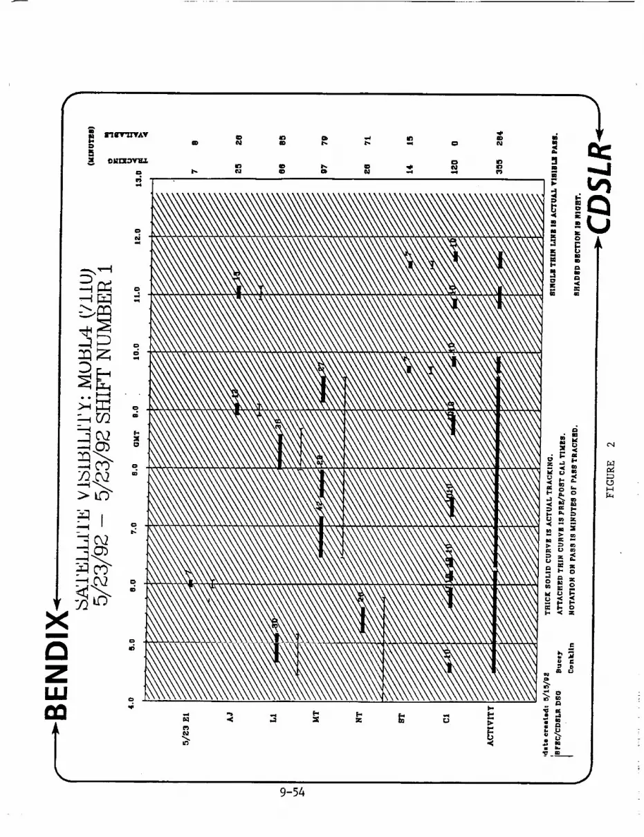
9-54
/

8
_ _ .i_O
i
;iiIu_ _°_
I!
I|
I_1,.<-_j
I ÷;__I._ _I_.
.,,..I
J
I"4
9-55

ZLU
,!I
---_ ._ o,-, Irh I:_ r.,o
I
i i_l..
II _|| _
i
iI_c:1--_ ._-
IL-.S
mmDm J
m
L_
"-'l,_ _,1_ E
®E
T __'_
9-56
6
J

N94-15597APPLICATIONOF THE ROBUST ESTI_tATE
IN SLR DATA PREPROCESSING
T. Detong, Z. Zhongping, X. HuaguanShanghai ObservatoryAcademia Sinica
J. PeizhangInstitute of Systems ScienceAcademia Sinica
ABSTRACT
M-estimator, one kind of robust estimator, has been used
in SLR data preprocessing. It has been shown that theM-estimator has 50% or more breakdown point.
9-57
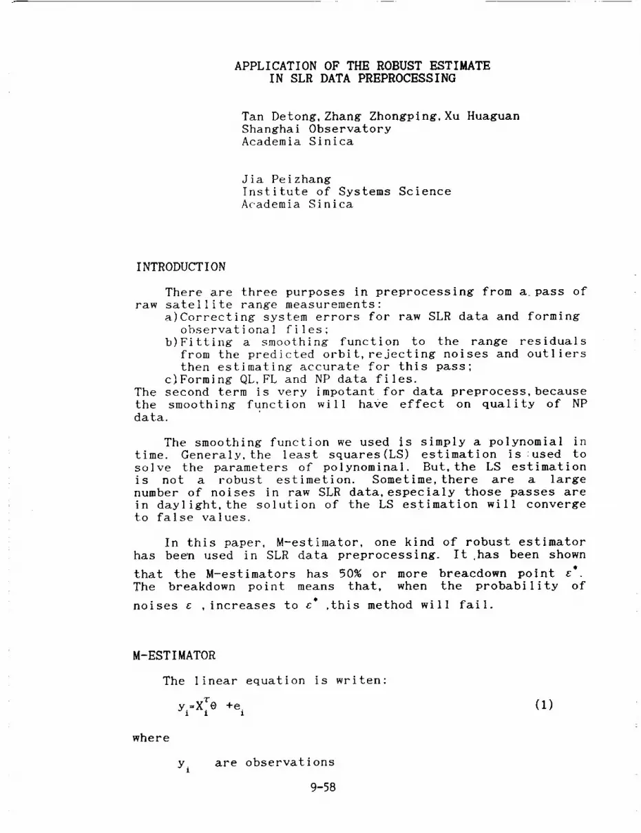
APPLICATION OF THE ROBUST ESTIMATEIN SLR DATA PREPROCESSING
Tan Detong, Zhang Zhongping, Xu HuaguanShanghai ObservatoryAcademia Sinica
Jia PeizhangInstitute of Systems ScienceAcademia Sinica
INTRODUCTION
There are three purposes in preprocessing from a_pass ofraw satellite range measurements:
a)Correcting system errors for raw SLR data and formingobservational files;
b)Fitting a smoothing function to the range residualsfrom the predicted orbit, rejecting noises and outliersthen estimating accurate for this pass;
c_Forming QL, FL and NP data files.The second term is very impotant for data preprocess, becausethe smoothing function will have effect on quality of NPdata.
The smoothing function we used is simply a polynomial intime. Generaly, the least squares(LS) estimation is:used tosolve the parameters of polynominal. But, the LS estimationis not a robust estimetion. Sometime, there are a largenumber of noises in raw SLR data, especialy those passes arein daylight, the solution of the LS estimation will convergeto false values.
In this paper, M-estimator, one kind of robust estimatorhas bee_ used in SLR data preprocessing. It ,has been shown
@
that the M-estimators has 50% or more breacdown point e .
The breakdown point means that, when the probability of@
noises e ,increases to e ,this method will fail.
M-ESTIMATOR
The linear equation is writen:
Yi=X: O +e i
where
y. are observations1
9-58
(i)

0 is the vector of paramaters to be estimated
X i is the vector of coefficients
e i are random errors.
The M-estimator, called Maximum Likelihood Type Estimator, is
such an estimator which makes the following objective
function minimum:
N
_.F{( yi-X:@ )/_}=min. (2)4=I
are values estimated for e2a is variance
F{'} is an even functionDifferent objective functions have different M-estimator.
this paper we used Hampel estimator, here -
In
F(ri
___ 2 ar I [ ri [ : _o
_,oo ( Ir I-_.o o) _-oo<Ir I"-_-_°
_'0 (X2(_[ri
ki XO 2 1.2 2 a<lri[<t (y
X2--Xl _ G ----_AOCT I i 2
l 0 (k2+li-kO) cy2/2 [r i [ >12o
(3)
ri=yi-X:O
10=3, Ii=4, 12=6.
Equation (2) can be rewriten as"
N
_,, Xi# { (yi-X:@)/c7} =01=1
where
+ {-}=F' {.}.Then
and
Wi=_ (ri/o')/(rl/a) .
From (3) we have
(4)
(5)
(6)
9-59
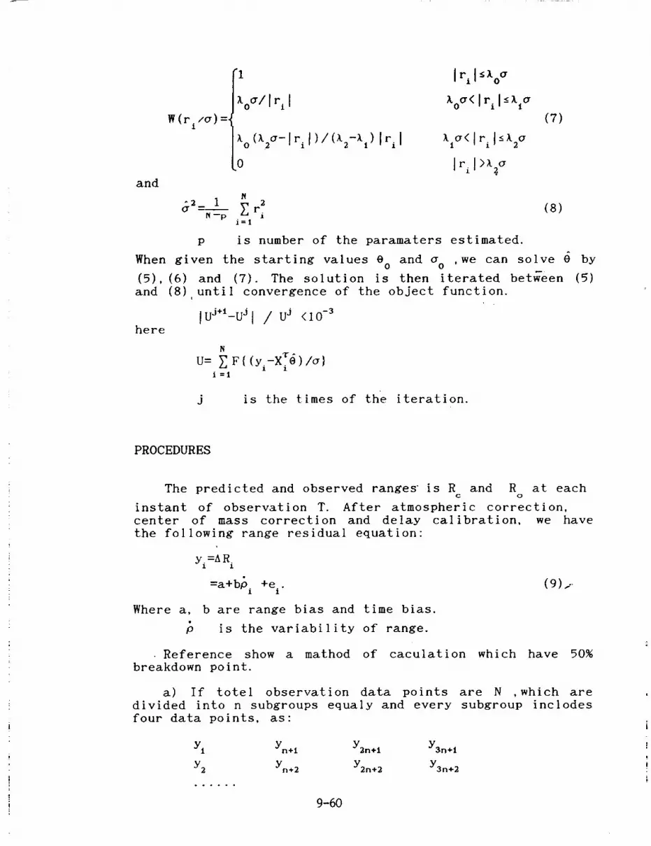
and
W(r,/:)=_
"1 Ir i I_oa
_oa/I ri i :o:<Iri I-<h_
>_o(_.2'_-Ir I)/ (_',.->',)Iq I
0
(7)
N
2 i _]r. (8)0" N--p l
i=1
p is number of the paramaters estimated.
When given the starting values e and a ,we can solve 0 by0 0
m.
(5), (6) and (7). The solution is then iterated between (5)and (8) until convergence of the object function.
IUj÷'-UjI / uJ <1o.3here
N
U= _ F { (yi-XT6,)/a}
i=i
is the times of the iteration.
PROCEDURES
The predicted and observed ranges is R and R at eachc o
instant of observation T. After atmospheric correction,center of mass correction and delay calibration, we havethe following range residual equation"
Yi=ARi
=a+bp. +e., i
Where a, b are range bias and time bias.
is the variability of range.
(9)i'
Reference show a mathod of caculation which have 50%
breakdown point.
a) If totel observation data points are N ,which aredivided into n subgroups equaly and every subgroup inclodes
four data points, as"
Yt Yn+l Y2n+l Y3n+l
Y2 Yn+2 Y2n+2 Y3n+2
9-60

Yk Yn+k Y2n+k Y3n+k
• • . • • •
Yn Yn+n Y2n+n Y3n+n
n=N/4.
i
When noise numbers in raw obsrevation data are less then
N/2, there must be a subgroup in which contains one noise
point at most.
b) For the linear model as (9), we can find the linear
estimated value of bk for any subgroup k"
4
bk = _ 31YI 410)I=I
If b is no-bias, we have"k
4
31=0I=i
4
B,_= I (II)l=l
and
where
4 i
-_S2=min1I=I I
5 =5 =12 3
T5= 2 C
1 2T 1 +T 2
T6 -- 2
4-- 3_ 2 C
TI=PI÷I-P I
By solving equations (11), we get_."
31=61_T i
where4
2T;E=I/E6, ,
I=I
(C is a constant to be selected)
(1-1, 2, 3)
(1=1,2,3,4)
¢ 4
PO 1=1 1=1
F T +T_ T l +T 2c:m ×Lv-/GT ]Thus, the residuats of k-subgroup are
9-61

rk|'Ykl--6k6k i (1=1, 2, 3, 4)
c) For each subgroup, the largest and smallest values of
rkl are rejeated. And we can get the initial values ako , bkofrom remained two data points through follows:
Ykl--akO+ bkoPk j (j=l, 2)
d) Then calcuiation the object function of M-estimateused all observations for every subgroups:
N
Uk= _ F{yi-ako-bko_i } (k=l, 2 .... n)i=l
where F{-} can be taken from (3),and the initial value of acan be arbitrarily given, for example 0.5'meters.
e) Select the minimum value from Uk (k=l,-2 .... n).Suppose k=m. that is
U =min.m
Then amo and bmo, those are taken from m-subgrop, can be used
as the initial values ao, bo. It is sure that the a ° and b °are taken from 'good' observation points.
f) Then we can get
ri=Yi-ao-boP i (i =l, 2 .... N)
N
(y2_ I Z r.- 1
i=1
Because a o,b ° are obtaied by two data points, they have just
lower accuracy. From (5) to (8) and iterated unti 1covergence, the accurate results a,b can be get as above.
g) Ai_'ter correcting range bias and time bias, we can geta polynomial in time as following-
a p: =y.-a-bp.1 1 1
=ao+a t +a t2+a t3+.I i 2 i 3 i .....
Useing M-estimator, the
ao,ai,a2,a 3 ...... can be solved.
parameters of polynomial
CONCLUSION AND DISCUSSION
Comparing with the LS estimator,advantage as follows:
9-62
M-estimator has its

a) It can" be preprocess observation data that contain a
large amount of noises, for example , a pass for LAGEOS
in daytime are shown in fig 1, (12/20/1991 8:45 UT). In this
pass rate of noise is up to 70%.
! s
b) At same accuracy, the order of polynomial fitting is
only 4 using M-estimator, while the order is up to 6-8 or
more with LS estimator. Seeing table I.
c) Noise mixed at the parts near the both ends of the
curve can be detected and deleted.
Besides, comparison with the method of screen-processinand LS estimator, one third time is saved with M-estimator.
REFERENCE
J. peizhang On Joint Robust Estimation of The
Parameters and The Variance. Acta AstronomicaSinica. Vol.33.No i. 1992.
9-63
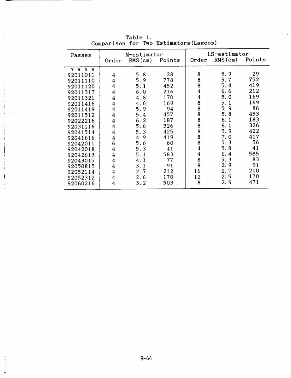
Table i.Comparison for Two Estimators(Lageos)
Passes
Y M D H
92011011
92011110
92011120
92011317
92011321
92011416
92011419
92011512
92022216
92031116
92041514
92041616
9204201192042018
9204261392043015
92050815
92052114
92052312
92060216
M-estimator
Order RMS(cm) Points
4 5.
4 5.
4 5.
4 6.
4 4.
4 4.4 5.
4 5.
4 6.
4 5.
4 5.
4 4.
6 5.
4 5.
4 5.4 4.
4 3.
4 2.
4 2.
4 3.
8 28
9 778
1 452
0 216
LS-es%imator
Order RMS (cm) Points
8 5.9
8 5.7
8 5.4
4 6.6
8 170
6 169
9 94
4 457
2 1876 326
3 4259 419
6 60
4 5.0
8 5.1
8 5.9
8 5.8
8 6.1
8 6.1
8 5.98 7.0
8 5.3
3 41
I 583
1 77
i 91
7 212
6 170
2 503
4
4
8
8
16
12
8
5.8
6.4
5.3
2.92.7
2.5
2.9
29
752
419
212
169
169
86
453
.183326
422
417
56
41585
83
91
210
170
471
9-64

Fig. l.
Residual for A Lageos Pass in Daytime
• A
_r
,_jED
I
<[.,r
U_O
GO._J
rn
09UJrr
STATION ID "7837
DATA: 12/20/g I
j o . .
°
•5 --J'.""• •
o
35 -] ""
I
2s -J ..i
SATELLITE: LAGEOS
TIME (UTC) 8:45
: ." • •
• o
I
.
t
°.
• . .. .
..
o.
.•
°.
I
• °
• • •°• :°"
• °
°
N= 1506
RMS=6CM
I
°.
.°
• • • .. • • .j
• • • . :.
|•
t_ -.tI
Ol
150!
• o•
• : • • .o .
"o• °
." °
375
°
I I _ 1
ELAPSE TIME (SECOND)
9-65


Lunar Laser Ranging

N94-15598
A Computer-Controlled x-y Offset Guiding Stage for the
by
MLRS
P. J. Shelus, A. L. Whipple, J. R. Wiant and R. L. Ricklefs
McDonald Observatory, University of Texas at Austin, Austin, Texas 78712
and
Frank M. Melsheimer
DFM Engineering, Inc., Longmont, Colorado 80501
ABSTRACT
The MLRS has experienced excellent success in its lunar and artificial satellite laser
ranging operations during its many years of operation, in spite of its relatively small "receive"
aperture. We continue to strive, however, for a greater volume of data, together with better
accuracy and precision. We have just now completed the design, construction, and
implementation of a computer controlled x-y offset guiding stage for the MLRS, analogous tothe manual one that had been a part of the original 2.7-m lunar laser ranging system on Mt.
Locke at McDonald Observatory. In the past we had been hampered by the lack of a
satisfactory hardware design which could fit within the very cramped quarters of the MLRS
telescope's tailpiece. Recently, with funding support from the U. S. Naval Observatory and the
design and construction expertise of DFM Engineering, Inc., a satisfactory instrument has
been specified, designed, built, and installed. This instrument will greatly expand MLRS
observational opportunities by allowing the observing crews to actively guide on visible off-axis lunar surface features or background stars while the on-axis lunar surface retroreflector
targets are in the dark. This paper describes this instrument and its present implementation atthe MLRS.
Introduction
The McDonald Observatory Laser Ranging Station (MLRS) is a dual purpose installation
(Shelus 1985) which was designed to obtain laser returns from both artificial satellite and lunarsurface retroreflector targets. It was originally constructed to replace the NASA Apollo LunarRanging Experiment (LURE) system which had been installed on the McDonald Observatory 2.7-m telescope in the late 1960's (Silverberg 1973) and was used up until the mid 1980's. TheMLRS is designed around a 0.76-m x-y mounted Cassegrain/Coud6 reflecting telescope and a veryshort pulsed, frequency doubled, 532-nm wavelength, neodymium-YAG laser, with associatedcomputer, electronic, meteorologic, and timing interfaces. The station was initially erected in thesaddle between Mt. Locke and Mt. Fowlkes at McDonald Observatory, near Fort Davis, in far
west Texas and first became operational in the summer of 1983. It was soon recognized that wind
tunnelling effects in and around this saddle site had very serious effects on what astronomers callatmospheric seeing. A new telescope pad was constructed and the MLRS was moved to its presentsite atop Mt. Fowlkes in early 1988 (Fig. 1).
Since the mid-1980's, the MLRS observing emphasis has been shifting dramatically fromthe Moon to artificial satellite targets (Fig. 2) but the Moon has always continued to be an important
part of its routine operations (Shelus 1987). Also, attesting to the splendid versatility of theMLRS, in a cooperative effort with the CERGA lunar laser ran.ging facility in France, we are usingthe Meteosat P-2 geostationary weather satellite in a laser ranging experiment to study the transferof time at the sub-nanosecond level over intercontinental distances. Most of the MLRS observing
systems are transparent to the observer and it is often the case that through the course of a single 8-hour observing shift an observing crew will routinely range to such diverse targets asToper/Poseidon, ERS-1, Starlette, Ajisai, Lageos, Etalon-1, Etalon-2, MP-2, and the Moon. The
I0-I
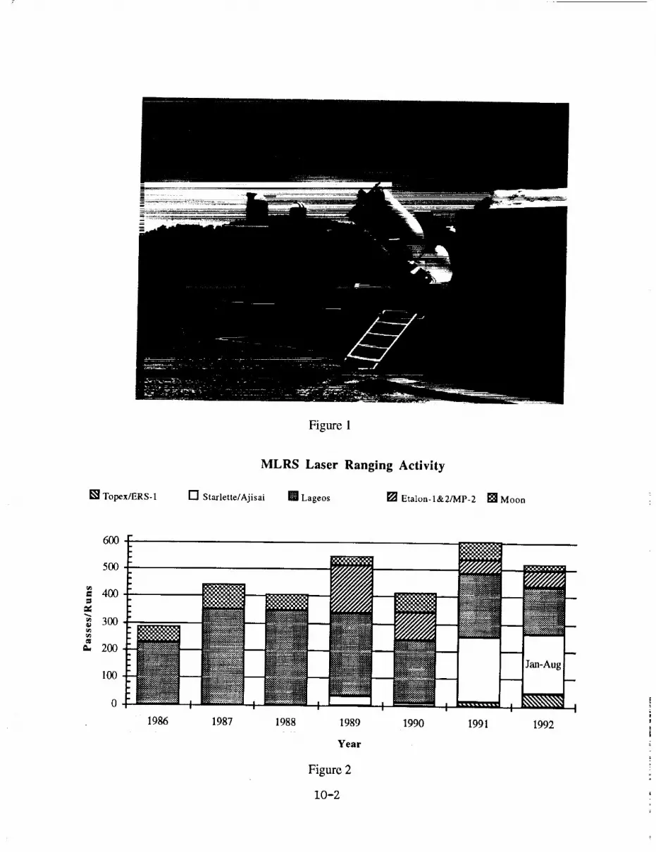
Figure 1
[] Topex/ERS-1
MLRS Laser Ranging Activity
[] Starlette/Ajisai ml Lageos [] Etalon-l&2/MP-2 [] Moon
60O
5OO
400
_ 300
_, 200
100
NNtN-
1986 1987
//1988 1989
Year
Figure 2
10-2
1990
r///7////,/_.:_,;:oj_
J _ILII-I_ I1 _ I
I991 1992

principal differences among all of these observations are the apparent angular speed of the target'smotion across the sky and the return signal strength. Of course, low targets move quickly and
high targets move slowly. Return signal strength is dictated primarily by the inverse-fourth-powernature of laser ranging. It is extremely important to realize that the return signal strength ratio,neglecting all parameters except the distance, for a near-Earth artificial satellite and the Moon is
something like 3 x 10¹². That is to say, it is more than one trillion times more difficult to laser
range to the Moon than it is to laser range to, say, Ajisai or Topex/Poseidon.
Increased Data Volume Requirements
In spite of these tremendous handicaps of low signal strength and small "receive" aperture, theMLRS has experienced remarkable success in its lunar laser ranging (LLR) measurements, and theresultant computation of lunar orbit and Earth orientation information therefrom (Whipple et al1991). However, we are always striving for an even greater number of observations which will,in turn, naturally lead to better accuracy and finer precision. It is evident that we can increaseMLRS LLR data volume in at least three ways:
1. spend more time on target;2. transmit more energy;3. increase "receive" aperture.
With support from a contract from the U. S. Naval Observatory we have found ourselves in aposition to make a viable attempt at implementing the first technique, i.e., spending more time ontarget, via the design, construction, and implementation of an x-y offset guiding stage for theMLRS.
An Offset Guiding Stage
The concept of an offset guiding stage is one that is commonly used in observationalAstronomy and it has surfaced many times during our deliberations about the logical up-grade ofthe MLRS during the past several years. It is merely the idea of installing an offset guiding stageon the MLRS, analogous to the one that had been in place and in use on the original 2.7-m LLR
system at McDonald Observatory. An MLRS x-y offset guiding stage would allow us to routinelyguide on a visible off-axis lunar surface feature (or, perhaps, even a star) while the on-axisretroreflector remains in the dark (i.e, it is on the "other" side of the lunar terminator). Not only
would there be a much greater number of observing opportunities during the course of a lunation,
perhaps, more importantly, ranging data to lunar surface retroreflectors in the dark would bevirtually noise free. In our past plannings we had been hampered by the lack of a suitablehardware design which could fit within the very cramped quarters of the MLRS telescope's tail-
piece, and the lack of money to actually construct and implement a design if a satisfactory onecould be found. Recently, within our interactions with the U. S. Naval Observatory and DFMEngineering, Inc., support has been provided and a new concept has been formulated for just suchan MLRS x-y offset guiding stage.
After a very successful series of bid and negotiating sessions, a contract was set up betweenthe University of Texas at Austin and DFM Engineering, Inc. of Longmont, Colorado for designand construction of a x-y stage for the MLRS. Design drawings for the mechanical systems of the
stage were received by us in February, 1992. These drawings were reviewed by McDonaldObservatory Laser Operations personnel, with support from our McDonald Observatorymechanical engineering colleagues. In general, the overall design was found to be very wellthought out and quite workable. A very small number of minor problems and severalenhancements were identified during the review. These were conveyed to DFM, Inc. and were
incorporated into the final design. Preliminary design drawings for the electrical systems of the
10-3

stage were received from DFM, Inc. at the end of March. An internal electrical systems designreview which was held at the MLRS during the first week in April. The results of that review were
conveyed to DFM, Inc. for implementation. Machining and assembly of the mechanical structureswere completed in May at DFM, Inc.. Delivery of the hardware to Austin took place in June andinitial testing and shake-down, before its shipment to the MLRS for final installation andimplementation, was performed. The instrument was transported to the MLRS at McDonaldObservatory in July. After a number of adjustments and relatively minor modifications, installationon the telescope took place at the end of August.
The instrument is a two-axis translation stage (Fig. 3) which mounts directly to the MLRStelescope's back-plate. It provides for the simultaneous mounting of two electronic TV cameraswith turning optics to direct the telescope's Cassegrain beam to either of the cameras. The cameras
are selectable from within the MLRS operation's tra_qer viacomputer control or an auxiliary switch.Each axis is driven by a DC servo motor/encoder combination at speeds in a range 0-8 mm/sec andis directly encoded using digital linear encoders. Positioning of each stage is accurate and
repeatable to 5 microns with a travel of more than 125 mm in each axis, centered on the optical axisof the MLRS telescope. The electronics control package includes a dedicated PC-type computerbased on an Intel 80386SX processor, a motor controller board inside the PC, together with all of
the necessary electronic/computer interfaces and controls. Software provides a closed servo loopbetween the encoders and the motors and communicates with the external MLRS control computervia a serial port. In addition to the source code, the software deliverable includes the developmentenvironment as well, so that future software changes, if necessary, can be accommodated withouta need to return to the vendor.
Figure 3
10-4

Conclusion
Once in operation, the completed x-y offset guider will have a very positive impact on thequality and quantity of lunar data acquisitions from the MLRS. Sufficient software currently existsto begin immediately the manual operation of the stage at the MLRS. In the coming months andyears it is our plan that additional software and hardware will be secured for eventual sem-automatic and completely automatic operation of the stage.
References
Shelus, P. J. 1985, IEEE Trans. on Geosci. and Rem. Sens., Vol. GE-23, No. 4, p. 385
Shelus, P. J. 1987, Discovery, Vol. 10, No. 4, p. 33Silverberg, E. C. 1974, Appl. Opt., Vol. 13, p. 565Whipple, A. L., Gy6rgyey-Ries, J., Ricklefs, R. L., Shelus, P. J., and Wiant, J. R. 1991, IERS
Tech. Note 8, p. 87
10-5

1 94-15599
Lunar Laser Ranging Data Processing ina Unix / X Windows Environment
by
Randall L. Ricklefs, Judit G. RiesMcDonald Observatory, University of Texas, Austin, TX 78712
In cooperation with the NASA Crustal Dynamics Project initiative placingworkstation computers at each of its laser ranging stations to handle data filtering andnormalpointing, MLRS personnel have developed a new generation of software to providethe same services for the lunar laser ranging data type. The Unix operating system and X-windows/Motif provides an environment for both batch and interactive filtering andnormalpointing as well as prediction calculations. The goal is to provide a transportableand maintainable data reduction environment. This software and some sample displays arepresented.
Introduction
The processes of reformatting, calibrating, filtering and normalpointing lunar rangingdata has taken several shapes during the years of University of Texas McDonaldObservatory participation in lunar laser ranging. During the days of the 2.7m rangingsystem, from 1969 to 1985, data was transferred on magnetic tape from the Observatory toAustin, where batch programs on the CDC Cyber computer systems were invoked on an
entire month's data. After a good deal of interaction with line printer, plots, listings, andpunch cards, the data was finally processed and ready for mailing -- on punch cards ormagnetic tape.
The part-time lunar ranging facilities on the 2.7m telescope were soon replaced by thededicated lunar and artificial satellite ranging system MLRS (McDonald Laser RangingSystem). From the first lunar observations in 1983 until mid-1990, data was processedinteractively on Data General NOVA 4/X computers. There were restrictions as to theamount of computer memory and the speed of processing. Fortunately, the station
contained 2 identical NOVAs sharing a hard disk, meaning that the lunar (or satellite) datacould be processed on one computer while data was taken on the other. The reduction ofthe data was totally interactive and in no way automated. In addition, lunar predictionswere produced on-site, another first in the effort to down-size historically mainframe-basedapplications. Extraction of earth rotation parameters was at one time attempted on site innear-realtime.
In 1988, the Crustal Dynamics Project SLR Computer Panel mandated the installationof Hewlett-Packard 9000/360 Unix workstations at each NASA-operated laser rangingstation to relieve the aging controller computers of much of their data and communicationshandling responsibility and to provide on-site data filtering and normalpointing for agrowing list of artificial satellite targets. This was seen by MLRS staff as an opportunity toprovide a better lunar data processing environment as well.
A New Environment
One of the important goals of the computer panel was to provide a standardenvironment for data handling that would allow portable code to be written for a non-
10-6

proprietary system. To this end Unix as well as X windows were chosen for the softwareenvironment. Both of these products can be found on workstations and mainframes frommany different vendors. Although there are many "flavors" of Unix, there is enough of acommon thread, especially with POSIX, SVID, and other standards to allow fairlyportable code to be written. In addition there are many useful tools generally available withUnix, from text editors to file manipulation utilities and operating system shells. Theavailability of shell scripts to cream batch jobs has also eased the task of systemdevelopment.
X windows (along with OSF/Motif) provide a network-oriented interactive graphicaluser interface that is quite portable and has been implemented on several operating systems.X-windows is policy free, meaning that there is no implied style imposed on code beingwritten for this interface. The Open Systems Foundation (OSF) Motif graphical userinterface was adopted to give a common style to this and other programs written for the X-windows environment.
i
Lunar Tasks
The process of obtaining lunar data requires several pre- and post-acquisition steps,which are at the heart of this discussion:
1) range and point angle predictions,2) data calibration and reformatting,3) data faltering,4) data normalpointing.
Much of the software for tasks 1), 2), and 4) was implemented in a FORTRAN 66 varianton the NOVA as well as in FORTRAN 77, after a joint port with the Australian NationalMapping organization. While the data filtering code also existed on the NOVA, it was notin a form that was readily usable on the Hewlett-Packard workstation. Common to allthese steps is the need for a flexible user interface which handles entry of parameters,plotting of data, and display of processing results.
Predictions
The first task of any ranging system is to provide point angle and range predictions.Lunar ranging is no exception. Most of the code required to produce lunar predictions isalso required in the production of the filtered lunar data and normalpoints, making the
maintenance of code relatively straightforward. This software can use either the MIT/UTPEP ephemeris or the JPL DE-303 ephemeris and its successors. Lunar and planetarypredictions as well as lunar librations are included in both of these packages. Since no fitof lunar or solar system parameters is made in the on-site processing, no partial derivativesare needed. Earth rotation data is updated weekly to provide the most accurate predictions
possible.
Parameters to run this software are set in the Lunar Data Editor program. Theprediction software itself is run automatically on a daily basis from a Unix "cron" script.The program reads the date and time, recognizes whether predictions already exist andproduces predictions as appropriate for the next day. The prediction program can also berun interactively from the command line of a terminal window as well as from XControl,the main user interface program, but that is never done in production. Lunar predictionsare moved to the ranging system control computer over an RS-232 serial link in the same
way as the artificial satellite predictions.
10-7

Batch Analysis
The reduction of the lunar ranging data after the moon is observed starts with the samesuite of programs as do the artificial satellite reductions. Once the data has been transferredfrom the controller computer and preliminary reformatting and collating of data has beendone a shell script is initated to calculate and apply geometric and electronic calibrations, tofilter the data using Poisson filtering techniques, and to normalpoint the data. (See figure1.) The results of processing are then displayed using the Lunar Data Editor program,giving the crew can get an objective view of the quality of the ranging data.
Interactive Analysis
During the time when lunar data was being entirely reduced on-site with NOVAsoftware, there was manpower available to scrutinize data. We no longer have that luxury.The lunar data is electronically transferred to Austin (using batch uucp over a dedicated
fine) for final f'dtering and lunar-network-oriented quality control.
To better interact with the data, the Lunar Data Editor (LDE) was developed. It uses Xwindows and OSF Motif to provide a modern environment in which to examine and
process the lunar data. Pull down menus, pop-up windows as well as both histogram andscatter plots of the data are available for operator use. Figures 2-7 show portions of theuser interface through which the user has control over the scale of the plots, the parametersused in the Poisson filtering and normalpointing and the sequence of reduction operations.Also included in the interface are provisions to manage up to 10 sets of station coordinates,
lunar ephemeris parameters, and control parameters as well as 5 sets of lunar reflectorcoordinates. This capability permits easy changes among ephemerides and stations as thesituation dictates.
LDE is comprised of several programs with distinct responsibilities. LDE itself is a Clanguage program that handles the user interface, including parameter input and datadisplay. The entire X-windows/Motif interface resides here. It in turn uses the Unix"system" call to invoke the lunar calibration program (C), the Poisson filtering program(FORTRAN), and the normalpoint program (which can also be called to recompute dataresiduals) (FORTRAN). This has the advantage of breaking up what would otherwise be ahuge program into more manageable units. It also provides a way to integrate existingFORTRAN and new C programs in a portable manner. Error codes and messages returnedby the called programs are used by LDE to provide pop-up error dialog boxes as needed.Results from each program's execution are shown in the scrolling text box at the bottom ofthe screen, as can be seen in figure 7. Each of the called programs can also be runindividually from the command line, as they are in the batch f'fle.
Since LDE is an X windows program, it can be run across a network. The programitself is run on the HP workstation, but the user can either be at the system console or, as isoften the case, running the eXodus X windows server on a Macintosh connected to theworkstation over the departmental ethernet network. One can even run this program acrossinternet from thousands of miles away (with some degradation in speed) and still have theadvantages of the graphics, pull-down menus and so forth.
It should be noted that none of the above discussion touches on performing quality
control by comparing multi-run or multi-station data or the computation of earth orientationparameters from the data. Due to the origins and complexity of that code, it will remain onan IBM mainframe for some time to come.
10-8
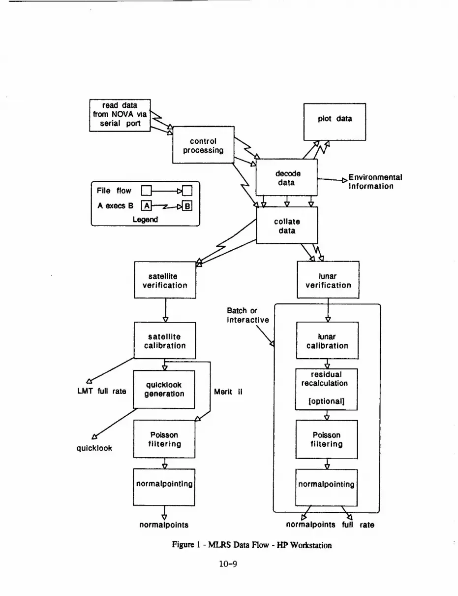
read datafrom NOVA via
serial port
File flow
A execs B
Legend
controlprocessing
\
decodedata
collatedata
plot data
EnvironmentalInformation
LMT full rate
quicklook
satelliteverification
lunarverification
satellitecalibration
quickiookgeneration
Poissonfiltering
normalpointing I
normalpoints
Batch orinteractive
Merit II
lunarcalibration
residualrecalculation
[optional]
Poissonfiltering
ln°' a'o°'n"°Oinormalpoints full rate
Figure 1 - MLRS Data Flow - HP Workstation
10-9

Ido
G._rapbE_dit pro_e_
O__n. **C Ion.c"
S;lx ,."
Select Predict/on ControL...
Select N_ormalpolnt Control...
Exit
0.10-t
-10.0_
-20.0_
-30.0_
-40 .N'r
-50.1_Flu
.oo .ge
ineoc)
I.O
).0
|.O
1.0
O.Oe
-lO.Oe
-2O.Oe
-38.N
-40.N
.Oil -S0,00 .00
L_pnvDKR Resid_#s
I t I I
i_..0 1_.. ;4...S'°_imeof o,,a (hour.)
Welcome to the Lunar Data Editor
H_elp
I I
Figure 2 -Lunar Data Editor file menu
-I 1.•File EdltJP_rocess Graph H__elp
- Ij Graph... •t Lunar Data Residuals ,_nots•-- * dot •
0-C (r Filtering... 0-C (nsec) --_l_
100.1 Normalpolnt... 100.00-t --_-_- ) ) "" ' : '
Station -_ MLRS (MIT) (71111)eO.|
Target -¢ McD (MIT) (71110)
50.t Ephemeris -¢ MAUl (MIT) (56610)
40.| Control --) MCD (JPL) (71110)
MLRS (JPL) (71111)
20"00+"- MAUI (JPL) (56610) + • • •
o.oo_ MLRS (MIT) (71112)-- x
-20.00_ MLRS (JPL) (71112)
L ORRL (MIT) (41410)
-40._'-- NOT DEFINED 10
-|0.001- -tO. 0
-i..o_.. _00 I ...-10"07_- 1_.. i_70 1_..0 I_.. ii o0Huwber of Points Time of Os_ (hours)
Pass Summary Information
s25y92dlTStlelS#103.1gHadley from HLR$ on Jun 23 1992 at le:15 UT
Data set:Pass info:
F
11.10
Figure 3 - Lunar Data Editor edit menu
10-10

Id*
File Edit P_r_e_J Graph
Rosidu Ca tibJ'a_e it
O-C (nsec) Recalculate
100.00"I----- Filter
80.001-- N.._ormalpolnt
$0. o81
40.00"1
20.00_ -
0.00_
-20.0_
-40.00"
-60.00"
-80.0t
-10°-°'i .00 _,,t,Humber of ' _0
Help
0-C (neec)
100 .li i
00 "I
60.0
40. x
20.
0.0o
-20.00
-40.00"
-60.00"
-00.00"
00 -L00.0_ .50
*÷ + _ *
• Tiue of Oa_j (hours)
N 'noise
• dot a
Pass Summary Information
Data set: s25y92d175ttO15#103.1gPass info: Hadley from HLR$ on Jun 23 1992 at 10:15 UT
Figure 4 - Lunar Data Editor process menu
-I Ida l'l-J
File Edit Process G raphJ
Residta# Histogr Zoom In
0-C (nse¢)
100.001 _--80.00_ _-
I
60.08"
40.00"
:)0. at ;--iir'---
0.00""
-20.0t
-40. elf
-60.N"
-80.01t-
"1°°'*t,i.0o '.00Hmsbev of loints
Zoom Out (nae¢)w
ri,.H
"" 80.00""
"" 60.00"" '
"" 40.00""
"" 20.00""
HeLp
"" 0.08
'" -20.00"
"40.08
-60.00
J -O0.00
i,.o0 -1oo.0_
x
.$o
L_nRr O#t l Res/dumls x nozze* data
4_I t _ I ;
4-+ + ÷ ÷
Time of O=_ (hours)
+
x
x -.
'fl.oo ii.10
Pass Summary Information
Data set: s25y92d175tle15#103.1gPass info: Hadley from HLRS on Jun 23 1992 at 10:15 UT
Figure 5 - Lunar Data Editor graph menu
10-11
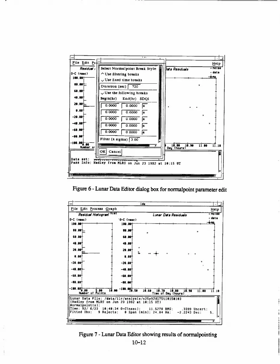
,J.
Select Normalpotnt Break Style
Use filtering breaks
v Use fixed time breaks
File E_dtt P_z
i
Data set:
Duration (sac) [ 720
,,/Use the following breaks
Begin(hr) End(hr) SDQI
Iio.ooo0i o.ooooF0,0000 J 0.0000
IIo.oooo I o,oo_ F!l o,_ j o,_ooF
Filter (x sigma) r 3 O0
Pass info: Hadley from HLRS on Jun 23 1992 at 10:15 UT
10
• data
I r
Figure 6 - Lunar Data Editor dialog box for normalpoint parameter edit
......1
--I Ida
"O-C (nile)
lO0.OO
U .OO"
50.08"
40.00
20.08
0.00'
-20.08
-40.08
-50.08
-80.08
-100.0I
x
1 tO
Lunar Data File: /data/llr/analysis/s25y92d175tl#lS#1e3Hadley from NLRS on Jun 23 1992 at 10:15 UT)
Iormall_oint(s):Time: 92/ 6/23 10:40:34 0-C[nsec): 11.5278 RHS: .3399 Uncert:Fitted 0bs: 9 Rejects: e Span (min): 24.84 HA: -2.2243 Dec:
Figure 7 - Lunar Data Editor showing results of normalpointing
10-12

Conclusions
The lunar prediction and data analysis at McDonald Observatory have made several bigtransitions over the years, the latest being a successful move to a X windows/Motifgraphical user interface and the Unix operating system. This move has proven to beworthwhile, producing more portable and flexible code and a network-based interactivedata reduction environment.
10-13

N94-15600
LLR- Activities in Wettzell
U. Schreiber, J. MueUer I
Forschungseinrichtung SatellitengeodaesieFundamentalstation Wet tzell
D - 8493 Koetzting
R. Dassing, N. Brandl, K. H. Haufe, G. Iterold, R. Kahn, K. Roettcher, R. Stoeger
Institut fuer Angewandte GeodaesieFundamentaistation Wettzell
D - 8493 Koetzting
Abstract
Following the idea of a fundamental station, the Wettzell Laser Ranging Station wasdesigned to rpnge to all types of satellites and to the moon [1]. After obtaining the firstlunar echos in October 1990, the system's operation was improved. A short report oflunar ranging activities is given.
1 Ranging to the moon in Wettzell
The WLRS was put to routine operation in the beginning of 1991. It was taking over the
task of the old Sylvania Ranging System (SRS). In the beginning it was ranging to LAGEOS
and" the two ETALON satellites. However, the design was such that it should also allow
ranging to the moon. This was shown very early, when in February of 1990 the first ranges
from Meteosat P2 were obtained. Unfortunately it took more than half a year to stabilize
the operation of this part of the ranging realtime software. For the measurements to the
moon a cooled PMT (RCA C 31034a) and a spectral Fabry- Perrot bandpass of 1.5 _1 width
around a centerwavelength of 532 nm is used. The laser energy was measured to be 180 raJ
with a pulse duration of 200 ps. As the telescope aperture is only 75 cm and the location
of the WLRS is on an altitude of only 600 m, there is a poor signal to noise ratio for these
measurements. For these reasons the WLRS is usually employing a semipulsetraln for lunar
ranging. The semitraJn contains 5 individual pulses, the first 3 of them are contributing
most to the energy budget. The semipulsetrain gives the additional advantage of producing
a known pattern of lunar returns within the random noise from other sources. Ranging
to the moon from Wettzell is challenging as the noise counts are usually hiding the lunar
returns. This requires a complex post ranging examination procedure, carried out at the
Technical University of Munich, to analyse the measurements. At Wettzell LLR has a
very high ranging priority. However there were only very few nights during the last year
permitting lunar ranging. In these nights hardly any passage of LAGEOS or ETALON was
lost as it takes only a few minutes to switch the WLRS from lunar mode to satellite mode
and the lunar ranging was interrupted for a short while.
1Techn. Universitaet Muenchen, Arcisstr. 21 D - 8000 Muenchen 2
10-14

2 Echos from the moon
In figure 1 a successful measurement is shown. Clearly the pattern of the used semitraJn
can be seen. The high noise rate is also evident. There is a fixed spacing in time between
the individual pulses in the semitrain. This separation is depending on the length of the
laser cavity and can be measured independendly. For the WLRS laser the pulses axe 6.902
ns apart. This relation can be used to fold the lunar returns from the second and the third
pulse of the semitrain onto the main pulse to increase the number of returns in the normal
point.
3 Status of the WLRS
The WLRS proofed it capability for lunar ranging. However, the ranging to the moon is
very complicated and not very well supported by the ranging software, which only provides
elementary features. At the present efforts are made to increase the signal to noise ratio
and to support blind tracking. The goal is a more efficient use of the few useful observation
nights per year in Wettzell.We would like to thank the lunar ranging team in Grasse (France) for for their help.
References
[1] Schlueter, W.; Hauck, H.; Dassing, R.; Schreiber, U.; Mueller, J.; Egger, D.; Wettzell
Laser Ranging System (WLRS) -- First 21racking Results to Satellites and to the Moon,
paper presented at the Crustal Dynamics Project Meeting, held in Pasadena, spring
1991.
10-15

2O
c-h_ 15
o'1
¢-.
> 10W
L..
I1)
E= 5
z
Semitrain Range Residuals (Apollo 15)
US 5/92
Semipulsetrain
0
0 10 20 30 40 50 60
Range Residuals [ns]
Figure 1: Histogram of the 'semitrain ranges' to APOLLO 15 during the night of Nov. 25th1991. The session lasted 15 minutes
10-16
Fixed Station
Upgrades/Developments


N94"15601
MATERA LASER RANGING OBSERVATORY (MLRO), AN OVERVIEW
Thomas Varghese, Winfield Decker, Henry Crooks
Allied-Signal Aerospace CompanyBendix/CDSLR Network
Seabrook, Maryland 20706U.S.A.
Giuseppe Bianco
Agenzia Spaziale Italiana/Centro di Geodesia Spaziale
Matera, Italy
Abstracl;:
The Agenzia Spaziale Italiana (ASI) is currently under negotiation with the
Bendix Field Engineering Corporation (BFEC) of the Allied Signal Aerospace
Company (ASAC) to build a state-of-the-art laser ranging observatory for the
Centro di Geodesia Spaziale, in Matera, Italy. The contract calls for the
delivery of a system based on a 1.5 meter afocal Cassegrain astronomical
quality telescope with multiple ports to support a variety of experiments for
the future, with primary emphasis on laser ranging. Three focal planes, viz.
Cassegrain, Coude, and Nasmyth will be available for these experiments.The open,telescope system will be protected from dust and turbulence using
a specialized dome which will be part of the building facilities to be provided
by ASI. The fixed observatory facility will be partitioned into four areas for
locating the following: laser, transmit/receive optics, telescope/dome
enclosure, and the operations console. The optical tables and mount rest on
a common concrete pad for added mechanical stability. Provisions will be in
place for minimizing the effects of EMI, for obtaining maximum cleanliness
for high power laser and transmit optics, and for providing an ergonomic
environment fitting to a state-of-the-art multipurpose laboratory.
The system is currently designed to be highly modular and adaptable for
scaling or changes in technology. It is conceived to be a highly automated
system with superior performance specifications to any currently operational
system. Provisions are also made to adapt and accommodate changes that
are of significance during the course of design and integration.
ii-i

MLRO :An Overview
Objective: Build a state-of-the-art, multi-purpose, laser rangingobservatory in Matera, Italy
General Features
I Day and night automated ranging capability on all CCR-equipped satellites
(> 400 km) and the moon
• Application of state-of-the-art technology in all sub-systems
• Real time calibration and interleaved multi-satellite tracking
• Multicolor ranging capability
• Advanced computing environment and data analysis tools
• Computerized documentation, with features such as relational database,
expert system and hypermedia text
System Specifications
LAGEOS ranging"
Single shot precision • --5 mm
.Normal point precision • < 1 mm
Low orbit satellite (ERS-1, Starlette, etc.) •
Single shot precision • 3 - 5 mm
i
Lunar ranging •
Single shot precision • -1 cm
Real time calibration/ground ranging •
Single shot precision • <=2 mm
Range accuracy: Better than 2mm
11-2

MLRO :An Overview
Telescope
Near diffraction limited afocal Cassegrain telescope with a 1.5 meter primary
and a 10 centimeter secondary; combination of a tertiary mirror and coude
optics for transmission/reception
Broadband coating for maximum spectral response from UV to near-IR
Maximum slew rate •
Azimuth axis • 20 degrees/second
Elevation axis • 5 degrees/second
Multiport system for other experiments
D
Laser
Diode pumped laser for injection seeding
Regenerative amplification followed by power amplifiers
Pulse duration : <125 psec
Pulse energy (532 nm): >200 rnJ
Repetition rate : >=10 Hz
Computer controlled beam divergence
Modularity for energy scaling / multi-wavelength generation
Laser firing stability : better than 20 nsec
11-3

MLRO :An Overview
D
D
t
D
Control System
Software in high level languages
Automatic recording of all operational parameters
Automated star calibration, mount modelling
Computer-assisted optical alignment and verification
Distributed data acquisition, processing, and control
Advanced computing/control environment
Automated system/sub-system simulation and debugging
D
D
D
Transmit/Receive Electronics
Detection" High Q.E, high speed MCP-PMT/APD
Signal processing :
Speed : 1 - 5 GHz
Dynamic range : 20
Jitter : <10 psec
Event timer
Clock frequency : 200 - 1000 MHzVerniers : 4 - 8
Time resolution : 1 - 2 psec
Accuracy : 5 - 10 psec
Jitter : 10 - 20 psec
Clock • Cesium with disciplined oscillator
Gating • Range gate adjustable from 10 nsec to 10 _tsec
11-4
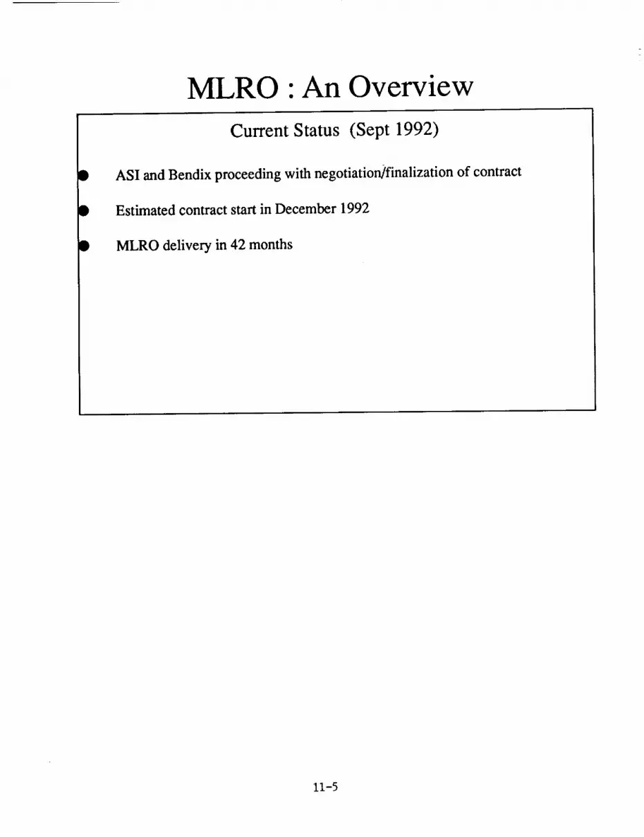
MLRO :An Overview
Current Status (Sept 1992)
D
I
ASI and Bendix proceeding with negotiation]finalization of contract
Estimated contract start in December 1992
• MLRO delivery in 42 months
11-5

' 94-15602
PERFORMANCE OF THE UPGRADED ORRORAL LASER RANGING SYSTEM
John McK. Luck
Orroral Geodetic Observatory
Australian Surveying and Land Information GroupDepartment of Administrative Services
PO Box 2, Belconnen ACT 2616, Australia
i. Upgrade Arrangements
An Agreement "being in respect of a project to develop Laser and
Control Systems Upgrade to Orroral Laser Ranging System" between
Electro Optic Systems Pty. Ltd. (EOS) and The Industry Research
and Development Board (IRDB) of the Commonwealth Department of
Industry, Technology and Commerce was signed on 23 March 1990.
On the same day, a corresponding 'Agreement for Collaborative
Research and Development of Laser and Control Systems Upgrade to
Orroral Laser Ranging System' between the Australian Surveying
and Land Information Group (AUSLIG) of the Commonwealth
Department of Administrative Services and EOS, was signed. Under
these Agreements, the research and development costs were shared
between the three parties according to a standard IRDB formula,
with AUSLIG having the option to purchase the prototype for itsresidual value upon successful demonstration. IRDB involvement
was directed towards fostering export-oriented Australian high-technology industry.
The old system was de-commissioned on 6 March 1991, although
preparatory work such as moving the laser and installing theheads and capacitor banks necessary for conversion to Active-
Active mode was completed prior to that date. LAGEOS I was
acquired a month later, on i0 April, and AJISAI on 12 April 1991
in Orroral's first-ever attempt at a 'low' target. The following
eight months were spent in debugging and refining the new system
and preparing for the ill-fated attempt to measure the geodetic
baseline between the Orroral Laser Ranging System (OLRS) and the
Saudi Arabian Laser Ranging Observatory (SALRO) set up at the
Camberra Deep Space Communications Complex, Tidbinbilla to
complement terrestrial and GPS surveys and to link SLR atOrroral with VLBI at Tidbinbilla.
The upgraded OLRS was deemed by AUSLIG to be operational from 1
January 1992, and final payment to EOS for purchase of the
residual prototype was made in June 1992. A contract for
software maintenance and further development was awarded to EOSin November 1992.
2. System Prior to 1991
The original system was the Orroral Lunar Laser Ranger (LLR),
lent to the Division of National Mapping (Natmap) in 1973 under
a Memorandum of Understanding involving NASA, Smithsonian
Astrophysical Observatory and US Air Force Geophysical
Laboratory. It was upgraded to include ranging to artificial
11-6

satellites under a contract from NASA signed in 1981, the firstreturns from LAGEOS-I being acquired in mid 1984. Some verifiedreturns from the moon were received in 1985, and ranging toETALON I & II started in 1990. It was not really possible toexpect results for two-way ranges less than 35 milliseconds,which is one of the main reasons for embarking on the upgradebeing described here.
Note : Natmap was merged with another Commonwealth agency inAugust 1987 to form AUSLIG.
DOME : The 9 metre diameter hemispherical dome by Ash Domes ofPlainfield,IL was installed atop the original cylindricalObservatory building in 1973. Its AC motors for rotation duringobserving were manually controlled by a Left-Off-Right lever.
TELESCOPE : 1.5 metre aperture Ritchey-Chretien reflectingtelescope, optics by University of Arizona. The tailpiece at the
Cassegrain focus carries an eyepiece mounted on an X-Y stage forstar observations and to facilitate offset guiding for lunar
ranging.
The telescope is used both for transmitting and for receiving.
It is depicted in figure i.
TELESCOPE MOUNT : The telescope tube is by Astro Mechanics of
Austin,TX. The original equatorial mount was replaced in 1981-2
by an X-Y ("alt over alt") mount by Contraves, and a Coude Pathand the Contraves MPACS drive and readout systems were added.
The drive accuracy is better than 0.002 degrees and encoder
resolution is 0.0001 degrees.
An interface/controller was built, and all interface drivers and
control and mount modelling software were written, by Natmap.
COUD_ PATH : The Coude path incorporates a Matching Assembly
consisting of two lenses whose combined focal point coincides
with the focal point of the telescope. These lenses are in the
East bearing of the telescope's inner axis. The Coude path
connects the telescope with the laser, transmitter and receiver
assemblies which are mounted on Newport optical benches in
environmentally stable rooms. A Times 5 Beam expander by Special
optics,NJ on the Coude bench expands the transmitted beam prior
to injection to the telescope through mirrors in the North
bearing.
TRANSMIT/RECEIVE ASSEMBLY (T/R) : A rotating aluminized mirror
with two holes in it, co-rotating 'dogbone' holding two ND
filters and CAMAC-controlled stepping motors constituted the T/R
assembly purchased from McDonald Observatory,TX in 1983. Laser
firing was triggered by optically sensed notches in the rim of
the rotating mirror.
The mirror was replaced in 1987 by an 'Appler mirror" in which
the holes were just glass left uncoated (glass-hole), and which
permitted positive, unambiguous ranging to a ground target and,
11-7

SOUTH
BEARING
SPIDER
VANE
" - I _- ----_ ROt
COUDE
MIRRORS 3 , 4 ._._
___ ANDE_EPI,._E _W HYRROR 8I
COUDE
TABLE
_ORTH PIER
Figure 1: Orroral Laser Ranging System telescope - elevation and
plan. (Derived from Contraves 'NLRS Telescope Manual.)
11-8

for real-time internal calibrations, to geodetically accessible
retro-reflectors placed on the spider vanes holding the
telescope's secondary mirror.
The interface was controlled by the CAMAC bus system, and driver
and high-level software was written by Natmap in collaboration
with the University of Texas.
RECEIVER/DETECTOR : A light-tight box containing a turret of 5
pinholes (spatial filters), a turret with a i0 A ° filter and a
hole, focussing optics and detector mount was provided by
McDonald Observatory. The detector mount was replaceable by an
eyepiece for star alignments.
The detector was an RCA 31034A PMT until 1986, when the first of
a series of ITT F4129f z-plate MCP PMTs was installed.
LASER : A Quantel YG 402 DP Nd:YAG laser frequency doubled to
532nm output wavelength was purchased as part of the 1981-3
upgrade. Its Q-switching and pulse slicing were accomplished
passively, the mode locking being active/passive. Two amplifierscombined to produce in excess of 250mJ per pulse at ten pulses
per second when needed. The pulse slicer was replaced by a
Quantel solid-state slicer model SPS411 in 1987.
The laser was removed from its Quantel plate in the Coude room
and relocated to an RF-shielded room one floor lower in the
Observatory building in August 1990. Its components were bolted
directly to a Newport optical table.
[The original Hughes 6943A ° ruby laser of the Orroral LLR priorto 1981 was bolted to the side of the telescope tube.]
LASER RANGING CONTROLLER (LRC) : This main interface/controller
was designed and built by Natmap. It set windows and gates,
controlled laser firing, and managed the epoch timing system.
EPOCH TIMING SYSTEM : Range measurements were accomplished by
measuring the "epoch" (time of day) of separate events, rather
than depending upon a Time Interval Counter. The LRC time base
was driven by a high spectral purity Oscilloquartz 2200 quartz
frequency standard at 10MHz, and its clock synchronised at the
start of each pass to an external Hewlett-Packard caesium beam
frequency standard whose own clock was kept within 1 microsecondof UTC. The LRC Clock was used to time tag events to i00
nanosecond resolution.
Each laser shot produces at least three events to be time
tagged: start diode pulse, internal calibration pulse from
MCP/PMT, and one or more satellite returns from MCP/PMT (the
quest to detect more than one 'satellite' return per shot was
abandoned in the mid-1980's). The epoch timing system philosophy
theoretically enables many events to be recorded per shot using
identical equipment, limited only by instrumental reset/read
times.
11-9
Two channels were used in practise to obtain fine resolution,one for start diode and one for MCP/PMT. Each comprised aseparate channel of the Tennelec 454 Quad Constant FractionDiscriminator (CFD), a LeCroy 4202A Time to Digital Converter(TDC), and a pair of 8-channel LeCroy 2228A TDCs as vernierscovering different 50ns sections. The 8 78-picosecond resolutionchannels of each 2228A were majority voted and meaned to improveresolution to about 28ps. A standard calibration routine was runwith each pass to relate the intrinsic 2228A delays to eachother, with the scale factors being calibrated periodicallyagainst the 4202A TDCs.
All TDCs were read via the CAMACbus system. Software for thesetasks was written by Natmap.
RECEIVE ENERGY MONITOR : A LeCroy 2249A Analog-to-Digital
Converter (ADC) ('charge digitiser') was installed on the MCP
line in March 1990. It is controlled and read through the CAMAC
bus system, and is gated by the 'AND' of the range gate window
and of the discriminator output pulse delayed appropriately. Its
input signal is amplified by a Stanford Research SR440.
OPERATING SOFTWARE : Apart from the lunar prediction package
based on EULER and the satellite prediction package based on
IRVINT, which were imported with the aid of Randall L. Ricklefs,
all interface drivers, control and operations software,
predictions, post-processing, mount modelling, simulation and
test software was written by Natmap.
SYSTEM CALIBRATION : Until the end of 1987, the internal
calibration pulse was picked off each transmitted laser pulse by
a minutely reflecting 'feedback plate' in the T/R box and fed to
the MCP/PMT through ND filters in the co-rotating 'dogbone'. The
optical and electronic delays between this feedback plate and
the epoch timing system were thus well calibrated, but the delay
between the feedback plate and the system reference point was
not well known, so it was not possible to assess system accuracy
properly as it was found impossible to measure or even estimate
the length of the convoluted Coude path (with its five
refracting elements as added complications) to better than 10cm.
The advent of the 'Appler mirror' in 1987 made it possible to
range to the 'Spider Retros' simultaneously with distant
targets. The effective reflection points of the retro-reflectors
were related to the instrumental reference point and external
survey marks early in 1988 with 3mm accuracy by precise survey,
enabling accurate correction constants to be calculated.
A ground target was installed at a distance of l.lkm across a
valley in November 1987, and surveyed in along with 'Spider
Retros'. A session of ranging to this target accompanied each
LAGEOS-I pass, and provided a check on the accuracy of the
correction constants referred to above. It is also invaluable
for assessing such things as the effect of signal strength on
range accuracy and the actual precision obtainable at any given
time.
II-i0

3. Elements of the Upgrade
DOME : Automated rotation was provided through hardware and
interface controllers. Two DC variable-speed motors were
installed in 1991 and new variable-speed controller, interface
and software are now under development.
TELESCOPE and COUDE PATH : Not affected by the upgrade.
TELESCOPE DRIVE : A new interface/controller for the MPACS, and
corresponding interface driver and high-level software, were
provided, as were two new handpaddles with their interface,controller and driver.
TRANSMIT/RECEIVE ASSEMBLY : A completely new box was provided
(figures 2,3). The T/R mirror has two genuine holes, and is
connected to the co-rotating 'dogbone' by a shaft incorporating
a clutch unit. Rotation rates up to 20 revs/second are possible,
and are controlled directly from the MRCS. Laser firing is
triggered by notches on the T/R mirror rim as before. Laser fire
commands may be inhibited through a 'divide by' facility so that
only every first, second, third or fourth notch actually causesa shot.
A minutely-reflecting wedged feedback plate (FBP) directs part
of the transmitted pulses to targets on the Coude Table for the
optical calibration of the timing system and, optionally, for a
real-time internal calibration target ('Table Target'). The
wedge also reflects a small part of return pulses through ND
filters in the 'dogbone' to the detector; this facility is
routinely used for the spider retro and ground target returns,
the bulk of whose energy passes back through the T/R hole and is
lost. Such returns therefore traverse a different path inside
the T/R box than do satellite returns which take 1.644ns longer.
An electrically controlled PLZT optical attenuator is placed
between the feedback wedge and the 'dogbone' to aid in matching
calibration and ground target signal strengths to satellite
return signal strengths. A special circuit ('wobbulator') can
sweep through the voltage range with 3 second period to give
varying energies when adjusting discriminator walk.
RECEIVER/DETECTOR : A new Receiver Box (figures 2,4) contains a
new 4-pinhole turret, separate ports for MCP mounting (with 10A °
filter built in) and eyepiece/RCA PMT mounting, a flip mirror to
switch between ports, a flip mirror to access a CCD camera, a
LED pulser to aid MCP characterisation, and new focussing
optics. The flip mirrors can be software controlled via theMRCS.
To date, only ITT F4129f MCPs have been used, while the CCDcamera and LED Pulser have not been used at all.
II-Ii

0
,,.<
Z
a..
t-..-
1
• i
r '-._J
f: m
,,_u "_-"_ ill-
'%'-
P
_A, -
,---..--
," _,_li_ o,ii.,,_'",_ 7 I
< "%%
"i_ t= =
,I",1 < i,C p-) ":_ L__---,
q
' I
_ I-'-1 1
",! I_-3.._
1 -" '
"_ [==_ _-_--_-L.>_-
I_#.j \'-AJ' _'
,.r"
c_
,... ,_
i
L"3,
i
I'"
b
.O
A
,--4
O
0
rj
0
0
M
11-12

Figure 3 : EOS Transmit/Receive assembly.
I
Figure 4: EOS Receiver assembly.
(From EOS drawings.)
(From EOS drawings.)
11-13
LASER : The oscillator was converted to Active Q-switching,
Active mode-locking to a design by the Centre for Laser Physics
of The Australian National University licenced to and developed
by EOS. The SPS411 is also connected to the Active-Active
circuitry to give positive pulse selection.
It was found necessary in 1990 to replace the laser heads with
high-efficiency heads, and the capacitor banks with new units
having simmer circuits. This work was supported by IRDB and
completed in January 1991 with the installation of a CB632 and
two CB631 units, and SF606-4, S_611-07 and SF611-09 heads, all
made by Continuum. Later, a Continuum MV 70 RF generator for the
Acousto Optic Modulator was also purchased, modified and
installed, and other components have needed replacement.
The Upgrade Specifications required a third amplifier, or alter-
natively, the first amplifier would be double-passed through a
spatial filter to keep the beam clean. Neither option has been
invoked, yet £he laser has achieved its overall goal of 250mJ
per shot at 532nm when everything is working properly.
MASTER RANGING CONTROL SYSTEM (MRCS) : Replaced the LRC. It is
based on EPLD chips, and sets windows and gates, controls T/R
rotation and laser firing, manages all clock and epoch timing
functions, and contains a full range of test and simulation
facilities. The MRCS communicates extensively with the Hewlett
Packard A900 1000-series minicomputer as shown in figure 5.
50 MHZ MULTIPLIER : The MRCS operates at 50MHz, so a box was
provided to multiply up the i0 MHz output from the Oscilloquartz
2200 crystal.
EPOC_ TIMING SYSTEM : The basic philosophy of "epoch' event
timing has been retained, and is accomplished by the MRCS Clockdown to 20ns with EOS-modified LeCroy 2229A TDC verniers
providing fine resolution. The intermediate 4202A TDC units are
no longer necessary, and only one 2229A TDC is needed on each of
the start diode and MCP lines. Each of the 8 channels of a 2229A
TDC has a resolution of 25ps (nominal), the average giving 10ps
(typical) resolution and precision.
The scale units (ns/count) of the verniers can be calibrated in
three ways:
• Programmable delay lines within the MRCS;
. LeCroy 4202A TDC verniers, assumed accurate;
Optical delay line. In a pseudo-ranging operation, part of a
transmitted laser pulse is reflected from the feedback wedge in
the T/R Assembly and directed to a retroreflector which slides
along a calibrated optical rail, thence back through the wedge
to the MCP (see figure 2). The change in TDC reading is then
related to change in retroreflector position•
The average offset of each vernier with respect to the first
vernier is calibrated daily by injecting a sequence of simulated
laser pulses generated within the MRCS into all the verniers.
11-14
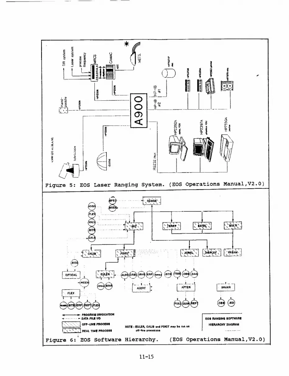
-c
_; 0
° i/ /" 1
\_.,__.Io
!|
I ........
<:
Figure 5: EOS Laser Ranging System. (EOS Operations Manual,V2.0)
_k___J
.,,. , ............
.,.i................. :
_,:__ ,.-:--,_ " ___:,._:, r......_....., .... , ....
_ PROGRAM INVOCATION
< ......... 0ATA FIlE IIO
_ OFF-LIHI! PROOESII
_ IIEAL TIME pROOEe_
Figure 6: EOS Software Hierarchy.
ooe
L_
EOII RAN(lING IIOFTWARI!
HIERARCHY DIAQRAMHOTI : EtJLER, OAUB lnd PDICT rely be ru_1 le
(EOS Operations Manual, V2.0 )
11-15

RECEIVE ENERGY MONITOR : The previous system based on a LeCroy
2249A ADC has been retained, with hardware gating as above. The
EOS software contains an option for automatic gating.
DISCRIMINATOR : As before, Tennelec 454 CFD units are used. EOS
has experimented extensively with high-speed comparator chips,
delay lines and "cascade' configurations, but to date Orroral
prefers to use unmodified single channels. The upgrade has also
provided several potentially useful features for establishing
the Z-walk on each channel, such as the PLZT "wobbulator' and
software, which are still being evaluated.
OPERATING SOFTWARE : The upgrade software provided, which is
summarised in figure 6, includes mount modelling observations
and analysis, pass predictions from receipt of IRV/ORBEL files,
revamped EULER and IRVINT, ranging operations, post-processing
to generation of normal point, full-rate data and time bias
files, timing system calibration, file repair, diagnostic and
reporting software. Source code was not included. The originalsoftware release was designed to apply 'generically' to all EOS
systems; it has required considerable tailoring to Orroral's
specific configurations, peculiarities, environment and
requirements and has necessitated considerable re-education froman entrenched laser ranging 'culture'. Orroral prefers to use
its own post-processing software, modified from the Natmapsoftware to handle the new file structures.
Each interface driver is accompanied by a program demonstrating
all its calls and providing extensive diagnostic and simulation
capabilities. They cover CAMAC, MRCS, MPACS, PADDLE and DOME.
Ranging operations are built around three separate programs that
handle ground targets, satellites out to about 70ms two-way
range, and 'multiple shots in flight' targets such as ETALON and
the moon, respectively.
SYSTEM CALIBRATION : To date, the same methods for real-time
internal calibration and ground target ranging have been used as
were used during 1987-91. The 'Table Target' on the Coude Table
has been tested inconclusively; its signal strengths are
expected to be controllable much better than those from the
spider retros.
4. Laser Performance
An assessment was performed in April-May 1991 by Dr Barry
Luther-Davies of the Laser Physics Centre, Australian National
University. The results and many quotations given below are
taken from his report (Luther-Davies,1991). The upgrade to an
active/active oscillator and high-efficiency simmered heads has
clearly provided very satisfactory performance.
pULSE DURATION : Output from the Second Harmonic Generator was
measured using a Hadland Photonics IMACON 500 $20 streak camera
11-16
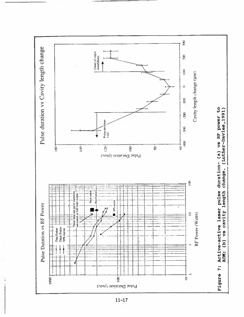
c-
o..)
P_
>
>
©
..,.A
(D
E_
t...
i I ,C _ C ¸
e-
g
v
C"
i..........................................
t
..-.__
II
...... I
---!1
(o_,_(I)uoT1_:.m_ _._In(l
.........'........2":--_-_---_-
t_lj
E
L,)
5,_0
L9
r_[.r,/
0 _
a_
.,-t
A_
t v
0
11),=
>-,.t gl
0
11),_>
O0
,u
t_
r_
11-17
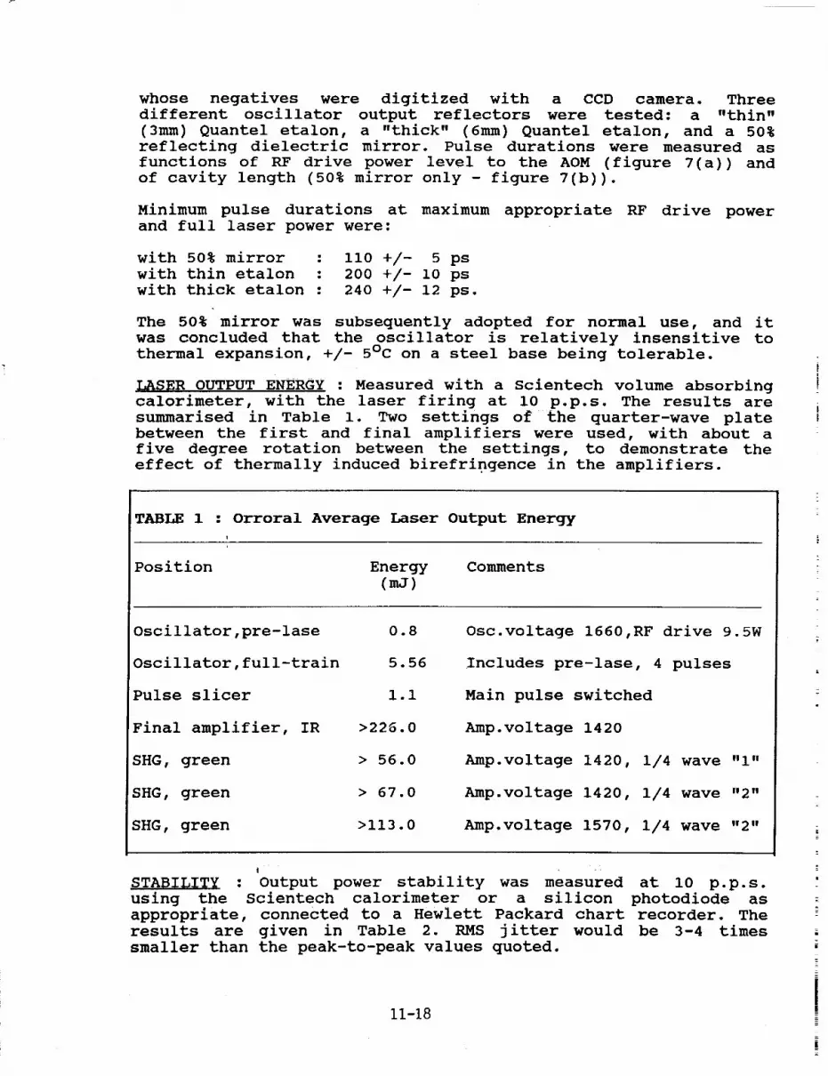
whose negatives were digitized with a CCD camera. Three
different oscillator output reflectors were tested: a "thin"
(3mm) Quantel etalon, a "thick" (6mm) Quantel etalon, and a 50%
reflecting dielectric mirror. Pulse durations were measured as
functions of RF drive power level to the AOM (figure 7(a)) and
of cavity length (50% mirror only - figure 7(b)).
Minimum pulse durations at maximum appropriate RF drive power
and full laser power were:
with 50% mirror :
with thin etalon :
with thick etalon :
II0 +/- 5 ps
200 +/- i0 ps
240 +/- 12 ps.
The 50% mirror was subsequently adopted for normal use, and it
was concluded that the oscillator is relatively insensitive to
thermal expansion, +/- 5°C on a steel base being tolerable.
_S_R OUTPUT ENERGY : Measured with a Scientech volume absorbing
calorimeter, with the laser firing at i0 p.p.s. The results are
summarised in Table I. Two settings of the quarter-wave plate
between the first and final amplifiers were used, with about a
five degree rotation between the settings, to demonstrate the
effect of thermally induced birefringence in the amplifiers.
TABLE 1 : Orroral Average Laser Output Energy
I
Position Energy Comments
(mJ)
Oscillator,pre-lase
Oscillator,full-train
Pulse slicer
Final amplifier, IR
SHG, green
SHG, green
SHG, green
0.8
5.56
I.I
>226.0
> 56.0
> 67.0
>113.0
Osc.voltage 1660,RF drive 9.5W
Includes pre-lase, 4 pulses
Main pulse switched
Amp.voltage 1420
Amp.voltage 1420, 1/4 wave "I"
Amp.voltage 1420, 1/4 wave "2"
Amp.voltage 1570, 1/4 wave "2"
| •
STABILITY : Output power stability was measured at i0 p.p.s.
using the Scientech calorimeter or a silicon photodiode as
appropriate, connected to a Hewlett Packard chart recorder. The
results are given in Table 2. RMS jitter would be 3-4 times
smaller than the peak-to-peak values quoted.
11-18
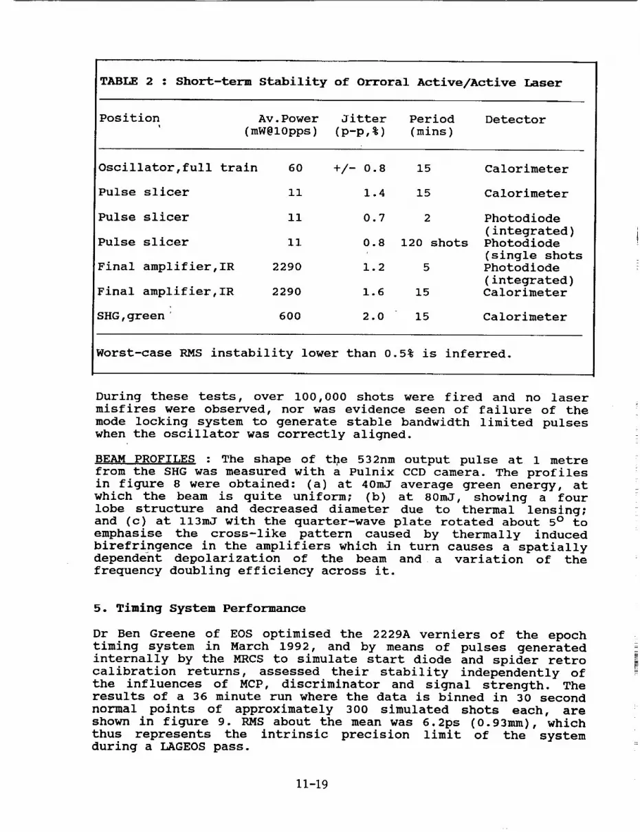
TABLE 2 : Short-term Stability of Orroral Active/Active Laser
Position Av.Power Jitter Period Detector
' (mW@10pps) (p-p,%) (mins)
Oscillator,full train 60 +/- 0.8 15
Pulse slicer Ii 1.4 15
Pulse slicer ii 0.7
Pulse slicer Ii 0.8
Final amplifier,IR 2290 1.2
Final amplifier,IR 2290 1.6
SHG,green 600 2.0 15
Calorimeter
Calorimeter
2 Photodiode
(integrated)120 shots Photodiode
(single shots5 Photodiode
(integrated)
15 Calorimeter
Calorimeter
Worst-case RMS instability lower than 0.5% is inferred.
During these tests, over i00,000 shots were fired and no laser
misfires were observed, nor was evidence seen of failure of the
mode locking system to generate stable bandwidth limited pulses
when the oscillator was correctly aligned.
BEAM PROFILES : The shape of the 532nm output pulse at 1 metre
from the SHG was measured with a Pulnix CCD camera. The profiles
in figure 8 were obtained: (a) at 40mJ average green energy, at
which the beam is quite uniform; (b) at 80mJ, showing a four
lobe structure and decreased diameter due to thermal lensing;
and (c) at ll3mJ with the quarter-wave plate rotated about 5 ° to
emphasise the cross-like pattern caused by thermally induced
birefringence in the amplifiers which in turn causes a spatially
dependent depolarization of the beam and a variation of the
frequency doubling efficiency across it.
5. Timing System Performance
Dr Ben Greene of EOS optimised the 2229A verniers of the epoch
timing system in March 1992, and by means of pulses generated
internally by the MRCS to simulate start diode and spider retro
calibration returns, assessed their stability independently of
the influences of MCP, discriminator and signal strength. Theresults of a 36 minute run where the data is binned in 30 second
normal points of approximately 300 simulated shots each, are
shown in figure 9. RMS about the mean was 6.2ps (0.93mm), which
thus represents the intrinsic precision limit of the systemduring a LAGEOS pass.
11-19
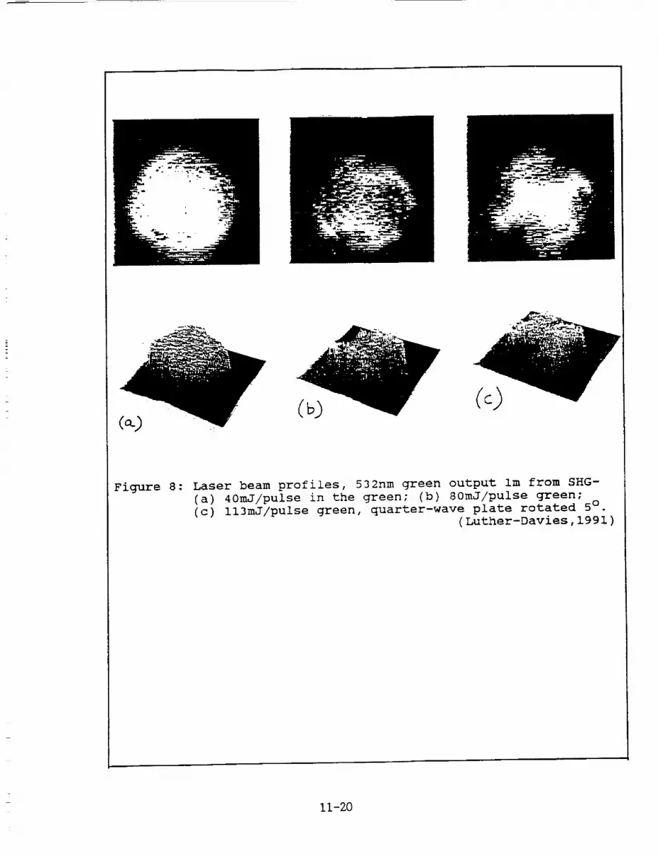
Figure 8: Laser beam profiles, 532nm green output Im from SHG-(a) 40mJ/pulse in the green; (b) 80mJ/pulse green;(c) ll3mJ/pulse green, quarter-wave plate rotated 5° .
(Luther-Davies,1991)
11-20

OF:LROFLALOAL STABILITY - _UN 4
-15oo
-20.00 --
Mean C_I = 95.426292 ._s
I£acm Bar is a 30 sec normal point
Figure 9: Timing system stability- residuals from mean of 36
minutes of simulated internal calibration data, binned
at 30 second intervals (300 shots).
11-21

A systematic variation visible in figure 9 may be due to
temperature variations in the CAMAC modules. The residuals from
a 20 minute run were more random, with RMS 2.4ps (0.36mm).
An estimate of long-term stability is obtained from the daily
calibration of the relative delay between verniers. In a 50 day
period analysed during which the vernier scale units (ps/count)were held fixed at their values determined at the start of the
period, the RMS variation of the delay difference between the
two units actually used in ranging was 6.6ps (l.0mm).
It is thus evident that the precision and stability of the
system, given perfect discriminator outputs, are imm or better.
Because range calculations necessarily involve only vernier
differences, this value also represents the accuracy limit of
the system.
Data on the optical rail method of timing system calibration insitu at Orroral has not been obtained,
6. Pass Productivity
In figure 10(a), the growth in the number of passes acquired perquarter as a result of the upgrade is demonstrated. Prior to
March 1991, only LAGEOS I and ETALON I & II (from June 1990)were observable. With the upgrade, STARLETTE, AJISAI and ERS-I
were immediately acquirable, with TOPEX/POSIDON and LAGEOS II
being added in the second half of 1992. It is notable that the
upgraded Orroral system was the first station to get returns
from LAGEOS II, on 24 October. Monthly statistics for January toOctober 1992 are given in figure 10(b).
An unexpected consequence of the upgrade is that, in view of the
enormous increase in number of passes available and the far
greater reliability of the upgraded segments of the OLRS, more
operational staff are needed in spite of greater system
efficiency, and more technical staff are needed to maintain the
other segments and bring them to an equal state of reliabilityand efficiency.
7. System Precision
The evolution of single-shot precision estimates for LAGEOS I
ranging from Orroral is shown in figure Ii. The data prior to
the upgrade come from analyses of full-rate data by Peter Dunn
of STX, and from in-house analysis thereafter. The failure to
achieve the upgrade's sub-centimetre potential is ascribed to
deterioration in laser aii_ment leading to longer pulses, to
the difficulties encountered in optimising the MCP-Discriminator
combination, and to a clear dependence of delay upon signal
strength. Every effort is made to equalise signal strength
distributions from satellite returns, spider retro cals and
11-22
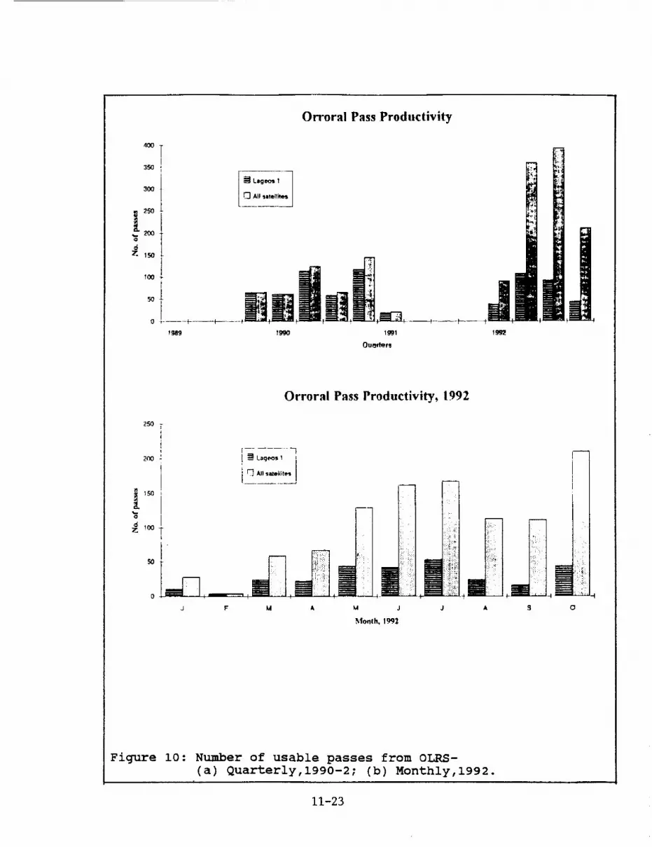
Orroral Pass Productivity
4OO
350
3O0
250
:_ ;so
+++ m,+i +°!+++__+NW0 ......... I- _- ,
19,99 I_30 1992
250
Orroral Pass Productivity, 1992
200
I
SO
[ .........
F-_ All saletlit_
F M A J s o
Figure i0: Number of usable passes from OLRS-
(a) Quarterly,1990-2; (b) Monthly,1992.
11-23

ground target returns by judicious manipulation of the PLZT and
telescope pointing, but it is difficult to do this in practice.
Ground target ranging offers more control over signal strengths.
RMS values of 30ps (4.5mm) have been obtained in 5 minute
sessions both for raw ground target returns uncorrected for
refraction, and for internal calibrations. About 7mm is normal
when everything is working properly, as illustrated for a good
month in figure 13.
8. System Accuracy
Agreement with external standards is assessed two ways. It has
not been possible to organise a co-location experiment.
COMPARTSON WITH GROUND SURVEYS : The distance from the ground
target retroreflector to all relevant instrumental points was
measured by precise geodetic survey in late 1987 and repeated by
independent methods and operators in late 1989. The formal one-
sigma uncertainty of each survey was 3mm, and agreement was 8mm.
The value adopted for the distance between the ground target and
spider retro #i from the more recent survey is i141624mm.
The same distance is estimated from laser ranging by subtracting
the calibration result from the raw range measurement, and
applying a refraction correction based on EDM theory and
meteorological readings (Rueger,1980). No other corrections for
delays inside the telescope are needed. Results for the first
ten months of 1992 are displayed in figure 13. The extent to
which improvements in signal strength control and laser pulseduration control will decrease the scatter and mean error,
remains to be seen.
LAGEOS _ RANGE BIAS : Figure 12 shows the range biasses before
and after the upgrade, relative to LAGEOS I orbits computed by
the Center for Space Research, University of Texas (Eanes,1992).
There is evidence of a jump of between 20 and 60mm, but it is
inconclusive as there could be contamination from orbit errors,
station position errors, inclusion of data from 1991 when the
upgrade was still being de-bugged, and truncation atMay 1992.
There has been no change in the constants and procedures used to
reduce raw ranges to the adopted instrumental reference point
(Coude mirror 7 - see figure i), nor in the refraction algorithm
applied to quick-look data. The Orroral reduction procedure is
given in Appendix i.
9. Telescope Pointing
MOUNT MODELLING : The analytical model developed previously for
the Contraves mount and MPACS encoder system was specially coded
into the generic EOS software. There are i0 parameters for each
axis. It is solved from star observations by a non-linear
process with observed encoder readings as the basic arguments.
(The previous implementation by Natmap was solved as a linear
11-24

7
6
5
g,2
1
0
ORRORAL OBSERVATORY
L_e_IRMS
//
/
Figure ii: Monthly single-shot precision estimates for rangingto LAGEOS 1 from Orroral.
0_
12 0 ---__--=_-_--_ , ' 1 '-- Orroral (7843) i --
1 O0 .........................................................................................................t.....................................................................................................t - -
60 _--- f!r
_. - i- -°-_i- --I
_t41i ._1 .... ' -"O .................................. :: ...-.. | 1 ""t ........................................................................................................
i --
"20 --------4 -- +------ ------4----_t--------+ f ÷
-0.5 0 0.5 1 1.5 2 2.5
Years Past 1990
Figure 12: Two-week range bias estimates for ranging to LAGEOS Ifrom Orroral,1989-92. (Eanes,1992)
11-25
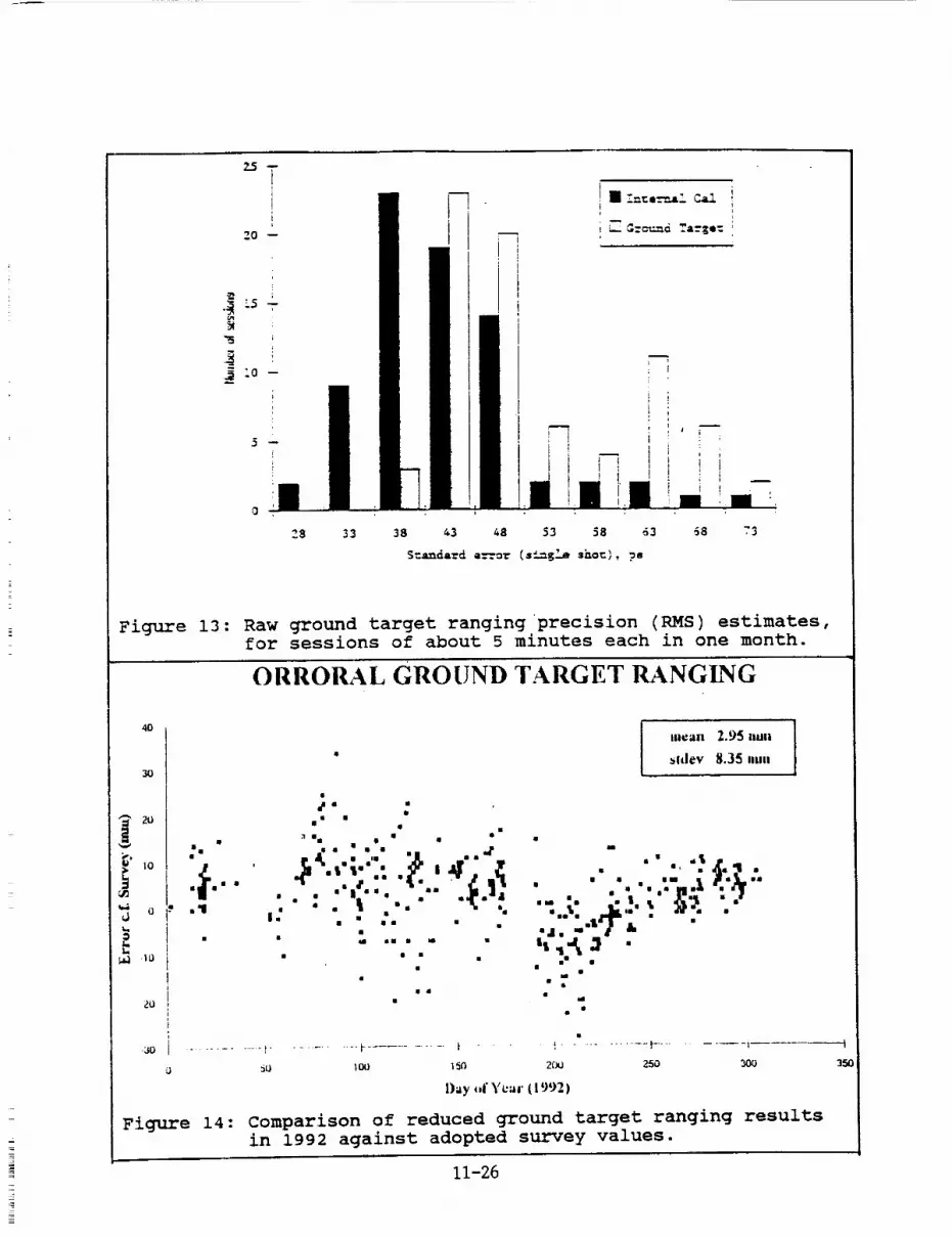
Figure 13: Raw ground target ranging precision (RMS) estimates,
for sessions of about 5 minutes each in one month.
ORRORAL GROUND TARGET RANGING
4O
30
20
0'3
d
.io
2o
._ ". .:ill • il •
=_I. • .,. 'Jr " " .' • .$_.q ••l''' .: ._'= I • ' •
• "'.'" _.'_r'"
" i_ """ _"" "" '""'_ :"
• : : 'l :'." " """" "., _", . . .. ...L .,h'- . _"-=d .,.11,'#11 &
_ _• 111 I
_o _oo _5c_ 2c_J 2so _oo
Day -1" Y¢;ir ( ! 992)
Figure 14: Comparison of reduced ground target ranging results
in 1992 against adopted survey values.
11-26
350

model with ideal encoder readings as arguments.) The model is
described in Appendix 2.
The star catalogue used is the FK4; previously, we used the
homogeneous Perth 70 catalogue, which has a denser distribution•
Star observations are accomplished at the eyepiece at the
Cassegrain focus• Star images are set, not on the eyepiece
graticule centre but on the image of the coincident 'green
spots' formed by returns from the two retroreflectors on the
secondary mirror's spider vanes while the laser is firing• Thus
the star is set in the direction in which the laser is actually
transmitted, which automatically accounts for mlsalignments in
the Coude path.
A feature of the upgraded system is that, between each repeat
observation (normally 3) on each star, the telescope is driven
off in a 'random direction to minimise personal bias and any
backlash• In other respects, observing speed and the star
selection algorithm are inferior to those prior to the upgrade•
HANDPADDLES : For operator convenience in both star observations
and ranging, the new handpaddles have thumbwheels to select the
resolution of each 'click' of the paddle buttons. This feature
has proven very useful•
POINTING ACCURACY AND PRECISION : The post-fit standard error of
a full mount model solution from more than 20 stars is typically
3 seconds of arc. The upgrade's solution software does not
provide the facility to asses numerically how closely the
current model points to stars, so it has to be done at the
eyepiece. Our estimate is 5-10 seconds of arc, which is also the
typical pointing error to the more distant satellites.
i0. Future Upgrades and Extensions
The EOS system is designed to be open-ended for future
development• Post-upgrade projects already completed or in-handinclude:
• Semi-automatic ranging operations;
• Variable speed dome automation;
• Implementation of 'Table Cals';
• Variable optical attenuation for satellite returns;
• Optical design and fabrication for SPAD installation;
• NP 9000-series Unix workstation for all displays, processing
and graphical user interface, leaving the HP A-900 only forinstrument control•
while projects made possible in the more distant future include:
• Fully automatic ranging;
• Converting laser to travelling-wave 'ring' design;
• Operating at 40 shots per second;
• Multi-colour ranging•
11-27

An important development not directly related to the upgrade butnecessary for lunar ranging and desirable for optimum focussingon to a SPAD, is a new telescope secondary mirror which shouldbe installed by July,1993. Its distance from the primary mirrorwas reduced by 4cm at the 1981 upgrade, which introducedenormous aberrations in the Ritchey-Chretien system because itwas inadvertently assumed to be a true Cassegrain at the time
(see,e.g. Schroeder,1987). A new optical prescription has beencalculated which retains the existing primary mirror, matching
assembly and tailpiece optics, reduces the inter-vertex distance
by a further 4.5cm, eliminates coma and spherical aberration
from the telescope, and reduces them considerably in the
matching lens assembly (James,1992).
The heavily aberrated field-of-view at the pinholes in the
receiver assembly is essentially zero (James,1992). The layout
of assemblies on the Coude Table is being studied, to bring the
receiver optically closer to the Beam Expander, if possible, in
order to increase the field-of-view somewhat.
II. Acknowledgements
The financial support of IRDB, EOS and AUSLIG is gratefully
acknowledged. The Orroral Observatory Advisory Committee chaired
by Kurt Lambeck, and AUSLIG management particularly Grahame
Lindsay, Wal Lamond, Peter O'Donnell and John Manning, were
instrumental in initiating the upgrade. The staff of EOS led by
Ben Greene with Grant Moule as Project Manager, and all the
staff of Orroral Observatory, worked long and hard to instal and
debug the new systems and mate them to Orroral's needs and
environment.
Special thanks to John Degnan for his patience waiting for this
manuscript, and to Mark Elphick and Steve Cootes for their
beautiful drawings and graphs.
12. References
Eanes,R.(1992): Private communication,May.
James,W.E.(1992): "Report on Visit to Orroral Valley Laser
Ranging Observatory",Contract Report,James Optics P/L,
July.Luther-Davies,B.(1991): "AUSLIC Laser Operating Manual and Test
Data",Contract Report,Australian National University,June
Rueger,J.M.(1980): ,,Introduction to Electronic Distance Measure-
ment",Monograph No.7 (2nd Ed),The School of Surveying,
University of New South Wales,March.
Schroeder,D.J.(1987): "Astronomical Optics",Academic Press Inc.
11-28

APPENDIX 1 : CORRECTIONS TO LASER RANGING OBSERVATIONS
Notation
r
R
c
a
h
s
g
A
E
X
Y
: Raw range measurement - time interval between start diode
epoch and MCP satellite return epoch (2-way, ns)
: Reduced range from instrumental reference point (Coude
mirror 7) to reflection point of target, influenced by
atmospheric delay (2-way, ns): Internal calibration - time interval between start diode
epoch and MCP spider retro cal epoch (2-way, ns)
: Excess path length traversed by satellite returns in T/R
box over path traversed by internal cal returns (l-way,ns)
: Distance between spider retro and centre of telescope
tertiary mirror, projected on to optical axis (l-way,ns)
: Distance between centre of telescope tertiary mirror and
system instrumental reference point which is the nominal
centre of Coude Mirror 7 (outside the North bearing) (ns)
: Angle subtended at Coude Mirror 7 by the separation
between the telescope's inner (Y) and outer (X) axes (rad)
: Telescope azimuth (ideal, ie assumes all mount model terms
are zero): Telescope elevation angle (ideal)
: Telescope outer axis angle - 0 ° W, 90 ° meridian, 180 ° E
: Telescope inner axis angle - 0 ° N, 90 ° prime vert, 180 ° S
Coordinate Transformations
cos Y = cos E cos A
cos X sin Y = -cos E sin A
sin X sin Y = sin E
Y = cos-l(cos E cos A)
X tan -l(sin E /(-cos E sin A))
Ra_qe Reduction
R = r - 2*[s*cos(Y + g) - h] - [c + a]
It is left to the analysts to convert to one-way range and to
apply refraction and centre-of-mass corrections.
Numerical Values of Constants
S
g =
h
10.0389 ns (corresponding to 3.010 metres)
0.16624 rad (corresponding to 9.525 degrees, axis offset
4958.9896 ns (corresponding to 2.695 metres)
a = I 1.644
I 0.000
ns (satellite targets)
ns (terrestrial targets)
11-29

A_L__2 : ORRORALMOUNT MODELNotation
X : Encoder reading, actual, outer axis
X O : mncoder reading, ideal, outer axis
Y : Encoder reading, actual, inner axis
Yo : Encoder readzng, ideal, inner axis
p : X o - 90 ° : zero at zenith
q : y - 90 ° : zero at zenith
ci, i=_,..,20 : Solution coefficients of mount model,either
fi, i=I''''20 : Mount model functions,either axis
Linear Model
X = X o + cl*fl(P,q)+ c3*f3(P,q) + c5,*f5(p,q) + .....Y Yo + c2q)*f2(p, + c4*f4(p,q) + c 6 f6(P,q) + .....
Functions
axis
i Function fi(p,q) Description Small Angle
Expansion
Quter axis (x!
1 1
3 p
5 q
7 1 - cos p
9 -sin p tan q
ii 1 - sac q
13 p - tan p
15 cos p tan q - q
17 p - sin p sac q
19 q - tan q
Inner Axis (Y)
X encoder zero point error 1
X encoder scale error p
Cross scale error (empirical)X encoder de-centering p2/
Outer axis inclination error pq
Optic axis non-perp to inner axis -q2/2
Yoke (outer axis) flexure _ -p_/3
Outer axis azimuth error -p_q/2+q_/3
Telescope tube flexure (sin z) p_/6-pq_/2Non-orthogonality of axes -q /3
2 1 Y encoder zero point error 1
4 q Y encoder scale error q
6 p Cross scale error (empirical)8 1 - cos q Y encoder de-centering q2/
L0 tan p sin q Empirical pq12 1 - cos p Outer axis inclination error 3 _ 2/2
14 q - cos p sin q Telescope tube flexure (sin z) q _6+p _/216 tan p cos q - p Empirical -pq /2+p_/6
18 sin q - q Empirical -q_/6
20 p - sin p Outer axis azimuth error p_/6
Empirical terms were determined by residual analysis. Terms are
ordered by small angle expansions around zenith which aids de-
correlation of solution parameters especially with few stars.
11-30

and
SUB--CM
other
in
N94-15603
Ranging
improvements
Sra z
Georg KIRCHNER, Franz KOIDL
SLR Graz / Institute for Space Research
Austrian Academy of sciences
Observatory Lustb_hel, Lustb0helstr. 46
A-8042 GRAZ, AUSTRIA
!
Tel.: +43-316-472231; Fax: +43-316-462678
E-Mail: [email protected]
1.0 Introduction
A lot of tests and experiments have been made in Graz during
the last 2 years to increase performance and accuracy; using the
SPAD from the Prag group as receiver, we have reached now about 5
mm RMS from the calibration target, and about 8 mm RMS from ERSI
and STARLETTE. In addition, routinely using the semitrain, the
number of returns has been increased significantly for most
satellites.
2.0 Experiments
In January 1991, together with the Prague group, we installed
their streak camera as a receiver in the Graz laser telescope,
and first echoes from AJISAI and STARLETTE could be recorded.
In December 1991, again together with the Prague colleagues,
2-color ranging experiments were performed, using Raman upshifted
red (683 nm) and 532 nm wavelengths; returns of both colors from
AJISAI and LAGEOS could be recorded. A detailed description of
both experiments is given elsewhere in these proceedings.
11-31
3.0 Accuracy Improvements
As stated already during the Matera workshop, the contribution
of the SPAD itself to the overall jitter can be decreased by
using higher voltages above break (Vab). Modifications of the
original SPAD electronics now allow us to increase this Vab to!
more than i0 V, resulting in a jitter of 5 mm RMS (fig. l) from
the calibration target. In this test, we used an SR620 counter,
which also contributes to the lower RMS (the start input of the
SR620 handles the output of the start Optoswitch significantly
better than our HP5370A).
The well known disadvantage of the high Vab is the increase in
noise; while a standard SPAD at 2.5 Vab at room temperature has
an acceptable noise of about 200 kHz or less, this increases at
I0 Vab to about 1 MHz (fig. 2). To reduce this, we cool the SPAD
now with Peltiers to -25°C, reaching again about 200 kHz noise.
Short before the workshop, we had 4 different counters
available for test purposes at the SLR Graz: HP5370A, HP5370B,
and 2 SR620. The RMS values of these specific instruments are
listed in table i; RMS 1 is measured with asynchronous, random
pulses, as it is the case during satellite ranging; RMS 2 is
measured with pulses synchronous to the internal frequencies, and
is listed here only for completeness.
RMS 1 RMS 2
HP 5370A 22 ps i0 ps
HP 5370B 40 ps 12 ps
SR620/I 21 ps 8 ps
SR620/2 20 ps 8 ps
Remarks
Our standard counter for SLR
Available for tests
Our future counter for SLR
Same type, available for tests
Table I: Counter Comparison
Using these counters in our station for calibration tests, we
got the results shown in fig. 3. We measured all counters with
"good alignment" (the returns focussed as good as possible on the
center of the SPAD) and "weak alignment" (focussing of the re-
11-32

turns on the S_AD far from optimum). It can be seen that good
SPAD alignment (together with optimizing all start/stop input
pulse rise times, pulse forms, trigger thresholds etc.) is of the
same importance than selecting the proper counter.
4.0 Routine use of the Semitrain
Since summer 1991, we routinely use the second half of the
pulse train (semitrain), delivered from our Nd:YAG laser, for allSLR measurements. The software has been modified to allow for au-
tomatic "folding" of the returns. Fig. 5 shows an example pass of
LAGEOS, with totally 7 tracks (or pulses from the semitrain)
identified later by the software.
By using all returns from the semitrain, the number of returns
for most satellites could be increased significantly (fig. 6);
for LAGEOS the increase in returns is more than 50%; for the
ETALON's, it is more than doubled.
5.0 Acousto-Optic Modelocker
In February 1992, we installed an Acousto-Optic Modelocker in
our old Nd:YAG laser oscillator, inceasing reliability and shot-
to-shot reproducibility of the laser pulses. Besides increasing
the number of valid shots from our previous average of about 70%
(it was an old, purely passiv modelocked oscillator!) to more
than 99%, the much better stability of the pulses had a notice-
able effect on the jitter (Fig. 4); the routine cal. values
showed better stability and even slightly lower RMS ..(the AO-
Modelocker was installed after calibration number 98, in fig. 4).
The AO-Modelocker requires temperature stabilization; this is
done by slighly heating it to 27 ° , using the hot side of Peltier
elements; the cold side of these elements is used at the same
time to cool the Dye Cell to about I0 ° , which should result in a
longer lifetime of the Dye. Results are promising (we used the
same dye from February to May), but still have to be verified
during the next years.
11-33
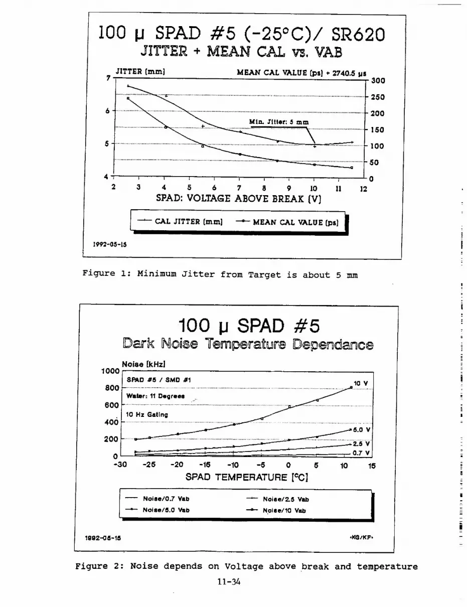
I00 _JSPAD #5 (-25°C)/ SR::0JITTER + MEAN CAL vs,VAB
JITTER [ram]?
MEAN" CAL VALUE [ps] ÷ 2740.5 Ms
.
5fl
4I 1 _ I ! I l ; J
2 3 4 5 6 7 8 9 10 11 12
SPAD: VOLTAGE ABOVE BREAK [V]
300
250
200
150
100
50
0
-- CAL JITTER [mm] "'6-- MEAN CAL VALUE [ps]
1992-05-15
Figure i: Minimum Jitter from Target is about 5 mm
1000
100 i.JSPAD #5Dark Noise Temperature Dependance
Noise [kHz]
800
600
406
200
0-30
$PAD #5 / SMD #1 10 V
10 Hz Gallng
-25 -20 -16 -10 -5 0 5 10 15
8PAD TEMPERATURE [¢C]
-- Noise/0.7 Wtb
--"- Noise/5.0 Vab
k-'_ Noise/2.5 V_b II
IN0ise/10 Vab
1992-05-15 ,KG/KF,
Figure 2: Noise depends on Voltage above break and temperature
11-34

C 9UNTER COMPARISONEXT, CALIBRATION JITTER
EXTERNAL CALIBRATION JITTER [mm]
]0-_ 9.02 ...............................
9 ................................................ :'<._i_::i ...... 8" ....................................................................
atiill .... i!iiiiii!iiii _ ............................_.= ......................., iiiiiiiiii__<iiiiiii_!_i_i_!_i_i_iiiiiii .....6 -ii!i!iiiii!ii .........iiiiiiiilili! ..........:i:_:i:i:i:_:i, iiil !ilili! ii
HP5370 A HP5370 B $R620 / 1 SR620 / 2
I SPAD ALIGNMENT iCOARSE; +15 C [_ FINE; -_ C
1992-05-1.1
Figure 3: Calibration with different counters and alignments
I0
LASEP STATION GRAZC_ibration Jitter
Calibration Jitter [mini
9t ...............................................;;.............._............................I.. or, _,n o [] _-_ o, "_o:_ o,', [] ac:__ o9._ --"_ c ___•.c o ............. 0. .............................._ .............
o
4 .....................................................................................................................................
3 n Cal Jitter [mml
_ ............................................
1 ' I '0 50 100 160
Calibration Number 1992
200 250
Cal Jitter of routine passes 1/92-3/92
Figure 4: Effect of Acousto-Optic Modelocker on Cal stability
11-35
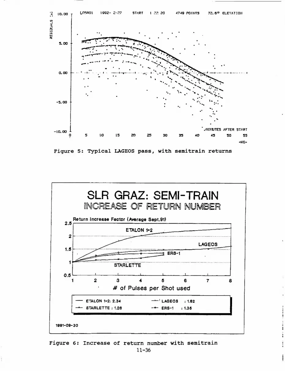
_. I0.00I,
-J
IN|11
-5. 011
Lt_ROt tgg2- _-._7 START ! ,".2 20 47,1g POitlTS 72.6 ° ELEVATTO:!
I
-LO. O0 ._.I|}IUTE$ AFTER START
0 5 L0 15 20 25 30 35 40 45 50 55
_KG>
Figure 5: Typical LAGEOS pass, with semitrain returns
2.5
SLR GRAZ: SEMI-TRAIN_[_CF_EASEOF _TU_N I_UMI_IEF_
Return Increase Factor (Average Sept.91)
2
1.5
1
0.51
ETALON 1-'2
......................................................................................
....................._ .......................................,........................,..................
___._______ ERS-1
STARLETTE
I I I l _ I
2 3 4 5 6 7 8
# of Pulses per Shot used
-- ETALON 1-2:2.34 --_-I LAGEOS : 1.62"-"- STARLETTE : 1.28 -4- ER8-1 : 1.35
lggl-Og-30
Figure 6: Increase of return number with semitrain
11-36
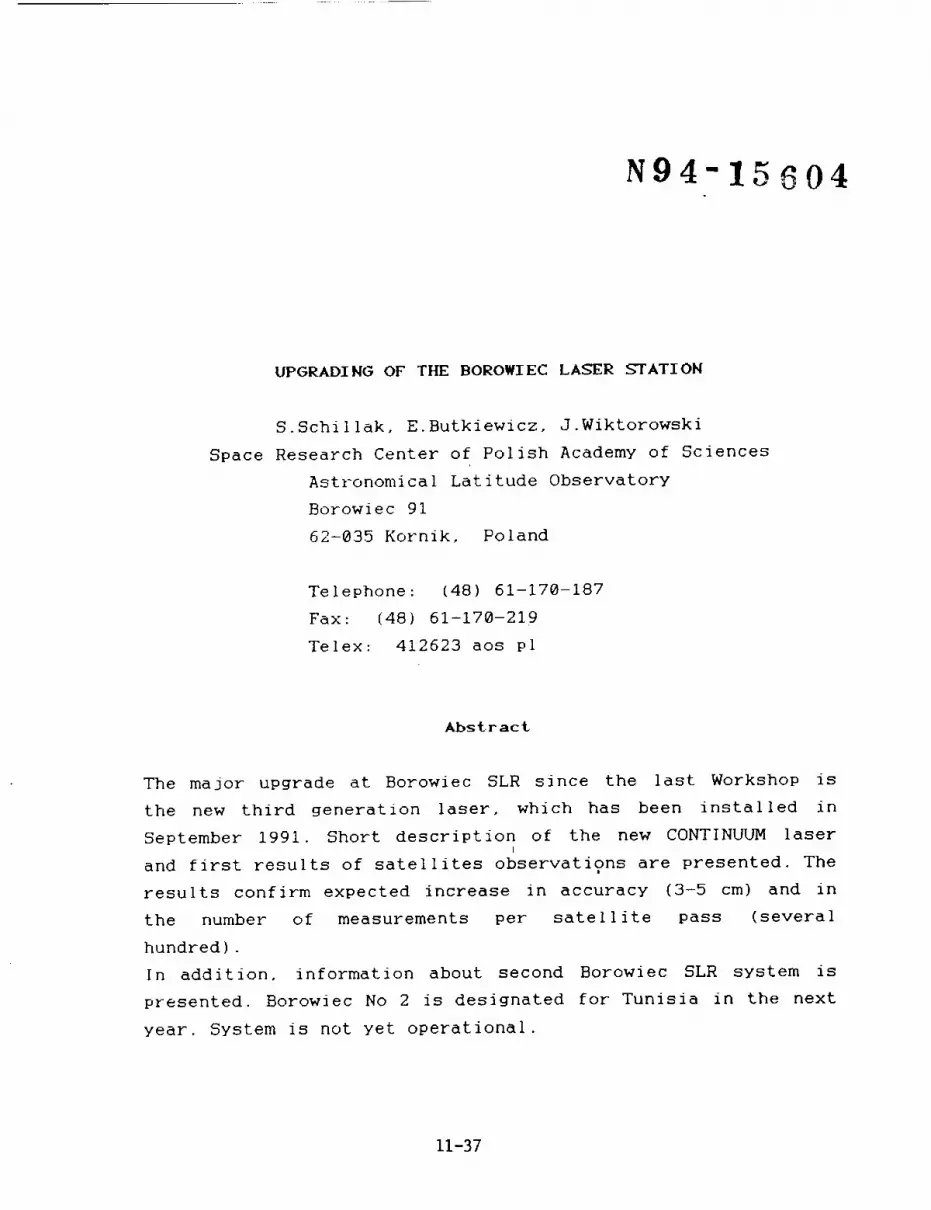
N94-15604
UPGRADING OF THE BOROWIEC LASER STATION
S.Schillak, E.Butkiewicz, J.Wiktorowski
Space Research Center of Polish Academy of Sciences
Astronomical Latitude Observatory
Borowiec 91
62-035 Kornik, Poland
Telephone: (48) 61-170-187
Fax: (48) 61-170-219
Telex: 412623 aos pl
Abstract
The major upgrade at Borowiec SLR since the last Workshop is
the new third generation laser, which has been installed in
September 1991. Short description of the new CONTINUUM laserl
and first results of satellites observations are presented. The
results confirm expected increase in accuracy (3-5 cm) and in
the number of measurements per satellite pass (several
hundred).
In addition, information about second Borowiec SLR system is
presented. Borowiec No 2 is designated for Tunisia in the next
year. System is not yet operational.
11-37

I. Introduction.
The Borowiec SLR System is operating since 1988 (Schillak,
1991). During this time the system has provided observations tosatellites LAGEOS, Ajisai, Starlette, GEO-IK-I and ERS-I. The
system has only night-time tracking capability. The single shot
precision was estimated to be about Z28 cm. Our activity
were strongly limi'ted by bad weather conditions and technical
problems (Fig.l).
Since the last workshop several upgrading in the system has
been done;
- 1998, February, transmitter telescope has been added and
divergence of laser beam changed 8X,
- 1998, October, generation of normal points onsite,
- 1998, October, replacement of the photomultipIier FEU-87 by
the RCA 8852,
- 1991, June, a received energy detector has been introduced,
- 1991, September, new third generation laser has been
inst'alled,
- 1991, October, new real-time software has been introduced,
- 1992, January, microcomputer PC/AT has been used for pre- and
post-observation programs, real-time graphic program on
PC/AT has been added.
The main upgrading of the system was installation of the newi
laser.
2. Laser CONTINUUM.
The Nd:YAG laser type CONTINUUI_ PY-62-18 has been employed in
September, 1991. The scheme of the laser transmitter is shown
in Fig.2. The laser is a cavity dumped active/passive
mode-locked system. The cavity dump consist of the
electro-optic Pockels cell triggered by a photodiode. The
selected output single pulse is ejected via polarizer when the
predetermined intensity level is reached. The oscillator
delivering about 3-5 mJ at 1864 nm. The oscillator and
preamplifier are pumped by the same flash]amp. A telescope for
beam expansion is placed before main amplifier. The amplifier
has four flashlamps. A type II KD P crystal is used for
11-38

doubling.The laser can be operated in two different modes;
- with ETALON (180' ps, 110 mJ at 532 nm),
- without ETALON (35 ps, 65 mJ at 532 nm).
The pulse repetition rate can be varied from 1 to 10 Hz (10 Hz
is optimum). Pulse stability. - 7%, diameter of output laser
beam - 12 mm, divergence - 0.4 mrad, jitter of ext. trig. _10
us.
3. Results.
The last pass with old 4 ns laser was performed on August 18,
1991, first pass with new CONTINUUM laser on September 28,
1991. The results of SLR using new laser are shown in Table i.
The table shows results of two periods of activity; I -
October, November, II - December, January. First period was
dedicated to the introducing of new real-time software , second
one to achieve maximum efficiency in actual station
configuration. The last results show that single shot RMS is
equal to 3-5 cm and further increasing of accuracy is limited
by classic photomultiplier RCA 8852 (jitter is about 1 ns).
Maximum number of returns per one pass was about 1500 for
LAGEOS and more than 3000 for _jisai. The Fig.3 and 4 shows the
advantages of new laser in comparison to the old one. To
further improve the single shot RMS the photomultiplier needs
to be changed to a micro-channel plate or an Avalanche
photodiode.
Table I. Results of the observations performed with CONTINUUM
laser from September 28, 1991 to January 31, 1992.
SATELLITE PERIOD PASSES RETI/RNS RETURNS/ RMS
ONE PASS cm
LAGEOS 8 416 52. 7. OOct-Nov
AI I SAI 1 2. 531 3 449 4, 8
8 3516 440 5.0LAGEOS Dec-lan
A/ISAI 13 17288 1328 4.0
11-39

Problems;
- delay of the mount as result of the short steps (100 ms),
step by step mode of the mount should be changed to continuous
mode, problem is especially hard for low satellites as ERS-I,
- small operational memory of old computer limits our
possibility to maximum 2500 returns per pass, also breaks of
about 1 min appeared due to 5 min bursts, microcomputer PC/AT
must be attached for real-time operations.
4. Status and parameters of Borowiec-2 SLR system.
The second SLR system has been installed in Borowiec
Observatory in 1990. The system is destined to place in
Tunisia. The parameters of actua| configuration are presented
in Table 2.
Table 2. The actual parameters (1992) of Borowiec-2 SLR system.
Laser - Nd:YAG
pulse energy - 250 mJ (green)
pulse width - 4 ns
repetition rate - i Hz
Mount - Az-EI computer controlled
tracking - continuous
tracking possibility - low satellites, Lageos, Etalons
encoder resolution - 1.8 arcsec
laser in Coude
Transmitting optics
diameter - 20 cm
gain - 8x
output divergence - 10 arcsec
Receiver - Cassegrain
diameter - 65 cm
diameter of secondary mirror - 20 cm
field of view - 5 arcmin
Guide telescope - Maksutov
diameter - 20 cm
field of view - 1°
11-40
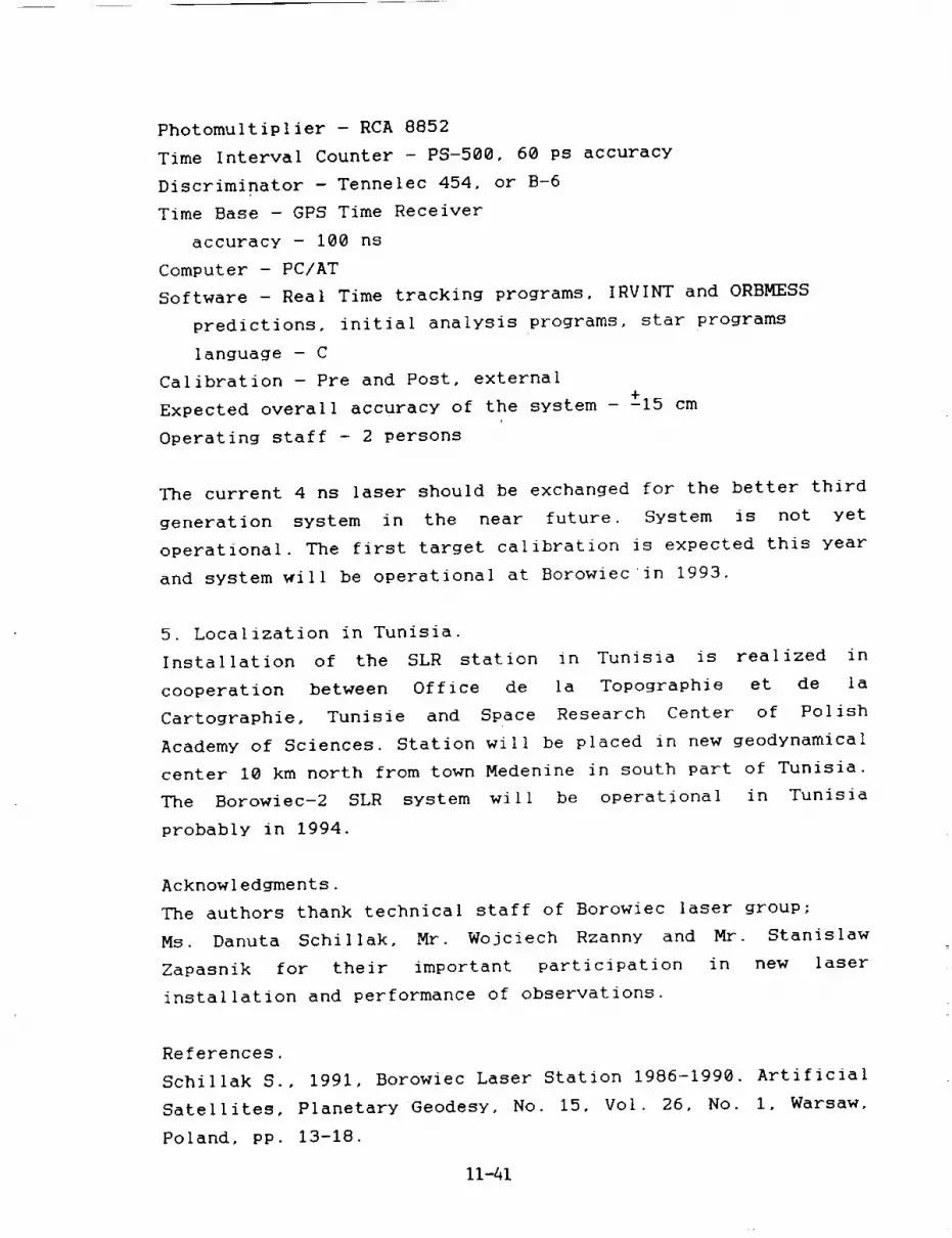
Photomultiplier - RCA 8852
Time Interval Counter - PS-500, 60 ps accuracy
Discriminator - Tennelec 454, or B-6
Time Base - GPS Time Receiver
accuracy - 100 ns
Computer - PC/ATSoftware - Real Time tracking programs, IRVINT and ORBMESS
predictions, initial analysis programs, star programs
language - CCalibration - Pre and Post, externalExpected overall accuracy of the system - ZI5 cm
Operating staff - 2 persons
The current 4 ns laser should be exchanged for the better third
generation system in the near future. System is not yet
operational. The first target calibration is expected this year
and system will be operational at Borowiec in 1993.
5. Localization in Tunisia.
Installation of the SLR station in Tunisia is realized in
cooperation between Office de la Topographie et de la
Cartographie, Tunisie and Space Research Center of Polish
Academy of Sciences. Station will be placed in new geodynamical
center 10 km north from town Medenine in south part of Tunisia.
The Borowiec-2 SLR system will be operational in Tunisia
probably in 1994.
Acknowledgments.
The authors thank technical staff of Borowiec laser group;
Ms. Danuta Schillak, Mr. Wojciech Rzanny and Mr. Stanislaw
Zapasnik for their important participation in new laser
installation and performance of observations.
References.
Schillak S., 1991, Borowiec Laser Station 1986-1990. Artificial
Satellites, Planetary Geodesy, No. 15, Vol. 26, No. i, Warsaw,
Poland, pp. 13-18.
11-41
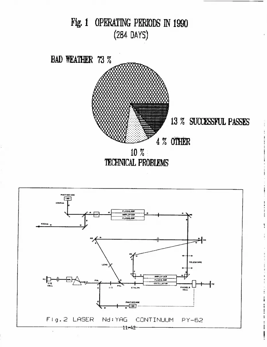
F_.I OP_T_G P_ODS_ 1990.(284DAYS)
T
LENS M_/'_'/
_ l______v 4#l I pOL_ ¢$CILLAT¢_
TI_LE$CCPE
---OF
CEU.
Fig. 2 LASER Nd : YAG CONT INUUM
11-42
P Y-I:S2

RMS(cm)25
20
15
10
5
0
OLD
21.6
NEW
5
OLD
18.9
LAGEOS AJISAI
Fig.3 Single shot RMS - old and new laser.
NEW4
1600
1400
1200
1000
800
600
400
200
0
N
NEW
440
lo °
LAGEO8FIg,4
OLD
114
AJISAI
Returns per one psss - old and new laser
NEW
1328
11-43

N94-15605
Development of Shanghai Satellite Laser Ranging Station
F.M. Yang, D.T. Tan, C.K. Xiao, W.Z. Chen, J.H. Zhang
Z.P. Zhang, W.H. Lu, Z.Q. Hu, W.F. Tang and J.P. Chen
Shanghai Observatory, Academia Sinica
80 Nandan Road, Shanghai 200030, ChinaTelex: 33164 SHAO CN
Fax: 86-21-4384618
Phone: 86-21-4386191
l. Improvement of the System Hardwares
1.1 Computer control subsystem _i_i:i_;!i_
An IBM/286 computer control system was set up during August 1989 to
March 1990. After three months, the realtlme display of range residuals
(O-C) on the computer screen was completed. Since then, only one
operator has been needed for the routine observation. The operator can
control the whole ranging system by using the computer keyboard during
the observation and can watch the image of the satellite while
illuminated by the sunlight on the monitor of a SIT TV camera side by
side. The system automation and reliability has been greatly improved.
1.2 Laser Subsystem
The Nd:YAG mode-locked laser, which was made by the Shanghai Institute
of Optics and Fine Mechanics and installed at the station in 1986,
contains an oscillator and three single-pass-ampliflers and can usuallyproduce 50 mJ (green) and 180 psec width.
Many work have been done in order to improve the stability on both the
laser beam direction and the output energy. A new chiller was installed
in November 1991 The repetition rate is I-2 Hz for Lageos and Etalon
ranging, and 2-4 Hz for low orbit satellites ranging. The divergence of
the laser is about 0.4 mrad. So, the optimum beam divergence from the
transmitting telescope which has a magnification of 6 is about 13
arcseconds. That is good for Etalon satellites ranging. The divergence
can be adjusted up to 3 arcminutes for the low orblt satellites ranging.
1.3 Receiver
The ordinary PMT (Type GDB49A, China-made) has been adopted from the set
up of the system in 1983 to May 7,1992 when a single photon avalanche
diode (SRAD) receiver made by the Czech Technical University has been
installed. The voltage for the diode is about 30 V and the break down
voltage is about 27.5 V. The field of view of the new receiver is about
45 arcsec. The noise rate of the SPAD working at above condition is200"300 KHz even in [he nighttime.
A 0.15 nm narrow band filter in a theomostat has been tested in
November-December 1991 and has been shown with good performance.
11-44
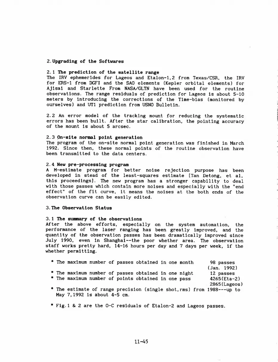
2. Upgrading of the Softwares
2.1 The prediction of the satellite range
The IRV ephemerides for Lageos and Etalon-l,2 from Texas/CSR, the IRV
for ERS-1 from DGFI and the SAO elements (Kepler orbital elements) for
AJisai and Starlette From NASA/GLTN have been used for the routine
observations. The range residuals of prediction for Lageos is about 5-10
meters by introducing the corrections of the Time-bias (monitored by
ourselves) and UT1 prediction from USNO Bulletin.
2.2 An error model of the tracking mount for reducing the systematic
errors has been built. After the star calibration, the pointing accuracyof the mount is about 5 arcsec.
2.3 On-slte normal point generation
The program of the on-slte normal point generation was finished in March
1992. Since then, these normal polnts of the routlne observation havebeen transmitted to the data centers.
2.4 New pre-processing program
A M-estimate program for better noise rejection purpose has been
developed in stead of the least-squares estimate [Tan Detong, et al,
this proceedings]. The new program has a stronger capability to deal
with those passes which contain more noises and especially with the "endeffect" of the fit curve, it means the noises at the both ends of the
observation curve can be easily edited.
3. The Observation Status
3.1 The summary of the observations
After the above efforts, especially on the system automation, the
performance of the laser ranging has been greatly improved, and the
quantity of the observation passes has been dramatically improved since
July 1990, even in Shanghai--the poor whether area. The observation
staff works pretty hard, 14-16 hours per day and 7 days per week, if the
whether permitting.
" The maximum number of passes obtained in one month 98 passes
(Jan. 1992)
• The maximum number of passes obtained in one night 12 passes
i The maximum number of points obtained in one pass 4265(Eta-2)
2865(Lageos)
" The estimate of range precision (single shot,rms) from 1988---up to
May 7,1992 is about 4-5 cm.
"Fig. l g 2 are the O-C residuals of Etalon-2 and Lageos passes.
11-45
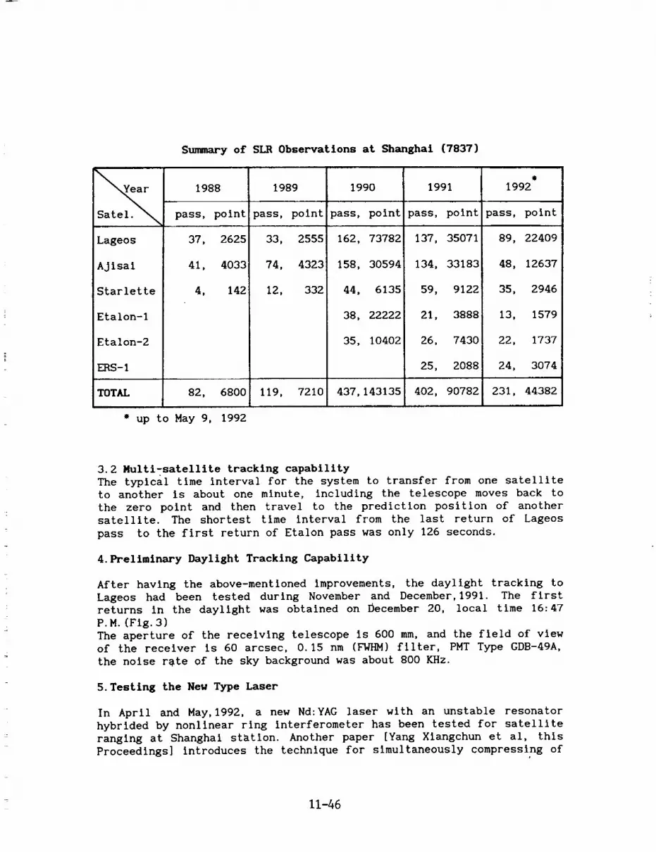
Summary of SIR Observations at Shanghai (7837)
Satel.
Lageos
Ajisal
Starlette
Etalon-1
Etalon-2
ERS-I
1988
pass, polnt
37, 2625
41, 4033
1989 1990 1991
pass, polntlpass, point pass, point
33, 25551 162, 73782 137, 35071
74, 4323 158, 30594 134, 33183
e
1992
pass, point
89, 22409
48, 12637
4, 142 12, 332 44, 6135
38, 22222
35, 10402
59, 9122
21, 3888
26, 7430
25, 2088
35, 2946
13, 1579
22, 1737
24, 3074
TOTAL 82, 6800 119, 7210 437,143135 402, 90782 231, 44382
* up to May 9, 1992
3.2 Multi-satellite tracking capability
The typlcal time interval for the system to transfer from one satellite
to another is about one minute, including the telescope moves back to
the zero point and then travel to the prediction position of another
satellite. The shortest time interval from the last return of Lageos
pass to the first return of Etalon pass was only 126 seconds.
4.Preliminary Daylight Tracking Capability
After having the above-mentioned improvements, the daylight tracking to
Lageos had been tested during November and December, 1991. The first
returns in the daylight was obtained on December 20, local time 16:47
P.M.(FIg. 3)
The aperture of the receiving telescope is 600 mm, and the field of view
of the receiver is 60 arcsec, 0.15 nm (FWHM) filter, PMT Type GDB-49A,
the noise r_te of the sky background was about 800 KHz.
5. Testing the New Type Laser
In April and May, 1992, a new Nd:YAG laser with an unstable resonator
hybrided by nonlinear ring interferometer has been tested for satellite
ranging at Shanghai station. Another paper [Yang Xiangchun et al, this
Proceedings] introduces the technique for simultaneously compressing of
11-46

the passive mode-locked pulsewldth and pulse train. For SLRapplication,one amplifier and one frequency doubler were added to the oscillator.Without the single pulse selector, the output of the laser system was in
pulse train containing only I-2 giant pulses, and the total energy of
the pulse train is about 18 mj (green), I0 psec width, 0.4 mrad beam
divergence, 2-4 Hz repetition rate. During May 8-9, the new laser system
and the SPAD receiver has been successfully used for Lageos and Etalon-I
ranging. The 2 cm range accuracy has been achieved in both satellite and
ground target ranging. (Fig. 4 & 5)
6. Future Plans
6.1 Routine daylight ranging to Lageos and other low orbit satellites.
6.2 Single shot range accuracy will be improved to better than 2cm for
routine operation.
6.3 Development of the millimeter level accuracy SLR system
A cooperative plan between Shanghai Observatory and Xi'an Institute of
Optics and Precision Mechanics has been set up to develop a mm- level
SLR system based on a circular-scan streak tube. A prototype tube has
been made by Xl'an Institute in March 1991. The main characteristics of
the tube is as follows:
• Photocathode: Type S-20, Sensitivity
Spectrum responseEffective area
" Sensitivity of deflection
• Double MCP internal intensifiers
" Gain
• Spatial resolution
• Temporal resolution
" Dynamic range
67 pA / im200-850 nm
12 mm
l0 cm / KV
1X 10⁶
24 Ip / mm
4.8 psec
390:1
This project has been supported by the Chinese National Science
Foundation and the Chinese Astronomical Committee, and expected to be
operational in 1994.
11-47

m m
mg
u}
i-4 -llm -bq
!
41=--
olU= --
u_ _,o • •
• -...Tv" . _ ._ • •
%
,#
% •
%
"_ ,F' °' • t •" _' '
& • ,A,, _
ELAPSE TIME (SECOND}
Fig. 1 One pass of Etalon-2 on August 13,1990, 4138 ObservationsTime (UTC):11:47 Accuracy(rms): 6cm
-1--
-Nm--
Fig. 2
ELAPSE TIME (SECOND}
One pass of Lageos on July 28,1990, 2865 ObservationsTime (UTC):18:17 Accuracy(rms): 5cm
11-48

m
U_
Ii
Fig. 3
ELAPSE TINE (SECOND)
Daylight tracking to Lageos on December 20, 1991
O_
m
L_o
m
t_
.o.... "9 •. • •°_°° °
°a
a
°
°• •',, .,• o, .- % •
• ° ", • • • • • ° •• ° °'Q", • •
. • .,:._.......,, ,.._'.. ,_ .:,:...._," ._.... :_._,......., •...:..,......_,*.
ELAPSE T I HE ( SECOND )
Fig. 4 Ground target callbratlon on May 9,1992
wlth 10 psec laser train and a SPAD receiver
11-49

STATION ID : 7837
DATA: 05/09/92
SATELLITE: LAGEOS
TINE(UTC): t7: t
i •
r,n
Hul
II
o •
,°
o,
• o
,,;" •.£
".::'.""5/• ;'"_:X,,"
I-
ELAPSE TIME (SECOND)
J- J=
STATION ID :7837
DATA:05/O9/92
SATELLZTE:ETALON-t N" t7g
TIME(UTC): 17:58 RMS=2.3CM
m --
J.
.o . _o. • • %.. o" •
; .,Q.... . q _,,e t ." ....
..._ . •
o. ° ° ""
ELAPSE TIME (SECOND)
ae
Fig. 5 Results of ranging to Lageos and Etalon-I
with a I0 psec laser and a SPAD receiver (Hay 9,1992)
Single shot accuracy(rms): 1.7--2.3 cm

N94-15606
STATUS-REPORT on WLRS
R. Dassing, W. Schliiter
Institut filr Angewandte Geod_sie
Fundamentalstation Wettzell
D - 8493 KStzting
U. Schreiber*
Forschungseinrichtung Satellitengeod_.sie
Fundamentalstation Wettzell
D - 8493 KStzting
Abstract
The Status-Report of WLRS gives an overview of its set up and the devel-
opments necessary to make the system operational.
1 History
After setting up the new Wettzell laser ranging system WLRS in the year 1989 the systemgot its first successful returns from Lh(;EOS at 29th January, 1990 (see table 1). As these
returns were not calibrated they were only of "engineering use". The system showed
that it was able to track to Etaion-type satellites and to NETEOS/T P2. Before the first
attempts to the moon were started the system was set up to a reliable and calibrated
state. In order to guarantee continous observations from Wettzell a co-location betweenSR$ and WLItS has been carried out. The old SRS-system is now replaced by WLRS.
At the beginning of 1991 WLRS started to track on a routine basis to the satellitesLAGEOS, ETAL01[-1 and ET,tLON-2. During the first six month of year 1991 the WLRS-
System was operated by one shift mostly during night times. Since 1st July 1991 there
were enough educated observers to track 24 hours a day. This can clearly be seen in
the amount of observed passes (see table 1). The number of returns per Lh(lE0S-pass
ranged from several hundred up to 6000. At the end of 1991 the operators had enough
experiences to track AJIS/I, ST/RLETTE and ERS-! satellites.
The first (calibrated) measurements from the moon were obtained in July 1991. InNovember 1991 a series of 52 echos from the moon could be measured, which resulted in
one normalpoint.
°Technische Universit_t Mfinchen, Arcisstr. 21, D - 8000 M_nchen 2
11-51
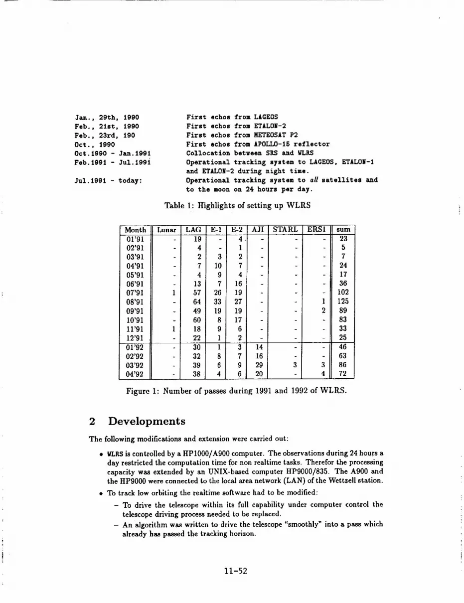
Jan., 29th, 1990
Feb., 21st, 1990
Feb., 23rd, 190
Oct., 19900ct.1990 - Jan.1991Feb.1991 - Ju1.1991
Ju1.1991 - today:
First echos from LAGEOS
First echos from ETALON-2
First ethos from METEOSAT P2
First echos from APOLLO-15 reflectorCollocation between SRS and _RS
Operational tracking system to LAGEOS, ETALON-1
and ETALON-2 during night time.
Operational tracking system to aH satellites and
to the moon on 24 hours per day.
Table 1: Highlights of setting up WLRS
Month Lunar LAG E-1 F,-2 AJI
01'91 19 402'91 4 1
03'91 2 3 2 -
04'91 7 10 7 -05'91 - 4 9 4 -
06'91 - 13 7 16 -
07'91 1 57 26 19 -
08'91 - 64 33 27 -
09'91 - 49 19 19 -
10'91 - 60 8 17 -11'91 1 18 9 6 -
12'91 - 22 1 2 -
01'92 - 30 1 3" 14
02'92 32 8 7 16
03'92 39 6 9 29
04'92 38 4 6 20
STARL ERS1
1
2
sum
235
7
24
1736
102
125
89
83
3325
46
63
3 86
4 72
Figure 1: Number of passes during 1991 and 1992 of WLRS.
2 Developments
The following modifications and extension were carried out:
• WLR$ is controlled by a HP1000/A900 computer. The observations during 24 hours a
day restricted the computation time for non realtime tasks. Therefor the processing
capacity was extended by an UNIX-based computer HP9000/835. The A900 and
the HPg000 were connected to the local area network (LAN) of the Wettzell station.
• To track low orbiting the realtime software had to he modified:
- To drive the telescope within its full capability under computer control the
telescope driving process needed to be replaced.
- An algorithm was written to drive the telescope "smoothly" into a pass which
already has passed the tracking horizon.
11-52

- The transmit/receive switch between outgoing and receiving laser pulses is
realized as a rotating mirror with two holes. To fire the laser with 10 Hz themirror must rotate with 5 Hz. To track to low orbiting satellites the software
to ramp up and control the rotating frequency of the T/R-switch up to 10 Hz
was replaced.
- To track low orbiting satellites a 'time bias' was built into the realtime soft-
ware. This 'time bias' moves the current epoch for the calculations of azimuth,
elevation and range.
• During winter 1991/1992 the analysists of the University of Texas and Bendix found
a sudden range bias of about 1.75 m. This was caused by the replacement of an
amplifier of MCP.The reason was found in the dead time of the detection electronics. The electronic
needs about 68 ns to be able to detect the realtime calibration pulse after the
detection of the start pulse of the laser. This means that the calibration returnmust take more than 68 ns to be recorded by the event timer. As the return
signal from the calibration retro was very close to 68 ns it was not obvious that theelectronic detected the "dead-time" instead of the real calibration echo. Now, the
calibration return moved away from this critical region to avoid any collisions.
• The quicklook-data generation was replaced by a normal point generation. An orbit
fitting algorithm is used.
• Experiments in 2-color ranging have been carried out by measuring several LA6EOS-
passes simultanously in green and infrared [Schreiber et al.].
3 Summary
After setting up WLRS in 1989 some essential modifications were carried out:
• High data acquisition rate (up to fi000 Returns per LAGEOS pass);
• Normalpoint precision of 3 - 5 mm (BEFC);
• A laser ranging system which can track all targets -- from E_tS-1 to the moon.
4 References.+,
[Schrelber et al.] U. Schreiber, K.H. Haufe, R. Dassing, "Measuring Atmospheric Dis-persion With WLRS In Multiple Wavelength Mode", published in this proceedings
11-53

N94-15607
GROUND BASED LASER RANGING
FOR SATELLITE LOCATION
by
G. C. Gilbreath
Optical Systems Section
Naval Center for Space Technology
Naval Research Laboratoryi
and
Harold D. Newby
Malabar Test Facility
Phillips Labs (AFMC)
ABSTRACT
In this article, we describe a new satellite laser ranging
capability which is a joint effort between the Naval Research
Laboratory and Air Force Optical Tracking Facility at Malabar,Florida. Initial measurements off LAGEOS indicates that
uncorrected radial range rms values of 8mm are readily
achievable. Number of photoelectron counts are on the order of
180 which are off by an order of Magnitude from predictedvalues.
I. INTRODUCTION
A new SLR capability designed and implemented by the Naval
Research Laboratory is now operational at the Air Force Optical
Tracking Facility in Malabar, Florida. The configuration is
based on the monostatic design utilized by a number of the NASA
systems in the geoscience network. The laser itself is more
powerful than those used by the NASA network, and electronics are
somewhat different. The system was designed for experimental
efforts in tracking unenhanced satellites (those satellites
without retroreflectors), plumes, and other targets which may or
may not have large laser ranging cross sections.
II. CONFIGURATION
A. Tracking & Acquisition:
Tracking and acquisition was done by the optical tracking
facility at Malabar, Florida. Malabar's facility provided a
bistatic optical acquisition capability when tracking in
"terminator" mode. In this mode, a platform is sunlit but the
tracking station is in the dark. The initial acquisition is done
passively with the 1.22 m aperture telescope. Once trained on
11-54

the satellite in question, the0.61 m aperture telescope can
track the target within 5-10 _R of accuracy. All vectors,
offsets, and tracking is done under computer control using a
MicroVax III. Video recordings of a laser ranging event is made
in addition to a digitized record of tracking vectors andrelated offsets.
The transmitter/receiver design is monostatic although
acquisition is bi-static. Once the 0.61 m telescope is trained
on the target, laser ranging commences. A diagram of the
overall method is shown in Figure I.
Satellite
FIGURE 1. NRL/Malabar Satellite Laser Ranging Acquistion
Diagram. Initial Acquisition is bistatic when platform is
acquired in "Terminator Mode". Once acquired by R1, T1 tracks.
The laser ranging T/R is monostatic using T1.
The return signal is collected by the telescope and
directed back through the optics where the light is directed to
a MCP/PMT using a specially designed annular mirror. The
return signal, if strong enough, is split, where part is sent to
the time interval counter, and part is sent to a wideband
oscilloscope (4Ghz) for waveform capture. An overall system
block diagram is shown in Figure 2.
11-55

i EphemerisGeneration
Computer
Walli i i =,1
Shutter
Annular Mirror
Laser Diverging
(Nd:YAG) Optics
:::::::
StreakCamera
• o ......
• ° ......
Acq.&Control
)uters
Receiver
Electronics
• • ..... • ..........
• ° , , . , , ° ....
• o , • ........
Baffled Receiver
Assembly
FIGURE 2. NRL/Malabar Satellite Laser Ranging Block Diagram.
Configuration shows laser and transmit optics directed through
an annular mirror; returned signal is directed via the mirror to
the baffled receiver assemby where time differences and
waveforms are recorded digitally for off-line analysis.
B. Transmitter:
The laser was designed for the effort by Continuum and is a
doubled-YAG, Q-switched, mode-locked laser . The cavity design
is "active-active" in that a pulse slicer is used rather than a
dye to select desired modes. The configuration includes an
oscillator stage and two single-pass amplification stages. The
laser provides 300 mJ per pulse in a 250 ps pulsewidth. The
pulse repetition rate is i0 Hz. The beam divergence is
approximately I0 times the diffraction limit.
Initial alignment in the active-active mode has proven to
require careful adjustment. For this reason, a streak camera is
configured into the testbed. It was found that initial
diagnostics are required at start-up but good alignment is
maintained thoughout a given ranging session.
Scattered infrared light is focused onto a PIN detector and
the output is directed through a constant fraction discriminator
(CFD). The signal is then split and sent to a SR 620 time
interval counter and to the IRIG board in the HP 9836
Controller, which time-tags the event.
11-56'

C. Optics :
Adjustable "zoom" optics are installed to vary the
divergence of the beam though computer control. The range of
variability is designed for an output at the antenna of 10_Rad-
100_Rad.
A special annular mirror was designed such that the
transmitted beam passes through a 4.57 cm hole in the 20.32 cm
mirror. The return beam is collimated by the telescope to
present a -11.4 cm beam to the flat. The return beam is then
directed to the baffled receiver assembly.
D. Receiver:
The return signal is directed through a 1 m focal length
lens to a mirror which can be switched in and out of the optical
path. When in place, this mirror directs the light toward aFairchild intensified CCD which enables verification of proper
optical alignment of the receive optics. When this mirror is
switched out, the beam is focused onto a 500mm pinhole and
directed into the gated ITT F4129 PMT/MCP detector. This
detector has a quantum efficiency of 16% with a gain of ~10^6 at
532nm. The detector itself is gated to reduce noise using a
programmable delay/width generator. The gatewidth can vary from
several hundred nanoseconds to I0 _.
The output from the PMT is amplified, inverted, and passed
through a constant fraction discriminator. The output is time-
tagged by the SR 620 time interval counter and the difference
stored in the computer. A portion of the output is also
directed to a Tektronix SCD 5000 4 GHz wideband oscilloscope
which digitizes and stores the waveform for later analysis. A
block diagram of the electronics is shown in Figure 3.
IiI. LAGEOS CALIBRATION
The system was calibrated by ranging off LAGEOS for a
series of passes. Radial RMS ranges (uncorrected) were
estimated to be -8mm using the system. Detected photoelectron
counts were on the order of 50-190. We initially estimated
returns on the order of ii00 p.e.'s. It is possible that the
divergence convolved with pointing accuracy has a greater error
than anticipated. However, scatter loss is most likely to have
been the major contributor to the lower returns.
IV. CONCLUSION
The Naval Research Laboratory and the Air Force Optical
Tracking Facility have installed a new satellite laser ranging
11-57

NCST-SLR
Receiver Hardware
Photo-diode (START
pulse detector)
20
RG-58
coax
InvertingTransformer
BNC 7085 Delay/
Width Generator
Beam _ Micro Kinetics IDiverging (micro-posit. control)
Optics
v| SR 620 UTIC
TC 454 CFD
(STARTChannel) DG535 Delay/Width Gen
(pseudo Stop pulse &
IRIG Board Freeze)
HP 8082 Delay/WidthGen.
|PS350 High Voltage Supplyfor _P/PMT)
(3-4 kV
IRIG Board
TC 454 CFD (Universal Time)(STOP
Channel) Universal
Time Code
(vernier delay control) _ Tek 7104
Avtech Pulse Transformer_PC Gate, Voltage (500V) AssemblyBaffledII v__ I'0 eHz Oscill°sc°pe'
Receiver ___Tek SCD 5000 4 GH 4
[ Digitizing Scope]
FIGURE 3.
Diagram.NRL Satellite Laser Ranging Receiver Hardware Block
capability in Malabar, Florida. The system is based on the NASA
monostatic designs used by MOBLAS and other ground sites. The
laser itself is a 300 mJ/pulse, 250 ps, 10Hz, Q-switched, mode-
locked, active-active design. The detection system includes a
gated ITT F4129 PMT/MCP detector and a 4 GHz wideband Tektronixdigitizing oscilloscope.
Initial mesurements off LAGEOS indicates that an 8mm
uncorrected radial range rms is easily achievable. However,
actual p.e. counts are smaller than predicted by an order of
magnitude. This may be due to larger than anticipateddlvergence and/or to back scatter.
Future efforts will require direct measurement of the
divergence in the far-field using the "dithering" technique
common to MOBLAS users. Corrections to divergence can be made
using the computer-controlled zoom optics in the transmit
11-58

optical train. Anticipated experiments will include ranging off
of platforms which may not have enhanced laser ranging cross
sections and ranging off plumes.
V. ACKNOWLEDGMENTS
We would like to thank John Degnan, Tom Varghese, Tom
Zagwodski, and the other NASA personnel who were so generous
with their time and advice. We would also like to acknowledge
the MacDonald Observatory, and especially Jerry Wiant whosesuggestions were invaluable.
We would especially like to acknowledege both the NRL and
Malabar teams, without whose the dedication, hard work, and
creativity, the system could not have been designed, integrated,and calibrated in such a timely manner, including W. C. Collins,
W. L. Lippincott, J. Pirozzoli, T. Murphy, S. Peterson, A.
Clement, J. Kobesky, R. Dasenbrock, R. Betz, T. Knox, M. Baciak,P. Patowski, and R. Orcutt.
11-59

N94-15608
NEW PROGRESS OF RANGING TECHNOLOGY
AT WUHAN SATELLITE LASER RANGING STATION
Xia Zhizhong, Ye Wenwei, Cai qingfu
Institute of Seismology State Seismological Bureau
430071 Wuhan China
ABSTRACT
A satellite laser ranging system with an accuracy of the level of centimeter has been devel-
oped. successfully at the Institute of Seismology, state Seismological Bureau with the coopera-
tion of the Institute of Geodesy and Geophysics, Chinese Academy of Science. With signifi-
cant improvements on the base of the second generation SLR system developed in 1985,rang-
ing accuracy of the new system has been upgraded from 15em to 3-4cm. Measuring range has
also been expanded, so that the ETALON satellite with an orbit height of 20,000Kin launched
by the former U. S. S. R. can now be tracked.
Compared with the 2nd generation ShR system, the newly developed system has the fol-
lowing improvements z
(1) A Q modulated laser is replaced by a mode-locked YAG laser. The new device has a
pulse width of 150ps and a repetition rate of 1-4pps.
(2)A quick response photomultiplier has beer adopted as the receiver for echo, for exam
pie, the adoption of MCP tube has obviously reduced the jitter error of the transit time and
therefore has improved the ranging accuracy.
(3)The whole system is controlled by an IBM.PC/XT Computer to guide automatic track
ing and measurement. It can carry out these functions for satellite orbit caculation, real-time
tracking and adjusting, data acquisition and the preprocessed of observing data etc. , the au
tomatization level and reliability of the observation have improved obviously.
INTRODUCTION
Satellite laser ranging (SLR) is a new measurement technology established with the ad
vancement of laser, optoelectronies, computer, and space science. It has been widely applied in
geoseience. Its observing date have already been used in many scientific fields such as geody
11-60
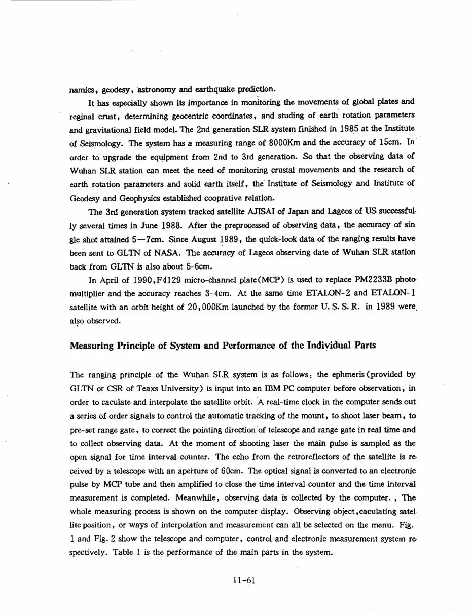
namics, geodesy, astronomy and earthquake prediction.
It has especially shown its importance in monitoring the movements of global plates and
reglnal crust, determining geocentric coordinates, and studing of earth rotation parameters
and gravitational field model. The 2nd generation SLR system finished in 1985 at the Institute
of Seismology. The system has a measuring range of 8000Kin and the accuracy of 15cm. In
order to upgrade the equipment from 2nd to 3rd generation. So that the observing data of
Wuhan SLR station can meet the need of monitoring crustal movements and the research of
earth rotation parameters and solid earth itself, the' Institute of Seismology and Institute of
Geodesy and Geophysics established cooprative relation.
The 3rd generation system tracked satellite AJISAI of Japan and Lageos of US successful-
ly several times in June 1988. After the preproC,essed of observing data, the accuracy of sin
gle shot attained 5--?cm. Since August 1989, the quick-look data of the ranging results have
been sent to GLTN of NASA. The accuracy of Lageos observing date of Wuhan SLR station
back from GLTN is also about S-6cm.
In April of 1990,F4129 micro-channel plate(MCP) is used to replace PM2233B photo
multiplier and the accuracy reaches 3-4cm. At the same time ETALON-2 and ETALON-1
sateLlite with an orbit height of 20,000Km launched by the former U. S. S.R. in 1989 were.
also observed.
Measuring Principle of System and Performance of the Individual Parts
The ranging principle of the Wuhan SLR system is as follows, the ephmeris(provided by
GLTN or CSR of Teaxs University) is input into an IBM PC computer before observation, in
order to caculate and interpolate the satellite orbit. _Areal-time clock in the computer sends out
a series of order signals to control the automatic tracking of the mount, to shoot laser beam, to
pre-sct range gate, to correct the pointing direction of telescope and range gate in real time and
to collect observing data. At the moment of shooting laser the main pulse is sampled as the
open signal for time interval counter. The echo from the retroreflectors of the satellite is re
ceived by a telescope with an aperture of 60cm. The optical signal is converted to an electronic
pulse by MCP tube and then amplified to close the time interval counter and the time interval
measurement is completed. Meanwhile, observing data is collected by the computer. , The
whole measuring process is shown on the computer display. Observing object,caculating satel-
lite position, or ways of interpolation and measurement can all be selected on the menu. Fig.
1 and Fig. 2 show the telescope and computer, control and electronic measurement system re
spectively. Table 1 is the performance of the main parts in the system.
11-61
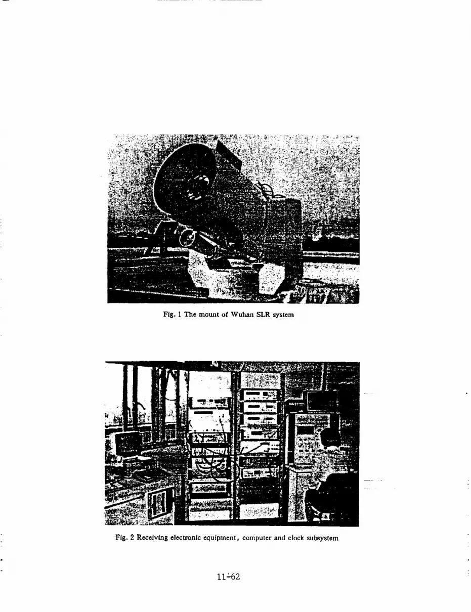
Fig. ] The mount of Wuhan SLR system
Fig. 2 Receiving electronic equipment, computer and clock subsystem
iI_62

Table 1 Specl/ication of the utelllie laser ranging system at Wuhan
Subsystem
Mount
Configuration
Tracking velocity
Synchronistic inductor
Drive
Orthogonality
Laser
type
Wave length
Energy
Pulse width
Repetition
Receiving telescope
Type
Diameter
Field of view
Filter
Transmitting telescope
Type
Diameter
Beam divergence
Sighting telescope
Diameter
Field of view
Receiving electronics
PMT
Amplifier
Discriminator
UTC clock
Type
Stability
Accuracy
Time interval counter
Type
Resolution
Micro computer
Specification
elevation-azimuth
18 arcsec-- O. 5° per second
resolution 1 arc._ec
DC torque motors
-I-4 arcsec
Nd :YAG
0.532_m
50mj
150ps
1-5pps
Cassegraln
60cm
l'-6'or l'(use for sighting satellite)
lnm
Galilean
10cm
0.6'-3' can adjustable
15cm
3"
ITr F4129 MCP/
H/P 8447 D
Canberra 1428A
Cesium H/P 5061A
1X 10 -12
2Ws
5370B
2.0ps
IBM PC/XT
II_63

Main Improvements
1. Nd : YAG ultra-short pulse mode-locked laser is used
An active and passive mode-- locked laser with Nd : YAG as laser material is used in the
new SLR system. Fig. 3 is block diagram of laser. Infrared light output of 100 nd in energy,
1.06_m in wavelength, and 150ps in pulse width is got from laser with one stage oscilator and
three stage optical amplifier. It is converted to green light of 50rrd in energy, 532nm in wave
length and 1-4pps adjustable in repetition rate. Compared with the Q modulated device(4.5ns
inpuise width, 0. 25J in energy) used in the 2nd generation system, The new laser improved
the ranging accuracy, because the pulse width is reduced greatly Table 2 shows the compari.
sion of ranging accuracy between adopting Q modulated device and mode-locked device, while
other conditions are the same.
Table 2. The Comparislon of ranging accuracy between Q modulated and mode--locked laser from LA-
GEOS
Wuhan GLTNDATE TIME OBS LASER
RMS(cm) RMS (era)
1985.08.02 23=44 103 13.9
8.03 22:20 370 15.8
8.14 21:26 131 14.6
8.16 22:21 105 15.4
9.11 22:01 280 14.9
9.28 20:02 320 14.7
10.05 21:03 101 16.1
10.07 21:50 170 15.7
1989.11.27 18:50 471 5.7
11.28 17:34 431 5.7
11.28 21:07 _ 303 5.7
12.01 17:04 144 6.1
12.01 20:28 483 6.3
12.02 19:04 176 7.3
12.03 17:44 330 7.5
12.03 21:18 438 6.7
5.1
5.1
6.5
6.5
6.5
5.1
5.3
YAG Modulated Q
YAG Mode-Locked
11-64

1 2 AOM F-P
High Repet£tfon Rate Ultra-short pulse Oscillator1-Reaxmirror contacted by dye cell wfth circulattr_
system. 2-Transverse mode selectfn_ aperture._-Xe flash lamp. 4-Front mirror.
1 , __C_ -\ _
532_ 9
4
1-Oltra-ehort p_lse oscillator. 2-Slr_le pulse selector.
_p4-45" ec[rrors. 5,7,9-Beam expanders. 6-Plrst sta_e ofamplifier. 8- Two sta_e of amplLffer. IO-Ha-r_onlc ge-nerator.
Fig. 3 Schematic Diagram of Repetition Rate Ultra-short Prise Laser System
2. Improvement of opto-electronie detector PM2233B photomultiplier is employed as de
tector for main and echo pulse in the 2nd generation SLR system, the transit time of electron
in the whole tube is relatively long so the jitter error will become very important for precise
ranging. In order to overcome this shortcoming, F4129 MCP photomultiplier with Ins transit
time is used for detecting echo in the 3rd generation system. The jitter error is sharply reduced
because the distance between the cathode and micro-channel plate is just 0. 6_m . Table 3
shows the observing results before and after the photomultiplier is replaced. Data processing
by GLTN, Delft University and ourselves, all show that the ranging accuracy has upgraded
from 5-Tem to 3-4cm.
Table 3. the Observing results before and after the photomultiplier b replaced from LAGEOS
Wu han GLTN DELT 1DATA AOS LOS OBS PMT
RMS (em)RMS (cm)RMS(cm)
SAT. LAGEOS
90.3.6 17:55:15 18:17:48 81 8.1 5.6 6.4
3.7 16:24:58 16:51:52, 210 7.1 6.4
4.4 13:32:14 14:11:08 308 8.4 7.2
4.12 13:11:49 13:50:55 47 8.8 7.8 8.0
4.13 15:25:13 15:56:08 265 7.5 4.7 6.1
4.19 14z16:44 14z57,38 675 6.4 5.4 6.1
PM2233B
11-65

4.25 1"3=04=01 13=44=19 312 4.5 414 4.9
4.26 11=48=11 12=19=58 346 6.3 6.1 4.9
4.26 15=18=14 15=47=42 387 4.6 4.8 4.9
5.4 11=49=50 12:00=50 40 4.1 3.7 3.5
5.4 15=01=39 15:26=16 274 3.9 5.0 3.5
5.5 13=36=30 14=11=07 643 3.8 3.2 3.3
5.6 12=17=38 12=41=51 123 3.9 2.9 3.3
5.9 11:50=05 12:06=31 252 4.0 3.4 3.3
5.17 14=54=44 15=16=12 355 3.8 2.1 1.6
5.18 13=26=49 14=05=00 1050 3.8 2.2 2.8
5.19 12=07=34 12=37=50 530 3.8 2.2 2.0
5.24 12z22=27 12=54=50 630 3.6 4.4 2.8
5.25 14=37=25 14=55=54 163 4.1 2.3 2.0
5.27 12=07=14 12=24=11 114 3.8 2.0 2.0
6.1 12=02=29 12=35:54" 491 3.8 1.3 1.8
6.8 13=13=31 13=31=57 294 3.6 1.8
6.10 13=54=12 14=16=18 164 4.3 1.8
F4129MCP
3. Automatization and reliability greatly improved with the use of IBM personal comput-
"er.
Though the 2rid generation system at Wuhan SLR station has realized automatic track for
the first time in China. "Automatic" only means the numerical guiding of the mount since on
ly two 8-bit single board micro-computer is used for real-time control while orbit elements of
the satellite(one set for every 20 second) is caeulated by VAX-750 computer and is input
from Keyboard manuUy. Heavy work loud, low information convey speed, frequent han
dling error are among the shortcoming, the 3rd 'generation SLR system adopts IBM PC as its
control center. ' Real-time clock range, gate controller, data acquisition and laser shooting con
troller, etc. which are originally in the instrument cabinet are extended in programmable func-J
tions and are reduced in volume, so that they combined on two extending boards to be installed
in the extension slot of IBM PC computer. With these change, the structure is compacted and
reliability raised. Software regarding ephemeris, data processing, numerical track guiding,
software managing,etc, are all transplanted to IBM PC computer. While working, the tele
scope is automatically guided towards the satellite by the track control part with the caculating
result from ephemeris. In order to improve tracking accdracy, tracking parameters( time, az
imuth, elevation) can be displayed and corrected in real time during the observation. Observ
ing results and o-c difference are also displayed in both digital and graphical ways, so that the
operator can understand working state and correct parameter to improve hit rate. Once obser
vation end, the preprocessing is selected to analyze ranging data. By the manner of the menu
11-66

the operational course are simplified greatly. These improvements decreased the misoperation
and raised the efficiency. Fig. 4 shows the display of some parameters on computer screen dur-
ing the operation.
4 ,1- _ _y. _ ._._ • S A T ELL I T E :11:50:20 _ _ 12.11.20 LAGEOS
TRACE: OH _ 00063Ms EEY : ONSCALE: 1 "'_ ON_,,.m..m2_s , MP VV243
_133 23 54._I_'77 54 27'_ 39805:i_
00015B_II - oO_OTm_3m ooo3O0959MH_I]m -0_05811L_ 0006O00011b_..4 00002JP;_4 0004O0040jlm_ 0002 Oj_Jm "
• °. .r .°.r v _.o .- |
Fig. 4 The display of some parameters on computer screen during the operation
In addition, other improvement are also carried out e.g. 5370 B time interval counter is
instead of old one and stability of laser output and the accuracy of mount pointing are also im-
proved. We are also striving to realize daytime observation and to improve other performance
of system to better the use of SLR technology for geoscience research.
Reference
1. Xia Zhizhong,Ye Wenwei,Cai Qingfu. "A satellite laser ranging system for tracking.,t
LAGEOS" proceedings of China- United states symposium on crustal deformation and earth.
quake, 1985 Wuhan China.
2. John J. Degnan "Sateilite Laser Ranging: Current status and Future Prospects" IEEE
Transactions on geoscience and remote sensing,Vol. GE--23 No. 4 July 1985.
3. Ye Wenwei, Xia Zhizhong, Liu Hangang, "Study on Improving Ranging Accuracy in
Wuhan SLR Station" in Chinese 1990. 10.
4. Guo Tangyong, et al. "A Track-Control and Data-process System for the Satellite
Laser Ranging" in Chinese,1990. 10
11-67


Mobile System
Upgrades/Developments


m
t_
N94"15609
t-0
Qm
0e,tI-.
00
t-im
cm
m
if
mm
e-
m
12-1

f
,°
12-2
0wm
i.-_
o
L_
00
Bm
Dm
m
_n
om
J

t_
t_
r_
r,.)
©r,.)
!
r_
Z
r,..)
Z©[...,<
Z
<
<r..)
©
<r,.)r..9
r..)
[-.,
r_
<
r..)
r_
Z
<
r_
Z
<
r..)<
12-3
C0um
L_
0
0
Cm
Cm
m
ml
X
m
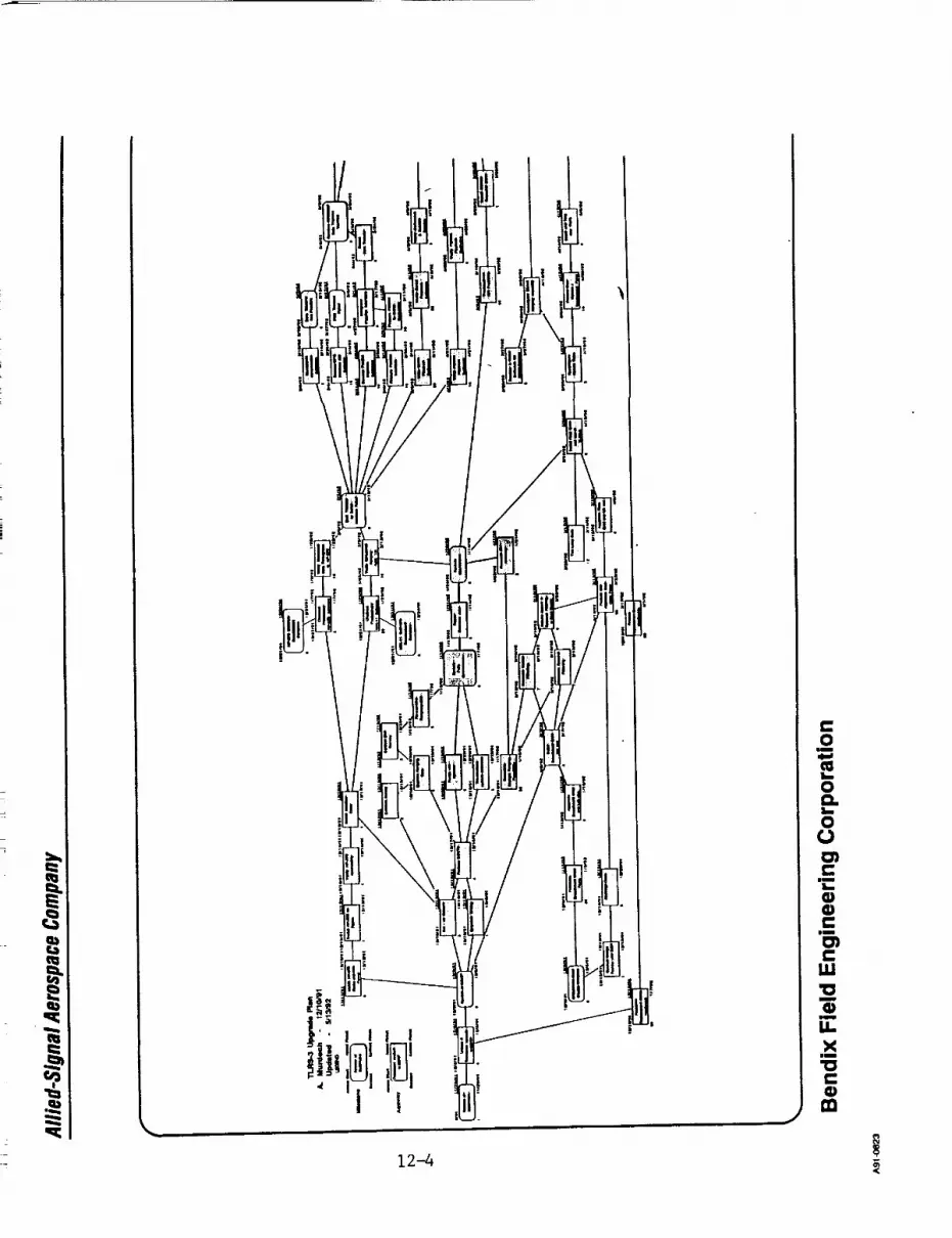
!I'I
I
- | !
'' I I I I
_1 !1 !I I
i I
12-4
c-O
I
L._
0
i.__
0
I
L_
CI
CW
"0I
0ii
u_
Xii
"0c-

¢I
12-5

12-6

m
II1r
os
12-7
I,Ll
u_
_x==

m
m
il
f
12-8
0ii
0
00
m
L-
m
C
m
m
m
m
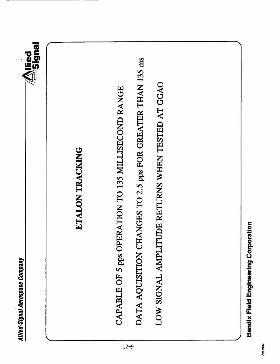
m
II1'UC
f
r,,)
z
°r_ r_
o _ _r,.) r_
© 2:
o _ _Z _
o r_
_ 7 z
r_ _ M
12-9
CO
um
0
L_
0
CmL_
m
m
m
m
C

12-10
C0
im
L_
Oo_
O
CmL_
n
CW
"0m
m
u_
XwM
"0C

::.v.
_]!:i::.b.
.,..,.,
%..
.,,,,.,
.- ,,..
-,.._
.-,,,
[..-,
,,<
._,,+
- _,o_
(:"_
;.+ ,
°1 _e . ,"
• ,o" ..
: i:._:i_:i:_,°_:,• " • ".";:.i •:°'11 :' ".' .,."
,o, oZ "'" '1_: s._,, •
%
i- .,. "" - - "*"• " _1 :',. !'" "." ":'._"p4
• b" :,|1 ".. ...,-.. : ."" .. ..... ./.'; , .
i i:'".... ® ""'":'"" ::'" ....
-
..... ,::;_.._:<._ : p w• ; ..:
!,. ;"
"_ ."/. .-" ".';; %'." _"" .I.'''
" I "" " "" _" ' "
i |
C:_ ".'.":11::: _........ ........................
::_::.'.:.i............ ;:::.'.::_ ...'.:':::::: _.':'.i; _'"- : ..... _:%'.:- .........
ilii/i i/_ii_ :ii_:"i!_:/,i'__i]ii!!_:i:i:="i:i:iii'i-:::iiiii.!i..i"i!"ii:i:i:ii..L:_,_,_!!:7_:
12-11
°,,.,,
:'/.i.
.:.£:!.
• _... _,:-[::-
;:--: :; ......
....17::
• ..'.'[.
-...;
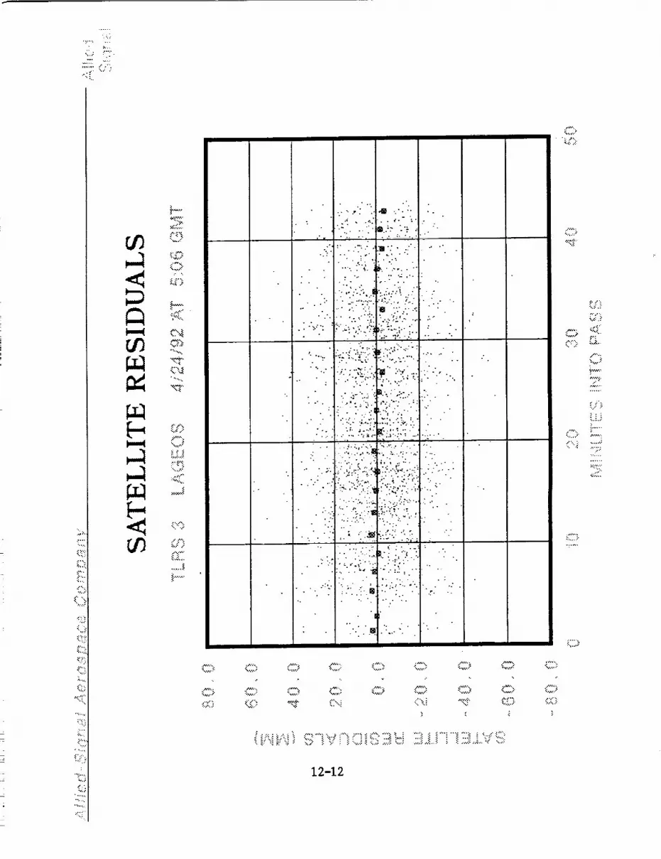
._, >,
"{ii]'..
":411
_o
4:11
.,..,• :.- ,. ..,
t.--(
h"
.?_"
C]'i: '"'"
C::, .......".,.:>:L'." k3_;::
%1
.... ' _=_" k_:i:: _;_:7
:!_"_ C,::: _'i'.?_-_ :=4"-"::_ ......._;__.:_
12-12
• .:...:
-',:::]]i:
•_.:.,.:_,.
_i.-.".:--
::_-:
•...-
LL.i......... i-....
.... ._:-;
,;:'..:-;:].;,._,"
.w.-,
.......i...::

0
r-r_
ol
_o
to
N0_
U_
m
rr<C12.
8_
l","
il0 ?
rr.J
0 0 0
_m
4
• St
r
II EO
0
aa_
0 0 0 0
(Lu,,,) SMH NOLI.VHEI'IVO
12-13
0 0
_J
w
0
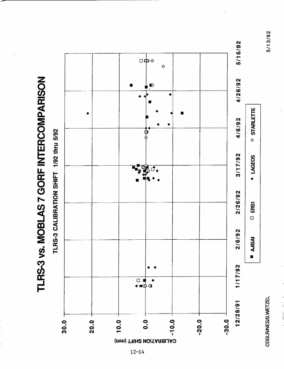
00')m
n-,<O.
J¢
n-
I->
n,".,J
0
c:;0')
.__._
• IO
4
4,
II
4.
]
>
0 m
0
¢
0 0 0 0
|
(wuJ) J_-IIHS NOI.I.VI::IEI'iVO
0
c_¢51
|
12-14
0
0
m
m
m
m
..J
m
<>
v
m
D_wmMm
[]
m
<
!
c_
Lo
._J
..J

0
CD"IP"
o'_
Z
D..
0
Ill "J
n"o
-J
0 0 0
I •
• ,%
Ol • • O
0
iI.I •
0
0 0 0 0
d K M _ g
(uu=) SIRi:I3111"INIY8
12-15
[]
O O
£N
£N
r,-
O
_am
m
ua
m
<>
IMv
m
D_w.Mm
[]
._Jw
W
tO
O

OU)
<13.=SO
in
5(%1
U.,ira
rrO
r,.
U.I<1: =_•.J com d)
..I
00>
CO
rr.-II--.
in
! •
I
"o _ •4, •
I_1_ • •
O
O O
O In o
(uJtu) SVI8 NV31tt
12-16
in|
O,!-.,
|
in (_1,ira ,ira,
|
C_Jcr)
O'J '--LD
CD
._JILl
ILl
U)C_

N94"15610
Results of the MTLRS-1 Upgrade
P. SPERBER, L. AMBERG, L. BEYER, G. BLENSKI, W. ETLING, U. HESSELS, R. MOTZ,INSTITUT FI_R ANGEWANDTE GEOD/_SIE
FUNDAMENTALSTATION WETTZELL
DER FORSCHUNGSGRUPPE SATELLITENGEODASIE
D-8493 K()TZTING
Abstract. In this report the results of the upgrade of the German Modular Transportable Laser RangingSystem MTLRS#I are summarized. A short description of the new components and their influenceon the system accuracy is given. It is shown, that the aingle shot accuracy of the MTLRS_I hambeenimproved from 5 cm to I cm.
1. Introduction
The German Modular Transportable Laser Ranging System MTLRS# 1 has been operated suc-cessfully since 1984. From 1985 to 1990 the system was employed in the Central and Eastern
Mediterranean area and in the U.S.A., contributing to the WEGENER-Medlas and the NASACrustal Dynamics project.
In order to improve the system reliability and the ranging accuracy from 5 cm to 1 cm a major
system upgrade was performed from December 1990 to July 1991.
This upgrade was planned and carried out in five steps:
• Exchange of the Laser
• Exchange of the Start Detector
• Exchange of the Receiving System
• 'Exchange of the Single Photon Detector
• Improvements in Periphery and Software
In this paper we will summarize the technical specifications of the new systems and show first
tracking results.
2. Technical description of the upgrade
2.1. The Laser
The duration and the energy of the emitted laser pulses are critical elements in the determination
of the accuracy and the number of returns produced by a satellite laser ranging system. To improve
this two points, we exchanged the original Nd:YAP Laser (Pulseduration: 370 ps; Pulseenergy at
536 nm: 10 mJ) for a new Nd:YAG Laser (Pulseduration: 30 ps, Pulseenergy at 532 nm: 30 mJ).
To ensure a good reliability of the laser in field, we made use of the self filtering unstable resonator(SFUR), described by R. Bianchi et.al, and K. Hamal et.al, which has a very simple optical layout.
This setup has three major adventages:
• insensitive to inaccurate adjustment
• homogenious spatial energy distribution
• very high pulse energy in the resonator.
Typeset by .A._S-
12-17.
The realisation of the optical setup of the laser delivered by Laser Vaifivre is shown in Fig. 1. To
save place, the resonator M1 - M2 is folded over the prism PR. The laser is cavity dumped through
a pockelscell PC and a polarizer PO. An active-passive configuration (acustooptic modelocker ML
and dye cell with Kodak 9860 in 1,2-Dichlorethan) is used to generate picosecond pulses.
In the SFUR configuration, the energy of the pulses in the resonator is already reasonable high,
therefore a Single Pass Amplifier (AMP) is sumcient to generate a puiseenergy of about 100 mJ in
the infrared which gives about 30-40 mJ in the Second Harmonic.
Due to the good isolation of the laser head and the power electronic to environmental influencesand due to remote control facilities in the laser head, we are able to operate the laser over long
period without opening the shielding.
2.2. The Start Detector
To take full advantage of the short laser pulses it is neccessary to use a start diode with very
fast risetime to generate the start signal for the counter. As each component between diode and
counter gives some additional jitter we were looking for a solution with a very simple electrical
layout. Mainly we tried to find a way where it was no longer neccessary to use a constant fraction
discriminator to compensate the amplitude fluctuations of the diode signal.
Therefor we integrated an optically triggered avalanche diode (I. Prochazka et.al.) as start de-
tector. This diode generates an electrical signal, which is independent from the energy fluctuations
of the laser pulses. This signal is directly used as start signal for the counter.
The signal has a risetime of 300-400 ps (Fig. 2), the jitter between laserpulse and electrical pulse
is less than 20 ps.
To obtain high stability and to have also the possibility to vary the pulse energy during tracking
the new start diode is placed before the amplifier to detect the infrared signal. In the previous
design the diode detected the green light after the second harmonic generation.
2.3. Receiving Package
In contrast to other SLR System the MTLRS is using an echelle grating for the spectral filtering
of the received light. Compared to the common used interference filters this has the advantageto be insensitive to environmental influences. Unfortunately an echelle grating generates a time
spread of a pulse due to the different light paths over the grating.In the old grating this was compensated with an accuracy of about 1 cm by sending the diverse
parts of the beam to different mirrors. Due to this splitting of one pulse into several beams, the
outcoming beam has not the high optical quality which is necessary for focusing on the small active
area (100pro) of an avalanche diode.
In the new package a second echelle grating in opposite position is used to make full compensa-
tion. The excellent optical quality of this configuration results in a very homogeneous beam which
is necessary to generate small focal spots.
Additionally a remote controled field-of-view pinhole and a better isolation against straylight is
installed in the new package. The sketch of the whole receiver is seen in Fig. 3. (It. Visser)
At the input the beam coming from the telescope is directed by a prism to an optical package
in which a rotating shutter and some small prism are used for filtering and guiding of the beam.
The light has to travel through the rotating shutter and is directed to an echelle grating. After
that the pulse is spread in time and frequency. An adjustable pinhole is used for the field of view
filtering and for selection of the correct wavelength. To compensate the time spread the beam now
propagatesa second time to the echelle grating before two lenses form a parallel, 8 mm diameter
output beam.
2.4. Single Photon Detector
A major improvement in the accuracy of the time interval measurement was achieved by the
exchange of the photomultiplier for a single photon avalanche diode (SPAD) (I. Prochazka et.al.,
G. Kirchner).
The signal out of the SPAD is independent of the signal strength, so the use of a constant fraction
discriminator is not necessary.
A description of the technical details is given in Sperber et.al.
3. System Accuracy
The main reason for the upgrade of the MTLRS was the demand to improve the system accuracy
from 5 cm to about 1 cm single shot r.m.s.
In Fig. 4 the developement of the accuracy during each step of the upgrade is depicted. Themain influence to the accuracy came from the exchange of the laser and the single photon detector.
The start detector has minor effect and the importance of the new receiver package can be seen in
the good optical quality which finally allows the usage of the SPAD.
The contribution of each single component of the system to the system accuracy is shown in
Fig. 5 for the old and the new configuration. The r.m.s of all components has now about the samesize. Further improvements are probably possible at the laser (10 ps) and at the counter. More
accurate start and stop detectors are not available at the moment.
The plot of a typical pass before and after the upgrade is given in Fig. 6. Here the significant
decrease of the system r.m.s is conspicious.
All this data are showing, that the single shot accuracy of the MTLRS# 1 is now 1 cm or less,
if all components (mainly start diode, SPAD and laser) are optimally adjusted.
Under field conditions we demonstrated (P. Sperber, H. Hauck) a system accuracy of 1 cm - 1.5
cm and a normalpoint accuracy of a few mm.
3. Perspectives into the next years
The receiving and transmitting part of MTLRS#1 is now again state of the art. To bring the
whole system to a status comparable with modern SLR systems two additional upgrade steps are
under discussion.
• Installation of a new control electronic and software, designed for future demands to Laser
Ranging Systems. IfAG has decided to develop such a control system based on a trans-puter network in cooperation with MTLRS#2 (OSG Kootwijk). The integration in the
MTLRS#I/2 is scheduled for 1993 (E. Vermaat et. al.)
• The Laser and the Receiving system are now prepared to make two color ranging. Only
the telescope does not meet the specifications for two color ranging as the reflecting mirrors
are optimized only for a wavelength of 532 nm. A further upgrade for two color ranging
capability depends strongly on the demand of the international SLR community for two
color ranging data.
12-19
5. Summary
After the upgrade of MTLRS#1 performed from December 1990 to Juli 1991 a system with thefollowing modified specifications is now available.
• 30 ps laser pulse-width with 30 mJ/pulse at 532 nm
• Optically triggered avalanche diode to start the time interval counter
• Compensated echelle grating filter
• Single Photon Avalanche Diode
• In field normal point generation
As a result of these modifications MTLRS# 1 is now capable of tracking high and low satellitesday and night with a single shot r.m.s, of about 1 cm.
12-20

REFERENCES
Laser V&lfivre, Specific4tion# o] a laser jyJtem for MTLRS#I , 1989.
A. Blanchi, A. Ferrario, P.G. Gobbi, C. M&lvicini,G.C. Re&li, SPIRE 701, p.132,. 1989.
K. Ham&l, V. Hraskova, H. Jellnkova, CLEO'85 Proceedings p.82, WE 4, 1987.
I. Prochazka, K. Ham&l,, S=beentlmeter Sittole Pitoton Ra_tgin 9 All Solid State Detectloft Package, 1990.
G. Kirchner, Proceedings of the seventh international Workshop on Laser Ranging Instrumentation p. 123,
1989.
P. Sperber, U. Hessels, R. Motz in this Proceedings, The new MTLRS#I Receiving SyJtem 199t.
P. Sperber, H. Hauck, in this Proceedings, Emperience and Res_lta o] the 1991 MTLRS#I USSR campaign,
199_.
E. Vermaat, J.W. Oflierski, K.H. Otten, W. Beak, C. van F_, P. Sperber, in this Proceedings, A Travt#pster
Baaed Control S_atem ]or MTLRS, 1992.
H. Visser, Technlsch Physische Dienste (TPD), Delft private communication, De#igu o/ a mew MTLRS#I
receiver pacl_afe, 1990.
12-21
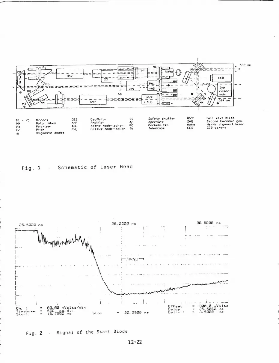
I
M| - H5 H;rrors OSZ 0scal_tor SS " SoFety shutter HVP I_GI_" *Qve plate
HH Motor-M&es AMP Anpll£ter Ap Aperture SHG Second hQrmonic gen.
Po Polor_zer AHL Active _ode-(oc_er PC Pockets-ce(( HeNe He-Ne o(_jn_ent loser
Pr Prls_ PHI_ Posslve mode-rocker Tk Tetescope CCD CCI) co.mero
® Dtognos tic diodes
Fig. 1 - Schematic of Laser Head
25.5D06 _s 28.3300 o_ 30.50_g _s
" 'mJl, ' : i : !
L..... '_ i : i........................ i ..............................................
"- ' '- ' ' ' ' ' ..... ' ' - i ............. 7 ..................................................
r ......i : i i ......... i ......... J_ i _ , _ -- -Ch. | = 8_._ mVolts/div OFfset = -3_._ mVolts
Timobose 5_C _s,"d_ Delcy = 25. 5_0 _s
Stort 16. 75_ _s Sto_ = 2_. 2589 _s Delt_ T = 3. 5gO_ _s
Fig. 2 - Signal of the Start Diode
12-22

//
/!li
/ /
/I
if // i ' !
\!
/
i!
0
...... k
/f!
/I!I
!
I
/
t, 7ii
\\ ' /t t
i
/!
1
,//
/!
u
f.4
>
ca
cot'i-__Jl--
t-..la
o
.la
o
._I
,-4
u
c_0
o
O*J
u_
12-23

Decrease of MTLR,C #1 r.m.s
0,5
0,4
0,3
0,2
0,1
r.m.s in ns r.m.s in cm
[]
r,m.s in n8 I
I[] r.m.s in cm
[]
I I I
10
9
8
7
6
5
4
3
2
1
0
old new Laser new Start Receiverpa(-k SPAD
Fig. 4: Decrease of the single shot r.m.s, during upgrade
400
300
200
lO0
R.M.S, of
r.m,_, In ps
MTLRS#1 Components
II
100
i
20
0
65
3O
0 I ..... _ I
La=er START Recelverpack. STOP Counter
Fig. 5. Single shot r.m.s before and after upgrading
12-24

typical Lageos nighttime pass (PMT) before upgrading
_.._
"T ..
_-- -.q8._._4 ns
Pre
Calibration PostCalibration
• • • ._ .._ ':_,-.- _ L,-_. _ "...: _:_]
I_V_.._._. _" .... :. -, _:,_:_,. _.'.v.,_-:,- . • : _ ,. . .,.., _._:_.-.
Fig.
typical Lageos day/nighttime pass (SPAD) after upgrading
-- -e@eS@@r,s
- Lageos Pass before and after upgrading
12-25

N94-15611
The new MTLRS_I Receiving System
P. SPERBER, U. HESSELS, R. MOTZ,
INSTITUT FI_R ANGEWANDTE GEODASIE
FUNDAMENTALSTATION WETTZELL
DER FORSCHUNGSGRUPPE SATELLITENGEODASIE
D-8493 K()TZTING
H.-M. GI.iTHER
HOECHST AG, MATERIALFORSCHUNGD-6230 FRANKFURT AM MAIN 80
Abstract.
In this report we are giving a detailed description of the new receiving system of the German Modular
Transportable Laser Ranging System MTLRS_I consisting of a spectral time and field of view filter
and a Single Photon Avalanche Diode (SPAD) aa single photon detector. The system gives full day
and night ranging capability to all satellltes with cm accuracy.
1. Introduction
In order to improve the ranging accuracy and the sensitivity of the German Modular Trans-
portable Laser Ranging System MTLRS-1 a major system upgrade was scheduled and performed
from Dec. 1990 to July 1991 (P. Sperber et.al•). Together with the exchange of the whole trans-
mitting part (Laser and Start Diode) (P. Sperber et.al.) the installation of a new receiving systemwas the main point of the upgrade.
The receiving system has two parts, which will be shown in detail
• Filter (Frequency, Range, Field of View)
• Single Photon Detector.
2. Receiving System
To extract reflected photons fr6m the satellite from noise photons which are entering the telescope
mainly in daylight, a powerful filter eqmpment has to be installed in SLR systems.
This filtering in modern systems is realized in three steps
• Range (time interval) filter: A rotating shutter is commonly used to supress straylight duringlaser firing and to open the detector at the time, the echo from the satellite is expected.
• Field of View: A pinhole ensures, that only light coming from a small angle around the
telescope axis can hit the detector.
• Spectral Filter: The most effective filtering process is the filtering in frequency which allows
just light of the well defined laserwavelength to propagate•
Typeset by .AA45-TEX
12-26

The new receiver package of MTLRS#1 is a very compact, field qualified realization of this three
requests, deliverd by Technisch Physische Dienste (TPD), Delft, Netherlands.
The setup is shown in Fig. 1.
The light from the telescope is focussed to a field of view pinhole, which is remote adjustable witha motor driven micrometer from 0 to about 30 millidegrees. Connected to the field of view filter
there is a rotating shutter, synchronized to the predicted range window, which opens the receiving
system 10 times per second for about 3 ms and mainly protects the single photon detector from
straylight during laser firing.The spectral filtering is done by an echelle grating (efficiency: 55 %) used in 7 th order, which
gives a bandwidth of 0.2 - 0.65 nm depending on the opening of the filed of view pinhole. The
grating has a surface of almost 100 mm top-top in air, therefore the range difference of the beams
over the grating surface is not neglegible. To compensate this range difference the grating is useda second time in opposite order. At the end of the receiving package a lens is generating a 8 mm
diameter, parallel beam with excellent optical quality.
3. Single PhotonDetector
To see the full advantage of the short laser pulses and of the errorfree receiving package a single
photon detector with high accuracy is necessary. In the world of SLR two types of high accuracyreceivers are used in the moment:
• Microchannel Plates
• Avalanche Diodes.
We decided to install a single photon avalanche diode (SPAD) (I. Prochazka et al.) developed
by the Czech Technical University in our system. The reasons for this decision were:
• High ruggedness under field conditions,
• High Quantum Efficiency (20 %)
• Low jitter (35 ps)
• Low operating voltage (25 V)
• High dynamic range and neglectable influence of signal strength to the range measurement
• No additional electronics (CFD) between detector and counter.!
The housing for the diode has to meet some demands:
• Adjustable in three dimensions in the pm range.
• Possihlity to cool the diode below -10 ° C.
• Protection against humidity (condensation).
• Flexible for usage of different types of diodes.
The cooling of the diode is necessary because of the high termal noise (some 100 kHz) at room
temperature. The temperature of-30°C, which is possible with this setup will decrease the noise
far below 100 kHz (Fig. 2) and therefor make the search for satellites at night more easy.
To meet all this points, we designed a new housing (Fig. 3) with the following specifications:
• adjustement accuracy in each dimension: 5 - 10pro
12-27
• input beam: 5-10 mm diameter, parallel
• optics: effective focal length: 11 mm
• field of view in our system (100 pm diode): 30 mrad
• copling: to -30°C with peltier cooler and water (5°C)
• good mechanical stability under field conditions (temperature change, humidity)
The housing is made from aluminium, the inner moving part which makes the termal isolation
of the diode to the housing is DELRIN.
For the fixing of the diode a very special material with high mechanical stability, high thermalconductivity and good electrical isolation was necessary.
To get a thermal equilibrium even at high outside temperatures we decided not only to cool the
diode, but the whole fixing plate with powerful peltiers (the hot side of the peltier is water cooled).As some diodes (mainly the diode we use) needs an electrical isolator around it, a material with
the mentioned specifications was necessary.
In cooperation with the Material Research D,epartement of Hoechst AG, a new ceramic material-
Aluminium Nitride- was selected. The important properties of this are its high thermal conductivity
of 170 W/ink (comparable to pure Aluminium) and its dielectric constant of about 8.5 (good
insulator). The powder, together with a sintering aid, are prepared for pressing. The cold isostaticpressed parts, in the form of rough discs, are then turned to improve their finish and a hole is bored
in the centre. The binder is then burned out. The samples are sintered at 1840°C for 3 h under
a nitrogen atmosphere in a special graphite crucible. After the heat treatment the ceramic parts
were finished. They were grond with diamond wheels in all directions to get the high dimensional
accuracy and surface smoothness for installation of the measuring diode and for the mounting ofthe peltier elements. The specifications of the material are given in table 1.
Due to the flexibility and the good experience with this housing in the last field campaign it is
now also used at the new Wettzeli Laser Ranging System (WLRS) for the tests of different diodes.
3. Summary
The new receiving system of MTLRS# 1, consisting of a filter package for field of view, time and
spectral filtering and a single photon avalanche diode as detector gives the possibility of SLR with
cm accuracy during night and day. The whole system is build very modular and flexible, so easyexchange or usage in other SLR systems is possible.
All parts are designed and manufactured in a way, that even under extreme environmentalchanges in field an adjustement is not necessary.
In the last field campaign the new receiver proved to work very reliable and satisfactory.
12-28

REFERENCES
P. Sperber, L. Amberg, L. Beyer, G. Blensid, U. Hessels, R. Motz, in this Proceedings, Res_lta o] the MTl, qstltlUpgrade, 199_.
P. Sperber, U. Hessels, R. Motz, W. Beck, in this Proceedings, The _ew MTLR5 TranJmltting ,.qyetem, 1992.
I. Prochazka, K. Kamal, B. Sopko, S. 219, Pl_otodlode Based Detector P*ekage for Centimeter Sstellite Ran#iBg,.
12-29

@
I--
o_z
C_
CO
L_
r_
(1)
>
U
_Jri-
ft
_.I
l--
r
4_
0
0
_0_,J
_00
C0
.C0
O_
LL
12-30
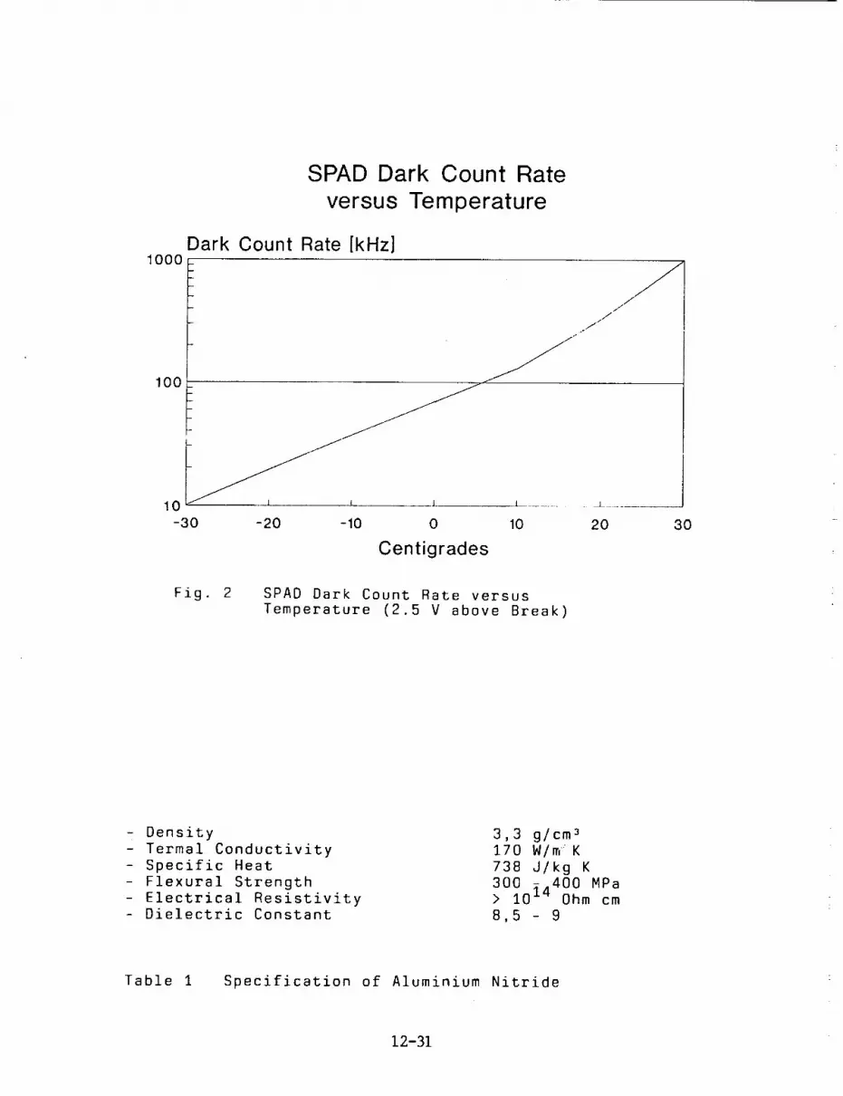
SPAD Dark Count Rate
versus Temperature
Dark Count Rate [kHz]1000
3O
Centigrades
Fig. 2 SPAD Dark Count Rate versusTemperature (2.5 V above Break)
- Density- Termal Conductivity- Specific Heat- Flexural Strength- Electrical Resistivity- Dielectric Constant
3,3 glcm 3170 W/m" K738 Jlkg K300 - 400 MPa> 1014 Ohm cm
8,5 - 9
Table 1 Specification of Aluminium Nitride
12-31
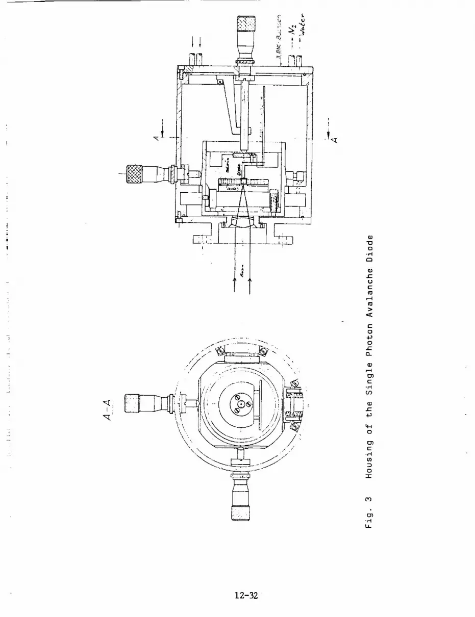
C" i,.
tl 'r.-,: ,
' I t_ _t _-
if
\ "\
"c T_I
q
_, =
iri
"0
0
-r-I
tm
.C
0
C
C
0
0
r-
O-
C_O
C
09
.C
_a
4-I
0
O%
C
0
mr-
CO
0%
-H
LL
12-32

N94-15612
The new MTLRS Transmitting System
P. SPERBER, U. HESSELS, R. MOTZINSTITUT FOR ANGEWANDTE GEOD)_SIE
FUNDAMENTALSTATION WETTZELL
D-8493 K6TZTING
GERMANY
W. BEEK, J.W. OFFIERSKI, C. VAN EsDELFT UNIVERSITY OF TECHNOLOGY
KOOTWIJK OBSERVATORY FOR SATELLITE GEODESY
POSTBOX 581, 7300 AN APELDOORNTHE NETHERLANDS
Abstract
This paper presents a detailed description about the new transmitting system of the ModularTransportable Laser Ranging Systems MTLRS-1/2. A simplified theory of the Self Filtering
Unstable Resonator (SFUR) is explaned. Laser design details are discussed concerning the
extreme environmental conditions in which these mobile systems are operating. Details are
given concerning the new avalanche START detector. The new SFUR laser and START
detector are necessary parts in order to bring both mobile systems towards 1 cm ranging
accuracy.
1. Introduction
Since 1984 the two European Modular Transportable Laser Ranging Systems MTLRS-1,
operated by the Institute for Applied Geodesy (IfAG, Germany), and MTLRS-2, operated by
the Delft University of Technology (DUT, The Netherlands), have supplied the internationalnetwork with laser ranging data from sites in Europe, CIS (former USSR) and North
America. To improve the ranging accuracy from 5 cm to the 1 cm level, both systems
carded out a major upgrade in 1991. The main part of this upgrade was the exchange of the
transmitting system consisting of the Laser and the Start Detector (The German MTLRS-1
system also upgraded the receiver package [1].
2. The Laser
The accuracy and the number of returns produced by a satellite laser ranging system is
mainly influenced by the duration and energy of the emitted laser pulses. To improve these
two points, the original Nd:YAP laser (370 ps FWHM pulse-duration, 10 mJ pulse-energy at
539 nm) was exchanged for a new Nd:YAG laser (30 ps FWHM pulse-duration, 30 mJ
pulse-energy at 532 nm). To realize this high demands with a simple and reliable optical
configuration, a new resonator setup, the Self Filtering Unstable Resonator (SFUR) [2,3]
was used. Together with a simple optical setup, this resonator has the advantage to be less
sensitive to optical adjustments and operates with a very homogeneous spatial pulse-shape,
minimizing the danger of destroying optical components at high resonator energy outputlevels.
12-33
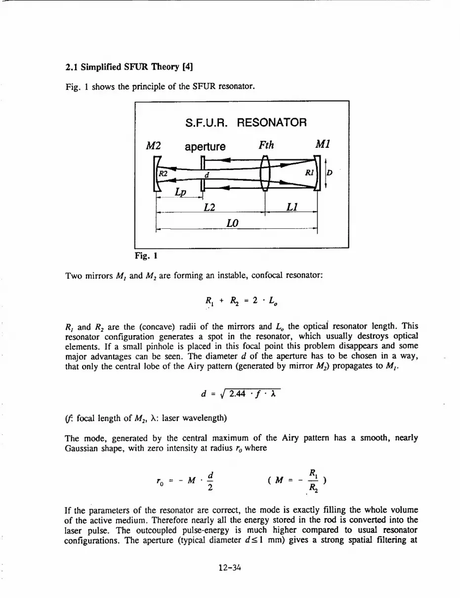
2.1 Simplified SFUR Theory [4]
Fig. 1 shows the principle of the SFUR resonator.
S.F.U.R.
M2 aperture
R2-" d
/.2
LO
RESONATOR
Fth M1
R1L
L1
Fig. 1
Two mirrors M 1 and M2 are forming an instable, confocal resonator:
R l + R 2 = 2 "Lo
RI and R 2 are the (concave) radii of the mirrors and Lo the optical' resonator length. This
resonator configuration generates a spot in the resonator, which usually destroys optical
elements. If a small pinhole is placed in this focal point this problem disappears and some
major advantages can be seen. The diameter d of the aperture has to be chosen in a way,
that only the central lobe of the Airy pattern (generated by mirror M2) propagates to M t.
d= x/ 2.44 "f " _.
(/2."focal length of M 2, X: laser wavelength)
The mode, generated by the central maximum of the Airy pattern has a smooth, nearly
Gaussian shape, with zero intensity at radius ro where
R 1
ro = - M • d- (M = - -- )2 ,R2
If the parameters of the resonator are correct, the mode is exactly filling the whole volume
of the active medium. Therefore nearly all the energy stored in the rod is converted into the
laser pulse. The outcoupled pulse-energy is much higher compared to usual resonator
configurations. The aperture (typical diameter d< 1 mm) gives a strong spatial filtering at
12-34

each round trip smoothing the energy distribution in the beam and avoiding hot spots. In an
exact analysis of the SFUR configuration the influence of the thermal lens (7"u,: focal length)
in the laser rod has to be taken into account.
Lo = L l +/,2
glRl
L 0 LI&=l
g = 2 "gl "g2 - I
M = g - _[g2 - 1
(L 1 and L 2 are the distances of M1 and M 2 to the virtual position of the thermal lens). The
optimum position Lp (distance from M_) of the aperture, the diameter d of the aperture anddiameter D of the laser beam are given by:
1 _ 1 ÷ _/g2 - 1
Lp /?2 2 "gl "Lo
d : 4.88 • Lp • _. "( 1 R'z )
D --- 1.5 .M "d". u . --
2 -i -L"
2.2 Technical Realization
The laser system consists of four separate units, the laser head,
electronics, an external dye-cooling unit and the control panel.
the power supply with
12-35
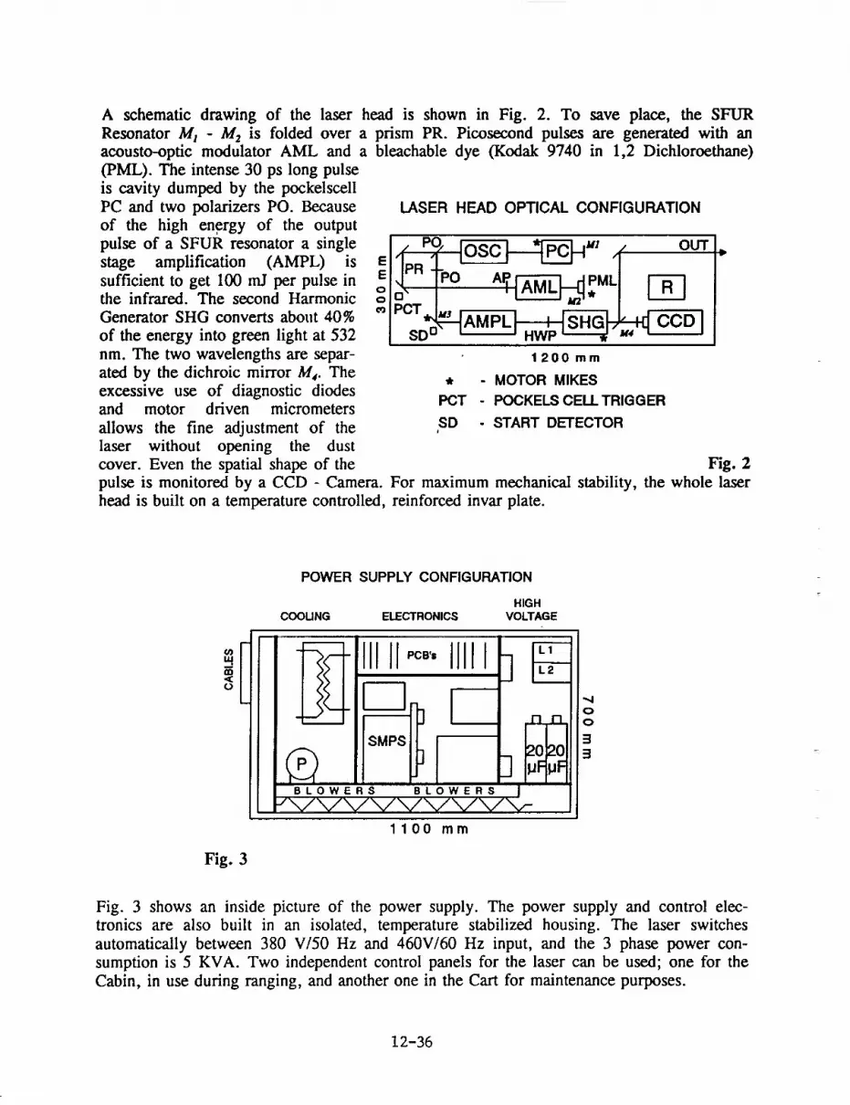
A schematicdrawing of the laser head is shown in Fig. 2. To save place, the SFUR
Resonator MI - M2 is folded over a prism PR. Picosecond pulses are generated with an
acousto-optic modulator AML and a bleachable dye (Kodak 9740 in 1,2 Dichloroethane)
(PML). The intense 30 ps long pulse
is cavity dumped by the pockelscell
PC and two polarizers PO. Because
of the high energy of the output
pulse of a SFUR resonator a single
stage amplification (AMPL) is
sufficient to get 100 mJ per pulse inthe infrared. The second Harmonic
Generator SHG converts about 40%
of the energy into green light at 532
nm. The two wavelengths are separ-
ated by the dichroic mirror M_. The
excessive use of diagnostic diodesand motor driven micrometers
allows the fine adjustment of the
laser without opening the dust
cover. Even the spatial shape of the
LASER HEAD OPTICAL CONFIGURATION
EE00
I I
1200 mm
* - MOTOR MIKES
PCT - POCKELS CELL TRIGGER
SD - START DETECTOR
Fig. 2
pulse is monitored by a CCD - Camera. For maximum mechanical stability, the whole laser
head is built on a temperature controlled, reinforced invar plate.
Uan<O
Fig. 3
POWER SUPPLY CONFIGURATION
HIGH
COOUNG ELECTRONICS VOLTAGE
I I lip08,.
]SMPS
]
IIIII
[--.£1_1"1
1100 mm
",4
0
0
33
Fig. 3 shows an inside picture of the power supply. The power supply and control elec-
tronics are also built in an isolated, temperature stabilized housing. The laser switches
automatically between 380 V/50 Hz and 460V/60 Hz input, and the 3 phase power con-
sumption is 5 KVA. Two independent control panels for the laser can be used; one for the
Cabin, in use during ranging, and another one in the Cart for maintenance purposes.
12-36
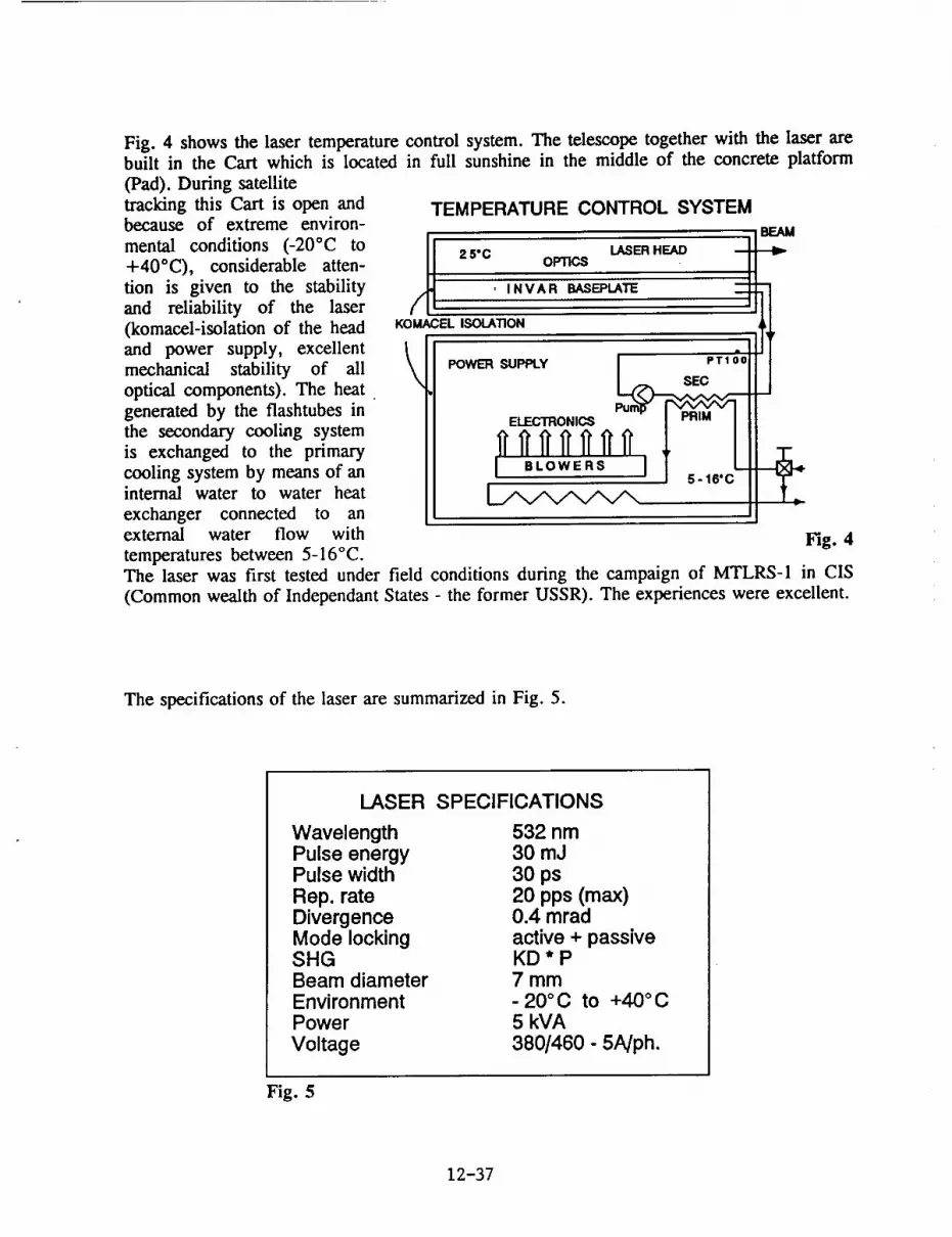
Fig. 4 shows the laser temperature control system. The telescope together with the laser arebuilt in the Cart which is located in full sunshine in the middle of the concrete platform
(Pad). During satellitetracking this Cart is open andbecause of extreme environ-
mental conditions (-20°C to+40°C), considerable atten-
tion is given to the stabilityand reliability of the laser(komacel-isolation of the head
and power supply, excellentmechanical stability of all
optical components). The heatgenerated by the flashtubes inthe secondary cooling systemis exchanged to the primary
cooling system by means of aninternal water to water heat
exchanger connected to anexternal water flow with
TEMPERATURE CONTROL SYSTEM
• BEAM
Ko_,c_ ,so.so. __ _fi,/ -II\ _o_. soPP.v I ..,oo I
\ ELEGTRONIGS _J
t ,.,,.cLFig. 4
temperatures between 5-16°C.The laser was first tested under field conditions during the campaign of MTLRS-I in CIS(Common wealth of lndependant States - the former USSR). The experiences were excellent.
The specifications of the laser are summarized in Fig. 5.
LASER SPECIFICATIONS
WavelengthPulse energyPulse width
Rep. rateDivergenceMode lockingSHGBeam diameterEnvironmentPower
Voltage
532 nm30 mJ
30 ps20 pps (max)0.4 mrad
active + passiveKD*P7 mm-20 °C to +40 °C5 kVA
380/460- 5Nph.
Fig. 5
12-37

3. Start Detector
To start the time interval counter with high accuracy, the optical output signal of the laser
has to be converted with minimum jitter to an electrical pulse, which is used in the start
channel of the counter. Until 1990 this problem was solved in the MTLRS in the conven-
tional way: a part .of the green pulse was sent to a fast photo diode which generates anelectrical pulse with an amplitude corresponding to the energy of the laser pulse which is
fluctuating from shot to shot. These amplitude fluctuations were compensated by a constantfraction discriminator. Changes in the temporal pulse shape and strong energy fluctuations in
this setup caused errors in the start-channel of the counter.
To minimize these errors, an optically triggered avalanche diode [5,6] was integrated into
the system. This diode delivers an output signal with a constant amplitude independent on
the energy of the laser pulse. The output signal is directly used as startsignal for the counter,
a constant fraction generator is superfluous. Furthermore, to introduce high stability and the
possibility to vary the pulse energy during tracking, the start diode is placed before the
amplifier (behind mirror M3 in Fig. 2) to detect the infrared light. Fig. 6 shows the output
signal of the start diode which has a risetime of 300 - 400 ps and the jitter between optical
and electrical pulse is less than 20 ps.
+ 7.8 V_
START DETECTOR OUTPUT SIGNAL
\
_ =.=....._
5 nsidiv
Fig. 6
In order to get stable results from the avalanche start detector under field conditions, the
fibre together with the electronics have to be built inside the laser head where the tempera-
ture of the optical bench is stabilized at 25°C.
4. Summary
The upgrade of the transmitting part of MTLRS-1/2 formes the basis to improve the ranging
accuracy of the systems significantly and makes them again some of the most advanced SLR
systems worldwide.First tracking' results [7] show, that the system's single shot accuracy is about 1 cm after the
upgrade of the receiver package which is already completed in MTLRS-1.
12-38

References:
[1] The new MTLRS-1 Receiving System, 1992 by P. Sperber, U. Hessels, R. Motz, in
this Proceedings.
[2] Paper 1989 by A. Bianchi, A. Ferrario, P.G. Gobbi, C. Malvicini, G.C. Reali, SPIE
701, p. 132.
[3] Paper 1987 by K. Hamal, V. Hraskova, H. Jelinkova, CLEO'85 Proceedings p.82,
WE4.
[4] Paper 1989 by C. Malvicini, A. Ferrario, G. Gabetta, G.P. Banff, G.C. Reali,Proce_lings of the seventh international Workshop on Laser Ranging Instrumentation
p. 181.
[5] Paper 1990 Subcentimeter Single Photon Ranging All Solid State Detection Package,
by I. Prochazka, K. Hamal, B. Sopko.
[6] Paper 1989 by I. Prochazka, K. Hamal, B. Sopko, Proceedings of the seventh
international Workshop on Laser Ranging Instrumentation p. 219.
[7] Results of the MTLRS-1 Upgrade by P. Sperber, L. Amberg, L. Beyer, G. Blenski,
W. Etling, U. Hessels, R. Motz, in this Proceedings.
12-39

N94-15613
Transputer Based Control System for MTLRS
E. Vermaat, J.W. Offierski, K.H. Otten, W. Beek, C. van Es
Kootwijk Observatory for Satellite Geodesy
Delft University of TechnologyP.O. Box 581
7300 AN APELDOORN
THE NETHERLANDS
P. Sperber
Institut ffir Angewandte Geod_ieFundamental Station Wettzell
8493 KtTZTINGGERMANY
Introduction
The Modular Transportable Laser Ranging Systems (MTLRS-1 and MTLRS-2) have beendesigned in the early eighties and have been in operation very successfully since 1984.
The original design of the electronic control system was based on the philosophy ofparallel processing, but these ideas could at that time only be implemented to a verylimited extent. This present system utilizes two MOTOROLA 6800 8-bit processors slaved
to a HP A-600 micro-computer. These processors support the telescope tracking system
and the data-acquisition/formatting respectively. Nevertheless the overall design still is
largely hardware oriented. Because the system is now some nine years old, aging ofcomponents increases the risk of malfunctioning and some components or units are
outdated and not available anymore.
The control system for MTLRS is now being re-designed completely, based on theoriginal philosophy of parallel processing, making use of contemporary advanced
electronics and processor technology [Beek, 1989]. The new design aims at the require-ments for, Satellite Laser Ranging (SLR) in the nineties, making use of the extensive
operational experience obtained with the two transportable systems.
Design goals
Major considerations followed in the design are to bring down the operational costs, to
ensure full capability for all present and future SLR satellites and to facilitate future
modifications and alternative applications through a highly structured and modularapproach.
I. Optimize cost of operations
Deploying SLR systems is quite expensive, in particular in transportable mode. A modern
design aiming at minimizing these costs, must minimize crew size, increase the mean-
time-between-failure (MTBF) and facilitate trouble shooting and repair.
a. Minimize crew size
The default mode of operation will be fully automatic. This means that the system willinitiate _d pei'form all basic tasks, e.g. maintaining satellite alert information,
ephemeris calculation, initiate and perform calibration and tracking procedures, data
screening, Normal Point calculation and data mailing. The routine task for the
operator (if any) will be to monitor system performance and to respond to problems.Manual mode of operation is always possible through operator intervention.
12-40

b. ReliabilityIncreasing the MTBF will be primarily accomplished through defining a maximum of
all functions in software, running in a multiprocessor parallel architecture. The remai-
ning hardware will be built from high quality, highly integrated components, including
Programmable Gate Array (PGA) logic. Integrated components also allow a great dealof miniaturization.
c. Self-diagnostics capability
Diagnostic tasks running concurrently with the control tasks will enable rapid detectionand localization of problems. Parallel processors are very convenient for hosting thesefunctions.
d. Modular hardware design
The hardware is designed with an optimum number of printed circuit (PC) boards.
Same processor-functions at different locations use identical PC-boards. Different
application-functions are realized with a minimum number of different PC-boards.Interface-functions are accomplished by separate PC-boards in order to optimize
hardware portability. Most spares will be available at PC-board level which enables
rapid replacement, reducing system down-time under field conditions.
II. All-satellite capability
a. Satellite altitude
This decade a variety of high and low SLR satellites are or will become available.Typical extreme altitudes are ARISTOTELES (200 km) and METEOSAT (geo-
stationary). A design goal is to eliminate any logical restriction to the satellite range in
the control system (e.g. by accommodating time interval measurement and eventtiming).
b. Satellite interleaving
Because the system will be designed for automatic ranging, the implementation of
decision schemes in software for interleaving observations to different satellites will be
relatively easy.
III. Flexible'design
The design of the control system must simplify future modifications in view of new or
modified requirements as well as implementation of more advanced technologies. This
calls for a highly structured design in software and hardware, which may also enhance the
portability of the design to other SLR stations, with different hardware environments.
a. Adaptation to modifications
Hardware, The general electronic design is separated into three major types of
functions: 1. interfaces, 2. applications and 3. processors. These different types arephysically separated in PC-boards which are individually exchangeable. The hardware
uses PGA logic, which can be easily modified (by software).
Software The RT-software system is strictly separated into three independent layers:
1. global (functional), 2. device dependent, 3. interface dependent. In this way,
modifications can be implemented locally in the related module at one layer, withoutaffecting other layers.
Because of this high level of structurization it is feasible to implement this design inSLR systems which are quite different from the MTLRS concept, with a minimum of
12-41

modifications, primarily in software.
b. Expanding processor capabilityIf new requirements dictate additional computer power (e.g. RT-filtering, FrameGrabbing) this capability can be easily implemented in the structured design by adding
standard processor boards hosting additional software tasks. To enable implementation
of different types of (parallel) processors than the transputer which has been selectedin the present design, all software is written in ANSI based high-level languages and
no RT-program modifications have to be made because the 3L-compiler [3L] supports
different processors.
c. Highly,manufacturer independentCustom made hardware usually increases the dependence on particular manufacturers.
This is avoided by full restriction to standard bought-out components and self-designedPC boards.
The parallel p_rocessor set-up eliminates the necessity of selecting a vendor dependent
RT operating system and thus ensures the flexibility of adopting any brand of (future)
parallel processor. In the current design the INMOS transputer (see below) has beenselected because of its early availability and its capabilities. Any future transition to
another parallel processor is possible and will basically only require the exchange of
the T805 credit card size processor board.
Lay-out of the design
I. Hardware,
In SLR the great progress in (opto-)electronics of the last decades has been applied to
aspects such as detection, laser technology and timing, but seems to have largely by-
passed the issue of Control System design. Here state-of-the-art electronics is introducedin the MTLRS Control System, resulting in a modular design with a high level of
reliability, miniaturization and flexibility.
Probably the most dominant feature in the design is the application of a parallel processorarchitecture. This choice supports most of the design goals in a unique way, in particular
the issues of modularity and of adaptivity to future requirements for extended computing
power.
The INMOS transputer
IM I
Fig 1
reads or writes
Parallel-processing computers [BYTE
nov '88] can be divided into two basicarchitectures; the shared-memory
multiprocessor (fig. 1) and themulticomputer type (fig. 2). All existing
microprocessors can be used in the firstarchitecture which will be limited in
practice to about 4 processors due to theso called "von Neumann" bottleneck. This
bottleneck arises when one processor
to the shared-memory while the other
processors have to wait during this time till the "shared- Fig 2
memory bus" is free! Only few processors like the INMOS TS00 transputer family
['INMOS 1989] and the Texas Instruments TMS320C40 [TMS User guide] can make an
optimal use of the multi-computer architecture because these processors possess high
12-42

speed communication ports besides their standard address and data busses. Through theseports Oinks) the processors communicate with each other in a network where each
processor possesses its own memory and thus eliminating the yon Neumann bottleneck. Ina practical multicomputer network the number of processors can be almost unlimited.
The INMOS transputer family consists of T2.., T4.., T8.. and "1"9... processors supported
by link-crossbarswitches and periferal link-adapters. All INMOS processors are equipped
with 4 links. Each link consists of one serial transmitting wire and one serial receivingwire both having an unidirectional speed of 20 Mbaud. If a link sends and receives data at
the same time, the total data transport will be limited to 23.5 Mbaud/link. The T9000 will
be available at the end of 1992 and has a peak performance of 200 MIPS and 25MFLOPS with link speeds up to 100 Mbaud.
T 805
64 bit Floating point unit
"//////t'__CPU
4 Kb ¢_SRAM
Peak performance25 MIPS3.6 MFLOPS
25 MHz (Internal)Reset
-- Boot from EPROM
-- 5 MHz clock
11_7_Etherne t
--_==_-I i HAM I SCSI
2O Mbau_-_d GPIB
Memory Interface 20 Mbaud
.... _ ................. it= up to 4 Km
:::::32::::::::::::::::::::::::::::::: ::: ::::::::1
Boot II 4Sbytell RS232/IEEEEPROMI I DRAM I ICENTRONICS
Fig 3
For the MTLRS Control System theT805 has been selected and is
running at an internal clock speed of
25 Mhz giving 25 MIPS and 3.6
MFLOPS peak performance. The
external 5 Mhz clock is internallymultiplied by 5. Fig. 3 illustrates
how the processor can be interfacedto the outside world in a flexible
way. The present Control System isdesigned around a minimum of 5
transputers T805 which are
interconnected through their links. A
link is connected to a server-program
running on a host-PC and through
this link all the different programsare distributed through the network
and loaded to a particular transputer.
Each program is started automaticallyafter it is loaded onto the destination
processor. The design makes no useof the boot-EPROM facility but this makes the processor also very powerful for embeddeddesigns. The word TRAM is an abbreviation for TRAnsputer Module which is an off-the-
shelf interface board delivered by several manufacturers.
For parallel processor networks the software can be programmed in various ways; onetask can be cutted into pieces which run in parallel at different processors, different taskscan run in two or more processors so that each processor runs a different task. Also
multitasking in one processor can be programmed in a partly parallel way because the
T805 can perform processes like cpu- operation, link-communication, timing and memory-IO concurrently. This means that while e.g. one task is busy with link-communication, the
cpu is free for other tasks, scheduled in a sequential way following task priority. When a
task consists of a number of processes, running concurrently in different processors,
process-synchronization can be accomplished by the use of channel I/O (inter process dataexchange) and semaphores.
Part of the internal CASH of 4 Kb SRAM is used to hold all registers for up to 99
different tasks and internal processes. If more than 99 modules are running concurrently,external DRAM is also used to hold registers. In contrast to conventional processors
where the cpu has to share time to all processes, the T805 is doing this partly parallelwhich leads to a much higher performance.
12-43

USER INTERFACE
. MAIN PC
[ 1,nk ]
REAL TIME PC
1 lin_ I
I interface
I/O
]IEEE II IEEE II
1 RS2a__k_2tlJ
MAIN CONTROL UNIT
I interface
i TIME
interface
MOUNTinterface
NET
:':'. :::::::
DATA ACQUISITION UNIT
interlace
I/O
[ IEEE
IEEE
RS232
_ ma, lpUtll _ timer _ relays _
Fig 4
MAINS POWER SUPPLY
l MainsflltedngMainsdisffibutlon
S_fetyalarmbutton
12-44

The hardware lay-out
The hardware system can be separated into four major units, the user interface, the maincontrol unit, the data acquisition unit and the mains power supply (fig. 4). It consists of
several printed circuit boards, which largely demonstrate the modularity of the design andmake it flexible to future modifications.
The basic board is the processor board 1"805. On this creditcard size board the T805
transputer is placed, which is dedicated to parallel processing (see above). In addition thisprocessor board contains 4 MByte memory, a special reset system for checking that the
processor is still alive (EMI protection) and four 20 MBaud serial link drivers.Other creditcard size boards in the system are IEEE-488 and RS-232 interfaces for
connection to standard devices. These creditcard size boards are daughter boards to theextended eurocard size boards of the Main Control Unit and the Data Acquisition Unit.
MAIN CONTROL UNIT
inte[[_ce
I/0
IEEE J11
RS-- 1tJ
i:!!:i:!:i:i:i:i:i:i:i?:
lit er _ce
TIME
[i!:TsOs:!:i:!:!:I
in el: ace
MOUNT
8 * RS232 Clock 2 - axis mount Computation2 * IEEE-488 Synchronization controller network
Timer limit-& safetyRange Gate switchesWindow
fig 5
The Main Control Unit (fig. 5) is made up of four extended eurocard size boards:
I) the I/0 board for connecting the processor to IEEE, RS-232 devices.
2) the TIME board for all time dependent tasks:
- 4 channel event counter (low accuracy 20 ns),- range gate programmable generator (400 ps one shot accuracy),
- window programmable generator (20 ns resolution),
- programmable generator/synchronizer for the shutter, independent fromwindow,
- RT-clock with battery backup,
- programmable synchronization for all required signals (e.g. laser firing).
The TIME board requires 10 Mhz and 1 pps input signals.
12-45
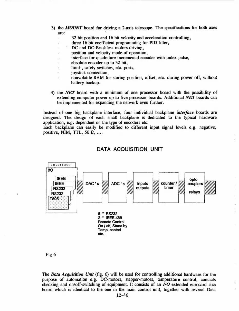
3) the MOUNT board for driving a 2-axis telescope. The specifications for both axesare:
- 32 bit position and 16 bit velocity and acceleration controlling,
- three 16 bit coefficient programming for PID filter,
- DC and DC-Brushless motors driving,
- position and velocity mode of operation,- interface for quadrature incremental encoder with index pulse,
- absolute encoder up to 32 bit,
- limit-, safety switches, etc. ports,- joystick connection,
- nonvolatile RAM for storing position, offset, etc. during power off, without
battery backup.
4) the NET board with a minimum of one processor board with the possibility ofextending computer power up to five processor boards. Additional NET boards can
be implemented for expanding the network even further.
Instead of one big backplane interface, four individual backplane interface boards aredesigned. The design of each small backplane is dedicated to the typical hardware
application, e.g. dependent on the type of encoders etc.
Each backplane can easily be modified to different input signal levels e.g. negative,positive, NIM, "VI'L, 50 fl, ....
DATA ACQUISITION UNIT
interface
lie
IEEEIEEE
RS232RS232
T805!:!:!:!:!:!:. -
':';':-:-;-:-:-:-:-:-:-2;!
DAC' s
_ ADC's
8 ° RS2322 * IEEE-488Remote ControlOn/off, StandbyTemp. controletc.
2"777
inputs
outputs
i///i///r///_-///
_-//JLL/-Z
counter /timer
opto_..._....couplers
_///_ relays
Fig 6
The Data Acquisition Unit (fig. 6) will be used for controlling additional hardware for the
purpose of automation e.g. DC-motors, stepper-motors, temperature control, contacts
checking and on/off-switching of equipment. It consists of an I/O extended eurocard sizeboard which is identical to the one in the main control unit, together with several Data
12-46

Acquisition boards like:
- 12 bit D/A-converter (multiplexed for 8 outputs) with programmable range andoffset.
- 12 bit A/D-converter (multiplexed for 8 inputs) with programmable range, offset
and auto-calibration.
- 24 parallel input/output ports.- Counter/timer for controlling counting/timing functions.
- Galvanic separation by opto-couplers and solid state relays.
The User Interface (fig. 4) consists of two identical 486 Personal Computers (PC) which
are linked to the transputer network by means of 20 Mbaud link extension boards locatedin each PC. At this level the system can also be connected to Local and Wide Area
Networks by adding standard interface boards to the PC-ISA bus, utilizing standard
protocols.
Finally the Mains Power Supply (fig. 4) is designed for distribution, switching and
filtering mains. It also features an alarm button for safety.
II. Software
General aspectsThe computer configuration includes a transputer network and two identical PC-486AT's, the Main PC and the Real-Time PC, each connected to the transputer net-
work by a so called 'link'(fig. 4). On both PC's the operating system MS-DOS is
running together with the highly efficient and friendly Microsoft WINDOWS which is
a widely accepted industry standard graphical environment for PC's. In the transputernetwork the RT-software is running without any operating system. On both PC's theWINDOWS TRANSPUTER FILE SERVER is running. The Main PC hosts the off-
line _oftware and is used for data storage. Tasks like: site installation, preparing
predictions, real time processes, data screening, normal point calculations and datamailing are initiated from or performed by the Main PC. The Real-Time PC interacts
with the ranging process as a terminal through the on-line Real-Time (RT) windows
transputer file server program, supporting graphics capabilities for the transputernetwork during all real time processes like: satellite ranging, target calibration,
telescope alignment and diagnostics. Through the Real-Time PC the operator interacts
with all ranging related processes. The transputer network is built around severaltransputers where the actual RT-software is running in order to directly control thehardware. Modification of (default) input parameters for the various modules by the
operator is based on WINDOWS dialogue boxes and menus which are on both PC's
supported by extensive help information. In case of malfunctioning of one of the PC's,the software is designed to run on one PC only, with minimum inconvenience to the
operator. Thus each PC is a back-up unit for the other one.
The off-line software
This software is largely based on the original MTLRS system and will be updated for
compatibility with the PC-hardware platform under MS-DOS. The software will beembedded in the WINDOWS graphical environment. Error handling is supported by
supplying help information and by allowing operator intervention in run-timewhenever feasible. Primarily the new software package has been re-written in C,
whereas individual existing modules are kept in FORTRAN-77, callable from C-
programmes. Both the C- and the FORTRAN coding are based on to the ANSI-standard to ensure maximum portability of the software. All data files have been
12-47

defined in ASCII-format, unless specific requirements dictated the use of a binaryformat.
The RT-software
The transputer software system consists of a set of communicating processes, logicallycombined in functions. To make the software usable for other ranging systems and to
facilitate future developments, the software has been structured into three layers:
a. the GLOBAL, SLR SYSTEM independent software
b. the DEVICE or data format dependent DRIVER software
c. the INTERFACE type dependent DRIVER software
Diagnostic capabilities are integrated in all three layers of the RT-software and are
running concurrently by default or can be activated to run concurrently.
a. Global system
The global system includes all functions of the present MTLRS RT-software. The
current MTLRS limitations concerning the observation range, the correction domain
and the fixed firing epoch have been eliminated. Interleaving satellite ranging is madepossib!e. To optimize this, the coarse pass prediction integration and the fine
prediction interpolation are moved into the RT-software, This also allows firing epochdependent range residual calculation to speed up data filtering. The meteo data and the
UTC-GPS time are made available to the RT-time system.
b. Device driver
A device driver prepares the standard information from the global system to meet the
requirements of the device and vice versa_ It executes a device function by preparing adevice command according to the operational device protocol and by calling interfacedrivers for data transfer. Device drivers are available for all external devices to be
accessed by the global software.
c. Interface driver
An interface driver transfers the data from the transputer network through a hardwareinterface'to each device and vice versa. No modifications are applied to the data.
Interface drivers are available for each type of interface and protocol used by the
external devices. Event interrupt processing is supported for devices which are capableof asserting the transputer event signal.
International design standard
Because of the structured approach to the design of this control system it is hoped thatthis activity will contribute to the establishment of an international standard for SLR
control systems.
References
- Beek, W. and K.H. Otten, "MTLRS-2 Upgrade", Proceedings Seventh
International Workshop On Laser Ranging Instrumentation, Matera, 1989,OCA/CERGA, Grasse, France.
INMOS, "The Transputer Databook", Second Edition, document No.72 TRN 203
01, 1989, Redwood Burn Ltd, Trowbridge.
TMS User guide, Texas Instruments Data Book: TMS320C40 User guide.
BYTE: November 1988, Parallel Processing in depth, TS00 and counting.
3L Ltd. 'Peel House, Ladywell, Livingston EH54 6AG SCOTLAND, UKTelefax: -506-415944.
12-48

Airborne and Spaceborne
Systems


N94-15614
AIRBORNE 2 COLOR RANGING EXPERIMENT
Pamela S. Millar
James B. Abshire
Jan F. McGarry÷
Thomas W. Zagwodzki*
Linda K. Pacini*
Experimental Instrumentation Branch, Code 924NASMGoddard Space Flight Center
Greenbelt, Maryland 20771
+Crustal Dynamics Project, Code 901*Photonics Branch, Code 715
ABSTRACT
Horizontal variations in the atmospheric refractivity are a limiting error source for many
precise laser and radio space geodetic techniques t-7. This experiment was designed todirectly measure horizontal variations in atmospheric refractivity, for the first time, byusing 2 color laser ranging_me_urements to an air_craf_t_.The^2.collor!a_r syste_k2t_e
a T-39 aircraft. Circular patterns wmcn extenaeo irom mv _,u _,D.C. Beltway to the southern edge of Baltimore, MD were flown counter clockwise aroundGreenbelt, MD. Successful acquisition, tracking and ranging for 21 circular paths wereachieved on three flights in August 1992, resulting in over 20,000 two color ranging
measurements.
INTRODUCTION
Atmospheric refractivity is a limiting error source in precise satellite laser ranging (SLR).Several models have been developed to correct SLR measurements for the increased optical
path length caused by atmospheric refractionl-3'8: 9. The first three fomr_Ul_c_S_et_ atatmospheric refraction is spherically symmetric, ano require surtace metero ogalaser ranging site. A higher order model developed by Gardner 8,9 can, in principlecompensate for spatially varying atmospheric refraction by utilizing pressure andtemperature measurements at many locations near the laser ranging site. However, thismodel depends on the surface measurements being strongly correlated to atmospheric
density at higher altitudes.
13-1
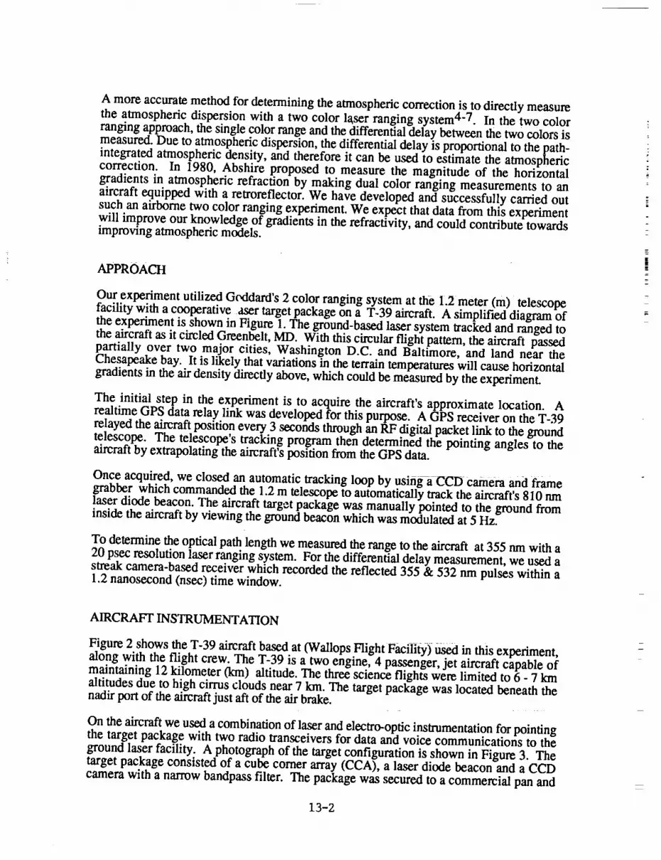
A more accurate method for determining the atmospheric correction is to directly measurethe atmospheric dispersion with a two color laser ranging system4-7. In the two colorranging approach, the single color range and the differential delay between the two colors is
measured. Due to atmospheric dispersion, the differential delay is proportional to the path-integrated atmospheric density, and therefore it can be used to estimate the atmosphericcorrection. In 1980, Abshire proposed to measure the magnitude of the horizontalgradients in atmospheric refraction by making dual color ranging measurements to an
aircraft equipped with a retroreflector. We have developed and successfully carried outsuch an airborne two color ranging experiment. We expect that data from this experimentwill improve our knowledge of gradients in the refractivity, and could contribute towardsimproving atmospheric models.
APPROACH
Our experiment utilized Goddard's 2 color ranging system at the 1.2 meter (m) telescopefacility with a cooperative aser target package on a T-39 aircraft. A simplified diagram ofthe experiment is shown in Figure 1. The ground-based laser system tracked and ranged tothe aircraft as it circled Greenbelt, MD. With this circular flight pattern, the aircraft passedpartially over two major cities, Washington D.C. and Baltimore, and land near theChesapeake bay. It is likely that variations in the terrain temperatures will cause horizontal
gradients in the air density directly above, which could be measured by the experiment.
The initial step in the experiment is to acquire the aircraft's approximate location. Arealtime GPS data relay link was developed for this purpose. A GPS receiver on the T-39
relayed the aircraft position every 3 seconds through an RF digital packet link to the groundtelescope. The telescope's tracking program then determined the pointing angles to theaircraft by extrapolating the aircraft's position from the GPS data.
Once acquired, we closed an automatic tracking loop by using a CCD camera and framegrabber which commanded the 1.2 m telescope to automatically track the aircraft's 810 nmlaser diode beacon. The aircraft target package was manually pointed to the ground frominside the aircraft by viewing the ground beacon which was modulated at 5 Hz.
To determine the optical path length we measured the range to the aircraft at 355 nm with a
20 psec resolution laser ranging system. For the differential delay measurement, we used astreak camera-based receiver which recorded the reflected 355 & 532 nm pulses within a1.2 nanosecond (nsec) time window.
AIRCRAFT INSTRUMENTATION
Figure 2 shows the T-39 aircraft based at (Wallops Flight Faciiity) _ in this experiment,along with the flight crew. The T-39 is a two engine, 4 passenger, jet aircraft capable ofmaintaining 12 kilometer (km) altitude. The three science flights were limited to 6 - 7 kmaltitudes due to high cirrus clouds near 7 km. The target package was located beneath thenadir port of the aircraft just aft of the air brake.
On the aircraft we used a combination of laser and electro-optic instrumentation for pointingthe target package with two radio transceivers for data and voice communications to the
ground laser facility. A photograph of the target configuration is shown in Figure 3. Thetarget package consisted of a cube comer array (CCA), a laser diode beacon and a CCD
camera with a narrow bandpass filter. The package was secured to a commercial pan and
13-2
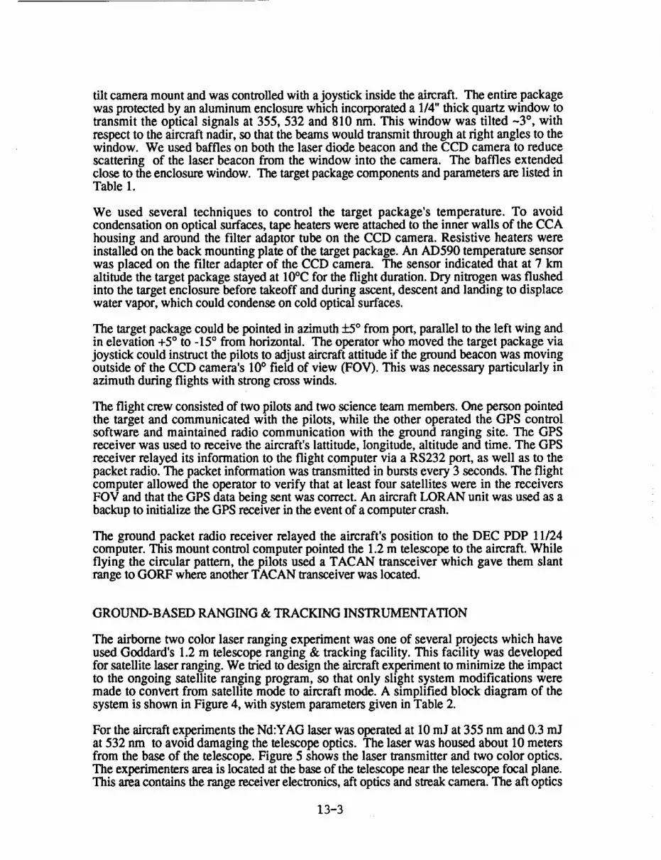
tilt camera mount and was controlled with a joystick inside the aircraft. The entire packagewas protected by an aluminum enclosure which incorporated a 1/4" thick quartz window totransmit the optical signals at 355, 532 and 810 nm. This window was tilted -3 °, withrespect to the aircraft nadir, so that the beams would transmit through at right angles to thewindow. We used baffles on both the laser diode beacon and the CCD camera to reduce
scattering of the laser beacon from the window into the camera. The baffles extendedclose to the enclosure window. The target package components and parameters are listed inTable 1.
We used several techniques to control the target package's temperature. To avoidcondensation on optical surfaces, tape heaters were attached to the inner walls of the CCAhousing and around the filter adaptor tube on the CCD camera. Resistive heaters wereinstalled on the back mounting plate of the target package. An AD590 temperature sensorwas placed on the filter adapter of the CCD camera. The sensor indicated that at 7 kmaltitude the target package stayed at 10°C for the flight duration. Dry nitrogen was flushedinto the target enclosure before takeoff and during ascent, descent and landing to displacewater vapor, which could condense on cold optical surfaces.
The target package could be pointed in azimuth :£5 ° from port, parallel to the left wing andin elevation +5 ° to -15 ° from horizontal. The operator who moved the target package viajoystick could instruct the pilots to adjust aircraft attitude if the ground beacon was movingoutside of the CCD camera's i0 ° field of view (FOV). This was necessary particularly in
azimuth during flights with strong cross winds.
The flight crew consisted of two pilots and two science team members. One person pointedthe target and communicated with the pilots, while the other operated the GPS controlsoftware and maintained radio communication with the ground ranging site. The GPSreceiver was used to receive the aircraft's lattitude, longitude, altitude and time. The GPSreceiver relayed its information to the flight computer via a RS232 port, as well as to thepacket radio. The packet information was transmitted in bursts every 3 seconds. The flightcomputer allowed the operator to verify that at least four satellites were in the receiversFOV and that the GPS data being sent was correct. An aircraft LORAN unit was used as abackup to initialize the GPS receiver in the event of a computer crash.
The ground packet radio receiver relayed the aircraft's position to the DEC PDP 11/24computer. This mount control computer pointed the 1.2 m telescope to the aircraft. Whileflying the circular pattern, the pilots used a TACAN transceiver which gave them slantrange to GORF where another TACAN transceiver was located.
GROUND-BASED RANGING & TRACKING INSTRUMENTATION
The airborne two color laser ranging experiment was one of several projects which haveused Goddard's 1.2 m telescope ranging & tracking facility. This facility was developedfor satellite laser ranging. We tried to design the aircraft experiment to minimize the impactto the ongoing satellite ranging program, so that only slight system modifications weremade to convert from satellite mode to aircraft mode. A simplified block diagram of thesystem is shown in Figure 4, with system parameters given in Table 2.
For the aircraft experiments the Nd:YAG laser was operated at 10 mJ at 355 nm and 0.3 mJat 532 nm to avoid damaging the telescope optics. The laser was housed about 10 metersfrom the base of the telescope. Figure 5 shows the laser transmitter and two color optics.The experimenters area is located at the base of the telescope near the telescope focal plane.This area contains the range receiver electronics, aft optics and streak camera. The aft optics
13-3

for the aircraft configuration is shown in Figure 6. The laser output is directed through ahole in the 45 ° bifurcated mirror through the telescope and to the aircraft.
The ranging operation can be described by referring to Figure 4. A start diode samples theoutgoing laser pulse to initiate the time interval measurement sequence. The aircraft returnpulses are then reflected at the 45 ° birfurcated mirror and into the aft optics receiver. In thereceiver a small percentage of the return is split and detected by the MCP photomultipliertube. This generates the stop signal for the time-of-flight measurement as well as the pre-trigger for the streak camera.
The majority of the received signal was then separated into 532 nm and 355 nm paths by adichroic mirror and bandpass filters. Each color was focussed into a fiber optic delay line.The optical delay was required to allow pre-triggering the streak camera with respect to theoptical pulse's arrival time. The delay fiber bundle was composed of 27 fused silica fibers
with 100 i.tm core for each color which were round at the input side and formed into a
single row at the output side. The signals were then imaged onto the streak cameraphotocathode by the streak camera's input lens. The streak camera's 1.2 ns sweep speedsetting was calibrated and used to achieve -4 psec/pixel resolution. During pre-flight teststhe detection threshold for optical pulses transmitted through the fiber optic cable to thestreak camera was measured to be 6,600 photoelectrons at 355 nm and 4,200
photoelectrons at 532 nm.
At the transmitter, an optical delay was added to the 532 nm pulses to allow both 532 and355 nm received pulses to be recorded within the 1.2 ns sweep window. The 532 nmpulse was delayed with respect to the 355 nm pulse by using a total internal reflection (TIR)cube corner mounted on a computer controlled linear motor stage. This time offset was
used to compensate for the additional -2.7 nsec round trip atmospheric delay at 355 nm.Each streak camera waveform pair was digitized to 256 time pixels by 8 bits amplitude andwas recorded on hard disk. The streak camera waveforms were stored on the PDP LSI
11/23 at a 2 Hz rate. Each file consisted of the optical waveform pair, the 355 nm time-of-flight measurement, the transmitter 532 nm delay setting, telescope azimuth and elevationangles, and, other relevant tracking information.
The aircraft was acquired by using the GPS measured aircraft positions which were relayedto the tracking computer. Every 20 msec, the computer tracking program extrapolated theaircraft's pre_ent angular position from the three most recent GPS data points and directedthe mount to that angular location. GPS tracking was usually sufficiently accurate to keepthe aircraft position within the CCD camera's -.0.3 ° FOV. The tracking loop was closed byreading an X-Y digitizer which determined the angular offset of the aircraft's 810 nm laserdiode beacon within the COD FOV. In this mode the mount was driven so that the
beacon's angular position stayed within the center of the CCD FOV. Optical backgroundfrom bright stars, the moon and other aircraft were suppressed with a 5 nm FWHMbandpass tilter in front of the tracking camera. The telescope was able to track the aircraftto a precision of-200 microradians, and successfully tracked the aircraft across the face ofa full moon.
STREAK CAMERA CALIBRATION
When making two color ranging measurements at 532 and 355 nm, the differential delay is-1/12 the 532 nm delay. The differential delay must be measured to better than 5 psec for i
cm single color corrections 10,11. The streak camera's sweep speed had to be carefully
calibrated to permit this accuracy.
13-4
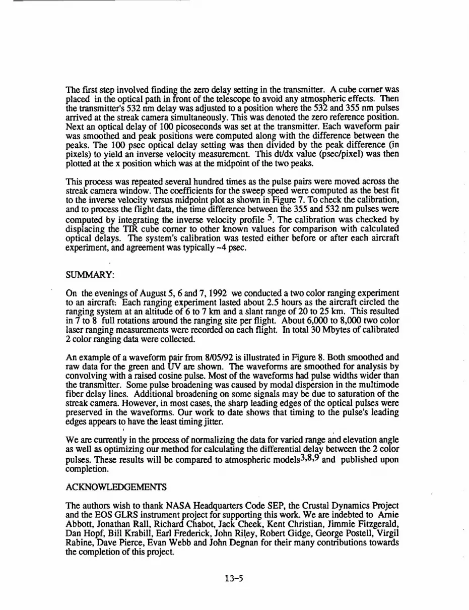
Thefirst stepinvolved finding thezerodelaysettingin thetransmitter.A cubecomerwasplaced in theopticalpathin front of thetelescopeto avoidanyatmosphericeffects. Thenthetransmitter's532nmdelaywasadjustedto apositionwherethe532and355nmpulsesarrivedatthestreakcamerasimultaneously.This wasdenotedthezeroreferenceposition.Next anoptical delayof 100picosecondswassetat the transmitter.Eachwaveformpairwassmoothedandpeakpositionswerecomputedalongwith the differencebetweenthepeaks.The 100 psecoptical delay settingwas then divided by the peak difference (inpixels) to yield aninversevelocity measurement.This dt/dx value(psec/pixel)wasthenplottedat thex positionwhichwasatthemidpointof thetwopeaks.
This processwasrepeatedseveralhundredtimesasthepulsepairsweremovedacrossthestreakcamerawindow.Thecoefficientsfor thesweepspeedwerecomputedasthebestfitto the inverse velocity versus midpoint plot as shown in Figure 7. To check the calibration,and to process the flight data, the time difference between the 355 and 532 nm pulses were
computed by integrating the inverse velocity profile 5. The calibration was checked bydisplacing the TIR cube comer to other known values for comparison with calculatedoptical delays. The system's calibration was tested either before or after each aircraft
experiment, and agreement was typically -4 psec.
SUMMARY:
On the evenings of August 5, 6 and 7, 1992 we conducted a two color ranging experimentto an aircraft: Each ranging experiment lasted about 2.5 hours as the aircraft circled theranging system at an altitude of 6 to 7 km and a slant range of 20 to 25 km. This resultedin 7 to 8 full rotations around the ranging site per flight. About 6,000 to 8,000 two colorlaser ranging measurements were recorded on each flight. In total 30 Mbytes of calibrated2 color ranging data were collected.
An example of a waveform pair from 8/05/92 is illustrated in Figure 8. Both smoothed andraw data for the green and UV are shown. The waveforms are smoothed for analysis byconvolving with a raised cosine pulse. Most of the waveforms had pulse widths wider thanthe transmitter. Some pulse broadening was caused by modal dispersion in the multimodefiber delay lines. Additional broadening on some signals may be due to saturation of thestreak camera. However, in most cases, the sharp leading edges of the optical pulses werepreserved in the waveforms. Our work to date shows that timing to the pulse's leadingedges appears to have the least timing jitter.
I
We are currently in the process of normalizing the data for varied range and elevation angle
as well as optimizing our method for calculating the differential delay between the 2 color
pulses. These results will be compared to atmospheric models3,8, 9 and published upon
completion.
ACKNOWLEDGEMENTS
The authors wish to thank NASA Headquarters Code SEP, the Crustal Dynamics Projectand the EOS GLRS instrument project for supporting this work. We are indebted to AmieAbbott, Jonathan Rail, Richard Chabot, Jack Cheek, Kent Christian, Jimmie Fitzgerald,
Dan Hopf, Bill Krabill, Earl Frederick, John Riley, Robert Gidge, George Postell, VirgilRabine, Dave Pierce, Evan Webb and John Degnan for their many contributions towardsthe completion of this project.
13-5

REFERENCES
1. Bender,P.L. and J.C. Owens,"Correctionof OpticalDistanceMeasurementsfor theFluctuatingAtmosphericIndexof Refraction," J.Geophys.Res.,70(10)pp.2461-2462,May 1965.
2. Marini, J. W., and C. W. Murray, Jr., "Corrections of Laser Range Tracking Data forAtmospheric Refractions at Elevations above 10 Degrees," NASA X-591-73-351,Nov. 1973.
. Herring; T. A., "Marini and Murray Atmospheric Range Correction Formula," Reportto the CSTG SLR Subcommission meeting NASACDP Principal Investigatorsmeeting, Munich, October 1988.
4. Abshire, J. B., "Plan for Investigation Atmospheric Errors in Satellite Laser RangingSystems," NASA X-723-80-10, January 1980.
. Abshire, J. B., and C. S. Gardner, "Atmospheric Refractivity Corrections in SatelliteLaser Ranging," IEEE Trans Geoscience & Remote Sensing, GE-23(4) pp. 414-425, 1985.
6. Degnan, J., J., "Satellite Laser Ranging: Current Status and Future Prospects," IEEETrans. Geoscience & Remote Sensing GE-23(4)pp. 398-413, 1985.
o Bender, P. L., "Atmospheric Refraction and Satellite Laser Ranging," submitted to:Syrup. on Refraction of Transatmospheric Signals in Geodesy: The Hague, May19-22, 1992.
8. Gardner, C, S., and B. E. Hendrickson, "Correction of Laser Tracking Data for theEffects of Horizontal Refractivity Gradients," Radio Research Ld_ratory 478,
University of Illinois, Urbana Illinois, December 1976.
9. Gardner, C. S., "Correction of Laser Tracking Data for the Effects of Horizontal
Refractivity Gradients," Appl. Optics 16(9) pp. 2427-2432, September 1977.
10. Im, K. E., C. S. Gardner, J. B. Abshire, and J. F. McGarry, "Experimentalevaluation of the performance of pulsed two-color laser-ranging systems," J. Opt.
Soc. Am. A 4(5) pp. 820-833, 1987.
11. Zagwodzld, T. W., J. F. McGarry, A. Abbot, J. W. Cheek, R. S. Chabot, J. D.Fitzgerald and D. A. Grolemund, "Streak Camera Returns from the Relay MirrorExperiment (RME) Satellite at Goddard space Flight Center's 1.2m TelescopeFacility," submitted to: American Geophysical Union Monograph, Space andGeodesy and Geodynamics, Fall 1992.
13-6

Table1. AircraftInstrumentationParameters
1.CubeComerArray Target
2. Laser Diode Beacon
3. CCD Camera
4. Pan & Tilt Camera Mount
5. GPS Receiver
6. Packet Radio Controller
7. Minicomputer
8. Voice Radio
23 element array, 2.5 cm cube comers,5 arc second accuracy, UV coated,R=78% @355 rim.
SDL-2460 A1GaAs Array,780 mW at 810 nm,
7 ° azimuth by 8 ° elevation divergence.
Philips model 56471 camera,25 mm lens, f/0.7, 10 ° FOV,
Bandpass Filter: 810 + 2.5 nm.
VICON model V353AtrI'V variable speeddrive system and tilt controller,
8" by 12.75" mounting plate
Motorola EagleVIII, 4-channel,simultaneous L1 C/A code carder tracking,
<25 m spherical error probability.
AEA, Inc. Model PK-87 ControllerICOM IC-37A FM Transceiver
217.55 MHz, 25 Watt.
Compaq 386 for GPS data control anddisplay.
ICOM IC3SAT FM Transceiver219.45 MHz, 5 Watt.
13-7

Table 2. Two Color Laser Ranging Aircraft Experiment System Parameters
1. Laser Transmitter
2. Telescope
3. Detectors:PMT
Sfi"eak Camera
4. Tune Interval Unit
5. Minicomputers:
Continuum PY62 Cavity Dumped,mode-locked, Nd:YAG System:
355 nm: 10 rrd, 150 grad
532 nm: 0.3 mJ, 300 grad
Pulsewidth: 30 psec FWHM.
1.2 meter diameter, f/28 Cassegrain.
1TI" F4128, Microchannel Plate.
Hammamatsu model C1370,
2 psec resolution,256 elements by 8 bit digitization.
Hewlett Packard HP5370,
20 psec resolution.
DEC PDP 11/24, Pointing.DEC LSI 11/23, Tracking, Streak Camera.
13-8

LI.I
Xi.LI
0
13-9

ORIGINAL PAGE
BLACK AND WHITE PHOTOGRAPH
g-,o.-q
o
"a
O
Ot_
C',I
O
o_O'h
<r_.<25
c.i
. ,,,.,q
13-10

ORIGINAE PAGE
BLACK AND WHITE PHOTOGRAPH
._-_=
l::_ O ,,'= O
o o _ _
_,_ L'd.,-,O,.E) o
•U_N ,
'-G o _. o
o,_._ = +_o..¢:,_ .-a.SE=St,j. _..) I.t3 --
e;_'_ >_
13-11

AJC Beacon
G RDB 8leacon,,r0 n mJ _,__ _
[ lRADIO _ I Calibration CC
L' ACK,NO,--PREDICT COMPUTER- -- RCVR OPTICSJ-_J AY I
ETC. BIFURCATEI_NMIRROR O
355 nm I STREAKMCP PMTI I CAMERAI
30pz, 4ppe TRIG _
I 99 • 1532 nm _ _ / DISCRIM. DISCRIM. I
UNEAR MOTOR j
DIFF. DELAY HARD I PMT&DISCGATES
(..S TO 10 NSEC) DISC i RANGE TIME
i A;°i°ATE'__ II,TERVALU.IT IOE.ERATORI
ICOMPUTER i"
Figure 4. Simple block diagram of i.2 m ranging and tracking facility in Greenbelt. MD, Thicklines, represent optical signals while thin lines indicate electrical signals. The systemoperated at 2 Hz (or pps). Single color range was measured at 355 nm with conventionaltime of flight instrumentation. Differential time between the 355 and 532 nm pulses wasmeasured with a streak camera based receiver. System calibration was performed by
inserting a comer cube in front of the telescope and setting known delay in the 532 nm
path with the TIR cube comer (cc).
A/C = aircraft, ACQ = acquisition, DISCRIM. = discriminator,MCP PMT = microchannel plate photomultiplier tube, TRK = Tracking
13-12

ORIGINAL PAGE
BLACK AND WHITE PHOTOGRAPH
Figure 5. Laser clean room housing the 30ps Continuum PY62 cavity dumped,mode-locked, doubled and tripled Nd:YAG laser. This system has twoamplifier stages. The TIR cube corner variable delay in the green path isshown on the left side of the optical table. Alignment and two color
optics are located outside of the primary, plexiglass, laser housing.
13-13
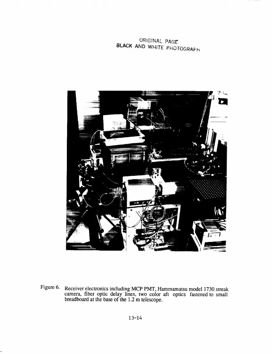
ORIGINAL PAGE
BLACK AND WHITE PHOTOGRAPh
Figure 6. Receiver electronics including MCP PMT, Hammamatsu model 1730 streak
camera, fiber optic delay lines, two color aft optics fastened to smallbreadboard at the base of the 1.2 m telescope.
13-14

SWEEP INVERSE VELOCITY VS WINDOW LOCATION
-3V -1 = -(2.28591 x 10 )X + (4.47)
II).x_13.
(J(I)O1Q.
v
q->
09
08
07
O6
05
O4
O3
02
01
00 -0
oO
O
_o o oo o° oOO o_ooo_ o°o @ o _ oo c_
0 0 O_
I I t I , I I I _ 1 z I t i1 I I L t
22 44 66 88 110 132 154 176 198
Streak Camera Window Location, X (pixels)
Figure 7. Streak camera sweep speed calibration for 2nsec sweep using data taken 3/24/92.The linear fit using 100 data points is displayed in the upper right hand corner ofthe plot. The units of inverse velocity are psec/pixel.
13-15

260
240
220
200
1BO
,6eX
_' 14o
I-,-, 100_.1O.
=: BO_C
60
40
20
00
260
240
220
20ff
180O3--I
"' 160x
_'14o
120
I,-
'--'100_I
.,_ BO
60
40
20
00
!
20
--T _----
= i
20
40
FLIGHT DATE 8/05/9ZI I I I I I ' ," I I" '" i !
I _ I , i i ! I i I = I i
60 BO 100 120 140 160 1B0 200 220 240
GREEN WAVE POSITION[P]XELS]
F'-----I ---_ I , I i I ] 1 _ I , 1 _ I , i I i
• , i . = I _i 1 I
40 60 80 100 120 t 40 160 100 200 220 240
U-V ',/AVE POSIT[ON [P]×EL5]
250
'60
Figure 8. Two color waveform pair recorded by Hammamatsu model C1370 StreakCamera. Each waveform is shown in both raw and smoothed form.
The horizontal scale factor is about 4.2 ps/pixel determined by calibration.For this pulse pair, the differential delay (including the optical delay setin the 532 nm path) was 2.667 nsec.
13-16

N94-15615
GLRS- R 2-COLOUR RETROREFLECTOR TARGET DESIGN ANDPREDICTED PERFORMANCE
Glenn LUND
Optical Department
AEROSPATIALE- Space & Defense Division
100 Boulevard du Midi
06322 CANNES LA BOCCA
FRANCE
ABSTRACT
This paper reports on the retroreflector ground-target design
for the GLRS_R spaceborne dual-wavelength laser ranging system.
The described passive design flows down from the requirements of
high station autonomy, high global FOV (up to 60 ° zenith angle),
little or no multiple pulse returns, and adequate optical cross-
section for most ranging geometries. The proposed solution makes
use of 5 hollow cube-corner retroreflectors of which one points
to the zenith and the remaining four are inclined from the
vertical at uniform azimuthal spacings.
The need for fairly large (~ I0 cm) retroreflectors is expected
(within turbulence limitations) to generate quite narrow
diffraction lobes, thus placing non-trivial requirements on the
vectorial accuracy of velocity aberration corrections. A good
compromise solution is found by appropriately spoiling just one
of the retroreflector dihedral angles from 90 °, thus generating
two symmetrically oriented diffraction lobes in the return beam.
The required spoil angles are found to have little dependance on
ground target latitude.
Various link budget analyses are presented, showing the
influence of such factors as point-ahead optimisation,
turbulence, ranging angle, atmospheric visibility and ground-
target thermal deformations.
13-17

i. BASIC GROUND TARGET REQUIREMENTS
During the various study phases investigated during the course
of the GLRS project, the Ground Target (GT) requirements
established to be of most significant importance were the
following :
• Choice of a multiple-retroreflector, passive target concept.
• As nearly full coverage of the sky as possible, up to local
zenith angles of at least 60 ° .
• Avoidance of ambiguous (multiple) pulse returns.
• Adequate velocity aberration correction, in keeping with the
link budget requirements.
• Adequate photon budget for sub-centimetric ranging accuracies
under most clear atmospheric conditions.
• Moderate cost and high reliability.
The requirement of a passive GT design leads to the choice of a
multiple fixed Retroreflector (RR) concept where full sky
coverage is achieved by the summation of several contributing RR
FOVs.
The inherent difficulties in this approach result firstly from
the non-uniform reflec[ed energy diagram of a static RR, and
secondly - because of the gradual fall-off of this diagram - from
the requirement of inter-RR crosstalk (i.e. multiple pulse
return) avoidance.
The adopted solution must therefore achieve an acceptable
compromise between somewhat conflicting requirements and the need
for accurate range measurements to be achieved under most
conditions.
In the following sections the proposed GLRS-R GT design is
described, and its numerically simulated performance is
illustrated as a function of several important system variables.
2. BASELINE GLRS-R TARGET CONCEPT
The baseline 5-retroreflector GT design illustrated in Fig. 1
provides a good compromise between full sky coverage, minimal FOV
overlap and minimal number of RRs. The individual retroreflectorshave a useful diameter of i00 mm, and will need to be of hollow
construction in order to minimise thermally induced wavefront
deformations. Although good thermal performance is achieved (in
space applications) with small solid cube-corners, there are
practical limits in size and temperature excursion beyond which
13-18
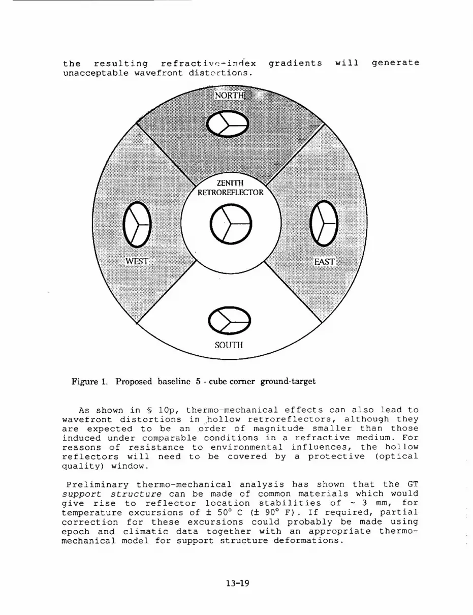
the resulting re fract iv_._-ind'exunacceptable wavefront distortions.
gradients will generate
SOUTtt
Figure 1. Proposed baseline 5- cube corner ground-target
As shown in 9 10p, thermo-mechanical effects can also lead to
wavefront distortions in hollow retroreflectors, although they
are expected to be an order of magnitude smaller than those
induced under comparable conditions in a refractive medium. For
reasons of resistance to environmental influences, the hollow
reflectors will need to be covered by a protective (optical
quality) window.
Preliminary thermo-mechanical analysis has shown that the GT
support structure can be made of common materials which would
give rise to reflector location stabilities of ~ 3 mm, for
temperature excursions of ± 50 ° C (± 90 ° F). If required, partial
correction for these excursions could probably be made using
epoch and climatic data together with an appropriate thermo-
mechanical model for support structure deformations.
13-19
As explained in §3 and §4, velocity aberration correction isachieved by designing the RR far-field diffraction patterns toexhibit a symmetrical twin-lobe structure. Each of the RRS must
be oriented (about its local normal) in a particular direction
with respect to the overhead spacecraft tracks, in order to
achieve appropriate alignment of the reflected lobes.
Although a 45 ° inclination of the peripheral reflectors provides
good overall FOV coverage and has been assumed in the following
analyses, the choice of this value is somewhat arbitrary.
Parametric analysis could reveal a more favourable inclination,
depending on the criteria used to trade link budget performance
at high zenith-angles against FOV overlap limitations. Variants
involving more than 4 peripheral reflectors could also be
considered, although they would incur an increase in the extent
of FOV overlap, and higher overall GT costs.
It is assumed that the spacecraft (S/C) ranging strategy will
inhibit operation for the small percentage of geometries where
crosstalk effects are expected to be strong and determines, for
any allowed ranging operation, which of the RRs must be providing
the return signal. An appropriate deterministic correction then
relates the measured RR range to a common GT reference point.
3. PRINCIPAL INFLUENCES IN LINK BUDGET PERFORMANCE
AS shown in Fig.2, there several quite different influences
which can affect the system link budget performance. Those which
are considered or referred to in the "present paper are listed
below :
• Two-way atmospheric transmission, depending on visibility
conditions, local zenith angle and GT altitude.
• Atmospheric turbulence, characterised by wavelength and the
mean long-exposure turbulent energy ( } Cn2 (h).dh).
• Ranging geometry, as determined by local zenith angle, local
RR incidence angle, satellite azimuth and range.
• Velocity aberration, depending on ranging geometry and
satellite height and velocity.
• Retroreflector characteristics such as size, optical quality
and dihedral angle spoiling.
• Detection techniques, which in the case of GLRS-R imply the
use of a receiving telescope, transfer optics and a streak
camera.
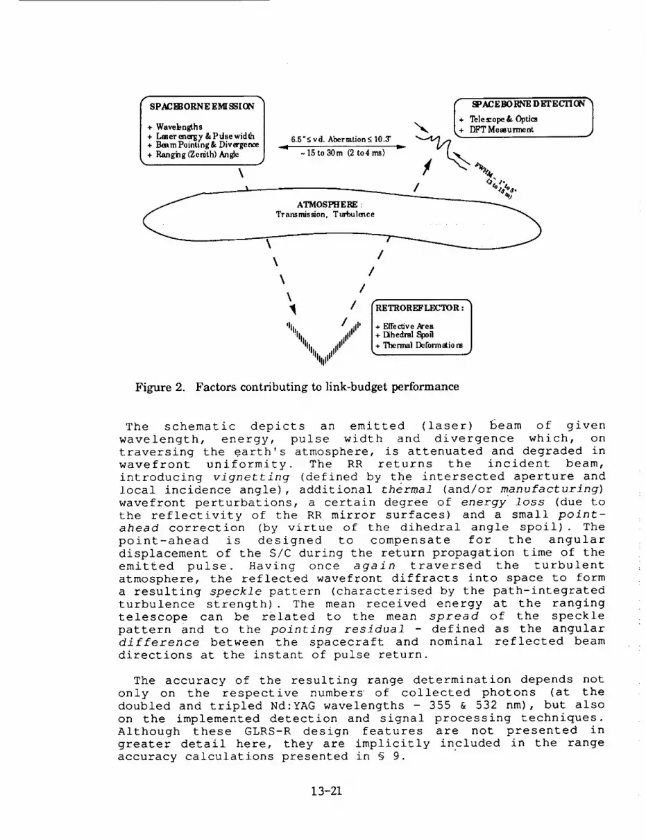
I SPACI_ORNE El_ SSION
+ Wavebngths+ Lasere_ergy&Pdsewid_h+ Be_mPointing& Divergence
+ Ranging(Zedth)Angle •
\
6.5"<vd. Aberration_ 10.3'
-15to30m (2 to4ms)
ATMOSPHERE :Transmission, T urbu]ence
\
\
\
_ACEBORNE DETECTION
-. l+ Telescope& Optics |_, _,+ DFT Measurment J
/
/
/\
/ rRETROREFLECTOR : "
qll!l /,11111I' 1+ Effec_veArean+ Dihedral Spoil
hillI ilip _+ Thermal Deformatiom.,lllliilllifl
Figure 2. Factors contributing to link-budget performance
The schematic depicts an emitted (laser) beam of given
wavelength, energy, pulse width and divergence which, on
traversing the earth's atmosphere, is attenuated and degraded in
wavefront uniformity. The RR returns the incident beam,
introducing vignetting (defined by the intersected aperture and
local incidence angle), additional thermal (and/or manufacturing)
wavefront perturbations, a certain degree of energy loss (due to
the reflectivity of the RR mirror surfaces) and a small point-
ahead correction (by virtue of the dihedral angle spoil). The
point-ahead is designed to compensate for the angular
displacement of the S/C during the return propagation time of the
emit£ed pulse. Having once again traversed the turbulent
atmosphere, the reflected wavefront diffracts into space to form
a resulting speckle pattern (characterised by the path-integrated
turbulence strength). The mean received energy at the ranging
telescope can be related to the mean spread of the speckle
pattern and to the pointing residual - defined as the angular
difference between the spacecraft and nominal reflected beam
directions at the instant of pulse return.
The accuracy of the resulting range determination depends not
only on the respective numbers' of collected photons (at the
doubled and tripled Nd:YAG wavelengths - 355 & 532 nm), but also
on the implemented detection and signal processing techniques.
Although these GLRS-R design features are not presented in
greater detail here, they are implicitly included in the range
accuracy calculations presented in _ 9.
13-21

4. POINT-AHEAD CORRECTION OF VELOCITY ABERRATION
As shown in the above figure, at the GLRS-R orbit the S/C is
displaced by an angular distance ranging between 6.5 and 10.3
arcseconds (equivalent to ~ 15 - 30 m) during the 2-way
propagation time. The FWHM of the return beam is however, for a
I00 mm RR, of the order of 1 to 5 arcseconds. The ambition of the
point-ahead correction is thus to compensate as well as possible
for this effect.
Fig. 3 illustrates the approach used in the GLRS-R GT concept,
in order to achieve acceptable velocity aberration correction by
means of a small degree of point-ahead applied to the
retroreflected beams. Both diagrams are scaled in arcseconds as
viewed from the RR, with the center corresponding to the
direction of any given incoming beam. The central spot would thus
also correspond to the required return beam direction if the S/C
had no transverse velocty with respect to the RR.
The left-hand diagram illustrates (relative to the origin
defined at the instant of pulse emission) the angular loci of the
S/C at the instant of pulse arrival back at the S/C. The
amplitude of any particular locus is commonly referred to as
velocity aberration. The size and shape Of these loci depend on
the transverse (relative to the instantaneous line of sight)
vectorial components of S/C velocity, within the foreseen limits
of ranging geometry. The presence of two loci subsets results
from the approximately opposite directions in which the S/C can
move, as observed from the ground (i.e for ascending or
descending tracks). These regions change and increase in size at
increasing GT latitudes, in accordance with the wider range of
directions of apparent S/C trajectory.
+lff'
_'i +5-
-5"
-10"
SPA CECRAFT VELOCI TY ABERRATION
N
W at in,ta nt ofpuke return _..0
e/
0_ s
.1o" .5" 0
S,C a t insta nt of E"qi pulse emission
+ I0"
Iq)i N'F AIt EAD FROM CC SPOILING
.y
.10"
w
N
opti_led for x /Day ._dy _ /
0 ..l Directional origin F:/_X _" ofimident beam
P_t-ahesd /
Day & N_,ht _
s
•_" +1 " -10"
I I I I
-5" 0 +5" +10"
Figure 3. Point-ahead correction of velocity aberration.
13-22

The right-hand diagram illustrates how the RR point-ahead"attempts" to compensate for velocity aberration, by generatingtwo return beams, offset in equal and opposite directions with
respect to the incoming beam. The wavefront fold is achieved by
what is commonly referred to as "dihedral angle spoiling",
whereby one (or more) of the 3 RR dihedral angles is offset from
the nominal value of 90.000 ° . Spoiling of a single angle leads to
2 reflected beams, whereas uniform spoiling of all 3 angles will
(as is the case for most geodetic satellite reflectors) generate
6 evenly distributed return beams. The exact shape of the
retroreflected directional loci is a geometrical consequence of
the local incidence angles of the incoming beam with respect to
the cube-corner retroreflector and to the orientation of its
spoiled dihedral angle(s). The inclination of the two loci shown
here can be modified in order to optimise the return signal
strength during either day (ascending) or night (descending) S/C
tracks. An alternative solution, as illustrated in Fig.3, would
be to incline the RR so as to achieve a compromise compensationfor both day and night tracks.
The degree to which velocity aberration is adequately
compensated for, at a given ranging geometry, is referred to here
as the beam pointing residual. It is expressed, in arcseconds, as
the difference between the required (velocity aberration)
direction and the applied (point-ahead) direction. In general,
the smaller the domain of ranging geometries for which the RR
point-ahead compensation is designed, the smaller the mean value
of pointing residual.
Other factors influencing this mean performance are local RR
incidence angle and ori4ntation, GT. lattitude, and the choice
between day (or night)-only and day+night E/R track compensation.
5. GLRS-R GROUND TARGET OPTIMISATION AND PERFORMANCE
In the following link budget analyses, the GT performance is
expressed in terms of cross-section profiles, which are derived
take into account the appropriately computed pointing residuals.
Although other performance criteria could have been chosen, these
tend to be more difficult to characterise with a single curve, as
they can depend on extrinsic influences such as turbulence and
wavelength.
Fig. 4 illustrates, for the required GLRS ranging geometries,
the variation in optimal values of dihedral spoil angle as a
function of GT latitude and RR orientation. The optimisation
process is designed to determine (for a given GT, S/C and
latitude characteristics) the dihedral spoil which minimises the
quadratic sum of pointing residuals.
13-23

6.0"
_ 5.g"
a, 4.5".
40"
3.5':
3.0":
30 °
.... I .... I , , , , J , , , ' ! ....
. ....... i ...................................
.................................i...................................7................ _ ,, st
.................................i....................................i..............................E..._.s...t....&.....Z....e.n.i.th...i_ ...............
"" i i i i North
40 o 50 ° 60 ° 70 ° 80 °LATITUDE
Figure 4. Optimal dihedral angle spoil as a function of latitude.
The curves shown here correspond to the nominal GLRS orbit and
to a day/night optimisation of the pointing residuals. The
following two figures illustrate the expected GT performance at a
GT latitude of 35 °, in terms of optical cross-section. The choice
of this quantity is partly due to its similarity to the familiar
notion of radar cross-section, and partly to its physical
significance; the RR cross-section can be thought of as the
equivalent surface area of a perfectly white (albedo = i)Lambertian diffuser. Such a diffuser, if exposed to a uniform
illumination equal in intensity to that intersected by its
equivalent retroreflector, would give rise to the same far-field
luminous flux as that produce'd by the retroreflector in the
considered point-ahead direction. For a perfect RR, on-axis and
in the absence of turbulence, the theoretical cross-section can
be shown (for a 2-1obe diffraction pattern) to be :
= (x3/16).(¢4/k2)-1500. 106 m 2 (~ i00 x greater than in Fig.5)
In practice, the RR is rarely ranged to directly on-axis, and
atmospheric turbulence induces considerable beam-spread. A
certain degree of spreading is in fact desireable since the
retroreflected beam would otherwise be extremely narrow ( ~i
arcsec in the above example), with a consequently dramatic fall-
off in received energy at pointing residuals beyond about 2
arcsecs.
13-24
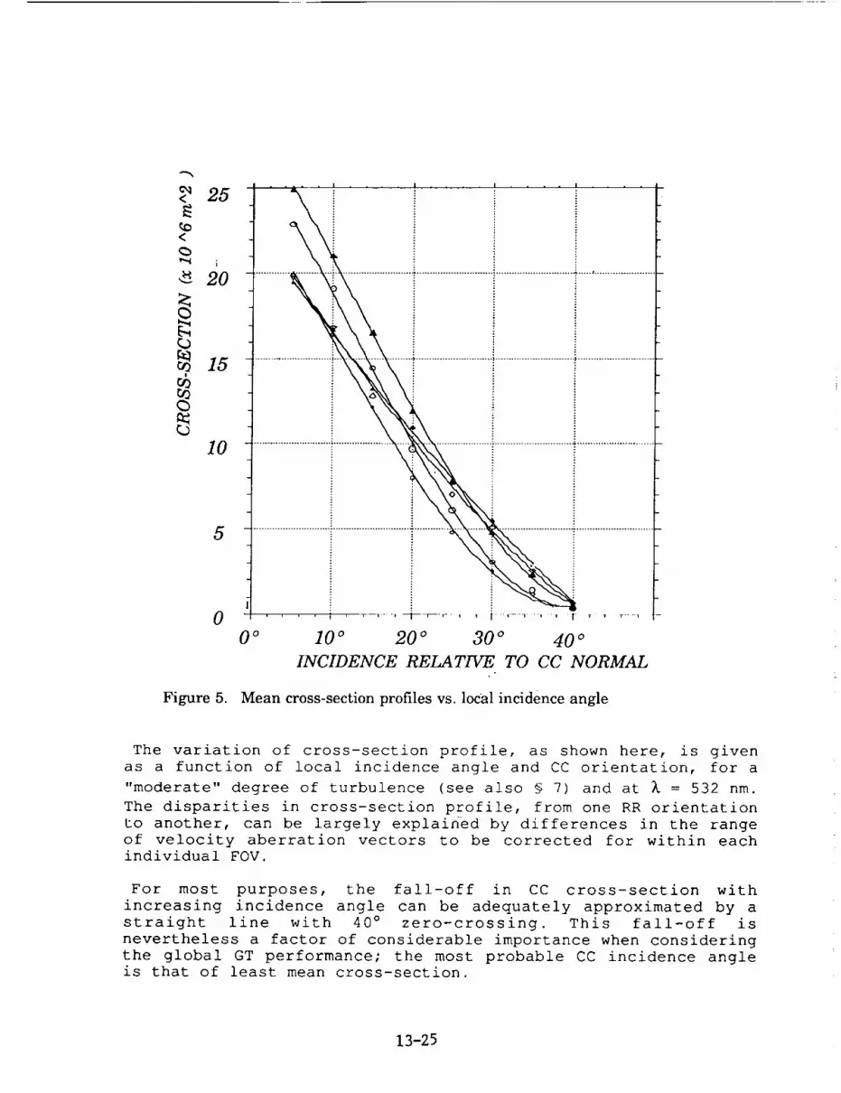
<_ 25
_ 20
10
5
00
t ¸ 1- _ , , | T ¸ T
10 o 20 o 30 ° 40 °INCIDENCE RELATIVE TO CC NORMAL
Figure 5. Mean cross-section profiles vs. local incidence angle
The variation of cross-section profile, as shown here, is given
as a function of local incidence angle and CC orientation, for a
"moderate" degree of turbulence (see also _ 7) and at I = 532 nm.
The disparities in cross-section profile, from one RR orientation
to another, can be largely explained by differences in the range
of velocity aberration vectors to be corrected for within each
individual FOV.
For most purposes, the fall-off in CC cross-section with
increasing incidence angle can be adequately approximated by a
straight line with 40 ° zero-crossing. This fall-off is
nevertheless a factor of considerable importance when considering
the global GT performance; the most probable CC incidence angleis that of least mean cross-section.
13-25

6. THE CHOICE BETWEEN DAY AND NIGHT TRACK OPTIMISATION
In the .GT design process, the choice can be made between a
preference for ranging during one only (Day/Night) or both (Day
and Night) of the S/C tracks (see also Fig. 3). The corresponding
point-ahead corrections are then computed to provide the least
overall pointing residuals.
In Fig. 6 the expected mean variations of RR cross-section aretraced for the above 2 cases, and for the unfavourable case of
ranging at night (day) to a day (night) -optimised GT. It can be
seen that the latter case gives rise to a considerable
degradation in mean cross-section. Alternatively, a good
compromise can be achieved between day and night optimisations,
as shown by the curve with ful_ triangles. Such an approach has
the advantage that it does not restrict the ranging opportunities
to just half of the S/C overhead tracks.
It could also be argued that night-time turbulence is in general
much lower than that encountered under hot daytime conditions,
thus compensating for the potential disadvantage of ranging at
night to a day-optimised GT.
For any given GT location, the choice of track optimisation
could forseeably be made, in accordance with an amalgum of site-
specific parameters, so as to enhance the global probability of
accurate range measurements.
25
_D<
20
10
I O DAY OPTIMIS.
• DAY & NIGHT OPTI_: ............
<> DAY OPTIM. AT NIGHT
5
0 t
0 10 20 30 40 50
INCIDENCE RELATIVE TO CC NORMAL (9
Figure 6. Mean peripheral retroreflector cross-section vs. track optimisation.
13-26

7. INFLUENCE OF ATMOSPHERIC TURBULENCE ON GT PERFORMANCE
The role of turbulence in the GLRS-R link budget performance is
of considerable importance, as it can introduce strong changes to
the overall system performance_
In Fig. 7, the expected mean peripheral cross-section profiles
are traced for 3 values of atmospheric turbulence strength,
considered to represent (respectively) low, moderate and high
levels of turbulence; i0, 50 & i00 x 10 -13 m I/3 Good night-time
conditions might correspond to the "low" level, whereas high
temperature daytime conditions could generate even worse
turbulence than that assumed under "high" conditions.
The unit of turbulence strength used here is that of refractive
index structure (or turbulent energy) integral :
S Cn 2 (h) dh (m 1/3)
The choice of this quantity, rather than Fried's parameter r o
or Seeing, has been made because of its independance from
wavelength. Table 1 provides conversions between these units, for
a few selected values of extreme and typical turbulence integral.
60
c_<
¢o<c5,-_ 40
r_
0
ii i
_ LowTurbu[enee 1
i / _ Med. Turbt_]ence
i k_ i [+ High Turbt_lence J
i ! i i o 1 --
0 ° 10 ° 20 ° 30 o 40 o 50 o
INCIDENCE RELATIVE TO CC NORMAL
Figure 7. Variation of mean peripheral cross-section as a function of turbulence.
13-27

] Cn 2 (h) .dh r o (355 nm) rO (532 nm) Seeing (355nm) Seeing (532nm)
(m 1/3) (cm) (cm) (arcsec) (arcsec)
i. 10 -13
5. 10 -13
i0. 10 -13
50. 10 -13
i00. 10 -13
21.
8.
5.3
2.0
1.3
34.
13.
8.6
3.3
2.1
0.35
0.92
1.4
3.7
5.6
0.32
0.85
1.3
3.4
5.2
TABLE 1. Fried's parameter r o and seeing as a function of turbulent energy integral _ Cn2(h). dh.
As can be seen in Fig. 7, strong atmospheric turbulence can give
rise to a considerable drop in the overall cross-section
performance of the GT retroreflectors due to overspreading of the
reflected diffraction patterns.
8. CROSSTALK EFFECTS AND SYSTEMATIC BIAS
The 3D plot shown in Fig. 8 illustrates the notion of inter-RR
crosstalk, expressed in terms of range measurement bias, which
results from the detection of retroreflected energy originating
from more than one RR.
The bias is determined at the level of the Streak Camera
differential flight time measurement, where the (temporal)
barycenters of the Green and UV return pulses are calculated. In
the case of multiple returns, the Streak Camera detection
algorithm can be confused by the presence of more than one pulsewithin the streak scan time-window (typically ~ i0 ns) . Assuming
the strongest pulse to be that of interest, the influence of a
secondary echo is evaluated here in terms of the (distance) bias
it would introduce into the timing determination.
The four crosstalk zones, generated by peripheral FOV overlap,
correspond in fact to ranging geometries of reduced interestbecause of the weak return signal strength to be expected at the
edge of any of the RR's local FOV (see 3 previous charts). In the
bias zones corresponding to overlap between the zenith RR and any
of the peripheral RRs, either one of the two following strategies
would need to be applied :
1 The GLRS system ranging controller software would forbid
ranging at this limited set of geometries.
2 The detection data processing would be designed to account
for the deterministic bias effects, giving preference to the
range determination based uniquely on the (clearly strongest)
pulse returns originating from the nearest RR.
13-28

Pulse FWHM 50ps
Orbit : 705 km
Wavelengths:
532 nm
355 nm
_)
u_
Bias (mm)
_ABOVE 50
25 -3020 -25
15 -20
10 -15
5 -10
IIIELOW 5
[-,1"='4
Z
N
5O
25
0
' I i i E I I
-50 -25 0 25 50
Figure 8. Systematic bias related to multiple pu}se returns arising from FOV overlap.
9. LINK BUDGET CALCULATIONS AND EXPECTED RANGE ACCURACY
Although the GT performance has been expressed, in Figs. 5 - 7,
in terms of cross-section, these figures need to be translated
into photons in order to assess the system range measurement
performance. The correspondance between these 2 quantities
depends on the following factors :
• Emitted pulse wavelength, energy and beam divergence.
• Two-way atmospheric transmission at the given range angle Z.
• Emitter - GT - receiver range (also a function of Z).
• Receiving telescope diameter.
• Mis'cellaneous optical component efficiencies.
The curves shown in Fig. 9 express the expected numbers of
received photons at the GLRS detector as a function of Z, at the
least transmitted (355 nm) wavelength, for two values (Skm and
23km) of standard atmospheric visibility and selected values of
cross-section. It can be seen that at high zenith angles there is
a sharp drop in received energy and a widening gap between the 5
and 23 km performances.
13-29
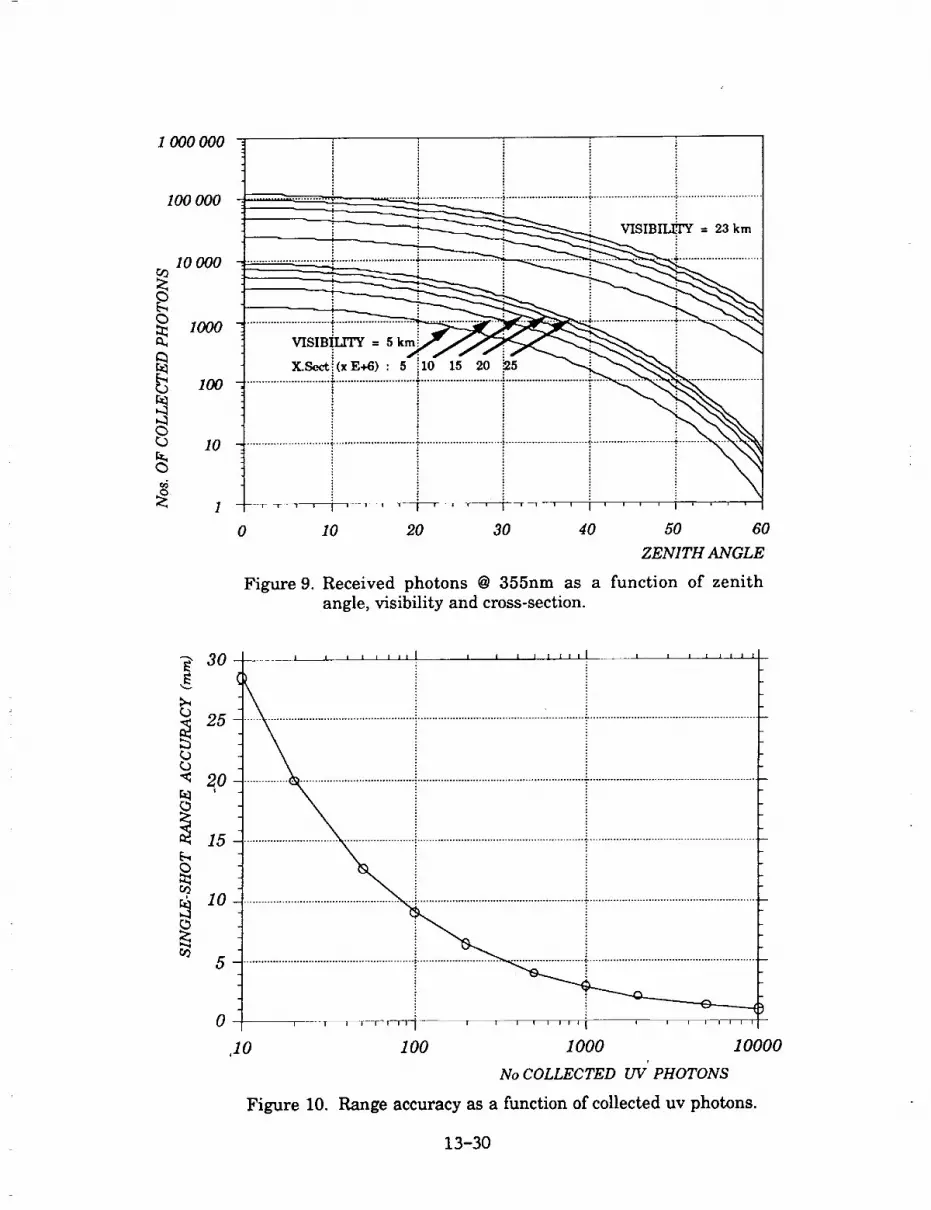
I 000 000
100000
10000
1000
,oo
10
i! :
VISIB] _ = 5 km
X.Sect_(xE+6) : 5 _10 15 20 '25
VISIBIIETY = 23 km
i
i
0 I0 20 30 40 50 60
ZENITH ANGLE
Figure 9. Received photons @ 355nm as a function of zenithangle, visibility and cross-section.
"_ 30
r_
25
"_ 20
r_5
0
1 L_ I I I I I 1 I I I I I I Ill
i
i
,10
gI I I I l-_]-_l ! ! I I I I • • I I I ! I I
100 1000 10000,
No COLLECTED UV PHOTONS
Figure 10. Range accuracy as a function of collected uv photons.
13-30

i0. INFLUENCE OF THERMAL EXTREMES ON DIFFRACTION PATTERNS
In all of the preceeding analyses, atmospheric turbulence has
been the only influence consid..red _n terms of a potential source
of wavefront deformation. However, thermal distortions of the RR
itself, under conditions of extreme ambient temperature or midday
solar illumination, could also be expected to introduce some
degree of change into the retroreflected beams. These effects
have been simulated firstly by running Nastran finite element
simulations of the structural distortions of an assumed
mechanical RR design. The resulting deformations of the
reflecting surfaces were then introduced into the optical codeused to generate retroreflected wavefronts and their
corresponding far-field diffraction patterns.
The diffraction pattern shown in Fig. Ii has been derived from
the simulated conditions of low ambient air temperature (-15°C)
in the absence of solar illumination (midnight), and shows that
there is indeed some spreading of the return beams. Various other
simulations have also been run, and show that extreme heat can
also have a detrimental effect on the retroreflected beam
quality. These simulations are of course highly (thermo-
mechanical) model dependant, but nevertheless show that under
conditions of moderate ambient temperature (-5 ° to +25°C) there
is no significant degradation of the diffaction lobes.
Cross-Sect{onz 10"6 m'2
I ABOVE X)OI e5- _oI 70- 85I 55- 70
I 40- 5s25- 40
lO- 25GLOW
:: !:!iii_;i!iii_i_̧ii_i,I_i!ili_i_,,i_i:_:_i_°¸::/:;:
" ii;ii!;i!!!i.-0_°-_.o:::::_!!i:i;_i:i!i::::_::ili':15!i_iiiiiii!!iiYli!iii!!!i:._!!):i!i:i)!_i_;_iiill!iiliii_!_ii
i
-,s.o -,o_ -s.o o_, _.o ,o.o ,s.oD_.j'/rac t_on J'_eZd (=resets)
Figure 11. Simulated GLRS diffraction lobe distortion at -15°C.
13-31
11. CONCLUSIONS
The GLRS-R Ground Target design approach and analyses described
in the present paper are found to satisfy the system requirements
under most ranging conditions, as summarised by the following
points:
• A relatively small number of retroreflectors can satisfact-
orily cover the observable sky up to zenith angles of 60 ° .
• Minimal zones of undesireable crosstalk are achieved.
• Appropriate spoiling of the retroreflectors can enable good
correction of velocity aberration to be assured while
maintaining high return signal strength at most rangiong
geometries.
• Just 2 values of dihedral spoil angle are needed for most
practical latitudes, thus leading to considerable simplific-
ation of their manufacture, assembly and testing.
• The Ground Target performance is found to have a minimal
dependance on site location, for latitudes up to 65 ° (north or
south).
• The system performance is quite strongly dependant on
atmospheric turbulence.
• Thermal influences can become non-negligeable under extreme
ambient temperature conditions.
• The overall link budget performance is found to be such that
under typical conditions, a single-shot ranging accuracy of
I cm or better can be expected.
13-32

N94"15616
Effects of Turbulence on the Geodynamic Laser Ranging System
James H. Churnside
NOAA Wave Propagation Laboratory
Boulder, Colorado 80303
1. INTRODUCTION
The Geodynamic Laser Ranging System (GLRS) is one of several instruments being
developed by the National Aeronautics and Space Administration (NASA) for implementation
as part of the Earth Observing System in the mid-1990s (Cohen et al., 1987; Bruno et al.,
1988). It consists of a laser transmitter and receiver in space and an array of retroreflectors
on the ground. The transmitter produces short (100 ps) pulses of light at two harmonics
(0.532 and 0.355 pm) of the Nd:YAG laser. These propagate to a retroreflector on the
ground and return. The receiver collects the reflected light and measures the round-trip
transit time. Ranging from several angles accurately determines the position of the
retroreflector, and changes in position caused by geophysical processes can be monitored.
The atmosphere will have several effects on the operation of the GLRS. The most
obvious atmospheric factor is cloud cover. When there are clouds between the satellite and a
particular retroreflector, no measurement from that reflector is possible. Fortunately, most of
the geophysical processes of interest are slow enough that many cloud-free observations are
expected before significant motion is observed. The next factor to consider is refraction
because of the overall temperature gradient in the atmosphere. This can be corrected using
the dispersion of the atmosphere, and is the reason for using two colors of light (Querzola,
1979; Abshire, 1980; Abshire and Gardner, 1985).
The final atmospheric factor to consider is refractive turbulence. This is a random
phase perturbation of the optical field as it propagates through a random field of refractiveindex inhomogeneities in the atmosphere. Possible effects on the optical field include a
random time delay, pulse spreading, beam wander, beam spreading, and irradiance
fluctuations or scintillation. Gardner (1976) and Abshire and Gardner (i985) calculated the
amount of random time delay and found it to' be negligible for the GLRS configuration. The
pulse spreading has also been calculated (Muchmore and Wheelan, 1951; Bramley, 1968;Brookner, 1969; Brookner, 1970) and is also negligible (<< 1 ps) for the GLRS case. The
other effects are considered in this report.
13-33

2. TURBULENCE CHARACTERISTICS
At optical frequencies, the refractive index of air can be approximated by
n = 1 + 7.76 x 10⁻⁷(1 + 7.52 x IO-33.-2)p/T, (1)
where P is the atmospheric pressure in millibars, T is the temperature in Kelvins, and k is
the wavelength of light in micrometers. _us, small changes in temperature cause small
changes in the refractive index. Small changes in temperature exist in the atmospherebecause of turbulent mixing of air parcels.
Refractive turbulence in the atmosphere can be characterized by three parameters. The
outer scale, Lo, is the length of the largest scales of turbulent eddies, The inner scale, Io, isthe length of the smallest scales. For separations gTeater than the inner scale and less than
the outer scale, the structure function of refractive index is given by
(2)
where p is the separation of two observation points at positions p and p + p, and thestructure function is defined by
On(p) = <[n(p) - n(p + p)]2>.
This implies that C, 2 is a measure of the strength of refractive turbulence.
In the lowest few hun&ed meters of the atmosphere, turbulence is generated by
radiative heating and cooling of the ground. During the day, solar heating of the ground
drives convective plumes. Refractive turbulence is generated when these warm plumes mix
with the cooler air mounding them. At night, the ground is cooled by radiation and winds
mix the cooler air near the ground with warmer air higher up. Periods of extremely low
turbulence exists at dawn and dusk when no temperature gradient exists in the lower
atmosphere. Turbulence levels are also very low when the sky is overcast and solar heatingand radiative cooling rates are low.
Values of turbulence strength near the ground vary widely. Lawrence et al. (1970)
measured values from less than 10 "t6 to greater than 10 "12 m "2/3 at a height of about 2 m.
These values are typical of what we see at this height. At 2.5 m, Kallistratova and
Timanovskiy (1971) measured values from less than 10 "17 to almost 10 -13 m "2/3. Under
certain conditions, the turbulence strength can be predicted from meteorological parameters
and characteristics of the underlying surface (Holtslag and Van Ulden, 1983; Thiermann andKohnle, 1988; Andreas, 1988).
(3)
13-34

Using a theory introduced by Monin and Obukhov (1954), Wyngaard et al. (1971)
derived a theoretical dependence of turbulence strength on height above fiat ground in the
boundary layer. During periods of convection (generally clear days), C,2 decreases as the
-4/3 power of height. At other times (night or overcast days), the power is nearly -2/3. No
theory for the turbulence profile farther from the ground exists. Measurements show large
variations in refractive turbulence strength. They all exhibit a sharply layered structure,
where the turbulence appears in layers of the order of 100 m thick with relatively calm air
in between. In some cases, these layers can be associated with orographic features; that is,
the turbulence can be attributed to mountain lee waves. Generally, the turbulence decreases
as height increases to a minimum value at a height of about 3-5 km. The level then increases
to a maximum at about the tropopause (10 km) and decreases rapidly above the tropopause.
Based on these type of data, Hufnagel and Stanley (1964) and Hufnagel (1974)
developed a model of an averaged profile of C_2 for altitudes of 3-20 km. It is probably the
best available model for investigation of optical effects. To extend the model to local ground
level, one should add the surface layer dependence (i.e., h-4/3). To see the general dependence
of C 2 on altitude, we plotted the average Hufnagel profile in Fig. 1. It has been extended to
ground level using a h -4/3 dependence with a value of 10"12 m "2/3 at a height of 2 m. Note
that this type of combination of models generally leaves a step in the prof'de at h = 3 kin.
Although this is not physical, it does not prevent the model from producing valid results inoptical propagation problems.
2O
15
Ex,,
4.., 10t-U_
03t-
........ I ........ I ........ I ........
1 ,
/)
_ t........ , ........ , . .-;...,,_'_--_ ...
10-I? i0.16 I0-Is I0-14
C° (m
Fig. 1. Typical height prof'de of the refractive turbulence structure parameter C_. The solid
line is the Hufnagel model with a -4/3 height dependence near the ground. The dashed line is
the Hufnagel-Valley model with 5-cm coherence length and 7-grad isoplanatic patch.
13-35

Another attempt to extend the model to ground level is the Hufnagel-Valley model
(Sasiela, 1988), referred to as the HVsn model because it produces a coherence diameter
(separation required for two receivers on the ground to observe incoherent fields from a
source at zenith) r 0 of about 5 cm and an isoplanatic angle (angular separation required for
two mutually .coherent sources at zenith to produce mutually incoherent fields at a point on
the ground) of about 7 prad for a wavelength of 0.5 ILm. It is plotted as a dashed line in
Fig. 1. Although it is not as accurate at modeling turbulence near the ground, it has the
advantage that the moments of turbulence profile important to propagation can be evaluated
analytically (Sasiela, 1988).
Less is known about the vertical profiles of inner and outer scales. Over fiat grassland
in Colorado, we typically observe inner scales of 5-10 mm near the ground (1-2 m). Banakh
and Mironov (1987) report calculated values of 0.5-9 mm at similar heights. Larger values
(up to -10 cm) are expected higher in the atmosphere.
Near the ground, the outer scale can be estimated using Monin-Obukhov similarity
theory (Monin and Obukhov, 1954). For typical daytime conditions, the outer scale is about
one-half the height above the ground. Above the boundary layer, the situation is more
complex. Weinstock (1978) calculated that L 0 should be about 330 m in moderate turbulence
in the stratosphere. Barat and Bertin (1984) measured outer scale values of 10-100 m in a
turbulent layer using a ball0on-bome instrument.
3. BEAM WANDER
The first effect to consider is the wander of an optical beam caused by refractive
inhomogeneities in the atmosphere. This wander is generally characterized statistically by the
variance of the angular displacement. Both the magnitude of the displacement and the
component along a single axis are used. For isotropic turbulence, the variance of the
magnitude is simply twice the variance of the component.
For the downlink, the beam wander variance can be written as
5 2 =
m
2.92 _-1/3 H-7/3 sec2/3 0 fdhh 2C2(h),0
(4)
where dpis the full-angle beam divergence, 0 is the zenith angle, and H is the orbital height.
For the GLRS system, _ is about 100 prad, H is 824 km, and 0 is between 0 ° and 70 °.
Using the C 2 profile of Fig. 1 with no inner or outer scale effects, the rms beam wander at
70 ° is 7.7 nrad. This is much less than the beam divergence and can be neglected.
13-36
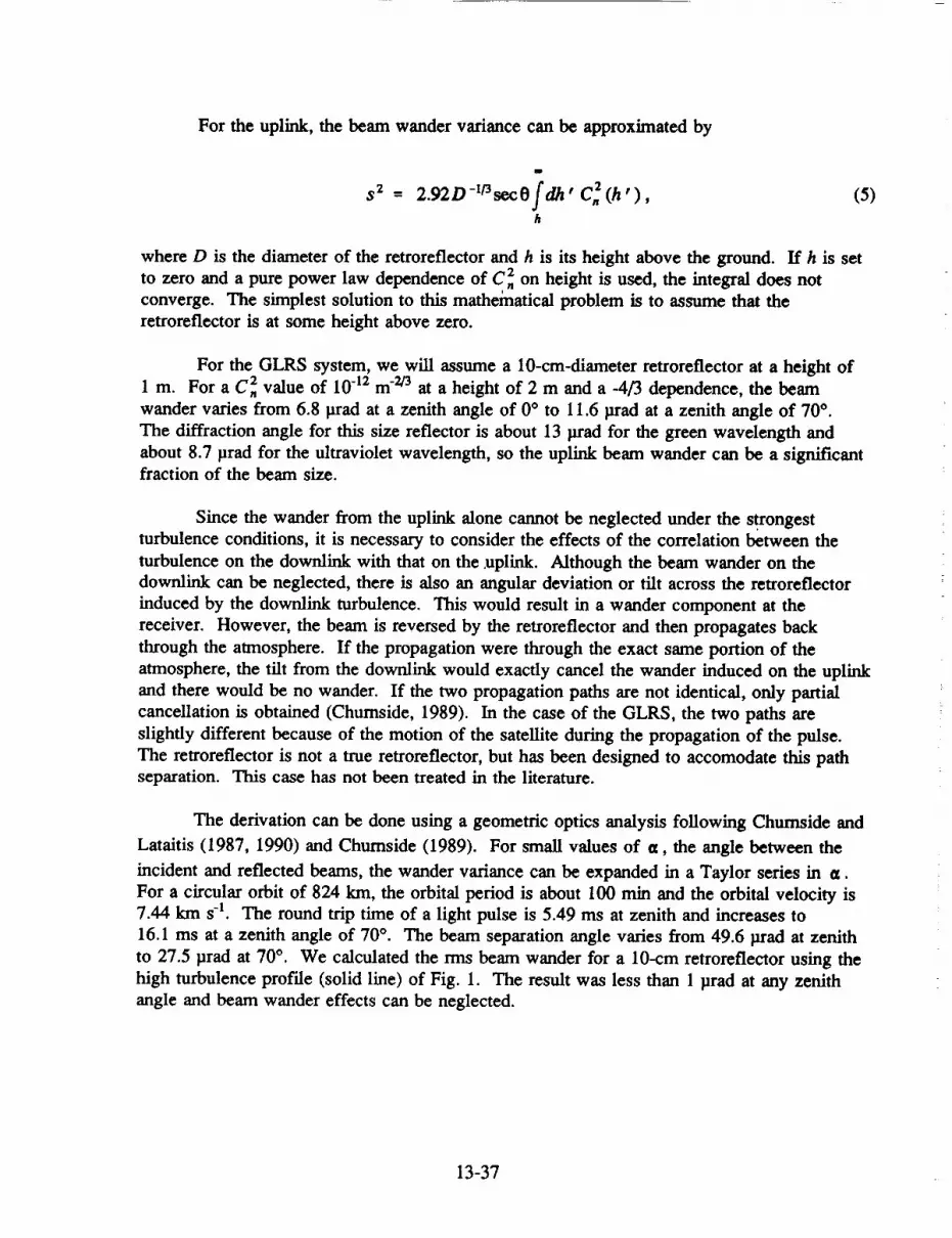
For the uplink, the beamwandervariancecanbe approximatedby
$2 _
m
2.92D-Ir sec0fdh ' (h'),h
(5)
where D is the diameter of the retroreflector and h is its height above the ground. If h is set
to zero and a pure power law dependence of C_ on height is used, the integral does not
converge. The simplest solution to this mathehaatical problem is to assume that the
retroreflector is at some height above zero.
For the GLRS system, we will assume a 10-cm-diameter retroreflector at a height of
1 m. For a Cn2 value of 10 -12 m -_ at a height of 2 m and a -4/3 dependence, the beam
wander varies from 6.8 grad at a zenith angle of 0 ° to 11.6 grad at a zenith angle of 70 °.
The diffraction angle for this size reflector is about 13 grad for the green wavelength and
about 8.7 grad for the ultraviolet wavelength, so the uplink beam wander can be a significantfraction of the beam size.
Since the wander from the uplink alone cannot be neglected under the strongestturbulence conditions, it is necessary to consider the effects of the correlation between the
turbulence on the downlink with that on the .uplink. Although the beam wander on the
downlink can be neglected, there is also an angular deviation or tilt across the retroreflector
induced by the downlink turbulence. This would result in a wander component at the
receiver. However, the beam is reversed by the retroreflector and then propagates back
through the atmosphere. If the propagation were through the exact same portion of the
atmosphere, the tilt from the downlink would exactly cancel the wander induced on the uplink
and there would be no wander. If the two propagation paths are not identical, only partial
cancellation is obtained (Chumside, 1989). In the case of the GLRS, the two paths are
slightly different because of the motion of the satellite during the propagation of the pulse.
The retroreflector is not a true retroreflector, but has been designed to accomodate this path
separation. This case has not been treated in the literature.
The derivation can be done using a geometric optics analysis following Chumside and
Lataitis (1987, 1990) and Chumside (1989). For small values of a, the angle between the
incident and reflected beams, the wander variance can be expanded in a Taylor series in ¢t.
For a circular orbit of 824 km, the orbital period is about 100 rain and the orbital velocity is7.44 km s -l. The round trip time of a light pulse is 5.49 ms at zenith and increases to
16.1 ms at a zenith angle of 70 °. The beam separation angle varies from 49.6 grad at zenith
to 27.5 grad at 70 °. We calculated the rms beam wander for a 10-cm retroreflector using the
high turbulence profile (solid line) of Fig. 1. The result was less than 1 grad at any zenith
angle and beam wander effects can be neglected.
13-37

4. BEAM SPREADING
The next effect to consider is the turbulence-induced spread of an optical beam as it
propagates through the atmosphere. Here we are talking about the short-term beam spread,which does not include the effects of beam wander. The primary effect of beam spreading is
to spread the average energy over a larger area. Thus, the average value of the on-axisirradiance is reduced and the average value of the irradiance at large angles is increased.
Since beam spreading is a statistical quantity, the amount of the spreading fluctuates in time.
This aspect has not been treated in depth in the literature.
We can consider beam wander to be caused by turbulent eddies that are larger than the
beam. Beam spread is caused by turbulent eddies that are smaller than the beam. There aremore small eddies in the beam at any time, which implies that the beam spread at any instant
is averaged over more eddies. Thus, the fluctuations of beam spread are smaller than those of
beam wander. Also, the smaller eddies are advected across the beam more quickly, and
changes in beam spread are faster than changes in pointing angle. The long-term beam
spread is defined as the turbulence-induced beam spread observed over a long time average.It includes the effects of the slow wander of the entire beam. The short-term beam spread is
defined as the beam spread observed at an instant of time. It does not include the effects of
beam wander, and is approximated by the long-term beam spread with the effects of wander
removed, although the two are not identical.
Yura (1973) and Tavis and Yura (1976) used the extended Huygens Fresnel principle
to calculate the short-term spread of a Gaussian beam. The results are collected and
summarized by Fante (1975, 1980). For O0 and l o much less than D, the short-term beam
spread is approximately given by
P, / [= 4 D 2 2 4k_ 2 + _ 1- + _2 1-0.62
k Po
(6)
where
0o = 1.46
L 5/3 1-315
f dz -£ c.(z)0
(7)
If Po is much greater than D, the turbulence-induced component of beam spreading can be
neglected.
Valley (1979) presents more complicated integral expressions that include inner-scale
and outer-scale effects. Breaux (1978) performed numerical calculations for the case of a
truncated Gaussian beam with a central obscuration. By curve fitting, he obtained the
following approximation:
13-38
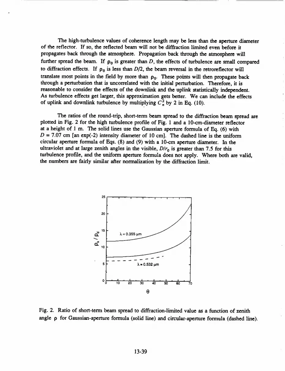
The high-turbulence values of coherence length may be less than the aperture diameterof the reflector. If so, the reflected beam will not be diffraction limited even before it
propagates back through the atmosphere. Propagation back through the atmosphere will
further spread the beam. If P0 is greater than D, the effects of turbulence are small compared
to diffraction effects. If Po is less than 1)/2, the beam reversal in the retroreflector will
translate most points in the field by more than P0- These points will then propagate back
through a pemzrbation that is uncorrelated with the initial perturbation. Therefore, it is
reasonable to consider the effects of the downlink and the uplink statistically independent.
As turbulence effects get larger, this approximation gets better. We can include the effects
of uplink and downlink turbulence by multiplying C_ by 2 in Eq. (10).
The ratios of the round-trip, short-term beam spread to the diffraction beam spread are
plotted in Fig. 2 for the high turbulence profile of Fig. 1 and a 10-cm-diameter refector
at a height of 1 m. The solid lines use the Gaussian aperture formula of Eq. (6) with
D = 7.07 cm [an exp(-2) intensity diameter of 10 cm]. The dashed line is the uniform
circular aperture formula of Eqs. (8) and (9) with a 10-cm aperture diameter. In the
ultraviolet and at large zenith angles in the visible, D/r o is greater than 7.5 for this
turbulence profile, and the uniform aperture formula does not apply. Where both are valid,
the numbers are fairly similar after normalization by the diffraction limit.
25
2O
15
I0
• II • I ' I I I I '--
k = 0.355 p.m
w
k = 0.532 l.tm
O0 . a • I , I ! • Jl_, . I 0 ,10 20 30 40 50 70
0
Fig. 2. Ratio of short-term beam spread to diffraction-limited value as a function of zenith
angle p for Gaussian-aperture formula (solid line) and circular-aperture formula (dashed line).
13-39
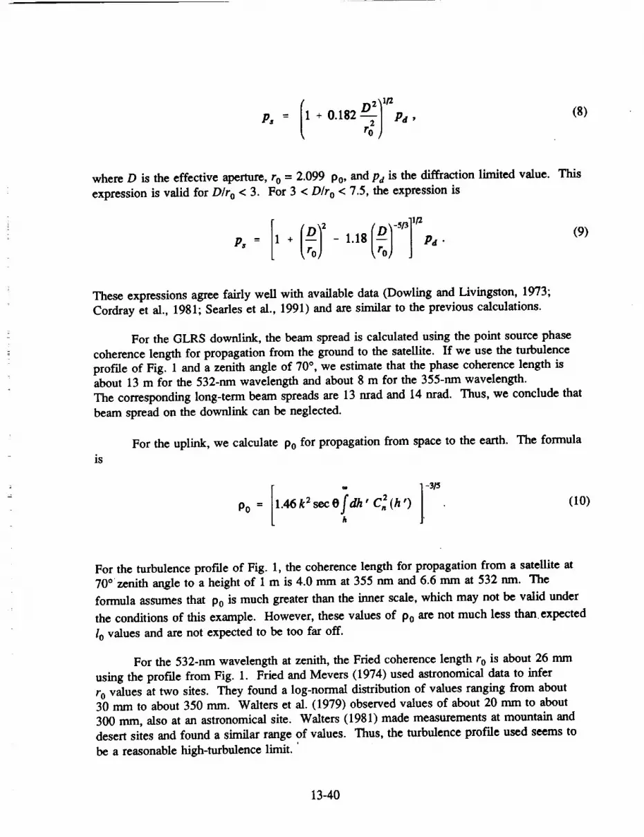
/x D2_ 1_
+ 0.182 ---_-| pa,
to/
(8)
where D is the effective aperture, ro = 2.099 Po, and Pd is the diffraction limited value. This
expression is valid for D/r o < 3. For 3 < D/r o < 7.5, the expression is
PS I(o) '°1 + _o - 1.18 pa. ro) ]
(9)
These expressions agree fairly well with available data (Dowling and Livingston, 1973;
Cordray et al., 1981; Searles et al., 1991) and are similar to the previous calculations.
For the GLRS downlink, the beam spread is calculated using the point source phase
coherence length for propagation from the ground to the satellite. If we use the turbulence
profile of Fig. 1 and a zenith angle of 70 °, we estimate that the phase coherence length isabout 13 m for the 532-nm wavelength and about 8 m for the 355-nm wavelength.
The corresponding long-term beam spreads are 13 nrad and 14 nrad. Thus, we conclude that
beam spread on the downlink can be neglected.
is
For the uplink, we calculate Po for propagation from space to the earth. The formula
[ ? 1Po = 1.46k2s°ce dh' C2.,(h')h
(10)
For the turbulence profile of Fig. 1, the coherence length for propagation from a satellite at
70 °. zenith angle to a height of 1 m is 4.0 mm at 355 nm and 6.6 mm at 532 nm. The
formula assumes that P0 is much greater than the inner scale, which may not be valid under
the conditions of this example. However, these values of P0 are not much less thanexpected
1o values and are not expected to be too far off.
For the 532-nm wavelength at zenith, the Fried coherence length r 0 is about 26 mm
using the profde from Fig. 1. Fried and Mevers (1974) used astronomical data to infer
r o values at two sites. They found a log-normal distribution of values ranging from about30 mm to about 350 mm. Walters et al. (1979) observed values of about 20 mm to about
300 ram, also at an astronomical site. Walters (1981) made measurements at mountain and
desert sites and found a similar range of values. Thus, the turbulence prof'de used seems to
be a reasonable high-turbulence limit.
13-40
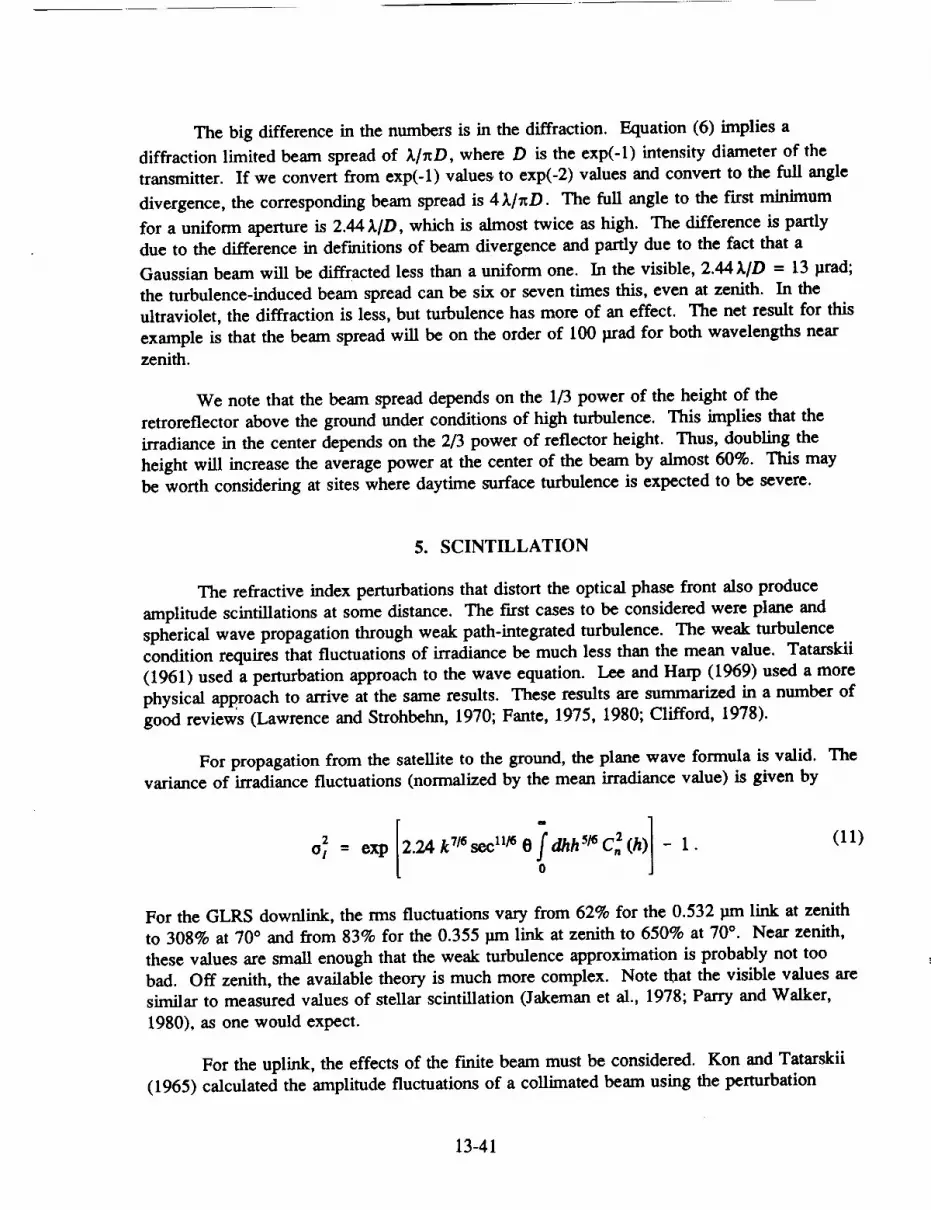
The big difference in the numbers is in the diffraction. Equation (6) implies a
diffraction limited beam spread of _./_rD, where D is the exp(-1) intensity diameter of the
transmitter. If we convert from exp(-1) values to exp(-2) values and convert to the full angle
divergence, the corresponding beam spread is 4 _./_D. The full angle to the first minimum
for a uniform aperture is 2.44 _./D, which is almost twice as high. The difference is partly
due to the difference in def'mitions of beam divergence and partly due to the fact that a
Gaussian beam will be diffracted less than a uniform one. In the visible, 2.44_./D = 13 prad;
the turbulence-induced beam spread can be six or seven times this, even at z_nith. In the
ultraviolet, the diffraction is less, but turbulence has more of an effect. The net result for this
example is that the beam spread will be on the order of 100 prad for both wavelengths near
zenith.
We note that the beam spread depends on the 1/3 power of the height of the
retroreflector above the ground under conditions of high turbulence. This implies that the
h-radiance in the center depends on the 2/3 power of reflector height. Thus, doubling the
height will increase the average power at the center of the beam by almost 60%. This may
be worth considering at sites where daytime surface turbulence is expected to be severe.
5. SCINTILLATION
The refractive index perturbations that distort the optical phase front also produce
amplitude scintillations at some distance. The first cases to be considered were plane and
spherical wave propagation through weak path-integrated turbulence. The weak turbulence
condition requires that fluctuations of irradiance be much less than the mean value. Tatarskii
(1961) used a perturbation approach to the wave equation. Lee and Harp (1969) used a more
physical approach to arrive at the same results. These results are summarized in a number of
good reviews (Lawrence and Strohbehn, 1970; Fante, 1975, 1980; Clifford, 1978).
For propagation from the satellite to the ground, the plane wave formula is valid. Thevariance of irradiance fluctuations (normalized by the mean irradiance value) is given by
I 1ot " exp 2.24 0 -0
(11)
For the GLRS downlink, the rms fluctuations vary from 62% for the 0.532 lma link at zenith
to 308% at 70 ° and from 83% for the 0.355 pm link at zenith to 650% at 70 °. Near zenith,
these values are small enough that the weak turbulence approximation is probably not too
bad. Off zenith, the available theory is much more complex. Note that the visible values are
similar to measured values of stellar scintillation (Jakeman et al., 1978; Parry and Walker,
1980), as one would expect.
For the uplink, the effects of the finite beam must be considered. Kon and Tatarskii
(1965) calculated the amplitude fluctuations of a collimated beam using the perturbation
13-41

technique. Schmeltzer (1967) extended these results to include focused beams. Fried and
Seidman (1967), Fried (1967), and Kinoshita et al. (1968) used these results to obtain
numerical values for a variety of propagation conditions. Ishimaru (1969a, 1969b, 1978) used
a spectral representation to obtain similar results.
The case of interest, however, is not a collimated beam transmitted from the ground.
Turbulence on the downlink adds scintillation. It also adds phase distortion at the reflector
that creates additional scintillation as the beam propagates back up to the satellite. The
case of a retroreflector embedded in refractive turbulence can be treated in the same weak-
turbulence approximation that has been used throughout. Most work in this area has been
done in the Soviet Union. An excellent review of this work is given in Banakh and Mironov
(1987).
One interesting feature of the results of retroreflector calculations is that the
fluctuations in the reflected light are maximum at the optical axis and decrease as the
observation point moves off the axis. This effect might tend to counteract the tendency of a
beam wave to have minimum fluctuations on the axis. However, these calculations are all for
uniform turbulence and do not account for the propagation to the far field. They have also
only been done for reflectors that are very large or very small in comparison to the Fresnelzone size.
where
For observation points near the center of the returned beam,
1o I = exp 8.70 2
0
4g_/_ - 4g_/¢
1 8u 2g! -
2 1+_ 2'
-1,
(12)
(13)
g_ = gl + i[u(1-u) + 1 82u2]2 1+82 '
g3 - (1 + 82) 2 1 - U + 1 + 82} '
1+82-Ug4 = 8U.
(1 + 82) 2 "
(14)
(15)
(16)
13-42
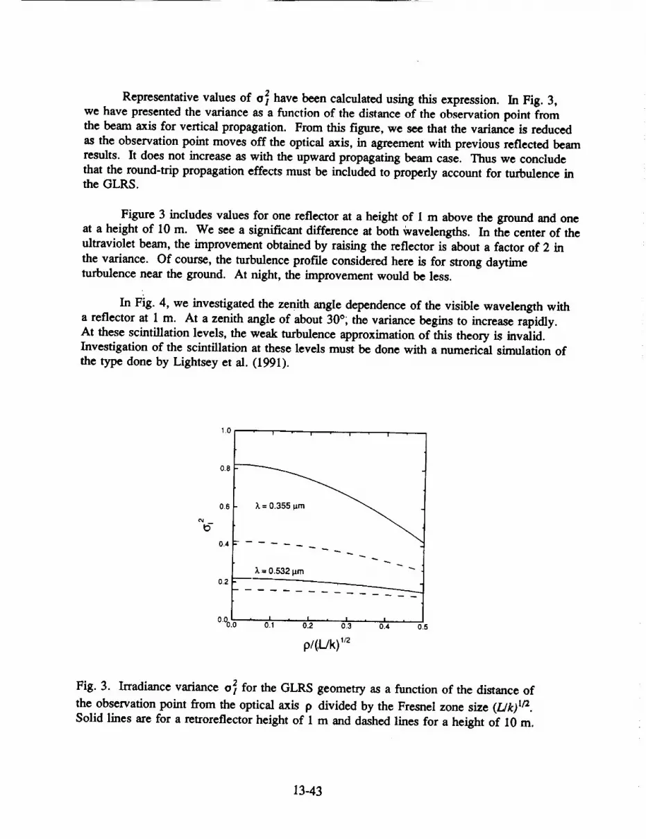
Representative values of ox2 have been calculated using this expression. In Fig. 3,
we have presented the variance as a function of the di_ance of the observation point fromthe beam axis for vertical propagation. From this figure, we see that the variance is reduced
as the observation point moves off the optical axis, in agreement with previous reflected beam
results. It does not increase as with the upward propagating beam case. Thus we conclude
that the round-trip propagation effects must be included to properly account for turbulence inthe GLRS.
Figure 3 includes values for one reflector at a height of 1 m above the ground and one
at a height of 10 m. We see a significant difference at both _vavelengths. In the center of the
ultraviolet beam, the improvement obtained by raising the reflector is about a factor of 2 in
the variance. Of course, the turbulence profile considered here is for strong daytime
turbulence near the ground. At night, the improvement would be less.
In Fig. 4, we investigated the zenith angle dependence of the visible wavelength with
a reflector at 1 m. At a zenith angle of about 30 °, the variance begins to increase rapidly.
At these scintillation levels, the weak turbulence approximation of this theory is invalid.
Investigation of the scintillation at these levels must be done with a numerical simulation of
the type done by Lightsey et al. (1991).
1.0
0.8
0.6
0,4
0.2 -
0"001,
k = 0.532 pm ""
0.1 0.2 0.3 04 0.5
p/(L/k) '/2
Fig. 3. Irradiance variance off for the GLRS geometry as a function of the distance of
the observation point from the optical axis p divided by the Fresnel zone size (Llk) 112.
Solid lines are for a retroreflector height of 1 m and dashed lines for a height of 10 m.
13-43
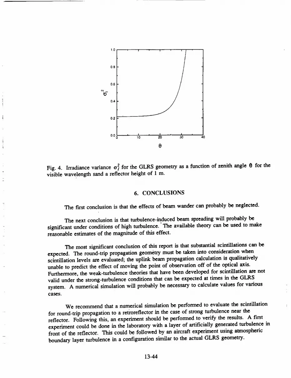
10
0.8
0.6
0.4
0.2
I " "
0,00 I , I , I ,' 10 20 30 40
0
Fig. 4. Irradiance variance o2t for the GLRS geometry as a function of zenith angle 0 for the
visible wavelength sand a reflector height of 1 m.
6. CONCLUSIONS
The first conclusion is that the effects of beam wander can probably be neglected.
The next conclusion is that turbulence-induced beam spreading will probably be
significant under conditions of high turbulence. 'The available theory can be used to make
reasonable estimates of the magnitude of this effect.
The most significant conclusion of this report is that substantial scintillations can be
expected. The round-trip propagation geometry must be taken into consideration whenscintillation levels are evaluated; the uplink beam propagation calculation is qualitatively
unable to predict the effect of moving the point of observation off of the optical axis.
Furthermore, the weak-turbulence theories that have been developed for scintillation are not
valid under the strong-turbulence conditions that can be expected at times in the GLRS
system. A numerical simulation will probably be necessary to calculate values for various
cases.
We recommend that a numerical simulation be performed to evaluate the scintillation
for round-trip propagation to a retroreflector in the case of strong turbulence near the
reflector. Following this, an experiment should be performed to verify the results. A first
experiment could be done in the laboratory with a layer of artificially generated turbulence infront of the reflector. This could be followed by an aircraft experiment using atmospheric
boundary layer turbulence in a configuration similar to the actual GLRS geometry.
13-44

REFERENCES
1
Abshire, J. B., 1980: Pulsed multiwavelength laser ranging system for measuring atmospheric
delay. Appl. Opt., 19, 3436-3440.
Abshire, J. B., and C. S. Gardner, 1985: Atmospheric refractivity corrections in satellite laser
ranging. IEEE Trans. Geosci. Remote Sens., GE-23, 414-425.
Andreas, E. A., 1988: Estimating C_ over snow and sea ice from meteorological data.
J. Opt. Soc. Am. A, 5, 481-494.
Banakh, V. A., and V. L. Mironov, 1987: Lidar in a Turbulent Atmosphere, Artech House,
Boston.
Barat, J., and .F. Bertin, 1984: On the contamination of stratospheric turbulence
measurements by wind shear. J. Atmos. Sci., 41,819-827.
Bramley, E. N., 1968: Correlation of signal fluctuations at two frequencies in propagation
through an irregular medium. Proc. IEEE, 115, 1439.
Breaux, H. J., 1978: Correlation of extended Huygens-Fresnel turbulence calculations for a
general class of tilt corrected and uncorrected laser apertures. U.S. Army Ballistic Research
Laboratory Interim Memorandum Report No. 600.
Brookner, E., 1969: Limit imposed by atmospheric dispersion on the minimum laser pulse
width that can be transmitted undistorted. Proc. IEEE, 57, 1234.i
Brookner, E., 1970: Atmospheric propagation and communication model for laser
wavelengths. IEEE Trans. Comm. Tech., COM-18, 396.
Bruno, R. C., W. W. Chapman, and P. W. Kwong, 1988: Ranging and Altimetry Link
Assessment for the Geodynamic Laser Ranging System, Stanford Telecommunications, Inc.
Report TR880142.
Chumside, J. H., 1989: Angle-of-arrival fluctuations of retroreflected light in the turbulent
atmosphere. J. Opt. Soc. Am. A, 6, 275-279.
Chumside, J. H., and R. J. Lataitis, 1987: Angle-of-arrival fluctuations of a reflected beam in
atmospheric turbulence. J. Opt. Soc. Am. A, 4, 1264-1272.
Chumside, J. H., and R. J. Lataitis, 1990: Wander of an optical beam in the turbulent
atmosphere. Appl. Opt., 29, 926-930.
13-45
Clifford, S. F., 1978: The classical theory of wave propagation in a turbulent medium.
In Laser Beam Propagation in the Atmosphere, J. W. Strohbehn, ed. (Springer-Vedag,
New York), 9-43.
Cohen, S. C., J. J. Degnan, HI, J. L. Burton, J. B. Garvin, and J. B. Abshire, 1987:
The geoscience laser altimetry/ranging system. IEEE Trans. Geosci. Remote Sens., GE-25,
581-591.
Cordray, D. M., S. K. Searles, S. T. Hanley, J. A. Dowling, and C. O. Gott, 1981:
Experiment_ measurements of turbulence-induced beam spread and wander at 1.06, 3.8, and
10.6 Inn. Proc. SPIE, 305, 273-280.
Dowling, J. A., and P. M. Livingston, 1973: Behavior of focused beams in atmospheric
turbulence: Measurements and comments on the theory. J. Opt. Soc. Am., 63, 846-858.
Fante, R. L., 1975: F,lectromagnetic beam propagation in turbulent media. Proc. IEEE, 63,
1669-1692.
Fante, R. L., 1980: Electromagnetic beam propagation in turbulent media: An update.
Proc. IEEE, 68, 1424-1443.
Fried, D. L., 1967: Scintillation of a ground-to-space laser illuminator. J. Opt. Soc. Am., 57,
980-983.
Fried, D. L., and G. E. Mevers, 1974: Evaluation of r o for propagation down through the
atmosphere. Appl. Opt., 13, 2620-2622.
Fried, D. L., and J. B. Seidman, 1967: Laser-beam scintillation in the atmosphere. J. Opt.
Soc. Am., 57, 181-185.
Gardner, C. S., 1976: Effects of random path fluctuations on the accuracy of laser ranging
systems. Appl. Opt., 15, 2539-2545.
Holtslag, A. A. M., and A. P. Van Ulden, 1983: A simple scheme for daytime estimates of
the surface fluxes from routine weather data. J. Clim. Appl. Meteor., 22, 517-529.
Hufnagel, R. E., 1974: Variations of atmospheric turbulence. In Technical Digest of Topical
Meeting on Optical Propagation through Turbulence (Optical Society of America,
Washington).
Hufnagel, R. E., and N. R. Stanley, 1964: Modulation transfer function associated with image
transmission through turbulent media. J. Opt. Soc. Am., 54, 52-61.
Ishimaru, A., 1969a: Fluctuations of a beam wave propagating through a locally
homogeneous medium. Radio Sci., 4, 295-305.
13-46
Ishimaru, A., 1969b: Fluctuations of a focused beam wave for atmospheric turbulenceprobing. Proc. IEEE, 57, 407-414.
Ishimaru, A., 1978: The beam wave case and remote sensing. In Laser Beam Propagation in
the Atmosphere, J. W. Strohbehn, ed. (Springer-Vedag, New York), 129-170.
Jakeman, E., G. Parry, E. R. Pike, and P. N. Pusey, 1978: The twinkling of stars. Contemp.Phys., 19, 127-145.
Kallistratova, M. A., 'and D. F. Timanovskiy, 1971: The distribution of the structure constan_
of refractive index fluctuations in the atmospheric surface layer, lzv., Atmos. Ocean. Phys.,7, 46-48.
Kinoshita, Y., T. Asakura, and M. Suzuki, 1968: Fluctuation distribution of a Gaussian beam
propagating through a random medium. J. Opt. Soc. Am., 58, 798-807.
Kon, A. I., and V. I. Tatarskii, 1965: Parameter fluctuations of a space-limited light beam ina turbulent atmosphere. Izv. VUZ Radiofiz., 8, 870-875.
Lawrence, R. S., and J. W. Strohbehn, 1970: A survey of clear-air propagation effects
relevant to optical communications. Proc. IEEE, 58, 1523-1545.
Lawrence, R. S.,' G. R. Ochs, and S. F. Clifford, 1970: Measurements of atmosphericturbulence relevant to optical propagation. J. Opt. Soc. Am., 60, 826-830.
Lee, R. W., and I. C. Harp, 1969: Weak scattering in random media, with applications toremote probing. Proc. IEEE, 57, 375-406.
Lightsey, P. A., J. Anspach, and P. Sydney, 1991: Observations of uplink and retroreflected
scintillation in the relay mirror experiment. Proc. SPIE, 1482 (in press).
Monin, A. S., and A. M. Obukhov, 1954: Basic laws of turbulent mixing in the ground layer
of the atmosphere. Trans. Geophys. Inst. Akad. Nauk. USSR, 151, 163-187.
Muchmore, R. B., and A. D. Wheelan, 1951: Frequency correlation of line-of-sight signalscintillations. IEEE Trans. Antennas Propag., AP-11, 46.
Parry, G., and J. G. Walker, 1980: Statistics of stellar scintillation. J. Opt. Soc. Am.70, 1157-1159.
Querzola, B., 1979: High accuracy distance measurement by two-wavelength pulsed lasersources. Appl. Opt., 18, 3035-3047.
Sasiela, R. J., 1988: A Unified Approach to Electromagnetic Wave Propagation in
Turbulence and the Evaluation of Multiparameter Integrals, Technical Report 807(MIT Lincoln Laboratory, Lexington).
13-47

Schmeltzer,R. A., 1967: Means, variances, and covariances for laser beam propagation
through a random medium. Quart. Appl. Math., 24, 339-354.
Searles, S. K., G. A. Hart, J. A. Dowling, and S. T. Hanley, 1991: Laser beam propagation
in turbulent conditions. Appl. Opt., 30, 401-406.
Tatarskii, V. I., 1961: Wave Propagation in a Turbulent Medium, (McGraw-Hill, New York).
Tavis, M. T., and H. T. Yura, 1976: Short-term average irradiance profile of an optical beam
in a turbulent medium. Appl. Opt., 15, 2922-2931.
Thiermann, T., and A. Kohnle, 1988: A simple model for the structure constant of
temperature fluctuations in the lower atmosphere. J. Phys. D: Appl. Phys., 21, $37-$40.
Valley, G. C., 1979: Long- and short-term Strehl ratios for turbulence with f'mite inner and
outer scales. Appl. Opt., 18, 984-987.
Waiters, D. L., 1981: Atmospheric modulation transfer function for desert and mountain
locations: ro measurements. J. Opt. Soc. Am., 71,406-409.
Waiters, D. L., D. L. Favier, and J. R. Hines, 1979: Vertical path atmospheric
MTF measurements. J. Opt. Soc. Am., 69, 828-837.
Weinstock, J., 1978: Vertical turbulent diffusion in a stably stratified fluid. J. Amos. Sci.,
35, 1022-1027.
Wyngaard, J. C., Y. Izumi, and S. A. Collins, Jr., 1971: Behavior of the refractive-index-
structure parameter near the ground. J. Opt. Soc. Am., 61, 1646-1650.
Yura, H. T., 1973: Short-term average optical-beam spread in a turbulent medium.
J. Opt. Soc. Am., 63, 567-572.
13-48
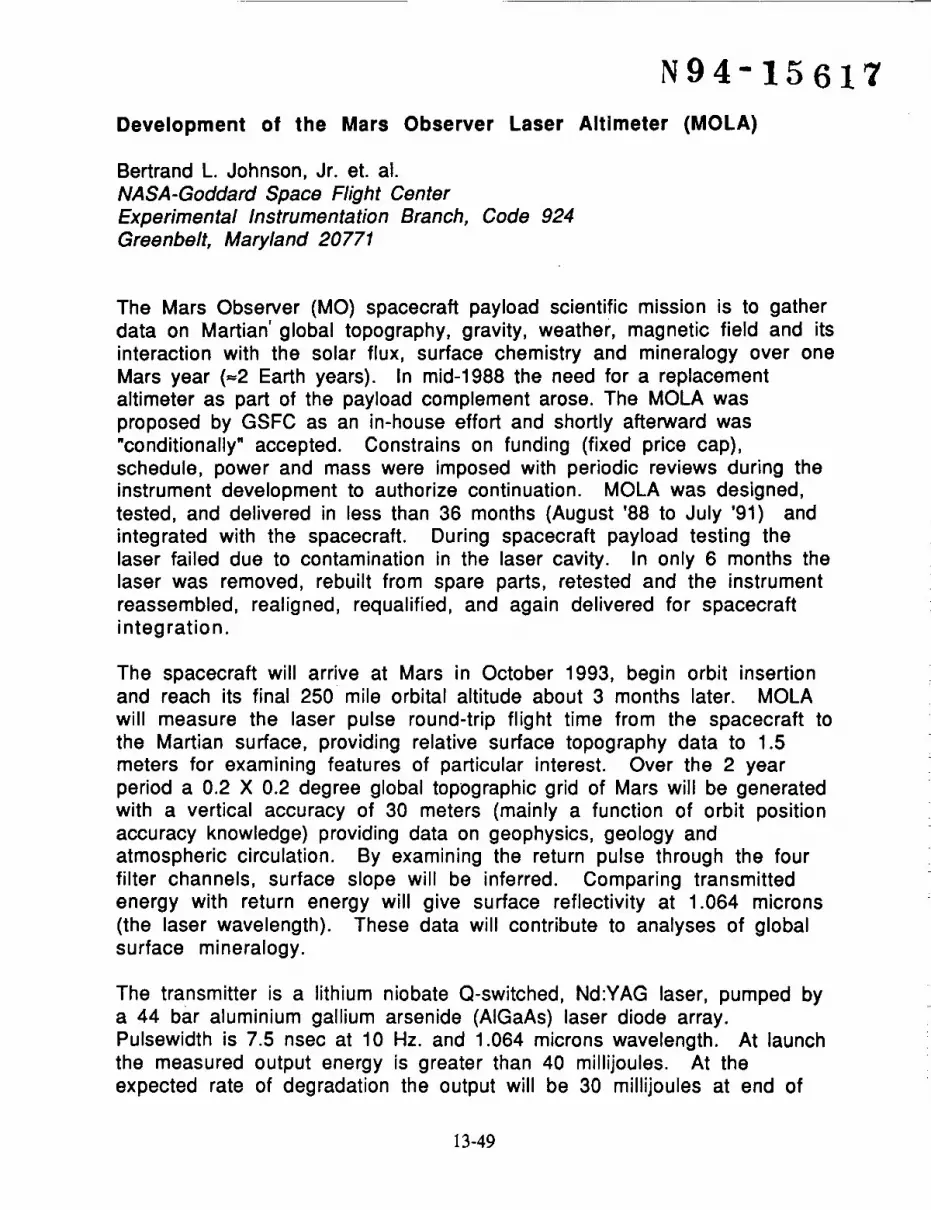
N94-15617
Development of the Mars Observer Laser Altimeter (MOLA)
Bertrand L. Johnson, Jr. et. al.
NASA-Goddard Space Flight Center
Experimental Instrumentation Branch, Code 924
Greenbelt, Maryland 20771
The Mars Observer (MO) spacecraft payload scientific mission is to gatherdata on Martian' global topography, gravity, weather, magnetic field and its
interaction with the solar flux, surface chemistry and mineralogy over one
Mars year (=2 Earth years). In mid-1988 the need for a replacementaltimeter as part of the payload complement arose. The MOLA was
proposed by GSFC as an in-house effort and shortly afterward was
"conditionally" accepted. Constrains on funding (fixed price cap),
schedule, power and mass were imposed with periodic reviews during theinstrument development to authorize continuation. MOLA was designed,
tested, and delivered in less than 36 months (August '88 to July '91) and
integrated with the spacecraft. During spacecraft payload testing the
laser failed due to contamination in the laser cavity. In only 6 months the
laser was removed, rebuilt from spare parts, retested and the instrument
reassembled, realigned, requalified, and again delivered for spacecraft
integration.
The spacecraft will arrive at Mars in October 1993, begin orbit insertionand reach its final 250 mile orbital altitude about 3 months later. MOLA
will measure the laser pulse round-trip flight time from the spacecraft to
the Martian surface, providing relative surface topography data to 1.5
meters for examining features of particular interest. Over the 2 year
period a 0.2 X 0.2 degree global topographic grid of Mars will be generated
with a vertical accuracy of 30 meters (mainly a function of orbit position
accuracy knowledge) providing data on geophysics, geology and
atmospheric circulation. By examining the return pulse through the four
filter channels, surface slope will be inferred. Comparing transmitted
energy with return energy will give surface reflectivity at 1.064 microns
(the laser wavelength). These data will contribute to analyses of global
surface mineralogy.
The transmitter is a lithium niobate Q-switched, Nd:YAG laser, pumped by
a 44 bar aluminium gallium arsenide (AIGaAs) laser diode array.
Pulsewidth is 7.5 nsec at 10 Hz. and 1.064 microns wavelength. At launch
the measured output energy is greater than 40 millijoules. At the
expected rate of degradation the output will be 30 millijoules at end of
13-49

mission, still providing sufficient link margin to meet measurement
requirements. Power consumption of the laser transmitter is 14 watts,
only about half of total instrument consumption. The laser was developed
by McDonnell Douglas Electronic Systems Inc. of St. Louis, MO.
A 100 MHz clock is the standard by which the time interval unit measures
the laser pulse round-trip flight time. The flight computer is set-up to
begin ranging as soon as the instrument is powered on. Laser firing
provides the range timing start pulse. The center of the laser beam is
sampled optically and focused onto a fiber optic cable which carries the
pulse to the PIN diode start detector. This starts the time interval unit(TIU). The clock provides timing for the laser firing as well as the TIU.
Laser output energy is inferred from the start detector output.
The laser signal return from the Mars surface is received by a 50 cm.diameter beryllium telescope and focused on a silicon avalanche photo
diode (40% quantum efficiency at 1.064 microns). In addition to focusing
optics, the aft optics contain a bandpass filter to minimize solar
background and a solar rejection filter for reducing solar input if the sunis viewed. The signal is amplified and passes through 4 low pass filters.Filter widths were selected to optimize detection probabilities for Mars
footprint-scale surface slopes of 1.7, 5, 15 and 39 degrees. The flight
computer continuously updates receiver channel thresholds, maximizing
detection probabilities and establishing a fixed rate of false alarms.
Physically the instrument is about 2' tall and its baseplate is triangular,about 2' on a side. It weighs 28 kg. and draws 30 watts including heater
power. The telescope sun shield is attached to the laser/telescopeinterface plate, acting as a radiator to cool the laser. Thermostaticallycontrolled heaters are mounted to the laser for additional thermal control.
The MOLA instrument underwent full environmental testing at the Goddard
Space Flight Center (thermal balance, thermal vacuum, vibration, acoustic,
and EMI/EMC) as well as thermal vacuum, EMI/EMC, and acoustic testing
while integrated with the spacecraft. The Mars Observer Spacecraft is
scheduled for launch in Sept./Oct. 1992.
For a comprehensive description of the MOLA experiment refer to the
paper by M.T. Zuber et. al., The Mars Observer Laser Altimeter
Investigation, Journal of Geophysical Research, vol. 97, No. E5, Pages
7781-7797, May 25, 1992.
13-50
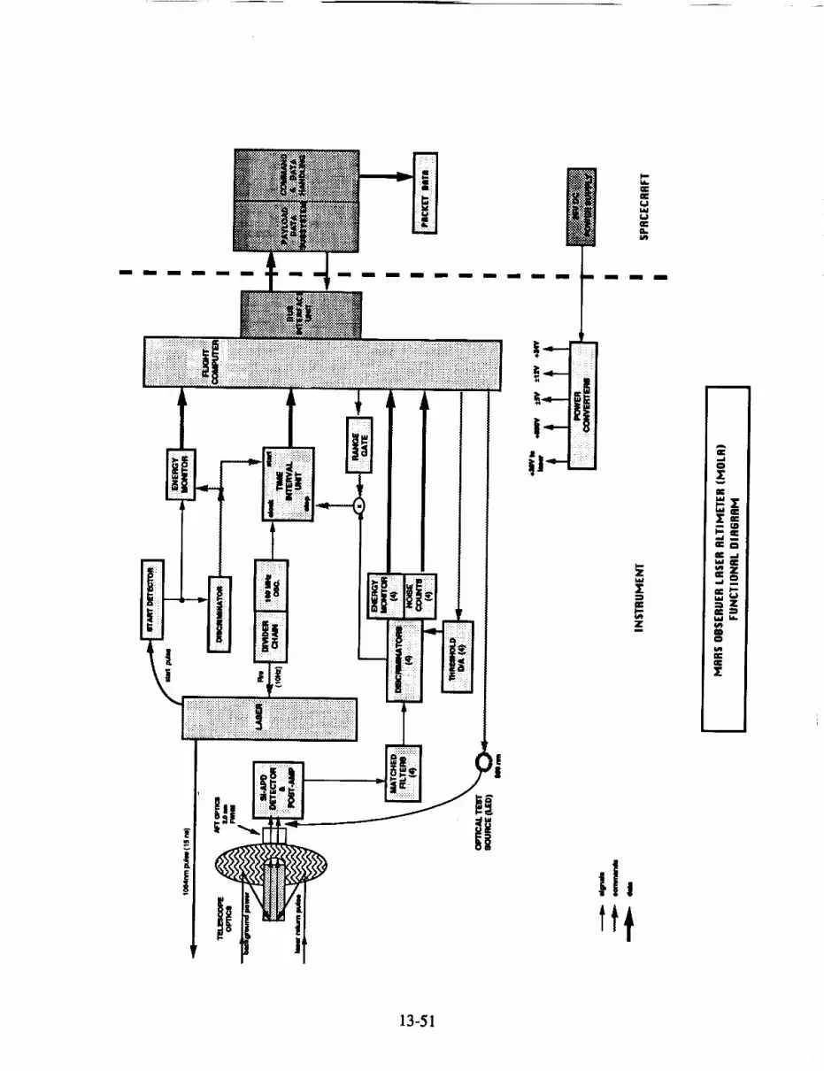
m m m m m mmm
::::::::::::::::::::::::::::::::::::::::::
k
mlmmm m
A
0
w
_rmJ m
L W.m
m m
_' ,md
m
1[
13-51

N94-15618
Bench Checkout Equipment for Spaceborne Laser Altimeter Systems
September 17, 1992
James C. Smith
NASA/Goddard Space Flight Center
Laboratory for Terrestrial Physics
Experimental Instrumentation Branch - Code 924
Greenbelt, MD 20771
Gregory C. Elman
Ressler Associates, Inc.
14440 Cherry Lane Court - Suite 212
Laurel, MD 20707
Kent D. Christian
Bendix Field Engineering
One Bendix Road
Columbia, MD 21045
John F. Cavanaugh
NASA/Goddard Space Flight Center
Laboratory for Terrestrial Physics
Experimental Instrumentation Branch - Code 924
Greenbelt, MD 20771
Luis Ramos-Izquierdo
NASA/Goddard Space Flight Center
Laboratory for Terrestrial Physics
Experimental Instrumentation Branch - Code 924
Greenbelt, MD 20771
Dan E. Hopf
Science Systems Applications, Inc.
5900 Princess Garden Parkway - Suite 300
Lanham, MD 20706
13-52

LIST OF FIGURES
1
2
3
3a
3b
3c
4
5
6
7
8
Title
BCE System Block Diagram
BCE Target Assembly
ATU Functional Block Diagram
ATU Optical Bench Layout
ATU Optical Head Position on the Target Assembly
ATU Optical Head Detail
LDU Functional Block Diagram
LDU Optical Path Layout
GPS Functional Block Diagram
BCE Controller Operation Flow Diagram
Data Analysis Performance Chart
13-53

ACRONYM LIST
A/D
ATU
BCE
CCD
D/A
DSA
EMC
EMI
GPS
GSFC
JPL
LDU
LEC
LED
MB
MO
MOLA
MOSCS
MSB
NASA
OTS
PC
PDS
RX
S/C
SCS
Si-APD
TBD
TBS
TIU
T/V
TX
Analog to Digital
Alitmetry Test Unit
Bench Checkout Equipment
Charge Coupled Device
Digital to Analog
Digital Signal Analyzer
Electromagnetic Compatibility
Electromagnetic Interference
Ground Power Supply
Goddard Space Flight Center
Jet Propulsion Laboratory
Laser Diagnostics UnitLaser External Cooler
Light Emitting Diode
Mega ByteMars Observer
Mars Observer Laser Altimeter
Mars Observer Spacecraft Checkout Station
Most Significant Bit
National Aeronautics and Space Administration
Optical Test Source
Personal Computer
Payload Data Sub-systemsReceive
Spacecraft
Spacecraft Checkout Station
Silicon Avalanche photo-diodeTo Be Determined
To Be Specified
Time Interval Unit
Thermal Vacuum
Transmit
13-54

INTRODUCTION
This paper addresses the requirements for testing and characterizing spaceborne laser
altimeter systems. The Bench Checkout Equipment (BCE) system, test requirements and flow-
down traceability from the instrument system's functional requirements will also be presented.
Mars Observer Laser Altimeter (/vIOLA) and the MOLA BCE are presented here as
representative of a 'typical' laser altimeter and its corresponding test system. The testing
requirements of other or future laser altimeter systems may vary slightly due to the specificspacecraft interface and project requirements.
MOLA, the first solid-state interplanetary laser altimeter, was designed to be operational
in Mars orbit for two Earth years (687 days). MOLA transmits a 7.5 ns pulse at a wavelength of
1.064 _m with a 0.25 mr beam divergence and a pulse repetition rate of 10 Hz. The output
energy is specified at 45 mj at the beginning of mapping orbit and 30 mj at the end of one Martian
year (687 Earth days). MOLA will measure the laser pulse transit time from the spacecraft to theMars surface and return to a resolution of 1.5 meters.
BCE FUNCTIONAL REQUIREMENTS
Functional 'requirements of an instrument and the associated performance specifications
are generated to accomplish specific scientific requirements of a project. The science team or
principal investigator work closely with the system engineer to develop instrument functional
requirements that will collect the necessary data to address the science requirement. These
functional requirements are osually a compromise between the best instrument that can be builtand what is minimally acceptable to obtain the required science data.
Typical functional requirements for a laser altimeter will address range resolution, laser
energy, pointing accuracy, etc.. Verifying that an instrument meets these functional requirements
becomes the Bench Checkout System (BCE) system functional requirements.
"A set of bench checkout equipment (BCE) is identified as that hardware equipment and
software, if applicable, necessary for performing a complete functional checkout of a flight
instrument. The BCE must be capable of simulating all functional spacecraft electrical interfaces,
exercising all normal instrument operating modes, and providing a hard copy record of instrument
output data in a form suitable for determining whether or not the instrument is performing
consistent with the environment in which it may be operating. The BCE also includes all cablesand instrument stimuli necessary for performing these functions.
The BCE will interface with the instrument primarily through those electrical connectors
that normally interface _,ith the spacecra/t. The BCE may, in addition,' interface with special test-access connectors located on the instrument.
The BCE also consist of stimuli (if applicable), stimuli controls, and whatever equipment
is necessary for monitoring essential internal instrument functions that cannot be monitored via
spacecraft telemetry when mounted on the spacecraft. The BCE also consist ofaU cables between
the instrument and/or stimuli and the system test complex. When on the spacecraft, the BCE may
13-55
interfacewith the instrument directly only through special test-access connectors located on the
instrument."1In addition, the BCE should be capable of " ... isolating equipment (instrument) faults or
malfunctions to an assembly level. Monitor and evaluate equipment performance during
spacecraft systems tests."2 The BCE should also continuously monitor Health and Welfare of theinstrument during spacecraft level testing via instrument telemetry data provided by the Spacecraft
Checkout Station (SCS).
Given the above project specific formal definition of the BCE, the following is a grouping
of the BCE functional requirement categories. These should be addressed individually with
regard to thoroughness and required complexity as separate requirements at the onset of the BCE
design. These tasks must be weighed against practical considerations such as instrument
schedule, budgets, and required project and spacecraft interfaces. Above all, the agreed upon
BCE design and performance specifications must be consistent with the requ!rement to validate
the instrument system functional requirements.
1) Validate the Instrument System Functional Requirements - This is the primary reason for
instrument system level testing and therefore is the primary BCE system requirement.
2) Perform Instrument calibration and/or performance characterization. - The level of
precision and accuracy required of the BCE System performance will dictate the overall system
cost and complexity.
3) Provide system interfaces durin_gall phases of testing (EMI/EMC, T/V, S/C inte_
- This mostly involves cabling, connectors and logistics of the BCE system. Particular
attention must be given to interfacing with the EMI/EMC and thermal vacuum test facilities.
These facilities often have very specific and unique requirements, but these interfaces are usually
straight forward and can be well defined in advance.
4) Monitor instrument sub-system oerformance_ - In a situation when instrument performance
severely degrades during system level testing it is extremely useful to know exactly which sub-
system is malfunctioning. This knowledge will be crucial in determining the strategy for any
corrective engineering efforts.
IMars Observer Payload Policies and Requirements Document, JPL 642-40, Appendix C, pp. C-12Mars Observer Spacecraft General Interface Specification Document, JPL 642-SE-001, Section 4.1 .a. 1,2, & 3
13-56

Instrument (MOLA) Functional Requirementsand BCE TestingRequirementsflow-down:
The following is a representative list of how the MOLA Functional Requirements flowed-
down to form the BCE Functional Requirements (i.e. Testing Requirement traceability).
L Instrument Functional Requirement:
Maintain a laser non-operating lifetime of two years and a operational lifetime of three
years. The three years operational lifetime is allocated to two years Mars orbit operation pluspre-launch testing.
Testing Requirement: Monitor the MOLA laser output energy with an integration
sphere and energy meter combination. Monitor MOLA packet data and recover the Laser Start-
Detector readings. Average these readings over TBD shot intervals. Record and monitor laser
transmit energy to establish an output energy trend to validate an "expectation" of>30 mj laser
output at end of Mars mission. In order to track total accumulated laser shots, a Laser Shot
Record Book will be maintained to record all laser "on" times. To help manage and conserve
laser life, each test will have a specific run-time allocation.
II. Instrument Functional Requirement:
Maintain an approximate 100 meter Mars surface laser illuminated footprint.
Testing Requirement: Monitor the far-field energy pattern of the laser output
beam with a CCD camera system. Record the laser beam divergence, and energy uniformity
(peak-to-average). These data and statistical readings will be taken as required.
HI. Instrument Functional Requirement:
Maintain a laser firing rate of 9.9999 Hz in order to achieve a greater than 30% along-
track coverage; assume nominal spacecraft orbit altitude of 380 km and orbital velocity of 3.3km/sec..
Testing Requirement: Monitor MOLA packet data to correlate the spacecraft time
and the laser fire offset interval timer with the 140 shots per packet constant rate (9.9999 Hz) to
identify long or short term drifts between the expected offset constants. This data will be
averaged over the total time for any given test length. Monitor the oscillator temperature data
within the MOLA packet to correlate timing changes due to temperature.
IV. Instrument Functional Requirement:
Acquire range timing measurements with 10 ns resolution (1.5 m).
Testing Requirement: Provide simulated range delay pulse returns (1.064 lam)
over the expected Mars orbital values corresponding to distances of 360-410 km. Provide range
13-57
delaypulsereturnsto simulatevariousMarstopographicprofiles. Thesesimulatedtopographieswill vary in rangedelaysbetweensuitablefor evaluatingthefunctionof thetimeintervalunit(TILT),TIU countertransitionboundaries,rangegate,andacquisition/trackingsoftware.
V. Instrument Functional Requirement:
Employ four (4) receiver channel filters matched to 20 ns, 60 ns, 180 ns, and 540 ns pulse
returns which correspond to Mars terrain variations of 3 to 80 meters over the laser footprint.
Testing Requirement: Utilize a light emitting diode (LED) source and
programmable pulse generator to simulate variable laser pulse width and pulse amplitude return
signals. Generate a sufficient number amplitude and pulse width combinations to verify properfour channel discrimination. These LED pulse inputs will also provide a data base necessary to
address the time-walk correction factors for each channel at different background thresholds and
return energy levels.
VI. Instrument Functional Requirement:
Measure laser transmit and received pulse amplitudes.
Testing Requirement: Utilize a fiber optic pick-off and integration sphere
combination to monitor the MOLA laser output beam pulse width and energy values. The
MOLA start detector value and the BCE data will be independent measurements for correlation of
laser transmit energy. The BCE pulsed 1.06 um laser source will supply variable receiver pulse
amplitudes that will encompass the Mars expected conditions. The MOLA packet data will be
reviewed for proper receive energy readings and correlated with the energy monitor readings
within the BCE data.
VII. Instrument Functional Requirement:
Provide a 90% orbit average ranging probability - Ch#1 and Ch#2 only. Provide 50%
orbit average ranging probability for Ch#3 and 10% orbit average ranging probability for Ch#4.
These probabilities are valid only during non-disturbing atmospheric conditions (no dust storms,
etc.).This functional requirement encompasses a variety of hardware and software design
features which require testing. Listed below are the functions which will require specific
verification
A. Bore-sight alignment - maximum deviation ±100 lar
Testing Requirement: Monitor the far-field energy pattern of the laser
output beam with the BCE CCD camera. Record the laser energy centroid location (bore-sight
alignment stability), centroid pointing jitter, divergence, and energy uniformity (peak-to-average).These data and statistical readings will be taken on shot averages as required. Also, the Ch#1 and
#2 energy readings obtained during the "zero range delay" operation mode will also be compared
13-58

with theLaserStartDetectorenergyreadingcontainedin theMOLA packetdatato helpcorrelatealignmentstatus.
The"absolute"laser-to-detectoralignmentverificationwill beperformedwith asetof adjustableRisleywedgesandaretro-reflectorcomer-cubecombination(BCE hardware).
B. 3 dB link margin at Mars orbit
Testing Requirement: Provide simulated expected Mars background
day/night 1.06 _tm power levels and associated return pulse energies using the BCE test hardware.
The test hardware will provide expected Mars signal conditions (with margin). The MOLA laser,
electronics box and detector assembly operating temperatures will be varied over the expected
operational ranges to verify adequate link margin.
C. Maximization of detection probabilities
Testing requirement: Provide the instrument with simulated return
stimulus necessary to verify proper discriminator threshold settings, range delays (360-410 km
orbit altitude), range windows (+/- 10 km tracking) and validate the flight software
acquisition/tracking algorithms.
Ranging profiles, background power and return pulse energies will be varied to simulate
loss of signal and verify correct re-acquisition software algorithms. Also "within norm" terrain
profiles, background power and expected return pulse energies will be tested to validate the
normal tracking software algorithms.
MOLA Flight software algorithms and parameters will be modified via up-link
commanding to verify software "patch" capabilities. Science and Maintenance Mode operationswill be validated.
D. General Housekeeping Data
Testing Requirement: These data will normally be retrieved within the
MOLA packet data during all MOLA "on" testing states and generally require no special testing
requirements other than periodic monitoring. These data need only be verified for proper
levels/contents for the given test conditions. All current, voltage and temperature monitors will
be cataloged into an appropriate trend files establishing the "norms". This data will also be used
to establish temperature correction factors for energy readings, time-walk corrections, timing
drifts, internal optical test source (OTS) output levels, all D/A threshold levels, A/D conversions,
detector responsivity, etc..
VIII. Instrument Functional Requirement:
Comply with Mars Observer Project Requirements
A. Spacecraft Interfaces - Software
13-59
Testing Requirements: The packet data will be reviewed to verify the
packet format and validate proper MOLA Science and Maintenance Mode packet data contents.All MOLA commands will be sent and validated by reviewing the MOLA packet data (Science
and Maintenance Modes) that the command has been properly executed. All MOLA packet
status data will be validated against the expected values particular to the test conditions. All
Spacecrat_ broadcast commands will be relayed to MOLA and packet reviewed to validate the
required action or no-action was taken.
B. Spacecraft Interfaces - Electrical
Testing Requirements: The MOLA +28V power consumption will be
measured to verify compliance with the power allocation as specified in the Interface Control
Document (ICD). The MOLA +28V power bus transient and ripple content will be measured to
verify compliance with the ICD.
C. Spacecraft Interfaces - Mechanical
Testing Requirements: The MOLA will be weighed to verify compliance
with the mass allocation specified in the ICD. MOLA will also be measured to determine mass,
center of gravity, and mass moment of inertia to verify compliance with the ICD.
D. Spacecraft Interfaces - Thermal
Testing Requirements: The MOLA instrument must be fully functional
according to the S/C environment specified by the ICD. The MOLA cruise phase replacement
and operational heaters along with the associated quad-redundant KLIXON thermostats will be
tested during system level thermal testing.
13-60

TESTING OBJECTIVES
The MOLA Instrument System consist of several sub-systems. These sub-systems have
certain performance specifications that need to be monitored and validated in order to ensure the
instrument meets it functional requirements and in the case of the power sub-system, the
spacecraft bus interface.
The following is the list in outline form of sub-systems for the MOLA instrument and the
associated parameters requiring testing, validation, and characterization.
Altimetry Electronics:
I. Define acquisition and tracking performanceA. under simulated Mars conditions
1. wide test parameters to show performance margins past
expected Mars day/night conditionsB. limited test conditions
1. parameters suited for collecting data to characterize
corrections for range walk
2. TX and RX pulse energy calibration
II. Define operational parameters
A. acquisition
1. probability of measurement
2. probability of false alarm (miss)
B. tracking
1. tracking window sensitivity
C. altimetry
1. altimetry accuracy (timing)
2. return pulse width discrimination
3. time walk variations (pulse width and amplitude)
D. reflectance measurement
1. start/stop pulse energy readings (pulse width and amplitude)
2. background noise counters
III. Temperature monitors - (packet data)
Computer:
I. Spacecraft commands
A. command execution
1. single word2. multi-word
II. Science and Maintenance mode commands (MOLA)A. command execution
1. single word2. multi-word
III. Temperature monitors - (packet data)
IV. Current and Voltage monitors - (packet data)
13-61

Power Supply:
I. MOLA power usage - +28V
A. turn on transient (250 kHz sampling)
B. total power
1. steady statea. science mode
b. maintenance mode
C. ripple spec
1. steady statea. science mode
b. maintenance mode
II. Temperature monitors - (packet data)
Laser:
I. Spatial characteristics
A. divergence
B. energy uniformity
C. shot-to-shot jitter (pointing)
II. Pulse parameters
A. energy
B. width
C. repetition rate
HI. Power consumption
A. science mode
B. maintenance mode
IV. Temperature monitors - (packet data)
Optics:
I. Laser and receiver boresight alignment stability
A. acceptance/verification level testing
B. thermal vacuum testing
Thermal:
I. Allowable temperature ranges - Instrument on and off states
A. launch and earth orbit
B. inner and outer cruise phase
C. anomalous spacecraft safe hold conditions
D. transition and mapping orbits
13-62
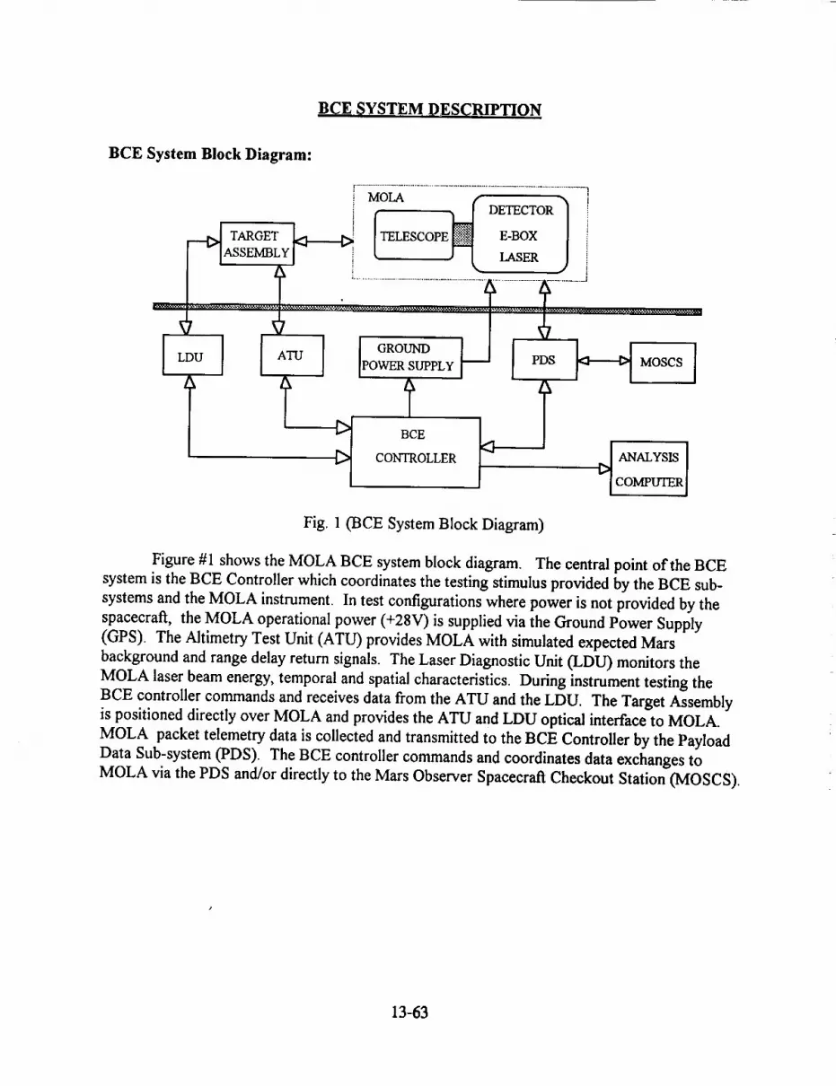
BCE SYSTEM DESCRIPTION
BCE System Block Diagram:
i [ DETECTORr_TARGET____ TELESCOPE E-BOX
[ ASSEMBLY [ - - i LASER
GROUNDLDU ATU IPOWER SUPPLY PDS
I
CONTROLLER
MOSCS
q ANALYSIS ]COMPLrrER]
Fig. 1 (BCE System Block Diagram)
Figure #1 shows the MOLA BCE system block diagram. The central point of the BCE
system is the BCE Controller which coordinates the testing stimulus provided by the BCE sub-
systems and the MOLA instrument. In test configurations where power is not provided by the
spacecraft, the MOLA operational power (+28V) is supplied via the Ground Power Supply
(GPS). The Altimetry Test Unit (ATU) provides MOLA with simulated expected Mars
background and range delay return signals. The Laser Diagnostic Unit (LDU) monitors the
MOLA laser beam energy, temporal and spatial characteristics. During instrument testing the
BCE controller commands and receives data from the ATU and the LDU. The Target Assembly
is positioned directly over MOLA and provides the ATU and LDU optical interface to MOLA.
MOLA packet telemetry data is collected and transmitted to the BCE Controller by the Payload
Data Sub-system (PDS). The BCE controller commands and coordinates data exchanges to
MOLA via the PDS and/or directly to the Mars Observer Spacecraft Checkout Station (MOSCS).
13-63

m
Target Assembly:
Fig. 2 (BCE Target Assembly)
The BCE Target Assembly is a mechanical test fixture (figure #2) that is mounted over
the MOLA instrument and holds the ATU and LDU testing apparatus. These apparatus will be
discussed in more detail under the ATU and LDU sections that follow. The three legs of the
Target Assembly are designed to have a ball-and-cup mounting interface with the MOLA
instrument. The MOLA instrument has three cup-like holding sockets located at the perimeter
comers of the instrument base mounting plate. The ends of the Target Assembly legs are rounded
to provide a ball mounting surface. This ball-and-cup mounting arrangement provide an easy and
self-aligning mechanism to ensure alignment repeatability over the MOLA instrument. The Target
Assembly is constructed of Invar and was designed for use within the thermal vacuum chamber
over wide ambient temperature ranges (+60 °C to -30 °C). The Target Assembly also houses a
combination of retro-reflector corner-cube and Risley adjustment wedges that are used to verify
the MOLA laser transmitter and telescope receiver boresight alignment.
13-64
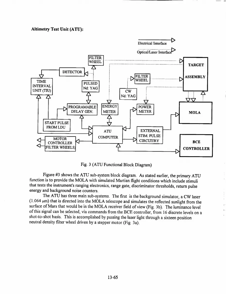
Altimetry Test Unit (ATU):
t>Electrical Interface
FILTER [_
VPROGRAMABLE [ ]ENERGY] POWER _l/ / I
STIM. PULSE
TARGET
ASSEMBLY
MOLA
BCE
CONTROLLER
Fig. 3 (ATU Functional Block Diagram)
Figure #3 shows the ATU sub-system block diagram. As stated earlier, the primary ATU
function is to provide the MOLA with simulated Martian flight conditions which include stimuli
that tests the instrument's ranging electronics, range gate, discriminator thresholds, return pulseenergy and background noise counters.
The ATU has three main sub-systems. The first is the background simulator, a CW laser
(1.064 v.m) that is directed into the MOLA telescope and simulates the reflected sunlight from the
surface of Mars that would be in the MOLA receiver field of view (Fig. 3b). The luminance level
of this signal can be selected, via commands from the BCE controller, from 16 discrete levels on a
shot-to-shot basis. This is accomplished by passing the laser light through a sixteen position
neutral density filter wheel driven by a stepper motor (Fig. 3a).
13-65

I1MOTORS&
_TERWHEELS
II
PULSED
LASER
STARTDET.
FIBERS TO/FROMTARGET
ASSEMBLEY
POWER ENERGY
METER METER
Fig. 3a (ATU Optical Bench Layout)
These filter wheel positions are programmed to provide simulated background levels ranging from
Mars night to twice the Mars expected daylight (average) levels. This feature exercises the
MOLA background noise counters, adjustable threshold discriminators, and the flight software
that autonomously adjust the receiver discriminator threshold levels to provide a predetermined
constant false alarm rate.The second ATU sub-system provides a 35 ns laser pulse (1.064 rtm) directed into the
MOLA telescope and is also located on the Target Assembly adjacent to the background
simulator (Fig. 3b).
13-66

FIBERSTO/FROM
MOL_I_cR_CNI3KARY_
L____ fMOLA PRIMARY MIRROR
& SUN SHIELD
ATU
.........OPTICAL
HEADS
\
N
TARGETASSEMBLY
Fig. 3b (ATU Optical Head Position on the Target Assembly)
This pulse simulates the laser return signal from the surface of Mars and exercises the altimetryelectronics return pulse energy monitors and ranging related functions. The luminance of this
signal can also be selected from 16 discrete levels on a shot-to-shot basis in the same manner as
the background simulator (Fig. 3a).
The third sub-system involves hardware and software programming that coordinates and
synchronizes these two laser test sources. This feature allows for simulated 'real-time' Mars
terrain topography profile data to be input into the MOLA receiver telescope thus providing an
end-to-end system functional test. This is accomplished by using a digital programmable delay
generator providing the pre-pr0grammed fire control signals to the pulsed laser. This 'canned'
topographic profile provides a means to evaluate MOLA range tracking performance, time
interval counter (TIU), range gate, and the flight software signal acquisition and trackingalgorithms.
The ATU also monitors and records the test laser output power and energy that is sent
into the MOLA telescope on a shot-to-shot basis (Fig. 3c). It also measures the actual delay ofthe pre-programmed delay times of the simulated return pulses.
........
DIFFUSE ...................................
LIGHT TO ........IMOLA .....................
FIBER /
o/y-::_:0"['_ER
50% BEAM SPLIT
Fig. 3c (ATU Optical Head Detail)
13-67

ThesimulatedMarsreturnpulses,backgroundstimuli,andmonitordataarerelayedto andfrom theATU opticalheadslocatedon theBCE TargetAssyandtheATU instrumentrackvia200ft. fiberoptic cables(200 gm corediametern= 1.4997@ 1.064_tm).
Thecontrolanddataacquisitionof theATU sub-systemsareperformedby theATUcomputerwhich interfacesto theBCE controller. TheATU computertranslatestestparameterssentby thecontrollerinto acoordinatedprocessof settingdelaysto simulateterrainpatterns,movingmotorsto setthefilter wheelssimulatingdifferentterrainalbedosandreadingthemonitoreddata. TheATU computerthenorganizesthestimulusandmonitordatain ashot-to-shotformatsothatit canbealignedandcomparedagainsttheMOLA performanceresultstherebyprovidinga meansof characterizingandcalibratingtheMOLA instrumentaltimetryelectronicsperformancefor eachtestenvironment.
Laser Diagnostic Unit (LDU):
t>Electrical Interface
START PULSE (To) [
<1 TOAn
l WAVEFORMDIGITIZER
I FAST PHOTO _ .......................ACTIVE DETECTOR
SPLITTER
LASER
DIAGNOSTICS
BOARD
(BEAMCODE)
GRABBER
BOARD
i ......................................
vENERGY
METER !
TARGET
ASSEMBLY
, ZX
MOLA
t BeECOMPUTER CONTROLLER
Fig. 4 (LDU Functional Block Diagram)
The LDU system block diagram is shown in Figure #4. The primary purpose of the LDUis to acquire data detailing the performance of the MOLA laser transmitter output. These dataconsist of laser pulse spatial and temporal characteristics as well as laser pulse energy. Opticaland electronic instrumentation to sample the transmitted laser pulse is mounted on the MOLA
Target Assembly. The Target Assembly itself is attached to the MOLA instrument during testingand evaluation ( see Target Assembly section ). Signals from the Target Assembly instrumentsare transmitted via optical fibers, coax and wire cables to the data acquisition hardware which
may be located up to 45 meters away from the MOLA instrument. The data acquisitioninstruments are housed in a 19" electronics rack. All data acquisition hardware is connected to
the LDU computer, a Compaq TM 386/20 MHz PC.
13-68
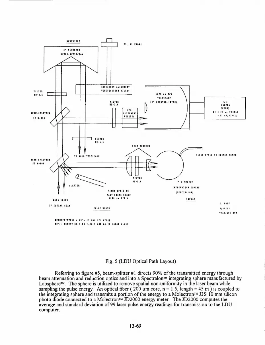
FILTU!
so-L5 I
S' UIA|[TII
117110- It£r LECTOll
IiI ] , ,
)c_ -- -"'7 t'ILIEP.
IG-G,G
1P
TO MOLA YEL£SCOPE
IO|£SlCQ! ALICIM[IT
V£|IPICI?IOI I]SL[Y
--] +L, _I llOl+
rlLTrlt
ID-I._
i
POLS[ VIDTI
1271 me [tL
T[L[SCOP[
I]" O|[STAR+IIV_|)
\
)/
I£M( It£DI_C £1t
IC-l,O 1" oIA,['r[m
I|TPCItAT 101 S pill Ill
I'll[I-OPTIC TO(SPPCIIIA LOl)
rA$1 F l O'J'O- [Il 0 Dt
12+1 .m OTA.| [IrltCt
|[AMSFLIT7£|$ I IO'! <l AIC S£C YEDG|
ID's: $CROTT [C-I,[C-2,[C-| £1D IG-%? COLOI GLASS
CCD
CAM[_A
icoie)
23 ! 27 us FIIELS
l -_I uRIPIX[L]
F;i[R-OPTIC 70 £i[RCY ME?[_
©. HoFr
S/|g/+2
YCADIIC£-OP?
Fig+ 5 (LDU Optical Path Layout)
Referring to figure #5, beam-splitter #1 directs 90% of the transmitted energy throughbeam attenuation and reduction optics and into a Spectralon TM integrating sphere manufactured byLabsphere TM. The sphere is utilized to remove spatial non-uniformity in the laser beam whilesampling the pulse energy. An optical fiber ( 200 lain core, n = 1.5, length = 45 m ) is coupled to
the integrating sphere and transmits a portion of the energy to a Molectron TM J3S 10 mm siliconphoto diode connected to a Molectron TM JD2000 energy meter. The JD2000 computes theaverage and standard deviation of 99 laser pulse energy readings for transmission to the LDU
computer.
13-69

A secondopticalfiber ( 200 iam core, n = 1.5, length = 45 m ) transmits a portion of thediffuse reflection from beam-splitter #1 to a high speed silicon avalanche photo-diode (Si-APD)
and amplifier manufactured by OptoElectronics TM Inc.. A screw-type attenuator is used to adjustthe optical throughput to the Si-APD. The Si-APD and amplifier bandwidth is 1 GHz. The pulseoutput of this detector is digitized at 2 GSamples/s and stored with a Tektronix_ DSA 602 SignalAnalyzer. The DSA 602 averages 100 pulses and calculates pulse width, peak voltage, rise timeand fall time.
The Si-APD signal is split after the amplifier to provide a To reference for the ATU and a
trigger for the Molectron TM JD2000 energy meter.Beam splitter #2 again splits the remaining energy. 90% of this energy is directed into a
1270 mm EFL Invar Schmidt Cassegrain telescope manufactured by Questar TM. The telescopefocuses the far-field beam pattern onto a 8.7 x 6.4 mm COHU TM, CCD camera. Neutral densityfilters are used to limit the beam intensity and a Risley alignment prism assembly adjusts the beamdisplacement. A typical beam cross section illuminates approximately 30 x 30 pixels on thecamera ( each pixel is 23 x 27 lam ). Power, synchronization and video signals are transferred tothe LDU rack over a 45 meter long wire cable. Camera scans are captured at the LDU computerwith an AT Vista TM video frame grabber and Big Sky Beamcode TM software. The softwarecomputes diameter, centroid and peak positions of the beam cross section.
The remainder of the pulse energy is transmitted through beam splitter #2 to a five inchretro-reflector which displaces and reflects the pulse back into the MOLA telescope. The MOLAreceiver detects this pulse and the signal is used to verify alignment of the MOLA receiver andtransmitter. A Risley prism assembly is used to manually translate this return pulse across thedetector field-of-view for alignment verification. This alignment check procedure is performedeach time after the instrument has been significantly relocated, vibration, thermal vacuum testingetc. to verify the internal laser-to-detector alignment is still within specification.
Ground Power Supply (GPS):
PROGRAMMABLEL_
POWER SUPPLY IMONITOR
& CONTROLCIRCUITRY
DATA _
ACQUISITION
BOARD
MOLA
BCE
CONTROLLER
Fig. 6 (GPS Functional Block Diagram)
A block diagram of the BCE GPS is shown in Figure #6. The GPS system consists of a
programmable power supply controlled and monitored (voltage and current) by custom circuitry
consisting of a current sensor, latching relay and accompanying electronics interfaced to a Data
Translation TM 2821 data acquisition board. The GPS system provides adjustable DC power to
MOLA, captures the instrument's current and voltage turn-on transients, and simulates over/under
voltage surges on the spacecraft power bus due spacecraft events such as battery switching, etc..
13-70

TheGPSisusedto verify thatMOLA functionsas designed over the possible range of spacecraftover/under voltage levels and transient events.
BCE Controller:
The BCE Controller consists of PC based hardware and custom menu driven software
that coordinates and controls the operation of the other BCE sub=systems with the related
spacecraft systems. The BCE Controller software provides the primary interface between a test
conductor/operator and the sub-systems shown in figure #1. Resident in the BCE Controllersoftware is a series of standard instrument tests.
BCE & PDS
INITILIZE 1ATU & LDU
TIALIZE [--""
MOLA )
___ START IATU & LDU ]
]
SEND SYNC
TO MOLA
A
PROCESS ] _",,Bu Rs USER rEST
READ & STORE DATA [__.___.J
VALIDATE TELEMETRY [
UPDATE DISPLAYS /
Fig. 7 (BCE Controller Operation Flow Diagram)
As shown in Figure #7, a typical test scenario begins with the power-up and initialization of all of
the BCE systems and the PDS. The BCE controller software sends test setup information to the
ATU and LDU software. After acknowledging the controllers setup commands the ATU and
LDU initialize their various components and then wait for a start command from the controller.
At this time the controller will either energize a relay to provide power to MOLA via the GPS or
monitor the MOLA telemetry data packets from the PDS to determine whether MOLA is
operational. Once MOLA is turned on and in the correct configuration the controller will
command the ATU and LDU to start and execute a test. Immediately after the start command is
received the ATU sends a pre-defined ranging pattern to MOLA which provides a means to align
the BCE stimulus (ATU) and laser monitor (LDU) data with the MOLA packet telemetry data.
The ATU software then sets its filter wheels, delay circuits and pulse generators to the settings
required for the specific test. As the test continues the controller acquires and processes the
13-71

stimulus,lasermonitorandtelemetrydatafrom the ATU, LDU and PDS. The controller
continues to acquire, monitor telem_etry and archive test data until the end of the test is reached or
until the test is stopped by an operator. At the end of a test the BCE Controller software updates
test logs and creates backup copies of all the data files generated from that test. The BCE test
data can then be fully processed off-line by the Analysis Computer.
Analysis Computer:
The Analysis Computer sub-system consist of data processing hardware and performance
assessment software. This BCE sub-system receives MOLA and BCE sub-system testing data
from the BCE Controller on 20 MB removable hard disk media (Bernoulli®). Raw test packet
data from MOLA and BCE sub-system stimulus data is then merged and aligned by post-
processing software on the analysis computer to form spreadsheet data files. These data files are
then processed to form summary data product files and hardcopy performance sheets (graphs and
tables). These summary performance data files are archived to form the data base for the
instrument performance trend analysis. The summary data products are used to quantitatively
determine the MOLA performance and determine that MOLA is meeting the instrument
functional requirements during that specific series of instrument tests. The instrument
performance trend data is continuously monitored for anomalous indications. The performance
data base will allow the MOLA data analysis team to evaluate mission data and predict instrument
performance trends (i.e. laser energy output, etc.).Shown in figure #8 below is a representative data analysis performance chart displaying
the MOLA range and range gate tracking performance to a triangular topographic profile
provided by the BCE/ATU stimulus.
MOLA TIU Range Values & Range Window - E-Box Temp. = 0 C & I/F Temp. = 0 C:data%011292cb.m01
455249.7188
445249.7188
435249.7188
425249.7188
415249.7188
405249.7188
395249.7188Y i t _'-
Shol #
Fig. 8 (Data Analysis Performance Chart)
= 13-72

FINAL COMMENT S
There are a few BCE sub-systems that were used with the MOLA instrument that bear
mentioning. These were not include in the main text of this paper because they were too MOLA
specific and may not be necessary or of the same design (implementation) on future altimeterinstrument systems.
The Laser External Cooler (LEC) was an off-the-shelf chiller that we used to cool a plate
that was used to conductively couple (clamped) to the side of the laser box to remove the heat
generated by the laser pumping diodes. This allowed operation the laser at or above normal room
temperatures preventing the overheating of the diodes and subsequent lifetime degradation. Also,
by varying the chiller temperature over a small range we were able to characterize the laser output
energy and pulse width as a function of temperature. For future spaceborne solid state laser
instruments, consideration should be given to having the cooling manifold integral to the laser
box. The added mass overhead will more than be compensated for by the increased operationalflexibility, simplification of hookup, and added system level safety considerations.
The laser cavity purge system was used on MOLA to prevent a laser cavity burst disk
assembly from rupturing during system level thermal vacuum testing. The burst disk assembly
was designed into the box wall of the laser cavity and is intended to rupture during the spacecraftlaunch and thus venting the laser cavity to deep space. This is necessary to avoid the critical
pressure region because of the high voltage used to operate the Lithium Niobate Q-switch. The
Class 100 cleanliness requirements of the laser cavity made this a very difficult task to manage.
Consideration should be given to future applications to implement a totally sealed laser cavity box
- fully pressurized or totally evacuated and maintained for the life of the system.
In conclusion, it is important to maintain an overall BCE system that is fairly flexible and
modular. There will always be testing anomalies and BCE component failures that will occur.
The ability of the BCE to absorb and accommodate these events must be planned for in advance.
In the end, this will greatly reduce testing cost and schedule impacts.
ACKNOWLEDGMENTS
We would like to express our deep appreciation to Mr. Roger RatliffofCode 727.3 who
spent long hours and many evenings completing the mechanical design of the MOLA BCE TargetAssembly. His innovative ideas and skilled craftsmanship are solely responsible for the success
and simplicity of an extremely complicated testing apparatus.
13-73
N94-1 619
MARS LASER ALTIMETER BASED ON
A SINGLE PHOTON RANGING TECHIVIQUE
I.Prochazka, K.Hamal, B.Sopko
Faculty of Nuclear Science and Physical Engineering, Czech Technical UniversityBrehova 7, 115 19 Prague 1, Czechoslovakia
ph/fax +42 2 848840, fix 121254 fjfi c, bitnet [email protected]
S.Pershin
Space Research Institute,Moscow,Russia
GENERAL
The MARS 94/96 mission [1] will carry, among others, the balloon probe experiment.
The balloon with the scientific cargo in the gondola underneath will drift in the Mars
atmosphere, its altitude will range from zero, in the night time, up to 5 km at noon. The
accurate gondola altitude will be determined by an altimeter. As the balloon gondola mass
is strictly limited, the altimeter total mass and power consumption are critical, maximum
allowed is a few hundreds grams and a few tens of mWatts of average power consumption,
only. We did propose, design and construct the laser altimeter based on the single photon
ranging technique.
PRINCIPLE OF OPERATION
The system operation is based on the single photon laser ranging technique : the short
and low power laser pulse is transmitted in the nadir direction, the signal reflected from the
planet surface is collected by the receiver lens and detected by the photon counting device.
The light time of flight is measured. Completing the series of measurements, the altitude, the
range to the surface, may be evaluated. The number of individual laser fires needed for one
altitude determination is limited by the altitude itself, the background illumination intensity
and hence the signal to noise ratio and the balloon gondola vertical velocity. Thanks to the
relatively high repetition rate of the laser transmitter (currently 7 kHz, the 25 kHz version
is expected to be available in the near future), one altitude measurement may be completed
within fractions of a second.The single photon ranging technique has several key advantages in this application •
• the low power, high repetition rate diode laser may be used as a transmitter,
• the wavelength of such a transmitter well coincides with the maximum sensitivity of the
semiconductor photon counting detector,• no analog signals are treated within the device, all the information is obtained from the
statistical treatment of the set of range measurements. This fact is resulting in overall
simplification of the device and its performance stability within a wide temperature range.All the electronics may be based on digital, low power CMOS circuits only, what is resulting
in low mass and low power consumption,
• the laser ranging system may be used, for the atmospheric clouds, haze and aerosols
monitoring, as well.
13-74

ALTIMETER CONSTRUCTION
As a transmitter, the integrated laser diode pulser LD191 is used. It delivers uniform,
fast risetime pulses at 880 nanometers wavelength 100 nanoseconds long with the energy of
2 microJoules. The receiver consists of a Single Photon Avalanche Diode detector package
[2], its operating voltage is controlled by a newly designed circuit in a wide temperature
range -60 to +20 Centigrade. The diode's quantum efficiency reaches 20 % at this
wavelength range. The transmitter and receiver share the same optics of 40mm aperture, the
optical path is separated by a polariser. To keep the optics as simple as possible, the diode
aperture and hence the receiver field of view is not perfectly matched to the laser transmitter
one. By this compromise the optics mass and alignment precision requirements have been
significantly reduced on the expense of the energy budget link. The bandpass filter 5
nanometers wide having the transparency of 60% is used to reduce the background
illumination. The altimeter electronics consists of a flying time counter having 33
nanoseconds resolution, the programmable range gate generator, the control logic andinterface to the board computer.
To facilitate the single photon ranging even under the Mars daylight conditions, the
combination of the detector limited field of view, optical ban@ass filtering, the adjustable
range gate electronics _md the data processing software have to be applied. One out of threemain strategies may be selected for setting up the range gate •
1. 'Start from scratch' all the possible range gate settings are consequently applied, the echo
signal is recognized. This is an emergency solution not requiring any a priori knowledge ofthe altitude to be measured.
2. ' Morning take off' starts from the range gate interval 0 - 150 meters. It is based on thepresumption, that the gondola will take off after the sunrise.
3. ' Routine operation ' the range gate setting is predicted on the basis of the previously
measured altitude and vertical velocity. The signal search in the +/- 1 range gate intervalmay be carded out, if necessary.
GROUND TESTS
To proof the feasibility of the device, the experimental system has been constructedat the Space Research Institute, Moscow
and tested in a series of ground test at the
Czech Technical University. The ultimate
single shot range resolution and the mea-
sured range dependence on the echo signalstrength (the range bias) have been mea-
sured. The LDI91 laser diode pulser, the
single photon detection package and a highresolution time interval unit has been used.
The results are plotted on Figure 1 together
with the return rate. From the single shot
range resolution of 4-5 meters one can
conclude, that the ranging precision of one
meter may be obtained averaging more than
25 returns. The ground target ranging with-
in the ranges 0-3.5 km has been obtained
t(
6
4
0:
0.I
bJas,i._.___2tte_,_2Imele_s. relurn rate
_ o..... ...................................... "_
0.1
........ J.01
I I0 I00 IOOI
sJcjnalslfenglh IpholonslecholI.Procha/kl,S.Pefskill, Pl'llglle, NOI'.Ig89
Figure 1 Indoor calibration test
using the optics aperture of 17 mm only. The example of the ranging result is on Figure 2,
13-75

Ground target ranging, 3.5 km distance
Fig. 2
L_ER md, se_ 600gO SPill)vulses 2593,6691
elevation angl e:Sg_leg
Gat_ 4 M_
Vertical humidity haze monitoring, daylight
multiple haze layer may be seen
13-76
Fig. 3

this is a horizontal ranging to the 3.5 km distant target in a light'haze visibility conditions.
Employing the full 40 mm aperture optics of the final version, the full range will be guaran-teed.
The single photon ranging system may be used for the atmospheric transparen-
cy/backscatter monitoring [3]. Currently, the proposal, that such a system may be used for
the Mars atmosphere monitoring, is under investigations. Either using the independent unit
installed in the 'Small Mars Station' [4] or directly from the balloon gondole in the night
time, when is it located on the surface and it is not used for altimetry. In another words, the
system may be used for the clouds distance and density profile monitoring, as well. On
Figure 3 there is an example of the results of the clouds monitoring. The laser rangefinder
was pointed to the zenith, the lower cloud boundary and its density profile may be
recognized. The clounds may be monitored day and night up to the height of 1 kin.
CONCLUSION
The altimeter based on the single photon ranging technique outranged the microwave
and Nd YAG laser systems by low weight, low power consumption and the compact design.
The mass, dimensions and price of such a system make it attractive not only for Mars
mission, but also for mobile, air and space born remote sensing applications. The excellent
stability of both the laser transmitter and the single photon detector permits to calibrate the
receiver sensitivity to high accuracy and thus to use the system as a precise visibility and
surface reflectivity sensor. The applications of a visibility sensor in automated meteo stations,
traffic safety, air and ship safety systems seem to be quite promising. In all these
applications, the eye safety of the laser transmitter is a significant advantage of the device
decsign. The air and space born remote sensing application in agriculture, geology, large area
forest monitoring, soil humidity and radioactive Cesium dust monitoring is underconsideration.
References
[1] R. Sagdeev, Physics Today, 5, 30 (1988)
[2] I. Prochazka, K.Hamal, B.Sopko, G.Kirchner , Technical Digest of the Conference on
Lasers and Electro Optics, CLEO 91, Baltimore, May 1990
[3] I.Prochazka, K.Hamal, S.Pershin, Capabilities of Single Photon Detection in LIDAR for
Atmospheric Studies, International Symposium On Radars and Lidars in Planetology, Cannes,France, Sept. 1991
[4] I.Prochazka, K.Hamal, et al, MARS 94 Mission Backscatter LIDAR for Small Mars
Stations, Gound Tests Results, European Geophysical Society XVII General Assembly,Edinburg, April 1992
13-77
94--156 0
MULTI-BEAM LASER ALTIMETER
Jack L. BurtonDavid J. Harding
Luis Ramos-lzquierdo
Laboratory for Terrestrial PhysicsGoddard Space Flight Center
Greenbelt, MD
Laser altimetry provides a high-resolution, high-accuracy method formeasurement of the elevation and horizontal variability of Earth-surface
topography. The basis of the measurement is the timing of the round-trippropagation of short-duration pulses of laser radiation between a spacecraft andthe Earth's surface. Vertical (i.e. surface elevation) resolution of the altimetrymeasurement is determined primarily by laser pulsewidth, surface-induced
spreading in time of the reflected pulse, and the timing precision of the altimeterelectronics. With conventional gain-switched pulses from solid-state lasers andsub-nsec resolution electronics, sub-meter vertical range resolution is possiblefrom orbital altitudes of several hundred kilometers. Horizontal resolution is afunction of laser beam footprint size at the surface and the spacing betweensuccessive laser pulses. Laser divergence angle and altimeter platform heightabove the surface determine the laser footprint size at the surface; while laserpulse repetition-rate, laser transmitter beam configuration, and altimeter platformvelocity determine the spacing between successive laser pulses.
Multiple laser transmitters in a single altimeter instrument provide across-track as well as along-track coverage that can be used to construct a range image(i.e. topographic map) of the Earth's surface. Figure,1 is an illustration of thepushbroom laser altimeter instrument measurement concept that utilizes multiplelaser beams. This multi-beam laser altimeter (MBLA) contains modular lasersources arranged in a linear, across-track array. Simultaneous or nearsimultaneous measurements of range to the surface are possible by independent
triggering of the multiple laser pulse transmitters and reception by a singletelescope that is staring at nadir and is equipped with a multi-element lineardetector array in its focal plane. This arrangement permits alignment of eachtransmitter output into a separate, dedicated receiver channel. The illustratedconfiguration is a linear, contiguous across-track array of 30 beams whichproduces a strip-image range map of the Earth's surface. This MBLA configurationis one possible arrangement to accomplish high accuracy terrestrial topographicmapping near the nadir track in a NASA Earth Probe mission devoted to globaltopographic measurements. The configuration can be changed in accord withrequired science products and available resources. Possible modifications in thedesign include variation of footprint size and/or footprint spacing both along-trackand cross-track to produce the desired coverage or sampling density within thesensor swath width.
The illumination pattern incident on the Earth's surface from any onetransmitter element is a two-dimensional circular pattern of laser irradiance, with aGaussian spatial distribution of illumination intensity, that is produced by a single
- 13-78
transverse (spatial) mode of the laser cavity. The transmitted laser pulsewidth isshort (i.e. ~ 5 nsec full-width-at-half-maximum). The temporal distribution of laserirradiance in the pulse is approximately Gaussian and is the result of multiplelongitudinal laser cavity modes produced by the gain-switched (Q-switched) lasercavity. In an ideal altimeter application (e.g. measurement of a smooth watersurface) the backscattered laser pulse retains the shape of the incident pulse.However in the general case, the height distribution (i.e. roughness) and slope ofthe surface within the laser footprint produce spreading in time of the laser pulsereflected to the receiver. After interaction of the laser footprint with a rough orsloping surface, the backscattered pulsewidth may be expanded to several tens toseveral hundreds of nsec. The spread pulse degrades range measurementaccuracy but analysis of the received pulse shape provides additional informationon surface structure.
Figure 2 illustrates the pulse spreading effect and portrays the measurementapproach in laser altimetry by providing the time varying amplitude of an altimeterdetector that observes both the transmitted and backscattered laser pulse. Pulsespreading, by re-distributing the available pulse energy into a larger time interval,acts to reduce the peak-power signal-to-noise-ratio, thus increasing the probabilityof error for the range measurement. Pulse spreading also adds timing uncertaintyby slowing the rise time of the return signal. Variability in pulse rise time in turnproduces a time-walk effect when conventional threshold-crossing time-interval-unit devices are used for the range measurement. The application of GHz-bandwidth digitization or multi-stop time-interval measurement to the receiver pulsewaveform provides pulse shape data. Digitization is indicated by the horizontalaxis tick marks in Figure 2. The centroid Ts of the pulse shape data is used tomake a timing correction that provides the measure of range-to-surface. Thecentroid is in effect the mean round-trip time-of-flight range to surface featureswithin the laser footprint, weighted by: (1) the input two-dimensional Gaussianillumination pattern; (2) the reflectivity and areal extent of the surface features; and(3) the laser altimeter receiver transfer function.
The pulsewidth (or rms pulse spreading) that is derived from digitizer ormulti-stop timing data is used to assess the magnitude of surface slope and/orsurface structure within the footprint• Pulse spreading data taken together withalong-track and across-track slope information provided by adjacent range pixels,enables calculation of the sub-pixel (footprint) slope or roughness. An analyticalexpression has been developed (Gardner, 1991) to express pulse spreading(mean square pulse width) in terms of the laser altimeter system parameters, beamcurvature, nadir angle of observation, surface slope, surface roughness, and laserreceiver operating signal-to-noise ratio.
The total area under the received pulse is proportional to pulse energy andis a measure of surface reflectance at the monochromatic 1 l_m laser wavelength.Effective use of this reflectance data requires normalization by laser transmitterenergy and consideration for atmospheric transmission. Reflectance data acquiredwith the pushbroom scan pattern of the laser altimeter provide an imagingcapability that supplements the ranging functions. Since this image is acquiredwith an active sensor that transmits and receives only near nadir (180 ° phasefunction, i.e. backscatter mode), the surface illumination angle is fixed within 1° ofzenith and the resultant image is free of bidirectional reflectance effects that exist inpassive _mages with variable solar dlummat_on geometries. Surface slope effects
13-79

on this reflectance image can also be directly characterized from the associatedlaser altimeter along-track and across-track range measurement record.
The functional block diagram of the multi-beam laser altimeter instrumentappears in Figure 3. The laser transmitter module, receiver telescope, detectorpackage, ranging and waveform electronics, GPS receiver, and pointing attitudemeasurement components form the major instrument subsystems. Thesesubsystems are packaged into a common structure that provides a rigid platform forthe laser transmitter, receiver optical components, and dual star cameras. The size
of this structure is primarily dependent on telescope a.perture (~ 0.9 m). The keycomponent of the laser altimeter instrument structure _s a lightweight, rigid opticalbench illustrated in the perspective view of the MBLA Instrument in Figure 4 andthe cross-sectional view of Figure 5. The altimeter telescope primary mirror isattached to the nadir-viewing side of the optical bench and the laser transmittermodules, detector package, and dual star cameras are attached to the oppositeside. This construction ties all the transmitter and receiver optics together formaintenance of arc sec alignment. Beryllium is the material of choice forfabrication of the telescope optics and structure, optical bench, laser module cases,and the star camera mounting brackets. Beryllium provides a rigid optical platform,superior thermal diffusivity for removal of waste heat, an athermal optical train, anda minimum total mass. With these beryllium components, the design illustrated inFigure 5 has a mass of ~ 60 kg. Mass of the altimetry electronics, instrumentcomputer, thermal, power, and GPS receiver subsystems bring the instrument totalto ~ 100 kg.
The pulsed transmitter is based on high-power neodymium (Nd)-dopedsolid-state laser crystals and employs the Q-switching technique to concentratelaser energy in a short pulse. Each of the 30 laser transmitter modules illustratedin Figure 5 is optically-pumped by separate AIGaAs laser diode arrays that arecoupled into the Nd laser crystal by fiber-optic cables. This results in an all-opticallaser module that is separated from the electronic and power supply components ofthe laser subsystem. The majority of thermal dissipation for the laser modules canthus be grouped together and placed at a remote radiator location in the spacecraftinstrument. The laser module design is a scaled version of present-daycommercial diode-pumped Nd laser technology that is in use in NASA airbornelaser altimeter systems. The illustrated array of laser transmitter modules iscapable of producing ~ 7000 pulses-per-sec and requires average input electricalpower of 1 kW when operational.
Optical backscatter from the Earth's surface is collected by the MBLAtelescope that is fixed in orientation at the nadir track of the spacecraft. A series oftwo optical lenses and optical bandpass filters are used to collimate, filter, and thenfocus the backscattered radiation on the detector plane. Each laser transmitterelement is angle-mapped into a silicon avalanche photodiode detector arrayelement for a continuous two-dimensional range and reflectivity image of thesurface. Energy measurements are made for the transmitted and received laserpulses and are affected by the reflectivity and transmission of the various opticalsurfaces in the instrument as well as detector sensitivity. Optical contamination anddegradation for long term exposure to the space environment are potentialproblems. An on-board laser diode emitter can be utilized as a calibration sourceand coupled with fiber optics into the optical detectors. This method will maintaincalibration for the energy measurement for surface reflectance studies.
13-80
Pointing attitude knowledge is generated by dual star cameras. Each camerais a second-generation star tracker that employs a 2-dimensional CCD array that iscapable of simultaneous tracking of as many as five stars. On-board Kalmann-
filtering is utilized to compare stellar angular position data with a star catalog andprovide an output pointing attitude estimate; in principle eliminating the need for aninertial reference unit. Both star cameras are capable of 1 arc sec (total angle)pointing knowledge limited by the quality of the star catalog. The dual star camerasystem can provide the 2 arc sec total angle (1-sigma) knowledge required for sub-meter accuracy altimetry. Pointing angle data are continuously generated with-respect-to the stellar inertial reference frame. Laser pointing angles are tied to thestar camera data through beam angle sensors which sample a portion of one ormore output laser pulses and measure the angle (at the arc-sec level) of reflectionfrom reference mirrors on the star cameras. Output laser pulse samples are alsocoupled with retroreflectors directly into the receiver telescope in order to assessalignment shifts between telescope and lasers.
The pulse timing data, waveform digitizer, and pulse energy data form thebasic laser altimeter dataset for each laser pulse. These data points accumulate ina buffer in digital form, are formatted into data blocks or files, and then enter thealtimeter platform data stream for recording or telemetry. The expected data rate ofthe laser altimeter resulting from 1000 - 7000 laser pulse measurements a
secondis estimated to range from 10 - 50 kbps. On-board processing is plannedfor the ranging centroid correction and waveform shape data products. Datatelemetry involves range-to-the-surface, waveform shape products, sensorhousekeeping, pointing attitude, and GPS position data. Post processing on theground is used to correct the altimetry data for the precision orbit and spacecraftpointing attitude. The basic data products are a gridded topographic mapcontaining >1010 surface elevation measurements with the selected horizontalresolution (grid size) and an image of Earth's surface reflectance at 1 _mwavelength with a similar level of detail. These products will be developed withminimal ground processing, stored on compact optical disks, and made available
to the scientific community in a timely fashion. Analysis and use of the topographicdata will be done by tl_e end user in the scientific community.
REFERENCE:
Gardner, C.S., "Generalized Target Signature Analysis for Laser Altimeters",Applied Optics, 1992.
ACKNOWLEDGMENTS:
The definition of the MBLA instrument was made possible through the efforts of anumber of individuals in the Laboratory for Terrestrial Physics (LTP) at the GoddardSpace Flight Center and' in the aerospace industry. Notable among these effortswere those of David Rabine in the University Research Foundation of the MarylandAdvanced Development Laboratory, Nita Walsh of Science Systems andApplications, Inc., Ying Hsu of the Optical Corporation of America, DavidThompson of Spectrum Astro, Inc., and Tom Baer, Spectra Physics, Inc.
13-81

MULTI-BEAM LASER ALTIMETER MISSION CONCEPT
EARTH PROBESPACECRAFT
400 km
SUN-SYNCHRONOUS6am/6pm
POLAR ORBIT
SUNLIGHT
LASER PULSES (30)
1 _mWAVELENGTH
NADIRTRACK
SENSORFOOTPRINT30 m diam.
9OO mSWATHWIDTH
ACROSSTRACK
DIRECTION
Fig. 1
13-82

n=0
oa=
n,'w)==w
I
==J
n,=W
=J
)
(
(
_.o
8_
E_
_=
v
(_E
oi
F=
t-_r: _'_ =m r t (_
-b°_
t--
i
1.1_
13-83

13-84
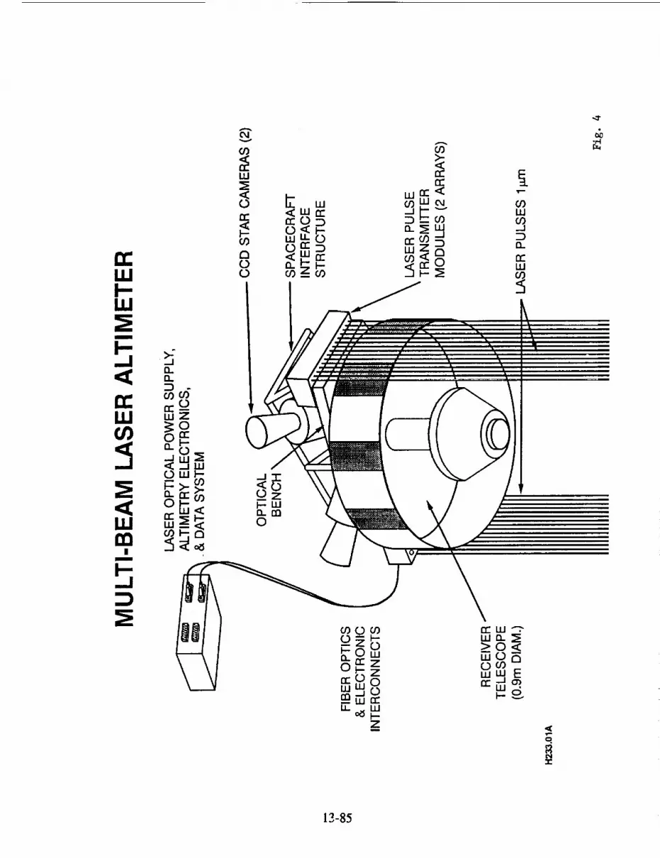
i
_J
g
13-85

LO
U-
n-W
W
m
-J
q)
Wrn
.J
] E
o
13-86

Poster Presentations


N94-156 1
SATELLITE LASER STATION HELWANSTATUS 1992
M (_ech, K.Hamal, H.Jelfnkov_l, A.Novotn)_, I.Proch_ka
Faculty of Nuclear Science and Physical Engineering, Czech Technical UniversityBrehova 7, 115 19 Prague 1, Czechoslovakia
phone / fax +42 2 848840, telex 121254 fjfi c, E-mail [email protected]
B.B.Baghos, Y. Helali, M.J.Tawadros
National Research Institute of Astronomy and Geophysics, Helwan, Egypt
phone / fax +20 2 782683, telex 93070 hiag un, E-mail [email protected]
GENERAL
The Satellite Laser Station Helwan has been ope'r.ated jointly by the National Research
Institute of Astronomy and Geophysics in Helwan, Egypt and the Czech Technical University
in Prague, Czechoslovakia (see Proceedings of the 7th International Workshop on Laser Ranging
Instrumentation, Matera, 1989). The station components have been carefully tuned to increase
the system overall stability and reliability critical for the remote location. The mount correction
model based on the Gaussian smoothing (Kabel:_, 1990) has been implemented to simplify the
blind satellite acquisition and tracking. The on-site normal points generation algorithm has been
implemented, the station has been connected to the international information network. The ERS-
1 satellite has been included into the tracking schedule. The station range capability has been
verified by experimental' Etalon 1 ranging by April 1992. The ranging precision of 2-3
centimeters is obtained when ranging to ERS-1, Starlette and Lageos satellites.
The station operation has been cosponsored by the DGFI contracts ERS-1/7831/91,92 and
the Smithonian Astrophysical Observatory contract, whose support in acknowledged.
14-1

N94-1562 '
C0
om
L-
0
L.
00
e"im
¢D
m
0')C
I.U
m
m
u_X
em
e-
ra
14-2
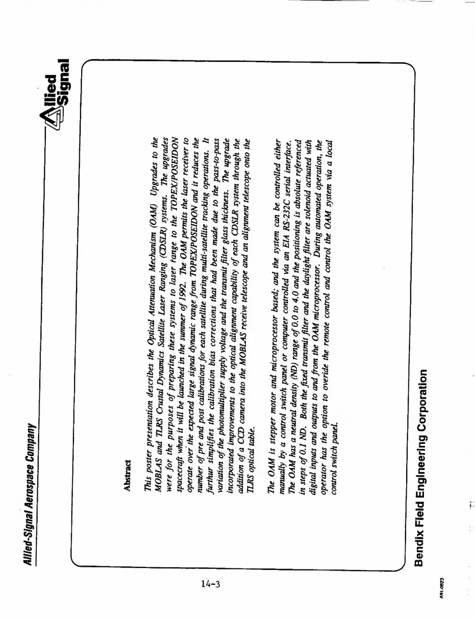
14-3

m
"_t-0_
im ,m
J8NOtl.l.O_rl=O.l.OHd NI HJ.IDNg'dJ.E "IYNDI8
m o
0Z
0Z<
N
ID
0
14-4
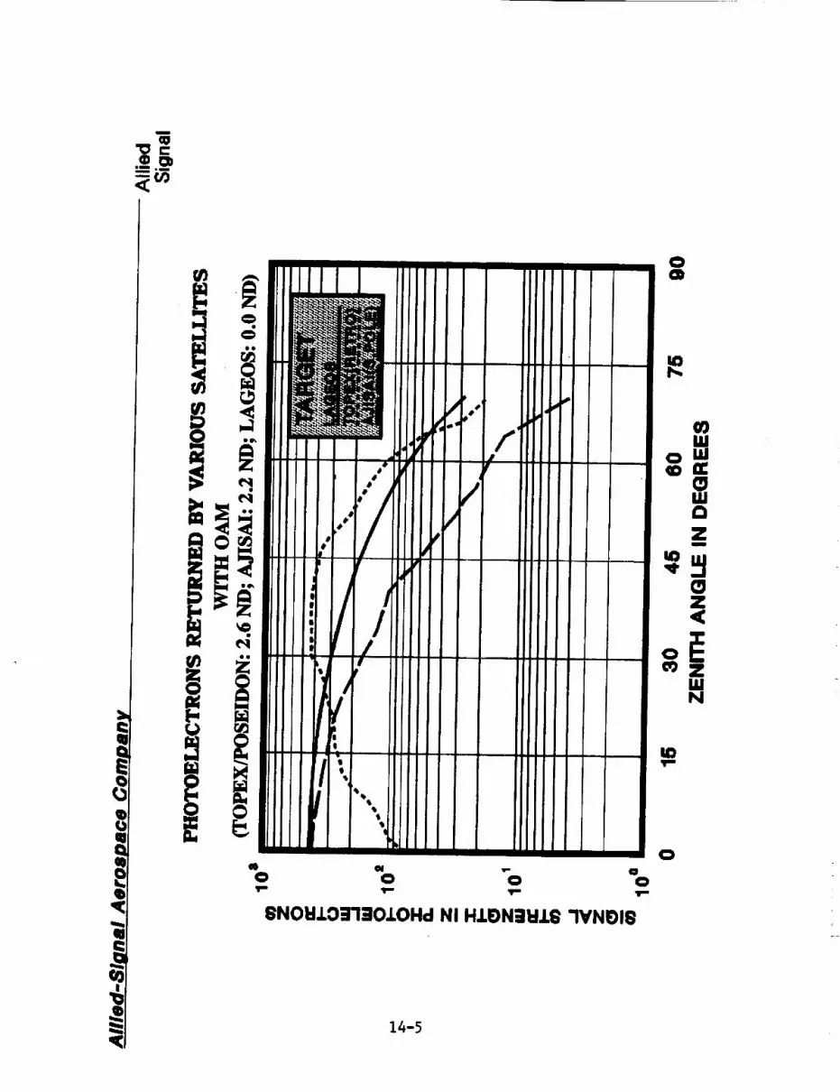
u
_,.,>
!1 14-5

!,i
11
c_
f
-- j\l I!l-I _ _ _ _ :r_ _ r--_- ................
-- -r I (41
=- 't I _!1 _ I ,i _7_ I
i _____.............
1 \ / i
[ .................................. ,i
14-6
im
C_
!11
IL
tD
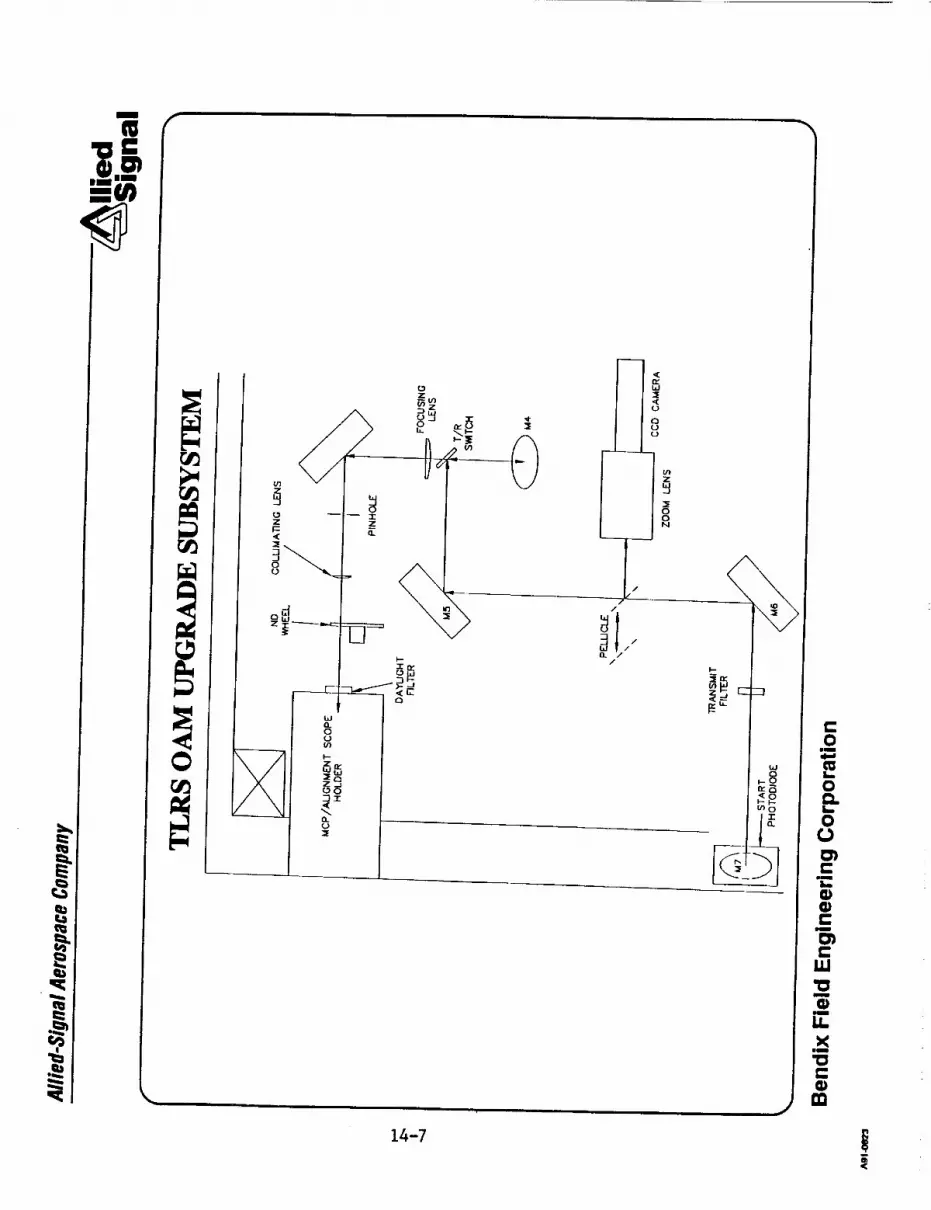
___N
0
0
l
/
/
o./
14-7

I
Iit
.&
r_Z0
r_
=
©
1II
'_1"- r,D ,,--' =
-g :_ "-1/ .< ,,e ,.e,°
.... _ c_'_ o
• ,-w
_ _ _'_-. ___
o_oAV_ _ -_,- o_._ _ :_
•__ _o° __ _ O
°_
g0 --
@_.9,o
[--,
Z
o,IL,
°°
14-8
0.m
I.-_
0
0o
.i
.m
m
.i
.m
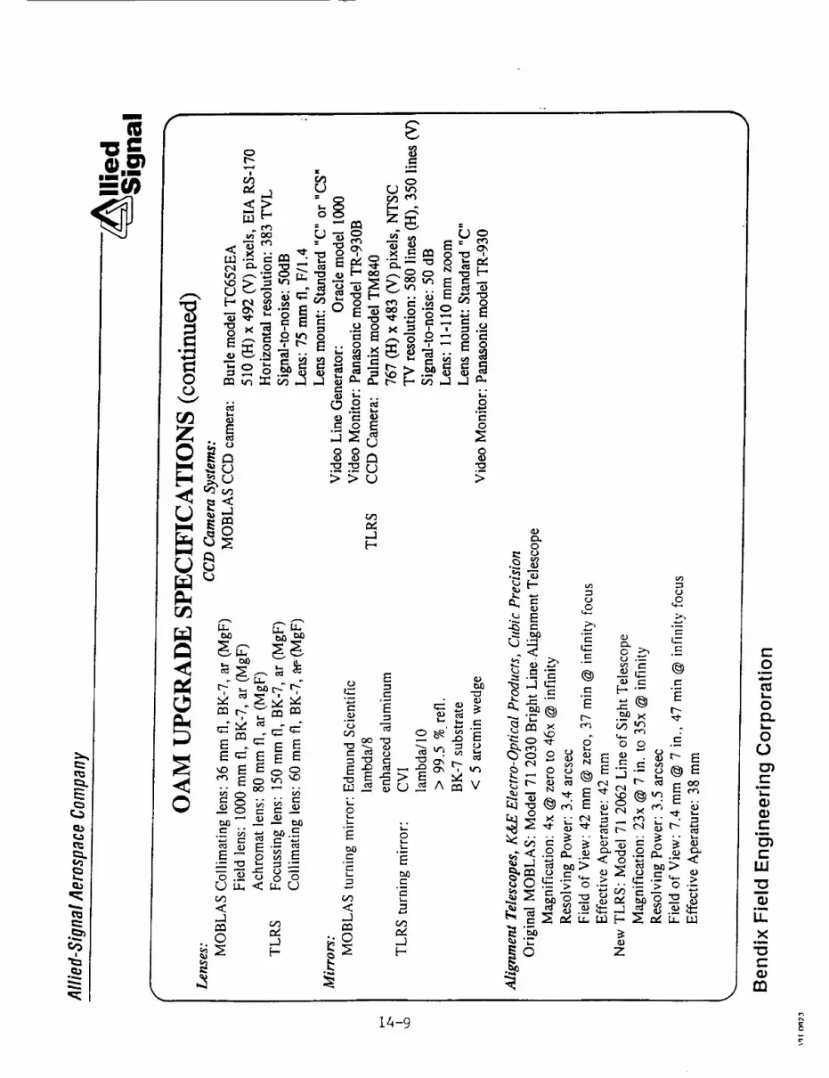
t_
t_
t_
_A
o
°_
°_
_ [.-.. ....
•;_o_ _oe_o_=_
_-_ _ _s_ _2-- __
_ o _-_ _ ._ _ ._-_ o ..-.
_'_
_° _
e-o
.m
0
00
r-_m
e-
r-
X.m
e-
m
14-9

ORIGINAL PAGE
BLACK AND WHITE PHOTOGRAP,'-t
14-10

ORIGINAE PAGE
8LACK AND WHITE PHOTOGRAPH
14-11
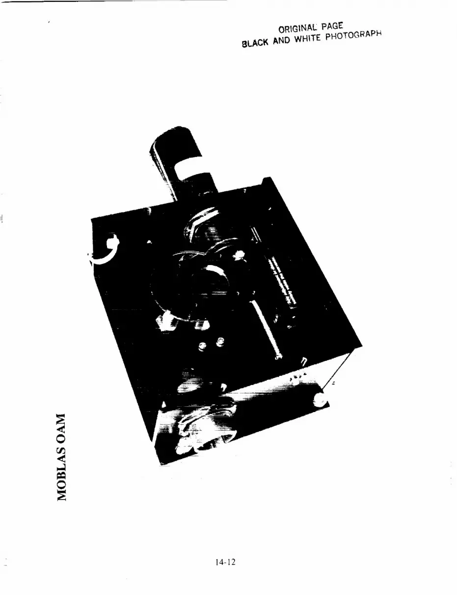
ORIGINAE PAGE
BLACK AND WHITE pHOTOGRAPF_
OC/3
.J
O
14-12

ORIGINAL PAGEBLACK AND WI-t_TE PHOTOC_APH
Or._
III
II
14-13

N94-15623
THE THIRD GENERATION
SLR STATION POTSDAM NO.7836
H.Fischer, L.Grunwaldt, R.Neubert
GeoForschungsZentrum Potsdam
Telegrafenberg A17, D-O-1 561 Potsdam
Phone: (037.33)-310-0
Fax: (03733)-310-648
(03733)-22824
E-Mail: [email protected]
The new SLR station Potsdam has been installed uuring Winter 1991/1992 in an
existing dome near to the old ruby laser at Helmert Tower. It has been built arounda one-meter-Coude telescope and is equipped by a 50 ps Nd-YAG laser and a
SPAD receiver. First successful LAGEOS passes were obtained in May 1992
demonstrating 2-3 cm rms at the single photon level.
The new station will be used for experimental work and selected observation
campaigns as well.
14-14

HARDWARE SPECIFICATIONS
Mount and Telescope:
One-meter Coude system type TPL (Riga University)common transmit-receive path switched by rotating mirrors
step motor drives for azimuth and elevation
Receiver Package:
Silicon avalanche photodiode type C 30902 S-TC (integrated Peltier cooling)
operated in the Geiger mode with passive quenchingstandard interference filter, spectral width 2 nm
Laser:
Nd-YAG with passive modeiocking by dye #3274 (own construction)KTP frequency doubler
main data at 532 nm: 10-20 m J, 35-50 ps, 10 Hz
Time Interval Counter:
Stanford Res. Labs. type SR 620
Time Base:
GPS- receiver Datum Inc. type 9390-55134, internal Rb- standard
Control System:
Standard PC (HP Vectra 386) interfaced via IEEE-488 to the
specially designed control unit (step motor controller,gate pulse generator, epoch counter with 100 ns resolution)
14-15
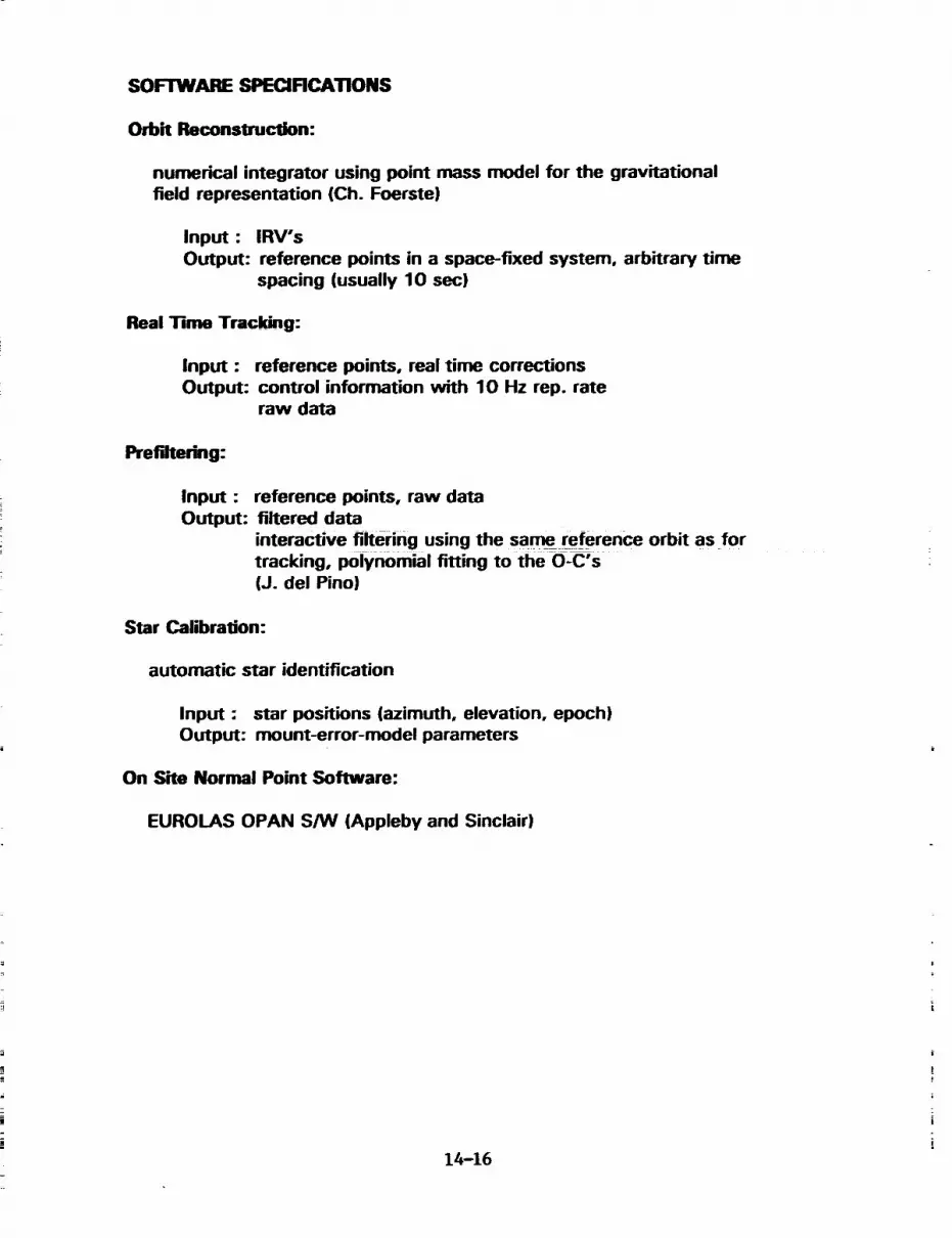
SOFTWARE SPECIRCATIONS
Orbit Reconstruction:
numerical integrator using point mess model for the gravitational
field representation (Ch. Foerste)
Input : IRV'sOutput: reference points in a space-fixed system, arbitrary time
spacing (usually 10 sec)
Real Time Tracking:
Input : reference points, real time corrections
Output: control information with 10 Hz rep. rateraw data
Prefiltedng:
Input : reference points, raw data
Output: filtered datainteractive filtering using the same reference orbit as for
tracking, polynomial fitting to the O-C's(J. del Pino)
Star Calibration:
automatic star identification
Input : star positions (azimuth, elevation, epoch)Output: mount-error-model parameters
On Site Normal Point Software:
EUROLAS OPAN S/_N (Appleby and Sinclair)
14-16

I I I I
÷ +÷
I I _ : +_'_ +÷
+ + + 4" +
÷ + ¢ t+ ÷
4,! ,! ! • l
I I. I :'÷I÷ :h÷,÷÷., ,4-
4. ÷p
Fri 8 /Na_tg2P_._S : 48758 O/E : 8 1>o ly t,
SHOTS: 171 ECHOES: 71 r 8.823X !=tosraNUnit: 8.8Z mNax= 25
:2 Filter F3 2r F4 l/O F6 Out F? Poly Order Fn Delete F9 Record FlO Histogram
Screen copy of a LAGEOS test pass after filtering and polynomial fitting
upper part: residuals versus time (23 mm rms)
lower right: histogram of the residuals
Optical scheme of the laser PLS-5
Symbols: Pr- prisms, M- mirrors, NDF- neutral density filtersMD- monitor photodiodes ; Pol- polarizers
14-17

Laser control room
14-18
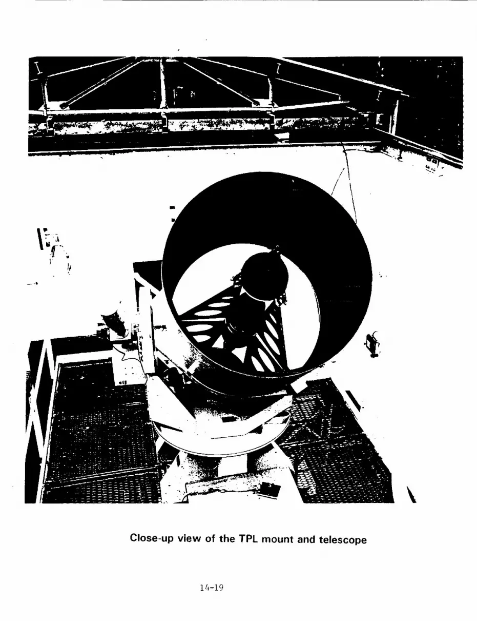
\
Close-up view of the TPL mount and telescope
14-19

N94-15624
PERFORMANCE COMPARISON OF HIGH SPEED MICROCHANNEL PLATEPHOTOMULTIPLIER TUBES
Thomas Varghese, Michael Selden, Thomas OldhamAllied-Signal Aerospace Company
Bendix/CDSLR Network
Seabrook, Maryland 20706U.S.A.
The transit time spread characteristics of high speed microchannel photomultipliershas improved since the upgrade of the NASA CDSLR network to MCP-PMT's in the mid1980's. The improvement comes from the incorporation of 6/_m (pore size)microchannels and offers significant improvement to the satellite ranging precision. Toexamine the impact on ranging precision, two microchannel plate photomultiplier tubes
(MCP-PMT) were evaluated for output pulse characteristics and temporal jitter. Thesewere a Hamamatsu R 2566 U-7 MCP-PMT (6#m) and an ITI 4129f MCP-PMT (12/_m).
An Opto-Electronics diode laser and a Hewlett Packard 50 GHz digital sampling scopewere used to sample a large number of pulses from each tube. The jitter of the
sampling scope trigger was independently measured by splitting the diode laserpretrigger signal; one portion of the signal was used to trigger the scope, while theremaining signal was measured by the sampling scope. The scope trigger jitter wasfound to be about 2.6 ps. The laser pulses were _,z40 ps in duration with a wavelength
of 764 rim; the pretrigger-to-fire jitter of the diode laser is _,z5 ps. During the experimentthe pre-fire output ,of the diode laser control unit was used to trigger the samplingscope while the output responses of each MCP-PMT was captured by the sampling
scope.
The optical input from the laser diode was adjusted to produce ~ 7 - 10 photoelectronson the average. To measure the detector response, several thousand MCP-PMT outputpulses were digitized to construct a pulse-distribution for each detector.Measurements were taken around the single (1 - 3 pe) photoelectron level as well as
the multi-photoelectron (-" 5 - 10 pe) level for each PMT. An average waveform wasused to determine pulse rise-time and duration, while the standard deviation of the
pulse distributions at the half-maximum point were used to determine the RMS of thetemporal distribution within each sample set. Statistical information is printed beloweach graph. Each MCP-PMT was tested separately but under identical conditions. Forthe above experimental conditions, the I'lq MCP-PMT produced about 36 ps jitter whilethe Hamamatsu MCP-PMT produced 9.1 ps jitter.
14-20
The sampling scope jitter and diode laser jitter has no significant effect on the 12/Jm
PMT measurement while deconvolution improves the jitter of the 6/Jm tube to ~ 7 ps.The single photoelectron jitter can be estimated from these measurements to be ~ 110
ps and ~ 25 ps respectively for each tube.
The results of these tests suggest that the MCP-PMTs with 6 micron pore size has the
potential to offer improved (x 2) satellite laser ranging data quality, especially at lowphotoelectron levels. Further testing of a gated Hamamatsu MCP tube in MOBLAS-7 in
a parallel configuration using the NASA Portable Standard is planned for later this year.
These tests will focus on relative performance at various signal levels as well as the
response of the constant fraction discriminator to the higher bandwidth detector output.
14-21

0m
F-
rorrW
0
tr
0UJ0
Wr_
I I|
m_,==
Or)!
m
D-.!
CO ---_
M')
rr
Z_ "-"Or)-I--
!
< eJ
<n-
Q.0
cO
I&!rr"
I--<LLILI_
m m
e- r-e- e-
.1_ e-
o oL_ t_O O
Bm Im
OO
_2
ffl
O
2_
OO
Vl
ffl ffl _
E o e-_0 _- (0 0 0 It)(0 x 0 0 _ OJ
, _ _ _
E
co
rr
E_n
F-_m
LL
m
0
t_ ._
00
!._
_m
c-oi....
0
_D00
n
t-_m
14-22

14-23

0Q.t_LU
,,,J,<I:I:i,,-.0i!1Q.t,/)
IlI
%
I
:::)¢0t,,,Oi.{")CMrr':::)r,_I--<
<
<-r"
_ Jmiua _._,,_ i ,-:.i1..•
.................:- '' :"""'+"'"B",_I:-I,,,,'.- ,i!
• !--". _ -i i,']. I_ -'""
=',I :I ! t!.'.-'" i,_ " I I.' ,LIJI I'1':
"' ', i .l., ! --:..:
mu
i!
I-
i,.
i'iii
g -u
_1111.......................,,,..... _ _ .o
-tllllli _""m///
Y.ir! I V 1':::: : : :::it l-I--- IIIIl'_'l-I-
IIII I I/1 t111
--Jill Vi i. -_-II1_1 I-t. -..-.-III I._ 1-1"- *
.........J!llll --IIINI I Iiiii i I
.......... • .--I..',II I..".."NII_ i IIIIIII
• _wl I I I I-I- I- =
"o o "o r,,
i-d_' I
_-iII
!-_m|
111 I II
14-24

g]
,-_ 0 rh m
,_ o o
o_ _ - _; 2_I !
II II II II II II
oc_ _ _ m 0_ o
i,iTt--
b_0
I--ZbJ
Ldn,-
<b_l
,-I0 Ld
00oO
Z
.J+J CL
® <
'0b_0
w0 O9
Z
0
'0
,_-_ 0 0 _0._O0
O"Cl :> > I_ I_ ,._ bJ
0 0 .,,-_r-O_lD _ .IJ ,¢--..
• 0 ,u_ • • • .I._ • _ /I
I r, _-"LL.
II _ O_
li l, Oil II II II II IIll_} _)I'_ _
_ .,._ ,_ _ _ 0 _,
mm_ i--- rl
uN_mm_m_: o I
__J
14-25

4-) ,-I
O_ _ O_
I !
II II II II II II,I-)
_N 0
O_ _= _ oO m o
4JcO
OJO_'0
-,--I 0
_-MO0 _] _00_> _'_-_ _
o _o(Nm o_ oooo_ •o _"I(_g_P_ u3 4J
oo .,-__o _ ooo_o_o_ b_
III 0
II II 0 II II II II II II II
_-,__ O) O_
._._ _)-,_O)n O)_J
w
-I-I--
C)
(p)I--Zw
WDd
Or)<I:W
iJ2EL0(DO0
_PZ
_JD_
<
b_0
WO0Z,--_
I
W_rM_
uO
0
2_7O_
I
O_h'- U'I01----1-<
"_ "r-
14-26

o1e0 4_4_ ,..4,-4n_ o _0 00o= _> _
E
N_ N _ _ N
0
<tY
W
¢_WX
LI_II II II ii II II,,_
,-.,
_,-i ,--t _ W
or_ _ ,..1 _ m o _J
Z
® N
NIZ
_ o _
•_ :>_,,-t • • --'1,-4"_4 0 0 nOn_ g_
0 O0,_P_'_ r.- r,-
0 .u_r,- • ._'_ .0 •
! " C3W0
II II _)II II II II It II II CL"0 l., 0= In _P 0
• _,-i ,_,,-i _-* _ _ ,_
• illlll i <E(,/)
14-27
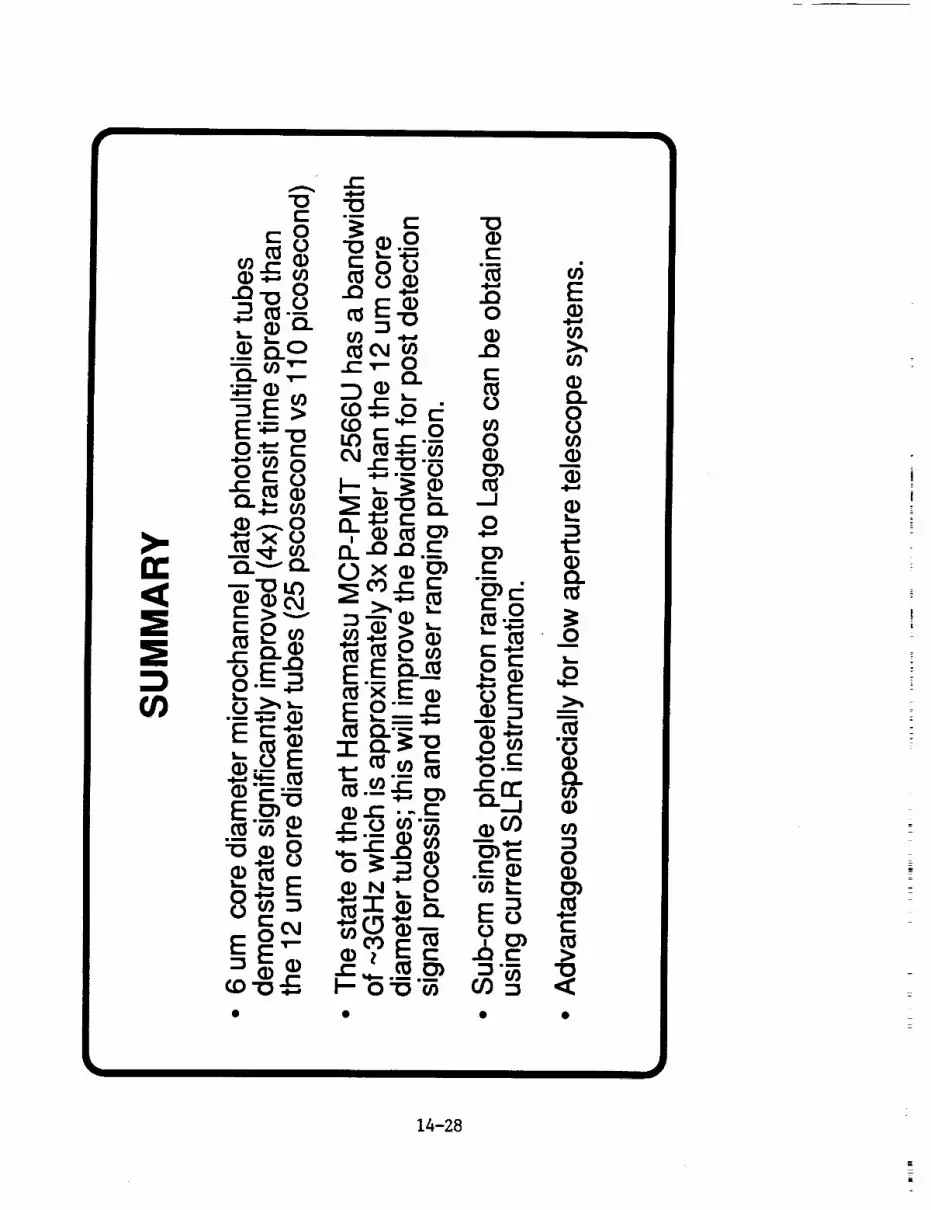
14-28
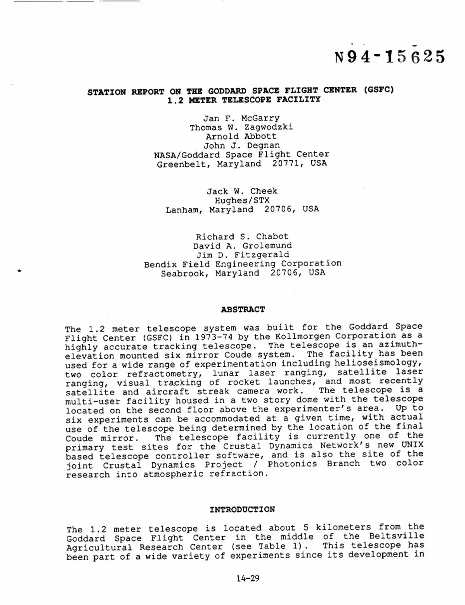
v
N94-15625
STATION REPORT ON THE GODDARD SPACE FLIGHT CENTER (GSFC)
1.2 METER TELESCOPE FACILITY
Jan F. McGarry
Thomas W. Zagwodzki
Arnold Abbott
John J. Degnan
NASA/Goddard Space Flight Center
Greenbelt, Maryland 20771, USA
Jack W. Cheek
Hughes/STX
Lanham, Maryland 20706, USA
Richard S. Chabot
David A. Grolemund
Jim D. Fitzgerald
Bendix Field Engineering Corporation
Seabrook, Maryland 20706, USA
ABSTRACT
The 1.2 meter telescope system was built for the Goddard Space
Flight Center (GSFC) in 1973-74 by the Kollmorgen Corporation as a
highly accurate tracking telescope. The telescope is an azimuth-
elevation mounted six mirror Coude system. The facility has been
used for a wide range of experimentation including helioseismology,
two color refractometry, lunar laser ranging, satellite laser
ranging, visual tracking of rocket launches, and most recentlysatellite and aircraft streak camera work. The telescope is a
multi-user facility housed in a two story dome with the telescope
located on the second floor above the experimenter's area. Up to
six experiments can be accommodated at a given time, with actual
use of the telescope being determined by the location of the final
Coude mirror. The telescope facility is currently one of the
primary test sites for the Crustal Dynamics Network's new UNIX
based telescope controller software, and is also the site of the
joint Crustal Dynamics Project / Photonics Branch two color
research into atmospheric refraction.
INTRODUCTION
The 1.2 meter telescope is located about 5 kilometers from the
Goddard Space Flight Center in the middle of the Beltsville
Agricultural Research Center (see Table I). This telescope has
been part of a wide variety of experiments since its development in
14-29

1973-74 by the Kollmorgen Corporation (now part of Contraves). Itwas originally built for Goddard as a highly accurate trackingtelescope to use in the development and testing of satellite laserranging (SLR) systems. Although there was preliminary work done inthis area by both T.Johnson (GSFC) and C.O.Alley (University ofMaryland), it was not until the mid 1980s that the telescopefacility realized its full potential in this area with thedevelopment of the Experimental Satellite Laser Ranging System(ESLRS). The telescope's primary usefulness is in the areas of
photon gathering and astronomical testing. As an astronomicalobservatory, it has drawbacks; these include the air bearings whichdistort the images, and the poor quality of seeing in theBaltimore-Washington region. The proximity to Goddard, however,makes the 1.2m telescope an excellent test facility forastronomical experiments, and the large aperture, highly accuratetracking capability, and excellent laboratory facilities make it anideal system for developing and testing new ideas in satellitelaser ranging.
TELESCOPE CHARACTERISTICS
The 1.2 meter telescope system is a multi-user azimuth-elevation
mount housed in a two story dome (see Figure I). The telescope is
located on the second floor above the experimenters' area. The 15
ton assembly, as seen in Figure 2, consists of three sections: the
yoke assembly, the trunnion with the primary mirror cell, and the
forward tube truss (holding the secondary mirror). Air bearings,
which raise the mount 0.005 millimeters above the support, are used
for azimuth rotation to avoid the friction caused by roller
bearings. The telescope is a six mirror Coude system with an
effective system focal length of 33.13 meters (shown in Figure 3).
The primary mirror is paraboloidal, 1.2 meters in diameter, with a
focal distance of 3.2 meters. The secondary mirror is
hyperboloidal, 0.4m in diameter, and is motor driven over a range
of approximately 1.5 centimeters, giving the system the ability to
focus from one kilometer to infinity. Three other flats direct the
light from the telescope down into the experimenters' area below.
Here a sixth mirror (the steering or pit mirror) can be ro_@ted todirect the light to amy Of six experimenters _ ports located at
equidistant points around the circular pit area. All mirrors have
been recently recoa.ted with a broadband aluminum coating and SiOx
overcoating. Peak reflectivity ranges from 88% to 92%.
The telescope was designed to meet a 20 arcsecond absolute
positioning with a 5 arcsecond repeatability. In the current
configuration the pointing is actually around 1 arcsecond due to
the 28 term trigonometric error model used by the Servo system
computer. The servo system computer is a COMPAQ 386/20Mhz with
4Mbytes of memory. The tracking programs are written mainly in
FORTRAN and run under the MS-DOS operating system. Timing for the
software tasking is provided by IHz and 20Hz signals (accurate to
1 microsecond) and by the 36-bit NASA time code generator which
14-30
consists of day of year and time of day. The computer closes theservo loop by reading the 22-bit encoders and performing softwareservo compensation; the telescope drive signals are output at 20Hzto provide a smooth track. The mount is able to track to the 1arcsecond level at rates of up to 1 deg/sec in azimuth and up to0.5 deg/sec in elevation. The actual speed of the mount issoftware limited to under 6 degrees per second in both axes.
The telescope facility has the ability to track satellites,aircraft, planets, the moon,_ the sun, and the stars. Predictionsfor satellites can either be in the form of Inter-Range-Vectors orNORADs. Aircraft acquisition uses onboard GPS data relayed to theground in real-time or just visual observation; tracking isaccomplished by using the digitized camera image of an onboardlight source (such as running lights or laser diode beacon). Theright ascension and declination of stars comes from the FK4 (soonto be FK5) catalog or from operator type-in of apparent position.Planetary prediction data, as well as the moon and the sun, comesyearly from the Flight Dynamics Support Branch at Goddard in theform of Chebyshev_polynomials.
Acquisition aids are also available with the telescope. Operatorsin the dome can view through a 0.3 meter finder telescopeboresighted with the main telescope. Also boresighted on the 1.2mtelescope are an RCA Silicon Intensified Tube (SIT) camera and aCCD camera. An RCA SIT camera is also located in the pit areabelow the telescope in the focal plane. This camera was usedduring the RME experiment (see experiments listed below) and isalso used for star calibrations. The video image from all threecameras can be viewed in the telescope control room and can be sentthrough the Colorado Video X-Y Digitizer for closed loop trackingby the servo computer. Table 2 lists the pertinent information onthe finder scope and cameras.
PAST TELESCOPE EXPERIMENTS
PLANETARY OBSERVATION
The telescope served as a field test facility for bread board
optical heterodyne spectrometers in the near and thermal infrared.
This work was in support of earth and planetary atmospheric
observations and was performed in the 1970s and early 1980s by M.
Mumma and colleagues at NASA/GSFC.
A Laser Heterodyne Spectrometer for .Helioseismology was an
experiment performed at the telescope facility in the early 1980s
to measure solar oscillations by mixing solar radiation with the
output of a frequency stabilized CO_ laser. D. Glenar of Colgate
University was the principal investigator in support of ongoingwork at GSFC.
14-31

ATM0$PHERI¢ LIDAR
A laser induced resonant fluorescence experiment took place in the
early 1980s. This experiment, conducted by C.Gardner of the
University of Illinois Department of Electrical Engineering,
measured the density of atomic sodium at altitudes up to 100km
using a dye laser mounted to the telescope trunnion.
LQNAR LASER RANGING
The design and testing of a high average power laser and special
electronics for lunar ranging was overseen by C.O.Alley of the
University of Maryland Department of Physics. Limited lunar
ranging from the telescope was also accomplished during the early
1980s.
TIME COMPARISQNS
C.O.Alley and colleagues at the University of Maryland set up and
operated a laser link to the United States Naval Observatory (USNO)
from the 1.2m telescope facility for time comparisons in support of
the LASSO experiment. This link provided the highest precision
time comparison (30 psec) as of that date (1983).
A comparison of East-West versus West-East one way propagation
times of laser light pulses was also performed by C.O.Alley and
R.A.Nelson. This was the first experiment to make such a direct
measurement and provided the highest precision ever achieved in a
time comparison with a transported atomic clock (40 picoseconds to
USNO and back).
AUTOMATED GUIDING AND TWO-COLOR REFRACTOMETRY
D.Currie and D.Wellnitz of the University of Maryland Department of
Physics developed the Automatic Guider System (AGS) during the
period from 1975 to 1978 for automated tracking of continuous light
sources. The AGS was used to perform automated star calibrations
at the 1.2m telescope during the late 1970s.
D.Currie and D.Wellnitz also developed and tested at the 1.2m
telescope a Two Color Refractometer, based on the AGS design, to
measure atmospheric refraction. The final experiment performed at
the USNO measured atmospheric refraction in a single night to a
precision previously requiring one month's observations.
SINGLE COLOR SATELLITE LASER RANGING
The Experimental Satellite Laser Ranging System (ESLRS) operated as
an R&D facility from 1982 to 1986. It was one of the first
centimeter level, high return to transmit ratio satellite laser
14-32

ranging systems. This system was developed by T.Zagwodzki,J.McGarry and J.Degnan of NASA/GSFC.
The NASA/RME experiment in 1991 used the U.S.Air Force loworbiting, high lidar cross-section Relay Mirror Experimentsatellite to investigate streak camera returns from satellites, andto develop and test a system design for later two color work.Streak camera waveforms from RME showed clearly resolved responsesfrom the individual cubes on the satellite. This experiment wasconducted by T.Zagwodzki and J.McGarry.
TWO-COLOR STREAK CAMERA AIRCRAFT LASER RANGING
The goal of this experiment was to determine the azimuthal
variations in the atmospheric induced range delay using doubled
(532nm) and tripled (355nm) frequencies from the facility's Nd:YAG
laser to a corner cube mounted on the NASA T-39 aircraft.
Waveforms were recorded with a Hamamatsu C1370 2-psec resolution
streak camera. The aircraft was acquired by using a GPS receiver
onboard the aircraft whose output was transmitted to the ground
computer via a radio link. Once the aircraft was visuallyacquired, the ground computer was able to lock onto and track the
aircraft's laser diode beacon by digitizing the image seen in a
camera mounted on the telescope. This experiment was successfully
completed in early August 1992. The principal experimenters were
P.Millar, J.Abshire, J.McGarry, and T.Zagwodzki, all of NASA/GSFC.
I
CURRENT TELESCOPE PROJECTS
Tw0-cO_0R STREAK CAMERA SATELLITE LASER RANGING
Recent upgrades to the ESLRS at the 1.2m telescope facility have
been made to allow measurements of two color differential delay to
the ERS-I, STARLETTE and AJISAI satellites using a single-
photoelectron sensitive Hamamatsu Streak Camera. Differential two
color measurements will be used to analyze the accuracy of existing
satellite ranging atmospheric refractivity models. This work is
being performed by T.Zagwodzki, J.McGarry, J.Degnan, all of GSFC,
T.Varghese of Bendix, and colleagues from GSFC, Bendix andHughes-STX.
SATELLITE LAUNCH TRAJECTORY TRACKING
In support of the Office of Naval Research and later the Air Force
SDIO work, the University of Maryland has been observing the
Firefly and Firebird series of launches from Wallops and Cape
Canaveral using a wide field camera installed on the 1.2m telescope
and the University of Maryland Optical Metric Mapper at the Coude
focus. Acquisition is provided by realtime Launch TrajectoryAcquisition System (LTAS) data via a high speed direct link. This
14-33

Work is being performed by D.Currie and D.Wellnitz of theUniversity of Maryland.
SUPPORT OF LASSO EXPERIMENT
Attempts at visual acquisition of the Meteosat satellite (MP2), in
order to range to the LASSO experiment, have been attempted using
both the RCA Silicon Intensified Target camera on the mount and at
the Coude focus, and using the University of Maryland Zibion camera
installed on an auxiliary 12-inch telescope mounted to the 1.2m
telescope. Due to the low magnitude of the visual MP2 and the poor
seeing in the Baltimore-Washington area, all attempts at seeing MP2to date have been unsuccessful. This work has been a Joint effort
between the Crustal Dynamics Project at GSFC, the Photonics Branch
at GSFC, and the University of Maryland Physics Department.
MQNITORING LAGEOS SATELLITE'S SPIN
Evaluation is in progress to determine the feasibility of
monitoring the spin .vector of the LAGEOS satellite (and later
LAGEOS II) to support the prospective experiment to measure the
Lense-Thirring Effect predicted by General Relativity. This is a
joint experiment involving NASA, the Italian Space Agency, and theU.S.Air Force. The University of Maryland effort is being
conducted by D.Currie, D.Wellnitz and P.Avizonis.
SOFTWARE DEVELOPMENT AND CHECKOUT
New CDP Network Telescope Controller Software is being designed to
replace all of the telescope computers in the NASA Network with 486
compatible computers. The 1.2m telescope is the primary test
system for the new software which will operate in the UNIX
environment and will provide a user friendly, menu driven,
graphical interface for the crews. The software team consists of
J.McGarry (GSFC), J.Cheek (Hughes-STX), R.Ricklefs (University of
Texas), P. Seery (Bendix), and K.Emenheiser (Bendix).
ACKNOWLEDGEMENTS
The authors would like to thank Jack Bufton (GSFC), Carol Alley
(University of Maryland), and Dennis Wellnitz (University of
Maryland) for detailed information on past projects at the
telescope. A special thanks goes to the CDP SLR Manager, Larry
Jessie, for photographing the telescope.
14-34

Table I:
1.2m TELESCOPE LOCATION
1.2 meter telescope location
North American Datum 1927
CLARK 1866 ellipsoid
LATITUDE (geodetic) 39.02136044 degrees
LONGITUDE (east) 283.31712961 degrees
HEIGHT (above ellipsoid) 0.053198 km
Table 2 : Acc
SIT camera in pier
Finder scope
CCD camera
SIT camera on mount
uisition and Tracking Aids
Field of View Dimmest objectthat can be seen
70 mdeg diameter 8th magnitude
250 mdeg diameter 9th magnitude
200 by 300 mdeg 3rd magnitude
2 by 3 degrees 8th magnitude
Figure i: 1.2 meter telescope facility
14-35ORIGINAL PAOE

Figure 2: Mount assembly
ciI!i
I /dI /
\\
AZIMUTH AXISII
• RIIVIARY FOCAL POINT
I
I\ _ SECONOAR¥MIRRORIII
f:f_]] M,RROR""SYSTEM
ORIGIN
C%V
ELEVATION
AXIS
SYSTEM | !IFOCUS AT .... _ PIT STEERING
EXPERIMENTER'S [ T-'I I MIRROR
""" IH I
2nd FLOOR
1st FLOOR
Figure 3: Coude system
14-36

Session Summaries

SESSION SUMMARIES
On the last day of the conference, each of the session chairman were asked to summarize, in
vu-graph form, major conclusions or observations distilled from the individual talks within their
sessions. These vu-graphs are reproduced in the following pages (with some minor editing on
my part to improve clarity and eliminate duplication) along with comments made by workshopparticipants following the formal presentation by the session chairman. I have made no attemptin this record to identify the source of individual comments.
John Degnan
15-1

SCIENTIFIC APPLICATIONS AND MEASUREMENTS REQUIREMENTSBob Schutz/Richard Eanes
The science applications of SLR were summarized as follows:
Mean Gravity Field
Gravity field improvements - GEM-T3, TIG2, GRIM
Gravity Field Fluctuations/Variability
Longterm J_
18.6 year tide
seasonal correlation with atmosphere
Terrestrial Reference Frame/Earth Orientation
Polar Motion .....
0.5 milliarcsecondroufine accuracy on X and Y for 3 day values
1 day series available
Rapid Service UTI
Possible use of ETALON to extend to higher frequencies
Motion of network relative to center of mass of Earth/oceans/atmosphereRMS 1 cm in X,Y; 3 cm in Z
Relative Station PositionsBest: 0.5 cm
Typical: 1-2 cmRelative Motion
Horizontal velocities: 1 to 10 mm/yr for 40 or 50 sitesVertical motions: Available for the "best-behaved sites"
Ocean Surface Study with SLR tracked altimetric satellites
ERS-1 orbits controlled by laser tracking
Time Transfer
Preliminary LASSO results from Grasse and MLRS < 100 ps
15-2
1
|
_-T
m=
==
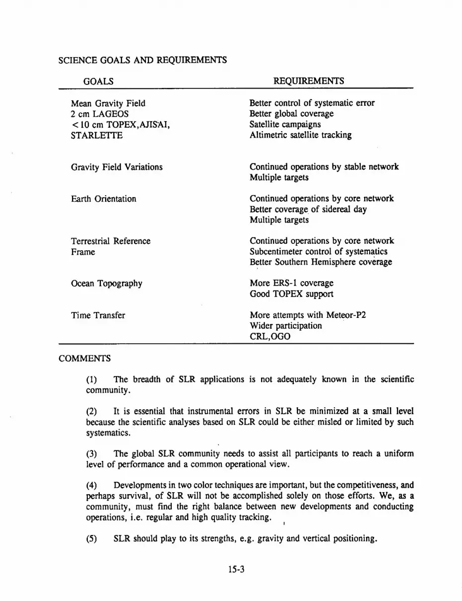
SCIENCE GOALS AND REQUIREMENTS
GOALS REQUIREMENTS
Mean Gravity Field2 cm LAGEOS
< 10 cm TOPEX,AJISAI,
STARLETTE
Better control of systematic error
Better global coverage
Satellite campaigns
Altimetric satellite tracking
Gravity Field Variations
Earth Orientation
Terrestrial Reference
Frame
Ocean Topography
Time Transfer
Continued operations by stable network
Multiple targets
Continued operations by core network
Better coverage of sidereal day
Multiple targets
Continued operations by core network
Subcentimeter control of systematicsBetter Southern Hemisphere coverage
More ERS-1 coverage
Good TOPEX support
More attempts with Meteor-P2
Wider participation
CRL,OGO
COMMENTS
(1) The breadth of SLR applications is not adequately known in the scientific
community.
(2) It is essential that instrumental errors in SLR be minimized at a small level
because the scientific analyses based on SLR could be either misled or limited by such
systematics.
(3) The global SLR community needs to assist all participants to reach a uniform
level of performance and a common operational view.
(4) Developments in two color techniques are important, but the competitiveness, and
perhaps survival, of SLR will not be accomplished solely on those efforts. We, as a
community, must find the right balance between new developments and conducting
operations, i.e. regular and high quality tracking.I
(5) SLR should play to its strengths, e.g. gravity and vertical positioning.
15-3

(6) The communityshould establish ties to Global Change.
(7) Can'oll Alley reminded the group that lunar ranging was developed to support
relativistic and fundamental physics studies whereas the present program appears to be
tightly tied to Earth science.
15-4
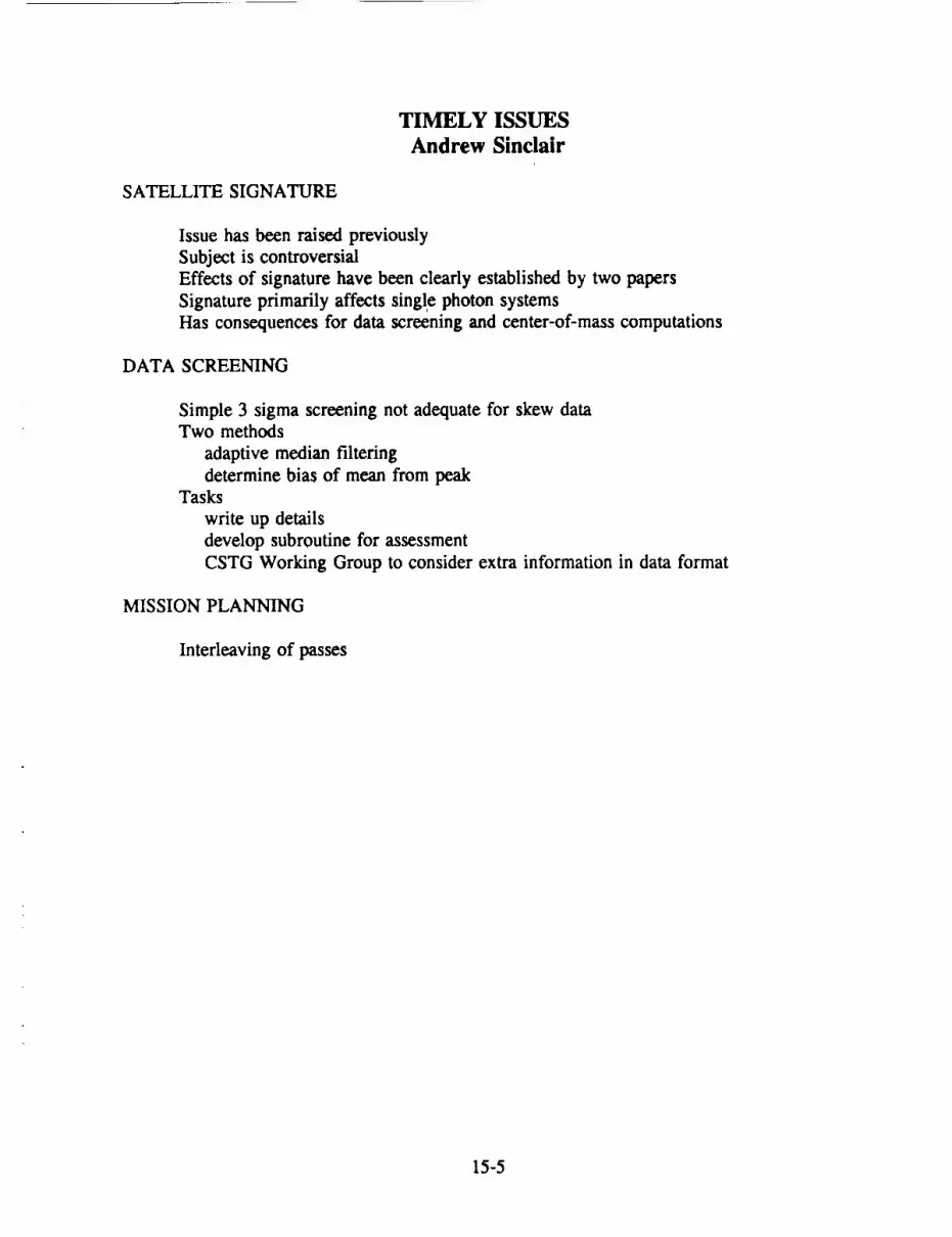
TIMELY ISSUES
Andrew Sinclair
SATELLITE SIGNATURE
Issue has been raised previously
Subject is controversial
Effects of signature have been clearly established by two papers
Signature primarily affects single photon systems
Has consequences for data screening and center-of-mass computations
DATA SCREENING
Simple 3 sigma screening not adequate for skew dataTwo methods
adaptive median filtering
determine bias of mean from peak
Tasks
write up details
develop subroutine for assessment
CSTG Working Group to consider extra information in data format
MISSION PLANNING
Interleaving of passes
15-5

LASER TECHNOLOGY
Helena Jelinkova
LASER TRANSMI'ITER SUMMARY
Wavelength
Length of pulses
Energy
Repetition Rate
Maintenance
0.53 #m (1.06 _m) Nd:YAG
30 psec to 4,00 psec
20 mJ to 300 rnJ
2 to 10 Hz
1 alignment/pass to 1 alignment/0.5 year(Improving)
GOALS AND ISSUES
Multipulse Transmitter (to maximize energy usage)
Semitrain
Full train
Multiwavelength Transmitters
Doubled and third harmonicStokes and Anti-stokes
New Active Materials
10 picosecond pulses compression by
Brillouin + Raman
Raman
Negative Feedback
Colliding Pulse Method
Space use of Diode-pumped lasers
High efficiency
Long life
COMMENTS
Billion shot flashlamps have been demonstrated but lamp failure is catastrophic whereas
diode arrays degrade.
15-6

EPOCH AND EVENT TIMING
Ben Greene
SUMMARY
Streak cameras presently at 2 psec; future resolution and accuracy = 0.5 psec
Electronic timing systems presently at 3 psec; future 1 psec resolution and accuracy
Both technologies are approximating useful levels for 5 mm two color ranging
COMMENTS
General agreement on first bullet
Disagreement on second bullet although new technologies (e.g. GaAs) are becoming
available
There has been insufficient vision on the part of the funding agencies in developing this
technology
15-7

DETECTOR TECHNOLOGY
Thomas Varghese
SUMMARY
High speed single photoelectron detectors (SPADS)
High speed, low jitter microchannel plate photomultipliers (230 psec) benefit fromeffects
Streak cameras represent the leading edge of high accuracy
COMMENTS
SPADs are useful for lunar ranging
Subcentimeter level ranging has been established on a global level and we are
approaching millimeter accuracies
15-8

CALIBRATION TECHNIQUES/TARGETS
Jean Gaignebet
SUMMARY
Recommended formation of a study group for the design of improved laser retroreflector
arrays. G. Lund offered to chair.
There is a need to monitor and keep records on individual SLR stations and
configurations.
An interesting comer cube design based on the Fizeau effect was presented by V.
Shargorodsky of Russia.
15-9

MULTIWAVELENGTH RANGING/STREAK CAMERASKarel Hamal
EXPECTED GOALS ACHIEVED
Optimum wavelength pair
Two Color Ranging MCPMCP
SPAD
Streak Camera
Optimum Satellite &Fizeau Cubes
Figure of Merit
Preliminary
Not yet
Some progress
single color
Promising
Controversial
Laser Stokes/Antistokes
Cr:LiSAF
COMMENTS
Raman systems will never have high figure of merit; frequency shift is relatively small.
A Fizeau target is already in a 620 Km orbit. V. Shargorodsky will send the satellite
orbit parameters by telex to the Smithsonian Astrophysical Observatory.
Russians will fly a new target at 1000 Km altitude by the end of the year. Only one cube
(Fizeau) is visible at a time.
15-10

SLR DATA ANALYSIS/MODEL ERRORS
Ron Kolenkiewicz, Richard Eanes
Dynamic, Semi-dynamic, and Geometric Analyses
Orbital models and nonconservative forces
With increased data precision, the effect of time-varying gravity on the satellites is important,
and the tracking site motions due to ocean and atmospheric loading needs to be considered.
Geopotential at the one to two level still exist for LAGEOS. More high quality data should
improve this below one cm - especially at new sites or recently improved sites.
Systematic errors in the data due to satellite signature and calibration errors must be reduced to
less than one era.
A large non-gravitational signal affecting the LAGEOS eccentricity and perigee at the few meter
level has been detected by the analysis groups at GSFC and UT/CSR. The effect was especially
large in 1989 and 1991. The current models that explain the along -track or "drag" acceleration
on LAGEOS do not explain the eccentricity anomaly. We need a physical explanation for the
once per revolution accelerations on LAGEOS.
An attempt should be made tb improve the atmospheric correction for single wavelength SLR
by means of acoustic and/or lidar sounding of the atmospheric temperature profile.
There is a need for improved second generation SLR satellites with much more stable and
deterministic center-of-mass corrections.
With the increased altitude and number of geodetic satellites (e.g., ETALONS and LAGEOS II),
the use of geometric analysis to obtain geophysical parameters should be utilized.
Partly random seasonal fluctuations in the mass distribution of the atmosphere limit our ability
to ever completely eliminate gravitational model error. Rather we must consider the error as an
opportunity and track the fluctuations over time.
Obtaining successful results for the variations of the vertical component of station positions
requires that biases in the SLR data be controlled much better than they have in the recent past.
Solutions for range bias show some interesting regionally correlated signals that are evidence of
either height variations or of some other model defect that is unknown. However, there are also
large sudden changes in the biases that are certainly due to problems at the stations.
15-11

OPERATIONAL SOFFWARE DEVELOPMENTS
Georg Kirchner
Software developments are freely exchanged between groups.
Community relies on exchanges, standardized formats, etc.
Conclusions from the Splinter Meeting:
Transputer-based SLR control system has no disadvantages (according to the engineerwho built it)
Stations should transmit full rate data by E-mail in compressed form
The community should investigate possible standardization of SLR operating and controlsystems.
15-12

LUNAR LASER RANGING
Christian Veillet
The loss of Haleakala to the LLR community is "very unfortunate".
There are presently only two, regularly working lunar stations (CERGA and MLRS).
LLR needs lots of observations in order to adequately support the science.
LLR is important to lunar studies and fundamental physics.
LLR pushes individual station performance to the limit.
LLR stations could range to cubes in lunar orbit.
15-13

FIXED STATION UPGRADES/DEVELOPMENTS
John Degnan
There appear to be at least two hardware configurations capable of subcentimeter range
accuracy:
150 psec pulse, MCP/PMT, and constant fraction discriminator
35 psec pulse, SPAD
There is a continued internati6nal interest in SLR as evidenced by the development of new
stations and continued upgrades of established stations
There is a new emphasis on higher degree of automation to drive down operational costs.
Countries continue to sponsor stations outside their national borders (e.g., Poland in Tunisia)
which will help to provide better global coverage.
15-14

MOBILE SYSTEM UPGRADES/DEVELOPMENTSErik Vermaat
Highly transportable systems are now demonstrating the same state-of-the-art quality as larger
stations (< 10 mm)
Mobile stations typically operate in the single or few photoelectron regime
Mobile stations are becoming more miniaturized as evidenced by the latest system, the French
Transportable Laser System (FTLRS).
Automation is a major driver in reducing costs.
Levels of standardization is a key issue.
15-15

F
L_z
_mE
II

Conference
Summary/Resolutions

i7.
!

CONFERENCE SUMMARY/RESOLUTIONS
Michael Pearlman
RESOLUTION
We wish to acknowledge and thank all of the representatives from NASA Headquarters, Goddard
Space Flight Center, and Bendix Field Engineering Corporation for their untiring efforts in
support of the 8th International Workshop on Laser Ranging Instrumentation. Without the hard
work, dedicated backing, and personal interest of each of these individuals, this workshop would
not have enjoyed the tremendous successes that it did. The help and support of John Degnan
is especially recognized.
RESOLUTION
As satellite ranging develops towards millimeter accuracy and the use of multiple wavelengths,
one of the most important contributions to the energy link budget and satellite signature to
ranging accuracy is the design of the laser retro array.
The SLR community appreciates the idea and proposal of the Russian Space Device Engineering
Institute to compensate for angular velocity aberrations via the Fizean effect.
We strongly recommend the continuation of space experimentation in this field.
The SLR community proposes that SLR stations and experts in this field should participate in
the construction and subsequent tracking of a satellite designed for this purpose.
RESOLUTION
Whereas the Workshop participants recognize the importance of improving the global distribution
of SLR sites and applauds the efforts of various member nations to extend coverage outside their
national borders through:
1. The establishment of fixed station (e.g., USA in South America, Czechoslovakia
in Egypt, Poland in Tunisia, and Germany in Cuba).
and,
2. The use of mobile systems (USA, Germany, the Netherlands, and France).
We resolve to encourage all member nations in the SLR community to assist, to the best of their
ability, in the development and/or operation of stations outside their national borders and
particularly in the Southern Hemisphere.
16-1

RESOLUTION
We would like to recommend the creation of a special study group to investigate all possible new
generation laser ranging retroreflector concepts for optical signature and (null) center of masscorrection.
RESOLUTION
Whereas, future analysis of our laser data products would benefit by a knowledge of the
configuration of the hardware and software by which it was obtained, we resolve to document
our operational configurations and changes there to and record these at a centralized facility ina manner as to be defined by the CSTG.
RESOLUTION
We resolve to initiate experiments designed to improve the atmospheric correction through the
use. of real-time temperature profiles based upon acoustic wave tracking (SODAR).
16-2

Business Meeting/
Next Workshop

!

BUSINESS MEETING/NEXT WORKSHOP
Carroll Alley
It was decided by the participants that the next workshop should be held within two years. Three
participants offered to host the next workshop. The proposers were John Luck of Australia,Yang Fu Min of the Peoples' Republic of China, and Erik Vermaat of the Netherlands.Sentiment was strong among many of the delegates that the ninth workshop should be held ineither Asia or Australia since previous workshops had all been located in Europe or the United
States. The delegates decided (in a very close vote) to hold the next meeting in the Septemberto November 1994 time frame in Canberra, Australia. The meeting will be hosted by the
Australian Survey and Land Information Group (AUSLIG).
17-1

REPORT DOCUMENTATION PAGE FormApprovedOMB NO.0704-0188
PuI:41c iw,;x_;.g burden for tht¢ collection Of Information b eetlrnated to average 1 hour pet re_oonse, Induding the time for reviewing instruc_ions, searching exlsttng data sources, g_hering
and maJnt_nfng the _ needed, and coml_etlng and reviewing the conectio_ of Information, Send oommerts regarding this burden estimate or any other a_ o4 this oollectton Of
klf=or.m_..,_, .k_d ._lk_=_l__ __..tons for reclucing, this burden, to Washingtofl Headq_ uattors Se_/ICM, Oirecto.rate for Informalion Operations and Reports. 1215 Jeffeclon Davis Highway, Suite
1L_/4, Anlri_Ofl, VA _-43_ _ _O the (_lce of Me_err_ mttd BuDget. Paperwork Reduct,on Project (0704-01881. Washlr_ton, DC
1. AGENCY USE ONLY (Leave blBnk) 2. REPORT DATE 3. REPORT TYPE AND DATES COVEREDJune 1993
4. TITLE AND SUBTITLE
Proceedings of the Eighth International Workshop
on Laser Ranging Instrumentation
6. AUTHOR(S)
Compiled and Edited by John J. Degnan
7. PERFORMING ORGANIZATION NAME(S) AND ADDRESS(ES)
Goddard Space Flight Center
Greenbelt, Maryland 20771
9. SPONSORING/MONITORING AGENCY NAME(S) AND ADDRESS(ES)
National Aeronautics and Space AdministrationWashington, D.C. 20546-0001
11. SUPPLEMENTARY NOTES
Conference Publication
5. FUNDING NUMBERS
920.1
8. PERFORMING ORGANIZATIONREPORT NUMBER
93B00079
10. SPONSORING/MONITORINGAGENCY REPORT NUMBER
CP-3214
12a. DISTRIBUTION/AVAILABILITY STATEMENTUnclassified-Unlimited
Subject Category 19
Report available from the NASA Center for AeroSpace Information, 800 ElkridgeLanding Road, Linthicum Heights, MD 21090; (301) 621-0390.
12b. DISTRIBUTION CODE
13. ABSTRACT (_ 200 words)
The Eighth International Workshop for Laser Ranging Instrumentation was held in Annapolis, Maryland in May 1992,
and was sponsored by the NASA Goddard Space Flight Center in Greenbelt, Maryland. The workshop is held once every
2 to 3 years under differing institutional sponsorship and provides a forum for participants to exchange informa-
tion on the latest developments in satellite and lunar laser ranging hardware, software, science applications, and data
analysis techniques. The satellite laser ranging (SLR) technique provides sub-centimeter precision range measurementsto artificial satellites and the Moon. The data has application to a wide range of Earth and lunar science issues inclu-
ding precise orbit determination, terrestrial reference frames, geodesy, geodynamics, oceanography, time transfer, lunar
dynamics, gravity and relativity. This Proceedings is a compendium of full papers based on material presented at theAnnapolis workshop.
14. SUBJJECT TERMSSatelhte Laser Ranging, Lunar Laser Ranging, lidar, ranging, optical radar, lasers,
optical detectors, timers, sa_dlite tracking, satellite orbits, software, geophysics, terrestrial reference
flames, Earth a'ientafion parameters, geodesy, geodynamics, oceanography, time transfer, Moon,gravity, lunar physics, $eopotential
17. SECURITY CLASSIFICATION 18. SECURITY CLASSIFICATIONOF REPORT OF THIS PAGE
19. SECURITY CLASSIFICATIONOF ABSTRACT
Unclassified Unclassified Unclassified
NSN7540-01-280-5500
15. NU_ER OF PAGES
16. PRICE CODE
20. LIMITATION OF ABSTRACT
Unlimited
Standard Form 295 (Roy.249)Preecrlbed by ANSI Sid. 239-18,298-102

