source parameters of microearthquakes at mount st helens (usa)

Geophys. J. Int. (2006) 166, 1193–1223 doi: 10.1111/j.1365-246X.2006.03025.x

GJI

Sei

smol

ogy

Source parameters of microearthquakes at Mount St Helens (USA)

Giuseppina Tusa,1 Alfonso Brancato,1 Stefano Gresta1 and Stephen D. Malone2

1Dipartimento di Scienze Geologiche, University of Catania, Corso Italia 55-95129 Catania—Italy. E-mail: [email protected]; [email protected];[email protected] of Earth & Space Sciences, University of Washington, Box 351310, Seattle, WA 98195, USA

Accepted 2006 March 28. Received 2006 March 27; in original form 2005 February 14

S U M M A R YWe estimate the source parameters for a selection of microearthquakes that occurred at MountSt Helens in the period 1995–1998. Excluding the activity of 2004 September, this time periodincludes the most intense episode of earthquake activity since the last dome-building eruptionin 1986 October. 200 seismograms were processed to obtain seismic moments, source radii,stress drops and average fault slip. The source parameters were determined from the spectralanalysis of P waves, after correction for attenuation and site effects. In particular, P-wavequality (Qp) and site (S) factors have been previously calculated in the frequency ranges2–7 Hz and 18–30 Hz. Because it was impossible to perform corrections for Qp and S over thewhole spectrum we applied a new approach, based on the notion of ‘holed spectrum’, to estimatespectral parameters. The term ‘holed spectrum’ indicates a spectrum lacking corrected spectralamplitude values at certain frequencies. We carried out a statistical study to verify that dealingwith the ‘holed spectrum’ does not lead to significant differences in the estimates of spectralparameters. We also investigated the dependence of spectral parameters (low-frequency level,corner frequency and high-frequency decay) on the bandwidth of spectral hole, and defined thethreshold values for three different spectral models. Displacement ‘holed spectra’, correctedby attenuation and site response, are then used to determine spectral parameters in order tocalculate seismic source parameters. Seismic moments range from 1017 to 1019 dyne-cm, sourcedimensions from 100 to 350 m, and average fault slip from 0.003 to 0.1 cm. Self-similarityseems to break down in that stress drops are very low (0.1–1 bars). We postulate that seismicityis associated with a brittle shear failure mechanism occurring in a highly heterogeneous materialunder a relatively low stress regime.

Key words: microearthquakes, Mt St Helens, source parameters, statistical analysis.

I N T RO D U C T I O N

After 18 yr of relative quiescence Mount St Helens volcano recap-

tured the attention of the world in 2004 September, when it showed

signs of reawakening. Indeed, on 2004 September 23, Mount St

Helens experienced an earthquake swarm with about 200 small (less

than magnitude 1) and shallow (less than 1 km) earthquakes that

began in and beneath the 1980–1986 lava dome. During the next

several days the seismic activity increased dramatically (with earth-

quakes larger than M 2.5 occurring about once per minute and peak

sizes of M 3.5), producing the first steam eruption on October 1

that was followed, over the next ten days, by larger steam explo-

sions which showered the crater and flanks with ash. By October 11

the first small fin of new lava broke the surface and a new lava

dome built up. Its top was already about 400 m above the level of

the 1980 crater floor in 2005 February. Growth of the new lava dome

inside the crater continues nowadays, accompanied by low rates of

seismicity, low emissions of steam and volcanic gases.

In this paper, we examine the path and site corrected P-wave

spectra from local microearthquakes (M ≤ 2) recorded at Mount St

Helens in order to estimate the source parameters and the scaling

relationships between these parameters. The seismic data used were

recorded between 1995 and 1998 by stations of the Pacific Northwest

Seismograph Network. Excluding the activity of 2004 September,

this time period includes the most intense episode of earthquake

activity since the last dome-building eruption in 1986 October. In

fact, during 1998 May–July more than 900 events were recorded.

Analysis of the source parameters is fundamental to infer infor-

mation about the rupture process of microearthquakes. In addition,

their estimates are useful for determining scaling laws and for eval-

uating the possible departures from self-similarity in the low mag-

nitude range. The concept of self-similarity was first introduced by

Aki (1967), who proposed the scaling law M 0 ∝ f −3c . It is based

upon the assumption that all earthquakes have the same stress drop

independent of seismic moment. Compilations of seismic moments

and corner frequencies assembled over a wide range of magnitudes

support the cubic relation between seismic moment and corner fre-

quency and indicate that crustal earthquakes have average stress

drops in the range 1 to 1000 bars (e.g. Hanks 1977; Abercrombie

& Leary 1993). Several studies of small earthquakes (∼1–4 M),

C© 2006 The Authors 1193Journal compilation C© 2006 RAS

1194 G. Tusa et al.

however, have found a breakdown in self-similarity below about

magnitude 3 (e.g. Archuleta et al. 1982; Guo et al. 1992). A com-

monly known problem in studies of source parameters is caused by

path and site effects observed in seismic spectra, which produce

a fundamental ambiguity with respect to the estimation of source

dimensions. This problem becomes very important in the study of

small (M < 3) earthquakes because their spectral properties at high

frequencies are most affected by attenuation along the path and by

near-surface site effects.

As discussed in several studies, severe attenuation of high-

frequency (>1 Hz) waves can occur at shallow depths beneath re-

ceiver sites producing apparent corner frequencies unrelated to the

source dimension of the earthquake and high-frequency spectral

levels often correlate with near-surface geology (e.g. Frankel 1982;

Hanks 1982; Malin & Waller 1985; Frankel & Wennerberg 1989;

Hough 1997). Anderson (1986) showed theoretically how near-

surface attenuation could remove high-frequency energy needed to

constrain the length of smaller sources, and so alter the apparent scal-

ing of corner frequency with seismic moment (breakdown in self-

similarity). Moreover, the shallower crustal material can produce

other phenomena that will alter the spectral shape of an incom-

ing waveform. Spectral amplification can occur over certain fre-

quency bands associated with plane-layered structure under a site

(Cranswick et al. 1985; Mueller & Cranswick 1985; Scherbaum

1987) or with topography near a site (Tucker et al. 1984). Even at

hard rock sites, the site response plays an important role in the shape

of the source spectra (e.g. Frankel 1982; Anderson & Hough 1984;

Singh et al. 1988; Castro et al. 1990; Jin et al. 2000; Moya et al.2000).

In light of the evidence discussed above, recent studies of source

properties have used the corner frequency of the spectra to esti-

mate the size of rupture areas and, hence, stress drops of small

earthquakes taking into account near-surface and path attenuation.

Despite these improvements, it is not always easy to resolve the dif-

ferences between path and source. Results suggest both self-similar

(Vila et al. 1995; Bindi et al. 2001) and not-self-similar behaviour

(Garcıa-Garcıa et al. 1996; Patane et al. 1997; Jin et al. 2000). It is

Figure 1. Map of the Mount St Helens target area (a) and locations of the 15 closest stations (triangles) of Pacific Northwest Seismograph Network (b). The

data from stations marked by black triangles were used in this study. (from Tusa et al. 2004).

clear that an appropriate correction for the whole path attenuation

and site effects is a crucial part of all studies of seismic source.

Investigations of P-wave attenuation (Qp) and site response (S) at

Mount St Helens were performed by Tusa et al. (2004) by applying

the frequency decay method (e.g. Bianco et al. 1999) on the same

data set used in this study. The method works on the asymptotic

approximation at low ( f < fc, where fc is the corner frequency)

and high frequencies ( f > fc) of the earthquake spectral source

shape. Tusa et al. (2004) performed the analysis in the frequency

bands 2–7 and 18–30 Hz in the low- and high-frequency approxi-

mation, respectively. The need for using this separate-bands method

rather than the whole spectrum was due to the presence of significant

spectral peaks around the corner frequency for many spectra. These

anomalous peaks are clearly associated with site effects, which can-

not be accounted for quantitatively. Owing to unknown Qp and

S factors in a given frequency range (from f > 7 to f < 18 Hz

in this study), Tusa et al. (2006) developed a technique based on

the use of this band limited spectrum to infer source parameters of

microearthquakes in southeastern Sicily. In particular, Tusa et al.(2006) introduced the term of ‘holed spectrum’ to indicate a spec-

trum that results after removing spectral amplitude values in a given

frequency band. Conversely, the authors refer to a typical spectrum,

that is, having spectral amplitude values in the whole analysed fre-

quency band (from 2 to 30 Hz in this study), as a ‘whole spectrum’.

Tusa et al. (2006) developed their technique accounting for a spectral

hole in the frequency range 9 < f < 16 Hz, thus involving a shorter

bandwidth than that considered in this study. Therefore, we first per-

form a statistical analysis to verify if using the ‘holed spectra’ leads

to significant differences in the estimate of the spectral parameters

as compared to using the ‘whole spectra’. Additionally, we investi-

gate the dependence of the spectral parameters on the bandwidth of

the spectral hole in order to define its maximum value (or critical

value) for which the ‘spectral hole technique’ is unstable. Finally,

the source parameters such as seismic moment, fault radius, stress

drop, and average fault displacement are computed after corrections

for quality (Qp) and site amplification (S) factors, and the scaling

relationships between these parameters are investigated.

C© 2006 The Authors, GJI, 166, 1193–1223

Journal compilation C© 2006 RAS

https://www.researchgate.net/publication/248812232_Source_scaling_of_microearthquakes_at_Mt_Etna_Volcano_and_in_the_Calabrian_Arc_southern_Italy?el=1_x_8&enrichId=rgreq-5d67adc7-3fd3-4adf-b368-331183515192&enrichSource=Y292ZXJQYWdlOzI0OTQyODkxMDtBUzo5OTExMzcwNjE5NzAxNUAxNDAwNjQxOTU3OTAy

https://www.researchgate.net/publication/227093849_Attenuation_and_source_parameters_at_Deception_Island_South_Shetland_Islands_Antarctica?el=1_x_8&enrichId=rgreq-5d67adc7-3fd3-4adf-b368-331183515192&enrichSource=Y292ZXJQYWdlOzI0OTQyODkxMDtBUzo5OTExMzcwNjE5NzAxNUAxNDAwNjQxOTU3OTAy

https://www.researchgate.net/publication/228675303_Source_parameters_of_microearthquakes_in_southeastern_Sicily_Italy?el=1_x_8&enrichId=rgreq-5d67adc7-3fd3-4adf-b368-331183515192&enrichSource=Y292ZXJQYWdlOzI0OTQyODkxMDtBUzo5OTExMzcwNjE5NzAxNUAxNDAwNjQxOTU3OTAy


https://www.researchgate.net/publication/228709817_Attenuation_of_short-period_P_waves_at_Mount_St_Helens?el=1_x_8&enrichId=rgreq-5d67adc7-3fd3-4adf-b368-331183515192&enrichSource=Y292ZXJQYWdlOzI0OTQyODkxMDtBUzo5OTExMzcwNjE5NzAxNUAxNDAwNjQxOTU3OTAy



https://www.researchgate.net/publication/250074591_Simultaneous_Determination_of_Site_Responses_and_Source_Parameters_of_Small_Earthquakes_along_the_Atotsugawa_Fault_Zone_Central_Japan?el=1_x_8&enrichId=rgreq-5d67adc7-3fd3-4adf-b368-331183515192&enrichSource=Y292ZXJQYWdlOzI0OTQyODkxMDtBUzo5OTExMzcwNjE5NzAxNUAxNDAwNjQxOTU3OTAy

Source parameters of microearthquakes at Mount St Helens 1195

Figure 2. Map (a), WNW–ESE (b), and NNE–SSW (c) vertical cross sections of all events representing our starting data set; grey and black dots represent

events shallower and deeper than 5.5 km, respectively (modified from Musumeci et al. 2002).

DATA S E L E C T I O N

Seismic stations recording Mount St Helens earthquakes are shown

in Fig. 1. Our original data set consists of the waveforms of 447

well-located microearthquakes (0 ≤ M ≤ 2) recorded at stations

YEL, HSR and CDF (solid triangles in Fig. 1). Each station was

equipped with a short-period vertical-component, velocity-type

seismometer with natural frequency of 1 Hz. The instrumentation

of these stations consisted of two Mark Products L-4C (YEL and

HSR) and one Geotech S-13 sensor (CDF). Waveforms are recorded

at 100 Hz. In detail, YEL is located inside the crater area, on dacitic

to andesitic, pumiceous pyroclastic-flow deposits of the 1980 erup-

tion (Lipman & Millineaux 1981). HSR is located on pre-1980 an-

desite with minor dacite flows (Walsh et al. 1987). Finally, CDF is

located on welded to non-welded dacite and rhyolite tuffs and brec-

cias (Walsh et al. 1987). These stations were chosen for analysis

because of their distance distribution, quality of seismic data and

well known high-gain response.

The seismic events were located with high precision by Musumeci

et al. (2002) using a combination of a seismogram cross-correlation

technique and a joint hypocentre-velocity inversion. The epicentre-

station distances range between 0.5 and 15.5 km. Fig. 2 shows the

map and two vertical cross-sections of the 447 earthquakes belong-

ing to our starting data set. The events are concentrated in a ver-

tically distributed volume directly beneath the crater around the

conduit system. A shallow zone, in the depth range of 2–5.5 km,

has foci clustered in a tight cylindrical volume about 1 km in radius

directly beneath the crater. In a deeper zone (5.5–10 km) many of

the hypocentres are aligned along a plane (Fig. 2), that is coherent

with a model containing a NNE–SSW striking, steeply dipping fault

with slip consistent with magma being periodically injected into a

truncated dike on the northwest side of this fault (Musumeci et al.2002). Although some other stations were in operation on the cone

of the volcano within 15 km, data from these stations were not anal-

ysed because of low signal-to-noise ratio and/or insufficient large

ts − tp time separation.

C© 2006 The Authors, GJI, 166, 1193–1223


https://www.researchgate.net/publication/251427834_Magma_system_recharge_of_Mount_St_Helens_from_precise_relative_hypocenter_location_of_microearthquakes?el=1_x_8&enrichId=rgreq-5d67adc7-3fd3-4adf-b368-331183515192&enrichSource=Y292ZXJQYWdlOzI0OTQyODkxMDtBUzo5OTExMzcwNjE5NzAxNUAxNDAwNjQxOTU3OTAy

1196 G. Tusa et al.

Figure 3. Velocity record (left), displacement spectra (thin line, middle) and signal-to-noise ratio (right) of same events recorded at three stations used in this

study; examples of shallow (a) and deep (b) events. Note the consistent peaks at about 15 Hz that characterize the spectra at station HSR (clearly due to site

effect). Spectra of the pre-event background noise are also shown (dashed line, middle). Also note that the signal-to-noise spectral ratio is greater than 2 in the

frequency band 2–30 Hz. In each panel, both station code and epicentral distance are reported. The time window used to compute the spectra is indicated by a

horizontal bar above the waveform (128 samples) (modified from Tusa et al. 2004).

C© 2006 The Authors, GJI, 166, 1193–1223




S P E C T R A L A N A LY S I S

The first step of the data processing consisted of selecting time win-

dows for which to compute the P-wave spectra. In order to obtain

the same frequency resolution for all spectra, a cosine taper window

of 128 samples (1.28 s) was used for each signal. At station CDF,

the starting point was fixed at 0.1 s before the P-wave onset and

the tapering affected 10 per cent of the window margins. Because

of very short ts − tp times at stations YEL and HSR, the amplitude

spectra for these stations were computed with a 25 per cent cosine

taper window beginning 0.3 s before the P-wave onset. Thus the ef-

fective analysis time window is smaller, including 0.6 s of P phases.

However, only the events with ts − tp > 1 s were considered for the

analysis. Instrument correction, integration of velocity seismograms

to displacement and fast Fourier transform (FFT) were applied to

the data.

In order to obtain spectra of the noise, a 1.28 s section of record

prior to the P-wave window was analysed. Fig. 3 shows examples

of velocity seismograms and P-wave displacement spectra of two

selected earthquakes as observed at the three stations. In general,

we observe that the signal-to-noise spectral ratio is greater than 2 in

the frequency band 2–30 Hz. This range was therefore chosen for

analysis, whereas the events that did not meet this signal-to-noise

ratio were excluded. These criteria reduced the original data set to

241, 342 and 299 records at YEL, HSR and CDF, respectively.

AT T E N UAT I O N A N D S I T E

C O R R E C T I O N : P RO B L E M D E F I N I T I O N

The far-field displacement spectrum �(f ) can be approximated by

a one-corner frequency model:

�( f ) = �0[1 + ( f

fc

)γ n]1/γ

, (1)

where �0 is the low-frequency spectral level, fc is the corner fre-

quency, n is the high-frequency spectral decay and γ is a constant.

If γ = 1, the eq. (1) is the spectral shape proposed by Brune (1970).

Boatwright (1978) proposed a modified version of the spectral shape

with γ = 2 that produces a sharper corner than the original Brune’s

model. The attenuation and site response will modify eq. (1) to give

an amplitude spectrum Aij( f ) observed at the jth station for the ithevent that can be generally written as

Ai j ( f ) = Gi j Ki ( f )Sj ( f ) exp

(−π f

Di j

Qc

), (2)

where Gij is the geometrical spreading term (which in a uniform

medium is approximated by 1/Dij, being Dij the slant distance be-

tween ith event and jth station), Ki( f ) is the source spectrum, Sj( f )

is the site response, c is the average wave velocity and Q is the aver-

age quality factor along the path Dij that may include both intrinsic

and scattering losses.

Tusa et al. (2004) applied the frequency decay method (Bianco

et al. 1999) to the spectra of P waves at Mt St Helens to study the

local attenuation structure. This method is based on the asymptotic

approximation at low and high frequencies of the earthquake spec-

tral source shape. For f < fc (low-frequency approximation or LF),

Ki( f ) can be approximated by a constant, Ki, based on the hypothe-

sis of a flat P-wave spectrum below the corner frequency. For f > fc

(high-frequency approximation or HF), Ki( f ) can be approximated

by K ′i ( f ) under the assumption of an ω−2 high-frequency spec-

tral decay (Scherbaum 1990; Abercrombie 1995; Hough & Dreger

1995; Ichinose et al. 1997). Following Bianco et al. (1999), the

Qp-quality factor and station site correction factor S were computed

under the condition that they are frequency-independent in each of

the two selected bands (2–7 and 18–30 Hz). Thus, they represent an

estimate of the average P-wave attenuation and site amplification

in each frequency band. Moreover, the station site corrections were

determined with respect to the average spectrum evaluated over both

stations and events.

Tusa et al. (2004) studied both spatial and temporal variation of

P-wave quality factors using the same data set analysed here. First,

the authors separated the seismicity into shallow (depth <5.5 km)

and deep (depth >5.5 km) groups; then they performed a further

division as a function of time of occurrence (1995 January–1998

April (period I); 1998 May–August (period II); 1998 September–

December (period III)). Since, in order to apply the frequency decay

methodology they used only microearthquakes shared by the three

stations, the sample was reduced to 200 events. Table A1 displays Qp

and S values for each station at low (QLF, SLF) and high (QHF, SHF)

frequencies, separated both in space and time.

Since, as previously stated, the quality (Qp) and site amplification

(S) factors are known only in two frequency bands, and thus we are

not able to correct the whole spectrum (2–30 Hz) before estimating

source parameters from the spectra, we apply the ‘holed spectrum’

technique by Tusa et al. (2006). To solve this problem the authors

developed a way to use only the part of the spectrum for which

these corrections are available to estimate the spectral parameters.

Following Tusa et al. (2006), first we calculate the asymptotes to

the low-frequency (2–7 Hz) and high-frequency (18–30 Hz) parts

to the uncorrected spectrum independently ignoring the part of the

spectrum in the frequency range 7 < f < 18 Hz. We then test the

resulting values of spectral parameters against those computed from

the traditional fitting technique involving the ‘whole spectrum’ to

determine any biases (Fig. 4).

In detail our procedure is to select a random subset (35 per cent of

600 spectra for a total of 219) of spectra chosen as much as possible

to include a representative sample of data within each time sub-

group (i.e. time period I, II and III). We consider this data set big

enough that statistically significant inferences can be made for all

200 events. One must keep in mind that no correction for attenuation

and site effects is performed during this phase.

The spectral parameters were estimated by fitting the selected

‘whole’ displacement spectra by linearization of the theoretical gen-

eral model for displacement spectra as expressed by eq. (1). It is not

possible to set up a linear algorithm to directly obtain all the param-

eters simultaneously. Therefore, to avoid potential biases due to in-

spection by eye an iterative non-linear, best-fitting search algorithm

was developed to minimize the difference between the theoretical

and observed displacement spectra. Fixing a starting model fit visu-

ally, �0, fc and n are allowed to vary in iteration steps of 10−11 m-s,

0.1 Hz and 0.1, respectively. The value of a misfit function, defined

by

ε = 1

N

fmax∑k= fmin

[�ob( fk) − �th( fk)]2, (3)

is computed at each step. In eq. (3) f min and f max define the working

frequency band permitted by the data, �ob( fk) and �th( fk) are the

observed and theoretical (computed from eq. 1) amplitude spectra at

the kth frequency, respectively, and N is the number of frequencies

in the frequency band f min ÷ f max. When a minimum of the misfit

function is found, the computed values are accepted as the best

estimated spectral parameters. With our iteration procedure, the

C© 2006 The Authors, GJI, 166, 1193–1223






1198 G. Tusa et al.

Figure 4. Examples of displacement ‘whole’ (a) and ‘holed’ (b) spectra. The bold line on the spectra represents the best-fitting of the theoretical model

computed by the inversion procedure. As comparison, the best-fit spectral models for the ‘holed’ and ‘whole’ spectra are plotted on the ‘whole’ and ‘holed’

spectra (dashed thin line), respectively.

absolute unique minimum value of the misfit function is not nec-

essarily found, because it essentially depends on both the starting

model and the variations set in iteration steps for the three spectral

parameters. To secure the stability of our estimations, we performed

different tests on a sample of spectra by varying both the starting

values of �0, fc and n, and their iteration steps. The resulting �0, fc

and n values from the different tests shown negligible differences,

being on average less than 2 per cent between the different models.

Additionally, we carried out another test by varying n first, then fc

and �0 in the inversion procedure, and we found variations on av-

erage of 1 per cent, 1.4 per cent, and 2 per cent for �0, fc and n,

respectively. Therefore, we retain that that our spectral parameter

estimates are pretty stable. The spectra are fit assuming both γ =1 (Brune’s model) and γ = 2 (Boatwright’s model). The latter bet-

ter matches the spectral shapes of our data. The revised version of

the source model proposed by Boatwright (1978) is, therefore, used

in this study. Table A2 lists the spectral parameters of the selected

‘whole spectra’ from the inversion.

Afterwards, we calculate the spectral parameters �0 and fc for

the ‘holed spectra’ by fixing the high-frequency fall-off rate values

equal to those obtained for the ‘whole’ ones, thus keeping the spec-

tral model unchanged in terms of high-frequency decay rate. This

working hypothesis is supported by the fact that we are interested

in variation of �0 and fc values for a given spectral model. On the

other hand, the interpretation of the low-frequency spectral level

and the corner frequency is often based on the assumption that n has

a fixed value, directly constrained by seismic source theories (Aki

1967; Brune 1970; Minster 1974; Madariaga 1976). Since, as men-

tioned above, at this stage we are operating on non-corrected seismic

spectra, we only need to do the comparison on the observed decay

rate without considering a specific source model. Table A3 gives

�0 and fc values for each ‘holed spectrum’ and for each station site

estimated from the spectral modelling.

S TAT I S T I C A L A N A LY S I S

O F T H E T W O M E T H O D S

Figs 5(a) and (b) show the frequency distributions of the differences

(�0w − �0h) and (fcw − fch) (the subscripts w and h stand for

‘whole’ and ‘holed’, respectively) for each group of events (deep

and shallow) at each station. The histograms are centred with respect

to the mean value and the width of the intervals is referred to the

standard deviation value.

Assuming that the low-frequency level (�0) and corner frequency

( fc) are random variables their differences coming from ‘whole’ and

‘holed’ spectra can be fit by the probability normal density function

given by

Pμ,σ (X ) = 1

σ√

2πexp

− (X−μ)2

2σ2 , (4)

where X is the random variable, μ is the arithmetic mean valueand σ is the standard deviation. In order to discuss the reliabil-

ity of our assumption, a χ2 test was applied. It gives a quantita-

tive measure for the goodness-of-fit of the model and is defined

as

χ 2 = 1

d

n∑m=1

(Om − Em)2

Em, (5)

Pd

(χ2 ≥ χ2

o

) = 2

2d/2(d/2)

∫ ∞

χo

xd−1 exp−x2/2 dx, (6)

where d is the number of degrees of freedom, m represents the

intervals in which we group the series of measurements (in our

study it is equal to 4), Om is the number of observations in themth interval, Em is the expected number of observations in the mth

interval (according the assumed probability distribution) and(d/2)

is the gamma function. If the χ 2 probability is large, the goodness-

of-fit is believable. Results show that the differences (�0w − �0h)

and (fcw − fch) match the assumed distribution well in 75 per cent

of the cases (see Table A4). We accept that this is good enough to

support our previous assumption.

There are cases where several samples deviate strongly from the

average trend suggested by most of the samples. For this reason,

we reject these as possible outliers due to noise of an unknown

cause. There are several formal rejection criteria available. We use

the criterion developed by Chauvenet (1863). Assuming a normal

distribution for all the differences (�0w − �0h) and (fcw − fch),

we determine the number of measurements that might be expected

to be at least as bad as the suspected outliers. If that number turns

C© 2006 The Authors, GJI, 166, 1193–1223



Figure 5. Histograms of the difference of spectral parameters �0 and fc at the three stations for both shallow (a) and deep (b) events. Symbols μ and σ

represent the arithmetic mean and the standard deviation, respectively (see Table A4 for their values).

C© 2006 The Authors, GJI, 166, 1193–1223


1200 G. Tusa et al.

Figure 5. (Continued.)

C© 2006 The Authors, GJI, 166, 1193–1223



Figure 6. Gaussian distributions of the difference values between low-frequency levels �0w and �0h (a) and corner frequencies fcw and fch (b), before (open

diamonds) and after (open circles) application of Chauvenet’s criterion. All the distributions are centred to the mean value μ. Dotted and dashed lines represent

the mean and (μ ± σ ) values, before and after application of the Chauvenet’s criterion, respectively. In the cases where just one curve is reported means no

discarding outliers by the criterion.

out to be less than half the total number of measurements, the sus-

pected outliers should be considered for rejection (cut-off value 0.5

is arbitrary, but nevertheless reasonable).

Gaussian distributions of the differences (�0w − �0h) and (fcw −fch), plotted before and after the application of Chauvenet’s criterion,

are shown in Figs 6(a) and (b). In general, the criterion allows us

to discard no more than 1 datum (with the exception of shallow

events at HSR station, where 2 data are discarded for the difference

(�0w − �0h)). This produces a narrower Gaussian curve around the

new arithmetic mean value.

Looking at the Gaussian distribution after discarding outliers, it

is evident (Fig. 6a) that the differences (�0w − �0h) spread over

an interval ranging from −0.5 × 10−9 to 0.5 × 10−9 (m-s), for

each group of events at each station. This clearly indicates that

the spectral ‘hole’ (7 < f < 18 Hz) is irrelevant for the estima-

tion of the low-frequency level (�0) and thus the seismic moment

M 0. Additionally, the histograms shown in Figs 7(a) and (b), in-

dicate that the effect of a ‘spectral hole’ turns into a variation of

low-frequency level �0 higher than −10 to 10 per cent in 81 to

96 per cent of the cases at stations YEL and CDF. At station HSR

differences larger than 20 per cent are observed in 28 and 53 per cent

of shallow and deep events, respectively. This is due to the spectral

shape that characterizes this receiver site. Indeed, the spectra of both

groups of events showed consistent peaks at about 15 Hz that do not

reflect source contributions, because they are not common among

stations for the same event (see Fig. 3). Rather, these peaks, which

are inside the produced ‘spectral hole’, suggest that local site effects

are strongly influencing the observed spectra.

C© 2006 The Authors, GJI, 166, 1193–1223


1202 G. Tusa et al.


The differences (fcw − fch) are more sensitive and a larger range

of variation is observed (Fig. 6b). However, a more detailed analysis

shows that at least 74 per cent of the considered events have a differ-

ence (fcw − fch) with respect to fcw higher than −20 to 20 per cent

(Figs 7c and d). This range of variation compares to uncertainties

in corner frequency routinely determined through other, more com-

mon inversion procedures. Such uncertainties are typically about

±20 per cent or higher. For example, Del Pezzo et al. (1987) used a

method of inversion based on the Taylor series expansion and found

a standard deviation associated to fc larger than 20 per cent for

78 per cent of their selected events. Hough & Dreger (1995) and De

Luca et al. (2000) computed standard deviation values associated

with fc over 20 per cent in about 50 per cent of estimates. Also Jin

et al. (2000) report uncertainties of fc more than 20 per cent for

about 50 per cent of the analysed earthquakes.

The effect of the spectral ‘hole’ on the spectral parameters has

been further checked by performing a regression analysis. Fig. 8(a)

shows the low-frequency level �0h compared to the low-frequency

level �0w for all the spectra of our statistical sample. Note that, in

terms of fitting, �0 at HSR station appears to be determined about as

well as �0 at the other stations, since the data do not show a larger

scatter. Least-squares fit to the sample yields straight line having

slope and intercept very close to 1 and 0, respectively, with neg-

ligible errors. The data agree with one another with a correlation

C© 2006 The Authors, GJI, 166, 1193–1223



Figure 7. Histograms of the percentage differences of the spectral parameters �0 (a, b) and fc (c, d) at each station and for both groups of events,

separately.

C© 2006 The Authors, GJI, 166, 1193–1223


1204 G. Tusa et al.


C© 2006 The Authors, GJI, 166, 1193–1223




coefficient equal to 0.999. In Fig. 8(b) fch is plotted versus fcw us-

ing the same least-squares-fit methodology. No lack of correlation

(correlation coefficient = 0.967) between fch and fcw is noticed and

the straight line again has slope and intercept close to 1 and 0, re-

spectively. We may conclude that the ‘hole’ on the spectra does not

significantly effect our estimate of seismic moment, while the un-

certainty on estimated corner frequency is no more than ones quoted

in the literature.

T H E O R E T I C A L T E S T O N T H E

S E N S I T I V I T Y O F T H E ‘ H O L E D

S P E C T RU M ’ T E C H N I Q U E U P O N

T H E B A N DW I D T H

In this section, the dependence of the spectral parameters on

the ‘bandwidth of the spectral hole’ (hereinafter referred to

as H) is investigated. We perform a further statistical test

C© 2006 The Authors, GJI, 166, 1193–1223


1206 G. Tusa et al.


by replacing observed spectra with theoretical spectral shapes

modelled by eq. (1), fixing γ = 2 (Boatwright 1978). This

approach starts from the idea of having displacement spectra span-

ning a large corner frequency range and evaluating the effect

of the ‘spectral hole’ and its bandwidth as a function of corner

frequency.

For the purpose, a suite of 9 theoretical displacement spectra (with

spectral resolution equal to 1 Hz) (Fig. 9) has been generated by mul-

tiplying different theoretical source spectral shapes by the Fourier

spectra of different windowed Gaussian noises. The Gaussian noise

has been generated by varying the seed of a pseudo-random number

generator, with zero expected mean and variance equal to unity.

C© 2006 The Authors, GJI, 166, 1193–1223



Figure 8. The relations between low-frequency levels �0w and �0h (a) and

corner frequencies fcw and fch (b). The straight lines represent the least-

squares’ fit to the data. The slope and the intercept of the lines are very close

to 1 and 0, respectively, as it theoretically expected.

Following the inversion procedure outlined above, each theoret-

ical displacement spectrum is fit to the model in eq. (1), resulting

in a best estimate for low-frequency level (�0w), corner frequency

(fcw) and high-frequency spectral decay (nw). As can be seen in

Fig. 9, the inversion of eq. (1) yields fcw and nw in the ranges 6–

23 Hz and 1.9–4.5, respectively. Although, the high-frequency spec-

tral decay (n) is bounded between 1.5 (required for conservation of

energy) and 3 (Haskell 1966), from a formal point of view there

is no reason to give preference to a particular n. Moreover, since

it has been shown by empirical comparisons that ω2 spectral form

generally provides the best match to observed ground motion (Boore

1983, 1986), as an alternative we fit again the theoretical spectra

fixing nw = 2 and thus varying �0w and fcw . This procedure yields

spectral fits that are observed to be (subjectively) quite good in all

cases.

Once a set �0w , fcw , and nw values is obtained, the problem of

evaluating the dependence of the spectral parameters on the band-

width of the ‘spectral hole’ is thus tackled considering a larger and

larger ‘hole’ bandwidth. In detail, starting from the fcw values ob-

tained from each theoretical spectrum, we create different spectral

holes in successive frequency bands range between (fcw – m) and

(fcw + m) Hz, with m = 1, 2, . . . , q Hz. Therefore, the ‘bandwidthof spectral hole’ (H) is symmetric around fcw , and equal to 3 Hz for

m = 1, equal to 5 Hz for m = 2, and so on. Moreover, for m = q, a

threshold for H is achieved. It is worth nothing, however, that when

(fcw − m) reaches to 2 Hz, H is limited at low frequency to 2 Hz and

extended only at high frequency. In this case, H will be asymmetric

around fcw .

For a given H , the next step is to determine the spectral parameter

(�0h , fch, nh) values by fitting each theoretical ‘holed spectrum’

with the Boatwright’s spectral model. In particular, three different

procedures of inversion are performed for each spectrum and each

H :

(1) allowing nh to vary (model A),

(2) fixing nh = 2 (model B),

(3) fixing nh to the value obtained from the respective whole

spectrum (nw) (model C),

thus obtaining three groups of spectral parameter values for a fixed

H . A comparative plot among the spectral parameters is presented in

Fig. 10, where �0h (circles), fch (triangles), and nh (diamonds) are

plotted as a function of �0w , fcw, and nw , respectively, for each H and

each model. The data standard deviation (SD) of the points relative

to the line of slope 1 is also indicated in each frame. In general,

we see that ‘intervariable’ scatter becomes larger as the bandwidth

of spectral hole (H) increases, as expected. We can define for each

spectral parameters and each model a maximum H , or critical value,

for which the ‘intervariable’ scatter can be considered large enough

to make the ‘spectral hole technique’ unstable. To do so, based on

the simple relative error, we fix an upper limit of 15 per cent on the

slope (an average value among those reported in literature); thus it

leads to a standard deviation common value of 0.15.

Different critical values for H can be inferred from the results

coming from each of the three models considered. In model A, the

values of 17, 7, and 5 Hz are the critical values of H for �0, fc,

and n, respectively. Conversely, in models B and C, no threshold is

found for �0, while we infer a critical value of 11 Hz for fc.

Finally, looking at Fig. 10(b), it is evident that, for a given H ,

the departure from the ideal distribution is not dependent on corner

frequency. In light of this evidence, the unique factor that affects the

‘intervariable’ scattering is the bandwidth of spectral hole.

S O U RC E PA R A M E T E R S A N A LY S I S

The source parameters were determined for the 200 events used by

Tusa et al. (2004) applying the ‘holed spectrum’ estimation tech-

nique after corrections for Qp and S factors. We briefly summarize

the procedure as follows.

The natural logarithm of the amplitude spectrum, Aij( f ), observed

at the jth station for the ith seismic event can be written as

ln Ai j ( f ) = − ln Di j + ln Ki ( f ) + ln SL Fj − π f(Di j/QL Fj α

),(7)

and

ln Ai j ( f ) = − ln Di j + ln K ′i ( f ) + ln SH Fj − π f

(Di j/Q H Fj α

),

(8)

for low- and high-frequency approximation, respectively, and where

α is the average P-wave velocity. Since Q(L ,H )Fj , S(L ,H )Fj (Tusa

C© 2006 The Authors, GJI, 166, 1193–1223



1208 G. Tusa et al.

Figure 9. The theoretical displacement spectra used for statistical test, showing the curves (thick lines) fit to determine spectral parameters labelled in the

respective plots. The dashed line indicates the maximum bandwidth (19 Hz) of the ‘spectral hole’ applied in this study.

et al. 2004), and Dij are known, Ki( f ) and K ′i ( f ) are computed

from eqs (7) and (8) in the frequency bands 2–7 and 18–30 Hz,

respectively. Then, the P-wave spectrum of each event was fit to

the model in eq. (1) for γ = 2 and the new spectral parameters

were used to estimate seismic moment, source dimension and stress

drop. An example illustrating the modelling procedure is shown in

Fig. 11.

The seismic moment (M 0) is estimated from the low-frequency

level (�0) by (Keilis-Borok 1959):

M0 = 4πρα3 R�0

Rθ,φ

, (9)

where ρ is the density (2.7 g cm−3), R is the source-to-recorder

distance, R θ,φ is the radiation pattern coefficient computed on the

basis of available fault-plane solutions (Musumeci et al. 2000). An

average seismic moment, 〈M 0〉, was determined from the average

of the logarithmic values obtained at different stations, as proposed

by Archuleta et al. (1982), following the equation:

〈M0〉 = 10∧{

1

N

N∑i=1

log M0i

}, (10)

where N is the number of stations used (3 in this study) and M 0i is

the seismic moment determined from eq. (9), for the ith record.

The source radius r is computed by using the modified Brune’s

formula:

r = 2.34α

2π fc, (11)

where fc is the corner frequency and α is the P-wave velocity near

the source (Hanks & Wyss 1972). Average values of source radius

〈r〉 for each earthquake were determined as follow:

〈r〉 = 10∧{

1

N

N∑i=1

log ri

}, (12)

where ri is the radius determined from the corner frequency at the

ith station. Additionally, the standard deviation of the logarithm,

S.D. [log 〈x〉] and multiplicative error factors, Ex, were computed

for both seismic moment and radius as (Archuleta et al. 1982):

S.D.[log〈x〉] =[

1

N − 1

N∑i=1

(log xi − log〈x〉)2

]1/2

, (13)

Ex = 10∧(S.D.[log〈x〉]). (14)

The average stress drop 〈�σ 〉 (Brune 1970, 1971) was also com-

puted by using average values of seismic moment and radius:

〈�σ 〉 = 7

16

〈M0〉〈r〉3

. (15)

C© 2006 The Authors, GJI, 166, 1193–1223



Figure 10. (a) Low-frequency level, (b) corner frequency, and (c) high-frequency decay plots for the 9 theoretical displacement spectra and different ‘spectral

hole’ bandwidths (H). SD is the standard deviation (in the y-axis) about the line with slope 1. The critical values of H for each spectral parameter and spectral

model are underlined.

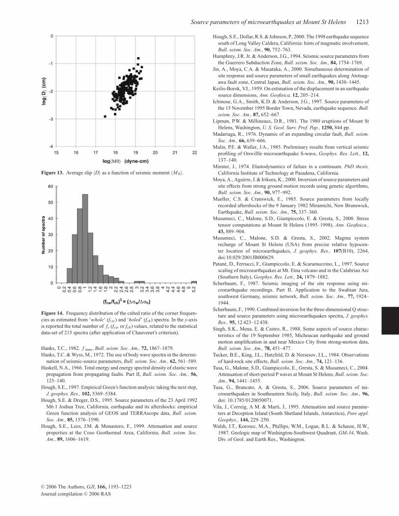
Finally, the average fault displacement 〈D〉 was computed from

〈M 0〉 and 〈r〉 for all events using:

〈D〉 = 〈M0〉μ(π〈r〉2)

, (16)

where μ (=ρ [α/1.78]2) is shear modulus and the product π〈r〉2 is

the rupture area supposed to be circular.

Table A5 gives the average values of M 0 and r, with their er-

ror factors, and stress drop �σ and 〈D〉. For shallow events, seis-

mic moment (M 0) ranges from 3.1 × 1017 to 2.2 × 1019 dyne-cm,

source radius (r) from 89 to 350 m and stress drop (�σ ) varies

from 0.01 to 6.6 bars. For deep events, the seismic moment (M 0)

ranges from 6.3 × 1017 to 1.3 × 1019 dyne-cm, source radius (r)

from 106 to 365 m and stress drop (�σ ) from 0.02 to 0.7 bars. The

relations between seismic moment and source radius for the three

time periods and for both groups of events (shallow and deep) are

shown in Fig. 12, coupled with contours of constant stress drop from

0.01 to 10 bars. We find a dependence of the seismic moment on

source radius and a large concentration of stress-drop values in the

range 0.1–1 bars. Moreover, the stress drops do not show depen-

dence on seismic moment. Finally, the data for 〈D〉 as a function of

〈M 0〉 are plotted in Fig. 13. 〈D〉 values are in the range from 0.001

to 0.154 cm and we can see a clear tendency of 〈D〉 to increase

with 〈M 0〉.

C© 2006 The Authors, GJI, 166, 1193–1223


1210 G. Tusa et al.


D I S C U S S I O N A N D C O N C L U S I O N S

In this study, we apply the ‘holed spectrum’ technique by Tusa et al.(2006) to analyse the source characteristics of 200 microearthquakes

occurred at Mount St Helens.

Our results indicate that the effect of the presence of a ‘spectralhole’ does not significantly effect the low-frequency level �0 and,

therefore, the seismic moment estimates. Conversely, the corner

frequency fc showed higher variation, even though its uncertainty

was no more than ones reported in studies of source parameters

(e.g. Humphrey & Anderson 1994; Hough et al. 1999; Jin et al.2000). We found no systematic change on (fcw − fch) with increasing

fcw (see Fig. 8b) and the bandwidth of spectral hole is the only factor

able to affect the corner frequency estimates (see Fig. 10b).

The variations of fc values translate to a variation in stress drop

that depends on f 3c . In order to evaluate the effect of the ‘spectral

hole’ on stress drop estimates, we used all fcw and fch values at each

station for both groups of microearthquakes (shallow and deep),

and the ratio (fcw/ fch)3 = �σ w/�σ h has been computed. This is

done under the assumption that �0w does not change with respect

to �0h , because the effect of the ‘spectral hole’ is negligible in

the determination of the low-frequency level. As shown in Fig. 14,

the ratio �σ w/�σ h falls between 0.4 and 5.2, with peaks (88 per

cent of the spectra) for ratio values higher than 0.4 to equal to 1.6.

Moreover, note that 97 per cent of the ratio values are less than or

equal to 2. This is significantly less than the typically quoted values

for stress drop errors of 10. The ratio values higher than 2 (only

3 per cent of spectra) are due to the spectral shape that characterizes

C© 2006 The Authors, GJI, 166, 1193–1223



Figure 11. Corrected P-wave source spectra for one event (M = 0.6) at the

three stations. The spectra are offset for clarity by the factor indicated next

to each one. Dashed line shows the best-fitting of ω−2 source model. Dark

tick marks indicate corner frequency results for each spectrum.

some spectra, above all at station HSR. In particular, the presence

of conspicuous peaks in a given frequency band about fc could

bias its estimates, producing a seeming poor computation of fc.

In fact, if the peaks are not due to the source (this is the case),

but represent the effect of some noisy source (such as instrumental

noise, background noise) or site amplification, their removal would

provide more reliable corner frequency estimates.

Corner frequency results show stress drop values are mainly in

the range, 0.1–1 bars and is not related to source moment (Fig. 12).

These low values are significantly lower than those obtained for

small earthquakes in other tectonic settings (Ichinose et al. 1997;

Hough et al. 1999; Bindi et al. 2001). This indicates a breakdown

in the hypothesis of self-similarity for these events, which might be

expected considering the limited area over which these earthquakes

take place and the likely very inhomogeneous stress field causing

them. Rapid and heterogeneous stress changes might be expected

in rocks surrounding a magma system undergoing magma or gas

pressure changes. Moreover, low stress drop events might be ex-

pected in or around active volcanic systems. Where strain rates are

high either ductile deformation or brittle shear failure in highly het-

erogeneous material in the vicinity of the magma chamber is likely

to prevent the accumulation of high stress. For example, Vila et al.(1995) find �σ values range from about 0.01 to 20 bars, with a ten-

dency to cluster within the range 0.1–1 bars, for microearthquakes

at Deception Island (South Shetland Islands, Antarctica). Cramer &

McNutt (1997) performed a detailed spectral analysis of the 1989

earthquake swarm beneath Mammoth Mountain. Their results show

stress drop values for high-frequency events in the 0.01 to less than

10 bars range. Hough et al. (2000) inferred stress drop values of

0.03–0.2 bars for a M 2.7 event that occurred in the volcanic system

of Long Valley Caldera and the authors conclude that this is most

probably associated with a fluid-controlled source.

We do not observe a decrease of stress drop at low seismic mo-

ments. Aki (1988) proposed the self-similarity to be valid within

individual ranges of seismic moments. Our data support this hy-

pothesis, because we observe a nearly constant stress drop value

within our range of seismic moments. Moreover, looking for time

and spatial variations in stress drop values, a few deep events show

slightly lower stress drop values (0.03 to 0.1 bars), in the period 1995

January–1998 May (Fig. 12, on the top right). This may be due to en-

vironmental conditions in the vicinity of the magma chamber where

a very high temperature gradient is probable. This may weaken the

crustal material allowing for activity on pre-existing fractures at

even lower stress drop values. Since, we observe minimum stress

drop values before the period of high seismicity (1998 May–July),

we suggest that this was due to pressure conditions during the initial

phases of the magmatic system recharging.

A C K N O W L E D G M E N T S

The authors deeply appreciate J. Johnson and an anonymous re-

viewer for their constructive comments and suggestions. Apprecia-

tion also goes to the editor Cindy Ebinger for her critical review of

this manuscript and advice. We are grateful to the staff of the Pacific

Northwest Seismograph Network for its effort to provide high qual-

ity recording of earthquakes. Data acquisition and analysis was

funded by USGS co-operative agreements such as 1434–95-A-1302.

Research supports come from INGV-DPC grants. GT was assisted

by a PhD fellowship from University of Catania.

R E F E R E N C E S

Abercrombie, R.E., 1995. Earthquake source scaling relationships from –1

to 5 ML using seismograms recorded at 2.5 km depth, J. geophys. Res.,100, 24 015–24 036.

Abercrombie, R.E. & Leary, P., 1993. Source parameters of small earth-

quakes recorded at 2.5 km depth, Canjon Pass, southern California: im-

plications for earthquakes scaling, Geophys. Res. Lett., 20, 1511–1514.

Aki, K., 1967. Scaling law of seismic spectrum, J. geophys. Res., 72, 1217–

1231.

Aki, K., 1988. Physical Theory of Earthquakes, in Seismic Hazard inMediterranean Regions, pp. 3–33, eds Bonnin, J., Cara, M., Cisternas,

A. & Fantechi, R., Kluwer, Dordrecht.

Anderson, J.G., 1986. Implications of attenuation for studies of the earth-

quake source, in Earthquake Source Mechanics, Vol. 37, pp. 311–318,

eds Das, S., Boathwright, J. & Scholz, C.H.J., Geophys. Monogr.

Anderson, J.G. & Hough, S.E., 1984. A model for the shape of the Fourier

amplitude spectrum of acceleration at high frequencies, Bull. seism. Soc.Am., 74, 1969–1993.

Archuleta, R.J., Cranswinck, E., Mueller, C. & Spudich, P., 1982. Source

parameters of the 1980 Mammoth Lakes, California earthquake sequence,

J. geophys. Res., 87, 4995–4607.

Bianco, F., Castellano, M., Del Pezzo, E. & Ibanez, J.M., 1999. Attenuation

of short-period waves at Mt Vesuvius. Italy, Geophys. J. Int., 138, 67–

76.

Bindi, D., Spallarossa, D., Augliera, P. & Cattaneo, M., 2001. Source pa-

rameters estimated from aftershocks of the 1997 Umbria-Marche (Italy)

seismic sequence, Bull. seism. Soc. Am., 91, 448–455.

Boatwright, J., 1978. Detailed analysis of two small New York State earth-

quake sequences, Bull. seism. Soc. Am., 68, 1117–1131.

Boore, D.M., 1983. Stochastic simulation of high-frequency ground motions

based on seismological models of the radiated spectra, Bull. seism. Soc.Am., 73, 1865–1894.

Boore, D.M., 1986. Short-period P- and S-wave radiation from large earth-

quakes: implications for spectral scaling relations, Bull. seism. Soc. Am.,76, 43–64.

Brune, J.N., 1970. Tectonic stress and the seismic shear waves from earth-

quakes, J. geophys. Res., 75, 4997–5009.

Brune, J.N., 1971. Correction, J. geophys. Res., 76, 5002.

Castro, R.R., Anderson, J.G. & Singh, S.K., 1990. Site response, attenuation

and source spectra of S waves along the Guerrero, Mexico, subduction

zone, Bull. seism. Soc. Am., 80, 1481–1503.

C© 2006 The Authors, GJI, 166, 1193–1223


https://www.researchgate.net/publication/240777017_The_1998_Earthquake_Sequence_South_of_Long_Valley_Caldera_California_Hints_of_Magmatic_Involvement?el=1_x_8&enrichId=rgreq-5d67adc7-3fd3-4adf-b368-331183515192&enrichSource=Y292ZXJQYWdlOzI0OTQyODkxMDtBUzo5OTExMzcwNjE5NzAxNUAxNDAwNjQxOTU3OTAy

1212 G. Tusa et al.

Figure 12. Plots of log-averages of source radius versus seismic moment for each time span. The lines are contours of equal stress-drops in bars. Open circles

refer to period I; crosses refer to period II; open squares refer to period III.

Chauvenet, W., 1863. Theory and use of astronomical instruments; method of

least squares, Vol. 2, pp. 558–566, eds Lippincott, J.B. & Co, Philadelphia.

Cramer, C.H. & McNutt, S.R., 1997. Spectral analysis of earthquake in

the 1989 Mammoth Mountain swarm near Ling Valley, California, Bull.seism. Soc. Am., 87, 1454–1462.

Cranswick, E., Wetmiller, R. & Boatwrigth, J., 1985. High frequency obser-

vations and source parameters of microearthquakes recorded at hard rock

sites, Bull. seism. Soc. Am., 75, 1535–1576.

De Luca, G., Scarpa, R., Filippi, L., Gorini, A., Marcucci, S., Marsan, P.,

Milana, G. & Zambonelli, E., 2000. A detailed analysis of two seismic

sequences in Abruzzo, Central Apennines, Italy, J. Seismol., 4, 1–21.

Del Pezzo, E., De Natale, G., Martini, M. & Zollo, A., 1987. Source param-

eters of microearthquakes at Phlegraen Fields (Southern Italy) volcanic

area, Phys. Earth planet. Int., 47, 25–42.

Frankel, A., 1982. The effects of attenuation and site response on the spectra

of microearthquakes in the Northeastern Caribbean, Bull. seism. Soc. Am.,72, 1379–1402.

Frankel, A. & Wennerberg, L., 1989. Microearthquake spectra from the

Anza, California seismic network: site response and source scaling, Bull.seism. Soc. Am., 79, 581–609.

Garcıa-Garcıa, J.M., Vidal, F., Romacho, M.D., Martın-Marfil, J.M., Posadas,

A. & Luzon, F., 1996. Seismic source parameters for microearthquakes

of the Granada basin (southern Spain), Tectonophysics, 261, 51–66.

Guo, H.A., Lerner-Lam, A. & Hough, S.E., 1992. Green’s function study of

Loma Prieta aftershocks: evidence for fault zone complexity (abstract),

Seism. Res. Lett., 63, 76.

Hanks, T.C., 1977. Earthquake stress drops, ambient tectonic stresses and

stresses that drive plate motions, Pure appl. Geophys., 115, 441–458.

C© 2006 The Authors, GJI, 166, 1193–1223



Figure 13. Average slip 〈D〉 as a function of seismic moment 〈M 0〉.

Figure 14. Frequency distribution of the cubed ratio of the corner frequen-

cies as estimated from ‘whole‘ (fcw) and ‘holed’ (fch) spectra. In the y-axis

is reported the total number of fc (fcw or fch) values, related to the statistical

data-set of 215 spectra (after application of Chauvenet’s criterion).

Hanks, T.C., 1982. f max, Bull. seism. Soc. Am., 72, 1867–1879.

Hanks, T.C. & Wyss, M., 1972. The use of body wave spectra in the determi-

nation of seismic-source parameters, Bull. seism. Soc. Am., 62, 561–589.

Haskell, N.A., 1966. Total energy and energy spectral density of elastic wave

propagation from propagating faults. Part II, Bull. seism. Soc. Am., 56,125–140.

Hough, S.E., 1997. Empirical Green’s function analysis: taking the next step,

J. geophys. Res., 102, 5369–5384.

Hough, S.E. & Dreger, D.S., 1995. Source parameters of the 23 April 1992

M6.1 Joshua Tree, California, earthquake and its aftershocks: empirical

Green function analysis of GEOS and TERRAscope data, Bull. seism.Soc. Am., 85, 1576–1590.

Hough, S.E., Lees, J.M. & Monastero, F., 1999. Attenuation and source

properties at the Coso Geothermal Area, California, Bull. seism. Soc.Am., 89, 1606–1619.

Hough, S.E., Dollar, R.S. & Johnson, P., 2000. The 1998 earthquake sequence

south of Long Valley Caldera, California: hints of magmatic involvement,

Bull. seism. Soc. Am., 90, 752–763.

Humphrey, J.R. Jr. & Anderson, J.G., 1994. Seismic source parameters from

the Guerrero Subduction Zone, Bull. seism. Soc. Am., 84, 1754–1769.

Jin, A., Moya, C.A. & Masataka, A., 2000. Simultaneous determination of

site response and source parameters of small earthquakes along Atotsug-

awa fault zone, Central Japan, Bull. seism. Soc. Am., 90, 1430–1445.

Keilis-Borok, V.I., 1959. On estimation of the displacement in an earthquake

source dimensions, Ann. Geofisica, 12, 205–214.

Ichinose, G.A., Smith, K.D. & Anderson, J.G., 1997. Source parameters of

the 15 November 1995 Border Town, Nevada, earthquake sequence. Bull.seism. Soc. Am., 87, 652–667.

Lipman, P.W. & Millineaux, D.R., 1981. The 1980 eruptions of Mount St

Helens, Washington, U. S. Geol. Surv. Prof. Pap., 1250, 844 pp.

Madariaga, R., 1976. Dynamic of an expanding circular fault, Bull. seism.Soc. Am., 66, 639–666.

Malin, P.E. & Waller, J.A., 1985. Preliminary results from vertical seismic

profiling of Orovillle microearthquake S-wave, Geophys. Res. Lett., 12,137–140.

Minster, J., 1974. Elastodynamics of failure in a continuum. PhD thesis,California Institute of Technology at Pasadena, California.

Moya, A., Aguirre, J. & Irikura, K., 2000. Inversion of source parameters and

site effects from strong ground motion records using genetic algorithms,


Mueller, C.S. & Cranswick, E., 1985. Source parameters from locally

recorded aftershocks of the 9 January 1982 Miramichi, New Brunswick,

Earthquake, Bull. seism. Soc. Am., 75, 337–360.

Musumeci, C., Malone, S.D., Giampiccolo, E. & Gresta, S., 2000. Stress

tensor computations at Mount St Helens (1995–1998), Ann. Geofisica.,43, 889–904.

Musumeci, C., Malone, S.D. & Gresta, S., 2002. Magma system

recharge of Mount St Helens (USA) from precise relative hypocen-

ter location of microearthquakes, J. geophys. Res., 107(B10), 2264,

doi:10.029/2001JB000629.

Patane, D., Ferrucci, F., Giampiccolo, E. & Scaramuzzino, L., 1997. Source

scaling of microearthquakes at Mt. Etna volcano and in the Calabrian Arc

(Southern Italy), Geophys. Res. Lett., 24, 1879–1882.

Scherbaum, F., 1987. Seismic imaging of the site response using mi-

croearthquake recordings. Part II. Application to the Swabian Jura,

southwest Germany, seismic network, Bull. seism. Soc. Am., 77, 1924–

1944.

Scherbaum, F., 1990. Combined inversion for the three-dimensional Q struc-

ture and source parameters using microearthquakes spectra, J. geophys.Res., 95, 12 423–12 438.

Singh, S.K., Mena, E. & Castro, R., 1988. Some aspects of source charac-

teristics of the 19 September 1985, Michoacan earthquake and ground

motion amplification in and near Mexico City from strong-motion data,


Tucker, B.E., King, J.L., Hatzfeld, D. & Nersesov, I.L., 1984. Observations

of hard-rock site effects, Bull. seism. Soc. Am., 74, 121–136.

Tusa, G., Malone, S.D., Giampiccolo, E., Gresta, S. & Musumeci, C., 2004.

Attenuation of short-period P waves at Mount St Helens, Bull. seism. Soc.Am., 94, 1441–1455.

Tusa, G., Brancato, A. & Gresta, S., 2006. Source parameters of mi-

croearthquakes in Southeastern Sicily, Italy, Bull. seism. Soc. Am., 96,doi: 10.1785/0120050071.

Vila, J., Correig, A M. & Marti, J., 1995. Attenuation and source parame-

ters at Deception Island (South Shetland Islands, Antarctica), Pure appl.Geophys., 144, 229–250.

Walsh, J.T., Korosec, M.A., Phillips, W.M., Logan, R.L. & Schasse, H.W.,

1987. Geologic map of Washington-Southwest Quadrant, GM-34, Wash.

Div. of Geol. and Earth Res., Washington.

C© 2006 The Authors, GJI, 166, 1193–1223


1214 G. Tusa et al.

A P P E N D I X A : TA B L E S

Tables A1 to A5 present the factors, parameters and data.

Table A1. Attenuation and site amplification (correction) factors at the three

stations for both shallow (a) and deep (b) events at low (LF) and high (HF)

frequencies. It is also considered the separation for the three different time

periods. Errors quoted with respect to the standard deviation of Q-inverse

mean are also reported.

Period Station Quality factor Site amplification factor

QLF QHF SLF SHF

Shallow events

I YEL 38−12+36 21−2

+2 0.9 ± 0.2 8.5 ± 1.1

HSR 20−5+9 214−57

+121 0.7 ± 0.2 0.4 ± 0.1

CDF 72−19+41 1020−300

+728 0.8 ± 0.1 0.1 ± 0.03

II YEL 30−10+22 23−2

+2 1.7 ± 0.4 16.2 ± 2.6

HSR 35−10+22 142−36

+74 0.5 ± 0.1 0.3 ± 0.1

CDF 44−5+7 435−130

+322 0.8 ± 0.1 0.1 ± 0.03

III YEL 33−5+7 20−2

+4 1.1 ± 0.2 7.9 ± 0.9

HSR 35−8+14 57−11

+19 0.6 ± 0.1 0.8 ± 0.2

CDF 77−20+42 380−75

+125 0.6 ± 0.1 0.1 ± 0.02

Deep events

I YEL 24−5+9 89−8

+10 1.7 ± 0.4 1.4 ± 0.2

HSR 45−12+24 354−87

+173 0.4 ± 0.05 0.5 ± 0.1

CDF 521−144+324 1238−335

+729 1.5 ± 0.2 1.2 ± 0.2

II YEL 36−7+11 37−4

+4 2.9 ± 0.5 8.6 ± 1.5

HSR 31−7+13 367−97

+205 0.4 ± 0.06 0.2 ± 0.04

CDF 240−62+128 393−114

+274 0.8 ± 0.1 0.5 ± 0.1

III YEL 22−5+9 36−3

+3 4.0 ± 1.1 5.1 ± 0.4

HSR 50−18+64 132−30

+54 0.2 ± 0.04 0.4 ± 0.1

CDF 298−46+66 375−100

+212 0.9 ± 0.1 0.5 ± 0.1

C© 2006 The Authors, GJI, 166, 1193–1223



Table A2. Spectral parameters (�0, fc, n) values as inferred from ‘whole spectra’ at the three stations for both shallow and deep events

of the statistical data set.

YEL HSR CDF

ID Time �0 (×10−9) fc n �0 (×10−9) fc n �0 (× 10−9) fc n(yy/mm/dd/hh/mm) (m-s) (Hz) (m-s) (Hz) (m-s) (Hz)

Shallow events

1s 9504040251 5.53 9.9 2.4 1.79 10.4 2.7 1.78 4.4 2.6

2s 9506220420 8.68 8.9 2.7 2.05 12.4 3.5 2.06 5.6 2.6

6s 9507052345 7.93 9.6 2.3 2.53 8.7 2.7 1.08 6.5 3.4

10s 9507241622 7.06 8.0 2.7 2.13 8.0 2.2 1.53 3.2 2.0

11s 9508310905 0.98 6.9 1.8 0.39 18.0 9.7 1.63 6.1 3.7

13s 9510052204 4.39 11.8 2.3 0.96 11.3 2.7 0.61 8.0 5.0

14s 9510061916 4.39 14.6 2.8 3.14 7.7 2.1 1.33 7.5 5.5

18s 9511210144 6.70 10.4 2.4 7.66 2.0 1.1 1.96 7.8 5.0

20s 9601170621 7.50 11.1 3.4 3.08 6.6 2.0 2.21 5.3 3.0

22s 9603061829 4.13 16.9 7.5 1.46 13.2 3.8 2.22 5.2 2.7

25s 9608280036 5.46 6.7 1.8 0.63 15.3 6.3 1.31 4.9 2.7

26s 9609040216 4.12 10.9 2.9 0.89 13.6 3.7 1.11 5.2 2.5

29s 9709050826 1.14 10.0 2.6 1.54 11.9 3.0 1.30 6.5 2.1

30s 9709081756 8.14 8.8 3.9 3.45 9.6 2.6 0.90 8.6 4.0

36s 9711060739 1.44 13.5 3.1 1.97 14.0 5.0 0.87 3.6 1.6

50s 9806060729 0.59 13.4 2.5 0.44 18.8 7.0 0.26 3.1 1.5

58s 9806150537 0.43 17.7 6.3 0.30 17.0 2.1 0.52 5.0 2.5

71s 9806201825 14.27 6.4 2.2 1.51 16.3 6.0 2.17 3.8 2.2

84s 9807020629 1.42 18.5 3.6 0.30 18.1 4.5 0.31 6.7 2.6

93s 9807060053 1.39 16.5 2.3 0.93 18.8 5.0 0.75 6.4 1.7

94s 9807060247 0.77 9.1 2.2 0.19 17.6 5.0 0.55 4.1 1.7

98s 9807081305 4.35 8.5 2.1 0.43 17.6 5.0 0.71 2.8 1.4

99s 9807090609 3.51 11.6 2.7 0.41 10.2 2.8 0.17 9.0 3.2

101s 9807101022 2.20 9.5 1.7 0.31 20.0 6.8 0.55 4.0 2.0

109s 9807111706 0.67 11.6 2.7 0.20 17.8 5.5 0.46 4.3 1.5

114s 9807121844 13.51 7.4 2.2 1.93 17.6 5.9 0.48 3.3 1.2

117s 9808141149 3.97 9.8 4.3 1.19 21.0 6.8 1.29 4.5 2.1

119s 9808181619 7.94 11.5 2.3 1.81 13.0 4.2 0.90 7.1 4.1

121s 9808260021 7.10 11.1 2.4 0.75 15.0 5.0 1.05 7.2 4.5

122s 9808260902 5.05 17.1 3.4 0.84 18.8 5.0 0.88 8.0 4.0

125s 9809050827 6.91 15.8 4.2 1.40 8.1 2.0 0.91 7.2 4.1

127s 9809110654 8.65 12.7 2.6 1.62 17.7 2.0 2.65 5.2 2.3

131s 9810292318 3.80 9.4 2.8 1.54 16.0 5.0 1.01 5.3 3.0

133s 9812030919 1.50 9.7 2.7 0.48 17.4 6.5 1.30 5.1 2.0

C© 2006 The Authors, GJI, 166, 1193–1223


1216 G. Tusa et al.

Table A2. (Continued.)

YEL HSR CDF

ID Time �0 (×10−9) fc n �0 (×10−9) fc n �0 (×10−9) fc n(yy/mm/dd/hh/mm) (m-s) (Hz) (m-s) (Hz) (m-s) (Hz)

Deep events

5d 9509140343 0.30 8.0 2.1 0.11 18.7 7.0 0.26 8.7 4.0

6d 9509170255 0.60 7.8 2.9 0.09 17.7 7.0 0.31 7.2 2.7

7d 9510110952 0.34 6.5 2.0 0.07 18.3 4.7 0.23 4.4 1.7

8d 9510180344 1.56 6.5 2.5 0.29 17.1 7.0 0.70 6.9 2.5

10d 9511042228 1.38 5.9 3.5 0.19 17.7 6.0 0.36 5.7 1.8

19d 9708152106 0.43 5.9 2.5 0.11 18.6 6.5 0.22 7.5 2.2

20d 9709031747 0.63 7.4 2.7 0.26 18.3 6.3 1.10 7.4 2.4

27d 9710171051 0.31 6.9 3.2 0.20 17.2 5.6 0.94 3.5 1.4

29d 9711160616 1.59 5.8 3.2 0.48 14.5 3.7 1.22 8.3 3.2

36d 9801050914 0.14 10.5 2.0 0.12 17.7 5.0 0.46 4.4 1.5

43d 9801160800 0.52 5.5 3.3 0.22 17.1 5.8 0.63 4.7 1.8

46d 9801252108 0.55 7.7 3.5 0.27 18.5 5.0 1.75 4.2 1.6

48d 9801280722 0.37 6.5 3.0 0.22 16.7 5.2 0.41 8.6 2.6

52d 9803251019 0.47 8.0 4.0 0.15 14.1 3.4 0.48 7.9 2.6

84d 9806170444 0.41 9.3 3.1 0.05 17.6 6.1 0.16 8.8 2.9

86d 9806180919 0.30 6.3 1.7 0.07 18.9 4.9 0.07 7.8 2.6

87d 9806181545 1.00 5.4 2.6 0.10 19.2 5.6 0.11 6.8 1.7

106d 9806271008 0.51 8.3 2.4 0.04 18.7 4.8 0.07 8.5 1.3

121d 9807020622 9.60 5.4 3.1 0.61 17.4 6.4 2.14 2.1 1.3

122d 9807020630 1.26 5.8 1.9 0.11 20.6 3.6 0.40 2.2 1.2

124d 9807020706 1.00 5.9 2.3 0.09 22.1 2.7 0.17 3.6 1.2

139d 9807082138 0.35 11.6 2.6 0.07 18.2 5.7 0.17 9.1 4.0

140d 9807091025 0.63 9.7 2.9 0.09 18.0 6.2 0.25 8.9 3.3

141d 9807091411 2.41 6.3 2.8 0.26 17.6 6.7 0.67 2.9 1.3

146d 9807120358 1.15 5.6 2.2 0.10 19.9 4.7 0.50 2.5 1.3

154d 9807140712 0.67 7.8 2.8 0.07 19.5 4.7 0.29 6.1 1.9

155d 9807140713 1.58 7.3 3.0 0.14 18.8 5.7 0.72 7.9 2.8

190d 9808291352 1.31 6.0 3.1 0.13 19.9 5.0 0.09 10.6 1.9

192d 9809080129 2.28 6.0 2.3 0.24 19.1 6.5 0.40 5.7 1.7

193d 9809080339 2.22 5.6 2.8 0.20 21.4 5.8 0.39 9.0 3.3

194d 9809081437 1.63 5.7 3.7 0.16 18.1 7.5 0.51 7.3 2.5

201d 9809251154 3.36 8.0 3.5 0.54 18.7 6.3 0.78 7.2 2.2

202d 9809270628 1.11 6.5 3.2 0.13 18.3 7.9 0.17 6.9 1.8

203d 9809300216 0.53 6.4 2.3 0.06 19.9 4.9 0.13 7.0 1.9

204d 9810100633 0.85 6.5 2.6 0.08 20.2 3.2 0.31 3.0 1.3

207d 9810252316 2.44 5.1 3.1 0.18 18.8 7.3 0.37 6.4 1.7

208d 9810272151 1.53 5.9 3.4 0.13 18.8 7.2 0.39 2.3 1.3

210d 9811090818 1.11 9.7 4.0 0.17 16.5 6.8 0.32 5.7 2.5

211d 9811091709 2.29 9.8 4.0 0.34 16.4 6.6 0.65 8.7 4.1

C© 2006 The Authors, GJI, 166, 1193–1223



Table A3. Spectral parameters (�0, fc) values as inferred from ‘holed spectra’ at the three stations for both shallow and deep events of

the statistical data set.

YEL HSR CDF

ID Time �0 (×10−9) fc �0 (×10−9) fc �0 (×10−9) fc

(yy/mm/dd/hh/mm) (m-s) (Hz) (m-s) (Hz) (m-s) (Hz)

Shallow events

1s 9504040251 5.43 14.4 1.92 8.7 1.74 4.6

2s 9506220420 8.73 7.5 2.10 7.7 1.79 11.3

6s 9507052345 8.60 5.6 2.55 10.2 0.75 10.0

10s 9507241622 6.62 14.3 2.13 8.1 1.48 3.3

11s 9508310905 0.94 9.4 0.37 16.3 1.64 6.0

13s 9510052204 4.01 16.4 1.01 11.8 0.62 11.9

14s 9510061916 4.32 13.6 3.20 7.3 1.37 11.2

18s 9511210144 6.36 13.3 8.37 1.8 1.98 12.0

20s 9601170621 7.19 14.0 3.11 6.5 2.27 5.3

22s 9603061829 4.32 15.4 1.38 15.1 2.18 5.5

25s 9608280036 5.35 7.3 0.78 6.8 1.32 4.8

26s 9609040216 3.76 12.4 1.03 7.3 1.07 5.8

29s 9709050826 1.10 12.7 1.71 7.4 1.23 9.7

30s 9709081756 8.15 12.6 3.58 7.1 0.91 11.8

36s 9711060739 1.58 7.7 2.06 10.1 0.81 4.0

50s 9806060729 0.60 15.0 0.25 20.2 0.28 2.9

58s 9806150537 0.47 14.5 0.30 16.5 0.53 4.8

71s 9806201825 14.37 6.5 2.03 6.9 2.07 4.1

84s 9807020629 1.26 18.9 0.26 13.5 0.31 6.9

93s 9807060053 1.25 21.7 0.65 18.4 0.73 7.5

94s 9807060247 0.76 11.3 0.12 16.8 0.56 4.1

98s 9807081305 4.34 14.3 0.39 15.1 0.81 2.7

99s 9807090609 3.42 13.4 0.41 8.6 0.18 12.0

101s 9807101022 2.06 16.1 0.24 20.3 0.57 3.8

109s 9807111706 0.69 12.2 0.14 14.5 0.46 4.7

114s 9807121844 13.36 10.9 2.26 5.8 0.48 3.5

117s 9808141149 3.64 11.6 0.89 22.4 1.29 4.2

119s 9808181619 8.07 11.4 1.76 11.5 0.86 9.0

121s 9808260021 6.92 12.2 0.69 12.7 1.25 8.0

122s 9808260902 4.53 18.9 0.57 17.7 0.88 8.4

125s 9809050827 7.04 15.7 1.40 7.0 0.92 8.7

127s 9809110654 9.10 14.6 1.07 13.5 2.64 5.3

131s 9810292318 3.79 14.6 1.23 7.1 1.02 5.0

133s 9812030919 1.56 12.8 0.30 17.5 1.26 5.7

C© 2006 The Authors, GJI, 166, 1193–1223


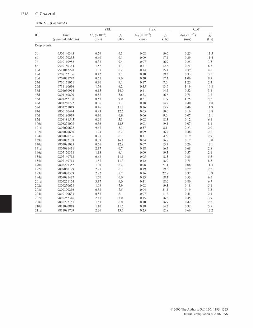
1218 G. Tusa et al.


YEL HSR CDF

ID Time �0 (×10−9) fc �0 (×10−9) fc �0 (×10−9) fc

(yy/mm/dd/hh/mm) (m-s) (Hz) (m-s) (Hz) (m-s) (Hz)

Deep events

5d 9509140343 0.29 9.3 0.08 19.0 0.25 11.5

6d 9509170255 0.60 9.1 0.09 17.1 0.29 11.4

7d 9510110952 0.33 9.4 0.07 16.9 0.25 3.5

8d 9510180344 1.52 7.7 0.31 12.6 0.71 6.5

10d 9511042228 1.37 6.2 0.14 15.1 0.39 4.6

19d 9708152106 0.42 7.1 0.10 19.2 0.33 3.5

20d 9709031747 0.61 9.6 0.20 17.3 1.06 9.7

27d 9710171051 0.30 9.1 0.17 7.0 1.25 2.3

29d 9711160616 1.56 6.2 0.45 13.9 1.19 10.8

36d 9801050914 0.15 14.0 0.11 14.2 0.52 3.4

43d 9801160800 0.52 5.6 0.23 16.6 0.71 3.7

46d 9801252108 0.55 9.0 0.21 11.9 1.75 4.2

48d 9801280722 0.36 7.1 0.18 14.7 0.40 14.8

52d 9803251019 0.46 11.7 0.16 13.9 0.46 11.9

84d 9806170444 0.43 12.5 0.05 10.0 0.16 10.8

86d 9806180919 0.30 6.9 0.06 9.0 0.07 13.1

87d 9806181545 0.99 5.3 0.08 18.3 0.12 6.1

106d 9806271008 0.56 12.8 0.03 19.4 0.07 8.1

121d 9807020622 9.67 5.3 0.57 8.1 2.23 2.0

122d 9807020630 1.24 6.2 0.09 16.7 0.48 2.0

124d 9807020706 0.97 6.7 0.11 4.6 0.19 2.9

139d 9807082138 0.39 16.1 0.04 16.8 0.17 13.0

140d 9807091025 0.66 12.9 0.07 13.7 0.26 12.1

141d 9807091411 2.37 6.7 0.18 16.5 0.68 2.8

146d 9807120358 1.13 6.1 0.09 19.5 0.57 2.1

154d 9807140712 0.68 11.1 0.05 18.5 0.31 5.3

155d 9807140713 1.57 11.3 0.12 18.0 0.71 8.5

190d 9808291352 1.30 6.2 0.08 21.4 0.08 11.3

192d 9809080129 2.27 6.3 0.19 19.5 0.79 2.2

193d 9809080339 2.22 5.7 0.16 22.8 0.37 13.9

194d 9809081437 1.60 6.0 0.13 18.3 0.53 6.5

201d 9809251154 3.37 9.0 0.41 18.0 0.80 6.7

202d 9809270628 1.08 7.9 0.08 19.3 0.18 5.1

203d 9809300216 0.52 7.5 0.04 21.4 0.19 3.3

204d 9810100633 0.83 8.1 0.07 11.2 0.41 2.1

207d 9810252316 2.47 5.0 0.15 16.2 0.45 3.9

208d 9810272151 1.53 6.0 0.10 16.9 0.42 2.2

210d 9811090818 1.10 11.5 0.18 14.2 0.32 5.9

211d 9811091709 2.26 13.7 0.25 12.8 0.66 12.2

C© 2006 The Authors, GJI, 166, 1193–1223



Table A4. Probability Pd after the application of χ2 test to the differences (�w0 − �h0) and (fwc − fhc) at the three stations for shallow

and deep events. Symbols μ and σ represent the arithmetic mean and standard deviation, respectively, as estimated from the data.

Station X μ σ Interval Om χ2 Pd (per cent)

Shallow events

YEL �0w − �0h 0.06 0.2 X < −0.14 4 1.22 24 < Pd < 27

−0.14 < X < 0.06 13

0.06 < X < 0.26 10

X > 0.26 7

HSR �0w − �0h 0.02 0.28 X < −0.26 3 3.39 6.1 < Pd < 8.3

−0.26 < X < 0.02 15

0.02 < X < 0.30 13

X > 0.30 3

CDF �0w − �0h −0.01 0.15 X < −0.16 2 5.85 1.4 < Pd < 1.9

−0.16 < X < −0.01 12

−0.01 < X < 0.14 17

X > 0.14 3

YEL fcw − fch −0.85 1.5 X < −2.35 6 2.03 14 < Pd < 16

−2.35 < X < −0.85 9

−0.85 < X < 0.65 15

X > 0.65 4

HSR fcw − fch 0.37 2.1 X < −1.73 3 6.88 0.5 < Pd < 1.4

−1.73 < X < 0.37 11

0.37 < X < 2.47 18

X > 2.47 2

CDF fcw − fch −0.51 0.86 X < −1.37 9 5.55 1.4 < Pd < 1.9

−1.37 < X < −0.51 6

−0.51 < X < 0.35 14

X > 0.35 5

Deep events

YEL �0w − �0h 0.01 0.03 X < −0.02 5 1.66 8.3 < Pd < 9.4

−0.02 < X < 0.01 14

0.01 < X < 0.04 16

X > 0.04 4

HSR �0w − �0h 0.03 0.031 X < −0.001 4 2.86 19 < Pd < 21

−0.001 < X < 0.03 18

0.03 < X < 0.061 12

X > 0.061 5

CDF �0w − �0h −0.01 0.044 X < −0.054 4 11.08 Pd < 0.05

−0.054 < X < −0.01 12

−0.01 < X < 0.034 22

X > 0.034 1

YEL fcw − fch −1.28 1.13 X < −2.41 7 2.19 14 < Pd < 16

−2.41 < X < −1.28 10

−1.28 < X < −0.15 17

X > −0.15 5

HSR fcw − fch −0.63 2.2 X < −2.83 4 19.53 Pd < 0.05

−2.83 < X < −0.63 8

−0.63 < X < 1.57 26

X > 1.57 1

CDF fcw − fch −0.32 1.13 X < −1.45 7 2.19 14 < Pd < 16

−1.45 < X < −0.32 10

−0.32 < X < 0.81 17

X > 0.81 5

C© 2006 The Authors, GJI, 166, 1193–1223


1220 G. Tusa et al.

Table A5. Source parameters. ID is the identification number of the events (the subscripts s and d refer to shallow and deep events,

respectively); M is the magnitude assigned by the staff of the Pacific Northwest Seismograph Network; 〈M 0〉 is the average seismic

moment; EM 0 is the multiplicative error factor for seismic moment; 〈r〉, is the average source radius; Er is the multiplicative error factor

for source radius; 〈�σ 〉 is the average stress drop; 〈D〉 is the average fault slip.

ID Time M Depth, 〈M 0〉, EM 0 〈r〉, Er 〈�σ 〉, 〈D〉,(yy/mm/dd/hh/mm) (km) (dyne-cm) (m) bars cm

1s 9504040251 0.7 2.01 4.71E+18 4.7 207 1.1 0.23 0.019

2s 9506220420 0.6 2.04 6.32E+18 4.6 208 1.1 0.31 0.026

3s 9506290116 0.4 4.28 7.41E+18 4.0 190 1.4 0.48 0.021

4s 9507022102 0.7 3.47 3.84E+18 1.7 189 1.1 0.25 0.011

5s 9507030601 1.0 3.93 6.28E+18 2.0 156 1.1 0.72 0.027

6s 9507052345 0.9 1.83 4.59E+18 3.0 210 1.3 0.22 0.018

7s 9507081828 0.2 2.01 4.97E+18 3.1 308 1.9 0.07 0.009

8s 9507220352 0.3 1.82 2.59E+18 3.6 183 1.2 0.19 0.014

9s 9507221914 0.6 2.80 6.58E+18 3.4 271 1.5 0.14 0.013

10s 9507241622 0.5 2.07 4.76E+18 3.3 232 1.2 0.17 0.016

11s 9508310905 1.5 4.91 9.24E+18 3.0 196 1.2 0.54 0.025

12s 9509020401 1.3 3.11 8.42E+18 2.3 209 2.5 0.40 0.028

13s 9510052204 1.1 1.97 2.68E+18 4.0 186 1.0 0.18 0.014

14s 9510061916 0.6 1.94 4.88E+18 4.8 192 1.1 0.30 0.023

15s 9510071812 0.7 4.46 6.36E+18 2.0 225 1.0 0.24 0.013

16s 9510091259 1.1 3.90 2.06E+19 4.4 274 1.4 0.44 0.029

17s 9511061403 0.5 2.98 6.91E+18 3.6 351 1.8 0.07 0.008

18s 9511210144 0.3 2.08 7.39E+18 3.2 199 1.0 0.41 0.033

20s 9601170621 0.6 4.11 1.78E+19 2.4 259 1.2 0.45 0.028

21s 9602060345 0.4 1.70 3.75E+18 4.2 227 1.7 0.14 0.013

22s 9603061829 0.9 2.10 4.80E+18 4.4 188 1.2 0.32 0.024

24s 9608060509 1.1 1.91 4.00E+18 2.8 201 1.2 0.21 0.017

25s 9608280036 1.7 4.93 1.04E+19 2.6 222 1.1 0.42 0.022

26s 9609040216 0.6 1.88 2.82E+18 3.4 189 1.1 0.18 0.014

27s 9708252137 0.8 4.92 1.22E+19 4.2 158 1.2 1.37 0.051

28s 9708280844 0.0 1.64 1.09E+18 4.5 156 1.1 0.13 0.008

29s 9709050826 1.5 4.92 9.65E+18 3.9 170 1.4 0.86 0.035

30s 9709081756 1.0 1.99 5.76E+18 3.1 184 1.1 0.41 0.030

31s 9709290916 1.0 1.86 1.54E+18 4.5 175 1.2 0.13 0.009

32s 9710101828 0.6 1.73 1.98E+18 4.1 175 1.1 0.16 0.011

33s 9710182306 0.6 2.98 4.59E+18 4.8 188 1.3 0.30 0.019

34s 9710210429 0.6 3.03 1.77E+18 3.2 126 1.6 0.39 0.016

35s 9711020100 1.3 1.83 6.30E+18 3.1 166 1.2 0.60 0.040

36s 9711060739 0.8 2.18 2.57E+18 3.0 181 1.3 0.19 0.014

37s 9712060308 1.0 1.91 5.62E+18 2.2 169 1.3 0.51 0.035

38s 9801261201 0.3 4.58 3.88E+18 2.7 141 1.9 0.60 0.020

50s 9806060729 0.2 2.83 8.76E+17 3.4 137 1.4 0.15 0.007

51s 9806090536 0.4 3.55 3.89E+18 3.4 192 1.1 0.24 0.011

53s 9806140613 0.8 3.81 4.53E+18 2.4 150 1.3 0.58 0.021

54s 9806150126 0.6 4.19 7.17E+18 3.8 275 1.4 0.15 0.010

55s 9806150509 0.2 5.25 1.80E+18 3.0 145 1.5 0.26 0.009

56s 9806150527 0.7 4.96 5.06E+18 2.3 159 1.3 0.55 0.021

57s 9806150529 1.5 4.51 1.13E+19 4.8 310 2.0 0.16 0.012

58s 9806150537 0.6 5.22 3.10E+18 4.5 158 1.0 0.34 0.013

59s 9806150551 0.9 4.38 5.22E+18 2.9 156 1.4 0.60 0.022

60s 9806160904 0.0 4.11 2.05E+18 2.6 151 1.6 0.26 0.009

61s 9806170302 0.2 2.93 8.04E+17 2.2 125 1.4 0.18 0.007

62s 9806170456 1.0 4.08 4.18E+18 4.0 150 1.4 0.54 0.019

65s 9806171348 0.1 1.47 7.65E+17 3.8 129 1.5 0.15 0.008

67s 9806171637 0.6 4.55 2.69E+18 3.0 118 1.9 0.71 0.020

68s 9806180700 0.2 4.04 1.29E+18 2.7 98 1.6 0.61 0.014

69s 9806190114 0.5 3.19 2.46E+18 5.1 168 1.1 0.23 0.013

70s 9806191209 0.3 3.16 2.62E+18 4.5 118 1.5 0.71 0.027

71s 9806201825 1.5 4.27 1.61E+19 2.5 195 1.3 0.94 0.044

72s 9806220118 0.9 3.49 8.81E+18 3.2 188 1.3 0.58 0.026

73s 9806231249 0.7 4.02 3.17E+18 3.0 133 1.4 0.59 0.019

74s 9806240014 0.8 3.74 9.31E+18 3.2 214 1.1 0.42 0.021

75s 9806250018 0.3 4.35 2.72E+18 1.4 177 1.5 0.21 0.009

C© 2006 The Authors, GJI, 166, 1193–1223




ID Time M Depth, 〈M 0〉, EM 0 〈r〉, Er 〈�σ 〉, 〈D〉,(yy/mm/dd/hh/mm) (km) (dyne-cm) (m) bars cm

76s 9806261017 0.3 4.24 2.74E+18 4.1 144 1.8 0.40 0.014

77s 9806271426 0.9 5.52 5.55E+18 3.7 149 1.7 0.74 0.026

78s 9806272053 0.7 4.90 2.64E+18 2.1 147 1.5 0.36 0.013

79s 9806281028 0.4 4.57 2.21E+18 4.6 126 1.3 0.48 0.014

80s 9807010432 1.2 4.20 5.56E+18 2.8 152 1.1 0.70 0.025

81s 9807010727 0.5 4.53 2.59E+18 2.4 116 1.2 0.73 0.020

82s 9807011703 0.5 3.86 2.15E+18 4.5 132 1.4 0.41 0.013

83s 9807020257 0.2 3.58 1.66E+18 4.7 149 1.2 0.22 0.008

84s 9807020629 0.8 4.62 3.74E+18 4.4 105 1.5 1.41 0.035

85s 9807020815 0.7 5.63 5.08E+18 1.9 126 1.2 1.11 0.033

87s 9807031213 0.0 4.56 1.49E+18 1.9 140 1.2 0.24 0.008

88s 9807031336 1.4 1.71 6.13E+18 4.3 246 1.7 0.18 0.018

89s 9807032244 2.0 5.08 2.19E+19 2.1 177 1.6 1.73 0.073

90s 9807051420 0.0 4.19 1.07E+18 3.7 136 1.2 0.18 0.006

92s 9807051753 0.2 2.96 8.60E+17 3.4 116 1.6 0.24 0.009

93s 9807060053 1.7 5.45 1.44E+19 3.7 98 1.2 6.61 0.154

94s 9807060247 0.8 5.43 3.05E+18 4.0 124 1.1 0.70 0.020

95s 9807060835 0.4 3.12 1.63E+18 4.9 89 1.5 1.02 0.030

96s 9807070303 0.8 3.28 4.10E+18 4.0 156 1.3 0.47 0.024

97s 9807072127 0.7 4.57 1.95E+19 3.2 199 1.6 1.09 0.051

98s 9807081305 1.1 4.43 4.58E+18 2.6 129 1.6 0.94 0.029

99s 9807090609 0.0 1.45 9.65E+17 3.0 169 1.1 0.09 0.006

100s 9807100746 1.2 3.48 2.68E+18 1.0 128 1.5 0.56 0.017

101s 9807101022 0.4 4.90 4.31E+18 3.7 153 1.3 0.52 0.019

102s 9807101115 1.3 3.92 3.42E+18 2.9 172 1.4 0.30 0.012

103s 9807101805 0.1 5.47 2.37E+18 4.3 133 1.3 0.44 0.014

106s 9807102338 0.2 5.40 1.65E+18 2.5 160 1.3 0.18 0.007

107s 9807110430 0.9 5.03 2.14E+18 3.1 135 1.3 0.38 0.012

108s 9807110720 0.6 4.81 2.38E+18 3.0 136 1.3 0.42 0.013

109s 9807111706 0.7 5.41 2.81E+18 4.6 121 1.4 0.70 0.020

110s 9807121130 2.0 3.17 5.92E+18 1.6 174 1.2 0.50 0.028

111s 9807121132 0.6 3.56 2.22E+18 1.7 116 1.3 0.63 0.017

112s 9807121428 0.0 3.68 7.63E+17 2.3 125 1.8 0.17 0.005

114s 9807121844 1.8 4.97 1.40E+19 1.3 126 1.6 3.09 0.092

115s 9807121944 1.1 5.05 8.37E+18 2.2 115 1.6 2.39 0.065

116s 9807131752 0.9 3.83 7.76E+18 4.2 187 1.1 0.52 0.023

117s 9808141149 1.3 4.20 1.29E+19 4.4 257 1.9 0.33 0.020

118s 9808172212 1.1 1.92 4.30E+18 4.7 152 1.2 0.54 0.033

119s 9808181619 1.1 1.90 4.58E+18 4.4 187 1.1 0.31 0.023

121s 9808260021 0.4 2.08 3.62E+18 3.3 183 1.1 0.26 0.019

122s 9808260902 0.7 2.07 2.76E+18 4.1 122 1.6 0.66 0.032

123s 9808261001 1.0 1.95 1.65E+18 2.3 154 1.2 0.20 0.012

124s 9808261003 0.8 1.93 6.69E+18 4.0 241 1.9 0.21 0.020

125s 9809050827 0.9 1.90 3.92E+18 4.2 176 1.0 0.31 0.022

127s 9809110654 1.4 1.84 5.23E+18 4.2 127 2.3 1.13 0.058

128s 9809200250 0.8 1.80 2.24E+18 5.1 147 1.2 0.31 0.018

129s 9809230506 1.1 1.69 1.28E+18 1.1 201 1.1 0.07 0.006

131s 9810292318 0.7 5.01 1.20E+19 2.9 194 2.0 0.72 0.033

132s 9811260743 0.3 1.92 3.07E+17 2.3 211 1.5 0.01 0.001

133s 9812030919 0.3 5.06 6.28E+18 5.4 142 1.3 0.96 0.032

1d 9505220534 0.4 8.07 2.53E+18 1.7 184 1.2 0.18 0.008

3d 9508250250 0.4 7.27 2.45E+18 2.1 264 1.2 0.06 0.004

4d 9509011256 0.5 7.23 1.29E+18 1.4 204 1.1 0.07 0.003

5d 9509140343 1.1 7.76 1.98E+18 1.4 207 1.1 0.10 0.005

6d 9509170255 0.1 7.21 2.69E+18 1.7 284 1.1 0.05 0.003

7d 9510110952 0.0 7.88 1.78E+18 1.5 257 1.6 0.05 0.003

8d 9510180344 0.7 7.02 6.63E+18 1.5 298 1.3 0.11 0.008

9d 9510280934 1.2 7.17 3.08E+18 1.8 296 1.4 0.05 0.004

C© 2006 The Authors, GJI, 166, 1193–1223


1222 G. Tusa et al.


ID Time M Depth, 〈M 0〉, EM 0 〈r〉, Er 〈� σ 〉, 〈D〉,(yy/mm/dd/hh/mm) (km) (dyne-cm) (m) bars cm

10d 9511042228 0.4 8.76 5.79E+18 1.9 323 1.3 0.08 0.006

11d 9511131409 0.8 7.17 8.26E+18 1.9 340 1.2 0.09 0.007

12d 9601081305 0.5 7.49 3.79E+18 1.9 324 1.3 0.05 0.004

13d 9603060512 1.5 7.47 1.02E+19 1.2 233 1.1 0.35 0.020

16d 9605310711 0.3 9.79 2.73E+18 1.8 183 1.2 0.20 0.008

17d 9707100951 1.2 7.12 6.84E+18 1.9 290 1.1 0.12 0.008

19d 9708152106 0.1 7.84 2.29E+18 1.3 221 1.2 0.09 0.005

20d 9709031747 1.2 7.17 5.17E+18 2.3 246 1.1 0.15 0.009

23d 9709280029 0.1 7.40 1.33E+18 1.6 233 1.3 0.05 0.003

24d 9709301358 0.8 6.94 7.60E+18 4.8 291 1.1 0.14 0.009

27d 9710171051 0.9 7.02 2.74E+18 2.3 253 1.1 0.07 0.004

29d 9711160616 1.9 7.31 1.02E+19 1.4 326 1.4 0.13 0.010

31d 9712241654 1.0 7.16 1.64E+18 1.3 276 1.7 0.03 0.002

33d 9712291015 1.1 7.82 2.24E+18 1.7 215 1.2 0.10 0.005

34d 9712310246 0.8 7.82 5.21E+18 2.9 202 1.3 0.28 0.013

36d 9801050914 0.7 7.34 2.99E+18 1.6 254 1.0 0.08 0.005

38d 9801100559 1.5 7.37 3.85E+18 1.5 308 1.3 0.06 0.004

43d 9801160800 1.1 6.96 3.30E+18 1.7 304 1.1 0.05 0.004

44d 9801171119 1.0 7.04 6.12E+18 2.9 235 1.3 0.20 0.011

46d 9801252108 1.0 7.04 5.15E+18 2.7 262 1.3 0.13 0.008

47d 9801252129 0.6 6.82 1.91E+18 2.8 217 1.2 0.08 0.004

48d 9801280722 1.1 6.98 2.73E+18 1.7 244 1.1 0.08 0.005

52d 9803251019 1.3 6.92 2.94E+18 2.0 245 1.1 0.09 0.005

79d 9806070908 1.5 7.66 3.21E+18 2.8 160 1.4 0.35 0.013

80d 9806090033 1.4 8.37 7.66E+18 2.4 333 1.9 0.09 0.007

81d 9806101528 1.1 6.85 3.73E+18 2.3 195 1.4 0.22 0.010

82d 9806141041 0.8 6.61 1.01E+18 1.5 222 1.4 0.04 0.002

84d 9806170444 0.2 7.14 1.67E+18 2.3 197 1.2 0.10 0.004

86d 9806180919 0.2 8.20 1.41E+18 1.6 147 1.4 0.19 0.007

87d 9806181545 0.7 7.42 1.92E+18 1.4 179 1.9 0.15 0.006

88d 9806181552 0.7 7.58 2.98E+18 1.6 242 1.6 0.09 0.005

90d 9806190002 0.1 7.41 9.73E+17 3.6 263 2.7 0.02 0.001

94d 9806211104 0.7 7.52 9.11E+17 2.5 145 1.2 0.13 0.004

97d 9806230711 0.8 6.93 2.79E+18 1.4 246 1.4 0.08 0.005

98d 9806230746 1.2 6.43 2.47E+18 2.5 198 1.4 0.14 0.007

103d 9806270206 0.3 6.14 7.38E+17 1.5 187 1.1 0.05 0.002

106d 9806271008 0.8 8.57 1.46E+18 1.7 111 1.4 0.47 0.012

107d 9806272051 0.7 8.79 1.29E+18 3.1 106 1.7 0.48 0.012

111d 9807010805 0.6 7.03 1.04E+18 1.5 127 1.5 0.22 0.007

114d 9807011649 0.9 8.15 1.90E+18 1.8 110 1.0 0.62 0.016

115d 9807011656 0.7 7.93 1.51E+18 2.2 122 1.0 0.36 0.011

116d 9807020038 1.1 7.83 4.44E+18 1.7 160 1.2 0.47 0.018

121d 9807020622 1.9 6.52 1.32E+19 1.7 277 1.6 0.27 0.018

122d 9807020630 0.9 7.32 2.69E+18 1.1 157 2.4 0.30 0.011

124d 9807020706 0.8 6.40 1.82E+18 1.4 186 3.1 0.12 0.005

126d 9807030031 1.3 6.09 1.91E+18 2.1 161 1.1 0.20 0.008

127d 9807030033 0.3 6.79 9.56E+17 1.7 128 1.3 0.20 0.006

133d 9807070447 0.9 7.85 2.52E+18 2.5 144 1.4 0.37 0.013

137d 9807081136 0.5 7.17 2.11E+18 3.3 150 1.9 0.28 0.010

139d 9807082138 0.0 7.46 2.49E+18 2.4 178 1.1 0.19 0.008

140d 9807091025 0.9 7.07 2.54E+18 2.4 194 1.2 0.15 0.007

141d 9807091411 1.3 7.31 6.00E+18 1.8 269 1.6 0.13 0.009

C© 2006 The Authors, GJI, 166, 1193–1223




ID Time M Depth, 〈M 0〉, EM 0 〈r〉, Er 〈� σ 〉, 〈D〉,(yy/mm/dd/hh/mm) (km) (dyne-cm) (m) bars cm

142d 9807092136 0.6 7.06 2.03E+18 1.6 190 1.4 0.13 0.006

143d 9807101815 0.8 7.27 1.10E+19 2.4 220 1.1 0.45 0.023

144d 9807110147 0.5 7.24 2.19E+18 2.5 175 1.5 0.18 0.007

146d 9807120358 1.2 7.25 2.57E+18 1.6 136 1.3 0.44 0.014

148d 9807120911 1.1 7.40 2.23E+18 1.5 190 1.9 0.14 0.006

152d 9807131114 0.8 7.75 1.88E+18 1.3 141 1.7 0.29 0.010

154d 9807140712 0.7 7.23 2.08E+18 2.4 146 1.5 0.29 0.010

155d 9807140713 1.4 7.18 4.91E+18 2.8 159 1.3 0.54 0.020

183d 9808090334 0.5 7.57 3.34E+18 1.4 128 1.5 0.69 0.021

185d 9808101258 0.4 7.39 2.16E+18 2.8 162 1.3 0.22 0.009

186d 9808121513 1.0 7.36 4.54E+18 1.8 162 1.1 0.47 0.018

187d 9808251724 0.3 7.76 1.64E+18 3.0 133 1.0 0.31 0.010

190d 9808291352 1.1 6.28 1.74E+18 1.1 157 1.8 0.20 0.007

191d 9809070037 1.3 6.83 1.18E+19 1.1 284 1.1 0.23 0.015

192d 9809080129 0.7 7.17 5.49E+18 1.3 228 1.6 0.20 0.011

193d 9809080339 1.2 7.82 6.18E+18 1.3 165 1.3 0.60 0.024

194d 9809081437 1.5 7.49 5.28E+18 1.6 238 1.3 0.17 0.010

195d 9809090943 1.5 6.98 1.01E+19 2.0 210 1.1 0.48 0.024

196d 9809110329 0.6 6.35 1.18E+18 1.7 133 1.4 0.22 0.007

197d 9809171452 0.3 7.46 3.36E+18 1.5 179 1.2 0.26 0.011

199d 9809200355 1.2 7.31 9.97E+18 1.5 365 1.1 0.09 0.008

200d 9809241904 0.3 7.38 1.79E+18 2.2 187 1.1 0.12 0.005

201d 9809251154 1.5 7.18 1.02E+19 1.3 184 1.2 0.72 0.031

202d 9809270628 1.0 7.45 2.47E+18 1.1 161 1.2 0.26 0.010

203d 9809300216 0.3 6.63 1.19E+18 1.5 161 1.3 0.12 0.005

204d 9810100633 0.8 7.48 2.17E+18 1.2 156 1.3 0.25 0.009

205d 9810170558 0.5 7.23 6.28E+17 1.4 163 1.1 0.06 0.002

206d 9810230912 1.3 7.48 3.04E+18 1.3 137 1.6 0.51 0.017

207d 9810252316 1.0 7.43 5.18E+18 1.2 217 1.7 0.22 0.011

208d 9810272151 0.4 6.94 2.62E+18 1.2 207 1.5 0.13 0.006

210d 9811090818 1.1 6.82 4.60E+18 1.9 238 1.1 0.15 0.008

211d 9811091709 1.4 6.51 7.02E+18 1.8 203 1.2 0.37 0.018

C© 2006 The Authors, GJI, 166, 1193–1223


source parameters of microearthquakes at mount st helens (usa)

Documents