sliding mode control handout - unipv
TRANSCRIPT

Sliding Mode Control HandoutAdvanced Automation and Control Course
Prof. Antonella Ferrara
University of PaviaDipartimento di Ingegneria Industriale e dell’Informazione
Pavia, Italy
Prof. Antonella Ferrara Sliding Mode Control, Advanced Automation and Control
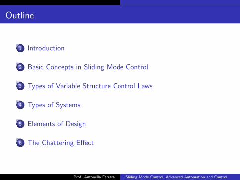
Outline
1 Introduction
2 Basic Concepts in Sliding Mode Control
3 Types of Variable Structure Control Laws
4 Types of Systems
5 Elements of Design
6 The Chattering Effect
Prof. Antonella Ferrara Sliding Mode Control, Advanced Automation and Control

Introduction
Introduction
Prof. Antonella Ferrara Sliding Mode Control, Advanced Automation and Control

Introduction
Historical Background
The origins of feedback control date back to the ancient world,with the advent of level control, water clocks, andpneumatics/hydraulics systems.
From the 17th century on-wards, systems were designed fortemperature control in furnaces, the mechanical control of mills,and the regulation of steam engines.
It was only during the 19th century that it became clear thatfeedback systems were prone to instability or oscillatorybehaviors.
Prof. Antonella Ferrara Sliding Mode Control, Advanced Automation and Control

Introduction
Historical Background
This was particularly true for Relay-based control systems:
A relay is an electrically operated switch.
The first relays were used in long distance telegraph circuits asamplifiers (a simple relay was included in the original 1840 telegraphpatent of Samuel Morse).
Relays were used extensively in early control systems to performlogical operations. In particular, they could implement on-offcontrol actions: these can be regarded as primordial sliding mode(or better, variable structure) control strategies.
A theory was needed!
Prof. Antonella Ferrara Sliding Mode Control, Advanced Automation and Control

Introduction
Historical Background
Spurred by servo and communications engineering developments ofthe 30s, the coherent body of theory known as classical controlemerged during and just after WWII in the US, UK and elsewhere.
In the 50s and 60s, an alternative approach to dynamic modellingwas developed in the Soviet Union based on the works by Poincaréand Lyapunov. Information was gradually disseminated, andstate-space or modern control techniques rapidly developed.
But only at the end of the 70s, with the first publications in Englishby Vadim I. Utkin (Ph.D. 1964, Institute for Control Sciences,Moscow, Russia), a theory of relay-based control was disclosed. Itwas the beginning of Sliding Mode Control Theory.
Prof. Antonella Ferrara Sliding Mode Control, Advanced Automation and Control

Basic Concepts in Sliding Mode Control
Introduction: Basic Concepts in SlidingMode Control
Prof. Antonella Ferrara Sliding Mode Control, Advanced Automation and Control

Basic Concepts in Sliding Mode Control
The Basic Terms
Consider a generic dynamical system S described by its state equation
x(t) = f(x(t), u(t), t)
with x(t0) = x0, and t, t0 ∈ [0, +∞)
x(t) ∈ Rn is the system state
u(t) ∈ Rm is the system input (i.e. the control input)
Consider a function of the system state σ(x(t)) ∈ Rm and the associatedmanifold σ(x(t)) = 0 (0 null vector of dimension m)
σ(x(t)) is the sliding variable
σ(x(t)) = 0 is the sliding manifold
Prof. Antonella Ferrara Sliding Mode Control, Advanced Automation and Control

Basic Concepts in Sliding Mode Control
The Concept of Sliding mode
The sliding manifold is a subspace of the system state spacehaving dimension n−m.It can be a single surface or be given by the intersection of severalsurfaces.When the state trajectory continuously crosses the slidingmanifold, since in its vicinity the state motion is always directedtowards the manifold, a sliding mode is enforced.
Prof. Antonella Ferrara Sliding Mode Control, Advanced Automation and Control

Basic Concepts in Sliding Mode Control
The Design IngredientsTwo elements need to be “designed”:
The sliding manifold: it is designed so that the system in slidingmode evolves in the desired way (e.g. it results in being linearizedand its state is asymptotically regulated to zero, or it satisfies someoptimality requirement, etc.).The control law: it has to be chosen in order to enforce a slidingmode.
An important design requirementThe sliding mode needs to be enforced in a finite time!
Prof. Antonella Ferrara Sliding Mode Control, Advanced Automation and Control
Basic Concepts in Sliding Mode Control
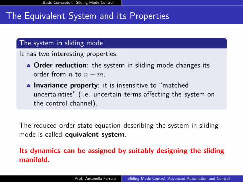
The Equivalent System and its Properties
The system in sliding modeIt has two interesting properties:
Order reduction: the system in sliding mode changes itsorder from n to n−m.Invariance property: it is insensitive to “matcheduncertainties” (i.e. uncertain terms affecting the system onthe control channel).
The reduced order state equation describing the system in slidingmode is called equivalent system.
Its dynamics can be assigned by suitably designing the slidingmanifold.
Prof. Antonella Ferrara Sliding Mode Control, Advanced Automation and Control

Basic Concepts in Sliding Mode Control
Two Simple Examples to Illustrate Some Facts
EXAMPLE 1: Consider an unstable second order system
[x1x2
]=[0 11 2
] [x1x2
]+[01
]u
Design the control input as u = −3x1 or u = 2x1
Prof. Antonella Ferrara Sliding Mode Control, Advanced Automation and Control

Basic Concepts in Sliding Mode Control
Example 1 (cont’ed)
The controlled system has an unstable focus if u = −3x1, and a saddlepoint if u = 2x1.
u = −3x1 u = 2x1
Prof. Antonella Ferrara Sliding Mode Control, Advanced Automation and Control
Basic Concepts in Sliding Mode Control
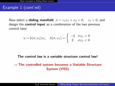
Example 1 (cont’ed)
Now select a sliding manifold: σ = c1x1 + x2 = 0, c1 > 0, anddesign the control input as a combination of the two previouscontrol laws:
u = k(σ, x1)x1, k(σ, x1) ={−3 σx1 > 02 σx1 < 0
The control law is a variable structure control law!
→ The controlled system becomes a Variable StructureSystem (VSS)
Prof. Antonella Ferrara Sliding Mode Control, Advanced Automation and Control
Basic Concepts in Sliding Mode Control
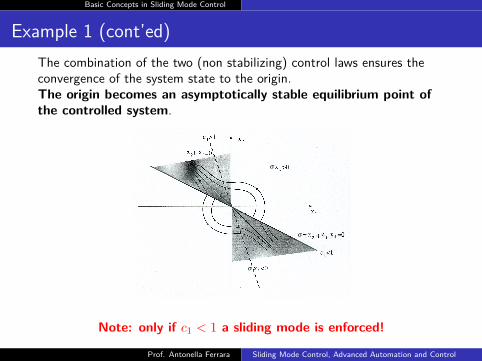
Example 1 (cont’ed)The combination of the two (non stabilizing) control laws ensures theconvergence of the system state to the origin.The origin becomes an asymptotically stable equilibrium point ofthe controlled system.
Note: only if c1 < 1 a sliding mode is enforced!
Prof. Antonella Ferrara Sliding Mode Control, Advanced Automation and Control
Basic Concepts in Sliding Mode Control
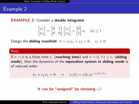
Example 2
EXAMPLE 2: Consider a double integrator[x1x2
]=[0 10 0
] [x1x2
]+[01
]u, |u| ≤ 1
Design the sliding manifold: σ = c1x1 + x2 = 0, c1 > 0
NoteIf σ = 0 in a finite time tr (reaching time) and σ = 0, ∀ t ≥ tr (slidingmode), then the dynamics of the equivalent system in sliding mode isof reduced order:
x1 + c1x1 = 0 → x1(t) = x(tr)e−c1(t−tr)
It can be “assigned” by choosing c1!
Prof. Antonella Ferrara Sliding Mode Control, Advanced Automation and Control
Basic Concepts in Sliding Mode Control
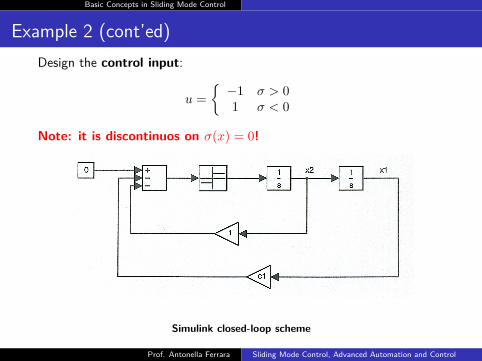
Example 2 (cont’ed)Design the control input:
u ={−1 σ > 01 σ < 0
Note: it is discontinuos on σ(x) = 0!
Simulink closed-loop scheme
Prof. Antonella Ferrara Sliding Mode Control, Advanced Automation and Control
Basic Concepts in Sliding Mode Control
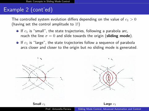
Example 2 (cont’ed)The controlled system evolution differs depending on the value of c1 > 0(having set the control amplitude to 1!)
If c1 is “small”, the state trajectories, following a parabola arc,reach the line σ = 0 and slide towards the origin (sliding mode).If c1 is “large”, the state trajectories follow a sequence of parabolaarcs closer and closer to the origin but no sliding mode is generated.
Small c1 Large c1
Prof. Antonella Ferrara Sliding Mode Control, Advanced Automation and Control

Basic Concepts in Sliding Mode Control
Example 2 (cont’ed)
Now perturb the double integrator with an uncertain bounded term[x1x2
]=[0 10 0
] [x1x2
]+[
0d(x1,x2, t)
]+[01
]u, |u| ≤ U
Design the sliding manifold: σ = c1x1 + x2 = 0, c1 > 0
NoteIf σ = 0 in a finite time tr (reaching time) and σ = 0, ∀ t ≥ tr (slidingmode), then the dynamics of the equivalent system in sliding mode isagain:
x1 + c1x1 = 0 → x1(t) = x(tr)e−c1(t−tr)
The uncertain term does not affect the system in sliding mode!
Prof. Antonella Ferrara Sliding Mode Control, Advanced Automation and Control

Basic Concepts in Sliding Mode Control
Lesson Learnt
A variable structure control making the system become avariable structure system can have a stabilizing effect.
The sliding mode enforcement depends on the choice of thecontrol law (correct sizing taking into account the slidingvariable definition and the initial conditions).
The system in sliding mode is of reduced order.
The system dynamics in sliding mode can be arbitrarilyassigned.
The system in sliding mode has a nice robustness property.
Prof. Antonella Ferrara Sliding Mode Control, Advanced Automation and Control

Types of Variable Structure Control Laws
Types of Variable Structure Control Laws
Prof. Antonella Ferrara Sliding Mode Control, Advanced Automation and Control
Types of Variable Structure Control Laws
Types of Variable Structure Control Laws
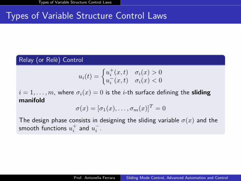
Relay (or Rele) Control
ui(t) ={u+
i (x, t) σi(x) > 0u−i (x, t) σi(x) < 0
i = 1, . . . ,m, where σi(x) = 0 is the i-th surface defining the slidingmanifold
σ(x) = [σ1(x), . . . , σm(x)]T = 0
The design phase consists in designing the sliding variable σ(x) and thesmooth functions u+
i and u−i .
Prof. Antonella Ferrara Sliding Mode Control, Advanced Automation and Control

Types of Variable Structure Control Laws
Types of Variable Structure Control Laws
State Feedback Control with Switching Gains
u = Ψ(x)x(t)
with Ψ = [ψij(x)] ∈ Rm×n, for instance,
ψij ={αij σi(x)xj > 0βij σi(x)xj < 0, i = 1, . . . ,m, j = 1, . . . , n
Unit Vector Control
u = Kσ(x)‖σ(x)‖
Prof. Antonella Ferrara Sliding Mode Control, Advanced Automation and Control

Types of Variable Structure Control Laws
Types of Variable Structure Control Laws
Control Based on a Simplex of VectorsIn the multi-input case the variable structure control philosophy can alsobe implemented by designing a set of m+ 1 control vectors forming asimplex in Rm.The controlled system switches from one to another ofm+ 1 different structures.
G. Bartolini and A. Ferrara, ”Multi-input sliding-mode control of a class ofuncertain nonlinear systems”, IEEE Trans. Automat. Contr., vol. 41,pp.1662-1666, 1996
Prof. Antonella Ferrara Sliding Mode Control, Advanced Automation and Control

Types of Systems
Types of Systems
Prof. Antonella Ferrara Sliding Mode Control, Advanced Automation and Control

Types of Systems
Canonical Forms
Assumption: The system is nonlinear with respect to the statevariable and linear with respect to the control variable (i.e. affine inthe control input)
The proof of the existence of a sliding mode and the design of thevariable structure control law are simplified if the considered nonlinearsystem is expressed in one of the following canonical forms.
1. Reduced Form
The state vector x(t) can be split into two vectors: x1 ∈ Rn−m andx2 ∈ Rm.
Matrix B(x, t) = [0 B∗]T , with B∗ ∈ Rm×m, is not singular.{x1 = A1(x, t)x2 = A2(x, t) +B∗u
Prof. Antonella Ferrara Sliding Mode Control, Advanced Automation and Control

Types of Systems
Canonical Forms
2. Controllability Form
The system is split into m subsystems (m is the number of controlinputs), each of them in Brunovsky canonical form.
Consider x = [x1 . . . xm]T , with dim(xi) = ni, Σmi=1ni = n.
The final system is x = Ax+ f(x) + b(x)u with A = diag(Ai) and
xi = Aixi + fi(x) + bi(x)u, i = 1, . . . ,m
Ai =[
0 Ini−10 0
], dim(Ai) = ni × ni
fi(x) =
0...
fi0(x)
, dim(fi) = ni
bi(x) =
0...
bi0(x)
, dim(bi) = ni ×m
Prof. Antonella Ferrara Sliding Mode Control, Advanced Automation and Control
Types of Systems
Canonical Forms
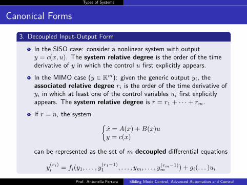
3. Decoupled Input-Output Form
In the SISO case: consider a nonlinear system with outputy = c(x, u). The system relative degree is the order of the timederivative of y in which the control u first explicitly appears.
In the MIMO case (y ∈ Rm): given the generic output yi, theassociated relative degree ri is the order of the time derivative ofyi in which at least one of the control variables ui first explicitlyappears. The system relative degree is r = r1 + · · ·+ rm.
If r = n, the system {x = A(x) +B(x)uy = c(x)
can be represented as the set of m decoupled differential equations
y(ri)i = fi(y1, . . . , y
(r1−1)1 , . . . , ym, . . . , y
(rm−1)m ) + gi(. . . )ui
Prof. Antonella Ferrara Sliding Mode Control, Advanced Automation and Control

Types of Systems
Canonical Forms
4. Normal Form
Under certain assumptions, if r < n, the following transformation ispossible: let zi,j be a vector including the output yi and itsderivatives up to order j = ri − 1 (for i = 1, . . . ,m, r externalvariables).
Consider the variables ηk, k = 1, . . . , n− r, called internalvariables, mutually independent and independent of zi,j .
The transformed system is of the following typezi,j = zi,j+1 j = 1, . . . , ri − 1zi,ri
= αi(z, η) +∑m
k=1 βi,k(z, η)uk, i = 1, . . . ,mη = γ(z, η), dim(η) = n− r
Prof. Antonella Ferrara Sliding Mode Control, Advanced Automation and Control

Elements of Design
Elements of Design
Prof. Antonella Ferrara Sliding Mode Control, Advanced Automation and Control

Elements of Design
Design of the Sliding Manifold
The sliding manifold σ(x) = 0 can be a nonlinear function of x.
Linear sliding manifolds are generally preferred, i.e.:
σ(x) = Cx(t) = 0
with C ∈ Rm×n.
An issue to clarifyHow is the sliding manifold designed when one of the previouslydescribed canonical forms is selected?
Prof. Antonella Ferrara Sliding Mode Control, Advanced Automation and Control

Elements of Design
Design of σ(x) for the Canonical Forms
Reduced Form
The state vector is split into x1 and x2. For the sake of simplicity,
σ(x) = σ(x1, x2) = [C1 C2][x1x2
]= 0
with C2 being not singular.
In sliding mode{x2 = C−1
2 C1x1x1 = A1(x, t) = A1(x1,−C−1
2 C1x1, t)
Prof. Antonella Ferrara Sliding Mode Control, Advanced Automation and Control

Elements of Design
Design of σ(x) for the Canonical Forms
Reduced Form
If A1 is linear,
x1 = A1(x, t) = A11x1 +A12x2
then, the reduced order dynamics is
x1 = [A11 −A12C−12 C1]x1 = [A11 +A12F ]x1
If (A11, A12) is controllable, it is possible to choose F so that thereduced order system has the desired dynamics in sliding mode(eigenvalues assignment, optimality, etc.).
Given F , since F = −C−12 C1, one can easily design
σ(x) = [C1 C2][x1 x2]T
Prof. Antonella Ferrara Sliding Mode Control, Advanced Automation and Control

Elements of Design
Design of σ(x) for the Canonical Forms
Controllability Form
The system is split into m subsystems
One hasσi = cT
i xi, i = 1, . . . ,m
Major requirement: to select ci for each subsystem so that theoverall controlled system in sliding mode is asymptoticallystable.
The dynamics of each subsystem in sliding mode can be assigned byselecting the the components of ci.
Each equivalent subsystem has order ni − 1 and has a canonicalcontrollability (Brunovsky) form. The corresponding characteristicpolynomial has the components of ci as coefficients.
Prof. Antonella Ferrara Sliding Mode Control, Advanced Automation and Control

Elements of Design
Design of σ(x) for the Canonical Forms
Decoupled Input-Output Form
It is analogous to the case of the controllability form.
Normal Form
The so-called “zero-dynamics”, obtained by posing equal to zero theoutputs and their derivatives (i.e. the external variables),{
z = 0η = γ(0, η)
has to be asymptotically stable.
A typical choice of the sliding variable components is:σi = cT
i zi, i = 1, . . . ,m.
ci is chosen as in the controllability form so as to assign thedynamics to the equivalent reduced order subsystem having zi hasstate vector.
Prof. Antonella Ferrara Sliding Mode Control, Advanced Automation and Control

Elements of Design
Existence of the Sliding Mode
After the design of the sliding manifold it is necessary to guarantee theexistence of the sliding mode.
Note:A sliding mode exists if in a vicinity of the sliding manifold σ(x) = 0 thevector tangent to the state trajectory of the controlled system is alwaysdirected towards the sliding manifold.
Prof. Antonella Ferrara Sliding Mode Control, Advanced Automation and Control
Elements of Design
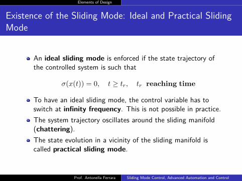
Existence of the Sliding Mode: Ideal and Practical SlidingMode
An ideal sliding mode is enforced if the state trajectory ofthe controlled system is such that
σ(x(t)) = 0, t ≥ tr, tr reaching time
To have an ideal sliding mode, the control variable has toswitch at infinity frequency. This is not possible in practice.The system trajectory oscillates around the sliding manifold(chattering).The state evolution in a vicinity of the sliding manifold iscalled practical sliding mode.
Prof. Antonella Ferrara Sliding Mode Control, Advanced Automation and Control

Elements of Design
Existence of the Sliding Mode: Ideal and Practical SlidingMode
Prof. Antonella Ferrara Sliding Mode Control, Advanced Automation and Control

Elements of Design
The Existence Problem
Note:The existence problem is a stability problem!
The existence of a sliding mode requires that the state trajectories,at least from a neighborhood of s(x) = 0 (attraction region), tendtowards the sliding manifold.
The attraction domain can coincide with the whole state space(globally reachable sliding mode).
The existence of a sliding mode can be proved by using a Lyapunovfunction V (x).
Prof. Antonella Ferrara Sliding Mode Control, Advanced Automation and Control
Elements of Design
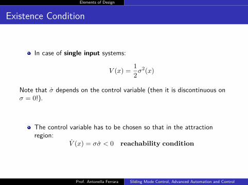
Existence Condition
In case of single input systems:
V (x) = 12σ
2(x)
Note that σ depends on the control variable (then it is discontinuous onσ = 0!).
The control variable has to be chosen so that in the attractionregion:
V (x) = σσ < 0 reachability condition
Prof. Antonella Ferrara Sliding Mode Control, Advanced Automation and Control

Elements of Design
To Prove the Finite Time Convergence
An alternative way to express the reachability condition is the following(for the sake of simplicity the single input case is considered):
σσ ≤ −γ|σ| η − reachability condition
with γ > 0, that isV (x) ≤ −γ′
√V (x)
In this case it is possible to find an upper bound for the reaching timetr, by integrating the η-reachability condition between t = 0 (or t0) andt = tr:
σ(tr)− σ(0) = 0− σ(0) ≤ −γ(tr − 0)
tr ≤|σ(0)|γ
Prof. Antonella Ferrara Sliding Mode Control, Advanced Automation and Control

Elements of Design
Useful ReferencesA. F. Filippov, Differential Equations with Discontinuous Right-hand Side, Amer.Math. Soc. Trans., Vol. 42, pp.199 -231, 1964.
A. F. Filippov, Differential Equations with Discontinuous Right-hand Side,Kluwer, 1988.
J. P. Aubin and A. Cellina, Differential Inclusions, Springer-Verlag, 1984.
V. I. Utkin, Sliding Modes in Control and Optimization, Springer-Verlag, 1992.
C Edwards and S Spurgeon, Sliding Mode Control: Theory and Applications,CRC Press, 1998.
G. Bartolini and T. Zolezzi, Control of Nonlinear Variable Structure Systems, J.Math. Anal. Appl., Vol. 118, pp.42-62, 1986.
G. Bartolini and A. Ferrara, Multi-input Sliding Mode Control of a Class ofUncertain Nonlinear Systems, IEEE Trans. Automat. Contr., Vol. 41,pp.1662-1666, 1996.
G. Bartolini, A. Ferrara, V.I. Utkin, T. Zolezzi, A Control Vector SimplexApproach to Variable Structure Control of Nonlinear System, Int. J. RobustNonlinear Control, Vol. 7, Issue 4, pp. 1099-1239, 1997.
Prof. Antonella Ferrara Sliding Mode Control, Advanced Automation and Control