Abstract—Estimation precision and bandwidth of sliding mode (SM) observers are analyzed in the

frequency domain for different settings of the observer design parameters. It was shown previously that the

SM observer could be analyzed as a relay feedback-feedforward system. It is feedback with respect to the

measured variable of the system being observed, and feedforward with respect to the control applied to the

system being observed. This approach is now further extended to analysis of effects of design parameter

change on observer performance. An example of SM observer design for estimation of DC motor speed from

the measurements of armature current is considered in the paper. The input-output properties of observer

dynamics are analyzed with the use of the Locus of a Perturbed Relay System (LPRS) method.

I. INTRODUCTION

HE idea of using a dynamical system, which is called observer, to obtain estimates of the system states

from measurable system variables was proposed by Luenberger [1]. The observer dynamics are driven by

the control and by the difference between the output of the observer and the output of the plant. In SM

observers, this difference is maintained equal to zero by means of SM organized in the observer loop. The

control should be designed to provide the existence of SM in the observer dynamical system. SM observers

were analyzed in a number of publications (see, for example, respective chapters of textbooks [2],[3] and

recent tutorials [4],[5]).

However, only ideal SM in the observer dynamical system was analyzed in [2]-[5]. To the best of our

knowledge, only in [6] for the first time the mechanism of generation of the observation error was found and

analyzed through a frequency-domain approach. The proposed approach was based on the Locus of a

Perturbed Relay System (LPRS) method [7] and the method of analysis of SM systems with parasitic

Frequency Domain Precision Analysis and Design of Sliding Mode

Observers

Igor Boiko

T

dynamics [8]. Further development of the approach of [6] was presented in [9] for second-order SM

observers. Publication [10] provides some results that can be considered as experimental verifications of the

approach of [6] and [9]. However, in publication [6] the proposed frequency-domain approach was just

outlined. The present paper further develops this approach extending it to the observer design problem and

providing an example of its application to DC motor speed observation. This new development is aimed at

reaching out to the area of engineering design of SM observers.

The objective of the present paper is, therefore, to extend the approach of [6] to design-related problems, in

particular, to investigation of precision dependence on observer design parameters (execution period of the

algorithm and values of the observer gain matrix). We aim to show that the observation precision has

complex dependence on the SM algorithm parameters. We investigate that dependence and provide a model

that allows for computing the observation error. The paper is organized as follows. At first, the problem

formulation is considered. Then a frequency-domain approach to SM observer analysis is presented, and a

model that provides precision of observation is given. After that, considering the example of DC motor

speed observation, an investigation of the dependence of the observation precision on the values of the

algorithm design parameters is done, and the design is outlined.

II. PROBLEM FORMULATION

Consider an n-dimensional version of the observer proposed in [2]. Let the linear plant, the states of which

are supposed to be observed, be the n-th order dynamical system:

uBAxx (1)

Cxy , (2)

where nRx is the state vector, 1Ry is the measurable system output, nnnn R,R,R 11

CBA are

the state matrix, the input matrix, and the output matrix of the plant, respectively. The pair (C,A) is assumed

to be observable.

The SM observer can be designed in the same form as the original system (1), (2) with the use of internal

model similar to the plant model and addition of an output injection that depends on the error between the

output of the observer and the output of the plant (system to be observed) [2]:

)sign( yyu LBxAx (3)

xC

y (4)

where nRx

is an estimate of the system state vector, 1Ry

is an estimate of the system output, and

1 nRL is a gain matrix. Consider now the SM observer. Denote the sliding variable as follows:

yy

(5)

The elements of L must be such that the reachability condition of the SM and stability of the reduced SM

dynamics should be insured. It is shown in [2], [3] that the matrix L can be selected to provide the

convergence of the sliding variable to zero in finite time and asymptotic convergence of the estimation

error for the system variables. We assume that conditions of existence of SM in the observer dynamics are

satisfied.

It is shown in [6] that a SM observer can be analyzed as a relay feedback-feedforward dynamical system

(Fig. 1). One of the two inputs y(t) must be followed (tracked) by the observer output )(ty

as precisely as

possible. The other input u(t) is as a feedforward. The discrete time implementation is accounted for as an

equivalent delay. The equivalent delay can be found through matching the frequencies of chattering in the

equivalent relay system (Fig. 1) and in the original discrete-time observer model with a given control

execution period (the digital implementation would exhibit chattering with the period equal to two execution

periods of the algorithm [11], [6]). A similar approach to analysis of discrete-time SM systems was

proposed in [12]. With this representation, we can analyze the observer performance in terms of the response

of the relay servo system to two inputs: u and y. This is a complex task, which, however, can be fulfilled via

application of the LPRS method that is designed for input-output analysis of relay systems. It is briefly

described below.

Fig.1. Plant and observer model

III. THE CONCEPTS OF THE LOCUS OF A PERTURBED RELAY SYSTEM (LPRS) APPROACH

In [7], [8], the LPRS was introduced as a method of analysis and design of relay servo systems having a

linear plant (Fig. 2). Let us call the part of the relay servo system that is given by the linear differential

equations the linear part. With respect to the SM observer, the linear part will be the one given by (3) and

(4).

Fig. 2. Relay servo system

The LPRS was defined as a complex function J() of the frequency as follows:

000

0

0)(lim

4lim

2

1)(

00

tff

tyc

ju

J

(6)

where t=0 is the time of the switch of the relay from "-c" to "+c", is the frequency of the periodic

motion. The frequency in (6) is the frequency of the self-excited oscillations varied by changing the

hysteresis 2b while all other parameters of the system are considered constant; u0 and y(t)t=0 can,

therefore, be considered functions of and be considered a function of the hysteresis 2b The limit in the

imaginary part of (6) is the value of y(t) at the time of the switch in the symmetric oscillations. Thus, J() is

defined as a characteristic of the response of the linear part to the unequally spaced pulse input u(t) subject

to f00, as the frequency is varied.

A few techniques of the LPRS computing – for different types of plant description - were proposed. If the

plant is represented by equations (1), (2) plus time delay then the LPRS is given by the following formula

[7]:

BAIICBIACAAAAA

1

112

1 24

25.0)(

ω

π

ω

π

ω

π

eeejeeω

πJ , (7)

where matrix A is assumed to be invertible.

With the plant model available, the LPRS can be computed at various frequencies and the LPRS plot can be

drawn on the complex plane (an example of the LPRS is given in Fig. 3). The LPRS is a characteristic of the

relay feedback system and can be computed from the plant model. Once the LPRS is computed, the

frequency of the symmetric periodic solution can be determined from the following equation:

c

πbΩJ

4)(Im , (8)

which corresponds to finding the point of intersection of the LPRS and the horizontal line that lies below the

real axis at –b/(4c) (Fig. 3), and the equivalent gain [7],[8] of the relay (the gain of the relay with respect

to the averaged motions propagation) can be determined as:

)Re2

1

00

0

0

J(Ω

ukn

, (9)

which corresponds to the distance between the intersection point and the imaginary axis [7].

Fig.3. The LPRS and oscillations analysis

With the formulas of the LPRS available, input-output analysis of the relay feedback system (Fig. 2) can be

done in the same manner as with the use of the describing function method [13] (however, involvement of

the filtering hypothesis is no longer needed). The relay function can be replaced with the equivalent gain

(9) and the input-output properties of the relay system can be analyzed as the properties of the resulting

linearized system.

IV. ANALYSIS AND CHARACTERISTICS OF SM OBSERVER PERFORMANCE

With the representation of the SM observer as a relay servo system, we formulate performance measures of

the observer. Using the LPRS method and the concept of the equivalent gain, we obtain a linear model of the

plant-observer dynamics for average (on the period of chattering) motions. We characterize the precision of

observation by the output error yyy

and by the state observation errors xxx

. We note

that the output error and state observation errors are not equal to zero [6], [9] due to the existence of time

delays (finite execution period of the algorithm), which act as parasitic dynamics in this SM system. It

follows from the LPRS approach that the averaged forced motions in the system Fig. 1 can be analyzed via

the use of the equivalent gain of the relay concept and the linearized model, which can be obtained from the

original model by replacing the relay function with the equivalent gain kn. The linear part of the system for

the LPRS analysis is the dynamics of the observer model and the parasitic dynamics (time delay) marked in

the diagram Fig. 1 with the dashed line.

The methodology of input-output analysis of the dynamics given in Fig. 1 is presented in [7], [8]. However,

the observer analysis has its specifics due to unknown value of the equivalent time delay. It needs to be

determined first. Considering that the execution period (time step) Tex is known, and the frequency of

chattering in the system is exT , which should be equal to the frequency of chattering in the equivalent

continuous-time model, the equation for the equivalent delay is as follows:

0),(Im ΩJ , (10)

where exT , and the LPRS ),( J is given by formula (7), which considering the matrices in the

loop, transforms into:

LAIICBIACAAAAA

1

112

1 24

25.0),(

ω

π

ω

π

ω

π

eeejeeω

πJ , (11)

As a result, analysis of precision of observation can be done via: (a) identification of the equivalent time

delay of the continuous-time model of the observer – through solving equation (10) with (11) being a

formula for LPRS; (b) computing the equivalent gain value using formula (9); and (c) replacing the relay

with the equivalent gain and carrying out analysis of the linearized averaged observer dynamics. The

linearized plant-observer averaged dynamics can be represented as in Fig. 4. In Fig. 4, subscript “0” is used

to indicate the averaged on the period of chattering variables.

Fig.4. Linearized model of plant and observer

In the Laplace domain, we write expressions for the output error as follows, which is a result of linearization

of the original model (Fig. 1) through replacement of the relay nonlinearity with the equivalent gain, for the

average motions:

s

n

s

uesWk

esWsW

su

s

)(1

1)()(

)(

)(*

0 (12)

where BAIC1)()( ssW , LAIC

1* )()( ssW .

From formula (12), other characteristics of the observer precision can be derived. If, for example, we follow

the conventional approach to servo systems analysis we can formulate a dynamical precision criterion as a

frequency response of the error signal (t) to the harmonic excitation u(t) of variable frequency. This

characteristic can be presented as a magnitude and a phase responses:

)(log20)( jWM u (13)

)(arg)( jWu (14)

where M is the magnitude response, is the phase response, Wu-(j) is the frequency response from u(t) to

(t) corresponding to transfer function (12). The observation error transfer functions can be found through

selection of appropriate output matrix as follows:

)()()(

)()( * sWksWsu

sxsx

jxnujj

, nj ,1 , (15)

where LAIC1* )()(

ssW jx j , njj ,1, C , n

j R 1C are row matrices with elements jici for0

and jici for1 . The observation error in % at frequency can be calculated now as

)()()(%100%100)(

)()( *

jWjWkjW

jx

jxjx

jj xuxnu

j

jj

, nj ,1 , (16)

where BAIC1)()(

ssW jxu j, nj ,1 .

The above-given formulas comprise a model suitable for design of SM observers. This design can be carried

out via selection of observer parameters: execution period Tex and elements of the matrix L. This design is

system-specific and depends on system dynamics. The example below illustrates an approach to selection of

those parameters.

V. SELECTION OF MATRIX L AND OBSERVER PRECISION

Apparently, selection of matrix L must have an effect on observer precision, which follows from formulas

(12), (15), (16). Yet, the choice of matrix L is limited by the conditions of the existence of the sliding mode

in the observer dynamics and other conditions that were discussed above. We now transform the condition of

the existence of the sliding mode. Assume the absence of parasitic dynamics and the autonomous mode

(u(t)0, which leads to y(t)0). We transform the condition 0 of the existence of the sliding mode as

follows: 0yy

or

0if0

0if0)sign(

y

yyy

CLxCAxC that can be rewritten as

CLxCACL

, (17)

which must hold for all feasible x

in the vicinity of the sliding surface 0xC

. Because matrix C may have

some elements equal to zero (that defines the relative degree of the system being observed), then for

inequality (17) to hold, generally matrix L must not have zero elements (to exclude the situation of

0CL ). This requirement, however, may contradict the objective of increasing the precision of observation

– as shown below.

It follows from formulas (12) and (15) that the state observation error can be presented as the product of two

factors:

)(

)(1

1)(

)(

)()( **

sWesWk

esWk

su

sxsx

jxs

n

snjj

, nj ,1

Since 1)(* sWkn and se

close to one the formula can be reduced to

LAIC

LAIC

BAIC 11

1*

*)(

)(

1)()(

)(

1)(

)(

)()(

s

es

essW

esWk

esWk

su

sxsxjs

s

xsn

snjj

j

, nj ,1 .

If the elements of matrix L were selected equal to the respective elements of matrix B then the formula for

the state observation error would be rewritten as follows:

LAIC1)(1

)(

)()(

sesu

sxsxj

sjj

,

which would provide minimum possible observation error at any frequency (note that multiplication of

matrix L by a factor does not change the result because of the presence of matrix L in the second multiplier).

Therefore, optimal selection of matrix L would be: L=B, where is a certain factor. However, matrix B

contains zeros and for the reason given above L cannot be designed as L=B. Nevertheless, selection of

elements of matrix L the way, so that all of them are selected as non-zero but the relationship between the

values of the elements of L at least resembles that of B, allows for better performance of the observer

(smaller observation error). This is illustrated in the example below.

VI. EXAMPLE OF SM OBSERVER PRECISION ANALYSIS

Consider an example of estimation of DC motor speed and acceleration from the measurement of armature

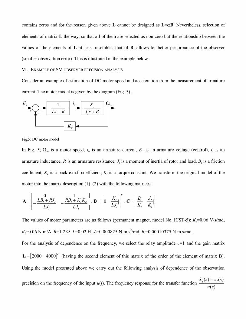
current. The motor model is given by the diagram (Fig. 5).

Fig.5. DC motor model

In Fig. 5, m is a motor speed, ia is an armature current, Ea is an armature voltage (control), L is an

armature inductance, R is an armature resistance, Jt is a moment of inertia of rotor and load, Bt is a friction

coefficient, Ke is a back e.m.f. coefficient, Kt is a torque constant. We transform the original model of the

motor into the matrix description (1), (2) with the following matrices:

t

ett

t

tt

LJ

KKRB

LJ

RJLB10

A ,

T

t

t

LJ

K

0B ,

t

t

t

t

K

J

K

BC

The values of motor parameters are as follows (permanent magnet, model No. ICST-5): Ke=0.06 Vs/rad,

Kt=0.06 Nm/A, R=1.2 , L=0.02 H, Jt=0.000825 Nms2/rad, Bt=0.00010375 Nms/rad.

For the analysis of dependence on the frequency, we select the relay amplitude c=1 and the gain matrix

T40002000L (having the second element of this matrix of the order of the element of matrix B).

Using the model presented above we carry out the following analysis of dependence of the observation

precision on the frequency of the input u(t). The frequency response for the transfer function )(

)()(

su

sxsx jj

given by formula (15) is presented in Fig. 6. It demonstrates that the observation precision is frequency-

dependent. The higher the frequency of the signals in the system is (the frequency of motor speed variation)

the lower the observation precision is.

Fig.6. Speed observation error [%] versus frequency

However, Fig. 6 gives estimates of the absolute error (absolute precision). To obtain precision estimates in

percent of the signal value, we need to use formula (16). Calculation of the speed observation error using

formula (16) provides the result that is depicted in Fig. 7. Those results show that the observation error is

high enough even at relatively low frequencies. For example, at the frequency 1rad/s the nominal

observation error is ~6%. Therefore, in practice observation would be too inaccurate at frequencies higher

than 0.4rad/s (the nominal error is higher than 1%).

Fig.7. Speed observation error [%] versus frequency

Consider now a design related problem. Let the required speed observation precision be 1%. The objective is

to maximize the observer bandwidth via adjusting elements of matrix L, considering also the constraints on

the algorithm execution period Tex. We note at first that observation precision depends on the ratio of the

values of matrix L but does not depend on the absolute values (as far as the ratio is the same). In addition to

that, the SM control amplitude must be comparable with the control injection term. Therefore, we will

consider matrix Tl 40001L with constant second element and variable first element. The SM

bandwidth is given in Table 1 by the maximum input signal frequency that provides observation precision of

1% (all frequencies higher than the bandwidth feature lower precision). Table 1 contains results of analysis

for three different values of the execution period. Table 2 has the results of the same analysis but presented

as the ratio of the period corresponding to the maximum frequency of the bandwidth to the execution period.

It characterizes the algorithm efficiency. If the available technical means (including the ones for ensuring the

required sampling frequency) allow for having small values of Tex then the bandwidth can be made wider,

and vice versa. This way of providing the required bandwidth is, essentially, a “brute force”. It is obvious,

and the results of analysis confirm the expectations. On the other hand, what is of most interest to the design

is widening the bandwidth via optimal selection of the gain matrix, which does not require additional

computing power. Analysis of the data of Table 2 shows that the highest efficiency of the algorithm is

achieved at higher values of Tex and lower values of l1. The dependence on Tex can, probably, be explained

by the dynamical properties of the system itself: the higher he bandwidth the harder is to further increase it.

As a result, the decrease of Tex by the factor of 10 does not result in the increase of the bandwidth by the

same factor. With respect to variation of parameter l1, the presented analysis provides results that can hardly

be predicted by other methods: the provided bandwidth significantly depends on the value of this parameter.

The explanation of this result can be obtained from the comparison of the matrices B and L. The former has

first element equal to zero. On the other hand, and the highest observation precision could be achieved if

matrix L replicated matrix B. However, the existence of non-zero elements in matrix L is essential for the

existence of SM in the observer. Therefore, the decrease of values of l1 results in a higher precision. We note

that consideration of the ideal SM in the observer does not allow for the same analysis.

The design of SM observer can be done on the basis of Table 1. From the required estimation precision and

bandwidth, the execution period and gain matrix L can be computed as in Table 1. After that the execution

period and optimal gain matrix L values are selected to provide the specified precision and bandwidth.

Table 1. Observer bandwidth [rad/s] as a function of execution period and parameter l1

l1=20 l1=50 l1=100 l1=200 l1=500 l1=1000 l1=2000 l1=5000 l1=10000

Tex =0.001s 9.9457 5.5474 3.2410 2.0385 1.6570 1.6208 1.6174 1.6185 1.6152

Tex =0.01s 1.6112 0.8905 0.5132 0.3898 0.3969 0.4084 0.4139 0.4137 0.4089

Tex =0.1s 1.1309 0.6556 0.4024 0.2365 0.0915 0.0037 0.0348 0.0633 0.0749

Table 2. Number of execution cycles per period corresponding to bandwidth

l1=20 l1=50 l1=100 l1=200 l1=500 l1=1000 l1=2000 l1=5000 l1=10000

Tex =0.001s 631.7 1132.6 1938.6 3082.2 3791.9 3876.5 3884.7 3882.1 3890.0

Tex =0.01s 389.9 705.5 1224.3 1611.8 1583.0 1538.4 1518.0 1518.7 1536.6

Tex =0.1s 55.5 95.8 156.1 265.6 686.6 6807.1 1805.5 992.6 838.8

VII. CONCLUSION

Analysis of a SM observer is done above as of a relay feedback-feedforward system. The frequency-domain

model of observation precision is obtained via application of the LPRS method. It is found that the

dynamical performance of the SM observer, which translates into observation precision, is not ideal.

Because of the existence of parasitic dynamics in the observer loop (time delay due to discrete

implementation of the algorithm) there always exists a nonzero observation error - even after the initial

transient. This result can be obtained only if the SM is considered and analyzed as a non-ideal SM, which is

possible if the LPRS method is used. This observation error depends on a number of factors, including the

selection of matrix L and of the execution period, which are analyzed in the paper. It is justified

theoretically and confirmed by an example that the relationship (proportion) between the elements of matrix

L should be like the one between the elements of matrix B – to ensure minimal observation error. The

provided example of analysis and design of SM observer for estimation of the DC motor speed from the

measurements of the armature current illustrates the proposed approach.

REFERENCES

[1] D.G. Luenberger, “Observers for multivariable systems,” IEEE Trans. on Automatic Control, vol. 11,

1966, pp. 190-197.

[2] V. Utkin, Sliding Modes in Control and Optimization, Springer-Verlag, 1992.

[3] C. Edwards, and S. Spurgeon, Sliding Mode Control: Theory and Application, Taylor & Francis,

London, 1998.

[4] J. Barbot, M. Djemai, and T. Boukhobza, “Sliding mode observers,” in Sliding Mode Control in

Engineering (W. Perruquetti and J. Barbot, eds.), Control Engineering, New York, Marcel Dekker, 2002,

pp. 103-130.

[5] C. Edwards, S. Spurgeon, and C. P. Tan, “On development and application of sliding mode observers,”

in Variable Structure Systems: Towards XXIst Century (J Xu and Y.Yu, eds), Lecture Notes in Control

and Information Science, Berlin, Germany: Springer Verlag, 2002, pp. 253-282.

[6] I. Boiko, L. Fridman, “Frequency domain input-output analysis of sliding mode observers,” IEEE

Trans. Automatic Control, Vol. 51, No. 11, 2006, pp. 1798-1803.

[7] I. Boiko, “Oscillations and transfer properties of relay servo systems – the locus of a perturbed relay

system approach,” Automatica, vol. 41, No. 4, 2005, pp. 677-683.

[8] I. Boiko, “Analysis of closed-loop performance and frequency-domain design of compensating filters

for sliding mode control systems,” IEEE Trans. Automatic Control, Vol. 52, No. 10, 2007, pp. 1882-1891.

[9] I. Boiko, I. Castellanos, L. Fridman “Analysis of response of second-order sliding mode controllers to

external inputs in frequency domain,” Internat. J. Robust Nonlinear Control, 18, 2008, pp. 502-514.

[10] S. Kobayashi, K. Furuta “Frequency characteristics of Levant’s differentiator and adaptive sliding

mode differentiator,” Internat. J. System Science, 38, No. 10, 2007, pp. 825-832.

[11] C. Miloslavljevic, “Discrete-time VSS,” in Variable Structure Systems: from Principles to

Implementation (A. Sabanovic, L. Fridman, and S. Spurgeon, eds.), London, UK: IEE, 2004, pp. 99-128.

[12] E. Fridman, A. Seuret, and J.-P. Richard, “Robust sampled-data stabilization of linear systems: an

input delay approach,” Automatica, 40, No. 8, 2004, pp. 1441-1446.

[13] D. P. Atherton, Nonlinear Control Engineering –Describing Function Analysis and Design,

Workingham, Berks, UK: Van Nostrand Company Limited, 1975.