Abstract—Optimal control force isdeveloped here to reduced the systemoscillatory. The purpose of this paperis to provide a framework of optimalcontrol force that can reduce the modalcoupling effects. We separate thecontrol force as linear and nonlinearcontrol physical and modal coordinatesystem. And separate the nonlinearcontrol on physical coordinate and modalcoordinate as coupled and uncoupledterm. Then to find Lyapunov function andperformance index. To introduce thecontrol force on each modal and controlit. A sliding mode controller ispresented here to compared with Optimalcontrol force. The result showed slidingmode control provides much bettercontrol effect than the Optimalcontroller. That is, using sliding modecontrol reduced the motion of the systemquickly.

Keywords: nonlinear modal transformation,normal mode, Lyapunov function, Non-

Manuscript received October 9, 2001. (Write thedate on which you submitted your paper for review.)This work was supported in part by the U.S.Department of Commerce under Grant BS123456(sponsor and financial support acknowledgment goeshere). Paper titles should be written in uppercaseand lowercase letters, not all uppercase. Avoidwriting long formulas with subscripts in the title;short formulas that identify the elements are fine(e.g., "Nd–Fe–B"). Do not write "(Invited)" in thetitle. Full names of authors are preferred in theauthor field, but are not required. Put a spacebetween authors' initials.

F. A. Author is with the National Institute ofStandards and Technology, Boulder, CO 80305 USA(corresponding author to provide phone: 303-555-5555; fax: 303-555-5555; e-mail: author@boulder.nist.gov).

quadratic Optimal Control, nonlinear normalmode, sliding mode control

Ⅰ.Introduction The nonlinear modal transformationwhich can transform a multi-degree offreedom system into groups of modalinvariant manifolds. The transformedmodal system can be used to set up anonlinear control technique referred toas nonlinear modal control[1] which issimilar to independent modal-spacecontrol(IMSC)[2] for linear system, theindependent design of the control can becarried out on each modal invariantspace rather than in the actual space.Since each nonlinear normal modesatisfies modal invariance property, thecontrol law designed in this modal spaceallows the behavior of the modalequation to be tailed to produce adesirable response. It is noted that thecontrol can be linear or nonlinear andthe design in the 2D modal space providea great benefit which can largely reducethe design difficulties as compared torequire the control direct on the actualphysical system. Currently, there have been many studies

of the controlling of a nonlinearoscillatory system. Liaw [3] design afeedback stabilization algorithm bycenter manifold reduction. Tuer [4] usedthe concept of internal resonance toregulated the oscillation. Abed and Fu[5] develop the local feedbackstabilization by Hopf bifurcationtheorem, Bacciotti [6] discuss thelinear stability of planar nonlinearsystem. Those researches are mainly

INDEPENDENT MODAL SPACE CONTROL ON NONLINEARMODAL SPACE

Ta-Ming Shih, Chin-Lung Chang

focus on single-input two-dimensionalsystem, and most of the controlalgorithm were using modal couplingeffect or local bifurcation theorem. Thecontrol force in those system has notbeen optimized. In order to put the control on theoptimization frame, the system Lyapunovfunction has to be know in prior.However, unlike linear system, theLyapunov function for nonlinear systemis not a quadratic form; hence, theapplication of conventional linear-qudratic(LQ) control theory is notpossible to be used on nonlinear system.Recently, there has been many researchesusing multilinear functions to study thenon-linear optimal control problem. Thesystem and cost function were analytic,and that the control force was series ofpolynomials in the state variables.Suharjo [7] has studies the optimalcontrol of a Duffing oscillator, Shyu[8] studies the optimal control of awing rock system. However, thecalculation in the process iscumbersome, Bernstein [9] has showedthat for a closed loop system if thesystem is asymptotically stable and theperformance index of optimal control arehomogeneous polynomial of order then itfollows the Lyapunov function are alsothe same form. Under this concept, hedeveloped a nonlinear feedbackcontroller for linear system. However,for a nonlinear system, if thenonlinearity can also be described byhomogeneous polynomial of order , thenwe can easily generalize the abovediscussion into nonlinear system. Our approach are focusing on the roleof the Lyapunov function in guaranteeingstability for 2D autonomous system on aninfinite horizon. Sufficient conditionsfor optimality are given in a form thatcorresponds to a steady-state version ofHamilton-Jacobi-Bellman equation [10].

The results can be used to provide thenonlinear feedback controller on each 2Dmodal manifold. However, when we apply linearcontrol on a nonlinear system, thelinear control will recouple the systemand also interacting with system’snonlinear part. Nonlinear coupled termsthat were not desired were also createdand deteriorate the control efforts.Therefore, in order to improve thiscondition, we need to study their effectto system and insert another controlterm to counteract the modal crosscoupling effects. To compare with it, we introduction the

sliding mode control technique to thissystem. Sliding mode control (SMC) is apowerful technique which widely appliedto linear and nonlinear system [11]-[13]successfully, including MIMOsystem、discrete time models、large scaleand infinite dimensional system, etc. Inthis paper , sliding mode control isapplied to nonlinear modal space. The paper will be arranged asfollows, in the next section, continuingour study of a cubic nonlinearitysystem, we will study the nonlinearmodal transformation of the same systemwith control force. we will analyze theform in the control force that cancontrol each modal space systemefficiently and also give us the leastmodal coupling effects, The thirdsection is to study the no-quadraticcost optimal control of system with oddnonlinearity. The relations betweenLyapunov function and performance indexfunction are studied. Specifically, thesystem with cubic nonlinearity isexamined to show that the Lyapunovfunction is homogeneous polynomials upto fourth order and performance indexfunction is homogeneous polynomials upto sixth order. An example is given insection Ⅴ, and section Ⅵ is conclusion.

Ⅱ. Nonlinear Modal Transformation ofSystem With Control

In this section, we study thenonlinear modal transformation of a non-internal resonance system with controlforce.

(1)C is the location matrix, is thecontrol force, is cubic nonlinearterm. Assume , and thetransformed system is given as

+(2) is the modal control force ,Let

is modally uncoupled terms,

is modally coupled terms, also

assume , can be separatedas linear and nonlinear control inphysical and modal coordinate system.

then

(4)the linear part in (4) is

assume is linear feedbackcontrol, then

(5)so the linear control on physical systemis (6)the nonlinear part in (4) is

(7)observing (7), in the last termwill interacting with the nonlinearpart. In order to counteract the effect,we decided to separate the nonlinearcontrol on physical coordinate and modalcoordinate as coupled and uncoupled term

(8)

(9)(7) can be expressed for modally coupledterms, as:

(10) As for modally uncoupled terms, we have

(11)now assume the nonlinear modal controlon modal space are

(12) is the control force for each

modal manifold. Then, we can relate themodally uncoupled control with thecontrol on physical coordinate as

(13)

so the control force in physical systemcan be transformed to physical system by(6)、(10) and(13)

(14)the control force include both linear

and nonlinear part ,

and the are both state feedback.

Note that, is used to eliminatethe nonlinear modal coupling effects insystem and , can bedesigned on each manifold separately.

Ⅲ. Non-quadratic Optimal Control In the previous section, we have derivedthe relation between modal control forceand physical control force. The nextstep is to find control on each modalspace. In this section we will look atthe non-quadratic optimal control whichis an extension from the traditionallinear quadratic (LQ) control for linearsystem. First, we will develop theformulation for a general class ofequation then we will use theformulation and focus on the control ofa 2-D system. Now, consider a nonlinear system as (1)

and is

nonlinear term with odd nonlinearity andthe performance index

(15)assume the cost function andLyapunov function are of the form

(16)

(17)

(18)

Where R1 、 P has to be positive semi-definite symmetric matrices, R2 has to bepositive definite symmetric matrix. Forthe system (1) to have optimal controlmust satisfy the following theorem.

Theorem 1 [9] Consider the controlledsystem (1). Assume there exist aLyapunov function and a control law Φ such that V(0)=0, ,

Φ(0)=0,

, min ,

min is refer toHamilton- Jacobi-Bellman(HJB) conditionsto the time-invariant, infinite-horizoncase. Then, with the feedback control

, the solution, of the closed-loop

system (1) is locally asymptotically.With (18), the Hamiltonian is

(19)

Setting , yields

the control law

(20)which minimize , With

the it follows that the timederivative of Lyapunov is

(21)

And the cost function is

.

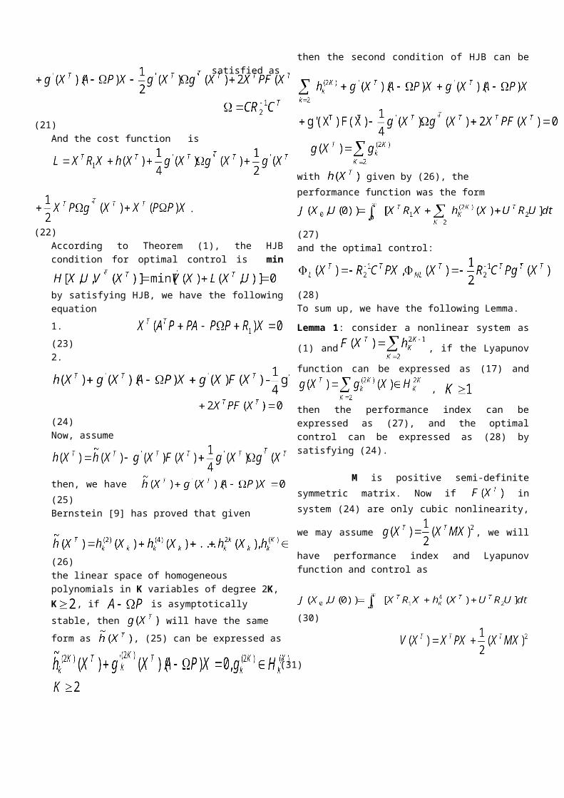
(22)According to Theorem (1), the HJBcondition for optimal control is min

by satisfying HJB, we have the followingequation1. (23)2.

(24)Now, assume

then, we have (25)Bernstein [9] has proved that given

(26) the linear space of homogeneous polynomials in K variables of degree 2K,K , if is asymptotically stable, then will have the same form as , (25) can be expressed as

then the second condition of HJB can besatisfied as

with given by (26), the performance function was the form

(27)and the optimal control:

(28)To sum up, we have the following Lemma.

Lemma 1: consider a nonlinear system as

(1) and , if the Lyapunov

function can be expressed as (17) and

,

then the performance index can beexpressed as (27), and the optimalcontrol can be expressed as (28) bysatisfying (24).

M is positive semi-definitesymmetric matrix. Now if insystem (24) are only cubic nonlinearity,

we may assume , we will

have performance index and Lyapunovfunction and control as

(30)

(31)

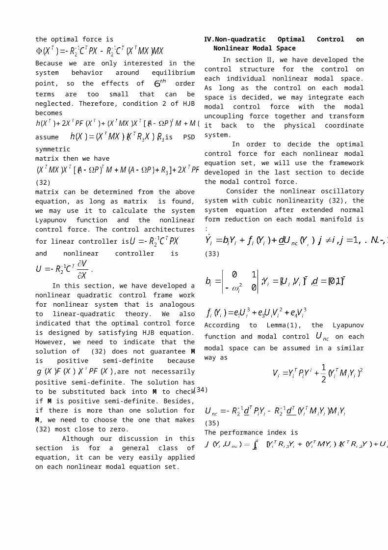
the optimal force is

Because we are only interested in thesystem behavior around equilibriumpoint, so the effects of orderterms are too small that can beneglected. Therefore, condition 2 of HJBbecomes

assume is PSDsymmetric matrix then we have

(32)matrix can be determined from the aboveequation, as long as matrix is found,we may use it to calculate the systemLyapunov function and the nonlinearcontrol force. The control architecturesfor linear controller isand nonlinear controller is

.

In this section, we have developed anonlinear quadratic control frame workfor nonlinear system that is analogousto linear-quadratic theory. We alsoindicated that the optimal control forceis designed by satisfying HJB equation.However, we need to indicate that thesolution of (32) does not guarantee Mis positive semi-definite because

,are not necessarilypositive semi-definite. The solution hasto be substituted back into M to checkif M is positive semi-definite. Besides,if there is more than one solution forM, we need to choose the one that makes(32) most close to zero. Although our discussion in thissection is for a general class ofequation, it can be very easily appliedon each nonlinear modal equation set.

Ⅳ.Non-quadratic Optimal Control onNonlinear Modal Space

In section Ⅱ, we have developed thecontrol structure for the control oneach individual nonlinear modal space.As long as the control on each modalspace is decided, we may integrate eachmodal control force with the modaluncoupling force together and transformit back to the physical coordinatesystem. In order to decide the optimalcontrol force for each nonlinear modalequation set, we will use the frameworkdeveloped in the last section to decidethe modal control force. Consider the nonlinear oscillatorysystem with cubic nonlinearity (32), thesystem equation after extended normalform reduction on each modal manifold is:

(33)

According to Lemma(1), the Lyapunovfunction and modal control on eachmodal space can be assumed in a similarway as

(34)

(35)The performance index is

are symmetric positive semi-

definite matrix is symmetricpositive definite matrix

Ⅴ. Design of Sliding Mode Controller To design sliding mode control , thefirst step is to determine the switchingfunctions. Assume a time varying surfaces(t) is defined in the state space R(n) byequating the variable s ( x ;t ) ,defined below, to zero：S(x)= cx = c1x1+ c2x2+…+ cn-1xn-1+ xn

(37)where c=[c1,…,cn] is the sliding surfacecoefficient vector. s ( x ;t ) verifying (37) is referred toas a sliding surface, and the system’sbehavior once on the surface is calledsliding mode or sliding regime. Thesecond step in the sliding mode controldesign is to choose the control law.From (37) we only need to differentiates once for the input u to appear. And wetake the control law as: ueq(t)=u(t)-k(x ;t)sgn(s(t)) (38) For system (1) the sliding function isdefined as： s=cx2 +x4, c > 0 the sliding surface is cx2+x4 = 0.

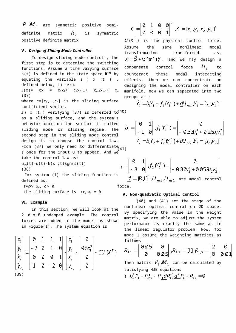
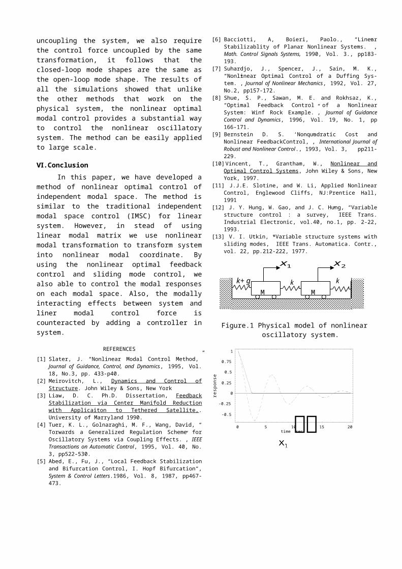
Ⅵ. Example In this section, we will look at the2 d.o.f undamped example. The controlforces are added in the model as shownin Figure(1). The system equation is

(39)

is the physical control force.Assume the same nonlinear modaltransformation transformed as,

, and we may design acompensate control force tocounteract these modal interactingeffects, then we can concentrate ondesigning the modal controller on eachmanifold. now we can separated into twogroups as :

(40)

(41)

are modal controlforce.

A. Non-quadratic Optimal Control (40) and (41) set the stage of thenonlinear optimal control on 2D space.By specifying the value in the weightmatrix, we are able to adjust the systemperformance as exactly the same as inthe linear regulator problem. Now, formode 1 assume the weighting matrices asfollows

Then matrix can be calculated bysatisfying HJB equations 1.

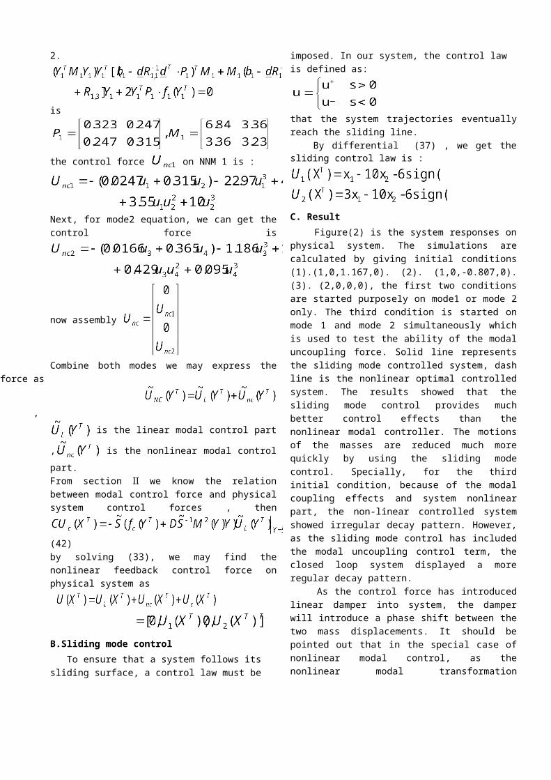
2.

is

the control force on NNM 1 is :

Next, for mode2 equation, we can get thecontrol force is

now assembly

Combine both modes we may express themodal force as

,

is the linear modal control part

, is the nonlinear modal controlpart.From section Ⅱ we know the relationbetween modal control force and physicalsystem control forces , then

(42)by solving (33), we may find thenonlinear feedback control force onphysical system as

B.Sliding mode control To ensure that a system follows its sliding surface, a control law must be

imposed. In our system, the control law is defined as:

that the system trajectories eventuallyreach the sliding line. By differential (37) , we get thesliding control law is :

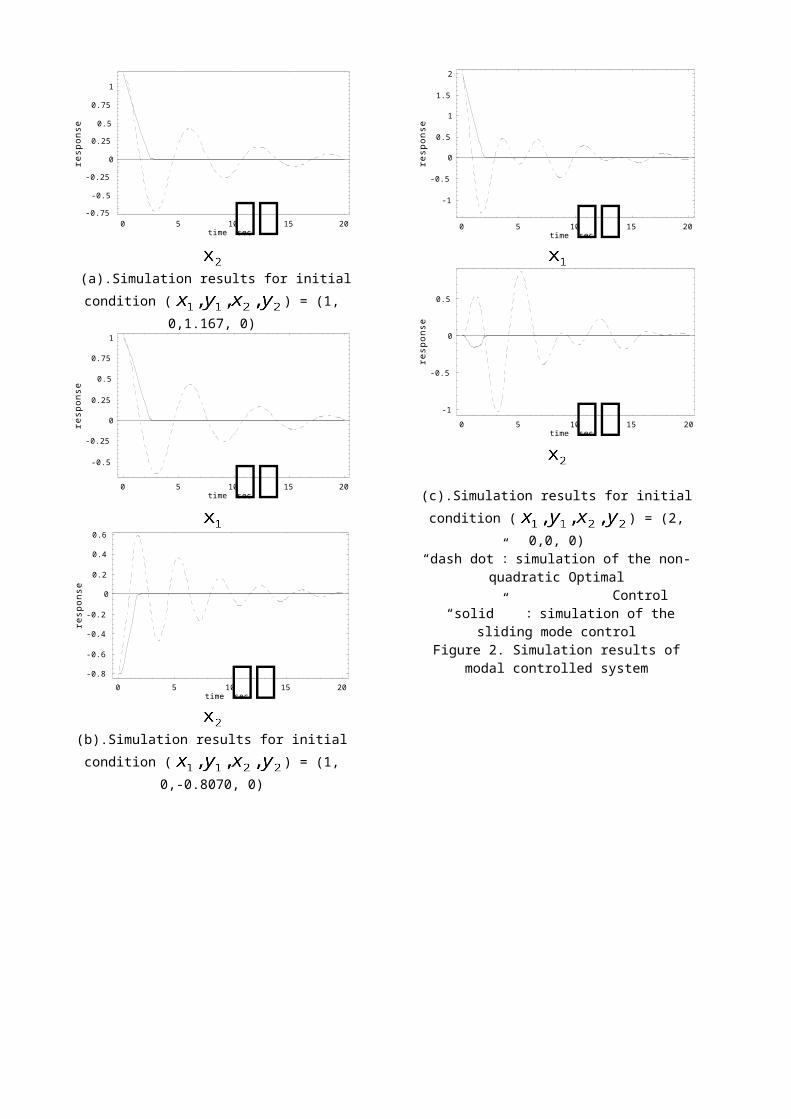
C. Result Figure(2) is the system responses onphysical system. The simulations arecalculated by giving initial conditions(1).(1,0,1.167,0). (2). (1,0,-0.807,0).(3). (2,0,0,0), the first two conditionsare started purposely on mode1 or mode 2only. The third condition is started onmode 1 and mode 2 simultaneously whichis used to test the ability of the modaluncoupling force. Solid line representsthe sliding mode controlled system, dashline is the nonlinear optimal controlledsystem. The results showed that thesliding mode control provides muchbetter control effects than thenonlinear modal controller. The motionsof the masses are reduced much morequickly by using the sliding modecontrol. Specially, for the thirdinitial condition, because of the modalcoupling effects and system nonlinearpart, the non-linear controlled systemshowed irregular decay pattern. However,as the sliding mode control has includedthe modal uncoupling control term, theclosed loop system displayed a moreregular decay pattern. As the control force has introducedlinear damper into system, the damperwill introduce a phase shift between thetwo mass displacements. It should bepointed out that in the special case ofnonlinear modal control, as thenonlinear modal transformation

uncoupling the system, we also requirethe control force uncoupled by the sametransformation, it follows that theclosed-loop mode shapes are the same asthe open-loop mode shape. The results ofall the simulations showed that unlikethe other methods that work on thephysical system, the nonlinear optimalmodal control provides a substantial wayto control the nonlinear oscillatorysystem. The method can be easily appliedto large scale.

Ⅵ.Conclusion In this paper, we have developed amethod of nonlinear optimal control ofindependent modal space. The method issimilar to the traditional independentmodal space control (IMSC) for linearsystem. However, in stead of usinglinear modal matrix we use nonlinearmodal transformation to transform systeminto nonlinear modal coordinate. Byusing the nonlinear optimal feedbackcontrol and sliding mode control, wealso able to control the modal responseson each modal space. Also, the modallyinteracting effects between system andliner modal control force iscounteracted by adding a controller insystem.

REFERENCES[1] Slater, J. “Nonlinear Modal Control Method,”

Journal of Guidance, Control, and Dynamics, 1995, Vol.18, No.3, pp. 433-p40.

[2] Meirovitch, L., Dynamics and Control ofStructure. John Wiley & Sons, New York

[3] Liaw, D. C. Ph.D. Dissertation, FeedbackStabilization via Center Manifold Reduc tion with Applicaiton to Tethered Satellite,.University of Marryland 1990.

[4] Tuer, K. L., Golnaraghi, M. F., Wang, David, “Torwards a Generalized Regulation Scheme forOscillatory Systems via Coupling Effects.”, IEEETransactions on Automatic Control, 1995, Vol. 40, No.3, pp522-530.

[5] Abed, E., Fu, J., “Local Feedback Stabilizationand Bifurcation Control, I. Hopf Bifurcation“,System & Control Letters.1986, Vol. 8, 1987, pp467-473.

[6] Bacciotti, A, Boieri, Paolo., “LinearStabilizablity of Planar Nonlinear Systems.” ,Math. Control Signals Systems, 1990, Vol. 3., pp183-193.

[7] Suhardjo, J., Spencer, J., Sain, M. K.,“Nonlinear Optimal Control of a Duffing Sys-tem.”, Journal of Nonlinear Mechanics, 1992, Vol. 27,No.2, pp157-172.

[8] Shue, S. P., Sawan, M. E. and Rokhsaz, K.,“Optimal Feedback Control of a NonlinearSystem: Winf Rock Example.”, Journal of GuidanceControl and Dynamics, 1996, Vol. 19, No. 1, pp166-171.

[9] Bernstein D. S. ‘Nonquadratic Cost andNonlinear FeedbackControl,”, International Journal ofRobust and Nonlinear Control., 1993, Vol. 3, pp211-229.

[10]Vincent, T., Grantham, W., Nonlinear andOptimal Control Systems, John Wiley & Sons, NewYork, 1997.

[11] J.J.E. Slotine, and W. Li, Applied NonlinearControl, Englewood Cliffs, NJ:Prentice Hall,1991

[12] J. Y. Hung, W. Gao, and J. C. Hung, “Variablestructure control : a survey,” IEEE Trans.Industrial Electronic, vol.40, no.1, pp. 2-22,1993.

[13] V. I. Utkin, “Variable structure systems withsliding modes,” IEEE Trans. Automatica. Contr.,vol. 22, pp.212-222, 1977.

Figure.1 Physical model of nonlinearoscillatory system.

0 5 10 15 20timesec-0.5

-0.25

0

0.25

0.5

0.75

1

esnopser

M Mk kk+ g

1x 2x

0 5 10 15 20timesec-0.75

-0.5

-0.25

0

0.25

0.5

0.75

1esnopser

(a).Simulation results for initialcondition ( ) = (1,

0,1.167, 0)

0 5 10 15 20timesec-0.5

-0.25

0

0.25

0.5

0.75

1

esnopser

0 5 10 15 20timesec-0.8

-0.6

-0.4

-0.2

0

0.2

0.4

0.6

esnopser

(b).Simulation results for initialcondition ( ) = (1,

0,-0.8070, 0)

0 5 10 15 20timesec-1

-0.5

0

0.5

1

1.5

2

esnopser0 5 10 15 20

timesec-1

-0.5

0

0.5

esnopser

(c).Simulation results for initialcondition ( ) = (2,

0,0, 0)“dash dot”：simulation of the non-

quadratic Optimal Control “solid” ：simulation of the

sliding mode controlFigure 2. Simulation results of

modal controlled system