stability notions and lyapunov functions for sliding mode

Available online at www.sciencedirect.com

Journal of the Franklin Institute 351 (2014) 1831–1865

0016-0032/$3http://dx.doi.o

nCorresponE-mail ad

1This work2Grant 190

Apoyo a Proy

www.elsevier.com/locate/jfranklin

Stability notions and Lyapunov functions for slidingmode control systems

Andrey Polyakova,n,1, Leonid Fridmanb,2

aNon-A INRIA - LNE, Parc Scientifique de la Haute Borne 40, avenue Halley Bat.A, Park Plaza, 59650 Villeneuved0Ascq, France

bDepartamento de Ingenieria de Control y Robotica, UNAM, Edificio T, Ciudad Universitaria D.F., Mexico

Received 3 September 2012; received in revised form 11 December 2013; accepted 3 January 2014Available online 15 January 2014

Abstract

The paper surveys mathematical tools required for stability and convergence analysis of modern slidingmode control systems. Elements of Filippov theory of differential equations with discontinuous right-handsides and its recent extensions are discussed. Stability notions (from Lyapunov stability (1982) to fixed-timestability (2012)) are observed. Concepts of generalized derivatives and non-smooth Lyapunov functions areconsidered. The generalized Lyapunov theorems for stability analysis and convergence time estimation arepresented and supported by examples from sliding mode control theory.& 2014 The Franklin Institute. Published by Elsevier Ltd. All rights reserved.

1. Introduction

During the whole history of control theory, a special interest of researchers was focused on systemswith relay and discontinuous (switching) control elements [1–4]. Relay and variable structure controlsystems have found applications in many engineering areas. They are simple, effective, cheap andsometimes they have better dynamics than linear systems [2]. In practice both input and output of asystem may be of a relay type. For example, automobile engine control systems sometimes use λ-sensorwith almost relay output characteristics, i.e. only the sign of a controllable output can be measured [5].

2.00 & 2014 The Franklin Institute. Published by Elsevier Ltd. All rights reserved.rg/10.1016/j.jfranklin.2014.01.002

ding author.dresses: [email protected] (A. Polyakov), [email protected] (L. Fridman).is supported by ANR Grant CHASLIM (ANR-11-BS03-0007).776 Bilateral Cooperation CONACyT(Mexico) – CNRS (France), Grant CONACyT 132125 y Programa deectos de Investiagacion e Inovacion Tecnologico (PAPIIT) 113613 of UNAM.


dx.doi.org/10.1016/j.jfranklin.2014.01.002

http://crossmark.crossref.org/dialog/?doi=10.1016/j.jfranklin.2014.01.002&domain=pdf





mailto:[email protected]

mailto:[email protected]

A. Polyakov, L. Fridman / Journal of the Franklin Institute 351 (2014) 1831–18651832

In the same time, terristors can be considered as relay “actuators” for some power electronicsystems [6].Mathematical backgrounds for a rigorous study of variable structure control systems were

presented in the beginning of 1960s by the celebrated Filippov theory of differential equationswith discontinuous right-hand sides [7]. Following this theory, discontinuous differentialequations have to be extended to differential inclusions. This extension helps us to describe,correctly from a mathematical point of view, such a phenomenon as sliding mode [3,8,6]. In spiteof this, Filippov theory was severely criticized by many authors [9,10,3], since it does notdescribe adequately some discontinuous and relay models. That is why, extensions andspecifications of this theory appear rather frequently [10,11]. Recently, in [12] an extension ofFilippov theory was presented in order to study Input-to-State Stability (ISS) and some otherrobustness properties of discontinuous models.Analysis of sliding mode systems is usually related to a specific property, which is called

finite-time stability [13,3,14–16]. Indeed, the simplest example of a finite-time stable system isthe relay sliding mode system: _x ¼ �sign½x�; xAR; xð0Þ ¼ x0. Any solution of this systemreaches the origin in a finite time Tðx0Þ ¼ jx0j and remains there for all later time instants.Sometimes, this conceptually very simple property is hard to prove theoretically. From apractical point of view, it is also important to estimate a time of stabilization (settling time). Boththese problems can be tackled by Lyapunov Function Method [17–19]. However, designing afinite-time Lyapunov function of a rather simple form is a difficult problem for many slidingmode systems. In particular, appropriate Lyapunov functions for second order sliding modesystems are non-smooth [20–22] or even non-Lipschitz [23–25]. Some problems of a stabilityanalysis using generalized Lyapunov functions are studied in [26–29].One more extension of a conventional stability property is called fixed-time stability [30]. In

addition to finite-time stability it assumes uniform boundedness of a settling time on a set ofadmissible initial conditions (attraction domain). This phenomenon was initially discovered inthe context of systems that are homogeneous in the bi-limit [31]. In particular, if anasymptotically stable system has an asymptotically stable homogeneous approximation at the 0-limit with negative degree and an asymptotically stable homogeneous approximation at theþ1�limit with positive degree, then it is fixed-time stable. An important application of thisconcept was considered in the paper [32], which designs a uniform (fixed-time) exactdifferentiator based on the second order sliding mode technique. Analysis of fixed-time stablesliding mode system requires applying generalized Lyapunov functions [30,32].The main goal of this paper is to survey mathematical tools required for stability analysis of

modern sliding mode control systems. The paper is organized as follows. The next section presentsnotations, which are used in the paper. Section 3 considers elements of the theory of differentialequations with discontinuous right-hand sides, which are required for a correct description of slidingmodes. Stability notions, which frequently appear in sliding mode control systems, are discussed inSection 4. Concepts of generalized derivatives are studied in Section 5 in order to present ageneralized Lyapunov function method in Section 6. Finally, some concluding remarks are given.

2. Notations

�
R is the set of real numbers and R ¼R [ f�1g [ fþ1g, Rþ ¼ fxAR : x40g andRþ ¼Rþ [ fþ1g.
�
I denotes one of the following intervals: ½a; b�, (a,b), ½a; bÞ or ða; b�, where a; bAR; aob.ffiffiffiffiffiffiffiffiffiffip � The inner product of x; yARn is denoted by ⟨x; y⟩ and JxJ ¼ ⟨x; x⟩.

A. Polyakov, L. Fridman / Journal of the Franklin Institute 351 (2014) 1831–1865 1833

�
The set consisting of elements x1; x2;…; xn is denoted by fx1; x2;…; xng. � The set of all subsets of a set MDRn is denoted by 2M . � The sign function is defined by
signs½ρ� ¼1 if ρ40;

�1 if ρo0;

s if ρ¼ 0;

8><>: ð1Þ

where sAR : �1rsr1. If s¼0 we use the notation sign½ρ�.
� The set-valued modification of the sign function is given by
sign½ρ� ¼f1g if ρ40;

f�1g if ρo0;

½�1; 1� if ρ¼ 0:

8><>: ð2Þ

�
x½α� ¼ jxjα sign½x� is a power operation, which preserves the sign of a number xAR. � The geometric sum of two sets is denoted by “ _þ”, i.e.
M1 _þM2 ¼ ⋃x1AM1;x2 AM2

fx1 þ x2g; ð3Þ

where M1DRn;M2DRn.
� The Cartesian product of sets is denoted by � . � The product of a scalar yAR and a set MDRn is denoted by “ � ” :
y �M¼M � y¼ ⋃xAM

fyxg: ð4Þ

�
The product of a matrix AARm�n and a set MDRn is also denoted by “ � ”:A �M¼ ⋃
xAMfAxg: ð5Þ

�
∂Ω is the boundary set of ΩDRn. � BðrÞ ¼ fxARn : JxJorg is an open ball of the radius rARþ with the center at the origin.
Under introduced notations, fyg _þBðɛÞ is an open ball of the radius ɛ40 with the center atyARn.

�
intðΩÞ is the interior of a set ΩDRn, i.e. xA intðΩÞ iff (rARþ : fxg þ BðrÞDΩ. � Let k be a given natural number. CkðΩÞ is the set of continuous functions defined on a set
ΩDRn, which are continuously differentiable up to the order k.
� If Vð�ÞAC1 then ∇VðxÞ ¼ ð∂V=∂x1;…; ∂V=∂xnÞT . If s : Rn-Rm, sð�Þ ¼ ðs1ð�Þ;…; smð�ÞÞT ,
sið�ÞAC1 then ∇sðxÞ is the matrix Rn�m of the partial derivatives ∂sj=∂xi.
� Wn
I is the set of vector-valued, componentwise locally absolutely continuous functions,which map I to Rn.

3. Discontinuous systems, sliding modes and disturbances

3.1. Systems with discontinuous right-hand sides

The classical theory of differential equations [33] introduces a solution of the ordinarydifferential equation (ODE)

_x ¼ f ðt; xÞ; f : R� Rn-Rn; ð6Þ


as a differentiable function x : R-Rn, which satisfies Eq. (6) on some segment (or interval)IDR. The modern control theory frequently deals with dynamic systems, which are modeled byODE with discontinuous right-hand sides [6,34,35]. The classical definition is not applicable tosuch ODE. This section observes definitions of solutions for systems with piecewise continuousright-hand sides, which are useful for sliding mode control theory.Recall that a function f : Rnþ1-Rn is piece-wise continuous iff Rnþ1 consists of a finite

number of domains (open connected sets) Gj �Rnþ1; j¼ 1; 2;…;N; Gi \ Gj ¼∅ for ia j andthe boundary set S ¼⋃N

i ¼ 1∂Gj of measure zero such that f ðt; xÞ is continuous in each Gj and foreach ðtn; xnÞA∂Gj there exists a vector f jðtn; xnÞ, possibly depended on j, such that for anysequence ðtk; xkÞAGj : ðtk; xkÞ-ðtn; xnÞ we have f ðtk; xkÞ-f jðtn; xnÞ. Let functions f j :Rnþ1-Rn be defined on ∂Gj according to this limiting process, i.e.

f jðt; xÞ ¼ limðtk ;xkÞ-ðt;xÞ

f ðtk ; xkÞ; ðtk; xkÞAGj; ðt; xÞA∂Gj:

3.1.1. Filippov definitionIntroduce the following differential inclusion:

_xAK½f �ðt; xÞ; tAR; ð7Þ

K½f �ðt; xÞ ¼ff ðt; xÞg if ðt; xÞARnþ1\S;

co ⋃jAN ðt;xÞ

ff jðt; xÞg !

if ðt; xÞAS;

8>><>>: ð8Þ

where coðMÞ is the convex closure of a set M and the set-valued index function N :Rnþ1-2f1;2;…;Ng defined on S indicates domains Gj, which have a common boundary pointðt; xÞAS, i.e.

N ðt; xÞ ¼ fjAf1; 2;…;Ng : ðt; xÞA∂Gjg:For ðt; xÞAS the set K½f �ðt; xÞ is a convex polyhedron.

Definition 1 (Filippov [7, p. 50]). An absolutely continuous function x : I-Rn defined onsome interval or segment I is called a solution of Eq. (6) if it satisfies the differential inclusion(7) almost everywhere on I .

Consider the simplest case when the function f ðt; xÞ has discontinuities on a smooth surfaceS ¼ fxARn : sðxÞ ¼ 0g, which separates Rn on two domains Gþ ¼ fxARn : sðxÞ40g and G� ¼fxARn : sðxÞo0g.Let P(x) be the tangential plane to the surface S at a point xAS and

fþðt; xÞ ¼ limxi-x;xiAGþ

f ðt; xiÞ and f � ðt; xÞ ¼ limxi-x;xiAG� f ðt; xiÞ

For xAS the set K½f �ðt; xÞ defines a segment connecting the vectors fþðt; xÞ and f � ðt; xÞ (seeFig. 1(a), (b)). If this segment crosses P(x) then the cross point is the end of the velocity vector,which defines the system motion on the surface S (see Fig. 1(b)). In this case the system (7) hastrajectories, which start to slide on the surface S according to the sliding motion equation

_x ¼ f 0ðt; xÞ; ð9Þ

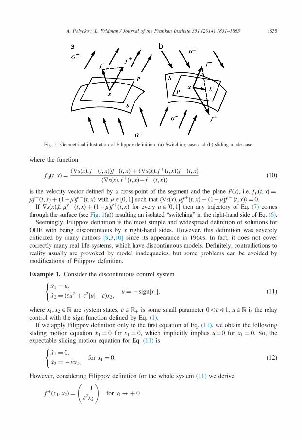
Fig. 1. Geometrical illustration of Filippov definition. (a) Switching case and (b) sliding mode case.


where the function

f 0 t; xð Þ ¼ ⟨∇sðxÞ; f � ðt; xÞ⟩fþðt; xÞ þ ⟨∇sðxÞ; fþðt; xÞ⟩f � ðt; xÞ⟨∇sðxÞ; fþðt; xÞ� f � ðt; xÞ⟩ ð10Þ

is the velocity vector defined by a cross-point of the segment and the plane P(x), i.e. f 0ðt; xÞ ¼μfþðt; xÞ þ ð1�μÞf � ðt; xÞ with μA ½0; 1� such that ⟨∇sðxÞ; μfþðt; xÞ þ ð1�μÞf � ðt; xÞ⟩¼ 0.

If ∇sðxÞ μf � ðt; xÞ þ ð1�μÞfþðt; xÞ for every μA ½0; 1� then any trajectory of Eq. (7) comesthrough the surface (see Fig. 1(a)) resulting an isolated “switching” in the right-hand side of Eq. (6).

Seemingly, Filippov definition is the most simple and widespread definition of solutions forODE with being discontinuous by x right-hand sides. However, this definition was severelycriticized by many authors [9,3,10] since its appearance in 1960s. In fact, it does not covercorrectly many real-life systems, which have discontinuous models. Definitely, contradictions toreality usually are provoked by model inadequacies, but some problems can be avoided bymodifications of Filippov definition.

Example 1. Consider the discontinuous control system

_x1 ¼ u;

_x2 ¼ ðɛu2 þ ɛ2juj�ɛÞx2; u¼ �sign½x1�;(

ð11Þ

where x1; x2AR are system states, ɛARþ is some small parameter 0oɛ51, uAR is the relaycontrol with the sign function defined by Eq. (1).

If we apply Filippov definition only to the first equation of Eq. (11), we obtain the followingsliding motion equation _x1 ¼ 0 for x1 ¼ 0, which implicitly implies u¼0 for x1 ¼ 0. So, theexpectable sliding motion equation for Eq. (11) is

_x1 ¼ 0;

_x2 ¼ �ɛx2;for x1 ¼ 0:

(ð12Þ

However, considering Filippov definition for the whole system (11) we derive

fþðx1; x2Þ ¼�1

ɛ2x2

!for x1-þ 0


f � ðx1; x2Þ ¼1

ɛ2x2

!for x1-�0

and the formula (10) for sðxÞ ¼ x1 gives another sliding motion equation:

_x1_x2

!¼ ⟨∇sðxÞ; f � ðt; xÞ⟩fþðt; xÞ þ ⟨∇sðxÞ; fþðt; xÞ⟩f � ðt; xÞ

⟨∇sðxÞ; fþðt; xÞ� f � ðt; xÞ⟩ ¼0

ɛ2x2

!

From the practical point of view the sliding motion equation (12) looks more realistic. Indeed,in practice we usually do not have ideal relays, so the model of switchings like Eq. (1) is justa “comfortable” approximation of real “relay” elements, which are continuous functions(or singular outputs of additional dynamics [36]) probably with hysteresis or delay effects. In thiscase, a “real” sliding mode is, in fact, a switching regime of bounded frequency. An averagevalue of the control input

jujaverage ¼1

t� t0

Z t

t0

ju τð Þj dτ; t4t0 : x1 t0ð Þ ¼ 0

in the “real” sliding mode is less than 1, particulary jujaverager1�ɛ (see [36] for details). Hence,ɛjuj2average þ ɛ2jujaverage�ɛr�ɛ2 and the system (11) has asymptotically stable equilibrium pointðx1; x2Þ ¼ 0AR2, but Filippov definition quite the contrary provides instability of the system.Such problems with Filippov definition may appear if the control input u is incorporated to the

system (11) in nonlinear way. More detailed study of such discontinuous models is presented in [11].

This example demonstrates two important things:

�
Filippov definition is not appropriate for some discontinuous models, since it does notdescribe a real system motion.
�
Stability properties of a system with discontinuous right-hand side may depend on a definitionof solutions.
Remark 1 (On Filippov regularization). The regularization of the ODE system withdiscontinuous right-hand side can also be done even if the function f ðt; xÞ in Eq. (6) is notpiecewise continuous, but locally measurable. In this case the differential inclusion (7) has thefollowing right-hand side [7]:

K½f �ðt; xÞ ¼ ⋂δ40

⋂μðNÞ ¼ 0

co f ðt; fxg _þBðδÞ\NÞ;

where the intersections are taken over all sets N �Rn of measure zero (μðNÞ ¼ 0) and all δ40,coðMÞ denotes the convex closure of the set M.

3.1.2. Utkin definition (equivalent control method)The modification of Filippov definition, which delivers an important impact to the sliding

mode control theory, is called the equivalent control method [3].Consider the system

_x ¼ f ðt; x; uðt; xÞÞ; tAR; ð13Þ


where f : R� Rn � Rm-Rn is a continuous vector-valued function and a piecewise continuousfunction

u : R� Rn-Rm; uðt; xÞ ¼ ðu1ðt; xÞ; u2ðt; xÞ;…; umðt; xÞÞT

has a sense of a feedback control.

Assumption 1. Each component uiðt; xÞ is discontinuous only on a surface

Si ¼ fðt; xÞARn : siðt; xÞ ¼ 0g;where functions si : R

nþ1-R are smooth, i.e. siAC1ðRnþ1Þ.

Introduce the following differential inclusion:

_xA f ðt; x;K½u�ðt; xÞÞ; tAR; ð14Þwhere

K½u�ðt; xÞ ¼ ðK½u1�ðt; xÞ;…;K½um�ðt; xÞÞT ;

K ui½ � t; xð Þ ¼fuiðt; xÞg; siðt; xÞa0;

co limðtj ;xjÞ-ðt;xÞsiðtj ;xjÞ40

ui tj; xj� �

; limðtj ;xj Þ-ðt;xÞsi ðtj ;xjÞo0

ui tj; xj� �( )

; siðt; xÞ ¼ 0:

8>><>>:

ð15Þ

The set f ðt; x;K½u1�ðt; xÞ;…;K½um�ðt; xÞÞ is non-convex in general case [11].

Definition 2. An absolutely continuous function x : I-Rn defined on some interval or segmentI is called a solution of Eq. (13) if there exists a measurable function ueq : I-Rm such thatueqðtÞAK½u�ðt; xðtÞÞ and _xðtÞ ¼ f ðt; xðtÞ; ueqðtÞÞ almost everywhere on I .

The given definition introduces a solution of the differential equation (13), which we callUtkin solution, since it follows the basic idea of the equivalent control method introduced byUtkin [3, p. 14] (see also [7, p. 54]).

Obviously, for ðt; xðtÞÞ=2S we have ueqðtÞ ¼ uðt; xðtÞÞ. So, the only question is how to defineueq(t) on a switching surface. The scheme presented in [3] is based on resolving of the equation_sðt; xÞ ¼ ∂s=∂t þ ∇TsðxÞf ðt; x; ueqÞ ¼ 0 in algebraic way. The obtained solution ueqðt; xÞ is calledequivalent control [3].

In order to show a difference between Utkin and Filippov definitions we consider the system (13)with uAR ðm¼ 1Þ and a time-invariant switching surface S ¼ fxARn : sðxÞ ¼ 0g.

Denote

uþðt; xÞ ¼ limxj-x;sðxjÞ40

uðt; xjÞ and u� ðt; xÞ ¼ limxj-x;sðxjÞo0

uðt; xjÞ;

fþðt; xÞ ¼ f ðt; x; uþðt; xÞÞ and f � ðt; xÞ ¼ f ðt; x; u� ðt; xÞÞ:The sliding mode existence condition

(μA ½0; 1� : ∇sðxÞ ? μf � ðt; xÞ þ ð1�μÞfþðt; xÞis the same for both definitions.

The sliding motion equation obtained by Filippov definition has the form (9) recalled here by

_x ¼ f 0 t; xð Þ;


f 0 t; xð Þ ¼ ⟨∇sðxÞ; f � ðt; xÞ⟩fþðt; xÞ þ ⟨∇sðxÞ; fþðt; xÞ⟩f � ðt; xÞ⟨∇sðxÞ; fþðt; xÞ� f � ðt; xÞ⟩ :

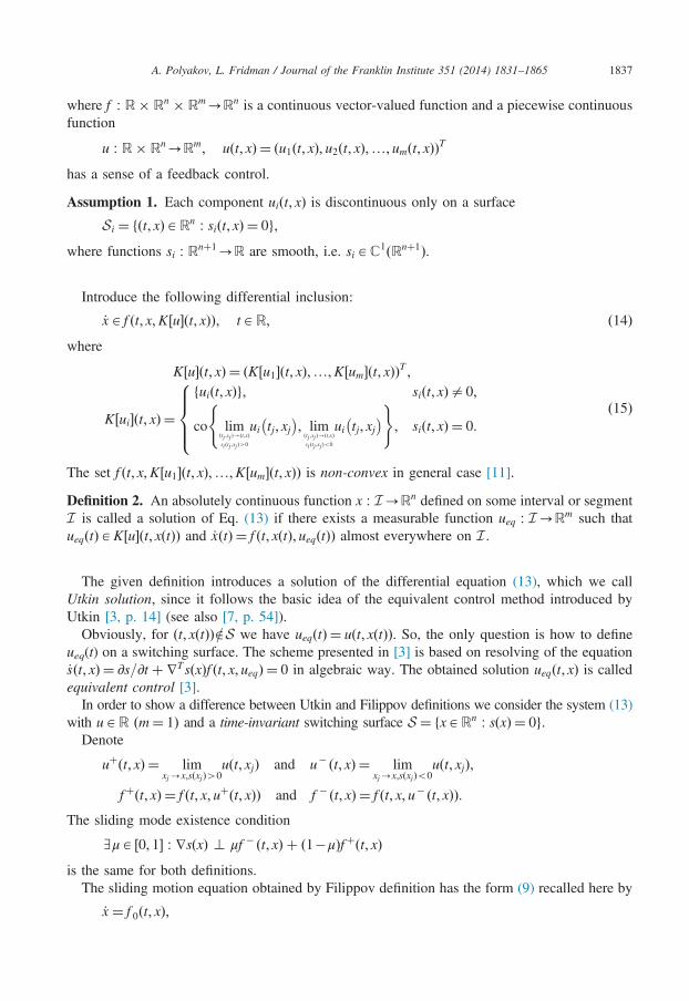
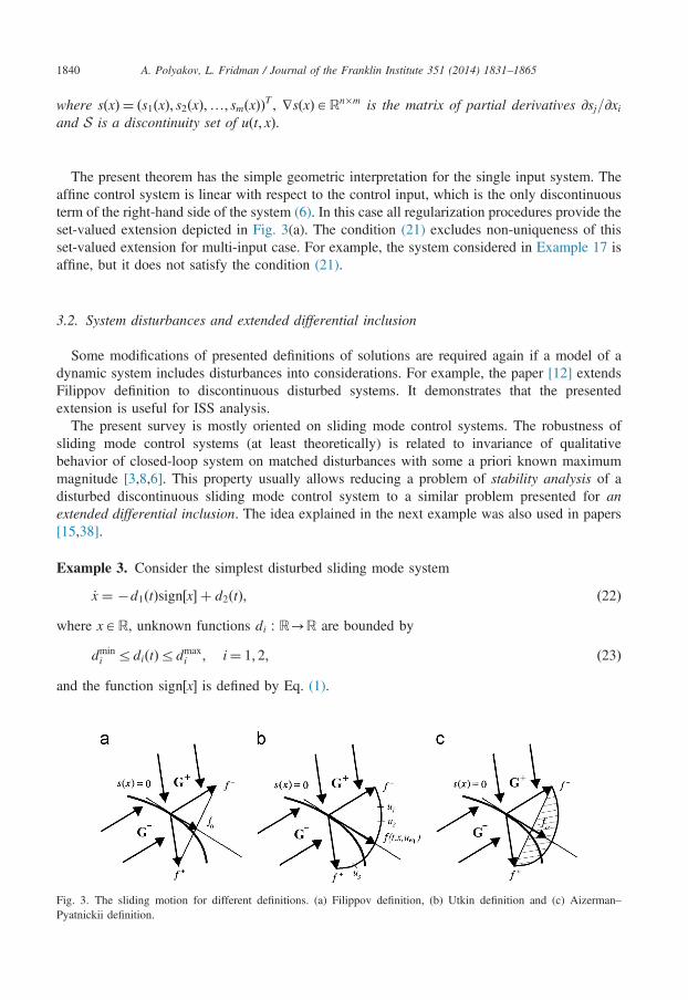
The corresponding vector f 0ðt; xÞ is defined by a cross-point of the tangential plane at the pointxAS and a segment connecting the ends of the vectors fþðt; xÞ and f � ðt; xÞ (see Fig. 3(a)).Utkin definition considers a set K½u�ðt; xÞ, which is the convex closure of a set of limit values

of a discontinuous control function uðt; xÞ. For different u1; u2; u3;…AK½u�ðt; xÞ the vectorsf ðt; x; u1Þ, f ðt; x; u2Þ, f ðt; x; u3Þ;… end on an arc connecting the ends of the vectors fþðt; xÞ andf � ðt; xÞ (see Fig. 3(b)). In this case the vector f ðt; x; ueqÞ defining the right-hand side of thesliding motion equation is derived by a cross-point of this arc and a tangential plane at the pointxAS (see Fig. 3(b)), i.e.

_x ¼ f ðt; x; ueqðt; xÞÞ; xAS; ð16Þwhere ueqðt; xÞAK½u�ðt; xÞ : ∇sðxÞ ? f ðt; x; ueqðt; xÞÞ.Sometimes Utkin definition gives quite strange, from mathematical point of view, results, but

they are very consistent with real-life applications.

Example 2 (Filippov [7]). Consider the system

_x ¼ Axþ bu1 þ cu2; u1 ¼ sign½x1�; u2 ¼ sign½x1�; ð17Þwhere x¼ ðx1; x2;…; xnÞTARn;AARn�n; c; bARn; cab. Filippov definition provides theinclusion

_xAfAxg _þðbþ cÞ � sign½x1�; ð18Þwhere _þ is the geometric (Minkovski) sum of sets (see Eq. (3)), sign is the set-valued modification ofthe sign function (see Eq. (2)) and the product of a vector to a set is defined by Eq. (5).If the functions u1 and u2 are independent control inputs, then Utkin definition gives

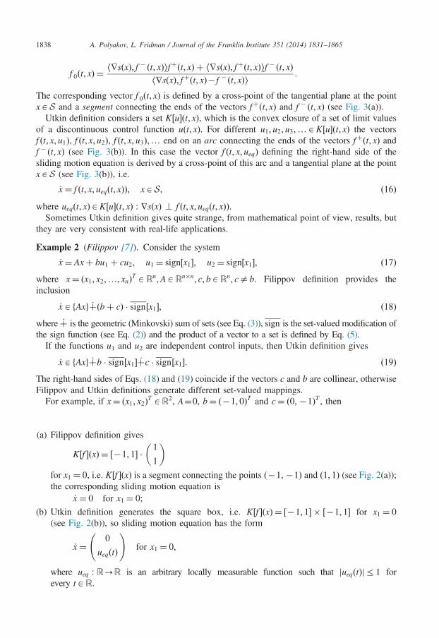
_xAfAxg _þb � sign½x1� _þc � sign½x1�: ð19ÞThe right-hand sides of Eqs. (18) and (19) coincide if the vectors c and b are collinear, otherwiseFilippov and Utkin definitions generate different set-valued mappings.For example, if x¼ ðx1; x2ÞTAR2, A¼0, b¼ ð�1; 0ÞT and c¼ ð0; �1ÞT , then

(a)
Filippov definition gives
K½f �ðxÞ ¼ ½�1; 1� � 1

1

� �for x1 ¼ 0, i.e. K½f �ðxÞ is a segment connecting the points ð�1; �1Þ and ð1; 1Þ (see Fig. 2(a));the corresponding sliding motion equation is

_x ¼ 0 for x1 ¼ 0;

(b)
Utkin definition generates the square box, i.e. K½f �ðxÞ ¼ ½�1; 1� � ½�1; 1� for x1 ¼ 0(see Fig. 2(b)), so sliding motion equation has the form
_x ¼0

ueqðtÞ

!for x1 ¼ 0;

where ueq : R-R is an arbitrary locally measurable function such that jueqðtÞjr1 forevery tAR.

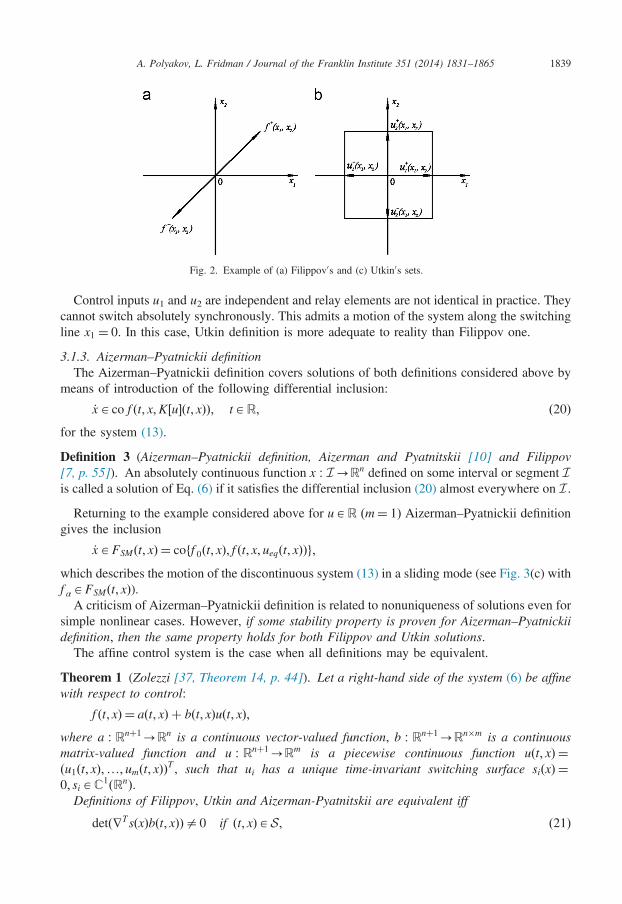
Fig. 2. Example of (a) Filippov0s and (c) Utkin0s sets.


Control inputs u1 and u2 are independent and relay elements are not identical in practice. Theycannot switch absolutely synchronously. This admits a motion of the system along the switchingline x1 ¼ 0. In this case, Utkin definition is more adequate to reality than Filippov one.

3.1.3. Aizerman–Pyatnickii definitionThe Aizerman–Pyatnickii definition covers solutions of both definitions considered above by

means of introduction of the following differential inclusion:

_xAco f ðt; x;K½u�ðt; xÞÞ; tAR; ð20Þfor the system (13).

Definition 3 (Aizerman–Pyatnickii definition, Aizerman and Pyatnitskii [10] and Filippov[7, p. 55]). An absolutely continuous function x : I-Rn defined on some interval or segment Iis called a solution of Eq. (6) if it satisfies the differential inclusion (20) almost everywhere on I .

Returning to the example considered above for uAR ðm¼ 1Þ Aizerman–Pyatnickii definitiongives the inclusion

_xAFSMðt; xÞ ¼ coff 0ðt; xÞ; f ðt; x; ueqðt; xÞÞg;which describes the motion of the discontinuous system (13) in a sliding mode (see Fig. 3(c) withf αAFSMðt; xÞ).

A criticism of Aizerman–Pyatnickii definition is related to nonuniqueness of solutions even forsimple nonlinear cases. However, if some stability property is proven for Aizerman–Pyatnickiidefinition, then the same property holds for both Filippov and Utkin solutions.

The affine control system is the case when all definitions may be equivalent.

Theorem 1 (Zolezzi [37, Theorem 14, p. 44]). Let a right-hand side of the system (6) be affinewith respect to control:

f ðt; xÞ ¼ aðt; xÞ þ bðt; xÞuðt; xÞ;where a : Rnþ1-Rn is a continuous vector-valued function, b : Rnþ1-Rn�m is a continuousmatrix-valued function and u : Rnþ1-Rm is a piecewise continuous function uðt; xÞ ¼ðu1ðt; xÞ;…; umðt; xÞÞT , such that ui has a unique time-invariant switching surface siðxÞ ¼0; siAC1ðRnÞ.

Definitions of Filippov, Utkin and Aizerman-Pyatnitskii are equivalent iff

detð∇TsðxÞbðt; xÞÞa0 if ðt; xÞAS; ð21Þ


where sðxÞ ¼ ðs1ðxÞ; s2ðxÞ;…; smðxÞÞT , ∇sðxÞARn�m is the matrix of partial derivatives ∂sj=∂xiand S is a discontinuity set of uðt; xÞ.

The present theorem has the simple geometric interpretation for the single input system. Theaffine control system is linear with respect to the control input, which is the only discontinuousterm of the right-hand side of the system (6). In this case all regularization procedures provide theset-valued extension depicted in Fig. 3(a). The condition (21) excludes non-uniqueness of thisset-valued extension for multi-input case. For example, the system considered in Example 17 isaffine, but it does not satisfy the condition (21).

3.2. System disturbances and extended differential inclusion

Some modifications of presented definitions of solutions are required again if a model of adynamic system includes disturbances into considerations. For example, the paper [12] extendsFilippov definition to discontinuous disturbed systems. It demonstrates that the presentedextension is useful for ISS analysis.The present survey is mostly oriented on sliding mode control systems. The robustness of

sliding mode control systems (at least theoretically) is related to invariance of qualitativebehavior of closed-loop system on matched disturbances with some a priori known maximummagnitude [3,8,6]. This property usually allows reducing a problem of stability analysis of adisturbed discontinuous sliding mode control system to a similar problem presented for anextended differential inclusion. The idea explained in the next example was also used in papers[15,38].

Example 3. Consider the simplest disturbed sliding mode system

_x ¼ �d1ðtÞsign½x� þ d2ðtÞ; ð22Þwhere xAR, unknown functions di : R-R are bounded by

dmini rdiðtÞrdmax

i ; i¼ 1; 2; ð23Þ

and the function sign½x� is defined by Eq. (1).

Fig. 3. The sliding motion for different definitions. (a) Filippov definition, (b) Utkin definition and (c) Aizerman–Pyatnickii definition.


Obviously, all solutions of the system (22) belong to a solution set of the following extendeddifferential inclusion:

_xA�½dmin1 ; dmax

1 � � sign½x� þ ½dmin2 ; dmax

2 �: ð24Þ

Stability of the system (24) implies the same property for Eq. (22). In particular, fordmin1 4maxfjdmin

2 j; jdmax2 jg both these systems have asymptotically stable origins.

This example shows that the conventional properties, like asymptotic or finite stability,discovered for differential inclusions may provide “robust” stability for original discontinuousdifferential equations. That is why, in this paper we do not discuss “robust” modifications ofstability notions for differential inclusions.

Models of sliding mode control systems usually have the form

_x ¼ f ðt; x; uðt; xÞ; dðtÞÞ; tAR; ð25Þ

where xARn is the vector of system states, uARm is the vector of control inputs, dARk is thevector of disturbances, the function f : Rnþmþkþ1-Rn is assumed to be continuous, the controlfunction u : Rnþ1-Rm is piecewise continuous, the vector-valued function d : R-Rk isassumed to be locally measurable and bounded as follows:

dmini rdiðtÞrdmax

i ; ð26Þ

where dðtÞ ¼ ðd1ðtÞ; d2ðtÞ;…; dkðtÞÞT , tAR.All further considerations deal with the extended differential inclusion

_xAFðt; xÞ; tAR; ð27Þ

where Fðt; xÞ ¼ coff ðt; x;K½u�ðt; xÞ;DÞg, the set-valued function K½u�ðt; xÞ is defined by Eq. (15)and

D¼ fðd1; d2;…; dkÞTARk : diA ½dmini ; dmax

i �; i¼ 1; 2;…; kg: ð28Þ

The same extended differential inclusion can be used if the vector d (or its part) has a sense ofparametric uncertainties.

3.3. Existence of solutions

Let us recall initially the classical result of Caratheodory about the existence of solutions forODEs with right-hand sides, which are discontinuous on time.

Theorem 2 (Coddington and Levinson [33, Theorem 1.1, Chapter 2]). Let the function

g : R� Rn-Rn

ðt; xÞ-gðt; xÞ


be continuous by x in Ω¼ fx0g þ BðrÞ; rARþ; x0ARn for any fixed tAI ¼ ½t0�a; t0 þ a�;aARþ; t0AR and it is measurable by t for any fixed xAΩ. If there exists an integrable functionm : R-R such that J f ðt; xÞJrmðtÞ for all ðt; xÞAI �Ω then there exist an absolutelycontinuous function x : R-Rn and a number bA ð0; a� such that xðt0Þ ¼ x0 and the equality

_xðtÞ ¼ gðt; xðtÞÞholds almost everywhere on ½t0�b; t0 þ b�.

Introduce the following distances:

ρðx;MÞ ¼ infyAM

Jx�yJ ; xARn; MDRn;

ρðM1;M2Þ ¼ supxAM1

ρðx;M2Þ; M1DRn; M2DRn: ð29Þ

Remark, the distance ρðM1;M2Þ is not symmetric, i.e. ρðM1;M2ÞaρðM2;M1Þ in the generalcase.

Definition 4. A set-valued function F : Rnþ1-2Rnþ1

is said to be upper semi-continuous at apoint ðtn; xnÞARnþ1 if ðt; xÞ-ðtn; xnÞ implies

ρðFðt; xÞ;Fðtn; xnÞÞ-0:

For instance, the function sign½x� defined by Eq. (2) is upper semi-continuous.

Theorem 3 (Filippov [7, p. 77]). Let a set-valued function F : G-2Rn

be defined and uppersemi-continuous at each point of the set

G¼ fðt; xÞARnþ1 : jt� t0jra and Jx�x0 Jrbg; ð30Þwhere a; bARþ; t0AR; x0ARn. Let Fðt; xÞ be nonempty, compact and convex for ðt; xÞAG.If there exists K40 such that ρð0;Fðt; xÞÞoK for ðt; xÞAG then there exists at least one

absolutely continuous function x : R-Rn defined at least on the segment ½t0�α; t0 þ α�,α¼minfa; b=Kg, such that xðt0Þ ¼ x0 and the inclusion _xðtÞAFðt; xðtÞÞ holds almost everywhereon ½t0�α; t0 þ α�.

Filippov and Aizerman–Pyatnickii set-valued extensions of the discontinuous ODE (seeformulas (7) and (20)) and the extended differential inclusion (27) satisfy all conditions ofTheorem 3 implying local existence of the corresponding solutions.The existence analysis of Utkin solutions is more complicated in general case. Since the

function f ðt; x; uÞ is continuous, then for any measurable bounded function u0 : I-Rm thecomposition f ðt; x; u0ðtÞÞ satisfies all conditions of Theorem 2 and the equation _x ¼ f ðt; x; u0ðtÞÞhas an absolutely continuous solution x0ðtÞ, but u0ðtÞ may not belong to the set K½u�ðt; x0ðtÞÞ.In some cases, the existence of Utkin solution can be proven using the celebrated Filippov0s

lemma.

Lemma 1 (Filippov [39, p. 78]). Let a function f : Rnþmþ1-Rn be continuous and a set-valued function U : Rnþ1-2R

mbe defined and upper-semicontinuous on an open set I �Ω,

where ΩDRn. Let Uðt; xÞ be nonempty, compact and convex for every ðt; xÞAI �Ω. Let afunction x : R-Rn be absolutely continuous on I , xðtÞAΩ for tAI and _xðtÞA f ðt; xðtÞ;Uðt; xðtÞÞÞ almost everywhere on I .


Then there exists a measurable function ueq : R-Rm such that ueqðtÞAUðt; xðtÞÞ and_xðtÞ ¼ f ðt; xðtÞ; ueqðtÞÞ almost everywhere on I .

If the differential inclusion (14) has a convex right-hand side then Theorem 3 together withLemma 1 results local existence of Utkin solutions. If the set-valued function f ðt; x;K½u�ðt; xÞÞ isnon-convex, the existence analysis of Utkin solutions becomes very difficult (see [11] for thedetails).

Some additional restrictions to right-hand sides are required for a prolongation of solutions. Inparticular, the famous Winter0s theorem (see, for example, [40, p. 515]) about a non-localexistence of solutions of ODE can be expanded to differential inclusions.

Theorem 4 (Gelig et al. [41, p. 169]). Let a set-valued function F : Rnþ1-Rnþ1 be definedand upper-semicontinuous in Rnþ1. Let Fðt; xÞ be nonempty, compact and convex for anyðt; xÞARnþ1.

If there exists a real valued function L : Rþ [ f0g-Rþ [ f0g such that

ρ 0;F t; xð Þð ÞrL JxJð Þ and

Z þ1

0

1LðrÞ dr ¼ þ1;

then for any ðt0; x0ÞARnþ1 the system (27) has a solution xðtÞ : xðt0Þ ¼ x0 defined for all tAR.

Based on Lyapunov function method, the less conservative conditions for prolongation ofsolutions are given below.

4. Stability and convergence rate

Consider the differential inclusion (27) for t4t0 with an initial condition

xðt0Þ ¼ x0; ð31Þwhere x0ARn is given.

Cauchy problem (27), (31) obviously may not have a unique solution for a given t0AR and agiven x0ARn. Let us denote the set of all solutions of Cauchy problem (27), (31) by Φðt0; x0Þ anda solution of Eqs. (27), (31) by xðt; t0; x0ÞAΦðt0; x0Þ.

Nonuniqueness of solutions implies two types of stability for differential inclusions (27): weakstability (a property holds for a solution) and strong stability (a property holds for all solutions)(see, for example, [27,13,7]). Weak stability is usually not enough for robust control purposes.This section observes only strong stability properties of the system (27). All conditions presentedin definitions below are assumed to be held for all solutions xðt; t0; x0ÞAΦðt0; x0Þ.

4.1. Lyapunov, asymptotic and exponential stability

The concept of stability introduced in the famous thesis of Lyapunov [17] is one of the centralnotions of the modern stability theory. It considers some nominal motion xnðt; t0; x0Þ of adynamic system and studies small perturbations of the initial condition x0. If they imply smalldeviations of perturbed motions from xnðt; t0; x0Þ then the nominal motion is called stable.We study different stability forms of the zero solution (or, equivalently, the origin) of thesystem (27), since making the change of variables y¼ x�xn we transform any problem of


stability analysis for some nontrivial solution xnðt; tn; xn0Þ to the same problem for the zerosolution.Assume that 0AFðt; 0Þ for tAR, where Fðt; xÞ is defined by Eq. (27). Then the function

x0ðtÞ ¼ 0 belongs to a solution set Φðt; t0; 0Þ for any t0AR.

Definition 5 (Lyapunov stability). The origin of the system (27) is said to be Lyapunov stable iffor 8ɛARþ and 8 t0AR there exists δ¼ δðɛ; t0ÞARþ such that for 8x0ABðδÞ

(1)
any solution xðt; t0; x0Þ of Cauchy problem (27), (31) exists for t4t0; (2) xðt; t0; x0ÞABðɛÞ for t4t0.
If the function δ does not depend on t0 then the origin is called uniformly Lyapunov stable. Forinstance, if Fðt; xÞ is independent of t (time-invariant case) and the zero solution of Eq. (27) isLyapunov stable, then it is uniformly Lyapunov stable.

Proposition 1. If the origin of the system (27) is Lyapunov stable then xðtÞ ¼ 0 is the uniquesolution of Cauchy problem (27), (31) with x0 ¼ 0 and t0AR.

The origin, which does not satisfy any condition from Definition 5, is called unstable.

Definition 6 (Asymptotic attractivity). The origin of the system (27) is said to be asymptoticallyattractive if for 8 t0AR there exists a set Uðt0ÞDRn : 0A intðUðt0ÞÞ such that 8x0AUðt0Þ

�
any solution xðt; t0; x0Þ of Cauchy problem (27), (31) exists for t4t0; � limt-þ1 Jxðt; t0; x0ÞJ ¼ 0.
The set Uðt0Þ is called attraction domain.

Finding the maximum attraction domain is an important problem for many practical controlapplications.

Definition 7 (Asymptotic stability). The origin of the system (27) is said to be asymptoticallystable if it is Lyapunov stable and asymptotically attractive.

If Uðt0Þ ¼Rn then the asymptotically stable (attractive) origin of the system (27) is calledglobally asymptotically stable (attractive).Requirement of Lyapunov stability is very important in Definition 7, since even global

asymptotic attractivity does not imply Lyapunov stability.

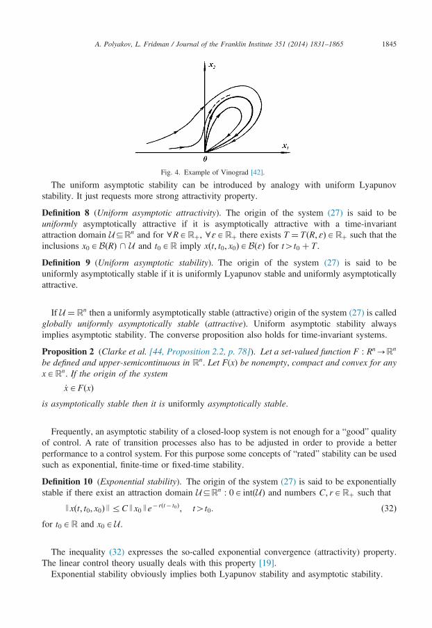
Example 4 (Vinograd [42, p. 433] or Hahn [43, p. 191]). The system

_x1 ¼x21ðx2�x1Þ þ x52

ðx21 þ x22Þð1þ ðx21 þ x22Þ2Þand _x2 ¼

x22ðx2�2x1Þðx21 þ x22Þð1þ ðx21 þ x22Þ2Þ

has the globally asymptotically attractive origin. However, it is not Lyapunov stable, since thissystem has trajectories (see Fig. 4), which start in arbitrary small ball with the center at the originand always leave the ball Bðɛ0Þ of a fixed radius ɛ0ARþ (i.e. Condition 2 of Definition 5 doesnot hold for ɛA ð0; ɛ0Þ).


The uniform asymptotic stability can be introduced by analogy with uniform Lyapunovstability. It just requests more strong attractivity property.

Definition 8 (Uniform asymptotic attractivity). The origin of the system (27) is said to beuniformly asymptotically attractive if it is asymptotically attractive with a time-invariantattraction domain UDRn and for 8RARþ, 8ɛARþ there exists T ¼ TðR; ɛÞARþ such that theinclusions x0ABðRÞ \ U and t0AR imply xðt; t0; x0ÞABðɛÞ for t4t0 þ T .

Definition 9 (Uniform asymptotic stability). The origin of the system (27) is said to beuniformly asymptotically stable if it is uniformly Lyapunov stable and uniformly asymptoticallyattractive.

If U ¼Rn then a uniformly asymptotically stable (attractive) origin of the system (27) is calledglobally uniformly asymptotically stable (attractive). Uniform asymptotic stability alwaysimplies asymptotic stability. The converse proposition also holds for time-invariant systems.

Proposition 2 (Clarke et al. [44, Proposition 2.2, p. 78]). Let a set-valued function F : Rn-Rn

be defined and upper-semicontinuous in Rn. Let F(x) be nonempty, compact and convex for anyxARn. If the origin of the system

_xAFðxÞis asymptotically stable then it is uniformly asymptotically stable.

Frequently, an asymptotic stability of a closed-loop system is not enough for a “good” qualityof control. A rate of transition processes also has to be adjusted in order to provide a betterperformance to a control system. For this purpose some concepts of “rated” stability can be usedsuch as exponential, finite-time or fixed-time stability.

Definition 10 (Exponential stability). The origin of the system (27) is said to be exponentiallystable if there exist an attraction domain UDRn : 0A intðUÞ and numbers C; rARþ such that

Jxðt; t0; x0ÞJrCJx0 Je� rðt� t0Þ; t4t0: ð32Þfor t0AR and x0AU.

The inequality (32) expresses the so-called exponential convergence (attractivity) property.The linear control theory usually deals with this property [19].

Exponential stability obviously implies both Lyapunov stability and asymptotic stability.

Fig. 4. Example of Vinograd [42].


4.2. Finite-time stability

Introduce the functional T0 : Wn½t0;þ1Þ-Rþ [ f0g by the following formula:

T0ðyð�ÞÞ ¼ infτZ t0:yðτÞ ¼ 0

τ:

If yðτÞa0 for all tA ½t0;þ1Þ then T0ðyð�ÞÞ ¼ þ1.Let us define the settling-time function of the system (27) as follows:

Tðt0; x0Þ ¼ supxðt;t0;x0ÞAΦðt0;x0Þ

T0ðxðt; t0; x0ÞÞ� t0; ð33Þ

where Φðt0; x0Þ is the set of all solutions of the Cauchy problem (27), (31).

Definition 11 (Finite-time attractivity). The origin of the system (27) is said to be finite-timeattractive if for 8 t0AR there exists a set Vðt0ÞDRn : 0A intðVðt0ÞÞ such that 8x0AVðt0Þ

�
any solution xðt; t0; x0Þ of Cauchy problem (27), (31) exists for t4t0; � Tðt0; x0Þoþ1 for x0AVðt0Þ and for t0AR.
The set Vðt0Þ is called finite-time attraction domain.

It is worth to stress that the finite-time attractivity property, introduced originally in [14], doesnot imply asymptotic attractivity. However, it is important for many control applications. Forexample, antimissile control problem has to be studied only on a finite interval of time, sincethere is nothing to control after missile explosion. In practice, Lyapunov stability is additionallyrequired in order to guarantee a robustness of a control system.

Definition 12 (Finite-time stability, Roxin [13] and Bhat and Bernstein [14]). The origin of thesystem (27) is said to be finite-time stable if it is Lyapunov stable and finite-time attractive.

If Vðt0Þ ¼Rn then the origin of Eq. (27) is called globally finite-time stable.

Example 5. Consider the sliding mode system

_x ¼ � 2ffiffiffiπ

p sign x½ � þ 2tx ; t4t0; xAR;jj

which, according to Filippov definition, is extended to the differential inclusion

_xA� 2ffiffiffiπ

p � sign x½ � _þ 2txjg; t4t0; xAR;jf ð34Þ

where t0AR. It can be shown that the origin of this system is finite-time attractive with anattraction domain Vðt0Þ ¼ Bðet20ð1�erfðjt0jÞÞÞ, where

erf zð Þ ¼ 2ffiffiffiπ

pZ z

0e� τ2 dτ; zAR

is the so-called Gauss error function. Moreover, the origin of the considered system is Lyapunovstable (for 8ɛ40 and for 8 t0AR we can select δ¼ δðt0Þ ¼minfɛ; et20 ð1�erfðjt0jÞÞg), so it is


finite-time stable. In particular, for t040 the settling-time function has the form

Tðt0; x0Þ ¼ erf �1ðjx0je� t20 þ erfðt0ÞÞ� t0;

where erf �1ð�Þ denotes the inverse function to erfð�Þ.

Proposition 1 implies the following property of a finite-time stable system.

Proposition 3 (Bhat and Bernstein [14, Proposition 2.3]). If the origin of the system (27) isfinite-time stable then it is asymptotically stable and xðt; t0; x0Þ ¼ 0 for t4t0 þ T0ðt0; x0Þ.

A uniform finite-time attractivity requests an additional property for the system (27).

Definition 13 (Uniform finite-time attractivity). The origin of the system (27) is said to beuniformly finite-time attractive if it is finite-time attractive with a time-invariant attractiondomain VDRn such that the settling time function Tðt0; x0Þ is locally bounded on R� Vuniformly on t0AR, i.e. for any yAV there exists ɛARþ such that fyg _þBðɛÞDV andsupt0AR; x0A fyg _þBðɛÞTðt0; x0Þoþ1.

Definition 14 (Uniform finite-time stability, Roxin [13] and Orlov [15]). The origin of thesystem (27) is said to be uniformly finite-time stable if it is uniformly Lyapunov stable anduniformly finite-time attractive.

The origin of Eq. (27) is called globally uniformly finite-time stable if V ¼Rn.Obviously, a settling-time function of time-invariant finite-time stable system (27) is independent

of t0, i.e. T ¼ Tðx0Þ. However, in contrast to asymptotic and Lyapunov stability, finite-time stabilityof a time-invariant system does not imply its uniform finite-time stability in general case.

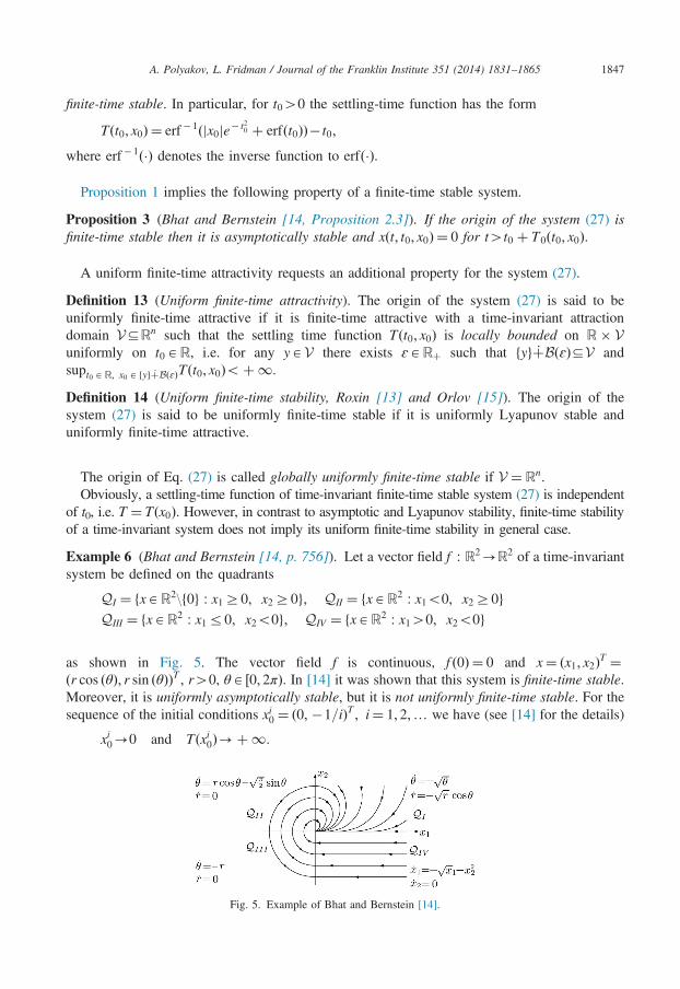
Example 6 (Bhat and Bernstein [14, p. 756]). Let a vector field f : R2-R2 of a time-invariantsystem be defined on the quadrants

QI ¼ fxAR2\f0g : x1Z0; x2Z0g; QII ¼ fxAR2 : x1o0; x2Z0gQIII ¼ fxAR2 : x1r0; x2o0g; QIV ¼ fxAR2 : x140; x2o0g

as shown in Fig. 5. The vector field f is continuous, f ð0Þ ¼ 0 and x¼ ðx1; x2ÞT ¼ðr cos ðθÞ; r sin ðθÞÞT , r40, θA ½0; 2πÞ. In [14] it was shown that this system is finite-time stable.Moreover, it is uniformly asymptotically stable, but it is not uniformly finite-time stable. For thesequence of the initial conditions xi0 ¼ ð0; �1=iÞT ; i¼ 1; 2;… we have (see [14] for the details)

xi0-0 and Tðxi0Þ-þ1:

Fig. 5. Example of Bhat and Bernstein [14].


So, for any open ball BðrÞ; r40, with the center at the origin we have

supx0 ABðrÞ

Tðx0Þ ¼ þ1:

Uniform finite-time stability is the usual property for sliding mode systems [15,38]. Thefurther considerations deals mainly with this property and its modifications.

4.3. Fixed-time stability

This subsection discusses a recent extension of the uniform finite-time stability concept, whichis called fixed-time stability [30]. Fixed-time stability asks more strong uniform attractivityproperty for the system (27). As it was demonstrated in [32,30], this property is very importantfor some applications, such as control and observation with predefined convergence time.In order to demonstrate the necessity of more detailed elaboration of uniformity properties of

finite-time stable systems let us consider the following motivating example.

Example 7. Consider two systems

ðIÞ _x ¼ �x½1=2�ð1�jxjÞ; ðIIÞ _x ¼ �x½1=2� for xo1;

0 for xZ1;

(

which are uniformly finite-time stable with the finite-time attraction domain V ¼ Bð1Þ. Indeed,the settling-time functions of these systems are continuous on V:

T ðIÞ x0ð Þ ¼ ln1þ jx0j1=21�jx0j1=2

� �; T ðIIÞ x0ð Þ ¼ 2jx0j1=2:

So, for any yAV we can select the ball fyg _þBðɛÞDV, where ɛ¼ð1�jyjÞ=2, such thatsupx0A fyg _þBðɛÞT ðIÞðx0Þoþ1 and supx0A fyg _þBðɛÞT ðIIÞðx0Þoþ1.On the other hand, T ðIÞðx0Þ-þ1 if x0-71, but T ðIIÞðx0Þ-2 if x0-71. Therefore, these

systems have different uniformity properties of finite-time attractivity with respect to the domainof initial conditions.

Definition 15 (Fixed-time attractivity). The origin of the system (27) is said to be fixed-timeattractive if it is uniformly finite-time attractive with an attraction domain V and the settling timefunction Tðt0; x0Þ is bounded on R� V, i.e. there exists a number TmaxARþ such thatTðt0; x0ÞrTmax if t0AR and x0AV.

Systems (I) and (II) from Example 7 are both fixed-time attractive with respect to attractiondomain BðrÞ if rA ð0; 1Þ, but the system (I) loses this property for the maximum attractiondomain Bð1Þ.Definition 16 (Fixed-time stability, Polyakov [30]). The origin of the system (27) is said to befixed-time stable if it is Lyapunov stable and fixed-time attractive.

If V ¼Rn then the origin of the system (27) is called globally fixed-time stable. Locallydifferences between finite-time and fixed-time stability are questionable. Fixed-time stabilitydefinitely provides more advantages to a control system in a global case [32,30].


Example 8. Consider the system

_x ¼ �x½1=2� �x½3=2�; xAR; t4t0;

which has solutions defined for all tZ t0:

x t; t0; x0ð Þ ¼sign x0ð Þ tan 2 arctan jx0j1=2

� �� t� t02

� �; tr t0 þ 2arctanðjx0j1=2Þ;

0; t4t0 þ 2arctanðjx0j1=2Þ:

8<:

Any solution xðt; t0; x0Þ of this system converges to the origin in a finite time. Moreover, for anyx0AR; t0AR the equality xðt; t0; x0Þ ¼ 0 holds for all tZ t0 þ π, i.e. the system is globally fixed-time stable with Tmax ¼ π.

5. Generalized derivatives

The celebrated Second Lyapunov Method is founded on the so-called energetic approach tostability analysis. It considers any positive definite function as a possible energetic characteristic(energy) of a dynamic system and studies evolution of this “energy” in time. If a dynamic systemhas an energetic function, which is decreasing (strongly decreasing or bounded) along anytrajectory of the system, then this system has a stability property and the corresponding energeticfunction is called Lyapunov function.

For example, to analyze asymptotic stability of the origin of the system

_x ¼ f ðt; xÞ; f ACðRnþ1Þ; tARþ; xARn ð35Þit is sufficient to find a continuous positive definite function Vð�Þ such that for any solution x(t) ofthe system (35) the function VðxðtÞÞ is decreasing and tending to zero for t-þ1. Theexistence of such function guarantees asymptotic stability of the origin of the system (35) due toZubov0s theorem (see [26,40]).

If the function V(x) is continuously differentiable then the required monotonicity property canbe rewritten in the form of the classical condition [17]:

_V ðxÞ ¼∇TVðxÞf ðt; xÞo0: ð36ÞThe inequality (36) is very usable, since it does not require knowing the solutions of Eq. (35) inorder to check the asymptotic stability. From the practical point of view, it is importantto represent monotonicity conditions in the form of differential or algebraic inequalities likeEq. (36).

Analysis of sliding mode systems is frequently based on non-smooth or even discontinuousLyapunov functions [13,27,45,20,24], which require consideration of generalized derivatives andgeneralized gradients in order to verify stability conditions. This section presents all necessarybackgrounds for the corresponding non-smooth analysis.

5.1. Derivative numbers and monotonicity

Let I be one of the following intervals: ½a; b�, (a,b), ½a; bÞ or ða; b�, where a; bAR; aob.The function φ : R-R is called decreasing on I iff

8 t1; t2AI : t1r t2 ) φðt1ÞZφðt2Þ:


Let K be a set of all sequences of real numbers converging to zero, i.e.

fhngAK 3 hn-0; hna0:

Let a real-valued function φ : R-R be defined on I .Definition 17 (Natanson [46, p. 207]). A number

Dfhngφ tð Þ ¼ limn-þ1

φðt þ hnÞ�φðtÞhn

; hnf gAK : t þ hnAI

is called derivative number of the function φðtÞ at a point tAI , if finite or infinite limit exists.The set of all derivative numbers of the function φðtÞ at a point tAI is called contingent

derivative:

DKφðtÞ ¼ ⋃fhngAK

fDfhngφðtÞgDR:

A contingent derivative of a vector-valued function φ : R-Rn can be defined in the sameway. If a function φðtÞ is differentiable at a point tAI then DKφðtÞ ¼ f _φðtÞg.Lemma 2 (Natanson [46, p. 208]). If a function φ : R-R is defined on I then

(1)
the set DKφðtÞDR is nonempty for any tAI ; (2) for any tAI and for any sequence fhngAK : t þ fhngAI there exists a subsequence
fhn0 gDfhng such that finite or infinite derivative number Dfhn0 gφðtÞ exists.

n
Remark, Lemma 2 remains true for a vector-valued function φ : R-R .Inequalities yo0, yr0, y40, yZ0 for yARn are understood in a componentwise sense. If
for 8yADKφðtÞ we have yo0 then we write DKφðtÞo0. Other ordering relations r , 4, Z forcontingent derivatives are interpreted analogously.The contingent derivative also helps us to prove monotonicity of a non-differentiable function.

Lemma 3 (Natanson [46], p. 266). If a function φ : R-R is defined on I and the inequalityDKφðtÞr0 holds for all tAI , then φðtÞ is decreasing function on I and differentiable almosteverywhere on I .Lemma 3 requires neither the continuity of the function φðtÞ nor the finiteness of its derivative

numbers. It gives a background for the discontinuous Lyapunov function method.

Example 9. The function φðtÞ ¼ � t�signs½t� has a negative contingent derivative for all tAR

and for any sA ½�1; 1�, where the function signs is defined by Eq. (1). Indeed, DKφðtÞ ¼ f�1gfor ta0, DKφð0Þ ¼ f�1g if sA ð�1; 1Þ and DKφð0Þ ¼ f�1; �1g if sAf�1; 1g.

The next lemma simplifies the monotonicity analysis of nonnegative functions.

Lemma 4. If

(1)
the function φ : R-R is nonnegative on I ; (2) the inequality DKφðtÞr0 holds for tAI : φðtÞa0; (3) the function φðtÞ is continuous at any tAI : φðtÞ ¼ 0;
then φðtÞ is decreasing function on I and differentiable almost everywhere on I .

Proof. Suppose the contrary: ( t1; t2AI : t1ot2 and 0rφðt1Þoφðt2Þ.If φðt0Þa0 for all tA ½t1; t2� then Lemma 3 implies that the function φðtÞ is decreasing on

½t1; t2� and φðt1ÞZφðt2Þ.If there exists t0A ½t1; t2� such that φðt0Þ ¼ 0 and φðtÞ40 for all tA ðt0; t2� then Lemma 3

guarantees that the function φðtÞ is decreasing on ðt0; t2�. Taking into account the condition (3)we obtain the contradiction φðt2Þrφðt0Þ ¼ 0.

Finally, let there exists a point tnA ðt1; t2� such that φðtnÞ40 and any neighborhood of thepoint tn contains a point t0A ½t1; tn� : φðt0Þ ¼ 0. In this case, let us select the sequencehn ¼ tn� tno0 such that φðtnÞ ¼ 0 and tn-tn as n-1. For this sequence we obviously have

Dfhngφ t1ð Þ ¼ limn-1

φðtn þ hnÞ�φðtnÞhn

¼ limn-1

�φðtnÞhn

¼ þ1:

This contradicts to the condition (2). □

Absolutely continuous functions are differentiable almost everywhere. Monotonicityconditions for them are less restrictive.

Lemma 5 (Szarski [47, p. 13]). If a function φ : R-R defined on I is absolutely continuousand _φðtÞr0 almost everywhere on I then φðtÞ is decreasing function on I .

Lemma below shows relations between solutions of a differential inclusion (27) and its


contingent derivatives.

Lemma 6 (Filippov [7, p. 70]). Let a set-valued function F : Rnþ1-2Rn

be defined, upper-semicontinuous on a closed nonempty set ΩARnþ1 and the set Fðt; xÞ be nonempty, compact andconvex for all ðt; xÞAΩ.

Let an absolutely continuous function x : R-Rn be defined on I and ðt; xðtÞÞAΩ if tAI .Then

_xðtÞAFðt; xðtÞÞalmost everywhere on I

)3

DKxðtÞDFðt; xðtÞÞeverywhere on I :

5.2. Dini derivatives and comparison systems

The generalized derivatives presented above are closely related with well-known Diniderivatives (see, for example, [47]).

�
Right-hand upper Dini derivative:
Dþφ tð Þ ¼ lim suph-0þ

φðt þ hÞ�φðtÞh

:

�
Right-hand lower Dini derivative:
Dþφ tð Þ ¼ lim infh-0þ


:

�
Left-hand upper Dini derivative:
D�φ tð Þ ¼ lim suph-0�


:


�
Left-hand lower Dini derivative:
D�φ tð Þ ¼ lim infh-0�


:

Obviously, DþφðtÞrDþφðtÞ and D�φðtÞrD�φðtÞ. Moreover, definitions of lim sup andlim inf directly imply that all Dini derivatives belong to the set DKφðtÞ and

DKφðtÞr0 3D�φðtÞr0;

DþφðtÞr0:

(

DKφðtÞZ0 3D�φðtÞZ0;

DþφðtÞZ0:

(

Therefore, all further results for contingent derivative can be rewritten in terms of Diniderivatives.

Theorem 5 (Denjoy–Young–Saks Theorem, Bruckner [48, p. 65]). If φ : R-R is a functiondefined on an interval I , then for almost all tAI Dini derivatives of φðtÞ satisfy one of thefollowing four conditions:

�
φðtÞ has a finite derivative; � DþφðtÞ ¼D�φðtÞ is finite and D�φðtÞ ¼ þ1, DþφðtÞ ¼ �1; � D�φðtÞ ¼DþφðtÞ is finite and DþφðtÞ ¼ þ1, D�φðtÞ ¼ �1; � D�φðtÞ ¼DþφðtÞ ¼ þ1, D�φðtÞ ¼DþφðtÞ ¼ �1.
This theorem has the following simple corollary, which is important for some furtherconsiderations.

Corollary 1. If φ : R -R is a function defined on I , then the equality DKφðtÞ ¼ f�1g(DKφðtÞ ¼ fþ1g) may hold only on a set ΔDI of measure zero.

Consider the system

_y ¼ gðt; yÞ; ðt; yÞAR2; g : R2-R; ð37Þwhere a function gðt; yÞ is continuous and defined on a set G¼ ða; bÞ � ðy1; y2Þ,a; b; y1; y2AR : aob; y1oy2. In this case the system (37) has the so-called right-hand maximumsolutions for any initial condition yðt0Þ ¼ y0; ðt0; y0ÞAG (see [47, Remark 9.1, p. 25]).

Definition 18. A solution ynðt; t0; y0Þ of the system (37) with initial conditionsyðt0Þ ¼ y0; ðt0; y0ÞAG is said to be right-hand maximum if any other solution yðt; t0; y0Þ of thesystem (37) with the same initial condition satisfies the inequality

yðt; t0; y0Þrynðt; t0; y0Þfor all tAI , where I is a time interval on which all solutions exist.

Now we can formulate the following comparison theorem.


Theorem 6 (Szarski [47, p. 25]). Let

(1)
the right-hand side of Eq. (37) be continuous in a region G; (2) ynðt; t0; y0Þ be the right-hand maximum solution of Eq. (37) with the initial condition
yðt0Þ ¼ y0, ðt0; y0ÞAG, which is defined on ½t0; t0 þ αÞ, αARþ;
(3) a function V : R-R be defined and continuous on ½t0; t0 þ βÞ, βARþ, ðt;VðtÞÞAG for
tA ½t0; t0 þ βÞ andVðt0Þry0; DþVðtÞrgðt;VðtÞÞ for tA ðt0; t0 þ βÞ;then

VðtÞrynðt; t0; y0Þ for tA ½t0; t0 þminfα; βgÞ:

Theorem 6 remains true if Dini derivative Dþ is replaced with some other derivative Dþ, D� ,
D� or DK (see [47, Remark 2.2, p. 11]).
5.3. Generalized directional derivatives of continuous and discontinuous functions

Stability analysis based on Lyapunov functions requires calculation of derivatives of positivedefinite functions along trajectories of a dynamic system. If Lyapunov function is non-differentiable, a concept of generalized directional derivatives (see, for example, [28,49,50]) canbe used for this analysis. This survey introduces generalized directional derivatives by analogywith contingent derivatives for scalar functions.

Let MðdÞ be a set of all sequences of real vectors converging to dARn, i.e.

fvngAMðdÞ 3 vn-d; vnARn:

Let a function V : Rn-R be defined on an open nonempty set ΩDRn and dARn.

Definition 19. A number

Dfhng;fvngV x; dð Þ ¼ limn-þ1

Vðxþ hnvnÞ�VðxÞhn

;

fhngAK; fvngAMðdÞ : xþ hnvnAΩ

is called directional derivative number of the function V(x) at the point xAΩ on the directiondARn, if finite or infinite limit exists.

The set of all directional derivative numbers of the function V(x) at the point xAΩ on thedirection dARn is called directional contingent derivative:

DK;MðdÞVðxÞ ¼ ⋃fhngAK;fvngAMðdÞ

fDfhng;fvngVðx; dÞg:

Similar to Lemma 2 it can be shown that if xAΩ then the set DK;MðdÞVðxÞ is nonempty for anyfunction V defined on an open nonempty set ΩDRn and any dARn. A chain rule for theintroduced contingent derivative is described by the following lemma.

Lemma 7. Let a function V : Rn-R be defined on an open nonempty set ΩDRn and a functionx : R-Rn be defined on I , such that xðtÞAΩ if tAI and the contingent derivative DKxðtÞDRn

is bounded for all tAI .


Then the inclusion

DKVðxðtÞÞD ⋃dADKxðtÞ

DK;MðdÞVðxÞ

holds for all tAI .Proof. Since xðtÞAΩ for tAI then Lemma 2 implies that DKVðxðtÞÞ is nonempty for any tAI .Let DfhngVðxðtÞÞADKVðxðtÞÞ be an arbitrary derivative number, i.e. by Definition 17 the finite orinfinite limit

limn-1

Vðxðt þ hnÞÞ�VðxðtÞÞhn

; hnf gAK : t þ hnAI

exists.Consider now the sequence:

vn ¼ xðt þ hnÞ�xðtÞhn

:

Lemma 2 and inequality jDKxðtÞjoþ1 imply that there exist finite dADKxðtÞ and asubsequence fhn0 g of the sequence fhng such that vn0-d. Hence,

DfhngV x tð Þð Þ ¼ limn-1

Vðxðt þ hnÞÞ�VðxðtÞÞhn

¼ limn0-1

Vðxðt þ hn0 ÞÞ�VðxðtÞÞhn0

¼ limn0-1

VðxðtÞ þ hn0vn0 Þ�VðxðtÞÞhn0

¼Dfhn 0g;fvn 0gV xð Þ: □

The proven lemma together with Lemmas 6 and 4 implies the following corollary, which isuseful for a non-smooth Lyapunov analysis.

Corollary 2. Let a set-valued function F : Rnþ1-2Rn

be defined and upper-semicontinuous onI �Ω and the set Fðt; xÞ be nonempty, compact and convex for any ðt; xÞAI �Ω, where ΩDRn

is an open nonempty set.Let xðt; t0; x0Þ be an arbitrary solution of Cauchy problem (27), (31) defined on ½t0; t0 þ αÞ,

where t0AI ; x0AΩ and αARþ. Let a function V : Rn-R be nonnegative on Ω.If the inequality DFðt;xÞVðxÞr0 holds for every tAI and every xAΩ : VðxÞa0 then the

function of time Vðxðt; t0; x0ÞÞ is decreasing on ½t0; t0 þ αÞ, whereDFðt;xÞVðxÞ ¼ ⋃

dAFðt;xÞDK;MðdÞVðxÞ: ð38Þ

5.4. Clarke0s gradient of Lipschitz continuous functions

Let a function V : Rn-R be defined and Lipschitz continuous on an open nonempty set.Then, by Rademacher theorem [51], its gradient exists almost everywhere on Ω and for eachxAΩ the following set can be constructed:

∇CVðxÞ ¼ co ⋃fxkgAMðxÞ:(∇VðxkÞ

limxk-x

∇VðxkÞ

; ð39Þ

which is called Clarke0s generalized gradient of the function V(x) at the point xAΩ. The set∇CVðxÞ is nonempty, convex and compact for any xAΩ and the set-valued mapping ∇CV :Rn-2R

n

is upper-semicontinuous on Ω (see [50, Proposition 2.6.2, p. 70]).


The formula (39) gives a procedure for calculation of the generalized gradient of a function.The next lemma presents a chain rule for Clarke0s generalized gradient.

Lemma 8 (Moreau and Valadier [52, Theorem 2, p. 336]). Let a Lipschitz continuous functionV : Rn-R be defined in an open nonempty set ΩDRn and an absolutely continuous functionx : R-Rn be defined on I such that xðtÞAΩ for every tAI .

Then there exists a function p : R-Rn defined on I such that pðtÞA∇CVðxðtÞÞ and_V ðxðtÞÞ ¼ pT ðtÞ_xðtÞ almost everywhere on I .Lemmas 8 and 5 imply the following corollary.

Corollary 3. Let a set-valued function F : Rnþ1-2Rn

be defined and upper-semicontinuous onI �Ω and a set Fðt; xÞ be nonempty, compact and convex for any ðt; xÞAI �Ω, where ΩDRn

is an open nonempty set. Let xðt; t0; x0Þ be an arbitrary solution of Cauchy problem (27), (31)defined on ½t0; t0 þ αÞ, where t0AI ; x0AΩ and αARþ. Let a function V : Rn-R be definedand Lipschitz continuous on Ω.

If the inequality DCFðt;xÞVðxÞr0 holds almost everywhere on I for every xAΩ then the

function of time Vðxðt; t0; x0ÞÞ is decreasing on ½t0; t0 þ αÞ, whereDC

Fðt;xÞVðxÞ ¼ ⋃dAFðt;xÞ

⋃pA∇CVðxÞ

fpTdg ð40Þ

If the function V : Rn-R is continuously differentiable then the usual total derivative

_VFðt;xÞðxÞ ¼ ⋃dAFðt;xÞ

f∇TVðxÞdg ð41Þ

can be used for monotonicity analysis instead of Clarke0s or contingent derivative. In this case wehave DFðt;xÞVðxÞ ¼DC

Fðt;xÞVðxÞ ¼ _VFðt;xÞðxÞ.

6. Lyapunov function method and convergence rate

Lyapunov function method is a very effective tool for analysis and design of both linear andnonlinear control systems [19]. Initially, the method was presented for “unrated” (Lyapunov andasymptotic) stability analysis [17]. A development of control theory had required to study aconvergence rate together with a stability properties of a control system. This section observesthe most important achievements of the Lyapunov function method related to a convergence rateestimation of sliding mode systems.

6.1. Analysis of Lyapunov, asymptotic and exponential stability

The continuous function W : Rn-R defined on Rn is said to be positive definite iff Wð0Þ ¼ 0and WðxÞ40 for xARn\f0g.Definition 20. A function V : Rn-R is said to be proper on an open nonempty set ΩDRn :0A intðΩÞ iff

(1)
it is defined on Ω and continuous at the origin; (2) there exists a continuous positive definite function V : Rn-R such that
V ðxÞrVðxÞ for xAΩ:


A positive definite function W : R -R is called radially unbounded if WðxÞ-þ1 forJxJ-þ1.

Definition 21. A function V : Rn-R is said to be globally proper iff it is proper on Rn and the

n

positive definite function V : Rn-R is radially unbounded.

If V is continuous on Ω, then V ðxÞ ¼ VðxÞ for xAΩ and Definition 21 corresponds to the usualnotion of proper positive definite function (see, for example, [44]).For a given number rAR and a given positive definite function W : Rn-R defined on Ω let

us introduce the set

ΠðW ; rÞ ¼ fxAΩ : WðxÞorgwhich is called the level set of the function W.Theorems on Lyapunov and asymptotic stability given below are obtained by a combination of

Zubov0s theorems (see, for example, [40, pp. 566–568]) with Corollary 2.

Theorem 7. Let a function V : Rn-R be proper on an open nonempty set ΩDRn : 0A intðΩÞand

DFðt;xÞVðxÞr0 for tAR and xAΩ\f0g: ð42ÞThen the origin of the system (27) is Lyapunov stable.

Proof. Since V(x) is proper, then there exists continuous positive definite function V ðxÞ such thatV ðxÞrVðxÞ for all xAΩ.Let h¼ suprARþ:BðrÞDΩr and λðɛÞ ¼ infxARn: J x J ¼ ɛV ðxÞ40, where ɛA ð0; h�.The function V(x) is continuous at the origin, so (δA ð0; ɛÞ : VðxÞoλðɛÞ if xABðδÞ. Moreover,

BðδÞDUðɛÞ ¼ΠðV ; λðɛÞÞ \ BðɛÞ.Let t0AR and x0AUðɛÞ (in partial case x0ABðδÞ). The system (27) satisfies Theorem 3 and it

has solutions, which can be continued up to the boundary of Ω. Consider an arbitrary solutionxðt; t0; x0Þ of Eq. (27). The inequality (42) and Corollary 2 imply that the function of timeVðxðt; t0; x0ÞÞ is decreasing for t4t0, i.e. Vðxðt; t0; x0ÞÞrVðx0ÞoλðɛÞ.In this case, xðt; t0; x0ÞABðɛÞ for t4t0. Indeed, otherwise there exists tn4t0 :

Jxðtn; t0; x0ÞJ ¼ ɛ, so Vðxðtn; t0; x0ÞÞZV ðxðtn; t0; x0ÞÞZλðɛÞ.The proven property also implies that even if a solution of Eq. (27) with t0AR and x0AUðɛÞ

was initially defined on finite interval ½t0; t0 þ αÞ; αARþ, it can be prolonged for all t4t0. □

Asymptotic stability requires analysis of an attraction set. Lyapunov function approach mayprovide an estimate of this set.

Theorem 8. Let a function V : Rn-R be proper on an open nonempty set ΩDRn : 0A intðΩÞ,a function W : Rn-R be a continuous positive definite and

DFðt;xÞVðxÞr�WðxÞ for tAR and xAΩ\f0g:Then the origin of the system (27) is asymptotically stable with an attraction domain

U ¼ΠðV ; λðhÞÞ \ BðhÞ; ð43Þwhere λðhÞ ¼ infxARn: J x J ¼ hV ðxÞ and hrsuprARþ:BðrÞDΩr.If V is globally proper and Ω¼Rn then the origin of the system (27) is globally asymptotically

stable (U ¼RnÞ.


Proof. Theorem 7 implies that an arbitrary solution xðt; t0; x0Þ of Eq. (27) with t0AR andx0AUðɛÞ is defined for all t4t0 and xðt; t0; x0ÞABðɛÞ, where ɛA ð0; h� and UðɛÞ ¼ΠðV ; λðɛÞÞ \ BðɛÞ. Moreover, the function of time ~V ðtÞ ¼ Vðxðt; t0; x0ÞÞ is decreasing for allt4t0. So, in order to prove asymptotic stability we just need to show that μ¼0, whereμ¼ inf t4t0

~V ðtÞ.Suppose a contradiction, i.e. μ40.The function V(x) is continuous at the origin, so there exists r40 such that VðxÞoμ for all

xABðrÞ. Since μ40 then xðt; t0; x0Þ=2BðrÞ for all t4t0.Introduce the following compact set Θ¼ fxARn : rr JxJrɛg. SinceW(x) is continuous and

positive definite, then we have W0 ¼ infxAΘWðxÞ40.The inequality DFðt;xÞVðxÞr�WðxÞ and the exclusion xðt; t0; x0Þ=2BðrÞ imply DK

~V ðtÞr�W0

for all t4t0.Since ~V ðtÞ is decreasing then it is differentiable almost everywhere on ½t0; t0 þ Δ�, where

Δ¼ Vðx0Þ=W0. Hence (see, for example, [53, p. 111]),

Vðt0 þ ΔÞ�Vðt0ÞrZ t0þΔ

t0

_V ðτÞ dτr�W0Δ¼ �Vðt0Þ;

i.e. Vðt0 þ ΔÞr0oμ. This contradicts our supposition. So, Vðxðt; t0; x0ÞÞ-0 or equivalentlyxðt; t0; x0Þ-0 if t-þ1.

If the function V is globally proper then global asymptotic attractiveness follows fromlimɛ-þ1λðɛÞ ¼ þ1 due to radial unboundedness of V . □

Exponential convergence asks for additional properties of Lyapunov functions.

Theorem 9. Let conditions of Theorem 8 hold, the function V(x) is continuous on an opennonempty set Ω�Rn : 0A intðΩÞ and there exist α; r1; r2ARþ:

r1 JxJrVðxÞrr2 JxJ and WðxÞZαVðxÞthen the origin of the system (27) is exponentially stable with a rate αARþ.

This theorem can be proven by analogy to a classical theorem on exponential stability (see, forexample, [19, p. 171]) using Lemma 6.

The presented theorems show that discontinuous and non-Lipschitzian Lyapunov functionscan also be used for stability analysis. If V(x) is Lipschitz continuous then all theorems onstability can be reformulated using Clarke0s gradient.

The following important theorem declares that a smooth Lyapunov function always exists fora time-invariant asymptotically stable differential inclusion (27).

Theorem 10 (Clarke et al. [44, Theorem 1.2]). Let a set-valued function F : Rn-Rn be definedand upper-semicontinuous in Rn. Let F(x) be nonempty, compact and convex for any xARn. Ifthe origin of the system

_xAFðxÞis globally uniformly asymptotically stable iff there exist a globally proper functionVð�ÞAC1ðRnÞ and a function Wð�ÞAC1ðRnÞ : WðxÞ40 for xa0 such that

maxyAFðxÞ

∇TVðxÞyr�WðxÞ; xARn\f0g:


However, the practice shows that designing of a Lyapunov function for nonlinear and/ordiscontinuous system is a nontrivial problem even for a two dimensional case. Frequently, inorder to analyze stability of a sliding mode control system it is simpler to design a non-smoothLyapunov function (see, for example, [3,20,24]).

6.2. Lyapunov analysis of finite-time stability

Analysis of finite-time stability using the Lyapunov function method allows us to estimate asettling time a priori. The proof of the next theorem follows the ideas introduced in [13,54].

Theorem 11. Let a function V : Rn-R be proper on an open nonempty set ΩDRn : 0A intðΩÞand

DFðt;xÞVðxÞr�1 for tAR and xAΩ\f0g: ð44ÞThen the origin of the system (27) is finite-time stable with an attraction domain U defined byEq. (43) and

Tðx0ÞrVðx0Þ for x0AU; ð45Þwhere Tð�Þ is a settling-time function.If a function V is globally proper on Ω¼Rn then the inequality (44) implies global finite-time

stability of the system (27).

Proof. Theorem 8 implies that the origin of the system (27) is asymptotically stable with theattraction domain U. This means that any solution xðt; t0; x0Þ; x0AU, of the system (27) exists for8 t4t0. Therefore, we need to show finite-time attractivity. Consider the interval ½t0; t1�; t1 ¼t0 þ Vðx0Þ.Suppose a contradiction: xðt; t0; x0Þa0 for 8 tA ½t0; t1�. Denote ~V ðtÞ ¼ Vðxðt; t0; x0ÞÞ. Lemma 7

implies

DK~V ðtÞrDFðt;xÞVðxðt; t0; x0ÞÞr�1; 8 tA ½t0; t1�

Hence, by Lemma 3 the function ~V ðtÞ is decreasing on ½t0; t1� and differentiable almosteverywhere on ½t0; t1�. Then

~V t1ð Þ� ~V t0ð ÞrZ t1

t0

d

dt~V τð Þ dτr� t1� t0ð Þ ¼ �V x0ð Þ

(see, for example, [53, p. 111]), i.e. ~V ðt1Þ ¼ Vðxðt1; t0; x0ÞÞr ~V ðt0Þ�Vðx0Þ ¼ Vðxðt0;t0; x0ÞÞ�Vðx0Þ ¼ 0. Since V(x) is positive definite then Vðxðt1; t0; x0ÞÞr0 ) Vðxðt1; t0; x0ÞÞ ¼03xðt1; t0; x0Þ ¼ 0, i.e. the origin of the system (27) is finite-time attractive with the settlingtime estimate (45). □

Evidently, if under conditions of Theorem 11 there exists a continuous function V : Rn-R

such that VðxÞrV ðxÞ for 8xAΩ then the origin of the system (27) is uniformly finite-timestable.

Example 10. Consider again the uniformly finite-time stable system

_x ¼ �x½1=2�ð1�jxjÞ; xAR;


and show that its settling-time function

T xð Þ ¼ ln1þ jxj1=21�jxj1=2

� �

satisfies all conditions of Theorem 11. Indeed, it is continuous and proper on Bð1Þ. Finally, it isdifferentiable for xABð1Þ\f0g and

_T xð Þ ¼ ∂T∂x

_x ¼ 1

x½1=2�ð1�jxjÞ _x ¼ �1 for xa0:

The last example shows that a settling-time function of finite-time stable system is a Lyapunovfunction in a generalized sense. Theorem 11 operates with a very large class Lyapunov functions.However, its conditions are still rather conservative. For example, the settling-time function fromExample 6 cannot be considered as a Lyapunov function candidate, since it is discontinuous atthe origin, so it is not proper. However, even proper settling-time functions of sliding modesystems may not satisfy the condition (44).

Example 11. Consider the twisting second order sliding mode system [55]

_x1_x2

!AFðx1; x2Þ ¼

y

�2sign½x1��sign½x2�

!; ð46Þ

which is uniformly finite-time stable with the settling-time function [54]:

Ttw xð Þ ¼ p

ffiffiffiffiffiffiffiffiffiffiffiffiffiffiffiffiffiffiffiffiffiffiffiffiffiffiffiffiffiffiffiffiffiffiffiffiffiffiffiffiffiffiffiffiffiffix1j j þ x22

2ð2þ sign½x1x2�Þ

sþ jx2jsign½x1x2�

2þ sign½x1x2�; p¼ 4

ffiffiffi2

p

3� ffiffiffi3

p

The function Ttw is globally proper, Lipschitz continuous outside the origin and continuouslydifferentiable for xya0

DFðx1;x2ÞTtw x1; x2ð Þ ¼ ∂Ttw

∂x1x2 þ

∂Ttw

∂x2�2sign x1½ ��sign x2½ �ð Þ ¼ �1 for x1x2a0:

However, DFðx1;x2ÞTtwðx1; x2Þ \ Rþa∅ for x1 ¼ 0. So, Ttwðx; yÞ does not satisfy Eq. (44).Applying Clarke0s gradient does not help us to avoid this problem.

In the same time, if xðt; t0; x0Þ is an arbitrary solution of the system (46), thenDKTtwðxðt; t0; x0ÞÞr�1 for 8 t4t0 : xðt; t0; x0Þa0 (see [54] for the details).

Remark, if p44ffiffiffi2

p=ð3� ffiffiffi

3p Þ then the function Ttw(x) satisfies the conditions of Theorem 11

and DFðx1;x2ÞTtwðxÞ ¼ f�1g for x1 ¼ 0.

Sometimes the less restrictive finite-time stability condition

DKVðxðt; t0; x0ÞÞr�1; tZ t0 : xðt; t0; x0Þa0;

xðt; t0; x0ÞAΦðt0; x0Þ; t0AR; x0AU ð47Þhas to be considered instead of Eq. (44). Examples of applying the condition (47) for analysis ofsecond order sliding mode systems can be found in [54,22]. They demonstrate that frequently wedo not need to know a solution xðt; t0; x0Þ of Eq. (27) in order to check the condition (47).


Example 12. Consider the system

_x ¼ � ð2�sign½x1x2�ÞJxJ

x; x¼ ðx1; x2ÞTAR2:

It is uniformly finite-time stable. Its settling time function is discontinuous

T xð Þ ¼JxJ for x1x2Z013JxJ for x1x2o0

(

However, the function T(x) is the generalized Lyapunov function, since it is globally proper and

DKTðxðt; t0; x0ÞÞ ¼ �1 for t4t0 : xðt; t0; x0Þa0;

where xðt; t0; x0ÞAΦðt0; x0Þ, t0AR and x0AR2.

Theorem 12 (Bhat and Bernstein [14, Theorem 4.2]). Let a continuous function V : Rn-R beproper on an open nonempty set ΩDRn : 0A intðΩÞ and

DFðt;xÞVðxÞr�rVρðxÞ; t4t0; xAΩ;

where rARþ, 0oρo1. Then the origin of the system (27) is uniformly finite-time stable with anattraction domain U defined by Eq. (43) and the settling time function Tð�Þ is estimated asfollows:

T x0ð Þr V1�ρðx0Þrð1�ρÞ for x0AU:

Proof. Let xðt; t0; x0Þ; x0AU, be any solution of Eq. (27) and ~V ðtÞ ¼ Vðxðt; t0; x0ÞÞ. SinceDK

~V ðtÞrDFðt;xÞVðxðt; t0; x0ÞÞr�r ~VρðtÞ

(see, Lemma 7) then Lemma 6 implies that ~V ðtÞryðtÞ; t4t0, where y(t) is a right-handmaximum solution of the following Cauchy problem:

_yðtÞ ¼ �ryρðtÞ; yðt0Þ ¼ Vðx0Þ;i.e.

y tð Þ ¼Vðx0Þ1�ρ�rð1�ρÞðt� t0Þ� �1=ð1�ρÞ

for tA t0; t0 þ V1�ρðx0Þrð1�ρÞ

� �;

0 for t4V1�ρðx0Þrð1�ρÞ :

8>>><>>>:

This implies Vðxðt; t0; x0ÞÞ ¼ 0 for 8 t4V1�ρðx0Þ=rð1�ρÞ. □

A global finite-time stability can be analyzed using globally proper Lyapunov functions inTheorems 11 and 12.

Example 13. Consider the so-called super-twisting system [55]

_x

_y

!AFðx; yÞ ¼ �αx½1=2� þ y

�β � sign½x�

!ð48Þ

where xAR; yAR; α40; β40. Recall, x½μ� ¼ jxjμsign½x�, μARþ.


The function [24]

Vðx; yÞ ¼ ð2β þ α2=2Þjxj þ y2�αyx½1=2�

is the generalized Lyapunov function for the system (48). Indeed, this function is globally properand continuous (but not Lipschitz continuous on the line x¼0).

For xa0 this function is differentiable and

DVFðx;yÞðx; yÞr�γffiffiffiffiffiffiffiffiffiffiffiffiffiVðx; yÞ

pwhere γ ¼ γðα; βÞ40 is a positive number (see [24] for details).

For x¼0 and ya0 we need to calculate a generalized directional derivative. So, consider thelimit

Dfhng;fungV 0; yð Þ ¼ limn-1

Vðhnuxn; yþ hnuynÞ�Vð0; yÞhn

where fhngAK; un ¼ ðuxn; uynÞT ; fungAMðdÞ; dAFð0; yÞ. In this case, uxn-y and uyn-q;qA ½�β; β�. Hence,

Dfhng;fungV 0; yð Þ ¼ limn-1

ð2β þ α2=2Þjhnyj þ ðyþ hnqÞ2�αðhnyÞ½1=2�ðyþ hnqÞ�y2

hn:

Obviously, Dfhng;fungVð0; yÞ ¼ �1. Therefore,

DFðx;yÞVð0; yÞ ¼ f�1gr�γffiffiffiffiffiffiffiffiffiffiffiffiffiffiffiVð0; yÞÞ

pfor ya0

and the super-twisting system is uniformly finite-time stable with the settling time estimateTðx; yÞr2

ffiffiffiffiffiffiffiffiffiffiffiffiffiVðx; yÞ

p=γ.

By Corollary 1, the set of time instants t4t0 : DKVðxðtÞ; yðtÞÞ ¼ f�1g may have only themeasure zero. This means that the line x¼0 for ya0 cannot be sliding set of the system (48).The sliding mode may appear only at the origin.

6.3. Fixed-time stability analysis

Locally fixed-time stability property is very close to finite-time stability, so it can beestablished using Theorem 11 just including additional condition: VðxÞrTmax for 8xAΩ, whereTmaxARþ. An alternative Lyapunov characterization of fixed-time stability can be obtainedusing the ideas introduced in the proof of Corollary 2.24 from [31].

Theorem 13 (Polyakov [30, p. 2106]). Let a continuous function V : Rn-R be proper on anopen connected set Ω : 0A intðΩÞ. If for some numbers μA ð0; 1Þ; νARþ; rμARþ; rνARþ thefollowing inequality

DFðt;xÞVðxÞr�rμV1�μðxÞ for xAΩ : VðxÞr1;

�rνV1þνðxÞ for xAΩ : VðxÞZ1;t4t0; xAΩ;

(ð49Þ

holds, then the origin of the system (27) is fixed-time stable with the attraction domain U definedby Eq. (43) and the maximum settling time is estimated by

T xð ÞrTmax r 1μrμ

þ 1νrν

: ð50Þ


If Ω¼Rn and a function V is radially unbounded then the origin of the system (27) is globallyfixed-time stable.

Proof. Theorem 8 implies that the origin of the system (27) is asymptotically stable with theattraction domain U. This means that any solution xðt; t0; x0Þ; x0AU, of the system (27) exists for8 t4t0. We just need to prove that the estimate (49) implies fixed-time attractivity.Indeed, for any trajectory xðt; t0; x0Þ of the system (6) with Vðx0Þ41, there exists a time instant

T1 ¼ T1ðx0Þr1=νrν : VðxðT1; t0; x0ÞÞ ¼ 1. On the other hand, for any trajectory xðt; t1; x1Þ withVðx1Þr1, there exists a time instant T2 ¼ T2ðx1Þr1=μrμ : Vðxðt; t1; x1ÞÞ-0 for t-T2. Thesefacts can be easily proven analogously to Theorem 12. □

This result also can be used for fixed-time stability analysis of high-order sliding mode controlsystems.

Example 14 (Polyakov [30, p. 2108]). Consider the sliding mode control system

_x ¼ y;

_y ¼ uþ dðtÞ;

u¼ �α1 þ 3β1x2 þ γ

2sign s½ �� α2sþ β2s

3� �½1=2�

;

8>>><>>>:

where xAR; yAR, jdðtÞjoC, α1; α2; β1; β2;CARþ; γ42C and the switching surface s¼0 isdefined by

s¼ yþ ðyt½2� þ α1xþ β1x3Þ½1=2�:

The original discontinuous systems correspond to the following extended differential inclusion:

_x ¼ y;

_yA �α1 þ 3β1x2 þ γ

2

� sign s½ � _þ

(�ðα2sþ β2s

3Þ½3=2�)

_þ �C;C½ �:

8>><>>:

Consider the function VðsÞ ¼ jsj and calculate its generalized derivative along trajectories of thelast system

DFVðsÞr�ðα2VðsÞ þ β2V3ðsÞÞ1=2 for sa0

(see [30] for the details). This implies that the sliding surface s¼0 is fixed-time attractive withthe estimate of a reaching time:

Tsr2ffiffiffiffiffiα2

p þ 2ffiffiffiffiffiβ2

p :

The sliding motion equation for s¼0 has the form

_x ¼ � α12xþ β1

2x3

� �½1=2�:


This system is fixed-time stable and a global estimate of the settling-time function Tðx; yÞ for theoriginal system is

T x; yð ÞrTmax r 2ffiffiffi2

pffiffiffiffiffiα1

p þ 2ffiffiffi2

pffiffiffiffiffiβ1

p þ 2ffiffiffiffiffiα2

p þ 2ffiffiffiffiffiβ2

p :

7. Conclusions

The paper surveys mathematical tools required for stability analysis of sliding mode systems.It discusses definitions of solutions for systems with discontinuous right-hand sides, whicheffectively describe sliding mode systems. It observes an evolution of stability notions,convergence rate properties and underlines differences between finite-time and fixed-time stablesystems in local and global cases. The paper considers elements of the theory of generalizedderivatives and presents a generalized Lyapunov function method for asymptotic, exponential,finite-time and fixed-time stability analysis of discontinuous systems. Theorems on finite-timeand fixed-time stability provide rigorous mathematical justifications of formal applying non-Lipschitz Lyapunov functions presented in [23–25] for stability analysis of second order slidingmode systems.

It is worth to stress that the presented tutorial summarize methods required for stabilityanalysis of the so-called “ideal” sliding modes. The practical realization of sliding mode controlrequires extended analysis, which takes into account sampling, hysteresis and delay effects,measurement errors, discretization, etc. Robustness analysis of “real” sliding modes goes out ofthe scope of this paper. Practical stability analysis of sliding mode systems based on twoLyapunov functions was presented in [56]. Stability of the real coordinates in the sliding modewas studied in [57]. More general approach to robustness analysis of “real” sliding modes basedon ISS theory of homogeneous systems can be found in [58].

Acknowledgments

We would like to thank the editor and the reviewers, who provided valuable commentshelping us to improve the presentation of the paper.

References

[1] I. Flugge-Lotz, Discontinuous Automatic Control, Princeton University Press, Princeton, 1953.[2] Y.Z. Tsypkin, Relay Control Systems, Cambridge University Press, Cambridge, UK, 1984.[3] V.I. Utkin, Sliding Modes in Control Optimization, Springer-Verlag, Berlin, 1992.[4] I. Boiko, Discontinuous Control Systems: Frequency-Domain Analysis and Design, Birkhauser, Boston, 2009.[5] S. Choi, J. Hedrick, Robust throttle control of automotive engines, ASME J. Dyn. Syst. Meas. Control 118 (1996)

92–98.[6] V. Utkin, J. Guldner, J. Shi, Sliding Mode Control in Electro-Mechanical Systems, CRC Press, Boca Raton, FL,

2009.[7] A.F. Filippov, Differential Equations with Discontinuous Righthand Sides, Kluwer Academic Publishers, Dordrecht,

The Netherlands, 1988.[8] C. Edwards, S. Spurgeon, Sliding Mode Control: Theory and Applications, Taylor & Francis, London, 1998.[9] Y.I. Neimark, Note on A. Filippov paper, in: Proceedings of 1st IFAC Congress II, Butterworths, London, 1961.[10] M.A. Aizerman, E. Pyatnitskii, Foundations of theory of discontinuous systems i, Autom. Remote Control 35 (1974)

1066–1079.[11] G. Bartolini, T. Zolezzi, Variable structure systems nonlinear in the control law, IEEE Trans. Autom. Control 30 (7)

(1985) 681–684.

http://refhub.elsevier.com/S0016-0032(14)00004-0/sbref1

















[12] W. Heemels, S. Weiland, Input-to-state stability and interconnections of discontinuous dynamical systems,Automatica 44 (2008) 3079–3086.

[13] E. Roxin, On finite stability in control systems, Rend. Circ. Mat. Palermo 15 (1966) 273–283.[14] S. Bhat, D. Bernstein, Finite time stability of continuous autonomous systems, SIAM J. Control Optim. 38 (3)

(2000) 751–766.[15] Y. Orlov, Finite time stability and robust control synthesis of uncertain switched systems, SIAM J. Control Optim.

43 (4) (2005) 1253–1271.[16] E. Moulay, W. Perruquetti, Finite-time stability conditions for non-autonomous continuous systems, Int. J. Control

81 (5) (2008) 797–803.[17] A.M. Lyapunov, The General Problem of the Stability of Motion, Taylor & Francis, London, 1992.[18] E.A. Barbashin, Lyapunov Functions, Nauka, Moscow, 1970 (in Russian).[19] A. Bacciotti, L. Rosier, Lyapunov Functions and Stability in Control Theory, 2nd edn., Springer, Berlin, 2005.[20] A. Polyakov, A. Poznyak, Reaching time estimation for “super-twisting” second order sliding mode controller via

Lyapunov function designing, IEEE Trans. Autom. Control 54 (8) (2009) 1951–1955.[21] A. Polyakov, A. Poznyak, Lyapunov function design for finite-time convergence analysis: “twisting” controller for

second order sliding mode realization, Automatica 45 (2009) 444–448.[22] A. Poznyak, A. Polyakov, V. Strygin, Analysis of finite-time convergence by the method of Lyapunov functions in

systems with second order sliding modes, J. Appl. Math. Mech. 75 (2011) 289–303.[23] J. Moreno, A Lyapunov approach to analysis and design of second order sliding mode algorithms, in: L. Fridman,

J. Moreno, R. Iriarte (Eds.), Lecture Notes in Control and Information Science, vol. 412, Springer Verlag, Berlin,2011, pp. 115–149.

[24] J. Moreno, M. Osorio, Strict Lyapunov functions for the super-twisting algorithm, IEEE Trans. Autom. Control 57(2012) 1035–1040.

[25] T. Gonzalez, J. Moreno, L. Fridman, Variable gain super-twisting sliding mode control, IEEE Trans. Autom.Control 57 (2012) 2100–2105.

[26] V. Zubov, Methods of A.M. Lyapunov, and Their Applications, Noordhoff, Groningen, 1964.[27] E. Roxin, On stability in control systems, J. SIAM Control 3 (1966) 357–372.[28] F. Clarke, Y.S. Ledyaev, R. Stern, P. Wolenski, Qualitative properties of trajectories of control systems: a survey,

J. Dyn. Control Syst. 1 (1) (1995) 1–48.[29] V. Chellaboina, A. Leonessa, W. Haddad, Generalized Lyapunov and invariant set theorems for nonlinear

dynamical systems, Syst. Control Lett. 38 (1999) 289–295.[30] A. Polyakov, Nonlinear feedback design for fixed-time stabilization of linear control systems, IEEE Trans. Autom.

Control 57 (99) (2012) 2106–2110.[31] A. Andrieu, L. Praly, A. Astolfi, Homogeneous approximation, recursive observer and output feedback, SIAM J.

Control Optim. 47 (2008) 1814–1850.[32] E. Cruz-Zavala, J. Moreno, L. Fridman, Uniform robust exact differentiator, IEEE Trans. Autom. Control 56 (11)

(2011) 2727–2733.[33] E.A. Coddington, N. Levinson, Theory of Ordinary Differential Equations, McGraw-Hill, New York, 1955.[34] D. Liberzon, Switchings in Systems and Control, Birkhauser, Boston, 2003.[35] A.K. Gelig, G.A. Leonov, V.A. Yakubovich, Stability of Stationary Sets in Control Systems with Discontinuous

Nonlinearities, World Scientific, River Edge, NJ, 2004.[36] L. Fridman, An averaging approach to chattering, IEEE Trans. Autom. Control 46 (2001) 1260–1265.[37] T. Zolezzi, Differential inclusions and sliding mode control, in: W. Perruquetti, J. Barbot (Eds.), Sliding Mode

Control in Engineering, Marcel Dekker, New York, 2002, pp. 29–52.[38] A. Levant, Quasi-continuous high-order sliding-mode controllers, IEEE Trans. Autom. Control 50 (11) (2005)

1812–1816.[39] A.F. Filippov, On certain questions in the theory of optimal control, J. SIAM Control 1 (1) (1962) 76–84.[40] Poznyak A. Advanced Mathematical Tools for Automatic Control Engineers. Volume 1: Deterministic Technique,

Elsevier, Amsterdam, The Netherlands, 2008.[41] A.K. Gelig, G.A. Leonov, V.A. Yakubovich, Stability of Nonlinear Systems with Nonunique Equilibrium Position,

Nauka, Moscow, 1978 (in Russian).[42] R.E. Vinograd, The inadequacy of the method of characteristic exponents for the study of nonlinear differential

equations, Math. Sb. 41 (83) (1957) 431–438.[43] W. Hahn, Stability of Motion, Springer-Verlag, Berlin, Heidelberg, New York, 1967.[44] F.H. Clarke, Y.S. Ledyaev, R. Stern, Asymptotic stability and smooth Lyapunov functions, J. Differ. Equ. 149

(1998) 69–114.

























































[45] F. Clarke, Y.S. Ledyaev, R. Stern, P. Wolenski, Nonsmooth Analysis and Control Theory, Springer, New York,1998.

[46] I. Natanson, Theory of Functions of a Real Variable, Frederick Ungar Publishing Co., New York, 1955.[47] J. Szarski, Differential Inequalities, Polish Scientific Publishers, Warsaw, 1965.[48] A. Bruckner, Differentiation of Real Functions, Springer Verlag, Berlin, Heidelberg, New York, 1978.[49] J.P. Aubin, I. Ekeland, Applied Nonlinear Analysis, Wiley, New York, 1984.[50] F. Clarke, Optimization and Nonsmooth Analysis, SIAM, Philadelphia, 1990.[51] H. Rademacher, Uber partielle und totale differenzierbarkeit von funktionen mehrerer variabeln und uber die

transformation der doppelintegrale, Math. Ann. 79 (1919) 340–359.[52] J. Moreau, M. Valadier, A chain rule involving vector functions of bounded variation, J. Funct. Anal. 74 (2) (1987)

333–345.[53] R. Wheeden, A. Zygmund, Measure and Integral: An Introduction to Real Analysis, Marcel Dekker, New York,

1977.[54] A. Polyakov, A. Poznyak, Unified Lyapunov function for a finite-time stability analysis of relay second-order sliding

mode control systems, IMA J. Math. Control Inf. 29 (4) (2012) 529–550.[55] A. Levant, Sliding order and sliding accuracy in sliding mode control, Int. J. Control 58 (6) (1993) 1247–1263.[56] F.H. Clarke, R.B. Vinter, Stability analysis of sliding-mode feedback control, Control Cybern. 38 (4A) (2009)

1169–1192.[57] T. Zolezzi, Real states of stable sliding mode control systems, Syst. Control Lett. 57 (9) (2008) 778–783.[58] E. Bernuau, A. Polyakov, D. Efimov, Perruquetti W. Robustness of finite-time stability property for sliding modes,

in: 5th Symposium on System Structure and Control, 2013, pp. 391–396.




















stability notions and lyapunov functions for sliding mode

Documents