An adaptive recursive sliding mode attitude control for tiltrotor UAV in flight mode

transition based on super-twisting extended state observer

Mengshan Xie1, Sheng Xu1, Cheng-yue Su1∗, Zu-yong Feng1, Yuandian Chen1, Zhenhua Shi1, Jiebo Lian1

1School of physics and Optoelectronic Engineering, Guangdong University of Technology, Guangzhou,

Guangdong, People’s Republic of China

* E-mail: cysu@gdut.edu.cn

Abstract

With the characteristics of vertical take-off and landing and long endurance, tiltrotor has attracted

considerable attention in recent decades for its potential applications in civil and scientific research.

However, the problems of strong couplings, nonlinear characteristics and mismatched disturbances

inevitably exist in the tiltrotor, which bring great challenges to the controller design in transition mode.

In this paper, we combined a super-twisting extended state observer (STESO) with an adaptive recursive

sliding mode control (ARSMC) together to design a tiltrotor aircraft attitude system controller in

transition mode using STESO-ARSMC (SAC). Firstly, the six degrees of freedom (DOF) nonlinear

mathematical model of tiltrotor is established. Secondly, the states and disturbances are estimated by the

STES observer. Thirdly, ARSM controller is designed to achieve finite time convergence. The Lyapunov

function is used to testify the convergence of the tiltrotor UAV system. The new aspect is that the

assessments of the states are incorporated into the control rules to adjust for disruptions. When compared

to prior techniques, the control system proposed in this work can considerably enhance anti-disturbance

performance. Finally, simulation tests are used to demonstrate the efficacy of the suggested technique.

1 Introduction

As a new type unmanned aerial vehicle (UAV), tiltrotor UAV is a complex multi-body system,

which can change its configuration by tilting the servos to realize three different flight modes, namely

hover mode, transition mode and forward mode [1,2]. Tiltrotor UAV combines the characteristics of

helicopter and fixed wing aircraft, so it has the ability of vertical takeoff and landing and high-speed

cruise. It has attracted considerable attention in recent decades for its potential applications in civil and

scientific research [3,4].

In the references [5-10]，researchers have studied the stable flight control and modeling and

simulation of tiltrotor UAV in hover mode, and proved the ability of hovering and attitude control. In

[11], a minimum energy controller is applied to linearize the tiltrotor model to achieve flight control in

hover mode and forward mode. In [12], the intelligent position control of tilt rotor UAV is realized by

using the hybrid control method of model reference adaptive controller (MRAC) and model predictive

control (MPC) for hover mode and forward mode respectively. It could be seen that the modes of hover

and forward have been widely studied experimentally and numerically. Transition mode is a relatively

new research field, including conversion phase (from hover to forward mode) and reconversion phase

(from forward to hover mode). In [13,14], the flight dynamics in transition mode is analyzed by studying

the flight conditions at several discrete tilt angles. In [15-17], the effectiveness of the controller in the

flight conversion phase is studied. In [2], researchers try to achieve rapid reconversion phase during

tiltrotor UAV landing. According to the investigation, most authors choose one of the three flight modes

of tiltrotor UAV for research, and the research on the transition process often only studies conversion

phase or reconversion phase. That is because the tiltrotor UAV system has the characteristics of strong

coupling, underactuated, nonlinear and so on. In practical application, there are still some problems, such

as complex and uncertain model, vulnerable to external interference, actuator saturation and so on, which

make the control of tiltrotor more challenging. However, in order to improve the vertical takeoff and

landing capability of tiltrotor, it is also of great significance to reduce the transition time of tiltrotor from

forward to hover mode, that is, to achieve fast mode transition [2]. Moreover, Yunus Govdeli’s research

indicated that the requirements for forward and reverse conversion phase are different [8]. And From [9],

we could assume that the conversion phase and reconversion phase are two different processes. Therefore,

this paper will study the attitude control of tiltrotor UAV in transition mode with both conversion phase

and reconversion phase.

Due to the changes of its structure and dynamic characteristics, tiltrotor UAV has the characteristics

of high nonlinearity, time-varying flight dynamics and inertia / control coupling, especially in the

transition mode. Therefore, an effective controller is the key to complete the transition task [18]. Several

control approaches have been applied on the tiltrotor aircraft flight control system, some of which include:

Higher Harmonic Control [18], Model Predictive Control [19], adaptive control techniques [20], Linear

Quadratic Regulator and Linear Quadratic Gaussian (LQG) approaches [4,5], classical Proportional-

Integral-Derivative (PID) controller [21], Neural and Fuzzy Control [13], minimum energy controllers

[22], sliding mode control (SMC) [6,10], etc. However, the major approaches listed above require an

accurate mathematical model, which is difficult to achieve for a variety of reasons. As a result, an

effective control strategy must be devised.

In [23], a nonlinear extended state observer (ESO) proposed by Han has been widely used in many

applications for its characteristics of simple structure and high estimation efficiency, which can estimate

the total disturbances based on output data. It could be seen that the observer could obtain good effects

in some simulation results. In [24-27], an adaptive sliding mode observer (ASMO), a second-order

sliding mode observer (SOSMO) and a time-varying discrete sliding mode observer (TVDSMO) are

employed to reduce the chattering. In [28], a strict Lyapunov super twisting algorithm (SLSTA) based

observer has been proposed. In [29], an adaptive super-twisting disturbance observer (ASTDO) is

designed to estimate the system disturbances in fixed time, and the adaptive method relaxes the

assumption about the system disturbances. In [30], a super-twisting ESO (STESO) is designed to estimate

total disturbances such that estimated errors of disturbances converge to zero in finite time.

SMC has been widely used in many motion control systems because of its ability of fast

convergence and strong robustness against disturbance. Nevertheless, the chattering phenomenon of the

system is the main disadvantage of the general SMC [31]. Another problem of the general SMC is its

relatively long asymptotic convergence property. This problem can be avoided by using the recursive

control structure, in which the reaching phase is eliminated while ensuring the finite-time convergence

[32]. In [33], the applications of terminal sliding mode (TSM) control have been extended to a variety of

systems like ground and flight vehicles. However, the main drawback of the TSM approaches is the

singularity problem of the controller that limits its implementation. To solve this problem, Khawwaf et

al. [34] employed a nonsingular terminal sliding mode (NTSM) controller for the tracking control of

IPMC actuators. Most of the methods mentioned, the signum function explicitly exists in the

discontinuous control law that may degrade the control signal smoothness. In [35], an adaptive full-order

recursive terminal sliding-mode (AFORTSM) controller is designed to develop a fast-response, high-

precision, and chattering-free sliding mode control scheme.

Based on the existing research, we combined a super-twisting extended state observer (STESO)

with an adaptive recursive sliding mode control (ARSMC) together to design a tiltrotor aircraft attitude

system controller using SAC.

To begin, a tiltrotor UAV nonlinear model of motion is developed, taking into account model

uncertainties and unknown disturbances. Second, for the tiltrotor attitude control system, a SAC control

method is presented. Furthermore, the Lyapunov function is used to testify the convergence of the tiltrotor

UAV system, and the sufficient conditions for the tracking error to approach zero are obtained. Finally,

simulation tests are carried out to validate the strong robustness, fast convergence, as well as superior

error tracking of the designed SAC.

The main contribution of this paper are as follows:

1) Different from ref [1], which only control conversion phase, or ref [19], which only control

reconversion phase, or ref [20], which only discuss full envelop flying without illustrate the transition

mode in detail, the proposed SAC is first used in tiltrotor UAV for the transition mode attitude control

with both conversion phase and reconversion phase.

2) The proposed strategy adopts the cascade method of STESO and ARSMC, in which STESO is

used to estimate the states and total disturbances of the system, so that the disturbance errors converge

to zero in a finite time, and its outputs are also used to replace the states requirements in ARSMC. And

the strategy has been proved by the stability of Lyapunov function. According to the authors’ best of

knowledge, there is no such method in the literature that attempts to realize tiltrotor UAV attitude control

in the whole transition mode.

3) Compared with the fast terminal sliding mode control (FTSMC) of a quadrotor UAV [36] and

the recursive sliding mode control (RSMC) of a linear motor [37], the SAC is proposed in this work for

the tiltrotor UAV to reduce the convergence time of attitude in a faster manner, displaying excellent

robustness against model uncertainties and unknown disturbances.

4) The effectiveness of the proposed control strategy is verified by the comparative simulation

demonstrations, making the proposed SAC practically applicable for the tiltrotor UAV, or even other

complex nonlinear systems.

This paper is organized as follows. In section 2, the nonlinear dynamic model of the tiltrotor UAV

is introduced. In section 3, the design of STESO- ARSMC is discussed. In section 4, the stability analysis

of the proposed ARSMC is elaborated. In section 5, the comparative simulation demonstrations are given.

Finally, conclusions are drawn in Section 6.

2 Dynamics Modeling

2.1 Model Description

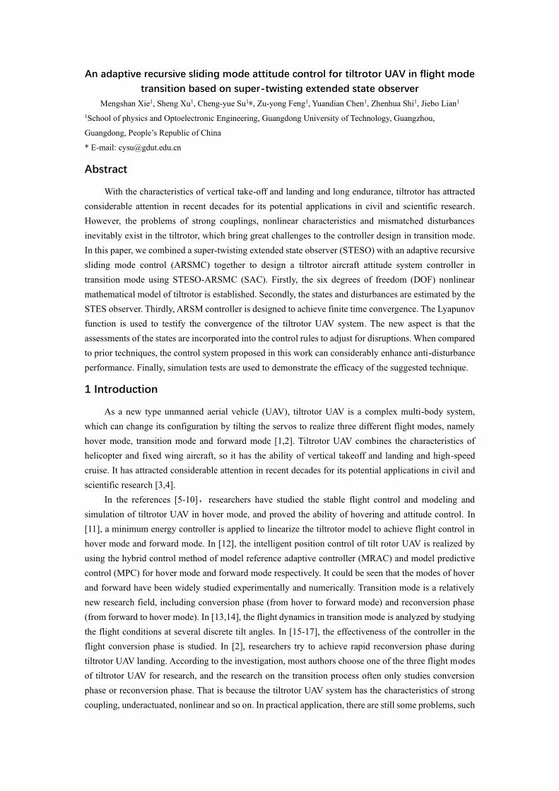
In this paper, a compact electrically powered tiltrotor UAV is presented in Figure 1. The tiltrotor

specified in this paper contains six actuators, including four rotors and two tilting servos, and uses a

traditional v-tail fixed-wing layout. To make the airplane physically sound, the rotors are attached to the

main structural sections. The front two rotors can be tilted from 0 to 90 degrees by tilting the servos,

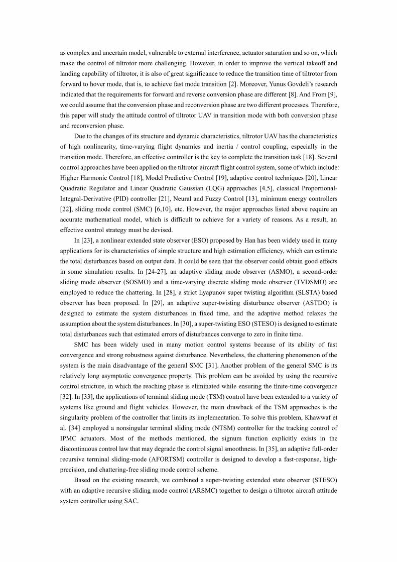
allowing the mode transition between the hover and forward mode to occur. Illustrated in Figure 2, the

tiltrotor UAV cruises in the forward mode, takes off and lands vertically in the hover mode, and enters

the conversion and reconversion stages in the transition mode. The tiltrotor is controlled by four rotors

and two tilting servos without the use of control surfaces in hover mode, while in the forward mode, the

tiltrotor is controlled by aerodynamic control surfaces: v-tail and aileron. In the transition mode, the

tiltrotor is controlled by rotors, tilting servos and aerodynamic control surfaces. We employed system

identification and direct measurement method to obtain the parameters and aerodynamic coefficients of

the aircraft.

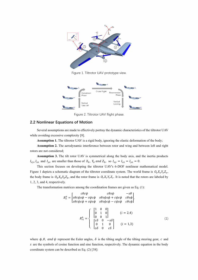
Figure 1. Tiltrotor UAV prototype view.

Figure 2. Tiltrotor UAV flight phase.

2.2 Nonlinear Equations of Motion

Several assumptions are made to effectively portray the dynamic characteristics of the tiltrotor UAV

while avoiding excessive complexity [8].

Assumption 1. The tiltrotor UAV is a rigid body, ignoring the elastic deformation of the body;

Assumption 2. The aerodynamic interference between rotor and wing and between left and right

rotors are not considered;

Assumption 3. The tilt rotor UAV is symmetrical along the body axis, and the inertia products

𝐼𝑥𝑦 , 𝐼𝑥𝑧 and 𝐼𝑦𝑧 are smaller than those of 𝑋𝑏, 𝑌𝑏 𝑎𝑛𝑑 𝑍𝑏 , so 𝐼𝑥𝑦 = 𝐼𝑥𝑧 = 𝐼𝑦𝑧 = 0.

This section focuses on developing the tiltrotor UAV's 6-DOF nonlinear mathematical model.

Figure 1 depicts a schematic diagram of the tiltrotor coordinate system. The world frame is 𝑂𝑒𝑋𝑒𝑌𝑒𝑍𝑒,

the body frame is 𝑂𝑏𝑋𝑏𝑌𝑏𝑍𝑏, and the rotor frame is 𝑂𝑟𝑋𝑟𝑌𝑟𝑍𝑟. It is noted that the rotors are labeled by

1, 2, 3, and 4, respectively.

The transformation matrices among the coordination frames are given as Eq. (1):

𝑅𝑒𝑏 = [

𝑐휃𝑐𝜓 𝑐휃𝑠𝜓 −𝑠휃𝑠휃𝑐𝜓𝑠𝜙 − 𝑠𝜓𝑐𝜙 𝑠휃𝑠𝜓𝑠𝜙 + 𝑐𝜓𝑐𝜙 𝑐휃𝑠𝜙𝑠휃𝑐𝜓𝑐𝜙 + 𝑠𝜓𝑠𝜙 𝑠휃𝑠𝜓𝑐𝜙 − 𝑐𝜓𝑠𝜙 𝑐휃𝑐𝜙

],

𝑅𝑟𝑖𝑏 =

{

[

1 0 00 1 00 0 1

] (𝑖 = 2,4)

[𝑐𝛿 0 −𝑠𝛿0 1 0𝑠𝛿 0 𝑐𝛿

] (𝑖 = 1,3)

(1)

where 𝜙, 휃, 𝑎𝑛𝑑 𝜓 represent the Euler angles, 𝛿 is the tilting angle of the tilting steering gear, 𝑐 and

𝑠 are the symbols of cosine function and sine function, respectively. The dynamic equation in the body

coordinate system can be described as Eq. (2) [38]:

{

[������] = [

𝑟𝑣 − 𝑞𝑤𝑝𝑤 − 𝑟𝑢𝑞𝑢 − 𝑝𝑣

] +1

𝑚[

𝐹𝑥𝐹𝑦𝐹𝑧

]

[������] =

[ 𝐼𝑦−𝐼𝑧

𝐼𝑥𝑞𝑟 +

1

𝐼𝑥𝜏𝑥

𝐼𝑧−𝐼𝑥

𝐼𝑦𝑝𝑟 +

1

𝐼𝑦𝜏𝑦

𝐼𝑥−𝐼𝑦

𝐼𝑧𝑝𝑞 +

1

𝐼𝑧𝜏𝑧]

[

��

휃��

] = [

1 s𝜙t휃 c𝜙t휃0 c𝜙 −s𝜙0 s𝜙/c휃 c𝜙/c휃

] [𝑝𝑞𝑟]

[��𝑛��𝐸��

] = [

𝑐휃𝑐𝜓 𝑠𝜙𝑠휃𝑐𝜓 − 𝑐𝜙𝜓 𝑠𝜙𝑠𝜓 + 𝑐𝜙𝑠휃𝑐𝜓𝑐휃𝑠𝜓 𝑠𝜙𝑠휃𝜓 + 𝑐𝜙𝑐𝜓 −𝑠𝜙𝑐𝜓 + 𝑐𝜙𝑠휃𝑠𝜓𝑠휃 −𝑠𝜙𝑐휃 −𝑐𝜙𝑐휃

] [𝑢𝑣𝑤]

(2)

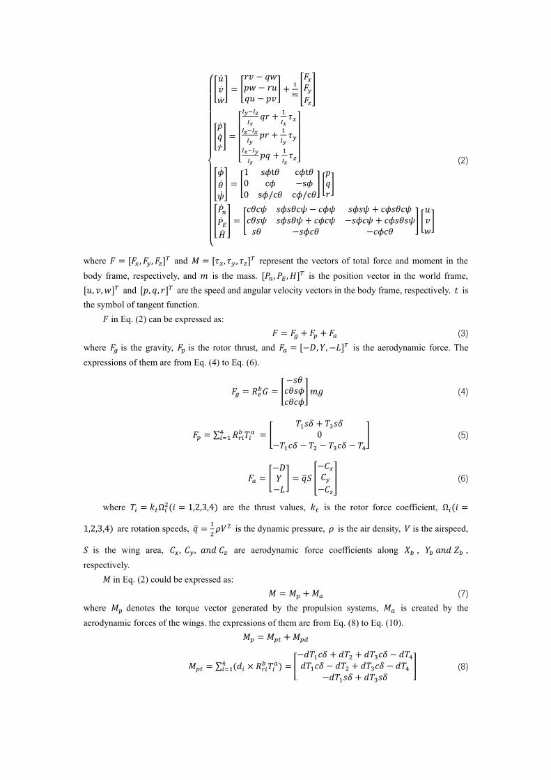
where 𝐹 = [𝐹𝑥, 𝐹𝑦, 𝐹𝑧]𝑇 and 𝑀 = [𝜏𝑥, 𝜏𝑦 , 𝜏𝑧]

𝑇 represent the vectors of total force and moment in the

body frame, respectively, and 𝑚 is the mass. [𝑃𝑛 , 𝑃𝐸 , 𝐻]𝑇 is the position vector in the world frame,

[𝑢, 𝑣, 𝑤]𝑇 and [𝑝, 𝑞, 𝑟]𝑇 are the speed and angular velocity vectors in the body frame, respectively. 𝑡 is

the symbol of tangent function.

𝐹 in Eq. (2) can be expressed as:

𝐹 = 𝐹𝑔 + 𝐹𝑝 + 𝐹𝑎 (3)

where 𝐹𝑔 is the gravity, 𝐹𝑝 is the rotor thrust, and 𝐹𝑎 = [−𝐷, 𝑌, −𝐿]𝑇 is the aerodynamic force. The

expressions of them are from Eq. (4) to Eq. (6).

𝐹𝑔 = 𝑅𝑒𝑏𝐺 = [

−𝑠휃𝑐휃𝑠𝜙𝑐휃𝑐𝜙

]𝑚𝑔 (4)

𝐹𝑝 = ∑ 𝑅𝑟𝑖𝑏 𝑇𝑖

𝑎4𝑖=1 = [

𝑇1𝑠𝛿 + 𝑇3𝑠𝛿0

−𝑇1𝑐𝛿 − 𝑇2 − 𝑇3𝑐𝛿 − 𝑇4

] (5)

𝐹𝑎 = [−𝐷𝑌−𝐿

] = ��𝑆 [

−𝐶𝑥𝐶𝑦−𝐶𝑧

] (6)

where 𝑇𝑖 = 𝑘𝑡Ω𝑖2(𝑖 = 1,2,3,4) are the thrust values, 𝑘𝑡 is the rotor force coefficient, Ω𝑖(𝑖 =

1,2,3,4) are rotation speeds, �� =1

2𝜌𝑉2 is the dynamic pressure, 𝜌 is the air density, 𝑉 is the airspeed,

𝑆 is the wing area, 𝐶𝑥, 𝐶𝑦 , 𝑎𝑛𝑑 𝐶𝑧 are aerodynamic force coefficients along 𝑋𝑏 , 𝑌𝑏 𝑎𝑛𝑑 𝑍𝑏 ,

respectively.

𝑀 in Eq. (2) could be expressed as:

𝑀 = 𝑀𝑝 +𝑀𝑎 (7)

where 𝑀𝑝 denotes the torque vector generated by the propulsion systems, 𝑀𝑎 is created by the

aerodynamic forces of the wings. the expressions of them are from Eq. (8) to Eq. (10).

𝑀𝑝 = 𝑀𝑝𝑡 +𝑀𝑝𝑑

𝑀𝑝𝑡 = ∑ (𝑑𝑖 × 𝑅𝑟𝑖𝑏 𝑇𝑖

𝑎) =4𝑖=1 [

−𝑑𝑇1𝑐𝛿 + 𝑑𝑇2 + 𝑑𝑇3𝑐𝛿 − 𝑑𝑇4𝑑𝑇1𝑐𝛿 − 𝑑𝑇2 + 𝑑𝑇3𝑐𝛿 − 𝑑𝑇4

−𝑑𝑇1𝑠𝛿 + 𝑑𝑇3𝑠𝛿] (8)

𝑀𝑝𝑑 = ∑ 𝑅𝑟𝑖𝑏 𝜏𝑖

𝑎4𝑖=1 = [

𝜏1𝑠𝛿 − 𝜏3𝑠𝛿0

−𝜏1𝑐𝛿 − 𝜏2 + 𝜏3𝑐𝛿 + 𝜏4

] (9)

𝑀𝑎 = ��𝑆 [

𝐶𝑙𝐶𝑚𝐶𝑛

] (10)

where 𝑀𝑝𝑡 is the torque vector caused by the thrust, 𝑑𝑖 are position vectors from the center of gravity

to the axis of each rotor, 𝜏𝑖 = 𝑘𝑑Ω𝑖2(𝑖 = 1,2,3,4) indicate the moment of force generated by rotor air

resistance, 𝑘𝑑 is the rotor torque coefficient, 𝑀𝑝𝑑 is the moment vector in the body frame. 𝐶𝑙 , 𝐶𝑚,

𝑎𝑛𝑑 𝐶𝑛 are aerodynamic moment coefficients of roll, pitch, yaw, respectively.

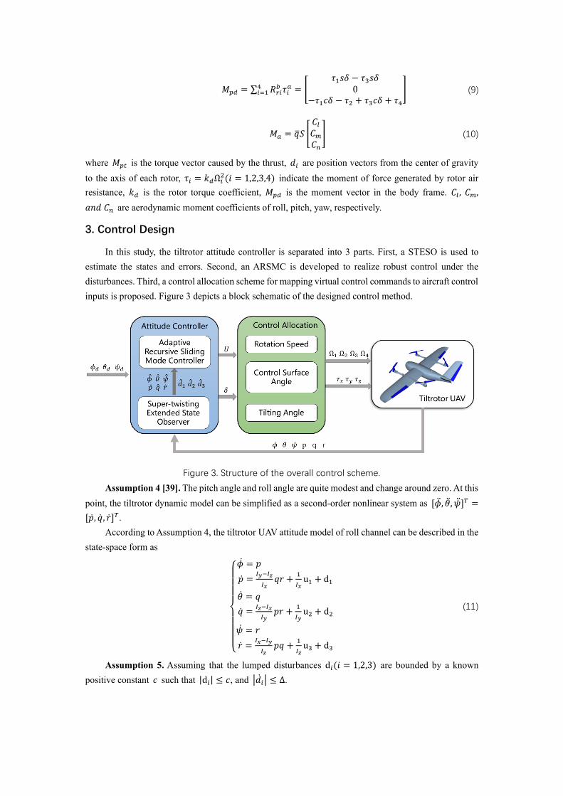
3. Control Design

In this study, the tiltrotor attitude controller is separated into 3 parts. First, a STESO is used to

estimate the states and errors. Second, an ARSMC is developed to realize robust control under the

disturbances. Third, a control allocation scheme for mapping virtual control commands to aircraft control

inputs is proposed. Figure 3 depicts a block schematic of the designed control method.

Figure 3. Structure of the overall control scheme.

Assumption 4 [39]. The pitch angle and roll angle are quite modest and change around zero. At this

point, the tiltrotor dynamic model can be simplified as a second-order nonlinear system as [��, 휃, ��]𝑇 =

[��, ��, ��]𝑇.

According to Assumption 4, the tiltrotor UAV attitude model of roll channel can be described in the

state-space form as

{

�� = 𝑝

�� =𝐼𝑦−𝐼𝑧

𝐼𝑥𝑞𝑟 +

1

𝐼𝑥u1 + d1

휃 = 𝑞

�� =𝐼𝑧−𝐼𝑥

𝐼𝑦𝑝𝑟 +

1

𝐼𝑦u2 + d2

�� = 𝑟

�� =𝐼𝑥−𝐼𝑦

𝐼𝑧𝑝𝑞 +

1

𝐼𝑧u3 + d3

(11)

Assumption 5. Assuming that the lumped disturbances d𝑖(𝑖 = 1,2,3) are bounded by a known

positive constant 𝑐 such that |d𝑖| ≤ 𝑐, and |��𝑖| ≤ ∆.

3.1 Super-Twisting Extended State Observer (STESO)

In this section, we take the roll channel as an example for controller design, the other two channels

including pitch channel and yaw channel are similar. Considering the nonlinear system in Eq. (11), whose

states 𝜙, 𝑝 and lumped disturbances d1 can be estimated through a STESO given by [40]

{

�� = �� − ℎ1sig

2

3(��)

�� = ��1 +𝐼𝑦−𝐼𝑧

𝐼𝑥qr +

1

𝐼𝑥𝑢1 − ℎ2sig

1

3(��)

��1 = −ℎ3sign (��)

(12)

where �� = 𝜙 − �� . Considering the estimation error dynamics for system in Eq. (12), which can be

written as

{

�� = 𝑝 − ℎ1sig

2

3(��)

�� = ��1 − ℎ2sig1

3(��)

��1 = −ℎ3sign (��) + ��1

(13)

where �� = 𝑝 − �� and ��1 = 𝑑1 − ��1.

The above equation is finite-time stable, which has been proved in [41]. Thus, when the appropriate

gains ℎ1, ℎ2, and ℎ3 being selected, ��, 𝑝, and ��1 will converge to zero in finite time 𝑡 > 𝑇0 . The

estimation errors eventually converge to zero in finite time.

3.2 Adaptive Recursive Sliding Mode Control (ARSMC)

Since ��𝑖 = 𝑑𝑖 − ��𝑖(𝑖 = 1,2,3), Eq. (11) can be rewrite as

{

�� = 𝑝

�� =𝐼𝑦−𝐼𝑧

𝐼𝑥𝑞𝑟 +

1

𝐼𝑥u1 + ��1 + ��1

휃 = 𝑞

�� =𝐼𝑧−𝐼𝑥

𝐼𝑦𝑝𝑟 +

1

𝐼𝑦u2 + ��2 + ��2

�� = 𝑟

�� =𝐼𝑥−𝐼𝑦

𝐼𝑧𝑝𝑞 +

1

𝐼𝑧u3 + ��3 + ��3

(14)

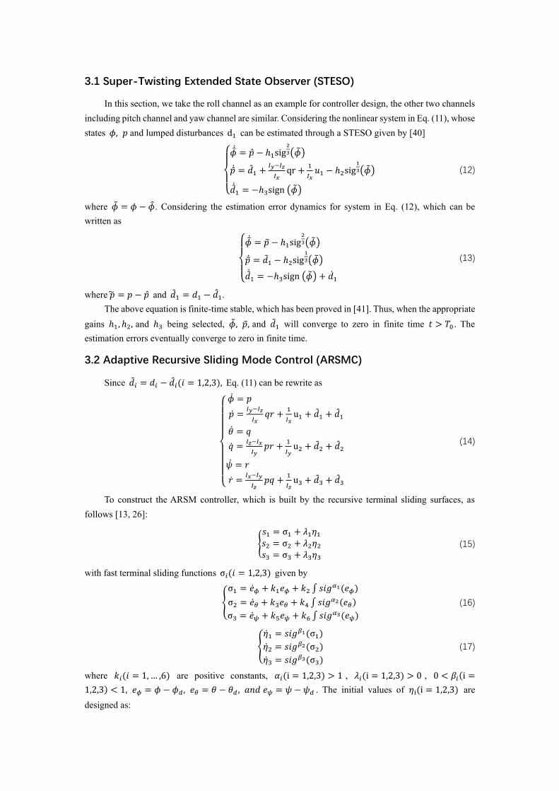
To construct the ARSM controller, which is built by the recursive terminal sliding surfaces, as

follows [13, 26]:

{

𝑠1 = σ1 + 𝜆1휂1 𝑠2 = σ2 + 𝜆2휂2 𝑠3 = σ3 + 𝜆3휂3

(15)

with fast terminal sliding functions σ𝑖(𝑖 = 1,2,3) given by

{

σ1 = ��𝜙 + 𝑘1𝑒𝜙 + 𝑘2 ∫ 𝑠𝑖𝑔𝛼1(𝑒𝜙)

σ2 = ��𝜃 + 𝑘3𝑒𝜃 + 𝑘4 ∫ 𝑠𝑖𝑔𝛼2(𝑒𝜃)

σ3 = ��𝜓 + 𝑘5𝑒𝜓 + 𝑘6 ∫ 𝑠𝑖𝑔𝛼3(𝑒𝜓)

(16)

{

휂1 = 𝑠𝑖𝑔𝛽1(σ1)

휂2 = 𝑠𝑖𝑔𝛽2(σ2)

휂3 = 𝑠𝑖𝑔𝛽3(σ3)

(17)

where 𝑘𝑖(𝑖 = 1,… ,6) are positive constants, 𝛼𝑖(i = 1,2,3) > 1 , 𝜆𝑖(i = 1,2,3) > 0 , 0 < 𝛽𝑖(i =

1,2,3) < 1, 𝑒𝜙 = 𝜙 − 𝜙𝑑, 𝑒𝜃 = 휃 − 휃𝑑 , 𝑎𝑛𝑑 𝑒𝜓 = 𝜓 − 𝜓𝑑 . The initial values of 휂i(i = 1,2,3) are

designed as:

{

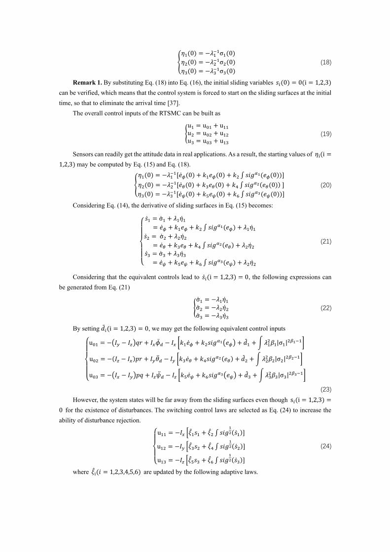
휂1(0) = −𝜆1−1σ1(0)

휂2(0) = −𝜆2−1σ2(0)

휂3(0) = −𝜆3−1σ3(0)

(18)

Remark 1. By substituting Eq. (18) into Eq. (16), the initial sliding variables 𝑠𝑖(0) = 0(i = 1,2,3)

can be verified, which means that the control system is forced to start on the sliding surfaces at the initial

time, so that to eliminate the arrival time [37].

The overall control inputs of the RTSMC can be built as

{

𝑢1 = u01 + u11𝑢2 = u02 + u12𝑢3 = u03 + u13

(19)

Sensors can readily get the attitude data in real applications. As a result, the starting values of 휂i(i =

1,2,3) may be computed by Eq. (15) and Eq. (18).

{

휂1(0) = −𝜆1−1[��𝜙(0) + 𝑘1𝑒𝜙(0) + 𝑘2 ∫ 𝑠𝑖𝑔

𝛼1(𝑒𝜙(0))]

휂2(0) = −𝜆2−1[��𝜃(0) + 𝑘3𝑒𝜃(0) + 𝑘4 ∫ 𝑠𝑖𝑔

𝛼2(𝑒𝜃(0)) ]

휂3(0) = −𝜆3−1[��𝜓(0) + 𝑘5𝑒𝜓(0) + 𝑘6 ∫ 𝑠𝑖𝑔

𝛼3(𝑒𝜓(0))]

(20)

Considering Eq. (14), the derivative of sliding surfaces in Eq. (15) becomes:

{

��1 = σ1 + 𝜆1휂1

= ��𝜙 + 𝑘1𝑒𝜙 + 𝑘2 ∫ 𝑠𝑖𝑔𝛼1(𝑒𝜙) + 𝜆1휂1

��2 = σ2 + 𝜆2휂2

= ��𝜃 + 𝑘3𝑒𝜃 + 𝑘4 ∫ 𝑠𝑖𝑔𝛼2(𝑒𝜃) + 𝜆2휂2

��3 = σ3 + 𝜆3휂3

= ��𝜓 + 𝑘5𝑒𝜓 + 𝑘6 ∫ 𝑠𝑖𝑔𝛼3(𝑒𝜓) + 𝜆2휂2

(21)

Considering that the equivalent controls lead to ��𝑖(i = 1,2,3) = 0, the following expressions can

be generated from Eq. (21)

{

σ1 = −𝜆1휂1σ2 = −𝜆2휂2σ3 = −𝜆3휂3

(22)

By setting ��𝑖(i = 1,2,3) = 0, we may get the following equivalent control inputs

{

u01 = −(𝐼𝑦 − 𝐼𝑧)𝑞𝑟 + 𝐼𝑥��𝑑 − 𝐼𝑥 [𝑘1��𝜙 + 𝑘2𝑠𝑖𝑔

𝛼1(𝑒𝜙) + ��1 +∫𝜆12𝛽1|σ1|

2𝛽1−1]

u02 = −(𝐼𝑧 − 𝐼𝑥)𝑝𝑟 + 𝐼𝑦휃𝑑 − 𝐼𝑦 [𝑘3��𝜃 + 𝑘4𝑠𝑖𝑔𝛼2(𝑒𝜃) + ��2 +∫𝜆2

2𝛽2|σ2|2𝛽2−1]

u03 = −(𝐼𝑥 − 𝐼𝑦)𝑝𝑞 + 𝐼𝑧��𝑑 − 𝐼𝑧 [𝑘5��𝜓 + 𝑘6𝑠𝑖𝑔𝛼3(𝑒𝜓) + ��3 +∫𝜆3

2𝛽3|σ3|2𝛽3−1]

(23)

However, the system states will be far away from the sliding surfaces even though s𝑖(i = 1,2,3) =

0 for the existence of disturbances. The switching control laws are selected as Eq. (24) to increase the

ability of disturbance rejection.

{

u11 = −𝐼𝑥 [𝜉1𝑠1 + 𝜉2 ∫ 𝑠𝑖𝑔

1

2(��1)]

u12 = −𝐼𝑦 [𝜉3𝑠2 + 𝜉4 ∫ 𝑠𝑖𝑔1

2(��2)]

u13 = −𝐼𝑧 [𝜉5𝑠3 + 𝜉6 ∫ 𝑠𝑖𝑔1

2(��3)]

(24)

where 𝜉i(𝑖 = 1,2,3,4,5,6) are updated by the following adaptive laws.

{

𝜉

1 = −𝜚��1

2

𝜉2 = −𝜚𝑠𝑖𝑔1

2(��1)

𝜉3 = −𝜚��22

𝜉4 = −𝜚𝑠𝑖𝑔1

2(��2)

𝜉5 = −𝜚��32

𝜉6 = −𝜚𝑠𝑖𝑔1

2(��3)

(25)

where 𝜚 is positive constant. The estimation errors of 𝜉i(𝑖 = 1,2,3,4,5,6) with respect to the desired

values 𝜉𝑖𝑑(𝑖 = 1,2,3,4,5,6) are constants and defined as

𝜉i = 𝜉𝑖𝑑 − 𝜉i (𝑖 = 1,2,3,4,5,6) (26)

where it is assumed that the conditions

𝜉1𝑑 ≥ |��1|

|��1|, 𝜉2𝑑 > 0, 𝜉3𝑑 ≥

|��3|

|��3|, 𝜉4𝑑 > 0, 𝜉5𝑑 ≥

|��5|

|��5|, 𝜉6𝑑 > 0 (27)

are met.

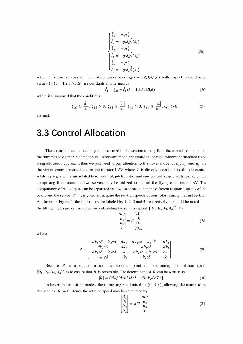
3.3 Control Allocation

The control allocation technique is presented in this section to map from the control commands to

the tiltrotor UAV's manipulated inputs. In forward mode, the control allocation follows the standard fixed

wing allocation approach, thus we just need to pay attention to the hover mode. 𝑇, 𝑢1, 𝑢2, and 𝑢3 are

the virtual control instructions for the tiltrotor UAV, where 𝑇 is directly connected to altitude control

while 𝑢1, 𝑢2, and 𝑢3 are related to roll control, pitch control and yaw control, respectively. Six actuators,

comprising four rotors and two servos, may be utilized to control the flying of tiltrotor UAV. The

computation of real outputs can be separated into two sections due to the different response speeds of the

rotors and the servos. 𝑇, 𝑢1, 𝑢2, and 𝑢3 acquire the rotation speeds of four rotors during the first section.

As shown in Figure 1, the four rotors are labeled by 1, 2, 3 and 4, respectively. It should be noted that

the tilting angles are estimated before calculating the rotation speed [Ω1, Ω2, Ω3, Ω4]𝑇. By

[

𝑢1𝑢2𝑢3𝑇

] = 𝑅 [

Ω1Ω2Ω3Ω4

] (28)

where

𝑅 = [

−𝑑𝑘𝑡𝑐𝛿 − 𝑘𝑑𝑠𝛿 𝑑𝑘𝑡 𝑑𝑘𝑡𝑐𝛿 − 𝑘𝑑𝑠𝛿 −𝑑𝑘𝑡𝑑𝑘𝑡𝑐𝛿 𝑑𝑘𝑡 −𝑑𝑘𝑡𝑐𝛿 −𝑑𝑘𝑡

−𝑑𝑘𝑡𝑠𝛿 − 𝑘𝑑𝑐𝛿−𝑘𝑡𝑐𝛿

−𝑘𝑑−𝑘𝑡

𝑑𝑘𝑡𝑠𝛿 + 𝑘𝑑𝑐𝛿−𝑘𝑡𝑐𝛿

𝑘𝑑−𝑘𝑡

] (29)

Because 𝑅 is a square matrix, the essential point in determining the rotation speed

[Ω1, Ω2, Ω3, Ω4]𝑇 is to ensure that 𝑅 is reversible. The determinant of 𝑅 can be written as

|𝑅| = 8𝑑𝑘𝑡2[𝑑2𝑘𝑡

2𝑠𝛿𝑐𝛿 + 𝑑𝑘𝑡𝑘𝑑(𝑐𝛿)2] (30)

In hover and transition modes, the tilting angle is limited to (0°, 90°), allowing the matrix to be

deduced as |𝑅| ≠ 0. Hence the rotation speed may be calculated by

[

Ω1Ω2Ω3Ω4

] = 𝑅−1 [

𝑢1𝑢2𝑢3𝑇

] (31)

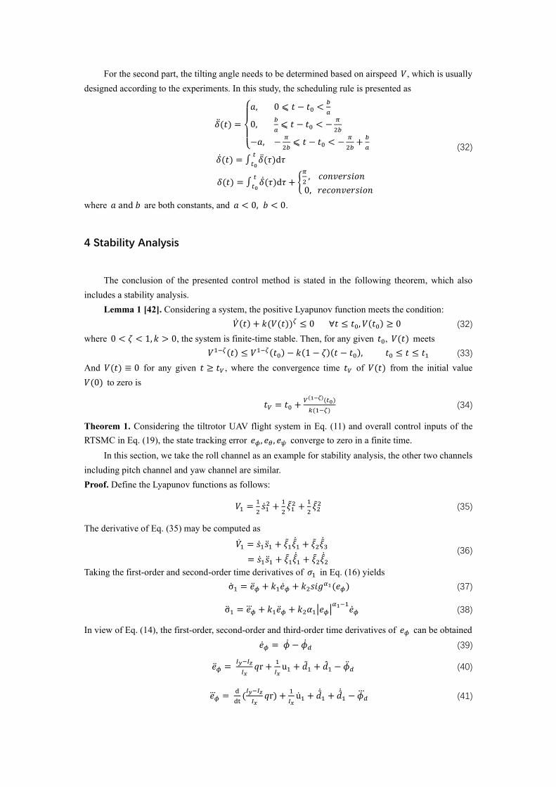
For the second part, the tilting angle needs to be determined based on airspeed 𝑉, which is usually

designed according to the experiments. In this study, the scheduling rule is presented as

��(𝑡) =

{

𝑎, 0 ⩽ 𝑡 − 𝑡0 <

𝑏

𝑎

0,𝑏

𝑎⩽ 𝑡 − 𝑡0 < −

𝜋

2𝑏

−𝑎, −𝜋

2𝑏⩽ 𝑡 − 𝑡0 < −

𝜋

2𝑏+

𝑏

𝑎

��(𝑡) = ∫𝑡0

𝑡 ��(𝜏)d𝜏

𝛿(𝑡) = ∫𝑡0

𝑡 ��(𝜏)d𝜏 + {

𝜋

2, 𝑐𝑜𝑛𝑣𝑒𝑟𝑠𝑖𝑜𝑛

0, 𝑟𝑒𝑐𝑜𝑛𝑣𝑒𝑟𝑠𝑖𝑜𝑛

(32)

where 𝑎 and 𝑏 are both constants, and 𝑎 < 0, 𝑏 < 0.

4 Stability Analysis

The conclusion of the presented control method is stated in the following theorem, which also

includes a stability analysis.

Lemma 1 [42]. Considering a system, the positive Lyapunov function meets the condition:

��(𝑡) + 𝑘(𝑉(𝑡))𝜁 ≤ 0 ∀𝑡 ≤ 𝑡0, 𝑉(𝑡0) ≥ 0 (32)

where 0 < 휁 < 1, 𝑘 > 0, the system is finite-time stable. Then, for any given 𝑡0, 𝑉(𝑡) meets

𝑉1−𝜁(𝑡) ≤ 𝑉1−𝜁(𝑡0) − 𝑘(1 − 휁)(𝑡 − 𝑡0), 𝑡0 ≤ 𝑡 ≤ 𝑡1 (33)

And 𝑉(𝑡) ≡ 0 for any given 𝑡 ≥ 𝑡𝑉 , where the convergence time 𝑡𝑉 of 𝑉(𝑡) from the initial value

𝑉(0) to zero is

𝑡𝑉 = 𝑡0 +𝑉(1−𝜁)(𝑡0)

𝑘(1−𝜁) (34)

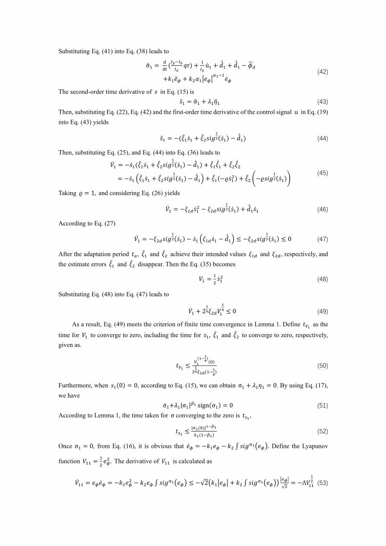
Theorem 1. Considering the tiltrotor UAV flight system in Eq. (11) and overall control inputs of the

RTSMC in Eq. (19), the state tracking error 𝑒𝜙, 𝑒𝜃 , 𝑒𝜓 converge to zero in a finite time.

In this section, we take the roll channel as an example for stability analysis, the other two channels

including pitch channel and yaw channel are similar.

Proof. Define the Lyapunov functions as follows:

𝑉1 =1

2��12 +

1

2𝜉12 +

1

2𝜉22 (35)

The derivative of Eq. (35) may be computed as

��1 = ��1��1 + 𝜉1𝜉1 + 𝜉2𝜉

3

= ��1��1 + 𝜉1𝜉1 + 𝜉2𝜉

2

(36)

Taking the first-order and second-order time derivatives of 𝜎1 in Eq. (16) yields

σ1 = ��𝜙 + 𝑘1��𝜙 + 𝑘2𝑠𝑖𝑔𝛼1(𝑒𝜙) (37)

σ1 = 𝑒𝜙 + 𝑘1��𝜙 + 𝑘2𝛼1|𝑒𝜙|𝛼1−1

��𝜙 (38)

In view of Eq. (14), the first-order, second-order and third-order time derivatives of 𝑒𝜙 can be obtained

��𝜙 = �� − ��𝑑 (39)

��𝜙 = 𝐼𝑦−𝐼𝑧

𝐼𝑥𝑞r +

1

𝐼𝑥u1 + ��1 + ��1 − ��𝑑 (40)

𝑒𝜙 = d

dt(𝐼𝑦−𝐼𝑧

𝐼𝑥𝑞r) +

1

𝐼𝑥u1 + ��1 + ��1 − 𝜙𝑑 (41)

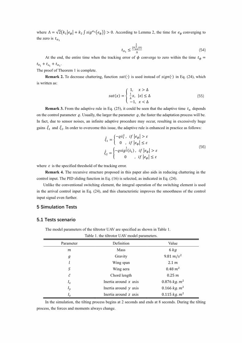
Substituting Eq. (41) into Eq. (38) leads to

σ1 = d

dt(𝐼𝑦−𝐼𝑧

𝐼𝑥𝑞r) +

1

𝐼𝑥u1 + ��1 + ��1 − 𝜙𝑑

+𝑘1��𝜙 + 𝑘2𝛼1|𝑒𝜙|𝛼1−1

��𝜙 (42)

The second-order time derivative of 𝑠 in Eq. (15) is

��1 = σ1 + 𝜆1휂1 (43)

Then, substituting Eq. (22), Eq. (42) and the first-order time derivative of the control signal u in Eq. (19)

into Eq. (43) yields

��1 = −(𝜉1��1 + 𝜉2𝑠𝑖𝑔1

2(��1) − ��1) (44)

Then, substituting Eq. (25), and Eq. (44) into Eq. (36) leads to

��1 = −��1(𝜉1��1 + 𝜉2𝑠𝑖𝑔1

2(��1) − ��1) + 𝜉1𝜉1 + 𝜉2𝜉

2

= −��1 (𝜉1��1 + 𝜉2𝑠𝑖𝑔1

2(��1) − ��1) + 𝜉1(−𝜚��12) + 𝜉2 (−𝜚𝑠𝑖𝑔

1

2(��1)) (45)

Taking 𝜚 = 1, and considering Eq. (26) yields

��1 = −𝜉1𝑑 ��12 − 𝜉2𝑑𝑠𝑖𝑔

1

2(��1) + ��1��1 (46)

According to Eq. (27)

��1 = −𝜉2𝑑𝑠𝑖𝑔1

2(��1) − ��1 (𝜉1𝑑 ��1 − ��1) ≤ −𝜉2𝑑𝑠𝑖𝑔1

2(��1) ≤ 0 (47)

After the adaptation period 𝑡𝑎, 𝜉1 and 𝜉2 achieve their intended values 𝜉1𝑑 and 𝜉2𝑑, respectively, and

the estimate errors 𝜉1 and 𝜉2 disappear. Then the Eq. (35) becomes

𝑉1 =1

2��12 (48)

Substituting Eq. (48) into Eq. (47) leads to

��1 + 21

4𝜉2𝑑𝑉1

1

4 ≤ 0 (49)

As a result, Eq. (49) meets the criterion of finite time convergence in Lemma 1. Define 𝑡𝑉1 as the

time for 𝑉1 to converge to zero, including the time for 𝑠1, 𝜉1 and 𝜉2 to converge to zero, respectively,

given as.

𝑡𝑉1 ≤𝑉1(1−

14)(0)

214𝜉2𝑑(1−

1

4)

(50)

Furthermore, when 𝑠1(0) = 0, according to Eq. (15), we can obtain σ1 + 𝜆1휂1 = 0. By using Eq. (17),

we have

σ1+𝜆1|σ1|𝛽1 sign(σ1) = 0 (51)

According to Lemma 1, the time taken for σ converging to the zero is 𝑡𝑠1 ,

𝑡𝑠1 ≤|σ1(0)|

1−𝛽1

λ1(1−𝛽1) (52)

Once σ1 = 0, from Eq. (16), it is obvious that ��𝜙 = −𝑘1𝑒𝜙 − 𝑘2 ∫ 𝑠𝑖𝑔𝛼1(𝑒𝜙). Define the Lyapunov

function 𝑉11 =1

2𝑒𝜙2 . The derivative of 𝑉11 is calculated as

��11 = 𝑒𝜙��𝜙 = −𝑘1𝑒𝜙2 − 𝑘2𝑒𝜙 ∫ 𝑠𝑖𝑔

𝛼1(𝑒𝜙) ≤ −√2(𝑘1|𝑒𝜙| + 𝑘2 ∫ 𝑠𝑖𝑔𝛼1(𝑒𝜙))

|𝑒𝜙|

√2= −Λ𝑉11

1

2 (53)

where Λ = √2(𝑘1|𝑒𝜙| + 𝑘2 ∫ 𝑠𝑖𝑔𝛼1(𝑒𝜙)) > 0. According to Lemma 2, the time for 𝑒𝜙 converging to

the zero is 𝑡σ1

𝑡σ1 ≤2𝑉11

12 (0)

Λ (54)

At the end, the entire time when the tracking error of 𝜙 converge to zero within the time 𝑡𝜙 =

𝑡𝑉1 + 𝑡𝑠1 + 𝑡σ1.

The proof of Theorem 1 is complete.

Remark 2. To decrease chattering, function 𝑠𝑎𝑡(∙) is used instead of 𝑠𝑖𝑔𝑛(∙) in Eq. (24), which

is written as:

𝑠𝑎𝑡(𝑥) = {

1, 𝑥 > ∆

1

∆𝑥, |𝑥| ≤ ∆

−1, 𝑥 < ∆

(55)

Remark 3. From the adaptive rule in Eq. (25), it could be seen that the adaptive time 𝑡𝑎 depends

on the control parameter 𝜚. Usually, the larger the parameter 𝜚, the faster the adaptation process will be.

In fact, due to sensor noises, an infinite adaptive procedure may occur, resulting in excessively huge

gains 𝜉1 and 𝜉2. In order to overcome this issue, the adaptive rule is enhanced in practice as follows:

𝜉1 = {−𝜚��1

2 , 𝑖𝑓 |𝑒𝜙| > 휀

0 , 𝑖𝑓 |𝑒𝜙| ≤ 휀

𝜉2 = {−𝜚𝑠𝑖𝑔

1

2(��1) , 𝑖𝑓 |𝑒𝜙| > 휀

0 , 𝑖𝑓 |𝑒𝜙| ≤ 휀

(56)

where 휀 is the specified threshold of the tracking error.

Remark 4. The recursive structure proposed in this paper also aids in reducing chattering in the

control input. The PID sliding function in Eq. (16) is selected, as indicated in Eq. (24).

Unlike the conventional switching element, the integral operation of the switching element is used

in the arrival control input in Eq. (24), and this characteristic improves the smoothness of the control

input signal even further.

5 Simulation Tests

5.1 Tests scenario

The model parameters of the tiltrotor UAV are specified as shown in Table 1.

Table 1. the tiltrotor UAV model parameters.

Parameter Definition Value

𝑚 Mass 6 𝑘𝑔

𝑔 Gravity 9.81 𝑚/𝑠2

𝑙 Wing span 2.1 𝑚

𝑆 Wing aera 0.48 𝑚2

𝑐 Chord length 0.25 𝑚

𝐼𝑥 Inertia around 𝑥 axis 0.876 𝑘𝑔.𝑚2

𝐼𝑦 Inertia around 𝑦 axis 0.166 𝑘𝑔.𝑚2

𝐼𝑧 Inertia around 𝑧 axis 0.115 𝑘𝑔.𝑚2

In the simulation, the tilting process begins at 2 seconds and ends at 8 seconds. During the tilting

process, the forces and moments always change.

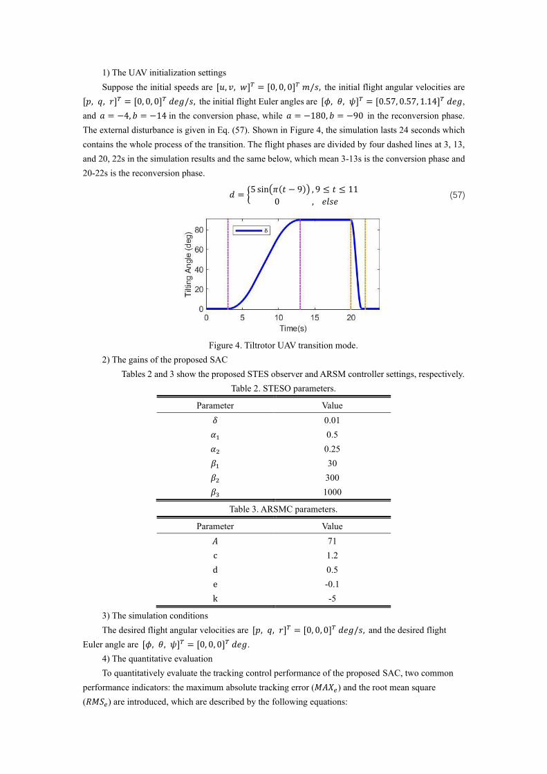
1) The UAV initialization settings

Suppose the initial speeds are [𝑢, 𝑣, 𝑤]𝑇 = [0, 0, 0]𝑇 𝑚/𝑠, the initial flight angular velocities are

[𝑝, 𝑞, 𝑟]𝑇 = [0, 0, 0]𝑇 𝑑𝑒𝑔/𝑠, the initial flight Euler angles are [𝜙, 휃, 𝜓]𝑇 = [0.57, 0.57, 1.14]𝑇 𝑑𝑒𝑔,

and 𝑎 = −4, 𝑏 = −14 in the conversion phase, while 𝑎 = −180, 𝑏 = −90 in the reconversion phase.

The external disturbance is given in Eq. (57). Shown in Figure 4, the simulation lasts 24 seconds which

contains the whole process of the transition. The flight phases are divided by four dashed lines at 3, 13,

and 20, 22s in the simulation results and the same below, which mean 3-13s is the conversion phase and

20-22s is the reconversion phase.

𝑑 = {5 sin(𝜋(𝑡 − 9)) , 9 ≤ 𝑡 ≤ 11

0 , 𝑒𝑙𝑠𝑒 (57)

Figure 4. Tiltrotor UAV transition mode.

2) The gains of the proposed SAC

Tables 2 and 3 show the proposed STES observer and ARSM controller settings, respectively.

Table 2. STESO parameters.

Parameter Value

𝛿 0.01

𝛼1 0.5

𝛼2 0.25

𝛽1 30

𝛽2 300

𝛽3 1000

Table 3. ARSMC parameters.

Parameter Value

𝐴 71

c 1.2

d 0.5

e -0.1

k -5

3) The simulation conditions

The desired flight angular velocities are [𝑝, 𝑞, 𝑟]𝑇 = [0, 0, 0]𝑇 𝑑𝑒𝑔/𝑠, and the desired flight

Euler angle are [𝜙, 휃, 𝜓]𝑇 = [0, 0, 0]𝑇 𝑑𝑒𝑔.

4) The quantitative evaluation

To quantitatively evaluate the tracking control performance of the proposed SAC, two common

performance indicators: the maximum absolute tracking error (𝑀𝐴𝑋𝑒) and the root mean square

(𝑅𝑀𝑆𝑒) are introduced, which are described by the following equations:

𝑀𝐴𝑋𝑒 = max𝑘=1,…,𝑁

(|𝑒(𝑘)|) (58)

𝑅𝑀𝑆𝑒 = √1

𝑁∑ 𝑒2(𝑘)𝑁𝑘=1 (59)

where 𝑘 is the sample index, and 𝑁 is the number of samples. We also compare the performance of

the proposed SAC to that of the FTSMC and RSMC, which were previously described in Ref. [36] and

Ref. [37], respectively.

5.2 Simulation Tests

In this part, we use the simulation of MATLAB R2019a / Simulink to verify the effectiveness and

robustness of the designed control scheme SAC during the tilting process of the tiltrotor UAV. In addition,

robustness tests of the proposed SAC are carried out in this section.

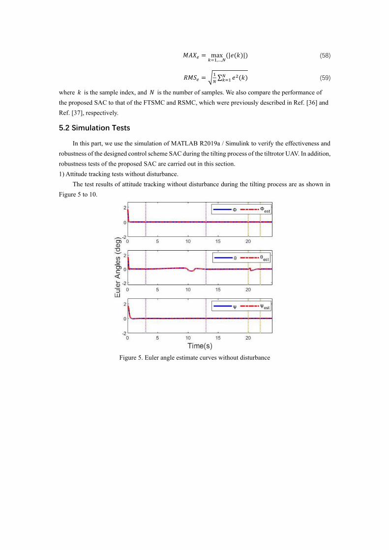
1) Attitude tracking tests without disturbance.

The test results of attitude tracking without disturbance during the tilting process are as shown in

Figure 5 to 10.

Figure 5. Euler angle estimate curves without disturbance

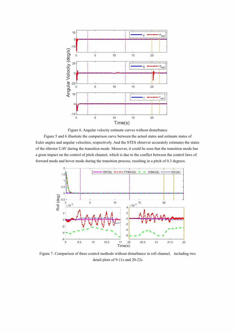
Figure 6. Angular velocity estimate curves without disturbance

Figure 5 and 6 illustrate the comparison curve between the actual states and estimate states of

Euler angles and angular velocities, respectively. And the STES observer accurately estimates the states

of the tiltrotor UAV during the transition mode. Moreover, it could be seen that the transition mode has

a great impact on the control of pitch channel, which is due to the conflict between the control laws of

forward mode and hover mode during the transition process, resulting in a pitch of 0.3 degrees.

Figure 7. Comparison of three control methods without disturbance in roll channel, including two

detail plots of 9-11s and 20-22s

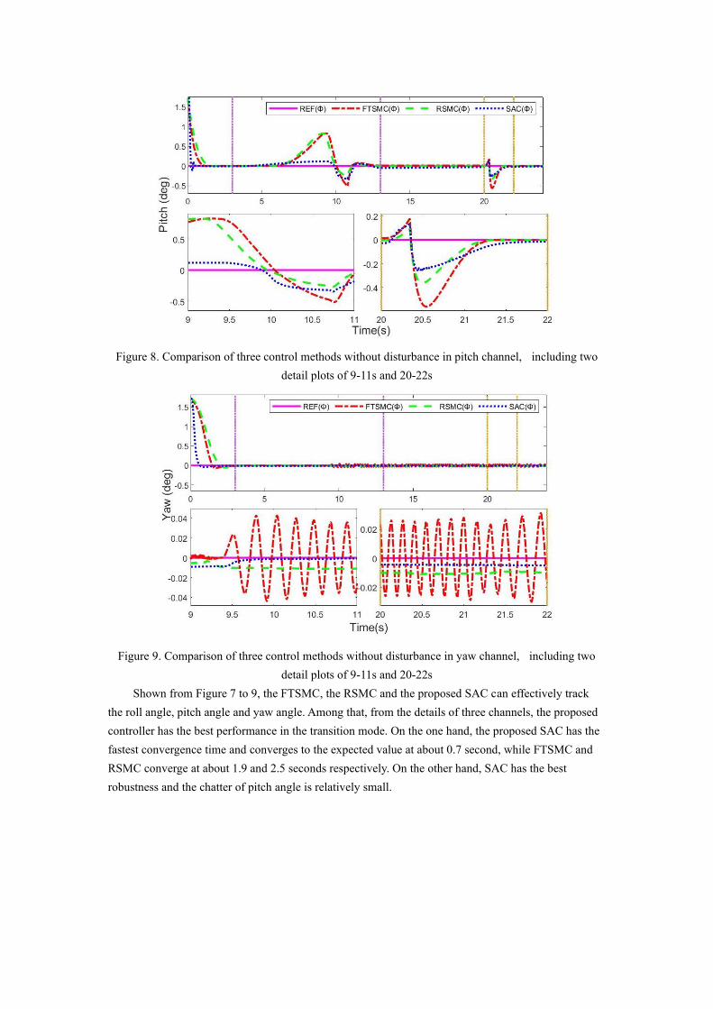
Figure 8. Comparison of three control methods without disturbance in pitch channel, including two

detail plots of 9-11s and 20-22s

Figure 9. Comparison of three control methods without disturbance in yaw channel, including two

detail plots of 9-11s and 20-22s

Shown from Figure 7 to 9, the FTSMC, the RSMC and the proposed SAC can effectively track

the roll angle, pitch angle and yaw angle. Among that, from the details of three channels, the proposed

controller has the best performance in the transition mode. On the one hand, the proposed SAC has the

fastest convergence time and converges to the expected value at about 0.7 second, while FTSMC and

RSMC converge at about 1.9 and 2.5 seconds respectively. On the other hand, SAC has the best

robustness and the chatter of pitch angle is relatively small.

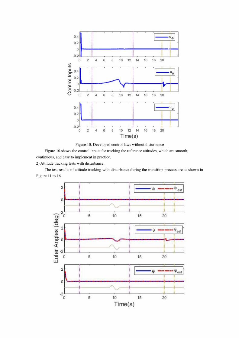
Figure 10. Developed control laws without disturbance

Figure 10 shows the control inputs for tracking the reference attitudes, which are smooth,

continuous, and easy to implement in practice.

2) Attitude tracking tests with disturbance.

The test results of attitude tracking with disturbance during the transition process are as shown in

Figure 11 to 16.

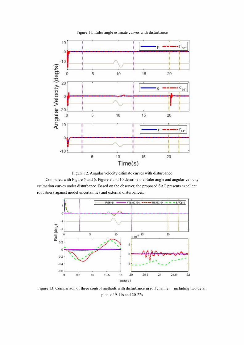
Figure 11. Euler angle estimate curves with disturbance

Figure 12. Angular velocity estimate curves with disturbance

Compared with Figure 5 and 6, Figure 9 and 10 describe the Euler angle and angular velocity

estimation curves under disturbance. Based on the observer, the proposed SAC presents excellent

robustness against model uncertainties and external disturbances.

Figure 13. Comparison of three control methods with disturbance in roll channel, including two detail

plots of 9-11s and 20-22s

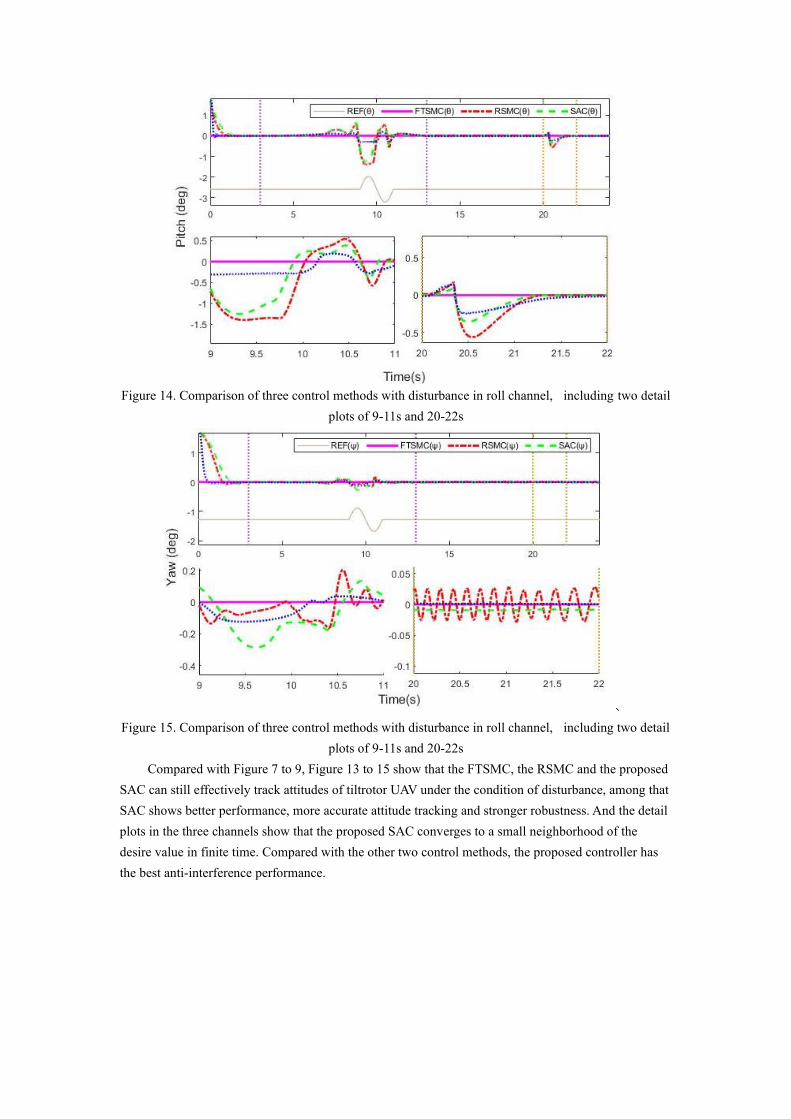
Figure 14. Comparison of three control methods with disturbance in roll channel, including two detail

plots of 9-11s and 20-22s

、

Figure 15. Comparison of three control methods with disturbance in roll channel, including two detail

plots of 9-11s and 20-22s

Compared with Figure 7 to 9, Figure 13 to 15 show that the FTSMC, the RSMC and the proposed

SAC can still effectively track attitudes of tiltrotor UAV under the condition of disturbance, among that

SAC shows better performance, more accurate attitude tracking and stronger robustness. And the detail

plots in the three channels show that the proposed SAC converges to a small neighborhood of the

desire value in finite time. Compared with the other two control methods, the proposed controller has

the best anti-interference performance.

Figure 16. Developed control laws with disturbance.

Compared with Figure. 10, Figure. 16 shows that even in the case of interference, the control

inputs of the proposed controller are still smooth, continuous, and easy to implement.

Table 4. Comparison of test results in conversion phase without disturbance.

Channel FTSMC RSMC SAC I1 I2

Roll 𝑀𝐴𝑋𝑒 0.011 0.006 0.001 0.89 0.81

𝑅𝑀𝑆𝑒 0.002 0.004 0.000 0.84 0.91

Pitch 𝑀𝐴𝑋𝑒 0.828 0.824 0.345 0.58 0.58

𝑅𝑀𝑆𝑒 0.286 0.279 0.102 0.64 0.63

Yaw 𝑀𝐴𝑋𝑒 0.044 0.014 0.013 0.70 0.70

𝑅𝑀𝑆𝑒 0.015 0.008 0.008 0.47 0.00

Table 5. Comparison of test results in conversion phase with disturbance.

Channel FTSMC RSMC SAC I1 I2

Roll 𝑀𝐴𝑋𝑒 0.335 0.291 0.029 0.91 0.90

𝑅𝑀𝑆𝑒 0.081 0.084 0.009 0.88 0.89

Pitch 𝑀𝐴𝑋𝑒 1.396 1.252 0.310 0.78 0.75

𝑅𝑀𝑆𝑒 0.384 0.312 0.116 0.70 0.63

Yaw 𝑀𝐴𝑋𝑒 0.203 0.286 0.124 0.39 0.57

𝑅𝑀𝑆𝑒 0.042 0.070 0.035 0.17 0.51

Table 6. Comparison of test results in reconversion phase without disturbance.

Channel FTSMC RSMC SAC I1 I2

Roll 𝑀𝐴𝑋𝑒 0.003 0.006 0.001 0.71 0.85

𝑅𝑀𝑆𝑒 0.001 0.004 0.001 0.05 0.85

Pitch 𝑀𝐴𝑋𝑒 0.561 0.363 0.256 0.54 0.29

𝑅𝑀𝑆𝑒 0.165 0.102 0.088 0.47 0.13

Yaw 𝑀𝐴𝑋𝑒 0.032 0.011 0.006 0.83 0.49

𝑅𝑀𝑆𝑒 0.020 0.010 0.005 0.75 0.50

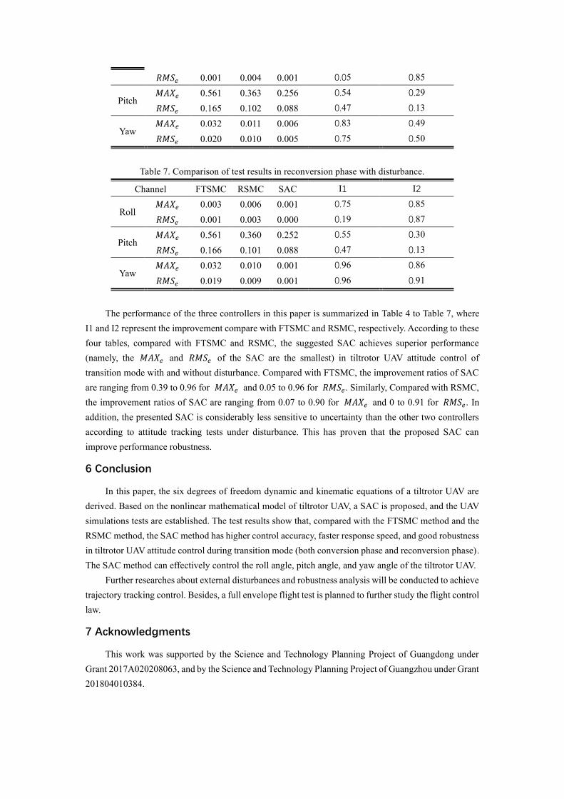
Table 7. Comparison of test results in reconversion phase with disturbance.

Channel FTSMC RSMC SAC I1 I2

Roll 𝑀𝐴𝑋𝑒 0.003 0.006 0.001 0.75 0.85

𝑅𝑀𝑆𝑒 0.001 0.003 0.000 0.19 0.87

Pitch 𝑀𝐴𝑋𝑒 0.561 0.360 0.252 0.55 0.30

𝑅𝑀𝑆𝑒 0.166 0.101 0.088 0.47 0.13

Yaw 𝑀𝐴𝑋𝑒 0.032 0.010 0.001 0.96 0.86

𝑅𝑀𝑆𝑒 0.019 0.009 0.001 0.96 0.91

The performance of the three controllers in this paper is summarized in Table 4 to Table 7, where

I1 and I2 represent the improvement compare with FTSMC and RSMC, respectively. According to these

four tables, compared with FTSMC and RSMC, the suggested SAC achieves superior performance

(namely, the 𝑀𝐴𝑋𝑒 and 𝑅𝑀𝑆𝑒 of the SAC are the smallest) in tiltrotor UAV attitude control of

transition mode with and without disturbance. Compared with FTSMC, the improvement ratios of SAC

are ranging from 0.39 to 0.96 for 𝑀𝐴𝑋𝑒 and 0.05 to 0.96 for 𝑅𝑀𝑆𝑒. Similarly, Compared with RSMC,

the improvement ratios of SAC are ranging from 0.07 to 0.90 for 𝑀𝐴𝑋𝑒 and 0 to 0.91 for 𝑅𝑀𝑆𝑒. In

addition, the presented SAC is considerably less sensitive to uncertainty than the other two controllers

according to attitude tracking tests under disturbance. This has proven that the proposed SAC can

improve performance robustness.

6 Conclusion

In this paper, the six degrees of freedom dynamic and kinematic equations of a tiltrotor UAV are

derived. Based on the nonlinear mathematical model of tiltrotor UAV, a SAC is proposed, and the UAV

simulations tests are established. The test results show that, compared with the FTSMC method and the

RSMC method, the SAC method has higher control accuracy, faster response speed, and good robustness

in tiltrotor UAV attitude control during transition mode (both conversion phase and reconversion phase).

The SAC method can effectively control the roll angle, pitch angle, and yaw angle of the tiltrotor UAV.

Further researches about external disturbances and robustness analysis will be conducted to achieve

trajectory tracking control. Besides, a full envelope flight test is planned to further study the flight control

law.

7 Acknowledgments

This work was supported by the Science and Technology Planning Project of Guangdong under

Grant 2017A020208063, and by the Science and Technology Planning Project of Guangzhou under Grant

201804010384.

8 References

[1] Jing, ZHANG, Liguo, SUN, Xiangju, & QU, et al. :’Time-varying linear control for tiltrotor

aircraft’, Chinese Journal of Aeronautics, 2018, 31, (4), pp. 632-642

[2] Liu, N., Cai, Z., Wang, Y., et al. :’Fast level-flight to hover mode transition and altitude control in

tiltrotor's landing operation’, Chinese Journal of Aeronautics, 2020, 34, (1), pp. 181-193

[3] Wu, Z., Li, C., Cao, Y. :’Numerical simulation of rotor–wing transient interaction for a tiltrotor in the

transition mode’, Mathematics, 2019, 7, (2), 116

[4] Liu, Z., He, Y., Yang, L., et al. :’Control techniques of tilt rotor unmanned aerial vehicle systems: a

review’. Chinese Journal of Aeronautics, 2017, 30, (1), pp. 135-148

[5] Garcia-Nieto, S., Velasco-Carrau, J., Paredes-Valles, F., et al. :’Motion equations and attitude control

in the vertical flight of a vtol bi-rotor uav’, Electronics, 2019, 8, (2), 208

[6] He, G., Yu, L., Huang, H. , et al. :’A nonlinear robust sliding mode controller with auxiliary dynamic

system for the hovering flight of a tilt tri-rotor uav’, Applied Sciences, 2020, 10, (18), 6551

[7] Chen, Z., Jia, H.. :’Design of flight control system for a novel tilt-rotor uav’, Complexity, 2020, 2020,

4757381

[8] Govdeli, Y., Muzaffar, S., Raj, R. , et al. :’Unsteady aerodynamic modeling and control of pusher and

tilt-rotor quadplane configurations’, Aerospace Science and Technology, 2019, 94, 105421

[9] Yu, L., He, G., Zhao, S. , et al. :’Design and implementation of a hardware-in-the-loop simulation

system for a tilt trirotor uav’, Journal of Advanced Transportation, 2020, 2020, 4305742

[10] Yu, L., He, G., Zhao, S. , et al. :’Immersion and invariance-based sliding mode attitude control of

tilt tri-rotor uav in helicopter mode’, International Journal of Control Automation and Systems, 2021, 19,

(2), pp. 722-735

[11] Oktay, Tugrul. :’Performance of minimum energy controllers on tiltrotor aircraft’, Aircraft

Engineering and Aerospace Technology, 2014, 86, (5), pp. 361–374

[12] Tavoosi, J. :’Hybrid intelligent adaptive controller for tiltrotor uav’, International Journal of

Intelligent Unmanned Systems, 2020, 9, (4), pp. 256-273

[13] Kim, B. M., Kim, B. S., Kim, N. W. :’Trajectory tracking controller design using neural networks

for a tiltrotor unmanned aerial vehicle’, Proceedings of the Institution of Mechanical Engineers Part G

Journal of Aerospace Engineering, 2010, 224, (8), pp. 881-896

[14] Asalani, Y. K., Arif, A. A., Sasongko, R. A.. :’Modelling and analysis of tiltrotor aircraft flight

dynamics based on numerical simulation’, AIP Conference Proceedings, 2020, 2226, (1), 030014

[15] Wang, Z., Gong, Z., Chen, Y. , et al. :’Practical control implementation of tri-tiltrotor flying wing

unmanned aerial vehicles based upon active disturbance rejection control’, Proceedings of the Institution

of Mechanical Engineers Part G Journal of Aerospace Engineering, 2020, 234, (4), pp. 943-960

[16] Wei, Zhao, Craig, Underwood. :’Robust transition control of a martian coaxial tiltrotor aerobot’,

Acta Astronautica, 2014, 99, (1), pp. 111-129

[17] Liu, N., Cai, Z., Zhao, J. , et al. :’Predictor-based model reference adaptive roll and yaw control of

a quad-tiltrotor uav’, Chinese Journal of Aeronautics, 2019, 33, (1), pp. 282-295

[18] Nixon, M.V., Kvaternik, R.G. Settle, T.B. :’Tiltrotor vibration reduction through higher harmonic

control’, Journal of American Helicopter Society, 1998, 43, (3), pp. 235-245

[19] Papachristos, Christos, Tzes, et al. :’Dual-authority thrust-vectoring of a tri-tiltrotor employing

model predictive control’, Journal of Intelligent & Robotic Systems: Theory & Application, 2016, 81,

(3/4), pp. 471-504

[20] Rysdyk, R., Calise, A. J.. :’Robust nonlinear adaptive flight control for consistent handling qualities’,

IEEE Transactions on Control Systems Technology, 2005, 13, (6), pp.896-910

[21] Papachristos, C., Alexis, K., Tzes, A. :’Design and experimental attitude control of an unmanned

Tilt-Rotor aerial vehicle’. International Conference on Advanced Robotics. IEEE, JUN 2011, pp. 465-

470

[22] Oktay, Tugrul. :’Performance of minimum energy controllers on tiltrotor aircraft’, Aircraft

Engineering and Aerospace Technology, 2014, 86, (5), pp. 361–374

[23] Cui Rongxin, Chen Lepeng, Yang Chenguang, et al. :’Extended State Observer-Based Integral

Sliding Mode Control for an Underwater Robot with Unknown Disturbances and Uncertain

Nonlinearities’, IEEE Transactions on Industrial Electronics, 2017, 64, (8), pp. 6785-6795

[24] Ning, B., Cao, B., Wang, B. , et al. :’Adaptive sliding mode observers for lithium-ion battery state

estimation based on parameters identified online’, Energy, 2018, 153, (JUN.15), pp. 732-742

[25] Du, J., Liu, Z., Wang, Y. , et al. :’An adaptive sliding mode observer for lithium-ion battery state of

charge and state of health estimation in electric vehicles’, Control Engineering Practice, 2016, 54, (SEP.),

pp. 81-90

[26] Nizami, T. K., Karteek, Y. V., Chakravarty, A., et al. :’Relay approach for parameter extraction of li-

ion battery and SOC estimation using finite time observer’, Control Conference ,IEEE, JAN 2017, pp.

59-64

[27] Dai, K., J Wang, He, H. :’An improved soc estimator using time-varying discrete sliding mode

observer’, IEEE Access, 2019, 7, (99), pp. 115463-115472

[28] Sethia, G. :’Strict lyapunov super twisting observer design for state of charge prediction of lithium-

ion batteries’, IET Renewable Power Generation, 2021, 15, (3), pp. 424-435

[29] Qiang, J., Liu, L., Xu, M., et al. :’Fixed-time backstepping control based on the adaptive super-

twisting disturbance observer for a class of nonlinear systems’. International Journal of Control, 2021

[30] Zhao, L., Zheng, C., Wang, Y. , et al. :’A Finite-Time Control for a Pneumatic Cylinder Servo System

Based on a Super-Twisting Extended State Observer’, IEEE, 2021, 51, (2), pp. 1164-1173

[31] Utkin, V. I., Chang, H.-C. :’Sliding mode control on electro-mechanical systems’, Mathematical

Problems in Engineering, 2002, 8(4-5), pp. 451–473

[32] Shao, K., Zheng, J., Huang, K. , et al. :’Finite-time control of a linear motor positioner using adaptive

recursive terminal sliding mode’, IEEE Transactions on Industrial Electronics, 2020, 67, (8), pp. 6659-

6668

[33] Sun, L., Wang, W., Yi, R. , et al. :’Fast terminal sliding mode control based on extended state

observer for swing nozzle of anti-aircraft missile’, Proceedings of the Institution of Mechanical

Engineers Part G Journal of Aerospace Engineering, 2014, 229, (g6), pp. 1103-1113

[34] Jasim, K., Zheng, J., Lu, R. , et al. :’Robust tracking control of an IPMC actuator using nonsingular

terminal sliding mode’, Smart Materials and Structures, 2017, 26, (9), 095042

[35] Ekbatani, R. Z., Shao, K., Khawwaf, J. , et al. :’Control of an IPMC soft actuator using adaptive

full-order recursive terminal sliding mode’, Actuators, 2021, 10, (2), 33

[36] Asl, S. F., Moosapour, S. S. :’Adaptive backstepping fast terminal sliding mode controller design

for ducted fan engine of thrust-vectored aircraft’, Aerospace Science & Technology, 2017, 71, pp. 521–

529

[37] Shao, K., J Zheng, Wang, H. , et al. :’Recursive sliding mode control with adaptive disturbance

observer for a linear motor positioner’, Mechanical Systems and Signal Processing, 2020, 146, 107014

[38] Chen, C., Wang, N., Zhang, J. , et al. :’Plan for the Tilt Angles of the Tilt Rotor Unmanned Aerial

Vehicle Based on Gauss Pseudospectral Method’. 2020 13th International Symposium on Computational

Intelligence and Design (ISCID), DEC 2020, pp. 76-80

[39] Chen, L., Liu, Z., Gao, H. , et al. :’Robust adaptive recursive sliding mode attitude control for a

quadrotor with unknown disturbances’, ISA Transactions, 2021

[40] Salas-Pea, O., JAC González, JD León-Morales. :’Observer-based super twisting design: a

comparative study on quadrotor altitude control’, ISA Transactions, 2020, 109, pp. 307-314

[41] Angulo, M. T., Moreno, J., Fridman, L. :’Robust exact uniformly convergent arbitrary order

differentiator’, Automatica, 2013, 49, (8), pp. 2489–2495

[42] Bhat, Sanjay P.; Bernstein, Dennis S. :’Finite-Time Stability of Continuous Autonomous Systems’,

SIAM Journal on Control and Optimization, 2000, 38, (3), pp. 751–766