gain-scheduling integrator-augmented sliding-mode control
TRANSCRIPT
Page 1 of 18
2010-01-1573
Gain-Scheduling Integrator-Augmented Sliding-Mode Control of
Common-Rail Pressure in Diesel-Dual-Fuel Engine
Withit Chatlatanagulchai and Kittipong Yaovaja Faculty of Engineering, Kasetsart University
Shinapat Rhienprayoon and Krisada Wannatong PTT Research and Technology Institute, PTT Public Company Limited
Copyright © 2010 SAE International
ABSTRACT
Accurate common-rail pressure control is vital to good engine performance and low emission. Injection strategy
of diesel-dual-fuel engine varies more greatly with speed and load than its diesel engine predecessor, and so
does the common-rail pressure set point. Along with this swift set point change, other control challenges exist;
they are speed-and-load variation, model uncertainty, sensor noise, actuator nonlinearity, and pressure
disturbance from injection. Traditional control such as the PID was proved to be only marginally effective
because of the swift set point change. We proposed integrating an integrator-augmented sliding-mode control
with gain scheduling and feed-forward term. The sliding-mode control has fast action and is low sensitive to
model uncertainty and disturbance. The augmented integrator ensures zero steady-state error. The gain
scheduling handles the speed-and-load variation. The feed-forward term helps with the actuator nonlinearity.
The proposed control system was implemented with four-cylindrical diesel-dual-fuel engines on an engine
dynamometer and in a prototype pick-up truck, which runs on a chassis dynamometer and in road test. The
common-rail pressure was accurately regulated both during the new European driving cycle test and the set
point changes test. The proposed method compared favorably with the best-tuned gain-scheduling PID
controller.
INTRODUCTION
There are about 300,000 new diesel pick-up trucks sold in Thailand each year. With an approximate shelf life of
ten years, about three million diesel pick-up trucks are currently used on the road. With minor engine
modifications, instead of using pure diesel, these trucks can possibly replace most of their diesel with
compressed natural gas (CNG) as their main fuel to reduce total fuel cost. This modified engine is called diesel-
dual-fuel (DDF) engine with CNG normally injected in either intake manifold or cylinders' inlet ports.
The biggest challenge for the DDF engine is the making of its control system. Control of the DDF engine is
more difficult than that of the gasoline, the diesel, or the pure CNG engines in that the DDF engine must now
handle the mixture of the two different fuels. To achieve high CNG replacement ratio, good performance, and
low emissions over all operating ranges of engine speed and load, different injection strategy is required for
each operating region.
Page 2 of 18
As a result of having various injection strategies, common-rail pressure has been an important factor affecting
performance and emissions of the DDF engine. In our well-tuned map of the desired common-rail pressure,
presented later in the paper, we saw as much as 100 MPa pressure variations. This wide range of the desired
common-rail pressure puts more burdens to the control system. Especially, during transients, when driver
quickly demands different engine speed and load, a more elaborate control system that can act quicker than the
traditional PID controller is needed.
Control of the common-rail pressure is challenging due to several reasons. First, it is well known that a
hydraulic solenoid actuator has unknown and time-varying dead zone and hysteresis. The control system must
cancel these hard nonlinearities either using the inverses of their mathematical models or using feed-forward
term. Second, since the cancellation is almost always imperfect and the engine has wide operating range, it is
difficult to obtain accurate plant model that is suitable for control design. Because the engine is to be operated
in different environments, this plant model also varies with time. Third, external disturbances do exist, most
notably the battery voltage and the fuel temperature variations. There is also small time delay due to the nature
of liquid inside the common rail and connecting hose. Being in mass production, low-cost pressure sensor also
contains noise.
Existing literature focuses on detailed models to predict the common-rail system behavior. Ref. [1] developed a
very detailed model for a common-rail system. The model was proved to match the experiment quite well.
However, their model comprises some partial-differential equations, which are not appropriate for control
design. Ref. [2] presented a common-rail system model based on energy principle. The model was shown to
match an experiment quite closely. No attempt has been made to design controller. Ref. [3] and [4] discussed
pressure fluctuations and formulated a detailed model of the common-rail system. No attempt has been made to
design controller.
Very few contain control-oriented models. Ref. [5] presented a control-oriented common-rail-system model,
developed from physical laws. The model is simplified yet still nonlinear. The sliding-mode control is used for
tracking. However, the signum function in the control law can cause excessive control shattering, and stability
is not always guaranteed. Ref. [6] proposed a hybrid model, with discrete and continuous interactions, of a
common-rail system and showed that, with PID control, the proposed model delivered better tracking
performance than the traditional mean-value model. Ref. [7] used single neuron adaptive PID controller to
control common-rail pressure of the diesel engine by controlling the overflow valve. Ref. [8] obtained a simple
second-order common-rail model and applied a common-rail pressure tracking controller based on quantitative
feedback theory to a one-cylinder test bed.
In this paper, we used a control system based on sliding-mode control method presented in [9]. Two advantages
of using this method are its order-reduction property and its robustness against plant uncertainty and
disturbances. Sliding-mode control has two phases: reaching and sliding phases. During the reaching phase, a
fast-switching control law is used to bring the error trajectory to a sliding surface and maintain it there. Once on
the sliding surface, the error trajectory will move toward the origin. The sliding surface dynamic is independent
of the plant model and the disturbance, which makes the control law robust.
Our proposed control system consists of a sliding-mode controller, an augmented integrator, a dead zone
compensator, and a gain scheduler. The sliding-mode controller provides robustness against plant model
uncertainty and external disturbances and also contains fast-switching control action. In implementation,
augmenting an integrator ensures low steady-state tracking error. The dead zone compensator cancels the effect
of the hard nonlinearities so that a linear controller can achieve good performance. The gain scheduler is
required to choose the most appropriate set of controller gains when the engine is operated in different speed
and load regions.
Page 3 of 18
The proposed control system was implemented with two DDF engines, in which the CNG is injected at the
cylinders' inlet ports. One engine was connected with an engine dynamometer and was used as a test bed. The
other engine was assembled in a pickup truck and was used on a chassis dynamometer and on the road in actual
road tests. A best-tuned PID controller with gain scheduling was used as a base line to compare with the
proposed control system.
The experimental results in following the new European driving cycle, in following step reference changes, and
of actual road tests have shown excellent tracking performance of the proposed control system compared to the
PID controller.
The content of this paper is divided into four sections, which are introduction, control system design,
experimental results, and conclusions. We have presented the introduction in this section. In control system
design section to follow, we present designs of the gain-scheduling PID controller and the gain-scheduling
integrator-augmented sliding-mode controller. The PID controller is used as a baseline for comparing with our
proposed sliding-mode controller. Then, in the experimental results section, various implementation results on a
pick-up truck and an engine test bed are presented. The paper is closed with a conclusions section followed by
all the necessary back matters.
CONTROL SYSTEM DESIGN
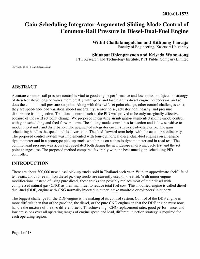
Figure 1 is a simplified diagram of diesel engine's common-rail system. A pump supplies high-pressure diesel
fuel to the common rail. Inside of the pump, a metering unit houses a plunger gate. The lift of the plunger gate
determines how much fuel is delivered. The amount of lift is controlled by varying the duty cycle of a PWM
signal sent to the plunger gate's solenoid by the ECU. A pressure sensor senses the pressure inside the common
rail. There is a relief valve to prevent over-pressure. Diesel injectors inject diesel fuel into cylinders.
Pump and
Metering Unit
Diesel Injectors
Pressure
Sensor
Common Rail
Relief
Valve
Figure 1: A simplified diagram of common-rail system.
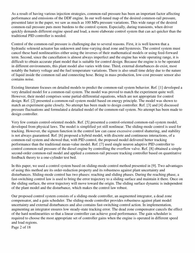
The control objective is to track desired common-rail pressure d
P as close as possible especially during swift
changes like in transients. Unlike the diesel engine, the DDF engine has many operating characteristics or zones
Page 4 of 18
that vary with engine speed and load. For example, during low load, only diesel is used for low emissions. For
low-to-medium load, DDF mode is used with cylinder skipping for good combustion. For medium and high
loads, different replacement ratios are used. This variation in operating characteristics results in extensive range
of the desired common-rail pressure. Figure 2 contains a map of the desired common-rail pressure of our DDF
engine, as a function of engine speed and torque. The map was tuned during calibration to obtain good
performance and low emissions. The desired common-rail pressure has an extensive range of 30 to 130 MPa
over the working ranges of the engine speed and torque. As a result, the control system must be able to follow
this quick change in the desired pressure, especially when under transient operations.
0
53
107
160
213
0
20
40
60
80
100
120
140
800 1200 1600 2000 2400 2800 3200 3600 4000 4400
120-140
100-120
80-100
60-80
40-60
20-40
0-20
( )dP MPa
( )Speed rpm
( )Torque Nm
Figure 2: Map of the desired common-rail pressure as a function of engine speed (rpm) and torque (Nm.)
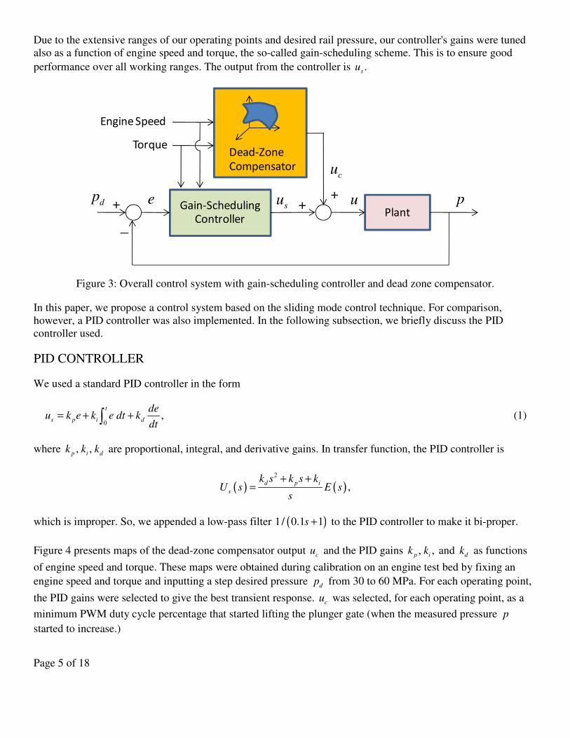
Figure 3 shows our overall control system. Here, plant is a relationship from the solenoid's PWM duty-cycle
percentage u to the measured pressure inside the common rail .p d
p is the desired pressure obtained from the
map in Figure 2. The error d
e p p= − is fed to the controller to be used in the algorithm.
It is well-known that the hydraulic solenoid has dead zone [10], that is, the insensitivity of an actuator to small
input. Our dead-zone compensator is a map, obtained during calibration, as a function of engine speed and
torque. The dead-zone compensator outputs a signal ,c
u which is the minimum amount of PWM duty cycle to
start lifting the plunger gate. Note that this c
u tries to cancel the deadzone effect as much as possible so that a
linear controller can achieve good performance.
Page 5 of 18
Due to the extensive ranges of our operating points and desired rail pressure, our controller's gains were tuned
also as a function of engine speed and torque, the so-called gain-scheduling scheme. This is to ensure good
performance over all working ranges. The output from the controller is .s
u
Gain-Scheduling
ControllerPlant
+
_
pe ++
Engine Speed
TorqueDead-Zone
Compensator
dp
su
cu
u
Figure 3: Overall control system with gain-scheduling controller and dead zone compensator.
In this paper, we propose a control system based on the sliding mode control technique. For comparison,
however, a PID controller was also implemented. In the following subsection, we briefly discuss the PID
controller used.
PID CONTROLLER
We used a standard PID controller in the form
0,
t
s p i d
deu k e k e dt k
dt= + +∫ (1)
where , ,p i d
k k k are proportional, integral, and derivative gains. In transfer function, the PID controller is
( ) ( )2
,d p i
s
k s k s kU s E s
s
+ +=
which is improper. So, we appended a low-pass filter ( )1/ 0.1 1s + to the PID controller to make it bi-proper.
Figure 4 presents maps of the dead-zone compensator output c
u and the PID gains , ,p i
k k and d
k as functions
of engine speed and torque. These maps were obtained during calibration on an engine test bed by fixing an
engine speed and torque and inputting a step desired pressure d
p from 30 to 60 MPa. For each operating point,
the PID gains were selected to give the best transient response. c
u was selected, for each operating point, as a
minimum PWM duty cycle percentage that started lifting the plunger gate (when the measured pressure p
started to increase.)
Page 6 of 18
0
80
160
240
28.5
29
29.5
30
30.5
31
80
0
12
00
16
00
20
00
24
00
28
00
32
00
36
00
40
00
44
00
0
80
160
240
0.9
1
1.1
1.2
1.3
1.4
80
0
12
00
16
00
20
00
24
00
28
00
32
00
36
00
40
00
44
00
0
80
160
240
0.08
0.09
0.1
0.11
0.12
0.13
0.14
80
0
12
00
16
00
20
00
24
00
28
00
32
00
36
00
40
00
44
00
0
80
160
240
0
0.005
0.01
0.015
0.02
0.025
0.03
80
0
12
00
16
00
20
00
24
00
28
00
32
00
36
00
40
00
44
00
( )%cu
( )Speed rpm
( )Torque Nm
pk
( )Speed rpm
( )Torque Nm
ik
( )Speed rpm
( )Torque Nm
dk
( )Speed rpm
( )Torque Nm
(a) (b)
(c) (d)
Figure 4: Several maps of design parameters in the PID control system. (a) Dead zone compensator output .c
u
(b) Proportional gain .p
k (c) Integral gain .i
k (d) Derivative gain .d
k
In the following subsection, we discuss, in details, a controller based on the sliding-mode control method.
SLIDING MODE CONTROLLER
The sliding-mode controller is model-free, that is, no plant model is required in the control algorithm. However,
an upper bound on the plant model functions is required to determine a design parameter. Therefore, we start
this section with finding a common-rail state-space model.
Common-Rail Model
A random PWM duty cycle percentage u was passed into the plant in Figure 3. The measured pressure p was
recorded, and the pair ,u p were used to find the plant transfer function using the command ident in Matlab.
The means of u and p were first removed to take away the effect of the dead-zone compensator output c
u and
Page 7 of 18
its corresponding pressure output .c
p Therefore, the resulting transfer function represents a relationship from
the controller output s
u and its corresponding pressure output .s
p
The plant's second-order transfer function is given by
( )( ) 2
16.02,
0.2297 1.181 1
s
s
P s
U s s s=
+ +
whose state-space model is
[ ]
1 1
22
1
2
0 1 0,
4.35 5.14 1
69.75 0 .
s
s
x xu
xx
xp
x
= + − −
=
Defining 69.75 ,s s
u u= 1 169.75 ,x x= and 2 269.75 ,x x= we have
1 2
2 1 2
1
,
4.35 5.14 ,
.
s
s
x x
x x x u
p x
=
= − − +
=
Now we are ready to formulate the tracking problem.
Tracking Problem
Let ds
p be desired common-rail pressure for .s
p Note that ds
p can be thought of as the desired pressure d
p in
Figure 2 subtracted by the corresponding pressure output of the dead-zone compensator .c
p Defining
1 s dse p p= − and 2 ,
s dse p p= − we have
( )
1 2
2 1 2
,
4.35 5.14 4.35 5.14 .s ds ds ds
e e
e e e u p p p
=
= − − + + − − −
(2)
So, the tracking problem becomes designing s
u to drive 1e and 2e to zeros. We can achieve this by considering
sliding phase and reaching phase.
Sliding Phase and Reaching Phase
Sliding mode control involves two phases: sliding and reaching phases. In the sliding phase, suppose we can
design a control law that constrains the trajectories of 1e and 2e in (2) to a surface
1 1 2 0.s a e e= + =
Page 8 of 18
On this surface, the motion is governed by 1 1 1.e a e= − Choosing 1 0a > ensures that ( )1e t and ( )2e t convert to
zeros as time t tends to infinity, and the rate of convergence can be adjusted by adjusting 1.a Note that the
motion on the surface 0s = is independent of plant parameters in (2).
In the reaching phase, we need to bring the trajectories of 1e and 2e to the surface 0s = and maintain it there.
Since
( )1 1 2 1 2 1 24.35 5.14 4.35 5.14 ,s ds ds dss a e e a e e e u p p p= + = − − + + − − −
suppose the desired pressure ds
p and its derivatives satisfy the inequality
( ) ( ) ( )1 2 1 2 1 2 1 2 1 2 1 24.35 5.14 4.35 5.14 , , , , ,ds ds ds
a e e e p p p a e h e e e e e e Rρ− − + − − − = + ≤ ∀ ∈ (3)
for a known function ( )1 2, ,e eρ with ( ) 21/ 2V s= as a Lyapunov function candidate, we have
( ) ( )1 2 1 2 1 2, , .s s
V ss s a e h e e su s e e suρ= = + + ≤ +
Taking
( ) ( )1 2, sgn ,su e e sβ= − (4)
where ( ) ( )1 2 1 2 0 0, , , 0,e e e eβ ρ β β≥ + > and the signum function
( )
1, 0
sgn 0, 0
1, 0
s
s s
s
>
= =− <
,
yields ( ) ( ) ( )1 2 1 2 0 0, , sgn .V s e e e e s s sρ ρ β β≤ − + = − Thus, / 2W V s= = satisfies the differential
inequality 0 / 2D W β+ ≤ − and, from the comparison lemma [11], we have ( )( ) ( )( ) 00 / 2.W s t W s tβ≤ −
Therefore, the trajectories of 1e and 2e reach the surface 0s = in finite time and, once on the surface, they
cannot leave it, as seen from the inequality 0 .V sβ≤ −
The control law (4) brings the trajectories of 1e and 2e to the surface 0s = and maintains it there. However,
nothing can be concluded about the bounds of 1e and 2e until we further investigate the region of attraction.
Region of Attraction
Suppose (3) becomes ( )1 2 1 2 1 1 2, , , ,a e h e e k e e+ ≤ ∀ ∈Ω where Ω is the region of attraction, for some known
nonnegative constant 1.k We can take ( ) 1sgn , .su k s k k= − > The condition 0ss ≤ in the set s c≤ makes it
positively invariant. From 1 2 1 1e e a e s= = − + and the function ( ) 2
1 11/ 2 ,V e= we have
Page 9 of 18
2 2
1 1 1 1 1 1 1 1 1 1 10, / .V e e a e e s a e e c e c a= = − + ≤ − + ≤ ∀ ≥
Thus, ( ) ( )1 1 1 10 / / , 0e c a e t c a t≤ ⇒ ≤ ∀ ≥ and the set 1 1/ ,x c a s cΩ = ≤ ≤ is positively invariant.
Since the control law (4) contains the discontinuous signum function, control chattering will occur as a result of
imperfection in switching devices and delays. Next, we present two schemes for reducing or eliminating control
chattering.
Chattering
The first scheme divides the control law into continuous and switching components to reduce the amplitude of
the switching one. Let ( )1 2ˆ ,h e e be an estimate of ( )1 2,h e e in (3). Taking ( )1 2 1 2
ˆ ,s
u a e h e e v = − + + yields
( ) ( ) ( )1 2 1 2 1 2ˆ, , , .s h e e h e e v e e vδ= − + ≤ + We can choose ( ) ( )1 2, sgn ,v e e sβ= − where
( ) ( )1 2 1 2 0 0, , , 0.e e e eβ δ β β≥ + > ( )1 2,e eδ is an upper bound of the perturbation term and is likely to be
smaller than the upper bound ( )1 2,e eρ of the whole term, hence, reducing chattering.
The second scheme replaces the discontinuous signum function with a continuous arctan function
( ) ( )2 / arctan / ,su k sπ ε= − (5)
where ε is a small number. The smaller the ε is, the closer the arctan function is to the signum function and
the more control chattering results.
Using continuous arctan function is a convenient way to prevent control chattering, however, the error
trajectories 1e and 2e will not go to zeros, but will be ultimately bounded. This proof can be seen in [11]. To
obtain zero steady-state errors, an integrator can be augmented to the system as detailed next.
Integral Augmented
Let 0 1 .e e dt= ∫ The augmented system becomes
( )
0 1
1 2
2 1 2
,
,
4.35 5.14 4.35 5.14 .s ds ds ds
e e
e e
e e e u p p p
=
=
= − − + + − − −
We can then choose
0 0 1 1 2 ,s a e a e e= + + (6)
where the matrix [ ]0 0 10,1; ,A a a= − − is Hurwitz.
In summary, our control law is (5), where s is given by (6). There are then four design parameters: 0, , ,k aε
and 1.a
Page 10 of 18
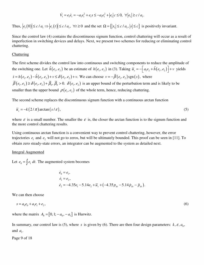
Gain Scheduling
Due to extensive range of the desired pressure d
p in the DDF engine and variety of operating points in terms of
engine speed and torque, the four design parameters were obtained during calibration on an engine test bed by
fixing an engine speed and torque and inputting a step desired pressure d
p from 30 to 60 MPa. For each
operating point, the four gains were selected to give the best transient response. Figure 5 presents maps of the
four gains in the sliding-mode control system. In Figure 3, the control input s
u is obtained from / 69.75.s s
u u=
The compensator input c
u is the same as that in Figure 4(a).
0
80
160
240
5
10
15
20
25
30
80
0
12
00
16
00
20
00
24
00
28
00
32
00
36
00
40
00
44
00
0
80
160
240
0.05
0.15
0.25
0.35
0.45
0.55
80
0
12
00
16
00
20
00
24
00
28
00
32
00
36
00
40
00
44
00
0
80
160
240
4
5
6
7
8
9
10
80
0
12
00
16
00
20
00
24
00
28
00
32
00
36
00
40
00
44
00
0
80
160
240
9
10
11
12
13
14
15
80
0
12
00
16
00
20
00
24
00
28
00
32
00
36
00
40
00
44
00
k
( )Speed rpm
( )Torque Nm
ε
( )Speed rpm
( )Torque Nm
0a
( )Speed rpm
( )Torque Nm
1a
( )Speed rpm
( )Torque Nm
(a) (b)
(c) (d)
Figure 5: Several maps of design parameters in the sliding-mode control system. (a) .k (b) .ε (c) 0.a (d) 1.a
EXPERIMENTAL RESULTS
We implemented the control algorithm in Figure 3 with an engine test bed and a pick-up truck using the same
engine model. The engine test bed was connected to an engine dynamometer, and the pick-up truck was
connected to a chassis dynamometer. The engine was modified from a Toyota 2KD-FTV diesel engine to run
Page 11 of 18
diesel-dual-fuel by injecting 375 kPa CNG to each of the four intake ports. The distance from the CNG injector
to the port is kept as small as possible at 25 cm to reduce time delay.
The engine has four cylinders, each of 2.5 liters, sixteen intake and exhausted valves with double overhead cam
shaft (DOHC), a turbocharger with an EGR valve and a throttle but without variable geometry turbine (VGT),
and common-rail direct fuel injection system.
The OEM ECU was replaced with an ECU whose hardwares are mainly from National Instruments. All control
algorithms were written in Labview graphical programming language. A desktop computer acts as a host to
communicate with human operator and is connected to a target running Labview Realtime and FPGA modules.
The PID controller (1) was implemented with a low-pass filter ( )1/ 0.1 1 .s + The PID gains and the dead-zone
compensator output c
u are given in Figure 4. The sliding mode controller (5) was used with an augmented
sliding surface (6). All gains are given in Figure 5.
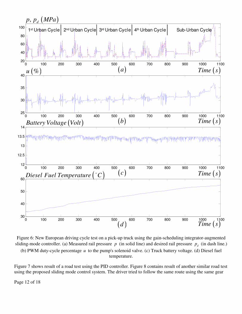
We first discuss the experimental results from the pick-up truck, followed by the results from the engine test
bed. The pick-up truck was commanded to follow the new European driving cycle (NEDC.) The whole cycle
comprises four urban cycles, each of about 200 seconds, and a sub-urban cycle of about 500 seconds.
Figure 6 contains the results of applying the gain-scheduling integrator-augmented sliding-mode controller. In
following the NEDC, Figure 6(a) shows the plots of the measured common-rail pressure p (in solid line) and
the desired pressure d
p (in dash line.) Both are plotted versus time. Excellent tracking results were obtained for
the whole NEDC. Figure 6(b) shows the plot of the PWM duty cycle percentage u versus time. Figure 6(c)
shows the plot of the battery voltage versus time, and Figure 6(d) shows the plot of the diesel fuel temperature
versus time. It can be seen from Figure 6(c) that the battery voltage is slightly decreasing, which directly affects
the increasing trend of the PWM duty cycle percentage in Figure 6(b). This is because when the supply voltage
is low, the controller must increase its effort to obtain the same plunger gate lift. Supply voltage is a main
disturbance we found to the common-rail pressure system since it can vary with electrical usage in the truck.
However, the sliding-mode controller seems to handle this disturbance well. Another important disturbance we
saw is the diesel fuel temperature which shows an increasing trend as in Figure 6(d). Usually, higher diesel fuel
temperature tends to increase the control effort .u
Page 12 of 18
0 100 200 300 400 500 600 700 800 900 1000 110020
40
60
80
100
0 100 200 300 400 500 600 700 800 900 1000 110025
30
35
40
0 100 200 300 400 500 600 700 800 900 1000 110012
12.5
13
13.5
14
0 100 200 300 400 500 600 700 800 900 1000 110030
40
50
60
4th Urban Cycle Sub-Urban Cycle
( )Time s
3rd Urban Cycle2nd Urban Cycle1st Urban Cycle
( )d
( )c
( )b
( )a
( )Time s
( )Time s
( )Time s
( ), dp p MPa
( )%u
( )Battery Voltage Volt
( )Diesel Fuel Temperature C
Figure 6: New European driving cycle test on a pick-up truck using the gain-scheduling integrator-augmented
sliding-mode controller. (a) Measured rail pressure p (in solid line) and desired rail pressure d
p (in dash line.)
(b) PWM duty-cycle percentage u to the pump's solenoid valve. (c) Truck battery voltage. (d) Diesel fuel
temperature.
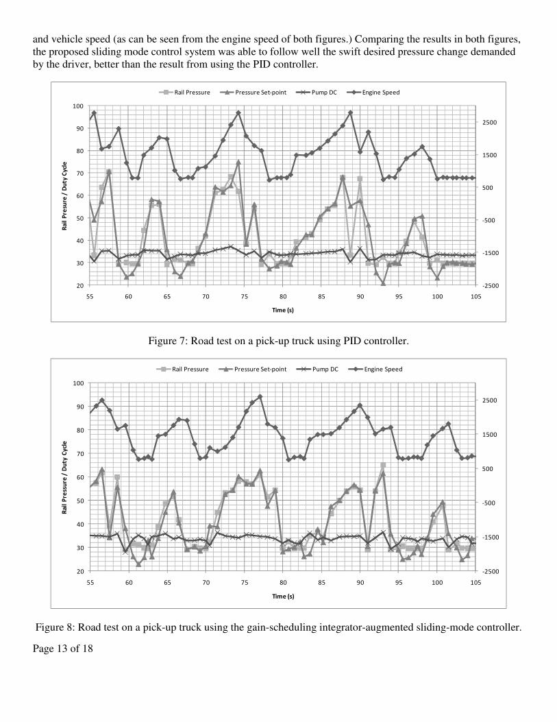
Figure 7 shows result of a road test using the PID controller. Figure 8 contains result of another similar road test
using the proposed sliding mode control system. The driver tried to follow the same route using the same gear
Page 13 of 18
and vehicle speed (as can be seen from the engine speed of both figures.) Comparing the results in both figures,
the proposed sliding mode control system was able to follow well the swift desired pressure change demanded
by the driver, better than the result from using the PID controller.
-2500
-1500
-500
500
1500
2500
20
30
40
50
60
70
80
90
100
55 60 65 70 75 80 85 90 95 100 105
Ra
il P
resu
re /
Du
ty C
ycl
e
Time (s)
Rail Pressure Pressure Set-point Pump DC Engine Speed
Figure 7: Road test on a pick-up truck using PID controller.
-2500
-1500
-500
500
1500
2500
20
30
40
50
60
70
80
90
100
55 60 65 70 75 80 85 90 95 100 105
Rai
l P
ress
ure
/ D
uty
Cy
cle
Time (s)
Rail Pressure Pressure Set-point Pump DC Engine Speed
Figure 8: Road test on a pick-up truck using the gain-scheduling integrator-augmented sliding-mode controller.
Page 14 of 18
0 20 40 60 80 100 120 140 16025
30
35
40
45
50
0 20 40 60 80 100 120 140 16036
38
40
42
0 20 40 60 80 100 120 140 16012
12.5
13
13.5
14
0 20 40 60 80 100 120 140 16052
52.5
53
53.5
54
( )Time s( )d
( )c
( )b
( )a
( )Time s
( )Time s
( )Time s
( ), dp p MPa
( )%u
( )Battery Voltage Volt
( )Diesel Fuel Temperature C
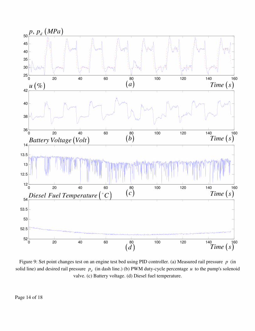
Figure 9: Set point changes test on an engine test bed using PID controller. (a) Measured rail pressure p (in
solid line) and desired rail pressure d
p (in dash line.) (b) PWM duty-cycle percentage u to the pump's solenoid
valve. (c) Battery voltage. (d) Diesel fuel temperature.
Page 15 of 18
0 20 40 60 80 100 120 140 16025
30
35
40
45
50
0 20 40 60 80 100 120 140 16036
38
40
42
0 20 40 60 80 100 120 140 16012
12.5
13
13.5
14
0 20 40 60 80 100 120 140 16052
52.5
53
53.5
54
( )Time s( )d
( )c
( )b
( )a
( )Time s
( )Time s
( )Time s
( ), dp p MPa
( )%u
( )Battery Voltage Volt
( )Diesel Fuel Temperature C
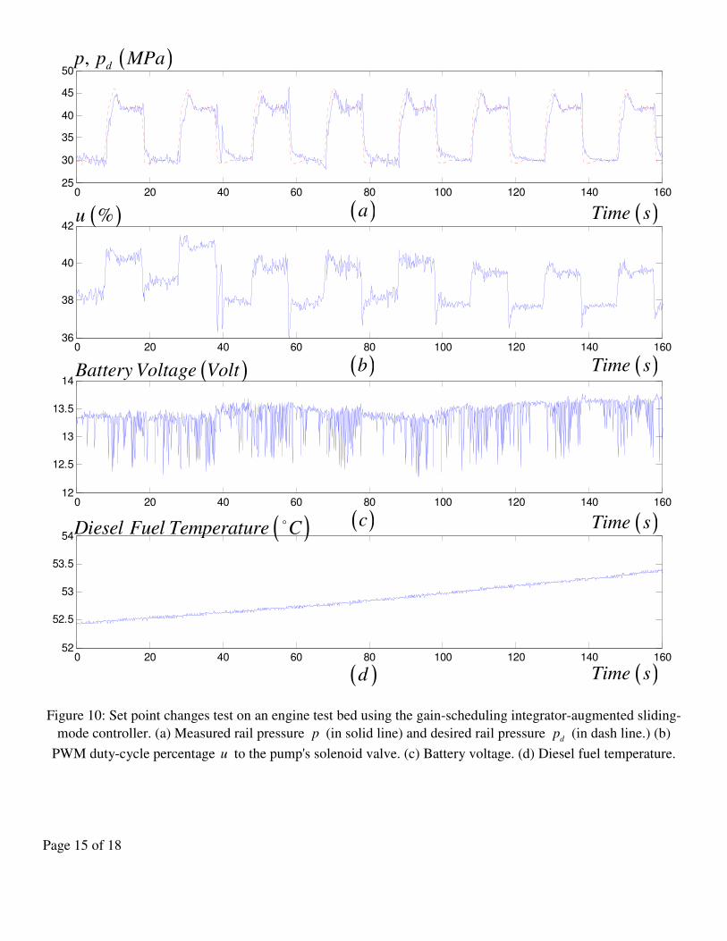
Figure 10: Set point changes test on an engine test bed using the gain-scheduling integrator-augmented sliding-
mode controller. (a) Measured rail pressure p (in solid line) and desired rail pressure d
p (in dash line.) (b)
PWM duty-cycle percentage u to the pump's solenoid valve. (c) Battery voltage. (d) Diesel fuel temperature.
Page 16 of 18
Figure 9 includes the experimental results from the engine test bed using the PID controller. The measured
common-rail pressure p was commanded to follow step changes in the desired pressure .d
p Figure 9(a)
contains plots of the measured pressure (in solid line) and the desired pressure (in dash line) versus time. The
measured pressure was unable to follow the desired pressure well, having both high overshoot and steady-state
error. The lag between the desired pressure and the measured pressure can be seen as a result of the control
system unable to react quickly enough with the desired pressure change. Figure 9(b) shows the plot of the PWM
duty cycle percentage u versus time. Figure 9(c) shows the plot of the battery voltage versus time, and Figure
9(d) shows the plot of the diesel fuel temperature versus time. When the battery voltage dropped the most at
around 70 to 80 seconds, the control effort u is at its highest point. During 120 to 160 seconds, even though the
battery voltage slightly increases, the control effort u also slightly increases. This is because the diesel fuel
temperature slightly increases as well, which counters the effect of the battery voltage.
Figure 10 contains the experimental results from the engine test bed using the proposed gain-scheduling
integrator-augmented sliding-mode controller. From Figure 10(a), the measured pressure is able to follow
closely the desired pressure with no overshoot and small steady-state error. Upon inspecting the control effort in
Figure 10(b), more control chattering can be seen than that of Figure 9(b), resulting in more active control
system. The effects of the battery voltage and the diesel fuel temperature to the control effort can be seen from
Figure 10(c) and (d).
CONCLUSIONS
Due to its extensive operating range and different injection strategies, the diesel-dual-fuel engine is required to
follow wide range of desired common-rail pressure. The disturbances from battery voltage and fuel temperature
variations make tracking control using traditional PID controller, even with gain scheduling, difficult. The
proposed sliding-mode control system has a dead zone compensator to compensate the dead zone effect, a gain-
scheduling scheme to handle wide operating range, an augmented integrator for zero steady-state error, and a
sliding-mode controller consisting of a reaching-phase continuous fast-acting controller for fast action and a
sliding surface for good robustness. Together, the proposed control system was able to deliver excellent
tracking results as seen from a pick-up truck following the NEDC and road test and an engine test bed by
varying the desired pressure set point.
There are several tasks that can be performed in future researches. First is the improvement on the dead-zone
compensator. Instead of using a calibrated map like ours, a mathematical model can be formulated for the dead
zone and hysteresis, which are the two hard nonlinearities normally found in hydraulic solenoid actuator. This
fixed model can be used to cancel the effect of the hard nonlinearities so that a linear plant model can be used to
represent the common-rail system more accurately. This will open up the possibilities of using many effective
linear model-based control techniques.
Second is the use of adaptive algorithms. Gain scheduling that we used can be viewed as a simple type of
adaptive controllers. Some adaptive control algorithms can be used to adapt either controller or plant parameters
over the changing operating points to always achieve good tracking performance. Some recursive system
identification can be used to learn hard nonlinearities and to cancel their effects in a scheme called adaptive
inverse control.
Third is improvement on the sliding mode algorithm itself. In the presence of model uncertainty, there is no
guarantee of robustness during reaching phase. An integral sliding mode method presented in [9] can be applied
to ensure robustness at all time. The trajectory dynamic during sliding phase can be viewed as pole-placement
control, where in our case 0a and 1a were designed to place the poles at the stable left-half-plane region. More
Page 17 of 18
elaborated controllers can be used in place of the pole-placement control to obtain better results during sliding
phase.
REFERENCES
[1] Coppo, M. and Dongiovanni, C., “Experimental Validation of a Common-Rail Injector Model in the Whole
Operation Field,” Journal of Engineering for Gas Turbines and Power, 129:596-608, 2007.
[2] Morselli, R., Corti, E., and Rizzoni, G., “Energy Based Model of a Common Rail Injector,” presented at
2002 IEEE Int. Conf. on Control App, Glasgow, Scotland, September 2002.
[3] Hu, Q., Wu, S. F., Stottler, S., and Raghupathi, R., “Modelling of Dynamic Responses of an Automotive
Fuel Rail System, Part I: Injector,” Journal of Sound and Vibration, 245(5):801-814, 2001.
[4] Wu, S. F., Hu, Q., Stottler, S., and Raghupathi, R., “Modelling of Dynamic Responses of an Automotive
Fuel Rail System, Part II: Injector,” Journal of Sound and Vibration, 245(5):815-834, 2001.
[5] Lino, P., Maione, B., and Rizzo, A., “Nonlinear Modeling and Control of a Common Rail Injection System
for Diesel Engines,” Applied Mathematical Modelling, 31:1770-1784, 1959.
[6] Balluchi, A., Bicchi, A., Mazzi, E., Vincentelli, A. S., and Serra, G., “Hybrid Modeling and Control of the
Common Rail Injection System,” Int. Journal of Control, 80(11):1780-1795, 2007.
[7] An, S., Shao, L., "Diesel Engine Common Rail Pressure Control Based on Neuron Adaptive PID," 2008
IEEE International Conference on Cybernetics and Intelligent Systems Paper 4670956, 2008.
[8] Chatlatanagulchai, W., Wannatong, K., and Aroonsrisopon, T., "Robust Common-Rail Pressure Control for
a Diesel-Dual-Fuel Engine Using QFT-Based Controller," 2009 SAE Powertrains, Fuels and Lubricants
Conference Paper 2009-01-1799, 2009.
[9] Utkin, V., Guldner, J., and Shi, J., Sliding Mode Control in Electromechanical Systems, CRC Press, Florida,
ISBN-0-7484-0116-4, 1999.
[10] Tao, G. and Kokotovic, P. V., Adaptive Control of Systems with Actuator and Sensor Nonlinearities, John
Wiley and Sons, New York, ISBN 0-471-15654-X:7-28, 1996.
[11] Khalil, H. K., Nonlinear Systems, 3rd Edition, Prentice Hall, New Jersey, ISBN-13 978-0130673893,
2001.
CONTACT INFORMATION
Contact Withit Chatlatanagulchai at mailing address:
Department of Mechanical Engineering
Faculty of Engineering
Kasetsart University
50 Phaholyothin Road,
Bangkok 10900, Thailand
or email address: [email protected]

Page 18 of 18
ACKNOWLEDGMENTS
Thanks are due to Nitirong Pongpanich for setting up the experimental hardware.