Shear banding analysis of plastic models

formulated for incompressible viscous flows

V. Lemiale a, H.-B. Muhlhaus b, L. Moresi a, J. Stafford a

aSchool of Mathematical Sciences, Monash University, Melbourne, Victoria, 3800,

Australia

bEarth Systems Science Computational Centre (ESSCC) The University of

Queensland, St Lucia, QLD 4072, Australia

Abstract

We investigate shear band orientations for a simple plastic formulation in the context

of incompressible viscous flow. This type of material modelling has been introduced

in literature to enable the numerical simulation of the deformation and failure of the

lithosphere coupled with the mantle convection. In the present article, we develop

a linear stability analysis to determine the admissible shear band orientations at

the onset of bifurcation. We find that the so-called Roscoe angle and Coulomb

angle are both admissible solutions. We present numerical simulations under plane

strain conditions using the hybrid particle-in-cell finite element code Underworld.

The results both in compressional and extensional stress conditions show that the

variation of the numerical shear bands angle with respect to the internal friction

angle follows closely the evolution of the Coulomb angle.

Key words: Shear banding, Linear stability analysis, Finite Element,

Particle-in-cell, Drucker-Prager failure criterion

Preprint submitted to Elsevier 2 July 2008

* Manuscript

Click here to view linked References

1 Introduction

A major challenge in geodynamics is understanding the thermal and mechanical coupling

between the brittle lithosphere and the ductile upper mantle. To study this problem, a

number of numerical models have been proposed (see for instance the summary in Moresi

and Muhlhaus [2006]). In this paper, we focus our attention on a fluid-dynamics based

formulation, in which the mechanical behaviour of the lithosphere is incorporated into

a finite element code originally developed to solve incompressible viscous flow problems.

With this formulation, it has been demonstrated that it is possible to simulate mantle

convection coupled to fine-scale shear band formation in the lithosphere [Lenardic et al.,

2000].

It is, however, critical to assess the mechanical characteristics of this class of models,

in order to define, and possibly further enhance, its range of applicability. While it has

been demonstrated that qualitatively realistic geological structures can be predicted with

this approach [Moresi et al., 2007a], a number a questions remain open: is it possible

to quantitatively predict the initiation of localization into shear bands and the post-

localization behaviour? How reliable is the prediction of shear bands, in terms of location,

orientation, instant of appearance? In other words, how can we correlate these simulations

with the geological features found in the field?

There has been significant research on the orientation of shear bands in elastoplastic

solids [Vardoulakis, 1980, Vermeer, 1990, Bardet, 1990]. While several empirical relations

have been proposed to predict the shear band orientation in granular materials, soils or

rocks [Vardoulakis et al., 1978, Vermeer, 1990], it appears that it is difficult to account

for the observed shear band orientation in all circumstances with a simple, unique model

[Bardet, 1990]. This orientation may depend on material parameters such as the angle of

internal friction and the angle of dilatancy, which may in turn be related to other factors

2

such as the particle size [Vermeer, 1990]. In this latter reference, a bifurcation analysis

is also proposed and shows that from a particular model, a range of possible shear band

orientations may be theoretically admissible.

In these conditions, and within a numerical context, it is important to properly assess

the mechanical response of a failure model used to predict the localization of deforma-

tion, especially in terms of shear band orientation. A numerical comparison of several

softwares published recently (Buiter et al. [2006]) has shown that although qualitatively

similar answers are obtained with these codes, the level of variability is rather significant,

particularly regarding the prediction of shear band characteristics. In the present paper

we will study both analytically and numerically the orientation of shear bands obtained

within the context of incompressible viscous flow coupled with plastic failure outlined

earlier. The primary objective is to gain a better understanding of this class of increas-

ingly popular numerical models in the geodynamic community, for which a number of

theoretical assessments are yet to be performed.

The paper is organised as follows: in the next section, we introduce the constitutive

behaviour considered in our analysis. This material model is a simple approach to in-

corporate the pressure dependent yield strength of the lithosphere in the context of the

viscous formulation usually used for the upper part of the mantle. In the third section, a

linear stability analysis is presented and the condition for the onset of a bifurcation mode

in localised shear bands is derived. The fourth and fifth sections are concerned with the

numerical formulation of our model, as well as with the numerical features of the exten-

sion/compression example considered here. In the last section, we give numerical results

and discussion.

3

2 Constitutive relations

We adopt the following viscous-plastic model for the constitutive material behaviour of

the lithosphere, Moresi and Muhlhaus [2006]:

σ = 2η (D −Dp)− p1 (1)

In this expression, σ is the Cauchy stress tensor, η is the viscosity, the total strain rate

tensor, D, is decomposed into a viscous contribution, Dv, and a plastic contribution, D

p,

p is the pressure and 1 is the identity tensor.

We consider the onset of yielding as being determined by a Drucker-Prager type failure

criterion:

f = τ − 3αp− k ≤ 0 (2)

Where τ =√

(τijτij)/2 and τ is the deviatoric stress tensor. Moreover, α and k are two

material parameters that are, in general, functions of the accumulated plastic strain.

This particular model may not be the most appropriate to reproduce the behaviour of the

lithosphere. It is however our objective to analyse how a simple model, which is routinely

used as a starting modelling approach in many engineering situations, may or may not

be capable to capture the appearance of localized shear bands properly in our numerical

context.

Upon yielding, a flow rule is needed to specify the plastic behaviour. The plastic strain

rate is written as:

Dp = λ

∂g

∂σ(3)

4

Where λ is a scalar plastic flow rate and g is the so-called plastic potential. A classical

choice for g, in conjunction with the incompressibility constraint, is:

g = τ (4)

leading in the general case to a non-associated plasticity model, since we have f �= g.

If we consider only the deviatoric part of the stress tensor in (1), we thus obtain:

τ = 2η(

D − λτ

2τ

)

(5)

Which can be written as:

(

1 + λη

τ

)

τ = 2ηD (6)

We introduce at this point a measure of the equivalent strain rate as:

γ =√

2DijDij (7)

It can be deduced from (6) that:

(

1 + λη

τ

)

τ = ηγ (8)

Thus we obtain the following expression for λ:

λ = γ −τ

η(9)

From the failure criterion (2), when plastic flow occurs we can write:

5

τ = 3αp + k (10)

Combining the equations (1), (9) and (10), the constitutive relation finally reads:

σ = 23αp + k

γD − p1 (11)

3 Linear stability analysis

Consider a rectangular box, under plane strain conditions, submitted to an extensional

or compressional loading. We examine in this section the condition of existence of a

shear band bifurcation mode. Needleman [1979] performed a similar analysis for the rate-

independent plasticity case.

Let us first consider the incremental equations of equilibrium:

δσ11,1 + δσ12,2 = 0

δσ12,1 + δσ22,2 = 0

(12)

Using (11), the following expression for the incremental stress tensor can be derived (see

Appendix A for details of the derivation):

δσij = 23αp + k

γ

(

1

2(δilδjk + δikδjl)−

2

γ2DklDij

)

δDkl

+ 23αδp

γDij − δpδij (13)

Note that in this calculation α and k have been assumed constants (see Appendix A).

It will be shown with the numerical results that this approximation does not affect the

overall results regarding the shear band angles.

6

Initially, the incompressible material is in a homogeneous state, i.e. D11 = −D22 = D0,

the other components of the strain rate tensor vanishing. From this homogeneous state,

the strain rate is then subsequently incremented so that the strain rate tensor now reads:

D =

D0 + δD11 δD12

δD12 − (D0 + δD11)

(14)

Replacing in (13) the strain rate components by their expressions, and neglecting the non

linear infinitesimal terms, the following relationships can be derived:

δσ11 = −δp (1− 3α)

δσ22 = −δp (1 + 3α)

δσ12 =3αp0 + k

D0δD12 = 2ηplδD12

(15)

In this set of equations, p0 represents the initial pressure before the onset of the bifurcation

mode, and the notation ηpl has been introduced as an equivalent plastic shear viscosity.

Moreover, under the assumption of plane strain conditions, the incompressibility con-

straint reads:

v1,1 + v2,2 = 0 (16)

This condition implies that the velocity field is of the form:

v1 = ψ,2 and v2 = −ψ,1 (17)

Inserting (15) and (17) into the incremental equilibrium conditions (12) gives:

7

−δp,1 (1− 3α) + ηpl (ψ,22 − ψ,11),2= 0

ηpl (ψ,22 − ψ,11),1− δp,2 (1 + 3α) = 0

(18)

The pressure can actually be eliminated by combining these two equations so that the

following relation can be derived:

(1 + 3α) (ψ,2222 − ψ,1122)− (1− 3α) (ψ,2211 − ψ,1111) = 0 (19)

In the case of a localized shear band bifurcation mode, the stream function ψ can be

further assumed to be of the form, Vardoulakis and Sulem [1995]:

ψ = Aeωt sin (n1x1 + n2x2) (20)

where A is a constant, ω is the growth rate of the instability and ni=1,2 are the components

of the normal vector with respect to the shear band.

Using the above expression for ψ, it is noted that:

ψ,ijkl = ninjnknlψ (21)

Thus, (19) can be rearranged to obtain:

(

n2

2− n2

1

) [

(1 + 3α)n2

2− (1− 3α)n2

1

]

= 0 (22)

From this calculation, two possible set of orientations for the incipient shear bands are

8

therefore deduced:

n2

1= n2

2

or

n2

1=

1 + 3α

1− 3αn2

2

(23)

If we note the component ni as follows:

n1 = − sinϕ and n2 = cosϕ (24)

Then the first condition in (23) actually corresponds to the following shear band orienta-

tion:

ϕ = ±π

4(25)

Let us now calibrate the Drucker-Prager criterion with the so-called Mohr-Coulomb failure

criterion. This criterion reads:

|σsn| + tanφσnn − c ≤ 0 (26)

Where σsn and σnn are the tangential and normal components of the traction resolved in

the plane of normal vector n. φ and c are respectively the internal friction angle and the

cohesion.

Under the plane strain conditions considered in the present study and for a deviatoric

flow, the following relationships can be derived:

α =sinφ

3and k = c cosφ (27)

Inserting (24) and (27) into the second equation of (23) leads to:

sin2 ϕ =1 + sinφ

2(28)

9

which is satisfied if:

ϕ = ±

(

π

4+φ

2

)

(29)

In summary, the linear stability presented here shows that for the constitutive viscous-

plastic behaviour (11) two possible orientations are admissible as extreme solutions for

the onset of shear banding, namely:

ϕ =π

4and ϕ =

π

4+φ

2(30)

which are often refered to as the Roscoe solution (ϕ =π

4+Ψ

2, with the angle of dilation

Ψ = 0 for an incompressible material) and the Coulomb solution respectively, Vermeer

[1990].

4 Numerical formulation

4.1 Finite element approach with Lagrangian integration points

The viscous-plastic formulation presented in the previous sections has been implemented

in our finite element particle-in-cell code Underworld [Moresi et al., 2007b]. The basic

concept of its formulation is as follows: a finite element mesh is used as a discretization

of the geometrical domain, i.e to calculate the volume integrals quantities. At the same

time, material points (or particles) are introduced to discretize material domains, and to

carry material properties that are history dependent (in our case, the plastic history of

the material). The main specificity of this approach compared to a classical finite element

method lies in the fact that the quadrature points usually used in the integration scheme

are now replaced by the (arbitrarily distributed) material points. This approach combines

several advantages of both the Lagrangian and Eulerian formulations, by allowing large

deformations at the same time as being capable of efficient solution of the underlying

10

momentum equation on the static mesh. More details on the formulation can be found in

Moresi et al. [2003].

In the present study the polynomial interpolation is piecewise linear in velocity, and

constant in pressure (calculated at the centre of each finite element). Higher order elements

could be used and would probably lead to a better accuracy for a comparable mesh

resolution. In addition, it may be useful to consider a gradient recovery method to obtain

a continuous pressure / strain-rate field from the individual element values [Boroomand

and Zienkiewicz, 1997]. However, our simulations indicate that it is possible to obtain

accurate results with low order elements, provided that the mesh is sufficiently refined.

4.2 Implementation of the viscous-plastic model in Underworld

It is easily seen from (11) that the deviatoric part of the stress tensor can be written as:

τ = 2ηeffD (31)

where the effective viscosity reads:

ηeff =3αp + k

γ(32)

Therefore, the momentum equation to be solved can be written as follows:

2∂ (ηeffDij)

∂xj

− p,i = fi (33)

where the term fi represents the volume forces, i.e. the gravity in our case.

So it is clear from (33) that the set of global equations to be solved is equivalent to that

of an incompressible viscous flow, the viscosity being replaced by an effective viscosity

determined to satisfy the yielding constraints.

For each particle, the actual viscosity is calculated locally by first computing the viscous

stress prediction τ v. If this prediction is such that f < 0, then the material behaviour is

11

viscous and the effective viscosity is unchanged from the initial value. If on the other hand

the failure criterion is such that f ≥ 0, then the behaviour is plastic and the viscosity

must be adjusted to ensure that the stress state lies on the yield surface f = 0. One can

use the relation (32), or alternatively it is readily shown that the effective viscosity can

be calculated using the following expression:

ηIeff

= η3αpI + k

τ v,I(34)

In this equation, the superscript I (corresponding to an iteration) has been inserted to

emphasize on the non linearity introduced by the plastic rheology, and therefore on the

need to solve the equations iteratively, Moresi et al. [2003].

The material parameters α and k are in general function of the accumulated plastic strain,

and therefore must be updated accordingly. The present numerical analysis is focused on

the orientation of shear bands as a function of the friction coefficient. Thus the parameter α

is not allowed to harden or soften. However, the parameter k, or equivalently the cohesion

c, see (27), can experience some strain hardening or strain softening.

We introduce the equivalent plastic strain rate as follows:

γp =√

2DpijD

pij (35)

Recalling (9), we obtain:

γp = λ = γ −τ

η(36)

Following Moresi and Muhlhaus [2006], we consider a linear relationship for the strain

dependency of the cohesion:

c = c0 + (c∞ − c0) min

(

1,γp

γ0

)

(37)

12

where c0 and c∞ represent the initial and final cohesion, respectively, and γ0 is a reference

strain that defines a maximum hardening or softening limit. With this simple relation,

the hardening case corresponds to a set of parameters such that c0 < c∞, whereas the

softening case is the opposite.

5 Numerical model

5.1 Introduction

In this section, we restrict ourselves to the simplest possible case of a single viscous-

plastic layer of the type described in the first section. This example allows us to analyze

separately the formation and properties of the incipient shear bands. We do not consider

here the case of two or more layers representing the brittle and ductile crust and mantle

layering typical of the Earth’s lithosphere, since the primary goal of the present article is

to characterize the formulation in itself in terms of shear banding. The influence of the

viscous layer on the formation of shear bands have been studied in Moresi et al. [2007a]

and is outside the scope of the present analysis. The main objective of the present work

is to assess the numerical response of shear banding with respect to a variation of the

internal friction coefficient, and to compare this behaviour with the analytical finding

discussed in the precedent sections.

5.2 Geometrical model and discretization

Consider a rectangular box of dimensions 3.0 x 1.0 in extension or 4.0 x 1.0 in compression,

submitted to a prescribed velocity boundary condition on the right and left sides, and on

free slip boundaries conditions on top and bottom edges. The plane strain hypothesis is

assumed here.

13

A longer box dimension in the compressional model is needed to ensure that the shear

bands, which are closer to the horizontal in this case, do not hit the side of the box. To

ensure there is no volume change due to the boundary conditions on the edges, the top

of the box is allowed to move down. A low viscosity layer (viscosity of 0.01 compared

to the reference viscosity of the plastic layer of 100) is placed above the plastic layer to

accommodate deformation of the surface. For most cases, the overall box (incompressible

viscous-plastic layer and compressible background) is discretized with an initial mesh

composed of 384x128 elements, however, various mesh resolutions have been tested to

assess the influence of the mesh size, see Table 2.

In order to centre the shear bands and therefore facilitate subsequent analysis, a small,

square, weak zone of viscosity 1.0 is introduced at the base of the layer; shear bands

propagate from upper the corners of the square. As mentioned in de Borst [1988], the

introduction of a small imperfection transfers the bifurcation problem to a limit problem.

However, since we are only interested in the orientation of incipient shear bands and not

on the determination of the limit load, this simple model is sufficient.

5.3 The initial homogeneous viscous prediction

In order to properly set up the various material parameters, it is of interest to discuss the

relevant quantities involved. In this subsection we do not consider the weak zone in order

to simplify the analysis. Initially, the deformation is homogeneous and since the material

is incompressible the components of the strain rate tensor are reduced to:

Dx = −Dy = 2V

L(38)

Where x and y correspond to the horizontal and vertical direction, respectively, V is the

prescribed velocity on each side and L is the initial length of the specimen.

14

The component of the deviatoric viscous stress are immediately found to be:

τx = −τy = 4ηV

L(39)

And, by using the momentum equations with the gravity as the unique volume force,

along with the free surface boundary condition, one can find the following expression for

the pressure:

p = −τx + ρgh = −4ηV

L+ ρgh (40)

Where ρ is the material density, g is the gravity, h is the height.

It follows that the components of the stress tensor read:

σx = 2τx − ρgh

σy = −ρgh

σz =σx + σy

2= τx − ρgh = −p

(41)

It can further be deduced from this set of equations that in extension we have σx > σz >

σy, while in compression σy > σz > σx.

5.4 Material parameters

As discussed earlier, the friction coefficient is not allowed to soften or harden in our

simulation. It is well known that a Drucker-Prager failure criterion is not appropriate for

materials with high angles of friction, such as sand or concrete, Vermeer and de Borst

[1984]. In addition, several authors have indicated that the use of arbitrarly large friction

angles would lead to unrealistic results, [Desrues, 2002, Vardoulakis and Sulem, 1995].

Therefore, the range of values considered here for the internal friction angle lies in the

interval tanφ ∈ [0;0.8] (or φ ∈ [0;38o]).

15

Initially, the solution is supposed to be homogeneous, i.e. each point deforms plastically.

Then, as soon as the shear bands develop, the material outside the bands begins to unload

and only the material within the bands remains in the yielding regime. To ensure that

each point yields initially, the following condition must be fulfilled, see (39):

τ = 4η| V |

L≥ 3αp + k (42)

Moreover, our formulation for incompressible viscous flow excludes the possibility of failure

in tensile mode. It is therefore necessary to ensure that the failure criterion is always

defined, i.e. that the yield stress does not become negative. This can be written as:

3αp + k ≥ 0 (43)

Using the calibration (27) along with the expresion for the pressure (40), the two equations

(42) and (43) imply:

1

cosφ

(

4η| V |

L

)

+ tanφ

(

4ηV

L− ρgh

)

≥ c ≥ tanφ

(

4ηV

L− ρgh

)

(44)

(44) provides an estimate of the conditions that the cohesion, c, must fulfill in order to

1) have an homogeneous solution initially, 2) avoid the unrealistic tensile failure mode. It

is of course an approximation, since the introduction of a weak zone changes the stress

locally; moreover, the length L varies with time, and so do the limits. However, this is

a useful guide to choose a relevant set of parameters for the range of friction coefficient

under inspection. Note the influence of gravity: its inclusion decreases the extreme admis-

sible values of the cohesion, which simply means that adding the effect of gravity helps

preventing the appearance of failure in mode I, and at the same time increases the yield

stress. Numerically, we set a condition on the minimum allowable yield stress to avoid

any locally tensile stress condition on a particle. For this particular set of runs, we chose

the minimum yield stress, τmin to be 0.001.

16

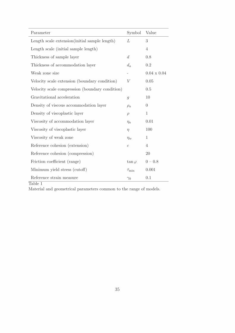
Table 1 summarizes the common geometrical and material parameters common to the

various models. The details of individual models are given in Table 2.

[Table 1 about here.]

[Table 2 about here.]

6 Results

In this section, we present numerical results obtained both in compression and extension.

In the former case, a velocity of 0.6666 and −0.6666 is prescribed on the left and right

hand sides of the box, respectively. In extension, the prescribed velocity is equal to ±0.05.

We begin our analysis by discussing the general characteristics of the simulated shear

bands. We then investigate the evolution of their orientation with several parameters.

6.1 Preliminary remarks

Figure 1 shows the shear band deformation obtained in compression for a friction angle of

11◦ and 38◦, respectively (or equivalently tanφ = 0.2 and tanφ = 0.8, respectively). The

viscous-plastic material is constructed from two sets of otherwise-identical, differently-

coloured layers in order to visualize the localized strain. There is a clear variation in the

orientation of the shear bands with the friction coefficient. In this figure, and in all the

subsequent ones, the orientation corresponding to the Coulomb angle is plotted with black

lines.

[Fig. 1 about here.]

[Fig. 2 about here.]

Figure 2 shows the strain rate invariant obtained for the same configurations as Figure

1, just at the initiation of shear banding. The deformation immediately localizes into two

symmetric shear bands initiating from the weak zone, closely aligned with the Coulomb

17

angle.

The orientation of the shear bands was determined from a high-resolution plot of the

strain-rate invariant by overlaying a line of similar width to the shear band and varying

the angle of the line until the shear band was just hidden on both sides. It is possible to

obtain repeatable results to ±2◦ this way. Where the shear bands have some curvature,

we report the orientation at the point of initiation of the shear band (adjacent to the

weak zone).

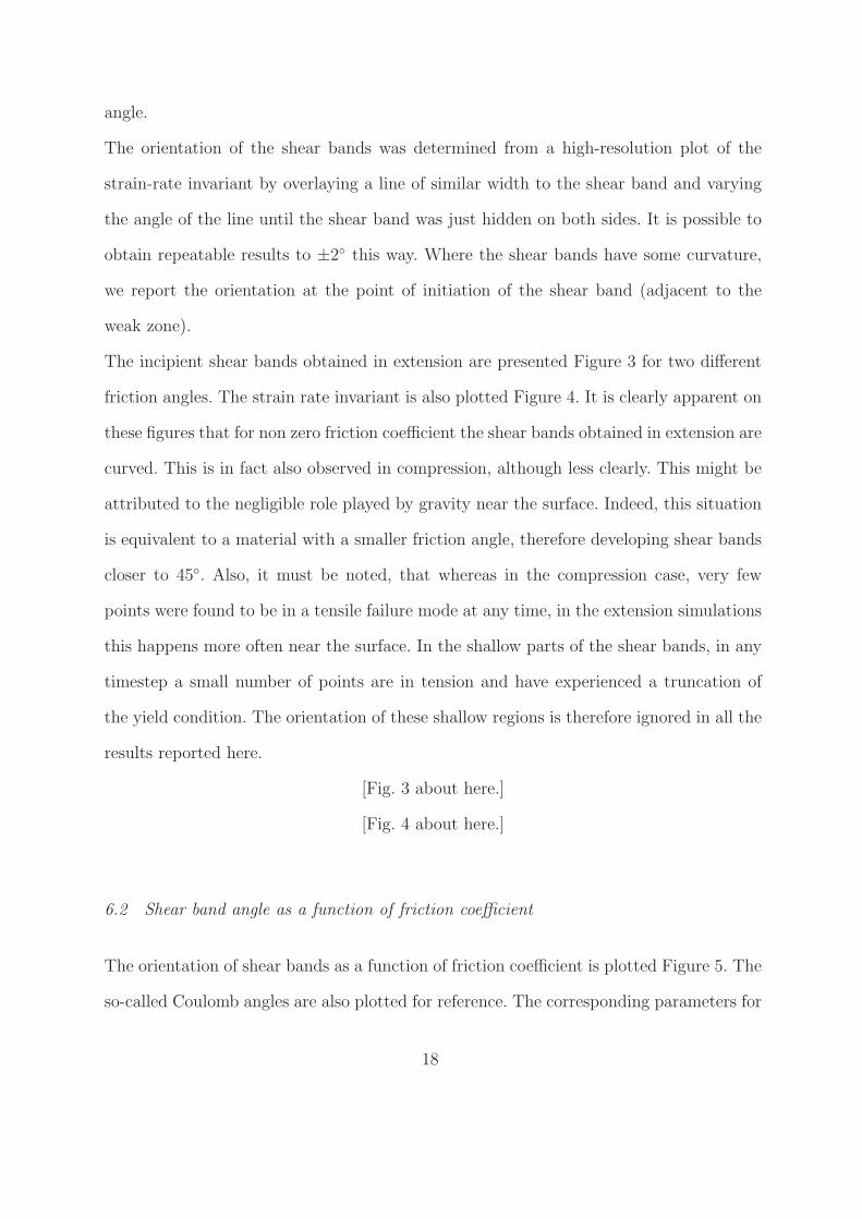
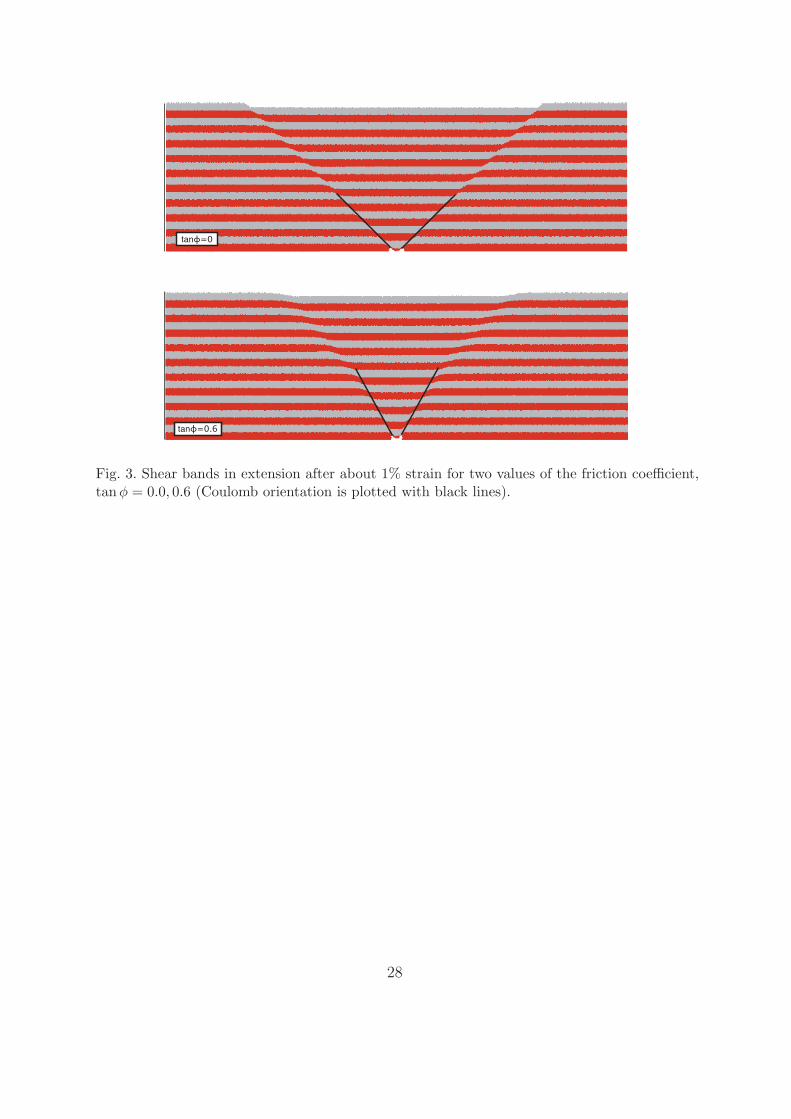
The incipient shear bands obtained in extension are presented Figure 3 for two different

friction angles. The strain rate invariant is also plotted Figure 4. It is clearly apparent on

these figures that for non zero friction coefficient the shear bands obtained in extension are

curved. This is in fact also observed in compression, although less clearly. This might be

attributed to the negligible role played by gravity near the surface. Indeed, this situation

is equivalent to a material with a smaller friction angle, therefore developing shear bands

closer to 45◦. Also, it must be noted, that whereas in the compression case, very few

points were found to be in a tensile failure mode at any time, in the extension simulations

this happens more often near the surface. In the shallow parts of the shear bands, in any

timestep a small number of points are in tension and have experienced a truncation of

the yield condition. The orientation of these shallow regions is therefore ignored in all the

results reported here.

[Fig. 3 about here.]

[Fig. 4 about here.]

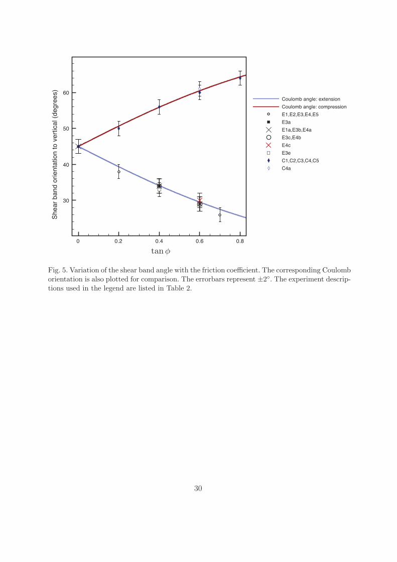
6.2 Shear band angle as a function of friction coefficient

The orientation of shear bands as a function of friction coefficient is plotted Figure 5. The

so-called Coulomb angles are also plotted for reference. The corresponding parameters for

18

these simulations may be found in Table 2.

[Fig. 5 about here.]

The shear-band angles obtained in our simulations follow quite closely the Coulomb angle,

both in extension and compression. This is consistent with the results of the linear stability

analysis, in that the Coulomb angle is an admissible solution for this particular class

of materials. As was discussed in previous sections, the Coulomb angle is not however

the unique potential solution. The reason why this solution is systematically observed is

therefore an important issue that needs to be investigated in future research.

6.3 Ideal plasticity and strain softening behaviour

As the results of the linear stability analysis suggest, the strain softening is not a necessary

condition for the development of shear bands. It is a well established fact that, for non

associated plasticity, shear bands can develop without material softening, including in

the hardening regime, [Rudnicki and Rice, 1975, Hobbs and Muhlhaus, 1990]. As an

illustration, the results of a calculation performed with a constant cohesion are provided

Figure 6. The initiation of shear bands is shown in this figure.

[Fig. 6 about here.]

Using the results provided in Figure 5 and Table 2, it is possible to compare the shear

band angles for various strain softening parameters. It is found that varying the final

cohesion, i.e. varying the relative importance of material softening does not affect the

orientation of macroscopic shear bands.

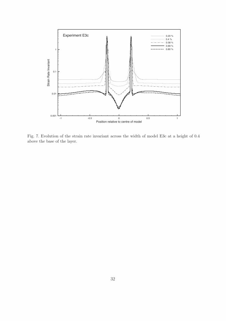
Figure 7 illustrates the growth of shear bands with deformation, and the unloading of the

material outside the shear bands as they take up the deformation and begin to soften.

This series of graphs corresponds to a test in tension (test E3c in Table 2). The strain rate

invariant at a height of 0.4 from the base is shown as a function of horizontal coordinate

19

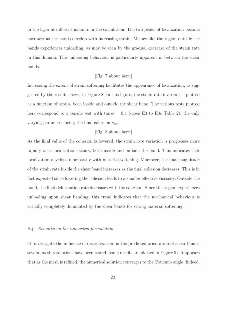
in the layer at different instants in the calculation. The two peaks of localization become

narrower as the bands develop with increasing strain. Meanwhile, the region outside the

bands experiences unloading, as may be seen by the gradual decrease of the strain rate

in this domain. This unloading behaviour is particularly apparent in between the shear

bands.

[Fig. 7 about here.]

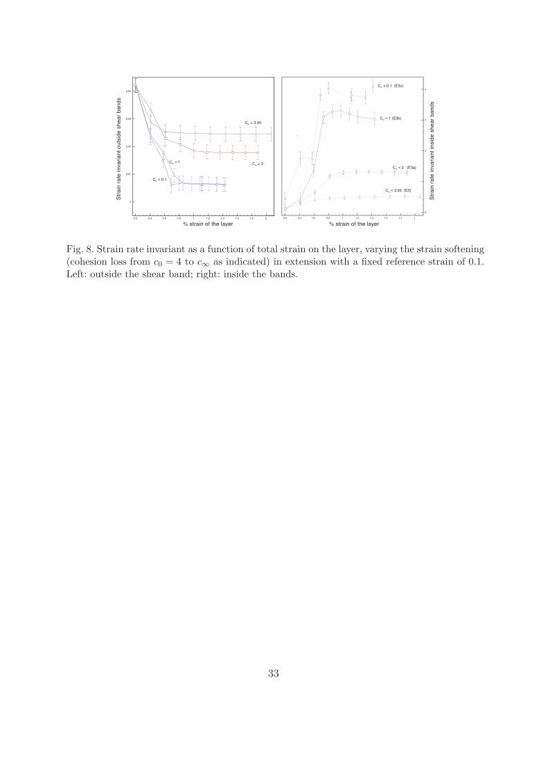
Increasing the extent of strain softening facilitates the appearance of localization, as sug-

gested by the results shown in Figure 8. In this figure, the strain rate invariant is plotted

as a function of strain, both inside and outside the shear band. The various tests plotted

here correspond to a tensile test with tanφ = 0.4 (cases E3 to E3c Table 2), the only

varying parameter being the final cohesion c∞.

[Fig. 8 about here.]

As the final value of the cohesion is lowered, the strain rate variation is progresses more

rapidly once localization occurs, both inside and outside the band. This indicates that

localization develops more easily with material softening. Moreover, the final magnitude

of the strain rate inside the shear band increases as the final cohesion decreases. This is in

fact expected since lowering the cohesion leads to a smaller effective viscosity. Outside the

band, the final deformation rate decreases with the cohesion. Since this region experiences

unloading upon shear banding, this trend indicates that the mechanical behaviour is

actually completely dominated by the shear bands for strong material softening.

6.4 Remarks on the numerical formulation

To investigate the influence of discretization on the predicted orientation of shear bands,

several mesh resolutions have been tested (some results are plotted in Figure 5). It appears

that as the mesh is refined, the numerical solution converges to the Coulomb angle. Indeed,

20

for early results obtained with a coarser mesh (not shown in the previous figure) the shear

band angles were found to be further away from this reference angle.

It has also been reported Sterpi [1999] that in a standard finite element formulation

there is a tendency for localization to follow the mesh lines. This is however not the case

in our present results, since the grid remains uniform throughout the calculation. The

use of Lagrangian points instead of the usual Gauss points for the evaluation of volume

integrals may be an important factor in favouring one orientation over the others in the

non linear range. This could be one parameter that explains why the Coulomb angle is

systematically obtained in our model. Further investigations are clearly needed to draw

reliable conclusions on this point.

It is also important to note that the development of shear bands introduces a strong non

linearity in the numerical solution. The slow convergence associated with the occurrence of

the instability clearly illustrates this fact. Figure 9 is a typical convergence graph obtained

numerically. The tolerance in the non linear solver was set to 10−3.

[Fig. 9 about here.]

In the first two steps, the initiation and development of shear bands make the convergence

rate decrease significantly. Once the shear band are fully developed, the non linear solution

is reached within a few iterations. The significant difference between the initial viscosity

and the effective viscosity within the band introduces strong gradients in the material

properties as localization occurs and softening progresses (typically, up to four or five

orders of magnitude variation from the inside to the outside of the shear band).

7 Conclusion

In an earlier analysis, Moresi et al. [2007a], the present authors did not find a noticeable

variation of the shear band angles with respect to the friction angle when using a Drucker-

21

Prager failure criterion. The numerical simulations considered involved a viscous-plastic

layer of the type described in the present article on top of a viscous layer. This is apparently

in contradiction with the outcome of the present analysis. However, the matter can be

reconciled by a closer inspection at the results shown in this earlier study. We have shown

in the present paper that the mesh must be sufficiently refined in order to capture the

Coulomb orientation numerically. Furthermore, the use of a viscous layer underneath

causes the localization to be less pronounced than in the present work, making the strain

rate invariant field somewhat more diffuse hence a proper estimation of the shear band

angles more difficult to achieve.

In this article, a linear stability analysis has been applied to an incompressible viscous-

plastic material model with a failure criterion of the Drucker-Prager type. The conditions

for the onset of a bifurcation mode in localized shear bands have been derived. It is found

that the so-called Roscoe solution and Coulomb solution are both admissible solutions for

this particular material model. The model has been implemented into the FEM/PIC code

Underworld, in order to assess its numerical behaviour. 2D plane strains extension and

compression examples have been performed. The main outcome of the numerical analysis

is that the predicted shear band angles closely follow the Coulomb orientation. However,

the reason why this solution is favoured numerically over another one is not clear. It

is suggested that the numerical formulation itself, in which the usual Gauss points are

replaced by mobile material points, could be one of the main factors in this observed

behaviour. This will be investigated in future work.

8 Acknowledgements

We acknowledge support of ARC grant DP044997; Underworld software development was

supported by the Australian Computational Earth Systems Simulator and by the Auscope

22

capability of the Australian National Collaborative Research Infractructure Strategy.

A Derivation of the incremental stress tensor

The differentiation of (11) yields:

δσ = 23αp + k

γδD − 2

3αp + k

γ2Dδγ + 2

3αδp + 3δαp + δk

γD − δp1 (A.1)

In the most general case, α and k may depend on the accumulated plastic strain, i.e α =

α (γp) and k = k (γp). However, it is found that the characteristics of the incipients shear

bands are unaffected if one accounts for this dependency on the subsequent calculations.

Thus, for the sake of simplicity, we only present the results derived for α and k constants.

Under this assumption, and without loss of generality, the incremental stress tensor be-

comes:

δσ = 23αp + k

γδD − 2

3αp + k

γ2Dδγ + 2

3αδp

γD − δp1 (A.2)

Considering that (see (7)):

δγ = 2DijδDij

γ(A.3)

We obtain:

δσij = 23αp + k

γ

(

1

2(δilδjk + δikδjl)−

2

γ2DklDij

)

δDkl

+ 23αδp

γDij − δpδij (A.4)

References

J.P. Bardet. A comprehensive review of strain localization in elastoplastic soils. Computers

and geotechnics, 10:163–188, 1990.

23

B. Boroomand and O. C. Zienkiewicz. Recovery by equilibrium in patches (rep). Int. J.

Numer. Methods Eng., 40:137–164, 1997.

S. Buiter, A. Babeyko, S. Ellis, T. Gerya, B. Kaus, A. Kellner, G. Schreurs, and Y. Ya-

mada. The numerical sandbox: comparison of model results for a shortening and an

extension experiment. In S.J.H Buiter and G. Schreurs, editors, Analogue and numer-

ical modelling of crustal-scale processes, volume Special Publication 253, pages 29–64.

Geological Society, London, 2006.

R. de Borst. Bifurcations in finite element models with a non-associated flow law. Int. j.

for num. and anal. methods in geomechanics, 12:99–116, 1988.

J. Desrues. Limitations du choix de l’angle de frottement pour le critere de plasticite de

drucker-prager. Revue francaise de genie civil, 6:853–862, 2002.

B.E. Hobbs and A. Muhlhaus, H.-B. Ord. Instability, softening and localization of defor-

mation. In R.J. Knipe and E.H Rutter, editors, Deformations mechanisms, rheology and

tectonics, volume Special Publication 54, pages 143–165. Geological Society, London,

1990.

A. Lenardic, L. Moresi, and H. Muhlhaus. The role of mobile belts for the longevity of

deep cratonic lithosphere: The crumple zone model. Geophysical Research Letters, 27:

1235–1238, 2000.

L. Moresi and H.-B. Muhlhaus. Anisotropic viscous models of large-deformation Mohr-

Coulomb failure. Philosophical Magazine, 86:3287–3305, 2006.

L. Moresi, F. Dufour, and H. B. Muhlhaus. A lagrangian integration point finite ele-

ment method for large deformation modeling of viscoelastic geomaterials. Journal Of

Computational Physics, 184:476–497, 2003.

L. Moresi, H.-B. Muhlhaus, V. Lemiale, and D. May. Incompressible viscous formula-

tions for deformation and yielding of the lithosphere. In G.D. Karner, G. Manatschal,

24

and L. Pinheiro, editors, imaging, mapping, and modelling extensional processes and

systems, volume Special Publication 282, pages 457–472. Geological Society, London,

2007a. doi: 10.1144/SP282.19.

L. Moresi, S. Quenette, V. Lemiale, C. Meriaux, W. Appelbe, and Muhlhaus. Computa-

tional approaches to studying non-linear dynamics of the crust and mantle. Physics of

the Earth and Planetary Interiors, 163:69–82, 2007b. doi: 10.1016/j.pepi.2007.06.009.

A. Needleman. Non-normality and bifurcation in plane strain tension and compression.

J. Mech. Phys. Sol., 27:231–254, 1979.

J. W. Rudnicki and J. R. Rice. Conditions for the localization of deformation in pressure

sensitive dilatant materials. J. Mech. Phys. Solids, 23:371–394, 1975.

D. Sterpi. An analysis of geotechnical problems involving strain softening effects. Int. j.

for num. and anal. methods in geomechanics, 23:1427–1457, 1999.

I. Vardoulakis. Shear band inclination and shear modulus of sand in biaxial tests. Int. j.

for num. and anal. methods in geomechanics, 4:103–119, 1980.

I. Vardoulakis and J. Sulem. Bifurcation Analysis in Geomechanics. Blackie Academics

and Professional, 1995.

I. Vardoulakis, M. Goldscheider, and Gudehus. Formation of shear band in sand bodies

as a bifurcation problem. Int. j. for num. and anal. methods in geomechanics, 2:99–128,

1978.

P.A. Vermeer. The orientation of shear bands in biaxial tests. Geotechnique, 40:223–236,

1990.

P.A. Vermeer and R. de Borst. Non-associated plasticity for soils, concrete and rock.

Heron, pages 1–64, 1984.

25

tan!=0.2

tan!=0.8

Fig. 1. Shear bands in compression after approximately 1% strain for two values of the frictioncoefficient (Coulomb orientation is plotted with black lines).

26

tan!=0.2

tan!=0.8

0 10

Fig. 2. Comparison of the strain rate invariant at the fifth timestep, in compression for frictioncoefficients of tanφ = 0.2, 0.8 (Coulomb orientation is plotted with black lines).

27

tan!=0

tan!=0.6

Fig. 3. Shear bands in extension after about 1% strain for two values of the friction coefficient,tanφ = 0.0, 0.6 (Coulomb orientation is plotted with black lines).

28

tan!=0

tan!=0.6

0 2

Fig. 4. Comparison of the strain rate invariant in the fifth timestep, in extension for two differentfriction coefficients, tanφ = 0.0, 0.6 (Coulomb orientation is plotted with black lines).

29

0 0.2 0.4 0.6 0.8

30

40

50

60

y=0.5 * 180/pi * atan(1/x) (0-1,1001)

y=90-0.5 * 180/pi * atan(1/x) (0-1,1001)

Extension C=4; Cinf=3.95

Extension C=4; Cinf=3.0

Extension C=4; Cinf=1.0

Extension C=4; Cinf=0.1

Extension C=6; Cinf=1.0

Extension C=4; high res

Compression C=20; Cinf=10.0

Compression C=20; Cinf=20.0

tanφ

Coulomb angle: extension

Coulomb angle: compression

E1,E2,E3,E4,E5

E3a

E1a,E3b,E4a

E3c,E4b

E4c

E3e

C1,C2,C3,C4,C5

C4a

Sh

ea

r b

an

d o

rie

nta

tio

n t

o v

ert

ica

l (d

eg

ree

s)

Fig. 5. Variation of the shear band angle with the friction coefficient. The corresponding Coulomborientation is also plotted for comparison. The errorbars represent ±2◦. The experiment descrip-tions used in the legend are listed in Table 2.

30

tan!=0.6

0 10

Fig. 6. Illustration of shear band formation in compression for a constant cohesion of 20. Upperfigure: strain rate invariant; lower figure: initiation of shear bands. Also plotted on these figuresis the Coulomb orientation (black lines).

31

-1 -0.5 0 0.5 1

Position relative to centre of model

0.001

0.01

0.1

1S

train

Rate

Invariant

0.20 %

0.4 %

0.58 %

0.69 %

0.80 %

Experiment E3c

Fig. 7. Evolution of the strain rate invariant across the width of model E3c at a height of 0.4above the base of the layer.

32

0.2 0.4 0.6 0.8 1 1.2 1.4 1.6 1.8 2

% extension

0

0.01

0.02

0.03

0.04

Str

ain

rate

invariant

outs

ide s

hear

bands

Mu4 background

Mu4-Cs3 background

Mu4-Cs01 background

Mu4-Cs1 background

0.2 0.4 0.6 0.8 1 1.2 1.4 1.6 1.8 2

% extension

0

1

2

3

4

Str

ain

rate

invariant

in s

hear

bands

C! = 0.1

C! = 1 C

! = 3

C! = 3.95

% strain of the layer

C! = 0.1 (E3c)

C! = 1 (E3b)

C! = 3 (E3a)

C! = 3.95 (E3)

% strain of the layer

Str

ain

ra

te in

va

ria

nt

ou

tsid

e s

he

ar

ba

nd

s

Str

ain

ra

te in

va

ria

nt

insid

e s

he

ar

ba

nd

s

Fig. 8. Strain rate invariant as a function of total strain on the layer, varying the strain softening(cohesion loss from c0 = 4 to c∞ as indicated) in extension with a fixed reference strain of 0.1.Left: outside the shear band; right: inside the bands.

33

1 2 3 4 5 6 7 8 9 10 11 12 13 14 15 16 17 18 19

Timestep

0.001

0.01

0.1N

on-lin

ear

itera

tion r

esid

ual

Fig. 9. Convergence graph for tanφ = 0.6 in compression. The tolerance of the non linear solveris set to 0.001 but is also set to truncate after 25 iterations. Truncation is observed in the firsttwo timesteps but stops once the shear bands are locked in place by strain softening.

34

Parameter Symbol Value

Length scale extension(initial sample length) L 3

Length scale (initial sample length) 4

Thickness of sample layer d 0.8

Thickness of accommodation layer da 0.2

Weak zone size - 0.04 x 0.04

Velocity scale extension (boundary condition) V 0.05

Velocity scale compression (boundary condition) 0.5

Gravitational acceleration g 10

Density of viscous accommodation layer ρa 0

Density of viscoplastic layer ρ 1

Viscosity of accommodation layer ηa 0.01

Viscosity of viscoplastic layer η 100

Viscosity of weak zone ηw 1

Reference cohesion (extension) c 4

Reference cohesion (compression) 20

Friction coefficient (range) tanϕ 0 – 0.8

Minimum yield stress (cutoff) τmin 0.001

Reference strain measure γ0 0.1

Table 1Material and geometrical parameters common to the range of models.

35

Experiment Mode Resolution Initial x x y tanφ C0 C∞ θ ± 2◦

E1 Extension 384x128 3.0 x 1.0 0.0 4.0 3.95 45

E1a 384x128 3.0 x 1.0 0.0 4.0 1.0 45

E2 384x128 3.0 x 1.0 0.2 4.0 3.95 38

E3 384x128 3.0 x 1.0 0.4 4.0 3.95 34

E3a 384x128 3.0 x 1.0 0.4 4.0 3.0 34

E3b 384x128 3.0 x 1.0 0.4 4.0 1.0 34

E3c 384x128 3.0 x 1.0 0.4 4.0 0.1 34

E3d 192x64 3.0 x 1.0 0.4 4.0 1.0 34 (±3◦)

E3e 768x256 3.0 x 1.0 0.4 4.0 1.0 33

E4 384x128 3.0 x 1.0 0.6 4.0 3.95 29

E4a 384x128 3.0 x 1.0 0.6 4.0 1.0 29

E4b 384x128 3.0 x 1.0 0.6 4.0 0.1 29

E4c 384x128 3.0 x 1.0 0.6 6.0 1.0 30

E5 384x128 3.0 x 1.0 0.7 4.0 3.95 26

C1 Compression 384x128 4.0 x 1.0 0.0 20.0 10.0 45

C2 384x128 4.0 x 1.0 0.2 20.0 10.0 50

C2a 384x128 4.0 x 1.0 0.2 20.0 1.0 50

C3 384x128 4.0 x 1.0 0.4 20.0 10.0 56

C4 384x128 4.0 x 1.0 0.6 20.0 10.0 60

C4a 384x128 4.0 x 1.0 0.6 20.0 20.0 61

C5 384x128 4.0 x 1.0 0.8 20.0 10.0 64

Table 2Numerical and material parameters for each configuration of the extension and compressionexamples. θ is the measured angle of the shear bands at the point of the perturbation, takingthe average value for the two shear bands.

36