a boundary condition capturing method for incompressible flame discontinuities
TRANSCRIPT
Journal of Computational Physics172,71–98 (2001)
doi:10.1006/jcph.2001.6812, available online at http://www.idealibrary.com on
A Boundary Condition Capturing Methodfor Incompressible Flame Discontinuities1
Duc Q. Nguyen,∗ Ronald P. Fedkiw,† and Myungjoo Kang∗∗Department of Mathematics, University of California Los Angeles, Los Angeles, California 90095;
and†Computer Science Department, Stanford University, Stanford, California 94305E-mail: †[email protected]
Received June 26, 2000; revised April 5, 2001
In this paper, we propose a new numerical method for treating two-phase incom-pressible flow where one phase is being converted into the other, e.g., the vaporizationof liquid water. We consider this numerical method in the context of treating dis-continuously thin flame fronts for incompressible flow. This method was designedas an extension of the Ghost Fluid Method (1999,J. Comput. Phys.152, 457) andrelies heavily on the boundary condition capturing technology developed in Liuet al. (2000,J. Comput. Phys.154, 15) for the variable coefficient Poisson equationand in Kanget al. (in pressJ. Comput. Phys.) for multiphase incompressible flow.Our new numerical method admits a sharp interface representation similar to themethod proposed in Helenbrooket al. (1999,J. Comput. Phys.148, 366). Since theinterface boundary conditions are handled in a simple and straightforward fashion,the code is very robust, e.g. no special treatment is required to treat the merging offlame fronts. The method is presented in three spatial dimensions, with numericalexamples in one, two, and three spatial dimensions.c© 2001 Academic Press
1. INTRODUCTION
Consider multiphase incompressible flow including the effects of viscosity, surface ten-sion, and gravity. Any numerical approach to this problem needs both a method for tracking(or capturing) the interface location as well as a method for enforcing the appropriate bound-ary conditions at the tracked interface. See [1, 19, 23] (and [2]) for numerical methods thatused front tracking, volume of fluid and level set methods, respectively, for tracking thelocation of the multiphase interface. All of these methods use aδ-function formulation toenforce the appropriate boundary conditions at the multiphase interface. Thisδ-function for-mulation was originally proposed as part of the “immersed boundary” method for computing
1 Research supported in part by ONR N00014-97-1-0027.
71
0021-9991/01 $35.00Copyright c© 2001 by Academic Press
All rights of reproduction in any form reserved.
72 NGUYEN, FEDKIW, AND KANG
solutions to the incompressible Navier–Stokes equations in the presence of a submersedelastic interface; see [16, 17]. The numerical methods in [1, 2, 19, 23] all extend theδ-function formulation of [16] to treat multiphase incompressible flow.
One drawback of theδ-function formulation is that it smears out numerical quantitiesacross the interface producing a continuous profile for the density, viscosity, and pressure.This numerical smearing can be problematic, e.g., a continuous pressure profile does notadequately model surface tension forces and [1, 2, 19, 23] need to add source terms to theright-hand side of the momentum equations in order to numerically model these forces. Analternative strategy for enforcing the interface boundary conditions is based on the GhostFluid Method (GFM) of [4]. In [13], the authors extended the GFM to treat the variablecoefficient Poisson equation in the presence of an immersed interface. In [12], the authorsused the method from [13] to devise a numerical method for multiphase incompressibleflow that allows for a nonsmeared numerical representation of the density, viscosity, andpressure. Moreover, since surface tension was modeled directly with a jump in pressureacross the interface, there was no need to add source terms to the right-hand side of themomentum equations as was done in [1, 2, 19, 23].
For multiphase incompressible flow, the interface moves with local fluid velocity onlyand individual fluid particles do not cross the interface. In this paper, we consider interfaceswhere a reaction is taking place and the interface moves with the local unreacted fluidvelocity plus a reaction term that accounts for the conversion of one fluid into the other.That is, we account for the movement of material across the interface. Consider, for example,an interface separating liquid and gas regions where the liquid is actively vaporizing intothe gaseous state. See [11] for a front tracking approach to this problem using aδ-functionformulation to treat the interface boundary conditions. See [22] and [24] for level set basedand volume of fluid based (respectively) approaches to this same problem also using aδ-function formulation. References [11, 22, 24] solve an equation for the temperature inorder to determine the rate at which one material is converted into another.
As another example of reacting interfaces, consider combustion in premixed flames.Assuming that the flame front is infinitely thin allows one to treat the flame front as a dis-continuity separating two incompressible flows. The unreacted material undergoes reactionas it crosses the interface producing a lower density (higher volume) reacted material. See[20] for a front tracking approach to this problem using aδ-function formulation. The flamespeeds in [20] were determined with the aid of the G-equation [14, 25], so an extra equationfor the temperature was not needed.
In the examples mentioned above, the density of the incompressible material tends to bedifferent on different sides of the interface. The material must instantaneously expand as itcrosses the interface implying that the normal velocity is discontinuous across the interface,i.e. in addition to discontinuity of the density, viscosity, and pressure. The methods in [11,20, 22, 24] are all based on theδ-function formulation and thus smear out this velocity jumpforcing a continuous velocity field across the interface. This can be quite problematic sincethis numerical smearing adds a compressible character to the flow field near the interface, i.e.the divergence-free condition is not exactly satisfied in each separate subdomain. In addition,difficulties arise when trying to determine the interface velocity which depends in part onthe local velocity of the unreacted material. Near the interface, the velocity of the unreactedmaterial contains largeO(1) numerical errors where it has been nonphysically forced tobe continuous with the velocity of the reacted material. Partial solutions to these problemswere proposed in [9] where the authors were able to remove the numerical smearing of the
BOUNDARY CONDITION CAPTURING METHOD 73
normal velocity obtaining a sharp interface profile. Unfortunately, the interface treatment in[9] was considerably intricate and the calculation had to be terminated if two flame frontswere significantly close to each other, i.e. this method cannot handle the simple merging offlame discontinuities. On the other hand, this method was used to obtain rather impressiveresults in [10] for problems in which the flame fronts do not merge or become highly curved.
In this paper, we propose a new numerical method for treating two-phase incompressibleflow where one phase is being converted into the other. This method was designed as anextension of the Ghost Fluid Method [4] and relies heavily on the boundary conditioncapturing technology developed in [13] for the variable coefficient Poisson equation and in[12] for multiphase incompressible flow. Our new numerical method admits a sharp interfacerepresentation similar to the method proposed in [9]. In addition, the interface boundaryconditions are handled in a simple and straightforward fashion making the code very robust,e.g., no special treatment is required to treat the merging of flame fronts. Numerical resultsare presented in one, two, and three spatial dimensions.
2. EQUATIONS
2.1. Euler Equations
The basic equations for inviscid incompressible flow are
ρt + EV · ∇ρ = 0 (1)
ut + EV · ∇u+ px
ρ= 0 (2)
vt + EV · ∇v + py
ρ= 0 (3)
wt + EV · ∇w + pz
ρ= 0, (4)
wheret is the time, (x, y, z) are the spatial coordinates,ρ is the density,EV = 〈u, v, w〉 isthe velocity field,p is the pressure, and∇ = 〈 ∂
∂x ,∂∂y ,
∂∂z〉. In addition, the divergence-free
condition is∇ · EV = 0. The equations for the velocities can be written in condensed notationas a row vector
EV + ( EV · ∇) EV + ∇ p
ρ= 0. (5)
2.2. Interface Velocity
When treating multiphase incompressible flow, one needs an expression for the velocity,EW, of the interface. If the interface is a simple contact discontinuity, then the interfacemoves with the local fluid velocity only, i.e.,EW = EV . Many numerical methods use onlythe normal velocity of the interface, i.e.,EW = D EN whereD is the normal component ofthe interface velocity andEN=〈n1, n2, n3〉 is the local unit normal to the interface. In thecase of a contact discontinuity,D = VN = EV · EN.
Throughout this text,unreactedand reactedincompressible flows are separated by aninterface across which the unreacted material is converted into the reacted material. The “u”and “r ” subscripts are used to refer to the unreacted and reacted materials, respectively. Thenormal component of the interface velocity is calculated by adding the unreacted local fluid
74 NGUYEN, FEDKIW, AND KANG
velocity to the flame speed,S. That is,D = (VN)u + Swhere(VN)u is calculated using thevelocity of the unreacted material only. This is important to note sinceVN is discontinuousacross the interface.
In the numerical examples, the flame speed is defined asS= So + σκ, whereSo andσare constants andκ is the local curvature of the interface.
2.3. Jump Conditions
Conservation of mass and momentum implies the standard Rankine–Hugoniot jumpconditions across the interface
[ρ(VN − D)] = 0 (6)[ρ(VN − D)2+ p
] = 0, (7)
where [A] = Ar − Au defines “[·]” as the jump in a quantity across the interface. WhenD 6= VN , the tangential velocities are continuous as well, i.e., [VT1] = [VT2] = 0, whereT1
andT2 are the unit tangent vectors. This is true as long asS 6= 0, i.e., it is true as long asthe front is not a contact discontinuity. In the case of a contact discontinuity,S= 0 andthe tangential velocities are completely uncoupled across the interface reducing equations6 and 7 to [VN ] = [ p] = 0. For more details, see [5].
Denoting the mass flux in the moving reference frame (speedD) by
M = ρr ((VN)r − D) = ρu((VN)u − D) (8)
allows Eq. (6) to be rewritten as [M ] = 0. Furthermore,
M = −ρuS (9)
follows from substitutingD = (VN)u + S into Eq. (8).Starting with [D] = 0, [
ρVN − ρ(VN − D)
ρ
]= 0 (10)[
ρVN − M
ρ
]= 0 (11)
and
[VN ] = M
[1
ρ
], (12)
where the last equation follows since [M ] = 0. It is more convenient to write
[ EV ] = M
[1
ρ
]EN (13)
as a summary of Eq. (12) and [VT1] = [VT2] = 0. Taking the dot product of Eq. (13) andENresults in Eq. (12), while taking the dot product of Eq. (13) andET1 or ET2, results in [VT1] = 0and [VT2] = 0, respectively.
Equation (7) can be rewritten as[M2
ρ+ p
]= 0 (14)
BOUNDARY CONDITION CAPTURING METHOD 75
or as
[ p] = −M2
[1
ρ
](15)
again using [M ] = 0.
2.4. Level Set Equation
The level set equation
φt + EW · ∇φ = 0 (16)
is used to keep track of the interface location as the set of points whereφ = 0. The unreactedand reacted materials are then designated by the points whereφ > 0 andφ ≤ 0, respectively.Usingφ ≤ 0 instead ofφ = 0 for the reacted points removes the measure zero ambiguityof points that happen to lie on the interface. In this sense, the numerical interface lies inbetweenφ = 0 and the positive values ofφ and can be located numerically by finding thezero level ofφ. To keep the values ofφ close to those of a signed distance function, i.e.,|∇φ| = 1, the reinitialization equation
φτ + S(φo)(|∇φ| − 1) = 0 (17)
is iterated for a few steps in ficticious time,τ . The level set function is used to compute thenormal
EN = ∇φ|∇φ| (18)
and the curvature
κ = −∇ · EN (19)
in a standard fashion. For more details on the level set function, see [4, 12, 15, 19].
3. NUMERICAL METHOD
A standard MAC grid is used for discretization, wherepi, j,k, ρi, j,k andφi, j,k exist at thecell centers (grid points) andui±1/2, j,k, vi, j±1/2,k, andwi, j,k±1/2 exist at the appropriate cellwalls. See [7] and [18] for more details.
3.1. Extending the Velocity Field
Since the normal velocity is discontinuous across the interface, one has to use cautionwhen applying numerical discretizations near the interface. For example, when discretizingthe unreacted fluid velocity near the interface, one should avoid using values of the reactedfluid velocity. Following the Ghost Fluid Methodology in [4], a band of ghost cells on thereacted side of the interface is populated with unreacted ghost velocities that can be usedin the discretization of the unreacted fluid velocity. Similarly, reacted ghost velocities aredefined on a band of ghost cells on the unreacted side of the interface and used in thediscretization of the reacted fluid velocity.
76 NGUYEN, FEDKIW, AND KANG
The termφ is defined at the grid nodes, and its values on the offset MAC grid are computedwith simple averaging, e.g.,φi+1/2, j,k = φi, j,k +φi+1, j,k
2 . The MAC grid values ofφ can thenbe used to determine which values of the velocity field correspond to unreacted materialand which correspond to reacted material. At each MAC grid location that corresponds toa reacted fluid velocity, the jump conditions in Eq. (13) are used to define a new unreactedghost velocity according to
uGu = ur − M
(1
ρr− 1
ρu
)n1 (20)
vGu = vr − M
(1
ρr− 1
ρu
)n2 (21)
and
wGu = wr − M
(1
ρr− 1
ρu
)n3, (22)
wheren1, n2, andn3 are computed at the appropriate MAC grid locations using simpleaveraging, e.g.,(n1)i+1/2, j,k = (n1)i, j,k + (n1)i+1, j,k
2 . Similarly, reacted ghost velocities are cal-culated at unreacted MAC grid locations using
uGr = uu + M
(1
ρr− 1
ρu
)n1 (23)
vGr = vu + M
(1
ρr− 1
ρu
)n2 (24)
and
wGr = wu + M
(1
ρr− 1
ρu
)n3. (25)
3.2. Level Set Equation
The level set function is evolved in time fromφn toφn+1 using nodal velocities,EW = D EN,where EN is computed at each grid node using Eq. (18) as described in [12]. In general,D =(VN)u + Swhere(VN)u is the normal velocity of the unreacted material andS= So + σκis the flame speed. IfS depends on the local curvature of the front, i.e.,σ 6= 0, then EW issplit into a purely convective componentEWc = ((VN)u + So) EN and a curvature componentσκ EN so that Eq. (16) can be rewritten as
φt + EWc · ∇φ = −σκ|∇φ|, (26)
with the curvature term isolated on the right-hand side. Thenκ is discretized according toEq. (19) as discussed in [12], and|∇φ| is discretized with standard central differencing.It is interesting to note that an alternate definition ofEWc = EVu + So EN can be used in Eq.(26) as well. Both of the two nonequivalent definitions ofEWc give the same result in thedot product EWc. ∇φ since they only differ in the direction tangential to∇φ.
The normal velocity of the unreacted material,(VN)u, is needed in a band about thefront so that Eq. (26) can be solved locally to update the interface location. The nodalvalues of the unreacted velocity,EVu, are determined using simple averaging of the MAC
BOUNDARY CONDITION CAPTURING METHOD 77
grid values making use of the appropriate ghost values (defined above) where needed, i.e.,ui, j,k = ui−1/2, j,k + ui+1/2, j,k
2 , vi, j,k = vi, j−1/2,k + vi, j+1/2,k
2 , andwi, j,k = wi, j,k−1/2+wi, j,k+1/2
2 are used tocalculate the nodal values of the unreacted velocity. Then(VN)u = EVu · EN is used to definethe unreacted normal velocity at each grid node.
Detailed discretizations for the convective part of Eq. (26), i.e.,EWc · ∇φ, and for Eq. (17)are given in [4]. Note that the fifth-order WENO discretization from [4] is used to discretizethe convective part of Eq. (26) and the spatial terms in Eq. (17) for the numerical examplesin this paper.
3.3. Projection Method
First, EV∗ = 〈u∗, v∗, w∗〉 is defined by
EV∗ − EVn
1t+ ( EV · ∇) EV = 0, (27)
and then the velocity field at the new time step,EVn+1 = 〈un+1, vn+1, wn+1〉, is defined by
EVn+1− EV∗1t
+ ∇ p
ρ= 0, (28)
so that combining Eqs. 27 and 28 to eliminateEV∗ results in Eq. (5). Taking the divergenceof Eq. (28) gives
∇ ·(∇ p
ρ
)= ∇ ·
EV∗1t
(29)
after setting∇ · EVn+1 to zero. Equations (28) and (29) can be rewritten as
EVn+1− EV∗ + ∇ p∗
ρ= 0 (30)
and
∇ ·(∇ p∗
ρ
)= ∇ · EV∗ (31)
eliminating their dependence on1t by using a scaled pressure,p∗ = p1t . See [3, 7, 18]for more details.
3.4. Convection Terms
The MAC grid storesu values atExi±1/2, j,k. Updatingu∗i±1/2, j,k in Eq. (27) requires thediscretization ofEV · ∇u at Exi±1/2, j,k. First, simple averaging can be used to defineEV atExi±1/2, j,k, i.e.,
vi+ 12 , j,k=vi, j− 1
2 ,k+ vi, j+ 1
2 ,k+ vi+1, j− 1
2 ,k+ vi+1, j+ 1
2 ,k
4(32)
78 NGUYEN, FEDKIW, AND KANG
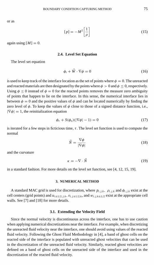
FIG. 1. Stationary flame.
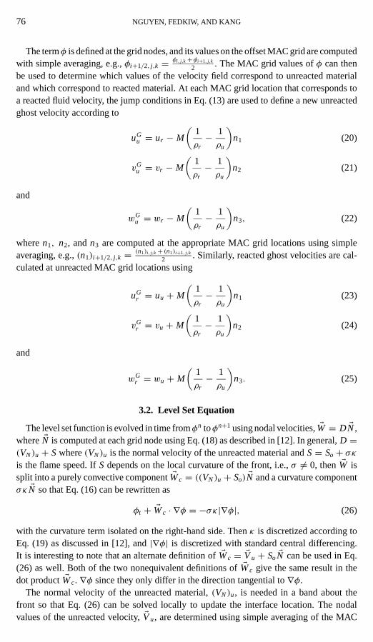
FIG. 2. Stationary flame with a poor choice of initial data.
BOUNDARY CONDITION CAPTURING METHOD 79
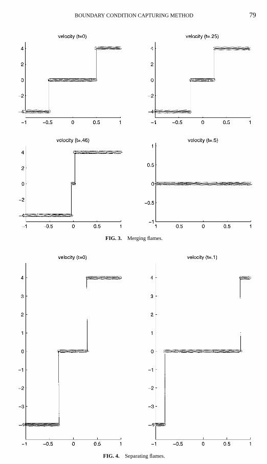
FIG. 3. Merging flames.
FIG. 4. Separating flames.

80 NGUYEN, FEDKIW, AND KANG
FIG. 5. Merging planar flames in two spatial dimensions.
and
wi+ 12 , j,k=wi, j,k− 1
2+ wi, j,k+ 1
2+ wi+1, j,k− 1
2+ wi+1, j,k+ 1
2
4(33)
definev andw at Exi+1/2, j,k while u is already defined there. Then theEV · ∇u term on theoffsetExi±1/2, j,k grid can be discretized in the same fashion as theEV · ∇φ term on the regularExi, j,k grid using the method outlined in [4] for Eq. (16). The termsv∗i, j±1/2,k andw∗i, j,k±1/2
are updated in a similar manner. For more details, see [12]. Note that the third-order ENOdiscretization from [4] is used in the examples section.
It is important to note that the ghost values of the extended velocity field are used inthis discretization ofEV∗. That is, unreacted fluid velocities are discretized with the aid ofthe unreacted ghost velocities avoiding the use of any reacted velocities that would pollutethe solution. Similarly, the reacted fluid velocities are discretized using their ghost valuesavoiding the unreacted fluid velocities in the discretization.
Once again, using the GFM philosophy [4], values forEV∗u and EV∗r are determined on theappropriate side of the interfaceandon a band including the interface. For example,EV∗u iscomputed on both the unreacted side of the interface and on a band of ghost cells on thereacted side of the interface. This is done to alleviate problems that occur when the interfacemoves through the grid, changing the character of the solution from unreacted to reacted or
BOUNDARY CONDITION CAPTURING METHOD 81
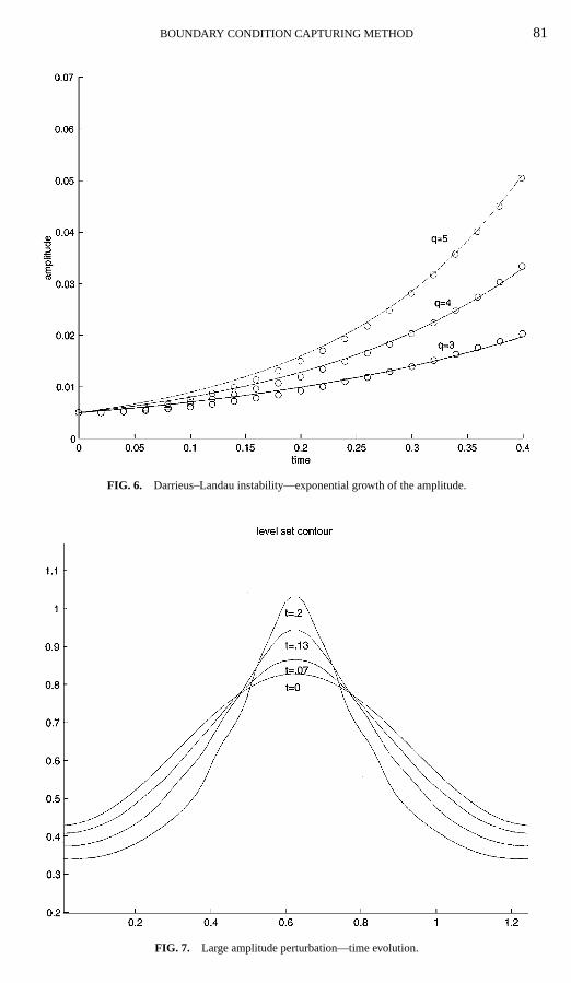
FIG. 6. Darrieus–Landau instability—exponential growth of the amplitude.
FIG. 7. Large amplitude perturbation—time evolution.
82 NGUYEN, FEDKIW, AND KANG
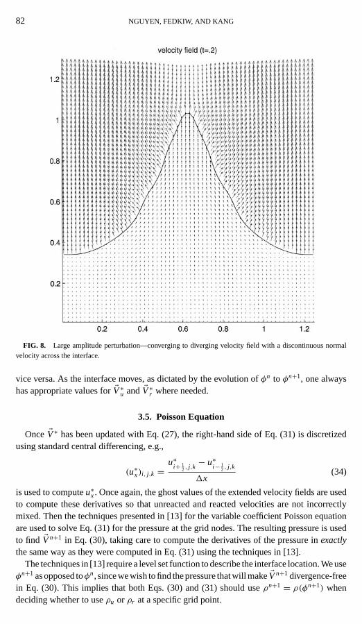
FIG. 8. Large amplitude perturbation—converging to diverging velocity field with a discontinuous normalvelocity across the interface.
vice versa. As the interface moves, as dictated by the evolution ofφn to φn+1, one alwayshas appropriate values forEV∗u and EV∗r where needed.
3.5. Poisson Equation
Once EV∗ has been updated with Eq. (27), the right-hand side of Eq. (31) is discretizedusing standard central differencing, e.g.,
(u∗x)i, j,k =u∗
i+ 12 , j,k− u∗
i− 12 , j,k
1x(34)
is used to computeu∗x. Once again, the ghost values of the extended velocity fields are usedto compute these derivatives so that unreacted and reacted velocities are not incorrectlymixed. Then the techniques presented in [13] for the variable coefficient Poisson equationare used to solve Eq. (31) for the pressure at the grid nodes. The resulting pressure is usedto find EVn+1 in Eq. (30), taking care to compute the derivatives of the pressure inexactlythe same way as they were computed in Eq. (31) using the techniques in [13].
The techniques in [13] require a level set function to describe the interface location. We useφn+1 as opposed toφn, since we wish to find the pressure that will makeEVn+1 divergence-freein Eq. (30). This implies that both Eqs. (30) and (31) should useρn+1 = ρ(φn+1) whendeciding whether to useρu or ρr at a specific grid point.
BOUNDARY CONDITION CAPTURING METHOD 83
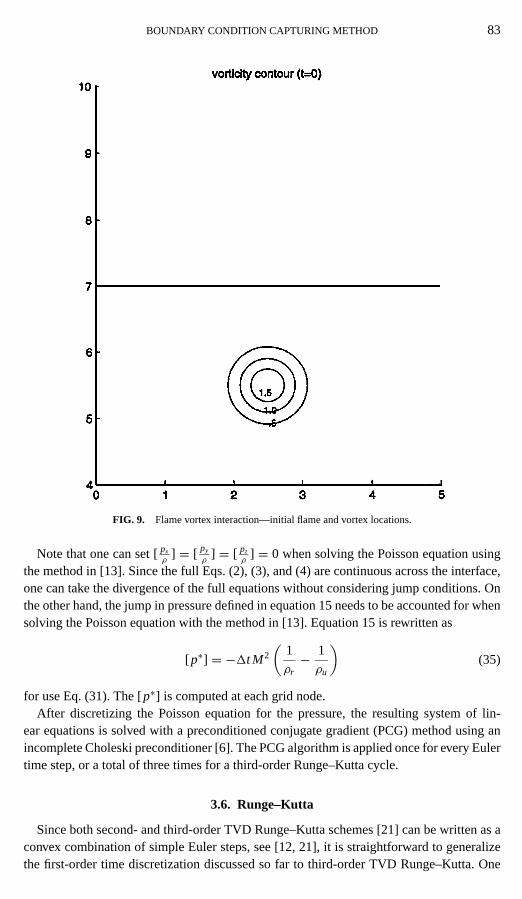
FIG. 9. Flame vortex interaction—initial flame and vortex locations.
Note that one can set [px
ρ] = [ py
ρ] = [ pz
ρ] = 0 when solving the Poisson equation using
the method in [13]. Since the full Eqs. (2), (3), and (4) are continuous across the interface,one can take the divergence of the full equations without considering jump conditions. Onthe other hand, the jump in pressure defined in equation 15 needs to be accounted for whensolving the Poisson equation with the method in [13]. Equation 15 is rewritten as
[ p∗] = −1t M2
(1
ρr− 1
ρu
)(35)
for use Eq. (31). The [p∗] is computed at each grid node.After discretizing the Poisson equation for the pressure, the resulting system of lin-
ear equations is solved with a preconditioned conjugate gradient (PCG) method using anincomplete Choleski preconditioner [6]. The PCG algorithm is applied once for every Eulertime step, or a total of three times for a third-order Runge–Kutta cycle.
3.6. Runge–Kutta
Since both second- and third-order TVD Runge–Kutta schemes [21] can be written as aconvex combination of simple Euler steps, see [12, 21], it is straightforward to generalizethe first-order time discretization discussed so far to third-order TVD Runge–Kutta. One
84 NGUYEN, FEDKIW, AND KANG
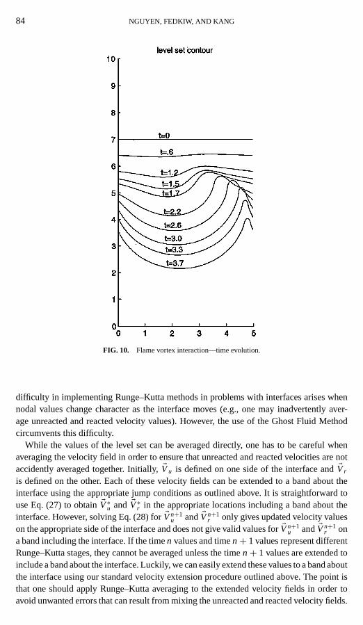
FIG. 10. Flame vortex interaction—time evolution.
difficulty in implementing Runge–Kutta methods in problems with interfaces arises whennodal values change character as the interface moves (e.g., one may inadvertently aver-age unreacted and reacted velocity values). However, the use of the Ghost Fluid Methodcircumvents this difficulty.
While the values of the level set can be averaged directly, one has to be careful whenaveraging the velocity field in order to ensure that unreacted and reacted velocities are notaccidently averaged together. Initially,EVu is defined on one side of the interface andEVr
is defined on the other. Each of these velocity fields can be extended to a band about theinterface using the appropriate jump conditions as outlined above. It is straightforward touse Eq. (27) to obtainEV∗u and EV∗r in the appropriate locations including a band about theinterface. However, solving Eq. (28) forEVn+1
u and EVn+1r only gives updated velocity values
on the appropriate side of the interface and does not give valid values forEVn+1u and EVn+1
r ona band including the interface. If the timen values and timen+ 1 values represent differentRunge–Kutta stages, they cannot be averaged unless the timen+ 1 values are extended toinclude a band about the interface. Luckily, we can easily extend these values to a band aboutthe interface using our standard velocity extension procedure outlined above. The point isthat one should apply Runge–Kutta averaging to the extended velocity fields in order toavoid unwanted errors that can result from mixing the unreacted and reacted velocity fields.
BOUNDARY CONDITION CAPTURING METHOD 85
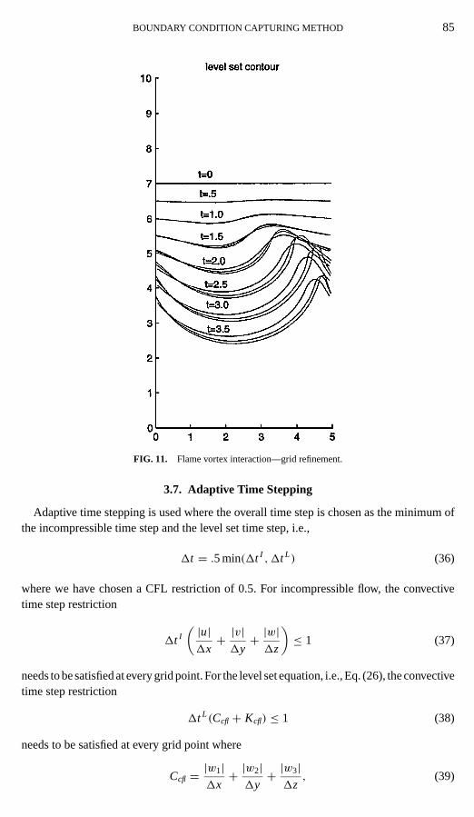
FIG. 11. Flame vortex interaction—grid refinement.
3.7. Adaptive Time Stepping
Adaptive time stepping is used where the overall time step is chosen as the minimum ofthe incompressible time step and the level set time step, i.e.,
1t = .5 min(1t I ,1t L) (36)
where we have chosen a CFL restriction of 0.5. For incompressible flow, the convectivetime step restriction
1t I
( |u|1x+ |v|1y+ |w|1z
)≤ 1 (37)
needs to be satisfied at every grid point. For the level set equation, i.e., Eq. (26), the convectivetime step restriction
1t L(Ccfl+ Kcfl) ≤ 1 (38)
needs to be satisfied at every grid point where
Ccfl = |w1|1x+ |w2|1y+ |w3|1z
, (39)
86 NGUYEN, FEDKIW, AND KANG
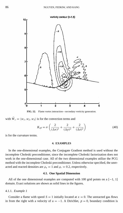
FIG. 12. Flame vortex interaction—secondary vorticity generation.
with EWc = 〈w1, w2, w3〉 is for the convection terms and
Kcfl = σ(
2
(1x)2+ 2
(1y)2+ 2
(1z)2
)(40)
is for the curvature terms.
4. EXAMPLES
In the one-dimensional examples, the Conjugate Gradient method is used without theincomplete Choleski preconditioner, since the incomplete Choleski factorization does notwork in the one-dimensional case. All of the two dimensional examples utilize the PCGmethod with the incomplete Choleski preconditioner. Unless otherwise specified, the unre-acted and reacted densities areρu = 1 andρr = 0.2, respectively.
4.1. One Spatial Dimension
All of the one dimensional examples are computed with 100 grid points on a [−1, 1]domain. Exact solutions are shown as solid lines in the figures.
4.1.1. Example 1
Consider a flame with speedS= 1 initially located atx = 0. The unreacted gas flowsin from the right with a velocity ofu = −1. A Dirichlet, p = 0, boundary condition is

BOUNDARY CONDITION CAPTURING METHOD 87
FIG. 13. Flame vortex interaction—secondary vorticity generation; 140 by 280 grid.
specified on the left-hand side of the domain, and a Neumann pressure boundary conditionis used on the right-hand side of the domain to keep the inflow velocity fixed. Figure 1 showsthe computed solution for this stationary flame. The calculation for Fig. 1 may seem rathertrivial, since the initial data is already the exact solution. In Fig. 2, the same calculation iscarried out starting with erroneous initial data. Even with this poor initial guess, the correctsolution is still obtained.
4.1.2. Example 2
Consider two flames both with speedS= 1 initially located atx = −0.5 andx = 0.5.The unreacted material is at rest in the center of the domain. Dirichlet,p = 0, bound-ary conditions are specified at both ends of the domain. Initially, the reacted velocities onthe left- and right-hand sides of the domain were specified asu = −4 andu = 4, respec-tively. Figure 3 shows the computed velocity, and illustrates the ability of our algorithmto treat merging in one dimension. After merging, the domain contains a single-phase in-compressible fluid which must have a constant velocity. In the case of compressible flow,a finite speed of propagation rarefaction wave would lower the velocity to the averageof the two reacted velocities (zero in this case). For incompressible flow, the “rarefactionwave” moves at infinite speed and the velocity drops to zero in one time step as shown inFig. 3.
88 NGUYEN, FEDKIW, AND KANG
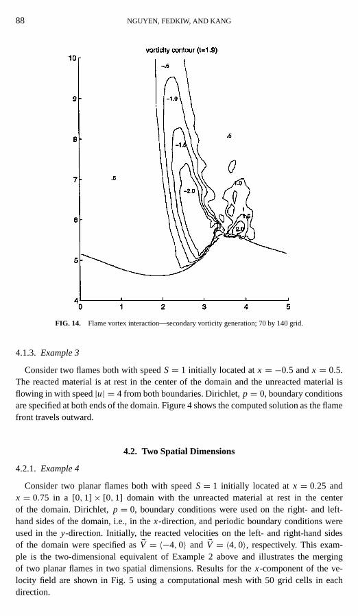
FIG. 14. Flame vortex interaction—secondary vorticity generation; 70 by 140 grid.
4.1.3. Example 3
Consider two flames both with speedS= 1 initially located atx = −0.5 andx = 0.5.The reacted material is at rest in the center of the domain and the unreacted material isflowing in with speed|u| = 4 from both boundaries. Dirichlet,p = 0, boundary conditionsare specified at both ends of the domain. Figure 4 shows the computed solution as the flamefront travels outward.
4.2. Two Spatial Dimensions
4.2.1. Example 4
Consider two planar flames both with speedS= 1 initially located atx = 0.25 andx = 0.75 in a [0, 1]× [0, 1] domain with the unreacted material at rest in the centerof the domain. Dirichlet,p = 0, boundary conditions were used on the right- and left-hand sides of the domain, i.e., in thex-direction, and periodic boundary conditions wereused in they-direction. Initially, the reacted velocities on the left- and right-hand sidesof the domain were specified asEV = 〈−4, 0〉 and EV = 〈4, 0〉, respectively. This exam-ple is the two-dimensional equivalent of Example 2 above and illustrates the mergingof two planar flames in two spatial dimensions. Results for thex-component of the ve-locity field are shown in Fig. 5 using a computational mesh with 50 grid cells in eachdirection.

BOUNDARY CONDITION CAPTURING METHOD 89
FIG. 15. Flame vortex interaction—secondary vorticity generation; 35 by 70 grid.
4.2.2. Example 5
In this example we consider the Darrieus–Landau instability withS= 1 in a [0, 2π5 ] ×
[0, 2π5 ] domain with 60 grid cells in each direction. The initial flame profile is a small am-
plitude cosine wave defined byy = 0.005 cos(5x)+ π5 . The unreacted material is flowing
in from the bottom of the domain with an initial velocity ofEV = 〈0, 1〉 and the reacted ma-terial flowing out of the top of the domain with an initial velocity ofEV = 〈0, 5〉. Dirichlet,p = 0, boundary conditions were used in they-direction, and periodic boundary conditionswere used in thex-direction. The initial values of|φ| were determined by placing 10,000points (equally spaced in thex-direction) on the flame front and computing the minimumdistance from this set of points to each Cartesian grid location where the values of the levelset are stored. The sign ofφ was calculated by comparing each Cartesian grid location toy = 0.005 cos(5x)+ π
5 .The Darrieus–Landau instability results in exponential growth of the amplitude of the
flame,A(t) = Ao exp(ωt), where
ω = k|M |ρu + ρr
(√1+ ρu
ρr− ρr
ρu− 1
)(41)
is the rate of exponential growth, e.g. see [9]. Figure 6 shows a plot of amplitude versustime (labeledq = 5 whereq = ρu
ρb) as compared to the exact solution. Initially there is some
disagreement, since we did not start out with the exact Darrieus–Landau velocity field, but
90 NGUYEN, FEDKIW, AND KANG
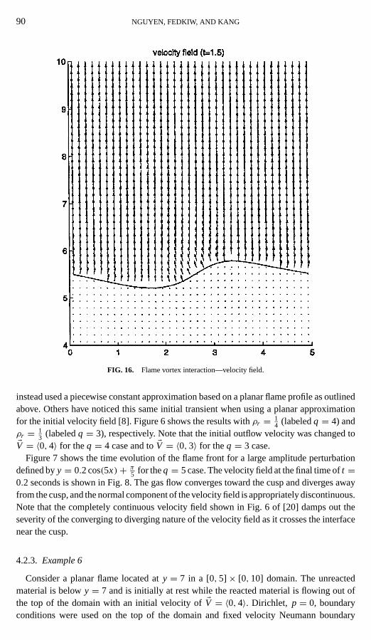
FIG. 16. Flame vortex interaction—velocity field.
instead used a piecewise constant approximation based on a planar flame profile as outlinedabove. Others have noticed this same initial transient when using a planar approximationfor the initial velocity field [8]. Figure 6 shows the results withρr = 1
4 (labeledq = 4) andρr = 1
3 (labeledq = 3), respectively. Note that the initial outflow velocity was changed toEV = 〈0, 4〉 for theq = 4 case and toEV = 〈0, 3〉 for theq = 3 case.
Figure 7 shows the time evolution of the flame front for a large amplitude perturbationdefined byy = 0.2 cos(5x)+ π
5 for theq = 5 case. The velocity field at the final time oft =0.2 seconds is shown in Fig. 8. The gas flow converges toward the cusp and diverges awayfrom the cusp, and the normal component of the velocity field is appropriately discontinuous.Note that the completely continuous velocity field shown in Fig. 6 of [20] damps out theseverity of the converging to diverging nature of the velocity field as it crosses the interfacenear the cusp.
4.2.3. Example 6
Consider a planar flame located aty = 7 in a [0, 5]× [0, 10] domain. The unreactedmaterial is belowy = 7 and is initially at rest while the reacted material is flowing out ofthe top of the domain with an initial velocity ofEV = 〈0, 4〉. Dirichlet, p = 0, boundaryconditions were used on the top of the domain and fixed velocity Neumann boundary

BOUNDARY CONDITION CAPTURING METHOD 91
FIG. 17. Flame vortex interaction—velocity field.
conditions were used on the bottom of the domain. Periodic boundary conditions wereused in thex-direction. To suppress the hydrodynamic instability development at shortwavelengths, a curvature term was added to the flame speed to obtainS= 1+ .1κ.
In order to simulate flame vortex interaction, an infinite array of Oseen vortices were addedto the unreacted material centered at spatial locations of(x, y) = (2.5+ 5k, 5.5), wherekis an integer. This adds only one vortex to the computational domain at(x, y) = (2.5, 5.5)as shown in Fig. 9, and accounts for the periodicity of the domain in thex-direction.Vortices very far away have little effect on the computational domain so our initial data onlyaccounts for the velocity prescribed by the vortices with−500≤ k ≤ 500. Each vortex isbest expressed in polar coordinates with zero velocity in the radial direction and
Vθ = 1.5
2πr
(1− exp
(− r 2
.52
))(42)
in the counterclockwise angular direction, wherer is the distance from the vortex core. Theinitial velocity of the unreacted material is determined by summing the contribution fromeach of the 1001 vortices considered. See [20] for more details.
Figure 10 shows the time evolution of the flame front for a 140 by 280 grid cellcomputation illustrating how the counterclockwise vortices distort the flame front. The
92 NGUYEN, FEDKIW, AND KANG
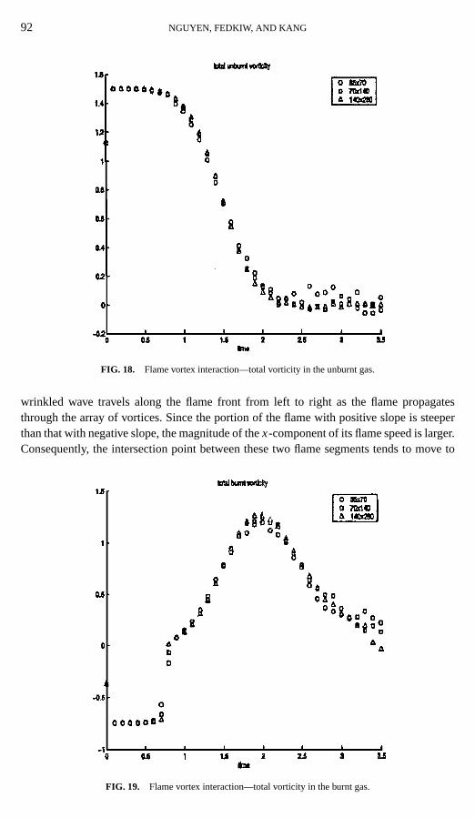
FIG. 18. Flame vortex interaction—total vorticity in the unburnt gas.
wrinkled wave travels along the flame front from left to right as the flame propagatesthrough the array of vortices. Since the portion of the flame with positive slope is steeperthan that with negative slope, the magnitude of thex-component of its flame speed is larger.Consequently, the intersection point between these two flame segments tends to move to
FIG. 19. Flame vortex interaction—total vorticity in the burnt gas.
BOUNDARY CONDITION CAPTURING METHOD 93
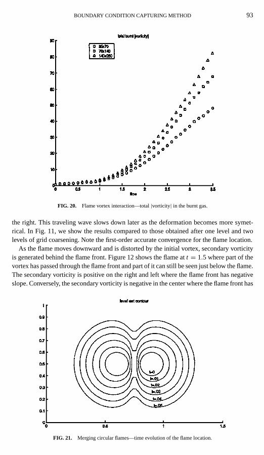
FIG. 20. Flame vortex interaction—total|vorticity| in the burnt gas.
the right. This traveling wave slows down later as the deformation becomes more symet-rical. In Fig. 11, we show the results compared to those obtained after one level and twolevels of grid coarsening. Note the first-order accurate convergence for the flame location.
As the flame moves downward and is distorted by the initial vortex, secondary vorticityis generated behind the flame front. Figure 12 shows the flame att = 1.5 where part of thevortex has passed through the flame front and part of it can still be seen just below the flame.The secondary vorticity is positive on the right and left where the flame front has negativeslope. Conversely, the secondary vorticity is negative in the center where the flame front has
FIG. 21. Merging circular flames—time evolution of the flame location.
94 NGUYEN, FEDKIW, AND KANG
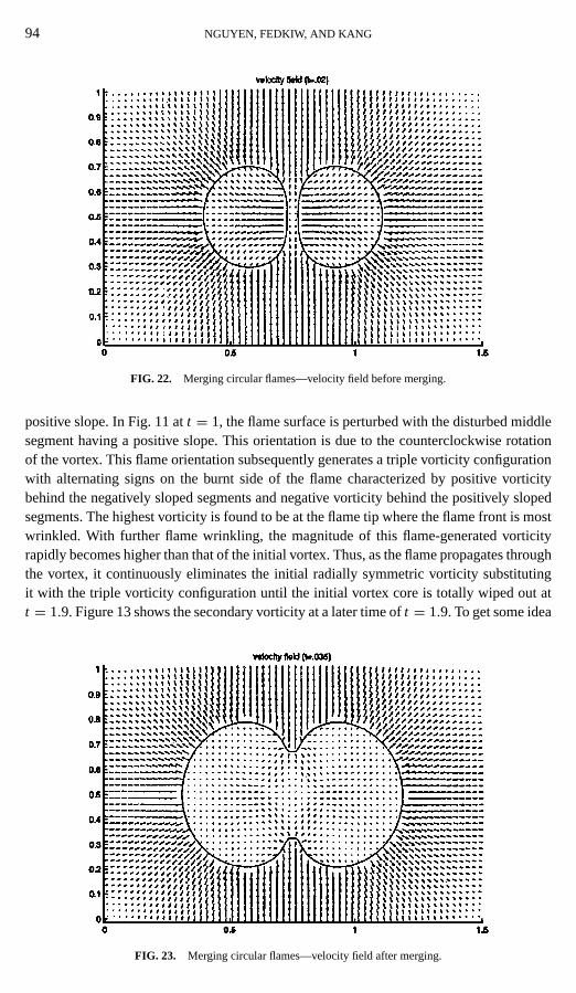
FIG. 22. Merging circular flames—velocity field before merging.
positive slope. In Fig. 11 att = 1, the flame surface is perturbed with the disturbed middlesegment having a positive slope. This orientation is due to the counterclockwise rotationof the vortex. This flame orientation subsequently generates a triple vorticity configurationwith alternating signs on the burnt side of the flame characterized by positive vorticitybehind the negatively sloped segments and negative vorticity behind the positively slopedsegments. The highest vorticity is found to be at the flame tip where the flame front is mostwrinkled. With further flame wrinkling, the magnitude of this flame-generated vorticityrapidly becomes higher than that of the initial vortex. Thus, as the flame propagates throughthe vortex, it continuously eliminates the initial radially symmetric vorticity substitutingit with the triple vorticity configuration until the initial vortex core is totally wiped out att = 1.9. Figure 13 shows the secondary vorticity at a later time oft = 1.9. To get some idea
FIG. 23. Merging circular flames—velocity field after merging.
BOUNDARY CONDITION CAPTURING METHOD 95
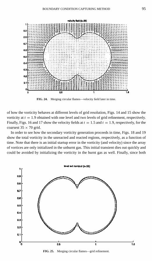
FIG. 24. Merging circular flames—velocity field later in time.
of how the vorticity behaves at different levels of grid resolution, Figs. 14 and 15 show thevorticity at t = 1.9 obtained with one level and two levels of grid refinement, respectively.Finally, Figs. 16 and 17 show the velocity fields att = 1.5 andt = 1.9, respectively, for thecoarsest 35× 70 grid.
In order to see how the secondary vorticity generation proceeds in time, Figs. 18 and 19show the total vorticity in the unreacted and reacted regions, respectively, as a function oftime. Note that there is an initial startup error in the vorticity (and velocity) since the arrayof vortices are only initialized in the unburnt gas. This initial transient dies out quickly andcould be avoided by initializing the vorticity in the burnt gas as well. Finally, since both
FIG. 25. Merging circular flames—grid refinement.
96 NGUYEN, FEDKIW, AND KANG
positive and negative vorticity increases the local turbulence, Fig. 20 shows the sum of themagnitudeof vorticity in the reacted material as a function of time.
4.2.4. Example 7
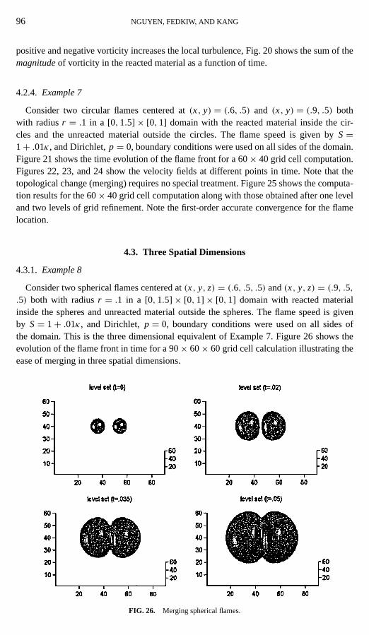
Consider two circular flames centered at(x, y) = (.6, .5) and (x, y) = (.9, .5) bothwith radiusr = .1 in a [0, 1.5]× [0, 1] domain with the reacted material inside the cir-cles and the unreacted material outside the circles. The flame speed is given byS=1+ .01κ, and Dirichlet,p = 0, boundary conditions were used on all sides of the domain.Figure 21 shows the time evolution of the flame front for a 60× 40 grid cell computation.Figures 22, 23, and 24 show the velocity fields at different points in time. Note that thetopological change (merging) requires no special treatment. Figure 25 shows the computa-tion results for the 60× 40 grid cell computation along with those obtained after one leveland two levels of grid refinement. Note the first-order accurate convergence for the flamelocation.
4.3. Three Spatial Dimensions
4.3.1. Example 8
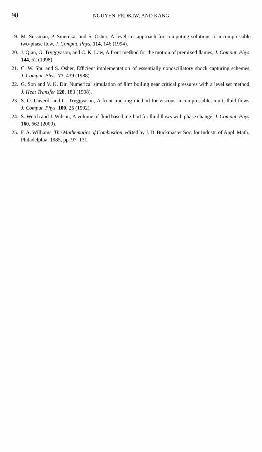
Consider two spherical flames centered at(x, y, z) = (.6, .5, .5) and(x, y, z) = (.9, .5,.5) both with radiusr = .1 in a [0, 1.5]× [0, 1]× [0, 1] domain with reacted materialinside the spheres and unreacted material outside the spheres. The flame speed is givenby S= 1+ .01κ, and Dirichlet, p = 0, boundary conditions were used on all sides ofthe domain. This is the three dimensional equivalent of Example 7. Figure 26 shows theevolution of the flame front in time for a 90× 60× 60 grid cell calculation illustrating theease of merging in three spatial dimensions.
FIG. 26. Merging spherical flames.

BOUNDARY CONDITION CAPTURING METHOD 97
5. CONCLUSION
A new simple numerical method based on the level set method and ghost fluid method wasdeveloped to simulate two-phase incompressible flow where one material is being convertedinto another. We presented this method in the context of premixed flame simulations. Theflame was assumed to be a surface of discontinuity separating the reacted and unreactedgases, and propagating with a prescribed flame velocity. The incompressible Euler equationswere solved on a stationary finite difference grid for both the reacted and the unreacted gases.The velocity and other material properties were modeled with jump discontinuities acrossthe flame front where appropriate.
We demonstrated the accuracy and fidelity of the method by comparing the numericalresults with exact solutions for a steady flame and the Darrieus–Landau instability. Therobustness of the method was demonstrated by the simplicity with which flame fronts canmerge. The method is fairly easily to implement and was extended to three spatial dimen-sions to treat a simple merging problem. Using this new numerical method, we studied theinteraction of a flame and vortex with the objective of gaining further insight into the funda-mental mechanisms governing flame generated vorticity resulting from baroclinic torque.
REFERENCES
1. J. U. Brackbill, D. B. Kothe, and C. Zemach, A continuum method for modeling surface tension,J. Comput.Phys.100, 335 (1992).
2. Y. C. Chang, T. Y. Hou, B. Merriman, and S. Osher, A level set formulation of Eulerian interface capturingmethods for incompressible fluid flows,J. Comput. Phys.124, 449 (1996).
3. A. J. Chorin, numerical solution of the Navier–Stokes equations,Math. Comp.22, 745 (1968).
4. R. Fedkiw, T. Aslam, B. Merriman, and S. Osher, A non-oscillatory Eulerian approach to interfaces inmultimaterial flows (the ghost fluid method),J. Comput. Phys.152, 457 (1999).
5. R. Fedkiw, T. Aslam, and S. Xu, The ghost fluid method for deflagration and detonation discontinuities,J. Comput. Phys.154, 393 (1999).
6. G. Golub and C. Van Loan,Matrix Computations(Johns Hopkins Press, Baltimore, 1989).
7. F. H. Harlow and J. E. Welch, Numerical calculation of time-dependent viscous incompressible flow of fluidwith a free surface,Phys. Fluids8, 2182 (1965).
8. B. T. Helenbrook, personal communication.
9. B. T. Helenbrook, L. Martinelli, and C. K. Law, A numerical method for solving incompressible flow problemswith a surface of discontinuity,J. Comput. Phys.148, 366 (1999).
10. B. T. Helenbrook and C. K. Law, The role of Landau–Darrieus instability in large scale flows,CombustionFlame117, 155 (1999).
11. D. Juric and G. Tryggvason, Computations of boiling flows,Int. J. Multiphase Flow24, 387 (1998).
12. M. Kang, R. Fedkiw, and X.-D Liu, A boundary condition capturing method for multiphase incompressibleflow, J. Sci. Comput.15, 323 (2000).
13. X.-D. Liu, R. P. Fedkiw, and M. Kang, A boundary condition capturing method for Poisson’s equation onirregular domains,J. Comput. Phys.154, 151 (2000).
14. G. H. Markstein,Nonsteady Flame Propagation(Pergamon, Oxford, 1964).
15. S. Osher and J. A. Sethian, Fronts propagating with curvature dependent speed: Algorithms based on Hamilton–Jacobi formulations,J. Comput. Phys.79, 12 (1988).
16. C. Peskin, Numerical analysis of blood flow in the heart,J. Comput. Phys.25, 220 (1977).
17. C. Peskin and B. Printz, Improved volume conservation in the computation of flows with immersed elasticboundaries,J. Comput. Phys.105, 33 (1993).
18. R. Peyret and T. D. Taylor,Computational Methods for Fluid Flow(Springer-Verlag, New York, 1983).
98 NGUYEN, FEDKIW, AND KANG
19. M. Sussman, P. Smereka, and S. Osher, A level set approach for computing solutions to incompressibletwo-phase flow,J. Comput. Phys.114, 146 (1994).
20. J. Qian, G. Tryggvason, and C. K. Law, A front method for the motion of premixed flames,J. Comput. Phys.144, 52 (1998).
21. C. W. Shu and S. Osher, Efficient implementation of essentially nonoscillatory shock capturing schemes,J. Comput. Phys.77, 439 (1988).
22. G. Son and V. K. Dir, Numerical simulation of film boiling near critical pressures with a level set method,J. Heat Transfer120, 183 (1998).
23. S. O. Unverdi and G. Tryggvason, A front-tracking method for viscous, incompressible, multi-fluid flows,J. Comput. Phys.100, 25 (1992).
24. S. Welch and J. Wilson, A volume of fluid based method for fluid flows with phase change,J. Comput. Phys.160, 662 (2000).
25. F. A. Williams,The Mathematics of Combustion, edited by J. D. Buckmaster Soc. for Industr. of Appl. Math.,Philadelphia, 1985, pp. 97–131.