a variational approach to estimate incompressible fluid flows

Noname manuscript No.(will be inserted by the editor)

A Variational Approach to Estimate IncompressibleFluid Flows.

Praveen Chandrashekar, Souvik Roy,A.S.Vasudeva Murthy

the date of receipt and acceptance should be inserted later

Abstract A variational approach is used to recover fluid motion governed byStokes and Navier-Stokes equations. Unlike previous approaches where opticalflow method is used to track rigid body motion, this new framework aims atinvestigating incompressible flows using optical flow techniques. We formulatea minimization problem and determine conditions under which unique solu-tion exists. Numerical results using finite element method not only supporttheoretical results but also show that Stokes flow forced by a potential arerecovered almost exactly.

Keywords variational, incompressible, finite element, optical flow, Stokes,Navier-Stokes.

Mathematics Subject Classifications 76M

1 Introduction

Our motivation for the present study is to understand cloud motion from satel-lite images. This in turn will help us in understanding the movement of rainbearing clouds during the monsoon over the Indian subcontinent. Previouswork in this direction are [1], [2], [3], [4], [5]. The methodology is to obtainfluid flow estimates from given image sequences by incorporating physical con-straints into a variational approach to optical flow method (OFM). Howevera major problem in applying OFM to fluid flow, leave alone cloud motion isthat the connection between optical flow in the image plane and fluid flow

Souvik Roy, Praveen Chandrashkehar, A. S. Vasudeva MurthyTIFR Center for Applicable MathematicsBangalore-560065,India.Tel.: +91 9035287250,(080)6695-3738, (080)6695-3719Fax: (080)6695-3799E-mail: praveen,souvik, vasu)@math.tifrbng.res.in

2 Praveen Chandrashekar, Souvik Roy, A.S.Vasudeva Murthy

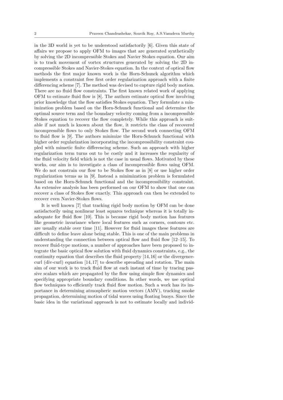
in the 3D world is yet to be understood satisfactorily [6]. Given this state ofaffairs we propose to apply OFM to images that are generated syntheticallyby solving the 2D incompressible Stokes and Navier Stokes equation. Our aimis to track movement of vortex structures generated by solving the 2D in-compressible Stokes and Navier-Stokes equation. In the context of optical flowmethods the first major known work is the Horn-Schunck algorithm whichimplements a constraint free first order regularization approach with a finitedifferencing scheme [7]. The method was devised to capture rigid body motion.There are no fluid flow constraints. The first known related work of applyingOFM to estimate fluid flow is [8]. The authors estimate optical flow involvingprior knowledge that the flow satisfies Stokes equation. They formulate a min-imization problem based on the Horn-Schunck functional and determine theoptimal source term and the boundary velocity coming from a incompressibleStokes equation to recover the flow completely. While this approach is suit-able if not much is known about the flow, it restricts the class of recoveredincompressible flows to only Stokes flow. The second work connecting OFMto fluid flow is [9]. The authors minimize the Horn-Schunck functional withhigher order regularization incorporating the incompressibility constraint cou-pled with mimetic finite differencing scheme. Such an approach with higherregularization term turns out to be costly and it increases the regularity ofthe fluid velocity field which is not the case in usual flows. Motivated by theseworks, our aim is to investigate a class of incompressible flows using OFM.We do not constrain our flow to be Stokes flow as in [8] or use higher orderregularization terms as in [9]. Instead a minimization problem is formulatedbased on the Horn-Schunck functional and the incompressibility constraint.An extensive analysis has been performed on our OFM to show that one canrecover a class of Stokes flow exactly. This approach can then be extended torecover even Navier-Stokes flows.

It is well known [7] that tracking rigid body motion by OFM can be donesatisfactorily using nonlinear least squares technique whereas it is totally in-adequate for fluid flow [10]. This is because rigid body motion has featureslike geometric invariance where local features such as corners, contours etc.are usually stable over time [11]. However for fluid images these features aredifficult to define leave alone being stable. This is one of the main problems inunderstanding the connection between optical flow and fluid flow [12–15]. Torecover fluid-type motions, a number of approaches have been proposed to in-tegrate the basic optical flow solution with fluid dynamics constraints, e.g., thecontinuity equation that describes the fluid property [14,16] or the divergence-curl (div-curl) equation [14,17] to describe spreading and rotation. The mainaim of our work is to track fluid flow at each instant of time by tracing pas-sive scalars which are propagated by the flow using simple flow dynamics andspecifying appropriate boundary conditions. In other words, we use opticalflow techniques to efficiently track fluid flow motion. Such a work has its im-portance in determining atmospheric motion vectors (AMV), tracking smokepropagation, determining motion of tidal waves using floating buoys. Since thebasic idea in the variational approach is not to estimate locally and individ-

Variational Approach for Incompressible Flows 3

ually but to estimate non-locally by minimizing a suitable functional definedover the entire image section, we therefore prefer a variational approach.

The paper is organised as follows. In Section 2, a minimization problem isformulated with a first order regularization term under the incompressibilityconstraint. In Section 3, we derive conditions on the image under which uniquesolution exists. Section 4 presents an outcome of the present work which showswhen the real unknown flow observed through images comes from a Stokes flowforced by a potential, then we are able to recover the velocity almost exactlyeven for very small viscosity coefficient. In Section 5, continuous Galerkin finiteelement method is used to solve the resulting set of equations using FENICS[18]. The reason for using finite element method for the variational modelarises from the fact that the numerical experiments done with finite elementmethod for the Horn-Schunck model to track underlying flows gave excellentresults [19]. Section 6 investigates motion satisfying Stokes and Navier-Stokesflows by performing numerical experiments on four test cases for low and highReynolds number flows. Section 7 summarizes the results obtained.

2 Variational Formulation

To estimate fluid flow, we trace passive scalars that are propagated by theflow. Examples of such scalars are smoke, brightness patterns of dense rain-bearing clouds whose intensity remains constant atleast for a short time span.These scalars can be represented by a function E : Ω × R+ −→ R so thatE(x, y, t) for (x, y) ∈ Ω represents a snapshot of the image of the scalarsat time t ∈ R+. Here Ω is a bounded convex subset of R2. Let us assumeour image E(x, y, t) ∈ W 1,∞(Ω), for each t and hence in L2(Ω) (as Ω isbounded). Let the field of optical velocities over Ω at a fixed time t = t0 beU(x, y, t0) = (u, v)(x, y, t0) and X = (H1(Ω))2. Define the functional,

J(U) =1

2

∫Ω

(Et + U · ∇E)2dxdy +K

2

∫Ω

‖∇U‖2dxdy, K > 0 (1)

where Et and ∇E are evaluated at t = t0, and

‖∇U‖2 = ‖∇u‖2 + ‖∇v‖2

Without loss of generality let t0 = 0. The first term in (1) represents theconstant brightness assumption of the tracers. The second term represents aregularization term for the flow velocities. Such a functional was first consid-ered by Horn and Schunck[7] and subsequently by many others [24–27,12,28]to efficiently estimate rigid body motion. Here it is used to track the under-lying fluid flow motion. Such a connection between optical flow and fluid flowtracking is essential because if a proper connection is found then techniquesfrom optical flow to determine high-resolution velocity fields from various im-ages in continuous patterns can be used. To use (1) to track fluid flows, we


need to include fluid dynamics and enforce proper boundary conditions. Hencewe enforce the incompressible fluid flow constraint

∇ · U = 0 (2)

The minimization problem can be stated as

minU∈X

J(U)| ∇ · U = 0 (P)

The boundary conditions on the flow velocity could be either Dirichlet orNeumann.

3 Existence and Uniqueness Of Minimizer

We show existence and uniqueness of minimizer for Problem (P). Before thatwe state some standard definitions and results.

3.1 Preliminary Results

Let (Z, ‖ · ‖Z) be a Banach space.

Theorem 1 Let J : Z → R ∪ −∞,∞ be a convex functional on Z. If J isbounded from above in a neighbourhood of a point U0 ∈ Z, then it is locallybounded i.e. each U ∈ Z has a neighbourhood on which J is bounded.

Definition 1 A functional J defined on Z is said to be locally Lipschitz ifat each U ∈ Z there exists a neighbourhood Nε(U) and a constant R(U) suchthat if V,W ∈ Nε(U), then

|J(V )− J(W )| ≤ R‖V −W‖Z

If this inequaltiy holds throughout a set Y ⊆ Z with R independent of U thenwe say that J is Lipschitz on Y .

Theorem 2 Let J be convex on Z. If J is bounded from above in a neigh-bourhood of one point of X, then J is locally Lipschitz in Z.

Theorem 3 Let J be convex on Z. If J is bounded from above in an neigh-bourhood of one point of Z, then J is continuous on Z.

Theorem 1, 2, 3 and Definition 1 can be found in [29]. The following theoremfrom [20] is used to establish an unique global minimizer for (P).

Theorem 4 (Existence and uniqueness of global minimizer) Let J :Z → R∪−∞,∞ be a lower semi-continuous strictly convex functional. Alsolet J be coercive i.e.

lim‖U‖Z→+∞

J(U) =∞.

Let C be a closed and convex subset of Z. Then J has a unique global minimumover C.


Let us now verify the conditions stated in Theorem (4) for the functional Jin (1). Let H = L2(Ω), H1 = (L2(Ω))2 and Z = X with norms ‖U‖H =‖u‖L2 + ‖v‖L2 and ‖U‖Z = ‖u‖H1 + ‖v‖H1 .

Theorem 5 The functional given in (1) is strictly convex with respect to Uunder the assumption that Ex and Ey are linearly independent i.e there doesnot exist non-zero constants c1 and c2 such that c1Ex(x, y) + c2Ey(x, y) = 0,for all (x, y) ∈ Ω .

Proof Let U1 =

(u1v1

)and U2 =

(u2v2

)where (·) is the usual inner product

on R2. Then for 0 < α < 1 and U1 6= U2, we have

J(αU1 + (1− α)U2) =1

2

∫Ω

((αU1 + (1− α)U2) · ∇E) + Et)2dxdy

+K

2

∫Ω

[‖∇(αu1 + (1− α)u2)‖2+‖∇(αv1 + (1− α)v2)‖2

]dxdy

≤ 1

2

∫Ω

[(αU1 + (1− α)U2) · ∇E2 + 2E2

t + 2Et(αU1 + (1− α)U2) · ∇E]dxdy

+K

2

∫Ω

[‖(α∇u1 + (1− α)∇u2)‖2 + ‖(α∇v1 + (1− α)∇v2)‖2

]dxdy

Now

K

2

∫Ω

[‖(α∇u1 + (1− α)∇u2)‖2 + ‖(α∇v1 + (1− α)∇v2)‖2

]dxdy

≤K2

(α

∫Ω

[‖∇u1‖2 + ‖∇v1‖2

]dxdy + (1− α)

∫Ω

[‖∇u2‖2 + ‖∇v2‖2

]dxdy

)(3)

and ∫Ω

[(αU1 + (1− α)U2) · ∇E]2dxdy ≤ α

∫Ω

(U1 · ∇E)2dxdy

+(1− α)

∫Ω

(U2 · ∇E)2dxdy.

(4)

Equality holds in (3) iff

∇u1 = ∇u2, ∇v1 = ∇v2 (5)

and in (4) iff

U1 · ∇E = U2 · ∇E. (6)

From (5) we have

u1 − u2 = c1, v1 − v2 = c2 (7)

where c1 and c2 are constants. From (6) we get

Ex(u1 − u2) + Ey(v1 − v2) = 0. (8)


But as Ex and Ey are linearly independent, (7) and (8) gives

u1 = u2, v1 = v2

which impliesU1 = U2.

Hence for U1 6= U2 we have,∫Ω

((αU1+(1−α)U2)·∇E)2dxdy < α

∫Ω

(U1·∇E)2dxdy+(1−α)

∫Ω

(U2·∇E)2dxdy.

This gives

J(αU1 + (1− α)U2) < αJ(U1) + (1− α)J(U2), 0 < α < 1. (9)

This implies that J is a strictly convex functional w.r.t U .

Theorem 6 The constraint set (2) given as C = U ∈ Z : ∇ · U = 0 is aclosed subspace of Z.

Proof For U1, U2 ∈ C we have

∇ · (αU1 + βU2) = α(∇ · U1) + β(∇ · U2) ∀α, β ∈ R.

HenceαU1 + βU2 ∈ C, α, β ∈ R.

Now consider a sequence Unn ∈ C such that it converges to U in ‖.‖Z . Weneed to show that U ∈ C. Since Un → U in C, we have Un → U in Z and∇ · Un = 0. Now Un → U in Z givesUn → U in H1 and ∇Un → ∇U in H1. This implies ∇ · Un → ∇ · U in H1

which in turn implies∇ · (Un − U) → 0 in H1. Finally writing ∇ · U = ∇ · (U − Un) + ∇ · Un wesee that ∇ · U → 0 as n → ∞. This shows that U ∈ C and so C is a closedsubspace of Z and hence convex.

Thus J is a strict convex function defined on H and the constraint set (2)denoted as K is a closed subspace of Z. We now show that J is continuousand coercive.

Theorem 7 The functional J as given in (1) is continuous

Proof We will use the Theorem 3 to prove our statement. We assume

‖E‖W 1,∞(Ω) ≤M.

As 0 ∈ Z, we consider a neighbourhood of zero given as N1 = U : ‖U‖Z < 1.Now

|J(U)| =∣∣∣∣12∫Ω

(U · ∇E + Et)2dxdy +

K

2

∫Ω

[‖∇u‖2 + ‖∇v‖2

]dxdy

∣∣∣∣≤ 1

2

∫Ω

(U · ∇E + Et)2dxdy +

K

2‖U‖2Z

≤ 1

2

∫Ω

(E2t + (U · ∇E)2 + 2Et(U · ∇E)

)dxdy +

K

2‖U‖2Z


Using Holder’s inequality and L∞ bound on E and its derivatives we get

|J(U)| ≤ 1

2

∫Ω

[M2 +M2(u+ v)2

]dxdy

+ 2M

(∫Ω

(∇E)2)1/2(∫

Ω

U2

)1/2

dxdy +K

2‖U‖2Z

≤ M2

2

∫Ω

[1 + 2(u2 + v2)

]dxdy +M(

∫Ω

M2)1/2‖U‖Z +K

2‖U‖2Z

≤ M2

2(

∫Ω

1) +M2‖U‖2Z +M2(

∫Ω

1) +K

2‖U‖2Z

<3M

2µ(Ω) +M2 +

K

2( as ‖U‖Z < 1)

<∞.

where µ(Ω) is the measure of Ω. This gives us J(U) is bounded above in N1.As J is convex (by Theorem 5), it implies J is continuous for all U ∈ Z (byThoerem 3).

Theorem 8 The functional J as given in (1) is coercive under the assumptionthat Ex and Ey are linearly independent.

Proof The functional J in (1) can be written as

J(U) = J1(U) +

∫Ω

E2t + 2Et(U · ∇E)dxdy

where

J1(U) =

∫Ω

(U · ∇E)2dxdy +K

2

∫Ω

‖∇U‖2dxdy. (10)

To show J(U) is coercive we need to show J1(U) is coercive as it is quadraticin U . We use the Poincare-Wirtinger’s Inequality∫

Ω

(U − T )2dxdy ≤ D∫Ω

‖∇U‖2dxdy (11)

where

T =1

µ(Ω)

∫Ω

Udxdy (12)

and D is a constant depending on Ω. Suppose J1 is not coercive. Then theredoes not exist any constant M > 0 such that

J1(U) ≥M‖U‖2Z ∀U ∈ Z

because if it was so then J1 → ∞ as ‖U‖Z → ∞. So for any M > 0 thereexists UM ∈ Z such that

J1(UM ) < M‖UM‖2Z .


We choose M = 1n and get a sequence of Mn’s and correspondingly get Un.

Without loss of generality, let us assume ‖Un‖Z = 1. If not, we can takeVn = Un

‖Un‖Z and replace Un with Vn. So we get a sequence Unn∈N in Z with

‖Un‖Z = 1 and J1(Un)→ 0 as n→∞. Using (10) and (11) we have∫Ω

(un − T 1n)2dxdy → 0 (13)

and ∫Ω

(vn − T 2n)2dxdy → 0 for n→∞. (14)

where

T 1n =

1

µ(Ω)

∫Ω

undxdy, T 2n =

1

µ(Ω)

∫Ω

vndxdy.

As ∫Ω

(Exu+ Eyv)2dxdy ≤ 2|E2x|∞

∫Ω

u2dxdy + 2|E2y |∞

∫Ω

v2dxdy

we have ∫Ω

(Ex(un − T 1

n) + Ey(vn − T 2n))2dxdy → 0 as n→∞. (15)

Now(∫Ω

(ExT1n + EyT

2n)2dxdy

)1/2

=

(∫Ω

(Exun + Eyvn + Ex(T 1n − un) + Ey(T 2

n − vn))2dxdy

)1/2

≤(∫

Ω

(Exun + Eyvn)2dxdy

)1/2

+

(∫Ω

(Ex(T 1n − un) + Ey(T 2

n − vn))2dxdy

)1/2

≤ (J1(Un))1/2

+

(∫Ω

(Ex(T 1n − un) + Ey(T 2

n − vn))2dxdy

)1/2

→ 0 for n→∞. (Using (15))

Let a = ExT1n , b = EyT

2n . Then

‖a+ b‖2H = ‖a‖2H + ‖b‖2H + 2(a, b)H

≥ ‖a‖2H + ‖b‖2H − 2‖a‖H‖b‖H|(a, b)|H‖a‖H‖b‖H

≥ ‖a‖2H + ‖b‖2H − (‖a‖2H + ‖b‖2H)|(a, b)|H‖a‖H‖b‖H

= (‖a‖2H + ‖b‖2H)1− |(a, b)|H‖a‖H‖b‖H


where (a, b)H is the usual inner product in H. So we get∫Ω

(ExT1n+EyT

2n)2dxdy ≥

(‖Ex‖2H(T 1

n)2 + ‖Ey‖2H(T 2n)2)1− |(Ex, Ey)|H

‖Ex‖H‖Ey‖H.

(16)As left hand side of (16) → 0 as n → ∞ and by linear independency of Exand Ey

1− |(Ex, Ey)|H‖Ex‖H‖Ey‖H

> 0

and since ‖Ex‖H and ‖Ey‖H are not identically 0, we have

T 1n → 0 and T 2

n → 0 as n→∞ (17)

But this gives a contradiction as ‖Un‖Z ≤ ‖(Un − Tn)‖Z + ‖Tn‖Z and hence‖Un‖Z → 0 as n→∞ (using (13),(14),(17)). So J1 is coercive and hence J iscoercive.

By Thoerem 4, the problem (P) has an unique global minimum.

4 Exact recovery of Stokes flow

We now write down the optimality conditions for the minimizer of (P). UsingLagrange multipliers, the auxillary functional can be written as

J(U, p) =1

2

∫Ω

(Et + U · ∇E)2 dxdy +K

2

∫Ω

‖∇U‖2 dxdy +

∫Ω

(∇ · U)p dxdy

Taking Gateaux derivative of J wrt U and p, the standard optimality condi-tions [23] are

∂J

∂U= 0 and

∂J

∂p= 0. (18)

The first equation in (18) gives∫Ω

(Et + (U · ∇E))(U · ∇E) +K

∫Ω

(∇u·∇u) + (∇v·∇v)+

∫Ω

(∇ · U)p = 0,

∀ U ∈ Z(19)

with prescribed Dirichlet boundary conditions

U = Ub on ∂Ω. (20)

The second equation in (18) gives∫Ω

(∇ · U)p = 0 ∀p ∈ L2(Ω) (21)


Performing an integration by parts on the second term on the left in (19) andtaking U to be an arbitrary function in Z, together with (21) the followingPDE is obtained

K∆U −∇p = −(Et + U · ∇E)∇E∇ · U = 0

(22)

subject to (20).

Theorem 9 Let E in the right hand side of (22) be advected with velocity Uei.e.

Et + Ue · ∇E = 0

with Ue satisfying (20) and incompressible Stokes equation

α∆Ue +∇q = f, α > 0

∇ · Ue = 0.(23)

If f is given by a potential f = ∇φ for smooth φ, then U = Ue is the onlysolution of (22) which is independent of any K > 0. In other words the flowis recovered exactly irrespective of K.

Proof Eq. (22) can rewritten as

α∆U − α

K∇p = − α

K(Et + U · ∇E)∇E (24)

Since f = ∇φ, Eq. (23) can be rewritten as

α∆Ue +∇(q + φ) = 0

As the image E is advected with velocity, Ue is a solution of Eq. (24) withp = −Kα (q + φ) and right hand side as zero. As the solution of (22) is unique,U = Ue is the unique solution of (22) which is independent of any K > 0.

The result of Theorem 9 is verified in the numerical examples in Section 6where we have considered incompressible Stokes flow under various boundaryconditions and find that the flow is recovered with a high precision. Also asNavier-Stokes flow at low Reynolds number represents Stokes flow, we recoverlow Reynolds number Navier-Stokes flow exactly.

5 Finite element method for the Optical flow problem (1)

Eq. (22) is solved using the finite element method. Combining equations (19)and (21) along with the boundary conditions (20) gives the weak formulationof the PDE to be solved to determine the minimizer. Let Th be a triangulationof domain Ω and let K be a triangle in Th. Let Zh and Xh be two finiteelement spaces with triangulation parameter h such that

Zh ⊂ Z, Xh ⊂ L2(Ω)


Then the discrete problem is to find (Uh, ph) ∈ (Zh ∩ Zb)×Xh such that∫Ω

(Et + (Uh · ∇E))(∇E·Uh) +K

∫Ω

(∇uh·∇uh) + (∇vh·∇vh) +

∫Ω

(∇ · Uh)ph = 0∫Ω

(∇ · Uh)ph = 0

(25)where (Uh, ph) ∈ Zh ×Xh.Let us define the following Taylor-Hood finite element spaces

Zh(Ω) = Uh ∈ (C0(Ω))2 : Uh|K is a polynomial of degree 2 and Uh = 0 on ∂Ω(26)

and

Xh(Ω) = ph ∈ C0(Ω) : ph|K is a polynomial of degree 1 (27)

which satisfy the LBB condition [22]. We now describe the procedure to de-termine E,Et and ∇E.

5.1 Image data

Our aim is to generate a sequence of synthetic images E and try to recoverthe velocity given the information of the derivatives of E. For this purposeE is chosen whose analytic expression is known at time t = 0 and hence itsgradients can be computed exactly. To advect E with velocity Ue exactly, Etat t = 0 is generated from the equation

Et(x, y, 0) = −Ue · ∇E(x, y, 0)

where Ue represents the velocity obtained by solving incompressible Stokesflow

∆U +∇p = f

∇ · U = 0(28)

or Navier-Stokes flow

−α∆U+(U · ∇)U +∇p = f,

∇ · U = 0(29)

using finite element method with appropriate boundary conditions, where α =1/Re and Re is the Reynolds number. In practice, derivatives of images willbe computed using some finite differences which will introduce errors in thecomputed velocity.


5.2 Test Flows

Two types of flows are considered: one in a lid-driven cavity and the other pasta cylinder. For flows in a lid-driven cavity, the domain is Ω = [0, 1]Ö[0, 1]. Theboundary conditions are

U =

(1, 0) on y = 1(0, 0) elsewhere

(30)

with image at time t0 defined as

E0(x, y) = E(x, y, 0) = e−50[(x−1/2)2+(y−1/2)2]

Fig. 1: Image at time t = 0

For flows past a cylinder, the domain Ω is a rectangle in R2 given as[0, 2.2] × [0, 0.41] with a closed disk inside it centered at (0.2, 0.2) and radius0.05. The boundary conditions are

U =

(0, 0) on y = 0, y = 0.41 and on the surface of the disk

(0, 6y(0.41−y)0.412 ) on x = 0(31)

with image at time t0 defined as

E0(x, y) = E(x, y, 0) = e−50[(x−1.1)2+(y−0.2)2]

To compute Ue, Eq. (28) or (29) is solved subject to the boundary conditionsgiven in (30) or (31). But exact analytic expressions of solutions to (28) or(29) with the specified boundary conditions are usually not known. So finiteelement method is used to obtain Ue.


Fig. 2: Image at time t = 0

(a) Zoomed View

Fig. 3: Zoomed view of mesh for the lid-driven cavity flows.

5.3 Mesh

For flows in a lid-driven cavity, the domain Ω = [0, 1] × [0, 1] is triangulatedwith 100 points on each side as shown in Figure 3. There are 20000 triangleswith 10201 degrees of freedom. For flows past a cylinder, the mesh used isshown in Figure 4. It comprises of 200 points on the longer boundary, 80 pointson the shorter boundary and 100 points on the circular boundary. There are28582 triangles with 14605 degrees of freedom.


(a) Zoomed View

Fig. 4: Zoomed view of mesh for the lid-driven cavity flows.

5.4 Solving the Stokes equation

To solve (28), let us write the weak formulation as: find U ∈ Zb = U ∈ Z :U = Ub on ∂Ω and p ∈ L2(Ω) such that∫Ω

∇U ·∇V +

∫Ω

(∇·V )p+

∫Ω

(∇·U)q+

∫Ω

f ·V = 0 ∀(V, q) ∈ Z×L2(Ω)

(32)We also fix the value of p to be zero at a point X0 ∈ ∂Ω to obtain uniqueness.The discrete problem is to find (Uh, ph) ∈ (Zh ∩ Zb)×Xh such that∫Ω

∇Uh ·∇Vh−∫Ω

(∇·Vh)ph−∫Ω

(∇·Uh)qh =

∫Ω

f ·Vh ∀(Vh, qh) ∈ Zh×Xh

(33)where Zh and Xh are defined in (26) and (27) respectively. Solving Eq. 33with domains, boundary conditions and meshes defined in Sections 5.2 and5.3 gives Ue.

5.5 Solving the Navier-Stokes equation

Equation (29) is a non-linear equation in U . So the method of Picard iteration,which is an easy way of handling nonlinear PDEs, is used. In this method, aprevious solution in the nonlinear terms is used so that these terms becomelinear in the unknown U . The strategy is also known as the method of succes-sive substitutions [21]. In our case, we seek a new solution Uk+1 in iterationk + 1 such that (Uk+1, pk+1) solves the linear problem

−α∆Uk+1+(Uk · ∇)Uk+1 +∇pk+1 = f,

∇ · Uk+1 = 0(34)

with given boundary conditions, where Uk is known. The variational formu-lation for (34) can be written as: find Uk+1 ∈ Zb = U ∈ Z : U = Ub on ∂Ω


and pk+1 ∈ L2(Ω) such that∫Ω

α∇Uk+1 · ∇V +

∫Ω

[(Uk · ∇)Uk+1

]· V −

∫Ω

(∇ · V )pk+1 −∫Ω

(∇ · Uk+1)q

−∫Ω

f · V = 0 ∀(V, q) ∈ Z × L2(Ω)

(35)We start with initial guess U0 = (0, 0) and employ the finite element methodas described in Section (5.4) to determine Uk+1. Finally, we stop at the k + 1th

stage if ‖Uk+1 − Uk‖ < ε. We choose ε = 10−7. Hence we have Ue = Uk+1.Finally, the relative L2 error in velocity is defined as

Relative L2 error =‖Ue − Uo‖‖Ue‖

(36)

and the advection error is defined as

Advection Error = ‖Et + Uo · ∇E‖ (37)

where Ue is the exact velocity and Uo is the obtained velocity and the norm‖ · ‖ is the usual L2 norm for vector functions as defined earlier.

6 Numerical Examples

6.1 Stokes Flow in a lid driven cavity

The exact flow is given by solving (28) with f = (1, 100) in lid-driven cavity.Figure (5) shows plots of velocity vectors for various K. The velocity is recov-ered with a very high degree of accuracy. This is also reflected in the relativeL2 errors given in Table (1). Also Table (1) shows that the advection errors arevery small and so the recovered velocity preserves the advection properties ofthe image. The streamline plots for the velocity given in Figures (6) shows thatlarge vortex in the center and the two small vortices at the bottom corners aredetected with good accuracy which is actually very important in atmosphericflows. It is notable that the regularization parameter K has minimal effecton the behaviour of the solutions which is consistent with the fact that it isnot a physical parameter and hence any positive value of K can be used todetermine the velocity. This perfectly justifies the result proved in Theorem9.

6.2 Stokes flow past a cylinder

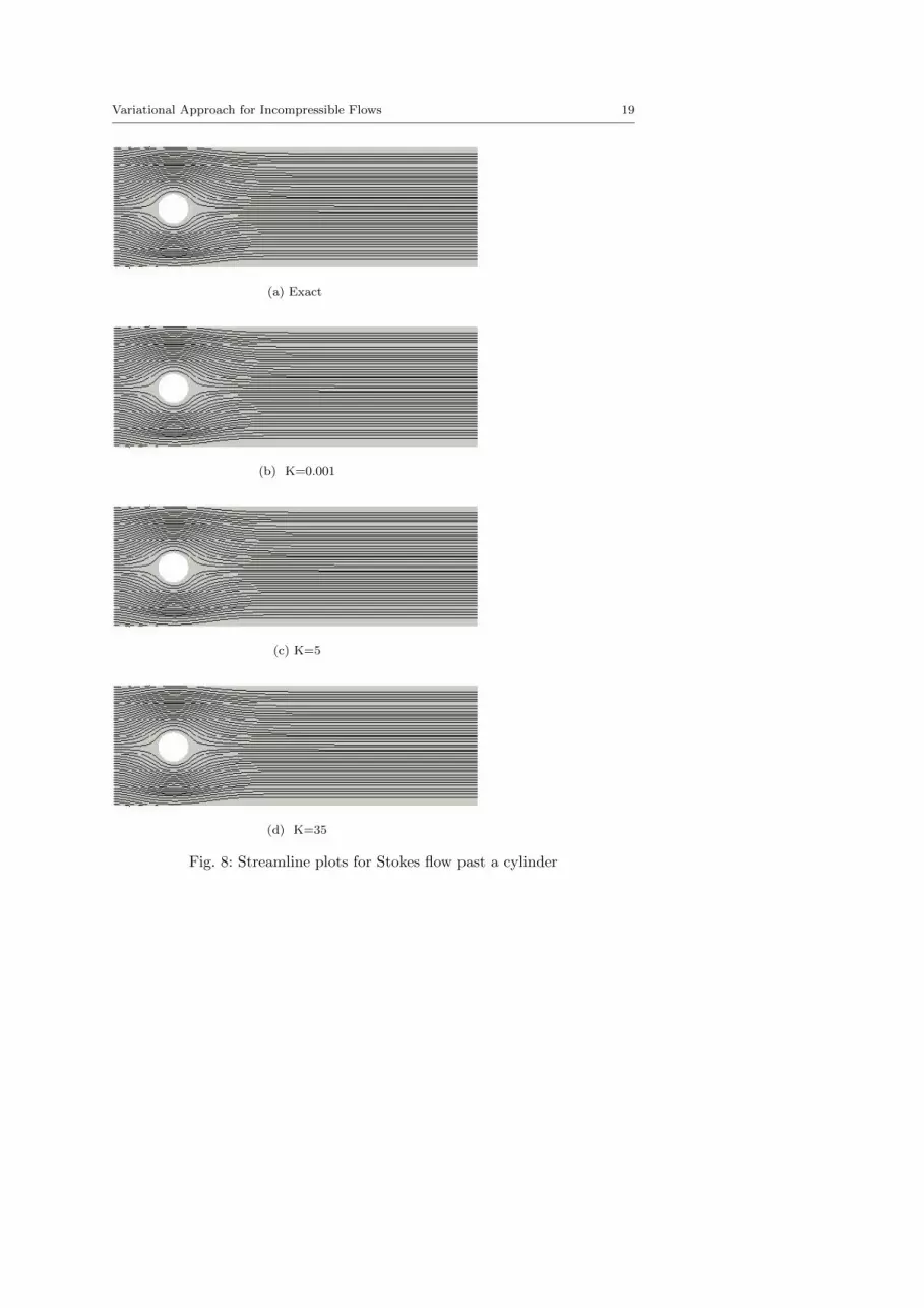
The exact flow is given by solving (28) as a flow past a cylinder with f =(1, 100). Figure (7) shows plots of velocity vectors for various K. Again thevelocity is recovered with a very high degree of accuracy. Table (2) shows therelative L2 errors and the advection errors, which are quite small, justifying


(a) Exact (b) K=0.001

(c) K=5 (d) K=35

Fig. 5: Velocity plots for Stokes flow in a lid driven cavity

K Relative L2 Error Advection Error

0.001 4.55e-08 9.62e-265 4.56e-08 6.83e-27

110 4.49e-08 2.51e-27300 4.48e-08 4.11e-27600 4.42e-08 3.57e-28

Table 1: Variation of relative L2 error and advection error with K for Stokesflow in a lid driven cavity

good recovery of flows. The streamline plots for the velocity is given in Figure(8). As with the case of Stokes flow in a lid driven cavity, there is no dependenceof the obtained solutions on K.


(a) Exact (b) K=0.001

(c) K=5 (d) K=35

Fig. 6: Streamline plots for Stokes flow in a lid driven cavity


0.001 1.44e-8 3.76e-285 1.53e-8 6.43e-27

110 1.47e-8 6.69e-28300 1.42e-8 5.25e-28600 1.69e-8 5.32e-28

Table 2: Variation of relative L2 error and advection error with K for Stokesflow past a cylinder

6.3 Navier-Stokes flow in a lid driven cavity for Re = 1 and 1000

Here we consider motion governed by Navier-Stokes flows for Re = 1 and 1000.The exact flow is given by solving (29) with f = (1, 100) in a lid-driven cavity.Figures (9) and (11) show the velcity vector plots for Re = 1 and Re = 1000respectively. The plots show good recovery for Re = 1, whereas for Re = 1000


(a) Exact

(b) K=0.001

(c) K=5

(d) K=35

Fig. 7: Velocity plots for Stokes flow past a cylinder


(a) Exact

(b) K=0.001

(c) K=5

(d) K=35

Fig. 8: Streamline plots for Stokes flow past a cylinder


(a) Exact (b) K=0.001

(c) K=5 (d) K=35

Fig. 9: Velocity plots for Navier-Stokes flow in a lid driven cavity for Re = 1

the relative L2 error is on the higher side. This is also reflected in Tables(3) and (4). The streamline plots given by Figures (10), (12) show that forlower Reynolds number flows the vortices are well recovered whereas for higherReynolds number flows the vortices are recovered though not to a greater de-gree of accuracy. Tables (3) and (4) suggests that the advection error for lowerReynolds number flows is very low compared to higher Reynolds number flows.This is because at low Reynolds number, Navier-Stokes flows represents Stokesflows and hence they are recovered well. For higher Reynolds number flows,the non-linear convection term dominates and so a very good flow recoveryis not possible with our linear model. However we note that even for higherReynolds number flows, the solution obtained is independent of K.


(a) Exact (b) K=0.001

(c) K=5 (d) K=35

Fig. 10: Streamline plots for Navier-Stokes flow in a lid driven cavity for Re = 1


0.001 3.56e-4 2.7e-115 3.61e-4 2.8e-11

110 3.44e-4 3.1e-11300 3.48e-4 2.9e-11600 3.4e-4 2.6e-11

Table 3: Variation of relative L2 error and advection error with K for Navier-Stokes flow in a lid driven cavity for Re = 1

6.4 Navier-Stokes flow past a cylinder.

The exact flow is given by solving (29) as a flow past a cylinder with f =(1, 100). Figures (13) and (15) show the velocity vector plots for Re = 1 andRe = 1000 respectively. The plots show good recovery for Re = 1, whereas forRe = 1000 the relative L2 error is on the higher side which is also reflected


(a) Exact (b) K=0.001

(c) K=5 (d) K=35

Fig. 11: Velocity plots for Navier-Stokes flow in a lid driven cavity for Re =1000


0.001 5.81e-1 2.8e-85 5.95e-1 3.6e-8

110 6.12e-1 4.1e-8300 6.07e-1 2.5e-8600 5.86e-1 5.2e-8

Table 4: Variation of relative L2 error and advection error with K for Navier-Stokes flow in a lid driven cavity for Re = 1000


(a) Exact (b) K=0.001

(c) K=5 (d) K=35

Fig. 12: Streamline plots for Navier-Stokes flow in a lid driven cavity for Re =1000


0.001 1.01e-4 2.0e-115 1.11e-4 2.0e-11

110 1.24e-4 2.1e-11300 1.15e-4 2.5e-11600 1.08e-4 2.6e-11

Table 5: Variation of relative L2 error and advection error with K for Navier-Stokes flow past a cylinder for Re = 1

in Tables (5) and (6). The streamline plots given by Figures (14) and (16)show that vortices for low Reynolds number flows are captured well whereasfor higher Reynolds number flows, the vortices behind the cylinder are notcaptured. This suggests there is a need to include extra assumptions in ourmodel for high Reynolds number flows.


(a) Exact

(b) K=0.001

(c) K=5

(d) K=35

Fig. 13: Velocity plots for Navier-Stokes flow past a cylinder for Re = 1


(a) Exact

(b) K=0.001

(c) K=5

(d) K=35

Fig. 14: Streamline plots for Navier-Stokes flow past a cylinder for Re = 1


(a) Exact

(b) K=0.001

(c) K=5

(d) K=35

Fig. 15: Velocity plots for Navier-Stokes flow past a cylinder for Re = 1000

7 Conclusion

A variational technique for tracking instantaneous motion from flow imagesusing the well-known OFM has been formulated. In the present work, theseflow images have been generated by numerically solving the 2D incompressible


(a) Exact

(b) K=0.001

(c) K=5

(d) K=35

Fig. 16: Streamline plots for Navier-Stokes flow past a cylinder for Re = 1000



0.001 7.23e-1 4.3e-85 6.56e-1 4.6e-8

110 6.12e-1 4.6e-8300 6.33e-1 4.5e-8600 6.86e-1 4.7e-8

Table 6: Variation of relative L2 error and advection error with K for Navier-Stokes flow past a cylinder for Re = 1000

Stokes equation (28) or the Navier-Stokes equations (29) for Re = 1 and 1000.Incompressibility is the only constraint imposed in the variational formulation.Using FEM in the present variational approach method, it is shown that thevelocities are recovered almost exactly for Stokes flow forced by potential. ForNavier-Stokes flow the method performs very well for Re = 1 compared toRe = 1000. This is because Stokes flow is a linearized version of the Navier-Stokes flow for low Reynolds number. But nevertheless, in both the cases thephysical features of fluid flow like vortex structures are captured well. Thisis particularly attractive for the cloud motion problem. The simplicity of ourvariational approach makes it computationally attractive. In future we plan toextend this variational approach to track high Reynolds number flows as well.


References

1. Cayula J.–F. and Cornillon P. Cloud detection from a sequence of SST images. RemoteSens. Env., 55(1996)80–88.

2. Leese J. A., Novak C. S. and Taylor V. R. The determination of cloud pattern motionsfrom geosynchronous satellite image data. Pattern Recog., 2(1970) 279–292.

3. Fogel S. V. The estimation of velocity vector-fields from time varying image sequences.CVGIP: Image Understanding, 53(1991) 253–287.

4. Wu Q. X. A correlation-relaxation labeling framework for computing optical flow-Template matching from a new perspective. IEEE Trans. Pattern Analysis and Ma-chine Intelligence, 17(1995) 843–853.

5. Parikh J. A., DaPonte J. S., Vitale J. N. and Tselioudis G. An evolutionary systemfor recognition and tracking of synoptic scale storm systems. Pattern RecognitionLetters, 20(1999) 1389–1396.

6. Liu T. and Shen L. Fluid Flow and optical flow. J. Fluid Mech, 614(2008) 253–291.7. Horn B. K. P. and Schunck B. G. Determining optical flow. Artificial Intelligence,

17(1-3)(1981) 185–203.8. Ruhnau P. and Schnorr C. Optical Stokes flow: An imaging based control approach.

Exp. Fluids, 42(2007) 61–78.9. Yuan J., Ruhnau P., Memin E., and Schnorr C. Discrete orthogonal decomposition

and variational fluid flow estimation. In Scale-Space, volume 3459(2005) of Lect. Not.Comp. Sci., pages 267–278. Springer.

10. Heitz D., Memin E. and Schnorr C. Variational fluid flow measurement from imagesequences: synopsis and perspectives. Exp. Fluids, 48(2010) 369–393.

11. Haussecker H. W. and Fleet D. J. Computing Optical Flow with Physical Models ofBrightness Variation, IEEE Transactions on Pattern Analysis and Machine Intelli-gence , 23(6)(2001) 661–673.

12. Nagel H.–H. On a constraint equation for the estimation of displacement rates inimage sequences. IEEE Trans. PAMI, 11(1989) 13-30.

13. Papadakis N. and Memin E. Variational assimilation of fluid motion from imagesequence. SIAM Journal on Imaging Sciences, 1(4)(2008) 343-363.

14. Corpetti T., Memin E., and Perez P. Dense estimation of fluid flows. IEEE Trans.Pattern Anal. Mach. Intell., 24(3)(2002) 365–380.

15. Mukawa N. Estimation of shape, reflection coefficients and illuminant direction fromimage sequences. In ICCV90, 1990, 507–512.

16. Nakajima Y., Inomata H., Nogawa H., Sato Y., Tamura S., Okazaki K. and ToriiS.. Physics-based flow estimation of fluids. Pattern Recognition, 36(5)(2003) 1203 –1212.

17. Arnaud E., Memin E., Sosa R. and Artana G. A fluid motion estimator for schlierenimage velocimetry. In ECCV06, I(2006) 198–210.

18. Logg A., Mardal K.–A., Wells G. N. Automated Solution of Differential Equationsby the Finite Element Method. Springer, 2012.

19. Souvik Roy. Optical Flows - Determination of 2-D velocities of a moving fluid. M.PhilThesis, Tata Institute of Fundamental Research, CAM, Bangalore, 2011.

20. Bauschke H. H. and Combettes P. L. Convex analysis and monotone operator theoryin Hilbert spaces. CMS Books in Mathematics, Springer xvi+468 pp. ISBN: 978-1-4419-9466-0, 2011.

21. Langtengen H. P. Computational Partial Differential Equations–Numerical meth-ods and Diffpack programming. Texts in Computational Science and Engineering,Springer LII, 860 pp. ISBN: 978-3-642-55769-9, 2003.

22. Girault V. and Raviart P.–A. Finite Element Methods for Navier-Stokes Equations.Theory and Algorithms. Springer Series in Computational Mathematics. Springer-Verlag, Berlin, Germany, 1986.

23. Troltzsch F. Optimal Control of Partial Differential Equations: Theory, Methods andApplications. Graduate Studies in Mathematics, American Mathematical Society,Vol-112, 2010.

24. Aubert G. and Kornprobst P. A mathematical study of the relaxed optical flow prob-lem in the space, SIAM Journal of Math. Anal, 30(6)(1999) 1282–1308.


25. Aubert G., Deriche R. and Kornprobst P. Computing Optical Flow via VariationalTechniques, SIAM Journal of Math. Anal, 60(1)(1999) 156-182.

26. Nagel H.–H. Displacement vectors derived from second-order intensity variations inimage sequences. CGIP, 21(1983) 85-117.

27. Nagel H.–H. On the estimation of optical flow: Relations between different approachesand some new results. AI, 33(1987) 299-324.

28. Nagel H.–H. and Enkelmann W. An investigation of smoothness constraints for theestimation of displacement vector fields from image sequences. IEEE Trans. PAMI,8(1986) 565-593.

29. Wayne Roberts A. and Varberg D. E. Convex Functions, Academic Press, New Yorkand London, 1973.

a variational approach to estimate incompressible fluid flows

Documents