knowledge-based systems layer-constrained variational

Knowledge-Based Systems 196 (2020) 105753

Contents lists available at ScienceDirect

Knowledge-Based Systems

journal homepage: www.elsevier.com/locate/knosys

Layer-constrained variational autoencoding kernel density estimationmodel for anomaly detection✩

Peng Lv b, Yanwei Yu a,b,∗, Yangyang Fan c, Xianfeng Tang d, Xiangrong Tong b

a Department of Computer Science and Technology, Ocean University of China, Qingdao, Shandong 266100, Chinab School of Computer and Control Engineering, Yantai University, Yantai, Shandong 264005, Chinac Shanghai Key Lab of Advanced High-Temperature Materials and Precision Forming, Shanghai Jiao Tong University, Shanghai 200240, Chinad College of Information Sciences and Technology, The Pennsylvania State University, University Park, PA 16802, USA

a r t i c l e i n f o

Article history:Received 16 October 2019Received in revised form 5 March 2020Accepted 7 March 2020Available online 10 March 2020

Keywords:Anomaly detectionVariational autoencoderKernel density estimationLayer constraintDeep learning

a b s t r a c t

Unsupervised techniques typically rely on the probability density distribution of the data to detectanomalies, where objects with low probability density are considered to be abnormal. However,modeling the density distribution of high dimensional data is known to be hard, making the problem ofdetecting anomalies from high-dimensional data challenging. The state-of-the-art methods solve thisproblem by first applying dimension reduction techniques to the data and then detecting anomaliesin the low dimensional space. Unfortunately, the low dimensional space does not necessarily preservethe density distribution of the original high dimensional data. This jeopardizes the effectiveness ofanomaly detection. In this work, we propose a novel high dimensional anomaly detection methodcalled LAKE. The key idea of LAKE is to unify the representation learning capacity of layer-constrainedvariational autoencoder with the density estimation power of kernel density estimation (KDE). Then aprobability density distribution of the high dimensional data can be learned, which is able to effectivelyseparate the anomalies out. LAKE successfully consolidates the merits of the two worlds, namelylayer-constrained variational autoencoder and KDE by using a probability density-aware strategy inthe training process of the autoencoder. Extensive experiments on six public benchmark datasetsdemonstrate that our method significantly outperforms the state-of-the-art methods in detectinganomalies and achieves up to 37% improvement in F1 score.

© 2020 Elsevier B.V. All rights reserved.

1. Introduction

Anomaly detection is a fundamental and hence well-studiedproblem in many areas, including cyber-security [1], manufac-turing [2], system management [3], and medicine [4]. The coreof anomaly detection is density estimation whether it is high-dimensional data or multi-dimensional data. In general, normaldata is large and consistent with certain distribution, while ab-normal data is small and discrete, therefore anomalies are resid-ing in low density areas.

Although excellent progress have been achieved in anomalydetection in the past decades, anomaly detection of complex and

✩ No author associated with this paper has disclosed any potential orpertinent conflicts which may be perceived to have impending conflict withthis work. For full disclosure statements refer to https://doi.org/10.1016/j.knosys.2020.105753.∗ Correspondence to: 238 Songling RD, Laoshan District, Qingdao,

Shandong 266100, ChinaE-mail addresses: [email protected] (P. Lv), [email protected]

(Y. Yu), [email protected] (Y. Fan), [email protected] (X. Tang),[email protected] (X. Tong).

high-dimensional data remains to be a challenge. It is hard toimplement density estimation in original data space with theincreasing of dimensionality, because as the data dimension in-creases, noise and extraneous features have a more negativeimpact on density estimation. But unfortunately for a real-worldproblem, the dimensionality of data could be very large, suchas video surveillance [5], medical anomaly detection [6], andcyber-intrusion detection [7]. To address this issue, a two-stepapproach [4] is usually applied and has proved to be successful.It first reduces the dimensionality of data and then adopt den-sity estimation in the latent low-dimensional space. Additionally,spectral anomaly detection [8–10] and alternative dimensionalityreduction [11–13] techniques are implemented to find the lowerdimensional representation of the original high-dimensional data,where anomalies and normal instances are expected to be sep-arated from each other. However, the low dimensional spacedoes not necessarily preserve the density distribution of theoriginal data, and thus it is not able to effectively identify theanomalies in high-dimensional data by estimating the density inlow-dimensional space.

Recently, deep learning has achieved great success in anomalydetection [7]. Autoencoder [14] and a range of variants have been

https://doi.org/10.1016/j.knosys.2020.1057530950-7051/© 2020 Elsevier B.V. All rights reserved.

https://doi.org/10.1016/j.knosys.2020.105753

http://www.elsevier.com/locate/knosys

http://www.elsevier.com/locate/knosys

http://crossmark.crossref.org/dialog/?doi=10.1016/j.knosys.2020.105753&domain=pdf



mailto:[email protected]






2 P. Lv, Y. Yu, Y. Fan et al. / Knowledge-Based Systems 196 (2020) 105753

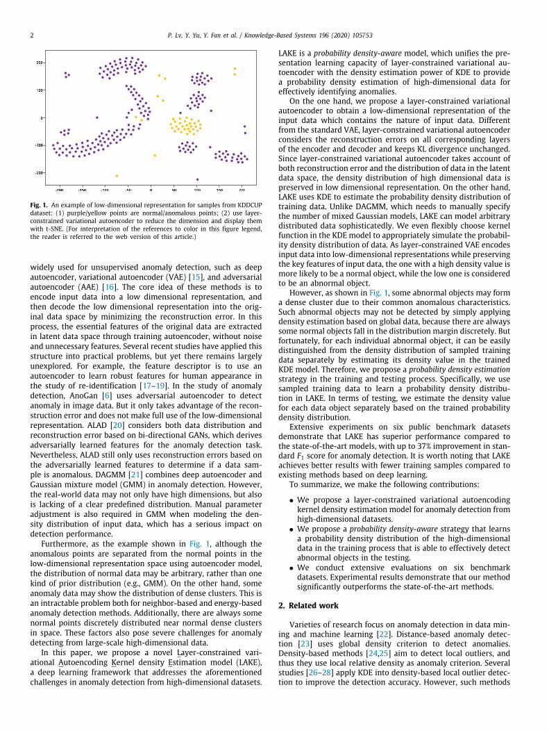
Fig. 1. An example of low-dimensional representation for samples from KDDCUPdataset: (1) purple/yellow points are normal/anomalous points; (2) use layer-constrained variational autoencoder to reduce the dimension and display themwith t-SNE. (For interpretation of the references to color in this figure legend,the reader is referred to the web version of this article.)

widely used for unsupervised anomaly detection, such as deepautoencoder, variational autoencoder (VAE) [15], and adversarialautoencoder (AAE) [16]. The core idea of these methods is toencode input data into a low dimensional representation, andthen decode the low dimensional representation into the orig-inal data space by minimizing the reconstruction error. In thisprocess, the essential features of the original data are extractedin latent data space through training autoencoder, without noiseand unnecessary features. Several recent studies have applied thisstructure into practical problems, but yet there remains largelyunexplored. For example, the feature descriptor is to use anautoencoder to learn robust features for human appearance inthe study of re-identification [17–19]. In the study of anomalydetection, AnoGan [6] uses adversarial autoencoder to detectanomaly in image data. But it only takes advantage of the recon-struction error and does not make full use of the low-dimensionalrepresentation. ALAD [20] considers both data distribution andreconstruction error based on bi-directional GANs, which derivesadversarially learned features for the anomaly detection task.Nevertheless, ALAD still only uses reconstruction errors based onthe adversarially learned features to determine if a data sam-ple is anomalous. DAGMM [21] combines deep autoencoder andGaussian mixture model (GMM) in anomaly detection. However,the real-world data may not only have high dimensions, but alsois lacking of a clear predefined distribution. Manual parameteradjustment is also required in GMM when modeling the den-sity distribution of input data, which has a serious impact ondetection performance.

Furthermore, as the example shown in Fig. 1, although theanomalous points are separated from the normal points in thelow-dimensional representation space using autoencoder model,the distribution of normal data may be arbitrary, rather than onekind of prior distribution (e.g., GMM). On the other hand, someanomaly data may show the distribution of dense clusters. This isan intractable problem both for neighbor-based and energy-basedanomaly detection methods. Additionally, there are always somenormal points discretely distributed near normal dense clustersin space. These factors also pose severe challenges for anomalydetecting from large-scale high-dimensional data.

In this paper, we propose a novel Layer-constrained vari-ational Autoencoding Kernel density Estimation model (LAKE),a deep learning framework that addresses the aforementionedchallenges in anomaly detection from high-dimensional datasets.

LAKE is a probability density-aware model, which unifies the pre-sentation learning capacity of layer-constrained variational au-toencoder with the density estimation power of KDE to providea probability density estimation of high-dimensional data foreffectively identifying anomalies.

On the one hand, we propose a layer-constrained variationalautoencoder to obtain a low-dimensional representation of theinput data which contains the nature of input data. Differentfrom the standard VAE, layer-constrained variational autoencoderconsiders the reconstruction errors on all corresponding layersof the encoder and decoder and keeps KL divergence unchanged.Since layer-constrained variational autoencoder takes account ofboth reconstruction error and the distribution of data in the latentdata space, the density distribution of high dimensional data ispreserved in low dimensional representation. On the other hand,LAKE uses KDE to estimate the probability density distribution oftraining data. Unlike DAGMM, which needs to manually specifythe number of mixed Gaussian models, LAKE can model arbitrarydistributed data sophisticatedly. We even flexibly choose kernelfunction in the KDE model to appropriately simulate the probabil-ity density distribution of data. As layer-constrained VAE encodesinput data into low-dimensional representations while preservingthe key features of input data, the one with a high density value ismore likely to be a normal object, while the low one is consideredto be an abnormal object.

However, as shown in Fig. 1, some abnormal objects may forma dense cluster due to their common anomalous characteristics.Such abnormal objects may not be detected by simply applyingdensity estimation based on global data, because there are alwayssome normal objects fall in the distribution margin discretely. Butfortunately, for each individual abnormal object, it can be easilydistinguished from the density distribution of sampled trainingdata separately by estimating its density value in the trainedKDE model. Therefore, we propose a probability density estimationstrategy in the training and testing process. Specifically, we usesampled training data to learn a probability density distribu-tion in LAKE. In terms of testing, we estimate the density valuefor each data object separately based on the trained probabilitydensity distribution.

Extensive experiments on six public benchmark datasetsdemonstrate that LAKE has superior performance compared tothe state-of-the-art models, with up to 37% improvement in stan-dard F1 score for anomaly detection. It is worth noting that LAKEachieves better results with fewer training samples compared toexisting methods based on deep learning.

To summarize, we make the following contributions:

• We propose a layer-constrained variational autoencodingkernel density estimation model for anomaly detection fromhigh-dimensional datasets.• We propose a probability density-aware strategy that learns

a probability density distribution of the high-dimensionaldata in the training process that is able to effectively detectabnormal objects in the testing.• We conduct extensive evaluations on six benchmark

datasets. Experimental results demonstrate that our methodsignificantly outperforms the state-of-the-art methods.

2. Related work

Varieties of research focus on anomaly detection in data min-ing and machine learning [22]. Distance-based anomaly detec-tion [23] uses global density criterion to detect anomalies.Density-based methods [24,25] aim to detect local outliers, andthus they use local relative density as anomaly criterion. Severalstudies [26–28] apply KDE into density-based local outlier detec-tion to improve the detection accuracy. However, such methods

P. Lv, Y. Yu, Y. Fan et al. / Knowledge-Based Systems 196 (2020) 105753 3

rely on an appropriate distance metric, which is only feasible forhandling low-dimensional data, but not for anomaly detectionof high dimensional data. One-class classification approachestrained by normal data, such as one-class SVMs [11,29], arealso widely used for anomaly detection. These methods usekernel methods to learn a decision boundary around the normaldata. Another line of studies use fidelity of reconstruction todetermine whether a sample is anomalous, such as conventionalPrincipal Component Analysis (PCA), kernel PAC, and Robust PCA(RPCA) [12,30]. Several recent researches [31,32] apply modelfitting to estimate model hypotheses for multistructure data withhigh outlier rates.

In recent years, varieties of anomaly detection methods basedon deep neural networks are proposed to detect anomalies [7].Autoencoder and its series of variants have been widely used inunsupervised anomaly detection, especially for high-dimensionaldata anomaly detection. Inspired by RPCA [12], Zhou et al. [14]design a Robust Deep Autoencoder (RDA), and use the recon-struction error to detect anomalies for high-dimensional data. Thevariational autoencoder is used directly for anomaly detection byusing reconstruction error in [15]. With the rise of adversarialnetworks, more models have added adversarial networks to au-toencoders. AnoGAN [33] uses a Generative Adversarial Network(GAN) [34] to detect anomalies in the context of medical imagesby reconstruction error. In a follow-up work, f-AnoGAN [35]introduces Wasserstein GAN (WGAN) [36] to improve AnoGANto be adaptable to real-time anomaly detection applications. Theabove methods can be classified as reconstruction based anomalydetection method. However, the performance of reconstructionbased methods is limited by the fact that they only considerreconstruction error as anomaly criterion.

Deep structured energy based model (DSEBM) [37] addressesthe anomaly detection problem by directly modeling the datadistribution with deep architectures. DSEBM integrates Energy-Based Models (EBMs) with different types of data such as staticdata, sequential data, and spatial data, and apply appropriatemodel architectures to adapt to the data structure. DSEBM hastwo decision criteria for performing anomaly detection: the en-ergy score (DSEBM-e) and the reconstruction error (DSEBM-r).Deep Autoencoding Gaussian Mixture Model (DAGMM) [21] uti-lizes a deep autoencoder to generate a low-dimensional represen-tation and reconstruction error for each input data point, whichis further fed into a Gaussian Mixture Model. These methods useautoencoder to model the distribution of data, and then derivethe criteria for determining anomalies through an energy modelor a Gaussian mixture model. As GANs are able to model the com-plex high-dimensional distributions of real-world data, so thatAdversarially Learned Anomaly Detection (ALAD) [20] derivesadversarially learned features based on bi-directional GANs, andthen uses reconstruction errors based on these learned featuresfor the anomaly detection task.

Our proposed model is most related to DAGMM. However,unlike DAGMM, LAKE uses a layer-constrained variational au-toencoder to extract useful features while preserving the datadistribution of the original data for anomaly detection. And LAKEleverages KDE to model the arbitrary density distribution of train-ing samples in the latent data space without parameter depen-dence, rather than a predefined GMM distribution. Most impor-tantly, LAKE estimates the probability density value for each testsample based on the trained KDE model individually, and show apowerful ability of anomaly detection with few training samples.

3. The proposed LAKE model

3.1. Overview

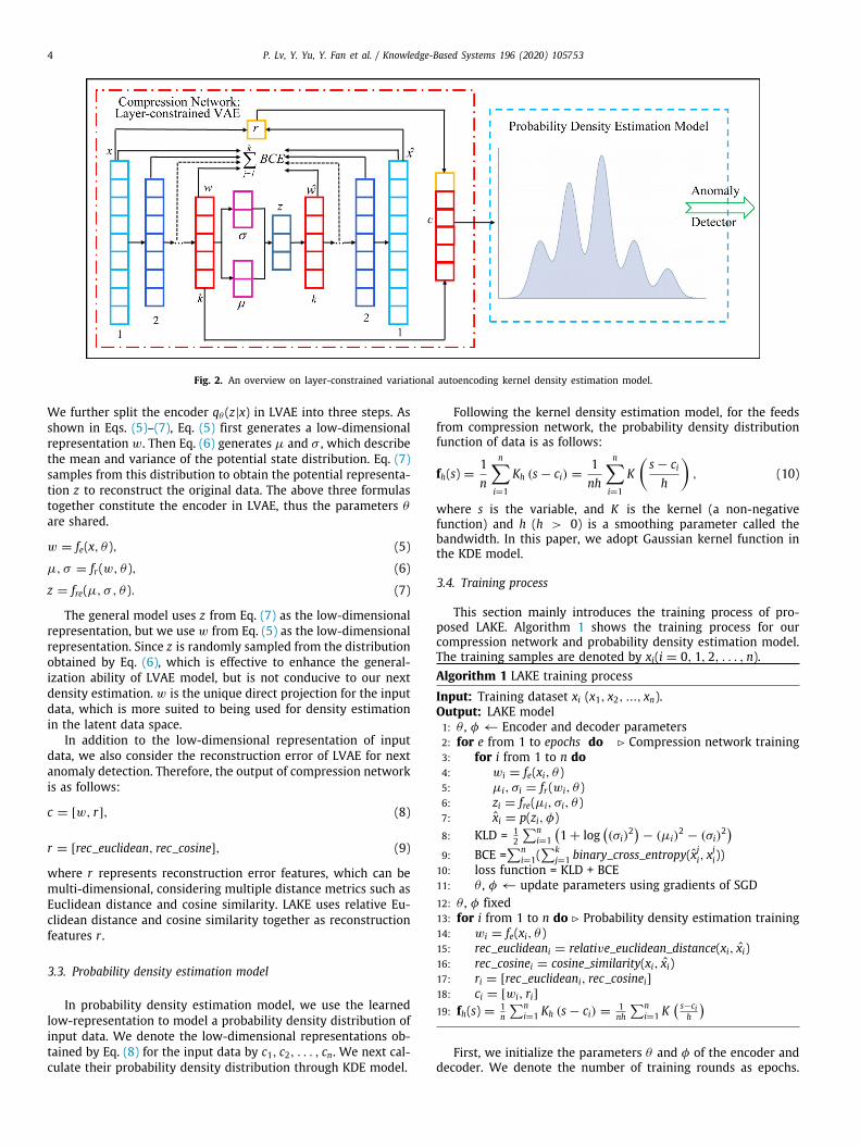
Fig. 2 shows the architecture of the proposed layer-constrainedvariational autoencoding kernel density estimation model. LAKE

is mainly composed of two parts: compression network andprobability density estimation model. First, in the compressionnetwork, LAKE compresses the input data to obtain their low-dimensional representations in latent data space by a proposedlayer-constrained variational autoencoder, and together with re-construction errors they are fed to the probability density esti-mation model. Second, the estimation model takes the feeds andlearns a probability density distribution using a Gaussian kerneldensity estimation.

3.2. Compression network

The compression network in LAKE is a layer-constrained vari-ational autoencoder (LVAE). The low-dimensional representationof the original data in latent data space is derived from thelayer-constrained variational autoencoder.

Variational autoencoder is a probabilistic graphical model thatcombines variational interference with deep learning [38,39],which includes an encoder and a decoder. For a given inputdata x, the variational autoencoder calculates its low-dimensionalrepresentation z as follows:

z = q(x, θ ), (1)

x = p(z, φ), (2)

where qθ (z|x) denotes the encoder, pφ(x|z) denotes the decoder,θ and φ are the network parameters of the encoder and decoder,and x is the reconstruction of original data.

The loss function of variational autoencoder is the negativelog-likelihood with a regularizer. Since there are no global repre-sentations that are shared by all data points, we can decomposethe loss function into only terms that depend on a single datapoint li. The total loss is then

∑Ni=1 li for N total data points. The

loss function li for data point xi is:

li(θ, φ) = −Ez∼qθ (z|xi)[log pφ (xi|z)

]+ KL (qθ (z|xi) ∥ p(z)) , (3)

where the first term is the reconstruction loss, or expected neg-ative log-likelihood of the ith data point. The second term is theKullback–Leibler (KL) divergence between the distribution qθ (z|x)and p(z). This divergence measures how much information is lost(in units of nats) when using q to represent p. It is one measureof how close q is to p.

To enhance the representation learning capacity of compres-sion network, we propose a layer-constrained variational autoen-coder (LVAE). Unlike the standard VAE that only reconstructs lossat the input and output layers, LVAE considers reconstructionlosses on all corresponding layers of the encoder and decoderand keeps KL divergence unchanged. The advantages of our LVAEmodel are twofold: First, layer constraints enhance the recon-struction ability of compression network by minimizing the infor-mation losses of input data between each pair of correspondinglayers, which retains the essential features of original data in thelow-dimensional representation as much as possible. Second, ourlayer constrained model would make the reconstruction error ofthe training samples smaller, which makes it easier to distinguishanomalies with the reconstruction error in the testing process.

Let k denote the number of corresponding layers in the en-coder and decoder, then our loss function is:

li(θ, φ) = −k∑

j=1

Ez∼qθ

(z|xji

) [log pφ

(xji|z

)]+ KL (qθ (z|xi) ∥ p(z)) ,

(4)

where xji is the representation of data point xi in jth layer.Although we use a LVAE as our compression network, we

do not directly use the low-dimensional representation of LVAE.


Fig. 2. An overview on layer-constrained variational autoencoding kernel density estimation model.

We further split the encoder qθ (z|x) in LVAE into three steps. Asshown in Eqs. (5)–(7), Eq. (5) first generates a low-dimensionalrepresentation w. Then Eq. (6) generates µ and σ , which describethe mean and variance of the potential state distribution. Eq. (7)samples from this distribution to obtain the potential representa-tion z to reconstruct the original data. The above three formulastogether constitute the encoder in LVAE, thus the parameters θ

are shared.

w = fe(x, θ ), (5)

µ, σ = fr (w, θ ), (6)

z = fre(µ, σ , θ ). (7)

The general model uses z from Eq. (7) as the low-dimensionalrepresentation, but we use w from Eq. (5) as the low-dimensionalrepresentation. Since z is randomly sampled from the distributionobtained by Eq. (6), which is effective to enhance the general-ization ability of LVAE model, but is not conducive to our nextdensity estimation. w is the unique direct projection for the inputdata, which is more suited to being used for density estimationin the latent data space.

In addition to the low-dimensional representation of inputdata, we also consider the reconstruction error of LVAE for nextanomaly detection. Therefore, the output of compression networkis as follows:

c = [w, r], (8)

r = [rec_euclidean, rec_cosine], (9)

where r represents reconstruction error features, which can bemulti-dimensional, considering multiple distance metrics such asEuclidean distance and cosine similarity. LAKE uses relative Eu-clidean distance and cosine similarity together as reconstructionfeatures r .

3.3. Probability density estimation model

In probability density estimation model, we use the learnedlow-representation to model a probability density distribution ofinput data. We denote the low-dimensional representations ob-tained by Eq. (8) for the input data by c1, c2, . . . , cn. We next cal-culate their probability density distribution through KDE model.

Following the kernel density estimation model, for the feedsfrom compression network, the probability density distributionfunction of data is as follows:

fh(s) =1n

n∑i=1

Kh (s− ci) =1nh

n∑i=1

K(s− cih

), (10)

where s is the variable, and K is the kernel (a non-negativefunction) and h (h > 0) is a smoothing parameter called thebandwidth. In this paper, we adopt Gaussian kernel function inthe KDE model.

3.4. Training process

This section mainly introduces the training process of pro-posed LAKE. Algorithm 1 shows the training process for ourcompression network and probability density estimation model.The training samples are denoted by xi(i = 0, 1, 2, . . . , n).Algorithm 1 LAKE training process

Input: Training dataset xi (x1, x2, ..., xn).Output: LAKE model1: θ , φ ← Encoder and decoder parameters2: for e from 1 to epochs do ▷ Compression network training3: for i from 1 to n do4: wi = fe(xi, θ )5: µi, σi = fr (wi, θ )6: zi = fre(µi, σi, θ )7: xi = p(zi, φ)8: KLD = 1

2

∑ni=1

(1+ log

((σi)

2)− (µi)

2− (σi)

2)9: BCE =

∑ni=1(

∑kj=1 binary_cross_entropy(x

ji, x

ji))

10: loss function = KLD + BCE11: θ , φ ← update parameters using gradients of SGD12: θ , φ fixed13: for i from 1 to n do ▷ Probability density estimation training14: wi = fe(xi, θ )15: rec_euclideani = relative_euclidean_distance(xi, xi)16: rec_cosinei = cosine_similarity(xi, xi)17: ri = [rec_euclideani, rec_cosinei]18: ci = [wi, ri]19: fh(s) = 1

n

∑ni=1 Kh (s− ci) = 1

nh

∑ni=1 K

( s−cih

)First, we initialize the parameters θ and φ of the encoder and

decoder. We denote the number of training rounds as epochs.


Specifically, in each epoch, for each input point, line 4 gets thelow-dimensional representation from encoder; line 5 gets themean and variance of the data distribution; line 6 gets the low-dimensional representation z; line 7 gets the decoder’s recon-struction. KLD is the Kullback–Leibler divergence. Specifically, weuse a binary_cross_entropy loss function as the reconstructionerror for each pair of corresponding layers, and the sum of recon-struction errors of all layer pairs in LVAE constitutes the BinaryCross Entropy (BCE) loss (line 9). KLD and BCE together form theloss function, and we use the Stochastic Gradient Descent (SGD)to update the parameters θ and φ.

Our probability density estimation model is based on KDEmodel. We first use a trained LVAE to get a low dimensionalrepresentation ci of the training data xi (lines 13–18). Amongthem, we calculate the relative Euclidean distance between theinput data x and the reconstruction x in line 15 and the cosinesimilarity between the input data x and the reconstruction x inline 16. Then, we get a probability density distribution functionfh(s) for simulating the distribution of training data in the latentspace, as shown in line 19.

Our model can capture the arbitrary density distribution oftraining data through KDE model without tuning parameter.

3.5. Testing strategy

This section introduces the testing strategy for the proposedLAKE model. As showed in Fig. 1, even though abnormal objectsare separated from normal data in low dimensional representa-tion, some anomalies may form dense clusters due to their com-mon anomalous characteristics preserved in the low-dimensionalrepresentation. On the other hand, there are always some normalobjects that discretely distributed at the edges of the normal datadense regions. These edge normal objects may have a relativelow density compared to the dense anomalies. Therefore, suchabnormal objects and edge normal objects cannot be effectivelydetected and differentiated by the density estimation based onglobal data. But fortunately, we learn a probability density distri-bution of sampled training data in training LAKE model. For eachindividual abnormal object, it can be easily distinguished from theprobability density distribution of training samples by estimatingits density value in this probability density distribution. Thisis because: (1) The training set is used not only to train theparameters of LVAE, but also to generate a probability densitydistribution fh(s); (2) The density of each test sample is notcalculated based on the entire test data distribution, but based onthe trained probability density distribution; (3) The vast majorityof the training samples are normal samples, that is, the trainedprobability density distribution of training samples approximatesthe distribution of normal samples; (4) This probability densitydistribution takes into account not only the latent representationbut also the reconstruction error features. The anomalous ob-jects usually have a relatively large reconstruction error [6,21,37].Therefore, when each test sample is independently mapped onthis probability density distribution, the edge normal objects arecloser to the distribution than the dense abnormal objects, that is,the edge normal samples can instead obtain higher density valuesin our probability density estimation model.

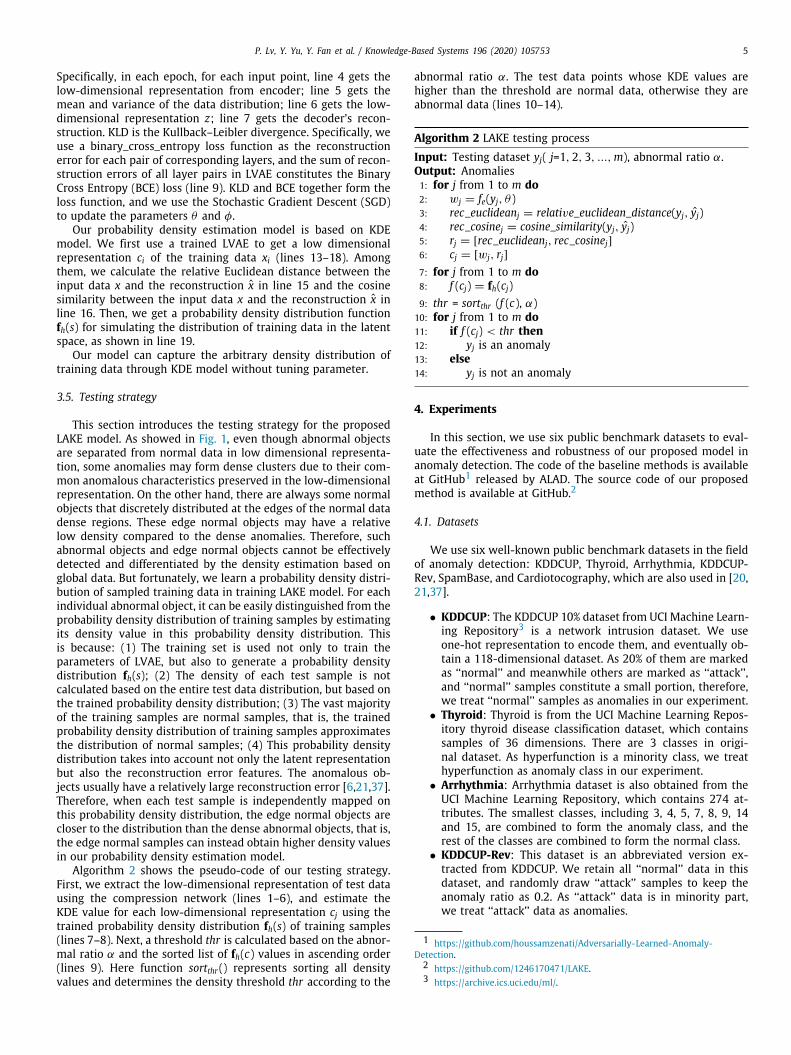
Algorithm 2 shows the pseudo-code of our testing strategy.First, we extract the low-dimensional representation of test datausing the compression network (lines 1–6), and estimate theKDE value for each low-dimensional representation cj using thetrained probability density distribution fh(s) of training samples(lines 7–8). Next, a threshold thr is calculated based on the abnor-mal ratio α and the sorted list of fh(c) values in ascending order(lines 9). Here function sortthr () represents sorting all densityvalues and determines the density threshold thr according to the

abnormal ratio α. The test data points whose KDE values arehigher than the threshold are normal data, otherwise they areabnormal data (lines 10–14).

Algorithm 2 LAKE testing process

Input: Testing dataset yj( j=1, 2, 3, ...,m), abnormal ratio α.Output: Anomalies1: for j from 1 to m do2: wj = fe(yj, θ )3: rec_euclideanj = relative_euclidean_distance(yj, yj)4: rec_cosinej = cosine_similarity(yj, yj)5: rj = [rec_euclideanj, rec_cosinej]6: cj = [wj, rj]7: for j from 1 to m do8: f (cj) = fh(cj)9: thr = sortthr (f (c), α)

10: for j from 1 to m do11: if f (cj) < thr then12: yj is an anomaly13: else14: yj is not an anomaly

4. Experiments

In this section, we use six public benchmark datasets to eval-uate the effectiveness and robustness of our proposed model inanomaly detection. The code of the baseline methods is availableat GitHub1 released by ALAD. The source code of our proposedmethod is available at GitHub.2

4.1. Datasets

We use six well-known public benchmark datasets in the fieldof anomaly detection: KDDCUP, Thyroid, Arrhythmia, KDDCUP-Rev, SpamBase, and Cardiotocography, which are also used in [20,21,37].

• KDDCUP: The KDDCUP 10% dataset from UCI Machine Learn-ing Repository3 is a network intrusion dataset. We useone-hot representation to encode them, and eventually ob-tain a 118-dimensional dataset. As 20% of them are markedas ‘‘normal’’ and meanwhile others are marked as ‘‘attack’’,and ‘‘normal’’ samples constitute a small portion, therefore,we treat ‘‘normal’’ samples as anomalies in our experiment.• Thyroid: Thyroid is from the UCI Machine Learning Repos-

itory thyroid disease classification dataset, which containssamples of 36 dimensions. There are 3 classes in origi-nal dataset. As hyperfunction is a minority class, we treathyperfunction as anomaly class in our experiment.• Arrhythmia: Arrhythmia dataset is also obtained from the

UCI Machine Learning Repository, which contains 274 at-tributes. The smallest classes, including 3, 4, 5, 7, 8, 9, 14and 15, are combined to form the anomaly class, and therest of the classes are combined to form the normal class.• KDDCUP-Rev: This dataset is an abbreviated version ex-

tracted from KDDCUP. We retain all ‘‘normal’’ data in thisdataset, and randomly draw ‘‘attack’’ samples to keep theanomaly ratio as 0.2. As ‘‘attack’’ data is in minority part,we treat ‘‘attack’’ data as anomalies.

1 https://github.com/houssamzenati/Adversarially-Learned-Anomaly-Detection.2 https://github.com/1246170471/LAKE.3 https://archive.ics.uci.edu/ml/.

https://github.com/houssamzenati/Adversarially-Learned-Anomaly-Detection

https://github.com/houssamzenati/Adversarially-Learned-Anomaly-Detection

https://github.com/1246170471/LAKE

https://archive.ics.uci.edu/ml/


Table 1Statistics of the public benchmark datasets.Dataset #Dimensions #Instances Anomaly ratio (α)

KDDCUP 118 494,021 0.2Thyroid 36 3772 0.025Arrhythmia 274 432 0.15KDDCUP-Rev 118 121,597 0.2SpamBase 58 3485 0.2Cardiotocography 22 2068 0.2

• SpamBase: SpamBase from UCI Machine Learning Reposi-tory includes 3485 emails classified as spam or non-spam.This dataset has 58 attributes. We treat spam as outliers. Theanomaly ratio is 0.2.• Cardiotocography: Cardiotocography data is also from UCI

Machine Learning Repository and is related to heart dis-eases. This dataset contains 22 attributes. It describes 3classes: normal, suspect, and pathological. Normal patientsare treated as inliers and the remaining as outliers. Theanomaly ratio as 0.2.

The details of the datasets are shown in Table 1.

4.2. Baseline methods

We compare our method with the following traditional andthe state-of-the-art deep learning methods:

• OC-SVM [29]: One Class Support Vector Machines(OC-SVM)is a classic kernel method for novelty detection that onlyuses normal data to learn a decision boundary. We adoptthe widely used radial basis function (RBF) kernel. In ourexperiments, we assume that the abnormal proportion isknown. We set the parameter ν to the anomaly proportion,and set γ to 1/m, where m is the number of input features.• DSEBM [37]: Deep Structured Energy Based Models (DSEBM)

is a deep learning method for anomaly detection, whichcontains two decision criteria for performing anomaly de-tection: the energy score (DSEBM-e) and the reconstructionerror (DSEBM-r).• DAGMM [21]: Deep Autoencoding Gaussian Mixture Model

(DAGMM) is a state-of-the-art method for anomaly detec-tion, which consists of two major components: a compres-sion network and an estimation network. The compres-sion network obtains low-dimensional representations, andfeeds the representations to the subsequent estimation net-work to predicts their likelihood/energy in the frameworkof GMM.• AnoGAN [6]: AnoGAN is a GAN-based method for anomaly

detection. AnoGAN is trained with normal data, and usesboth reconstruction error and discrimination componentsas the anomaly criterion. There are two approaches for theanomaly score in the original paper and we choose the bestvariant in our tasks.• ALAD [20]: Adversarially Learned Anomaly Detection (ALAD)

is also a state-of-the-art method based on bi-directionalGANs, which derives adversarially learned features for theanomaly detection task. ALAD uses reconstruction errorsbased on the adversarially learned features to determine ifa data sample is anomalous.

In addition to the above baseline methods, we also performthree variations of our model to demonstrate the advantages ofLAKE as the compression network.

• DAE-KDE: In this variation, we use a deep autoencoderas compression network, and the KDE estimation model isunchanged.

• AAE-KDE: This variation uses a multi-layer adversarial au-toencoder as our compression network, and the KDE modelremains the same.• VAE-KDE: VAE-KDE uses a standard variational autoencoder

as our compression network, and the KDE estimation modelis unchanged.

4.3. Experiment configuration

The network structure of LAKE used on each dataset is sum-marized in Tables A.8–A.12 in the Appendix. And LAKE usesrelative Euclidean distance and cosine similarity together as re-construction features r . The configurations of baselines used inexperiments follows their original configurations.

We follow the setting in [21,37] with completely clean trainingdata:

in each run, we take τ% of data by uniformly random samplingfor training with the rest (1-τ%) reserved for testing, and onlydata samples from the normal data are used for training models.Each experiment is conducted repeatedly 20 runs using indepen-dent training data sampling, and the average results are reported.Specifically, for our LAKE method and three variations, we setτ = 10 in KDDCUP, τ = 80 in Thyroid, τ = 80 in Arrhythmia,and τ = 10 in KDDCUP-Rev.

4.4. Evaluation metrics

We use average precision, recall, and F1 score to quantify theresults. The precision and recall are defined as follows: Precision =|G|∩|R||R| and Recall = |G|∩|R|

|G| , where G denotes the set of ground

truth anomalies in the dataset, and R denotes the set of anomaliesreported by the methods. F1 score is defined as follows: F1 =2∗Precision∗RecallPrecision+Recall . Based on the anomaly ratio α in Table 1, thethreshold can be determined to identify anomalous objects.

4.5. Effectiveness evaluation

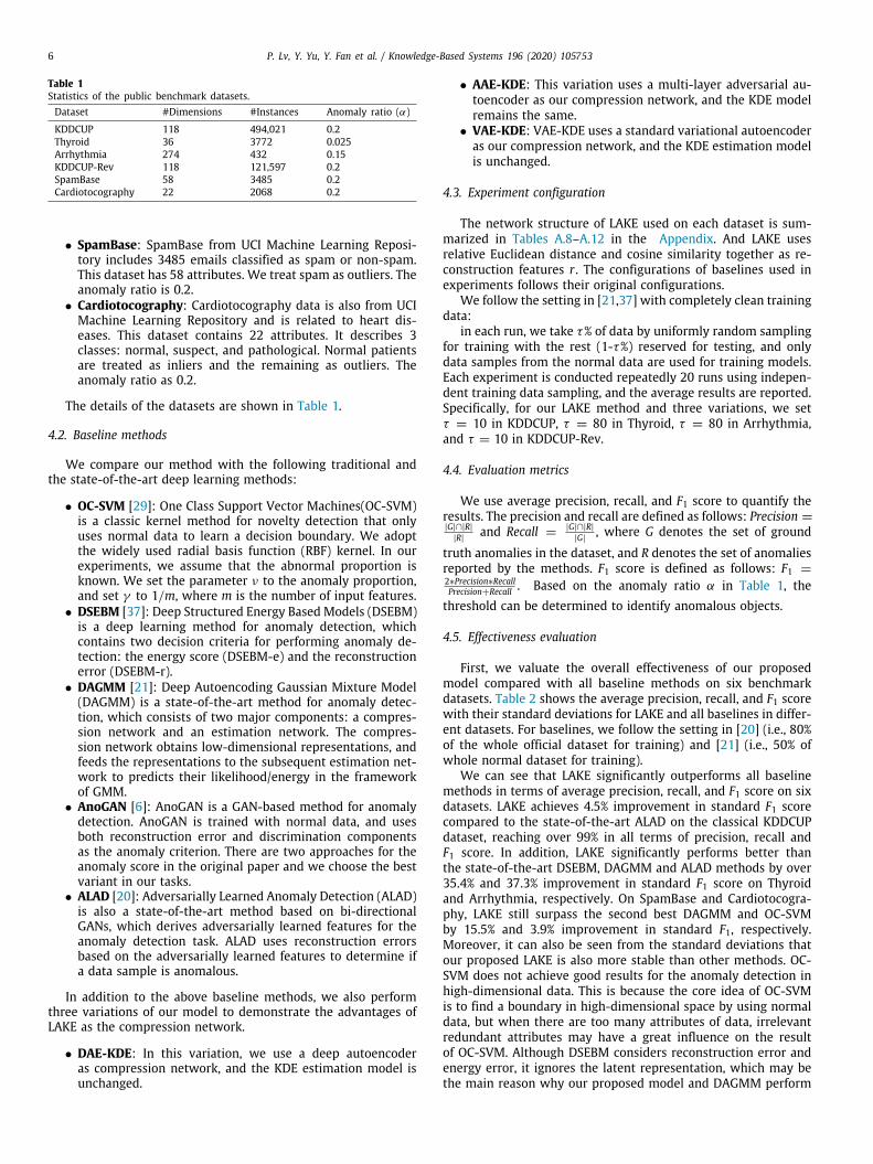
First, we valuate the overall effectiveness of our proposedmodel compared with all baseline methods on six benchmarkdatasets. Table 2 shows the average precision, recall, and F1 scorewith their standard deviations for LAKE and all baselines in differ-ent datasets. For baselines, we follow the setting in [20] (i.e., 80%of the whole official dataset for training) and [21] (i.e., 50% ofwhole normal dataset for training).

We can see that LAKE significantly outperforms all baselinemethods in terms of average precision, recall, and F1 score on sixdatasets. LAKE achieves 4.5% improvement in standard F1 scorecompared to the state-of-the-art ALAD on the classical KDDCUPdataset, reaching over 99% in all terms of precision, recall andF1 score. In addition, LAKE significantly performs better thanthe state-of-the-art DSEBM, DAGMM and ALAD methods by over35.4% and 37.3% improvement in standard F1 score on Thyroidand Arrhythmia, respectively. On SpamBase and Cardiotocogra-phy, LAKE still surpass the second best DAGMM and OC-SVMby 15.5% and 3.9% improvement in standard F1, respectively.Moreover, it can also be seen from the standard deviations thatour proposed LAKE is also more stable than other methods. OC-SVM does not achieve good results for the anomaly detection inhigh-dimensional data. This is because the core idea of OC-SVMis to find a boundary in high-dimensional space by using normaldata, but when there are too many attributes of data, irrelevantredundant attributes may have a great influence on the resultof OC-SVM. Although DSEBM considers reconstruction error andenergy error, it ignores the latent representation, which may bethe main reason why our proposed model and DAGMM perform


Table 2Average precision, recall and F1 from LAKE and all baselines. For each metric, the best result is shown in bold.Method KDDCUP Thyroid

Precision ± Std Recall ± Std F1 ± Std Precision ± Std Recall ± Std F1 ± Std

OC-SVM 0.7457 ± 0.0157 0.8523 ± 0.0177 0.7954 ± 0.0166 0.3639 ± 0.0131 0.4239 ± 0.0156 0.3887 ± 0.0142DSEBM-r 0.8744 ± 0.0607 0.8414 ± 0.0428 0.8575 ± 0.0516 0.0400 ± 0.0049 0.0403 ± 0.0043 0.0403 ± 0.0047DSEBM-e 0.2151 ± 0.0757 0.2180 ± 0.0756 0.2170 ± 0.0755 0.1319 ± 0.0037 0.1319 ± 0.0059 0.1319 ± 0.0048DAGMM 0.9297 ± 0.0103 0.9442 ± 0.0112 0.9369 ± 0.0107 0.4766 ± 0.0171 0.4834 ± 0.0101 0.4782 ± 0.0133AnoGAN 0.8786 ± 0.0370 0.8297 ± 0.0160 0.8865 ± 0.0115 0.0412 ± 0.0119 0.0430 ± 0.0128 0.0421 ± 0.0123ALAD 0.9427 ± 0.0060 0.9577 ± 0.0062 0.9501 ± 0.0061 0.3196 ± 0.0063 0.3333 ± 0.0094 0.3263 ± 0.0055

DAE-KDE 0.9840 ± 0.0033 0.9655 ± 0.0108 0.9710 ± 0.0086 0.7934 ± 0.0027 0.7849 ± 0.0095 0.7891 ± 0.0068AAE-KDE 0.9842 ± 0.0045 0.9697 ± 0.0098 0.9754 ± 0.0065 0.7501 ± 0.0026 0.7419 ± 0.0010 0.7459 ± 0.0010VAE-KDE 0.9913 ± 0.0010 0.9912 ± 0.0085 0.9912 ± 0.0106 0.7548 ± 0.0110 0.7548 ± 0.0007 0.7548 ± 0.0090LAKE 0.9985 ± 0.0002 0.9912 ± 0.0035 0.9948 ± 0.0010 0.8369 ± 0.0026 0.8279 ± 0.0010 0.8324 ± 0.0019

Method Arrhythmia KDDCUP-Rev



DAE-KDE 0.8461 ± 0.0059 0.8333 ± 0.0083 0.8396 ± 0.0067 0.9890 ± 0.0021 0.9889 ± 0.0072 0.9890 ± 0.0065AAE-KDE 0.8553 ± 0.0034 0.8424 ± 0.0030 0.8488 ± 0.0002 0.9907 ± 0.0029 0.9906 ± 0.0101 0.9906 ± 0.0072VAE-KDE 0.8461 ± 0.0060 0.8333 ± 0.0123 0.8396 ± 0.0091 0.9936 ± 0.0054 0.9812 ± 0.0006 0.9874 ± 0.0030LAKE 0.8953 ± 0.0026 0.8818 ± 0.0078 0.8885 ± 0.0089 0.9914 ± 0.0023 0.9915 ± 0.0013 0.9914 ± 0.0005Method SpamBase Cardiotocography



DAE-KDE 0.9311 ± 0.0058 0.9282 ± 0.0011 0.9230 ± 0.0011 0.7170 ± 0.0358 0.3185 ± 0.1256 0.4296 ± 0.1146AAE-KDE 0.9376 ± 0.0074 0.9282 ± 0.0073 0.9329 ± 0.0074 0.6502 ± 0.1081 0.4247 ± 0.1066 0.5011 ± 0.0969VAE-KDE 0.9437 ± 0.0087 0.9335 ± 0.0092 0.9384 ± 0.0093 0.6914 ± 0.0805 0.5582 ± 0.1429 0.6117 ± 0.1127LAKE 0.9576 ± 0.0037 0.9480 ± 0.0036 0.9528 ± 0.0036 0.7483 ± 0.0110 0.7410 ± 0.0109 0.7446 ± 0.0109

better than DSEBM. The reasons why LAKE is better than DAGMMmay be attributed as: (1) LVAE is better than autoencoder inlearning low-dimensional representation preserving the distribu-tion of original data due to the existence of a variational structureand layer constraint; (2) LAKE adopts kernel density estimationto model the probability density distribution of data instead ofGaussian mixture model. KDE is superior to Gaussian mixturemodel, because GMM is a parameter estimation that refers to theprocess of using sample data to estimate the parameters of theselected distribution, while KDE is a nonparametric estimationthat allows the functional form of a fit to data to be obtainedin the absence of any guidance or constraints from theory. Addi-tionally, GMM also needs to manually select the number of mixedGaussian models, which is very tricky in the absence of domainknowledge. For AnoGAN, it adopts adversarial autoencoder torecover a latent representation for each input data, and usesboth reconstruction error and discrimination components as theanomaly criterion, but AnoGAN does not make full use of thelow-dimensional representation. Although ALAD can simulate thedistribution of data well when the experimental data is largeenough, it also ignores the consideration of latent representation.Another potential reason why our method is better than all base-lines is that we adopt a novel probability density-aware strategythat only estimates density value of each input data with respectto the learned probability density distribution of normal trainingsamples. This strategy helps our method to effectively separatedensely distributed anomalies out in latent data space.

From Table 2, we also observe that LAKE outperforms its vari-ations (i.e., DAE-KDE, AAE-KDE and VAE-KDE) on six datasets. In

particular, LAKE significantly performs better than the three vari-ations on four small datasets (i.e., Thyroid, Arrhythmia, SpamBaseand Cardiotocography). This is because LVAE better preserves thekey information during data dimension reduction. So that LVAElearns the distribution of data better in latent data space whenusing very few training data compared to DAE, AAE and VAE. Butstill, our variations are significantly better than all competitivebaselines in terms of precision, recall and F1 score.

4.6. Hypothesis testing

To further verify the superiority of our proposed method, weuse Welch’s t-test to statistically assess the proposed methodcompared with baselines over 6 datasets. More specifically, weuse the code4 from SciPy.org for statistical testing.

To compare our proposed method with each baseline (onevs. one), we evaluate the following null hypothesis H0 and thealternative hypothesis H1 for each pair of methods:

H0 : A ≈ B,

H1 : A < B,

where B stands for the result of LAKE on a specific dataset, andA denotes the result of a specific baseline on the correspondingdataset. We calculate p-value for each test, and the hypothesis ischecked at p = 0.05 significance level. The statistical assessment

4 https://docs.scipy.org/doc/scipy/reference/generated/scipy.stats.ttest_ind.html.

https://docs.scipy.org/doc/scipy/reference/generated/scipy.stats.ttest_ind.html

https://docs.scipy.org/doc/scipy/reference/generated/scipy.stats.ttest_ind.html


Table 3p-values of Welch’s t-test for precision.Dataset OC-SVM DSEBM-r DSEBM-e DAGMM AnoGAN ALAD

KDDCUP 3.229e−12 2.816e−06 5.762e−16 4.766e−08 4.197e−06 9.073e−06Thyroid 1.430e−12 7.901e−29 1.340e−22 9.334e−21 8.667e−25 8.399e−27Arrhythmia 3.995e−16 8.030e−14 1.156e−12 2.526e−13 2.702e−17 1.132e−15KDDCUP-Rev 8.913e−11 5.011e−14 3.435e−17 2.393e−10 4.773e−09 5.328e−08SpamBase 7.251e−08 9.450e−17 5.318e−16 1.411e−02 1.812e−11 4.121e−15Cardiotocography 2.806e−03 1.120e−14 9.638e−16 4.774e−14 5.367e−12 1.885e−14

Table 4p-values of Welch’s t-test for recall.Dataset OC-SVM DSEBM-r DSEBM-e DAGMM AnoGAN ALAD


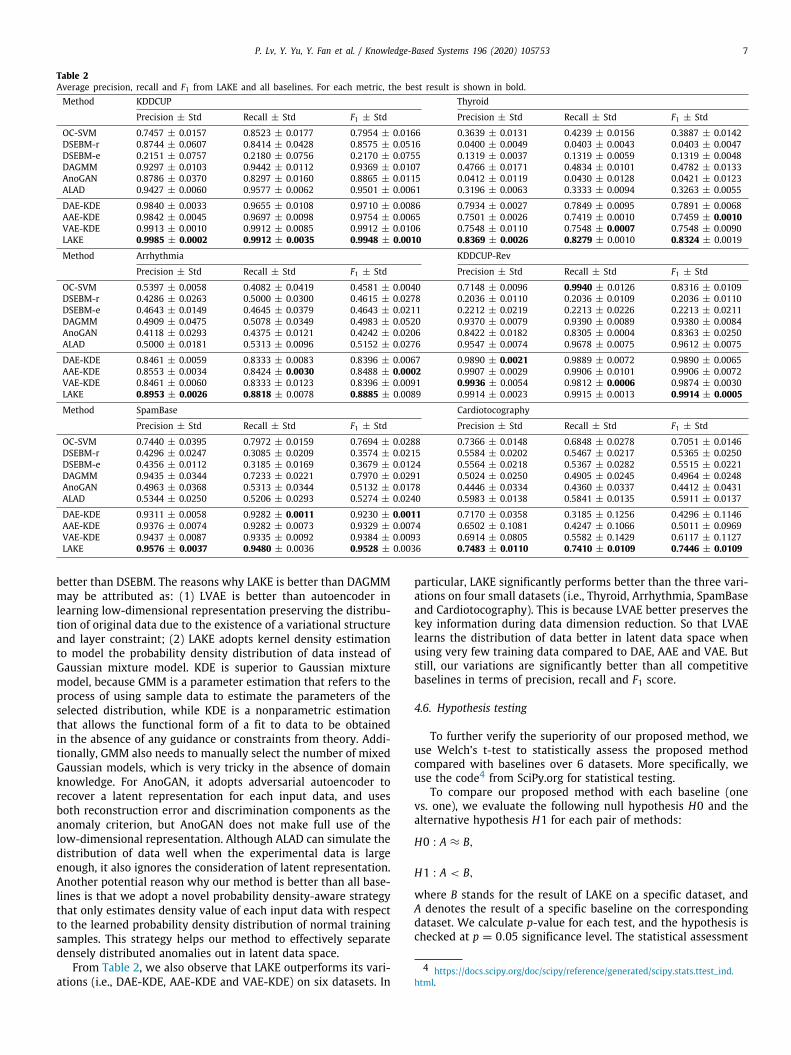
results of precision, recall and F1 are shown in Tables 3, 4, and 5respectively.

As shown in Tables 3, 4 and 5, Except for the recall of OC-SVM on KDDCUP-Rev, all Welch’s t-test results of precision andrecall are significant at p = 0.05. More importantly, Welch’s t-testresults on the more comprehensive F1 score are all significant atp = 0.05. Thus we can reject the null hypothesis H0 and acceptalternative Hypothesis H1. That is, our proposed LAKE performssignificantly better than all baselines.

In summary, this experiment confirms that the improvementof our proposed method over the state-of-the-art methods indetecting anomalies is statistically significant.

4.7. Performance w.r.t. training set

In this experiment, we mainly study the performance of ourmethod and baselines with respective to the number of trainingset. We use τ% of the normal dataset as the training set for allmethods. Tables 6 and 7 show the average precision, recall, andF1 score of LAKE and the competitive baselines on Arrhythmia andKDDCUP datasets, respectively.

As we can see, with only 30% and 10% training data, LAKEhas already shown better performance than all baselines withthe best performance in terms of precision, recall and F1 scoreon Arrhythmia and KDDCUP respectively. As the training dataincreases, the performance of LAKE increases on both datasets,especially on Arrhythmia LAKE achieves a significant improve-ment. ALAD and AnoGAN basically keep stable in term of F1score when performing on KDDCUP, and have slight fluctuationswhen performing on Arrhythmia. This may be because ALADand AnoGAN mainly use reconstruction error as the anomalycriterion, and as a consequence the results are influenced by thedegree to which the models fit to the training samples. FromTable 7, DSEBM-e that uses energy score as detection criterionis not suitable for KDDCUP, as the data distribution in KDDCUP ismore complex than energy based models. The results of DSEBM-r are similar to those of ALAD and AnoGAN, because it alsouse reconstruction error as the criterion for anomaly detection.Although DAGMM has increased performance as the number oftraining set increases, LAKE is far superior to it, even using lesstraining data.

In summary, this experiment confirms that the proposed LAKEcan achieve better results with fewer training samples comparedto the state-of-the-art methods.

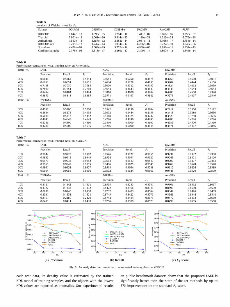
4.8. Robustness evaluation

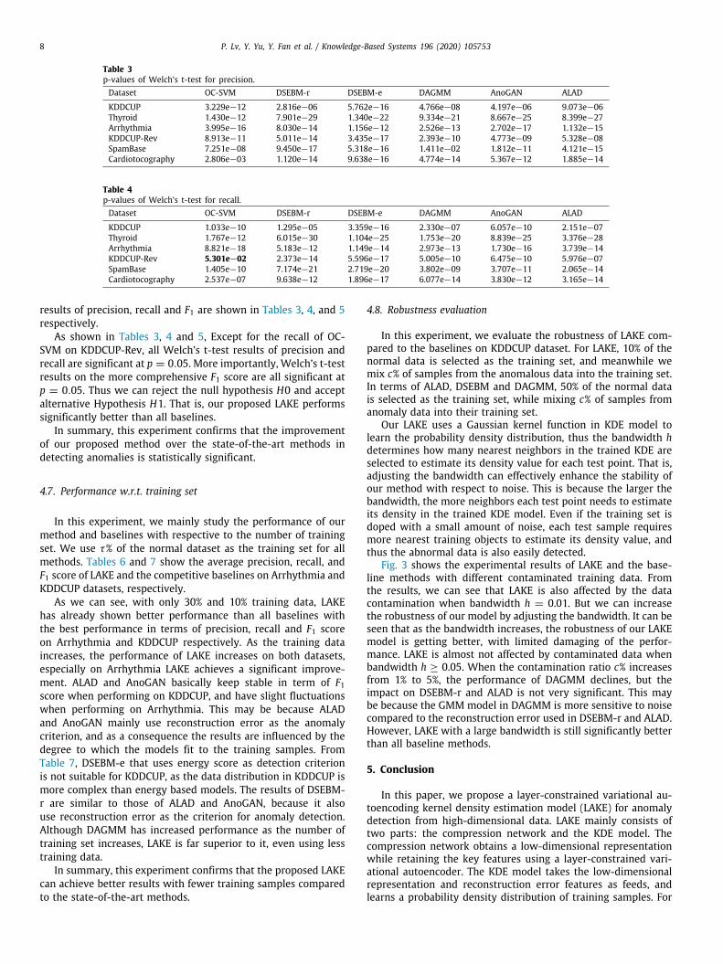
In this experiment, we evaluate the robustness of LAKE com-pared to the baselines on KDDCUP dataset. For LAKE, 10% of thenormal data is selected as the training set, and meanwhile wemix c% of samples from the anomalous data into the training set.In terms of ALAD, DSEBM and DAGMM, 50% of the normal datais selected as the training set, while mixing c% of samples fromanomaly data into their training set.

Our LAKE uses a Gaussian kernel function in KDE model tolearn the probability density distribution, thus the bandwidth hdetermines how many nearest neighbors in the trained KDE areselected to estimate its density value for each test point. That is,adjusting the bandwidth can effectively enhance the stability ofour method with respect to noise. This is because the larger thebandwidth, the more neighbors each test point needs to estimateits density in the trained KDE model. Even if the training set isdoped with a small amount of noise, each test sample requiresmore nearest training objects to estimate its density value, andthus the abnormal data is also easily detected.

Fig. 3 shows the experimental results of LAKE and the base-line methods with different contaminated training data. Fromthe results, we can see that LAKE is also affected by the datacontamination when bandwidth h = 0.01. But we can increasethe robustness of our model by adjusting the bandwidth. It can beseen that as the bandwidth increases, the robustness of our LAKEmodel is getting better, with limited damaging of the perfor-mance. LAKE is almost not affected by contaminated data whenbandwidth h ≥ 0.05. When the contamination ratio c% increasesfrom 1% to 5%, the performance of DAGMM declines, but theimpact on DSEBM-r and ALAD is not very significant. This maybe because the GMM model in DAGMM is more sensitive to noisecompared to the reconstruction error used in DSEBM-r and ALAD.However, LAKE with a large bandwidth is still significantly betterthan all baseline methods.

5. Conclusion

In this paper, we propose a layer-constrained variational au-toencoding kernel density estimation model (LAKE) for anomalydetection from high-dimensional data. LAKE mainly consists oftwo parts: the compression network and the KDE model. Thecompression network obtains a low-dimensional representationwhile retaining the key features using a layer-constrained vari-ational autoencoder. The KDE model takes the low-dimensionalrepresentation and reconstruction error features as feeds, andlearns a probability density distribution of training samples. For


Table 5p-values of Welch’s t-test for F1 .Dataset OC-SVM DSEBM-r DSEBM-e DAGMM AnoGAN ALAD


Table 6Performance comparison w.r.t. training ratio on Arrhythmia.Ratio τ% LAKE ALAD DAGMM

Precision Recall F1 Precision Recall F1 Precision Recall F130% 0.6046 0.5863 0.5953 0.4641 0.5250 0.4474 0.3750 0.4500 0.409140% 0.6651 0.6651 0.6651 0.4634 0.5278 0.4935 0.3902 0.4444 0.415650% 0.7138 0.7030 0.7083 0.5000 0.5312 0.5152 0.3824 0.4062 0.393960% 0.7890 0.7651 0.7769 0.4643 0.4643 0.4643 0.4643 0.4643 0.464370% 0.8484 0.8484 0.8484 0.3810 0.4000 0.3902 0.4286 0.4500 0.439080% 0.8953 0.8818 0.8885 0.3571 0.4167 0.3846 0.3571 0.4167 0.3846

Ratio τ% DSEBM-e DSEBM-r AnoGAN


Table 7Performance comparison w.r.t. training ratio on KDDCUP.Ratio τ% LAKE ALAD DAGMM


Ratio τ% DSEBM-e DSEBM-r AnoGAN


Fig. 3. Anomaly detection results on contaminated training data on KDDCUP.

each test data, its density value is estimated by the trainedKDE model of training samples, and the objects with the lowestKDE values are reported as anomalies. Our experimental results

on public benchmark datasets show that the proposed LAKE issignificantly better than the state-of-the-art methods by up to37% improvement on the standard F1 score.


Table A.8LAKE architecture and hyperparameters on KDDCUP and KDDCUP-Rev.Operation Units Activation function

EncoderDense (118,90) TanhDense (90,60) TanhDense (60,25) Tanh

mu (25,20) Nonevar (25,20) None

DecoderDense (20,25) TanhDense (25,60) TanhDense (60,90) TanhDense (90,118) Sigmoid

Optimizer Adam(learning_rate = 0.00001)Batch size 1000Epochs 1000Bandwidth 0.001

Table A.9LAKE architecture and hyperparameters on Arrhythmia.Operation Units Activation function

EncoderDense (274,130) TanhDense (130,60) TanhDense (60,25) TanhDense (25,20) Tanh


DecoderDense (10,20) TanhDense (20,25) TanhDense (25,60) TanhDense (60,130) TanhDense (130,274) Sigmoid


In future work, we plan to investigate the effective semi-supervised anomaly detection method based on deep autoen-coder variations in high-dimensional data. We also plan to ex-plore the generalized autoencoder-based model for unsupervisedanomaly detection in some domains.

CRediT authorship contribution statement

Peng Lv: Methodology, Software, Data curation, Visualization,Writing - original draft. Yanwei Yu: Conceptualization, Supervi-sion, Writing - review & editing, Funding acquisition. YangyangFan: Data curation, Investigation, Writing - review & editing.Xianfeng Tang: Validation, Writing - review & editing. XiangrongTong: Resources, Funding acquisition.

Acknowledgments

The authors would like to thank the anonymous reviewers fortheir valuable comments and helpful suggestions. This work ispartially supported by the National Natural Science Foundationof China under Grant Nos.: 61773331, 61572418 and 61403328.The views and conclusions contained in this paper are those ofthe authors and should not be interpreted as representing anyfunding agencies.

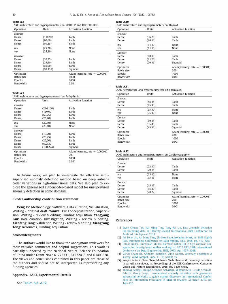
Appendix. LAKE Experimental Details

See Tables A.8–A.12.

Table A.10LAKE architecture and hyperparameters on Thyroid.Operation Units Activation function

EncoderDense (36,20) TanhDense (20,11) Tanh


DecoderDense (10,11) TanhDense (11,20) TanhDense (20,36) Sigmoid


Table A.11LAKE Architecture and hyperparameters on SpamBase.Operation Units Activation function





Table A.12LAKE architecture and hyperparameters on Cardiotocography.Operation Units Activation function





References

[1] Swee Chuan Tan, Kai Ming Ting, Tony Fei Liu, Fast anomaly detectionfor streaming data, in: Twenty-Second International Joint Conference onArtificial Intelligence, 2011.

[2] Fei Tony Liu, Kai Ming Ting, Zhi-Hua Zhou, Isolation forest, in: 2008 EighthIEEE International Conference on Data Mining, IEEE, 2008, pp. 413–422.

[3] Fabian Keller, Emmanuel Muller, Klemens Bohm, HiCS: high contrast sub-spaces for density-based outlier ranking, in: 2012 IEEE 28th InternationalConference on Data Engineering, IEEE, 2012, pp. 1037–1048.

[4] Varun Chandola, Arindam Banerjee, Vipin Kumar, Anomaly detection: Asurvey, ACM Comput. Surv. 41 (3) (2009) 15.

[5] Waqas Sultani, Chen Chen, Mubarak Shah, Real-world anomaly detectionin surveillance videos, in: Proceedings of the IEEE Conference on ComputerVision and Pattern Recognition, 2018, pp. 6479–6488.

[6] Thomas Schlegl, Philipp Seeböck, Sebastian M Waldstein, Ursula Schmidt-Erfurth, Georg Langs, Unsupervised anomaly detection with generativeadversarial networks to guide marker discovery, in: International Confer-ence on Information Processing in Medical Imaging, Springer, 2017, pp.146–157.

http://refhub.elsevier.com/S0950-7051(20)30163-5/sb1


























[7] Raghavendra Chalapathy, Sanjay Chawla, Deep learning for anomalydetection: A survey, 2019, arXiv:1901.03407.

[8] Tsuyoshi Idé, Hisashi Kashima, Eigenspace-based anomaly detection incomputer systems, in: Proceedings of the Tenth ACM SIGKDD InternationalConference on Knowledge Discovery and Data Mining, ACM, 2004, pp.440–449.

[9] Weiren Yu, Charu C. Aggarwal, Shuai Ma, Haixun Wang, On anomaloushotspot discovery in graph streams, in: 2013 IEEE 13th InternationalConference on Data Mining, IEEE, 2013, pp. 1271–1276.

[10] Ryohei Fujimaki, Takehisa Yairi, Kazuo Machida, An approach to spacecraftanomaly detection problem using kernel feature space, in: Proceedingsof the Eleventh ACM SIGKDD International Conference on KnowledgeDiscovery in Data Mining, ACM, 2005, pp. 401–410.

[11] Sarah M Erfani, Sutharshan Rajasegarar, Shanika Karunasekera, ChristopherLeckie, High-dimensional and large-scale anomaly detection using a linearone-class SVM with deep learning, Pattern Recognit. 58 (2016) 121–134.

[12] Emmanuel J. Candès, Xiaodong Li, Yi Ma, John Wright, Robust principalcomponent analysis? J. ACM 58 (3) (2011) 11.

[13] Tingquan Deng, Dongsheng Ye, Rong Ma, Hamido Fujita, Lvnan Xiong, Low-rank local tangent space embedding for subspace clustering, Inform. Sci.508 (2020) 1–21.

[14] Chong Zhou, Randy C. Paffenroth, Anomaly detection with robust deepautoencoders, in: Proceedings of the 23rd ACM SIGKDD InternationalConference on Knowledge Discovery and Data Mining, ACM, 2017, pp.665–674.

[15] Jinwon An, Sungzoon Cho, Variational autoencoder based anomalydetection using reconstruction probability, Spec. Lect. IE 2 (2015) 1–18.

[16] Mahdyar Ravanbakhsh, Moin Nabi, Hossein Mousavi, Enver Sangineto, NicuSebe, Plug-and-play cnn for crowd motion analysis: An application in ab-normal event detection, in: 2018 IEEE Winter Conference on Applicationsof Computer Vision (WACV), IEEE, 2018, pp. 1689–1698.

[17] Cairong Zhao, Xuekuan Wang, Wai Keung Wong, Weishi Zheng, Jian Yang,Duoqian Miao, Multiple metric learning based on bar-shape descriptor forperson re-identification, Pattern Recognit. 71 (2017) 218–234.

[18] Cairong Zhao, Xuekuan Wang, Duoqian Miao, Hanli Wang, Weishi Zheng,Yong Xu, David Zhang, Maximal granularity structure and generalizedmulti-view discriminant analysis for person re-identification, PatternRecognit. 79 (2018) 79–96.

[19] Cairong Zhao, Xuekuan Wang, Wangmeng Zuo, Fumin Shen, Ling Shao,Duoqian Miao, Similarity learning with joint transfer constraints for personre-identification, Pattern Recognit. 97 (2020) 107014.

[20] Houssam Zenati, Manon Romain, Chuan-Sheng Foo, Bruno Lecouat, VijayChandrasekhar, Adversarially learned anomaly detection, in: 2018 IEEEInternational Conference on Data Mining (ICDM), IEEE, 2018, pp. 727–736.

[21] Bo Zong, Qi Song, Martin Renqiang Min, Wei Cheng, Cristian Lumezanu,Daeki Cho, Haifeng Chen, Deep autoencoding gaussian mixture model forunsupervised anomaly detection, in: International Conference on LearningRepresentations, 2018.

[22] Rémi Domingues, Maurizio Filippone, Pietro Michiardi, Jihane Zouaoui, Acomparative evaluation of outlier detection algorithms: Experiments andanalyses, Pattern Recognit. 74 (2018) 406–421.

[23] Edwin M. Knorr, Raymond T. Ng, Vladimir Tucakov, Distance-based out-liers: algorithms and applications, VLDB J.—Int. J. Very Large Data Bases 8(3–4) (2000) 237–253.

[24] Markus M Breunig, Hans-Peter Kriegel, Raymond T Ng, Jörg Sander, LOF:identifying density-based local outliers, in: ACM Sigmod Record, Vol. 29,(2) ACM, 2000, pp. 93–104.

[25] Yizhou Yan, Lei Cao, Elke A. Rundensteiner, Scalable top-n local out-lier detection, in: Proceedings of the 23rd ACM SIGKDD InternationalConference on Knowledge Discovery and Data Mining, ACM, 2017,pp. 1235–1244.

[26] Rikard Laxhammar, Goran Falkman, Egils Sviestins, Anomaly detection insea traffic-a comparison of the gaussian mixture model and the kerneldensity estimator, in: 2009 12th International Conference on InformationFusion, IEEE, 2009, pp. 756–763.

[27] Erich Schubert, Arthur Zimek, Hans-Peter Kriegel, Generalized outlierdetection with flexible kernel density estimates, in: Proceedings of the2014 SIAM International Conference on Data Mining, SIAM, 2014, pp.542–550.

[28] Weiming Hu, Jun Gao, Bing Li, Ou Wu, Junping Du, Stephen John Maybank,Anomaly detection using local kernel density estimation and context-basedregression, IEEE Trans. Knowl. Data Eng. (2018).

[29] Yunqiang Chen, Xiang Sean Zhou, Thomas S. Huang, One-class SVM forlearning in image retrieval, in: ICIP (1), Citeseer, 2001, pp. 34–37.

[30] Simon Günter, Nicol N. Schraudolph, S.V.N. Vishwanathan, Fast iterativekernel principal component analysis, J. Mach. Learn. Res. 8 (Aug) (2007)1893–1918.

[31] Taotao Lai, Riqing Chen, Changcai Yang, Qiming Li, Hamido Fujita, AlirezaSadri, Hanzi Wang, Efficient robust model fitting for multistructure datausing global greedy search, IEEE Trans. Cybern. (2019).

[32] Taotao Lai, Hamido Fujita, Changcai Yang, Qiming Li, Riqing Chen, Robustmodel fitting based on greedy search and specified inlier threshold, IEEETrans. Ind. Electron. 66 (10) (2018) 7956–7966.

[33] Christoph Baur, Benedikt Wiestler, Shadi Albarqouni, Nassir Navab, Deepautoencoding models for unsupervised anomaly segmentation in brain mrimages, in: International MICCAI Brainlesion Workshop, Springer, 2018, pp.161–169.

[34] Ian Goodfellow, Jean Pouget-Abadie, Mehdi Mirza, Bing Xu, David Warde-Farley, Sherjil Ozair, Aaron Courville, Yoshua Bengio, Generative adversarialnets, in: Advances in Neural Information Processing Systems, 2014, pp.2672–2680.

[35] Thomas Schlegl, Philipp Seeböck, Sebastian M Waldstein, Georg Langs,Ursula Schmidt-Erfurth, F-anoGAN: Fast unsupervised anomaly detectionwith generative adversarial networks, Med. Image Anal. 54 (2019) 30–44.

[36] Martin Arjovsky, Soumith Chintala, Léon Bottou, Wasserstein generativeadversarial networks, in: International Conference on Machine Learning,2017, pp. 214–223.

[37] Shuangfei Zhai, Yu Cheng, Weining Lu, Zhongfei Zhang, Deep structuredenergy based models for anomaly detection, in: Proceedings of the 33rdInternational Conferernce on Machine Learing, Vol. 48, JMLR, 2016.

[38] Carl Doersch, Tutorial on variational autoencoders, 2016, arXiv preprintarXiv:1606.05908.

[39] Diederik P. Kingma, Max Welling, Auto-encoding variational bayes, in:Proceedings of 2nd International Conference on Learning Representations,2014.

http://arxiv.org/abs/1901.03407







































































































































































http://arxiv.org/abs/1606.05908

knowledge-based systems layer-constrained variational

Documents