HIGH ORDER ACCURATE SOLUTION OF THE

INCOMPRESSIBLE NAVIER-STOKES EQUATIONS

ARNIM BRUGER1 BERTIL GUSTAFSSON2

PER LOTSTEDT2 JONAS NILSSON2

1Dept of Mechanics, Royal Institute of Technology, SE-10044 Stockholm, Sweden.2Dept of Information Technology, Scientific Computing, Uppsala University, P. O. Box 337,

SE-75105 Uppsala, Sweden.

Abstract

High order methods are of great interest in the study of turbulent flowsin complex geometries by means of direct simulation. With this goal inmind, the incompressible Navier-Stokes equations are discretized in spaceby a compact fourth order finite difference method on a staggered grid. Theequations are integrated in time by a second order semi-implicit method.Stable boundary conditions are implemented and the grid is allowed to becurvilinear in two space dimensions. In every time step, a system of linearequations is solved for the velocity and the pressure by an outer and aninner iteration with preconditioning. The convergence properties of theiterative method are analyzed. The order of accuracy of the method isdemonstrated in numerical experiments. The method is used to computethe flow in a channel, the driven cavity and a constricted channel.

Keywords: finite difference method, high order, incompressible flow,iterative solution

AMS subject classification 2000: 65N50, 76M12

1 Introduction

Spectral and pseudospectral methods are accurate methods for direct numericalsimulation of turbulent flow governed by the incompressible Navier-Stokes equa-tions. The disadvantage with these methods is that they are restricted to simplegeometries such as channels. Finite difference methods of high order do not havethis restriction and are almost as accurate as a spectral method. In this paperwe develop such a method of fourth order accuracy in space and second order intime for two-dimensional problems. The level of the discretization error is the im-portant issue, not so much the order of accuracy, but a certain error level is more

1

easily obtained with a high order method. The same accuracy is achieved withfewer grid points or the solution has better accuracy on the same grid compared toa second order method. The solution in curvilinear body-fitted coordinates is ob-tained by a mapping of the equations to a rectangular grid where the derivativesare approximated. The solution is computed in the primitive variables definedon a staggered grid with local velocity components to avoid spurious oscillations.The method will be extended to the third dimension by a spectral representationaiming at direct numerical simulation of turbulent flow. High order accuracy inthe spatial approximations is also necessary for large eddy simulation in ordernot to interfere with the subgrid model with terms proportional to the square ofthe grid size [16].

Let u and v be the velocity components in the x- and y-direction, respectively,p the pressure, and ν the kinematic viscosity. The Reynolds number is definedby Re = ub`/ν for some characteristic velocity ub and length scale `. By definingw = (u v)T , differentiation with respect to an independent variable, such as timet, by a subscript, and the nonlinear and linear terms

N (w) = (w · ∇)w , L(w, p) = ∇p−Re−1∆w ,

the Navier-Stokes equations in two dimensions are

wt +N (w) + L(w, p) = 0 , (1)

∇ ·w = 0 . (2)

The space discretization of N and L in (1) is in compact form [26] and theequations are integrated in time by a semi-implicit method. The approximationsof the first and second derivatives are defined implicitly and they satisfy systemsof linear equations with a tridiagonal system matrix. The number of terms inthe computational domain is reduced by orthogonal grids in the physical domain.The nonlinear convection term N is extrapolated from the previous time steps.The linear part of the discretized momentum equations L and the discretized di-vergence equation (2) are solved simultaneously at the new time level. A systemof linear equations has to be solved for w and p in every time step. The solutionis computed by an iterative method until convergence is reached. The method isshown to be of fourth order in space and of second order in time in w and p innumerical experiments. The method is analyzed with respect to boundary con-ditions and stability in [19], [20], [25], and [34]. Other examples of the accuracyand performance of the method are found in [4], [5]. There are stability con-straints on the the timestep ∆t due to the semi-implicit time integration. Otherconstraints on ∆t are introduced by accuracy requirements and the convergenceof the iterative solvers. It is shown in [8] that an implicit method is faster than asemi-implicit method for fully developed turbulent flow in a boundary layer butthe CFL-number for good accuracy is rather low, 0.5− 1. In other flow regimes,

2

such as transitional flow, a much smaller timestep is necessary for accuracy [14],thus reducing the time savings with an implicit method.

Direct numerical simulation of turbulent flow is reviewed in [14]. Other finitedifference methods of high order for the Navier-Stokes equations are found in [2],[22], [27], [29], [32], [33], [40]. The velocity-vorticity equations are solved in [2]with a fourth order compact method and advanced in time by a semi-implicitscheme. The stencil is a wide fourth order centered difference in [22] appliedto the equations (1) and in [29] the fourth order differential equation for thestreamfunction is discretized by fourth order centered differences. The coupledstreamfunction-vorticity equation is solved with a compact scheme in [27]. Afourth order method is developed and tested for incompressible flow in [32] and asixth order method for compressible flow is presented in [33] on a staggered gridin a straight channel.

In the next section, the space and time discretizations are described andcompared to other high order schemes. The method for computation of w andp in every timestep is discussed in Sect. 3. The convergence of the iterativemethod is studied and it is compared to other similar methods. Finally, theflows in a straight channel, in a lid-driven cavity and a constricting channel witha curvilinear grid are computed. The accuracy and efficiency of the method isdemonstrated in the numerical experiments.

2 The discretization

In this section the discrete equations in space and time are derived for a curvilin-ear grid. The approximations in space are compact and of fourth order accuracy.The solution is advanced in time by a method where the space operator is split sothat the linear term in (1) and the divergence relation (2) are treated implicitlyand the nonlinear term is extrapolated. Such methods are reviewed in [23] and[42].

2.1 Time discretization

The equations (1) and (2) are discretized in time by extrapolating N (w) fromtime tn−r+1 up to tn with an r:th order formula to tn+1 and applying the r:thorder backward differentiation formula (BDF-r) [21] to wt and L(w, p) at tn+1 toobtain

r∑j=0

αjwn+1−j + ∆tL(wn+1, pn+1) = −∆t

r∑j=1

βjN (wn+1−j) . (3)

3

The coefficients αj are such that the sum approximates wt at tn+1 and the βcoefficients are defined by

wn+1 =r∑

j=1

βjwn+1−j +O(∆tr),

cf. [23]. The time step ∆t = tn+1 − tn is constant in the interval of interest.In addition to (3), wn+1 satisfies the discretization of the divergence equation in(2). The result is a linear system of equations to solve for wn+1 and pn+1 in everytime step. We have implemented the second order method with r = 2 implyingα0 = 3/2, α1 = −2, α2 = 1/2, β1 = 2, β2 = −1. The integration can be started att0 with r = 1.

The explicit part of the integration introduces restrictions on the the timestepfor stability. This is analyzed in [18] assuming Oseen flow with periodic boundaryconditions.

A different class of time discretizations is derived from integrating (1) in time

wn+1 −wn = −∫ tn+1

tnN (w) dt−

∫ tn+1

tnL(w, p) dt. (4)

The first integral is then approximated by an explicit Adams-Bashforth methodand the second integral by an implicit Adams-Moulton method [21]. The con-tinuity equation is simultaneously satisfied by wn+1. A common combination isthe Adams-Bashforth method of second order and the implicit trapezoidal (orCrank-Nicolson) method [24], [28], [37]. The Crank-Nicolson scheme is combinedwith an explicit Runge-Kutta method in [2].

2.2 Space discretization

To be able to solve the Navier-Stokes equations in more complicated geometriesthan a straight channel with a Cartesian grid, the equations are mapped fromcomputational space (ξ, η) into physical space (x, y) by a univalent right handsided orthogonal transformation

x = x(ξ, η) , y = y(ξ, η) . (5)

The topology of the physical domain Ω is assumed to be like a channel: an upperand a lower wall with no-slip boundary conditions, an inflow boundary to the leftand an outflow boundary to the right or with no-slip conditions on all walls. Thecomputational domain is a rectangle.

4

v

u

p

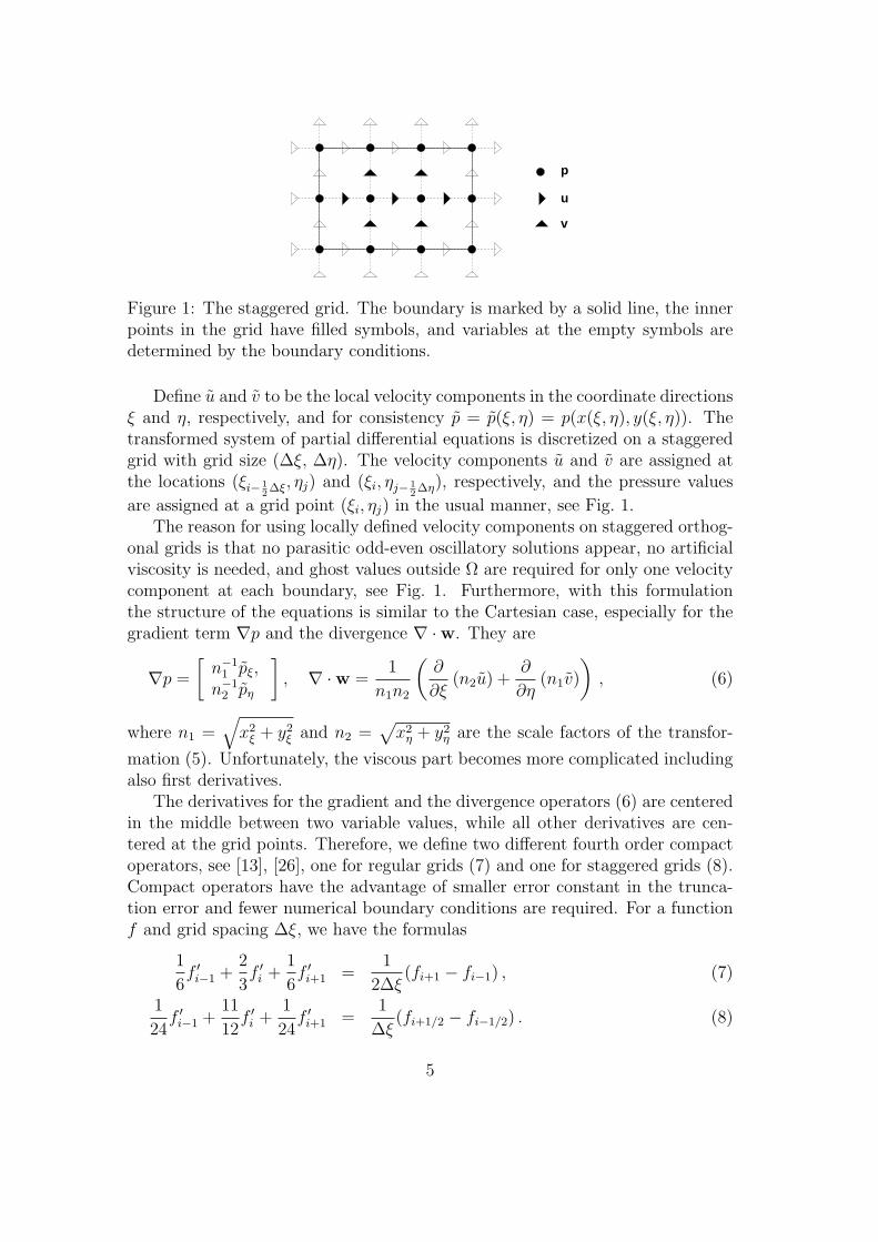
Figure 1: The staggered grid. The boundary is marked by a solid line, the innerpoints in the grid have filled symbols, and variables at the empty symbols aredetermined by the boundary conditions.

Define u and v to be the local velocity components in the coordinate directionsξ and η, respectively, and for consistency p = p(ξ, η) = p(x(ξ, η), y(ξ, η)). Thetransformed system of partial differential equations is discretized on a staggeredgrid with grid size (∆ξ, ∆η). The velocity components u and v are assigned atthe locations (ξi− 1

2∆ξ, ηj) and (ξi, ηj− 1

2∆η), respectively, and the pressure values

are assigned at a grid point (ξi, ηj) in the usual manner, see Fig. 1.The reason for using locally defined velocity components on staggered orthog-

onal grids is that no parasitic odd-even oscillatory solutions appear, no artificialviscosity is needed, and ghost values outside Ω are required for only one velocitycomponent at each boundary, see Fig. 1. Furthermore, with this formulationthe structure of the equations is similar to the Cartesian case, especially for thegradient term ∇p and the divergence ∇ ·w. They are

∇p =

[n−1

1 pξ,n−1

2 pη

], ∇ ·w =

1

n1n2

(∂

∂ξ(n2u) +

∂

∂η(n1v)

), (6)

where n1 =√

x2ξ + y2

ξ and n2 =√

x2η + y2

η are the scale factors of the transfor-

mation (5). Unfortunately, the viscous part becomes more complicated includingalso first derivatives.

The derivatives for the gradient and the divergence operators (6) are centeredin the middle between two variable values, while all other derivatives are cen-tered at the grid points. Therefore, we define two different fourth order compactoperators, see [13], [26], one for regular grids (7) and one for staggered grids (8).Compact operators have the advantage of smaller error constant in the trunca-tion error and fewer numerical boundary conditions are required. For a functionf and grid spacing ∆ξ, we have the formulas

1

6f ′i−1 +

2

3f ′i +

1

6f ′i+1 =

1

2∆ξ(fi+1 − fi−1) , (7)

1

24f ′i−1 +

11

12f ′i +

1

24f ′i+1 =

1

∆ξ(fi+1/2 − fi−1/2) . (8)

5

In order to solve for the unknowns f ′, we need closed systems of the formPf ′ = Qf for the regular grids and Rf ′ = Sf for the staggered grids. No bound-ary conditions are available for the derivatives, and we use one-sided formulas forthem. For the function itself on the right hand side of (7) and (8), we could usethe physical boundary conditions. However, it is convenient to define P,Q, R, Sindependently of the particular problem, and therefore we use one-sided formulasalso for f , see [4], [5], [20], [34].

Extra indices ξ and η on the operators are introduced to indicate the coordi-nate direction. These formulas are one-dimensional, and are applied for all gridlines in the ξ- or the η-direction. Since u and v are not stored at the same points,fourth order averaging formulas Eu and Ev are required for the advection terms.Let w = (u, v). Then the complete discrete equations are

α0un+1 + ∆t

(1

n1

R−1ξ Sξp

n+1 −Re−1Lξ(wn+1)

)=

−q∑

j=1

αjun+1−j −∆t

q∑j=1

βjNξ(wn+1−j) , (9a)

α0vn+1 + ∆t

(1

n2

R−1η Sηp

n+1 −Re−1Lη(wn+1)

)=

−q∑

j=1

αj vn+1−j −∆t

q∑j=1

βjNη(wn+1−j) , (9b)

1

n1n2

(R−1

ξ Sξ(n2un+1) + R−1

η Sη(n1vn+1)

)= 0 . (9c)

The Laplace operators Lξ and Lη are

Lξ(w) = 1n1n2

(P−1ξ Qξ(

n2

n1P−1

ξ Qξu) + P−1η Qη(

n1

n2P−1

η Qηu)− n21,η+n2

2,ξ

n1n2u

+2n1,η

n1P−1

ξ QξEv − 2n2,ξ

n2P−1

η QηEv + P−1ξ Qξ(

n1,η

n1− n2,η

n2)Ev) ,

Lη(w) = 1n1n2

(P−1ξ Qξ(

n2

n1P−1

ξ Qξv) + P−1η Qη(

n1

n2P−1

η Qηv)− n21,η+n2

2,ξ

n1n2v

−2n1,η

n1P−1

ξ QξEu +2n2,ξ

n2P−1

η QηEu− P−1ξ Qξ(

n1,η

n1− n2,η

n2)Eu) ,

(10)

and the non-linear terms are

Nξ(w) = u(

1n1

P−1ξ Qξu + n1,η

n1n2Ev

)+ Ev

(1n2

P−1η Qηu− n2,ξ

n1n2Ev

),

Nη(w) = Eu(

1n1

P−1ξ Qξv − n1,η

n1n2Eu

)+ v

(1n2

P−1η Qηv +

n2,ξ

n1n2Eu

),

and ni,ξ, ni,η, i = 1, 2, are derivatives of the scale factors with respect to ξ and η.They are evaluated with fourth order accurate numerical differentiation.

6

2.3 Boundary conditions

Stable boundary conditions for the Stokes and the linearized Navier-Stokes equa-tions on staggered grids have been developed in [20], [25], [34]. We apply theseconditions to our Navier-Stokes solver in the domain Ω. At solid walls the veloc-ity satisfies the no-slip condition. No numerical boundary condition is necessaryfor p.

Suppose that Ω has an inflow boundary at x = xin for y ∈ [yin1, yin2] andan outflow boundary at x = xout for y ∈ [yout1, yout2]. With Dirichlet boundaryconditions at the inflow and the outflow, the set of boundary conditions in thecontinuous formulation in a Cartesian coordinate system is

u(xin, y)− 1

lin

∫ yin2

yin1

u(xin, y) dy = win(y) , u(xout, y) = uout(y) ,

v(xin, y) = vin(y) , v(xout, y) = vout(y) ,∫ yin2

yin1

p(xin, y) dy +

∫ yin2

yin1

u(xin, y) dy = pin ,

(11)

where∫ yin2

yin1win(y) dy = 0 and lin = yin2 − yin1. The velocity profiles at the inlet

and the outlet are given by (uin, vin) and (uout, vout) and pin is a constant. In thediscretization, the last condition in (11) replaces the first condition at xin at onegrid point of the inflow boundary. This point is usually chosen as the midpointbut other points also work well.

An alternative at the outflow boundary is to prescribe a zero streamwisederivative of the velocity, i.e. a Neumann condition (cf. [2]). Then the continuousconditions are

u(xin, y) = uin(y) ,∂u(xout, y)

∂x− 1

lout

∫ yout2

yout1

∂u(xout, y)

∂xdy = 0 ,

v(xin, y) = vin(y) ,∂v(xout, y)

∂x= 0 ,∫ yout2

yout1

p(xout, y)dy +

∫ yout2

yout1

∂u(xout, y)

∂xdy = pout ,

(12)

where pout is an arbitrary constant and lout = yout2 − yout1. Also here the lastcondition replaces the first condition at xout in the midpoint of the discrete im-plementation. The well-posedness of the boundary conditions (11) and (12) isanalyzed in [19], [25], and [34]. The pressure is well defined by the last conditionsin (11) and (12) and their discretization is easily incorporated in our iterativemethod in the next section. Furthermore, the system matrix of the discretizedequations is non-singular and the equations can be solved to machine precision.

7

The boundary of the domain Ω is located at the grid points where p is defined,see Fig. 1. One row of extra ghost variables for one of the velocity componentsare defined outside Ω to simplify the application of the boundary conditions.

3 Iterative method

A system of linear equations has to be solved for the velocity and the pressure atthe inner points of the grid and t = tn+1 according to (9). The iterative methodfor solution of the system is described here and its convergence properties areanalyzed. A comparison with other iteration algorithms is made. The norm inthis section is the Euclidean vector norm and its subordinate spectral matrixnorm.

3.1 Algorithm

Let w denote the vector of local velocity variables in Ω, w the ghost values outsideΩ and on the boundary (see Fig. 1), and let p be the pressure vector. Then w, w,and p satisfy a system of linear equations

A0 A1 GA2 C BD0 D1 0

wwp

=

bb0

. (13)

Let L denote the discretization of the Laplace operator in the inner points, see(10). Then A0 is defined by

A0 = α0I −Re−1∆tL. (14)

The part of the Laplace operator operating on the velocity components on andoutside the boundary is represented by A1. The gradient approximation G haslinearly dependent columns and p is not uniquely defined unless B 6= 0. With ourchoice of boundary conditions in (11) and (12), C is nonsingular and diagonal ex-cept for a diagonal block with non-zero elements and B has rank one and one rowdifferent from zero. An LU-factorization of a small part of C due to the boundaryintegrals is stored for use in the iterative solver. The values in the interior arecoupled to the boundary values and the outer ghost values via the sparse matrixA2. The boundary conditions supported by a stability analysis define A2, B, andC. The approximation of the divergence is (D0, D1). The matrices A0, D0, andG are dense due to the implicit approximation of the derivatives and are notknown explicitly. The right hand side, b and b, depends on old values of w andthe boundary conditions.

After expressing w in w, p, and b and defining

A = A0 − A1C−1A2, G = G− A1C

−1B, c = b− A1C−1b,

D = D0 −D1C−1A2, B = −D1C

−1B, d = −D1C−1b,

8

the system to be solved is

(A G

D B

)(wp

)=

(cd

). (15)

Since A1 ∼ h−2∆t/Re and C−1 and A2 are of O(1), A has the same form as A0

in (14)

A = α0I −Re−1∆tL, (16)

but now the boundary conditions are included in the discrete Laplace operator.For the gradient approximation we have G ∼ h−1∆t and G ∼ h−1∆t, and thedivergence approximation satisifes D0 ∼ h−1, D1 ∼ h−1, and D ∼ h−1, where∆ξ, ∆η ∼ h.

In the iterative method we propose for solving (15), only the result of amultiplication of an arbitrary vector by the matrix is needed. It follows from(9) that this operation is performed by operating with Q,S, or E on w and pand one or two solutions of a tridiagonal system defined by P or R.

The system (15) is rewritten as

Mx = b, (17)

where xT = (xT1 , xT

2 ) = (wT , pT ), bT = (bT1 , bT

2 ) = (cT , dT ). An approximatefactorization of M in (17) is determined in a manner similar to [37]

M =

(A 0

D I

)(I α−1

0 G

0 −(α−10 DG− B)

)=

(A α−1

0 AG

D B

). (18)

The difference between M and its approximation M is

M − M =

(0 α−1

0 Re−1∆tLG0 0

). (19)

Suppose that M is invertible. In an outer fixed point iteration the correction δxis computed as

x(k+1) = x(k) + δx(k) = x(k) + M−1(b−Mx(k)) = x(k) + M−1r(k). (20)

One or two outer iterations usually suffice depending on how well M approximatesM .

The solution of

Mδx(k) = r(k) (21)

9

is computed using the factorization (18). Then with forward and back substitu-tion we have

1. Ay1 = r1, (22a)

2. y2 = r2 − Dy1, (22b)

3. (α−10 DG− B)δx2 = −y2, (22c)

4. δx1 = y1 − α−10 Gδx2, (22d)

where δx(k) = (δxT1 , δxT

2 )T and r(k) = (rT1 , rT

2 )T . If B = 0 then B = 0 andG = G. Since G does not have full rank, DG in (22c) is singular. This is nota problem for straight channels but for curvilinear geometries the equation hasno solution. From the definition of the residual in (20) it follows that the righthand side in (22b) can be written as Dz for some z. The reason why Dz is notnecessarily in the range of DG for a curvilinear channel is the difference therebetween D and GT in (9) when n1, n2 6= 1. By choosing B of low rank but suchthat α−1

0 DG− B is nonsingular, a solution δx2 is guaranteed. The singularity isremoved by letting a stable choice of boundary conditions define B.

The first system of equations

Ay1 = r1, (23)

is solved by fixed point iteration and a preconditioning matrix A as in (20)

y(k+1)1 = y

(k)1 + δy

(k)1 = y

(k)1 + A−1(r1 − Ay

(k)1 ). (24)

The simplest choice of A is α−10 I.

The third equation in (22)

(α−10 DG− B)δx2 = −y2 (25)

is similar to the Poisson equation but the system matrix is not necessarily sym-metric due to B, the coordinate transformation, and boundary conditions. Thematrix is not available explicitly and an iterative Krylov method [17], only requir-ing the computation of the matrix-vector product (α−1

0 DG−B)y for an arbitraryy, is chosen for solution of (25). Bi-CGSTAB [44] is such a method suitable fornonsymmetric matrices with eigenvalues away from the imaginary axis and theequivalent of only about five solution vectors is used as workspace.

The convergence of the iterations is slow without a preconditioner of thematrix. Incomplete LU factorization (ILU) [30] is often efficient in improvingthe convergence rate for discretizations of elliptic equations. A disadvantage isthat an ILU preconditioner may have high storage requirements depending onthe chosen amount of fill-in in the algorithm. The same ILU factorization is usedrepeatedly in every time step since α−1

0 DG− B is constant. It requires access to

10

the matrix elements of α−10 DG− B but their values are not known. Instead, the

second order accurate approximations of the divergence and the gradient, D2 andG2, are generated and their composition D2G2. It is sparse and the ILU factorsL and U for α−1

0 DG− B are based on D2G2.

3.2 Convergence analysis and termination criteria

Assume that the equations in steps 1 and 2 in the inner iterations in (22) aresolved so that the residuals are ρ1 and ρ2 in the k:th outer iteration

(A 0

D I

)(y1

y2

)=

(r1 + ρ1

r2 + ρ2

)= r(k) + ρ(k). (26)

Then the recursion for the residual in (20) is

r(k+1) = b−Mx(k+1) = b−Mx(k) −MM−1(r(k) + ρ(k))

= (I −MM−1)r(k) −MM−1ρ(k).(27)

After some algebraic manipulations we find from (18) and (16) that

MM−1 =

(I − FDA−1 F

0 I

), F = −α−1

0 Re−1∆tLG(α−10 DG− B)−1. (28)

A necessary condition for the iterations (27) to converge is that the spectral radiusof I −MM−1 is less than one, i.e. the eigenvalues of FDA−1 have modulus lessthan one. The conclusion from F in (28) is that for a Re and a given grid, ∆thas to be sufficiently small for the outer iterations to converge.

The expression for the residual in (27) is

r(k+1) = (I −MM−1)k+1r(0) −k∑

j=0

(I −MM−1)jMM−1ρ(k−j),

and if ‖I −MM−1‖ ≤ µ the termination criterion for the inner iterations (26) is‖ρ(j)‖ ≤ εi then

‖r(k+1)‖ ≤ µk+1‖r(0)‖+(1 + µ)(1− µk+1)

1− µεi.

A sufficient condition for convergence is µ < 1. It follows from (28) that this ispossible if F is sufficiently small, e.g. by taking ∆t sufficiently small. Then

limk→∞

‖r(k)‖ =1 + µ

1− µεi,

11

and for r(k) to satisfy the termination criterion for the outer iterations ‖r(k)‖ ≤ εo,εi should be chosen

εi ≤ (1− µ)εo/(1 + µ). (29)

Since µ < 1 the requirements on the inner iterations are slightly more strictcompared to the outer termination condition.

It follows from (22) and (26) that

ρ1 = Ay1 − r1, ρ2 = −(α−10 DG− B)δx2 − r2 + Dy1.

Hence, ρ1 and ρ2 are the remaining residuals when the linear systems in steps 1and 3 in (22) are solved iteratively. In order to satisfy (29) the stopping criteriain (22) are ε1 = ε3 = εi/

√2 so that

‖ρ(k)‖2 = ‖ρ1‖2 + ‖ρ2‖2 ≤ ε2i ≤ ε2

o(1− µ)2/(1 + µ)2.

The same analysis applied to (24) shows that the iterations converge if

I − A−1A = α−10 Re−1∆tL (30)

satisfies Re−1∆t‖L‖ < α0. The right hand side in (30) is also a multiplying factorin F defined in (28). Since L ∼ h−2, the fixed point iteration (24) converges ifh−2∆t/Re is sufficiently small.

The discrete Laplacian of fourth order DG is approximated by the correspond-ing D2G2 of second order when the preconditioning (here the ILU factorization)is computed. The assumption that −DG, −D2G2, and the preconditioner aresymmetric and positive definite and Fourier analysis give a clue why this precon-ditioner has an effect on the convergence rate of the iterative solution in (22c).

A rectangular physical domain with periodic boundary conditions is dis-cretized with a Cartesian grid with constant step sizes ∆x and ∆y. Let ω1

and ω2 be the discrete wavenumbers in the x and y directions and introduce thenotation

ϕ1 = ω1∆x , ϕ2 = ω2∆y , 0 ≤ |ϕ1|, |ϕ2| ≤ π ,κ1 = ∆t/∆x , κ2 = ∆t/∆y , sj = sin ϕj/2 , cj = cos ϕj/2, j = 1, 2 .

For the Fourier transformation of the equations we need the following coefficients

b1 =24is1

11 + cos ϕ1

=12is1

5 + c21

, b2 =24is2

11 + cos ϕ2

=12is2

5 + c22

.

The symbol of DG is (cf. [18])

µDG = κ1b21 + κ2b

22 = −144

(κ1s

21

(5 + c21)

2+

κ2s22

(5 + c22)

2

).

12

The second order approximation D2G2 has the symbol

µD2G2 = −4(κ1s21 + κ2s

22).

Since

36

25µD2G2 = −144

25(κ1s

21 + κ2s

22) ≤ µDG ≤ −4(κ1s

21 + κ2s

22) = µD2G2 , (31)

the two operators are spectrally equivalent.Suppose that H, K, and L are symmetric and positive definite and that λj(C)

is the j:th eigenvalue of C. Then one can show using Corr. 3.14 in [1] that

λj(H−1L)λmax(L

−1K) ≥ λj(H−1K) ≥ λj(H

−1L)λmin(L−1K).

For the quotient λmax/λmin for H−1K we have

λmax(H−1L)λmax(L

−1K)

λmin(H−1L)λmin(L−1K)≥ λmax(H

−1K)

λmin(H−1K)≥ λmax(H

−1L)λmin(L−1K)

λmin(H−1L)λmax(L−1K). (32)

Let H denote the preconditioning matrix, L = −D2G2, and K = −DG in (32).The convergence rate of an iterative method usually improves when λmax/λmin issmall for the system matrix. Without preconditioning λmax(−DG)/λmin(−DG)is of O(h−2). With a suitable preconditioner H such as a modified ILU factoriza-tion, see [1], [17], λmax(−H−1D2G2)/λmin(−H−1D2G2) is of O(h−1). Since D2G2

and DG are spectrally equivalent according to (31) andλmax((D2G2)

−1DG)/λmin((D2G2)−1DG) is of O(1), we have from (32) that also

λmax(−H−1DG)/λmin(−H−1DG) is of O(h−1).

3.3 Comparison with other approaches

In a fractional step method [3], [24], [41], the momentum equation is first ad-vanced and then a correction to the velocity is introduced so that the divergencecondition is satisfied. These are the steps also in (22). First, the implicit part ofthe momentum equation is solved for y1. Then a Poisson-like equation is solvedfor a pressure correction so that the continuity equation is satisfied. Finally, thevelocity correction is updated. The SIMPLE and SIMPLER algorithms are alsoof this form, see [36]. The boundary conditions of the intermediate variablescause no problems here as they do in [3] and [41], since they are defined by thematrices in the semi-implicit discretization. The fractional step method is simliarto a projection method [3] where a provisional w is computed and then projectedinto the divergence free subspace. Instead of solving the continuity equation (2),an elliptic equation for p can be derived. How to construct accurate and stableboundary conditions for p in a second order method is investigated in [38]. Thesedifficulties are avoided in our approach.

13

An alternative to the approximate factorization in (18) is to solve for w in(15) and then insert w into the continuity equation to arrive at

(DA−1G− B)p = DA−1c− d, (33)

followed by

w = A−1(c− Gp). (34)

This idea can be viewed as the result of an exact factorization of M in (17), wherethe left hand side matrix in (33) is the Schur complement. An outer iteration isnot employed here but in our iterative method (22) only one outer iteration isneeded in most cases to satisfy the convergence criterion (see Fig. 9 in Sect. 4). Inan iterative solution of (33), the inverse of A is a dense matrix and expensive tocompute. Therefore, A−1 in (33) and (34) is usually approximated by some A−1

which is easy to compute. In (25), A−1 = α−10 I and other alternatives including

different approximations of A−1 in (33) and (34) for second order time accuracyare found in [7], [9] and [35]. The Schur complement in (33) is approximatedin [43] yielding an approximate factorization of M different from (18). Withapproximations of A−1 and outer iterations in (33) and (34) the algorithm is ofUzawa type [6], [37].

For rapid solution of (17) and (25) a method accelerating the convergence isneeded. An overview of iterative methods and preconditioners for (17) is foundin [10] and the convergence of a particular preconditioning operator is analyzedin [12] and applied in [11]. The multigrid method is applied to the solution ofthe incompressible Navier-Stokes equations in [2], [15], [31], [36]. A possibility isto apply the multigrid algorithm only to (25) instead of the ILU preconditioner.Multigrid iteration is often very efficient for the Poisson equation and explicitknowledge of DG is not necessary.

4 Numerical results

The spatial and temporal accuracy of the solution is verified in four differentgeometries with non-uniform grids. Small perturbations in the form of Orr-Sommerfeld eigenmodes are added to plane Poiseuille flow in a straight channel.The solution is compared to a solution obtained with a spectral method. Thesteady state flow in a driven cavity is calculated at high Re and compared toresults from [15]. Two channels with a constriction and non-Cartesian grids arethe last two examples. The accuracy of the steady state solution is evaluatedusing a forcing function and by comparing with a fine grid solution.

4.1 Orr-Sommerfeld modes for plane Poiseuille flow

Eigensolutions can be derived for the linearized form of the Navier-Stokes equa-tions in a straight 2D channel according to the Orr-Sommerfeld theory as dis-

14

cussed in e.g. [39]. The analysis provides eigenmodes that are well suited forconvergence tests. A time dependent reference solution of high accuracy is com-puted for this purpose.

For plane 2D Poiseuille flow, an eigenmode (wm, pm) is of the form

wm(x, y, t) = w(y)ei(αx−ωt), pm(x, y, t) = p(y)ei(αx−ωt),

with the streamwise wavenumber α and ω = αc where c is the correspondingeigenvalue. The imaginary part of c determines the stability of the mode. Un-stable modes appear when Re exceeds a critical threshold.

Since the Orr-Sommerfeld modes result from linear stability theory we intro-duce the mode as a perturbation to the Poiseuille base flow Ub as

U = Ub + εwm = Ub + εw(y)ei(αx−ωt), Ub =

(1− y2

0

), (35)

for a small ε. For the pressure we have

p = εpm = ε p(y)ei(αx−ωt). (36)

ci

cr y0.2 0.3 0.4 0.5 0.6 0.7 0.8 0.9 1

−1.5

−1

−0.5

0

−1 −0.8 −0.6 −0.4 −0.2 0 0.2 0.4 0.6 0.8 10

0.2

0.4

0.6

0.8

1

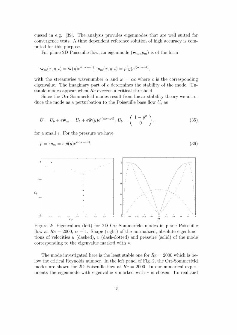
Figure 2: Eigenvalues (left) for 2D Orr-Sommerfeld modes in plane Poiseuilleflow at Re = 2000, α = 1. Shape (right) of the normalized, absolute eigenfunc-tions of velocities u (dashed), v (dash-dotted) and pressure (solid) of the modecorresponding to the eigenvalue marked with ∗.

The mode investigated here is the least stable one for Re = 2000 which is be-low the critical Reynolds number. In the left panel of Fig. 2, the Orr-Sommerfeldmodes are shown for 2D Poiseuille flow at Re = 2000. In our numerical exper-iments the eigenmode with eigenvalue c marked with ∗ is chosen. Its real and

15

imaginary parts are cr = 0.3121 and ci = −0.0198, respectively. The eigenfunc-tions for u, v and p are computed using a solver developed in [39] and can beconsidered to be very accurate since they are obtained in Chebyshev space ex-panded in a large number of modes. The shape of the specific eigenfunctions isshown to the right in Fig. 2.

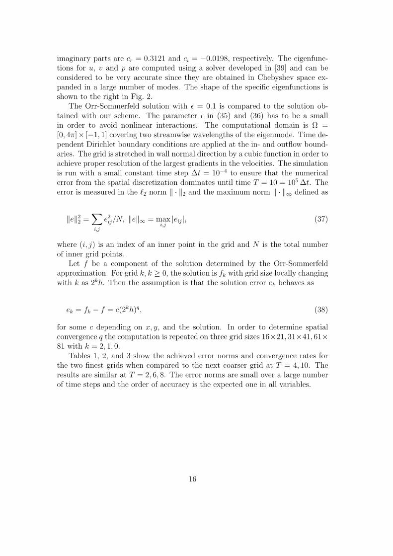
The Orr-Sommerfeld solution with ε = 0.1 is compared to the solution ob-tained with our scheme. The parameter ε in (35) and (36) has to be a smallin order to avoid nonlinear interactions. The computational domain is Ω =[0, 4π]× [−1, 1] covering two streamwise wavelengths of the eigenmode. Time de-pendent Dirichlet boundary conditions are applied at the in- and outflow bound-aries. The grid is stretched in wall normal direction by a cubic function in order toachieve proper resolution of the largest gradients in the velocities. The simulationis run with a small constant time step ∆t = 10−4 to ensure that the numericalerror from the spatial discretization dominates until time T = 10 = 105 ∆t. Theerror is measured in the `2 norm ‖ · ‖2 and the maximum norm ‖ · ‖∞ defined as

‖e‖22 =

∑i,j

e2ij/N, ‖e‖∞ = max

i,j|eij|, (37)

where (i, j) is an index of an inner point in the grid and N is the total numberof inner grid points.

Let f be a component of the solution determined by the Orr-Sommerfeldapproximation. For grid k, k ≥ 0, the solution is fk with grid size locally changingwith k as 2kh. Then the assumption is that the solution error ek behaves as

ek = fk − f = c(2kh)q, (38)

for some c depending on x, y, and the solution. In order to determine spatialconvergence q the computation is repeated on three grid sizes 16×21, 31×41, 61×81 with k = 2, 1, 0.

Tables 1, 2, and 3 show the achieved error norms and convergence rates forthe two finest grids when compared to the next coarser grid at T = 4, 10. Theresults are similar at T = 2, 6, 8. The error norms are small over a large numberof time steps and the order of accuracy is the expected one in all variables.

16

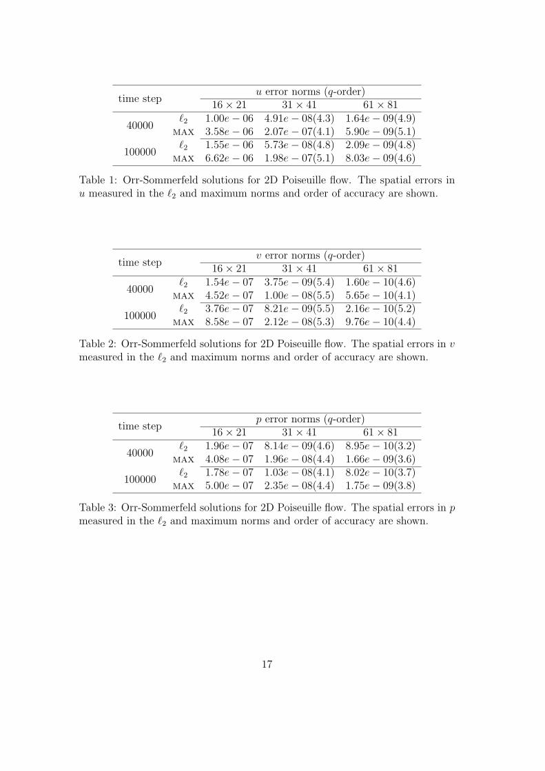
time stepu error norms (q-order)

16× 21 31× 41 61× 81

40000`2 1.00e− 06 4.91e− 08(4.3) 1.64e− 09(4.9)

max 3.58e− 06 2.07e− 07(4.1) 5.90e− 09(5.1)

100000`2 1.55e− 06 5.73e− 08(4.8) 2.09e− 09(4.8)

max 6.62e− 06 1.98e− 07(5.1) 8.03e− 09(4.6)

Table 1: Orr-Sommerfeld solutions for 2D Poiseuille flow. The spatial errors inu measured in the `2 and maximum norms and order of accuracy are shown.

time stepv error norms (q-order)

16× 21 31× 41 61× 81

40000`2 1.54e− 07 3.75e− 09(5.4) 1.60e− 10(4.6)

max 4.52e− 07 1.00e− 08(5.5) 5.65e− 10(4.1)

100000`2 3.76e− 07 8.21e− 09(5.5) 2.16e− 10(5.2)

max 8.58e− 07 2.12e− 08(5.3) 9.76e− 10(4.4)

Table 2: Orr-Sommerfeld solutions for 2D Poiseuille flow. The spatial errors in vmeasured in the `2 and maximum norms and order of accuracy are shown.

time stepp error norms (q-order)

16× 21 31× 41 61× 81

40000`2 1.96e− 07 8.14e− 09(4.6) 8.95e− 10(3.2)

max 4.08e− 07 1.96e− 08(4.4) 1.66e− 09(3.6)

100000`2 1.78e− 07 1.03e− 08(4.1) 8.02e− 10(3.7)

max 5.00e− 07 2.35e− 08(4.4) 1.75e− 09(3.8)

Table 3: Orr-Sommerfeld solutions for 2D Poiseuille flow. The spatial errors in pmeasured in the `2 and maximum norms and order of accuracy are shown.

17

ci

cr y0.2 0.3 0.4 0.5 0.6 0.7 0.8 0.9 1

−1.5

−1

−0.5

0

−1 −0.8 −0.6 −0.4 −0.2 0 0.2 0.4 0.6 0.8 10

0.2

0.4

0.6

0.8

1

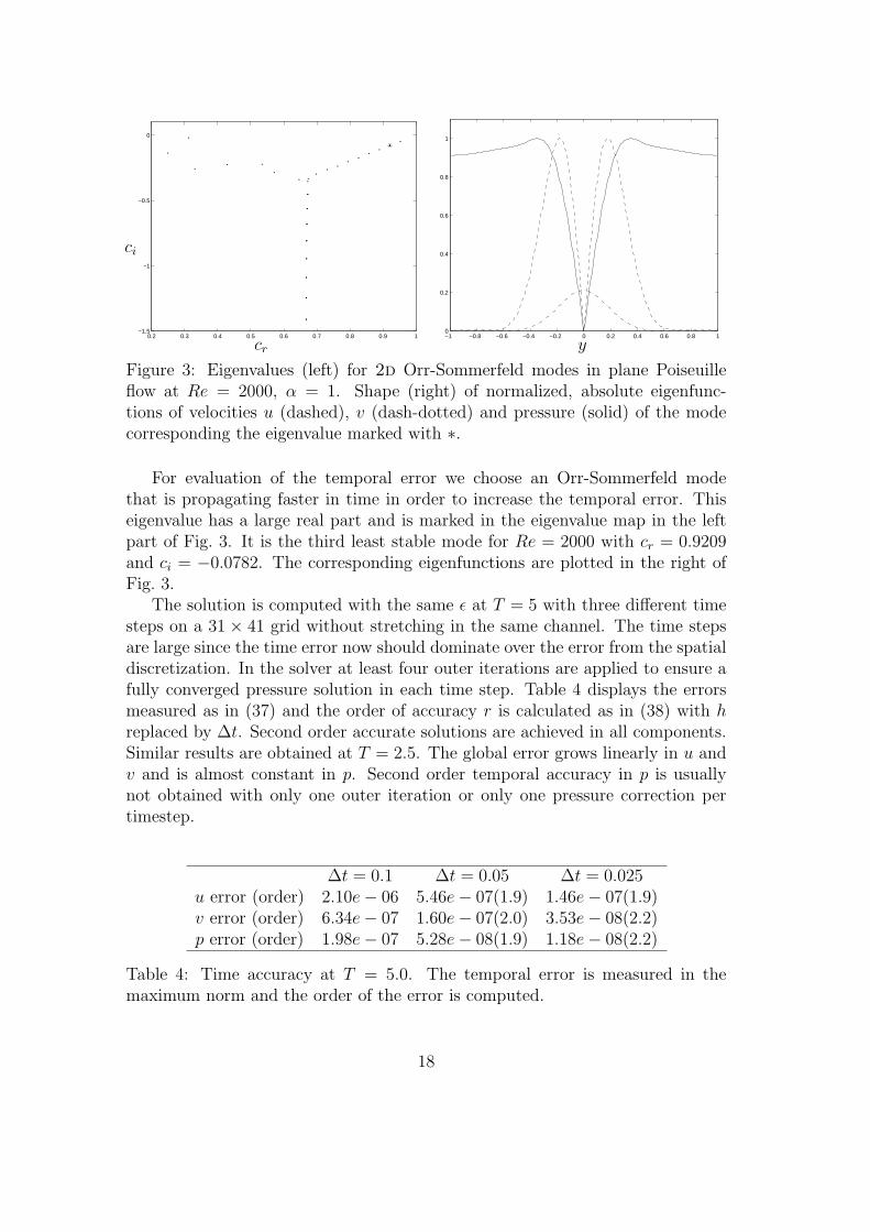
Figure 3: Eigenvalues (left) for 2d Orr-Sommerfeld modes in plane Poiseuilleflow at Re = 2000, α = 1. Shape (right) of normalized, absolute eigenfunc-tions of velocities u (dashed), v (dash-dotted) and pressure (solid) of the modecorresponding the eigenvalue marked with ∗.

For evaluation of the temporal error we choose an Orr-Sommerfeld modethat is propagating faster in time in order to increase the temporal error. Thiseigenvalue has a large real part and is marked in the eigenvalue map in the leftpart of Fig. 3. It is the third least stable mode for Re = 2000 with cr = 0.9209and ci = −0.0782. The corresponding eigenfunctions are plotted in the right ofFig. 3.

The solution is computed with the same ε at T = 5 with three different timesteps on a 31 × 41 grid without stretching in the same channel. The time stepsare large since the time error now should dominate over the error from the spatialdiscretization. In the solver at least four outer iterations are applied to ensure afully converged pressure solution in each time step. Table 4 displays the errorsmeasured as in (37) and the order of accuracy r is calculated as in (38) with hreplaced by ∆t. Second order accurate solutions are achieved in all components.Similar results are obtained at T = 2.5. The global error grows linearly in u andv and is almost constant in p. Second order temporal accuracy in p is usuallynot obtained with only one outer iteration or only one pressure correction pertimestep.

∆t = 0.1 ∆t = 0.05 ∆t = 0.025u error (order) 2.10e− 06 5.46e− 07(1.9) 1.46e− 07(1.9)v error (order) 6.34e− 07 1.60e− 07(2.0) 3.53e− 08(2.2)p error (order) 1.98e− 07 5.28e− 08(1.9) 1.18e− 08(2.2)

Table 4: Time accuracy at T = 5.0. The temporal error is measured in themaximum norm and the order of the error is computed.

18

4.2 Driven cavity

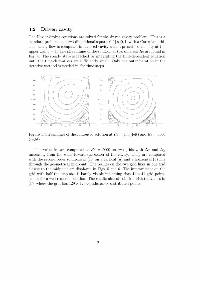
The Navier-Stokes equations are solved for the driven cavity problem. This is astandard problem on a two-dimensional square [0, 1]× [0, 1] with a Cartesian grid.The steady flow is computed in a closed cavity with a prescribed velocity at theupper wall y = 1. The streamlines of the solution at two different Re are found inFig. 4. The steady state is reached by integrating the time-dependent equationuntil the time-derivatives are sufficiently small. Only one outer iteration in theiterative method is needed in the time steps.

0 0.2 0.4 0.6 0.8 1

0.1

0.2

0.3

0.4

0.5

0.6

0.7

0.8

0.9

x

y

0 0.2 0.4 0.6 0.8 1

0.1

0.2

0.3

0.4

0.5

0.6

0.7

0.8

0.9

x

y

Figure 4: Streamlines of the computed solution at Re = 400 (left) and Re = 5000(right).

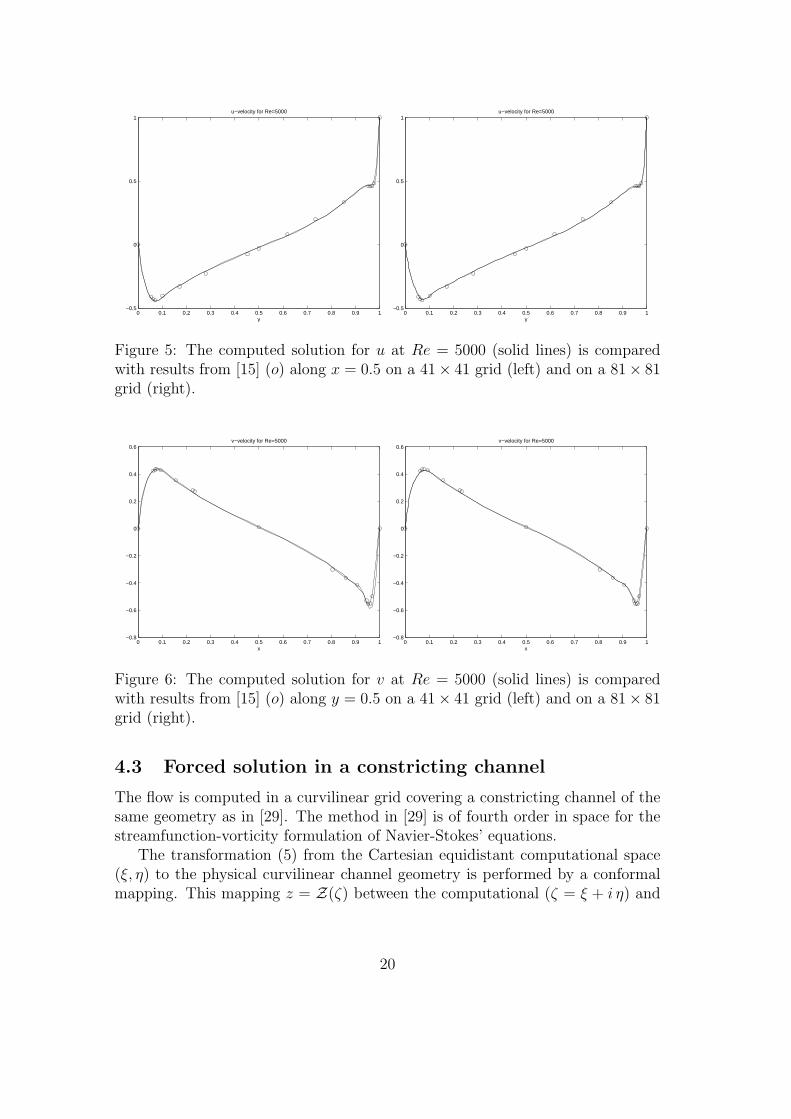
The velocities are computed at Re = 5000 on two grids with ∆x and ∆yincreasing from the walls toward the center of the cavity. They are comparedwith the second order solutions in [15] on a vertical (u) and a horizontal (v) linethrough the geometrical midpoint. The results on the two grid lines in our gridclosest to the midpoint are displayed in Figs. 5 and 6. The improvement on thegrid with half the step size is barely visible indicating that 41 × 41 grid pointssuffice for a well resolved solution. The results almost coincide with the values in[15] where the grid has 129× 129 equidistantly distributed points.

19

0 0.1 0.2 0.3 0.4 0.5 0.6 0.7 0.8 0.9 1−0.5

0

0.5

1u−velocity for Re=5000

y0 0.1 0.2 0.3 0.4 0.5 0.6 0.7 0.8 0.9 1

−0.5

0

0.5

1u−velocity for Re=5000

y

Figure 5: The computed solution for u at Re = 5000 (solid lines) is comparedwith results from [15] (o) along x = 0.5 on a 41× 41 grid (left) and on a 81× 81grid (right).

0 0.1 0.2 0.3 0.4 0.5 0.6 0.7 0.8 0.9 1−0.8

−0.6

−0.4

−0.2

0

0.2

0.4

0.6v−velocity for Re=5000

x0 0.1 0.2 0.3 0.4 0.5 0.6 0.7 0.8 0.9 1

−0.8

−0.6

−0.4

−0.2

0

0.2

0.4

0.6v−velocity for Re=5000

x

Figure 6: The computed solution for v at Re = 5000 (solid lines) is comparedwith results from [15] (o) along y = 0.5 on a 41× 41 grid (left) and on a 81× 81grid (right).

4.3 Forced solution in a constricting channel

The flow is computed in a curvilinear grid covering a constricting channel of thesame geometry as in [29]. The method in [29] is of fourth order in space for thestreamfunction-vorticity formulation of Navier-Stokes’ equations.

The transformation (5) from the Cartesian equidistant computational space(ξ, η) to the physical curvilinear channel geometry is performed by a conformalmapping. This mapping z = Z(ζ) between the computational (ζ = ξ + i η) and

20

the physical space (z = x + i y) is here computed analytically by the relation

z = ζ(A + B tanh(ζ)), (39)

or in component form

x = Aξ+B

H[ξ sinh(2ξ)− η sin(2η)] , y = Aη+

B

H[η sinh(2ξ) + ξ sin(2η)] , (40)

where H = cosh(2ξ) + cos(2η) as in [29]. The channel width far away from theconstriction is 2a at the inlet and 2b at the outlet. The constants A and B aredefined as

A =a + b

2λ, B =

b− a

2λ, (41)

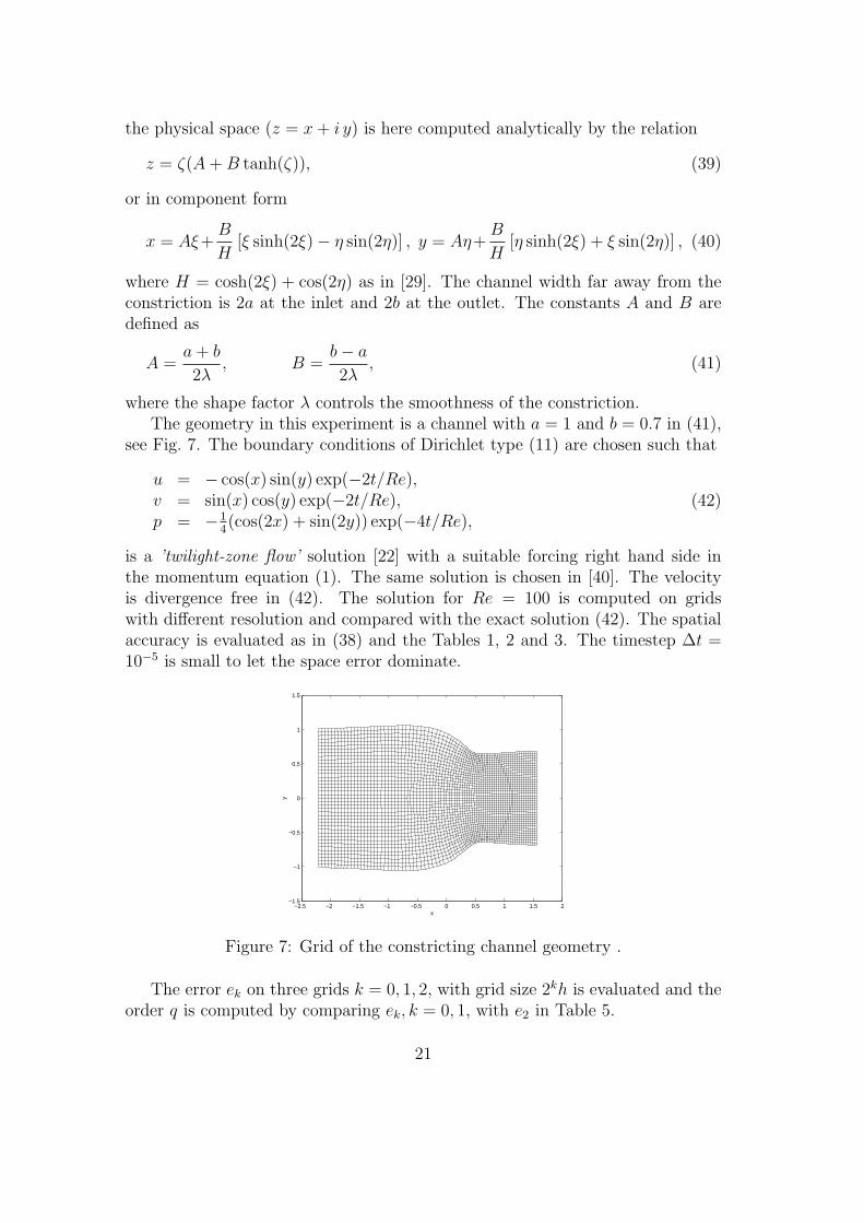
where the shape factor λ controls the smoothness of the constriction.The geometry in this experiment is a channel with a = 1 and b = 0.7 in (41),

see Fig. 7. The boundary conditions of Dirichlet type (11) are chosen such that

u = − cos(x) sin(y) exp(−2t/Re),v = sin(x) cos(y) exp(−2t/Re),p = −1

4(cos(2x) + sin(2y)) exp(−4t/Re),

(42)

is a ’twilight-zone flow’ solution [22] with a suitable forcing right hand side inthe momentum equation (1). The same solution is chosen in [40]. The velocityis divergence free in (42). The solution for Re = 100 is computed on gridswith different resolution and compared with the exact solution (42). The spatialaccuracy is evaluated as in (38) and the Tables 1, 2 and 3. The timestep ∆t =10−5 is small to let the space error dominate.

−2.5 −2 −1.5 −1 −0.5 0 0.5 1 1.5 2−1.5

−1

−0.5

0

0.5

1

1.5

x

y

Figure 7: Grid of the constricting channel geometry .

The error ek on three grids k = 0, 1, 2, with grid size 2kh is evaluated and theorder q is computed by comparing ek, k = 0, 1, with e2 in Table 5.

21

Time stepMaximum error and order

41× 21 81× 41 161× 81u 7.59e− 05 4.34e− 06(4.1) 2.41e− 07(4.2)

600 v 1.67e− 04 7.42e− 06(4.5) 2.43e− 07(4.9)p 2.85e− 04 1.56e− 05(4.2) 7.94e− 07(4.3)u 7.83e− 05 4.81e− 06(4.0) 3.00e− 07(4.0)

1000 v 1.66e− 04 7.32e− 06(4.5) 2.41e− 07(4.9)p 2.84e− 04 1.55e− 05(4.2) 8.16e− 07(4.3)

Table 5: Spatial errors and convergence rates measured in the `2 norm of theforced solution in the constricting channel at Re = 100

4.4 Unforced solution in a constricting channel

−10 −8 −6 −4 −2 0 2 4 6 8 10−1.5

−1

−0.5

0

0.5

1

1.5

x

y

−2.5 −2 −1.5 −1 −0.5 0 0.5 1 1.5 2−2

−1.5

−1

−0.5

0

0.5

1

1.5

2

x

y

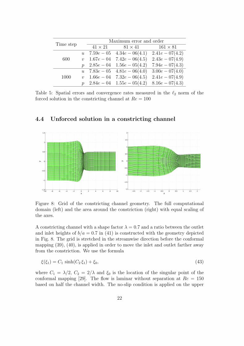
Figure 8: Grid of the constricting channel geometry. The full computationaldomain (left) and the area around the constriction (right) with equal scaling ofthe axes.

A constricting channel with a shape factor λ = 0.7 and a ratio between the outletand inlet heights of b/a = 0.7 in (41) is constructed with the geometry depictedin Fig. 8. The grid is stretched in the streamwise direction before the conformalmapping (39), (40), is applied in order to move the inlet and outlet farther awayfrom the constriction. We use the formula

ξ(ξ1) = C1 sinh(C2 ξ1) + ξ0, (43)

where C1 = λ/2, C2 = 2/λ and ξ0 is the location of the singular point of theconformal mapping [29]. The flow is laminar without separation at Re = 150based on half the channel width. The no-slip condition is applied on the upper

22

and lower walls and a Poiseuille profile is given at the inflow boundary. Theoutflow conditions are as in (12).

In the absence of an exact reference solution, the steady state solution iscomputed on four different grids with resolution 2kh, k = 0, 1, 2, 3, and 81×81(k =0), 41 × 41(1), 21 × 21(2), and 11 × 11(3) grid points. The error in a variablefk on grid k behaves as in (38) and the order of accuracy is estimated by thefollowing two relations

f3 − f2

f2 − f1

≈ 2q1 ,f2 − f1

f1 − f0

≈ 2q2 , (44)

from which we can compute two spatial convergence rates q1and q2. The spatialerror can be estimated on the finest grid by assuming that q = 4 and eliminatingf in (38). Then

e0 ≈ 1

15(f1 − f0). (45)

Due to the strong stretching in the streamwise coordinate, spatial convergence isinvestigated in the region around the constriction only, shown in the right panelof Fig. 8.

The error in the `2 norm on the finest grid (45) and the convergence rates(44) are summarized in Table 6. The error behaves as expected with the bestorder of accuracy q2 between the finest grids where the asymptotic regime of theerror expansion in h is reached.

componentconvergence rate (q-order)

error normq1 q2

u 3.33 4.02 9.78e− 6v 2.92 3.45 1.04e− 5p 2.65 4.18 1.92e− 5

Table 6: Spatial convergence rates and estimates of the numerical error on 81×81grid measured in the `2 norm for laminar flow in the constricting channel atRe = 150

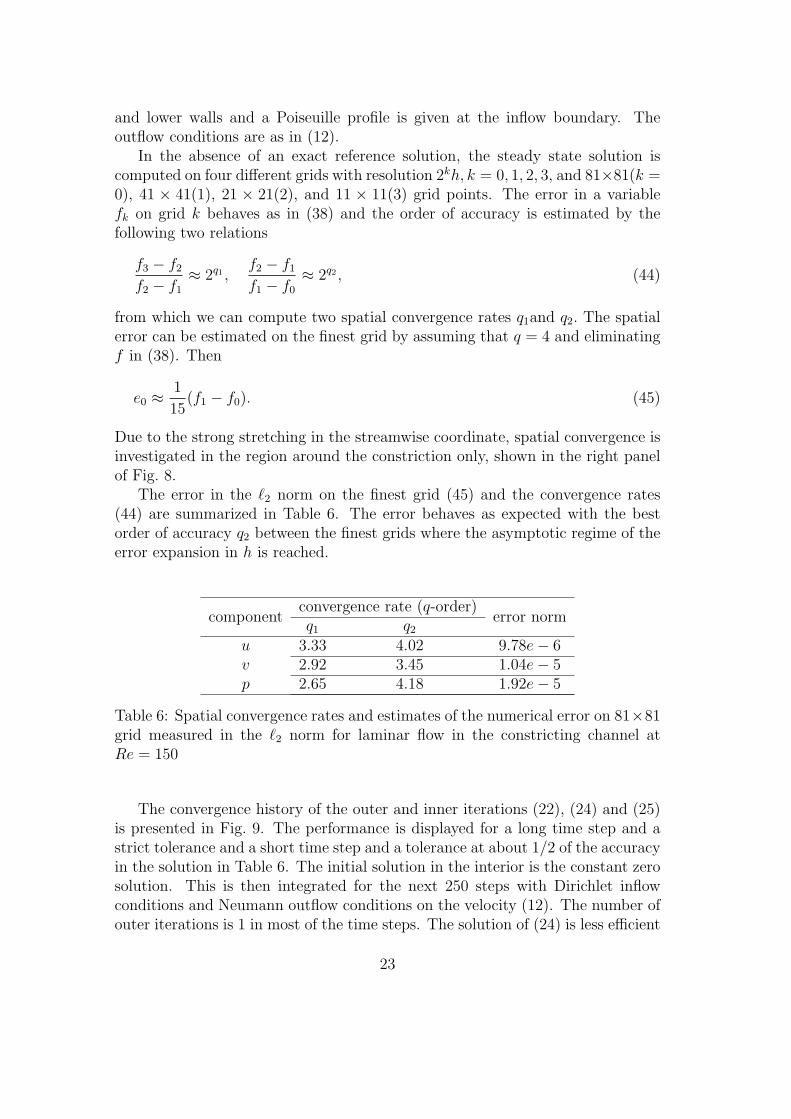
The convergence history of the outer and inner iterations (22), (24) and (25)is presented in Fig. 9. The performance is displayed for a long time step and astrict tolerance and a short time step and a tolerance at about 1/2 of the accuracyin the solution in Table 6. The initial solution in the interior is the constant zerosolution. This is then integrated for the next 250 steps with Dirichlet inflowconditions and Neumann outflow conditions on the velocity (12). The number ofouter iterations is 1 in most of the time steps. The solution of (24) is less efficient

23

for a smaller ε and a larger ∆t as expected from (30). The most time consumingpart is the solution of the Poisson-like equation (25). This part is not sensitiveto changes in ∆t and the increase in number of iterations from the left to theright figure in Fig. 9 is caused by the decrease in ε. To improve the efficiency ofthe method, the focus should be on reducing the computing time spent on thesolution of (25).

0 50 100 150 200 2500123

5

10

15

20

25outerADG

0 50 100 150 200 25001

3

5

10

15

20

25

30outerADG

Figure 9: Convergence of the iterative method in the constricting channel with a41×41 grid in each time step. The parameters are ∆t = 0.001, εo = εi = 5 ·10−6,(left), and ∆t = 0.005, εo = εi = 5 · 10−9, (right).

5 Conclusions

An accurate discretization of the incompressible Navier-Stokes equations in theprimitive variables has been developed for two space dimensions. The methodcan be extended in the third dimension by a spectral approximation without toomuch difficulty. It is of fourth order accuracy in space and of second order intime in all variables. These orders have been verified in numerical experimentsincluding curvilinear grids. The boundary conditions have been proved to bestable for Cartesian grids and are so in practice also for non-Cartesian grids. Thecompact difference operators simplify the treatment at the numerical boundariesand no extra numerical boundary conditions are needed for the pressure. Thevariables are located in a staggered grid to improve the accuracy and to makethe method less prone to oscillatory behavior. A system of linear equations issolved in every time step using outer and inner iterations with preconditioningof the subproblems. The difficulty with the nonuniqueness of the pressure and asingular system matrix is avoided by the definition of the boundary conditions.The outer iterations are preconditioned by an approximate factorization withcontrol of the iteration errors.

24

Acknowledgment

Financial support has been obtained from the Swedish Research Council for Engi-neering Science and the Swedish Research Council. We grateful to Professors DanHenningson and Arne Johansson for helping us with their profound knowledge inflow physics.

References

[1] O. Axelsson, Iterative Solution Methods, Cambridge Univ. Press, Cam-bridge, 1994.

[2] K. Bhaganagar, D. Rempfer, J. Lumley, Direct numerical simulationof spatial transition to turbulence using fourth-order vertical velocity second-order vertical vorticity formulation, J. Comput. Phys., 180 (2002), 200–228.

[3] D. L. Brown, R. Cortez, M. L. Minion, Accurate projection meth-ods for the incompressible Navier-Stokes equations, J. Comput. Phys., 168(2001), 464–499.

[4] A. Bruger, Higher order methods suitable for direct numerical simulationof flows in complex geometries, Licentiate thesis, Dept of Mechanics, RoyalInstitute of Techonolgy, Stockholm, Sweden, 2002.

[5] A. Bruger, J. Nilsson, W. Kress, A compact higher order finite differ-ence method for the incompressible Navier-Stokes equations, J. Sci. Com-put., 17 (2002), 551–560.

[6] J. Cahouet, J.-P. Chabard, Some fast 3D finite element solvers for thegeneralized Stokes problem, Int. J. Numer. Meth. Fluids, 8 (1988), 869–895.

[7] W. Chang, F. Giraldo, B. Perot, Analysis of an exact fractional stepmethod, J. Comput. Phys., 180 (2002), 183–199.

[8] H. Choi, P. Moin, Effects of the computational time step on numericalsolutions of turbulent flow, J. Comput. Phys., 113 (1994), 1–4.

[9] J. K. Dukowicz, A. S. Dvinsky, Approximate factorization as a highorder splitting for the implicit incompressible flow equations, J. Comput.Phys., 102 (1992), 336–347.

[10] H. C. Elman, Preconditioners for saddle point problems arising in compu-tational fluid dynamics, Appl. Numer. Math., 43 (2002), 75–89.

25

[11] H. C. Elman, V. E. Howle, J. N. Shadid, R. S. Tuminaro, A paral-lel block multi-level preconditioner for the 3D incompressible Navier-Stokesequations, J. Comput. Phys., 187 (2003), 504–523.

[12] H. C. Elman, D. J. Silvester, A. J. Wathen, Performance and analysisof saddle point preconditioners for the discrete steady-state Navier-Stokesequations, Numer. Math., 90 (2002), 665–688.

[13] B. Fornberg, M. Ghrist, Spatial finite difference approximations forwave-type equations, SIAM J. Numer. Anal., 37 (1999), 105–130.

[14] R. Friedrich, T. J. Huttl, M. Manhart, C. Wagner, Direct numer-ical simulation of incompressible turbulent flows, Computers & Fluids, 30(2001), 555–579.

[15] U. Ghia, K. N. Ghia, C. T. Shin, High Re solutions for incompressibleflow using the Navier-Stokes equation and multigrid methods, J. Comput.Phys., 48 (1982), 387–411.

[16] S. Ghosal, An analysis of numerical errors in large-eddy simulations ofturbulence, J. Comput. Phys., 125 (1996), 187–206.

[17] A. Greenbaum, Iterative Methods for Solving Linear Systems, SIAM,Philadelphia, 1997.

[18] B. Gustafsson, P. Lotstedt, A. Goran, A fourth order differencemethod for the incompressible Navier-Stokes equations, in M.M. Hafez, ed-itor, Numerical simulations of incompressible flows , World Scientific Pub-lishing, Singapore, 2003, 263–276.

[19] B. Gustafsson, J. Nilsson, Boundary conditions and estimates for thesteady Stokes equations on staggered grids, J. Sci. Comput., 15 (2000), 29–54.

[20] B. Gustafsson, J. Nilsson, Fourth order methods for the Stokes andNavier-Stokes equations on staggered grids, in D. A. Caughey, M. M. Hafez,editors, Frontiers of Computational Fluid Dynamics – 2002, World ScientificPublishing, Singapore, 2002, 165–179.

[21] E. Hairer, S. P. Nørsett, G. Wanner, Solving Ordinary DifferentialEquations I, Nonstiff Problems, 2nd ed., Springer-Verlag, Berlin, 1993.

[22] W. D. Henshaw, A fourth-order accurate method for the incompressibleNavier-Stokes equations on overlapping grids, J. Comput. Phys., 113 (1994),13–25.

26

[23] G. E. Karniadakis, M. Israeli, S. A. Orszag, High-order splittingmethods for incompressible Navier-Stokes equations, J. Comput. Phys., 97(1991), 414.

[24] J. Kim, P. Moin, Application of a fractional-step method to incompressibleNavier-Stokes equations, J. Comput. Phys., 59 (1985), 308–323.

[25] W. Kress, J. Nilsson, Boundary conditions and estimates for the lin-earized Navier-Stokes equations on a staggered grid, Computers & Fluids,32 (2003), 1093–1112.

[26] S. K. Lele, Compact finite difference schemes with spectral-like resolution,J. Comput. Phys., 103 (1992), 16–42.

[27] M. Li, T. Tang, B. Fornberg, A compact fourth-order finite differencescheme for the steady incompressible Navier-Stokes equations, Int. J. Nu-mer. Meth. Fluids, 20 (1995), 1137–1151.

[28] A. Lundbladh, D. S. Henningson, A. V. Johansson, An efficientspectral integration method for the solution of the time-dependent Navier-Stokes equations, Report FFA-TN 1992-28, Aeronautical Research Instituteof Sweden, Bromma, Sweden, 1992.

[29] P. F. De A. Mancera, R. Hunt, Fourth order method for solving theNavier-Stokes equations in a constricting channel, Int. J. Numer. Meth. Flu-ids, 25 (1997), 1119–1135.

[30] J. A. Meijerink, H. A. van der Vorst, An iterative solution methodfor linear systems of which the coefficient matrix is a symmetric M-matrix,Math. Comp., 31 (1977), 148–162.

[31] R. S. Montero, I. M. Llorente, M. D. Salas, Robust multigrid al-gorithms for the Navier-Stokes equations, J. Comput. Phys., 173 (2001),412–432.

[32] Y. Morinishi, T. S. Lund, O. V. Vasilyev, P. Moin, Fully conservativehigher order finite difference schemes for incompressible flow, J. Comput.Phys., 143 (1998), 90–124.

[33] S. Nagarajan, S. K. Lele, J. H. Ferziger, A robust high-order com-pact method for large eddy simulation, J. Comput. Phys., 191 (2003), 392–419.

[34] J. Nilsson, Initial-boundary-value problems for the Stokes and Navier-Stokes equations on staggered grids, PhD thesis, Dept of Scientific Com-puting, Uppsala University, Uppsala, Sweden, 2000.

27

[35] M. Ofstad Henriksen, J. Holmen, Algebraic splitting for incompress-ible Navier-Stokes equations, J. Comput. Phys., 175 (2002), 438–453.

[36] M. Pernice, M. D. Tocci, A multigrid-preconditioned Newton-Krylovmethod for the incompressible Navier-Stokes equations, SIAM J. Sci. Com-put., 23 (2001), 398–418.

[37] J. B. Perot, An analysis of the fractional step method, J. Comput. Phys.,108 (1993), 51–58.

[38] N. A. Petersson, Stability of pressure boundary conditions for Stokes andNavier-Stokes equations, J. Comput. Phys., 172 (2001), 40–70.

[39] P. J. Schmid, D. S. Henningson, Stability and Transition in Shear Flows,Springer, New York, 2001.

[40] J. C. Strikwerda, High-order-accurate schemes for incompressible viscousflow, Int. J. Numer. Meth. Fluids, 24 (1997), 715–734.

[41] J. C. Strikwerda, Y. S. Lee, The accuracy of the fractional step method,SIAM J. Numer. Anal., 37 (1999), 37–47.

[42] S. Turek, A comparative study of time-stepping techniques for the incom-pressible Navier-Stokes equations: From fully implicit non-linear schemes tosemi-implicit projection methods, Int. J. Numer. Meth. Fluids, 37 (1999),37–47.

[43] A. Veneziani, Block factorized preconditioners for high-order accurate intime approximation of the Navier-Stokes equations, Numer. Meth. Part.Diff. Eq., 19 (2003), 487–510.

[44] H. A. van der Vorst, BiCGSTAB: A fast and smoothly converging vari-ant of Bi-CG for the solution of nonsymmetric linear systems, SIAM J. Sci.Comput., 13 (1992), 631–644.

28