on the smallest scale for the incompressible navier-stokes equations
TRANSCRIPT
Theoret. Comput. Fluid Dynamics (1989) 1:65-95 Theoretical and Computational Fluid Dynamics © 1989 Springer-Verlag Berlin Heidelberg
On the Smallest Scale for the Incompressible Navier-Stokes Equations
W.D. Henshaw
Mathematical Sciences, IBM Thomas J. Watson Research Center, Yorktown Heights, NY 10598, U.S.A.
H.O. Kreiss 1
Department of Mathematics, University of California at Los Angeles, Los Angeles, CA 90024, U.S.A.
L.G. Reyna
Mathematical Sciences, IBM Thomas J. Watson Research Center, Yorktown Heights, NY 10598, U.S.A.
Communicated by M.Y. Hussaini
Abstract. We prove that, for solutions to the two- and three-dimensional incompressible Navier- Stokes equations, the minimum scale is inversely proportional to the square root of the Reynolds number based on the kinematic viscosity and the maximum of the velocity gradients. The bounds on the velocity gradients can be obtained for two-dimensional flows, but have to be assumed in three dimensions. Numerical results in two dimensions are given which illustrate and substantiate the features of the proof. Implications of the minimum scale result, to the decay rate of the energy spectrum are discussed.
1. Introduct ion
We cons ider so lu t ions to the incompress ib le N a v i e r - S t o k e s equat ions
ut + uux + vu r + wux + Vp = vAu, v > 0,
ux + vy + Wx = 0,
on a 2n-per iodic box, where u = (u, v, w) is the veloci ty vector, p the pressure, and v the k inemat ic viscosity. Solut ions of the N a v i e r - S t o k e s equat ions for small viscosi ty are usual ly turbulent; such flows possess a lot of s t ructure in bo th space and time. The viscosi ty of the fluid cont ro l s the level of turbulence wi thin a flow by affecting the energy dissipat ion. As the viscosity is decreased, the size of the smallest features, or scales, diminishes. The re la t ion between the viscosity, the m i n i m u m scale, and the to ta l energy d iss ipa t ion is of fundamenta l interest for the under s t and ing of turbulence.
1 Research was supported in part by the National Acronautics and Space Administration under NASA Contract No. NASI-18107, while the second author was in residence at the Institute for Computer Applications in Science and Engineering (ICASE), NASA Langley Research Center, Hampton, VA 23665. Additional support was provided by the National Science Foundation under Grant DMS-8312264 and the Office of Naval Research under Contract N-00014-83-K-0422.
66 W.D. Henshaw, H.O. Kreiss, and L.G. Reyna
The mathematical theory for the Navier-Stokes equations is not complete for three-dimensional flows: the global regularity is not known and no global bound for the velocity gradients is available. However, both these results are known in two-space dimensions. Whether the results from two- dimensional flows are of physical relevance is open to discussion since, in the absence of viscosity, flows in two dimensions conserve both energy and enstrophy, while in three dimensions only the energy is conserved. Nevertheless, results on two-dimensional turbulence may be of significance for large scale oceanographic and atmospheric motions.
Assuming global regularity, we relate the minimum scale of the flow to [Dul~o, the global bound of the velocity gradients. Our main result, precisely stated in Theorem 2.1, is that the minimum scale is essentially no smaller than
/~min = vl/2/IDul~2.
By comparison, a commonly accepted minimum scale for two-dimensional flows, 220 (see [19] and 1-20]), is based on the total dissipation rate of the enstrophy per unit volume. The enstrophy is defined as the square of the L2-norm of the vorticity. From dimensional arguments it follows that
/~2D = y1/2/~ 1/6,
where
n=2vff(ll~xll2÷ll~rll2)dxdy is the total rate of enstrophy dissipation per unit volume and ¢ is the vorticity.
In three-space dimensions the corresponding minimum scale is the Kolmogoroff dissipation scale [15]
'~3D = y3/4-//~1/4,
where
e=2vfff(IVu~ll2+jjuyll2+liu~ll2)dxdydz is the total rate of energy dissipation per unit volume.
The estimates for the minimum scale can be used to determine the decay rate of the energy spectrum, assuming that a power law does in fact exist.
From our results in two dimensions we conclude that the energy spectrum, E(k), behaves like k -3 when there is a maximum rate of enstrophy dissipation in the flow. The k -3 power law is in accordance with the Batchelor-Kraichnan theory of enstrophy cascade [3], [16]. The high rate of dissipation cannot remain for long times without the flow disappearing. Indeed, numerical experi- ments show that the solutions rearrange themselves into organized structures which dissipate enstrophy at a much smaller rate. Staffman's work [22], which predicts a power law k -4, seems to describe the behavior of the system at this later stage of evolution. Our theory does not predict the power law but only relates it to the rate of enstrophy dissipation; the k -4 law would correspond to t/ of order 1 ' 1 / 2 .
In three-space dimensions there is no a priori bound for [DuLo. However, if we assume that
IOul~ ~ v -x/2,
then when the energy dissipation rate e is of order one, we obtain the Kolmogoroff power law, E(k) = k -5/3, and the Kolmogoroff scale '(min = 23D = v3/4.
Some of the first calculations on two-dimensional turbulence were performed by Lilly [19], Fox and Orszag [9], Herring et al. [12], Fornberg [8], and Barker [1], among others. More recent computations on meshes of up to 1024 x 1024 points are described in, for example, Brachet and Sulem [7], Brachet et al. [6], Herring and McWilliams [11], and Benzi et al. [4]. In some cases the small viscosity limit of the equations was approximated by the continuous removal of the high frequency Fourier coefficients [8-]. In other cases, the true dissipation term is integrated although some extra smoothing of high frequencies is sometimes required to suppress the growth of aliasing errors [1]. Another approach is to replace the viscosity term by a super-viscosity, that is, a higher
On the Smallest Scale for the Incompressible Navier-Stokes Equations 67
power of the Laplacian operator [7-1, [11]. This operator allows simulations with a formal viscosity which is much smaller. The minimum scale is nevertheless comparable to the computations presented in this paper.
The numerical simulation of three-dimensional flows is still limited by the power of current computing machines. Currently, the largest three-dimensional simulations seem to have been per- formed on 1283 meshes. However, by exploiting the symmetries of the Taylor -Green problem, Brachet et al. were able to effectively solve with a 2563 resolution [5-1. They find the slope of the spectrum to be least steep when the rate of energy dissipation reaches a maximum. The numerical results seem to agree at this point with the Kolmogoroff scale. For further references on three- dimensional computations, see the review article by Hussaini and Zang [14].
We restrict ourselves to two-dimensional simulations. Our numerical approach has been to attempt to solve faithfully the viscous Navier-Stokes equations. The computations were performed using the pseudospectral method [18], [21]. There is no extra viscosity added to the numerical sim- ulation through smoothing or chopping of the high frequencies, although the fourth-order predictor- corrector time integrator produces a small amount of it. Numerical simulations are used to confirm the theoretical estimates and to show that the estimates can be achieved for certain initial conditions. Results are shown for the time development of a flow which initially is maximal dissipative. We also show results of forced problems. In this case, there is no easy a priori bound for the maximum norm of the vorticity. We found numerically that the forcing should be proportional to the viscosity in order to obtain order one velocities. More numerical work on this subject is still necessary.
In Section 2, we present the analytical results. In Section 3, we present numerical computations in two-space dimensions which substantiate and illustrate various features of the proof. Finally, in Section 4, we discuss the implications of the minimum scale result to the decay rate of the energy spectrum.
2. Ana ly t i ca l Resul t s
In this section, we will prove some results about the rate of decay of the Fourier coefficients for solutions of the incompressible Navier-Stokes equations,
ut + uux + vuy + wuz + Vp = vAu, v > 0, (2.1a)
ux + vy + w~ = 0, (2.1b)
on the region ~ =: {0 _< x, y, z _< 2~z} and for t _> 0. We assume that u = (u(x, t), v(x, t), w(x, t)) is 2re-periodic in x = (x, y, z).
At t = 0 we give the initial data
u(x, 0) = Uo(X), V'uo = 0.
For simplicity, we assume that
which implies
f u o dx = 0,
f u(x, t) = t _> (2.2) dx 0 for 0.
We assume that (2.1) has a bounded solution for all times and want to show that the smallest scale is essentially proportional to (v/IDuloo) v2. Here
I Dul~ = sup I Dul~ and t
In general, let
DPu - -
IDul~ : sup (10u/~xl, 10u/~yl, 10u/~zl). x
~Pu
dx m dyp2 ¢?zp3 '
denote any derivative of u of order p, where p = Pl + P2 + P3-
68 W.D. Henshaw, H.O. Kreiss, and L.G. Reyna
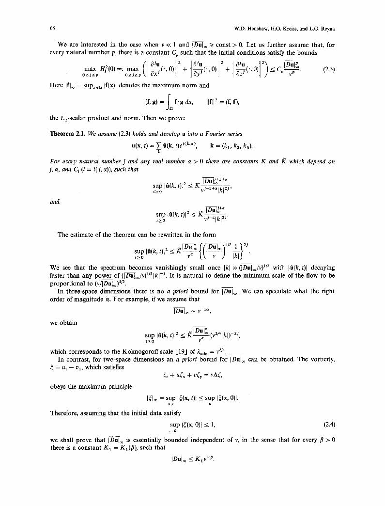
We are interested in the case when v << 1 and IDuLo _ const > 0. Let us further assume that, for every natural number p, there is a constant Cp such that the initial conditions satisfy the bounds
( ~ J l l 2~JH 2 ~Ju ) c lDUl~ max H~(0)=: max < O<j<p O<j<.p ~Xj(" , O) -[- ~ y j ( ' , O) -~ ~ Z j ( ' ' O ) 2 _ _ P yP "
Here Ifloo = SUpx~ If(x)[ denotes the m a x i m u m n o r m and
Ilfl[ 2 = (f, f), (f, g) = f~ f- g dx,
(2.3)
we obtain
The estimate of the theorem can be rewritten in the form
sup I~(/, 012 < ~ - ; - IklJ "
We see that the spectrum becomes vanishingly small once Ikl >> (IDuloo/v) ~/2 with I~(k, t)l decaying faster than any power of (IDutoo/v)l/Zlkl-1. It is natural to define the minimum scale of the flow to be proportional to (v/IDuto~) x/z.
In three-space dimensions there is no a priori bound for IDuloo. We can speculate what the right order of magnitude is. For example, if we assume that
IDuL ~ v -~/2,
obeys the maximum principle
IDul~ .,3/4 ~ ~-2j sup l~(k, t)[ z _ < . , ~ , - . . , , t___0
which corresponds to the Kolmogoroff scale [19] of '~min = r3/4" In contrast, for two-space dimensions an a priori bound for IDuloo can be obtained. The vorticity,
= uy -- vx, which satisfies 4, + uCx + v~, = vA~,
I¢[o~ = sup I~(x, t)l ~ sup I~(x, O)l. X,t X
Therefore, assuming that the initial data satisfy
sup I¢(x, 0)l < 1, (2.4) • X
we shall prove that IDuloo is essentially bounded independent of v, in the sense that for every fl > 0 there is a constant K1 = K~(fl), such that
]Du]oo --< K1v -#.
and
sup I~(k, 012 < g IDu[~+~ t>_o - v~+~lkl2J"
the L2-scalar product and norm. Then we prove:
Theorem 2.1. We assume (2.3) holds and develop u into a Fourier series
u(x, t) = ~ ~(k, t)e i(k'x>, k = (k l , k2, k3). k
For every natural number j and any real number ~ > 0 there are constants K and K which depend on j, or, and C z (I = l(j, a)), such that
ID,.I j+1+~ _ K i - - , o o sup l~(k, 012 <
t>_ o vJ-l +~lkl 2j '
On the Smallest Scale for the Incompressible Navier-Stokes Equations 69
is essentially of the
where
2.1. Estimates for p ~ 3
F r o m now on we shall assume that an est imate for IDuLo exists. In tegra t ion by parts gives us the basic energy est imate
l a - - - I l u l l 2 = -vn~, 2 dt
where
~/J = / - / J ( t ) = o , 'u( - , t) ~ ~ - , t) ~ # " u ( . , t) + + . #yP
Since by assumpt ion (2.3), Ilu(', 0)112 _< const, it follows
2v ;o H~(t) dt <_ Ilu(', 0)ll 2 _< c o n s t a n d [lu(', t)ll 2 -< Ilu(', 0)ll 2 -< cons t .
N o w differentiate (2.1). Fo r any first space derivative Du we obtain
0t IlDull2 + I = -v(l lDu~ll 2 + [IDurll 2 + IIDuzll2),
Therefore
that is,
I = (Du, D(uu~ + vuy + wu~)) = II + III,
I I = (Du, uDu,~ + vDuy + wDuz),
I I I = (Du, Duu, + Dvur + Dwuz)
In tegra t ion by parts and V ' u = 0 show that I I = O. Again, by integrat ion by part , we obta in
I I I <_ const IDuI~H~.
1 0
2 0 t - - - I l O u l l 2 ~ const IOuLoHt z - v(llDu~ll 2 + IlOu, II 2 + IlDuzll2),
2 at H~ < const [DuLoH z -- vH~.
Integrat ing the last inequali ty with respect to t gives us,
; fo Hf(t) < H~(O) + const IDul® nf ( z ) dz - 2v H~(z) dz.
Therefore, by (2.3) and (2.6),
IDuL n~(t) <_ const
v
F o r the second derivatives, we obta in
1 0
2 0t
and v f o H](t) d t < const IOulo~.v
- - - I lD2u l [ 2 + I = --v([ID2uxl[ 2 + I[D2uyll 2 + [ID2u~[12),
(2.5)
(2.6)
(2.7)
Thus if the initial da ta have derivatives of order one then the smallest scale order v 1/2.
O u r p roof is also valid for Burger 's equation. In this case, we can prove that
[Dul~ < const v -1 sup IDu(x, 0)lo~. X
Thus our result predicts that the min imum scale is of order v -1. This bound can be a t ta ined in the presence of shocks.
70 W.D. Henshaw, H.O. Kreiss, and L.G. Reyna
where
Therefore,
I = (D2a, D2(uUx -Fvuy -t- WUx) ) --- II + III + IV,
II = (D2u, uD2ux q- vD2ny -F wD2ux) = 0,
III = 2(D2u, DuDux + DvDur + DwDux) <_ const IDul~oH2 2,
IV = (D2u, D2uux -F O2vuy "Jr O2wuz) ~ const IDulo~H 2.
1 ~ H 2 _ 2 Ot 2 <~ const IDuI~H 2 - vH 2.
Integrating the last inequality with respect to t and using (2.3), (2.7) gives us
IDaI~ ~ : IDul~ H2(t) < const v2 and v Hi(t) dt < const v ~
For the third derivatives, we obtain
½(Dan, Dall)t q- I = -v ( l lDaux l l 2 + IID3u, II 2 + IIDauxll2),
where by Leibniz's rule
I = (D3u, Da(uux + vur + WUz)) = II + III + IV+ V,
II = (Dau, uD3ux -t- vDauy q- wDaUz) = 0,
III = 3(Dau, DuD2ux + DvD2ur + DwD2uz) <. const IDuLoHE,
IV = 3(D3u, D2uDux + D2vDuy + D2wDuz) < const IDuI~HgH2,
V --= (Dau, D3uux -}- Davur + D3wux) <_ const IDul~H 2.
Therefore
l O
2 Ot - - - H j < const IDuI~(H j + H4H2) - vH 2
< const IDaI~H E + const IDul~ H~
thus using (2.3), (2.7), and (2.8)
Hi(t) < const IDul~
1
(2.8)
and v f : H2(t)dt < const IDvu313 . (2.9)
2.2. The Estimates for General p
We now prove Theorem 2.1 for arbitrary p. First we obtain energy estimates for Hp in terms of IDJul~, 1 < j < max(l, [(p - 1)/3]). These estimates are used to obtain bounds for [DJul~o in terms of IDul®. Finally, improved estimates are obtained for Hp, IDPaI®, and IDJul~ using interpolation inequalities; the theorem then follows. We start with:
Lemma 2.1. For every p there is a constant Kp such that
I(DPu, DP(uu~ + vu, + wn~)l < KpQDuI~H 2 + lip+ 1
Here
max(1,[(p-1)/3]) \ [DJulooH,-j)"
[x] = largest integer <_ x and IDJnloo = max IDkul. x, lkt=j
On the Smallest Scale for the Incompressible Navier-Stokes Equations 71
Proof. We need to estimate expressions of the form
(DPu, DP-kuDkUx d- Dt'-kvDkur -t- DP-kwDkUz) for k = 0 . . . . . p - 1.
We integrate by parts to decrease the order of DPu. In doing this, the order of DP-ku, DP-kv, and DP-kw or the order of OkUx, Dkuy, and DkUz will increase. For each new term generated through integration by parts,
(Dqu, D~uDq~u~) + (Dqu, Dq~vDq~uy) + (Dqu, D~wDq3uz),
we can decrease the order q and increase one of q2 or q3 until one of the following conditions is satisfied:
(1) q - 1 < q 3 _ < q a n d q 2 _ < q ; (2) q_<q2 < q + l a n d q a < q - 1 .
Note that in case (1), if q3 = q, then
(Dqu, Dq~uDqu~ + D~vD~uy + D~2wD~u~) = O.
It follows that
can be written
A := (Dqu,
B := (D~u,
C := (Dqu,
I = (DPu, DP(uu~ + vuy + WUz))
as a sum of terms
O 2p-2q+l uD q-I ux + O 2p-2q+l vD q-1 u r + D 2p-2q+l wD ~-1Uz),
D ~+x uD 2p-2q-1 U x -'}- D q+x vO 2p-2q-1Uy -1- O q+l wD 2p-2q-1Uz) ,
DquD2p- 2qUx -}- DqvD2p-2quy -]- DqwD2p-2qUz),
l < 2 p - 2 q + l < q ,
l < 2 p - 2 q - l < q - 1 ,
0 < 2 p - 2q_<. q - 2.
q j < p + l and q~ + q 2 = p + q + l.
p -- q _< max(l , [½(p -- 1)]).
The required estimates can be obtained in the following cases:
(i) If p - q = 1, then either qx = q2 = P or one of the qj = p + 1 and the other is equal to p - 1. (ii) One of the q~ is equal to p + 1.
When neither (i) nor (ii) is satisfied, then qj < p + 1 and p - q > 1, and we can reduce D p-q further. This shows that A can be estimated in the desired way.
Expression B. Correspondingly, by reducing the order of DzP-z~-lu~, DzP-zq-auy, and DZP-Zq-lu~, B can be written as sum of terms
(D~lu, D~2uDP-q-lu~ + Dq~vDP-~-luy + D~2wDP-q-luz) := II,
where
q i < p + l , q l + q 2 = p + q + l and p - q - l > O .
Also 2p - 2q < q implies 0 < p - q - 1 < [½(p - 3)]. II can be estimated in the following two cases:
where p - q > l,
Also, 1 < 2p - 2q + 1 _< q implies
Expression A. If 2p -- 2q + 1 = 1, then the estimate follows, otherwise integration by parts is applied to expression A,
A = (DP-~u, O p-q+1 (DquD ~-1 ux) ) + (Ot'-qv, DP-q+l(DquDq-1 uy)) + (DP-qw, D p-q+1 (DquD ~-1 Uz)),
to reduce the order of the factors D2p-2q+lu, D2p-2q+lv, and D2p-2~+~w. In this way, we can write A as a sum of terms
(Dqlu, DP-~uDq2-1u x + DP-%D~2-1u~ + DP-~wDq2-1uz),
72 W.D. Henshaw, H.O. Kreiss, and L.G. Reyna
(i) I f p - q - 1 = O, then qi = P + 1, q2 = P - 1, or ql = q2 = P, and
II <__ const IDu]®Hp+l Hp-1,
or II < const lDulo~Hn 2.
(ii) I f q i = p + 1 o r q 2 = p + 1.
Otherwise, qj < p + 1 and p - q - 1 > 0, and hence we can diminish p - q - 1 further. Therefore we obtain the desired estimates for B.
Expression C. Integrat ion by parts allows us to diminish the order of D2p-2qll obtaining terms of the form
(D ql u, Dq~uD p-q-i ux + D~vD p-q-1 u r + Dq2wD n-q-x Uz) ,
where
q j < p + l , q ~ + q 2 = p + q + l and p - q - l > _ O .
Using the same argument as for B we obtain the desired estimate. This proves the lemma. [ ]
Differentiating (2.1) p-times gives us
2 ~t (oÈu' Dnu) + (Dnu' DP(uux + vur + wu=)) = --v(llDnu~[I a + IlDPur[I 2 + IlOPuzll2).
Therefore, we obtain from L e m m a 2.1
2 ( max(l, [(p-i)/3]) ) ~ H ~ < const I D u L H 2 + Hp+l ~ ID~uI~Hn_ j -- 2vH~+l
j=l
( lmax(l'[(P-1)/3]) J 2 2 ) 2 < const IDul®H 2 + - ~ [D ul®H~_j - vH[,+l.
j = l
Using the nota t ion
the last inequality implies
and
Lp = f o H~(t) dt,
[IDul~ 1 max(1,t(p- 1)]3]) HZ(t) < const ~ - b - - + IOuL g~ + -v j=lZ IWul~ g~_jj, (2.10)
IDuI 3 L3 ~< const[Dv31~u and L 4 _< const v ~
Therefore (2.10) and (2.11) give us
H~(t) < const \ ~4
L 5 _< const \ v5 + V L4 + ~ [ ~ 2 L 3 ] __< const
The estimates for Hi, L6, H26, and L 7 follow in the same way.
1 ~ . IDul~ +-IDul~L3v J - c o n s t ~ ,
IDul~ V 5
/fOul& I bu~® 1 max(i,l(p-i)/31) _ _ Lp+l <- cons t~ v---V4q- + v Lp + v- ~ j=l~ IDJul2 Lp_jj. (2.11)
To begin with, let us obtain estimates for Hp and Ln+ 1 for p = 4 . . . . . 7. In mos t applications this is all that is needed. F r o m our previous results we know that
On the Smallest Scale for the Incompressible Navier-Stokes Equations 73
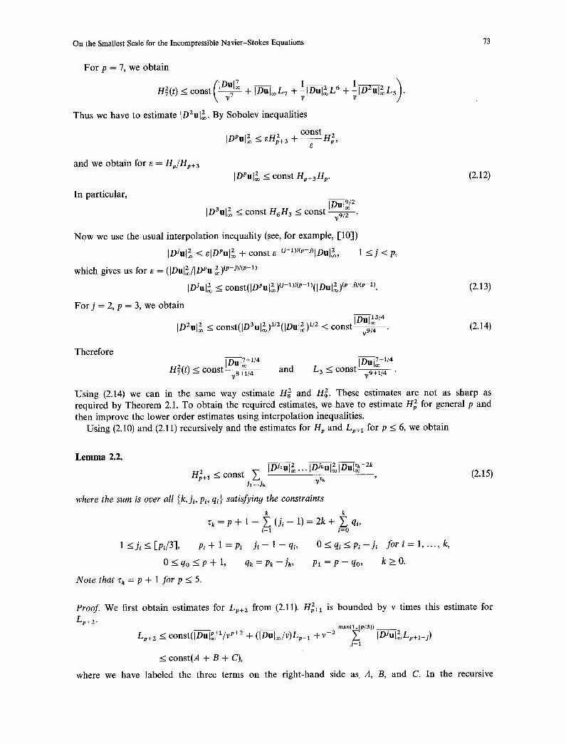
For p = 7, we obtain
H2(t) <_ c o n s t / - - ~ - + IOul®Z7 + ! , ,~ L6 "[- [D2~2L5 I
Thus we have to estimate ID2ul 2. By Sobolev inequalities
const 2 2 Hp, IDPul 2 < 8H~+ 3 +
and we obtain for e = Hp/Hp+ 3
In particular,
ID"ulL -< c o n s t Hp+3Hp.
IDul9/2 [D3ul 2 < const H 6 H 3 <_ c o n s t v 9 / ~
Now we use the usual interpolation inequality (see, for example, [103)
IDJul~ < elDPu[~ + const e-°-l)/¢P-~)lDul~, 1 <_ j < p,
which gives us for e = (IDul~/IDPul~) tp-g)/tp-1)
[Diul~ __ const(IDPui~)u-1)/tP-1)(IDul~)¢P-J)/t"-l).
For j = 2, p = 3, we obtain
IDul~3/4 ID2u[ 2 _< const(lDaul2 )l/2(lDul2 ) 1/2 < const v 9 / ~
(2.12)
(2.13)
(2.14)
Therefore IDu~[7+l/4 Dn 7+1/4
H2(t) _< const v8+1/4 and L a _< const --y 9+1/4"°° •
Using (2.14) we can in the same way estimate H 2 and H 2. These estimates are not as sharp as required by Theorem 2.1. To obtain the required estimates, we have to estimate H 2 for general p and then improve the lower order estimates using interpolation inequalities.
Using (2.10) and (2.11) recursively and the estimates for Hp and Lp+ 1 for p < 6, we obtain
Lemma 2.2. IDe~ul~... ~ ID-~ -2k 2 Up+ 1 ~ const ~
Jl ..-Jk V~k
where the sum is over all {k, ji, Pi, qi} satisfying the constraints
k k
z k = p + l - - ~ ( j i - - 1 ) = 2 k + ~ q,, i=1 /=0
1 < Ji < [pl/3], Pl + 1 = Pi --Jl -- 1 -- qi, 0 <_ qi < Pi - J i
0 < qo < P + 1, qk = Pk - - J k , P t = P - - q o ,
Note that "c k = p + 1 for p < 5.
f o r i = l . . . . . k,
k > O .
(2.15)
Proof. We first obtain estimates for Lp+2 from (2.11). 2 H~+I is bounded by v times this estimate for
L p + 2. max(l, [p/3]) _ _
Zp+2 < const(IDul~+l/v p+2 + (IOul~/v)Lp+l + v -2 Y', IDJul2Zp+l-j) j= l
< const(A + B + C),
where we have labeled the three terms on the right-hand side as A, B, and C. In the recursive
74 W.D. Henshaw, H.O. Kreiss, and L.G. Reyna
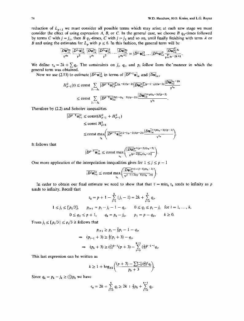
reduction of Lp+ 2 we must consider all possible terms which may arise; at each new stage we must consider the effect of using expression A, B, or C. In the general case, we choose B qo-times followed by terms C wi th j = J l , then B q~-times, C w i th j =J2 and so on, until finally finishing with term A or B and using the estimates for Lp with p < 6. In this fashion, the general term will be
IDul~ E~, IOul~v qo IOJ'ul2v 2 IOUt~v ql IOS2Ul~v 2 IOul~vq~+ ~ -IOS, ul 2 ... IOS~ul~ v2~,+2~+~"
We define Zk = 2k + ~q~. The constraints on j~, q~, and p~ follow from t h e ' m a n n e r in which the general term was obtained.
Now we use (2.13) to estimate IDJ, ui 2 in terms of IDp-IuI~o and IDul~o,
n2+l (t) <_ const E IDP-iul2EO~-~)lCp-2)l--ffffl 2E(p-~-j')ICp-2~ IDul~-2k J~ .--Jk V *k
_ _ I Dul l+p(~ k - 3)/(p-2) < c o n s t ~ IDP-lul m-t~-ai / t"-2)) ' ,~o
Ji .--Jk V~k
Therefore by (2.2) and Sobolev inequalities
ID~-Xul~ -< const(H2+l + Hfl-1)2
< const H2+l
. I Dul i +PO:k- 3 )/(p- 2 ) \ <cons t max iDP-lul 2tl-(~-a)I¢p-21) ~ - - I
zk \ V ~k ) "
It follows that "x
IDp-lul 2 < const max t ~ ] . ~k \ /
One more application of the interpolation inequalities gives for 1 < j < p - 1
~ [ u j + l + ( j - 1 ) t O; k - 3 ) x _< c o n s t m a x ;
In order to obtain our final estimate we need to show that that ~ = min k Zk tends to infinity as p tends to infinity. Recall that
k k
Zk= p + l -- ~, ( j i - - 1 ) = 2k + ~ qi, i=1 i = 0
1 < Ji < [Pi/3], Pi+l = Pi --Ji -- 1 -- qi, 0 <_ qi <- Pi --Ji for i = 1 . . . . . k,
0 <_ qo < P + 1, qk = Pk - - J k , Pl = P -- qo, k > O.
From Ji < [pl/3] < Pi/3 it follows that
Pi+l >-- Pi -- 2pi i 1 -- qi,
(P,+I + 3) _> {(Pi + 3) -- q,,
k - 1 (Pk + 3) >_ (2)k-~(p + 3) -- ~ (2)k- l - 'qv
i=o
This last expression can be written as
k > e + logal2(!p + 3 ) - ~'k-t°(~)iqi) - "
Since qk = Pk --Jk >- (~)Pk we have
k k - -1
"~k = 2k + ~ qi >- 2k + 2pk + ~ ql. i = 0 i = 0
On the Smallest Scale for the Incompressible Navier-Stokes Equations 75
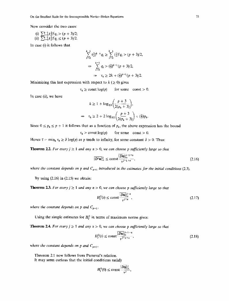
Now consider the two cases:
k-X 3)/2; (i) ~i=o (~)iql > (p + k - - i (ii) ~i=o (~)'q~ <- (P + 3)/2.
In case (i) it follows that
k - 1 k - 1
(~)k-Xqi >_ ~ (~)iqi > (p + 3)/2, i = 0 i = 0
k - 1
=> Z qi > (2)k-1 (p + 3)/2, i = 0
:~ ~k --> 2k + (2)k-l(p + 3)/2.
Minimizing this last expression with respect to k (> 0) gives
rk > const log(p) for some const > 0.
In case (ii), we have p + 3
k _> 1 + loga/z \2(pk + 3) ] '
( p + 3 ) Zk > 2 + 2 log3/2 \2(pk + 3)// + (2)pk"
Since 0 < Pk < P + 1 it follows that as a function of Pk, the above expression has the bound
Zk > const log(p) for some const > 0.
Hence g = min k Zk > 6 log(p) as p tends to infinity, for some constant 6 > 0. Thus:
Theorem 2.2. For every j >_ 1 and any ~ > O, we can choose p sufficiently large so that
,Du/+1+~ IDJu] 2 < const ~ , (2.16)
where the constant depends on p and Cp+ 1 introduced in the estimates for the initial conditions (2.3).
By using (2.16) in (2.15) we obtain:
Theorem 2.3. For every j >>_ 1 and any ~ > O, we can choose p sufficiently large so that
//jz(t) < const IDu[~+~ (2.17) - - V j + ~ '
where the constant depends on p and Cp+ 1.
Using the simple estimates for H f in terms of maximum norms gives:
Theorem 2.4. For every j >_ 1 and any o~ > O, we can choose p sufficiently large so that
,Du,J +1+~ H:(t) < const ~ , (2.18)
where the constant depends on p and Cv+ 1.
Theorem 2.1 now follows from Parseval 's relation. It may seem curious that the initial conditions satisfy
Hf(0) < const ID.u~l~ ,-- v "
76 W.D. Henshaw, H.O. Kreiss, and L.G. Reyna
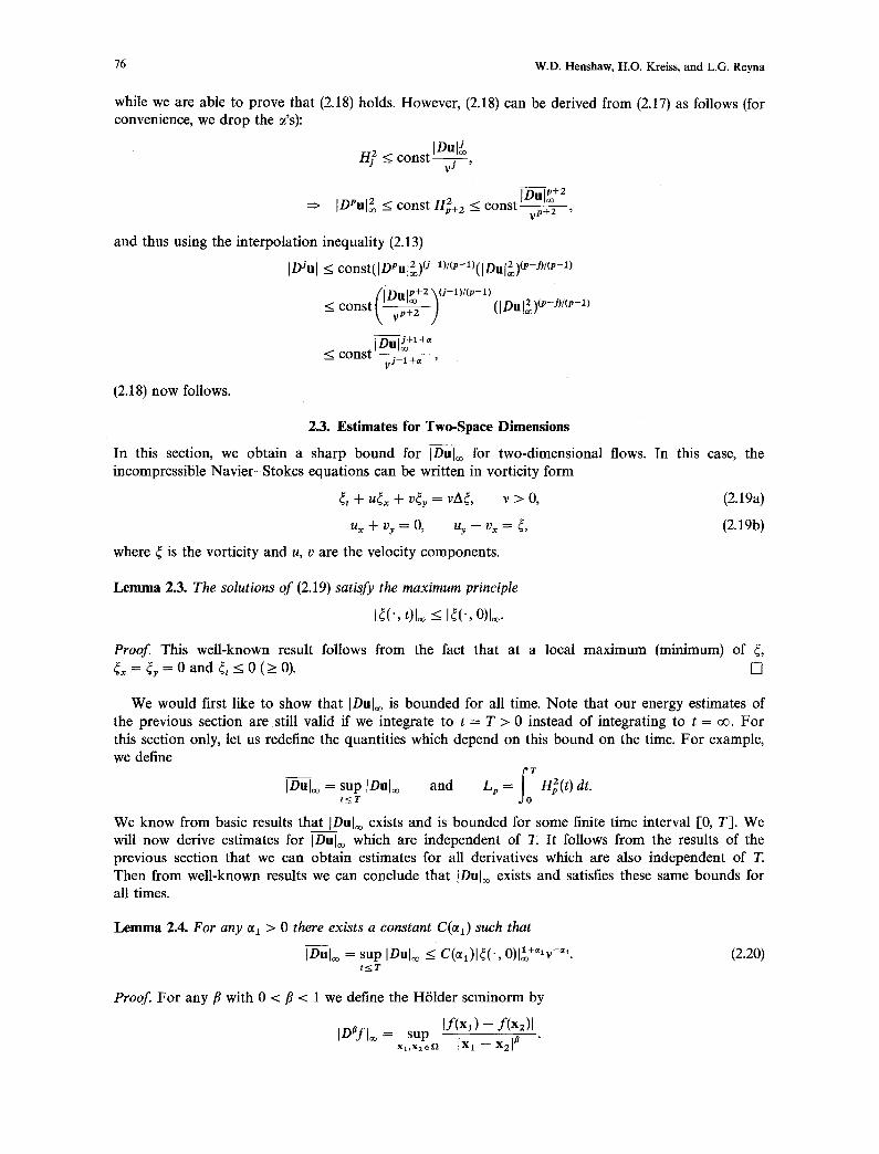
while we are able to prove that (2.18) holds. However, (2.18) can be derived from (2.17) as follows (for convenience, we drop the ~'s):
_ _ 1
/-//< const rD :, - - V j
IDul~ +z =~ IDPul~ < const H~+2 < const ~ ,
and thus using the interpolation inequality (2.13)
IDJul < const(IDPulZ)~J-'/(p-~)(tDul2)(p-J)/~p-~)
[[Dulp+ 2 "~ (j-1)/(p-1) < const~ v,+----T- ) (IDul2) "-j)/''-l)
IDu[~ +1+~ _< const ~ ,
(2.18) now follows.
2.3. Est imates for Two-Space Dimens ions
In this section, we obtain a sharp bound for IDul~ for two-dimensional flows. In this case, the incompressible Navier-Stokes equations can be written in vorticity form
~t + u4x + v4r = vA~, v > 0, (2.19a)
Ux + vy = 0, u r - v~ = 4, (2.19b)
where 4 is the vorticity and u, v are the velocity components.
L e m m a 2.3. The solutions of (2.19) satisfy the maximum principle
I~(', t)[~ < 14(', 0)l~o.
Proof. This well-known result follows from the fact that at a local maximum (minimum) of 4, ix = 4y = 0 and Ct -< 0 (> 0). []
We would first like to show that [Du[® is bounded for all time. Note that our energy estimates of the previous section are still valid if we integrate to t = T > 0 instead of integrating to t = ~ . For this section only, let us redefine the quantities which depend on this bound on the time. For example, we define
I Dulo~ = sup [Dul~o and Lp = 1 " H i(t) dt. t<T do
We know from basic results that IDuLo exists and is bounded for some finite time interval [0, T]. We will now derive estimates for [Du]oo which are independent of 7~ It follows from the results of the previous section that we can obtain estimates for all derivatives which are also independent of T. Then from well-known results we can conclude that [Du[~ exists and satisfies these same bounds for all times.
L e m m a 2.4. For any ~1 > 0 there exists a constant C(cq) such that
IDul~ = sup IDu[~ < C(~I)I~(', 0)l~+~lv -~1. t<.T
(2.20)
Proof. For any fl with 0 < fl < 1 we define the H61der seminorm by
[f(xl) -- f(x2) [ ]Daf].= sup
xl,x2~n Ix1 -- x2l p
On the Smallest Scale for the Incompressible Navier-Stokes Equations 77
Using the notation IDaul~ = max{lOaul~o, IDPvI~},
the usual H61der estimates for the solutions of Laplace's equation (see, for example, [10]), tell us that for any fl > 0 there is a constant ~(fl) such that
IDa-aul~ < C(//)l~[o~. (2.21)
Also, the convexity of H61der norms (see [13])
IOk+~fk o < constlOk,+=lfl~lDk2+=2fl~-' ,
k + ~ = t (kl + ~1) + (1 - t)(k 2 + ct2) >_ 1, 0 < t < 1, ~, cq, ~2 >- O,
and Young's inequality give us, for any e > O,
]Dulo~ < elD2uLo + const e-#lDl-aul~o.
Using the Sobolev inequality (2.12) for ID2uLo and (2.21) we obtain
IDuI~ 2 IDuloo --- const e v - ~ - + const e-alDl-aulo~
./' Iou12 2 )
Choosing - - V 7/2
gives _ _ / / _ _ V7/2 ~ - f l / ( l + f l )
IOulo~ < const e(/~)l~l® ~ c ( f l ) l ~ l ~ ) •
Thus IDu[~o < const(C(~)~loo)l/(1-sa/Z)v - Tt~/(z- sa)
and the lemma follows since I~l~o < I~(', 0)1o~. []
In two-space dimensions estimates on the vorticity appear more naturally. In [17] we proved the results of Theorem 2.1 in the two-dimensional case using the vorticity formulation of the equations. In that paper, the quantities
J:( t ) = c~'¢ 2 Op¢ 2 (2.22) ax p + ~yp
take the place of the H~. The estimate corresponding to (2.18) is
] ) n p + 2 + ~
J~(t) <_ const H~+x(t) <_ const --;[+~ . (2.23)
We refer to the Jp in the section on numerical results.
3. Numerical Results
We first describe the procedure we use to solve numerically the two-dimensional Navier-Stokes equations. In brief, we discretize in space using the Fourier (pseudospectral) method and solve in time using a fourth-order predictor-corrector method. The equations are solved in Fourier space and the diffusion term vAo) is treated in a fully implicit manner. We now proceed to present more details.
We solve the two-dimensional incompressible Navier-Stokes equations in the vorticity stream function formulation:
it + (u~)x + (v~), = vA~ + f, (3.1a)
AO = - 4 , (u,v) = (Or, -¢x)- (3.1b)
78 W.D. Henshaw, H.O. Kreiss, and L.G. Reyna
The computational domain is taken to be a 2n-periodic square. The solution is represented as a truncated Fourier series with co denoting the discrete approximation to ~ and 03 denoting the discrete Fourier transform of co:
(1/2)N1-1 (1/2)N2-1 co(x, y, t) = E Z 03(kl, k2, t) e'(*lx+k2r'"
-(I/2)NI +1 -(1/2)N2 +1
Similarly, the Fourier transform of ~b and f are denoted by ~ and 3~ respectively. The equation for the Fourier coefficient 03(kl, k2, t) is
03t + ikl(u'~) + ik2(v"~) = - v ( k ~ + k2)03 + f , (3.2a)
(k~ + k~)~ = 03. (3.2b)
The convolutions u~ and b~ (i.e., the Fourier transforms of the products uo and vco) and computed from, a, ~, and 03 by transforming to real space, forming the products and then transforming hack to Fourier space (pseudospectral method). It is not hard to see that the computation of 03t can be done with five two-dimensional fast Fourier transforms (FFTs). In fact, only four FFTs are needed since we can write (see [2])
~xco, - O, co~ = ( ( 0 ~ ) ~ - ( ~ , ) ~ ) ~ , - [ ( ~ O , ) x ~ - ( ~ 0 , ) , ] .
However, in the calculations presented here the less efficient method was used. Equations (3.2) can be written in the form of a large system of ordinary differential equations:
dy d t = F(y, t), (3.3)
where y is the vector with components 03(kl, k2). Time stepping is performed using a predictor-corrector applied directly to equation (3.3). Let y,
denote the approximation to y(nAt) and F, = F(y,, nat). We use the fourth-order Adams predictor- corrector scheme given by
yp = y, + ~ ( 2 3 F , - 16F,_~ + 5Fn_2) , (3.4a)
At 9F y,+~ = y, + ~ ( p + 19F, - 5F,-1 + F,-2). (3.4b)
Here yp is the result of the Adams-Bashforth predictor, Fp = F(yp, (n + 1)At) and y,+~ is the corrected value obtained from approximating the implicit Adams-Moulton scheme. A single time step thus requires two evaluations of the right-hand side F. The classical fourth-order Runge-Kut ta method is used to obtain starting values for (3.4). These are required initially and whenever the time step is changed.
For stability reasons, we may want to integrate the diffusion term, vAco, in an implicit manner. In the Fourier representation this term is very simple and thus can be easily treated in a fully implicit and accurate manner. We write equations (3.3) in the following way:
dy d t = G(y, t) - Ay, A = diag( . . . . v(k 2 + k 2) . . . . ),
where the right-hand side F has been split with A the diagonal matrix corresponding to the diffusion term. This last equation can be written in the form
d At ~ ( e y) = eAtG.
Now apply the time-stepping procedure (3.4) to this equation viewed in terms of the new dependent variable enty. After division by e At the predictor-corrector scheme which results is
yp = e-AZty, + A~t(23e-AZ~G~ - 16e-2AatG~_ 1 + 5e-3AatG,_2), (3.5a) Z l
At Y n + l = e-Aatyn + ~ ( 9 G p + 19e-AatGn -- 5e-2AatGn_t + e-3AAtGn_2). (3.5b)
On the Smallest Scale for the Incompressible Navier-Stokes Equations 79
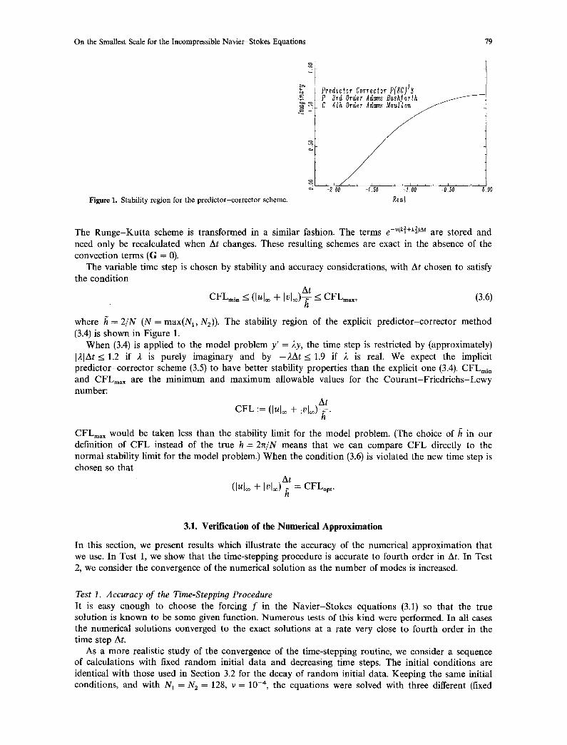
Figure 1. Stability region for the predictor-corrector scheme.
Predictor Corrector P(gC)t~ ~ ] P 3rd Order Ad~ns Bashf0rth ~ - _ C 4 t h
-2.00 -1.50 -l.O0 -0,50 0.00
Re~l
The Runge-Kut ta scheme is transformed in a similar fashion. The terms e -v(kE+k~)At a r e stored and need only be recalculated when At changes. These resulting schemes are exact in the absence of the convection terms (G = 0).
The variable time step is chosen by stability and accuracy considerations, with At chosen to satisfy the condition
CFLmi~ ~ (lul~ + IvL) h < CFLmax, (3.6)
where h = 2/N (N = max(N1, N2)). The stability region of the explicit predictor-corrector method (3.4) is shown in Figure 1.
When (3.4) is applied to the model problem y' = 2y, the time step is restricted by (approximately) I AJAt_< 1.2 if 2 is purely imaginary and by -2At_< 1.9 if 2 is real. We expect the implicit predictor-corrector scheme (3.5) to have better stability properties than the explicit one (3.4). CFLmi n and CFLma x are the minimum and maximum allowable values for the Courant-Fr iedr ichs-Lewy number:
:= (lul~ + [vL) h . CFL
CFLma x would be taken less than the stability limit for the model problem. (The choice of h in our definition of CFL instead of the true h = 2n/N means that we can compare CFL directly to the normal stability limit for the model problem.) When the condition (3.6) is violated the new time step is chosen so that
At (lul~o + IvL)~- = CFLopt.
3.1. Verification of the Numerical Approximation
In this section, we present results which illustrate the accuracy of the numerical approximation that we use. In Test 1, we show that the time-stepping procedure is accurate to fourth order in At. In Test 2, we consider the convergence of the numerical solution as the number of modes is increased.
Test 1. Accuracy of the Time-Stepping Procedure It is easy enough to choose the forcing f in the Navier-Stokes equations (3.1) so that the true solution is known to be some given function. Numerous tests of this kind were performed. In all cases the numerical solutions converged to the exact solutions at a rate very close to fourth order in the time step At.
As a more realistic study of the convergence of the time-stepping routine, we consider a sequence of calculations with fixed random initial data and decreasing time steps. The initial conditions are identical with those used in Section 3.2 for the decay of random initial data. Keeping the same initial conditions, and with N1 = Nz = 128, v = 10 -4, the equations were solved with three different (fixed
80 W . D . H e n s h a w , H .O. Kreiss , a n d L.G. R e y n a
time steps: At = 0.05, At = 0.025, and At = 0.0125. The computed maximum value for the C F L number in each run was 1.2, 0.6, and 0.3, respectively. (Recall that the stability limit for the explicit version of the predictor-corrector scheme is about 1.2 on the imaginary axis. We were able to obtain good results for values of the C F L number as large as 1.5, which substantiates the belief that the implicit predictor-corrector scheme has better stability properties.) We use the results from the three runs to estimate the rate of convergence as a function of At as well as to estimate the actual error. We measure both the discrete maximum error and the/2-error defined by
1 = [a~(xi, yj)[2. I~o1~ tx,,yj)max [co(xi, Yj)I and I~o1~ : - N1N2 (x,,~j)r
By assuming that the computed solution is converging to the true solution as O(At p) we can determine approximate values for p and the errors
Eoo(t, At) : = [(.Oeomputed(" , t ; At) - mtrue(" , t; At)[oo = O(AtP),
E2(t, At) := ]Ogco~puted(', t; At) -- e;tru~(', t; At)[ 2 = O(AtV).
These values are given in Table 1 for the maximum norm errors and in Table 2 for the/2-errors.
Test 2. Convergence for Random Initial Data. We consider the computat ion which is described in Section 3.2 under the heading of Run 1: Decay of Random Initial Data. This computat ion was run with N = N1 = N2 = 128(o9128) and also with
Table 1. Es t ima ted m a x i m u m er rors and convergence rate: O(AtP).
t E~o(At = 0.05) E~(At = 0.025) E~(At = 0.0125) p
10 0.68 x 10 -2 0.47 × 10 -3 0.32 × 10 -4 3.9
20 0.27 x 10 -2 0.18 x 10 -3 0.13 x 10 -4 3.9
30 0.97 x 10 -3 0.69 x 10 -4 0.49 x 10 -5 3.8
40 0.69 x 10 -3 0.47 x 10 -4 0.32 x 10 -5 3.9
50 0.48 x 10 -3 0.31 x 10 -4 0.20 x 10 -5 4.0
Table 2. E s t i m a t e d 12-errors a n d conve rgence rate: O(AtP).
t E2(At = 0.05) E2(At = 0.025) E2(At = 0.0125) p
10 0.40 x 10 -3 0,29 x 10 -4 0.21 × 10 -5 3.8
20 0.17 x 10 -3 0.12 x 10 -4 0.86 × 10 -6 3.8
30 0.73 x 10 -4 0.50 x 10 -5 0.34 × 10 -6 3.9
40 0.56 x 10 -4 0.37 x 10 -5 0.24 x 10 -6 3.9
50 0.48 x 10 -4 0.31 x 10 -5 0.20 x 10 -6 4.0
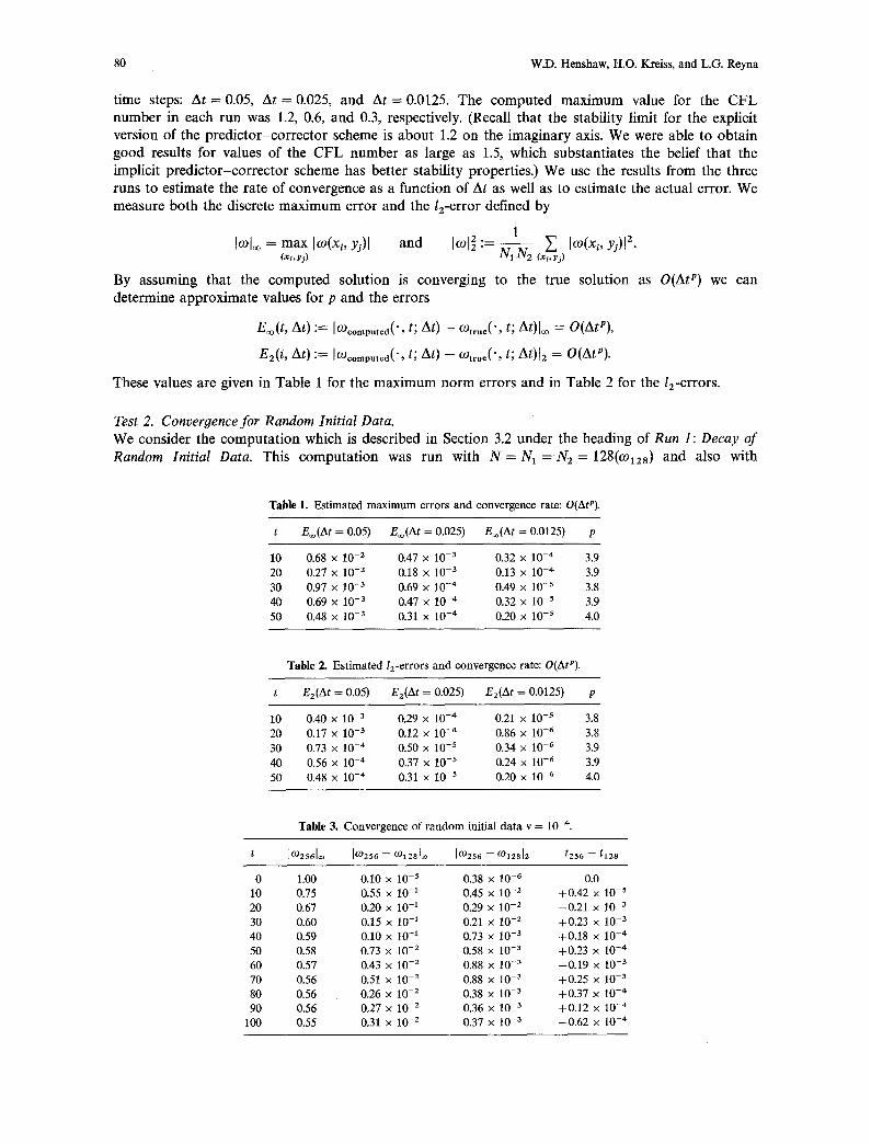
Table 3. C o n v e r g e n c e of r a n d o m init ial d a t a v = 10 -4.
t ]~2561~ 10)256 - - 0)1281QO [C0256 -- 0912812 t256 -- t12a
0 1.00 0.10 x 10 - s 0.38 × 10 -6 0.0
10 0.75 0.55 x 10 -1 0.45 x 10 -2 + 0 . 4 2 x 10 - s
20 0.67 0.20 × 10 -1 0.29 x 10 - z --0.21 × 10 -3
30 0.60 0.15 x 10 -1 0.21 x 10 -2 +0 .23 x 10 -3
40 0.59 0.10 x 10 -1 0.73 x 10 -3 + 0 . 1 8 x 10 -4
50 0.58 0.73 x 10 -z 0.58 x 10 -3 +0 .23 × 10 -4
60 0.57 0.43 x 10 -2 0.88 x 10 -a --0.19 x 10 -3
70 0.56 0.51 x 10 -2 0.88 x 10 - s + 0 . 2 5 x 10 -3
80 0.56 0.26 x 10 -2 0.38 × 10 -3 + 0 . 3 7 × 10 -4
90 0.56 0.27 x 10 -2 0.36 x 10 -3 + 0 . 1 2 x 10 -4
100 0.55 0.31 x 10 -2 0.37 x 10 -3 - -0 .62 × 10 -4
On the Smallest Scale for the Incompressible Navier-Stokes Equations 81
N = 256(09256). The initial conditions for the two runs were the same to single precision (about 6 -7 decimal digits), although the actual computations were done in double precision. The variable time step was determined by the parameters (CFLml n, CFLop t, CFLmax) = (0.8, 1, 1.2). In Table 3 we indicate the maximum difference and the /2-difference between the two runs at various times. Due to the variable time step the solutions were not compared at exactly the same times. The difference between the times is given in the table as tz56-t128. Note that the maximum difference between the two solutions occurs at smaller times. Later, when the solution becomes smoother, the errors are smaller. Further details of this run can be found in the next section.
3.2. C o m p u t a t i o n a l Resul ts
In this section we present the results of four different runs:
(1) Run I: Decay of random initial data, v = 10 -4, N = 256, and N = 128. (2) Run II: Decay of random initial data, v = 10 -5, N = 512. (3) Run III: Decay of smooth random initial data, v = 2 x 10 -s, N = 256. (4) Run IV: Random forcing, v = 0.5 x 10 -3, v = 0.5 x 10 -4.
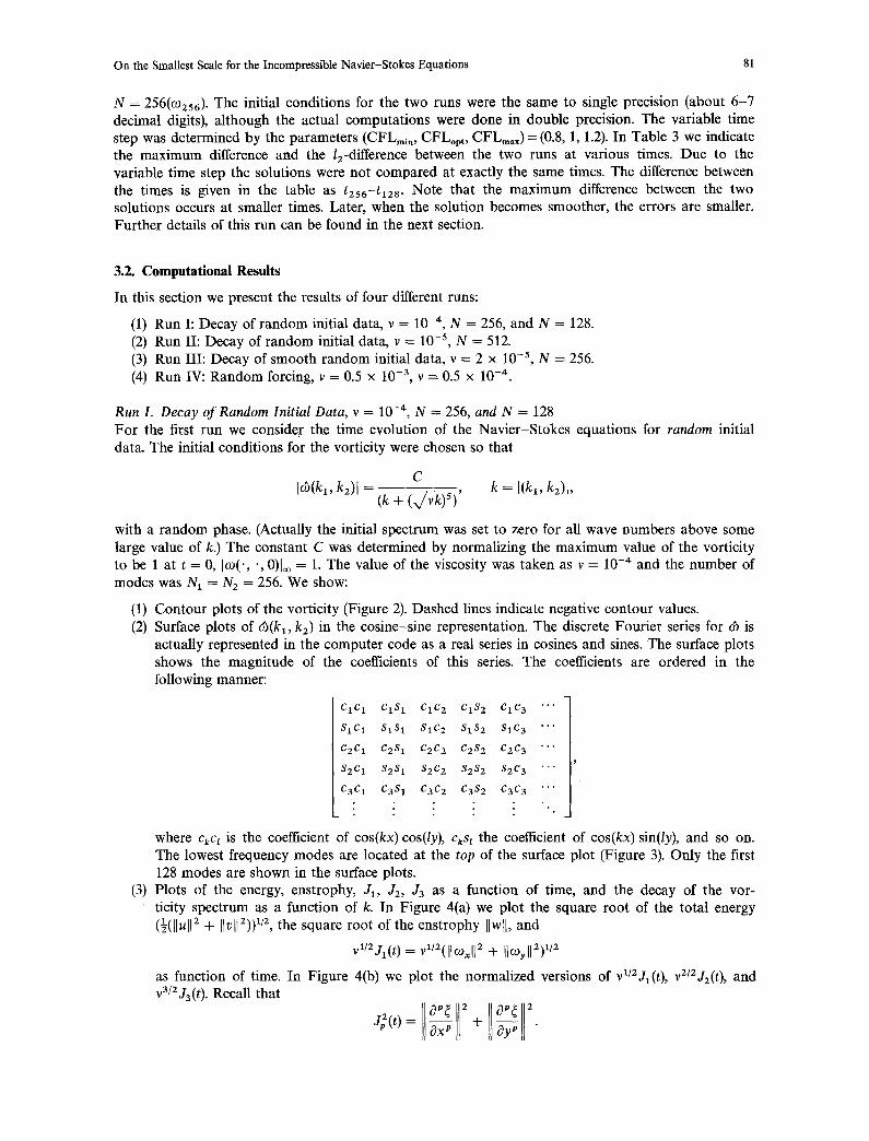
Run I. Decay of Random Initial Data, v = 10 -4, N = 256, and N = 128 For the first run we consider the time evolution of the Navier-Stokes equations for random initial data. The initial conditions for the vorticity were chosen so that
C Icb(k~, k2)l (k + (v~k)5) ' k = I(ka, kz)l,
with a random phase. (Actually the initial spectrum was set to zero for all wave numbers above some large value of k.) The constant C was determined by normalizing the maximum value of the vorticity to be 1 at t = 0, Ico(-, ", 0)[~ = 1. The value of the viscosity was taken as v = 10 -4 and the number of modes was N 1 = N 2 = 256. We show:
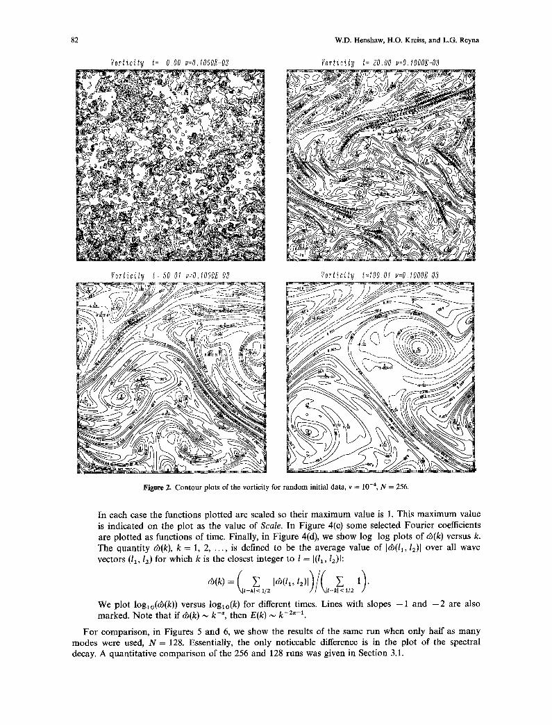
(1) Contour plots of the vorticity (Figure 2). Dashed lines indicate negative contour values. (2) Surface plots of cb(k~, k2) in the cosine-sine representation• The discrete Fourier series for (b is
actually represented in the computer code as a real series in cosines and sines. The surface plots shows the magnitude of the coefficients of this series. The coefficients are ordered in the following manner:
ClCl ClS 1 ClC 2 ClS 2 ClC 3
S l C 1 S1S 1 SlC 2 $1S2 SlC3
C2Cl C2S 1 C2C2 C2S2 C2C 3
$2C 1 S2S 1 $2C 2 $2S2 $2C3
C3C 1 C3S 1 C3C2 C 3 8 2 C3C 3
. . .
• . .
where CkC l is the coefficient of cos(kx) cos(/y), CkS, the coefficient of cos(kx) sin(/y), and so on. The lowest frequency modes are located at the top of the surface plot (Figure 3). Only the first 128 modes are shown in the surface plots•
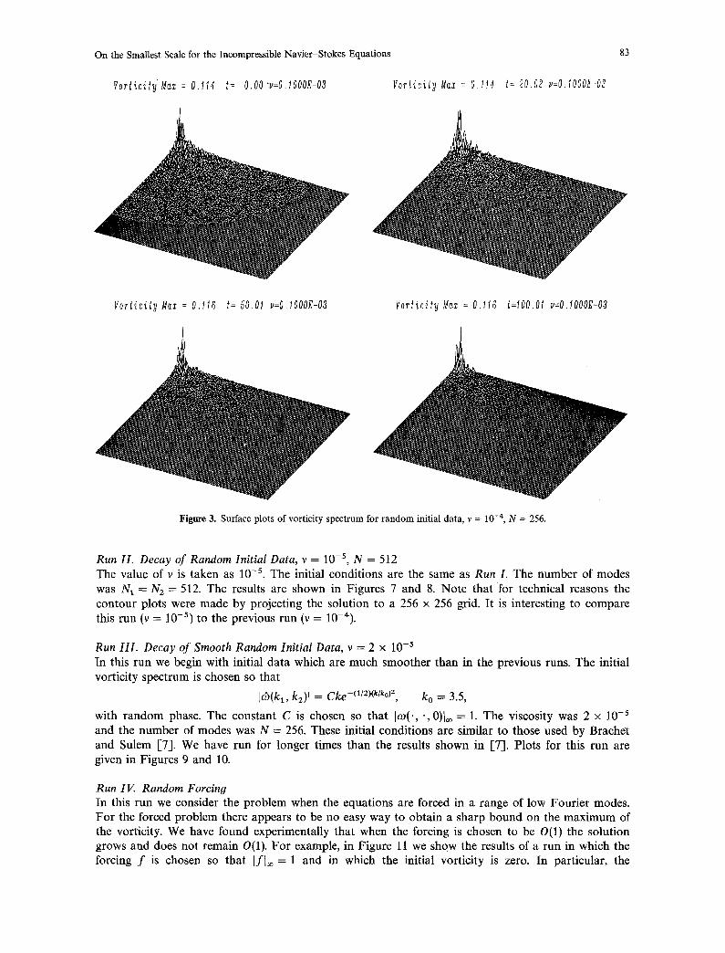
(3) Plots of the energy, enstrophy, J1, J2, Ja as a function of time, and the decay of the vor- ticity spectrum as a function of k. In Figure 4(a) we plot the square root of the total energy (l([lU[12 -t- 1t/)[12)) 112, the square root of the enstrophy Ilwl[, and
vl/zj l( t ) _ - vV~(ll~II ~ + II%11~) I/~
as function of time• In Figure 4(b) we plot the normalized versions of vt/2Jl(t), v2/2J2(t), and •3/2 J3(t ). Recall that
ax p +
82 W.D. Henshaw, H.O. Kreiss, and L.G. Reyna
Vorticity t= 0.00 i,=O.lO00E-03 i . i i " "1,1 i i i " ~ i aiill~ll7 ' - ~111111 [,i . . . . . i~ll " ii . . . . i,
-~ - ~ " ' " t , . ) 3 v C~'Kc
, ~ , ~ ~,~ ; 2 . , 4 -~ , ,~e-'- ~
Porticity t=20.00 u=O.lOOOg-03
,-.~, .e.,,,,,' &'%.'.. ,', ; , i v" '~,j~./]"~'.~.
t Y I j ' t
Vorticity t= 50.01 v=O.lO00£ 03
~ . " f,~;~,',,~ / Y J / ~;. . . . . . . . ._
ro r t i c i t y t:lO0.Ol IJ:O.lOOOE-03
~ 5 ~ ," ..y ;q'" /.-->~ .-~ ..... °s ° ~ - - ~ _
~ / . ~ . "...U;~~.j." . / . . - - ~ - - ~ ~ ~- / ~ f
~3~. ~ ....;.~~ ._-_7~..j ' ( ,
, ~ " / I c s ' , t I , , ~ J /
~/.9" I.~~_L"' u " - ~ ~ . J 1,? 7; I ,' ) ."
~ - ~ " ~ 4 " ~ " \'t, r //;" '~--~-~d- .,,
,,T,~ .................. ,~,~,i, ,,,,,~ ..........
Figure 2. Contour plots of the vorticity for random initial data, v = 10 -4, N = 256.
In each case the functions plotted are scaled so their maximum value is 1. This maximum value is indicated on the plot as the value of Scale. In Figure 4(c) some selected Fourier coefficients are plotted as functions of time. Finally, in Figure 4(d), we show log- log plots of ~b(k) versus k. The quantity &(k), k = 1, 2 . . . . . is defined to be the average value of kb(ll, 12)1 over all wave vectors (11, 12) for which k is the closest integer to l = I(1~, 12)1:
We plot log~o(~b(k) ) versus loglo(k) for different times. Lines with slopes - 1 and - 2 are also marked. Note that if o3(k) ,~ k - ' , then E(k) ,,, k -2~'-~.
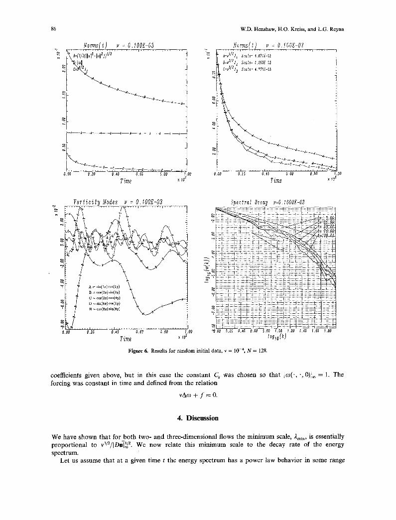
For comparison, in Figures 5 and 6, we show the results of the same run when only half as many modes were used, N = 128. Essentially, the only noticeable difference is in the plot of the spectral decay. A quantitative comparison of the 256 and 128 runs was given in Section 3.1.
On the Smartest Se~eforthe Incompressible Navier-Stokes Equations 83
VorticityMaz : 0.114 t : O.O0"v:O.IOOOE-03 VorticityMax = 0.114 t : 20.02 v:0,I000£-03
VorlicityMax = 0.11G t= 50.01 v=O,lOOOg-03 VorticityMaz = 0.116 t=100.01 v=O.lOOOE-03
Figure 3. Surface plots of vorticity spectrum for random initial data, v = 10 -4, N = 256.
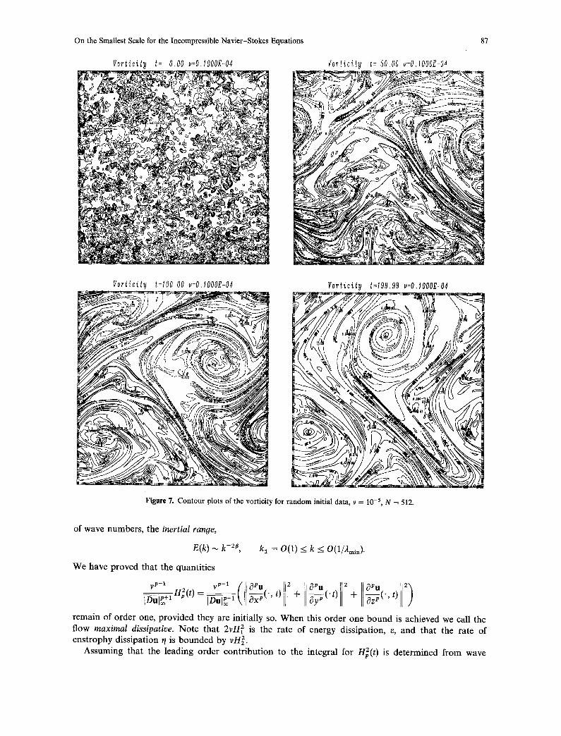
Run II. Decay of Random Initial Data, v = 10 -5, N = 512 The value of v is taken as 10 -5. The initial conditions are the same as Run I. The number of modes was N1 = N2 = 512. The results are shown in Figures 7 and 8. No te that for technical reasons the contour plots were made by projecting the solution to a 256 x 256 grid. It is interesting to compare this run (v = 10 -5) to the previous run (v = 10-4).
Run III. Decay of Smooth Random Initial Data, v = 2 x 10 -5 In this run we begin with initial da ta which are much smoother than in the previous runs. The initial vorticity spectrum is chosen so that
[a~(kl, k2) I --- Cke -(1~2)(k/k°}2, k o = 3.5,
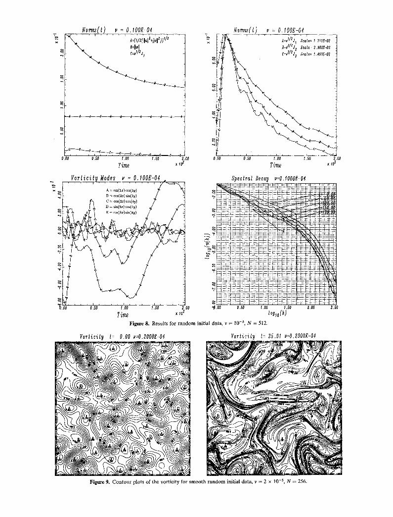
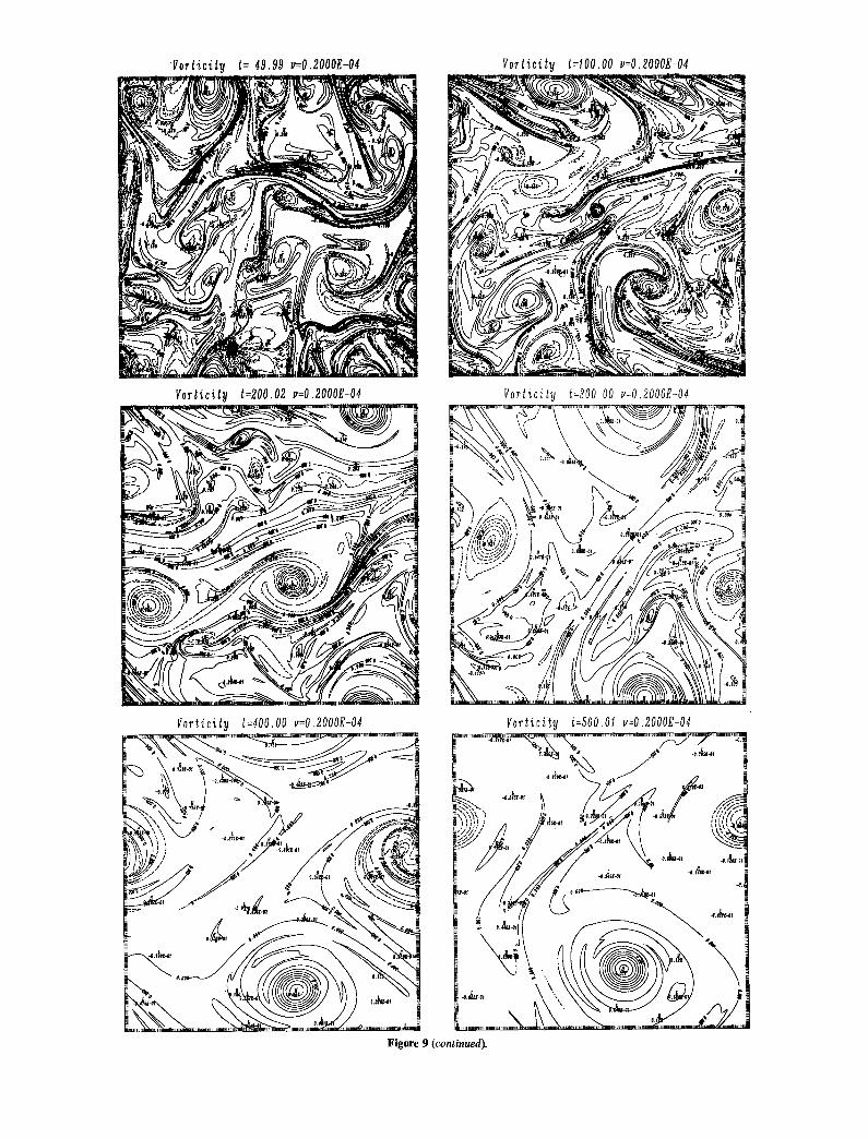
with r andom phase. The constant C is chosen so that leo(.,-, 0)1~o = 1. The viscosity was 2 x 10 -s and the number of modes was N = 256. These initial condit ions are similar to those used by Brachet and Sulem [-7]. We have run for longer times than the results shown in [7]. Plots for this run are given in Figures 9 and 10.
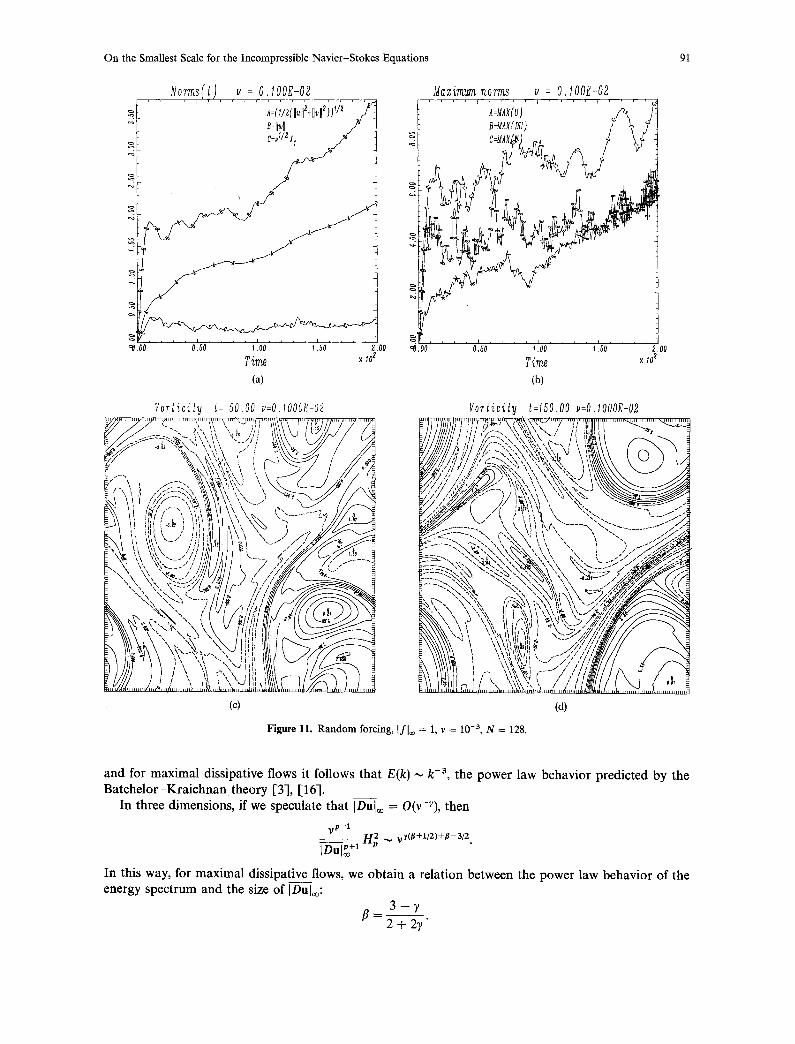
Run IV. Random Forcing In this run we consider the problem when the equations are forced in a range of low Fourier modes. For the forced problem there appears to be no easy way to obtain a sharp bound on the max imum of the vorticity. We have found experimentally that when the forcing is chosen to be O(1) the solution grows and does not remain O(1). For example, in Figure 11 we show the results of a run in which the forcing f is chosen so that Ifl~o = 1 and in which the initial vorticity is zero. In particular, the
84 W.D. Henshaw, H.O. Kreiss, and L.G. Reyna
T e~
x
...2
. . . . . . . . . . : , q . , l , ! O E 2 , 3 . . . . . . . . . . . . .
, , , . . . . . . . ~ . . . . . . . 0.00 0.20 0.40 0.60 0.00 1.00
Time x ~o ~
(c)
=:=
(a)
0.00
NoTrrts(t) v : O . I O O E - 0 3
A=v l/2 J Scale= 4,071E-02 B=u2/2j~ Scale= 1,263E-02 C=t.,a/2J3 Scr~.le= 4,778E-03
0.20 0.40 0.60 0.80 1.00
Time x to 2
(b)
.,. O. I00E-03 V o r t i c i t y Modes v = _ _
\ , _ _ , / ,
r m,,o \ ,~L~" 7 = "( )c s(ly) \
,I~ .................................... -, ......... 0.00 o.20 0.40 0.00 o.ao 1.00
Time x lo z
(d)
S p e c t r a l Beeay u=O.lOOOE-03
~,00 0,50 I ,OU I .~0
zOglo(~) £,PU
Figure 4. Results for random initial data, v = 10 -4 , N = 256 .
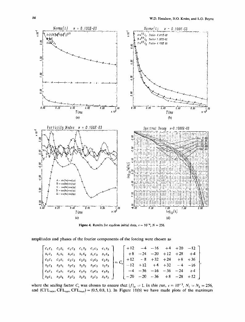
amplitudes and phases of the fourier components of the forcing were chosen as
C1C 1 C I S 1 CIC2 ClS2 C I C 3 C 1 S 3
S1C 1 S1S1 $1C2 S1S2 $1C3 SIS 3
C 2 C 1 C2S1 C2C 2 C2S2 C2C3 C2S3
$2C 1 S 2 S 1 S2C2 $2S2 $2C3 $2S 3
C3C 1 C 3 S 1 C 3 C 2 C3S3 C3C3 C3S3
$3C 1 $3S1 $3C2 $3S2 $3C3 $3S 3
=c~
+ 1 2 - -4 --16 + 4 + 2 0 --12
+ 8 --24 - -20 + 1 2 + 2 8 + 4
+ 1 2 - -8 + 3 2 + 2 4 + 8 + 3 6
- -12 + 1 2 + 4 + 3 2 - -4 --16
- -4 --36 --16 - -36 - -24 + 4
- -20 - -20 --36 + 8 --28 + 1 2
where the scaling factor C a was chosen to ensure that [f[o~ = 1. In this run, v = 10 -a, N1 = N2 = 256, and (CFLmI,, CFLopt, CFLma~)= (0.5, 0.8, 1.). In Figure l l(b) we have made plots of the maximum
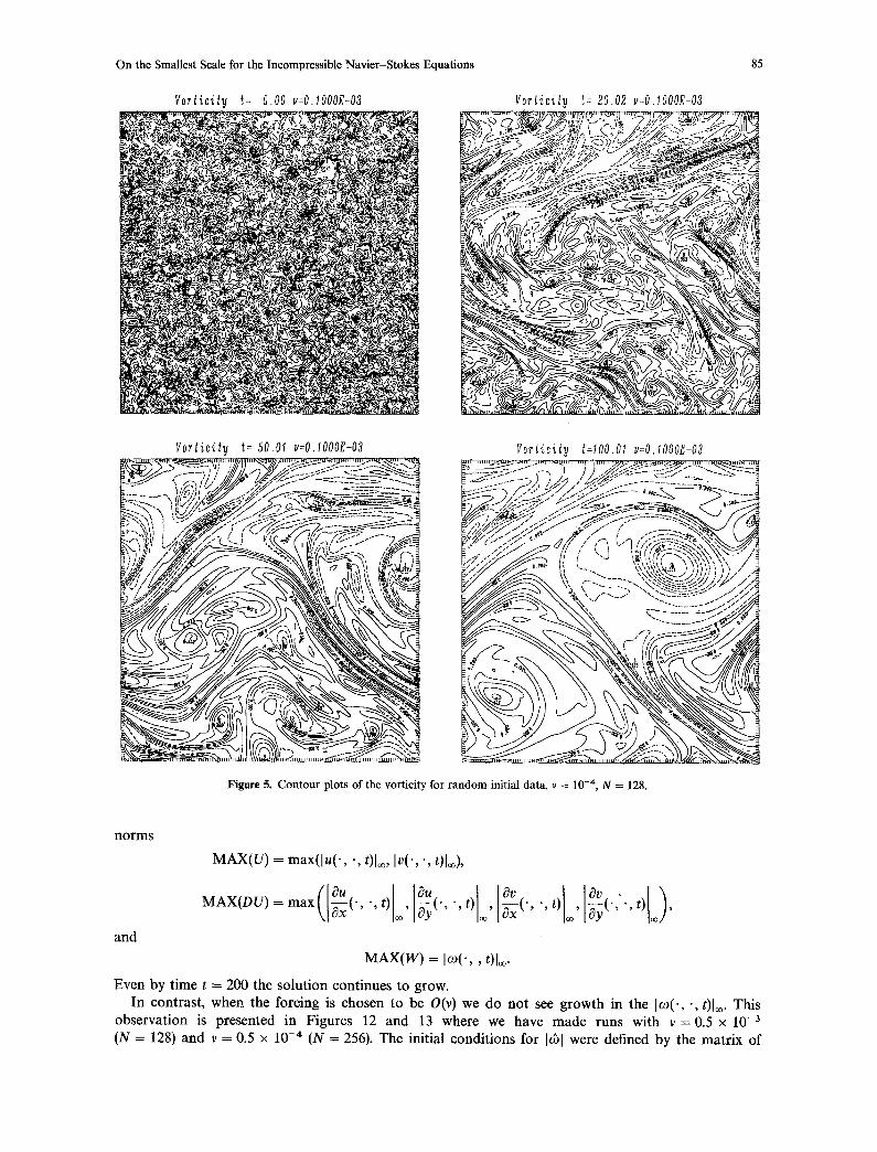
On the Smallest Scale for the Incompressible Navier-Stokes Equations 85
I
Vorlicity t= 0.00 u=O.lOOOE-03
, " . ez.
(" . . ? ) ~
?,2
Vortieity (= 20.02 v=O.lOOOE-03
~Z-C'.~C/~4 -~gL.;, . 4C, i :v.,,,,.~ ~ > ~ - _Z.C?N! e,,','~
B,o Vorticity t= 50.01 v=O.lOOOE-03
, ',z4/.~'~.23- i,'_ . . . . _-_-=-=_-- . . . . =__- . . . . , ~ / ~ ~ / ~ i " n ~ . . . ~ n, . : H - ~ ' - ~ . . . . . . . . ----_~_--S--~=--!
.... d(Wrfl.,L&., .... , ~ . ~ , , : ' - ~ - - " : ~ ' , ' I ra ' , ---- ,~>--~
. , ' , , , , , o - -
. 'Ji
Vorticity t:lO0 O1 v=O.1OOOE-03 ~ , t ; ~ , ~ , ~ a , , , ,~, ,,~ ,, ~, , , , , ,, ~ , ; ~ > ~ ,~ ~ ~ , : , ~ k 3 . > . ~ " . . . . . . . . . . . ~ . . . . . .
.4- ' -. ' ~ ~;TT- -.%S,\'. "X'-_." "
////~o \\ $.~ ,, f-.. . "\'~2-2~-=~2-x" /.//.
" \\ " ':,, k:,
Figure 5. Contour plots of the vorticity for random initial data, v = 10 -4, N = 128.
n o r m s
a n d
M A X ( U ) = m a x ( l u ( . , . , t)l~, Iv( ' , ", t)l~),
' "' ' ~ y "' ' 8 x ~o' oo M A X ( D U ) = m a x fiX-X(- d u o , ( - , . , ,
M A X ( W ) = Io9(-, , t)l~o.
E v e n by t i m e t --- 200 the s o l u t i o n c o n t i n u e s to grow.
In con t r a s t , w h e n the fo rc ing is c h o s e n to be O(v) we d o n o t see g r o w t h in the le~(', ", t)[oo. Th is
o b s e r v a t i o n is p r e s e n t e d in F i g u r e s 12 a n d 13 whe re we h a v e m a d e runs wi th v = 0.5 x 1 0 - 3
(N = 128) a n d v = 0.5 x 10 -4 (N = 256). T h e ini t ia l c o n d i t i o n s for I~1 were def ined by the m a t r i x o f
86
x
~2
N o r m s ( t ) v = O . I O O E - 0 3
1 ~ =(*/e(ll=[Iz+ll~llz))~/e
2 !
"~"~....~....~._.
--A---A--A--A--A~--A--.4--A----~--A--d--
c - - - - - c
0 , 0 0 0 . 2 0 0 . 4 0 0 . 0 0 0 . 0 0 1 . 0 0
Time × ~°2
"7-
x
W.D. Henshaw, H.O. Kreiss, and L.G. Reyna
N o ~ ( t ) v : 0 .100E-03
A=ul/gJ, Scale= 4,071E-02 B:v2/2j I Scale= 1.263E-02
C = v 3 / 2 j 3 S c a l e = 4 . 7 7 8 [ - 0 3
o.oo o,2o 0.40 0.00 0.00 1,oo Time x ~o 2
V o r t i e i t y M o d e s v = O.lOOE-03
.
0.00 0.20 0.40 0.60 0,80 1.00
Time x ,:
Spec tra l Decay v=O.IOOOE-03
. . . . . . . . . . . :
:[iiii?iii:iiiiiiiiii:i;ilili!i:ii T T T r 1 ~ ~ T i:::=i:=:::,::: " - i ..................... , ..................... "~ ..................... i - ? ' - , -"- ' """[ ........................ i ...................
~.00 0.20 0.40 0.60 0.80 1.00 1.20 1.40 1.60 1.80
ZOglo(k)
Figure 6. Results for random initial data, v = 10 -4, N = 128.
coefficients given above, but in this case the constant Cs was chosen so that ]co(., . , 0)1oo forcing was constant in time and defined from the relation
vAco + f = 0.
= 1. The
4. Discuss ion
We have shown that for both two- and three-dimensional flows the minimum scale, )~min, is essentially proportional to vl/2/IDul~2. We now relate this minimum scale to the decay rate of the energy spectrum.
Let us assume that at a given time t the energy spectrum has a power law behavior in some range
On the Smallest Scale for the Incompressible Navier-Stokes Equations
V o r t i c i t y l= 0.00 v=O.IOOOE-04
r o r [ i c i l y ~: I00.00 v:O.lO00~-04
87
Vo~[~c~ty t= 50.00 v:O.lOOOE-04
V o r f i c i l y t=199.99 v=O.lOOOE-04
~ i t ~ .4',:,'%
~; - ~ ,',',';' I ,' iU.///~f~--~'~ 'It * l,' l l ;; ' ' 'd .++, ++,
' " $
~ ~ 1 1 1 11l]lll411111ll I I', I fill, I ~ / / / l l l l H ~ m him ]m+,)ltAWm,,m m,,m .m,,m,m,m, ~ x ~ . m A~l~,m me,,,,m,m~d~,,,~,m.;lljal+
l ~ ]~A,.'; / f C r Z ; ' ~ 7 . ' , h ~ \ il#' ~Ja V / / ~ ~ I # ' ~ ~ .]!//~£'i~i-l~,) ", lily ,,¢- V B ~ A / ? ' * f 'EXll I I ~9, ,;,',i~ II+Vf..4/ ! i,.!I//i m ~ J - ' , ' ] l ; l ~'1/ ,~ V, T P / / , V t I . " a//lJt ,: ~,,,.,, \/..o// ,,/,J v,~f MJ~,"°.~_, FI ~.. "q~", / 7.* ~in~\ k¢_ . . . . ~#5 ' /~ ' dZ/X.# .~' /
k--..----~.~N .x,~-~ . . . ( ( { ~ ~,//(j
"% , ~ :,i~
Figure 7. Contour plots of the vorticity for random initial data, v = 10 -s, N = 512.
I of wave numbers , the inertial range,
E(k) ,,, k -2~, k 1 = 0(1) _< k _< O(1/~.min).
W e have p roved tha t the quant i t ies
llP--I~(t'-- ~P--I ( OPu t' 2 opu 2 2) louiS+ 1 iOnia+ x ~-;x,(', ~-7('t) + ~ ( . , t)
remain of o rder one, p rov ided they are ini t ial ly so. W h e n this o rder one b o u n d is achieved we call the flow maximal dissipative. N o t e tha t 2vH~ is the rate of energy diss ipat ion, ~, and tha t the ra te of ens t rophy d iss ipa t ion ~ is b o u n d e d by vH22.
Assuming tha t the leading o rde r con t r ibu t ion to the in tegral for H2,(t) is de te rmined f rom wave
~'~ . . . . . . ;:(,/,(ll,dT+ii,ii 'j)','
~f -~""~'"-'~,_._~___,~ -4 ,~ J J J , I - - - - ~ - - - - 4 J . . - ~ J . . J
"<--7<,'~,~,--~,-__~,___r__~,__.~ 0.00 0.50 l.O0 f.50 'c2
Time x ~0 z
Norms(t) v = O. IOOE-04
A:vt/2J Scale= 1.711~-02 B=u~'/2,/. 5'c~Je= 3.002~-03 C=v3/2 j~ Scale= 1.453F,-03
. . . . . . . . . , ' 7 ~ . C 0.00 0.50 t.O0 1.50 2.00
Time x ~o ~
V o r t i c i ! y M o d e s u = 0.100E-04 ,
~'~-- ~ . . . . . . A' sJn(i~;)co's(ly')'' / ~ % i ~'I B ~ cos(2~:)sin(ly)Z '" f'~ C . . . . (2x) cOS(4y) / "
~ ' f ~ A ~ " (8x)sin(8y) . . . . 7 / '
j T ~ ' " %_? /
~.oo o.5o ~.oo s.~o ~.oo Time x ~o z
Spectral Decay v=0.1000~-04
"~.00 0.50 1.00 1.50 2,00 2.50
F i g u r e 8. Resu l t s fo r r a n d o m ini t ia l d a t a , v = 10 -~, N = 512.
7ort ici ty t= 0.00 v=0.2000~-04
,,. ~.,)'i ~
• o . . . .
~ ~ " , 2 ) . . 5 v , 7 : ~ ]
~ ,7~..';~ "--~ ~ ; ' ~ L'--"_ f F(r'fx'D).l
Vorticity t=25.01 u=O.2000E-04 ~ , . , . . . . . . . . . . . ,, ,.~.,,,,;., ~$, . . . . . . . . . . . . . . . . . . . . ....................
,~,~,~-~:~ zL V,, ,~ ~ zt;4 , j " l,
F i g u r e 9. C o n t o u r p lo t s o f t he v o r t i c i t y fo r s m o o t h r a n d o m ini t ia l d a t a , v = 2 x 10 -5, N = 256.
7orticit~ t: 49.91 u=O.2000g-04 ..... ~97 . . . . r;~ 7 - I ..... , ~ , .
i! i, ~ ,~.7 --
¢ ,"~- 7 ,~
7odicity t=200.02 v=O.2OOOg-04
7orticity t : lO0.O0 ~=0.2000E-04
----_-~--Z: - i d ~ : 7 - " ~
Vorticity h300.O0 u=O.2000E-04
- - = 7 , . , . - i - _ ~ i l
- - ~ ( ~ ) . i ~.,,. 7 / ~ , ,, .
m _,., ,,;,( t ' : / (e ~ ............... .:.;.-k.,../..L_.L\,,,_.I_.L21U~}~.~..k~LLU..L ..........
Voriicily l:400.00 v=O.2000E-04
~"-~ ,k""" '~ .,~.G:'~ - ' - , "~,.~K-"
K~. , , ' ~ " , ~A .x , , , ~
l !'i~l~,', ~ , ' V ....... / ," !i , ' ~ ' - " "ft ~,-~""~", ~ - ,(, ..... r ,~..r,,. ,,,~,<.~-,,.~
-,,,~ ¢.( ~:'~\~ ,.,.~
Vodicily h500.Ol v=O.2000E-04 ......................... ~,,?,I,~F=,,,~. ~ . ~" ~ " ...................................................................... ~ ........................................................... ~ ~'.
-~.,,.-. ~ / ( . - / 2 " . 4 / / 2 " . . ~
-Y..?;,.' / / // ~d-X t l \~'~_~
.... / I , / / i f ( , . , o ~ - ~ . 4.,
............................... ~ .... i. - . , " .
Figure 9 (continued).
90 W.D. Henshaw, H.O. Kreiss, and L.G. Reyna
"7 ~<
8.00
Norms(t) v = 0.200E-04
~ C=v3/2,I3 Scale= 2.826g-03
B
1.08 2.00 3.00 4,00 ~ .00
Time x M
x
i
O.O0
Norms(t) v : 0 .200g-04
X~ ........................ ,:i ;;,iii:,"+~i,e J ; ';'~ . . . . .
\ B4,,II
~. ,~, , ,~. . , ~ . ~ , . . ~ . ,~, . . . . . . . . 1.oo z.oo a.oo 4.00
? ime x 10 z
V o r t i c i t y 11odes v = 0,200E-04
tti . _ . v :
0 ~ 0 0 Time x lo z
"T'
¢m
Spectral Decay v : O . 2 0 0 0 E - 0 4
~.oo 0.50 1.00 1.50 2.00
loglo(k)
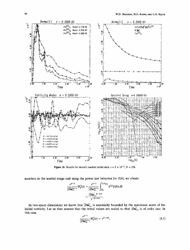
Figure 10, Results for smooth random initial data, v = 2 x 10 -5, N = 256.
numbers in the inertial range and using the power law behavior for E(k), we obtain
vp--1 Hg(t) ~ __vV-1 f l/Zm,, k2PE(k) dk
IDul~ +1 IDul~ +~ jK,
IDulJ-x/2 y-f l+3/2
In two-space d imens ions we k n o w that ]Du]~o is essentially bounded by the m a x i m u m norm of the initial vorticity. Let us thus assume that the initial values are scaled so that [Duloo is of order one. In this case
v P - 1
]DuI~ +1 H i ( t ) ,,~ v a-3/2, (4.1)
On the Smallest Scale for the Incompressible Navier-Stokes Equations 91
NoTms(t) u = 0.100E-02
N , O 0 0 5 0 ' ' ' ~ . . . . ~ . . . . ~ oo ~.5o z.oo T i ~ x ~o ~
(a)
Maximwmnorms ~ : 0 .100~-02
~.00 0,~0 l . O 0 1.5O 2 . 0 0
Time x I°Z
(b)
Yor~icily l: 50.00 v=O,lOOOE-02 H H I ' I I I ~ t l l ' ~ l ' f l H l ~ l l l ~ t l I1 '1 ' l l ' l l ' > t l ' ~ l l ] ~ l I t l r i ' i ' ' H I , I ' ,
g \\ ~l i / i l l I i ! l t lPt/I \'~ \t~ \-'~ -/llll/i'Y~ I I l ' i . l l I i i I I "~ t t /
Wk &tt .,' ,G!dl)/' k\', ,.> .-, ' I 1 ~ , .# I I 1 I ~ . / / -
',~ ',','. • .... / I i/itt 171:/i . . . . , ; : / : / / / t ~ i , . . . . . . . ~'.',, t, " + ? . - ' , ' / , Y / I / / i t l k I , ; . ' ; # ( " c . . '
x~ ~ \ , ! I • i l l I I rl , ~ i
- ,,
k '.,,2-., k ~ ~ • ,:-.-x ,, \ t l/~lltTi ',~,ii v, ,~(I L t - - ~ B3~\\ ~ ' , " : ~ , , , , , \ v /sl/n frill k ~ / ~
s \ , k ~ - - \ I l l l I V /
~, / Hh' ' \ \ ~,. ' , , "-.,',J l l i llttt( ~ ( / / . . . . ~ - ~ . b 71111 j ) / \ ,,~ ~-,,, ;~il ~tttt/ _ I 1 . ~ - - , , ~
: ~ i \ ,~I { \ , " . - - : , I I~ I
(c)
Vortici ty l=150.00 ~:0.1000E-02
~lll l l l l l ,~si,/,f ' ,:;." ~ k ~,~tt~\\ :' : - - , \ "x V// I I I I I~ ' A;/' /Tt?--? ~ , " ', ~\\\\\ t { 3 "~ 1.,1
~ilY//l A J" ;'F~ J ,; '~~.~-' V,X\\\\\\\ ///2
~ .... ~Y k ' ~ ~ - - - - J - ~ ' . ~ ~ U - ' - ~ ' 7 . - / ~ = . . . . . -. " \ ~ \ ~ ' , ~ : ~ . . ~ ' , ' ~ ~ ~ " ~ "- / ;-C/-"~ ; / . / . ~
~. ~. ",,',o~ ,~~-----...~--...~-y,~ ~ , ~. • ' ~\ i • ~ ~ , i. \ , ,¢ ,*# :1#,
~,\\\x$_\ x, k ',,%,. t t I ~is.;,,S~/// "~ \\\\\\\, 1 \\ ;\~tl~alJll It I ! I / / i d : l l l I I n \~
\\\\\~'A ! '~\,, "~ ~ t . , ? l / , # l l l l / ~
k\//~t//T1 I :~ " ' ~ . "II/#1111 ix, -" / _ "~
( d )
Figure 11. Random forcing, Ifl. = 1, v : 10 -3, N = 128,
and for maximal dissipative f lows it fo l lows that E ( k ) ,-., k -a, the power law behavior predicted by the B a t c h e l o r - K r a i c h n a n theory [3], [16].
In three dimensions , if we speculate that IDuloo -- O(v-e), then
vP--1
[Dul~ +x Up: ,-, ~)y(p+l/2)+p-3/2.
In this way, for max imal dissipative flows, we obtain a relation between the power law behavior of the energy spectrum and the size of IDuloo:
3 - - 7 /7- 2 + 2 7 "
92 W.D. Henshaw, H.O. Kreiss, and L.G. Reyna
x
Norms(t) u =. 0.500E-03 . . . . . . . . . ,
0.00
Time 0.50 1.00 1.50 2.00
x 10 2
eo
Norms(t) v = 0.500E-04
0.00 0,50 1.00 !.50
Time 2.00
x 102
¢,g
0.00
Maxirmun norms v = 0.500E-03
C--MAX(W)
0.50 1.00 1.50 2.00
Time x ~o 2
..2
¢;
ca ¢>
0.00
Maxirmun norms y = 0.500E-04
. . . . . . . . . , . ; ~ , . . , /~ , , . , - . ~ 0.50 ! .00 ~.50 2.00
Time x 1o 2
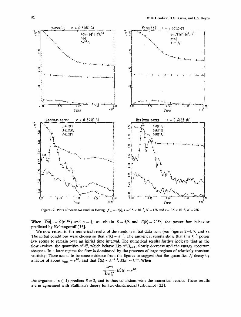
Figure 12. Plots of norms for random forcing, [fl® = O(v), v = 0.5 x 10 -3, N = 128 and v = 0.5 x 10 -4, N = 256.
When IDulo~ = O(v -1/2) and 7 = ½, we obtain fl = 5/6 and E ( k ) = k -5/3, the power law behavior predicted by Kolmogorof f 1-15].
We now return to the numerical results of the random initial data runs (see Figures 2 - 4 , 7, and 8). The initial conditions were chosen so that E(k) ,-~ k -3. The numerical results show that this k - 3 power law seems to remain over an initial time interval. The numerical results further indicate that as the flow evolves, the quantities v~'J 2, which behave like vVHp+,, slowly decrease and the energy spectrum steepens. In a later regime the flow is dominated by the presence of large regions of relatively constant vorticity. There seems to be some evidence from the figures to suggest that the quantities j2 decay by a factor of about /~mjrt = Vl/2, and that ~(k) ~ k -1"5, E(k) ,--, k -4. When
vP-1 iDul~+l H2(t) ~ vl/2,
the argument in (4.1) predicts f l ---2, and is thus consistent with the numerical results. These results are in agreement with Staffman's theory for two-dimensional turbulence 1-22].
O n t h e S m a l l e s t Scale fo r t h e I n c o m p r e s s i b l e N a v i e r - S t o k e s E q u a t i o n s 93
Vorticity l=50.00 v=O.5000E-03 .... %z ,27 ' " , ~ . . . . . . . . . . . . '~'.";~ " - -
~ ~ " . "~.:~,.,
~ _ --'---~c=c-@~-¢J~%,~ v ~.~
Vorticity g= 50.00 v-O.5000E-04
Vorticity t=150,00 v=O.5000R-03 .......... ~ ............ ~i ................................ ~,w ........ ',,' . . . . . . . . . . . . . . . . . ~,~,,~
i ~ l \~\ \\",?")%. ('i'1 I I ( ~ I I f ~ F l l ~kt \~",",L,',,. ',,~t / I t l \ : ( t k t ( ' 3
I I I i i ) ',% ' , , \ \ \ \ \ ~ / / / 4 / / / .,.:.?,,~ \~. :
I / u / / / / / / ",,'-',:',",.. \ \ \ b i / / / / / 7 ,, . . . . . . - . . ,,,., \ \ \ \ ~
}': / /:7 / . . . . . . . " , \ ,,', r /1 *, / / ¢ f - - ~ , "-,, x \ ~ %
Y 7 , / , , , , . . . . . . . ..,... ,,,, , , , , / _ I / ' - \ / ' I I
i ~1 I I L 1 I ~ ] I I i
~ \ \ ~ ',{,,', '.,,,.'.- . . . . ..,',,'.',, ,,'; L , a / / . - - . I \ \ \ ' : . , , ....... .-:,' ,,', 7//// L ........ 2X.'a......,;., ........... - ~ ................................. - - , , ///Z,,.A.....~
Vorticity t=150.00 ~=0.5000E-04
..,'!:' ',,:,,,, ) ; 1% ',._.-' !,,'s:;/, ,~ .'.~ : - : ( ~ . f / / , : : _ , \ , . J3~ . . / ,,~ - D':,/ / ¢s
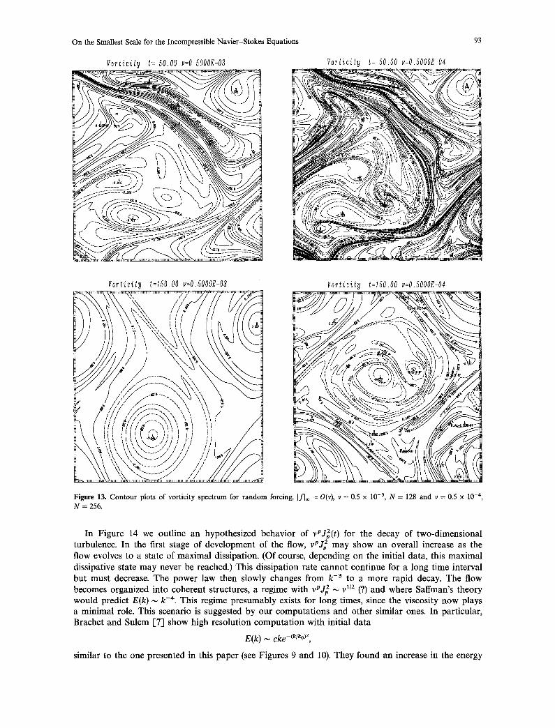
Figure 13. C o n t o u r p lo t s o f v o r t i c i t y s p e c t r u m for r a n d o m forc ing , [fLo = O(v), v = 0.5 x 10 -3, N = 128 a n d v = 0.5 x 10 -4,
N = 256.
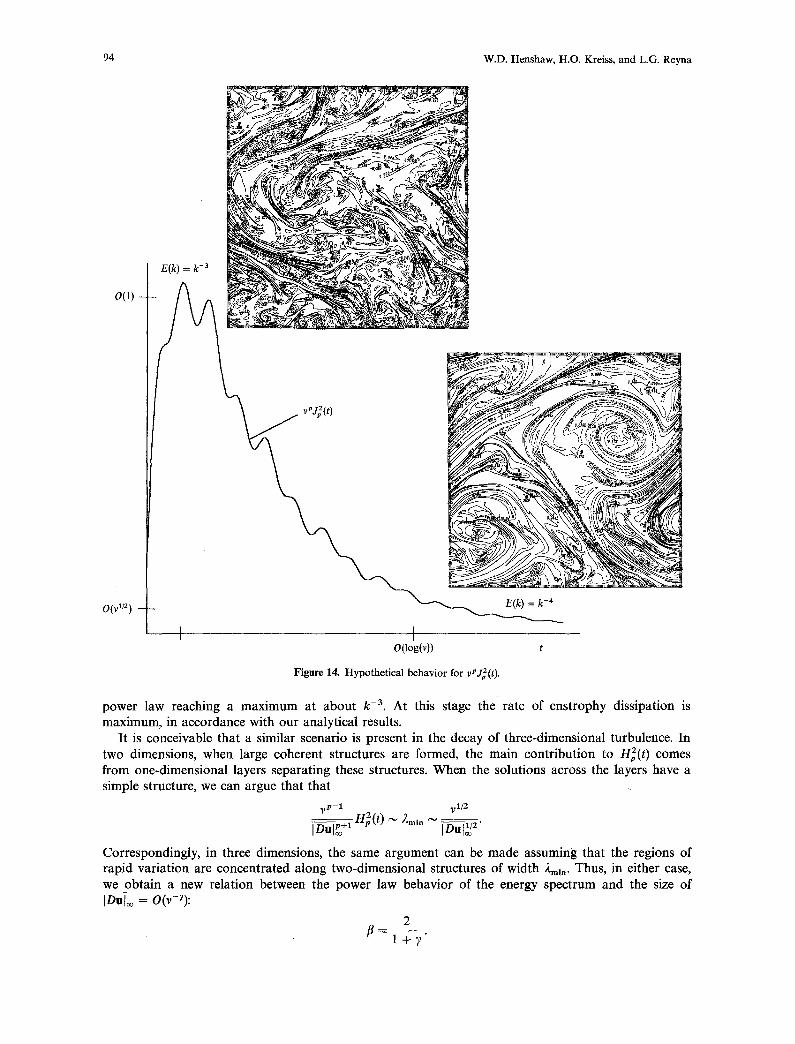
In Figure 14 we outline an hypothesized behavior of vPd~(t) for the decay of two-dimensional turbulence. In the first stage of development of the flow, vPJZp may show an overall increase as the flow evolves to a state of maximal dissipation. (Of course, depending on the initial data, this maximal dissipative state may never be reached.) This dissipation rate cannot continue for a long time interval but must decrease. The power law then slowly changes from k - 3 to a more rapid decay. The flow becomes organized into coherent structures, a regime with vPJ~ ~ v 1/2 (?) and where Saffman's theory would predict E(k) ~ k -4. This regime presumably exists for long times, since the viscosity now plays a minimal role. This scenario is suggested by our computations and other similar ones. In particular, Brachet and Sulem I-7] show high resolution computation with initial data
E(k) ~ c k e -(k/k°)2,
similar to the one presented in this paper (see Figures 9 and 10). They found an increase in the energy
94 W.D. Henshaw, H.O. Kreiss, and L.G. Reyna
o ( 1 ) -
0 ( ~ , ~ ) -
E(k) = k -a
E (k ) = k - 4
I I O(log(v)) t
Figure 14. Hypothetical behavior for vp j2 ( t ) .
power law reaching a maximum at about k -3. At this stage the rate of enstrophy dissipation is maximum, in accordance with our analytical results.
It is conceivable that a similar scenario is present in the decay of three-dimensional turbulence. In two dimensions, when large coherent structures are formed, the main contribution to H2(t) comes from one-dimensional layers separating these structures. When the solutions across the layers have a simple structure, we can argue that that
~)p-I ~I/2
IDnI~+ 1 H~(t) ~ "~min "~ ~D-~loo/~.
Correspondingly, in three dimensions, the same argument can be made assuming that the regions of rapid variation are concentrated along two-dimensional structures of width 2mi.. Thus, in either case, we obtain a new relation between the power law behavior of the energy spectrum and the size of IDul~ = Off-e):
2
On the Smallest Scale for the Incompressible Navier-Stokes Equations 95
In two dimensions 7 = 0 and we again obtain E(k)~ k -4. If, in three dimensions, IDul~ ~ v 1/2, we obtain E(k) ~ k -8/3. Large three-dimensional simulations are necessary to confirm the validity of the assumption made on the size of IDul~o, on the time evolution of H2(t) and the sharpness of our estimates.
References
[1] Barker, J.: A Numerical Experiment on the Structure of Two-Dimensional Turbulent Flow. Ph.D. Thesis, Applied Mathematics Department, Caltech, 1982.
E2] Basdevant, C.: Technical improvements for direct numerical simulation of homogeneous three-dimensional turbulence. J. Comput. Phys., 50 (1983), 209-214.
[3] Batchelor, G.K.: Computation of the energy spectrum in homogeneous two-dimensional turbulence. Phys. Fluids, Supp. II (1969), 233-239.
[4] Benzi, R., Paladini, G., Patarnello, S., Santangelo, P., Vulpiani, A.: Intermittency and coherent structures in two- dimensional turbulence, d. Phys. A, 19 (1986), 3771-3784.
[5] Braehet, M.E., Meiron, D.I., Orszag, S.A., Nickel, B.G., Morf, R.H., Frisch, U.: Small-scale structure of the Taylor-Green vortex. J. Fluid Mech. 150 (1983), 411-452.
[6] Brachet, M.E., Meneguzzi, M., Sulem, P.L.: Small-scale dynamics of high Reynolds number, two-dimensional turbulence. Submitted to Phys. Rev. Lett.
[7] Brachet, M.E., Sulem, P.L.: Direct Numerical Simulation of Two-Dimensional Turbulence. Proc. 4th Beer Sheva of MHD Flows and Turbulence, March 1984, Israel.
[8] Fornberg, B.: A numerical study of 2-D turbulence, d. Comput. Phys., 25 (1977), 1-31. [9] Fox, D.G., Orszag, S.A.: Pseudospectral approximation to two-dimensional turbulence. J. Comput. Phys., 11 (1973),
612-619. [10] Gilbarg, D., Trudinger, N.S.: Elliptic Partial Differential Equations of Second Order. Springer-Verlag, New York, 1983. [11] Herring, J.R., McWilliams, J.C.: Comparison of direct simulation of two-dimensional turbulence with two-point closure:
The effects of intermittency. J. Fluid Mech., 153 (1985), 229-242. [12] Herring, J.R., Orszag, S.A., Kraichnan, R.H., Fox, D.G.: Decay of two-dimensional turbulence. J. Fluid Mech., 66 (1974),
417-444. [13] Hfrmander, L.: The boundary problems of physical geodesy. Arch. Rational Mech. Anal., 62 (1976), 1-52. [14] Hussaini, M.Y., Zang, T.A.: Spectral methods in fluid dynamics. Ann. Rev. Fluid Mech., 19 (1987), 339-367. [15] Kolmogoroff, A.N.: C. R, Acad. Sci U.S.S.R., 30 (1941), 301. [16] Kraichnan, R.: Inertial ranges in two-dimensional turbulence. Phys. Fluids, 10 (1967), 1417-1423. [17] Kreiss, H.O., Henshaw, W.D., Reyna, L.G.: On the Smallest Scale for the Incompressible Navier-Stokes Equations in
Two Space Dimensions. IBM Research Report No. 13204, 1987. [18] Kreiss, H.O., Oliger, J.: Comparison of accurate methods for the integration of hyperbolic equations. Tellus, 24 (1972),
199-215. [19] Lilly, D.K.: Numerical Simulation of Developing and Decaying of Two Dimensional Turbulence, J. Fluid Mech., 45
(1971), 395-415. [20] Orszag, S.A.: Analytical theories of turbulence. J. Fluid Mech., 41 (1970), 363-386. E21] Orszag, S.A.: Numerical simulation of incompressible flows within simple boundaries: I. Galerkin (spectral) representa-
tions. Stud. Appl. Math., 50 (1971), 293-327. [22] Saffman, P.G.: On the spectrum and decay of random two-dimensional vorticity distributions at large Reynolds numbers.
Stud. Appl. Math., 50 (1971), 377-383.