part ii - unsteady incompressible viscous flows - core

Manuscript submitted to CMES

Local Moving Least Square - One-Dimensional IRBFNTechnique: Part II - Unsteady Incompressible Viscous

Flows

D. Ngo-Cong1,2, N. Mai-Duy1, W. Karunasena2 and T. Tran-Cong1,3

Abstract: In this study, local moving least square - one dimensional integratedradial basis function network (LMLS-1D-IRBFN) method is presented and demon-strated with the solution of time-dependent problems such as Burgers’ equation,unsteady flow past a square cylinder in a horizontal channel and unsteady flow pasta circular cylinder. The present method makes use of the partition of unity conceptto combine the moving least square (MLS) and one-dimensional integrated radialbasis function network (1D-IRBFN) techniques in a new approach. This approachoffers the same order of accuracy as its global counterpart,the 1D-IRBFN method,while the system matrix is more sparse than that of the 1D-IRBFN, which helpsreduce the computational cost significantly. For fluid flow problems, the diffusionterms are discretised by using LMLS-1D-IRBFN method, whilethe convectionterms are explicitly calculated by using 1D-IRBFN method. The present numericalprocedure is combined with a domain decomposition technique to handle large-scale problems. The numerical results obtained are in good agreement with otherpublished results in the literature.

Keywords: Unsteady flow, Burgers’ equation, square cylinder, circular cylinder,moving least square, integrated radial basis function, domain decomposition.

1 Introduction

Time-dependent analysis plays a very important role in the design of diverse en-gineering products and systems, e.g. in aerospace, automotive, marine and civilapplications. In this paper, a new efficient numerical method is developed for

1 Computational Engineering and Science Research Centre, Faculty of Engineering and Surveying,The University of Southern Queensland, Toowoomba, QLD 4350, Australia.

2 Centre of Excellence in Engineered Fibre Composites, Faculty of Engineering and Surveying, TheUniversity of Southern Queensland, Toowoomba, QLD 4350, Australia.

3 Corresponding author, Email: [email protected].


2

the solution of time-dependent problems and illustrated with examples such asthe well-known Burgers’ equation, unsteady flows past a square cylinder in a hor-izontal channel, and unsteady flows past a circular cylinder. Burgers’ equationhas been studied by many authors to verify their proposed numerical methods be-cause it is the simplest nonlinear equation that includes convection and dissipationterms. Caldwell, Wanless, and Cook (1987) presented a moving node finite ele-ment method to obtain a solution of Burgers’ equation under different prescribedconditions. Iskander and Mohsen (1992) devised new algorithms based on a com-bination of linearization and splitting-up for solving this equation. Hon and Mao(1998) solved Burgers’ equation using multiquadric (MQ) for spatial discretisationand a low order explicit finite difference scheme for temporal discretisation. Theirnumerical results indicated that the major numerical erroris from the time inte-gration instead of the MQ spatial approximation. Hassanien, Salama, and Hosham(2005) developed fourth-order finite difference method based on two-level three-point finite difference for solving Burgers’ equation. Hashemian and Shodja (2008)proposed a gradient reproducing kernel particle method (GRKPM) for spatial dis-cretisation of Burgers’ equation to obtain equivalent nonlinear ordinary differen-tial equations which are then discretised in time by the Gear’s method. Hosseiniand Hashemi (2011) presented a local-RBF meshless method for solving Burgers’equation with different initial and boundary conditions.

Flows past a circular cylinder have been extensively studied by many researchersto verify their new numerical methods for irregular domains. There is no singu-larity on a circular cylinder surface and the flow field behindthe cylinder containsa variety of fluid dynamic phenomena, which makes the probleminteresting as abenchmark. Cheng, Liu, and Lam (2001) applied a discrete vortex method to inves-tigate an unsteady flow past a rotationally oscillating circular cylinder for differentvalues of oscillating amplitude and frequency at a Reynoldsnumber of 200. Basedon the numerical results obtained, they provided a map of lock-on and non-lock-on regions which helps to classify the different vortex structure in the wake withrespect to the oscillating amplitude and frequency of the cylinder.

For the problem of flow past a square cylinder, singularitiesoccur at the cornersof the square cylinder, which poses some challenges in termsof accurate determi-nation of such singularities. In order to obtain a convergent solution, very densegrids are usually generated near the singularities. Davis and Moore (1982) stud-ied unsteady flow past a rectangular cylinder using finite difference method (FDM)with third-order upwind differencing for convection, standard central scheme fordiffusion terms and a Leith-type scheme for time integration. Zaki, Sen, and el Hak(1994) conducted a numerical study of flow past a fixed square cylinder at variousangles of incidence for Reynolds numbers up to 250. Their numerical simula-


3

tion was based on the stream function-vorticity formulation of the Navier-Stokesequation together with a single-valued pressure conditionto make the problemwell-posed. Sohankar, Norberg, and Davidson (1998) presented calculations ofunsteady 2-D flows around a square cylinder at different angles of incidence usingan incompressible SIMPLEC finite volume code with a non-staggered grid arrange-ment. The convective terms were discretised using the third-order QUICK differ-encing scheme, while the diffusive terms were discretised using central differences.Breuer, Bernsdorf, Zeiser, and Durst (2000) investigated aconfined flow around asquare cylinder in a channel with blockage ratio of 1/8 by a lattice-Boltzmannautomata (LBA) and a finite volume method (FVM). Turki, Abbassi, and Nasral-lah (2003) studied an unsteady flow and heat transfer characteristics in a chan-nel with a heated square cylinder using a control volume finite element method(CVFEM) adapted to a staggered grid. In their work, the influences of blockageratio, Reynolds number and Richardson number on the flow pattern were investi-gated. Berrone and Marro (2009) applied a space-time adaptive method to solveunsteady flow problems including flows over backward facing step and flows pasta square cylinder in a channel. Moussaoui, Jami, Mezrhab, and Naji (2010) simu-lated a 2-D flow and heat transfer in a horizontal channel obstructed by an inclinedsquare cylinder using a hybrid scheme with lattice Boltzmann method to determinethe velocity field and FDM to solve the energy equation.

Dhiman, Chhabra, and Eswaran (2005) investigated influences of blockage ratio,Prandtl number and Peclet number on the flow and heat transfercharacteristics ofan isolated square cylinder confined in a channel in a 2-D steady flow regime (1≤Re≤ 45) using semi-explicit FEM on a non-uniform Cartesian grid. The third orderQUICK scheme was used to discretise the convection terms, while the second-ordercentral difference scheme was used to discretise the diffusion terms. The semi-explicit FEM was also applied to a steady laminar mixed convection flow acrossa heated square cylinder in a channel [Dhiman, Chhabra, and Eswaran (2008)].Sahu, Chhabra, and Eswaran (2010) conducted a study of 2-D unsteady flow ofpower-law fluids past a square cylinder confined in a channel for different val-ues of Reynolds number (60≤ Re≤ 160), blockage ratio (β0 = 1/6,1/4 and 1/2)and power-law flow behaviour index (0.5≤ n≤ 1.8) using the semi-explicit FEM.Bouaziz, Kessentini, and Turki (2010) employed a control volume finite elementmethod (CVFEM) adapted to the staggered grid to study an unsteady laminar flowand heat transfer of power-law fluids in 2-D horizontal planechannel with a heatedsquare cylinder.

In the past decades, some mesh-free and local RBF-based methods have been de-veloped for solving fluid flow problems. Shu, Ding, and Yeo (2003) presented alocal RBF-based differential quadrature method (local RBF-DQ) for a simulation


4

of natural convection in a square cavity. In their study, three layers of orthogonalgrid near and including the boundary were generated for imposing the Neumanncondition of temperature and the vorticity on the wall. The derivatives of the fieldvariables in the boundary conditions were then discretisedby the conventional one-sided second order finite difference scheme. The local RBF-DQ method was alsoemployed for solving several cases of incompressible flows including a driven-cavity flow, flow past a cylinder, and flow around two staggeredcircular cylin-ders [Shu, Ding, and Yeo (2005)]. Ding, Shu, Yeo, and Xu (2007) presented themesh-free least square-based finite difference (MLSFD) method to simulate a flowfield around two circular cylinders arranged in tandem and side-by-side. Vertnikand Šarler (2006) presented an explicit local RBF collocation method for diffusionproblems. Sanyasiraju and Chandhini (2008) developed a local RBF based gridfreescheme for unsteady incompressible viscous flows in terms ofprimitive variables.Chen, Hu, and Hu (2008) employed a partition of unity concept[Babuska and Me-lenk (1997)] to combine the reproducing kernel and RBF approximations to yield alocal approximation that enjoys the exponential convergence of RBF and improvesthe conditioning of the discrete system. Le, Rabczuk, Mai-Duy, and Tran-Cong(2010) proposed a locally supported moving IRBFN-based meshless method forsolving various problems including heat transfer, elasticity of both compressibleand incompressible materials, and linear static crack problems.

Another approach for solving PDEs is the so-called Cartesian grid method wherethe governing equations are discretised with a fixed Cartesian grid. This approachsignificantly reduces the grid generation cost and has a great potential over the con-ventional body-fitted methods when solving problems with moving boundary andcomplicated geometry. Udaykumar, Mittal, Rampunggoon, and Khanna (2001)presented a Cartesian grid method for computing fluid flows with complex im-mersed and moving boundaries. The incompressible Navier-Stokes equations arediscretised using a second-order FVM, and second-order fractional-step schemeis employed for time integration. Russell and Wang (2003) presented a Cartesiangrid method for solving 2-D incompressible viscous flows around multiple movingobjects based on stream function-vorticity formulation. Zheng and Zhang (2008)employed an immersed-boundary method to predict the flow structure around atransversely oscillating cylinder. The influences of oscillating frequency on thedrag and lift acting on the cylinder were investigated.

As an alternative to the conventional differentiated radial basis function network(DRBFN) method [Kansa (1990)], Mai-Duy and Tran-Cong (2001a) proposed theuse of integration to construct the RBFN expressions (the IRBFN method) for theapproximation of a function and its derivatives and for the solution of PDEs. Nu-merical results showed that the IRBFN method achieves superior accuracy [Mai-


5

Duy and Tran-Cong (2001a); Mai-Duy and Tran-Cong (2001b)].A one-dimensionalintegrated radial basis function network (1D-IRBFN) collocation method for thesolution of second- and fourth-order PDEs was presented by Mai-Duy and Tan-ner (2007). Along grid lines, 1D-IRBFN are constructed to satisfy the govern-ing differential equations with boundary conditions in an exact manner. In the1D-IRBFN method, the Cartesian grids were used to discretise both rectangularand non-rectangular problem domains. The 1D-IRBFN method is much more effi-cient than the original IRBFN method reported in Mai-Duy andTran-Cong (2001a).Le-Cao, Mai-Duy, Tran, and Tran-Cong (2011) employed the 1D-IRBFN methodto simulate unsymmetrical flows of a Newtonian fluid in multiply-connected do-mains using the stream-function and temperature formulation. Ngo-Cong, Mai-Duy, Karunasena, and Tran-Cong (2011) extended this methodto investigate freevibration of composite laminated plates based on first-order shear deformationtheory. Ngo-Cong, Mai-Duy, Karunasena, and Tran-Cong (2012) proposed a lo-cal moving least square - one dimensional integrated radialbasis function net-work method (LMLS-1D-IRBFN) for simulating 2-D steady incompressible vis-cous flows in terms of stream function and vorticity. In the present study, we fur-ther extend the LMLS-1D-IRBFN method for solving time-dependent problemsand demonstrate the new procedure with the simulation of Burgers’ equation, un-steady flows past a square cylinder in a horizontal channel, and unsteady flows pasta circular cylinder. The present numerical procedure is combined with a domaindecomposition technique to handle large-scale problems.

The paper is organised as follows. The LMLS-1D-IRBFN methodis presented inSection 2. The governing equations for incompressible viscous flows are given inSection 3. Several numerical examples are investigated using the proposed methodin Section 4. Section 5 concludes the paper.

2 Local moving least square - one dimensional integrated radial basis func-tion network technique

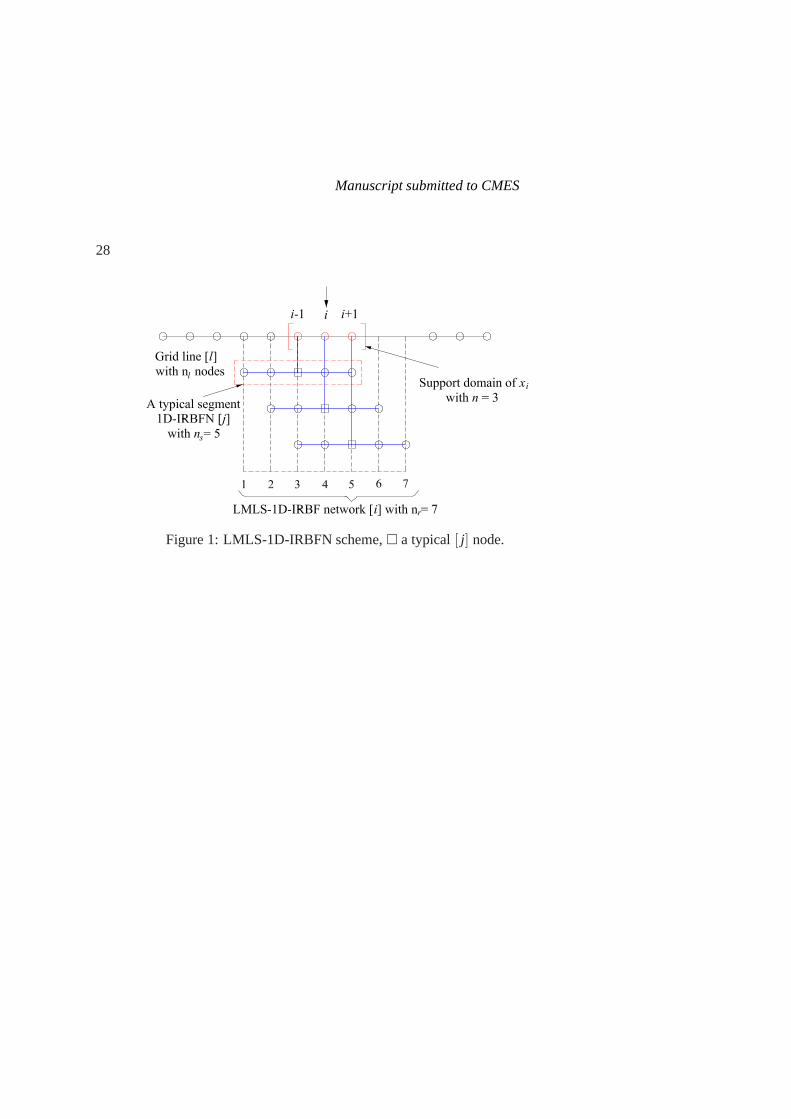
A schematic outline of the LMLS-1D-IRBFN method is depictedin Fig. 1. Theproposed method with 3-node support domains (n= 3) and 5-node local 1D-IRBFnetworks (ns = 5) is presented here. On anx-grid line [l ], a global interpolant forthe field variable at a grid pointxi is sought in the form

u(xi) =n

∑j=1

φ j(xi)u[ j](xi), (1)

where{

φ j}n

j=1 is a set of the partition of unity functions constructed using MLS

approximants [Liu (2003)];u[ j](xi) the nodal function value obtained from a local


6

interpolant represented by a 1D-IRBF network[ j]; n the number of nodes in thesupport domain ofxi . In (1), MLS approximants are presently based on linearpolynomials, which are defined in terms of 1 andx. It is noted that the MLS shapefunctions possess a so-called partition of unity properties as follows.

n

∑j=1

φ j(x) = 1. (2)

Relevant derivatives ofu at xi can be obtained by differentiating (1)

∂u(xi)

∂x=

n

∑j=1

(

∂ φ j(xi)

∂xu[ j](xi)+ φ j(xi)

∂u[ j](xi)

∂x

)

, (3)

∂ 2u(xi)

∂x2 =n

∑j=1

(

∂ 2φ j(xi)

∂x2 u[ j](xi)+2∂ φ j(xi)

∂x∂u[ j](xi)

∂x+ φ j(xi)

∂ 2u[ j](xi)

∂x2

)

, (4)

where the valuesu[ j](xi),∂u[ j](xi)/∂x and∂ 2u[ j](xi)/∂x2 are calculated from 1D-IRBFN networks withns nodes.

Full details of the LMLS-1D-IRBFN method can be found in [Ngo-Cong, Mai-Duy,Karunasena, and Tran-Cong (2012)].

3 Governing equations for 2-D unsteady incompressible viscous flows

The governing equations for 2-D incompressible viscous flows written in terms ofstream functionψ and vorticityω are given by

∂ 2ψ∂x2 +

∂ 2ψ∂y2 =−ω , (5)

1Re

(

∂ 2ω∂x2 +

∂ 2ω∂y2

)

=∂ω∂ t

+

(

∂ψ∂y

∂ω∂x

−∂ψ∂x

∂ω∂y

)

, (6)

whereRe is the Reynolds number,t the time, and(x,y)T the position vector. Thex andy components of the velocity vector can be defined in terms of the streamfunction as

u=∂ψ∂y

, (7)

v=−∂ψ∂x

. (8)


7

The computational boundary conditions for vorticity can becomputed as

ωw =−

(

∂ 2ψw

∂x2 +∂ 2ψw

∂y2

)

(9)

where the subscriptw is used to denote quantities on the boundary. For curvedboundaries, a formula reported in [Le-Cao, Mai-Duy, and Tran-Cong (2009)] isemployed here to derive the vorticity boundary conditions at boundary points onx-andy-grid lines as follows.

ω(x)w =−

[

1+

(

txty

)2]

∂ 2ψw

∂x2 −qy, (10)

ω(y)w =−

[

1+

(

tytx

)2]

∂ 2ψw

∂y2 −qx, (11)

whereqx andqy are known quantities defined by

qx =−tyt2x

∂ 2ψw

∂y∂s+

1tx

∂ 2ψw

∂x∂s, (12)

qy =−txt2y

∂ 2ψw

∂x∂s+

1ty

∂ 2ψw

∂y∂s, (13)

in which tx = ∂x/∂s, ty = ∂y/∂s and s is the direction tangential to the curvedsurface.

Boundary conditions for stream function are specified in thefollowing examples.

4 Numerical results and discussion

Several time-dependent problems are considered in this section to study the perfor-mance of the present numerical procedure. The domains of interest are discretisedusing Cartesian grids. The simple Euler scheme is used for time integration. ForBurgers’ equation, the LMLS-1D-IRBFN method is employed todiscretise bothdiffusion and convection terms. For fluid flow problems, the LMLS-1D-IRBFNis used to discretise the diffusion terms while the convection terms are explicitlycalculated by using the 1D-IRBFN technique. A domain decomposition techniqueis employed for solving the fluid flow problems. By using the LMLS-1D-IRBFNmethod to discretise the left hand side of governing equations and the LU decom-position technique to solve the resultant sparse system of simultaneous equations,the computational cost and data storage requirements are reduced.


8

4.1 Example 1: Burgers’ equation

The present numerical method is first verified through the solution of Burgers’equation as follows.

∂u∂ t

+u∂u∂x

=1

Re∂ 2u∂x2 . (14)

The diffusion and convection terms in Equation (14) are discretised on a uniformgrid using LMLS-1D-IRBFN method implicitly and explicitly, respectively.

4.1.1 Approximation of shock wave propagation

Consider the Burgers’ equation (14) defined on a segment 0≤ x≤ 1, t ≥ 0 and sub-ject to Dirichlet boundary conditions. The initial and boundary conditions can becalculated from the following analytical solution [Hassanien, Salama, and Hosham(2005); Hosseini and Hashemi (2011)]

uE(x, t) =[α0+µ0+(µ0−α0)exp(η)]

1+exp(η), (15)

whereη = α0Re(x−µ0t −β0), α0 = 0.4,β0 = 0.125,µ0 = 0.6,Re= 100.

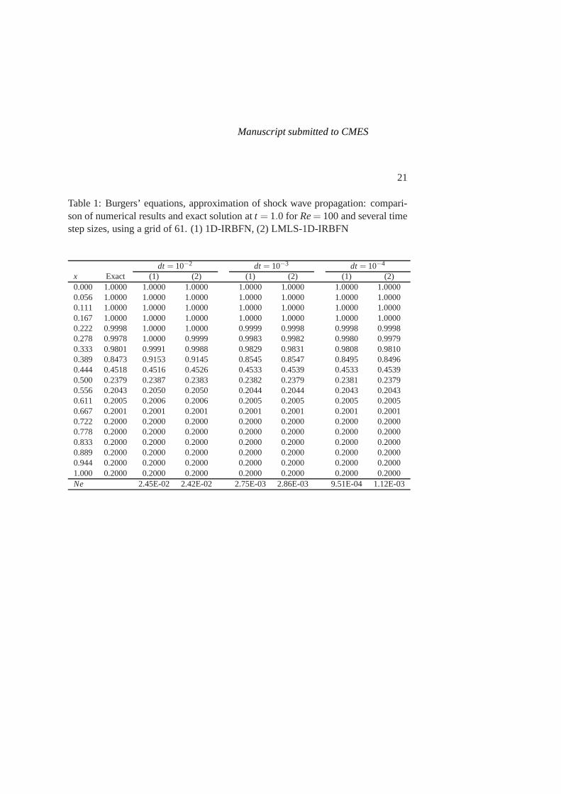
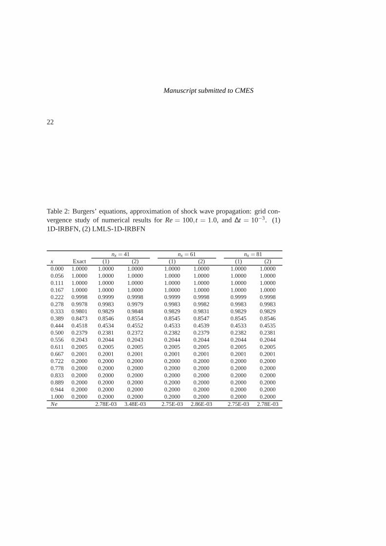
Tab. 1 shows the comparison among the numerical results of LMLS-1D-IRBFNand 1D-IRBFN methods and the exact solution at timet = 1.0 for several time stepsizes and using a grid of 61. It can be seen that the accuracy isgreatly improved byreducing the time step. Grid convergence studies for both methods with the sametime step of 10−3 are given in Tab. 2. The numerical results show that the accu-racy is not improved much with increasing grid density for both methods, whichindicates that the major numerical error is not from the LMLS-1D-IRBFN and 1D-IRBFN spatial approximation, but from the temporal discretisation. It is noted thatthe LMLS-1D-IRBFN method offers the same level of accuracy as the 1D-IRBFNmethod.

4.1.2 Sinusoidal initial condition

Consider the Burgers’ Equation (14) defined on a segment 0≤ x ≤ 1, t ≥ 0 andsubject to the following Dirichlet boundary conditions andinitial condition.

u(0, t) = u(1, t) = 0, t > 0, (16)

u(x,0) = sinπx, 0≤ x≤ 1. (17)


9

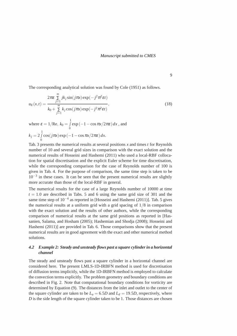
The corresponding analytical solution was found by Cole (1951) as follows.

uE(x, t) =

2πε∞∑j=1

jk j sin( jπx)exp(− j2π2εt)

k0+∞∑j=1

k j cos( jπx)exp(− j2π2εt), (18)

whereε = 1/Re, k0 =1∫

0exp(−1−cosπx/2πε)dx , and

k j = 21∫

0cos( jπx)exp(−1−cosπx/2πε)dx.

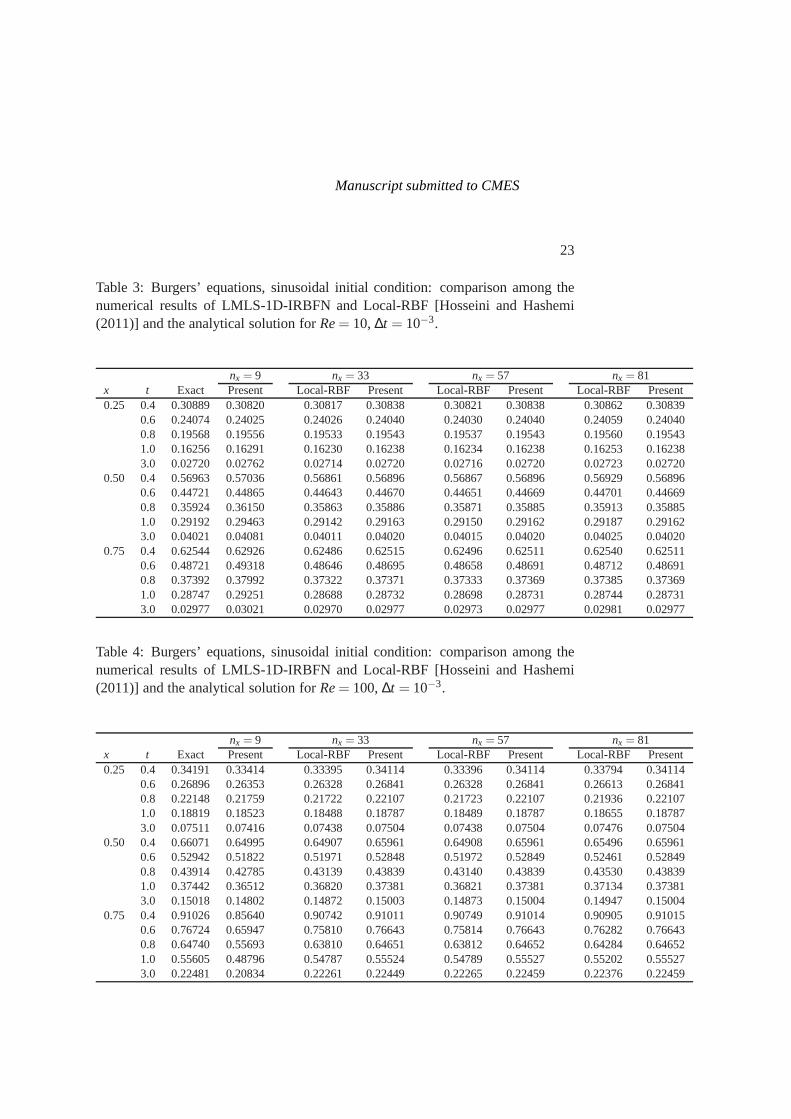
Tab. 3 presents the numerical results at several positionsx and timest for Reynoldsnumber of 10 and several grid sizes in comparison with the exact solution and thenumerical results of Hosseini and Hashemi (2011) who used a local-RBF colloca-tion for spatial discretisation and the explicit Euler scheme for time discretisation,while the corresponding comparison for the case of Reynoldsnumber of 100 isgiven in Tab. 4. For the purpose of comparison, the same time step is taken to be10−3 in these cases. It can be seen that the present numerical results are slightlymore accurate than those of the local-RBF in general.

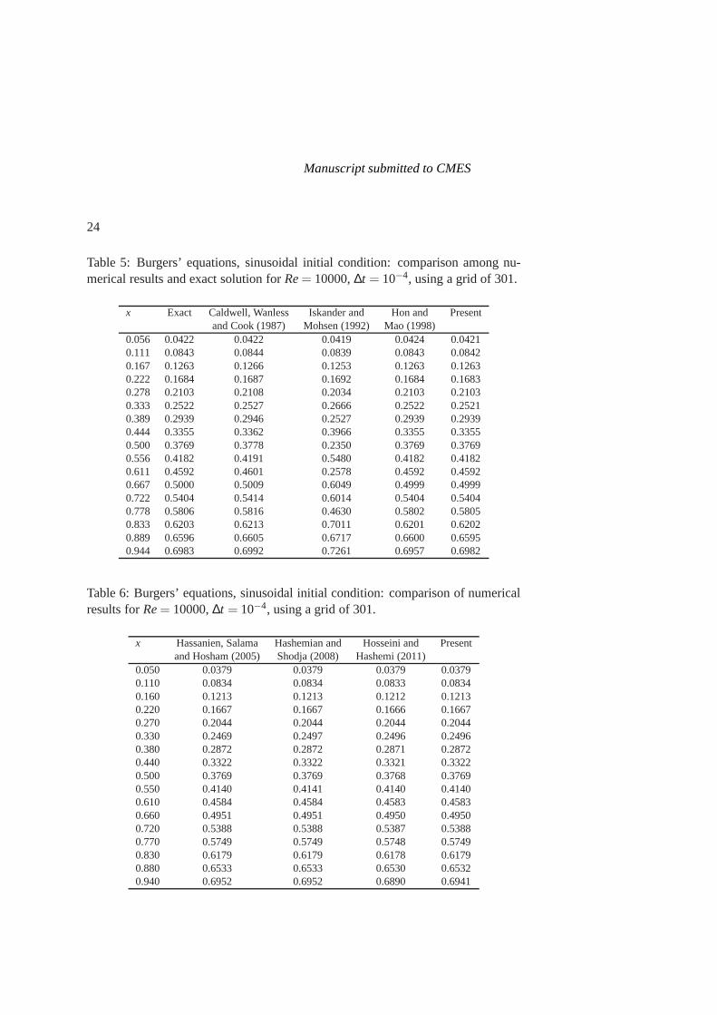
The numerical results for the case of a large Reynolds numberof 10000 at timet = 1.0 are described in Tabs. 5 and 6 using the same grid size of 301 and thesame time step of 10−4 as reported in [Hosseini and Hashemi (2011)]. Tab. 5 givesthe numerical results at a uniform grid with a grid spacing of1/8 in comparisonwith the exact solution and the results of other authors, while the correspondingcomparison of numerical results at the same grid positions as reported in [Has-sanien, Salama, and Hosham (2005); Hashemian and Shodja (2008); Hosseini andHashemi (2011)] are provided in Tab. 6. Those comparisons show that the presentnumerical results are in good agreement with the exact and other numerical methodsolutions.

4.2 Example 2: Steady and unsteady flows past a square cylinder in a horizontalchannel

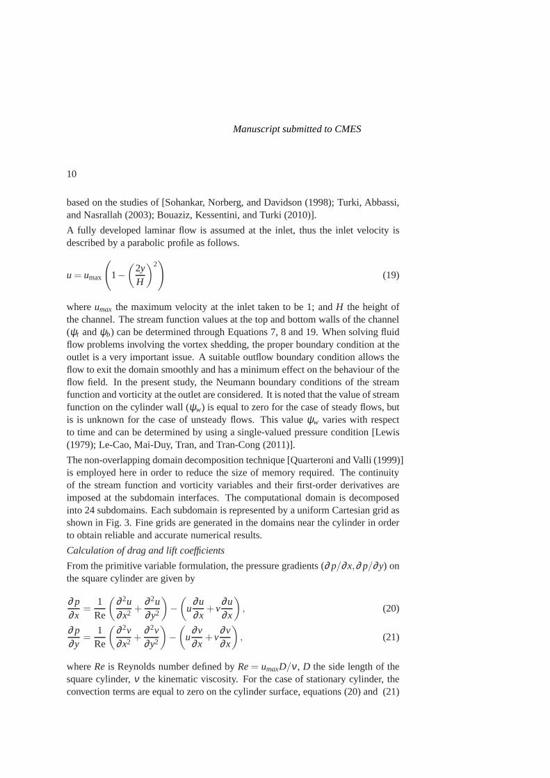
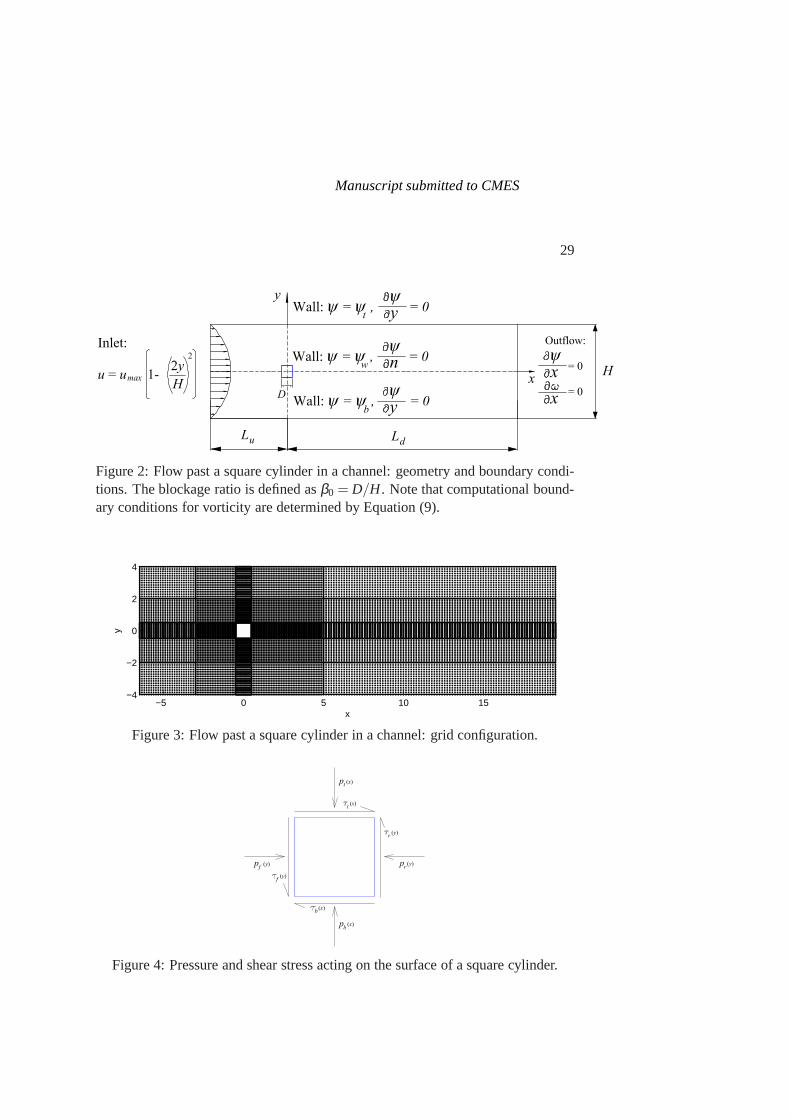
The steady and unsteady flows past a square cylinder in a horizontal channel areconsidered here. The present LMLS-1D-IRBFN method is used for discretisationof diffusion terms implicitly, while the 1D-IRBFN method isemployed to calculatethe convection terms explicitly. The problem geometry and boundary conditions aredescribed in Fig. 2. Note that computational boundary conditions for vorticity aredetermined by Equation (9). The distances from the inlet andoutlet to the center ofthe square cylinder are taken to beLu = 6.5D andLd = 19.5D, respectively, whereD is the side length of the square cylinder taken to be 1. Those distances are chosen


10

based on the studies of [Sohankar, Norberg, and Davidson (1998); Turki, Abbassi,and Nasrallah (2003); Bouaziz, Kessentini, and Turki (2010)].

A fully developed laminar flow is assumed at the inlet, thus the inlet velocity isdescribed by a parabolic profile as follows.

u= umax

(

1−

(

2yH

)2)

(19)

whereumax the maximum velocity at the inlet taken to be 1; andH the height ofthe channel. The stream function values at the top and bottomwalls of the channel(ψt andψb) can be determined through Equations 7, 8 and 19. When solving fluidflow problems involving the vortex shedding, the proper boundary condition at theoutlet is a very important issue. A suitable outflow boundarycondition allows theflow to exit the domain smoothly and has a minimum effect on thebehaviour of theflow field. In the present study, the Neumann boundary conditions of the streamfunction and vorticity at the outlet are considered. It is noted that the value of streamfunction on the cylinder wall (ψw) is equal to zero for the case of steady flows, butis is unknown for the case of unsteady flows. This valueψw varies with respectto time and can be determined by using a single-valued pressure condition [Lewis(1979); Le-Cao, Mai-Duy, Tran, and Tran-Cong (2011)].

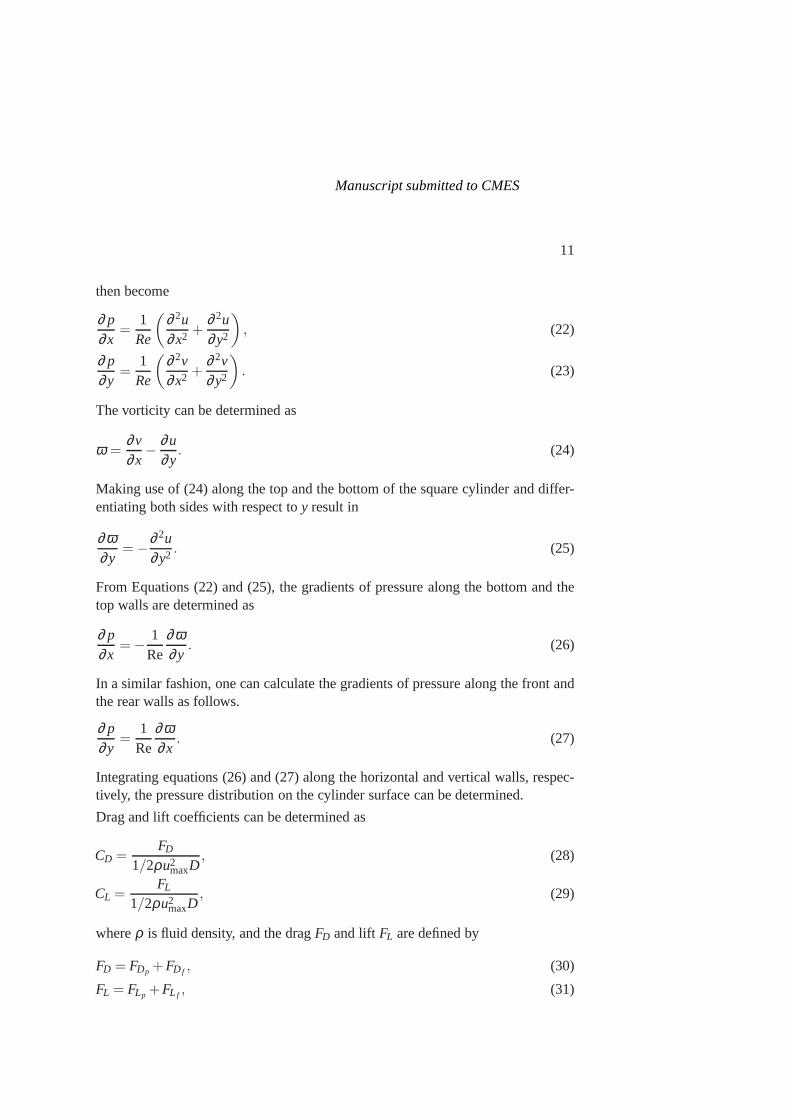
The non-overlapping domain decomposition technique [Quarteroni and Valli (1999)]is employed here in order to reduce the size of memory required. The continuityof the stream function and vorticity variables and their first-order derivatives areimposed at the subdomain interfaces. The computational domain is decomposedinto 24 subdomains. Each subdomain is represented by a uniform Cartesian grid asshown in Fig. 3. Fine grids are generated in the domains near the cylinder in orderto obtain reliable and accurate numerical results.

Calculation of drag and lift coefficients

From the primitive variable formulation, the pressure gradients (∂ p/∂x,∂ p/∂y) onthe square cylinder are given by

∂ p∂x

=1

Re

(

∂ 2u∂x2 +

∂ 2u∂y2

)

−

(

u∂u∂x

+v∂u∂x

)

, (20)

∂ p∂y

=1

Re

(

∂ 2v∂x2 +

∂ 2v∂y2

)

−

(

u∂v∂x

+v∂v∂x

)

, (21)

whereReis Reynolds number defined byRe= umaxD/ν , D the side length of thesquare cylinder,ν the kinematic viscosity. For the case of stationary cylinder, theconvection terms are equal to zero on the cylinder surface, equations (20) and (21)


11

then become

∂ p∂x

=1

Re

(

∂ 2u∂x2 +

∂ 2u∂y2

)

, (22)

∂ p∂y

=1

Re

(

∂ 2v∂x2 +

∂ 2v∂y2

)

. (23)

The vorticity can be determined as

ω =∂v∂x

−∂u∂y

. (24)

Making use of (24) along the top and the bottom of the square cylinder and differ-entiating both sides with respect toy result in

∂ω∂y

=−∂ 2u∂y2 . (25)

From Equations (22) and (25), the gradients of pressure along the bottom and thetop walls are determined as

∂ p∂x

=−1

Re∂ω∂y

. (26)

In a similar fashion, one can calculate the gradients of pressure along the front andthe rear walls as follows.

∂ p∂y

=1

Re∂ω∂x

. (27)

Integrating equations (26) and (27) along the horizontal and vertical walls, respec-tively, the pressure distribution on the cylinder surface can be determined.

Drag and lift coefficients can be determined as

CD =FD

1/2ρu2maxD

, (28)

CL =FL

1/2ρu2maxD

, (29)

whereρ is fluid density, and the dragFD and lift FL are defined by

FD = FDp +FD f , (30)

FL = FLp +FL f , (31)


12

in which

FDp =

1∫

0

(pf − pr)dy, (32)

FLp =

1∫

0

(pb− pt)dx, (33)

FD f =

1∫

0

(τt − τb)dx, (34)

FL f =

1∫

0

(τr − τ f )dy, (35)

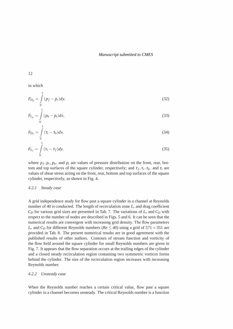
wherepf , pr , pb, andpt are values of pressure distribution on the front, rear, bot-tom and top surfaces of the square cylinder, respectively; and τ f ,τr ,τb, andτt arevalues of shear stress acting on the front, rear, bottom and top surfaces of the squarecylinder, respectively, as shown in Fig. 4.

4.2.1 Steady case

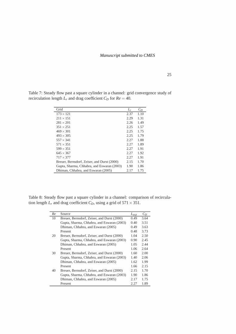
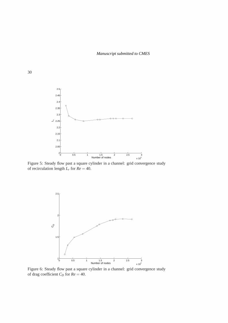
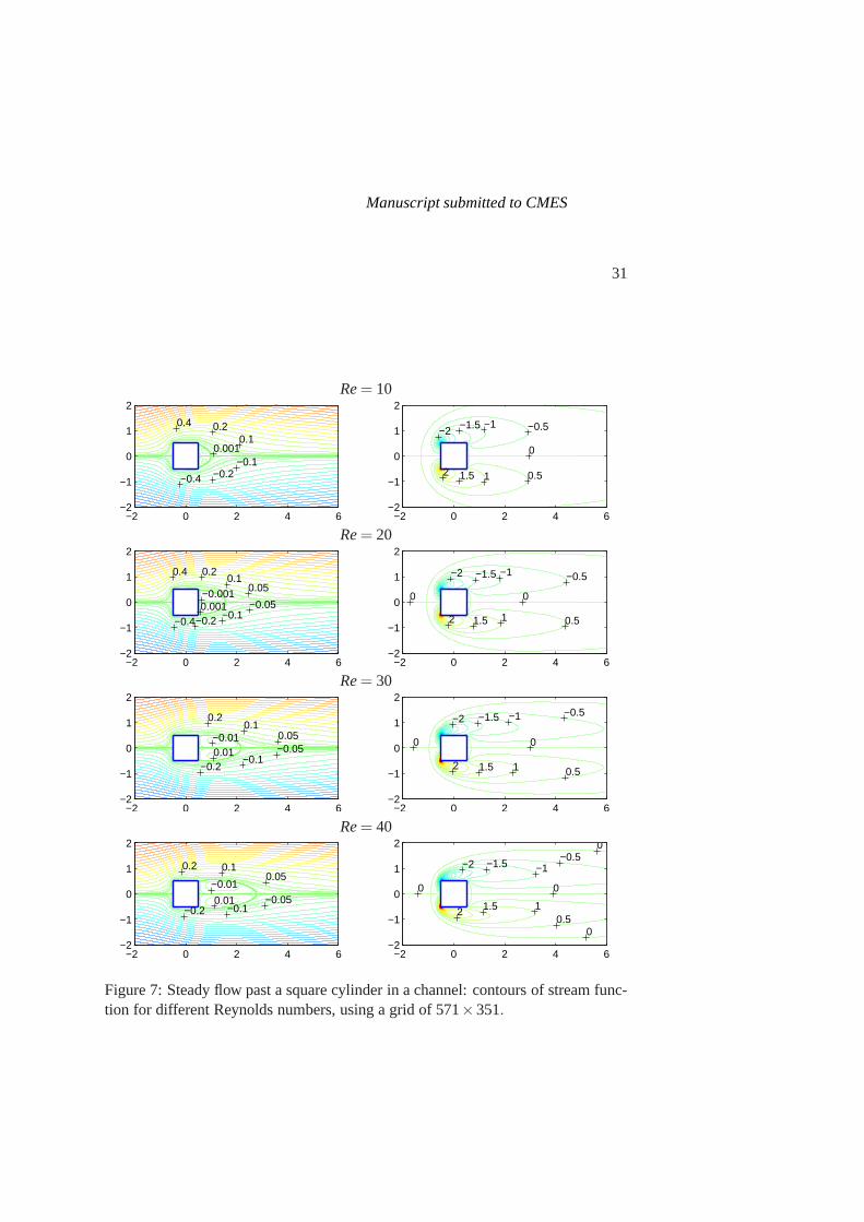
A grid independence study for flow past a square cylinder in a channel at Reynoldsnumber of 40 is conducted. The length of recirculation zoneLr and drag coefficientCD for various grid sizes are presented in Tab. 7. The variations of Lr andCD withrespect to the number of nodes are described in Figs. 5 and 6. It can be seen that thenumerical results are convergent with increasing grid density. The flow parametersLr andCD for different Reynolds numbers (Re≤ 40) using a grid of 571×351 areprovided in Tab. 8. The present numerical results are in goodagreement with thepublished results of other authors. Contours of stream function and vorticity ofthe flow field around the square cylinder for small Reynolds numbers are given inFig. 7. It appears that the flow separation occurs at the trailing edges of the cylinderand a closed steady recirculation region containing two symmetric vortices formsbehind the cylinder. The size of the recirculation region increases with increasingReynolds number.

4.2.2 Unsteady case

When the Reynolds number reaches a certain critical value, flow past a squarecylinder in a channel becomes unsteady. The critical Reynolds number is a function


13

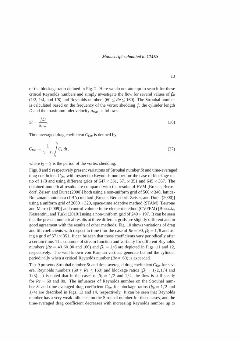
of the blockage ratio defined in Fig. 2. Here we do not attempt to search for thesecritical Reynolds numbers and simply investigate the flow for several values ofβ0

(1/2, 1/4, and 1/8) and Reynolds numbers (60≤ Re≤ 160). The Strouhal numberis calculated based on the frequency of the vortex sheddingf , the cylinder lengthD and the maximum inlet velocityumax as follows.

St=f D

umax. (36)

Time-averaged drag coefficientCDm is defined by

CDm =1

t2− t1

t2∫

t1

CDdt, (37)

wheret2− t1 is the period of the vortex shedding.

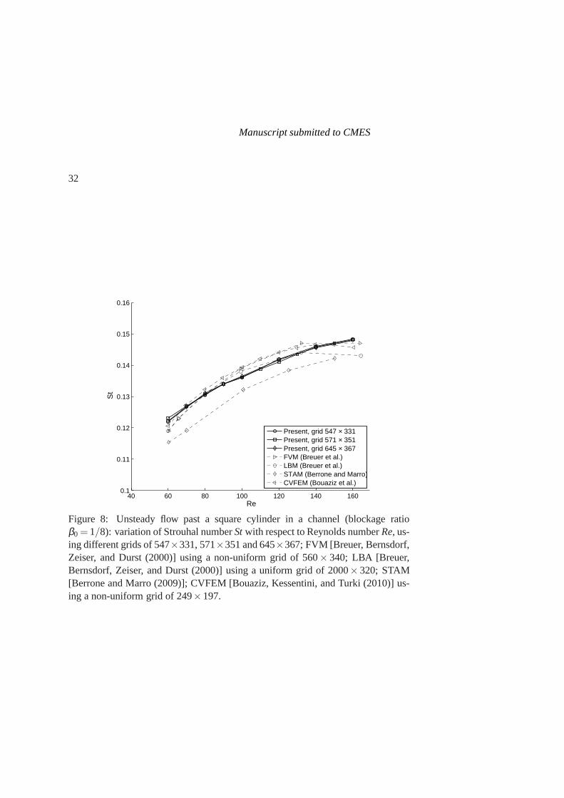
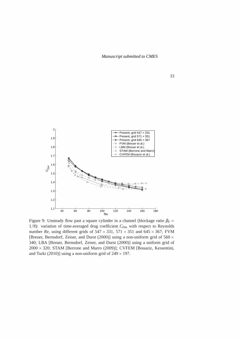
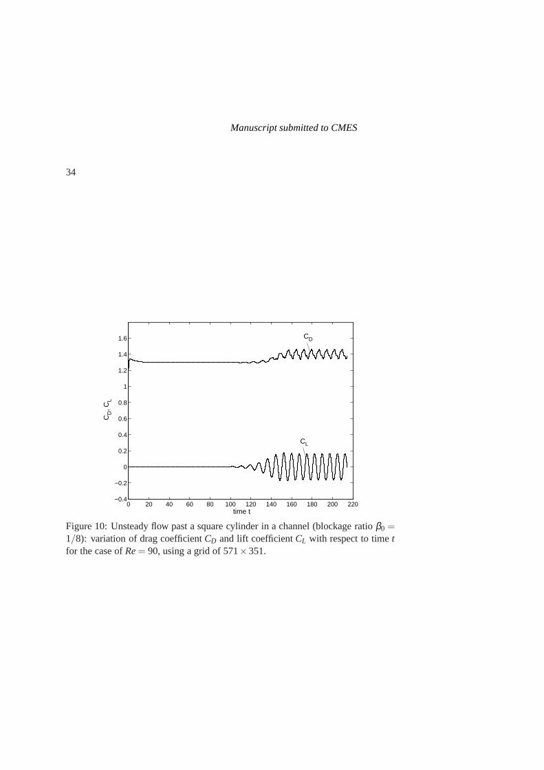
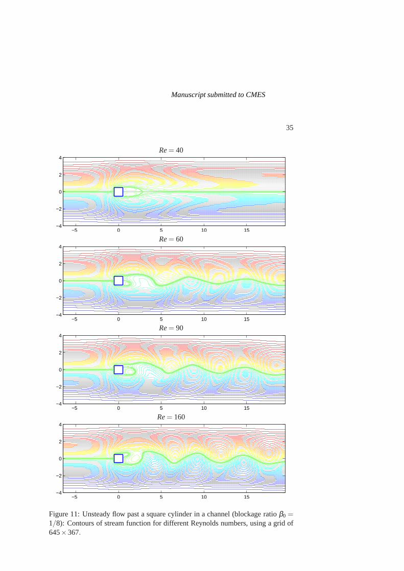
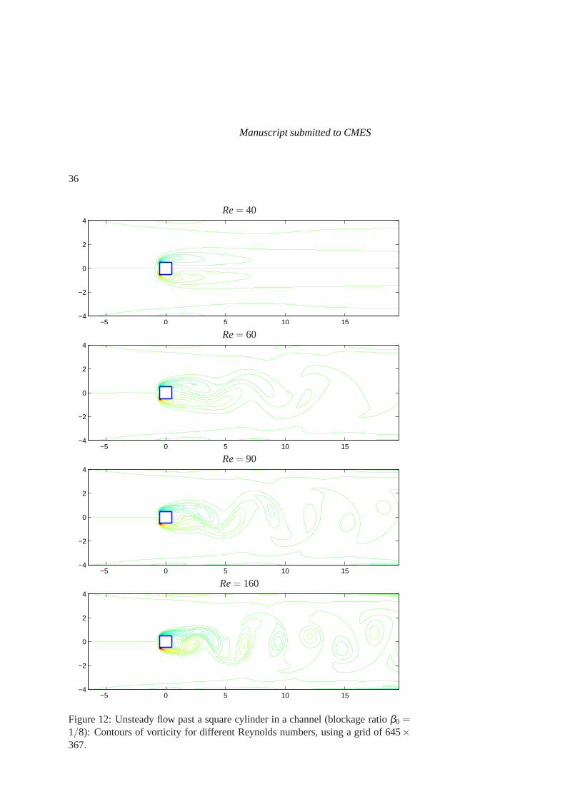
Figs. 8 and 9 respectively present variations of Strouhal numberStand time-averageddrag coefficientCDm with respect to Reynolds number for the case of blockage ra-tio of 1/8 and using different grids of 547× 331, 571× 351 and 645× 367. Theobtained numerical results are compared with the results ofFVM [Breuer, Berns-dorf, Zeiser, and Durst (2000)] both using a non-uniform grid of 560×340, lattice-Boltzmann automata (LBA) method [Breuer, Bernsdorf, Zeiser, and Durst (2000)]using a uniform grid of 2000×320, space-time adaptive method (STAM) [Berroneand Marro (2009)] and control volume finite element method (CVFEM) [Bouaziz,Kessentini, and Turki (2010)] using a non-uniform grid of 249×197. It can be seenthat the present numerical results at three different gridsare slightly different and ingood agreement with the results of other methods. Fig. 10 shows variations of dragand lift coefficients with respect to timet for the case ofRe= 90,β0 = 1/8 and us-ing a grid of 571×351. It can be seen that those coefficients vary periodicallyaftera certain time. The contours of stream function and vorticity for different Reynoldsnumbers (Re= 40,60,90 and 160) andβ0 = 1/8 are depicted in Figs. 11 and 12,respectively. The well-known von Karman vortices generatebehind the cylinderperiodically when a critical Reynolds number (Re≈ 60) is exceeded.

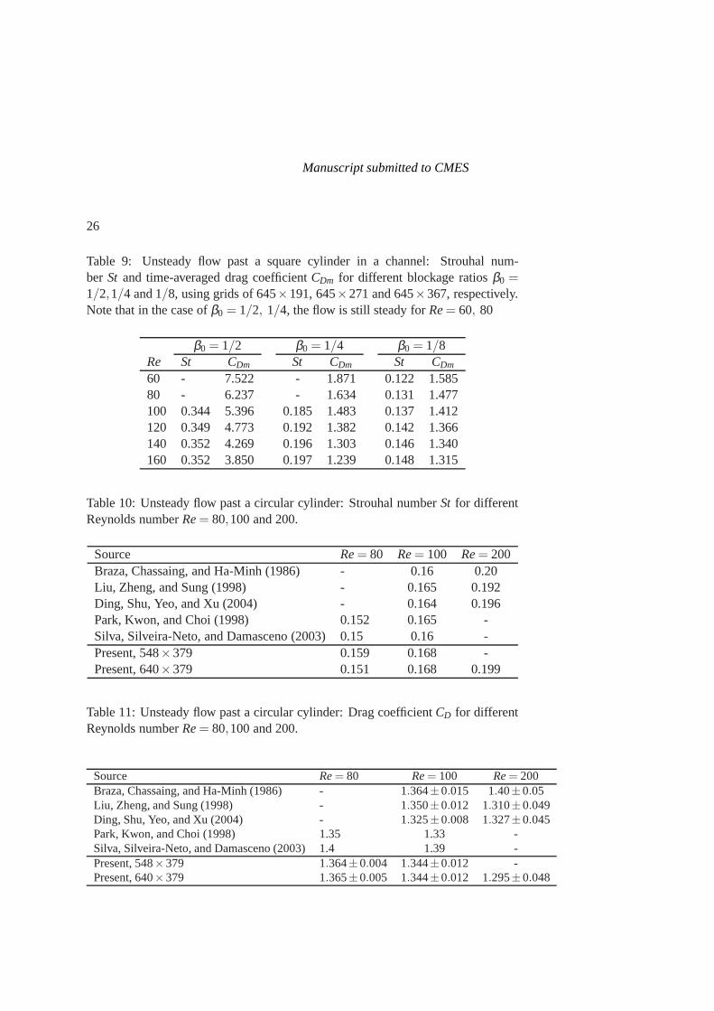
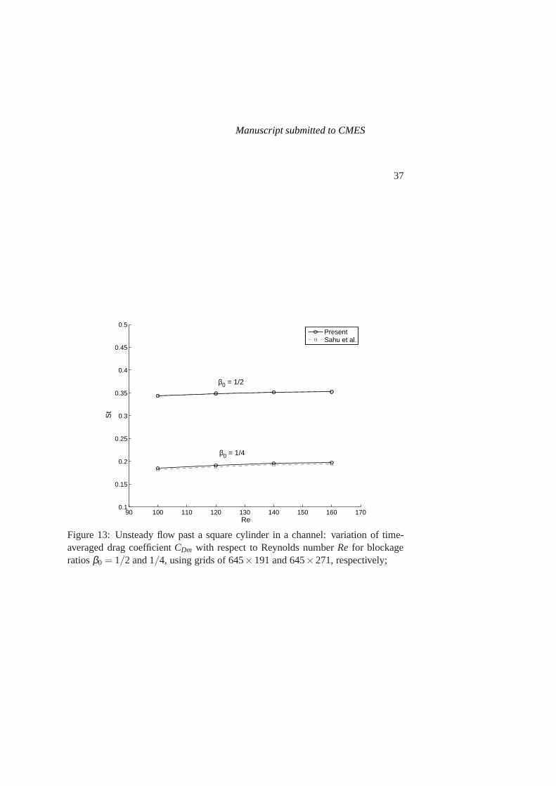
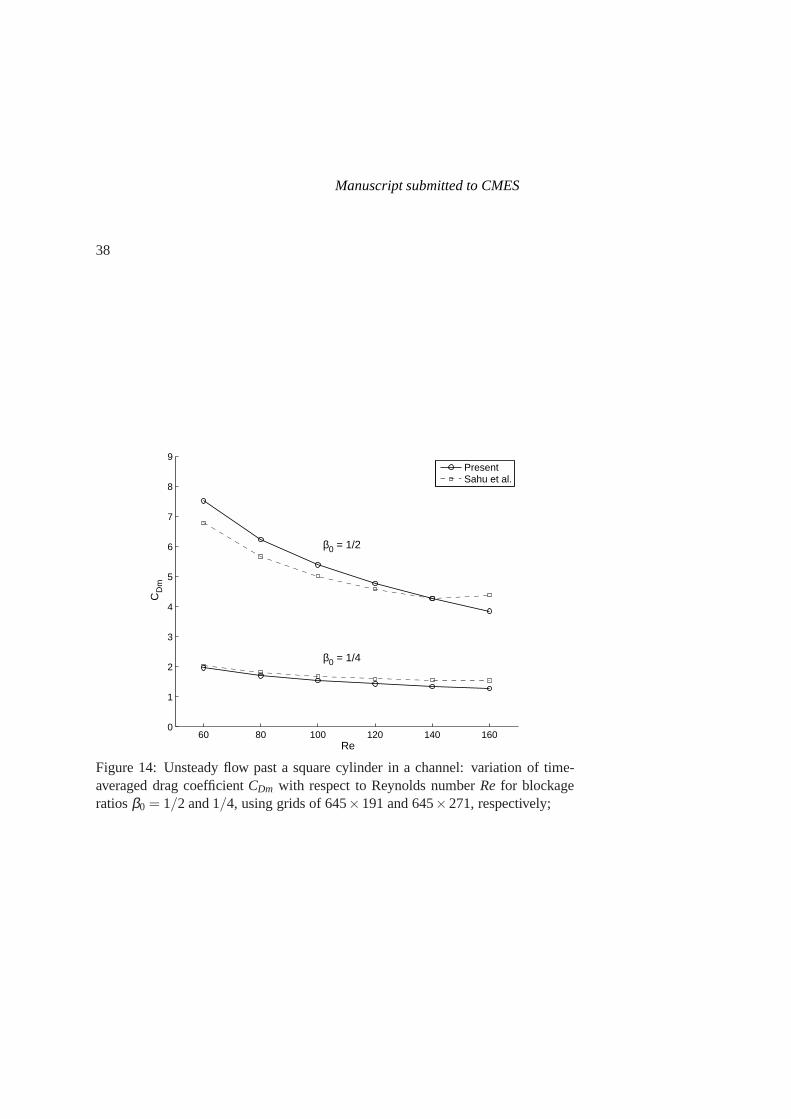
Tab. 9 presents Strouhal numberStand time-averaged drag coefficientCDm for sev-eral Reynolds numbers (60≤ Re≤ 160) and blockage ratios (β0 = 1/2,1/4 and1/8). It is noted that in the cases ofβ0 = 1/2 and 1/4, the flow is still steadyfor Re= 60 and 80. The influences of Reynolds number on the Strouhal num-ber St and time-averaged drag coefficientCDm for blockage ratios (β0 = 1/2 and1/4) are described in Figs. 13 and 14, respectively. It can be seen that Reynoldsnumber has a very weak influence on the Strouhal number for those cases, and thetime-averaged drag coefficient decreases with increasing Reynolds number up to


14

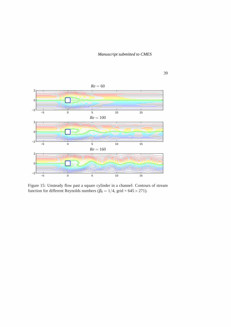
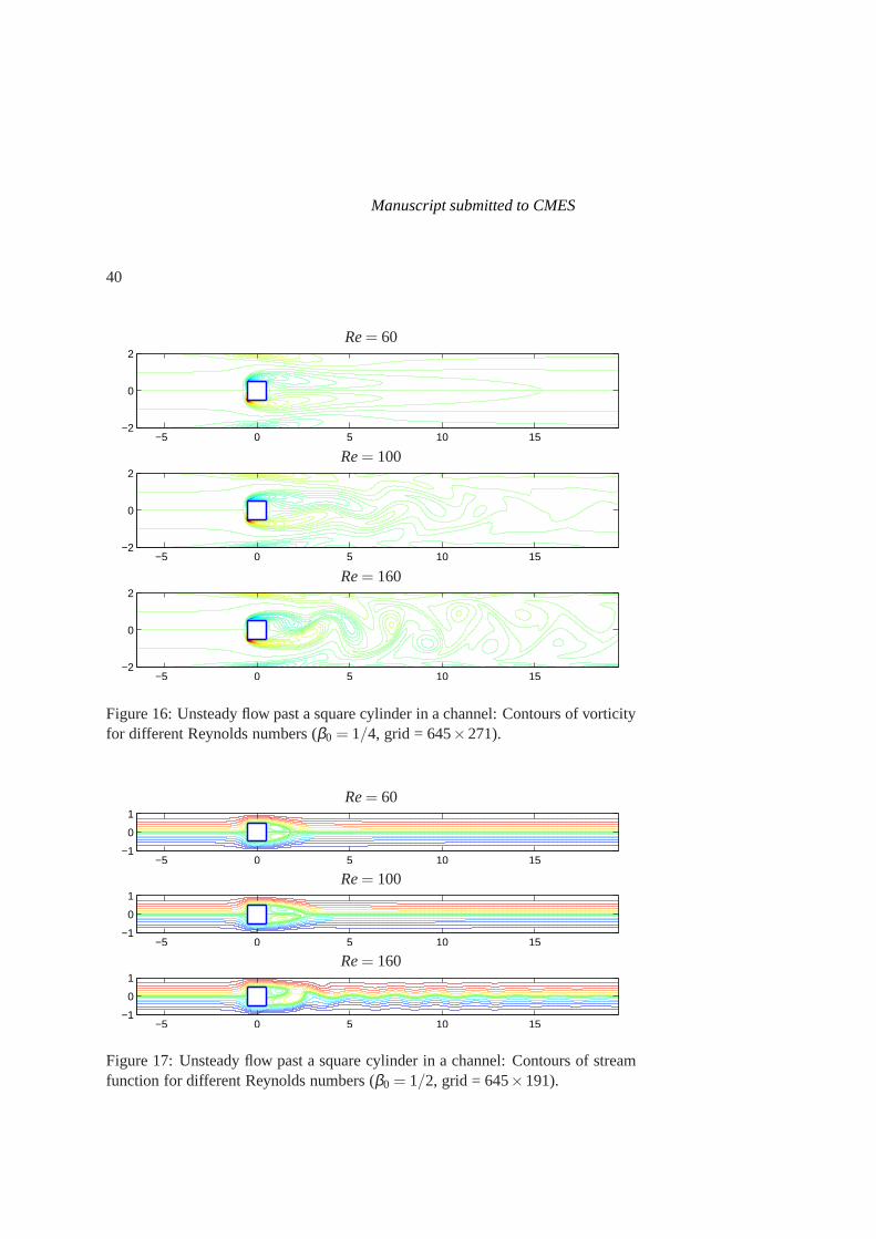
160. Figs. 15 and 16 presents the contours of stream functionand vorticity of flowfield around the square cylinder in a channel with blockage ratio of 1/4, while thecorresponding contours for the case of blockage ratio of 1/2 are given in Figs. 17and 18. Figs. 11, 15 and 17 indicate that the critical Reynolds number (at whichthe flow becomes unsteady) increases with increasing blockage ratio. For example,at Re= 60, the flow becomes unsteady in the case ofβ0 = 1/8, but is still steadyin the case ofβ0 = 1/4. At Re= 100, the flow becomes unsteady in the case ofβ0 = 1/4, but remains nearly steady in the case ofβ0 = 1/2. The numerical resultsobtained are in good agreement with those of Sahu, Chhabra, and Eswaran (2010)who used the semi-explicit FEM.

4.3 Example 3: Unsteady flows past a circular cylinder

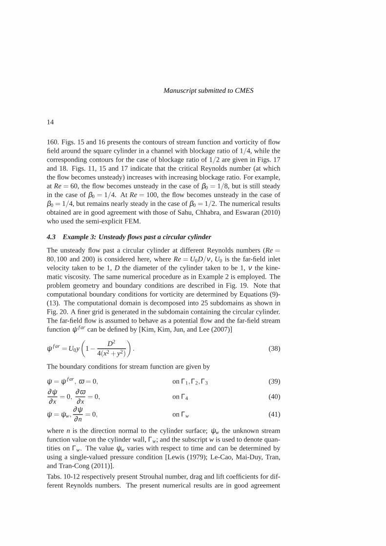
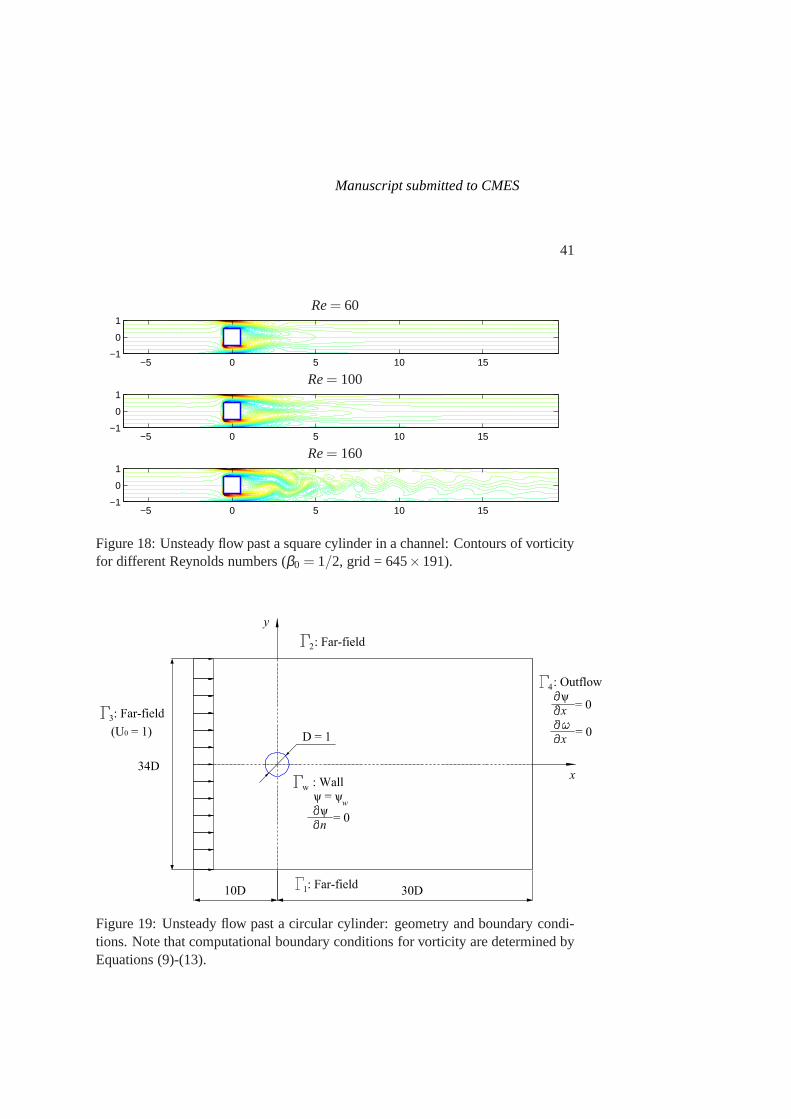
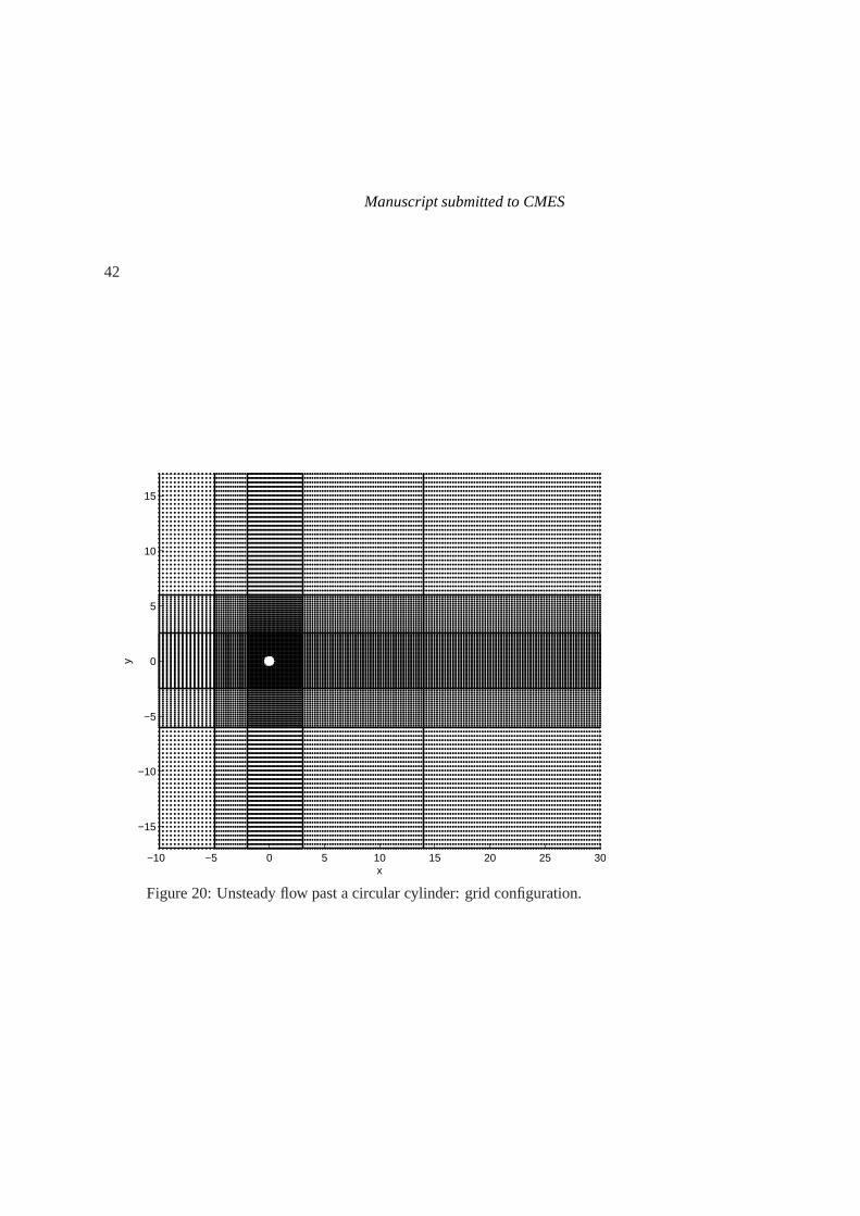
The unsteady flow past a circular cylinder at different Reynolds numbers (Re=80,100 and 200) is considered here, whereRe= U0D/ν , U0 is the far-field inletvelocity taken to be 1,D the diameter of the cylinder taken to be 1,ν the kine-matic viscosity. The same numerical procedure as in Example2 is employed. Theproblem geometry and boundary conditions are described in Fig. 19. Note thatcomputational boundary conditions for vorticity are determined by Equations (9)-(13). The computational domain is decomposed into 25 subdomains as shown inFig. 20. A finer grid is generated in the subdomain containingthe circular cylinder.The far-field flow is assumed to behave as a potential flow and the far-field streamfunctionψ f ar can be defined by [Kim, Kim, Jun, and Lee (2007)]

ψ f ar =U0y

(

1−D2

4(x2+y2)

)

. (38)

The boundary conditions for stream function are given by

ψ = ψ f ar, ω = 0, onΓ1,Γ2,Γ3 (39)

∂ψ∂x

= 0,∂ω∂x

= 0, onΓ4 (40)

ψ = ψw,∂ψ∂n

= 0, onΓw (41)

wheren is the direction normal to the cylinder surface;ψw the unknown streamfunction value on the cylinder wall,Γw; and the subscriptw is used to denote quan-tities onΓw. The valueψw varies with respect to time and can be determined byusing a single-valued pressure condition [Lewis (1979); Le-Cao, Mai-Duy, Tran,and Tran-Cong (2011)].

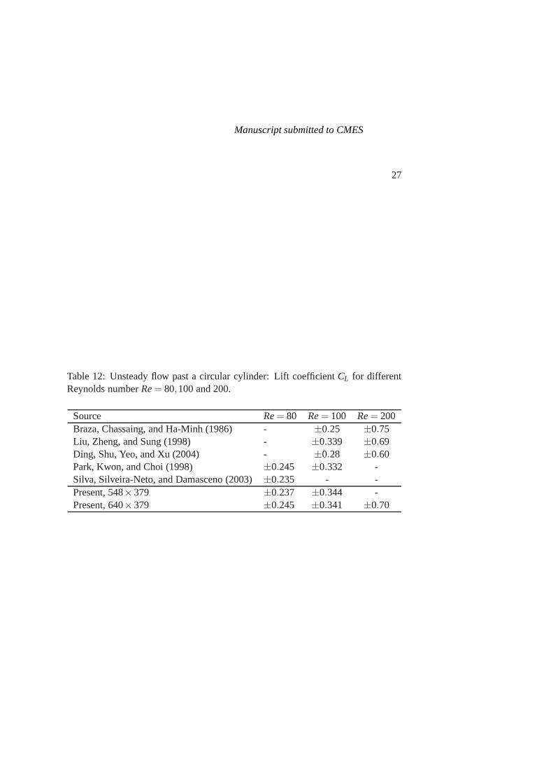
Tabs. 10-12 respectively present Strouhal number, drag andlift coefficients for dif-ferent Reynolds numbers. The present numerical results arein good agreement


15

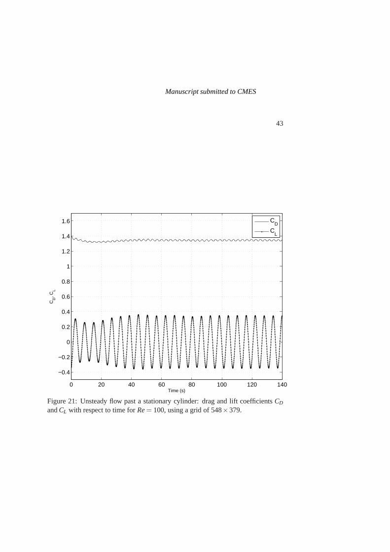
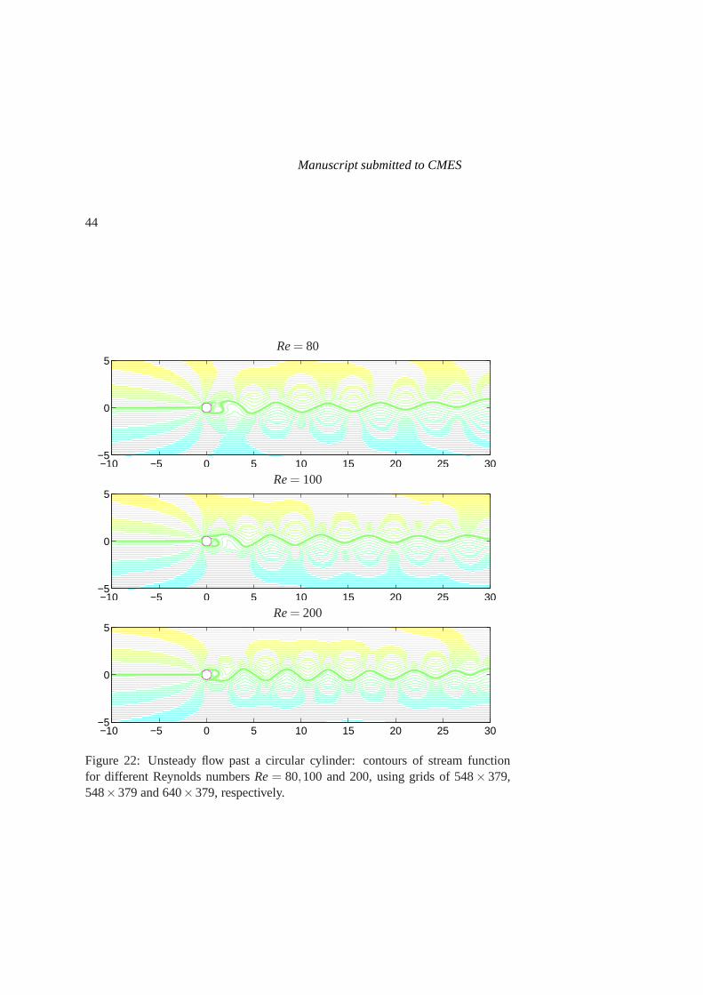
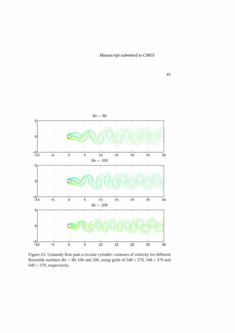
with the published results of other authors. Fig. 21 presents the variations of dragand lift coefficients with respect to time forRe= 100. The periodic variations ofthese coefficients are observed as time goes on. The contoursof stream functionand vorticity of the flow field around the circular cylinder atdifferent Reynoldsnumbers are provided in Figs. 22 and 23, respectively. With increasing Reynoldsnumber, the vortex shedding frequency increases and the vortices become smaller.

5 Conclusions

A new numerical procedure based on the local MLS-1D-IRBFN method is pre-sented for time-dependent problems. The numerical resultsfor Burgers’ equationindicate that the LMLS-1D-IRBFN approach yields the same level of accuracy asthe 1D-IRBFN method, while the system matrix is more sparse than that of the1D-IRBFN, which helps reduce the computational cost significantly. The LMLS-1D-IRBFN shape function possesses the Kronecker-δ property which allows anexact imposition of the essential boundary condition. Cartesian grids are employedto discretise both regular and irregular problem domains. The combination of thepresent numerical procedure and a domain decomposition technique is success-fully developed for simulating steady and unsteady flows past a square cylinderin a horizontal channel with different blockage ratios and unsteady flows past acircular cylinder. The influence of blockage ratio on the characteristics of flowpast a square cylinder in a channel is investigated for a range of Reynolds num-bers (60≤ Re≤ 160) and several blockage ratios (β0 = 1/2,1/4 and 1/8). Theobtained numerical results indicate that (i) the critical Reynolds number (at whichthe flow becomes unsteady) increases with increasing blockage ratio; (ii) time-averaged drag coefficient decreases with increasing Reynolds number up to 160;and (iii) the Reynolds number has a very weak influence on the Strouhal numberfor the cases ofβ0 = 1/2 and 1/4.

Acknowledgement: This research is supported by the University of SouthernQueensland, Australia through a USQ Postgraduate ResearchScholarship awardedto D. Ngo-Cong.

References

Babuska, I.; Melenk, J. M. (1997): The partition of unity method.InternationalJournal for Numerical Methods in Engineering, vol. 40, pp. 727–758.

Berrone, S.; Marro, M. (2009): Sapce-time adaptive simulations for unsteadyNavier-Stokes problems.Computers & Fluids, vol. 38, pp. 1132–1144.


16

Bouaziz, M.; Kessentini, S.; Turki, S.(2010): Numerical prediction of flow andheat transfer of power-law fluids in a plane channel with a built-in heated squarecylinder. International Journal of Heat and Mass Transfer, vol. 53, pp. 5420–5429.

Braza, M.; Chassaing, P.; Ha-Minh, H. (1986): Numerical study and physicalanalysis of the pressure and velocity fields in the near wake of a circular cylinder.The Journal of Fluid Mechanics, vol. 165, pp. 79–130.

Breuer, M.; Bernsdorf, J.; Zeiser, T.; Durst, F. (2000): Accurate computationsof the laminar flow past a square cylinder based on two different methods: lattice-Boltzmann and finite-volume.International Journal of Heat and Fluid Flow, vol.21, pp. 186–196.

Caldwell, J.; Wanless, P.; Cook, A. E.(1987): Solution of Burgers’ equationfor large Reynolds number using finite elements with moving nodes. AppliedMathematical Modelling, vol. 11, pp. 211–227.

Chen, J. S.; Hu, W.; Hu, H. Y. (2008): Reproducing kernel enhanced localradial basis collocation method.International Journal for Numerical Methods inEngineering, vol. 75, pp. 600–627.

Cheng, M.; Liu, G. R.; Lam, K. Y. (2001): Numerical simulation of flow past arotationally oscillating cylinder.Computer & Fluids, vol. 30, pp. 365–392.

Cole, J. D.(1951): On a quasi-linear parabolic equation occuring in aerodynamics.Quarterly Journal of Applied Mathematics, vol. 9, pp. 225–236.

Davis, R. W.; Moore, E. F. (1982): A numerical study of vortex shedding fromrectangles.The Journal of Fluid Mechanics, vol. 116, pp. 475–506.

Dhiman, A. K.; Chhabra, R. P.; Eswaran, V. (2005): Flow and heat transferacross a confined square cylinder in the steady flow regime: Effect of Peclet num-ber. International Journal of Heat and Mass Transfer, vol. 48, pp. 4598–4614.

Dhiman, A. K.; Chhabra, R. P.; Eswaran, V. (2008): Steady mixed convectionacross a confined square cylinder.International Communications in Heat andMass Transfer, vol. 35, pp. 47–55.

Ding, H.; Shu, C.; Yeo, K. S.; Xu, D. (2004): Simulation of incompressibleviscous flows past a circular cylinder by hybrid FD scheme andmeshless leastsquare-based finite difference method.Computer Methods in Applied Mechanicsand Engineering, vol. 193, pp. 727–744.


17

Ding, H.; Shu, C.; Yeo, K. S.; Xu, D. (2007): Numerical simulation of flowsaround two circular cylinders by mesh-free least square-based finite differencemethods. International Journal for Numerical Methods in Fluids, vol. 53, pp.305–332.

Gupta, A. K.; Sharma, A.; Chhabra, R. P.; Eswaran, V. (2003): Two-dimensional steady flow of a power-law fluid past a square cylinder in a planechannel: Momentum and heat-transfer characteristics.Industrial & EngineeringChemistry Research, vol. 42, pp. 5674–5686.

Hashemian, A.; Shodja, H. M. (2008): A meshless approach for solution ofBurgers’ equation.Journal of Computational and Applied Mathematics, vol. 220,pp. 226–239.

Hassanien, I. A.; Salama, A. A.; Hosham, H. A.(2005): Fourth-order finitedifference method for solving Burgers’ equation.Applied Mathematics and Com-putation, vol. 170, pp. 781–800.

Hon, Y. C.; Mao, X. Z. (1998): An efficient numerical scheme for Burgers’equation. Applied Mathematics and Computation, vol. 97, pp. 37–50.

Hosseini, B.; Hashemi, R.(2011): Solution of Burgers’ equation using a local-RBF meshless method.International Journal for Computational Methods in En-gineering Science and Mechanics, vol. 12, pp. 44–58.

Iskander, L.; Mohsen, A. (1992): Some numerical experiments on splitting ofBurgers’ equation. Numerical Methods for Partial Differential Equations, vol. 8,pp. 267–276.

Kansa, E. J. (1990): Multiquadrics - A Scattered Data Approximation Schemewith Applications to Computational Fulid-Dynamics - II: Solutions to parabolic,Hyperbolic and Elliptic Partial Differential Equations.Computers & Mathematicswith Applications, vol. 19 (8-9), pp. 147–161.

Kim, Y.; Kim, D. W.; Jun, S.; Lee, J. H. (2007): Meshfree point collocationmethod for the stream-vorticity formulation of 2D incompressible Navier-Stokesequations. Computer Methods in Applied Mechanics and Engineering, vol. 196,pp. 3095–3109.

Le, P. B. H.; Rabczuk, T.; Mai-Duy, N.; Tran-Cong, T. (2010): A movingIRBFN-based integration-free meshless method.CMES: Computer Modeling inEngineering & Sciences, vol. 61 (1), pp. 63–109.


18

Le-Cao, K.; Mai-Duy, N.; Tran, C.-D.; Tran-Cong, T. (2011): Numerical studyof stream-function formulation governing flows in multiply-connected domains byintegrated RBFs and Cartesian grids.Computers & Fluids, vol. 44 (1), pp. 32–42.

Le-Cao, K.; Mai-Duy, N.; Tran-Cong, T. (2009): An effective integrated-RBFNCartesian-grid discretization for the stream function-vorticity-temperature formu-lation in nonrectangular domains.Numerical Heat Transfer, Part B, vol. 55, pp.480–502.

Lewis, E. (1979): Steady flow between a rotating circular cylinder andfixedsquare cylinder.The Journal of Fluid Mechanics, vol. 95 (3), pp. 497–513.

Liu, C.; Zheng, Z.; Sung, C. H. (1998): Preconditioned multigrid methods forunsteady incompressible flows.Journal of Computational Physics, vol. 139, pp.35–57.

Liu, G. R. (2003): Meshfree Methods: Moving Beyond the Finite ElementMethod. CRC Press, London.

Mai-Duy, N.; Tanner, R. I. (2007): A Collocation Method based on One-Dimensional RBF Interpolation Scheme for Solving PDEs.International Journalof Numerical Methods for Heat & Fluid Flow, vol. 17 (2), pp. 165–186.

Mai-Duy, N.; Tran-Cong, T. (2001): Numerical solution of differential equationsusing multiquadric radial basis function networks.Neural Networks, vol. 14, pp.185–199.

Mai-Duy, N.; Tran-Cong, T. (2001): Numerical Solution of Navier-Stokes Equa-tions using Multiquadric Radial Basis Function Networks.International Journalfor Numerical Methods in Fluids, vol. 37, pp. 65–86.

Moussaoui, M. A.; Jami, M.; Mezrhab, A.; Naji, H. (2010): MRT-LatticeBolztmann simulation of forced convection in a plane channel with an inclinedsquare cylinder.International Journal of Thermal Sciences, vol. 49, pp. 131–142.

Ngo-Cong, D.; Mai-Duy, N.; Karunasena, W.; Tran-Cong, T. (2011): Freevibration analysis of laminated composite plates based on FSDT using one-dimensional IRBFN method.Computers & Structures, vol. 89, pp. 1–13.

Ngo-Cong, D.; Mai-Duy, N.; Karunasena, W.; Tran-Cong, T.(2012): LocalMoving Least Square - One-Dimensional IRBFN Technique for IncompressibleViscous Flows. International Journal for Numerical Methods in Fluids, pg. (pub-lished online 9/Jan/2012 DOI: 10.1002/fld.3640).


19

Park, J.; Kwon, K.; Choi, H. (1998): Numerical solutions of flow past a circularcylinder at Reynolds numbers up to 160.KSME International Journal, vol. 12 (6),pp. 1200–1205.

Quarteroni, A.; Valli, A. (1999): Domain Decomposition Methods for PartialDifferential Equations. Clarendon Press, Oxford.

Russell, D.; Wang, Z. J.(2003): A Cartesian grid method for modeling multiplemoving objects in 2D incompressible viscous flow.Journal of ComputationalPhysics, vol. 191, pp. 177–205.

Sahu, A. K.; Chhabra, R. P.; Eswaran, V.(2010): Two-dimensional laminarflow of a power-law fluid across a confined square cylinder.Journal of Non-Newtonian Fluid Mechanics, vol. 165, pp. 752–763.

Sanyasiraju, Y. V. S. S.; Chandhini, G.(2008): Local radial basis function basedgridfree scheme for unsteady incompressible viscous flows.Journal of Computa-tional Physics, vol. 227, pp. 8922–8948.

Shu, C.; Ding, H.; Yeo, K. S.(2003): Local radial basis function-based differen-tial quadrature method and its application to solve two-dimensional incompressibleNavier-Stokes equations.Computer Methods in Applied Mechanics and Engineer-ing, vol. 192, pp. 941–954.

Shu, C.; Ding, H.; Yeo, K. S.(2005): Computation of Incompressible Navier-Stokes equations by local RBF-based differential quadrature method.CMES: Com-puter Modeling in Engineering & Sciences, vol. 7 (2), pp. 195–205.

Silva, A. L. F. L. E.; Silveira-Neto, A.; Damasceno, J. J. R.(2003): Numericalsimulation of two-dimensional flows over a circular cylinder using the immersedboundary method.Journal of Computational Physics, vol. 189, pp. 351–370.

Sohankar, A.; Norberg, C.; Davidson, L. (1998): Low-Reynolds-number flowaround a square cylinder at incidence: study of blockage, onset of vortex sheddingand outlet boundary condition.International Journal for Numerical Methods inFluids, vol. 26, pp. 39–56.

Turki, S.; Abbassi, H.; Nasrallah, S. B. (2003): Two-dimensional laminarfluid flow and heat transfer in a channel with a built-in heatedsquare cylinder.International Journal of Thermal Sciences, vol. 42, pp. 1105–1113.

Udaykumar, H. S.; Mittal, R.; Rampunggoon, P.; Khanna, A. (2001): Asharp interface Cartesian grid method for simulating flows with complex movingboundaries.Journal of Computational Physics, vol. 174, pp. 345–380.


20

Vertnik, R.; Šarler, B. (2006): Meshless local radial basis function collocationmethod for convective-diffusive solid-liquid phase change problems.InternationalJournal of Numerical Methods for Heat and Fluid Flow, vol. 16, pp. 617–640.

Zaki, T. G.; Sen, M.; el Hak, M. G. (1994): Numerical and experimental in-vestigation of flow past a freely rotatable square cylinder.Journal of Fluids andStructures, vol. 8, pp. 555–582.

Zheng, Z. C.; Zhang, N.(2008): Frequency effects on lift and drag for flow pastan oscillating cylinder.Journal of Fluids and Structures, vol. 24, pp. 382–399.


21

Table 1: Burgers’ equations, approximation of shock wave propagation: compari-son of numerical results and exact solution att = 1.0 for Re= 100 and several timestep sizes, using a grid of 61. (1) 1D-IRBFN, (2) LMLS-1D-IRBFN

dt = 10−2 dt = 10−3 dt = 10−4

x Exact (1) (2) (1) (2) (1) (2)0.000 1.0000 1.0000 1.0000 1.0000 1.0000 1.0000 1.00000.056 1.0000 1.0000 1.0000 1.0000 1.0000 1.0000 1.00000.111 1.0000 1.0000 1.0000 1.0000 1.0000 1.0000 1.00000.167 1.0000 1.0000 1.0000 1.0000 1.0000 1.0000 1.00000.222 0.9998 1.0000 1.0000 0.9999 0.9998 0.9998 0.99980.278 0.9978 1.0000 0.9999 0.9983 0.9982 0.9980 0.99790.333 0.9801 0.9991 0.9988 0.9829 0.9831 0.9808 0.98100.389 0.8473 0.9153 0.9145 0.8545 0.8547 0.8495 0.84960.444 0.4518 0.4516 0.4526 0.4533 0.4539 0.4533 0.45390.500 0.2379 0.2387 0.2383 0.2382 0.2379 0.2381 0.23790.556 0.2043 0.2050 0.2050 0.2044 0.2044 0.2043 0.20430.611 0.2005 0.2006 0.2006 0.2005 0.2005 0.2005 0.20050.667 0.2001 0.2001 0.2001 0.2001 0.2001 0.2001 0.20010.722 0.2000 0.2000 0.2000 0.2000 0.2000 0.2000 0.20000.778 0.2000 0.2000 0.2000 0.2000 0.2000 0.2000 0.20000.833 0.2000 0.2000 0.2000 0.2000 0.2000 0.2000 0.20000.889 0.2000 0.2000 0.2000 0.2000 0.2000 0.2000 0.20000.944 0.2000 0.2000 0.2000 0.2000 0.2000 0.2000 0.20001.000 0.2000 0.2000 0.2000 0.2000 0.2000 0.2000 0.2000Ne 2.45E-02 2.42E-02 2.75E-03 2.86E-03 9.51E-04 1.12E-03


22

Table 2: Burgers’ equations, approximation of shock wave propagation: grid con-vergence study of numerical results forRe= 100, t = 1.0, and∆t = 10−3. (1)1D-IRBFN, (2) LMLS-1D-IRBFN

nx = 41 nx = 61 nx = 81x Exact (1) (2) (1) (2) (1) (2)0.000 1.0000 1.0000 1.0000 1.0000 1.0000 1.0000 1.00000.056 1.0000 1.0000 1.0000 1.0000 1.0000 1.0000 1.00000.111 1.0000 1.0000 1.0000 1.0000 1.0000 1.0000 1.00000.167 1.0000 1.0000 1.0000 1.0000 1.0000 1.0000 1.00000.222 0.9998 0.9999 0.9998 0.9999 0.9998 0.9999 0.99980.278 0.9978 0.9983 0.9979 0.9983 0.9982 0.9983 0.99830.333 0.9801 0.9829 0.9848 0.9829 0.9831 0.9829 0.98290.389 0.8473 0.8546 0.8554 0.8545 0.8547 0.8545 0.85460.444 0.4518 0.4534 0.4552 0.4533 0.4539 0.4533 0.45350.500 0.2379 0.2381 0.2372 0.2382 0.2379 0.2382 0.23810.556 0.2043 0.2044 0.2043 0.2044 0.2044 0.2044 0.20440.611 0.2005 0.2005 0.2005 0.2005 0.2005 0.2005 0.20050.667 0.2001 0.2001 0.2001 0.2001 0.2001 0.2001 0.20010.722 0.2000 0.2000 0.2000 0.2000 0.2000 0.2000 0.20000.778 0.2000 0.2000 0.2000 0.2000 0.2000 0.2000 0.20000.833 0.2000 0.2000 0.2000 0.2000 0.2000 0.2000 0.20000.889 0.2000 0.2000 0.2000 0.2000 0.2000 0.2000 0.20000.944 0.2000 0.2000 0.2000 0.2000 0.2000 0.2000 0.20001.000 0.2000 0.2000 0.2000 0.2000 0.2000 0.2000 0.2000Ne 2.78E-03 3.48E-03 2.75E-03 2.86E-03 2.75E-03 2.78E-03


23

Table 3: Burgers’ equations, sinusoidal initial condition: comparison among thenumerical results of LMLS-1D-IRBFN and Local-RBF [Hosseini and Hashemi(2011)] and the analytical solution forRe= 10,∆t = 10−3.

nx = 9 nx = 33 nx = 57 nx = 81x t Exact Present Local-RBF Present Local-RBF Present Local-RBF Present0.25 0.4 0.30889 0.30820 0.30817 0.30838 0.30821 0.30838 0.30862 0.30839

0.6 0.24074 0.24025 0.24026 0.24040 0.24030 0.24040 0.24059 0.240400.8 0.19568 0.19556 0.19533 0.19543 0.19537 0.19543 0.19560 0.195431.0 0.16256 0.16291 0.16230 0.16238 0.16234 0.16238 0.16253 0.162383.0 0.02720 0.02762 0.02714 0.02720 0.02716 0.02720 0.02723 0.02720

0.50 0.4 0.56963 0.57036 0.56861 0.56896 0.56867 0.56896 0.56929 0.568960.6 0.44721 0.44865 0.44643 0.44670 0.44651 0.44669 0.44701 0.446690.8 0.35924 0.36150 0.35863 0.35886 0.35871 0.35885 0.35913 0.358851.0 0.29192 0.29463 0.29142 0.29163 0.29150 0.29162 0.29187 0.291623.0 0.04021 0.04081 0.04011 0.04020 0.04015 0.04020 0.04025 0.04020

0.75 0.4 0.62544 0.62926 0.62486 0.62515 0.62496 0.62511 0.62540 0.625110.6 0.48721 0.49318 0.48646 0.48695 0.48658 0.48691 0.48712 0.486910.8 0.37392 0.37992 0.37322 0.37371 0.37333 0.37369 0.37385 0.373691.0 0.28747 0.29251 0.28688 0.28732 0.28698 0.28731 0.28744 0.287313.0 0.02977 0.03021 0.02970 0.02977 0.02973 0.02977 0.02981 0.02977

Table 4: Burgers’ equations, sinusoidal initial condition: comparison among thenumerical results of LMLS-1D-IRBFN and Local-RBF [Hosseini and Hashemi(2011)] and the analytical solution forRe= 100,∆t = 10−3.

nx = 9 nx = 33 nx = 57 nx = 81x t Exact Present Local-RBF Present Local-RBF Present Local-RBF Present0.25 0.4 0.34191 0.33414 0.33395 0.34114 0.33396 0.34114 0.33794 0.34114

0.6 0.26896 0.26353 0.26328 0.26841 0.26328 0.26841 0.26613 0.268410.8 0.22148 0.21759 0.21722 0.22107 0.21723 0.22107 0.21936 0.221071.0 0.18819 0.18523 0.18488 0.18787 0.18489 0.18787 0.18655 0.187873.0 0.07511 0.07416 0.07438 0.07504 0.07438 0.07504 0.07476 0.07504

0.50 0.4 0.66071 0.64995 0.64907 0.65961 0.64908 0.65961 0.65496 0.659610.6 0.52942 0.51822 0.51971 0.52848 0.51972 0.52849 0.52461 0.528490.8 0.43914 0.42785 0.43139 0.43839 0.43140 0.43839 0.43530 0.438391.0 0.37442 0.36512 0.36820 0.37381 0.36821 0.37381 0.37134 0.373813.0 0.15018 0.14802 0.14872 0.15003 0.14873 0.15004 0.14947 0.15004

0.75 0.4 0.91026 0.85640 0.90742 0.91011 0.90749 0.91014 0.90905 0.910150.6 0.76724 0.65947 0.75810 0.76643 0.75814 0.76643 0.76282 0.766430.8 0.64740 0.55693 0.63810 0.64651 0.63812 0.64652 0.64284 0.646521.0 0.55605 0.48796 0.54787 0.55524 0.54789 0.55527 0.55202 0.555273.0 0.22481 0.20834 0.22261 0.22449 0.22265 0.22459 0.22376 0.22459


24

Table 5: Burgers’ equations, sinusoidal initial condition: comparison among nu-merical results and exact solution forRe= 10000,∆t = 10−4, using a grid of 301.

x Exact Caldwell, Wanless Iskander and Hon and Presentand Cook (1987) Mohsen (1992) Mao (1998)

0.056 0.0422 0.0422 0.0419 0.0424 0.04210.111 0.0843 0.0844 0.0839 0.0843 0.08420.167 0.1263 0.1266 0.1253 0.1263 0.12630.222 0.1684 0.1687 0.1692 0.1684 0.16830.278 0.2103 0.2108 0.2034 0.2103 0.21030.333 0.2522 0.2527 0.2666 0.2522 0.25210.389 0.2939 0.2946 0.2527 0.2939 0.29390.444 0.3355 0.3362 0.3966 0.3355 0.33550.500 0.3769 0.3778 0.2350 0.3769 0.37690.556 0.4182 0.4191 0.5480 0.4182 0.41820.611 0.4592 0.4601 0.2578 0.4592 0.45920.667 0.5000 0.5009 0.6049 0.4999 0.49990.722 0.5404 0.5414 0.6014 0.5404 0.54040.778 0.5806 0.5816 0.4630 0.5802 0.58050.833 0.6203 0.6213 0.7011 0.6201 0.62020.889 0.6596 0.6605 0.6717 0.6600 0.65950.944 0.6983 0.6992 0.7261 0.6957 0.6982

Table 6: Burgers’ equations, sinusoidal initial condition: comparison of numericalresults forRe= 10000,∆t = 10−4, using a grid of 301.

x Hassanien, Salama Hashemian and Hosseini and Presentand Hosham (2005) Shodja (2008) Hashemi (2011)

0.050 0.0379 0.0379 0.0379 0.03790.110 0.0834 0.0834 0.0833 0.08340.160 0.1213 0.1213 0.1212 0.12130.220 0.1667 0.1667 0.1666 0.16670.270 0.2044 0.2044 0.2044 0.20440.330 0.2469 0.2497 0.2496 0.24960.380 0.2872 0.2872 0.2871 0.28720.440 0.3322 0.3322 0.3321 0.33220.500 0.3769 0.3769 0.3768 0.37690.550 0.4140 0.4141 0.4140 0.41400.610 0.4584 0.4584 0.4583 0.45830.660 0.4951 0.4951 0.4950 0.49500.720 0.5388 0.5388 0.5387 0.53880.770 0.5749 0.5749 0.5748 0.57490.830 0.6179 0.6179 0.6178 0.61790.880 0.6533 0.6533 0.6530 0.65320.940 0.6952 0.6952 0.6890 0.6941


25

Table 7: Steady flow past a square cylinder in a channel: grid convergence study ofrecirculation lengthLr and drag coefficientCD for Re= 40.

Grid Lr CD

173×121 2.37 1.10211×151 2.29 1.31281×201 2.26 1.49351×251 2.25 1.57469×301 2.25 1.75493×305 2.25 1.79557×341 2.27 1.88571×351 2.27 1.89599×351 2.27 1.91645×367 2.27 1.92717×377 2.27 1.91Breuer, Bernsdorf, Zeiser, and Durst (2000) 2.15 1.70Gupta, Sharma, Chhabra, and Eswaran (2003) 1.90 1.86Dhiman, Chhabra, and Eswaran (2005) 2.17 1.75

Table 8: Steady flow past a square cylinder in a channel: comparison of recircula-tion lengthLr and drag coefficientCD, using a grid of 571×351.

Re Source Lsep CD

10 Breuer, Bernsdorf, Zeiser, and Durst (2000) 0.49 3.64Gupta, Sharma, Chhabra, and Eswaran (2003) 0.40 3.51Dhiman, Chhabra, and Eswaran (2005) 0.49 3.63Present 0.48 3.73





26

Table 9: Unsteady flow past a square cylinder in a channel: Strouhal num-ber St and time-averaged drag coefficientCDm for different blockage ratiosβ0 =1/2,1/4 and 1/8, using grids of 645×191, 645×271 and 645×367, respectively.Note that in the case ofβ0 = 1/2, 1/4, the flow is still steady forRe= 60, 80

β0 = 1/2 β0 = 1/4 β0 = 1/8Re St CDm St CDm St CDm

60 - 7.522 - 1.871 0.122 1.58580 - 6.237 - 1.634 0.131 1.477100 0.344 5.396 0.185 1.483 0.137 1.412120 0.349 4.773 0.192 1.382 0.142 1.366140 0.352 4.269 0.196 1.303 0.146 1.340160 0.352 3.850 0.197 1.239 0.148 1.315

Table 10: Unsteady flow past a circular cylinder: Strouhal numberSt for differentReynolds numberRe= 80,100 and 200.

Source Re= 80 Re= 100 Re= 200Braza, Chassaing, and Ha-Minh (1986) - 0.16 0.20Liu, Zheng, and Sung (1998) - 0.165 0.192Ding, Shu, Yeo, and Xu (2004) - 0.164 0.196Park, Kwon, and Choi (1998) 0.152 0.165 -Silva, Silveira-Neto, and Damasceno (2003) 0.15 0.16 -Present, 548×379 0.159 0.168 -Present, 640×379 0.151 0.168 0.199

Table 11: Unsteady flow past a circular cylinder: Drag coefficientCD for differentReynolds numberRe= 80,100 and 200.

Source Re= 80 Re= 100 Re= 200Braza, Chassaing, and Ha-Minh (1986) - 1.364±0.015 1.40±0.05Liu, Zheng, and Sung (1998) - 1.350±0.012 1.310±0.049Ding, Shu, Yeo, and Xu (2004) - 1.325±0.008 1.327±0.045Park, Kwon, and Choi (1998) 1.35 1.33 -Silva, Silveira-Neto, and Damasceno (2003) 1.4 1.39 -Present, 548×379 1.364±0.004 1.344±0.012 -Present, 640×379 1.365±0.005 1.344±0.012 1.295±0.048


27

Table 12: Unsteady flow past a circular cylinder: Lift coefficient CL for differentReynolds numberRe= 80,100 and 200.

Source Re= 80 Re= 100 Re= 200Braza, Chassaing, and Ha-Minh (1986) - ±0.25 ±0.75Liu, Zheng, and Sung (1998) - ±0.339 ±0.69Ding, Shu, Yeo, and Xu (2004) - ±0.28 ±0.60Park, Kwon, and Choi (1998) ±0.245 ±0.332 -Silva, Silveira-Neto, and Damasceno (2003)±0.235 - -Present, 548×379 ±0.237 ±0.344 -Present, 640×379 ±0.245 ±0.341 ±0.70


28

Figure 1: LMLS-1D-IRBFN scheme,� a typical[ j] node.


29

Figure 2: Flow past a square cylinder in a channel: geometry and boundary condi-tions. The blockage ratio is defined asβ0 = D/H. Note that computational bound-ary conditions for vorticity are determined by Equation (9).

−5 0 5 10 15−4

−2

0

2

4

x

y

Figure 3: Flow past a square cylinder in a channel: grid configuration.

Figure 4: Pressure and shear stress acting on the surface of asquare cylinder.


30

0 0.5 1 1.5 2 2.5 3

x 105

2

2.05

2.1

2.15

2.2

2.25

2.3

2.35

2.4

2.45

2.5

Number of nodes

Lr

Figure 5: Steady flow past a square cylinder in a channel: gridconvergence studyof recirculation lengthLr for Re= 40.

0 0.5 1 1.5 2 2.5 3

x 105

1

1.5

2

2.5

Number of nodes

CD

Figure 6: Steady flow past a square cylinder in a channel: gridconvergence studyof drag coefficientCD for Re= 40.


31

Re= 10

0.0010.1

0.20.4

−0.1−0.2−0.4

−2 0 2 4 6−2

−1

0

1

2

0

−0.5−1−1.5−2

0.511.52

−2 0 2 4 6−2

−1

0

1

2

Re= 20

−0.0010.001

0.050.1

0.20.4

−0.05−0.1−0.2−0.4

−2 0 2 4 6−2

−1

0

1

2

0

−0.5

0

−1

1 0.51.5

−1.5−2

2

−2 0 2 4 6−2

−1

0

1

2

Re= 30

−0.010.01

0.050.1

0.2

−0.05−0.1

−0.2

−2 0 2 4 6−2

−1

0

1

2

0 0

−0.5−1−1.5−2

0.511.52

−2 0 2 4 6−2

−1

0

1

2

Re= 40

−0.01

0.01

0.050.10.2

−0.05−0.1−0.2

−2 0 2 4 6−2

−1

0

1

2

0 0

−1−0.5

0

10.5

0

−1.5

1.5

−2

2

−2 0 2 4 6−2

−1

0

1

2

Figure 7: Steady flow past a square cylinder in a channel: contours of stream func-tion for different Reynolds numbers, using a grid of 571×351.


32

40 60 80 100 120 140 1600.1

0.11

0.12

0.13

0.14

0.15

0.16

Re

St

Present, grid 547 × 331Present, grid 571 × 351Present, grid 645 × 367FVM (Breuer et al.)LBM (Breuer et al.)STAM (Berrone and Marro)CVFEM (Bouaziz et al.)

Figure 8: Unsteady flow past a square cylinder in a channel (blockage ratioβ0 = 1/8): variation of Strouhal numberStwith respect to Reynolds numberRe, us-ing different grids of 547×331, 571×351 and 645×367; FVM [Breuer, Bernsdorf,Zeiser, and Durst (2000)] using a non-uniform grid of 560× 340; LBA [Breuer,Bernsdorf, Zeiser, and Durst (2000)] using a uniform grid of2000× 320; STAM[Berrone and Marro (2009)]; CVFEM [Bouaziz, Kessentini, and Turki (2010)] us-ing a non-uniform grid of 249×197.


33

40 60 80 100 120 140 160 1801.1

1.2

1.3

1.4

1.5

1.6

1.7

1.8

1.9

2

Re

CD

m

Present, grid 547 × 331Present, grid 571 × 351Present, grid 645 × 367FVM (Breuer et al.)LBM (Breuer et al.)STAM (Berrone and Marro)CVFEM (Bouaziz et al.)

Figure 9: Unsteady flow past a square cylinder in a channel (blockage ratioβ0 =1/8): variation of time-averaged drag coefficientCDm with respect to ReynoldsnumberRe, using different grids of 547× 331, 571× 351 and 645× 367; FVM[Breuer, Bernsdorf, Zeiser, and Durst (2000)] using a non-uniform grid of 560×340; LBA [Breuer, Bernsdorf, Zeiser, and Durst (2000)] using a uniform grid of2000× 320; STAM [Berrone and Marro (2009)]; CVFEM [Bouaziz, Kessentini,and Turki (2010)] using a non-uniform grid of 249×197.


34

0 20 40 60 80 100 120 140 160 180 200 220−0.4

−0.2

0

0.2

0.4

0.6

0.8

1

1.2

1.4

1.6

time t

CD

, CL

CD

CL

Figure 10: Unsteady flow past a square cylinder in a channel (blockage ratioβ0 =1/8): variation of drag coefficientCD and lift coefficientCL with respect to timetfor the case ofRe= 90, using a grid of 571×351.


35

Re= 40

−5 0 5 10 15−4

−2

0

2

4

Re= 60

−5 0 5 10 15−4

−2

0

2

4

Re= 90

−5 0 5 10 15−4

−2

0

2

4

Re= 160

−5 0 5 10 15−4

−2

0

2

4

Figure 11: Unsteady flow past a square cylinder in a channel (blockage ratioβ0 =1/8): Contours of stream function for different Reynolds numbers, using a grid of645×367.


36

Re= 40

−5 0 5 10 15−4

−2

0

2

4

Re= 60

−5 0 5 10 15−4

−2

0

2

4

Re= 90

−5 0 5 10 15−4

−2

0

2

4

Re= 160

−5 0 5 10 15−4

−2

0

2

4

Figure 12: Unsteady flow past a square cylinder in a channel (blockage ratioβ0 =1/8): Contours of vorticity for different Reynolds numbers, using a grid of 645×367.


37

90 100 110 120 130 140 150 160 1700.1

0.15

0.2

0.25

0.3

0.35

0.4

0.45

0.5

Re

St

β0 = 1/2

β0 = 1/4

PresentSahu et al.

Figure 13: Unsteady flow past a square cylinder in a channel: variation of time-averaged drag coefficientCDm with respect to Reynolds numberRe for blockageratiosβ0 = 1/2 and 1/4, using grids of 645×191 and 645×271, respectively;


38

60 80 100 120 140 1600

1

2

3

4

5

6

7

8

9

Re

CD

m

β0 = 1/2

β0 = 1/4

PresentSahu et al.

Figure 14: Unsteady flow past a square cylinder in a channel: variation of time-averaged drag coefficientCDm with respect to Reynolds numberRe for blockageratiosβ0 = 1/2 and 1/4, using grids of 645×191 and 645×271, respectively;


39

Re= 60

−5 0 5 10 15−2

0

2

Re= 100

−5 0 5 10 15−2

0

2

Re= 160

−5 0 5 10 15−2

0

2

Figure 15: Unsteady flow past a square cylinder in a channel: Contours of streamfunction for different Reynolds numbers (β0 = 1/4, grid = 645×271).


40

Re= 60

−5 0 5 10 15−2

0

2

Re= 100

−5 0 5 10 15−2

0

2

Re= 160

−5 0 5 10 15−2

0

2

Figure 16: Unsteady flow past a square cylinder in a channel: Contours of vorticityfor different Reynolds numbers (β0 = 1/4, grid = 645×271).

Re= 60

−5 0 5 10 15−1

0

1

Re= 100

−5 0 5 10 15−1

0

1

Re= 160

−5 0 5 10 15−1

0

1

Figure 17: Unsteady flow past a square cylinder in a channel: Contours of streamfunction for different Reynolds numbers (β0 = 1/2, grid = 645×191).


41

Re= 60

−5 0 5 10 15−1

0

1

Re= 100

−5 0 5 10 15−1

0

1

Re= 160

−5 0 5 10 15−1

0

1

Figure 18: Unsteady flow past a square cylinder in a channel: Contours of vorticityfor different Reynolds numbers (β0 = 1/2, grid = 645×191).

Figure 19: Unsteady flow past a circular cylinder: geometry and boundary condi-tions. Note that computational boundary conditions for vorticity are determined byEquations (9)-(13).


42

−10 −5 0 5 10 15 20 25 30

−15

−10

−5

0

5

10

15

x

y

Figure 20: Unsteady flow past a circular cylinder: grid configuration.


43

0 20 40 60 80 100 120 140

−0.4

−0.2

0

0.2

0.4

0.6

0.8

1

1.2

1.4

1.6

Time (s)

CD

, CL

CD

CL

Figure 21: Unsteady flow past a stationary cylinder: drag andlift coefficientsCD

andCL with respect to time forRe= 100, using a grid of 548×379.


44

Re= 80

−10 −5 0 5 10 15 20 25 30−5

0

5

Re= 100

−10 −5 0 5 10 15 20 25 30−5

0

5

Re= 200

−10 −5 0 5 10 15 20 25 30−5

0

5

Figure 22: Unsteady flow past a circular cylinder: contours of stream functionfor different Reynolds numbersRe= 80,100 and 200, using grids of 548× 379,548×379 and 640×379, respectively.


45

Re= 80

−10 −5 0 5 10 15 20 25 30−5

0

5

Re= 100

−10 −5 0 5 10 15 20 25 30−5

0

5

Re= 200

−10 −5 0 5 10 15 20 25 30−5

0

5

Figure 23: Unsteady flow past a circular cylinder: contours of vorticity for differentReynolds numbersRe= 80,100 and 200, using grids of 548×379, 548×379 and640×379, respectively.

part ii - unsteady incompressible viscous flows - core

Documents