1

PRELIMINARY STUDIES WITH PVM ON A HP-735 CLUSTER AND CM-5

FOR THE TIME DEPENDENT SOLUTION OF THE

INCOMPRESSIBLE NAVIER- STOKES EQUATIONS

- LAPLACE EQUATION

BY

WEICHENG HUANG1

AND

DANESH TAFTI

NATIONAL CENTER FOR SUPERCOMPUTING APPLICATIONS

UNIVERSITY OF ILLINOIS AT URBANA CHAMPAIGN

URBANA, ILLINOIS 61801

JANUARY 1994

1Aeronautical and Astronautical Department, University of Illinois Urbana-Champaign, Urbana, IL 61801.

2

ABSTRACT

A preliminary study was conducted with the message passing library PVM for the

iterative solution of a two-dimensional Laplace equation. A line iterative procedure and

Stone's strongly implicit solution procedure were tested in this environment as they have

direct applicability to the solution of the pressure-Poisson equation. The intent of this

study was not so much to study the solution of the Laplace equation as it was to establish

the necessary groundwork and to understand the issues involved in parallel programming

in a domain-decomposed environment for the incompressible Navier-Stokes equations.

Two machine configurations were looked at in this study, a 6 processor HP-735 cluster at

NCSA and a 512 processor CM-5. There were some differences in the F77 compilers

between the two machines and suitable modifications had to be made in the computer

program. It was found that although the Stone's method did not parallelize as effectively

as the line iterative procedure, it took much less CPU time to give a converged solution.

It was also found that the HP-735 processors performed more uniformly than the CM-5

processing nodes.

3

1. Introduction

The accurate simulation of turbulent flows for complex geometries and large

Reynolds numbers is one of the most challenging applications of massively parallel

processing (MPP) architectures. Turbulence manifests itself in almost all applications of

engineering physics and is a major bottleneck in the accurate representation and

interpretation of flow physics. Computationally, the accurate simulation of such flows

using Reynolds Averaged Navier-Stokes (RANS) is limited by the turbulence models

used. Further, these simulations are often done in a steady or time-independent

framework, which precludes much of the important flow physics. An alternative to the

RANS approach is the Direct Numerical Simulation of turbulence (DNS) in which the full

three-dimensional Navier-Stokes equations are integrated in time to resolve all or most of

the scales of motion present in the flow. Another alternative to DNS is Large-Eddy

Simulation (LES), where explicit models are used to account for the unresolved or subgrid

scales. Both, DNS and LES require a high order of accuracy in resolving the grid scales of

turbulence. Commonly used methods are finite difference discretizations [1], spectral

methods [2] and spectral-element methods [3]. DNS and LES require the resolution of

multiple length and time scales and subsequently require more than ten million degrees of

freedom at moderate Reynolds numbers.

For such large scale computational complexity, scalable parallel processing is

becoming an important tool for scientists and engineers. By coupling together tens to

thousands of distributed processing nodes together by high speed networks, these systems

can be scaled to have GBytes of collective memory and peak processing speeds in the

GFlops to TeraFlops range. These systems can be broadly classified as coarse grained

(tens of processors) versus fine grained (thousands of processors). An example of coarse

grained parallelism is that offered by a heterogeneous network of workstations which are

4

loosely coupled via a network. Fine grained parallelism is evidenced in massively parallel

machines such as the CM-5, where thousands of processing nodes are tightly coupled by a

high speed data network and associated hardware.

The two most commonly used programming paradigms in parallel environments

are the Single Instruction Multiple Data (SIMD) approach (also referred to as the data

parallel mode), and the Multiple Instruction Multiple Data (MIMD) approach which is

also referred to as the message passing mode. In the former, data in each array is laid out

across all the processors and a single instruction acts on all the data simultaneously. In this

environment, the compiler generates the required communication directives between

processing nodes. By using suitable parallel extensions to Fortran 90, this method can be

quite powerful in extracting the inherent parallelism in solution algorithms [4]. Although

this programming paradigm is good for simple data structures which map onto each other

with relative ease, it becomes exceedingly difficult to extract parallel performance as the

data structures become complex and do not conform with each other.

In such instances the message passing programming model is quite useful. In this

model each processing node acts independently of the other with suitable coupling

between processors provided by explicit exchange of information or message passing

between them. This type of parallelism is more coarse grained than that implied by the

data parallel model. In this environment one is not restricted to data parallelism, and

consequently different types of parallelism can be enforced. Parallelism can be functional,

i.e., each or a group of processing nodes can be performing different independent

functions over the same or different calculation domains. Functional parallelism is

inherent in the coupling between inter-disciplinary problems. In fluid-structure interaction,

the functional parallelism would be extracted from the fluid and structure calculation

procedures, which would proceed independently of each other with information exchange

5

occurring when needed. Another example of this would be the post-processing of data

from a time dependent flow calculation. Once data is transferred from the solution module

to the post-processing module, each can proceed with their respective tasks independently

of the other. Parallelism can be also be operator based. An example of this would be the

solution of an elliptic system using a mixed Fourier-finite difference discretization. Each

wave number (or combination of wave numbers) can be assigned to a processing node,

with a tri-diagonal or penta-diagonal system being solved for each combination of wave

number locally to the processing node. The third type of parallelism is based on domain

decomposition [5]. In this type of parallelism, the computational domain itself is

decomposed into sub-domains. Each sub-domain or task is then mapped to a processing

node with each processing node performing computations independently of the others.

In the message passing mode, parallel efficiency is dependent on a number of

factors. The most important is the cost of communications between processing nodes. All

other conditions being the same, function and operator based parallelism involve large

scale global data movement and are seldom cost effective if required to be done

repeatedly. On the other hand domain decomposition seldom involves large scale global

data movement, and only requires message passing between contiguous sub-domain

boundaries. In a three dimensional calculation domain the communications at internal

boundaries between sub-domains are of O(N2) while the computations are of O(N3). To

maintain a favorable ratio between the time spent in computations to communications, the

sub-domains should have a low surface to volume ratio.

Besides having a low communications overhead, domain decomposition fits in

intuitively with the concept of block structured or composite grids in CFD[6]. Similar to

the block structured grids it results in a simplification of complex systems by

decomposing them into smaller parts. There are two basic ways in which domain

6

decomposition can be applied. In the first there exists a small overlap region between each

sub-domain [5]; the boundary of a sub-domain lie in the interior of the other and vice-

versa. This decomposition is particularly useful in iterative methods, where the boundary

values for each sub-domain are obtained from the overlap region at a previous iterate. At

the end of each iteration the overlap regions are updated via message passing to provide

new boundary values for the next iteration. In the other partitioning, the domains do not

have overlap regions and share a common boundary interface [7]. To ensure continuity

between sub-domains, the dependent variables and their respective normal fluxes are

balanced at the boundary interfaces.

In CFD applications the direct inversion of tri- or penta-diagonal is an important

part of the solution procedure. This is often required to be done in an implicit algorithm

[8,9], which requires the solution of linear systems in the different coordinate directions.

In a parallel distributed environment this can be achieved in a number of ways. In one, the

coordinate direction in which the linear system has to be solved is kept local to each

processing unit with parallelism extracted from the other coordinate directions. Although,

this eliminates the need for special algorithms in solving the linear system, it requires

global data transposes which can be computationally quite expensive [10]. Other methods

based on divide and conquer [11,12] techniques do not require the global transposition of

data and can be applied to distributed linear systems. They involve the local solution of

interior nodes in each sub-domain, therefore all the sub-systems in a given coordinate

direction can be solved in parallel. Then a secondary smaller system has to be solved

which has a somewhat limited potential for parallelism. However for large problems, the

serial component inherent in the second step is negligible.

In addition to the solution of independent linear systems in different coordinate

directions for implicit time integration, a three-dimensional elliptic Poisson/Laplace

7

equation has to be solved in incompressible flows. A direct inversion of the sparse linear

system generated is limited by available memory and is only a possibility for small simple

systems. Direct solvers based on matrix diagonalization techniques [13] are limited to

separable coefficients and special techniques have to be used for non-separable

coefficients[14]. On the other hand, iterative solvers provide a flexible and economical

means of solving the sparse system. For a general system of linear equations with no

special properties, point and line iterative techniques coupled with multigrid acceleration

provide a robust and efficient means to obtain convergence, particularly in a domain

decomposed environment. Krylov subspace based methods like BI-CGSTAB [15] and

GMRES [16] are also quite amenable for efficient convergence in the domain

decomposed environment.

An important issue in efficient utilization of all the processing nodes is load

balancing. A well balanced algorithm is one in which all processing nodes are kept busy

all the time and do not have to wait on each other to finish a given task. Efficient load

balancing can be achieved by equal distribution of work between processors. However, in

most instances it is not always possible to do this without paying a severe penalty in

communications overheads. This is true for the application of time-dependent boundary

conditions. It is more economical to process the boundary locally to a few processing

nodes than to re-distribute boundary data to all processing nodes. Only the processors

which hold the boundary data are active during this time and the rest are idle. This is also

true during inter-grid communications in multi-block algorithms where data has to be

transferred and processed between processors which hold inter-grid boundary data, while

the rest of the processors are idle [17]. However, for large systems these calculations are a

sufficiently small percentage of the total, to be of any major significance.

8

2. Objectives

The long term objectives of this work is to develop and implement a general

purpose algorithm in non-orthogonal generalized coordinates using high-order finite-

volume methods for the Direct Numerical Simulations of turbulent flows in complex

geometries. This algorithm will be implemented in a scalable distributed parallel

environment using domain decomposition with a generic message passing library like

PVM [18] and will be portable to a range of parallel machines, ranging from coarse

grained network of workstations to fine grained tightly coupled architectures like the

Thinking Machines Connection Machine (CM-5). In this implementation, portability will

be an important consideration. It is our hope that the algorithm developed in this

environment will be portable to a range of current and future parallel architectures without

major modifications to the body of the program. The programming language used will be

Fortran-77.

The current report, summarizes our preliminary experiences with PVM on the HP-

735 cluster and the CM-5 at NCSA. A model two-dimensional elliptic Laplace equation

is solved using domain decomposition. This study provides useful insight into the

solution of the pressure-Poisson equation in solving the incompressible Navier-Stokes

equations. It also establishes the required programming framework for data distribution,

I/O, and the use of PVM for message passing between domains. Two iterative procedures

are tested and their performance compared on the HP cluster and the CM-5. In the first

method, line iterations are performed in which a tri-diagonal system is solved in one

direction with sweeps in the other direction. In the other, Stone's strongly implicit

solution procedure[19] is used to perform the iterations. The parallel efficiency of these

two methods is compared along with the CPU time required to achieve convergence to a

pre-determined level of accuracy.

9

3. Governing Equation and Discretization

The two-dimensional Laplace equation is given by:

∇2φ = 0 (1)

over 0 ≤ x,y ≤ 1.The two-dimensional Laplacian is discretized on a uniform two-

dimensional cartesian grid using centered differences with second-order truncation error.

Dirichlet boundary conditions are provided at the four boundary faces. The discretized

equation is of the form:

φi+1,j + φi-1,j + φi,j+1 + φi,j-1 - 4φi,j = 0 (2)

This can be written in a general form:

APφP = AEφE + AWφW + ANφN + ASφS (3)

where P refers to the node (i,j) and (E)ast, (W)est, (N)orth and (S)outh are the

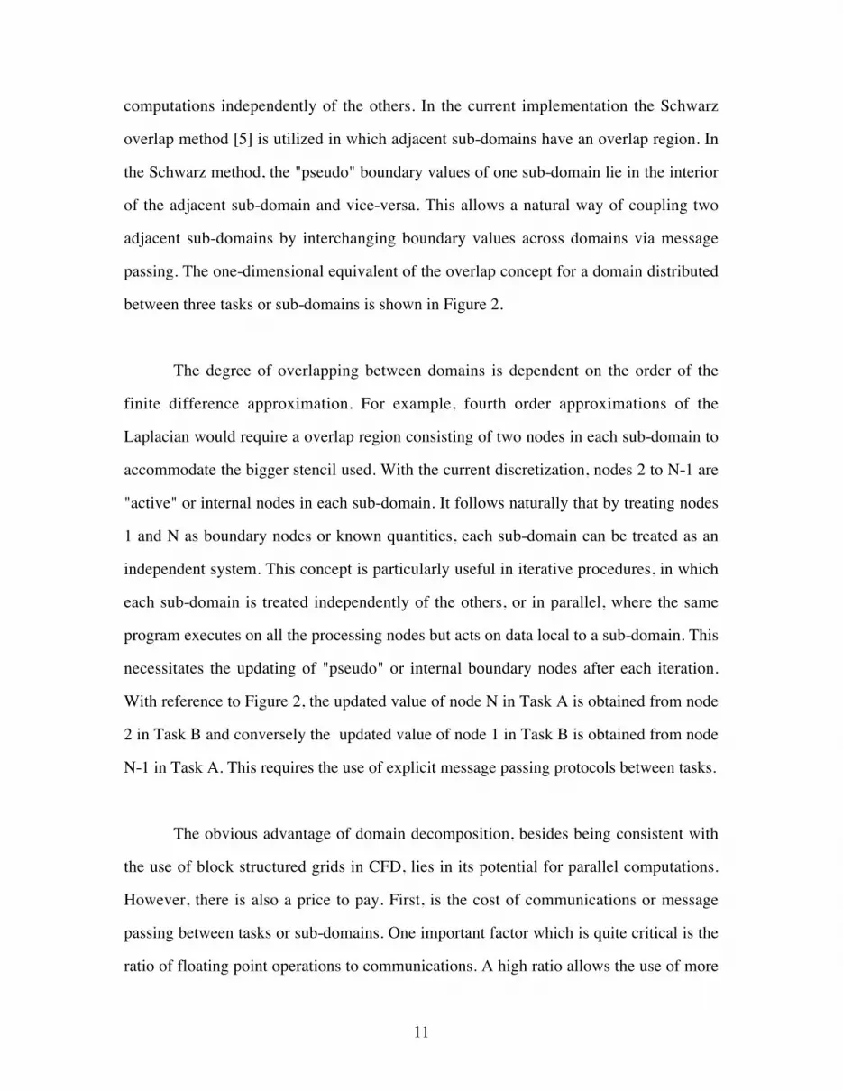
surrounding nodes. The resulting system matrix has a banded form of the type shown in

Figure 1.

4. Solution Strategy

A number of iterative techniques can be used to solve this system of linear

equations ranging from point iterative methods where each node in the domain is updated

in a lexicographic manner to a strategy where an approximate system to that shown in

Figure 1 is solved directly at each iteration. Two strategies which are pertinent to the

solution of the pressure-Poisson equation are implemented in the current study. One

utilizes line iterations where an approximate system comprising the inner tri-diagonal

system in Figure 1. is solved at each iteration with the outer bands being treated as known

quantities on the right hand side. For a Gauss-Siedel type line iterative procedure in

10

which the tri-diagonal system is solved in the y direction and sweeps are performed in the

x direction from left to right, equation (3) can be represented as:

- ASφSk+1

+ APφPk+1 - ANφN

k+1= AEφEk+ AWφW

k+1 (3)

where k represents the iteration count. For each iteration over the whole domain, NX-2

tri-diagonal systems are solved. The tri-diagonal system is solved by using the standard

Thomas Algorithm [20].

The other iterative procedure used is Stone's Strongly Implicit solution

procedure[19]. In this procedure the original system denoted in Figure 1 is suitably

modified into an approximate system in such a way that a LU decomposition on the

modified system would yield only three non-zero elements in each row of L and U. This

considerably reduces the work required to solve the modified set. A "variable iteration

parameter" is introduced in the calculation procedure which is used to approximate

additional unknowns (nodes (i+1,j+1), (i-1,j+1), (i+1,j-1), (i-1,j-1) ) in terms of existing

unknowns (N,S,E,W and P). This parameter takes on values between 0 and 1. The

optimum value for convergence depends on the solution characteristics and is usually

between 0.85 and 0.95.

5. Domain Decomposition

The Multiple Instruction Multiple Data (MIMD) paradigm allows greater control

over data layout, particularly in dealing with complex data structures as is the case in

complex computational geometries. The method of domain decomposition falls into this

category and provides an effective way to solve the Navier-Stokes equations by

decomposing the physical/computational domain into sub-domains. Each sub-domain or

task is then mapped to a processing unit with each processing unit performing

11

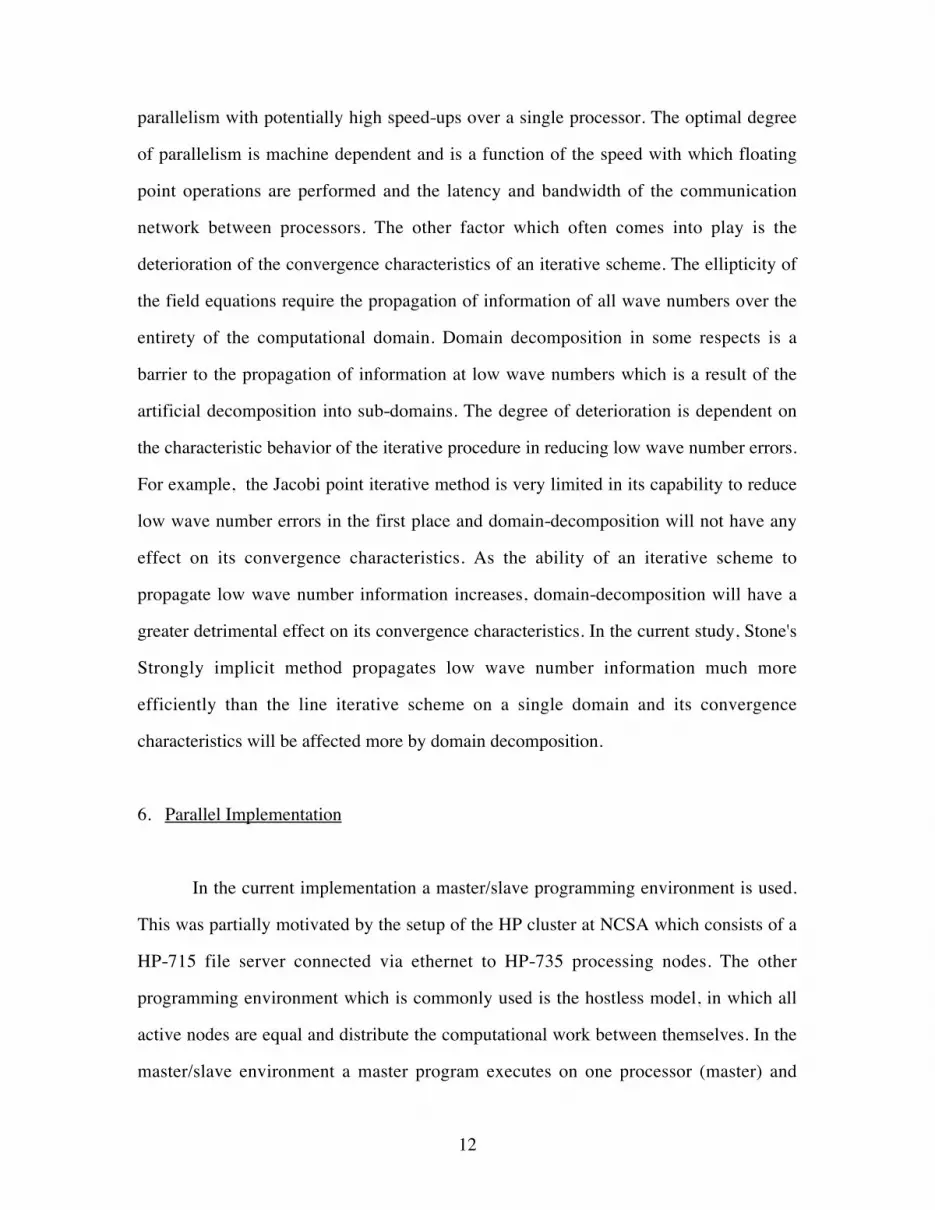
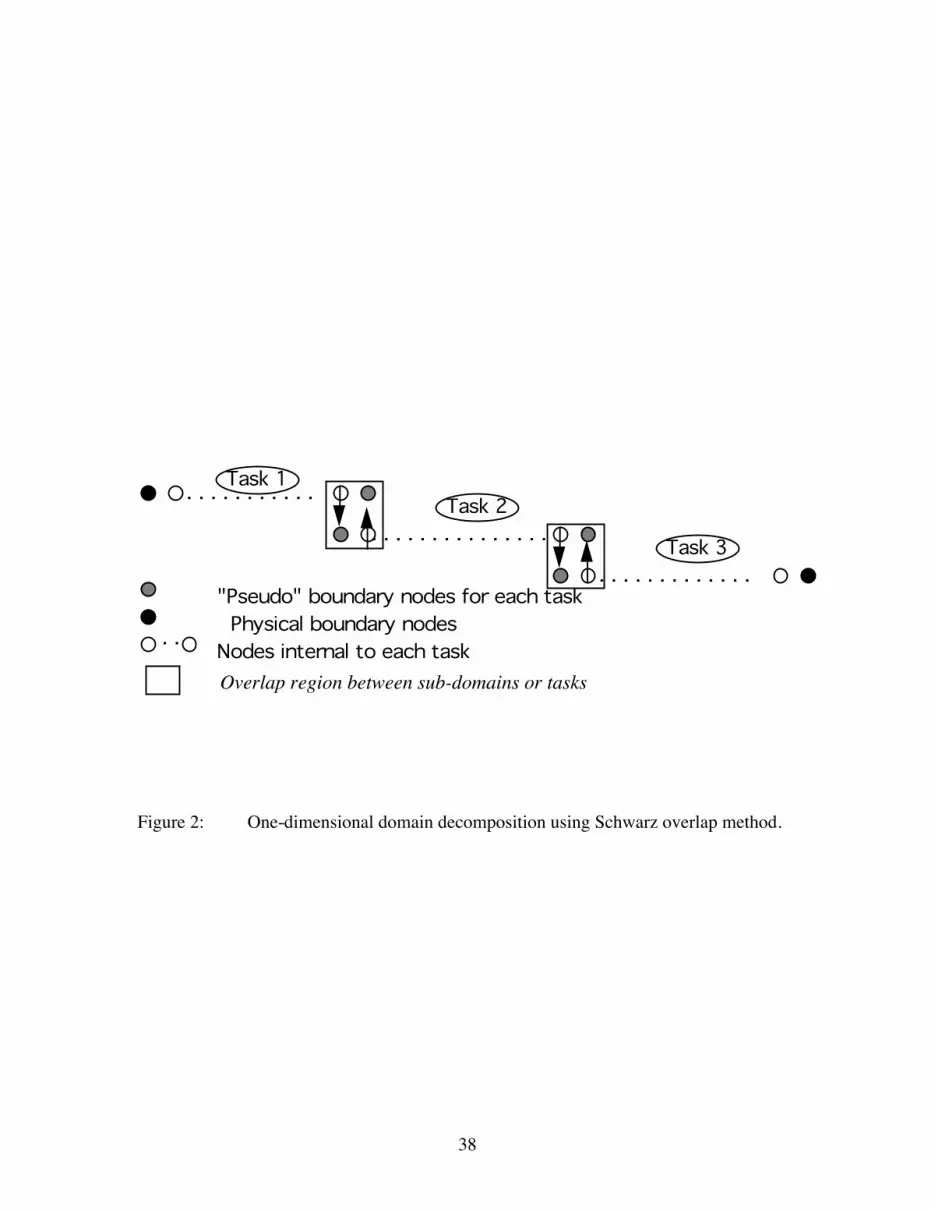
computations independently of the others. In the current implementation the Schwarz

overlap method [5] is utilized in which adjacent sub-domains have an overlap region. In

the Schwarz method, the "pseudo" boundary values of one sub-domain lie in the interior

of the adjacent sub-domain and vice-versa. This allows a natural way of coupling two

adjacent sub-domains by interchanging boundary values across domains via message

passing. The one-dimensional equivalent of the overlap concept for a domain distributed

between three tasks or sub-domains is shown in Figure 2.

The degree of overlapping between domains is dependent on the order of the

finite difference approximation. For example, fourth order approximations of the

Laplacian would require a overlap region consisting of two nodes in each sub-domain to

accommodate the bigger stencil used. With the current discretization, nodes 2 to N-1 are

"active" or internal nodes in each sub-domain. It follows naturally that by treating nodes

1 and N as boundary nodes or known quantities, each sub-domain can be treated as an

independent system. This concept is particularly useful in iterative procedures, in which

each sub-domain is treated independently of the others, or in parallel, where the same

program executes on all the processing nodes but acts on data local to a sub-domain. This

necessitates the updating of "pseudo" or internal boundary nodes after each iteration.

With reference to Figure 2, the updated value of node N in Task A is obtained from node

2 in Task B and conversely the updated value of node 1 in Task B is obtained from node

N-1 in Task A. This requires the use of explicit message passing protocols between tasks.

The obvious advantage of domain decomposition, besides being consistent with

the use of block structured grids in CFD, lies in its potential for parallel computations.

However, there is also a price to pay. First, is the cost of communications or message

passing between tasks or sub-domains. One important factor which is quite critical is the

ratio of floating point operations to communications. A high ratio allows the use of more

12

parallelism with potentially high speed-ups over a single processor. The optimal degree

of parallelism is machine dependent and is a function of the speed with which floating

point operations are performed and the latency and bandwidth of the communication

network between processors. The other factor which often comes into play is the

deterioration of the convergence characteristics of an iterative scheme. The ellipticity of

the field equations require the propagation of information of all wave numbers over the

entirety of the computational domain. Domain decomposition in some respects is a

barrier to the propagation of information at low wave numbers which is a result of the

artificial decomposition into sub-domains. The degree of deterioration is dependent on

the characteristic behavior of the iterative procedure in reducing low wave number errors.

For example, the Jacobi point iterative method is very limited in its capability to reduce

low wave number errors in the first place and domain-decomposition will not have any

effect on its convergence characteristics. As the ability of an iterative scheme to

propagate low wave number information increases, domain-decomposition will have a

greater detrimental effect on its convergence characteristics. In the current study, Stone's

Strongly implicit method propagates low wave number information much more

efficiently than the line iterative scheme on a single domain and its convergence

characteristics will be affected more by domain decomposition.

6. Parallel Implementation

In the current implementation a master/slave programming environment is used.

This was partially motivated by the setup of the HP cluster at NCSA which consists of a

HP-715 file server connected via ethernet to HP-735 processing nodes. The other

programming environment which is commonly used is the hostless model, in which all

active nodes are equal and distribute the computational work between themselves. In the

master/slave environment a master program executes on one processor (master) and

13

spawns tasks on slave processors, which do all the computational work. The master acts

as a control processor and does not interact heavily with the slaves. In the current

implementation the master program performs the following duties:

M(a) Reads input data regarding problem size, and miscellaneous constants used in the

solution procedure. The input also specifies the number of sub-domains or

partitions in each coordinate direction. It also specifies the degree of overlap

between sub-domains. Although in the current calculation, the overlap is one, by

treating this parameter as a variable generalizes the programming environment

considerably.

M(b) Based on the input, the master calculates the beginning and ending indices in each

coordinate direction for each partition. In doing so it distinguishes between

physical boundary and boundaries between sub-domains (pseudo boundaries) and

adjusts the beginning and ending indices by taking the overlap region into

consideration.

M(c) Once all the parameters needed by the slave processors to perform their tasks have

been calculated, the master sends all this information to the respective slave

processors.

M(d) Once this is done the master idles and waits till it receives the maximum

calculated residue from each sub-domain. It then performs a convergence check

by comparing the residues to a set convergence criterion. If this criterion is

satisfied for all the sub-domains it instructs the slave processors to send the final

solution which it subsequently receives from all sub-domains and assembles it in

global coordinates to be printed out. If convergence is not reached then the master

instructs the slave processors to continue with the calculation and waits for the

next convergence check.

14

In a master/slave model, it is important to realize that the assembly or storage of

global arrays on the master processor will at some point restrict the maximum problem

size which can be solved. Therefore, it is prudent to construct and store all geometrical

and finite-difference coefficient arrays on the slave processors specific to the sub-

domains which reside on them.

In the current domain-decomposed environment the slave program is identical on

each slave processor and perform the same sequential tasks on their respective sub-

domains. The slave program performs the following tasks:

S(a) It receives all the data sent by the master in M(c) above. Based on this data it

establishes the active calculation domain indices and the boundary node indices.

On each slave processor the indices vary from 1 to N and are oblivious of the

global indexing. However, the slave processor is cognizant of its global order.

Efficient memory management on the slave processors is hampered by the

inability of Fortran-77 compilers to allocate arrays dynamically. In light of this

shortcoming, the sub-domain arrays that reside on slave processors have to be

hardwired before compilation. Although not a serious impediment to efficient

implementation, it often results in wasted resources.

S(b) In the next step, the slave program generates the grid in x and y directions based

on global ordering. For uniform Cartesian grids, this is quite straight forward.

However, if complex grids are generated a priori , then it would be necessary to

read the grid coordinates. This could be accomplished by reading the grid file on

the master processor and sending relevant sub-domains to each slave processor or

conversely by reading the grid coordinates directly on the slave processor.

S(c) Next the slave program provides an initial guess for the solution domain. Also a

check is made to determine whether any physical boundaries reside on that

15

processor. If the sub-domain is bounded by physical boundaries, then the

appropriate boundary condition is applied to the boundary nodes.

S(d) Once the initial guess and boundary conditions are applied, the iterative solution

procedure is invoked. After every iteration, the boundary values in each sub-

domain are updated with values from their adjacent sub-domains as shown in

Figure 2. Before information is exchanged between adjacent sub-domain

boundaries, the nature of the boundary is established (whether it is an internal or

physical boundary). More detailed implementation details are given in section 6.1.

S(e) The iterative procedure is resumed once the appropriate internal boundary updates

are done. Every few iterations (in this study 10), the maximum residue within

each sub-domain is calculated and sent to the master for a global convergence

check as in (d) in the master program. If convergence is not satisfied, then the

master instructs the slaves to proceed with the calculations. If convergence is

satisfied then the master instructs the slaves to send their sub-domain solutions

back to it.

These are basic tasks performed by the master and slave programs. These tasks

can vary considerably from one application to the other. However, the programming

environment established in the current study can be readily extended to more complex

problems involving the solution of the Navier-Stokes equations with domain

decomposition. Message passing between processors are an implicit part of the master

and slave programs. In the interests of portability, the message passing library PVM [18]

is used for this purpose. The following section describes some aspects of using PVM. A

more thorough description can be found in reference [18].

16

6.1. Message Passing with PVM

PVM (version 3.1) software permits a network of heterogeneous Unix computers

to be used as a single large parallel computer by allowing these computers or processing

units to communicate in a coherent manner between each other. It supports heterogeneity

at the machine and network level and handles all data conversion between computers

which use different integer and floating point representations. Currently PVM is

supported on a wide range of Unix machines from workstations to vector processors like

the Cray C-90, Convex C-series and massively parallel architectures like the CM-5 and

Intel Paragon. In order to use PVM it has to reside on all the machines in the

heterogeneous system. Before running the application, the PVM daemon has to started on

all the machines comprising the virtual system. For more details regarding installation

and starting PVM on a system of machines see reference [18].

In the master/slave version, first the master is enrolled in PVM by calling

pvmfmytid. This command enrolls the process (in this case the master program) in PVM

and returns a unique task identification. Once the master is enrolled in PVM, it spawns a

task (the slave program) on the slave processors by calling pvmfspawn. Each of the slave

processors return a task identification number once the spawning has been done

successfully. The slave program or task on each processor enrolls in PVM by calling

pvmfmytid. Since the slaves already have a specific task identification assigned to them

through the pvmfspawn command from the master, the task identification numbers

returned through pvmfmytid are the same as those assigned to them from the pvmfspawn

command. Once the calculation procedure has been completed, both the master and the

slave program call pvmfexit, which tells the local PVM daemon that they are leaving

PVM.

17

Message passing between master and slave processors and between slave

processors is accomplished by using message passing commands in PVM. To send a

message, pvmfinitsend, pvmfpack and pvmfsend are used. Pvmfinitsend clears the send

buffer and prepares for packing a new message. The data encoding scheme has to be

specified in this call which prepares data to be sent to a different machine in a

heterogeneous environment. Pvmfpack packs the data in the send buffer. The type of data

to be packed (integer, real*4 ...) has to be specified, the name of the data entry, a pointer

to the beginning of the data entry, number of elements to be sent and the stride have to be

specified. Once all the data to be sent has been packed in the buffer, the pvmfsend

command is used. The user specifies the task identification number the message is to be

sent to, and also a message identification tag. The task identification number ensures that

the message is directed to the appropriate task, while the message identification tag is

matched at the receiving end to make sure that the right message has been received.

Pvmfsend is non-blocking or asynchronous, that is, computation on the sending processor

resumes as soon as the message is sent.

Conversely, to receive a message the commands used are in the opposite sequence

of sending a message. Pvmfrecv and pvmfunpack are the counterparts of pvmfsend and

pvmfpack.. Pvmfrecv is supplied with the task identification number of the sending

processor and also the message identification tag of the message itself. Once the receiving

processor makes certain of the legality of the message in its receive buffer, it places the

message in a new active receive buffer and clears the current receive buffer. Unlike

pvmfsend, pvmfrecvis blocking or synchronous; that is, it won't proceed with any

calculations till the message is received by it. Pvmfunpack transfers the data from the

active receive buffer to the specified destination array.

18

The send and receive message passing protocols are used to communicate

between master/slave and between slave processors. As outlined in section 6, data

transfer between processing nodes occurs in M(c) to S(a), S(d) to S(d), S(e) to M(d) and

back from M(d) to S(e). The transfer of messages between slave processors at the end of

each iteration in the solution kernel has the largest overhead associated with it. Some of

the logistical issues associated with this data transfer are described in greater detail.

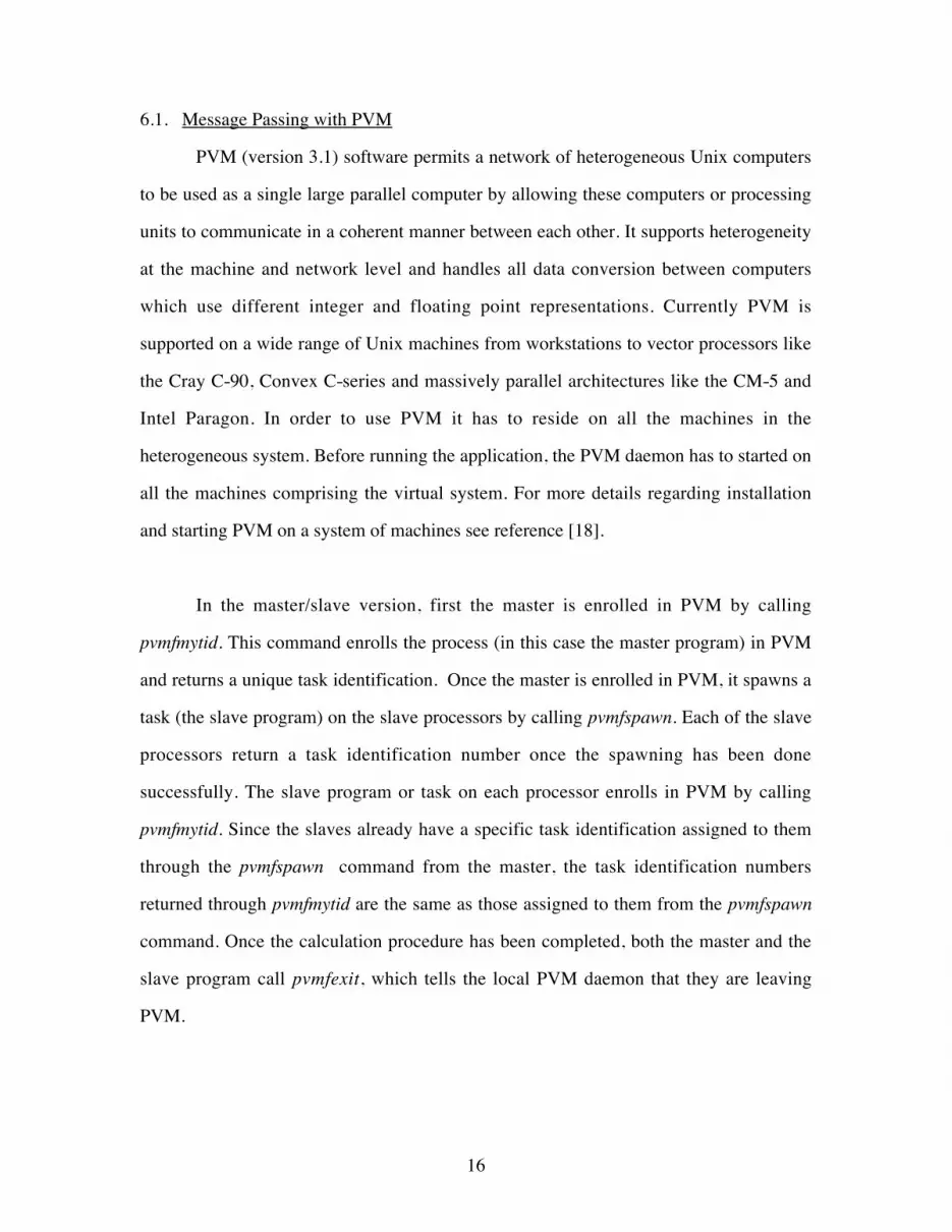
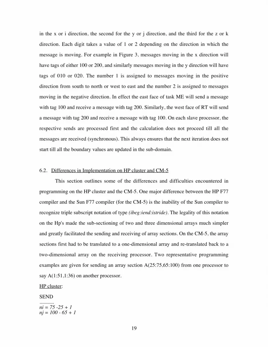
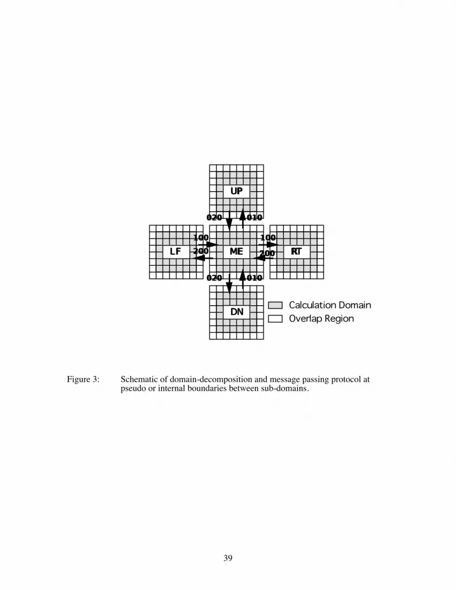
Figure 3 shows a slave processor doing calculations on a given sub-domain and

surrounded by its four neighboring sub-domains. Each sub-domain performs calculations

on local nodes (2:nx-1,2:ny-1), which are represented by the shaded area in Figure 3.

Nodes (1, 2:ny-1) on the west face, (nx,2:ny-1) on the east face, (2:nx-1,1) on the south

face and (2:nx-1, ny) on the north face act as pseudo or internal boundary nodes. At the

end of each iteration these boundary values have to be updated by values from the

adjacent processor or sub-domain. For example on the east face of task ME, ME will

send values φ(nx-1,2:ny-1) which will be received by task RT in φ(1,2:ny-1) and

similarly task RT will send φ(2, 2:ny-1) which will be received in task ME and placed in

φ(nx,2:ny-1). In effect, each task or sub-domain will send four messages and receive four

messages (unless the sub-domain contains a physical boundary where the data transfer is

not necessary).

In implementing the message passing between slave processors, the slave program

has two routines, one for sending messages out and the other for receiving messages. In

the send routine, the task identification of the ME task is established, and also the task

identifiers for the surrounding tasks UP, DN RT, and LF are determined. This establishes

to which task a particular message has to be sent. In sending messages, the message

identification tag should be unique, since each task receives four messages from

surrounding tasks and should know on receiving the message its final destination in array

φ. The message identification tag used is a three digit code; the first digit is for messages

19

in the x or i direction, the second for the y or j direction, and the third for the z or k

direction. Each digit takes a value of 1 or 2 depending on the direction in which the

message is moving. For example in Figure 3, messages moving in the x direction will

have tags of either 100 or 200, and similarly messages moving in the y direction will have

tags of 010 or 020. The number 1 is assigned to messages moving in the positive

direction from south to north or west to east and the number 2 is assigned to messages

moving in the negative direction. In effect the east face of task ME will send a message

with tag 100 and receive a message with tag 200. Similarly, the west face of RT will send

a message with tag 200 and receive a message with tag 100. On each slave processor, the

respective sends are processed first and the calculation does not proceed till all the

messages are received (synchronous). This always ensures that the next iteration does not

start till all the boundary values are updated in the sub-domain.

6.2. Differences in Implementation on HP cluster and CM-5

This section outlines some of the differences and difficulties encountered in

programming on the HP cluster and the CM-5. One major difference between the HP F77

compiler and the Sun F77 compiler (for the CM-5) is the inability of the Sun compiler to

recognize triple subscript notation of type (ibeg:iend:istride). The legality of this notation

on the Hp's made the sub-sectioning of two and three dimensional arrays much simpler

and greatly facilitated the sending and receiving of array sections. On the CM-5, the array

sections first had to be translated to a one-dimensional array and re-translated back to a

two-dimensional array on the receiving processor. Two representative programming

examples are given for sending an array section A(25:75,65:100) from one processor to

say A(1:51,1:36) on another processor.

HP cluster:

SEND...........ni = 75 -25 + 1nj = 100 - 65 + 1

20

np = ni * njmsgtype = 1call pvmfinitsend(.....call pvmfpack(REAL4, a(25:75, 65:100), np, 1, info)...................

RECEIVE...............ni = 75 -25 + 1nj = 100 - 65 + 1np = ni * njmsgtype = 1call pvmfrecv(..........call pvmfunpack(REAL4, a(1:51, 1:36), np, 1, info)................

CM-5

SEND

..........ni = 75 -25 + 1nj = 100 - 65 + 1np = ni * njmsgtype = 1

do 99 j = 65, 100jj = j - 65 + 1do 99 i = 25, 75ii = i - 25 + 1izz = (jj-1) * ni + iiatemp(izz) = a(i,j)99continuecall pvmfinitsend(...........call pvmfpack(REAL4, atemp, np, 1, info)....................

RECEIVE........ni = 75 -25 + 1nj = 100 - 65 + 1np = ni * njmsgtype = 1call pvmfrecv(REAL4, atemp, np, info)do 99 j = 1, njdo 99 i = 1, niizz = (j-1) * ni + ia(i,j) = atemp(izz)99continue.......................

21

Other differences were encountered in the use of timers. On the HP cluster the

function calls dime and etime were used to time different code sections. Dtime returns the

difference in time between two calls and etime returns the absolute time at each call. On

the CM-5, the timing utilities cmmd_node_timer_clear(), cmmd_node_timer_start(), and

cmmd_node_timer_stop() were used. There were some difficulties encountered with I/O

from the slave processors. Separate files were opened from each processing unit on the

HP and the CM-5 where all the I/O from a given processing unit was directed. This did

not prove to be a problem on the Hp cluster due to the small number of processing nodes

used. However, on the CM-5, since UNIX sets a limit on the number of files that can be

opened at any one time, this approach was not feasible for a large number of processors

and was abandoned. Alternate modes of I/O for slave processors on the CM-5 will be

looked into in future studies[21].

7. Results and Discussion

The two solution strategies outlined in section (4) were tested on the HP cluster

and the CM-5. The purpose of this section is to compare the parallel efficiency of the

solution strategy and also to compare the relative performance between the HP cluster

and the CM-5. It should be noted that except for the changes outlined above the same

codes were used on both the systems. No attempt was made to utilize the vector units on

the CM-5 by writing the slave program in CM-Fortran. To see the effect of domain

decomposition on the convergence of the Gauss-Siedel line iterative procedure (denoted

as GSL), only a one dimensional decomposition was used. Since the tri-diagonal line

solves are performed in the y direction, the domain was decomposed only in that

direction to form a multitude of smaller tri-diagonal systems for each x location. To

facilitate comparison, a similar decomposition was also used for Stone's method (denoted

as Stones).

22

On the HP cluster two-dimensional domains with 50x50, 100x100, and 200x200

nodes were tested for both GSL and Stones on 1, 2, 4, and 6 processors of the HP cluster

(during the time of this study more processors were not available). On the CM-5 a

200x200 calculation was done for up to 64 processing nodes for both GSL and Stones. In

addition a 1024x1024 calculation for Stones was done on 8 to 64 processing nodes. For

the Stones method the iteration parameter was set to 0.9 in all the calculations. The

optimum value of this parameter was established with the domain decomposed on 6 HP

processing units. In all the calculations, the convergence criterion was set to 2.E-5 for the

maximum allowable residue over the whole calculation domain. On the HP cluster the

master program executed on a HP-715 and the slave programs on Hp-735s. On the CM-5,

the master executed on the partition manager, while the slaves executed on the nodal

SPARC-2 chips. Timers were used to estimate the time spent in different sections of the

kernel (the kernel just included the floating point operations in the solver,

communications between slave processors at the end of each iteration, communication of

residues to master and corresponding reply from master). Also, none of the timing studies

were done in a dedicated mode. However, the timings obtained on the HP cluster and on

the CM-5 were comparable between multiple runs (within ± 10%). The following

procedures were timed independently

(a) Timer 1: time in floating point operations of solver.

(b) Timer 2: time used by pvmfinitsend for communications between slave processors.

(c) Timer 3: time used by pvmfpack for communications between slave processors.

(d) Timer 4: time used by pvmfsend for communications between slave processors.

(e) Timer 5: time used by pvmfrecvfor communications between slave processors. This

included the idle time till the message was received. If processor A finished its work

earlier than processor B from which it is (A) expecting a message, then the time spent in

waiting for this message will accumulate in this timer.

23

(f) Timer 6: time used by pvmfunpack for communications between slave processors.

(g) Timer 7: time used for convergence checking. This would include the time used in

sending the maximum residue to the master, reception by the master from all slave

processors, the time taken by the master to make a decision, to broadcast that decision

back to all the slave processors and the reception of this message by the slave. During this

time, all the slave processors remained idle.

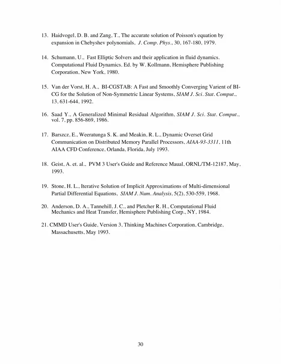
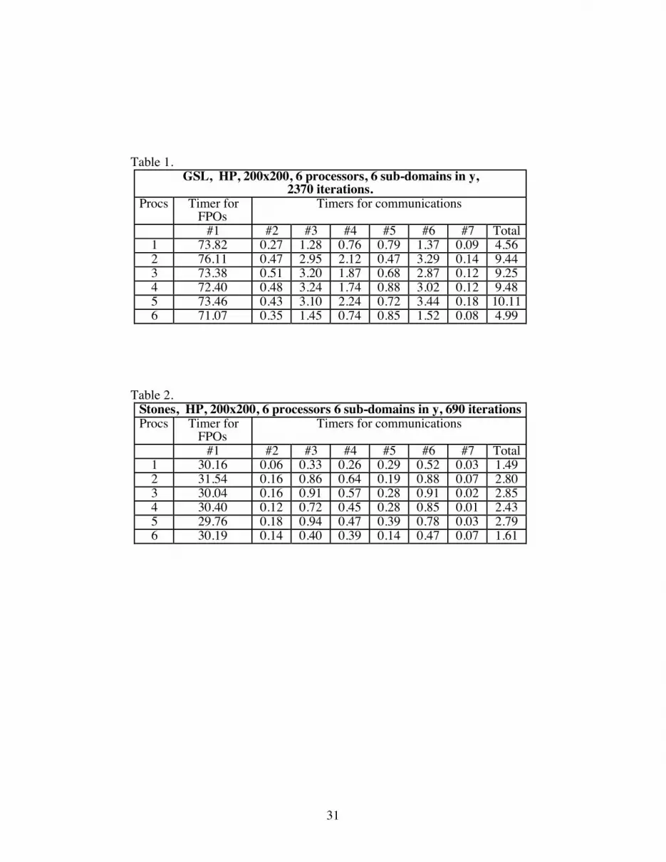
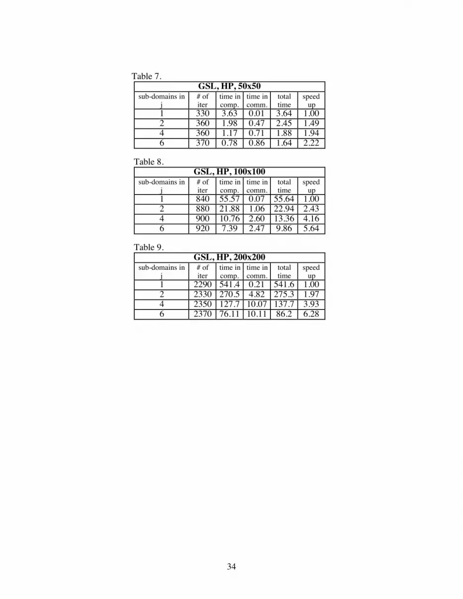
Table 1 through 4 give detailed timings on representative runs with a 200x200

resolution, and six sub-domains in the y direction. Timings for GSL and Stones are given

on the HP cluster and CM-5. By dividing the physical domain into equal sub-domains,

good load balancing is achieved between the different processing nodes. Domain 1 and 6

contain physical boundaries and send and receive boundary values only at one boundary

interface. The following observations can be made from these tables.

(a) Stones method converges in fewer iterations than GSL (690 v/s 2370 for GSL).

(b) The approximate ratio of time spent in floating point operations (timer #1) between

the CM-5 and HP cluster for GSL is 2.1 (163/76) and for Stones is 1.33 (40/30). For

consistency both ratios should be the same and the reason for these discrepancy is not

known.

(c) Each HP-735 processor performed at approximately 3.5 MFLOPS in the calculation

kernel2. On the other hand, a Sparc chip on the CM-5 varied in performance anywhere

between 1.1 to 3 MFLOPS.

(d) On the HP cluster, packing (timer #4) and unpacking (timer #6) were the most costly

operations in the communication calls. Convergence checks (timer #7) used the least

amount of time. Total communication times in processors 1 and 6 on the HP-cluster are

2Each add and each multiply were assumed to represent a floating point operation. All tests were performedwithout any optimization switches activated. Level 1 and 2 optimization on the Hp-735's gave speedups of3.5 to 4, resulting in 12-13 MFLOPS per processor.

24

about half those of the other processors, which is consistent with the fact that they have to

send and receive only at one boundary.

(e) On the other hand, the receiving of data on the CM-5 was by far the most

expensive communication call (timer #5). Also the convergence checks (timer #7), are

much more expensive than on the HP cluster. It can also be observed that the processors

which contain the physical boundaries (processors 1 and 6), take much longer to receive

their data than the rest of the processors. Conversely, processor 2 receives its data

extremely fast compared to the other processors. These were not chance events, and the

exact same trends were observed for multiple runs and for different levels of domain

decomposition. In order to clarify the cause of these discrepancies in timer #5, forced

synchronization through the CMMD function call cmmd_sync_with_nodes was

introduced at the beginning of the slave program, between the end of each iteration sweep

and the pvmfinitsend command and between the pvmfsend and pvmfrecv call on each

slave processor. This made sure that the calculations started at the same time on all slave

processors, that each iterative sweep was finished on all slave processors before the send

to neighboring processors was initiated, and that the receive on each processor was

initiated after the send sequence was completed on all processors.

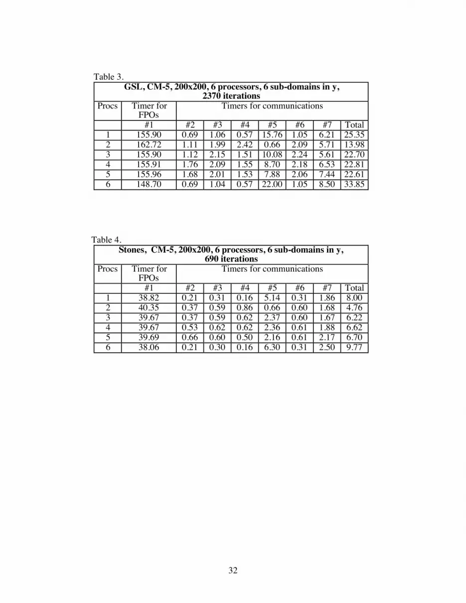
Table 5. shows a run with synchronization in place. It can be seen that timer #5 is

much more uniform across all the slave processors. So it can be concluded that the non-

uniformity in timer #5 was caused by slave procesors not finishing their calculations at

the same time and one processor waiting on its neighbor to receive data. In the current

implementation, the number of nodes in each domain were calculated in such a way that

the first processor had 33 active nodes in the y direction, the second processor had 34,

and the rest had 33 except node six which had 32. This decomposition was done based on

the total nodes (200) rather than on the number of active or internal nodes (198), which is

a better strategy and will be followed in future.

25

However, using the same type of synchronization on the HP cluster (this was done

by using pvmfjoingroup and then pvmfbarrier for each slave processor) did not make any

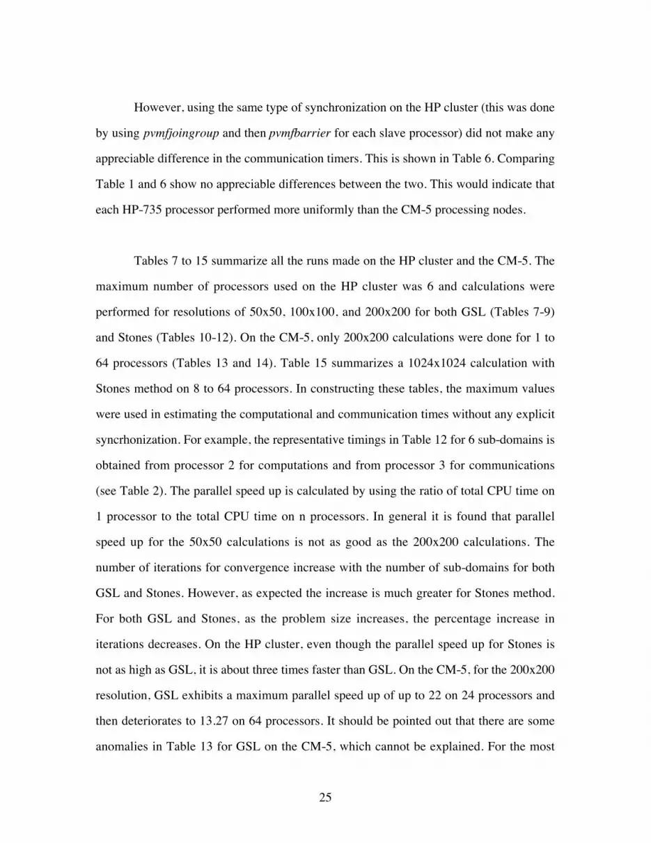
appreciable difference in the communication timers. This is shown in Table 6. Comparing

Table 1 and 6 show no appreciable differences between the two. This would indicate that

each HP-735 processor performed more uniformly than the CM-5 processing nodes.

Tables 7 to 15 summarize all the runs made on the HP cluster and the CM-5. The

maximum number of processors used on the HP cluster was 6 and calculations were

performed for resolutions of 50x50, 100x100, and 200x200 for both GSL (Tables 7-9)

and Stones (Tables 10-12). On the CM-5, only 200x200 calculations were done for 1 to

64 processors (Tables 13 and 14). Table 15 summarizes a 1024x1024 calculation with

Stones method on 8 to 64 processors. In constructing these tables, the maximum values

were used in estimating the computational and communication times without any explicit

syncrhonization. For example, the representative timings in Table 12 for 6 sub-domains is

obtained from processor 2 for computations and from processor 3 for communications

(see Table 2). The parallel speed up is calculated by using the ratio of total CPU time on

1 processor to the total CPU time on n processors. In general it is found that parallel

speed up for the 50x50 calculations is not as good as the 200x200 calculations. The

number of iterations for convergence increase with the number of sub-domains for both

GSL and Stones. However, as expected the increase is much greater for Stones method.

For both GSL and Stones, as the problem size increases, the percentage increase in

iterations decreases. On the HP cluster, even though the parallel speed up for Stones is

not as high as GSL, it is about three times faster than GSL. On the CM-5, for the 200x200

resolution, GSL exhibits a maximum parallel speed up of up to 22 on 24 processors and

then deteriorates to 13.27 on 64 processors. It should be pointed out that there are some

anomalies in Table 13 for GSL on the CM-5, which cannot be explained. For the most

26

part, parallel speed up in Table 13 is greater than the number of processors. It seems as if

the floating point operations/processor are performed faster as the number of processors

increase. Stones exhibits a maximum speed up of 5 on 16 processors. For a 1024x1024

calculation, Stones exhibits a parallel speed up of 5.7 against a maximum possible of

64/8.

An approximate general expression for parallel speed up can be written as:

S = NxNy

NnfSf

Nx

Px

NyPy

N'nfSf

+2OxN'cNy

PySc+2Oy

N'cNxPxSc

(4)

where,

Nx total number of active degrees of freedom (dof) in the x coordinate

direction.

Ny total number of active degrees of freedom in the y coordinate direction.

nf number of floating point operations / degree of freedom.

Sf speed of computation, expressed in floating point operations per second.

N multiplicative factor for number of floating point operations on single

processor. e.g. number of iterations.

N' multiplicative factor for number of floating point operations on multiple

processors. e.g. number of iterations.

N'c multiplicative factor for communications on multiple processors. e.g.

number of iterations.

Px number of processors/decomposition in x direction.

Py number of processors/decomposition in y direction.

Ox number of overlap points in x direction. If Px=1 then Ox = 0.

Oy number of overlap points in y direction. If Py=1 then Oy = 0.

27

Sc speed of communications. This is calculated as the average time taken for

one processor to send and receive a word to its neighboring processor.

Expressed as words per second.

The numerator quantifies the time taken for a single processor calculation and the

denominator quantifies the time taken by each processor for computations and

communications. Equation (4) can be used to get an estimate of the speed up for a given

calculation kernel if Sf and Sc are known for the system. For the calculations in this

study, equation (4) can be further simplified given that N' = N'c and Px = 1. This gives

S = Py

N'

N{1+

2Oynf

PyNy

Sf

Sc}

(5)

Equation (5) implies that for a given calculation and communication kernel, parallel

speed up is directly proportional to the number of floating point operations per processor

and inversely proportional to the ratio Sf/Sc and to the extent of the overlap region.

Having an estimate of these values on a given machine configuration and assuming N=N',

an upper bound on parallel speed up can be estimated. On the HP cluster Sf was found to

be 3.5E+63 and Sc was found to vary between 40,000 for 50x50 to about 100,000

words/second for 200x200.

8. Conclusions and Future Work

A preliminary study was conducted with the message passing library PVM for the

iterative solution of a two-dimensional Laplace equation. A line iterative procedure and

Stones strongly implicit solution procedure were used. The intent of this study was not so

much to study the solution of the Laplace equation as it was to establish the necessary

3See footnote 2 on page 23.

28

groundwork and to understand the issues involved in parallel programming in a domain-

decomposed environment for the incompressible Navier-Stokes equations.

Two machine configurations were looked at in this study, a 6 processor HP-735

cluster at NCSA and a 512 processor CM-5. There were some differences in the F77

compilers between the two machines and suitable modifications had to be made in the

computer program. It was found that although the Stones method did not parallelize as

effectively as the line iterative procedure, it took much less CPU time to give a converged

solution. It was found that the HP-735 processors performed more uniformly than the

CM-5 processing nodes. For comparing the CM-5 and the HP cluster, partial CM

partitions (< 32 nodes) were used for most of the calculations. This is not the best or the

most efficient utilization of the machine and some of the anomalies seen in this study

could be a result of this.

Future work will concentrate on implementing a three-dimensional

incompressible Navier-Stokes solver with domain-decomposition. The pressure Poisson

equation will be solved using an iterative multigrid solution procedure.

9. Acknowledgements

The authors would like to thank United Technologies for their financial support.

Technical support from NCSA staff, John Quinn, and Rick Kufrin and TMC site

representative Dr. Charlie Liu is gratefully acknowledged.

29

References

1. M. Rai, and P. Moin, Direct Simulations of Turbulent Flow Using Finite-Difference Schemes, J. Comput. Phys., vol. 96, pp. 15-53, 1991.

2. C. Canuto, M. Y. Hussaini, A. Quarteroni, and T. A. Zang, Spectral Methods inFluid Dynamics, Springer-Verlag, New York, 1987.

3. A. T. Patera, A Spectral Element Method for Fluid Dynamics, J. Comput. Phys., vol.54, pp. 468-488, 1984.

4. CM Fortran User's Guide for the CM-5, Thinking Machines Corporation, Cambridge,

Massachusetts, January 1992.

5. Schwarz, H. A., Uber Enen Grenz Bergang Durich Alternirender Verfahren, Ges.

Math. Abhandlungen, Bd. 1, Berlin, 133-143, 1870.

6. Benek, J. A., Buning, P. G. and Steger, J. L., A 3-D Chimera Grid Embedding

Technique, AIAA Paper AIAA 85-1523, July 1985.

7. H.S. McFaddin, and J.R. Rice , Collaborating PDE Solvers, Applied Numerical

Mathematics, vol. 10, 279-295, 1992.

8. J. Kim, and P. Moin, Application of a Fractional-Step Method to IncompressibleNavier-Stokes, J. Comput. Phys., vol. 59, pp. 308-323, 1985.

9. Pulliam, T. H., and Chaussee, D.S., A Diagonal Form of an Implicit Approximate-

Factorization Algorithm, J. Comp. Physics, 39, 347-363, 1981.

10. Chyczewski, T., Marconi, F., Pelz, R. and Curchitser, E., Solution of the Euler and

Navier-Stokes Equations on a Parallel Processor Using a Transposed/Thomas ADI

Algorithm, AIAA paper 93-3310, 11th AIAA Computational Fluid Dynamics

Conference, July 6-9, 1993.

11. Bondeli, S., Divide and Conquer: A Parallel Algorithm for the Solution of a

Tridiagonal Linear System of Equations, Parallel Comput. 17, 419-434, 1991.

12. Wang, M.Y. and Vanka, S.P., A parallel ADI Algorithm for High-Order Finite-

Difference Solution of the Unsteady Heat Conduction Equation, and its

Implementation on the CM-5, Numerical Heat Transfer-B, 24(2), 143-159, Sep.

1993.

30

13. Haidvogel, D. B. and Zang, T., The accurate solution of Poisson's equation by

expansion in Chebyshev polynomials, J. Comp. Phys., 30, 167-180, 1979.

14. Schumann, U., Fast Elliptic Solvers and their application in fluid dynamics.

Computational Fluid Dynamics. Ed. by W. Kollmann, Hemisphere Publishing

Corporation, New York, 1980.

15. Van der Vorst, H. A., BI-CGSTAB: A Fast and Smoothly Converging Varient of BI-

CG for the Solution of Non-Symmetric Linear Systems, SIAM J. Sci. Stat. Comput.,

13, 631-644, 1992.

16. Saad Y., A Generalized Minimal Residual Algorithm, SIAM J. Sci. Stat. Comput.,vol. 7, pp. 856-869, 1986.

17. Barszcz, E., Weeratunga S. K. and Meakin, R. L., Dynamic Overset Grid

Communication on Distributed Memory Parallel Processors, AIAA-93-3311, 11th

AIAA CFD Conference, Orlanda, Florida, July 1993.

18. Geist, A. et. al., PVM 3 User's Guide and Reference Maual, ORNL/TM-12187, May,

1993.

19. Stone, H. L., Iterative Solution of Implicit Approximations of Multi-dimensional

Partial Differential Equations, SIAM J. Num. Analysis, 5(2), 530-559, 1968.

20. Anderson, D. A., Tannehill, J. C., and Pletcher R. H., Computational FluidMechanics and Heat Transfer, Hemisphere Publishing Corp., NY, 1984.

21. CMMD User's Guide, Version 3, Thinking Machines Corporation, Cambridge,

Massachusetts, May 1993.

31

Table 1.GSL, HP, 200x200, 6 processors, 6 sub-domains in y,

2370 iterations.Procs Timer for

FPOsTimers for communications

#1 #2 #3 #4 #5 #6 #7 Total1 73.82 0.27 1.28 0.76 0.79 1.37 0.09 4.562 76.11 0.47 2.95 2.12 0.47 3.29 0.14 9.443 73.38 0.51 3.20 1.87 0.68 2.87 0.12 9.254 72.40 0.48 3.24 1.74 0.88 3.02 0.12 9.485 73.46 0.43 3.10 2.24 0.72 3.44 0.18 10.116 71.07 0.35 1.45 0.74 0.85 1.52 0.08 4.99

Table 2.Stones, HP, 200x200, 6 processors 6 sub-domains in y, 690 iterationsProcs Timer for

FPOsTimers for communications

#1 #2 #3 #4 #5 #6 #7 Total1 30.16 0.06 0.33 0.26 0.29 0.52 0.03 1.492 31.54 0.16 0.86 0.64 0.19 0.88 0.07 2.803 30.04 0.16 0.91 0.57 0.28 0.91 0.02 2.854 30.40 0.12 0.72 0.45 0.28 0.85 0.01 2.435 29.76 0.18 0.94 0.47 0.39 0.78 0.03 2.796 30.19 0.14 0.40 0.39 0.14 0.47 0.07 1.61

32

Table 3.GSL, CM-5, 200x200, 6 processors, 6 sub-domains in y,

2370 iterationsProcs Timer for

FPOsTimers for communications

#1 #2 #3 #4 #5 #6 #7 Total1 155.90 0.69 1.06 0.57 15.76 1.05 6.21 25.352 162.72 1.11 1.99 2.42 0.66 2.09 5.71 13.983 155.90 1.12 2.15 1.51 10.08 2.24 5.61 22.704 155.91 1.76 2.09 1.55 8.70 2.18 6.53 22.815 155.96 1.68 2.01 1.53 7.88 2.06 7.44 22.616 148.70 0.69 1.04 0.57 22.00 1.05 8.50 33.85

Table 4.Stones, CM-5, 200x200, 6 processors, 6 sub-domains in y,

690 iterationsProcs Timer for

FPOsTimers for communications

#1 #2 #3 #4 #5 #6 #7 Total1 38.82 0.21 0.31 0.16 5.14 0.31 1.86 8.002 40.35 0.37 0.59 0.86 0.66 0.60 1.68 4.763 39.67 0.37 0.59 0.62 2.37 0.60 1.67 6.224 39.67 0.53 0.62 0.62 2.36 0.61 1.88 6.625 39.69 0.66 0.60 0.50 2.16 0.61 2.17 6.706 38.06 0.21 0.30 0.16 6.30 0.31 2.50 9.77

33

Table 5.GSL, CM-5, 200x200, 6 processors, 6 sub-domains in y,

2370 iterations, with synchronizationProcs Timer for

FPOsTimers for communications

#1 #2 #3 #4 #5 #6 #7 Total1 155.01 0.69 1.06 1.05 0.96 1.05 7.15 11.962 161.74 1.23 1.96 3.09 1.13 2.05 6.94 16.403 155.02 1.17 1.99 2.53 1.12 2.05 6.91 15.784 155.02 1.16 2.00 2.88 1.11 2.05 6.90 16.115 155.02 1.19 2.02 2.64 1.13 2.06 6.89 15.936 148.00 0.69 1.08 0.60 0.98 1.06 7.07 11.48

Table 6.GSL, HP, 200x200, 6 processors, 6 sub-domains in y,

2370 iterations, with synchronizationProcs Timer for

FPOsTimers for communications

#1 #2 #3 #4 #5 #6 #7 Total1 72.89 0.16 1.17 0.61 0.69 1.49 0.18 4.302 75.53 0.35 2.96 1.24 0.92 2.83 0.14 8.443 76.99 0.43 2.73 1.17 0.45 2.62 0.08 7.484 72.70 0.46 2.93 0.96 0.90 2.63 0.12 8.005 73.02 0.39 2.61 1.03 0.80 2.73 0.2 7.756 70.14 0.17 1.10 0.57 0.55 1.56 0.16 4.11

34

Table 7.GSL, HP, 50x50

sub-domains inj

# ofiter

time incomp.

time incomm.

totaltime

speedup

1 330 3.63 0.01 3.64 1.002 360 1.98 0.47 2.45 1.494 360 1.17 0.71 1.88 1.946 370 0.78 0.86 1.64 2.22

Table 8.GSL, HP, 100x100

sub-domains inj

# ofiter

time incomp.

time incomm.

totaltime

speedup

1 840 55.57 0.07 55.64 1.002 880 21.88 1.06 22.94 2.434 900 10.76 2.60 13.36 4.166 920 7.39 2.47 9.86 5.64

Table 9.GSL, HP, 200x200

sub-domains inj

# ofiter

time incomp.

time incomm.

totaltime

speedup

1 2290 541.4 0.21 541.6 1.002 2330 270.5 4.82 275.3 1.974 2350 127.7 10.07 137.7 3.936 2370 76.11 10.11 86.2 6.28

35

Table 10.Stones, HP, 50x50

sub-domains inj

# ofiter

time incomp.

time incomm.

totaltime

speedup

1 60 0.92 0.00 0.92 1.002 110 1.01 0.18 1.19 0.774 120 0.39 0.31 0.70 1.316 130 0.27 0.27 0.60 1.53

Table 11.Stones, HP, 100x100

sub-domains inj

# ofiter

time incomp.

time incomm.

totaltime

speedup

1 170 10.77 0.00 10.77 1.002 240 7.61 0.31 7.92 1.364 250 4.23 0.70 4.93 2.186 280 3.33 0.74 4.07 2.65

Table 12.Stones, HP, 200x200

sub-domains inj

# ofiter

time incomp.

time incomm.

totaltime

speedup

1 520 135.1 0.00 135.1 1.002 580 74.5 1.20 75.7 1.794 630 41.7 2.23 43.7 3.076 690 31.6 2.85 34.4 4.45

36

Table 13.GSL, CM-5, 200x200

sub-domains inj

# ofiter

time incomp.

time incomm.

totaltime

speedup

1 2290 1443 3.78 1447 1.002 2330 609.7 10.38 620.1 2.334 2350 266.8 25.55 292.4 5.026 2370 162.7 33.85 196.6 7.368 2400 96.68 29.15 125.8 11.5010 2430 57.99 28.86 86.85 16.6612 2450 47.79 31.40 79.19 18.2714 2480 42.75 29.81 72.56 19.9416 2500 36.48 33.93 70.41 20.5518 2530 34.06 33.87 67.93 21.3020 2550 29.03 37.17 66.20 21.8522 2580 29.61 38.35 67.96 21.2924 2610 26.34 39.13 65.47 22.1026 2620 23.46 49.58 73.31 19.7332 2710 21.65 50.93 72.58 19.9364 3040 15.69 93.34 109.0 13.27

Table 14.Stones, CM-5, 200x200

sub-domains inj

# ofiter

time incomp.

time incomm.

totaltime

speedup

1 520 176.4 0.94 177.4 1.002 580 99.9 4.11 103.0 1.714 630 54.6 7.35 62.0 2.866 690 40.3 9.77 50.12 3.538 740 32.7 10.13 42.79 4.1412 830 24.8 11.99 36.80 4.8216 930 21.3 14.68 35.98 4.9318 980 20.0 16.75 36.74 4.83

Table 15.Stones, HP, 1024x1024

sub-domains inj

# ofiter

time incomp.

time incomm.

totaltime

speedup

8 4540 5940 989 6929 1.0016 4710 2873 599 3473 2.032 5020 1524 323 1848 3.7564 5470 870 338 1208 5.7

37

0

0

0

0

Figure 1: System matrix for second-order central difference discretization of 2-D Laplacian.

38

. . . . . . . . . . . . . . .

. . . . . . . . . . . . .

. . . . . . . . . . . Task 1

Task 2

Task 3

"Pseudo" boundary nodes for each task

Physical boundary nodes. . .

Nodes internal to each task

Overlap region between sub-domains or tasks

Figure 2: One-dimensional domain decomposition using Schwarz overlap method.

39

ME

UP

DN

RTLF 200

100

200

100

010

010

020

020

Calculation Domain

Overlap Region

Figure 3: Schematic of domain-decomposition and message passing protocol at pseudo or internal boundaries between sub-domains.