ri-18-3-full.pdf - journal of mechanical engineering
TRANSCRIPT


JOURNAL OF MECHANICAL ENGINEERING
An International Journal
Vol 18 (3) 15 September 2021 ISSN 1823-5514 eISSN 2550-164X 1 The Numerical Analysis of Hyperelastic Properties in Commercial and Original
Aloe Vera Gels Nur Nabila Mohd Nazali, and Nor Fazli Adull Manan*
1
2 Computational Evaluation of Frictional Force Changes in Three-Point and Three-Bracket Bending Models S. A. H. A. Seman, M. F. Razali*, A. S. Mahmud, and M. H. Hassan
21
3 Enhancement of Surface Quality of DMLS Aluminium Alloy using RSM Optimization and ANN Modelling A.P.S.V.R. Subrahmanyam*, P.Srinivasa Rao, and K.Siva Prasad
37
4 Improving the Technical Level of Hydraulic Machines, Hydraulic Units and Hydraulic Devices using a Definitive Assessment Criterion at the Design Stage Pavel Andrenko, Iryna Hrechka, Serhii Khovanskyi, Andrii Rogovyi*, and Maksym Svynarenko
57
5 Effect of Injection Pressure on the Performance and Emission Characteristics of Niger-Diesel-Ethanol Blends in CI Engine Bikkavolu Joga Rao*, Vadapalli Srinivas, Kodanda Ramarao Chebattina, and Pullagura Gandhi
77
6 Experimental Analysis on Grain Growth Kinetics of SS316L Austenitic Stainless Steel Muhd Faiz Mat, Yupiter H. P. Manurung*, Yusuf Olanrewaju Busari, Mohd Shahriman Adenan, Mohd Shahar Sulaiman, Norasiah Muhammad, and Marcel Graf
97
7 A Simulation Study of Lubricating Oil Pump for an Aero Engine Tarique Hussain*, Niranjan Sarangi, M. Sivaramakrishna, and M. Udaya Kumar
113
8 DSC Assessment on Curing Degree of Micron-scaled Adhesive Layer in Lamination-pressed Flexible Printed Circuit Panels Kok-Tee Lau*, Hoi Ern Kok, and Nur Hazirah Rosli
131

9 Development and Testing of a Turning Process Monitoring System using Acoustic Emission Keiichi Ninomiya*, Shun Yoshida, Kenji Okita, Toshihiko Koga, and Shuzo Oshima
147
10 PV System Based Dynamic Voltage Restorer (DVR) in Water Pumping System for Agricultural Application Awais Farooqi, Muhammad Murtadha Othman*, Ismail Musirin, Mohd Fuad Abdul Latip, Mohd Amran Mohd Radzi, Izham Z.Abidin, and Daw Saleh Sasi Mohammed
163
11 Determination of River Water Level Triggering Flood in Manghinao River in Bauan, Batangas, Philippines C E F Monjardin*, K M Transfiguracion, J P J Mangunay, K M Paguia, F A A Uy, and F J Tan
181
12 Simultaneous Load Management Strategy for Electronic Manufacturing Facilities by using EPSO Algorithm M.F. Sulaima*, N.Y. Dahlan, Z.H. Bohari, M.N.M. Nasir, R.F. Mustafa, and Duc Luong Nguyen
193
13 Design of Power Device Sizing and Integration for Solar-Powered Aircraft Application Safyanu Bashir Danjuma*, Zamri Omar, and Mohd Noor Abdullah
215
14 Design Selection for New In-Flight Food Delivery and Waste Collection System of Commercial Passenger Transport Aircraft using TOPSIS Farah Diana Ishak, and Fairuz Izzuddin Romli*
233
15 Computational Mechanics Analysis in Elevated Shell Platform Structures Azizah Abdul Nassir, Yee Hooi Min*, and Syahrul Fithry Senin
247
16 Pressure Drop Analysis in a Pin Type Mini Channel Nurul Izzati Azmi, Wan Nur Fatini Syahirah Wan Dagang, Hazwani Izzati Muhammad Arif, and Khairul Imran Sainan*
261

Journal of Mechanical Engineering Vol 18(3), 1-20, 2021
___________________ ISSN 1823-5514, eISSN 2550-164X © 2021 College of Engineering, Universiti Teknologi MARA (UiTM), Malaysia.
Received for review: 2021-02-09
Accepted for publication: 2021-08-19 Published: 2021-09-15
The Numerical Analysis of Hyperelastic Properties in Commercial and Original
Aloe Vera Gels
Nur Nabila Mohd Nazali, Nor Fazli Adull Manan* School of Mechanical Engineering, College of Engineering, Universiti Teknologi MARA (UiTM), Shah Alam, Selangor
ABSTRACT
A basic purpose of a good healing patch is to reduce the reproduction of bacteria in the wounded area with minimal effect of mechanical properties. This study focuses on the basic mechanical and biomechanical properties of the material for a healing patch application with a new composition of biodegradable ingredients by using the estimation of hyperelastic models to fit with the experimental data and the comparison between the commercial Aloe vera gels and original Aloe vera leaves. This project was started with a material selection which is gelatine and Aloe vera leaves as the main ingredient. Secondly, the specimen sets undergo a uniaxial tensile test to obtain the raw data. For numerical phases, the conventional theory of large deformation based on hyperelastic constitutive equations and Stress-Strain Energy Theory were identified. The final step for this project is curve fitting between experimental data (Ogden and Mooney-Rivlin hyperelastic models). New parameters were carried out for healing patch materials made of hybrid biomaterials from the hyperelastic theory. The Ogden and Mooney Rivlin trends were closely followed by the curve fit presented with a minor difference. Overall, the original Aloe vera leaves’ values were Ogden (α=1.8792, µ=0.1881 Mpa) and Mooney-Rivlin (C1=0.0713, C2=0.0304) respectively. The significance of this project is to expand the knowledge about mechanical properties of natural polymers for wound healing application instead of depending on semi-synthetic polymers. Keywords: Commercial Aloe vera; Mooney-Rivlin; Ogden; Minor cuts; Biomaterial

Nur Nabila Mohd Nazali, Nor Fazli Adull Manan
2
Introduction Aloe vera (Aloe barbadensis Miller) is a longstanding plant of a liliaceous family with swollen green leaves attached to the stem in a rosette pattern [1]. It was produced by a thick Aloe vera epidermis layer containing the largest amount of healing properties for cure burns and minor cuts. In terms of leaf composition, Maan considered that Aloe vera is a moist and breakable plant containing a high water content (99–99.5%) while solid contents range from 0.5–1% and consist of a variety of active components i.e. fat and water-soluble minerals, vitamins, simple/complex polysaccharides, organic acids, enzymes and phenolic compounds [2]. In addition, Baghersad noted that the lack of electrospinnability and adequate mechanical properties are the main limitations to the use of this natural extract in the form of nano-fibrous mats [3].
In this project, gelatine was the main material for combining it with Aloe vera gels to obtain the raw data. Technically, the gelatine was harvested from pigskin (46%), bovine (29.4%), cattle bones (29.4%), and 1.5% from fish [4]. Therefore, gelatine generally can be divided into two major types which are Type A (porcine skin) and Type B (bovine and fish skin). Type A gelatine is more elastic and has greater acidity than Type B.
The case studies in the dermatology field were related to this project for wound dressing application. The crucial minor cuts that often occur are on the face, elbow, forearm, and legs, whereas our bare eyes can easily notice it. The basic wound dressing instruction, such as the laceration procedure, can easily be followed by anyone. After the laceration procedure, the aesthetic value is rarely taken care of. The material composition did not get much attention especially if it could be made of natural biopolymer. The basic mechanical and biomechanical capacity of gelatine combined with natural biopolymer, particularly the load capacity, had to be uncovered. Load capacity refers to axial load, vertical load, horizontal load, and many more. However, in this project, the axial or vertical load has been put into practice.
Commercial Aloe Vera The commercial Aloe vera is the processed Aloe vera gels with a combination of controlled preservatives, proper manufacturing methods, and increasing the healing period on human skin. Originally, Aloe vera (AV) has been known as a venerable therapeutic herb belonging to the Liliaceae family [5]. Both the original Aloe vera extract and the commercial Aloe vera have a good treatment effect, but the healing period and mechanical effect on the skin differ. The minimum mechanical characteristics would therefore be presented in this project in order to carry out the raw data. Based on the review paper by Ramachandra, the Aloe vera gels were usually processed through three

The Numerical Analysis of Hyperelastic Properties in Commercial and Original Aloe Vera Gels
3
methods which are traditional hand filleted Aloe processing, whole-leaf Aloe vera processing, and total process Aloe vera processing [1].
The benefits of processed Aloe vera as an output of a commercial product are, rapid processing to prevent the breakdown of bioactive components, optimum tested and proven biologically active, and enhancing bioactivity on human skin. The entire leaf Aloe vera processing has a simple procedure, although the filtration process took a long time taken to complete. The mechanical properties of the end product would be affected by tiny particles such as fibers or the finest soil inside the gel. However, 99 % of aloin (the yellow-brown coloured compound) and Aloe-emodin were removed. Hyperelastic models for incompressible materials Hyperelastic models are one of the mechanical terminologies for nonlinear material. An extra strain ratio of every 100 percent is called the stretch ratio. The stretch ratio is the maximum hyperelasticity contained within the incompressible material. The hyperelastic models such as Ogden and Mooney-Rivlin are the reference for identifying the material constants for producing a healing patch through the curve fit performance. The closer the experimental data to the models of Ogden or Mooney-Rivlin, the more ideal the material it is for the application of healing patches. Stress-strain energy theory The Stretch-Strain Energy Theory was defined as the material failure prediction when any combination of the load has been added at axially or compression. In other words, the Stress-Strain Energy Theory defines the energy ability of the incompressible material after deformation. Stress is directly proportional to strain, which contributes to general Equation (1), based on Hooke's Law. The elasticity modulus or Young’s modulus (E) indicates the elasticity of the material.
First, due to the external force applied, the linear elastic material starts to elongate, and the internal force reacts to allow the material to retain the original shape when releasing the external force. Secondly, in Equation (2), the material deformation and elongation are derived from elastic modulus (Young's Modulus). Third, the stress-strain curve represents the linear or straight line in the curve of material behaviour (Hooke's Law). A law stating that the strain in a solid is proportional (also known as linear) to the stress applied within the elastic limit of that solid was stated by Hooke's law. As the material conducts beyond the elastic region, this opposes the hyperelastic theory. In addition, the stress-strain relationship represents the non-linear curve along with the loading or unloading in the curve diagram [6], [7]. The stress-strain curve is crucial to indicate the loading ability of the material. The basic formula of strain is referred to Equation (1).

Nur Nabila Mohd Nazali, Nor Fazli Adull Manan
4
(1)
(2)
Where:
lo = Original length, mm l = Extended length, mm Ɛ=Strain, no unit E = Young’s Modulus, GPa
Ogden constitutive model Ogden hyperelastic model is a numerical guide to a material that can be used for predicting the nonlinear stress-strain behaviour of materials such as rubber, silicone, or any incompressible polymers. Practically, the gelatine was categorized in food technology and pharmaceutical products as a natural biopolymer category. The model of Ogden differs from the other models (Neo-Hookean, Mooney-Rivlin, model of Arruda-Boyce) expressed by invariants known as alpha and μ. In addition, it has the advantage that the experimental data can be directly used, and it shows good agreement with the test data up to 700% of the tensile test results [8]. It was founded in 1972 by Ogden until he quantifies a general Equation (3) while Equation (4) shows the adoption of first-order Ogden constitutive equation for an incompressible material.
𝑊 =%𝜇𝛼
!
"#$
(𝜆$%! + 𝜆&
%" + 𝜆'%# − 3-
(3)
(4)
where;
λj, σ αi or α μi or μ
= = = =
(j=1,2,3) is the principal stretch ratio, no unit Predicted tensile stress, MPa Material constant related with strain hardening, no unit Material constant related with shear modulus, MPa
Mooney-Rivlin constitutive model Melvin Mooney and Ronald Rivlin have carried out two invariants of the left Cauchy-Green deformation tensor B [8]. In Equation (5), W is the energy density of the hyperelastic material from the general formula, while Equation
0
0
lll -
=e
es
=E
÷÷ø
öççè
æ-=
-22 a
a llaµs

The Numerical Analysis of Hyperelastic Properties in Commercial and Original Aloe Vera Gels
5
(6) shows the equation for incompressible material expressed. The denominator U was designated as the internal energy density. Overall, the output is identical.
Based on N. Kumar and V. Rao [9], Mooney-Rivlin material constants can be classified into 2 to 9 parameters. In this project, the two material constants were sufficient which were identified as α and µ for Ogden while C1
and C2 for Mooney-Rivlin respectively. Most of the curve fitting by the specimen set was obey both Ogden and Mooney-Rivlin’s single curvature until the constants were carried out.
𝑊 = 𝐶$(𝐼$ − 3) + 𝐶&(𝐼& − 3) (5)
𝜎 = 2(1 − 𝜆(')𝜆(𝐶$ − 𝐶&) (6)
where; C1, C2 σ I1 I2
= = = =
Mooney-Rivlin’s material constants Predicted tensile stress First invariant deviator component of the left Cauchy-Green deformation tensor Second invariant deviator component of the left Cauchy-Green deformation tensor For incompressible material, I3 is considered as 1
Methodology This section summarises the steps involving material selection, mechanical experimentation, numerical analysis, and data comparison for original Aloe vera gels and commercial Aloe vera. The commercial Aloe vera data was excluded from material preparation to mechanical experiment stages. There were different versions of journals referring to experiments based on gelatine from a journal paper written by Nazali [10]. The material composition was distributed uniformly through the double boiling method and let them solidify at room temperature. The data comparison between original Aloe vera leaves and commercial Aloe vera was simplified to identify the mechanical properties differences.
Material preparation To ensure longer shelf life and greater productivity on human skin, commercial Aloe vera has a long-lasting material composition. The material was consisting of gelatine, glycerine, distilled water, and original Aloe vera. The purpose of using the same ratio is to balance the water content within the sample. At the same time, the texture of the material would be able to be almost exactly to

Nur Nabila Mohd Nazali, Nor Fazli Adull Manan
6
human skin. The material composition for the original Aloe vera specimen set was gelatine (25 g), distilled water (50 ml), Aloe vera gels (25 g), and glycerine (25 ml).
The mixture was heated up to 90 °C in twenty (20) minutes on the water bath by the double boiling method. The maximum temperature was set up at 90 °C to increase the viscosity and improve the molecules' bonding. The longer the heating duration, the mixtures would be tackier or loses a lot of water. Thus, 20 minutes was an acceptable temperature. Technically, the double boiling method was applied to avoid direct heating in gelatine mixtures. If the mixtures are heated up directly using stoves, the water content could lose rapidly. Based on the fresh Aloe vera leaves, the aloin and emodin extracts were not filtered as suggested because we need to test the material combination of whole content inside the Aloe vera leaves and its mechanical effects. Mechanical experiment procedures This mechanical experiment was inclusive of original Aloe vera leaves to obtain the original raw data. The main challenge in using natural polymers for wound dressing applications is their poor mechanical and biomechanical properties and adaption to the patient movements [11]. That was the reason researchers combine synthetic polymer to enhance their mechanical skin, adaptable to human skin. Furthermore, the tensile test is one of the compatible mechanical experiments for an incompressible material to execute the internal rubber characteristics inside the natural biopolymer. The specimen dimension as illustrated in Figure 1 based on ASTM D412 Type C with 3 mm thickness.
Figure 1: Specimen dimension (mm).
Data analysis by numerical approaches The hyperelastic models' equations were adopted to carry out the material constants. The material constants are consisting of shear modulus and maximum tensile test. The larger the material constant ratio, the quality of the specimen tested has a higher chance to be improved in the future. For example, artificial skin needs a higher shear modulus and maximum tensile test to ensure that the material is most compatible with human skin. Based on Ogden’s model, Equation (4) would carry out the strain hardening and shear modulus, while Equation (6) by Mooney-Rivlin would carry out C1 and C2.

The Numerical Analysis of Hyperelastic Properties in Commercial and Original Aloe Vera Gels
7
Results and Discussion The Aloe vera leaves contain polysaccharide extracts that make the texture thicker and heat reversible. Furthermore, Baghersad was confirmed that the incorporation of Aloe vera increased the cell viability without any toxicity [3]. Apart from Aloe vera, the hydrogel is also one of the potential biomaterials in the tissue engineering industry, but higher costs need to be bear. In addition, Vedadghavami stated that the hydrogel biomaterial has a benefit from retaining a large amount of water, similarity to natural tissues, and the ability to form any different shapes [12]. The final texture of the specimen in Figure 2 shows a clear textured healing patch skin with minimal bubbles. Therefore, as a precaution, the double boiler should be installed with a vertical vacuum to reduce the bubbles due to oxidation between water particles. The bubbles would influence the data error during the mechanical experiment because it is considered as a breaking point on a specimen.
Figure 2: Specimen texture after a pilot test.
Mean load and tensile stress Original Aloe Vera The basic mechanical properties presented in this project were consisting of external load (N), extension (mm), strain ratio (no unit), and tensile stress (MPa). There were thousands of data recorded for every second. However, the highest range for every set was selected based on the similarity of each specimen. For example, the mean external load for both two samples at the 50 mm/min tensile speed was 9.416 N. Beyond the load in a static condition, the graph trends will show fluctuate lines because of unstable polymer reaction on the specimen. In the field of tissue engineering or biomaterial sciences, the mechanical properties of scaffolds in both macroscopic and microscopic scales play crucial roles in the regulation of cell behaviour [12]. The biomechanical properties are the interactions between the extracellular matrix (ECM) of the structure. A poor mechanical strength is a limiting factor for using the Aloe vera alone. Thus, the combination with other polymers is an effective method to modify the biodegradation rate and to optimize the mechanical properties of

Nur Nabila Mohd Nazali, Nor Fazli Adull Manan
8
Aloe vera [13]. The mean load tabulated in Table 1 shows a large gap range between 50 mm/min to 500 mm/min. The load was based on the specimen dimension and complied with different speeds to observe the physical and raw data effects. The higher the tensile speed, the larger the external load needed until the specimen breaks into two pieces. In the end, the specimen sets were unable to be returned to their original length which should be 115 mm. The other terminology for this situation is hyperelasticity properties.
As referred to a research article written by Garcia, the slight differences found between the membranes tensile strength lied in the different compositions of the membranes, since the Aloe vera extract gave the nanofibers more elasticity to endure tensile different compositions of the membranes [14]. Moreover, the mechanical properties of the membranes indicated that commercial and original Aloe vera leaves are adequate for wound dressing application, since the obtained values were very similar to the human skin tensile strength, within an acceptable range between 5.7 MPa to 12.6 MPa according to Jacquemoud et al. [14].
Table 1: Mean load based on tensile speed
Tensile Speed, mm/min 50 500 Mean load, N 9.416 14.772 Mean Tensile Stress, MPa 0.408 0.7 Mean Strain 2.7298 3.3081 Mean Stretch 3.7298 4.3081 Ogden α 2.8192 1.8792
µ 0.0366 MPa 0.1881 MPa Mooney-Rivlin C1 0.0714 MPa 0.0713 MPa
C2 -0.0706 MPa 0.0304 MPa
Commercial Aloe Vera Based on the commercial Aloe vera combined with chitosan which was conducted by Shirin, the Aloe vera reduces the significant modulus after being combined with a semi-synthetic polymer. The minimum elongation break at 13.24% with 30.54 MPa tensile stress while the maximum elongation break at 4.33% with 49.81 MPa tensile stress [11]. Based on the mechanical data obtained from the experiment, the mean tensile stress was at 0.408 MPa to 0.7 MPa with elongation more than three times from its original length. The different material combinations would show the different mechanical strengths. The tensile strength of original Aloe vera leaves combined with gelatine was lower than commercial Aloe vera with chitosan. The main difference was between the combination of natural polymer (Aloe vera and gelatin) and semi-synthetic polymers (Aloe vera and chitosan).

The Numerical Analysis of Hyperelastic Properties in Commercial and Original Aloe Vera Gels
9
Load and extension Original Aloe Vera The load versus extension in Figure 3 for 50 mm/min and 500 mm/min tensile speed shows the almost linear graph from the beginning. The difference was only from the beginning of the mechanical experiment process with the maximum extension of 118.3 mm while the maximum load on this speed was 13.37 N in Table 2. The graph trends by both specimen sets were differing from each other. Therefore, the texture of the specimen itself was thicker in a small force. If the graph performance becomes almost linear, it shows that the specimen’s texture is thicker and needs a higher tensile speed to tear it into two pieces.
Figure 3: Load versus Extension nonlinear graph.
Table 2: Load and extension data
0
5
10
15
0 50 100 150
Load
, N
Extension (mm)
Mean Load versus Extension
50 mm/min 500 mm/min
Mean Load, N Mean Extension, mm 50 mm/min 500 mm/min 50 mm/min 500 mm/min
0 0 0 0 0.8603 2.6208 9.5834 4.1463 1.7476 3.7744 21.4167 15.8336 2.7162 5.0348 34.3751 34.5833 3.7901 6.2626 47.8751 51.6668 4.6114 7.5270 59.7917 64.5838 5.5936 8.7347 73.3334 78.3332 6.4463 10.1820 81.9168 92.9168 7.0881 11.4456 87.2916 101.6667 7.9044 12.4435 93.0834 110.8337 8.5056 13.3737 95.2084 118.3334

Nur Nabila Mohd Nazali, Nor Fazli Adull Manan
10
Commercial Aloe Vera The natural fiber that was contained in Aloe vera leaves influenced the viscoelasticity properties. Arulmurugan [15] supported that the applications of natural fibers are versatile, and the composite is used in various manufacturing industries due to its low cost, flexibility, biodegradable, renewable, low specific weight, and suitable for an eco-friendly environment. Discussing low specific weight, the load exerted on the specimen is variable and can be decided as low as possible, or vice versa. An experiment with 54 N maximum force at the breaking point for the specimen of Aloe vera powder in the year 2013 [5]. Thus, it is possible to increase the tensile speed or maximum load for the other material composition involving natural biopolymers. Stress and strain Original Aloe Vera Stress and strain have a strong theory relation to Strain Energy Density Function. In other definition, the stress on the specimen was dependent on the load by the tensile machine. As Aloe vera is one of the potential materials for healing patch and tissue engineering, the mechanical properties are one of the most important properties to be considered as scaffolds for skin tissue engineering, which maintains the scaffold stability when it is used as a skin substitute.
However, the approximation of tensile speed plays an important part which is to illustrate the toughness of artificial skin after it is stretched by human hands. The stress-strain graph in Figure 4 was a bit unstable from the middle of the tensile testing process. Baghersad stated that artificial skin similar in structure to the natural tissue has a tensile strength of 5–10 kPa, Young's modulus of ≥5 kPa, and a maximum strain of ≥35% [3]. Technically, the graph trends are supposed to be nonlinear at the first order of derivation from the general equations.
Figure 4: Stress versus strain ratio.
0
0.5
1
0 1 2 3 4
Stre
ss, M
Pa
Strain (no unit)
Stress versus Strain
50 mm/min 500 mm/min

The Numerical Analysis of Hyperelastic Properties in Commercial and Original Aloe Vera Gels
11
However, the second set (500 mm/min) specimen indicated a smooth and arranged order. The maximum mean strain obtained was three times its original length as refer to the Table 3.
Table 3: Stress and strain data
Commercial Aloe Vera The stress-strain graph in Figure 5 shows the strain breaking point for respective polyvinyl alcohol (PVA) and nanocomposite materials. The Aloe vera was also included as a nanocomposite material which was denoted as PVA as their first specimen set. The breaking point of the commercial Aloe vera after the mixture with polyvinyl alcohol was greater than other nanocomposites such as cellulose [16]. However, as the commercial Aloe vera and original Aloe vera data were compared, the commercial Aloe vera has higher tensile stress but a lower strain ratio. It was due to the tensile speed as an influencing factor. Biomechanical properties The biomechanical properties of biomaterials determine the micro-movement between the polymers including stretch (no unit), and material constants. The material constants indicate the maximum shear modulus and strain hardening if tensile happens on the healing patch. In other applications, Tran said that biopolymers are the source of inexpensive materials that possess excellent mechanical properties and are easy to process, making them the first consideration to be a part of the material for tissue engineering [5]. Therefore, the biomechanical properties in biopolymers such as Aloe vera itself contributing to medical or tissue engineering industries.
Mean Stress, MPa Mean Strain 50 mm/min 500 mm/min 50 mm/min 500 mm/min
0 0 0 0 0.03 0.07 0.1919 0.0992 0.072 0.14 0.5076 0.2652 0.114 0.21 0.9205 0.4924 0.156 0.28 1.303 0.8333 0.198 0.35 1.5278 1.3005 0.24 0.42 1.8636 1.8561 0.282 0.49 2.0859 2.2601 0.324 0.56 2.3409 2.6641 0.366 0.63 2.5833 3.0303 0.408 0.7 2.7298 3.3081

Nur Nabila Mohd Nazali, Nor Fazli Adull Manan
12
Figure 5: Stress versus strain ratio for PVA and its nanocomposites [16]. Stress and stretch The stretch is an additional 100% from the strain ratio to indicate the maximum hyperelasticity of a material. The maximum stretch was indicated in Table 4 proves that Aloe vera were able to elongate more than 4 times from their original length which was 33 mm. The second set has a good elasticity after the specimen was elongated at 500 mm/min tensile speed. Despite the fibers or other unfiltered components, the second set in Figure 6 remains to have a good mechanical performance. The other application of Aloe vera is tissue scaffolding that was combining with other biomaterials such as tetracycline hydrochloride (TCH) through electrospinning. It was found that the fabricated nanofibrous scaffolds possessed potential mechanical properties within the range of human skin [17]. Therefore, the hybrid natural polymer would execute a group of biomechanical properties after combination in respective proportion. During extraction of the biomechanical data, the variance between each specimen set was manually tabulated in separate programming to reduce numerical errors. Chaitanya supported that Aloe Vera fibers have a strong potential to be used as a reinforcement in polymer matrix composites used in various structural and non-structural applications [18].

The Numerical Analysis of Hyperelastic Properties in Commercial and Original Aloe Vera Gels
13
Figure 6: The Stress-Stretch nonlinear graph. Table 4: Stress and stretch data
Curve fitting The curve fitting between the experimental value and hyperelastic constitutive models was meant to indicate the gap error on the graph. The closer the curve fitting, the material constants would be more accurate and reliable. The Ogden hyperelastic model was one of the oldest references but still relevant to be the main reference during data validation. At the same time, the graph should be nonlinear and smooth. Moreover, the polycaprolactone (PCL) nanofibrous scaffolds with 10% aloe vera showed that finer fiber morphology with improved hydrophilic properties and higher tensile strength of 6.28 MPa with Young’s modulus of 16.11 MPa that are desirable properties for skin tissue engineering [19]. In biological conditions, human skin is incredible and stretchable in all areas but different in thicknesses. For example, the skin
0
0.2
0.4
0.6
0.8
0 1 2 3 4 5
Stre
ss, M
Pa
Stretch (no unit)
Mean Stress versus Stretch
50 mm/min 500 mm/min
Mean Stress, MPa Mean Stretch Variance 50
mm/min 500
mm/min 50
mm/min 500
mm/min 50
mm/min 500
mm/min 0 0 1 1 0 0
0.03 0.07 1.1919 1.0992 0.0003 0 0.072 0.14 1.5076 1.2652 0.0000 0.0003 0.114 0.21 1.9205 1.4924 0.0007 0.0003 0.156 0.28 2.3030 1.8333 0.0003 0.0013 0.198 0.35 2.5278 2.3005 0.0008 0.0080 0.24 0.42 2.8636 2.8561 0.0001 0.0080 0.282 0.49 3.0859 3.2601 0.0001 0.0386 0.324 0.56 3.3409 3.6641 0.0013 0.0258 0.366 0.63 3.5833 4.0303 0.0001 0.0625 0.408 0.7 3.7298 4.3081 0.0005 0.1033

Nur Nabila Mohd Nazali, Nor Fazli Adull Manan
14
grafting technology can be cultured by the original (host) stem cells and reducing skin donors gradually. Besides that, there would be less DNA confusion between the host and donor. Therefore, the material that has potential usage in dermatology or tissue engineering could be compatible with human skin.
The predicted tensile stress was calculated to ensure the similarity with experimental tensile stress. The curve fit in Figure 7 shows the almost linear trends between Ogden, Mooney-Rivlin, and experiment data. Even though the gap between them was very close, the trends were not too acceptable as a hyperelastic material from a slower tensile speed. On the other side, the curve fit from Figure 8 illustrates a smooth and very close gap compared to Figure 7.
Figure 7: The curve fit at the speed of 50 mm/min.
However, the strain hardening in Table 5 which is 2.82 while 1.89 from Table 6 were within an average range. As we can observe from the previous tables, both sample sets were on average strain hardening and shear modulus. In terms of the Mooney-Rivlin model, both sample sets have almost the same material constants for each invariant (C1 and C2). Overall, the material constants for Ogden and Mooney-Rivlin are acceptable and relevant to be used for validation purposes. Chaitanya proved that an optimum fiber treatment time of 72 hours exhibited the highest improvement in tensile, flexural, and compressive behaviour of the developed biocomposites, which is the biocomposites incorporating treated (72 hours) Aloe Vera fibers exhibited 104.9% higher impact strength as compared to neat polylactic acid (PLA) [20].
0
0.1
0.2
0.3
0.4
0.5
0 1 2 3 4
Stre
ss, M
Pa
Stretch (no unit)
Curve Fit
Ogden Mooney-Rivlin Experiment

The Numerical Analysis of Hyperelastic Properties in Commercial and Original Aloe Vera Gels
15
Table 5: The material constants for 50 mm/min
No. Model Constants Value 1 Ogden α 2.8192 µ 0.0366 MPa 2 Mooney-Rivlin C1 0.0714 MPa
C2 -0.0706 MPa
Figure 8: The curve fit at the speed of 500 mm/min.
Table 6: The material constants for 500 mm/min
No. Model Constants Value 1 Ogden α 1.8792 µ 0.1881 MPa 2 Mooney-Rivlin C1 0.0713 MPa
C2 0.0304 MPa Data comparison with previous researchers Based on research completed by Czerner in Table 7, the strain hardening from bovine skin has related data to the current study in this project. The collagen content inside bovine (cow) skin has high compatibility with human skin. The gelatine with Aloe vera gels mixture is acceptable to improvise as a future biodegradable healing patch. At the same time, the commercial Aloe vera also has the potential as a future healing patch with a longer lifespan. Based on average, the strain hardening from the specimen set was 1.5 times lower than the rubber or human skin. Minjares-Fuentes concluded that it is a normal effect when all processed Aloe vera (commercial products) exhibited lower water
0
0.2
0.4
0.6
0.8
0 1 2 3 4 5
Stre
ss, M
Pa
Stretch (no unit)
Curve Fit
Ogden Mooney-Rivlin Experiment

Nur Nabila Mohd Nazali, Nor Fazli Adull Manan
16
activity (<0.4), higher solubility (>90%), and higher hygroscopy (>80%) than the Aloe vera leaves [21]. Moreover, a shear-thinning behavior, exhibited by the fresh Aloe vera gel, was modified to a Newtonian group. Biodegradable products especially in medical lines are gradually marked as an important industry to the world. In the future, we need to improvise the Aloe vera healing patch which could comply with human skin. Apart from that, Shahzad has completed an experiment on rubber material through planar shear and equi-biaxial tensile test until the result came out at α = 3.2898, µ = 4.3753 MPa as their shear modulus [22]. As expected from the beginning of the procedure, the rubber material was incompressible condition almost as human skin.
The specific material constants from Mooney-Rivlin comparison also show the large differences in Table 8. Among the materials compared, the rubber or silicone material has good hyperelasticity properties. However, the material is not compatible with all the human skin types as a healing patch. It was preferable as a permanent derma transplant with upcoming side effects such as thermal sensitivity and itchiness. To avoid further complications, the material from natural sources is recommended. Table 7: Compilation of Ogden material constants results between the current
study and previous researchers
Author Tests Sample Result Source Concluded description
Data
Current study
Uniaxial tensile
test
Gelatine with Aloe vera gels
Smooth, clear texture,
incompressible
Ogden: α= 1.8792 µ=0.1881
MPa
-
Czerner Uniaxial compression test
Bovine and
porcine gelatine
The material was
incompressible
Bovine, α= -1.44 ±
0.01 µ= 12.07 ± 0.06 kPa Porcine,
α= -1.38 ± 0.04
µ= 13.52 ± 0.19 kPa
[23]
Evans In-plane compre-
ssion
In vitro human
skin
Wrinkling simulation
α = 3 µ = 10 kPa
[24]

The Numerical Analysis of Hyperelastic Properties in Commercial and Original Aloe Vera Gels
17
Table 8: Compilation of Mooney-Rivlin material constants results between the current study and previous researchers
Author Tests Sample Result Source
Concluded description
Data
Current study
Uniaxial tensile test
Gelatine with Aloe vera gels
Smooth, clear texture,
incompressible
C1 = 0.0713 C2 =
0.0304
-
Shahzad Planar shear and equi-
biaxial tensile test
Rubber The rubber is compressible
C1 = 0.3339 C2=–
0.000337
[22]
Lagan Uniaxial tensile test
Abdomen and spine
region from pig skin
(130 kg, 8 months old)
Abdomen region was more elastic than spine
region
C1 = 0.057 C2 = 7.728
[25]
Shirin simplified that an ideal wound dressing is not the one with high
modulus or tensile strength, but it is soft, flexible, and easy to handle [11]. Apart from that, Zhang concluded that four major components in the commercial powdered aloe juice samples-organic acids, minerals, monosaccharides, and polysaccharides accounted for 78–84% of the total composition [26]. The major constituents of Aloe vera fresh leaf are fibers, proteins, organic acids, minerals, monosaccharides, and polysaccharides, which were approximated to about 85–95% of the total composition [26]. In a mathematical term, there were slight percentage differences in respective major components. It was a normal effect after the natural polymers combine with other materials to be commercial products. The crosslinked natural rubber and Aloe vera are hydrophilic (water absorbent). A stabilizer or emulsifier is necessary to produce a uniformed mixture of artificial skin if involving the hydrophilic (water absorbent) and hydrophobic (water repellent) material. The other factor influenced during extracting the mechanical data was the fiber content inside the original Aloe vera leaves. In the future, the Aloe vera gels extraction needs to be refined to reduce the data error in the mechanical testing phase.

Nur Nabila Mohd Nazali, Nor Fazli Adull Manan
18
Conclusion The first objective that was to classify the suitable composition between gelatine and Aloe vera gels was successfully achieved. Both gelatine and Aloe vera needs an equal ratio to maintain their elasticity during mechanical testing. The effect on exceeding distilled water ratio could distract the connection between polymers. However, the stabilizer or any supportive ingredients that could improve the texture need to be explored soon. Secondly, basic mechanical and biomechanical data were successfully extracted. Overall, the second specimen set with 500 mm/min tensile speed indicates a smooth nonlinear graph. The strain ratio decreasing is influenced by the tensile speed. Therefore, the tensile speed would be more improvised based on the composition constructed. The final objective which was to carry out the material constants of hyperelastic models also follows the Ogden and Mooney-Rivlin trends with minimal gap. The original Aloe vera leaves also have their mechanical properties after combining with other natural polymers such as gelatine. As a recommendation, sustainable sources of the natural polymer are necessary to be produced as a biodegradable healing patch. The commercial Aloe vera also has a good potential as a conventional healing patch with a good aesthetical value compared to original Aloe vera leaves. Acknowledgment I want to extend my appreciation to the Ministry of Higher Education for the Fundamental Research Grant Scheme (FRGS) as referring to the grant number 600-IRMI/FRGS 5/3 (363/2019) as our official funding during my research. References [1] C. T. Ramachandra and P. Srinivasa Rao, “Processing of Aloe vera leaf
gel: A review,” Am. J. Agric. Biol. Sci., vol. 3, no. 2, pp. 502–510, 2008. [2] A. A. Maan et al., “The therapeutic properties and applications of Aloe
vera: A review,” J. Herb. Med., vol. 12, pp. 1–10, 2018. [3] S. Baghersad, S. Hajir Bahrami, M. R. Mohammadi, M. R. M. Mojtahedi,
and P. B. Milan, “Development of biodegradable electrospun gelatin/aloe-vera/poly(ε‑caprolactone) hybrid nanofibrous scaffold for application as skin substitutes,” Mater. Sci. Eng. C, vol. 93, pp. 367–379, 2018.
[4] M. C. Gomez-Guillen, B. Gimenez, M. E. Lopez-Caballero, and M. P. Montero, “Functional and bioactive properties of collagen and gelatin from alternative sources: A review,” Food Hydrocoll., vol. 25, no. 8, pp. 1813–1827, 2011.

The Numerical Analysis of Hyperelastic Properties in Commercial and Original Aloe Vera Gels
19
[5] T. T. Tran, Z. A. Hamid, and K. Y. Cheong, “A Review of Mechanical Properties of Scaffold in Tissue Engineering: Aloe Vera Composites,” J. Phys. Conf. Ser., vol. 1082, no. 1, 2018.
[6] W. A. B. Wan Abas and J. C. Barbenel, “Uniaxial tension test of human skin in vivo,” J. Biomed. Eng., vol. 4, no. 1, pp. 65–71, 1982.
[7] H. Zahouani, C. Pailler-Mattei, B. Sohm, R. Vargiolu, V. Cenizo, and R. Debret, “Characterization of the mechanical properties of a dermal equivalent compared with human skin in vivo by indentation and static friction tests,” Ski. Res. Technol., vol. 15, no. 1, pp. 68–76, 2009.
[8] B. Kim et al., “A comparison among Neo-Hookean model, Mooney-Rivlin model, and Ogden model for Chloroprene rubber,” Int. J. Precis. Eng. Manuf., vol. 13, no. 5, pp. 759–764, 2012.
[9] N. Kumar and V. V. Rao, “Hyperelastic Mooney-Rivlin Model : Determination and Physical Interpretation of Material Constants,” MIT Int. J. Mech. Eng., vol. 6, no. 1, pp. 43–46, 2016.
[10] N. N. Mohd Nazali, N. A. A. Anirad, and N. F. Adull Manan, “The Mechanical Properties of Mimic Skin,” Appl. Mech. Mater., vol. 899, pp. 73–80, 2020.
[11] S. Rafieian, H. Mahdavi, and M. E. Masoumi, “Improved mechanical, physical and biological properties of chitosan films using Aloe vera and electrospun PVA nanofibers for wound dressing applications,” J. Ind. Text., vol. 50, no. 9, pp. 1456–1474, 2021.
[12] A. Vedadghavami et al., “Manufacturing of hydrogel biomaterials with controlled mechanical properties for tissue engineering applications,” Acta Biomater., vol. 62, pp. 42–63, 2017.
[13] N. Aghamohamadi, N. S. Sanjani, R. F. Majidi, and S. A. Nasrollahi, “Preparation and characterization of Aloe vera acetate and electrospinning fibers as promising antibacterial properties materials,” Mater. Sci. Eng. C, vol. 94, no. September 2018, pp. 445–452, 2019.
[14] I. Garcia-Orue et al., “Novel nanofibrous dressings containing rhEGF and Aloe vera for wound healing applications,” Int. J. Pharm., vol. 523, no. 2, pp. 556–566, 2017.
[15] M. Arulmurugan, K. Prabu, G. Rajamurugan, and A. S. Selvakumar, “Viscoelastic behavior of aloevera/hemp/flax sandwich laminate composite reinforced with BaSO4: Dynamic mechanical analysis,” J. Ind. Text., vol. 50, no. 7, pp.1040-1064, 2019.
[16] A. R. Kakroodi, S. Cheng, M. Sain, and A. Asiri, “Mechanical, thermal, and morphological properties of nanocomposites based on polyvinyl alcohol and cellulose nanofiber from Aloe vera rind,” J. Nanomater., vol. 2014, pp. 12–18, 2014.
[17] H. Ezhilarasu et al., “Biocompatible aloe vera and tetracycline hydrochloride loaded hybrid nanofibrous scaffolds for skin tissue engineering,” Int. J. Mol. Sci., vol. 20, no. 20, 2019.

Nur Nabila Mohd Nazali, Nor Fazli Adull Manan
20
[18] S. Chaitanya and I. Singh, “Novel Aloe Vera fiber reinforced biodegradable composites - Development and characterization,” J. Reinf. Plast. Compos., vol. 35, no. 19, pp. 1411–1423, 2016.
[19] S. Rahman, P. Carter, and N. Bhattarai, “Aloe Vera for Tissue Engineering Applications,” J. Funct. Biomater., vol. 8, no. 1, p. 6, 2017.
[20] S. Chaitanya and I. Singh, “Ecofriendly treatment of aloe vera fibers for PLA based green composites,” Int. J. Precis. Eng. Manuf. Technol., vol. 5, no. 1, pp. 143–150, 2018.
[21] R. Minjares-Fuentes et al., “Effect of different drying procedures on physicochemical properties and flow behavior of Aloe vera (Aloe barbadensis Miller) gel,” LWT - Food Sci. Technol., vol. 74, pp. 378–386, 2016.
[22] M. Shahzad, A. Kamran, M. Z. Siddiqui, and M. Farhan, “Mechanical characterization and FE modelling of a hyperelastic material,” Mater. Res., vol. 18, no. 5, pp. 918–924, 2015.
[23] M. Czerner, J. Martucci, L. A. Fasce, R. Ruseckaite, and P. M. Frontini, “Mechanical and fracture behavior of gelatin gels,” 13th Int. Conf. Fract., vol. 16, no. 21, pp. 4439–4448, 2013.
[24] S. L. Evans, “On the implementation of a wrinkling, hyperelastic membrane model for skin and other materials,” Comput. Methods Biomech. Biomed. Engin., vol. 12, no. 3, pp. 319–332, 2009.
[25] S. D. Łagan and A. Liber-Kneć, “Experimental testing and constitutive modeling of the mechanical properties of the swine skin tissue,” Acta Bioeng. Biomech., vol. 19, no. 2, pp. 93–102, 2017.
[26] Y. Zhang, B. Zhichao, X. Ye, and Z. Xie, “Chemical Investigation of Major Constituents in Aloe vera Leaves and Several Commercial Aloe Juice Powders,” J. AOAC Int., vol. 101, no. 6, pp. 1741–1751, 2018.

Journal of Mechanical Engineering Vol 18(3), 21-35, 2021
___________________ ISSN 1823-5514, eISSN 2550-164X Received for review: 2021-02-10 © 2021 College of Engineering, Accepted for publication: 2021-05-06 Universiti Teknologi MARA (UiTM), Malaysia. Published: 2021-09-15
Computational Evaluation of Frictional Force Changes in
Three-Point and Three-Bracket Bending Models
S. A. H. A. Seman, M. F. Razali*, A. S. Mahmud, M. H. Hassan School of Mechanical Engineering, Engineering Campus,
Universiti Sains Malaysia, 14300 Nibong Tebal, Pulau Pinang, Malaysia *[email protected]
ABSTRACT
NiTi arch wires are commonly used at the initial stage of orthodontic treatment, due to their superelastic and biocompatibility properties. Numerous bending models have been considered to anticipate the mechanical responses of the superelastic NiTi wire in the oral environment. It is known that the magnitude of bending force exerted by the NiTi wire is relatively influenced by the magnitude of friction generated at the wire-support interfaces. These data on the variability of friction magnitude for various bending models, however, are very limited in the literature. This study investigated the magnitude of frictional force generated in different bending models through the numerical method. The frictional force in a three-point and a three-bracket model was quantified from the force difference, measured when the wire was deflected in friction and frictionless conditions. Overall, the frictional force magnitude gradually increased as the wire further pressing the support surface at higher deflection. The highest frictional force was recorded when the bracket support was considered, with values of 2.01 N during loading and 1.61 N during unloading. These loading and unloading frictional forces were significantly reduced to 0.25 N as soon as the point support was considered. The high frictional force generated in the bracket model transformed the constant force-deflection trend of superelastic NiTi wire into a gradient force. Keywords: Superelastic; Orthodontic; Bending; Friction; Fradient Force

S. A. H. A. Seman, M. F. Razali, A. S. Mahmud, M. H. Hassan
22
Introduction Orthodontic treatment is typically performed using fixed appliance therapy because it facilitates correct alignment of the tooth [1]. The process of moving the malposed tooth can be categorized into three stages. The first stage aims to align and level the teeth, the second stage aims to correct the bite between the top and bottom teeth and the last stage aims to minimize the gap between the teeth [2]. These stages of treatment are performed due to the bending recovery of the arch wire after it has been inserted into the bracket slot. When the arch wire seeks to restore its straight form over the process of therapy, the malposed tooth is pushed slowly in the direction of bending recovery, thus induces tooth movement.
The force needed to initiate tooth movement originates from the spring-back ability of the bent arch wire. Several arch wire materials are available to generate this force, ranging from stainless steel and nickel-titanium to cobalt-chromium and beta-titanium [3]. Owing to its potential to exert light and constant force at a large deflection range, superelastic NiTi wires are often used for levelling and aligning purposes. This unique constant force mechanic is manifested from its thermo-elastic martensitic transformation, which can be defined as a first order displacive non-diffusion mechanism [4].
Superelastic NiTi wire shows the force of bending over a force plateau when loading and unloading in a three-point model [5]. In truth, this constant force behaviour is a portion of interest since it represents the capacity of NiTi wire to provide consistent and light force to the dentition. As the classic bending model ignored the function of bracket engagement, the tendency for manufacturers to advertise their arch wire products centered on the force-deflection curves obtained from three-point bending experiments was found to be incorrect. Whenever the dental bracket is considered, arch wire unloading inside the bracket configuration induces sliding friction at wire-bracket interfaces. As a result, several studies documented a gradient force-deflection behaviour of NiTi wires in the bracket model when bending at high deflection (over 2.0 mm) [6–9]. These gradient force plateaus are believed to be created by the variation in the frictional force intensity, as the wire deflected further at large deflection [8, 10]. However, due to the limitation of the current experimental setup, no research work has been carried out to measure the friction-deflection data from the bending test.
In this study, a numerical approach was utilized to determine the strength of frictional force encountered by superelastic NiTi wire while bent under various models. For this purpose, two finite-element models were developed, denoting the bending of superelastic NiTi wire under three-point and three-bracket configurations. The three-point model was used in this work as a reference, due to the current trend of wire manufacturers to record

Frictional forces in three-point and three-bracket bending models
23
the NiTi wire force using this setup. The frictional force of both models was obtained from bending force differences measured in friction and frictionless bending condition. This numerical approach allows the quantification of frictional force differences in both bending models, as well as foreseeing its impact on the flexural nature of the superelastic NiTi arch wire. Methodology A commercial finite-element analysis package, Abaqus/CAE v6.12.2 was used to develop two finite-element bending models. The assembly of the NiTi wire in the three-bracket and the three-point models are shown in Figure 1(a) and Figure 1(b), respectively. Both bending models considered asymmetrical configuration of wire bending. The three-bracket model was developed by considering the instances of a single round arch wire and three dental brackets. An instance of 0.4-mm diameter straight wire was modelled from 72,144 linear hexahedral C3D8R elements. The wire was set to be 30 mm in length. The global element size was set to 0.060 mm, with a finer element size of 0.035 defined at the potential region of contact between the wire and the bracket.
As shown in Figure 1(a), the bracket instance was created by placing two bracket halves in opposite directions. The bracket halves were distanced by 0.46 mm to mimic the slot height of the common dental bracket. The bracket instance was created from a bilinear rigid quadrilateral element (R3D4). Every bracket was distanced from its midpoint by 7.5 mm in between. The two halves of the bracket were assigned to a single reference point to allow the boundary condition set at this point to be applied to the whole bracket instance. The wire bending was accomplished by vertically displacing the centre bracket by 3.0 mm, while the adjacent brackets were limited from moving by using the 'encastre' option.
The bending (loading) and recovery (unloading) of the wire were achieved by moving the central bracket in negative and positive y-direction, respectively. The displacement rate of the central bracket was set to 0.016 mm/s. The model 's temperature was set to stay constant at 26 °C throughout the bending duration. The forces-deflection curve of the bent superelastic NiTi arch wire was obtained from the vertical reaction force and displacement data of the central bracket.

S. A. H. A. Seman, M. F. Razali, A. S. Mahmud, M. H. Hassan
24
Figure 1: Engagement of NiTi wire in the: (a) three-bracket and (b) three-point model.
Simulations of wire bending were conducted under friction and
frictionless settings, which were accomplished by changing the coefficient of contact friction at the wire-bracket interface. The friction coefficient for the friction case was set at 0.27 and this value was obtained from the norm friction coefficient reported for the contact of NiTi wire and stainless-steel bracket [11]. Hence, the force data obtained from this condition is contributed from the summation of bending and frictional force. Meanwhile, in the frictionless situation, a minimum friction coefficient of 0.01 was specified to preserve the numerical solution's stabilization. Since this coefficient value is very tiny, it is assumed that the force-deflection result produced from this setting will only feature the actual bending force of the NiTi wire.
The three-point bending model was developed by considering a single NiTi wire placed on two-fixed supports distanced at 10 mm. As seen in Figure 1(b), a rigid semi-circle element of 0.1 mm radius was depicted as the supports and the indenter. Similar to the three-bracket model, the appropriate element form, mesh size, contact properties, and analysis steps were set, except that the supports were modified to point support distanced at 5.0 mm in between. The supports and indenter were allocated to their point of reference. Only the indenter was set to travel in the y-direction, while the motion was limited in all directions on the neighbouring supports (where Ux, Uy, and Uz are set to 0). The overall deflection was set at 3.0 mm deflection and the bending was done at a displacement rate of 0.016 mm/s by traveling the indenter vertically downwards and then upwards.
A user material subroutine based on Aurrichio and Taylor's algorithms [11], was utilized to anticipate the superelasticity response of the NiTi arch wire. The material subroutine was enabled by providing the 13 material parameters needed in the material property section. The value of each parameter is listed in Table 1. These material data were measured against uniaxial tensile and bending tests from our previous experimental study [12].

Frictional forces in three-point and three-bracket bending models
25
Table 1: Mechanical properties and superelastic behavior of NiTi arch wire [12]
Parameter Description Value (unit)
EA Austenite elasticity 44 (GPa) (νA) Austenite Poisson’s ratio 0.33 EM Martensite elasticity 23 (GPa)
(νM) Martensite Poisson’s ratio 0.33 (εL) Transformation strain 0.06
(δσ/δT)L Stress rate during loading 6.7 (MPa/°C) σSL Start of transformation loading 377 (MPa) σEL End of transformation loading 430 (MPa) T0 Reference temperature 26 (°C)
(δσ/δT)U Stress rate during unloading 6.7 (MPa/°C) σSU Start of transformation unloading 200 (MPa) σEU End of transformation unloading 140 (MPa) σSCL Start of transformation stress in compression 452 (MPa)
Results The force-deflection curves of NiTi wire generated from the three-point and three-bracket models are shown in Figure 2. The arch wire exhibited the loading and unloading curves over a force plateau in the three-point model. The formation of the force plateau implied that the deformation of the wire was commenced under superelastic behaviour. On the opposite, these loading and unloading curves in the presence of brackets have turned into a positive and negative gradient slope, respectively.
The gradient bending force pattern was formed due to the gradual increase in friction intensity as the wire curvature hardly pressed the bracket corners at large deflection. Meanwhile, the intense friction created at the beginning of the bending recovery greatly reduced the unloading force, before this force rose progressively following a reduction in wire deflection. It is important to notice that the load force from the bracket model surpassed the force from the point model by 2.5 times at a 3.0-mm deflection. This observation is supported by the previous finding in [13], who reported up to 40 times increment of wire loading forces upon replacing the point supports of the bending setup with the dental brackets.

S. A. H. A. Seman, M. F. Razali, A. S. Mahmud, M. H. Hassan
26
Figure 2: Force-deflection curves of NiTi arch wire undergoing bending in the three-point and three-bracket model.
Figure 3(a) and Figure 3(b) portray the force-deflection behaviours of
superelastic NiTi wire under frictionless and friction conditions when using three-point and three-bracket models, respectively. The variations in force level between the two curves were defined as floading and funloading, showing, respectively, the extent of the friction the arch wire encountered during the loading and unloading cycles. The wire from the three-point model exhibited a typical force-deflection behaviour in both friction and frictionless conditions, indicated by the presence of the force plateaus. Due to the lack of a friction factor in the frictionless case, the loading of the wire from 1.0 mm to 3.0 mm was accompanied by a natural reduction of the force. This force reduction pattern relates to the reduction of the flexural stiffness of the wire due to the addition of wire length involved during the bend. As the input from friction was ideally eliminated during frictionless bending, the wire deformation alone contributes to the registered bending force. Fortunately, this pattern of force reduction does not occur in the situation of friction, as the loading and unloading force is steadily increased and delayed by progress in friction intensity. Note that at 3.0 mm, friction raised the loading force from 1.74 N to 1.99 N and decreased the unloading force from 1.51 N to 1.26 N.
0
1
2
3
4
5
6
0 0.5 1 1.5 2 2.5 3 3.5
Three-bracketThree-point
Forc
e (N
)
Deflection (mm)
Loading
Unloading

Frictional forces in three-point and three-bracket bending models
27
(a)
(b)
Figure 3: Force-deflection curves of NiTi wires undergoing bending in
frictionless and friction conditions using: (a) three-point bending model and (b) three-bracket bending model.
On the other hand, a considerable effect of frictional force was
observed on the NiTi wire's bending response in the bracket model. As seen in Figure 3(b), the consideration of the friction factor in the bracket model
0
0.5
1
1.5
2
2.5
3
0 0.5 1 1.5 2 2.5 3 3.5
Forc
e (N
)
Deflection (mm)
Friction(µ=0.27) Frictionless
(µ=0.01)
floading.
funloading.
a)
0
1
2
3
4
5
6
0 0.5 1 1.5 2 2.5 3 3.5
floading.
funloading.
Slope
Friction (µ=0.27)
Frictionless(µ=0.01)
Forc
e (N
)
Deflection (mm)
b)
Valley

S. A. H. A. Seman, M. F. Razali, A. S. Mahmud, M. H. Hassan
28
caused the wire to deliver the loading and unloading force over a positive and negative slope curve. For example, the friction intensity generated at 3.0 mm deflection significantly increased the loading force from 3.22 N to 5.21 N. Contrarily, at the same wire deflection, friction delayed the unloading force from 2.95 N to 1.34 N. All in all, this frequent change of force magnitude provides an insight into the fact that NiTi wire no longer exerts a constant and light force on the dentition when the bracket model was utilized during orthodontic treatment.
Figure 4(a) and Figure 4(b) display the differences in friction magnitude experienced by the NiTi wire during bending in the three-point and three-bracket models. In short, friction increased gradually as a function of wire deflection, and higher friction values were registered at the loading cycle than during unloading. Over the 3.0 mm deflection, the friction values gradually increased to 0.25 N and 2.01 N when the point and bracket model were considered, respectively. It is worth noting that in the presence of the bracket, greater friction was produced, given that the curvature of the wire was restricted within the bracket slot. For instance, during unloading at 3.0 mm, the wire in the bracket model experienced about 1.6 N friction, which is 6.4 times higher than the friction recorded in the point model. This explains the sudden force reduction (force valley) at the onset of the bending recovery, as shown in Figure 3(b). This force valley was not observed on the point model's unloading curve, as the magnitude of friction is very small at about 0.25 N.
(a)
0
0.05
0.1
0.15
0.2
0.25
0.3
0 0.5 1 1.5 2 2.5 3 3.5
Fric
tion
(N)
Deflection (mm)
a) floading.
funloading.

Frictional forces in three-point and three-bracket bending models
29
(b)
Figure 4: Variation of friction magnitude in the (a) three-point and (b) three-
bracket bending model.
The rise in the strength of friction with respect to the deflection added can be related to the degree of the deformation of the wire at the edge of the bracket. Figure 5 presents the progress of the local stress, σ along the wire length throughout the 3.0 mm bracket displacement. In total, there are four deformed regions were spotted on the wire: one at the edge of each adjacent bracket and the other two at both edges of the central bracket. The blue and red color regions represent the compression and tension area of the wire curvature, respectively. Following the linear strain profile concept, the stress was observed to increase from the core to the outer region of the wire.
The stress contour reflects the rise in the principal stress value from the middle line region to the outermost tensioned region. It is seen that as the wire being deflected from 1.0 mm to 3.0 mm, the principal stress of the wire curvature near the bracket corners has increased from 399 MPa to 678 MPa. To preserve the rise of wire curvature at higher deflections, a larger pinching force must be applied at the neighbouring bracket surfaces, resulting in an increased degree of friction. In general, this stress distribution obtained from the finite-element model corresponds favourably to the findings stated in [14].
0
0.5
1
1.5
2
2.5
0 0.5 1 1.5 2 2.5 3 3.5
Fric
tion
(N)
Deflection (mm)
b)
funloading.
floading.

S. A. H. A. Seman, M. F. Razali, A. S. Mahmud, M. H. Hassan
30
Figure 5: A view cut of principal stress contour of superelastic NiTi wire in the three-bracket model.
On the other hand, Figure 6 shows the deformation behaviour of the
superelastic NiTi wire when bend in a three-point model. It is seen that the wire deformation was concentrated only at the middle region, where the indenter was displaced. The inset shows that the maximum principal stress at the wire curvature greatly increased from 398 MPa to 870 MPa as the wire was deflected from 1.0 mm to 3.0 mm. During the bending course, a less pinching force can be expected to be exerted on the support surfaces as no wire deformation has been observed near the support area. Consequently, during the sliding motion, the wire encountered less resistance, resulting in lesser changes in the pattern of force-deflection as seen in Figure 3(a).

Frictional forces in three-point and three-bracket bending models
31
Figure 6: A view cut of principal stress contour of superelatic NiTi wire in the three-point model.
Discussion In this computational study, the magnitude of frictional force encountered by NiTi arch wire during bending in the three-point and three-bracket model were measured by using the numerical approach. The numerical model considered the standard case of tooth levelling treatment, considering the engagement of 0.4 mm round NiTi wire inside the 0.46 mm-slot height bracket. The numerical approach provides advantages in terms of having room for adjustment of the friction coefficient at wire-bracket interfaces, as well as in predicting material responses in the simulated environment [15–17]. For each bending model, the frictional force was determined by measuring the difference in loading and unloading force exhibited by the wire during bending in frictionless and frictionless conditions. The friction data obtained in this study offers a clear insight into how the sliding friction
S. A. H. A. Seman, M. F. Razali, A. S. Mahmud, M. H. Hassan
32
of the wire differs over various bending models, as well as the effects of friction on the force-deflection trend.
It should be remembered that the friction data obtained from the wire-bracket model are only relevant to the existing bracket configuration. If, for example, the same wire size is bent in a narrower inter-bracket setting, greater frictional force can be expected from Figure 4(b). This is because, due to the shortening of the wire length available between brackets, the wire is supposed to indent the bracket corner harder as the wire curvature getting wider. In addition, since the thermomechanical behaviour of NiTi wire is known to be very sensitive to temperature change [18, 19], the magnitude of friction is also expected to differ as soon as hot or cold intakes are consumed by the patient.
The key goal of orthodontic therapy is to accelerate tooth movement and produce as minimal pain as possible. An ideal wire-bracket arrangement is required to produce minimal friction during bending to allow the wire to provide a constant force to the dentition. In the friction state of the bracket model, a regular change in the unloading force such as those observed in Figure 3(b) should be completely hindered as this will cause delays in the formation of bone cells [20, 21] and tooth movement [22]. The study shows the impact of the friction component on the force-deflection response of superelastic NiTi wires upon changing models for the bending. Therefore, the wire and bracket manufacturer should begin finding a new way to reduce the role of friction in orthodontics, so that the constant force behaviour of superelastic NiTi wire can be fully manifested for tooth movement.
It is understood at this juncture that in the three-bracket model, the superelastic NiTi wire experienced greater friction than in the three-point model. Based on Figure 3(b), the intensity of friction at 3.0 mm deflection successfully delayed the unloading force from 2.95 N to 1.34 N. Further care should be paid on this phenomenon as high friction was believed to delay the unloading force further to zero magnitudes, as stated in previous bending studies [23, 24]. As this is the case, it would be important to build a detailed friction database in the near future while using various wire sizes, various bracket materials, and different deflection magnitude. This is important so that the orthodontist can prepare the correct wire bracket combination with regard to the malocclusion status of the patient, thus resulting in a quicker and more relaxed experience of orthodontic care.
Conclusion The friction intensity at the contact surface gradually increased as a function of deflection magnitude applied to the wire. The wire bent in the bracket model withstands considerably more friction than the point model. The

Frictional forces in three-point and three-bracket bending models
33
highest frictional force was obtained when the wire was deflected to 3.0 mm in the bracket model, with the friction magnitude of 2.01 N during loading and 1.61 N during unloading. As soon as the point support was considered, the friction values associated with unloading drastically reduced to 0.25 N. At higher magnitude, friction transformed the constant force trend of superelastic NiTi to a slope. Acknowledgments The works have initially been accepted and presented at the MERD'20/AMS'20. The authors thank the financial support provided by Universiti Sains Malaysia under short-term grant 304/PMEKANIK/6315343. References [1] A. Fathallah, T. Hassine, F. Gamaoun, and M. Wali, "Three-dimensional
coupling between orthodontic bone remodeling and superelastic behavior of a NiTi wire applied for initial alignment," Journal of Orofacial Orthopedics, vol. 82, no. 2, pp. 99–110, 2021.
[2] W. R. Proffit, H. W. Fields Jr, and D. M. Sarver, Contemporary Orthodontics, St. Louis, Mo: Elsevier/Mosby, 2014.
[3] B. Tran, D. S. Nobes, P. W. Major, J. P. Carey, and D. L. Romanyk, "The three-dimensional mechanical response of orthodontic archwires and brackets in vitro during simulated orthodontic torque," Journal of the Mechanical Behavior of Biomedical Materials, vol. 114, pp. 104196, 2021.
[4] R. Xiao, B. Hou, Q. P. Sun, H. Zhao, and Y. L. Li, "An experimental investigation of the nucleation and the propagation of NiTi martensitic transformation front under impact loading," International Journal of Impact Engineering, vol. 140, pp.103559, 2020.
[5] M. N. Nashrudin, M. F. Razali, and A. S. Mahmud, "Fabrication of step functionally graded NiTi by laser heating," Journal of Alloys and Compounds, vol. 828, pp. 154284, 2020.
[6] H. M. Badawi, R. W. Toogood, J. P. R. Carey, G. Heo, and P. W. Major, “Three-dimensional orthodontic force measurements,” Am. J. Orthod. Dentofac. Orthop., vol. 136, no. 4, pp. 518–528, 2009.
[7] R. Nucera et al., “Influence of bracket-slot design on the forces released by superelastic nickel-titanium alignment wires in different deflection configurations,” Angle Orthod., vol. 84, no. 3, pp. 541–7, 2014.

S. A. H. A. Seman, M. F. Razali, A. S. Mahmud, M. H. Hassan
34
[8] T. D. Thalman, “Unloading behavior and potential binding of superelastic orthodontic leveling wires,” M.Sc dissertation, Dentistry, Saint Louis University, 2008.
[9] T. Baccetti, L. Franchi, M. Camporesi, E. Defraia, and E. Barbato, “Forces produced by different nonconventional bracket or ligature systems during alignment of apically displaced teeth,” Angle Orthod., vol. 79, no. 3, pp. 533–539, 2009.
[10] J. Q. Whitley and R. P. Kusy, “Influence of interbracket distances on the resistance to sliding of orthodontic appliances,” Am. J. Orthod. Dentofac. Orthop., vol. 132, no. 3, pp. 360–372, Sep. 2007.
[11] F. Auricchio and R. L. Taylor, “Shape-memory alloys: modelling and numerical simulations of the finite-strain superelastic behavior,” Comput. Methods Appl. Mech. Eng., vol. 143, no. 1–2, pp. 175–194, Apr. 1997.
[12] M. F. Razali, A. S. Mahmud, and N. Mokhtar, “Force delivery of NiTi orthodontic arch wire at different magnitude of deflections and temperatures: A finite element study,” J. Mech. Behav. Biomed. Mater., vol. 77, pp. 234–241, 2018.
[13] P. G. Miles, R. J. Weyant, and L. Rustveld, “A clinical trial of Damon 2 vs conventional twin brackets during initial alignment,” Angle Orthod., vol. 76, no. 3, pp. 480–485, 2006.
[14] I. Ben Naceur, A. Charfi, T. Bouraoui, and K. Elleuch, “Finite element modeling of superelastic nickel-titanium orthodontic wires,” J. Biomech., vol. 47, no. 15, pp. 3630–8, 2014.
[15] A. H. Kadarman, S. Shuib, A. Y. Hassan, and M. A. I. A Zahrol, "Thin-walled box beam bending distortion analytical analysis" Journal of Mechanical Engineering, vol.14, no. 1, pp. 1-17, 2017.
[16] A. Manap, M. Faris, S. Shuib, A. Z. Romli, and A. Shokri, “Finite element study of acetabular cup contact region for total hip replacement,” Journal of Mechanical Engineering, vol 1, pp.71–82, 2017.
[17] Z. Yusof, A Rasid, and J. Mahmud, “The active strain energy tuning on the parametric resonance of composite plates using finite element method,” Journal of Mechanical Engineering, vol 15, no. 1, pp.104–119, 2018.
[18] K. Otsuka and X. Ren, “Physical metallurgy of Ti-Ni-based shape memory alloys,” Prog. Mater. Sci., vol. 50, no. 5, pp. 511–678, 2005.
[19] M. Khairi, N. Aliah, A. Ibrahim, and H. A. Hamid. "Influence of pre-strain on the strain rate response of Ni-Ti shape memory alloy," Journal of Mechanical Engineering, vol. 16, no. 2, pp. 157–166, 2019.
[20] M. T. Cobourne and A. T. DiBiase, Handbook of Orthodontics, 2nd ed. Edinburgh, London: Elsevier Health Sciences, 2015. [E-book] Available: Google Books.

Frictional forces in three-point and three-bracket bending models
35
[21] V. Krishnan and Z. E. Davidovitch, “Biological basis of orthodontic tooth movement: A historical perspective,” Biological Mechanisms of Tooth Movement, pp. 1–15, 2021.
[22] V. Krishnan and Z. E. Davidovitch, “Biology of orthodontic tooth movement: the evolution of hypotheses and concepts,” Biological Mechanisms of Tooth Movement, pp. 16–31, 2021.
[23] K. Naziris, N. E. Piro, R. Jäger, F. Schmidt, F. Elkholy, and B. G. Lapatki, “Experimental friction and deflection forces of orthodontic leveling archwires in three-bracket model experiments,” J. Orofac. Orthop., vol. 80, no. 5, pp. 223–235, 2019.
[24] M. N. Ahmad, A. S. Mahmud, M. F. Razali, and N. Mokhtar, “Binding friction of NiTi archwires at different size and shape in 3-bracket bending configuration,” In Progress in Engineering Technology II, pp. 25–32, 2020.

Journal of Mechanical Engineering Vol 18(3), 37-56, 2021
___________________ ISSN 1823-5514, eISSN 2550-164X © 2021 College of Engineering, Universiti Teknologi MARA (UiTM), Malaysia.
Received for review: 2021-03-26 Accepted for publication: 2021-06-29 Published: 2021-09-15
Enhancement of Surface Quality of DMLS Aluminium Alloy using RSM Optimization and ANN Modelling
A.P.S.V.R. Subrahmanyam* Department of Mechanical Engineering, CUTM, Parlakhemundi
Department of Mechanical Engineering, ANITS, Sangivalasa, Andra Pradesh, India
P.Srinivasa Rao Department of Mechanical Engineering,
Centurion University of Technology and Management, Parlakhemunid, Odisha, India
K.Siva Prasad
Department of Mechanical Engineering, Anil Neerukonda Institute of Science and Technology,
Sangivalasa, Andra Pradesh,India
ABSTRACT
Direct Metal Laser Sintering (DMLS) is an additive manufacturing technology gaining popularity due to its ability to produce near net-shaped functional components. As there is a great need to improve the surface quality of DMLS components to upgrade their dynamic properties, an attempt was made to study the influence of process parameters like laser power, scan speed, and overlap rate on the surface quality of DMLS Aluminum alloy (AlSi10Mg) in as-built condition. The optimized process window to generate the best surface quality was achieved using Response Surface Method (RSM). Artificial Neural Network (ANN) modeling is also developed to map the influence of process parameters on surface quality. Conclusively, Scan speed is found to be most influential over surface quality as per the F and P test results. The optimized process parameters for best surface quality (3.52 µm) were 300 W laser power, 600 mm/sec scan speed, and 25% overlap rate. Both RSM and ANN models were accurate in

A.P.S.V.R. Subrahmanyam*, P.Srinivasa Rao, K.Siva Prasad
38
prediction. However, ANN is recorded as superior with the highest coefficient of correlation (R). Keywords: DMLS; Aluminum alloy; Surface quality; RSM and ANN Nomenclature DMLS-Direct Metal Laser Sintering LP- Laser Power SS-Scan Speed OR-Overlap Rate SR-Surface Roughness R- Coefficient of correlation
Introduction The most preferred technology of today’s manufacturing sector is an additive manufacturing (AM) due to its aptitude for producing end-use products. In this technology, the desired product can be produced in a layer-by-layer manner. Selective laser melting (SLM)/direct metal laser sintering (DMLS) is one of the metal additive manufacturing technology in which, final part can be produced by melting metal powder using a laser at designed points as per the stereolithography file. It has many advantages like near net shape, low cycle time, and litheness in the design of the product. The AM process has its application in aerospace, automobile, and biomedical industries due to the possibility of producing functional components [1]. Since the metal is being melted in a layer-by-layer approach, the conduction of heat takes place from the molten zone to the surrounding material quickly. Due to the high solidification rate in the DMLS process, the microstructure is usually fine and has several phases. So, better mechanical properties can be achieved than the conventional processes like casting and forging [2]. However, by choosing the proper combination of process parameters, one can tailor the microstructure and thereby final properties. This is the area of research interest to look up the quality of this AM product through process parameters optimization and by applying statistical models.
The present area of interest is to make components for aerospace and automobile industries using lightweight, high-strength materials to meet the challenges. Aluminum alloy AlSi10Mg is the trending material for these applications. The manufacturing of this material using the DMLS process attracted more attention from the industry due to the versatile character of the process. The AlSi10Mg has high strength, hardness, and better dynamic

Enhancement of Surface Quality of DMLS Aluminium Alloy
39
properties. Lore Thijs et al. [3] reported that the SLM AlSi10Mg product has a very fine microstructure consisting of FCC Aluminum cells covered with diamond-like silicon phase due to unique process conditions. This peculiar microstructure of SLM AlSi10Mg offers more mechanical advantages. The laser sintering process has inherent defects that depend on process parameters, building orientation, and powder characteristics. The process parameters like laser power, scan speed, hatch distance, and layer thickness, etc., have a significant influence over the quality of a product. Mainly in AlSi10Mg, an oxide layer will readily be formed due to residual oxygen present on the surface of the DMLS part, which decreases wettability and generates a lack of fusion defect by obstructing molten metal flow between deposited layers [4]. The rapid heating and cooling of metal powder will create high residual thermal stresses, leading to the generation of micro-cracks, which will always originate from the surface. These residual thermal stresses will compromise AM part tensile and fatigue strengths [5]. The surface defects were responsible for crack instigation during fatigue loading in laser sintered Al-Si alloys [6]. The majority of failures in AM products are due to surface-initiated cracking [7].
The surface quality of DMLS AlSi10Mg is less than that of the conventionally made component. This is probably due to the balling effect associated with the laser sintering process, which leads to the formation of discontinuous tracks and prevents the even allocation of a new powder layer. This phenomenon will lead to the formation of porosity and delamination defects [8]. The poor surface quality of the as-built DMLS part has a detrimental effect on the mechanical and tribological properties [9]. So, there is concern that remained open for research to improve its surface quality to enhance its fatigue life [10]. The surface treatments like sandblasting, vibratory polishing, micro-shot peening [11], and electrochemical etching [12] were applied to improve the surface quality of AM specimens. But, adopting these kinds of post-processes will increase time and expenses, and thereby AM process losing its advantage of producing complex shapes with ease. AM machine makers are trying hard to produce machine quality that can turn out good quality products [13]. However, employing advanced machines and post processes could not completely eliminate these defects [10].
So, continuous research is required to find optimized process parameters to minimize or nullify these defects. Since it is a costly affair, careful and effective experiments are required to use optimized process parameters to give reliable and best results. So, the adoption of statistical and modeling tools to this DMLS process could be a better option to research. Different optimization tools like Taguchi, Screening, Factorial, Response surface, etc are widely used by the researchers [14, 15] and reveal that these methods will reduce the overall experimental runs results in low experimental costs. Compared to other optimization techniques response

A.P.S.V.R. Subrahmanyam*, P.Srinivasa Rao, K.Siva Prasad
40
surface method (RSM) is popular due to its prediction ability. Also, it can reveal the interaction effect of important process parameters, which show a significant effect on the output results.
As per the latest studies, the application of artificial neural network (ANN) modeling is gaining wide popularity and it could possibly decrease the complexity of the process. ANN empirical modeling uses both experimental data and statistical theory [16]. This modeling uses the data from experiments to create a correlation function between process parameters and ultimate properties like surface roughness and fabrication time. This function helps in adjusting process parameters to produce parts as per user requirements Mallikharjun et al. [17] developed an ANN model to suggest process parameters and to estimate build time in the SLM process. The more data is fed to ANN, the more precisely it can anticipate the results. Munguia et al. [18] applied an ANN model to estimate build time in the SLS process. From the available literature, it is found that different authors investigated the suitability of DMLS AlSi10Mg for specific engineering applications, generally static applications but very limited works were reported on its dynamic behavior. However, the adaptability of advanced statistical and optimization with modeling tools in the evolution of its dynamic properties are still in an infant state. The present research work aims at revealing the dynamic behavior of DMLS AlSi10Mg. For this purpose, RSM optimization and ANN modeling are performed to enhance the surface quality of as-built DMLS AlSi10Mg.
Material and Methods This section describes the material procurement, fabrication, and experimental procedure carried out to get the surface roughness values and application of RSM and ANN methods applied for analysis purposes. Material The material AlSi10Mg is known for its applications in structural components of space vehicles, airplanes, and automobiles due to versatile characteristics like high strength, lightweight, good thermal properties, and corrosion resistance and is also available at low cost [19]. Though it is a prominent material with many advantages, fewer works reported on this alloy produced using the DMLS route. So, it still needs further exploration. The gas atomized metal powder AlSi10Mg_200C is received from EOS GmbH; Germany is used in this experiment. The particle size ranges from 10-90 microns. It is not desirable to have fine powder particles due to the agglomeration problem. Large size powder particles will form voids [20]. So, broad dissemination of both size powder particles will give better product density. The SEM image of the powder material used for this experiment is

Enhancement of Surface Quality of DMLS Aluminium Alloy
41
shown in Figure 1. The powder particle of 10-micron size and almost spherical shape can be seen in the same image. The spherical particles will give the advantage of even spreading the powder layer.
Figure 1: SEM image of AlSi10Mg powder used in the experiment.
The EOS Aluminum alloy AlSi10Mg is processed at a build platform temperature of 200 0C. Preheating built platforms will reduce the effect of residual thermal stresses that generally arise due to the rapid heating and cooling of metal powder [21]. The rapid melting and resolidification of the DMLS process will affect the microstructural features and corresponding mechanical properties. Since the DMLS is a layer-wise building process, anisotropy is a common problem in the product. Some post-treatments are necessary to decrease/ eliminate this anisotropy.
The AlSi10Mg castings normally require some post-heat treatment processes like T6 to improvise its mechanical properties. But, the definite heat treatment cycles were not yet prescribed for this laser sintered Aluminum AlSi10Mg alloy. To date, minor research works were conducted to study the effect of various heat treatment cycles on the mechanical and metallurgical properties of DMLS AlSi10Mg. But, seemingly, they were not sure about improving aimed properties [22]. The chemical composition of AlSi10Mg_200C metal powder is shown in Table 1. The AlSi10Mg mechanical properties provided by the material supplier are shown in Table 2. These values were obtained from the tensile test conducted according to ISO 6892-1:2009 (B) Annex D.
Table 1: AlSi10Mg metal alloy powder chemical composition
Element Al Si Mg Fe Cu Zn Ti Mn Ni Pb
Weight (%) Bal. 9 -
11 0.2 - 0.45
≤ 0.55
≤ 0.55
≤ 0.10
≤ 0.15
≤ 0.45
≤ 0.05
≤ 0.05

A.P.S.V.R. Subrahmanyam*, P.Srinivasa Rao, K.Siva Prasad
42
Table 2: Mechanical Properties of AlSi10Mg Powder
Build orientation
Tensile strength (MPa)
Yield Strength (MPa)
Modulus of elasticity
(GPa)
Elongation at break
(%) Horizontal 360 220 70 8
Vertical 390 210 70 6 Methodology Design of experiments In order to achieve better output results with limited usage of resources, well-planned experiments are essential. Therefore, in the present investigation, Box-Behnken assisted response surface method (RSM) optimization technique was used to study the effect of three process variables of laser power (LP), scan speed (SS), and overlap rate (OR) on the surface quality of DMLS aluminum alloy (AlSi10Mg). A statistical software Minitab-19 was employed and 27 experiments were conducted by varying the three process variables of laser power, scan speed, and overlap rate as shown in Table 3.
Table 3: Experimental input parameter conditions
S. No Input Parameters Units Levels 1 Laser power (LP) Watt 320, 360, 380 2 Scan Speed (SS) mm/sec 500, 600, 700 3 Overlap Rate (OR) % 25, 30, 35
Specimen preparation and surface roughness measurement The EOSINT M 280 machine is used for the fabrication of specimens is shown in Figure 2. The maximum build volume is 250×250×325 mm. The laser used is a Ytterbium fiber laser with a maximum power of 400 W. The argon inert medium is provided here to avoid the oxidation of powder material during the process.

Enhancement of Surface Quality of DMLS Aluminium Alloy
43
Figure 2: EOSINT M280 DMLS Machine used for manufacturing.
The strict management of process parameters is necessary to improve the quality of the DMLS AlSi10Mg product [23]. The process parameters chosen for our experiment are presented in Table 3. The process parameters altered are laser power, scan speed, and overlap rate at three different levels. The fixed layer thickness of 30 microns is used in the fabrication of all specimens. The build orientation is vertical, i.e., perpendicular to the build platform. A total of 27 specimens with dimensions 10×8×12 mm are prepared as per the design matrix in Table 3 to find out surface roughness.
The specimens are cleaned in acetone for 15 minutes before the test to ensure that the surface is perfectly clean. The average surface roughness is measured for all specimens by using the Mitutoyo instrument with a conisphere stylus of 4 µm diameter. The parameters in the test are taken as per EN ISO 4287 standard. The surface roughness values are measured at three random positions of each specimen. The Ra value is taken as the arithmetic mean of absolute ordinates from the mean line of roughness profile.
Since DMLS is a multivariable process, the Response Surface Method (RSM) can be a better option to optimize process parameters in order to develop superior quality products. These influencing factors are independent in nature and the response is a dependent variable [24]. RSM offers an advantage by defining the interaction between independent variables and developing a mathematical model. RSM method examines the relationship between input and output and marks the optimized response of the system of interest. The experimental data is evaluated to fit a statistical model. It may be a linear, quadratic or cubic model [25]. Therefore in the present experimental investigation, the RSM optimization technique was used to study the three process variables of laser power, scan speed, and overlap rate on the surface quality of DMLS aluminum alloy (AlSi10Mg). Based on the design conditions from Table 3, 27 experiments are conducted randomly by

A.P.S.V.R. Subrahmanyam*, P.Srinivasa Rao, K.Siva Prasad
44
varying the three process variables and the surface roughness (SR) was measured with a Talysurf surface meter. Table 4 represents the experimental as well as RSM surface roughness results.
Table 4: The process parameters combinations as per DoE
Specimen LP SS OR SR(Exp) SR(RSM)
1 300 500 0.25 4.17 4.106
2 300 500 0.3 4.25 4.534
3 300 500 0.35 3.64 3.691
4 300 600 0.25 3.52 3.448
5 300 600 0.3 4.23 4.114
6 300 600 0.35 3.91 3.508
7 300 700 0.25 4.24 4.094
8 300 700 0.3 5.14 4.998
9 300 700 0.35 4.32 4.629
10 340 500 0.25 5.18 5.373
11 340 500 0.3 5.82 5.530
12 340 500 0.35 4.52 4.415
13 340 600 0.25 5.87 5.680
14 340 600 0.3 6.66 6.075
15 340 600 0.35 4.52 5.197
16 340 700 0.25 7.25 7.292
17 340 700 0.3 7.26 7.924
18 340 700 0.35 7.69 7.283
19 380 500 0.25 5.36 5.009
20 380 500 0.3 4.37 4.894
21 380 500 0.35 3.75 3.507
22 380 600 0.25 5.89 6.281
23 380 600 0.3 6.71 6.404
24 380 600 0.35 4.95 5.254
25 380 700 0.25 8.96 8.857
26 380 700 0.3 9.25 9.218
27 380 700 0.35 8.49 8.306 ANN Modeling The industries of today’s manufacturing sector are heartening the integration of information technology with their system to improve their efficiency and

Enhancement of Surface Quality of DMLS Aluminium Alloy
45
to reduce cost and time. For this purpose, optimization and modeling tools are popular in vogue. These tools are known for solving the complex problems of the manufacturing process by utilizing the limited available resources more efficiently with limited experimental runs [26]. In recent times, artificial intelligence (AI) modeling is gaining wide popularity among other statistical techniques due to its exceptional prediction capabilities. The available studies [27] show that optimization and modeling tools can unveil the informative relationship between the important variables in the manufacturing process. However, a clear and definite relationship between process parameters and the product's final quality is not yet defined in DMLS. Therefore artificial neural network (ANN) model in MATLAB®2019 is used in the present endeavor. The experimental results from RSM are trained in the ANN network to predict better surface roughness values. For this purpose, the three process variables (laser power, scan speed, and overlap rate) are trained to the input layer and surface roughness to the output layer as shown in Figure 3. The hidden layer was trained with 20 neurons based on trial and error techniques. In the first layer i.e. input layer, three neurons (process parameters) are trained; the hidden layer will process the input data and the data is trained continuously by trial and error until a low mean square error (MSE) is achieved. Out of 100% data, 70% data is used for training, 15% for testing, and 15% for validation purposes. Levenberg-Marquardt feed-forward backpropagation training algorithm was used due to the complex nonlinear problem-solving capability and high precision accuracy of the algorithm [28].
Figure 3: ANN network model.
Results and Discussions Analysis of Variance (ANOVA) With the advent of powerful statistical tools, the best outputs are predicted within limited experiments, which are considered a time and cost-saving, that play a vital role, especially in manufacturing. Apart from the cost and time, the prediction capabilities of these software tools are also appreciable. Naiju et al. [29] revealed that the important contributing parameters that are

A.P.S.V.R. Subrahmanyam*, P.Srinivasa Rao, K.Siva Prasad
46
significant during the manufacturing process pecan be assessed by analyzing variance (ANOVA). In ANOVA analysis, the significance of process parameters can be verified with the P and F test. Lower the P-value indicates strong evidence against the null hypothesis. The F-value can measure the statistical significance of the parameter or model. So, the parameter with more F-value and low P-value is the most significant factor. Minitab®2019 software is used for statistical analysis of the model. Table 5 shows LP, SS, and OR process parameters' influence on the surface quality of DMLS parts is given from the ANOVA model.
As per the F-test and P-test, SS is recorded as the most influential parameter with the highest F-value (152.67) and lowest P-value (<0.0001), followed by LP with 139.77 and <0.0001 (F and P values). The possible reasons may acclaim due to the increase in scan speed might have created lower energy density and resulted in partial melting, whereas too low scan speeds will create balling effect due to over melting of the pool. These findings are also agreed with by Calignano et al. [30]. The ANOVA results for surface roughness are presented in Table 5. The coefficient of correlation (R2) for the model is 96.17% and the adjusted coefficient of correlation (R2) is 94.15% (Equations 1-3). These values can be considered an accurate model since the model developed by Arfan Majeed et al. [31] given a coefficient of determination (R2) value of 56.75% only. The regression equation to forecast the surface roughness for a given set of input parameters is given below. The regression equation in uncoded units is:
SR = -23.9 + 0.2715LP - 0.1626SS + 165.5OR - 0.000510LP*LP
+ 0.000065 SS*SS - 254.4 OR*OR + 0.000241 LP*SS - 0.1358 LP*OR + 0.0475SS*OR
𝑅 =
∑ (#!,#$#!,$%&)(#$,#$#$,$%&)'#()
&'∑ (#!,*$'#() #!,$%+),('∑ (#$,#$'
#() #$,$%+),( (1)
𝑅) = 1 −
∑ (#$,#$#!,#),'#()
∑ (#!,#$#$,$%+),'#()
(2)
𝐴𝑑𝑗. 𝑅) = 1 − [(1 − 𝑅)) × *$+
*$,$+] (3)
where Xj and Yp were input to node j and P respectively. W was the weight of linking neutron. The number of experimental data and input variables were given by n and k respectively. Xp,i was the estimated value, Xa,i was the experimental values, Xa,avg was the average experimental values.

Enhancement of Surface Quality of DMLS Aluminium Alloy
47
Table 5: ANOVA results
Source DF Adj SS Adj MS F-Value P-Value Model 9 72.1395 8.0155 47.47 <0.0001 Linear 3 50.4259 16.8086 99.56 <0.0001 LP 1 23.5985 23.5985 139.77 <0.0001 SS 1 25.7762 25.7762 152.67 <0.0001 OR 1 1.0512 1.0512 6.23 0.023 Square 3 8.9764 2.9921 17.72 <0.0001
LP*LP 1 3.9962 3.9962 23.67 <0.0001 SS*SS 1 2.5524 2.5524 15.12 0.001
OR*OR 1 2.4278 2.4278 14.38 0.001 2-Way Interaction 3 12.7372 4.2457 25.15 <0.0001 LP*SS 1 11.1747 11.1747 66.19 <0.0001 LP*OR 1 0.8856 0.8856 5.25 0.035 SS*OR 1 0.6769 0.6769 4.01 0.061 Error 17 2.8702 0.1688
Total 26 75.0097
Model Summary S R2 R2 (adj) R2 (pred)
0.410897 96.17 % 94.15 % 91.25 %
A Pareto chart is used to visualize the parameters that are most critical in the given process. The parameters which contain 20% can be treated as critical/significant factors. In this model, scan speed (A) and laser power (B) are shown in Figure 4 as critical factors which is already evident from ANOVA results Table 5.

A.P.S.V.R. Subrahmanyam*, P.Srinivasa Rao, K.Siva Prasad
48
Figure 4: Pareto chart showing significant process parameters.
A normal probability plot is drawn to check whether the data fit a normal distribution or not. From Figure 5, it is clear that all points are fall on a straight line indicating that the data obtained fit a normal probability distribution. Almost all points fall below the confidence level of 95%. Hence, this model developed is accurate enough to predict surface roughness.
Figure 5: Normal probability of residuals for surface roughness (SR).

Enhancement of Surface Quality of DMLS Aluminium Alloy
49
The effect of process parameters on surface roughness From Figure 6, it can be observed that increasing laser scan speed resulted in track instability that increased surface roughness. Low laser power (300 W) with medium scan speed (600 mm/s) resulted in better surface roughness. This is probably due to the fact that sufficient laser intensity is applied with good track steadiness. Too low laser power and high scan speed will create unmelted regions, due to which the surface roughness will be more. However, high laser power and high scan speed result in balling effect due to over melting. This effect will also generate a rough surface. This analysis is carried at a constant overlap rate of 30%.
Figure 6: LP vs SS on Surface Roughness (SR).
The percentage area that is influenced by repeated melting with the laser beam is known as the overlap rate. The combined effect of overlap rate and scan speed over surface roughness at a constant laser power of 340 W revealed that higher overlap rate and lower scan speeds lead to forming a smooth surface. The overlap rate is higher means the scanning tracks are overlapping on each other largely. At the same time, low scan speed has made the laser power concentrate on the same area for an adequate time. This can be attributed to the generation of smooth surfaces. However, low overlap rate and higher scan speeds will lead to form higher surface roughness that is evident from Figure 7. The reason is higher scan speeds will generate a distortion effect in the melt pool.
OR 0.3Hold Values
LP
SS
380370360350340330320310300
700
650
600
550
500
> – – – – < 5
5 66 77 88 9
9
SR

A.P.S.V.R. Subrahmanyam*, P.Srinivasa Rao, K.Siva Prasad
50
Figure 7: SS vs OR on Surface Roughness (SR).
It is clear from Figure 8 that when laser power increased, the surface roughness is also increased. This might be due to the waving of the melt pool. The laser power of 300 W with an overlap rate of 25% resulted in the best surface quality, i.e., 3.52 µm when laser scan speed is 600 mm/s, which is an optimum value. The surface roughness value is below 4 µm for laser power 300 W at low and high overlap rates of 25% and 35% and an optimum scan speed of 600 mm/s.
Figure 8: LP vs OR on Surface Roughness (SR).
Based on the analysis of results, it is clear that optimum values of process parameters will result in the excellent quality of the final product. These optimized process parameters resulted in the best surface quality of the DMLS product. The optimized values with experimental and predicted values of surface roughness are shown in Table 6. It can be noted that the difference between experimental and predicted surface roughness values is
LP 340Hold Values
SS
OR
700650600550500
0.350
0.325
0.300
0.275
0.250
> – – – – – – < 4.5
4.5 5.05.0 5.55.5 6.06.0 6.56.5 7.07.0 7.5
7.5
SR
SS 600Hold Values
LP
OR
380370360350340330320310300
0.350
0.325
0.300
0.275
0.250
> – – – – – – < 3.5
3.5 4.04.0 4.54.5 5.05.0 5.55.5 6.06.0 6.5
6.5
SR

Enhancement of Surface Quality of DMLS Aluminium Alloy
51
very less. Hence, it is clear that the experimental results obtained are accurate and in good agreement with model values.
Table 6: Optimized process variables and recorded response
Purpose Optimum values of process variables
Experimental surface
roughness (Ra)
ANOVA Predict surface roughness
(Ra) Reducing surface
roughness of DMLS AlSi10Mg
LP = 300 W SS = 600 mm/s
OR = 25%
3.52 µm 3.448 µm
Prediction capabilities of ANN and RSM The 27 experimental results of laser power (LP), scanning speed (SS) overlap rate (OR), and surface roughness (SR) from Table 4 are used for ANN modeling. A supervised learning mechanism is adapted, and 20 hidden neurons are used during the training of the ANN model. Neuron selection plays a vital role in ANN modeling as the numbers of hidden neurons are more than there is a possibility of losing the ANN ability to generalize. On the other hand, fewer neurons will inhibit appropriate pattern classification. Therefore optimum hidden neurons of 20 are selected based on trial and error technique. “Levenberg- Marquardt” backpropagation algorithm is used to determine the relationship between surface quality and laser input parameters (LP, SS, OR) of the DMLS process.
Figure 9 shows the correlation coefficient (R) plots for training, validation, and testing. The corresponding R values obtained are 0.9969, 0.9959, and 0.9989. Thus, the R values for validation and testing are high, denoting a significant correlation between the experimental and estimated results. The comparison of surface roughness values obtained from experimental, RSM, and ANN are plotted in Figure 10. It is evident that the experimental results are in good agreement with both models RSM and ANN.

A.P.S.V.R. Subrahmanyam*, P.Srinivasa Rao, K.Siva Prasad
52
Figure 9: Coefficient of correlation (R) values for ANN.
Figure10: Surface roughness values comparison graph of experimental, RSM and ANN models.
012345678910
1 2 3 4 5 6 7 8 9 101112131415161718192021222324252627
Surf
ace
Roug
hnes
s
No of Experiments
EXP RSM ANN

Enhancement of Surface Quality of DMLS Aluminium Alloy
53
Conclusions From this experiment, the set of optimized process parameters that can give good surface quality are explored. The RSM is used to design a set of experiments and ANOVA is used to identify significant process parameters. The regression analysis is done to generate an equation that can be used to predict surface roughness values for any set of process parameters. The following conclusions can be drawn from the observed results. i. The optimum process parameters are laser power 300 W, laser scan
speed 600 mm/s, and overlap rate of 25% when the layer thickness is constant at 30 µm.
ii. The surface quality has deteriorated when high laser powers and high scan speeds are used. This is because increases in laser power and scan speed will cause the over-melting of the melt pool, resulting in possible adverse effects like balling.
iii. The small overlap rate (25%) with low laser power (300 W) leads to good surface quality due to the formation of favourable temperature gradients within the melt pool.
iv. High laser power (380 W) and overlap rate (35%) with lower scan speed (500 mm/s) also resulted in better surface quality. This might be due to the higher laser energy density (LED) available in the melt pool since LED is directly proportional to laser power and inversely proportional to scan speed.
v. From the ANOVA analysis, the most influential parameter is identified as scan speed.
vi. The prediction capabilities of ANN are observed superior to RSM based on the coefficient of correlation values (R)
vii. RSM and ANN are given the best model to achieve good surface quality for DMLS AlSi10Mg alloy.
References [1] F.Chen, J.-M.Wu, H.-Q.Wu, Y.Chen, C.-H.Li, Y.-S.Shi,
“Microstructure and mechanical properties of 3Y-TZP dental ceramics fabricated by selective laser sintering combined with cold isostatic pressing,” International Journal of Lightweight Materials and Manufacture, vol. 1, pp. 239-245, 2018.
[2] P. Hanzl, M. Zetek, T. Bakša, T. Kroupa, “The Influence of Processing Parameters on the Mechanical Properties of SLM Part,” Procedia

A.P.S.V.R. Subrahmanyam*, P.Srinivasa Rao, K.Siva Prasad
54
Engineering, vol. 100, pp. 1405-1413, 2015. [3] L.Thijs, K.Kempen, J.-P. Kruth, J.V. Humbeeck, “Fine-structured
Aluminum products with controllable texture by selective laser melting of pre-alloyed AlSi10Mg powder,”.Acta Materialia, vol. 61, pp. 1809–1819, 2013.
[4] N.Read, W. Wang, K. Essa , Moataz M. Attallah, “Selective laser melting of AlSi10 Mg alloy: process optimization and mechanical properties development,” Materials & Design, vol. 65, pp. 417-424, 2015.
[5] A.Yadollahi, M.J Mahtabi, A.Khalili, H.R.Doude. J.C.Newman Jr, “Fatigue life prediction of additively manufactured material: Effects of surface roughness, defect size, and shape,” Fatigue and Fracture of Engineering Materials and Structures, vol. 41, pp. 1602–1614, 2018.
[6] E.Brandl, U.Heckenberger, V.Holzinger, D.Buchbinder,“Additive manufactured AlSi10Mg samples using Selective Laser Melting (SLM): Microstructure, high cycle fatigue, and fracture behavior,” Materials and Design, vol. 34, pp. 159-169, 2012.
[7] Anish Sachdeva & Sharanjit Singh & Vishal S. Sharma, “Investigating surface roughness of parts produced by SLS process,” Int J Adv Manuf Technology, vol. 64, pp. 1505–1516, 2013.
[8] G.Strano, L.Hao, R.M.Everson, K.E.Evans, “Surface roughness analysis, modeling and prediction in selective laser melting,” Journal of Material Processing Technology, vol. 213, no. 4, pp. 589-597, 2013.
[9] Y.Kok, X.P.Tan, P.Wang, M.L.S. Nai , NH. Loh, E. Liu, SB Tor, “Anisotropy and heterogeneity of microstructure and mechanical properties in metal additive manufacturing: A critical review,” Materials & Design, vol. 139, pp. 565-586, 2018.
[10] A. P. S. V. R. Subrahmanyam, K. S. Prasad, and P. S. Rao, “A Review on Mechanical and Corrosion Behaviour of DMLS Materials,” Engineering Science & Technology, vol. 1, no. 2, pp. 62–83, 2020.
[11] Ana D.Brandão, J.Gumpinger, M.Gschweitl, C. Seyfert, P. Hofbauer, T.Ghidini, “Fatigue properties of additively manufactured AlSi10Mg – surface treatment effect,” Structural Integrity Procedia, vol. 7, pp. 58-66, 2017.
[12] T.Persenot, J.-Y.Buffière, E.Maire, R.Dendievel, G.Martin, “Fatigue properties of EBM as-built and chemically etched thin parts,” Structural Integrity Procedia, vol. 7, pp. 158-165, 2017.
[13] R.Klingvall Ek, L.-E.Rännar, M.Bäckstöm, P.Carlsson, “The effect of EBM process parameters upon surface roughness,” Rapid Prototyping Journal,vol. 22, no. 3, pp. 495–503, 2016.
[14] Y.Rajesh, K.Aditya, B.G.ChandraSheakar, J.Bhargavi, “Optimization of biodiesel production from iste frying palm oil using definitive

Enhancement of Surface Quality of DMLS Aluminium Alloy
55
screeningdesign,” International Journal of Engineering, Science and Technology, vol. 11, no. 2, pp. 48-57, 2019.
[15] S.Satya, K.Aditya, B.Naga Raju, R.Shyam Sundar, Ranga Rao, “Optimization of palm methyl ester and its effect on fatty acid compositions and cetane number,” Mathematical models in engineering, vol. 5, no. 1, pp. 25-34, 2019.
[16] K.Aditya, P.Jha, M.Prakasa Rao, M.Manohar, K.T.Ganesh, “Optimization and modeling of mahua oil biodiesel using RSM and genetic algorithm techniques,” Mathematical models in engineering, vol. 6, no. 2, pp. 134-146, 2020.
[17] M.Mallikharjun, M. Ehsan, H. El-Mounayri and E.J.Faierson, “A Framework for Optimizing Process Parameters in Direct Metal Laser Sintering (DMLS) using Artificial Neural Network (ANN),” Procedia manufacturing, vol. 34, pp. 505-515, 2019.
[18] J.Mungua, J. Ciurana, and C. Riba, “Neural-network-based model for build-time estimation in selective laser sintering,” Journal of Engineering Manufacture, vol. 223, no. 8, pp. 995-1003, 2009.
[19] E.O. Olakanmi , R.F. Cochrane , K.W. Dalgarno, “A review on selective laser sintering/melting (SLS/SLM) of Aluminum alloy powders: Processing, microstructure and properties,” Progress in Materials Science, vol. 74, pp. 401–477, 2015.
[20] D.Sofia, R.Chirone, P.Lettieri, D.Barletta, M.Poletto, “Selective laser sintering of ceramic powders with bimodal particle size distribution,” Chemical Engineering Research and Design, vol. 136, pp. 536–547, 2018.
[21] A.Aversa, G.Marchese, A.Saboori, E.Bassini, D. Manfredi, S.Biamino, D.Ugues, P.Fino and M.Lombard, “New Aluminum Alloys Specifically Designed for Laser Powder Bed Fusion: A Review,” Materials, vol. 12, pp. 1007, 2019.
[22] LG de Oliveira, A.P. de Paiva, P.P.Balestrassi, J.R.Ferreira, S.C.da Costa, P.H.da Silva Campos, “Response surface methodology for advanced manufacturing technology optimization: theoretical fundamentals, practical guidelines, and survey literature review,” The International Journal of Advanced Manufacturing Technology, vol.104, pp. 1785-1837, 2019.
[23] B.J. Mfusi , N.R. Mathe , L.C. Tshabalala and P. AI. Popoola, “The Effect of Stress Relief on the Mechanical and Fatigue Properties of Additively Manufactured AlSi10Mg Parts,” Metals, vol. 9, pp. 1216, 2019.
[24] M.N.Braimah, A.N.Anozie, O.Odejobi, “Utilization of Response Surface Methodology (RSM) in the Optimization of Crude Oil Refinery Process, New Port-Harcourt Refinery, Nigeria,” Journal of Multidisciplinary Engineering Science and Technology, vol. 3, no. 3, pp. 4361-4369, 2016.

A.P.S.V.R. Subrahmanyam*, P.Srinivasa Rao, K.Siva Prasad
56
[25] E.Beevers, Ana D. Brandão, J.Gumpinger, M.Gschweitl , C.Seyfert, P.Hofbauer, T.Rohr, T.Ghidini, “Fatigue properties and material characteristics of additively manufactured AlSi10Mg – Effect of the contour parameter on the microstructure, density, residual stress, roughness and mechanicalproperties,” International Journal of Fatigue, vol. 117, pp. 148-162, 2018.
[26] L.A.C.De Filippis, L.M.Serio, F.Facchini, G.Mummolo, “ANN Modeling to Optimize Manufacturing Process,” Advanced Applications for Artificial Neural Networks, In Adel El-Shahat (Ed.), IntechOpen Limited, London. pp. 201-225, 2018.
[27] Aditya kolakoti, “An experimental based artificial neural network modeling in prediction of optimum combustion, performance, and emission from diesel engine operated with three biodiesels,” World Journal of Engineering, vol. ahead-of-print, no. ahead-of-print, 2021.
[28] Aditya Kolakoti & G Satish (2020) “Biodiesel production from low-grade oil using heterogeneous catalyst: an optimisation and ANN modelling,” Australian Journal of Mechanical Engineering, Vol. ahead-of-print No. ahead-of-print, 2020
[29] C.D. Naiju, M. Adithan, P. Radhakrishnan, “Statistical analysis of compressive strength for the reliability of parts produced by direct metal laser sintering (DMLS),” International Journal of Materials Engineering Innovation, vol. 3, no. 3, pp. 282-294, 2012.
[30] F.Calignano, D.Manfredi, E.P.Ambrosio, L.Luliano, P.Fino, “Influence of process parameters on surface roughness of aluminum parts produced by DMLS,” International Journal of Advanced Manufacturing Technology, vol. 67, pp. 2743–2751, 2013.
[31] A.Majeed, A.Ahmed, A.Salam, S.M.Zakir, “Surface quality improvement by parameters analysis, optimization and heat treatment of AlSi10Mg parts manufactured by SLM additive manufacturing,” International Journal of Lightweight Materials and Manufacture, vol. 2, pp. 288-295, 2019.

Journal of Mechanical Engineering Vol 18(3), 57-76, 2021
___________________ ISSN 1823-5514, eISSN 2550-164X Received for review: 2020-03-18 © 2021 College of Engineering, Accepted for publication: 2021-06-01 Universiti Teknologi MARA (UiTM), Malaysia. Published: 2021-09-15
Improving the Technical Level of Hydraulic Machines, Hydraulic
Units and Hydraulic Devices using a Definitive Assessment Criterion at
the Design Stage
Pavel Andrenko, Iryna Hrechka National Technical University Kharkiv Polytechnic Institute,
Kharkiv, Ukraine
Serhii Khovanskyi Sumy State University, Sumy, Ukraine
Andrii Rogovyi*
Kharkiv National Automobile and Highway University, Kharkiv, Ukraine
Maksym Svynarenko Kharkiv National University of Construction and Architecture,
Kharkiv, Ukraine
ABSTRACT
To date, the assessment of the technical level of individual elements of hydraulic drive systems has been significantly addressed, but most of them were positive-displacement machines. Thus, the development of a criterion which takes into account the maximum number of indicators and hydraulic devices and is based on common methodological principles is an important scientific and technical task for the assessment of the technical level of hydraulic machines, hydraulic units, and hydraulic devices. Based on a systematic analysis of the technical level evaluation indicators of a wide range of hydraulic drive system elements, namely hydraulic machines, hydraulic units, and hydraulic devices, a definitive criterion for assessing their technical level is synthesized. There were two stages in the study: theoretical and experimental. Initially, the most important factors influencing the reliability

Pavel Andrenko et al.
58
and efficiency of hydraulic devices were defined on the basis of operations research methods (hierarchy analysis method and multicriteria optimization). After the synthesis of the criterion, an experimental test was carried out based on a comparison of maintenance costs of real hydraulic devices. The obtained criterion allows one to make an assessment depending on constructive and operational indicators, based on common methodological principles. A comparison of the characteristics of maintenance costs of hydraulic devices per unit of power was made. Characteristic curves are hyperbolic, which proves the validity of the criterion. Keywords: Technical level; Criterion; Hydraulic machine; Hydraulic device; Energy efficiency Introduction The creation of fundamentally new machines and equipment, improvement of existing ones using resource and energy-saving technologies are topical scientific and technical tasks [1]–[4]. The most complete requirements for resource savings are met by machines and process equipment with a hydraulic drive [5], which due to its known advantages has been widely used in various branches of mechanical engineering as actuating mechanisms of modern mechatronic modules [6], production process control systems technological and mobile machinery [7]–[9]. At the same time, the level of use of hydraulic drives and devices in machines is an indirect indicator of their technical level. When designing new machines and equipment, it is necessary to take into account the parameters of the hydraulic drive to be guided by. The solution of this issue is on a plane of establishing the technical level of its components, namely hydraulic machines, hydraulic units, and hydraulic devices, on the basis of comparison of their indicators with the indicators of the world's leading manufacturers of such equipment [10].
Considering only one element of the hydraulic drive pumps one can come to a conclusion that there are more than twenty of their varieties [11]. First of all, engineers consider the main indicators of the technical level: pressure, flow rate, and efficiency [12]. However, the great variety of other indicators complicates the selection process. In addition, for turbomachines, the coverage charts almost do not overlap, which allows one to select a particular pump in a rather unobtrusive way according to its characteristics and compare it with the pumps of other manufacturers (Figure 1) [13]–[15]. For positive displacement pumps, the task is more complicated, as illustrated in Figure 2. The main problem of selection is that pumps of various types and manufacturers have almost the same coverage charts [16, 17]. Also, proper pump selection is complicated by the possible use of jet pumps with low pressure, but high reliability and service life [18, 19].

Improving the Technical Level of Hydraulic Machines, Hydraulic Units and Hydraulic Devices
59
Figure 1: Coverage charts of turbomachines.
Figure 2: Coverage charts of positive displacement pumps.
A similar situation is observed for other elements of hydraulic drives: motors and hydraulic units. In addition, it is necessary to take into consideration many technical parameters that have an impact on the overall performance and life cycle [20, 21]. It leads to the generation of a variety of different parameters, factors, and coefficients that help researchers to make choices [22]–[24]. A large number of criteria for selecting hydraulic devices leads to significant errors during the selection process and to the fact that the final product, a hydraulic drive, does not meet the basic condition – economic viability.
When so many alternatives exist, it is possible to use the hierarchy analysis method [25, 26]. But it is known that this method is subjective, cumbersome, and requires the determination of weight coefficients, which does not allow one to compare clearly the technical level of pumps of various manufacturers (Figure 3).

Pavel Andrenko et al.
60
Figure 3: Hierarchical structural model for choosing hydraulic devices.
The main objective of the present study is to develop a detailed methodology towards the formulation of definitive assessment criteria of the technical level of hydraulic machines, hydraulic units, and devices. To achieve this objective, the following tasks are to be solved: to set problems and calculate the quality criteria for output characteristics of hydraulic machines, hydraulic units, and devices; to do a numerical study of the definitive assessment criterion of the technical level of hydraulic machines, hydraulic units, and devices; to discuss the obtained results and draw conclusions.
Progress in assessment criterion of technical level In the scientific and technical literature, sufficient attention is given to the definition of the assessment criterion of the technical level of the individual elements of the hydraulic drive, but most of them relate to positive displacement hydraulic machines. The assessment of their technical level is carried out on the following indicators [27]:
Mass, which refers to the unit of the hydraulic motor torque (specific torque indicator):
𝑘! =
"!
(1) where 𝑚 is the hydraulic motor mass; 𝑇 is the torque.
Mass, which refers to the unit of the power in the outlet of the hydraulic motor (specific power indicator):
𝑘# =
"#!(#)
(2)
where 𝑃$(𝑃#) is the theoretical power of the motor or pump. Indices: M – hydraulic motor; P – hydraulic pump; ha – hydraulic drive or activator; n – hydraulic unit; hm – hydraulic device.
Mass, which refers to the unit of the volume that the hydraulic machine occupies (compactness factor):

Improving the Technical Level of Hydraulic Machines, Hydraulic Units and Hydraulic Devices
61
𝑘! ="%
(3) where 𝑊 is the volume that the hydraulic machine occupies. Note that material content is an indirect indicator of the economic efficiency of a product.
Power by a unit of the volume, which occupies a hydraulic motor (coefficient of power intensity):
𝑘#/% = #!
% (4)
Speed indicator:
𝐶' = 𝑛)𝑞% (5)
Power coefficient:
𝐶# = Δ𝑝𝑛)𝑞% (6)
where 𝑛 is the rotating speed; 𝑝 is the pressure at the device outlet; 𝑞 is the displacement.
It should be noted that each of the above criteria separately does not adequately characterize the technical level of the hydraulic machines. Therefore, one should compare the machines according to several criteria or select the main one, which reflects the greatest extent of the requirements imposed on a particular machine. It should be noted that these indicators of the technical level of hydraulic machines must be considered together with their efficiency.
Andrenko et al. [28] show a rise in the technical level of the hydraulic unit of the machine for coil winding of electric motors. Improvement is achieved by setting the optimal values of the tensile load of the wire and the rotating speed of the hydraulic motor shaft. The above methodology cannot be used to determine the technical level of hydraulic units, as it requires experimental research.
Kreinin et al. [29] consider factors influencing the selection of hydraulic drives decoupling, but in fact, the criterion was not given and it is proposed to consider all factors in aggregate. The application of the analytic hierarchy process when selecting layout schemes for a geokhod pumping station was reviewed in the study [30]. A fairly large number of investigators applied the method of analyzing hierarchies [26, 30, 31]. However, the hierarchical selection procedure is rather complicated, cumbersome, and dependent on subjective assessments.
In order to quantify the energy efficiency of an electrohydraulic drive with throttle control, the following criterion uses:

Pavel Andrenko et al.
62
𝐼( =() ∫
**&
)+ 𝑑𝑡 (7)
where 𝜏 is the operating time of the device; 𝑄 is the volume flow rate; 𝑄, is the theoretical volume flow rate through the hydraulic driver.
To find the optimal value of the criterion (Equation 1), it should be considered together with the criterion of the rotation uniformity, on the basis of which the goal function is determined, the form of which is not known in advance. This problem is solved by the method of conditional optimization. The criterion (Equation 7) does not fully take into account the power of the drive, as generally, the power of the hydraulic drive is a product of the pressure loss. In addition, it is impossible to compare drives of different types by the energy efficiency criterion, as their operating time 𝑇 can vary significantly [32, 33]. It does not allow one to determine the technical level of the drive and to compare drives of a different type.
A relative integral estimate is often used for assessing the transient processes quality of hydraulic units:
𝐽* =∫ |/'(,)2/((,)|3,&)*
∫ /'(,)3,&)*
∙ 100% (8)
where 𝑦((𝑡) is the set point of the reference quantity; 𝑦4(𝑡) is the real value of the reference quantity; 𝑡5 is the time of the transient process.
Estimation (Equation 8) defines the ratio of the inequality of the area under the curves 𝑦((𝑡) and 𝑦4(𝑡) to the area under the curve 𝑦((𝑡) for the time of the transient process 𝑡5. The estimation allows comparing hydraulic units by a single criterion. Note that similarly to (Equation 8) one can take expressions for other variables. However, the relative integral estimate (Equation 8) does not allow one to do a comprehensive assessment of the characteristics of the hydraulic unit and to determine its technical level.
In world practice, the technical level of pumping equipment is determined by its energy efficiency. According to [34, 35], the energy efficiency index EEI (Energy Efficiency Index) is determined by the expression:
𝐸𝐸𝐼 = #+,-./
#012𝐶4+% (9)
where 𝑃7,9:; is the average power consumed by the pump with the standardized loading profile. It is calculated according to expression (Equation 10) as the average power value consumed by the pump during its periods of operation:
𝑃7,9:; = 0.06𝑃7,(++% + 0.15𝑃7,<=% + 0.35𝑃7,=+% + 0.44𝑃7,4=% (10)

Improving the Technical Level of Hydraulic Machines, Hydraulic Units and Hydraulic Devices
63
where 𝑃>?@ is the reference power, design value for a circulating pump, defined for its specific type; 𝐶4+% is the legislative correction factor, which determines that only 20% of existing circulation pumps meet the requirements of EEI 0.20, 𝐶4+% = 0.49.
The above energy efficiency index (Equation 9) is the integral efficiency of the pump, defined for its range of operation at nominal and non-nominal modes close to it, and only partially characterizes its technical level.
Standards [36, 37] show the energy efficiency determination method of five types of water pumps with power up to 150 kW. Standard [36] defines the evaluation procedure of the pump technical level at three points of the efficiency characteristic: 𝑄#7 is the volume flow rate at the part load, 𝑄#7 = 0.75𝑄AB#; 𝑄AB# is the volume flow rate at the best efficiency point; 𝑄C7 is the volume flow rate at the overload, 𝑄C7 = 1.1𝑄AB#. The minimum permissible efficiency is determined by the dependence, which includes the pump volume flow rate at the best efficiency point and the specific speed. In addition, the correction factor 𝐶, which takes into account the technical level of pumping equipment manufactured by European companies, is reduced to the value of the required minimum efficiency value. This coefficient depends on the type of pump, the rotating speed, and the index MEI. MEI is the minimum efficiency index, which reflects the share of low-tech products available on the market, which is subject to phasing out of sales.
To determine the correction factor 𝐶, prior knowledge of the equipment level is required. This coefficient depends on the pump type. It is impossible to determine it for the pump being designed. Thus, this approach cannot be effectively applied to determine the technical level of pumping equipment.
Andrenko et al. [38] determine the rational values of the labyrinth screw pumps parameters by their specific parameters, which cannot be used to determine their technical level. In order to evaluate the constructive and operational parameters of the hydraulic motors in [27], it is proposed to use a dimensionless efficiency criterion:
𝐾 = !D!)3;"7
= 367.35 !D!)3"7
(11) where 𝜏E is the service life of the device; 𝑔 is the gravitational acceleration; 𝐿is the characteristic dimension of the device:
𝐿 = )𝐷$𝐿$ (12)
𝐷 is the diameter of the device. However, criterion (Equation 11) does not consider such important
indicators of the hydraulic motor technical level as total efficiency, power factor, noise level caused by the operation of the hydraulic motor, vibration resistance, excessive overload (strength of the hydraulic motor parts). Such

Pavel Andrenko et al.
64
parameters are considered in [39]–[44]. The assessment criterion of the technical level of hydraulic units is calculated by comparing the aggregate of the quality indices of hydraulic devices being designed with the corresponding aggregate of indicators of the analog. An important indicator that determines the feasibility of production and their introduction into the industry is the economic effect, carried out by known methods. In this approach, a consolidated index of the technical level indicator is calculated for the technical level of the hydraulic machine, hydraulic unit, or device. It includes the weight of the parameter 𝑖, the definition of which encounters certain difficulties and significantly affects the values of this indicator. In addition, the results obtained greatly depend upon the selection accuracy of analog and standard. Thus, the above approach needs to be clarified.
Often the integral index of the hydraulic machine technical level, which is invariant to the level of the quality model, is determined by solving the nonhomogeneous linear equations system:
⎣⎢⎢⎢⎢⎡𝑞(( 𝑞(40 𝑞4∙4
𝑞(G 𝑞(H𝑞4G 𝑞4H
𝑞(= −1𝑞4= −1
0 00 0
𝑞GG 𝑞GH0 𝑞HH
𝑞G= −1𝑞H= −1
0 01 1
0 01 1
𝑞== −11 0 ⎦
⎥⎥⎥⎥⎤
∙
⎣⎢⎢⎢⎢⎡𝜆(𝜆4𝜆G𝜆H𝜆=𝑈⎦⎥⎥⎥⎥⎤
=
⎣⎢⎢⎢⎢⎡000001⎦⎥⎥⎥⎥⎤
(13)
where 𝑈 is the integral index of construction’s technical level; 𝑞IJ is the normalized values of the single indices; 𝜆 = (𝜆(, 𝜆4, 𝜆G, 𝜆H, 𝜆=) is the column of unknown weight coefficients that do not depend on the subject of expert examination and is determined by solving the system of equations.
This versatile model does not require the use of subjective expert methods. At each of its levels, one can consider the new properties that are inherent to the system as a whole. It is also possible to implement the analysis of analogs and the selection of options by a single comprehensive criterion of the technical level. Equation 13 can be written as follows equation:
𝐾 = 60 !D);"7@!
(14)
However, in this study, interrelated parameters such as the probability of failure-free operation and failure to work are used as a reliability indicator. They are associated with medium resources and longevity and therefore are correlated. In addition, the developed single vibrational stability criteria are given only for positive displacement hydraulic machines, the value of the scale dimensional coefficient 𝑓$ included in (Equation 14) is not determined, there is no criterion that takes into account the noise level. The noise level is now one of the main criteria in the manufacturers’ competition of hydraulics

Improving the Technical Level of Hydraulic Machines, Hydraulic Units and Hydraulic Devices
65
components, primarily pumps [45]. Moreover, the main parameters that determine the noise of pumps are their rotating speed and pressure. So, with a decrease in the rotating speed from 30 s-1 to 3.3 s-1, the noise level is reduced by 15.20 dBA. The solution of the system of inhomogeneous linear equations (Equation 14), due to the uncertainty of their kind, in some cases, encounters great difficulty. The criterion (Equation 14) does not contain a precision indicator 𝐾5>?K that characterizes the proximity to zero of the error of reproduction of the control signal.
In addition, (Equation 14) does not consider the inequality, which is determined by the dependence:
𝛿 = /4-52/467
/-./ (15)
where 𝑦"9L is the maximum output value; 𝑦"ID is the minimum output value; 𝑦9:; is the average output value.
This factor is important especially for hydraulic machines. In general, we have not found a comprehensive assessment criterion of technical level for components of the hydraulic drive – hydraulic devices which are based on unified methodological bases. The development of such a criterion that takes into account the maximum number of indicators is based on common methodological principles. Thus, the development of this criterion is an actual scientific and technical task.
Definitive assessment criterion of technical level The proposed definitive assessment criterion of technical level for hydraulic devices is as follows:
𝐾 = 7∙M#/9∙N∙#O(,)∙P15&∙Q∙M)01:∙M7);∙R;∙7<∙P9∙S2∙7T4=>?
(16)
𝐿 = #$𝑞! 𝑓𝑜𝑟𝑡ℎ𝑒ℎ𝑦𝑑𝑟𝑎𝑢𝑙𝑖𝑐𝑝𝑢𝑚𝑝𝑎𝑛𝑑𝑚𝑜𝑡𝑜𝑟
𝐷!𝑓𝑜𝑟𝑡ℎ𝑒ℎ𝑦𝑑𝑟𝑎𝑢𝑙𝑖𝑐𝑢𝑛𝑖𝑡𝑠$𝐴"#
(17)
where 𝐷D is the diameter of the nominal bore; 𝐴U9 is the area of the blind side of the hydraulic actuator or its effective area; 𝐾#/% is the coefficient of the power intensity determined by (Equation 4). In the (Equation 4) 𝑃 is the output power of the hydraulic motor or hydraulic device; 𝜂 is the efficiency of the hydraulic device or its energy efficiency index EEI which determined by (Equation 9); 𝑃X(𝑡) is the probability of non-failure operation of the hydraulic device; 𝑘?L, is the criterion of excessive overload:

Pavel Andrenko et al.
66
𝑘?L, =54-5
[D@]57A4 (18)
where 𝑝"9L is the maximum pressure in the device; 𝑝DX" is the nominal pressure in the device; [𝑛Y] is the safety factor; 𝐶' is the speed indicator.
𝐶$ = ;𝑛$𝑞! 𝑓𝑜𝑟ℎ𝑦𝑑𝑟𝑎𝑢𝑙𝑖𝑐𝑚𝑎𝑐ℎ𝑖𝑛𝑒𝑠%"#&"#𝑓𝑜𝑟ℎ𝑦𝑑𝑟𝑎𝑢𝑙𝑖𝑐𝑑𝑒𝑣𝑖𝑐𝑒𝑠
(19)
where 𝑙U9 is the length of the displacement of the hydraulic actuator or the locking and regulating element of the hydraulic unit; 𝑡U9 is the piston rod movement time or movement time of the locking and regulating element of the hydraulic unit.
𝐿Z is the characteristic size of the hydraulic device [27]. 𝐿Z = )𝐷U$𝐿U$, 𝑘% is the coefficient of compactness (Equation 4); 𝐷@ is the quality factor of the hydraulic device that characterizes its vibrational stability:
𝐷@ =4[∙@*∙B#)AB
(20)
where 𝑓+ is the resonant frequency of the hydraulic device; 𝐸 is the energy stored by the oscillating system; 𝑃5X\ is the dissipating power of the oscillating system; 𝐿\"3A] is the relative noise level of the hydraulic device. 𝐿\"3A] == 𝐿"3A]/𝐿"+3A], where 𝐿"3A] is the noise level when a hydraulic device is running; 𝐿"+3A] is the basic noise level in the design engineering bureau [45]; 𝛿 is the irregularity (Equation 15).
The proposed criterion allows evaluating the technical level of hydraulic devices, depending on their design and operational parameters. It can be done at the CAD (Computer-aided design) stage [46]–[49]. This criterion is based on common methodological principles based on the data given in the relevant directories or technical specifications for the design of the product.
The greater value of the definitive criterion, the higher the technical level of the hydraulic device, the higher energy efficiency, and other indicators. The designed hydraulic system will have the best efficiency and reliability. Note that if any coefficient included in the formula (Equation (16)) cannot be determined, then a unit is substituted for it. In this case, the coefficient of dimension is set before the definitive criterion. If any coefficient included in Equation 16 cannot be determined then this one is excluded from consideration for all other hydraulic devices, even if the necessary information has been found.

Improving the Technical Level of Hydraulic Machines, Hydraulic Units and Hydraulic Devices
67
Calculated investigation For calculations, we used the data of pumps, hydraulic motors, and directional valves given in the study [50]. We wrote down them in the corresponding tables and calculated the complex universal definitive criterion of the technical level according to (Equation 16). It has been established that the highest technical level of the examined pumps (Table 1) has an axial piston pump. It can be explained by its high power compared to other types of pumps.
Table 1: Technical characteristics and the definitive assessment criterion of
the technical level of pumps
Pumps technical data, dimension
Pumps Axial piston
pump, 310
Pump RKP Moog
Gear pump,
G11-24А
Rotary vane pump, NPL 40/6,3
Displacement 𝑞 [sm3] 28 45 40 40 Working pressure [MPa] 20 28 2.5 6.3 Rotating speed [1/min] 1920 2000 1450 960 Power [kW] 28 3.5 40 50 Nominal volume flow rate [l/min]
54 22 40 50
Efficiency 0.91 0.9 0.72 0.85 l [m·10-2] 14.0 26.7 18.0 19.7 а [m·10-2] 10.0 12.5 9.3 15.0 Mass [kg] 9 33 12 9.7 Service life [h] - - - 4000 Average sound level [dBA] - 64 - 74 𝐾'/)/𝑘* [W/kg] 3111 106 250 443 𝐶$ [m/s] 3498 4268 2975 1970 𝐾 97.6 2.08 8.58 9.4
The results of the technical level calculation of the hydraulic motors
(Table 2) show that the highest technical level has a gerotor hydraulic motor. It also indicates the legitimacy of the developed criterion application for the technical level assessment of hydraulic devices. The highest technical level is shown by Atos directional valves (Table 3). It can be explained by a higher nominal flow rate at the same diameter of the conventional passage and practically the same nominal pressure. In addition, the following example will show how easy to use the criterion in practice. Comparison of hydraulic devices using criterion To substantiate the criterion applicability, a comparison of the economic costs is made. The financial costs of the service:

Pavel Andrenko et al.
68
Φ = Φ\ +Φ\5 +ΦDXDK (22) where Φ\ is the maintenance costs associated with shutting down production equipment and determined by the reliability of the devices; Φ\5 is the costs of spare parts for hydraulic machines and apparatus; ΦDXDK is the cost of the loss of financial resources associated with the fact that the hydraulic equipment was not used in optimal conditions for pressure and volume flow rate, which reduces the efficiency of the hydraulic drive.
Figure 4 shows the comparative characteristics of the costs of servicing hydraulic devices per unit of power (𝐸). Indicators are given in the relative form. All parameters are divided by the minimum indicator in each group of hydraulic devices.
Table 2: Technical characteristics and the definitive assessment criterion of
technical level for hydraulic motors
Motors technical data, dimension
Motors Axial
pistons motor, 310
Radial pistons
motor, MRF
Gear motor,
G11-24А
Gerotor motor
Displacement ·q [sm3] 28 160 14 100 Working pressure [MPa] 20 25 23 21 Torque [Nm] 84 597 2.83 250 Rotating speed [1/min] 1920 480 3500 160 Power [kW] 16.7 29.4 9.9 25 Efficiency 0.91 0.9 0.84 0.78 l [m·10-2] 19.2 23.8 18.0 19.7 а [m·10-2] 12.7 26.5 11.4 10.4 Mass [kg] 9 33.3 11.0 16.5 Service life [h] - - - 4000 K+/,/k- [W/kg] 1855 170 900 1515 C. [m/s] 3498 720 5061 446 K 60.5 19.7 19.1 290
The experimental cost values are taken from the literature and operating
experience of hydraulic equipment. Analyzing Figure 4, we can conclude that all the dependencies are hyperbolic in nature, which proves the validity of the application of the criterion obtained in the study. In addition, the dashed lines in the figure show the lines that bound all the experimental points. The nature of the dashed lines is also hyperbolic.

Improving the Technical Level of Hydraulic Machines, Hydraulic Units and Hydraulic Devices
69
(a)
(b)
(c)
Figure 4: Economic costs of the operation of hydraulic devices depending on
the complex 𝐾: a) pumps; b) hydraulic motors; c) hydraulic directional valves.

Pavel Andrenko et al.
70
Table 3: Technical characteristics and the definitive assessment criterion of technical level for hydraulic directional valves
Directional valves technical data,
dimension Bosh Rexroth Atos
Control valve diameter 𝐷![m·10-3] 6 10 6 10 Working pressure [MPa] 31,5 31,5 35 31,5 Nominal volume flow rate [l/min] 60 120 80 120 Power consumption [W] 8 35 30 39 Efficiency 0,94 0,94 0,93 0,95 Response time 𝑡"# [s] 25 45 50 60 l [m·10-2] 20,6 29,7 22,9 30,6 а [m·10-2] 6,0 8,0 6,0 8,0 Sleeve valve travel 𝑙"# [mm] 2 2 2 2 Mass [kg] 1,95 6 2 5 𝐾'/)/𝑘* [W/kg] 4,103 5,833 15 7,8 𝐶$ [m/s] 4,103 5,833 15 7,8
𝐾 29,1 23,9 55,6 24,6 When a new hydraulic device is developed, it is impossible to determine
the parameters of a technical level for it. In this case, methods of numerical solution of hydrodynamics (CFD - Computational fluid dynamics) come to the rescue [51, 52]. Using numerical simulation, you can predict the parameters of the device [53]–[56].
Conclusions For the first time, the definitive assessment criterion of the technical level of hydraulic machines, hydraulic units, and devices is proposed. It allows assessing hydraulic devices depending on constructive and operational parameters based on unified methodological principles. The criterion is synthesized on the basis of the system analysis of the technical level estimated indicators of a wide range of the hydraulic drives element systems. The proposed criterion does not require the use of subjective expert evaluations and is obtained in the form of a simple algebraic expression that allows to determine the technical level of hydraulic devices according to catalogs or specifications and to assess their energy efficiency at the design stage. The efficiency of using the developed criterion is proved. An example of calculating the proposed criterion for a specific hydraulic device is given. Using the proposed criterion, the best hydraulic devices are determined.
After the synthesis of the criterion, an experimental test based on a comparison of maintenance costs of hydraulic devices was carried out. Maintenance costs consisted of maintenance service costs, spare part costs, and

Improving the Technical Level of Hydraulic Machines, Hydraulic Units and Hydraulic Devices
71
power losses due to the use of hydraulic devices in non-optimal duties. The comparison of cost characteristics is carried out in accordance with the power of the devices, i.e. all costs are attributed to the minimum power in each group 𝐸"ID = Φ/𝑃. Characteristic curves are hyperbolic, which proves the validity of the criterion. Devices with better technical indicators have higher indicators of the developed criterion. References [1] C. Yuan, Min Pan, and A. Plummer, “A Review of Switched Inertance
Hydraulic Converter Technology.” BATH/ASME 2018 Symposium on Fluid Power and Motion Control. American Society of Mechanical Engineers, С. V001T01A013-V001T01A013, 2018.
[2] S. Arhun, V. Migal, A. Hnatov, H. Hnatova, and O. Ulyanets, “System approach to the evaluation of the traction electric motor quality” EAI Endorsed Transactions on Energy Web, vol. 7 no. 27, pp. 1–9, 2020.
[3] A. Rogovyi, V. Korohodskyi, and Y. Medvediev, “Influence of Bingham fluid viscosity on energy performances of a vortex chamber pump”, Energy, vol. 218, pp. 119432, 2021.
[4] S. Arhun, A. Hnatov, V. Migal, and S. Ponikarovska, “Determining the quality of electric motors by vibro-diagnostic characteristics”, EAI Endorsed Transactions on Energy Web, vol. 7, no. 29(e6), pp. 1–8, 2020.
[5] J. Koivumäki, W.H. Zhu, J. Mattila, “Energy-efficient and high-precision control of hydraulic robots”, Control Engineering Practice, vol. 85, pp. 176–193, 2019.
[6] A. Gubarev, O. Yakhno, O. Ganpantsurova, “Control Algorithms in Mechatronic Systems with Parallel Processes”, Solid State Phenomena, vol. 164, pp. 105–110, 2010.
[7] P.A. Simionescu, “Optimum synthesis of oscillating slide actuators for mechatronic applications”, Journal of Computational Design and Engineering, vol. 5, no. 2, pp. 215–231, 2018.
[8] H.Y., Yang, M. Pan, “Engineering research in fluid power: a review”, Journal of Zhejiang University-SCIENCE A, vol. 16, pp. 427–442, 2015.
[9] O. Krol and V. Sokolov, “Research of modified gear drive for multioperational machine with increased load capacity”, Diagnostyka, vol. 21, no. 3, pp. 87–93, 2020.
[10] I. Tverdokhleb, V. Yamburenko, “Development (design and systematization) of HMS Group pump ranges”, In IOP Conference Series: Materials Science and Engineering, vol. 233, no. 1, 2017.
[11] A. Voloshina, A. Panchenko, I. Panchenko, O. Titova and A. Zasiadko, Improving the output characteristics of planetary hydraulic machines. IOP Conference Series: Materials Science and Engineering, vol. 708, no. 1,

Pavel Andrenko et al.
72
pp. 012038, 2019. [12] A. Voloshina, A. Panchenko, I. Panchenko and A. Zasiadko. Geometrical
parameters for distribution systems of hydraulic machines. In Modern Development Paths of Agricultural Production, pp. 323–336, 2019.
[13] V.K. Shankar, S. Umashankar, S. Paramasivam, N. Hanigovszki, “A comprehensive review on energy efficiency enhancement initiatives in centrifugal pumping system”, Applied Energy, vol. 181, pp. 495–513, 2016.
[14] N. Yamburenko, I. Tverdokhleb, G. Vizenkov, “Approaches to the Rational Solution of the Problem of Creating New Pumping Equipment in the Practice of the HMS GROUP Company”, Procedia Engineering, vol. 39, pp. 303–314, 2012.
[15] R. X. Perez, How to select the right centrifugal pump: a brief survey of centrifugal pump selection best practices. Bloomington, IN: AuthorHouse, 2015.
[16] Y. Gao, J. Cheng, J. Huang, L. Quan, “Simulation analysis and experiment of variable-displacement asymmetric axial piston pump”, Applied Sciences, vol. 7, no. 4, pp. 328, 2017.
[17] A. P. Moreira, H. A. Lepikson, L. Schnitman, G. L. Ramalho, and F. F. Matos, “Characterization of the Driving Unit of Linear Submerged Double Acting Pumping System,” All Days, 2015.
[18] N.C. Maideen, S. Budin, S.Sahudin, and H.A. Samat, “Synthesizing the Machine’s Availability in Overall Equipment Effectiveness (OEE)”, Journal of Mechanical Engineering, vol. 4.3, pp. 89–99, 2017.
[19] A. Rogovyi, V. Korohodskyi, S. Khovanskyi, I. Hrechka, and Y. Medvediev, “Optimal design of vortex chamber pump,” In Journal of Physics: Conference Series, vol. 1741, no. 1, pp. 012018, 2021.
[20] X.W. Luo X.W, B. Ji, Y. Tsujimoto, “A review of cavitation in hydraulic machinery”, Journal of Hydrodynamics, vol. 28, no. 3, pp. 335–358, 2016.
[21] A. Panchenko, A. Voloshina, I. Panchenko, O. Titova, and A. Pastushenko, “Reliability design of rotors for orbital hydraulic motors,” IOP Conference Series: Materials Science and Engineering, vol. 708, pp. 012017, 2019.
[22] V. Sokolov, O. Porkuian, O. Krol, and Y. Baturin, “Design Calculation of Electrohydraulic Servo Drive for Technological Equipment,” Advances in Design, Simulation and Manufacturing III, pp. 75–84, 2020.
[23] A. Panchenko, A. Voloshina, O. Titova, I. Panchenko, and A. Caldare, “Design of Hydraulic Mechatronic Systems with Specified Output Characteristics,” Advances in Design, Simulation and Manufacturing III, pp. 42–51, 2020.
[24] V. Korohodskyi, S. Kryshtopa, V. Migal, A. Rogovyi, A. Polivyanchuk, G. Slyn’ko, V. Manoylo, O. Vasylenko, and O. Osetrov, “Determining the characteristics for the rational adjusting of a fuel-air mixture composition

Improving the Technical Level of Hydraulic Machines, Hydraulic Units and Hydraulic Devices
73
in a two-stroke engine with internal carburation,” Eastern-European Journal of Enterprise Technologies, vol. 2, no. 5 (104), pp. 39–52, 2020.
[25] M. Brunelli, Introduction to the Analytic Hierarchy Process. Cham: Springer International Publishing, 2015.
[26] A.Z. Noor, H.F. Muhammad, and A.Z. Fairul, “Fuzzy analytic hierarchy process (FAHP) for better selection during implementation of design for remanufacturing,” Journal of Mechanical Engineering, vol. 16, no. 1, pp. 99-121, 2019.
[27] R. K. Bansal, A textbook of fluid mechanics and hydraulic machines: (in S. I. units). Bengaluru etc.: Laxmi Publications, 2015.
[28] P. Andrenko, I. Grechka, S. Khovanskyy, and M. Svynarenko, “Experimental Study of the Power Characteristics Influence on the Hydraulic Efficiency,” Lecture Notes in Mechanical Engineering, pp. 227–236, 2018.
[29] G.V. Kreinin, S.Y. Misyurin, “On choosing the drive type for the power unit of a mechatronics system”, Journal of Machinery Manufacture and Reliability, vol. 44, no. 4, pp. 305–311, 2015.
[30] R.V. Chernukhin, A.A. Dronov, M.Y. Blashchuk, “The application of the analytic hierarchy process when choosing layout schemes for a geokhod pumping station”, IOP Conference Series: Materials Science and Engineering, vol. 91, no. 1, pp. 012086, 2015.
[31] J. Alkhatib, I. Engelhardt, L. Ribbe and M. Sauter, “An integrated approach for choosing suitable pumping strategies for a semi-arid region in Jordan using a groundwater model coupled with analytical hierarchy techniques”, Hydrogeology Journal, pp. 1–15, 2019.
[32] V. Sokolov and O. Krol, “Determination of Transfer Functions for Electrohydraulic Servo Drive of Technological Equipment,” Lecture Notes in Mechanical Engineering, pp. 364–373, 2018.
[33] V. Sokolov, O. Krol and O. Stepanova, “Choice of Correcting Link for Electrohydraulic Servo Drive of Technological Equipment”, In: Advances in Design, Simulation and Manufacturing II. Lecture Notes in Mechanical Engineering, Springer, Cham, pp. 702-710, 2020.
[34] Draft European Standart prEN 16480 Pumps – Minimum required efficiency of rotodynamic water.
[35] B. Stoffel, Assessing the energy efficiency of pumps and pump units: background and methodology. Amsterdam: Elsevier, 2015.
[36] Commission regulation (EU) № 547/2012 of 25 June 2012. [37] European standard prEN 16480 Pumps — Minimum required efficiency of
rotodynamic water pumps. [38] P. Andrenko, A. Rogovyi, I. Hrechka, S. Khovanskyi, and M. Svynarenko,
“Characteristics improvement of labyrinth screw pump using design modification in screw,” Journal of Physics: Conference Series, vol. 1741, pp. 012024, 2021.
[39] V. Migal, A. Lebedev, M. Shuliak, E. Kalinin, S. Arhun, and V.

Pavel Andrenko et al.
74
Korohodskyi, “Reducing the vibration of bearing units of electric vehicle asynchronous traction motors,” Journal of Vibration and Control, pp. 107754632093763, 2020.
[40] O. Krol, V. Sokolov, and P. Tsankov, “Modeling of vertical spindle head for machining center,” Journal of Physics: Conference Series, vol. 1553, pp. 012012, 2020.
[41] O. Krol and V. Sokolov, “Modeling of Spindle Node Dynamics Using the Spectral Analysis Method,” Advances in Design, Simulation and Manufacturing III, pp. 35–44, 2020.
[42] A. Panchenko, A. Voloshina, I. Milaeva, and P. Luzan, “Operating Conditions’ Influence on the Change of Functional Characteristics for Mechatronic Systems with Orbital Hydraulic Motors,” Modern Development Paths of Agricultural Production, pp. 169–176, 2019.
[43] O. Sakno, D. Moisia, I. Medvediev, T. Kolesnikova, and A. Rogovyi, “Linear and Non-linear Hheel Slip Hypothesis in Studying Stationary Modes of a Double Road Train,” 2020 IEEE 15th International Conference on Computer Sciences and Information Technologies (CSIT), 2020.
[44] I. Pavlenko, V. Ivanov, O. Gusak, O. Liaposhchenko, and V. Sklabinskyi, “Parameter Identification of Technological Equipment for Ensuring the Reliability of the Vibration Separation Process,” 4th EAI International Conference on Management of Manufacturing Systems, pp. 261–272, 2020.
[45] L. L. Beranek, Noise and vibration control. Washington: Institute of Noise Control Engineering, 1988.
[46] O. Krol and V. Sokolov, “Research of toothed belt transmission with arched teeth,” Diagnostyka, vol. 21, no. 4, pp. 15–22, 2020.
[47] I. Pavlenko, M. Saga, I. Kuric, A. Kotliar, Y. Basova, J. Trojanowska, and V. Ivanov, “Parameter Identification of Cutting Forces in Crankshaft Grinding Using Artificial Neural Networks,” Materials, vol. 13, no. 23, pp. 5357, 2020.
[48] M. Tkachuk, “A numerical method for axisymmetric adhesive contact based on kalker’s variational principle,” Eastern-European Journal of Enterprise Technologies, vol. 3, no. 7 (93), pp. 34–41, 2018.
[49] M. М. Tkachuk, A. Grabovskiy, M. А. Tkachuk, M. Saverska, and I. Hrechka, “A semi-analytical method for analys of contact interaction between structural elements along aligned surfaces,” Eastern-European Journal of Enterprise Technologies, vol. 1, no. 7 (103), pp. 16–25, 2020.
[50] V.K. Sveshnikov and A.A. Usov, Hydrodrives of tools: Handbook, Machinery Engineering, Moscow, 2008.
[51] A. Rogovyi, S. Khovanskyi, I. Hrechka, and A. Gaydamaka, “Studies of the Swirling Submerged Flow Through a Confuser,” Advances in Design, Simulation and Manufacturing III, pp. 85–94, 2020.
[52] I.B. Matveev, A.A. Tropina, S.I. Serbin, V.Y. Kostyuk, “Arc modeling in

Improving the Technical Level of Hydraulic Machines, Hydraulic Units and Hydraulic Devices
75
a plasmatron channel”, IEEE Transactions on Plasma Science, vol. 36, no. 1, pp. 293-298, 2008.
[53] S.N. Ashwindran, A.A. Azizuddin, A. N. Oumer and A. Abd Razak, “An introductory cfd analysis study of novel cavity vane driven wind turbine blade design”, Journal of Mechanical Engineering, vol. 17, no, 3, pp. 55-68, 2020
[54] N. Chernetskaya-Beletskaya, A. Rogovyi, A. Shvornikova, I. Baranov, M. Miroshnikova, and N. Bragin, “Study on the Coal-Water Fuel Pipeline Transportation Taking Into Account the Granulometric Composition Parameters,” International Journal of Engineering & Technology, vol. 7, no. 4.3, pp. 240, 2018.
[55] M.H.M. Noh, A.H.A. Hamid, S. Alam, and K. Mori, Two equations turbulent model simulation for subsonic turbine blade, Journal of Mechanical Engineering, vol. SI 9, no. 1, pp. 129-136, 2020.
[56] K.R. Mahmud, R. MM, and A.K. Al Azad, “Parametric studies and reliability of near-wall turbulence modeling for large eddy simulation of incompressible flows,” Journal of Mechanical Engineering (JMechE), vol.14, no. 2, pp. 125-147, 2017
Appendix This example illustrates the use of definitive assessment criterion. The rotary vane pump NPL 40/6,3 has parameters that indicated in Table 1 (𝑞 = 40sm3, 𝑝 = 6.3 MPa, 𝑛 = 960 1/min, 𝑃 = 4.3 kW, 𝑄 = 50 l/min, 𝜂 == 0.85, 𝑙 = 19.7 ∙ 1024m, 𝑎 = 15 ∙ 1024 m, 𝑚 = 9.7 kg, 𝜏E = 4000 h, 𝐿"3A] = 74 dBA). Solution The proposed definitive assessment criterion of technical level of hydraulic machines:
𝐾 =𝐿 ∙ 𝐾#/% ∙ 𝜂 ∙ 𝑃X(𝑡) ∙ 𝑘?L, ∙ 𝛿 ∙ 𝐾5>?K ∙ 𝐾D5
𝑔 ∙ 𝐶' ∙ 𝐿Z ∙ 𝑘% ∙ 𝐷@ ∙ 𝐿\"3A]
Power by unit of the volume, which occupies a hydraulic motor (coefficient of power intensity):
𝐾#/% = #!%= HG++
((=∙(+C()(∙(_.<∙(+C(= 0.97 ∙ 10a W/m3
The probability of no-failure operation of the hydraulic device is:
𝑃X(𝑡) = 𝑒2(+++/)B = 𝑒2(+++/H+++ = 0.779

Pavel Andrenko et al.
76
Since the coefficients 𝑘?L, , 𝛿, 𝐾5>?K , 𝐾𝑛𝑝 could not be determined, we substitute them into the final formula with the values 1. The speed indicator is:
𝐶' = 𝑛)𝑞% = 60 ∙ 960 ∙ √40 ∙ 102a% = 1970 m/s. The characteristic size of the pump:
𝐿Z = )𝐷U$𝐿U$ = √15 ∙ 1024 ∙ 0.197 = 0.172 m
The coefficient of compactness:
𝑘% = "
%= "
9(b= _.<
((=∙(+C()(∙+.(_<= 2190kg/m3
The relative noise level of the hydraulic device:
𝐿\"3A] =
74=>?74*=>?
= <HH+= 1.85
The proposed definitive assessment criterion of technical level for hydraulic machines 𝐾 = 9.4.

Journal of Mechanical Engineering Vol 18(3), 77-95, 2021
___________________ ISSN 1823-5514, eISSN 2550-164X Received for review: 2020-03-18 © 2021 College of Engineering, Accepted for publication: 2021-06-01 Universiti Teknologi MARA (UiTM), Malaysia. Published: 2021-09-15
Effect of Injection Pressure on the Performance and Emission
Characteristics of Niger-Diesel-Ethanol Blends in CI Engine
Bikkavolu Joga Rao*, Vadapalli Srinivas, Kodanda Ramarao Chebattina, Pullagura Gandhi
Department of Mechanical Engineering, GITAM Deemed to be University, Visakhapatnam
ABSTRACT Biodiesel is promising as the best substitute/alternative fuel to most diesel engines due to its low sulfur content, lower aromatic hydrocarbon, renewable, and more oxygenated fuel. The dried Niger seeds were collected for their oil extraction and biodiesel production in the current research. This paper concerns about the influence of injection pressure on a single-cylinder VCR direct injection diesel engine using Niger oil biodiesel, diesel and ethanol blends, B5+D90+E5 (5% Biodiesel + 90% Diesel + 5% Ethanol), B10+D80+E10 (10% Biodiesel + 80% Diesel + 10% Ethanol) and B15+D70+E15 (15% Biodiesel + 70% Diesel + 15% Ethanol). The performance, combustion, and emission characteristics are observed for the above blends at the various pressures of 180 bar to 220 bar with 20 bar variations. At low injection pressures, the two blends (B5+D90+E5 and B10+D80+E10) show considerable improvement in brake thermal efficiency and mechanical efficiency compared to baseline diesel. At high injection, pressures blend B15+D70+E15 produce higher brake thermal efficiency and mechanical efficiency. Consequently, less brake-specific fuel consumption and less ignition delay period for the blends respectively. The exhaust pipe emissions such as Carbon Dioxide (CO2), Carbon Monoxide (CO), Hydrocarbons (HC), Nitrogen oxides (NOX) are measured at rated power at all injection pressures. CO2, CO, and HC are low at high injection pressure, but NOX increases as injection pressure increases. Keywords: Diesel; Niger oil methyl ester; Ethanol; Ignition delay; Missions

Bikkavolu Joga Rao et al.
78
Nomenclature B5+D90+E5 (5% Biodiesel + 90% Diesel + 5% Ethanol) B10+D80+E10 (10% Biodiesel + 80% Diesel + 10% Ethanol) B15+D70+E15 (15% Biodiesel + 70% Diesel + 15% Ethanol) BTE Brake Thermal Efficiency BSFC Brake Specific Fuel Consumption CO2 Carbon Dioxide CO Carbon Monoxide COME Cotton Seed Oil Methyl Ester FFA Free Fatty Acid FIP Fuel Injection Pressure HC Hydro Carbons IP Injection Pressure NOX Nitrogen Oxides NOME Niger Oil Methyl Ester O2 Oxygen VCR Variable Compression Ratio
Introduction Global utilization of automotive, industrialization, power generation units, and other sectors diminish the energy resources in a few decades. Depletion of fossil fuels and environmentally stringent pollutants encourages searching for alternative fuels. Biodiesel is derived from mono-alkyl esters of free fatty acids derived from animal fats or vegetable oils with small chain alcohols in combination with catalysts. Biodiesel is likely to be anticipated due to its many advantages such as being renewable, environment friendly, stands up in its performance against diesel, and reduced tailpipe emissions over fossil fuels [1]-[3]. Bio ethanol, vegetable oils, and animal fats for producing biodiesel are considered as the best substitute for the diesel fuel. Ethanol is easily accessible in every country from the feedstocks such as sugar cane, rice straw, corn, maize, red seaweed, starch, lignocellulosic and algal biomass through a fermentation process. Since the 19th century, bio ethanol has been widely used in conventional diesel engines due to its many advantages like ease of production, availability, low price, and more oxygenated content. It helps in improving low-temperature properties. It also aids to improve the performance of diesel engines and reduce emission characteristics [4]-[5].
Diesel engine performance mainly depends on the combustion process. As biodiesel possesses high viscosity, combustion is even more complicated. In such cases, additives such as ethanol or H2O2 when mixed with diesel-biodiesel blend in different proportions at various injection pressures (IPs) can

Effect of Injection Pressure on CI Engine using Niger-Diesel-Ethanol Blends
79
improve the combustion quality of biodiesel in conventional diesel engines [6]-[7].
Fuel is usually injected into the cylinder at the end of the compression stroke. As it is disintegrated into the combustion chamber at high pressures, it atomizes into very fine droplets. By atomization, its surface area of tiny fuel droplets increases thus resulting in better mixing with air. During this period vaporization takes place due to heat transfer from the surrounding bulk air. This continues heat from the air to the fuel droplets raises auto-ignition temperature of the fuel and combustion starts spontaneously.
At low injection pressure, fuel droplets size, and vaporization time increases thus causing more ignition delay period and engine performance decreases. For improving combustion efficiency and reducing environmental impact, fuel injection characteristics such as spray tip penetration, spray angle, fuel droplet size, and velocities are very important.
The equal diffusion of fuel droplets in a spray significantly influences the combustion parameters of the CI engine. A rise in the injection pressure reduces the diameter of fuel particles ensuring better fuel-air mixing during ignition. Generally, the injection pressure of a normal diesel engine varies from 200 to 1700 atm, with respect to engine size and the kind of combustion system used [8]. A high-pressure difference across the injector nozzle is needed to atomize the liquid fuel into small droplets, allowing rapid vaporization and high jet penetration in the combustion chamber [9]-[10]. The size distribution of droplets in a spray has a major influence on CI engine combustion. Smaller fuel droplets evaporate more rapidly than larger droplets, but their dissemination is shorter, requiring optimization of the size distribution. According to researchers’ point of view, tiny droplets and a high penetration depth of the fuel jet improves the fuel-air mixture efficiency, resulting in shorter ignition delays and absolute combustion [10]-[13].
In a study by Channapattana et al. [14], the effect of injection pressure was studied on variable compression ratio (VCR) engines fuelled with honne biodiesel. The experiment was conducted at a constant compression ratio of 18 and a constant injection default timing of 23◦ bTDC. The experimental findings denote that the thermal performance of honne biodiesel is close to diesel and also reduced emissions were observed at full load conditions and 240 bar. As blend proportions and injection pressures increase, NOX emissions are also increased. The advanced injection pressure system results in higher efficiency in the CI engine compared to the older injector system [9]. It is imperative to examine the impact of fuel injection pressure (FIP) on CI engine characteristics fuelled with biodiesel fuel and neat diesel fuel. Parameters that have been significant impacts on the CI engine efficiency. Previously, various authors have applied the parameters to improve the engine performance and emission characteristics [10]-[11].
The study of biodiesel and bioethanol blended diesel was observed on a diesel engine. The rice bran oil biodiesel, biodiesel-diesel, and diesel-

Bikkavolu Joga Rao et al.
80
biodiesel-ethanol were used on the engine for its performance characteristics [15]. The results show that maximum brake thermal efficiency with 30% ethanol in diesel-biodiesel-ethanol blends. The carbon monoxide, smoke, tailpipe temperature, and exhaust sound intensity are minimum with the same blend. Whereas NOX and CO2 increased as the ethanol is increased diesel-biodiesel-ethanol blends.
The effect of fuel injection pressures on the diesel engine was conducted with cottonseed oil methyl ester (COME) blends [16]. The test was conducted on a 3.72 kW four-stroke, single-cylinder, water-cooled engine at injection pressures of 170 to 220 bar in the variation of 10 bar using standard diesel, 100% biodiesel, 10% biodiesel and 90% diesel, 20% biodiesel, and 80% diesel and 30% biodiesel and 70% diesel. At higher injection pressures the test results show improved brake thermal efficiency at 70% load with 20% biodiesel and 80% diesel at an optimized injection pressure of 200 bar. Similarly, reduced brake-specific fuel consumption was noticed. From the emission results, it was concluded that at high injection pressures the better emission characteristics were noticed compared to diesel but NOX was found to be slightly higher due to higher combustion temperature than diesel.
An investigation was conducted on the performance and emission characteristics of diesel engines using diesel-Niger seed oil biodiesel blends at 16.5:1 compression ratio and nozzle opening pressure of 200 to 225 bar [17]. Ethanol was blended as an additive in diesel-biodiesel blends in the volume of 7.5%. A considerable brake thermal efficiency was noticed with the blends (D72.5, B20, E7.5), (D52.5, B40, E7.5), and (D32.5, B60, E7.5) of diesel-biodiesel-ethanol blends at all loads compared to diesel. Due to the addition of ethanol in diesel-biodiesel blends, exhaust temperature, CO, unused HC, and O2 were reduced for all blends whereas NOX emissions were increased for all loads and all blends. The optimum blend is considered as (D72.5, B20, E7.5) at all loadings.
From the above literature results, the diesel-biodiesel-ethanol blends can be significantly used as alternatives to diesel fuel in diesel engines with no modifications. Research also reveals that due to oxygen content in ethanol and biodiesel, performance is improved and emissions such as CO2, CO, HC, and particulate matter are reduced with increased injection pressures. While NOX emissions are increased because of higher combustion temperature than diesel fuel.
The Botanical name of Niger seed in guizotia abyssinica and mainly cultivated in Ethiopia and India (particularly in the states of Orissa, West Bengal, Andhra Pradesh, Assam, etc.) with cereals and pulses. The guizotia abyssinica has highest productivity in India among its six species such as g. abyssinica (ga), g. scara, g. reptans, g. villosa, g. arbosrescens and g. zavattarii [17]-[28]. This crop is found to be easily grown in low fertility areas such as acidic soils and on rock soils etc [17]-[27]. In India, the average productivity of this crop is 253 kg/ha. Recent studies have shown that the

Effect of Injection Pressure on CI Engine using Niger-Diesel-Ethanol Blends
81
content of free fatty acids in raw materials varies the physio-chemical properties of biodiesel to a greater extent. The free fatty acid percentage of Niger seed oil is about 75-80% linolenic, 7-8% palmatic and stearic acids, and 5-8% oleic acid. While Indian seeds contain the fatty acid composition of 30% oil with 25% oleic and 55% linoleic acids [18]-[20]. Materials and Methodology Oil extraction Niger seeds are available in Andhra Pradesh forests in India. The seeds were left in sunlight for one week for drying and crushed for their oil extraction. The collected oil was taken into a soxhlet apparatus. The soxhlet apparatus was fitted on a round-bottomed flask that contains hexane (250 ml). Hexane was heated at 65-70 °C and extraction was observed by thin-layer chromatography. After a few hours, hexane was distilled off and light-yellowish viscous Niger seed oils were collected for further studies. Pre-esterification The extracted Niger oil contains approximately 3 wt.% free fatty acids and 0.15% moisture content. The oil was heated up to 110 °C and refined to reduce moisture and free fatty acid content (FFA). Niger oil (1000 g), sodium hydroxide (4.36 g), and distilled water (30 ml distilled water) were collected in a round neck bottle with a stirrer at a temperature of 35-40 °C. After 15 minutes, the temperature was raised to 65 °C and ran for the next 30 minutes. The mixture was kept in observation for 24 hours to bring in a steady state to the flocculent particles. The refined oil (920 g) was dried in a rotary evaporator at 65 °C at reduced pressure. The refined oil has 0.05% free fatty acid and 0.06% moisture content. As FFA content is less than 1%, Alkali (Base) Trans-esterification was adopted. This process is generally conducted for breaking long-chain fatty acids in Niger oil and also to bring the viscosity of the yield closer to diesel. Biodiesel synthesis From the recent studies, biodiesel synthesis was carried out at optimized conditions. Initially, the catalyst (0.6 wt.% of sodium methoxide) was mixed in methanol and then directly added to the Niger oil (Molar ratio 8:1). These products were stirred using an electromagnetic stirrer till the product was found to be thick brownish. This process was held at 65 °C and 500 rpm for 3 hours. After this process, the solution was decanted to a separating funnel and left for 8 hours. After 8 hours, the solution was found to be in two layers. The upper layer was (non-polar compound) biodiesel and the bottom layer was found to be glycerol (polar compound) and other sediments. Once methyl ester

Bikkavolu Joga Rao et al.
82
was separated, it was washed with warm water till it was purified from glycerin. Finally, it was dried at a temperature of 120 °C to remove moisture content in biodiesel. The physiochemical properties of diesel, ethanol, Niger oil methyl ester (NOME), and its blends were determined and compared in Table 1. Characterization and evaluation of fuels After pure biodiesel was prepared by a trans-esterification process, on a volume basis biodiesel-diesel-ethanol blends were prepared. The main objective of this fuel preparation is to have complete combustion in the cylinder during its operation and to reduce emissions as biodiesel and ethanol contain more oxygen. Different blends were prepared and ensured that all fuel properties are in line with standards. The blend preparation is as follows. First ethanol was mixed into diesel properly on a volume basis then biodiesel was added on a volume basis to form the various blends. They are B5+D90+E5 (5% Biodiesel + 90% Diesel + 5% Ethanol), B10+D80+E10 (10% Biodiesel + 80% Diesel + 10% Ethanol) and B15+D70+E15 (15% Biodiesel + 70% Diesel + 15% Ethanol). The following fuel properties were measured experimentally. They were calorific value, density, viscosity, flash point, cloud point and pour point. A bomb calorimeter was used to find calorific value. Specific gravity was measured by using a hydrometer to determine the density of various fuels. By using a dynamic viscometer, viscosity was measured, and this method consists of the measurement of time to drop the known volume of fuel from the viscometer. Cleveland Flash Point Apparatus with digital temperature indicator and digital controller was used to find the flashpoint of fuels. Pour and cloud point was determined by keeping in a low-temperature cooling fridge. The fuel sample was taken in a standard glass tube with a thermometer. The circumstantial properties of various fuel blends are compared with diesel and listed in Table 1. Experimental Setup A Kirloskar made four-stroke single-cylinder naturally aspired water-cooled direct injection computerized variable compression ratio (12 to 18) diesel engine of 3.75 kW with 1500 rpm is directly coupled to eddy current dynamometer. Fuel, air, water flow rates, loads, and temperatures are directly obtained from a computer. The engine setup and engine specifications are seen in Figure 1 and Table 2.
Table 1: Properties of Diesel, Ethanol, and NOME and its Blends

Effect of Injection Pressure on CI Engine using Niger-Diesel-Ethanol Blends
83
Properties Diesel Bio- Ethanol
Niger oil Methyl Ester
(NOME)
B5+D90+E5
B10+D80+E10
B15+D70+E15
Calorific value (kJ/kg)
43626 27500 39100 43548 42194 41342
Density (kg/m3)
825 789 832.5 835.8 836.6 838.6
Viscosity at 40 °C (cSt)
3.1 1.35 4.30 2.56 2.73 2.97
Flash Point (°C)
65 13 157 45 48 52
Cloud Point (°C)
-2 37.9 4 -2 -1 2
Pour Point (°C)
-6 -27 -4 -15 -12 -9
Figure 1: Flowline diagram of variable compression ratio engine setup.
Where: T1 = Inlet temperature of the engine water jacket,
T2 = Outlet temperature of the engine water jacket, T3 = Inlet temperature of water at calorimeter, T4 = Outlet temperature of water from calorimeter, T5 = Inlet temperature of exhaust gases into calorimeter, T6 = Outlet temperature of exhaust gases from calorimeter, N = speed sensor (Non-contact type), Wt = Load sensor (Eddy current dynamometer),
F1 = Fuel supply to engine cylinder, F2 = Air flow to engine, F3 = Water flow into the jacket, F4 = Water flow into the calorimeter.

Bikkavolu Joga Rao et al.
84
Table 2: Engine specifications
Make Type Kirloskar Engine Type 4-Stroke Single Cylinder, water-cooled engine Compression ratio Ranging from 12 to18 Rated power 3.75 kW at 1500 R.P.M Stroke and Bore 110 mm and 87.5 mm Loading device Eddy current type dynamometer Load indicator Digital, range 0-50 kg, supply 230 V AC Load sensor Load cell, strain gauge type, range 0-50 kg Speed indicator Digital with non-contact type speed sensor Temperature sensor Thermocouple, K Type Calorimeter 25-250 LPH Rotameter Engine cooling 40-400 LPH
Emissions such as (carbon monoxide (CO), carbon dioxide (CO2),
unburnt hydrocarbons (HC), nitrogen oxide (NOX), and unused oxygen (O2)) are determined by using INDUS 5 Gas Analyzer. The measuring principle is based on light absorption in the infrared region, called “non-dispersive infrared absorption”. Experimental procedure Initially, the engine was started with standard diesel at no-load conditions for a few minutes to reach a steady state at speed of 1500 rpm so that the coolant in the engine and lubricating oil reached a standard value and they were maintained throughout the experiment with all blends. The different blends were prepared with NOME, Diesel, and ethanol. From different studies, it was observed that the biodiesel and ethanol content in diesel should not exceed more than 20%. Based on this criterion and calorific values of NOME blends were selected as follows. B5+D90+E5 (5% Biodiesel + 90% Diesel + 5% Ethanol), B10+D80+E10 (10% Biodiesel + 80% Diesel + 10% Ethanol) and B15+D70+E15 (15% Biodiesel + 70% Diesel + 15% Ethanol). The required readings were taken for diesel fuel and then for NOME blends at injection pressures of 180, 200, and 220 bar at all loads respectively. Results and Discussion Effect of Brake Thermal Efficiency (BTE) The effect of BTE on engine performance at various loads and at various injection pressures such as 180, 200, and 220 bar when diesel and biodiesel-diesel-ethanol blends are injected in the cylinder are shown in Figure 2. At low injection pressure (180 and 200 bar), the BTE is higher for B10+D80+E10 and B5+D90+E5 compared to diesel whereas BTE of B15+D70+E15 is decreased

Effect of Injection Pressure on CI Engine using Niger-Diesel-Ethanol Blends
85
due to high viscosity. In such a case, it requires a large amount of heat for effective burning of fuel at low injection pressures. The other reason is due to the lack of a large heat source and leaner combustion, the ignition delay was delayed. At higher fuel injection pressures, the B15+D70+E15 blend shows better BTE than other blends. This is because of deeper penetration of fuel, nozzle cone angle, and viscosity of blend is quite enough for better atomization. In a similar study by Govinda Rao et al. [20] BTE increased with an increase of IPs for all the blends. This is because of the fact that at higher IP better atomization is observed which results in enhanced efficiency. Highest BTE is observed for the blend P90D5E5 at a pressure of 260 bar.
(a)
(b)

Bikkavolu Joga Rao et al.
86
(c)
Figure 2: The effect of Brake thermal efficiency VS load at different injection pressures for various blends.
Effect on Brake Specific Fuel Consumption (BSFC) The effect of BSFC at different loads and injection pressures is shown in Figure 3. BSFC decreases as load increases for all injection pressures. The BSFC of blends B10+D80+E10 and B5+D90+E5 decreases at injection pressures of 180 and 200 bar respectively at higher loads. While BSFC of blend B15+D70+E15 decreases at higher injection pressure (220 bar). This is attributed to the spraying of fuel in the combustion chamber as very fine droplets lead to a decrease in specific fuel consumption for the plastic oil ethanol blends when compared with diesel [13, 21]. The droplet's momentum is rapid and burns spontaneously in the first stage of combustion thus releasing high temperature. During the second stage of combustion, it attains maximum peak pressure. Hence greater power output. The increase in IP decreases the fuel droplet size resulting in better vaporization and mixing of the fuel [21].
(a)

Effect of Injection Pressure on CI Engine using Niger-Diesel-Ethanol Blends
87
(b)
(c) Figure 3: The variation of BSFC VS load at different injection pressures for
different blends. NOX Emissions During biodiesel performance, NOX emissions are more common as it is more oxygenated fuel and more residence time for combustion which leads to producing a high temperature of gasses. The effect of NOX emissions at various injection pressures is represented in Figure 4. At all fuel injection pressures, the NOX emissions are noticed to be increased compared to baseline fuel. At low pressures, B10+D80+E10 and B5+D90+E5 show higher values of NOX emissions than B15+D70+E15 and diesel. However, at higher injection pressures, blends B15+D70+E15 and B10+D80+E10 are higher values. The main reason is at low injection pressures, the oxygen content of the fuel is very rich in biodiesel and as well as ethanol which releases high heat in the combustion zone hence NOX emissions are increased [13]. Whereas at high injection pressures, due to fine spray of biodiesel and ethanol content fuel particles high heat release takes place which is evidence for increasing

Bikkavolu Joga Rao et al.
88
temperature. But more ethanol in the blends cools the cylinder temperature which causes a reduction in NOX emissions [13]-[21].
Figure 4: The effect of NOX Emissions at different injection pressures for
various blends. CO Emissions Figure 5 is the evidence for the effect of CO emissions with respect to fuel injection pressures. From the following figures, the CO emissions are decreased at all injection pressures in comparison to standard diesel. At 180 bar and 200 bar injection pressures, the blends B10+D80+E10 and B5+D90+E5 are found to be low which means that the complete combustion is due to more oxygen content in the biodiesel and ethanol. Complete combustion would be achieved which leads to a reduction in CO emissions [21]. In the same manner at higher injection pressures, the blend B15+D70+E15 also shows lower CO emissions. [21]-[23] CO emissions were found to reduce for all the blends with the increase of IPs due to the high temperatures inside the combustion chamber. The CO emissions are reduced by 42 and 61% for the blend P80D10E10 when compared with diesel and pure plastic oil respectively at IT 210 BTDC, IP 260 bar, and CR18.

Effect of Injection Pressure on CI Engine using Niger-Diesel-Ethanol Blends
89
(a)
(b)
(c)
Figure 5: Effect of CO Emissions at various injection pressures for various blends.
CO2 Emissions The effect of carbon dioxide at three injection pressures for various blends is shown in Figure 6. From the below results, it is found that CO2 emissions are

Bikkavolu Joga Rao et al.
90
increased for all blends at different injection pressures than diesel. At higher injection pressures B15+D70+E15 shows higher CO2 emissions than other blends. As biodiesel and ethanol are more oxygenated fuels, a higher amount of biodiesel and ethanol in diesel blends convert all the carbon particles to CO2 emissions when absorb oxygen during combustion.
Figure 6: The effect of CO2 Emissions at different injection pressures for
various blends. HC Emissions The effect of HC Emissions for Niger biodiesel-ethanol blends with diesel at different fuel injection pressures are given in Figure 7. It is observed from the following figures that the HC Emissions are reduced significantly with an increase in injection pressure and also found that all HC Emissions are lower than diesel fuel. The Blends B15+D70+E15 and B10+D80+E10 show lower HC emissions at various injection pressures than other blended fuels. HC mass emissions decreased with increasing IP due to superior fuel-air mixing in the combustion chamber [11, 21]. The decrease in HC emissions is due to the oxygen content in biodiesel and ethanol which aids to complete combustion. It is evident that as the percentage of ethanol content in the blend increases, the quantity of HC emissions is reduced. This is because of the increase of oxygen content with the ethanol blend. HC emissions decrease with the increase of IPs for all the blends because of the better atomization in the combustion chamber [5, 21, 24-26].

Effect of Injection Pressure on CI Engine using Niger-Diesel-Ethanol Blends
91
(a)
(b)
(c)
Figure 7: The effect of HC Emissions at different injection pressures for various blends.

Bikkavolu Joga Rao et al.
92
Conclusion The effect on performance and emission characteristics of direct injection diesel engines with Niger biodiesel, diesel, and ethanol blends were investigated at different injection pressure in this work. The following were noticed during engine testing: i. The engine could successfully run at three injection pressures of 180, 200,
and 220 bars with diesel and Niger biodiesel-diesel-ethanol blends at a constant engine speed of 1500 rpm.
ii. At higher injection pressures the blend B15+D70+E15 shown high BTE compared to diesel. While the blends B10+D80+E10 and B5+D90+E5 proved better BTE than diesel at low injection pressures.
iii. BSFC of the blends B15+D70+E15, B10+D80+E10 and B10+D80+E10 are lower (0.34, 0.32 and 0.32 kg/kWh) than diesel at high and low injection pressures (220 bar, 200 bar and 180 bar) respectively.
iv. NOX emissions of Niger biodiesel-diesel-ethanol blends are increased than diesel at three fuel injection pressures due to the high temperature of exhaust gasses and high heat release rate.
v. At three fuel injection pressures, CO emissions of all blends are found to be lower than diesel.
vi. Due to the effective heat release rate of all blends CO2 emissions are increased than diesel at three different injection pressures.
vii. HC emissions of Niger biodiesel- diesel- ethanol blends are lower than diesel.
From the above experimentation and analysis, it is concluded that Niger oil biodiesel-diesel-ethanol blends are well suitable in diesel engines. These blends can also sustain at higher fuel injection pressures and produce better efficiency, reliable performance, and less harmful emissions. References [1] Hira A, Das D. and Thakur R, “Performance, Emissions, and Combustion
Evaluations of a Diesel Engine Fuelled with Biodiesel Produced from High FFA Crude Mahua (Madhuca longifolia) Oil,” Introduction to Diesel Emissions, pp. 33, 2020.
[2] Jogarao B. and Kumari A.S, “Biodiesel Production Using Second-Generation Feedstocks: A Review,” Recent Advances in Material Sciences, Lecture Notes on Multidisciplinary Industrial Engineering, Springer, Singapore, pp. 693-709, 2019.
[3] Srikanth H.V, Sharanappa G, Manne B. and Kumar S.B, “Niger seed oil biodiesel as an emulsifier in diesel-ethanol blends for compression ignition engine,” Renewable Energy, vol. 163, pp. 1467-1478, 2021.

Effect of Injection Pressure on CI Engine using Niger-Diesel-Ethanol Blends
93
[4] Sakthivel R, Ramesh K, Purnachandran R, Shameer PM, “A review on the properties, performance and emission aspects of the third-generation biodiesels,” Renew Sustain Energy Rev, vol. 82, pp. 2970–299, 2018.
[5] Jaikumar S, Bhatti SK, Srinivas V, “Experimental investigations on performance, combustion, and emission characteristics of niger (Guizotia abyssinica) seed oil methyl ester blends with diesel at different compression ratios,” Arab J Sci Eng, vol. 44, pp. 5263–5273, 2019.
[6] Paolo Sementa, Bianca Maria Vaglieco, and Francesco Catapano, “Influence of the Injection Pressure on the Combustion Performance and Emissions of Small GDI Engine Fuelled with Bio-Ethanol,” SAE Paper Number, vol. 37, pp. 0007, 2011.
[7] Al-Mashhadani H. and Fernando S, “Properties, performance, and applications of biofuel blends: a review,” AIMS Energy, vol. 5, no. 4, pp. 735-767, 2017.
[8] Kannan and M. Udayakumar, “Experimenal study of the effect of fuel injection pressure on diesel engine performance and emission,” ARPN Journal of Engineering and Applied Sciences, vol. 5, no. 5, 2010.
[9] Khandal SV, Banapurmath NR, Gaitonde VN., “Effect of exhaust gas recirculation, fuel injection pressure and injection timing on the performance of common rail direct injection engine powered with honge biodiesel (BHO),” Energy, vol. 139, pp. 828–41, 2017.
[10] Deep A, Sandhu SS, Chander S., “Experimental investigations on the influence of fuel injection timing and pressure on single cylinder CI engine fueled with 20% blend of castor biodiesel in diesel,” Fuel, vol. 210, pp. 15–22, 2017.
[11] Nanthagopal K, Ashok B, Raj RT, “Influence of fuel injection pressures on Calophyllum inophyllum methyl ester fuelled direct injection diesel engine. Energy Convers Manage,” vol. 116, pp. 165–73, 2016.
[12] Srinath Pai, Abdul Sharief and Shreeprakash B, “Study of the effect of fuel injection pressure on diesel engine performance and emission-a review,” IEEE- International conference on research and development prospectus on engineering and technology, pp. 221-226, 2013.
[13] Avinash Kumar Agarwal, Dhananjay Kumar Srivastava, AtulDhar, Rakesh Kumar Maurya, Pravesh Chandra Shukla, AkhilendraPratap Singh, “Effect of Fuel Injection Timing and Pressure on Combustion, Emissions and Performance Characteristics of a Single Cylinder Diesel Engine,” Fuel, vol. 111, pp. 374-383, September 2013.
[14] S V Channapattana, Abhay A Pawar and Prashant G Kamble, “Effect of injection pressure on the performance and emission characteristics of VCR engine using honne biodiesel as a fuel,” Materials Today: Proceedings, vol. 2, pp. 1316-1325, 2015.
[15] G. Venkata Subbaiah, K. Raja Gopal and Syed Altaf Hussain, “The effect of biodiesel and bioethanol blended diesel fuel on the performance and

Bikkavolu Joga Rao et al.
94
emission characteristics of a direct injection diesel engine,” Iranica journal of energy & environment, vol. 1, no. 3, pp. 211-221, 2010.
[16] C. V. Subba Reddy, C. Eswara Reddy and K. Hemachandra Reddy, “Effect of fuel injection pressures on the performance and emission characteristics of D.I. diesel engine with biodiesel blends cotton seed oil methyl ester,” International journal of recent research and applied studies, vol. 13, no. 1, pp. 139-149, October 2012.
[17] Bharath Kumar S, Shankar Nag G L, Srikanth H V and Sharnappa Godiganur, “Experimental investigation on performance and emission characteristics of diesel engine using diesohol-Niger oil biodiesel blends,” International journal of latest technology in engineering management & applied science, vol. 3, no. 7, pp. 17-23, July 2014.
[18] Getinet, A. and A. Teklewold, “An agronomic and seed quality evaluation of niger (Guizotia abyssinica cass.) germplasm grown in ethiopia,” Plant breed, vol. 114, pp. 375-376, 1995.
[19] Nasirullah, K., T. Mallika, S. Rajalakshmi, K.S. Pashupathi, K.N. Ankaiah, S. Vibhakar, M.N. Krishnamurthy, K.V. Nagaraja and O.P Kapur, “Studies on Niger seed oil (Guizotia abyssinica) seed oil,” J. Food Sci. and Technol., vol. 19, pp. 147-149, 1982.
[20] Rakesh Sarin, Meeta Sharma and Arif Ali Khan, “Studies on guizotia abyssinica L. oil: Biodiesel synthesis and process optimization,” Bioresource Technology, vol. 100, pp. 4187-4192, 2009.
[21] Govinda Rao, B., Datta Bharadwaz, Y., Virajitha, C., & Dharma Rao, V, “Effect of injection parameters on the performance and emission characteristics of a variable compression ratio diesel engine with plasti˚oil blends–An experimental study,” Energy & Environment, vol. 29, no. 4, pp. 492-510, 2018.
[22] Celıkten, I., “An experimental investigation of the effect of the injection pressure on engine performance and exhaust emission in indirect injection diesel engines,” Applied Thermal Engineering, vol. 23, no. 16, pp. 2051-2060, 2003.
[23] Zhang G, Qiao X, Miao X, Hong J, Zheng J., “Effects of highly dispersed spray nozzle on fuel injection characteristics and emissions of heavy-duty diesel engine,” Fuel, vol. 102, pp. 666–673, 2012.
[24] Kuti OA, Zhu J, Nishida K, Wang X, Huang Z., “Characterization of spray and combustion processes of biodiesel fuel injected by diesel engine common rail system,” Fuel, vol. 104, pp. 838–846, 2013.
[25] Jinghua Z, Hong Wei H, Xuejun L, Fangxi X, Li J., “Study about effects of EGR and injection parameters on the combustion and emissions of high-pressure common-rail diesel engine,” In: 2nd International Conference on Industrial Mechatronics and Automation, 2010.
[26] H V Srikanth, Sharanappa Godiganur, Bhaskar Manne, S Bharath Kumar., “Niger seed oil biodiesel as an emulsifier in diesel-ethanol blends for

Effect of Injection Pressure on CI Engine using Niger-Diesel-Ethanol Blends
95
compression ignition engine,” Renewable Energy, vol. 163, pp. 1467-1478, 2021.
[27] Srikanth, H. V., Sharanappa, G., Manne, B., & Kumar, S. B., “Niger seed oil biodiesel as an emulsifier in diesel-ethanol blends for compression ignition engine,” Renewable Energy, vol. 163, pp. 1467-1478, 2021.
[28] Kadam S. S., Burkul R.M, Andhale Y. S., “Optimization of Neem and Niger Oil Blends and IOP Used for Diesel Engine Using Taguchi Method,” International Journal for Research in Engineering Application & Management (IJREAM), vol. 3, no. 4, pp. 2454-9150, July 2017.

Journal of Mechanical Engineering Vol 18(3), 97-111, 2021
___________________ ISSN 1823-5514, eISSN 2550-164X © 2021 College of Engineering, Universiti Teknologi MARA (UiTM), Malaysia.
Received for review: 2020-12-29 Accepted for publication: 2021-04-14
Published: 2021-09-15
Experimental Analysis on Grain Growth Kinetics of SS316L Austenitic Stainless Steel
Muhd Faiz Mat, Yupiter H. P. Manurung*, Yusuf Olanrewaju Busari, Mohd Shahriman Adenan, Mohd Shahar Sulaiman Smart Manufacturing Research Institute (SMRI),
UiTM Shah Alam, Malaysia *[email protected]
Norasiah Muhammad
Jabatan Kejuruteraan Mekanikal, Politeknik Sultan Salahuddin Abdul Aziz Shah,
Shah Alam, Malaysia
Marcel Graf Professorship of Virtual Production Engineering, TU Chemnitz,
Chemnitz, Germany
ABSTRACT
This paper presents an investigation of austenitic stainless steel grain growth kinetics of SS316L under different heating temperature ranges and holding times. The main variables such as apparent activation energy (Q), rate constant (K), and kinetic exponent (n) were analyzed to understand the grain growth kinetics in austenitic stainless steel. The empirical procedure was developed leading to the obtainment of variables that could define the grain growth kinetics based on different temperature ranges. The heat treatment process was isothermally held using quenching and deformations dilatometer at a temperature ranging from 900 °C to 1200 °C and holding times between 30 s to 240 s. The kinetic rates were estimated using an empirical equation. Based on the observations obtained by using optical microscopy. The result shows that the grain size can be predicted at a lower temperature than 1200 °C. However, the grains show irregular growth at a recrystallization temperature of 1200 °C which leads to a difficult estimation of grain size. It was observed that the variation in values of n and K are associated with the precipitation of the different micro-alloyed elements presented in the stainless steel SS316L. It can be also concluded that the texture plays an important role in the resulting kinetics change.

Muhd Faiz Mat et al.
98
Keywords: Grain growth kinetics; Kinetic exponent; Rate constant; Activation energy; Austenitic stainless steel Introduction Grain size in stainless steel has been recently considered related to mechanical properties and fatigue strength by [1]–[4] while the grain size related to corrosion resistance has been studied by [5]–[7]. The final grain size after recovery, recrystallization, and phase transformations, will be the last microstructure and mechanical properties of stated metals. Knowledge on metallic alloys grain growth behaviour is important to control their physical and mechanical properties. Specifically, in welding, grain growth is an important aspect that can influence the metallurgical behaviour of certain materials. Physically, the formation of a larger grain structure will concurrently be related to the loss of good mechanical properties and corrosion resistance. Along with different changes brought by welding measures, retardation of grain growth occurs at a high temperature inside the heat-affected zone (HAZ) because of the consideration of alloying and contamination components. Changes in grain size may happen during the transformation, recrystallization process as well as the temperature influence. As stated by a previous researcher, a finer grain will increase the corrosion resistance, while a coarser grain will also increase the corrosion resistance but with an added side effect of losing the good mechanical properties [8]. Therefore, the grain size in the austenite grain structure during the manufacturing processes can be crucial, which is worth investigating.
To consider the phenomenon of grain growth more intently, the main spurred grain growth models were created in the mid-1950s [9]. In 1980, information for grain growth in the heat-affected zone of a weld can be gathered into a chart demonstrating the degree of various weld cycles at various focuses in the zone [10]. Since the significance of microstructure affects the mechanical properties, it is necessary to control grain structures in alloys and metals. Previous researchers have investigated the grain development conduct at a raised temperature and have endeavoured to show the recrystallization and grain growth of steels. Two models; the Potts model [11] and the Arrhenius model [12] were the most frequently used and further developed by other researchers.
In the last part of the 1980s, another methodology dependent on computer simulation was investigated and explored. The hard observation and processes during the experiment, for example, the volume change rate of specific grains can be regarded as simulation calculation. Various computer simulation was created with the advancement of computerized simulation software, the Monte Carlo Potts model was the most utilized and modified model [13]. An improved model along with topological contemplation of a

Experimental Analysis on Grain Growth Kinetics of SS316L Austenitic Stainless Steel
99
nonlinear effective growth law results was additionally researched [13]. A recent investigation of this model of grain growth during multi-pass welding of 304 treated steel was concentrated theoretically and experimentally [14].
Different from the grain growth Monte Carlo Potts model, the Arrhenius grain growth model proposed by [12] is more suitable for low carbon stainless steel with different alloying elements. These steels are materials that present the additional alloying elements at the grain boundaries such as molybdenum, vanadium, titanium, or niobium [15]. Grain size monitoring at elevated temperature by precipitation processes is known to have commercial significance as the microstructure greatly affects the mechanical properties of the material. Many studies on the kinetic energy of the grain growth for low carbon steel and micro-alloyed steel have just been accounted for [16], [17], but few attempts have been expended to comprehend the grain growth conducted on low carbon 316 stainless steel at elevated temperature. Several studies were reporting the direct impact of grain size towards the declining corrosion resistance and mechanical properties.[5], [6], [18]–[20]. Thus, very little knowledge is known about the stated material grain growth behaviour especially at higher temperatures. This material is most familiar used in high resistance applications such as heat exchangers, jet engine parts and also suitable in marine application, in petrochemical reactor as well as gas industries.
The austenitic stainless steels contain many alloying elements which may influence grain growth. Previous studies have attempted to calculate the grain growth behaviour of SS316L material theoretically and experimentally and found that the grain growth behaviour of SS316L becomes abnormal at elevated temperatures as suggested by [21]–[23]. The development of austenite grains in micro-alloyed steels are controlled by different constituents, consider temperature and austenitization time, hot work history, chemical composition, beginning grain size and heating range at austenitization temperature.
In this research, it is aimed to investigate the grain growth of a locally sourced SS316L plate considering the initial grain size and the effect of temperature and time on the grain size development of the stated austenitic stainless steel using an empirical equation. This research will also investigate the abnormal grain growth stated by previous researchers regarding the abnormal grain growth that can occur at a temperature range of higher than 1200 °C.
Experimental Setup and Procedure

Muhd Faiz Mat et al.
100
The experiment was conducted for a 4 mm SS316L austenitic stainless steel base plate. The weight percentage of the important chemical composition for the stated material is shown in Table 1. The chemical composition analysis was completed using the Bruker Q4 Tasman machine. The heat treatment was set at 900 °C, 1000 °C, 1100 °C and 1200 °C utilizing quenching and deformations dilatometers (DIL 805A/D) with holding times of 30 s, 60 s, 120 s, and 240 s followed by cooling at room temperature.
The grain growth at the Heat Affected Zone (HAZ) area was calculated using the experimental value of material activation energy and material constant which mutually describe the grain growth kinetics. The grain growth activation energy of the stated stainless-steel plate was observed. After heating at the austenitizing temperature, the sspecimens were prepared by the usual metallurgical grinding and polishing techniques combined with chemical etching. A strong chemical etching solution V2A was used to reveal the austenite grain size. Since stainless steel’s chemical composition is highly resistant to corrosion, very strong acids are required to reveal its structure. Austenite grain size was calculated based on ASTM E112 standard using a single circle method measured by Leica Material Workstation.
Table 1: Chemical Composition Results (Weight percent)
C Si Mn P S Ni Cr Mo Fe 0.017 0.34 1.47 0.02 0.069 10.19 16.76 2.148 68.44
In order to analyze the microstructure, the samples were cut parallel to
the thickness. The samples were then fixed on an epoxy sample mounting, grinded using various grades of silica carbide, and polished. Using a V2A solution of 100 ccs of water, 100 ccs of hydrochloric acid, 10 ccs of nitric acid, and 2 ccs of Sparbeize solution for etching. The observations of microstructure were done using a metallurgical microscope Olympus BX60 with an image analysis system. Results and Discussion The distinctive micrographs of austenite grain boundaries under various heating temperatures and holding times are represented in Figure 1 to Figure 4. It is evident that from Figure 4(a), Figure 4(b), Figure 4(c), and Figure 4(d) the austenite grains steadily expand when the heating temperature rises from 900 °C to 1200 °C. As stated in previous studies, observable grain growth can be seen only at a temperature over 900 °C for most steels [21]. The rate of grain growth increases as the temperature rises, but there are several

Experimental Analysis on Grain Growth Kinetics of SS316L Austenitic Stainless Steel
101
influences that delay the kinetics of growth. This can also be called retardation of grain growth.
The presence of alloying elements that can prevent the mobility of the grain boundaries movement is a common factor. These particles are basically very small particles of sulphides, nitrides, carbides, or silicate [24]. Austenitic stainless steel with a low carbon content that includes chromium content within it can enhance molybdenum in inhibiting recrystallization and retardation of grain growth. This is very useful commercially as it can enhance the microstructure of the stated stainless steel as a smaller grain size will provide a better mechanical property. To achieve reasonable mechanical integrity of low carbon austenitic stainless steel the heat treatment or the thermal history should be identified precisely to achieve a near-optimal grain size.
(a)
(c)
(b)
(d)
Figure 1: Austenite grain boundaries micrograph under various conditions of heat treatment: (a) 900 °C, 30 s; (b) 900 °C, 60 s; (c) 900 °C, 120 s; (d) 900
°C, 240 s.
Detailed precipitation studies have been investigated in austenitic stainless steel by previous researchers that indicate four distinct stages of precipitation. The four stages are its grain coarsening, initiation of grain boundary precipitation, σ phase, and finally M23C6 (chromium carbide) precipitation [25]. The first precipitation stage was noted at 500 °C after 61 minutes. This clearly indicates that the precipitation in austenitic stainless steel requires enough time to materialize. This was also previously

Muhd Faiz Mat et al.
102
investigated under the Time-Temperature-Sensitization diagram for austenitic stainless steel. The carbon content will be the major chemical composition that is related to the precipitation of the stated material at a certain temperature range. During the experimental investigation, it was observed that the second, third, and fourth stages of precipitation did not occur as the time was too rapid to allow the precipitation to happen and the temperature range varies outside the precipitation temperature range. This has allowed the investigation of the grain growth on the stated material without any obstacle or retardation. Thus, the free grain growth model proposed by previous researchers can be investigated further for the prediction that can be integrated with numerical simulation or modelling.
(a)
(c)
(b)
(d)
Figure 2: Austenite grain boundaries micrograph under various conditions of heat treatment: (a) 1000 °C, 30 s; (b) 1000 °C, 60 s; (c) 1000 °C, 120 s; (d)
1000 °C, 240 s.

Experimental Analysis on Grain Growth Kinetics of SS316L Austenitic Stainless Steel
103
(a)
(c)
(b)
(d)
Figure 3: Austenite grain boundaries micrograph under various conditions of heat treatment: (a) 1100 °C, 30 s; (b) 1100 °C, 60 s; (c) 1100 °C, 120 s; (d)
1100 °C, 240 s.
It demonstrates that larger austenite grains would be combined with smaller ones and progressively expanded with the increasing temperature. The foremost difference can be seen in Figure 4(d), as it shows the grain boundaries movement was growing abnormally. The findings are close to those of other materials recorded previously [26], [27]. The grain size was measured and shown in Table 2.
Table 2: Average grain size (µm)
Temperature Holding Time
30 s 60 s 120 s 240 s 900 °C 20 25 27 30 1000 °C 28 33 35 37 1100 °C 40 43 47 50 1200 °C 63 94 113 131

Muhd Faiz Mat et al.
104
(a)
(c)
(b)
(d)
Figure 4: Austenite grain boundaries micrograph under various conditions of heat treatment: (a) 1200 °C, 30 s; (b) 1200 °C, 60 s; (c) 1200 °C, 120 s; (d)
1200 °C, 240 s.
As seen in Figure 5, at both temperature and holding time, the grain size d of the heat-treated SS316L stainless steel plate is increased. From the normal grain growth theory proposed by previous researchers, after primary recrystallization, the normal grain growth formula form is expressed in the simplified kinetic form:
D = (Kt)n (1) where D is the average grain size, t is the holding time, K is a constant grain growth rate and n is the grain growth exponent.
According to Arrhenius form, the constant K depends on the activation energy and the temperature. While K can be expressed with the inclusion of Q the apparent activation energy. It can be defined in the following form:
K=𝑘0 exp (-QRT
) (2)
where T is the temperature, k0 is a constant, and R a constant with a value of 8.314 J/mol.K.

Experimental Analysis on Grain Growth Kinetics of SS316L Austenitic Stainless Steel
105
The grain size data for the stainless-steel plate SS316L was formulated using a simple kinetic model Equation (1). As presented in Figure 6, the constant grain growth exponent n is attained by the gradient of the straight line. The exponent of grain growth n shows a declining trend appropriately towards the increase of temperature, while the constant grain growth rate increases. As shown in Table 3, the predicted values of K and n were calculated. From the result, the grain growth rate decline at higher temperatures varying from 900 °C to 1200 °C. Using Equation (2) the association of value K and the activation energy value were obtained. The curve of the grain growth rate constant shows a linear connection with the decreasing value of temperature. Consequently, from Figure 7 the activation energy value for bulk SS316L stainless steel with a 4 mm thick base plate was estimated to be 62 kJ/mol to 110 kJ/mol. The value obtained was similar to the research done by previous researchers on the same SS316L austenitic stainless steel. This will be very interesting for welding simulation applications such as Wire-Arc Additive Manufacturing (WAAM) that has garnered a lot of interest recently with the advantage of a high deposition rate compared to the traditional machining process. This will allow the prediction of the stated material grain size that has been calibrated towards the temperature distribution history of the welding process.
Figure 5: Isothermal grain growth kinetics at temperatures of 900 °C to 1200 °C.

Muhd Faiz Mat et al.
106
Figure 6: Grain size and holding time at selected temperatures.
Figure 7: Growth rate constant relationship at different temperatures.
The temperature, time, chemical composition, and sample form are the main factors influencing grain growth. The activation energy for austenitic stainless steel of SS316L was previously stated at a value of 52 kJ/mol [22], comparable to the result obtained. This exhibits the chemical composition of the stated bulk material within the specimen has a significant effect on the result, as the carbon content was significantly high. Another previous study of HSLA low carbon steel has indicated a mean activation
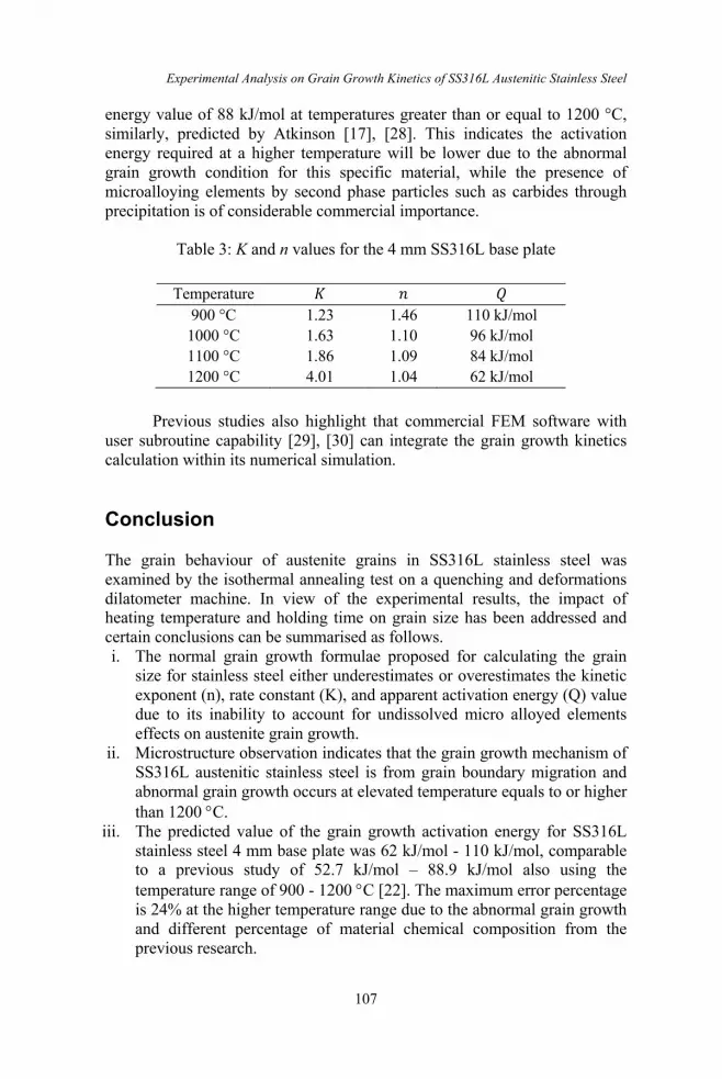
Experimental Analysis on Grain Growth Kinetics of SS316L Austenitic Stainless Steel
107
energy value of 88 kJ/mol at temperatures greater than or equal to 1200 °C, similarly, predicted by Atkinson [17], [28]. This indicates the activation energy required at a higher temperature will be lower due to the abnormal grain growth condition for this specific material, while the presence of microalloying elements by second phase particles such as carbides through precipitation is of considerable commercial importance.
Table 3: K and n values for the 4 mm SS316L base plate
Previous studies also highlight that commercial FEM software with
user subroutine capability [29], [30] can integrate the grain growth kinetics calculation within its numerical simulation. Conclusion The grain behaviour of austenite grains in SS316L stainless steel was examined by the isothermal annealing test on a quenching and deformations dilatometer machine. In view of the experimental results, the impact of heating temperature and holding time on grain size has been addressed and certain conclusions can be summarised as follows. i. The normal grain growth formulae proposed for calculating the grain
size for stainless steel either underestimates or overestimates the kinetic exponent (n), rate constant (K), and apparent activation energy (Q) value due to its inability to account for undissolved micro alloyed elements effects on austenite grain growth.
ii. Microstructure observation indicates that the grain growth mechanism of SS316L austenitic stainless steel is from grain boundary migration and abnormal grain growth occurs at elevated temperature equals to or higher than 1200 °C.
iii. The predicted value of the grain growth activation energy for SS316L stainless steel 4 mm base plate was 62 kJ/mol - 110 kJ/mol, comparable to a previous study of 52.7 kJ/mol – 88.9 kJ/mol also using the temperature range of 900 - 1200 °C [22]. The maximum error percentage is 24% at the higher temperature range due to the abnormal grain growth and different percentage of material chemical composition from the previous research.
Temperature 𝐾 𝑛 𝑄 900 °C 1.23 1.46 110 kJ/mol 1000 °C 1.63 1.10 96 kJ/mol 1100 °C 1.86 1.09 84 kJ/mol 1200 °C 4.01 1.04 62 kJ/mol

Muhd Faiz Mat et al.
108
iv. The apparent activation energy (Qapp) should be considered as a temperature dependant value for austenitic stainless steel as the existence of microalloying elements will affect the grain growth behaviour of the material.
As for further recommendation, the kinetic exponent (n), rate constant
(K), and apparent activation energy (Qapp) will be considered as a temperature dependant value for further investigation on the austenitic grain growth using numerical computation. The prediction of the grain size using the same model and material with numerical computation software for the welding process will be further developed. As most of the value stated above from previous researchers was also collected from numerous resources, it was necessary to verify the local source material grain growth kinetics value as it can have different chemical compositions that can affect the grain growth. This research will continue to further investigate the same material at different temperature ranges and holding times to obtain the near-optimal condition of the grain size while exploring the mechanical and fatigue properties changes due to the grain size effect that is very important for the stainless-steel industry. Acknowledgment The finance of this research was supported by the German Academic Exchange Service (DAAD) with Project Code: 57525437 (Future Technology Additive Manufacturing). The authors acknowledged their gratitude to the staff members of Smart Manufacturing Research Institute (SMRI) at Universiti Teknologi MARA (UiTM), Malaysia. The authors would like to also acknowledge with gratitude for the experiment that was carried out at TU Chemnitz in Germany as well as the Professorship of Virtual Production Engineering for encouraging the research. The authors also appreciated the infrastructure provided by the School of Mechanical Engineering, College of Engineering, Universiti Teknologi MARA (UiTM). References [1] Y. Wang, M. Ding, Y. Zheng, S. Liu, W. Wang and Z. Zhang, “Finite-
element thermal analysis and grain growth behavior of HAZ on argon tungsten-arcwelding of 443 stainless steel,” Metals, vol. 6, no. 4, pp. 1-16, 2016.
[2] S. Zaman, M. A. Khattak and M. N. Tamin, “Effects of Welding on the Microstructural Properties of AISI 430 Ferritic Stainless Steel,” Akademia Baru, vol. 1, no. 1, pp. 25–32, 2018.

Experimental Analysis on Grain Growth Kinetics of SS316L Austenitic Stainless Steel
109
[3] A. Turnbull and E. R. De Los Rios, “The Effect of Grain Size on Fatigue Crack Growth in an Aluminium Magnesium Alloy,” Fatigue & Fracture of Engineering Materials and Structure, vol. 18, no. 11, pp. 1355-1366, 1995.
[4] J. Moravec, I. Novakova, J. Sobotka and H. Neumann, “Determination of Grain Growth Kinetics and Assessment of Welding Effect on Properties of S700MC Steel in the HAZ of Welded Joints,” Metals, vol. 9, no. 6, pp. 707, 2019.
[5] R. V. Taiwade, R. Shukla, H. Vashishtha, A. V. Ingle and R. K. Dayal, “Effect of Grain Size on Degree of Sensitization of Chrome-Manganese Stainless Steel,” ISIJ International, vol. 53, no. 12, pp. 2206–2212, 2014.
[6] S. X. Li, Y. N. He, S. R. Yu and P. Y. Zhang, “Evaluation of the effect of grain size on chromium carbide precipitation and intergranular corrosion of 316L stainless steel,” Corrosion Science, vol. 66, pp. 211–216, 2013.
[7] C. R. Cunningham, J. Wang, V. Dhokia, A. Shrokani and S. T. Newman, “Characterisation of Austenitic 316LSi Stainless Steel Produced by Wire Arc Additive Manufacturing with Interlayer Cooling,” Proceedings of the 30th Annual International Solid Freeform Fabrication Symposium – An Additive Manufacturing Conference, pp. 426-439, 2019.
[8] P. Bajaj, A. Hariharan, A. Kini, P. Kürnsteiner, D. Raabe and E. A. Jägle, “Steels in additive manufacturing: A review of their microstructure and properties,” Materials Science & Engineering A, vol. 772, no. 138633, 2020.
[9] J. E. Burke and D. Turnbull, “Recrystallization and grain growth,” Progress in Metal Physics., vol. 3, no. C, pp 220-292, 1952.
[10] M. F. Ashby and K. E. E. Easterling, “A first report on diagrams for grain growth in welds,” Acta Metallurgica, vol. 30, pp. 1969–1978, 1982.
[11] A. Ayad, F. Wagner, N. Rouag and A. D. Rollett, “Accelerated Potts model for grain growth - Application to an IF steel,” Computational Material Science, vol. 68, pp. 189-197, 2013.
[12] I. Andersenj and O. Grong, “Analytical modelling of grain growth in metals and alloys in the presence of growing and dissolving precipitates. I- Normal grain growth,” Acta Metallurgica, vol. 43, no. 7, pp. 2673–2688, 1995.
[13] D. Zöllner and P. Streitenberger, “Normal grain growth: Monte Carlo Potts model simulation and mean-field theory,” Micro-Macro-interaction in Structured media and Particle Systems., pp. 3–18, 2008.
[14] X. Chen, X. Chen, H. Xu and B. Madigan, “Monte Carlo simulation and experimental measurements of grain growth in the heat affected zone of 304 stainless steel during multipass welding,” International Journal of Advance Manufacturing Technology., vol. 80, no. 5, pp. 1197-1211,

Muhd Faiz Mat et al.
110
2015. [15] T. T. Gladman and D. Dulieu, “Grain-Size Control in Steels,” Metal
Science, vol. 8, no. 1, pp. 167-174, 1974. [16] J. Moon, J. Lee and C. Lee, “Prediction for the austenite grain size in the
presence of growing particles in the weld HAZ of Ti-microalloyed steel,” Material Science and Engineering A, vol. 479, no.1, pp. 40-46, 2007.
[17] S. Illescas, J. Fernández and J. M. Guilemany, “Kinetic analysis of the austenitic grain growth in HSLA steel with a low carbon content,” Materials Letters, vol. 62, no. 20, pp. 3478–3480, 2008.
[18] X. H. Chen, J. Lu, L. Lu and K. Lu, “Tensile properties of a nanocrystalline 316L austenitic stainless steel,” Scripta Materialla, vol.52, no. 10, pp. 1039-1044, 2005.
[19] X. Feaugas and H. Haddou, “Grain-size effects on tensile behavior of nickel and AlSl 316L stainless steel,” Metallurgical and Materials Transactions: Physical Metallurgy and Materials Science, vol. 34 A, no. 10, pp. 2329–2340, 2003.
[20] G. Dini, A. Najafizadeh, R. Ueji and S. M. Monir-Vaghefi, “Tensile deformation behavior of high manganese austenitic steel: The role of grain size,” Materials and Design, vol. 31, no. 7, pp. 3395–3402, 2010.
[21] D. Priadi, R. A. M. Napitupulu and E. S. Siradj, “Austenite grain growth calculation of 0.028% Nb steel,” Journal of Mining and Metallurgy Section B: Metallurgy, vol. 47, no. 2, pp. 199–209, 2011.
[22] B. P. Kashyap and K. Tangri, “Grain growth behaviour of type 316L stainless steel,” Materials Science and Engineering A, vol. 149, no. 2, pp. 13-16, 1992.
[23] M. Faiz Mat, Y. H.P. Manurung, N. Muhammad, S. N. S. Ahmad, M. Graf and M. S. Sulaiman, “Variable Analysis for Grain Size Prediction of Austenitic Stainless Steel SS316l Using Heat Treatment,” Journal of Applied Science, vol. 20, no. 3, pp. 91–96, 2020.
[24] R. Abbaschian, L. Abbaschian and R. Reed-Hill, “Physical Metallurgy Principles”, in Annealing, 4th ed. Cengage Learning, USA, 2009, pp. 216-260.
[25] D. N. Wasnik, G. K. Dey, V. Kain and I. Samajdar, “Precipitation stages in a 316L austenitic stainless steel,” Scripta Materialla, vol. 49, no. 2, pp. 135–141, 2003.
[26] M. Shirdel, H. Mirzadeh and M. H. Parsa, “Abnormal Grain Growth in AISI 304L Stainless Steel,” Materials Characterization, vol. 97, pp 11-17, 2014.
[27] R. C. Chen, C. Hong, J. J. Li, Z. Z. Zheng and P. C. Li, “Austenite grain growth and grain size distribution in isothermal heat-treatment of 300M steel,” Procedia Engineering, vol. 207, pp. 663–668, 2017.
[28] H. V. Atkinson, “Overview no. 65. Theories of normal grain growth in pure single phase systems,” Acta Metallurgica, vol. 36, no. 3, pp. 469-

Experimental Analysis on Grain Growth Kinetics of SS316L Austenitic Stainless Steel
111
491, 1988. [29] O. Yahya, Y. H. P. Manurung, M. S. Sulaiman and P. Keval, “Virtual
Manufacturing for Prediction of Martensite Formation and Hardness Value induced by Laser Welding Process using Subroutine Algorithm in MSC Marc / Mentat,” Journal of Mechanical Engineering, vol. 15, no. 2, pp. 107–125, 2018.
[30] Y. H. P. Manurung, M. S. Sulaiman, S. K. Abas, G. Tham and E. Haruman, “Investigation on welding distortion of combined butt and T-joints with 9-mm thickness using FEM and experiment,” International Jornal of Advance Manufacturing Technology, vol. 77, no. 5, pp. 775-782, 2015.

Journal of Mechanical Engineering Vol 18(3), 113-129, 2021
___________________ ISSN 1823-5514, eISSN 2550-164X © 2021 College of Engineering, Universiti Teknologi MARA (UiTM), Malaysia.
Received for review: 2020-08-27 Accepted for publication: 2021-04-14
Published: 2021-09-15
A Simulation Study of Lubricating Oil Pump for an Aero Engine
Tarique Hussain*, Niranjan Sarangi, M. Sivaramakrishna Gas Turbine Research Establishment, DRDO, Bangalore, India
M. Udaya Kumar National Institute of Technology Tiruchirappalli, India
ABSTRACT
The lubrication system of an aeroengine is intended to lubricate and cool bearings, gears, and splines to ensure a high level of safety and reliability for many operating hours of an aircraft. One of the important accessories of the lubrication system of an aeroengine is the oil pump which consists of multiple pumps with tandem gerotor elements housed in a single casing. The lubrication pump consists of multi positive displacement pumps of “GEROTOR” type, driven by a single shaft. The aim of this paper is to study the influence of altitude conditions on the pump performance and develops a simulation technique for the prediction of output flow rate at various on and off-design conditions. A numerical study has been conducted using commercial CFD code ANSYS-Fluent. Volumetric efficiency is considered as the main parameter for the evaluation of pump performance at various operating conditions. Further, the experimental study has been carried out by simulating low inlet pressure conditions at the inlet of the pump. The comparison between simulation and experimental results shows that results are matching within a 6% deviation. Thus, the simulation method is appropriate for predicting the altitude performance of gerotor pump used in the lubrication system of an aero engine. The study concludes that the contribution of inlet pressure to the pump performance is significant.
Keywords: Gerotor Pump; Trochoidal Profiles; Altitude; CFD; Lubrication
Introduction An aero-engine or gas turbine requires a lubrication system for the smooth functioning of rotating components of the engine. Another function of the

Tarique Hussain, et al.
114
lubrication system is to collect worn-out matters from the gearbox and bearing housings which if left may cause failures in these rotating components. Most of the present-day aircraft gas turbine engines use a closed-loop lubrication system. The closed-loop lubrication system has three characteristic sections. The first section covers pipelines between the supply pump and the engine bearings. This is referred to as the supply line section. In this section, the oil after being filtered and cooled is then supplied to lubricate the main shaft bearings, gear drives, and gearbox. The second section is called scavenge pipeline section and that covers pipelines between bearing sumps and scavenge pumps. To safeguard positive suction of oil during the different altitudes of the engine in flight usually several scavenge pumps are installed in this section. The third section is between scavenge pumps to supply pumps through the filter, air-oil separator, and oil tank. The oil from scavenge pumps passes through the filter and goes to the air-oil separator where oil gets separated from air before falling back in the oil tank as shown in Figure 1. The pump discussed in this present work is the supply pump.
The oil pump of the lubrication system ensures a continuous and pertinent flow of lubricant. It is considered one of the most critical parts of a lubrication system since the failure of the pump will cause a rapid shut down of the engine. Oil pump delivers high-pressure oil to engine bearings, seals, gears, etc., and low-pressure oil is scavenged out from bearing housing and send back to the oil tank. The most demanding case for the oil pump corresponds to the altitude running conditions. So, the pump is usually designed for this case with some margin. For the other running conditions, the pump delivers more than the necessary flow rate.
Generally, a gerotor type oil pump is used in the aero-engine due to the number of their advantages, some being less noisy, reliable, simplicity due to fewer numbers of components, no sealing units, compactness leading to a lighter weight, and the possibility of higher speeds. The gerotor is a positive displacement pump, consisting of three elements: an inner rotor, an outer rotor, and an eccentric ring. Profile of inner is referred to as the trochoidal and the outer rotor is having a circular arc profile which is conjugate to inner rotor profile. An inner rotor is having one tooth less than the outer rotor. As the gerotor revolves, the liquid is drawn into the enlarging chamber to a maximum volume equal to that of the missing tooth on the inner element. When the chamber has reached its maximum volume, the tips and lobes seal the chamber from both the inlet side (low pressure) and the outlet side (high pressure). Further shaft rotation causes the chamber to become connected to the discharge port and, as additional rotation occurs, the chamber volume becomes smaller, forcing the fluid out until it is empty. This process occurs constantly for each chamber, providing a smooth pumping action.

Altitude Performance of Lubricating Oil Pump of an Aero engine
115
Figure 1: Schematic diagram of the lubrication system.
The outer and inner profile is described by Fabiani et al. [1] as shown in Figure 2. Figure 2 illustrates that the outer rotor is drawn by N circular arc with centers at a distance K from the center O1. The inner rotor profile is conjugate with the outer rotor. Therefore, the inner and outer rotor rotates about their respective centers O1 and O2 at angular velocities ω1 and ω2 with a gear ratio of (N-1)/N.
The inner rotor is driven by a prime mover and the outer gear is driven by the motion of the inner rotor. This results in an increasing volume between the inner and outer rotor. This increasing volume decreases the pressure in the volume, which allows pushing the fluid into the pump. On another side, it creates a decreasing volume between the gears. This decreasing volume increases the pressure, subsequently squeezing the fluid out of the pump as shown in Figure 3. Kidney shape inlet and outlet ports are designed which facilitate entry and exit of oil.

Tarique Hussain, et al.
116
Figure 2: Geometrical parameter of the gerotor pump.
Figure 3: Gerotor pump.
Aero-engine oil pump operates at various flight conditions like attitude and altitude of aircraft which affect the performance of gerotor pump. Effect of operating conditions like pump speed, outlet pressure, and design parameters like clearances was studied and discussed by Hussain et al. [2]. Generally, the oil reservoir of an aeroengine is breathed into the atmosphere, thus the oil pump inlet pressure is also close to the atmospheric pressure. Low inlet pressure reduces the pump volumetric efficiency as described by Ippoliti et al. [3]. A significant drop in efficiency was observed at lower inlet pressure when the engine is operating at high altitude conditions. Such degraded performance during high-speed rotation can cause a reduction in oil supply to engine main bearing and gears which will cause

Altitude Performance of Lubricating Oil Pump of an Aero engine
117
overheating of bearing, oil cocking, oil fire, etc. Thus, it is important to design the gerotor pump in terms of its performance and the life of the pump.
In past decades, gerotors have been studied for investigation of their performance and structural integrity [4-17]. Lozica et al. [18] performed load analysis on the gerotor pump using analytical and numerical methods. A simple analytical model was developed to determine the load acting on the rotors. The contact forces and the pressure forces were taken into consideration for load calculations. Further, the FEM model of the pump was used to calculate the loads. The values of the loads obtained by analytical methods and numerical methods were compared. It was concluded that the results obtained by numerical methods are close to results obtained by analytical methods.
Kumar et al. [19] did a comprehensive study for the development of the gerotor pump inlet components for application in engine lubrication. CFD simulations results were validated with actual experiments. Adolfo et al. [20] modelled the gerotor pump using AMESim software. One dimensional model using AMESim software was developed to find out the volume variations of the chambers and to show the variation in the instantaneous flow rate. Good agreement was concluded between the model and experimental values. Altare et al. [21] rigorously studied the influence of the geometric parameters on the filling of the chamber volumes of the gerotor pump. The effect of variation in inlet port design, inlet port direction, the width of the rotor and external rotor diameter was studied using the CFD model. Karthikeyan et al. [22] studied the flow through the gerotor pump using CFD with the view of designing the pump for application in automobiles. CFD model was used to determine the mean flow, pressure, velocity vectors, and wall shear stress contours. The experimental mass flow rate is compared with the results obtained from the simulation. Jamadar et al. [23] did a complete design of Gerotor pump for application in a high-speed diesel engine. A GUI-based program was used for the profile generation of the inner rotor, outer rotor, and inlet-outlet ports. The program was also able to calculate the output parameters like the flow rate and instantaneous flow ripple.
Despite their simplicity, very few studies relevant to the development of a simulation model for altitude conditions are available in open literature due to the complexity of the geometry of the variable volume chambers and two-phase flow phenomena. In the present work, flow analysis at various operating conditions was carried out by using Commercial CFD code ANSYS-Fluent with realizable k-e turbulence and a multiphase model [24]. A prototype pump has been manufactured and tested for its performance and compared with the simulation result. The comparison indicates that simulation results match well with the measured data. From this study, the simulation method and technique adapted are appropriate for predicting the performance of gerotor pump at high altitude conditions of an aero engine.

Tarique Hussain, et al.
118
Pump Performance Gerotor pumps is a positive displacement pump, the flow rate is depended on pump speed, inlet pressure, outlet pressure, and fluid temperature. In the present study, outlet pressure and fluid temperature are maintained constant to reduce the number of variables. Pump performance is decided by its volumetric efficiency. Volumetric efficiency is calculated by the ratio of the effective volume flow rate from analysis or experimental result on the theoretical flow rate computed from the pump displacement. High rotational speed and low inlet pressure induce the incomplete filling of the chamber which results in a reduction in volumetric efficiency. Low inlet pressure of fluid causes the aeration of lubricating oil which results in partly filling of chamber with air and reduction in flow rate. This phenomenon also induces a cavitation mechanism within the pump cavity.
The volume of dissolved gas in the fluid is estimated by Henry-Dalton’s law [3] as mentioned in Equation (1).
Vgas= B. Vliq (P + Patm ) / Patm (1)
where; Vgas is the dissolved volume of air under normal conditions (20 °C, 101.3 kPa), Vliq is the volume of liquid under normal conditions, P is relative pressure and Patm is atmospheric pressure, and B is Bunsen coefficient which is 0.08-0.1 for lubricating oil.
According to this law, the amount of dissolved air/gas is directly proportional to fluid pressure. In other words, the amount of dissolved air in the fluid is reduced by decreasing inlet pressure. Consequently, the amount of free air at the inlet of the pump is increased which resides with bulk fluid in the form of small bubbles. The aeration or air content is defined by the volume of air to the total volume. AAs per As CFD Analysis
Gerotor elements like inner rotor, outer rotor, and cover plates were modelled in Unigraphics software using geometrical parameters tabulated in Table 1.
Table 1: Geometrical parameter of gerotors
Geometrical parameter Value in mm

Altitude Performance of Lubricating Oil Pump of an Aero engine
119
Outer Lobe radius (S) 17.60 Eccentricity (e) 3.50
Radius of circle to complete external gear (G) 21.80 Number of outer lobes (n) 5.00
Distance of the centers of circular arc from center O1 (K) 31.60 Thickness of rotor 7.00 Rotor tip clearance 0.02
Radial clearance between outer rotor and housing 0.05 Axial clearance between rotor and cover plate 0.03
The commercial computational fluid dynamics (CFD) tool ANSYS-
Fluent was used for the flow analysis and to predict the performance of the pump. Leakage flow through micron-scale gaps in gerotor pump was considered in the present analysis except for leakage flow through shaft is neglected due to complexity in analysis. The computational domain along with the surrounding region of the gerotor pump is as shown in Figure 4. To achieve a good quality mesh along with the best compromise between the computational time and accuracy, the computational domain (control volume) was decomposed into four smaller sub-domains, chamber volumes between the inner and outer rotor, inlet and outlet cover plate volume, radial clearance passage and extension of inlet and outlet port. The mesh pictures for chamber volumes are shown in Figure 5.
Figure 4: 3D view of CFD domain.

Tarique Hussain, et al.
120
Figure 5: Mesh picture of chambers.
As can be seen, several elements were employed in the radial direction to achieve accurate results when resolving the radial gap fluid dynamics. In Solver, the boundary conditions and fluid properties as per lubricating oil specification MIL-PRF-23699 F were prescribed. Setting the boundary conditions mimics the operation of a real test, in that speed and pressure boundaries, are specified. A transient simulation was performed with a time step calculated based on the 0.25-degree rotation of the inner rotor. Here to perform a CFD simulation for a gerotor inside Fluent, the deforming fluid volume is identified as the region between the gerotor gears. This fluid region is known as gerotor core as shown in Figure 5 and the entire fluid volume is decomposed into moving and deforming volumes. Approximately three million elements were used after the grid-independent study. A realizable k-e turbulence model [24] was used for analysis. A multiphase model was employed to simulate the two-phase flow phenomenon inside the chamber. Four altitude conditions with four different speeds and two outlet pressures were selected for the analysis as tabulated in Table 2. Air content value is estimated from Henry-Dalton’s law and mentioned in Table 2.

Altitude Performance of Lubricating Oil Pump of an Aero engine
121
Table 2: Various simulation and test condition
Case Sl. No.
Altitude (km)
Pump Speed (rpm)
Inlet pressure (kPa)
Outlet pressure (kPa)
Air content (%)
1 0 3000 4500 5090 5600
100 200 400
0
2 5.0 3000 4500 5090 5600
54 200 400
4.2
3 8.0 3000 4500 5090 5600
35 200 400
5.9
4 10.0 3000 4500 5090 5600
26 200 400
6.7
Output volumetric flow along with radial and axial internal leakage
flow rate were estimated at various simulation cases as mentioned in Table 2. Contour plot of static pressure, the volume fraction of air was extracted from the simulation results. A contour plot of static pressure for simulation case no. 2 is shown in Figure 6.
Figure 6: Static pressure contour at top surface of gerotor for case no.2.

Tarique Hussain, et al.
122
Experimental Setup
A gerotor pump was manufactured and assembled (shown in Figure 7) in the test rig for validation of the simulation model with a set geometrical parameter as mentioned in Table 1. The layout of the rig setup is shown in Figure 8.
Test unit (oil pump) (8) draws the oil from the oil reservoir (1) and delivers it to a pressure and temperature sensors (10) turbine flow meter (11), pressure control valve (12) and then the oil is sent back to the oil reservoir (1). In the test bench, a thermocouple, and a speed sensor (not shown in Figure) were used for measuring oil temperature and rotation speed respectively. The test unit (oil pump) is driven by a variable frequency electric motor (9) which can vary the pump shaft speed; a control valve (12) is used for varying delivery line pressure. Low inlet pressure in the oil reservoir is maintained by a vacuum pump (5) and proportional valve (14). Inlet pressure and temperature are measured by pressure and temperature sensor (7). Oil is filtered by a fine filter (3) and heated by a heater (4). A Separate oil pump (2) is equipped for the filtration and heating of oil. Lubrication oil used was as per MIL-PRF-23699F. The oil temperature was maintained constant at 100 ˚C in all tests.
Figure 7: Picture of assembled pump with test rig.

Altitude Performance of Lubricating Oil Pump of an Aero engine
123
Figure 8: Schematic diagram of test setup.
Results and Discussion
Tests were performed at various speeds and inlet oil pressure as mentioned in Table 2. Tests were repeated for two outlet pressures i.e., 200 kPa and 400 kPa. Figure 9 shows the behaviour of volumetric efficiency of the pump at various inlet pressure when the pump was operating at outlet pressure 400 kPa and oil temperature 100 °C. A significant drop in volumetric efficiency was observed at maximum pump speed and low inlet pressure. Volumetric efficiency is reduced by 29% at maximum pump speed when oil inlet pressure is reduced to 26 kPa. Reduction in outlet flow rate is due to incomplete filling of the chamber by bulk oil when the pump is operating at low inlet pressure. Undissolved/free air occupies the space available in gerotor chambers at the low inlet pressure of the pump inlet.
Pump performance was presented at inlet pressures of 120 kPa to 20 kPa by Ippoliti et al. [8] which corresponds to seal level to 11.8 km altitude condition respectively. Similar kind of results was found and discussed. Volumetric efficiency was dropped to 51% and 40% at maximum pump speed when the pump was operating at an inlet pressure of 30 kPa and 20 kPa respectively. Whereas tested pump was performed with 75% and 64% volumetric efficiency when it was operating at an inlet pressure of 35 kPa and 26 kPa respectively as shown in Figure 9. The difference in pump performance results by Ippoliti et al. [8] with the tested result as shown in Figure 9 could be due to the difference in geometry of tested gerotors with the one presented by Ippoliti et al. [8].

Tarique Hussain, et al.
124
Figure 9: Pump performance curve (tested result).
Further, simulation results from CFD analysis were compared with tested results. A very close match was found between simulated values and experimental results at sea level conditions as shown in Figure 10. Simulation model prediction at maximum speed is 1.2% and 6.5% more than the experimental result when the pump was operating at outlet pressure 200 kPa and 400 kPa respectively.
Volumetric efficiency was estimated at different operating conditions and compared with experimental results. Comparison of model and test results at two different altitude conditions (8 km and 10 km) is shown in Figures 11 and 12 respectively. Good agreement is found between prediction from the simulation model and experimental results. It is also observed that simulation model results are not closely matching when the pump is operating at a lower speed compared to higher speed operation. Model is able to predict within 2-3% of volumetric efficiency at higher speed and 4-6% at lower speed. This difference is due to shaft internal leakage which is not considered in this study. As stated earlier, internal leakages are a direct function of the pressure gradient across the pump. In the present study, the pressure gradient is maintained the same during all speed operations. Therefore, the proportion of internal leakage value on the total flow rate is more at a lower speed.
50556065707580859095
2500 3500 4500 5500Vol
umte
ric
Effic
ienc
y (%
)
Speed(rpm)
Performance Curve (Outlet Pressure -400 kPa)
Vol. Efficiency (Pin- 100 kPa) Vol. Efficiency (Pin-54 kPa) Vol. Effieciency( Pin-35 kPa) Vol. Efficiency (Pin-26 kPa)

Altitude Performance of Lubricating Oil Pump of an Aero engine
125
Figure 10: Comparison of volumetric efficiency between CFD results and experimental results (sea level condition).
Figure 11: Comparison of volumetric efficiency between CFD results and
experimental results (H=8 km).
50556065707580859095100
2500 3000 3500 4000 4500 5000 5500 6000
Vol
umet
ric
Effie
cien
cy(%
)
Speed(RPM)CFD Vol. Efficiency (P=200 kPa) Exp. Vol. efficiency(P=200 kPa)CFD Vol efficiency (P=400 kPa) Exp. Vol. Efficiency(P=400 kPa)
50556065707580859095
2500 3500 4500 5500
Vol
umte
ric
Effic
ienc
y (%
)
Speed(rpm)
Exp. Vol. Efficiency(P-200kPa) Exp. Vol.efficiency (P-400kPa)CFD Vol. Efficiency (P-200 kPa) CFD Vol. Efieciency (P-400 kPa)

Tarique Hussain, et al.
126
Approximately 10-12% drop in volumetric efficiency is observed when the pump is operating at 8 km altitude condition as shown in Figure 11. Significant degradation of pump performance was observed at higher altitude conditions i.e., 10 km.
It is shown in Figure 12 that volumetric efficiency is dropped by approximately 20% at high altitude conditions. This drop inefficiency is due to an increase in free air volume in oil which causes incomplete filling of the chamber which results in the reduction of flow rate and volumetric efficiency.
Figure 12: Comparison of volumetric efficiency between CFD results and experimental results (H=10 km).
Conclusion
This paper presented the numerical and experimental study for investigating the performance of gerotor type lubricating oil pumps. The focus of this study is to evaluate the pump performance for high-altitude conditions. A significant drop in volumetric efficiency was observed during rig testing at simulated high-altitude conditions. Pump performance at sea level and altitude condition has been measured. Unsteady multi-phase CFD analysis of flow through a gerotor oil pump was carried out at various operating conditions. The results obtained by these analyses were compared with the
50556065707580859095
2500 3500 4500 5500
Vol
umte
ric
Effic
ienc
y (%
)
Speed(rpm)
Exp. Vol. Effieciency (P-200 kPa) Exp. Vol. Efficiency (P-400 kPa)CFD Vol. Effieciency( P-200 kPa) CFD Vol. Efficiency (P-400 kPa)

Altitude Performance of Lubricating Oil Pump of an Aero engine
127
experimental values and results predicted by the simulation model have good agreement with experimental values. The simulation model is able to predict the degradation of pump performance with a maximum difference of 4-6% of volumetric efficiency. It was clearly shown that the contribution of inlet pressure to the pump flow efficiency was significant. Future studies will be focused on modelling shaft leakage flow in order to get closer results from CFD simulation. This methodology can be extended for a flow analysis of multistage gerotor pumps.
Thus, this methodology provides useful information to the lubrication system designer to design the system more easily and accurately. This proposed technique of simulation will be useful for design iteration through the fast modification of the pump design of an aero gas turbine engine. Acknowledgment
Authors acknowledge Director, GTRE for permission to publish material. References
[1] Fabiani, M., Mancò, S., Nervegna, N. Rundo, M., et. al., “Modelling and
simulation of gerotor gearing in lubricating oil pumps”, Society of Automotive Engineers Technical Paper 1999-01-0626, pp. 989-1003, 1999.
[2] Hussain, T., Sivaramakrishna, M., Suresh Kumar, S.P., “In-house development of gerotor pump for lubrication system of a gas turbine engine,” Proceedings of the ASME 2015 Gas Turbine India Conference, Hyderabad, India, 2–3 December 2015.
[3] Ippoliti, L., Berten, O., “Influence of inlet piping conditions on the performance of an aircraft engine lubrication system pump,” Proceedings of the 9th National Congress on Theoretical and Applied Mechanics, Brussels, Belgium, 9–10 May 2012.
[4] Ivantysyn, J., Ivantysynova, M., “Hydrostatic pumps and motors, principles, designs, performance, modelling, analysis, control and testing”, Akademia Books International: New Delhi, India, 2002.
[5] Rundo, M., Nervegna, N., “Lubrication pumps for internal combustion engines, a review,” Int. J. Fluid Power, vol. 16, pp. 59–74, 2015.
[6] Ruvalcaba, M.A.; Hu, X., “Gerotor fuel pump performance and leakage study”, Proceedings of the ASME 2011 International Mechanical Engineering Congress & Exposition, Denver, CO, USA, pp. 11–17 November 2011.

Tarique Hussain, et al.
128
[7] Prakash, H.R., Manjula, S., “Design and analysis of gerotors of main gear box lubricating oil pump”, Int. J.Eng. Tech. Res., vol 2, pp. 79–81, 2014.
[8] Ippoliti, L., Steimes J., Hendrick P., “Investigation of an oil aeration measurement technique for the study of pump performance in an aircraft engine lubrication system”, Proceedings of the ASME Turbo Expo 2015, Montréal, Canada, June 15 – 19, 2015.
[9] Min-Cheol Lee, Hyo-Seo Kwak, Han-saem Seong and Chul Kim, “A study on theoretical flowrate of gerotor pump using chamber areas”, International Journal of Precision Engineering and Manufacturing, vol. 19, pp. 1385–1392, 2018.
[10] Andrea De Martin, Giovanni Jacazio and Massimo Sorli, “optimization of gerotor pumps with asymmetric profiles through an evolutionary strategy algorithm”, Machines, vol. 7, pp. 17, 2019.
[11] P J Gamez- Montero and E Codina, “Flow characteristics of a trochoidal- gear pump using bond graphs and experimental measurements. Part 1,” Proc. IMechE vol. 221 Part: J. Systems and control engineering, pp. 331-346, May 2007.
[12] P J Gamez- Montero and E Codina, “Flow characteristics of a trochoidal- gear pump using bond graphs and experimental measurements. Part 2,” Proc. IMechE vol. 221 Part: J. Systems and control engineering, pp. 347-363, May 2007.
[13] Jiang, Y. and Perng, C. Y., “An efficient 3d transient computational model for vane oil pump and gerotor oil pump simulation”, SAE-970841, International Congress & Exposition, Detroit, MI, USA, Session: New Diesel Engines & Component, February 1997.
[14] Natchimuthu, K., Sureshkumar, J. and Ganesan, V., “CFD analysis of flow through a gerotor oil pump”, SAE-2010-01-1111, SAE 2010 World Congress & Exhibition, Detroit, MI, USA, Session: New Engines and Components, April 2010.
[15] Zhang, D., Perng, C. Y. and Laverty, M., “Gerotor oil pump performance and flow/pressure ripple study,” SAE-2006-01-0359, SAE 2006 World Congress & Exhibition, Detroit, MI, USA, Session: Transmission and Drivelines Components, April 2006.
[16] Heisel, U., and Mishev, A., “Development of a new gerotor pump with innovative gerotor design and investigation of its hydraulic characteristics through cfd analysis,” 9th International Fluid Power Conference, Aachen,Germany, vol. 1, pp. 50–59, 2014.
[17] Hao Liu, Jae-Cheon Lee, “Profile design and volumetric efficiency analysis of gerotor pumps for awd vehicles” International Journal of Mechanical And Production Engineering, vol. 5, no. 4, April 2017.
[18] Lozica Ivanović,Mirko Blagojević,Goran Devedžić,Yasmina Assoul, “Analytical and numerical analysis of load gerotor pumps” Scientific Technical Review, vol. 60, no. 1, pp. 30-38, 2010.

Altitude Performance of Lubricating Oil Pump of an Aero engine
129
[19] M Suresh Kumar, K Manonmani, “Computational fluid dynamics integrated development of gerotor pump inlet components for engine lubrication” Proc. IMechE Vol. 224 Part D: J. Automobile Engineering, vol. 224, pp. 1555, 2010.
[20] Adolfo Senatore, Dario Buono, Emma Frosina, Luca Santato, “Analysis and simulation of an oil lubrication pump for the internal combustion engine,” Proceedings of the ASME 2013 International Mechanical Engineering Congress and Exposition, November 15-21, 2013.
[21] Giorgio Altare, Massimo Rundo, “Computational fluid dynamics analysis of gerotor lubricating pumps at high-speed: geometric features influencing the filling capability”, Journal of Fluids Engineering, vol. 138 / 111101-1, November 2016.
[22] Karthikeyan N, Suresh Kumar J, Ganesan V, “Development of a gerotor oil pump using cfd” Proceedings of the 37th National & 4th International Conference on Fluid Mechanics and Fluid Power, December 16-18, 2010
[23] Mohammad Jamadar, Alen Jose, Sushil S Ramdasi, Neelkanth V Marathe, “Development of in-house competency to build compact gerotor oil pump for high-speed diesel engine application” SAE International, 01-2738, 2013.
[24] ANSYS 14 Theory Guide, section 4.3.2 standard k-e model, http://www.ansys.com, 2011.

Journal of Mechanical Engineering Vol 18(3), 131-145, 2021
___________________ ISSN 1823-5514, eISSN 2550-164X © 2021 College of Engineering, Universiti Teknologi MARA (UiTM), Malaysia.
Received for review: 2021-02-03 Accepted for publication: 2021-08-19 Published: 2021-09-15
DSC Assessment on Curing Degree of Micron-scaled Adhesive Layer in Lamination-pressed Flexible Printed
Circuit Panels
Kok-Tee Lau*, Hoi Ern Kok Fakulti Teknologi Kejuruteraan Mekanikal dan Pembuatan,
Universiti Teknikal Malaysia Melaka, 76100 Durian Tunggal, Melaka, Malaysia
Nur Hazirah Rosli MFS Technology (Malaysia) Sdn. Bhd., 75350 Batu Berendam,
Melaka, Malaysia.
ABSTRACT
Continuous monitoring and optimisation of the lamination process are critical in negating flexible printed circuit (FPC) delamination risk during operation. The main QC inspection criterion of the lamination adhesive’s curing degree is adhesive thickness. However, this method is prone to measurement error due to poor microscopy image definition and the inspector’s measurement parallax error. The feasibility of using thermal characterisation to measure the difference in curing degrees of micron-scaled adhesive layer of laminated FPC was investigated. Differential scanning calorimetry (DSC) and thermogravimetric analysis (TGA) were used according to IPC standards. Polyimide-epoxy adhesive coverlays were laminated onto both sides of FPC at 120 kgf/cm2 pressure and 180 °C temperature for 120 s. Then, the coverlays were subjected to oven curing at 150 °C for 60 min. The DSC detected a small difference in the curing degree of adhesive layers in the two cured FPC laminated in different laminating-press openings (T1 and T2). T2 had a glass transition temperature (Tg) of 106.5 °C, which was higher than that for T1 (105 °C), thereby suggesting that the former had a higher curing degree than the latter. This result was consistent with the adhesive thickness measurement result of the DSC samples. The adhesive thickness of T2 was smaller (30.97 µm) than that of the T1 (31.76 µm). T2 had a higher curing degree than T1 because of the larger shrinkage percentage. In comparison with DSC, TGA

Kok-Tee Lau, Hoi Ern Kok, Nur Hazirah Binti Rosli
132
was unable to detect the curing degree difference between the samples because of the undetected weight loss resulting from the adhesive curing. Keywords: Flexible printed circuit; Epoxy adhesive; Coverlay lamination; Thermal properties; Curing degree Introduction The increasing number of applications of flexible and stretchable electronics has led to high demand for flexible printed circuit boards (FPC) [1]–[5]. FPC is developed using copper-clad laminate (CCL) to create electronics circuit patterns and simultaneously provide mechanical strength to withstand deformation during operation [6]. The quality control process improvement on FPC largely focuses on the use of vision-based inspection technologies to detect defects in the FPC circuit [7]–[9]. Lamination is performed at the last stage of FPC manufacturing to increase the mechanical robustness of FPC [6]. Previous risk assessment findings on the escape defects from unknown FPC suppliers of a flexible printed circuit board (FPCB) for smartphones showed a defective rate between 1.50% and 4.99%, but failure modes can be detected by operators' self-check [10]. The two main failure modes for flexible electronic devices are crack propagation and delamination, which are generally more common in the conductive layer than in the polyimide structure [11].
Escape defects contributed by the FPC supplier should be reduced to as few as possible through continuous monitoring and optimisation of the FPC manufacturing process [10]. Thus, lamination integrity is critical in protecting the FPC circuit; it negates FPC failure mode risk during subsequent FPCB assembly at the OEM stage. During lamination, heat and pressure are applied simultaneously in a controlled manner to bond a protective coverlay onto the surface of the FPC’s circuit pattern [6]. A typical coverlay is a two-layer material composed of a polyimide sheet as base material and a suitable thermosetting adhesive [6]. The commonly used adhesives are epoxy- and acrylic-based; they require different lamination temperatures and pressure parameter settings [6]. Optimised parameters ensure good conformation (no air entrapment) of the adhesive layer on the circuit pattern and sufficient curing degree or degree of cure of the adhesive after lamination [12].
Curing degree increases with increasing adhesive viscosity [13]. Careful setting of lamination temperature and pressure enables the smooth flow of the adhesive onto the circuit pattern, thereby eliminating void formation risk. Currently, adhesive thickness is measured according to the IPC standard and is the main QC inspection criterion of the lamination adhesive’s curing degree [6, 14]. When a coverlay adhesive is applied to the FPC under high pressure and temperature, the thickness of the adhesive layer reduces dimensionally as a result of increased curing degree. Despite the feasibility of

DSC Assessment on Curing Degree of Micron-scaled Adhesive Layer in Laminating-Pressed
133
adhesive thickness measurement by microscopy technique, the method is prone to measurement error caused by thickness tolerance error of the as-received coverlay-adhesive, limitation in microscopy image definition or inspector’s measurement parallax error [15].
Several alternative methods have been used to measure adhesive curing degree, as follows: change in adhesive strength is determined by peel strength tester; viscoelasticity is determined by rheometer; the functional group is determined by FT-IR, and heating value is determined by thermal analysis instruments [16]. Although adhesive strength can be determined directly using a peel strength tester, the sample preparation is tedious because of the micron-scale thickness of the two adhered layers [17]. Rheometer characterisation for adhesive viscoelasticity is not in-situ, and the sample at a sufficient amount needs to be extracted for testing [18]. Similarly, sample preparation for FT-IR spectrophotometer is tedious, because the challenge of signal contamination from the FPC’s polyimide layer needs to be addressed [19].
Compared with these techniques, DSC and TGA require only a small sample; the sample is cut from the inspected large-area FPC without additional sample preparation steps (in-situ) [20]. Furthermore, technological advancement in the DSC and TGA equipment in terms of their measurement capabilities creates a new opportunity for faster and more accurate detection [21]. DSC and TGA data analyses require basic knowledge of thermodynamics and materials’ quantitative data [22]. Thus, the use of DSC and TGA in the quality control of manufactured products has become popular. The use of DSC and TGA in studies on the manufactured FPC coverlay adhesive’s curing degree has not been reported.
DSC and TGA can be used as qualitative characterisation techniques for root-cause analysis to verify if the delamination or air entrapment failures of the defect FPC could be traced to the inadequate adhesive curing. Inadequate curing degree of the adhesive of the laminated FPC is a major contributor to the high delamination failure risk in lamination samples [12]. An adhesive’s curing degree correlates directly with its polymerisation or molecular cross-linking density and thus could be picked up easily as a jump in the DSC baseline (e.g., at glass-transition temperature) [22].
Conventional thickness measurement has been used as a cost-effective technique in the manufacturing industry to qualify the laminated FPC product. Nevertheless, the technique has a limitation to detect small curing degree variation, particularly on thin and micron-scaled adhesive layers. The current paper investigates the feasibility of using DSC and TGA as qualitative characterisation tools to assess the curing degree of lamination pressed FPC. Furthermore, this investigation intends to validate the inadequate adhesive curing using DSC or TGA for the case where the laminating pressed FPCs produced by different laminating press openings displays insignificant shrinkage’s variation in the cured adhesive layers.

Kok-Tee Lau, Hoi Ern Kok, Nur Hazirah Binti Rosli
134
Methodology Laminating press and cure processes Coverlay-adhesive sheet (i.e., polyimide (PI) sheet thickness = 12.7 µm, epoxy adhesive thickness = 35.56 µm and model = ThinFlex-Q2, Q-0514TA-mb, TopFlex Co.), which had 5-mm diameter holes at its four corners and centre, were used for the lamination of FPC. The CAS number of the halogen-free epoxy adhesive material was not disclosed by the supplier due to confidentiality issues [23]. Before conducting the laminating press, the coverlay-adhesive sheet and FPC were stacked in sequence with other elements (from top-to-bottom) as follows: steel plate, kraft paper, HTRF releasing paper, coverlay sheet, blank doubled-sized FPC, coverlay sheet, HTRF releasing paper, kraft paper and steel plate. A similar stack arrangement was prepared carefully to ensure consistency in the lamination quality.
Figure 1: Lamination-pressed FPC obtained from different laminating press
openings were labelled accordingly as T1, T2, B1 and B2. The zoom-in view shows a schematic cross-sectional view of one of the laminated FPC.
The lamination press of the stacks was performed by using the four-
opening laminating press (platen size = 545 × 660 mm, Beyond China) under fast and hot-pressing conditions, as recommended by the coverlay supplier [24]. All four openings (see Figure 1) were set at a temperature of 180 °C and

DSC Assessment on Curing Degree of Micron-scaled Adhesive Layer in Laminating-Pressed
135
pressure of 120 kgf/cm2 for a time interval of 120 s. Then, all stacks underwent post-cure condition using an oven (model Gol-8D) at 150 °C for 60 min. After cooling, the cured laminated FPC sheets were labelled based on their laminating press’s opening location, as shown in Figure 1. For example, the sample obtained from the top opening at zone 1 was labelled as T1. Characterisation methods Adhesive thickness was characterised according to IPC TM-650, 2.2.18.1 standard [25] to quantify the curing degree of adhesive in the laminated FPC. IPC stands for the Institute for Interconnecting and Packaging Electronic Circuits, which develops standards for the assembly and production requirements of electronic equipment. Five 1 cm2 strips were cut from each of the T1, T2, B1 and B2 FPCs at different planar regions (see Figure 2). The strips were then subjected to a conventional cross-sectioned sample preparation process, which involved cold resin mounting followed by cross-sectioning and surface polishing of the FPC sample. The images of a polished and smooth cross-section of the samples were captured using a 3D laser scanning microscope (VK-X200 series, Keyence). Each of the upper and lower adhesive layers displayed in the cross-sectioned samples was measured using VK-Analyser software. After that, the average and standard deviation of the measured data from the five planar regions of the upper and lower adhesive layer of T1, T2, B1 and B2 samples were calculated.
To assess the validity of the thickness measurement data in relation to curing degree variation, the adhesive layer of laminated T1 and T2 FPC were characterised by TGA 1 from Mettler Toledo and DSC is characterised using Jade DSC from PerkinElmer. T1 and T2 FPCs were chosen to investigate the curing degree, because the former and the latter had the smallest and the largest thickness variations, respectively. TGA and DSC characterisations were performed according to IPC TM-650, Method 2.3.40 [26] and IPC TM-650, Method 2.4.25 [27]. Both characterisations were conducted in an inert nitrogen gas environment. Samples for characterisations were cut from the centre region of their respective laminated T1 and T2 (Figure 2). The respective initial weights were 7.27 and 6.41 mg for TGA and 10.4 and 9.9 mg for DSC. DSC characterisations were performed by heating the DSC sample from room temperature to 400 °C and then cooling it to ambient temperature. In contrast, TGA characterisation was only performed during heating until 800 °C.

Kok-Tee Lau, Hoi Ern Kok, Nur Hazirah Binti Rosli
136
Figure 2: Bird’s eye view shows that thickness measurement samples were cut from the five planar regions (indicated by the dashed boxes) on a single
laminated FPC. Only the Centre region was used for DSC and TGA characterisations.
Result and Discussion Thickness and shrinkage percentage’s averages of the upper and lower adhesive layers (Figure 1) obtained from the five planar regions (Figure 2) of the cured T1, T2, B1 and B2 samples were plotted in Figure 3. The shrinkage percentage of each measured adhesive layer was calculated using Equation 1 adapted from the volume shrinkage equation [28].
Shrinkage% = $1 − cured adhesive thicknessuncured adhesive thickness
' × 100% (1) where thickness is in µm, and 35.56 µm is the uncured adhesive thickness (as provided by the manufacturer). The shrinkage percentage’s error bar represents the degree of adhesive thickness’s variation along with the planar FPC sheet, thus provided an analogy of volume shrinkage of the cured adhesive thickness.
Corner 2
Corner 3
Corner 1
Corner 4
Centre

DSC Assessment on Curing Degree of Micron-scaled Adhesive Layer in Laminating-Pressed
137
(a)
(b)
Figure 3: Interval plot with a 95% confidence interval of the: (a) lower and
upper adhesives’ thicknesses, and (b) shrinkage percentage of different lamination pressed FPC samples. Data point represents the average value,
and error bar indicates the standard deviation. The average adhesive thicknesses of the four laminated FPC samples
shrunk between 7% and 14% from the original thickness of 35.56 μm after curing. The adhesive underwent shrinkage because of the epoxy polymer cross-linking process. One-way ANOVA analysis (see Table 1) shows that the

Kok-Tee Lau, Hoi Ern Kok, Nur Hazirah Binti Rosli
138
P-value is 0.32 and more than 0.05 at a 95% confidence level. This result implied the lack of significant difference between the average lamination-pressed (cured) adhesive thickness with respect to the laminating press opening positions and adhesive layer positions (upper and lower adhesive layers) [29, 30]. Nevertheless, T2 samples’ thickness for the Lower adhesive layer had the largest margin of error, which varied from 27.1 µm to 34.6 µm. The T1 sample’s thickness (for the Upper adhesive layer) had the lowest variation, which varied from 31.1 µm to 33.9 µm. Cross-sectional images of Figures 4(a) and 4(b) show the adhesive layer thickness of T2, which varied from 28.0–30.7 µm at Corner 2 to 35.6 µm at Corner 4. Images obtained at Corner 2 and Corner 4 regions respectively exhibited the smallest (thinnest) and largest (thickest) adhesive layers after laminating press. The variation of measured adhesive thickness throughout the different locations in the T2 sample, including data from the Corner 2 and 4 regions were represented as the interval plot’s error bar of Figure 3(a) which was determined statistically at a 95% confidence level.
Table 1: One-way ANOVA analysis at 95% confidence interval for the
adhesive thickness data of Figure 3(a)
Source of Variation SS df MS F P-value Fcrit
Between Groups 28.77 7 4.11 1.22 0.32 2.31
Within Groups 108.18 32 3.38
Total 136.95 39
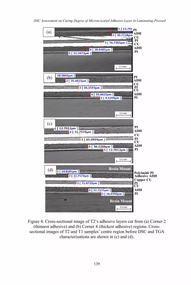
DSC Assessment on Curing Degree of Micron-scaled Adhesive Layer in Laminating-Pressed
139
Figure 4: Cross-sectional image of T2’s adhesive layers cut from (a) Corner 2 (thinnest adhesive) and (b) Corner 4 (thickest adhesive) regions. Cross-
sectional images of T2 and T1 samples’ centre region before DSC and TGA characterisations are shown in (c) and (d).
(a) PI ADH CU
PI
PI
PI
CU ADH
ADH
ADH
PI
PI
CU
CU
(d)
(b)
(c) PI
ADH
ADH PI
PI
CU CU
Polyimide PI
PI
PI
Copper CU CU
Adhesive ADH
ADH
Resin Mount
Resin Mount

Kok-Tee Lau, Hoi Ern Kok, Nur Hazirah Binti Rosli
140
According to the adhesive thickness measurement method, the large variation in cured adhesive thickness of T2 samples suggested that the adhesive’s curing degree varied more significantly over the FPC area for T2 compared with the other three samples. However, ANOVA analysis showed that the average adhesive thickness of samples produced by the four openings had no significant difference. This analysis result suggested that the thickness variation was random and was not caused by systematic error sources, such as sheet’s position accuracy, non-uniform applied temperature and pressure distribution throughout the lamination press platen [6]. As mentioned in the previous section, the possible sources of the random error were the thickness variation of the as-received raw materials, e.g. coverlay-adhesive has a thickness tolerance of ±10% [24], microscopy image definition limitation or the inspector’s measurement parallax error [15].
It is important to validate the inadequate adhesive curing using DSC or TGA when the laminating-pressed FPC produced by different laminating press openings displays insignificant variation in shrinkage percentages (as shown by Figure 3(b)) after adhesive layer curing. When the curing process was performed by lamination press followed by curing at 150 °C, the combined effects of pressure, as received cover lay thickness tolerance and temperature resulted in a small curing degree variation in the adhesive layer. Thus, assessing the validity of thickness measurement data by DSC and TGA characterisations is important. For the sake of this investigation, T1 and T2 samples were chosen for comparison because their SEM micrographs showed an obvious discrepancy in the thickness variation. SEM micrographs of the T1 show adhesive layer thicknesses of 31.76 µm, which was slightly thicker than T2 with a value of 30.97 µm, as shown in Figures 4(c) and 4(d).
The DSC and TGA assessments were performed on small cut from the centre region of the T1 and T2 sample. DSC curves of T1 and T2 samples were compared only between 75 °C and 120 °C (Figure 5) to clearly reveal the weak glass transition temperature (𝑇") peaks. 𝑇" of T1 were observed as a slight jump in the DSC baseline at ~88.5 °C during heating and 105 °C during cooling. However, the 𝑇" of T2 only appeared on the cooling curve at 106.5 °C. The obtained 𝑇" values were near the previously reported Tg values [16, 30]. 𝑇" has been widely used as a measure of the degree of crosslink in epoxy adhesives [22]. Higher Tg on the cooling curve for T1 indicated an increase in crosslink density of T1’s adhesive after the heating process. Menczel et al. [22] argued that 𝑇" depends on the polymer chains’ mobility; polymers possessing more mobile chains have a lower 𝑇" value. A comparison between T1 and T2 samples during cooling however showed that the latter has a higher 𝑇" (1.5 °C difference), thereby showing a higher curing degree. The DSC results agreed with the adhesive thickness data of the T1 and T2 samples, as shown in Figures 4(c) and 4(d). The consistency of DSC’s 𝑇" value with the thickness data proved the effectiveness of using the DSC technique to differentiate the cure

DSC Assessment on Curing Degree of Micron-scaled Adhesive Layer in Laminating-Pressed
141
quality of cured laminated FPC sample of Figure 3, which demonstrated a thickness difference of 0.79 µm between the two DSC samples.
Figure 5: Glass transition temperature (Tg) of epoxy in T1 and T2 samples during the heating and cooling stages of DSC curves. Bold arrow shows the
direction of temperature change during DSC measurement.
TGA results (Figure 6) only exhibited observed weight loss at temperatures above 350 °C. T2 recorded a lower weight loss (~11.9%) and a higher pyrolysis temperature (383.05 °C) than T1. A slight weight loss at 260 °C was observed in the T1 and T2 samples probably due to the epoxy adhesive’s decomposition [31]. The larger weight loss of above 350 °C may be due to the polyimide’s decomposition because it had a larger initial weight percentage than the epoxy adhesive. The claims on epoxy and polyimide decompositions were supported by Wypych data, which showed that their maximum service temperatures were 350 °C and 500 °C, respectively [31]. According to the current study’s TGA finding, TGA was unable to detect the curing degree difference among the varied samples because of the extremely low weight loss caused by adhesive pyrolysis.
Endothermic

Kok-Tee Lau, Hoi Ern Kok, Nur Hazirah Binti Rosli
142
Figure 6: TGA curve.
Conclusion and Recommendation DSC can detect the differences in the curing degree of the micron-scaled adhesion layer of two cured FPCs laminated at different laminating-press openings (T1 and T2). This result was consistent with the adhesive layer thickness measurement results obtained from the same laminated samples. The adhesive layer of the T1 sample (31.76 µm) was thicker than the sample from T2 (30.97 µm). TGA was unable to characterise the curing degree of epoxy adhesive in the cured and laminated FPC sample because of the extremely low weight loss caused by adhesive pyrolysis. Future work needs to investigate the effects of stacking conditions (stacking materials and sequence) on the curing degree of the laminated FPC adhesive layer using DSC. The outcome of the paper can be used to minimise the adhesive layer non-uniformity under improper stacking conditions.
Acknowledgement The authors wish to thank MFS Technology for providing sample preparation and 3D laser microscopy characterisation facilities. They would like to acknowledge Universiti Teknikal Malaysia Melaka for the technical support in DSC and TGA characterisations.
T1 -12.1573 % -0.8842 mg
Onset 382.96 °C Endset 427.32 °C T2
-11.9016 % -0.7630 mg
Onset 383.05 °C Endset 423.53 °C
Onset Endset

DSC Assessment on Curing Degree of Micron-scaled Adhesive Layer in Laminating-Pressed
143
References [1] Z. Cui, "Printing practice for the fabrication of flexible and stretchable
electronics," Science China Technological Sciences, vol. 62, no. 2, pp. 224-232, 2019.
[2] R. Dahiya, "E-Skin: From Humanoids to Humans," Proceedings of the IEEE, vol. 107, no. 2, pp. 247-252, 2019.
[3] Chung, K. -C. and B. W. Moon, U.S. Patent No. 10 887 997, 5 January 2021.
[4] M. M. Mahat, M. F. Aizamddin, N. C. Roslan, M. A. Kamarudin, S. N. I. Omar, M. I. A. Halim and M. M. Mazo, “Conductivity, morphology and thermal studies of polyaniline fabrics,” Journal of Mechanical Engineering, vol. 9, no. 1, pp. 137-150, 2020.
[5] M. F. M. Sharif, A. A. Saad, F. C. An, M. Y. T. Ali and Z. Samsudin, "Effect of Stretchable Circuit Deformation on Its Electrical Performance for Automotive Lighting Application,” Journal of Mechanical Engineering, vol. 4, no. 2, pp. 279-287, 2017.
[6] J. Fjelstad, Flexible Circuit Technology, 4th ed., Seaside: BR Publishing, 2011.
[7] W. Luo, J. Luo and Z. Yang, "FPC surface defect detection based on improved Faster R-CNN with decoupled RPN," 2020 Chinese Automation Congress (CAC), IEEE, Shanghai, 2020, pp. 7035-7039.
[8] X. Tao, D. Zhang, W. Ma, X. Liu and D. Xu, "Automatic metallic surface defect detection and recognition with convolutional neural networks," Applied Sciences, vol. 8, no. 9, pp. 1575, 2018.
[9] Z. Zhao, B. Li, F. Gao, L. Chen and M. Xin, "Online vision system for battery FPC connector defect detection based on active shape model template matching," Proceedings of SPIE: Tenth International Symposium on Precision Engineering Measurements and Instrumentation, vol. 11053, pp. 11053 0Z, 2019.
[10] S. Krasaephol and P. Chutima, "Quality control process improvement of flexible printed circuit board by FMEA," IOP Conference Series: Materials Science and Engineering, vol. 311, no. 1, pp. 012009, 2018.
[11] B. P. DeFigueiredo, T. K. Zimmerman, B. D. Russell and L. L. Howell, "Regional stiffness reduction using lamina emergent torsional joints for flexible printed circuit board design," J. Electronic Packaging, vol. 140, no. 4, pp. 041001, 2018.
[12] J. J. Licari and D. W. Swanson, Adhesives technology for electronic applications: materials, processing, reliability, 2nd ed., Norwich: William Andrew, pp. 194-233, 2011.
[13] T. Löbel, D. Holzhüter, M. Sinapius and C. Hühne, "A hybrid bondline concept for bonded composite joints," International Journal of Adhesion and Adhesives, vol. 68, pp. 229-238, 2016.

Kok-Tee Lau, Hoi Ern Kok, Nur Hazirah Binti Rosli
144
[14] K. -T. Lau, H. E. Kok, H. E. B. A. Maulod, N. Z. B. A. Latiff, A. N. B. A. Aziz and N. H. B. Rosli, "Effect of Laminating Press’s Opening-Stacking Position on Adhesive Thickness in Coverlay/Adhesive/Flexible-Printed-Circuit Sheet," Journal of Engineering Technology and Applied Physics, vol. 1, no. 1, pp. 1-3, 2019.
[15] M. E. Keeble, "Error and Uncertainty in Metallographic Measurement," in 100 Years of E04 Development of Metallography Standards, West Conshohocken: ASTM International, 2019, pp. 53-65.
[16] S. Tanaka, T. Kiryu and H. Takebe, "Curing Degree Evaluation of Reactive Adhesives Using Measurement Devices," ThreeBond Technical News, vol. 1 July 2015, pp. 1-8, 2015.
[17] M. Valori, V. Basile, S. P. Negri, P. Scalmati, C. Renghini and I. Fassi, “Towards the Automated Coverlay Assembly in FPCB Manufacturing: Concept and Preliminary Tests,” in Smart Technologies for Precision Assembly: 9th IFIP WG 5.5 International Precision Assembly Seminar, IPAS 2020, Cham: Springer Nature, pp. 36-50, 2021.
[18] M. Jährling, "The curing behaviour of reaction resin compounds," Application Note LR-12, [Online]. Available: ThermoFisher Scientific, https://www.thermofisher.com. [Accessed Apr 26, 2021].
[19] PerkinElmer Life and Analytical Sciences," Applications and Design of a Micro-ATR Objective," Technical Note, [Online]. Available: Perkin Elmer, https://www.perkinelmer.com. [Accessed Apr 26, 2021].
[20] S. Mestry and S. Mhaske, "Synthesis of epoxy resins using phosphorus-based precursors for flame-retardant coating," J. Coatings Technology and Research, vol. 16, no. 3, pp. 807-818, 2019.
[21] W. Qiao, B. Li and Z. Kang, "Differential scanning calorimetry and electrochemical tests for the analysis of delamination of 3PE coatings," International Journal of Electrochemical Science, vol. 14, pp 7389-7400, 2019.
[22] J. D. Menczel, L. Judovits, R. B. Prime, H. E. Bair, M. Reading and S. Swier, "Differential Scanning Calorimetry (DSC)," in Thermal analysis of polymers, New Jersey: John Wiley & Sons, 2009, pp. 7-240.
[23] W. H. Hsu, "Material Safety Data Sheet ThinFlex-Q (Q2,Q3, Q4, Q5, Q6, Q8, Q9)," Kunshan City: TopFlex Co., 2014, pp. 1-5.
[24] TopFlex Co., "ThinFlex-Q2,Q-0514TA-mb Halogen Free Coverlay," Kunshan City: TopFlex Co., 2014, pp. 1-3.
[25] Determination of Thickness of Metallic Clad Laminates, Cross-sectional 12/94, IPC Standard IPC-TM-650 Test Method Manual 2.2.18.1, 1994.
[26] TGA, IPC Standard IPC-TM-650 Test Method Manual 2.3.40, 1995. [27] Glass Transition Temperature and Cure Factor by DSC, IPC Standard
IPC-TM-650 Test Method Manual 2.4.25, 1994. [28] D. Kaisarly, M. El Gezawi, P. Rösch and K. -H. Kunzelmann, "Shrinkage
vectors and volumetric shrinkage percentage of differently applied

DSC Assessment on Curing Degree of Micron-scaled Adhesive Layer in Laminating-Pressed
145
composites," International Journal of Adhesion and Adhesives, vol. 105, pp. 102793, 2021.
[29] I. Nevliudov, E. Razumov-Fryzyuk, D. Nikitin, D. Bliznyuk and R. Strelets, "Technology For Creating The Topology Of Printed Circuit Boards Using Polymer 3d Mask," Innovative Technologies and Scientific Solutions for Industries, vol. 1, no. 15, pp. 120-131, 2021.
[30] K. Y. Wong, P. J. Liew, K. T. Lau and J. Wang, "Optimization of copper via filling process for flexible printed circuit using response surface methodology," J. Advanced Manufacturing Technology (JAMT), vol. 14, no. 2, pp. 1-14, 2020.
[31] G. Wypych, Handbook of polymers, 2nd ed., Toronto: ChemTec Publishing, pp. 117-432, 2016.

Journal of Mechanical Engineering Vol 18(3), 147-162, 2021
__________________ ISSN 1823-5514, eISSN 2550-164X © 2021 College of Engineering, Universiti Teknologi MARA (UiTM), Malaysia.
Received for review: 2021-03-15 Accepted for publication: 2021-05-06
Published: 2021-09-15
Development and Testing of a Turning Process Monitoring System
using Acoustic Emission
Keiichi Ninomiya*, Shun Yoshida, Kenji Okita, Toshihiko Koga Polytechnic University, Japan
Shuzo Oshima Miyazaki Polytechnic Center, Japan
ABSTRACT
Studies on in-process measurement have suggested techniques for sensing tool wear and machine status in a machining center and turning center, for example by measuring cutting resistance. However, there appear to be no reports of effective uses of machine sensing in practical machine tools, perhaps due to problems such as limitations on the number and density of sensors and the possibility that attaching sensors may affect machine rigidity and thus processing quality. The purpose of this research is to develop a system that can monitor the state of the cutting process and maintain it in a normal or optimal state at all times, based on the acoustic emission (AE) method. To realize the development of such a system, it is very important to evaluate the tool wear qualitatively and quantitatively. This report describes a tool wear experiment that collected AE signals, cutting force data, and high-speed camera images during metal turning. The collected basic data are comprehensively evaluated and examined to determine the effectiveness of in-process measurement by the AE method. The results suggest that evaluating various AE parameters obtained from the AE original waveform is an effective parameter for monitoring tool wear and cutting conditions that affect product quality. The findings from the basic data obtained in this study were found to be useful information for the practical application of in-process measurement by the AE method using machine learning methods. Keywords: In-process Measurement; Turning processes; Tool wear; Cutting phenomena; Acoustic Emission

Keiichi Ninomiya*, Shun Yoshida, Kenji Okita, Toshihiko Koga, Shuzo Oshima
148
Introduction In recent years, it has become clear that continued technological growth will require the innovations of the 4th industrial revolution, such as big data and artificial intelligence, to be incorporated into a wider variety of industries. In support of this goal, there is an urgent technical need for improved in-situ digital visualization and analysis of manufacturing processes [1]–[3]. When introducing Internet of Things (IoT) at a manufacturing site, one of the most important elements is the sensing technology that records key process parameters in real-time and converts these signals into useful data [4, 5]. For example, recent studies have measured machining status and tool wear in a turning center, based on cutting resistance as the in-process measurement [6]–[10]. However, this approach presents practical issues, such as the machining area being limited by mounting the cutting dynamometer and the decrease in rigidity during tool mounting, which may adversely affect the machining quality and machining accuracy.
Continued basic research is needed to advance the development of the Industrial Internet of Things (IIoT). To that end, a prior study constructed and tested an in-process measurement system to monitor the cutting state [11]. The acoustic emission (AE) method, a non-destructive inspection technique, was used for sensing in this system. The AE approach does not impair the tool rigidity during processing and is capable of detecting minute levels of cutting energy in real-time [12]–[14]. In this application, the AE method enables real-time detection of elastic waves generated when a solid deforms or breaks. A practical example of in-process measurement using this AE method is crack detection of a moulded product during drawing [15]. In grinding processing, the AE method may be applied to the evaluation of grinding conditions, allowing the user to judge the deterioration of the cutting edge of the grindstone and extent of clogging [16]; these applications have already been automated. However, it seems that there are few studies that apply AE techniques to visualize cutting operations, that is, using an AE-based sensor system to fully grasp the state of the cutting tool with practical application in mind. The qualitative and quantitative evaluation of the wear state of the cutting tool can be very useful information when evaluating parameters by the machine learning method [17]–[19].
Therefore, this study employed AE measurements to characterize machine-cutting performance. In particular, the relationship between AE signal and tool wear was considered by utilizing cutting power data, observations of cutting state using a high-speed camera, finite element method (FEM) modelling, and physical characterization of cutting chips. Experimental system

Development and Testing of a Turning Process Monitoring System Using Acoustic Emission
149
Figure 1 shows the system used for the experiment. The system is designed to acquire cutting power measurements, AE signals, high-speed camera images, and various basic chip data during turning. A semi-automatic lathe (TAC360, Takisawa Co., Ltd.) that can maintain constant cutting speed was used as the machine tool. Cutting power was measured with a multi-component dynamometer (model 9257A, Kistler Co., Ltd.). The dynamometer signal was amplified by a multi-channel charge amplifier (model 5070A).
A wide-band type AE sensor (AE-900S-WB, NF Circuit Design Block Co., Ltd.) with low resonance was used for the AE measurements. The signal from the AE sensor was passed through the preamplifier and the discriminator (models 9917 and AE-9922S respectively); the processed AE signal and the envelope signal were recorded on a PC. The time constant of the envelope signal was 0.1 msec. The sampling frequency was 8 MHz, and signals were processed with a total gain of 20 dB using a high-pass filter of 50 kHz. In the experimental apparatus, the optimal mounting position of the AE sensor is generally considered to be near the processing point. However, when installing the AE sensor near the tool edge, it is necessary to lengthen the tool protrusion due to chip disposal problems and structural issues with the dynamometer. Therefore, in this experiment, the AE sensor was installed behind the shank as shown in Figure 1. In addition, a calibration experiment using a mechanical pencil (based on the NDIS 2110 standard) has confirmed that there is no difference in the output signal level between when it is installed near the cutting edge and when it is installed behind the tool shank.
Figure 1: Experiment system. Figure 2 illustrates the mounting method between the AE sensor and
the tool shank. The AE sensor was shielded against off-axis noise with
Workpiece
Cutting tool
Cutting force measurement
AE sensor
Preamp(Overall Gain:20dB)(HPF:50kHz)
Recorder
High-speed camera
Cutting tool
Workpiece
Discriminator

Keiichi Ninomiya*, Shun Yoshida, Kenji Okita, Toshihiko Koga, Shuzo Oshima
150
insulating tape, then inserted into the sensor jig, and mechanically fixed with screws from the rear of the AE sensor via an elastic material. Petroleum jelly was applied as a contact medium between the AE sensor and the tool shank.
In addition, for the purpose of observing the chip evacuation state, images were taken from above the work material with two high-speed cameras (models VW-9000 and VW-Z2, Keyence Co, Ltd.). The frame rate was set to 2000 fps considering the maximum spindle rotation speed during the experiment. To evaluate the work material after processing, the surface roughness was measured using a Surfpak-SV instrument (Mitutoyo CO., Ltd.), and surface gloss was measured with a mirror-TRI-gloss universal gloss meter (BYK-Gardner Co., Ltd.). The glossiness was measured according to JIS Z 8741:1997 with an incident angle of θ = 85 °, and the measurement direction was the feed direction of the cutting tool.
Figure 2: Structural diagram of AE sensor mounting.
Experimental Method and FEM Analysis Table 1 shows the main experimental conditions. The work material was C45 structural carbon steel. An insert tip with a corner radius of 0.03 mm was selected to reduce the effect of the contact arc length of the nose radius on the cutting depth. The machining method employed dry cutting and outer diameter finishing. The cutting conditions were determined within the recommended condition range of the insert tip. The cutting conditions were as follows: cutting speed 200 m/min, feed rate 0.01 mm/rev, and cutting depth 0.15 mm. The minimum feed rate of the machine tool was 0.01 mm/rev because the corner radius of the insert tip used was small.
Figure 3 shows the relationship between flank wear VB and boundary wear VBN during cutting. Here, flank wear is defined as the length from the non-wearing position of the main cutting edge to the wear bottom, excluding boundary wear. In this experiment, in which the flank wear was applied by artificial polishing, it was difficult to reproduce the frictional state with the
Target of measurement
Screw
AE sensor
Sensor jig
Contact medium
Insulating tape
Elastic rubber

Development and Testing of a Turning Process Monitoring System Using Acoustic Emission
151
actual cutting surface on the flank. Therefore, the flank wear produced by the cutting work was measured over long-term cutting. To determine flank wear VB, 11 types of worn tools were prepared in advance within the range of 0 to 200 µm with reference to the tool life judgment standard JIS B 4011:1971 for precision light cutting. These 11 cases correspond to the points in Figure 3.
Table 1: Cutting conditions
Insert
DCGT 11T3003R-FX Tool material Cermet Rake angle [ ° ] 15 Clearance angle [ ° ] 7 Corner radius [mm] 0.03
Work material Carbon steel (C45) Cutting speed Vc [m/min] 200 Feed rate f [mm/rev] 0.01 Depth of cut ap [mm] 0.15 Coolant Dry
Figure 3: Relation between flank wear width and boundary wear over the range of cutting time.
Figure 4 shows the relationship between the maximum height roughness RZ and glossiness GS (85°) for a range of cutting times. Note that the values obtained after a cutting time of 12 min are excluded from the figure because these data cannot be guaranteed to conform to the measurement
Flan
k w
earVB
[µm
]
Bou
ndar
y w
earVB N
[µm
]
0
20
40
60
80
100
120
140
160
180
200
0
20
40
60
80
100
120
140
160
180
200
0 5 10 15 20 25 30 35 40
Flank wear VB
Boundary wear VBN
Initialwear Steady-State wear Late stage of
Steady-State wear
Cutting time [min]

Keiichi Ninomiya*, Shun Yoshida, Kenji Okita, Toshihiko Koga, Shuzo Oshima
152
standard (i.e., relative to the specular glossiness at a specified incident angle θ on a glass surface with a refractive index of 1.567, with the reflectance being 100%) [20]. From the results in Figure 4, it is clear that the maximum height roughness and gloss are significantly inferior at the cutting time of 17 min.
Therefore, from the viewpoint of the change in the inclination of the tool wear curve and the finished surface (that is, the product quality), the cutting time can be divided into three segments in this experiment: from 0 to 6 min was the initial wear region, from 6 to 17 min was the initial stage of the steady wear region, and the remainder was the steady wear region. Each stage is labelled in Figures 3 and Figure 4 [21, 22].
Figure 4: Relation between maximum height roughness RZ and glossiness GS (85°) over the range of cutting time.
Next, FEM analysis was performed to clarify the source of the AE
signal during tool wear. AdvantEdge FEM Ver. 7.0 (Third Wave System CO., Ltd.) software was used as the analysis solver. In this analysis, a two-dimensional cutting model was created as a plane strain problem, and the analysis results of strain rate were obtained [23]. The tool model follows Table 1. The cutting conditions consisted of a cutting speed of 200 m/min, a feed rate of 0.05 mm/rev, and a cutting depth of 0.1 mm. Table 2 shows the analysis conditions and the physical property values determined. In addition, the database in the analysis package was used for physical property values relating to the tool and the work material. Since the analysis element is re-meshing in
Max
imum
hei
ght R
Z[µ
m]
Glo
ssin
ess GS
(85゚
)[%
]
0
10
20
30
40
0
1
2
3
4
5
0 5 10 15 20 25 30 35 40
Late stage of Steady-State wear
Initialwear
Steady-State wear
Maximum height RZGlossiness GS (85!)
Cutting time [min]

Development and Testing of a Turning Process Monitoring System Using Acoustic Emission
153
the workpiece being analyzed, it was automatically divided with the minimum mesh size set to 0.0071 mm.
Table 2: Material properties and simulation conditions
Tensile strength [MPa] 1 027 Yield strength [MPa] 612 Hardness [HB] 305 Maximum number of nodes 24 000
Maximum element size [mm] Tool 0.1 Work material 0.1
Minimum element size [mm] Tool 0.01 Work material 0.0071
Experimental Results and Discussion Table 3 presents representative types of AE signals that were frequently detected during different phases of the experiment, along with images taken by the high-speed camera. The symbols (a), (b), and (c) in the table correspond to the points as labelled in Figure 5.
Figure 5 shows the relationship between cutting time and AE count. Here, the AE count is the number of signals that exceeded the amplitude threshold value of 0.3 mV, which was assumed to be the stable AE signal level during cutting. From the results in Table 3 and Figure 5, it can be seen that the amplitude of the AE signal and the AE count tended to increase as the tool wear progressed. In the initial wear area, due to the effect of the tip former, the chips are ejected toward the cutting direction side, though they are chips with a small curl radius and a flow type as shown in part (a) of the table. As a result, the amplitude and the number of counts is stages of the steady wear area, the chip curl radius gradually increased as shown in part (b) of the table, and the frequency with which the chips interfered with the shank also increased. As a result, although the amplitude of the AE waveform became larger than that in the initial wear region, it is considered that the number of counts was partly reduced because the chips were appropriately divided, and a large fluctuation was not seen overall. Furthermore, as the effect of the tip former diminished in the latter part of the steady wear region, the curl radius became larger, as shown in part (c) of the table. As a result, the number of counts is considered to increase because the chips were less likely to be divided and the frequency of observing the chips becoming entangled with the tool increased [24]. Here, the sources of AE signals in turning reported by Xiaoli Li [25] are the continuous signals of AE is associated with shearing in the primary zone and wear on the tool face and flank, and the burst signal or excess signal of AE is

Keiichi Ninomiya*, Shun Yoshida, Kenji Okita, Toshihiko Koga, Shuzo Oshima
154
the result from either tool fracture or chip breakage. Consistent with the report. Therefore, it is considered that the amplitude of the AE signal and the AE count can be effective indicators for diagnosing the state of chip discharge, that is, the abnormal state during cutting, such as chip entanglement in the tool.
Figure 6 shows the relationship between the main cutting force and the AE average value during the cutting time. Here, the AE average value was derived from the envelope waveform. The signal evaluation was performed at a position 2 mm from the tool’s initial cutting position, which has high data reproducibility. From the results, it can be seen that both the main cutting force and the AE average value decreased in the early stage of the steady wear region and tended to increase in the initial wear region and the latter stage of the steady wear region. This is because, especially in the initial stage of the steady wear area, the effective rake angle changed as the tool wear progressed, resulting in a larger shear angle, that is, an optimum shear angle can be obtained. As a result, the main component force and the AE average value tended to decrease. The correlation coefficient between the two is 0.88, indicating a strong positive correlation. Generally, one of the evaluation methods for tool wear is the evaluation of the dynamic component of cutting resistance [26, 27]. Therefore, it is considered that the AE average value, which shows a tendency similar to the cutting resistance, can be an effective parameter for performing the in-process measurement.
Table 3: AE waveform and cutting image for each wear area
Symbols in the
Figure 5 (a) (b) (c)
Wear state (Cutting time)
Initial wear (1min)
Steady-State wear (17min)
Late-stage of Steady-State wear
(36min)
AE source characterization
Cutting state (High-speed
camera 2000fps)
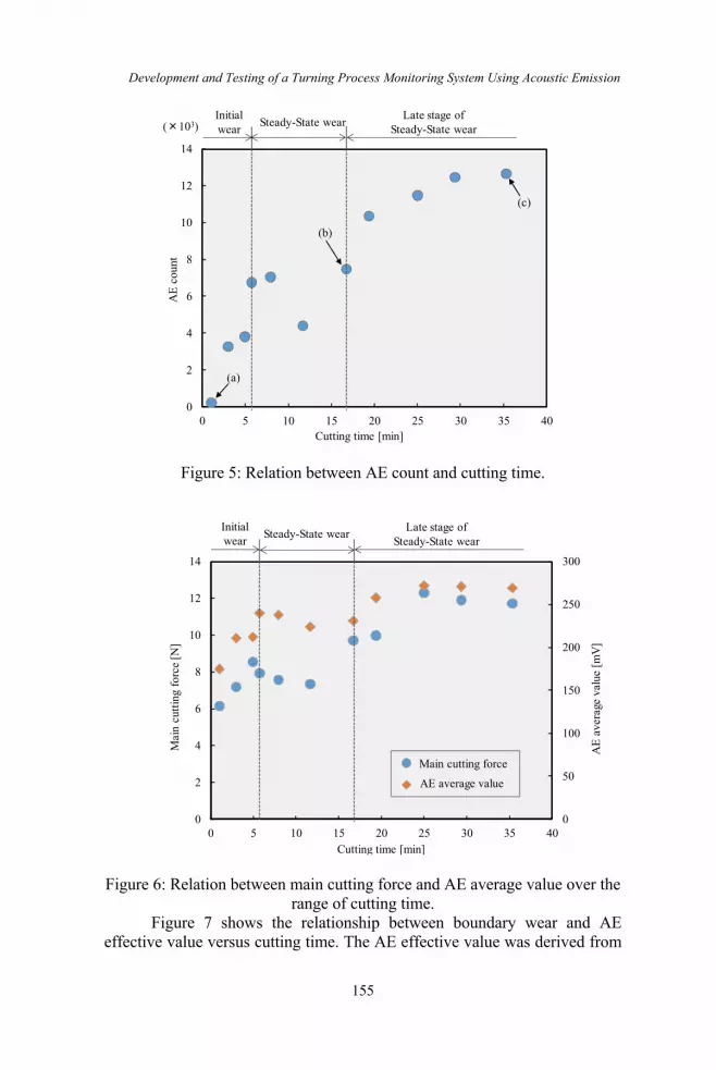
Development and Testing of a Turning Process Monitoring System Using Acoustic Emission
155
Figure 5: Relation between AE count and cutting time.
Figure 6: Relation between main cutting force and AE average value over the range of cutting time.
Figure 7 shows the relationship between boundary wear and AE effective value versus cutting time. The AE effective value was derived from
AE
coun
t
0
2
4
6
8
10
12
14
0 5 10 15 20 25 30 35 40
Initialwear Steady-State wear Late stage of
Steady-State wear
Cutting time [min]
(×103)
(c)
(b)
(a)
0
50
100
150
200
250
300
0
2
4
6
8
10
12
14
0 5 10 15 20 25 30 35 40
AE average value
Main cutting force
Mai
n cu
tting
forc
e[N
]
AE
aver
age
valu
e[m
V]
Initialwear Steady-State wear Late stage of
Steady-State wear
Cutting time [min]

Keiichi Ninomiya*, Shun Yoshida, Kenji Okita, Toshihiko Koga, Shuzo Oshima
156
the envelope waveform and was used to evaluate the AE average value. In this analysis, the AE effective value is used as one of the AE parameters indicating the signal magnitude, similar to the AE average value. On the other hand, since the AE effective value is calculated using the root mean square of the waveform, the two values were both used in the present study to indicate statistical data variability. From the results, it can be seen that the AE effective value greatly increased in the initial wear region, had a slightly decreasing tendency in the initial stage of the steady wear region, and again tended to increase in the latter period of the steady wear region. This is due to the changes in the cutting angle and the state of chip evacuation due to the changes in shear angle with the progress of tool wear. In the latter part of the steady wear region, it is probable that the flank wear, especially that of the boundary of the front flank and the corner radius, have greatly progressed because the cutting finish surface in Figure 4 is inferior. Therefore, it is conceivable that a large compressive force or a shear force acts between the flank and the chip to increase the AE effective value in the latter part of the steady wear region. In other words, as a result of its size predominantly expanding from the tip of the cutting edge to the plastic region below the flank, the work-affected layer on the finished surface appears to have had an effect [28]. Since the AE effective value has a strong positive correlation with the main cutting force (correlation coefficient 0.89), this value can be a useful index in terms of product quality. Iwamoto et al. [29] have been reported that the area of flank wear land is associated with static and dynamic components of cutting force, and the area of rake wear land can be associated with the AE effective value. The experimental results are consistent with this report.
Figure 8 shows the FEM analysis results of modelling the strain rates over a 2-D plain centered on the cutting tool. Model results for 0, 15, and 30 min of machining are given in the figure. The cutting distance was set to 10 mm, which is a sufficient distance to reach the steady machining state. The analytical results qualitatively agree with those obtained by the experiment, confirming that the principal component force increases with the progress of tool wear. From the strain rate distributions shown in Figure 8, the strain rate accompanying the progress of tool wear appears strongly in the vicinity of the tooltip (Figure 8(a)). On the other hand, Figure 8(b) shows that the contact length between the flank and the work material becomes longer over time so that the range expands to the plastic region below the flank and the secondary plastic region. Figure 8(c) suggests that the distribution range of each strain rate further expands, and the magnitude becomes stronger over 30 min of processing. Therefore, it was found that the AE source is the main shear region in the early stage of tool wear. Furthermore, it was found that as the tool wear progressed, it expanded to the secondary plastic region and the plastic region below the flank, and the size became dominant [30].

Development and Testing of a Turning Process Monitoring System Using Acoustic Emission
157
Figure 7: Relation between AE effective value and boundary wear in cutting time.
Figure 8: Distribution of strain rate. Figure 9 shows an example of the results of FFT analysis from the AE
signal. In Figure 9(a), the cutting time is 1 min, and in Figure 9(b), the cutting time is 36 min. Both figures are shown focusing on the frequency band 500-1000 kHz.
Bou
ndar
y w
ear[
µm]
AE
effe
ctiv
e va
lue
[mV
]
0
20
40
60
80
100
120
140
0
50
100
150
200
250
300
0 10 20 30 40
AE effective value
Boundary wear
Initialwear Steady-State wear
Late stage of Steady-State wear
Cutting time [min]
[mm]
[mm](a) Cutting Time 0min
0.3
0.2
9.9 10.0
[mm]
[mm](b) Cutting Time 15min
0.3
0.2
9.9 10.0
[mm]
[mm](c) Cutting Time 30min
0.3
0.2
9.9 10.0
Strain Rate[/s]30 000
90 000
150 000
Tool
Chips
Work material
Secondary plasticity zone
Clear plane lower plasticity zone
Main shear zone

Keiichi Ninomiya*, Shun Yoshida, Kenji Okita, Toshihiko Koga, Shuzo Oshima
158
Figure 10 shows images of the tip of the tool edge and of chips taken with a digital microscope at a cutting time of 36 min. Figure 10(a) shows an image of the rake face at the tip of the tool edge (photograph magnification is 500 x), and Figure 10(b) shows an image of chips on the tool rake face side (magnification 1000 x).
From the results in Figure 9, the amplitude of the frequency spectrum increased as the tool wear progressed. This occurs for two reasons: a) as seen in Figure 10, transfer marks due to the flow of chips can be observed between the tool and the chips due to the progress of tool wear; and b) from the result of FEM analysis, the AE source changes from the main shear zone to the secondary plasticity zone. Since friction and wear extend to the next plastic region and the plastic region below the flank, the influence of chip friction and wear on the rake face predominantly changes in this frequency band [11]. This is consistent with the findings reported by Takuma et al. [31] that the frequency range and wear conditions corresponding to the wear phenomenon can be grasped by wavelet analysis. Therefore, monitoring the frequency band above 500 kHz appears to be effective for understanding the transition of tool wear while performing the in-process measurement.
Figure 9: AE waveform FFT analysis result. (Frequency 500~1000 kHz).
AE frequency [kHz] AE frequency [kHz](a) Cutting time 1min (b) Cutting time 36min
0.5
0.4
0.3
0.2
0.1
0500 600 700 800 900 1000
0.5
0.4
0.3
0.2
0.1
0500 600 700 800 900 1000
Linearspectrum[mV]
Linearspectrum[mV]

Development and Testing of a Turning Process Monitoring System Using Acoustic Emission
159
Figure 10: Insert cutting edge and chip image (cutting time 36 min).
Conclusions In this study, a tool wear experiment was conducted to support the development of in-process measurement applied to turning operations. In the experiment, we collected basic data using an AE sensor, a cutting dynamometer, and a high-speed camera. From the experimental results, the following findings were obtained regarding the possibility of in-process measurement of tool wear using the AE method.
Firstly, the magnitude of the amplitude of the AE original waveform and the AE count is effective for monitoring the state of chip evacuation during tool wear, that is, detecting abnormal conditions such as chip entanglement in the tool.
Secondly, the AE mean value and the main component force have a strong positive correlation, as do the AE effective value and the boundary wear. Therefore, it was found that the AE average value and AE effective value can be effective parameters to monitor the state of the cut surface, that is, the product quality, when performing the in-process measurement.
Lastly, from the results of FEM analysis and FFT analysis, the frequency spectrum due to the progress of tool wear shows that the influence of friction and wear due to the flow of chips on the rake face between the tool and the chips changes its behaviour in the frequency band around 500 kHz. Therefore, it was found that monitoring the frequency band above 500 kHz is effective for characterizing the transition of tool wear.
Therefore, it was suggested that a detailed analysis of the AE waveform pattern and parameter over each frequency band may be effective for in-process measurement.
(b) Chip rake face side(a) Insert cutting edge rake face
100µm ×500 50µm ×1000
Transfer marks

Keiichi Ninomiya*, Shun Yoshida, Kenji Okita, Toshihiko Koga, Shuzo Oshima
160
References [1] Ray Y. Zhonga, Lihui Wangb and Xun Xu, “An IoT-enabled Real-time
Machine Status Monitoring Approach for Cloud Manufacturing,” Procedia CIRP, vol. 63, pp. 709 – 714, 2017.
[2] Y. Nishioka, “Connected Systems for Connected Factories. -Academic Frontier with a New Systems Theory-,” Journal of the Japan Society for Precision Engineering, vol. 83, no. 1, pp. 17 – 20, 2017.
[3] Ray Y Zhong, Xun Xu and Lihui Wang, “IoT-enabled Smart Factory Visibility and Traceability using Laser-scanners,” Procedia Manufacturing, vol. 10, pp. 1 – 14, 2017.
[4] Xingzheng Chen, Congbo Li, Ying Tang, Li Li and Qinge Xiao, “A framework for energy monitoring of machining workshops based on IoT,” Procedia CIRP, vol. 72, pp. 1386 – 1391, 2018.
[5] D. Mourtzis, E. Vlachou and N. Milas, “Industrial Big Data as a result of IoT adoption in Manufacturing,” Procedia CIRP, vol. 55, pp. 290 – 295, 2016.
[6] Jun Huang, Duc Truong Pham, Chunqian Ji and Zude Zhou, “Smart Cutting Tool Integrated With Optical Fiber Sensors for Cutting Force Measurement in Turning,” IEEE Transactions on Instrumentation and Measurement, vol. 69, no. 4, pp. 1720 – 1727, 2020.
[7] I. Nishida, M. Tatekawa, R. Sato and K. Shirase, “Cutting trouble detection system based on quantitative comparison between predicted and measured cutting torques. (1st report Cutting trouble detection for tool wear.),” Transactions of the JSME, vol. 84, no. 857, pp. 17-00433, 2018.
[8] X. Y. Zhang, X. Lu, S. Wang, W. Wang and W.D. Li, “A multi-sensor based online tool condition monitoring system for milling process,” Procedia CIRP, vol. 72, pp. 1136 – 1141, 2018.
[9] Franci Čuš-Uroš and Župerl, “Real-Time Cutting Tool Condition Monitoring in Milling,” Journal of Mechanical Engineering, vol. 57, no. 2, pp. 142 – 150, 2011.
[10] Ahmed Aly Diaa Sarhan, A. Matsubara, M. Sugihara, H. Saraie, S. Ibaraki and Y. Kakino, “Monitoring Method of Cutting Force by Using Additional Spindle Sensors,” JSME International Journal Series C, vol. 49, no. 2, pp. 307 – 315, 2006.
[11] K. Ninomiya, Y. Matumoto, T. Koga and M. Wada, “Development of In-process Measuring System for Turning Process Using Acoustic Emission Method. (1st Report, Experimental Study on Elucidation of Mechanism of Cutting Phenomena),” journal of Japan Society for Design Engineering, vol. 54, no. 10, pp. 669 – 680, 2019.
[12] T. Koga, A. Hase, K. Ninomiya, M. Wada and K. Konishi, “Experimental Study on Monitoring of Cutting Process by Acoustic Emission Method. -Tool Wear Detection in End Milling of Stainless Steel-,” Japanese Society of Tribologists, vol. 63, no. 7, pp. 487 – 498, 2018.

Development and Testing of a Turning Process Monitoring System Using Acoustic Emission
161
[13] T. Koga, A. Hase, K. Ninomiya, M. Wada, H. Mishina and K. Konishi, “Proposal and Evaluation of On-machine Measurement System for Square End Milling in Machining Center by Acoustic Emission Technique,” Journal of the Japan Society for Precision Engineering, vol. 83, no. 11, pp. 1025 – 1032, 2017.
[14] Vadim A. Pechenin, Alexander I. Khaimovich, Alexsandr I. Kondratiev and Michael A. Bolotov, “Method of controlling cutting tool wear based on signal analysis of acoustic emission for milling,” Procedia Engineering, vol. 176, pp. 246 – 252, 2017.
[15] R. Kakinoki, Y. Segawa, Y. Marumo, Y. Imamura, T. Nonaka and Y. Sakata, “Evaluation of Wrinkling States Using In-Process Ultrasonic Examination during Sheet Metal Forming,” Materials Transactions, vol. 59, no. 5, pp. 799 – 804, 2018.
[16] T. Sawa, Y. Ikuse, K. Unno, T. Odaki, S. Tomita, N. Morita and S. Toe, “Relationship between the Grinding Conditions in Constant Cutting Grinding of Fine-Ceramics and AE Wave. (1st Report) -Formulation of the Amplitude of AE Wave-,” Journal of the Japan Society for Precision Engineering, vol. 77, no. 9, pp. 878 – 882, 2011.
[17] M. Kaladhar, “Parametric Optimization and Modeling for Flank Wear of TiSiNTiAlN Nanolaminate Cutting Insert,” Journal of Mechanical Engineering, vol. 17, no. 3, pp. 69 – 84, 2020.
[18] Emiliano Traini, Giulia Bruno, Gianluca D’Antonio and Franco Lombardi, “Machine Learning Framework for Predictive Maintenance in Milling,” IFAC, vol. 52, no. 13, pp. 177 – 182, 2019.
[19] Vishal S. Sharma, S. K. Sharma and Ajay K. Sharma, “Cutting tool wear estimation for turning,” Journal of Intelligent Manufacturing, vol. 19, no. 1, pp. 99 – 108, 2007.
[20] M. Yonehara, “Quantitative Evaluation Method of Texture Using Surface Texture Parameters,” Journal of the Japan Society for Precision Engineering, vol. 82, no. 11, pp. 944 – 947, 2016.
[21] R. Serra and W. Rmili, “Experimental Evaluation of Flank Wear in Dry Turning from Accelerometer Data,” International Journal of Acoustics and Vibration, vol. 21, no. 1, pp. 50 – 58, 2016.
[22] R. Hood, S. L. Soo, D. K. Aspinwall and A. L. Mantle, “Tool life and workpiece surface integrity when turning an RR1000 nickel-based superalloy,” The International Journal of Advanced Manufacturing Technology, vol. 98, pp. 2461 – 2468, 2018.
[23] Mehmet Erdi Korkmaz, Mustafa Günay, “Finite Element Modelling of Cutting Forces and Power Consumption in Turning of AISI420 Martensitic Stainless Steel,” Arabian Journal for Science and Engineering, vol. 43, pp. 4863 – 4870, 2018.
[24] A. Hase, M. Wada, T. Koga and H. Mishina, “The relationship between acoustic emission signals and cutting phenomena in turning process,”

Keiichi Ninomiya*, Shun Yoshida, Kenji Okita, Toshihiko Koga, Shuzo Oshima
162
The International Journal of Advanced Manufacturing Technology, vol. 70, pp. 947 – 955, 2014.
[25] Xiaoli Li, “A brief review: acoustic emission method for tool wear monitoring during turning,” International Journal of Machine Tools & Manufacture, vol. 42, pp. 157 – 165, 2002.
[26] Xu Chuangwen, Dou Jianming, Chai Yuzhen, Li Huaiyuan, Shi Zhicheng and Xu Jing, “The relationships between cutting parameters, tool wear, cutting force and vibration,” Advances in Mechanical Engineering, vol. 10, no. 1, pp. 1 – 14, 2018.
[27] E. García Plaza and P.J. Núñez López, “Analysis of cutting force signals by wavelet packet transform for surface roughness monitoring in CNC turning,” Mechanical Systems and Signal Processing, vol. 98, pp. 634 – 651, 2018.
[28] Mourad Bendifallah, Mourad Brioua and Abderrahim Belloufi, “Cutting Tool Life And Its Effect On Surface Roughness When Turning With WC-6% CO,” International Journal of Modern Manufacturing Technologies, vol. 12, no. 2, pp. 7 – 16, 2020.
[29] R. Iwamoto, E. Kondo, S. Yoshidome, K. Ichiki, N. Kawagoishi, “Monitoring of Tool Wear of Single Crystal Diamond Tool in Ultra-Precision Cutting of Aluminum Alloy (1st Report) -Consideration of Effective Parameters in Indirect Method for Monitoring of Tool Wear-,” Japan Society of Precision Engineering, vol. 75, no. 6, pp. 757 – 761, 2009.
[30] Mohammad Lotfi, Saeid Amini and Mohsen Aghaei, “Tool Wear Prediction and Surface Improvement in Vibration Cutting,” Tribology Transactions, vol. 61, no. 3, pp. 414 – 423, 2018.
[31] M. Takuma, N. Shinke, T. Nishiura and S. Okamoto, “Evaluation of Wear Conditions with AE Method (1st Report, Application of Wavelet Transform Results),” Transactions of the Japan Society of Mechanical Engineers. A, vol. 70, no. 694, pp. 802 – 809, 2004.

Journal of Mechanical Engineering Vol 18(3), 163-180, 2021
___________________ ISSN 1823-5514, eISSN 2550-164X © 2021 College of Engineering, Universiti Teknologi MARA (UiTM), Malaysia.
Received for review:
Accepted for publication: Published:
2020-09-09 2021-06-01 2021-09-15
PV System Based Dynamic Voltage Restorer (DVR) in Water Pumping
System for Agricultural Application
Awais Farooqi, Muhammad Murtadha Othman*, Ismail Musirin, Mohd Fuad Abdul Latip
Solar Research Institute (SRI), Faculty of Electrical Engineering, Universiti Teknologi MARA, 40450 Shah Alam, Selangor, Malaysia
*[email protected], [email protected]
Mohd Amran Mohd Radzi Department of Electrical and Electronic Engineering,
Faculty of Engineering, Universiti Putra Malaysia, 43400 UPM Serdang, Malaysia
Izham Z.Abidin
Department of Electrical Power Engineering, Universiti Tenaga Nasional, Jalan IKRAM-UNITEN, 43000 Kajang, Selangor
Daw Saleh Sasi Mohammed
Department of Electrical and Electronic Engineering, Bright Star University, Brega 858, Libya
ABSTRACT
Modern solar-powered pumping systems are already being utilized in various fields and industrial applications especially in agricultural water irrigation systems where pumping water at a remote location is required with fewer electricity accessibility from the grid is not feasible. PV solely depends on solar hours per day, and it is not reliable when a location exhibits variable weather conditions, such as in Malaysia, having 12 solar hours daily but maximum 5-6 peak performance hours are as usually achieved due to the cloudy and rainy nature of the weather. In this case, PV-grid is not able to generate power as per daily demand and would create voltage sags, swell, and power outage when it is directly connected with the water pumping system for irrigation. To overcome this problem, a PV-DVR solar water pumping system (PV-DVRWP) is proposed in this paper that can mitigate power quality issues

Awais Farooqi et. al.
164
arising from PV-grid side such as voltage sags, voltage swells, and power outage by injecting the required amount of voltage into the line to maintain constant load voltage supply. The DVR controller strategy uses dq-abc frame mechanism to extract fault signals by using Park’s transformation method, PID, and hysteresis band PWM signal generator to drive the inverter of DVR connected with a battery storage system. The proposed methodology of the PV-DVRWP system mitigates power quality issues occurring from the PV-grid side by injecting compensating voltage as well as being able to support water pumping systems in case of power outage for a three-phase system. Keywords: Renewable energy; Dynamic Voltage Restorer; Solar water pumping system; Power quality issues; PV-Grid; PV irrigation system Introduction Modern solar water pumping systems are field-proven methods providing water pumping aid in locations where grid-connected pumping systems are not reliable or easily accessible. Photovoltaic (PV) based solar cells are used in these systems that convert sunlight into electric power to operate the DC/AC motors to drain the groundwater or surface water pumping systems [1].
This case study covers a procedure design for the Malaysian agriculture and irrigation system upgrade by the solar-powered water pumping system. Due to the rapid increase in diesel/fuel costs, the energy demand by farmers in Malaysia is facing severe difficulties in irrigating their crops under such circumstances [2, 3]. An alternative facility is required to fulfill the need of farmers to power the water pumping systems in an economical way that can bring revolution in agriculture and provide energy independence whilst solar pumping systems are key to it [4, 5, 6, 7].
This paper outlines the application of a dynamic voltage regulator (DVR) with a solar water pumping system and demonstrates the potential advantages of this method. DVR is a series active power filter device that is used to protect sensitive loads from power quality issues such as voltage sag, swell, harmonics, or disturbances [8]. Though, the main objective of the solar-powered irrigation system design is to meet the intended water requirement through cost-effective and proper selection of different systems and components. Solar-powered water pumping systems are like any other pumping system, where the power source is solar energy i.e., by the Photovoltaic (PV) panels. A conventional solar pumping system may consist of a PV array to power the water pump motor usually used to extract water from the ground or stream (river) to fill up water storage tanks. So that gravity feed is used to irrigate without any external energy system. PV-based water

PV-DVR in Water Pumping System for Agricultural Application
165
pumping systems are cost-effective and alternatives to agricultural wind turbines for remote area water supply [9, 10].
Solar power is less ideally used to run heavy machinery such as AC motors for pumps that roughly require 100,000 times more power consumption than a PV cell generating small DC power. Therefore, batteries are usually used with PV systems to provide some means of storing energy. An inverter is used to convert DC power from the PV array and battery into AC power. However, the phenomenon of converting DC to AC and storing energy to the battery by PV array is not that efficient therefore a further 10% margin must be added to the required array size. A complete solar power system is expensive to install and its power generation by PV array is controlled by MPPT technique that generates maximum power and regulates the voltage to operate the motor smoothly [11]. Figure 1 shows the block diagram of a typical solar-powered water pumping system.
Figure 1: Solar-powered water pump motor system.
The scope of using renewable energy applications is increasing rapidly in past decades. They are being used in simple applications or in certain fields where solar energy is utilized extensively in each field [12]. Where agriculture has captured its advantage by using solar energy for the benefit and profiting of both the farmers and the environment. By replacing fossil fuel as a source of energy in the farms, solar energy helps to keep the environment clean and healthy by reducing the bad emissions as well as the noise generated. Also, it helps the farmers to be more self-dependent and make more revenue by reducing the costs of energy and the cost of maintenance [13]. Agricultural/irrigation improvement by solar powered pumping system Solar pumping systems are ideal to implement in remote locations where grid-based electricity reach is not available or limited. The solar-powered pumping system can only be justified if it is properly designed and linked with high-

Awais Farooqi et. al.
166
efficiency irrigation systems such as drips, bubbler, sprinkler, or bed and furrow irrigation methods [14].
The usage of Malaysian agriculture total water consumption is about 68% of total water although the irrigation efficiency in larger irrigation schemes is 50% and less than 40% in the smaller ones [2]. The majority of developing and under-developed countries' economies are mainly dependent upon its agriculture and the continuous energy supply at an affordable price is the major factor affecting the agricultural sector. Energy crises countries are struggling to conceive conventional energy sources to support their agricultural sector that affects the corps water requirements in the irrigated areas and almost entire irrigation requirements within the rainfed areas are dependent on water pumping. Therefore, solar energy sources are highly considered to minimize the energy crises as estimated in [15]. Hence, by exploiting solar energy effectively in the agricultural sector it can increase its productivity and help to improve the environment as well. Potential benefits of solar-powered irrigation system implementation The solar-powered agricultural systems are capable to reduce operational cost as compared with direct grid-connected pumps by providing easy operational methods as compared with conventionally fuelled pumping systems as it, (i) generates uninterrupted energy for pumping systems daily for about 5-10 hours, (ii) provides flexibility of direct coupling or through batteries for irrigations purpose, (iii) supports as free energy source for remote watershed and rainfed areas, (iv) withstands long working life, (v) integrates with different drip, bubbler, micro-sprinklers and rain guns, (vi) stabilizes the climate due to no emissions of greenhouse gasses during irrigation process, (vii) responses swiftly towards the water flow requirements according to the weather conditions as in summer the water is needed at higher scale or else vice versa for winter periods, (viii) pumps in wide ranges to suit different farm sizes and socio-economic conditions and (xi) assures small payback periods, particularly if high-value crops is grown [16]. Other main applications of solar energy in agriculture are crop and gain drying space, water heating, greenhouse heating, and remote electricity supply (PV). Each of these systems has its own benefit for a specific use and purpose as given in [17]. Evolution of Solar Power Water Pumping System Applications In the last decades, the issue of using PV cells for water pumping has been discussed and reviewed from different aspects. PV technology usage in water pumping is considered a very good alternative for conventional pumps which use fossil fuels. The importance of using renewable energy resources is

PV-DVR in Water Pumping System for Agricultural Application
167
suggested by [18] after considering the fact that the oil reserves are limited and the electricity cost is high. The acceptance of PV performance and reliability in remote areas for water pumping has increased significantly for many reasons. Firstly, unlike the limited availability of electricity grid connections, solar energy is available almost everywhere. Also, it is very reliable and can stand difficult weather conditions such as snow and ice [9].
However, solar technology requires different sets of expertise for installation, operation, and maintenance, since it has electrical, mechanical, and electronic components. There are other constraints such as the overall cost and energy storage. The main components in the PV water pumping system are solar PV array, charge controller, pump controller, batteries, inverter, Motor, storage tank, mounting structures and wiring, and discharge tubing or piping. PV pumping systems can be classified based on four main configurations such as energy storage, input electric power, type of pumps, and sun-tracking. Furthermore, solar-powered water pumping systems can be configured into two types, battery coupled and direct-coupled [19].
PV water-pumping systems (PVWPs) are reliable and becoming much cheaper due to inexpensive PV modules. PVWP systems prices have dropped by 2/3rd as compared to fuel prices which have risen >250% since 2000. These systems are durable and are operational for a long period such as the one installed in Estacio Torres in Sonora Mexico is operating for more than 20 years. PVWPs off-the-shelf capabilities have grown to 25 kW and are expected to exceed 100 kW. PVWPs global sales are steadily growing and approaching 100,000 systems per year. PVWPs are becoming a choice for millions of small farmers/ranchers due to its reliability and affordability with increased agricultural productivity around the globe. Whereas the productivity of irrigated land is approximately three times greater than that of rain-fed land [20].
Most of the developing countries face issues of power interruptions or blackouts because the generated electrical power is less than the power in demand. Therefore, consumers face power quality issues due to voltage sag, short-duration voltage swell, and long duration power interruption [21]. Dynamic voltage restorer (DVR) is a cost-effective solution to mitigate voltage sag and voltage swell, conveniently. It is also able to withstand long-term power outages by injecting the required voltage quality level for the sensitive loads when connected with an energy storage device [8]. The limitation of the DVR system proposed by [21] is that it can recover sags up to 10% of source voltage only and the PV-DVR system is focused to mitigate the distribution system only.
SolarVest Malaysia stated that the efficiency of solar energy generation is dependent on the weather condition, which drops consequently due to the cloudy and rainy weather nature of Malaysia [22]. PVWPs would not run effectively due to the variability of solar energy. Therefore, DVR is proposed

Awais Farooqi et. al.
168
in PVWPs to mitigate voltage sag and voltage drops caused by PV systems in absence of sunlight. The aim of this research is to develop a DVR-based solar-powered water pumping system for agricultural irrigation systems to continuously supply constant power for the pump. The pumping system shall be designed to meet the intended water requirement through cost-effective means by careful selection of different systems and components. However, the design criterion for the solar-powered irrigation system is based on: i. The peak water requirements.
ii. The lowered solar energy availability in a year of time, so if water needs are fulfilled during the lean solar time, it will ensure peak water needs when solar energy availability is at maximum.
Design Consideration and Methodology The estimation of water demand is an important factor to be considered before the design. Therefore, a precise calculation is required to set up the operation of the pumping system up to the scale. For example, in our project case, the solar system irrigates a cropped field. Therefore, the demand of water required, size of the field, and type of crop must be known. Table 1 shows the water demand in millions cubic meters (mcm) for the year 2010 and the projection of water demand by the year 2050 in the agricultural sector of Malaysia [23]. However, for full water irrigation system design, the peak water requirement should be estimated to develop the solar water pumping system. Table 1: Estimation of yearly water requirement for the agricultural sector of
Malaysia [23]
Water Demand mcm / year
2010 2050 Agriculture Sector 9,512 8,959 a. Paddy (irrigation) 8,266 7,205 b. Non-Paddy Corps 1,117 1,176 c. Livestock 126 578
Rice paddy field water irrigation system is selected in this study for the
Penang state of Malaysia, as it is one of the most water-deprived regions during paddy field season with the water withdrawal requirement of an average of 2788 mm3 per season. Paddy field season in Malaysia starts from March/April till mid-May (estimated about 40 - 105 days). The irrigation water requirement for 1.82 hectares of paddy field is 755 mm/season [23, 24]. Therefore, the daily water needed estimated for the paddy field is about 3 mm/day for a minimum field size of 1 acre.

PV-DVR in Water Pumping System for Agricultural Application
169
Malaysia has the potential to have an average of 12 hours of sunshine daily [25]. However, due to variable cloudy weather conditions of Malaysia, the maximum performance achieved by solar hours is about 6 hours of daily sunshine with 250 days of water pumping system operation per year, are considered.
The PV water pumping system is designed to provide power supply for agriculture loads such as centrifugal water pumps operating 5 hours daily. The system is to be installed in a small farmhouse to support a ¼ acre of paddy field to pump about 317.5 gallons (1.202 m3) of water per day for a remote region. A three-phase water pump motor is used with the following specifications: 2.5 kW, 415 V, 6 A, 2850 rpm, and 50 Hz. The system is designed to provide energy source through PV system connected with the grid and as well as runs the pump from stored energy from batteries by a DVR system during the times when sunlight is not efficient or in cloudy weather.
Single-crystal silicon cells (c-Si or mono-Si) array is selected for the proposed application to run the pump motor due to its reason of limiting the cost reduction. c-Si is an indirect band-gap semiconductor with 1.1 eV and with a much smaller absorption constant as compared to direct band-gap materials. 33 to 36 individual cells are connected in series in a PV array. Individual silicon cell open-circuit voltage ranges from 0.5-0.6 V depending upon irradiance level and cell temperature which results in a module having an open-circuit voltage between 18 V to 21.6 V. Whereby, the cell current is directly proportional to the irradiance and the area of a cell [26]. Thus, for the one-acre (4046.86 m2) of land, a PV module of size 4 ft2 (0.372 m2) is proposed with an active cell area expected to produce a maximum power of 55 W at approximately 17 V and 3.2 A under direct sunlight.
The block diagram of the proposed photovoltaic DVR water pumping system (PV-DVRWP) is illustrated in Figure 2. In this case a 100 kW PV array is connected to the utility grid which is also connected to the water pumping system. In this process, the water pump is operated by either grid or PV system. However, whenever the PV-Grid efficiency is low it will create voltage sag, long-term voltage interruption, or outage. To mitigate the voltage sag DVR is activated and injects the required amount of voltage into the system to maintain constant and smooth power, delivered to the water pump motor.
DVR works as a power quality conditioner to compensate for power quality issues coming from the source side [8]. PV-DVR system consists of a source side PV array connected to a booster converter that regulates the PV array voltage at 500 V in accordance with the MPPT controller. PV inverter converts the incoming DC voltage to AC voltage (260 V) that is further boosted by the step-up transformer converting low AC voltage to high AC voltage (25 kV), to feed the excessive solar energy generation into the utility grid. Table 2 shows the parameters used to set up the PV array in Matlab-Simulink.

Awais Farooqi et. al.
170
A second step-down transformer is used to convert High-Voltage to Low-Voltage (415 VAC), to match the load capacity of the water pump three-phase AC motor. In a DVR system, a DC energy source (a battery in this case) is connected with the inverter that is able to convert DC voltage to AC voltage and injects the compensation AC voltage into the distribution line by an injection transformer through the passive filter. The DVR parameters are given in Table 3.
Figure 2: PV-DVR water pumping system (PV-DVRWP).
Table 2: Parameters of PV Array
Module
Apollo Solar Energy ASEC-305G6s
No. Cell per Module 72 Max. Power (W) 305.019
Open circuit voltage Voc (V) 35.55 Voltage at max. powerpoint Vmp (V) 35.55
Short Circuit current Isc (A) 8.99 Current at max. powerpoint Imp (A) 8.58

PV-DVR in Water Pumping System for Agricultural Application
171
Table 3: Parameters of DVR
Input Source from Utility Transformer 5 kV, 50 Hz Unbalanced Load 3.7 kW or 5 HP Machine
3-Phase Coupling Transformer 10 MVA, 50 Hz, Winding Ratio: 5:8
Winding 1 - Ripple Filter R= 60 Ω; C = 100 mF Passive Filter L = 200 mH
Switching Filter: Capacitor 1 µF Voltage Source Inverter 3 arms; 6 pulses
Carrier Frequency 5 kHz Battery 800 V
DC-Link Capacitor 10 mF The DVR controller block diagram is shown in Figure 3, it is designed
to work on the following principles, (i) generation of a fixed reference voltage, as expressed in Equation (1), (ii) detection of imbalance voltage in the system by using Park’s Transformation as given by Equation (2), as dq components, and then converting abc-to-dq0 frame system, (iii) reference voltage generation by coordinate transformation method, vi) comparison of imbalance voltage with the constant sine wave reference voltage as given by Equation (3), (v) two PID controllers with a feedback signal to extract control gain signal to transform dq0-abc frame system by inverse park transformation method as given by Equation (4) and (vi) furthermore, this signal is fed into hysteresis band voltage controller to generate gate pulse for DVR (inverter). Consequently, the dq0-abc frame control signal is generated as expressed by Equation (5).
Figure 3: DVR controller strategy block diagram.

Awais Farooqi et. al.
172
!"!,#$%"&,#$%"',#$%$ = "%.#$% &'()*+'() ,*+ − )*+ . '() ,*+ +
)*+ .0 (1)
!","-".$ = )+ &12'(*+)12' ,*+ −
)*+ . 12' ,*+ +
)*+ .− '()(*+) −
'() ,*+ − )*+ .− '() ,*+ +
)*+ .
/) /) /)0 × ["0"1"2] (2)
893,,-.8 = :;"#$%,, − "4,,<) + ;"#$%,- − "4,-<
) + ;"#$%,. − "4,.<) (3)
!"2/,0"2/,1"2/,2$ = &'()(*+)12'(*+)1'() ,*+ − )*
+ . 12' ,*+ −)*+ . 1'() ,*+ +
)*+ . 12' ,*+ +
)*+ . 10 × !"2/,,"2/,-"2/,.$ (4)
"5,012 = >6"2/,012 +>7 ∫ "2/,012@+/
. +>, ,8!",$%!,3 (5)
Results and Discussion Matlab/Simulink is used to simulate the proposed system to determine the performance of the DVR system connected with a battery and a PV water pumping system for mitigating voltage sags, swells, and outages. A PV-grid connected system with DVR Water Pumping system (PV-DVRWP) is shown in Figure 4.

PV-DVR in Water Pumping System for Agricultural Application
173
Figure 4: PV-DVRWP system. Case I: balanced voltage sag Figure 5(a) shows a 30% balanced voltage sag occurs from the source side when the demand of electrical energy is increased by the utility while the PV grid is operating at low irradiance sunlight condition, at time intervals from t = 0.1 s to t = 0.6 s. Voltage recovery mode is initiated as soon as the DVR controller detects the voltage loss in the system and injects the required amount of voltage to mitigate the voltage sag, as shown in Figure 5(b). The improved load voltage condition with mitigated balanced voltage sag is shown in Figure 5(c), assuring the performance robustness of the DVR. As compared with the system presented in [21], the proposed DVR can mitigate more than 10% of voltage sag errors. Case II: balanced voltage swell When voltage swell happens in the PV-Utility grid, the DVR should activate its operation by absorbing the power from the grid. Figure 6(a) shows a 15% balanced voltage swell that occurs from t = 0.1 s to t = 0.6 s. DVR detects the incoming exceeded voltage from the source side and injects the voltage with 180o shift but in phase with system voltage, which is subtracted from the excessive voltage magnitude, as given in Figure 6(b). However, once the

Awais Farooqi et. al.
174
voltage stabilizes to its nominal limit the DVR shifts back to standby mode to maintain minimum conduction loss. From Figure 6(c) the DVR can maintain a load voltage peak closer to the nominal voltage limit. Whereas the proposed system can inject compensating voltage to mitigate more than 10% of voltage swell as compared with [21]. Case III: power outage A total power outage can happen when the PV system is down and the utility feeder is at fault, hence producing zero voltage. In this case, the water pumping system can be disrupted. A short circuit fault in one of the feeders from the grid side will also affect the line causing balanced voltage sag. However, in this case, DVR is operated during power outages from the PV-grid side as seen in Figure 7(a), at intervals t = 0.1 s to t = 0.6 s. DVR can support the zero-volt error by injecting about 70% of nominal voltage into the system as shown in Figure 7(b). Figure 7(c) shows the load voltage profile after compensation. [21] presented a system that mitigates voltage disturbances in a single-phase system only. However, the proposed DVR system acts as a microgrid and is able to withstand longer and deeper voltage sags.

PV-DVR in Water Pumping System for Agricultural Application
175
Figure 5: DVR in solving power quality problem with (a) balanced voltage sag of 30%, (b) voltage injected by DVR, and (c)
improved load voltage.

Awais Farooqi et. al.
176
Figure 6: DVR in solving power quality problem with (a) balanced voltage swell of 10%, (b) voltage injected by DVR, and (c)
improved load voltage.

PV-DVR in Water Pumping System for Agricultural Application
177
Figure 7: DVR in solving power quality problem with (a) Voltage Outage, (b) voltage injected by DVR, and (c) compensated
load voltage.

Journal of Mechanical Engineering Vol 18(3), 163-180, 2021
___________________ ISSN 1823-5514, eISSN 2550-164X © 2021 College of Engineering, Universiti Teknologi MARA (UiTM), Malaysia.
Received for review:
Accepted for publication: Published:
2020-09-09 2021-06-01 2021-09-15
Conclusion This paper discussed the use of DVR in the application of the Solar Renewable Energy sector used for irrigation purposes to mitigate power quality problems occurring from the PV grid-connected with a water pumping system for agricultural use. The results show that the proposed DVR system can mitigate power quality issues occurring from the PV-grid side by injecting compensating voltage in case of voltage sag and voltage swell as well as. It is also able to support water pumping systems in case of a power outage. This implies that the battery storage attached with DVR can support and deliver constant voltage during DVR operation mode for a longer duration. Acknowledgments This research was supported by the Long-Term Research Grant (LRGS), Ministry of Education Malaysia for the program titled "Decarbonisation of Grid with an Optimal Controller and Energy Management for Energy Storage System in Microgrid Applications" with project code 600-IRMI/LRGS 5/3 (001/2019). The authors would also like to acknowledge the Research Management Centre (RMC), Universiti Teknologi MARA (UiTM), Shah Alam, Selangor, Malaysia for the facilities provided to support this research. References [1] S. Kalasathya and P. S. Khanna, "Implementation of Solar Power Ac
Motor Pump Set on MPPT With Battery Backup For Agriculture System," International Journal Of Engineering And Computer Science, vol. 5, no. 11, pp. 18928-18932, 2016.
[2] T. S. Lee, M. E. Toriman and M. Mokhtar, "Irrigation: Types, Sources and Problems in Malaysia," in Irrigation Systems and Practices in Challenging Environments, IntechOpen, pp. 361-370, 2012.
[3] C. Siwar, N. D. M. Idris, M. Yasar and G. Morshed, "Issues and Challenges Facing Rice Production and Food Security in the Granary Areas in the East Coast Economic Region (ECER), Malaysia," Research Journal of Applied Sciences, Engineering and Technology, vol. 7, no. 4, pp. 711-722, 2014.
[4] F. M. Bhutta, "Solar Pumping Issues and Solutions in Pakistan," AltEnergyMag, July 30, 2013. [Online]. Available: https://www.altenergymag.com/article/2013/07/solar-pumping-issues-

PV-DVR in Water Pumping System for Agricultural Application
179
and-solutions-in-pakistan/1268. [Accessed March 10, 2020]. [5] M. Signs, "Here comes the sun: solar technology for agriculture,"
Eco-Bussiness , April 30, 2018. [Online]. Available: https://www.eco-business.com/opinion/here-comes-the-sun-solar-technology-for-agriculture/. [Accessed March 10, 2020].
[6] N. Pushpraj, N. Gupta, V. Gupta and M. A. Mulla, "Solar Energy Harvesting for Irrigation Water Pumping System," IEEE International Conference on Power, Control, Signals and Instrumentation Engineering (ICPCSI), pp. 1398-1402, 2017.
[7] R. K. Megalingam and V. V. Gedela, "Solar Powered Automated Water Pumping System for Eco-Friendly Irrigation," in Proceedings of the International Conference on Inventive Computing and Informatics (ICICI), Coimbatore, 2017.
[8] A. Farooqi, M. M. Othman, A. F. Abidin, S. I. Sulaiman and M. A. M. Radzi, "Mitigation of Power Quality Problems using Series Active Filter in a Microgrid System," International Journal of Power Electronics and Drive System (IJPEDS), vol. 10, no. 4, pp. 2245-2253, 2019.
[9] A. Ghoneim, "Design optimization of photovoltaic powered water pumping systems," Energy Conversion and Management, vol. 47, pp. 1449-1463, 2006.
[10] World Bank Group, "Solar Pumping: The Basics," International Bank for Reconstruction and Development / The World Bank, Washington, 2018.
[11] L. P. &. H. L. Willis, "Renewable Power Generation," in Understanding Electric Utilities and De-Regulation, Boca Raton, Taylor & Francis Group, pp. 183-197, 2006.
[12] P. A. Owusu and S. A. Sarkodie, "A review of renewable energy sources, sustainability issues and climate change mitigation," Cogent Engineering, vol. 3, pp. 1-14, 2016.
[13] M. Al-Saidi and N. Lahham, "Solar energy farming as a development innovation for vulnerable water basins," Development in Practice, vol. 29, no. 6, pp. 619-634, 2019.
[14] A. H. C, V. A, K. V, K. K. N and R. R. Reagon, "Development of Smart Solar Irrigation System," International Journal of Recent Trends in Engineering & Research (IJRTER), vol. 02, no. 09, pp. 16-20, 2016.
[15] M. Saleem, M. Ashraf and J. Fripp, "Solar-Powered Pumping Systems for High Efficiency Iffigation: Design Manual for Practitioners," International Center for Agricultural Research in the Dry Areas (ICARDA) under Pakistan USDA project, Pakistan , 2015.
[16] H. Hartung and L. Pluschke, The benefits and risks of solar-powered irrigation - a global overview, Bonn: the Food and Agriculture Organization of the United Nations and Deutsche Gesellschaft für Internationale Zusammenarbeit, 2018.

Awais Farooqi et. al.
180
[17] O. Prakash and A. Kumar, "Historical Review and Recent Trends in Solar Drying Systems," International Journal of Green Energy, vol. 10, no. 7, pp. 690-738, 2013.
[18] A. Demirbaş, "Global Renewable Energy Resources," Energy Sources, Part A: Recovery, Utilization, and Environmental Effects, vol. 28, no. 8, pp. 779-792, 2006.
[19] B. Eker, "Solar Powered Water Pumping Systems," Trakia Journal of Sciences, vol. 3, no. 7, pp. 7-11, 2005.
[20] R. Fostera and A. Cota, "Solar water pumping advances and comparative economics," Energy Procedia, vol. 57, pp. 1431-1436, 2014.
[21] M. Ramasamy and S. Thangavel, "Experimental verification of PV based Dynamic Voltage Restorer (PV-DVR) with significant energy conservation," Electrical Power and Energy Systems, vol. 49, pp. 296-307, 2013.
[22] SolarVest, "Solar Farms in Malaysia," SolarVest, September 21, 2018. [Online]. Available: https://solarvest.my/2018/09/21/solar-farms-malaysia/. [Accessed March 12, 2020].
[23] Academy of Sciences Malaysia, "Agriculture Water Services for Agribusiness," Academy of Sciences Malaysia, Kuala Lumpur, 2017.
[24] M. M. Hanafiaha, N. F. Ghazali, S. N. Harun, H. S. Abdulaali, M. J. AbdulHasan and M. K. A. Kamarudin, "Assessing water scarcity in Malaysia: a case study of rice production," Desalination and Water Treatment, vol. 149, pp. 274-287, 2019.
[25] M. A. M. Zawawi, S. Mustapha and Z. Puasa, "Determination of Water Requirement is a Paddy Field at Sebrang Perak Rice Cultination Area," Journal - The Institution of Engineers, Malaysia: Environmental Science, vol. 71, no. 4, pp. 32-41, 2010.
[26] L. Sing, T. L. K. Calvin Kong, L. K. Yee, J. O. Kamadinata, N. A. B. C. Sidik, Y. Asako and L. K. Quen, "Solar Radiation Forecast Using Cloud Velocity for Photovoltaic Systems," Journal of Engineering and Technological Sciences (JETS), vol. 50, no. 4, pp. 479-491, 2018.
[27] S. Rahman, G. L. Johnson and R. A. Messenger, "Electric Power Generation: Non-Conventional Methods," in The Electric Power Engineering Handbook, Florida, CRC Press LLC, 2001, pp. 19-40.

Journal of Mechanical Engineering Vol 18(3), 181-192, 2021
___________________ ISSN 1823-5514, eISSN 2550-164X © 2021 College of Engineering, Universiti Teknologi MARA (UiTM), Malaysia.
Received for review:
Accepted for publication: Published:
2020-09-14 2021-06-01 2021-09-15
Determination of River Water Level Triggering Flood in Manghinao
River in Bauan, Batangas, Philippines
C E F Monjardin*, K M Transfiguracion, J P J Mangunay, K M Paguia, F A A Uy, F J Tan
School of Civil, Environmental and Geological Engineering, Mapua University, Manila Philippines
ABSTRACT
Flooding is one of the problems experienced by many countries no matter what their economic status is. Even rich and developed countries experience it too. Flooding is mainly caused by natural events such as typhoons and monsoon rains even anthropogenic causes that sometimes could not be stopped even if there are flood control structures in place. The Philippines is located in the Pacific Ring of Fire and is visited by an average of 20 typhoons each year. People are used to experiencing flooding and it is about time that we somehow do something about it. There have been many technologies available right now that could aid us to improve our capability to adapt to such phenomena. Heavy precipitation is usually experienced during the monsoon season that leads to severe flooding in a specific area. The application of HEC-RAS (Hydrologic Engineering Centre’s River Analysis System) Modelling Software was used in the study in Manghinao River for comprehensive hazard mapping and risk assessment in the downstream area of the Bauan River for 100-year return period flood. 2D flood hazard simulation was done and the river water level that would trigger flooding downstream was identified. At 0.5 m of flood height, people are considered immobilized to move from one place to another so the best time to evacuate people is before the flood reaches that level. Results showed that LGU has 4 hours to evacuate people starting when the river water at the gaging station reads 0.5 m, this gives them enough time to give warning and ask people to move to evacuations sites to prevent them being stranded in their houses. This study can support future planning and for the development of flood control plans and flood mitigation measures to minimize

C E F Monjardin et al.
182
the losses due to flood disasters in Batangas Province, Philippines particularly in the Bauan area. Keywords: Flood; HEC-RAS Modelling Software; 2D flood modeling; Return Period Introduction Many urban areas in the Philippines experience extreme flooding problems when heavy rainfall occurs. Flooding is caused by different factors such as insufficient drainage systems, improper waste disposal, and deforestation [1]. Flooding is severe in areas near rivers due to the rising of river levels that may cause danger to the community [2]. Bauan, Batangas as shown in Figure 1 is one of the first-class and most industrialized municipalities in the region. It is one of the low-lying areas in central Batangas as it is situated in the southern part of the province along the coastal area.
Figure 1: Location Map of Bauan, Batangas.
In 2011, tropical storm Noul hit southern Luzon. Two days of heavy rainfall caused a 2-meter flood in some parts of Bauan. The municipal council immediately declared a state of calamity to address the needs of its people. Lowland areas were swept specifically Aplaya, New Danglayan, San Roque, San Pedro, Poblacion 2, Santo Domingo, San Andres I, and San Andres proper. A lot of flood-prone areas do not have enough flood risk reduction programs that can help people in the community to be ready when the flood comes [3]. The sudden water level rise of a river can cause panic and disaster in areas near the river if not monitored. A system in monitoring the status of river water level and a forecast on how the river water level will rise as soon as the rainfall occurs are very useful in preparation for evacuation and will also lessen the damage of the flood [4].
This study has a purpose to determine the water level in rivers that will trigger flooding in the downstream area using 2D HEC-RAS Modelling

River Water Level Triggering Flood in Manghinao River in Bauan, Batangas, Philippines
183
System. The study specifically aimed to provide hydrologic and hydraulic models in the area which are necessary to identify the timing of flooding in the area [5]. Another is to determine flood inundation extent in the area using Lidar DEM. LiDAR is known to have a vertical accuracy of ± 15 cm [6]. And lastly is to have an integrated warning and emergency response program that can detect flood threats and most probably provide a timely warning. It could be done by having a gaging station in the river located in the upstream part of the watershed. The water level in that gaging station will be monitored and could be the basis to know if people downstream will be flooded and to know how much time they have to evacuate. For example in Marikina city, they have this warning system that when the river reaches a certain depth they are enforcing different warning signals to notify people if there is a need to evacuate but unlike in the said city where that gaging station is already downstream [7], the one to be implemented in Bauan is much better since the gaging station will be located in the upstream to give people enough time to evacuate since the detection was done upstream.
The research was limited to the Manghinao River in Bauan, Batangas only, and didn’t include nearby areas. The study aimed to prepare the community in the areas of Bauan against the sudden and unexpected rise of the river water level. The main concern is to provide a protocol to prepare the people living in the community and inform them how they should react if the river water level suddenly rises. This could greatly help the local government to give warnings and precautions to its people so that panic will be prevented, and people will be organized. Early preparation for flooding leads to a ready community and that lessens severe danger: loss of lives, disruption of livelihoods, damage to property, etc [8]. Methodology Description of study area A flood is an overflow of water outside its typical course [9]. Also, according to [10], flooding occurs when a stream comes up short of its limits and submerges encompassing zones. One of the many municipalities in the Province of Batangas is Bauan which is usually hit by typhoons causing major flooding in the area. The area is flood-prone, and most floods were caused by the swelling of rivers. In this study, we were able to determine the water level of rivers in Bauan, Batangas that will trigger flooding in the communities. The researchers were able to gather data with the help of the Mapua FRAMER project which is a government-funded project whose main objective is to provide communities with flood risk maps. Data acquisition The researchers in the study used LiDaR technology to capture the terrain of the area which is a very important input in floodplain modeling [11].

C E F Monjardin et al.
184
Hydrologic and hydraulic models were also developed using HEC HMS and HEC RAS. Models were validated using the data gathered during a typhoon event in the area. Typhoon’s name at that time was “Tisoy” (local name) which falls under category 3. Rainfall data were collected, together with the river discharge. These data were acquired by the Mapua-FRAMER team and authorize the researchers to use them in this study. These rainfall and flow hydrograph data are necessary to calibrate the watershed model [12]. HEC-RAS model description HEC-RAS is a Windows-based hydraulic model also developed by the U.S. Army Corps of Engineers and Hydrologic Engineering Centre (HEC). The model uses an output hydrograph from HEC-HMS as an input to calculate and analyze the floodplain hydraulics. In investigating the hydraulic characteristics of flow in rivers HEC-RAS model can be used to provide the appropriate numerical values. The model is used to simulate steady, gradually varied, rapidly varied, and unsteady one-dimensional flow and to delineate flood zones. The primary procedure used by HEC-RAS to compute water surface profiles assumes a steady, gradually varied flow scenario. The HEC-RAS model could be used to simulate water level, depths, and flow velocities for different flow configurations and different cross-sectional zones [13]. Application of HEC-RAS This provides an overview of how a study is performed with the HEC-RAS Software. The user may want to formulate several different plans. Each plan represents a specific set of geometric data and flows data. Once the basic data are entered into the HEC-RAS, the modeler can easily formulate new plans. After simulations are made for the various plans, the results can be compared simultaneously [14]. The hydraulic RAS model has the capability to simulate and predict flooding in a continuous time discretization, but calibration should be taken into consideration [15]. Unsteady flow analysis using HEC-RAS 5.0.7 Perform an unsteady flow simulation The hydraulic model was developed in this study using some of the data collected by the Mapua FRAMER. They gave the researchers full authorization to use the data for this study. Using those data, models were calibrated and were then used to simulate flooding events in the area considering different return periods. Simulation of different return periods plays an important factor to fully understand how floods occur in a certain area [16]. Shown in Figure 2 is the sample settings used in the run of unsteady flow simulation. Shown here is the sample coverage of flood simulation in the area considering a 100-year return period as this is considered to be the most critical scenario in the Philippine setting [17].

River Water Level Triggering Flood in Manghinao River in Bauan, Batangas, Philippines
185
Figure 2: Unsteady Flow Analysis.
Shown in Figure 3 is the RAS Mapper where terrain data is displayed together with the simulation results and other maps/layers that you would like to add. HEC-RAS versions above 5.0 could now load terrain models unlike before that it is dependent on other software for its GIS processing. HEC-RAS now could be considered as standalone software that could function without the help of other software. It can be seen in the figure the terrain of the Bauan area using the Lidar-derived Digital Terrain Model. Using lidar data could produce an accurate flood depth simulation compared to those terrain models with lower accuracy [18].
Figure 3: RAS Mapper. Figure 4 to Figure 6 show the flood arrival time, depth, and velocity in
the Municipality considering the 100-year return period. Knowing such data could help the local government to plan ahead of time if there is a need to evacuate people and how much time they have before flood reaches the community [19]. Of course, the simulation cannot predict 100% accurately but

C E F Monjardin et al.
186
at least with this they have an idea of what are they expecting, and these could also help them to convince people to evacuate if needed.
Figure 4: RAS Mapper – Arrival Time.
Figure 5: RAS Mapper – Depth.
Figure 6: RAS Mapper – Velocity. Results and Discussion Disasters such as floods and landslides are very common here in the Philippines, with different transboundary floods with a high number of

River Water Level Triggering Flood in Manghinao River in Bauan, Batangas, Philippines
187
fatalities [14]. After gathering data and thorough calibration and analysis of the model, the researchers arrived at the important findings of the study.
Using HEC-RAS, researchers were able to simulate the flood extent and depth in the area considering a 100-year rainfall event. Map layers were produced in the RAS mapper where the data in Table 1 were extracted. The elevation model used in the simulation was a Terrain model that captures the elevation of the bare earth which is usually used in flood simulations. Depth Table 1 shows the gaging stations and other stations considered in the river. Utilizing the 100-year return period simulation done in Ras, researchers were able to identify the maximum flood height that could occur in the area and the time of arrival considering 12:00 am as the start of the simulation. Stations were named 1 to 4 and the location of each station could be seen in Figure 7 starting from the upstream area of the river to downstream. The peak river depth at the gaging station was 2.9 m at 9:20 am, this indicates that water that could flood downstream already passed through this station. This could be used as a basis to determine how long it will take before floods reach the downstream. At 10:10, the water already reached the downstream area at station 1 with a maximum flood depth of 4.53 m. Station 4 had the lowest flood depth with 3.7 m and was expected to be flooded 3 hours after the peak flood occurred in the gaging stations. Knowing these peak floods in each station is not enough to be used in flood evacuation plans. We should also identify at what certain level of flood height people could be immobilized. Researchers did a survey to the local government in the area, they were asked based on their experience at what flood level people are having a hard time moving from one place to another. Researchers decided that it is much better to ask this from the people living in the area rather than rely on other studies which could have a different situation with the concerned area in this study.
Table 1: Peak River Depth
Station (m) Date and Time Peak River Depth (m) Gaging Station 09:20 am 2.9
Station 1 10:10 am 4.53 Station 2 10:50 am 4.30 Station 3 11:50 am 4.12 Station 4 12:15 pm 3.7

C E F Monjardin et al.
188
Figure 7: RAS Mapper Depth Simulation.
Arrival time Arrival time is the computed time in hours or days from a defined time in the simulation when the depth of water reaches a specified threshold depth [11]. Based on the interview done with the LGUs of the municipality, it was found out that at a flood depth of 0.5 m people are starting to have a hard time moving from one place to another. That’s why this flood depth was considered by the researchers to be the threshold value in the analysis.
Figure 8 shows the arrival time in the downstream area. The map indicates the time when the area will experience a flood depth of 0.5 m. The simulation ranges from 0 to 12 hours as a reference. HEC-RAS was able to simulate the flood arrival time in Bauan, Batangas using the 100 return period data. The generated flood arrival time could also serve as an early warning for the people to evacuate their places.
Figure 8: RAS Map Arrival Time Simulation.
Shown in Table 2 are the simulated flood arrival time using the 2D unsteady flow analysis of RAS. A Flood of 0.5 m is a flood height known that could immobilize people in moving from one place to another. That is why it

River Water Level Triggering Flood in Manghinao River in Bauan, Batangas, Philippines
189
was the threshold used in the study. The table shows that when the level at the gaging station reads 0.5 m, people still have 4 hrs to evacuate before a flood height of 0.5 m reaches their area as an example for station 1. Station 4 which is located at the farthest point will experience a flood height of 0.5 m 5 hrs after the flood level in the gaging station reached 0.5 m. These data could really be utilized by the local government to improve their emergency response procedures/protocol.
Table 2: Arrival time of Flood at 0.5 m depth
Station (m) Date and Time Peak River Depth (m) Gaging Station 0 (reference) 0(reference)
Station 1 4.16 hours 0 (Possible max flood height is less than 1m)
Station 2 4.56 hours 4.5 hours Station 3 4.76 hours 4.7 hours Station 4 5.10 hours 5.3 hours
Velocity The velocity of a river is the speed of water that moves along its channel, according to [15] river velocities are not constant all through its cross-sectional area. In RAS, it just calculates the mean velocity of the river, so it doesn’t need to be cross-section specific. Velocities at max flood depth were shown in Table 3. It could be seen that there’s only one station where the velocity of the water is at its maximum and it is located at station 4. It may be because station 4 is in the lowest elevation and bed slope there could be much steeper compared to other stations.
Table 3: Velocity
Station (m)
Date and Time Peak River Depth (m)
Velocity (m/s)
Gaging Station 09:20 am 2.9 0.23 Station 1 10:10 am 4.53 0.41 Station 2 10:50 am 4.30 0.20 Station 3 11:50 am 4.12 2.0 Station 4 12:15 pm 3.7 2.19
Conclusions and Recommendations

C E F Monjardin et al.
190
The main objective of this study was to create a hydraulic model using the software HEC-RAS in simulating different water levels of the Manghinao river that could trigger flooding in the downstream area. The Manghinao river is usually causing the flood in Bauan. The data acquired from the DOST-MAPUA-FRAMER project played a significant role in the success of this study. The result of the 2D unsteady flow simulation showed that many areas in Bauan will be inundated or flooded when a 100-year rain return period event occurs in the area. The model was able to utilize lidar data with a vertical accuracy of ± 15 cm.
Bauan is one of the many towns in Batangas that has a large boundary. It has an area of 53.31 km2 (20.58 sq. mi) placing it as the 19th largest town in the province. Manginao river is known to swell most of the time, causing flooding in the area when a strong typhoon hits the municipality. In this paper, the researchers were able to determine the maximum flood heights in the area. Max flood height in the area could happen in station 1 with a height of 4.53 m at which a typical household with 1 floor could be totally flooded. Using HEC-RAS, researchers were able to come up with a flood inundation map showing which area in the municipality could be flooded and at what level. Flood inundation map can also be used for preparation for “what-if” scenarios, and timely response for forecast information.
This paper was able to provide a systematic way of how to notify people in the downstream area if there is already a need for evacuation, that is by having a gaging station upstream that monitors the water level. A certain level of water in the gaging station will give the local government an idea of what announcement to be issued to their community. These flooding scenarios were simulated using HEC-RAS’s 2D flow capability with the aid of Lidar DEM. Researchers are very confident of the result and hope that the local government will adopt it.
After conducting the research, the results showed that the possible maximum water levels in each station are 4.53, 4.30, 4.12, and 3.7. Considering the flood height itself it could produce a max of 0.97 m flood height in the community. The said flood height is enough to cause problems to the people in the area. Flooding is most of the time inevitable, but we could adapt by creating a systematic way of evacuating people. The study provided the local government of Bauan with a reliable early warning procedure for evacuation by monitoring the river water level at the gaging station. It was shown that when the water level at the gaging station reaches 0.5 m, the LGU has 4 hours to evacuate the people before the flood height of the area reaches 0.5 m. This gives the LGU enough time to convince people to evacuate.

River Water Level Triggering Flood in Manghinao River in Bauan, Batangas, Philippines
191
References [1] W. Sohn, S. D. Brody, J. H. Kim and M. H. Li, “How effective are
drainage systems in mitigating flood losses?,” Cities, vol. 107, 102917, 2020.
[2] M. S. H. Mondal, T. Murayama and S. Nishikizawa, “Assessing the flood risk of riverine households: A case study from the right bank of the Teesta River, Bangladesh,” International Journal of Disaster Risk Reduction, vol. 51, pp. 101758, 2020.
[3] Kundzewicz, Z. W., Su, B., Wang, Y., Xia, J., Huang, J., & Jiang, T., “Flood risk and its reduction in China,” Advances in Water Resources, vol. 130, pp. 37-45, 2019.
[4] Z. Zeng, Y. Gan, A. J. Kettner, Q. Yang, C. Zeng, G. R. Brakenridge and Y. Hong, “Towards high resolution flood monitoring: An integrated methodology using passive microwave brightness temperatures and Sentinel synthetic aperture radar imagery,” Journal of Hydrology, vol. 582, pp. 124377, 2020.
[5] J. Pinos and L. Timbe, “Performance assessment of two-dimensional hydraulic models for generation of flood inundation maps in mountain river basins,” Water Science and Engineering, vol. 12, no. 1, pp. 11-18, 2019.
[6] “GIS Geography, A Complete Guide to LiDAR: Light Detection and Ranging,” [Online]. Available: GISGeography, https://gisgeography.com/lidar-light-detection-and-ranging/#:~:text=LiDAR%20systems%20are%20very%20accurate,from%20side%2Dto%2Dside.
[7] J. R. Santillan, E. C. Paringit, R. V. Ramos, J. R. T. Mendoza, N. C. Española and J. Alconis, “Near-Real Time Flood Extent Monitoring in Marikina River Philippines: Model Parameterisation Using Remotely-Sensed Data And Field Measurements,”.
[8] W. Bissett, C. Huston and C. B. Navarre, “Preparation and response for flooding events in beef cattle.,” Veterinary Clinics: Food Animal Practice, vol. 34, no. 2, pp. 309-324, 2018.
[9] S. A. Nelson, “River systems and causes of flooding,” 2009. [10] M. L. González-Arqueros, M. E. Mendoza, G. Bocco and B. S. Castillo,
“Flood susceptibility in rural settlements in remote zones: The case of a mountainous basin in the Sierra-Costa region of Michoacán, Mexico,” Journal of environmental management, vol. 223, pp. 685-693, 2018.
[11] J. R. Santillan, M. Makinano-Santillan and L. C. Cutamora, “Integrating LiDAR and flood simulation models in determining exposure and vulnerability of buildings to extreme rainfall-induced flood hazards,” Proceedings in 2016 IEEE International Geoscience and Remote Sensing Symposium (IGARSS), pp. 7585-7588, 2016.
[12] Y. Wang, G. Sang, C. Jiao, Y. Xu and H. Zheng, “Flood simulation and

C E F Monjardin et al.
192
parameter calibration of small watershed in hilly area based on HEC-HMS model,” In IOP Conference Series: Earth and Environmental Science, vol. 170, no. 3, pp. 032093, 2018.
[13] A. Azouagh, R. El Bardai, I. Hilal, and J.S. El Messari, “Integration of GIS and HEC-RAS in Floods Modeling of Martil River (Northern Morocco,” Eur. Sci. J, vol. 14, no. 12. 2018
[14] USACE, United States Army Corps of Engineers. Hydrologic engineering center “River Analysis System HEC-RAS. Hydraulic Reference manual. version 3.0” [Online]. Available USACE, www.usace.army.mil [Accessed 2001]
[15] M. Cerri. Flood simulation using HEC-RAS model calibrated with remotely sensed water mask: a case study of Mulde River, Germany. 2017
[16] Z. Wu, Y. Zhou, H. Wang and Z. Jiang, “Depth prediction of urban flood under different rainfall return periods based on deep learning and data warehouse,” Science of The Total Environment, vol. 716, pp. 137077, 2020.
[17] C. E. Monjardin, F. A. Uy, F. Tan, A. Altecin, L.K. Apolinario, and E.A. Peregil, “Downstream Risk Analysis of Magat Dam Breach Using Geographic Information System and HEC,” Journal of Taiwan Water Conservancy, 2020
[18] S. J. Noh, J. H. Lee, S. Lee, K. Kawaike and D. J. Seo, “Hyper-resolution 1D-2D urban flood modelling using LiDAR data and hybrid parallelization,” Environmental Modelling & Software, vol.103, pp. 131-145, 2018.
[19] J. Kim, Y. Kuwahara, and M. Kumar, “A DEM-based evaluation of potential flood risk to enhance decision support system for safe evacuation,” Natural hazards, vol. 59, no. 3, pp. 1561-1572, 2011.
[20] E. J. Ollet,(2008). “Flash flood and landslide disasters in the Philippines: reducing vulnerability and improving community resilience,” University of Newcastle, 2018.
[21] Y. Yang, B. Wen, C. Wang and Y. Hou, “Two-dimensional velocity distribution modeling for natural river based on UHF radar surface current,” Journal of Hydrology, vol. 577, pp. 123930, 2019.

Journal of Mechanical Engineering Vol 18(3), 193-214, 2021
___________________ ISSN 1823-5514, eISSN 2550-164X © 2021 College of Engineering, Universiti Teknologi MARA (UiTM), Malaysia.
Received for review: 2020-09-10
Accepted for publication: 2021-06-01 Published: 2021-09-15
Simultaneous Load Management Strategy for Electronic
Manufacturing Facilities by using EPSO Algorithm
M.F. Sulaima* Faculty of Electrical Engineering,
Universiti Teknikal Malaysia Melaka (UTeM), 76100, Hang Tuah Jaya, Durian Tunggal, Melaka, Malaysia
N.Y. Dahlan
Faculty of Electrical Engineering, Universiti Teknologi Mara (UiTM), 40450, Shah Alam, Selangor, Malaysia
Z.H. Bohari, M.N.M. Nasir
Faculty of Electrical and Electronic Engineering Technology, Universiti Teknikal Malaysia Melaka (UTeM),
76100, Hang Tuah Jaya, Durian Tunggal, Melaka, Malaysia
R.F. Mustafa
Faculty of Electrical Engineering, Universiti Teknologi Mara (UiTM) Johor Branch, Pasir Gudang Campus, 81750, Masai, Johor, Malaysia
Duc Luong Nguyen
Faculty of Environmental Engineering, National University of Civil Engineering (NUCE),
55 Giai Phong, Hanoi, Vietnam
ABSTRACT
Increased power demand has contributed to the power generation tension. Thus, there were critical needs for a better Price Based Program (PBP) policy for the consumers. In Peninsular Malaysia, through the development of a policy for the regulated market plan, the Enhanced Time of Use (ETOU) tariff was introduced by the utility to promote better price signals to the industrial

M.F. Sulaima et al.
194
consumers who contribute to the most massive energy consumption every year. However, fewer industrial consumers join the program due to a lack of Load Management (LM) knowledge while not confident in the price rate signal compared to the previous tariffs. Due to that reason, this study proposed simultaneous LM strategies for the selected power consumption profile in the electronic manufacturing facilities. Meanwhile, the Evolutionary Particle Swarm Optimization (EPSO) was adopted to search for the upright power consumption profiles of those average 11 locations of the manufacturing. The analysis of the results has compared to the baseline existing flat and Time of Use (TOU) tariffs. The results show an improvement in the energy consumption and maximum demand costs reduction of ~14-16% when load management was applied correctly. It is hoped that this study's results could help companies’ management of developing a strategic plan for the successful load management program. Keywords: Demand response; Price-based program; Manufacturing facility; Optimization algorithm; Enhanced time of use tariff Introduction Due to the global temperature surge, the disaster has led to collective knowledge in the environment and energy study. It was reported that 95% of countries in the world contributed to the increase of 1.5 degrees of the earth's temperature [1]. Thus, this situation has to upsurge the CO2 emission and contribute to global warming that impacts the ecosystem of human activities [2]. The factor of energy consumption from the demand side, such as manufacturing facilities, has a significant effect on this global issue. In Malaysia, ~80% of the energy consumption from the electricity source has been demanded by industrial consumers, which was ~60% of them are from the electronic related manufacturer [3], [4], [5]. Thus, to balance the energy supply, the government through the energy commission of Malaysia has approved the utility's new PBP policy to the commercial and industrial consumers who are using the ETOU tariff scheme. The purpose of the tariff was to mitigate the peak demand on the generation side while promoting the electricity bill reduction among participants. The impact of the TOU tariff in the regulated market was determined by changing the price in the consumers' TOU tariff has contributed to the significant impact on the cost of generation [6]. The details disaggregated the appliance on the consumers’ side, promoting a better effect on the TOU and ETOU tariff load management strategy [7]. A study on the ETOU tariff by promoting the load shifting strategy for an industrial power consumption profile results in electricity cost savings with 50% of the load changing from peak to mid-peak and off-peak zone as presented in [8].

Simultaneous Load Management Strategy for Electronic Manufacturing Facilities
195
Nevertheless, no appropriate formulation that reflects the industry's group and does not involve any optimization technique. The authors in [9] have promoted the bubble chart solution to identify the appropriate percentage of the load to be transferred in peak and mid-peak zones. Meanwhile, the application of the optimization algorithm proposed by [10] only focuses on the load shifting strategy for the manufacturing operation. On the other hand, the application of the optimization algorithm in the perspective of the price-based program for the demand-side was divided into three purposes: i) for the tariff design, ii) for the operation schedule, and iii) for the load management [11]. Since this study focuses on load management, the art of the literature has scrolled down to that particular issue accordingly. Thus, in supporting this program, the optimization algorithms have been effectively applied in dealing with load management, such as studies of PSO [12], improve PSO [13],[14], Evolutionary Algorithm (EA) [15], [16] and Genetic Algorithm (GA) [17], [18]. Most of the references presented the single application of the load management strategy, either load shifting, peak clipping, and valley filling, separately. The simultaneous integration of the strategies was proposed by authors in [19]. However, the study did not involve any optimization algorithm during the load management strategies available only in a single load profile under a similar bus system.
Regarding the EPSO algorithm, there were colossal applications in power system studies where few related to the demand response application. As in [20], [21], the use of the distribution network reduces the power network losses while improving the voltage factor. The related study of EPSO on the demand response program was concentrating on load forecasting, such as presented in [22]–[24]. Compared to the other optimization method, EPSO has produced improved RMS percentage value on the various load types forecasting. Meanwhile, the convergence time of EPSO was identified as fasters among heuristic algorithms. There is no application of the EPSO available in the past literature for the proposed of tariff PBP program in Malaysia to the best of our knowledge. The EPSO has not yet been considered in dealing with load management as well. Thus, this study proposes the EPSO algorithm to solve the optimal ETOU tariff program's objectives, reducing energy consumption and maximum demand costs, respectively.
The paper's arrangement is as follows: Section 2 presents problem formulation of the optimal ETOU tariff; Section 3 discusses the implementation of the EPSO algorithm; Section 4 explains the case of study while results and analysis of the finding have been written in Section 5 accordingly. The last Section 6 concludes the overall paper arrangement and contribution.

M.F. Sulaima et al.
196
Problem Formulation Optimal total electricity cost The general optimal total ETOU electricity cost (MYR/kWh+kW) has been presented in Equation (1) where the formulation has referred [25]:
𝐸𝑇𝑂𝑈!"#$% + 𝑀𝐷&'%()*)"#$% (1)
Optimal energy consumption cost 𝐸𝑇𝑂𝑈!"#$%, is the electricity cost of the desired load curve after load management strategies are applied, which reflects the six-time segmentation of ETOU tariff price zones according to Equation (2).
𝐸𝑇𝑂𝑈!"#$% = *+ ∆𝑃#' × 𝑇𝑃#'
+,-.
%
/ + *+∆𝑃)'- × 𝑇𝑃)'
+,/
%
/
+*+∆𝑃'- × 𝑇𝑃'
+,-
%
/ + *+∆𝑃)'0 × 𝑇𝑃)'
+,0
%
/
+*+∆𝑃'0 × 𝑇𝑃'
+,/
%
/ + *+∆𝑃)'/ × 𝑇𝑃)'
+,1
%
/(2)
where, ΔPop : changing of off-peak desired load curve with changing of time,
N=10; ΔPmp1, ΔPmp2, ΔPmp3= changing of mid-peak wanted load curve with the different time change, N=3, N=2, and N=5, respectively; ΔPp1, ΔPp2 = changing of peak wanted load curve at a time changing N=1 and N=3 separately
TPop : tariff price for off-peak zone TPmp : tariff price for mid-peak zone TPp : tariff price for peak zone Optimal maximum demand cost Optimal MD cost reduction has been written Equation (3). Meanwhile, Equations (4) and Equation (5) summarize the MD power load selection to separate MD charges congruently.
𝑀𝐷23#$% ≥ 𝑀𝐷&'%()*)"#$% = 𝑀𝐷423#$%(3)
𝑀𝐷423#$% = 𝑀𝑎𝑥[𝐿50; 𝐿56; 𝐿57] ×𝑀𝐷4252 (4)
𝑀𝐷23#$% = 𝑀𝑎𝑥[𝐿5/; 𝐿51] ×𝑀𝐷252 (5)

Simultaneous Load Management Strategy for Electronic Manufacturing Facilities
197
where, 𝑀𝐷423#$% : Optimum power load selection at Mid-Peak area; 𝑀𝐷23#$% : Optimum power load selection at Peak area; 𝐿58 : Selected power load for n number at particular time segmentation (ts); 𝑀𝐷4252 , and 𝑀𝐷252: the MD charge for different mid-peak and peak Simultaneous load management strategies The concurrent Load Management (LM) strategies can be written as in Equation (6). The demand-side strategy that had been proposed was Valley Filling (VF), Peak Clipping (PC), and Load Shifting (LS).
∆𝑃&2,42-,2-,420,20,42/:!8!;<= = ∑ ;∆𝑃%$,(>? ×𝑊>?=>?%$,( + ;∆𝑃%$,(2" ×𝑊2"= +
;∆𝑃%$,(AB ×𝑊AB=(6) where, ∆𝑃%$,(>? , is the changing amount of the desired load based on VF strategy by LM at random load (i) in time segmentation (ts). ∆𝑃%$,(2" and ∆𝑃%$,(AB are the changing amount of the desired load based on PC and LS strategies by LM at random load (i) in time segmentation (ts), respectively. Temporarily, WVF, WPC, and WLS are the weightage of LM strategies to be implemented in load profile concurrently, which is set 50% as referred to [8]. Constraints The constraints of the simultaneous LM strategies to achieve satisfying performance had been decided as follows: Constraint for VF ∆𝑃%$,(>? , will be selected during time segmentation with a minimum value of baseload price. The (ts) adjustment of VF selection must be as: 𝐴𝑣𝑒𝑟𝑎𝑔𝑒𝑙𝑜𝑎𝑑𝑝𝑟𝑖𝑐𝑒 > ∆𝑃%$,(>? ≥ 𝑏𝑎𝑠𝑒𝑙𝑜𝑎𝑑𝑝𝑟𝑖𝑐𝑒 (7) Constraint for PC ∆𝑃%$,(2" , will be selected during the two highest prices of time segmentation loads as well as where the maximum demand is located, where (ts) adjustment of PC selection must be as:
𝐴𝑣𝑒𝑟𝑎𝑔𝑒𝑙𝑜𝑎𝑑𝑝𝑟𝑖𝑐𝑒 < ∆𝑃%$,(2" ≤ 𝑏𝑎𝑠𝑒𝑙𝑜𝑎𝑑𝑝𝑟𝑖𝑐𝑒 (8)

M.F. Sulaima et al.
198
Constraint for LS LS in the LM program shall lead to perform at randomly selected three-time segmentations. Thus, the best way to put LS is after VF and PC selection, while the rest of the time segmentations will be the location for LS to perform randomly. The process of the proposed LS procedure is written as in Equations (9), (10), and (11) accordingly.
∆𝑃%$,(AB ≅ ∆𝑍%$,(
$C(D%(9)
∆𝑍%$,($C(D%E#F8 = R∆𝑍*'
$C(D% − T;∆𝑍*'$C(D% − ∆𝑍E#F8
$C(D%= × 𝜔VW(10)
∆𝑍%$,($C(D%*' = R∆𝑍*'
$C(D% − T;∆𝑍*'$C(D% + ∆𝑍E#F8
$C(D%= × 𝜔VW(11) where, ∆𝑍E#F8
$C(D% : changing of load decrease at certain time segmentation (ts) for the load, i;
∆𝑍*'$C(D% : changing of load increase at certain time segmentation (ts) for the
load, i; 𝛺 : The random weightage of load decrease and increase at lower bound
and upper bound load setting. Constraints for total energy consumption Total energy before and after the optimization throughout the process of LM strategies should not be more than ±5%[26]. Equation (12) describes the constraints for total energy consumption (kWh) before and after optimization.
∑ 𝐸𝑇 ≅ ∑ 𝐸𝑇′ (12) EPSO algorithm implementation EPSO is essentially a hybrid of PSO and evolutionary programming. EPSO is a modified version of the PSO algorithm, which involves additional combination and selection processes.
This step is implemented after 𝑃I!$% and 𝐺I!$% are determined and after the new position and velocity of the particles are updated. Figure 1 shows the combination and selection processes (tournament) incorporated into the PSO algorithm (inspired from evolutionary programming), resulting in the EPSO algorithm. The EPSO implementation steps are followed.

Simultaneous Load Management Strategy for Electronic Manufacturing Facilities
199
Initialization The EPSO algorithm begins with initializing the number of particles D and the number of populations NP. In this study, NP was set as 20. The initial number of particles D was determined by calling the load profile that represents the daily average 24-h energy consumption, which was randomly generalized. Equation (13) shows the initial condition of the load arrangement. The constant parameters such as the social and cognitive coefficients were set at 1.0, and the initial weight coefficient was set at 0.2. The maximum inertia, minimum inertia, and the number of iterations were set at 0.9, 0.1, and 1000.
𝑗 = [𝑗J-, 𝑗J0, 𝑗J/……………𝑗J8] (13)
Velocity and position update The initializing number of Equations (14) and (15) were used to update the position and velocity of the particles, respectively.
𝑥((𝑡 + 1) = 𝑥((𝑡) + 𝑣((𝑡 + 1)(14)
𝑣((𝑡 + 1) = 𝑣((𝑡) + 𝐶-(𝑃Kddd⃗ (𝑡) − 𝑥Kddd⃗ (𝑡)) + 𝐶0(𝐺(𝑡) − 𝑥Kddd⃗ (𝑡)) (15)
The modified velocity and inertia weightage proposed by [27] has been applied in immense power and energy study such as integrated demand response [14], home energy management [28], power network reconfiguration [29], and load scheduling in manufacturing [30]. The modified velocity and inertia weightage of PSO was used to improve the optimal solution for the complex problem. Equation (16) represents the inertia weightage. The value for 𝜔 was set between 0 and 1, and it is the so-called friction factor. The inertia weightage is used to ensure that the particles remain in the original course. The particles do not affect the motion of other particles (by pulling other particles into their path) and preventing oscillations around the optimal value.
𝜔(𝑛) = 𝜔𝑚𝑎𝑥 − '𝜔𝑚𝑎𝑥−𝜔𝑚𝑖𝑛𝑖𝑡𝑒𝑟max
( × 𝑛 (16)
Equation (17) is used to update the velocity of the particles in the
standard PSO algorithm, and Figure 1 shows the vector movement of the particles. In this study, the particles' velocity and position were updated according to Equation (18) and Equation (19); respectively, the local and global best were allocated to produce a clear presentation. 𝑣(U(𝑡 + 1) = 𝜔𝑣(U(𝑡)
+ 𝑟-𝐶- RT𝑃(U(𝑡) −𝑥(U(𝑡)V + 𝑟-𝐶0 T𝐺U(𝑡)𝑥(U(𝑡)VW(17)

M.F. Sulaima et al.
200
Figure 1: Updating the velocity and position of the particles in the standard PSO algorithm to determine the optimal solution.
𝑉UVW- = ;𝜔 × 𝑉UV= + T𝐶-𝑟-;𝑃I!$%UV − 𝑋UV=V + T𝐶0𝑟0;𝐺I!$%UV − 𝑋UV=V(18)
𝑋UVW- = 𝑋UV + 𝑉UVW-(19)
where, 𝑉UV : Velocity of Particle 𝑗 in Iteration 𝑘 𝑋UV : Position of Particle 𝑗 in Iteration 𝑘 𝜔 : Inertia weightage 𝑃I!$%UV : Best value by Particle 𝑗 in Iteration 𝑘 𝐺I!$%UV : Best value among the fitness values 𝐶- , 𝐶0 : Constants weightage factor [0, 1] 𝑉UVW- : New velocity 𝑋UVW- : New position Determine Pbest and Gbest and update the new velocity and position of the particles During the searching process, the two best values were updated and recorded. The 𝑃I!$% and 𝐺I!$% represent the best energy consumption cost and optimum MD cost generated during the execution of the algorithm, respectively. In this step, the particle’s current fitness value was compared with the particle’s 𝑃I!$%. If the current fitness value was better than the 𝑃I!$% value, the 𝑃I!$%position was adjusted to the current best position. The same procedure was performed for 𝐺I!$%, where the 𝐺I!$% value was reset to the current fitness value, representing the optimal daily energy consumption cost and the minimum MD charge. The new velocity and new position were updated in each iteration according to Equation (18) and Equation (19).

Simultaneous Load Management Strategy for Electronic Manufacturing Facilities
201
Combination and selection (tournament) Since EPSO is a hybrid of PSO and evolutionary programming, it has combination and selection (tournament) processes. After the second fitness function calculation, the old and new particles' fitness values were combined, which was not available in the original PSO algorithm. In this manner, the potential optimal particles can be selected, considering the randomly produced particles at the old and new positions. After the combination, the selection process was carried out, where all of the particles (each with its position number) were contested in the tournament. The percentage of contestants in the tournament was set using simple numbers of the particles’ positions selected to the percentage of challengers.
Figure 2 shows an example of the combination and selection processes. If 10 positions are chosen, and the percentage of contestants was set at 40%, this means that four other random contestants challenge all of the particles. Each position has its weightage, which is based on the number of wins obtained so far. Only the particles with the higher scores remain during the selection process. These particles are sorted and ranked to determine 𝑃I!$% and 𝐺I!$% in the next iteration. With the combination and selection processes, the EPSO algorithm can determine the optimal solution quickly and accurately compared with the PSO algorithm.
Figure 2: Example of the combination and selection (tournament) processes in the EPSO algorithm.
Convergence test The convergence criterion was set as follows:
𝑓𝑡)<J − 𝑓𝑡)(8 ≤ 0.0001 (20) This termination criterion was used to determine if the desired optimal solution was achieved. The searching process will be repeated until the values converge

M.F. Sulaima et al.
202
to the optimal load curve with the minimum energy consumption cost and minimum MD cost. Figure 3 presents the EPSO flow summary to find the optimal results while the combination and selection technique is involved.
Figure 3: The flow of the EPSO process for searching for the best solution.
Case Study Case studies were carried out to assess the effectiveness of the proposed EPSO algorithm. The EC of Malaysia provided the load profiles used for the case studies for 1 year with 30-min intervals. These load profiles were converted
Initialization (randomize population x)
Start
Calculate the fitness function f(x)
Find and for all populations.
Calculate the new velocity and adjust
new position of the particles.
Combination and selection (tournament): Combine the fitness values of the old and new particles, and select the optimum potential
particles for the next iteration.
Is the requirement fulfilled?
End
Optimal solution
No
Yes

Simultaneous Load Management Strategy for Electronic Manufacturing Facilities
203
into 24-h load profiles with 1-h intervals. Several electronics manufacturers were chosen for the flat industrial tariff (Category E1) case studies. Category E1 consumers have the highest power demands, considering that electronics-related industries have been established in Peninsular Malaysia since 1988.
The case studies for both commercial and industrial tariffs are listed as follows:
i. Case 1: baseline load profile with flat tariff pricing ii. Case 2: baseline load profile with TOU tariff pricing
iii. Case 3: baseline load profile with ETOU tariff pricing and without LM strategies and optimization algorithms
iv. Case 4: load profile with ETOU tariff pricing and optimization algorithms. There are two cases: (1) Case 4a: PSO algorithm and (2) Case 4b: EPSO algorithm
v. Case 5: load profile with ETOU tariff pricing, LM strategies, and optimization algorithms. There are two cases: (1) Case 5a: PSO algorithm with 50% LM weightage and (2) Case 5b: EPSO algorithm and 50% LM weightage
The tariff prices to compare and validate the results are presented in
Table 1 and Table 2, which serve as the limits to set daily electricity costs in this study. For the case studies, flat and TOU costs were used as the baseline to compare the results. The time zones under the ETOU tariff were separated as in Table 3 accordingly.
Table 1: Flat and TOU tariff rates
Consumer Tariff Types
MD: MYR/kW
Peak: cents/kWh
Off-peak: cents/kWh
Industrial E1 Flat 29.60 33.60 NA Industrial E2 TOU 32.90 33.60 19.10
Table 2: ETOU tariff rate
Tariff category Demand charge
(MYR/kW/month) Energy charge (cents/kWh)
Peak Mid-peak Peak Mid-peak Off-peak Industrial E1 MV ETOU
35.50 29.60 56.60 33.30 22.50

M.F. Sulaima et al.
204
Table 3: ETOU time zone
Time (military) 2200-0800
0800-1100
1100-1200
1200-1400
1400-1700
1700-2200
Zone (Monday-Friday)
Off-peak
Mid-peak
Peak Mid-peak
Peak Mid-peak
Zone (Saturday-Sunday)
Off-peak
Off-peak
Off-peak
Off-peak
Off-peak
Off-peak
Results and Analysis The baseline profiles were obtained from 11 electrical installations in electronics manufacturers. Based on the observations, the peak demand was less than 1,000 kW. The power consumption was static for 2 days each week because of holidays, and there was an upsurge in power consumption in regular working days. Thus, Figure 4 shows the active power consumption for 11 electrical installations in electronics manufacturing facilities with similar product types. Figure 5 shows the average weekday load profile, where the working hours were 0700–1900 and the average peak demand was 609 kW. Meanwhile, Figure 6 shows the average weekend load profile over a 24-h period. The peak demand was 356kW, while the baseline was a cover-up to 50% of the total demand.
Figure 4: Average load profiles for 11 locations over 2 weeks.
0
500
1000
1500
2000
2500
0:30
:00
12:3
0:00
0:30
:00
12:3
0:00
0:30
:00
12:3
0:00
0:30
:00
12:3
0:00
0:30
:00
12:3
0:00
0:30
:00
12:3
0:00
0:30
:00
12:3
0:00
0:30
:00
12:3
0:00
0:30
:00
12:3
0:00
0:30
:00
12:3
0:00
0:30
:00
12:3
0:00
0:30
:00
12:3
0:00
0:30
:00
12:3
0:00
0:30
:00
12:3
0:00
Pow
er C
onsu
mpt
ion
(kW
)
Time
M-1 M-2 M-3 M-4 M-5 M-6
M-7 M-8 M-9 M-10 M-11

Simultaneous Load Management Strategy for Electronic Manufacturing Facilities
205
Figure 5: Average weekday load profile for electronics manufacturing facilities over a 24-h period.
Figure 6: Average weekend load profile for electronics manufacturing facilities over a 24-h period.
Power consumption profile Figure 7 presents the power consumption profile of all cases. Case 5b records a minimum reading of about 17 kW during the transaction of the off-peak and mid-peak zones. For both Case 5 s, the peak zones demand has been reduced by about 50%, while the off-peak zone has increased tremendously. It was observed that peak demand in the off-peak zone was 1,240 kW by Case 5a. For Case 4 s, there was a slight change in the power consumption profile compared to baseline cases. The EPSO algorithm's performance can transfer the appropriate loads from the critical high price charge to the middle and low-price rates within the convergence time.
0100200300400500600700
0:00
2:00
4:00
6:00
8:0010
:0012
:0014
:0016
:0018
:0020
:0022
:00Pow
er C
onsu
mpt
ion
(kW
)
Time (Hours)
050
100150200250300350400
0:00
2:00
4:00
6:00
8:0010
:0012
:0014
:0016
:0018
:0020
:0022
:00Pow
er C
onsu
mpt
ion
(kW
)
Time (hours)

M.F. Sulaima et al.
206
Figure 7: Tabulated power consumption profile for all cases.
Energy consumption cost minimization Under the ETOU tariff scheme, there were two types of energy consumption cost determination: weekday and weekend, reflecting Table 3. Thus, the observation of the daily energy consumption cost for both conditions produced by all cases has been promoted by Table 4 and Table 5, respectively. Meanwhile, Table 6 presents the total calculation of the monthly energy consumption cost and represents a part of the total electricity bill for the consumers. The monthly electricity bill was calculated using the procedure in [8], where the bill was calculated for 30 days, where 8 days were weekends. For the weekdays (Monday to Friday), the average daily energy consumption cost was ~MYR 3,300.00. Case 5a recorded the minimum value.
It was observed that without any optimization algorithm and LM applied to the profile of power consumption, and the ETOU tariff scheme increases the cost by about 6.82% compared to baseline flat tariff by manufacturers. Also, there was a surge in the costs for Case 4a and Case 4b, where the PSO and EPSO algorithms have been trapped in the early stage since the LM strategy formulation with a certain percentage of the weightage factor was not applied. Hence, using the LM strategies, the results turn to achieve cost saving with the PSO, and EPSO algorithms perform the optimal solution. However, due to the fast convergence process, the application of the EPSO algorithm has recorded a slightly higher cost compared to PSO’s case. This finding shows that for the small solution, such as the movement of the 24 numbers of loads, other medium-fast algorithms could be trying to achieve better results than the daily energy consumption cost.
0200400600800
100012001400
0 1 2 3 4 5 6 7 8 9 1011121314151617181920212223Pow
er C
onsu
mpt
ion
(kW
)
Time (hours)
Case 1
Case 2
Case 3
Case 4a
Case 4b
Case 5a
Case 5b

Simultaneous Load Management Strategy for Electronic Manufacturing Facilities
207
Table 4: Cost for daily energy consumption (weekday)
Cases Weekday Daily Energy Consumption Cost
(MYR/kWh)
Saving Compared to Case 1 (%)
Saving Compared to Case 2 (%)
Case 1 3,452.90 NA NA Case 2 3,255.17 5.73 NA Case 3 3,688.38 -6.82 -13.31 Case 4a 3,691.57 -6.91 -13.41 Case 4b 3,690.32 -6.88 -13.37 Case 5a 3,022.48 12.47 7.15 Case 5b 3,043.48 11.86 6.50
Apart from that, the cost for the weekends (Friday and Sunday), the
ETOU tariff scheme offers a better price rate with a reduction of ~MYR 590.00/day. The idea of the ETOU scheme by the government was, consumers, handle the operation on the weekends instead of general working days. So, power generation stress could be reduced. Nevertheless, on the side of the consumers, the difficulty happened because of the increase of human resources costs due to overtime allowance and extra cost for the transportation charge during weekends. Due to that reason, in this study, the power consumption cost for the weekend was set as constant. In the ETOU tariff scheme's overall performance compared to baseline Case 1 and Case 2 as the existing tariff and optional TOU, the energy consumption cost marginally increased for ~0.5-7.0% for Case 3, Case 4a, and Case 4b. Meanwhile, cost-saving ~9.78-15.74% has been achieved by implementing the LM strategies along with optimization algorithms in Case 5a and Case 5b, respectively.
Table 5: Cost for daily energy consumption (weekend)
Baseline Cases Weekend Daily Consumption Cost (MYR/kWh)
Case 1 1,775.74 Case 2 1,639.62 Case 3 1,185.58

M.F. Sulaima et al.
208
Table 6: Monthly energy consumption cost
Cases Monthly Energy
Consumption Cost (MYR/kWh)
Saving Compared to Case 1 (%)
Saving Compared to Case 2 (%)
Case 1 90,169.76 NA NA Case 2 84,730.70 6.03 NA Case 3 90,628.89 -0.51 -6.96 Case 4a 90,699.08 -0.59 -7.04 Case 4b 90,671.67 -0.56 -7.01 Case 5a 75,979.19 15.74 10.33 Case 5b 76,441.12 15.23 9.78
Maximum demand cost reduction Table 7 demonstrates the findings of the MD cost for all cases. The cost has been reduced for all ETOU tariff scheme cases, with Case 5b indicating the best reduction of ~MYR 3,713.12. The power demand was reduced by about 148kW, where the maximum demand had been transferred from peak to mid-peak accordingly.
Table 7: Maximum Demand (MD) findings
Cases MD Cost (MYR/kW) MD (kW) Allocation Zone Case 1 18,884.80 638 Peak Case 2 23,606.00 638 Peak Case 3 18,821.00 638 Peak Case 4a 18,715.78 634 Mid-Peak Case 4b 18,606.21 629 Mid-Peak Case 5a 16,307.84 552 Mid-Peak Case 5b 15,171.68 490 Mid-Peak
On the other hand, the comparison of the MD cost mitigation percentage
for the cases involved was presented in Figure 8. In the evolutionary engagement condition to the optimization process, the EPSO algorithm has produced better mitigation value for the MD. After the initial Pbest and Gbest finding, the selection and tournament process has contributed to the proper allocation for the maximum demand minimum value. The consideration of the rejection fitness function has produced additional options to provide better value [31]. Thus, in the environment of the selection for the best MD value and allocation reflecting the ETOU time zones, the EPSO algorithm would be chosen as the progressive solution. For those reasons, the importance of the MD saving was ~19-35% compared to Case 1 and Case 2, respectively.

Simultaneous Load Management Strategy for Electronic Manufacturing Facilities
209
Figure 8: MD cost saving compared to baselines. Total electricity cost The total electricity bill for a month has involved two parts: energy consumption cost and MD cost. After considering the calculation method, as explained in the previous section, the value of the monthly electricity charge to the average electronic manufacturing facilities was demonstrated in Figure 9. Case 5b records the best reduction for approximately MYR 17,442 and MYR 16,724 compared to the existing flat tariff Case 1 and optional tariff TOU Case 2, respectively. Hence, the saving percentage of the cases have been presented in Figure 10 and Figure 11. Case 2 shows a small saving value while Case 3, Case 4a, and 4b were used ETOU price without any LM strategy has little increased the bill. The achievement of saving by both Case 5a and Case 5b was ~15.38-16% compared to Case 1 and ~14.81-15.44% compared to Case 2. The PSO and EPSO to arrange the optimal power consumption curve have contributed to these results. Thus, considering the strategic planning of load management strategies while adopting the superior optimization algorithm could help companies’ management to better plan for an excellent energy policy. Meanwhile, as industrial consumers, the contribution through peak demand mitigation to the generation side would help the country sustain the power system supply congruently.
0
5
10
15
20
25
30
35
40
-30.00
-20.00
-10.00
0.00
10.00
20.00
30.00
Case 1 Case 2 Case 3 Case 4a Case 4b Case 5a Case 5b
Perc
enta
ge o
f sav
ing
(%)
CaseCost saving compared to Case 1 (%)
Cost Saving Compared to Case 2 (%)

M.F. Sulaima et al.
210
Figure 9: Total electricity cost based on monthly calculation.
Figure 10: Monthly electricity cost saving compared to Case 1 (flat tariff).
Figure 11: Monthly electricity cost saving compared to Case 2 (TOU tariff).
80,000.00 85,000.00 90,000.00 95,000.00
100,000.00 105,000.00 110,000.00
Case1
Case2
Case3
Case4a
Case4b
Case5a
Case5b
Tot
al M
onth
ly E
lect
rici
ty
Cos
t (M
YR
)
Case
0.66%
-0.36%
-0.33%-0.20%15.38%
15.99%
-5.000.005.0010.0015.0020.00
Case 2
Case 3
Case 4a
Case 4b
Case 5a
Case 5b
-1.03%
-1.00%
-0.87%14.81%
15.44%
-5.000.005.0010.0015.0020.00
Case 3
Case 4a
Case 4bCase 5a
Case 5b

Simultaneous Load Management Strategy for Electronic Manufacturing Facilities
211
Conclusion This study presents the effectiveness of the EPSO algorithm to perform in the LM strategies condition while achieving an optimal reduction of the electricity cost. The formulation of the ETOU tariff scheme has been referred to with the PBP policy introduced by the government. Meanwhile, the cost reduction objectives, which are energy consumption and MD, have been meritoriously mitigated. The additional integration of the evolutionary algorithm to the PSO brought the advantage where MD allocation was adequately located in the mid-peak zone, and the peak demand value was decreased simultaneously.
In the regulated electricity market environment, such as in Peninsular Malaysia, the study's advantage will go to the consumers. Such as developing the company’s energy policy on the demand response program. The policy could bring benefits to the company's profit but also carries benefits to the power generation side to reduce the fuel cost by reducing the peak power supply. Future works' recommendation would be to improve the EPSO algorithm to perform effectively, mainly for the mitigation of the energy consumption cost. The additional objectives would be added such as load factor and other policy indices. The effectiveness of the integration of LM strategies to the optimization algorithm has been analyzed effectively.
Acknowledgment The authors would like to thank Universiti Teknikal Malaysia Melaka (UTeM) and Univesiti Teknologi Mara (UiTM) for all the support given. References [1] Q. Sun et al., “Global heat stress on health, wildfires, and agricultural
crops under different levels of climate warming,” Environ. Int., vol. 128, pp. 125–136, 2019.
[2] W. Zhang and T. Zhou, “Increasing impacts from extreme precipitation on population over China with global warming,” Sci. Bull., vol. 65, no. 3, pp. 243–252, 2019.
[3] Energy Commission (Malaysia), “Malaysia Energy Statistics Handbook 2018,” 2019.
[4] Energy Commision, “Peninsular Malaysia Electricity Supply Industry Outlook 2014,” p. 73, 2016.
[5] S. Tenaga, “Laporan Tahunan Suruhanjaya Tenaga 2016,” 2017. [6] M. Pauzi Abdullah, M. N. Nazatul Shiema, M. Y. Hassan, and F. Hussin,
“Optimizing Time of Use Electricity Pricing in Regulalted Market,” J.

M.F. Sulaima et al.
212
Teknol., vol. 7, pp. 31–39, 2013. [7] N. F. Asa, M. P. Abdullah, M. Y. Hassan, and F. Hussin, “Disaggregated
electricity bill base on utilization factor and Time-of-Use (ToU) tariff,” Int. J. Electr. Comput. Eng., vol. 7, no. 3, pp. 1498–1505, 2017.
[8] N. A. M. Azman, M. Pauzi Abdullah, M. Y. Hassan, and D. M. Said, “Enhanced Time of Use Electricity Pricing for Industrial Customers in Malaysia,” Indones. J. Electr. Eng. Comput. Sci., vol. 6, no. 1, pp. 155–160, 2017.
[9] N. A. M. Azman, M. P. Abdullah, M. Y. Hassan, D. M. Said, and F. Hussin, “Enhanced time of use electricity pricing for commercial customers in Malaysia,” Pertanika J. Sci. Technol., vol. 25, pp. 285–294, 2017.
[10] M. F. Sulaima, N. Y. Dahlan, M. H. Isa, M. N. Othman, Z. M. Yasin, and H. A. Kasdirin, “ETOU electricity tariff for manufacturing load shifting strategy using ACO algorithm,” Bull. Electr. Enginnering Informatics, vol. 8, no. 1, pp. 21–29, 2019.
[11] M. F. Sulaima, N. Y. Dahlan, Z. M. Yasin, M. M. Rosli, Z. Omar, and M. Y. Hassan, “A review of electricity pricing in peninsular Malaysia: Empirical investigation about the appropriateness of Enhanced Time of Use (ETOU)electricity tariff,” Renew. Sustain. Energy Rev., vol. 110, pp. 348–367, 2019.
[12] J. C. Chen, J. C. Hwang, J. S. Pan, and Y. C. Huang, “PSO algorithm applications in optimal demand decision,” in 2009 IEEE 6th International Power Electronics and Motion Control Conference, IPEMC ’09, 2009, vol. 3, pp. 2561–2565.
[13] T. Y. Lee and C. L. Chen, “Iteration particle swarm optimization for contract capacities selection of time-of-use rates industrial customers,” Energy Convers. Manag., vol. 48, no. 4, pp. 1120–1131, 2007.
[14] H. T. Yang, C. T. Yang, C. C. Tsai, G. J. Chen, and S. Y. Chen, “Improved PSO based home energy management systems integrated with demand response in a smart grid,” in 2015 IEEE Congress on Evolutionary Computation, CEC 2015 - Proceedings, 2015, pp. 275–282.
[15] A. R. S. Vidal, L. a. a. Jacobs, and L. S. Batista, “An Evolutionary Approach For The Demand Side Management Optimization In Smart Grid,” in IEEE Symposium on Computational Intelligence Applications in Smart Grid (CIASG), pp. 1–7, 2014
[16] T. Logenthiran, D. Srinivasan, and T. Z. Shun, “Demand side management in smart grid using heuristic optimization,” IEEE Trans. Smart Grid, vol. 3, no. 3, pp. 1244–1252, 2012.
[17] J. Ding, S. Song, R. Zhang, R. Chiong, S. Member, and C. Wu, “Parallel Machine Scheduling Under Time-of-Use Electricity Prices: New Models and Optimization Approaches,” IEEE Trans. Autom. Sci. Eng., vol. 13, no. 2, pp. 1138–1154, 2016.
[18] D. Yu, H. liu, and C. Bresser, “Peak load management based on hybrid

Simultaneous Load Management Strategy for Electronic Manufacturing Facilities
213
power generation and demand response,” Energy, vol. 163, pp. 969–985, 2018.
[19] W. Xu, M. Zhou, H. Wang, and H. Liu, “A load management optimization approach considering economic efficiency and load profile,” in International Conference on Electricity Distribution, China, 2014, pp. 907–911.
[20] A. S. T. States, “Application of Metaheuristic Methods to Reactive Power Planning :,” IEEE Proceeding, pp. 3755–3760, 2007.
[21] J. J. Jamian, M. W. Mustafa, and H. Mokhlis, “Optimal multiple distributed generation output through rank evolutionary particle swarm optimization,” Neurocomputing, vol. 152, pp. 190–198, 2015.
[22] G. J. Osório, J. C. O. Matias, and J. P. S. Catalão, “Electricity prices forecasting by a hybrid evolutionary-adaptive methodology,” Energy Convers. Manag., vol. 80, pp. 363–373, 2014.
[23] H. Mori and K. Nakano, “An Efficient Hybrid Intelligent Method for Electricity Price Forecasting,” in Procedia Computer Science, vol. 95, pp. 287–296, 2016.
[24] H. Mori, “EPSO-based Gaussian Process for Electricity Price Forecasting,” in IEEE Congress on Evolutionary Computation (CEC), Sendai, Japan, pp. 291–296, 2015.
[25] M. Sulaima, N. Dahlan, and Z. Yasin, “Effective Electricity Cost Management in a Manufacturing Operation by Using Optimal ETOU Tariff Formulation,” Int. J. Electr. Electron. Syst. Res., vol. 15, pp. 82–93, 2019.
[26] M. F. Sulaima, N. Y. Dahlan, Z. M. Yasin, N. A. M. Asari, and Z. H. Bohari, “Optimum enhance time of use (ETOU) for demand side electricity pricing in regulated market: An implementation using evolutionary algorithm,” Indones. J. Electr. Eng. Comput. Sci., vol. 8, no. 1, 2017.
[27] Y. Shi and R. Eberhart, “A modified particle swarm optimizer,” in IEEE International Conference on Evolutionary Computation Proceedings, USA, pp. 69–73, 2002.
[28] H. T. Yang, C. T. Yang, C. C. Tsai, G. J. Chen, and S. Y. Chen, “Improved PS[1] H. T. Yang, C. T. Yang, C. C. Tsai, G. J. Chen, and S. Y. Chen, ‘Improved PSO based home energy management systems integrated with demand response in a smart grid,’ in 2015 IEEE Congress on Evolutionary Computation, CEC 2015 - Proceedings, ,” in 2015 IEEE Congress on Evolutionary Computation, CEC 2015 - Proceedings, pp. 275–282, 2015.
[29] M. F. Sulaima, M. K. Yunus, A. A. Rahman, Z. H. Bohari, and H. I. Jaafar, “A comparative study of hybridization methods of particle swarm optimization (PSO) family for network reconfiguration,” Int. J. Soft Comput., vol. 11, no. 6, 2016.
[30] P. Loganthurai, V. Rajasekaran, and K. Gnanambal, “Evolutionary algorithm based optimum scheduling of processing units in rice industry

M.F. Sulaima et al.
214
to reduce peak demand,” Energy, vol. 107, pp. 419–430, 2016. [31] V. Miranda, “Evolutionary algorithms with particle swarm movements,”
in International Conference on Intelligent Systems Application to Power Systems, vol. 1, pp. 6–21, 2005.

Journal of Mechanical Engineering Vol 18(3), 215-232, 2021
___________________ ISSN 1823-5514, eISSN 2550-164X © 2021 College of Engineering, Universiti Teknologi MARA (UiTM), Malaysia.
Received for review: 2020-12-10
Accepted for publication: 2021-05-18 Published: 2021-09-15
Design of Power Device Sizing and Integration for Solar-Powered
Aircraft Application
Safyanu Bashir Danjuma*, Zamri Omar
Faculty of Mechanical and Manufacturing Engineering, Universiti Tun Hussein Onn Malaysia (UTHM), 86400 Parit Raja, Batu Pahat, Johor, Malaysia
Mohd Noor Abdullah
Faculty of Electrical and Electronics Engineering, Universiti Tun Hussein Onn Malaysia (UTHM), 86400 Parit Raja, Batu Pahat, Johor, Malaysia
ABSTRACT
The power device constitutes the PV cell, rechargeable battery, and maximum power point tracker. Solar aircraft lack proper power device sizing to provide adequate energy to sustain low and high altitude and long endurance flight. This paper conducts the power device sizing and integration for solar-powered aircraft applications (Unmanned Aerial Vehicle). The solar radiation model, the aerodynamic model, the energy and mass balance model, and the adopted aircraft configuration were used to determine the power device sizing, integration, and application. The input variables were aircraft mass 3 kg, wingspan 3.2 m, chord 0.3 m, aspect ratio 11.25, solar radiation 825 W/m2, lift coefficient 0.913, total drag coefficient 0.047, day time 12 hour, night time 12 hours, respectively. The input variables were incorporated into the MS Excel program to determine the output variables. The output variables are; the power required 10.92 W, the total electrical power 19.47 W, the total electrical energy 465.5 Wh, the daily solar energy 578.33 Wh, the solar cell area 0.62 m, the number of PV cell 32, and the number of the Rechargeable battery 74 respectively. The power device was developed with the PV cell Maxeon Gen III for high efficiency, the rechargeable battery sulfur-lithium battery for high energy density, and the Maximum power point tracker neural network algorithm for smart and efficient response. The PD sizing was validated with three existing designs. The validation results show that 20%

Safyanu Bashir Danjuma et. al.
216
reduction of the required number of PV cells and RB and a 30% increase in flight durations. Keywords: Power Device; Solar Radiation Model; Energy Balance Model; Aerodynamics Model; Solar-Powered Aircraft Introduction Solar-powered aircraft (SPA), in this era, have witness a technological advancement in terms of energy conversion efficiency, energy storage capability, and energy utilization [1]. Solar aircraft can fly at high altitudes and long endurance from 24 to 72 hours and fly across the world, both unmanned and manned aircraft [2]. These fits were achieved based on the technological advancement in the solar aircraft power device (PD) and technological improvement in structural materials with lighter and stronger materials [3, 4].
The (PD) of solar aircraft constitutes the photovoltaic cell (PV), the rechargeable battery (RB), and the maximum power point tracker (MPPT). The PD is the main component that powered solar aircraft [5]. The efficiency of the solar aircraft is the function of an efficient PD. Solar aircraft required more solar energy, which means more PV cells are needed and required more conserved energy when solar energy is not available. Therefore, it required more RB. Consistently, more energy means more PD, and more weight is added to the aircraft. And the more the weight, the more energy is required to power the aircraft. For the PD problem to be solved, a PD sizing is imperative to determine the number of PV cells required and the number of RB needed [6]. Given the total weight and aircraft configuration, the PD size can be calculated using Microsoft Excel.
The main drawback of the solar-powered aircraft is the PD sizing and the energy management system to power the solar aircraft. These are significant issues that are affecting solar aircraft to compete with conventional aircraft. The energy density of solar aircraft’s energy storage is too low to sustain a high altitude and long endurance flight. In contrast, conventional aircraft that use fossil fuel has a far higher energy density that can support long flight hours [7, 8]. A solar aircraft has a long way to go if it must compete or replace conventional aircraft. But, indeed, steady progress has been achieved recently.
The study aimed to design PD sizing and integration for solar aircraft unmanned aerial vehicles (UAV) with efficient PD to sustain low and high altitude and long endurance flight. The PD sizing is essential to provide the actual number of PV cells and RB to power the solar aircraft.

Design of Power Device Sizing and Integration for Solar-Powered Aircraft Application
217
Methodology The design concept methodology in Figure 1 clearly shows the procedure the study is carried out. The approach involves implementing a solar radiation model, energy and balance model, aerodynamic model, and adopted aircraft configuration into the MS Excel program. These are used to develop PD sizing (number of PV cells and RB required). The developed PD is integrated into the solar aircraft to power the system.
Figure 1: Design concept methodology.
Solar radiation model Solar energy is the primary energy source for solar aircraft; for this reason, it becomes imperative to determine its operation and the best way to harness it. Solar energy varies from a particular place, the period of the year, and the time of the day. A software using Photovoltaic Geography Information System (PVGIS) and R.SUN IET 2015 was used to obtain an annual daily average solar radiation of Malaysia as a case study for both peninsula and Borneo. Figure 2 shows the solar radiation map of Malaysia obtained from PVGIS, a free software. The model was formulated using the 6th order polynomial.
Start
Solar radiation model Aerodynamic modelEnergy and Mass Balance model
Developed Power Device Sizing
Integration of Power Device
End
Adopted aircraft configuration
No No
Yes Yes
No of solar cell Required
No of battery Required

Safyanu Bashir Danjuma et. al.
218
Figure 2: Solar radiation map for Malaysia [9]. Available daily solar energy The daily solar energy is the maximum daily energy available when considering the average annual daily solar radiation from the sun. Therefore, the daily electrical energy [10] is given as:
𝐷!" = $!"#%$"%
&'
𝐴&' 𝜂()*+ 𝜂!, 𝜂,-+ (1) Where daily solar energy -𝐷!", solar cell efficiency - 𝜂!,, cambered
efficiency -𝜂,-+, MPPT efficiency - 𝜂.//),maximum irradiance - 𝐼.01, solar cell area- 𝐴&' and the day duration - 𝑇203 Aerodynamic model The aerodynamic model was used to analyze the lift and drag coefficient of an airfoil. In this present study, five airfoils were selected from the literature, and analysis was conducted to determine the high lift coefficient, low drag coefficient, and the high ratio of lift/drag. The five airfoils are namely; AQUILA 9.3%, LA2573, S9000 (9%), S9037 (9%) and WE-3.55 respectively. The airfoils were analyzed using XFLR5 v6.0. The batch and the direct foil analysis were conducted at Reynold number (5.0 × 10⁵ – 6.0 × 10⁵) with an interval of 1.0 × 10⁴ and angle of attack -3° to 15° increment of 1°. Energy and mass balance model

Design of Power Device Sizing and Integration for Solar-Powered Aircraft Application
219
The energy and mass balance model deals with the mass of the individual part that constitutes the aircraft’s total mass. The total mass is a prerequisite that determines the total sum of energy required to produce a lift force equivalent to the aircraft’s total mass, known as energy and mass balance. The mass and energy balance must be achieved for the aircraft to fly successfully. Total mass The total mass is all the various masses that constitute the aircraft mass. The total mass 𝑚)4) [10];
𝑚)4)= 𝑚5 + 𝑚05 + 𝑚!, + 𝑚.//) + 𝑚-0) + 𝑚/+4/ (2) Refer to Table 1 for values of constant and variable and their corresponding definitions.
𝑚5= 𝑚06 + 𝑚/72 (3) Fixed Masses - 𝑚5; Avionic mass - 𝑚06; payload mass - 𝑚/72.
𝑚05= 𝑘05𝐴𝑅1'𝑏1( (4)
Airframe structure mass - 𝑚05; structural mass area exponent - x1 ; structural mass aspect ratio component; structural mass constant - 𝑘05; wingspan – b; aspect ratio – AR.
𝑚!, = (𝑘!, + 𝑘"8,)𝐴!, (5) Mass of the solar cell - 𝑚!,; solar cell area - 𝐴!,; mass density of solar cell - 𝑘!,; mass density of encapsulation - 𝑘"8,.
𝑚.//) = 𝑘.//) ×𝐼.01 × 𝜂!, × 𝜂,-+×𝜂.//)×𝐴!, (6) Mass of the MPPT - 𝑚.//); mass/power ratio of MPPT - 𝑘.//); maximum solar radiation - 𝐼.01; solar cell efficiency - 𝜂!,; MPPT efficiency - 𝜂.//); Camber efficiency - 𝜂,-+.
𝑚-0) = %)*+,-
:$.,/+12"- 𝑃"7",)4) (7)
Mass of the battery - 𝑚-0); Night duration - 𝑇8;<*); energy density of battery - 𝑘-0); discharge efficiency - 𝜂2,*+<; total electrical power - 𝑃"7",)4).
𝑚/+4/ = 𝑘/+4/𝑃=57;<*) (8)

Safyanu Bashir Danjuma et. al.
220
Mass of the propulsion group – 𝑚/+4/; mass/power ratio of propulsion – 𝑘/+4/; electrical power for level flight – 𝑃=57;<*). Power required for level flight The power required is the amount of power needed to fly the aircraft on a level flight.
𝑃.",* = '3'45/'
2(.<)5
& 2@
A (9)
𝐶B = 𝐶B057 + 𝐶B;82 + 𝐶B/0+ (10)
𝐶C and 𝐶B are the lift and drag coefficients, ρ is the air density, S is the wing area, and 𝜐 is the aircraft’s relative speed; this is comparable to the ground speed when the wind is approximately negligible. 𝐶C and 𝐶B, are both determined by the airfoil, the angle of attack α, and the Reynold number Re, which is the function of airflow viscosity, 𝐶B057 is airfoil drag, 𝐶B;82 is induced and 𝐶B/0+ parasitic drag.
𝐶B;82 = '3'
"DEF (11)
𝑒 is the Oswald efficiency factor, a variable with a number between 0 to 1. In reality, the values range from 0.75 to 0.85 and in an ideal situation is 1, as when the load distribution is elliptical. 𝐴𝑅 is the aspect ratio, a relationship between the wingspan and the chord length i.e. AR = b/c = b2/(bc) = b2/S. Total electrical power consumption The total electrical power is the sum of all electrical power; avionic, payload, and battery elimination circuit [10].
𝑃"7",)4), = 𝑃=57;<*) + G:-",
(𝑃06+𝑃/72) (12) where electrical power - 𝑃=57;<*), the avionics power - 𝑃06 and the payload power - 𝑃/72. and the BEC (Battery Elimination Circuit) efficiency - 𝜂-",. Daily energy consumption The daily energy consumption is the total electrical energy required to fly the aircraft for 24 hours [10]. The total electrical energy considered the duration of the aircraft 𝑇203 for daytime and 𝑇8;<*) for the nighttime. The 𝑇203 is the period when solar energy is available, 12 hours. The period when solar energy

Design of Power Device Sizing and Integration for Solar-Powered Aircraft Application
221
is not available in the nighttime is 𝑇8;<*) 12 hours. Therefore, the duration is included in the calculation of PD sizing for solar aircraft. Also, the total electrical power and the charging and discharging efficiencies of the battery are included in calculating the total electrical energy required.
𝐸"7",)4)= 𝑃"7",)4) (𝑇203 + %)*+,-
:,*+<:2,*+< ) (13)
where total electrical energy - 𝐸"7",)4), total electrical power - 𝑃"7",)4), the charge efficiency - 𝜂𝑐ℎ𝑟𝑔, discharge efficiency of the battery for the night period - 𝜂𝑑𝑐ℎ𝑟𝑔, the night duration - 𝑇8;<*) and the day duration - 𝑇203. Solar cell area The solar area is the surface area required by the PV cell to be arranged on the wings [10]. 𝐴!, = 𝑃=)4)
DA:7.:.2/:!88-:9-,/
=1 +%)*+,-%$"%
G:.,/+:$.,/+
? G$!"#
(14)
where total electrical power -𝑃=)4), solar cell efficiency - 𝜂!,, cambered efficiency -𝜂,-+, MPPT efficiency -𝜂.//), the efficiency of the solar cell in different weather conditions -𝜂()*+, length of the - day𝑇203, length of the night -𝑇8;<*), the charging 𝜂,*+< and discharging efficiency - 𝜂2,*+< and the maximum irradiance - 𝐼.01.

Safyanu Bashir Danjuma et. al.
222
Table 1: Variable and constant [9, 10]
Constants /Variables Value Units Notes
𝐶! 0.913 - Airfoil lift coefficient 𝐶"#$%& 0.008 - Airfoil drag coefficient. To be added to the
parasitic and induced drag CD-Parasitic 0.0065 - Parasitic drag
e 0.9 - Oswald’s efficiency factor (assumed value) 𝜌$'( 1.1655 kg/m3 The density of air at 500 m altitude 𝐼)$* 825 W/m2 Maximum sun irradiance [9] (a typical value for
Malaysia) 𝑘+$, 700 Wh/kg The energy density of LS battery (assumed value) 𝑘-. 0.32 kg/m2 The mass density of solar cells (based on ([10]) 𝑘/0. 0.26 kg/m2 Mass density of encapsulation (based on ([10]) 𝑘)11, 0.00047 kg/W Mass/power ratio of MPPT (based on ([10]) 𝑘1(21 0.008 kg/w Mass/power ratio of the propulsion system (based
on ([10]) 𝑚$3 0.15 kg Mass of avionics system (based on ([10]) 𝑚1&4 0.05 kg Mass of telecommunication payload (based on
([10]) 𝜂+/. 0.65 - The efficiency of the step-down converter (based
on ([10]) 𝜂5,6 1 - Weather factor, which reduces the energy
captured. Value of 1 is the clear sky (assumed value)
𝜂-. 0.169 - The efficiency of solar cells (based on ([10]) 𝜂.+( 0.90 - The efficiency of curved solar panels (based on
[10]) 𝜂.6( 0.95 The efficiency of the battery charge (based on
[10]) 𝜂.,( 0.95 The efficiency of the motor controller (based on
[10]) 𝜂4.6( 0.95 The efficiency of battery discharge (based on
[10]) 𝜂7(+ 0.97 The efficiency of the gearbox (based on ([10]) 𝜂)2, 0.85 The efficiency of the motor (based on [10]) 𝜂)11, 0.97 The efficiency of MPPT (based on ([10])) 𝜂1&( 0.85 - The efficiency of the propeller (based on ([10]) 𝑃$3 1.5 W Power for avionics (based on [10]) 𝑃1&4 0.5 W Power for telecommunication payload (based on
[10]) 𝑇4$8 43200 s Day duration (based on [9]) 𝑇0'76, 43200 s Night duration (based on [9])

Design of Power Device Sizing and Integration for Solar-Powered Aircraft Application
223
Develop a power device for solar aircraft The PD is the main engine and only source of energy for solar aircraft; thus, it is essential to develop a very efficient PD that can efficiently and effectively perform the mission. For solar aircraft (UAV) to efficiently fly near-space; so that, it can be applied in intelligent surveillance and renaissance (ISR) and relay communication [11], hazard warning, rescue and assessment, agricultural surveillance and decision support systems, and near-future planetary atmospheric exploration by NASA [12, 13]. The application of manned solar aircraft demonstrated by Solar Impulse II makes the aviation industry’s prospect very bright [8]. Calculation of the number of solar cells for the design The calculation of the required number of solar cells is derived from the mechanical power for level flight and the total electrical power consumption, with the flight profile mission’s duration. All these factors are considered concerning peak solar hour (PSH); it is the day that the solar intensity is high [14, 15]. Table 2 is the specification of the PV cell used in the design.
𝑆𝑜𝑙𝑎𝑟𝑐𝑒𝑙𝑙𝑤𝑎𝑡𝑡𝑎𝑔𝑒 = B0;73"8"+<3H&I
(15)
𝑁𝑜. 𝑜𝑓𝑠𝑜𝑙𝑎𝑟𝑐𝑒𝑙𝑙 = !470+,"77(0))0<"!470+,"77/4("+
(16)
Table 2: Specification of sun power maxeon GEN III solar cell [16]
Material SI Unit Mass of the solar cell 0.0065 kg
Length and Width 0.125 × 0.125 m Area of single solar Panel 0.0156 m2
The efficiency of the solar cell 22% Rated voltage 0.580 V Rated current 6.01 A
Calculation of number of batteries for the design The number of batteries in the design is a function of the daily energy available for the autonomous days of the non-availability of solar radiation [17]. Table 3 depicts the specification of the RB used in the design.
𝐴𝑚𝑝𝑒𝑟𝑒𝐻𝑜𝑢𝑟 = E60;70-7"20;73&470+=8"+<3J0))"+3'*0+<"K47)0<"
(17)
𝑁𝑢𝑚𝑏𝑒𝑟𝑜𝑓𝐵𝑎𝑡𝑡𝑒𝑟𝑖𝑒𝑠 = E./"+"I4L+(E*)J0))"+3M4.;807,0/0,;)3(E*)
(18) Table 3: Specification of lithium-sulfur rechargeable battery [18]

Safyanu Bashir Danjuma et. al.
224
Electrical Specifications Mechanical Specifications Parameter SI Unit Parameter SI Unit
Nominal voltage 2.15 V Length (top flanged folded)
55 mm
Max charge voltage 2.5 V Width 37 mm Min voltage on discharge 1.7 V Thickness 11.5 mm Nominal capacity @ 25ºC 2.5 Ah@C/5 Weight 16 g
Max continuous discharge rate 2C Max charge rate C/5 Specific Energy 350 Wh/kg Energy Density 320 W/l Cell Impedance 25 mΩ
Integration of power device in solar-powered aircraft Arrangement of solar cell and rechargeable battery The number of solar cells on the wing was designed, then the arrangement and minimum area of the wing were calculated. A type of wing with a 7º polyhedral angle is shown in Figure 3. The wing is tapered, tip chord 0.2 m, length 0.5 m, and root chord 0.3 m. The solar cells are arranged in rows on the wingspan. The number of RB was designed and arranged in rows and packed inside the fuselage.
Figure 3: A wing with 7º polyhedral and conventional-tail.
Results and Discussion

Design of Power Device Sizing and Integration for Solar-Powered Aircraft Application
225
Solar radiation model for Malaysia The solar radiation model for Malaysia was formulated using the 6th polynomial. Figure 4 presented the global radiation graph with blue lines, the diffuse radiation with a brown line, the direct radiation with a brown line, and Malaysia’s predicted model radiation with a yellow dotted line. The coefficient of correlation of the global radiation and Malaysia’s predicted radiation model is very strong, with the value of R2 = 0.998, which shows that they are 100% convergence and positive. The highest value of the solar radiation model of Malaysia, i.e., the maximum irradiance 𝐼.01 of the annual daily average was found to be 825 W/m2, and the time duration for the availability of solar radiation (𝑇203), was 12 hours [9]. The data is incorporated into the MS Excel program to calculate the PD sizing of solar aircraft.
Figure 4: Solar radiation model for Malaysia.
Aerodynamic airfoil analysis Table 4 presents the results of five airfoils, namely; AQUILA 9.3%, LA2573, S9000 (9%), S9037 (9%) and WE-3.55 respectively [17, 18]. The airfoils were analyzed using XFLR5 v6.0. The batch and direct foil analysis conducted, Reynolds number ranges (5.0 × 10⁵ – 6.0 × 10⁵), 1.0 × 10⁴ intervals. The angle of attack ranges from -3° to 15° increment of 1°. The aerodynamic characterization and the comparisons of the five airfoils of the direct foil analysis were determined at 500,000 Reynolds number and 4° angles of attack and view at the operating point. The angle of attack and the Reynold number was chosen because it presents the best aerodynamic characteristics. The high
-200
0
200
400
600
800
1000
5 6 7 8 9 10 11 12 13 14 15 16 17 18 20 21
Radiation
Time
Global RadiationDiffuse RadiationDirect RadiationSolar Radiation Model for Malaysia

Safyanu Bashir Danjuma et. al.
226
lift and low drag coefficient and high lift/drag ratio were the criteria for selecting the best airfoil.
Table 4 shows that WE-3.55 airfoil has the highest lift coefficient CL of 0.913, lowest drag coefficient CD of 0.008, and the highest ratio of lift/drag coefficient CL/ CD of 117.248 [19]. The airfoil was selected and incorporated into the MS Excel program to develop the PD sizing for solar aircraft.
Table 4: The aerodynamic characterization and comparisons of the airfoils
Airfoil AQUILA-
9.3% LA2573A S9000
(9%) S9037 (9%)
WE-3.55
Thickness (%) 9.3 13.70 9.01 9.00 9.30 Max Camber
(%) 4.05 3.19 2.37 3.49 3.55
CL 0.833 0.630 0.757 0.828 0.913 CD 0.008 0.012 0.008 0.008 0.008
CL/ CD 101.911 53.004 93.235 104.897 117.248 No.of Panels 69 101 121 121 117
Aircraft configuration Table 5 depicts aircraft configuration adopted from [10, 17] and slightly modified to give a robust and efficient PD sizing performance. The aircraft was incorporated into the MS Excel program that was used for PD sizing design.
Table 5: Aircraft configuration
Parameter Value Unit Aspect Ratio (AR) 11.25
Wingspan (b) 3.2 m Total Mass (m) 3 kg
Chord (a) 0.3 m Power device sizing Table 6 presents the input variables that range from; aircraft configuration, solar radiation annual daily average data, the aerodynamic configuration of lift and drag coefficients, and various constants and variables in Table 1 are incorporated in the MS Excel program. And the output variables were determined as; the Powered required, the total electrical power, total electrical energy, the daily solar energy, and the number of PV cells and RB’s.
Table 6: Design of power device sizing for solar-powered aircraft
Input Variable Output Variable

Design of Power Device Sizing and Integration for Solar-Powered Aircraft Application
227
Parameter Value Units Parameter Value Units Mass (m) 3 Kg Mechanical Power 10.92 W
Wing Span (b) 3.2 m Total Elect Power 19.47 W Chord (a) 0.3 m Total Elect Energy 465.55 Wh
Radiation (H) 825 W/m2 Daily Solar Energy 578.33 Wh Aspect Ratio (AR) 11.25 - Solar Cell Area 0.62 m2
Lift Coefficient (CL) 0.913 - Total Wattage 107.09 W Drag Coefficient (CD) 0.047 - No. of Solar Cell 32 -
Velocity 10 m/s2 No of Battery 74 - Day duration 12 h Total Mass 2.72 kg
Night duration 12 h Develop a power device for solar-powered aircraft Figure 5 presents the developed, efficient PD for solar aircraft application. The technology advancement of PD provides the opportunity to develop efficient PD in solar aircraft applications. The PV cell monocrystalline (MAXEON GEN III) was selected due to its high energy conversion efficiency of 25% to 30% [16]. The MPPT, intelligent, and smart algorithm (Artificial Neural Network) was proposed for its effectiveness in partial shading, and the response/speed is fast. The rechargeable battery (Li-Sulfur) was used for its possible theoretical high energy density of 700 Wh/kg; prolong’s flight endurance [2, 20].
Figure 5: Developed efficient power device for solar aircraft applications. Integration of power device in solar-powered aircraft Figure 6 presents the integration of PD in solar aircraft. The PV cells are 32 cells arranged in two rows of 16 cells each on the aircraft’s wingspan. The RB is 74 in number, arranged in 12 rows, and packaged in an RB pack situated in the aircraft’s fuselage [8, 17]. Note: the arrangement of the PD in the solar aircraft is not drawn to scale.
PV Cell(Monocrystalline
MAXEON GEN III)
Battery (Li-Sulfur)
Motor
MPPT(Neural Network
Algorithm)Sun

Safyanu Bashir Danjuma et. al.
228
Figure 6: Integration of power device in solar-powered aircraft. Validation of the PD sizing using existing solar-powered aircraft design Three solar aircraft designs were used to validate the efficacy of the developed PD sizing. The input variables are; mass, wingspan, chord, radiation, velocity, lift coefficient, and drag coefficient. And the output variables are; total electrical energy, daily solar energy, number of the solar cell, number of batteries, duration, and total mass. Table 7 presents the results of the previous three solar aircraft designs. Table 8 presents the improved results of the previous three solar aircraft designs obtained from the developed PD sizing and the results of the current research design. The output variables results of Table 8 show that the number of solar cells and number RB required reduced by 20%, except for design 2 because of ineffectiveness in determining the total electrical energy required and the available solar energy. And the flight duration increased by 30% from previous designs for all three designs. When compared with the output variable result of Table 7. The improved results of the previous designs in Table 8 conform to the current study and conventional domestic solar energy sizing. Based on the validation results, the developed PD sizing is viable and effective for designing PD sizing for solar aircraft.
Table 7: Result of the previous PD designs for solar aircraft
Variable Design 1 [10] Design 2 [22] Design 3 [23] Mass (kg) 2.6 3.46 5
Wingspan (m) 3.2 3 3 Chord (m) 0.25 0.25 0.32
Radiation (W/m2) 950 950 900 Velocity (m/s2) 8.3 9.85 10
Propeller
Motor
Solar cell
MPPT
Rechargeable battery

Design of Power Device Sizing and Integration for Solar-Powered Aircraft Application
229
Lift coefficient 0.8 0.8 0.8 Drag coefficient 0.037 0.038 0.036
Total elect energy (Wh) 431.51 616.56 484 Daily solar energy (Wh) 605.24 924.75 557
No. of solar cell 72 46 48 No. of battery 62 130 125
Duration (hours) 27 19 24 Total mass (kg) 2.68 3.35 4.35
Note: All three designs used a Monocrystalline PV cell, and the rechargeable batteries used are Lithium-ion and Lithium Polymer but were replaced with Lithium-Sulfur for fair comparisons. Lithium-sulfur rechargeable batteries were used in the current study. Therefore, the batteries’ numbers have increased from previous designs due to the lighter weight and higher ampere-hour (Ah) of Lithium-sulfur batteries.
Table 8: Result of the improved previous PD design run on the developed PD
sizing and current research (CR) design
Variable Design 1 [10]
Design 2 [22]
Design 3 [23] Design CR
Mass (kg) 2.6 3.46 5 3 Wingspan (m) 3.2 3 3 3.2
Chord (m) 0.25 0.25 0.32 0.3 Radiation (W/m2) 950 950 900 825 Velocity (m/s2) 8.3 9.85 10 10 Lift coefficient 0.8 0.8 0.8 0.913 Drag coefficient 0.037 0.038 0.036 0.041
Total elect energy (Wh) 425.51 646.47 906.81 465.55 Daily solar energy (Wh) 608.66 924.75 1160.61 578.33
No. of solar cell 30 46 66 32 No. of battery 68 104 146 74
Duration (hours) 34 34 31 30 Total mass (kg) 2.68 3.35 4.35 2.76
Note: The input variables are; mass, wingspan, chord, radiation, velocity, lift coefficient, and drag coefficient. And the output variables are; total electrical energy, daily solar energy, the number of solar cells, number of batteries, duration, and total mass. Table 7 is the previous results from the literature on the PD design of solar aircraft. While Table 8 is the results of the current research and improved output variable results of previous designs obtained from the developed PD sizing with the inputted variables of the previous designs in Table 7. The output variable results in Table 8 show a significant reduction in the number of solar cells, the number of batteries and improvement in the duration of the aircraft, when compared to the output variables results of the previous designs of Table 7. The results in Table 8 show the efficacy of the developed power device sizing of solar-powered aircraft.

Safyanu Bashir Danjuma et. al.
230
Conclusion Photovoltaic information system (PVGIS) software was used to develop the solar radiation model for Malaysia, and the annual average daily solar radiation was obtained. The aerodynamic model analyzed five airfoils at 500,000 Reynolds numbers and a 4-degree angle of attack. The WE-355 airfoil was selected because it was the best lowest drag coefficient and highest lift coefficient, and the highest lift/drag ratio, and used for the PD design. The aircraft configuration was adopted from the literature and modified to give a robust and efficient performance. The configurations of the aircraft are; mass, wingspan, and chord. All the variables were incorporated into the MS Excel program.
The power required for the level flight was calculated as 10.92 W, the daily total electrical energy required by the solar aircraft was determined as 465.55 Wh. Also, the available daily solar energy was determined as 578.33 Wh. The efficient PD was developed, the number of PV cells required was calculated as 32, and the number of RB was calculated as 74. The integration of the PD on the solar aircraft, the PV cells were arranged on the wing in two rows of 16 cells. The RB’s were arranged in a pack of 12 rows of 6 batteries situated in the solar aircraft’s fuselage. The developed PD sizing was validated with the previous existing three solar aircraft designs. The results show improvement in the flight duration by 30%, and the numbers of PD were reduced by 20%. Reference [1] A. S. Brown, “Solar Impulse Closes the Circle,” Mechanical Engineering,
no. October, pp. 11–12, 2016. [2] P. Davey, “Zephyr HALE UAS,” in High Altitude Long Endurance
Unmanned Aerial System, no. June 2009. [3] S. Morton, R. D’Sa, and N. Papanikolopoulos, “Solar powered UAV:
Design and experiments,” in IEEE International Conference on Intelligent Robots and Systems, vol. 2015-December 2015.
[4] X. Du Xing Ju, Chao Xu, Yangqing Hu, Xue Han, Gaoshen Wei, “A review on the development of photovoltaic / concentrated solar power ( PV- CSP ) hybrid systems,” Sol. Energy Mater. Sol. Cells, vol. 161, no. March, pp. 305–327, 2017.
[5] S. Wang, D. Ma, M. Yang, L. Zhang, and G. Li, “Flight strategy optimization for high-altitude long-endurance solar-powered aircraft based on Gauss pseudo-spectral method,” Chinese J. Aeronauctics, vol. 32, no. 10, pp. 1–13, 2019.

Design of Power Device Sizing and Integration for Solar-Powered Aircraft Application
231
[6] D. Pande and D. Verstraete, “Impact of solar cell characteristics and operating conditions on the sizing of a solar powered nonrigid airship,” vol. 72, pp. 353–363, 2018.
[7] G. Abbe and H. Smith, “Technological development trends in Solar-powered Aircraft Systems,” Renewable and Sustainable Energy Reviews, vol. 60. pp. 770–783, 2016.
[8] B. D. Safyanu, M. N. Abdullah, and Z. Omar, “Review of Power Device for Solar-Powered Aircraft Applications,” J. Aerosp. Technol. Manag., vol. 11, pp. 1–16, 2019.
[9] PVGIS, “Photovoltaic Information Geography Information,” 2019. [Online]. Available: https://photovoltaic-software.com/pv-softwares-calculators/online-free-photovoltaic-software/pvgis. [Accessed: 06-Dec-2019].
[10] A. Noth, “Design of Solar Powered Airplanes for Continuous Flight,” Swiss Federal Institute of Technology, Zurich, 2008.
[11] Y. Najafi, “Design of a High Altitude Long Endurance Solar Powered UAV. San Jose State University: Master Thesis,” 2011.
[12] D. Gómez-Candón, F. López-Granados, J. J. Caballero-Novella, M. Gómez-Casero, M. Jurado-Expósito, and L. García-Torres, “Geo-referencing remote images for precision agriculture using artificial terrestrial targets,” Precis. Agric., vol. 12, no. 6, pp. 876–891, 2011.
[13] X. Wei, P. Yao, and Z. Xie, “Comprehensive Optimization of Energy Storage and Standoff Tracking for Solar-Powered UAV,” IEEE Syst. J., pp. 1–11, 2020.
[14] J. Li, “Optimal sizing of grid-connected photovoltaic battery systems for residential houses in Australia,” Renew. Energy, vol. 136, pp. 1245–1254, 2019.
[15] D. Chiras, Solar Electricity Basics. New Society Publishers, 2020. [16] SunPower, “Maxeon III Monocrystalline Photovoltaic Cell,” 2020.
[Online]. Available: https://www.enfsolar.com/pv/cell-datasheet/1740. [Accessed: 18-Mar-2020].
[17] V. S. Dwivedi, P. Kumar, A. K. Ghosh, and G. M. Kamath, “Selection of Size of Battery for Solar Powered Aircraft,” IFAC-PapersOnLine, vol. 51, no. 29, pp. 424–430, 2018.
[18] SionPower, “Lithium Sulphur Rechargeable Battery,” 2020. [Online]. Available: https://sionpower.com/. [Accessed: 18-Mar-2020].
[19] K. Reddy, B. Sri, P. Aneesh, K. Bhanu, and M. Natarajan, “Design Analysis of Solar-Powered Unmanned Aerial Vehicle,” J. Aerosp. Technol. Manag., vol. 8, pp. 397–407, 2016.
[20] C. J. Hartney, “Design of Small Solar-Powered Unmanned Aerial Vehicle. San Jose State University: Master Thesis.,” 2011.
[21] M. Kane, “INSIDE-EVS-443709,” 443709, Sep-2020. [22] Z. Hargreaves, B. Kim, A. Ou, Q. Nguyen, and M. Maharbiz, “Berkeley
Solar Drone,” Calfornia, 2011.

Safyanu Bashir Danjuma et. al.
232
[23] S. Montgomery and N. Mourtos, “Design of a 5 Kilogram Solar-Powered Unmanned Airplane for Perpetual Solar Endurance Flight,” 49th AIAA/ASME/SAE/ASEE Jt. Propuls. Conf., pp. 1–27, 2013.

Journal of Mechanical Engineering Vol 18(3), 233-245, 2021
___________________ ISSN 1823-5514, eISSN 2550-164X © 2021 College of Engineering, Universiti Teknologi MARA (UiTM), Malaysia.
Received for review: 2020-12-27
Accepted for publication: 2021-05-19 Published: 2021-09-15
Design Selection for New In-Flight Food Delivery and Waste Collection System of Commercial Passenger Transport Aircraft using TOPSIS
Farah Diana Ishak, Fairuz Izzuddin Romli* Department of Aerospace Engineering, Faculty of Engineering, Universiti Putra Malaysia, 43400 Serdang, Selangor, Malaysia
ABSTRACT
One of the important airline services that can influence the passengers’ loyalty is the in-flight meal service. In this study, the conceptual design process of new in-flight food delivery and waste collection system is carried out using the standard engineering design method to improve the current system. A critical step in this process is the design concept evaluation and selection where the best alternative design concept solution is chosen for further development. The Technique for Order of Preference by Similarity to Ideal Solution (TOPSIS) method is applied to facilitate the selection process of the best design concept for the new improved in-flight food delivery and waste collection system. The design evaluation criteria for the TOPSIS assessment procedures are taken from previous work done on design requirements analysis for the new in-flight food delivery and waste collection system. Similarly, five alternative design concepts for the new system are taken from the results of the previous research work done. Furthermore, an online public survey is conducted to acquire the assessment rating of all alternative design concepts for each design evaluation criterion. The assessment rating is assigned using a simple Likert rating scale. From the resultant TOPSIS ranking, Concept 3 has emerged as the best design concept with a closeness rating of 0.9589, which is very close to 1. For future research work, this selected final design concept for the new in-flight food delivery and waste collection system will be forwarded to the next engineering design stage for further development.

Farah Diana Ishak & Fairuz Izzuddin Romli
234
Keywords: In-flight meal; TOPSIS; Commercial transport aircraft; Passenger cabin; Waste collection; In-flight services Introduction In-flight meal services have been indicated as one of the essential services that can shape up the flying passengers’ loyalty towards a particular airline for their offered flight services. The in-flight dining experience does not only influence the overall satisfaction level of passengers for the flight services but also their re-flying intentions with the same airline [1]. A similar notion has been shared and highlighted through the findings in a few other conducted studies including Han et al. [2] and Dolekoglu et al. [3]. This realization underlines the ongoing need to offer better in-flight meal services for airlines to positively differentiate their services from their market competitors. It can be observed that, while the meal options have been significantly improved over time to better serve the passengers, the method or mechanism applied onboard the cabin to deliver the meals and collect the waste afterward from seated passengers is still largely like when the in-flight services were first offered decades ago [4]. This creates a good opportunity for better service competitiveness to the airlines if they can enhance their cabin process of food delivery and waste collection during flight.
Thus far, several improvements to in-flight meal services have already been proposed or studied. For instance, the design pattern of a “moving cabinet system” has been filed in 1965 [5], which closely resembles the current service carts, but its movement is supported by tracks along the aisle. This invention is not automated, and it still requires the cabin crew to manually push it along the track during the food delivery and waste collection process. On the other end, an automated mechanism for in-flight meal services has been patented in 2016 [6], where the meals are delivered, and wastes are collected through a conveyor system underneath the cabin floor. The outlet for this system is proposed to be placed at aisle seats of each row, requiring assistance from occupants of those seats to get the meal or discard waste materials afterward for other passengers in the same seat row. Moreover, another conceptual proposal of an automated system design for the in-flight meal services has been described in Ishak et al. [7] and based on the accompanied survey results from the same study, it has been shown that 63.7% of respondents agreed that current food delivery and waste collection process can be further improved.
Overall, though these improvement efforts have yet to make it into cabin implementation at this moment, they nevertheless highlight the ongoing needs and motivations for progress in the offered in-flight meal services, which become the main objective of this study. In this case, a systematic engineering design approach is undertaken to derive a new proposal for an improved system or mechanism of in-flight food delivery and waste collection process onboard the aircraft cabin.

Design Selection for New In-Flight Food Delivery and Waste Collection System
235
Methodology The engineering design process often involves multi-criteria decision-making steps, which require the designer to make essential design decisions in the presence of multiple, often conflicting, evaluation criteria [8]. In general, there are some methods that can be used to support the multi-criteria decision-making process for designers and one of the commonly applied methods is Technique for Order of Preference by Similarity to Ideal Solution (TOPSIS). For the engineering design process, one of the most crucial decisions to be made is during design concept evaluation and selection since the chosen design concept greatly influences the success of the final product development [9]. A poorly chosen design concept often causes costly compensation at later design stages as the direction of most activities in the product development has already been tailored to it, with any changes made will subsequently lead to increased development cost and time [10]. This puts a big emphasis on the need to select a good design concept for development during the early stages. In this perspective, TOPSIS method helps to systematically rank available alternative design solutions according to their assessment ratings of the evaluation criteria and the best concept is taken to be the one with the farthest Euclidean distance from the negative ideal solution and the shortest Euclidean distance from the positive ideal solution [11]. This method is largely popular primarily because it has the advantages of being simple, easy to understand, and easy to compute [12]. In addition, although it is simple, it can provide an indisputable ranking or order of preference for the considered alternatives to assist the decision-making process [13].
The effectiveness of TOPSIS method in facilitating good quality design decisions has been demonstrated in many products development studies such as for dry soybean cracking machines [14] and car bumpers [15]. The main steps in the typical design concept selection process using TOPSIS are shown in Figure 1. In short, the process starts with the establishment of the design evaluation criteria and the identification of considered alternative design concepts to be assessed. Each of the alternative design concepts is given the assessment rating for every design evaluation criterion. Based on the given rating, the TOPSIS evaluation procedure is performed to rank the alternative design concepts and determine the best among them.
The numerical computations involved in the TOPSIS method have been discussed and explained in many published studies including Kumar and Singh [16], Azis et al. [17], and Jasri et al. [18]. It should be noted that although some small variations for the computations can be found between these studies such as the inclusion of importance weighting for the evaluation criteria, the fundamental of the TOPSIS method in ranking alternative solutions remains similar. In this study, the evaluation process is started with the creation of the

Farah Diana Ishak & Fairuz Izzuddin Romli
236
decision matrix, which denotes all alternative design concepts that are being considered and the assessment ratings that they received for each of the design evaluation criteria.
Figure 1: Methodology flowchart for design concept selection. As indicated in Equation (1), the decision matrix D consists of elements
xij that correspond to the obtained rating of the alternative design concept Xj for design evaluation criterion Yi. Note that the assessment ratings can also be initiated in the form of qualitative measures and in such cases, they need to be converted into quantitative measures for the TOPSIS computations by using a standard numerical scale such as a simple Likert rating scale.

Design Selection for New In-Flight Food Delivery and Waste Collection System
237
(1)
The next step is to normalize the decision matrix. Equation (2) is applied for the normalization of each element inside the decision matrix, which is denoted by rij. Furthermore, given the importance weightage for each design evaluation criterion Ai, as denoted by Wi, then the weighted normalized elements wij for the decision matrix can be calculated using Equation (3).
𝑟!" =𝑥!"
$∑ 𝑥!"#""$%
(2)
𝑤!" = 𝑊!(𝑟!") (3)
In TOPSIS evaluation, the positive ideal solution A+ matrix is derived
from a combination of the best values for each evaluation criterion regardless of the alternative design concepts. On the contrary, the matrix for the negative ideal solution A- is derived from a combination of the worst values for each evaluation criterion. Based on the positive and negative ideal solution matrices, separation distance from them, S+ and S-, is calculated for each alternative using Equation (4) and Equation (5), respectively.
𝑆"& = +,(𝑤!" − 𝐴!&)#
!
!$%
(4)
𝑆"' = +,(𝑤!" − 𝐴!')#
!
!$%
(5)
Finally, the closeness rating for each considered alternative design
concept, Cj is calculated using Equation (6). This closeness rating will be used to rank the alternative design concepts whereby the best solution has the highest rating value that is closest to 1.
úúúúúú
û
ù
êêêêêê
ë
é
=
ijii
j
j
i
j
xxx
xxxxxx
A
AA
D
XXX
!!
""
""
!!
!!
"
"
!!
21
22221
11211
2
1
21

Farah Diana Ishak & Fairuz Izzuddin Romli
238
𝐶" =𝑆"'
𝑆"& + 𝑆"' (6)
Results and Discussion For this study, the design requirements for the improved in-flight food delivery and waste collection system have been previously established by conducting focus group study, public survey, and interview sessions with several consulted experts in the aviation field. Table 1 lists these design requirements, which become the design evaluation criteria for the TOPSIS evaluation, and their importance rating. Detailed discussions on the establishment of these design requirements can be found in [19]. Table 1: Established design requirements for new in-flight food delivery and
waste collection system
Requirement Importance Rating Importance Weightage Passenger safety perception 4 0.10
Privacy level 4 0.10 Flexible waste disposal time 3 0.08
Low waiting time 3 0.08 Flexible meal time 3 0.08 Operational safety 5 0.13
Operational reliability 4 0.10 Cleanliness 5 0.13
Weight 4 0.10 Operational Cost 4 0.10
Table 2: Likert rating scale for design concept assessment
Description Rating Very poor 5
Poor 4 Neutral 3 Good 2
Very Good 1 Based on the requirements analysis, several alternative design concepts
for new in-flight food delivery and waste collection systems have been derived through the Quality Function Deployment and Morphological Matrix methods. The alternative design concepts are shown in Figure 2. A detailed discussion on the derivation of these alternative design concepts and their design descriptions are available in [20]. For the TOPSIS evaluation, each of these

Design Selection for New In-Flight Food Delivery and Waste Collection System
239
five considered alternative design concepts has to be assessed for all design evaluation criteria. The assessment ratings for the alternative design concepts are obtained through a conducted online public survey and the rating process is done using a simple Likert scale as shown in Table 2.
(a) Concept 1
(b) Concept 2
(c) Concept 3
(d) Concept 4
(e) Concept 5
Figure 2: Considered alternative design concepts [20].

Farah Diana Ishak & Fairuz Izzuddin Romli
240
In total, 240 respondents have participated in this survey, which is taken as sufficient in reference to the total participants in a rather similar study in [21]. It should be noted that the involvement of the public in assessing the alternative design concepts enables unbiased evaluation and selection of the best design concept. From the collected survey responses, the resultant decision matrix for TOPSIS evaluation is presented in Table 3.
Table 3: Decision matrix for TOPSIS evaluation
Evaluation Criteria Concept 1
Concept 2
Concept 3
Concept 4
Concept 5
Passenger safety perception
2.8500 3.1833 4.2091 3.0250 2.9833
Privacy level 2.7667 3.1917 4.1091 3.2167 3.1167 Flexible waste disposal time 3.5333 3.4917 3.5083 3.2500 3.2250
Low waiting time 3.6417 3.5083 3.6500 3.2000 3.2750 Flexible meal time 3.6250 3.5417 3.7167 3.2917 3.2250 Operational safety 2.9167 2.9833 3.4000 2.8333 3.1000
Operational reliability 3.1500 3.3667 3.4167 2.9667 3.0083
Cleanliness 3.2424 3.2750 3.2000 3.1917 3.0417 Weight 3.1750 3.2833 3.2917 3.1583 3.1750
Operational Cost 3.1167 3.2833 3.6333 3.0500 2.9333
Using the importance weightage for the design evaluation as presented in previous Table 1, the weighted normalized decision matrix can be calculated using Equation (3) and it is as presented in Table 4. Subsequently, the positive and negative ideal solution matrices can now be derived. For this study, from the Likert rating scale that is used for the assessment of each alternative design concept as described in previous Table 2, it is inferred that the most preferable solution is the one with the highest assessment rating while the worst possible solution is the one with the lowest assessment rating. With this notion, positive and negative ideal solution matrices have been defined and they are as shown in Table 5.
Finally, the separation Euclidean distances and the closeness rating for each of the alternative design concepts can be evaluated as indicated in Table 6, using Equation (4), Equation (5), and Equation (6), and the closeness rating values are used to determine the ordered ranking of the design concepts. From the ranking in Table 6, alternative design Concept 3 has emerged as the clear winner with a closeness rating value of 0.9589. Design Concept 2, which is ranked second, has the closeness rating value of only 0.3782 and is far behind the rating for design Concept 3.

Design Selection for New In-Flight Food Delivery and Waste Collection System
241
Table 4: Weighted normalized decision matrix
Evaluation Criteria Concept 1
Concept 2
Concept 3
Concept 4
Concept 5
Passenger safety perception
0.0398 0.0444 0.0587 0.0422 0.0416
Privacy level 0.0383 0.0442 0.0569 0.0446 0.0432 Flexible waste disposal time 0.0357 0.0353 0.0355 0.0328 0.0326
Low waiting time 0.0362 0.0349 0.0363 0.0318 0.0326 Flexible mealtime 0.0358 0.0350 0.0367 0.0325 0.0318 Operational safety 0.0548 0.0560 0.0639 0.0532 0.0582
Operational reliability 0.0453 0.0485 0.0492 0.0427 0.0433 Cleanliness 0.0583 0.0588 0.0575 0.0573 0.0546
Weight 0.0453 0.0468 0.0469 0.0450 0.0453 Operational Cost 0.0445 0.0469 0.0519 0.0435 0.0419
Table 5: Positive and negative ideal solutions
Evaluation Criteria A + A - Passenger safety perception 0.0587 0.0398
Privacy level 0.0569 0.0383 Flexible waste disposal time 0.0357 0.0326
Low waiting time 0.0363 0.0318 Flexible mealtime 0.0367 0.0318 Operational safety 0.0639 0.0532
Operational reliability 0.0492 0.0427 Cleanliness 0.0588 0.0546
Weight 0.0469 0.0450 Operational Cost 0.0519 0.0419
Table 6: Separation distances, closeness rating, and final ranking
Alternative Design Concepts S + S - C Rank Concept 1 0.0293 0.0086 0.2266 3 Concept 2 0.0214 0.0130 0.3782 2 Concept 3 0.0014 0.0320 0.9589 1 Concept 4 0.0265 0.0074 0.2193 4 Concept 5 0.0267 0.0073 0.2140 5
Another illustration of the best Concept 3 is depicted again in Figure 3
for better clarity. This result can be rather expected by looking at the obtained

Farah Diana Ishak & Fairuz Izzuddin Romli
242
assessment rating for Concept 3 through the conducted survey, in which it has been consistently rated with the highest score for nearly all design evaluation criteria. It is believed that Concept 3 is greatly favored by survey respondents mainly due to its simple design and the fact that its implementation inside the cabin does not involve any significant additions of mechanism that may affect their perception of safety during flight. This is also in line with the preference in the design of other cabin features. For instance, as indicated by Akl et al. [22], the design of in-flight entertainment components for passengers is often made very simple and easy to use. This notion is also supported by Syakirah et al. [23], who have established that passengers tend to favor simple, easy to use and safe design while designing their child-restraint system for aircraft use. Overall, it can be taken that the choice of Concept 3 is highly consistent with the design characterization of most aircraft cabin features.
Figure 3: Selected Concept 3 [20]. Conclusion Based on findings from previous studies, the improvement of the in-flight food delivery and waste collection process is necessary to address some of the issues highlighted with the current cabin meal services. In conjunction to this, a new development of in-flight food delivery and waste collection systems is pursued through systematic engineering design methodology. One of the critical steps in the engineering design and development process is the evaluation and selection of the best alternative concept. In this study, the TOPSIS method has been used to facilitate the decision-making process in selecting the best alternative design concept for the improved in-flight food delivery and waste collection system. The inputs from the potential passengers have been included

Design Selection for New In-Flight Food Delivery and Waste Collection System
243
in the assessment process through the conducted online survey, which is done to avoid any biasness in deciding the final design concept selection. From the TOPSIS results, design Concept 3 is chosen as the best alternative design concept for the new in-flight food delivery and waste collection system, with a closeness rating of 0.9589. With this decision, design Concept 3 will be forwarded to the next stage of the process for further development in future research work. In general, in the following design step, the concept will be ergonomically sized and preliminary analysis such as finite element analysis and ergonomic analysis can be done to ensure that it comfortably meets the operational requirements. Acknowledgment The authors like to acknowledge that this research is funded by Universiti Putra Malaysia through research grant GP/2018/9591600. References [1] M. S. Mohd Zahari, N. K. Salleh, M. S. Y. Kamaruddin and M. Z. Kutut,
“In-flight meals, passengers’ level of satisfaction and re-flying intention,” International Journal of Humanities and Social Sciences, vol. 5, no. 12, pp. 1777-1784, 2011.
[2] H. Han, K. Lee, B. Chua, S. Lee and W. Kim, “Role of airline food quality, price reasonableness, image, satisfaction and attachment in building re-flying intention,” International Journal of Hospitality Management, vol. 80, pp. 91-100, 2019.
[3] C. O. Dolekoglu, P. Veziroglu and S. Keiyinci, “Analyzing passenger behavior towards perception on in-flight food safety and quality,” New Trends and Issues Proceedings on Humanities and Social Sciences, vol. 4, no. 10, pp. 417-425, 2017.
[4] F. I. Romli, K. Abdul Rahman and F. D. Ishak, “In-flight food delivery and waste collection service: the passengers perspective and potential improvement,” IOP Conf. Series: Materials Science and Engineering, vol. 152, no. 012040, 2016.
[5] U. Martin, U.S. Patent No. US3179208 A, 20 April 1965. [6] B. Appolt, M. Bitter and M. Novak, U.S. Patent No. US20160200439 A1,
14 July 2016. [7] F. D. Ishak, F. I. Romli and K. Abdul Rahman, “Public survey on new in-
flight food delivery and waste collection system,” Journal of Mechanical Engineering, vol. SI 5, no. 4, pp. 142-152, 2018.
[8] E. K. Zavadskas, A. Mardani, Z. Turskis, A. Jusoh and K. Md Nor, “Development of TOPSIS method to solve complicated decision-making

Farah Diana Ishak & Fairuz Izzuddin Romli
244
problems: an overview on development from 2000 to 2015,” International Journal of Information Technology and Decision Making, vol. 15, no. 3, pp. 645-682, 2016.
[9] M. Augustine, O. Yadav, R. Jain and A. Rathore, “Concept convergence process: a framework for improving product concepts,” Computers and Industrial Engineering, vol. 59, pp. 367-377, 2010.
[10] R. Ullah, D. Zhou and P. Zhou, “Design concept evaluation and selection: a decision making approach,” Applied Mechanics and Materials, vol. 155-156, pp. 1122-1126, 2012.
[11] N. O. Aminian and F. I. Romli, “Study on the potential of airships as urban mass public transport in Malaysia,” Journal of Mechanical Engineering, vol. SI 4, no. 2, pp. 221-232, 2017.
[12] Syamsudin and R. Rahim, “Study approach technique for order of preference by similarity to ideal solution (TOPSIS),” International Journal of Recent Trends in Engineering and Research, vol. 3, no. 3, pp. 268-285, 2017.
[13] R. Szpotowicz and C. Toth, “Revision of sustainable road rating systems: selection of the best suited system for Hungarian road construction using TOPSIS,” Sustainability, vol. 12, 8884, 2020.
[14] R. A. Anugraha, N. M. Darmawan and M. Iqbal, “Best concept selection for dry-soybean cracking machine process optimization using TOPSIS method,” IOP Conf. Series: Materials Science and Engineering, vol. 528, 012005, 2019.
[15] M. Davoodi, S. Sapuan, D. Ahmad, A. Aidy, A. Khalina and M. Jonoobi, “Concept selection of car bumper beam with developed hybrid bio-composite material,” Materials and Design, vol. 32, no. 10, pp. 4857-4865, 2011.
[16] R. Kumar and S. Singh, “Selection of vacuum cleaner with Technique for Order Preference by Similarity to Ideal Solution method based upon multi -criteria decision-making theory,” Measurement and Control, vol. 53, no. 3-4, pp. 627-634, 2020.
[17] A. Azis, B. A. Kusuma and A. Maselia, “Support system for determination of low-income students’ scholarship with Technique for Order Preference by Similarity to Ideal Solution,” International Journal of Informatics and Information System, vol. 3, no. 1, pp. 1-11, 2020.
[18] Jasri, D. Siregar and R. Rahim, “Decision support system best employee assessments with Technique for Order of Preference by Similarity to Ideal Solution,” International Journal of Recent Trends in Engineering and Research, vol. 3, no. 3, pp. 6-17, 2017.
[19] F. D. Ishak, F. I. Romli, M. Y. Harmin and A. S. Mohd Rafie, “Design requirements for new food delivery and waste collection system onboard commercial transport aircraft,” International Journal of Innovative Technology and Exploring Engineering, vol. 9, no. 3, pp. 2207-2212, 2020.

Design Selection for New In-Flight Food Delivery and Waste Collection System
245
[20] F. D. Ishak and F. I. Romli, “Conceptual design alternatives for new in-flight food delivery and waste collection system in commercial transport aircraft,” International Journal of Advanced Science and Technology, vol. 29, no. 4, pp. 10165-10175, 2020.
[21] N. Dasuki and F. I. Romli, “Quality function deployment for new standing cabin concept of commercial transport aircraft,” Journal of Mechanical Engineering, vol. SI 5, no. 2, pp. 247-257, 2018.
[22] A. Akl, P. Berthou and T. Gayraud, “Key factors in designing in-flight entertainment systems”, in Recent Advances in Aircraft Technology, InTech, London, 2012, pp. 331-360.
[23] K. Syakirah, A. Faeiza and I. Fairuz, “Conceptual design of the ergonomic child restraint system for infants in the aircraft using TRIZ method”, International Journal of Advance Research in Science and Engineering, vol. 4, pp. 64-73, 2015.

Journal of Mechanical Engineering Vol 18(3), 247-259, 2021
___________________ ISSN 1823-5514, eISSN 2550-164X © 2021 College of Engineering, Universiti Teknologi MARA (UiTM), Malaysia.
Received for review: 2021-01-22
Accepted for publication: 2021-05-20 Published: 2021-09-15
Computational Mechanics Analysis in Elevated Shell Platform
Structures
Azizah Abdul Nassir, Yee Hooi Min*, Syahrul Fithry Senin Universiti Teknologi MARA, Cawangan Pulau Pinang,
13500 Permatang Pauh, Pulau Pinang, Malaysia. *[email protected]
ABSTRACT
Shell structures are usually used in roof applications and aerospace structures. The advantage of these structures is not fully utilized in transmitting applied force. A thin-shell structure can be used for building construction and aerospace structures due to its lightweight nature. The township high load in this study refers to the high-speed airflow in the case of aerospace. This study was conducted to justify the feasibility of applying a thin-shell structure as an elevated shell platform for township foundations, where several different geometries were analyzed using finite element analysis (FEA) and artificial neural network (ANN). In the findings, all maximum stresses from different geometries are lower than the design value, thus verifying the feasibility of constructing a shell platform for heavy loading applications. The regression plots from the ANN output show that all geometries approached the value of 1, which means that the predicted ANN output and actual datasets of FEA are almost similar. From the ANN predicted output, the mean square error (MSE) was calculated. All the MSE values obtained from each geometry approached zero, indicating the analysis is precise and has a minimal error. Thus, this study has justified the feasibility of proposing elevated shells for township applications, which can be used as a reference in the design phase for future implementation. Keywords: Shell structure; Township; Finite element analysis; Artificial neural network; Stresses; Deformation; Regression

Azizah Abdul Nassir, Yee Hooi Min, Syahrul Fithry Senin
248
Introduction The construction of a shell roof structure is economical as it provides a large space area without any column underneath. The ability of the structure to resist its own load under normal stresses is economical in terms of material [1]. A thin-shell structure eliminates the requirement of higher thickness due to the lower bending moment to resist, which is categorized as a lightweight structure. In aerospace system design, the improvement in-flight performance, such as better acceleration, higher structural strength and stiffness, and better safety performance, can also be achieved by lightweight design [2]. A shell has an unstressed state compared to a flat plate due to its curvature [3].
Flood is the current arising issue in Malaysia that severely affects people, and most of them experienced damaged houses caused by the disaster. There is still no implementation of an elevated platform as an alternative in minimizing the damage caused by the catastrophic event. Cyclic loads from structural defects and failures in buildings are a real concern as natural disasters can cause serious damage to both offshore and onshore structures [4]. Thus, this study has proposed an elevated shell structure to minimize the damage caused by natural disasters.
Several investigations about shell structures have been made but limited to roof structures only. Some of the values and formulas are included in calculations and all the references have been cited in this paper. A study on stress and deflection of folded plates and cylindrical shells found that barrel roofs produced lower stresses and deflections than folded plates. This is due to different surface profiles affecting the load distribution for both shells [5]. A curve folded shell was investigated to study the effect of surface configuration with a fixed support condition. The finding showed that the highest deflection occurred at the center of the shell's surface [6]. Therefore, the proposed geometries in this study have different surface profiles to study the effect on load distribution and stresses while resisting the load of the township.
Research on strengthening an open support elliptical paraboloid concrete shell justified that the failure load increased to 14% for shells with non-continuous support compared to shells with continuous support [7]. Standard guidelines and historical data for flood have been used in this paper to identify the required minimum dimensions of the shell proposed. The minimum clear vertical height must be more than 6.5 m [8]. In Malaysia, it was found that the worst flood level was 2.11 m above the danger level [9]. Methodology Three different geometries were chosen to be analyzed: dome, cone, and toroidal. Constant dimensions and parameters were used to study the effect of

Computational Mechanics Analysis in Elevated Shell Platform Structures
249
different geometries in township implementation. A convergence test can be used to verify the approximation in the method applied [10]. Thus, the convergence test was performed to identify the height of the shell in this study. The value of the diameter calculated can fit up to 230 houses, which is the common total number of houses constructed for residential development. The boundary condition for all geometries is fixed support to simulate the actual conditions in construction. The dimensions of the shell proposed are shown in Table 1.
Table 1: Dimensions of proposed shell structure platform
Parameters Unit Values
Height m 20 Diameter m 200 Thickness m 0.3
Distributed Load kN/m2 20 Material - Concrete Density kN/m3 24
Characteristic Strength, fck (Design value)
N/mm2 40
The characteristic strength of concrete is one of the important
parameters in this study, which is used to justify the feasibility of the proposed shell in resisting the heavy loading applied. In the design term, this characteristic strength is the ultimate compression strength where the material will fail or break when the maximum stress generated is exceeding the ultimate value. For this study, the concrete grade chosen is C40 with a 40 N/mm2 design value that is commonly applied for foundation or substructure.
Figure 1: Structural modelling with loading and boundary conditions.
LUSAS software was utilized in modelling and analysis phases to study the stress, load distribution, and deformation of geometries. The outputs were extracted into an artificial neural network (ANN) computing system using

Azizah Abdul Nassir, Yee Hooi Min, Syahrul Fithry Senin
250
MATLAB software. The data extracted include node coordinates, note rotation, and node deformation. The ANN output produces a regression graph indicating the relationship between the input and output of the data. From the regression graph, the correlation coefficient, r should be near 1, which means that there is a positive relationship between the data [11]. Meanwhile, the mean squared error (MSE) can be calculated to justify that the neuron output matches the actual neuron output when the MSE calculated approaches 0 [12]. The visualization of the structures with the load applied and the boundary conditions are shown in Figure 1. The number of nodes and members for each geometric is listed in Table 2.
Table 2: Total number of nodes and members for each geometrics
Geometric Total number of nodes Total number of element plane Dome 2752 900
Toroidal 1889 960 Cone 937 912
(a) (b)
(c)
Figure 2: (a) Modelling of dome geometric, (b) Modelling of cone geometric,
(c) Modelling of toroidal geometric.

Computational Mechanics Analysis in Elevated Shell Platform Structures
251
Results and Discussion Modelling of shell Three different geometries proposed for this study are dome, cone, and toroidal. The modelling was done using LUSAS software, and the outputs are presented in Figure 2. Maximum stresses The stress distribution contours for all geometries are shown in Table 3, Table 4, and Table 5. Based on the equivalent resultant stress contours of all geometries, the dome geometry distributed the load uniformly along its surface. Meanwhile, the toroidal geometry showed that the high stress concentrated at the middle of the boundary condition, and the rest of the surface recorded the lowest value of stress. On the other hand, the cone geometry showed that the high stress concentrated at the peak of the geometry. This is due to the different surface profiles of each geometry and its boundary conditions. The maximum stress was calculated using Equation (1) [13] and tabulated in Table 6.
𝑀𝑎𝑥𝑖𝑚𝑢𝑚𝑠𝑡𝑟𝑒𝑠𝑠 =𝑁𝐸𝑡
(1) where NE is the equivalent resultant stress and t is the thickness of the shell structure. Equivalent stress is the combination of individual component stresses in direction X and direction Y, in a scalar stress state [14]. The values are obtained from software output based on the von Mises yield criterion [15]. For a shell structure, the resultant stress is expressed in force per unit length.
Thus, to obtain the maximum stress generated by each geometry, the resultant stress should be divided by the thickness to convert the stress into per unit area.

Azizah Abdul Nassir, Yee Hooi Min, Syahrul Fithry Senin
252
Table 3: Stresses contour of dome geometric
Stresses Contour
Stress Resultant in Local X, Nx
Stress Resultant in Local Y, Ny
Equivalent Resultant Stress, Ne

Computational Mechanics Analysis in Elevated Shell Platform Structures
253
Table 4: Stresses contour of toroidal geometric
Stresses Contour
Stress Resultant in Local X, Nx
Stress Resultant in Local Y, Ny
Equivalent resultant stress, Ne
Table 5: Stresses contour of cone geometric

Azizah Abdul Nassir, Yee Hooi Min, Syahrul Fithry Senin
254
Stresses Contour
Stress Resultant in Local X, Nx
Stress Resultant in Local Y, Ny
Equivalent resultant stress, Ne

Computational Mechanics Analysis in Elevated Shell Platform Structures
255
Table 6: Stresses of geometric
Geometric Equivalent resultant stress, NE x103 Maximum stress
[N/m] [N/mm2] Dome 187.3 0.62
Toroidal 575.0 1.92 Cone 1,038.5 3.46
The cone geometry recorded the highest equivalent resultant stress as
the geometry obtained a stress surface profile compared to the dome and toroidal geometries that consisted of a smooth surface profile. Nevertheless, all the geometries proposed recorded lower maximum stress than the strength of the concrete proposed which is 40 N/mm2 [16].
Artificial Neural Network [ANN] ANN specializes in recognizing patterns, predicting time series, and modelling [17]. Processing layers are combined using a simple operation that consists of several layers, which are the input, hidden, and output layers [18].
All the proposed geometries were used in the ANN computing system, where all the input data were transposed in Microsoft Excel before being imported into MATLAB. The datasets consisted of the training input, training target, testing input, and testing target. The training input was 70% of the overall data of geometries' node coordinate and node rotation. Meanwhile, the remaining 30% was used as the testing input. The training target used 70% of the deformation data and another 30% was used for the testing target. All the data were extracted from the LUSAS output. A MATLAB tool, nntool, was used to set up the system. The neural network, as shown in Figure 3, was obtained after the nntool manager was completed. After starting the training of the data, regression plots were produced as the output of ANN, as shown in Figure 4. The training parameters differed for each geometry as the value of iterations was varied to achieve the best-fit line in the regression plot.
Figure 3: Neural network of ANN.
This study consists of five hidden layers for training, and the testing input comprises five parameters (the node in global direction X, the node in global direction Y, the node in global direction Z, node rotational 1, and node

Azizah Abdul Nassir, Yee Hooi Min, Syahrul Fithry Senin
256
rotational 2). The training and testing output consisted of the sets of node displacement.
(a)
(b)

Computational Mechanics Analysis in Elevated Shell Platform Structures
257
(c)
Figure 4: Regression plots of a) dome geometry, b) toroidal geometry, and c)
cone geometry.
Based on the regression plots in Figure 4, all geometries achieved a positive linear function with the correlation coefficient approached the value of 1. This finding indicates that the existing relationship will be stronger as it provides a more linear relationship between the two variables [19]. Based on the ANN computation, the MSE was calculated based on the predicted and actual data, and the results are presented in Table 7. The equation used for MSE calculation is shown in Equation (2) [20]:
𝑀𝑆𝐸 =∑(𝐴𝑐𝑡𝑢𝑎𝑙𝑑𝑎𝑡𝑎 − 𝑃𝑟𝑒𝑑𝑖𝑐𝑡𝑒𝑑𝑑𝑎𝑡𝑎)!
∑ 𝑁𝑢𝑚𝑏𝑒𝑟𝑜𝑓𝑑𝑎𝑡𝑎𝑠𝑒𝑡 (2)
Table 7: MSE for ANN data of each geometric
Geometric MSE
Dome 0.00000874 Toroidal 0.00000099
Cone 0.00000042
MSE is commonly used to measure model performance as a standard statistical metric [21]. The error will be lower if the value of MSE is lower. Based on Table 7, the calculated MSE of all proposed geometries approached

Azizah Abdul Nassir, Yee Hooi Min, Syahrul Fithry Senin
258
zero which indicates that the value from actual data extracted from LUSAS is approximately the same as the output from data trained using ANN.
Conclusion The proposed elevated shell platform is feasible to be constructed as the foundation platform for township applications because the maximum stresses for all geometries are lower than the design value [22], 40 N/mm2.
MSE was used to define the proposed model from the mathematical equation. The calculated MSE concludes that the three proposed geometries have an almost similar relationship with the models' variables, which are the models' coordinates and rotation as the input and deformation value as the output. The ANN output showed that the predicted data are almost similar to the actual data as all the regression plots approached the value of 1.
Computational analysis of different shell geometries can serve as a useful guideline for structural engineers and aerospace design engineers. Although the structure is used in township applications, some aerospace structures are mainly composed of thin-walled and lightweight structures, such as aircraft and spacecraft [23]. Thus, the design concept of this study can be applied widely for aerospace and conventional constructions because both fields consider the same type of structures.
References [1] M. Georgescu, "Long span structures: part 1", European Erasmus Mundus
Master Course, 2017. https://www.ct.upt.ro/suscos/files/2016-2018/L18_Long%20Span%20Structures.pdf
[2] L. Zhu, N. Li and P. Childs, "Light-weighting in Aerospace Component and System Design", Propulsion and Power Research, vol. 7, no. 2, pp. 103-119, 2018.
[3] J. Chilton and C. Chuang, "Rooted in Nature: Aesthetics, Geometry and Structure in the Shells of Heinz Isler", Nexus Network Journal, vol. 19, no. 3, pp. 763-785, 2017.
[4] T. Tafsirojjaman, S. Fawzia, D. Thambiratnam and X. Zhao, "Study on the Cyclic Bending Behaviour of CFRP Strengthened Full-scale CHS Members", Structures, vol. 28, pp. 741-756, 2020.
[5] A. Hrennikoff, "Discussion of “Analysis of Curved Folded Plate Structures”", Journal of the Structural Division, vol. 98, no. 8, pp. 1877-1877, 1972.
[6] R. Rohim, K. Choong. “Structural Behaviour of Origami Inspired Folded Shell Surface.” World Applied Sciences Journal, vol. 24, no. 4, pp. 497-502, 2013.

Computational Mechanics Analysis in Elevated Shell Platform Structures
259
[7] M. Massimo. “Conceptual Design and Analysis of Long Span Structures,” IUAV University of Venice, Italy. 2012.
[8] Public Work Department, "A Guide on Geometric Design of Roads", Arahan Teknik (Jalan) 8/86, 2000.
[9] Department of Irrigation and Drainage, "Floods in Malaysia Historical Reviews, Causes, Effects and Mitigations Approach", 2015.
[10] D. Hegyi, "Numerical Stability Analysis of Arch-supported Membrane Roofs", Structures, vol. 29, pp. 785-795, 2021.
[11] R. Taylor, “Interpretation of the Correlation Coefficient: A Basic Review,” JDMS, vol. 1, pp. 35-39, 1990.
[12] Veaux, D. R., Velleman, P., & Bock, D., Stats: Data and Models (5th ed.), Boston, Pearson, Addison-Wesley, 2019.
[13] B. J. Goodno and J. M. Gere, Mechanics of Materials. Cengage Learning, 2016.
[14] LUSAS©, Version 19, FEA Ltd., 2020. [15] Kovrizhnykh, A. M., Plane Stress Equations for the Von Mises–
Schleicher Yield Criterion, Journal of Applied Mechanics and Technical Physics, vol. 45, no. 6, pp. 894–901 2004.
[16] "BSI Standards, ISO Standards and TSO Publications", Standardsuk.com, 2021. [Online]. Available: http://www.standardsuk.com.
[17] A. Shabri, R. Samsudin and Z. Ismail, "Forecasting of the Rice Yields Time Series Forecasting using Artificial Neural Network and Statistical Model", Journal of Applied Sciences, vol. 9, no. 23, pp. 4168-4173, 2009.
[18] B. Tarawneh, "Predicting standard penetration test N-value from cone penetration test data using artificial neural networks", Geoscience Frontiers, vol. 8, no. 1, pp. 199-204, 2017.
[19] B. Ratner, "The correlation coefficient: Its values range between +1/−1, or do they?", Journal of Targeting, Measurement and Analysis for Marketing, vol. 17, no. 2, pp. 139-142, 2009.
[20] S. K. Paul, “Determination of Exponential Smoothing Constant to Minimize Mean Square Error and Mean Absolute Deviation,” Global Journal of Research in Engineering, vol. 11, no. 3, 2011.
[21] H. Yee, J. Kim and O. Chong Yong, "Form-Finding Analysis of Tensioned Fabric Structures Using Nonlinear Analysis Method", Advanced Materials Research, vol. 243-249, pp. 1429-1434, 2011.
[22] J. He, X. Li, C. Li, J. A. Correia, H. Xin, and M. Zhou, “A novel asynchronous-pouring-construction technology for prestressed concrete box girder bridges with corrugated steel webs,” Structures, vol. 27, pp. 1940–1950, 2020.
[23] F. Yuan, “Structural Health Monitoring (SHM) in Aerospace Structures (Woodhead Publishing Series in Composites Science and Engineering) (1st ed.).” Woodhead Publishing, pp. 479-495, 2016.

Journal of Mechanical Engineering Vol 18(3), 261-270, 2021
___________________ ISSN 1823-5514, eISSN 2550-164X © 2021 College of Engineering, Universiti Teknologi MARA (UiTM), Malaysia.
Received for review: 2020-12-18
Accepted for publication: 2021-06-11 Published: 2021-09-15
Pressure Drop Analysis in a Pin Type Mini Channel
Nurul Izzati Azmi, Wan Nur Fatini Syahirah Wan Dagang, Hazwani Izzati Muhammad Arif, Khairul Imran Sainan*
School of Mechanical Engineering, Universiti Teknologi MARA *[email protected]
ABSTRACT
The mini channel is used widely in industrial applications. The application includes a heat exchanger device, as a part of a cooling system or as a reactant transport channel. However, unlike the pressure drop determination of a piping network, where the loss coefficient values for the bends and fittings are available, similar cannot be done for the mini channel. The loss coefficient values for the channel are rarely determined and reported. The aim of this study is to propose a correlation for the prediction of total pressure drop in a mini channel resulting from the loss coefficient. The results were compared against a numerical simulation. A 42 mm x 50 mm pin type mini channel was used as the sample of the study. The fluid was hydrogen. The flow regime was kept as laminar. The numerical simulation was performed on the whole active area. The correlation was calculated using the loss coefficient values of bends that were determined beforehand. Three correlations were proposed. Statistical values were used as the comparison parameters. Based on the results, an almost similar pressure drop was predicted by correlation III (diff. mean ± SD = 0.005 ± 0.006 kPa). The correlation I and correlation II were not able to predict the expected results at all. The results were from a low Reynolds (range of Re < 200) number. In general, the correlation proposed successfully predicted the pressure drop in a pin-type mini channel using the loss coefficient value of the individual bends. Keywords: Mini channel; Pin type; Pressure drop; Loss coefficient value Introduction In recent years, small channels are used widely in the industry such as in electronics [1][2], fuel cells [3][4], and electric vehicle batteries [5][6]. The

Nurul Izzati Azmi et al.
262
usage includes as a heat transfer device, reactant transport channel, or as a part of a cooling system. A mini channel is a channel with a very small diameter. An existing paper in [7][8] proposed the classification of these types of channels. The channel was classified into mini (200 µm ≥ Dh > 3000 µm) channel based on the hydraulic diameter size, 𝐷!.
In most cases, there are two factors affecting the value of pressure drop in a mini channel. The friction factor and the loss coefficient value. The friction factor is influenced by material roughness. This restricts the fluid from flowing. The loss coefficient, k is caused by the bends, fittings, and the change of dimension within the system. A study by [9], concluded that at low Reynold’s number, the mini channel has a similar friction factor with the conventional theory. Studies by [10][11] stated that friction factor was dependent on the channel aspect ratio. The long-wetted channel perimeter and small 𝐷! usually have a high-pressure drop. In addition, a proper evaluation 𝐷! is important to ensure a valid friction factor value. Paper by [12], pointed out that friction factor is strongly related towards the 𝐷!. Meanwhile, the loss coefficient, k is influenced by the geometrical parameter. The abrupt change of flow contributed to the pressure drop. This is true for the circular piping network. However, the contribution of these losses on the mini channel is rarely determined and emphasized. Most of the studies were focused on the total pressure drop.
Determination of pressure drop for a mini channel is not an easy task. In a normal case, complete experimentation or simulation needs to be conducted. In contrast, a pump engineer, for example, is able to estimate the pressure drop of a circular piping network using Bernoulli’s equation. Apart from the friction factor, the loss coefficient, k was also tabulated. The tables are widely available [13][14]. The values were extensively determined [15][16]. However, a similar estimation cannot be done for the mini channel. The loss coefficient, k is rarely determined and reported. In addition, limited study has determined or proved that the pressure drop of a mini channel is able to be estimated using such a method.
In this study, the authors are trying to fill the gap stated above. A pin-type flow channel was used as the sample of the study. The results from a numerical analysis were compared with the conventional calculation method. Initially, the loss coefficient values of each bend were determined. Three correlations were proposed. Methodology Test sample A pin-type flow channel was used as the test sample. The test sample selected was based on an industrial fuel cell. A pin-type flow channel has a network of series and parallel flow paths. The active area is 42 mm x 50 mm. The channel

Pressure drop in a pin type channel
263
width and height are 2 mm x 2 mm respectively. There are a total of 110 pins with a dimension of 2 mm x 2 mm each. Figure 1 shows the schematic diagram of the pin-type mini channel used. As seen, the channel has a combination of square pins and bends sections.
(a) (b)
Figure 1: A pin type mini channel where (a) the test sample and (b) the
structured grid setup used. Physical properties and operating parameters The fluid analyzed was hydrogen. The temperature was assumed at 20 °C. Table 1 shows the physical properties and the operating parameters used. Based on the fluid temperature, the density and the dynamic viscosity were 0.084 kg/m3 and 8.805 x 10⁻⁶ kg/m.s. The flow was kept laminar. The operating pressure was set as atmospheric.
Table 1: Physical properties and operating parameters
Parameter Value Unit Operating pressure, P 101325 Pa Density, ρ 0.084382 kg.m-3
Dynamic viscosity, μ 8.8054 x 10⁻⁶ kg/m.s Reynolds number, Re Laminar - Operating temperature, T 20 °C Cell active area, A 40x50 mm2
*The wall was assumed to be smooth. The calculations carried out under the pressure-velocity coupling
Numerical solution

Nurul Izzati Azmi et al.
264
A numerical simulation was carried out on the test sample. A structured grid setup was used. Prior to the simulation, a grid independence study was performed. At least 10 grids per minimum length with a growth rate of 1.2 were applied. The number of grids was increased accordingly to eliminate the effect of geometry discretization. The outlet velocity was observed for consistency. This is vital to ensure the accuracy of results. Proper boundary conditions were set. The model chosen was based on the standard laminar flow. The inlet boundary was set based on the Reynolds (2 < Re < 1000) number. Analyses were ended if the loss coefficient values were becoming constant. Velocity inlet was set at the inlet boundary. At the outlet, the pressure was kept atmospheric. This is similar to the setup by [16] where uniform velocity distribution was prescribed at the inlet and average static pressure at the outlet. In contrast with the study by [5], the heat transfer was neglected, therefore, the energy equation was not considered. SIMPLE algorithm was used [17]. The governing equations are mass conservation and the conservation of momentum. The equations are as the following: Mass conservation equation:
𝜕(𝑈")𝜕𝑥"
= 0(1)
Momentum conservation equation:
𝜕(𝑈#𝑈")𝜕𝑥"
= −1𝜌𝜕𝑃𝜕𝑥"
+𝜕𝜕𝑥"
/𝜈𝜕𝑈"𝜕𝑥#
1(2)
where i = 1, 2, 3 etc. In this case, Ui is the component of velocity in the i-direction, P is the static pressure, ρ and v are the fluid density and kinematics viscosity, respectively. The model constants were not altered, and the default standards were used. The wall was assumed to be smooth. A no-slip condition was applied to the wall boundaries. The calculations were carried out under the velocity-pressure coupling. The total pressure of the inlet and the outlet were the main parameters observed. Computation of proposed correlations Three correlations were proposed. The correlation I, correlation II, and correlation III. Table 2 shows the individual bends that were involved with the computation. The correlation I assumed the loss coefficient was based on a square pin in a straight channel. The total value was determined by multiplying the k value by the number of pins. Correlation II assumed the loss coefficient was based on a square pin in a z channel. The value was also a sum of the number of pins. Correlation III was based on the individual bends within the pin-type channel. A total of 19 tee branch ends, 110 tee branch entrances, 2 of

Pressure drop in a pin type channel
265
the 900 sharp edges, and 1 tee branch exit bends were considered. Subsequently, the pressure drop was calculated using Bernoulli’s equation. The comparison of these values against the simulation is shown in Table 3.
Table 2: The individual bends that were estimated
Bends Geometry
Pin in straight channel ka
Pin in z-geometry kb
Tee branch entrance
kc
Tee branch end
kd
Tee branch exit
ke
900 sharp edge
kf
The total loss coefficient, kT of each correlation was calculated. The equation is used as the following: The correlation I equation: 3𝑘$ = 110𝑘%(3) Correlation II equation: 3𝑘$ = 110𝑘&(4) Correlation III equation: 3𝑘$ = 19𝑘' + 110𝑘( + 2𝑘) + 𝑘*(5) Therefore, the losses were estimated by:

Nurul Izzati Azmi et al.
266
ℎ+ =∑𝑘$ 𝑣,
2𝑔 (6)
where the 𝑣 is the average velocity within the channel. Results Validation Validation was performed against an existing work [18]. Figure 2 shows the results from the comparison. The geometry used was a 90° sharp edge bend channel with a rectangular hydraulic diameter. The hydraulic diameter, Dh was 1 mm. A similar trend was observed in the present work. The loss coefficient, k decreased with the increase of Reynolds number. The error was reduced at a larger Reynold’s number. Both results were in good agreement.
Figure 2: Comparison between the present and the existing work. Loss coefficient, k for the individual bends The numerical simulation on the individual bends produced a series of loss coefficients, k values. The values are varied based on the Reynolds number. The values were found by comparing the results from two corresponding channels. As an example, take the pin in z. Two channels were analyzed, a pin in a z channel and a z channel without the pin. Theoretically, the smaller pressure drop is expected by the z channel. This is because of the absence of the pin. Meanwhile, the larger pressure drop is expected by the pin in the z channel. Subtracting between both values, produced the net loss coefficient values, k for the pin. The calculation was continued at different Reynolds numbers. A similar approach was performed to find the loss coefficients at
1
10
100
1000
10000
0 500 1000 1500 2000 2500
Maharudrayya & Jayanti (2004)
Present work
Reynolds Number, Re
Loss
Coe
ffici
ent,
k

Pressure drop in a pin type channel
267
different geometry. Subsequently, the pressure drop of the proposed correlations was determined. In order to achieve this, the information from the tabulated data was referred to. Interpolation should be used when necessary. Results of the proposed correlations against the simulation data The results from the proposed correlations were compared against the simulation data. The three correlations together with the simulation data recorded similar friction factors. Similar to the study by [19], the trend decreased with the increase of Reynolds number. As mentioned, the channels were assumed to be smooth. The effect of surface roughness was not considered. In contrast with the research by [20], the friction factor was solely contributed by the channel cross-sectional area. This was intentional to eliminate the effect of the major loss. As the major loss is constant, the effect of the loss coefficient can be observed. In addition, horizontal orientation was assumed. The previous study by [21], shows that a channel with a vertical orientation contributed towards the sum of pressure drop.
Figure 3: Loss coefficient values for Correlation I, II and III.
Reynolds Number, Re

Nurul Izzati Azmi et al.
268
Figure 4: Pressure drop for Correlation I, II and III.
Figure 3 shows the comparison of the loss coefficient. The values of all three correlations decreased with the increase of Reynold’s number. Simulation data recorded a similar trend. Almost similar loss coefficient values were predicted by correlation III. The correlation I and correlation II were not able to predict the loss coefficient result at all. Figure 4 shows the comparison of the pressure drop. A descriptive statistical analysis was performed as shown in Table 3. The pressure drops of correlation I (mean ± SD = 0.044 ± 0.034 kPa), correlation II (mean ± SD = 0.043 ± 0.034 kPa) and correlation III (mean ± SD = 0.091 ± 0.070 kPa) increased with the increase of Reynolds number. Simulation (mean ± SD = 0.094 ± 0.077 kPa) data recorded a similar trend. As expected from the results of the loss coefficient, only correlation III (diff. mean ± SD = 0.005 ± 0.006 kPa) successfully predicted the pressure drop.
Table 3: Descriptive difference of the proposed correlations
Rater Difference mean±SD % mean difference SD as CV%
Correlation I 0.050±0.042 53.5 45.7 Correlation II 0.049±0.042 53.1 45.3 Correlation III 0.005±0.006 5.41 6.63
Correlation I (diff. mean ± SD = 0.050 ± 0.042 kPa) and correlation II
(diff. mean ± SD = 0.049 ± 0.042 kPa) failed to do the same. Contrary to the other two correlations, Correlation III considers all bends. Thus, it produced better predictions.
Reynolds Number, Re

Pressure drop in a pin type channel
269
Conclusion The aim was satisfied and achieved. A correlation was proposed. Correlation III produced almost similar results with the pin-type channel. The tabulated data from each bend and fittings were valid. The authors successfully proved that the mini channel can be estimated conventionally. Acknowledgment The authors would like to thank Fakulti Kejuruteraan Mekanikal, RMI UiTM through the MOHE grants (600-RMI/FRGS5/3(54/2012) and (600-RMI/ERGS 5/3 (17/2013) for providing the facilities and the financial support. References [1] S. M. Sohel Murshed and C. A. Nieto de Castro, “A critical review of
traditional and emerging techniques and fluids for electronics cooling,” Renewable and Sustainable Energy Reviews, vol. 78. Elsevier Ltd, pp. 821–833, Oct. 01, 2017.
[2] M. Bahiraei and S. Heshmatian, “Electronics cooling with nanofluids: A critical review,” Energy Conversion and Management, vol. 172, pp. 438–456, Sep. 15, 2018.
[3] J. Wu, Y. Li, and Y. Wang, “Three-dimension simulation of two-phase flows in a thin gas flow channel of PEM fuel cell using a volume of fluid method,” Int. J. Hydrogen Energy, vol. 45, no. 54, pp. 29730–29737, Nov. 2020.
[4] K. Imran Sainan, A. S. Tijani, I. A. Zakaria and W. A. N, W. Mohamed, “Study of multiple 2:1 and single 1:1 inlet/outlet ratio for serpentine PEMFC performance,” J. Mech. Eng., vol. 5, no. 6, pp. 1–9, 2018.
[5] Y. Kim, M. Kim, C. Ahn, H. U. Kim, S. W. Kang, and T. Kim, “Numerical study on heat transfer and pressure drop in laminar-flow multistage mini-channel heat sink,” Int. J. Heat Mass Transf., vol. 108, pp. 1197–1206, May 2017.
[6] K. Monika, C. Chakraborty, S. Roy, S. Dinda, S. A. Singh, and S. P. Datta, “Parametric investigation to optimize the thermal management of pouch type lithium-ion batteries with mini-channel cold plates,” Int. J. Heat Mass Transf., vol. 164, p. 120568, Jan. 2021.
[7] S. G. Kandlikar and W. J. Grande, “Evolution of microchannel flow passages-thermohydraulic performance and fabrication technology,” Heat Transf. Eng., vol. 24, no. 1, pp. 3–17, 2003.
[8] S. G. Kandlikar, “Fundamental issues related to flow boiling in minichannels and microchannels,” Exp. Therm. Fluid Sci., vol. 26, no. 2–

Nurul Izzati Azmi et al.
270
4, pp. 389–407, Jun. 2002. [9] M. Mala and D. Li, “Flow characteristics of water in microtubes,” Int. J.
Heat Fluid Flow, vol. 20, no. November 1997, pp. 142–148, 1999. [10] X. F. Peng and G. P. Peterson, “Convective heat transfer and flow friction
for water flow in microchannel structures,” Int. J. Heat Mass Transf., vol. 39, no. 12, pp. 2599–2608, 1996.
[11] H. Wang, Z. Chen, and J. Gao, “Influence of geometric parameters on flow and heat transfer performance of micro-channel heat sinks,” Appl. Therm. Eng., vol. 107, pp. 870–879, Aug. 2016.
[12] N. Caney, P. Marty, and J. Bigot, “Friction losses and heat transfer of single-phase flow in a mini-channel,” Appl. Therm. Eng., vol. 27, no. 10, pp. 1715–1721, Jul. 2007..
[13] Y. A. Cengel and J. M. Cimbala, Fluid Mechanics - Fundamentals and Applications, 3rd Edition. New York: Mc Graw Hill Education, 2014.
[14] B. R. Munson, T. H. Okiishi, W. W. Huebsch, and A. P. Rothmayer, Fundamentals of Fluid Mechanics, 7th Edition. Hoboken, NJ: John Wiley & Sons, 2013.
[15] M. S. de Moraes et al., “Experimental quantification of the head loss coefficient K for fittings and semi-industrial pipe cross section solid concentration profile in pneumatic conveying of polypropylene pellets in dilute phase,” Powder Technol., vol. 310, pp. 250–263, Apr. 2017.
[16] P. Csizmadia and C. Hos, “CFD-based estimation and experiments on the loss coefficient for Bingham and power-law fluids through diffusers and elbows,” Comput. Fluids, vol. 99, pp. 116–123, 2014.
[17] S. V. Patankar, Numerical Heat Transfer and Fluid Flow., 1st Edition. United States: Taylor & Francis, 1980.
[18] S. Maharudrayya, S. Jayanti, and A. P. Deshpande, “Pressure losses in laminar flow through serpentine channels in fuel cell stacks,” J. Power Sources, vol. 138, no. 1–2, pp. 1–13, Nov. 2004.
[19] H. Zhao, Z. Liu, C. Zhang, N. Guan, and H. Zhao, “Pressure drop and friction factor of a rectangular channel with staggered mini pin fins of different shapes,” Exp. Therm. Fluid Sci., vol. 71, pp. 57–69, Feb. 2016.
[20] B. Dai, M. Li, and Y. Ma, “Effect of surface roughness on liquid friction and transition characteristics in micro- and mini-channels,” Appl. Therm. Eng., vol. 67, no. 1–2, pp. 283–293, Jun. 2014.
[21] M. Ashrafi and M. Shams, “The effects of flow-field orientation on water management in PEM fuel cells with serpentine channels,” Appl. Energy, vol. 208, no. 17, pp. 1083–1096, 2017.