SELECTION OF NEW ACHIASMATIC PARENTAL

ACCESSIONS FOR REVERSE BREEDING IN

ARABIDOPSIS THALIANA

（Photo from José van de Belt）

M.Sc. Thesis

Yufeng Mao

September 2013- June 2014

SELECTION OF NEW ACHIASMATIC PARENTAL

ACCESSIONS FOR REVERSE BREEDING IN

ARABIDOPSIS THALIANA

Yufeng Mao

September 2013- June 2014

Reg. Nr. 891013543030

M.Sc. Thesis

Plant Science Group

WAGENINGEN UNIVERSITY

Supervisor: Joost Keurentjes, Cris Wijnen & José van de Belt

Table of contents

Abstract ....................................................................................................................................... I

1 Introduction ............................................................................................................................. 1

2 Material & Methods ................................................................................................................ 7

2.1 Overall Workflow ............................................................................................................ 7

2.2 Transformation ............................................................................................................... 7

2.3 Transformation selection ............................................................................................... 7

2.3.1 Preparation of ½ MS medium + Kanamycin .......................................................... 7

2.3.2 Seeds sterilization .................................................................................................. 8

2.3.3 Transformants selection ........................................................................................ 8

2.3.4 DNA isolation ......................................................................................................... 8

2.3.5 TAIL-PCR & Gel-electrophoresis ............................................................................. 8

2.4 QTL analysis on shoot fresh weight ................................................................................ 9

3 Results ................................................................................................................................... 11

3.1.1 Transformed lines tested ..................................................................................... 11

3.1.2 Genotypic Data from transgenic plants ............................................................... 13

3.1.3 Phenotypic Observations ..................................................................................... 14

3.1.4 TAIL-PCR Results .................................................................................................. 16

3.2 QTL analysis for Shoot fresh weight ............................................................................. 24

4 Discussions and Recommendations ...................................................................................... 30

4.1 Discussions .................................................................................................................... 30

4.2 Recommendations ........................................................................................................ 33

5 Acknowledgments ................................................................................................................. 35

6 Bibliography ........................................................................................................................... 36

Appendices ............................................................................................................................... 41

Appendix 1 TAIL-PCR & Gel-electrophoresis protocol ....................................................... 41

1.1 Plant DNA Preparation ............................................................................................ 41

1.2 Oligonucleotides ..................................................................................................... 41

1.3 TAIL-PCR protocol ................................................................................................... 42

1.4 PCR Programs .......................................................................................................... 42

1.5 Gel-electrophoresis protocol .................................................................................. 44

1.6 Gel extraction by QIAquick Gel Extraction Kit ........................................................ 44

Appendix 2 Scheme of DMC1:RNAi construct .................................................................... 45

Appendix 3 Primer design ................................................................................................... 46

I

Abstract

Reverse breeding (RB) is a novel breeding method which can be used to generate

homozygous lines. The chromosome compositions of these lines are complementing to each

other which means when two parents are crossed, any desired heterozygote can be

reconstructed (Wijnker et al., 2012). Achiasmatic parental lines are accessions that have the

DMC1 gene down regulated and they are used as starting materials in a RB program to

generate non-recombination haploids by crossing to a haploid inducer called cenH3. CenH3

is a genome elimination mutant in Col-0 background. After floral dip transformation and

growth on selective media, plants were selected on phenotypic sterility. Among 12 early

flowering accessions, Shakdara and Est-1 transgenic plants were selected as achiasmatic

lines. Thermal Asymmetric Interlaced polymerase chain reaction (TAIL-PCR) was performed

to identify the location of the inserted DMC1:RNAi construct in these potential achiasmatic

candidates. Gel-electrophoresis showed bands representing flanking sequence adjacent to

the insertion site after TAIL-PCR. However, sequencing has not yielded any results so far. As

a second experiment, Quantitative Trait Loci (QTL) analysis for shoot fresh weight (SFW) was

performed in a Double Haploid population. Double haploids are a second type of mapping

population that can be derived from RB using the haploid inducer line CenH3. Multiple

variables were integrated in the QTL model to see their effects on possible QTL detection.

Using the different models four QTLs were identified for SFW on chromosome 1, 2 and 4.

Key words: reverse breeding, achiasmatic line, shakdara, DMC1, cenH3

Abbreviation: RB, TAIL-PCR, QTL

1

1 Introduction

Heterosis has frequently been observed in hybrids for multiple traits such as biomass

production, yield, growth speed, disease resistance, tolerance to biotic and abiotic stress etc.

Hybrids obtain improvements in different biological qualities. In general inbred lines such as

recombinant inbred lines and introgression lines need to be developed for multiple research

purposes including mapping and hybrid seeds production, which makes the breeding

progress slow and time-consuming. Reverse breeding can be considered as a new approach

for superior hybrid seeds production which is much faster than conventional breeding. In

traditional plant breeding programs, if breeding companies are interested in a certain F1

hybrid, it is impossible to fix a specific unknown heterozygous genotype. However by

applying RB strategy, it is feasible to reconstruct the original hybrid in perpetuity by creating

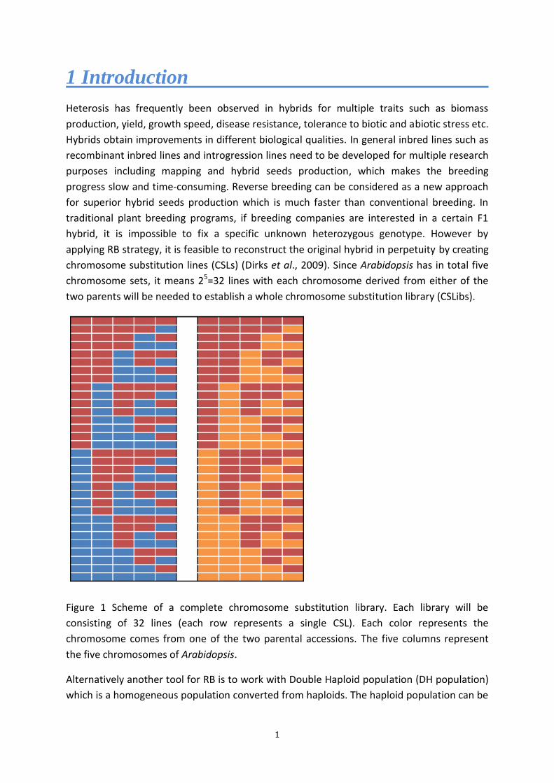
chromosome substitution lines (CSLs) (Dirks et al., 2009). Since Arabidopsis has in total five

chromosome sets, it means 25=32 lines with each chromosome derived from either of the

two parents will be needed to establish a whole chromosome substitution library (CSLibs).

Figure 1 Scheme of a complete chromosome substitution library. Each library will be

consisting of 32 lines (each row represents a single CSL). Each color represents the

chromosome comes from one of the two parental accessions. The five columns represent

the five chromosomes of Arabidopsis.

Alternatively another tool for RB is to work with Double Haploid population (DH population)

which is a homogeneous population converted from haploids. The haploid population can be

2

generated by crossing one parental accession (not necessarily be achiasmatic) to cenH3-1.

CenH3 is a null mutant in the Col-0 accession that is complemented by a cenH3 transgene

called GFP-tailswap (cenH3 is embryo lethal) (Maruthachalam and Chan, 2010). After

crossing with the haploid inducer female, whole genome from the mutant will undergo self-

elimination at a high frequency, 25%-45% of the progenies were viable (Maruthachalam and

Chan, 2010). The haploid F1 generated from this cross will only have the chromosome sets

from the wild-type parental line but in the Col-0 cytoplasmic background (Wijnen and

Keurentjes, 2014). After selfing, the haploids will be converted into double haploids. The

advantage of working with DH population is that it is bi-parental and only takes in total three

generations to generate.

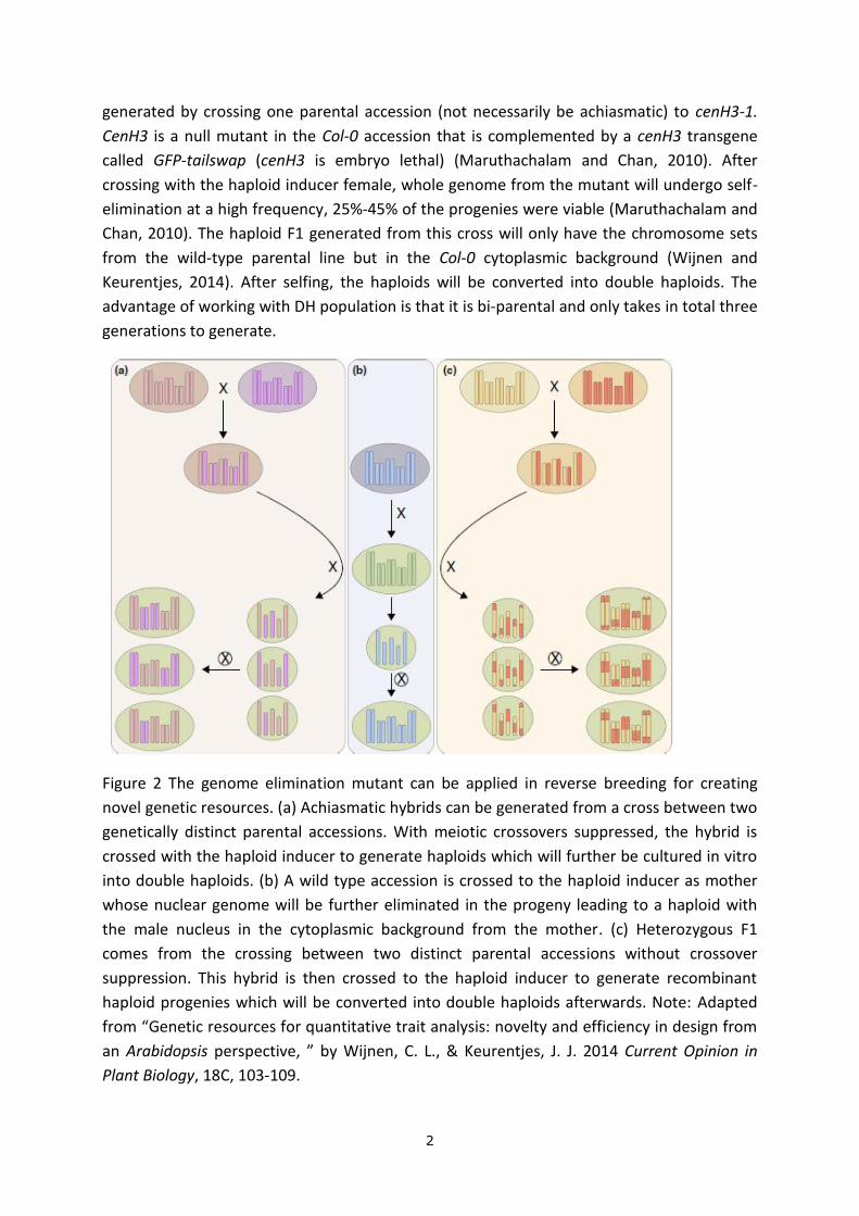
Figure 2 The genome elimination mutant can be applied in reverse breeding for creating

novel genetic resources. (a) Achiasmatic hybrids can be generated from a cross between two

genetically distinct parental accessions. With meiotic crossovers suppressed, the hybrid is

crossed with the haploid inducer to generate haploids which will further be cultured in vitro

into double haploids. (b) A wild type accession is crossed to the haploid inducer as mother

whose nuclear genome will be further eliminated in the progeny leading to a haploid with

the male nucleus in the cytoplasmic background from the mother. (c) Heterozygous F1

comes from the crossing between two distinct parental accessions without crossover

suppression. This hybrid is then crossed to the haploid inducer to generate recombinant

haploid progenies which will be converted into double haploids afterwards. Note: Adapted

from “Genetic resources for quantitative trait analysis: novelty and efficiency in design from

an Arabidopsis perspective, ” by Wijnen, C. L., & Keurentjes, J. J. 2014 Current Opinion in

Plant Biology, 18C, 103-109.

3

In RB, an RNAi construct is introduced into the plant genome and is targeting for meiotic

recombinase DISRUPTED MEIOTIC cDNA1 (DMC1). DMC1 is considered to be one of the

crucial genes involved in meiosis. DMC1 interacts with Rad51, Tid1 and also other genes and

together assemble recombination in meiosis. By inhibiting DMC1 gene expression, it is

possible to suppress crossovers during meiosis (Wijnker et al., 2012). Usually, absence of

crossovers will cause abnormal meiosis segregation and thus leads to achiasmatic gametes

(Bishop et al., 1992). Hence achiasmatic meiosis will cause univalent segregation at meiotic

metaphase I and thus aneuploidy gametes will be produced. In rare cases, 2n gametes can

still be formed which means seeds will be produced and transgenic plants are expected to be

semi-sterile in this case (Wijnker et al., 2014).

Once DMC1 is silenced, it is possible to have non-recombination double haploids which can

be used for RB strategies together with CenH3. Firstly, recombinant crossovers are

suppressed by RNAi-based gene silencing which generates achiasmatic parental accessions.

Secondly DH population can be created by using CenH3. This is an application of both

strategies in RB (DH mapping population and Achiasmatic parental lines). TAIL-PCR will be

performed to identify the location of the inserted RNAi construct. Afterwards, haploids need

to be generated by crossing to haploid inducer. Then these haploids are converted to double

haploids and a CSLib will be established (Fig 3). TAIL-PCR is able to amplify the flanking

sequence adjacent to the inserted construct. By sequencing the PCR products and perform a

BLAST, the location of the construct in the F1 hybrid can be identified (on which

chromosome). Afterwards it is possible to select the haploids without the DMC1:RNAi

construct and further select the double haploids. Finally when two complementing CSLs

(which are free of genetic modification) are crossed, the original F1 hybrid can be recreated.

(Wijnker et al., 2014)

4

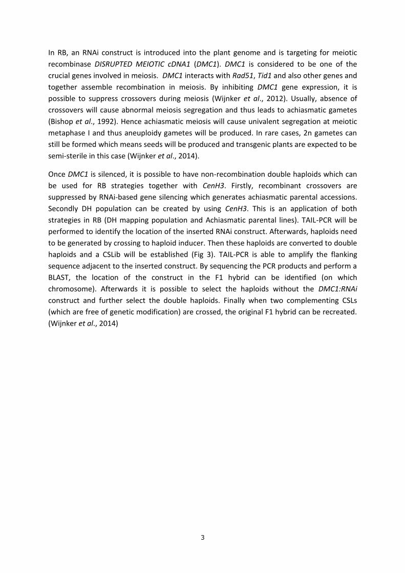
Figure 3 Scheme of creation of CSLs. (a) Creation of F1 hybrids by crossing achiasmatic

parental accessions to a second accession. (b) Generation of haploids by crossing to GFP-

tailswap, part of the haploids will be free of DMC1:RNAi construct. (c) Complementing CSLs

can be generated.

In current studies, Col-0 has been identified as the first achiasmatic parental line with the

construct located on both chromosome 4 and 5. Two complete CSLibs (Col-Mib & Col-Ler)

have already been established till now (Fig 4). The limitation of working with the current two

libraries is that CSL populations always have Columbia as one of the parents. Further study

requires new achiasmatic parental lines to be developed, these lines can be a new

achiasmatic accession containing the construct or the previous achiasmatic parent but with

the construct located on different chromosomes apart from 4 & 5. They can be used as

starting materials to expand the crossing design.

5

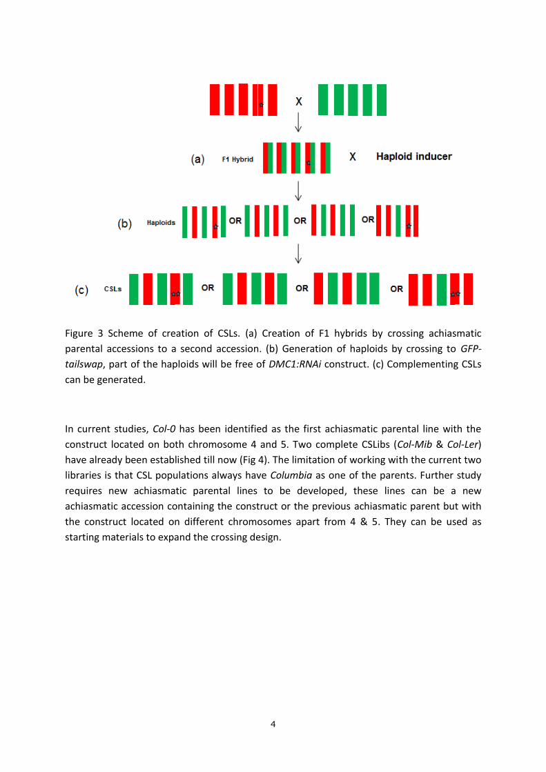
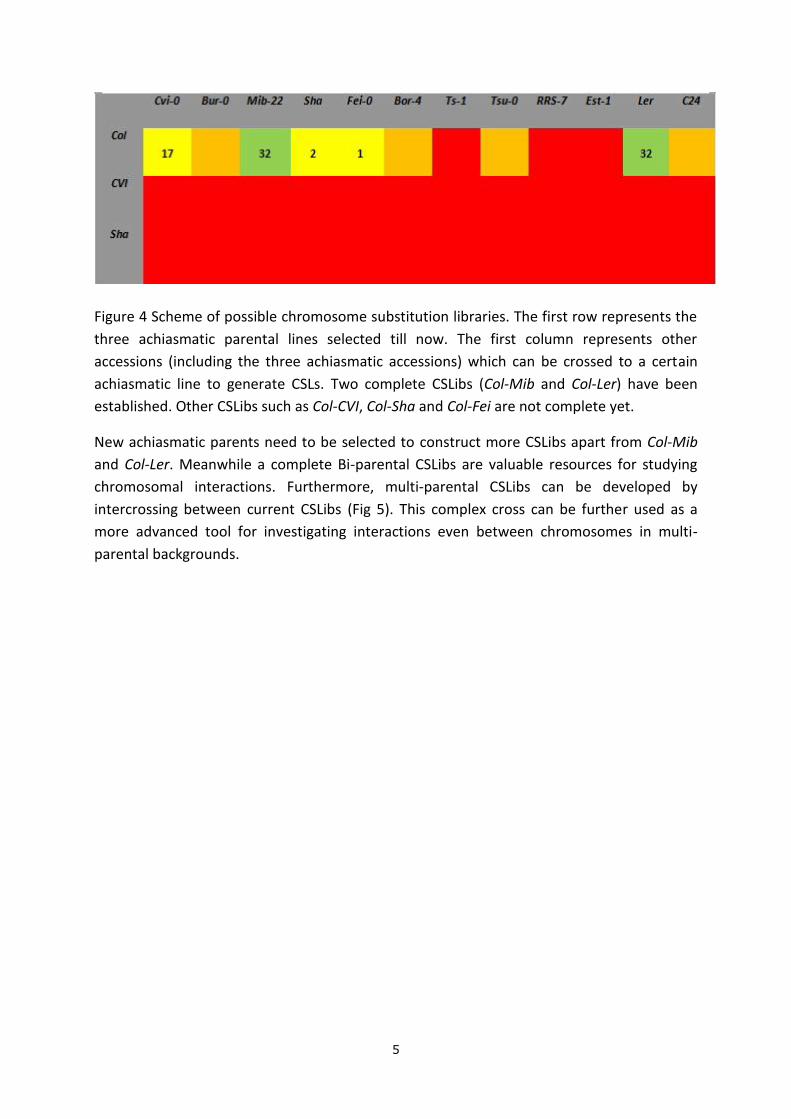
Figure 4 Scheme of possible chromosome substitution libraries. The first row represents the

three achiasmatic parental lines selected till now. The first column represents other

accessions (including the three achiasmatic accessions) which can be crossed to a certain

achiasmatic line to generate CSLs. Two complete CSLibs (Col-Mib and Col-Ler) have been

established. Other CSLibs such as Col-CVI, Col-Sha and Col-Fei are not complete yet.

New achiasmatic parents need to be selected to construct more CSLibs apart from Col-Mib

and Col-Ler. Meanwhile a complete Bi-parental CSLibs are valuable resources for studying

chromosomal interactions. Furthermore, multi-parental CSLibs can be developed by

intercrossing between current CSLibs (Fig 5). This complex cross can be further used as a

more advanced tool for investigating interactions even between chromosomes in multi-

parental backgrounds.

6

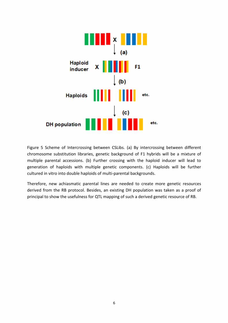
Figure 5 Scheme of Intercrossing between CSLibs. (a) By intercrossing between different

chromosome substitution libraries, genetic background of F1 hybrids will be a mixture of

multiple parental accessions. (b) Further crossing with the haploid inducer will lead to

generation of haploids with multiple genetic components. (c) Haploids will be further

cultured in vitro into double haploids of multi-parental backgrounds.

Therefore, new achiasmatic parental lines are needed to create more genetic resources

derived from the RB protocol. Besides, an existing DH population was taken as a proof of

principal to show the usefulness for QTL mapping of such a derived genetic resource of RB.

7

2 Material & Methods

2.1 Overall Workflow

Growing the parental lines→Performing floral dip transformation→Harvesting seeds→

Selection of transgenic seeds on antibiotic plates→Growing transgenic seeds selected out→

Genotyping the achiasmatic candidates→Selection of semi-sterile achiasmatic lines→

Performing TAIL-PCR to amplify flanking sequence adjacent to insertion tag→Sequencing

TAIL-PCR products→Identification of the insertion tag→Generation achiasmatic hybrid

seeds→Generation of haploid seeds by crossing to GFP-tailswap→Selection of haploids and

production of DH seeds→Construction of CSLibs→Regeneration of the desired starting

hybrid by crossing complementing CSLs.

2.2 Transformation

All achiasmatic lines were transformed by floral dip. Two types of agrobacterium strains:

LBA4404 and C58 were used. Flowers of the plants were dipped into a solution of

Agrobacterium tumefaciens that carry the desired DMC1:RNAi construct in their plasmid.

See the Scheme of the RNAi construct in Appendix 2.

2.3 Transformation selection

2.3.1 Preparation of ½ MS medium + Kanamycin

Selection for achiasmatic seeds were performed on standard ½ MS medium with kanamycin.

Survived seedlings were transplanted onto soil in the first several trial experiments and later

on rockwool. These seedlings were kept in the greenhouse until they flowered.

Kanamycin stock solution (100 mg/ml) was made in advance. Medium for 10 plates were

made for each round of selection, 50 ml for each square petridish plate. 1.1 gram MS basal

medium powder was dissolved in 500 ml of demi-water. pH was checked and adjusted to 5.8

with KOH, after that 5 grams of Daishin agar was added. Medium was sterilized by

autoclaving. The bottle was cooled down till hand warm and 0.5 ml kanamycin stock solution

(100 mg/ml) was added per 500 ml medium. Afterwards the final concentration of

kanamycin in MS medium is 100 µg/ml.

8

2.3.2 Seeds sterilization

Potential achiasmatic seeds were placed in a 1.5 ml Eppendorf tube and the lid was kept

open. 50 ml of 4% Sodium Hychlorite was added in a 100 ml beaker and normally two

beakers were put into one small desiccator. If more seeds needed to be sterilized at one

time, a larger desiccator together with four beakers was used. 1.5 ml of 1M HCl was added

to each beaker and bubbles should be observed to make sure that there was a chemical

reaction undergoing (ClO- + Cl- + 2H+ = Cl2↑ + H2O) and if not, use new hydrogen chloride.

Eppendorf tubes with seeds were placed in the desiccator with lids kept open, and then the

desiccator was sealed with parafilm. The desiccator was kept sealed for anywhere between

1.5 and 5 hours depending on the amount of seeds to be sterilized. After sterilization, gloves

were needed to operate with the seeds to ensure the seeds remained sterile. The open

eppendorf tubes were placed in the flow cabinet and leave them under airflow for 30 to 45

minutes to allow the remaining chlorine gas to evaporate. Sterilized seeds were stored for

further selection.

2.3.3 Transformants selection

Sterilized seeds were equally spread on standard ½ MS. Afterwards these plates were sealed with parafilm. Seeds were vernalized on the plates for at least 48 hours in the fridge at 40C. After 48 hours, all the plates were transferred to climate chamber (240C, 16 hours light) to allow the seeds to germinate and grow. It took about two weeks to observe apparent differences due to antibiotic stress.

2.3.4 DNA isolation

To isolate DNA from leaf samples, pretreatment by liquid nitrogen was required for disrupting cell wall and releasing nuclear material. The protocol of DNA Extraction with CTAB from Maloof was used. The protocol was suitable for 96-Well format DNA extraction. However in our case, very limited numbers of DNA samples were required for isolation so the protocol was adapted. See the DNA isolation protocol in Appendix 1.

2.3.5 TAIL-PCR & Gel-electrophoresis

To identify where the insertion tag was located, a special type of Polymerase Chain Reaction

(PCR) called TAIL-PCR would be used. It was an efficient PCR to amplify sequence flanking

the inserted construct. The advantage of TAIL-PCR is that it is fully automated which means

no further manipulation of DNA is required. And relatively low amount of genomic DNA (20-

30 ng) is enough to perform TAIL-PCR (Tan and Singh, 2011). Arbitrary degenerate primers

(AD primers) were used as the forward primers and construct specific primers as reverse

primers. AD primers were random primers which could anneal to a random site throughout

9

the whole genome. The two primer-sets differed in their length and melting temperatures,

which is why the PCR is called thermal asymmetric. By using the combination of two types of

primers, TAIL-PCR combined with sequencing can be used for mapping the location of the T-

DNA within the genome. TAIL-PCR was performed on T100TM Thermal Cycler from BIO-RAD.

See TAIL-PCR protocol in Appendix 1 and primer designs in Appendix 3.

In total three rounds of single TAIL-PCR were performed to get high dose of specific DNA

fragment flanking the insertion. After the 1st round of TAIL-PCR, high amount of unspecific

PCR products were amplified. For round 2 and 3, these unspecific products would be less but

still present.

After 2nd or 3rd round TAIL-PCR, products were checked for presence and size by gel-

electrophoresis. See the protocol in Appendix 1.

2.4 QTL analysis on shoot fresh weight

An existing DH population was used for mapping the QTL related to SFW in the greenhouse.

Seeds were derived from the crossing between Ge-0 and T540. Afterwards seeds were firstly

stored on filter paper for three days at 40C. Then germinated seedlings were transplanted

onto rockwool in the greenhouse (light: 16 hours day length; temperature: 200C during the

day and 180C during the night). Subsequently, they were sown onto rockwool in a

completely randomized design. For each genotype 10 replicates were used from DH001 to

DH210 and 20 replicates were used for parental lines (76135-Ge0 & 76135-T540). 10

replicates of reciprocal F1 (one parent is used as father and mother respectively) from the

two parents were also included in the experiment. After three weeks of growth, the

seedlings above rockwool were cut off and weighed on precise scales. Original data was

input into excel file. GenStat was used to analyze genotypic data combined with phenotypic

data afterwards.

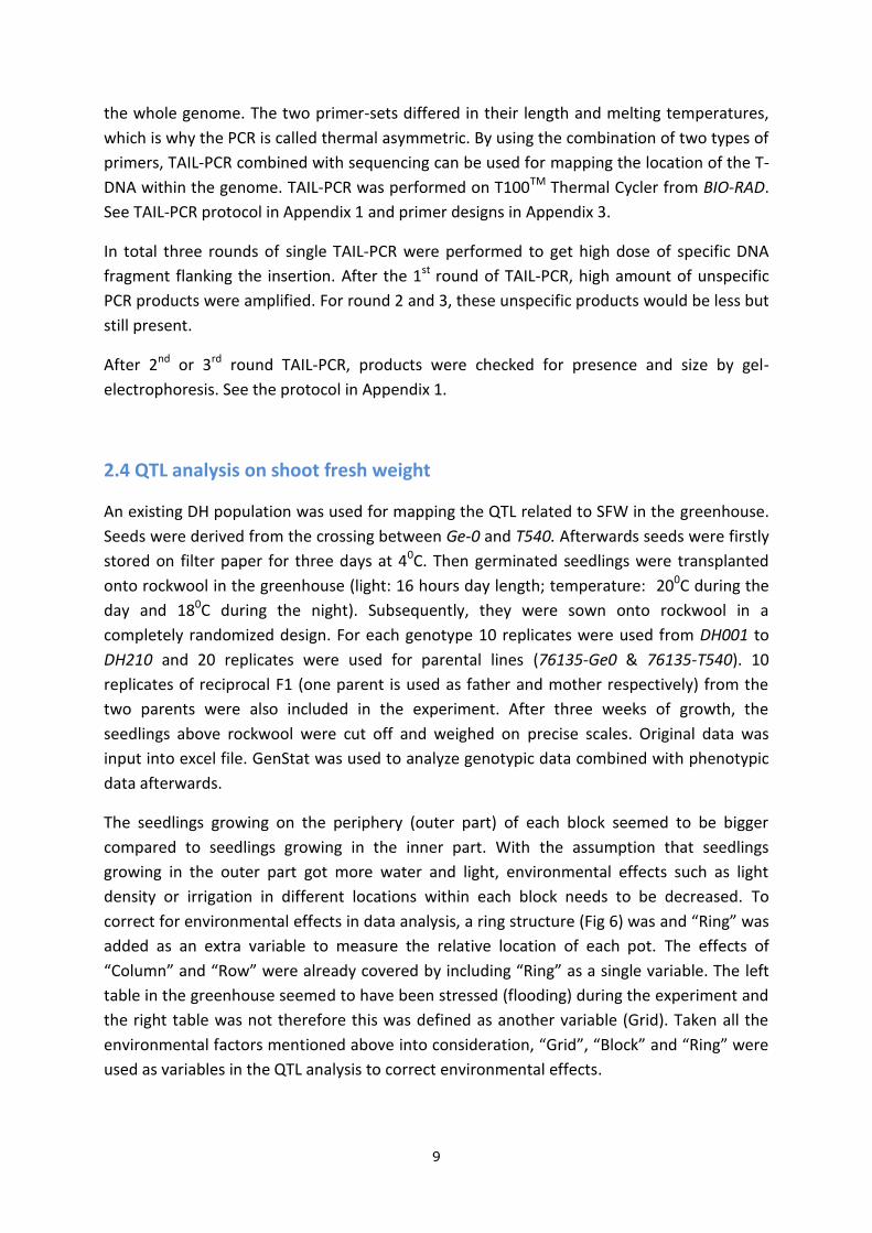
The seedlings growing on the periphery (outer part) of each block seemed to be bigger

compared to seedlings growing in the inner part. With the assumption that seedlings

growing in the outer part got more water and light, environmental effects such as light

density or irrigation in different locations within each block needs to be decreased. To

correct for environmental effects in data analysis, a ring structure (Fig 6) was and “Ring” was

added as an extra variable to measure the relative location of each pot. The effects of

“Column” and “Row” were already covered by including “Ring” as a single variable. The left

table in the greenhouse seemed to have been stressed (flooding) during the experiment and

the right table was not therefore this was defined as another variable (Grid). Taken all the

environmental factors mentioned above into consideration, “Grid”, “Block” and “Ring” were

used as variables in the QTL analysis to correct environmental effects.

10

Figure 6 Ring structure of each block. Each block was divided into eight rings. Each square

represents one spot for an individual plant. The overall rings structure is indicated by the

gradual change of color.

11

3 Results

3.1 Selection of achiasmatic parental lines

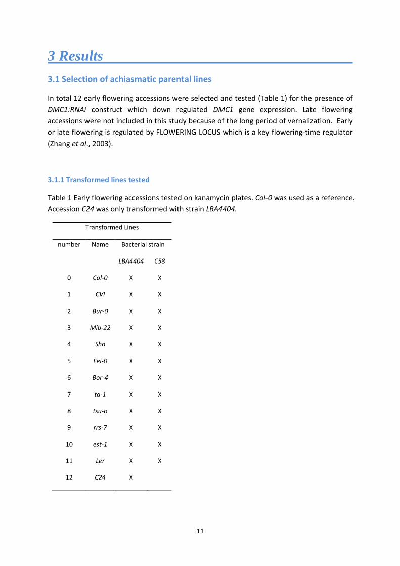
In total 12 early flowering accessions were selected and tested (Table 1) for the presence of

DMC1:RNAi construct which down regulated DMC1 gene expression. Late flowering

accessions were not included in this study because of the long period of vernalization. Early

or late flowering is regulated by FLOWERING LOCUS which is a key flowering-time regulator

(Zhang et al., 2003).

3.1.1 Transformed lines tested

Table 1 Early flowering accessions tested on kanamycin plates. Col-0 was used as a reference.

Accession C24 was only transformed with strain LBA4404.

Transformed Lines

number Name Bacterial strain

LBA4404 C58

0 Col-0 X X

1 CVI X X

2 Bur-0 X X

3 Mib-22 X X

4 Sha X X

5 Fei-0 X X

6 Bor-4 X X

7 ta-1 X X

8 tsu-o X X

9 rrs-7 X X

10 est-1 X X

11 Ler X X

12 C24 X

12

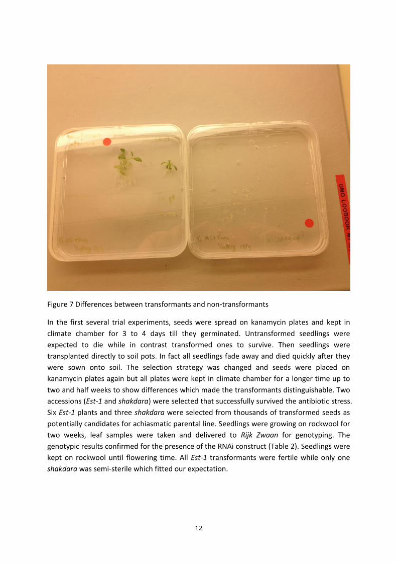
Figure 7 Differences between transformants and non-transformants

In the first several trial experiments, seeds were spread on kanamycin plates and kept in

climate chamber for 3 to 4 days till they germinated. Untransformed seedlings were

expected to die while in contrast transformed ones to survive. Then seedlings were

transplanted directly to soil pots. In fact all seedlings fade away and died quickly after they

were sown onto soil. The selection strategy was changed and seeds were placed on

kanamycin plates again but all plates were kept in climate chamber for a longer time up to

two and half weeks to show differences which made the transformants distinguishable. Two

accessions (Est-1 and shakdara) were selected that successfully survived the antibiotic stress.

Six Est-1 plants and three shakdara were selected from thousands of transformed seeds as

potentially candidates for achiasmatic parental line. Seedlings were growing on rockwool for

two weeks, leaf samples were taken and delivered to Rijk Zwaan for genotyping. The

genotypic results confirmed for the presence of the RNAi construct (Table 2). Seedlings were

kept on rockwool until flowering time. All Est-1 transformants were fertile while only one

shakdara was semi-sterile which fitted our expectation.

13

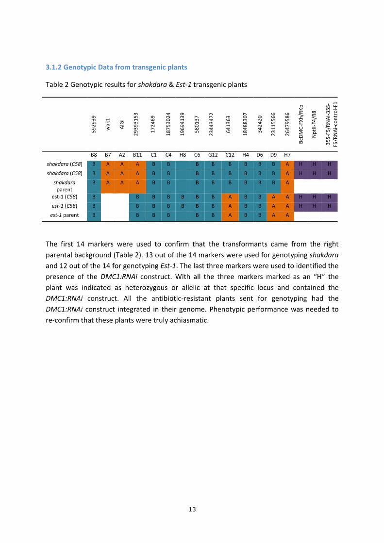
3.1.2 Genotypic Data from transgenic plants

Table 2 Genotypic results for shakdara & Est-1 transgenic plants

59

29

39

wak

1

AIG

I

29

39

31

53

17

24

69

18

75

30

24

19

69

41

39

58

01

37

23

44

34

72

64

13

63

18

48

83

07

34

24

20

23

11

55

66

26

47

95

86

BcD

MC

-FX

h/R

Kp

Np

tII-

F4/R

8

35

S-F5

/RN

Ai-

35

S-

F5/R

NA

i-co

ntr

ol-

F1

B8 B7 A2 B11 C1 C4 H8 C6 G12 C12 H4 D6 D9 H7

shakdara (C58) B A A A B B B B B B B B A H H H

shakdara (C58) B A A A B B B B B B B B A H H H

shakdara parent

B A A A B B B B B B B B A

est-1 (C58) B B B B B B B A B B A A H H H

est-1 (C58) B B B B B B B A B B A A H H H

est-1 parent B B B B B B A B B A A

The first 14 markers were used to confirm that the transformants came from the right

parental background (Table 2). 13 out of the 14 markers were used for genotyping shakdara

and 12 out of the 14 for genotyping Est-1. The last three markers were used to identified the

presence of the DMC1:RNAi construct. With all the three markers marked as an “H” the

plant was indicated as heterozygous or allelic at that specific locus and contained the

DMC1:RNAi construct. All the antibiotic-resistant plants sent for genotyping had the

DMC1:RNAi construct integrated in their genome. Phenotypic performance was needed to

re-confirm that these plants were truly achiasmatic.

14

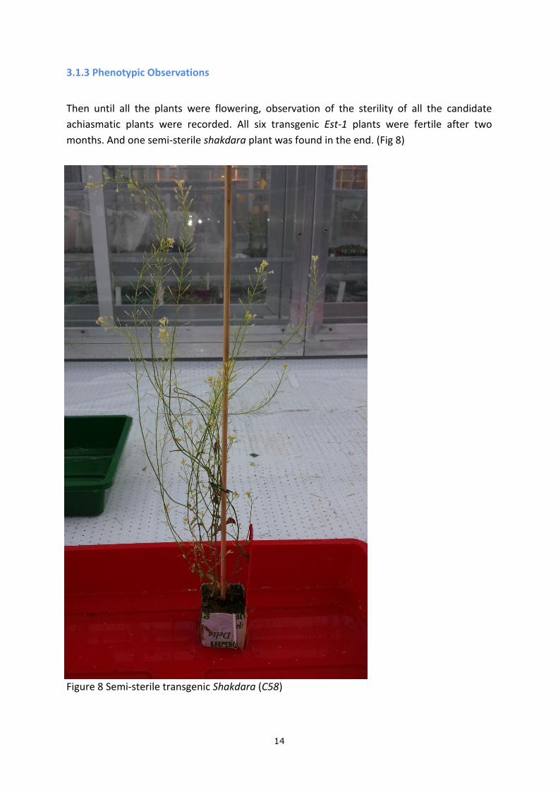
3.1.3 Phenotypic Observations

Then until all the plants were flowering, observation of the sterility of all the candidate

achiasmatic plants were recorded. All six transgenic Est-1 plants were fertile after two

months. And one semi-sterile shakdara plant was found in the end. (Fig 8)

Figure 8 Semi-sterile transgenic Shakdara (C58)

15

Efficiency was very low in both transformations. Each time a selection was done, about 100

seeds (transformed by one single agrobacterium strain from each accession were put on

kanamycin plates and in total three rounds of selection were done which means about 600

seeds from each accession were used for selection. In the LBA4404 no transformants were

found and from C58 transformation, six Est-1 and three shakdara transgenic plants were

found. So transformation efficiency was about 1% for Est-1 and 0.5% for shakdara. For other

accessions, no achiasmatic lines were found. Within all the seedlings selected, all six Est-1

plants were found to be fertile and 1 out of 3 shakdara were found to be semi-sterile.

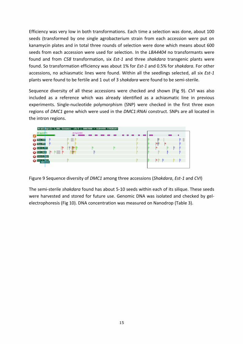
Sequence diversity of all these accessions were checked and shown (Fig 9). CVI was also

included as a reference which was already identified as a achiasmatic line in previous

experiments. Single-nucleotide polymorphism (SNP) were checked in the first three exon

regions of DMC1 gene which were used in the DMC1:RNAi construct. SNPs are all located in

the intron regions.

Figure 9 Sequence diversity of DMC1 among three accessions (Shakdara, Est-1 and CVI)

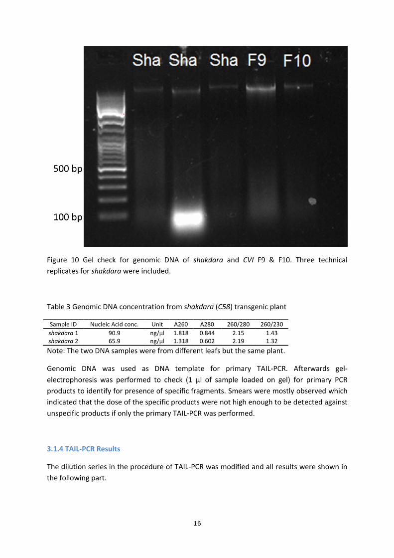
The semi-sterile shakdara found has about 5-10 seeds within each of its silique. These seeds

were harvested and stored for future use. Genomic DNA was isolated and checked by gel-

electrophoresis (Fig 10). DNA concentration was measured on Nanodrop (Table 3).

16

Figure 10 Gel check for genomic DNA of shakdara and CVI F9 & F10. Three technical

replicates for shakdara were included.

Table 3 Genomic DNA concentration from shakdara (C58) transgenic plant

Sample ID Nucleic Acid conc. Unit A260 A280 260/280 260/230

shakdara 1 90.9 ng/µl 1.818 0.844 2.15 1.43 shakdara 2 65.9 ng/µl 1.318 0.602 2.19 1.32

Note: The two DNA samples were from different leafs but the same plant.

Genomic DNA was used as DNA template for primary TAIL-PCR. Afterwards gel-

electrophoresis was performed to check (1 µl of sample loaded on gel) for primary PCR

products to identify for presence of specific fragments. Smears were mostly observed which

indicated that the dose of the specific products were not high enough to be detected against

unspecific products if only the primary TAIL-PCR was performed.

3.1.4 TAIL-PCR Results

The dilution series in the procedure of TAIL-PCR was modified and all results were shown in

the following part.

17

After the primary PCR gel-electrophoresis was impossible to distinguish between specific

and unspecific products which acted like noise. So gel check was only possible after at least 2

rounds of TAIL-PCR. CVI F9 and F10 were included as positive control. Fermentas

GeneRulerTM DNA Ladder Mix #SM0331 was used as marker for all gel-electrophoresis.

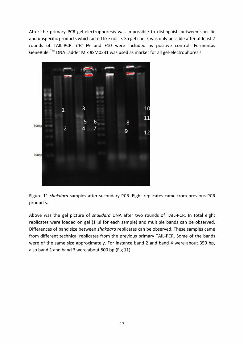
Figure 11 shakdara samples after secondary PCR. Eight replicates came from previous PCR

products.

Above was the gel picture of shakdara DNA after two rounds of TAIL-PCR. In total eight

replicates were loaded on gel (1 µl for each sample) and multiple bands can be observed.

Differences of band size between shakdara replicates can be observed. These samples came

from different technical replicates from the previous primary TAIL-PCR. Some of the bands

were of the same size approximately. For instance band 2 and band 4 were about 350 bp,

also band 1 and band 3 were about 800 bp (Fig 11).

18

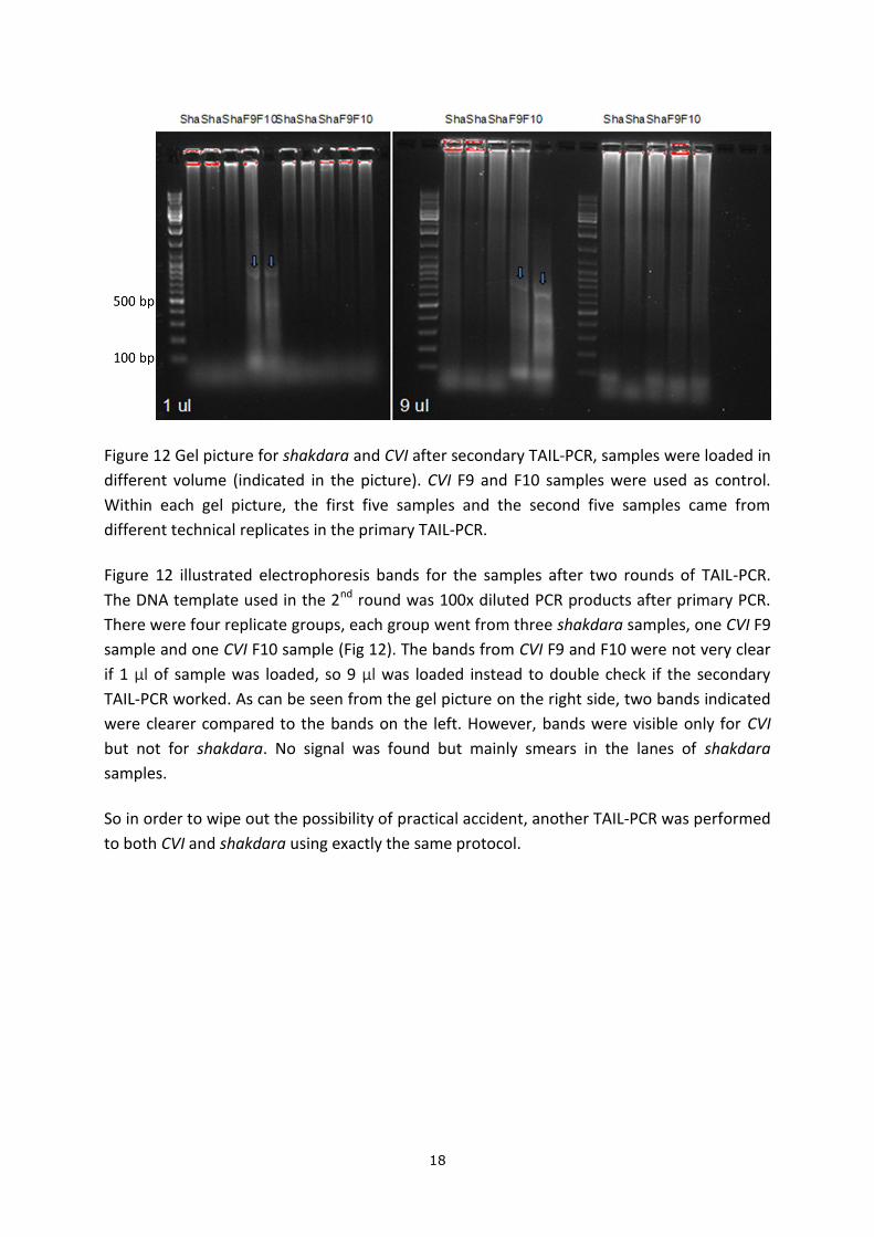
Figure 12 Gel picture for shakdara and CVI after secondary TAIL-PCR, samples were loaded in

different volume (indicated in the picture). CVI F9 and F10 samples were used as control.

Within each gel picture, the first five samples and the second five samples came from

different technical replicates in the primary TAIL-PCR.

Figure 12 illustrated electrophoresis bands for the samples after two rounds of TAIL-PCR.

The DNA template used in the 2nd round was 100x diluted PCR products after primary PCR.

There were four replicate groups, each group went from three shakdara samples, one CVI F9

sample and one CVI F10 sample (Fig 12). The bands from CVI F9 and F10 were not very clear

if 1 µl of sample was loaded, so 9 µl was loaded instead to double check if the secondary

TAIL-PCR worked. As can be seen from the gel picture on the right side, two bands indicated

were clearer compared to the bands on the left. However, bands were visible only for CVI

but not for shakdara. No signal was found but mainly smears in the lanes of shakdara

samples.

So in order to wipe out the possibility of practical accident, another TAIL-PCR was performed

to both CVI and shakdara using exactly the same protocol.

19

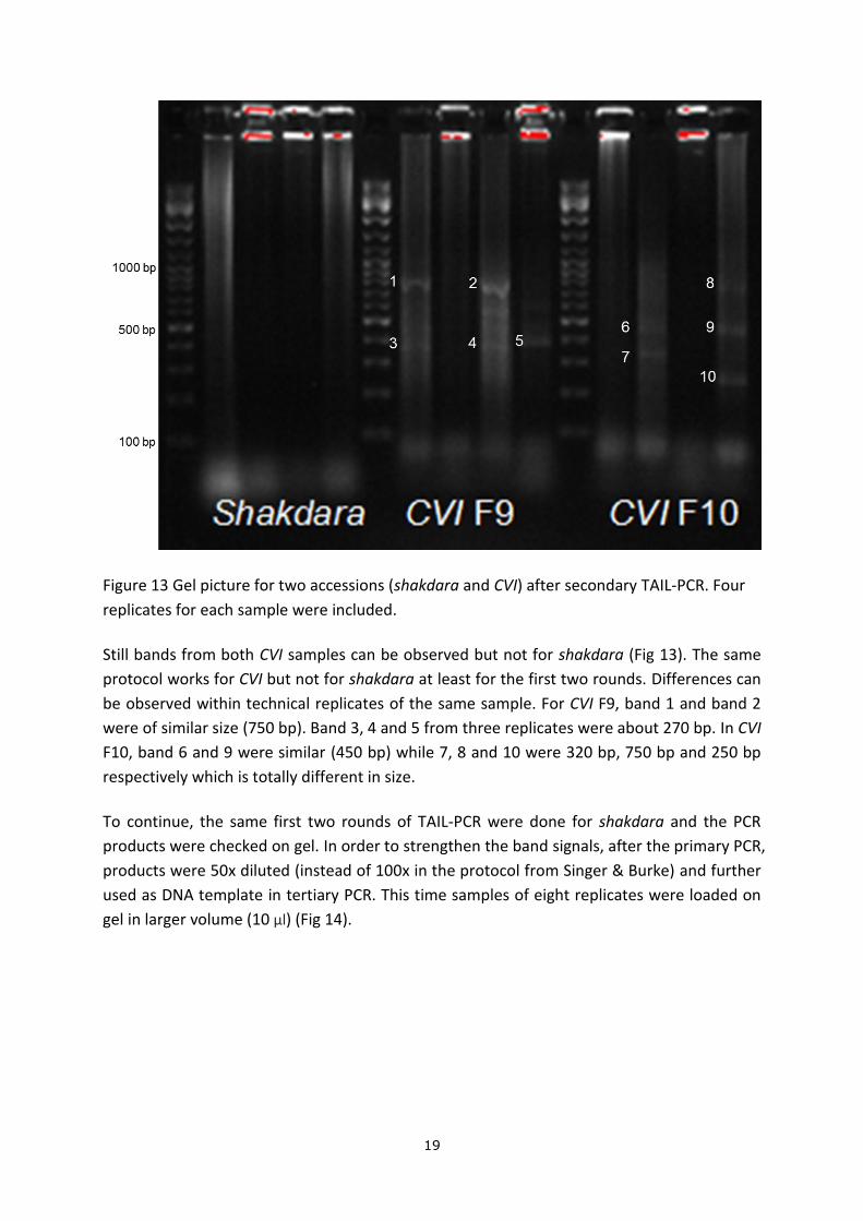
Figure 13 Gel picture for two accessions (shakdara and CVI) after secondary TAIL-PCR. Four

replicates for each sample were included.

Still bands from both CVI samples can be observed but not for shakdara (Fig 13). The same

protocol works for CVI but not for shakdara at least for the first two rounds. Differences can

be observed within technical replicates of the same sample. For CVI F9, band 1 and band 2

were of similar size (750 bp). Band 3, 4 and 5 from three replicates were about 270 bp. In CVI

F10, band 6 and 9 were similar (450 bp) while 7, 8 and 10 were 320 bp, 750 bp and 250 bp

respectively which is totally different in size.

To continue, the same first two rounds of TAIL-PCR were done for shakdara and the PCR

products were checked on gel. In order to strengthen the band signals, after the primary PCR,

products were 50x diluted (instead of 100x in the protocol from Singer & Burke) and further

used as DNA template in tertiary PCR. This time samples of eight replicates were loaded on

gel in larger volume (10 µl) (Fig 14).

20

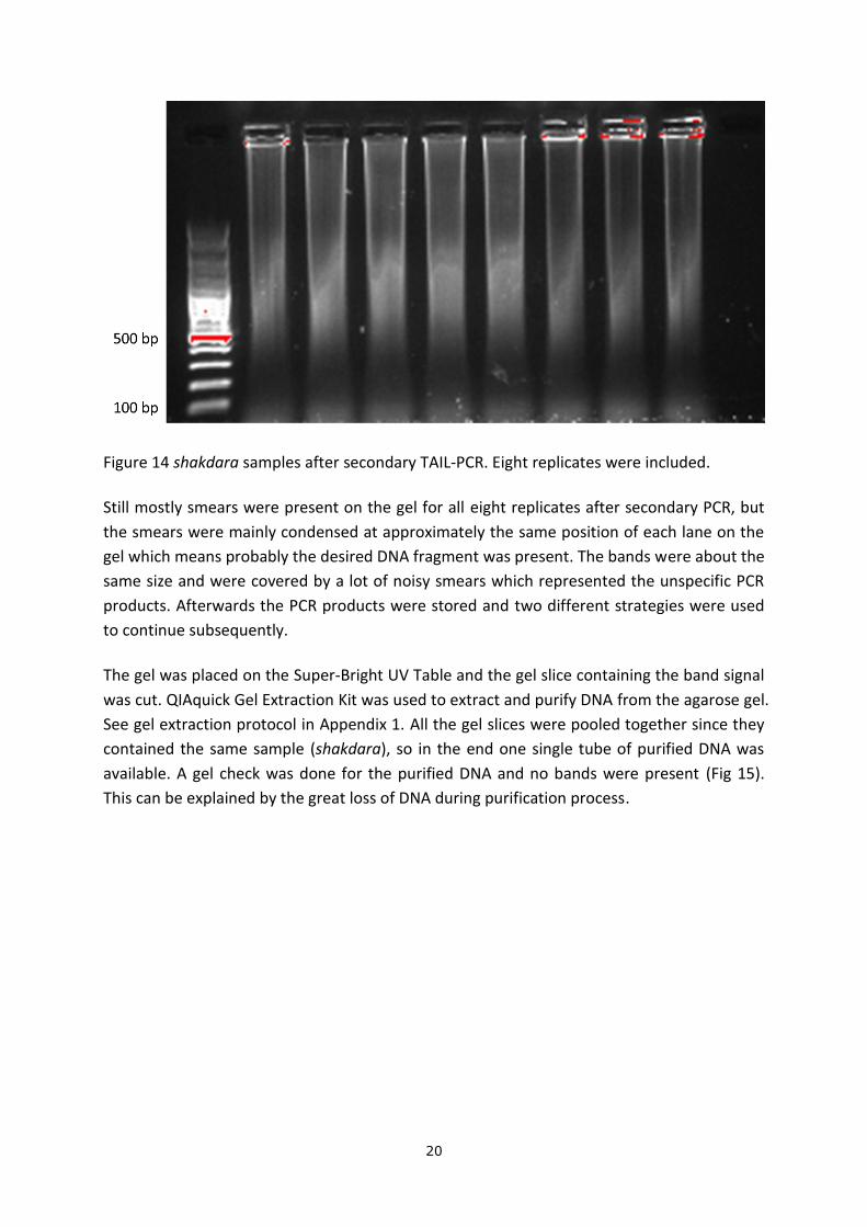
Figure 14 shakdara samples after secondary TAIL-PCR. Eight replicates were included.

Still mostly smears were present on the gel for all eight replicates after secondary PCR, but

the smears were mainly condensed at approximately the same position of each lane on the

gel which means probably the desired DNA fragment was present. The bands were about the

same size and were covered by a lot of noisy smears which represented the unspecific PCR

products. Afterwards the PCR products were stored and two different strategies were used

to continue subsequently.

The gel was placed on the Super-Bright UV Table and the gel slice containing the band signal

was cut. QIAquick Gel Extraction Kit was used to extract and purify DNA from the agarose gel.

See gel extraction protocol in Appendix 1. All the gel slices were pooled together since they

contained the same sample (shakdara), so in the end one single tube of purified DNA was

available. A gel check was done for the purified DNA and no bands were present (Fig 15).

This can be explained by the great loss of DNA during purification process.

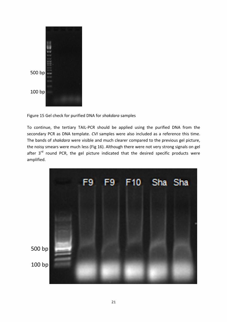
21

Figure 15 Gel check for purified DNA for shakdara samples

To continue, the tertiary TAIL-PCR should be applied using the purified DNA from the

secondary PCR as DNA template. CVI samples were also included as a reference this time.

The bands of shakdara were visible and much clearer compared to the previous gel picture,

the noisy smears were much less (Fig 16). Although there were not very strong signals on gel

after 3rd round PCR, the gel picture indicated that the desired specific products were

amplified.

22

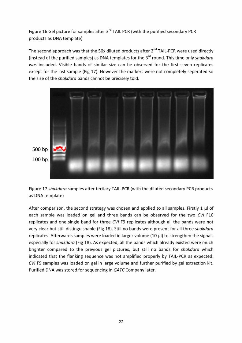
Figure 16 Gel picture for samples after 3rd TAIL PCR (with the purified secondary PCR

products as DNA template)

The second approach was that the 50x diluted products after 2nd TAIL-PCR were used directly

(instead of the purified samples) as DNA templates for the 3rd round. This time only shakdara

was included. Visible bands of similar size can be observed for the first seven replicates

except for the last sample (Fig 17). However the markers were not completely seperated so

the size of the shakdara bands cannot be precisely told.

Figure 17 shakdara samples after tertiary TAIL-PCR (with the diluted secondary PCR products

as DNA template)

After comparison, the second strategy was chosen and applied to all samples. Firstly 1 µl of

each sample was loaded on gel and three bands can be observed for the two CVI F10

replicates and one single band for three CVI F9 replicates although all the bands were not

very clear but still distinguishable (Fig 18). Still no bands were present for all three shakdara

replicates. Afterwards samples were loaded in larger volume (10 µl) to strengthen the signals

especially for shakdara (Fig 18). As expected, all the bands which already existed were much

brighter compared to the previous gel pictures, but still no bands for shakdara which

indicated that the flanking sequence was not amplified properly by TAIL-PCR as expected.

CVI F9 samples was loaded on gel in large volume and further purified by gel extraction kit.

Purified DNA was stored for sequencing in GATC Company later.

23

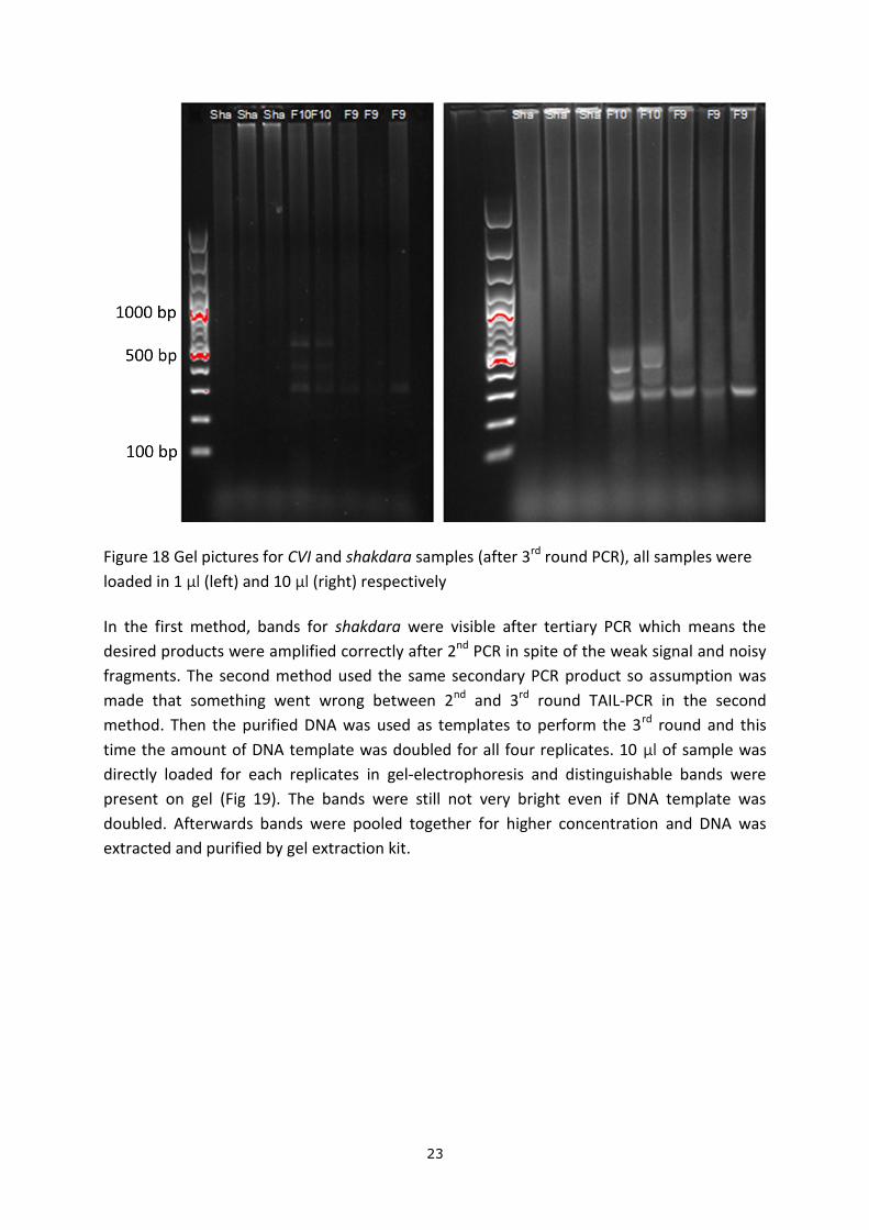
Figure 18 Gel pictures for CVI and shakdara samples (after 3rd round PCR), all samples were

loaded in 1 µl (left) and 10 µl (right) respectively

In the first method, bands for shakdara were visible after tertiary PCR which means the

desired products were amplified correctly after 2nd PCR in spite of the weak signal and noisy

fragments. The second method used the same secondary PCR product so assumption was

made that something went wrong between 2nd and 3rd round TAIL-PCR in the second

method. Then the purified DNA was used as templates to perform the 3rd round and this

time the amount of DNA template was doubled for all four replicates. 10 µl of sample was

directly loaded for each replicates in gel-electrophoresis and distinguishable bands were

present on gel (Fig 19). The bands were still not very bright even if DNA template was

doubled. Afterwards bands were pooled together for higher concentration and DNA was

extracted and purified by gel extraction kit.

24

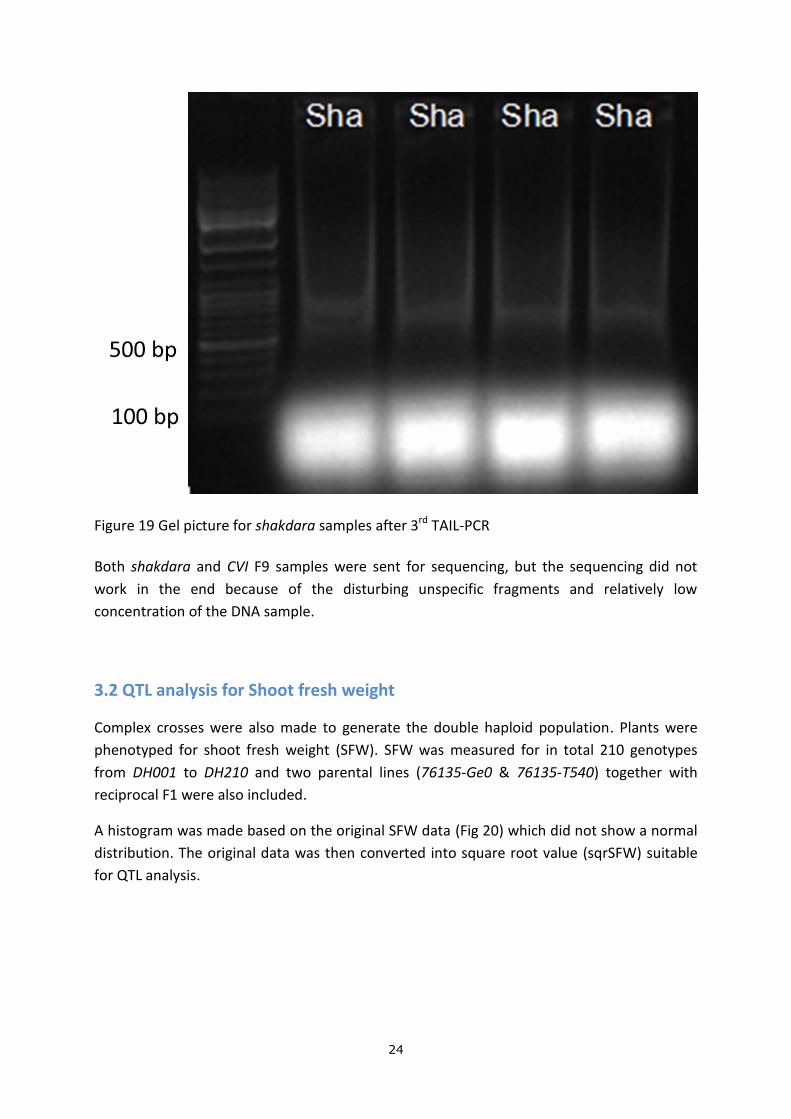
Figure 19 Gel picture for shakdara samples after 3rd TAIL-PCR

Both shakdara and CVI F9 samples were sent for sequencing, but the sequencing did not

work in the end because of the disturbing unspecific fragments and relatively low

concentration of the DNA sample.

3.2 QTL analysis for Shoot fresh weight

Complex crosses were also made to generate the double haploid population. Plants were

phenotyped for shoot fresh weight (SFW). SFW was measured for in total 210 genotypes

from DH001 to DH210 and two parental lines (76135-Ge0 & 76135-T540) together with

reciprocal F1 were also included.

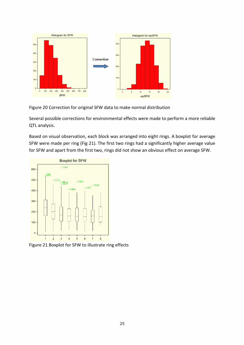
A histogram was made based on the original SFW data (Fig 20) which did not show a normal

distribution. The original data was then converted into square root value (sqrSFW) suitable

for QTL analysis.

25

Figure 20 Correction for original SFW data to make normal distribution

Several possible corrections for environmental effects were made to perform a more reliable

QTL analysis.

Based on visual observation, each block was arranged into eight rings. A boxplot for average

SFW were made per ring (Fig 21). The first two rings had a significantly higher average value

for SFW and apart from the first two, rings did not show an obvious effect on average SFW.

Figure 21 Boxplot for SFW to illustrate ring effects

26

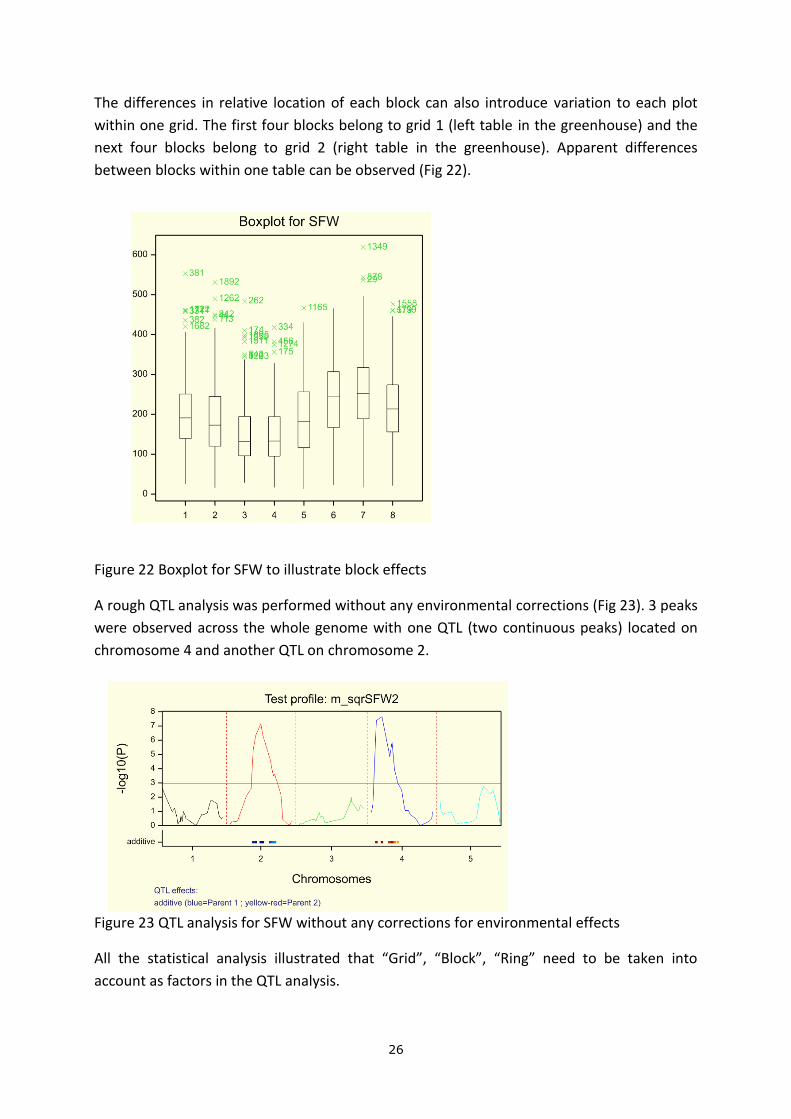
The differences in relative location of each block can also introduce variation to each plot

within one grid. The first four blocks belong to grid 1 (left table in the greenhouse) and the

next four blocks belong to grid 2 (right table in the greenhouse). Apparent differences

between blocks within one table can be observed (Fig 22).

Figure 22 Boxplot for SFW to illustrate block effects

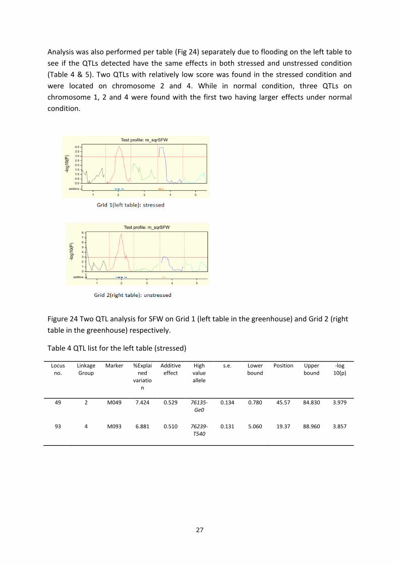
A rough QTL analysis was performed without any environmental corrections (Fig 23). 3 peaks

were observed across the whole genome with one QTL (two continuous peaks) located on

chromosome 4 and another QTL on chromosome 2.

Figure 23 QTL analysis for SFW without any corrections for environmental effects

All the statistical analysis illustrated that “Grid”, “Block”, “Ring” need to be taken into

account as factors in the QTL analysis.

27

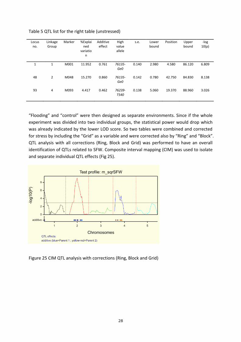
Analysis was also performed per table (Fig 24) separately due to flooding on the left table to

see if the QTLs detected have the same effects in both stressed and unstressed condition

(Table 4 & 5). Two QTLs with relatively low score was found in the stressed condition and

were located on chromosome 2 and 4. While in normal condition, three QTLs on

chromosome 1, 2 and 4 were found with the first two having larger effects under normal

condition.

Figure 24 Two QTL analysis for SFW on Grid 1 (left table in the greenhouse) and Grid 2 (right

table in the greenhouse) respectively.

Table 4 QTL list for the left table (stressed)

Locus no.

Linkage Group

Marker %Explained

variation

Additive effect

High value allele

s.e. Lower bound

Position Upper bound

-log 10(p)

49 2 M049 7.424 0.529 76135-Ge0

0.134

0.780 45.57 84.830

3.979

93 4 M093 6.881 0.510 76239-T540

0.131

5.060 19.37 88.960 3.857

28

Table 5 QTL list for the right table (unstressed)

Locus no.

Linkage Group

Marker %Explained

variation

Additive effect

High value allele

s.e. Lower bound

Position Upper bound

-log 10(p)

1 1 M001 11.952 0.761 76135-Ge0

0.140 2.980 4.580 86.120

6.809

48 2 M048 15.270 0.860 76135-Ge0

0.142 0.780 42.750 84.830

8.138

93 4 M093 4.417 0.462 76239-T540

0.138 5.060 19.370 88.960 3.026

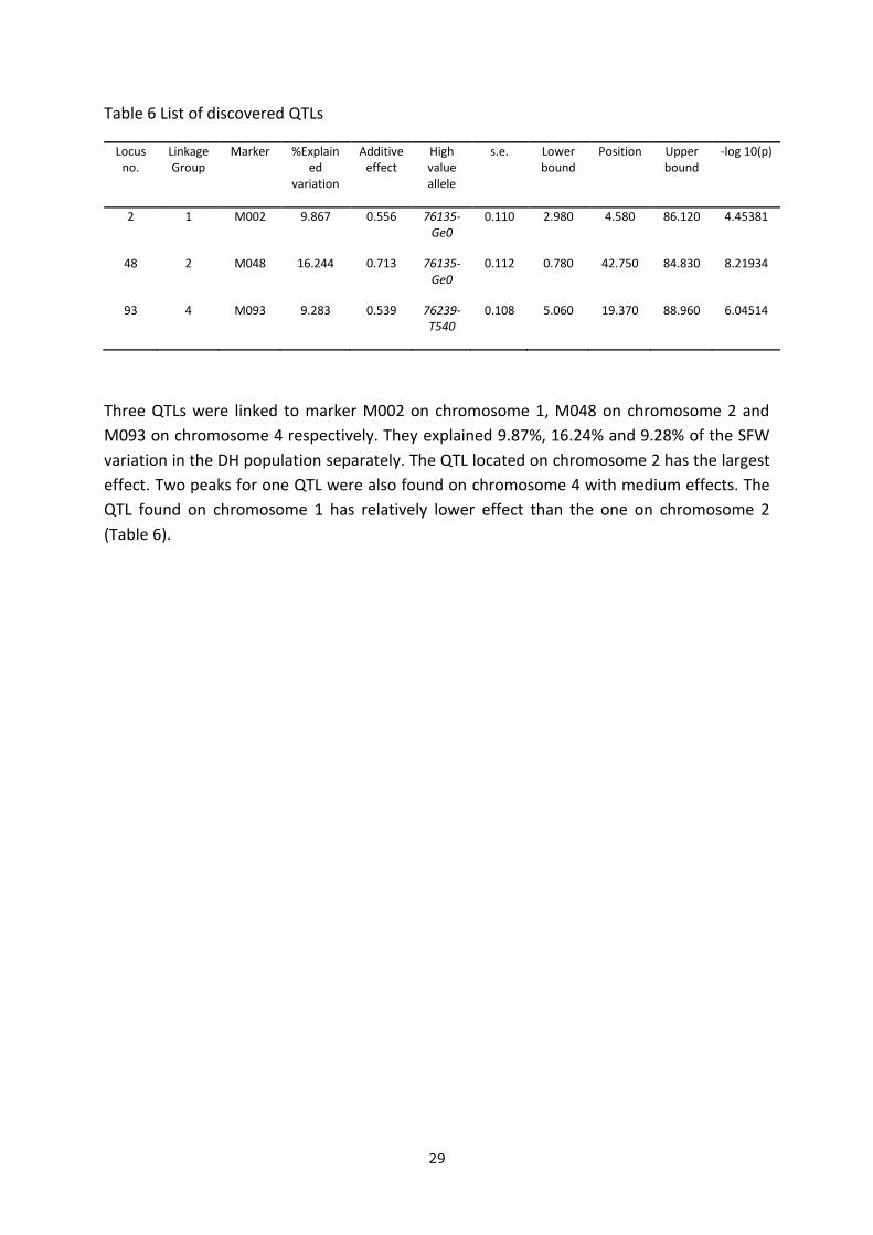
“Flooding” and “control” were then designed as separate environments. Since if the whole

experiment was divided into two individual groups, the statistical power would drop which

was already indicated by the lower LOD score. So two tables were combined and corrected

for stress by including the “Grid” as a variable and were corrected also by “Ring” and “Block”.

QTL analysis with all corrections (Ring, Block and Grid) was performed to have an overall

identification of QTLs related to SFW. Composite interval mapping (CIM) was used to isolate

and separate individual QTL effects (Fig 25).

Figure 25 CIM QTL analysis with corrections (Ring, Block and Grid)

29

Table 6 List of discovered QTLs

Locus no.

Linkage Group

Marker %Explained

variation

Additive effect

High value allele

s.e. Lower bound

Position Upper bound

-log 10(p)

2 1 M002 9.867 0.556 76135-Ge0

0.110

2.980 4.580 86.120

4.45381

48 2 M048 16.244 0.713 76135-Ge0

0.112 0.780 42.750 84.830

8.21934

93 4 M093 9.283 0.539 76239-T540

0.108

5.060 19.370 88.960 6.04514

Three QTLs were linked to marker M002 on chromosome 1, M048 on chromosome 2 and

M093 on chromosome 4 respectively. They explained 9.87%, 16.24% and 9.28% of the SFW

variation in the DH population separately. The QTL located on chromosome 2 has the largest

effect. Two peaks for one QTL were also found on chromosome 4 with medium effects. The

QTL found on chromosome 1 has relatively lower effect than the one on chromosome 2

(Table 6).

30

4 Discussions and Recommendations

4.1 Discussions

Currently the DMC1:RNAi construct is located on Col-0 chromosome 4 and 5. Two complete

chromosome substitution libraries have been successfully established (“Col-Mib” and “Col-

Ler”). The bottleneck for current study is both CSLibs are at the Columbia background which

limits the cross design we can make. The main aim of my thesis work is to discover new

achiasmatic parental accessions. So firstly more parental accessions need to be transformed.

However, the transformation efficiency was very low in the previous transformation

especially if the LBA4404 strain was used. For floral dip transformation it is better to only use

C58 (Shamloul et al., 2014). Alternatively, literature review can be done to figure out for

another agrobacterium strain which works best for floral dip transformation.

Within all the transformants that were selected, majority of these kanamycin resistant plants

were fertile in the end which did not match the genotyping results. These plants were

sampled at a relatively early stage and sent for genotyping. The positive results indicated

that at that time point the construct did integrate into the genome and introduced different

alleles and cause heterozygosity at that locus. Somehow during growth, the RNAi construct

lost its function for some reasons. A differential expression pattern can be one of the factors

which can explain the mismatch between genotypic results and phenotypic observations.

The construct can be inserted into a certain region which was only expressed in the early

stage while in the later stage the suppression of crossovers collapsed because the whole

region was not expressed any longer. Cells were undergoing normal chromosomal

segregation again and lead to fertile phenotype. An alternative explanation for this can be

tissue-specific expression of the transgene. Leaf samples were taken and sent for genotyping.

Presence of the transgene in leaf does not guarantee the same expression level in other

plant tissues including silique. Meanwhile we observed different silencing effects between

accessions. One possibility can be that the expression level of DMC1 in Est-1 is much higher

than in shakdara which lead to an unsuccessful silencing.

31

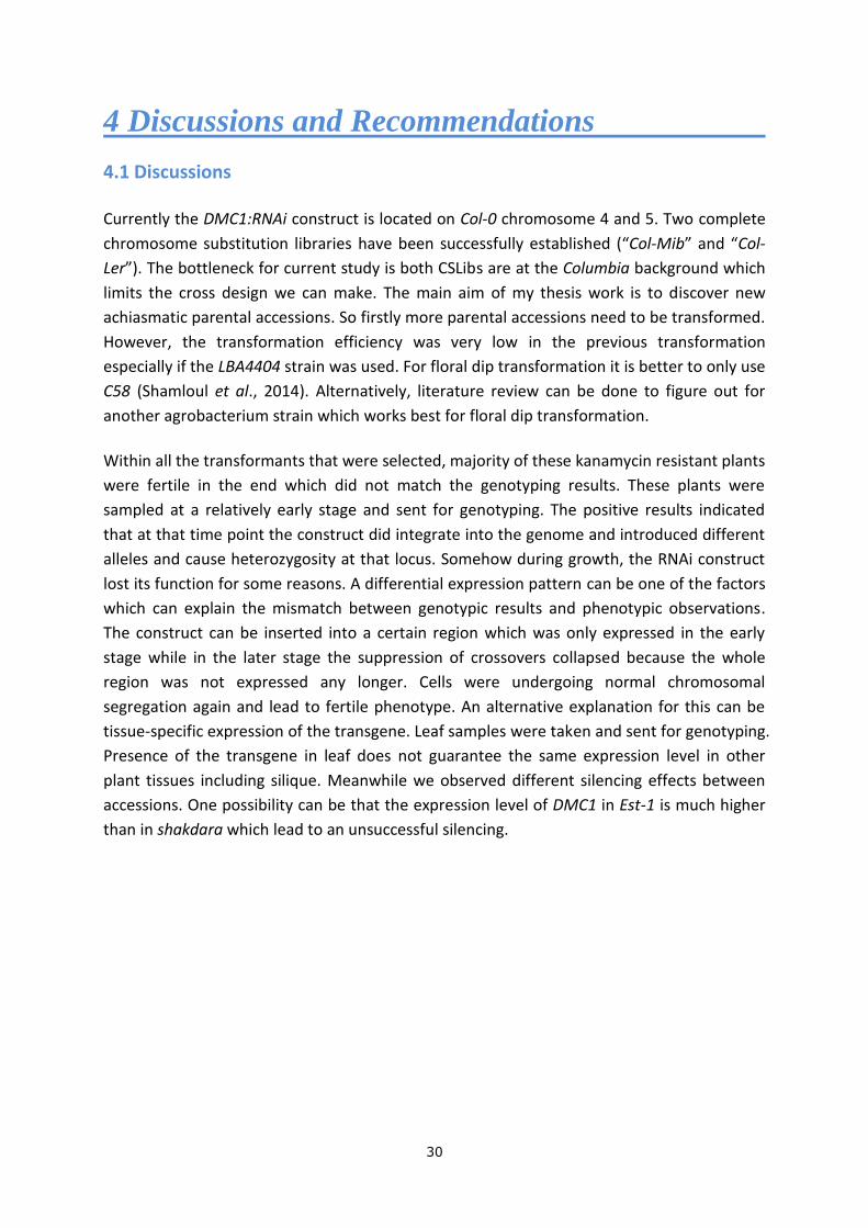
Figure 26 Illustration of how AD primer and T-DNA-specific insertion primers works. T-DNA-

specific insertion primers will anneal to the T-DNA region as reverse primer while AD primers

have multiple annealing sites throughout the whole genome.

The reason for presence of multiple bands with different sizes can be that within the

genome, multiple annealing sites can be provided for AD primers (Fig 26). Figure 26

illustrates the first three closest annealing sites for AD primer. Besides, the length of all AD

primer is relatively short (16 bp) which means not only the chromosome where the RNAi

construct located but also other chromosomes can provide multiple annealing sites. This

lead to production of multiple undesired DNA fragments with different length. This

assumption was also confirmed by the differences of TAIL-PCR results between the technical

replicates for the same sample (Fig 11 & 13). Meanwhile unspecific PCR products can also be

amplified which were primed by T-DNA-specific insertion primers on both sides. All these

unspecific products could also be amplified as TAIL-PCR was under way. As long as these

DNA fragments were short enough to be detected, they act as noisy smears on gel.

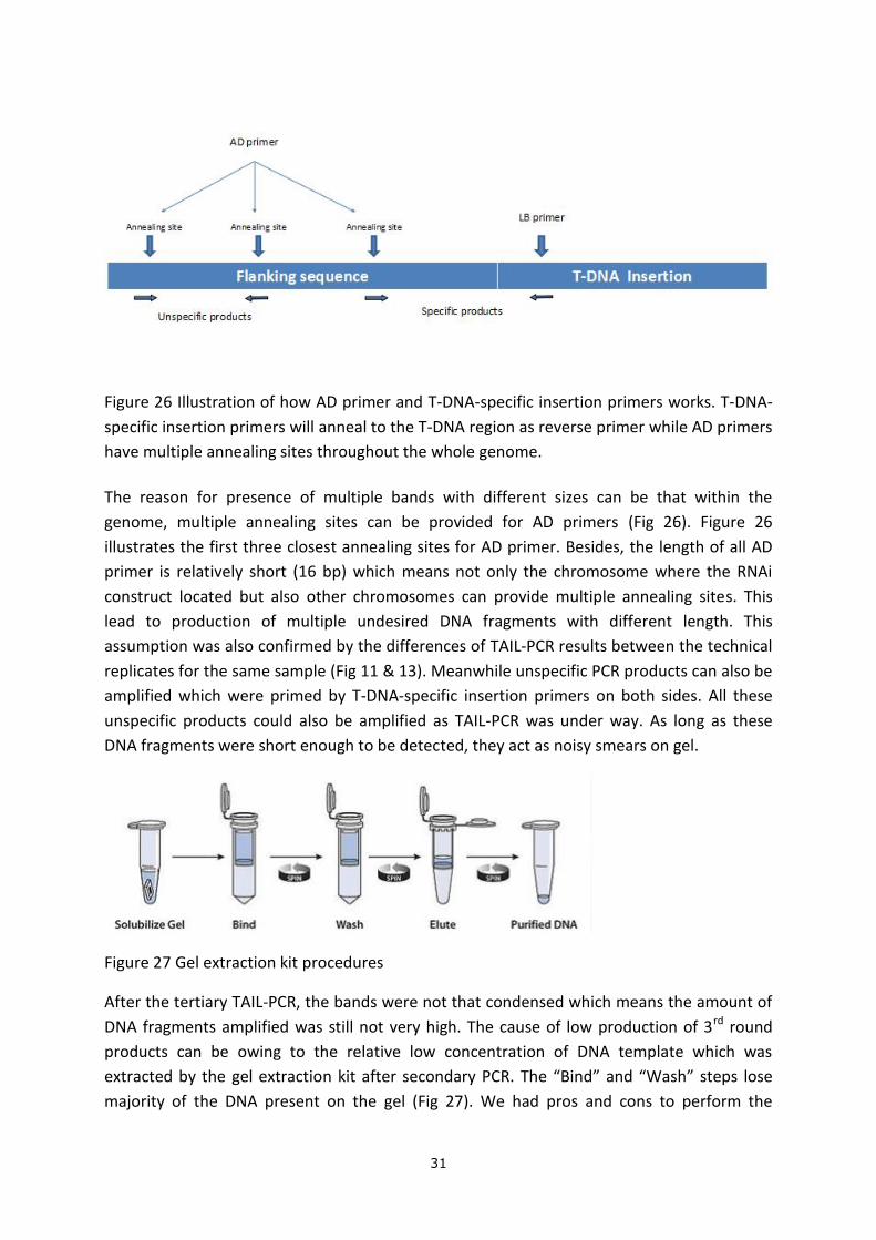
Figure 27 Gel extraction kit procedures

After the tertiary TAIL-PCR, the bands were not that condensed which means the amount of

DNA fragments amplified was still not very high. The cause of low production of 3rd round

products can be owing to the relative low concentration of DNA template which was

extracted by the gel extraction kit after secondary PCR. The “Bind” and “Wash” steps lose

majority of the DNA present on the gel (Fig 27). We had pros and cons to perform the

32

tertiary TAIL-PCR using purified DNA from the previous PCR. Noisy smears were much less

and we had more distinguishable bands. But the drawback of doing this was low DNA

concentration in the end which did not reach the basic requirements for sequencing.

Alternatively if dilution of the PCR products after 2nd round was directly used as template, a

larger amount of smears can be observed from the gel check and the desired bands were not

as much clear as the previous method. And the unspecific noisy DNA fragments would

influence the sequencing a lot. One possibility of pooling the advantages from both methods

together is to do the purification and increase the volume of DNA template for the 3rd round

TAIL-PCR.

Flanking sequence amplification by TAIL-PCR is relatively low cost and direct. Restriction

enzyme digestion of DNA template is skipped in this method. However, TAIL-PCR is a time-

consuming technique which consists of multiple rounds of amplification. Production of

unspecific PCR products can be a bottleneck due to the short AD primers and relatively low

annealing temperature.

In this report, QTL analysis was performed to investigate possible QTLs controlling SFW using

210 DH lines derived from the cross between 76135-Ge0 and 76135-T540. Several variables

“Grid”, “Block”, and “Ring” were included in the analysis for correction of environmental

effects. Differences can be observed between the QTL analysis with and without corrections

for these variables. If the corrections were not included, two QTLs with relatively large

effects can be identified on chromosome 2 and 4. With the correction for all the

environmental variables, a new QTL emerged on chromosome 1 and the effect of QTL on

chromosome 4 decreased. Environmental factors had a large influence on plant performance.

Extra variations were introduced into phenotypes. These undesired variations were not

caused by differences between genotypes which means it would lead to possible errors or

differences in QTL detection. For instance this analysis found large differences if QTL analysis

was done for two tables separately. QTL located on chromosome 2 had an impact on

biomass production consistently no longer if there is stress or not. Under normal condition,

the peak for the QTL on chromosome 4 was small and not statistically significant to be

considered as a real QTL. However, under stressed condition that QTL had a larger effect.

The QTL located on chromosome 1 was only present when plants were under normal

condition which means it is possible to miss QTLs controlling SFW when there is stress to the

plant.

33

4.2 Recommendations

Transgenic parental lines are necessary for generating achiasmatic hybrids. In my

experiments I selected very limited number of achiasmatic candidate lines and majority of

them turned out to be fertile in the end. The presence of the DMC1:RNAi construct was

confirmed by genotyping in Rijk Zwaan but the phenotypic observation did not match with

the genotypic data. The inserted construct cannot provide a long-lasting effect on down-

regulation of the DMC1 gene. If we want to further investigate DMC1 silencing effect, we can

take tissues samples from different parts of the plant and perform a Quantitative PCR (qPCR)

to quantify gene expression to see at which stages and which parts of the plant DMC1 is

stably and efficiently down regulated.

Flanking sequence adjacent to the DNA insertion can be amplified by TAIL-PCR. After

sequencing information is available, a BLAST can be done to identified the location of the

DMC1:RNAi construct. The main bottleneck during my thesis work can be that it is not handy

to perform the TAIL-PCR which consists of three rounds of single PCR. The main difference

between TAIL-PCR and a normal PCR is that only the reverse primers are specific and the

forward primers are random which cause uncertainty of where these primers will anneal to

and lead to multiple PCR products. In my thesis experiments, this technique was poorly

efficient and amplified high amount of unspecific products. And even electrophoresis bands

were visible after 3rd round PCR, the quality and quantity was not sufficient enough for

downstream sequencing. We expect to have an ideal result which we got clear bands after

the secondary TAIL-PCR. Consequently, we are able to send the samples after secondary PCR

and use the DMC-3 primer (which represent for the 3rd exon in DMC1 gene) for sequencing.

However due to different genomic landscape of different Arabidopsis ascensions, we do

expect that random distribution of these annealing sites for AD primers will lead to

complexity in PCR products. The construct might integrated into a region which is not close

enough to the AD primer annealing sites for instance not on the same chromosome. It would

be hard to amplify short and specific flanking sequence. Meanwhile the complexity differs a

lot between accessions. However, we are able to get bands after tertiary TAIL-PCR despite

the fact that the concentration was still relatively low. It is possible to amplify more PCR

products by increasing number of cycles in the TAIL-PCR program. Amount of reagents like

dNTP and DNA polymerase also need to be increased. However, which round needs more

cycles still needs to be investigated. For instance if we get clear but weak bands after the

secondary TAIL-PCR, more cycles in the 3rd round can be a solution to increase the amount of

PCR products.

In addition, a check for each AD primer can be done in advance. Combination of each AD

primer instead of AD pool with an insertion-specific primer can be used to perform the PCR.

However, single round of the primary and secondary TAIL-PCR takes more than 4 hours to

perform which means it will be time-consuming to use separate AD primer. One possibility is

to use single AD primers instead of AD pool only in tertiary TAIL-PCR. In this case one

34

complete TAIL-PCR (consists of one round of primary, one round of secondary and three

rounds of tertiary TAIL-PCR) will take about 12 hours.

Based on the quality and quantity of amplified specific PCR products, an indication of

feasibility of each AD primer can be given to have a better quality of PCR products.

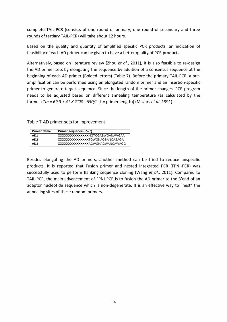
Alternatively, based on literature review (Zhou et al., 2011), it is also feasible to re-design

the AD primer sets by elongating the sequence by addition of a consensus sequence at the

beginning of each AD primer (Bolded letters) (Table 7). Before the primary TAIL-PCR, a pre-

amplification can be performed using an elongated random primer and an insertion-specific

primer to generate target sequence. Since the length of the primer changes, PCR program

needs to be adjusted based on different annealing temperature (as calculated by the

formula Tm = 69.3 + 41 X GC% - 650/L (L = primer length)) (Mazars et al. 1991).

Table 7 AD primer sets for improvement

Primer Name Primer sequence (5'–3')

AD1 XXXXXXXXXXXXXXXNGTCGASWGANAWGAA

AD2 XXXXXXXXXXXXXXXTGWGNAGSANCASAGA

AD3 XXXXXXXXXXXXXXXAGWGNAGWANCAWAGG

Besides elongating the AD primers, another method can be tried to reduce unspecific

products. It is reported that Fusion primer and nested integrated PCR (FPNI-PCR) was

successfully used to perform flanking sequence cloning (Wang et al., 2011). Compared to

TAIL-PCR, the main advancement of FPNI-PCR is to fusion the AD primer to the 3’end of an

adaptor nucleotide sequence which is non-degenerate. It is an effective way to “nest” the

annealing sites of these random primers.

35

5 Acknowledgments

At First, I would like thank my adviser Prof. Joost Keurentjes for his support of my thesis

work. I would also like to thank my supervisor Cris Wijnen and José van de Belt for their

insightful and inspirational help during my work in the lab and greenhouse. Lastly, I would

like to express my gratitude to all the fellow labmates in the Genetics Group.

36

6 Bibliographies 1. Akbudak, M. A., Nicholson, S. J., & Srivastava, V. (2013). Suppression of Arabidopsis

genes by terminator-less transgene constructs. Plant Biotechnology Reports, 7(4), 415-

424. doi: 10.1007/s11816-013-0278-z

2. Bhaskar, P. B., Venkateshwaran, M., Wu, L., Ané, J-M., & Jiang, J. (2009). Agrobacterium-

Mediated Transient Gene Expression and Silencing: A Rapid Tool for Functional Gene

Assay in Potato. PLoS ONE, 4(6): e5812. doi:10.1371/journal.pone.0005812

3. Bilichak, A., Yao, Y., & Kovalchuk, I. (2014). Transient down-regulation of the RNA

silencing machinery increases efficiency of Agrobacterium-mediated transformation of

Arabidopsis. Plant Biotechnol J. doi: 10.1111/pbi.12165

4. Couteau, F. (1999). Random chromosome Segregation without Meiotic Arrest in Both

Male and Female Meiocytes of a dmc1 Mutant of Arabidopsis. The Plant Cell Online,

11(9), 1623-1634. doi: 10.1105/tpc.11.9.1623

5. Dirks, R., van Dun, K., de Snoo, C. B., van den Berg, M., Lelivelt, C. L., Voermans, W., . . .

Wijnker, E. (2009). Reverse breeding: a novel breeding approach based on engineered

meiosis. Plant Biotechnol J, 7(9), 837-845. doi: 10.1111/j.1467-7652.2009.00450.x

6. Dunwell, J. M., (2010). Haploids in flowering plants: origins and exploitation. Plant

Biotechnol J, 8(4), 377-424. doi: 10.1111/j.1467-7652.2009.00498.x

7. El-Lithy, M. E., Clerkx, E. J., Ruys, G. J., Koornneef, M., & Vreugdenhil, D. (2004).

Quantitative trait locus analysis of growth-related traits in a new Arabidopsis

recombinant inbred population. Plant Physiol, 135(1), 444-458. doi:

10.1104/pp.103.036822

8. El-Soda, M., Boer, M. P., Bagheri, H., Hanhart, C. J., Koornneef, M., & Aarts, M. G. (2014).

Genotype-environment interactions affecting preflowering physiological and

morphological traits of Brassica rapa grown in two watering regimes. J Exp Bot, 65(2),

697-708. doi: 10.1093/jxb/ert434

9. Gao, X., Britt, R. C., Jr., Shan, L., & He, P. (2011). Agrobacterium-mediated virus-induced

gene silencing assay in cotton. J Vis Exp(54). doi: 10.3791/2938

10. Gelvin, S. B. (2003). Agrobacterium-Mediated Plant Transformation: the Biology behind

the "Gene-Jockeying" Tool. Microbiology and Molecular Biology Reviews, 67(1), 16-37.

doi: 10.1128/mmbr.67.1.16-37.2003

11. Gobron, N., Waszczak, C., Simon, M., Hiard, S., Boivin, S., Charif, D., Ducamp, A., Wenes,

E., Budar, F. (2013). A cryptic cytoplasmic male sterility unveils a possible gynodioecious

past for Arabidopsis thaliana. PLoS ONE, 8:e6245.

37

12. Henry, I. M., Dilkes, B. P., Miller, E. S., Burkart-Waco, D., & Comai, L. (2010). Phenotypic

consequences of aneuploidy in Arabidopsis thaliana. Genetics, 186(4), 1231-1245. doi:

10.1534/genetics.110.121079

13. Harrison, S. J., Mott, E. K., Parsley, K., Aspinall, S., Gray, J. C., & Cottage, A. (2006). A

rapid and robust method of identifying transformed Arabidopsis thaliana seedlings

following floral dip transformation. Plant Methods, 2(19). doi: 10.1186/1746-4811-2-19

14. Jia, G., Chen, P., Qin, G., Bai, G., Wang, X., Wang, S., . . . Liu, D. (2006). QTLs for Fusarium

head blight response in a wheat DH population of Wangshuibai/Alondra‘s’. Euphytica,

146(3), 183-191. doi: 10.1007/s10681-005-9001-7

15. Kasajima, I.(2004). A protocol for rapid DNA extraction from Arabidopsis thaliana for

PCR analysis. Plant Mol. Biol. Rep. 22, 49–52.

16. Kiani, B. H., Suberu, J., Barker, G. C., & Mirza, B. (2014). Development of efficient

miniprep transformation methods for Artemisia annua using Agrobacterium

tumefaciens and Agrobacterium rhizogenes. In Vitro Cellular & Developmental Biology -

Plant.

17. Koumproglou, R., Wilkes, TM., Townson, P., Wang, XY., Beynon, J., Pooni, HS., Newbury,

HJ., Kearsey, MJ. (2002) STAIRS: a new genetic resource for functional genomic studies

of Arabidopsis. Plant J, 31:355-364.

18. Li, J. Z., Huang, X. Q., Heinrichs, F., Ganal, M. W., & Roder, M. S. (2005). Analysis of QTLs

for yield, yield components, and malting quality in a BC3-DH population of spring barley.

Theor Appl Genet, 110(2), 356-363. doi: 10.1007/s00122-004-1847-x

19. Link, W., & Melchinger, A.E. (1995). An approach to the genetic improvement of clonal

cultivars via backcrosing. Crop Sci. 35, 931

20. Liu, Y. G., & Chen, Y. (2007). High-efficiency thermal asymmetric interlaced PCR for

amplification of unknown flanking sequences. BioTechniques, 43(5), 649-656.

21. Liu, Y. G., Mitsukawa, N., Oosumi, T., & Whittier, R. F. (1995). Efficient isolation and

mapping of Arabidopsis thaliana T-DNA insert junctions by thermal asymmetric

interlaced PCR. Plant Journal, 8(3), 457-463.

22. Mazars GR, Moyret C, Jeanteur P, Theillet CG (1991) Directing sequencing by thermal

asymmetric PCR. Nucleic Acids Res 19:4783

23. Meyer, R. C., Kusterer, B., Lisec, J., Steinfath, M., Becher, M., Scharr, H., . . . Altmann, T.

(2010). QTL analysis of early stage heterosis for biomass in Arabidopsis. Theor Appl

Genet, 120(2), 227-237. doi: 10.1007/s00122-009-1074-6

38

24. Nadeau, JH., Singer, JB., Matin, A., Lander, ES. (2000): Analysing complex genetic traits

with chromosome substitution strains. Nat Genet, 24:221-225.

25. Pang, J., Zhu, Y., Li, Q., Liu, J., Tian, Y., Liu, Y., & Wu, J. (2013). Development of

Agrobacterium-mediated virus-induced gene silencing and performance evaluation of

four marker genes in Gossypium barbadense. PLoS One, 8(9), e73211. doi:

10.1371/journal.pone.0073211

26. Pillai, M. M., Venkataraman, G. M., Kosak, S., & Torok-Storb, B. (2008). Integration site

analysis in transgenic mice by thermal asymmetric interlaced (TAIL)-PCR: segregating

multiple-integrant founder lines and determining zygosity. Transgenic Res, 17(4), 749-

754. doi: 10.1007/s11248-007-9161-4

27. Qiu, B., Zeng, F., Xue, D., Zhou, W., Ali, S., & Zhang, G. (2011). QTL mapping for

chromosomeomium-induced growth and zinc, and chromosomeomium distribution in

seedlings of a rice DH population. Euphytica, 181(3), 429-439. doi: 10.1007/s10681-011-

0480-4

28. Ravi, M., & Chan, S. W. (2010). Haploid plants produced by centromere-mediated

genome elimination. Nature, 464(7288), 615-618. doi: 10.1038/nature08842

29. Saha, P., Datta, K., Majumder, S., Sarkar, C., China, S. P., Sarkar, S. N., . . . Datta, S. K.

(2014). Agrobacterium mediated genetic transformation of commercial jute cultivar

Corchorus capsularis cv. JRC 321 using shoot tip explants. Plant Cell, Tissue and Organ

Culture (PCTOC).

30. Sanei, M., Pickering, R., Kumke, K., Nasuda, S., & Houben, A. (2011). Loss of centromeric

histone H3 (cenH3) from centromeres precedes uniparental chromosome elimination in

interspecific barley hybrids. Proc Natl Acad Sci U S A, 108(33), E498-505. doi:

10.1073/pnas.1103190108

31. Seymour, D. K., Filiault, D. L., Henry, I. M., Monson-Miller, J., Ravi, M., Pang, A., . . .

Maloof, J. N. (2012). Rapid creation of Arabidopsis doubled haploid lines for quantitative

trait locus mapping. Proc Natl Acad Sci U S A, 109(11), 4227-4232. doi:

10.1073/pnas.1117277109

32. Shamloul, M., Trusa, J., Mett, V., & Yusibov, V. (2014). Optimization and utilization of

Agrobacterium-mediated transient protein production in Nicotiana. Journal of Visualized

Experiments(86).

33. Singer, J. B., Hill, A. E., Burrage, L. C., Olszens, K. R., Song, J., Justice, M., . . . Nadeau, J. H.

(2004). Genetic dissection of complex traits with chromosome substitution strains of

mice. Science, 304(5669), 445-448. doi: 10.1126/science.1093139

39

34. Singer, T., & Burke, E. (2003). High throughput TAIL-PCR as a Tool to identify DNA

flanking Insertions. Plan Func Geno: Meth Prot, 241-270.

35. Tian, R., Jiang, G.-H., Shen, L.-H., Wang, L.-Q., & He, Y.-Q. (2005). Mapping quantitative

trait loci underlying the cooking and eating quality of rice using a DH population.

Molecular Breeding, 15(2), 117-124. doi: 10.1007/s11032-004-3270-z

36. Wang, G. H., Xiao, J. H., Xiong, T. L., Li, Z., Murphy, R. W., & Huanga, D. W. (2013). High-

efficiency thermal asymmetric interlaced PCR (hiTAIL-PCR) for determination of a highly

degenerated prophage WO Genome in a Wolbachia strain infecting a fig wasp species.

Applied and Environmental Microbiology, 79(23), 7476-7481.

37. Wang, Z., Ye, S., Li, J., Zheng, B., Bao, M., & Ning, G. (2011). Fusion primer and nested

integrated PCR (FPNI-PCR): a new high-efficiency strategy for rapid chromosome walking

or flanking sequence cloning. BMC Biotechnol, 11, 109. doi: 10.1186/1472-6750-11-109

38. Wijnen, C. L., & Keurentjes, J. J. (2014). Genetic resources for quantitative trait analysis:

novelty and efficiency in design from an Arabidopsis perspective. Curr Opin Plant Biol,

18C, 103-109. doi: 10.1016/j.pbi.2014.02.011

39. Wijnker, E., Deurhof, L., van de Belt, J., de Snoo, C. B., Blankestijn, H., Becker, F., . . .

Keurentjes, J. J. (2014). Hybrid recreation by reverse breeding in Arabidopsis thaliana.

Nat Protoc, 9(4), 761-772. doi: 10.1038/nprot.2014.049

40. Wijnker, E., van Dun, K., de Snoo, C. B., Lelivelt, C. L., Keurentjes, J. J., Naharudin, N.

S., . . . Dirks, R. (2012). Reverse breeding in Arabidopsis thaliana generates homozygous

parental lines from a heterozygous plant. Nat Genet, 44(4), 467-470. doi:

10.1038/ng.2203

41. Wu, E., Lenderts, B., Glassman, K., Berezowska-Kaniewska, M., Christensen, H., Asmus,

T., . . . Zhao, Z. Y. (2014). Optimized Agrobacterium-mediated sorghum transformation

protocol and molecular data of transgenic sorghum plants. In Vitro Cellular and

Developmental Biology - Plant, 50(1), 9-18.

42. Yin, X., Yi, B., Chen, W., Zhang, W., Tu, J., Fernando, W. G. D., & Fu, T. (2009). Mapping of

QTLs detected in a Brassica napus DH population for resistance to Sclerotinia

sclerotiorum in multiple environments. Euphytica, 173(1), 25-35. doi: 10.1007/s10681-

009-0095-1

43. Zhang, H., Ransom, C., Ludwig, P., & Van Nocker, S. (2003). Genetic analysis of early

flowering mutants in Arabidopsis defines a class of pleiotropic developmental regulator

required for expression of the flowering-time switch FLOWERING LOCUS C. Genetics,

164(1), 347-358.

40

44. Zhou, Z., Ma, H., Qu, L., Xie, F., Ma, Q., & Ren, Z. (2012). Establishment of an improved

high-efficiency thermal asymmetric interlaced PCR for identification of genomic

integration sites mediated by phiC31 integrase. World J Microbiol Biotechnol, 28(3),

1295-1299. doi: 10.1007/s11274-011-0877-1

41

Appendices

Appendix 1 TAIL-PCR & Gel-electrophoresis protocol

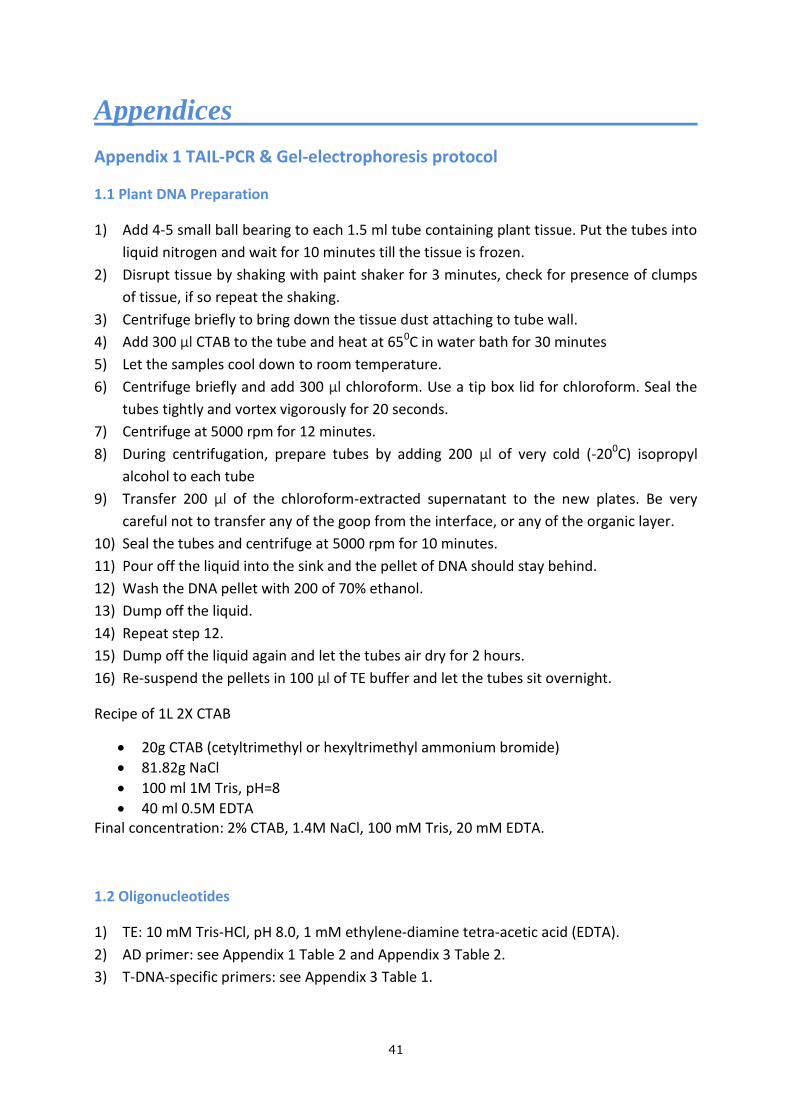
1.1 Plant DNA Preparation

1) Add 4-5 small ball bearing to each 1.5 ml tube containing plant tissue. Put the tubes into

liquid nitrogen and wait for 10 minutes till the tissue is frozen.

2) Disrupt tissue by shaking with paint shaker for 3 minutes, check for presence of clumps

of tissue, if so repeat the shaking.

3) Centrifuge briefly to bring down the tissue dust attaching to tube wall.

4) Add 300 µl CTAB to the tube and heat at 650C in water bath for 30 minutes

5) Let the samples cool down to room temperature.

6) Centrifuge briefly and add 300 µl chloroform. Use a tip box lid for chloroform. Seal the

tubes tightly and vortex vigorously for 20 seconds.

7) Centrifuge at 5000 rpm for 12 minutes.

8) During centrifugation, prepare tubes by adding 200 µl of very cold (-200C) isopropyl

alcohol to each tube

9) Transfer 200 µl of the chloroform-extracted supernatant to the new plates. Be very

careful not to transfer any of the goop from the interface, or any of the organic layer.

10) Seal the tubes and centrifuge at 5000 rpm for 10 minutes.

11) Pour off the liquid into the sink and the pellet of DNA should stay behind.

12) Wash the DNA pellet with 200 of 70% ethanol.

13) Dump off the liquid.

14) Repeat step 12.

15) Dump off the liquid again and let the tubes air dry for 2 hours.

16) Re-suspend the pellets in 100 µl of TE buffer and let the tubes sit overnight.

Recipe of 1L 2X CTAB

20g CTAB (cetyltrimethyl or hexyltrimethyl ammonium bromide)

81.82g NaCl

100 ml 1M Tris, pH=8

40 ml 0.5M EDTA Final concentration: 2% CTAB, 1.4M NaCl, 100 mM Tris, 20 mM EDTA.

1.2 Oligonucleotides

1) TE: 10 mM Tris-HCl, pH 8.0, 1 mM ethylene-diamine tetra-acetic acid (EDTA).

2) AD primer: see Appendix 1 Table 2 and Appendix 3 Table 2.

3) T-DNA-specific primers: see Appendix 3 Table 1.

42

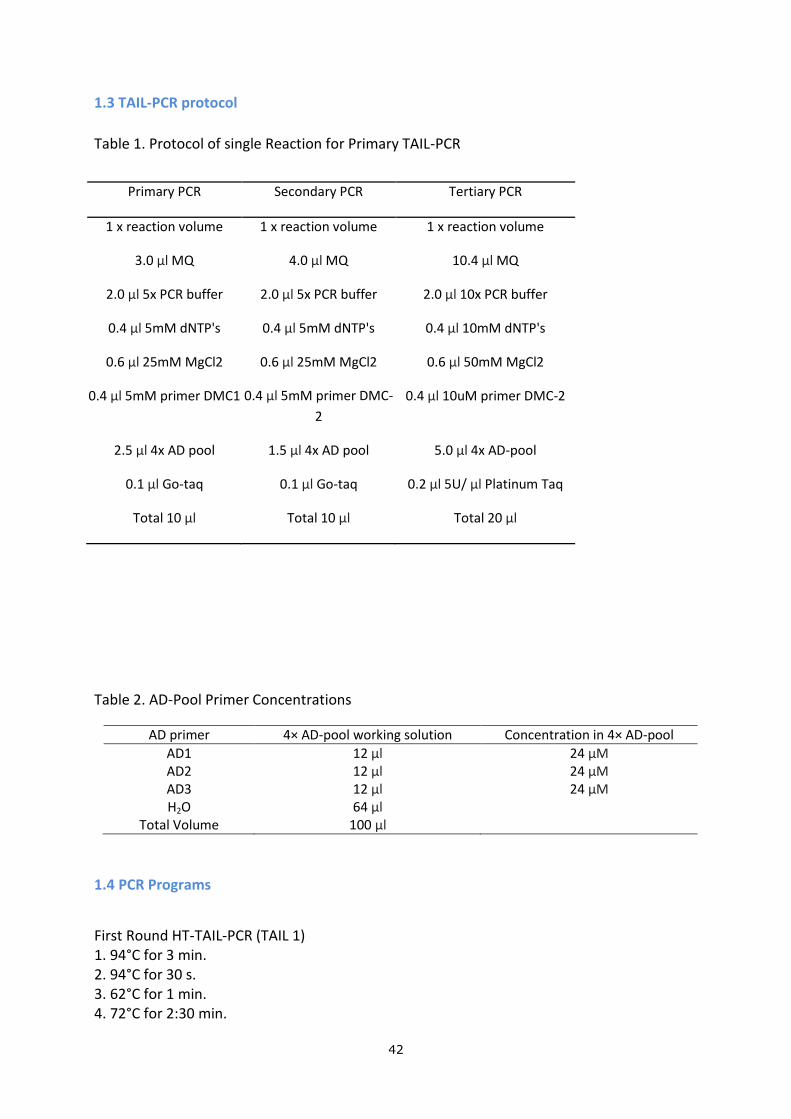
1.3 TAIL-PCR protocol

Table 1. Protocol of single Reaction for Primary TAIL-PCR

Primary PCR Secondary PCR Tertiary PCR

1 x reaction volume 1 x reaction volume 1 x reaction volume

3.0 µl MQ 4.0 µl MQ 10.4 µl MQ

2.0 µl 5x PCR buffer 2.0 µl 5x PCR buffer 2.0 µl 10x PCR buffer

0.4 µl 5mM dNTP's 0.4 µl 5mM dNTP's 0.4 µl 10mM dNTP's

0.6 µl 25mM MgCl2 0.6 µl 25mM MgCl2 0.6 µl 50mM MgCl2

0.4 µl 5mM primer DMC1 0.4 µl 5mM primer DMC-

2

0.4 µl 10uM primer DMC-2

2.5 µl 4x AD pool 1.5 µl 4x AD pool 5.0 µl 4x AD-pool

0.1 µl Go-taq 0.1 µl Go-taq 0.2 µl 5U/ µl Platinum Taq

Total 10 µl Total 10 µl Total 20 µl

Table 2. AD-Pool Primer Concentrations

AD primer 4× AD-pool working solution Concentration in 4× AD-pool

AD1 12 µl 24 µM AD2 12 µl 24 µM AD3 12 µl 24 µM H2O 64 µl

Total Volume 100 µl

1.4 PCR Programs

First Round HT-TAIL-PCR (TAIL 1) 1. 94°C for 3 min. 2. 94°C for 30 s. 3. 62°C for 1 min. 4. 72°C for 2:30 min.

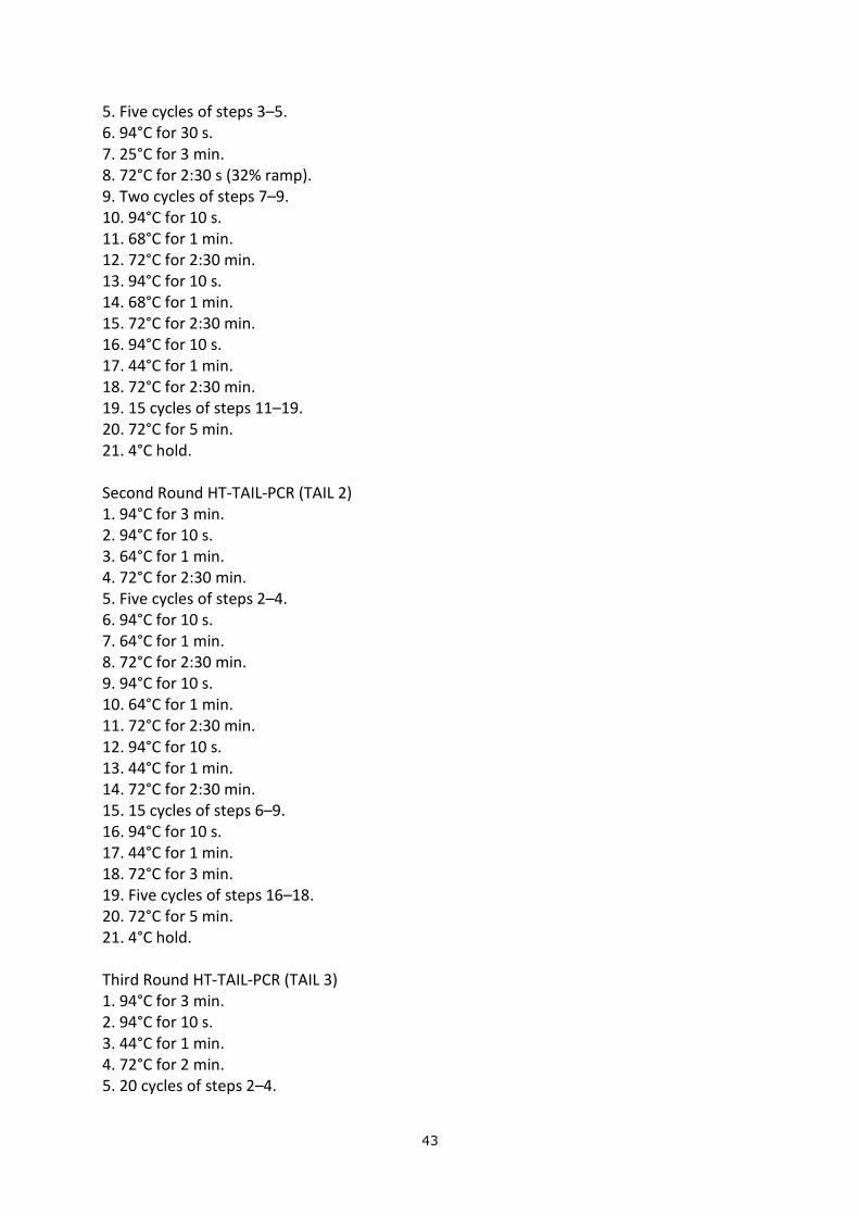
43

5. Five cycles of steps 3–5. 6. 94°C for 30 s. 7. 25°C for 3 min. 8. 72°C for 2:30 s (32% ramp). 9. Two cycles of steps 7–9. 10. 94°C for 10 s. 11. 68°C for 1 min. 12. 72°C for 2:30 min. 13. 94°C for 10 s. 14. 68°C for 1 min. 15. 72°C for 2:30 min. 16. 94°C for 10 s. 17. 44°C for 1 min. 18. 72°C for 2:30 min. 19. 15 cycles of steps 11–19. 20. 72°C for 5 min. 21. 4°C hold. Second Round HT-TAIL-PCR (TAIL 2) 1. 94°C for 3 min. 2. 94°C for 10 s. 3. 64°C for 1 min. 4. 72°C for 2:30 min. 5. Five cycles of steps 2–4. 6. 94°C for 10 s. 7. 64°C for 1 min. 8. 72°C for 2:30 min. 9. 94°C for 10 s. 10. 64°C for 1 min. 11. 72°C for 2:30 min. 12. 94°C for 10 s. 13. 44°C for 1 min. 14. 72°C for 2:30 min. 15. 15 cycles of steps 6–9. 16. 94°C for 10 s. 17. 44°C for 1 min. 18. 72°C for 3 min. 19. Five cycles of steps 16–18. 20. 72°C for 5 min. 21. 4°C hold. Third Round HT-TAIL-PCR (TAIL 3) 1. 94°C for 3 min. 2. 94°C for 10 s. 3. 44°C for 1 min. 4. 72°C for 2 min. 5. 20 cycles of steps 2–4.

44

6. 72°C for 5 min. 7. 4°C forever.

1.5 Gel-electrophoresis protocol

Material needed: Agarose, TBE Buffer, 6X PCR sample loading buffer, DNA ladder,

Electrophoresis chamber, Gel casting tray and combs, electric power, GelRed stain, Staining

tray, Gloves, Pipette and tips.

Recipe of 1L 5X TBE Buffer stock solution

54 g of Tris base

27.5 g of boric acid

20 ml of 0.5 M EDTA (pH 8.0)

1.6 Gel extraction by QIAquick Gel Extraction Kit

1) Excise the DNA fragment from the agarose gel with a clean, sharp scalpel.

2) Weigh the gel slice in a colorless tube( Weigh the tube first to get the weight of the gel

slice). Add 3 volumes of Buffer QG to 1 volume of gel (100 mg for 100 µl). For slice larger

than 400 mg, use a larger tube.

3) Incubate at 500C until the gel slice is completely dissolved, vortex the tube to help

dissolving.

4) After dissolve the gel slice completely, check that the color of the mixture is yellow

(similar to Buffer QG without dissolved agarose), if not, adjust the color by adding 10 µl

of 3M sodium acetate, pH 5.0, and mix, the color of the mixture will turn yellow.

5) Add 1 gel volume of isopropanol to the sample and mix.

6) Place a QIAquick spin column in a provided 2 ml collection tube.

7) To bind DNA, apply the sample to the QIAquick column and centrifuge for 1 min, if the

sample volume is larger than 800 µl which is the maximum volume of the column

reservoir, load the samples again and repeat the procedure.

8) Discard the flow-through and place QIAquick column back in the sample collection tube.

9) If the DNA will be subsequently be used for sequencing, add 500 µl Buffer QG to the

QIAquick column and centrifuge for 1 min to remove all traces of agarose.

10) To wash, add 0.75 ml of Buffer PE to QIAquick column and centrifuge for 1 min.

11) Discard the flow through and centrifuge the QIAquick column for additional 1 min

at >13,000 rpm.

12) Place QIAquick column into a clean 1.5 ml micro-centrifuge tube.

13) Add 50 µl of Buffer EB (10 mM Tris-Cl, pH 8.5) or H2O to the center of the QIAquick

membrane and centrifuge the column for 1 min at maximum speed. To increase DNA

concentration, add 30 µl Buffer EB instead and let the column stand for 3 minutes, and

then centrifuge for 1 min.

45

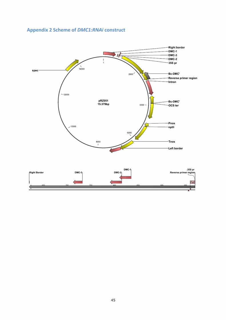
Appendix 2 Scheme of DMC1:RNAi construct

46

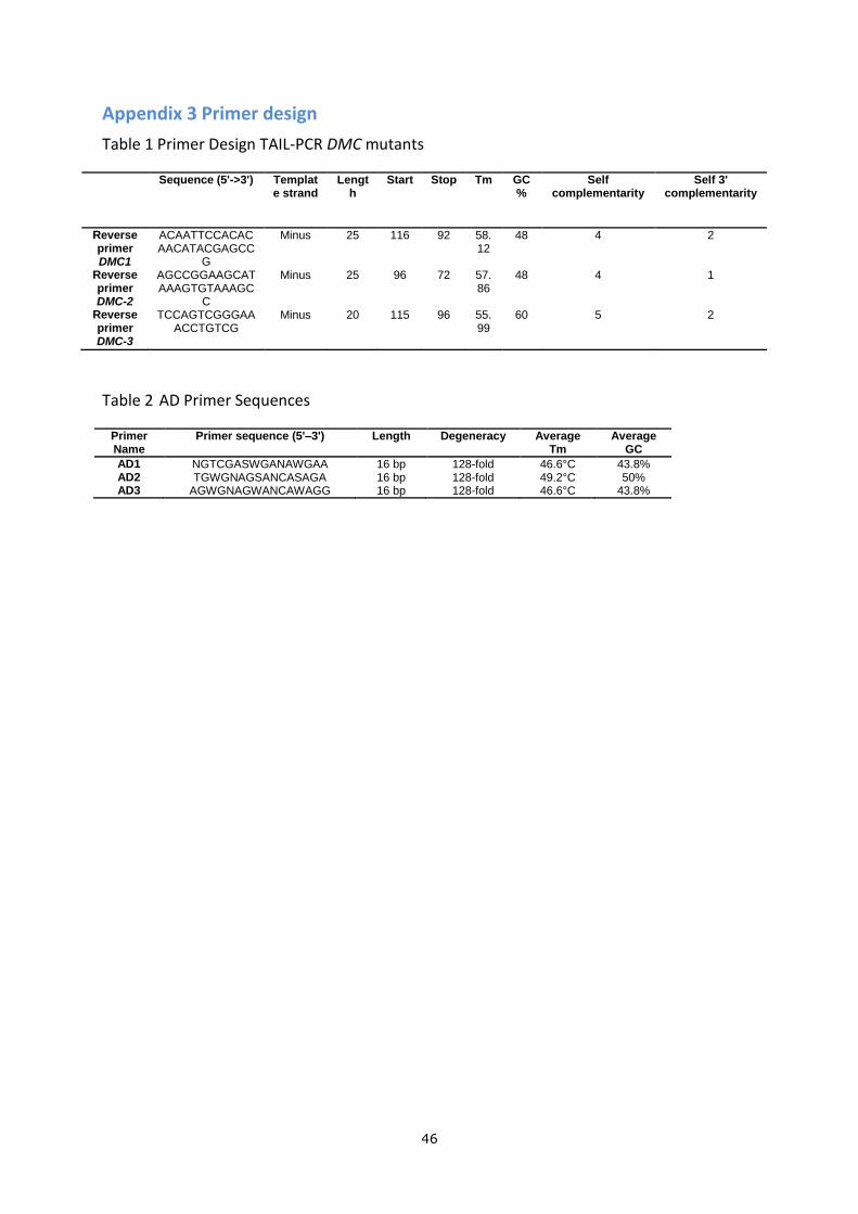
Appendix 3 Primer design

Table 1 Primer Design TAIL-PCR DMC mutants

Sequence (5'->3') Template strand

Length

Start Stop Tm GC%

Self complementarity

Self 3' complementarity

Reverse primer DMC1

ACAATTCCACACAACATACGAGCC

G

Minus 25 116 92 58.12

48 4 2

Reverse primer DMC-2

AGCCGGAAGCATAAAGTGTAAAGC

C

Minus 25 96 72 57.86

48 4 1

Reverse primer DMC-3

TCCAGTCGGGAAACCTGTCG

Minus 20 115 96 55.99

60 5 2

Table 2 AD Primer Sequences

Primer Name

Primer sequence (5'–3') Length Degeneracy Average Tm

Average GC

AD1 NGTCGASWGANAWGAA 16 bp 128-fold 46.6°C 43.8% AD2 TGWGNAGSANCASAGA 16 bp 128-fold 49.2°C 50% AD3 AGWGNAGWANCAWAGG 16 bp 128-fold 46.6°C 43.8%