u0c(5\ - wur edepot
TRANSCRIPT

LOAD-BEARING PROCESSES IN
AGRICULTURAL WHEEL-SOIL SYSTEMS
0000 0248 9975
OiYiVAKSEH
EüttJOTÏIMI^v ï:ANDr-QTJ\Yu:sr>;
Y'.STTEIT
U0C(5\
Promotor: ir. H. Kuipers hoogleraar in de grondbewerking en de gronddynamica
Co-promotor: Dr. ir. A.J. Kooien universitair hoofddocent in de gronddynamica
^ O ^ I J C ^ W ^ Z ,
F.G.J. Tijink
LOAD-BEARING PROCESSES IN AGRICULTURAL WHEEL-SOIL SYSTEMS
Proefschrift
ter verkrijging van de graad van doctor in de landbouwwetenschappen, op gezag van de rector magnificus, Dr. C.C. Oosterlee, in het openbaar te verdedigen op woensdag 13 januari 1988 des namiddags te vier uur in de aula van de Landbouwuniversiteit te Wageningen
k y X .

ABSTRACT
Tljink, F.G.J. (1988). Load-Bearing Processes in Agricultural Wheel-So il Systems. Doctoral thesis, Agricultural University Wageningen, The Netherlands, 173 p., 98 figs, 25 tables, 203 refs, English and Dutch summaries.
In soil dynamics we distinguish between loosening and load-bearing processes. Load-bearing processes which can occur under agricultural rollers, wheels, and tyres are dealt with in this dIssertat ion. We classify rollers, wheels, and tyres and treat some general aspects of these devices. Fundamentals of load-bearing processes, I.e. kinematic, dynamic, and soil physical aspects are discussed a I so. Not only soil characteristics concerning load-bearing processes are dealt with but also the suitability of these characteristics for use In prediction methods. Special attention has been paid to predicting some process aspects of a towed tyre under different soil conditions and In different soil types. Under laboratory conditions the use of characterizing processes (cone, vane, and falling weight) and empirical prediction methods resulted in accurate predictions of rolling resistance, rut depth, and compaction caused by a towed tyre.
Additional keywords: load-bearing processes, soil dynamics, tyre performance, soil compaction, soil mechanical properties, soil characteristics, prediction methods.
ISBN 90-9001968-5 Printed by: Krips Repro, Meppel
Copyright F.G.J. Tijink, 1988.
No part of this book (with the exception of the abstract on this page) may be reproduced or published In any form and by any means without permission from the author.
JMÙ'?7.0\ ( \\^'
STELLINGEN
1 Het nauwkeurig voorspellen van roIweerstand, dichting bij het berijden van homogene grond emp i r i sehe voorspeI IIngsmethoden.
Insporing en i s mogel i jk
vermet
D i t proef sehr I ft
Inspor i ng I s nlet a Itijd een geschikte maat voor verdichting. Dlt proefsehr I ft
Voor het weergeven van de karakteristieken dient een "standaard" ontwikkeld te worden.
van Iandbouwbanden
Dit proefschrift
De benutting van het voor ploegwerk beschikbare kan nog verbeterd worden.
trekkervermogen
Dlt proefsehr I ft
Indien het gewenst is bovenover te rijden bij de hoofdgrond-bewerking dienen er grondbewerkIngswerktuI gen ter beschikking te komen die een kerende werking hebben en door de aftakas worden aangedreven.
De specifieke ploegweerstand neemt af bij een toename van de werkbreedte van een ploeg.
Voor ploegwerkzaamheden Is een slipregeling een goede aanvuI I Inç op de weerstandsregeling.
Het gebruik van een schijfkouter bij het voorste ploeglichaam vereist een langer ploegframe en een grotere hefkracht.
Een wentel ploeg, gebouwd volgens het bouwdoossysteem, vereist een wentel systeem dat het wentelen over 180 graden kan ondersteunen.

10 Bij onderzoek naar verdichting van bewerkte ondergrond behoort de invloed van de massa van de bouwvoor niet verwaarloosd te worden.
11 Het gebruik van gepllleerd zaaI zaad komt de zaadverdeling ten goede bij het zaaien van bleten.
12 Bij het ontwerpen van frames voor IandbouwwerktuI gen met een lange gebruiksduur, dient meer aandacht geschonken te worden aan het optreden van vermoeidheIdsverschiJnseI en.
13 Het verminderen van de hoeveelheid spuitvloeI stof in de gewasbescherming dient samen te gaan met een beter gebruik van persoon Ii Jke bescherm IngsmIddeI en.
14 Conus, shear vane en valgewlcht zijn bruikbare hulpmiddelen bij het karakteriseren van mechanische eigenschappen van grond.
Di t proefsehr i ft
15 Bij het ontwikkelen van een bewerkbaarheidstest verdient het aanbeveling het onderzoek te concentreren op methoden, die gebaseerd zijn op verkruImeIIng.
D i t proefsehr i ft
16 De invloed van de gelaagde opbouw van grond (toplaag, bouwvoor, ploegzool, ondergrond) op afsteunende processen Is nog onvoldoende onderzocht.
Dit proefschrift
F.G.J. Ti J ink Load-bearing processes in agricultural wheel-so I I systems Wageningen, 13 januari 1988

voor Agnes
VOORWOORD
Dit kleine stukje gebruik ik graag om iedereen te bedanken die een bijdrage heeft geleverd aan dit proefschrift.
Hiervoor ben ik allereerst dank verschuldigd aan mijn promotor prof. ir. H. Kuipers, die dit onderzoek mogelijk heeft gemaakt en die mij enthousiast heeft gemaakt voor dit vakgebied. Zijn warme belangstelling heeft mij erg geholpen bij het voltooien van dit proef sehr I ft. Mijn co-promotor Dr. ir. A.J. Kooien wil ik vooral danken voor de begeleiding van het onderzoek en de ondersteuning bij enkele met deze dissertatie samenhangende publicaties.
De heren B.W. Peelen en A. Boers dank Ik voor hun hulp bij het verrichten van metingen.
De volgende studenten ben ik erkentelijk voor hun medewerking aan het promotie-onderzoek: Wim den Haan, Simon Hofstra, Harry Swinkels, Gertjan van Dijk, Jan Broekhuizen en Pleter Vaandrager.
Voor het tot stand komen van het manuscript wil ik graag danken: de heer B.W. Peelen voor het met zorg uitvoeren van al het tekenwerk en Mevr. drs. A.S.R. Riepma voor het met grote inzet corrigeren van de Engelse tekst.
De Stichting "Fonds Landbouw Export Bureau 1916/1918" en de Landbouwuniversiteit wil ik dank zeggen voor het beschikbaar stellen van subsidies ter bijdrage In de kosten verbonden aan dit proef sehr I ft.
Dordrecht, 6 Juli 1987

CONTENTS
CHAPTER 1 INTRODUCTION 13
CHAPTER 2 AGRICULTURAL ROLLERS, WHEELS, AND TYRES 15
2.1. 2.1, 2.1. 2.1. 2.1. 2.2, 2.3, 2.3,
ROLLERS 15 Roller-packers 15
1. Single roller-packers 15 2. Composed roller-packers 16
Rol ler-harrows 17 WHEELS 17 TYRES 18
Hlghl ights In tyre development 18 3.2. Tyre construction 18 3.3. Tyre size specification 20 3.4. Tyres used in agriculture 22
1. Tyres for driven wheels 23 2. Tyres for undrlven steered wheels . . . . 24 3. Tyres for garden tractors 24 4. Implement tyres 24 5. Farm ut I I I ty tyres 25 6. Sem I-tyres 25 7. Other tyres used In agriculture 25
1
CHAPTER 3 KINEMATIC ASPECTS OF LOAD-BEARING PROCESSES 27
1 . 1 . 1
3 3 3 3 3 3.1.2
1.1.1. 1.1.2. 1.1.3.
3.1.2.1,
3.1.2.2.
3.2.
3.2.1. 3.2.1.1.
3.2.1.2. 3.2.1.3.
STATE OF MOVEMENT OF A ROLLER, WHEEL OR TYRE 27 Slip 28 Zero-slip conditions 28 Measuring methods for slip 32 Wheel slip during ploughing 36 Movements of a point at the rim of a rol 1er or wheel 38 Trajectory of a point at the rim of a rol 1er or wheel 38 Velocity of a point at the rim of a roller or wheel 39
MOVEMENTS IN THE CONTACT AREA 39 Tyre deformations 39 Radial tyre deformation and sidewaI I bu I g I ng 39 Tangential carcass and lug deformations . 44 Influence of tyre deformations on slip . 46
3.2.2. Movements of a point at the circumference of a roller, wheel, or tyre during motion In the mutual contact area 46
3.2.3. Trajectories of soil particles In the contact area between the soil and a roller, a wheel , or a tyre 47
3.3. SUBSURFACE MOVEMENTS 51 3.3.1. Soil movements under rollers 51 3.3.1.1. Distribution of soil velocities relative
to the centre of a rol 1er 51 3.3.1.2. Flow zones under rollers 52 3.3.2. So I I movements under wheels 52 3.3.3. So I I movements under a tyre 53
CHAPTER 4 DYNAMIC ASPECTS OF LOAD-BEARING PROCESSES 55
4.1. FORCES, MOMENTS, AND STRESSES ON ROLLERS, WHEELS, AND TYRES ' 55
4.1.1. Mechanical equilibrium of rollers, wheels, and tyres 55
4.1.2. Tractive performance 57 4.1.2.1. Analysis 57 4.1.2.2. Towed tyres 58 4.1.2.3. Driven tyres 60 4.1.2.4. Tractor tractive performance 64 4.1.2.5. Ploughing capacity 68 4.2. STRESSES IN THE CONTACT AREA 70 4.2.1. Stresses In the contact area between soil
and rigid wheel or rol 1er 70 4.2.1.1. Radial stress distribution 71 4.2.1.2. Tangential stress distribution 71 4.2.2. Stresses In the tyre contact area . . . . 71 4.2.2.1. Average contact pressure 72 4.2.2.2. Radial stress distribution 73 4.2.2.3. Shear stress distribution 73 4.3. STRESSES IN THE SOIL 75 4.3.1. Stress distribution in the soil under
tyres, wheels, and rol Iers 75 4.3.2. Parameters that affect the stress distri
butions under agricultural driving equipment 77
4.3.2.1. Soil parameters 77 4.3.2.2. Trailer tyre concept 78 4.3.2.3. Tractor type 79
5 5 5 5 5
5 5 5 5 5
3 3 3 3 3
3 3 4 4 4
1 1 1 1
2 3
1 2
1 2 3
CHAPTER 5 SOIL CHARACTERISTICS CONCERNING LOAD-BEARING PROCESSES 81
5.1. RELATIONSCHIPS BETWEEN "TREATMENT" AND "BEHAVIOUR" OF SOIL 81
5.2. CHARACTERIZING PROPERTIES USED IN SOIL SCIENCE 84 MECHANICAL PROPERTIES 87
Compact IbI I Ity . 87 Measures for compaction 87 Measuring compact I b I I I ty 88 The Influence of repeated loading, loading speed, and vibrations on compact IbI I Ity 92 Deformabl I I ty 94 Resistance against shear 95
CHARACTERIZATION PROCESSES 97 Comparison of different cones 99 Comparison of cone penetrometer, mlcro-penetrometer, vane, and torvane 101
5.4.3. Relationships between cone-penetrometer, shear vane, and falling weight 103
CHAPTER 6 RELATIONSHIPS BETWEEN SOIL CHARACTERISTICS AND PROCESS ASPECTS AND THEIR SUITABILITY TO PREDICT PROCESS ASPECTS 105
6.1. COMPARATIVE METHODS 105 6.2. EMPIRICAL METHODS 106 6.2.1. Empirical graphs 106 6.2.2. Empirical methods using relationships be
tween soil characteristics and process aspects 107
6.2.2.1. Relationships between soil characteristics and tyre rolling resistance 109
6.2.2.2. Relationships between soil characteristics and soil compaction due to wheel action . 113
6.2.2.3. Relationships between soil characteristics and ruth depth 117
6.2.3. Empirical formulas based on dimensional analys Is 117
6.2.3.1. Predicting off the road tyre rolling resistance 117
6.2.3.2. Predicting tyre rolling resistance on a hard surface 126
6.3. APPROXIMATE METHODS 128 6.4. EXACT METHODS 131 6.4.1. Slip line methods 131 6.4.2. Finite element methods 131 6.5. CLOSING REMARKS ON PREDICTION METHODS . . . 131
CHAPTER 7
7. 1
7.1.1
7.2.1
7.2
7.2.2.3.
CHAPTER 8
CHAPTER 9
SOIL PHYSICAL ASPECTS OF LOAD-BEARING PROCESSES 133
THE INFLUENCE OF PHYSICAL PROPERTIES ON MECHANICAL PROPERTIES 133
The Influence of aggregate diameter on uniaxial compresslbl I I ty 134 The Influence of soil air on rebound . . . 139
THE INFLUENCE OF MECHANICAL TREATMENT ON PHYSICAL PROPERTIES 146
The Influence of mechanical treatment on micro-factors and soil qualities 146 Tl I labl I I ty 147 Tl I labl I Ity test 147 Tl I labl I Ity tests based on processes other than crumbl Ing 148 TillablIIty tests based on crumbling processes 150
SUMMARY 161
SAMENVATTING 162
REFERENCES 163
CHAPTER 1
INTRODUCTION
Research in agricultural soil mechanics focused first on soli loosening processes. Scientific papers on load-bearing processes have been published In fair amounts since the early 1950s. Generally these papers only deal with one single aspect of a particular load-bearing process. Load-bearing processes can be Induced by rollers, wheels, tyres, penetrating bodies, sliding and shearing bodies, or tracks. Agricultural traction and transport devices generally have rolling machine parts that touch the soil directly. Therefore, this dissertation concentrates on systems with rollers, wheels, or tyres.
The aim of this study Is to cover fundamental, characterizing, and predicting aspects of load-bearing processes in agricultural wheel-so I I systems.
A classification of agricultural rollers, wheels, and tyres Is presented In chapter 2.
Process fundamentals are kinematic, dynamic, and soil physical aspects. The kinematic and dynamic aspects are discussed as fo I lows :
- the kinematics of the roller, wheel, or tyre (3.1.) - the movements In the contact area (3.2.) - the subsurface movements (3.3.) - the dynamics of a roller, wheel, or tyre (4.1.) - the stresses In the contact area (4.2.) - the stresses In the soil (4.3.)
The kinematics of the "wheel" concentrates on wheel slip, measuring methods for slip, and wheel slip during ploughing. Several parameters that affect the kinematic and dynamic aspects are discussed also.
Soli characteristics concerning load-bearing processes are discussed In chapter 5. Special attention Is paid to characterizing processes (5.4.). We have made comparisons of different characterizing processes In order to choose those tests with which maximum information about the soil can be obtained with a minimum of tests.
Prediction methods have been divided Into: - comparative methods (6.1.) - empirical methods (6.2.) - approximate methods (6.3.) - exact methods (6.4.)
13
The relat pects hav aspects. tance, ru towed tyre
Chapter processes. mechan i ca1 ertles on trates on wh1 I e the
ionshlps between soil characteristics and process as-e been tested for their suitability to predict process Predictions concentrate on predicting rolling resls-t depth, and soi I compaction due to the passing of a
7 deals with the soil physical aspects of load-bearing Both the Influence of soli physical properties on properties and the Influence of soli mechanical prop-
physical properties are discussed. The former concentre Influence of soil aggregate diameter and soil air, latter pays special attention to til lability.
14
CHAPTER 2
AGRICULTURAL ROLLERS, WHEELS, AND TYRES
A distinction needs to be made between rollers and wheels. Therefore, it is necessary to give some definitions before a classification can be made. Rollers have as most important functions: pressing and firming of the surface soil. The most important characteristic of wheels Is their transport function. So a rolling device, with a narrow width relative to the diameter, Is called roller when It Is used for firming a strip of soil. The same device Is called wheel If it has a transport function.
2.1. ROLLERS
Rollers can be divided into two groups: roller-packers and roller-harrows. Roller-packers have as most Important functions: pressing and firming of soil. Roller-harrows are the Intermediates between roller-packers and harrows. Rollers are often components of seed-bed preparing combinations.
2.1.1. ROLLER-PACKERS
Rollers can have one or more sections. A section consists of an operating part that has been mounted on a rectangular frame. An operating part can have one or more elements. Main parameters of agricultural roller-packers have been given by Schilling (1962), Bernackl et al. (1972), and Estler et al. (1984).
2.1.1.1. SINGLE ROLLER-PACKERS
These have operating parts with only one element. Plane rollers have smooth cylindrical elements. The light plane rollers are used for firming and smoothing of arable land. Clods are crushed to some extent and pressed into the soil. Narrow plane rollers, often fitted with semi-tyres, are used In drills to firm the seed-bed. The heavy plane rollers are used on grassland for recompactlon after frost damage. Driven plane rollers are used as
15
part of disinfection equipment for soil. Rollers fitted with prickers can be used for maintenance of sports fields. A sheep-foot roller can be used for the puddling of wet rice fields. Sometimes a mudroller Is used for this (Scheltema, 1974).
2.1.1.2. COMPOSED ROLLER-PACKERS
The sections of these rol Iers are composed of a number of elements which are either rings or discs. The elements can move Independently of each other.
Smooth ring rollers. This type of roller leaves a rougher soil surface than a plane roller. As a result there Is less danger of erosI on.
Serrated rollers. Serrated rings have better ground contact than smooth rings. These rollers are often used In grass seeders.
Toothed rollers have crust-breaking qualities.
CambrIdge rollers consist of smooth rings and flat-toothed discs of greater diameter set alternately. The toothed disc can rotate freely of the ring hub. Slight differences in number of revolutions of rings and discs, resulting from different diameters, cause the Cambridge rollers to be self-cleaning. Compared with smooth ring rollers Cambridge rollers crush soil clods more intensively and firm the soli more deeply, leaving shallow crevices on the surface and a slightly pulverized soli.
Crosklll rollers consist of rings secured to the periphery with several lateral lugs. Crosklll rollers provide aggressive breaking and crushing of clods and a somewhat shallower packing than Cambridge rollers. Similarly to the Cambridge roller the Crosklll rings can be separated by toothed discs.
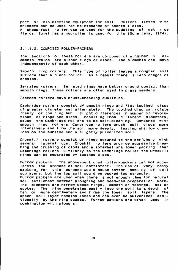
Furrow packers. The above-mentioned roller-packers can not accelerate the process of soil settlement. The use of very heavy packers^ for this purpose would cause better packing of soil sublayers, but the top soil would be packed too strongly. Furrow packers are used when there is not enough time for natural soil settlement between ploughing and seed-bed preparation. Working elements are narrow wedge rings, smooth or toothed, set on spokes. The ring penetrates easily Into the soil to a depth of ten or more centimeters and firms the lower soli layers. The upper soil layer remains loose and can even be pulverized additionally by the ring spokes. Furrow packers are often used In combination with ploughs.
16
2.1.2. ROLLER-HARROWS
These rollers have no pronounced packing task, but are used for so I I crush Ing.
RoI ler-crumbIers or string-rollers form a thin we I I-pu I ver I zed surface on top of a slightly packed layer. Especially the roller-crumb Iers with small diameters have good crushing qualities. Roller-crumbIers generally are components of combined tillage Implements and are available In many designs and constructions.
Rotary harrows with spiked teeth or knives move like rollers, but according to their effects they should be classified as harrows.
2.2. WHEELS
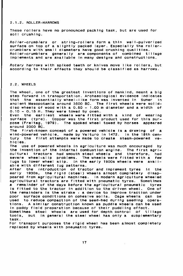
The wheel, one of the greatest Inventions of mankind, meant a big step forward In transportation. Archaeological evidence Indicates that the essentially wheel-like form was Invented in Sumer in ancient Mesopotamia around 3500 BC. The first wheels were solid-disc wheels of wood with a 0.50 - 1.00 m diameter and a width of 0.10 - 0.15 m. They were towed by oxen. Even the earliest wheels were fitted with a kind of wearing surface (tyre). Copper was the first product used for this purpose (Freitag, 1979). The spoked wheel towed by horses appeared around 2000 BC. The first-known concept of a powered vehicle Is a drawing of a wind-powered vehicle, made by Valturo In 1472. In the 18th century the first attempts were made to create steam-powered vehicles. The use of powered wheels In agriculture was much encouraged by the Invention of the internal combustion engine. The first agricultural tractors had smooth steel wheels and therefore, had severe wheel-slip problems. The wheels were fitted with a few lugs to lower wheel slip. In the early 1900s wheels were available with different lug patterns. After the introduction of tractor and implement tyres In the early 1930s, the rigid (steel) wheels almost completely disappeared from agricultural machines. In modern agriculture wheeled agricultural tractors are fitted with pneumatic tyres. Sometimes a remainder of the days before the agricultural pneumatic tyres Is fitted to the tractor in addition to the driven wheel. One of the remainders Is the strake : a device to improve traction under poor surface conditions on cohesive soils. Cage wheels can be used to reduce compaction of the seed-bed during seeding operations. A similar construction known as puddle wheels can be used In paddy field preparation because of their puddling effect. Sometimes steel wheels are used for depth control of tillage tools, but In general the steel wheel has only a supplementary task.
For transport purposes the rigid wheel has been almost completely replaced by wheels with pneumatic tyres.
17
2.3. TYRES
2.3.1. HIGHLIGHTS IN TYRE DEVELOPMENT
The first patent describing a pneumatic tyre was granted to R.W. Thompson In 1845 and the first practical tyred wheel was developed by J.B. Dunlop In 1888. His tyre was fitted on a bicycle wheel. Further development resulted In passenger car tyres at the turn of the century and availability of truck tyres In the early 1920s. Because operating conditions In agriculture are considerably more rigorous than on the road It was not until the early 1930s that tyres with an adequate field performance were generally available. The first tractor rear tyres were Introduced by Fyrestone and Continental, while Dunlop Introduced the first Implement tyre. A further highlight in history of agricultural tyres was the introduction of the radial-ply tractor rear tyre by Pirelli about 1957. Other Important factors in the development of modern low pressure tyres are: - the use of nylon as carcass material
- wide base rIms - tube I ess tyres.
2.3.2. TYRE CONSTRUCTION
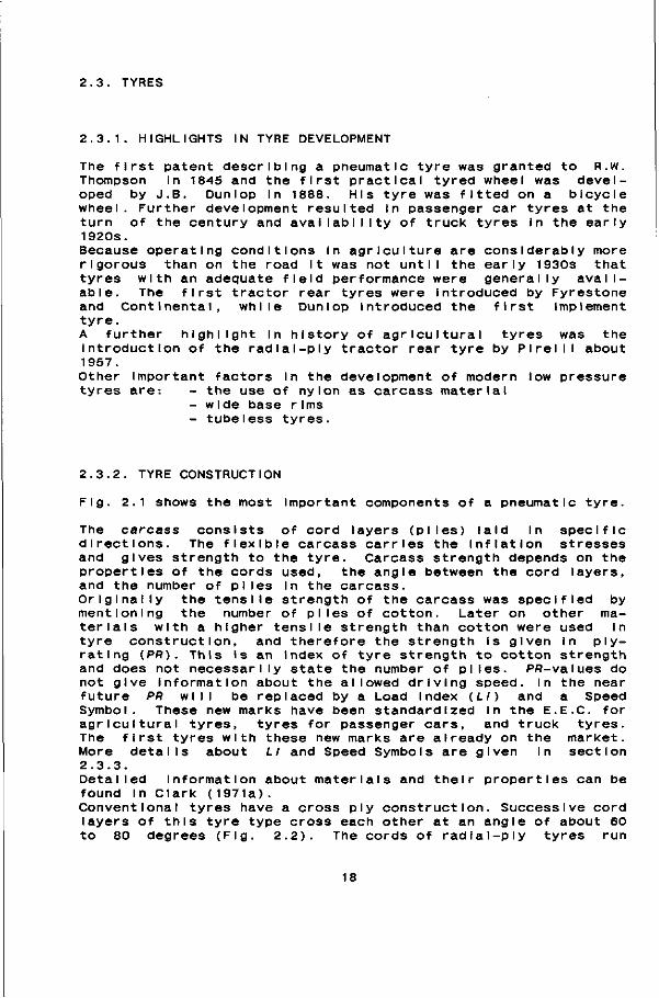
Fig. 2.1 shows the most Important components of a pneumatic tyre.
The carcass consists of cord layers (plies) laid In specific directions. The flexible carcass carries the Inflation stresses and gives strength to the tyre. Carcass strength depends on the properties of the cords used, the angle between the cord layers, and the number of pI I es In the carcass. Originally the tensile strength of the carcass was specified by mentioning the number of piles of cotton. Later on other materials with a higher tensile strength than cotton were used In tyre construction, and therefore the strength is given in ply-rating (PR). This is an index of tyre strength to cotton strength and does not necessarily state the number of plies. Pfl-vaIues do not give information about the allowed driving speed. In the near future PR will be replaced by a Load Index {LI) and a Speed Symbol. These new marks have been standardized in the E.E.C. for agricultural tyres, tyres for passenger cars, and truck tyres. The first tyres with these new marks are already on the market. More details about LI and Speed Symbols are given In section 2.3.3. Detailed Information about materials and their properties can be found In Clark (1971a). Conventional tyres have a cross ply construction. Successive cord layers of this tyre type cross each other at an angle of about 60 to 80 degrees (Fig. 2.2). The cords of radial-ply tyres run
18
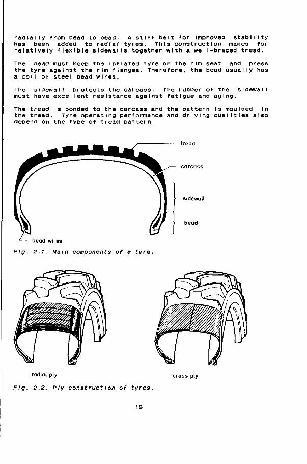
radially from bead to bead. A stiff belt for Improved stability has been added to radial tyres. This construction makes for relatively flexible sidewalls together with a wel I-braced tread.
The bead must keep the Inflated tyre on the rim seat and press the tyre against the rim flanges. Therefore, the bead usually has a coI I of steel bead wires.
The sldewall protects the carcass. The rubber of the s IdewaI I must have excellent resistance against fatigue and aging.
The tread Is bonded to the carcass and the pattern Is moulded In the tread. Tyre operating performance and driving qualities also depend on the type of tread pattern.
bead wires
Fig. 2.1. Main components of a tyre.
tread
carcass
sidewall
bead
radial ply
Fig. 2.2. Ply construct Ion of tyres.
cross ply
19
2.3.3. TYRE SIZE SPECIFICATION
The size of the the sect Ion wI I f Ied In Inches of about 1.0. a rim dIamete overaII dIamete Introduction o 1950s resulted height h, and t 1.0 to about 0. tlon: 12.4/11-3 Nowadays the designation so 12.4-36. The developmen In the IncI us 9.0/75-18. At present the ture. The rea agricultural t appIIcatIon In
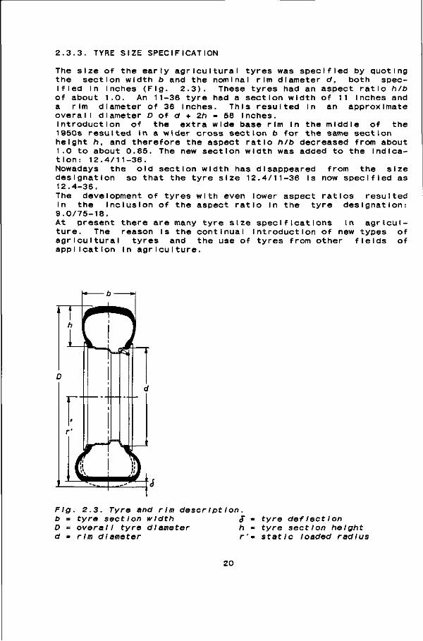
early agricultural tyres was specified by quoting dth b and the nominal rim diameter d, both spec-
(Flg. 2.3). These tyres had an aspect ratio h/b An 11-36 tyre had a section width of 11 Inches and r of 36 Inches. This resulted In an approximate r D of d + 2h - 58 Inches. f the extra wide base rim In the middle of the in a wider cross section b for the same section herefore the aspect ratio h/b decreased from about 85. The new section width was added to the Indica-6. old section width has disappeared from the size
that the tyre size 12.4/11-36 Is now specified as
t of tyres with even lower aspect ratios resulted ion of the aspect ratio in the tyre designation:
re are many tyre size specifications In agrlcul-son Is the continual Introduction of new types of yres and the use of tyres from other fields of agrIculture.
Fig. 2.3. Tyre and rim descrIptIon. b « tyre section width S » tyre deflectIon D * overall tyre diameter h = tyre section height d m rim diameter r'= static loaded radius
20

Recently standards for tyre size, Load Index (Lit, and Speed Symbol have been accepted within the E.E.C. Load Index Indicates the allowed tyre load W^ In a number Tyre catalogues generally contain tables with LI and Wf^. LI can have values between 0 range from 450 N to 185,000 N. can be expressed as:
and 209; corresponding M^ The relationship between W/^
code.
va Iues and LI
U//80) Wt 450.10
Speed symbols up until 40 km/h are Important f purposes. The speed symbol for this field of app I letter A and a number between 1 and 8. This number shows the allowed driving speed. A6, for example ed driving speed of 30 km/h.
Although there was no agreement about a symbol pressure, some manufacturers nowadays mark thel symbol for this aspect as well. Inflation pressur one, two, or three stars. One star means that t load Is based on an Inflation pressure of 1.6 ba three stars allowed loads are based on Inflation p bar and 3.2 bar respectively.
Fig. 2.4 shows an example of the marks that ca modern West European tractor rear tyre:
or agricultural Icatlon is the mu111p i ed by 5
means an a Ilow-
for Inflation r tyres with a e Is marked by he a I lowed tyre r. At two or ressures of 2.4
n be found on a
Where, 18.4 R 38 146 A8 *
18.4 R 38 146 A8 *
tyre width of 18.4 Inches (=46.7 cm) Radial tyre; Cross ply tyres do not have letter R rim diameter of 38 Inches (-96.5 cm) Load Index: maximum allowed load of 30 kN maximum allowed driving speed of 40 km/h allowed load Is based on an Inflation pressure of 1.6 bar.
Fig. 2.4. IndlcatIons on a modern West European tractor tyre.
21
2.3.4. TYRES USED IN AGRICULTURE
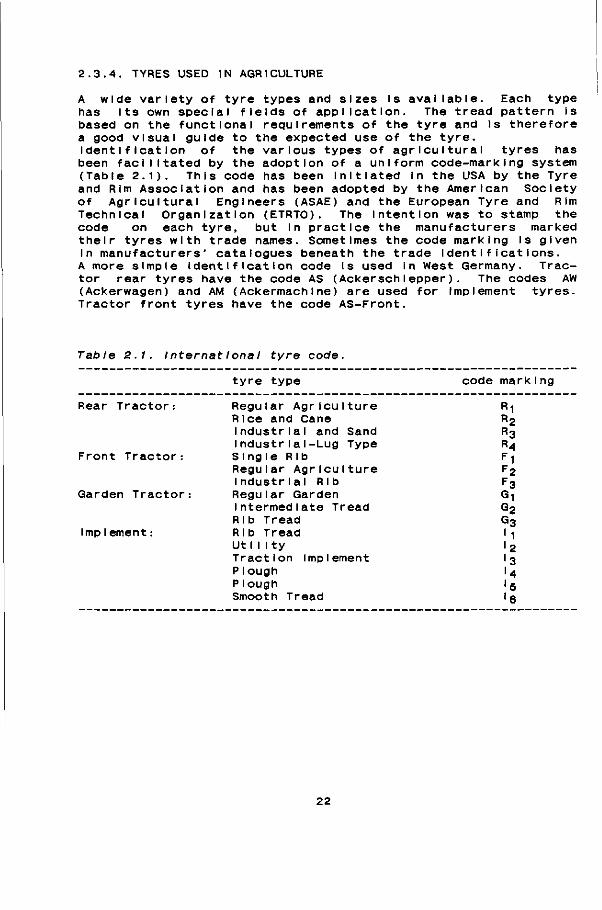
A wide variety of tyre types and sizes Is available. Each type has Its own special fields of application. The tread pattern Is based on the functional requirements of the tyre and Is therefore a good visual guide to the expected use of the tyre. Identification of the various types of agricultural tyres has been facilitated by the adoption of a uniform code-marking system (Table 2.1). This code has been Initiated In the USA by the Tyre and Rim Association and has been adopted by the American Society of Agricultural Engineers (ASAE) and the European Tyre and Rim Technical Organization (ETRTO). The Intention was to stamp the code on each tyre, but In practice the manufacturers marked their tyres with trade names. Sometimes the code marking Is given In manufacturers' catalogues beneath the trade Identifications. A more simple identification code Is used in West Germany. Tractor rear tyres have the code AS (Ackerschlepper). The codes AW (Ackerwagen) and AM (Ackermach I ne) are used for implement tyres. Tractor front tyres have the code AS-Front.
Table 2.1. International tyre code.
tyre type code mark Ing
Rear Tractor :
Front Tractor:
Garden Tractor :
Implement:
Regular Agr icu1ture Rice and Cane 1ndustrla 1 1ndustr1 a 1 -SIngIe Rib
and -Lug
Sand Type
Regular Agriculture 1 ndustrla 1 Regular Gar
Rib den
Intermediate Tread Rib Tread Rib Tread Ut11Ity Traction Implement Plough Plough Smooth Tread
G 2
G3 1 2 3 4 5 6
22
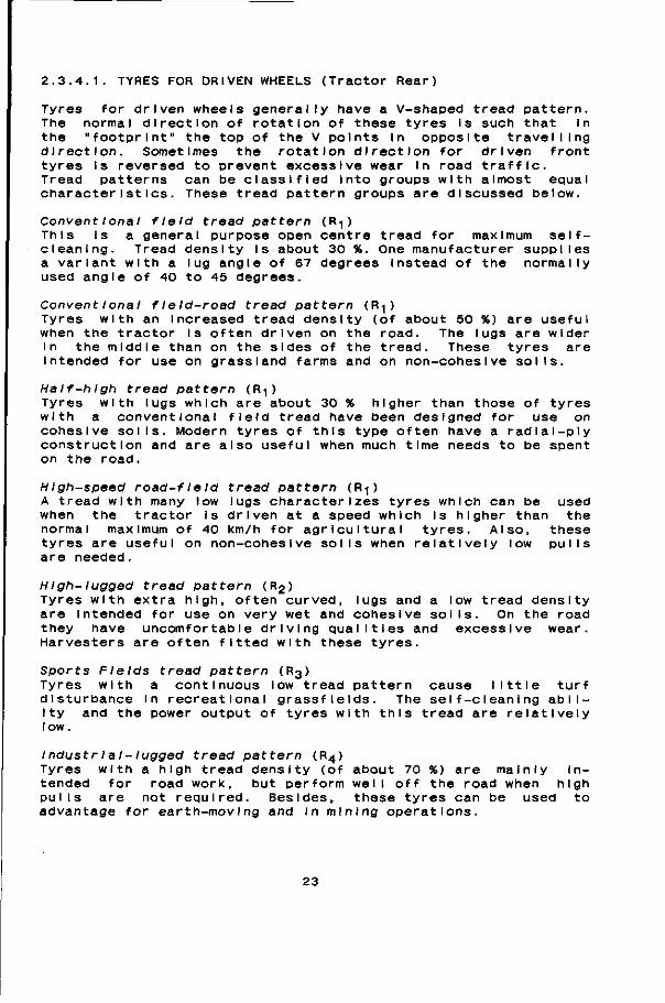
2.3.4.1. TYRES FOR DRIVEN WHEELS (Tractor Rear)
Tyres for driven wheels generally have a V-shaped tread pattern. The normal direction of rotation of these tyres Is such that In the "footprint" the top of the V points In opposite travelling direction. Sometimes the rotation direction for driven front tyres Is reversed to prevent excessive wear In road traffic. Tread patterns can be classified Into groups with almost equal characteristics. These tread pattern groups are discussed below.
Convent lonal field tread pattern (R-j) This Is a general purpose open centre tread for maximum self-cleaning. Tread density Is about 30 %. One manufacturer supplies a variant with a lug angle of 67 degrees Instead of the normally used angle of 40 to 45 degrees.
Convent I onal f le Id-road tread pattern (R-|) Tyres with an Increased tread density (of about 50 %) are useful when the tractor Is often driven on the road. The lugs are wider In the middle than on the sides of the tread. These tyres are Intended for use on grassland farms and on non-cohesive soils.
Half-high tread pattern (R^) Tyres with lugs which are about 30 % higher than those of tyres with a conventional field tread have been designed for use on cohesive soils. Modern tyres of this type often have a rad la I-ply construction and are also useful when much time needs to be spent on the road.
HIgh-speed road-f le Id tread pattern (R-|) A tread with many low lugs characterizes tyres which can be used when the tractor is driven at a speed which Is higher than the normal maximum of 40 km/h for agricultural tyres. Also, these tyres are useful on non-cohesive soils when relatively low pulls are needed.
High-lugged tread pattern (R2) Tyres with extra high, often curved, lugs and a low tread density are intended for use on very wet and cohesive sol Is. On the road they have uncomfortable driving qualities and excessive wear. Harvesters are often fitted with these tyres.
Sports Fields tread pattern (R3) Tyres with a continuous low tread pattern cause little turf disturbance In recreational grassflelds. The self-cleaning ability and the power output of tyres with this tread are relatively low.
IndustrIal-lugged tread pattern (R4) Tyres with a high tread density (of about 70 %) are mainly intended for road work, but perform wel I off the road when high pulls are not required. Besides, these tyres can be used to advantage for earth-moving and In mining operations.
23
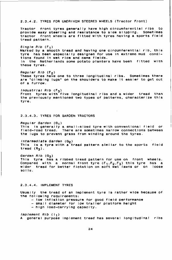
2.3.4.2. TYRES FOR UNDRIVEN STEERED WHEELS (Tractor Front)
Tractor front tyres generally have high circumferential ribs to provide easy steering and resistance to side slipping. Sometimes tractor front wheels are fitted with tyres having a sports field tread pattern.
Single Rib (F^ ) Marked by a smooth tread and having one circumferential rib, this tyre has been especially designed for use In extreme mud conditions found In wet rice and cane fields. In the Netherlands some potato planters have been fitted with these tyres.
Regular Rib (F2) These tyres have one to three longitudinal ribs. Sometimes there are "climbing lugs" on the shoulders to make it easier to get out of a furrow.
Industrial Rib (F3) Front tyres with five longitudinal ribs and a wider tread than the previously mentioned two types of patterns, characterize this tyre.
2.3.4.3. TYRES FOR GARDEN TRACTORS
Regular Garden (G-| ) This is generally a smaI I-sI zed tyre with conventional field or field-road tread. There are sometimes narrow connections between the lugs to prevent grass from winding around the tyres.
Intermedlate Garden (G2) This Is a tyre with a tread pattern similar to the sports field tread ( R 3 ) .
Garden Rib (G3) This tyre has a ribbed tread pattern for use on front wheels. Compared with a normal front tyre (F1.F2.F3) this tyre has a wider tread for better flotation on soft wet lawns or on loose so I Is.
2.3.4.4. IMPLEMENT TYRES
Usually the tread of an Implement tyre Is rather wide because of the following requirements:
- low Inflation pressure for good field performance - small diameter for low trailer platform height - high load-carrying capacity.
Implement Rib (I1) A general purpose Implement tread has several longitudinal ribs
24
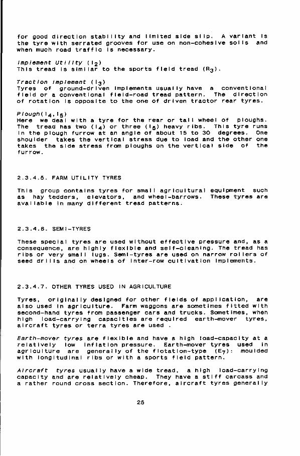
for good direction stability and limited side slip. A variant Is the tyre with serrated grooves for use on non-coheslve soils and when much road traffic Is necessary.
Implement UtI 11ty (l2) This tread is similar to the sports field tread ( R 3 ) .
Traction Implement (I3) Tyres of ground-driven Implements usually have a conventional field or a conventional field-road tread pattern. The direction of rotation Is opposite to the one of driven tractor rear tyres.
Plough(l4>I5) Here we deal with a tyre for the rear or tall wheel of ploughs. The tread has two (l 4 ) or three (l 5 ) heavy ribs. This tyre runs In the plough furrow at an angle of about 15 to 30 degrees. One shoulder takes the vertical stress due to load and the other one takes the side stress from ploughs on the vertical side of the f u r r ow.
2.3.4.5. FARM UTILITY TYRES
This group contains tyres for small agricultural equipment such as hay tedders, elevators, and wheeI-barrows. These tyres are available In many different tread patterns.
2.3.4.6. SEM I-TYRES
These special tyres are used without effective pressure and, as a consequence, are highly flexible and self-cleaning. The tread has ribs or very small lugs. Semi-tyres are used on narrow rollers of seed drills and on wheels of Inter-row cultivation Implements.
2.3.4.7. OTHER TYRES USED IN AGRICULTURE
Tyres, originally designed for other fields of application, are also used ln agriculture. Farm waggons are sometimes fitted with second-hand tyres from passenger cars and trucks. Sometimes, when high load-carrying capacities are required earth-mover tyres, aircraft tyres or terra tyres are used .
Earth-mover tyres are flexible and have a high load-capacity at a relatively low Inflation pressure. Earth-mover tyres used In agriculture are generally of the flotation-type ( E 7 ) : moulded with longitudinal ribs or with a sports field pattern.
Aircraft tyres usually have a wide tread, a high load-carrying capacity and are relatively cheap. They have a stiff carcass and a rather round cross section. Therefore, aircraft tyres generally
25
show lower field performance than tyres designed for agricultural purposes. Size specification deviates from normal agricultural specification. When aircraft tyres are remoulded with an agricultural tread pattern, they normally get an agricultural tyre size speel f I cat Ion .
Terra tyres have been developed especially for applications where very high flotation properties are required. In comparison with conventional tyres they have a wider cross section, a larger air volume, a more flexible carcass, and they operate at lower inflation pressures. Because of the high flotation effect they have a rather good go-anywhere performance. The tread pattern of terra tyres is available In different designs: smooth, ribbed and lugged. They can be used, depending on tyre size and loading, at Inflation pressures of 0.35 bar and higher. Tyre size specification Is different from normal agricultural Indications. In the Netherlands some heavy self-propelled slurry tanks, combine harvesters, and sugar beet harvesters are fitted with terra tyres.
26
CHAPTER 3
KINEMATIC ASPECTS OF LOAD-BEARING PROCESSES
3.1. STATE OF MOVEMENT OF A ROLLER, WHEEL, OR TYRE
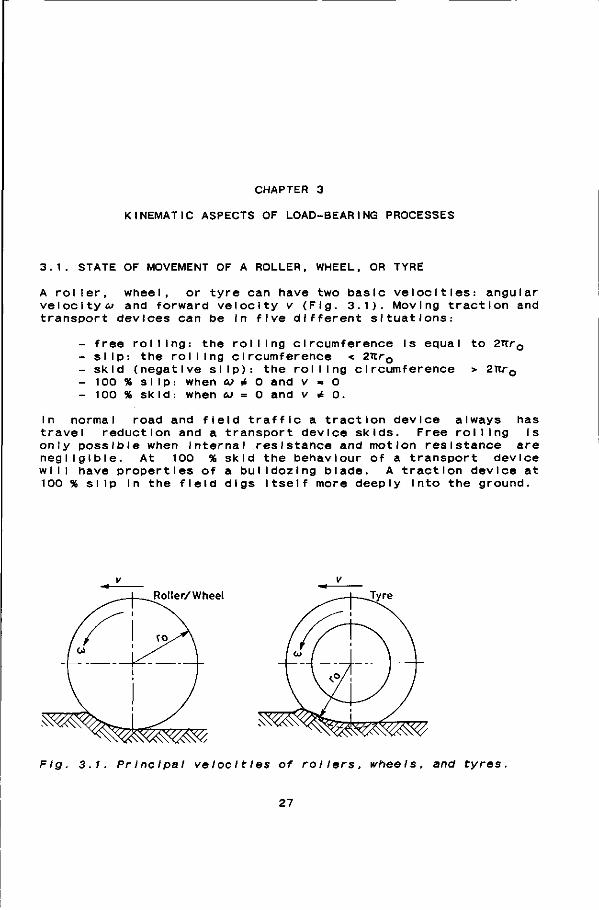
A roller, wheel, or tyre can have two basic velocities: angular v e l o c i t y ^ and forward velocity v (Fig. 3 . 1 ) . Moving traction and transport devices can be In five different situations:
- free rolling: the rolling circumference Is equal to 2Ttr0
slip: the rolling circumference < 2TCr0
skid (negative s l i p ) : the rolling circumference 100 % slip: when cj é 0 and v = 0 100 % skid: when u = 0 and v * 0.
2Ttr,
In normal road and field traffic a traction device always has travel reduction and a transport device skids. Free rolling Is only possible when Internal resistance and motion resistance are negligible. At 100 % skid the behaviour of a transport device will have properties of a bulldozing blade. A traction device at 100 % slip In the field digs Itself more deeply into the ground.
Roller/Wheel
^W^% ^ ^
Fig. 3.1. PrIncI pal velocIt les of rollers, wheels, and tyres.
27
3.1.1. SLIP
Slip Is the relative movement In the direction of travel at the mutual contact surface of the traction or transport device and the surface which supports it (ASAE Standard S296.2; Hahn et al., 1984). Travel reduction Is defined as one minus the ratio of distance travelled per revolution of the traction device to the rolling circumference under the specified zero conditions. Slip and travel reduction are often used synonymously, and are frequently expressed In percentages. Slip S (Bock, 1952; Söhne, 1952) Is defined as:
S = 1 [3.1] S,
'o - °a
5o
where, s a = real travelled distance s 0 = travelled distance at zero slip.
Slip can also be defined In velocities (Bailey et al., 1974):
co - v/rQ
S m [3.2] co
where, co = angular velocity of the traction device v = linear velocity of the traction device r 0 = rolling radius under specified zero condition.
Analyses of Söhne (1969) and Steiner (1979) show that wheel slip of a tyre on deformable soil Is composed of three components:
- tangential carcass and lug deformation - tangential soil deformation - slipping In the contact area.
3.1.1.1. ZERO-SLIP CONDITIONS
For a flexible device such as a pneumatic tyre It is difficult to define zero slip and no one has been able to determine the exact position of the zero-slip point. The problem is that there is always relative movement in the mutual contact area when a vehicle system Is in motion. Using the slip formulas has the following problems: rQ can not be measured directly and s 0 can not be measured at zero slip. According to Gill and Van den Berg (1967) the problem of measuring wheel slip Is a problem of defining and measuring zero slip.
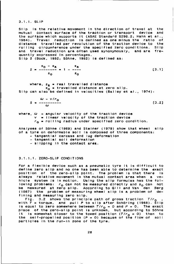
Fig. 3.2 shows the principle path of gross traction T/rQ , with T = torque, and pull P to slip after Schuring (1968). Slip Is equal to zero somewhere between T/r0 = 0 and P = 0. The exact place of the zero-slip point Is unknown, but according to Söhne it is somewhat closer to the towed position (T/rQ = 0) than to the self-propelled position (P = 0) because of the flow of soil particles In the run-in zone of the tyre.
28
P> £ c o o o
• * *
Q. in _ w •=: o D t. Q. o
/ 0
1
/ SI
, r/f0
p ^
-p
Flg. 3.2. PrInclpal (Schuring, 1968).
path of gross traction and pull to slip
The zero condition generally Is a performance condition or Is calculated from performance conditions. Conditions used to define zero slip are: the self-propelled position, the towed position, and the point halfway between the self-propelled position and the towed position. Other zero conditions may be used, but no other practical solutions have been found In literature. The specific zero conditions chosen should always be mentioned.
Sel f-propel led position (SPP) The SPP on a hard surface was used by Wlsmer and Luth (1973), Melzer (1976), and others. Terpstra and van Maanen (1972) used the SPP on a grass-field as zero condition. Bailey et al. (1974), Dwyer et al. (1974), Gee-Clough et al. (1977), and many others used the SPP on the test surface.
The distance between SPP and towed point (TP) on the slip axis will be longer when the field conditions get worse. The definition slip Is zero In the SPP will then be undesirable. A single wheel operating In the SPP on a field, where the performance conditions change gradually from good to bad, only has to over-
Ing rolling resistance. If even In the worst Is supposed to be zero as long as P - 0 the stuck. However, a spinning wheel has 100 % slip
come an increas cond i tIons slip wheel can not get and stI I I P - 0.
On sandy loam measured with a 12 s l i p (r.
with a moisture content of 23.5 % Holm 4/11-28 buffed tyre that pull was zero
calculated from tyre deflection moisture content of 16.5 % and a somewhat found zero pull at zero slip.
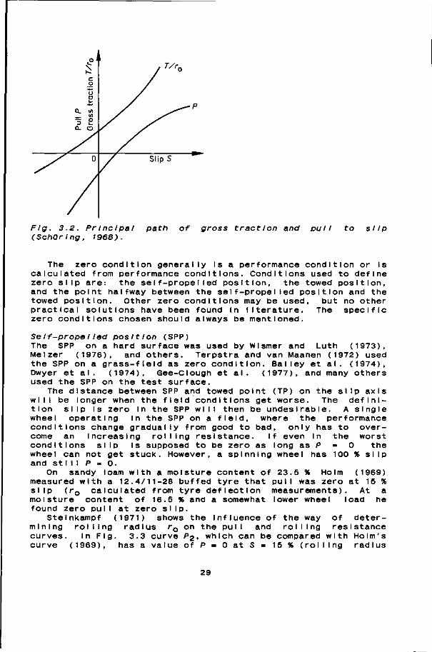
Steinkampf (1971) shows the Influence of
measurements) lower wheel
(1969) at 15 %
At a oad he
the way of determining rol Ii ng curves. In Fig. curve (1969),
radius rQ 3.3 curve
has a value
on P? o f
the pul I and rol I Ing resistance , which can be compared with Holm's P - 0 at S - 15 % (rolling radius
29
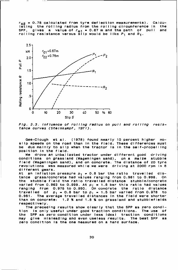
ro2 = °-78 calculated from tyre deflection measurements). Calculating the rolling radius from the rolling circumference In the SPP, gives a value of r0i - 0.67 m and the path of pul I and rolling resistance versus slip would be like P-\ and R^ .
Fig. 3.3. Influence of rolling radius on pull and rolling resistance curves (Stelnkampf, 1971).
Gee-Clough et al slip speeds on the r be due ma i nI y to si pos 11Ion In the fiel
We drove an unba conditions on grass field (Wagen Ingen sa revolutions was mea different gears. At an Inflation pre tance grass/concret the stubble field t varied from 0.963 to ranging from 0.975 traveI Ied of p\ » 0.981. The average than on concrete: 1 respect I vel y.
The preceding res tlon is only useful the SPP as zero con may give ml s lead In zero condition Is th
(1978) found nearly 10 percent higher no-oad than In the field. These differences must Ip when the tractor Is in the self-propelling d. I lasted tractor under different good driving land (Wageningen sand), on a maize stubble nd), and on concrete. The distance of 20 tyre sured whI I e we were driving at 2000 rpm In 6
ssure P| = 0.8 bar the ratio travelled dIs-e had values ranging from 0.981 to 0.998. On he ratio travelled distance stubble/concrete
0.999. At p\ = 1.5 bar this ratio had values to 0.990. On concrete the ratio distance
0.8 bar to p\ » 1.5 bar varied from 0.978 to travelled distances in the field were shorter .2 % and 1.5 % on grassland and stubbIeflelds
ults show clearly that the SPP as zero condI-under good traction conditions. The use of
ditlon under less Ideal traction conditions g and even useless results. The best SPP as e one measured on a hard surface.
30
Towed position (TP) Analogous to the self-propelled position the use of the towed point as zero slip condition Is realistic under good traction conditions. The use of the TP as zero condition under less ideal traction conditions Is undesirable. The most useful TP as zero condition Is the one measured on a hard surface.
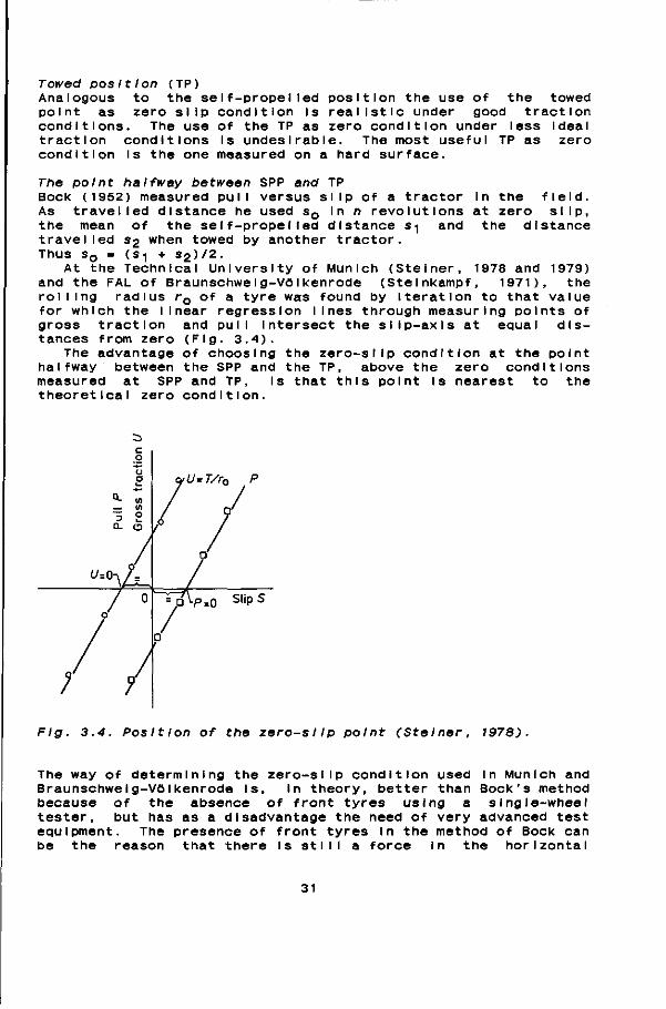
The point halfway between SPP and TP Bock (1952) measured pull versus slip As travelled distance he used s 0 In the mean of the self-propelled dis travelled S2 when towed by another tr Thus s 0 = (s-| + S2)/2.
At the Technical University of Mun and the FAL of BraunschweIg-VoIkenrod rol I Ing radius r 0 of a tyre was foun for which the linear regression lines gross traction and pull Intersect t tances from zero (Fig. 3.4).
The advantage of choosing the zero halfway between the SPP and the TP, measured at SPP and TP, Is that th theoretical zero condition.
of a tractor in the field. n revolutions at zero slip, tance s^ and the distance actor.
Ich (Stelner, 1978 and 1979) e (Steinkampf, 1971), the d by Iteration to that value
through measuring points of he slip-axis at equal dis-
-sI Ip condition at the point above the zero conditions s point is nearest to the
U=T/r0 P
Fig. 3.4. Position of the zeros IIp point (Stelner, 1978).
The way of determining the zero-slip condition used In Munich and Braunschweig-VoIkenrode Is, in theory, better than Bock's method because of the absence of front tyres using a single-wheel tester, but has as a disadvantage the need of very advanced test equipment. The presence of front tyres In the method of Bock can be the reason that there Is still a force In the horizontal
31
direction at s0. Under good traction conditions this force can be neglected. Under worse conditions this force can cause small deviations from the theoretical zero-slip point. The advantage of the method of Bock is Its simplicity of making measurements and caleu lat Ions.
3.1.1.2. MEASURING METHODS FOR SLIP
There are many known slip-measuring methods. Two groups can be distinguished: methods measuring Instantaneous slip and methods measuring mean slip over a travelled distance.
MeasurIng Instantaneous slip To measure Instantaneous slip advanced measuring equipment is needed. In wheel testers as used by IMAG In Wageningen (Werkhoven, 1975) and NTML in Auburn (Bailey et al., 1974) electronic pulses for forward velocity and angular velocity, processed by a computer, can give instantaneous values of slip. Thansandote et al.(1977) used a microwave Doppler radar to measure the true ground velocity of the tractor and the circumferential velocity of the driven wheel. They concluded that the Doppler radar slip monitor seems to be feasible as a practical device for use on agricultural tractors. Since the late 1970s Doppler radar sensors are being installed In automatic sprayer control systems. In such a system the radar sensor, mounted on the tractor, is used for measuring the true driving speed. If the forward speed changes, the control system automatically alters the sprayer settings to maintain the target application rate. Since the early 1980s many makes of tractors can be equipped, standard or as an opt InaI, with a tractor monitor. Such an instrument can display the true driving speed or the slip percentage of the driven wheels. A new generation Doppler radar sensors was Introduced In 1985. According to Kellermann (1985) these sensors can achieve an accuracy of + 1 %. Bol I and Isensee (1987) found a much lower accuracy In farm fields.
A radar sensor must be mounted on the tractor so that It Is pointing to the ground at a correct angle. This angle is crucial concerning the accuracy of the instrument: a change In this angle results in a deviation of about 1 % per degree (Schmitt, 1986).
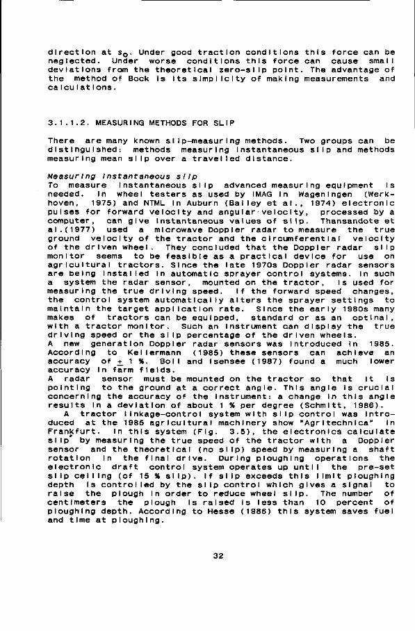
A tractor linkage-control system with slip control was Introduced at the 1985 agricultural machinery show "Agritechnica" In Frankfurt. In this system (Fig. 3.5), the electronics calculate slip by measuring the true speed of the tractor with a Doppler sensor and the theoretical (no slip) speed by measuring a shaft rotation in the final drive. During ploughing operations the electronic draft control system operates up until the pre-set slip ceiling (of 15 % slip). If slip exceeds this limit ploughing depth Is controlled by the slip control which gives a signal to raise the plough In order to reduce wheel slip. The number of centimeters the plough Is raised Is less than 10 percent of ploughing depth. According to Hesse (1986) this system saves fuel and time at ploughing.
32
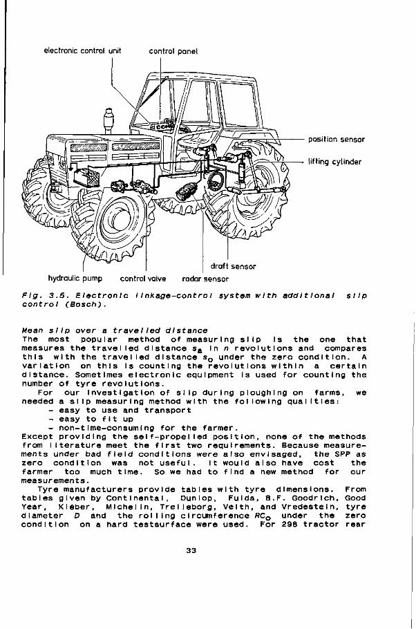
electronic control unit control panel
position sensor
lifting cylinder
hydraulic pump control valve
draft sensor
radar sensor
Fig. 3.5. Electronic 11nkage-controI system with add 11lonal control (Bosch).
slip
Mean slip over a travel led distance The most popular method of measur measures the travelled distance s a In
the travelled distance s 0 under the on this Is counting the revolutions
ng slip Is the one that n revolutions and compares
zero condItIon. A within a certaIn
the
For needed
this with variation „.. .„ „„_ „ , v^.w..- ... -distance. Sometimes electronic equipment Is used for counting number of tyre revolutions.
our Investigation of slip during ploughing on farms, we a slip measuring method with the following qualities:
- easy to use and transport - easy to fit up - non-tIme-consumIng for the farmer.
Except providing the self-propelled position, none of the methods from literature meet the first two requirements. Because measurements under bad field conditions were also envisaged, the SPP as zero so have cost
new method for condition was not useful. It would a
farmer too much time. So we had to find measurements.
Tyre manufacturers provide tables with tyre dimensions, tables given by Continental, Dunlop, Fulda, B.F. Goodrich, Year, Kléber, Michelin, Trelleborg, Veith, and Vredeste diameter D and the rolling circumference RC0 under condition on a hard testsurface were used. For 298
n, the
tractor
the our
From Good tyre zero rear
33
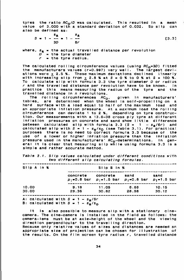
tyres the ratio RC0/D was calculated. This resulted In a mean value of 3.000 with a standard deviation of 0.032. So slip can also be defined as:
s a S - 1 - — . 1 - — [3.3]
s a
3D
s a
Br
where, s a » the actual travelled distance per revolution D » the tyre diameter r - the tyre radius.
The calculated rolling circumference values (using RC0=3D) fitted the manufacturers values (r-0.997) very well. The largest deviations were ± 2.5 %. These maximum deviations dec I Ined I I near I y with increasing slip from + 2.5 % a t S = 0 % t o 0 % a t S = 100 %. To calculate slip with formula 3.3 the tyre diameter D or radius r and the travelled distance per revolution have to be known. In practice this means measuring the radius of the tyre and the travelled distance in n revolutions.
The rolling circumferences RC0, given In manufacturers' tables, are determined when the wheel Is self-propelling on a hard surface with a load equal to half of the maximum load and an appropriate Inflation pressure. At a maximum load the rolling circumference can deviate 1 to 2 %, depending on tyre construction. Our measurements with a 13.6-38 cross ply tyre at different Inflation pressures on concrete and sand show little difference between calculated slip with formula 3.3 (S = 1 - sa/6r) and calculated slip with S - 1 - S^/SQ (see Table 3.1). For practical purposes there Is no need to correct formula 3.3 because of the use of a lower or higher Inflation pressure than the inflation pressure used In the manufacturers' flC0-determI nat ions. In general it Is clear that measuring slip while using formula 3.3 Is a simple and rather accurate method.
Table 3.1. Slip values calculated under different condltIons with two different slip calcuI at Ing formulas .
Slip A In » Slip B In X
concrete concrete sand sand Pl=0.8 bar D|=1.5 bar P|=0.8 bar p(=1.5 bar
10.00 9 .18 11.05 8 .68 10.15 30 .00 29 .36 30 .82 28 .98 30 .12
A: calculated with s - 1 - sa/6r B: calculated with S = 1 - sa/s0
It Is also possible to measure slip with a stationary cinecamera. The cine-camera Is Installed In the field as follows: the camera-1 ens must be at axle-height of the wheel and the viewing direction perpendicular to the travelling direction. Because only relative values of sizes and distances are needed an appropriate size of projection can be chosen for Illustration of the results. On the film screen tyre radius r, travelled distance
34
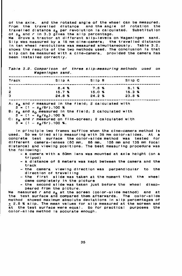
of the axle, and the rotated angle of the wheel can be measured. From the travelled distance and the angle of rotation the travelled distance s a per revolution is calculated. Substitution of s a and r In 3.3 gives the slip percentage. We drove a tractor at different slip-levels on Wagen Ingen sand. Slip was measured by a 16 mm cine-camera; the travelled distance In ten wheel revolutions was measured simultaneously. Table 3.2. shows the results of the two methods used. The conclusion Is that slip can be measured with a cine-camera, provided the camera has been Installed correctly.
Table 3.2. Comparison of three s 11p-measurIng methods used on Wagen Ingen sand.
Track Slip A S l i p B S l i p C
1 8.4 % 7.6 % 8 . 1 % 2 15.7 % 15.0 % 15.3 % 3 24.8 % 24.2 % 23.8 %
A: s a and r measured In the field; S calculated with S - (1 - sa/6r).100 %
B: s a and s 0 measured in the field; S calculated with S = (1 - sa/s0).100 %
C: s a and r measured on film-screen; S calculated with S = (1 - sa/6r).100 %.
In principle two frames suffice when the cine-camera method is used. So we tried slip measuring with 35 mm color-slides. At a concrete test surface the color-slide method was tested for different camera-Ienses (50 mm, 85 mm, 105 mm and 135 mm focal distance) and viewing positions. The best measuring procedure was the foI low Ing:
- a camera with a 50mm lens was mounted at axle height (on a trIpod)
- a distance of 8 meters was kept between the camera and the track
- the camera viewing direction was perpendicular to the direction of travelling
- the first slide was taken at the moment that the wheel came completely In the picture
- the second slide was taken Just before the wheel disappeared from the picture.
We measured r and s a at the screen (color-slide method) and at the test surface and compared them afterwards. The color-slide method showed maximum absolute deviations In slip percentages of i 2.5 % slip. The mean values for slip measured at the screen and at the test surface were equal. So for practical purposes the color-slide method Is accurate enough.
35

3.1.1.3. WHEEL SLIP DURING PLOUGHING
There Is much discussion about wheel slip but information on slip In normal field work seems to be lacking completely. There Is some literature about slip measurements taken during ploughing demonstrations in West Germany (Traulsen and Splngies, 1978) and Great Britain (N.N., 1980 and 1981a). Some results of these demonstrations can be found In Table 3.3 and 3.4.
Table 3.3. Slip during plough!ng demonstratI on with 11 four-wheel drive tractors In West Germany ( Traulsen and Splngies, 1978).
tractor lowest slip % highest slip % mean slip %
front wheel rear wheel
14 13
39 31
24 22
Table 3.4. Some results from Tractor at Work Events (N.N. and 1981a).
1980
tractor year lowest si ip %
hIghest si Ip %
mean si ip %
number of entrants
two-wheel drive 1980 13.4 28.0 two-wheel drive 1981 11.8 19.4 four-wheel drive 1980 8.0 18.4 four-wheel drive 1981 6.9 16.9
17.1 16.3 12.2 13.2
9 3
25 24
These ploughing demonstrations give I during regular farm work, because all same field conditions and because prepared manufacturers or Importers o
To collect more Information about ured wheel slip during ploughing o places all over the Netherlands. For necessary to develop a new measuring to measure slip "at a distance", b ploughing behaviour of the farmer to ence. Thus the cine-camera method w camera method is rather expensive and decided to use the color-slide method
During spring 1980 we drove aroun light soils until we saw a ploughing slip was measured with the color-sli ploughing depth, ploughing width, drI tractor, plough and tyres were also r It soon became clear that the plough was not notably Influenced by the pre Therefore, and also because the co consuming, the measurements of tyre r
Ittle information about slip tools are working under the
the participants are we I I-f tractors. slip on the farm, we meas-peratlons In 189 different
this slip measuring it was method. The first Idea was
ecause we did not want the be Influenced by our pres-
as born. Because the cine-its use time-consuming, we
d in the Dutch regions with farmer. With his permission, de method. Driving speed, vlng conditions, and type of ecorded. Ing behaviour of the farmer sence of the measuring team, lor-slide method was tlme-adlus and distance travelled
36
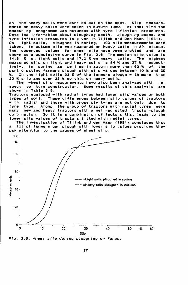
on the heavy so I I s were carried out on the spot. Slip measurements on heavy sol Is were taken In autumn 1980. At that time the measuring programme was extended with tyre Inflation pressures. Detailed Information about ploughing depth, ploughing speed, and tyre Inflation pressures Is given In TI J Ink and Den Haan (1981). On light soils, ploughed In spring, 100 slip measurements were taken. In autumn slip was measured on heavy soils In 89 places. The observed values for wheel slip have been plotted shown as a cumulative curve In Fig. 3.6. The median slip 14.6 % on light soils and 17.0 % on heavy soils. The measured slip on light and heavy soils I s 54 % and 37 % Ively. In spring as we I I as In autumn more than 60 % participating farmers plough with slip values between 10 %. On the light soils 23 % of the farmers plough with more 20 % slip and even 33 % do this on heavy soi Is.
The wheel-slip measurements have also been analysed with spect to tyre construction. Some results of this analysis shown in Table 3.5. Tractors equipped with radial tyres had lower slip values on both types of soil. These differences between slip values of tractors with radial and those with cross ply tyres are not only due to tyre type. Among the group of tractors with radial tyres were many new and heavy tractors with a well-adjusted tractor-plough combination. So It Is a combination of factors that leads to the lower slip values of tractors fitted with radial tyres.
The Investigation of TIJ ink and den Haan (1981) concluded that a lot of farmers can plough with lower slip values provided they pay attention to the causes of wheel slip.
100
80
and are value Is
h i ghest respect-
of the % and 20
than
r e -are
60
40
20
= Light soils, ploughed in spring
= Heavy soils, ploughed in autumn
10 20 30
Slip 40 50 60
Fig. 3.6. Wheel slip during pi oughtng on farms.
37
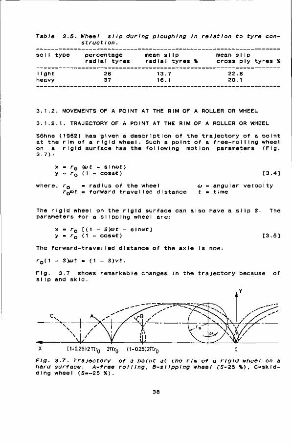
Table 3.5. Wheel slip during plough!ng In relation to tyre construction .
so I I type percentage radial tyres
mean slip radial tyres %
mean slip cross ply tyres %
I Ight heavy
26 37
13.7 16. 1
22.8 20. 1
3.1.2. MOVEMENTS OF A POINT AT THE RIM OF A ROLLER OR WHEEL
3.1.2.1. TRAJECTORY OF A POINT AT THE RIM OF A ROLLER OR WHEEL
Söhne (1952) has given a description of the trajectory of a point at the rim of a rigid wheel. Such a point of a free-rolling wheel on a rigid surface has the following motion parameters (Fig. 3.7):
x - rQ («t - si nut ) y - r 0 (1 - cos<ut )
where, rQ = radius of the wheel
[3.4]
CJ = angular velocity rQ«*t = forward travelled distance t = time
The rigid wheel on the rigid surface can also have a slip S. The parameters for a slipping wheel are:
x - r 0 [ ( l - S ) « t - sln<ut]
y = rQ (1 - coswt) [3.5]
The forward-travelled distance of the axle is now:
rQ( 1 - S)6Jt = ( 1 - S)vt. Fig. 3.7 shows remarkable changes In the trajectory because of slip and skId.
(1+0.25)2Ttr0 2TtrQ (1-0.25)2rtr0
Fig. 3.7. Trajectory of a point at the rim of a rigid wheel on a hard surface. A=free rolling, B=sIIpplng wheel (S=25 % ) , C=skld-dlng wheel (S=-25 % ) .
38
3.1.2.2. VELOCITY OF A POINT AT THE RIM OF A ROLLER OR WHEEL
A moving wheel with a radius r 0 and n revolutions per second, has a theoretical forward velocity v t n = 2 TTrQn and an actual forward velocity v a = (1 - S)2nrQn. The effective radius r e is the actual displaced distance s a per circumference divided by 2TT(ASAE Standard 296.2;Hahn et al., 1984). In a formula:
s a (1 - S)2TTr0
re - — = (1 - S)rQ [3.6] 2it 2Tt
This means that re<rQ for a slipping wheel and re>r0 for a skidding wheel. A wheel with a radius re moves without slip, with the same n, on an imaginary plane. The point where this plane touches the equivalent wheel Is the instantaneous centre of rotation I. All the points of this wheel rotate around this instantaneous centre I. It is possible by means of this instantaneous centre of rotation I and by using instantaneous kinematics to give the direction and the length of the absolute velocity vectors of points at the rim of a wheel. This Is shown In Fig. 3.8. Note the influence of slip and skid on the velocity vectors. All the points at the rim of a skidding wheel have a forward velocity above zero. A slipping wheel has two zones. The upper one with forward velocities above zero, while in the lower zone it is the opposite.
3.2. MOVEMENTS IN THE CONTACT AREA
3.2.1. TYRE DEFORMATIONS
A tyre under a static load shows radial deformation and sidewall bulging, whI le a moving tyre can show tangential carcass and lug déformât i ons.
3.2.1.1. RADIAL TYRE DEFORMATION AND SIDEWALL BULGING
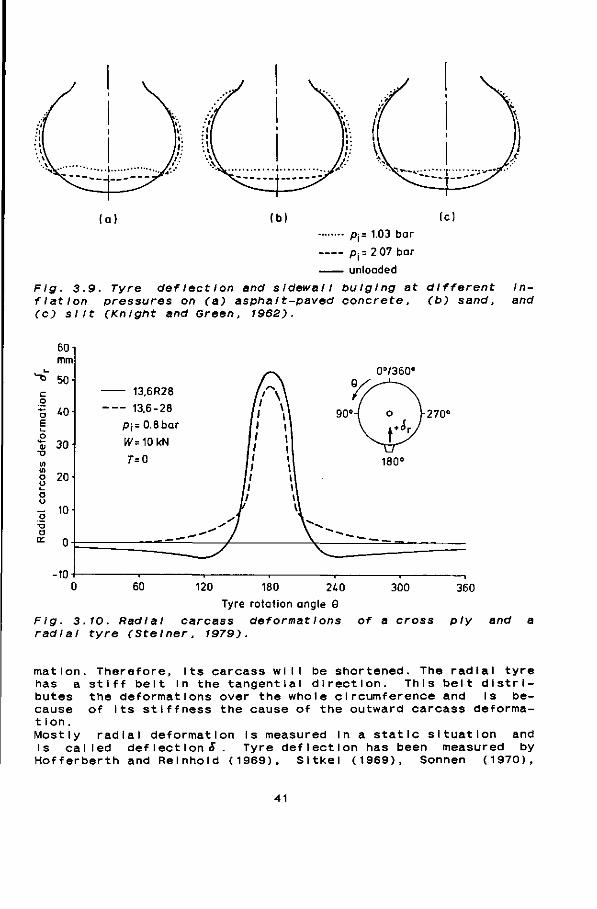
In general radial tyre deformation is accompanied by sidewall bulging. Measurements of Knight and Green (1962) show deflection and sidewall bulging of a moving tyre on surfaces ranging from f Irm to soft (Fig. 3.9).
In addition to inward carcass deformation (deflection) there can be outward deformation. Fig. 3.10 shows radial carcass deformation versus rotation angle of a radial and cross ply tyre. The radial tyre has an outward deformation in a rotation angle range from about 220 to 140 degrees. This outward deformation can be explained as follows. The cross ply tyre shows only Inward defor-
39
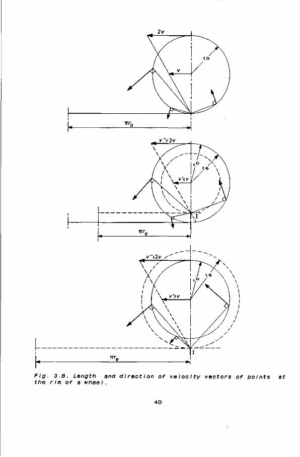
Flg. 3.8. Length and dl reet Ion of velocity vectors of points at the rim of a wheel.
40
(a] (b)
Pj= 1.03 bar
Fig. 3 . 9 f lat ion Cc) si It
601 mm
^ 50-c o o ^ 0 -E o "ai 30-•o
l/>
8 20-
. Tyre deflect ton and s Idewal I pressures on (a) asphalt-paved (Knight and Green, 1962).
- 10
o cc
-10
' i
- unloaded
bulging at concrete,
0°/360°
(c)
different (b) sand,
In-and
0 60 120 180 240
Tyre rotation angle 9
Fig. 3.10. Radial carcass deformations radial tyre (SteIner, 1979).
300 360
of a cross ply and
mat I on has a butes cause t Ion. Most I y i s ca
. Therefore, Its carcass will be shortened. The radial tyre stiff belt In the tangential direction. This belt dlstri-the deformations over the whole circumference and Is be-of Its stiffness the cause of the outward carcass deforma-
radlal deformation led deflectIon S .
is measured In a static situation and Tyre deflection has been measured by
Hofferberth and Relnhold (1969) Sitkel (1969) Sonnen (1970)
41

and others. Static tyre deflection depends on Inflation pressure, load, tyre construction, and on the character of the supporting surface. Sonnen measured remarkable differences In the deflection curves for loading and unloading. Sltkel (1969) measured tyre deflection and sinkage. Tyre deflection decreases with Increasing slnkage (Fig. 3.11).
x 8.5kN:pi=0.8bar
a 6.5 kN :/Oj = 0.8bar
• 6.5kN:pj= 1.2 bar
20 1.0 100
Fig. 3.11 1969).
60 80 Sinkage
I nf luence of sinkage
120 mm HO
on tyre deflectI on (Sltkel,
Max I mum The max from man Sltkel tractor Krick (1 Terpstra from Eu between max Imum I Imlted prevent
allowed tyre deflectIon Imum allowed tyre deflection ( £ / ^ ) m a x can be calculated ufacturers' tables. (1969) found S/h = 0.15 at maximum load for cross ply rear tyres. From technical Information from Continental, 969) calculated that (<57ft)max lies between 0.13 and 0.17.
(1978) based his calculations of (S/h) max on Information
ropean and American tyre manufacturers. He found values 0.14 and 0.20. According to Inns and Kllgour (1978)
deflection of agricultural tractor and Implement tyres is to about 18 % to 20 % of the section height h In order to carcass damage.
DeflectI on models and geometry of the contact area Bekker (1956) has provided a mathematical tyre deflection model. Furthermore, he assumes that the contact area A may be determined as an area of a rectangle reduced by 15 %. In a formula:
0.85/.B C3.7]
where, A = the area / = the length of the contact area B = the width of the contact area.
42
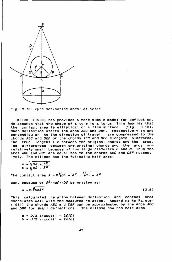
Flg. 3.12. Tyre def/eet Ion model of Kriek.
K He a the When perp chor The The rel a arcs Ivel
rick (1969) has provided ssumes that the shape of a
contact area Is elliptica deflection starts the arc
endlcular to the dlrectlo ds AEC and DEF or the chor
true lengths lie between differences between the
11 vel y small because of th ABC and DBF are equalized
y. The ellipse has the fol
a more simple model for deflection. tyre Is a torus. This Implies that
I on a firm surface (Fig. 3.12). s ABC and DBF, respectively In and n of travel, are compressed to the ds AEC and DEF elongate sidewards.
the original chords and the arcs, original chords and the arcs are e large diameters D and d. Thus the
to the chords AEC and DEF respect-lowing half axes:
a = \[pf~ b T2" \fdS
The c o n t a c t a rea A .TV^DS - <T2 . \ld<S - S2
c a n , because o f S2<<dS«D6 be w r i t t e n a s :
A =TT VDdJ2 [ 3 . 8 ]
This calculated relation between deflection and contact area correlates well with the measured relation. According to Painter (1981) the chords AEC and DEF can be approximated by the arcs ABC and DBF for small deflections . The ellipse now has half axes:
a = D/2 arccosd - 2<T/D) b = d/2 arccosd - 2<$7d)
43
and an area :
A = ( I T / 4 ) .D .d .a rccosd - 2&/D) ,arccos( 1 - 2S/d) [3.9]
Although the formulas 3.8 and 3.9 are both based on the same deflection model, formula 3.8 is easier to use.
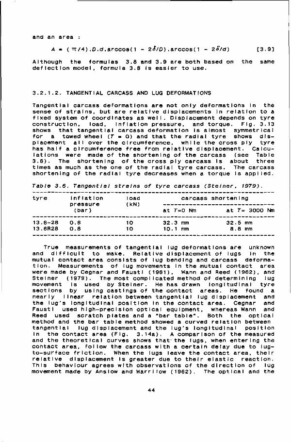
Tangential ca sense of stra f Ixed system construct Ion, shows that t for a towed placement a I has ha I f a cl latlons were 3.6). The s tImes as much shortening of
3.2.1.2. TANGENTIAL CARCASS AND LUG DEFORMATIONS
rcass deformations are not only deformations in the Ins, but are relative displacements In relation to a of coordinates as well. Displacement depends on tyre
load, inflation pressure, and torque. Fig. 3.13 angential carcass deformation is almost symmetrical
wheel (F - 0) and that the radial tyre shows dis-I over the circumference, while the cross ply tyre rcumference free from relative displacement. Calcu-
made of the shortening of the carcass (see Table hortenlng of the cross ply carcass Is about three
as the one of the radial tyre carcass. The carcass the radial tyre decreases when a torque is applied.
Table 3.6. Tangent Ial strains of tyre carcass (Stelner, 1979).
tyre inflation load carcass shortening pressure (kN)
(bar) at r=0 Nm at T= 3000 Nm
13.6-28 0.8 10 32.3 mm 32.5 mm 13.6R28 0.8 10 10.1 mm 8.8 mm
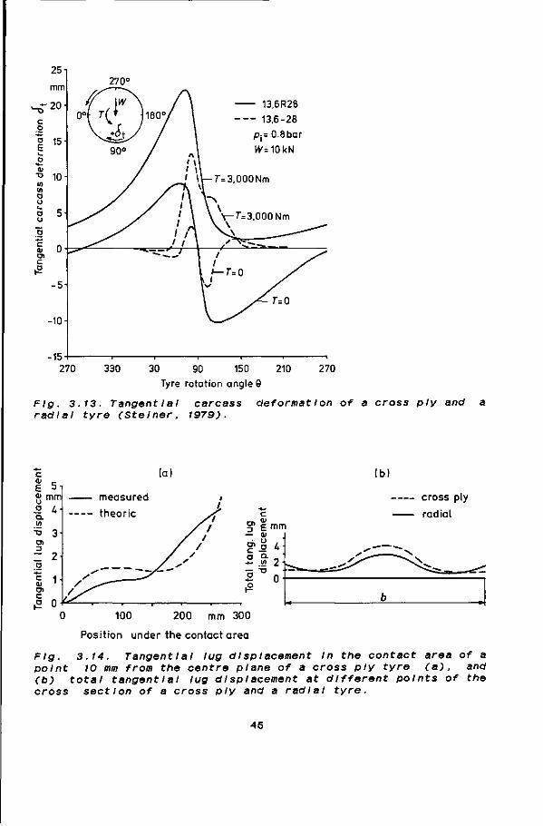
True measurements of tangential lug deformations are unknown and difficult to make. Relative displacement of lugs In the mutual contact area consists of lug bending and carcass deformation. Measurements of lug movements In the mutual contact area were made by Cegnar and Faust I (1961), Wann and Reed (1962), and Stelner (1979). The most complicated method of determining lug movement Is used by Stelner. He has drawn longitudinal tyre sections by using castings of the contact areas. He found a nearly linear relation between tangential lug displacement and the lug's longitudinal position in the contact area. Cegnar and Faust I used high-precision optical equipment, whereas Wann and Reed used scratch plates and a "bar table". Both the optical method and the bar table method showed a curved relation between tangential lug displacement and the lug's longitudinal position In the contact area (Fig. 3.14a). A comparison of the measured and the theoretical curves shows that-the lugs, when entering the contact area, follow the carcass with a certain delay due to lug-to-surface friction. When the lugs leave the contact area, their relative displacement Is greater due to their elastic reaction. This behaviour agrees with observations of the direction of lug movement made by Ans low and Warrllow (1962). The optical and the
44
30 90 150
Tyre rotation angle 9 270
Fig. 3.13. Tangential carcass radial tyre (Stelner, 1979).
déformât Ion of a cross ply and a
c e Ol o o Q. UI
(a) 5
mm U
measured
theor ie
lb)
— cross ply
— radial
200 mm 300
Posit ion under the contact area
Fig. 3.14. Tangent lal lug displacement In the contact area of a point 10 mm from the centre plane of a cross ply tyre (a), and (b) total tangent lal lug displacement at different points of the cross section of a cross ply and a radial tyre.
45
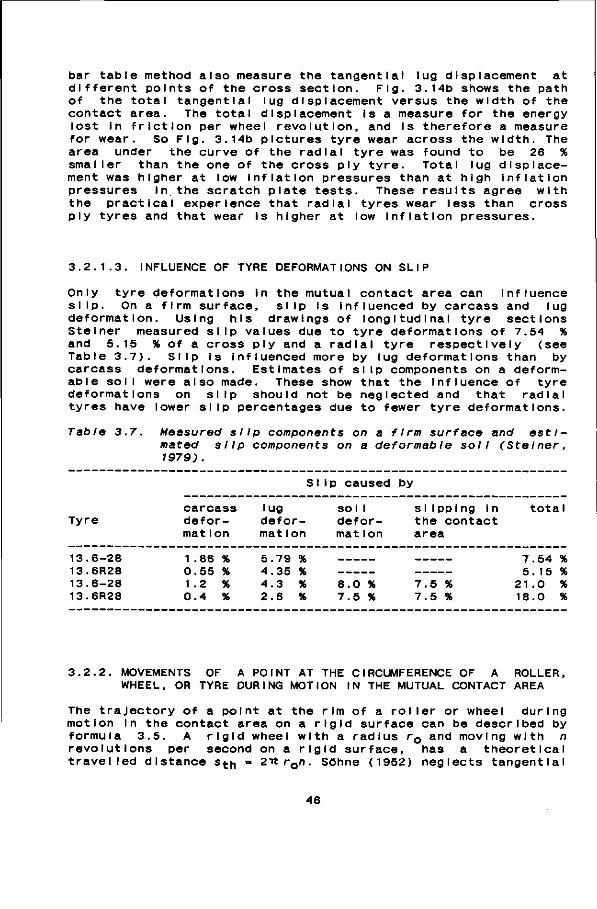
bar table method also measure the tangential lug displacement at different points of the cross section. Fig. 3.14b shows the path of the total tangential lug displacement versus the width of the contact area. The total displacement Is a measure for the energy lost In friction per wheel revolution, and Is therefore a measure for wear. So Fig. 3.14b pictures tyre wear across the width. The area under the curve of the radial tyre was found to be 26 % smaller than the one of the cross ply tyre. Total lug displacement was higher at low Inflation pressures than at high inflation pressures in the scratch plate tests. These results agree with the practical experience that radial tyres wear less than cross ply tyres and that wear is higher at low Inflation pressures.
3.2.1.3. INFLUENCE OF TYRE DEFORMATIONS ON SLIP
Only tyre deformations In the mutual contact area can Influence slip. On a f Irm surface, slip Is influenced by carcass and lug deformation. Using his drawings of longitudinal tyre sections Stelner measured slip values due to tyre deformations of 7.54 % and 5.15 % of a cross ply and a radial tyre respectively (see Table 3.7). Slip is influenced more by lug deformations than by carcass deformations. Estimates of slip components on a deform-able soil were also made. These show that the Influence of tyre deformations on slip should not be neglected and that radial tyres have lower slip percentages due to fewer tyre deformations.
Table 3.7. Measured slip components on a firm surface and estimated slip components on a deformable soll (Stelner, 1979).
Slip caused by
s I IppIng In totaI Tyre defor- defor- defor- the contact
area
carcass déformât Ion
1 .86 % 0.55 % 1 .2 % 0.4 %
lug déformât ion
5.79 % 4.35 % 4.3 % 2.6 %
sol I déformât Ion
8.0 % 7.5 %
13.6-28 1.86 % 5.79 % 7.54 % 13.6R28 0.55 % 4.35 % 5.15 % 13.6-28 1.2 % 4.3 % 8.0 % 7.5 % 21.0 % 13.6R28 0 . 4 % 2 . 6 % 7 . 5 % 7 . 5 % 1 8 . 0 %
3.2.2. MOVEMENTS OF A POINT AT THE CIRCUMFERENCE OF A ROLLER, WHEEL, OR TYRE DURING MOTION IN THE MUTUAL CONTACT AREA
The trajectory of a point at the rim of a roller or wheel during motion in the contact area on a rigid surface can be described by formula 3.5. A rigid wheel with a radius rQ and moving with n revolutions per second on a rigid surface, has a theoretical travelled distance s^n • 2ttr0n. Söhne (1952) neglects tangential
46
tyre deformations and therefore assumes that tyres only deform In the radial direction. The trajectory of a point at the circumference of a tyre on a deformable surface can now be written as:
x = r Q . ( 1 - Sfc) .<ut - r.slnÄ>t y m r0 - r.cosat [ 3 .10]
where, r = r0 - Sr
Sr = radial tyre deformation St = (s t n - s)/sth
When we take tangential deformation 6± Into account, the formulas change into:
x = r0.{^ - S^) .<»t - r.s\not + <ft.cosot
y = rQ - r.cosut - S^.s\nat [3.11]
The formulas for a point at the Inside of the tyre carcass are:
x = r Q . ( 1 - Sf.) .ot - ( r + h).sin<yt + <ft.cos<ut y = rQ - ( r + ri).cos<ut - <T t.sln»t [3 .12]
where, h = the distance between the Inside of the carcass and the lug face.
Stelner (1979) calculates the parameters of a point at the lug face as follows: starting with a point (X2.Y2) a t t n e Inside of the carcass, he assumes that the lug Is perpendicular to the line through the nearest measuring points (x^,y^) and (x3,y^) at the Inside of the carcass. There are measuring points at each 2.5 degrees. The direction of the lug Is:
tan eCL - (y3 - y^)/(xy - x3) So the parameters of a point at the lug face are:
X|_ = Xg - r».slncC|_ /l_ = y2 - rt.cos«|_ [3.13]
These calculations do not take the bending of the lugs Into account.
3.2.3. TRAJECTORIES OF SOIL PARTICLES IN THE CONTACT AREA BETWEEN THE SOIL AND A ROLLER, A WHEEL, OR A TYRE
Poletayev (1964) used the angle between the direction of the velocity vector and the radial at a point on a wheel rim to demarcate different zones in the wheel-soil interface. Theoretical analyses of tangential displacement of a soil particle at the rim circumference were made by JanosI (1962), Onafe-ko and Reece (1967), and Wong and Reece (1967a,1967b).
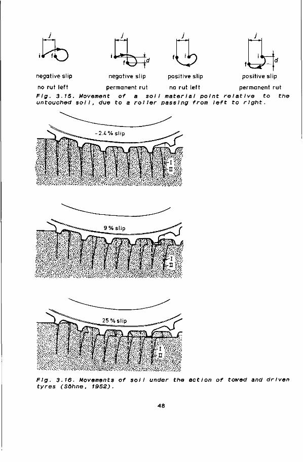
Wong (1967) determined the path of particles, on a clay soil, Influenced by a roller (Fig. 3.15). The particles were first pushed forward and up In a straight line by the oncoming roller. They were then shifted backwards In a circle. After the roller
47
negative slip
no rut left Fig. 3.15.
, u w %z> <Utc negative slip positive slip positive slip
permanent rut no rut left permanent rut Movement of a soil material point relative to the
untouched soil, due to a roller passing from left to right.
mm* •mmmmmmâÊÈmmM
mgm»ÈËËÊÊËÊmÊm
marl *$$$:;
Flg. 3.16. Movements of soil under the action of towed and driven tyres (Söhne, 1952).
48
had passed by the particles were at the same vertical level as in their Initial position because of the IncompressibI I Ity of the soli used. The final positions of soli surface particles were ahead of their initial positions when a towed roller was used, while the final positions of the particles were behind their Initial positions when a driven roller was used.
Söhne (1952) showed the trajectory of soil between the lugs of a tyre and of soli particles at the soli-lug Interface (See Fig. 3.16).
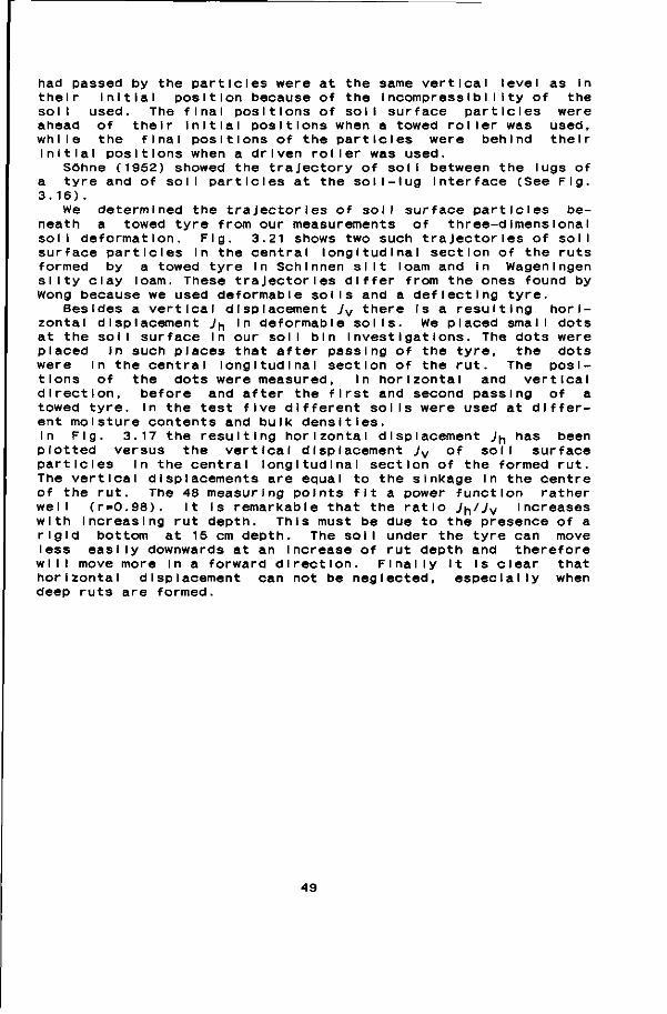
We determined the trajectories of soil surface particles beneath a towed tyre from our measurements of three-dimensional soli deformation. Fig. 3.21 shows two such trajectories of soil surface particles in the central longitudinal section of the ruts formed by a towed tyre in Schinnen silt loam and in Wagen Ingen sllty clay loam. These trajectories differ from the ones found by Wong because we used deformable soils and a deflecting tyre.
Besides a vertical displacement Jv there is a resulting horizontal displacement _/n In deformable soils. We placed small dots at the soil surface In our soil bin Investigations. The dots were placed in such places that after passing of the tyre, the dots were In the central longitudinal section of the rut. The positions of the dots were measured, In horizontal and vertical direction, before and after the first and second passing of a towed tyre. In the test five different soils were used at different moisture contents and bulk densities. In Fig. 3.17 the resulting horizontal displacement 7n has been plotted versus the vertical displacement Jv of soil surface particles In the central longitudinal section of the formed rut. The vertical displacements are equal to the sinkage In the centre of the rut. The 48 measuring points fit a power function rather well (r=0.98). It Is remarkable that the ratio Jn/Jy Increases with Increasing rut depth. This must be due to the presence of a rigid bottom at 15 cm depth. The soil under the tyre can move less easily downwards at an increase of rut depth and therefore
will move more in a forward direction. Finally It is clear that horizontal displacement can not be neglected, especially when deep ruts are formed.
49

o O-jp
20 i0
horizontal displacement j.
60 80 100 120 mm U0
T.
20
i.0 c <D
E
!0 60
80
mm
100
o«
• after f i rs t pass
o af ter second pass
- y v = 6 . 3 1 y h0 5 8 ( r=0.97)
Fig. 3.17. HorIzontal and vertical dIsplacement s of points at the soil surface In the wheel-centre plane.
50
3.3. SUBSURFACE MOVEMENTS
dimensional deformation already a projection of plane.
e two-dimensional movement Is the one under because of the absence of a sideward
wheel or a tyre can escape sideways In the central longitudinal
Is also possible to show the two-
The most simp nI te I y w i de roI Iers ment. Soll under a wheel or sideward transport does not exist section of the formed rut
Inf I-move-
This
In the cross section of the rut. This is a three-dimensional deformation on a flat
3.3.1. SOIL MOVEMENTS UNDER ROLLERS
When rollers are considered as true two-dimensional problem.
Infinitely wide rollers we have a
3.3.1.1 DISTRIBUTION OF A ROLLER
OF SOIL VELOCITIES RELATIVE TO THE CENTRE
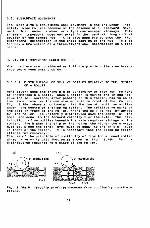
Wong (1967) used the principle of continuity of flow for rollers at Incompressible soils. When a roller is moving and In equilibrium the soil surface, after passing of this roller, has to be at the same level as the undisturbed soil In front of the roller. Fig. 3.18a shows a horizontal distribution of soil velocities under the centre of a slipping roller. The relative velocity of the soli In front of the roller, where the soli is not Influenced by the roller, Is uniformly distributed down the depth of the soli and equal to the forward velocity v of the axle. The distribution of velocities beneath the axle requires sinkage of the roller. The higher the slip of the roller the higher the sinkage must be. Since the final level must be equal to the initial level In front of the roller, It is necessary that the slipping roller affects rut recovery. The use of the principle of continuity of flow for a towed roller gives a velocity distribution as shown in Fig. 3.18b. Such a distribution requires no sinkage of the roller.
at positive slip at negative slip
Fig. 3. at Ions.
"act "act
18a,b. Velocity profiles deduced from contInulty conslder-
51
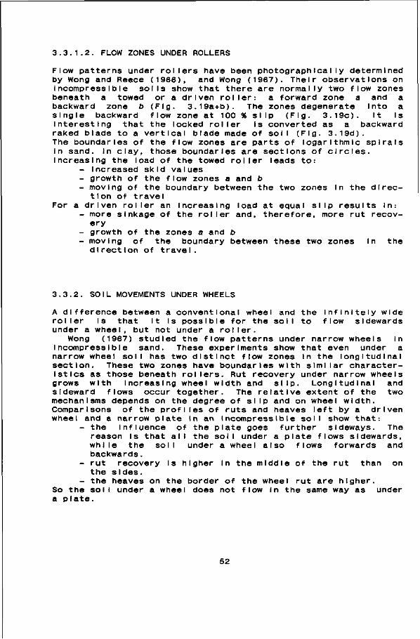
3.3.1.2. FLOW ZONES UNDER ROLLERS
Flow patterns under rollers have been photographically determined by Wong and Reece (1966), and Wong (1967). Their observations on Incompressible soils show that there are normally two flow zones beneath a towed or a driven roller: a forward zone a and a backward zone b (Fig. 3.19a+b). The zones degenerate Into a single backward flow zone at 100 % slip (Fig. 3.19c). It Is Interesting that the locked roller Is converted as a backward raked blade to a vert Ical blade made of sol I (Fig. 3.19d). The boundaries of the flow zones are parts of logarithmic spirals In sand. In clay, those boundaries are sections of circles. Increasing the load of the towed roller leads to:
- Increased skid values - growth of the flow zones a and b - moving of the boundary between the two zones in the direc
tion of travel For a driven roller an Increasing load at equal slip results In:
- more sinkage of the roller and, therefore, more rut recovery
- growth of the zones a and b - moving of the boundary between these two zones In the
direction of travel.
3.3.2. SOIL MOVEMENTS UNDER WHEELS
A difference between a conventional wheel and the Infinitely wide roller Is that It Is possible for the soil to flow sidewards under a wheel, but not under a roller.
Wong (1967) studied the flow patterns under narrow wheels in Incompressible sand. These experiments show that even under a narrow wheel soil has two distinct flow zones In the longitudinal section. These two zones have boundaries with similar characteristics as those beneath rollers. Rut recovery under narrow wheels grows with Increasing wheel width and slip. Longitudinal and sideward flows occur together. The relative extent of the two mechanisms depends on the degree of slip and on wheel width. Comparisons of the profiles of ruts and heaves left by a driven wheel and a narrow plate In an Incompressible soil show that:
- the Influence of the plate goes further sideways. The reason is that all the soil under a plate flows sidewards, while the soil under a wheel also flows forwards and backwards.
- rut recovery is higher In the middle of the rut than on the sides.
- the heaves on the border of the wheel rut are higher. So the soil under a wheel does not flow In the same way as under a plate.
52
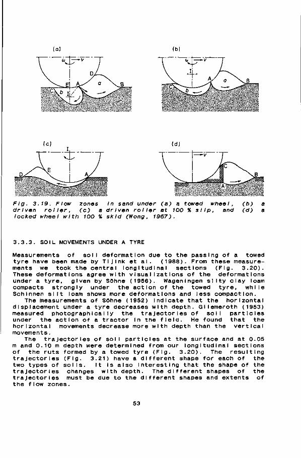
(a) (b)
Fig. 3.19. Flow zones In sand under (a) a towed wheel, (b) driven roller, (c) a driven roller at 100 % slip, and (d) locked wheel with 100 % skid (Wong, 1967).
3.3.3. SOIL MOVEMENTS UNDER A TYRE
Measurements of soil deformation due to the passing of a towed tyre have been made by Tij Ink et al. (1988). From these measurements we took the central longitudinal sections (Fig. 3.20). These deformations agree with visualizations of the deformations under a tyre, given by Söhne (1956). Wageningen sllty clay loam compacts strongly under the action of the towed tyre, while Schinnen silt loam shows more deformations and less compaction.
The measurements of Söhne (1952) Indicate that the horizontal displacement under a tyre decreases with depth. Gliemeroth (1953) measured photographically the trajectories of soil particles under the action of a tractor In the field. He found that the horizontal movements decrease more with depth than the vertical movements.
The trajectories of soil particles at the surface and at 0.05 m and 0.10 m depth were determined from our longitudinal sections of the ruts formed by a towed tyre (Fig. 3.20). The resulting trajectories (Fig. 3.21) have a different shape for each of the two types of soils. It is also Interesting that the shape of the trajectories changes with depth. The different shapes of the trajectories must be due to the different shapes and extents of the f low zones.
53
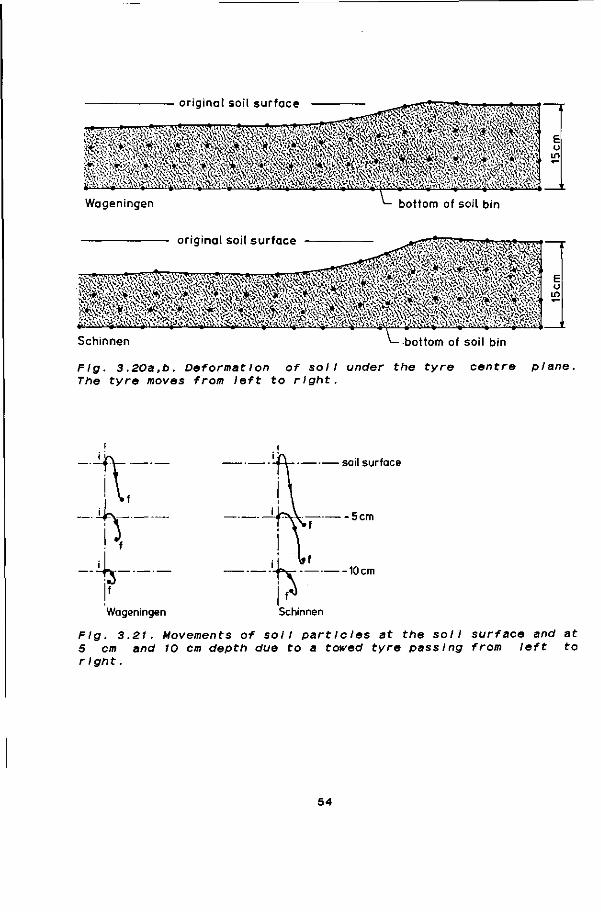
original soil surface
g.N^..,..! ........v.,.! T^,,..yt,.\ ^ . t ^ V ^ i y t ^ . . . . ^ . < r r , ^ , ... ..s, ..-..v.^.t..\ 4 ]
bottom of soil bin
Fig. 3.20a,b. Déformât Ion of soil under the tyre centre plane. The tyre moves from left to right.
soil surface
Wageningen
10 cm
Schinnen
Flg. 3.21. Movements of soil particles at the soil surface and at 5 cm and 10 cm depth due to a towed tyre passing from left to right.
54

CHAPTER 4
DYNAMIC ASPECTS OF LOAD-BEARING PROCESSES
4.1. FORCES, MOMENTS, AND STRESSES ON ROLLERS, WHEELS, AND TYRES
There are three forces and three moments acting from the ground on a tyre. Fx is the longitudinal, Fy is the cornering (-lateral), and Fz the normal component of the force from the ground to the tyre. The force Fv is important for steered wheels, but wi I I not be discussed in this chapter. The overturning moment 7"x Is the moment of force about the X-axis acting on the tyre from the road. The moment about the Y-axis is called rolling resistance moment 7V. Aligning torque 7"z is the moment about the Z-axI s acting on the tyre. A driving torque T about the rotation axis of the tyre produces a force that can accelerate or decelerate the vehicle.
4.1.1. MECHANICAL EQUILIBRIUM OF ROLLERS, WHEELS, AND TYRES
The forces, torques, and stresses acting on a roller, wheel, or tyre on a horizontal soil surface are illustrated In Fig. 4.1.
crn(9 Fig. (b)
4.1. Forces, a towed tyre,
crn(9)
torques, and stresses on (a) a driven roller, and (c) a driven tyre on deformatie soll.
55

Roller and rigid wheel The equilibrium of a stationary moving roller or rigid wheel on horizontal soil surface can be described by means of the following equations:
W = 51 vertical components of oj + vertical components ofrtf [4.1] P = Z horizontal ,, of <r. + horizontal ,, of x0 [4.2] T = £ r.Ti [4.3]
For a towed roller or wheel, Input torque T » 0 and, therefore, shear stresses must occur In forward as well as backward direction. The rolling resistance of a towed roller or wheel can be equalized to the towing force (equation 4.2). For a driven roller or wheel rolling resistance Is more complex and can be Illustrated by means of an energy balance:
Input = Output + Loss.
According to Corcoran (1979) energy components can be based on unit wheel travel and unit ground travel.
Based on unit wheel travel the components of the energy balance are :
Input = T/(r0.W) output = P(1-S)/W loss = rolling resistance energy = {T-P-re)IrQ.W
Based on unit ground travel the components are:
Input = r/[r0(1-S).W\ output = P/W loss » rolling resistance energy = (T-P.re)/re.W
PneumatIc tyres The equations for P and W are the same as those for rollers and wheels. Because of the tyre deflection the equation for T changes. Because of this deflection the normal stresses <r contribute to the torque T and the equation for the torque now becomes :
T = Y.r. (components of eg and T6 that are perpendicular to r ) .
Components of rolling res I stance Rolling resistance defines the total amount of energy lost and Is composed of several components:
- rut forming In the sol I - friction between the rolling device and the travelling sur
face caused by sliding - hysteresis in tyre materials due to deflections when the
tyre is roI I Ing - resistance due to air circulating Inside the tyre - fan effect of the rotating wheel on the outside air - friction of the wheel bearings.
The last three components are of secondary Importance and can be
56
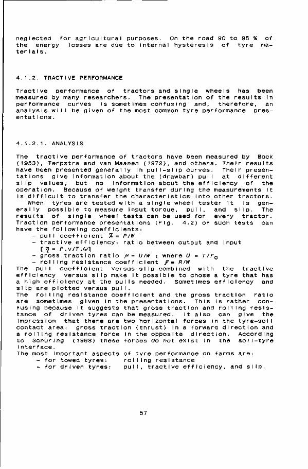
neglected for agricultural purposes. On the road 90 to 95 % of the energy losses are due to internal hysteresis of tyre mater I a I s .
4.1.2. TRACTIVE PERFORMANCE
Tractive performance of tractors and single wheels has been measured by many researchers. The presentation of the results in performance curves is sometimes confusing and, therefore, an analysis will be given of the most common tyre performance présentât ions.
4.1.2.1. ANALYSIS
The tractive performance of tractors have been measured by Bock (1953), Terpstra and van Maanen (1972), and others. Their results have been presented generally in pu I I-sI ip curves. Their presentations give information about the (drawbar) pull at different slip values, but no information about the efficiency of the operation. Because of weight transfer during the measurements It is difficult to transfer the characteristics Into other tractors.
When tyres are tested with a single wheel tester It Is general ly possible to measure input torque, pu I I, and si Ip. The results of single wheel tests can be used for every tractor. Traction performance presentations (Fig. 4.2) of such tests can have the following coefficients:
- pull coefficient %= P/W - tractive efficiency: ratio between output and input
[ -q = p.v/T.o] - gross traction ratio M - U/W -, where U = T/rQ - rolling resistance coefficient / = R/W
The pull coefficient versus slip combined with the tractive efficiency versus slip make it possible to chose a tyre that has a high efficiency at the pul Is needed. Sometimes efficiency and si Ip are plotted versus pul I . The rolling resistance coefficient and the gross traction ratio are sometimes given in the presentations. This is rather confusing because it suggests that gross traction and rolling resistance of driven tyres can be measured. It also can give the impression that there are two horizontal forces in the tyre-soil contact area: gross traction (thrust) in a forward direction and a rolling resistance force in the opposite direction. According to Schuring (1968) these forces do not exist in the soil-tyre Interface. The most important aspects of tyre performance on farms are:
- for towed tyres: rolling resistance - for driven tyres: pull, tractive efficiency, and slip.
57
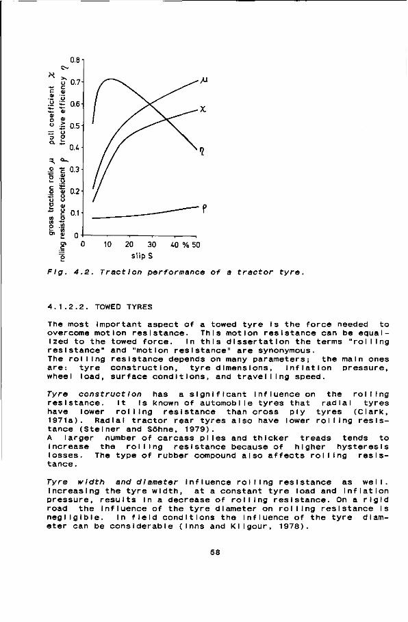
u
0.8
0.7
.ï ö
.y = 0.6 H « * - *•-«ê- Qt (V
o « ° ~ 0.5-= o => P o. iz
O.i.
3. ° -o o t _
c o ^ o o
V) in o L-Ol
<u u "Si o o 01
r o
Dl C
0.3
n?
0.1
0 10 20 30 i.0 % 50
'S s l ip S
Flg. 4.2. Tract Ion performance of a tractor tyre.
4.1.2.2. TOWED TYRES
The most important aspect of a towed tyre is the force needed to overcome motion resistance. This motion resistance can be equalized to the towed force. In this dissertation the terms "rolling resistance" and "motion resistance" are synonymous. The rolling resistance depends on many parameters; the main ones are: tyre construction, tyre dimensions. Inflation pressure, wheel load, surface conditions, and travelling speed.
Tyre construction has a significant Influence on the rolling resistance. It Is known of automobile tyres that radial tyres have lower rolling resistance than cross ply tyres (Clark, 1971a). Radial tractor rear tyres also have lower rolling resistance (Stelner and Söhne, 1979). A larger number of carcass piles and thicker treads tends to increase the rolling resistance because of higher hysteresis losses. The type of rubber compound also affects rolling resistance.
7"yre width and diameter influence rolling resistance as well. Increasing the tyre width, at a constant tyre load and Inflation pressure, results In a decrease of rolling resistance. On a rigid road the Influence of the tyre diameter on rolling resistance Is negligible. In field conditions the influence of the tyre diameter can be considerable (Inns and Kllgour, 1978).
58
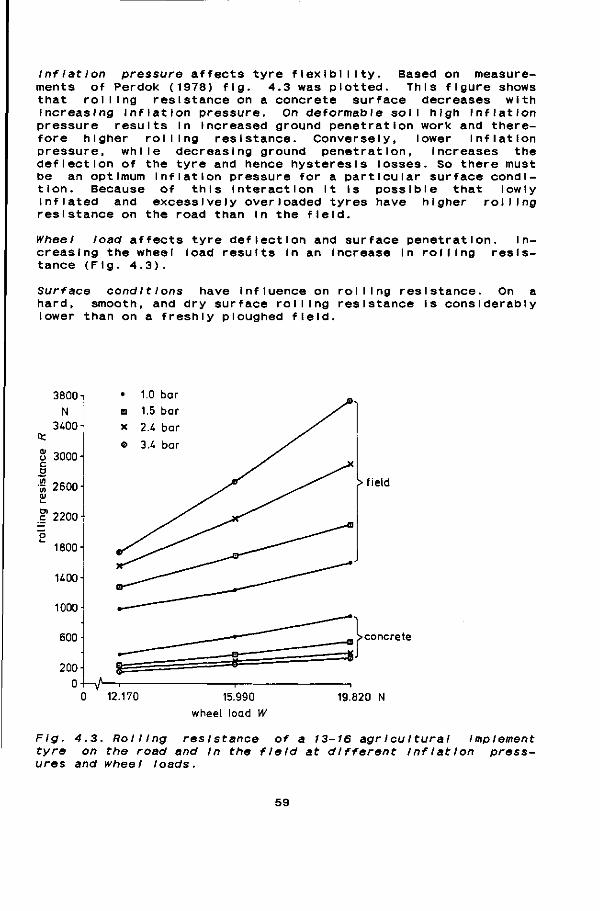
Inflation pressure affects tyre flexibility. Based on measurements of Perdok (1978) fig. 4.3 was plotted. This figure shows that rolling resistance on a concrete surface decreases with Increasing inflation pressure. On deformable soil high inflation pressure results In Increased ground penetration work and therefore higher rolling resistance. Conversely, lower Inflation pressure, while decreasing ground penetration, Increases the deflection of the tyre and hence hysteresis losses. So there must be an optimum inflation pressure for a particular surface condition. Because of this Interaction It is possible that lowly Inflated and excessively overloaded tyres have higher rolling resistance on the road than in the field.
Wheel load affects tyre deflection and surface penetration. Increasing the wheel load results In an Increase In rolling resistance (Fig. 4.3).
Surface conditions have influence on rolling resistance. On a hard, smooth, and dry surface rolling resistance Is considerably lower than on a freshly ploughed field.
ft: 01 o c o
VI 01
c
3800 N
3400
3000
2600
2200
1800-
K 0 0 -
1000
600
200-
o-l—y^
1.0 bar
> f ield
concrete
12.170 15.990
wheel load W
19.820 N
Fig. 4.3. Rolling reslstance of a 13-16 agricultural Implement tyre on the road and In the field at different Inflation pressures and wheel loads.
59
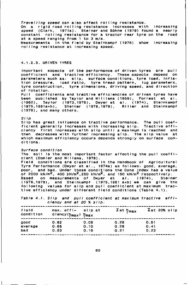
Travel IIng speed can also affect rolling resistance. On a rigid road rolling resistance Increases with Increasing speed (Clark, 1971a). Stelner and Söhne (1979) found a nearly constant rolling resistance for a tractor rear tyre on the road at a speed ranging from 1 to 3 m/s. Measurements In the field by Stelnkampf (1975) show Increasing rolling resistance at increasing speed.
4.1.2.3. DRIVEN TYRES
Important aspects of the performance of driven tyres are pull coefficient and tractive efficiency. These aspects depend on parameters such as: slip, surface conditions, tyre load, Inflation pressure, load ratio, tyre tread pattern, lug parameters, tyre construction, tyre dimensions, driving speed, and direction of rotation. Pull coefficients and tractive efficiencies of driven tyres have been published by Taylor and Williams (1959), Forrest et al. (1962), Taylor (1973,1976), Dwyer et al. (1974), Stelnkampf (1975,198la+b), Stelner (1978,1979), BI I 1er and Stelnkampf (1978), and many others.
SI lp Slip has great Influence on tractive performance. The pull coefficient generally Increases with Increasing slip. Tractive efficiency first Increases with slip until a maximum Is reached and then decreases with further Increasing slip. The slip value at which maximum efficiency occurs depends strongly on surface con-d11 ions.
Surface condltIon The soil Is the most important factor affecting the pull coefficient (Domler and WI I Iams, 1978). Field conditions are classified in the Handbook of Agricultural Tyre Performance (Dwyer et al., 1974a) as follows: good, average, poor, and bad. Under these conditions the Cone Index has a value of 2000 kN/m2, 400 kN/m2,250 kN/m2, and 150 kN/m2 respectively. Based on measurements of Dwyer et al. (1974), Steiner (1978,1979), and Stelnkampf (1975,1981 a+b) we can give the following values for slip and pull coefficient at maximum tractive efficiency under different field conditions (Table 4.1).
Table 4.1. Slip and pull coefficlent at maximum tractive efficiency and at 20 % slip.
field max. effl- slip at %aty)m&x %&*• 20% slip condition c lency (7?max) 7?max
0.08 0.28 0.51 0.10 0.28 0.41 0.16 0.21 0.23
60
good average bad
0.82 0.68 0.53

Tractive efficiency is highest on rigid surfaces and decreases with increasing deformabI I Ity of the soil surface. The pull coefficient also decreases with worsening surface conditions.
Tyre load Under good and generally results d11 ions there I s tlve performance.
average conditions Increasing the wheel load In better tractive performance. Under bad con-no significant Influence of wheel load on trac-
Tyre InfI at Ion pressure Under good and average conditions decreasing the Inflation pressure creates a larger contact area. This results In better tyre performance. At s Inkage due to high slip and under bad conditions the Influence of decreasing tyre Inflation is less because the tyre becomes more rigid in relation to the soil.
Load ratio The load ratio is the ratio of the wheel load to the maximum allowed wheel load. The load ratio can be increased by decreasing the tyre Inflation pressure or by Increasing the tyre load. Under good and average conditions Increasing the load ratio results In better tyre performance. This effect Is more Influenced by tyre Inflation than by wheel load (Fig. 4.4). Under worse conditions the Influence of the load ratio Is less clear.
56
%
53
a« 50-
o o
E •D
XI
E
i.7-
U
W=UkN
\ 0.8
0.75 barA
0.88 ba r /
1.05 b a r / / 11
16kN Z__—^-
>>. load ratio y=i.3
12 \
^rr?^^ \ / 1 . 0 IS.OKIN / 0 . 9 /
/ U 5 b a r ^-pj=1.2bar=cons
/ -W=18kN=constant
>.=1.75bar
6 7 8
medium pull P
kN 10
Flg. A.A. Median tractive performance of a 16.9-30 tractor rear tyre at several tyre load ratios. Load ratio (If) was changed by changing wheel load W (p/ = constant) or by changing Inf lat Ion pressure p/ (W « constant) (Stelner, 1978).
61
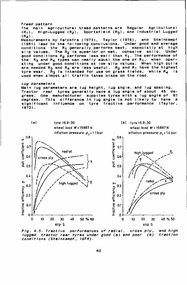
Tread pattern The main agrlcul (Rl), High-Lugged (Ft4) • Measurements by Te (1981) lead to the cond i 11 ons the R slip values. The good conditions R2 the R3 and R4 typ at Ing under good are needed R3 and tyre wear. R3 I s used when almost a
tural tread patterns are Regu (R 2 ), Sportsfleld (R3), and
rpstra (1973), Taylor (1976), following conclusions. Under
1 generally performs best, es R2 Is superior on wet, cohesI
performs less well than R-| . T es can nearly equal the one of conditions at low slip values. R4 are less useful. R2
intended for use on gra I traffic takes place
Iar Agrleu IturaI Industrial Lugged
and Stelnkampf good and average
pec I a I I y at hIgh ve sol Is. Under he performance of
'1 when oper-When hIgh pu I I s
and R] have the highest ss f le I ds, whI le R4 Is on the road.
Lug parameters Main lug parameters are lug height, lug angle, and lug spacing. Tractor rear tyres generally have a lug angle of about 45 degrees. One manufacturer supplies tyres with a lug angle of 67 degrees. This difference In lug angle Is not likely to have a significant Influence on tyre tractive performance (Taylor, 1973).
0.8
.1 0.7 u
8 0.6
o. 0.5
(a) tyre 16.9-30
wheel load W=15887N
inflation pressure :p- = 1.1 bar
0.4
0.3
ö 0.2
01
> °-1 o • ~ 0
10 20 30
slip S
40 50 % 60
(b) tyre 16.9-30
wheel load W= 15887 N
inflation p r e s s u r e ^ = 1.4 bar 0.8 -1
. Ï 0.7 o
o 0.6 H o
i . 0.5
0.4-
c« >, 0.3 u c <u '.Ü 0.2-1 a»
> aH u o - 0
0 10 20 30
slip S
Flg. 4.5. Tractive performances of radial, cross ply, lugged tractor rear tyres under good (a) and poor (b) condltIons (Stelnkampf, 1974).
40 % 50
and high tract Ion
62
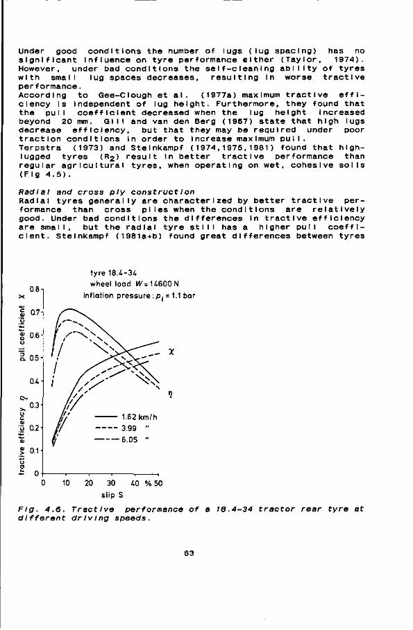
Under good conditions the significant Influence on ty However, under bad condItI with small lug spaces dec performance. According to Gee-Clough e clency Is independent of lu the pull coefficient deer beyond 20 mm. Gill and va decrease efficiency, but traction conditions in orde Terpstra (1973) and Stelnk lugged tyres (R2) result regular agricultural tyres, (Fig 4.5).
number of lugs (lug spacing) has no re performance either (Taylor, 1974). ons the self-cleaning ability of tyres reases, resulting In worse tractive
t al. (1977a) maximum tractive effl-g height. Furthermore, they found that eased when the lug height increased n den Berg (1967) state that high lugs that they may be required under poor r to increase maximum pull, ampf (1974,1975,1981) found that high-in better tractive performance than when operating on wet, cohesive soils
Radial and cross ply construct Ion Radial tyres generally are characterized by better tractive performance than cross plies when the conditions are relatively good. Under bad conditions the differences In tractive efficiency are small, but the radial tyre still has a higher pull coefficient. Steinkampf (1981a+b) found great differences between tyres
0.8
S 0.6-I u
o. 0.5-
0.4
o c <v ;Ö 0.2-"oi
I 0. o o £ 0
tyre 18.4-34
wheel load W= 14600 N
inflation pressure : p j = 1.1 bar
1.62 km/h
3.99 " 6.05 "
0 10 20 30 40 % 50
slip S
Flg. 4.6. Tractive performance of a 18.4-34 tractor rear tyre at different driving speeds.
63
in the groups of radiais and cross piles as well. The tractive performance of a good radial tyre can be 25 % better than the one of a bad cross ply; on the other hand, the tractive performance of a good cross ply can be as much as 14 % better than the one of a bad radial one.
Tyre diameter and width Increasing the diameter and Increasing the width both result In a small Improvement of tractive performance. The effect of width Is more pronounced than the effect of diameter.
Driving speed Under poor driving conditions Steinkampf (1975) measured the performance of a 18.4-34 tractor rear tyre at driving speeds of 1.62, 3.99 and 6.05 km/h. An Increase In speed resulted In a decrease of pull coefficient and tractive efficiency (Fig. 4.6). These results only show a tendency and they need to be proved for tyres driven at higher speeds and under better field conditions.
DlrectIon of rotation Sometimes the direction of the rotation of front tyres of four-wheel drive tractors Is reversed In order to decrease tyre wear. Reversed rotation direction results In a longer life of the front tyres when much road travel Is done (Blller, 1983). B M I er and Stelnkampf (1978) found that the direction of rotation hardly Influenced tractive performance under good driving conditions. Under less Ideal conditions the performance of the reversed tyres decreased. The choice between low front tyre wear (reversed mounting) and best tractive performance under bad conditions (normal mounting) will depend on the use of the tractor.
Tyre wear Tyre wear results In a decrease of lug height and an Increase In the area of the lug faces. Therefore, on dry roads tyre performance Increases with Increasing tyre wear. In the field starting tyre wear has no pronounced Influence on tractive performance. When driving conditions are poor tyre wear can result In a worse performance.
4.1.2.4. TRACTOR TRACTIVE PERFORMANCE
Tractive performance depends on the tractor type, the traction properties of the tyres, the weight, and the surface conditions.
Tractor type The tractor type Includes the number of driven axles and weight distribution. There are 4 tractor types available:
- TWD : a two-wheel drive tractor with driven rear tyres and towed front tyres
- FWDa : a four-wheel drive tractor with driven front tyres that are smaller In diameter and width compared to the driven rear tyres
64
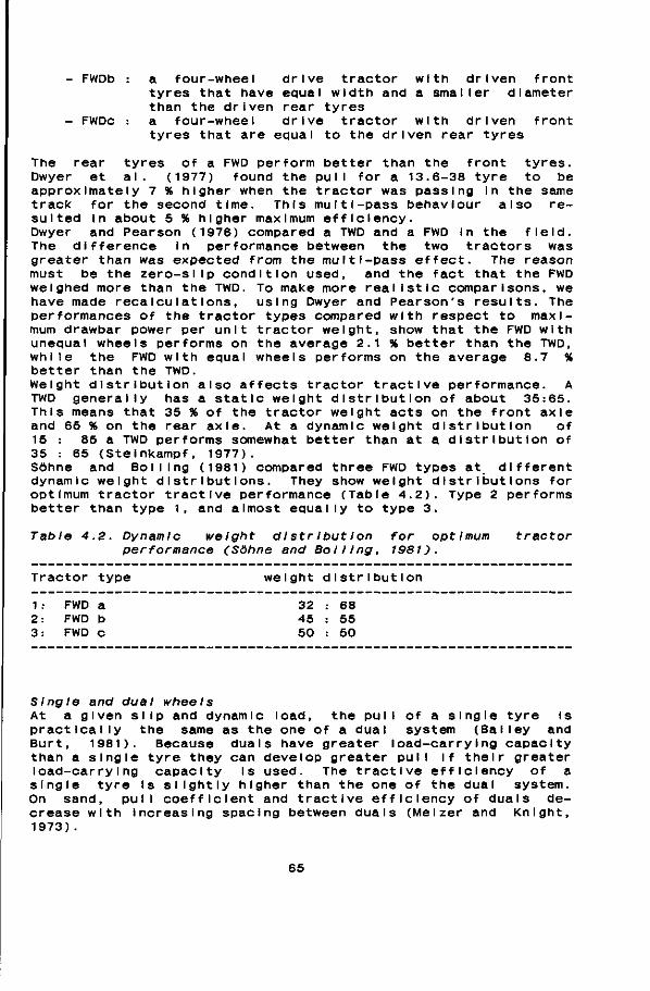
- FWDb : a four-wheel drive tractor with driven front tyres that have equal width and a smaller diameter than the driven rear tyres
- FWDc : a four-wheel drive tractor with driven front tyres that are equal to the driven rear tyres
The rear tyres of a FWD perform better than the front tyres. Dwyer et al. (1977) found the pull for a 13.6-38 tyre to be approximately 7 % higher when the tractor was passing In the same track for the second time. This multi-pass behaviour also resulted in about 5 % higher maximum efficiency. Dwyer and Pearson (1976) compared a TWD and a FWD In the field. The difference In performance between the two tractors was greater than was expected from the multi-pass effect. The reason must be the zero-slip condition used, and the fact that the FWD weighed more than the TWD. To make more realistic comparisons, we have made recalculations, using Dwyer and Pearson's results. The performances of the tractor types compared with respect to maximum drawbar power per unit tractor weight, show that the FWD with unequal wheels performs on the average 2.1 % better than the TWD, while the FWD with equal wheels performs on the average 8.7 % better than the TWD. Weight distribution also affects tractor tractive performance. A TWD generally has a static weight distribution of about 35:65. This means that 35 % of the tractor weight acts on the front axle and 65 % on the rear axle. At a dynamic weight distribution of 15 : 85 a TWD performs somewhat better than at a distribution of 35 : 65 (Steinkampf, 1977). Söhne and Bolling (1981) compared three FWD types at different dynamic weight distributions. They show weight distributions for optimum tractor tractive performance (Table 4.2). Type 2 performs better than type 1, and almost equally to type 3.
Table A.Z. Dynamic weight dlstrI but I on for optimum tractor performance (Sohne and Boiling, 1981).
Tractor type weight distribution
1 : 2: 3:
FWD FWD FWD
a b c
32 45 50
68 55 50
Single and dual wheels At a given slip and dynamic load, the pull of a single tyre Is practically the same as the one of a dual system (Bailey and Burt, 1981). Because duals have greater load-carrying capacity than a single tyre they can develop greater pull If their greater load-carrying capacity Is used. The tractive efficiency of a single tyre is slightly higher than the one of the dual system. On sand, pull coefficient and tractive efficiency of duals decrease with increasing spacing between duals (Melzer and Knight, 1973).
65

Weight Many researchers give formulas for the optimum ratio of weight to available power (Table 4.3).
Table 4.3. Weight to power ratio for optimum tractor tractive performance.
tractor
TWD FWD FWD TWD and TWD and TWD
type
FWD FWD
formula
W/Pe . 1 W/Pe = 0 W&/P - 1 W&/P - 1 W&/P - 1 W/Pe = 1
17/v 82/v
.50/v
.33/v
.79/v
.2/v
references
Reece (1970) Reece (1970) Br Ixlus and Zoz (1976) Hofman (1977) Dwyer (1978) Melborg and Perdok (1979)
P « power available for a driven axle (kW)
W engine power (kW) tractor weight (kN)
v m driving speed (m/s) W. - weight on driven axle (kN)
We can see from these formulas th ratio a TWD needs a higher velocl formance. The drawback of all t valid under one particular condI formulas take Into account the Inf tl ons on the weight needed for opt of slip on the weight to power rat (1975).
To calculate the optimum weigh field conditions, velocities, an to use a more detailed formula:
at at the same weight to power ty than a FWD for optimum per-hese formulas Is that they are tlon only. Neither do those luence of slip and field condI -imum performance. The Influence lo has been shown by Stelnkampf
t to power ratio for different d tractor types It Is necessary
+ Pr + P, [4.4]
where, *t = 3t -Pf = Pr -
effective engine power (kW) transmission power [Pt - (1-7?t)Pe] transmission efficiency front axle power (kW) rear axle power (kW)
For a TWD this formula changes into:
n - 7t>pe + F-Wf-V + 7.wr.v
[4.5]
where, ƒ> - rolling resistance coefficient Wf - dynamic front axle load (kN) Wr - dynamic rear axle load (kN) v - velocity % = pull coefficient n - tractive efficiency
66

For a FWD f o r m u l a 4 . 4 . c h a n g e s into:
1 ?1 ?2
where, X-\ = pull c o e f f i c i e n t 1st p a s s 22. = pu I I c o e f f i c i e n t 2nd p a s s 7?1 = t r a c t i v e e f f i c i e n c y 1st p a s s 7j2 = tractive efficiency 2nd pass
Calculations of optimum tractor - tillage Implement combinations have been presented by Jahns and Stelnkampf (1982), and Schäfer(1983).
For optimum performance the ratio of weight on driving axle to engine power generally lies under 900 N/kW. Tractors available In the Netherlands generally have a tractor weight to engine power ratio between 500 and 700 N/kW. About two thirds of the weight of a TWD acts on the rear axle. At the often used ploughing velocities of 5 to 7 km/h the standard available weight to power ratio Is not optimal. Therefore, the transfer as well as the adding of
weight are important for optimum tractive performance during ploughing operations. The ratio W&/Pe can also be enlarged by ballasting weights and filling the tyres with water.
When the tractor is driven In the furrow when the ploughing Is done with a mouldboard plough, the largest allowed tyre width Is 13.6, 16.9, or 18.4 Inches depending on ploughing width. Therefore, the load-carrying capacity of the rear tyres determines up to which engine power TWD can be used and when FWD Is needed for optimum performance. Table 4.4 shows the maximum TWD engine power that can be used for different tyre sizes and at certain weight to power ratios. The maximum power at a load to power ratio of W a / P e = 900 N/kW is also the heaviest TWD that can be loaded to 900 N/kW.
Table 4.4. Maximum allowed engine power (kW) of TWD at different levels of weight to power ratio for 3 tyre sizes. InfI at Ion pressure 1.0 bar; load ratio 120 %.
weight to power ratio Wa/Pe N/kW
Tyre Size 600 700 800 900
13.6-38 16.9-30 16.9-38 18.4-30 18.4-38
51 66 74 80 90
44 56 63 69 77
38 49 55 60 68
34 44 49 53 60
67
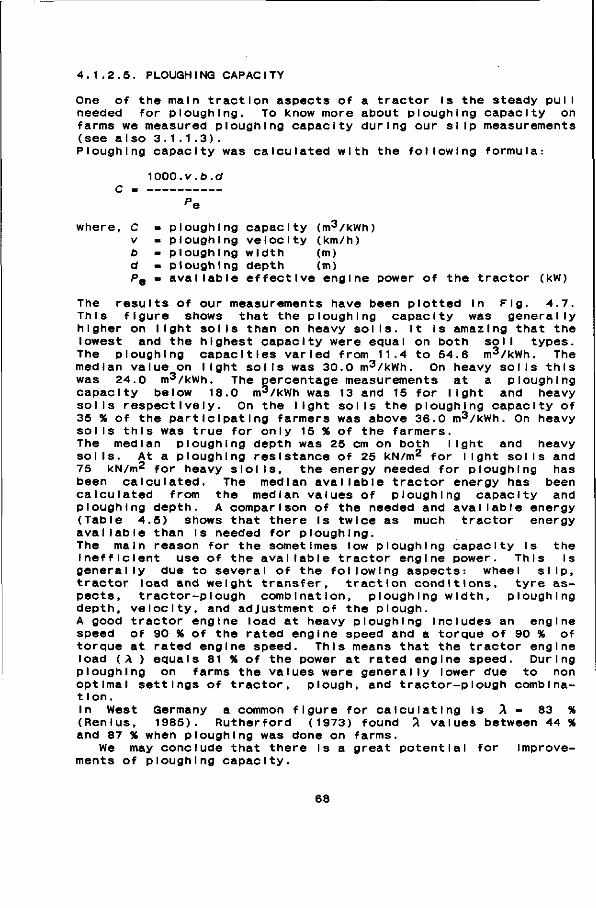
4.1.2.5. PLOUGHING CAPACITY
One of the main traction aspects of a tractor is the steady pull needed for ploughing. To know more about ploughing capacity on farms we measured ploughing capacity during our slip measurements (see also 3.1.1.3). Ploughing capacity was calculated with the following formula:
C = ^000.v.b.d
where, C • ploughing capacity (m3/kWh) v - ploughing velocity (km/h) b - ploughing width (m) d - ploughing depth (m) P e - available effective engine power of the tractor (kW)
The results of our measurements have been plotted in Fig. 4.7. This figure shows that the ploughing capacity was generally higher on light soils than on heavy soils. It Is amazing that the lowest and the highest capacity were equal on both soil types. The ploughing capacities varied from 11.4 to 54.6 m3/kWh. The median value on light soils was 30.0 m3/kWh. On heavy soils this was 24.0 m3/kWh. The percentage measurements at a ploughing capacity below 18.0 m3/kWh was 13 and 15 for light and heavy soils respectively. On the light soils the ploughing capacity of 35 % of the participating farmers was above 36.0 m3/kWh. On heavy soils this was true for only 15 % of the farmers.
The median ploughing depth was 25 cm on both light and heavy soils. At a ploughing resistance of 25 kN/m2 for light soils and 75 kN/m2 for heavy s lol Is, the energy needed for ploughing has been calculated. The median available tractor energy has been calculated from the median values of ploughing capacity and ploughing depth. A comparison of the needed and available energy (Table 4.5) shows that there Is twice as much tractor energy available than is needed for ploughing. The main reason for the sometimes low ploughing capacity Is the Inefficient use of the available tractor engine power. This Is generally due to several of the following aspects: wheel slip, tractor load and weight transfer, traction conditions, tyre aspects, tractor-plough combination, ploughing width, ploughing depth, velocity, and adjustment of the plough. A good tractor engine load at heavy ploughing Includes an engine speed of 90 % of the rated engine speed and a torque of 90 % of torque at rated engine speed. This means that the tractor engine load (A ) equals 81 % of the power at rated engine speed. During ploughing on farms the values were generally lower due to non optimal settings of tractor, plough, and tractor-plough combination. In West Germany a common figure for calculating Is A - 83 % (Renlus, 1985). Rutherford (1973) found A values between 44 % and 87 % when ploughing was done on farms.
We may conclude that there Is a great potential for Improvements of ploughing capacity.
68
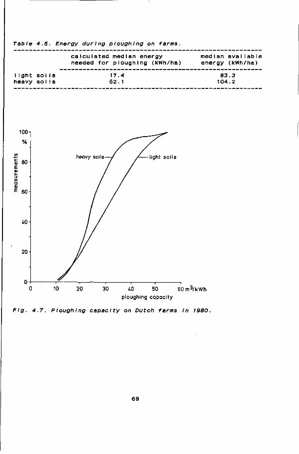
Table 4.5. Energy during ploughing on farms.
calculated median energy needed for ploughing (kWh/ha)
med Ian aval I ab I e energy (kWh/ha)
I Ight so I I s heavy sol I s
1 7 . 4 5 2 . 1
8 3 . 3 1 0 4 . 2
100
%
vi
£ 80 E ai t-D (A O ai E 60
40-
20
heavy soils ight soi ls
0 10 20 30 i.0 50 60m3 /kWh
ploughing capacity
Fig. 4.7. Ploughing capacity on Dutch farms In 1980.
69

4.2. STRESSES IN THE CONTACT AREA
Radial (normal) stresses and tangential (shear) stresses general Iy occur in the contact area between the sol I and a towed or drIven devIce. Stresses can be measured by making use of pressure transducers In the soil or by pressure cells embedded In the wheel periphery. The disadvantage of using pressure transducers in the soil Is that they can move during the compacting process and, therefore, can provide erroneous information. All researchers referred to In section 4.2 have used pressure cells embedded In the wheel periphery .
4.2.1 STRESSES OR ROLLER
IN THE CONTACT AREA BETWEEN SOIL AND RIGID WHEEL
Hegedus (1965) measured normal stress distribution in the so I I-wheel Interface and the influence of wheel load and slip on this distribution (Fig. 4.8). The distribution of both normal and shear stresses In the soil-wheel Interface has been measured by Onafeko and Reece (1967) and Krlck (1969). Wong and Reece (1967a,1967b) and Wong (1967,1978) relate stress distribution to flow zones beneath rollers and wheels.
(b)
S = 100% IV=227N W=45£N
W=680N
W=907N
Fig. 4.8. Normal pressure dlstrI but Ions under a wheel on dry sand. (a) non-slip with load as parameter (b) constant load with slip as parameter.
70
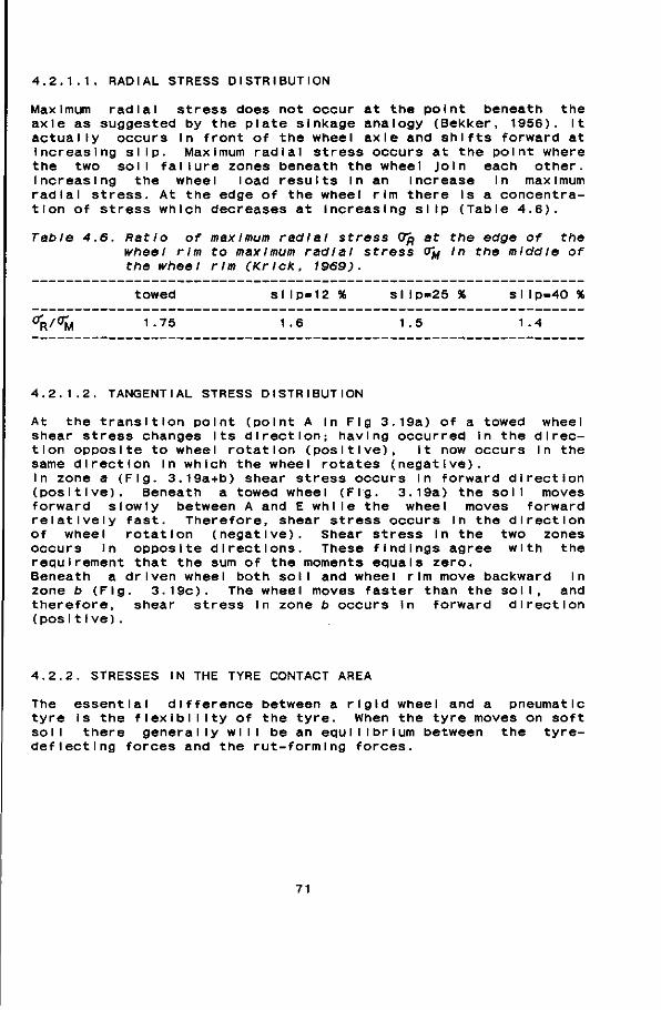
4.2.1.1. RADIAL STRESS DISTRIBUTION
Maximum radial stress does not occur at the point beneath the axle as suggested by the plate slnkage analogy (Bekker, 1956). It actually occurs In front of the wheel axle and shifts forward at Increasing slip. Maximum radial stress occurs at the point where the two soil failure zones beneath the wheel Join each other. Increasing the wheel load results In an Increase In maximum radial stress. At the edge of the wheel rim there Is a concentration of stress which decreases at Increasing slip (Table 4.6).
Table 4.6. Ratio of maximum radial stress OR at the edge of the wheel rim to maximum radial stress Vy In the middle of the wheel rim (Krlck, 1969).
towed
1 .75
silp=12 %
1 .6
Silp=25 %
1 .5
Sllp=40 %
1 .4 V^M
4.2.1.2. TANGENTIAL STRESS DISTRIBUTION
At the transition point (point A In Fig 3 shear stress changes Its direction; having tlon opposite to wheel rotation (positive) same direction In which the wheel rotates In zone a (Fig. 3.19a+b) shear stress occu (positive). Beneath a towed wheel (Fig. forward slowly between A and E while the relatively fast. Therefore, shear stress of wheel rotation (negative). Shear st occurs In opposite directions. These fi requirement that the sum of the moments eq Beneath a driven wheel both soil and whee zone b (Fig. 3.19c). The wheel moves fas therefore, shear stress In zone b occurs (pos 11 ive).
.19a) of a towed wheel occurred In the dI réc
it now occurs In the (negatIve). rs In forward direction
3.19a) the soil moves wheel moves forward
occurs In the direction ress In the two zones ndlngs agree with the uaI s zero.
rlm move backward In ter than the soil, and
in forward direction
4.2.2. STRESSES IN THE TYRE CONTACT AREA
The essential difference between a rigid wheel and a pneumatic tyre Is the flexibility of the tyre. When the tyre moves on soft soil there genera Ily wiI I be an equilibrium between the tyre-deflecting forces and the rut-forming forces.
71

wh
I n
e r e , Pm W A
t e r r a
4.2.2.1. AVERAGE CONTACT PRESSURE
Average contact pressure Is defined as : p m = W/A [4.7]
= average contact pressure = vertical wheel load = area of the tyre-road Interface mechanics this average contact pressure Is often given
as sum of tyre Inflation pressure p\ and a pressure p c for carcass stI f fness :
p m - p, + p c [4.8]
Average contact pressure on a rigid surface This pressure depends on Inflation pressure, wheel load, and tyre parameters. An Increase In Inflation pressure (at a constant wheel load) results In a decrease of carcass stiffness pressure p c . An Increase in wheel load (at a constant P|) results In a small increase in p c (Söhne, 1952). The dynamic contact area of a tyre Is larger than the static contact area (Van den Berg and Gill, 1962). Tractor tyres with a closed centre tread have a higher average contact pressure than tyres with an open centre tread (Söhne, 1952) . Kriek (1969) tested smooth tractor rear tyres, at nominal wheel load, over an Inflation pressure range from 0.6 to 2.0 bar. He found a constant carcass stiffness pressure p c of about 0.45 bar. Steiner and Söhne (1979) tested several lugged tractor rear tyres of different sizes and construction. They found the following empirical equations for the average contact pressure:
Cross ply tractor rear tyres: pm = 1.128 + 0 .665p | + 0.0091? - 0.004D [ 4 . 9 ]
Radial tractor rear tyres: pm = 2 .677 + 0 . 575p | + 0.0111V - 0.016D [ 4 . 1 0 ]
where, p m = average contact pressure (bar) P| = tyre inflation pressure (bar) W = wheel load (kN) D = tyre diameter (cm).
Average contact pressure on deformable soil Contact pressure Is generally smaller on deformable soli than on a rigid surface because the contact area Is enlarged when ruts are formed. When a tyre passes In a track for the second time wheel slnkage Is generally lower than when It does so In the first pass. When the tyre passes for the second time the contact area Is smaller and the average contact pressure is therefore higher than when the tyre passes for the first time. Average contact pressure on deformable soil can be remarkably lower than Inflation pressure (Baganz and Kunath, 1963; Söhne 1952 and 1963). Formula 4.8. is therefore not very useful for
72
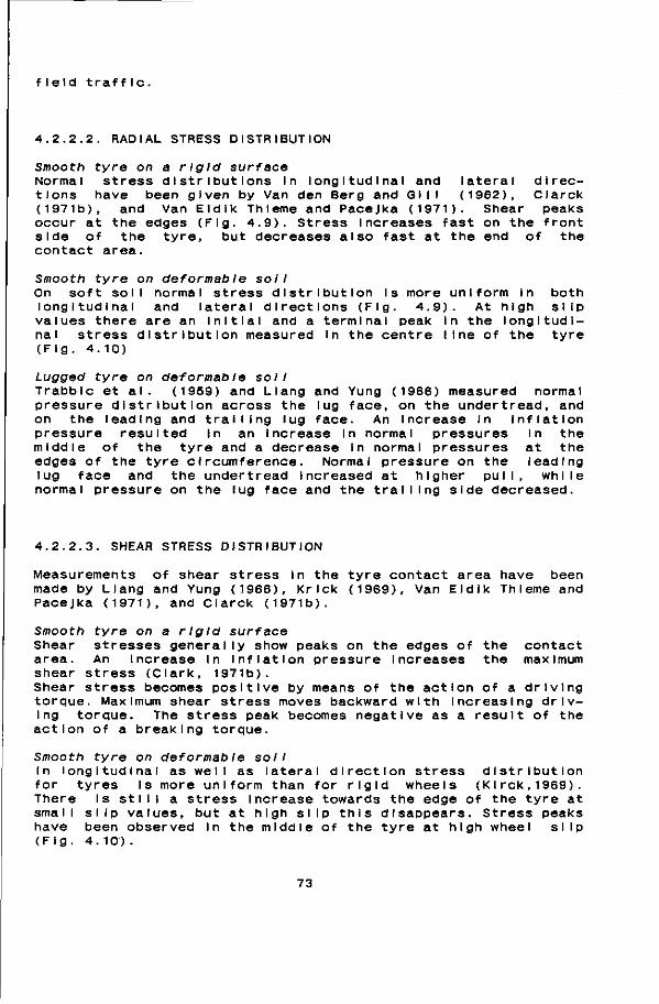
field traf f le.
4.2.2.2. RADIAL STRESS DISTRIBUTION
Smooth tyre on a rigid surface Normal stress distributions In longitudinal and lateral directions have been given by Van den Berg and Gill (1962), Clarck (1971b), and Van EIdIk Thleme and Pacejka (1971). Shear peaks occur at the edges (Fig. 4.9). Stress Increases fast on the front side of the tyre, but decreases also fast at the end of the contact area.
Smooth tyre on deformable soil On soft soil normal stress distribution Is more uniform In both longitudinal and lateral directions (Fig. 4.9). At high slip values there are an initial and a terminal peak In the longitudinal stress distribution measured In the centre line of the tyre (Fig. 4.10)
Lugged tyre on deformable soil Trabblc et al. (1959) and Liang and Yung (1966) measured normal pressure distribution across the lug face, on the undertread, and on the leading and trailing lug face. An increase In inflation pressure resulted in an increase In normal pressures In the middle of the tyre and a decrease In normal pressures at the edges of the tyre circumference. Normal pressure on the leading lug face and the undertread Increased at higher pull, while normal pressure on the lug face and the trailing side decreased.
4.2.2.3. SHEAR STRESS DISTRIBUTION
Measurements of shear stress In the tyre contact area have been made by Liang and Yung (1966), Krlck (1969), Van Eldik Thleme and Pacejka (1971), and Clarck (1971b).
Smooth tyre on a rigid surface Shear stresses generally show peaks on the edges of the contact area. An Increase in Inflation pressure Increases the maximum shear stress (Clark, 1971b). Shear stress becomes positive by means of the action of a driving torque. Maximum shear stress moves backward with Increasing driving torque. The stress peak becomes negative as a result of the action of a breaking torque.
Smooth tyre on deformable soil In longitudinal as well as lateral direction stress distribution for tyres Is more uniform than for rigid wheels (KIrck,1969). There Is still a stress Increase towards the edge of the tyre at small slip values, but at high slip this disappears. Stress peaks have been observed In the middle of the tyre at high wheel slip (Fig. 4.10).
73
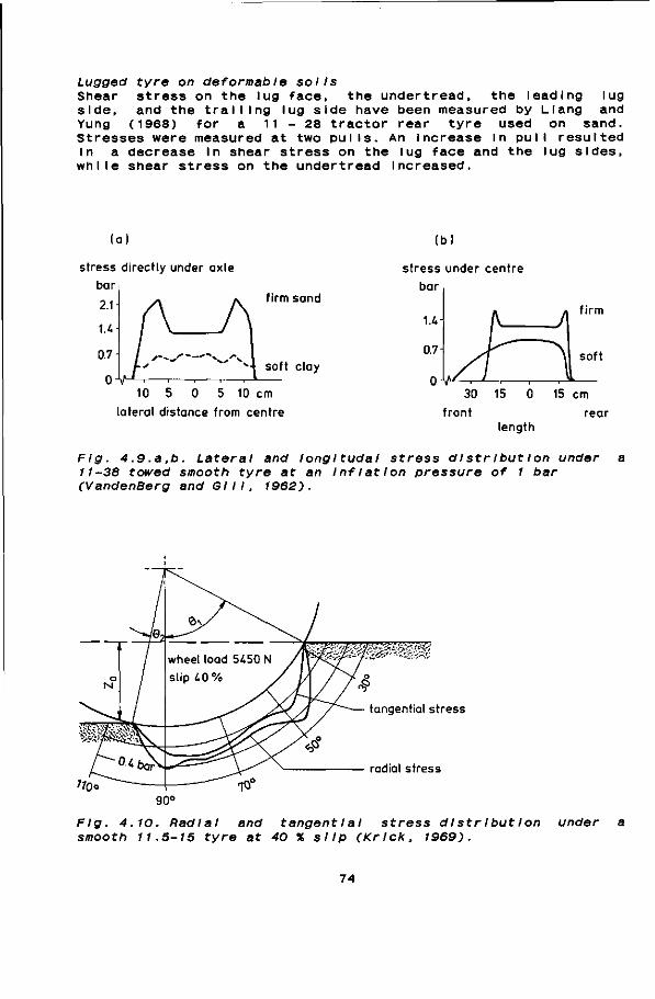
Lugged tyre on deformable soils Shear stress on the lug face, the undertread, the leading lug side, and the trailing iug side have been measured by Liang and Yung (1968) for a 1 1 - 2 8 tractor rear tyre used on sand. Stresses were measured at two pulls. An increase In pull resulted In a decrease in shear stress on the lug face and the lug sides,
while shear stress on the undertread Increased.
(a) (b)
stress directly under axle
bar
2.1-
1.4-
0.7
0
• - - „ ' ' - N . ."
firm sand
soft clay
10 5 0 5 10 cm
lateral distance from centre
stress under centre
bar
U
0.7
A
Jr 30 15 0
f ront length
A f i rm
>°" 15 cm
rear
Fig. 4.9.a.b. Lateral and longltudal stress dlstrIbutIon under a 11-38 towed smooth tyre at an InfI at Ion pressure of 1 bar (VandenBerg and Gill, 1962).
tangential stress
radial stress
Fig. 4.10. Radial and tangent Ial stress dlstrIbutIon smooth 11.5-15 tyre at 40 % slip (Krlck, 1969).
under
74
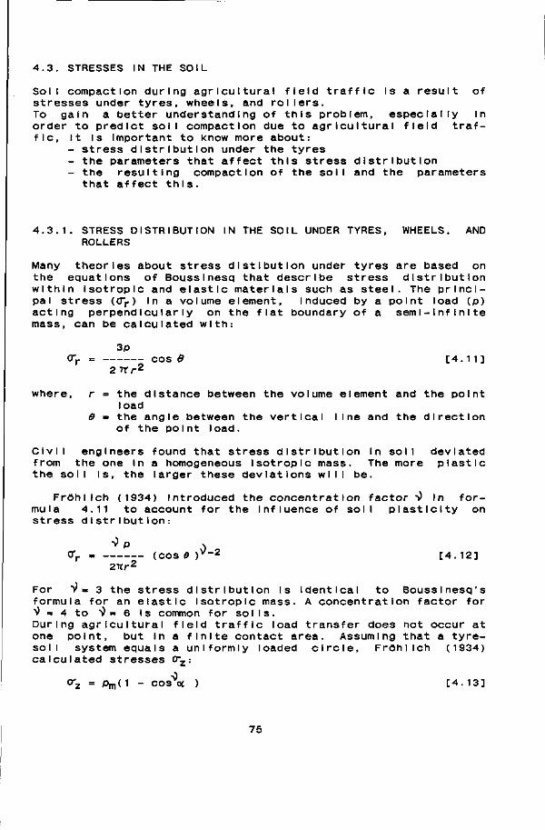
4.3. STRESSES IN THE SOIL
Soll compaction during agricultural field traffic Is a result of stresses under tyres, wheels, and rollers. To gain a better understanding of this problem, especially In order to predict soil compaction due to agricultural field traffic, It Is Important to know more about:
- stress distribution under the tyres - the parameters that affect this stress distribution - the resulting compaction of the soil and the parameters
that affect this.
4.3.1. STRESS DISTRIBUTION IN THE SOIL UNDER TYRES, WHEELS, AND ROLLERS
Many theories about stress dlstlbutlon under tyres are based on the equations of Bousslnesq that describe stress distribution within Isotropic and elastic materials such as steel. The principal stress (<Tr) In a volume element, Induced by a point load (p) acting perpendicularly on the flat boundary of a semI - InfInI te mass, can be calculated with:
3p <rr = cos 6 [4.11]
2TTr2
where, r = the distance between the volume element and the point load
8 - the angle between the vertical line and the direction of the point load.
Civil engineers found that stress distribution In soil deviated from the one In a homogeneous Isotropic mass. The more plastic the soil Is, the larger these deviations will be.
Fröhlich (1934) Introduced the concentration factor T) In formula 4.11 to account for the Influence of soil plasticity on stress distribution:
IP N Crr » (COS 9 ) V " 2 [ 4 . 1 2 ]
2K r 2
For V = 3 the stress distribution Is Identical to Bousslnesq's formula for an elastic Isotropic mass. A concentration factor for •v = 4 to ~i = 6 Is common for soils. During agricultural field traffic load transfer does not occur at one point, but in a finite contact area. Assuming that a tyre-soil system equals a uniformly loaded circle, Fröhlich (1934) calculated stresses crz:
°z - %i<1 - cos'3« ) [4.13]
75
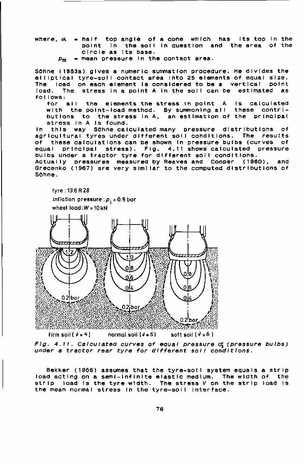
where, oc - half top angle of a cone which has Its top in the point In the soil In question and the area of the circle as Its base.
pm = mean pressure In the contact area.
Söhne (1953a) gives a numer elliptical tyre-soil contac The load on each element load. The stress In a poi fo I lows :
for a I I the elements with the point-load met butions to the stress stress In A Is found.
In this way Söhne calcul agricultural tyres under di of these calculations can equal principal stress), bulbs under a tractor tyre Actually pressures measur Grecenko (1967) are very si Söhne.
c summation procedure. He divides the t area Into 25 elements of equal size, is considered to be a vertical point nt A In the soil can be estimated as
the stress in point A is calculated hod. By summoning all these contrl-In A, an estimation of the principal
ated many pressure distributions of fferent soil conditions. The results be shown In pressure bulbs (curves of
Fig. 4.11 shows calculated pressure for different soil conditions, ed by Reaves and Cooper (1960), and mllar to the computed distributions of
t y re : 13.6 R 28
inflation press
wheel load:W = 10kN
inflation pressure : p , = 0.9 bar
f i rm soil ( >> = 4 ) normal soil (»1 = 5) soft soil (V =6 )
Fig. 4.11. CalcuIated curves of equal pressure aj (pressure bulbs) under a tractor rear tyre for different soil condltIons.
Bekker (1956) assumes that the tyre-soil system equals a strip load acting on a semi -infInI te elastic medium. The width of the strip load Is the tyre width. The stress V on the strip load Is the mean normal stress In the tyre-soil interface.
76
The major principal stress follows:
V 0\ = ( d + sin««')
TT
where, / » the angle (In radians) between the lines that connect the point considered with the sides of the strip load In a vertical plane.
From this equation Bekker assimilated the following rule of thumb: at a depth equal to the width of the loaded strip, the stress under the center of the strip load Is about half of the stress on the strip load. Compared with the method of Söhne, the approach of Bekker results In values which are too high.
4.3.2. PARAMETERS THAT AFFECT THE STRESS DISTRIBUTION UNDER AGRICULTURAL DRIVING EQUIPMENT
Not only the soil but also the technical concept of the machinery affects stress distribution. The concept of agricultural traction and transport devices with pneumatic tyres has changed drastically during the last 30 years. The mean engine power of the tractors Increased by more than 300 %. The ratio tractor weight to engine power decreased with a factor of about 1.5. Therefore the driving speed of tractors at work Increased. The mean weight of tractors more than doubled. By Increasing tractor power the tractor type changed from two-wheel drive (TWD) to four-wheel drive (FWD). By Increasing tractor power the load-carrying capacity of the transport devices Increased. Numerical data of these developments have been given by Danfors (1980), Söhne (1980), Söhne and Bolling (1981), Perdok and Terp-stra (1983), and Renlus (1986).
4.3.2.1. SOIL PARAMETERS
Soil properties Influence stress distribution In the soil underneath the tyres. In the theories based on the Bousslnesq equations, soil properties are characterized by the concentration factor V . For agricultural soils i) has values between 4 and 6 . This Implies that soils are supposed to be Isotropic. In agricultural soils two or more layers can be distinguished: top soil, ploughing layer, plough sole, and subsoil. Most likely this layered structure of soil will influence the actual stress dIstrI but Ion.
77
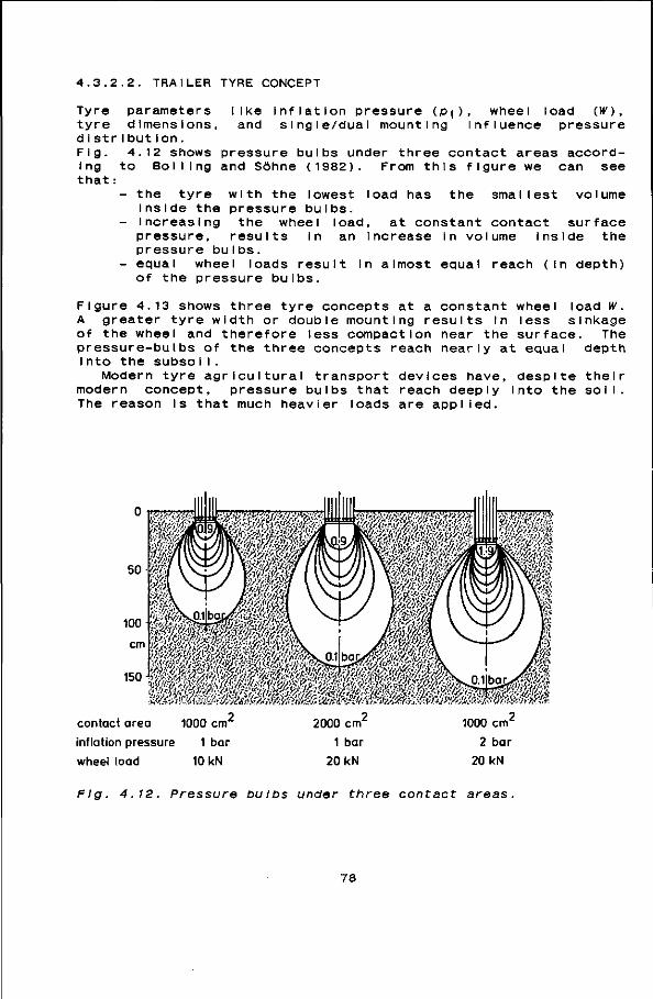
4.3.2.2. TRAILER TYRE CONCEPT
Tyre tyre d Istr Fig. I ng that:
parameters like inflation pressure (P|), wheel load (W), dimensions, and single/dual mounting Influence pressure
i but i on. 4.12 shows pressure bulbs under three contact areas accord-
to Boiling and Söhne (1982). From this figure we can see
- the tyre with the lowest load has the smallest volume inside the pressure bulbs.
- Increasing the wheel load, at constant contact surface pressure, results In an Increase In volume inside the pressure bulbs.
- equal wheel loads result In almost equal reach (In depth) of the pressure bulbs.
Figure 4.13 shows three tyre concepts at a constant wheel load W. A greater tyre width or double mounting results In less s Inkage of the wheel and therefore less compaction near the surface. The pressure-bulbs of the three concepts reach nearly at equal depth Into the subsoI I .
Modern tyre agricultural transport devices have, despite their modern concept, pressure bulbs that reach deeply into the soil. The reason is that much heavier loads are applied.
contact area 1000 cm
inflation pressure 1 bar
wheel load 10 kN
Fig. 4.12. Pressure bulbs under three contact areas
78

4.3.2.3. TRACTOR TYPE
Increasing tractor power generally Implies that tractor weight Increases. To support this heavier weight, the tractor needs tyres with larger dimensions. A limiting factor In Increasing tractor tyre width Is the width of the open furrow during ln-furrow ploughing. Therefore at greater tractor power the front axle load Increases. To prevent the front wheel rolling resistance from getting too high and to Improve the weight-pull ratio, driven front wheels may be used. For these four-wheel drive tractors (FWD-tractors) different types are available. The pull-slip behaviour of these types has been discussed In section 4.1.2.4. Boiling and Söhne (1982) present calculated pressure bulbs under one TWD and two FWD tractors (Fig. 4.14). We can see that, despite larger tyre dimensions, the pressure bulbs reach more deeply when tractor power Is Increased. This Is mainly due to the Increase of tractor weight at Increasing tractor power. The backward bend In the pressure bulbs Is caused by the pulling force. To calculate these distributions advanced computing programmes and extensive calculation facilities are needed.
170-20AW 10-18AW 170-20AW 10-18AW
Q.
XI
'5
Fig. 4.13. Ca leu I ated pressure bulbs under tyres with 7.0 kN axle loads. From left to right: narrow tyres, wide tyres, and dual trailer tyres at Inf lat Ion pressures of 3.0, 1.5 and 0.74 bar respectIvely (Söhne, 1953a).
79
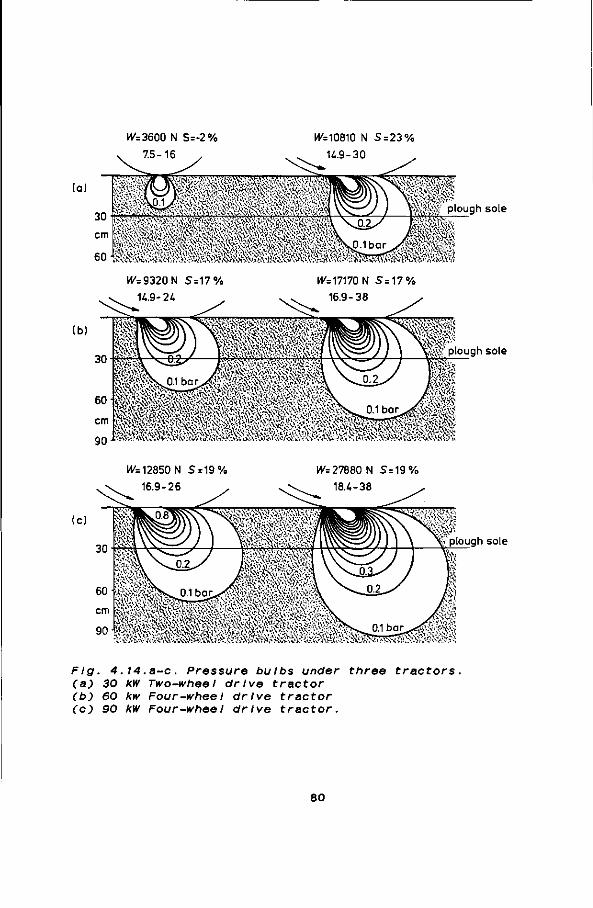
W=3600 N S=-2%
7.5-16
W=10810 N S = 23%
U.9-30
.'Xv.v
"Vf -.">îo\ plough sole
(b)
(c)
W=9320N S=17%
U.9-24
W=17170N S=17%
16.9-38
'•^v. plough sole
IV= 12850 N S = 19%
16.9-26
W= 27880 N S=19%
18.4-38
^ plough sole
Fig. 4.14.a-c. Pressure bulbs under three tractors, (a) 30 kW Two-wheel drive tractor (b) 60 kw Four-wheel drive tractor (c) 90 kW Four-wheel drive tractor.
80
CHAPTER 5
SOIL CHARACTERISTICS CONCERNING LOAD-BEARING PROCESSES
5.1. RELATIONSHIPS BETWEEN "TREATMENT" AND "BEHAVIOUR" OF SOIL
The compaction behaviour of a soli depends on prior processes to which the soil has been subjected. If these prior processes are known they can be used as a basis for prediction of subsequent behaviour (Kooien, 1977). The treatment of the soil may comprise a series of tillage operations, changes In temperature, changes In moisture content, etc.
In a uniaxial compression test the behaviour of Lexkesveer sandy loam was tested for repeated compressions while the soli was subjected to different treatments between the compressions. Cylinders (81 mm in diameter and with a height of 50 mm) were filled with about 300 grammes of soil. The samples were compressed with a hydraul ic press at a speed of 2 mm/s up to pressures of 1.5 and 4.0 bar. The test consisted of 4 series. Each series had a moisture content range between 10 and 21 percent water content by weight. To get the same starting position for all cylinders, they were precompressed at 0.5 bar. Series 1: repeated compressions were made with negligible In
tervals between the compressions. Series 1a was loaded 15 times to 1.5 bar; series 1b 15 times to 4.0 bar.
Series 2: the soil samples were compressed to 4.0 bar and there was a rest-period of 3.5 days. Series 2a was loaded 5 times to 4.0 bar with a rest-period of 3.5 days between compressions; series 2b was loaded 15 times to 4.0 bar with a rest-period of 3.5 days after every 3 compress I ons.
Series 3: the samples were compressed to 4.0 bar followed by a rest-period of 7 days. Series 3a was loaded 5 times to 4.0 bar with a rest-period of 7 days after every compression; series 3b was loaded 15 times to 4.0 bar with a rest-period of 7 days after every 3 compressions.
Series 4: like 3, but during the rest-period the soil sample was subjected to a drying/wetting cycle. We used the following procedure during a drying/wetting cycle: after compression the samples were dried in an oven at 105 °C during 0.5 hour. The samples were dried afterwards during one day at room temperature. After one
81

day the samples were rewetted with crushed Ice to the original moisture content.
The results of these tests are given in Fig. 5.1. From these results we can see that In the dry area (under 16 % m.c.) soils do not behave differently as a result of the different treatments. In the moisture content range above 16 % soil behaviour depends on the treatment. From the series 2 and 3 we can see that a rest-period between compressions results In a higher compressibility of the soil. This can be explained by the phenomenon of entrapped air. When a soil is compressed air pressure builds up In this entrapped air before the density of saturation Is reached. This phenomenon of "entrapped air" has been mentioned by Faure (1980). When the rest-period between compressions is long enough the air pressure In the sample will return to normal values. During the next compression this soli can be compressed further than when a rest-period between the compressions Is lacking. There is no difference In soli behaviour when the rest-period lasts 3.5 or 7 days. Series 4 shows less compaction of the samples (in the range >16 % m.c.) when they are subjected to a drying/wetting cycle In the rest-period. Because of this drying/wetting cycle this soil partly regains its resistance to compaction. A clear explanation of this phenomenon Is difficult to give. Swelling and shrinking processes are not likely to be the cause because this soli hardly has a swelling and shrinking capacity.
In the field soli Is exposed to natural forces like freezing and thawing, and shrinking and swelling as a consequence of drying and wetting respectively. The results of studies on the persistence of compaction after freezing and thawing are contradictory. Krumbach and White (1964) reported decreased bulk densities on a freezing surface soli of Cel Ina loam in Michigan. Wittsell and Hobbs (1965) found a decrease of bulk density after 1 year of freezing and thawing In the 2.5 to 10 cm and the 18 to 25 cm layer of a compacted silt loam. More recent research results tend to disagree with the above results. In Sweden wheeI - Induced soli compaction persisted under freezing and thawing (Danfors, 1974). Mech et al.(1967) found that on a compacted silt loam In Washington crop yield problems persisted over a four-year period, even though extreme frost heaving took place. NJds (1976) found on loam and clay-loam soils an effect of autumn compaction on the yield of cereals In Norway. Compactions made In spring resulted In significant yield reductions even after two years. Blake et al. (1976) noted no change In bulk density below the plough layer over a nine-year period In Nicollet clay loam In Minnesota. Neither crop nor the soil water content in the frozen period affected the compacted subsoil. From these studies we can conclude that in the top soil, freezing and thawing can reduce soil compaction because of lateral soil displacements and a small overburden. Compaction in the subsoil (below the plough layer) persists even after freezing.
82

1.80
1.70
3
£
vi c Ol
•o
3
g/cm
1.60
1.50
1.40-
Saturation line -10 vol. % air
•1-4*-^r=-t*
u 8 10 12 U 16 18 % 20
moisture content
F/g. 5.1. Behaviour of Lexkesveer loam In uniaxial compression tests during different treatments. Series 1 ( • ) , Series 2 (à), series 3 ( a ) , and series 4 (o) after 15 loadings to 4.0 bar.
Shrinking and swelling, content, depend mainly on so I I . Upon sweI I ing there excessive shrinkage, man cracks faci I I täte water In with a high sand content Wetting and drying do no Porosities hardly change with a naturally compacted kerk (1968) observed the e soil poros-ity In a sandy decreased due to natural f clally compacted layer, VomocI I and Flocher (1965) which 75 percent montmo compacted, a persistance periods of wetting and dry
as a result of changes In the type and proportion of Is an Increase in soi I por
y cracks are formed in the filtration and root pénétra
have a small capacity for t seem to a I lev I ate sol I d in the compacted zone of
layer (Mech et al, 1967). f feet of time and wetting a loam. The surface porosit orces. Where the subsoi I ha
porosity did not Increase found on Yolo loam (20 per
ril Ion I te) that had been of the compaction effect d
I ng.
the moisture clay In the
oslty. After so i I. These tIon. So I I s
shrInk i ng. compact ion.
a silt loam Van Ouwer-
nd drying on y gradua I I y d an art I f I -
with tIme. cent clay of art I fIcially esp I te many
83
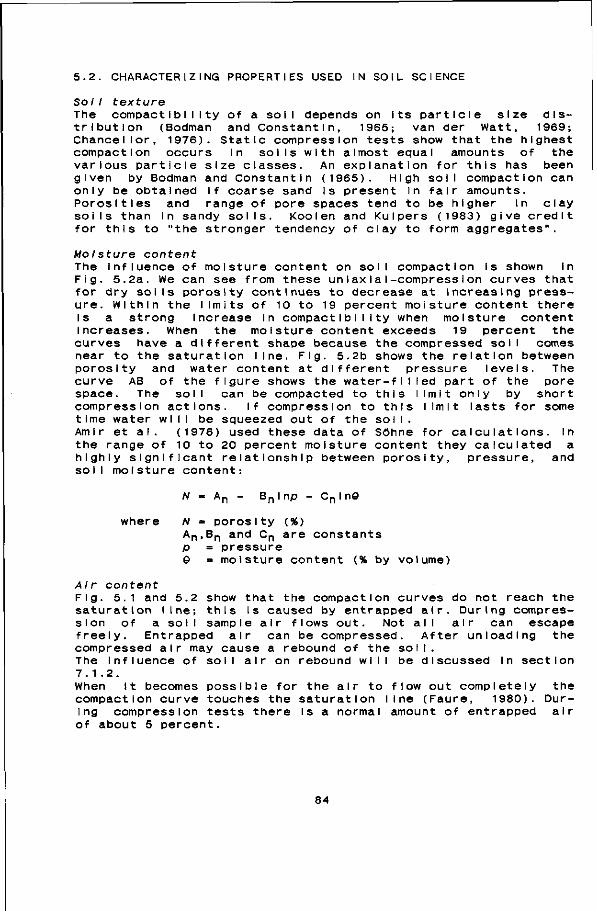
5.2. CHARACTERIZING PROPERTIES USED IN SOIL SCIENCE
Sol I texture The compact IbI I Ity of a soil depends on Its particle size distribution (Bodman and Constantin, 1965; van der Watt, 1969; Chancellor, 1976). Static compression tests show that the highest compaction occurs In soils with almost equal amounts of the various particle size classes. An explanation for this has been given by Bodman and Constantin (1965). High soil compaction can only be obtained if coarse sand Is present in fair amounts. Porosities and range of pore spaces tend to be higher In clay soils than in sandy soils. Kooien and Kuipers (1983) give credit for this to "the stronger tendency of clay to form aggregates".
Mo/s tu re content The Influence of moisture content on soli compaction Is shown In Fig. 5.2a. We can see from these un I ax I a I-compress I on curves that for dry soils porosity continues to decrease at increasing pressure. Within the limits of 10 to 19 percent moisture content there Is a strong increase in compact IbI I ity when moisture content Increases. When the moisture content exceeds 19 percent the curves have a different shape because the compressed soli comes near to the saturation line. Fig. 5.2b shows the relation between porosity and water content at different pressure levels. The curve AB of the figure shows the water-fI I led part of the pore space. The soil can be compacted to this limit only by short compression actions. If compression to this limit lasts for some time water will be squeezed out of the sol I .
Amir et al. (1976) used these data of Söhne for calculations. In the range of 10 to 20 percent moisture content they calculated a highly significant relationship between porosity, pressure, and soil moisture content:
N - An - BnInp - CnI no
where N = porosity (%) A n ,B n and C n are constants p = pressure © = moisture content (% by volume)
Air content Fig. 5.1 and 5.2 show that the compaction curves do not reach the saturation line; this Is caused by entrapped air. During compression of a so I I sample air flows out. Not all air can escape freely. Entrapped air can be compressed. After unloading the compressed air may cause a rebound of the soil. The Influence of soil air on rebound will be discussed In section 7.1.2. When it becomes possible for the air to flow out completely the compaction curve touches the saturation line (Faure, 1980). During compression tests there Is a normal amount of entrapped air of about 5 percent.
84
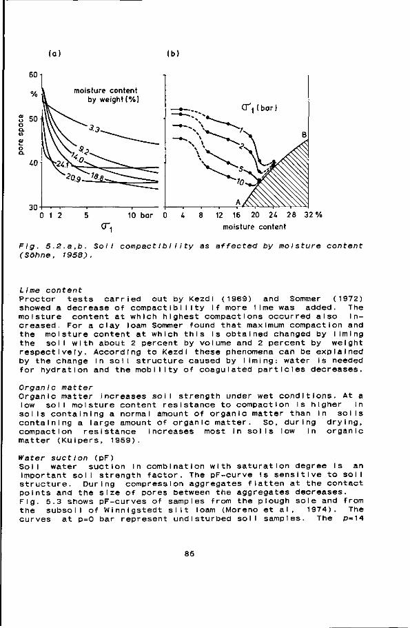
(a) (b)
60 i
% moisture content by weight I%)
O", (bar)
0 1 2 10 bar 0 U 8 12 16 20 2U 28 32% moisture content
Fig. 5.2.a,b. Soil compactibI 11ty as affected by moisture content (Söhne, 1958).
Lime content Proctor tests carried out by Kezdi (1969) and Sommer (1972) showed a decrease of compact Ibi I ity if more lime was added. The moisture content at which highest compactions occurred also increased. For a clay loam Sommer found that maximum compaction and the moisture content at which this Is obtained changed by liming the soil with about 2 percent by volume and 2 percent by weight respectively. According to Kezdi these phenomena can be explained by the change in soil structure caused by liming: water is needed for hydration and the mobility of coagulated particles decreases.
Organic matter Organic matter increases soil strength under wet conditions. At a low soil moisture content resistance to compaction is higher In soils containing a normal amount of organic matter than in soils containing a large amount of organic matter. So, during drying, compaction resistance increases most in soils low in organic matter (Kuipers, 1959).
Water suction (pF) Soli water suction in combination with saturation degree Is an important soil strength factor. The pF-curve Is sensitive to soil structure. During compression aggregates flatten at the contact points and the size of pores between the aggregates decreases. Fig. 5.3 shows pF-curves of samples from the plough sole and from the subsoil of Winnigstedt silt loam (Moreno et al, 1974). The curves at p=0 bar represent undisturbed soil samples. The p=14
85
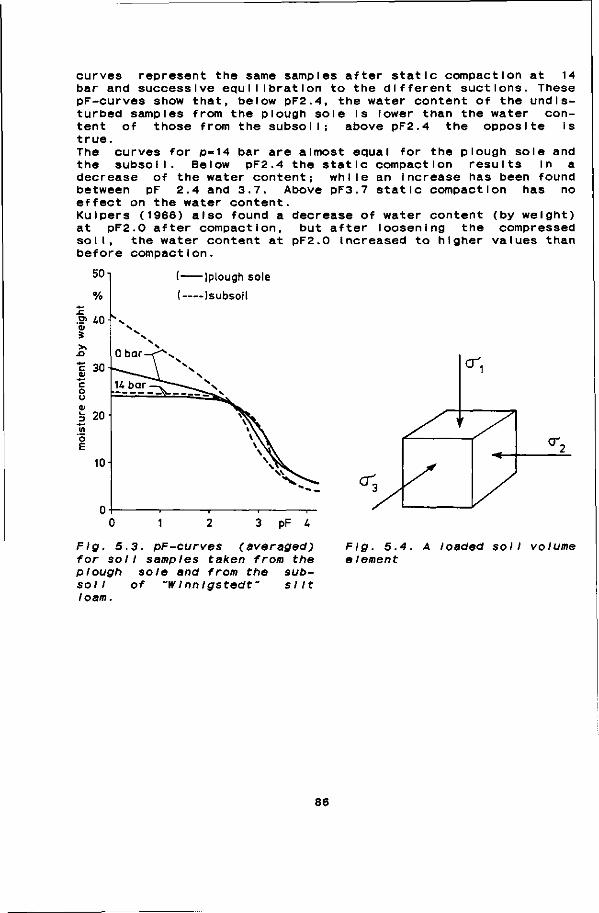
curves represent the same samples after static compaction at 14 bar and successive equilibration to the different suctions. These pF-curves show that, below pF2.4, the water content of the undisturbed samples from the plough sole Is lower than the water content of those from the subsoil; above pF2.4 the opposite Is true. The curves for p-14 bar are almost equal for the plough sole and the subsoil. Below pF2.4 the static compaction results In a decrease of the water content; while an Increase has been found between pF 2.4 and 3.7. Above pF3.7 static compaction has no effect on the water content. Kuipers (1966) also found a decrease of water content (by weight) at pF2.0 after compaction, but after loosening the compressed soil, the water content at pF2.0 increased to higher values than before compaction.
( Iplough sole
( (subsoil
Fig. 5.3. pF-curves (averaged) for soil samples taken from the plough sole and from the sub-sol I of "Wlnnlgstedf silt loam.
Fig. 5.4. element
A loaded soil volume
86
5.3. MECHANICAL PROPERTIES
The soil mechanical properties comprise the geometrical changes (compaction, deformation, and failure) that a loaded soil volume element (Fig. 5.4) will show for all possible values of CT-\ , CT 2 and 0"3. The most Important mechanical properties of load-bearing processes are compactibi I Ity, deformabM Ity, and resistance against shear fa I I ure.
5.3.1. COMPACTIBILITY
The loading of soil during soil tillage and agricultural field traffic Is a relatively quick type of transient loading. Therefore, we can safely assume that the developed pore-water pressures will not have sufficient time to dissipate and that the role of water In the sol I can be I imited to its effect on sol I strength.
5.3.1.1. MEASURES FOR COMPACTION
Compaction can be expressed In volumetric properties of solid, liquid, and gas phases:
Porosity of a soi I volume element is the ratio of volume of pores (water + air) to the total volume of the element. It is expressed as a percentage or as a fraction. Porosity has the advantage of being dimensI on I ess and independent of particle density. Other names for porosity are pore space and total pore space.
Void ratio (e) is the total volume of pores divided by the total volume of solids. According to Karaf lath and Nowatzkl (1978) void ratio is easier to handle than porosity when the volume of the solids remains essentially constant for a given Initial total volume of soil solids whereas with porosity both the volume of voids and the total volume change.
Dry bulk density ( yd ) is the weight of sol ids in a unit of volume. It is usually expressed in g/cm^ or kg/m3. For the interpretation of dry bulk density we need to know the specific density of the so I Ids.
Bulk weight volume (BWV) is 1/tfd (cm3/g).
The relationships between these quantities are given in Fig. 5.5. Besides changes In volumetric quantities compaction is often associated with Increased penetration resistance and changes in pore structure properties such as reduction of conductivity, diffusiveness and permeability by water and air.
87
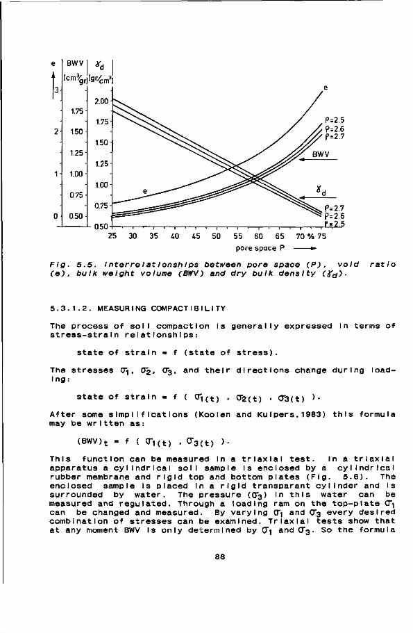
BWV I Xà I
2.00
25 30 35 40 45 50 55 60 65 70 % 75 pore space P *•
Fig. 5.5. InterreI atlonshIps between pore space (P), void ratio (e), bulk weight volume (BWV) and dry bulk density (fa).
5.3.1.2. MEASURING COMPACT IBILITY
The process of soil compaction Is generally expressed In terms of stress-strain relationships:
state of strain f (state of stress)
The stresses 0 , Ojj, O3, and their directions change during loading:
state of strain - f ( G\(t) • 02(t) • 0"3(t) >•
After some simplifications (Kooien and Kuipers,1983) this formula may be written as:
(Bwv)t - f ( cr1 ( t ) , çr3(t) )•
This function can be measured In a trlaxlal test. In a triaxial apparatus a cylindrical soli sample is enclosed by a cylindrical rubber membrane and rigid top and bottom plates (Fig. 5.6). The enclosed sample Is placed In a rigid transparant cylinder and Is surrounded by water. The pressure (O3) In this water can be measured and regulated. Through a loading ram on the top-plate 0~i can be changed and measured. By varying 0"i and 0*3 every desired combination of stresses can be examined. Trlaxlal tests show that at any moment BWV Is only determined by (Ji and <T3. So the formula
88
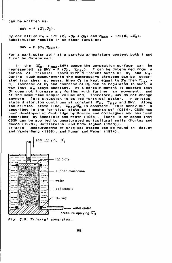
can be written as:
BWV = f (0"i.0*3).
By definition <Tm - 1/3 ( CT-! +0*2 + 03) and T m a x - 1/2(0i -°3> Substitution results In an other function:
BWV F «rm,T. m> "-max ) .
For a particular soil at a particular moisture content both f and F can be determined.
In the (0"m, T m a x > B W V ) space the compaction surface can be represented as BWV • F (0~m, T m a x ) - F can be determined from a series of triaxlal tests with different paths of (7 and CT3. During such measurements the compressive stresses can be separated from shear stresses. When 0~i Is kept equal to 0~3 then T m a x -0; Increase of a\ and decrease of O3 can be regulated In such a way that 0"m stays constant. At a certain moment it appears that 0"i does not increase any further with further ram movement, and at the same time sample volume and, therefore, BWV do not change anymore. This situation is called "critical state". In critical state distortion continues at constant <Tm, T m a x and BWV. Along the critical state line, "^max^m l s constant. This behaviour Is described In the "critical state soil mechanics" (CSSM). CSSM has been developed at Cambridge by Roscoe and colleagues and has been described by Schofleld and Wroth (1968). There Is evidence that CSSM can be applied to unsaturated agricultural soils (Kurtay and Reece (1970); Hettlaratchl and O'Callaghan (1980)). Triaxlal measurements of critical states can be found In Bailey and VandenBerg (1968), and Kumar and Weber (1974).
top plate
rubber membrane
Fig. 5.6. Triaxlal
— water under
pressure applying 0"^
apparatus.
89

In the (BWV, cTi ,03) s sented as BWV - f(0~i, O3 Compaction caused by ag surface f between the c paction at a constant constant values of 0~3/0~i published by Bailey and these calculations, made and Vaandrager (1984), Influence on the major (see Fig. 5.7). In agricultural operatlo So soil compact lb I I Ity Q\ and degree of compact uniaxial compression Is
pace the compaction surface can be repre-). rlcultural activities will be along the rltical state line and the line for corn-diameter of the sample. For a number of
f was calculated from the functions F Vandenberg, and Dunlap and Weber. From by Kooien and Kuipers (1983), and Kooien we can conclude that 0*3 only has I Ittle
principal stress-pore space relationship
ns O3/O1 generally Is 0.5 (Kooien, 1974). can be represented by a relation between Ion. For this no trlaxal test is needed; suf f iel ent.
£ Congaree
• silt loam
,# Lloyd clay
9 Hiwassee + sandy loam
0.8 1.2 1.6 2.0 2M bar
Fig. 5.7. O) ratlo.
-pore space relat lonshlps as affected by O3/ CTj
90
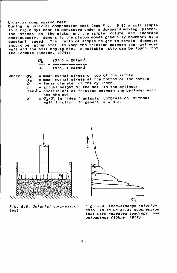
Uniaxial compression test During a uniaxial compression test (see Fig. 5.8) a soil sample in a rigid cylinder Is compacted under a downward moving piston. The stress on the piston and the sample volume are recorded continuously. Generally the piston moves gradually downward at a constant speed. The ratio of sample height to sample diameter should be rather small to keep the friction between the cylinder wall and the soil negligible. A suitable ratio can be found from the formula (Kooien, 1974):
<Jj (D/h) - 2Ktan S
0~t (D/h) + 2Ktan£
where: o> = mean normal stress on top of the sample mean normal stress at the bottom of the sample inner diameter of the cylinder, actual height of the soli In the cylinder coefficient of friction between the cylinder wall and the sol I
CTt CTb D h tan S
= <T3/0\ In "ideal" uniaxial wall friction. In general
compress ion, K m 0.5.
wlthout
Fig. 5.8. test.
Uniaxial compress Ion
u1 Fig. 5.9. Loads Inkage relationship In an uniaxial compress Ion test with repeated loadings and un loadings (Söhne, 1952).
91

5.3.1.3. THE INFLUENCE OF REPEATED LOADING, LOADING SPEED, AND VIBRATIONS ON COMPACT IBILITY
Repeated loading Agricultural field traffic is a process of loading, and several unloadlngs and reloadings. In uniaxial compression tests the path of unloading and reloading, in a pressure - s Inkage relationship, shows a hysteresis effect (see Fig. 5.9). Such hysteresis effects were found by Söhne (1951,1952,1956), and Yong and Warkentin (1966,1975). This hysteresis effect occurs in many materials; NadaI (1950) shows the same effect in metals. After reloading the sample behaves In the same way as it would have done If the last (re)loading was continued without unload i ng . A uniaxial compression test with several cycles of unloading and reloading shows that compaction continues. Every reloading results in extra compaction. This extra compaction decreases with number of loadings. Söhne (1956) found that further compressibility was still possible after 10 reloadings with no rest-period between the unloading and the next reloading (see Fig. 5.10). In the field there is generally a rest-period between successive reloadings. During this rest-period the soil can regenerate. If there is entrapped air In the soil during loading, the air pressure can equalize in the rest-period. During the next reloading the soil can be further compressed than when the rest-period is negligllble (see Section 5.1). If there is a drying-wetting cycle during the rest-period the compressibility of the soil Is lower (see Section 5.1). During our measurements we found still additional compaction after 15 re-load i ngs.
Rebound A loaded sol I sample will rebound when the sample is unloaded. A rebound has two components: elastic recovery and creep. Elastic recovery occurs Immediately at unloading. Creep Increases with 11 me (see Fig. 5.11). Elastic recovery depends on soil type, soil density, and moisture content. In soil samples where air was entrapped during loading we found an Increase In elastic recovery (see Section 7.1.2). Creep velocity decreases with time. Creep values can well be higher than elastic recovery. We found that rebound can decrease bulk density up to 0.1 g/cm3.
Loading speed In uniaxial compression tests using Lexkesveer loam, we found no difference in compact IbI I Ity between loading speeds of 0.25 mm/s and 3.0 mm/s. Söhne (1953a) found a difference in pore space of about 0.5 % between loading speeds of 20 mm/s and 120 mm/s. These speed effects, measured in uniaxial compression tests, are much lower than those found in the field under rollers and tyres; see Baganz (1963/1964), Abaoba (1969), Sltkei and Fekete (1975), Steinkamp (1975), and Karczewskl (1978).
92
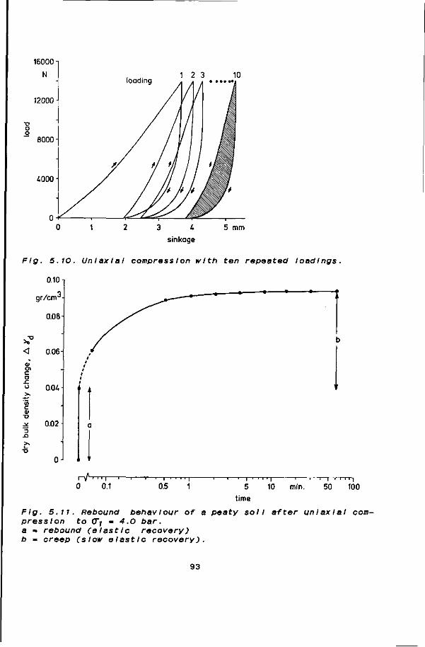
1 2 3 10
5 mm
Flg. 5.W. Uniaxial compress Ion with ten repeated loadings,
0.10 n
3
* '
0) Ol c o
X o
U)
c (V
X )
X I
gr/cm
0.08
0.06
0.04
0.02
nA r-n-, 0.1
- l 1—|—i
0.5 5
time
10 mm. 50 100
Fig. 5.11. Rebound behavlour of a peaty soil after uniaxial compression to CTj » 4.0 bar. a - rebound (elastic recovery) b - creep (slow elastic recovery).
93
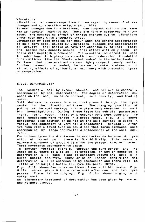
V I brat Ions Vlbrat ions can cause compaction in two ways: by means of stress changes and acceleration effects (Wu, 1971). Stress changes due to vibrations, can compact soi I in the same way as repeated loadings do. There are hardly measurements known about the compacting effect of stress changes due to vibrations under machinery with pneumatic tyres. Compaction by acceleration can occur when the upward acceleration of soil particles, caused by vibrations, exceeds the acceleration of gravity; soil particles have the opportunity to fall freely and become very densely packed. This effect will only occur in soils with negligible cohesion. The acceleration effect Is used to advantage in highway construction and underwater foundation constructions like the "OosterscheI de-dam" In the Netherlands. We know that crawler-tractors can highly compact sandy soils. Further research Is needed, before we can make statements on vibrating effects of agricultural machinery with pneumatic tyres on compact i on.
5.3.2. DEFORMABILITY
The loading of soli by tyres, wheels, and rollers Is generally accompanied by soil deformation. The degree of deformation depends on the load, moisture content, soil density, and loading speed. Soli deformation occurs In a vertical plane A through the tyre center In the direction of travel. The changing position of points at the soli surface In this plane were observed In soil bin investigations. During these tests the vehicle parameters (tyre, load, speed, Inflation pressure) were kept constant. The soli conditions were varied in a broad range. Fig. 3.17 shows horizontal displacement of points at the soil surface In plane A versus the accompanying vertical displacement (sinkage). After two runs with a towed tyre we could see that large sinkages were accompanied by large horizontal displacements at the soil surface. For driven tyres the displacements are backwards because of tyre si Ip. At normal pul I there is 15 - 20 % si ip. This means a backward movement of about 0.25 m for the present tractor tyres. These movements decrease with depth. In another vertical plane B, through the tyre center and Its wheel axle, there is also soil deformation. In wet or dense soils deformation wl I I take place at constant volume and sol I will bulge be%I de the tyre. Under drier or looser conditions the deformation will be accompanied by compaction and there will be little or no bulging beside the tyre (Kuipers, 1970). Fig. 5.12 shows two cross sections of our soil bin tests. Fig. 5.12a shows plane B for a dense soil after one and two tyre passes. There Is no bulging. Fig. 5.12b shows bulging In a softer so i I . An elementary treatment of deformation has been given by Kooien and Ku i pers (1983).
94
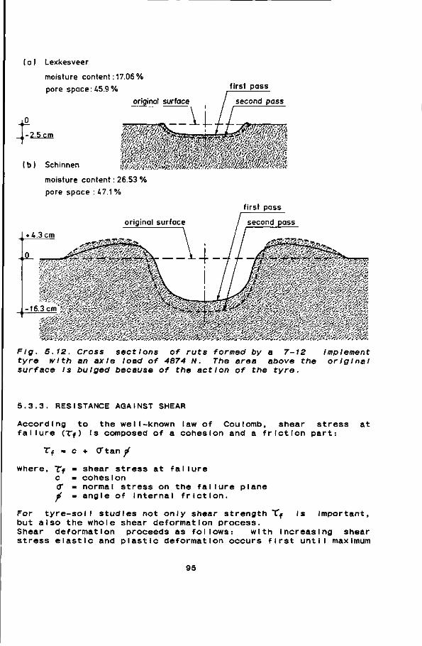
(a) Lexkesveer
moisture content : 17.06%
pore space: 45.9%
original surface
-2.5cm
f i rst pass
second pass
( b ) Schinnen Vts'K
moisture content : 26.53 %
pore space : 47.1 %
f i rst pass
original surface
Fig. 5.12. Cross sections of ruts formed by a 7-12 Implement tyre with an axle load of 4874 N. The area above the original surface Is bulged because of the action of the tyre.
5.3.3. RESISTANCE AGAINST SHEAR
According to the well-known law of Coulomb, shear stress at failure (Tf) Is composed of a cohesion and a friction part:
T f « c + Ctan tf
where, Tf • shear stress at failure c » cohesion <T - normal stress on the failure plane é - angle of Internal friction.
For tyre-soil studies not only shear strength Xf Is Important, but also the whole shear deformation process. Shear deformation proceeds as follows: with Increasing shear stress elastic and plastic deformation occurs first until maximum
95
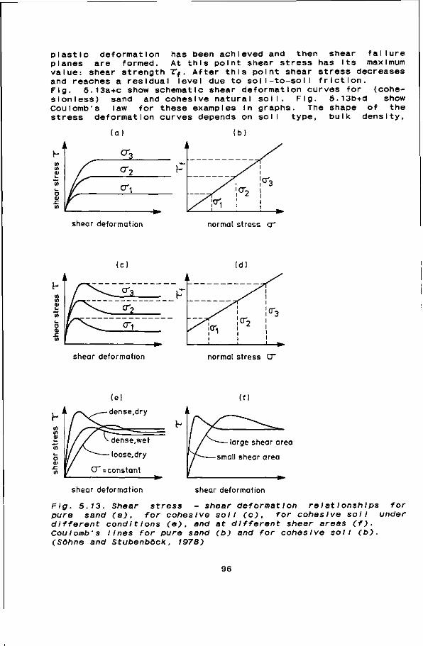
plastic deformation has been achieved and then shear failure planes are formed. At this point shear stress has Its maximum value: shear strength Tf. After this point shear stress decreases and reaches a residual level due to soll-to-soil friction. Fig. 5.13a+c show schematic shear deformation curves for (cohe-sionless) sand and cohesive natural soil. Fig. 5.13b+d Coulomb's law for these examples In graphs. The stress deformation curves depends on soil type,
(a)
show shape of the bulk density,
<T1
shear deformation normal stress a "
shear deformation normal stress CT
• dense,wet
• loose,dry
O~ = constant
shear deformation shear deformation
Fig. 5.13. Shear stress - shear déformât Ion re I atlonshIps for pure sand (a), for cohesive soil (c), for cohesive soil under different condltIons (e), and at different shear areas (f). Coulomb's lines for pure sand (b) and for cohesive soil (b). (Söhne and Stubenböck, 1978)
96
molsture content, and the area of the shear failure plane. Fig. 5.13e shows schematically shear deformation curves for dry, loose and dense, cohesive soil with equal moisture content and for dry and wet cohesive soils of equal density. For dense, cohesive soil with a moderate moisture content shear deformation curves are given at two different areas of shear planes (Fig. 5.13f).
5.4. CHARACTERIZATION PROCESSES
During passing of a wheel the state of stress and strain varies continuously. This makes It very difficult to relate the processes to specific mechanical properties. Research workers therefore often use simpler but comparable processes Induced by measuring devices as a method of characterization. A problem with this method of characterization Is that there are many different tests in common use. In section 5.4.2 results of comparisons of different methods are shown and discussed. It Is clear that if two tests are highly correlated it is enough to use one of them to characterize soil behaviour.
Cone pénétrât I on tests With a cone penetration test resistance to penetration, as a composite soil property, can be measured and described rapidly and in s I tu. This test gives no specific soli values such as angle of friction, cohesion, or coefficient of soil-metal friction. Because the results are Influenced by the cone type and method used, a standardization of cone type and method is needed for comparing measurements. A widely accepted cone penetrometer Is the one standardized by ASAE (Fig. 5.14). ASAE Standard S313.1 (Hahn et al., 1984) specifies two standard 30 degrees cone sizes (20.27 and 12.83 mm base diameter) with a smooth finish (63 microlnches maximum) and a penetration velocity of 30.5 mm/s. Cone resistance Is usually expressed as the quotient of penetration force and the base area, called cone Index (CI). Cone base size should always be stated. CI strongly depends on many factors other than bulk density. The most Important of the factors are soil moisture content, type of soil, and pore space. Chancellor (1976) gives examples of relationships between CI and dry bulk density obtained by several Investigators. . In these examples the relationships vary from almost linear to strongly curved. Chessners et al. (1972) show that even when the same soil and the same moisture content are used the relationship between CI en bulk density can be different for sol I compacted In the laboratory and sol I compacted In the field. Despite its limitations CI Is frequently used for comparative Indications of soil conditions because of the ease and rapidity with which numerous measurements can be made. With the newly developed electronic recording hand-held penetrometer which can be linked to a programmable calculator, CI can be measured more eas M y st I I I .
97
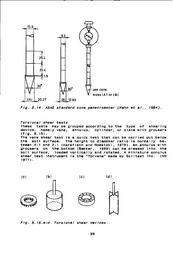
15.9
9.5
20.27 (B)
V-° r: use cone
sizes (A) or (B)
12.83
Flg. 5.14. ASAE standard cone penetrometer (Hahn et al 1984).
Torsional shear tests These tests may be grouped according to the type of shearing device, namely vane, annulus, cylinder, or plate with grousers (Fig. 5.15). The vane shear test Is a quick test that can be carried out below the soil surface. The height to diameter ratio Is normally between 4:1 and 2:1 (Karaf lath and Nowatzki, 1978). An annulus with grousers on the bottom (Bekker, 1969) can be pressed into the soil surface, loaded vertically and rotated. A miniature annulus shear test Instrument Is the "Torvane" made by Solltest Inc. (NN 1971).
(a) (d)
<*>
Fig. 5.15.a-d. Torsional shear devices.
98
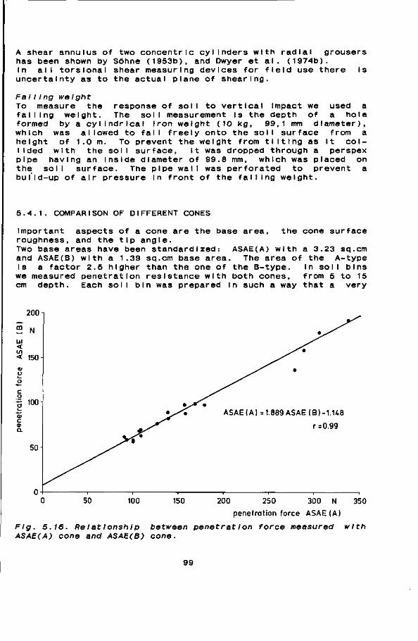
A shear annulus of two concentric cylinders with radial grousers has been shown by Söhne (1953b), and Dwyer et al. (1974b). In all torsional shear measuring devices for field use there is uncertainty as to the actual plane of shearing.
Fa IIIng weight To measure the response of soil to vertical impact we used a falling weight. The soil measurement Is the depth of a hole formed by a cylindrical iron weight (10 kg, 99,1 mm diameter), which was allowed to fall freely onto the soil surface from a height of 1.0 m. To prevent the weight from tilting as it collided with the soil surface, It was dropped through a perspex pipe having an inside diameter of 99.8 mm, which was placed on the soil surface. The pipe wall was perforated to prevent a bul'ld-up of air pressure In front of the falling weight.
5.4.1. COMPARISON OF DIFFERENT CONES
Important aspects of a cone are the base area, the cone surface roughness, and the tip angle. Two base areas have been standardized: ASAE(A) with a 3.23 sq.cm and ASAE(B) with a 1.39 sq.cm base area. The area of the A-type Is a factor 2.5 higher than the one of the B-type. In soil bins
we measured penetration resistance with both cones, from 5 to 15 cm depth. Each soil bin was prepared In such a way that a very
200
200 250 300 N
penetration force ASAE (A)
Fig. 5.16. Relatlonshlp between pénétrât Ion force measured ASAE(A) cone and ASAE(B) cone.
350
with
99
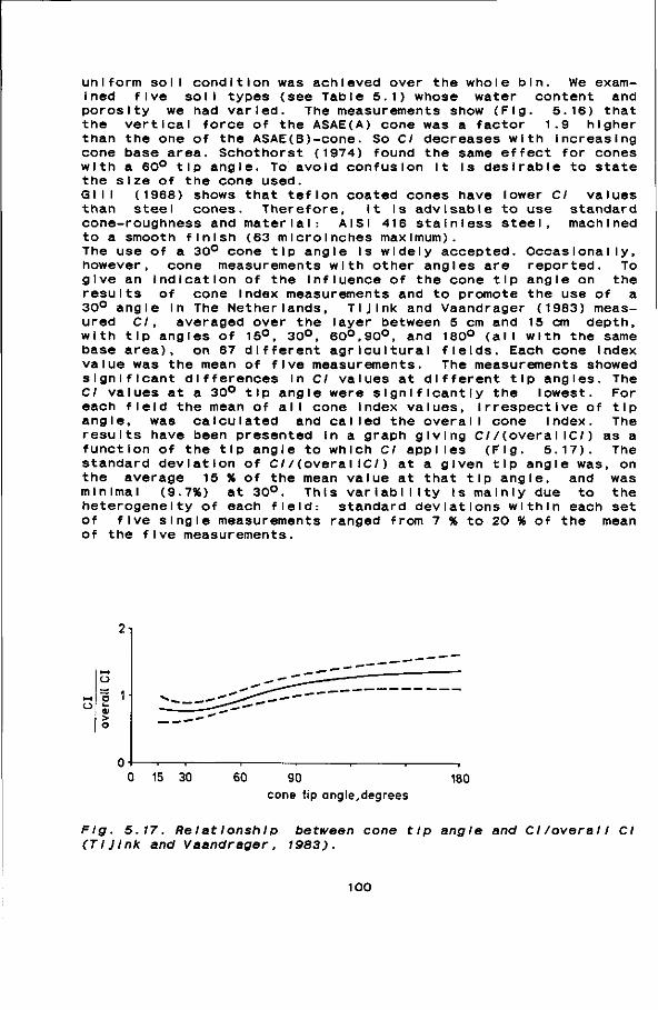
uniform soil condition was achieved over the whole bin. We examined five soil types (see Table 5.1) whose water content and porosity we had varied. The measurements show (Fig. 5.16) that the vertical force of the ASAE(A) cone was a factor 1.9 higher than the one of the ASAE(B)-cone. So CI decreases with increasing cone base area. Schothorst (1974) found the same effect for cones with a 60° tip angle. To avoid confusion it Is desirable to state the size of the cone used. Gill (1968) shows that teflon coated cones have lower CI values than steel cones. Therefore, it Is advisable to use standard cone-roughness and material: A IS I 416 stainless steel, machined to a smooth finish (63 mlcroinches maximum). The use of a 30° cone tip angle Is widely accepted, however, cone measurements with other angles are give an indication of the Influence of the cone tip results of cone index measurements and to promote 30° angle In The Netherlands, TIJInk and Vaandrager
Occas I ona M y , reported. To angle on the the use of a
(1983) measured CI, averaged over the layer between 5 cm and 15 cm depth, with tip angles of 15°, 30°, 60°,90°, and 180° (all with the same base area), on 67 different agricultural fields. Each cone index value was the mean of five measurements. The measurements showed significant differences In CI values at different tip angles. The CI values at a 30° tip angle were significantly the lowest. For each field the mean of all cone index values, irrespective of tip angle, was calculated and called the overall cone Index. The results have been presented In a graph giving C//(overaI\CI) as a function of the tip angle to which CI applies (Fig. 5.17). The standard deviation of CI/(overaI\CI) at a given tip angle was, on the average 15 % of the mean value at that tip angle, and was minimal (9.7%) at 30°. This variability Is mainly due to the heterogeneity of each field: standard deviations within each set of five single measurements ranged from 7 % to 20 % of the mean of the five measurements.
o | 1 > o
15 30 60 90
cone tip angle,degrees 180
Fig. 5.17. Relatlonshlp between cone tip angle and Cl/overal I CI (TIJInk and Vaandrager, 1983).
100
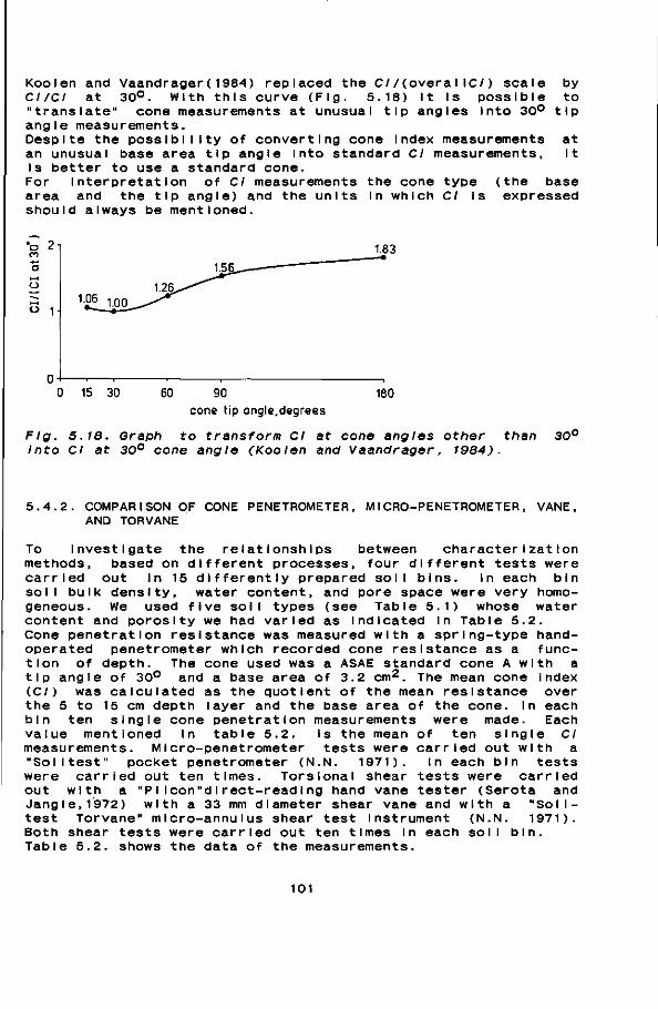
Kooien and Vaandrager(1984) replaced the Cl/(overaI IC/) scale by CI/CI at 30°. With this curve (Fig. 5.18) It Is possible to "translate" cone measurements at unusual tip angles Into 30° tip angle measurements. Despite the possibility of converting cone Index measurements at an unusual base area tip angle Into standard CI measurements, It Is better to use a standard cone. For Interpretation of CI measurements the cone type (the base area and the tip angle) and the units In which CI Is expressed should always be mentioned.
o o
o !•
1.83
1.56.
1.06 1.26.
1.00
0 15 30 60 90
cone tip angle,degrees 180
Fig. 5.18. Graph to transform CI at cone angles other than 30° Into CI at 30° cone angle (Kooien and Vaandrager, 1984).
5.4.2. COMPARISON OF CONE PENETROMETER, AND TORVANE
MICRO-PENETROMETER, VANE,
To investigate the relationships between characterization methods, based on different processes, four different tests were carried out In 15 differently prepared soil bins. in each bin soil bulk density, water content, and pore space were very homogeneous. We used five soil types (see Table 5.1) whose water content and porosity we had varied as Indicated in Table 5.2. Cone penetration resistance was measured with a spring-type hand-operated penetrometer which recorded cone resistance as a function of depth. The cone used was a ASAE standard cone A with a tip angle of 30° and a base area of 3.2 cm2. The mean cone index (C/) was calculated as the quotient of the mean resistance over the 5 to 15 cm depth layer and the base area of the cone. In each bin ten single cone penetration measurements were made. Each value mentioned In table 5.2. Is the mean of ten single CI measurements. Micro-penetrometer tests were carried out with a "Solltest" pocket penetrometer (N.N. 1971). in each bin tests were carried out ten times. Torsional shear tests were carried out with a "PIlcon"dIrect-readIng hand vane tester (Serota and Jangle,1972) with a 33 mm diameter shear vane and with a "Soll-test Torvane" micro-annuI us shear test Instrument (N.N. 1971). Both shear tests were carried out ten times In each soil bin. Table 5.2. shows the data of the measurements.
101

Table 5.1. Soll descrlptIon.
Moisture Soll % of minerals % of soll PHKCI content
at pF2 (100 cm
<2/u 2-16/* ^6-50JU Humus CaC03 suction), %
Wagen Ingen s IIty clay Lexkesveer Seh Innen s I 11 Ioam, Ede sand, Almkerk si Ity clay.
loam, loam,
36 15
17 3.5
40
27 12
14 2.5
24
21 17
57 4.5
24
2.3 1 .6
2. 1 3.6
1 .2
3.3 10.4
2.9 -
0. 1
7.4 7.2
7.2 4.4
6.8
27.3 20.2
27.2 17.4
26.9
Table 5.2. Measurements of soll character 1st les.
Bin Soll* MC P CI CIM Si S2 T NR. % vol.% (kPa) (kPa) (kPa) (kPa) (kPa)
1 L 16.96 43.1 782 1.28 3.4 2 L 17.16 40.4 933 1.69 4.3 3 L 20.18 39.7 497 0.84 2.7 4 A 24.79 53.4 539 0.76 3.3 5 A 24.47 48.1 761 1.17 5.4 6 A 26.66 46.1 532 0.75 3.9 7 W 22.85 52.4 700 1.18 4.0 8 W 23.12 46.5 870 1.83 6.6 9 W 27.58 46.2 436 0.58 3.1
10 S 19.76 47.5 779 1.13 3.4 11 S 20.05 42.8 1122 2.01 5.0 12 S 26.83 42.7 237 0.23 1.1 13 E 16.47 46.3 821 1.32 3.0 14 E 16.24 44.1 996 1.64 3.6 15 E 19.24 45.9 696 0.93 2.2
*: soll type (see Table 5.1) MC = moisture content by weight P = porosity CI = cone Index measured with ASAE type A CIM = cone Index measured with MIcro-penetrometer S-) = shear strength In the 0 - 4 cm layer S2 = shear strength in the 3 - 7 cm layer F = Torvane shear strength.
4 6 3 4 6 4 5 9 3 4 6 1 4 5 3
8 1 7 6 9 8 7 5 8 6 9 6 1 7 8
22 25 26 22 40 30 25 44 25 18 26 12 12 13 12
4 8 7 7 0 5 6 9 3 0 3 4 6 2 3
102
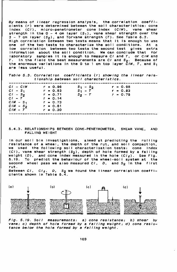
By means of linear regression analysis, the co d e n t s (r) were determined between the soil cha Index (CI), micro-penetrometer cone Index ( strength in the 0 - 4 cm layer (Si), vane shear 3 - 7 cm layer (S2), and Torvane strength (7") . High correlation between two tests means that I one of the two tests to characterize the sol I low correlation between two tests the second Information about the soli condition. We can laboratory samples It Is enough to measure CI T. In the field the best measurements are CI a the enormous variations In the 0 to 1 cm top la are I ess usefuI.
rrelation coeffi-racterIstles : cone CIM), vane shear
strength over the See Table 5.3. t i s enough to use conditions. At a test gives extra conclude that for and T, or CIM and nd S' Because of yer CIM, T, and S1
Table 5.3. Correlation coeffle lents (r) showing the linear relationship between soil character IstIcs .
CI - CIM Cl - Si CI - S2 CI - T CIM - S-] CIM - S2
CIM - T
r r r r r r r
» = -a
--=
0.96 0 .63 0 .71 0 . 14 0 .73 0 .81 0 . 30
s1 - s 2
s, - T S 2 - T
0.98 0.83 0.75
5.4.3. RELATIONSHIPS BETWEEN CONE-PENETROMETER, FALLING WEIGHT
SHEAR VANE, AND
In our soil bin Investigations, aimed at predicting the rolling resistance of a wheel, the depth of the rut, and soil compaction, we used the following soli characterization tests: cone Index (CI), vane shear strength (S2) , depth of hole formed by a falling weight (D), and cone Index measured In the hole (Clf). See Fig. 5.19. To predict the behaviour of the wheel-soil system at the second wheel pass we also measured CI, D, and S2 In the first rut. Between CI, Clf, D, S2 we found the linear correlation coefficients shown In Table 5.4.
Fig. 5.19. Soil measurements : a) cone res I stance; b) shear by vane; c) depth of hole formed by a falling weight; d) cone resistance below the hole formed by a falling weight.
103
The combination of CI, Clf, and D proved to be suitable for predicting rolling resistance, soil compaction, and ruth depth in the first and second pass of a wheel (see chapter 6.2.2).
Table 5.4. CorrelatIon coeffIclents (r) showing the relatlonshlp between the different soil character Istles used.
CI - Clf r m 0.96 CI - D r - -0.78 CI - S 2 r » 0.96 Clf- D r - -0.75 Clf- S 2 r = 0.95 D - S 2 r - -0.73
104
CHAPTER 6
RELATIONSHIPS BETWEEN SOIL CHARACTERISTICS AND PROCESS ASPECTS AND THEIR SUITABILITY TO PREDICT PROCESS ASPECTS
It is useful to predict certain aspects of the processes Involved In agricultural field traffic. It Is particularly useful to predict required pull (rolling resistance), compaction, and rut depth. To predict a process, we need data on the characteristics of the wheel, the behaviour of the wheel, and the soil. Data on tyre characteristics and the kinematic and dynamic aspects of tyre behaviour are discussed In sections 2 through 4. Soil characteristics concerning load-bearing processes are discussed In section 5. Two general catagorles of prediction methods can be distinguished (Kooien, 1977): a) methods that are mainly based on observations of relationships
between characteristics and process aspects and b) methods that are mainly based on knowledge of the mechanism of
the process under consideration. The first category Is the most Important and may be divided Into: comparative methods and methods using empirical formulas or graphs. A method from the second category Is called exact when this method uses a hypothetical mechanism almost equal to the mechanism that Is simulated. When this Is not the case, the method Is called approximate.
6.1. COMPARATIVE METHODS
These methods start with the assumption that a tyre-process aspect y depends on characteristics x-j ,xn of soil and tyre which can be expressed by the following formula:
y = f (xi xn) ,
Where, f Is the way y depends on Xi xn.
Even when f Is unknown these methods can be used because a once observed value y at certain values of x-| xn, will be found again when the same values of x-| xn occur again. This means that soils which have equal soli mechanical properties will show equal behaviour in the so I I-wheeI process.
105
Rolling resistance as process characteristic depends strongly on the soil mechanical property known as cone Index (CI)- Table 6.1 shows examples of the same rolling resistance at equal cone index values. These examples are from the Investigations reported In 6.2.2.1.
Table 6.1. Equal behaviour at equal soil mechanical properties.
Sol 1
Sch1nnen Wagen 1nge
R-\ = Rol 1 R2 = Ro11
n
Ing 1 ng
pore space (%)
47.9 42.2
res i stance resistance
moIsture content (%)
17.97 16.98
In the first In the second
cone Index (MPa)
0.95 0.90
pass pass
«1 (N)
225 223
«2 (N)
221 221
6.2. EMPIRICAL METHODS
These methods use empirical relationships, formulas, or graphs. It Is assumed that a process aspect y is dependent on characteristics xi xn :
y = f(x1, ,xn)
Where, f represents the way in which y depends on x-| x n •
The prediction function f be calculated for any arb certa in I Im Its). Methods that use relations process aspects are not I These methods only try to f prediction purposes. Sectio Empirical methods based on between soli character IstI main difference, compared attempts are made to formu functIons.
is known to such an extent that y can Itrary values of x-| xn (within
hips between soil characteristics and ntended to be dimenslonaI I y correct. Ind relationships that can be used for n 6.2.2. deals with these methods, dimensional analysis use relationships cs and process aspects as well. The
to the methods from 6.2.2, is that late dimenslonaIly correct prediction
6.2.1. EMPIRICAL GRAPHS
Examples of empirical graphs are presented by Zoz (1972), and Witney and OskouI (1982). Zoz (1972) presents a chart that may be used to determine the expected drawbar horse power, travel speed and travel reduction of any two-wheel drive tractor under various soil conditions. This graphical solution Is based on average tyre performance for single tyres on four surfaces. Three weight transfer coefficients are used for each soil type. This predictor does not require actual tractor specifications such as tyre sizes, tyre Inflation
106
pressures and front-axle load. Only a reasonable relationship between tractor weight and tyre size Is necessary. Therefore, the accuracy of prediction will generally not be very high. At the Edinburgh School of Agriculture a ploughing performance predictor nomograph has been devised by Witney and OskouI (1982). This chart, one of the results of a five-year research programme on tractor power selection for ploughing, eliminates laborious calculations to find the most efficient tractor/plough combination for any specific conditions. The predictor uses three plough body types, three compaction levels of the top layer, six soil types, three traction efficiency levels, and several possibilities of depth of cut, width of cut, and drawbar power. The chart can be used In several ways. It shows the work rate obtainable and the sensitivity of the power requirements to changes In the various characteristics of a particular plough. Specific I terns such as the best plough type, travel speed and best working depth can be selected by trial and error. In agricultural field practice this chart can be used to examine the existing ploughing procedure. This predictor is most accurate when the soil moisture content is close to field capacity and the compaction level agrees with the one of med I urn loam soils.
6.2.2. EMPIRICAL METHODS USING RELATIONSHIPS BETWEEN SOIL CHARACTERISTICS AND PROCESS ASPECTS
The main characteristics of a towed tyre-soli system are rolling resistance of the wheel, depth of the rut, and soli compaction caused by the wheel. The numerical value of these characteristics depends not only on tyre parameters, such as size, vertical load exerted by the wheel on the soil, Inflation pressure, and forward speed, but also on properties of the soil. A wide range of methods to predict the value of these characteristics from tyre parameters and soli properties are mentioned In literature. Usually, these methods are Intended for a range of tyre sizes, vertical loads and Inflation pressures. Very often, verification of predictions Is limited to one or two typical soil types whose porosity and moisture content were almost always constant. Moreover only a single characteristic to express soil properties (e.g., cone Index) or a combination of very few soli characteristics selected a priori are used. In the Investigation presented In this paragraph, tyre parameters were kept constant, and soli types and conditions varied considerably. Different measurements of soli mechanical properties were carried out to predict rolling resistance, rut depth, and compaction under a wide range of soli conditions for the particular tyre parameters tested. In these tests, the soil was moving instead of the wheel axis. The wheel was suspended In a rigid frame that had been built over a set of fixed rails. Soli bins had been prepared in a separate building and were transported to a carriage which could be pulled along the rails by an electrically-powered cable winch. The linear dimensions of the tyre tested were about half of those of current agricultural trailer tyres. The depth of the soli In the
107
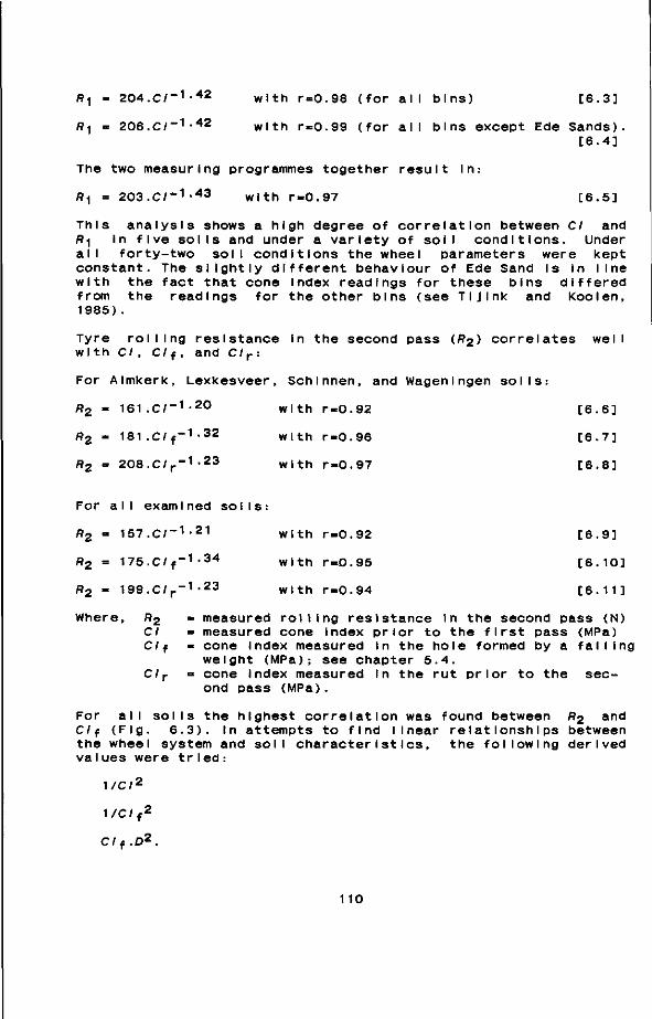
/?1 - 204.C/ - 1 - 4 2 with r-0.98 (for all bins) [6.3]
«1 = 206.C/ - 1 - 4 2 with r=0.99 (for all bins except Ede Sands).
[6.4]
The two measuring programmes together result In:
«1 = 203.C/ - 1 - 4 3 with r-0.97 [6.5] This analysis shows a high degree of correlation between CI and R-\ In five soils and under a variety of soil conditions. Under all forty-two soil conditions the wheel parameters were kept constant. The slightly different behaviour of Ede Sand Is In line with the fact that cone Index readings for these bins differed from the readings for the other bins (see TI J Ink and Kooien, 1985).
Tyre rolling resistance In the second pass (R2) correlates well with CI, Cl f, and C/r:
For Almkerk, Lexkesveer, Schinnen, and Wagen Ingen soils:
R2 = 161.C/- 1-2 0 with r-0.92 [6.6]
R2 = 181.C/ f- 1 - 3 2 with r-0.96 [6.7]
R2 = 208.C/ r- 1 - 2 3 with r-0.97 [6.8]
For all examined soils:
R2 = 157.C/~1-21 with r=0.92 [6.9]
R2 = 175.C/ f- 1 - 3 4 with r-O.95 [6.10]
R2 = 199.C/ r- 1 - 2 3 with r-0.94 [6.11]
Where, R2 * measured rolling resistance in the second pass (N) CI » measured cone Index prior to the first pass (MPa) Cl f - cone Index measured in the hole formed by a falling
weight (MPa); see chapter 5.4. C/r - cone index measured In the rut prior to the sec
ond pass (MPa).
For all soils the highest correlation was found between R2 and Cl f (Flg. 6.3). In attempts to find linear relationships between the wheel system and soil characteristics, the following derived values were tried:
1/C/2
1/C/f2
CI f.D2.
110
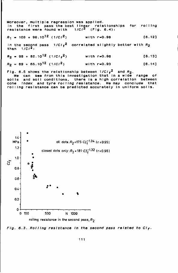
Moreover, multiple regression was applied. In the first pass the best linear relationships for rolllnç
1/C/2 resistance were found with
/?! - 109 + 96. 1 0 1 2 (1/C/2)
(Fig. 6.4):
with r-0.98 [6.12]
In the second pass 1/C/f2 correlated slightly better with Rz than 1/C/2:
98 + 82.101 2 (1/C/f2)
89 + 65.101 2 (1/C/2)
with r=0.96
with r=0.93
[6.13]
[6.14]
Fig. 6.5 shows the relationship between 1/C/f2 and R^. • We can see from this Investigation that In a wide range of
soils and soil conditions, there Is a high correlation between cone Index and tyre rolling resistance. We may conclude that rolling resistance can be predicted accurately In uniform soils.
o
u MPa
1.2
1.0
0.8
0.6
0M
0.2
S*
all dots:fl2=175-CJ f-1-34 ( r=0.95)
closed dots only:/?2 = 181 CJ f"1 '3 2 (r = 0.96)
-1 r-
0 100 500 N 1000
rolling resistance in the second pass,/?2
Fig. 6.3. Rolling rest stance In the second pass related to Clf.
111
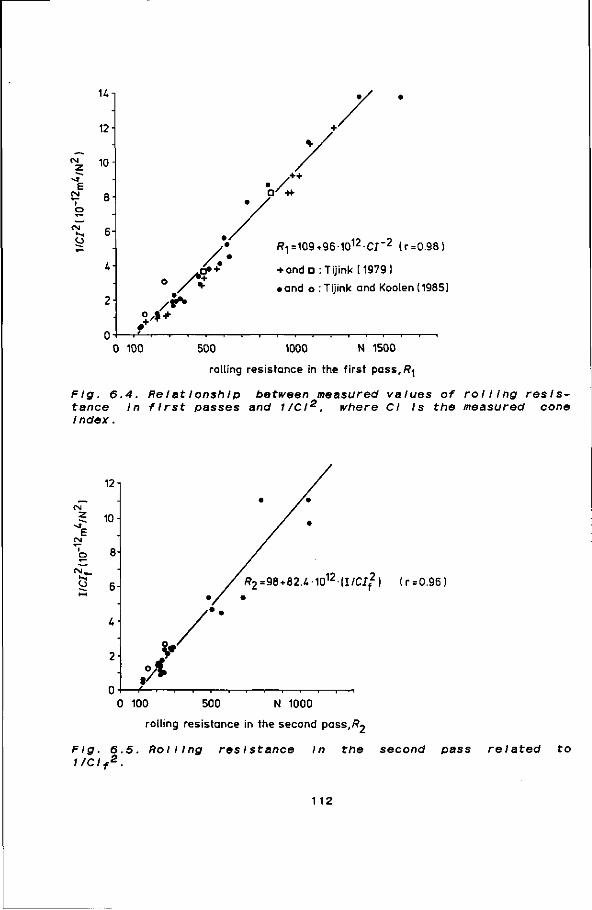
u
12-
10
e » 8
fM
2-
fl.|=:109*96-1012-CJ~2 ( r = 0.98)
+ ando : Tijink (1979)
• and o : Tijink and Kooien (1985)
0 100 500 1000 N 1500
rolling resistance in the f irst pass,/?^
Flg. 6 tance Index.
A. Relatlonshlp between measured values of rolling resls-In first passes and 1/CI2, where CI Is the measured cone
o""
12
10
8-
6-
U-
2
0
y P
R2 =98+82.4 -1012-(I /C/ f2) ( r=0.96)
0 100 500 N 1000
rolling resistance in the second pass,/?2
Fig. 6.5. Rolling res I stance In the second pass related to 1/Clf2.
112
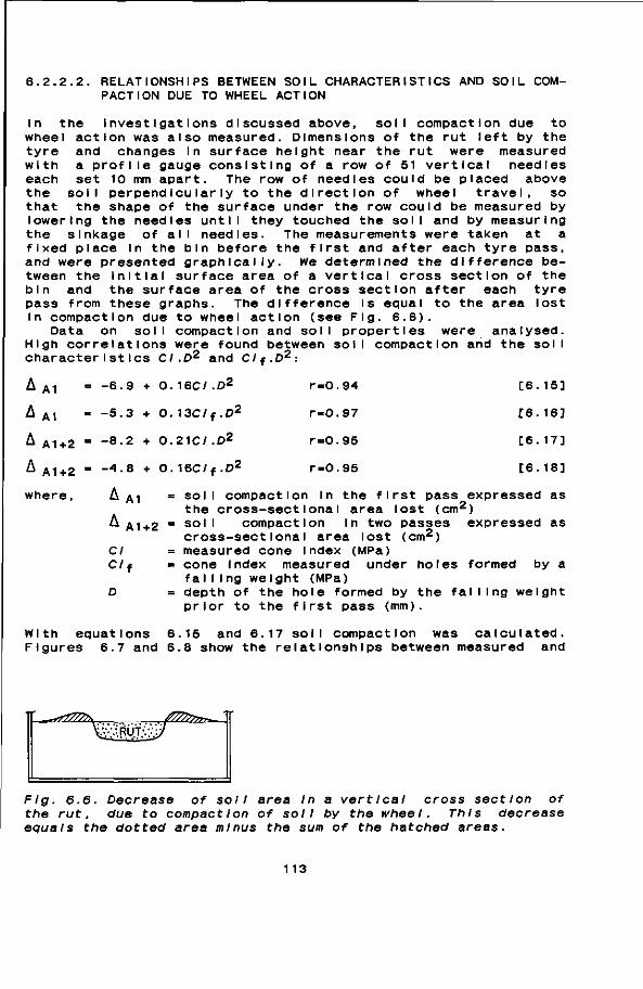
6.2.2.2. RELATIONSHIPS BETWEEN SOIL CHARACTERISTICS AND SOIL COMPACTION DUE TO WHEEL ACTION
In the Investigations discussed above, soil compaction due to wheel action was also measured. Dimensions of the rut left by the tyre and changes In surface height near the rut were measured with a profile gauge consisting of a row of 51 vertical needles each set 10 mm apart. The row of needles could be placed above the soil perpendicularly to the direction of wheel travel, so that the shape of the surface under the row could be measured by lowering the needles until they touched the soil and by measuring the s Inkage of all needles. The measurements were taken at a fixed place In the bin before the first and after each tyre pass, and were presented graphically. We determined the difference between the Initial surface area of a vertical cross section of the bin and the surface area of the cross section after each tyre pass from these graphs. The difference is equal to the area lost In compaction due to wheel action (see Fig. 6.6).
Data on soil compaction and soil properties were analysed. High correlations were found between soil compaction and the soil characteristics CI .D2 and Clf.D2-.
A A1 -
A A1 -
A A1+2 "
A A1+2 -
where,
-6.9 + 0.16C/.D'
-5.3 + 0.13C/f .D2
-8.2 + 0.21C/.D2
-4.8 + 0.16C/f.0'
r-0.94
r-0.97
r=0.95
r=0.95
[6.15]
[6.16]
[6.17]
[6.18]
A A1 = soil compaction in the first pass expressed as the cross-sectional area lost (cm2)
A A1+2 " so'' compaction in two passes expressed as cross-sectional area lost (cm2)
CI = measured cone Index (MPa) Cl f = cone index measured under holes formed by a
falI ing weight (MPa) D = depth of the hole formed by the falling weight
prior to the first pass (mm).
With equations 6.15 and 6.17 soil compaction was calculated. Figures 6.7 and 6.8 show the relationships between measured and
Fig. 6.6. Decrease of soil area In a vertical cross section of the rut, due to compact Ion of soil by the wheel. This decrease equals the dotted area minus the sum of the hatched areas.
113

c o o CL E o Ü
£ o D O O O
70-1
cm2
60-
50-
40-
30-
20-
10 H
( r=0 .97)
I 1 -I 1 1 1 1 1
0 10 20 30 CO 50 cm2 60 70
measured compaction,A^ Flg. 6.7. Re I atlonshlp between measured and predicted compact Ion In the first pass. Compact Ion Is expressed In cross-sectlonal area lost due to tyre action.
i.0 50 60 70 cm2 80
measured compaction, AA1 + 2
90
Fig. 6.8. Re I atlonshlp between measured and predicted compact Ion due to the first and the second wheel passes.
114
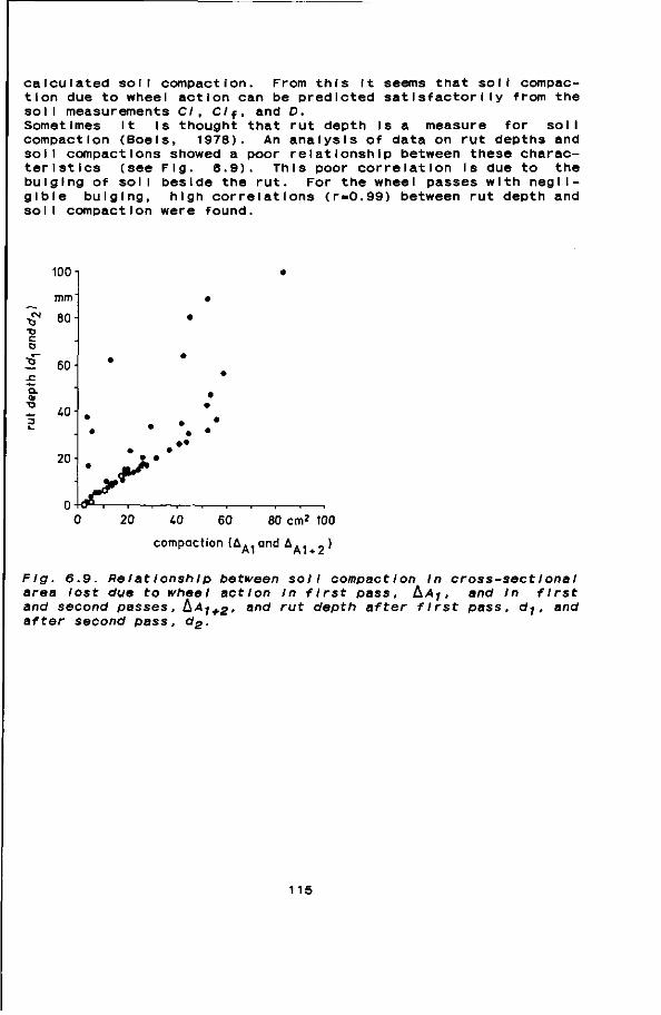
calculated soll compaction. From this It seems that soil compaction due to wheel action can be predicted satisfactorily from the soil measurements CI, C/f, and D. Sometimes It Is thought that rut depth Is a measure for soil compaction (Boels, 1978). An analysis of data on rut depths and soil compactions showed a poor relationship between these characteristics (see Fig. 6.9). This poor correlation Is due to the bulging of sol I beside the rut. For the wheel passes with neg I I-glble bulging, high correlations (r-0.99) between rut depth and soil compaction were found.
100
CM
"O T3 C O
mm
80 H
° 60
Q.
Z i.0
20 • •
uc 20 i.0 60 80 cm2 100
compaction (AA- and A . . _ )
Fig. 6.9. RelatlonshIp between soil compact Ion In cross-sectlonal area lost due to wheel action In first pass, AAJ, and In first and second passes, hAj+2' ancl rut depth after first pass, d j , and after second pass, d2.
115
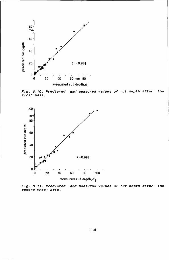
.c CL
TD
-) t _
•o <u o •D Ol Q.
ÖU-mm
60-
" 40-
20
n j
• / /
*• /
* / »'
y • X
( r = 0.98)
0 20 40 60 mm 80
measured rut depth,d^
Flg. 6.10. Predicted and measured values of rut depth after the first pass.
100-
mm'
80-
Q.
"° 60
ai y 40
T> <V
201 °*y'
? • •
( r=0.99)
0 20 40 60 80 100
measured rut depth, d ^
Fig. 6.11. Predicted and measured values of rut depth after the second wheel pass.
116
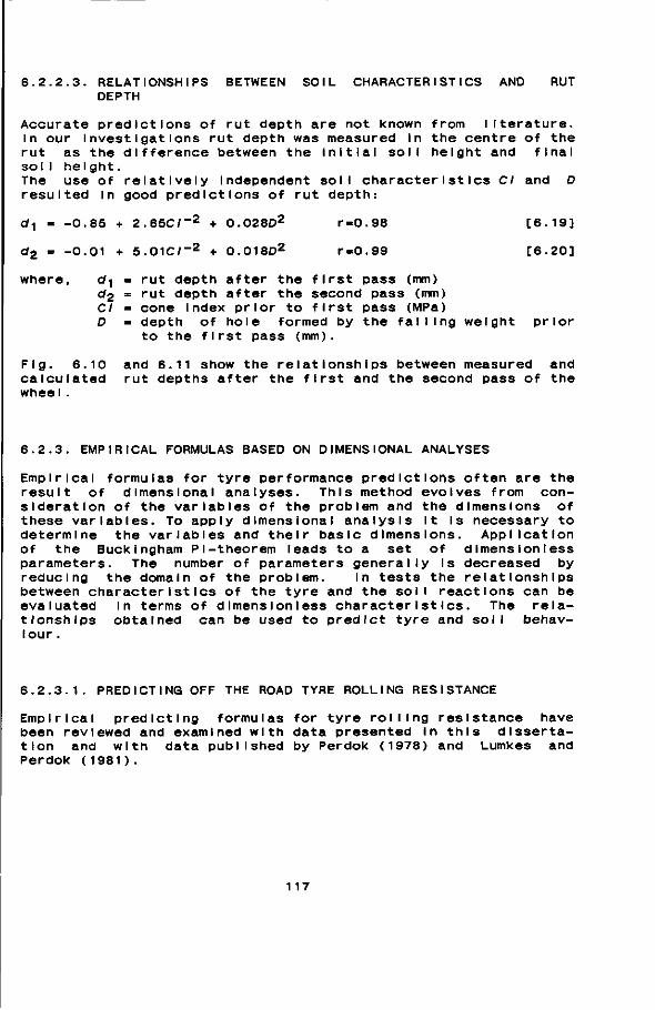
6.2.2.3. RELATIONSHIPS BETWEEN SOIL CHARACTERISTICS AND RUT DEPTH
Accurate predictions of rut depth are not known from literature. In our Investigations rut depth was measured In the centre of the rut as the difference between the initial soil height and final sol I helght. The use of relatively Independent soil characteristics CI and D resulted In good predictions of rut depth:
'1 -0.85 + 2.65C/-2 + 0.028D2 r-0.98 [6.19]
-0.01 + 5.01C/-2 + 0.018D2 r-0.99 [6.20]
where, tf^ « rut depth after the first pass (mm) d2 - rut depth after the second pass (mm) CI - cone Index prior to first pass (MPa) D » depth of hole formed by the falling weight prior
to the first pass (mm).
Fig. 6.10 and 6.11 show the relationships between measured and calculated rut depths after the first and the second pass of the whee I .
6.2.3. EMPIRICAL FORMULAS BASED ON DIMENSIONAL ANALYSES
Empirical formulas for tyre performance predictions often are the result of dimensional analyses. This method evolves from consideration of the variables of the problem and the dimensions of these variables. To apply dimensional analysis it Is necessary to determine the variables and their basic dimensions. Application of the Buckingham Pl-theorem leads to a set of dimension less parameters. The number of parameters generally is decreased by reducing the domain of the problem. In tests the relationships between characteristics of the tyre and the soil reactions can be evaluated In terms of dImensionless characteristics. The relationships obtained can be used to predict tyre and soil behaviour.
6.2.3.1. PREDICTING OFF THE ROAD TYRE ROLLING RESISTANCE
Empirical predicting formulas for tyre rolling resistance have been reviewed and examined with data presented in this dissertation and with data published by Perdok (1978) and Lumkes and Perdok (1981).
1 17
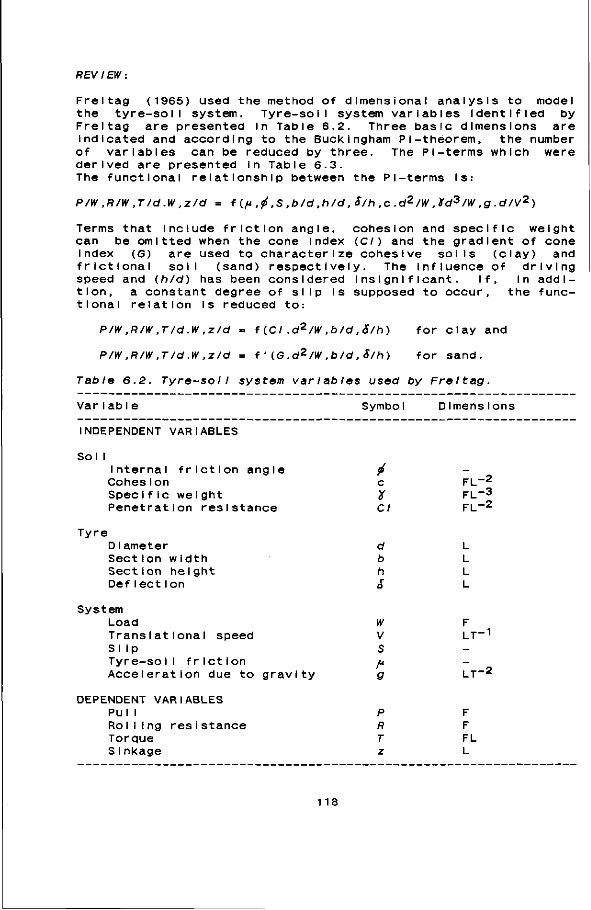
REV IEW:
F r e i t a g ( 1 9 6 5 ) u s e d t h e m e t h o d of d i m e n s i o n a l a n a l y s i s to m o d e l t h e t y r e - s o i l s y s t e m . T y r e - s o i l s y s t e m v a r i a b l e s i d e n t i f i e d by F r e i t a g a r e p r e s e n t e d in T a b l e 6 . 2 . T h r e e b a s i c d i m e n s i o n s a r e i n d i c a t e d and a c c o r d i n g to t h e B u c k i n g h a m P i - t h e o r e m , t h e n u m b e r
of v a r i a b l e s c a n be r e d u c e d by t h r e e . T h e P l - t e r m s w h i c h w e r e d e r i v e d a r e p r e s e n t e d in T a b l e 6.3. T h e f u n c t i o n a l r e l a t i o n s h i p b e t w e e n t h e P l - t e r m s is:
P/W ,R/W ,T/d.W ,zld m f(ft,f(,S,b/d,h/d,S/h,c.d2/W,Xd3/W,g.d/V2)
T e r m s that i n c l u d e f r i c t i o n a n g l e , c o h e s i o n and s p e c i f i c w e i g h t c a n b e o m i t t e d w h e n t h e c o n e index (C/) and t h e g r a d i e n t of c o n e index (G) a r e used to c h a r a c t e r i z e c o h e s i v e s o i l s ( c l a y ) and f r i c t l o n a l soli ( s a n d ) r e s p e c t i v e l y . T h e i n f l u e n c e of d r i v i n g s p e e d and (h/d) h a s b e e n c o n s i d e r e d I n s i g n i f i c a n t . If, In a d d i t i o n , a c o n s t a n t d e g r e e of s l i p is s u p p o s e d to o c c u r , t h e f u n c tional r e l a t i o n Is r e d u c e d t o :
P/W,R/W,T/d.W,z/d = f(Cl.d2/W,b/d,6/h) for clay and
P/W,R/W,T/d.W,z/d = f ' { G . d 2 / W , b / d , S/h) for sand.
Table 6.2. Tyre-sol I system var I ab les used by Freitag.
Variable Symbol Dimensions
INDEPENDENT VARIABLES
Sol I Internal friction angle CohesIon Spec i f le we Ight Penetration resistance
Tyre D I ameter Sect Ion w i dth Section height DefIectIon
System Load Transi ationaI speed Slip Tyre-so II fr let ion Acceleration due to gravity
DEPENDENT VARIABLES Pu I I Rol I Ing r e s i s t a n c e Torque S I nkage
• c y CI
d b h S
W V
s f* g
p R T z
FL-2 FL-3 FL-2
L L L L
LT-1
LT-2
F F FL L
1 18
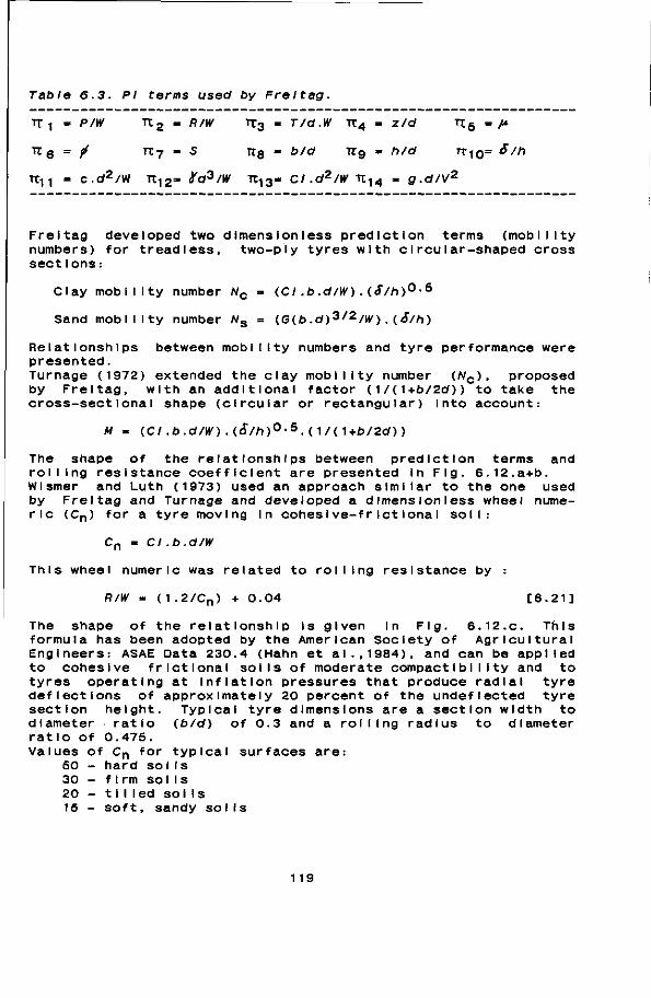
Table 6.3. PI terms used by Freitag.
TT 1 = P/W T C 2 - R/W TT 3 - T/d.W TT 4 - Z/d TT. 5 =/*
Tt g = / TT7 = S Tts - b/d TTg • h/d ^10°° S/h
Ttn = cd2/VI Tt12- Xd*/W K13- CI .d2/W Mit - g.d/V2
Freitag developed two dimens I on less prediction terms (mobility numbers) for treadless, two-ply tyres with circular-shaped cross sect I ons :
Clay mobility number Nc = (CI.b.d/W).(S/h)°'5
Sand mobility number N s = (G(fc.d)3/2/^).( S/h)
Relationships between mobility numbers and tyre performance were presented. Turnage (1972) extended the clay mobility number (Nc) , proposed by Freitag, with an additional factor (1/(1+b/2c0 ) to take the cross-sectional shape (circular or rectangular) into account:
M - (CI.b.d/W).(S/h)0-5.(1/(1+b/2c0 )
The shape of the relationships between prediction terms and rolling resistance coefficient are presented in Fig. 6.12.a+b. Wlsmer and Luth (1973) used an approach similar to the one used by Freitag and Turnage and developed a dImension I ess wheel numeric (Cn) for a tyre moving In cohesive-frletlonaI soli:
C n = CI.b.d/W
This wheel numeric was related to rolling resistance by :
R/W - (1.2/Cn) + 0.04 [6.21]
The shape of the relationship Is given In Flg. 6.12.C. Tri I s formula has been adopted by the American Society of Agricultural Engineers: ASAE Data 230.4 (Hahn et al.,1984), and can be applied to cohesive frletlonaI soils of moderate compact lb I Iity and to tyres operating at inflation pressures that produce radial tyre deflections of approximately 20 percent of the undeflected tyre section height. Typical tyre dimensions are a section width to diameter ratio (b/d) of 0.3 and a rol I ing radius to diameter ratio of 0.475. Values of C n for typical surfaces are:
50 - hard so I I s 30 - f Irm sol I s 20 - 11 I led sol Is 15 - soft, sandy soils
119
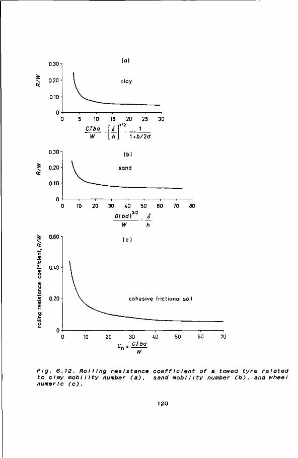
0.30-
\ 0.20 • Q:
clay
0.10-
0-5 10 15 20 25 30
CIbd
W £ h
1
1+b/2d
0.301
^ 0.20 i
0.10-
0
k 0.60
Q:
"c. <u V
iE o.io o
u c a « 0.20 U) ai L-
Dl C
10 20 30 £0 50 60 70 80
Gibd)3'2 {
W h
( c )
cohesive fr ict ional soil
10 20 30 i.0 r . CIbd
50 60 70
W
Flg. 6.12. Rolling resistance coefficient of a towed tyre related to clay mobility number (a), sand mobility number (b), and wheel numeric (c).
120
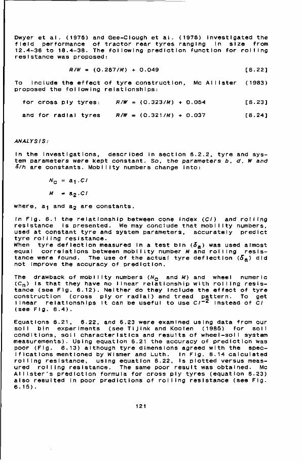
Dwyer et al. (1975) and Gee-Clough et al. (1978) Investigated the field performance of tractor rear tyres ranging In size from 12.4-36 to 18.4-38. The following prediction function for rolling resistance was proposed:
R/W = (0.287/M) + 0.049 [6.22]
To Include the effect of tyre construction, Me AI I Ister (1983) proposed the following relationships:
for cross ply tyres: R/W = (0.323/M) + 0.054 [6.23]
and for radial tyres R/W = (0.321/M) + 0.037 [6.24]
ANALYSIS:
In the Investigations, described In section 6.2.2, tyre and system parameters were kept constant. So, the parameters b, d, W and S/h are constants. Mobility numbers change into:
Nc = & 1 .C/
M = a2.C/
where, a-) and az a r e constants.
In Fig. 6.1 the relationship between cone Index (C/) and rolling resistance Is presented. We may conclude that mobility numbers, used at constant tyre and system parameters, accurately predict tyre rolling resistance. When tyre deflection measured In a test bin (£a) was used almost equal correlations between mobility number M and rolling resistance were found. The use of the actual tyre deflection (ó"a) did not Improve the accuracy of prediction.
The drawback of mobility numbers (Nc and M) and wheel numeric (Cn) Is that they have no linear relationship with rolling resistance (see Fig. 6.12). Neither do they Include the effect of tyre construction (cross ply or radial) and tread pattern. To get linear relationships It can be useful to use C / - 2 Instead of CI (see Fig. 6.4).
Equations 6.21, 6.22, and 6.23 were examined using data from our soil bin experiments (see TIJInk and Kooien (1985) for soil conditions, soil characteristics and results of wheel-soil system measurements). Using equation 6.21 the accuracy of prediction was poor (Fig. 6.13) although tyre dimensions agreed with the specifications mentioned by Wismer and Luth. In Fig. 6.14 calculated rolling resistance, using equation 6.22, Is plotted versus measured rolling resistance. The same poor result was obtained. Mc AI lister's prediction formula for cross ply tyres (equation 6.23) also resulted In poor predictions of rolling resistance (see Fig. 6. 15).
121
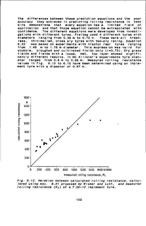
The differences between these prediction equations and the poor accuracy they achieved In predicting rolling resistance In test bins demonstrate that every equation has a limited field of application and that those equation cannot be extrapolated with confidence. The different equations were developed from Investigations with different tyres. Freitag used 4 different tyres with diameters ranging from 0.36 m to 0.72 m. These were all tread-less, thln-walled, cross ply tyres with two-ply rating. Equation 6.22 was based on experiments with tractor rear tyres ranging from 1.45 m to 1.75 m diameter. This expression was valid for stubble, ploughed and cultivated fields only (r-0.73). Dry grass fields and fields with a loose, wet, top layer showed significantly different results. In Me AI lister's experiments tyre diameter ranged from 0.8 m to 0.95 m. Measured rolling resistance values In Fig. 6.13 to 6.15 have been determined using an Implement tyre with a diameter of 0.67 m.
1600 i
<D O c o
Ol c o 1000
O
200 400 600 800 1000 1200 U00 1600N1800
measured rolling resistance, R^
Flg. 6.13. Relation between calculated rolling resistance, calculated using equ. 6.21 proposed by Wlsmer and Luth, and measured rolling rest stance (Rj) of a 7.00-12 Implement tyre.
122
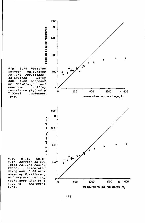
1600
O c o
Ï 1200 •
at c
•o 01 'S 800
Flg. 6 between rol I1ng calcuIated equ. 6.22
14. Relation calculated
reslstance, us Ing
proposed by Gee-Clough, and measured rolling reslstance (Rj) of a 7.00-12 Implement tyre.
400
400 800 1200 N 1600
measured rolling resistance,/?^
ai o o Vi
O) c
Flg. 6.15. Relation between calculated rolling resistance, calculated using equ. 6.23 proposed by McAlI Ister, and measured rolling res I stance (Rj) of a 7.00-12 Implement tyre.
1600
1200
~ 600-
400
400 1200 1400 N 1600
measured roll ing resistance,/?^
123
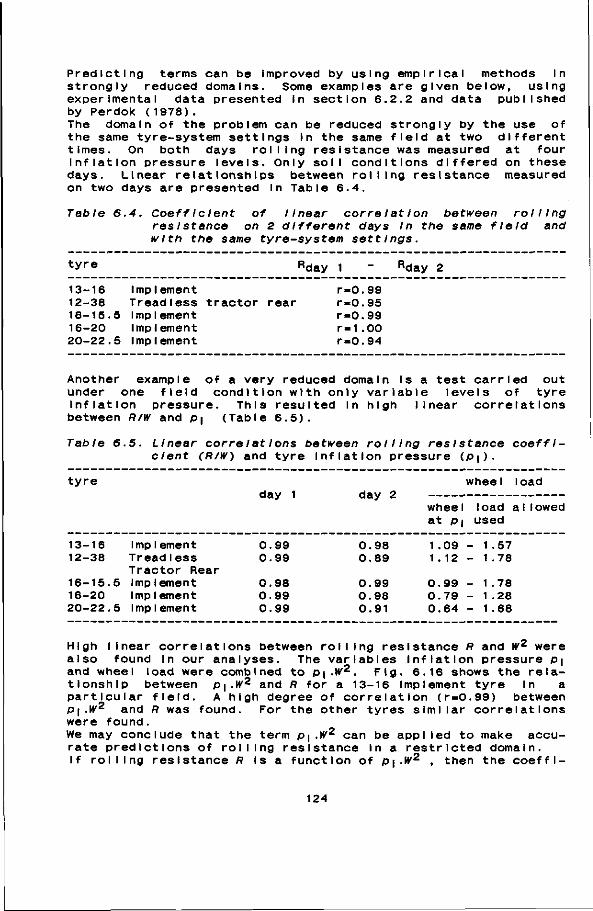
Predicting terms can be Improved by using empirical methods In are given below, using 2.2 and data published
strongly reduced domains. Some examples experimental data presented In section 6 by Perdok (1978). The domain of the problem can be reduced the same tyre-system settings In the same times. On both days rol I ing resistance was measured at Inflation pressure levels. Only soli conditions differed on
strongly f leid at
by the use of two dI f ferent
four these
days. Linear relationships between rolling resistance on two days are presented In Table 6.4.
measured
Table 6.4. Coeff/clent of linear correlation between rolling res I stance on 2 different days In the same field and with the same tyre-system sett Ings.
tyre Rday 1 <day 2
13-16 Implement 12-38 Tread less 16-15.5 Implement 16-20 Implement 20-22.5 Implement
tractor rear r=0.99 r-0.95 r-0.99 r=1.00 r-0.94
Another example of a very reduced domain Is a test carried out under one field condition with only variable levels of tyre inflation pressure. This resulted In high linear correlations between R/W and p\ (Table 6.5).
Table 6.5. Linear correI at Ions between rolling res I stance coefficient (R/W) and tyre Inflation pressure (P|).
tyre
13-16 12-38
16-15.5 16-20 20-22.5
Implement Tread I ess Tractor Rear Imp Iement Implement Imp Iement
day 1
0.99 0.99
0.98 0.99 0.99
day 2
0.98 0.89
0.99 0.98 0.91
wheel load
wheel load allowed at p\ used
1.09 - 1.57 1.12 - 1.78
0.99 - 1.78 0.79 - 1.28 0.64 - 1.68
High linear correlations between rolling resistance R and W 2 were also found In our analyses. The variables Inflation pressure p\ and wheel load were combined to p\.W2. Fig. 6.16 shows the relationship between P\.WZ and R for a 13-16 implement tyre in a particular field. A high degree of correlation (r=0.99) between P\.WZ and R was found. For the other tyres similar correlations were found. We may conclude that the term p\.Wz can be applied to make accurate predictions of rolling resistance in a restricted domain. If rolling resistance A Is a function of P\.WZ , then the coeffI-
124
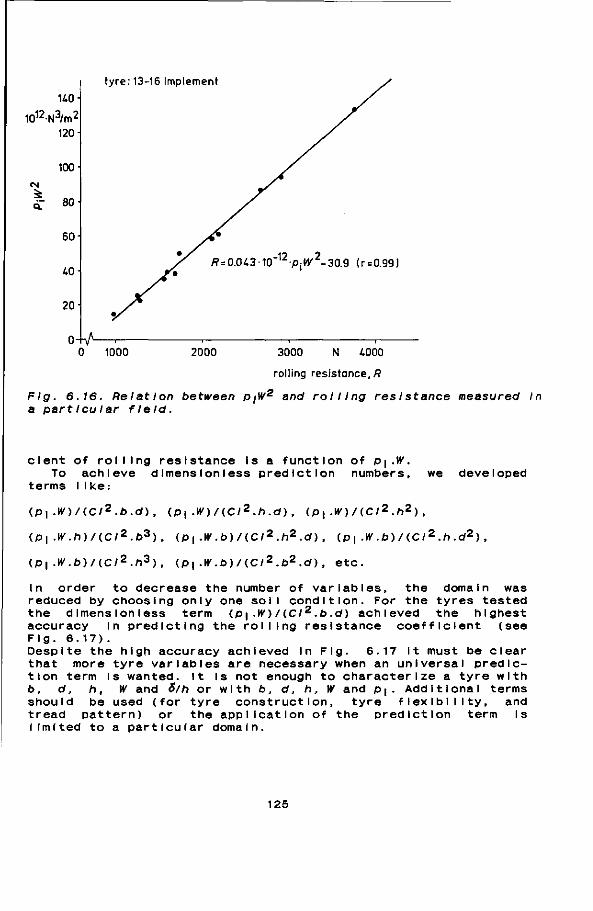
uo-10 1 2N 3 /m 2
120-
100-
CM
| - 80
60
40
20-
oV
ty re: 13-16 Implement
R = 0 .043-10"1 2-Pj^2-30.9 (r=0.99)
1000 2000 3000 N 4000
rolling resistance,/?
Flg. 6.16. Relation between p/W2 and rolling resistance measured In a part leu Iar field.
clent of rolling resistance is a function of P\.W. To achieve dImension less prediction numbers, we developed
terms I Ike:
( p , . W ) / ( C I 2 . b . d ) , (ps.W)/(CI2.h.d), ( p , . W ) / ( C I 2 . h 2 ) ,
(p, .W./7)/(C/2.to3) , (P| .W.b)/(CI2.h2.d) , (p\.W .b)/(.CI2.h.d2) ,
( P l . W . b ) / ( C I 2 . h 3 ) , ( P | . W . b ) / { C I 2 . b 2 . d ) , etc.
In order to decrease the number of variables, the domain was reduced by choosing only one soil condition. For the tyres tested the dimensIon I ess term (P| .W) / (C I 2 .b .d ) achieved the highest accuracy In predicting the rolling resistance coefficient (see Fig. 6.17). Despite the high accuracy achieved In Fig. 6.17 It must be clear that more tyre variables are necessary when an universal prediction term Is wanted. It Is not enough to characterize a tyre with b, d, h, W and S/h or with b, d, h, W and p ( . Additional terms should be used (for tyre construction, tyre flexibility, and tread pattern) or the application of the prediction term Is limited to a particular domain.
125
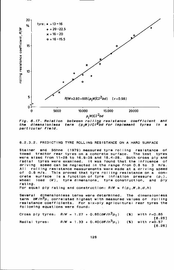
20
%
i= 15
10
5
o£
t y re : • =13-16
+ =20-22.5
x = 1 6 - 2 0
o =16-15.5
R/W=2.60*695lpiW/CI2bd) ( r=0.98)
5000 10.000 15.000 20.000
p\NlCIlbd 6.17. Relation between rolling rest stance coeffIclent and dI mens I on less term (p/W)/Cl^bd for Implement tyres In a
Fig. the particular field.
6.2.3.2. PREDICTING TYRE ROLLING RESISTANCE ON A HARD SURFACE
Stelner and Söhne (1979) measured tyre rolling resistance of towed tractor rear tyres on a concrete surface. The test tyres were sized from 11-28 to 16.9-38 and 18.4-26. Both cross ply and radial tyres were examined. It was found that the Influence of driving speed can be neglected in the range from 0.8 to 3 m/s. All rolling resistance measurements were made at a driving speed of 0.8 m/s. This proved that tyre rolling resistance on a concrete surface Is a function of tyre inflation pressure (P|), wheel load (W) , tyre dimensions, tyre construction, and ply rat Ing. For equal ply rating and construction: R/W = f(p|,W,b,d,h)
Several dImensIon I ess terms were determined. The dimension less term bW/h3pi correlated highest with measured values of rolling resistance coefficients. For six-ply agricultural rear tyres the following equations were found:
Cross ply tyres: R/W = 1.27 + 0.65(bW/h3p|) (%) with r=0.85 [6.25]
R/W = 1.33 + 0.40(bW//i3P| ) (%) with r=0.57 [6.26]
Radial tyres:
126
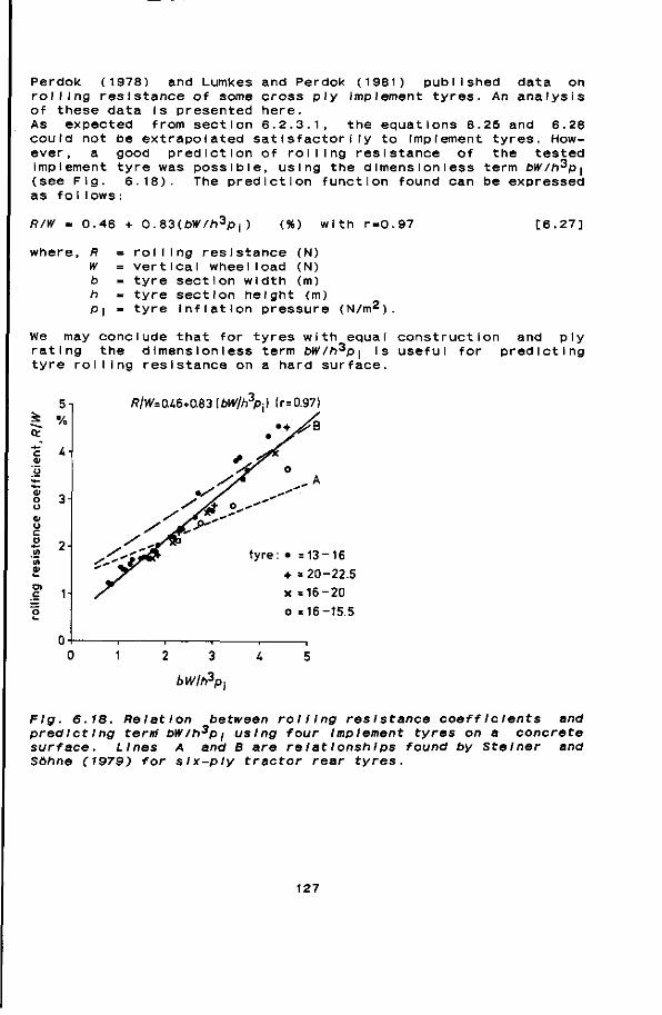
Perdok (1978) and Lumkes and Perdok (1981) published data on rolling resistance of some cross ply Implement tyres. An analysis of these data Is presented here. As expected from section 6.2.3.1, the equations 6.25 and 6.26 could not be extrapolated satisfactorily to Implement tyres. However, a good prediction of rolling resistance of the tested implement tyre was possible, using the dimension I ess term bW/h^p\ (see Fig. 6.18). The prediction function found can be expressed as fol lows :
R/W = 0.46 + 0.83(bW/h3p,) (%) with r=0.97 C6.27]
where, R = rolling resistance (N) W = vertical wheel load (N) to = tyre section width (m) h = tyre section height (m) P\ = tyre Inflation pressure (N/m2)
We m rati tyre
may conclude that for tyres with equal ng the dimensIon I ess term bW/h3p\ is •• rolling resistance on a hard surface.
with equal construction and ply "* useful for predicting
5
^ %
<u
0) o o ai o c o
3-
- 2
O) c
R/W= 0X6+0.83 lbW/h3p-.) (r=0.97)
tyre: • =13-16
+ =20-22.5
x =16-20
o = 16-15.5
0 1 2 3 4 5
bWlh2pi
Flg. 6.18. Relation between rolling reslstance coeffIclents and predict Ing term' bW/h3Pi using four Implement tyres on a concrete surface. Lines A and B are relatlonshlps found by Stelner and Sohne (1979) for six-ply tractor rear tyres.
127
6.3. APPROXIMATE METHODS
Approximate methods to predict off-the-road wheel performance are generally based on pressure-sInkage relationships. Bernstein (1913) stated that rolling resistance of a wheel is due to the vertical work done In rut forming. Predictions have been based on the pressure-sinkage relationships of a rectangular p i ate:
p « K.zn
where, p » pressure on the plate k m modulus of soil deformation z - s Inkage n - exponent of deformation.
Bernstein found n = 0.5 for agricultural soils. The parameter k proved to be dependent on plate dimensions.
Bekker (1956, 1960, 1969) used the Bernstein theory to predict rolling resistance. To get independent parameters Bekker proposed that the modulus of soli deformation has two components; kc Is the cohesive component and k^ the frlctlonal component:
k = kc/b + k$
B e k k e r ' s p r e s s u r e - s I n k a g e r e l a t i o n s h i p of a rectangular plate states that:
p = (kc/b + kó)zn
To o b t a i n v a l u e s for kc and k^, p e n e t r a t i o n tests w i t h different plate w i d t h b a re needed. Assuming that rolling resistance Is equal to vertical work done In rut forming and that soil reaction, at a point In the contact area, Is a l w a y s radial to the wheel and equal to the pressure under a vertical plate at the same depth, Bekker formulated the following rolling r e s i s t a n c e e x p r e s s i o n :
b(kc/b + k^)
n + 1
ZW
b(kc/b + *0)c*o-5(3 n)
(2n+2/2n+1)
To determine ground pressure (Pg) under a tyre Bekker proposed to use the following expression:
Pg - P\ + Pc-
where, p\ =• Inflation pressure of the tyre pc - carcass stiffness.
Rolling resistance now becomes: R [£>(P| + p c ) ] C + 1 ) / n
(kc + ö * Ä ) 1 / n ( n + 1)
128
Uffelmann (1961) also assumed that the soil reaction Is radial to the wheel and that the rolling resistance Is equal to vertical work done. The pressure beneath a track Is expressed as:
p = 5.7c
where, c - cohesion of the soli.
Uffelmann's rolling resistance equation for towed rigid wheels Is:
R = W2/5.7cbd
In fact this Is a special case of Bekker's theory with n-0 and p=kc/b + k^.
Wills et a I.(1965) Investigated the validity of the Bekker theories. They found that:
- rolling resistance Is not only due to vertical work done - the assumption of a pure radial soil reaction Is not cor
rect - n Is a so M parameter - kc, k$ and k are dependent on plate dimensions.
In his theory Gee-Clough (1976,1979) Included the effects of slip and deep slnkage on rolling resistance of rigid wheels In sand. He proposed to determine soil slnkage parameters from measurements with a wheel of known dimensions. This principle Is the basis of the "Wheel Bevameter". It Is less difficult to determine the Bekker soil parameters with the "Wheel Bevameter". The soil reaction under a "Wheel Bevameter" Is more similar to the one under a wheel than to the one under a strip footing.
To make the Bekker theory applicable to pneumatic tyres, Perdok (1978) assumed that a flexible tyre of a defined size behaves like a rigid wheel of a larger diameter (see Fig. 6.19). A defor
mation factor C was introduced:
D* = CD
where, D* = alternative rigid wheel diameter D m tyre dlameter.
The deformation factor depends on Inflation pressure, wheel load, and soil conditions. Full-si zed rigid wheels were used as "Wheel Bevameter". The "Wheel Bevameter" gives better predictions than the plate slnkage tests. It also makes the pressure-sInkage method more empIrIcal.
Kooien (1976) gives an approximate method for soil compaction under a towed tyre. His theory is based on the hypothesis that the compaction of a volume element of soil under a certain tyre for a certain soil and wheel load can be predicted by uniaxial compression of a sample of that soil (Fig. 6.20). In this unl-
129
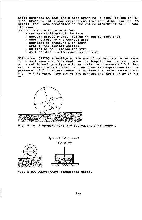
axial compression test the piston pressure Is equal to the Inflation pressure plus some corrections that should be applied to obtain the same compaction as the volume element of soil under the wheel. Corrections are to be made for:
- carcass stiffness of the tyre - unequal pressure distribution In the contact area - shear stress In the contact area - decrease of pressure with depth - area of the contact surface - bulging of soli beside the tyre - wall friction In the compression test.
Stienstra (1976) investigated the sum of corrections to be made for a sol I sample at 5 cm depth In the longitudinal centre plane of a rut formed by a tyre with an inflation pressure of 3.3 bar and a wheel load of 30 kN. In the uniaxial compression test a pressure of 7.1 bar was needed to achieve the same compaction. So, in this case, the sum of the corrections had a value of 3.8 bar .
Fig equivalent rigid wheel
tyre inflation pressure
+ corrections
•A"\".-V
Äs « » vc^
Fig. 6.20. Approximate compaction model
130

6.4. EXACT METHODS
Exact methods try to model soil deformation in a mathematical way. Two approaches to predict soil-wheel behaviour have been adopted: the s I Ip-1 I ne method and the finite element method.
6.4.1. SLIP-LINE METHODS
In the longitudinal plane of a wheel-so I I system two fields of soil failure were found by Wong and Reece (1966,1967). A mathematical model based on limit equilibrium was used to predict the stress distribution under two-dimensional wheels. Good agreement between measured and predicted values was achieved. The model assumes an Incompressible med I urn and is therefore not adequate for predicting soil compaction due to wheel action. Karaf lath and Nowatzkl (1978) showed similar failure zones. Their solutions assumed that a rut was formed. However, this can not be combined with plain strain and an incompressible medium.
6.4.2. FINITE ELEMENT METHODS
Perumpral et al.(1971) adopted the finite element method (FEM) to predict wheel-soil behaviour. The FEM assumes linear stress-strain relationships. Soils do not satisfy this assumption. Therefore, a variable elastic modulus for the soil was assumed. So, each finite element was given such different elastic values that the non-linear stress-strain curve was approximated. Strictly speaking this Is incorrect. Yong and Fattah (1976) used a similar method. Wheel performance was predicted In terms of energy components as a function of wheel slip. Investigations with tyres operating on an undeformable surface were made by Yong et al.(1978) to Include tyre deformation in the prediction model. Although attemps have been made to apply the FEM to flexible wheels, the FEM-approach Is two-dimensional and therefore less useful In predicting wheel and tyre performance In field operations, where bulging occurs beside the wheel.
6.5. CLOSING REMARKS ON PREDICTION METHODS
With empirical methods wheel-soil characteristics can be predicted accurately in uniform soils. The relationships discussed In section 6.2.2 show that easily obtainable soil characteristics can be used for these predictions. In agricultural field practice soli conditions usually vary with depth. Therefore, further studies should be made to account for sol I var lat Ions. Under uniform soil conditions dImensionaIly correct empirical methods can also achieve a high degree of accuracy In predictions (see section 6.2.3).
131
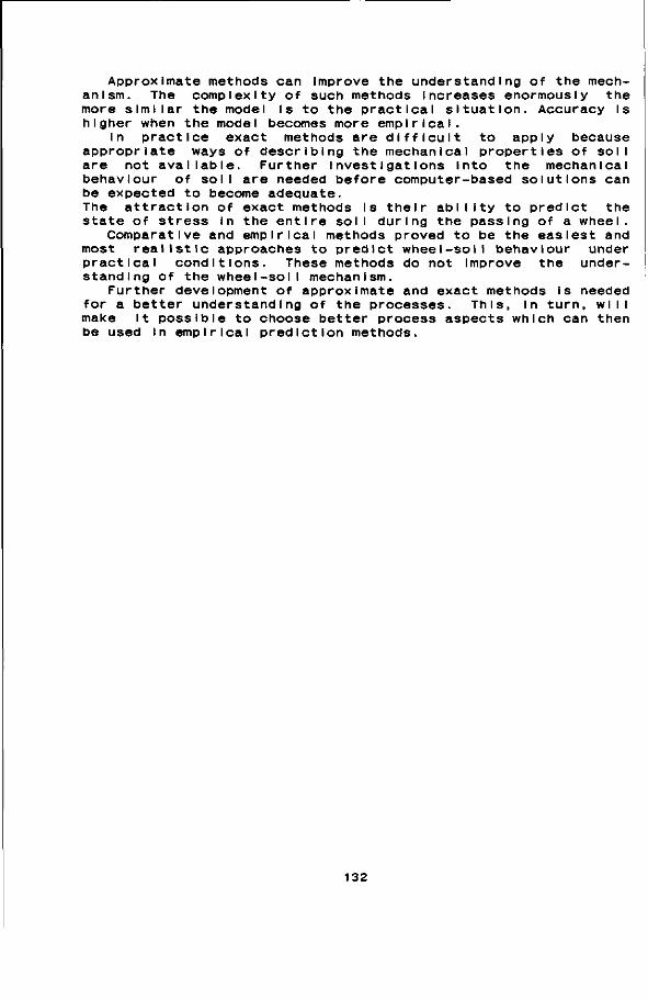
Approximate methods can Improve the understanding of the mechanism. The complexity of such methods Increases enormously the more similar the model Is to the practical situation. Accuracy Is higher when the model becomes more empirical.
In practice exact methods are difficult to apply because appropriate ways of describing the mechanical properties of soil are not available. Further Investigations into the mechanical behaviour of soil are needed before computer-based solutions can be expected to become adequate. The attraction of exact methods Is their ability to predict the state of stress In the entire soil during the passing of a wheel.
Comparative and empirical methods proved to be the easiest and most realistic approaches to predict wheel-so I I behaviour under practical conditions. These methods do not Improve the understanding of the wheel-so I I mechanism.
Further development of approximate and exact methods is needed for a better understanding of the processes. This, In turn, will make It possible to choose better process aspects which can then be used in empirical prediction methods.
132
CHAPTER 7
SOIL PHYSICAL ASPECTS OF LOAD-BEARING PROCESSES
can change due to load-bearing physical properties influence
(partIcI e content,
the
The physical properties of a soil processes. On the other hand soil the mechanical behaviour of a soil. For a given soil with specific Intrinsic properties size distribution, types of minerals, organic matter etc.) Important physical factors on the micro level are: - pore space and the distribution of pore sizes - the d istrI but Ion of soi I part le les within the so I I - soil water content and the distribution of water within
sol I - soli air content and the distribution of air within the soil - points of contact: number of contacts, bonds, and distributions
of these bonds. These properties, so-called micro-factors, can be changed not only by tillage processes but also by natural forces (freezing, thawing, etc). Tillage processes Influence the mechanical properties of the so I I as wel I. In general farmers are not interested in micro-factors, but In
as: pF-curves, water and gas conductivities, penetration resistance, erodiblllty, till-
thls point of view soli mechanical properties qua Ii tles as wel I. can be seen as the Interface between tillage
qua I 11les.
so I I qua I 111 es such thermal properties, ab I I Ity, etc. From can be seen as sol I The micro-factors processes and sol Kooien (1986) deals with the relationships between micro-factors, soil mechanical properties, mechanical processes, and process effects. In this chapter we discuss the Influence of some physical properties on mechanical properties and the Influence of mechanical treatment on physical properties.
7.1. THE INFLUENCE PROPERTIES
OF PHYSICAL PROPERTIES ON MECHANICAL
Soil mechanical properties often are divided Into compact IbI I Ity, deformabl Iity, and breakablI Ity. Kooien (1986) who uses a more fundamental approach distinguishes between stable and unstable behaviour. The behaviour of a process
133
Is called stable if the process tends to occur throughout the entire soil. An example of stable behaviour Is the compaction of loose soil. Unstable behaviour occurs when the process has a tendency to concentrate on a spot. Unstable behaviour occurs on the spots where soil breaking starts. In practice physical soil degradation generally Is not only associated with the effects of Increased bulk density but also with those of large soil deformations that occur when the soil volume remains almost constant. Compact IbI I Ity and deformabI I Ity are therefore Important mechanical properties In relation to soil physical degradation. A simple test to measure compactibI I Ity Is the uniaxial compression test. This test and the test facility parameters that influence this test have been discussed In section 5.3. Soils used in uniaxial compression tests generally have been sieved. Depending on the screens used the soil sample can have a small or a wide aggregate diameter range. For soil samples this may result In different bulk densities during filling and/or a different number of contact points between aggregates. A different number of contact points between aggregates may result In a different compact IbI I Ity. To Investigate a possible effect of aggregate diameter on compact IbI I Ity, uniaxial compression tests were carried out for different aggregate diameter classes and mixtures of aggregate diameter classes. Section 7.1.1 deals with these tests.
In uniaxial compression tests on a soil with specific Intrinsic properties (particle size distribution, type of minerals, organic matter content, etc) the moisture content Is probably the major strength-determining factor for compact IbI I Ity. Kooien (1986) distinguishes between dry compaction and wet compaction. After dry compaction the initial structure Is at least locally preserved in the compacted soil. During wet compaction of soil, the bulk density Increase is limited by partial water saturation. In this final phase of wet compaction air may be entrapped. In this entrapped air pressure may build up. When the soil Is unloaded this air pressure may contribute to rebound. Uniaxial compression tests have been carried out investigate the Influence of soil air on rebound. These tests are discussed In 7.1.2.
7.1.1. THE INFLUENCE OF AGGREGATE DIAMETER ON UNIAXIAL COMPRESSIBILITY.
The uniaxial compression behaviour of soil samples with different aggregate diameters has been examined for two soils as follows: Wagen Ingen s I Ity clay loam and Lexkesveer loam were passed through a 10 mm screen. After having been dried at room temperature to a moisture content below the hygroscopic point, each soil was sieved into 3 aggregate diameter classes:
3.0 - 3.4 mm 4.0 - 4.8 mm 6.8 - 8.0 mm.
Aggregate portions of 1 kg were placed on soil water suction bins at a value of pF2.0. One day later suctions were decreased to
134
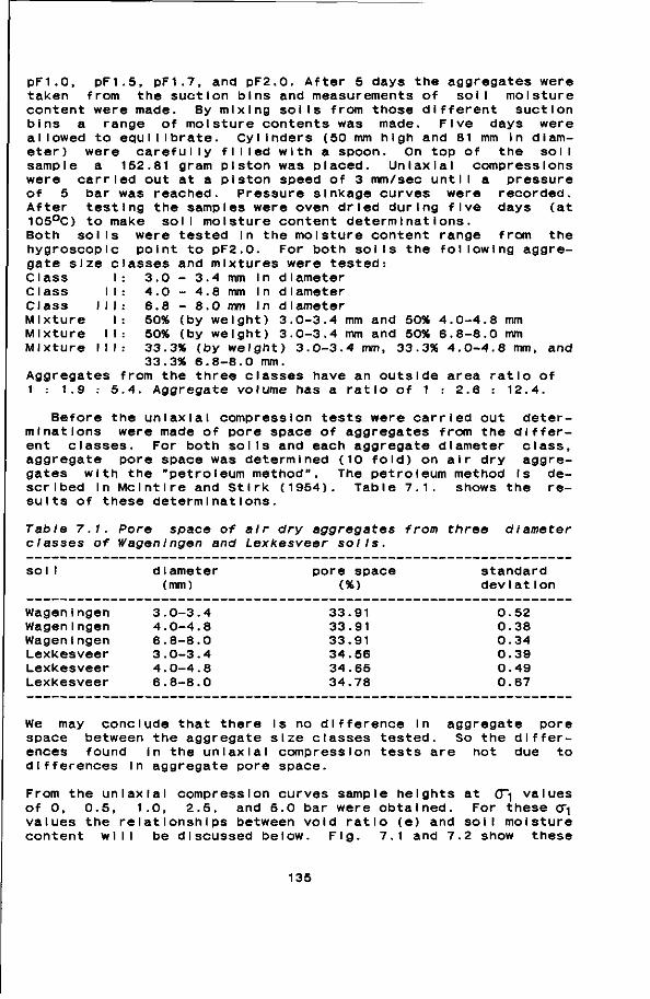
pF1.0, pF1.5, pF1.7, and pF2.0. After 5 days the aggregates were taken from the suction bins and measurements of soil moisture content were made. By mixing soils from those different suction bins a range of moisture contents was made. Five days were a I lowed to equI I I brate. CyI Inders (50 mm high and 81 mm in diameter) were carefully filled with a spoon. On top of the soil sample a 152.81 gram piston was placed. Uniaxial compressions were carried out at a piston speed of 3 mm/sec until a pressure of 5 bar was reached. Pressure slnkage curves were recorded. After testing the samples were oven dried during five days (at 105°C) to make soil moisture content determinations. Both soils were tested in the moisture content range from the hygroscopic point to pF2.0. For both soils the following aggregate size classes and mixtures were tested: Class Class l Class I I Mlxture Mixture I Mixture I I
3.0 - 3.4 mm In diameter 4.0 - 4.8 mm In diameter 6.8 - 8.0 mm in diameter 50% (by weight) 3.0-3.4 mm and 50% 4.0-4.8 mm 50% (by weight) 3.0-3.4 mm and 50% 6.8-8.0 mm 33.3% (by weight) 3.0-3.4 mm, 33.3% 4.0-4.8 mm, and 33.3% 6.8-8.0 mm.
Aggregates from the three classes have an outside area ratio of 1 : 1.9 : 5.4. Aggregate volume has a ratio of 1 : 2.6 : 12.4.
Before the uniaxial compression tests were carried out determinations were made of pore space of aggregates from the different classes. For both soils and each aggregate diameter class, aggregate pore space was determined (10 fold) on air dry aggregates with the "petroleum method". The petroleum method Is described In Mc Int I re and St irk (1954). Table 7.1. shows the results of these determinations.
Table 7.1. Pore space of air dry aggregates from three diameter classes of Wagenlngen and Lexkesveer soils.
soil diameter pore space standard (mm) (%) deviation
33.91 0.52 33.91 0.38 33.91 0.34 34.56 0.39 34.65 0.49 34.78 0.67
We may conclude that there Is no difference In aggregate pore space between the aggregate size classes tested. So the differences found in the uniaxial compression tests are not due to differences In aggregate pore space.
From the uniaxial compression curves sample heights at <Ti values o f O , 0.5, 1.0, 2.5, and 5.0 bar were obtained. For these o"i values the relationships between void ratio (e) and soil moisture content will be discussed below. Fig. 7.1 and 7.2 show these
Wagen Ingen Wagen Ingen Wagen i ngen Lexkesveer Lexkesveer Lexkesveer
3 4 6 3 4 6
0-3 0-4 8-8 0-3 0-4 8-8
4 8 0 4 8 0
135
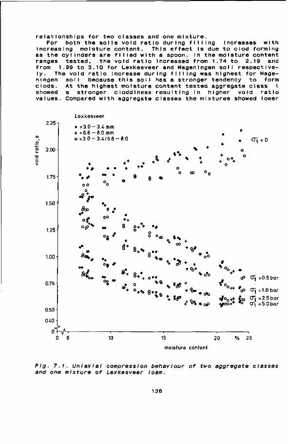
relationships for two classes and one mixture. For both the soils void ratio during f Mil
Increasing moisture content. This effect Is as the cylinders are filled with a spoon. In t ranges tested, the void ratio Increased from from 1.99 to 3.10 for Lexkesveer and Wagen Ing ly. The void ratio Increase during filling wa nIngen soil because this soil has a stronger clods. At the highest moisture content tested showed a stronger cI odd I ness resulting in values. Compared with aggregate classes the ml
ng increases with due to clod forming he moisture content
1 .74 to 2.19 and en soil respect Ive-s highest for Wage-
tendency to form aggregate class I
higher void ratio xtures showed lower
2.251
01 o
P 2.00
1.75
1.50
1.25
1.00
0.75
0.50
O.i.0
Lexkesveer
• = 3 . 0 - 3 . i. mm + =6 .8-8 .0 mm 0 = 3 . 0 - 3 . 4 / 6 . 8 - 8 . 0
+
\ * 0 0 o
0 6
• \ + +
+
o
r 8<x>
oo
0+ + o
M
o o +„
$<
*+
\%ï + 8 + * fi"
+ %'
"O ' oo
8+# + %•
» + 0„
en =0
+ o»»
+ o * » o * +
o° <Xj =0.5bar
** '<P Q] =1.0 bar
-t/°o+t fa &l =2.5 bar •yoo++ *o <r^ =5.0 bar
10 15 20
moisture content
% 23
Fig. 7.1. Uniaxial compression behaviour of two aggregate classes and one mixture of Lexkesveer loam.
136
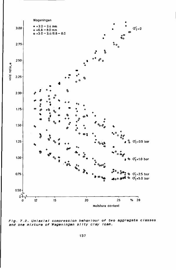
3.00
2.75
2.50
2.25-
2.00
1.75-
1.50
1.25-
1.00
0.75
0.50
0 i/-
Wageningen
• =3.0 - 3.4 mm + =6.8 -8 .0 mm o =3 .0-3 .4 /6 .8-8 .0
* '<s> % OD
O o
° ° *
+<è
>
»
° t + +
.• %
+ +
<o
• o o
j * 9> o o + + o ° "o » . . * +
• + <$> • +
h O
+ +
+ OD* +
+ / +
°ooV
O (DJ +
o« * o +
* • +
V •°oo«t
K +
<J;=O
* 0
+ + o
0 £+ t o CTÏ = 0.5 bar
o » , t <b CTj =1.0 bar
*a> • •0°3*:9> q = 2.5bar
* * dfoOoW1 * CT, =5.0 bar
12 15 20 25 % 28
moisture content
Flg. 7.2. Uniaxial compress Ion behaviour of two aggregate classes and one mixture of Wageningen s I Ity clay loam.
137
void ratio values during filling. When the moisture content Increases the difference disappeared gradually due to clod forming. The lower void ratio of dry mixtures could have been expected because It Is known that a denser packing can be achieved with different diameters.
The compaction of a relatively dry sample starts as dry compaction but with Increasing pressure compaction It can change Into wet compaction. The line that represents 10 volume percent air content was chosen more or less arbitrarily as transition between the dry and wet compaction areas. In the wet compaction area there is no difference In behaviour between aggregate classes and/or mixtures. In this area aggregates have been damaged to such an extent that they almost disappear . In the dry compaction area It seems sometimes that a certain aggregate class has more resistance to compaction than another one. For example, in the moisture content range between 7 % and 15 % Lexkesveer class I shows for the pressures applied a somewhat higher pore ratio level compared to class III. The values for class II M e between those of the other classes. These small differences, however, are not due to aggregate size but to differences In packing during filling. Samples with denser packing during filling have somewhat higher void ratio values during compaction. When the moisture content Increases these differences disappear both during filling and during compaction. The Wagen In-gen soil class III has In the moisture content range between 12 % and 20 % a somewhat denser packing during filling and therefore somewhat higher void ratio values during compaction than the other classes. Also these small differences disappear when the moisture content Increases In this soil. At the lower moisture contents the mixtures have lower void ratio values during compaction, but these differences also disappear when the moisture content Increases.
From these tests we may conclude that aggregate size has no Influence on uniaxial compactiblI Ity. This can be explained by the stable behaviour of the compaction process as described by Kooien (1986). The weakest spot Is compacted first and gets stronger. Compaction stops at this spot and starts at the second weakest spot. In this way compaction will occur throughout the ent I re so I I.
For both soils the relationship between critical pressure and moisture content has been calculated from the uniaxial compressions (Fig. 7.3). Critical pressure Is the value of the applied pressure at the moment that the critical pore space is reached. Kuipers (1959) defines critical pore space as the pore space at which there Is an air content of 10 % at the pF2 moisture content. Critical pore space is reached at void ratio values of 0.71 and 0.92 for Lexkesveer and Wagen Ingen soil respectively. The difference between the two lines in Fig. 7.3 is comparable to the differences In moisture content at pF2. These comparable equal shapes of the curves of these soils agree with the results of uniaxial compression tests carried out by Kooien (1974) for the same soils. At pF2 both soils have a critical pressure of 1.2 bar. For field traffic Fig. 7.3 means that the critical pore
138
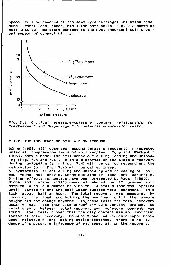
space will be reached at the same tyre settlngs( Inflation pressure, wheel load, speed, etc.) for both soils. Fig. 7.3 shows as well that soil moisture content Is the most Important soil physical aspect of compact IblI Ity.
c "c o u
PF2 Wageningen
PF2 Lexkesveer
Wageningen
Lexkesveer
2 3 U _ 5 bar 6
cr i t ical pressure
Fig. 7.3. Critical pressure-mo Isture content relatlonshlp for "Lexkesveer" and "WagenIngen" In uniaxial compression tests.
7.1.2. THE INFLUENCE OF SOIL AIR ON REBOUND
Söhne (1952,1956) observed rebound (elastic recovery) In repeated uniaxial compression tests of soil samples. Yong and Warkentln (1966) show a model for soil behaviour during loading and unloading (Fig. 7.4 and 7.5). In this dissertation the elastic recovery during unloading (a in Fig. 7.4) will be called rebound and the relaxation (b In Fig. 7.4) will be called creep. A hysteresis effect during the unloading and rel was found not only by Söhne but also by Yong Similar effects for metals have been presented by Stone and Larson (1980) measured rebound on
load Ing of soi I and Warkentln. Nadal (1950).
60 gramme sol I samples with a diameter of 5.65 cm. A static load was applied until sample volume and soil water suction were constant. This took about half an hour. The total recovery was measured by reducing the load and holding the new load until the sample height did not change anymore. In these tests the total recovery usually was less than 0.05 gr/cm3 dry bulk density change. No relationship between total recovery and moisture content was found. The tests proved that the clay content was an Important factor of total recovery. Because Stone and Larson's experiments used relatively long lasting static loadings, there Is no evidence of a possible influence of entrapped air on the recovery.
139

c 'o
Elastic recovery
Constant stress ö* released here time
Loading
Unload
Reload'
Fig. 7.4. Course of strain In time of a volume element of soil at constant stress and after re leas Ing stress.
log of pressure
Fig. 7.5. Behavlour of soil at loading, un loading, and reload!ng.
pressure CHj
Fig. 7.6. Typical uniaxial pressures Inkage curve.
140
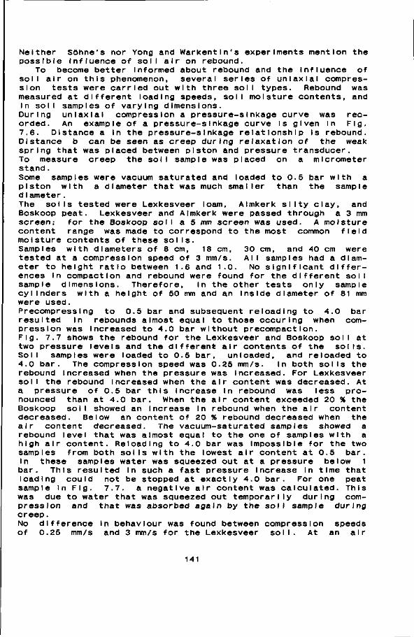
Neither Söhne's nor Yong and Warkentin's experiments mention the possible influence of soil air on rebound.
To become better Informed about rebound and the influence of soil air on this phenomenon, several series of uniaxial compression tests were carried out with three soil types. Rebound was measured at different loading speeds, soil moisture contents, and In soil samples of varying dimensions. During uniaxial compression a pressure-sInkage curve was recorded. An example of a pressure-sInkage curve Is given In Fig. 7.6. Distance a in the pressure-sInkage relationship Is rebound. Distance b can be seen as creep during relaxation of the weak spring that was placed between piston and pressure transducer. To measure creep the soil sample was placed on a micrometer stand. Some samples were vacuum saturated and loaded to 0.5 bar with a piston with a diameter that was much smaller than the sample dIameter. The soils tested were Lexkesveer loam, Almkerk s I Ity clay, and Boskoop peat. Lexkesveer and Almkerk were passed through a 3 mm screen; for the Boskoop soll a 5 mm screen was used. A moisture content range was made to correspond to the most common field moisture contents of these soils. Samples with diameters of 8 cm, 18 cm, 30 cm, and 40 cm were tested at a compression speed of 3 mm/s. All samples had a diameter to height ratio between 1.6 and 1.0. No significant differences In compaction and rebound were found for the different soil sample dimensions. Therefore, in the other tests only sample cylinders with a height of 50 mm and an inside diameter of 81 mm were used. PrecompressIng to 0.5 bar and subsequent reloading to 4.0 bar resulted in rebounds almost equal to those occur Ing when compression was Increased to 4.0 bar without precompactIon. Fig. 7.7 shows the rebound for the Lexkesveer and Boskoop soil at two pressure levels and the different air contents of the soils. Soil samples were loaded to 0.5 bar, unloaded, and reloaded to 4.0 bar. The compression speed was 0.25 mm/s. In both soils the rebound Increased when the pressure was Increased. For Lexkesveer soil the rebound Increased when the air content was decreased. At a pressure of 0.5 bar this increase In rebound was less pronounced than at 4.0 bar. When the air content exceeded 20 % the Boskoop soil showed an Increase In rebound when the air content decreased. Below an content of 20 % rebound decreased when the air content decreased. The vacuum-saturated samples showed a rebound level that was almost equal to the one of samples with a high air content. Reloading to 4.0 bar was Impossible for the two samples from both soils with the lowest air content at 0.5 bar. In these samples water was squeezed out at a pressure below 1 bar. This resulted In such a fast pressure Increase In time that loading could not be stopped at exactly 4.0 bar. For one peat sample In Fig. 7.7. a negative air content was calculated. This was due to water that was squeezed out temporarily during compression and that was absorbed again by the soil sample during creep.
No difference in behaviour was found between compression speeds of 0.25 mm/s and 3 mm/s for the Lexkesveer soil. At an air
141
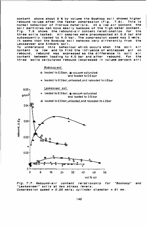
content above about 5 % by vo rebound values after the faste normal behaviour of fibrous ma soil particles can move easily Fig. 7.9 shows the rebound-three soils tested. All samp I subsequently loaded to 4.0 bar It seems that the Boskoop soll Lexkesveer and Almkerk soil. To understand this behavlou content Is low and to find rebound, rebound was expres content between loading to 4 three soils calculated reboun
Iume the Boskoop soll showed higher r compression (Fig. 7.8). This Is terlals. At a low air content the
because of the high water content, air content relationships for the es were precompacted at 0.5 bar and . The compression speed was 3 mm/s. behaves very differently from the
r which occurs when the soil air the influence of entrapped air on sed as the difference In soil air 0 bar and after rebound. For the d (expressed in volume percent air)
Boskoop soil
O loaded to0.5bar; o vacuum saturated and loaded to 0.5 bar
• loaded to 0.5 bar,unloaded,and reloaded to £..0 bar
Lexkesveer soil
+ loaded to 0.5 bar; $ vacuum saturated and loaded to 0.5 bar
A loaded to 0.5bar,unloaded,and reloaded toA.Obar
Fig. 7.7. Rebound-alr content relationshlp for "Boskoop" and "Lexkesveer" soils at two stress levels. Compress I on speed «= 0.25 mm/s; cylinder diameter = 81 mm.
142
0.05-
g/crn^
0.04-
)? 003
TD C O
ï 0.02
0.01
—1 1
16 24 32 £0 48
vol.% air
Flg. 7.8. Rebound-alr content relatlonshlp for "Boskoop" soil at two compress Ion speeds. PrecompactIon stress = 0.5 bar; compaction stress = 4.0 bar-, cylinder diameter = 81 mm.
0.05 T
g/cm3
0.04
<3
c 0.03 o _o (V 1_
0.02
0.01
Boskoop
Lexkesveer
10 20 30 vol.% air 40 after unloading
Flg. 7.9. Rebound after loading to 4.0 bar for three soils. Compress Ion speed - 3 mm/s.
143
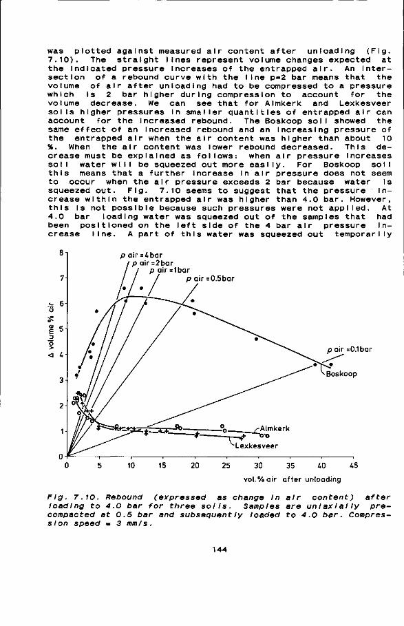
was plotted against measured air content after unloading (Fig. 7.10). The straight lines represent volume changes expected at the Indicated pressure Increases of the entrapped air. An Intersection of a rebound curve with the line p-2 bar means that the volume of air after unloading had to be compressed to a pressure which is 2 bar higher during compression to account for the volume decrease. We can see that for Almkerk and Lexkesveer soils higher pressures In smaller quantities of entrapped air can account for the Increased rebound. The Boskoop soll showed the same effect of an Increased rebound and an Increasing pressure of the entrapped air when the air content was higher than about 10 %. When the air content was lower rebound decreased. This decrease must be explained as follows: when air pressure Increases soli water will be squeezed out more easily. For Boskoop soil this means that a further increase In air pressure does not seem to occur when the air pressure exceeds 2 bar because water Is squeezed out. Fig. 7.10 seems to suggest that the pressure Increase within the entrapped air was higher than 4.0 bar. However, this Is not possible because such pressures were not applied. At 4.0 bar loading water was squeezed out of the samples that had been positioned on the left side of the 4 bar air pressure Increase line. A part of this water was squeezed out temporarily
p air = 4bar 1 p air =2bar
p air = 1bar p air =0.5bar
pa i r =0.1 bar
30 35 i.0 45
vol. % air a f ter unloading
Fig. 7.10. Rebound (expressed as change In air content) after loading to 4.0 bar for three soils. Samples are uni axially pre-compacted at 0.5 bar and subsequently loaded to 4.0 bar. Compression speed - 3 mm/s.
144
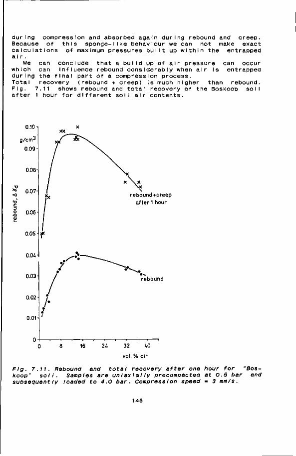
during compression and absorbed again during rebound and creep. Because of this sponge-I ike behaviour we can not make exact calculations of maximum pressures built up within the entrapped air.
We can conclude that a build up of air pressure can occur which can influence rebound considerably when air Is entrapped during the final part of a compression process. Total recovery (rebound + creep) is much higher than rebound. Fig. 7.11 shows rebound and total recovery of the Boskoop soil after 1 hour for different soil air contents.
0.10 n
g/cmJ
0.09
0.08-
*» 0.07i <3 •D C
I 0.06 i 01
0.05
0.04-1
0.03-
0.02
0.01
x \ x x
rebound+creep after 1 hour
rebound
16 24 32 40
vol. % air
Fig. 7.11. Rebound and total recovery after one hour for "Boskoop" soll. Samples are untax Ially precompacted at 0.5 bar and subsequently loaded to 4.0 bar. Compression speed - 3 mm/s.
145

7.2. THE INFLUENCE OF MECHANICAL TREATMENT ON PHYSICAL PROPERTIES
Mechanical treatment of the soil by wheels results In compaction and/or deformation. Because of this treatment micro-factors and soil qualities can change. Changes on the micro level Influence soil qualities such as pF-curves and conductivities. A review of the Influence of mechanical treatment on micro-factors and soil qualities Is given In 7.2.1. In arable farming It Is Important to know the Influence of soli compaction on subsequent tillage operations. The major soil mechanical quality that can change due to compaction is til lability. To Investigate the Influence of soli compaction on til lability a test Is needed that can characterize this influence. Til lability, til lability tests, and attempts to use the unconflned compression test to characterize til lability are discussed in 7.2.2.
7.2.1. THE INFLUENCE OF MECHANICAL TREATMENT ON MICRO-FACTORS AND SOIL QUALITIES
On the macro level compaction reduces pore space. On the micro-level this pore space reduction Is at the expense of the largest pores (Sommer et al., 1972; Sommer et al.,1975; Ma IdI and F Isch-beck,1985). This effect is strongest during wet compaction. Table 7.2 shows the Influence of autumn ploughing on pore size distributions under dry and wet soil conditions.
Table 7.2. The Influence of ploughing condltIons on pore size dlstrI but Ions (after Maldl and FIschbeck. 1985)
Depth top soil plough sole (0 - 35 cm) (35 - 40 cm)
Ploughing Adry Awet Adry Awet
Vol . % pores>10 jj. Vol. % pores 10 - 0.2 /* Vol. % pores <0.2/U
11 14 17
2 0 5
6 13 21
5 0 3
7 1 1 22
9 3
. 2
6 1 1 22
0 8 2
Adry = autumn ploughed under dry soil conditions Awet = autumn ploughed under wet soil conditions
Pores >10/U are Important for air conductivity. After wet ploughing the content of these pores was lower than after dry ploughing; in the top soil this amounted to a reduction to 58 % and in the plough pan to 76 % of the values measured after dry ploughing. This reduced air conductivity. The pores 10 - 0.2/u. determine the amount of water available for plants. Compared to dry conditions the amount of available water decreased In the top soil after ploughing under wet conditions. Water In pores <0.2^< Is not available for plants. The content of pores < 0.2/u. Increased strongly in the top soil after ploughing under wet conditions as well. A wet compacted soil has a higher content of unavailable water
146
and a lower content of pores for air conductivity. This means that such a so I I is wetter and colder than a dry compacted so I I .
Maidl and FIschbeck (1985) also examined the influence of these differences in pore size distributions, due to ploughing under wet and dry conditions, on plant growth. Their investigation proved that the decrease of yield after wet compaction was mainly due to an insufficient supply of nitrogen. The decrease of N supply after wet compaction indicates a lower N mineralization due to lower soil temperature, and higher gaseous N losses (denl-trification) due to lower air conductivity.
Inter-partle I e bonds not arising from water suction can be destroyed at large deformations. The strength of these bonds influences the water suction - moisture content relationship. Dawidowskl and Kooien (1987) applied triaxial tests to field samples of Wagen Ingen silty clay loam. The sample volume was almost constant during deformation. Samples were deformed to 50 % of the original sample heights. Many bonds were destroyed by the deforming and smearing action of the test, resulting In a strong increase in water suction. Compared with undeformed samples, the samples tested showed higher values for volumetric shrinkage and dry tensile strength.
Influences of compaction on pF-curves have been reported by Warkentln (1971), Sommer et al. (1972), and Moreno et al. (1974). Kooien (1978) found that the precompactIon moisture content greatly Influences moisture contents at pF2.0 and pF2.7.
7.2.2. TILLABILITY
Tl I I abi I ity Is defined as the degree of ease with which a soi I may be manipulated for a specific purpose (ASAE Engeneerlng Practice ASAE EP291.1, Hahn et al. 1984). In agricultural field practice farmers decide on how to till from experience. However, their experience does not suffice when they need to choose new Implements and when they find themselves In unknown situations. Also, field experience is not easy to convey. To obtain an objective approach to til lability, a measurable parameter of til lability, and therefore a til lability test Is needed .
7.2.2.1. TILLABILITY TEST
To develop a til lability test It Is necessary to take the following factors into account: - the Initial soil condition. This condition depends on soil
physical properties and the history of the soil. - the type of tillage operation. Primary tillage and field traf
fic have other demands than secondary tillage operations. In this dissertation we concentrate til lability on seed-bed preparation in spring.
- the processes that occur. In tillage operations we should distinguish between Intended processes and accidental pro-
147
cesses. In seed-bed preparation the major Intended process is "crumbling". This process Is accompanied by the accidental process of "compaction". Til lability tests should concentrate on the major intended process, but must also take into account the major accidental process. the energy needed for the tillage operatI on. Energy needed for tillage is associated with energy needed for tillage processes and for locomotion of the tractor on the field. Gross energy consumption Is the amount of energy needed for both tillage processes and tractor locomotion. Net energy consumption only deals with the energy needed for the tillage process (for Instance draft). In the Netherlands soil conditions generally are too wet In the period before seed-bed preparation. Therefore, till ab tIty research has concentrated on the upper tillage limits. It is advisable to increase the ratio net energy consumption to gross energy consumption. Ultimately til lability depends not only on the results of the tillage operations but also on the energy required. An optimum ratio of tillage results to energy consumption Is pursued. Energy Is not yet a limiting factor. Therefore, the Interest in t iI I ab I Ity nowadays is limited to a till ab iIty test that indicates whether or not the soil can be tilled in order to achieve the Intended results. In times of energy scarcity the tiI lab II-Ity test should also pay much attention to the energy aspects. the Intended tillage results. The Dutch farmer Is generally mostly Interested In the results of the tillage operations. Therefore criteria for the results of tillage operations are required In order to determine til lability. Tillage criteria have been published In "Tillage Advice" for cereals (Andrlnga et al, 1979), sugar beets (Perdok et al, 1974a), and potatoes (van Gl ist et al, 1975).
the tillage Implement to be used. The tillage implement should also be considered because of the energy consumption and the kind of the work expected. The capacity of the tillage implement can also play an Important part in farm management dec I -s ions.
7.2.2.2. TILLABILITY TESTS BASED ON PROCESSES OTHER THAN CRUMBLING
Boekel (1977) tried to relate soil til lability to deformabiI Ity measured with a plasticity meter. The pressure that is needed to force the soil through a small nozzle Is measured with this Instrument. The required pressure is lower for a wet plastic soil than for a dry crumbly soil. It is proposed that this Is a measure for crumbling. This test is not suitable for field samples and does not account for the effect of pore 11 IlablIity.
Havlnga and Perdok (1969) developed a tillablIIty relates tlIlablIIty to mechanical properties of sol is. presslblllty of loose soil is chosen as major process, piled pressure Is a measure for the energy consumption.
148
space on
test The The In
that com-
ap-thls
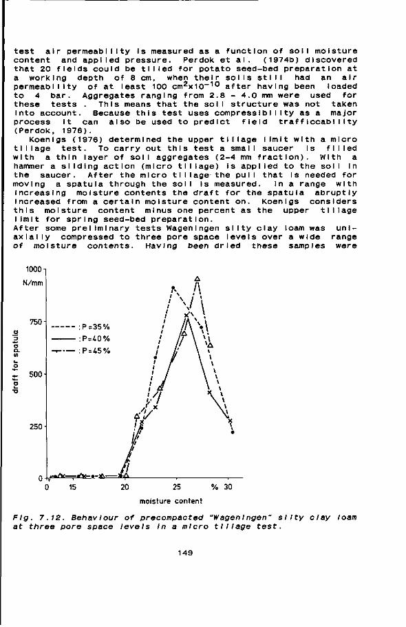
test air permeability is measured as a function of soil moisture content and applied pressure. Perdok et al. (1974b) discovered that 20 fields could be tilled for potato seed-bed preparation at a working depth of 8 cm, when their soils still had an air permeability of at least 100 c m 2 x l 0 - 1 0 after having been loaded to 4 bar. Aggregates ranging from 2.8 - 4.0 mm were used for these tests . This means that the soil structure was not taken Into account. Because this test uses compressibility as a major process It can also be used to predict field traf fIccabiI Ity (Perdok, 1976).
Koenigs (1976) determined the upper tillage limit with a micro tillage test. To carry out this test a small saucer Is filled with a thin layer of soil aggregates (2-4 mm fraction), with a hammer a sliding action (micro tillage) is applied to the soli in the saucer. After the micro tl I lage the pul I that is needed for moving a spatula through the soil Is measured. In a range with increasing moisture contents the draft for the spatula abruptly increased from a certain moisture content on. Koenigs considers this moisture content minus one percent as the upper tillage limit for spring seed-bed preparation. After some preliminary tests Wageningen sllty clay loam was uniaxial I y compressed to three pore space levels over a wide range of moisture contents. Having been dried these samples were
1000-
N/mm
750 o •D
O Q. U) 4.
O II 500 «•— o i_ •o
250-
P=35%
P = 4 0 %
P = 4 5 %
0 -ty«^—r^x- *~*t— % 30
moisture content
Fig. 7.12. Behavlour of precompacted "WagenIngen" silty clay loam three pore space levels In a micro tillage test. at
149

crushed and sieved. For each sample the 3.4-4.8 mm fraction was rewetted to the moisture content before compression. After one day of equI I Ibratlon these aggregates were used in a micro tl I I-age test. The relationships between spatula draft and moisture content are shown In Fig. 7.12. For the three pore space levels tested the draft for the spatula suddenly Increased. It is remarkable that for each Initial pore space level this sudden increase occurs at the same moisture content. This means that this upper tillage limit is independent of pore space at precompact Ion. Neither does this test use field samples. The micro tl I lage with the hammer and the draft measurement with the spatula depend on the person who does the test. Some other drawbacks of this test are that soil sometimes sticks to the hammer and that soil may curl up when wet cohesive.
7.2.2.3. TILLABILITY TESTS BASED ON CRUMBLING PROCESSES
These tests try to determine the intensity of crumbling. Furthermore, the energy needed for this crumbling can be measured. In field practice the most interesting aspects of spring seed-bed preparation are Indeed crumbling and the energy needed for the tillage operation. Therefore, it Is attractive to use these methods to characterize field processes.
Kooien (1977) used a pendulum-type impact machine to measure tillage process aspects on soil blocks in the laboratory. For each test he measured the volume and the mean aggregate size of the loosened soil, and the energy consumption. Although his test showed good results for soil blocks prepared in the laboratory it is difficult to use It for undisturbed field samples.
For our examination the unconfined compression test has been chosen to characterize the crumbling process. in an unconfined compression test a soil sample is made to fail between two plates (Fig. 7.13). At the moment of failure, the sample shortening expressed as a fraction of Initial height (£f ) and the prevailing failure stress (CTm a x) are measured. The failure strain £f represents the soli deformation that occurs before failure. This means that £f gives an indication of breakabillty and therefore of crumbling as well. The unconfined compressive strength (0"max) Is a measure of the energy consumption. Kooien (1973 and 1978) successfully used the unconfined compression test to characterize soil mechanical properties. When laboratory samples are used the Influence of bulk density on the crumbling process can be examined by adjusting different levels of pore space. The unconfined compression test can also be applied to field samples.
150
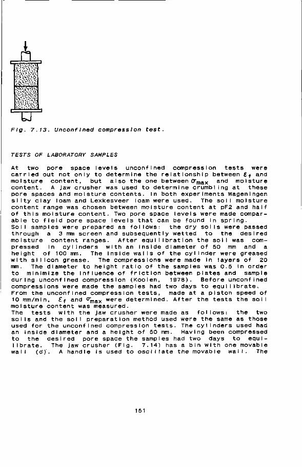
Flg. 7.13. Unconflned compression test.
TESTS OF LABORATORY SAMPLES
At two pore space levels unconflned compression tests were carried out not only to determine the relationship between Sf and moisture content, but also the one between<Tmax and moisture content. A jaw crusher was used to determine crumbling at these pore spaces and moisture contents. In both experiments Wagen Ingen si Ity clay loam and Lexkesveer loam were used. The sol I moisture content range was chosen between moisture content at pF2 and half of this moisture content. Two pore space levels were made comparable to field pore space levels that can be found in spring. Soi I samples were prepared as fol lows: the dry soi I s were passed through a 3 mm screen and subsequently wetted to the desired moisture content ranges. After equilibration the soil was compressed in cylinders with an inside diameter of 50 mm and a height of 100 mm. The Inside walls of the cylinder were greased with si I Icon grease. The compressions were made in layers of 20 mm. The diameter to height ratio of the samples was 0.5 in order to minimize the influence of friction between plates and sample during unconfined compression (Kooien, 1978). Before unconflned compressions were made the samples had two days to equilibrate. From the unconflned compression tests, made at a piston speed of 10 mm/min, £f and c m a x were determined. After the tests the soil moisture content was measured. The tests with the Jaw crusher were made as follows: the two soils and the soil preparation method used were the same as those used for the unconflned compression tests. The cylinders used had an inside diameter and a height of 50 mm. Having been compressed to the desired pore space the samples had two days to equilibrate. The jaw crusher (Fig. 7.14) has a bin with one movable wal I (d). A handle is used to ose I I late the movable waI I. The
151
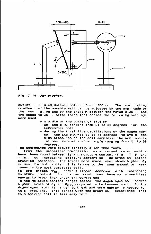
200-/.00 0-105
Fig. 7.14. Jaw crusher.
outlet (f) Is adjustable between O and 200 mm. The oscillating movement of the movable wall can be adjusted by the amplitude of the osei I I at I on and by the angle ot between the movable wal I and the opposite wall. After three test series the following settings were used:
- a width of the outlet of 11.5 mm - an angle oc ranging from 21 to 59 degrees for the
Lexkesveer soi I - during the first five oscillations of the Wagen Ingen
sol I the angle oc was 32 to 41 degrees (to avoid too high pressures on the soli samples); the next oscillations were made at an angle ranging from 21 to 59 degrees.
The aggregates were sieved directly after thhe tests. From the unconfined compression tests curved relationships
have been found between £ f and moisture content (Fig. 7.15 and 7.16). At increasing moisture content soil deformation before breaking increases. The lowest pore space level shows higher f f
values for both soils. This is due to the lower amount of weak zones in the most compacted soi I.
'max shows a I I near decrease with increasing these so I I s need less
Fa I lure stress moisture content. So under wet conditions energy to break than under dry conditions. In the moisture content ranges tested, the Wageningen soil showed higher levels of £f and 0"max compared to Lexkesveer soli So the Wageningen soil is harder to break and more energy is needed for this breaking. This agrees with the practical experience that this heavier soil Is less easy to till.
152
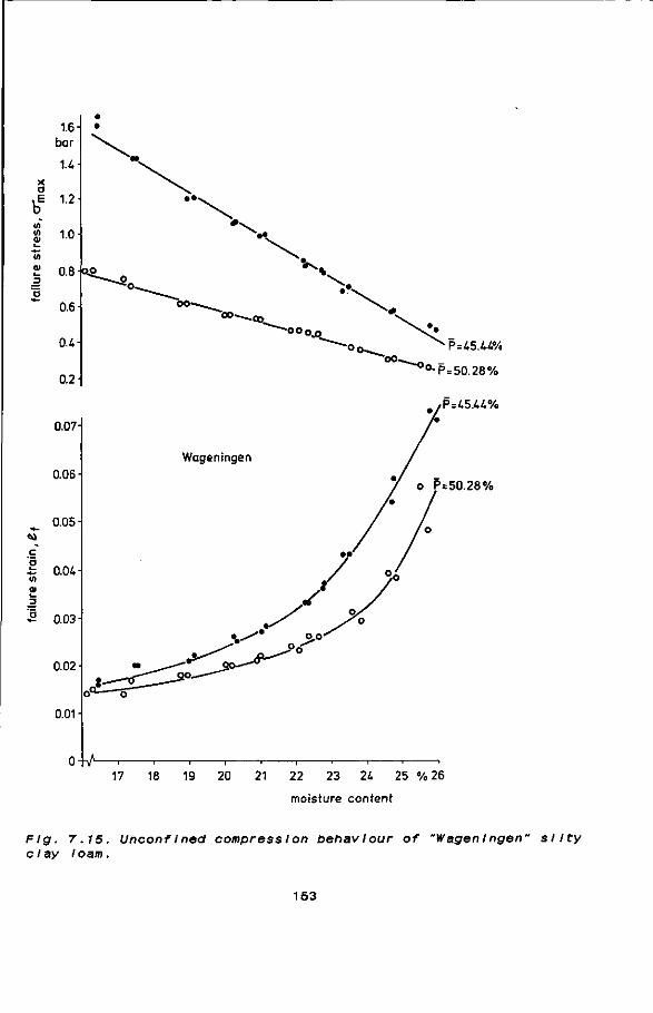
17 18 19 20 21 22 23 2U 25 % 26
moisture content
Flg. 7.15. UnconfI ned compression behaviour of "Wageningen" sllty clay loam.
153

The measuremen of the amount o creasing moisture moisture content passed through th content at which the upper t iI lage 11 I lage limit II about 21 %. This t i llage test acco limit for Lexkesv 19 %. Because moisture content estImatIon.
ts with the Jaw c f so I I re leased f content (see Fig the Mass Median
e Jaw crusher str these sudden cha IImlt. For Wagen
es for both pore agrees with the
rdIng to Koen igs eer I les between of the low number s It was not pos
rusher showed a sudden decrease rom the crusher outlet at In-
7.17 and 7.18). At the same Diameter (MMD) of the soil that ongI y Increased. The moisture nges occured can be considered Ingen s I Ity clay loam the upper spaces at a moisture content of tests caried out with the micro (Fig. 7.12). The upper tillage a moisture content of 18 % and
of measurements made at these sib le to make a more precise
x • E
in ui a> i_
In 0»
'5 -oo cP-p = 4 9 8 2 o/o
0.06
to . 0.05
c 'o Tn * 0.04 _2 '5
0.03-
0.02
Lexkesveer
0.01?—•
oV-
F = 45.12%
P = 49.62%
11 12 13 14 15 16 17 18 19 % 20
moisture content
Fig. 7.16. UnconfI ned compress Ion behaviour of "Lexkesveer" loam.
154
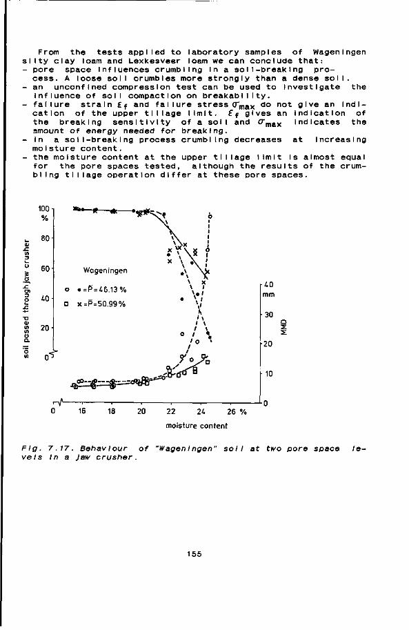
From the tests applied to laboratory samples of Wagen Ingen s I Ity clay loam and Lexkesveer loam we can conclude that: - pore space Influences crumbling In a sol I-break Ing pro
cess. A loose soil crumbles more strongly than a dense soil. - an unconflned compression test can be used to Investigate the
Influence of soil compaction on breakabI I Ity. - failure strain £f and failure s t r e s s < T m a x do not give an Indi
cation of the upper tillage limit. €f gives an indication of the breaking sensitivity of a soil and < T m - v Indicates the amount of energy needed for breaking.
- i n a soiI-break Ing process crumbling moisture content.
at the upper tillage limit is almost equal tested, although the results of the crum-
max
decreases at Increasing
the for
moisture content the pore spaces
bllng tillage operation differ at these pore spaces.
100 %
,_ 80 JZ
o -C
Ol
O
-o O) U) U)
o Q.
60
40
20-
Wageningen
n-r
0
o • = P = 46.13%
• x=P = 50.99%
J&ï"
i.0 mm
•30 o
•20
10
16 18 20 22 24 26 %
moisture content
Fig. 7.17. Behavlour of "WagenIngen" soil at two pore space levels In a Jaw crusher.
155
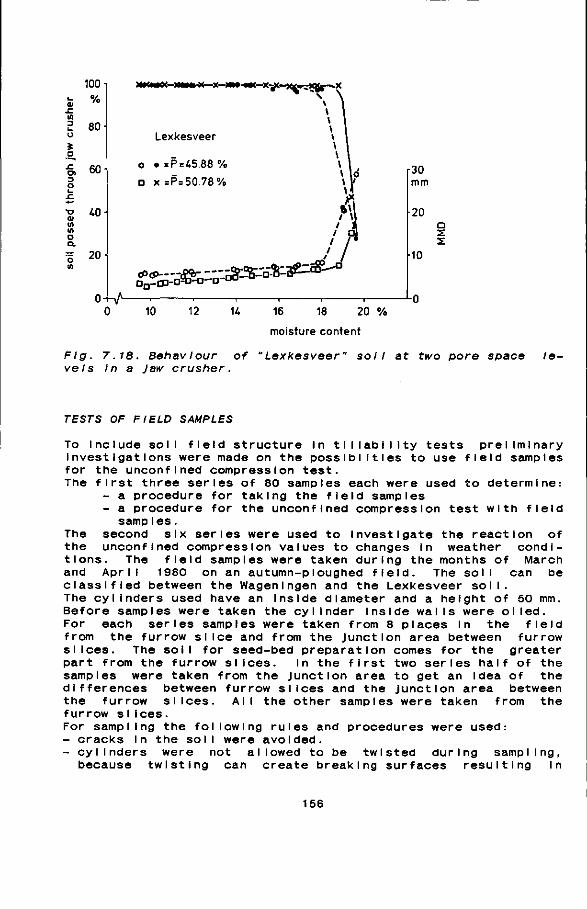
<u in 3
100 %
80-
S
sz 3 O
T3 (U UI UI O Q.
60
i.0-
S 20
Mt<*«0<-X4a»-X—X—«•••(-X
Lexkesveer
o • = P =45.88%
o x = P= 50.78%
**--&;:=&!&&&=&
o-l-A-^ i -ä^D- D - ° °
10 12 U 16 18 20 %
moisture content
30 mm
20 o
10
F/g. 7.18. Behavlour of vel s In a Jaw crusher.
'Lexkesveer" soll at two pore space le-
TESTS OF FIELD SAMPLES
To Include soil field structure In til lability tests preliminary Investigations were made on the possIbI 111 es to use field samples for the unconfined compression test. The first three series of 80 samples each were used to determine:
- a procedure for taking the field samples - a procedure for the unconfined compression test with field
samp les. The second six series were used to investigate the reaction of the unconfined compression values to changes In weather conditions. The field samples were taken during the months of March and April 1980 on an autumn-ploughed field. The soil can be classified between the Wagen Ingen and the Lexkesveer soil. The cylinders used have an Inside diameter and a height of 50 mm. Before samples were taken the cylinder Inside walls were oiled. For each series samples were taken from 8 places in the field from the furrow slice and from the Junction area between furrow slices. The soil for seed-bed preparation comes for the greater part from the furrow slices. In the first two series half of the samples were taken from the Junction area to get an Idea of the differences between furrow slices and the Junction area between the furrow slices. All the other samples were taken from the furrow s I ices. For sampling the following rules and procedures were used: - cracks In the soli were avoided. - cylinders were not allowed to be twisted during sampling,
because twisting can create breaking surfaces resulting In
156
smaller £f values. When the cylinder was pushed far enough Into the soll It was lifted with a spade, and trimmed with a knife.
- on sampling the soil was compressed. Therefore only samples with a decrease In height of less than 0.5 cm were accepted.
- the thin dry top layer of about 1 cm In thickness was removed before samples were taken.
The mean moisture content in furrow slices Is higher than In the Junction area. This difference Is Just below significance for the first series and significant (95 % probability) for the second series. The mean difference has a value of 1 - 1.5 percent by weight. The average pore space was about 5 percent higher In the Junction area. This could have been expected because this soil was loosened from the furrow slices by weathering.
To obtain a height to diameter ratio of 2 In the unconflned compression test two samples were been put on top of each other according to Kooien (1978). Before testing the samples were weighed. The sample pairs were composed of two samples with almost equal weight. This was done to avoid that samples with very different pore space were used as a sample pair In the unconflned compression test. In the field the moisture content Increases with depth. Therefore, soil samples topsldes are drier and more crumbly than bottoms I des. So there are three ways to combine the sample pairs: - loose/loose: the upside of the first sample against the upside
of the second sample. - loose/firm: the upside of the first sample against the under
side of the second sample. - firm/firm: the underside of the first sample against the under
side of the second sample. In the sample height values which exist at the beginning of the unconflned compression tests, the decrease in sample height which occurs when the samples are pushed out of the cylinders is accounted for . In the different combinations no significant differences were found in moisture content and pore space. So the differences found as a result of unconflned compression are due to the method used. For each series the loose/loose method resulted In the lowest values for _mean failure strain £f and mean unconflned compressive strengthOmax. The firm/firm method showed the highest values while the loose/firm method resulted in Intermediate values. The differences between loose/loose and firm/firm are significant (95 % probability) but no significant differences were found between loose/loose and loose/firm and between loose/firm and firm/firm. Compared with the firm/firm method the standard deviation of Zf Is a factor 2.5 lower In the loose/loose method. For <rmax standard deviations are almost equal for loose/loose and firm/firm. It is remarkable that the standard deviation values for Zf are almost constant for all the series within a soil. Standard deviation Increases for Srm a x when the soil becomes drier. The standard deviation of if was almost equal for a series of field samples (loose/loose method) and a series of laboratory samples. Forön,^ the laboratory samples had a factor 3 lower standard deviation than the field samples (loose/loose). Fig. 7.19 shows the crmav - moisture content rela-
157

tlonshIp cuItles t tory samp The crack the loos mIddI e of this part the f Irm the samp start eve
The if s IgnI f lea compress This cou crumb le. of the r the seed
for a loose/loose series. This clearly shows the diffl-hat arise when field samples are used Instead of labora-Ies (Fig. 7.15 and 7 . 1 6 ) .
formation differed for the different combinations. In e/loose method crack formation always occurred In the
the sample pairs. This could have been expected because Is driest and has more weak zones. Crack formation for
/firm method always started on top or at the bottom of e pairs. In the loose/firm method crack formation could rywhere.
values for furrow slices and the Junction area are not ntly different for the three m e t h o d s . The unconflned ve stength values are much lower for the Junction area. Id be expected because this weathered soil is easy to Further sampling concentrated on furrow slices because
eported differences and the knowledge that the soil for bed comes mostly from the furrow slices.
Six series of forty samp slices on six different compression values (loose climate diagram. The cllma had a wet spring. There was In this period a seed-bed pared for potatoes. Fig. 7 time as w e l l . We can see t tend to follow the drying conditions are known at whI limit, we can draw no cone I 1980 on which a seed-bed f
les each were taken from the furrow dates. The course of the unconflned /loose m e t h o d ) Is compared with the te diagram (Fig. 7.20) shows that 1980
a dry period between 10 and 18 April. could dry enough in order to be pre-20 shows the course of f f and 0 " m a x In
hat the unconflned compression values of the field top layer. Even when the eh this soil reaches the upper tillage usions about the date in the spring of or potatoes could have been prepared.
1.00 -i x bar o
b 0.80 in IA
a> i-" 0.60 « _2 a
0.40 i
0.20
0 V
-y=1.89-0.05x (r = -0.82 )
0 20 22 24 26 28 30 % 32
moisture content
Fig. 7.19. UnconfIned compressive strength of field samples.
158

First, the following questions are to be answered: - are the sampling depth and the thickness of the top layer that
is needed for the seed-bed equal? - has the dry layer that was removed been taken Into account? - have cracks been avoided?
The thickness of the top layer that Is used to prepare a seed-bed has two components: the layer that Is used for surface levelling and the thickness of the loose layer that Is needed for the seedbed. The thickness of the levelling layer can be calculated using a rellefmeter (Kuipers, 19S7). For a level field a loose top layer of 8 cm Is needed for potatoes (Kouwenhoven, 1974). For our test field the necessary sampling depth Is estimated at 10.8 cm (2.8 cm of levelling layer and 8 cm for the seed-bed). Our sampling depth was 9 cm: 1.5 cm for the removed top layer, 2 cm for
| CT 0.080
ai (_ _2 '5 H— c o <u E
0.060
0.040-lbC
« 0.50 <u bar
-•„ • » »
U 18
March
E3 = rain — = potential evaporation
Fig. 7.20. Course of climate and the unconfIned compress Ion characteristics of field samples.
159
trimming, 0.5 cm compression during sampling, and 5 cm cylinder height. This means that the height and diameter of our cylinders were 1.8 cm too smaI I.
From the tests with field samples we can conclude that: - field samples can be used for unconflned compressions tests. - for high accuracies a standard sampling method Is necessary. - sampling depth depends on roughness of the field, the needed
thickness of the seed-bed, the compressibility of the soil, and the thickness of the removed dry top layer.
- the highest accuracy in unconflned compression tests Is achieved when two samples are combined with the upsides against each other (loose/loose method).
- the course offf and (fmax tend to follow the drying of a field sol I .
160
CHAPTER 8
SUMMARY
In soil dynamics we distinguish between loosening and load-bearing processes. This dissertation deals with load-bearing processes under agricultural rollers, wheels, and tyres. Agricultural rollers, wheels, and tyres have been classified. In addition some general aspects of these devices are presented. This report presents the fundamentals of load-bearing processes, I.e. kinematic, dynamic, and soil physical aspects. Kinematic and dynamic aspects are discussed on three levels: device (roller, wheel, or tyre), contact area, and soil under the device. Physical properties of a soil can change due to load-bearing processes. On the other hand the soil physical properties influence the mechanical behaviour of a soil. In the section on soil physical aspects we have paid special attention to the influence of aggregate diameter and soil air on compression behaviour of soil and to 11 I labi I Ity. Soil characteristics concerning load-bearing processes are presented. Different tests that were used to characterize soli mechanical behaviour are compared. Relationships between soil characteristics and process aspects and their suitability to predict process aspects are discussed. Contributions are made to the prediction of some process aspects of a towed tyre under different soil conditions and in different soli types. Under laboratory conditions the use of characterizing processes (cone, vane, and falling weight) and empirical prediction methods resulted In accurate predictions of rolling resistance, rut depth, and compaction caused by a towed tyre.
161
CHAPTER 9
SAMENVATTING
In de gronddynamlca onderscheidt men losmakende en afsteunende processen. BIJ het rijden over grond treden afsteunende processen op onder rollen, wielen en banden. Dit proefschrift behandelt afsteunende processen onder rollen, wielen en banden in de landbouw. In deze dissertatie worden een indeling en enkele algemene aspecten gepresenteerd van In de landbouw voorkomende rollen, wielen en banden. De grondslagen van afsteunende processen worden behandeld: kinematische, dynamische en bodemfysische aspecten. De bespreking van kinematische en dynamische aspecten vindt plaats op drie niveau 's : werkend deel (rol, wiel of band), contactvlak en de grond onder het werkend deel. Bodemfyslche eigenschappen kunnen veranderen als gevolg van afsteunende processen. Anderzijds hebben bodemfysische eigenschappen invloed op het mechanische gedrag van grond. In het hoofdstuk over bodemfysische aspecten krijgen met name aandacht: bewerkbaarheid van grond en de Invloed van aggregaat diameter en bodem-lucht op het verdichtingsgedrag van grond. Bodemkarakteristieken, die verband houden met afsteunende processen worden gepresenteerd. Verschillende voor het karakteriseren van het mechanisch gedrag van grond gebruikte testen worden vergeleken. De betrekkingen tussen bodemkarakteristieken en procesaspecten worden behandeld. Evenals de mogelijkheid om deze betrekkingen te gebruiken In voorspellingsmethoden. Er worden nieuwe bijdragen geleverd aan de voorspelling van enkele procesaspecten van een getrokken band. Nauwkeurige voorspellingen van rolweerstand, InsporIng en verdichting waren mogelijk met behulp van karakteriserende processen (conus, vane en val gewicht) en empIrI sehe voorspeI IIngsmethoden.
162
REFERENCES
Aboaba, F.O., 1969. Effects of time on compaction of soils by rollers. Trans. ASAE 12(1):302.
Amir, I., G.S.V. Raghavan, E. Mckyes and R.S. Broughton, 1976. Soil compaction as a function of contact pressure and soil moisture content. Canadian Agrlc. Eng. 18(1):54-57.
Andrlnga, J.T. et al., 1979. GrondbewerkIngsadvI es voor granen. BedrIjfsontwlkkelIng 10(5): 495-501.
Anslow, B.J. and R.J. Warrllow, 1962. Tractor tyres. I. Mech. E. Referred In Inns and Kllgour (1978).
Baganz, K. und L. Kunath, 1963. Einige Spannungs- und Verdichtungsmessungen unter SchIepperIaufwerken. Agrartechnik 13:180-182.
Baganz, K., 1963/1964. Spannungs- und Verdichtungsmessungen Im boden bel verschiedenen Fahrgeschwindigkeiten. Archiv für Landtechnik 4(1):35-45.
Bai ley, A.C. and G.E. VandenBerg, 1968. Yielding by compaction and shear In unsaturated soil. Trans. ASAE 11:307-311,317.
Bailey, A.C., E.C. Burt and R.L. Schäfer, 1974. Digital calculation of rolling radius for wheels and tracks. Trans. ASAE 17(5): 871-873.
Bailey, A.C. and E.C. Burt, 1981. Performance of tandem, dual and single tires. Trans. ASAE 24(5): 1103-1107.
Bekker, M.G., 1956. Theory of land locomotion. University of Michigan Press, Ann Arbor.
Bekker, M.G., 1960. Off-the-road locomotion. University of Michigan Press, Ann Arbor.
Bekker, M.G., 1969. Introduction to terrain-vehicle systems. University of Michigan Press, Ann Arbor.
VandenBerg, G.E. and W.R. Gill, 1962. Pressure distribution between a smooth tire and the soli. Trans. ASAE 5:105-107.
Bernackl, H., J. Haman and Cz. Kanafojsk, 1972. Agricultural machines, theory and construction. Vol. I, Warsaw.
Bernstein, R., 1913. Probleme zur experimentellen Motorpflugmechanik. Der Motorwagen, Vol. 16.
B N 1er, R.H. and H. Steinkampf, 1978. Elnfluss der Prof I IrIchtung von AS-Relfen auf die Zugkraftübertragung des Schleppers. Landtechnik 33:57-60.
Bil 1er, R.H., 1983. Richt Ige Montage von Fronttriebreifen hilft sparen, ohne Zugkraft einzubüssen. dlz 34(11):1444-1446.
Blake, G.R., W.W. Nelson and R.R. AIImaras, 1976. Persistance of subsoI I compact I on In a Mo I I I so I. Soil Sc I. Soc. Am. J. 40(6): 943-948.
163
Bock, G., 1952. Feldversuche über die Zugfählgkelt von Ackerschlepperreifen. Grundl. Landtechnik 3:88-100.
Bock, G., 1953. Beobachtungen bei Feldversuchen über die Zug-fählgkelt von Ackerschleppern. Grundl. Landtechnik 5:42-48.
Bodman, G.B. and G.K. Constantin, 1965. The Influence of particle size distribution In soil compaction. Hllgardia 36(15): 567-591.
Boekel, P., 1977. De werkbaarheid van de grond In het voorjaar In verband met de ontwatering en de samenstelling van de grond. Symposium werkbaarheid en bedrijf, Wagen Ingen.
Boels, D., 1978. Kanttekeningen bij bestekvoorwaarden ter beperking van bandspanning van dumpers en trekkers. Nota 1081, ICW-Wageningen.
Boll, E. und E. I sensée, 1987. Eignung von Geschwindigkeitsgebern. Landtechnik 42(2):57-59.
Boiling, I. und W. Söhne, 1982. Der Bodendruck schwerer Ackerschlepper und Fahrzeuge. Landtechnik 37(2):54, 56-57.
Brlxlus, W.W. and F.M. Zoz, 1976. Tires and tracks In agriculture. Am. Soc. Automotive Eng., Paper 760653, Milwaukee.
Buckingham, F., 1976. Fundamentels of machine operations. Tillage. Deere and Company, Mol Ine.
Cegnar, A. and F. Fausti, 1961. Movements under the contact area of radial and conventional tires. Trans. ASAE 4:224-225.
Chancellor, W.J., 1976. Compaction of soil. Bull. 1881, Dlv. Agrlc. Sei. University of California, Davis.
Chessness, J.L., E.E. Ruiz, and C. Cobb, 1972. Quantitative description of soil compaction in peach orchards using a portable penetrometer. Trans. ASAE 15(2): 217-219.
Clark, S.K. (Ed.), 1971a. Mechanics of pneumatic tires. National Bureau of Standards Monograph 122. U.S. Government Prltlng Office, Washington USA.
Clark, S.K., 1971b. The contact between tire and roadway. Chapter 6 in Mechanics of pneumatic tires. National Bureau of standards Monograph 122. U.S. Government Prltlng Office, Washington :445-500.
Corcoran, P.T., 1979. Analysis of tractive performance. ASAE-paper, No. 79-1550, New Orleans, L.A.
Danfors, B., 1974. Packning I a I ven. SpeciaImeddelande S24, Jordbruksteknlska Institutet, Ultuna, Uppsala, Sweden.
Danfors, B., 1980. Dack for traktorer och redskap. Meddelande 386, JordbruksteknI ska InstI tutet,UppsaI a, Sweden.
Davies, D.B., D.J. Eagle and J.B. Finney, 1972. Soli management. Farming Press, Ipswich.
Dawidowskl, J.B. and A.J. Kooien, 1987. Changes of soli suction, conductivity, and dry strength during deformation of wet undisturbed samples. Soil and Tillage Research 9(2): 169-180.
Domler, K.W. and A.E. Wil lams, 1978. Tractive efficiency -maximum or optimum? Trans. ASAE 21(4): 650-653.
Dwyer, M.J., D.R. Comely and D.W. Evernden, 1974a. Handbook of Agricultural tyre performance. NIAE, Sllsoe.
Dwyer, M.J., D.R. Comely and D.W. Evernden, 1974b. The field perfomance of some tractor tyres related to soil mechanical properties. Journ. Agr. Eng. Res. 19(1):35-50.
164
Dwyer, M.J., D.W. Evernden and M. McAllister, 1975. The development of a handbook of agricultural tyre performance. Proc. 5th Int. Conf. ISTVS, Detroit, USA.
Dwyer, M.J. and G. Pearson, 1976. A field comparison of the tractive performance of two- and four-wheel drive tractors. Journ. Agr. Eng. Res. 21:77-85.
Dwyer, M.J., M. McAllister and D.W. Evernden, 1977. Comparison of the tractive performance of a tractor driving wheel during Its first and second passes In the same track. J. Terramech. 14(1): 1-10.
Dwyer, M.J., 1978. Maximising Agricultural Tractor Performance by Matching Weight, Tyre Size and Speed to the Power Available. Proc. 6th Int. Conf. ISTVS, Vienna, Vol. 1:479-499.
Eldlk Thleme, H.C.A. van, and H.B. Pacejka, 1971. The tire as a vehicle component In Clark (Ed): Mechanics of Pneumatic Tires. National Bureau of Standard Monograph 122, Wash Ington,545-839.
Estler, M., H. Knlttel und E. Zeltner, 1984. Bodenbearbeitung aktuel. DLG-Verlag Frankfurt (Main).
Faure, A., 1980/1981. A new conception of the plastic and liquid limits of clay. Soil and Tillage Research 1:97-105.
Forrest, P.J., I.F. Reed and G.V. ConstantakIs, 1962. Tractive characteristics of radial-ply tires. Trans. ASAE 5:108,115.
Freitag, D.R, 1965. A dimensional analysis of the performance of pneumatic tyres on soft soils. Tech. Rep. 3-688. U.S. Army Engineers Waterways Experiment Station, Vlcksburg.
Freitag, D.R., 1979. History of wheels for off-road transport. J. Terramech. 16(2):49~68.
Fröhlich, O.K., 1934. Druckverteilung Im Baugrunde. Springer-Verlag, Wien.
Gee-Clough, D., 1976. The Bekker theory of rolling resistance amended to take account of skid and deep slnkage. J. Terramech. 13(2)-.87-105.
Gee-Clough, D., M. McAllister and D.W. Evernden, 1977a. Tractive performance of tractor drive tyres. I. The effect of lug height. Journ. Agr. Eng. Res. 22(4): 373-384.
Gee-Clough, D., M. McAllister and D.W. Evernden, 1977b. Tractive performance of tractor drive tyres. II. A comparison of radial and cross-ply carcass construction. Journ. Agr. Eng. Res. 22(4): 385-395.
Gee-Clough, D., M. McAllister and D.W. Evernden, 1977c. Tractive performance of tractor drive tyres. III. Running In the furrow bottom. Journ. Agr. Eng. Res. 22.
Gee-Clough, D. et al., 1978. The empirical prediction of tractor-implement field performance. J. Terramech. 15(2):81-94.
Gee-Clough, D., 1979. The effect of wheel width on the rolling resistance of rigid wheels In sand. J. Terramech. 15(4): 161-194.
Gee-Clough, D., G. Pearson and M. McAllister, 1982. Ballasting wheeled tractors to achieve maximum power output In frictlonaI-cohesIve soils. Journ. Agr. Eng. Res. 27(1):1-19.
Gill, W.R. and G.E. VandenBerg, 1967. Soli dynamics In tillage and traction. Agricultural handbook 316. U.S. Dep. of Agr., Washington.
Gill, W.R., 1968. Influence of Compaction Hardening of soil on penetration resistance. Trans. ASAE 11:741-745.
165
Gl 1st, K.B. van, J.K. Kouwenhoven en L.M. Lumkes, 1975. GrondbewerkIngsadvles voor aardappelen. BedrIJfsontwlkkel Ing 6(10): 819-824.
Gllemeroth, G., 1953. Untersuchungen über Ver fest Igungs- und Verlagerungsvorgange Im Ackerboden unter Rad- und Raupenfahrzeugen. Zeltschrift für Acker- und Pflanzenbau 96:219-234.
Grecenko, A., 1967. Vllv nekollka alternativ podvozku koloveho traktoru na napetI v pude. Zemedelska Technika 13(7): 361-378.
Hahn R.H., M.A. Purschwitz and E.E. Rosentreter (editors), 1984. ASAE Standards 1984. Standards, Engineering Practices and Data adopted by the American Society of Agricultural Engineers. American Society of Agricultural Engineers, St. Joseph, Ml.
Havlnga, L. en U.D. Perdok, 1969. Methode ter karakterisering van het mechanisch gedrag van grond. Nota 534, ICW Wageningen.
Hegedus, E., 1965. Pressure distribution under rigid wheels. Trans. ASAE 8:305-308,311.
Hesse, H., 1986. Schlupfregeln - Sprit sparen. Lohnunternehmen 41(1):39-40.
HettlaratchI, D.R.P. and J.R. O'Callaghan, 1980. Mechanical behaviour of agricultural soils. Journ. Agr. Eng. Res. 25:239-259.
Hofferberth, W. and R. Relnhold, 1969. Probleme der Reifenentwicklung für die derzeitige Schlepper und Landmachinen. Proc. 3th Int. Conf. ISTVS, Essen, Vol. II1:44-67.
Hofman, V.L., 1977. Model tractor demonstration on ballasting 2WD und 4WD tractors for efficient use of horsepower. ASAE Paper No.77-1519, Chlchago.
Holm, J.C., 1969. Das Verhalten von Reifen beim mehrmaligen überfahren einer Spur. Proc. 3th Int. Conf. ISTVS, Essen, Vol. 2:96-123.
Inns, F.M. and J. Kllgour, 1978. Agricultural tyres. Dun I op, London.
Jahns, G. und H. Steinkampf, 1982. Einflussgrössen auf Flächenleistung und Energieaufwand beim SchIeppereInsatz. Grundl. Landtechnik 32(1):20-27.
Janosl, Z., 1962. Theoretical analysis of the performance of tracks and wheels operating on deformable soils. Trans. ASAE 5:133,134,146.
Karaf lath, L.L. and E.A. Nowatzki, 1978. Soil mechanics for off-road vehicle engineering. Trans. Tech. Pub I., Clausthal, Germany.
Karczewskl, T.,1978. The Influence of passing speed of agricultural machinery wheels on soil compaction. Zeszyty Problemowe Postepow Nauk, Rolnlczych.
Kellermann, F., 1985. 1 Impuls » 1 Zentimeter. Die Formel für exacte Geschwindigkeitsmessung. Agrartechnik 64(11):46.
KezdI, A., 1969. Handbuch der bodenmechanIk. Band II, V.E.B. Verlag, Berlin.
Knlght, S.J. and A.J. Green, 1962. Deflection of a moving tire on firm to soft surfaces. Trans. ASAE 5:116-120.
Koenigs, F.F.R., 1976. Determination of the Upper Tillage Limit for spring tillage by lab. test. Proc. 7th Conf. ISTRO, Sweden 19.1-19.7.
166
Kooien, A.J., 1973. Failure patterns In different soils produced by a curved blade with a small angle of approach. NIAE Subject Day on the mechanical behaviour of agricultural soil. Sllsoe.
Kooien, A.J., 1974. A method for soil compactabI I Ity determination. Journ. Agr. Eng. Res. 19:271-278.
Kooien, A.J., 1976. De Invloed van de mechanisatie op de bodem-struktuur. 100 Jaar onderwijs, voorlichting en onderzoek In de landbouw. Wagen Ingen.
Kooien, A.J., 1977. Soil loosening processes In tillage. Analysis systematics and predictability. Mededelingen Landbouwhogeschool Wagen Ingen,77-17.
Kooien, A.J., 1978. The Influence of a soil compaction process on subsequent soil tillage processes. A new research method. Neth Journ. Agr. Sc I. 26:191-199.
Kooien, A.J. and H. Kuipers, 1983. Agricultural soil mechanics. Springer-Verlag, Berlin etc.
Kooien, A.J. and P. Vaandrager, 1984. Relationships between soil mechanical properties. Journ. Agr. Eng. Res. 29:313-319.
Kooien, A.J., 1986. Behaviour of elemental soil volumes In compaction and effects on properties of significance In soli use. Transactions XIII Congress of the Int. Soc. of Soil Science, Hamburg, Vol. IV:1368-1371.
Kouwenhoven, J.K., 1974. Ruggenteelt: tee ItmaatregeI en groelre-gulator. Landbouwmechanisatie 25:677-682.
Kr Ick, G., 1969. Druck- und SchubverteI Iung unter Rädern und Reifen auf nachgiebigem Boden unter Berücksichtigung der Rel fendeformat Ion. Proc. 3th Int. Conf. ISTVS, Essen, Vol. 11:50-75.
Krumbach, A.W. and D.P. White, 1964. Moisture pore space, and bulk density changes In frozen soil. Soll Sel. Soc. Am. Proc. 28:422-425.
Kuipers, H., 1957. A reliefmeter for soll cultivation studies. Neth. Journ. Agr. Sei. 5(4): 255-262.
Kuipers, H., 1959. Confined compression tests on soil aggregate samples. Meded. Landbouwhogeschool en Opzoekingsstations Staat Gent 24(1): 349-357.
Kuipers, H., 1966. Die Bearbeitung schwerer Böden in den Niederlanden. Tagungsberichte 82, Teil II. Deutsche Akad. der Landw. zu Berlln:233-240.
Kuipers, H., 1970. Entgegengesetzte Effekte von Reifen und Bodenbearbeitungen. Ber. Int. Symp. Warna, Sofia :59-65.
Kumar, L. and J.A. Weber, 1974. compaction of unsaturated soil by different stress paths. Trans. ASAE 17:1064-1069,1072.
Kurtay, T. and A.R. Reece, 1970. Plasticity theory and critical state soil mechanics. J. Terramech. 7:23-56.
Liang, T. and C. Yung, 1966. A microscopic study of tractive performance of a lugged tire operating on sand. Trans. ASAE 9:513-515.
Lumkes, L.M. en U.D. Perdok, 1981. Volgteelt van stamslabonen na doperwten. Pub I. 17, PAGV Lelystad.
Maid I, F.x. und G. Fischbeck, 1985. Wenn dem Boden die Luft ausgeht. DLG-Mlttel lungen 100(13): 1354-1356.
McAllister, M., 1983. Reducing the rolling resistance of tyres for trailed agricultural machinery. Journ. Agr. Eng. Res. 28:127-137.
167
Mclntlre, D.S. and G.B. Stlrk, 1954. A method for determination of apparent density of soil aggregates. Austr. J. Agrlc. Research 5:291-296.
McKlbben, E.G. and J.B. Davidson, 1940. Transport wheels for agricultural machines. Agr. Eng. 21(2):57-58.
Mech, S.J., G.M. Horner, L.M. Cox and E.E. Cary, 1967. Soil profile modification by backhoe mixing and deep plowing. Trans. ASAE 10(6): 775-779.
Melborg, R.H. en U.D. Perdok, 1979. Grondbewerking en vermogensbehoefte. Rapport 11, IMAG Wagen Ingen.
Melzer, K.J. and S.J. Knight, 1973. Dual-wheel performance In sand. Trans. ASAE 16:204-207.
Melzer, K.J., 1976. Power requirements for wheels operating in sand. J. Terramech. 13(2):75-85.
Moreno, F., C. Sommer und W. Czeratzki, 1974. Einige bodenphysi-kallsche Untersuchungen an der Schleppersohle einer degradierten Schwarzerde. Landbauforschung Völkenrode 24(2): 123-132.
Nadai, A., 1950. Theory of flow and fracture of solids. Vol. I. New York.
NJds, A., 1976. Long term effects of tractor traffic In two field experiments In Norway. Report 45, Division of Soil Management of the Agr. Coll. of Sweden, Uppsala.
N.N., 1971. Solltest Inc. Gen. Catalog, vol 2a. Evanston. N.N., 1980. Two-wheel-drIve tractor slip down the field.
Farmers weekly sept. 26th. N.N., 1981a. There's danger In use too much tyre ballast.
Farmers weekly septh. 18th. N.N., 1981b. Landbouwbanden. Vlugschrift voor de landbouw 335,
Wagen Ingen. Onafeko, O. and A.R. Reece, 1967. Soil stresses and deformations
beneath rigid wheels. J. Terramech. 4:59-80. Ouwerkerk, C. van, 1968. Two model experiments on the
durability of subsoil compaction. Neth. Journ. Agr. Sc I . 16:204-210.
Painter, D.J., 1981. A simple deflection model for agricultural tyres. Journ. Agr. Eng. Res. 26:9-20.
Perdok, U.D., P. Boekel en J. Jorrltsma, 1974a. Het grondbewerkIngsadvles voor suikerbieten. BedrIJfsontwlkkel Ing 5(10): 861-865.
Perdok, U.D., J.J. Klooster en M.C. Sprong, 1974b. De bewerkbaarheid van de grond tijdens de voor Jaarswerkzaamheden. Rapport 249, lLR Wagen Ingen.
Perdok, U.D., 1976. Bewerkbaarhe Id en berijdbaarheid van grond. Landbouwkundig Tijdschrift 88(6): 173-178.
Perdok, U.D., 1978. A prediction model for the selection of tyres for towed vehicles on tilled soil. Journ. Agr. Eng. Res. 23:369-383.
Perdok, U.D. en J. Terpstra, 1983. Ber ij dbaarheId van landbouwgrond. Bandspanning en grondverdichtIng. LandbouwmechanIsat le 34(4):363-366.
Perumpral, J.V., J.B. Llljedahl andW.H. Perloff, 1971. The finite element method for predicting stress distribution and soil deformation under a tractive device. Trans. ASAE 14(6): 1184-1188.
168

Poletayev, A.F., 1964. The compaction of soil under a rolling wheel. J. Terramech. 1(3):7-17.
Reaves, C.A. and A.W. Cooper, 1960. Stress distribution In soils under tractor loads. Agrlc. Engineering 41(1):20-21, 31.
Reece, A.R., 1970. The shape of the farm tractor. Paper presented at Inst. Mech. Eng. Conf. "Agricultural and Allied Industrial Tractors", London.
Renlus, K.T., 1985. Traktoren. Technik und Ihre Anwendung. BLV Ver lag, München.
Renlus, K.T., 1986. Zur Entwicklung des Traktors nach 1945. Landtechnik 41(10):420-425.
Riemer, G., P.W. Bakker Arkema en L.H. Hulsman, 1957. Handboek voor IandbouwwerktuI gen en trekkers. Tjeenk WiI I Ink, Zwol Ie.
Rutherford, l., 1973. Wheeled and tracklaylng tractors - utilization, performance and tyre and track costs. Proc. Int. Conf. "Perspectives of Agricultural Tractor Development", Warsawa:115-156.
Schäfer, W., 1983. Theoretische Untersuchungen zur optimalen Kombination von Allradschleppern und gezogenen Geräten zur Bodenbearbeitung. Dissertation Univ. Hohenhelm, Stuttgart.
Scheltema, W., 1974. Puddling against dry plowing for lowland rice culture In Surinam. Dissertation Agricultural University Wagen Ingen.
Schilling, E., 1962. Landmaschinen. Schilling, Köln. Schmitt, H., 1986. Einsatz von Radarmessgeräten in der Landwirt
schaft. Landtechnik 41(10):434-435. Schofleld, A. and P. Wroth, 1968. Critical State Soll Mechanics.
McGraw Hill, London. Schothorst, C.J., 1974. De meting van IndrIngIngsweerstanden In
het terrein. Intern rapport, ICW Wagen Ingen. Schuring, D., 1968. Zur Theorie des Geländerads.
Forsch. Ing.-Wes 34:165-200 und 35:7-12. Serota, S. and A. Jangle, 1972. A direct-reading pocket shear
vane. Civil Engineering - ASCE 42(1):73-74. Sltkel, G., 1969. Die Kennzahlen von AS-Reifen und die Probleme
der BereI fung. Proc. 3th Int. Conf. ISTVS, Essen, Vol. I I 1:23-43.
Sitkei, G. and A. Fekete, 1975. Design of Off-the-road vehicles for minimum soil compaction. Proc. 5th Int Conf. ISTVS, DetroIt,534-545.
Söhne, W., 1951. Das mechanische Verhalten des Ackerbodens bei Belastungen, unter rollenden Rädern sowie bei der Bodenbearbeitung. Grundl. Landtechnik 1:87-94.
Söhne, W., 1952. Die Kraftübertragung zwischen Schlepperreifen und Ackerboden. Grundl. Landtechnik 3:75-87.
Söhne, W., 1953a. Druckverteilung im Boden und Bodenverformung unter Seh IepperreI fen. Grundl. Landtechnik 5:49-63.
Söhne, W., 1953b. Reibung und kohäsion bei Ackerboden. Grundl. Landtechnik 5:64-80.
Söhne, W., 1956. Einige Grundlagen für eine Landtechnische Soden-mechanlk. Grundl. Landtechnik 7:11-27.
Söhne, W., 1958. Fundamentals of pressure distribution and soll compaction under tractor tires. Agr. Eng. 39:276-281,290.
169
Söhne, W., 1963. Beitrag zur Mechanik des Systems Fahrzeug-Boden unter besonderer Berücksichtigung der Ackerschlepper. Grundl. Landtechnik 17:5-16.
Söhne, W., 1969. St. Christopher Lecture. Agricultural engineering and terramechanles. Third Int. Conf. ISTVS, Essen.
Söhne, W. und H. Stubenböck, 1978. Theoretische Grundlagen der Mechanik der Bodenbearbeitung. Berichte über Landwirtschaft 56:390-414.
Söhne, W., 1980. Entwicklungstendenzen und -mögIIchkeI ten bel Allradschleppern. Landtechnik 35(4): 156-161.
Söhne, W. und I. Bol ling, 1981. Der Elnfluss der Lastvertel Iung auf die TrIebkraft-SchIupf-Kurve von Ackerschleppern. Grundl. Landtechnik 31(3).81-85.
Sommer, C , 1972. Modellversuche über den Elnfluss hoher Kalkgaben auf die Verformung und VerdIchtbarkelt eines Bodens. Mitteilungen Deutschen BodenkundlIchen Gesellschaft 15:65-72.
Sommer, C , K. Stolnev und H.J. Altemüller, 1972. Das verhalten vier verschlendener Modellböden unter vertikaler Belastung. Landbauforschung VöI kenrode 22:45-56.
Sommer, C , H. Steinkampf, M. Zach und W. Czeratzkl, 1975. Ein Beitrag zum Problem der Bodenverdichtung beim einsatz leistungsstarker Schlepper. Landbauforschung Völkenrode 25(2):69-74.
Sonnen, F.J., 1970. über den Elnfluss von Form und Länge der Aufstandsflache auf die Zugfähigkeit und den Rollwiderstand von AS-Relfen. Landbauforsch. Völkenrode, Sonderheft 3.
Stelner, M., 1978. Messungen für Triebkraft-Schlupf-Kurven verschiedener Ackerschlepperreifen In der Bodenrinne. Grundl. Landtechnik 28(5): 169-208.
Stelner, M., 1979. Analyse, Synthese und Berechnungsmethoden der Triebkraft-Schlupf-Kurve von Luftreifen auf nachgiebigen Boden. Dissertation Technische Universität München.
Stelner, M. und W. Söhne, 1979. Berechnung der Tragfähigkeit von Ackerschlepperrelfen sowie des Kontaktflächen mltteIdruckes und des Rollwiderstandes auf starrer Fahrbahn. Grundl. Landtechnik 29(5): 145-152.
Steinkampf, H., 1971. Zur Methodik der Rollradien- und Radschlupfmessung. Grundl. Landtechnik 21:40-44.
Steinkampf, H., 1974. Probleme der effizienten Umwandlung der Motorleistung In Zugleistung bei Leistungsstarken Schleppern. Grundl. Landtechnik 24(1):14-20.
Steinkampf, H., 1975. Ermittlung von Re I fenkennI Inlen und Gerätezugleistungen für Ackerschlepper. Dissertation Techn. Universität Braunschweig.
Steinkampf, H., 1977. Problematik der Leistungsumwandlung über die Triebräder bei Leistungsstarken Schleppern. Grundl. Landtechnik 27(5): 168-172.
Steinkampf, H., 1981a. Zur Entwicklung der Schlepperreifen. Landtechnik 4:178-181.
Steinkampf, H., 1981b. Ergebnisse aus RelfenvergI e Ichsversuchen. Landtechnik 10:479-482.
Stlenstra, J., 1976. De voorspelbaarheid van verdichting onder banden. Unpublished thesis, Tillage Laboratory, Agricultural University, Wagen Ingen.
170
Stone, J.A. and W.F. Larson, 1980. Rebound of five one-dImensIon-ally compressed unsaturated granular soils. Soil Sel. Soc. Am. Journ. 44:819-822.
Taylor, P.A. and N.Y. Williams, 1959. Traction characteristics of 11-36 agricultural tractor tyres on hard surfaces. Journ. Agr. Eng. Res. 4:3-8.
Taylor, J.H., 1973. Lug angle effect on traction performance of pneumatic tractor tires. Trans. ASAE 16:16-18.
Taylor, J.H., 1974. Lug spacing effect on traction of pneumatic tractor tires. Trans. ASAE 17(2): 195-197.
Taylor, J.H., 1976. Comparative traction performance of R-1, R-3, and R-4 tractor tires. Trans. ASAE 19(1):14-16.
Terpstra, J. en J. van Maanen, 1972. Aspecten van het trekkerban-denonderzoek. Pub I. 160, ILR Wageningen.
Terpstra, J., 1973. Performance characteristics of deep lug tires. Beitrage der Int. Konferenz "Entwicklungsperspektive landwirtschaftlicher Schlepper", Warschau, Vol 1:233-258.
Terpstra, J., 1978. Wetenswaardigheden over banden. Publ. 108, IMAG Wageningen.
Thansandote, A. et al., 1977. A new slip monitor for traction equipment. Trans. ASAE 20:851-856.
TijInk, F.G.J., 1979. Mechanische e I genschapsmet Ingen en band-proeven gericht op het ontwikkelen van voorspeI I Ingsmethodes. Unpublished thesis, Tillage Laboratory, Agr. University Wage-nIngen.
Tijlnk, F.G.J, en W.P. den Haan, 1981. Wlelsllp tijdens ploegen. Landbouwmecnan I satie 32(10):961-964.
Tijlnk, F.G.J, en P. Vaandrager, 1983. De conusvorm bij penetro-meterwaarnemIngen. CuI tuurtechn. TIJdschr. 22(6): 377-383.
Tijlnk, F.G.J, and A.J. Kooien, 1985. Prediction of tire rolling resistance and soil compaction, using cone, shear vane, and a falling weight. Proc. Int. Conf. on Soil Dynamics, Auburn, Alabama USA, Vol. 4:800-813.
Tijlnk, F.G.J., P. LerInk and A.J. Kooien, 1988. Summation of shear deformation In stream tubes In soil under a moving tyre. To be published In Soil and Tillage Research.
Trabbic, G.W., K.V. Lask and W.F. Buchele, 1959. Measurements of soil-tire Interface pressures. Agr. Eng. 40:678-681.
Traulsen, H. und W. Spingies, 1978. Schlepper mussten auf schwerem Boden ihr Können beweisen. Top Agrar:68-71.
Turnage, G.W., 1972. Tire selection and performance prediction for off-road wheeled-vehicle operations. Proc. 4th Int. Conf. ISTVS, Stockholm, Vol. 1:61-81.
Uffelmann, F.L., 1961. The performance of rigid wheels on clay-soils. Proc. 1st Int. Conf. So I I VehIcI e Mechanles, TurIn.
VomocI I, J.A. and W.J. Flocker, 1965. Degradation of stucture of Yolo Loam by compaction. Soll Sei. Soc. Am. Proc. 29(1):7-12.
Wann, R.L. and I.F. Reed, 1962. Studies of tractor tire-tread movement. Trans. ASAE 5:130-132.
Warkentin, B.P., 1971. Effects of compaction on content and transmission of water In soils. Chapter 5 In Compaction of Agricultural Soils. ASAE St. Jozeph, Ml.:126-153.
Watt, H.v.H. van der, 1969. Influence of particle size distribution on soil compactabI I Ity. Agrochemophyslea 1:79-86.
171

Werkhoven, C , 1975. Ontwikkeling van een enkelwl e I tester voor het bandenonderzoek. Publ. 17, IMAG Wagen Ingen.
Wills, B.M.D., E.M. Barret and G.J. Shaw, 1965. An Investigation Into rolling resistance theories for towed rigid wheels. J. Terramech. 1(1):24-53.
Wlsmer, R.D. and H.J. Luth, 1973. Off-road traction prediction for wheeled vehicles. J. Terramech. 10(2):49-61.
Witney, B.D. and K.E. OskouI, 1982. Ploughing performance predictor. Power farming 61(12):46-49.
Wlttsell, L.E. and J.A. Hobbs, 1965. Soil compaction effects on field plant growth. Agron. J. 57:534-537.
Wong, J.Y. and A.R. Reece, 1966. Soil failure beneath rigid wheels. Proc. 2nd Int. Conf. ISTVS, Quebec, Canada.
Wong, J.Y., 1967. Behaviour of soil beneath rigid wheels. Journ. Agr. Eng. Res. 12(4): 257-269.
Wong, J.Y. and A.R. Reece, 1967a. Prediction of rigid wheel performance based on the analysis of soil-wheel stresses. Part I, Performance of driven rigid wheels. J. Terramech. 4(1):81-98.
Wong, J.Y. and A.R. Reece, 1987b. Prediction of rigid wheel performance based on the analysis of soil-wheel stresses. Part II, Performance of towed rigid wheels. J. Terramech. 4(2):7-25.
Wong, J.Y., 1978. Theory of ground vehicles. John Wiley & Sons, New York.
Wu, T.H., 1971. Soil Dynamics. Allyn and Bacon, Boston. Yong, R.N. and B.P. Warkentln, 1966. Introduction to soil behav
iour. Mac Ml I Ian Co, New York. Yong, R.N. and B.P. Warkentln, 1975. Soil properties and behav
iour. Elsevier, Amsterdam. Yong, R.N. and E.A. Fattah, 1976. Prediction of wheel-soil Inter
action and performance using the finite element method. J. Terramech. 13(4): 227-240.
Yong, R.N., E.A. Fattah and P. Boonslnsuk, 1978. Analysis and prediction of tyre-soil Interaction and performance using finite elements. J. Terramech. 15(l):43-63.
Zoz, F.M., 1972. Predicting tractor field performance. Trans. ASAE 15:249-255.
172
CURRICULUM VITAE
Franciscus Gerhardus Jozeph TIJ Ink werd geboren op 11 september 1955 te Denekamp. Na het behalen van het diploma HBS-b in 1973 aan het Twents Carmel lyceum te Ol denzaal begon hij zijn studie aan de Landbouwhogeschool te Wagen Ingen. Het doctoraalexamen in de studierichting Landbouwtechniek legde hij af in september 1979. Naast de hoofdvakken GrondbewerkIng en Landbouwbedrijfsgebouwen omvatte de doctoraalstudie het vak LandbouwwerktuIgkunde. In aansluiting daarop trad hij In dienst als promotie-assistent bij de Landbouwhogeschool, waar hij tot 1 augustus 1982 bij de vakgroep GrondbewerkIng het onderzoek naar af steunende processen in wlel-grond systemen heeft uitgevoerd. Vervolgens was hij als docent verbonden aan de Agrarische Hogeschool te Dordrecht. In deze periode heeft hij dit proefschrift voltooid. Per 1 september 1987 Is hij in dienst getreden als hoofd van de afdeling Tractie en GrondbewerkIng bij het Instituut voor Mechanisatie, Arbeid en Gebouwen (IMAG) te Wagen Ingen.
173