osmosis-based pressure generation: dynamics and application

Osmosis-Based Pressure Generation: Dynamics andApplicationBrandon R. Bruhn1., Thomas B. H. Schroeder2., Suyi Li3, Yazan N. Billeh1, K. W. Wang3, Michael Mayer1,2*

1 Department of Biomedical Engineering, University of Michigan, Ann Arbor, Michigan, United States of America, 2 Department of Chemical Engineering, University of

Michigan, Ann Arbor, Michigan, United States of America, 3 Department of Mechanical Engineering, University of Michigan, Ann Arbor, Michigan, United States of America

Abstract

This paper describes osmotically-driven pressure generation in a membrane-bound compartment while taking into accountvolume expansion, solute dilution, surface area to volume ratio, membrane hydraulic permeability, and changes in osmoticgradient, bulk modulus, and degree of membrane fouling. The emphasis lies on the dynamics of pressure generation; thesedynamics have not previously been described in detail. Experimental results are compared to and supported by numericalsimulations, which we make accessible as an open source tool. This approach reveals unintuitive results about thequantitative dependence of the speed of pressure generation on the relevant and interdependent parameters that will beencountered in most osmotically-driven pressure generators. For instance, restricting the volume expansion of acompartment allows it to generate its first 5 kPa of pressure seven times faster than without a restraint. In addition, thisdynamics study shows that plants are near-ideal osmotic pressure generators, as they are composed of many smallcompartments with large surface area to volume ratios and strong cell wall reinforcements. Finally, we demonstrate twoapplications of an osmosis-based pressure generator: actuation of a soft robot and continuous volume delivery over longperiods of time. Both applications do not need an external power source but rather take advantage of the energy releasedupon watering the pressure generators.

Citation: Bruhn BR, Schroeder TBH, Li S, Billeh YN, Wang KW, et al. (2014) Osmosis-Based Pressure Generation: Dynamics and Application. PLoS ONE 9(3): e91350.doi:10.1371/journal.pone.0091350

Editor: Gennady Cymbalyuk, Georgia State University, United States of America

Received October 17, 2013; Accepted February 10, 2014; Published March 10, 2014

Copyright: � 2014 Bruhn et al. This is an open-access article distributed under the terms of the Creative Commons Attribution License, which permitsunrestricted use, distribution, and reproduction in any medium, provided the original author and source are credited.

Funding: This work was supported by: Agency: NSF, Federal Award ID Number: 0937323. The funders had no role in study design, data collection and analysis,decision to publish, or preparation of the manuscript.

Competing Interests: The authors have declared that no competing interests exist.

* E-mail: [email protected]

. These authors contributed equally to this work.

Introduction

The osmotic pressure gradient across a semipermeable mem-

brane separating compartments of differing solute concentrations

generates an important driving force in nature. This gradient,

represented as DP, quantifies the entropically-driven tendency of

the solvent in such systems to flow into the region of higher solute

concentration; its value is equal to the pressure gradient that must

be applied across the membrane to counteract this flow. As

osmotic pressure varies with concentration, a concentration

gradient established across a semipermeable membrane will create

a pressure gradient if volume expansion on one side of the

membrane is limited, as in an enclosed chamber. Plants in

particular exploit this phenomenon, extensively employing

osmotically-generated pressure gradients (known as turgor) for

support and transport of water and solutes (Figure 1A). [1] In

addition, certain specialized plants have evolved the ability to

change the turgor inside different cells in response to external

stimuli. These turgor shifts actuate for instance the opening and

closing of guard cells in leaves or the swift nastic motions of the

‘‘sensitive plant’’ mimosa pudica in response to touch via clusters of

motor cells called pulvini (Figure 1B).

Two classes of osmotic processes are relevant here: forward

osmosis (FO) and pressure retarded osmosis (PRO). FO processes

are driven by an osmotic gradient DP in the absence of a pressure

gradient DP and are often used to concentrate a solute on one side

of a membrane. FO’s applications include desalination, purifica-

tion, and concentration of solute.[2] PRO processes also make use

of DP as the dominant driving force; here, DP is used to generate

a DP in the opposite direction. The hydrostatic pressure generated

by osmosis can be used to generate electric power using only fresh

and salt water; this is a very clean alternative energy source.[3–5]

A 10 kW power plant has recently been built in Tofte, Norway

using PRO technology; a megawatt-scale plant is in the works.[6]

Herein we consider osmosis as a driving force for pressure and

shape changes in small devices. Given that approximately 1.3

billion people worldwide lacked access to electricity as of 2012, the

development and characterization of devices that can perform

tasks without an external power source is critical.[7] Inspired by

plants that use osmotic gradients to accomplish mechanical work,

we propose that an osmosis-driven device with a high-osmolarity

working fluid could similarly serve as a means of liberating usable

potential energy from the chemical potential of the fluid via

pressure generation simply upon watering the device (Figure 1D).

The mathematical model that we used and tested against

experimental results revealed a dependency of the speed of

pressure generation on volume expansion and membrane area to

volume ratio not immediately apparent from the well-known

relation between solvent flux and osmotic gradient: [8–10]

Jv~Lp(sDP{DP) ð1Þ

PLOS ONE | www.plosone.org 1 March 2014 | Volume 9 | Issue 3 | e91350

http://creativecommons.org/licenses/by/4.0/

where Jv (m s21) is the volumetric flux of water across the

membrane, Lp is the membrane’s hydraulic permeability or

filtration coefficient (m Pa21 s21), s is the dimensionless osmotic

reflection coefficient representing the outward diffusion of the

osmotic agent, DP (Pa) is the difference in osmotic pressure

between the working fluid compartment and the external solution

(e.g. water), and DP (Pa) is the pressure difference across the

membrane.

PRO and FO have largely been explored as industrial processes

with parameters (DP, DP) that are kept constant via circulation

mechanisms. By contrast, the pressure generation that occurs in

plant cells and our proposed devices is a transient process that

builds up a continually increasing pressure gradient in opposition

to the osmotically-driven influx of water into the compartment. To

our surprise, a review of the literature revealed few previous

studies of the dynamics of osmotically-driven pressure generation

despite the potential usefulness of this information to actuate

shape-changing materials and other devices. In 2007, Good et al.

examined and modeled the displacement of liquid by an

expanding (i.e. osmotically swelling) hydrogel compartment in a

micropump over time.[11] The modeling, however, was based on

the dynamics of polymer swelling rather than osmotic pressure

generation. Swelling osmotic compartments have been devel-

oped[12–14] and modeled[9,10,15] for drug delivery applications,

but the focus of the modeling has been on the displacement of a

pharmaceutical agent rather than internal pressure or volume.

Microactuators powered by osmosis have been reported, such as in

2002 by Su et al., but a mathematical model of their dynamics has

yet to be developed.[16] The work presented here closes this gap.

Materials and Methods

General Procedure for Pressure Generation ExperimentsTo provide simple and accessible systems for studying the

dynamics of osmotically-driven pressure generation, we construct-

ed a restraint around commercially available 3 mL Slide-A-Lyzer

dialysis cassettes (Thermo Scientific) with a molecular weight

cutoff (MWCO) of 2,000 Da (Product #66203) or 3,500 Da

(Product #66330) using perforated stainless steel plates (see

Figure 1C). After bolting the dialysis cassette into the restraint,

we hydrated it in water (Millipore Milli-Q purification system) for

at least 2 min. We produced a working fluid of the desired

concentration by diluting a 50% w/v (125 mM) aqueous

poly(ethylene glycol) solution (PEG-4000, Hampton Research,

HR2-529) with Milli-Q water, then added 3 mL to the restrained

cassette. We attached a pressure transducer (ICU Medical,

Transpac IV Disposable Pressure Transducer) to a length of rigid

tubing with a needle at the end, filled this transducer setup with

working fluid, and inserted the needle into the cassette through

one of its ports, taking care to ensure that no air bubbles were

Figure 1. Biological and bioinspired pressure generation and actuation. A. Generation of turgor pressure due to an osmotic gradient acrossthe semi-permeable cell membrane of a plant. Blue circles represent water molecules; red circles represent solute molecules. B. The nastic motion ofmimosa pudica. Adapted from Dumais and Forterre, 2012 [52]. C. Prototype pressure generator consisting of a restrained dialysis cassette filled withworking fluid used in this work. D. Schematic of the pressure generator being used to actuate a soft robotic gripper.doi:10.1371/journal.pone.0091350.g001

Osmosis-Based Pressure Generation Dynamics


allowed into the system. We monitored the pressure continuously

via a custom-built LabView VI after connecting the transducer to

a DAQ board (National Instruments BNC-2110) and a DC power

supply (Hewlett Packard E3612A) at 6 V. Prior to submerging the

cassette, we added working fluid via syringe until the internal

pressure reached approximately 5 kPa. At this point, we lowered

the restrained cassette into a large reservoir containing Milli-Q

water to start pressure generation. Recording proceeded until

failure of the cassette or of a fluidic connection. For the

experiments in Figure 2, we generally used 3 mL cassettes with

a 3.5 kDa MWCO and initial PEG concentration of 70 mM. In

Figure 2A, we varied the initial PEG concentration; in Figure 2B,

we submerged one cassette without restraint; in Figure 2C, we

varied the cassette size; in Figure 2D, we varied the MWCO of the

dialysis membrane. Note that the initial membrane area to volume

ratios for the 3 mL cassettes used were usually approximately

400 m21 while the ratio for 30 mL cassette was approximately

170 m21.

Pumping Experiment for Lp,0 DeterminationFor each MWCO, we restrained and hydrated a 3 mL cassette

as described before, filled it slightly over capacity with pure water,

and resubmerged it in a water bath. We attached a length of thin,

rigid tubing of known diameter to the cassette. The other end of

the tubing was connected to a constant-pressure pump (Nanion

Suction Control Pro). Upon attachment to the cassette, the excess

water from the cassette filled the tubing to a large extent before the

meniscus stopped moving. The tubing was laid against a ruler and

the pump was set to 30 kPa. The meniscus began moving toward

the cassette; when it reached the ruler, its time and position were

periodically recorded to obtain a volumetric flux.

Volume Delivery ExperimentAfter filling the dialysis cassette slightly over capacity with

working fluid (PEG concentration 125 mM), we attached a length

of rigid tubing of known volume filled with the same fluid to the

cassette via a needle. We suspended the other end of the tubing

above a graduated cylinder. We allowed fluid to exit the tube until

the pressure inside the overfilled cassette fully equilibrated to

atmospheric pressure. We emptied and replaced the graduated

cylinder, then wrapped the cylinder opening and tubing loosely

with parafilm to slow evaporation. We submerged the cassette in

Milli-Q water and periodically recorded the time and volume of

fluid in the cylinder.

Soft Robot Actuation ExperimentWe submerged a soft robotic gripper[17] obtained from the

Whitesides group in water (Millipore Milli-Q purification system)

and put it under vacuum until all air bubbles had escaped. We

then fitted the gripper with rigid tubing and a needle filled with

Milli-Q water. We prepared the osmotic pressure generator and

pressure transducer as described in the pressure generation

section, although for this experiment we used a 30 mL Slide-A-

Lyzer dialysis cassette (Thermo Scientific) with a molecular weight

cutoff of 3,500 Da (Product #66130), pre-filling it with 18 mL of

solution. Just prior to initiating pressure generation, we attached

the gripper to the cassette. We set up a camera to take images of

the gripper every 20 seconds, then lowered the restrained cassette

into the water and promptly initiated pressure recording and

photography. Recording proceeded until failure of a fluidic

connection to the gripper. The gripper depressurized upon failure

or disconnection from the cassette.

Results and Discussion

We constructed prototypical pressure generators using com-

mercially available dialysis cassettes with MWCOs of 2,000 and

3,500 Da and various concentrations of aqueous PEG-4000 as a

working fluid. Dialysis cassettes are commercially available and

easy to set up as pressure generators; PEG solution was chosen as a

working fluid due to its compatibility with the cassettes. We

restrained the dialysis membranes of these cassettes with a porous

steel screen to delay membrane failure and restrict volume

expansion (Figure 1C). Upon submersion, the device generated

pressure as shown in Table 1 and Figure 2.

To characterize the dynamics of the system, we modeled the

pressure generation by using two differential equations for the

change in mass within the cassette over time. First,

dm

dt~A � rsolvent � Jv~A � rsolvent � Lp � (DP{Pin) ð2Þ

where A (m2) is the total membrane area and rsolvent (kg m23) is the

density of water. This equation assumes that the reflection

coefficient s equals one, representing a leak-free membrane over

the course of the entire experiment. For ideal solutions, P is

known to vary linearly with concentration according to the van’t

Hoff relation. However, polymer solutions often deviate from this

linearity; the slope of P versus concentration increases as a

function of concentration.[18] Using a freezing-point depression

osmometer, we established that the osmotic pressure of aqueous

PEG-4000 solutions increases as a function of PEG concentration

following a third-order polynomial function (N = 14, R2.0.99, see

Appendix S1 and Figure S1). PEG’s favorably non-linear osmotic

pressure curve and large size make it an attractive osmotic working

fluid. A 0.125 M solution of PEG-4000 generates an osmotic

driving force comparable to that of a solution of NaCl at its

solubility limit of 5.28 M [19] while being easily retained by a

dialysis cassette with a MWCO in the kDa range.

Additionally, we determined from a series of volume delivery

experiments that the effective Lp decreases drastically with

increasing PEG concentration (see Appendix S2 and Figure S2).

We conjecture that PEG molecules bind to the pores in the dialysis

membrane, impeding the flux of water. Such membrane fouling is

one of two phenomena observed in industrial osmotic processes

that could cause a similar reduction in Lp – the other,

concentration polarization, is considered negligible across dialysis

membranes such as ours (see Appendix S3).[20,21] We therefore

split Lp into two parameters according to Lp = Lp,0 (1 - f), where Lp,0

is the Lp value in the absence of PEG and f is a ‘‘fouling factor’’

that represents the percentage of blocked pores. We found that f

varies as a function of PEG concentration and is described well by

the Hill equation for cooperative binding (R2.0.98, see Appendix

S3).

Second, from the definition of bulk modulus K (Pa), while K..

Pin we obtain

Lm

Lt~

LLt

(rinVin)~LLt

ratmVin

1{Pin=K

!ð3Þ

where ‘‘in’’ denotes a characteristic of the cassette’s interior, ratm

(kg m23) is the density of the working fluid at atmospheric

pressure. We determined the bulk modulus of aqueous PEG

solutions with different concentrations and at various pressures by

measuring the velocity of a pressure wave in solution and found

that K follows a second-order polynomial function with respect to



PEG concentration and varies linearly with pressure (N = 58,

R2 = 0.93, see Appendix S4 and Figures S3 and S4). Finally, we

measured the pressure-dependent volume expansion Vin(Pin) for

each type of cassette and restraint using a procedure described in

Appendix S5. Considering volume expansion as a function of

pressure ensures that time-dependent changes in the PEG

concentration (i.e. solute dilution) as well as the resulting

implications for DP, K, f, and Pin are accounted for.

Combining Equation 2 and Equation 3 yields a governing

equation:

LLt

ratmVin

1{Pin=K

!~A � rsolvent � Lp,0 1{fð Þ DP{Pinð Þ ð4Þ

This differential equation has no simple analytical solution for

Pin versus t even when all parameters are fixed, so we solved

Equation 4 numerically using a variable step Runge-Kutta method

in MATLAB (the ode45 function). In order to solve for Pin(t), we

needed to find values or functional relations for each of the other

parameters in Equation 4. We used the Vin(Pin) relationship and the

initial PEG concentration to obtain an expression for the

concentration of the working fluid, which is simply the ratio of

the number of moles of PEG inside the cassette (assumed to be

constant) over the volume of the cassette, Vin(Pin). Since the K, f,

and DP functions determined previously are dependent on

concentration, it was then possible to express each as a function

of Pin. We used the density of water [22] for rsolvent and a density

calculated as a function of initial PEG concentration at

atmospheric pressure for ratm [23] We assumed that the

membrane hydraulic permeability Lp,0, which we obtained in a

manner described in Appendix S3, would stay constant over the

course of the experiment. The Lp,0 value obtained for dialysis

cassettes with a MWCO of 3.5 kDa was 6.26610213 m Pa21 s21,

over three times the value obtained for cassettes with a MWCO of

2.0 kDa, which had an Lp,0 of 1.70610213 m Pa21 s21. This

analysis confirms the expectation that membranes with a large

MWCO are more permeable than membranes with a smaller

MWCO.

After defining these values and relations, the parameter most

difficult to obtain a definite value for is A, as it is unclear from

observation whether the available membrane area increases with

bulging upon pressurization or decreases due to blocking by the

restraint. To determine A for each experiment, we ran a fitting

script with a set of experimental data in which the area was

allowed to vary. The script returns the A value that minimizes the

residual sum of squares between the experimental data of Pin as a

function of time and the pressure generation curve predicted by

Equation 4. In this way, we are able to determine A based on Pin(t)

data or predict a Pin(t) curve for a given A in compartments of

known Lp,0, fouling behavior, and Vin(Pin) relationship. For 3 mL

Figure 2. Dynamics of osmotically-driven pressure generation and comparison of the model based on Equation 4 withexperimental data. A. Time-dependent pressure generation as a function of PEG-4000 concentration inside the dialysis cassette. B. Time-dependent pressure generation as a function of various mechanical constraints of the volume inside the dialysis cassette. C. Pressure generationdynamics as a function of various initial surface area to volume ratios. The dashed orange curve represents an initial A/V ratio taken from extensorcells of the plant Phaseolus coccineus.[24] D. Pressure generation dynamics as a function of various Lp,0 values.doi:10.1371/journal.pone.0091350.g002



Ta

ble

1.

Dyn

amic

so

fp

ress

ure

ge

ne

rati

on

asa

fun

ctio

no

fva

rio

us

par

ame

ters

.Ea

chro

wre

pre

sen

tso

ne

exp

eri

me

nt.

Me

mb

ran

eC

uto

ff(k

Da

)In

itia

lv

olu

me

(10

26

m3

)In

itia

lA

/Vra

tio

(m2

1)a

Init

ial

[PE

G]

(mM

)In

itia

lo

smo

tic

pre

ssu

re(1

06

Pa

)T

ime

tog

ain

10

kP

a(m

in)

Tim

eto

ga

in5

0k

Pa

(min

)C

alc

ula

ted

A(c

m2

)

2.0

5.0

34

35

.43

00

.38

28

20

62

1.9

2.0

4.9

34

44

.25

01

.31

26

13

22

3.0

2.0

4.7

34

63

.07

03

.09

23

75

32

.3

2.0

4.7

54

61

.17

03

.09

14

58

41

.3

2.0

4.5

24

84

.51

25

14

.73

26

53

41

.4

2.0

4.6

64

70

.01

25

14

.73

10

38

51

.9

2.0

[un

rest

rain

ed

]6

.47

33

8.5

70

3.0

91

34

[n/a

]b

18

.9

3.5

5.9

83

66

.23

00

.38

15

10

42

1.2

3.5

5.9

23

69

.95

01

.31

14

54

20

.4

3.5

5.9

93

65

.67

03

.09

63

02

6.4

3.5

6.2

83

48

.77

03

.09

5[n

/a]

b2

1.4

3.5

5.8

83

72

.41

25

14

.73

62

22

2.3

3.5

5.8

63

69

.91

25

14

.73

6[n

/a]

b2

3.9

3.5

[30

mL]

35

.21

70

.57

03

.09

27

31

16

1.5

3.5

[un

rest

rain

ed

]6

.97

31

4.2

70

3.0

9[n

/a]

b[n

/a]

b3

6.2

Pu

lvin

us

ext

en

sor

cell

3.2

361

02

7c

6.2

761

04

cc

1.9

8d

5d

8d

2.0

361

02

4c

aIn

itia

lm

em

bra

ne

are

aw

asas

sum

ed

tob

e2

1.9

cm2

for

3m

Lca

sse

tte

s,6

0.0

cm2

for

30

mL.

b[n

/a]

ind

icat

es

failu

reb

efo

rep

ress

ure

po

int.

cEx

ten

sor

cell

surf

ace

are

aan

dvo

lum

eta

ken

fro

mP

ha

seo

lus

cocc

ineu

s[2

4];

L p(3

.636

10

21

4m

Pa2

1s2

1)

take

nfr

om

Sam

an

eaSa

ma

nin

the

eve

nin

g.[2

5]

dO

smo

lalit

yo

fan

acti

vep

ulv

inar

cell

<1

00

0m

Osm

/kg

.[26

]T

his

calc

ula

tio

nw

asm

ade

usi

ng

the

van

’tH

off

eq

uat

ion

rath

er

than

Equ

atio

nS1

inA

pp

en

dix

S1as

the

osm

oti

cag

en

tsin

ap

lan

tce

llar

ep

rim

arily

sug

ars

and

ion

sra

the

rth

anp

oly

me

rs.

Th

efo

ulin

gfa

cto

rw

asas

sum

ed

tob

eze

rofo

rth

esa

me

reas

on

.d

oi:1

0.1

37

1/j

ou

rnal

.po

ne

.00

91

35

0.t

00

1



cassettes, the mean area of the 2.0 kDa MWCO membranes was

determined to be 35.3611.7 cm2 while the mean area of the

3.5 kDa MWCO membranes is 22.162.5 cm2. For reference, the

estimated bulging membrane area is approximately 21.9 cm2, so

the calculated A values are in reasonably good agreement,

especially for the 3.5 kDa MWCO cassettes. These values indicate

that the steel mesh does not reduce the membrane area available

for flux.

The variation between the A values shown in Table 1 that were

obtained by fitting data from experiments using membranes of the

same type is likely a result of simplifications in our model’s

assumptions. Since A is the only fitting parameter, any discrepancy

between our modeled Pin(t) curve and the experimental data will be

reflected in the best-fit value of A. Hence, A may vary between

experiments as it compensates for a number of different factors.

Commercial dialysis cassettes are not designed to be pressurized;

we had to assemble and disassemble an external reinforcement for

experiments. As a result, Vin(Pin) may vary between cassettes of the

same type, but the model does not account for such variation.

Further, the possible expansion of dialysis membranes upon

pressurization as a function of time could increase the effective

MWCO of the membrane. Our model assumes that Lp,0 and A

remain constant over the course of the experiment and that the

reflection coefficient s remains 1. The polynomial equation for

DP as a function of PEG concentration may also introduce some

error at concentrations above 80 mM, which are above the range

of our osmometer. At low concentrations, the DP driving force is

less dominant than in experiments using a concentrated PEG

solution, so artifacts caused by small variations in the experimental

setup such as air bubbles or slight inaccuracies in initial volume

and concentration would have a more noticeable effect. Consid-

ering that one or several of these factors may influence the

determination of A, the observed variations of A seem to be within

a reasonable range and are generally accurate within a factor of

two.

Solving Equation 4 for Pin(t) yielded excellent fits of pressure

generation curves to the experimental data (Figure 2A). The

agreement between the data and the fits validates the approach

and shows that solving Equation 4 iteratively makes it possible to

predict the pressure generation dynamics for a range of osmotic

driving forces and relevant parameters. For example, we were able

to predict the dynamics of osmotic pressure generation in

chambers with the dimensions and Lp values of plant cells and

compare them to our systems; see Figure 2C and Figure 2D. This

comparison revealed, for instance, the importance of restraining

the cassettes as shown in Figure 2B: restricting Vin(Pin) accelerates

pressure generation dramatically. The hypothetical constant

volume case would be capable of generating megapascals of

pressure within seconds. For practical reasons, a constant Vin(Pin)

relationship is more readily attainable on a small scale. In addition,

scaling down the compartment for the working fluid increases the

initial membrane-area-to-volume ratio (A/V) of the system, as A/V

for any object is inversely proportional to characteristic length. A

high A/V value is beneficial for rapid pressure generation as

displayed in Figure 2C: the projected pressure generation curve

using the A/V value of plant motor cells (extensors in Phaseolus

coccineus)[24] increases so quickly that the curve appears completely

vertical when plotted on the timescale shown in the figure.

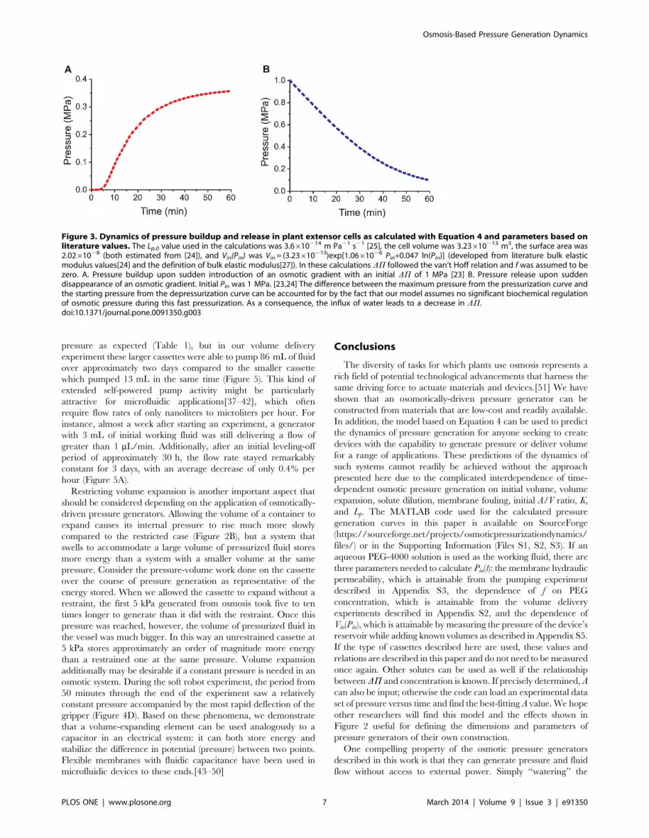
Using the dimensions,[24] Lp value,[25] the final DP value[26]

from plant pulvini, and a f value of zero, along with a Vin(Pin) curve

developed from values of bulk elastic modulus in Phaseolus coccineus

extensor cells [24] and the definition of bulk elastic modulus[27],

we used Equation 4 to predict the dynamics of pressure generation

in these motor cells (Figure 3A). As summarized in Table 1, this

approach suggests that these plant motor cells are able to generate

50 kPa within 8 minutes. This rate is threefold faster than the

fastest pressure generators tested here. We point out, however, that

the mechanism of motor cell function in mimosa pudica and other

plants that undergo fast motions is slightly different than the

devices presented here. In fast-moving plants, turgid cells are

prefilled with osmotic agents (often potassium and chloride ions)

via protein-mediated active transport, an energy-intensive process

that takes place on the time scale of minutes to hours.[28] Upon

receiving a stimulus, ion channels open in these cells, causing the

osmotic agents to equilibrate with the extracellular fluid.[29] This

flux eliminates the osmotic driving force necessary to maintain

turgor, so the cells depressurize. A demonstration of this effect

assuming instantaneous working fluid equilibration is shown in

Figure 3B. The same parameters were used as in the calculated

Pin(t) curve in Figure 3A, but the initial pressure Pin(0) was set to

1 MPa[30,31] and upon stimulation DP was set to zero. This

approach predicts that cells with these characteristics are able to

lose 10% of their osmotic pressure (,100 kPa) in 4.5 minutes. By

comparison, mimosa pudica extensor cells lose 10% of their pressure

within 5 minutes.[32] In principle, strategies for generating an

osmotic gradient on-demand such as electro-osmosis and ion

transport via membrane proteins could be explored in membrane-

bound synthetic actuators and described by our model. The

implementation of these methods is beyond the scope of our

research.

After modeling the dynamics of pressure generation, we created

a bio-inspired actuator system by attaching a 30 mL cassette filled

with saturated (125 mM PEG-4000) working fluid to a soft robotic

gripper (Figure 1D).[17] Each arm of the gripper is filled with

channels that run perpendicular to its length (Figure 4B). The

inside walls of the channels are thicker than the outside walls so

that when positive pressure is applied, the outer walls deform more

than the walls on the interior. When such channels are lined up in

a row, the system curves upon pressurization, causing the arms of

the gripper to bend inward.[17,33–35] Guard cells open and close

plant stomata using a similar mechanism. On each pair of guard

cells, the cell wall that faces the pore is thicker than the wall on the

outside of the stoma. When coupled with microfibrils that restrict

the guard cell circumference to remain relatively constant, this

wall architecture causes the cells to curve into an ‘‘O’’ shape when

pressure is delivered via osmosis, thus opening the pore in response

to external stimuli (Figure 4A).[36]

We recorded the pressure and deflection angle of the soft robot

over time (Figure 5C, Figure 4D, Video S1). Full deflection took

approximately three hours, after which the fluidic connection to

the gripper sprang a leak. The slow timescale of this actuation was

noteworthy, especially considering the quick action of the mimosa

plant. Our model confirmed that using larger compartments with

lower A/V ratios such the prototypes and robot used here slows

down pressure generation more dramatically than intuition may

suggest (Figure 2C).

Using these relatively large commercially available dialysis

cassettes does, however, also have its advantages. First, this system

is sufficiently simple and inexpensive that any laboratory could set

up a pressure generator with ease – large-scale industrial

production of the cassettes should also result in relatively constant

values of parameters such as initial A/V ratio, Lp,0 value, Vin(Pin),

etc. Second, near-instantaneous pressure generation is only useful

in some scenarios and may not be the most important parameter

for a given application. Slow but continuous volume delivery is, for

instance, another interesting application of these devices. A 30 mL

cassette with a lower initial A/V ratio than the 3 mL cassettes

typically used in this work took significantly longer to generate



pressure as expected (Table 1), but in our volume delivery

experiment these larger cassettes were able to pump 86 mL of fluid

over approximately two days compared to the smaller cassette

which pumped 13 mL in the same time (Figure 5). This kind of

extended self-powered pump activity might be particularly

attractive for microfluidic applications[37–42], which often

require flow rates of only nanoliters to microliters per hour. For

instance, almost a week after starting an experiment, a generator

with 3 mL of initial working fluid was still delivering a flow of

greater than 1 mL/min. Additionally, after an initial leveling-off

period of approximately 30 h, the flow rate stayed remarkably

constant for 3 days, with an average decrease of only 0.4% per

hour (Figure 5A).

Restricting volume expansion is another important aspect that

should be considered depending on the application of osmotically-

driven pressure generators. Allowing the volume of a container to

expand causes its internal pressure to rise much more slowly

compared to the restricted case (Figure 2B), but a system that

swells to accommodate a large volume of pressurized fluid stores

more energy than a system with a smaller volume at the same

pressure. Consider the pressure-volume work done on the cassette

over the course of pressure generation as representative of the

energy stored. When we allowed the cassette to expand without a

restraint, the first 5 kPa generated from osmosis took five to ten

times longer to generate than it did with the restraint. Once this

pressure was reached, however, the volume of pressurized fluid in

the vessel was much bigger. In this way an unrestrained cassette at

5 kPa stores approximately an order of magnitude more energy

than a restrained one at the same pressure. Volume expansion

additionally may be desirable if a constant pressure is needed in an

osmotic system. During the soft robot experiment, the period from

50 minutes through the end of the experiment saw a relatively

constant pressure accompanied by the most rapid deflection of the

gripper (Figure 4D). Based on these phenomena, we demonstrate

that a volume-expanding element can be used analogously to a

capacitor in an electrical system: it can both store energy and

stabilize the difference in potential (pressure) between two points.

Flexible membranes with fluidic capacitance have been used in

microfluidic devices to these ends.[43–50]

Conclusions

The diversity of tasks for which plants use osmosis represents a

rich field of potential technological advancements that harness the

same driving force to actuate materials and devices.[51] We have

shown that an osomotically-driven pressure generator can be

constructed from materials that are low-cost and readily available.

In addition, the model based on Equation 4 can be used to predict

the dynamics of pressure generation for anyone seeking to create

devices with the capability to generate pressure or deliver volume

for a range of applications. These predictions of the dynamics of

such systems cannot readily be achieved without the approach

presented here due to the complicated interdependence of time-

dependent osmotic pressure generation on initial volume, volume

expansion, solute dilution, membrane fouling, initial A/V ratio, K,

and Lp. The MATLAB code used for the calculated pressure

generation curves in this paper is available on SourceForge

(https://sourceforge.net/projects/osmoticpressurizationdynamics/

files/) or in the Supporting Information (Files S1, S2, S3). If an

aqueous PEG-4000 solution is used as the working fluid, there are

three parameters needed to calculate Pin(t): the membrane hydraulic

permeability, which is attainable from the pumping experiment

described in Appendix S3, the dependence of f on PEG

concentration, which is attainable from the volume delivery

experiments described in Appendix S2, and the dependence of

Vin(Pin), which is attainable by measuring the pressure of the device’s

reservoir while adding known volumes as described in Appendix S5.

If the type of cassettes described here are used, these values and

relations are described in this paper and do not need to be measured

once again. Other solutes can be used as well if the relationship

between DP and concentration is known. If precisely determined, A

can also be input; otherwise the code can load an experimental data

set of pressure versus time and find the best-fitting A value. We hope

other researchers will find this model and the effects shown in

Figure 2 useful for defining the dimensions and parameters of

pressure generators of their own construction.

One compelling property of the osmotic pressure generators

described in this work is that they can generate pressure and fluid

flow without access to external power. Simply ‘‘watering’’ the

Figure 3. Dynamics of pressure buildup and release in plant extensor cells as calculated with Equation 4 and parameters based onliterature values. The Lp,0 value used in the calculations was 3.6610214 m Pa21 s21 [25], the cell volume was 3.23610213 m3, the surface area was2.0261028 (both estimated from [24]), and Vin(Pin) was Vin = (3.23610213)exp[1.0661026 Pin+0.047 ln(Pin)] (developed from literature bulk elasticmodulus values[24] and the definition of bulk elastic modulus[27]). In these calculations DP followed the van’t Hoff relation and f was assumed to bezero. A. Pressure buildup upon sudden introduction of an osmotic gradient with an initial DP of 1 MPa [23] B. Pressure release upon suddendisappearance of an osmotic gradient. Initial Pin was 1 MPa. [23,24] The difference between the maximum pressure from the pressurization curve andthe starting pressure from the depressurization curve can be accounted for by the fact that our model assumes no significant biochemical regulationof osmotic pressure during this fast pressurization. As a consequence, the influx of water leads to a decrease in DP.doi:10.1371/journal.pone.0091350.g003



https://sourceforge.net/projects/osmoticpressurizationdynamics/files/


device initiates the process in a manner similar to watering a plant.

The novelty of the work presented here – in addition to providing

insight into the fundamental and unintuitive time dependence of

establishing or releasing turgor pressure in plants (Figures 2 and 3)

– lies in a detailed characterization of the dynamics of these

engineered osmotic pressure generators such that they may be

used in microfluidics and microactuation with predictable

outcomes.

Supporting Information

Figure S1 Osmotic pressure as a function of PEGconcentration.

Figure 4. Bioinspired application of an osmotic pressure generator for actuation of a soft robot. A. Design concept of a previouslydescribed elastomeric soft robot whose arms curve and can grip objects in response to pressurization of parallel channels with boundaries ofdiffering thickness. Adapted from [17]. B. Guard cells in their open and closed states. Thick interior walls make guard cells curl when osmoticallypressurized, opening stomata. Adapted from [28]. C. Actuation of the soft robotic gripper used in this work in response to watering an attachedosmotic pressure generator. The extent of deflection is shown after 1, 2, and 3 hours. D. System pressure and deflection angle (as defined in C) of thegripper as a function of time.doi:10.1371/journal.pone.0091350.g004

Figure 5. Time-dependent volume delivery using an osmotically-driven pressure generator as a pump. A. Cumulative volume deliveredby a 3 mL dialysis cassette. B. Cumulative volume delivered by a 30 mL cassette. Both cassettes were restrained and filled with a 125 mM PEG-4000solution and had a MWCO of 3.5 kDa.doi:10.1371/journal.pone.0091350.g005



(TIF)

Figure S2 Effects of Membrane Fouling at IncreasingPEG Concentrations. A. Effective Lp values calculated from

volume delivery experiments as described in Appendix S2 at

different PEG concentrations and MWCOs. The Lp value in the

absence of PEG, Lp,0, was determined by the procedure in

Appendix 3. B. The fouling factor f at different PEG concentra-

tions and MWCOs. f is determined by f ~1{Lp

Lp,0

and has been

fit with the Hill equation.

(TIF)

Figure S3 Experimental setup for measuring wavevelocity. The Tygon tubing and stainless steel pipe are filled

with aqueous PEG solution. An air compressor attached to the

accumulator applies a static pressure (Pin) that is measured by a

DC pressure transducer (PDC; 840065, Sper Scientific). Both valves

are closed prior to measuring wave velocity to prevent fluid flow. A

shaker actuates the piston to create a pressure or sound wave. The

time delay between two AC pressure transducers (P1 and P2) is

used to determine wave velocity (V~L1=Dt). The downstream

pressure transducer (P2) was mounted at a length L2 away from the

end of the pipe to ensure that reflections from the pipe/tubing

interface did not interfere with the time delay measurements. L1 is

60.7 cm, L2 is 77.0 cm, the inner diameter of the stainless steel

pipe is 1.39 cm, and the pipe wall thickness is 3.7 mm (1/2 NPS

SCH80).

(TIF)

Figure S4 Bulk modulus calibration and measurementsA. Calibration of bulk modulus measurement apparatus with air.

B. Bulk modulus measurements of aqueous PEG solutions from

the apparatus. The fit lines represent a fit of the entire data set, not

just the points from that concentration.

(TIF)

File S1 MATLAB script for calculation of pressure as afunction of time. This script calculates pressure as a function of

time for a pressure generator of specified dimensions and

permeability containing an aqueous PEG solution as an osmotic

driver. It can also be used to determine the effective membrane

area available for flux from a set of experimental data. This code is

also available on SourceForge: https://sourceforge.net/projects/

osmoticpressurizationdynamics/files/.

(M)

File S2 Sample data set to accompany File S1. Contains

pressure and time data. This code is also available on SourceForge:

https://sourceforge.net/projects/osmoticpressurizationdynamics/files/.

(M)

File S3 Sample calculation from File S1. Contains input

parameters and resulting calculated pressure and time values. This

file is also available on SourceForge: https://sourceforge.net/

projects/osmoticpressurizationdynamics/files/.

(XLSX)

Video S1 Actuation of soft robot attached to a pressuregenerator.

(MOV)

Appendix S1 Osmotic Pressure Measurements.

(DOCX)

Appendix S2 Determining Lp from Volume Delivery.

(DOCX)

Appendix S3 Discussion of Correction to Lp.

(DOCX)

Appendix S4 Bulk Modulus Measurements.

(DOCX)

Appendix S5 Determination of Vin(Pin).

(DOCX)

Acknowledgments

We thank the Whitesides Group, in particular Filip Ilievski, for donating a

soft robotic gripper to our research efforts.

Author Contributions

Conceived and designed the experiments: BRB TBHS MM KWW.

Performed the experiments: BRB TBHS SL YNB. Analyzed the data: BRB

TBHS YNB. Contributed reagents/materials/analysis tools: MM KWW.

Wrote the paper: TBHS.

References

1. Stroock AD, Pagay VV, Zwieniecki MA, Holbrook NM (2013) The

Physicochemical Hydrodynamics of Vascular Plants. Annu Rev Fluid Mech.

2. Cath TY, Childress AE, Elimelech M (2006) Forward osmosis: Principles,

applications, and recent developments. J Membr Sci 281: 70–87. doi:10.1016/

j.memsci.2006.05.048.

3. McGinnis RL, McCutcheon JR, Elimelech M (2007) A novel ammonia–carbon

dioxide osmotic heat engine for power generation. J Membr Sci 305: 13–19.

doi:10.1016/j.memsci.2007.08.027.

4. Achilli A, Cath TY, Childress AE (2009) Power generation with pressure

retarded osmosis: An experimental and theoretical investigation. J Membr Sci

343: 42–52. doi:10.1016/j.memsci.2009.07.006.

5. Logan BE, Elimelech M (2012) Membrane-based processes for sustainable

power generation using water. Nature 488: 313–319. doi:10.1038/nature11477.

6. Achilli A, Childress AE (2010) Pressure retarded osmosis: From the vision of

Sidney Loeb to the first prototype installation — Review. Desalination 261: 205–

211. doi:10.1016/j.desal.2010.06.017.

7. International Energy Agency (2012) World energy outlook. Paris, France:

International Energy Agency. Available: http://iea.org/publications/

freepublications/publication/WEO_2012_Iraq_Energy_Outlook-1.pdf. Ac-

cessed 2013 May 8 May.

8. Benedek GB, Villars FMH (2000) Physics with Illustrative Examples from

Medicine and Biology: Statistical Physics. 2nd ed. New York: Springer-Verlag.

9. Theeuwes F (1975) Elementary osmotic pump. J Pharm Sci 64: 1987–1991.

10. Theeuwes F, Yum SI (1976) Principles of the design and operation of generic

osmotic pumps for the delivery of semisolid or liquid drug formulations. Ann

Biomed Eng 4: 343–353.

11. Good BT, Bowman CN, Davis RH (2007) A water-activated pump for portable

microfluidic applications. J Colloid Interface Sci 305: 239–249. doi:10.1016/

j.jcis.2006.08.067.

12. Rose S, Nelson JF (1955) A Continuous Long-Term Injector. Nature 33: 415–

420.

13. Will PC, Cortright RN, Hopfer U (1980) Polyethylene Glycols as Solvents in

Implantable Osmotic Pumps. J Pharm Sci 69: 747–749.

14. Liu L, Wang X (2008) Solubility-modulated monolithic osmotic pump tablet for

atenolol delivery. Eur J Pharm Biopharm 68: 298–302. doi:10.1016/

j.ejpb.2007.04.020.

15. Swanson DR, Barclay BL, Wong PS, Theeuwes F (1987) Nifedipine

gastrointestinal therapeutic system. Am J Med 83: 3–9.

16. Yu-Chuan Su, Liwei Lin, Pisano AP (2002) A water-powered osmotic

microactuator. J Microelectromechanical Syst 11: 736–742. doi:10.1109/

JMEMS.2002.805045.

17. Ilievski F, Mazzeo AD, Shepherd RF, Chen X, Whitesides GM (2011) Soft

Robotics for Chemists. Angew Chem Int Ed 50: 1890–1895. doi:10.1002/

anie.201006464.

18. Money NP (1989) Osmotic pressure of aqueous polyethylene glycols relationship

between molecular weight and vapor pressure deficit. Plant Physiol 91: 766–769.

19. Pinho SP, Macedo EA (2005) Solubility of NaCl, NaBr, and KCl in Water,

Methanol, Ethanol, and Their Mixed Solvents. J Chem Eng Data 50: 29–32.

doi:10.1021/je049922y.

20. Strathmann H (2000) Membrane Separation Processes, 4. Concentration

Polarization and Membrane Fouling. Ullmann’s Encyclopedia of Industrial

Chemistry. Wiley-VCH Verlag GmbH & Co. KGaA. Available: http://








http://iea.org/publications/freepublications/publication/WEO_2012_Iraq_Energy_Outlook-1.pdf

http://iea.org/publications/freepublications/publication/WEO_2012_Iraq_Energy_Outlook-1.pdf

http://onlinelibrary.wiley.com/doi/10.1002/14356007.o16_o05/abstract

onlinelibrary.wiley.com/doi/10.1002/14356007.o16_o05/abstract. Accessed 3

December 2013.

21. McCutcheon JR, Elimelech M (2006) Influence of concentrative and dilutive

internal concentration polarization on flux behavior in forward osmosis.

J Membr Sci 284: 237–247. doi:10.1016/j.memsci.2006.07.049.

22. Haynes WM,editor (2013) CRC Handbook of Chemistry and Physics Boca

Raton, FL: CRC Press.

23. Eliassi A, Modarress H, Mansoori GA (1998) Densities of poly (ethylene glycol)+water mixtures in the 298.15–328.15 K temperature range. J Chem Eng Data

43: 719–721.

24. Mayer W-E, Flach D, Raju MVS, Starrach N, Wiech E (1985) Mechanics of

circadian pulvini movements in Phaseolus coccineus L. Planta 163: 381–390.

25. Moshelion M, Becker D, Biela A, Uehlein N, Hedrich R, et al. (2002) Plasma

Membrane Aquaporins in the Motor Cells of Samanea saman. Plant Cell 14:

727–739. doi:10.1105/tpc.010351.

26. Gorton HL (1987) Water Relations in Pulvini from Samanea saman: I. Intact

Pulvini. Plant Physiol 83: 945–950. doi:10.2307/4270542.

27. Zimmermann U, Steudle E (1979) Physical Aspects of Water Relations of Plant

Cells. In: H.W. . Woolhouse, editor. Advances in Botanical Research. Academic

Press, Vol. Volume 6. pp. 45–117. Available: http://www.sciencedirect.com/

science/article/pii/S0065229608603298. Accessed 2013 Aug 7.

28. Hill BS, Findlay GP (1981) The power of movement in plants: the role of

osmotic machines. Q Rev Biophys 14: 173–222.

29. Samejima M, Sibaoka T (1980) Changes in the extracellular ion concentration

in the main pulvinus of Mimosa pudica during rapid movement and recovery.

Plant Cell Physiol 21: 467–479.

30. Fleurat-Lessard P (1988) Structural and Ultrastructural Features of Cortical

Cells in Motor Organs of Sensitive Plants. Biol Rev 63: 1–22. doi:10.1111/

j.1469-185X.1988.tb00467.x.

31. Allen RD (1967) Studies of the Seismonastic Reaction in the Main Pulvinus of

Mimosa Pudica [Ph.D.]. United States — California: University of California,

Los Angeles.Available: http://search.proquest.com.proxy.lib.umich.edu/

docview/302242706. Accessed 2013 Aug 7.

32. Kagawa H, Saito E (2000) A Model on the Main Pulvinus Movement of Mimosa

Pudica. JSME Int J 43: 923–928.

33. Martinez RV, Fish CR, Chen X, Whitesides GM (2012) Elastomeric Origami:

Programmable Paper-Elastomer Composites as Pneumatic Actuators. Adv Funct

Mater 22: 1376–1384. doi:10.1002/adfm.201102978.

34. Martinez RV, Branch JL, Fish CR, Jin L, Shepherd RF, et al. (2013) Robotic

Tentacles with Three-Dimensional Mobility Based on Flexible Elastomers. Adv

Mater 25: 205–212. doi:10.1002/adma.201203002.

35. Shepherd RF, Ilievski F, Choi W, Morin SA, Stokes AA, et al. (2011) Multigait

soft robot. Proc Natl Acad Sci 108: 20400–20403.

36. Sharpe, Peter J H., Wu Hsin-i, Spence, Richard D (1987) Stomatal Mechanics.

In: Zeiger E, Farquhar GD, Cowan IR, editors. Stomatal Function. Stanford

University Press.

37. Iverson BD, Garimella SV (2008) Recent advances in microscale pumping

technologies: a review and evaluation. Microfluid Nanofluidics 5: 145–174.doi:10.1007/s10404-008-0266-8.

38. Walker GM, Beebe DJ (2002) A passive pumping method for microfluidic

devices. Lab Chip 2: 131–134. doi:10.1039/B204381E.39. Bessoth FG, deMello AJ, Manz A (1999) Microstructure for efficient continuous

flow mixing. Anal Commun 36: 213–215. doi:10.1039/A902237F.40. Erbacher C, Bessoth FG, Busch M, Verpoorte E, Manz A (1999) Towards

Integrated Continuous-Flow Chemical Reactors. Microchim Acta 131: 19–24.

doi:10.1007/s006040050004.41. Kopp MU, Mello AJ de, Manz A (1998) Chemical Amplification: Continuous-

Flow PCR on a Chip. Science 280: 1046–1048. doi:10.2307/2895434.42. Laurell T, Drott J, Rosengren L (1995) Silicon wafer integrated enzyme reactors.

Biosens Bioelectron 10: 289–299. doi:10.1016/0956-5663(95)96848-S.43. Huang S-B, Wu M-H, Cui Z, Cui Z, Lee G-B (2008) A membrane-based

serpentine-shape pneumatic micropump with pumping performance modulated

by fluidic resistance. J Micromechanics Microengineering 18: 045008.doi:10.1088/0960-1317/18/4/045008.

44. Kim Y, Kuczenski B, LeDuc PR, Messner WC (2009) Modulation of fluidicresistance and capacitance for long-term, high-speed feedback control of a

microfluidic interface. Lab Chip 9: 2603. doi:10.1039/b822423d.

45. Leslie DC, Easley CJ, Seker E, Karlinsey JM, Utz M, et al. (2009) Frequency-specific flow control in microfluidic circuits with passive elastomeric features. Nat

Phys 5: 231–235. doi:10.1038/nphys1196.46. Mescher MJ, Swan E, Fiering J, Holmboe ME, Sewell WF, et al. (2009)

Fabrication Methods and Performance of Low-Permeability MicrofluidicComponents for a Miniaturized Wearable Drug Delivery System.

J Microelectromechanical Syst 18: 501–510. doi:10.1109/JMEMS.

2009.2015484.47. Sewell WF, Borenstein JT, Chen Z, Fiering J, Handzel O, et al. (2009)

Development of a Microfluidics-Based Intracochlear Drug Delivery Device.Audiol Neurotol 14: 411–422. doi:10.1159/000241898.

48. Herz M, Horsch D, Wachutka G, Lueth TC, Richter M (2010) Design of ideal

circular bending actuators for high performance micropumps. Sens ActuatorsPhys 163: 231–239. doi:10.1016/j.sna.2010.05.018.

49. Gong MM, MacDonald BD, Vu Nguyen T, Sinton D (2012) Hand-poweredmicrofluidics: A membrane pump with a patient-to-chip syringe interface.

Biomicrofluidics 6: 044102. doi:10.1063/1.4762851.50. Kim S-J, Yokokawa R, Takayama S (2013) Microfluidic oscillators with widely

tunable periods. Lab Chip 13: 1644. doi:10.1039/c3lc41415a.

51. Mayer M, Genrich M, Kunnecke W, Bilitewski U (1996) Automateddetermination of lactulose in milk using an enzyme reactor and flow analysis

with integrated dialysis. Anal Chim Acta 324: 37–45. doi:10.1016/0003-2670(95)00576-5.

52. Dumais J, Forterre Y (2012) ‘‘Vegetable Dynamicks’’: The Role of Water in

Plant Movements. Annu Rev Fluid Mech 44: 453–478. doi:10.1146/annurev-fluid-120710-101200.



http://onlinelibrary.wiley.com/doi/10.1002/14356007.o16_o05/abstract

http://www.sciencedirect.com/science/article/pii/S0065229608603298

http://www.sciencedirect.com/science/article/pii/S0065229608603298

http://search.proquest.com.proxy.lib.umich.edu/docview/302242706

http://search.proquest.com.proxy.lib.umich.edu/docview/302242706

osmosis-based pressure generation: dynamics and application

Documents