optical flow from motion blurred color images

Optical Flow from Motion Blurred Color Images

Yasmina Schoueri Milena ScacciaIoannis Rekleitis

School of Computer Science, McGill University[yasyas,yiannis]@cim.mcgill.ca, [email protected]

Abstract

This paper presents an algorithm for the estimation ofoptical flow from a single, motion-blurred, color image. Theproposed algorithm is based on earlier work that estimatedthe optical flow using the information from a single greyscale image. By treating the three color channels separatelywe improved the robustness of our approach. Since firstintroduced, different groups have used similar techniquesof the original algorithm to estimate motion in a variety ofapplications. Experimental results from natural as well asartificially motion-blurred images are presented.

1 Introduction

In a scene observed by a camera, motion blur may beproduced from a combination of the movement of the cam-era and of the independent motion of the objects in thescene. In many cases, motion blur is regarded as undesir-able noise that is to be removed to render a clearer image ofthe observed scene. Despite being regarded as a nuisance tothe photographer, studies have shown that motion blur in animage has some practical interest in one of the fundamen-tal problems of computer vision —the measurement of theapparent motion in an image, referred to as optical flow.

Estimating the motion blur parameters is useful for twodifferent reasons. First, having an accurate estimate of theblurring parameters, image restoration in the form of de-blurring can be achieved [9]. Second, by calculating theoptical flow from a single motion blurred image, motionparameters for separate objects in the scene as well as ego-motion can be inferred.

Different applications have been suggested to benefitfrom the motion blur estimation. Traffic cameras can inferthe speed of passing vehicles using only the motion blur,thus avoiding detectable active sensing, such as radar. Themotion blurred images can further be cleaned up to provideevidence in the form of licence plate numbers.

A methodology for the detection and subsequent correc-

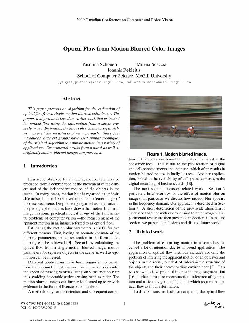
Figure 1. Motion blurred image.tion of the above mentioned blur is also of interest at theconsumer level. This is due to the proliferation of digitaland cell-phone cameras and their use, which often results inmotion blurred photos in badly lit areas. Another applica-tion, linked to the availability of cell phone cameras, is thedigital recording of business cards [18].

The next section discusses related work. Section 3presents a brief overview of the effect of motion blur onimages. In particular we discuss how motion blur appearsin the frequency domain. Our approach is described in Sec-tion 4. A short description of the grey scale algorithm isdiscussed together with our extension to color images. Ex-perimental results are then presented in Section 5. In the lastsection, we present conclusions and discuss future work.

2 Related work

The problem of estimating motion in a scene has re-ceived a lot of attention due to its broad application. Theapplication of optical flow methods includes not only theproblem of inferring the apparent motion of an observer andobjects in the scene, but that of inferring the structure ofthe objects and their corresponding environment [2]. Thiswas shown to have practical interest in image segmentation[16], surface structure reconstruction, inference of egomo-tion and active navigation [11], all of which require the op-tical flow as input information.

To date, various methods for computing the optical flow

2009 Canadian Conference on Computer and Robot Vision

978-0-7695-3651-4/09 $25.00 © 2009 IEEE

DOI 10.1109/CRV.2009.15

1

Authorized licensed use limited to: McGill University. Downloaded on December 24, 2009 at 18:43 from IEEE Xplore. Restrictions apply.

have been proposed, the most widely used being differentialmethods. The first global differential method, introduced in1980 by Horn and Schunck, consists of optimizing a func-tion based on residuals from the brightness constancy con-straint and a regularization term expressing the expectedsmoothness of the flow field [12]. There have been manyextensions of this method, mainly varying the constraintsused to solve the problem.

Global differential techniques have the advantage ofyielding dense flow fields, yet are not as robust to noise asare local approaches such as the Lucas-Kanade method [15]which regards image patches and an affine model for theflow field. There have since been studies evaluating hybridapproaches that attempt to combine the main advantages ofglobal and local approaches [3].

A drawback to the above mentioned traditional algo-rithms is that optical flow is calculated using a series ofconsecutive images under the assumption that pixels keeptheir brightness from one frame to the other, having changedtheir position only. That is, it is assumed that each image istaken with an infinitely small exposure time. Thus blurringdue to motion within a frame is disregarded or treated as anadditional source of noise.

Instead of being considered a degradation that is to beremoved using one of the many deblurring methods devel-oped [1], it has been shown that motion blur in an imagemay have some practical interest in fundamental computervision problems, such as in the measurement of the opticalflow [19].

In 1981, a series of psychophysical studies suggestedthat the human visual system [10] is able to process infor-mation about motion blur in order to infer information aboutobjects in the scene. This has motivated the development ofalgorithms that take advantage of information encoded inthe motion blur. This motivation, in conjunction with theuse of a deblurring mechanism to distinguish features in aspecific image, gave rise to a novel approach for obtaininginformation about motion in an image.

In 1995, an algorithm for extracting the parameters ofmotion blur in a single image in order to compute the opticalflow was presented by Rekleitis. His approach relies heavilyon the information present in the frequency domain. In par-ticular, it exploits the key observation that motion blur in-troduces a ripple in the Fourier transform [19], from whichwe may extract information about the magnitude and ori-entation of the velocity vector given an image patch. Thisalgorithm can be used in a stand-alone manner or to com-plement previous algorithms to address the issue of motionblur in a sequence of frames instead of merely ignoring it.

There has since been research that builds on the ideas ofusing information from motion blur. In 1996, Chen et al.presented a computational model that attempts to emulatethe behavior of the human visual system in order to use it

in machine vision systems [5]. Further research on the hu-man visual system carried out in 1999 by Geisler exploresanother potential neural mechanism for resolving motionorientation, which uses a spatial signal known as “motionstreak” created by a fast enough moving localized imagefeature [8].

Aside from in-depth studies of the human visual sys-tem, other methods for identifying motion blur parametersfrom a single blurred image have been developed. In 1997,Yitzhaky and Kopeika developed a method for characteriz-ing the point spread function of the blur. Their identificationmethod bases itself on the concept that image characteristicsalong the direction of motion are different from characteris-tics in other directions [20].

There has also been research examining the usefulnessand limitations of Rekleitis’ approach of estimating blur pa-rameters, which has been adapted in 2005 by Qi et al. to en-hance optical character recognition (OCR) in blurred text.Rekleitis’ algorithm has been shown to work for most blurorientations and extents. However the average error estima-tion of blur extent was shown to be quite large, not making itsuitable for OCR. Qi et al. thus adopt a different threshold-ing technique in blur orientation estimation and further es-timate motion parameters due to uniform acceleration [18].

The use of motion blur has also had an increasing num-ber of applications in areas such as real-time ball-trackingsystems in live sports programs [7], in vehicle speed de-tection [14], in object depth recovery [4], as well as in theestimation of motion for a tracking vision system [13].

3 Motion Blur

As mentioned previously, most motion estimation algo-rithms infer optical flow by considering a sequence of im-ages. In addition, they assume that pixels maintain theirbrightness in subsequent frames, their positions being theonly thing that changes. That is, they assume that each im-age is acquired with a very small exposure time. But if thisdoes not happen to be the case, then with a somewhat largeexposure time, different points traveling in the scene causetheir corresponding projections on the image plane to affectseveral pixels. Hence in the capturing of any single point, anumber of scene points get projected onto the image planeduring the time of exposure, each of them contributing tothe final color and brightness of the image point.

More formally, the motion blur can be described as theeffect of applying the linear filter:

B(x, y) = I(x, y) ∗ h(x, y) (1)

where B is the blurred image, I is the image taken withexposure time Te = 0, and h is the convolution kernel:

2


(a) (b)

(c) (d)

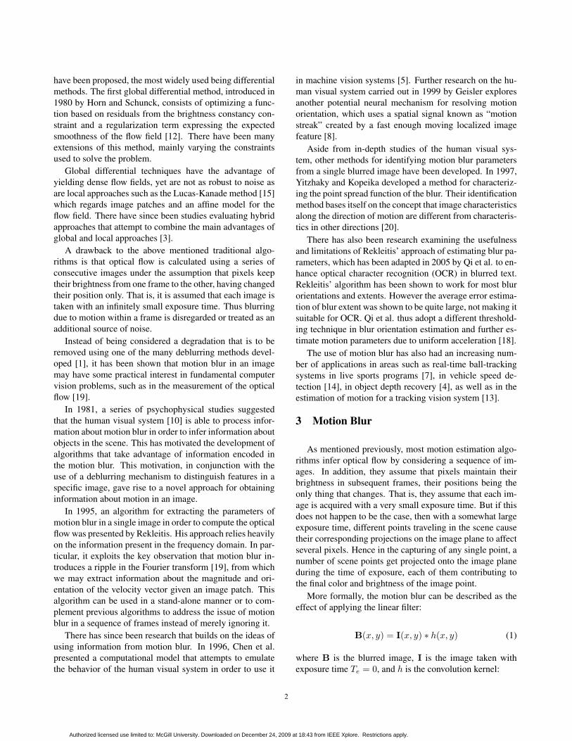
Figure 2. (a) A color Image of random noise.(b) The power spectrum of (a). (c) The sameimage affected by an artificial motion blur. (d)The power spectrum of the motion blurredimage.

h(x, y) ={

1d , 0 ≤ |x| ≤ d cos(α) y = d sin(α)0, otherwise (2)

where α is the angle of the motion that caused the blur, andd = VoTe is the number of scene points that affect a specificpixel. Given the convolution kernel, we can also produceartificially blurred images, which can serve as ground truthto test our approach.

In the frequency domain the convolution described in Eq.1 results in the multiplication of the Fourier transform ofimage I times the Fourier transform of the convolution ker-nel h. It has been shown [19] that one prominent character-istic of the convolution kernel in the frequency domain is aripple that extends perpendicular to the direction of the blur;cf. Fig. 2d. This ripple is thus used to detect the directionof the blur. In the most favorable case the observed sceneconsists of random noise, as in Fig. 2a. In that case theFourier of the non-blurred image has no prominent struc-ture, cf. Fig. 2b, and the detection of the optical flow isvery easy. Clearly when there is structure in the scene, theoptical flow detection is more challenging. The followingsection presents an outline of the proposed algorithm.

4 Optical Flow Estimation

In order to apply our algorithm to color images we treatthe three color channels (red, green, and blue) as individualgrey scale images. The optical flow is estimated in each

color channel using the algorithm proposed in [19] and theresults are combined to form the final optical flow estimates.

4.1 Windowing and Zero-Padding

A significant source of error is the well studied ringingeffect. When we take the Fourier transform of an imagepatch, the abrupt transition results in artifacts in the fre-quency domain. To mitigate the ringing effect, each imagepatch is masked using a 2D Gaussian function. Then, to in-crease the frequency resolution of the Fourier transform, themasked image patch, originally of sizeN , is zero-padded tosize 2N . However, if the patch pixel values are much larger,the blur is then harder to detect, thus the difference betweenthe pixel value and the mean of the patch is zero-paddedinstead [17].

4.2 Orientation Estimation

As seen earlier, the power spectrum of the blurred im-age is characterized by a central ripple that goes across thedirection of the motion. In order to extract this orienta-tion we treat the power spectra as an image and a linearfilter is applied in order to identify the orientation of theripple. More specifically the second derivative of a two di-mensional Gaussian is used. The second derivative of theGaussian along the x-axis is G0

2 = ∂2G∂x2 . In order to extract

the orientation of the ripple, we have to find the angle θ forwhich the response of the second derivative of a Gaussianfilter – oriented at that angle (Gθ2) – is maximum. Fortu-nately, the second derivative of the Gaussian Gθ2 belongs toa family of filters called “steerable filters” [6], whose re-sponse can be calculate at any angle θ based only on theresponses of three basis filters.

The response of the second derivative of the Gaussianat an angle θ (RGθ2) is given in equation 3. The set of thethree basis filters is shown in the left column of the table 1and in the right column we could see the three interpolationfunctions that are used.

RGθ2 = ka(θ)RG2a + kb(θ)RG2b + kc(θ)RG2c (3)

4.3 Cepstral Analysis

If only one line of the blurred image is taken (across thedirection of the motion) then the blurred signal is equiva-lent to the convolution of the unblurred signal by the stepfunction which in the frequency domain is transformed intothe sinc function (sinc(x) = sin x

x ). The period of the sincpulse is equivalent to the length of the step function, whichis in turn equivalent to the velocity magnitude. If we takethe Fourier transform of the sinc function, its period appears

3


G2a = 0.921(2x2 − 1)eµ ka(θ) = cos2(θ)

G2b = 1.843xyeµ kb(θ) = −2 cos(θ) sin(θ)

G2c = 0.921(2y2 − 1)eµ kc(θ) = sin2(θ)

µ = −(x2 + y2)

Table 1. The three basis filters and their interpo-lation functions

(a) (b)

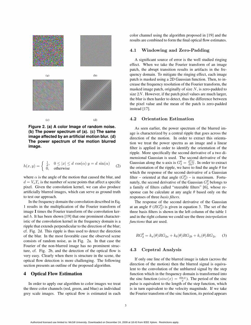
Figure 3. (a) The collapsed power spectrumof Fig. 2d. (b) The power spectrum of thecollapsed power spectrum.

as a negative peak. To improve robustness, we compute themagnitude of the velocity by using a 1D projection of thepower spectra onto the line across the velocity vector orien-tation that passes through the origin.

To approximate the 1D signal, the power spectra is col-lapsed from 2D into 1D. The resulting signal also takes onthe shape of the sinc function, because the ripple caused bythe motion blur is the dominant feature; cf. Fig. 2d. Ev-ery pixel P(x,y) in the power spectra is mapped into the linethat passes through the origin O at an angle θ with the x-axis equal to the orientation of the motion, and at distanced = x cos(θ) + y sin(θ). The Fourier transform of the sincfunction is almost identical in shape to the one that appearswhen we take the Fourier transform of the collapsed spec-trum cf. Fig. 3a,b.

4.4 Color Image Optical Flow Estimation

The results from the three color channels are combinedas a weighted sum. Currently, there is a binary decisionto select if a channel contributes based on the response ofthe steerable filters. If the difference between the maximumand the minimum response of the steerable filter is not sig-nificant, then the flow estimate from that channel for thespecific location is not considered. All the estimates thatare above a threshold then are weighted equally.

5 Experimental Results

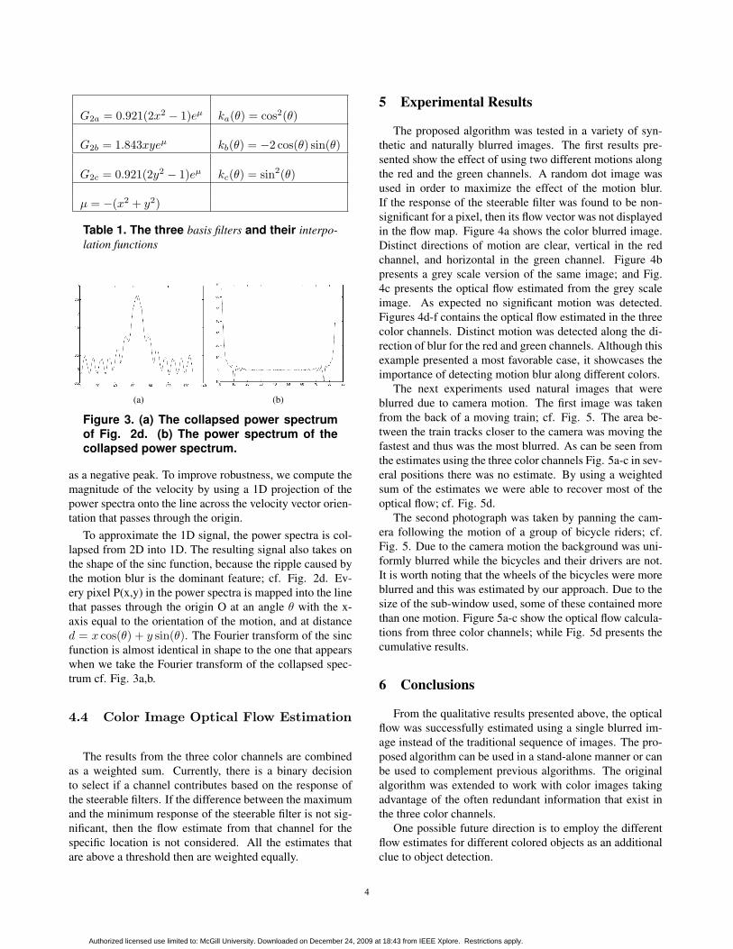
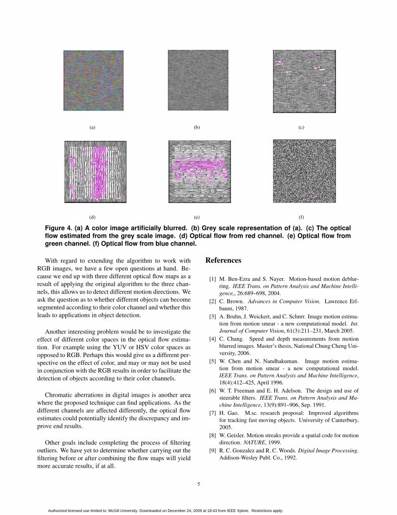
The proposed algorithm was tested in a variety of syn-thetic and naturally blurred images. The first results pre-sented show the effect of using two different motions alongthe red and the green channels. A random dot image wasused in order to maximize the effect of the motion blur.If the response of the steerable filter was found to be non-significant for a pixel, then its flow vector was not displayedin the flow map. Figure 4a shows the color blurred image.Distinct directions of motion are clear, vertical in the redchannel, and horizontal in the green channel. Figure 4bpresents a grey scale version of the same image; and Fig.4c presents the optical flow estimated from the grey scaleimage. As expected no significant motion was detected.Figures 4d-f contains the optical flow estimated in the threecolor channels. Distinct motion was detected along the di-rection of blur for the red and green channels. Although thisexample presented a most favorable case, it showcases theimportance of detecting motion blur along different colors.

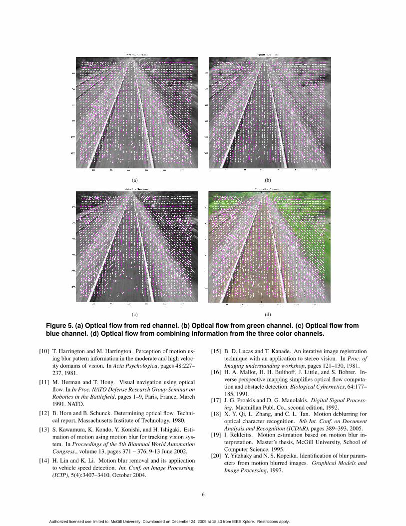
The next experiments used natural images that wereblurred due to camera motion. The first image was takenfrom the back of a moving train; cf. Fig. 5. The area be-tween the train tracks closer to the camera was moving thefastest and thus was the most blurred. As can be seen fromthe estimates using the three color channels Fig. 5a-c in sev-eral positions there was no estimate. By using a weightedsum of the estimates we were able to recover most of theoptical flow; cf. Fig. 5d.

The second photograph was taken by panning the cam-era following the motion of a group of bicycle riders; cf.Fig. 5. Due to the camera motion the background was uni-formly blurred while the bicycles and their drivers are not.It is worth noting that the wheels of the bicycles were moreblurred and this was estimated by our approach. Due to thesize of the sub-window used, some of these contained morethan one motion. Figure 5a-c show the optical flow calcula-tions from three color channels; while Fig. 5d presents thecumulative results.

6 Conclusions

From the qualitative results presented above, the opticalflow was successfully estimated using a single blurred im-age instead of the traditional sequence of images. The pro-posed algorithm can be used in a stand-alone manner or canbe used to complement previous algorithms. The originalalgorithm was extended to work with color images takingadvantage of the often redundant information that exist inthe three color channels.

One possible future direction is to employ the differentflow estimates for different colored objects as an additionalclue to object detection.

4


(a) (b) (c)

(d) (e) (f)

Figure 4. (a) A color image artificially blurred. (b) Grey scale representation of (a). (c) The opticalflow estimated from the grey scale image. (d) Optical flow from red channel. (e) Optical flow fromgreen channel. (f) Optical flow from blue channel.

With regard to extending the algorithm to work withRGB images, we have a few open questions at hand. Be-cause we end up with three different optical flow maps as aresult of applying the original algorithm to the three chan-nels, this allows us to detect different motion directions. Weask the question as to whether different objects can becomesegmented according to their color channel and whether thisleads to applications in object detection.

Another interesting problem would be to investigate theeffect of different color spaces in the optical flow estima-tion. For example using the YUV or HSV color spaces asopposed to RGB. Perhaps this would give us a different per-spective on the effect of color, and may or may not be usedin conjunction with the RGB results in order to facilitate thedetection of objects according to their color channels.

Chromatic aberrations in digital images is another areawhere the proposed technique can find applications. As thedifferent channels are affected differently, the optical flowestimates could potentially identify the discrepancy and im-prove end results.

Other goals include completing the process of filteringoutliers. We have yet to determine whether carrying out thefiltering before or after combining the flow maps will yieldmore accurate results, if at all.

References

[1] M. Ben-Ezra and S. Nayer. Motion-based motion deblur-ring. IEEE Trans. on Pattern Analysis and Machine Intelli-gence,, 26:689–698, 2004.

[2] C. Brown. Advances in Computer Vision. Lawrence Erl-baum, 1987.

[3] A. Bruhn, J. Weickert, and C. Schnrr. Image motion estima-tion from motion smear - a new computational model. Int.Journal of Computer Vision, 61(3):211–231, March 2005.

[4] C. Chang. Speed and depth measurements from motionblurred images. Master’s thesis, National Chung Cheng Uni-versity, 2006.

[5] W. Chen and N. Nandhakuman. Image motion estima-tion from motion smear - a new computational model.IEEE Trans. on Pattern Analysis and Machine Intelligence,18(4):412–425, April 1996.

[6] W. T. Freeman and E. H. Adelson. The design and use ofsteerable filters. IEEE Trans. on Pattern Analysis and Ma-chine Intelligence, 13(9):891–906, Sep. 1991.

[7] H. Gao. M.sc. research proposal: Improved algorithmsfor tracking fast moving objects. University of Canterbury,2005.

[8] W. Geisler. Motion streaks provide a spatial code for motiondirection. NATURE, 1999.

[9] R. C. Gonzalez and R. C. Woods. Digital Image Processing.Addison-Wesley Publ. Co., 1992.

5


(a) (b)

(c) (d)

Figure 5. (a) Optical flow from red channel. (b) Optical flow from green channel. (c) Optical flow fromblue channel. (d) Optical flow from combining information from the three color channels.

[10] T. Harrington and M. Harrington. Perception of motion us-ing blur pattern information in the moderate and high veloc-ity domains of vision. In Acta Psychologica, pages 48:227–237, 1981.

[11] M. Herman and T. Hong. Visual navigation using opticalflow. In In Proc. NATO Defense Research Group Seminar onRobotics in the Battlefield, pages 1–9, Paris, France, March1991. NATO.

[12] B. Horn and B. Schunck. Determining optical flow. Techni-cal report, Massachusetts Institute of Technology, 1980.

[13] S. Kawamura, K. Kondo, Y. Konishi, and H. Ishigaki. Esti-mation of motion using motion blur for tracking vision sys-tem. In Proceedings of the 5th Biannual World AutomationCongress,, volume 13, pages 371 – 376, 9-13 June 2002.

[14] H. Lin and K. Li. Motion blur removal and its applicationto vehicle speed detection. Int. Conf. on Image Processing,(ICIP), 5(4):3407–3410, October 2004.

[15] B. D. Lucas and T. Kanade. An iterative image registrationtechnique with an application to stereo vision. In Proc. ofImaging understanding workshop, pages 121–130, 1981.

[16] H. A. Mallot, H. H. Bulthoff, J. Little, and S. Bohrer. In-verse perspective mapping simplifies optical flow computa-tion and obstacle detection. Biological Cybernetics, 64:177–185, 1991.

[17] J. G. Proakis and D. G. Manolakis. Digital Signal Process-ing. Macmillan Publ. Co., second edition, 1992.

[18] X. Y. Qi, L. Zhang, and C. L. Tan. Motion deblurring foroptical character recognition. 8th Int. Conf. on DocumentAnalysis and Recognition (ICDAR), pages 389–393, 2005.

[19] I. Rekleitis. Motion estimation based on motion blur in-terpretation. Master’s thesis, McGill University, School ofComputer Science, 1995.

[20] Y. Yitzhaky and N. S. Kopeika. Identification of blur param-eters from motion blurred images. Graphical Models andImage Processing, 1997.

6


(a)

(b)

(c)

(d)

Figure 6. (a) Optical flow from red channel. (b) Optical flow from green channel. (c) Optical flow fromblue channel. (d) Optical flow from combining information from the three color channels.

7


optical flow from motion blurred color images

Documents