Adaptive Color Demosaicing and False Colors Removal

Mirko Guarnera, Giuseppe Messina, and Valeria Tomaselli∗

Advanced System Technology GroupSTMicroelectronics

Stradale Primosole 50,95121 Catania, Italy

AbstractColor interpolation solutions drastically influence the quality of the whole image generation

pipeline, so they must guarantee the rendering of high quality pictures avoiding typical artifactssuch as blurring, zipper effects and false colors. Moreover, demosaicing should avoid emphasizingtypical artifacts of real sensors data, such as noise and green imbalance effect, which would befurther accentuated by the subsequent steps of the processing pipeline. In this paper we propose anew adaptive algorithm, which decides the interpolation technique to apply to each pixel, accordingto its neighborhood analysis. Edges are effectively interpolated through a directional filteringapproach which interpolates the missing colors selecting the suitable filter depending on the edgeorientation. Regions close to edges are interpolated through a simpler demosaicing approach. Thusflat regions are identified and heavily low pass filtered in order to eliminate some residual noise andto minimize the annoying green imbalance effect. Finally an effective false colors removal algorithmis used as a post-processing step, in order to eliminate residual color errors. The experimentalresults show how sharp edges are preserved whereas undesired zipper effects are reduced, improvingthe edge resolution itself and obtaining superior image quality.

Keywords: Color Interpolation, False Color Removal.

∗Electronic address: (mirko.guarnera,giuseppe.messina,valeria.tomaselli)@st.com

1

BGBB

RRGR GR

GB

BB

RRGR GR

GB GB

FIG. 1: Bayer Pattern

I. INTRODUCTION

Imaging consumer, prosumer and professional devices, such as digital still and videocameras, mobile phones, personal digital assistants, visual sensors for surveillance and au-tomotive applications, usually capture the scene content by means of a single sensor (CCDor CMOS), covering its surface with a Color Filter Array (CFA), thus significantly reducingcosts, sizes and registration errors. The most common arrangement of spectrally selectivefilters is known as Bayer pattern [1]. Since each image sensing element can only detect onecolor of illumination, the sensor provides a grayscale image, which then undergoes a colorinterpolation process to reconstruct the full resolution image.

Traditional color interpolation methods usually result in color edge artifacts in the image,due to the non-ideal sampling performed by the CFA. Given an input image I(x,y), let I(m,n)be its CFA image. From the sampling theory it is well known that the Fourier transformof the sampled image I(m,n) contains scaled, periodic replications of the Fourier transformof the original image I(x,y) [2]. If the sampling is ideal, the repetitions do not overlapeach other, thus the image I(x,y) can be faithfully reconstructed, otherwise the aliasingphenomenon occurs. The non-overlapping constraint implies a limited band, thus a notlimited space, which cannot be performed on sensors . For this reason, in real cases, aliasingeffects appear. The aliasing arises with false patterns or colors, and happens when theimage frequencies exceed the sampling one. The two main types of demosaicing artifacts areusually named false colors and zipper effect. False colors are evident color errors which arisenear the object boundaries, whereas zipper effect artifacts manifest as “on-off” patterns andare caused by an erroneous interpolation across edges. The green channel is less affected byaliasing than the red and blue channels, because it is sampled at a higher rate.

Color interpolation techniques should be implemented by considering the artifacts in-troduced by the sensor and the interactions with the other modules composing the imageprocessing pipeline, as it has been well analyzed in [3]. This means that demosaicing ap-proaches have to guarantee the rendering of high quality pictures avoiding typical artifacts,which could be emphasized by the sharpening module, thus drastically deteriorating thefinal image quality. In the meantime, demosaicing should avoid introducing false edge struc-tures due to residual noise (not completely removed by the noise reduction block) or greenimbalance effects. Green imbalance is a mismatch arising at GR and GB locations. Thiseffect is mainly due to crosstalk [4].

A wide variety of papers and patents has been produced about color interpolation inthe last years, exploiting a lot of different approaches. A dissertation of some of them canbe found in [5]. As it is disclosed in [6], a well performing demosaicing technique has to

2

exploit two types of correlation: spatial correlation and spectral correlation. According tothe first principle, within a homogeneous image region, neighboring pixels have similar colorvalues, so a missing value can be retrieved by averaging the pixels which belong to the sameobject. Spatial correlation is well exploited by those techniques which interpolate missinginformation along edges, and not across them [7, 8]. Spectral correlation states that there isa high correlation between the three color channels (R, G, B) in a local image neighborhood.For real world images the color difference planes (∆GR=G-R and ∆GB=G-B) are rather flatover small regions, and this property is widely exploited in demosaicing and antialiasingtechniques.

The algorithms exploiting spatial correlation are less affected by zipper effect, whichusually appears when directional information is disregarded. Among the most recent andinteresting techniques belonging to this class, we mention the techniques disclosed in [9–11].Wu and Zhang in [9] interpolate a single image multiple times, under different hypotheseson edge or texture directions; then the final estimate is chosen in the full resolution colorimage, according to the reconstruction which better preserves the highest correlation ofthe color gradients. The technique in [11], similarly to the previous one, reconstructs theoriginal CFA image by both a horizontal and a vertical interpolation process; at the end, thedecision between the two estimates is performed according to the local homogeneity of theimage. Menon et al. in [10] propose a technique where the decision between two differentlyinterpolated green estimates is achieved on a window basis, thus reducing the complexity ofthe algorithm.

The paper [12] proposes a color interpolation method, which expands the gradient basedschemes by adopting Gaussian low-pass filter. It starts from the assumption that highfrequency components of the green plane in an image are almost the same as those of thered or blue planes in the same image. After reconstructing the green plane, the red andblue planes are interpolated and then refinement is performed by median processing whichconsiders edge direction.

To reduce aliasing, Gunturk et al. in [13] use the property according to which highfrequency components of the three color planes are highly correlated; they demonstrated thischaracteristic by calculating the correlation values between the detail wavelet coefficients.In addition to this, Lian et al. in [14] have reported that the detail wavelet coefficients arealso very similar to each other. This suggests that if there is a strong edge in the R channel,there is usually a strong edge at the same location in the G and B channels.

The algorithm proposed in [15] removes image blurs caused by an optical low-pass filterby using the Total Variation (TV) regularization approach. This method interpolates colorsignals while preserving their sharp color edges and, in addition to the TV regularization ofeach primary color signal, the TV regularization of color differences is performed, achievingmore accurate color interpolation near sharp color edges, reducing the zipper and aliasingartifacts.

Although demosaicing solutions aim to eliminate false colors, some artifacts still remain.Thus imaging pipelines often include a post-processing module, with the aim of removingresidual artifacts [16]. Post-processing techniques are usually more powerful in achievingfalse colors removal and sharpness enhancement, because their inputs are fully restoredcolor images. Moreover, they can be applied more than once, in order to meet some qualitycriteria. For obtaining better performances, the antialiasing step often follows the colorinterpolation process, as a postprocessing step. Freeman’s method [17] uses median filteredinter-channel differences to force pixels with distinct colors to be more similar to their

3

neighbors, avoiding false colors. The CFA color value at each pixel is not altered, andhence sharp edges are preserved. On the other side, it does not remove all the artifactsintroduced by conventional color interpolation techniques, and moreover, it often producesan annoying zipper effect along horizontal and vertical directions. On the contrary, Luand Tan’s approach [16], taking into account the spectral correlation between color planes,removes more false colors and artifacts than Freeman’s method, but it considerably blursimages, because it adjusts all three colors of each pixel without maintaining the CFA colorsamples unchanged.

The color correction method proposed in [18], based on Lu and Tan’s technique, updatesthe R,G,B values adaptively; in particular two green estimates are calculated, starting fromthe two color difference domains (G-R and G-B), and then the final estimate is producedweighted-averaging these two values depending on their variances. Moreover, the paper [18]explicitly addresses the problem of noise in real sensors data, proposing to achieve noisereduction and color interpolation in a single step. The same idea is expressed by Hirakawaand Parks in [19].

We present a new adaptive demosaicing algorithm, with the aim of not magnifying theeffect of noise, which is particularly visible in flat regions. The proposed technique decidesamong three different interpolation approaches, depending on the statistical characteristicsof the neighborhood of the pixel to be interpolated. Edges are effectively interpolatedthrough a directional filtering approach, which interpolates the missing colors selecting thesuitable filter depending on the edge orientation. Regions close to edges are filtered througha simpler filter. Flat regions are identified and heavily low pass filtered in order to eliminatesome residual noise and to minimize the green imbalance issue. A new powerful false colorsremoval algorithm has been also developed and used as a post-processing step, in orderto eliminate residual color artifacts. The experimental results show how sharp edges arepreserved, false colors and zipper effects are drastically reduced without accentuating noise.

The remainder of this paper is organized as follows. In Section II, the proposed color in-terpolation approach, based on directional and texture analysis, is presented. In Section III,a novel false color removal approach based on variances of channel differences is presented.Experimental results are reported in Section IV. Finally, some conclusions are addressed inSection V.

II. COLOR INTERPOLATION

As already outlined, the proposed color interpolation approach adaptively chooses thereconstruction methodology to recover the missing color information, upon the statisticalcharacteristics of the surrounding pixels. As it is visible in Fig. 2 , the method is compoundof three main steps:

1. The direction estimation stage computes the direction to be used in the interpolationstep, if needed;

2. The neighbor activity analysis stage selects which interpolation algorithm shall beperformed, according to the surrounding features (edge, texture, flat area, etc.);

3. The interpolation stage executes a particular demosaicing algorithm, depending onthe choice performed by the neighbor activity analysis block; the demosaicing algo-rithms could use the direction information provided by the direction estimation block

4

Read NxN Neighbor

Gradient on Bayer data

Variance Analysis

Direction

EstimationNeighbor

Analysis

TexturemapBayer data

Moda

Analysis

Activity Analysis

Interpolation

map

FIG. 2: Scheme of the color interpolation algorithm

for choosing the suitable filter to be applied. Moreover, the available demosaicingalgorithms could have different kernel sizes.

Each phase of the algorithm will be extensively described in the following subsections.

A. Direction Estimation Block

The quality of demosaiced images is clearly dependent on the extracted gradient infor-mation from the input CFA image, but the information on mosaic image is not so accurate,as each pixel in the mosaic image only has one color channel, as stated in [20]. The directionestimation block is based on the one proposed in the patent [21], where the derivatives alongboth horizontal and vertical directions are computed through the classical 3x3 Sobelx andSobely filters, which are shown in equation (1).

Sobelx =

−1 0 1−2 0 2−1 0 1

Sobely =

1 2 10 0 0−1 −2 −1

(1)

Although these filters are widely used on full color images, their employment on Bayerimages is not a commonly defined procedure. We introduced this technique after fixing thefollowing assumptions. Let Q be the generic 3x3 neighborhood from the Bayer pattern asit is defined in (2):

Q =

G11 J12 G13

H21 G22 H23

G31 J32 G33

(2)

where Gi are the green components and Hi and Ji are the generic red and/or blue com-ponents. In order to compute the derivatives only on the green channel, we exploit thespectral correlation property. In particular, as already mentioned, Gunturk et al. in [13]demonstrated that high frequency components of the three color planes are highly correlated.

5

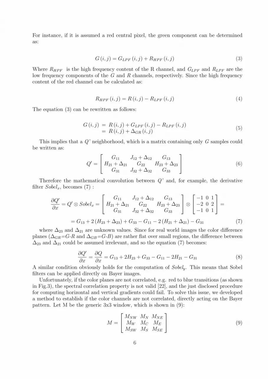
For instance, if it is assumed a red central pixel, the green component can be determinedas:

G (i, j) = GLPF (i, j) + RHPF (i, j) (3)

Where RHPF is the high frequency content of the R channel, and GLPF and RLPF are thelow frequency components of the G and R channels, respectively. Since the high frequencycontent of the red channel can be calculated as:

RHPF (i, j) = R (i, j)−RLPF (i, j) (4)

The equation (3) can be rewritten as follows:

G (i, j) = R (i, j) + GLPF (i, j)−RLPF (i, j)= R (i, j) + ∆GR (i, j)

(5)

This implies that a Q’ neighborhood, which is a matrix containing only G samples couldbe written as:

Q′ =

G11 J12 + ∆12 G13

H21 + ∆21 G22 H23 + ∆23

G31 J32 + ∆32 G33

(6)

Therefore the mathematical convolution between Q’ and, for example, the derivativefilter Sobelx, becomes (7) :

∂Q′

∂x= Q′ ⊗ Sobelx =

G11 J12 + ∆12 G13

H21 + ∆21 G22 H23 + ∆23

G31 J32 + ∆32 G33

⊗

−1 0 1−2 0 2−1 0 1

=

= G13 + 2 (H23 + ∆23) + G33 −G11 − 2 (H21 + ∆21)−G31 (7)

where ∆23 and ∆21 are unknown values. Since for real world images the color differenceplanes (∆GR=G-R and ∆GB=G-B) are rather flat over small regions, the difference between∆23 and ∆21 could be assumed irrelevant, and so the equation (7) becomes:

∂Q′

∂x=

∂Q

∂x= G13 + 2H23 + G33 −G11 − 2H21 −G31 (8)

A similar condition obviously holds for the computation of Sobely. This means that Sobelfilters can be applied directly on Bayer images.

Unfortunately, if the color planes are not correlated, e.g. red to blue transitions (as shownin Fig.3), the spectral correlation property is not valid [22], and the just disclosed procedurefor computing horizontal and vertical gradients could fail. To solve this issue, we developeda method to establish if the color channels are not correlated, directly acting on the Bayerpattern. Let M be the generic 3x3 window, which is shown in (9):

M =

MNW MN MNE

MW MC ME

MSW MS MSE

(9)

6

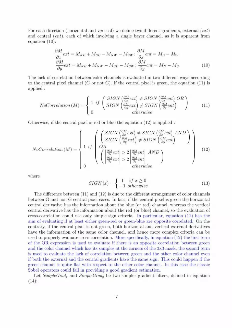
For each direction (horizontal and vertical) we define two different gradients, external (ext)and central (cnt), each of which involving a single bayer channel, as it is apparent fromequation (10):

∂M

∂xext = MNE + MSE −MNW −MSW ;

∂M

∂xcnt = ME −MW

∂M

∂yext = MNE + MNW −MSE −MSW ;

∂M

∂ycnt = MN −MS (10)

The lack of correlation between color channels is evaluated in two different ways accordingto the central pixel channel (G or not G). If the central pixel is green, the equation (11) isapplied :

NoCorrelation (M) =

1 if

(SIGN

(∂M∂x

ext) 6= SIGN

(∂M∂x

cnt)

OR

SIGN(

∂M∂y

ext)6= SIGN

(∂M∂y

cnt)

)

0 otherwise

(11)

Otherwise, if the central pixel is red or blue the equation (12) is applied :

NoCorrelation (M) =

1 if

(SIGN

(∂M∂x

ext) 6= SIGN

(∂M∂x

cnt)

AND

SIGN(

∂M∂y

ext)6= SIGN

(∂M∂y

cnt)

)

OR( ∣∣∂M∂x

ext∣∣ > 2

∣∣∂M∂x

cnt∣∣ AND∣∣∣∂M

∂yext

∣∣∣ > 2∣∣∣∂M

∂ycnt

∣∣∣

)

0 otherwise

(12)

where

SIGN (x) =

{1 if x ≥ 0−1 otherwise

(13)

The difference between (11) and (12) is due to the different arrangement of color channelsbetween G and non-G central pixel cases. In fact, if the central pixel is green the horizontalcentral derivative has the information about the blue (or red) channel, whereas the verticalcentral derivative has the information about the red (or blue) channel, so the evaluation ofcross-correlation could use only simple sign criteria. In particular, equation (11) has theaim of evaluating if at least either green-red or green-blue are opposite correlated. On thecontrary, if the central pixel is not green, both horizontal and vertical external derivativeshave the information of the same color channel, and hence more complex criteria can beused to properly evaluate cross-correlation. More specifically, in equation (12) the first termof the OR expression is used to evaluate if there is an opposite correlation between greenand the color channel which has its samples at the corners of the 3x3 mask; the second termis used to evaluate the lack of correlation between green and the other color channel evenif both the external and the central gradients have the same sign. This could happen if thegreen channel is quite flat with respect to the other color channel. In this case the classicSobel operators could fail in providing a good gradient estimation.

Let SimpleGradx and SimpleGrady be two simpler gradient filters, defined in equation(14):

7

SimpleGradx =

−1 0 10 0 0−1 0 1

; SimpleGrady =

1 0 10 0 0−1 0 −1

(14)

These gradient operators could be used every time a lack of correlation between the threecolor channels is suspected, because they involve a single color channel, and hence they arenot negatively influenced by the different variations of the R, G and B channels. Thus, thegradient for the central pixel of the Q neighborhood could be calculated according to thefollowing equation :

∇Q =

(∂Q

∂x,∂Q

∂y

) {(Q⊗ Sobelx, Q⊗ Sobely) if NoCorrelation (Q) = 0

(Q⊗ SimpleGradx, Q⊗ SimpleGrady) if NoCorrelation (Q) = 1(15)

It is worthwhile to underline that the equations (11) and (12) have especially the aim toidentify the cases where the bayer channels are not correlated, to avoid the application ofSobel operators, which involve different color channels. On the contrary, even if the simplergradient operators were applied on a region where the bayer channels are correlated thiswould not be a problem, because they provide a quite good gradient estimation, even ifSobel operators are better. Moreover, the final gradient estimation for the central pixeldepends on the gradients within its 3x3 neighborhood, as it will be further explained. Oncethe gradient is computed, its direction and magnitude are calculated by the (16) and (17),respectively.

ψ (∇Q) =

{arctg

(∂Q/∂y∂Q/∂x

)if ∂Q/∂x > 0

π2

otherwise(16)

|∇Q| =√(

∂Q

∂x

)2

+

(∂Q

∂y

)2

(17)

It is important to specify that ψ (∇Q) and |∇Q| represent the direction and magnitudeof the gradient of the central pixel of Q. If we set (x,y) as the coordinates of the centralpixel of Q, the direction and magnitude associated to its gradient could be indicated as:

or (x, y) = ψ (∇Q)mag (x, y) = |∇Q| (18)

The gradient orientation or(x,y) could be quantized into k predefined directions:

directioni =i · πk

i ∈ [0, k − 1] , k ∈ ℵ (19)

and, according to the equation (19), the gradient orientation or (x, y) is set as follows:

or(x, y) = {directioni|directioni ≤ or(x, y) < directioni+1, i ∈ [0, k − 1]} (20)

To avoid the influence of noise on the gradient estimation, a “weighted-mode” (WM) opera-tor is applied on each pixel (x,y) computing the prominent direction in its 3x3 neighborhood.For estimating this direction, the magnitudes of the pixels in the neighborhood are firstlyaccumulated according to their associated directions:

8

Acc (x, y, i) =1∑

u=−1

1∑v=−1

mag(x + u, y + v) · t(x + u, y + v, i) (21)

where

t (x, y, i) =

{1 if or (x, y) = directioni

0 otherwise(22)

for i∈ [0, k-1], k∈ ℵTherefore the WM operator selects the direction associated to the maximum sum of

magnitudes in the neighborhood of the considered pixel:

WM(x, y) = j such that Acc (x, y, j) = maxi=0..k−1

(Acc (x, y, i)) , j ∈ [0, k − 1] (23)

Finally, after the gradient direction is retrieved, through the process already described, theedge direction is obtained by taking the orthogonal direction to the gradient one. The edgedirection is provided to the neighbor analysis block for the texture analysis, and to theinterpolation block when the directional color interpolation is selected.

�� �Levels

EdgeEdge

�� �x

FIG. 3: Uncorrelated planes: example of red to blue transitions.

B. Neighbor Analysis

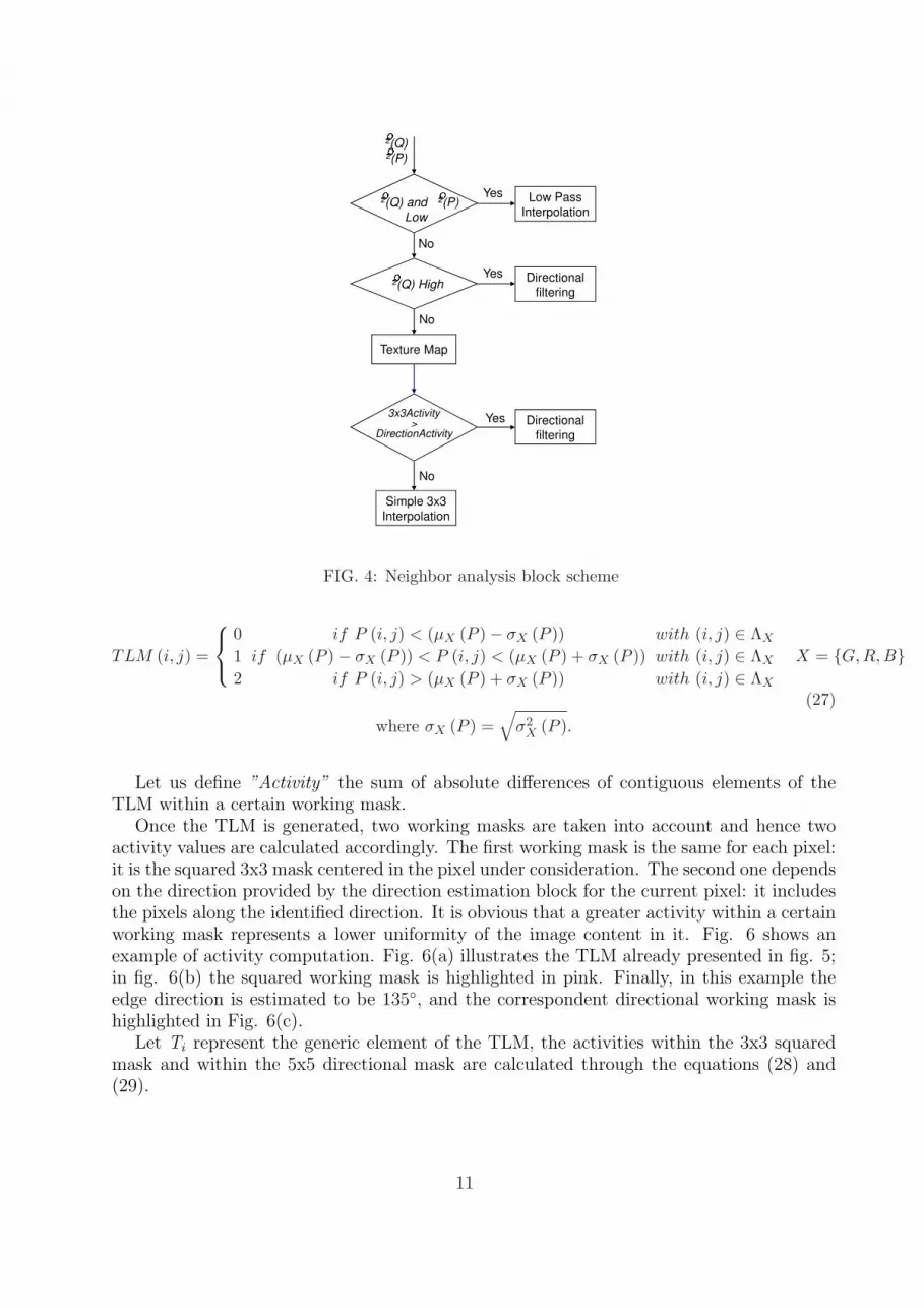
The aim of this part of the proposed method (whose detailed functional scheme is shownin Fig. 4) is to evaluate the presence of texture, edges or flat zones in the pixel neighbor.This analysis is performed by estimating the variances very close to the pixel and on a largersurrounding. The comparison of these variances provides useful information about neighboractivity. In case of textured zones, an additional analysis is necessary, in order to validatethe texture direction estimated by the Direction Estimation Block. According to the resultsof this analysis, the appropriate interpolation scheme is then used. For our purposes weused two kernel sizes: 5x5 for the larger surrounding analysis and 3x3 for the analysis closeto the pixel. The variance is computed, as a measure of the activity within a neighborhood.In particular, let P and Q be the generic 5x5 and 3x3 windows from the Bayer pattern,respectively.

9

P =

G11 H12 G13 H14 G15

J21 G22 J23 G24 J25

G31 H32 G33 H34 G35

J41 G42 J43 G44 J45

G51 H52 G53 H54 G55

Q =

G22 J23 G24

H32 G33 H34

G42 J43 G44

(24)

where Gi are the green components and Hi and Ji are the generic red and/or blue compo-nents. The mean value and the variance, for a generic neighborhood S of the central pixel,are computed according to the following equations:

µX (S) =

∑(i,j)∈S

(S(i,j)∗MaskX(i,j)

)

∑(i,j)∈S MaskX(i,j)

σ2X (S) =

∑(i,j)∈S

(S(i,j)∗MaskX(i,j)−µX(S)

)2

∑(i,j)∈S MaskX(i,j)

σ2 (S) = (σ2G (S) + σ2

H (S) + σ2J (S))

S ∈ {P,Q} X ∈ {G,H, J}

(25)

where MaskX identifies the involved pixels components present in the pattern of theprocessed color component. Let ΛG, ΛH and ΛJ be the set of pixel locations, (x,y), thathave the samples of green, red (blue) and blue (red) channels, respectively. The binary maskMaskX is defined as:

MaskX(x, y) =

{1 if (x, y) ∈ ΛX

0 otherwise(26)

where X = G,H or J .By using the equations in (25) on the neighborhoods P and Q, defined by the equation

(24), two values are calculated, σ2 (P ) and σ2 (Q), which represent a measure of the activityin the relative neighborhoods.

Two thresholds are set for distinguishing different conditions. With reference to Fig. 4 ,if both the variance values are under the lower threshold, the region is considered flat, andhence a low pass filter based interpolation could be used, in order to remove residual noise.

When the variances have values not too high or low, the evaluation is not straightforward,because it could be due either to a zone nor flat nor textured, or to a zone with a texturewithout strong edges. In the first case a directional interpolation could introduce artifacts,while in the second one the directional interpolation could highlight the texture.

The mean values and the standard deviations of each color channel, within the P neigh-borhood, are used to build a texture Mask (we call it TLM, three level mask), which isa matrix having the same size as P and having each element calculated according to theequation (27).

It is straightforward to note that each value within the current P window is associated, inthe TLM, with one of three possible levels: Low (value 0), Medium (value 1) or High (value2), according to its position with respect to its mean value and its standard deviation. Thegeneration of the TLM is illustrated in Fig. 5. In the top left of the figure, a 5x5 crop of aBayer image is represented, then its numeric representation is shown. The mean values andthe standard deviations of each color channel are reported in a box.

10

�2(Q)�2(P)

�2(Q) High

No

No

Yes

Yes Low Pass

Interpolation

Directional

filtering

�2(Q) and �2(P)

Low

NoDirectional

filtering

Yes3x3Activity>

DirectionActivity

No

Simple 3x3

Interpolation

Texture Map

FIG. 4: Neighbor analysis block scheme

TLM (i, j) =

0 if P (i, j) < (µX (P )− σX (P )) with (i, j) ∈ ΛX

1 if (µX (P )− σX (P )) < P (i, j) < (µX (P ) + σX (P )) with (i, j) ∈ ΛX

2 if P (i, j) > (µX (P ) + σX (P )) with (i, j) ∈ ΛX

X = {G,R, B}

(27)

where σX (P ) =√

σ2X (P ).

Let us define ”Activity” the sum of absolute differences of contiguous elements of theTLM within a certain working mask.

Once the TLM is generated, two working masks are taken into account and hence twoactivity values are calculated accordingly. The first working mask is the same for each pixel:it is the squared 3x3 mask centered in the pixel under consideration. The second one dependson the direction provided by the direction estimation block for the current pixel: it includesthe pixels along the identified direction. It is obvious that a greater activity within a certainworking mask represents a lower uniformity of the image content in it. Fig. 6 shows anexample of activity computation. Fig. 6(a) illustrates the TLM already presented in fig. 5;in fig. 6(b) the squared working mask is highlighted in pink. Finally, in this example theedge direction is estimated to be 135◦, and the correspondent directional working mask ishighlighted in Fig. 6(c).

Let Ti represent the generic element of the TLM, the activities within the 3x3 squaredmask and within the 5x5 directional mask are calculated through the equations (28) and(29).

11

Three Level Mask

Bayer image Numeric representation

132 194 180 208

126 176 205 19149

84 155 159 20257

65 103 156 17449

64 71 84 136110

73 132 194 180 208

126 176 205 19149

84 155 159 20257

65 103 156 17449

64 71 84 136110

73 132 194 180 208

126 176 205 19149

84 155 159 20257

65 103 156 17449

64 71 84 136110

73

0 1 2 2 2

0 1 1 2 2

0 1 1 1 2

0 0 1 1 1

1 0 0 1 1

406567123

775624135

794617117

..

..

..

BB

GG

RR

==

==

==

σµ

σµ

σµ

µ-σ µ+σµ

0 1 2

Three Level Mask

Bayer image Numeric representation

132 194 180 208

126 176 205 19149

84 155 159 20257

65 103 156 17449

64 71 84 136110

73 132 194 180 208

126 176 205 19149

84 155 159 20257

65 103 156 17449

64 71 84 136110

73 132 194 180 208

126 176 205 19149

84 155 159 20257

65 103 156 17449

64 71 84 136110

73 132 194 180 208

126 176 205 19149

84 155 159 20257

65 103 156 17449

64 71 84 136110

73 132 194 180 208

126 176 205 19149

84 155 159 20257

65 103 156 17449

64 71 84 136110

73 132 194 180 208

126 176 205 19149

84 155 159 20257

65 103 156 17449

64 71 84 136110

73 132 194 180 208

126 176 205 19149

84 155 159 20257

65 103 156 17449

64 71 84 136110

73

0 1 2 2 2

0 1 1 2 2

0 1 1 1 2

0 0 1 1 1

1 0 0 1 1

406567123

775624135

794617117

..

..

..

BB

GG

RR

==

==

==

σµ

σµ

σµ

406567123

775624135

794617117

..

..

..

BB

GG

RR

==

==

==

σµ

σµ

σµ

µ-σ µ+σµ

0 1 2

FIG. 5: Example of the Three Level Mask (TLM) generation

Three Level Mask

0 1 2 2 2

0 1 1 2 2

0 1 1 1 2

0 0 1 1 1

1 0 0 1 1

0 1 2 2 2

0 1 1 2 2

0 1 1 1 2

0 0 1 1 1

1 0 0 1 1

(a)First

Activity = 2

Squared Working Mask

T2T3T4T5

T7T8T9T10

T6

T12T13T14T15

T11

T17 T18 T19 T20T16

T22T23T24T25

T21

T1

T2T3T4T5

T7T8T9T10

T6

T12T13T14T15

T11

T17 T18 T19 T20T16

T22T23T24T25

T21

T1

T2T3T4T5

T7T8T9T10

T6

T12T13T14T15

T11

T17 T18 T19 T20T16

T22T23T24T25

T21

T1

T2T3T4T5

T7T8T9T10

T6

T12T13T14T15

T11

T17 T18 T19 T20T16

T22T23T24T25

T21

T1

T2T3T4T5

T7T8T9T10

T6

T12T13T14T15

T11

T17 T18 T19 T20T16

T22T23T24T25

T21

T1

T2T3T4T5

T7T8T9T10

T6

T12T13T14T15

T11

T17 T18 T19 T20T16

T22T23T24T25

T21

T1

T2T3T4T5

T7T8T9T10

T6

T12T13T14T15

T11

T17 T18 T19 T20T16

T22T23T24T25

T21

T1

Activity = 2

(b)Second

Activity = 1

Directional Working Mask

T2T3T4T5

T7T8T9T10

T6

T12T13T14T15

T11

T17 T18 T19 T20T16

T22T23T24T25

T21

T1

T2T3T4T5

T7T8T9T10

T6

T12T13T14T15

T11

T17 T18 T19 T20T16

T22T23T24T25

T21

T1

T2T3T4T5

T7T8T9T10

T6

T12T13T14T15

T11

T17 T18 T19 T20T16

T22T23T24T25

T21

T1

T2T3T4T5

T7T8T9T10

T6

T12T13T14T15

T11

T17 T18 T19 T20T16

T22T23T24T25

T21

T1

T2T3T4T5

T7T8T9T10

T6

T12T13T14T15

T11

T17 T18 T19 T20T16

T22T23T24T25

T21

T1

T2T3T4T5

T7T8T9T10

T6

T12T13T14T15

T11

T17 T18 T19 T20T16

T22T23T24T25

T21

T1

T2T3T4T5

T7T8T9T10

T6

T12T13T14T15

T11

T17 T18 T19 T20T16

T22T23T24T25

T21

T1

Activity = 1

(c)Third

FIG. 6: Example of the Activity evaluation assuming that the estimated direction is 135◦.

3× 3Activity = |T7 − T13|+ |T8 − T13|+ |T9 − T13|+ |T14 − T13|+ |T19 − T13|+ |T18 − T13|+ |T17 − T13|+ |T12 − T13| (28)

Direction Activity(135◦) = |T1 − T7|+ |T2 − T7|+ |T7 − T12|+ |T7 − T13|+ |T13 − T19|+ |T14 − T19|+ |T19 − T24|+ |T19 − T25| (29)

It is straightforward that the 5x5 directional working mask and its related activity com-putation formula depend on the edge direction, which is provided by the direction estimationblock. Finally the activity values computed in equations (28) and (29) are compared to eval-uate if the activity within the 3x3 squared mask is less than the activity along the directionprovided by the direction estimation block. If this is the case, a simple 3x3 interpolationcould be used. This control allows avoiding the directional 5x5 interpolation in case of awrong estimated direction, or in case of a region close to an edge, thus reducing the intro-duction of unpleasant artifacts. In the example of fig. 5, the directional interpolation ischosen for the central pixel, because the 3x3 squared mask activity (Fig. 6(b)) is greaterthan the 5x5 directional one (Fig. 6(c)).

12

For the sake of completeness, the activity computation formulas applied in case of edgedirection equal to 0◦ and 22.5◦ are shown in equations (30) and (31), respectively. All theother activity computation formulas can be easily derived from the three examples alreadypresented.

DirectionActivity(0◦) = |T6 − T8|+ |T8 − T10|+ |T11 − T12|+ |T12 − T13|+ |T13 − T14|+ |T14 − T15|+ |T16 − T18|+ |T18 − T20| (30)

DirectionActivity(22.5◦) = |T9 − T10|+ |T11 − T12|+ |T12 − T13|+ |T13 − T14|+ |T14 − T15|+ |T16 − T17|+ |T13 − T10|+ |T13 − T16| (31)

C. Interpolation

As already pointed out, according to the analysis of the ”Direction Estimation” and”Neighbor Analysis”, the appropriate color interpolation scheme is used. in particular weuse:

• 5x5 directional filter;

• 3x3 simple interpolation;

• 5x5 omnidirectional low pass filter.

In the following paragraphs each one of the aforementioned algorithms will be described.

1. Directional filtering color interpolation

If a strong edge or a texture is detected, the directional filtering is used. This interpolationis carried out through elliptical shaped Gaussian filters, given by:

f(u, v, α) = he− u2

2σ2u− v2

2σ2v (32)

where

u = u cos(α)− v sin(α),v = u sin(α) + v sin(α),

(33)

and σ2u, σ2

v are the variances along the two dimensions, h is a normalization constant andα is the orientation angle. Through heuristic experiments σu = 8 and σv = 0.38 have beenfixed.

These interpolation kernels can be computed only once, after the number of admissibledirections, k, has been set. More specifically, fixing the coordinates (u,v) in a given range(i.e., 5x5), the kernel filters DFi can be generated, for i ∈ [0, k − 1]. The generic element ofthese matrices, DFi(u,v), is defined as follows:

DFi (u, v) = f (u, v, i · π/k) (34)

During the directional filtering color interpolation, once the direction j for the centralpixel is derived by the direction estimation block, the kernel DFj is applied to the central

13

pixel to obtain the low pass filter (LPF) color components RLPF DF , GLPF DF and BLPF DF ,preserving the image from zigzag effect and partially from false colors.

Let P be the generic 5x5 neighborhood from the Bayer pattern as it is defined in equation(24).

The LPF components, for the central pixel (x,y), are computed by assuming the followingrules:

HLPF DF = P ⊗MaskH ⊗DFj

GLPF DF = P ⊗MaskG ⊗DFj

JLPF DF = P ⊗MaskJ ⊗DFj

(35)

where MaskX , which has been already defined in equation (26), identifies the pixelsbelonging to the processed color component.

As already aforementioned, the high frequency components of the three color channelsare highly correlated, and hence any color component can be exploited to reconstruct thehigh frequencies of the remaining color components. For this reason, the directional LPFcomponent of the central pixel is likewise computed in order to calculate its high pass filter(HPF) component, which will be added to the other two color channels. Assuming a greencentral pixel, its high pass component can be calculated according to the equation (36).

GHPF = G−GLPF DF (36)

The resulting GHPF value is added to the unknown values, in this case R and B (e.g. H ),to increase their high frequency content:

HDF = HLPF DF + GHPF (37)

The central pixel value will be maintained to its original value:

GDF = G (38)

2. Simple 3x3 interpolation

The 5x5 directional filtering color interpolation could produce some artifacts near edges,especially in text images. This problem could arise when a wrong direction is estimatedor when a large interpolation window is used for interpolating a small region, enclosed byedges. To overcome this problem a 3x3 interpolation could be performed in regions whichare close to edges.

A wide variety of 3x3 interpolation algorithms exists: bilinear interpolation, edge sensing,etc. In order to achieve good quality results near corners and edges, it is possible to use analgorithm which analyzes the 5x5 neighborhood of the central pixel, and then applies a 3x3interpolation, avoiding the interpolation across edges.

Taking idea from the paper in [7], the proposed 3x3 interpolation algorithm uses athreshold-based variable number of gradients. According to the central pixel channel, four(G case) or eight (R or B case) gradients are computed in a 5x5 neighborhood. Each gradientis defined as the sum of absolute differences of the like-colored pixels in this neighborhood.For each color channel to be interpolated, a proper subset of these gradients is selected

14

to determine a threshold of acceptable gradients. Each missing color channel is then ob-tained by averaging the color values of the same channel in the 3x3 neighborhood, whichare associated with gradients lower than the calculated threshold.

3. Omnidirectional low pass filter

This interpolation is performed on flat regions. A simple 5x5 omnidirectional low passfilter is applied for smoothing the image, removing some residual noise from it. In this casethe original sampled values are also modified. The kernels used to achieve the interpolationare shown in equation (39). In particular, the A kernel is applied in case of G central pixel,whereas the B kernel is used in case of R/B central pixel.

A =

0 8 4 8 08 8 16 8 84 16 16 16 48 8 16 8 80 8 4 8 0

64B =

0 3 9 3 03 16 10 16 39 10 28 10 93 16 10 16 30 3 9 3 0

64

(39)

III. FALSE COLORS REMOVAL

Since the color interpolation step quite well exploits spatial correlation, zipper effect doesnot often arises. On the contrary, residual false colors can be introduced by the directionalfilters. For this reason, a postprocessing technique has been developed, which eliminates theresidual false colors, thus considerably improving the final image quality.

Many methods have been developed in the past to reduce false colors. Among them, themost interesting techniques median filter the inter-channel differences, thus removing spikesand valley from them, which usually correspond to false colors. Freeman’s approach [17] andLu and Tan’s technique [16] have been already presented in the introduction section. Thepost-processing approach described in [23] not only is based on the color difference model,but also uses an edge-sensing mechanism. Another interesting technique, which is proposedin [18], updates the R, G, B values adaptively, modifying also the original pixel value whichcould be corrupted, due to the effect of noise. Two updated values for the green channel arecalculated using each color difference domain:

GR (i, j) = R (i, j) + vGR (i, j)GB (i, j) = B (i, j) + vGB (i, j)

(40)

where

vGR (i, j) = median {G (k, l)−R (k, l) |(k, l) ∈ A}vGB (i, j) = median {G (k, l)−B (k, l) |(k, l) ∈ A} (41)

And A denotes the support of the 5x5 local window centered in (i, j).The updated G value is determined by the weighted sum of two updated GR and GB

values of each color difference domain and original G value. Subsequently, R and B valuesare updated using the updated G value. This process is expressed as:

15

G′ (i, j) = 12G (i, j) + 1

2

{(1− a (i, j)) GR (i, j) + a (i, j) GB (i, j)

}R′ (i, j) = 1

2R (i, j) + 1

2{G′ (i, j)− vGR (i, j)}

B′ (i, j) = 12B (i, j) + 1

2{G′ (i, j)− vGB (i, j)}

(42)

where a(i, j) is a weight, expressed as:

a (i, j) =σ2

(G−R) (i, j)

σ2(G−R) (i, j) + σ2

(G−B) (i, j), 0 < a (i, j) < 1 (43)

σ2(G−R) and σ2

(G−B) represent the variances of interchannel differences.

As it is apparent from the equation (42), the color correction algorithm proposed in [18],thanks to the variance information, weights more the flatter color difference domain thanthe other. Moreover, the initial interpolated value is not totally exchanged by the updatedvalue, but it is equally weighted for correction. Subsequently, the color values of the centralpixel are replaced by R′, G′ and B′ so that they will be involved in filtering the updatingpixels.

The local statistics are effectively estimated from a running square window, through theformulas in (44):

E [A (i, j)] =∑

k,l∈A e(k,l)·A(k,l)∑k,l∈A e(k,l)

σ2A (i, j) =

∑k,l∈A e(k,l)·(A(k,l)−E[A(i,j)]) 2

∑k,l∈A e(k,l)

e (k, l) = 1− (A (i, j)− A (k, l))

(44)

The just described technique has the disadvantage of weighting the unfiltered valuestogether with the filtered ones, so false colors are reduced, without being completely removed.If the unfiltered values were not weighted in the color correction process, false colors wouldbe removed much better but true colors could be removed as well. In fact, it is well known[24] that a window width 2k + 1 median filter can only preserve details lasting more thank + 1 points. To preserve smaller details in signals, a smaller window width median filtermust be used. Unfortunately, the smaller the filter window is, the poorer its false colorreduction capability becomes.

To overcome this problem, we have developed a new solution which takes into accountboth a 3x3 window median filter and a 5x5 window median filter. In particular, localvariances of interchannel differences are evaluated through the equation (44) in both 3x3and 5x5 square windows, thus obtaining σ2

(G−R)3×3, σ2(G−B)3×3,σ

2(G−R)5×5, σ

2(G−B)5×5. Similarly,

four median values (vGR3x3, vGB3x3, vGR5x5, vGB5x5) are computed.Due to the Bayer arrangement and to a quite good interpolation achieved by the previous

demosaicing step, the green plane is less affected by false colors than the R and B planes, andhence it is left unmodified. The color correction on R and B planes is performed accordingto the following rules:

R′ (i, j) = G (i, j)− [(1− krratio (i, j)) · vGR3×3 (i, j) + krratio (i, j) · vGR5×5 (i, j)]B′ (i, j) = G (i, j)− [(1− kbratio (i, j)) · vGB3×3 (i, j) + kbratio (i, j) · vGB5×5 (i, j)]

(45)

Where

krratio (i, j) =σ2(G−R)3×3

(i,j)

σ2(G−R)3×3

(i,j)+σ2(G−R)5×5

(i,j)

kbratio (i, j) =σ2(G−B)3×3

(i,j)

σ2(G−B)3×3

(i,j)+σ2(G−B)5×5

(i,j)

(46)

16

�2(G-X)5x5

vGX5x5

�2(G-X)3x3

vGX3x3vGX5x5vGX3x3

Color Correction

Corrected RGB values

FIG. 7: Schematic representation of the proposed approach

By this way, the greatest weight is assigned to the median value associated to the neighbor-hood having the lowest variance. So, if the pixel being processed belongs to an edge, the3x3 variances of interchannel differences are likely to be greater than the correspondent 5x5variances, and hence the filtering action will be stronger. Vice versa, if the 3x3 neighborhoodis flatter than the 5x5 neighborhood, the 3x3 median is weighted more than the 5x5 median,and hence details lasting 2 pixels at least are preserved.

Fig.7 shows a schematic representation of the proposed approach. Since variances couldbe used as measures of the flatness of a region, it is possible to perform the color correctionprocess only where it is needed, thus reducing the power consumption. In the color differencedomain, a flat color difference neighborhood is characterized by: expectation values close tothe central pixel values, low variance values. Defined DiffGR(i, j) = G(i, j) − R(i, j) andDiffGB(i, j) = G(i, j) − B(i, j), these two conditions can be expressed with the followingformulas:

|E [DiffGR(i, j)]−DiffGR(i, j)| < MeanThreshold

|E [DiffGB(i, j)]−DiffGB(i, j)| < MeanThreshold

σ2(G−R)3×3 (i, j) < V arianceThreshold

σ2(G−B)3×3 (i, j) < V arianceThreshold

(47)

where MeanThreshold and VarianceThreshold are two thresholds, which can be set to 16 for8 bits images.

If the conditions stated above are satisfied, the region is considered flat, thus the centralpixel can be left unchanged.

According to the expectation value and to the variance, a map of homogeneous (black)vs. inhomogeneous (white) regions can be achieved, as it is apparent from Fig.8.

17

(a)Processed image (b)Map of homogeneous vs.inhomogeneous regions

FIG. 8: Map of homogeneous vs. inhomogeneous regions

Homogeneous regions (black) can be left unchanged or can be low pass filtered. Inhomo-geneous regions (white) are processed by the color correction algorithm.

IV. EXPERIMENTAL RESULTS

In this section, we will show the experimental results obtained using the proposed al-gorithm compared with other demosaicing techniques. The results are highligthed bothvisually and numerically. For coherence with the most of papers on demosaicing, whichuse the Kodak image test set to make comparisons with other techniques, we downloadedthis database from [25] and then we processed these images through the proposed approach.These images contains a lot of edges and textures, thus they are useful for highlight how thevarious algorithms handle the high frequency content. Since the Kodak image test set is fullcolor, CFA images are simulated by subsampling the color channels according to the BayerPattern. This means that the algorithms are not applied on genuine Bayer data (derivedfrom a real sensor), but on images that have already had matrix and gamma applied, sotheir gamut is far wider than that of data coming from a sensor. Moreover they are immunefrom noise and other impairments related to the sensor technology. For these reasons wealso applied the proposed algorithm to Bayer data from real sensors.

In our experiments, we have used the PSNR (Peak signal to Noise Ratio) for evaluatingthe quality of the images (only for Kodak database). Given two N ×M images A and B,the PSNR is expressed as:

PSNR = 20× log10

255√

1N×M

∑N×Mi=1 (Ai −Bi)

2

(48)

Higher values (expressed in decibel) of the PSNR generally imply better quality.For demonstrating the effectiveness of the proposed algorithm, we will compare it with

other five demosaicing algorithms: bilinear interpolation (the simplest), edge sensing inter-polation, Gunturk’s method, and the directional interpolations proposed by Hirakawa et al.in [11] and by Menon et al. in [10], respectively. The matlab codes of both bilinear and

18

edge sensing interpolation were obtained from [26], while the source codes of Gunturk’s,Hirakawa’s and Menon’s approaches were downloaded from [13], [19] and [10], respectively.The PSNRs have been computed separately for each color channel. The Table I shows thecollected PSNR measures for each image of the test set. The proposed method, Gunturk’sand Menon’s approaches give the highest PSNR values. However, as it is well known, thePSNR is not always representative of the visual quality of an image. Two images having thesame PSNR could appear very different from the visual standpoint. Moreover, the PSNRapproach is a full-reference metric which cannot be applied on real sensor data. For thesereasons, a subjective image quality analysis has been also achieved.

Figures 10 and 11 illustrate the ROIs (region of interest) relative to the “hats” test image(kodim03) and to the “mountain” test image (kodim13), respectively. They were obtainedcropping a detail from the originals and interpolated images. In these figures, (a) representsthe ROI of the original image, (b) is the result of the bilinear interpolation, (c) is the resultof the edge sensing algorithm, (d) is obtained applying the interpolation by Gunturk, (e) isthe result of the Hirakawa’s approach, (f) is the output of the technique proposed by Menonet al. and, finally, (g) is obtained using the proposed algorithm. The ROIs show how ouralgorithm drastically reduces both the zipper and false color defects. Fig. 10.b presents agreat amount of false colors and blur. Edge sensing algorithm quite well interpolates alongedges but introduces many false colors (see fig. 10.c). Figs. 10.d and 10.f show that bothGunturk’s and Menon’s approach still maintain few zipper artifacts near edges, although forthis image the PSNR of the Menon’s technique is comparable to ours and higher than theHirakawa’s approach, which outputs an image free from zipper effects and false colors (seefig. 10.e) like our demosaicing technique. Looking at fig. 11, it is possible to see that theproposed technique (fig. 11.g) outperforms all the others in removing false colors, providingan image where also edges are effectively interpolated and sharpness is maintained. Bothbilinear (fig. 11.b) and edge sensing (11.c) techniques produce images heavily affected byfalse colors. Gunturk’s (fig. 11.d) and Menon’s (11.f) approaches also introduce some visiblefalse colors. Finally, Hirakawa’s technique still maintains a minimum amount of false colorsin comparison with our approach.

As it has been aforementioned, some tests were performed on real sensor images. Somevisual results will be shown in comparison with both Hirakawa’s and Menon’s algorithms,which are both based on directional approaches, like the proposed technique. The imageshown in fig. 12.a has a huge high frequency content, especially in the windows, whichhave details at the Nyquist’s frequency of the sensor. A ROI from the output images of theHirakawa’s, Menon’s and our techniques are shown in figs. 12.b, 12.c and 12.d, respectively.It is readily apparent, in this example, that the proposed technique outperforms the othertwo in interpolating edges and in removing false colors.

Another test which is usually performed to compare different demosaicing algorithm is theinterpolation of a colored resolution chart, which allows to see how each algorithm resolvescolor details. For this purpose, the image shown in fig. 13.a was taken into consideration.Looking at fig. 13.d it is quite evident that the proposed technique resolves color detailsmuch better than the other two approaches (see figs. 13.b and 13.c). This is due to theproposed direction estimation block which evaluates the correlation among different Bayercolors, to determine the direction to be used in the interpolation phase.

As it has been already discussed, images coming from real sensors are often affected byartifacts due to noise and green imbalance, so it is important to design an interpolationalgorithm able to not exalt and even to reduce these kinds of issues, which would be further

19

(a)Original image (b)Map of interpolation

FIG. 9: Map of interpolation method

enhanced by the successive sharpening step. As the proposed technique low pass filters flatregions, green imbalance and noise are heavily reduced, thus producing high quality images.Looking at fig. 14.c it is possible to notice that residual noise is quite well reduced bythe proposed technique, whereas edges are still well interpolated. Both figs. 14.a and 14.bare still affected by noise. In order to have a numeric measure of the noise immunity ofthe presented demosaicing technique, we added three different amounts of gaussian noise(having standard deviations equal to 8, 12 an 25, respectively) to a subset of the originalKodak images, and then interpolated them with some state of the art color interpolationapproaches and the proposed technique. Afterwards, we calculated the PSNR with respectto the original kodak images. The PSNR values are reported in TableXXX, where theproposed approach is compared with the algorithms proposed in [10], [27] and [9]. From thistable it is evident how the proposed demosaicing algorithm has the greates PSNR values foralmost all the processed images. Moreover, the improvement is geater especially in imageshaving large flat areas, where the human visual system is more sensitive to noise. The noiseimmunity of the algorithm depends on the threshold used to identify flat regions. In theaforementioned experiment it was set to 300, even if it should be made dependent on thenoise level of the input image. Fig. 9 is a map showing which interpolation is chosen foreach pixel of the ’lighthouse’ image, where gaussian noise having sigma equal to 12 wasadded. In particular, black regions are interpolated through the 5x5 omnidirectional lowpass filter, red regions are interpolated by the directional approach and green regions areinterpolated through the simple 3x3 technique. It is quite evident that strong edges areinterpolated by the directional technique, whereas regions near edges are reconstructed bythe 3x3 approach. Noise in flat regions is reduced by the omnidirectional low pass filter. AROI of the ’lightouse’ image is shown in fig. 15 where the original kodak image is comparedwith the noisy image (with gaussian noise, sigma=12)interpolated by the Menon’s technique[10], the Li’s approach [27], the Wu and Zhang’s algorithm [9] and the proposed technique.

Finally, one more visual comparison is presented to validate the effectiveness of the pro-posed post-processing false colors removal algorithm with respect to other state of the art

20

approaches. In particular, the images from the Kodak data set were interpolated throughthe demosaicing step proposed in Section II, then they were processed by the Freeman’stechnique [17], the Lu’s algorithm [16], the post-processing approach proposed by Lukacet al. in [23], the color correction technique presented in [18] and the proposed algorithm,already disclosed in Section III. Fig. 16 is a ROI from the ”hotel” test image (kodim08). Inparticular, (a) represents the ROI of the original image, (b) is the result of the color inter-polation disclosed in Section II, (c) is obtained processing (b) with the Freeman’s approach,(d) is the result of the Lu’s technique, (e) is the output of the Lukac’s post-processing tech-nique, (f) is the result of [18] and, finally, (g) is obtained processing (b) with the algorithmpresented in Section III, so it corresponds to the output of the method proposed in thispaper. It is quite evident that the proposed color interpolation technique (fig. 16.b) verywell exploits spatial correlation, but lots of false colors are introduced, and hence the appli-cation of a post-processing aliasing removal is indispensable. Freeman’s technique (fig. 16.c)not only does not remove many false colors but also introduces annoying zipper artifacts.Lu’s approach does not introduce zipper effects, but considerably blurs the image. Lukac’salgorithm is neither able to remove all the color artifacts. Kim’s approach, weighting theinitially interpolated values to produce the corrected ones, is not able to effectively reducethe false colors. The proposed technique (fig. 16.g) quite well reduces false colors withoutintroducing zipper effects.

V. CONCLUSION

In this paper, we have presented a color interpolation method based on edge and textureanalysis. According to this analysis we proposed the usage of different interpolation ap-proaches, where the novel proposed directional filtering exploits spatial-spectral correlation.A powerful post-processing algorithm effectively removes residual impairments introducedby the color interpolation step. This paper compares demosaicing performance of our im-proved method with the state-of-the-art demosaicing methods. The cascading structure ofthe proposed method has a merit of the pipelined real-time processing for the hardwareimplementation, while some other methods require iterative computations. The proposedmethod still opens a possibility of further improvement, for example, applying stripe detec-tion to improve the performances in near Nyquist frequencies.

[1] B. E. Bayer, Color imaging array, US Patent 3,971,065 (1976).[2] N. Lian, L. Chang, Y.-P. Tan, and V. Zagorodnov, Adaptive filtering for color filter array

demosaicking, IEEE Transactions on Image Processing pp. 2515–2525 (2007).[3] J. E. Adams, Interactions between color plane interpolation and other image processing func-

tions in electronic photography, in Society of Photo-Optical Instrumentation Engineers (SPIE)Conference Series, edited by C. N. Anagnostopoulos and M. P. Lesser (1995), vol. 2416 ofPresented at the Society of Photo-Optical Instrumentation Engineers (SPIE) Conference, pp.144–151.

[4] K. Hirakawa, Cross-talk explained, in IEEE Int. Conference on Image processing, (ICIP 2008)(2008), pp. 677–680.

21

(a) (b) (c)

(d) (e) (f)

(g)

FIG. 10: Example of ROI visual comparison relative to the ”hats” test image (kodim03). (a)Original image; (b) Bilinear Interpolation; (c) Edge sensing [26]; (d) Gunturk [13]; (e) Hirakawa[11]; (f) Menon [10]; (g) Proposed solution.

22

(a) (b) (c)

(d) (e) (f)

(g)

FIG. 11: Example of ROI visual comparison relative to the ”mountains” test image (kodim13). (a)Original image; (b) Bilinear Interpolation; (c) Edge sensing [26]; (d) Gunturk [13]; (e) Hirakawa[11]; (f) Menon [10]; (g) Proposed solution.

23

TABLE I: Prova di tabellaBilinear Edge Sensing Gunturk Hirakawa Menon Proposed

Image Name R G B R G B R G B R G B R G B R G B

kodim01 25.39 29.45 24.91 30.84 31.47 30.89 34.99 40.12 35.08 34.61 36.26 34.77 36.24 38.30 36.46 35.68 39.78 36.55kodim02 31.92 35.75 31.34 35.64 37.41 36.84 38.46 40.29 35.25 36.38 41.52 40.12 37.86 43.08 41.10 36.82 42.99 40.71kodim03 33.36 36.49 32.48 38.09 38.54 37.64 40.80 43.31 36.15 40.58 43.69 40.10 41.67 44.95 40.94 41.63 44.64 41.05kodim04 32.34 36.07 32.77 35.27 37.57 37.38 37.91 42.25 37.58 35.56 41.70 40.91 36.78 43.37 42.12 37.24 43.42 41.94kodim05 25.83 29.25 25.66 31.28 31.08 31.05 37.05 39.50 34.10 35.13 37.44 34.42 37.05 39.63 36.30 36.11 39.31 35.80kodim06 26.60 30.84 26.59 32.51 33.00 32.12 37.69 41.29 34.00 37.58 39.11 36.45 39.29 41.06 37.91 37.16 40.92 36.73kodim07 32.55 36.04 31.89 38.25 38.40 37.76 41.29 43.34 36.93 40.06 42.66 39.01 41.39 44.09 40.22 40.64 43.77 40.19kodim08 22.55 27.37 22.45 29.60 30.42 29.48 34.27 38.08 32.59 33.21 35.35 33.24 34.66 37.33 34.76 33.50 37.93 33.67kodim09 31.33 35.43 31.36 37.47 38.16 37.81 40.98 44.10 38.74 40.31 43.01 40.64 41.25 44.39 42.94 40.87 43.97 40.39kodim10 31.50 35.04 31.04 36.87 37.37 36.73 39.83 44.36 38.50 39.48 42.87 39.80 40.84 44.47 41.62 40.68 44.13 40.49kodim11 28.25 32.15 28.25 33.38 33.81 33.47 38.42 41.03 36.83 36.63 39.01 37.46 38.33 40.93 39.02 37.05 41.43 38.38kodim12 32.01 36.35 31.67 37.93 39.01 37.93 40.55 44.36 38.22 40.54 43.96 40.78 42.00 45.43 42.18 40.84 44.57 41.35kodim13 23.12 26.51 22.99 27.18 27.28 26.80 33.80 36.86 32.15 31.53 32.40 30.61 33.38 34.49 32.38 33.78 36.58 32.75kodim14 28.18 31.79 28.06 32.89 33.46 32.91 35.87 37.87 32.55 34.16 38.00 34.93 35.74 39.52 36.08 35.14 39.16 35.51kodim15 30.80 34.34 29.67 34.52 36.31 35.67 36.80 40.17 34.87 35.49 40.66 38.56 36.77 42.15 39.76 36.57 42.01 40.04kodim16 30.34 34.30 29.61 36.04 36.80 35.90 40.25 44.47 35.44 41.36 42.86 40.55 42.89 44.59 41.98 40.29 43.95 39.91kodim17 31.43 34.48 30.67 35.97 35.69 35.47 40.38 43.75 37.80 39.18 40.65 38.61 40.45 42.33 40.35 40.06 42.70 39.69kodim18 27.27 30.40 26.72 31.23 31.28 30.89 35.71 39.35 34.96 33.72 35.60 33.83 35.14 37.57 35.90 35.21 38.41 35.61kodim19 26.85 31.75 27.01 34.48 35.04 34.60 38.14 42.62 38.44 37.61 39.50 37.86 38.78 41.23 39.98 37.86 41.69 38.39kodim20 30.25 33.11 30.45 36.17 36.26 35.10 36.72 43.23 37.14 38.90 40.65 36.91 40.23 42.26 37.84 40.29 43.20 38.51kodim21 27.68 31.43 27.46 32.74 33.02 32.30 38.01 41.58 35.90 36.62 37.93 35.57 37.79 39.62 36.83 37.63 40.91 36.56kodim22 29.94 33.13 29.22 34.17 34.71 33.80 37.78 39.89 35.91 35.68 38.45 35.47 37.00 39.80 36.70 36.39 39.43 36.11kodim23 34.53 37.17 33.83 39.41 39.84 38.23 42.20 43.48 38.64 38.96 43.27 39.57 39.97 45.08 39.92 41.16 44.79 41.76kodim24 26.39 29.30 25.29 30.24 30.06 28.81 34.37 37.29 32.26 32.62 34.95 31.60 34.34 36.58 32.59 34.29 37.29 32.58

Average 29.18 32.83 28.81 34.26 34.83 34.15 38.01 41.36 35.83 36.91 39.65 37.16 38.33 41.34 38.58 37.79 41.54 38.11

[5] S. Battiato, M. Guarnera, G. Messina, and V. Tomaselli, Recent patents on color demosaicing,Recent Patents on Computer Science, Bentham Science Publishers Ltd pp. 194–207 (2008).

[6] L. Chang and Y.-P. Tan, Effective use of spatial and spectral correlations for color filter arraydemosaicking, Consumer Electronics, IEEE Transactions on pp. 355–365 (2004), ISSN 0098-3063.

[7] E. Chang, S. Cheung, and D. Y. Pan, Color filter array recovery using a threshold-basedvariable number of gradients, in Society of Photo-Optical Instrumentation Engineers (SPIE)Conference Series, edited by N. Sampat and T. Yeh (1999), vol. 3650 of Presented at theSociety of Photo-Optical Instrumentation Engineers (SPIE) Conference, pp. 36–43.

[8] T. Kuno, H. Sugiura, and N. Matoba, Digital still cameras, Consumer Electronics, IEEETransactions on pp. 259–267 (1999), ISSN 0098-3063.

[9] X. Wu and N. Zhang, Primary-consistent soft-decision color demosaicking for digital cameras(patent pending), IEEE Transactions on Image Processing pp. 1263–1274 (2004).

[10] D. Menon, S. Andriani, and G. Calvagno, Demosaicing with directional filtering anda posteriori decision, IEEE Transactions on Image Processing pp. 132–141 (2007),http://www.danielemenon.it/ pub/ dfapd/ dfapd.html.

[11] K. Hirakawa and T. W. Parks, Joint demosaicing and denoising, IEEE Transactions on ImageProcessing pp. 2146–2157 (2006).

[12] E. Yun, J. Kim, and S. Kim, Color interpolation by expanding a gradient method, IEEETransactions on Consumer Electronics pp. 1531–1539 (2008).

[13] B. K. Gunturk, Y. Altunbasak, and R. M. Mersereau, Color plane interpolation us-ing alternating projections, IEEE Transactions on Image Processing pp. 997–1013 (2002),http://www.ece.gatech.edu/ research/ labs/ MCCL/ research/ p demosaick.html.

[14] N. Lian, V. Zagorodnov, and Y.-P. Tan, Edge-preserving image denoising via optimal colorspace projection, IEEE Transactions on Image Processing pp. 2575–2587 (2006).

24

(a)

(b) (c) (d)

FIG. 12: Example of visual comparison on real sensor image.(a) Real sensor image; (b) ROI byHirakawa [11]; (c) ROI by Menon [10]; (d) ROI by proposed solution.

[15] T. Saito and T. Komatsu, Demosaicing approach based on extended color total variation reg-ularization, in IEEE Int. Conference on Image Processing, (ICIP 2008) (2008), pp. 885–888.

[16] W. Lu and Y.-P. Tan, Color filter array demosaicking: new method and performance measures,IEEE Transactions on Image Processing pp. 1194–1210 (2003).

[17] T. W. Freeman, Median filter for reconstructing missing color samples, US Patent 4,724,395(1988).

[18] C. W. Kim and M. G. Kang, Noise insensitive high resolution demosaicing algorithm consid-

25

(a)

(b) (c) (d)

FIG. 13: Example of visual comparison on colored resolution chart.(a) Real sensor image; (b) ROIby Hirakawa [11]; (c) ROI by Menon [10]; (d) ROI by proposed solution.

(a) (b) (c)

FIG. 14: Example of visual comparison on noise reduction effects.(a) ROI by Hirakawa [11]; (b)ROI by Menon [10]; (c) ROI by proposed solution.

26

(a) (b)

(c) (d)

(e)

FIG. 15: Example of ROI visual comparison relative to the ”lighthouse” test image (kodim19)corrupted by gaussian noise with sigma=12. (a) Original image; (b) Menon [10]; (c) Li [27]; (d)Wu and Zhang [9]; (e) Proposed solution.

ering cross-channel correlation, in ICIP (3) (2005), pp. 1100–1103.[19] K. Hirakawa and T. W. Parks, Adaptive homogeneity-directed demosaicing algorithm, IEEE

Transactions on Image Processing pp. 360–369 (2005), http://www.accidentalmark.com/ re-search/ packages/ MNdemosaic.zip.

[20] K. Chung, W. Yang, W. Yan, and C. Wang, Demosaicing of color filter array captured imagesusing gradient edge detection masks and adaptive heterogeneity-projection, IEEE Transactionson Image Processing pp. 2356–2367 (2008).

[21] M. Guarnera, V. Tomaselli, and G. Messina, Method and relative device of color interpolationof an image acquired by a digital color sensor, US Patent Application 2009/0010539 (2009).

27

(a) (b) (c)

(d) (e) (f)

(g)

FIG. 16: Example of ROI visual comparison relative to the ”hotel” test image (kodim08). (a)Original image; (b) Interpolation through proposed approach (Sec.II); (c) image (b) filtered byFreeman [17]; (d) image (b) filtered by Lu [16]; (e) image (b) filtered by Lukac [23]; (f) image (b)filtered by Kim [18]; (g) Proposed solution.

28

[22] R. Kimmel, Demosaicing: Image reconstruction from ccd samples, IEEE Transactions onImage Processing pp. 1221–1228 (1999).

[23] R. Lukac and K. N. Plataniotis, A robust, cost-effective postprocessor for enhancing demo-saicked camera images, Real-Time Imaging, Special Issue on Spectral Imaging II pp. 139–150(2005), http://www.dsp.utoronto.ca/ ˜lukacr/ download.

[24] R. Yang, L. Yin, M. Gabbouj, J. Astola, and Y. Neuvo, Optimal weighted median filteringunder structural constraints, Signal Processing, IEEE Transactions on pp. 591–604 (1995),ISSN 1053-587X.

[25] R. Franzen, Kodak lossless true color image suite, Internet Link, http://r0k.us/ graphics/kodak/.

[26] T. Chen, A study of spatial color interpolation algorithms for single-detector digital cameras,Internet Link, http://scien.stanford.edu/ class/ psych221/ projects/ 99/ tingchen/ main.htm.

[27] X. Li, Demosaicing by successive approximation, IEEE Transactions on Image Processing pp.370–379 (2005).

29