on the relationship between illiquidity, aggregate market return and conditional volatility of the...

KJBM Vol. 7 Issue No. 1

© 2016 KCA University, Nairobi, Kenya

On The Relationship between Illiquidity, Aggregate Market Return

and Conditional Volatility of the NIFTY Index

Som Sankar Sen, PhD1

Department of Commerce, University of Burdwan, Burdwan,

West Bengal, India

Email: [email protected], [email protected]

Abstract This study investigated the relationship between daily returns and illiquidity of the NIFTY Index

(one of the broad based market indices of the National Stock Exchange of India). In this paper,

illiquidity was used as an exogenous variable in the EGARCH (1, 1) framework. The empirical

results clearly indicate the presence of a liquidity premium in the National Stock Exchange of

India, as evidenced by the positive relationship between illiquidity and returns of the NIFTY

Index. They also imply a relationship between liquidity and volatility since illiquidity was used

as an exogenous variable in estimating the mean equation and hence it influenced the values of

the residuals. The lags of residuals, lags of conditional standard deviation, and lags of

conditional variance in turn were inputs in the determination of (the natural logarithm of)

conditional variance in the EGARCH framework.

JEL classification: G10; G12; C22.

Keywords: Illiquidity; Return; Conditional Volatility

INTRODUCTION

Market liquidity may be defined as the ability to trade large volumes of securities in a market

quickly and without heavy discounting of the prevailing security prices. It is an important factor

which affects the functional efficiency of the market. Given that market liquidity is an indicator

which represents market depth and signifies the extent to which the seller’s discount perpetuates

demand in an illiquid stock, the condition of market liquidity can be considered as one of the

factors affecting the price discovery function of capital markets.

There may be lack of liquidity (illiquidity) in a security market due to various reasons.

Amihud, Mendelson and Pederson (2005) opined that due to the presence of exogenous trading

costs (e.g., brokerage cost or fees), order processing costs, and transaction taxes, a security might

face liquidity risk through its entire life. They suggested that illiquidity might also arise due to

information asymmetry between the buyer and seller, difficult in locating a counterparty, and

lack of friction-less trading. If an investor does not find a buyer for his security in a timely

1 Dr. Som Sankar Sen is an Assistant Professor at the Department of Commerce, University of Burdwan,

West Bengal, India.

mailto:[email protected]

mailto:[email protected]



manner, he may be compelled to sell it to a market maker. The market maker, in turn, faces the

risk of an adverse price change while holding the security in his inventory and, as such, should

be compensated for this risk. This compensation is known as the liquidity risk premium.

The “clientele effects” theory (Amihud et al., 2005) might also be used to justify the

liquidity premium concept. This theory signifies that different groups of investors have different

expected holding periods. On one hand, there are investors who buy-and-hold securities (with no

immediate needs for liquidity) while on the other hand; there are mark-to-market investors who

are interested in trading their assets in the short term. Investors with the shortest holding periods

will therefore tend to hold the assets with the lowest trading costs and investors with the longest

holding periods will hold assets with the highest trading costs. Correspondingly, illiquid assets

must offer higher returns relative to more liquid assets. This implies that one should expect

investors with long horizons to earn a liquidity premium by holding relatively illiquid assets.

It is now well established that the liquidity premium exists and therefore it is necessary to

move from the commonplace two-dimensional (risk – return) framework to a novel three-

dimensional framework (which incorporates illiquidity) of formulating asset pricing models.

Bodie, Kane, Marcus and Mohanty (2006) proposed that trading costs (the surrogate of the

liquidity premium) should be added to the CAPM when estimating the required rate of return on

illiquid assets; thus accounting for the increase in the required rate of return occasioned by an

increase in the liquidity risk.

It can be readily observed that most of the studies regarding the subject matter of this

paper deal with cross sectional data. Although many of the previous studies have tried to figure

out the time varying property of liquidity, this research utilizes a different approach by

incorporating illiquidity as an exogenous variable in modeling the conditional volatility of

market returns in an EGARCH (1, 1) framework. In the backdrop of the Indian Stock Market this

area remains scantily researched. This paper is therefore an attempt at filling this research gap,

particularly in the Indian context by investigating the relationship between returns, conditional

volatility, and illiquidity in an Indian Stock Market Index: the NSE NIFTY index.

REVIEW OF LITERATURE

A number of studies have shown that the liquidity of financial assets has a significant bearing on

their prices. There is evidence of a negative liquidity-return relationship in the literature, and this



result has been yielded using a variety of liquidity measures. This has shown that the level of

liquidity is an important characteristic of individual securities (Amihud and Mendelson, 1986,

Brennan and Subrahmanyam, 1996). Amihud and Mendelson (1986) proposed that illiquidity

(foregone liquidity) is a risk and investors require more return to compensate for their loss of

liquidity. According to them, investors anticipate that at a future date they will have to sell their

assets and at that time they will have to incur transaction costs. This implies therefore that a

positive relationship between prospective future returns and illiquidity prevails.

According to Amihud and Mendelson (1988), an improvement in stock liquidity

decreases the firm’s cost of capital. The cost of capital incorporates a proportionate risk premium

for the magnitude of each risk that the investors’ funds are exposed to and therefore an increment

in liquidity will decrease the liquidity risk premium leading to a corresponding decrease in the

required rate of return. In the three dimensional framework, taking into account returns, liquidity

and risk, the required rate of return decreases proportionately with decrease in liquidity risk. This

increases the firm’s set of viable investment opportunities because with a lower cost of capital,

managers are likely to accept projects which previously had negative net present values (NPV).

Improvements in stock liquidity expand the investment opportunity set and therefore, influence

subsequent corporate investment activity. By increasing liquidity, firms reduce their cost of

capital and increase their value. Amihud and Mendelson (1988) further analyzed the role of some

financial management policies and institutional mechanisms in enhancing the secondary market

liquidity of firms. The implication of their findings is that there is a need to move from the two

dimensional risk/return framework to a three dimensional risk/return/liquidity framework in

appraising the firm’s required rate of return.

In their study, Eleswarapu and Reinganum (1993) raised some doubts regarding the

findings of Amihud and Mendelson (1986). Using bid-ask spreads as the illiquidity measure for

1961-1990, they reported positive and seemingly seasonal association between bid-ask spreads

and returns, i.e. this effect was confined to the month of January only. Later, Brennan et al

(1996) contradicted Eleswarapu and Reinganums’ (1993) observation. They found out that the

regression coefficients of indicator variables for price impact groups increase monotonically

from low (more liquid) to high (less liquid) portfolios, suggesting that excess returns are higher

for less liquid stocks. Haugen and Baker (1996) also found a statistically significant negative

relationship between return and liquidity. Brennan et al (1996) re-established Amihud and



Mendelson (1986) by applying the methodology of Fama and French (1993). Their results

suggested a positive relationship between illiquidity and return.

Using Turnover Ratio as the proxy for liquidity, Datar et al (1998) reported that liquidity

plays a significant role in explaining the cross-sectional variation in stock returns. After

controlling for firm size, book to market ratio, and firm beta they concluded that liquidity is not

restricted to the month of January, as suggested by Eleswarapu and Reinganum (1993), but it

persists throughout the year. They reported that on average, a decrease of 1% in turnover

increased the required rate of return by 4.5 basis points per month.

Brennan et al. (1998) reported strong evidence on the importance of trading activity in

forecasting stock returns. Using dollar volume as a proxy for liquidity, they posited a significant

negative effect of volume on returns. However, they added that this effect is robust to the choice

of risk-adjustment model. For a sample covering 1966-1995, and after controlling for the usual

non-risk factors, a one standard deviation increase in dollar volume led to a decrease in excess

returns of 0.11% per month.

Using NYSE data, Chordia, Roll and Subrahmanyam (2000) concluded that liquidity,

trading costs, and other specific microstructure components have common determinants. This

study also reported that individual stock liquidity and industry liquidity move together. Chordia

et al (2001) reported that daily changes in market averages of liquidity are highly volatile and

negatively serially correlated. This study also observed that both long term and short term

interest rates influence liquidity. Pastor and Stambaugh (2003) found out that cross-sectional

variations in expected returns are explained by the sensitivities of returns to fluctuations in

aggregate liquidity. Liquidity was measured in this study by order flow-induced price

fluctuations of daily data for the 1966 to 1999 time-period. Stocks with higher sensitivity to

liquidity were found to outperform stocks with low sensitivity by 7.5 percent per year.

Jones (2002) used the proportional spread of Dow Jones stocks and the share turnover of

NYSE stocks over the 1900 - 2000 century and concluded that both spread and turnover predict

annual excess market returns up to three years ahead. Amihud (2002), using Fama and MacBeth

(1973)’s methodology, explored the effect of illiquidity on stock returns for NYSE stocks over

the period between 1963 and 1977. This study reported that the ex-ante excess return of a stock

is an increasing function of expected illiquidity and unexpected stock returns.



Gibson and Nicholas (2004) inferred that the liquidity risk premium varies significantly

over time. Chordia, Sarkar and Subrahmanyam (2005) explored the causes of daily liquidity

movements of NYSE stocks for the January 1, 1988 to December 31, 2002 period. Their study

revealed that volatility shocks in a market are informative of shifts in liquidity. Salehi et al.

(2011), using monthly data for the 2002 to 2009 time period, confirmed a negative relationship

between stock returns and liquidity at the Tehran Stock Exchange.

Sen and Ghosh (2006) investigated the relationship between market liquidity and

volatility at the NSE by taking impact cost as the proxy of liquidity. This study reported a

negative relationship between monthly volatility of NIFTY returns and monthly liquidity, while

Sen (2009) analyzed the nature and properties of monthly illiquidity data at the NSE. His study

concluded that there was no month effect on mean illiquidity.

DATA AND VARIABLES

The time series data used in this study comprises the daily closing values and Rupee volume of

the CNX NIFTY index for the March 3, 2003 to October 31, 2013 period - a total of 2664

observations. The data was obtained from the National Stock Exchange of India website

(www.nseindia.com).

Variables

Daily Market Returns. The values for daily Market Returns (Rt) were computed as follows:

)ln()ln( 1 ttt IIR (1)

Where:

It is the closing value of the CNX NIFTY for day t

It-1 is the closing value of the CNX NIFTY for day t-1

Log transformation was done to obtain the continuously compounded rate of return.

Illiquidity. Amihud (2002) developed a measure of illiquidity which can be interpreted as the

daily stock/index price impact per unit currency of trading volume. This measure defines

illiquidity as the ratio of the daily absolute returns of a stock/index to its daily unit currency

trading volume (Turnover):

510t

t

VOL

RyIlliquidit

(2)



Where:

tR is the absolute value of returns (in Rupees) of a stock/index on day t.

VOLt, is the trading volume (in Rupees) of stock/index on day t.

Here, illiquidity for NIFTY index on day ‘t’ gives the absolute return per Rupee traded. Thus,

illiquidity represents the absolute returns (in terms of decimals of the rupee) corresponding to a

trading volume of one rupee. In order to get meaningful results, 105 is multiplied with this very

ratio. If a stock/index is illiquid, then it will have lesser depth and more resilience. Therefore, for

an illiquid stock/index, the estimated daily illiquidity should be higher than for a liquid

stock/index.

METHODOLOGY

Since the study dealt with time series data, we tested whether the data had goodness of fit for the

desired model. First, the Unit Root Test was applied to test for stationarity. Next, using an AR

(1) process, an initial model was built to test the time series data for ARCH effects. The

EGARCH (1, 1) model was then utilized to investigate a possible relationship between returns

and illiquidity under the conditional volatility framework. The logic behind incorporating

illiquidity as an exogenous variable in the mean equation was to investigate whether illiquidity

was a significant regressor and therefore a plausible determinant of the residuals of the mean

equation. The residuals of the mean equation in turn determined the inputs of the EGARCH (1,

1) model, i.e. their own lags, lagged conditional standard deviations, and lagged conditional

variances.

Diagnostic Testing

Unit Root Test. To test for stationarity, the Phillips-Perron Unit Root Test (PP Test) was used.

Phillips and Perron (1988) proposed a nonparametric method of controlling for serial correlation

when testing for a unit root. The PP method estimates the non-augmented DF test equation

tttt xyy

'

1 (3)



and modifies the t-ratio of the coefficient so that serial correlation does not affect the asymptotic

distribution of the test statistic. The PP test is based on the statistic

s

sefT

ftt

f2/1

0

^

002

0

0~

2

(4)

Where:

^

is the estimate

t is the t ratio of

^

se is the coefficient of standard error

s is the standard error of the test regression

0 is a consistent estimate of the error variance in (3) (calculated as T

skT 2 where k is the

number of regressors)

0f is an estimator of the residual spectrum at frequency zero.

The MacKinnon (1996) critical values are compared with the computed t value and if the p value

is significant, it is deduced that there is no unit root in the series.

Testing for ARCH Effects. Before estimating a GARCH-type model, one should first compute

the Engle (1982) test for ARCH effects to make sure that this class of models is appropriate for

the data. Specifying the mean equation is usually the first step in testing for ARCH effects. In

this paper, the following AR (1) model was the mean equation:

tittt IllqRR ,2110 (5)



Where:

Rt is the NIFTY return for day ‘t’,

Rt-1 is the NIFTY return for day ‘t-1’,

Illqt is illiquidity for day ‘t’, computed in line with Amihud (2002) as discussed above.

Next, the regression for the mean equation is run and the residuals saved. The squared residuals

are then run through a second regression on p lags. In our case, p was taken as 5 as there are at

most five trading days in a week.

t

p

sstst

1

2

0

2 (6)

The number of observations multiplied by the R-squared statistic gives Engle’s LM test statistic,

which is asymptotically distributed as p2

. If the LM statistic is significant, then it is

concluded that there is an ARCH effect.

The GARCH Model

It is unlikely in the context of financial time series data that the variance of the errors will be

homoscedastic, and hence it makes sense to consider a model that assumes that the variance is

heteroscedastic and which describes how the variance of the errors evolves. The GARCH (1, 1)

model (Bollerslev, 1986) is one of the most popular frameworks for modeling heteroscedastic

data.

Estimation of the GARCH (1, 1) Model. The estimation of the GARCH (1, 1) model involves

joint estimation of both mean equation (equation 5) and a conditional variance equation

(equation 7).

The conditional variance 2

t is stated as:

2

1

2

110

2

ttt (7)



Where:

0 = mean

1

2

t = volatility from the last period, measured as the lag of the squared residuals from the

mean equation. It is also called the ARCH term.

1

2

t = last period’s forecast variance. It is also called the GARCH term.

For non negativity, 1 0 and 0 and 11

A large GARCH lag coefficient ( ) indicates that shocks to conditional variance take a long

time to die out and so volatility is 'persistent', while a large GARCH error coefficients ( 1 )

means that volatility reacts quite intensely to market movements. So, if 1 is relatively high and

is relatively low, volatilities tend to be more 'spiky'.

The EGARCH Model

GARCH models enforce a symmetric response of volatility to positive and negative shocks and

the conditional variance in equation (7) is a function of the magnitudes of the lagged residuals

and not their signs (by squaring the lagged error in (7), the sign is lost). However, it has been

observed that a negative shock to stock market return time series is likely to cause volatility to

rise by more than a positive shock of the same magnitude (Black, 1976).This is called the

leverage effect. The EGARCH (Exponential GARCH) model was proposed by Nelson (1991) to

remedy this problem.

Estimation of the EGARCH (1, 1) Model. The estimation of this model also involves the

estimation of mean and conditional variance equations. For the EGARCH Model the mean

equation is similar to equation (5) but the conditional variance specification is:

2

1

1

1

1

12 lnln

t

t

t

t

tt a

(8)



The logarithmic form of the conditional variance implies that the leverage effect is exponential,

and that forecasts of the variance are non-negative. The asymmetry effect is highlighted by .

This estimated parameter must be significant and lower than zero.

There is a difference between the EViews specification of the EGARCH model and that of the

original Nelson model in that the Nelson specification assumes that the error terms follow a

Generalized Error Distribution (GED) while EViews gives a choice of the GED, Students’ t or

normal distributions. Estimating the Nelson model yields identical estimates to those reported by

EViews except for the intercept term . For example if the error terms are normally distributed

the difference will be /21 . In this study, it was assumed that error terms follow the student t

distribution. All computations were carried out using the EViews 7 software.

RESULTS AND DISCUSSION

Preliminary Statistics of Time Series Data

Descriptive statistics of the daily CNX NIFTY returns and illiquidity time series data were

reported in Table 1. The return series was negatively skewed but the illiquidity series was

positively skewed. Kurtosis was in excess of 3 in both cases, indicating heavy tails and implying

that the two distributions were leptokurtic. Moreover, highly significant & large JB statistics

confirmed that both series were not normally distributed.

Unit Root Test Results

The PP test results were reported in the Table 2. The computed values of the PP test statistic

were -48.20576 and -51.55389 for the return and illiquidity series respectively. These statistics

are far greater (in absolute term) than the critical value of -3.4363 at 1% significant level,

implying therefore that the time series used in this study were stationary.



Table 1

Descriptive Statistics

RETURN ILLIQUIDITY

Mean 0.000669 3.036616

Median 0.001346 1.785142

Maximum 0.163343 1432.960

Minimum -0.130539 0.002669

Std. Dev. 0.016298 27.85307

Skewness -0.259787 50.84325

Kurtosis 11.86615 2610.452

Jarque-Bera 8752.231 7.56E+08

Probability 0.000000 0.000000

Observations 2663 2663

Table 2

Unit Root Test Results

Variable Computed PP

Daily NIFTY Return Series -48.20576*

Daily illiquidity -51.55389*

* Significant at 1% level

ARCH Effects Test Results

In conducting the ARCH effects test, the mean equation was first estimated using illiquidity and

the first lag of returns as the predictor variables of returns. The residuals of this regression were

then squared and regressed on five lags of their own. The R-Squared from this second regression

was multiplied with the number of observations to give a test statistic for the ARCH – LM test,

which was compared with the tabulated chi square statistic at 1% level of significance and p (5)

degrees of freedom.

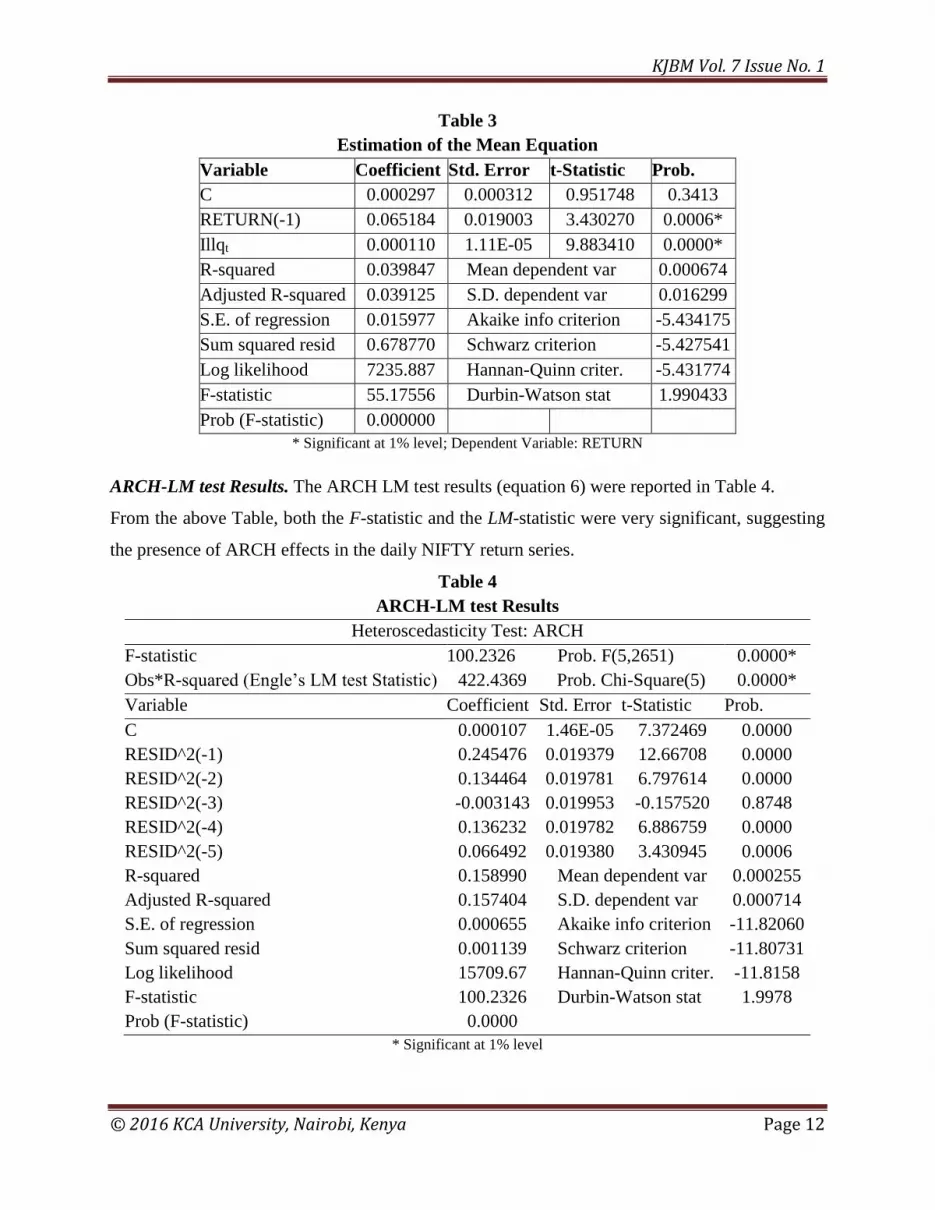
Regression Results of the Mean Equation. The regression results of the AR (1) model (equation

5) were reported in Table 3. It is clear from the above table that illiquidity was positively related

with return as the coefficient of illiquidity was positive and highly significant. The F statistic was

also significant and the D-W statistic was quite satisfactory.



Table 3

Estimation of the Mean Equation

Variable Coefficient Std. Error t-Statistic Prob.

C 0.000297 0.000312 0.951748 0.3413

RETURN(-1) 0.065184 0.019003 3.430270 0.0006*

Illqt 0.000110 1.11E-05 9.883410 0.0000*

R-squared 0.039847 Mean dependent var 0.000674

Adjusted R-squared 0.039125 S.D. dependent var 0.016299

S.E. of regression 0.015977 Akaike info criterion -5.434175

Sum squared resid 0.678770 Schwarz criterion -5.427541

Log likelihood 7235.887 Hannan-Quinn criter. -5.431774

F-statistic 55.17556 Durbin-Watson stat 1.990433

Prob (F-statistic) 0.000000

* Significant at 1% level; Dependent Variable: RETURN

ARCH-LM test Results. The ARCH LM test results (equation 6) were reported in Table 4.

From the above Table, both the F-statistic and the LM-statistic were very significant, suggesting

the presence of ARCH effects in the daily NIFTY return series.

Table 4

ARCH-LM test Results

Heteroscedasticity Test: ARCH

F-statistic 100.2326 Prob. F(5,2651) 0.0000*

Obs*R-squared (Engle’s LM test Statistic) 422.4369 Prob. Chi-Square(5) 0.0000*

Variable Coefficient Std. Error t-Statistic Prob.

C 0.000107 1.46E-05 7.372469 0.0000

RESID^2(-1) 0.245476 0.019379 12.66708 0.0000

RESID^2(-2) 0.134464 0.019781 6.797614 0.0000

RESID^2(-3) -0.003143 0.019953 -0.157520 0.8748

RESID^2(-4) 0.136232 0.019782 6.886759 0.0000

RESID^2(-5) 0.066492 0.019380 3.430945 0.0006

R-squared 0.158990 Mean dependent var 0.000255

Adjusted R-squared 0.157404 S.D. dependent var 0.000714

S.E. of regression 0.000655 Akaike info criterion -11.82060

Sum squared resid 0.001139 Schwarz criterion -11.80731

Log likelihood 15709.67 Hannan-Quinn criter. -11.8158

F-statistic 100.2326 Durbin-Watson stat 1.9978

Prob (F-statistic) 0.0000




Estimated Results of the EGARCH (1, 1) Model

The estimated EGARCH (1, 1) mean and variance equations were reported in Table 5. From the

table, it can be readily observed that the coefficient of the Illqt variable (0.000116) in the mean

equation was positive and highly significant. This suggests that, there existed a positive return-

illiquidity relationship in Indian stock market at an aggregate level during the study period. Note

that the estimated EGARCH mean equation differs slightly from the one in Table 3 because

EViews computes both mean equation and variance equation simultaneously and the number of

iterations is different for different models.

The asymmetry effect is highlighted by . Because this parameter was significant and lower than

zero (-0.109431), it can be inferred that the daily volatilities of the NIFTY returns were

characterized by asymmetry. This is consistent with the notion that new negative information

elicits a higher volatility relative to new positive information. The large coefficient

(0.965552) implies that volatility persists over a long period of time in the pertinent market.

Table 5

Regression Results of EGARCH (1, 1) Mean and Variance Equations

Variable Coefficient Std. Error z-Statistic Prob.

Mean Equation

C 0.000709 0.000239 2.970825 0.0030*

RETURN(-1) 0.077717 0.020369 3.815460 0.0001*

Illqt 0.000116 2.64E-05 4.398878 0.0000*

Variance Equation

-0.461588 0.060060 -7.685387 0.0000*

a 0.210697 0.023275 9.052384 0.0000*

-0.109431 0.014950 -7.319533 0.0000*

0.965552 0.006156 156.8547 0.0000*


AC, PAC, and Box-Pierce Q Statistics of Squared Residuals

To test whether any ARCH effects were still present in the mean equation, the AC and PAC

functions & the Q statistics of the standardized residuals were calculated. The results are

reported in Table 6. Since none of the AC functions, PAC functions or Q statistics at any lag

were significant, we can conclude that there was no ARCH effects remaining.

CONCLUSION



This study sought to investigate the relationship between daily NIFTY return and illiquidity time

series data. The EGARCH (1, 1) model was applied to model conditional volatility and

illiquidity, following Amihud (2002), was used as an exogenous variable in the mean equation.

After diagnostic testing, the model was deemed a good fit. The estimated results clearly showed

that illiquidity was positively related to aggregate returns and therefore a liquidity premium

existed in the Indian Stock Market during the study period. The empirical results also indicated a

relationship between liquidity and volatility since illiquidity was used as an exogenous variable

in estimating the mean equation and hence it influenced the values of the residuals. The lags of

residuals, lags of conditional standard deviation, and lags of conditional variance in turn were

inputs in the determination of (the natural logarithm of) conditional variance in the EGARCH

framework.

Table 6

AC, PAC, and Box-Pierce Q Statistics of Squared Residuals

Lag AC PAC Q-Stat Prob

1 0.007 0.007 0.1272 0.721

2 -0.023 -0.023 1.5668 0.457

3 0.027 0.028 3.5459 0.315

4 0.020 0.020 4.6638 0.324

5 -0.026 -0.025 6.5126 0.259

6 -0.019 -0.018 7.4615 0.280

7 0.024 0.022 8.9392 0.257

8 0.004 0.004 8.9931 0.343

9 0.029 0.032 11.207 0.262

10 0.021 0.020 12.438 0.257

11 -0.031 -0.032 15.055 0.180

12 0.006 0.007 15.160 0.233

13 0.022 0.020 16.490 0.224

14 0.027 0.029 18.460 0.187

15 -0.012 -0.009 18.861 0.220

16 -0.003 -0.005 18.886 0.275

17 0.036 0.032 22.412 0.169

18 -0.000 0.000 22.412 0.214

19 -0.016 -0.013 23.115 0.232

20 -0.022 -0.022 24.359 0.227



In conclusion, it can be noted that the liquidity-return relationship deserves further investigation

because of a number of factors: First, since the identification of factors that predict market

returns has been an interest to academicians and practitioners, a study that examines the

robustness of past empirical findings using different liquidity measures is important. It is also

desirable to examine the return-liquidity relationship using various liquidity measures. This is

because, unlike other financial variables such as price and volume, liquidity (illiquidity) is

unobservable and has many facets that cannot be captured in a single measure.



REFERENCES Amihud, Y. (2002), “Illiquidity and stock returns cross-section and time-series effects”, Journal

of Financial Markets, 5, 31-56.

Amihud, Y., Mendelson, H. (1986), “Asset pricing and the bid-ask spread”, Journal of Financial

Economics, 17, 223-249.

Amihud, Y., Mendelson, H. (1988), “Liquidity and asset prices: financial management

implications”. Financial Management 17, 5-15.

Amihud, Y., Mendelson, H., & Pedersen, L.H. (2005), “Liquidity and asset prices”, Foundation

and Trends in Finance, 1(4), 269-364.

Black, F. (1976), “Studies of stock price volatility changes”. Proceedings of the 1976 meetings

of the American Statistical Association, Business and Economics Statistics Section.

Washington, DC: American Statistical Association, 177-181.

Bodie, Z., Kane, A., Marcus, A.J., & Mohanty, P. (2006), “Investment”- Tata-McGraw-Hill.

Bollerslev, T. (1986), “Generalized Autoregressive Conditional Heteroskedasticity,” Journal of

Econometrics, 31 (April): 307-327.

Brennan, M., Chordia, T. & Subrahmanyam, A. (1998), “Alternative factor specifications,

security characteristics an d cross-sectional of expected returns”, Journal of Financial

Economics, 49, 345-373.

Brennan, M., Subrahmanyam, A. (1996), “Market micro structure and asset pricing”, Journal of

Financial Economics, 41, 441-464.

Chordia, T., Roll, R. & Subrahmanyam, A. (2000), “Commonality in liquidity”, Journal of

Financial Economics 56, 3-28.

Chordia, T., Roll, R. & Subrahmanyam, A. (2001), “Market liquidity and trading activity”, The

Journal of Finance 56(2), 501-530.

Chordia, T., Sarkar, A., & Subrahamanyam, A. (2005), “The Joint Dynamics of Liquidity,

Reforms and Volatility across Small and Large Firms”, UCLA Anderson 2005 Working

Papers.

Datar, V.T. (1998), “Liquidity and Stock Returns: An Alternative Test”, Journal of Financial

Markets, 1, 205-219.

Eleswarapu, V.R., Reinganum, M. (1993). The Seasonal Behavior of Liquidity Premium in Asset

Pricing. Journal of Financial Economics 34, 373–386.



Engle, Robert F. (1982). “Autoregressive Conditional Heteroskedasticity with Estimates of the

Variance of U.K. Inflation,” Econometrica, 50, 987–1008.

Fama, E.F., MacBeth, J.D., (1973). “Risk, return and equilibrium: empirical tests”. Journal of

Political Economy, 81, 607–636.

Fama, Eugene F. and Kenneth R. French, (1993), “Common risk factors in the returns on stocks

and bonds”, Journal of Financial Economics 33, 3-56.

Gibson, R., Nicolas, M. (2004), “The pricing of systematic liquidity risk: Empirical evidence

from the US Stock Market, Journal of Banking and Finance, 28,157-178.

Haugen, R.L, Baker, N. L, (1996), “Commonality in the Determinants of Expected Stock

Returns”, Journal of Financial Economics, 41, 401-439

Jones, C.M., (2000), “A century of stock market liquidity and trading costs”, Working paper,

Columbia University.

MacKinnon, J.G. (1996). “Numerical Distribution Functions for Unit Root and Cointegration

Tests,” Journal of Applied Econometrics, 11, 601-618.

Nelson, D.B. (1991). “Conditional Heteroskedasticity in Asset Returns: A New Approach,”

Econometrica, 59, 347-370.

Pastor, L., Stambaugh, R. (2003), “Liquidity Risk and Expected Stock Returns”, Journal of

Political Economy, 111, 642-685

Phillips, P.C.B., P, Perron. (1988), “Testing for a Unit Root in Time Series Regression,”

Biometrika, 75, 335-346.

Salehi, M., Talebnia, G. & Ghorbani, B. (2011), “A Study of the Relationship between Liquidity

and Stock Returns of Companies Listed in Tehran Stock Exchange”, World Applied

Science Journal, 12(9), 1403-1408.

Sen, S.S., Ghosh, S.K. (2006), Relationship between Stock Market Liquidity and Volatility at an

Aggregate Level: A Case Study on NSE”. The ICFAI Journal of Applied Finance, 12(4),

39-46.

Sen, S.S. (2009). On Stock Market Illiquidity of the NSE of India. The ICFAI Journal of

Financial Economics, VII (3&4), 95-104.

on the relationship between illiquidity, aggregate market return and conditional volatility of the...

Documents