Working Paper Series

This paper can be downloaded without charge from: http://www.richmondfed.org/publications/

Aggregate Demand Management with Multiple Equilibria *

Huberto M. Ennis Research Department, Federal Reserve Bank of Richmond

Todd Keister

Department of Economics and Centro de Investigación Económica ITAM

Federal Reserve Bank of Richmond Working Paper No. 03-04 June 2003

Abstract

We study optimal government policy in an economy where (i) search frictions create a coordination problem and generate multiple Pareto-ranked equilibria and (ii) the government finances the provision of a public good by taxing trade. The government must choose the tax rate before it knows which equilibrium will obtain, and therefore an important part of the problem is determining how the policy will affect the equilibrium selection process. We show that when the equilibrium selection rule is based on the concept of risk dominance, higher tax rates make coordination on the Pareto-superior outcome less likely. As a result, taking equilibrium-selection effects into account leads to a lower optimal tax rate. We also show that public-employment policies that appear to be inefficient based on a standard equilibrium analysis may be justifiable if they influence the equilibrium selection process.

JEL Classification Numbers: E61, E62, H21 Keywords: Search Frictions, Coordination, Equilibrium Selection, Government Policy ________________________________________________ * We thank Scott Freeman, Preston McAfee, and seminar participants at Kentucky, Miami, Queens, Texas, Vanderbilt, the Federal Reserve Bank of Dallas, the 2002 Midwest Macro Conference, the First Annual University of Texas - ITAM workshop and the Economic Fluctuations workshop at the University of Essex. Part of this work was completed while Keister was visiting the University of Texas at Austin, whose hospitality and support are gratefully acknowledged. The views expressed herein are those of the authors and do not necessarily reflect those of the Federal Reserve Bank of Richmond or the Federal Reserve System. E-mail addresses: huberto.ennis@rich.frb.org (H. M. Ennis), keister@itam.mx (T. Keister)

1 Introduction

We present a model where the search and matching process creates externalities and, as

a result, the market for output becomes more efficient as more people enter it. Following

Diamond (1982), we refer to the intensity of participation in the market as the level of

aggregate demand. There is also a government in our model that can tax market transactions

and use the proceeds to provide a public good. Our interest is in Þnding the welfare-

maximizing tax rate. If the model has a unique equilibrium for every possible policy choice,

this task is straightforward. The optimal tax rate will balance the marginal beneÞt of the

public good against the marginal cost of providing it, including the decrease in aggregate

demand and hence the loss in output-market efficiency that the tax causes. However, as

is common in models with trading frictions, our model has multiple equilibria for a broad

range of parameter values. We assume that the government must set the tax rate before

knowing the actions of private agents, which implies that the government does not know

which equilibrium will obtain. It seems entirely possible in such a setting that the choice of

tax rate may inßuence which of the equilibria the economy ends up in, an effect that should

be taken into account in determining the optimal policy. In fact, Diamond (1982, p. 882)

states that �... one of the goals for macro policy should be to direct the economy toward

the best [equilibrium] ... after any sufficiently large macro shock.� Hence it is important to

try to understand the effects that government policy can have on the process of equilibrium

selection and how these effects inßuence the government�s optimal choice of policy.

In our model, there is a continuum of identical agents, each of whom must decide whether

or not to produce for the market. If an agent produces, she must exert costly effort in order

to Þnd a trading partner. For a given tax rate there are two possible (symmetric, pure-

strategy) equilibria: one where all agents produce and search, and one where no one produces

and there is no market activity. Following Howitt and McAfee (1992), we label these the

1

�optimistic� and �pessimistic� outcomes, respectively. The search level that agents choose

in the optimistic outcome is decreasing in the tax rate, and if the tax rate is set too high the

optimistic outcome is no longer an equilibrium. The pessimistic outcome is an equilibrium

regardless of the tax rate; if an individual agent believes that no one else is producing for

the market, then she believes that searching for a trading partner will be in vain and she

will therefore choose not to produce. Whenever the optimistic outcome is an equilibrium, it

Pareto dominates the pessimistic outcome.

What tax rate should the government in this economy choose? If the policy had no

inßuence on the equilibrium selection process, then the simple structure of our model would

lead to a clear answer: the tax rate should be chosen to maximize expected welfare in

the optimistic equilibrium. This is because the tax policy has no effect on welfare in the

pessimistic equilibrium, and therefore the same policy choice is (weakly) optimal in each of

the equilibria. However, we argue that in general the likelihood of agents coordinating on a

speciÞc outcome will depend on the individual payoffs associated with each possible choice

of action, which implies that the equilibrium selection process will be inßuenced by the tax

rate. In particular, we discuss a class of equilibrium selection rules that are based on the

concept of risk dominance. We show that under any of these rules, the fact that a higher

tax rate decreases the beneÞt of producing implies that a higher tax rate also decreases the

likelihood that the optimistic equilibrium will obtain. This is an additional cost of taxation

that a traditional analysis that ignores equilibrium selection would miss. This cost has clear

implications for policy: the optimal tax rate must be lower than the rate that maximizes

welfare in the optimistic equilibrium. The reason for this result is simple: If the tax rate is

decreased slightly from this starting point, there is a small (second order) loss in utility should

the optimistic equilibrium obtain. At the same time, there is a larger (Þrst-order) increase in

the probability of reaching the optimistic equilibrium, and therefore expected utility (across

2

equilibria) increases. Thus the effect of taking equilibrium selection into account is clear:

it lowers the optimal tax rate. In other words, discouraging market activity is more costly

than a standard equilibrium analysis would indicate.

When additional policy tools are introduced, taking equilibrium selection into account can

also change the composition of the optimal policy. We demonstrate this in Section 4 by giving

the government an additional policy tool: it can directly control the actions of a fraction

of the agents in the economy. In other words, it can directly produce the public good by

employing agents and dictating their production and search decisions. We choose parameter

values so that public production is inefficient in the following sense: if government policy had

no inßuence over the equilibrium selection process, this second policy should never be used.

However, we show that when equilibrium selection effects are taken into account, the optimal

policy involves a positive amount of public production. There are two key elements behind

this result. First, taking equilibrium selection into account lowers the optimal tax rate, as we

discussed above. This increases the marginal value of the public good and therefore makes

public production more attractive. Second, unlike taxation, public production does not

necessarily decrease the probability of the optimistic equilibrium obtaining; in our example,

it actually increases that probability. This is because public production increases the level of

aggregate demand and therefore makes a private agent willing to produce for a wider range

of beliefs about the market environment. Therefore the cost of public production is lower

than an equilibrium analysis would indicate, and at the new, higher marginal valuation of

the public good, some public production is optimal. Hence, looking at equilibrium selection

shows that public sector employment/production may be a useful policy for coordination

purposes.

There is a large literature in which models with multiple equilibria are used to discuss

policy issues without imposing an equilibrium selection mechanism as we do here. This lit-

3

erature is based on the idea that sometimes a meaningful comparison can be made between

the sets of equilibria resulting from different policy choices, and hence a policy recommen-

dation can be made independent of the equilibrium selection process. Suppose, for example,

that one policy choice leads to a unique, Pareto optimal equilibrium while another choice

generates that same equilibrium plus some other, inferior equilibria. A strong case can

then be made for choosing the former policy. Early work along these lines includes Grand-

mont (1986), Reichlin (1986), and Woodford (1986), where the inferior equilibria involve

endogenous ßuctuations and the preferred policy has a natural interpretation as a stabiliza-

tion policy.1 In many situations, however, bad equilibria cannot be costlessly eliminated by

the proper policy choice. Cooper and Corbae (2002) study a model with a strategic com-

plementarity in the Þnancial intermediation process. Monetary policy can eliminate some

undesirable equilibria, but not all of them. The authors conclude that �without a theory

of equilibrium selection, predictions about the effects of monetary policy are impossible to

make.� (p. 23) The simpler model presented in this paper contains the essential features

that give rise to this problem. We provide a method for dealing with such situations, and in

doing so, we show how models where undesirable equilibria cannot be easily eliminated can

still be brought to bear on policy issues in interesting ways.

In the next section, we describe the model and the properties of equilibrium. In Section 3,

we show how to formulate the optimal policy problem in the presence of multiple equilibria.

For this, we introduce the concept of an equilibrium selection mechanism and derive the

optimal policy under several different mechanisms. In Section 4, we introduce the public-1The �stabilization� approach has since been applied in a wide variety of settings. See,

for example, Smith (1991) and the symposium introduced by Woodford (1994). In an en-

vironment where multiple equilibria exist for all policy choices, Keister (1998) shows that

meaningful policy statements can sometimes be made without imposing an equilibrium se-

lection rule.

4

employment policy and show how equilibrium-selection effects can lead the government to

use this policy even though it is inefficient from a standard equilibrium perspective. Finally,

in Section 5 we offer some concluding remarks.

2 The Model

Consider an economy with a [0, 1] continuum of identical agents and a single commodity that

is produced using only labor. Each agent faces a binary production decision; she must either

produce at a Þxed scale or not at all. Producing requires labor input that gives disutility

c ≥ 0. Agents receive no utility from consuming their own output, but have a utility value Fof consuming the output of someone else.2 Finding a trading partner in the output market

requires costly search effort. After observing the production decisions of all other agents, an

agent who has produced chooses a search intensity. This intensity determines the probability

that she will Þnd a trading partner. If a partner is found, the two agents exchange output

and consume; all exchanges are one-for-one trades. If an agent chooses not to produce, she

does not enter the output market and has zero utility from trade (a normalization).

There is also a public good that can be produced using units of output that have been

traded and are therefore consumable. All agents receive utility from the public good. How-

ever, because there is a continuum of agents, there is a pure free-rider problem and the public

good will not be privately provided. Instead, there is a benevolent government that can tax

trade at a rate τ ≥ 0 and use the proceeds to produce the public good. Our interest is in howthe policy variable τ should be set. An important aspect of the problem we consider is the

2We think of this as a form of specialization in production; see Diamond (1982). One

could instead allow agents to consume their own output but assume that doing so yields less

utility than consuming the output of someone else. By relabelling utility values and costs,

this approach is easily shown to be equivalent to the model here.

5

timing of decisions. We study the case where the government must set the tax rate before

observing the actions of agents. In particular, the government must set τ before knowing

which equilibrium will obtain. It is in such settings that our question of interest � how the

policy choice affects the equilibrium selection process � arises. In addition, we assume that

the government must set τ before the exact cost of production c is known. At this point

the cost is a random variable with support [cL, cH ] and density function f , which we take

(without any real loss of generality) to be uniform. In other words, the tax rate must be

set with less information than private agents will have when they decide whether or not to

produce. This uncertainty plays an important role in our formulation of the optimal policy

problem; we discuss this issue in detail in Section 3 below.

Before we can study the problem of an agent deciding whether or not to produce, we

must calculate the beneÞt of producing. For this we need to look at the workings of the

output market.

2.1 Output Market

If agent i has produced, she can search for a trading partner by choosing a search intensity

γi ∈ [0, 1] . In this setting, externalities naturally arise: An increase in individual searcheffort not only makes it more likely that the individual will Þnd a partner, it also makes

it more likely that other agents in the economy will Þnd a partner. The fraction of agents

Þnding a match in the output market is given by an aggregate matching function m.3 Let γ3Assuming a matching function simpliÞes matters considerably, but it clearly does not

come without cost. In particular, policy changes may affect the nature of the matching

process, and this effect will be absent in our analysis. See Lagos (2000) for an interesting

study in this direction.

6

denote the average level of search intensity in the economy, so that we have

γ =

Z 1

0

γidi. (1)

Note that γ is also the total amount (�units�) of search intensity in the market. We assume

that the value of m depends only on γ (and not on the distribution of γi across agents). We

assume that m : [0, 1] → [0, 1] is a smooth, strictly increasing bijection, so that m (0) = 0

and m (1) = 1 hold. In addition, we assume that m is strictly convex. This assumption

captures the externality described above and implies that there are increasing returns in

the matching process; if the number of searching agents doubles (holding search intensity

constant), the number of matches formed more than doubles. Hence the efficiency of the

output market is increasing in the number of searching agents and in their search intensities.

Following Diamond (1982), we refer to the aggregate amount of search intensity as the level

of aggregate demand.

Notice that the above assumptions imply that we have m (γ) ≤ γ for all possible valuesof γ. Since the search intensity of each agent is less than unity, the number γ is necessarily

lower than the fraction of agents who are searching with positive effort levels. Therefore, the

fraction of agents who are matched, m (γ), is necessarily lower than the fraction of agents

who are searching with positive effort levels. This shows that the matching function always

yields a feasible outcome.

While the function m gives the fraction of agents who Þnd a partner, which agents

actually get matched is random, with the probability of an individual agent being matched

proportional to her search intensity. SpeciÞcally, deÞne

ρ(γ) =m(γ)

γ. (2)

Then ρ is the probability of being matched per unit of search intensity. An individual

agent choosing intensity level γi will be matched with probability ρ(γ)γi. Note that our

7

assumptions on m and the upper bound on γi ensure that this probability is always between

zero and one.

Output that has been traded can be converted one-for-one into units of the public good.

Let x denote the amount of public good produced per agent. This will be equal to the tax

rate multiplied by the number of agents who make a trade (the tax base). Then all agents

receive utility v (x) , where the function v is strictly increasing and strictly concave, and

satisÞes

v(0) = 0 and limx→0

v0 (x) =∞.

2.2 The Agent�s Problem

Each agent Þrst decides whether or not to produce. If she produces, she then chooses a search

intensity γi after observing the production decisions of all other agents. We examine the

latter choice Þrst. The cost function for search intensity d (γi) is smooth, strictly increasing,

strictly convex, and satisÞes

limγi→0

d0 (γi) = 0.

If an agent meets a partner, they exchange output. If she does not meet a partner, she does

not consume. We use the variable φi to represent the production choice; φi = 1 corresponds

to producing and φi = 0 to not producing. If the agent produces, she will choose γi to

maximize expected utility. The agent takes the level of provision of the public good as given

and (since it enters her utility function in an additively separable way) her production and

search decisions are independent of this level. She also takes as given the probability ρ of

Þnding a match per unit of search intensity and the tax rate τ . We use λ (ρ, τ) to denote

8

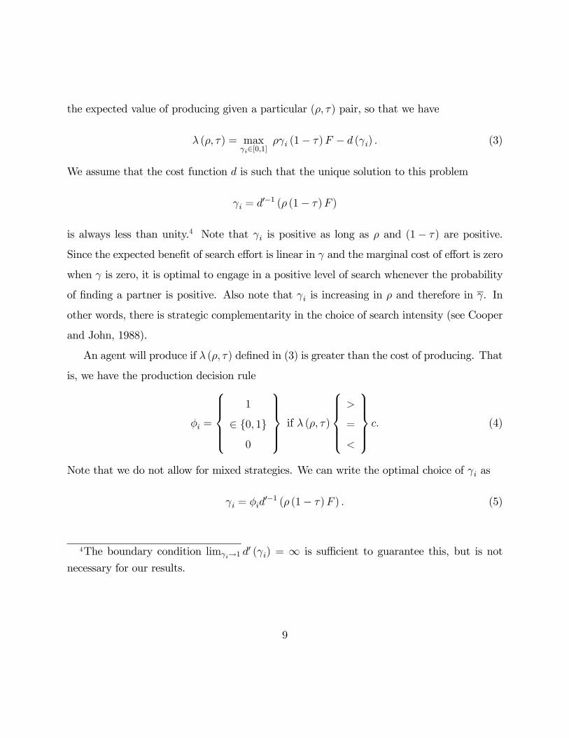
the expected value of producing given a particular (ρ, τ) pair, so that we have

λ (ρ, τ) = maxγi∈[0,1]

ργi (1− τ)F − d (γi) . (3)

We assume that the cost function d is such that the unique solution to this problem

γi = d0−1 (ρ (1− τ)F )

is always less than unity.4 Note that γi is positive as long as ρ and (1− τ) are positive.Since the expected beneÞt of search effort is linear in γ and the marginal cost of effort is zero

when γ is zero, it is optimal to engage in a positive level of search whenever the probability

of Þnding a partner is positive. Also note that γi is increasing in ρ and therefore in γ. In

other words, there is strategic complementarity in the choice of search intensity (see Cooper

and John, 1988).

An agent will produce if λ (ρ, τ) deÞned in (3) is greater than the cost of producing. That

is, we have the production decision rule

φi =

1

∈ {0, 1}0

if λ (ρ, τ)

>

=

<

c. (4)

Note that we do not allow for mixed strategies. We can write the optimal choice of γi as

γi = φid0−1 (ρ (1− τ)F ) . (5)

4The boundary condition limγi→1 d0 (γi) = ∞ is sufficient to guarantee this, but is not

necessary for our results.

9

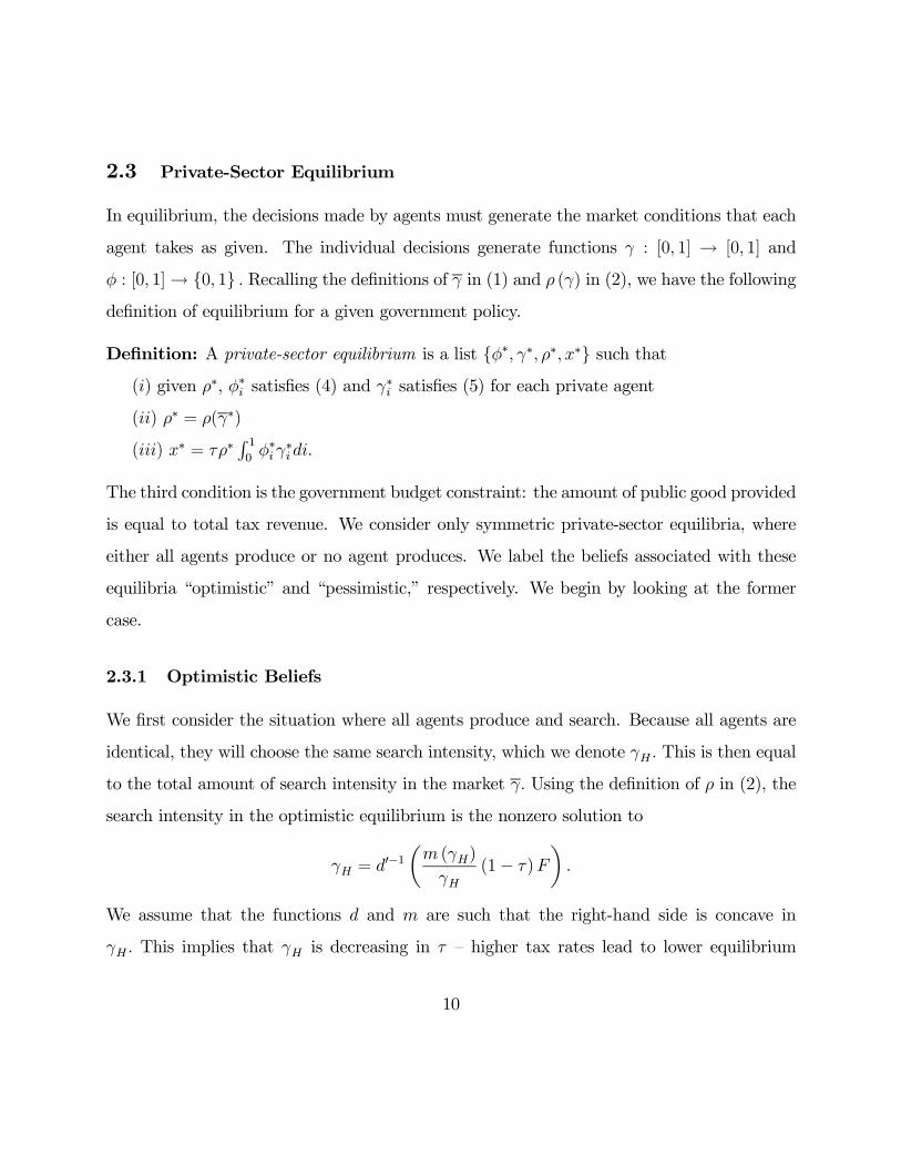
2.3 Private-Sector Equilibrium

In equilibrium, the decisions made by agents must generate the market conditions that each

agent takes as given. The individual decisions generate functions γ : [0, 1] → [0, 1] and

φ : [0, 1]→ {0, 1} . Recalling the deÞnitions of γ in (1) and ρ (γ) in (2), we have the followingdeÞnition of equilibrium for a given government policy.

DeÞnition: A private-sector equilibrium is a list {φ∗, γ∗, ρ∗, x∗} such that(i) given ρ∗, φ∗i satisÞes (4) and γ

∗i satisÞes (5) for each private agent

(ii) ρ∗ = ρ(γ∗)

(iii) x∗ = τρ∗R 10φ∗i γ

∗i di.

The third condition is the government budget constraint: the amount of public good provided

is equal to total tax revenue. We consider only symmetric private-sector equilibria, where

either all agents produce or no agent produces. We label the beliefs associated with these

equilibria �optimistic� and �pessimistic,� respectively. We begin by looking at the former

case.

2.3.1 Optimistic Beliefs

We Þrst consider the situation where all agents produce and search. Because all agents are

identical, they will choose the same search intensity, which we denote γH . This is then equal

to the total amount of search intensity in the market γ. Using the deÞnition of ρ in (2), the

search intensity in the optimistic equilibrium is the nonzero solution to

γH = d0−1µm (γH)

γH(1− τ)F

¶.

We assume that the functions d and m are such that the right-hand side is concave in

γH . This implies that γH is decreasing in τ � higher tax rates lead to lower equilibrium

10

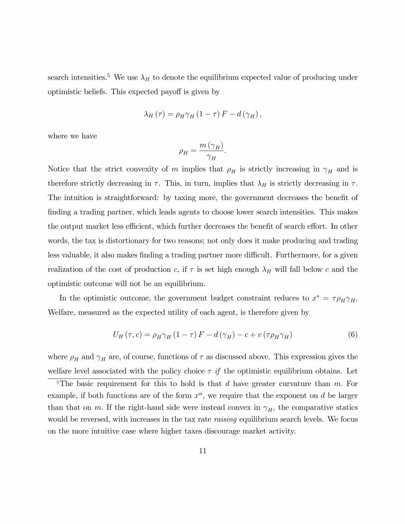
search intensities.5 We use λH to denote the equilibrium expected value of producing under

optimistic beliefs. This expected payoff is given by

λH (τ) = ρHγH (1− τ)F − d (γH) ,

where we have

ρH =m (γH)

γH.

Notice that the strict convexity of m implies that ρH is strictly increasing in γH and is

therefore strictly decreasing in τ . This, in turn, implies that λH is strictly decreasing in τ .

The intuition is straightforward: by taxing more, the government decreases the beneÞt of

Þnding a trading partner, which leads agents to choose lower search intensities. This makes

the output market less efficient, which further decreases the beneÞt of search effort. In other

words, the tax is distortionary for two reasons; not only does it make producing and trading

less valuable, it also makes Þnding a trading partner more difficult. Furthermore, for a given

realization of the cost of production c, if τ is set high enough λH will fall below c and the

optimistic outcome will not be an equilibrium.

In the optimistic outcome, the government budget constraint reduces to x∗ = τρHγH .

Welfare, measured as the expected utility of each agent, is therefore given by

UH (τ , c) = ρHγH (1− τ)F − d (γH)− c+ v (τρHγH) (6)

where ρH and γH are, of course, functions of τ as discussed above. This expression gives the

welfare level associated with the policy choice τ if the optimistic equilibrium obtains. Let5The basic requirement for this to hold is that d have greater curvature than m. For

example, if both functions are of the form xα, we require that the exponent on d be larger

than that on m. If the right-hand side were instead convex in γH , the comparative statics

would be reversed, with increases in the tax rate raising equilibrium search levels. We focus

on the more intuitive case where higher taxes discourage market activity.

11

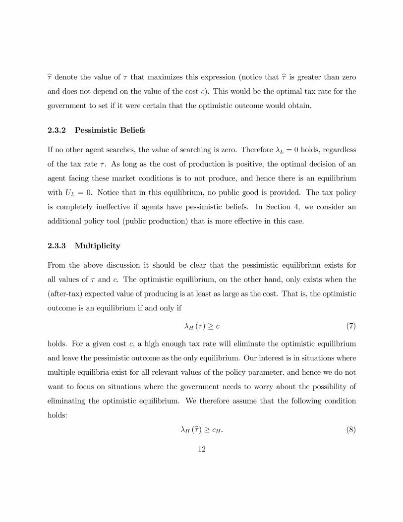
bτ denote the value of τ that maximizes this expression (notice that bτ is greater than zeroand does not depend on the value of the cost c). This would be the optimal tax rate for the

government to set if it were certain that the optimistic outcome would obtain.

2.3.2 Pessimistic Beliefs

If no other agent searches, the value of searching is zero. Therefore λL = 0 holds, regardless

of the tax rate τ . As long as the cost of production is positive, the optimal decision of an

agent facing these market conditions is to not produce, and hence there is an equilibrium

with UL = 0. Notice that in this equilibrium, no public good is provided. The tax policy

is completely ineffective if agents have pessimistic beliefs. In Section 4, we consider an

additional policy tool (public production) that is more effective in this case.

2.3.3 Multiplicity

From the above discussion it should be clear that the pessimistic equilibrium exists for

all values of τ and c. The optimistic equilibrium, on the other hand, only exists when the

(after-tax) expected value of producing is at least as large as the cost. That is, the optimistic

outcome is an equilibrium if and only if

λH (τ) ≥ c (7)

holds. For a given cost c, a high enough tax rate will eliminate the optimistic equilibrium

and leave the pessimistic outcome as the only equilibrium. Our interest is in situations where

multiple equilibria exist for all relevant values of the policy parameter, and hence we do not

want to focus on situations where the government needs to worry about the possibility of

eliminating the optimistic equilibrium. We therefore assume that the following condition

holds:

λH (bτ) ≥ cH . (8)

12

Recalling that λH is decreasing in τ , this condition implies that for any τ ≤ bτ the optimisticoutcome will be an equilibrium regardless of the realization of the cost variable c. In par-

ticular, the government can set the tax rate to maximize expected utility in the optimistic

outcome and be assured that this outcome will be an equilibrium once the cost is realized.

What value of τ should the government set? Our primary interest is in answering this

question. In other words, we want to formulate and solve an optimal policy problem.

3 The Optimal Tax Rate

Formulating an optimal policy problem in general requires calculating the level of welfare that

is generated by each possible policy choice. When there are multiple equilibria associated

with at least some policy choices, it is not immediately clear how to do this. By far the

most common approach in the literature is to essentially ignore the issue of multiplicity by

assuming that the Pareto-best equilibrium will obtain (see, for example, Diamond, 1982).

This gives a clear policy prescription: the policy should be chosen to maximize expected

utility in the Pareto-best equilibrium. In our setting, the optimal policy would then be bτ .Because of the simple structure of our model, this approach might even seem to be without

any loss of generality. In the pessimistic outcome, no trade takes place and hence the tax rate

is irrelevant. Therefore, what could be wrong with setting the tax rate to maximize welfare

in the optimistic outcome? In other words, the tax rate bτ is (weakly) optimal regardless ofwhich outcome obtains in equilibrium, and thus it seems like this rate must be the optimal

policy. In this section, we show that this prescription is correct only if the process by which

an equilibrium is selected is completely independent of the value to individual agents of

producing and searching. We argue that such selection rules are intuitively unappealing. We

introduce other selection rules, based on the notion of risk dominance, that allow for the

13

selection process to depend on individual incentives, and we show that under such (more

realistic) rules the optimal tax rate is lower than bτ .3.1 Formulating the Optimal Policy Problem

In order to have a completely-speciÞed optimal policy problem, the government must be

able to assign a probability distribution over outcomes to each of its possible policy choices.

With these probabilities, expected welfare can be calculated for each policy choice and the

best policy can be determined. We refer to a complete speciÞcation of such probabilities as

an equilibrium selection mechanism.

DeÞnition: An equilibrium selection mechanism (ESM) is a function π : R+ × C → [0, 1]

that assigns, for each pair (τ , c), a probability π (τ , c) to the optimistic outcome generated

by that pair and a probability (1− π (τ , c)) to the pessimistic outcome. These probabilitiesmust be consistent with equilibrium, in that:

(i) π (τ , c) = 0 holds if the optimistic outcome is not an equilibrium for that (τ , c) pair,

and

(ii) π (τ , c) = 1 holds if the pessimistic outcome is not an equilibrium for that (τ , c) pair.

The two restrictions say that an outcome should be assigned positive probability only if it is

actually an equilibrium of the economy based on that (τ , c) pair. For the moment we place

no further restrictions on the function π. Suppose, for example, that the government believes

that the Pareto-best equilibrium will always obtain. Then π will equal one whenever the pair

(τ , c) is such that the optimistic equilibrium exists and zero otherwise. Another ESM could

be generated by assuming that private agents base their beliefs (and hence their actions)

on the realization of a two-state sunspot variable. Suppose that whenever τ and c are such

that both equilibria exist, agents produce and search if sunspots appear and stay home if

14

sunspots do not appear. Then, whenever τ and c are such that both equilibria exist, π (τ , c)

would be equal to the probability of sunspots appearing. In general, any rule by which a

private-sector equilibrium is selected can be represented by some function π satisfying the

two restrictions given above.

Putting aside for the moment the question of where the function π would come from,

notice that using an ESM does allow us to formulate an optimal policy problem. Given

π, a benevolent government should choose the tax rate that maximizes the expected utility

of private agents, where the expectation is both across values of the cost c and across the

possible equilibrium outcomes. In other words, the optimal policy problem is given by

maxτ

Z cH

cL

[π (τ , c)UH (τ , c) + (1− π (τ , c))UL (τ , c)] f (c) dc,

which, since UL = 0 holds in this model, simpliÞes to

maxτ

Z cH

cL

π (τ , c)UH (τ , c) f (c) dc. (9)

The best tax rate for the government to choose will clearly depend on the equilibrium

selection mechanism π. For a given function π, we call the solution to (9) the π-optimal tax

rate and denote it by τ ∗π. We provide next an expanded equilibrium concept that explicitly

incorporates the equilibrium selection mechanism and the government�s optimal choice of

policy given this mechanism.

DeÞnition: A selection-based equilibrium is a function π, a tax rate τπ, and two lists©φj, γj, ρj, xj

ªwith j = H,L, such that

(i) the list©φj, γj, ρj, xj

ªis a private-sector equilibrium for j = H,L,

(ii) the function π is a well-deÞned equilibrium selection mechanism, and

15

(iii) given the function π and the lists©φj, γj, ρj, xj

ª, the tax rate τπ solves the policy

problem (9).

Note that if the model allows for a constant function π to be a well-deÞned ESM, then

the above deÞnition with such a function reduces to the deÞnition of a sunspot equilibrium

(Cass and Shell, 1983), expanded to include an optimizing government. In what follows,

when the meaning is clear from the context, we will drop the preÞxes private-sector and

selection-based, and refer simply to an equilibrium. We now turn to a characterization of the

optimal policy under two different classes of equilibrium selection rules.

3.2 Traditional Selection Rules

As we discussed above, the most common approach to dealing with multiple equilibria in a

policy problem is to simply assume that the Pareto-best equilibrium will always obtain. This

selection rule is sometimes called payoff dominance. We argued above that the π-optimal tax

rate under this rule is given by bτ . We now verify this argument formally. The equilibriumselection mechanism under payoff dominance is given by

π (τ ; c) =

1

0

if (7) holds

otherwise

.Under assumption (8), we have that π (bτ , c) = 1 for all c. Recall that the tax rate bτ maximizesUH (τ , c) for all values of c (see (6)). Therefore bτ maximizes the integrand in (9) for everyvalue of c, and hence maximizes the integral. This veriÞes that under the payoff dominance

ESM, bτ is indeed the optimal policy.Another common approach to equilibrium selection is to assume that all agents base

their actions on the realization of a sunspot variable. Suppose that after the tax rate is set

and the cost of production becomes known, but before private agents choose their actions,

16

one of two states of nature is revealed. With probability πs ∈ (0, 1) sunspots appear andwith probability (1− πs) there are no sunspots. Suppose further that all private agents havethe following belief: If the pair (τ , c) is such that both equilibria exist, then the optimistic

equilibrium will obtain if sunspots appear and the pessimistic equilibrium will obtain if they

do not. Then it is individually optimal for each agent to produce and search if sunspots

appear and to stay home if they do not. That is, there is a sunspot equilibrium where

the optimistic outcome obtains with probability πs whenever both equilibria exist. The

equilibrium selection mechanism for the sunspots selection rule is given by

π (τ , c)

πs

0

if (7) holds

otherwise

.Notice that the government�s objective function in (9) under the sunspots ESM is equal

to the objective function under the payoff-dominance ESM multiplied by the constant πs.

Therefore, the policy prescription generated by the sunspots selection rule is exactly the

same as that generated by payoff dominance, and we have the following result.

Proposition 1 Under both the payoff-dominance ESM and the sunspots ESM, the π-optimal

tax rate is given by τ ∗π = bτ .This result can be interpreted as giving conditions under which the issue of multiplicity

can be essentially ignored. If the policy only affects allocations in one of the equilibria and

the probability assigned to that equilibrium is a constant, unaffected by the policy choice,

then the policy should be chosen to maximize welfare in that equilibrium.

The sunspots selection rule is probabilistic, meaning that the government�s policy does

not completely determine the Þnal outcome. Instead, the policy typically determines a non-

degenerate probability distribution over the set of equilibria. We argue below in favor of

probabilistic selection mechanisms because they are intuitively more plausible and because

17

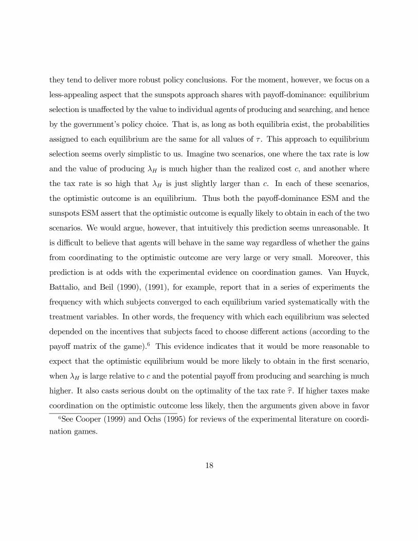
they tend to deliver more robust policy conclusions. For the moment, however, we focus on a

less-appealing aspect that the sunspots approach shares with payoff-dominance: equilibrium

selection is unaffected by the value to individual agents of producing and searching, and hence

by the government�s policy choice. That is, as long as both equilibria exist, the probabilities

assigned to each equilibrium are the same for all values of τ . This approach to equilibrium

selection seems overly simplistic to us. Imagine two scenarios, one where the tax rate is low

and the value of producing λH is much higher than the realized cost c, and another where

the tax rate is so high that λH is just slightly larger than c. In each of these scenarios,

the optimistic outcome is an equilibrium. Thus both the payoff-dominance ESM and the

sunspots ESM assert that the optimistic outcome is equally likely to obtain in each of the two

scenarios. We would argue, however, that intuitively this prediction seems unreasonable. It

is difficult to believe that agents will behave in the same way regardless of whether the gains

from coordinating to the optimistic outcome are very large or very small. Moreover, this

prediction is at odds with the experimental evidence on coordination games. Van Huyck,

Battalio, and Beil (1990), (1991), for example, report that in a series of experiments the

frequency with which subjects converged to each equilibrium varied systematically with the

treatment variables. In other words, the frequency with which each equilibrium was selected

depended on the incentives that subjects faced to choose different actions (according to the

payoff matrix of the game).6 This evidence indicates that it would be more reasonable to

expect that the optimistic equilibrium would be more likely to obtain in the Þrst scenario,

when λH is large relative to c and the potential payoff from producing and searching is much

higher. It also casts serious doubt on the optimality of the tax rate bτ . If higher taxes makecoordination on the optimistic outcome less likely, then the arguments given above in favor

6See Cooper (1999) and Ochs (1995) for reviews of the experimental literature on coordi-

nation games.

18

of bτ are no longer valid. We now examine a class of equilibrium selection mechanisms that

embody the above intuition, and we show that under these rules the optimal tax rate is less

than bτ .3.3 Risk Dominance

Harsanyi and Selten (1988) have proposed using risk dominance as an equilibrium selection

criterion.7 In models of the type we are considering, the risk-dominance criterion has a simple

interpretation. Suppose an agent believes that the optimistic and pessimistic equilibrium

outcomes are equally likely to occur (that is, she has a diffuse prior that places equal weight

on the possible equilibrium levels of aggregate demand). Then the optimistic equilibrium is

risk dominant if her optimal action given these beliefs is to produce, while the pessimistic

equilibrium is risk dominant if her optimal action is to not produce. Furthermore, if all

agents assign equal probability to the possible equilibrium levels of aggregate demand, all

agents will choose the risk-dominant action and the risk-dominant equilibrium will obtain.

In this section, we show that applying this approach to our model generates a π function

that can be used as an equilibrium selection mechanism, and we derive the implications of

this mechanism for the optimal policy.

Suppose that the government has set a particular tax rate τ . The crucial question is

then: For what values of the cost c will the optimistic outcome be risk dominant (and hence

obtain)? This will happen if an agent who assigns equal probability to the two possible7See Harsanyi and Selten (1988, Section 3.9) and the discussion in Young (1998). Carlsson

and van Damme (1993) provide additional justiÞcation for this criterion. They study global

games (where the payoff structure is determined by a random draw) and show that as

the noise vanishes, iterated elimination of dominated strategies leads to the risk dominant

equilibrium as the unique outcome.

19

equilibrium levels of aggregate demand is willing to produce; that is, if we have

1

2λH (τ) +

1

2λL (τ) ≥ c.

Using the fact that λL = 0 holds for all values of τ , we can rewrite this condition as

1

2λH (τ) ≥ c. (10)

Recall that λH is strictly decreasing in τ . Therefore, a higher tax rate implies that an even

lower draw for the cost of production will be required to make the optimistic equilibrium

risk dominant. The risk-dominance equilibrium selection mechanism is given by

π (τ ; c) =

1

0

if (10) holds

otherwise

. (11)

Notice that condition (10) is clearly stronger than the condition for the existence of the

optimistic equilibrium (7). If λH is only slightly above c, then the optimistic equilibrium

exists but is not risk dominant, and hence under this mechanism the pessimistic equilibrium

will obtain. Only if the incentive to produce is �large enough� does this mechanism predict

that the optimistic equilibrium will obtain.

Before returning to the optimal policy problem, we note that the (unconditional) proba-

bility of the optimistic outcome is given by

Π (τ) ≡Z cH

cL

π (τ ; c) f (c) dc = Prob·c <

1

2λH (τ)

¸.

If 12λH (τ) ∈ (cL, cH) holds, then using the fact that the distribution of c is uniform allows

us to rewrite this expression as

Π (τ) =12λH (τ)− cLcH − cL .

20

This expression is clearly strictly decreasing in τ . In other words, setting a higher tax rate

makes it less likely that the optimistic equilibrium will be risk dominant and hence makes it

more likely that the pessimistic equilibrium will obtain.

We now impose two conditions on the support of the cost variable that make the equi-

librium selection problem nontrivial. SpeciÞcally, we assume that

λH (0) > 2cL and λH (bτ) < 2cH (12)

hold. The Þrst condition says that if the tax rate is set to zero, then it is possible for the

optimistic equilibrium to be risk dominant. If this condition did not hold, the pessimistic

equilibrium would be risk-dominant for all (τ , c) pairs, and hence the choice of policy would

be irrelevant. Recall that λH is independent of the distribution of the cost variable, and

hence this condition can always be made to hold by setting cL close enough to zero. The

second condition says that when the government chooses the tax rate bτ , it is possible for thepessimistic equilibrium to be risk-dominant. If this did not hold, the optimistic equilibrium

would always be risk dominant under bτ , and hence using risk dominance would essentiallyreduce to using payoff dominance. This condition can always be made to hold by setting cH

high enough.

We now show that the equilibrium-selection effect of taxation implies that the government

should set the tax rate lower than bτ .Proposition 2 If (12) holds, the π-optimal tax rate under the risk-dominance ESM satisÞes

τ ∗π < bτ .Proof: We need to consider two cases. First suppose that λH (bτ) < 2cL holds. Then if thegovernment chooses bτ the pessimistic equilibrium will be risk dominant for all values of c.

In this case, the optimal policy clearly satisÞes τ ∗π < bτ , since choosing bτ gives an expected21

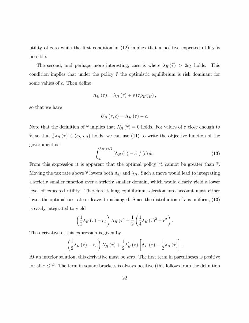
utility of zero while the Þrst condition in (12) implies that a positive expected utility is

possible.

The second, and perhaps more interesting, case is where λH (bτ) > 2cL holds. This

condition implies that under the policy bτ the optimistic equilibrium is risk dominant for

some values of c. Then deÞne

ΛH (τ) = λH (τ) + v (τρHγH) ,

so that we have

UH (τ , c) = ΛH (τ)− c.

Note that the deÞnition of bτ implies that Λ0H (bτ) = 0 holds. For values of τ close enough tobτ , so that 12λH (τ) ∈ (cL, cH) holds, we can use (11) to write the objective function of the

government as Z λH(τ)/2

cL

[ΛH (τ)− c] f (c) dc. (13)

From this expression it is apparent that the optimal policy τ ∗π cannot be greater than bτ .Moving the tax rate above bτ lowers both ΛH and λH . Such a move would lead to integratinga strictly smaller function over a strictly smaller domain, which would clearly yield a lower

level of expected utility. Therefore taking equilibrium selection into account must either

lower the optimal tax rate or leave it unchanged. Since the distribution of c is uniform, (13)

is easily integrated to yieldµ1

2λH (τ)− cL

¶ΛH (τ)− 1

2

µ1

4λH (τ)

2 − c2L¶.

The derivative of this expression is given byµ1

2λH (τ)− cL

¶Λ0H (τ) +

1

2λ0H (τ)

·ΛH (τ)− 1

2λH (τ)

¸.

At an interior solution, this derivative must be zero. The Þrst term in parentheses is positive

for all τ ≤ bτ . The term in square brackets is always positive (this follows from the deÞnition22

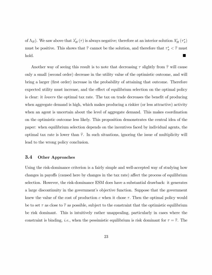
of ΛH). We saw above that λ0H (τ) is always negative; therefore at an interior solution Λ

0H (τ

∗π)

must be positive. This shows that bτ cannot be the solution, and therefore that τ ∗π < bτ musthold. ¥

Another way of seeing this result is to note that decreasing τ slightly from bτ will causeonly a small (second order) decrease in the utility value of the optimistic outcome, and will

bring a larger (Þrst order) increase in the probability of attaining that outcome. Therefore

expected utility must increase, and the effect of equilibrium selection on the optimal policy

is clear: it lowers the optimal tax rate. The tax on trade decreases the beneÞt of producing

when aggregate demand is high, which makes producing a riskier (or less attractive) activity

when an agent is uncertain about the level of aggregate demand. This makes coordination

on the optimistic outcome less likely. This proposition demonstrates the central idea of the

paper: when equilibrium selection depends on the incentives faced by individual agents, the

optimal tax rate is lower than bτ . In such situations, ignoring the issue of multiplicity willlead to the wrong policy conclusion.

3.4 Other Approaches

Using the risk-dominance criterion is a fairly simple and well-accepted way of studying how

changes in payoffs (caused here by changes in the tax rate) affect the process of equilibrium

selection. However, the risk-dominance ESM does have a substantial drawback: it generates

a large discontinuity in the government�s objective function. Suppose that the government

knew the value of the cost of production c when it chose τ . Then the optimal policy would

be to set τ as close to bτ as possible, subject to the constraint that the optimistic equilibriumbe risk dominant. This is intuitively rather unappealing, particularly in cases where the

constraint is binding, i.e., when the pessimistic equilibrium is risk dominant for τ = bτ . The23

government would then be setting a policy that makes the optimistic outcome barely risk

dominant, with arbitrarily close policies leading to the pessimistic outcome. In our model,

the fact that the government faces some uncertainty about the cost of production eliminates

this sharp discontinuity in the government�s objective function, leading to more robust policy

conclusions.

However, in general it seems more realistic to assume that even for a given value of

c, the government faces some uncertainty about which equilibrium will be selected. In

discussing the sunspots ESM above, we referred to mechanisms that have this property as

being probabilistic. We showed that while the sunspots ESM has the advantage of being

probabilistic, is has the disadvantage of assuming that equilibrium selection is completely

unaffected by the value of producing. At this point it seems natural to ask how one could

combine the probabilistic aspect of the sunspots approach with the payoff-sensitive properties

of risk dominance. In order to do this, we build on the intuition discussed above in which

the likelihood of an equilibrium occurring is related to the strength of the incentives that

agents have to choose that action. Following Young (1998), we deÞne the risk factor of the

optimistic equilibrium to be the smallest probability p such that if an agent believes that

with probability p the likelihood of Þnding a match in the output market is given by ρH

(the level in the optimistic equilibrium), and with probability (1− p) this likelihood is zero(its level in the pessimistic equilibrium), then she (weakly) prefers producing (and searching

with effort level γH) to not producing.8 The risk factor of the pessimistic equilibrium is then

(1− p). The risk factor measures how willing an agent is to choose an equilibrium action8Young�s deÞnition applies to 2 × 2 games, but the extension to our setting is straight-

forward. Morris, Rob, and Shin (1995) introduce the related notion of p-dominance for

two-player, multi-action games. In the binary-choice environment, the risk factor of an equi-

librium is equal to the smallest number p such that the action proÞle where both agents

choose that equilibrium action is p-dominant.

24

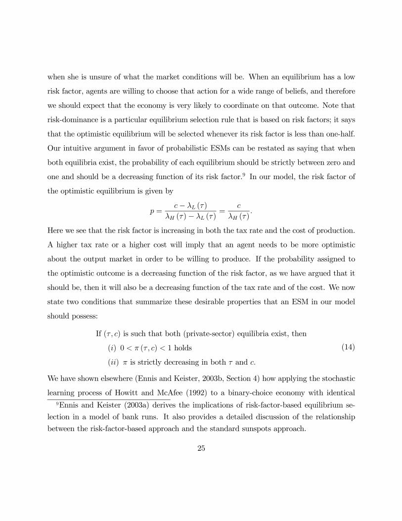
when she is unsure of what the market conditions will be. When an equilibrium has a low

risk factor, agents are willing to choose that action for a wide range of beliefs, and therefore

we should expect that the economy is very likely to coordinate on that outcome. Note that

risk-dominance is a particular equilibrium selection rule that is based on risk factors; it says

that the optimistic equilibrium will be selected whenever its risk factor is less than one-half.

Our intuitive argument in favor of probabilistic ESMs can be restated as saying that when

both equilibria exist, the probability of each equilibrium should be strictly between zero and

one and should be a decreasing function of its risk factor.9 In our model, the risk factor of

the optimistic equilibrium is given by

p =c− λL (τ)

λH (τ)− λL (τ) =c

λH (τ).

Here we see that the risk factor is increasing in both the tax rate and the cost of production.

A higher tax rate or a higher cost will imply that an agent needs to be more optimistic

about the output market in order to be willing to produce. If the probability assigned to

the optimistic outcome is a decreasing function of the risk factor, as we have argued that it

should be, then it will also be a decreasing function of the tax rate and of the cost. We now

state two conditions that summarize these desirable properties that an ESM in our model

should possess:

If (τ , c) is such that both (private-sector) equilibria exist, then

(i) 0 < π (τ , c) < 1 holds

(ii) π is strictly decreasing in both τ and c.

(14)

We have shown elsewhere (Ennis and Keister, 2003b, Section 4) how applying the stochastic

learning process of Howitt and McAfee (1992) to a binary-choice economy with identical9Ennis and Keister (2003a) derives the implications of risk-factor-based equilibrium se-

lection in a model of bank runs. It also provides a detailed discussion of the relationship

between the risk-factor-based approach and the standard sunspots approach.

25

agents like the one we study here generates an equilibrium selection mechanism with exactly

these two properties. In the learning approach, information about the true value of the

cost c arrives gradually, and agents take actions and learn about market conditions as this

information is arriving. The coevolution of agents� beliefs about c and about market con-

ditions determines where the economy converges. In other words, which equilibrium agents

end up coordinating on depends on the actual path taken by the beliefs about c en route to

the true value. Equilibrium selection thus depends on the realization of a sequence of ran-

dom variables, and is therefore random. Rather than presenting the details of the learning

process here, we will derive the policy implications of any equilibrium selection mechanism

that satisÞes the two conditions given in (14). To keep things simple, we will assume that π

is everywhere differentiable in τ . This is stronger than is necessary, but allows us the prove

the proposition in a simple and transparent way.

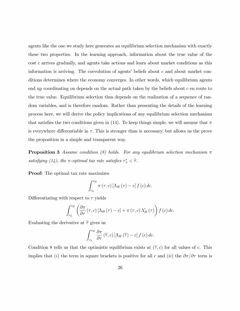
Proposition 3 Assume condition (8) holds. For any equilibrium selection mechanism π

satisfying (14), the π-optimal tax rate satisÞes τ ∗π < bτ .Proof: The optimal tax rate maximizesZ cH

cL

π (τ , c) [ΛH (τ)− c] f (c) dc.

Differentiating with respect to τ yieldsZ cH

cL

µ∂π

∂τ(τ , c) [ΛH (τ)− c] + π (τ , c)Λ0H (τ)

¶f (c) dc.

Evaluating the derivative at bτ gives usZ cH

cL

∂π

∂τ(bτ , c) [ΛH (bτ)− c] f (c) dc.

Condition 8 tells us that the optimistic equilibrium exists at (bτ , c) for all values of c. Thisimplies that (i) the term in square brackets is positive for all c and (ii) the ∂π/∂τ term is

26

negative for all c. Therefore, the entire derivative is negative and the optimal tax rate must

be less than bτ . ¥

The point of Propositions 2 and 3 can be summarized as follows. When higher tax rates

adversely affect the process of equilibrium selection, ignoring the issue of multiplicity of

equilibrium will lead to the wrong policy conclusion. In such cases, there is an additional

cost of taxation that a standard equilibrium analysis will not recognize. Even though the tax

rate bτ is (weakly) optimal in each of the private-sector equilibria separately, the propositionsshow that the true optimal tax rate must be less than bτ .4 A Public Employment Policy

In previous sections, we showed how taking equilibrium selection effects into account can

change the optimal level of a policy variable. In this section, we show how these effects also

tend to inßuence the types of instruments that are used as part of the optimal policy. To

demonstrate this, we give the government a second policy tool: it can produce the public

good by employing a fraction of the agents in the economy and directing their production

and search decisions. We use ψ to denote this fraction, and we refer to these agents as the

public sector. We assume that the government must choose ψ at the same time that it sets

the tax rate τ , before the cost of production c is known and before private agents make their

production decisions. However, the government chooses the search intensity of public sector

agents γG later, at the time that private agents set their search intensity. In other words,

while τ and ψ are policies that must be set in advance, the level of γG can be adjusted to

the ex-post situation in the economy. We think that this treatment of the decision-making

process captures an important feature of the actual situations faced by policy makers: some

policy instruments are more ßexible while others must be set in advance and hence require

27

making predictions about future market outcomes.

If the public sector were assumed to be as efficient as the private sector, the optimal policy

would involve having a large public sector (thereby reducing the fraction of the economy

subject to coordination failures) and not using taxation. This would not be very interesting.

Our goal is to show that even a very inefficient public employment/production policy �

one that would never be used based on a standard equilibrium analysis � can be part of

the optimal policy when equilibrium selection effects are considered. We therefore assume

that public sector agents are relatively inefficient in the production of the public good. In

particular, when a public sector agent is matched in the output market, only a fraction σ < 1

of the output she receives in trade is transformed into the public good; the rest is lost. In

our example below, we will set σ at a fairly low level so that, in general, taxation is the most

efficient way of providing the public good.

An important difference between taxation and public production is the effect these poli-

cies have on the value of producing for private agents. As we have shown above, taxation

decreases the value of producing. Public production, on the other hand, can increase this

value, especially in the case where no other private agents produce. When an agent is decid-

ing whether or not to produce, she may be unsure about the actions of other private agents,

but she knows that at least the ψ public agents will be in the market. Thus the public

employment policy can achieve something that the tax policy cannot: it can decrease the

potential loss associated with having produced when no one else has. Because these losses

never happen in equilibrium, this beneÞt of the policy is not captured in a simple equilib-

rium analysis or when equilibrium selection follows a payoff-insensitive rule. However, when

equilibrium selection is sensitive to individual incentives (as reßected in the risk factors),

this beneÞt implies that public production increases rather than decreases the probability of

reaching the optimistic equilibrium outcome. Combined with the lower optimal tax rate (see

28

the previous section) and the resulting higher marginal utility of the public good, this prop-

erty makes public production much more attractive, and in our example makes the optimal

level of such production positive. Hence the set of policy instruments used when equilibrium

selection issues are taken into consideration can be different than those prescribed by an

analysis that ignores the selection problem.

For the sake of simplicity, we assume that the government randomly chooses the agents

who will comprise the public sector and that it does not compensate them. In a more realistic

situation the government would compensate public sector agents to make them indifferent

between public-sector and private-sector work. We work with the former case because it is

notationally much simpler, and does not change the main message. In either case, a natural

objective for the government is to maximize the integral of all agents� utilities (where all

agents are equally weighted), which in our setting is the same as maximizing the expected

utility of an agent before she is assigned to the public or private sector.

It is worth pointing out here that the public production policy makes it possible for the

government to eliminate the pessimistic outcome as an equilibrium. If the public sector is

made large enough, there will be enough output-market activity to induce a private agent

to produce and search regardless of the actions of other private agents. However, having a

large public sector is costly, both because public production is inefficient and because there

is diminishing marginal utility of the public good. For most parameter values, eliminating

the pessimistic equilibrium is not optimal; expected utility is higher when the Pareto-inferior

outcome is allowed to occur with positive probability.10

10This point seems relevant for the type of research undertaken by Chatterjee and Corbae

(2000). They study the potential gains of eliminating the possibility of events like the Great

Depression in the U.S. The authors correctly point out that their calculation does not take

into account the cost of implementing the policies that would eliminate these Depression-

like episodes. We show that when the choice of policies is studied explicitly, it may not be

29

The timing of events is as follows. The government Þrst chooses the pair (ψ, τ). Then the

cost of production c is revealed and agents decide whether to produce or not. Finally both

the government and the agents chose their search intensities. If the economy has a unique

private-sector equilibrium, this is equivalent to saying that the government chooses ψ and

τ before uncertainty about c is revealed and then chooses γG as a Stackelberg leader in the

determination of the public and private levels of search intensity. If there is more than one

such equilibrium, it also means that the government must choose the policies (ψ, τ) before

it knows what the level of aggregate demand will be for each possible value of c.

In the Appendix, we describe how to compute the two equilibrium outcomes for given

values of (ψ, τ) and c. We denote the welfare level in the optimistic outcome by UH (ψ, τ ; c)

and that in the pessimistic outcome by UL (ψ; c). These functions reßect the optimal decision

rules of: (i) private agents, who choose whether to produce or not, and if producing, the

optimal level of search intensity, and (ii) the government, which chooses the search intensity

γG to maximize welfare in a given private-sector equilibrium.

We now discuss how the government determines the optimal policy pair (ψ, τ). We

concentrate on this stage because it is where the equilibrium selection issues arise. Suppose

that the government completely ignores the question of equilibrium selection and simply

assumes that the optimistic outcome will always obtain. Then the government chooses ψ

and τ to maximize Z cH

cL

UH (ψ, τ ; c) f(c)dc.

Let (bψ,bτ) be the solution to this problem.11 Alternatively, when the government believesoptimal to fully eliminate the possibility of these types of events. See Dagsvik and Jovanovic

(1994) for a study where a coordination failure of the type we examine here is considered to

represent a Depression-like episode.11Later, we will choose parameter values such that λH(bψ,bτ) > cH holds, and therefore the

30

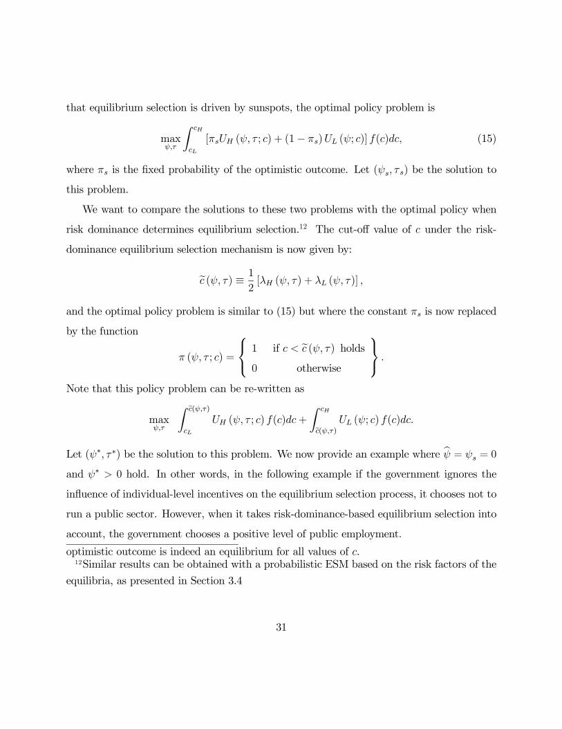
that equilibrium selection is driven by sunspots, the optimal policy problem is

maxψ,τ

Z cH

cL

[πsUH (ψ, τ ; c) + (1− πs)UL (ψ; c)] f(c)dc, (15)

where πs is the Þxed probability of the optimistic outcome. Let (ψs, τ s) be the solution to

this problem.

We want to compare the solutions to these two problems with the optimal policy when

risk dominance determines equilibrium selection.12 The cut-off value of c under the risk-

dominance equilibrium selection mechanism is now given by:

ec (ψ, τ) ≡ 1

2[λH (ψ, τ) + λL (ψ, τ)] ,

and the optimal policy problem is similar to (15) but where the constant πs is now replaced

by the function

π (ψ, τ ; c) =

1

0

if c < ec (ψ, τ) holdsotherwise

.Note that this policy problem can be re-written as

maxψ,τ

Z ec(ψ,τ)cL

UH (ψ, τ ; c) f(c)dc+

Z cH

ec(ψ,τ) UL (ψ; c) f(c)dc.

Let (ψ∗, τ ∗) be the solution to this problem. We now provide an example where bψ = ψs = 0and ψ∗ > 0 hold. In other words, in the following example if the government ignores the

inßuence of individual-level incentives on the equilibrium selection process, it chooses not to

run a public sector. However, when it takes risk-dominance-based equilibrium selection into

account, the government chooses a positive level of public employment.

optimistic outcome is indeed an equilibrium for all values of c.12Similar results can be obtained with a probabilistic ESM based on the risk factors of the

equilibria, as presented in Section 3.4

31

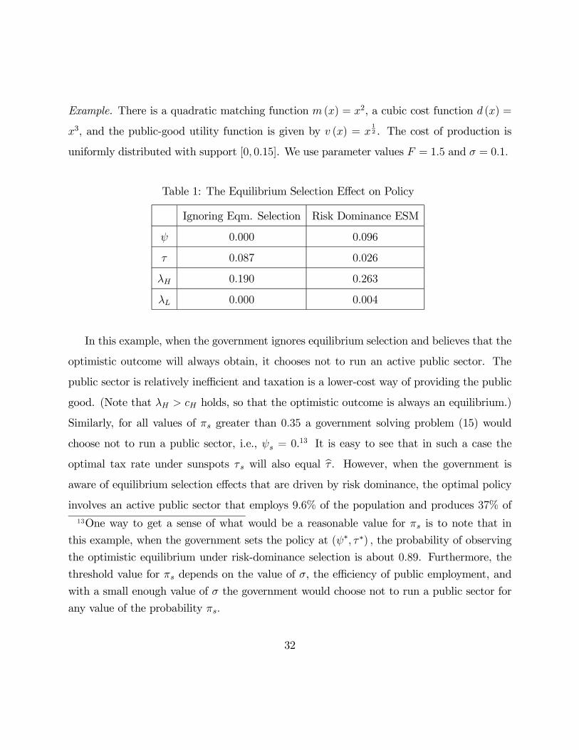
Example. There is a quadratic matching function m (x) = x2, a cubic cost function d (x) =

x3, and the public-good utility function is given by v (x) = x12 . The cost of production is

uniformly distributed with support [0, 0.15]. We use parameter values F = 1.5 and σ = 0.1.

Table 1: The Equilibrium Selection Effect on Policy

Ignoring Eqm. Selection Risk Dominance ESM

ψ 0.000 0.096

τ 0.087 0.026

λH 0.190 0.263

λL 0.000 0.004

In this example, when the government ignores equilibrium selection and believes that the

optimistic outcome will always obtain, it chooses not to run an active public sector. The

public sector is relatively inefficient and taxation is a lower-cost way of providing the public

good. (Note that λH > cH holds, so that the optimistic outcome is always an equilibrium.)

Similarly, for all values of πs greater than 0.35 a government solving problem (15) would

choose not to run a public sector, i.e., ψs = 0.13 It is easy to see that in such a case the

optimal tax rate under sunspots τ s will also equal bτ . However, when the government isaware of equilibrium selection effects that are driven by risk dominance, the optimal policy

involves an active public sector that employs 9.6% of the population and produces 37% of13One way to get a sense of what would be a reasonable value for πs is to note that in

this example, when the government sets the policy at (ψ∗, τ ∗) , the probability of observing

the optimistic equilibrium under risk-dominance selection is about 0.89. Furthermore, the

threshold value for πs depends on the value of σ, the efficiency of public employment, and

with a small enough value of σ the government would choose not to run a public sector for

any value of the probability πs.

32

the public good in the optimistic equilibrium. This demonstrates how taking into account

(risk-factor-based) incentives in the equilibrium selection process can have a signiÞcant effect

on the types of policies that are optimal for a government to use. ¤

5 Concluding Remarks

The above analysis has illustrated what we think is a fairly general property of equilibrium

selection in environments where aggregate demand matters: Policies that reduce the value

to an individual agent of participating in the market will make it less likely that agents

coordinate on a high-market-activity equilibrium. We have shown that risk-factor-based

equilibrium selection mechanisms have clear policy implications: Taking equilibrium selection

into account reveals policies like taxation to be more costly than a simple equilibrium analysis

would indicate, and therefore such policies should be used less. If the government has a

variety of tools available, taking selection effects into account will lead it to substitute away

from the ones that decrease the value of producing and toward the ones that do not, even

if the latter are inefficient from the standard equilibrium viewpoint. We also intend for

the analysis to make a larger point: By taking a stand on the properties of the equilibrium

selection process, one can derive meaningful predictions and policy prescriptions from models

with multiple equilibria.

Our result in Section 4 with respect to public employment is reminiscent of a colorful

suggestion by Keynes (1936, p. 129).

If the Treasury were to Þll old bottles with banknotes, bury them at suitable depthsin disused coal mines which are then Þlled up to the surface with town rubbish, andleave it to private enterprise on well-tried principles of laissez-faire to dig the notesup again (the right to do so being obtained, of course, by tendering for leases of thenote-bearing territory), there need be no more unemployment and, with the help ofthe repercussions, the real income of the community, and its capital wealth also, would

33

probably become a good deal greater than it actually is. (Emphasis added.)14

In other words, Keynes suggests that the government undertake a costly activity solely in

order to increase the beneÞt to private agents of engaging in market activity. This seems

difficult to justify from a traditional equilibrium point of view. While encouraging agents

to choose higher search intensities does improve the efficiency of the output market, it is

hard to believe that the multiplier effect could possibly be large enough to justify the initial

(entirely wasteful) outlay. It seems likely to us that Keynes instead believed that government

policy could be used to direct the economy toward a good equilibrium (as in the quote from

Diamond (1982) in our introduction). Viewed in this light, such a policy recommendation

seems less absurd. Perhaps it is just an exaggerated way of making our same point: policies

that encourage market activity are more likely to bring about coordination on outcomes with

high levels of market activity.

Appendix: Computing Equilibria with Public Employ-ment

In this appendix, we describe how to compute an equilibrium of the economy for a given

policy (ψ, τ) and a cost of production c. The economy�s average level of search intensity is

given by

γ = ψγG +

Z 1−ψ

0

φiγidi,

and the total amount of the public good provided in equilibrium is equal to

x = ψργGσ + τ

Z 1−ψ

0

ρφiγidi.

14We thank Tom Humphrey for bringing this passage to our attention.

34

The optimal decision rules of a private agent are still given by (4) and (5). We again only

consider symmetric outcomes, so that either all private agents produce and search at intensity

γH or no private agent produces.

In the optimistic outcome, when private agents produce, the total amount of search

intensity in the market is given by γ = (1− ψ) γH + ψγGH , and the probability of beingmatched per unit of search intensity is given by

ρ(γH , γGH ,ψ) =m ((1− ψ) γH + ψγGH)(1− ψ) γH + ψγGH

.

We can Þnd the equilibrium search intensity by inserting ρ(γH , γGH ,ψ) into (5) and solving

for γH . This intensity is a function of the policy parameters, and we denote it γH(γG,ψ, τ).

DeÞne also the function ρH(γG,ψ, τ) ≡ ρ(γH(γG,ψ, τ), γG,ψ). Welfare in this case is givenby

UH = (1− ψ) [λH − c] + ψ [−d (γG)− c] + v (xH) ,

where we have xH = (1− ψ) τρHγH + ψσρHγG, and λH = ρHγH(1 − τ)F − d(γH). Usingthe deÞnitions of γH(γG,ψ, τ) and ρH(γG,ψ, τ) given above, we can obtain the function

UH(γG,ψ, τ ; c) that gives agents� expected utility as a function of the policy parameters.

The government then chooses the public sector�s search intensity in the optimistic outcome

to maximize the function UH(γG,ψ, τ ; c). The solution is given by

γGH(ψ, τ) = argmaxUH(γG,ψ, τ ; c).

The optimistic outcome is an equilibrium as long as λH (ψ, τ) > c holds.

In the pessimistic outcome, when no private agent produces, the total level of search

intensity is given by γ = ψγG and the average probability of being matched is given by

ρL (γG,ψ) =m (ψγG)

ψγG.

35

Welfare is then given by UL (γG,ψ; p) = ψ (−d (γG)− c)+v¡ρL¡γG,ψ

¢ψγGσ

¢. Since private

agents do not produce, welfare is equal to the utility provided by the public good minus the

production and search costs of the public sector agents. The government chooses the search

intensity γG according to

γGL(ψ) = argmaxUL (γG,ψ; c) .

Note that γGL is only a function of the size of the public sector ψ. Since private agents are

not producing, the tax policy is irrelevant in this outcome.

For given values of (ψ, τ) and c, the pessimistic outcome is an equilibrium whenever

a private agent who believes that the average probability of being matched is equal to

ρL (ψ) ≡ ρL (γGL(ψ),ψ) decides not to produce. If she were to produce, she would set hersearch intensity to

γL(ψ, τ) = d0−1 (ρL (ψ) (1− τ)F ) ,

and her expected beneÞt from producing would be given by

λL (ψ, τ) = ρL (ψ) γL(ψ, τ)(1− τ)F − d (γL(ψ, τ)) .

If λL (τ ,ψ) < c holds, then the expected beneÞt of producing is lower than the cost, she

would choose not to produce, and the pessimistic outcome is an equilibrium. However, if

the government sets (τ ,ψ) so that λL (τ ,ψ) > c holds for a given c, then even an agent with

pessimistic beliefs would choose to produce and therefore such beliefs are not self-fulÞlling.

In other words, the policy has eliminated the pessimistic outcome as an equilibrium and only

the optimistic outcome is possible. However, notice that even if the government recruits all

of the agents in the economy (so that ψ = 1), the value of ρ only reaches m(γG)γG

< 1. Hence

there is a bound on the ability of the government to increase λL, and it may be the case that

36

no level of ψ can eliminate the pessimistic equilibrium for some realizations of c.

References

Carlsson, Hans, and Eric van Damme, 1993, Global Games and Equilibrium Selection, Econo-

metrica 59, 1487-1496.

Cass, David, and Karl Shell, 1983, Do Sunspots Matter?, Journal of Political Economy 91,

193-227.

Chatterjee, Satyajit, and Dean Corbae, 2000, On the Welfare Gains of Reducing the Likeli-

hood of Economic Crises, Working Paper No. 00-14, Federal Reserve Bank of Philadelphia,

November.

Cooper, Russell, 1999, Coordination Games: Complementarities andMacroeconomics, (Cam-

bridge University Press, Cambridge, UK).

Cooper, Russell, and Dean Corbae, 2002, Financial Collapse: A Lesson from the Great

Depression, Journal of Economic Theory 107, 159-190.

Cooper, Russell, and Andrew John, 1988, Coordinating Coordination Failures in Keynesian

Models, Quarterly Journal of Economics 103, 441-463.

Dagsvik, John, and Boyan Jovanovic, 1994, Was the Great Depression a Low-Level Equilib-

rium?, European Economic Review 38, 1711-1729.

Diamond, Peter, 1982, Aggregate Demand Management in Search Equilibrium, Journal of

Political Economy 90, 881-894.

Ennis, Huberto, and Todd Keister, 2003a, Economic Growth, Liquidity, and Bank Runs,

Journal of Economic Theory 109, 220-245.

Ennis, Huberto, and Todd Keister, 2003b, Government Policy and the Probability of Coor-

dination Failures, European Economic Review, forthcoming.

37

Grandmont, Jean Michel, 1986, Stabilizing Competitive Business Cycles, Journal of Eco-

nomic Theory 40, 57-76.

Harsanyi, John, and Reinhard Selten, 1988, A General Theory of Equilibrium Selection in

Games (MIT Press, Cambridge, MA).

Howitt, Peter, and R. Preston McAfee, 1992, Animal Spirits, American Economic Review

82, 493-507.

Keister, Todd, 1998, Money Taxes and Efficiency when Sunspots Matter, Journal of Eco-

nomic Theory 83, 43-68.

Keynes, John Maynard, 1936, The General Theory of Employment, Interest, and Money,

(Harcourt, Brace & World, New York, NY).

Lagos, Ricardo, 2000, An Alternative Approach to Search Frictions, Journal of Political

Economy 108, 851-873.

Morris, Stephen, Rafael Rob, and Hyun Song Shin, 1995, p-Dominance and Belief Potential,

Econometrica 63, 145-157.

Ochs, Jack, 1995, Coordination Problems, in: J. H. Kagel and A. E. Roth, eds., The Hand-

book of Experimental Economics (Princeton University Press, Princeton, NJ) 195-252.

Reichlin, Pietro, 1986, Equilibrium Cycles in an Overlapping Generations Economy with

Production, Journal of Economic Theory 40, 89-102.

Smith, Bruce, 1991, Interest on Reserves and Sunspot Equilibria: Friedman�s Proposal Re-

considered, Review of Economic Studies 58, 93-105.

Van Huyck, John, Raymond Battalio, and Richard Beil, 1990, Tacit Coordination Games,

Strategic Uncertainty, and Coordination Failure, American Economic Review 80, 234-248.

Van Huyck, John, Raymond Battalio, and Richard Beil, 1991, Strategic Uncertainty, Equi-

librium Selection Principles, and Coordination Failure in Average Opinion Games, Quarterly

38

Journal of Economics 106, 885-910.

Woodford, Michael, 1986, Stationary Sunspot Equilibria in a Finance Constrained Economy,

Journal of Economic Theory 40, 128-137.

Woodford, Michael, 1994, Introduction to the Symposium: Determinacy of Equilibrium

under Alternative Policy Regimes, Economic Theory 4, 326.

Young, Peyton, 1998, Individual Strategy and Social Structure (Princeton University Press,

Princeton, NJ).

39