Comparing Cournot and Bertrand Equilibria in a

Differentiated Duopoly with Product R&D

George Symeonidis

University of Essex

Abstract: This paper compares Bertrand and Cournot equilibria in a differentiated

duopoly with substitute goods and product R&D. I find that R&D expenditure, prices

and firms’ net profits are always higher under quantity competition than under price

competition. Furthermore, output, consumer surplus and total welfare are higher in the

Bertrand equilibrium than in the Cournot equilibrium if either R&D spillovers are

weak or products are sufficiently differentiated. If R&D spillovers are strong and

products are not too differentiated, then output, consumer surplus and total welfare are

lower in the Bertrand case than in the Cournot case. Thus a key finding of the paper is

that there are circumstances where quantity competition can be more beneficial than

price competition both for consumers and for firms.

Keywords: Product R&D, price versus quantity competition, welfare.

JEL classification: L13, D43.

Address for correspondence: Department of Economics, University of Essex,

Wivenhoe Park, Colchester CO4 3SQ, U.K.

Phone: +44 1206 872511, fax: +44 1206 872724, e-mail: symeonid@essex.ac.uk

brought to you by COREView metadata, citation and similar papers at core.ac.uk

provided by University of Essex Research Repository

1

1. Introduction.

The standard view that Bertrand competition is more efficient than Cournot

competition has recently been challenged by a number of theoretical models. A

common feature of these models is the idea that firms compete both in variables that

can be easily changed in the short run, such as price or output, and in variables that

constitute longer-term commitments, such as capacity or R&D expenditure. Much of

this literature has specifically focused on expenditure in process R&D as the long-run

decision variable. Product R&D, although empirically more important (see Scherer

and Ross 1990), has received little attention in these studies.

This paper compares Bertrand and Cournot equilibria in a differentiated

duopoly with substitute goods and product R&D. Vives (1985) and Singh and Vives

(1984) found that Bertrand competition results in higher consumer surplus, lower

profits and higher overall welfare than Cournot competition in a duopoly model where

goods are substitutes and the firms’ only choice variable is either price or output.

Motta (1993) found price competition to result in higher consumer surplus, profits and

overall welfare than quantity competition in the context of a vertically differentiated

duopoly with either fixed or variable costs of quality improvement. Although the case

of fixed costs of quality improvement can be naturally interpreted as product R&D,

the study by Motta did not allow for R&D spillovers. On the other hand, Delbono and

Denicolo (1990) found that the welfare comparison between Bertrand and Cournot is

generally ambiguous in the context of a homogeneous product duopoly with process

R&D in the form of a patent race, although R&D investment is higher in the Bertrand

equilibrium (in fact, it is even higher than the socially optimal level). Finally, Qiu

(1997), who used the Singh and Vives (1984) linear demand structure but introduced

a stage of process R&D competition prior to the price or quantity-setting stage, found

2

that R&D expenditure is higher under Cournot than under Bertrand; that the opposite

is true for consumer surplus; that the Bertrand equilibrium is more efficient than the

Cournot equilibrium if either R&D productivity is low, or spillovers are weak, or

products are very differentiated; and that the Bertrand equilibrium is less efficient

than the Cournot equilibrium if R&D productivity is high, spillovers are strong, and

products are close substitutes.1

This paper addresses these issues in the context of a model with both

horizontal and vertical product differentiation, the latter of which is due to product

R&D. An important difference between process and product R&D is that the latter

directly affects gross consumer surplus. This is because product R&D raises product

quality, and quality enters directly into each consumer’s utility function. On the other

hand, process R&D affects gross consumer surplus only indirectly, through a

reduction in marginal cost and a consequent increase in output. Thus it is not clear

whether the results from models with process R&D carry over to the case of product

R&D. Moreover, the present model differs from models of ‘pure vertical

differentiation’, such as the one used by Motta (1993), in important ways, including

key properties of the firms’ profit functions, as will be explained in the next section. It

is therefore also an open question whether the existing results from the literature on

vertical product differentiation are robust to alternative ways of introducing quality

into the utility function.

1 Bester and Petrakis (1993), who also analysed a game of investment in process R&D

using a linear demand structure, obtained results different from those of Qiu (1997)

because in their model only one firm was allowed to invest in R&D.

3

I analyse here a variant of the standard linear demand model. In particular, I

use the quality-augmented linear demand structure proposed by Sutton (1997, 1998),

and I also introduce a cost structure that allows for R&D spillovers. I also check the

robustness of my results to alternative demand systems and R&D cost functions. I

find that R&D expenditure, prices and firms’ net profits are always higher under

quantity competition than under price competition. Furthermore, output, consumer

surplus and total welfare are higher in the Bertrand equilibrium than in the Cournot

equilibrium if either R&D spillovers are weak or products are sufficiently

differentiated. If R&D spillovers are strong and products are not too differentiated,

then output, consumer surplus and total welfare are lower in the Bertrand case than in

the Cournot case.

Some of these results are consistent with those obtained by Qiu (1997) in the

context of a model with process R&D. There are also, however, important differences.

Under process R&D, consumer surplus is always higher under Bertrand competition,

just as in Singh and Vives (1984), but the overall efficiency comparison of the two

regimes is ambiguous, presumably because Cournot profits can be a lot higher than

Bertrand profits, thus causing the ambiguity. On the other hand, in the present model

of product R&D, the overall welfare comparison is also ambiguous, but for different

reasons. In particular, not only profits but also consumer surplus can be higher in the

Cournot equilibrium; this will occur if both R&D spillovers are strong and the goods

are not too differentiated. This is a new result and suggests that both consumers and

producers can be better off under quantity competition than under price competition.

4

2. The Model.

Consider a duopoly where each firm produces one variety of a differentiated product.

Firms invest in R&D in order to enhance product quality. More specifically,

competition in the industry is described by a two-stage game as follows. At stage 1

each firm chooses a variety, described by a vertical attribute u that I will call ‘quality’

and is associated with some physical product characteristic. Quality increases the

consumers’ willingness to pay for the firm’s variety, but it comes at a cost, namely

expenditure on product R&D. At stage 2 the firms set quantities or prices.

The structure of this game reflects the fact that (i) decisions on R&D

expenditure involve significant sunk costs and (ii) product characteristics cannot be

changed as easily or as quickly as price or quantity choices. However, I abstract from

issues of uncertainty regarding the outcome of R&D projects, as do many models

within the general class of ‘non-tournament’ models of R&D rivalry, of which the

present model is an example. The key underlying assumption of these models, as

opposed to the literature on patent races, is that each firm can achieve product or

process improvements through its R&D expenditure without preventing other firms

from obtaining equivalent benefits from their own R&D.

There are S identical consumers, and the utility function of each consumer

takes the form

Mux

ux

u

x

u

xxxU

j

j

i

i

j

j

i

iji +−−−+= σ2

2

2

2

, (1)

following Sutton (1997, 1998) (see also Symeonidis 1999, 2000). Note that (1) is a

quality-augmented version of the standard quadratic utility function used, among

others, by Singh and Vives (1984), Vives (1985), and Qiu (1997). Thus xi and ui are,

respectively, the quantity and quality of variety i and jjii xpxpYM −−= denotes

5

expenditure on outside goods. This utility function implies that each consumer spends

only a small part of her income on the industry’s product (which also ensures that the

maximisation of U has an interior solution) and hence income effects on the industry

under consideration can be ignored and partial equilibrium analysis can be applied.

The parameter σ, σ∈ (0,2), is an (exogenous) inverse measure of the degree of

horizontal product differentiation: in the limit as σ → 0 the goods become

independent, while in the limit as σ → 2 they become perfect substitutes when ui = uj.

The inverse demand function of each consumer for variety i is given by

,,2,1,,2

1 2 jijiu

x

uu

xp

j

j

ii

ii ≠=−−=

σ(2)

in the region of quantity spaces where prices are positive. The demand function is

,,2,1,,)2)(2(

)1()1(2jiji

pupu

u

x jjii

i

i ≠=+−

−−−=

σσσ

(3)

in the region of prices where quantities are positive. It can be easily seen that xi is

decreasing in pi and increasing in ui. Also, it is increasing in pj and decreasing in uj.

An attractive feature of the present model – and one that distinguishes it from models

of ‘pure vertical differentiation’, which do not have this property – is that it gives rise

to reduced-form profit functions where (gross) profit increases in own quality and

decreases in rival quality (see below). Since there are S consumers, firm i sells

quantity Sxi. Let each firm have a constant marginal cost of production c, where c < 1.

Admittedly, the demand system used in this paper is rather specific. To check

the robustness of my results with respect to other specifications of demand, I analyse

in the appendix an alternative extension of the quadratic utility model, following

Häckner (2000). The results from this alternative demand system are very similar to

6

those presented in the main body of the paper: all the propositions proved below are

robust to the choice of demand specification.

The function linking quality ui to R&D expenditures Ri and Rj is a modified

version of the one used by Motta (1992) and is given by ui = ,4/14/1ji RR ερε + where ε, ε

> 0, is an inverse measure of the cost of R&D or an index of technological

opportunity in the industry and ρ, ρ∈ [0,1], captures the extent of technological

spillovers. Both these parameters are industry-specific and exogenously determined

by technology. Note that the above function implies that there are decreasing returns

to R&D. This assumption, which is very common in this class of models, is necessary

if the second-order condition for an interior maximum in the R&D stage is to be

satisfied.2 Apart from that assumption, the particular form of the R&D cost function is

not crucial: for instance, none of the results reported below changes if one uses the

function ui = 3/13/1ji RR ερε + instead, although the model becomes analytically more

complicated.

The use of the R&D cost function ui = 4/14/1ji RR ερε + to model R&D spillovers

is based on the commonly made assumption that the spillovers take place in R&D

2 As pointed out in Sutton (1998), the economics of this model depends only on the

composite mapping from firms’ fixed costs to firms’ gross profits, rather than on the

separate mappings of fixed costs to qualities and from qualities to gross profits. Thus

the results would not change if we replaced u by uγ, γ > 0, in the utility function and

modified the R&D cost function accordingly so that the second-order condition for an

interior maximum in the R&D stage were always satisfied. Under this more general

formulation, both gross profit and R&D cost could be either concave or convex in u,

although gross profit would still need to be concave in R&D cost.

7

outcomes. An alternative approach is to regard spillovers as taking place in R&D

inputs or expenditures (see Amir 2000 for a comparison of the two approaches). To

check whether the results of the present paper are robust to the choice of approach to

modelling spillovers I also analysed a version of the model using the alternative R&D

cost function ui = 4/1)( ji RR ρε + .3 The results were very similar to those reported

below: none of the propositions proved in the paper are affected by the choice of

R&D cost function.

A symmetric subgame-perfect equilibrium in pure strategies in the two-stage

game can be easily computed. In the next two sections this equilibrium is

characterised first for the quantity-setting (Cournot) case and then for the price-setting

(Bertrand) case.

3. Cournot Equilibrium.

When firms set quantities in the final-stage subgame, firm i chooses xi to maximise

,,2,1,2

1)( 2 ijixcuu

x

u

xSxcpS i

ji

j

i

iiii ≠=

−−−=−=

σπ

in the regions where prices and quantities are positive. In the Cournot-Nash

equilibrium we have

,,2,1,)4()4(

)4()1(2,

)4)(4(

)4()1(22

22

ijiuucSuuuc

x jiCi

jiiCi ≠=

+−

−−=

+−

−−=

σσ

σπ

σσσ

(4)

in the region of quality spaces where xi and xj are both positive, i.e. for ui/uj < 4/σ, i =

1,2, j ≠ i. Note that if this condition did not hold, then one of the two firms

(specifically, the low-quality one) would have zero sales and the other would make

3 I am indebted to a referee for suggesting this alternative R&D cost function.

8

monopoly profit 8)1( 22 ucSM −=π . However, this case is not relevant as a potential

equilibrium of the game: for one thing, a firm would never choose a level of R&D

that resulted in zero output, since it would then be making negative net profit.

At stage 1 each firm chooses a quality level to maximise net profit R−π ,

given the choice of the other firm. The first-order condition for firm i is

,,2,1,1 ijiRu

uRu

udRd

i

j

j

Ci

i

i

i

Ci

i

Ci ≠==

∂

∂

∂

∂+

∂

∂

∂

∂=

πππ(5)

i.e. each firm spends on R&D up to the point where the cost of an extra unit of R&D

is equal to the profit it creates in the final stage of the game. Substituting the

expressions for the various partial derivatives in (5), setting ui = ,4/14/1ji RR ερε + and

solving for the (symmetric) equilibrium, we obtain

.)4()4(

)1()4()1()1( 2/1

2/32/122/14/1

σσ

ρρσερε

+−

+−−=+=

cSRu CC (6)

The second-order condition for an interior maximum at the symmetric equilibrium is

given by 022 <∂∂ iCi Rπ when evaluated at ui = uj = uC. After some straightforward

manipulations this gives

[ ],0

)4)(4(4

)6(238)1(2

2/322

<+−

−+−−− −

σσ

σρσε CRcS

which is always true.

To compute the equilibrium price and quantity we set ui = uj = uC in (4). We

obtain:

.4

)1(2,

4

)1( 2

σσ +

−+=

+

−=

ccp

ucx C

CC (7)

9

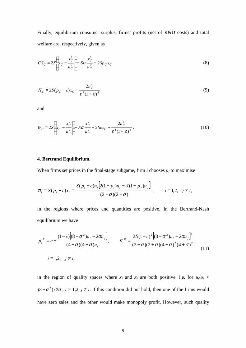
Finally, equilibrium consumer surplus, firms’ profits (net of R&D costs) and total

welfare are, respectively, given as

CCC

C

C

CCC xSp

u

xS

u

xxSCS 22 2

2

2

2

−−

−= σ (8)

44

4

)1(

2)(2

ρε +−−= C

CCC

uxcpSΠ (9)

and

44

4

2

2

2

2

)1(

222

ρεσ

+−−−

−= C

CC

C

C

CCC

uScx

u

xS

u

xxSW . (10)

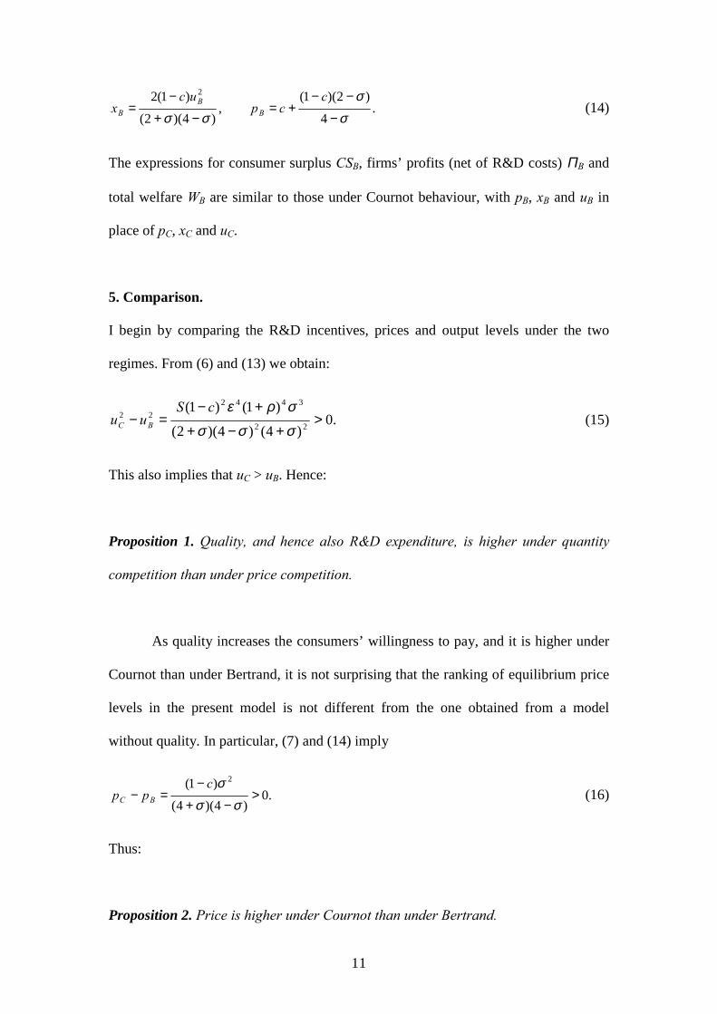
4. Bertrand Equilibrium.

When firms set prices in the final-stage subgame, firm i chooses pi to maximise

[ ],,2,1,

)2)(2(

)1()1(2)()( iji

upupucpSxcpS

jjiiiiiii ≠=

+−

−−−−=−=

σσ

σπ

in the regions where prices and quantities are positive. In the Bertrand-Nash

equilibrium we have

[ ] [ ]

,,2,1

,)4()4)(2)(2(

2)8()1(2,

)4)(4(

2)8()1(22

2222

iji

uucSu

uuccp jiB

ii

jiBi

≠=

+−+−

−−−=

+−

−−−+=

σσσσ

σσπ

σσσσ

(11)

in the region of quality spaces where xi and xj are both positive, i.e. for ui/uj <

σσ 2/)8( 2− , i = 1,2, j ≠ i. If this condition did not hold, then one of the firms would

have zero sales and the other would make monopoly profit. However, such quality

10

configurations can be ruled out (see the discussion in the previous section), so the

above condition is always met in the two-stage game.

At stage 1 each firm chooses a quality level to maximise net profit R−π ,

given the choice of the other firm. The first-order condition for firm i is

ijiRu

uRu

udRd

i

j

j

Bi

i

i

i

Bi

i

Bi ≠==

∂

∂

∂

∂+

∂

∂

∂

∂= ,2,1,1

πππ. (12)

Substituting the expressions for the various partial derivatives in (12), setting ui

= ,4/14/1ji RR ερε + and solving for the (symmetric) equilibrium, we obtain

.)2()4)(4(

)1()28()1()1( 2/12/1

2/32/1222/14/1

σσσ

ρρσσερε

++−

+−−−=+=

cSRu BB (13)

The second-order condition for an interior maximum at the symmetric equilibrium is

given by 022 <∂∂ iBi Rπ when evaluated at ui = uj = uB. This simplifies to

[ ].0

)2)(2()4()4(4

)3424()38(2)28()1(22

2/322222

<+−+−

−−+−−−−−− −

σσσσ

σσρσσρσσε BRcS

This condition is satisfied provided 0)3424()38(2 22 >−−+−− σσρσσ , which I

assume in what follows.4

The equilibrium price and quantity are derived by setting ui = uj = uB in (11).

We obtain:

4 It is easy to check that the second-order condition always holds if 0 < σ <

2/)413( +− . If 2/)413( +− ≤ σ < 2, then for any particular value of σ, say σ0,

there is a corresponding value of ρ∈ [0,1), say ρ0, such that the second-order condition

holds for all ρ > ρ0. As σ0 increases, so does ρ0.

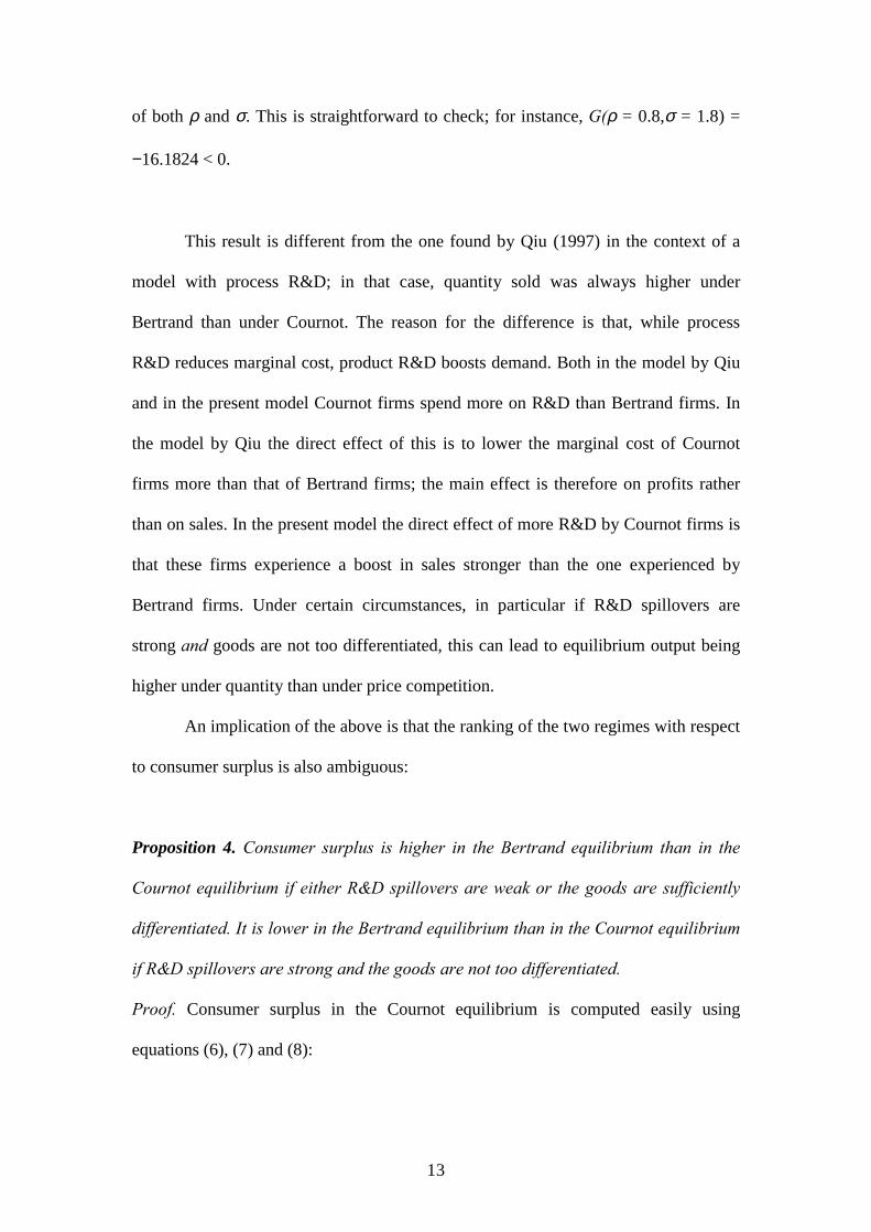
11

.4

)2)(1(,

)4)(2(

)1(2 2

σσ

σσ −

−−+=

−+

−=

ccp

ucx B

BB (14)

The expressions for consumer surplus CSB, firms’ profits (net of R&D costs) ΠB and

total welfare WB are similar to those under Cournot behaviour, with pB, xB and uB in

place of pC, xC and uC.

5. Comparison.

I begin by comparing the R&D incentives, prices and output levels under the two

regimes. From (6) and (13) we obtain:

.0)4()4)(2(

)1()1(22

344222 >

+−+

+−=−

σσσ

σρεcSuu BC (15)

This also implies that uC > uB. Hence:

Proposition 1. Quality, and hence also R&D expenditure, is higher under quantity

competition than under price competition.

As quality increases the consumers’ willingness to pay, and it is higher under

Cournot than under Bertrand, it is not surprising that the ranking of equilibrium price

levels in the present model is not different from the one obtained from a model

without quality. In particular, (7) and (14) imply

.0)4)(4(

)1( 2

>−+

−=−

σσσc

pp BC (16)

Thus:

Proposition 2. Price is higher under Cournot than under Bertrand.

12

Unlike price, there is no clear ranking of the two regimes with respect to

quantity produced. It is easy to check that, for any given quality, Bertrand firms

produce more output than Cournot firms. However, since quality is higher under

quantity competition than under price competition and high quality boosts demand,

the overall ranking is ambiguous. More specifically:

Proposition 3. Output is higher in the Bertrand equilibrium than in the Cournot

equilibrium if either R&D spillovers are weak or the goods are sufficiently

differentiated. It is lower in the Bertrand equilibrium than in the Cournot equilibrium

if R&D spillovers are strong and the goods are not too differentiated.

Proof. From equations (6), (7), (13) and (14) we obtain

[ ].

)4()4()2(

)416()316(2)1()1(332

222343

σσσ

σσρσσσρε

+−+

−+−−+−=−

cSxx CB (17)

The sign of this expression is the same as the sign of the term in brackets. Let G

denote that term; it can be positive or negative depending on the values of σ and ρ

within the range of pairs (σ,ρ) such that the second-order condition in the Bertrand

case is satisfied and ΠB > 0 (see below). It is easy to check that G(ρ = 0,σ = 0) = 32 >

0, G(ρ = 0,σ = 2) = 8 > 0, and G(ρ = 1,σ = 0) = 32 > 0. By continuity, whenever

either ρ is close or equal to 0 or σ is close to 0 (or both), we have G > 0, and hence xB

> xC. Moreover, ∂G/∂ρ = )416( 2σσσ −+− < 0 and ∂G/∂σ = )3816(12 2σσρσ −+−−

< 0 for all ρ∈ [0,1], σ∈ (0,2); that is, G decreases in both ρ and σ. To complete the

proof we only need to show that xB – xC becomes negative for sufficiently large values

13

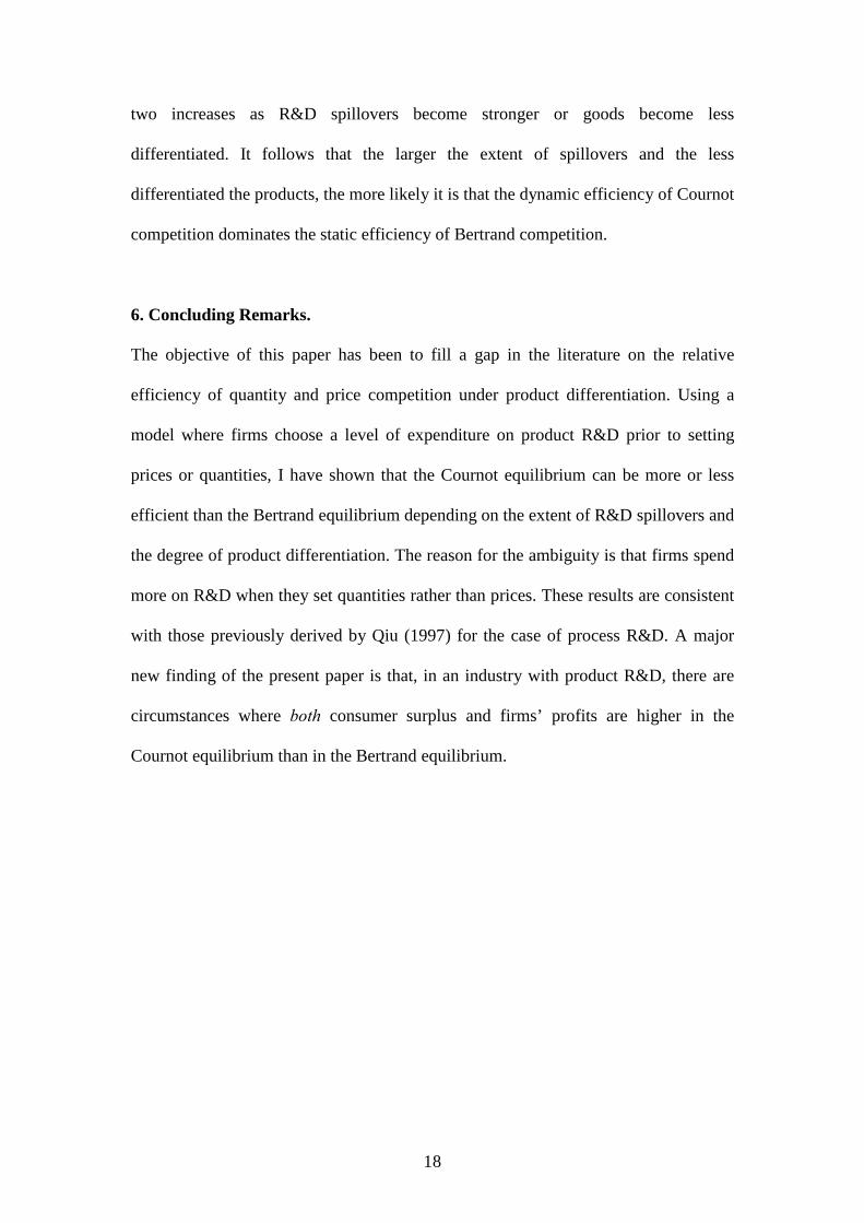
of both ρ and σ. This is straightforward to check; for instance, G(ρ = 0.8,σ = 1.8) =

−16.1824 < 0.

This result is different from the one found by Qiu (1997) in the context of a

model with process R&D; in that case, quantity sold was always higher under

Bertrand than under Cournot. The reason for the difference is that, while process

R&D reduces marginal cost, product R&D boosts demand. Both in the model by Qiu

and in the present model Cournot firms spend more on R&D than Bertrand firms. In

the model by Qiu the direct effect of this is to lower the marginal cost of Cournot

firms more than that of Bertrand firms; the main effect is therefore on profits rather

than on sales. In the present model the direct effect of more R&D by Cournot firms is

that these firms experience a boost in sales stronger than the one experienced by

Bertrand firms. Under certain circumstances, in particular if R&D spillovers are

strong and goods are not too differentiated, this can lead to equilibrium output being

higher under quantity than under price competition.

An implication of the above is that the ranking of the two regimes with respect

to consumer surplus is also ambiguous:

Proposition 4. Consumer surplus is higher in the Bertrand equilibrium than in the

Cournot equilibrium if either R&D spillovers are weak or the goods are sufficiently

differentiated. It is lower in the Bertrand equilibrium than in the Cournot equilibrium

if R&D spillovers are strong and the goods are not too differentiated.

Proof. Consumer surplus in the Cournot equilibrium is computed easily using

equations (6), (7) and (8):

14

.)4)(4(

)2()1)(4()1(4

3442

σσσρρσε

+−++−−= cSCSC (18)

Similarly, in the Bertrand equilibrium we have

.)4()4()2(

)1)(28()1(442

32442

σσσρσρσε

+−++−−−= cSCSB (19)

Hence

,)4()4()2(

)1()1(442

32442

σσσρσε+−+

+−=− HcSCSCS CB (20)

where

).61296192()72448128(4 432432 σσσσρσσσσσ +−−+−+−−+=H

The sign of CB CSCS − is the same as the sign of H: it can be positive or negative

depending on the values of σ and ρ within the range of pairs (σ,ρ) such that the

second-order condition in the Bertrand case is satisfied and ΠB > 0 (see below). We

have H(ρ = 0,σ = 0) = 512 > 0, H(ρ = 0,σ = 2) = 352 > 0, and H(ρ = 1,σ = 0) = 512 >

0. By continuity, whenever either ρ is close or equal to 0 or σ is close to 0 (or both),

we have H > 0 and BCS > CCS . Also, ∂H/∂ρ = )61296192( 432 σσσσσ +−−+− <

0 for all ρ∈ [0,1], σ∈ (0,2); that is, H decreases in ρ. On the other hand, ∂H/∂σ =

)52436192192()4214848(4 43232 σσσσρσσσ +−−+−+−− , which can be positive

or negative. But since ∂ 2H/∂σ 2 = )51848(4)37(24)4(48 322 σσρρσσσ +−−−−−−

< 0 for all ρ∈ [0,1], σ∈ (0,2), we can conclude that H first increases and then decreases

in σ. To complete the proof, then, we only need to show that CB CSCS − becomes

negative whenever ρ and σ are both sufficiently large. This is indeed the case; for

instance, H(ρ = 0.8,σ = 1.8) = −8.79846 < 0.

15

Next, we compare total net profits under the two regimes. The result is not

immediately obvious, since both gross industry profit and R&D cost are higher in the

Cournot equilibrium. Under quantity competition, we get from (6), (7) and (9)

[ ].

)4()4(

)8()2(2)1)(4()1(242

2442

σσ

σρσρρσε

+−

−+−+−−=

cSΠC (21)

Similarly, under price competition we obtain

[ ],

)4()4()2(

)8(248)1)(28()1(2242

2222442

σσσ

σσρσσρσρσε

+−+

−−+−−+−−−=

cSΠB (22)

which I assume to be positive.5 It follows that:

[ ],

)4()4()2(

)1664()1(1620128)1()1(2442

323233442

σσσ

σσρρσσσρσε

+−+

+−+−+−−+−=−

cSΠΠ BC (23)

which is positive for all ρ∈ [0,1], σ∈ (0,2). Hence:

Proposition 5. Profits net of R&D costs are higher under quantity competition than

under price competition.

As pointed out in the Introduction, Motta (1993), who also examined a model

of vertical product differentiation with fixed costs of quality improvement, found that

profits are always higher in the Bertrand rather than the Cournot equilibrium, which is

5 This is always the case if 0 < σ < 2/)31( +− . If 2/)31( +− ≤ σ < 2, then for any

particular value of σ, say σ1, there is a corresponding value of ρ∈ [0,1), say ρ1, such

that ΠB > 0 for all ρ > ρ1. As σ1 rises, so does ρ1.

16

the opposite of my result. However, Motta used a model that allows for quality

differences between firms. In that context, firms differentiate their products (i.e.

increase their quality difference), and hence ‘relax’ competition in the final-stage

subgame, more under the price-setting regime than under the quantity-setting regime.

This effect is absent from the present model, which focuses on symmetric equilibria.

Finally, we show that the overall efficiency ranking of the two regimes is

ambiguous, a result which is largely a consequence of Proposition 4:

Proposition 6. Total welfare is higher in the Bertrand equilibrium than in the Cournot

equilibrium if either R&D spillovers are weak or the goods are sufficiently

differentiated. It is lower in the Bertrand equilibrium than in the Cournot equilibrium

if R&D spillovers are strong and the goods are not too differentiated.

Proof. In the Cournot equilibrium, welfare is given by substituting equations (6) and

(7) into (10):

[ ].)4()4(

)24(216)1)(4()1(42

222442

σσσρσσρρσε

+−−+−−+−−= cSWC (24)

For the Bertrand equilibrium we get:

[ ].)4()4()2(

)12(2216)1)(28()1(2242

2222442

σσσσρσσρσρσε

+−+−+−−+−−−= cSWB (25)

Hence:

,)4()4()2(

)1()1(442

32442

σσσ

ρσε

+−+

+−=−

JcSWW CB (26)

where

).44464320()366432256(2 432432 σσσσρσσσσσ +−−+−++−−=J

17

The sign of WB – WC is the same as the sign of J: it can be positive or negative

depending on the values of σ and ρ within the range of pairs (σ,ρ) such that the

second-order condition in the Bertrand case is satisfied and ΠB > 0. Now J(ρ = 0,σ =

0) = 512 > 0, J(ρ = 0,σ = 2) = 32 > 0, and J(ρ = 1,σ = 0) = 512 > 0. By continuity,

when either ρ is close or equal to 0 or σ is close to 0 (or both), we have J > 0, and

hence WB – WC > 0. Moreover, ∂J/∂ρ = )44464320( 432 σσσσσ +−−+− < 0 and

∂J/∂σ = [ ])52640)(2(246016()4( 22 σσσρσσσ −+−+−++− < 0 for all ρ∈ [0,1],

σ∈ (0,2); that is, J decreases in both ρ and σ. To complete the proof we need to show

that WB – WC < 0 when both ρ and σ are sufficiently large. This is straightforward to

check; for instance, J(ρ = 0.8,σ = 1.8) = −287.876 < 0.

Why does the ranking of the two equilibria with respect to consumer surplus

and welfare depend on the extent of R&D spillovers and the degree of horizontal

product differentiation? Recall that in the present model it is the dynamic efficiency

of Cournot competition versus the static efficiency of Bertrand competition that

causes the ambiguity in the overall comparison of consumer surplus and welfare in

the two regimes. It is therefore not surprising that the larger the difference uC – uB, the

more likely it is that the dynamic efficiency of Cournot competition dominates the

static efficiency of Bertrand competition. Now it can be checked that ∂(uC – uB)/∂ρ >

0 and ∂(uC – uB)/∂σ > 0.6 In other words, not only is R&D expenditure higher in the

Cournot equilibrium than in the Bertrand equilibrium, but the difference between the

6 This is true independent of the particular form of the R&D cost function, i.e. it is

true also when using the function ui = 4/1)( ji RR ρε + .

18

two increases as R&D spillovers become stronger or goods become less

differentiated. It follows that the larger the extent of spillovers and the less

differentiated the products, the more likely it is that the dynamic efficiency of Cournot

competition dominates the static efficiency of Bertrand competition.

6. Concluding Remarks.

The objective of this paper has been to fill a gap in the literature on the relative

efficiency of quantity and price competition under product differentiation. Using a

model where firms choose a level of expenditure on product R&D prior to setting

prices or quantities, I have shown that the Cournot equilibrium can be more or less

efficient than the Bertrand equilibrium depending on the extent of R&D spillovers and

the degree of product differentiation. The reason for the ambiguity is that firms spend

more on R&D when they set quantities rather than prices. These results are consistent

with those previously derived by Qiu (1997) for the case of process R&D. A major

new finding of the present paper is that, in an industry with product R&D, there are

circumstances where both consumer surplus and firms’ profits are higher in the

Cournot equilibrium than in the Bertrand equilibrium.

19

APPENDIX

I analyse here an alternative version of the quality-augmented quadratic utility model,

following Häckner (2000). The structure of the game is the same as before. There are

S identical consumers, and the utility function of each consumer takes the form

MxxxxxuxuU jijijjii +−−−+= σ22 , (A1)

where the notation is the same as in section 2. The inverse demand function of each

consumer for variety i is given by

,,2,1,,2 jijixxup jiii ≠=−−= σ (A2)

in the region of quantity spaces where prices are positive. The demand function is

,,2,1,,)2)(2(

)()(2jiji

pupux jjii

i ≠=+−

−−−=

σσσ

(A3)

in the region of prices where quantities are positive. Note that this demand function is

separable in pi, ui, pj and uj – unlike the demand function used in the main body of the

paper. Since there are S consumers, firm i sells quantity Sxi. The R&D cost function is

given by ui = ,4/14/1ji RR ερε + where ε and ρ are as defined in section 2.

In the quantity-setting case, the Cournot-Nash equilibrium of the final-stage

subgame involves

[ ],,2,1,

)4()4()4(42

,)4)(4(

)4(422

2

ijicuuScuu

x jiCi

jiCi ≠=

+−−−−

=+−

−−−=

σσσσ

πσσ

σσ (A4)

in the region of quality spaces where xi and xj are both positive. To obtain

analytical solutions for the two-stage game, we need to set the marginal cost c = 0.

At the (symmetric) equilibrium of the two-stage game,

20

)4()4(

)1()4()1( 2/1

2/32/122/14/1

σσ

ρρσερε

+−

+−=+=

SRu CC (A5)

(the second-order condition is always satisfied for c = 0). We also obtain

σσ +=

+=

42

,4

CC

CC

upux (A6)

( ) 4

3422

)4)(4(

)2()1)(4(222

σσ

σρρσεσ

+−

++−=−+−=

SxSpxSxSuCS CCCCCC (A7)

[ ]42

242

44

4

)4()4(

)8()2(2)1)(4(2

)1(

22

σσ

σρσρρσε

ρε +−

−+−+−=

+−=

SuxSpΠ C

CCC (A8)

and

[ ].

)4()4(

)24(216)1)(4(42

22242

σσ

σρσσρρσε

+−

−+−−+−=+=

SΠCSW CCC (A9)

In the price-setting case, the Bertrand-Nash equilibrium of the final-stage

subgame involves

[ ],,2,1,

)4()4)(2)(2()28(2)8(2

,)4)(4(

)28(2)8(

22

222

22

ijicuuS

cuucp

jiBi

jiBi

≠=+−+−

−−−−−=

+−−−−−−

+=

σσσσσσσσ

π

σσσσσσ

(A10)

in the region of quality spaces where xi and xj are both positive. To obtain

analytical solutions for the two-stage game, we need again to set c = 0. At the

(symmetric) equilibrium of the two-stage game,

2/12/1

2/32/1222/14/1

)4()2)(4(

)1()28()1(

σσσ

ρσρσερε

++−

+−−=+=

SRu BB (A11)

(the second-order condition is always satisfied for c = 0). We also obtain

21

σσ

σσ −

−=

−+=

4

)2(,

)4)(2(

2 BB

BB

up

ux (A12)

)4()4()2(

)1)(28(442

3242

σσσ

ρσρσε

+−+

+−−=

SCS B (A13)

[ ]242

222242

)4()4()2(

)8(248)1)(28(2

σσσ

σσρσσρσρσε

+−+

−−+−−+−−=

SΠB (A14)

and

[ ].

)4()4()2(

)12(2216)1)(28(2242

222242

σσσ

σρσσρσρσε

+−+

−+−−+−−=

SWB (A15)

Comparing the two equilibria is straightforward. From (A6), (A5), (A12) and

(A11) we obtain

,)4()4)(2(

)1(44

23422

σσσ

σρε

−++

+=−

KSpp BC (A16)

where

.0)2(2)36)(2(16)1(64)880)(4( 22322 >++−+−+−+−−−= σρσρσσσρσσσσK

Hence pC > pB, as in proposition 2. Next, from (A6), (A5), (A12) and (A11) we

obtain

,)4()4()2(

)1(443

23422

σσσ

σρε

−++

+=−

HSxx CB (A17)

where H is defined in the proof of proposition 4. Using a similar argument as the one

used for proving proposition 4, we can show that xB > xC unless both ρ and σ are

sufficiently large, in which case xB < xC – as in proposition 3. Finally, note that the

expressions for equilibrium quality, consumer surplus, net profit and total welfare

22

under both Cournot and Bertrand are identical to those obtained in the main body

of the text (for c = 0). It follows that propositions 1, 4, 5 and 6 are also robust to

the choice of demand specification.

23

ACKNOWLEDGMENTS

I would like to thank Dan Kovenock (the editor) and two referees for very helpful

comments on an earlier version of this paper.

REFERENCES

Amir, R., 2000, Modelling imperfectly appropriable R&D via spillovers,

International Journal of Industrial Organization, 18, 1013-1032.

Bester, H. and E. Petrakis, 1993, The incentives for cost reduction in a differentiated

industry, International Journal of Industrial Organization, 11, 519-534.

Delbono, F. and V. Denicolo, 1990, R&D investment in a symmetric and

homogeneous oligopoly, International Journal of Industrial Organization, 8,

297-313.

Häckner, J., 2000, A note on price and quantity competition in differentiated

oligopolies, Journal of Economic Theory, 93, 233-239.

Motta, M., 1992, Co-operative R&D and vertical product differentiation,

International Journal of Industrial Organization, 10, 643-661.

Motta, M., 1993, Endogenous quality choice: Price versus quantity competition,

Journal of Industrial Economics, 41, 113-131.

Qiu, L.D., 1997, On the dynamic efficiency of Bertrand and Cournot equilibria,

Journal of Economic Theory, 75, 213-229.

Singh, N. and X. Vives, 1984, Price and quantity competition in a differentiated

duopoly, RAND Journal of Economics, 15, 546-554.

24

Scherer, F.M. and D. Ross, 1990, Industrial Market Structure and Economic

Performance (Houghton Mifflin, Boston).

Sutton, J., 1991, Sunk Costs and Market Structure (M.I.T. Press, Cambridge, MA).

Sutton, J., 1997, One smart agent, RAND Journal of Economics, 28, 605-628.

Sutton, J., 1998, Technology and Market Structure (M.I.T. Press, Cambridge, MA).

Symeonidis, G., 1999, Cartel stability in advertising-intensive and R&D-intensive

industries, Economics Letters, 62, 121-129.

Symeonidis, G., 2000, Price and non-price competition with endogenous market

structure, Journal of Economics and Management Strategy, 9, 53-83.

Vives, X., 1985, On the efficiency of Bertrand and Cournot equilibria with product

differentiation, Journal of Economic Theory, 36, 166-175.