firm microstructure and aggregate productivity
TRANSCRIPT
HUGO A. HOPENHAYN
Firm Microstructure and Aggregate Productivity
Models of firm microstructure are becoming now a standard build-ing block in macroeconomics, trade, and development. This literaturebuilds on the recognition that firm heterogeneity and the allocation ofresources across firms plays a key role in determining aggregate pro-ductivity and the gains from trade. Barriers to the efficient allocationof resources across firms have been recently recognized to play a keyrole in economic development. This paper focuses on this methodolog-ical contribution, the link between firm microstructure and economicaggregates.
JEL codes: D24, D92, E25, L11, L16, O11Keywords: firm size distribution, aggregate productivity.
I WAS ASKED TO CONSIDER the impact of industrial organizationon recent research in macroeconomics. This is a difficult question for at least tworeasons. In the first place, macroeconomics is probably one of the broadest areas ineconomics so its boundaries are hard to define. Research ranges from abstract theoryto very applied work, traditional topics, such as monetary economics, business cycles,and growth, to others in labor economics, public finance, education, health, interna-tional, development, contract theory and many others. Modern macro is defined bothon the basis of some central questions and by the application of a common method-ology to many different areas, combining dynamics and some general equilibriumconcept.
Industrial organization (IO) is not an easy field to define either, ranging alsofrom abstract theory to very applied work and a broad set of questions relatingto the behavior of firms and markets: pricing decisions, determinants of marketstructure, entry and exit, productivity, research and development, advertising, etc.Most research has taken the form of partial equilibrium analysis in game theoreticsettings, combined with important advances in applied econometrics and a recent
HUGO A. HOPENHAYN is with the Department of Economics, University of California at LosAngeles and National Bureau of Economic Research (E-mail: [email protected]).
Received September 1, 2010; and accepted in revised form March 29, 2011.
Journal of Money, Credit and Banking, Supplement to Vol. 43, No. 5 (August 2011)C© 2011 The Ohio State University
112 : MONEY, CREDIT AND BANKING
tendency to focus on narrowly defined empirical studies that do not lend easily toaggregation.1
I will not make an attempt to provide a broad survey of the interface between IOand macroeconomics but rather take a narrower focus on firm dynamics and some ofits implications for macroeconomics. This work is at the nexus of a central interestto IO—the behavior of firms and markets—and one central to macroeconomics—thedeterminants of aggregate productivity.
In his discussion about the state of IO, Sutton (1995) argues the need for:
. . . sharp empirical regularities arising over a wide cross-section of industries. That suchregularities appear in spite of the fact that every industry has many idiosyncratic featuressuggests that they are molded by some highly robust competitive mechanisms—and ifthis is so, then these would seem to be mechanisms that merit careful study. If ideasfrom the IO field are to have relevance in other areas of economics, such as InternationalTrade or Growth Theory, that relevance is likely to derive from mechanisms of thisrobust kind. . . .
It is thus not surprising that one of the areas of greater intersection between IO andmacro—as indicated in the analysis in the Appendix—is precisely an area relating tomarket structure and size distribution of firms. I will describe in this paper a body oftheoretical and empirical work that focuses on regularities suggested by Sutton thatprovides the firm-microstrucutre foundations of the aggregate production functionand aggregate productivity.
Economists have long been interested in firm dynamics and the size distributionof firms. The turnover of firms and reallocation of factors of production has been aninseparable part of the history of industrialization and the development of a marketeconomy. In the early part of the century, Viner (1932) emphasized the role ofeconomies of scale as a determinant of firm size. This came out also as an importantdeterminant of market structure, together with sunk costs, in the extensive empiricalwork by Bain (1951, 1954, 1956) and others. Lucas’, (1978) classic paper was the firstto derive size distribution from an economic model as the solution to the problemof optimally allocating resources to managers with different talents. As in Viner,this theory relies on economies of scale given by the indivisibility of managers anddecreasing returns on capital and labor for a given firm, resulting in the analogueto the classic U-shaped average cost curve. In contrast to Viner that focused at theindustry level, Lucas interprets his results as applying to the size distribution of firms
1. Peltzman (1991) famous critique pointed to “the seeming inability of the recent theory to lead to anypowerful generalization. . .an almost interminable series of special cases,. . .” suggesting as an explanationthe “gulf between theory and empirical work.” The response of recent new empirical industrial organizationhas also generated skepticism about the possibility of generalization. As pointed out by Sutton (1995),“Many researchers . . ..natural response . . .. focus on some specific market . . . ‘ultra-micro’ work . . ..ledto a growing skepticism about the value of searching for statistical regularities that hold across a broad runof different industries.. . .” This concern is also echoed by Schmalensee (1989), “. . .inter-industry researchin industrial organization should generally be viewed as a search for empirical regularities, not as a set ofexercises in structural estimation.”
HUGO A. HOPENHAYN : 113
in general. Lucas’ model—or variants of this type—are now the standard way ofmodeling the firm size distribution.
The interest of applied economists on the size distribution of firms was accom-panied by a parallel interest in firm dynamics: stochastic growth, entry, and exit offirms. Gibrat’s (1931) law of proportionate growth stating that firm growth is inde-pendent of firm size is a cornerstone of firm dynamics and is used frequently as anassumption in the building of economic models.2 Hart and Prais (1956), Simon andBonini (1958), and Adelman (1958) derived with great success size distribution asthe stationary distribution of a process of idiosyncratic shocks to firm size. Jovanovic(1982) was the first paper to develop an economic model of firm dynamics that ismotivated by these and other facts. His model of selection provides a very elegantand persuasive Darwinian story to explain firm dynamics. Firms learn about theirunderlying value, as productivity shocks are drawn from a distribution with unknownand firm-idiosyncratic mean. Firm size is determined by the posterior mean of thisshock and as it changes over time, firms adjust their sizes. Among other implications,the model predicts a decline in the variance of growth rates and the hazard rates forexit of firms as a function of age, which has been extensively confirmed by a largebody of empirical work (see, e.g., Evans 1987a, 1987b, Hall 1987, Leonard 1988,Dunne et al. 1988, 1989a, 1989b, Davis et al. 1998, Davis and Haltiwanger 1992,Geroski 1995, Caves 1998).
Jovanovic’s (1982) model gives a nonstationary process for firm size which in thelimit converges to a fixed value, and in the long run there is no entry and exit. Inspite of the model’s appeal, it lacks the tractability to be used as a microfounda-tion for aggregate productivity, in the way Lucas’ (1978) model has been utilized.Hopenhayn (1992a) incorporates entry and exit and firm dynamics in a tractableway in a Lucas-type model, assuming productivity shocks follow a Markov processwith a well-defined and nondegenerate limiting distribution. The stochastic processassumed on the shocks is in the spirit of the early empirical papers cited earlier.Firm size is determined each period in a similar fashion to Lucas, as the solutionto the problem of allocating resources to firms to maximize total output. Entry andexit are also determined as part of a stationary equilibrium. This model and othervariants have been used extensively as firm microstructure in many recent papers inmacroeconomics.
The work by Davis and Haltiwanger (1982) and others, had a tremendous impact byconsiderably extending the interest on job creation and destruction and the importanceof firm microstructure among macroeconomists. This work and the work of followers,greatly contributed to an established view on the economic relevance of reallocationas a determinant of aggregate productivity and in this way established the relevanceof firm micro-structure in macroeonomics. Hopenhayn and Rogerson (1993) wasthe first paper to assess the quantitative importance of reallocation for aggregateproductivity by analyzing the cost of policies that restrict labor mobility. Firing costs
2. The large accumulated evidence on firm dynamics suggests that firm size is a highly persistentstochastic process, but with some degree of mean reversion (see Sutton 1997).
114 : MONEY, CREDIT AND BANKING
introduce a wedge between the marginal products of labor across firms and havethus an impact on aggregate productivity. A calibrated general equilibrium version ofHopenhayn (1992a) is used to provide a quantification. The methodology developedto incorporate firm heterogeneity in a general equilibrium macro model had probablya more widespread impact in macroeconomics than the reallocation analysis itself.
Firing costs in Hopenhayn and Rogerson (1993) introduce a wedge between themarginal products of different firms that explains productivity losses. More recently,there is a growing literature in macro/development that evaluates the impact of wedgesto marginal products, taking a more agnostic view of where these wedges come from.The aim of this literature is to learn of the potential effects of firm level misallocationon aggregate productivity. Restuccia and Rogerson (2008) was the first paper toaddress this question by evaluating the impact of different distributions of wedges—modeled as implicit taxes/subsidies—on total factor productivity (TFP). Hsieh andKlenow (2009) develop an empirical methodology to compute this distribution andused it to perform a decomposition of TFP differences between India, China, and theUnited States, establishing the quantitative importance of these distortions.3,4
The rest of the paper is structured as follows. Section 1 describes a simplifiedversion of a Lucas-type model and provides the key link between the aggregate pro-duction function and the firm microstructure. Section 2 generalizes this approachto an economy with firm dynamics, entry and exit. Section 3 provides a summaryof empirical regularities on firm dynamics and the size distribution of firms. Sec-tion 4 considers an economy with distortions. Section 5 reviews the results on thequantitative analysis of distortions discussed earlier. Section 6 considers implica-tions of firm-microstructure on the macro response to aggregate shocks. Section 7concludes.
1. A SIMPLIFIED LUCAS MODEL
There is a collection of firms i = 1, ...M, with production functions
yi = ei nη
i .
The only input is labor, and the total endowment in the economy is N. As in Lucas(1978), each firm has decreasing returns to scale.
3. This is a growing literature and there are many papers. As an example, Guner, Ventura, and Xu(2008) and Alfaro, Charlton, and Kanczuk (2007).
4. A related research has developed in international economics. A series of recent papers (see Melitz2003, Eaton and Kortum 2002, Bernard et al. 2003, Alvarez and Lucas 2007) consider the effect of tariffsas barriers to the efficient allocation of resources across the world. The spirit of the exercise and overallmethodology is very similar to Hopenhayn and Rogerson (1993).
HUGO A. HOPENHAYN : 115
An optimal allocation solves
maxni
∑i
ei nη
i
subject to :∑
ni ≤ N .
The first-order conditions for this problem imply that
ln ni = a + 1
1 − ηln ei , (1)
where a is a constant that depends on η, N and the vector of firm-level productivities.Substituting in the production function,
ln yi = ln ei + η
(a + 1
1 − ηln ei
)
= ηa + 1
1 − ηln ei
(2)
is also proportional to ei, implying that at the efficient allocation yi/ni = y/n for all i.Finally, using the aggregate resource constraint to substitute for a, it follows that
y =(∑
i
e1
1−η
i
)1−η
N η.
This is an aggregate production function of the same class as the underlying firm-level
production function, with TFP parameter given by (∑
i e1
1−η
i )1−η. This technologyexhibits decreasing returns in the aggregate, as firms here are treated as a fixed factor.This can be more clearly seen, dividing the first term by M1−η
y =(
Ee1
1−η
i
)1−η
M1−η N η. (3)
This aggregate production function has constant returns to scale in firms and otherinputs (in our example, labor), where aggregate TFP is a geometric mean of firmlevel productivity.
1.1 More General Production Function
Our analysis considers the case of a single input for convenience. The aggregationresults presented earlier and most of what follows is easily generalizable. The keyassumptions are that all firm production functions are homogeneous of the samedegree in all inputs and productivity shocks are multiplicative. Based on Lucas(1978), this can be represented as follows:
yi = ei ( f (x))η

116 : MONEY, CREDIT AND BANKING
where f is a constant returns to scale production function on a vector of inputs x,giving rise to the aggregate production function:
y =(
Ee1
1−η
i
)1−η
M1−η f (X )η,
where iX is the aggregate vector of inputs. The parallel with the above analysis can beeasily seen, by interpreting f (x) as a technology for producing an intermediate inputthat is transformed into output by firms according to the homogeneous productionfunction used in the previous section.
1.2 Endogenizing Entry
Suppose that ce workers are need to create a firm with productivity that is randomlydrawn from a cdf G, independently for all entrants. A competitive equilibrium isdefined as follows. In the first stage, a large mass of identical potential entrantsdecide whether to enter or not. An entrant must pay the cost of entry given by ce
units of labor and then draws its productivity e according to a cdf G. Assuming thereis a large number of entrants and that draws of potential entrants are independent, thedistribution of realizations is approximately given by G. Entry decisions are driven bythe expected profits of a firm Eπ (w) = ∫
π (e, w)G(de), where π (e, w) = maxnenη −wn. In equilibrium, Eπ (w) = cew.
In this simple economy, the welfare theorems hold so equilibrium and Paretooptimal allocations—those that maximize total output—coincide. For fixed numberof firms I constructed an equilibrium and optimal allocation in the previous section.The optimal choice of number of firms solves:
y = maxM,Ne
(Ee
11−η
i
)1−η
(M)1−η (Ne)η
subject to: ce M + Ne ≤ N .
(4)
The solution to this problem is Ne = ηN, the number of firms M = (1−η)Nce
and theequilibrium wage is the multiplier of the constraint. The corresponding productionfunction in terms of the labor endowment is given by:
y =(
Ee1
1−η
i
)1−η ((1 − η) N
ce
)1−η
(ηN )η
=[(
Ee1
1−η
i
)1−η ((1 − η)
ce
)1−η
ηη
]N . (5)
HUGO A. HOPENHAYN : 117
Given the aggregate production function above, total output will be split betweenwages and firm profits with shares η and (1 − η), respectively, and the equilibriumentry condition Eπ (w) = ∫
π (e, w)G(de) = wce is verified.Two features of this aggregation are noteworthy: (i) The aggregate production
function with endogenous entry is constant returns in the available employment Nand multiplicative in a productivity factor that now includes both the geometricaverage of firms’s productivities and the efficiency at creating firms. (ii) The numberof firms is independent of the distribution of productivity shocks and only depends once, that is a measure of the efficiency of creating new firms. These are both immediateimplications of the Cobb–Douglass property of (4). These results easily generalizeto the formulation given in Section 1.1 assuming that the technology for producingfirms is linear in the constant returns to scale aggregator f ( · ).
1.3 Connection to Monopolistic Competition
In a monopolistically competitive economy (Dixit and Stiglitz 1977), output yis produced by aggregating a continuum of intermediate inputs yi with productionfunction
y =(∫
yη
i di
) 1η
and each intermediate good is produced with a linear function of labor
yi = ei ni ,
where ei is the productivity of intermediate producer i. As it is well known, in equi-librium firms choose a constant markup over marginal cost such that pi = 1
η(w/ei ) .
Letting ei = eη
i it is easy to show that yη
i ∝ e1
1−η
i and ni ∝ e1
1−η
i . Comparing to thederivations in the first section, it follows that output under monopolistic competitionym = y
1η . Hence, I can rewrite the expression for equation (3) as
y =(
Ee1
1−η
i
) 1−η
η
M1−η
η N
=(
Eeη
1−η
i
) 1−η
η
M1−η
η N . (6)
These are the familiar equations (see Melitz 2003) for the monopolistically competi-tive case. Note that for fixed M aggregate TFP is the same (given the transformationof the e′
is) as in the perfectly competitive case, and the only difference remains inthe increasing returns to scale in M, N. As for the determination of entry, it is wellknown that in the monopolistic competition setting the equilibrium zero profit condi-tion for entrants implies that the number of firms is efficient, subject to pricing at the
118 : MONEY, CREDIT AND BANKING
markup rule. That is, the equilibrium number of firms solves the problem of assigningefficiently labor to the creation of new firms to maximize total output. It must also
maximize yη = (Eeη
1−η
i )1−η M1−η N η, since this is a monotone transformation of out-put y. It follows that the optimal and equilibrium number of entrants is also identicalto the one obtained in the previous section.
2. A SEQUENCE ECONOMY
In this section, I add dynamics to the evolution of firms. Suppose that all firmsproductivities follow a Markov process with transition function given by the con-ditional cdf F(ds′; s). Again assuming that the stochastic processes faced by firmsare independent, repeated application of the transition function on the distribution ofentrants generates a sequence of probability measures μs for firms of age s. I alsoassume that there is a fraction 1 − δ of firms die exogenously every period.5 At timet, if the sequence of entries of firms has been {m0, ..., mt}, there will be Mt = δtm0 +δt−1m1 + ...δmt−1 + mt firms producing in period t with probability distribution
μt = M−1t
(mt μ0 + δmt−1
t−1μ1 + ... + δt m0μt). (7)
The aggregation results from the previous sections apply, so
yt =(∫
e1
1−η dμt (e)
)1−η
M1−ηt N η.
The planner’s problem for this economy is:
max∞∑
t=0
β t
(∫e
11−η dμt (e)
)1−η
M1−ηt N η
t
subject to: Mt = δt m0 + δt−1m1 + ...δmt−1 + mt
Nt = N − cemt
To define a competitive equilibrium, let vt(e; w) denote the value for a firm attime t for a given sequence of wages w = {ws}∞
s=0. This value satisfies the followingrecursive equation:
vt (e; w) = maxn
enη − wt n + βδEvt+1(e′; w|e) .
5. A more satisfying procedure is to have endogenous exit, as in several papers in the literature. Theexogenous death rate simplifies considerably the analysis and is commonly used to obtain a well-definedsteady state with entry and exit of firms. Extensions of the results presented here to the case of endogenousexit are given in Fattal-Jaef and Hopenhayn (2011).

HUGO A. HOPENHAYN : 119
Let vet = ∫
vt(e; w) dG(e) − wtce denote the expected value for an entrant.
DEFINITION 1. A competitive equilibrium is a sequence {mt, nt(e), vt} and wages {wt}that satisfy the following conditions:
(i) Employment decisions are optimal given wages.(ii) The value functions are as defined earlier.
(iii) vet ≤ 0 and mtve
t = 0.(iv) mtce + ∫
nt(e)μt(de) = N.
Condition (iii) is the free entry condition and assumes that there is an unlimitednumber of ex ante identical potential entrants. If there is positive entry, then the valueof entry has to be exactly equal to zero. Condition (iv) is the labor market clearingcondition. The analysis can be easily extended to a growing population.
2.1 Stationary Equilibrium
Firms in this model can be thought as pieces of capital with idiosyncratic pro-ductivity. In the same spirit as a steady state (or balanced growth path) in a Solowtype model, I can define here a stationary equilibrium. In a stationary equilibriumall allocations are stationary and in particular the entry flow mt = m for all t. Thisimplies that the total mass of firms M = m
1−δand the probability distribution over
firm states is given by:
μ = (1 − δ)∞∑
s=0
δsμs,
that is, a weighted mixture of the distribution of cohorts of different ages, weighted bythe corresponding survival probability. In a stationary equilibrium wages are constantand the value of firms given by:
v (e) = maxn
enη − wn + βδ
∫v
(e′) F
(de′|e) ,
which gives also an employment decision rule n(e). The definition of a stationaryequilibrium follows immediately from the general conditions of an equilibrium plusthe requirement of stationarity in prices and allocations.
PROPOSITION 1. There exists a unique stationary equilibrium.
The calculation is very straightforward using the condition for an entrant ve(w) = 0that pins down a unique equilibrium wage. Total labor demand is given by:
mce + M∫
n (e) dμ (e) = mce + m
1 − δ
∫n (e) dμ (e)
so there is a unique value m that clears the market.
120 : MONEY, CREDIT AND BANKING
2.2 Endogenous Exit
The model given earlier is a simplified version of Hopenhayn (1992a), where exitis exogenous Assume instead that there is no exogenous death (δ = 0) but firms mustpay every period a fixed cost f in units of labor. Hopenhayn shows that the stationaryequilibrium will be characterized by an exit threshold e such that all firms witheit < e exit the market. The aggregation procedure given earlier can be carried outwith the simple modification that now μs is interpreted as the distribution of shocks forage s cohort—that is conditional on survival for s periods—and total mass equal to thesurvival rate. The exit rule described earlier gives a stopping time τ , that correspondsto the age at exit. Hopenhayn (1992b) shows that a stationary equilibrium exists ifand only if the expectation Eτ < ∞, and in that case the rate of entry/exit in theeconomy is simply 1/Eτ and thus only depends on the exit threshold e. Hopenhayn(1992a, 1992b) shows that the exit threshold is decreasing in the cost of entry ce and,under some mild regularity conditions increasing in the fixed cost f .
2.3 General Equilibrium or Partial Equilibrium
The standing framework in macroeconomics is general equilibrium, while in IO itis partial equilibrium. It turns out that within the model described earlier, there is notmuch difference. Indeed, consider an industry where firms produce an homogenousgood according to the technology given earlier in a perfectly competitive setting withaggregate demand function D(p). Normalizing wage to one define the firm’s costfunction
c (e, q) = f −1 (q/e)
and supply function s(e, p). Taking ce as the cost of entry, it is easy to show that thezero profit condition for entrants determines a unique price p∗ which is the inverseof the wage rate w obtained in the general equilibrium version. The mass of firms ischosen to equate demand and supply, according to:
M Ees(e, p∗) = D
(p∗) .
All implications for firm dynamics and aggregate productivity are exactly the same.
3. EMPIRICAL REGULARITIES AND CALIBRATION
Over the last 20 years there has been an abundance of empirical papers documentingfirm and employment dynamics. This section provides a very brief summary offindings.
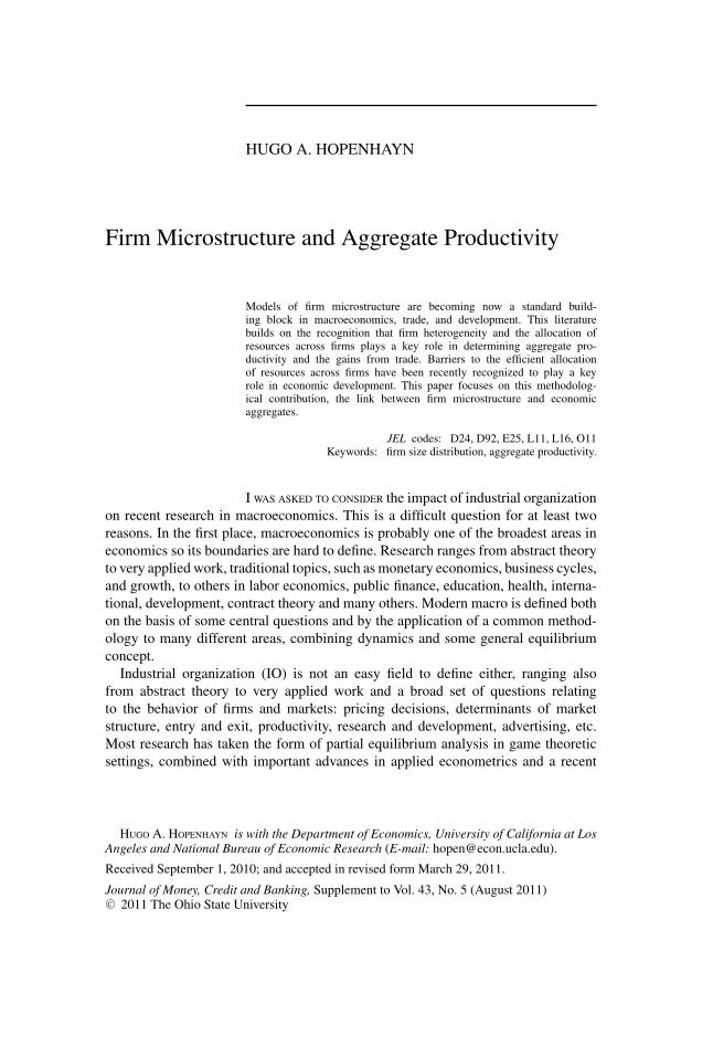
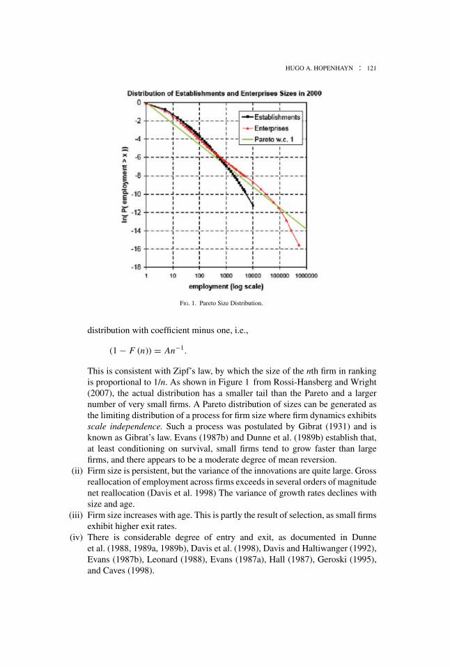
(i) The size distribution of firms and establishments is highly skewed. In particu-lar, the size distribution for the United States follows approximately a Pareto
HUGO A. HOPENHAYN : 121
FIG. 1. Pareto Size Distribution.
distribution with coefficient minus one, i.e.,
(1 − F (n)) = An−1.
This is consistent with Zipf’s law, by which the size of the nth firm in rankingis proportional to 1/n. As shown in Figure 1 from Rossi-Hansberg and Wright(2007), the actual distribution has a smaller tail than the Pareto and a largernumber of very small firms. A Pareto distribution of sizes can be generated asthe limiting distribution of a process for firm size where firm dynamics exhibitsscale independence. Such a process was postulated by Gibrat (1931) and isknown as Gibrat’s law. Evans (1987b) and Dunne et al. (1989b) establish that,at least conditioning on survival, small firms tend to grow faster than largefirms, and there appears to be a moderate degree of mean reversion.
(ii) Firm size is persistent, but the variance of the innovations are quite large. Grossreallocation of employment across firms exceeds in several orders of magnitudenet reallocation (Davis et al. 1998) The variance of growth rates declines withsize and age.
(iii) Firm size increases with age. This is partly the result of selection, as small firmsexhibit higher exit rates.
(iv) There is considerable degree of entry and exit, as documented in Dunneet al. (1988, 1989a, 1989b), Davis et al. (1998), Davis and Haltiwanger (1992),Evans (1987b), Leonard (1988), Evans (1987a), Hall (1987), Geroski (1995),and Caves (1998).
122 : MONEY, CREDIT AND BANKING
(v) Most of the firm level changes in employment respond to idiosyncratic shocks;i.e., they cannot be explained by aggregate, geographic or industry variables.
3.1 The Model and the Data
The model described earlier provides a simple structure to assess quantitativelythe costs of different potential distortions. Starting with Hopenhayn and Rogerson(1993), most papers in the literature calibrate the model to the U.S. manufacturingsector under the assumption that there are no distortions. In static versions of themodel, there is a one-to-one relationship between the size distribution of firms andthe distribution of productivity shocks. To calibrate a dynamic version, Hopenhaynand Rogerson (1993) use data on firm employment dynamics as follows. Assume theln eit follows an AR1 process
ln eit+1 = e (1 − ρ) + ρ ln eit + εi t+1,
where εit is an iid process, normally distributed with mean zero and variance σ 2.Using equation (1) it follows that:
ln nit+1 =(
a + e
1 − η
)(1 − ρ) + ρ lni t + εi t+1
1 − η,
where a is a constant term determined by aggregates (a function of price, in the partialequilibrium setting and a function of N and the distribution of productivities, in thegeneral equilibrium case). This implies that ln nit also follows an AR1 process with thesame persistence and normally distributed innovations with zero mean and varianceσ 2/(1 − η)2. Parameters ρ, a + e
1−ηand σ 2/(1 − η)2 can be estimated using panel
data on firm employment. The parameter η equals labor share. The distribution G forthe initial draw of firms can be inferred from the size distribution of entrants, up toan endogenous scale parameter a that is monotonically decreasing in the equilibriumwage rate. This leaves three more parameters to calibrate, namely, the cost of entryce, fixed cost f , and e. There is clearly an identification problem between a and eas they enter additively in the determination of average employment. Hence there isan extra degree of freedom and an arbitrary value of a can be chosen, without anymeaningful implications.
3.2 Implications for Macroeconomics
As our aggregation exercise shows, firm level productivities are a key determinantof aggregate TFP. The data suggest that there is considerable variation in firm-levelproductivities/demand and a high degree of resource flows across firms. Misallocationof resources could thus be a potentially important explanation of the wide differencesin TFP across countries. Recent papers have tried to establish the relevance of thissource of variation, suggesting it can be quite large. In particular, barriers to thereallocation of resources can also be a potentially important source of differences inTFP. Section 5 will discuss recent papers in this area.
HUGO A. HOPENHAYN : 123
e
Ln n
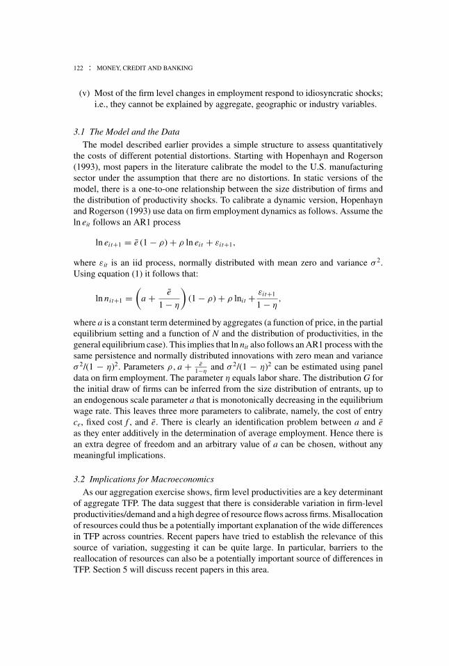
FIG. 2. Wedges in Marginal Product.
The heterogeneity in firm growth rates can also have implications for transitionaldynamics. In particular, the process of growth of firms with age leads to “time tobuild” in the aggregate and can have implications for the evolution of investment andproductivity after large shocks hit the economy. This is discussed in Section 6.
4. THE DISTORTED ECONOMY
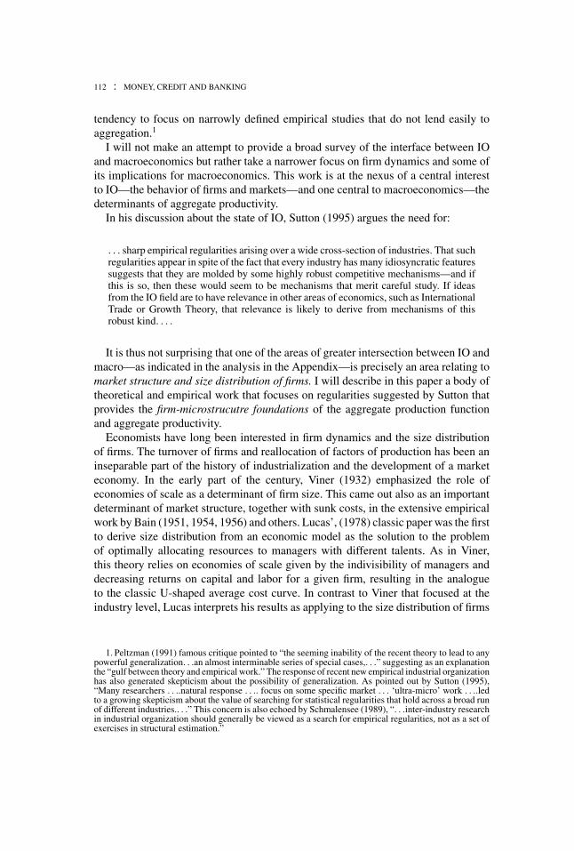
This section analyzes the consequences of deviations from the optimal allocationof resources across productive units. Figure 2 provides a useful picture of the type ofdistortions that might occur: The solid line shows an optimal allocation, where ln ni
is a linear function of ei. The dotted lines illustrate two types of distortions:
(i) ni not equal for all firms with the same ei, termed uncorrelated distortions, and(ii) average ln ni (e) �= a + 1
1−ηe, termed correlated distortions; in the case of
Figure 2 it is a distortion that results in reallocation of labor from more toless productive firms.
Both of these distortions result in losses of productivity as marginal product (orthe marginal value of labor) is not equated across productive units. As an accountingdevice, it is useful to model these distortions as firm-specific implicit taxes/subsidiesthat create a wedge between its revenues and output:
ri = (1 − τi ) yi = (1 − τi ) ei nη
i
= α (ei (1 − τi ))1
1−η ,
where α is a constant that depends only on the equilibrium wage. Equilibrium in thiseconomy will be identical in terms of allocations to the equilibrium of an undistortedeconomy where the distribution of firm productivities is changed to ei(1 − τ i). Totalrevenues are given by
r = N η M1−η(
E [ei (1 − τi )]η
1−η
)1−η
(8)
124 : MONEY, CREDIT AND BANKING
and total output
y =∫
yi di =∫
ri (1 − τi )−1 di
y
r=
∫ri (1 − τi )
−1 di∫ri
= E (1 − τi )−1 (ei (1 − τi ))1
1−η
E (ei (1 − τi ))1
1−η
. (9)
Using equations (8) and (9), it follows that6
y = N η M1−η E (1 − τi )−1 (ei (1 − τi ))1
1−η(E (ei (1 − τi ))
11−η
)η .
Interestingly, note that in the static case, if a planner were to choose optimally theentry of firms subject to the existing employment decisions, the choice would beindependent of the distortions.7 Indeed, it can also be shown that the equilibriumentry decisions would give rise to exactly the same number of firms. These resultsare not true in general for the sequence economy. Suppose the joint distribution ofimplicit taxes and efficiency for firms of age s is μs (de, dτ ) and let
rs =∫
e1
1−η (1 − τ )1
1−η dμs (e, τ ) (10)
be the average revenue productivity. Hopenhayn (2010) shows that in a stationaryequilibrium for the distorted economy, the equilibrium number of firms is determinedby:
N − cem = ηce
(1 − η)
∞∑s=0
δs rs
∞∑s=0
βsδs rs
. (11)
Notice the similarity between the numerator and the denominator, which becomeidentical as β → 1. Though the optimal program is not bounded at this limit, thesolution converges to the objective of maximizing the long-run average, which is thesteady state utility. I will refer to this solution as the case where β = 1.
6. Again, this result generalizes to the case considered in Section 1.1.7. This would not be true if the cost of entry for creating new firms was not entirely denominated in
units of labor but also in terms of the homogenous consumption good. More generally, in an economywith intermediate goods, the cost of entry needs to be produced with the same inputs as all intermediategoods.
HUGO A. HOPENHAYN : 125
PROPOSITION 2. (Fattal-Jaef and Hopenhayn 2011) If β = 1, the equilibrium numberof firms and the optimal number of firms are independent of distortions.
As indicated earlier, the first part of this proposition follows directly from equa-tion (11); the second is derived in Fattal-Jaef and Hopenhayn (2011). Equation (11)also suggests what are the key elements in determining the effects of distortions onentry. Letting m0 denote the number of firms in an undistorted economy and rs isdefined by the right-hand side of equation 10 when all τ s are zero.
N − cem
N − cem0=
⎛⎜⎜⎜⎜⎝
∞∑s=0
δs rs
∞∑s=0
βsδs rs
⎞⎟⎟⎟⎟⎠
/ ∞∑s=0
δsrs
∞∑s=0
βsδsrs
=
∞∑s=0
βsδsrs
∞∑s=0
δsrs
/⎛⎜⎜⎜⎜⎝
∞∑s=0
βsδs rs
∞∑s=0
δs rs
⎞⎟⎟⎟⎟⎠
PROPOSITION 3. (Fattal-Jaef 2011, Fattal-Jaef and Hopenhayn 2011) If distortions areage neutral, i.e rs/rs is independent of s, then the equilibrium and optimal numberof firms are independent of distortions (Fattal-Jaef 2011, Fattal-Jaef and Hopenhayn2011).
Again, the first part of the proposition follows immediately from the aforemen-tioned equation. Aside from these extreme cases, the net effect of distortions on entrydepends on the specific age patterns. A sufficient condition for distortions to lead tomore (less) entry is given below.
DEFINITION 2. The sequence {δsrs} dominates (is dominated by) the sequence {δs rs}if and only if
t∑s=0
δsrs
∞∑s=0
δsrs
≤ (≥)
t∑s=0
δs rs
∞∑s=0
δs rs
for all t.
PROPOSITION 4. (Fattal-Jaef and Hopenhayn 2011) Suppose {δsrs} dominates (isdominated by) {δs rs} Then m ≥ ( ≤ ) m0.
126 : MONEY, CREDIT AND BANKING
A sufficient condition for the sequence {δsrs} to dominate (be dominated by)the sequence {δs rs} is that
∑ts=0 δsrs∑ts=0 δs rs
be increasing (decreasing) in t. The followingCorollary gives simpler necessary conditions.
COROLLARY 1. Suppose that
t∑s=0
δsrs
t∑s=0
δs rs
≤ (≥)rt+1
rt+1.
Then m ≥ ( ≤ ) m0.
Finally, an even stronger sufficient condition is that rs/rs ≤ (≥) rs+1/rs+1, whichsays that distortions are relatively larger (smaller) for older cohorts. An economy thatbenefits relatively established firms (e.g., as a consequence of their increased lobbypower) will have less firms in equilibrium. Alternatively, an economy that tends tosubsidize smaller firms will have the opposite effect, taking into account the wellestablished fact that firm size increases with age.8
5. QUANTITATIVE ANALYSIS OF DISTORTIONS
The earlier framework has been used to assess the quantitative impact of distortions.The first paper to do that was Hopenhayn and Rogerson (1993), which studies theeffect of layoff costs. A baseline model is calibrated using U.S. firm dynamics dataas indicated in Section 3.1. Layoff costs are introduced to this benchmark as follows.Assume that there is a cost f of firing a worker. The value of a firm with n0 workersand productivity shock e is given by the following Bellman equation:
v (e, n0) = maxn
enη − wn − f max(n0 − n, 0) + βE[v
(e′, n
) |e] .
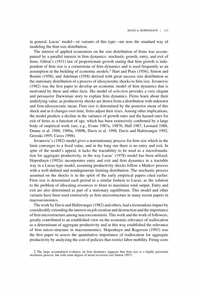
The solution to this problem is an s − S type policy that can be easily characterizedby two increasing functions nL(e) ≤ nH(e) with the following interpretation. Supposea firm enters a period with employment n0. I choose employment n in the currentperiod according to the following rule:
(i) If n0 < nL(e), then n = nL(e).(ii) If n0 > nH(e), then n = nH(e).
(iii) If nL(e) ≤ n0 ≤ nH(e), then n = n0.
8. Fattal-Jaef (2011) has a similar characterization for the equilibrium number of firms and provides avery interesting quantitative work showing the relevance of the entry and exit margins in evaluating thecosts of distortions.
HUGO A. HOPENHAYN : 127
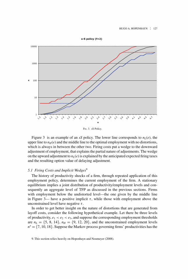
FIG. 3. sS Policy.
Figure 3 is an example of an sS policy. The lower line corresponds to nL(e), theupper line to nH(e) and the middle line to the optimal employment with no distortions,which is always in between the other two. Firing costs put a wedge to the downwardadjustment of employment, that explains the partial nature of adjustments. The wedgeon the upward adjustment to nL(e) is explained by the anticipated expected firing taxesand the resulting option value of delaying adjustment.
5.1 Firing Costs and Implicit Wedges9
The history of productivity shocks of a firm, through repeated application of thisemployment policy, determines the current employment of the firm. A stationaryequilibrium implies a joint distribution of productivity/employment levels and con-sequently an aggregate level of TFP as discussed in the previous sections. Firmswith employment below the undistorted level—the one given by the middle linein Figure 3— have a positive implicit τ , while those with employment above theunconstrained level have negative τ .
In order to get better insight on the nature of distortions that are generated fromlayoff costs, consider the following hypothetical example. Let there be three levelsof productivity, e1 < e2 < e3, and suppose the corresponding employment thresholdsare nL = {5, 8, 14}, nH = {9, 12, 20}, and the unconstrained employment levelsn∗ = {7, 10, 18}. Suppose the Markov process governing firms’ productivities has the
9. This section relies heavily on Hopenhayn and Neumeyer (2008).
128 : MONEY, CREDIT AND BANKING
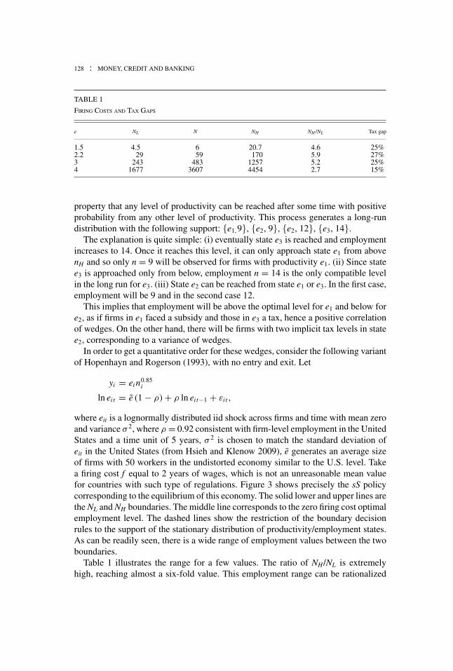
TABLE 1
FIRING COSTS AND TAX GAPS
e NL N NH NH /NL Tax gap
1.5 4.5 6 20.7 4.6 25%2.2 29 59 170 5.9 27%3 243 483 1257 5.2 25%4 1677 3607 4454 2.7 15%
property that any level of productivity can be reached after some time with positiveprobability from any other level of productivity. This process generates a long-rundistribution with the following support: {e1,9}, {e2, 9}, {e2, 12}, {e3, 14}.
The explanation is quite simple: (i) eventually state e3 is reached and employmentincreases to 14. Once it reaches this level, it can only approach state e1 from abovenH and so only n = 9 will be observed for firms with productivity e1. (ii) Since statee3 is approached only from below, employment n = 14 is the only compatible levelin the long run for e3. (iii) State e2 can be reached from state e1 or e3. In the first case,employment will be 9 and in the second case 12.
This implies that employment will be above the optimal level for e1 and below fore2, as if firms in e1 faced a subsidy and those in e3 a tax, hence a positive correlationof wedges. On the other hand, there will be firms with two implicit tax levels in statee2, corresponding to a variance of wedges.
In order to get a quantitative order for these wedges, consider the following variantof Hopenhayn and Rogerson (1993), with no entry and exit. Let
yi = ei n0.85i
ln eit = e (1 − ρ) + ρ ln eit−1 + εi t ,
where eit is a lognormally distributed iid shock across firms and time with mean zeroand variance σ 2, where ρ = 0.92 consistent with firm-level employment in the UnitedStates and a time unit of 5 years, σ 2 is chosen to match the standard deviation ofeit in the United States (from Hsieh and Klenow 2009), e generates an average sizeof firms with 50 workers in the undistorted economy similar to the U.S. level. Takea firing cost f equal to 2 years of wages, which is not an unreasonable mean valuefor countries with such type of regulations. Figure 3 shows precisely the sS policycorresponding to the equilibrium of this economy. The solid lower and upper lines arethe NL and NH boundaries. The middle line corresponds to the zero firing cost optimalemployment level. The dashed lines show the restriction of the boundary decisionrules to the support of the stationary distribution of productivity/employment states.As can be readily seen, there is a wide range of employment values between the twoboundaries.
Table 1 illustrates the range for a few values. The ratio of NH/NL is extremelyhigh, reaching almost a six-fold value. This employment range can be rationalized
HUGO A. HOPENHAYN : 129
TABLE 2
FIRING COSTS AND TFP LOSSES
Firing cost (years) TFP loss Gap (range of equivalent labor taxes)
2 years −2.8% 32.95 years −7.5% 56.025 years −24.3% 97.6
by taxes and subsidies to employment as described earlier. The tax gap, reflecting thedifference between implicitly subsidy and tax rates for a given level of productivity,ranges from 15% to 27%.
These gaps might seem substantial, but what are their implications for aggregateTFP? Table 2 provides an answer to this question: the level of firing costs that Ihave considered (f = 2 years) results in a 2.8% reduction in TFP. If f = 5 years,the TFP loss is 7.5% and if f = 25 years, it is 24.3%. This level of firing cost isclose to prohibitive and firms respond by not adjusting employment at all. With suchdegree of firing costs, it seems very likely that firms would negotiate and bargainwith workers and induce quits in order to get around these barriers to adjustment.Hence, a moderate range of firing costs seems a more plausible realistic scenario foremployment rigidity and consequent TFP losses.
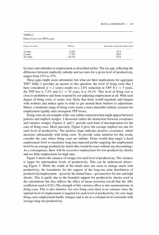
Firing costs are an example of the very subtle connection that might appear betweenpolicies and implicit wedges. I discussed earlier the distinction between covarianceand variance wedges. Figures 4 and 5 provide such kind of decomposition for thecase of firing costs. More precisely, Figure 4 gives the average implicit tax rate foreach level of productivity. The positive slope indicates positive covariance, whichincreases substantially with firing costs. To provide some intuition for this result,consider the case where firing costs are infinite. Firms would then target a fixedemployment level to maximize long-run expected profits targeting the employmentlevel for an average productivity shock (this would be exact without any discounting).As a consequence, there will be excessive employment for low-productivity shocksand too little employment for high ones.
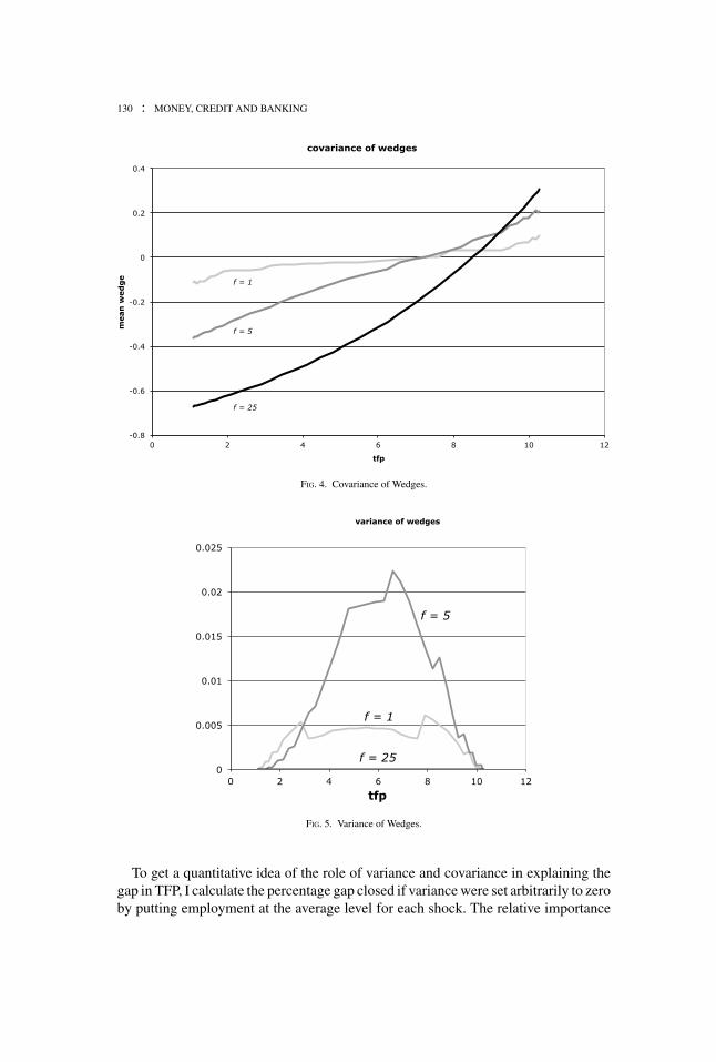
Figure 5 shows the variance of wedges for each level of productivity. The varianceis larger for intermediate levels of productivity. This can be understood observ-ing Figure 3. While the width of the bands does not seem to change much withproductivity, the boundaries for the support of the long-run joint distribution ofproductivity/employment—given by the dotted lines—get narrower for low and highshocks. This is partly due to the bounded support for productivity shocks used inthe calculations but also reflects the effect of mean reversion (recall that the AR1coefficient used is 0.92.) The strength of this variance effect is also nonmonotonic infiring costs. This is also intuitive: for zero firing costs there is no variance since theoptimal level of employment is targeted for each level of productivity; for very largefiring costs employment hardly changes and is set at a constant level consistent withaverage long-run productivity.
130 : MONEY, CREDIT AND BANKING
FIG. 4. Covariance of Wedges.
FIG. 5. Variance of Wedges.
To get a quantitative idea of the role of variance and covariance in explaining thegap in TFP, I calculate the percentage gap closed if variance were set arbitrarily to zeroby putting employment at the average level for each shock. The relative importance

HUGO A. HOPENHAYN : 131
of variance shocks decreases with firing costs: 64% of the gap is closed when f = 1,41% when f = 5, and 0 when f = 25.
The model calibrated in this section has no entry and exit. This might affectsomewhat the results. Though most of the employment adjustment takes place forincumbent firms, young firms are the ones that exhibit highest variance of innovations.Including entry in the model would change firm demographics, generating in steadystate a cross-section of different-aged firms as I have described earlier. In addition,firms start small and tend to grow over time. This should imply that for youngervintages employment levels near the lower boundaries are more likely. Moreover, ifI were to include higher variance of growth rates for younger firms, as occurs in thereal world, the width of the bands would widen for young firms, generating higherimplicit wedges. This would appear as taxation to employment, as younger firmsconcentrate in the lower part of the sS band.
5.2 The Potential Effect of Inter-firm Distortions
In contrast to Hopenhayn and Rogerson (1993) where wedges arise as the resultof a specific policy, the recent literature takes a more agnostic view and directlyexamines the effects on productivity of different distributions of wedges. The firstpaper to do this is Restuccia and Rogerson (2008). Expanding the above model toinclude capital, distortions occur both as departures in the output of a firm from itsoptimal value and the use of an inefficient capital/labor ratio.
Restuccia–Rogerson (2008). There is a fixed set (measure) of firms with distributionof productivities calibrated to match U.S. size distribution, taken as a benchmark foran undistorted economy. In the distorted economy, profits for firm i are given by:π i = (1 − τ i)yi − wni − (1 + τ ki)rki, where τ i and τ ki are two wedges wedges aredistributed according to a conditional density ω(τ , τ k|e).10 The exercise performedconsists in taxing a subset of firms and subsidizing the remaining set so that steadystate capital remains invariant. I consider here quantitative results for level taxes only.Table 3 gives a summary of the effects of distortions. The first two columns consideruncorrelated wedges and the remaining the correlated ones. Two observations follow:(i) correlated distortions have significantly stronger effects and (ii) the impact onproductivity is larger the higher is the fraction taxed. The latter can be explained bythe fact that when a group of firms is taxed, the remaining firms are subsidized at arate that makes total capital stock invariant. The larger the group taxed, the higher thesubsidy has to be for the other group, thus creating a very large disparity in wedges.There is also an intuition for why correlated distortions have a bigger impact on TFP.In the extreme case where firms have near constant returns to scale, there is no effectof variance distortions as output can be totally reallocated within productivity groups.
10. A more transparent interpretation of wedges would be obtained using π i = (1 − τ i)yi − w(1 +τ ni)ni − r(1 + τ ki)ki and setting (1 + τ ki)β (1 + τ ni)α = 1. This would make the tax on capital a pure inputmix distortion.
132 : MONEY, CREDIT AND BANKING
TABLE 3
RELATIVE TFP AND DISTORTIONS
Uncorrelated Correlated% Estab. taxed τ t τ t
0.2 0.4 0.2 0.490 0.84 0.74 0.66 0.5150 0.96 0.92 0.80 0.6910 0.99 0.99 0.92 0.86
The same is not true with correlated distortions, as output is reallocated to firms withlower productivity. In particular, when the 90% most efficient firms are taxed thelowest 10% receive a 107% subsidy when τ = 0.2 and 114% when τ = 0.4. Whilehere correlated distortions are an assumption, in a related paper Guner, Ventura, andXu (2008) derive these from size-dependent policies.
The analysis done by Restuccia and Rogerson suggest that large inter-firm dis-tortions can have substantial aggregate TFP effects. But the distortions assumed arehypothetical. In contrast, Hsieh and Klenow (2009) derive these distortions from firmlevel data.
Hsieh–Klenow (2009). The setting they consider is one of monopolistic competition.As mentioned in Section 1.3, this is not a major difference as for a fixed number offirms the model is isomorphic to the Lucas-style model. The major novelty in theirapproach is the exercise of recovering wedges from firm-level data. This can beexplained easily in terms of the model developed in Section 2. Measured TFP foreach firm i is simply ei = yi/n
ηi . This requires measuring inputs and outputs (or
sales).11 Leaving aside measurement error, one can calculate aggregate TFP in anefficient allocation using equation (3) as follows:
TFPe =(
Ee1
1−η
i
)1−η
=(
E
(yi
nη
i
) 11−η
)1−η
.
In contrast, actual TFP is given by
TFP = y/N η = y(∑i
ni
)η .
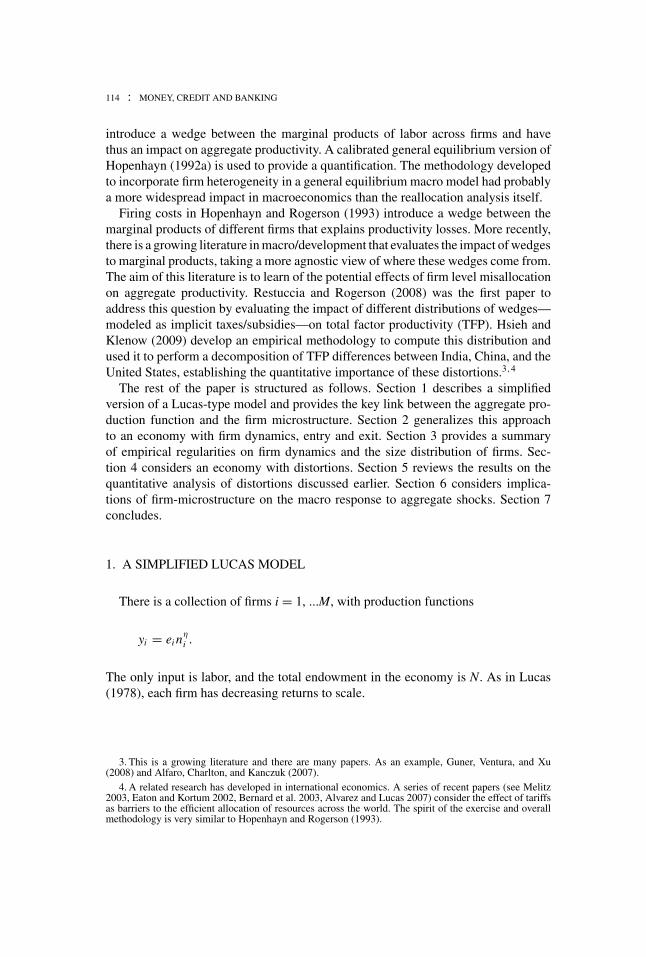
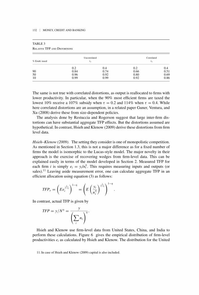
Hsieh and Klenow use firm-level data from United States, China, and India toperform these calculations. Figure 6 gives the empirical distribution of firm-levelproductivities ei as calculated by Hsieh and Klenow. The distribution for the United
11. In case of Hsieh and Klenow (2009) capital is also included.
HUGO A. HOPENHAYN : 133
FIG. 6. Distributions of Firm TFP.
TABLE 4
DISPERSION OF LN TFPR
United States (97) China (98) India (94)
SD 0.49 0.74 0.6775-25 0.53 0.97 0.8190-10 1.19 1.87 1.60
States stochastically dominates that of China, which in turn stochastically dominatesthat of India—which also exhibits the highest levels of dispersion—except for veryhigh levels of productivity.
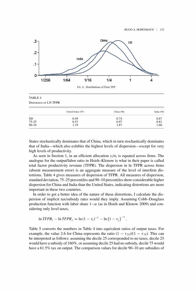
As seen in Section 1, in an efficient allocation yi/ni is equated across firms. Theanalogue for the output/labor ratio in Hsieh–Klenow is what in their paper is calledtotal factor productivity revenue (TFPR). The dispersion in ln TFPR across firms(absent measurement error) is an aggregate measure of the level of interfirm dis-tortions. Table 4 gives measures of dispersion of TFPR. All measures of dispersion,standard deviation, 75–25 percentiles and 90–10 percentiles show considerable higherdispersion for China and India than the United States, indicating distortions are moreimportant in these two countries.
In order to get a better idea of the nature of these distortions, I calculate the dis-persion of implicit tax/subsidy rates would they imply. Assuming Cobb–Douglassproduction function with labor share 1−α (as in Hsieh and Klenow 2009) and con-sidering only level taxes,
ln TFPRi − ln TFPR j = ln (1 − τi )−1 − ln
(1 − τ j
)−1.
Table 5 converts the numbers in Table 4 into equivalent ratios of output taxes. Forexample, the value 2.6 for China represents the ratio (1 − τ 25)/(1 − τ 75). This canbe interpreted as follows: assuming the decile 25 corresponded to no taxes, decile 25would have a subsidy of 160%, or assuming decile 25 had no subsidy, decile 75 wouldhave a 61.5% tax on output. The comparison values for decile 90–10 are subsidies of
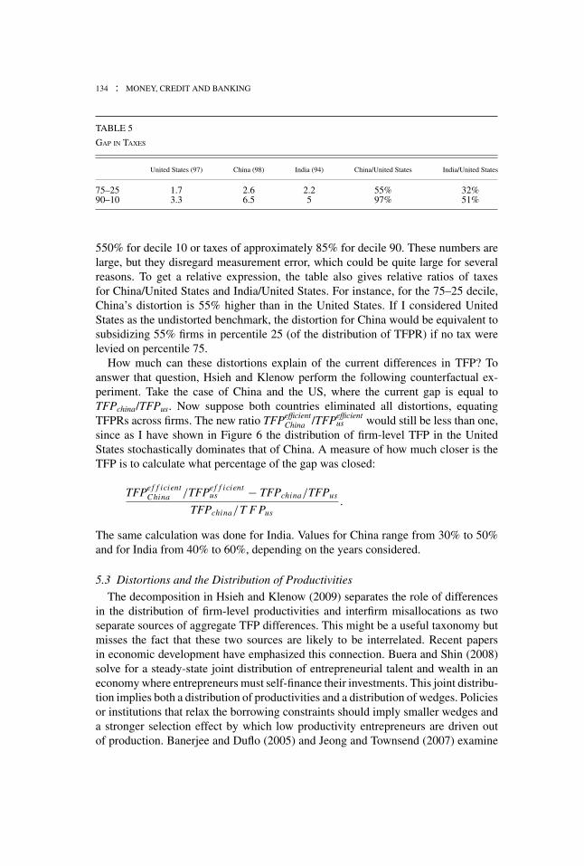
134 : MONEY, CREDIT AND BANKING
TABLE 5
GAP IN TAXES
United States (97) China (98) India (94) China/United States India/United States
75–25 1.7 2.6 2.2 55% 32%90–10 3.3 6.5 5 97% 51%
550% for decile 10 or taxes of approximately 85% for decile 90. These numbers arelarge, but they disregard measurement error, which could be quite large for severalreasons. To get a relative expression, the table also gives relative ratios of taxesfor China/United States and India/United States. For instance, for the 75–25 decile,China’s distortion is 55% higher than in the United States. If I considered UnitedStates as the undistorted benchmark, the distortion for China would be equivalent tosubsidizing 55% firms in percentile 25 (of the distribution of TFPR) if no tax werelevied on percentile 75.
How much can these distortions explain of the current differences in TFP? Toanswer that question, Hsieh and Klenow perform the following counterfactual ex-periment. Take the case of China and the US, where the current gap is equal toTFPchina/TFPus. Now suppose both countries eliminated all distortions, equatingTFPRs across firms. The new ratio TFPefficient
China /TFPefficientus would still be less than one,
since as I have shown in Figure 6 the distribution of firm-level TFP in the UnitedStates stochastically dominates that of China. A measure of how much closer is theTFP is to calculate what percentage of the gap was closed:
TFPef f icientChina /TFPef f icient
us − TFPchina/TFPus
TFPchina/T F Pus.
The same calculation was done for India. Values for China range from 30% to 50%and for India from 40% to 60%, depending on the years considered.
5.3 Distortions and the Distribution of Productivities
The decomposition in Hsieh and Klenow (2009) separates the role of differencesin the distribution of firm-level productivities and interfirm misallocations as twoseparate sources of aggregate TFP differences. This might be a useful taxonomy butmisses the fact that these two sources are likely to be interrelated. Recent papersin economic development have emphasized this connection. Buera and Shin (2008)solve for a steady-state joint distribution of entrepreneurial talent and wealth in aneconomy where entrepreneurs must self-finance their investments. This joint distribu-tion implies both a distribution of productivities and a distribution of wedges. Policiesor institutions that relax the borrowing constraints should imply smaller wedges anda stronger selection effect by which low productivity entrepreneurs are driven outof production. Banerjee and Duflo (2005) and Jeong and Townsend (2007) examine
HUGO A. HOPENHAYN : 135
the link between borrowing constraints and technology selection. As borrowing con-straints are relaxed, firms can adopt more productive technologies that to be profitablerequire a considerably larger scale and investment.
6. FIRM DEMOGRAPHICS AND TFP
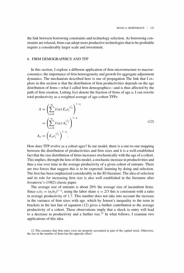
In this section, I explore a different application of firm microstructure to macroe-conomics: the importance of firm heterogeneity and growth for aggregate adjustmentdynamics. The mechanism described here is one of propagation The link that I ex-plore in this section is that the distribution of firm productivities depends on the agedistribution of firms—what I called firm demographics—and is thus affected by thepath of firm creation. Letting δ(a) denote the fraction of firms of age a, I can rewritetotal productivity as a weighted average of age-cohort TFPs:
A =( ∞∑
a=0
δ (a) Eae1
1−η
i
)1−η
=( ∞∑
a=0
δ (a) A1
1−η
a
)1−η
Aa =(
Eae1
1−η
i
)1−η
.
(12)
How does TFP evolve as a cohort ages? In our model, there is a one-to-one mappingbetween the distribution of productivities and firm sizes and it is a well-establishedfact that the size distribution of firms increases stochastically with the age of a cohort.This implies, through the lens of this model, a stochastic increase in productivities andthus a rise over time in the average productivity of a given cohort of entrants. Thereare two forces that suggest this is to be expected: learning by doing and selection.The first has been emphasized considerably in the IO literature. The idea of selectionand its role for increasing firm size is also well established in the literature afterJovanovic’s (1982) classic paper.
The average size of entrants is about 20% the average size of incumbent firms.Since ei/ej = (ni/nj)1−η, using the labor share η = 2/3 this is consistent with a ratioin average productivity of 1.7. This number does not take into account the increasein the variance of firm sizes with age, which by Jensen’s inequality to the term inbrackets in the last line of equation (12) gives a further contribution to the averageproductivity of a cohort. These observations imply that a shock to entry will leadto a decrease in productivity and a further rise.12 In what follows, I examine twoapplications of this idea.
12. This assumes that firm entry costs are properly accounted as part of the capital stock. Otherwise,the rise in the number of firms has the opposite effect.
136 : MONEY, CREDIT AND BANKING
TABLE 6
LIFE CYCLE OF AN INDUSTRY
Mean annual Mean annualStage Mean duration net entry rate growth rate
II 9.7 years 24.8% 35%III 7.5 years 0.2% 12%IV 5.4 years −9% 8%V - −0.5% 1%
6.1 Shakeout of Firms
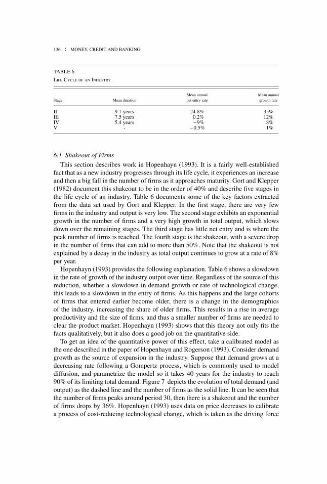
This section describes work in Hopenhayn (1993). It is a fairly well-establishedfact that as a new industry progresses through its life cycle, it experiences an increaseand then a big fall in the number of firms as it approaches maturity. Gort and Klepper(1982) document this shakeout to be in the order of 40% and describe five stages inthe life cycle of an industry. Table 6 documents some of the key factors extractedfrom the data set used by Gort and Klepper. In the first stage, there are very fewfirms in the industry and output is very low. The second stage exhibits an exponentialgrowth in the number of firms and a very high growth in total output, which slowsdown over the remaining stages. The third stage has little net entry and is where thepeak number of firms is reached. The fourth stage is the shakeout, with a severe dropin the number of firms that can add to more than 50%. Note that the shakeout is notexplained by a decay in the industry as total output continues to grow at a rate of 8%per year.
Hopenhayn (1993) provides the following explanation. Table 6 shows a slowdownin the rate of growth of the industry output over time. Regardless of the source of thisreduction, whether a slowdown in demand growth or rate of technological change,this leads to a slowdown in the entry of firms. As this happens and the large cohortsof firms that entered earlier become older, there is a change in the demographicsof the industry, increasing the share of older firms. This results in a rise in averageproductivity and the size of firms, and thus a smaller number of firms are needed toclear the product market. Hopenhayn (1993) shows that this theory not only fits thefacts qualitatively, but it also does a good job on the quantitative side.
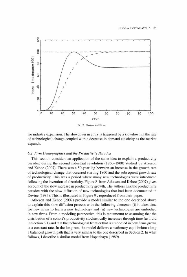
To get an idea of the quantitative power of this effect, take a calibrated model asthe one described in the paper of Hopenhayn and Rogerson (1993). Consider demandgrowth as the source of expansion in the industry. Suppose that demand grows at adecreasing rate following a Gompertz process, which is commonly used to modeldiffusion, and parametrize the model so it takes 40 years for the industry to reach90% of its limiting total demand. Figure 7 depicts the evolution of total demand (andoutput) as the dashed line and the number of firms as the solid line. It can be seen thatthe number of firms peaks around period 30, then there is a shakeout and the numberof firms drops by 36%. Hopenhayn (1993) uses data on price decreases to calibratea process of cost-reducing technological change, which is taken as the driving force
HUGO A. HOPENHAYN : 137
FIG. 7. Shakeout of Firms.
for industry expansion. The slowdown in entry is triggered by a slowdown in the rateof technological change coupled with a decrease in demand elasticity as the marketexpands.
6.2 Firm Demographics and the Productivity Paradox
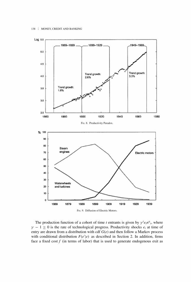
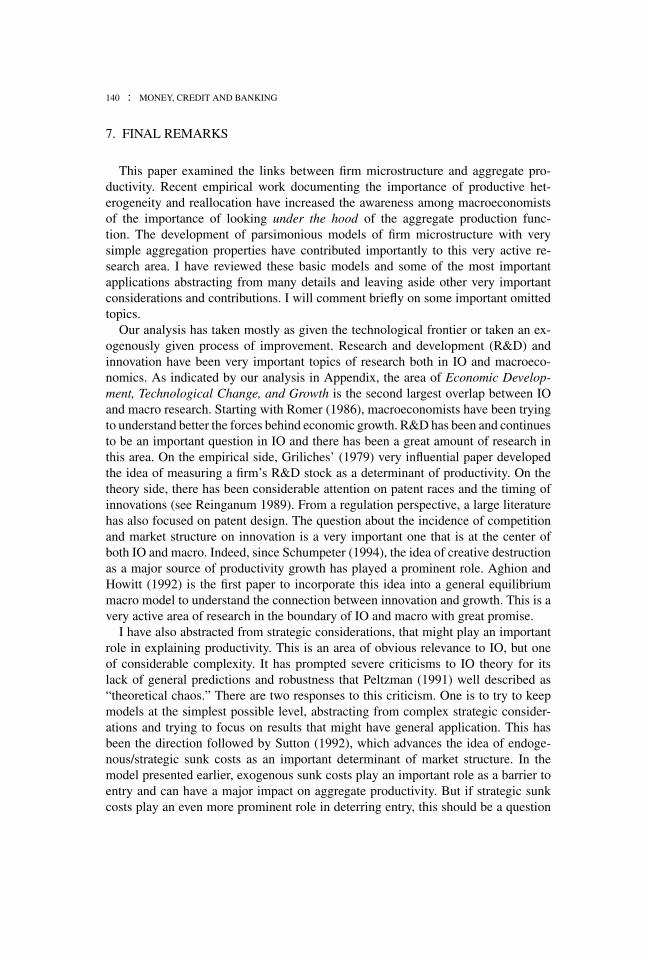
This section considers an application of the same idea to explain a productivityparadox during the second industrial revolution (1860–1900) studied by Atkesonand Kehoe (2007). There was a 50-year lag between an increase in the growth rateof technological change that occurred starting 1860 and the subsequent growth rateof productivity. This was a period where many new technologies were introducedfollowing the invention of electricity. Figure 8 from Atkeson and Kehoe (2007) givesaccount of the slow increase in productivity growth. The authors link the productivityparadox with the slow diffusion of new technologies that had been documented inDevine (1983). This is illustrated in Figure 9 , reproduced from their paper.
Atkeson and Kehoe (2007) provide a model similar to the one described aboveto explain this slow diffusion process with the following elements: (i) it takes timefor new firms to learn a new technology and (ii) new technologies are embodiedin new firms. From a modeling perspective, this is tantamount to assuming that thedistribution of a cohort’s productivity stochastically increases through time (as I didin Section 6.1) and that the technological frontier that is embodied in new firms growsat a constant rate. In the long run, the model delivers a stationary equilibrium alonga balanced growth path that is very similar to the one described in Section 2. In whatfollows, I describe a similar model from Hopenhayn (1989).
138 : MONEY, CREDIT AND BANKING
FIG. 8. Productivity Paradox.
FIG. 9. Diffusion of Electric Motors.
The production function of a cohort of time t entrants is given by γ teinηi, where
γ − 1 ≥ 0 is the rate of technological progress. Productivity shocks ei at time ofentry are drawn from a distribution with cdf G(e) and then follow a Markov processwith conditional distribution F(e′|e) as described in Section 2. In addition, firmsface a fixed cost f (in terms of labor) that is used to generate endogenous exit as

HUGO A. HOPENHAYN : 139
in Hopenhayn (1992a). In a balanced growth path, the wage rises at the rate oftechnological progress, so wt = γ tw0. The value of a firm of age τ is given by
vτ
(e, γ tw0
) = max(0, πτ
(e, γ tw0
) + βEvτ
(e′, γ t+1w0|e
)),
where
πτ (e, w) = maxn
γ τ enη − wn − w f.
It is immediate that πτ is homogeneous of degree one in e, w and easy to show thatso is vτ . So dividing through by γ t
vτ (e, γ tw0) = γ tv0(γ −(t−τ )e, w0)
= γ t max(0, π0(γ −(t−τ )e, w0) + βγ t Evτ (γ −(t−τ )e′, γw0|e))
and thus
v0(γ −(t−τ )e, w0) = max(0, π0(γ −(t−τ )e, w0) + βγ Evτ (γ −(t−τ )e′/γ,w0|e)).
Letting the state of a firm e = γ −(t−τ )e, this value function can be rewritten as:
v0(e, w0) = max(0, π0(e, w0) + βγ Evτ (e/γ,w0|e)).
This is exactly the same as the value function for a firm in a stationary economy withno technological change with an appropriate shift in the conditional distribution ofproductivity F(e′|e) = F(γ e′|e). The equilibrium is solved exactly as in the modelwith no growth.
This shift introduces a depreciating element to a firm’s productivity as it ages andfalls further behind the technological frontier. There are now two forces workingin opposite directions: the original property of the Markov process by which thedistribution of a cohort’s productivity increases with the age of the cohort (whatAtkeson and Kehoe 2007 call learning) and the counteracting force introduced bytechnological depreciation. These two forces determine the sequence of age-cohortproductivities {Aa}∞
a=0 and in particular imply that Aa+1/Aa < γ . This is importantfor transitional dynamics. Start the economy in the steady state corresponding to alow γ 0 and consider a permanent increase to γ > γ 0. There will be a jump in theentry rate that will shift the demographics to lower ages. Though these new entrantsembody the new technology, the average productivity of the cohort will does not fullyreflect the higher productivity of the new technology, so average productivity willgrow less than γ (it could even fall!). As time goes by the economy converges (frombelow) to a balanced growth path where output and productivity grow at the new rateγ . In their calibrated model, Atkeson and Kehoe (2007) show that these forces canexplain quite well the productivity paradox.
140 : MONEY, CREDIT AND BANKING
7. FINAL REMARKS
This paper examined the links between firm microstructure and aggregate pro-ductivity. Recent empirical work documenting the importance of productive het-erogeneity and reallocation have increased the awareness among macroeconomistsof the importance of looking under the hood of the aggregate production func-tion. The development of parsimonious models of firm microstructure with verysimple aggregation properties have contributed importantly to this very active re-search area. I have reviewed these basic models and some of the most importantapplications abstracting from many details and leaving aside other very importantconsiderations and contributions. I will comment briefly on some important omittedtopics.
Our analysis has taken mostly as given the technological frontier or taken an ex-ogenously given process of improvement. Research and development (R&D) andinnovation have been very important topics of research both in IO and macroeco-nomics. As indicated by our analysis in Appendix, the area of Economic Develop-ment, Technological Change, and Growth is the second largest overlap between IOand macro research. Starting with Romer (1986), macroeconomists have been tryingto understand better the forces behind economic growth. R&D has been and continuesto be an important question in IO and there has been a great amount of research inthis area. On the empirical side, Griliches’ (1979) very influential paper developedthe idea of measuring a firm’s R&D stock as a determinant of productivity. On thetheory side, there has been considerable attention on patent races and the timing ofinnovations (see Reinganum 1989). From a regulation perspective, a large literaturehas also focused on patent design. The question about the incidence of competitionand market structure on innovation is a very important one that is at the center ofboth IO and macro. Indeed, since Schumpeter (1994), the idea of creative destructionas a major source of productivity growth has played a prominent role. Aghion andHowitt (1992) is the first paper to incorporate this idea into a general equilibriummacro model to understand the connection between innovation and growth. This is avery active area of research in the boundary of IO and macro with great promise.
I have also abstracted from strategic considerations, that might play an importantrole in explaining productivity. This is an area of obvious relevance to IO, but oneof considerable complexity. It has prompted severe criticisms to IO theory for itslack of general predictions and robustness that Peltzman (1991) well described as“theoretical chaos.” There are two responses to this criticism. One is to try to keepmodels at the simplest possible level, abstracting from complex strategic consider-ations and trying to focus on results that might have general application. This hasbeen the direction followed by Sutton (1992), which advances the idea of endoge-nous/strategic sunk costs as an important determinant of market structure. In themodel presented earlier, exogenous sunk costs play an important role as a barrier toentry and can have a major impact on aggregate productivity. But if strategic sunkcosts play an even more prominent role in deterring entry, this should be a question
HUGO A. HOPENHAYN : 141
of major interest to macroeconomists. This is definitely an area that should receiveimportant contributions in the near future. Following Ericson and Pakes (1995), asecond response to theoretical chaos has been to focus on Markov perfect equilibriaof a dynamic game. This research is usually tied to structural estimation and hasconcentrated on somewhat narrow analysis of industries that do not easily aggregateinto general insights of use in macroeconomics.
Needless to say, a very important area to analyze the importance of the firmmicrostructure for the aggregate economy is measurement. As an example, measur-ing firm-level productivity is a complex task given the endogenous nature of inputchoices. Starting with the work of Olley and Pakes (1996), this question has receivedconsiderable attention. The availability of new longitudinal databases, such as theLBD and the role of the Bureau of the Census data centers in facilitating the accessof these data to researchers is of considerable importance.
These are very exciting times for research at the boundary of IO and macro. It isan opportunity for IO economists interested in broadening perspectives to look intomacro/development/international applications and more macroeconomists to lookinto IO. Central questions in economics such as the need for a better understandingof the determinants of productivity, innovation, and growth are at the core of thesetwo fields.
APPENDIX: ON THE BOUNDARY OF IO AND MACRO
I took a random sample of articles published between 1992 and 2010 in RANDJournal and Journal of Monetary Economics (JME), the two top field journals inIO and macro, respectively. I classified each of the papers in the sample—330 from
FIG. A1. IO and Macro—JEL Codes.
142 : MONEY, CREDIT AND BANKING
TABLE A1
SUBFIELDS INTERSECTION
JEL Description RAND JME
L110 Production, Pricing and Market Structure; Size Distribution of Firms 39 7D830 Search; Learning; Information and Knowledge; Communication; Belief 22 5G210 Banks, Other Depository Institutions, Micro Financ Inst.; Mortgages 5 23J240 Human Capital; Skills; Occupational Choice; Labor Productivity 5 5J310 Wage Level and Struct; Wage Diff. by Skill; Training, Occupation, etc. 5 7O330 Technological Change: Choices and Consequences; Diffusion Proc. 11 5D120 Consumer Economics Empirical Analysis 4 4D820 Asymmetric and Private Information 4 4
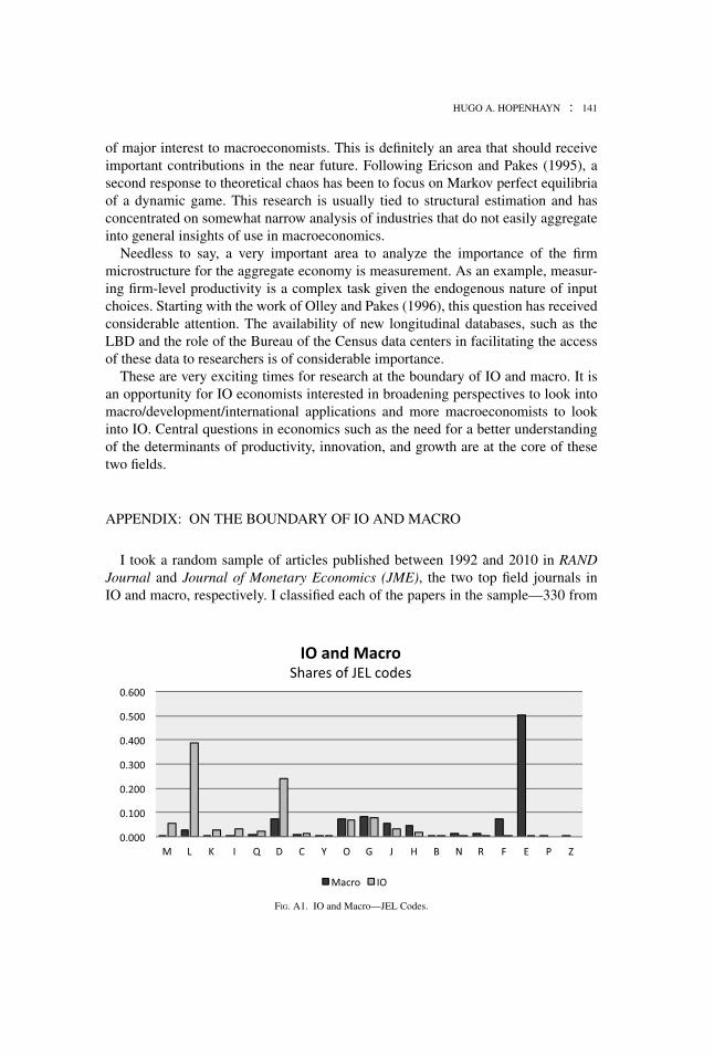
RAND out of 761 published and 300 in JME out of 1234— according to JEL codes,averaging between two and three codes per paper. Figure A1 provides a distributionof the relative shares of JEL codes in IO and macro, ordered from left to right by therelative importance of IO. Excluding the small share codes, I can do the followingclassification:
(i) Almost exclusively IO: Codes L (Industrial Organization) and M (BusinessAdministration and Business Economics; Marketing; Accounting).
(ii) Almost exclusively Macro: Codes E (Macroeconomics and Monetary Eco-nomics) and F (International Economics).
(iii) Largely IO but important share of macro: Code D (Microeconomics). Thesubcodes of more overlap are those related to consumer.
(iv) Mixed. Ordered by importance: G (Financial Economics), O (Economic De-velopment, Technological Change, and Growth), J (Labor and DemographicEconomics), and H (Health Economics).
The distribution shows pretty clearly two things: (i) that both fields seem to inter-sect with many other fields and (ii) the shared boundary between the two fields ispretty large. In order to get a finer impression on the nature of the intersection, it isuseful to look at subfields within these JEL aggregates. These are ordered in Table A1taking the minimum of the frequencies in RAND and in JME as a measure of inter-section.
LITERATURE CITED
Adelman, I.G. (1958) “A Stochastic Analysis of the Size Distribution of Firms.” Journal ofthe American Statistical Association, 53(284), 893–904.
Aghion, P., and P. Howitt. (1992) “A Model of Growth through Creative Destruction.” Econo-metrica: Journal of the Econometric Society, 60, 323–51.
Alfaro, L., A. Charlton, and F. Kanczuk. (2007) “Firm-Size Distribution and Cross-CountryIncome Differences.” Manuscript, Harvard Business School.

HUGO A. HOPENHAYN : 143
Alvarez, F., and R.E. Lucas. (2007) “General Equilibrium Analysis of the Eaton–KortumModel of International Trade.” Journal of Monetary Economics, 54, 1726–68.
Atkeson, A., and P.J. Kehoe. (2007) “Modeling the Transition to a New Economy: Lessonsfrom Two Technological Revolutions.” American Economic Review, 97, 64–88.
Bain, J.S. (1951) “Relation of Profit Rate to Industry Concentration: American Manufacturing,1936–1940.” Quarterly Journal of Economics, 65, 293–324.
Bain, J.S. (1954) “Economies of Scale, Concentration, and the Condition of Entry in TwentyManufacturing Industries.” American Economic Review, 44, 15–39.
Bain, J.S. (1956) Barriers to New Competition: Their Character and Consequences in Manu-facturing Industries. Cambridge, MA: Harvard University Press.
Banerjee, A., and E. Duflo. (2005) “Growth Theory through the Lens of Economic Develop-ment.” Handbook of Development Economics, 1, 473–552.
Bernard, A.B., J. Eaton, J.B. Jensen, and S. Kortum. (2003) “Plants and Productivity inInternational Trade.” American Economic Review, 93, 1268–90.
Buera, F.J., and Y. Shin. (2008) “Financial Frictions and the Persistence of History: A Quanti-tative Exploration.” Manuscript, Washington University, St. Louis.
Caves, R.E. (1998) “Industrial Organization and New Findings on the Turnover and Mobilityof Firms.” Journal of Economic Literature, 36, 1947–82.
Davis, S.J., and J. Haltiwanger. (1992) “Gross Job Creation, Gross Job Destruction, andEmployment Reallocation.” Quarterly Journal of Economics, 107, 819–63.
Davis, S.J., J.C. Haltiwanger, and S. Schuh. (1998) Job Creation and Destruction. Cambridge,MA: MIT Press.
Devine, W.D., Jr. (1983) “From Shafts to Wires: Historical Perspective on Electrification.”Journal of Economic History, 43, 347–72.
Dixit, A.K., and J.E. Stiglitz. (1977) “Monopolistic Competition and Optimum Product Diver-sity.” American Economic Review, 297–308.
Dunne, T., M.J. Roberts, and L. Samuelson. (1988) “Patterns of Firm Entry and Exit in USManufacturing Industries.” RAND Journal of Economics, 19, 495–515.
Dunne, T., M.J. Roberts, and L. Samuelson. (1989) “Plant Turnover and Gross EmploymentFlows in the US Manufacturing Sector.” Journal of Labor Economics, 7, 48–71.
Dunne, T., M.J. Roberts, and L. Samuelson. (1989) “The Growth and Failure of US Manufac-turing Plants.” Quarterly Journal of Economics, 104, 671–98.
Eaton, J., and S. Kortum. (2002) “Technology, Geography, and Trade.” Econometrica, 70,1741–79.
Ericson, R., and A. Pakes. (1995) “Markov-Perfect Industry Dynamics: A Framework forEmpirical Work.” Review of Economic Studies, 62, 53–82.
Evans, D.S. (1987) “Tests of Alternative Theories of Firm Growth.” Journal of PoliticalEconomy, 95, 657–74.
Evans, D.S. (1987) “The Relationship between Firm Growth, Size, and Age: Estimates for 100Manufacturing Industries.” Journal of Industrial Economics, 35, 567–81.
Fattal-Jaef, Roberto. (2011) “Idiosyncratic Distortions with Firm Dynamics: Implications forAggregate Productivity and Welfare.” Working Paper.
Fattal-Jaef, Roberto, and H.A. Hopenhayn. (2011) “Idiosyncratic Distortions with Firm Dy-namics.” Working Paper.
144 : MONEY, CREDIT AND BANKING
Geroski, P.A. (1995) “What Do We Know about Entry?” International Journal of IndustrialOrganization, 13, 421–40.
Gibrat, R. (1931) Les Inegalites Economiques. Paris: Librairie du Recueil Sirey.
Gort, M., and S. Klepper. (1982) “Time Paths in the Diffusion of Product Innovations.”Economic Journal, 92(367), 630–53.
Griliches, Z. (1979) “Issues in Assessing the Contribution of Research and Development toProductivity Growth.” Bell Journal of Economics, 10, 92–116.
Guner, N., G. Ventura, and Y. Xu. (2008) “Macroeconomic Implications of Size-DependentPolicies.” Review of Economic Dynamics, 11, 721–44.
Hall, B.H. (1987) “The Relationship between Firm Size and Firm Growth in the US Manufac-turing Sector.” Journal of Industrial Economics, 35, 583–606.
Hart, P.E., and S.J. Prais. (1956) “The Analysis of Business Concentration: A Statis-tical Approach.” Journal of the Royal Statistical Society. Series A (General), 119,150–91.
Hopenhayn, H., and A. Neumeyer. (2008) “Productivity and Distortions.” Documento Inedito.Washington, DC: Departamento de Investigacion, Banco Interamericano de Desarrollo.
Hopenhayn, H., and R. Rogerson. (1993) “Job Turnover and Policy Evaluation: A GeneralEquilibrium Analysis.” Journal of Political Economy, 101, 915–38.
Hopenhayn, Hugo. (1989) Essays in Industry Dynamics. Doctoral Dissertation, University ofMinnesota.
Hopenhayn, H.A. (1992) “Entry, Exit, and Firm Dynamics in Long Run Equilibrium.” Econo-metrica, 60, 1127–50.
Hopenhayn, H.A. (1992) “Exit, Selection, and the Value of Firms.” Journal of EconomicDynamics and Control, 16, 621–53.
Hopenhayn, H.A. (1993) “The Shakeout.” Economics Working Papers.
Hsieh, C.T., and P.J. Klenow. (2009) “Misallocation and Manufacturing TFP in China andIndia.” Quarterly Journal of Economics, 124, 1403–48.
Jeong, H., and R.M. Townsend. (2007) “Sources of TFP Growth: Occupational Choice andFinancial Deepening.” Economic Theory, 32, 179–221.
Jovanovic, B. (1982) “Selection and the Evolution of Industry.” Econometrica: Journal of theEconometric Society, 50, 649–70.
Leonard, J.S. (1988) “In the Wrong Place at the Wrong Time: The Extent of Frictionaland Structural Unemployment.” In K. Lang and J. Leonard (eds.), Unemployment and theStructure of Labor Markets, pp. 141–163. Oxford, UK: Basil Blackwell.
Lucas, R.E., Jr., (1978) “On the Size Distribution of Business Firms.” Bell Journal of Eco-nomics, 9, 508–23.
Melitz, M.J. (2003) “The Impact of Trade on Intra Industry Reallocations and AggregateIndustry Productivity.” Econometrica, 71, 1695–725.
Olley, G.S., and A. Pakes. (1996) “The Dynamics of Productivity in the TelecommunicationsEquipment Industry.” Econometrica: Journal of the Econometric Society, 1263–97.
Peltzman, S. (1991) “The Handbook of Industrial Organization: A Review.” Journal of PoliticalEconomy, 99, 201–17.
Reinganum, J.F. (1989) “The Timing of Innovation: Research, Development, and Diffusion.”In Handbook of Industrial Organization, Vol. 1, pp. 849–908.

HUGO A. HOPENHAYN : 145
Restuccia, D., and R. Rogerson. (2008) “Policy Distortions and Aggregate Productivity withHeterogeneous Establishments.” Review of Economic Dynamics, 11, 707–20.
Romer, P.M. (1986) “Increasing Returns and Long-run Growth.” Journal of Political Economy,94, 1002–37.
Rossi-Hansberg, Esteban, and M. Wright. (2007) “Establishment Size Dynamics in the Ag-gregate Economy.” American Economic Review, 97, 1639–66.
Schmalensee, R. (1989) “Inter-industry Studies of Structure and Performance.” In Handbookof Industrial Organization, Vol. 2, pp. 951–1009. Amsterdam: North Holland.
Schumpeter, J.A. (1994) Capitalism, Socialism, and Democracy. London: Routledge.
Simon, H.A., and C.P. Bonini. (1958) “The Size Distribution of Business Firms.” AmericanEconomic Review, 48, 607–17.
Sutton, J. (1992) Sunk Costs and Market Structure. Cambridge, MA: MIT Press.
Sutton, J. (1995) Sunk Costs and Market Structure: Price Competition, Advertising, and theEvolution of Concentration. Cambridge, MA: MIT Press.
Sutton, J. (1997) “Gibrat’s Legacy.” Journal of Economic Literature, 35, 40–59.
Viner, J. (1932) “Cost Curves and Supply Curves.” Journal of Economics, 3, 23–46.