high-water marks, redemption and illiquidity

Directeur de mémoire : David Thesmar

Rapporteur : Johan Hombert

High-Water Marks, Redemption and Illiquidity

Stephane Esquerre

Master d'Analyse et Politique Economiques

Paris School of Economics

Ecole des Hautes Etudes en Sciences Sociales-Ecole Normale Supérieure

2

High Water Marks, Redemption and Illiquidity

Stéphane Esquerré

Abstract

In this paper, I try to understand how illiquidity impacts on the fees asked by manager

in the Hedge Fund industry. Conversely with previous works, the relation between High-

Water Mark is shown less obvious. I explain it because of other devices, redemption

constraints. One of the main achievements of this paper is to provide a characterization of

"illiquid asset holding" funds, relating the asset holding with the strategy of the fund and

its compensation scheme.

CONTENTS 3

Contents

1 Introduction 5

2 Related Literature 7

3 The Model 9

3.1 Expected Outcomes of the game . . . . . . . . . . . . . . . . . . . . . . . . . . 12

3.2 Stay or leave? . . . . . . . . . . . . . . . . . . . . . . . . . . . . . . . . . . . . . 12

3.3 Play the game or not . . . . . . . . . . . . . . . . . . . . . . . . . . . . . . . . . 13

4 First considerations 14

4.1 High-Water Mark or not . . . . . . . . . . . . . . . . . . . . . . . . . . . . . . . 14

4.2 Adding possibility of redemption . . . . . . . . . . . . . . . . . . . . . . . . . . 16

4.3 Risk-Taking Alternative . . . . . . . . . . . . . . . . . . . . . . . . . . . . . . . 17

5 Empirical Analysis 18

5.1 Data . . . . . . . . . . . . . . . . . . . . . . . . . . . . . . . . . . . . . . . . . . 18

5.2 Summary Statistics: . . . . . . . . . . . . . . . . . . . . . . . . . . . . . . . . . 20

5.3 Regressions: . . . . . . . . . . . . . . . . . . . . . . . . . . . . . . . . . . . . . . 22

5.3.1 High-Water Marks . . . . . . . . . . . . . . . . . . . . . . . . . . . . . . 23

5.3.2 Redemption fee . . . . . . . . . . . . . . . . . . . . . . . . . . . . . . . . 25

6 Holding Illiquidity and High-Water Mark: 28

6.1 Determining Illiquidity: . . . . . . . . . . . . . . . . . . . . . . . . . . . . . . . 28

6.2 Results: . . . . . . . . . . . . . . . . . . . . . . . . . . . . . . . . . . . . . . . . 30

7 Conclusion: 32

8 Bibiliography: 34

9 Appendix: 36

9.1 Appendix A: . . . . . . . . . . . . . . . . . . . . . . . . . . . . . . . . . . . . . 36

9.1.1 Proof of Proposition 1: . . . . . . . . . . . . . . . . . . . . . . . . . . . . 36

9.1.2 Proof of Proposition 2: . . . . . . . . . . . . . . . . . . . . . . . . . . . . 37

9.2 Appendix B: . . . . . . . . . . . . . . . . . . . . . . . . . . . . . . . . . . . . . . 37

9.3 Appendix C: . . . . . . . . . . . . . . . . . . . . . . . . . . . . . . . . . . . . . 39

LIST OF TABLES 4

9.4 Appendix D: . . . . . . . . . . . . . . . . . . . . . . . . . . . . . . . . . . . . . 42

9.4.1 A rst autocorroletion test: . . . . . . . . . . . . . . . . . . . . . . . . . 42

9.4.2 Controling the impact of the recent dowturn: . . . . . . . . . . . . . . . 43

List of Tables

1 Strategies in the base . . . . . . . . . . . . . . . . . . . . . . . . . . . . . . . . 21

2 Summary statistics . . . . . . . . . . . . . . . . . . . . . . . . . . . . . . . . . 22

3 Probit with High-Water Mark as dependent variable . . . . . . . . . . . . . . . 23

4 Probit with Redemption Fees as dependent variable . . . . . . . . . . . . . . . . 26

5 Test for Autocorrelation of returns with AR(2) model . . . . . . . . . . . . . . 29

6 Probit Regression with Illiquid Holding Strategy as the dependent variable . . . 30

7 HWM probit 3 . . . . . . . . . . . . . . . . . . . . . . . . . . . . . . . . . . . . 39

8 HWM probit 1 . . . . . . . . . . . . . . . . . . . . . . . . . . . . . . . . . . . . 40

9 HWM probit 3 . . . . . . . . . . . . . . . . . . . . . . . . . . . . . . . . . . . . 41

10 Test for Autocorrelation of returns with AR(1) model . . . . . . . . . . . . . . 42

11 Test for Autocorrelation of returns with AR(2) model, from 31/12/2007 to

30/05/2009 . . . . . . . . . . . . . . . . . . . . . . . . . . . . . . . . . . . . . . 43

List of Figures

1 Payos with liquid asset . . . . . . . . . . . . . . . . . . . . . . . . . . . . . . . 10

2 Payos with illiquid asset . . . . . . . . . . . . . . . . . . . . . . . . . . . . . . 10

3 Manager's payo with illiquid asset . . . . . . . . . . . . . . . . . . . . . . . . . 12

4 Investor's payo with illiquid asset . . . . . . . . . . . . . . . . . . . . . . . . . 13

1 INTRODUCTION 5

1 Introduction

High Water Mark, redemption fees, lock-up periods and so on, the Hedge Fund industry has

developed many tools which are confusing for the outsider. This profusion of terms mainly

concerns how the fund's manager is compensated and how money can be withdrawn. A re-

cent literature in corporate nance has decided to question why there is a decision ex-ante of

privileging High-Water Mark rather than regular incentive fees.

A wide range of literature already existed on the subject. High Water Mark can actually be

looked upon as a perpetually renewed call option on the fund's portfolio value, where the last

maximum value reached by the fund, aka the High Water Mark, stands as the strike price. It

is commonly linked with a management fee on the base of a "2/20" that is, a 2% management

fee and 20% for the High Water Mark.

Strangely, most papers have studied the consequences of implementing a High Water Mark

contract on risk-taking behavior. Yet, only few have regarded the decision process that leads to

this peculiar compensation and only two try to provide a justication for the use of it. Surely,

it raises interest because, on the contrary to what one may expect due to the interest given to

High Water Mark, looking at the data shows that most of funds 1 do not practice High Water

Mark. The decision is thus less straightforward than one may have fought and trying to explain

it is a lot more of a challenge.

In their paper, Aragon et ali (2006) has chosen to explain why there is peculiar use for

High Water Marks, because of illiquid assets. Illiquid assets are dened with return reversal,

i.e. assets whom the probability of underperforming in the rst period may be higher than for

liquid ones but their overall cumulative return is higher because of possibility of rebounding in

the bad state. If they can leave the fund, investor may thus be tempted to sell their share when

bad results, refraining investment in illiquid assets. Thus, their model relates Hedge Fund's

strategy, since the strategy of investment implies more or less liquid assets, and managers'

type of compensations schemes. Their assumption states that High Water Mark acts as a

commitment device, allowing managers to invest in illiquid assets. I will, in this paper, try to

understand how High Water Mark may solve the problem but taking into consideration two

elements that were eluded.

First, Hedge Funds already have a device that can be used against withdrawal, redemption

fees. I will question whether there is some use for it in order to invest in illiquid assets or if

1about 40% in the 2009 TASS-FAR database

1 INTRODUCTION 6

it is best suited to ensure against unexpected liquidity shocks that investors may face. In this

paper, I show how High-Water Mark justied as a state-dependent tool used to invest in illiquid

assets may not be the optimal device because of the same redemption fee. I also consider the

use of redemption fee and all the various withdrawal constraint devices such as limits on the

redemption period or lock-ups.

The main line of research will be to understand the interactions between fees, insisting on

the fact that Hedge Fund managers often use several at the same time. This multiplicity leads

to think that each fee is an answer to a certain problem. For example, Goetzmann et ali(2004)

emphasize the idea that all the incentive fees, will it be the regular one or High Water Mark are

the result of a particularity of the Hedge Fund industry. According to them, it is impossible,

in this industry, to make the manager's payos depend on the future assets growth. More

generally, all this prot sharing compensations are the results of a moral hazard problem, the

risk of the agent shirking. They may, in return, imply moral hazard in the sense of risk-shifting.

Still, there is relative absence of general framework. Authors tend to base their conclusion

thanks to other contributions. While attempting to understand why High Water Mark may be

implemented, Aragon et ali disregard the risk-shifting question argumenting the Panageas and

Westereld (2007) or Carpenter (2000) papers question, trying to gure out whether there is

truly a high appetite because of option-like contracts.

The Hedge Funds vary with the fees they are asking but they also do with their style of

investment. Most of the theoretical papers which question High Water Mark consider Hedge

Fund as a black box: the fund's portfolio summed up to a stochastic process. The manager may

choose its drift and/or its volatility without any regards for the specic investment they may

be doing. Aragon et ali's interest on the link between strategy and fees gives a new approach

to High Water Mark used as a signaling process. Yet, in their model, they deliberately adding

other fees but incentive's. If I chose in this paper to add redemption fees it is mostly because

of the main argument sustaining Aragon and Qian's theory, the risk of withdrawal.

Another point I wished to stress out was the impact of risk-taking. Numerous papers have

shown that risk-shifting was not so obvious because of Hedge Fund characteristic being open-

ended. The undened horizon of manager's investment quiets their "appetite". The models as

Carpenter's, with risk-averse manager, try to show that convex compensation in general do not

need to imply risk-shifting. I could not look the impact of this possibility theoretically because

the contract I considered were not state-dependent.

In this paper, I am not questioning which contract may be set in order to achieve the optimal

2 RELATED LITERATURE 7

sharing rule among agents but: which role the various compensation schemes are playing, how

they are signaling information on the fund and which information is truly coherent with the

use of a peculiar fee? To answer this question, it is also important to face the data.

To sum up, this study proves wrong the relation between HWM and illiquid assets. The-

oretically, Aragon et ali's analysis may be a bit simplistic, and, avoiding to take into account

other type of compensation schemes has lead to conclusions that may not be necessarily true.

High Water Mark may not t the prevention from withdrawing. The state dependency char-

acteristic that is evoked can be reproduced by pairing regular incentive fee with redemption

fees. Still, no model has been developped in order to explain such a fee. I am personnaly

convinced that HWM are used with great prot-opportunities, when assets can overperform.

This point of view has largely been refuted in the literature and lack some empirical evidence.

Nonetheless, the diculty to provide some links between a certain characteristic of funds and

HWM stands as an important issue.

Despite a small sample on redemption fees which could not be used to assert this theory,

redemption fees seems more likely used with regular incentive fees than with High-Water Mark.

Such a statement allows departing from the model and questioning the characteristics of "illiq-

uid" funds. At last, following the works of Getmanski et ali (2004), I derive strategies that

must be linked with detention of illiquid assets and I try to

2 Related Literature

As I have noted above, the literature has considered the High Water Mark in various ways

that can be analyzed independently even if they all interconnect. The literature can thus be

separated in three main concerns: the possibility of risk-shifting; the optimality of asymmetric

fees rather than symmetric and the decision of High-Water Mark contracts rather than others.

A great number of papers concerning High Water Mark try to model in continuous time.

As such, the way to optimize convex payos, like High Water Mark is an important concern

of the contract theory in continuous time. Every paper concerned by this modeling tries to

analyze the impact of convex scheme on risk-shifting. One of the main assumptions in all

this paper was the impossibility for the manager to hedge on her compensation otherwise there

would have been no constraint for her risk-taking. Where one would expect that convex payos

would imply taking risky positions, most of the conclusions state that risk-shifting is generally

balanced by many parameters. Carpenter (2000) rst gave conditions to prevent the manager

2 RELATED LITERATURE 8

from risk-shifting by assuming her risk-aversion. Hodder and Jackwert were the rst to also

defend the weight of the horizon of the manager. By relaxing the assumptions on the risk-

aversion, Panageas and Westereld (2007) go further and show that the manager may actually

behave like a risk-averse manager because of the indenite time horizon. They insist on the

tradeo between current and future payos, i.e. between taking inconsiderate risks and being

able to continue the fund.

There is also a peculiarity of High-Water Mark that is generally underlined, the asymme-

try of payos resulting in a convex shape, as opposed to symmetric compensation. A paper

underlines the institutional impact, mainly the Investment Act in the USA that precludes the

use of asymmetric compensations. Cassar and Gerakos (2009) insist on this peculiarity, the

Hedge Funds are exempt of many acts regulating investment vehicles. They may use more

easily portfolio nancing with leverage, undertake substantial short selling and my main point

here, fees based on performance, while other institutional investors such as mutual funds can

only use fees based on assets under management (Fung and Hsieh, 1999). The Hedge Fund

escapes from the fulcrum law legislation. Cassar and Gerakos try to prove that this apparent

lack of regulation is actually only a lack of externally imposed internal regulation and is com-

pensated by self-imposed regulation such as mandatory disclosures. Their goal is to show that

the free legislation on compensation, notably on High-Water Mark is not chaotic because of

this internal regulation.

Such questions necessarily raise the idea of costs and benets of asymmetric fees. Das and

Sundaram (1998) investigates this question, in the the mutual fund industry, with a three-

state model, controlling optimality though risk-shifting alternatives. Their contracts are state-

dependent, i.e. the level asked can depend on the state of the world. They nally show that

asymmetric fees may lead to optimal solutions rather than the symmetric ones.

I have decided to look High-Water Mark questioning the decision process. I chose here to

extend Aragon et ali's analysis, that is, High Water Mark as the optimal answer to a certain

investment strategy, investment in illiquid assets. Relating both strategies and fees seems quite

appealing to explain the use of HWM. Goetzmann et ali (2003) gives another explanation. They

assume that the Hedge Fund industry suer from decreasing return to scale in the number of

amount to manage. The more, the harder to overperform. As such, on the contrary of other

funds' managers, the revenue sharing rule based on assets growth is not tted: the Decreasing

Return to Scale assumption means that asset under management is limited. The managers

cannot be rewarded only with a percent of the value of the portfolio. The percent promised

3 THE MODEL 9

with incentive fees is far larger, as I have mentioned, generally a '2x20' contract but the payo

depends on active management of the investment.

Most authors try to question their results empirically or at least with simulations. Yet, one

issue is generally overlooked, fees' interaction. Schwarz (2007) underlines how few attempts

to understand how the dierent fees interact concretely while he displays evidence on this,

for example by empirically showing that the fee level is generally negatively correlated. My

conclusion in this paper is to show that the use of High-Water Mark is a subsitute to the use

redemption fees or other withdrawal-restricting devices, and more generally, to the withdrawal

risk.

3 The Model

I use two models in this paper, Aragon et ali (2006) and Biais and Casamatta (2003). Aragon

et ali's model gives a useful framework where the manager (she) can either invest in liquid

assets (called L) or illiquid (I). Illiquidity is characterized by reversal in returns: if in the bad

state in the rst period, the return can rebound so that it reaches u2.

There is also an outside opportunity, a riskless asset, which yields r0 at each period that

can be understood as the returns from passive management. It is the same tradeo between

whether he wants his money to be invested actively or whether he wants to let it "stay" on an

index, which returns could be summed up to its mean. Thus, he only compares his expected

prot for staying in the fund and his expected prot in the index, a mean value, r0, independent

from the fund's performance 2.

2Reasoning in partial equilibrium and thus assuming the fund's investment will not aect the value of r0 is

an assumption widely used in the literature that makes computation easier and does not seem so implausible

for a specic Hedge Fund.

3 THE MODEL 10

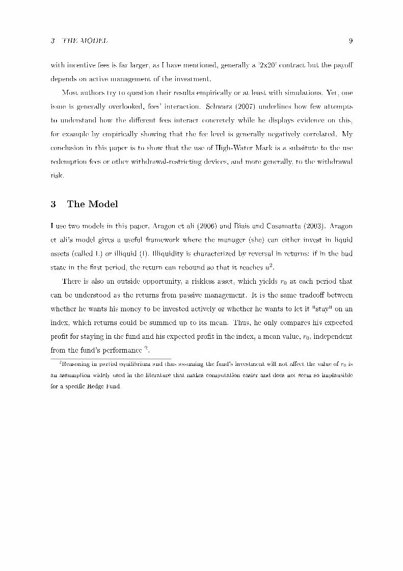
Figure 1: Payos with liquid asset

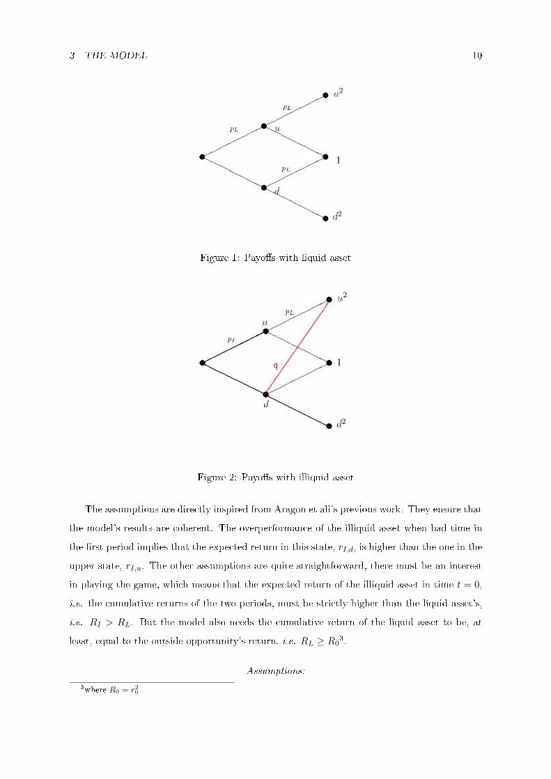
Figure 2: Payos with illiquid asset

The assumptions are directly inspired from Aragon et ali's previous work. They ensure that

the model's results are coherent. The overperformance of the illiquid asset when bad time in

the rst period implies that the expected return in this state, rI,d, is higher than the one in the

upper state, rI,u. The other assumptions are quite straightforward, there must be an interest

in playing the game, which means that the expected return of the illiquid asset in time t = 0,

i.e. the cumulative returns of the two periods, must be strictly higher than the liquid asset's,

i.e. RI > RL. But the model also needs the cumulative return of the liquid asset to be, at

least, equal to the outside opportunity's return, i.e. RL ≥ R03.

Assumptions:

3where R0 = r20

3 THE MODEL 11

1. No investor can join the fund in the rst period.

2. The cumulative return of the illiquid asset is higher than the one liquid's. The probability

of overperforming is lower in the rst period. For the illiquid asset, the expected return

in the second period is higher conditionnal on bad state than conditionnal on the good

one4.

3. The liquid asset's return is at least equal to the outside opportunity's.

The rst assumption is made out of tractability. I wanted to avoid new entries in the

rst period since we would have to dened its eect on the fund value and the possibility of

renegociation it may imply. Overall I wanted to properly see how are set the compensation

schemes. As I noted above The two following assumptions are justied by the necessity for the

player to enter the game with incentives too.

The idea of this paper is to apprehend the possibility of redemption, i.e. the investor can

withdraw from the fund but may need to lose a part of his investment for the purpose.

As noted above, each fee's impact is generally regarded without considering the others',

this explains why, in this model, I stress out how High-Water Mark, regular incentive fees and

redemption fee interact. As I have already mentioned, the choice of implementing redemption

fee is biased, the presence of an illiquid asset necessarily question its use.

The game can be considered in two stages:

• stage 1: Investors decide whether to invest or not in the funds considering the contract,

Ω oered by the manager and with regards to the outside opportunity.

• stage 2: Investors learn the state of the world in t = 1 and can withdraw their money in

the funds in order to invest in the outside opportunity.

The manager oers the contract like a take-it-or-leave-it oer. With such a setting, it

must be solved by backward induction, with fees designed that the investor "stay-in-the-fund

constraint" is bounded. The idea will be that, depending on the level of r0, some contracts will

be built in order to let fund ow in some states, i.e. some contract will prevent the investor

from leaving in the state down without any care for his behavior in the upper state. This can

be understood because of the shape of the returns of the illiquid asset, as it will be shown latter

4Since the distribution of return is i.i.d. for the liquid asset, the expected return are the same.

3 THE MODEL 12

since there is asymmetric payos in the two states and, more importantly, even if the investor

leaves at time t = 1, the manager earns something in the upper state while it is not the case

3.1 Expected Outcomes of the game

3.2 Stay or leave?

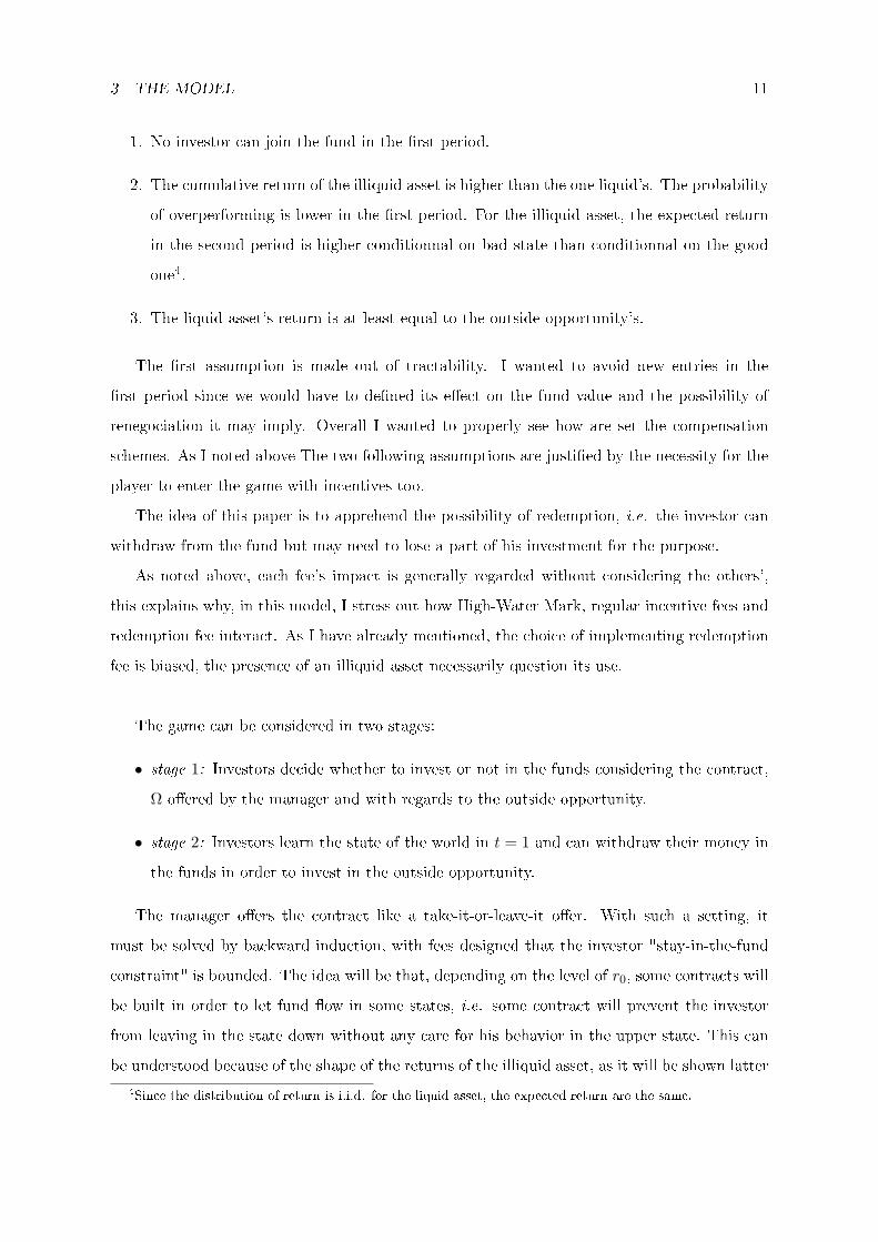
I rst derive the expected outcomes by considering each node. The manager's and investor's

payos are respectively plotted in Figure 3 and Figure 4 in the case of an investment in the

illiquid asset.

Due to the form of the assets' returns, it is obvious that expected fee income will be the

same either with liquid or illiquid assets at node 1u, While the choice of assets will be quite

important when at node 1d, let Ω = f, h,

→ at node 1d for the liquid asset, the manager's expected payo is:

mL(Ω|1u) = pLd(u− 1)f(1− h)

→ at node 1d for the liquid asset, the investor's expected payo is:

πL(Ω|1u) = d[pL(u− (u− 1)f(1− h)) + (1− pL)d]

Figure 3: Manager's payo with illiquid asset

3 THE MODEL 13

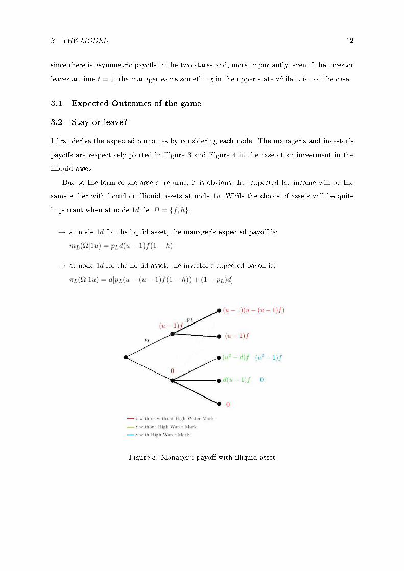
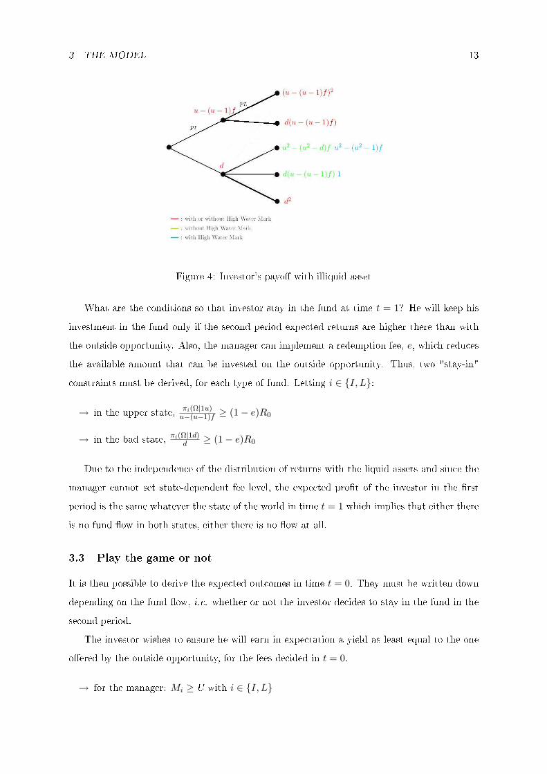
Figure 4: Investor's payo with illiquid asset

What are the conditions so that investor stay in the fund at time t = 1? He will keep his

investment in the fund only if the second period expected returns are higher there than with

the outside opportunity. Also, the manager can implement a redemption fee, e, which reduces

the available amount that can be invested on the outside opportunity. Thus, two "stay-in"

constraints must be derived, for each type of fund. Letting i ∈ I, L:

→ in the upper state, πi(Ω|1u)u−(u−1)f ≥ (1− e)R0

→ in the bad state, πi(Ω|1d)d ≥ (1− e)R0

Due to the independence of the distribution of returns with the liquid assets and since the

manager cannot set state-dependent fee level, the expected prot of the investor in the rst

period is the same whatever the state of the world in time t = 1 which implies that either there

is no fund ow in both states, either there is no ow at all.

3.3 Play the game or not

It is then possible to derive the expected outcomes in time t = 0. They must be written down

depending on the fund ow, i.e. whether or not the investor decides to stay in the fund in the

second period.

The investor wishes to ensure he will earn in expectation a yield as least equal to the one

oered by the outside opportunity, for the fees decided in t = 0.

→ for the manager: Mi ≥ U with i ∈ I, L

4 FIRST CONSIDERATIONS 14

→ for the investor: Πi ≥ R0 with i ∈ I, L

As I have noted above, the main focus must be on the form in the case of the illiquid asset

since only two cases can be found with the liquid one. Three cases can be gured out, either

there is no ow, either there is a ow in node 1u or ow in both nodes. Only the two rst are

truly relevant to be expressed. The contract may contain incentive and redemption fees.

• if no fund ow

→ MI(Ω) = pIf(u− 1) + pIf(u− 1) ([pL(u− (u− 1)f)] + (1− pL)[d(1− h)]),

→ ΠI(Ω) = pIπI|1u + (1− pI)πI|1d

• if ow in the 1u node

→ MI(Ω) = pIf(u− 1) + pIf(u− 1) ([pL(u− (u− 1)f)] + (1− pL)[d(1− h)]),

→ ΠI(Ω) = pI(u− (u− 1)f)r0(1− e) + (1− pI)πI|1d

4 First considerations

4.1 High-Water Mark or not

I start with the simplest form of the model. The manager can only propose a contract with

incentive fee and with High Water Mark and see when High Water Mark contract will arise.

The rst issue will be on managing the illiquid asset.

To determine how the oered contract evolves, it is useful to look at the tradeo the investor

must make in time 1 between staying in the fund or investing in the outside opportunity. In

our model, the manager makes a take-it-or-leave-it oer, thus she will set her compensation

scheme so that the investor becomes indierent when arriving at the node. Due to the expected

prot of staying in the fund, the higher the outside opportunity returns, the less aordable it

is to retain the investor in both nodes. The payos with the illiquid asset are asymmetric and

state dependent on contrary with the liquid asset. Furthermore, we know by assumption that

the expected return in node 1d is higher than those from 1u.

Thus, there will be a level of r0 from which she knows there will be fund ow if we are in

the upper state and no fund ow in. The two agents are sharing the cumulative return of the

asset which is equal to a constant, and the investor's payos is strictly increasing with r0, thus

the manager's expected income decreases with the riskless rate.

Our results are summed up in Proposition 1.


Proposition 4.1 There exists r1, r2,

1. ∃r1, where for r0 < r1, the investor never withdraws from the fund whatever node and the

manager oers a contract with a regular incentive fee.

2. ∃r2, where for r1 < r0 < r2, the investor withdraws from the fund in node 1u, and is

oered a High-Water Mark. For r0 > r2, no value of f , with or without High-Water

Mark can make the investor stay.

Proof: In Appendix A

To prove the point, it is simpler to rst consider how the investor's average expected payos

evolve with each node. For a given incentive fee, the highest average expected return is naturally

conditional on state d (due to assumption 2). Obviously, it follows that this return is higher for

a contract with High-Water Mark. Finally, the latter overperforms whatever contract in state

1u. Since the manager can make a take-it-or-leave it oer, she will set this payo equal to the

risk free rate. As the latter rises, some of the "stay-in" constraint will no longer be ensured

and she will be forced to set fee so that only one node For small level of r0, the manager can

ensure that the investor is not leaving the fund in both states.

The returns are thus distributed so that his payo is the highest in state d and when he is

oered a High Water Mark. This latter point is actually the central result of Aragon et ali's

demonstration. Due to the asymmetry in the illiquid asset's return between the two nodes and

because in node 1d, she has still received no compensation, the manager is more willing to

retain the investor. For that, the High Water Mark is used as a "commitment-device" on the

fund performance. As I reckoned before, the larger the riskless rate, the tighter the tradeo

with staying in the fund, by waiving a part of her fee-income she is ensured to gain as.

It is still possible that depending on the values of the riskfree rate, the manager is forced

to set a contract with a regular incentive fee instead of the HWM but it will only because of

some few values. This will be the case because the HWM fee is larger than the regular one and

it may be too costly in the good state in the second period.

4.2 Adding possibility of redemption

I then question the use of a redemption fee in such a framework. Since High Water Mark is

used only for a certain level of r0, i.e. when the manager is willing to let the investor withdraw

in 1u and prevent fund ow in 1d, can we implement another contract including a redemption

fee that could be substitute to the one with High Water Mark?


Proposition 4.2 There exists a contract f,0,e that is identical to the contract f,1,0.

Proof: In Appendix A.

The idea is simple. With High Water Mark, the incentive fee is set higher than the regular

incentive fee without High Water Mark. In the node 1u, setting a redemption fee to be paid

when withdrawing can get the fee-income to be the same in both contracts, we have already

seen before that the dierence in fee-income between the two situations lay in the upper state

compensation since as we have noted before fh∗I > f∗I . Thus the only need for the manager to

be better o is to set e so that the two incomes get equal. Since the incentive levels are such

that the investor would earn r0 for staying in the fund, his well-being remaining unchanged.

Furthermore, now he is comparing between staying in the fund and the outside opportunity

with an amount invested decreased by the redemption fees, i.e. (1 − e)r0. There is a room

for raising the regular incentive fee as long as the participation constraint in t = 0 is not yet

binding.

There is thus a use for the redemption fee as a substitute for High Water Mark. Such

a statement tends to question Aragon et ali's theory. Yet, we must consider the specicity

of our model that may have impacted on this result. As noted above, the manager makes a

take-it-or-leave-it oer, deriving his contract by maximizing his payo and without any care

for the optimization of the investor's payo. As such, the monopolistic frame that the model

oer needs only to check that he is given at least his reservation payo. If the investor was

given some bargaining power results may have diered and the High Water Mark contract may

have been preferred. The question it raises come down to the level of competition between

fund. Competition in Hedge Funds was studied in Pan et ali paper (2008) where they use the

Herndahl-Hirschman Index to plot an objective measure.

Another argument is left aside by the model, there may be a signal eect while implementing

redemption fees or even lockups. The mechanisms are indeed dierent while High Water Mark

is a commitment to reimburse the loss by waiving a part of the fund's earning, redemption

fees are designed to prevent the investor from leaving. Unfortunately, it seems quite tough to

measure the impact of this dierences in devices namely when we consider rational agents but

this reputational eect that may be caused by some beliefs on the fund poor return.

5 EMPIRICAL ANALYSIS 17

4.3 Risk-Taking Alternative

The Biais and Casamatta model allows thinking risk-shifting alternatives. For this, the possi-

bility of risk shifting would be added in the case of illiquid assets. I have assumed there is a

probability q that the asset, when it has underperformed in the rst period, may overperform

to u2, from this node (1d), the manager is oered to take risk which will rise the probability of

earning u2 and d2 by, respectively, α and β and will decrease the probability of earning 1 by

(α+ β). The idea is to induce moral hazard with a new asset which returns are dominated in

the sense of stochastic second order dominance. How the contract must been changed in order

to prevent her from taking it?

But such a model faces a main issue in the contracts, there are not state-dependent in the

sense that neither the incentives fees', neither the redemption fees' level depend on the state of

the world. In models with risk shifting, one must condition such that the incentive of taking

inconsiderate risk is reduced with a punishment device. In this game, no credible threat can

prevent the manager from taking an alternative strategy as one can see when writing down her

incentive constraint.

A possible extension of this model would consist in extending the "rebounce" of the illiquid

asset. Here, the issue when oering a risk-shifting alternative was that the game will end after

two periods and just after the manager will earn the benet from this behaviour. If one would

implement an evolution of the return of the asset after bad state, not only in the rst period

but ever after, the results may change. Just like in the nancial microstructure literature, the

illiquid asset would be dened as an autoregressive vector, and will have these bounces and

rebounces. Thus, like the Panageas and Westereld model, there would be a tradeo between

the possibility of a one time deviation and the risk when the asset really overperforms that it

will really underperforms afterwards.

Another element may not appear in a model. Although with HWM, the manager only earns

incentives if he overcomes all his past performances, her payos are occuring in far more states

with regular incentive fees since she must only overcome her last performance. For this reason,

there may be a self-regulating eect, i.e. a hindrance to her appetite.

5 Empirical Analysis

Corporate nance is developing going back and forth between empirical and theoretical work.

The main subject of this paper is indeed to understand theoretically what is going on practically


and why there is such a diversication of fees in the Hedge Fund industry. Our model has given

hindsight on the complementarities of fees but we lack some tests to conrm it. Thus I will

use the database TASS-FAR Lipper, which sums up a great number of information on Hedge

Fund, on their structure and on their results.

The main hypotheses I would like to test concerns how the presence of High Water Mark is

related to other fees, the Hedge Fund strategy but also the holding of illiquid assets. For this

latter point, I will refer to the work of Getmansky et ali (2003) who link serial autocorrelation

in the fund returns and illiquid assets, showing that other causes of autocorrelation5 were not

large enough to explain it.

The other goal remains to understand how fees may be linked to signaling process, in our

model for strategy purpose, but it appears as plausible that high redemption fees

5.1 Data

I had to make some choices while addressing the amount of redemption fees. Another problem

with redemption fees lies in the denition taken. Actually, two "types" of redemption fees can

be considered, redemption fee used to prevent the investor in the beginning of his subscription

and redemption fee as thought in the model, i.e. prevailing all the time, that can be considered

like the restrictions on the timing of withdrawal, and thus, can be used against the liquidity

problem. This confusion in the meaning is quite troublesome for our study since, when building

the redemption variable, it is quite hard to disentangle both uses. Furthermore, there is quite

variation in the application of redemption fees, it may depend on the type of shares that are

held, on the impact of the withdrawal on the total value on the fund (Gate restriction), on the

manager's discretion, as well as on the time period since the entry in the fund. Because our

goal is mainly to understand how redemption fees interact with other fees and how they can

be explained by investment in illiquid assets, I consider two variables.

First, in order to overcome this disentanglement issue, I decided to build a dummy that

could be use to give some hindsight and trend but could not be used as a proof. It gives one

whenever redemption fees are mentioned and, since the average lifespan of a fund is 5 years6, I

assume that all redemptions fees asked for an investment time period higher than one year may

also be relevant. Its use should surely be limited since the fees are not necessarily mentioned.

Also, I arbitrarily take fee for period longer than a year but if I had taken smaller time period

5time-varying expected returns, time-varying leverage, incentive fees with High-Water Marks6AGEFI Luxembourg, November 2007


the number of observations would have greatly increased. Finally, since it is in the lock-up

comment, it is easily associated with redemption fees as a short-term device and not to prevent

from withdrawal all along the investment. Because of this, it is generally not mentioned how

the fee evolves after that

Then, a more wise variable concerns the possibility of redemption and is given by the variable

indicating the dierent timing for redemption, "Redemption Frequency"7.

Also, the multiple regressions have shown the weaknesses of some variables such as the

transformation of the redemption period into a continuous variable. The redemption frequenci is

originally given with expressions varying from continuous redemption to redemption triennially.

Because of only few funds imposing longer redemption delay than six months, I regrouped them

into a same variable, "More than Semi-Annually". Unfortunately, we cannot take into account

some comments that are sometimes made, mainly restrictions on the amount that can be

withdrawn in a single shot. Thus other restrictions on redemption are completely demined, .

The distribution of some variables must also be questioned, mainly the incentive fee without

High-Water Mark. The value the latter can take is quite wide and some observations seems

nonsensical, namely a 200% incentive fee, while others are hard to justify, some really low

incentive fee, between O and 1%.

I also developed several variables, inspiring from previous empirical works. In order to

control for specicities such as the style of strategy the Hedge Funds are using. I regroup the

strategies supposed to imply some holding of illiquid assets 8 in a same group since they are the

ones who should be linked with High Water Mark. Such a naive group allows a rst test of the

model. Also, since they develop a portfolio based on other funds, funds of funds are generally

confusing the estimates and they cannot completely suit our model. The onshore variable tries

to pin down how institutional matter may limit the use of the fees and one can see, all along

the regressions that the funds benet from being in weak-legislation countries.

7I use this second variable because of imprecision when describing the amounts asked or the eective period

of time. Actually, the issue of considering such a variable is that there is no necessary indication of whether or

not a fee is asked.8Event Driven, Fixed Income Arbitrage, Emerging Markets and Convertible Arbitrage as described in Ap-

pendix B.


5.2 Summary Statistics:

For the summary statistics, we looked at the complete database of "living" funds 9

The TASS-FAR Lipper Database is well-known when studying the Hedge Fund. It is a

query which reports the funds' performance and form, in particular the fees they are asking.

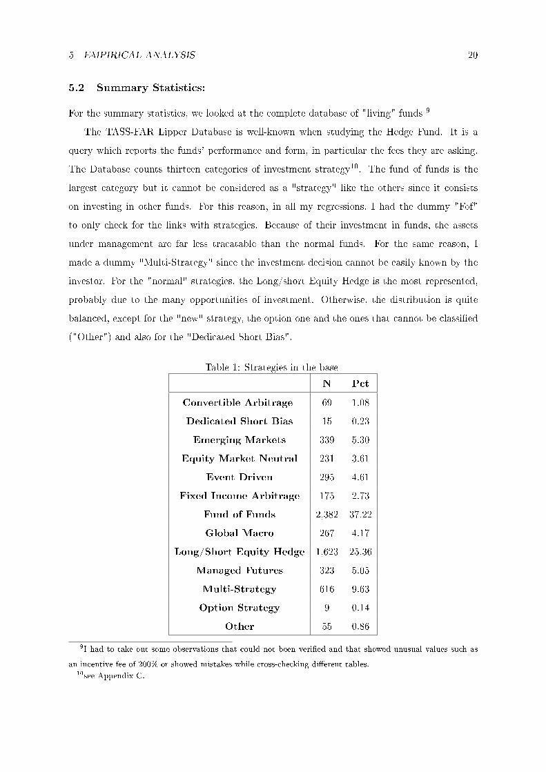
The Database counts thirteen categories of investment strategy10. The fund of funds is the

largest category but it cannot be considered as a "strategy" like the others since it consists

on investing in other funds. For this reason, in all my regressions, I had the dummy "Fof"

to only check for the links with strategies. Because of their investment in funds, the assets

under management are far less tracatable than the normal funds. For the same reason, I

made a dummy "Multi-Strategy" since the investment decision cannot be easily known by the

investor. For the "normal" strategies, the Long/short Equity Hedge is the most represented,

probably due to the many opportunities of investment. Otherwise, the distribution is quite

balanced, except for the "new" strategy, the option one and the ones that cannot be classied

("Other") and also for the "Dedicated Short Bias".

Table 1: Strategies in the base

N Pct

Convertible Arbitrage 69 1.08

Dedicated Short Bias 15 0.23

Emerging Markets 339 5.30

Equity Market Neutral 231 3.61

Event Driven 295 4.61

Fixed Income Arbitrage 175 2.73

Fund of Funds 2,382 37.22

Global Macro 267 4.17

Long/Short Equity Hedge 1,623 25.36

Managed Futures 323 5.05

Multi-Strategy 616 9.63

Option Strategy 9 0.14

Other 55 0.86

9I had to take out some observations that could not been veried and that showed unusual values such as

an incentive fee of 200% or showed mistakes while cross-checking dierent tables.10see Appendix C.


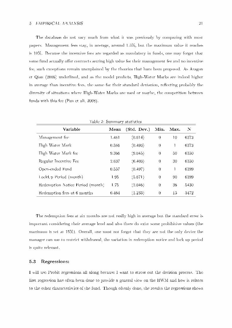
The database do not vary much from what it was previously by comparing with most

papers. Management fees stay, in average, around 1.5%, but the maximum value it reaches

is 10%. Because the incentive fees are regarded as mandatory in funds, one may forget that

some fund actually oer contracts setting high value for their management fee and no incentive

fee, such exceptions remain unexplained by the theories that have been proposed. As Aragon

et Qian (2006) underlined, and as the model predicts, High-Water Marks are indeed higher

in average than incentive fees, the same for their standard deviation, reecting probably the

diversity of situations where High-Water Marks are used or maybe, the competition between

funds with this fee (Pan et ali, 2008).

Table 2: Summary statistics

Variable Mean (Std. Dev.) Min. Max. N

Management fee 1.481 (0.614) 0 10 6373

High Water Mark 0.586 (0.493) 0 1 6373

High Water Mark fee 9.366 (9.045) 0 50 6350

Regular Incentive Fee 2.637 (6.403) 0 30 6350

Open-ended Fund 0.557 (0.497) 0 1 6399

LockUp Period (month) 1.95 (5.671) 0 90 6399

Redemption Notice Period (month) 1.75 (2.046) 0 36 5430

Redemption fees at 6 months 0.464 (1.233) 0 15 3472

The redemption fees at six months are not really high in average but the standard error is

important considering their average level and also there do exist some prohibitive values (the

maximum is set at 15%). Overall, one must not forget that they are not the only device the

manager can use to restrict withdrawal, the variation in redemption notice and lock up period

is quite relevant.

5.3 Regressions:

I will use Probit regressions all along because I want to stress out the decision process. The

rst regression has often been done to provide a general view on the HWM and how it relates

to the other characteristics of the fund. Though oftenly done, the results the regressions shows


do not t what has been previously observed and are in line with my theoretical results.

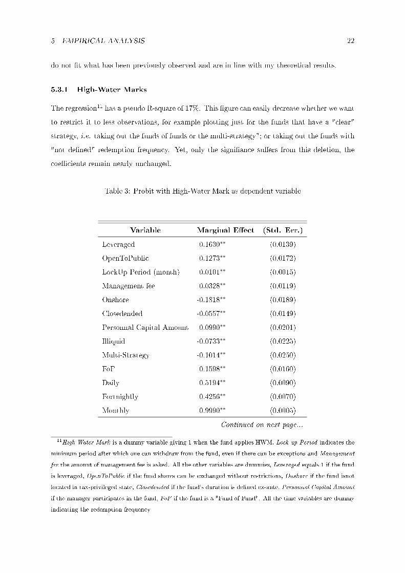
5.3.1 High-Water Marks

The regression11 has a pseudo R-square of 17%. This gure can easily decrease whether we want

to restrict it to less observations, for example plotting just for the funds that have a "clear"

strategy, i.e. taking out the funds of funds or the multi-strategy"; or taking out the funds with

"not dened" redemption frequency. Yet, only the signiance suers from this deletion, the

coecients remain nearly unchanged.

Table 3: Probit with High-Water Mark as dependent variable

Variable Marginal Eect (Std. Err.)

Leveraged 0.1630∗∗ (0.0139)

OpenToPublic 0.1273∗∗ (0.0172)

LockUp Period (month) 0.0101∗∗ (0.0015)

Management fee 0.0328∗∗ (0.0119)

Onshore -0.1818∗∗ (0.0189)

Closedended -0.0557∗∗ (0.0149)

Personnal Capital Amount 0.0990∗∗ (0.0201)

Illiquid -0.0733∗∗ (0.0225)

Multi-Strategy -0.1014∗∗ (0.0250)

FoF -0.1598∗∗ (0.0160)

Daily 0.5194∗∗ (0.0090)

Fortnightly 0.4256∗∗ (0.0070)

Monthly 0.9990∗∗ (0.0005)

Continued on next page...

11High Water Mark is a dummy variable giving 1 when the fund applies HWM. Lock-up Period indicates the

minimum period after which one can withdraw from the fund, even if there can be exceptions and Management

fee the amount of management fee is asked. All the other variables are dummies, Leveraged equals 1 if the fund

is leveraged, OpenToPublic if the fund shares can be exchanged without restrictions, Onshore if the fund isnot

located in tax-privileged state, Closedended if the fund's duration is dened ex-ante, Personnal Capital Amount

if the manager participates in the fund, FoF if the fund is a "Fund of Fund". All the time variables are dummy

indicating the redemption frequency


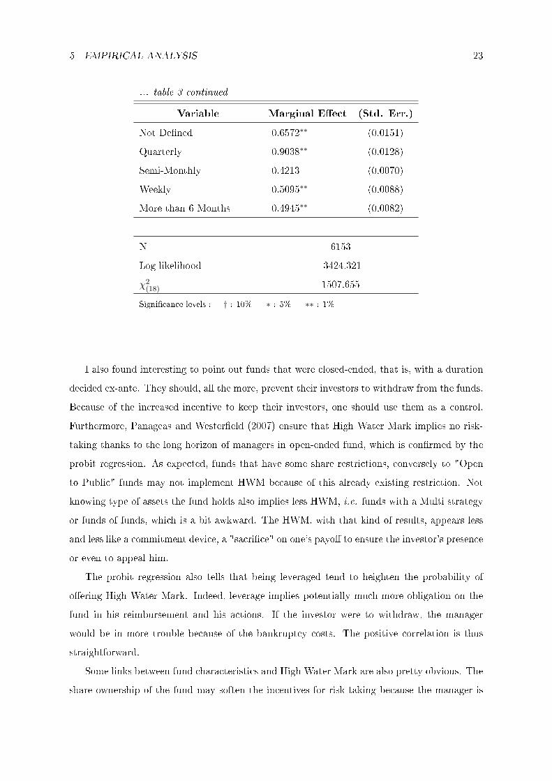
... table 3 continued


Not Dened 0.6572∗∗ (0.0151)

Quarterly 0.9038∗∗ (0.0128)

Semi-Monthly 0.4213 (0.0070)

Weekly 0.5095∗∗ (0.0088)

More than 6 Months 0.4945∗∗ (0.0082)

N 6153

Log-likelihood -3424.321

χ2(18) 1507.655

Signicance levels : † : 10% ∗ : 5% ∗∗ : 1%

I also found interesting to point out funds that were closed-ended, that is, with a duration

decided ex-ante. They should, all the more, prevent their investors to withdraw from the funds.

Because of the increased incentive to keep their investors, one should use them as a control.

Furthermore, Panageas and Westereld (2007) ensure that High Water Mark implies no risk-

taking thanks to the long horizon of managers in open-ended fund, which is conrmed by the

probit regression. As expected, funds that have some share restrictions, conversely to "Open

to Public" funds may not implement HWM because of this already existing restriction. Not

knowing type of assets the fund holds also implies less HWM, i.e. funds with a Multi strategy

or funds of funds, which is a bit awkward. The HWM, with that kind of results, appears less

and less like a commitment device, a "sacrice" on one's payo to ensure the investor's presence

or even to appeal him.

The probit regression also tells that being leveraged tend to heighten the probability of

oering High Water Mark. Indeed, leverage implies potentially much more obligation on the

fund in his reimbursement and his actions. If the investor were to withdraw, the manager

would be in more trouble because of the bankruptcy costs. The positive correlation is thus

straightforward.

Some links between fund characteristics and High Water Mark are also pretty obvious. The

share ownership of the fund may soften the incentives for risk-taking because the manager is


then gambling his own wealth( Hodder and Jackwerth, 2006), and may thus explained why

High-Water Mark are more present in funds where manager have a participation. This partic-

ipation may work as a signal on the manager's behavior. Since the age variable do not play

any role in the regression, the coecients associated to age and size when these two variables

are added to the regression are close to zero, it may not seem to be the experience nor the

importance of the fund that are relevant.

Some estimates look like a riddle. I found appealing to use in the probit regression the

dierent redemption periods, the less frequent, the more one should use High Water Mark in

the conclusions of the model. But there is no trend appearing in the results, on the contrary.

Two main explanations come in mind. First, the database is not suciently detailed about the

redemption fees and there is a tradeo between the timing and the amount asked to the investor,

one can only conclude that the probability of High-Water Mark is positively correlated with

redemption notice period since the point of comparison is actually the possibility to withdraw

whenever is desired.

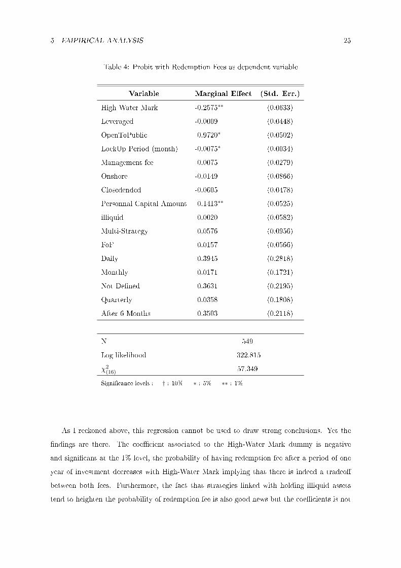
5.3.2 Redemption fee

This second probit regression12 is using the lockup comment in order to derive the redemption

fee. As I have already discussed above, the main issue concerns the loss in number of obser-

vations and it should only give some trend to test the model. The fact that information on

redemption remain generally blurred is appealing. In the query only 26 funds do not mention

the presence of High Water Marks. But the situation is quite dierent with redemption fees.

It is generally a challenge to understand if and how they charge redemptions fee.

The R-square of the regression is not really high, 16,5% but the regression oers mainly

signicant coecients. In order to avoid the confusion that may be lead with the two notions

behind redemption, I use the redemption fee dummy asked for withdrawal after a year of

investment. Even if this regression is lacking observations, it gives fortunate conrmation of

the model.

12Redemption fee is a dummy variable giving 1 when the fund asked for an amount when withdrawal after

a year. Lock-up Period indicates the minimum period after which one can withdraw from the fund, even if

there can be exceptions and Management fee the amount of management fee is asked. All the other variables

are dummies, Leveraged equals 1 if the fund is leveraged, OpenToPublic if the fund shares can be exchanged

without restrictions, Onshore if the fund isnot located in tax-privileged state, Closedended if the fund's duration

is dened ex-ante, Personnal Capital Amount if the manager participates in the fund,FoF if the fund is a "Fund

of Fund". All the time variables are dummy indicating the redemption frequency


Table 4: Probit with Redemption Fees as dependent variable


High Water Mark -0.2575∗∗ (0.0633)

Leveraged -0.0009 (0.0448)

OpenToPublic 0.9720∗ (0.0502)

LockUp Period (month) -0.0075∗ (0.0034)

Management fee 0.0075 (0.0279)

Onshore -0.0149 (0.0866)

Closedended -0.0605 (0.0478)


illiquid 0.0020 (0.0582)

Multi-Strategy 0.0576 (0.0956)

FoF 0.0157 (0.0566)

Daily 0.3945 (0.2818)

Monthly 0.0171 (0.1721)

Not Dened 0.3631 (0.2195)

Quarterly 0.0358 (0.1808)

After 6 Months 0.3503 (0.2118)

N 549


χ2(16) 57.349


As I reckoned above, this regression cannot be used to draw strong conclusions. Yet the

ndings are there. The coecient associated to the High-Water Mark dummy is negative

and signicant at the 1% level, the probability of having redemption fee after a period of one

year of investment decreases with High-Water Mark implying that there is indeed a tradeo

between both fees. Furthermore, the fact that strategies linked with holding illiquid assets

tend to heighten the probability of redemption fee is also good news but the coecients is not


signicant, so one may doubt of this result. I have noted before that there may be a selection

bias in this data which is why such a result do not mean so much, it will be quite judicious,

since they are not compelled to, for most funds with redemption fees throughout time not to

mention them, and if the model is correct, that would mainly be those "illiquid" should take

into account. Another interesting point stands in the positive relation between management

and redemption fee which may be an alternative contract form than the one I underlined,

regular incentive and redemption fee.

A positive relation between redemption period and fees can be drawn. The less one can

withdraw, the more one may face redemption fees. As I mentioned when describing the data,

the regressions miss the redemption notice period and the possible restrictions that can be

imposed on withdrawal, and if they could be taken into account, that may heighten this result.

Also, these coecients are not signicant so even if they go in line with the model, thay cannot

be completely relied on.

Some results do not really need to be commented because straightforward. The negative

coecient associated to the strategies Fund of Fund or Multi-Strategy sounds logical, the

investor has not obvious information on the fund's type of investment, it is the model I have been

presented with only ex-ante probability about the type of the fund. When the fund suers bad

performance, the incentive to leave it must be way higher than for explicitly dened strategies.

The fact that the fund is closed-ended decrease the probability of redemption fee which do not

seem straightforward and may be actually linked to the poor number of observations.

The fact that the coecient associated with the lock-up period is negative is not so surpris-

ing and continue to prove the importance of the tradeo between these "withdrawal restricting"

devices. Actually two kinds of lock-up can be met: "soft" ones, where investor can withdraw

against some fee and "hard" ones where investors is prevented to do so13. And, as I mentioned

earlier, one still lack other variables to explain this tradeo, illiquid assets holding do not seem

sucient. Yet this fact can also uphold the link between bad performing funds and multiple

devices to prevent anyone from leaving the fund.

13actually, when describing their fund some with "hard" lock-up dene it as such because of high redemption

fees.

6 HOLDING ILLIQUIDITY AND HIGH-WATER MARK: 27

6 Holding Illiquidity and High-Water Mark:

The rst regressions tend to prove the point made in the theoretical part, there do not seem

to be the slightest interest in using High-Water Mark to prevent from withdrawal. Though the

illiquid asset holding variable was based on which strategies is supposed to be implying that

kind of holding, the denition was not as straightforward as many papers quote it. As such,

I thought that it would be useful to dig in the links between assets holding and strategies. I

thus tried to identify which strategies imply illiquid positions.

A great number of researches has tried to empirically assess the holding of illiquidity namely

by looking at the return of the funds, with as most signicant returns, monthly ones. A common

way to do so has become to check for autocorrelation, the higher the persistence, the more

plausible the fund is holding illiquid assets. These tests are being run out by Aragon et ali but

also by Gemantski et ali to confront their point.

While many papers have focused on a simple AR(1), I have preferred to also use an esti-

mation closer to the one made by Gemantski et ali, i.e. to use a second lag in order to test for

the persistence of correlation as such two equations are actually estimated:

ri,t = α+ ρri,t−1 + ei,t

ri,t = ρ1ri,t−1 + ρ2ri,t−2 + ei,t

I had to use this second equation because the results in Table 10 were not satisfactory.

The persistence was much too higher than expected for many supposed to be "liquid" funds.

Modeling the returns with an autoregressive vector with two lags allows checking for a longer

time period with keeping the monthly gap between observations. Such a model is designed

hoping the returns in t will be less predicted by the returns two periods before.

6.1 Determining Illiquidity:

I display here only the table for the AR(2) model regression since the rst equation has given

some unexpected results. Actually all funds which were supposed to show some little autocor-

relation except for the "Managed Future" strategy show as high autocorrelation as the other

funds. since high ρ is supposed to be related with holding illiquid assets. When checking for

more persistency in returns,


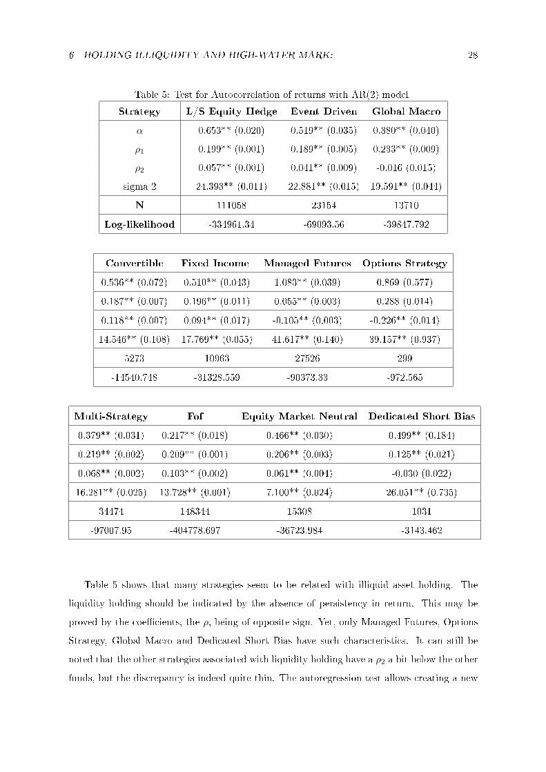
Table 5: Test for Autocorrelation of returns with AR(2) model

Strategy L/S Equity Hedge Event Driven Global Macro

α 0.653** (0.020) 0.519** (0.035) 0.380** (0.040)

ρ1 0.199** (0.001) 0.189** (0.005) 0.233** (0.009)

ρ2 0.057** (0.001) 0.041** (0.009) -0.016 (0.015)

sigma 2 24.393** (0.011) 22.881** (0.015) 19.591** (0.044)

N 111058 23154 13710

Log-likelihood -334961.34 -69093.56 -39847.792

Convertible Fixed Income Managed Futures Options Strategy

0.536** (0.072) 0.510** (0.043) 1.083** (0.039) 0.869 (0.577)

0.187** (0.007) 0.196** (0.011) 0.055** (0.003) 0.288 (0.014)

0.118** (0.007) 0.094** (0.017) -0.105** (0.003) -0.226** (0.014)

14.546** (0.108) 17.769** (0.055) 41.617** (0.140) 39.157** (0.937)

5273 10963 27526 299

-14540.748 -31328.559 -90373.33 -972.565

Multi-Strategy Fof Equity Market Neutral Dedicated Short Bias

0.379** (0.031) 0.217** (0.018) 0.466** (0.030) 0.499** (0.184)

0.219** (0.002) 0.209** (0.001) 0.206** (0.003) 0.125** (0.021)

0.068** (0.002) 0.103** (0.002) 0.061** (0.004) -0.030 (0.022)

16.281** (0.025) 13.728** (0.001) 7.100** (0.024) 26.051** (0.735)

34474 148344 15308 1031

-97007.95 -404778.697 -36723.984 -3143.462

Table 5 shows that many strategies seem to be related with illiquid asset holding. The

liquidity holding should be indicated by the absence of persistency in return. This may be

proved by the coecients, the ρ, being of opposite sign. Yet, only Managed Futures, Options

Strategy, Global Macro and Dedicated Short Bias have such characteristics. It can still be

noted that the other strategies associated with liquidity holding have a ρ2 a bit below the other

funds, but the discrepancy is indeed quite thin. The autoregression test allows creating a new


"illiquid" variable in order to test if the illiquidity that is revealed by the test may be linked

with High-Water Mark.

The results of the Probit regression are so dierent from what Aranagon and Qian's, it

seemed useful to try to control them. It was indeed possible that most funds analyzed in this

paper are new funds that have new characteristics. The time period from fall 2007 to 2009 has

actually seen the world entering in a major crisis and it is interesting to ask to what extent

this may have changed the behavior of funds' strategy which may be a good explanation for

the results. I have redone the second test for this period only14 and there is a lot of changes

that can be noted. One should expect all the funds to show less autocorrelation in their return,

becaue of a ight to liquidity but there is no such trend. What one can see, is the impossibility

to predict autocorrelation from the strategies.

I then wanted to use these ndings in order to draw some conclusions on the renewed form

of funds, as an adaptation to this context. Unfortunately, only six funds are reported between

the 31st December 2007 and now on, with only six observations it will be hard to derive some

trends. The Graveyard database given by TASS-FAR is not more useful, information about

why the fund stops reporting are often missing.

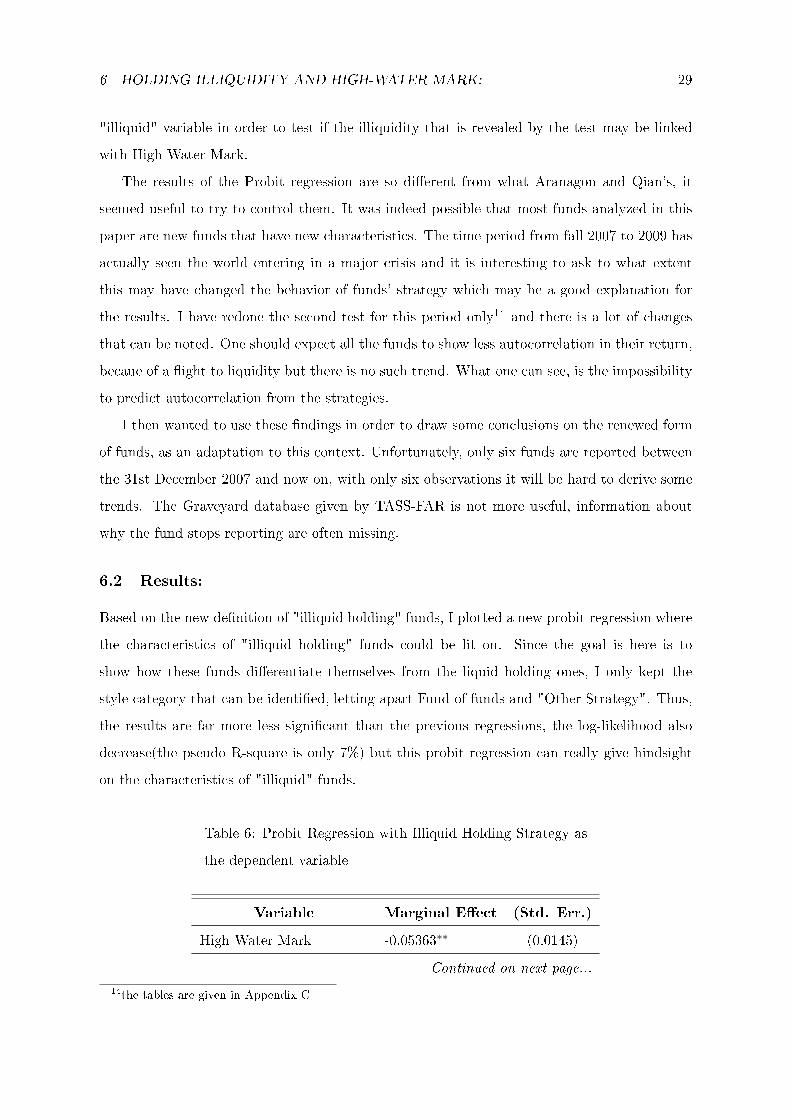
6.2 Results:

Based on the new denition of "illiquid holding" funds, I plotted a new probit regression where

the characteristics of "illiquid holding" funds could be lit on. Since the goal is here is to

show how these funds dierentiate themselves from the liquid holding ones, I only kept the

style category that can be identied, letting apart Fund of funds and "Other Strategy". Thus,

the results are far more less signicant than the previous regressions, the log-likelihood also

decrease(the pseudo R-square is only 7%) but this probit regression can really give hindsight

on the characteristics of "illiquid" funds.

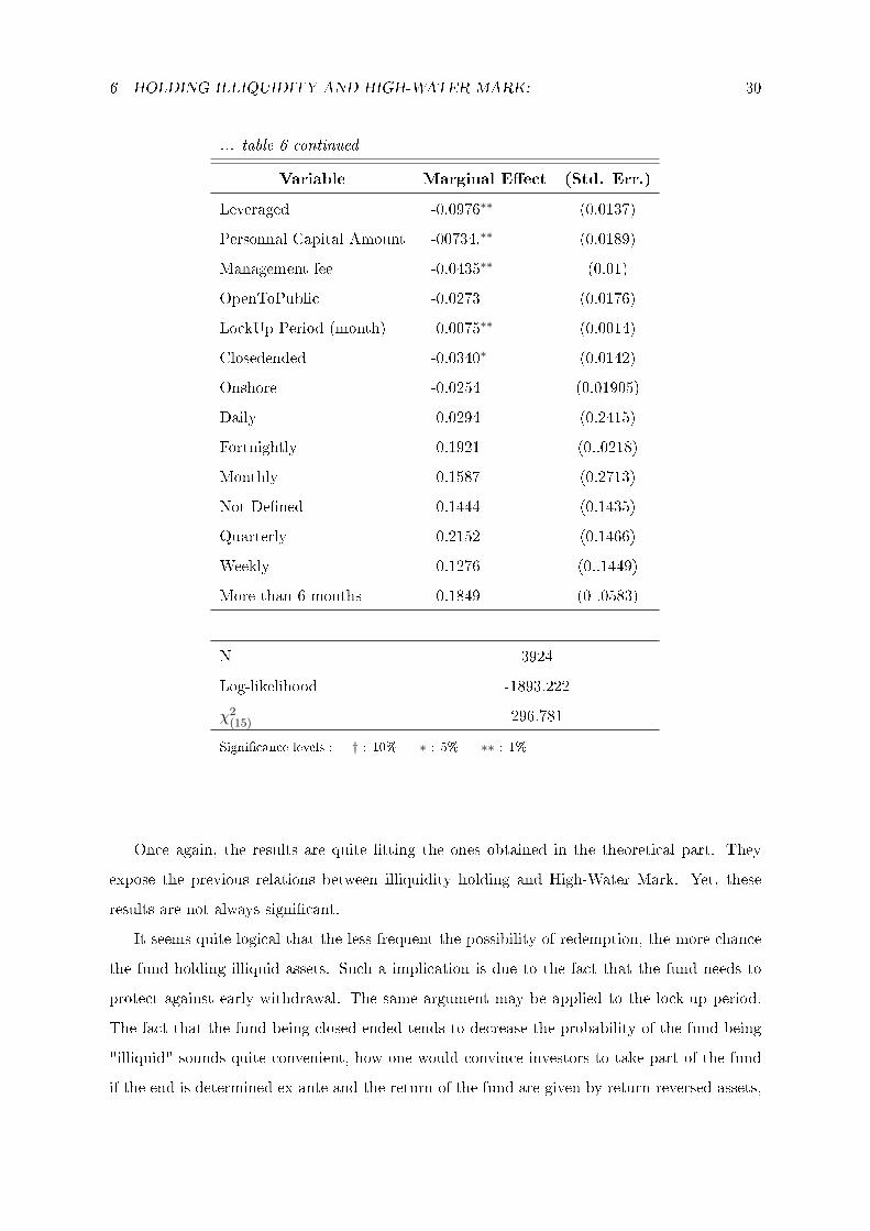
Table 6: Probit Regression with Illiquid Holding Strategy as

the dependent variable


High Water Mark -0.05363∗∗ (0.0145)

Continued on next page...

14the tables are given in Appendix C


... table 6 continued


Leveraged -0.0976∗∗ (0.0137)

Personnal Capital Amount -00734.∗∗ (0.0189)

Management fee -0.0435∗∗ (0.01)

OpenToPublic -0.0273 (0.0176)


Closedended -0.0340∗ (0.0142)

Onshore -0.0254 (0.01905)

Daily 0.0294 (0.2415)

Fortnightly 0.1921 (0..0218)

Monthly 0.1587 (0.2713)

Not Dened 0.1444 (0.1435)

Quarterly 0.2152 (0.1466)

Weekly 0.1276 (0..1449)

More than 6 months 0.1849 (0 .0583)

N 3924


χ2(15) 296.781


Once again, the results are quite tting the ones obtained in the theoretical part. They

expose the previous relations between illiquidity holding and High-Water Mark. Yet, these

results are not always signicant.

It seems quite logical that the less frequent the possibility of redemption, the more chance

the fund holding illiquid assets. Such a implication is due to the fact that the fund needs to

protect against early withdrawal. The same argument may be applied to the lock-up period.

The fact that the fund being closed-ended tends to decrease the probability of the fund being

"illiquid" sounds quite convenient, how one would convince investors to take part of the fund

if the end is determined ex-ante and the return of the fund are given by return-reversed assets,

7 CONCLUSION: 31

there will always be an incentive to leave the fund ex-ante in case of good results or to make it

go on in case of bad results. Also, the participation of manager is associated with a negative

coecient. It can be understood because of the challenging aspect of investing in illiquid assets,

as soon as a manager begins to develop his own fund with his own money, he may want to take

safer positions. The age and size of fund variables are associated with coecients close to zero

so it is not the case that this is linked with a size matter,(which could mean that the funds

being smaller and thus needing less participation from the manager or, on the contrary, they

being enough big and old to reassure the investors).

Yet some links are still uneasy to explain. While it remains understandable that banks do

not want to invest in funds which are riskier due to liquidity risk (inherent to the asset and

the possibility of withdrawal), no apparent trend can be found with redemption notice periods.

But the same arguments as before can be applied there.

Thus, the portrait of an "illiquid" fund shows some originality. Even if their size or age do

not seem to make them dierent from others, there do exist many particular characteristics.

Management fee are lower, as the probability of HWM. There must be a competition eect

explaining this waiving from manager and, as I so much tried to underline, there must be

some intern controls, that remain mainly hidden and compensate this lowered payo. Ther

ought to be some interest in providing a more sociological portrait of these funds' managers,

to link the style of the fund with less rational but as intersting elements. But also, adding such

characterists will help in determining what elements determine for example, why the "illiquid

funds" seem less leveraged.

7 Conclusion:

By trying to look after explanation of the use of High Water Mark, I have developed arguments

against Aragon et ali's theory which relates High Water Mark to the investment on illiquid

assets. The large variety of tools that are used in the Hedge fund industry seems to really have

a use, . But such an answer is also relatively linked to our model.

Another point is completely overlooked in this paper, the share of bargaining power. I took

a take-it-or-leave-it type of oer which implied that Hedge fund's manager had a monopolistic

power and could impose her price with a program where she maximizes her utility. But results

would have changed whether one would have try to model the whole range of intermediary

situations where each individual own some bargaining power but also, and mainly, reshape the

7 CONCLUSION: 32

model to understand it when the investor has all bargaining power. Maybe, the increasing

number of Hedge funds in the industry may force to soften this assumption but at the same

time. On the other hand, the multiplicity of strategies may ensure that the fund still have a

monopolistic power. The paper lacks some checking, maybe using the Herndhal index. Yet

such a control do not seem too certain.

The empirical study has shown a main source of concern, the need for revamping the data

on redemptions. Since the query is not mandatory, it is understandable that lots of values

are missing. Yet the lack of precise questions on the subject itself remains a problem. It also

lacks information on the manager herself. The literature always insist on the prevalence of

her ability to explain investment in Hedge Fund relatively to investment in Mutual Fund for

example (Goetzman et ali, 2003) and understanding what characteristics explain strategies and

fees would be an interesting question. Would we have young manager, attempting to achieve

overperformance by investing in illiquid assets or rather more experienced manager, notably

because they may seem much more trustworthy and may also be able to commit more, for

example by participating to the fund.

The main achievement of this paper remains to show there is, also empirically, doubts about

the explanation of High-Water Mark that Aragon et ali gave. I have tried to defend the idea

according to which High-Water Mark is more of a fad when there is economic expansion.

According to the idea that High-Water Mark is not necessarily used in order to take excessive

risks and thus generating excess payos because of time consideration, it may be the best

suited to economic contexts where there do exist really high return opportunities. This idea

also implies that, in an economic downturn, expected prot for the manager may decrease due

to the lack of overperforming opportunities and makes him rather shut down his fund. What I

would like to check, that the managers change their contracts with the business cycles and that

new funds ask more or less HWM according to the cycles. But these results seem hard to prove.

First there is to know how fast the manager can change his contract and what signals this must

send to the investors. Then, although appealing, looking at both TASS-FAR databases do not

show less funds with HWM than usual. And nally, I use the economic downturn to explain

the strange results that have appeared lately in the funds' returns, but the markets where the

funds invest may not suer from the same uctuations than one thinks. The regulation issue

may be a more critic question.

8 BIBILIOGRAPHY: 33

8 Bibiliography:

References

[1] Aragon, G., Qian, J., 2007. Liquidation Risk and High-Water Marks, Boston College.

[2] Berle A. A. and Means G. C. (1932), The Modern Corporation and Private Porperty, New

York, Macmillan.

[3] Basak, Suleyman, Alex Shapiro, and Lucie Tepla, 2004, Risk management with bench-

marking, NYU Finance Working paper.

[4] Biais B. and Casamatta C., 2003, Optimal Leverage and Aggregate Investment,

[5] Browne, Sid, 1997, Survival and growth with a liability: Optimal portfolio strategies in

continuous time, Mathematics of Operations Research 22, 468-493.

[6] Carpenter, Jennifer, 2000, Does option compensation increase managerial risk appetite?,

Journal of Finance 21, 2311-2331.

[7] Frank, Douglas H. and Obloj, Tomasz, 2009, Ability and Agency Costs: Evidence from

Polish Banking

[8] Fung, William, and David Hsieh, 1997, Empirical characteristics of dynamic trading strate-

gies, Review of Financial Studies 10, 275-302.

[9] Fung, William, and David Hsieh, 1999, A primer on hedge funds, Journal of Empirical

Finance 6, 309-331.

REFERENCES 34

[10] Getmansky, M., A. Lo, and I. Makarov. 2004. An econometric model of serial correlation

and illiquidity in hedge fund returns. Journal of Financial Economics 74, 529-609.

[11] Goetzmann W. N., Ingersoll J., and Ross S., 2003, High-water marks and hedge fund

management contracts, Journal of Finance 58, 1685-1717.

[12] Heinricher, Arthur C., and Richard H. Stockbridge, 1991, Optimal control of the running

max, SIAM Journal on Control and Optimization 29.

[13] Hodder, James, and Jens Carsten Jackwerth, 2004, Incentive contracts and hedge fund

management, Working Paper, University of Konstanz.

[14] Pan F., Zhao H. and Tang K., 2008, The Impact of Competition on Manager Compensa-

tion: Theory and Evidence in Hedge funds

[15] Panageas, S., Westereld, M., 2007. High-Water Marks: High Risk Appetites? Convex

Compensation, Long Horizons, and Portfolio Choice. Journal of Finance

[16] Ross, Stephen A., 2004, Compensation, incentives, and the duality of risk aversion and

riskiness, Journal of Finance 59, 207-225.

9 APPENDIX: 35

9 Appendix:

9.1 Appendix A:

Lemme 1 For a given level the manager wants to ensure the investor, she is always better o

with a contract without High-Water Mark.

Proof:

It is actually quite obvious to show that her payo will necessarily be equal or higher

without High-Water Mark. With the liquid asset, High-Water Mark implies that she waives

her income as soon as the state was down in the rst period. For the illiquid one, while there is

no change between the two contracts if in the upper state in the rst period, the income with

High-Water Mark is far smaller. When the asset "rebounds", she must compare u2 to 1 and

not to the last performance d, and also, she must waive her compensation when the asset only

reaches 1.

9.1.1 Proof of Proposition 1:

As noted before, the manager sets his fee so that the investor is ensured of earning as if he

would invests in the outside opportunity.

Since I have shown with lemma 1 that she is always better o without High-Water Mark

for a given amount to ensure, for High-Water Mark to be implemented a situation must exist

such that the investor would not agree for a regular fee incentive.

A rst important remark is to rank the average expected return for staying in the fund in

the rst period, one nds:

πHI (Ω|1d)d ≥ πI(Ω|1d)

d ≥ πI(Ω|1u)u−(u−1)f

The level of fee that can be asked for the investor to stay in the fund, i.e. for his payo

to be equal to r0 as r0 increases in the following way depend on when the manager agrees on

letting him go.

First, if the riskfree interest rate is low enough, the investor never withdraws and the

manager oers a regular incentive fee, f∗ = rL−r0(u−1)pL

Then, for higher level of r0, the investor withdraws in the good state, but, though the

manager earns some payo with his withdrawal, there is nothing for her in the bad states. As

such, she will set f so that the investor stays in the fund. And since the expected average

return with High-Water Mark is higher than the one without, she can set a higher fee, which

9 APPENDIX: 36

will earn her the same expected amount in the bad state but a higher return in the good one.

Since the investor withdraws from the fund, she knows she would earn (u − 1)f , High-Water

Mark or not.

Thus there exists a range of r0 where f∗,H = qu3+(1−q)rL−r0qu(u2−1)

For higher level of the riskfree rate, it is obvious that no compensation schemes will let the

investor stay in.

9.1.2 Proof of Proposition 2:

To prove that there exists e level of e such as both contracts are the same for the investors, one

needs to showh that the investor will still enter the game in rst period even when is oered

a regular incentive scheme,f , AND a redemption fee, e. Since the only dierence between the

High-Water Mark, fH and the regular incentive fee is in the good state in time t = 1, the

investor only needs to insure that it costs as much for the investor to be oered a High-Water

Mark than a redemption fee.

One wants:u − (u − 1)f∗,H = u − (u − 1)f∗(1 − e), where f∗ is the equilibrium regular

incentive fee for which the investor is indierent.

By computation, one nds: f∗ = qu3+(1−q)rL−r0q(u3−1)+(1−q)(u−1)pL

and one easily sees that f∗,H > f∗

Thus e∗ = 1−(u−(u−1)f∗,H

u−(u−1)f∗

), which do exist and is necessarily under 1.

9.2 Appendix B:

I borrow the idea of Getmansky in providing a small description of the main strategies I consider

in the paper:

Equity Hedge: This directional strategy involves equity-oriented investing on both the long

and short sides of the market. The objective is not to be market neutral. Managers have

the ability to shift from value to growth, from small to medium to large capitalization stocks,

and from a net long position to a net short position. Managers may use futures and options to

hedge. The focus may be regional, such as long/short US or European equity, or sector specic,

such as long and short technology or healthcare stocks.

Long/short equity funds tend to build and hold portfolios that are substantially more

concentrated than those of traditional stock funds with dierent regional focus: US equity

Hedge, European equity Hedge, Asian equity Hedge and Global equity Hedge. Dedicated

Short Seller Short biased managers take short positions in mostly equities and derivatives. The

9 APPENDIX: 37

short bias of a manager's portfolio must be constantly greater than zero to be classied in this

category.

Fixed Income Directional: This directional strategy involves investing in Fixed Income

markets only on a directional basis.

Convertible Arbitrage: This strategy is identied by hedge investing in the convertible

securities of a company. A typical investment is to be long the convertible bond and short

the common stock of the same company. Positions are designed to generate prots from the

identied income security as well as the short sale of stock, while protecting principal from

market moves.

Event Driven: This strategy is dened as `special situations' investing designed to cap-

ture price movement generated by a signicant pending corporate event such as a merger,

corporate restructuring, liquidation, bankruptcy or reorganization. There are three popular

sub-categories in event-driven strategies: risk (merger) arbitrage, distressed/high yield securi-

ties, and Regulation D.

Non Directional/Relative Value: This investment strategy is designed to exploit equity

and/or xed income market ineciencies and usually involves being simultaneously long and

short matched market portfolios of the same size within a country. Market neutral portfolios

are designed to be either beta or currency neutral, or both.

Global Macro: Global macro managers carry long and short positions in any of the world's

major capital or derivative markets. These positions reect their views on overall market

direction as inuenced by major economic trends and or events. The portfolios of these funds

can include stocks, bonds, currencies, and commodities in the form of cash or derivatives

instruments. Most funds invest globally in both developed and emerging markets.

Managed Futures: This strategy invests in listed nancial and commodity futures markets

and currency markets around the world. The managers are usually referred to as Commod-

ity Trading Advisors, or CTAs. Trading disciplines are generally systematic or discretionary.

Systematic traders tend to use price and market specic information (often technical) to make

trading decisions, while discretionary managers use a judgmental approach.

Emerging Markets: This strategy involves equity or xed income investing in emerging

markets around the world.

Fund of funds: A `Multi Manager' fund will employ the services of two or more trading

advisors or Hedge funds who will be allocated cash by the Trading Manager to trade on behalf

of the fund.

9 APPENDIX: 38

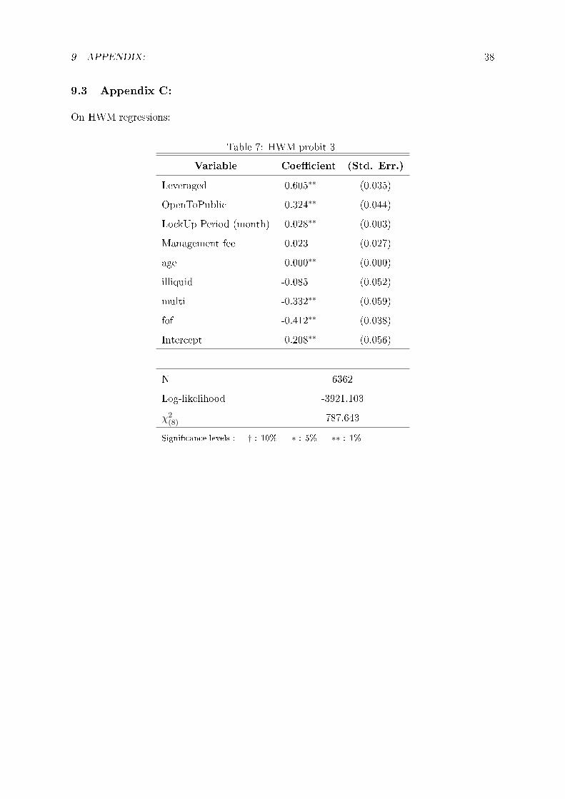
9.3 Appendix C:

On HWM regressions:

Table 7: HWM probit 3

Variable Coecient (Std. Err.)

Leveraged 0.605∗∗ (0.035)




age 0.000∗∗ (0.000)

illiquid -0.085 (0.052)

multi -0.332∗∗ (0.059)

fof -0.412∗∗ (0.038)

Intercept 0.208∗∗ (0.056)

N 6362


χ2(8) 787.643


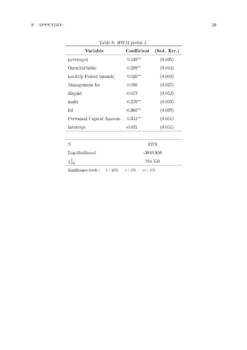
9 APPENDIX: 39



Leveraged 0.539∗∗ (0.035)




illiquid -0.073 (0.052)

multi -0.270∗∗ (0.059)

fof -0.366∗∗ (0.038)


Intercept -0.031 (0.051)

N 6373


χ2(8) 764.550


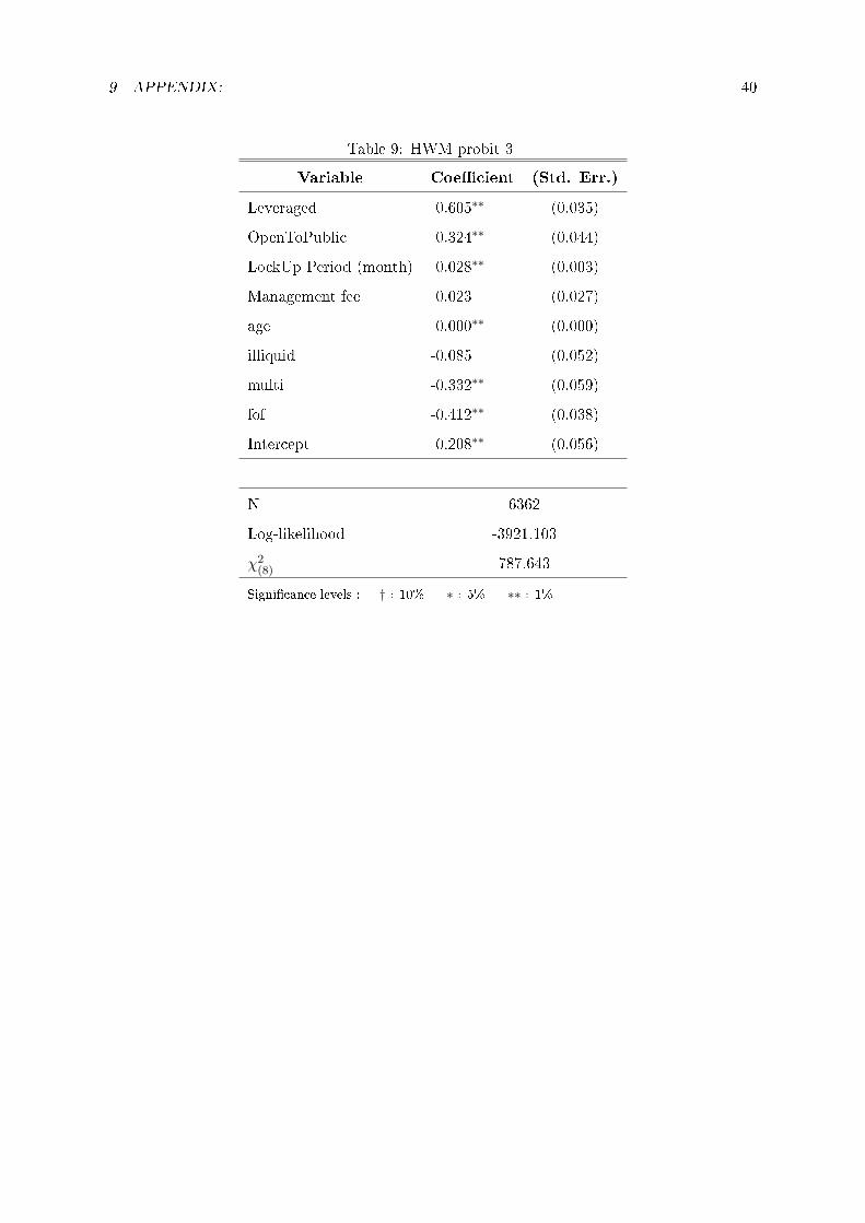
9 APPENDIX: 40



Leveraged 0.605∗∗ (0.035)




age 0.000∗∗ (0.000)

illiquid -0.085 (0.052)

multi -0.332∗∗ (0.059)

fof -0.412∗∗ (0.038)

Intercept 0.208∗∗ (0.056)

N 6362


χ2(8) 787.643


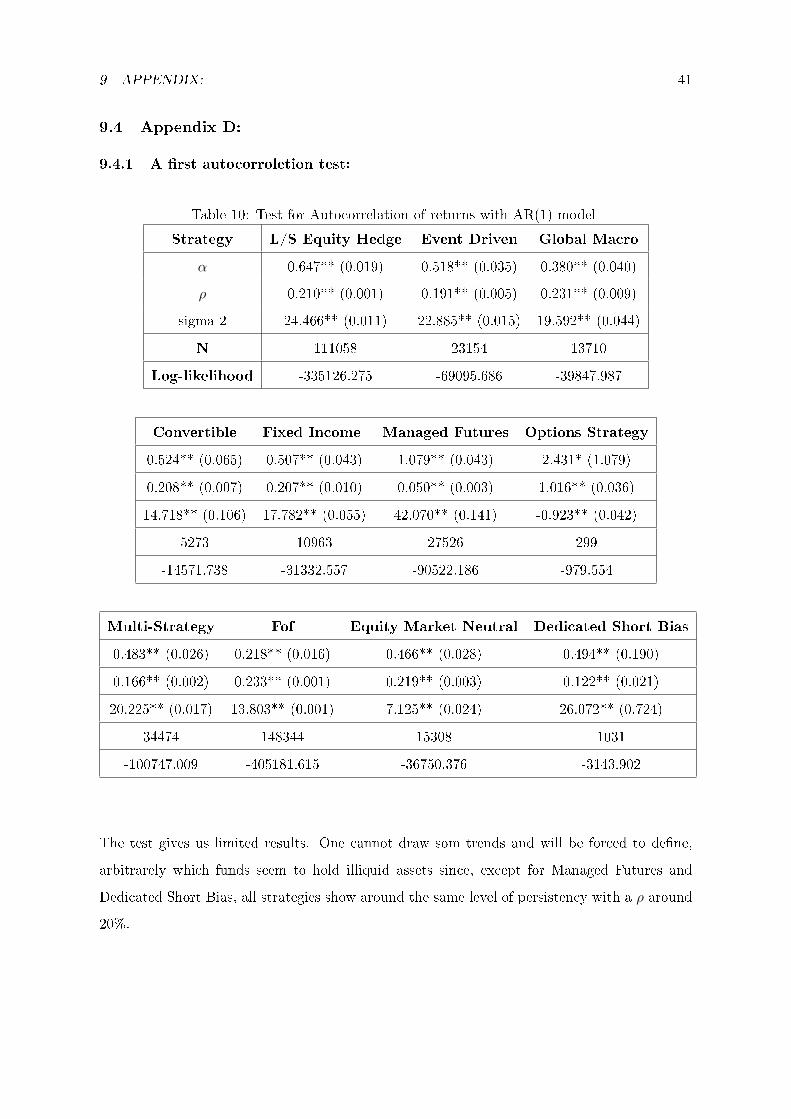
9 APPENDIX: 41

9.4 Appendix D:

9.4.1 A rst autocorroletion test:

Table 10: Test for Autocorrelation of returns with AR(1) model


α 0.647** (0.019) 0.518** (0.035) 0.380** (0.040)

ρ 0.210** (0.001) 0.191** (0.005) 0.231** (0.009)

sigma 2 24.466** (0.011) 22.885** (0.015) 19.592** (0.044)

N 111058 23154 13710

Log-likelihood -335126.275 -69095.686 -39847.987


0.524** (0.065) 0.507** (0.043) 1.079** (0.043) 2.431* (1.079)

0.208** (0.007) 0.207** (0.010) 0.050** (0.003) 1.016** (0.036)

14.718** (0.106) 17.782** (0.055) 42.070** (0.141) -0.923** (0.042)

5273 10963 27526 299

-14571.738 -31332.557 -90522.186 -979.554


0.483** (0.026) 0.218** (0.016) 0.466** (0.028) 0.494** (0.190)

0.166** (0.002) 0.233** (0.001) 0.219** (0.003) 0.122** (0.021)

20.225** (0.017) 13.803** (0.001) 7.125** (0.024) 26.072** (0.724)

34474 148344 15308 1031

-100747.009 -405181.615 -36750.376 -3143.902

The test gives us limited results. One cannot draw som trends and will be forced to dene,

arbitrarely which funds seem to hold illiquid assets since, except for Managed Futures and

Dedicated Short Bias, all strategies show around the same level of persistency with a ρ around

20%.

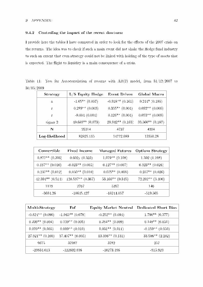
9 APPENDIX: 42

9.4.2 Controling the impact of the recent dowturn:

I provide here the tables I have computed in order to look for the eects of the 2007 crisis on

the returns. The idea was to check if such a main event did not shake the Hedge fund industry

to such an extent that even strategy could not be linked with holding of the type of assets that

is expected. The ight to liquidity is a main consequence of a crisis.

Table 11: Test for Autocorrelation of returns with AR(2) model, from 31/12/2007 to

30/05/2009


a -1.05** (0.057) -0.918** (0.161) 0.244* (0.105)

r 0.289** (0.003) 0.355** (0.004) 0.092** (0.006)

r -0.004 (0.004) 0.126** (0.004) 0.053** (0.009)

sigma 2 40.688** (0.073) 29.942** (0.163) 33.560** (0.187)

N 25314 4737 4204

Log-likelihood -82825.115 -14772.689 -13350.28


-0.877** (0.306) -0.602y (0.323) 1.079** (0.108) 1.392 (1.198)

0.437** (0.010) -0.023** (0.005) 0.127** (0.007) 0.323** (0.026)

-0.237** (0.012) -0.050** (0.010) -0.075** (0.008) -0.257** (0.026)

42.394** (0.514) 128.597** (0.367) 53.166** (0.345) 72.202** (3.400)

1119 2767 5357 146

-3684.26 -10645.427 -18244.057 -519.565


-0.824** (0.090) -1.045** (0.078) -0.252** (0.094) 1.790** (0.377)

0.239** (0.004) 0.239** (0.005) 0.284** (0.009) 0.148** (0.051)

0.070** (0.005) 0.099** (0.010) 0.031** (0.011) -0.159** (0.050)

27.921** (0.100) 37.407** (0.005) 13.396** (0.131) 33.506** (2.202)

9675 37987 3782 257

-29834.013 -122692.836 -10273.486 -815.923

9 APPENDIX: 43

The gures are quite dierent from what they have been while computing from 1990-2009.

Most trends that wanted to be tested are no more, some "liquidity-holding" strategies actually

show persistency in return that can only mean that the portfolio have suered from the crisis.

It may be dicult to gure out why some "illiquid funds" do not show autocorrelation anymore

rather than others. Yet it is possible to discuss some results. For example, the strategy Global

Macro with autocorrelation is probably linked with the tightness of markets and the limits of

exchange during the period.

high-water marks, redemption and illiquidity

Documents