On GLS-detrending for deterministic seasonalitytesting∗

ANTON SKROBOTOV†

The Russian Presidential Academyof National Economy and Public Administration

April 22, 2014

Abstract

In this paper we propose tests based on GLS-detrending for testing the null hypothesis ofdeterministic seasonality. Unlike existing tests for deterministic seasonality, our tests do notsuffer from asymptotic size distortions under near integration. We also investigate the behav-ior of the proposed tests when the initial condition is not asymptotically negligible.Key words: Stationarity tests, KPSS test, seasonality, seasonal unit roots, deterministic sea-sonality, size distortion, GLS-detrending.JEL: C12, C22.

1 Introduction

Deterministic seasonality describes the behavior of a time series in which the unconditional meanschange in different seasons of the year. One way to record this is a seasonal dummies representa-tion. On the other hand, the presence of a seasonal unit root in the data could distort the seasonalcorrection procedure for the time series, so dividing the processes using deterministic seasonalityand seasonal unit root processes is important in the time series analysis. Most of the work, fol-lowing Hylleberg et al. (1990) (hereinafter HEGY), focuses on testing for seasonal unit roots atdifferent frequencies against the alternative that all the roots are less than one. This procedure isrelated to the testing of the unit root (at zero frequency) against the alternative of stationarity inthe nonseasonal case.

Similar to the nonseasonal case (the stationarity test against the alternative hypothesis ofa unit root, see Kwiatkowski et al. (1992)) the procedures for deterministic seasonality testingagainst the case of the presence of at least one seasonal unit root has also been developed. Theproblem of deterministic seasonality testing was first considered by Canova and Hansen (1995).

∗We thank Editor, Associate Editor and two anonymous referees for helpful suggestions.†Adress correspondence to: Institute of Applied Economic Research, Russian Presidential Academy of National

Economy and Public Administration, 82, Vernadsky pr., 117571, Moscow, Russia.E-mail: antonskrobotov@gmail.com

1

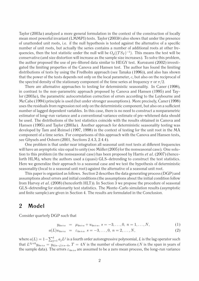
Taylor (2003a) analyzed a more general formulation in the context of the construction of locallymean most powerful invariant (LMMPI) tests. Taylor (2003b) also shows that under the presenceof unattended unit roots, i.e. if the null hypothesis is tested against the alternative of a specificnumber of unit roots, but actually the series contains a number of additional roots at other fre-quencies, then the test statistic under the null will be Op((TST )−1). This means the test will beconservative (and size distortion will increase as the sample size increases). To solve this problem,the author proposed the use of pre-filtered data similar to HEGY test. Kurozumi (2002) investi-gated the limiting properties of the Canova and Hansen test. The author has found the limitingdistributions of tests by using the Fredholm approach (see Tanaka (1996)), and also has shownthat the power of the tests depends not only on the local parameter, c, but also on the reciprocal ofthe spectral density of the stationary component of the time series at frequency π or π/2.

There are alternative approaches to testing for deterministic seasonality. In Caner (1998),in contrast to the non-parametric approach proposed by Canova and Hansen (1995) and Tay-lor (2003a), the parametric autocorrelation correction of errors according to the Leybourne andMcCabe (1994) principle is used (but under stronger assumptions). More precisely, Caner (1998)uses the residuals from regression not only on the deterministic component, but also on a sufficientnumber of lagged dependent variables. In this case, there is no need to construct a nonparametricestimator of long-run variance and a conventional variance estimate of pre-whitened data shouldbe used. The distributions of the test statistics coincide with the results obtained in Canova andHansen (1995) and Taylor (2003a). Another approach for deterministic seasonality testing wasdeveloped by Tam and Reinsel (1997, 1998) in the context of testing for the unit root in the MAcomponent of a time series. For comparisons of this approach with the Canova and Hansen tests,see Ghysels and Osborn (2001, Sections 2.4.3, 2.4.4).

One problem is that under near integration all seasonal unit root tests at different frequencieswill have an asymptotic size equal to unity (see Muller (2005) for the nonseasonal case). One solu-tion to this problem (in the nonseasonal case) has been proposed by Harris et al. (2007) (hence-forth HLM), where the authors used a (quasi) GLS-detrending to construct the test statistics.Here we generalize their approach to a seasonal case and we test the hypothesis of deterministicseasonality (local to a seasonal unit root) against the alternative of a seasonal unit root.

This paper is organized as follows. Section 2 describes the data generating process (DGP) andassumptions about errors and initial conditions (the assumptions about the initial condition followfrom Harvey et al. (2008) (henceforth HLT)). In Section 3 we propose the procedure of seasonalGLS-detrending for stationarity test statistics. The Monte-Carlo simulation results (asymptoticand finite sample) are given in Section 4. The results are formulated in the Conclusion.

2 Model

Consider quarterly DGP such that

y4n+s = µ4n+s + u4n+s, s = −3, . . . , 0, n = 1, . . . , N, (1)

a(L)u4n+s = ε4n+s, s = −3, . . . , 0, n = 2, . . . , N, (2)

where a(L) = 1−∑4

j=1 ajLj is a fourth order autoregressive polynomial, L is the lag operator such

that L4j+ky4n+s = y4(n−j)+s−k, T = 4N is the number of observations (N is the span in years ofthe sample data). The errors ε4n+s are assumed to be a zero mean process, the long-run variance

2

of which is bounded and strongly positive at zero and seasonal spectral frequencies, ωk = 2πk/4,k = 0, 1, 2.

The deterministic component µ4n+s = µt is defined as a linear combination of spectral indicatorvariables, corresponding to the zero and seasonal frequencies, zt,0 = 1, zt,1 = (cos[2πt/4], sin[2πt/4])′

and zt,2 = (−1)t. Define the vector Zt = (zt,0, z′t,1, zt,2)′ and the deterministic component µt =

d′ξZt,ξ for three possible cases, ξ = 1, . . . , 3 (see Smith and Taylor (1998)). The first case corre-sponds to the constants at zero and seasonal frequencies, Zt,1 = Zt, the second case also allowsfor the trend at zero frequency, Zt,2 = (Z ′t, zt,0t)

′, the third case allows for the trend at zero andseasonal frequencies, Zt,3 = (Z ′t, tZ

′t)′.

The polynomial a(L) can be factorized as∏2

k=0 ωk(L) = (1−a0L)(1−2β1L+(a21 +β2

1)L2)(1−a2L). We are interested in testing for deterministic seasonality (local to the seasonal unit root), inother words to test the hypothesisH0 : ci ≥ ci > 0 for all i in ai = 1− ci/T , against the alternativeabout the unit root at least one of the frequencies, i.e. H1 : ci = 0 for at least one i, where ci isthe minimal amount of mean reversion for the specific frequency under the null hypothesis. Thenull hypothesis H0 can be partitioned as H0 =

⋂2k=0 H0,ck , where H0,ci : ai = 1 − ci/T , i = 0, 2

and H0,c1 : a1 = 1 − c1/T , β1 = 0. In other words, testing the null hypothesis of stationarity(local to the unit root) at zero frequency, ω0 = 0, against the alternative of a unit root at thisfrequency is equivalent to testing H0,c0 : c0 ≥ c0 > 0 against H0,c0 : c1 = 0. Similarly, testingthe null hypothesis for stationarity (local to unit root) at the Nyquist frequency, ω2 = π, againstthe alternative of a unit root at this frequency is equivalent to testing H0,c2 : c2 ≥ c2 > 0 againstH2,c2 : c2 = 0, and testing the null hypothesis of stationarity (local to unit root) at seasonalharmonic frequencies, (π/2, 3π/2), against the alternative of unit roots at these frequencies isequivalent to testing H0,c1 : c1 ≥ c1 > 0 against H1,c1 : c1 = 0.

This approach differs to the usual testing for deterministic seasonality, where either the localasymptotic behavior is not considered or parameters related to the signal-to-noise ratio are as-sumed to be local (see Taylor (2003a)). The reason for considering near integration is the sameas in Muller (2005): it explains the increasing size in finite samples for highly autocorrelated sta-tionary series. As demonstrated in Muller (2005) in the context of nonseasonal models, the con-ventional KPSS test with the bandwidth parameter in the long-run variance estimator increasingat a slower rate than the length of the sample leads to an asymptotic size equal to unity under thenull hypothesis of near integration. It is easy to show that the same problem arises in the seasonalmodels, if we use the tests of Canova and Hansen (1995), Taylor (2003a) and Taylor (2003b), in-ter alia. One way to solve this problem will be considered in the next section where we extend theHLM test to a seasonal case.

Also we set the initial condition ui, i = 1, . . . , 4, according to Assumption 1 (see HLT).

Assumption 1 Under H0 with c < 0, the initial conditions are generated according to

ui = αi

√ω2ε/(1− ρ2

N), i = 1, . . . , 4, (3)

where ρN = 1 − c/N and αi ∼ IN(µα,iI(σ2α = 0), σ2

α), i = 1, . . . , 4, independent of ε4n+s,s = −3, . . . , 0, n = 2, . . . , N . For c = 0, under H1, the initial conditions can be set equal tozero, ui = 0, i = 1, . . . , 4, without loss of generality, due to the exact similarity of the teststo the initial conditions in this case.

In this assumption αi controls the magnitude of the initial condition in season i relative to themagnitude of the standard deviation of a stationary seasonal AR(1) process with parameter ρN

3

and innovation long-run variance ω2ε . The form given for the ui allow the initial conditions to be

either random and ofOp(N1/2), or fixed and ofO(N1/2) depending on the value of variance σ2

α (> 0or 0, respectively).

3 Deterministic seasonality testing based on GLS-detrending

HLM proposed the following test using a (quasi) GLS-detrended series. More precisely, let uξt bethe residuals from regression yc = yt − ρTyt−1 on Zi,c = zt − ρT zt−1, t = 2, . . . , T , where zt = 1 inconstant case (ξ = µ) and zt = (1, t)′ in trend case (ξ = τ ) and ρT = 1− c/T . Then the Sξ(c) testis constructed as following:

Sξ(c) =T−2

∑Tt=2 (

∑tj=2 u

ij)

2

ω2, (4)

where the kernel based long-run variance estimator ω2 is calculated by using GLS-detrendedresiduals uit.

For a seasonal time series consider the following GLS-transformation (see also Rodrigues andTaylor (2007) in the context of seasonal unit root testing), by using a vector c = (c0, c1, c2). Letthe series yc and Zξ,c be defined as

yc = (∆cyS+1, . . . ,∆cyT )′

Zξ,c = (∆cZS+1,ξ, . . . ,∆cZT,ξ)′,

where

∆c = 1−S∑j=1

acjLj =

(1−

(1− c0

T

)L)(

1 +(

1− c2

T

)L)(

1 +(

1− c1

T

)2

L2

)(respectively, ∆0 = 1 − LS). GLS-detrended series are the OLS-residuals from regression yc onZξ,c. Define these residuals as ut,ξ.

Before constructing the test statistics, we note that one of the basic principles of unit roottesting in a seasonal time series is that when we test for a unit root at a specific frequency, thedata should be prefiltered to reduce the order of integration at each of the remaining (unattended)frequencies by one (see HEGY and Taylor (2003b)). If we are testing the stationarity against thepresence of a unit root at zero frequency it is necessary to use the data y0,t = (1 +L)(1 +L2)yt in-stead of yt, and then perform GLS-detrending. Accordingly for testing the stationarity at Nyquistfrequency it is necessary to use the data y2,t = (1 − L)(1 + L2)yt, and for testing the stationarityat the seasonal harmonic frequencies it is necessarily to use the data y1,t = (1 − L)(1 + L)yt.However, due to the principle of constructing the GLS-detrended series (see Appendix) there isno need to prefilter unit roots at specific frequencies. Moreover, based on preliminary simulationswe conclude that the use of prefiltered data reduces the finite sample power considerably whileeven for T = 100 (and i.i.d. errors) our GLS-based test with no prefiltering of unit roots has sizecurves very close to asymptotic.

Thus, a final test can be written as follows:

Sξ,j(c) = T−2tr

[(C ′jΩZCj)

−1C ′j

T∑t=1

(t∑

s=1

ujs,ξZs

)(t∑

s=1

ujs,ξZ′s

)Cj

], (5)

4

where ΩZ is a consistent long-run variance estimator of Ztεt, where

ΩZ =T−1∑

l=−T+1

k

(j

ST

)Γ(l), (6)

with the bandwidth parameter ST →∞, ST/T 1/2 → 0 and the autocovariance estimator

Γ(l) = T−1

T∑s=l+1

ujs,ξZtujs−l,ξZ

′s−l, Γ(−l) = Γ(l), l ≥ 0. (7)

The matrix Cj depends on the frequencies at which we test the stationarity. For zero frequencyC0 is the first column of identity matrix I4, for Nyquist frequency C2 is the fourth column of I4, forseasonal harmonic frequencies C1 is the matrix consisting of the second and third columns of I4.For testing the stationarity at all seasonal frequencies the C12 matrix contains the second, thirdand forth columns, and for testing the stationarity at all seasonal and nonseasonal frequenciesC012 is the identity matrix I4.

The following proposition gives the limiting distributions of all test statistics to test the sta-tionarity (local to the seasonal unit root) at specific frequencies under the null and alternativehypotheses.

Proposition 1 Let ySn+s be generated as (1)-(2) under Assumption 1. For i = 1, . . . , 4 wedefine

Kic(r) =

Wi(r), if c = 0,

αi(erc − 1)(−2c)−1/2 +Wic(r), if c < 0,

where Wi(r), i = 1, . . . , 4, are independent standard Wiener processes, Wic(r), i = 1, . . . , 4,are independent Ornstein-Uhlenbeck processes, and the spectral magnitudes αi are definedas

α1 = (α1 + α2 + α3 + α4)/2,

α2 = (−α1 + α2 − α3 + α4)/2,

α3 = (α4 − α2)/√

2,

α4 = (α3 − α1)/√

2.

Then

Sj(cj) ⇒∫ 1

0

Hjc,cj(r)2dr, j = 0, 2, (8)

S1(c1) ⇒∫ 1

0

(H1c,c1(r) +H3c,c1(r))2dr, (9)

S12(c1) ⇒∫ 1

0

(H1c,c1(r) +H2c,c2(r) +H3c,c1(r))2dr, (10)

S012(c1) ⇒∫ 1

0

(H0c,c0(r) +H1c,c1(r) +H2c,c2(r) +H3c,c1(r))2dr, (11)

5

where

Hic,cj(r) = Kic(r) + cj

∫ r

0

Kic(s)ds− r[Kic(1) + cj

∫ 1

0

Kic(s)ds

],

i = 1, . . . , 4, for j = 0, ξ = 0 and for j = 1, 2, ξ = 0, 1, and

Hic,cj(r) = Hic,cj(r)− 6r(1− r)∫ 1

0

Hic,cj(s)ds,

i = 1, . . . , 4, for j = 0, ξ = 1, 2 and for j = 1, 2, ξ = 3, and⇒ denotes weak convergence.

The proof of this proposition follows from HLM, Taylor (2003a) and HLT and is omitted forbrevity. Similar to HLM, it can be shown that for cj = cj the limiting distribution of the Sj testcoincides with the results obtained in Canova and Hansen (1995) and Taylor (2003a) (under thenull hypothesis) and does not depend on initial conditions. Similar results will be occurred forc1 = c1 and c2 = c2 for the S12 test and for c0 = c0, c1 = c1 and c2 = c2 for the S012 test. SeeSection 4.2 for a discussion of calculating the finite sample critical values.

Also it can be noted that the limiting distributions depend not on the values of the initial con-ditions αi, but on the so-called spectral initial conditions αi in the terminology of HLT. Hence forsome given nonzero initial conditions, their linear combination may be zero and some tests willnot depend on their magnitudes.

4 Monte-Carlo simulations

4.1 Asymptotic results

In this subsection, we analyze the asymptotic behavior of S0, S2, S1, S12 and S012 tests undervarious magnitudes for the initial conditions1. Figure 1 shows results for the case of a fixed initialcondition (σ2

α = 0 in Assumption 1), while Figure 2 shows results for the case of a random initialcondition (σ2

α > 0 in Assumption 1). Everywhere we consider a model with seasonal constantsand a nonseasonal trend (since this model is most often used in practice) and use c0 = 13.5, c2 = 7,c1 = 3.75.

Parts (a), (b) and (c) in Figure 1 represent, respectively, asymptotic size (a(L) = 1 − (1 −c/N)L4, c > 0) and power (c = 0) of S0, S2 and S1 tests for various magnitudes of initial conditionsα1, α2 and α3 = α4, respectively. The magnitudes of the initial conditions αi = |µ| = 0, 2, 4, 6,i = 1, . . . , 4 are used for all the tests being considered. Parts (d), (e) and (f) represent results for theS12 test under: α2 = |µ|, α3 = α4 = 0; α2 = 0, α3 = α4 = |µ|; α2 = α3 = α4 = |µ|, respectively.Parts (g), (h) and (i) represent results for the S012 test under: α1 = |µ|, α2 = α3 = α4 = 0;α1 = α2 = 0, α3 = α4 = |µ|; α1 = α2 = α3 = α4 = |µ|, respectively. Corresponding results forthe case of random initial conditions are given in Figure 2 for σ2

α = |µ| = 0, 2, 4, 6, i = 1, . . . , 4.In all cases critical values are obtained at cj = cj .

The size curves of S0, S2 and S1 tests are tangent to each other for different initial conditionsat points cj = cj , which confirms the invariance with respect to the initial conditions of each of

1Here and in the following subsection results are obtained by simulations of the limiting distributions in Propo-sition 1, approximating the Wiener process using i.i.d.N(0, 1) random variates and with integrals approximated bynormalized sums of 1,000 steps, with 50,000 replications.

6

the tests at c = cj . When c < cj the size of each test grows as the corresponding spectral initialcondition is increased, although the size distortion is less pronounced for the S0 test (intuitivelybecause a larger value is used for cj). For c > cj the size of the test is lower that the nominal one,except for the S1 test with |µ| = 6 (because a very small value of cj is used). Similar behavior isobserved for S12 and S012.

For the case of random initial conditions, the size distortions for c < cj are smaller that in caseof fixed initial conditions, but larger than for c > cj .

4.2 Finite sample comparisons

In finite samples, when the error term εt is i.i.d., the size curves are close to asymptotic. However,if εt has a MA form, the power can be very low. One way to solve this issue is to sacrifice the sizeat some small c = cj (proposed above) and use a higher value of cj , which will control the sizeat a higher c. One alternative is to use parameters cj such that the asymptotic size of S0, S2 andS1 tests (e.g., in case of a seasonal constant and nonseasonal trend) is equal to 0.5 at c0 = 13.5,c2 = 7, c1 = 3.75. These new values of cj are equal to c0 = 29.55, c2 = 20.05 and c1 = 10.7(in case of seasonal trend c1 = 17.75 and c2 = 29.55). Corresponding values of power in finitesamples (T = 300) for S0, S2, S1, S01 and S012 tests will then be equal to 0.90, 0.86, 0.85, 0.97 and0.99, respectively. Of course, the researcher can choose any values of cj for his desired trade-offbetween size and power. However, if we choose the greater value of cj , the critical values are moredownward-biased. Therefore, for a hypothesis testing the finite sample, critical values should beused. Moreover, for large cj the size distortion increases under AR or MA error.2

In this subsection we investigate the finite sample behavior of tests based on DGP (1)-(2)with ξ = 2 (seasonal intercept, nonseasonal trend) and Assumption 1. Results are presentedfor T = 300 with 10,000 replications and, without loss of generality, with the absence of thedeterministic term. For simplicity, the initial conditions are assumed to be random. The long-run variance estimator (6) is constructed by using a quadratic spectral window and automaticbandwidth selection based on AR(1) approximation (see Andrews (1991)). As a comparison, weuse conventional deterministic seasonality tests proposed by Taylor (2003b), where the long-runvariance estimator is constructed by using a Bartlett kernel with bandwidth ST = 6.3 Becausethese two tests have different natures, we compare their size (c > 0) by fixing power (c = 0)at a predetermined level. More precisely, critical values are obtained so that the power is equalto 0.70 for T = 100. Based on obtained critical values we calculate the size of all tests for c ∈5, 10, . . . , 30. It should be noted that the choice of setting power at a value of 0.70 is not crucial,and this value is chosen for the convenience of visualizing the comparison. In simulations we usethe values of c0 = 29.55, c2 = 20.05 and c1 = 10.7. Other values of cj produce similar results.

Tables 1-9 show the power-adjusted size of a conventional deterministic seasonality test (de-noted as Sj) and our proposed GLS-based test (denoted as Sj(c)) under various DGP, includingi.i.d, AR and MA forms of error. More precisely, a(L) = 1 − (1 − c/N)L4,4 and the error εt havethe both AR form,

(1− ΦL4)εt = et, (12)

2Ox-code for computing the finite sample critical values based on the parameters cj and the corresponding powerof all tests are available in https://sites.google.com/site/antonskrobotov/.

3This choice in a long-run variance estimation shows the best properties in finite samples.4Results in which unit roots are present at some but not all frequencies are similar.

7

or MA form,εt = (1−ΘL4)et, (13)

where et ∼ i.i.d.N(0, 1). We perform simulations with Φ = ±0.3,±0.5 for (12) and with Θ =±0.3,±0.5 for (13), and also for εt = et.

For i.i.d. errors in most cases the Sj(c) tests have a smaller size than the Sj , except for asmall number of cases for small c. The results are similar for AR errors except for a small initialconditions for the S12 and S012 tests. For large Φ, the S12 and S012 tests outperform the S12(c)and S012(c) even for large initial conditions. For MA errors in most DGPs the GLS-based testsoutperform conventional tests although for negative Θ the size of S1(c) is much higher than theone of S1. For positive Θ, the results are similar to AR cases. In general, our proposed GLS-basedtests show the best properties in view of the fact that they have better size control specified for thelocal parameters c.

It should be noted that GLS-based tests are superior to conventional tests for deterministicseasonality only in finite samples, as the latter are consistent. Due to the nature of their con-struction, GLS-tests are not consistent in the sense that their power will not tend to unity withthe growth of the sample size. Therefore, in large samples, conventional tests will outperformGLS-based tests.

5 Conclusion

In this paper, we consider GLS-detrendng in the context of deterministic seasonality testing (lo-cal to a seasonal unit root) against the alternative of a seasonal unit root. Unlike existing tests,the proposed tests do not suffer from asymptotic size distortions in the local to unity autoregres-sion parameters and, at the same time, have a well-controlled size for a given level of (seasonal)mean reversion. The behavior of the proposed tests was also analyzed for fixed and random initialconditions of various magnitudes. Finite sample behavior confirms the superiority of GLS-basedtests over conventional tests for deterministic seasonality.

Appendix

Proof of Proposition 1 : Without loss of generality let the deterministic term µt = 0. Also forconvenience define x4n+s = u4n+s − us. For simplicity consider the case with a seasonal interceptand no trend, ξ = 1. The extension on nonseasonal or seasonal trends are similar. GLS-residualsut,1 are defined as

ut,1 = ∆cxt − µt,

where µt = d′1Zt,1, d′1 is a vector of GLS-estimates for spectral indicator variables Zt,1. Note thatnow ∆cyt can be decomposed as

∆cxt =

((1− L4) +

c0

T(L+ L2 + L3 + L4) +

c2

T(−L+ L2 − L3 + L4) +

2c1

T(−L2 + L4)

)xt+op(1)

Consider deterministic seasonality testing against a unit root at the zero frequency (ω0 = 0).

8

Then

T−1/2

t∑i=5

ut,1 = T−1/2

t∑i=5

∆cxt − T−1/2

T∑i=5

µt

= T−1/2

t∑i=5

∆cxt − tT−3/2

T∑i=5

∆cxt

= T−1/2(xt + xt−1 + xt−2 + xt−3 − x5 − x6 − x7 − x8)

+c0T−3/2

t∑i=5

(xi−1 + xi−2 + xi−3 + xi−4)

−t[T−1/2(xT + xT−1 + xT−2 + xT−3 − x5 − x6 − x7 − x8)

−c0T−3/2

T∑i=5

(xt−1 + xt−2 + xt−3 + xt−4)] + op(1).

The second equality follows from the orthogonality of spectral indicator variablesZt,1, and the thirdequality from x1 = · · · = x4 = 0 and from

c2T−3/2

t∑i=5

(−xt−1 + xt−2 − xt−3 + xt−4) = Op(T−1)

and

2c1T−3/2

t∑i=5

(−xt−2 + xt−4) = Op(T−1).

Thus,

T−1/2

[rT ]∑i=5

ut,1 ⇒ ω1,ZHic,c0(r),

where ω21,Z is a (1,1) element of covariance matrix ΩZ . Further, applying the CMT, we obtain

T−1

T∑t=5

(T−1/2

t∑i=5

ut,1)2 ⇒ ω21,Z

∫ 1

0

Hic,c0(r)2.

The consistency of ω21,Z is proved similarly HLM, p. 362.

For analysis of the limiting distribution of the test statistics at Nyquist frequency (ω2 = π) andat harmonic seasonal frequencies (ω1 = ±π/2), consider decomposition of the polynomial ∆c upto the order T−1:

(1−L)(1+L+L2 +L3)+c0

T(L+L2 +L3 +L4)+

c2

T(−L+L2−L3 +L4)+

2c1

T(−L2 +L4). (A1)

When we obtained the limiting distribution at zero frequency, the third and fourth terms wereasymptotically negligible. If we analyze the behavior of the test statistics at Nyquist frequency,then instead of considering partial sums T−1/2

∑ti=5 ut,1, we should consider partial sums

T−1/2∑t

i=5 ut,1(−1)i. This leads to the fact that the first term in (A1) becomes (1− L)(−1 + L−

9

L2+L3), and the second and fourth terms can be neglected, so that only the modified first and thirdterms are remain. There is a similar case with testing at harmonic seasonal frequencies, when thesecond and third terms in (A1) can be neglected.

Note also that the specified type of polynomial (A1) presupposes taking the filtered data, soadditional filtering for possibly unattended unit roots is not required.

10

References

Andrews, D.W.K. (1991). Heteroskedasticity and Autocorrelation Consistent Covariance MatrixEstimation. Econometrica, 59, 817–858.

Caner, M. (1998). A Locally Optimal Seasonal Unit-Root Test. Journal of Business & Eco-nomic Statistics, 16, 349–356.

Canova, F. and Hansen, B.E. (1995). Are seasonal patterns constant over time A test for seasonalstability. Journal of Business & Economic Statistics, 13, 237–252.

Ghysels, E. and Osborn, D.R. (2001). The Econometric Analysis of Seasonal Time Series.Cambridge University Press, Cambridge.

Harris, D., Leybourne, S., and McCabe, B. (2007). Modified KPSS Tests for Near Integration.Econometric Theory, 23, 355–363.

Harvey, D.I., Leybourne, S.J., and Taylor, A.M.R. (2008). Seasonal unit root tests and the role ofinitial conditions. Econometrics Journal, 11, 409–442.

Hylleberg, S., Engle, R. F., Granger, C. W. J., and Yoo, B. S. (1990). Seasonal integration andcointegration. Journal of Econometrics, 44, 215–238.

Kurozumi, E. (2002). The Limiting Properties of the Canova and Hansen Test under Local Alter-natives. Econometric Theory, 18, 1197–1220.

Kwiatkowski, D., Phillips, P.C.B., Schmidt, P., and Shin, Y. (1992). Testing the Null Hypothesisof Stationarity against the Alternative of a Unit Root: How Sure Are We That Economic TimeSeries Have a Unit Root? Journal of Econometrics, 54, 159–178.

Leybourne, S. and McCabe, B. (1994). A Consistent Test for a Unit Root. Journal of Businessand Economic Statistics, 12, 157–166.

Muller, U. (2005). Size and Power of Tests for Stationarity in Highly Autocorrelated Time Series.Journal of Econometrics, 128, 195–213.

Rodrigues, P. M. M. and Taylor, A. M. R. (2007). Efficient tests of the seasonal unit root hypoth-esis. Journal of Econometrics, 141, 548–573.

Smith, R.J. and Taylor, A.M.R. (1998). Additional critical values and asymptotic representationsfor seasonal unit root tests. Journal of Econometrics, 85, 269–288.

Tam, W.-K. and Reinsel, G.C. (1997). Tests for seasonal moving-average unit root in ARIMAmodels. Journal of the American Statistical Association, 92, 724–38.

Tam, W.-K. and Reinsel, G.C. (1998). Seasonal moving-average unit root tests in the presenceof a linear trend. Journal of Time Series Analysis, 19, 609–625.

Tanaka, K. (1996). Time Series Analysis: Nonstationary and Noninvertible DistributionTheory. Wiley, New York.

11

Taylor, A. M. R. (2003a). Locally Optimal Tests Against Unit Roots in Seasonal Time SeriesProcesses. Journal of Time Series Analysis, 24, 591–612.

Taylor, A. M. R. (2003b). Robust Stationarity Tests in Seasonal Time Series Processes. Journalof Business & Economic Statistics, 21, 156–163.

12

Table 1. Power adjusted size of tests, i.i.d errors

c S0 S0(c) S2 S2(c) S1 S1(c) S12 S12(c) S012 S012(c)

µ = 0

5 0.562 0.599 0.400 0.384 0.187 0.222 0.090 0.155 0.082 0.15510 0.367 0.357 0.236 0.153 0.044 0.023 0.009 0.013 0.006 0.01215 0.229 0.154 0.139 0.038 0.009 0.001 0.001 0.000 0.000 0.00020 0.138 0.048 0.082 0.006 0.002 0.000 0.000 0.000 0.000 0.00025 0.087 0.010 0.051 0.001 0.000 0.000 0.000 0.000 0.000 0.00030 0.054 0.001 0.031 0.000 0.000 0.000 0.000 0.000 0.000 0.000

µ = 2

5 0.622 0.642 0.523 0.471 0.376 0.264 0.305 0.239 0.301 0.24310 0.430 0.384 0.295 0.170 0.086 0.024 0.033 0.016 0.027 0.01415 0.267 0.162 0.164 0.039 0.017 0.001 0.002 0.001 0.001 0.00020 0.160 0.048 0.095 0.006 0.003 0.000 0.000 0.000 0.000 0.00025 0.096 0.009 0.056 0.001 0.001 0.000 0.000 0.000 0.000 0.00030 0.061 0.001 0.034 0.000 0.000 0.000 0.000 0.000 0.000 0.000

µ = 4

5 0.709 0.702 0.667 0.591 0.553 0.370 0.471 0.386 0.525 0.40310 0.538 0.455 0.392 0.199 0.136 0.026 0.065 0.023 0.067 0.02315 0.344 0.173 0.210 0.038 0.026 0.006 0.004 0.000 0.003 0.00020 0.205 0.046 0.115 0.009 0.005 0.001 0.000 0.000 0.000 0.00025 0.118 0.010 0.067 0.002 0.001 0.000 0.000 0.000 0.000 0.00030 0.073 0.002 0.038 0.000 0.000 0.000 0.000 0.000 0.000 0.000

µ = 6

5 0.779 0.748 0.755 0.674 0.659 0.487 0.532 0.490 0.660 0.51710 0.631 0.526 0.483 0.244 0.165 0.032 0.079 0.033 0.119 0.03515 0.427 0.194 0.263 0.035 0.031 0.022 0.006 0.001 0.007 0.00020 0.255 0.043 0.140 0.011 0.005 0.013 0.000 0.000 0.000 0.00025 0.145 0.012 0.074 0.004 0.001 0.002 0.000 0.000 0.000 0.00030 0.081 0.003 0.042 0.001 0.000 0.000 0.000 0.000 0.000 0.000

13

Table 2. Power adjusted size of tests, AR errors, Φ = −0.5

c S0 S0(c) S2 S2(c) S1 S1(c) S12 S12(c) S012 S012(c)

µ = 0

5 0.560 0.558 0.398 0.351 0.190 0.207 0.093 0.127 0.083 0.11710 0.350 0.287 0.218 0.101 0.036 0.016 0.006 0.006 0.004 0.00415 0.193 0.086 0.108 0.014 0.005 0.000 0.000 0.000 0.000 0.00020 0.098 0.015 0.050 0.001 0.001 0.000 0.000 0.000 0.000 0.00025 0.048 0.001 0.022 0.000 0.000 0.000 0.000 0.000 0.000 0.00030 0.021 0.000 0.008 0.000 0.000 0.000 0.000 0.000 0.000 0.000

µ = 2

5 0.667 0.644 0.602 0.512 0.475 0.297 0.394 0.288 0.409 0.28510 0.467 0.344 0.325 0.124 0.092 0.017 0.033 0.009 0.028 0.00715 0.267 0.096 0.155 0.014 0.011 0.002 0.001 0.000 0.001 0.00020 0.134 0.015 0.069 0.001 0.001 0.000 0.000 0.000 0.000 0.00025 0.062 0.002 0.029 0.000 0.000 0.000 0.000 0.000 0.000 0.00030 0.028 0.000 0.010 0.000 0.000 0.000 0.000 0.000 0.000 0.000

µ = 4

5 0.776 0.744 0.751 0.672 0.680 0.498 0.552 0.551 0.667 0.57410 0.622 0.468 0.473 0.183 0.149 0.022 0.058 0.021 0.089 0.01915 0.401 0.122 0.232 0.014 0.018 0.016 0.002 0.000 0.003 0.00020 0.213 0.015 0.101 0.003 0.001 0.013 0.000 0.000 0.000 0.00025 0.098 0.002 0.041 0.001 0.000 0.006 0.000 0.000 0.000 0.00030 0.043 0.001 0.015 0.000 0.000 0.002 0.000 0.000 0.000 0.000

µ = 6

5 0.840 0.810 0.826 0.765 0.785 0.673 0.599 0.742 0.793 0.77010 0.719 0.575 0.585 0.266 0.176 0.037 0.070 0.046 0.188 0.04715 0.516 0.164 0.311 0.014 0.021 0.073 0.003 0.001 0.009 0.00020 0.297 0.016 0.133 0.007 0.001 0.083 0.000 0.000 0.000 0.00025 0.142 0.006 0.050 0.006 0.000 0.048 0.000 0.000 0.000 0.00030 0.058 0.004 0.018 0.003 0.000 0.013 0.000 0.000 0.000 0.000

14

Table 3. Power adjusted size of tests, AR errors, Φ = −0.3

c S0 S0(c) S2 S2(c) S1 S1(c) S12 S12(c) S012 S012(c)

µ = 0

5 0.560 0.571 0.399 0.359 0.187 0.204 0.090 0.123 0.080 0.11610 0.354 0.305 0.224 0.115 0.039 0.016 0.007 0.006 0.005 0.00415 0.204 0.102 0.118 0.019 0.006 0.000 0.000 0.000 0.000 0.00020 0.111 0.021 0.062 0.002 0.001 0.000 0.000 0.000 0.000 0.00025 0.059 0.002 0.032 0.000 0.000 0.000 0.000 0.000 0.000 0.00030 0.030 0.000 0.015 0.000 0.000 0.000 0.000 0.000 0.000 0.000

µ = 2

5 0.647 0.639 0.572 0.493 0.438 0.274 0.359 0.248 0.365 0.24410 0.448 0.349 0.311 0.135 0.090 0.017 0.032 0.009 0.027 0.00615 0.263 0.111 0.157 0.019 0.013 0.001 0.001 0.000 0.001 0.00020 0.141 0.021 0.078 0.002 0.001 0.000 0.000 0.000 0.000 0.00025 0.072 0.003 0.038 0.000 0.000 0.000 0.000 0.000 0.000 0.00030 0.037 0.000 0.017 0.000 0.000 0.000 0.000 0.000 0.000 0.000

µ = 4

5 0.751 0.725 0.724 0.642 0.635 0.442 0.523 0.470 0.614 0.48510 0.589 0.456 0.441 0.181 0.144 0.021 0.061 0.017 0.078 0.01615 0.375 0.131 0.222 0.018 0.021 0.009 0.003 0.000 0.003 0.00020 0.206 0.020 0.105 0.004 0.002 0.005 0.000 0.000 0.000 0.00025 0.103 0.003 0.049 0.001 0.000 0.001 0.000 0.000 0.000 0.00030 0.052 0.001 0.022 0.000 0.000 0.000 0.000 0.000 0.000 0.000

µ = 6

5 0.819 0.782 0.804 0.732 0.741 0.604 0.575 0.634 0.749 0.65810 0.687 0.553 0.549 0.249 0.172 0.031 0.073 0.033 0.157 0.03315 0.480 0.164 0.291 0.017 0.025 0.043 0.004 0.000 0.007 0.00020 0.276 0.020 0.135 0.006 0.003 0.043 0.000 0.000 0.000 0.00025 0.140 0.006 0.059 0.004 0.000 0.016 0.000 0.000 0.000 0.00030 0.064 0.002 0.026 0.001 0.000 0.002 0.000 0.000 0.000 0.000

15

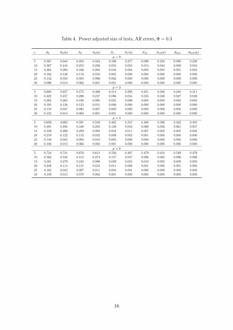
Table 4. Power adjusted size of tests, AR errors, Φ = 0.3

c S0 S0(c) S2 S2(c) S1 S1(c) S12 S12(c) S012 S012(c)

µ = 0

5 0.567 0.640 0.403 0.424 0.189 0.277 0.098 0.250 0.090 0.25810 0.387 0.444 0.255 0.226 0.055 0.053 0.013 0.044 0.008 0.04515 0.264 0.260 0.166 0.093 0.016 0.004 0.002 0.005 0.001 0.00420 0.182 0.126 0.116 0.030 0.005 0.000 0.000 0.000 0.000 0.00025 0.132 0.050 0.085 0.006 0.002 0.000 0.000 0.000 0.000 0.00030 0.098 0.014 0.062 0.001 0.001 0.000 0.000 0.000 0.000 0.000

µ = 2

5 0.600 0.657 0.475 0.469 0.314 0.295 0.251 0.300 0.240 0.31110 0.422 0.457 0.288 0.237 0.086 0.054 0.035 0.048 0.027 0.04815 0.284 0.265 0.180 0.095 0.023 0.006 0.004 0.005 0.002 0.00420 0.193 0.126 0.123 0.031 0.006 0.000 0.000 0.000 0.000 0.00025 0.134 0.047 0.085 0.007 0.002 0.000 0.000 0.000 0.000 0.00030 0.102 0.013 0.063 0.001 0.001 0.000 0.000 0.000 0.000 0.000

µ = 4

5 0.659 0.693 0.591 0.548 0.462 0.347 0.406 0.386 0.422 0.40310 0.491 0.494 0.348 0.250 0.128 0.054 0.069 0.056 0.061 0.05715 0.329 0.268 0.209 0.094 0.034 0.011 0.007 0.005 0.005 0.00420 0.219 0.122 0.135 0.032 0.009 0.002 0.001 0.000 0.000 0.00025 0.148 0.045 0.094 0.010 0.003 0.000 0.000 0.000 0.000 0.00030 0.106 0.013 0.066 0.002 0.001 0.000 0.000 0.000 0.000 0.000

µ = 6

5 0.724 0.721 0.676 0.613 0.556 0.407 0.479 0.454 0.549 0.47910 0.562 0.530 0.412 0.274 0.157 0.057 0.086 0.065 0.096 0.06915 0.381 0.279 0.242 0.088 0.039 0.024 0.010 0.005 0.008 0.00520 0.248 0.114 0.151 0.034 0.011 0.008 0.001 0.000 0.001 0.00025 0.162 0.043 0.097 0.011 0.003 0.001 0.000 0.000 0.000 0.00030 0.109 0.013 0.070 0.002 0.001 0.000 0.000 0.000 0.000 0.000

16

Table 5. Power adjusted size of tests, AR errors, Φ = 0.5

c S0 S0(c) S2 S2(c) S1 S1(c) S12 S12(c) S012 S012(c)

µ = 0

5 0.574 0.675 0.407 0.467 0.190 0.342 0.111 0.354 0.099 0.37010 0.408 0.526 0.275 0.303 0.062 0.106 0.017 0.112 0.010 0.11515 0.301 0.372 0.194 0.174 0.022 0.019 0.003 0.022 0.001 0.02220 0.226 0.235 0.149 0.088 0.009 0.002 0.001 0.004 0.000 0.00425 0.177 0.133 0.120 0.036 0.004 0.000 0.000 0.000 0.000 0.00030 0.144 0.060 0.097 0.010 0.002 0.000 0.000 0.000 0.000 0.000

µ = 2

5 0.590 0.679 0.446 0.489 0.275 0.349 0.219 0.382 0.206 0.39710 0.431 0.535 0.293 0.312 0.086 0.108 0.038 0.115 0.028 0.12015 0.309 0.376 0.202 0.175 0.030 0.023 0.007 0.025 0.003 0.02520 0.231 0.235 0.154 0.089 0.010 0.003 0.001 0.004 0.000 0.00425 0.176 0.128 0.119 0.035 0.005 0.000 0.000 0.001 0.000 0.00030 0.145 0.056 0.096 0.011 0.003 0.000 0.000 0.000 0.000 0.000

µ = 4

5 0.627 0.698 0.529 0.538 0.396 0.370 0.356 0.430 0.351 0.44710 0.470 0.553 0.329 0.315 0.123 0.107 0.072 0.119 0.058 0.12415 0.335 0.373 0.218 0.174 0.041 0.030 0.012 0.026 0.007 0.02520 0.242 0.231 0.156 0.086 0.015 0.007 0.002 0.004 0.000 0.00425 0.183 0.119 0.123 0.037 0.006 0.001 0.000 0.000 0.000 0.00030 0.144 0.049 0.098 0.010 0.003 0.000 0.000 0.000 0.000 0.000

µ = 6

5 0.681 0.715 0.605 0.584 0.476 0.400 0.434 0.474 0.460 0.49410 0.518 0.570 0.371 0.329 0.151 0.104 0.093 0.125 0.086 0.13315 0.366 0.378 0.238 0.168 0.047 0.043 0.015 0.027 0.010 0.02620 0.259 0.219 0.168 0.086 0.017 0.013 0.003 0.005 0.001 0.00425 0.189 0.107 0.124 0.035 0.006 0.001 0.001 0.000 0.000 0.00030 0.142 0.040 0.098 0.008 0.002 0.000 0.000 0.000 0.000 0.000

17

Table 6. Power adjusted size of tests, MA errors, Θ = −0.5

c S0 S0(c) S2 S2(c) S1 S1(c) S12 S12(c) S012 S012(c)

µ = 0

5 0.564 0.564 0.403 0.381 0.215 0.251 0.115 0.157 0.106 0.14610 0.352 0.301 0.201 0.115 0.038 0.025 0.007 0.008 0.006 0.00615 0.186 0.096 0.087 0.019 0.004 0.001 0.000 0.000 0.000 0.00020 0.089 0.017 0.036 0.002 0.001 0.000 0.000 0.000 0.000 0.00025 0.040 0.002 0.015 0.000 0.000 0.000 0.000 0.000 0.000 0.00030 0.018 0.000 0.005 0.000 0.000 0.000 0.000 0.000 0.000 0.000

µ = 2

5 0.702 0.674 0.664 0.580 0.584 0.385 0.505 0.397 0.531 0.40210 0.508 0.378 0.358 0.152 0.116 0.028 0.041 0.014 0.041 0.01115 0.292 0.108 0.154 0.018 0.011 0.006 0.001 0.000 0.001 0.00020 0.140 0.018 0.059 0.002 0.001 0.002 0.000 0.000 0.000 0.00025 0.061 0.002 0.022 0.001 0.000 0.001 0.000 0.000 0.000 0.00030 0.029 0.001 0.008 0.000 0.000 0.000 0.000 0.000 0.000 0.000

µ = 4

5 0.813 0.778 0.801 0.734 0.806 0.618 0.713 0.692 0.803 0.72610 0.679 0.521 0.550 0.240 0.214 0.038 0.076 0.041 0.151 0.03915 0.459 0.147 0.277 0.019 0.021 0.054 0.002 0.001 0.005 0.00020 0.255 0.020 0.110 0.007 0.001 0.060 0.000 0.000 0.000 0.00025 0.120 0.005 0.040 0.006 0.000 0.043 0.000 0.000 0.000 0.00030 0.056 0.003 0.013 0.003 0.000 0.021 0.000 0.000 0.000 0.000

µ = 6

5 0.870 0.838 0.865 0.813 0.897 0.777 0.797 0.854 0.904 0.88210 0.769 0.630 0.665 0.351 0.278 0.066 0.092 0.097 0.306 0.10615 0.588 0.208 0.397 0.018 0.028 0.188 0.003 0.005 0.022 0.00420 0.377 0.021 0.172 0.019 0.002 0.230 0.000 0.004 0.001 0.00125 0.199 0.013 0.058 0.027 0.000 0.190 0.000 0.000 0.000 0.00030 0.093 0.013 0.019 0.021 0.000 0.115 0.000 0.000 0.000 0.000

18

Table 7. Power adjusted size of tests, MA errors, Θ = −0.3

c S0 S0(c) S2 S2(c) S1 S1(c) S12 S12(c) S012 S012(c)

µ = 0

5 0.559 0.566 0.397 0.362 0.189 0.214 0.092 0.129 0.082 0.12110 0.350 0.302 0.215 0.114 0.037 0.018 0.007 0.006 0.005 0.00415 0.195 0.100 0.107 0.019 0.005 0.000 0.000 0.000 0.000 0.00020 0.102 0.021 0.052 0.002 0.001 0.000 0.000 0.000 0.000 0.00025 0.052 0.002 0.026 0.000 0.000 0.000 0.000 0.000 0.000 0.00030 0.027 0.000 0.011 0.000 0.000 0.000 0.000 0.000 0.000 0.000

µ = 2

5 0.658 0.644 0.591 0.509 0.464 0.298 0.381 0.273 0.393 0.27210 0.456 0.352 0.316 0.137 0.091 0.019 0.033 0.009 0.028 0.00715 0.264 0.109 0.151 0.019 0.012 0.001 0.001 0.000 0.001 0.00020 0.137 0.021 0.070 0.002 0.001 0.000 0.000 0.000 0.000 0.00025 0.067 0.003 0.032 0.000 0.000 0.000 0.000 0.000 0.000 0.00030 0.034 0.001 0.014 0.000 0.000 0.000 0.000 0.000 0.000 0.000

µ = 4

5 0.765 0.736 0.741 0.661 0.675 0.480 0.557 0.518 0.654 0.53610 0.607 0.468 0.462 0.191 0.153 0.023 0.061 0.019 0.086 0.01915 0.390 0.132 0.228 0.019 0.020 0.014 0.002 0.000 0.003 0.00020 0.211 0.020 0.101 0.004 0.002 0.010 0.000 0.000 0.000 0.00025 0.102 0.004 0.045 0.002 0.000 0.004 0.000 0.000 0.000 0.00030 0.051 0.001 0.019 0.000 0.000 0.000 0.000 0.000 0.000 0.000

µ = 6

5 0.831 0.792 0.819 0.750 0.786 0.645 0.616 0.692 0.786 0.71910 0.705 0.568 0.574 0.267 0.186 0.036 0.075 0.039 0.178 0.04215 0.502 0.171 0.308 0.017 0.024 0.064 0.004 0.000 0.009 0.00020 0.293 0.020 0.136 0.008 0.002 0.072 0.000 0.000 0.000 0.00025 0.148 0.007 0.056 0.006 0.000 0.036 0.000 0.000 0.000 0.00030 0.068 0.003 0.023 0.002 0.000 0.007 0.000 0.000 0.000 0.000

19

Table 8. Power adjusted size of tests, MA errors, Θ = 0.3

c S0 S0(c) S2 S2(c) S1 S1(c) S12 S12(c) S012 S012(c)

µ = 0

5 0.564 0.627 0.401 0.409 0.188 0.263 0.093 0.220 0.087 0.22710 0.379 0.421 0.246 0.203 0.051 0.045 0.011 0.032 0.007 0.03215 0.251 0.234 0.154 0.076 0.014 0.003 0.001 0.003 0.001 0.00220 0.165 0.108 0.102 0.022 0.004 0.000 0.000 0.000 0.000 0.00025 0.116 0.040 0.071 0.004 0.001 0.000 0.000 0.000 0.000 0.00030 0.083 0.011 0.051 0.000 0.000 0.000 0.000 0.000 0.000 0.000

µ = 2

5 0.603 0.651 0.484 0.462 0.326 0.286 0.259 0.277 0.250 0.28610 0.419 0.437 0.284 0.215 0.083 0.046 0.032 0.036 0.026 0.03615 0.274 0.240 0.171 0.077 0.021 0.005 0.003 0.003 0.002 0.00220 0.179 0.107 0.110 0.022 0.004 0.000 0.000 0.000 0.000 0.00025 0.120 0.038 0.072 0.005 0.002 0.000 0.000 0.000 0.000 0.00030 0.089 0.010 0.052 0.001 0.001 0.000 0.000 0.000 0.000 0.000

µ = 4

5 0.669 0.692 0.611 0.555 0.484 0.348 0.420 0.378 0.444 0.39510 0.498 0.479 0.355 0.232 0.128 0.046 0.065 0.043 0.058 0.04415 0.327 0.245 0.203 0.075 0.031 0.010 0.006 0.003 0.004 0.00220 0.209 0.104 0.124 0.024 0.008 0.002 0.000 0.000 0.000 0.00025 0.135 0.036 0.083 0.007 0.002 0.000 0.000 0.000 0.000 0.00030 0.094 0.011 0.055 0.001 0.001 0.000 0.000 0.000 0.000 0.000

µ = 6

5 0.737 0.725 0.695 0.623 0.587 0.418 0.494 0.453 0.576 0.47910 0.576 0.522 0.427 0.260 0.159 0.050 0.082 0.053 0.098 0.05715 0.387 0.256 0.242 0.070 0.037 0.023 0.008 0.003 0.008 0.00320 0.244 0.097 0.144 0.027 0.008 0.009 0.001 0.000 0.000 0.00025 0.154 0.036 0.088 0.009 0.002 0.001 0.000 0.000 0.000 0.00030 0.100 0.011 0.060 0.002 0.001 0.000 0.000 0.000 0.000 0.000

20

Table 9. Power adjusted size of tests, MA errors, Θ = 0.5

c S0 S0(c) S2 S2(c) S1 S1(c) S12 S12(c) S012 S012(c)

µ = 0

5 0.566 0.636 0.402 0.422 0.190 0.286 0.095 0.254 0.089 0.26310 0.384 0.445 0.250 0.228 0.053 0.061 0.012 0.048 0.008 0.04915 0.259 0.272 0.160 0.100 0.015 0.007 0.002 0.005 0.001 0.00520 0.176 0.145 0.109 0.037 0.005 0.000 0.000 0.001 0.000 0.00025 0.127 0.069 0.079 0.011 0.002 0.000 0.000 0.000 0.000 0.00030 0.095 0.027 0.059 0.002 0.001 0.000 0.000 0.000 0.000 0.000

µ = 2

5 0.595 0.650 0.468 0.463 0.303 0.303 0.235 0.300 0.225 0.31010 0.415 0.456 0.281 0.238 0.080 0.064 0.031 0.051 0.024 0.05115 0.276 0.275 0.173 0.101 0.021 0.008 0.003 0.006 0.002 0.00520 0.185 0.145 0.115 0.037 0.005 0.001 0.000 0.000 0.000 0.00025 0.129 0.066 0.080 0.012 0.002 0.000 0.000 0.000 0.000 0.00030 0.100 0.026 0.060 0.003 0.001 0.000 0.000 0.000 0.000 0.000

µ = 4

5 0.652 0.686 0.580 0.539 0.452 0.349 0.392 0.380 0.402 0.39710 0.481 0.487 0.339 0.249 0.122 0.062 0.063 0.058 0.054 0.06015 0.318 0.279 0.200 0.100 0.031 0.015 0.007 0.006 0.004 0.00520 0.210 0.141 0.127 0.038 0.008 0.003 0.001 0.001 0.000 0.00025 0.142 0.062 0.089 0.014 0.003 0.000 0.000 0.000 0.000 0.00030 0.103 0.024 0.063 0.004 0.001 0.000 0.000 0.000 0.000 0.000

µ = 6

5 0.715 0.715 0.666 0.602 0.551 0.402 0.473 0.449 0.532 0.47210 0.549 0.521 0.403 0.271 0.153 0.065 0.081 0.066 0.088 0.07215 0.369 0.287 0.233 0.094 0.037 0.028 0.009 0.006 0.008 0.00620 0.240 0.134 0.145 0.041 0.010 0.010 0.001 0.001 0.000 0.00025 0.158 0.058 0.093 0.016 0.003 0.001 0.000 0.000 0.000 0.00030 0.108 0.022 0.068 0.004 0.001 0.000 0.000 0.000 0.000 0.000

21

0 5 10 15 200.0

0.2

0.4

0.6

0.8

1.0

c

(a) S0: α1 = |µ|

0 5 10 15 200.0

0.2

0.4

0.6

0.8

1.0

c

(b) S2: α2 = |µ|

0 5 10 15 200.0

0.2

0.4

0.6

0.8

1.0

c

(c) S1: α3 = α4 = |µ|

0 5 10 15 200.0

0.2

0.4

0.6

0.8

1.0

c

(d) S12: α2 = |µ|, α3 = α4 = 0

0 5 10 15 200.0

0.2

0.4

0.6

0.8

1.0

c

(e) S12: α2 = 0, α3 = α4 = |µ|

0 5 10 15 200.0

0.2

0.4

0.6

0.8

1.0

c

(f) S12: α2 = α3 = α4 = |µ|

0 5 10 15 200.0

0.2

0.4

0.6

0.8

1.0

c

(g) S012: α1 = |µ|,α2 = α3 = α4 = 0

0 5 10 15 200.0

0.2

0.4

0.6

0.8

1.0

c

(h) S012: α1 = α2 = 0,α3 = α4 = |µ|

0 5 10 15 200.0

0.2

0.4

0.6

0.8

1.0

c

(i) S012:α1 = α2 = α3 = α4 = |µ|

Figure 1. Asymptotic size, fixed initial condition

µ = 0 : , µ = 2 : , µ = 4 : · , µ = 6 : · · ·

22

0 5 10 15 200.0

0.2

0.4

0.6

0.8

1.0

c

(a) S0

0 5 10 15 200.0

0.2

0.4

0.6

0.8

1.0

c

(b) S2

0 5 10 15 200.0

0.2

0.4

0.6

0.8

1.0

c

(c) S1

0 5 10 15 200.0

0.2

0.4

0.6

0.8

1.0

c

(d) S12

0 5 10 15 200.0

0.2

0.4

0.6

0.8

1.0

c

(e) S012

Figure 2. Asymptotic size, random initial condition, αi ∼ N(0, σ2α), i = 1, 2, 3, 4

µ = 0 : , µ = 2 : , µ = 4 : · , µ = 6 : · · ·

23