�����������������

Citation: Antic, S.; Djordjevic

Milutinovic, L.; Lisec, A. Dynamic

Discrete Inventory Control Model

with Deterministic and Stochastic

Demand in Pharmaceutical

Distribution. Appl. Sci. 2022, 12, 1536.

https://doi.org/10.3390/app12031536

Academic Editor: Piera Centobelli

Received: 27 October 2021

Accepted: 24 January 2022

Published: 31 January 2022

Publisher’s Note: MDPI stays neutral

with regard to jurisdictional claims in

published maps and institutional affil-

iations.

Copyright: © 2022 by the authors.

Licensee MDPI, Basel, Switzerland.

This article is an open access article

distributed under the terms and

conditions of the Creative Commons

Attribution (CC BY) license (https://

creativecommons.org/licenses/by/

4.0/).

applied sciences

Article

Dynamic Discrete Inventory Control Model with Deterministicand Stochastic Demand in Pharmaceutical DistributionSlobodan Antic 1, Lena Djordjevic Milutinovic 1,* and Andrej Lisec 2

1 Department for Production and Services Management, Faculty of Organizational Sciences,University of Belgrade, 11000 Belgrade, Serbia; slobodan.antic@fon.bg.ac.rs

2 Department of Logistics, Faculty of Logistics, University of Maribor, 3000 Celje, Slovenia; andrej.lisec@um.si* Correspondence: lena.djordjevic.milutinovic@fon.bg.ac.rs; Tel.: +38-169-889-3256

Abstract: This paper presents an inventory control problem in a private pharmaceutical distributioncompany from the Republic of Serbia. The company realizes that distribution within nine neigh-bouring countries and inventory control in the pharmaceutical supply chain is centralized. In orderto constitute a conceptual model of the problem, we propose the modern control theory concept.The conceptual model is based on the specific practical assumptions and constraints of the supplychain. Thereafter, a dynamic discrete mathematical model of inventory control is formulated to reflectelements of the system and their relations. The model considers multiple pharmaceutical products,variable lead time, realized stochastics and deterministic demand, and different ordering policies(Lot for Lot and Fixed Order Quantity). Deterministic demand is represented as a sales forecastfor each product per month, while stochastic demand is generated as a random variation of salesforecast in a range of ±20%. Two objective functions are defined as the maximization of the differencebetween planned average inventory level and realized average inventory level, and the minimizationof stock-out situations. We develop a procedure for the determination of reorder points and thenumber of deliveries to achieve proposed objective functions. The model overcomes shortages oftheoretically-based distribution requirements planning models and offers solutions to the limitationsin inventory control practice. Real-life data, collected over two years, are used for the validation ofthe proposed model and the solution procedure. Numerical examples illustrate the model applicationand behaviour.

Keywords: distribution; inventory model; fixed order quantity; lot for lot order policy; pharmaceuticalcompany

1. Introduction

The importance of the pharmaceutical industry is directly associated with the fact thatit deals with human life. Since the quality and security of pharmaceutical products mustbe constantly maintained, inventory management of the industry is quite a challengingjob. According to [1], pharmaceutical companies handle approximately 500–600 types ofproducts, and are responsible for a large quantity of unprocessed materials movement,packaging, secondary packaging of finished goods, and delivery to the customer. Inventorymanagement of pharmaceutical products has become challenging for companies fromhealth care industries, given that they continuously attempt to reduce costs and improvetheir customer service levels in a progressively competitive business environment [2].Distribution management should ensure the delivery of required pharmaceuticals and in-ventory maintenance for facilities where they are needed, while costs of distribution shouldbe the lowest. Distribution costs relate to storage, transport, customs and analysis, etc. Thedevelopment of a model that enables effective control of storing and distribution of phar-maceuticals and medical supplies is important, but it is not a simple task. Pharmaceuticaldistribution effectiveness depends on the quality of control system design [3].

Appl. Sci. 2022, 12, 1536. https://doi.org/10.3390/app12031536 https://www.mdpi.com/journal/applsci

Appl. Sci. 2022, 12, 1536 2 of 27

The topic of inventory control has been studied for many decades, within differentbusiness and scientific areas. Regardless of the implementation area, inventory controlmodels are usually oriented toward cost reduction and maintaining appropriate inventorylevels that satisfy customer demands and improve customer satisfaction [4]. Servicelevel improvement is directly related to efficient management of the inventory level foreach participant within the supply chain [5]. The importance of inventory holding anddistribution in production and sale systems and their high associated costs are consideredwithin numerous studies, aimed at examination and analysis of various models of inventoryand distribution management [6–9].

Pharmaceutical supply chain (PSC) models are usually aimed at the optimization ofspecific unit operations, but according to [10], the implementation of theoretical approachesis often impossible due to complex dynamics of supply, distribution, and delivery systems.When it comes to mathematical models of PSC, papers are often oriented more on solvingtechniques than modelling itself (for example, [11]). Mathematical programming-typemodels of PSC are usually developed in order to optimize some figure of merit, for examplein production-delivery system planning [12], strategic game-theoretic models of supplychain networks [13], and statistical frontier analysis models for supply chain manage-ment [14]. Although related to different categories, these types of models are based on asimilar constrained optimization intent. PSC mathematical models should reflect currentand alternative states of the modelled system (structural and behavioural characteristics)and enable their analytical evaluation, considering circumstances related to changes inmarket demands and resource availability [10]. A conceptual model of the modelled systemshould enable an overview of relevant facts for a mathematical model and actions thatshould be recognized as the identified solution. Furthermore, it is necessary to discuss theimplementation of the models in real-world settings and the possible implications of such.

In order to overcome the described problems, we propose an integrated system ap-proach, including problem conceptualization and the definition of boundaries, design,mathematical model formulation and solution, as well as the real-world implementation ofidentified solutions. A system of defining considers a combination of interacting discreteelements, which are organized in a manner that enables the achievement of the modelpurpose, which will be described within the paper.

The authors investigated a real-life inventory control problem in a private pharma-ceutical distribution company, within a period of two years. The first, preliminary resultswere published in [15]. The final study, presented in this paper, extends the previouswork in terms of methodology, mathematical model complexity, objective function, andpractical applicability.

Aimed at the recognition of relevant elements that constitute the structure of thepharmaceutical distribution system in the real-world company, the authors of this paperpropose the modern control theory concept for a conceptual model defining. Based onthe defined conceptual model, a dynamic discrete mathematical model is formulated.The model implementation is realized in a spreadsheet, while practical evaluation isperformed in the private pharmaceutical distribution company from the Republic of Serbia.The resulting dynamic discrete inventory control model is evaluated in the companyPharma 4U DOO, Serbia [16]. Some of the main characteristics of the proposed approach,compared to the related research analysed within the paper, are presented in Table 1. Underthe term approach, we consider a real-life problem conceptualization, the correspondingmathematical modelling, the model implementation in real-world settings, and the softwaresolution choice. The related research comprised of papers dealing with the pharmaceuticalsupply chain and inventory management and related topics. Comparison criteria arechosen in accordance with the previously mentioned lack of PSC studies and requestsdefined by the company for which the inventory management solution was created.

Appl. Sci. 2022, 12, 1536 3 of 27

Table 1. Comparison of the proposed approach characteristics and related research.

Reference Real-Life ProblemSettings

ConceptualModel

MathematicalModel

Real-World SettingsImplementation/

Practical Validation

SoftwareSolution

[1] No NoInventory

managementsimulation model.

No Arena simulationsoftware

[2] No No

Inventory modelthat integrates

continuous reviewwith productionand distribution

for a supply chaininvolving a

pharmaceuticalcompany and ahospital supply

chain.

No MATLAB

[13] No

Graphicalrepresentation ofthe supply chain

network topologywith outsourcing.

A supply chainnetwork game

theory model withproduct

differentiation,outsourcing ofproduction and

distribution, andprice and quality

competition.

No Not mentioned

[17]

The authorsanalysed data from

a large urbanhospital in order tomodel the patientdemand processfor Meropenemand proposed anonstationary

model formanaging the

drug.

No

A two-stage(multi-echelon)

perishableinventory model

The modelevaluation based on

data from a largeurban hospital that

has over 350inpatient beds andmore than 14,000

adult admissions peryear

Not mentioned

[18]

The studyaddresses the

liquidpharmaceutical

preparationsinventory problem

of a hospital.

No

A stochastic leadtime inventory

model fordeteriorating

drugs with fixeddemand.

The authors usedrelevant data from ahospital in order toobtain the optimal

reordering point, theoptimal ordering lot

sizes and optimalordering cycle in

weighting the shelflife of drugs and

service level.

Not mentioned

Appl. Sci. 2022, 12, 1536 4 of 27

Table 1. Cont.

Reference Real-Life ProblemSettings

ConceptualModel

MathematicalModel

Real-World SettingsImplementation/

Practical Validation

SoftwareSolution

[19]

Optimization ofthe sustainablehumanitarian

supply chain ofblood products in

Tehran.

A five-echelonblood supply chain

network ispresented that

includes donors,mobile, fixed and

regional bloodcollection centres,

and hospitals.

A robustmulti-echelon

multi-objectivemixed integer

linearprogrammingoptimization

model.

The application ofthe proposed modelis investigated in a

case problem inTehran, where realdata is utilized to

design a network foremergency supply of

blood duringpotential disasters.

The model iscoded in GAMSand solved byCPLEX solver.

[20]

No, but theproposed

sustainabledistribution

network model inpharmaceuticalsupply chain is

customized for areal case study in

Iran.

No

A multi-objectivemodel

fordesigning of apharmaceutical

distributionnetwork according

to the mainconcepts of

sustainability i.e.,economic,

environmental andsocial.

The model isvalidated in thepharmaceutical

distributioncompany in Iran,

DarupakhshDistributionCompany.

Not mentioned

[21]

A systems thinkingand modelling

methodology wasused to explore thefunctioning of thereverse logisticsprocess in the

Indianpharmaceutical

industry, at astrategic level.

Based on SystemDynamics. No

Data collection wasconfined to

stakeholdersbelonging to a PSCin the South Indianstate of Kerala. The

application ofsystems thinking

and modelling waslimited to the

qualitative phases ofthe methodology.

Not mentioned

[22]

The consideredcase study is based

on acomprehensive

empirical study ofnine different

North Europeanpharmaceutical

companies.

A fully-specifiedcase study research

underpins theformulation of a

mathematicalmodel of the PSC.

A two-stagestochastic MILP

model foraddressing marketlaunch planning inthe pharmaceutical

industry.

The model is appliedto a case based on an

empirical study.Only the market datahas been generated

through randomsampling based on

literature data.

OPL Studio 6.0

Appl. Sci. 2022, 12, 1536 5 of 27

Table 1. Cont.

Reference Real-Life ProblemSettings

ConceptualModel

MathematicalModel

Real-World SettingsImplementation/

Practical Validation

SoftwareSolution

Current study

A real-lifeinventory control

problem in aprivate

pharmaceuticaldistribution

company from theRepublic of Serbia.

The moderncontrol theory,

System Dynamicsand feedback

control conceptsbased.

Dynamic discretemulti-echelonmulti-product

inventory controlmodel.

Real-life data,collected over twoyears, are used for

the validation of theproposed model and

the solutionprocedure. The

applicability of themodel has been

proven by its usagefor procurementplanning in the

company within theperiod of two years.

The created plancomprised more

than 50 products percountry for several

countries fromEastern-Central

Europe.

The model isimplemented in a

spreadsheetenvironment, and

procedures areautomated

through VisualBasic for

Application. It isaffordable, butdynamic and

flexible softwaresolution, relativelyeasy to implement

and use.

Starting from this point, the paper is organized as follows. Section 2 presents anoverview of related research, concerning multi-echelon pharmaceutical supply chain man-agement, centralized or decentralized network design, distribution planning and controlsystems, with emphasis on the distribution requirements planning approach (DRP), fixedorder quantity (FOQ) and lot for lot (LFL) lot-sizing rules. Additionally, this section tacklesthe novelty of the study against the existing literature in the field. Section 3 outlines theproblem description, while the methodology including modern control theory concept usedfor the conceptual model definition, system dynamics modelling and discrete-time systemcontrol, is addressed in Section 4. The mathematical model, assumptions and notation arepresented in Section 5. Section 6 refers to the model implementation and Section 5 to thesensitivity analysis and numerical results. Finally, the last section relates to the conclusions,a summary of all the above-mentioned content, and future work directions.

2. An Overview of Related Research

In this paper, we develop a centralized multi-echelon inventory control model forpurchasing pharmaceutical products from a manufacturer and distributing them amongmultiple foreign markets under deterministic and stochastic demand. In the context ofsupply chain management, the echelon represents the physical location where the productsare located [17]. A multi-echelon system is characterized by the connection of inventorydecisions from downstream locations and upstream locations, such as, different marketsand central warehouses or manufacturers [23], for example.

Multi-echelon inventory problems have been extensively studied for different ap-plications. Nevertheless, most of the existing inventory models are not appropriate forpharmaceutical products. Pharmaceutical products are often more expensive than otherproducts to purchase and distribute, while shortages cause a high cost related to wastedresources and preventable illness. Thus, inventory control of pharmaceutical products hasto ensure high product availability, at the right time, at the right cost. Inadequate inventorymanagement strategies in the pharmaceutical industry may have a significant impact onfinancial losses and people’s health. Consequently, inventory management of pharmaceuti-cal products is more critical than for other products [2]. Based on the above-mentioned, a

Appl. Sci. 2022, 12, 1536 6 of 27

specific inventory model that reflects real-life problems is necessary for the control of phar-maceutical products, in order to maintain patients’ health and reduce unnecessary costs.Depending on the country, the procurement and distribution of pharmaceutical productscan be organized regionally or in commercial supply systems, existing parallel with publicsystems. According to [3], considering national and regional levels, private distributioncompanies offer cost-effective alternatives for delivering and storing medicines.

From a supply chain network design point of view, a system can be either centralizedor decentralized. The centralized system implies that all local warehouses deliver theirdemand information, like a forecasted demand, to a central warehouse or manufacturer.Aggregated demand, based on the received demand information, is used for the definingof the inventory control parameters in the central warehouse. When it comes to thedecentralized system, local warehouses define inventory decisions independently. Schmittet al. [24] suggest the centralization approach for deterministic supply and stochasticdemand. In this case, the centralization results in a lower expected cost without affectingthe variance of the cost compared to a decentralization approach. Enns and Suwanruji [25]state that centralized planning and control, characteristic for DRP, is beneficial underrealistic situations of time-varying demand and replenishment time uncertainty. Theyexamined performances of two common distribution planning and control systems, DRPand Order Point replenishment, within networks involving manufacturing, distributionand retail facilities. Results indicate that a centralized system performs best when demandsvary through time and when there is significant uncertainty with respect to demand andreplenishment times. The high performance is related to the ability of DRP to anticipatechanges, based on forecast information, in demand along the supply chain and release time-phased orders in anticipation of future requirements. DRP and Order Point replenishmentstrategies require very different information. According to [25], complex and extensivesoftware information systems are necessary for DRP systems. This is explained by thevarious nodes in the supply chain or distribution network that must communicate withthe central planning function. Additionally, this constraint is important when the networknodes are controlled by independent enterprises. Intelligent information sharing in supplynetworks is analysed in [26]. Order Point systems require less coordination of information.The system implementation is much easier if it uses only inventory and order informationlocal to the upstream replenishment loop.

Since this paper deals with the inventory control problem in the private pharma-ceutical distribution company characterized by the transparency of information withinthe distribution network, we will review the DRP approach. According to [25], DRP is atime-phased replenishment approach, with inventory level monitoring and periodicallyrealized delivery plans. In order to foresee requirements, companies use forecasting. Or-ders are realized, in accordance with inventory status and lead times, in a manner thatminimizes inventory cost and, at the same time, prevents unnecessary shortages. The DRPsystem implies planned lead times and defined lot sizes. The fixed order quantity (FOQ)and lot-for-lot (LFL) lot-sizing rules, considered in this paper, are often used because theyapply to each of the planning and control systems. FOQ and LFL ordering policy systemsbelong to a group of classical static inventory models. Some of the main assumptions ofthe model indicate the known total deterministic demand and order quantity that shouldbe determined in a manner that minimizes stock-outs and the average level of inventories.As can be seen in [4,27–32], these classical inventory control models and their variationsrepresent a starting point for understanding inventory dynamics, even in new books relatedto inventory control.

The mentioned DRP logic can be analogous with material requirements planning(MRP) logic, where forecasts are made based on customer demand (often a retail eche-lon). Planning of the orders in this manner is similar to order realizing for independentdemand items in accordance with an MRP concept. A detailed comparison of MRP andproduction and inventory control theory, including their similarities and differences, isdescribed in [33]. According to [33], unlike MRP logic, the inventory control approach in-

Appl. Sci. 2022, 12, 1536 7 of 27

cludes forecasting and up-to-date re-planning based on system state changes. MRP reflectsreal-world planning, but decision-making procedure becomes difficult after incorporationof real-life constraints, while inventory control systems incorporate the presumption ofreal-life decision-making. Production inventory systems are often characterized by theuncertainty of external demand. MRP is applicable when future demands are known,on the contrary of production inventory control model defined by known inputs, previ-ous actions and rescheduling. Grubbström et al. [33] proposed the integration of MRP,production, and inventory control logic in order to overcome their main disadvantages.Similarly, the authors of this paper propose the inter-linking of DRP and the modern controltheory concepts aimed at the constitution of dynamic discrete inventory control modelsof the pharmaceutical distribution system in the real-world company. Some of the maindisadvantages of the dynamic DRP model, which imply its improvement in order to solvethe inventory control problem considered in this paper, can be defined as [25]:

• DRP does not determine the lot size or safety stock. These decisions represent inputsto the process;

• DRP does not explicitly consider any costs. These costs are still relevant because a usermust evaluate costs of delivery;

• DRP systems cannot recalculate forecast if demand is changed in real-time (stochastic demand).

Inventory management of pharmaceutical products represents a ubiquitous topic intheory and practice. Consequently, there are numerous overview papers of high qualitydealing with the subject. For example, [10,34,35] and many others. However, despite vari-ous studies, inventory control is still a daily burning issue for pharmaceutical companies.The implementation of different optimization models is often impossible in real-worldsettings. A possible solution implies a conceptual model of a system that enables anoverview of relevant facts for a mathematical model and actions that should be recognizedas the identified solution [10]. The aim of this paper is not the comparison of and withdifferent approaches to pharmaceutical inventory control, and thus we will not furtheranalyse related papers. This paper represents a real-life inventory control problem in aprivate pharmaceutical distribution company. The authors studied the problem within twoyears and noticed specific practical assumptions and constraints of the supply chain in thecompany. Another important request, defined by the company, was a software solutionthat is affordable, but dynamic, flexible, and relatively easy to implement and use. To thebest of the authors’ knowledge, there is no research in the literature that has developedan inventory control solution appropriate to the identified characteristics of the problem,specific practical assumptions, constraints, and the company’s requests. This comprises:

• a centralized multi-echelon multi-product inventory control system with transparencyof information within the distribution network, but without the necessary softwareinformation systems;

• nine regional pharmaceutical markets should be managed by a centralized inventorycontrol model in PSC;

• the products should be distributed directly from the manufacturer to the customersbecause the distribution company does not store items in the main branch;

• a different FOQ or LFL order quantity should be considered for each product;• a lead time (LT) is variable (approximately five months) and different for each product;• an inventory plan is based on a monthly sales forecast for three months after the lead

time period expiration and realized stochastic demand;• shortages are allowed but not backlogged;• two objective functions should be considered, the maximization of the difference

between the planned average inventory level and the realized average inventory leveland the minimization of the stock-out situations;

• the software solution should be affordable, but dynamic, flexible, and relatively easyto implement and use.

Appl. Sci. 2022, 12, 1536 8 of 27

Additionally, we propose the conceptual model, which reflects the specificities of thesystem that are necessary for the mathematical model’s development. The conceptualmodel is in accordance with the modern control theory; consequently, the system is basedon feedback control. The modern control theory concept and its implementation aredescribed further in the paper, as is a discrete-time system control used for the systemdynamics modelling.

3. Problem Description

4U Pharma GMBH is a Swiss company that produces and sells the highest qualitynatural pharmaceutical products, mainly for newborns, infants, and children [16]. Thecompany production is grounded on the expertise and the knowledge of medical and herbalsciences of world-recognized scientists who are taking part in the creation and developmentof products. The company uses advanced and innovative technologies, combined withingredients of the highest quality. Testing of the products is realized during every phasethrough clinical studies in order to confirm their efficacy in preventing and treating diseases.The head office of 4U Pharma is located in Switzerland. It is responsible for financialinvestments, technical, technological, and medical developments of products, and control ofthe financial operations of the company. There are registered subsidiaries in some markets,which are owned by the Swiss company, and in other markets 4U Pharma conducts itsbusiness operations through its partners or distributors. The products of 4U Pharma areregistered and sold in twelve countries in Europe. In all counties in which it operates,the company is a credible partner of the national pediatric associations and neonatologyassociations. 4U Pharma products are recommended in all countries by local authoritiesand relevant government bodies, such as the ministry of health. Furthermore, in mostcountries, the products have become part of the national recommendations of neonatologyassociations, pediatric associations, ministries of health, as well as expert groups.

A branch in Serbia is the company Pharma 4U DOO [16], established for pharmaceu-tical distribution in the Balkan and neighbouring countries. The distribution companysupplies wholesalers and pharmacies from Bulgaria, Rumania, Serbia, Croatia, Macedonia,Montenegro, Slovenia, Bosnia and Herzegovina, and Albania. Inventory management isvery important for the company and represents its core activity. The inventory controlproblem, analysed in this paper, is related to the determination of order quantities andreorder points and the improvement of overall ordering policy concerning stock-outs, theaverage level of inventories, the number of orders, and costs. The specifics of the inventoryproblem solution, required by the company, consider the assumptions listed at the end ofthe previous section.

Based on the forecast and personal experience, the logistics manager of the companydefines a sales plan for the next year at the end of the current year. The forecast refersto historical data from previous years. During a year, the manager receives stock reportsfrom all customers within the region at the beginning of each month. The supplier, i.e.,production plant, defines the fixed order quantity for each product. The FOQ is usedfor the calculation of order quantities and periods in which the ordering will be realized.The FOQ is not unique for each product, and, consequently, the unit price is differentfor different order quantities. Product sales forecasts for all countries represent a basefor the determination of order quantities. The defined order quantity should meet thedemand per product for all countries. The company Pharma 4U DOO does not havewarehouses in the Republic of Serbia. Products are distributed to customers directly, aftercustoms and analysis. The process specificity is reflected through the long lead time ofapproximately five months (118–148 days). The total lead time consists of the productionlead time (90–120 days), transportation lead time (up to 7 days), and custom and analysis(up to 21 days).

The ordering problem is defined for two instances related to FOQ and LFL orderingpolicy, respectively. Both instances imply maximization of the difference between theplanned and the realized average inventory level, as well as minimization of the number

Appl. Sci. 2022, 12, 1536 9 of 27

of stock-out situations. In the case of FOQ ordering policy, the reorder quantities andreordering periods should be determined for each product for all countries, in a mannerthat provides enough inventories to satisfy the cumulative monthly sales forecast. LFLordering policy refers to a moving horizon situation. The reorder quantities and reorderingperiods should provide enough inventories to cover the cumulative monthly sales forecastcalculated for three months occurring after the lead time period expiration.

4. Methodology

The study presented in this paper considers a real-life inventory control problemdetected in a private pharmaceutical distribution company. The study is realized over twoyears, from 2017–2019. As previously mentioned, the authors of the paper proposed aconceptual model based on the modern control theory concept and in accordance with thespecific practical assumptions and constraints of the supply chain noticed in the company.Thereafter, a dynamic discrete mathematical model of inventory control is formulatedin order to reflect elements of the system and their relations. Aimed at satisfying thecompany’s request, related to the affordable but dynamic and flexible software solutionthat is relatively easy to implement and use, the model is implemented in a spreadsheetenvironment, and procedures are automated through Visual Basic for Application (VBA).In order to evaluate the model’s performance, sensitivity analysis is performed for twoinstances related to the FOQ and LFL ordering policy. Validation of the proposed modeland the solution procedure is realized in the company, for a few consecutive years, andbased on real-world data.

The remainder of this chapter describes the mentioned concepts and approaches thatwere applied in order to solve the inventory control problem identified in the companyPharma 4U DOO.

4.1. Modern Control Theory

A large number of natural laws, features, and capabilities of flora and fauna areused in the design of technical solutions. One of the main features of living systems andprocesses is self-regulation and feedback. For example, when the body’s temperature rises,the body begins to sweat in order to lower the body temperature. This reaction happensautomatically and is enabled by the feedback of a self-regulation system. The concept ofself-regulation and feedback could be used in the control of organizational systems. Forexample, a feedback control could be applied to developing a decision model for inventorycontrol. According to [36], “The modern control theory (MCT) is a discipline dealing withformal foundations of analysis and design of computer control and management systems.The basic scope of MCT includes problems and methods of control algorithms design. Thecontrol algorithms are understood as formal prescriptions (formulas, procedures, programs)for the determination of control decisions. The control decisions may be executed bytechnical devices related to information processing and decision-making”. The importanceof this area of application is indisputable. Contemporary business development, closelyrelated to information systems and technology development, influences the expansion ofMCT application areas. As stated in [36], automation of the control includes automationof manipulation operations, control of executing mechanisms, intelligent tools and robots,and inner control of devices and systems. Modern control science has developed in linewith new needs related to the control of numerous technical processes in factories, butit also includes project management and computer systems control and management.Consequently, the scope of modern control science is much wider than the traditionalcontrol theory. The development directions of MCT comprise methods that improve thedesign and the usage of computer tools in the decision support systems. Control andmanagement systems represent one of the largest classes of such systems [36]. A controlsystem design typically implies many steps, described in [37].

One of the most common concepts related to control systems is a feedback loop. Thesystem output represents the signal that should be controlled. Comparing this signal

Appl. Sci. 2022, 12, 1536 10 of 27

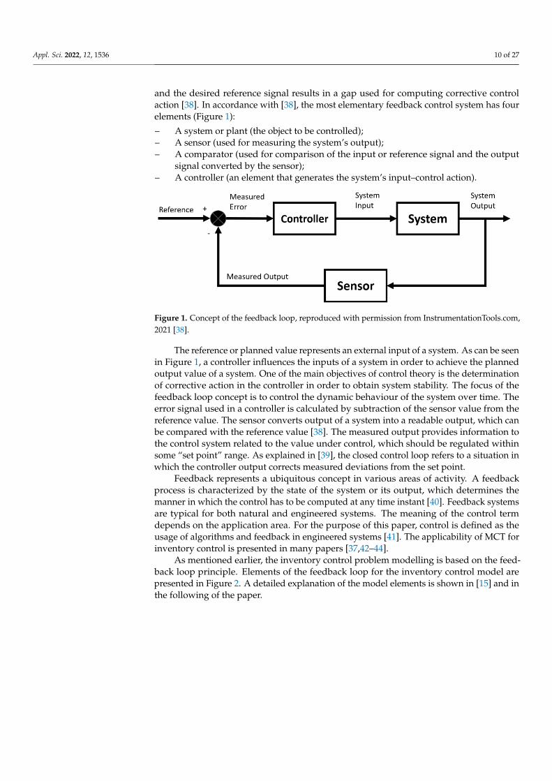
and the desired reference signal results in a gap used for computing corrective controlaction [38]. In accordance with [38], the most elementary feedback control system has fourelements (Figure 1):

– A system or plant (the object to be controlled);– A sensor (used for measuring the system’s output);– A comparator (used for comparison of the input or reference signal and the output

signal converted by the sensor);– A controller (an element that generates the system’s input–control action).

Appl. Sci. 2022, 12, x FOR PEER REVIEW 9 of 26

and management. Consequently, the scope of modern control science is much wider than

the traditional control theory. The development directions of MCT comprise methods that

improve the design and the usage of computer tools in the decision support systems. Con-

trol and management systems represent one of the largest classes of such systems [36]. A

control system design typically implies many steps, described in [37].

One of the most common concepts related to control systems is a feedback loop. The

system output represents the signal that should be controlled. Comparing this signal and

the desired reference signal results in a gap used for computing corrective control action

[38]. In accordance with [38], the most elementary feedback control system has four ele-

ments (Figure 1):

− A system or plant (the object to be controlled);

− A sensor (used for measuring the system’s output);

− A comparator (used for comparison of the input or reference signal and the output

signal converted by the sensor);

− A controller (an element that generates the system’s input–control action).

The reference or planned value represents an external input of a system. As can be

seen in Figure 1, a controller influences the inputs of a system in order to achieve the

planned output value of a system. One of the main objectives of control theory is the de-

termination of corrective action in the controller in order to obtain system stability. The

focus of the feedback loop concept is to control the dynamic behaviour of the system over

time. The error signal used in a controller is calculated by subtraction of the sensor value

from the reference value. The sensor converts output of a system into a readable output,

which can be compared with the reference value [38]. The measured output provides in-

formation to the control system related to the value under control, which should be regu-

lated within some “set point” range. As explained in [39], the closed control loop refers to

a situation in which the controller output corrects measured deviations from the set point.

Figure 1. Concept of the feedback loop, reproduced with permission from Instrumentation-

Tools.com, 2021 [38].

Feedback represents a ubiquitous concept in various areas of activity. A feedback

process is characterized by the state of the system or its output, which determines the

manner in which the control has to be computed at any time instant [40]. Feedback sys-

tems are typical for both natural and engineered systems. The meaning of the control term

depends on the application area. For the purpose of this paper, control is defined as the

usage of algorithms and feedback in engineered systems [41]. The applicability of MCT

for inventory control is presented in many papers [37,42–44].

As mentioned earlier, the inventory control problem modelling is based on the feed-

back loop principle. Elements of the feedback loop for the inventory control model are

presented in Figure 2. A detailed explanation of the model elements is shown in [15] and

in the following of the paper.

Figure 1. Concept of the feedback loop, reproduced with permission from InstrumentationTools.com,2021 [38].

The reference or planned value represents an external input of a system. As can be seenin Figure 1, a controller influences the inputs of a system in order to achieve the plannedoutput value of a system. One of the main objectives of control theory is the determinationof corrective action in the controller in order to obtain system stability. The focus of thefeedback loop concept is to control the dynamic behaviour of the system over time. Theerror signal used in a controller is calculated by subtraction of the sensor value from thereference value. The sensor converts output of a system into a readable output, which canbe compared with the reference value [38]. The measured output provides information tothe control system related to the value under control, which should be regulated withinsome “set point” range. As explained in [39], the closed control loop refers to a situation inwhich the controller output corrects measured deviations from the set point.

Feedback represents a ubiquitous concept in various areas of activity. A feedbackprocess is characterized by the state of the system or its output, which determines themanner in which the control has to be computed at any time instant [40]. Feedback systemsare typical for both natural and engineered systems. The meaning of the control termdepends on the application area. For the purpose of this paper, control is defined as theusage of algorithms and feedback in engineered systems [41]. The applicability of MCT forinventory control is presented in many papers [37,42–44].

As mentioned earlier, the inventory control problem modelling is based on the feed-back loop principle. Elements of the feedback loop for the inventory control model arepresented in Figure 2. A detailed explanation of the model elements is shown in [15] and inthe following of the paper.

Appl. Sci. 2022, 12, 1536 11 of 27Appl. Sci. 2022, 12, x FOR PEER REVIEW 10 of 26

Input:

Sales forecast,

FOQ,

Stock level report

Sensor:

Stock level

Controller:

Logistics manager;

Realization of control actions;

Confirmation of Order quantity

calculated based on stock level

compared with necessary inventory

levels

System:

Inventory

control model

Output:

Ordering plan

(quantity and

reorder periods)

Figure 2. Elements of the feedback loop for the inventory control model.

4.2. Discrete-Time System Control—System Dynamics Modelling

System dynamics (SD) is a modelling approach widely used in logistics and supply

chain management [45]. System dynamics (SD) relates the modelling of processes over

time. SD is often considered a modelling technique based on continuous time [46]. In this

paper, we consider SD modelling also for the discrete concept of time. Finite changes over

time mode means dealing with changes over time in a manner that resembles our every-

day experience. It is based on a simple principle: “In order to notify some change, some

time has to pass by” [46]. Changes are related to time intervals, whereas the state of a

variable is specified for specific points of time. The distinction between time-points and

time-intervals yields two distinct types of data: data related to time-points and data re-

lated to time-intervals. The data relating to time-points will be named stocks and the data

related to time-intervals flows. If the stocks are considered as state variables for time-

points and the flows as changes of the stocks for certain time-intervals, the relation be-

tween the stocks and the flows is trivial arithmetic. For a given time interval (t0, t1) and

given flows for that time interval we can calculate the “new” value of the stock at the end

of the time interval according to the following equation [46]:

stock(t1) = stock(t0) + inflows(t0, t1) − outflows(t0, t1)

A stock accumulates its flows. According to the stock-flow principle [46], the new

stock(t) is defined through the initial stock(t0) plus all inflow(s) subtracted by all the out-

flow(s) between the time t0 and time t. The core idea of SD modelling is the accumulation

of flows over finite time intervals of duration discrete time periods, t. On the stock-flow

diagram, there are two main types of elements: flow regulators (actions) and stock as state

variable (accumulations) [47].

The control model of the problem defined in this paper implies two flows (Figure 3),

the information flow of the planned inventory state and the material flow of the actual

state of inventory. Each flow has three phases, one phase of accumulation and two phases

of action. The action phases represent input and output flow regulators, respectively. The

accumulation, representing inventory level, for each flow, is calculated with the quantity

of the inventory from the end of the previous time period and is increased by the planned

or realized quantity for delivery over the observed period of time, and it is reduced by the

planned or realized sales over the period of time. For example, Figure 3 shows the stock-

flow diagram for one item (one stock keeping unit–SKU, t = 1 … 24 months). In order to

define a discrete-time mathematical model of the problem, a notation will be defined per

type of element of the system and from the position of the element on stock-flow diagram

(from top to bottom, and from left to right). For the stock-flow diagram presented by Fig-

ure 3, the following notations will be used:

Figure 2. Elements of the feedback loop for the inventory control model.

4.2. Discrete-Time System Control—System Dynamics Modelling

System dynamics (SD) is a modelling approach widely used in logistics and supplychain management [45]. System dynamics (SD) relates the modelling of processes overtime. SD is often considered a modelling technique based on continuous time [46]. Inthis paper, we consider SD modelling also for the discrete concept of time. Finite changesover time mode means dealing with changes over time in a manner that resembles oureveryday experience. It is based on a simple principle: “In order to notify some change,some time has to pass by” [46]. Changes are related to time intervals, whereas the state of avariable is specified for specific points of time. The distinction between time-points andtime-intervals yields two distinct types of data: data related to time-points and data relatedto time-intervals. The data relating to time-points will be named stocks and the data relatedto time-intervals flows. If the stocks are considered as state variables for time-points andthe flows as changes of the stocks for certain time-intervals, the relation between the stocksand the flows is trivial arithmetic. For a given time interval (t0, t1) and given flows for thattime interval we can calculate the “new” value of the stock at the end of the time intervalaccording to the following equation [46]:

stock(t1) = stock(t0) + inflows(t0, t1) − outflows(t0, t1)

A stock accumulates its flows. According to the stock-flow principle [46], the newstock(t) is defined through the initial stock(t0) plus all inflow(s) subtracted by all the out-flow(s) between the time t0 and time t. The core idea of SD modelling is the accumulationof flows over finite time intervals of duration discrete time periods, t. On the stock-flowdiagram, there are two main types of elements: flow regulators (actions) and stock as statevariable (accumulations) [47].

The control model of the problem defined in this paper implies two flows (Figure 3),the information flow of the planned inventory state and the material flow of the actual stateof inventory. Each flow has three phases, one phase of accumulation and two phases ofaction. The action phases represent input and output flow regulators, respectively. Theaccumulation, representing inventory level, for each flow, is calculated with the quantity ofthe inventory from the end of the previous time period and is increased by the plannedor realized quantity for delivery over the observed period of time, and it is reduced bythe planned or realized sales over the period of time. For example, Figure 3 shows thestock-flow diagram for one item (one stock keeping unit–SKU, t = 1 . . . 24 months). In orderto define a discrete-time mathematical model of the problem, a notation will be defined pertype of element of the system and from the position of the element on stock-flow diagram

Appl. Sci. 2022, 12, 1536 12 of 27

(from top to bottom, and from left to right). For the stock-flow diagram presented byFigure 3, the following notations will be used:

• X1t —State variable. Planned stock level of a product on hand at the end of period t.

• X2t —State variable. Realized stock level of a product on hand at the end of period t.

• Y1t —Inflow regulator variable (left upper). Planned stock input of a product at the

beginning of period t.• Y2

t —Inflow regulator variable (left lower). Realized stock input of a product at thebeginning of period t.

• Y3t —Outflow regulator variable (right upper). Forecasted sales plan for a product for

period t.• Y4

t —Outflow regulator variable (right lower). Realized sales of a product at period t.

Appl. Sci. 2022, 12, x FOR PEER REVIEW 11 of 26

• 𝑋𝑡1–State variable. Planned stock level of a product on hand at the end of period t.

• 𝑋𝑡2–State variable. Realized stock level of a product on hand at the end of period t.

• 𝑌𝑡1–Inflow regulator variable (left upper). Planned stock input of a product at the

beginning of period t.

• 𝑌𝑡2–Inflow regulator variable (left lower). Realized stock input of a product at the

beginning of period t.

• 𝑌𝑡3–Outflow regulator variable (right upper). Forecasted sales plan for a product for

period t.

• 𝑌𝑡4–Outflow regulator variable (right lower). Realized sales of a product at period t.

Figure 3. Graphical representation of information and material flows.

The regulator variables have the same notation Y, because of the same nature of the

flow, but have different superscripts suitable for the writing of equations describing the

system. Defined notation is used for the formulation of the control system model, for ex-

ample:

𝑋𝑡1 = 𝑋𝑡−1

1 + 𝑌𝑡1 − 𝑌𝑡

3, 𝑡 = 1, 24

𝑋𝑡2 = 𝑋𝑡−1

2 + 𝑌𝑡2 − 𝑌𝑡

4, 𝑡 = 1, 24

Or summarized as follows:

𝑋𝑡𝑖 = 𝑋𝑡−1

𝑖 + 𝑌𝑡𝑖 − 𝑌𝑡

𝑖+2, 𝑡 = 1, 24 , 𝑖 = 1,2

In the following of the paper, the notation of variables is defined in the described

manner, for two distinctive flows, the planned flow of stock and the realized flow of stock,

for each SKU. Each flow implies the same elements: two regulators, and one state variable.

According to [47] a discrete-time system control, used for the system modelling, rep-

resents a natural manner for describing inventory dynamics. Many papers describe the

usage of the discrete-time system control for dynamic deterministic inventory problems.

Frequently, they consider lot-sizing problems, beginning with [48,49]. Solving proposals

for dynamic lot-sizing problems include dynamic programming algorithms [50] and dif-

ferent special heuristics and metaheuristics [51,52]. The dynamic discrete-time system

modelling approach is used for the inventory control system in this paper due to its wide

applicability and many benefits. These models enable relatively simple and not time-con-

suming modifications in accordance with newly discovered facts about an observed prob-

lem by changing some of the discrete control object elements. For example, adjusted ele-

ments related to the objective function allow model variations or even the setting of a new

model, without modifications of other model elements, such as the law of behaviour for

state variables, flow regulators, and the control space. Definitions and implementation

guidance for dynamic discrete inventory control models can be found in [47,53]. Accord-

ing to [47], relations of the law of dynamics and control domain determine a discrete con-

trolled object. These relations also represent the simulation model of the controlled object.

System state changes are observed at the end of the discrete period t (day, month, year,

etc.) of a time horizon. Decisions made in one period of time influence states and, conse-

quently, new decisions in future periods. The success of the control is measured for each

period by a defined objective function. The performance criterion is an objective function

that adds values throughout the time horizon [47].

Figure 3. Graphical representation of information and material flows.

The regulator variables have the same notation Y, because of the same nature ofthe flow, but have different superscripts suitable for the writing of equations describingthe system. Defined notation is used for the formulation of the control system model,for example:

X1t = X1

t−1 + Y1t − Y3

t , t = 1, 24X2

t = X2t−1 + Y2

t − Y4t , t = 1, 24

Or summarized as follows:

Xit = Xi

t−1 + Yit − Yi+2

t , t = 1, 24, i = 1, 2

In the following of the paper, the notation of variables is defined in the describedmanner, for two distinctive flows, the planned flow of stock and the realized flow of stock,for each SKU. Each flow implies the same elements: two regulators, and one state variable.

According to [47] a discrete-time system control, used for the system modelling, rep-resents a natural manner for describing inventory dynamics. Many papers describe theusage of the discrete-time system control for dynamic deterministic inventory problems.Frequently, they consider lot-sizing problems, beginning with [48,49]. Solving proposals fordynamic lot-sizing problems include dynamic programming algorithms [50] and differentspecial heuristics and metaheuristics [51,52]. The dynamic discrete-time system modellingapproach is used for the inventory control system in this paper due to its wide applica-bility and many benefits. These models enable relatively simple and not time-consumingmodifications in accordance with newly discovered facts about an observed problem bychanging some of the discrete control object elements. For example, adjusted elementsrelated to the objective function allow model variations or even the setting of a new model,without modifications of other model elements, such as the law of behaviour for statevariables, flow regulators, and the control space. Definitions and implementation guidancefor dynamic discrete inventory control models can be found in [47,53]. According to [47],relations of the law of dynamics and control domain determine a discrete controlled object.These relations also represent the simulation model of the controlled object. System statechanges are observed at the end of the discrete period t (day, month, year, etc.) of a timehorizon. Decisions made in one period of time influence states and, consequently, newdecisions in future periods. The success of the control is measured for each period by a

Appl. Sci. 2022, 12, 1536 13 of 27

defined objective function. The performance criterion is an objective function that addsvalues throughout the time horizon [47].

5. Mathematical Formulation, Assumptions and Notation

The considered problem is represented as a dynamic discrete multiproduct inventorycontrol model. This section represents the mathematical formulation of the model, alongwith notation and assumptions.

5.1. Assumptions

In addition to the assumptions described within the problem description, the inventoryreplenishment problem is modelled in accordance with the following assumptions:

• Lead time (LT) includes the time necessary for the delivery of goods from the manufac-turer to the distributor. Delivery time includes time periods from ordering to receivingthe goods.

• Shortages are allowed but not backlogged, i.e., stock-out situations should be minimized.• The initial inventory level is known.• Order quantity depends on the observed instance:

# Fixed, i.e., the manufacturer defines the fixed order quantity per each product,but periods between orders are not fixed.

# Lot-for-lot, i.e., cumulative monthly sales forecast for three months, in a movinghorizon situation, after the lead time period is expired, but periods betweenorders are not fixed.

• The sales forecast is known and forecasted for two years.

5.2. Notation

In order to explain the model, the following notations are used:

– m–Total number of products (i = 1, 2, . . . , m).– T–Finite time horizon T = 24 months (t = 1, 2, . . . , T).– LT–Delivery lead time.– Xi1

t –Planned stock level of product i on hand at the end of period t. This phase ofaccumulation represents the total amount of product i remaining on the stock at theend of period t on the flow of the planned state of inventory

(t = 1, 24, i = 1, m

).

– Xi2t –Realized stock level of product i on hand at the end of period t. This phase of

accumulation represents the total amount of product i remaining in the stock at theend of period t, on the flow of the realized state of inventory

(t = 1, 24, i = 1, m

).

– Yi1t –Planned stock input of product i at the beginning of period t. This inflow regulator

represents the amount of product i expected to be delivered after the lead time at thebeginning of period t. It is the regulator of the flow of the planned inventory state(t = 1, 24, i = 1, m

).

– Yi2t –Realized stock input of product i at the beginning of period t. The inflow regulator

represents the input variable that relates to the inventory fulfilment at the beginningof the month. This flow regulator represents the amount of product i delivered to thewarehouse after the lead time expiry. It pertains to the flow of the realized state ofinventory. The variable value is confirmed in the company’s software when orderquantity arrives in the stock

(t = 1, 24, i = 1, m

).

– Yi3t –Forecasted sales plan for product i for period t. This outflow regulator represents

the amount of product i planned for withdrawing from the accumulation of theplanned inventory state continuously per month. The sales manager forecasts thesales plan for 24 months

(t = 1, 24, i = 1, m

).

– Yi4t –Realized sales of product i at period t. This outflow regulator represents the

amount of product i actually withdrawn from the accumulation of the realized stateof inventory continuously per month

(t = 1, 24, i = 1, m

).

– minQit–FOQ for the product i in period t, defined by manufacturer

(t = 1, 24, i = 1, m

).

Appl. Sci. 2022, 12, 1536 14 of 27

– LQit–LFL order quantity for each product i

(t = 1, 24, i = 1, m

).

– Sit–The auxiliary variable representing value from a stock level report for product i at

the beginning of period t(t = 1, 24, i = 1, m

), and representing value obtained from

stock level report, which is provided each month from a warehouse of a distributor.This variable presents an exact level of inventory for product i.

– Ait–The auxiliary variable indicates if the planned stock level on hand Xi1

t is greaterthan security stock SSi

t for product i in period t(t = 1, 24, i = 1, m

).

– Qit–The planned re-order quantity for product i in period t

(t = 1, 24, i = 1, m

).

– SSit–The security stock for product i in period t of time horizon T (t = 1, 24, i = 1, m).

– ASit–The planned average level of stock for product i in period t of time horizon T

(t = 1, 24, i = 1, m).– ∆ti–The auxiliary variable for calculation of the LQi

t in the case of a lot-for-lot orderingpolicy (i = 1, m).

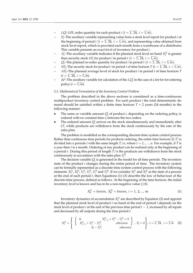
5.3. Mathematical Formulation of the Inventory Control Problem

The problem described in the above sections is considered as a time-continuousmultiproduct inventory control problem. For each product i the total deterministic de-mand should be satisfied within a finite time horizon T = 2 years (24 months) in thefollowing manner:

• The same or variable amount Qit of product i, depending on the ordering policy, is

ordered with no constant time ti between the two orders.• The ordered amount Qi

t arrives on the stock simultaneously and immediately afterLT, while products are withdrawn from the stock continuously by the rate of thesales plan.

The problem is modelled as the corresponding discrete-time system control process.Rather than continuous time periods for products ordering, the entire time horizon [0, T] isdivided into n periods t with the same length T/n, where t = 1, . . . , n. For example, if T isa year then t is a month. Ordering of any product can be realized only at the beginning ofa period t. During this period of length T/n the products are withdrawn from the stockcontinuously in accordance with the sales plan Yi3

t .The decision variable Qi

t is generated in the model for all time periods. The inventorystate of the product i changes during the entire period of time. The inventory systemcan be formally represented as a discrete-time system control process with the followingelements: Xi1

t , Xi2t , Yi1

t , Yi2t , Yi3

t and Yi4t . If we consider Xi1

t and Xi2t as the state of a process

at the end of each period t, then Equations (1)–(3) describe the low of behaviour of thediscrete-time process, defined as follows. At the beginning of the time horizon, the initialinventory level is known and has to be a non-negative value (≥0).

Xi10 = known, Xi2

0 = known, i = 1, 2, ..., m (1)

Inventory dynamics of accumulation Xi1t are described by Equation (2) and appoint

that the planned stock level of product i on hand at the end of period t depends on thestock level of product i at the end of the previous time period t − 1, increased by all inputsand decreased by all outputs during the time period t.

Xi1t =

{

0, Xi1t−1 + Yi1

t − Yi3t < 0

Xi1t−1 + Yi1

t − Yi3t , otherwise

}Si

t − Yi3t , otherwise

, Sit = 0

, t = 1, 24, i = 1, m (2)

Appl. Sci. 2022, 12, 1536 15 of 27

A similar Equation (3) is developed for the realized stock level of product i on hand atthe end of period t.

Xi2t =

{

0, Xi2t−1 + Yi2

t − Yi4t < 0

Xi2t−1 + Yi2

t − Yi4t , otherwise

}Si

t − Yi4t , otherwise

, Sit = 0

, t = 1, 24, i = 1, m (3)

The value of the planned input of stock (Yi1t ) depends on the planned re-order quantity

(Qit) and variable realized input of stock (Yi2

t ). This variable can be formally expressed as:

Yi1t =

{Yi2

t , Yi2t > 0

Qit, otherwise

}, t = 1, 24, i = 1, m (4)

The sales forecast plan (Yi3t ) represents the amount of product planned for withdraw-

ing from the stock continuously per month, and this flow regulator is planned by salesmanagement for two years.

Yi3t = known, t = 1, 24, i = 1, m (5)

Flow regulator Yi2t represents the realized input of stock when the inventory is physi-

cally delivered to the distributor warehouse at the beginning of time period t and can beformally described as:

Yi2t = known, t = 1, 24, i = 1, m (6)

Realized sales (Yi4t ) represents the amount of product physically withdrawn from the

realized stock level on hand continuously per month. This flow regulator is known at theend of the current time period t (at the end of each month). In the case of deterministicdemand, the flow regulator is described as:

Yi4t = Yi3

t = known, t = 1, 24, i = 1, m (7)

However, in the case of stochastic demand (i.e., time-varying demand), the flowregulator is presented as the variable sales forecast Yi3

t , which is changed randomly in therange of ±20% for each period of time horizon T. More formally:

Yi4t =

{0, Si

t = 0Y3

t ∗ (100 ∗ (20 − RAND() ∗ 40)/100), otherwise

}, t = 1, 24, i = 1, m (8)

where function RAND() generates random numbers, evenly distributed.According to [15], the process described by Equations (1)–(8) represents a typical

discrete-time system control process, where the current state in period t depends on boththe previous state in period t-1 and the chosen value of Qi

t.The auxiliary variable Si

t represents the inventory level in the stock level report ofproduct i. It is obtained from a customer warehouse at the beginning of each month, and itrepresents a real level of inventory for a product i. The quantity received at the beginning ofa month Yi2

t increases the level of inventory in the stock level report of product i, generatedat the beginning of each month.

Sit = known, t = 1, 24, i = 1, m (9)

The security stock represents the maximum amount of all monthly values in the salesforecast plan (Yi3

t ) in time horizon T and covers demand for one month. It is expressed as:

SSit = max(Yi3

t ), t = 1, 24, i = 1, m (10)

The planned average level of stock ASit in time horizon T is an auxiliary variable

calculated as a product of the amount of safety stock (SSit) and half of a lead time period

Appl. Sci. 2022, 12, 1536 16 of 27

(LT/2). The amount of average stock corresponds to the average sale for at least half of alead time period. It is expressed as:

ASit = SSi

t ∗LT2

, t = 1, 24, i = 1, m (11)

The planned re-order quantity Qit realizes at the beginning of a period t only in the

case when the stored quantity of product i remaining at the end of the previous time periodt − 1 is not greater than the average stock on hand in time horizon T. This decision variableis generated by relation (12) and depends on the ordering policy. For FOQ policy, quantityof product i is defined by the manufacturer (minQi

t), and for LFL policy it is LQit quantity.

LFL order quantity LQit is based on a moving horizon for each product i. It is calculated in

accordance with the precisely needed order quantity for three months of sales that occurafter the expiry of a defined lead time. The decision variable planned re-order quantity Qi

tfor period t can be expressed as:

Qit =

{

minQit(or LQi

t), Xi1

t < ASit − SSi

t0, otherwise

}, ∏t+LT

t Ait = 1

minQit(or LQi

t), otherwise

, Xi1t+LT < ASi

t

0, otherwise

, t = 1, 24, i = 1, m (12)

The stock level alarm Ait is an auxiliary variable representing the signal indicating if

the planned stock level on hand Xi1t is greater than security stock SSi

t for product i. Thisbinary variable takes the value of 1 if the described condition is satisfied and 0 otherwise.The Ai

t value is calculated as:

Ait =

{1, Xi1

t > SSit

0, otherwise

}, t = 1, 24, i = 1, m (13)

The control domain of the model includes two constraints. These constraints securethat the inventory level in the accumulation cannot be negative. Inequality (14) showsthat the planned stock level on hand (Xi1

t ) and realized stock level on hand (Xi2t ) cannot be

negative, and these rules are included in relation (2) and (3) of the model.

Xi1t−1 + Yi1

t − Yi3t ≥ 0 t = 1, 24, i = 1, m

Xi2t−1 + Yi2

t − Yi4t ≥ 0

(14)

Let us determine the performance criterion function for the inventory system describedby (1)–(8). Performances of the model can be observed through two objective functions:

- (max) J1–The maximization of the difference between the planned average level ofinventory and the realized average level of inventory.

- (min) J2–The minimization of the number of stock-out situations.

Relations (15) and (16) describe the objective functions.

(max) J1 =∑T

t=1 Xi1t

T− ASi, t = 1, 24, i = 1, m (15)

(min) J2 = ∑Tt=1(1, Xi1

t < 0), t = 1, 24, i = 1, m (16)

For the second instance, referring to LFL ordering policy, the order quantity LQit of

product i is calculated in accordance with the forecasted sale for three months that occursafter the expiry of a defined lead time LT. The auxiliary variable ∆ti represents the numberof time periods in a moving average horizon after the expiry of a lead time for whichdemand is summarized. Additionally, due to the fact that the moving horizon does notcover t > T periods, this factor is multiplied by the amount of security stock

(SSi

t)

in order

Appl. Sci. 2022, 12, 1536 17 of 27

to obtain the demand (e.g., demand for three months at the end of the time horizon) in thecase of LFL policy. The discrete controlled object model, with the previously describedlaw of dynamics, control domain, performance criterion, and all discrete equations andinequalities, remains the same as the model of the first instance, but the minQi for FOQpolicy will be changed with the LFL order quantity LQi

t. The new decision variable LQit for

period t can be defined as:

∆ti = known, i = 1, m

LQit =

{∆ti·SSi

t, Yi3t+LT+∆ti = 0

∑t+LT+∆ti

t+LT Yi3t , otherwise

}, t = 1, 24, i = 1, m

(17)

6. The Inventory Control Model Implementation

The discrete simulation control model is implemented in a spreadsheet environment,and procedures are automated through Visual Basic for Application (VBA) for all productsi = 1, . . . , m. Input elements for the model are the sales forecast, the FOQ, the stock levelreport, the realized input of stock, and the realized sales (Figure 4). In the case of LFLordering policy, the ordering quantity is not the FOQ. LFL quantity, represented by variableLQi

t, is calculated in accordance with Equation (17). In addition, the level of inventory in acolumn planned stock level on hand (Figure 4) must be calculated. Customers send theinventory level report at the beginning of each month, and it corresponds to the actualinventory level at the end of the previous month. Values from these reports are presentedin the column stock level report (Figure 4). The planned stock level on hand for a currentmonth is calculated as a sum of the stock level quantity at the end of the previous monthand the planned input of stock, reduced for the forecasted sale in a current month. Themodel refers to all periods within 2 years, even future months. In this manner, we definethe sensor function of the feedback model, which prepares data for comparison in thecomparator.

Appl. Sci. 2022, 12, x FOR PEER REVIEW 16 of 26

∆𝑡𝑖 = 𝑘𝑛𝑜𝑤𝑛, 𝑖 = 1,𝑚

𝐿𝑄𝑡𝑖 = {

∆𝑡𝑖 ∙ 𝑆𝑆𝑡𝑖 , 𝑌

𝑡+𝐿𝑇+∆𝑡𝑖𝑖3 = 0

∑ 𝑌𝑡𝑖3

𝑡+𝐿𝑇+∆𝑡𝑖

𝑡+𝐿𝑇, 𝑜𝑡ℎ𝑒𝑟𝑤𝑖𝑠𝑒

} , 𝑡 = 1, 24 , 𝑖 = 1,𝑚 (17)

6. The Inventory Control Model Implementation

The discrete simulation control model is implemented in a spreadsheet environment,

and procedures are automated through Visual Basic for Application (VBA) for all prod-

ucts 𝑖 = 1, …, m. Input elements for the model are the sales forecast, the FOQ, the stock

level report, the realized input of stock, and the realized sales (Figure 4). In the case of LFL

ordering policy, the ordering quantity is not the FOQ. LFL quantity, represented by vari-

able 𝐿𝑄𝑡𝑖, is calculated in accordance with Equation (17). In addition, the level of inventory

in a column planned stock level on hand (Figure 4) must be calculated. Customers send

the inventory level report at the beginning of each month, and it corresponds to the actual

inventory level at the end of the previous month. Values from these reports are presented

in the column stock level report (Figure 4). The planned stock level on hand for a current

month is calculated as a sum of the stock level quantity at the end of the previous month

and the planned input of stock, reduced for the forecasted sale in a current month. The

model refers to all periods within 2 years, even future months. In this manner, we define

the sensor function of the feedback model, which prepares data for comparison in the

comparator.

Figure 4. Elements of the spreadsheet model.

An unusually long lead time (LT) indicates that the reorder point and reorder quan-

tity have to be calculated based on the inventory level and sales forecast for all months

between the current period (t) and the delivery period (t + LT). The column planned order

quantity (Figure 4) represents the variable defined as the difference between the necessary

inventory level for observed months and the actual stock level. Calculated differences are

used for the determination of order quantities that will be distributed to each customer

and the time periods when orderings have to be realized, i.e., reorder periods. This varia-

ble represents the comparator and controller function of the control model.

The column realized input of stock (Figure 4) relates to the situations when an order

arrives earlier or later than expected. This is not a common case because t = 1 month or

approximately 30 days, and delay in the delivery is notated only in cases exceeding t = 1

month. In these cases, the entire spreadsheet simulation model is recalculated automati-

cally.

According to the comparison algorithm presented in Figure 5, stock levels are com-

pared with average inventory levels and security stock. The average inventory levels and

security stock provide demand satisfaction. Based on these differences, the order quantity

and reorder periods are calculated and presented by the variable planned order quantity

(Figure 5). However, if the delivery of articles ordered in January is realized with a 2-

month delay, the ordering plan has to be updated.

Figure 4. Elements of the spreadsheet model.

An unusually long lead time (LT) indicates that the reorder point and reorder quantityhave to be calculated based on the inventory level and sales forecast for all months betweenthe current period (t) and the delivery period (t + LT). The column planned order quantity(Figure 4) represents the variable defined as the difference between the necessary inventorylevel for observed months and the actual stock level. Calculated differences are used forthe determination of order quantities that will be distributed to each customer and the timeperiods when orderings have to be realized, i.e., reorder periods. This variable representsthe comparator and controller function of the control model.

The column realized input of stock (Figure 4) relates to the situations when an order ar-rives earlier or later than expected. This is not a common case because t = 1 month or approx-imately 30 days, and delay in the delivery is notated only in cases exceeding t = 1 month.In these cases, the entire spreadsheet simulation model is recalculated automatically.

According to the comparison algorithm presented in Figure 5, stock levels are com-pared with average inventory levels and security stock. The average inventory levels andsecurity stock provide demand satisfaction. Based on these differences, the order quantityand reorder periods are calculated and presented by the variable planned order quantity(Figure 5). However, if the delivery of articles ordered in January is realized with a 2-monthdelay, the ordering plan has to be updated.

Appl. Sci. 2022, 12, 1536 18 of 27Appl. Sci. 2022, 12, x FOR PEER REVIEW 17 of 26

IF (Planned stock level on hand (t+LT) < Planned average level of stock) THEN

IF (Planned stock level on hand (t+LT) > Security stock) THEN

IF (Planned stock level on hand (t) < Planned average level on stock- Security stock) THEN

Planned order quantity = FOQ (or LQ)

ELSE

Planned order quantity = 0

END IF

ELSE

Planned order quantity = FOQ (or LQ)

END IF

ELSE

Planned order quantity = 0

END IF

Figure 5. Pseudocode for planned order quantity.

After approval of the quantities, the order is sent to supplier 4U Pharma GMBH.

These actions affect inventories and demand for all domestic clients, wholesalers, and

pharmacies from different countries. Additionally, when the order quantity and delivery

are confirmed by the production plant, the entire ordered quantity is assigned to the coun-

tries and clients. In this manner, the logistics manager controls the distribution of ordered

quantities, which provides inventory to satisfy all customer requirements.

7. Sensitivity Analysis and Numerical Results

Sensitivity analysis is realized for a single product in order to evaluate the model

performances. Consequently, because 𝑖 = 1, the variables’ exponents declared for “𝑖” will

be omitted in further text. Sensitivity analysis and numerical results will be presented for

two instances. Instance 1 is related to the FOQ ordering policy and Instance 2 refers to the

LFL ordering policy.

7.1. Instance 1: FOQ Ordering Policy

The following assumptions are considered for Instance 1:

• The initial level of inventory for products is zero in the case of launching a new prod-

uct into the market. In this case, the first order will be launched at the beginning of

January and delivered at the beginning of June (LT = 5 months).

• Based on historical data from previous years and experience, the manager forecasts

monthly sales at the beginning of the first year for the next 2 years.

• The supplier defines the FOQ for each product. Since the FOQ is not unique for each

product, the unit price depends on the ordered quantity.

• At the beginning of every month, customers from all countries send stock level re-

ports to the company’s logistics manager. This report represents the prescribed form

and format in an Excel spreadsheet.

• The delivery lead time is five months. The quantity ordered at the beginning of Feb-

ruary is in stock at the beginning of July.

• At the beginning of the first year, there are no realized inputs of stock for launched

orders from the previous periods.

Instance 1 is analysed for two separate cases. Case 1 considers FOQ policy with de-

terministic demand, where the forecasted sale is equal to the realized sale. Case 2 reflects

FOQ policy with stochastic demand, when the realized sale is the forecasted sale changed

randomly in range ±20%.

Figure 5. Pseudocode for planned order quantity.

After approval of the quantities, the order is sent to supplier 4U Pharma GMBH. Theseactions affect inventories and demand for all domestic clients, wholesalers, and pharmaciesfrom different countries. Additionally, when the order quantity and delivery are confirmedby the production plant, the entire ordered quantity is assigned to the countries and clients.In this manner, the logistics manager controls the distribution of ordered quantities, whichprovides inventory to satisfy all customer requirements.

7. Sensitivity Analysis and Numerical Results

Sensitivity analysis is realized for a single product in order to evaluate the modelperformances. Consequently, because i = 1, the variables’ exponents declared for “i” willbe omitted in further text. Sensitivity analysis and numerical results will be presented fortwo instances. Instance 1 is related to the FOQ ordering policy and Instance 2 refers to theLFL ordering policy.

7.1. Instance 1: FOQ Ordering Policy

The following assumptions are considered for Instance 1:

• The initial level of inventory for products is zero in the case of launching a new productinto the market. In this case, the first order will be launched at the beginning of Januaryand delivered at the beginning of June (LT = 5 months).

• Based on historical data from previous years and experience, the manager forecastsmonthly sales at the beginning of the first year for the next 2 years.

• The supplier defines the FOQ for each product. Since the FOQ is not unique for eachproduct, the unit price depends on the ordered quantity.

• At the beginning of every month, customers from all countries send stock level reportsto the company’s logistics manager. This report represents the prescribed form andformat in an Excel spreadsheet.

• The delivery lead time is five months. The quantity ordered at the beginning ofFebruary is in stock at the beginning of July.

• At the beginning of the first year, there are no realized inputs of stock for launchedorders from the previous periods.

Instance 1 is analysed for two separate cases. Case 1 considers FOQ policy withdeterministic demand, where the forecasted sale is equal to the realized sale. Case 2 reflects

Appl. Sci. 2022, 12, 1536 19 of 27

FOQ policy with stochastic demand, when the realized sale is the forecasted sale changedrandomly in range ±20%.

In Case 1, regulators Y3t = Y4

t = Sales f orecast = known, t = 1, 24. From the beginningof June there are no stock-out situations, with exception of the first 5 months when thesystem waits for the delivery of the initial inventory (Figure 6).

Appl. Sci. 2022, 12, x FOR PEER REVIEW 18 of 26

In Case 1, regulators 𝑌𝑡3 = 𝑌𝑡

4 = 𝑆𝑎𝑙𝑒𝑠 𝑓𝑜𝑟𝑒𝑐𝑎𝑠𝑡 = 𝑘𝑛𝑜𝑤𝑛, 𝑡 = 1,24 . From the begin-

ning of June there are no stock-out situations, with exception of the first 5 months when

the system waits for the delivery of the initial inventory (Figure 6).

Figure 6. Elements of the spreadsheet model for Case 1: FOQ policy with deterministic demand.

In addition, except for the first five months, the value of the objective function de-

fined by Equation (16) is 0, without stock-out situations (Figure 7).

Figure 7. Dynamic of accumulation for Case 1: FOQ policy with deterministic demand.

Figure 6. Elements of the spreadsheet model for Case 1: FOQ policy with deterministic demand.

In addition, except for the first five months, the value of the objective function definedby Equation (16) is 0, without stock-out situations (Figure 7).

Appl. Sci. 2022, 12, x FOR PEER REVIEW 18 of 26

In Case 1, regulators 𝑌𝑡3 = 𝑌𝑡

4 = 𝑆𝑎𝑙𝑒𝑠 𝑓𝑜𝑟𝑒𝑐𝑎𝑠𝑡 = 𝑘𝑛𝑜𝑤𝑛, 𝑡 = 1,24 . From the begin-

ning of June there are no stock-out situations, with exception of the first 5 months when

the system waits for the delivery of the initial inventory (Figure 6).

Figure 6. Elements of the spreadsheet model for Case 1: FOQ policy with deterministic demand.

In addition, except for the first five months, the value of the objective function de-

fined by Equation (16) is 0, without stock-out situations (Figure 7).

Figure 7. Dynamic of accumulation for Case 1: FOQ policy with deterministic demand. Figure 7. Dynamic of accumulation for Case 1: FOQ policy with deterministic demand.

Appl. Sci. 2022, 12, 1536 20 of 27

According to Case 2 (Figure 8), the variable Realized sales is presented as the variableSales forecast, which is changed randomly in the range of ±20% for each period of timehorizon T, as it is presented by Equation (8).

Appl. Sci. 2022, 12, x FOR PEER REVIEW 19 of 26

According to Case 2 (Figure 8), the variable Realized sales is presented as the variable

Sales forecast, which is changed randomly in the range of ±20% for each period of time

horizon T, as it is presented by Equation (8).

Figure 8. Elements of the spreadsheet model for Case 2: FOQ policy with stochastic demand.

For Case 2, the total number of planned orders and received deliveries is the same as

for Case 1. From the company manager’s point of view, forecasted sales never deviate

more than ±20%. This stochastic demand generates very similar values of the objective

functions 𝐽1 and 𝐽2 as for Case 1, concerning the average level of inventories and stock-

outs (Figure 9).

Figure 8. Elements of the spreadsheet model for Case 2: FOQ policy with stochastic demand.

For Case 2, the total number of planned orders and received deliveries is the same asfor Case 1. From the company manager’s point of view, forecasted sales never deviate morethan ±20%. This stochastic demand generates very similar values of the objective functionsJ1 and J2 as for Case 1, concerning the average level of inventories and stock-outs (Figure 9).

Appl. Sci. 2022, 12, x FOR PEER REVIEW 19 of 26

According to Case 2 (Figure 8), the variable Realized sales is presented as the variable

Sales forecast, which is changed randomly in the range of ±20% for each period of time

horizon T, as it is presented by Equation (8).

Figure 8. Elements of the spreadsheet model for Case 2: FOQ policy with stochastic demand.

For Case 2, the total number of planned orders and received deliveries is the same as

for Case 1. From the company manager’s point of view, forecasted sales never deviate

more than ±20%. This stochastic demand generates very similar values of the objective

functions 𝐽1 and 𝐽2 as for Case 1, concerning the average level of inventories and stock-

outs (Figure 9).

Figure 9. Dynamic of accumulation for Case 2: FOQ policy with stochastic demand.

Appl. Sci. 2022, 12, 1536 21 of 27

The numerical results of Case 1 and Case 2 for Instance 1 are presented in Table 2.

Table 2. Numerical results of Case 1 and Case 2 for Instance 1.

No. Instance 1:FOQ Ordering Policy

Case 1: DeterministicDemand

Case 2:StochasticDemand

1 Lead time (month) 5 52 Planned average level of stock (unit) 63,000.00 63,000.003 Security stock (unit) 25,200.00 25,200.004 Max level of stock T = 24 months (unit) 70,400.00 70,472.005 Average level of stock T = 24 months (unit) 45,595.00 45,646.006 Total number of stock outs 5 57 Total number of launched orders 14 148 Total number of received orders 11 119 max (J1) = (2)–(5) 17,405.00 17,354.0010 min (J2) = (6) 5 5

The total number of planned orders is 14, and the total number of received deliveries is11. As shown in Figures 6 and 8 and Table 2, at the beginning of the first year, the columnsStock level report, Realized input of stock and Realized sales are empty because there areno launched orders from the previous year for delivery in the first five months of timehorizon T. For Case 1, the model shows that the planned average level of inventory for theproduct in the warehouse (63,000 units) is greater than the realized average level of stockin time horizon T = 24 months (45,595 units) for 17,405 units, according to the objectivefunction (15). In addition, except for the first five months, the value of the objective function(16) is zero, without stock-out situations.

If we compare the numerical results of Case 1 and Case 2 for FOQ ordering policy(Table 2), it can be appointed that the differences between the values of the objectivefunctions are small, even in Case 2, when the realized sales are randomly changed in therange of ±20%. An insignificant deviation of the objective functions results for Cases 1and 2 confirms that the model is sensitive and stable. One of the main questions related tofuture research, also significant from a company perspective, can be: “What will happenwith the Total number of orders, Stock-outs, and Costs, if the business environment isunstable and uncertainty is higher, e.g., if realized sales vary more than ±30% or ±50%?”.

7.2. Instance 2: LFL Ordering Policy

In the case of LFL ordering policy, the order quantity is calculated in accordance withthe moving horizon, i.e., the forecasted sales for three months which occurs after the expiryof the defined lead time. The variable LQi

t (Equation (17)) represents the order quantity forthe LFL model. General assumptions for Instance 2 are the same as for Instance 1. Instance2 is analysed for two separate cases, as well as Instance 1. Case 1 considers LFL orderingpolicy with deterministic demand, where the forecasted sale is equal to the realized sale.Case 2 reflects LFL ordering policy with stochastic demand, where the realized sales arethe forecasted sales changed randomly in the range ±20%. For Case 1, shown in Figure 10,regulators Y3

t = Y4t = Sales f orecast = known, t = 1, 24.

As mentioned, Case 2 considers LFL ordering policy with stochastic demand. Thevariable realized sales is described by Equation (8). Except for the values of this variable,elements of the spreadsheet model for Case 2 are the same as for Case 1. Since the dynamicof accumulation for both cases of Instance 2 is pretty similar as for Instance 1, there wasno need for graphic representation. For Case 2 of Instance 2, the total number of plannedorders and received deliveries is the same as for Case 1 of Instance 2. The numerical resultsof Case 1 and Case 2, for Instance 2, are presented in Table 3.

Appl. Sci. 2022, 12, 1536 22 of 27Appl. Sci. 2022, 12, x FOR PEER REVIEW 21 of 26

Figure 10. Elements of the spreadsheet model for Case 1: LFL policy with deterministic demand.

As mentioned, Case 2 considers LFL ordering policy with stochastic demand. The

variable realized sales is described by Equation (8). Except for the values of this variable,

elements of the spreadsheet model for Case 2 are the same as for Case 1. Since the dynamic

of accumulation for both cases of Instance 2 is pretty similar as for Instance 1, there was

no need for graphic representation. For Case 2 of Instance 2, the total number of planned

orders and received deliveries is the same as for Case 1 of Instance 2. The numerical results

of Case 1 and Case 2, for Instance 2, are presented in Table 3.

Table 3. Numerical results of Case 1 and Case 2 for Instance 2.

No. Instance 2:break//LFL Ordering

Policy

Case 1:break//Determinis-

tic Demand

Case 2:break//Stochastic

Demand

1 Lead time (month) 5 5

2 Planned average level of stock

(unit) 63,000.00 63,000.00

3 Security stock (unit) 25,200.00 25,200.00

4 Max level of stock T = 24 months

(unit) 94,600.00 94,599.00

5 Average level of stock T = 24

months (unit) 59,979.00 59,967.00

6 Total number of stock outs 5 5

7 Total number of launched orders 10 10

8 Total number of received orders 7 7

9 max (J1) = (2)–(5) 3021.00 3033.00

10 min (J2) = (6) 5 5

Figure 10. Elements of the spreadsheet model for Case 1: LFL policy with deterministic demand.

Table 3. Numerical results of Case 1 and Case 2 for Instance 2.

No. Instance 2:LFL Ordering Policy

Case 1:Deterministic Demand

Case 2:Stochastic Demand

1 Lead time (month) 5 52 Planned average level of stock (unit) 63,000.00 63,000.003 Security stock (unit) 25,200.00 25,200.004 Max level of stock T = 24 months (unit) 94,600.00 94,599.005 Average level of stock T = 24 months (unit) 59,979.00 59,967.006 Total number of stock outs 5 57 Total number of launched orders 10 108 Total number of received orders 7 79 max (J1) = (2)–(5) 3021.00 3033.0010 min (J2) = (6) 5 5

If we compare the numerical results of Case 1 and Case 2 for LFL ordering policy(Table 3), it can be noted that the differences between the values of the objective functionsare small, even in Case 2, when the realized sales are randomly changed in the rangeof ±20%. An insignificant deviation of the objective functions results for Cases 1 and 2confirms that the model is sensitive and stable.

7.3. Comparison of Numerical Results for Instance 1 and Instance 2

A comparative review of results for Instances 1 and 2 in the situation of deterministicdemand is shown in Table 4. The value of the objective function J1 is decreased for14,384 units, i.e., to the amount of 3021 units for the LFL ordering policy. The averagelevel of inventories is increased by 14,384 units, which is a consequence of the decreasednumber of launched and received orders. The number of planned and realized deliveriesis decreased by four, which significantly impacts delivery costs, but the average order

Appl. Sci. 2022, 12, 1536 23 of 27

quantity is also increased from 32,000 units (Figure 6) to 48,338 units (Figure 10). Thedecreased number of deliveries drives the increase of the average inventory level. Exceptfor the first five months, the criterion function J2 is zero, i.e., without stock-out situations.

Table 4. Comparison of numerical results for Instance 1 and Instance 2 in Case 1.

No. Parameters

Instance 1: FOQOrdering Policy

Case 1:Deterministic

Demand

Instance 2:LFL Ordering Policy

Case 1:Deterministic

Demand

∆

(Instance 1–Instance 2)

1 Lead time (month) 5 5 02 Planned average level of stock (unit) 63,000.00 63,000.00 03 Security stock (unit) 25,200.00 25,200.00 04 Max level of stock T = 24 months (unit) 70,400.00 94,600.00 24,200.005 Average level of stock T = 24 months (unit) 45,595.00 59,979.00 14,384.006 Total number of stock outs 5 5 07 Total number of launched orders 14 10 −48 Total number of received orders 11 7 −49 max (J1) = (2)–(5) 17,405.00 3021.00 −14,384.0010 min (J2) = (6) 5 5 0

However, if we compare the numerical results of Case 2 for Instance 1 and Case 2 forInstance 2 (Table 5), the number of orders and consequently delivery costs are decreased.Therefore, based on previously declared assumptions of this control model, taking intoaccount the defined objective functions (15) and (16), the performed numerical experimentsshow that the FOQ gives better results than the LFL policy.

Table 5. Comparison of numerical results for Instance 1 and Instance 2 in Case 2.

No. Parameters

Instance 1: FOQOrdering Policy

Case 2: StochasticDemand

Instance 2: LFLOrdering Policy

Case 2: StochasticDemand

∆

(Instance 1–Instance 2)

1 Lead time (month) 5 5 02 Planned average level of stock (unit) 63,000.00 63,000.00 03 Security stock (unit) 25,200.00 25,200.00 04 Max level of stock T = 24 months (unit) 70,472.00 94,599.00 24,127.005 Average level of stock T = 24 months (unit) 45,646.00 59,967.00 14,321.006 Total number of stock outs 5 5 07 Total number of launched orders 14 10 −48 Total number of received orders 11 7 −49 max (J1) = (2)–(5) 17,354.00 3033.00 −14,321.0010 min (J2) = (6) 5 5 0

The FOQ ordering policy will decrease the average amount of inventories and increasethe stability in the supplier production process, i.e., the production series will be based onFOQ quantity. Nevertheless, considering the delivery costs, which are not assumptionsof this model, the LFL policy could obtain better results than the FOQ policy due to theimpact of the decreased number of deliveries.

Moreover, for the LFL ordering policy (Table 5), the total number of launched andreceived orders is decreased for four orders. Bearing in mind that the average lead time ofdelivery is five months, the waiting time for deliveries is decreased by 20 months, and therisk of undelivered orders is much lower.

Appl. Sci. 2022, 12, 1536 24 of 27

8. Conclusions

This paper describes a multiproduct inventory control problem in a pharmaceuticaldistribution company, modelled as a corresponding dynamic discrete-time system controlprocess. The actuality of the topic elaborated in the paper is consistent with the importanceof the pharmaceutical inventory and distribution management. The improvement of thementioned processes management in pharmaceutical companies implies cost reductionand customer service level improvements.

The paper is aimed at the development of an inventory control model for a phar-maceutical distribution company, with an emphasis on reorder quantities and reorderperiods, and the satisfaction of specific constraints. The mathematical model is based onthe proposed conceptual model, developed in accordance with the modern control theoryconcept and specific practical assumptions and constraints of the supply chain, as noticedin the company. The authors proposed two variations of the model, implemented in thespreadsheet environment of MS Excel and automated through Visual Basic for Applications.The model allows analysis from many different perspectives and can be easily modifiedand enhanced in order to reflect new scenarios. The developed model represents a baselinemodel that enables the creation of alternative scenarios and comparison of those scenariosto the baseline. Furthermore, the presented solution of the problem satisfies the request de-fined by the company which is related to the affordable but dynamic and flexible softwaresolution that is relatively easy to implement and use. These contributions, detailed in thepaper, represent an important aspect of managerial implications.

The theoretical contribution and some of the main advantages of the developed controlmodel concerning the traditional DRP model are:

– FOQ- and LFL-based models determine lot size and safety stock.– These models recalculate order quantities and reorder points if demand is changed in

real-time.– The full automation of the model is based on the concept of feedback control.– The structure of the model is precisely defined according to the object of discrete

control with an adequate mathematical apparatus.

In order to emphasize specificities of the research presented in this paper, and at thesame time the improvements of the previous study mentioned in [15], the authors of thepaper point out the following contributions:

– Modern control theory (MCT), i.e., self–regulation and feedback control concepts, withrelevant elements (sensor, comparator, controller, system) of the feedback loop areapplied during the development of the conceptual model.

– The mathematical model presented in the paper is comprised of two flows. Theplanned inventory state represents information flow, while the actual inventory staterefers to material flow. Each flow has one phase of accumulation and two phases ofaction. Two sales variables and two inventory state variables, planned and realized,are precisely mathematically defined, with their mutual influence, i.e., the impact ofthe actual state of inventory on the future, and the planned inventory state.

– The performance criterion of the inventory system is defined and described throughtwo objective functions, the maximization of the difference between the plannedaverage inventory level and the realized average inventory level and the minimizationof the number of stock-out situations.

– The originally developed comparison algorithm for the planned order quantity reflectsthe decision tree for comparison of all relevant stock variables.

– Sensitivity analysis is conducted, and numerical results are explained clearly with allsupporting data.

– Stochastic demand is generated as a random variation of sales forecast in the range of±20%. Numerical results are compared for deterministic and stochastic actual sales.

The applicability of the model has been proven by its usage for procurement planningin the described company within the period of two years. The created plan comprised more

Appl. Sci. 2022, 12, 1536 25 of 27

than 50 products per country for several countries from Eastern-Central Europe. Researchdirections imply further research of the model efficiency for real-life problems but withlarger dimensions. For example, the number of units and constraints could be increased,the model could include delivery costs, and the stochastic demand could be randomlyvaried in a range more than ±20.

Author Contributions: Conceptualization, S.A., L.D.M. and A.L.; methodology, S.A. and L.D.M.;software, S.A. and L.D.M.; validation, S.A., L.D.M. and A.L.; formal analysis, S.A., L.D.M. andA.L.; investigation, S.A. and L.D.M.; resources, S.A. and L.D.M.; data curation, S.A. and L.D.M.;writing—original draft preparation, S.A., L.D.M. and A.L.; writing—review and editing, L.D.M.;visualization, S.A. and L.D.M.; supervision, S.A., L.D.M. and A.L.; project administration, L.D.M.;funding acquisition, S.A., L.D.M. and A.L. All authors have read and agreed to the published versionof the manuscript.

Funding: This research received no external funding. The APC was funded by Faculty of Organiza-tional Sciences, University of Belgrade, Belgrade, Serbia.

Institutional Review Board Statement: Not applicable.

Informed Consent Statement: Not applicable.

Data Availability Statement: Not applicable.

Conflicts of Interest: The authors declare no conflict of interest.

References1. Hoque, M.E.; Paul, N. Inventory Management of Pharmaceutical Industries in Bangladesh. In Proceedings of the International

Conference on Mechanical Engineering 2011 (ICME2011), Dhaka, Bangladesh, 18–20 December 2011.2. Uthayakumar, R.; Priyan, S. Pharmaceutical supply chain and inventory management strategies: Optimization for a pharmaceuti-

cal company and a hospital. Oper. Res. Health Care 2013, 2, 52–64. [CrossRef]3. Management Sciences for Health. MDS-3: Managing Access to Medicines and Health Technologies; Management Sciences for Health:

Arlington, VA, USA, 2012.4. Axsäter, S. Inventory Control; Springer: Berlin/Heidelberg, Germany, 2015; Volume 225. [CrossRef]5. Kwak, C.; Choi, J.S.; Kim, C.O.; Kwon, I.H. Situation reactive approach to vendor managed inventory problem. Expert Syst. Appl.

2009, 36, 9039–9045.6. Grob, C. Inventory Management in Multi-Echelon Networks: On the Optimization of Reorder Points; Springer: Berlin/Heidelberg,

Germany, 2018; Volume 128.7. Qiu, Y.; Qiao, J.; Pardalos, P.M. Optimal production, replenishment, delivery, routing and inventory management policies for

products with perishable inventory. Omega 2019, 82, 193–204. [CrossRef]8. Perez, H.D.; Hubbs, C.D.; Li, C.; Grossmann, I.E. Algorithmic Approaches to Inventory Management Optimization. Processes

2021, 9, 102.9. Srinivasarao, G. Overview of Inventory Optimization in Operations Management. In Business Research and Innovation, Proceedings

of the International Conference on Business Research and Innovation ICBRI 2021, Murshidabad, India, 26–27 February 2021; Excel IndiaPublishers: New Delhi, India, 2021; pp. 486–492.

10. Settanni, E.; Harrington, T.S.; Srai, J.S. Pharmaceutical supply chain models: A synthesis from a systems view of operationsresearch. Oper. Res. Perspect. 2017, 4, 74–95. [CrossRef]

11. Lemmens, S.; Decouttere, C.; Vandaele, N.; Bernuzzi, M. A review of integrated supply chain network design models: Key issuesfor vaccine supply chains. Chem. Eng. Res. Des. 2016, 109, 366–384. [CrossRef]

12. Fahimnia, B.; Farahani, R.Z.; Marian, R.; Luong, L. A review and critique on integrated production—Distribution planningmodels and techniques. J. Manuf. Syst. 2013, 32, 1–19. [CrossRef]

13. Nagurney, A.; Li, D. A supply chain network game theory model with product differentiation, outsourcing of production anddistribution, and quality and price competition. Ann. Oper. Res. 2015, 226, 479–503. [CrossRef]

14. Agrell, P.J.; Hatami-Marbini, A. Frontier-based performance analysis models for supply chain management: State of the art andresearch directions. Comput. Ind. Eng. 2013, 66, 567–583.

15. Antic, S.; Djordjevic, L.; Lisec, A. Case study: Dynamic discrete model of fixed order point quantity system for inventories inpharmaceutical distribution. In Proceedings of the 21st International Symposium on Logistics (ISL 2016), Kaohsiung, Taiwan, 3–6July 2016; pp. 455–462.

16. 4U Pharma. 4youpharma. 2018. Available online: http://4youpharma.com/ (accessed on 12 April 2019).17. Vila-Parrish, A.R.; Ivy, J.S. Managing supply critical to patient care: An introduction to hospital inventory management for

pharmaceuticals. In Handbook of Healthcare Operations Management; Springer: New York, NY, USA, 2013; pp. 447–463.

Appl. Sci. 2022, 12, 1536 26 of 27

18. Li, J.; Liu, L.; Hu, H.; Zhao, Q.; Guo, L. An inventory model for deteriorating drugs with stochastic lead time. Int. J. Environ. Res.Public Health 2018, 15, 2772. [CrossRef]

19. Khodaverdi, R.; Shahbazi, M.; Azar, A.; Fathi, M.R. A Robust Optimization Approach for Sustainable humanitarian supply chainmanagement of blood products. Int. J. Hosp. Res. 2022, 11. Available online: http://ijhr.iums.ac.ir/article_139129.html (accessedon 20 January 2022).

20. Zandieh, M.; Janatyan, N.; Alem-Tabriz, A.; Rabieh, M. Designing sustainable distribution network in pharmaceutical supplychain: A case study. Int. J. Supply Oper. Manag. 2018, 5, 122–133.

21. Narayana, S.A.; Arun, E.A.; Rupesh, P.K. Reverse logistics in the pharmaceuticals industry: A systemic analysis. Int. J. Logist.Manag. 2014, 25, 379–398. [CrossRef]

22. Hansen, K.R.N.; Grunow, M. Planning operations before market launch for balancing time-to-market and risks in pharmaceuticalsupply chains. Int. J. Prod. Econ. 2015, 161, 129–139. [CrossRef]

23. Ahmadi, E.; Masel, D.T.; Metcalf, A.Y.; Schuller, K. Inventory management of surgical supplies and sterile instruments in hospitals:A literature review. Health Syst. 2019, 8, 134–151. [CrossRef] [PubMed]

24. Schmitt, A.J.; Sun, S.A.; Snyder, L.V.; Shen, Z.J.M. Centralization versus decentralization: Risk pooling, risk diversification, andsupply chain disruptions. Omega 2015, 52, 201–212. [CrossRef]

25. Enns, S.T.; Suwanruji, P. Distribution planning and control: An experimental comparison of DRP and order point replenishmentstrategies. In Proceedings of the Academy of Business and Administrative Sciences, 2000 International Conference, Prague, CzechRepublic, 10 July 2000.

26. Seok, H.; Nof, S.Y. Intelligent information sharing among manufacturers in supply networks: Supplier selection case. J. Intell.Manuf. 2018, 29, 1097–1113. [CrossRef]

27. Chapman, S.N.; Arnold, J.T.; Gatewood, A.K.; Clive, L.M. Introduction to Materials Management; Pearson Education Limited:New York, NY, USA, 2017.

28. Russell, R.S.; Taylor, B.W. Operation Management: Quality and Competitiveness in a Global Environment; John Wiley &Sons: New York, NY, USA, 2006; pp. 529–552.

29. Chase, R.; Aquilano, N. Operations Management for Competitive Advantage; IRWIN: New York, NY, USA, 2004; pp. 542–560.30. Barlow, J.F. Excel Models for Business and Operations Management; John Wiley & Sons: New York, NY, USA, 2005; pp. 244–258.31. Muller, M. Essentials of Inventory Management; Harper Collins Leadership: New York, NY, USA, 2019.32. Wild, T. Best Practice in Inventory Management; Elsevier Science: London, UK, 2017; pp. 112–148.33. Grubbström, R.W.; Bogataj, L.; Bonney, M.C.; Disney, S.C.; Tang, O. Inter-Linking MRP Theory and Production and Inventory

Control Models. In Proceedings of the 13th International Working Conference on Production Economics, Igls, Austria, 16–20February 2004.

34. Franco, C.; Alfonso-Lizarazo, E. A structured review of quantitative models of the pharmaceutical supply chain. Complexity 2017,2017, 5297406. [CrossRef]

35. Saha, E.; Ray, P.K. Modelling and analysis of inventory management systems in healthcare: A review and reflections. Comput. Ind.Eng. 2019, 137, 106051. [CrossRef]

36. Bubnicki, Z. Modern Control Theory; Springer: Berlin/Heidelberg, Germany, 2002.37. Antic, S.; Kostic, K.; Dordevic, L. Spreadsheet Model of Inventory Control Based on Modern Control Theory. In Proceedings of

the 13th International Symposium SymOrg: Innovative Management and Business Performance, Zlatibor, Serbia, 5–9 June 2012.38. Doyle, J.; Francis, B.; Tannenbaum, A. Feedback Control Theory; Macmillan Publishing Co.: Basingstoke, UK, 1990.39. Zook, D.; Bonne, U.; Samad, T. Control Systems, Robotics and Automation; Eoloss publishers: Oxford, UK, 2009.40. Andrei, N. Modern Control Theory-A historical perspective. Stud. Inform. Control 2006, 15, 51.41. Aström, K.J.; Murray, R.M. Feedback Systems: An Introduction for Scientists and Engineers; Princeton University Press: Princeton, NJ,

USA, 2010.42. Azarskov, V.N.; Skurikhin, V.I.; Zhiteckii, L.S.; Lypoi, R.O. Modern Control Theory Applied to Inventory Control for a Manufac-

turing System. IFAC Proc. Vol. 2013, 46, 1200–1205. [CrossRef]43. Ying, Z.; Weiguo, W.; Qiushuang, H.; Ye, X.; Hong, J. Inventory control based on a real-moment dynamic model. In Proceedings

of the 2011 International Conference on Management Science and Industrial Engineering (IEEE), Harbin, China, 6–11 January2011; pp. 838–841.

44. Shin, J.; Lee, J.; Park, S.; Koo, K.K.; Lee, M. Analytical design of a proportional-integral controller for constrained optimalregulatory control of inventory loop. Control Eng. Pract. 2008, 16, 1391–1397. [CrossRef]

45. Tako, A.A.; Robinson, S. The application of discrete event simulation and system dynamics in the logistics and supply chaincontext. Decis. Support Syst. 2012, 52, 802–815. [CrossRef]

46. Ossimitz, G.; Mrotzek, M. The Basics of System Dynamics: Discrete vs. Continuous Modelling of Time. In Proceedings of the 26thInternational Conference of the System Dynamics Society, Athens, Greece, 20–24 July 2008.

47. Kostic, K. Inventory control as a discrete system control for the fixed-order quantity system. Appl. Math. Model. 2009, 33,4201–4214. [CrossRef]

48. Wagner, H.M.; Whitin, T.M. Dynamic version of the economic lot size model. Manag. Sci. 1958, 5, 89–96. [CrossRef]49. Scarf, H. The Optimality of (s; S) Policies in the Dynamic Inventory Problem. In Mathematical Methods in the Social Sciences; Arrow,

K.J., Karlin, S., Suppes, P., Eds.; Stanford University Press: Stanford, CA, USA, 1959.

Appl. Sci. 2022, 12, 1536 27 of 27

50. Bertsekas, D.P. Dynamic Programming, Deterministic and Stochastic Models; Prentice-Hall: Englewood Cliffs, NJ, USA, 1987.51. Jans, R.; Degraeve, Z. Meta-heuristics for dynamic lot sizing: A review and comparison of solution approaches. Eur. J. Oper. Res.

2007, 177, 1855–1875. [CrossRef]52. Ðordevic, L.; Antic, S.; Cangalovic, M.; Lisec, A. A metaheuristic approach to solving a multiproduct EOQ-based inventory

problem with storage space constraints. Optim. Lett. 2017, 11, 1137–1154. [CrossRef]53. Antic, S.; Djordjevic, L.; Kostic, K.; Lisec, A. Dynamic discrete simulation model of an inventory control with or without allowed

shortage. UPB Sci. Bull. Ser. A 2015, 77, 163–176.