1 Author for correspondence

A Decoupled GLS-Based Path Flow Estimator For Inferring Origin-Destination Matrices Yu Nie1

Graduate Student Researcher Department of Civil and Environmental Engineering University of California, Davis CA 95616, U.S.A Tel: 530-754-6429 Email:ynie@ucdavis.edu H. Michael Zhang Associate Professor Department of Civil and Environmental Engineering University of California, Davis CA 95616, U.S.A. Will W. Recker Professor Department of Civil and Environmental Engineering University of California, Irvine CA 92697, U.S.A. Submitted to TRB Committee A1C05 – Transportation Network Modeling

For consideration of presentation at the 82nd Annual Meeting of the Transportation Research Board and publication

in Transportation Research Record

July 2002

TRB 2003 Annual Meeting CD-ROM Paper revised from original submittal.

Nie, Zhang and Recker

- 2 -

ABSTRACT

Recently, path flow estimator (PFE) has been used for the estimation of origin-destination (O-D) matrices.

This paper develops a formulation that incorporates the decoupled path flow estimator in a generalized least squares

(GLS) framework. The approach seeks to solve a GLS problem that minimizes the sum of errors in traffic counts

and O-D matrices based on equilibrium assignment mapping, which is derived from a K-shortest path ranking

procedure exogenously. Solving the GLS-PFE model inevitably involves non-invertible linear systems and

nonnegative constraints. A solution algorithm is thus designed to iteratively identify active constraints and solve

linear systems by computing the pseudo-inverse. A simplified version of this algorithm is further developed to

improve its computational efficiency. The solution properties and computational efficiency of the two methods are

tested and compared with small to mid-size networks. It is concluded that the simplified algorithm is efficient in

solving the large-scale decoupled GLS-PFE model for O-D estimation.

TRB 2003 Annual Meeting CD-ROM Paper revised from original submittal.

Nie, Zhang and Recker

- 3 -

INTRODUCTION

One of the essential elements of transportation planning and/or operations is to “allocate” travelers onto a

transportation network according to either a static or dynamic assignment mapping. A fundamental input to traffic

assignment is the origin-destination (O-D) matrix that depicts traffic demands between each origin and destination

pair. Unfortunately, the “true” O-D matrices are rarely, if ever, directly obtainable in practice, which gives rise to

many studies for its estimation from limited observations of traffic conditions on the network.

Traditionally, O-D matrices are derived from household or roadside surveys. However, survey-based

approaches have two main shortcomings: they are costly and labor intensive, and they often fail to capture temporal

changes in O-D demand patterns. Consequently, research efforts of O-D estimation have been focusing on inferring

O-D matrices from traffic counts on road segments, which is a faster, cheaper and more convenient method than

household or roadside surveys.

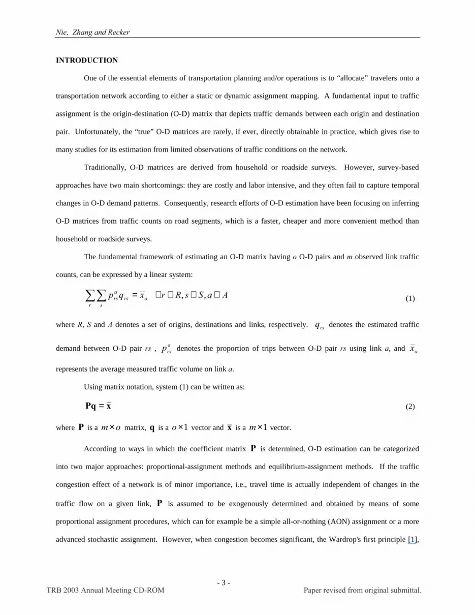
The fundamental framework of estimating an O-D matrix having o O-D pairs and m observed link traffic

counts, can be expressed by a linear system:

AaSsRrxqpr s

arsars ∈∈∈∀=∑∑ ,, (1)

where R, S and A denotes a set of origins, destinations and links, respectively. rsq denotes the estimated traffic

demand between O-D pair rs , arsp denotes the proportion of trips between O-D pair rs using link a, and ax

represents the average measured traffic volume on link a.

Using matrix notation, system (1) can be written as:

xPq = (2)

where P is a om × matrix, q is a 1×o vector and x is a 1×m vector.

According to ways in which the coefficient matrix P is determined, O-D estimation can be categorized

into two major approaches: proportional-assignment methods and equilibrium-assignment methods. If the traffic

congestion effect of a network is of minor importance, i.e., travel time is actually independent of changes in the

traffic flow on a given link, P is assumed to be exogenously determined and obtained by means of some

proportional assignment procedures, which can for example be a simple all-or-nothing (AON) assignment or a more

advanced stochastic assignment. However, when congestion becomes significant, the Wardrop's first principle [1],

TRB 2003 Annual Meeting CD-ROM Paper revised from original submittal.

Nie, Zhang and Recker

- 4 -

which states the well-known user-equilibrium (UE) condition in a congested transportation network, should be taken

into consideration. Consequently, P is no longer a simple proportion matrix that depicts the proportion of each O-

D trips using each link. Instead, P becomes an equilibrium assignment mapping, which maps the O-D demand

matrix to a flow pattern satisfying the UE state described by Wardrop's first principle. In a certain sense, the

equilibrium-based O-D matrix estimation can be thought of as an inverse of the UE traffic assignment.

It now becomes evident that the problem of O-D matrix estimation is to solve the linear system (2) for q

according to a given rule of determining coefficient matrix P . Conventional solution approaches solve system (2)

by minimizing a generalized distance function, namely a least squares or maximum entropy (minimum information)

function, between estimated and observed traffic counts when P is specified either in a proportional or equilibrium-

assignment form. In order to find a more realistic solution, a historical O-D matrix that is obtained from previous

surveys would be used as the “target” of the estimated OD matrix, which suggests that the objective function of the

minimization program will also take the distance between the estimated and the target O-D matrices into account.

Note that this distance function between the two O-D matrices is in general weighted appropriately according to the

relative belief between traffic counts and the target matrix. The earlier research efforts using proportionality-

assignment O-D estimation approach were credited to Willumsen [2], for introducing the maximum entropy form,

Van Zuylen [3] for using the concept of minimizing information, and Cascetta [4] for casting the problem in a

generalized least squares framework. Many researchers, such as Bell [5], Brennigner-Göthe et al. [6], Lo et al. [7],

conducted tests or proposed improvements along the line of proportional-based estimation. On the other hand,

Nguyen [8], Fisk and Boyce [9] led the way in equilibrium-based O-D matrix estimation. Yang [10] has shown that

a bi-level optimization technique can be used to model the problem by integrating an upper level, where the distance

function is minimized, with a lower level where the user-equilibrium flow pattern, thereby the coefficient matrix P ,

is sought through a standard traffic assignment routine. Instead of estimating the O-D matrix directly, Sherali et al.

[11] proposed to infer optimal path flows by formulating a linear programming problem, which is referred to here as

the linear path flow estimator (LPFE). The optimal path flows in Sherali’s approach will be estimated so as to

approach the user-equilibrium flow pattern, regenerate link traffic counts and concur with a target O-D matrix as

closely as possible. Bell et al. [12, 13] extended Shearli’s path flow estimator to the log-linear path flow estimator

by using stochastic user-equilibrium assignment. In order to avoid enumerating paths or applying a column

generation procedure, which is required by LPFE but computationally inefficient, Nie and Lee [14] suggested

TRB 2003 Annual Meeting CD-ROM Paper revised from original subm

Nie, Zhang and Recker

- 5 -

decoupling Sherali’s linear model through seeking equilibrium paths independently by a K-shortest path ranking

procedure.

The LPFE model, either coupled or decoupled, has difficulty in driving its estimates to the real O-D matrix

(not target matrix) as close as possible when the target matrix subjects to considerable errors, even if the equilibrium

flow pattern can be precisely regenerated. This shortcoming is mainly due to the limitation of a linear programming

structure. This paper attempts to fix the problem by incorporating the decoupled path flow estimator [9] with the

well-known generalized least squares (GLS) technique. Although GLS-based O-D estimation has been extensively

studied, our decoupled GLS-PFE model sheds light on two problems deserving further investigation. First, one may

have to invert a matrix whose strict inversion does not exist when solving the GLS-based PFE model. This is

typically caused by the fact that path-link matrix P is not full rank, which can be physically explained as some

paths can be decomposed into other two or more paths. In this research, a pseudo-inverse of a non-invertible matrix,

computed based on singular value decomposition, is adopted to find a least squares solution (or minimum distance

solution) for the corresponding linear system. Second, non-negative constraints for path flows cannot be ignored, as

many previous researchers did, because a good many of constraints will get activated during estimation when paths

are used as estimated variables. Based on Lawson and Hanson’s method [15] for a standard nonnegative least

squares (NNLS) problem, we present an algorithm for the constrained PFE model (ACPFE), which iterates between

figuring out the set of active constraints and solving the least squares problem consecutively. ACPFE is further

simplified in order to improve the computational efficiency while maintaining sufficient estimation accuracy.

The remaining of this paper is structured as follows. The next section reviews the ordinary least squares

(OLS) model for proportional-based O-D matrix estimation. Section 3 develops the GLS path flow estimator that

integrates the equilibrium assignment mapping and covariance matrices of measurement errors of link traffic counts

and the target O-D matrix. The discussions of solving non-invertible linear systems and dealing with nonnegative

constraints are also covered in Section 3. Solution algorithms are presented in Section 4, and Section 5 reports

numerical results. In the last section, we draw some conclusions and give directions for further research.

OLS PROPORTIONAL-ASSIGNMENT MODEL FOR O-D ESTIMATION

We first assume that P is given as the link-use proportion matrix. The O-D estimation problem can be

formulated as a classic ordinary least squares problem:

TRB 2003 Annual Meeting CD-ROM Paper revised from original submittal.

Nie, Zhang and Recker

- 6 -

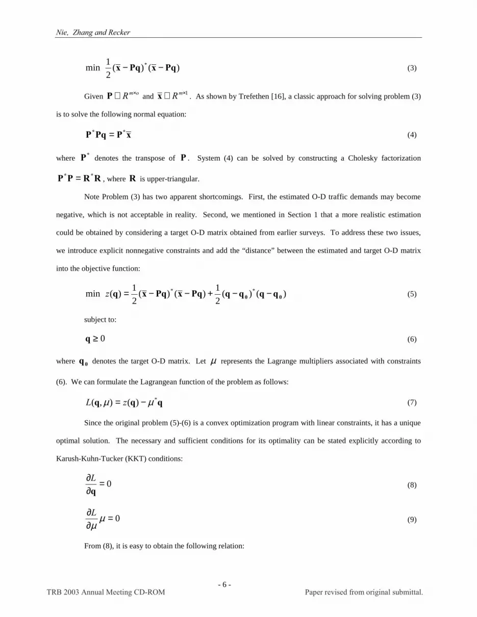
)()(21min * PqxPqx −− (3)

Given omR ×∈P and 1×∈ mRx . As shown by Trefethen [16], a classic approach for solving problem (3)

is to solve the following normal equation:

xPPqP ** = (4)

where *P denotes the transpose of P . System (4) can be solved by constructing a Cholesky factorization

RRPP ** = , where R is upper-triangular.

Note Problem (3) has two apparent shortcomings. First, the estimated O-D traffic demands may become

negative, which is not acceptable in reality. Second, we mentioned in Section 1 that a more realistic estimation

could be obtained by considering a target O-D matrix obtained from earlier surveys. To address these two issues,

we introduce explicit nonnegative constraints and add the “distance” between the estimated and target O-D matrix

into the objective function:

)()(21)()(

21)(min **

00 qqqqPqxPqxq −−+−−=z (5)

subject to:

0≥q (6)

where 0q denotes the target O-D matrix. Let µ represents the Lagrange multipliers associated with constraints

(6). We can formulate the Lagrangean function of the problem as follows:

qqq *)(),( µµ −= zL (7)

Since the original problem (5)-(6) is a convex optimization program with linear constraints, it has a unique

optimal solution. The necessary and sufficient conditions for its optimality can be stated explicitly according to

Karush-Kuhn-Tucker (KKT) conditions:

0=∂∂qL

(8)

0=∂∂ µµL

(9)

From (8), it is easy to obtain the following relation:

TRB 2003 Annual Meeting CD-ROM Paper revised from original submittal.

Nie, Zhang and Recker

- 7 -

0)()( ** =−−−− µPPqxqq 0 (10)

After taking transformation on both sides and collecting terms, we reach

µqxPqIPP 0** ++=+ )( (11)

Note Equation (11) is structurally similar to the normal equation (4). To obtain a clear physical

interpretation for (11), we proceed to derive an explicit expression for q using the well-known Matrix Inversion

Lemma:

PIPPPΙIPP *** 11 )()( −− +−=+ (12)

Applying relation (12) in (11) and let DIPP* =+ , we get:

µ)()(* PDPIxPPDPIPqDPqq 1**1*0

10

−−− −+−+−= (13)

Furthermore, note that the following relation holds:

xDPxPPDPI 1**1* −− =− )( (14)

Now, putting (14) into Equation (13), we obtain

µ)()(* PDPIPqxDPqq 1*0

10

−− −+−+= (15)

The second and third terms on the right-hand side of Equation (15) can be interpreted as two adjustments to

the prior estimation (or survey results): the first is related to the difference between the observed traffic counts and

those inferred on the basis of the prior estimates, and the second is adjusted according to the Lagrange multipliers

due to the nonnegative requirement on O-D demands.

DECOUPLED GLS PATH FLOW ESTIMATOR

The basic OLS model introduced in Section 2 is based on two assumptions: the measurement errors of

observed traffic counts and the target O-D matrix are uncorrelated and have same values, and the traffic assignment

mapping matrix P is known a priori. These assumptions are relaxed in this section.

Introduce The Equilibrium Assignment Mapping

Since the effects of peak-time congestion are unavoidable in urban transportation network, using a

proportional assignment mapping for O-D matrix estimation will produce inconsistence in system (2). A

conventional way of introducing the equilibrium assignment mapping into the O-D estimation is to combine the

TRB 2003 Annual Meeting CD-ROM Paper revised from original submittal.

Nie, Zhang and Recker

- 8 -

user-equilibrium (UE) traffic assignment procedure and the estimation process as an integrated model. This means

the assignment and estimation will be performed simultaneously. Consequently, the computational overhead is

substantially high even for mid-size networks since the formulation is no longer cast in the form of simple convex

optimization. Moreover, obtaining a converged solution becomes more difficult. It is thus desirable to maintain the

simple convex structure of the original problem while taking the equilibrium assignment into consideration.

Nie and Lee [9] proposed an algorithm to solve the LPFE model by Sherali et al. [12] for O-D estimation,

where the equilibrium path flow pattern is determined by an exogenous K-shortest path ranking procedure. The K-

shortest path ranking problem is a generalization of the shortest path tree problem, in which not one but a set of

shortest paths will be produced according to user-specified criteria. If the UE condition is held exactly in a given

network, in general, there exist more than one path connecting each O-D pair with the smallest and identical travel

cost. Intuitively, performing a sequence of K-shortest paths search could pick up all of these UE paths. Once these

paths are available, they will serve to form the coefficient matrix P whose columns are equal to the paths in the UE

flow pattern. Since P has been accommodated within the UE condition, the inconsistency from proportional

assignment assumption is prevented while the computation is kept relatively simple. Consequently, this strategy

"decouples" the equilibrium-based O-D estimation problem by determining the equilibrium assignment mapping

matrix P from the observed link traffic counts independently.

We in this paper apply this “decoupled” idea in a least squares framework instead of solving a linear

programming problem as done in [9]. Note that an important difference in a PFE model is that we do not estimate

the O-D demand q directly. Instead, path flows are inferred and each O-D demand is derived by summing up flows

of its associated equilibrium paths.

Let rskf denotes the flow on the kth equilibrium path between origin r and destination s, and rs

ka,δ denotes

the path-link incidence matrix, where rska,δ equals to 1 if link a belongs to path k, and 0 otherwise. We have the

following expression:

∑ ∑ ∑ ∈∈∈∈∀=r s

rsars

kak

rsk SsRrKkAaxf ,,,,δ

or

x∆f = (16)

TRB 2003 Annual Meeting CD-ROM Paper revised from original submittal.

Nie, Zhang and Recker

- 9 -

where ∆ plays a similar role as P in (2). However, ∆ is regarded to represent an equilibrium assignment mapping

since its columns are so generated as to conform with the UE condition. It will be shown how to obtain ∆ from a

K-shortest path ranking procedure in the next section. At this point, let us assume ∆ is known. The ordinary least

squares path flow estimator for O-D matrix estimation can be formulated as follows:

Model [OLS-PFE]

)()(21)()(

21)(min **

00 qMfqMf∆fx∆fxf −−+−−=z (17)

subject to:

0≥f (18)

where M is an no × (n is the total number of paths) matrix which converts equilibrium path flows to O-D

demands. Note constraint (18) guarantees

0≥= Mfq

Some may argue that restricting q to be nonnegative would be a preferable way than using (18) since

negative path flows might not necessarily generate negative O-D demands. However, using 0≥Mf as constraints

makes the problem much harder to solve, as we will see later on. Furthermore, the estimated path flow pattern itself

is an important output of a PFE model because it has to conform to a UE state when the optimality is reached. Thus,

a path flow pattern having negative path flows, on which the final O-D estimation is directly based, is not

acceptable.

According to the first-order optimality condition, we get the following normal-type equation:

λ++=+ 0**** qMx∆fMM∆∆ )( (19)

where λ is Lagrange multiplier associated with the constraint (18).

Consider Correlated and Homoskedastic Errors

We proceed to consider the case where the observed link counts and the target matrix subject to correlated

and homosekdastic random errors by extending the OLS-PFE model to a generalized least squares (GLS) PFE. It

should be noted, however, that observation errors of traffic counts are assumed to be small enough to keep all paths

contained in the UE state unchanged. This assumption is to guarantee that the K-shortest path ranking algorithm can

produce a “real” UE assignment mapping.

TRB 2003 Annual Meeting CD-ROM Paper revised from original submittal.

Nie, Zhang and Recker

- 10 -

A GLS-PFE model can be obtained by introducing the variance-covariance matrices of x and 0q . Let S

and T represent the variance-covariance matrices for target matrix and traffic counts respectively, [OLS-PFE] can

be reformulated as:

Model [GLS-PFE]

)()(21)()(

21)(min 1*1*

00 qMfSqMf∆fxT∆fxf −−+−−= −−z subject to 0≥f (20)

where both S and T are positive definite symmetric matrices. The normal equation of model (20) can be derived

from its first-order optimality condition as:

λ++=+ −−−−0

**** qSMxT∆fMSM∆T∆ 1111 )( (21)

We refer to Equation (21) as the fundamental equation for solving the uncoupled GLS-PFE model. In case

the matrix MSM∆T∆V ** 11 −− += is invertible and all constraints are inactive, the solution for the fundamental

equation can be straightforwardly expressed as follows:

bVf 1−= (22)

where 0** qSMxT∆b 11 −− += .

However, both the path-link incidence matrix ∆ and the path-OD matrix M are in general neither full

rank nor over-determined. To see this, first note that M becomes non-full rank and underdetermined whenever an

O-D pair has more than one path, which often happens in a transportation network with reasonable amount of

congestion. Moreover, the number of paths available is often larger than that of observed link counts. Even if this is

not the case, different paths still possibly correlate with one another so as to produce a non-full rank ∆ . As a result,

V is non-invertible thereby Equation (22) cannot be adopted to solve the fundamental equation (21).

Solve The Fundamental Equation With Non-Invertible V

It has been shown [15] that a pseudoinverse of a matrix V , denoted by +V , which always exists, provides

a unique minimum distance solution bV + (i.e., a solution for a least squares problem) for the linear system

bVf = . Penrose [15] proved that a matrix += VX if and only if the following conditions hold:

VVXV =

TRB 2003 Annual Meeting CD-ROM Paper revised from original submittal.

Nie, Zhang and Recker

- 11 -

XXVX =

VX(VX)* =

XV(XV)* = (23)

Therefore, in case of non-invertible V , one has to resort to the pseudoinverse of V to obtain an

approximate solution (minimum distance solution) for the fundamental equation. A classical approach of obtaining

a pseudoinverse of V is to decompose V through singular value decomposition (SVD) as follows:

*UWV Σ= (24)

where both W and U are nn × unitary matrices, i.e., 1−= WW* and 1−= UU* , and Σ is nn × and

diagonal with non-negative entries. When the rank of V is nl < , we can rewrite Σ as:

=Σ

000S

where S is a ll × diagonal matrix whose all entries are positive. It is easy to prove, using Penrose’s conditions,

that the pseudoinverse of Σ is:

=Σ

−+

0001S

Consequently, the pseudoinverse of V is given by:

*WUV ++ Σ= (25)

To prove this is true, we show that Equation (25) satisfies all Penrose conditions:

VUWUWUWWUUWVVV =Σ=ΣΣΣ=ΣΣΣ= +++ ***** )(

++++++++ =Σ=ΣΣΣ=ΣΣΣ= VWUUUWUUWWUVVV ***** )(

+++++ =ΣΣ=ΣΣ=ΣΣ= VVWWWWWUUW)(VV * ****** )()(

VVUUUUUWWUV)(V * +++++ =ΣΣ=ΣΣ=ΣΣ= ****** )()(

Thus, a solution for Equation (21) is given in form of the pseudoinverse as:

bWUbVf *++ Σ== (26)

TRB 2003 Annual Meeting CD-ROM Paper revised from original submittal.

Nie, Zhang and Recker

- 12 -

Computing the SVD of V, which is highly related to the eigenvalue decomposition of VV* , has been

available in some software packages like MATLAB as a standard subroutine. For conciseness, we will not

introduce details of SVD computation in this paper. Readers who are interested can refer to [16] (Chapter 31, page

234-240).

Deal with Nonnegative Constraint

A good many researchers ignored the nonnegative constraints when applying GLS-based O-D estimation

because they observed these constraints are rarely active. This might be true if a compact link-use proportion (OD-

link) matrix is adopted. However, the path flow estimator significantly increases the possibility of activating

nonnegative constraints, as shown by these authors’ experience, since it manipulates directly upon path-link and

path-OD matrices. Moreover, the increase of problem size will likely activate more constraints. We thus have to

seriously consider these nonnegative constraints.

Bell [1] has presented a simple algorithm for solving this constrained generalized least squares problem.

The algorithm iterates between solving the fundamental equation and updating Lagrange multipliers by scaling

negative estimated O-D entries with principal diagonal entries of 1−V . Yet, to the best of our knowledge, no

implementation and/or computational experiments for Bell’s algorithm is found in literature. Furthermore, this

algorithm neither considers the case where 1−V does not exist not appears to work well for the GLS-PFE model.

Lawson and Hanson [7] proposed an algorithm for a standard nonnegative least squares problem (NNLS),

based on which they proved the following important theorem that describes the property of a NNLS solution:

Theorem 1: Lawson and Hanson’s Theorem

The optimal solution 0f for the problem NNLS

)(21min * x(Pfx)Pf −− subject to 0≥f

satisfies the following conditions simultaneously, given Φ and Ω denotes the index sets of active and inactive

constraints respectively:

1.

Φ∈=Ω∈>

=ii

f i if0if0

:0

TRB 2003 Annual Meeting CD-ROM Paper revised from original submittal.

Nie, Zhang and Recker

- 13 -

2.

Φ∈>Ω∈=

=ii

i if0if0

:λ where xPPfPλ ** −= 0

3. 0f is a solution vector for the following least squares problem

)(21min * xf(Px)fP −− ΩΩ where

Φ∈Ω∈

=Ω iii

if0ifofcolumn

:P

P

Note λ in the theorem denotes the Lagrange multipliers and Conditions 1 and 2 are corresponding to KKT

conditions (8) and (9). We are going to show in the following that this theorem can be easily extended to our

decoupled PFE model.

Theorem 2

The optimal solution 0f for Model [OLS-PFE] satisfies the following conditions simultaneously, given Φ and Ω

denotes the index sets of active and inactive constraints respectively:

1.

Φ∈=Ω∈>

=ii

f i if0if0

:0

2.

Φ∈>Ω∈=

=ii

i if0if0

:λ where

bVfλ −= 0 MM∆∆V ** += , 0** qMx∆b += (27)

3. 0f is a solution vector for the following least squares problem

)(21)(

21min 0

*0

* qf(M)qfMxf(x)f −−+−∆−∆ ΩΩΩΩ

where

Φ∈Ω∈∆

=∆Ω iii

if0ifofcolumn

: and

Φ∈Ω∈

=Ω iii

if0ifofcolumn

:M

M (28)

Proof: We first show that [OLS-PFE] is equivalent to the following standard NLLS problem:

))(21min * ππ −Η−Η f(f subject to 0≥f , (29)

where

∆=Η

M is a nom ×+ )( matrix and

=

0qx

π is a 1)( ×+ om matrix. To see this, note

TRB 2003 Annual Meeting CD-ROM Paper revised from original submittal.

Nie, Zhang and Recker

- 14 -

))( * ππ −Η−Η f(f = ))( *

−

∆

−

∆

00 qx

fM

(qx

fM

= )()()()( **********0000 qqxxfMqxqxffMMf +++∆−∆+∆−+∆∆

= )()( ************0000 qqMfqqfMfMfxxfxxfff +−∆−++∆−∆−∆∆

= )()()()( **00 qMfqMf∆fx∆fx −−+−−

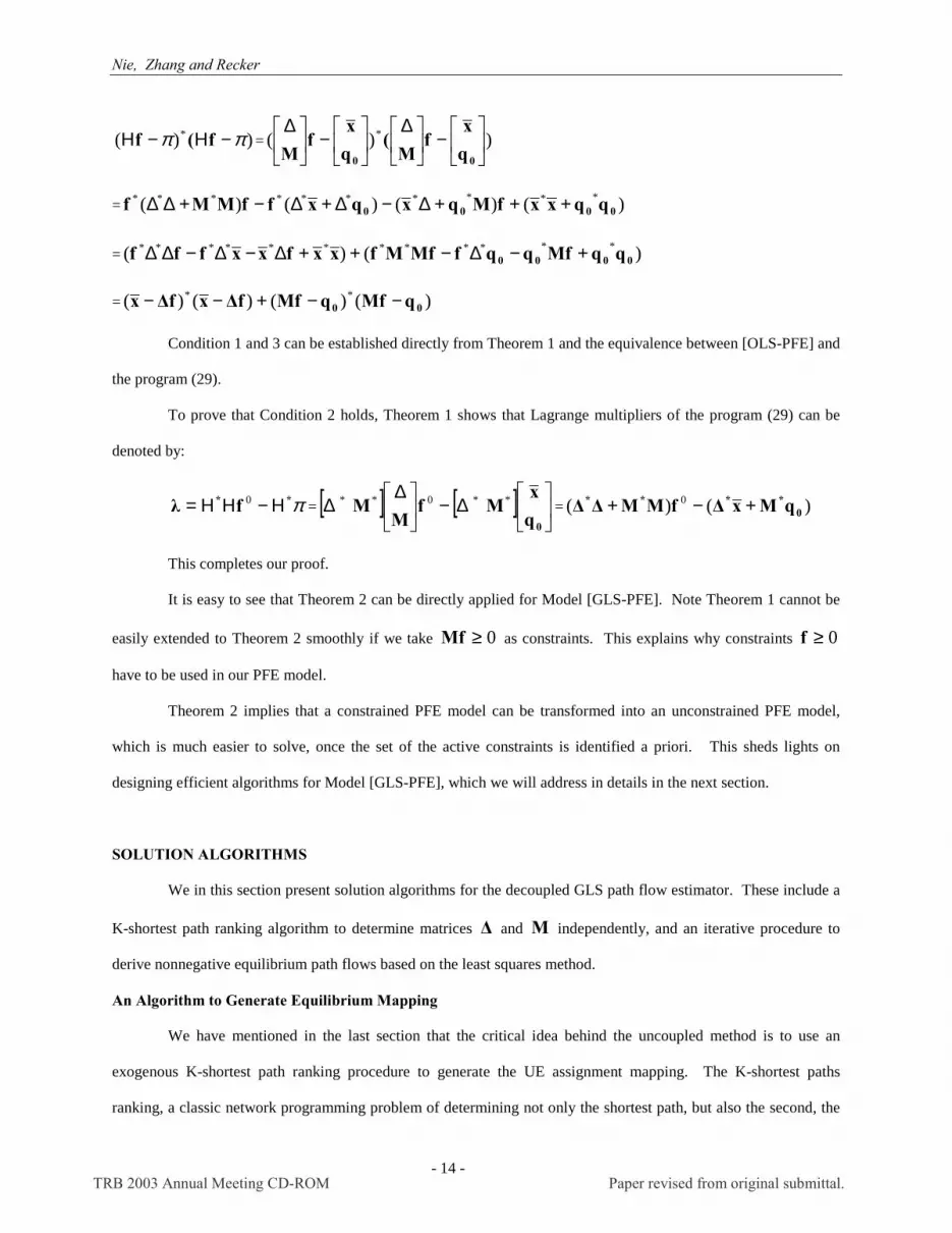
Condition 1 and 3 can be established directly from Theorem 1 and the equivalence between [OLS-PFE] and

the program (29).

To prove that Condition 2 holds, Theorem 1 shows that Lagrange multipliers of the program (29) can be

denoted by:

π** fλ Η−ΗΗ= 0 = [ ] [ ]

∆−

∆∆

0qx

MfM

M **0** = )()( 00

**** qMx∆fMM∆∆ +−+

This completes our proof.

It is easy to see that Theorem 2 can be directly applied for Model [GLS-PFE]. Note Theorem 1 cannot be

easily extended to Theorem 2 smoothly if we take 0≥Mf as constraints. This explains why constraints 0≥f

have to be used in our PFE model.

Theorem 2 implies that a constrained PFE model can be transformed into an unconstrained PFE model,

which is much easier to solve, once the set of the active constraints is identified a priori. This sheds lights on

designing efficient algorithms for Model [GLS-PFE], which we will address in details in the next section.

SOLUTION ALGORITHMS

We in this section present solution algorithms for the decoupled GLS path flow estimator. These include a

K-shortest path ranking algorithm to determine matrices ∆ and M independently, and an iterative procedure to

derive nonnegative equilibrium path flows based on the least squares method.

An Algorithm to Generate Equilibrium Mapping

We have mentioned in the last section that the critical idea behind the uncoupled method is to use an

exogenous K-shortest path ranking procedure to generate the UE assignment mapping. The K-shortest paths

ranking, a classic network programming problem of determining not only the shortest path, but also the second, the

TRB 2003 Annual Meeting CD-ROM Paper revised from original submittal.

Nie, Zhang and Recker

- 15 -

third,..., to the kth (for a given integer 1>k ) shortest path, was found [9] to be appropriate for recognizing paths

that reproduces the user-equilibrium flow pattern, so as to determine matrices ∆ and M in (20). The K-shortest

path ranking algorithm presented in [9] is based on Eppstein's approach [17], which picks shortest paths from a

graph representing all possible deviations from a standard shortest path tree. However, Eppstein's method was

originally designed for the unconstrained shortest path ranking and allows cycles of the repeated nodes in the

generated paths. Nie and Lee [9] incorporated a heuristics procedure into Eppstein’s algorithm, which guarantees

the generated paths to be cyclic-free and cost-identical. We in this paper focus on procedures of generating matrices

∆ and M . Reader may refer to [6, 9] for details of the K-shortest path ranking algorithm.

The complete algorithmic steps to obtain ∆ and M is summarized as follows:

Step0: Initialization. Set the current O-D pair k=0 and path number l=0.

Step1: Let k=k+1, if ok > , stop, the total number of paths m = l. r and s denotes the origin and

destination corresponding to O-D pair k.

Step2: Calculating the shortest path tree *rT rooted at r.

Step3: Build the pseudo path tree that contains all cost-identical (in terms of the tolerant error specified by

users) shortest paths.

Step4: Get paths and update matrices ∆ and M .

Step4.1: Using a backward tracking procedure to obtain a cyclic-free path rsp . If no path can be found,

go to Step1; otherwise Set l = l+1.

Step4.2: Set rspl =∆ )(:, and 1),( =lkM . Go to Step4.1.

Algorithms for Estimating Nonnegative Equilibrium Path Flows

Once equilibrium assignment maps, that is, matrices ∆ and M , are available, we can estimate the

corresponding path flows as well as O-D traffic demands by solving the constrained PFE model. Theorem 2 shows

that the optimal solution of this constrained GLS problem heavily depends on the set of active constraint. Since

specifying a priori these constraints is impossible, one has to apply iterative methods in which solving the

unconstrained GLS problem and identifying active constraint are carried out iteratively.

In the following, we first present an algorithm for solving the constrained PFE model based on Lawson and

Hanson’s iterative method for a standard NNLS problem:

TRB 2003 Annual Meeting CD-ROM Paper revised from original submittal.

Nie, Zhang and Recker

- 16 -

Algorithm for constrained PFE (ACPFE)

Step0: Initialization. Set φ=Ω , ,...,2,1 n=Φ and 0=f .

Step1: Compute the Lagrange multipliers λ according to (27). If φ=Φ or 0≥iλ for all Φ∈i , stop.

Step2: Move the index ,minarg Φ∈= kt kk λ from Φ to Ω .

Setp3: Set ∆ and M according to (28).

Step4: Compute bVf +=t using SVD decomposition (25), then set 0=tif if Φ∈i .

where MSM∆T∆V ** 11 −− += and 0** qSMxT∆b 11 −− += .

Step5: If 0>tif for all Ω∈i , set tff = and go to Step1; otherwise, go to Step6.

Step6: Set )( ffff −+= tα , where ,0:min Φ∈≤−

= ifff

f tit

ii

iα

Step7: Move all indices from Ω to Φ for which 0=if , go to Step3.

The convergence of ACPFE has been proven in [7]. However, the algorithm is not efficient enough even

for mid-size problems since the number of its major iteration, in which an unconstrained GLS problem has to be

solved, is bounded from below by the number of non-active constraints. Experience has shown that the number of

non-active constraints can be substantially large in a real-size estimation problem, which makes the computational

overhead of the algorithm prohibitively high. In order to overcome this computational difficulty, a heuristic

algorithm is designed to decrease the number of iterations in ACPFE while making the solution satisfy the

conditions given in Theorem 2. We describe this simplified ACPFE (SACPFE) as follows:

Step0: Initialization. Set φ=Φ , ,...,2,1 n=Ω and 0=f .

Step1: Set ∆ and M according to (28).

Step2: Compute bVf += using SVD decomposition (25).

Step3: If 0≥if for all ni ,...,2,1= , stop; otherwise, move all indices from Ω to Φ for which

0<if , go to Step1.

Note that this algorithm will terminate after a limited number of iterations. This is due to that all if

associated with active constraints will be actually set to zero compulsorily when ∆ and M is changed accordingly

TRB 2003 Annual Meeting CD-ROM Paper revised from original submittal.

Nie, Zhang and Recker

- 17 -

by (28), which means a constraint, if it is activated in some iteration, will never become inactive later. The

simplified ACPFE can dramatically decrease the number of iterations required by the original method, as our

numerical experiments would show later on. However, the algorithm may jeopardize the solution accuracy in

misestimating the set of active constraints. Intuitively, activating some constraints can cause other active constraint

to be inactive, which cannot be detected precisely by SACPFE. Nevertheless, it turns out that the simplified

algorithm can produce an approximate optimal path solution that is comparable to ACPFE in reproducing UE link

flow pattern and driving estimated O-D traffic matrix to approach a real ones. From a practical point of view, the

considerable gain in computational efficiency is well-worth the modest degradation in solution accuracy.

We will end this section by mentioning that the algorithms presented here demand all link counts being

available, which is definitely an unreasonable requirement in reality. This demand could be relaxed by either

applying flow conservation principle and prior information (as suggested by Sherali [11]), or introducing an outer

loop that consecutively updates link flows as well as link travel times according to estimated path flow pattern.

Options of these improvements will be investigated subsequently in a separate work.

NUMERICAL RESULTS

In this section, we give numerical results to demonstrate how algorithms presented in the last section work

using small- to mid-size examples. The cyclic-free Eppstein's K-shortest path ranking algorithm was implemented

on PC using VC++ 6.0 while the GLS path flow estimator algorithm was implemented on PC using MATLAB 6.0.

We choose C++ to implement K-shortest path ranking because MATLAB is not efficient enough for this type of

problem where a huge number of iterations are unavoidable.

In all simulation experiments, “observed” traffic counts are generated from a standard traffic assignment

procedure that allocates real O-D traffic demands onto a given network such that a UE flow pattern is produced. For

simplicity, we assume that the traffic counts generated from TAP subject to error whose covariance matrix IT = ,

where I is an identity matrix. Link travel time, based on which the K-shortest path ranking algorithm recasts the

equilibrium paths, is assumed to be only dependent on the traffic flow on that link, that is, link interactions are

ignored. In this paper, link travel time is computed from the standard BPR (Bureau of Public Road) function, which

takes the following form:

TRB 2003 Annual Meeting CD-ROM Paper revised from original submittal.

Nie, Zhang and Recker

- 18 -

))(15.01( 40 C

xtt += (30)

where t0 denotes the free flow travel time, C is the link capacity and x denotes the traffic volume/counts.

In order to obtain a target O-D demand matrix, an artificial deviation is applied upon the real O-D matrix

that is used for producing “observed” link counts. There are three types of target matrix being tested for each

example: an error-free (EF) target matrix that is exactly equivalent to the real matrix, a weak-prior-information

(WPI) matrix whose O-D entries take the same values of demands crossing the same origin (total demands from the

origin divided by its associated number of O-D pair), and a strong-prior-information (SPI) matrix whose all O-D

entries are changed in small proportions (less than 30%).

To specify the variance-covariance matrix of q, we introduce a weighting parameter γ that depicts the

relative belief in the traffic counts compared to the target matrix, following Brenninger-Gothe et al [4]. The

covariance matrix S is set as a diagonal matrix with principal diagonal elements equivalent to the inverse of γ . γ

can take values between 0 and 1, which means the target matrix is at most regarded as accurate as the observed link

counts, when the covariance matrix of target demands S=I. This is a reasonable assumption because the model will

make no improvement upon the target matrix from using link counts that are even inaccurate than the given target

itself. In our experiments, we use the following heuristic to calculate γ :

),1min( 20qq −

= oγ (31)

where 0q denotes the real O-D matrix.

Note Equation (31) cannot be applied for practical situations since it requires information of the “real” O-

D, which is very thing one sets up to estimate, and unavailable in reality.

Yang’s 9-node Network

The first test example, which contains 9 nodes, 14 links and 4 O-D pairs, is taken from Yang [18]. Figure 1

depicts the network topology and real O-D matrix. The “observed” link traffic counts as well as travel times, which

are produced by a UE traffic assignment subroutine, are reported in Table 1.

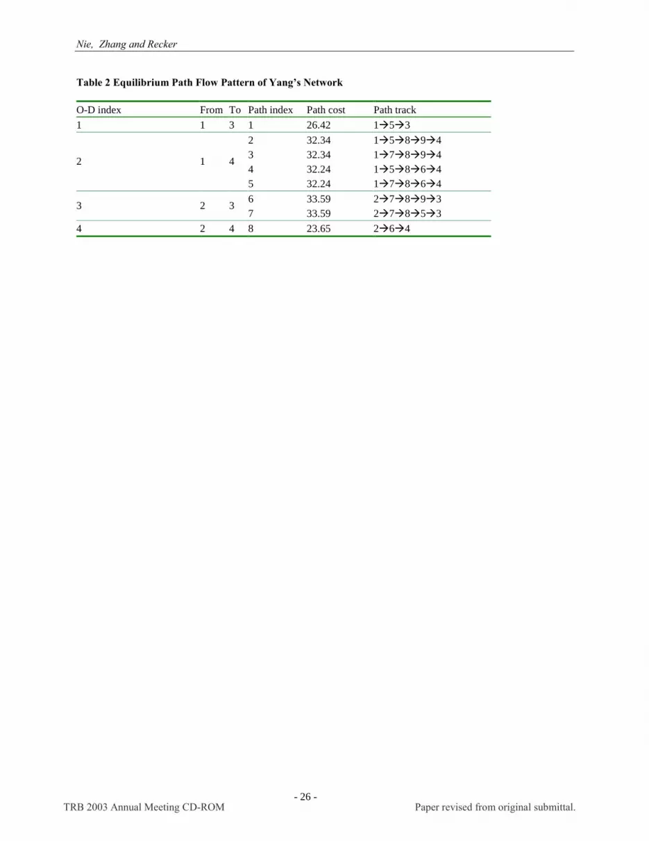
Eight equilibrium paths (see Table 2) are picked up from the K-shortest path ranking algorithm, with the

tolerant error of 0.001% (which means all cyclic-free paths whose costs is less than or equal to 1.00001 times of the

shortest path cost will be regarded as identical to the shortest one).

TRB 2003 Annual Meeting CD-ROM Paper revised from original submittal.

Nie, Zhang and Recker

- 19 -

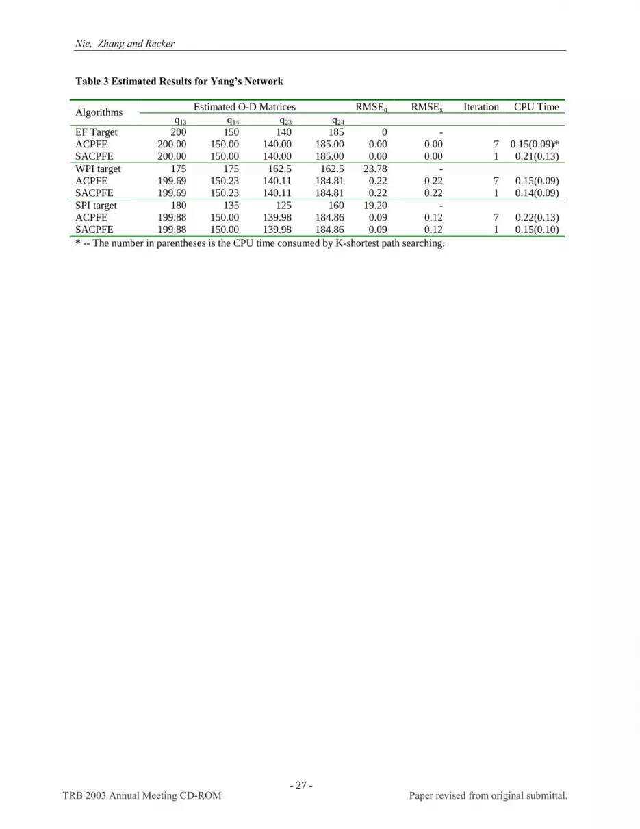
Three different target matrices, as described before, are adopted and given in Table 3. Table 3 also

provides the estimated O-D matrix, root means square error between the estimated and the real matrix (RMSEq), and

RMSE between the estimated link traffic flows and the observed link counts (RMSEx), based on algorithms ACPFE

and SACPFE for the three different targets. The equilibrium path solution as well as Lagrange multipliers is

reported in Table 4.

When an error-free (EF) target matrix is applied ( 1=γ ), both RMSEq and RMSEx are observed to be

nearly zero, which implies in this case the real O-D matrix is exactly obtained from our decoupled path flow

estimator while the user-equilibrium link flow pattern is reproduced perfectly. As shown in Table 3 and 4, the

algorithm ACPFE took seven iterations to identify the second constraint, whose associated Lagrange multipliers is 0,

as being active. On the other hand, SACPFE only consumed one iteration to terminate with a different path flow

pattern whose active constraint is the fourth one with the associated Lagrange multipliers of zero.

For weak-prior-information (WPI) target matrix, whose RMSE from the real matrix is about 23.78, the

relative belief parameter γ is calculated according to (30) as 002.078.23/1 2 ≈ . Both ACPFE and its simplified

version generated an estimation that is much closer to the real O-D matrix than the given target (RMSEq = 0.22),

indicating that the target matrix can be improved substantially by applying traffic counts. At the same time, the

observed link counts are regenerated precisely from estimation, with RMSEx of 0.22.

A similar observation was made when the strong-prior-information (SPI) target matrix was adopted:

RMSEq of the O-D matrix estimated (0.09) is much less than that of SPI target (19.20), while the user-equilibrium

flow pattern is reproduced with a satisfying accuracy (RMSEx=0.12).

We further highlight the following facts for algorithms ACPFE and SACPFE. Firstly, the two algorithms

generated nearly the same link flow pattern and the estimation of O-D matrix for three target matrices, even though

they came up with different path flow patterns. This is a positive indication that the SACPFE can offer satisfying

solutions for the proposed decoupled PFE model. Secondly, this example shows that ACPFE needs much more

iterations to converge than the proposed simplified method, a phenomenon coincident with theoretical expectations.

Because of the small size of the network, CPU time consumed by both algorithms seems to have no significant

difference in this example, as shown in Table 4. However, the computational merit of the simplified algorithm

would emerge when the network size becomes reasonably large. Moreover, more than half of the CPU time has

been spent on finding equilibrium paths and form matrices ∆ and M in both algorithms. One may thus doubt the

TRB 2003 Annual Meeting CD-ROM Paper revised from original submittal.

Nie, Zhang and Recker

- 20 -

overall efficiency of the presented model since the K-shortest path ranking seems to be a computationally expensive

module. However, as we will see later on, this is again due to the small size of the example. The proportion of CPU

time taken by K-shortest path ranking will drop steeply as network size increases.

A 100-Node Hypothetical Network

This example presents computational experiments with two algorithms using a larger network, which is

obtained from a random grid-network generator. A 10 by 10 hypothetical network is generated in such a way that its

nodes are arranged in a square planar grid with a grid arc (whose link performance function is also randomly

determined) connecting each pair of adjacent grid nodes in each direction. A node at a corner has two successors

while a node at an edge has three. All other nodes have four successors. Twelve nodes are chosen as zone centroid,

that is, a 12 by 11 matrix will be randomly produced to be the real O-D trip matrix.

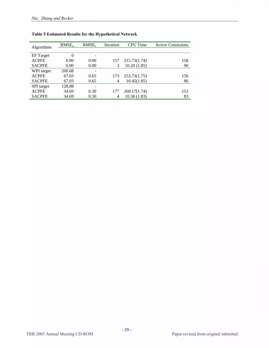
The K-shortest path ranking procedure found 312 paths contained in the UE flow pattern, given a tolerant

error of 0.01%. Estimated results for three target matrices are given in Table 5.

When an error-free O-D matrix is used as the target, the presented algorithms regenerate the observed link

counts precisely and obtain an estimation that is exactly equivalent to both target and real O-D matrices (RMSEq =

RMSEx= 0). Again, the optimal path solutions from the two algorithms are quite different. ACPFE recognized 158

active constraints when optimality is reached while the simplified algorithm got only 90. However, it seems that the

two distinctive path flow patterns produced quite similar link flows as well as the estimated O-D matrices, which

once again shows that the SACPFE maintains the accuracy of O-D estimates while dramatically improving the

computational performance of ACPFE.

Figures 2 and 3 visualize the WPI target and estimated O-D matrices for ACPFE and SACPFE

respectively. X axis of the plot represents the real O-D traffic demands while Y axis stands for the target demands

(denoted by crossing) or estimated demands (denoted by circle). It is obvious that a perfect estimation, that is,

estimated demands equals to real demands exactly, should follow a straight line with a slope of 1, which we refer to

as the perfect estimation line hereafter. An immediate observation from these two figures is that ACPFE and

SACPFE have produced nearly identical O-D matrix estimates. Furthermore, it can be seen that the estimated

demands from both algorithms have an apparent tendency to approach the perfect estimation line compared with the

target demands pattern. This can be also verified numerically by noting that RMSEq of the estimated matrix (67.03)

is much smaller than that of the WPI target (200.68).

TRB 2003 Annual Meeting CD-ROM Paper revised from original submittal.

Nie, Zhang and Recker

- 21 -

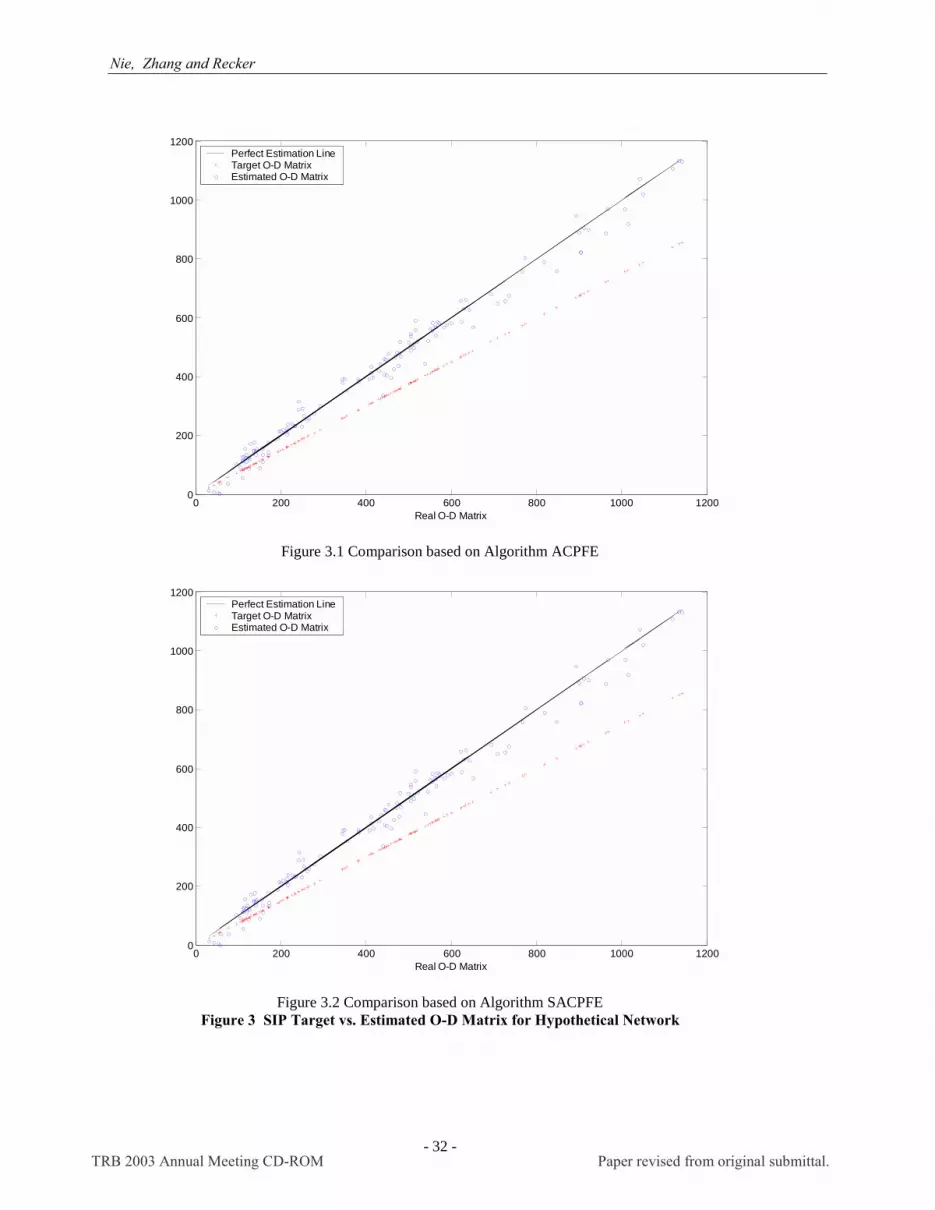
We obtained the SPI target matrix in this example by uniformly scaling down all real O-D demands for 25

percent. This produced a SPI target with RMSEq equivalent to 128.88. The estimated O-D matrices obtained from

ACPFE and SACPFE significantly reduced the RMSEq of SPI target to about 34.69. The improvement of estimated

O-D matrices upon the SPI target is shown in Figures 4 and 5, which explicitly demonstrate, how the proposed

algorithms drive the SPI target toward the perfect estimation line with link counts information.

In this example, the simplified method outperforms ACPFE significantly for three tested scenarios in terms

of the computational overhead. Taking the WPI target case as an example, SACPFE spent only 4 iterations and

10.45 seconds CPU time to converge while ACPFE took about 173 iterations and 253.73 seconds CPU time. Note

SACPFE cannot obtain as accurate optimal path solution as ACPFE does since it is likely to fail to recognize all

active constraints. However, estimates of SACPFE for O-D matrices and link counts turn out to be sufficiently

precise.

Moreover, CPU time consumed by K-shortest path ranking in this example becomes relatively trivial

compared with those spent in the estimation: it takes around 18% of total CPU time for SACPFE, and only 0.8% for

ACPFE, to find all equilibrium paths. Therefore, K-shortest path ranking will not become a computation bottleneck

for the overall decoupled GLS-based PFE model.

CONCLUSIONS

This paper combines the decoupled path flow estimator with the generalized least squares techniques for

equilibrium-based O-D trip matrix estimation. The presented formulation incorporates measurement errors of link

counts and target matrix naturally through the GLS structure, and maintains the major advantage of the decoupled

PFE model, that is, simplifying the work of determining the equilibrium assignment mapping by exogenously

identifying the optimal paths conforming to a user-equilibrium state.

The solution of the GLS-PFE model differs from previous GLS-based models in two aspects: the former

often requires the solution of a non-invertible linear system and imposes nonnegative constraints. The algorithm

ACPFE, which is developed based on Lawson and Hanson’s method, was presented to solve the GLS-PFE model.

The algorithm continuously solves the restricted GLS problem through singular value decomposition and determines

the set of active constraints. ACPFE suffers from slow convergence due to its one-at-a-time update strategy for the

TRB 2003 Annual Meeting CD-ROM Paper revised from original submittal.

Nie, Zhang and Recker

- 22 -

active constraint set. We thus simplified ACPFE by applying an all-at-a-time update strategy, which simply marks

all constraints that are violated in an estimation to be active.

Our limited numerical experiments lead to the following findings:

1. When solved by either ACPFE or its simplified version, GLS-PFE model can substantially

improve the given target O-D matrix (i.e., producing an estimate that is much closer to the real O-D matrix than

the target) after using link traffic counts, while producing a path flow pattern which concurs with a UE state.

2. SACPFE would generate optimal path solutions and active constraint sets that are quite different

from those of ACPFE. However, these different path solutions correspond to quite similar estimates for the O-

D matrix and link traffic counts. Given its computational advantage, it is recommended that SACPFE be

considered in solving the large-scale congested O-D matrix estimation problem.

3. The computational cost used for finding equilibrium paths is fairly modest when the problem size

is reasonably large.

One of the most important further work, as we mentioned earlier in this paper, is to relax the assumption

that all link traffic counts are available. It is also interesting to investigate the statistical characteristics of the GLS-

based path flow estimator when many constraints are activated, and to study the effects of the relative belief

parameter γ on estimation results.

REFERENCES

[1] Wardrop, J. G. Some Theoretical Aspects of Road Traffic Research. Proceedings of the Institute of Civil

Engineers, Part II, 1, 1952, pp. 325-378.

[2] Willumsen, L. G. Simplified Transport Models Based Traffic Counts. Transportation, Vol. 10, 1981, pp. 257-

278.

[3] Van Zuylen, J. H., and L. G. Willumsen. The Most Likely Trip Matrix Estimated from Traffic Counts.

Transportation Research, Vol. 14B, 1980, pp. 281-293.

[4] Cascetta, E. Estimation of Trip Matrices from Traffic Counts and Survey Data: a Generalized Least Squares

Estimator. Transportation Research, Vol. 18B, 1984, pp. 289-299.

[5] Bell, M. The Estimation of Origin-Destination Matrices by Constrained Generalized Least Squares.

Transportation Research, Vol. 25B, 1991, pp.13-22.

TRB 2003 Annual Meeting CD-ROM Paper revised from original submittal.

Nie, Zhang and Recker

- 23 -

[6] Brenninger-Göthe, M., K. O. Jörnsten, and J. T. Lundgren. Estimation of Origin-Destination Matrices from

Traffic Counts Using Multi-objective Programming Formulations. Transportation Research, Vol. 23B, 1989,

pp. 257-269.

[7] Lo, H. P., N. Zhang, and W. H. K. Lam. Estimation of an Origin-Destination Matrix with Random Link Choice

Proportions: a Statistical Approach. Transportation Research, Vol. 30B, 1996, pp. 309-324.

[8] Nguyen, S. Estimating an OD Matrix from Network Data: a Network Equilibrium Approach. University of

Montreal Publication, No. 60, 1977.

[9] Fisk, C. S., and D. E. Boyce. A Note on Trip Matrix Estimation from Link Traffic Count Data. Transportation

Research, Vol. 17B, 1983, pp. 245-250.

[10] Yang, H, T. Sasaki, Y. Iida, and Y. Asakura. Estimation of Origin-Destination Matrices from Link Traffic

Counts on Congested Networks. Transportation Research, Vol. 26B, 1992, pp. 417-434.

[11] Sherali, H. D., R. Sivanandan, and A. G. Hobeika. A Linear Programming Approach for Synthesizing Origin-

Destination Trip Tables from Link Traffic Volumes. Transportation Research, Vol. 28B, 1994, pp. 213-233.

[12] Bell, M. G. H., C. M. Shield, F. Busch, and K. Kruse. A Stochastic User Equilibrium Path Flow Estimator.

Transportation Research, Vol. 5C, 1997, pp. 197-210.

[13] Bell, M. G. H., and Y. Iida. Transportation Network Analysis. John Wiley & Sons, Inc., New York, 1997.

[14] Nie, Y. and Lee, D.-H. (2002). An Uncoupled Method for the Equilibrium-Based Linear Path Flow Estimator

for Origin-Destination Trip Matrices. Paper accepted for publication in transportation research record (TRR).

[15] Lawson, C. and Hanson R. Solving Least Squares Problems. Prentice-Hall, Englewood Cliffs, New Jersey,

1974.

[16] Trefethen, L. and Bau, D. Numerical Linear Algebra. SIAM, Philadelphia, 1997.

[17] Eppstein, D. Finding the K Shortest Paths. SIAM Journal of Computing, Vol. 28, No. 2, 1999, pp. 652-673.

[18] Yang, H. Heuristic Algorithms for the Bi-Level Origin-Destination Matrix Estimation Problem. Transportation

Research, Vol. 29B, 1995, pp. 231-242.

TRB 2003 Annual Meeting CD-ROM Paper revised from original submittal.

Nie, Zhang and Recker

- 24 -

LIST OF TABLES AND FIGURES TABLE 1 Input Data For Yang’s Network TABLE 2 Equilibrium Path Flow Pattern of Yang’s Network TABLE 3 Estimated Results for Yang’s Network TABLE 4 Equilibrium Path Solutions and Lagrange Multipliers for Yang’s Network TABLE 5 Estimated Results for the Hypothetical Network FIGURE 1 Topology and Real O-D Trip Matrix of Yang’s Network FIGURE 2 WIP Target vs. Estimated O-D Matrix for Hypothetical Network FIGURE 3 SIP Target vs. Estimated O-D Matrix for Hypothetical Network

TRB 2003 Annual Meeting CD-ROM Paper revised from original submittal.

Nie, Zhang and Recker

- 25 -

Table 1 Input Data For Yang’s Network Index From To Capacity “Observed” Travel Time “Observed” Traffic Counts

1 1 5 250 13.18 225.032 1 7 150 4.29 124.973 2 6 250 11.49 185.004 2 7 150 4.46 140.005 5 3 250 13.24 227.676 5 8 150 3.00 25.037 6 4 250 12.16 228.858 6 8 150 5.00 0.009 7 8 250 11.89 264.97

10 8 5 150 4.00 27.6711 8 6 150 4.00 43.8512 8 9 250 13.05 218.4813 9 3 150 4.19 112.3314 9 4 150 3.11 106.15

TRB 2003 Annual Meeting CD-ROM Paper revised from original submittal.

Nie, Zhang and Recker

- 26 -

Table 2 Equilibrium Path Flow Pattern of Yang’s Network O-D index From To Path index Path cost Path track 1 1 3 1 26.42 153

2 32.34 15894 3 32.34 17894 4 32.24 15864

2 1 4

5 32.24 17864 6 33.59 27893 3 2 3 7 33.59 27853

4 2 4 8 23.65 264

TRB 2003 Annual Meeting CD-ROM Paper revised from original submittal.

Nie, Zhang and Recker

- 27 -

Table 3 Estimated Results for Yang’s Network

Estimated O-D Matrices RMSEq RMSEx Iteration CPU Time Algorithms q13 q14 q23 q24

EF Target 200 150 140 185 0 - ACPFE 200.00 150.00 140.00 185.00 0.00 0.00 7 0.15(0.09)* SACPFE 200.00 150.00 140.00 185.00 0.00 0.00 1 0.21(0.13) WPI target 175 175 162.5 162.5 23.78 - ACPFE 199.69 150.23 140.11 184.81 0.22 0.22 7 0.15(0.09) SACPFE 199.69 150.23 140.11 184.81 0.22 0.22 1 0.14(0.09) SPI target 180 135 125 160 19.20 - ACPFE 199.88 150.00 139.98 184.86 0.09 0.12 7 0.22(0.13) SACPFE 199.88 150.00 139.98 184.86 0.09 0.12 1 0.15(0.10) * -- The number in parentheses is the CPU time consumed by K-shortest path searching.

TRB 2003 Annual Meeting CD-ROM Paper revised from original submittal.

Nie, Zhang and Recker

- 28 -

Table 4 Equilibrium Path Solutions and Lagrange Multipliers for Yang’s Network

EF Target WPI Target SPI Target ACPFE SACPFE ACPFE SACPFE ACPFE SACPFE

Path Index

Flow λ Flow λ Flow λ Flow λ Flow λ Flow λ 1 200.00 0.00 200.00 0.00 199.69 0.00 199.69 0.00 199.88 0.00 199.88 0.00 2 0.00 0.00 25.03 0.00 0.00 0.00 25.25 0.00 0.00 0.00 25.06 0.00 3 106.15 0.00 81.12 0.00 106.23 0.00 80.98 0.00 106.13 0.00 81.07 0.00 4 25.03 0.00 0.00 0.00 25.25 0.00 0.00 0.00 25.06 0.00 0.00 0.00 5 18.82 0.00 43.85 0.00 18.75 0.00 44.00 0.00 18.82 0.00 43.87 0.00 6 112.33 0.00 112.33 0.00 112.29 0.00 112.29 0.00 112.30 0.00 112.30 0.00 7 27.67 0.00 27.67 0.00 27.82 0.00 27.82 0.00 27.68 0.00 27.68 0.00 8 185.00 0.00 185.00 0.00 184.81 0.00 184.81 0.00 184.86 0.00 184.86 0.00

TRB 2003 Annual Meeting CD-ROM Paper revised from original submittal.

Nie, Zhang and Recker

- 29 -

Table 5 Estimated Results for the Hypothetical Network

RMSEq RMSEx Iteration CPU Time Active Constraints Algorithms

EF Target 0 - ACPFE 0.00 0.00 157 215.73(1.74) 158 SACPFE 0.00 0.00 3 10.20 (1.85) 90 WPI target 200.68 - ACPFE 67.03 0.65 173 253.73(1.75) 156 SACPFE 67.03 0.65 4 10.45(1.85) 86 SPI target 128.88 - ACPFE 34.69 0.30 177 260.17(1.74) 153 SACPFE 34.69 0.30 4 10.36 (1.83) 83

TRB 2003 Annual Meeting CD-ROM Paper revised from original submittal.

Nie, Zhang and Recker

- 30 -

1

7

2

5 3

8

6

9

4

3

1

2

4

5

6 7

8 9

10

11

12

13

14

Zone Centroid Real OD Trip Matrix:From To Demands1 3 2001 4 1502 3 1402 4 185

Figure 1 Topology and Real O-D Trip Matrix of Yang’s Network

TRB 2003 Annual Meeting CD-ROM Paper revised from original submittal.

Nie, Zhang and Recker

- 31 -

0 200 400 600 800 1000 12000

200

400

600

800

1000

1200

Real O-D Matrix

Perfect Estimation LineTarget O-D MatrixEstimated O-D Matrix

Figure 2-1 Comparison based on Algorithm ACPFE

0 200 400 600 800 1000 12000

200

400

600

800

1000

1200

Real O-D Matrix

Perfect Estimation LineTarget O-D MatrixEstimated O-D Matrix

Figure 2.2 Comparison based on Algorithm SACPFE

Figure 2 WIP Target vs. Estimated O-D Matrix for Hypothetical Network

TRB 2003 Annual Meeting CD-ROM Paper revised from original submittal.

Nie, Zhang and Recker

- 32 -

0 200 400 600 800 1000 12000

200

400

600

800

1000

1200

Real O-D Matrix

Perfect Estimation LineTarget O-D MatrixEstimated O-D Matrix

Figure 3.1 Comparison based on Algorithm ACPFE

0 200 400 600 800 1000 12000

200

400

600

800

1000

1200

Real O-D Matrix

Perfect Estimation LineTarget O-D MatrixEstimated O-D Matrix

Figure 3.2 Comparison based on Algorithm SACPFE

Figure 3 SIP Target vs. Estimated O-D Matrix for Hypothetical Network

TRB 2003 Annual Meeting CD-ROM Paper revised from original submittal.