modeling and forecasting the urban volume using stochastic differential equations

IEEE TRANSACTIONS ON INTELLIGENT TRANSPORTATION SYSTEMS, VOL. XX, NO. XX, XXXX 1

Abstract— Traffic flow prediction can be used for the

management of traffic control systems, and can be applied towards improving traffic light split times at intersections. In this article, we developed a methodology for the short-term prediction of traffic flow using the Stochastic Differential Equation (SDE). Since the current volume depends on the previous short term volume as well as time, we used the Hull-White Model. With the proposed method, a flexible short-term prediction of volume is suggested. It is possible to simulate traffic conditions easily and also detect incidents precisely. This method is applied in Tehran’s highways, and the obtained results are compared to the previous artworks. Our results offered a better fit to the traffic volume.

Index Terms— Ito integral, Hull-White Model, Stochastic

differential equation, Traffic flow.

I. INTRODUCTION

VER the last few decades, vehicular congestion has increased in many big cities. This has led to a growing

need for accurate predictions of the traffic-condition. The implementation of intelligent transportation systems using dynamic traffic management is a common method for reducing the congestion. The evolution of traffic conditions over time is an important tool for modeling and predicting congestion in a transport network. Short-term (time horizon of 15 minutes or less [1]) traffic forecasting can provide information to support short-range operational modifications, in order to improve the efficiency of the transport network.

Both short- and long-term volume predictions can be used in traffic management systems. For example, in flexible control systems that anticipate the rapid changes in demand, short-term predictions are useful; Long-term predictions are used in general management applications such as the

Manuscript received October 9, 2001. (Write the date on which you

submitted your paper for review.) This work was supported in part by the U.S. Department of Commerce under Grant BS123456 (sponsor and financial support acknowledgment goes here).

R. Tahmasbi is with Amirkabir University of Technology, Tehran, Iran. He is also a member of Intelligent Transportation Systems Research Institute (ITSRI) at Amirkabir University of Technology (phone: +982166406322; fax: +982166406322; e-mail: [email protected]).

S. M. Hashemi is with Amirkabir University of Technology, Tehran, Iran. He is also president of Intelligent Transportation Systems Research Institute (ITSRI) at Amirkabir University of Technology, Tehran, Iran (e-mail: [email protected]).

optimization of traffic signal plans. Several authors have used different approaches for

predicting traffic volumes. Extrapolation models are used for short-term predictions, e.g., [2], [3], [4], [5] and [6]. However, this method can only give accurate predictions for small prediction horizons. For horizons longer than 15 min, volume measurements can also be matched to historical patterns. For these predictions, neural networks, e.g., [7] and [3], or clustering methods, e.g., [8] were used.

Different methods have been used by researchers. The parametric and nonparametric empirical approaches employ a fairly standard statistical methodology, or use a heuristic method for forecasting traffic flow without referring to the actual traffic dynamics. The nonparametric techniques include nonparametric regressions [9], Kernel estimators [10], neural networks (e.g., [11], [12], [13], [14] and [15]), integrated neural networks (e.g. [16], [17], [18], [19], [20] and [21]), support vector machine [22], and bootstrap-based interval predictions [23]. The parametric techniques include different time-series models, such as linear and nonlinear regression, historical average algorithms, smoothing techniques (e.g., [11]), and autoregressive linear processes (e.g., [24] and [25]). Williams and Hoel [26], Smith et al. [1], and Ghosh et al. [27] used the Seasonal Autoregressive Integrated Moving Average (SARIMA) models, and obtained better results than the other autoregressive linear models.

Recently, the Generalized Autoregressive Conditional Heteroscedasticity (GARCH) methodology was used for short-term prediction of urban traffic variability. To provide forecasts of the traffic variability, Kamarianakis et al. [28] used a standard GARCH model. Guo [29] followed a similar GARCH approach for the prediction of the conditional variance of traffic flow. In 2006, Tsekeris and Stathopoulos [30] used the standard GARCH model and a long-memory extension of it, called the fractionally integrated asymmetric power autoregressive conditional heteroscedasticity model, for the out-of-sample forecasting of traffic variability in the same network. Recently, Chen et al. [31] used an ARIMA-GARCH Model to forecast short term traffic flow.

Since the real-time variability of high-frequency time series data (such as traffic data) is truly complex and cannot be modeled properly via some parametric models like GARCH or ARIMA, some authors have used other types of volatility modes. Tsekeris and Stathopoulos [32] employed the stochastic volatility model. They described the traffic variability in terms of volatility metric, by assuming that the

Modeling and Forecasting the Urban Volume Using Stochastic Differential Equations

Rasool Tahmasbi, Student Member, IEEE, and S. Mehdi Hashemi

O


conditional variance of traffic flow is a latent stochastic low-order Markov process.

In addition to the methods mentioned above, the Kalman filter [33] and [34], dynamic traffic assignment [35], state-space [36], and chaos theory methods [37] are also incorporated in modeling the short-term prediction of traffic flow.

In this paper, we developed a pattern for the short-term prediction of traffic flow using Stochastic Differential Equations (SDEs). The formal definition of SDEs is presented in Section II. The biggest challenge in working with SDEs is to estimate the parameters of the model. In Subsection B, we estimate the parameters of a well-known class of SDEs known as Hull-White model, theoretically. To use these theories in modeling the traffic flow, we should first estimate the mean and variance of a set of traffic data over time. In order to achieve a smooth and continuous function of mean and variance, we will employ a quadratic spline curve. Spline functions are defined in Subsection C. SDE parameters are estimated using smooth and continuous estimations of mean and variance.

Applications of the proposed method are described in Section III. The data used in this study is obtained from the municipality of Tehran, one of the biggest cities in world. The extraordinary characteristics of this city are described in Subsection A. The traffic volume data is obtained from one of the speed control cameras, which is discussed in more details in Subsection B. As previously mentioned, the Hull-White model is used for modeling the traffic flow. The reasons for selecting this model are presented in Subsection C. This subsection also illustrates the application and use of the

theories in modeling traffic flow. Two other applications of the proposed method in simulating traffic flow and automatic incident detection are demonstrated in Subsections D and E, respectively. Subsection F completes the parameter estimation of the Hull-White model, and Subsection G compares the results of the proposed method with recent methods. And finally in Section IV, we summarized the obtained results.

II. THEORETICAL BACKGROUND

A. Stochastic Differential Equations The analysis of complex systems by nonlinear deterministic

differential equations has attracted much attention in recent years. Given a parameterized differential equation, best-fit parameters can be obtained by a least squares minimization, see e.g. [38].

However, the dynamics does not follow a strict deterministic law. SDEs are an intelligent choice to model the time evolution of dynamic systems, which are subject to random changes. Before defining the SDEs, we will explain the Weiner process which is a critical term in SDEs.

The Wiener process is a continuous-time stochastic process and is often called the standard Brownian motion. This process is used to represent the integral of a Gaussian white noise process.

The Wiener process tW is characterized by three properties

[39]: - The initial position of the process starts from zero, i.e.,

00,W =

- The function t

t W→ is almost surely continuous

Fig. 1. Map of Tehran’s highways. Cameras installed in highways and center. The green dots are center cameras and the blue triangles are speed control cameras.The camera witch is marked by star is used in this study.


everywhere, -

tW has independent increments with

(0, );t sW W N t s− −∼ 0 .s t≤ <

2( , )N μ σ denotes the normal distribution with expected

value μ and variance 2σ . Having independent increments

means that if 1 1 2 2

0 s t s t≤ < ≤ < then 1 1t s

W W− and

2 2t sW W− are independent random variables. For a Weiner

process, the unconditional probability density function at a fixed time t is

2/21( ) .

2t

x tWf x e

tπ−=

Therefore, with simple computations one can verify that( )t

E W , var( )tW t= and cov( , ) min( , )

s tW W s t= .

A parametric Ito stochastic differential equation is defined by:

0( , , ) ( , ) , 0, ,

t t t tdX t X dt t X dW t Xμ θ σ ζ= + ≥ = (1)

where { , 0}tW t ≥ is a standard Wiener process. The

functions : [0,T]μ Θ× × → and : [0,T]σ +× → are called the drift and diffusion coefficients, respectively. These functions are known functions except for the unknown parameter θ ∈ Θ . Note that ζ is a random start variable with

2( )E ζ < ∞ , T is the time horizon and Θ ∈ is a subinterval of real line . Under local Lipschitz and the linear growth conditions on the coefficients μ and σ , a unique strong solution of the above Ito SDE, called the diffusion process exists, which is a continuous strong Markov semi-martingale. The drift and the diffusion coefficients are the instantaneous mean and standard deviation of the process, respectively. To study the properties of Ito integrals, see [40].

B. Hull-White Model In this subsection, we review some properties of the Hull-

White Model [41]. The Hull-White model is popular choice in modeling financial time processes. As an extension of the Vasicek Model, Hull-White assumes that the short rate follows the mean-reverting SDE:

( ( ) ) ( ) , 0.t t t

dX t X dt t dW tμ θ σ= − + ≥ (2)

The solution of the above SDE can be found by employing the Ito’s lemma [40] to find the dynamics of t

te Xθ and then

integrating up. This leads to ( ) ( )

0 0 0( ) ( ) .

t tt t s t s

t sX e X e s ds e s dWθ θ θμ σ− − − − −= + +∫ ∫ (3)

Theorem 1: The function ( )tμ in the drift coefficient of a Hull-White model can be estimated by

ˆ( ) ( ) ( ).t t

t E X E Xt

μ θ∂

= +∂

Proof: Taking expectation from both sides of (3), we have

( )0 0

( ) ( ) ( ) ,t

t t st

E X e E X e s dsθ θ μ− − −= + ∫ (4)

where 0

( ) 0t

sE f s dW⎛ ⎞⎟⎜ =⎟⎜ ⎟⎜⎝ ⎠∫ , for every measurable function f .

In order to estimate function ( )tμ , we use Leibniz’s rule for differentiating integrals, as follows:

( )0 0

( ) ( ) ( )

( ) ( ),

tt t s

t

t

E X e X t e s dst

t E X

θ θθ μ θ μ

μ θ

− − −∂= − + −

∂= −

∫ (5)

or

ˆ( ) ( ) ( ).t t

t E X E Xt

μ θ∂

= +∂

(6)

Theorem 2: the diffusion coefficient of a Hull-White model

can be estimated by 2ˆ ( ) var( ) 2 var( ).t t

t X Xt

σ θ∂

= +∂

Proof: To obtain the variance of tX , since

( )

0( ) 0

tt s

sE e s dWθ σ− −⎛ ⎞⎟⎜ =⎟⎜ ⎟⎜⎝ ⎠∫ , we have

2( )

0var( ) ( ) .

tt s

t sX E e s dWθ σ− −⎛ ⎞⎟⎜= ⎟⎜ ⎟⎜⎝ ⎠∫ (7)

Using the Ito isometry [40], we lead to 2 ( ) 2

0var( ) ( ) .

tt s

tX e s dsθ σ− −= ∫ (8)

Using Leibniz’s rule for differentiating integrals, we obtain

2 2 ( ) 2

02

var( ) ( ) 2 ( )

( ) 2 var( ),

tt s

t

t

X t e s dst

t X

θσ θ σ

σ θ

− −∂= −

∂= −

∫ (9)

or 2ˆ ( ) var( ) 2 var( ).

t tt X X

tσ θ

∂= +

∂ (10)

In Section III, we will use a smooth version of (6) and (10) for modeling the volume data. We smooth these estimated functions via the spline, which is defined in the following subsection.

C. Spline The spline is useful for modeling arbitrary functions.

Splines belong to nonparametric methods. They are based on global approximation and are an extension of polynomial regression techniques. In interpolating problems, splines are often used because they yield good results even with low-degree polynomials.

We know that a polynomial of degree (order) n is a function defined by : [ , ]P a b → and has the general form:

20 1 2

( ) ,nn

P x a a x a x a x= + + + +

where , 0ia i n≤ ≤ are some real coefficients.

Clearly, an ordinary polynomial function, possessing all derivatives at all locations, is not very flexible for approximating various functions with different degrees of smoothness at different locations. In order to enhance the flexibility of the approximations, it is possible to allow the


derivatives of the approximating functions to have discontinuities at certain locations. This results in piecewise polynomials called splines [42]. The locations where the derivatives of the approximating functions may have discontinuities are called knots.

The spline is a piecewise polynomial function that can have a very simple local form, yet at the same time be globally flexible and smooth. Mathematically, a spline is a piecewise-polynomial real function : [ , ]S a b → on an interval [ , ]a b

composed of k ordered disjoint subintervals 1

[ , )i it t−

with

0 1 1... .

k ka t t t t b−= < < < < =

The restriction of S to an interval i is a polynomial function

1: [ , ) ,

i i iP t t− → such that

1 0 1

2 1 2

1

( ), ,

( ), ,( )

( ), .k k k

P t t t t

P t t t tS t

P t t t t−

⎧⎪ ≤ <⎪⎪⎪ ≤ <⎪⎪= ⎨⎪⎪⎪⎪ ≤ <⎪⎪⎩

(11)

The highest order of the polynomials ( )iP t is said to be the

order of the spline S . If all subintervals are of the same length, the spline is said to be uniform, otherwise it is non-uniform.

We are now in a position to use splines to smoothly approximate a function f (we will discuss more about this function in Section III [C]). If we assume that the knot positions are fixed, then the unknown coefficients can be estimated simply using a least square method for each polynomial ( )

iP t (see Chapter 6 of [42]).

Since the position of knots has a great impact on the achievable accuracy of spline approximation, finding their

best position is also important. To find the optimal knot position, we followed the method mentioned in [43], i.e., we first use a least square approximation to find some basic intervals, and then the new knot position is chosen to subdivide the basic interval of the piecewise-polynomial f in such a way that the integral

( 1)( ) 1/

( )| ( ) | ; 1,..., 1

newkont ir r

newkont if t dt i l

+= −∫ (12)

becomes constant, where r is the order of spline, ( )rf is the rth derivation of f , and l is the total number of new knots.

An equivalent form of (12) is ( 1)

( ) 1/ ( ) 1/

( )

1| ( ) | | ( ) | ; 1,..., 1.

newkont ib

r r r r

anewkont i

f t dt f t dt i ll

+

= = −∫ ∫

This later problem is easy to solve if we replace the function ( )rf by some piecewise constant approximation ( )| |rh f∼ .

For getting more information about the theory of this method, one can see chapter XII of [43]. Another alternative method is also illustrated in chapter 6 of [42].

In the following section, we predict the traffic volume using the models mentioned above.

III. APPLICATIONS OF THE PROPOSED METHOD We studied the urban network of Tehran, the capital city of

Iran, which is one of the 10 largest cities in the world. Because of the concentration of over 12 million residents in a city without a large effective public transportation network, automobiles have easily become the leading cause of urban traffic.

A. About Tehran Air pollution and heavy traffic jams have increased fuel

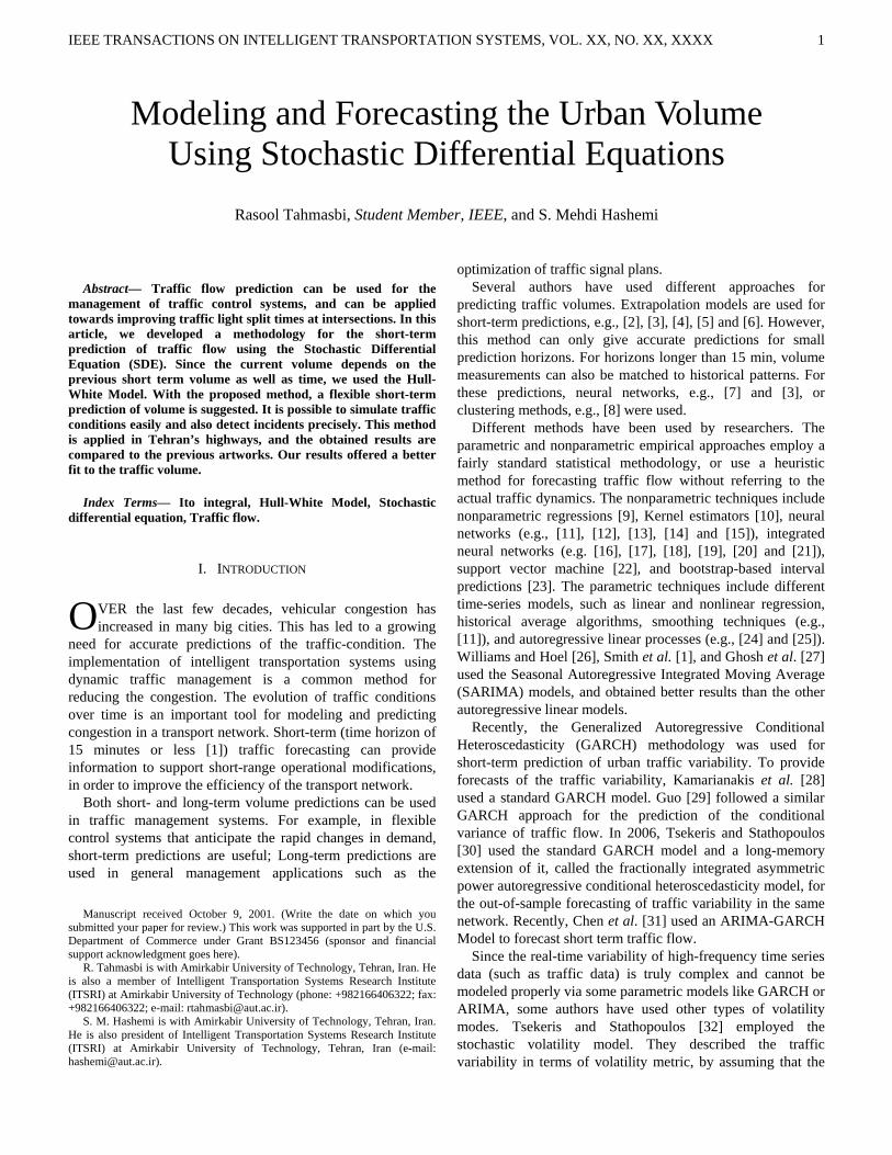
Fig. 2. Number of cars divided into three categories: holidays (Red), Thursdays (Green) and weekdays (Blue). The black lines are the means of each category.


consumption, and led to the depreciation of roads, vehicles, and facilities. Spending several hours in dense traffic coupled with insufficient parking spaces, has disrupted the citizens' comfort. These are among several reasons which have contributed to the decision of establishing traffic restrictions in downtown Tehran.

Most of Tehran’s highways are jammed in the mornings and evenings. The lack of any ramp metering, lane management, incident detection, Advanced Traveler Information System (ATIS), High Occupancy Vehicle (HOV), and other management systems has further complicated the issue.

The metropolis of Tehran has a huge network of highways (280 km) and interchanging ramps and loops (180 km). In 2007 there were 130 kilometers of highways and 120 kilometers of ramps and loops under construction. The city

has a wide line of buses, and has established Bus Rapid Transit (BRT) lines as of 2007, stretching across the city from the east side to the west. There are many private taxis and taxi agencies in Tehran. In 2001, the first two of seven projected metro lines were opened in the city’s metro system which had been dormant since the 1970’s. Work has been slow and coverage remains very limited. The development of Tehran’s metro system was interrupted by the Islamic Revolution and the Iran-Iraq War. Problems arising from the late completion of the metro led to buses taking the role of the metro lines, serving mainly long distance routes. Taxis filled the void for local journeys. The taxis only drive on main avenues, and only within the local area, so it may be necessary to take several taxis to get to one's final destination. All of these factors have led to extreme congestion and air pollution within the city. More than 3.5 million cars commute in Tehran, which is four times more than its road capacity.

In Tehran, research on various solutions and technologies for the downtown traffic congestion problem began in 2006. The major concern in the research development phase was to find a comprehensive solution, which was feasible based on the traffic situation and driving behavior in Iran, keeping the technical and economic limitations in mind. After conducting many field tests and studies, and collecting a large amount of documentations, finally Tehran Traffic Control Company (TTCC), as the leading ITS specialized company in Iran and the major technical body of the Municipality of Tehran, enforced Traffic Restricted Zones (TRZ) around the central business district.

In recent years, the Municipality of Tehran has received several global awards for its efforts in trying to solve the city’s traffic problems. One of these awards was GLOBELICS, Global Network for Economics of Learning, Innovation, and Competence Building Systems. Tehran received this award in innovation and commercialization at the 9th annual conference held in Buenos Aires, Argentina in 2011. The 10th Congress of Metropolis has rewarded Tehran for being one of the top 10 cities in the world which has improved the living standards of its citizens, particularly in the area of public transportation. In 2010, the award of Sustainable Transportation was given to the Municipality of Tehran as one of the top five cities in sustainable transportation. The award was granted at the Transportation Research Board meeting in Washington, DC, USA.

B. Data Apart from the loop detectors, there are two kinds of

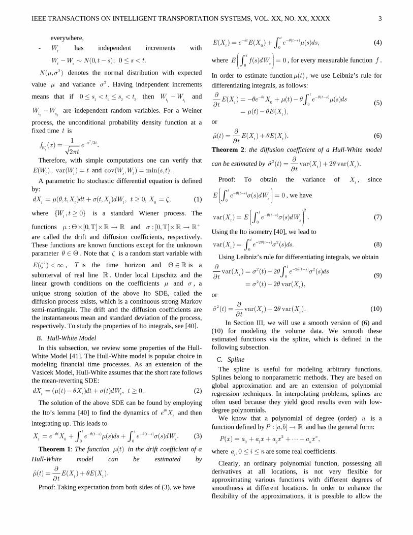
cameras used to gather different traffic data in Tehran. The first camera monitors traffic continuously in most city roads. There are 434 cameras shown in Fig. 1, with green dots. Most of these cameras are controlled manually. The second camera records the speed and counts the number of cars, continuously. These laser cameras are installed in most highways. There are 79 cameras of this type shown in Fig. 1 with a blue triangle. The data for this study was obtained from one of the second type of these cameras, marked with a black star.

To use the data for this study, the volume measurements

Fig. 3. Mean and standard deviation of traffic data, spline estimation of mean and std.

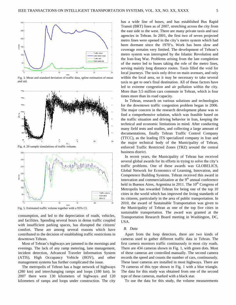
Fig. 4. 20 sample simulations of traffic volume.

Fig. 5. Estimated traffic volume together with a 95% CI.


were studied, and invalid data were rejected. Invalid data results from errors in the measurements (e.g., failures in the electronic systems). These errors were detected manually. The data from the last four days of the calendar year was also removed.

With a primary investigation, we found that the number of cars in a week can be divided into three homogeneous categories: 1) Weekends (Fridays) and (un)official public holidays, 2) Thursdays and, 3) Weekdays (Saturday-Wednesday). Fig. 2 approves the accuracy of these categories. These categories differ in mornings between 5 and 11 o’clock and are almost identical during other daylight hours.

In order to predict the volume, we examined several time intervals; Time intervals of 30 min are too long to follow sharp changes in demand during the rush hours. The strength of the volume fluctuations also depends on the average number of traffic signal cycles per time interval. If this number is low, the relative variation in the total green time per time interval will increase, which may lead to a significant variation in volumes when traffic loads are high. To reduce

this effect, we decided to aggregate our measurements to 10-min rather than 5-min time intervals. As a result, information may have been lost. However, in regular situations, volumes generally do not change so dramatically to impose a problem for our predictions.

C. Modeling the Volume As expected and also shown in Fig. 2, the fundamental fact

about volume is its dependence on time. It is also clear that the traffic condition at a link is affected by the immediate past traffic conditions and some of its neighboring links. In the mornings around 6 o’clock, most people go to work and return home near 6 o’clock in the evening. The number of cars decreases after midnight and in the early morning. The variance in data is also different at peak and off-peak times. These facts suggest modeling the traffic volumes via the following SDE (known as Ho-Lee model)

( ) ( ) , 0,t t

dX t dt t dW tμ σ= + ≥ (13)

where ( )tμ and ( )tσ are the mean and standard deviation of the volume, respectively. In the above model the changes in the volume over a short time interval depend on the function

( )tμ and a stochastic term. Since the traffic condition also depends on the previous volume, thus incorporating a ratio of the volume is useful. So we modeled the data using the Hull-White Model:

( ( ) ) ( ) , 0.t t t

dX t X dt t dW tμ θ σ= − + ≥ (14)

Fitting the data to this model requires for the functions ( )tμ and ( )tσ to be known. To estimate these functions we performed the following steps.

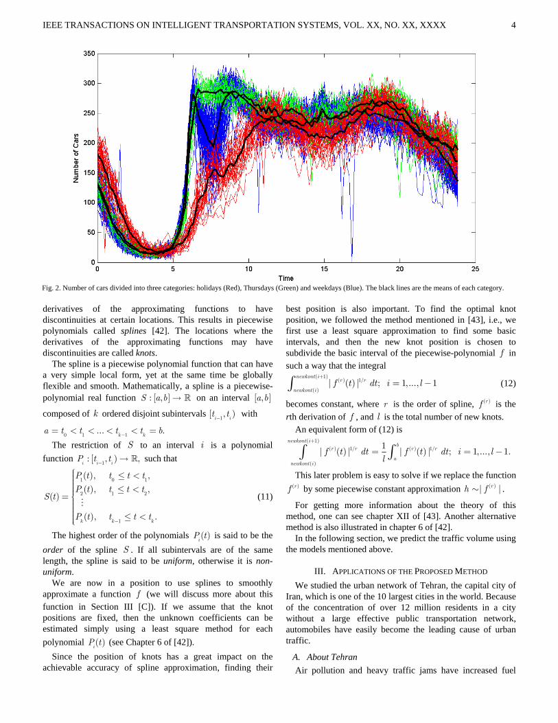
We modeled each of the three daily categories separately. The same processes can be determined for the other two categories. For example, the model for the weekdays is illustrated in Fig. 3. For the weekdays we first computed the sample mean of the data, denoted by ˆ( )

tE X . Clearly ˆ( )

tE X

is obtained in some sample time (e.g., every 10 minutes). In order to obtain a smooth continuous estimation of ˆ( )

tE X , we

estimate it via a quadratic non-uniform spline curve, denoted by ˆ ( )

S tE X . Finally, using equation (6) for estimating the

function ( )tμ , we employ the following equation

ˆ ˆˆ( ) ( ) ( ).S t S t

t E X E Xt

μ θ∂

= +∂

(15)

This process is also done for estimating the function ( )tσ , i.e.,

2ˆ ˆ ˆ( ) var ( ) 2 var ( ),S t S t

t X Xt

σ θ∂

= +∂

(16)

where ˆvar ( )S tX is a quadratic spline curve estimation of

sample variance.

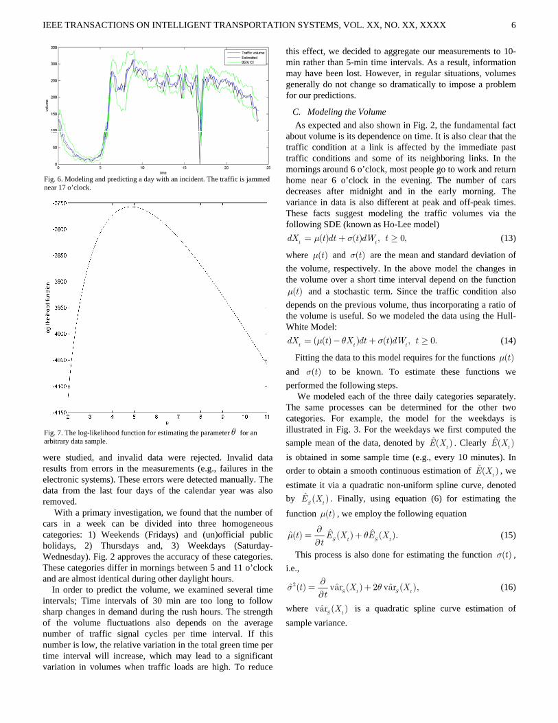
Fig. 6. Modeling and predicting a day with an incident. The traffic is jammed near 17 o’clock.

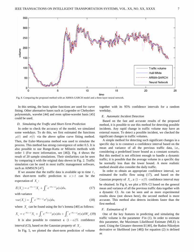
Fig. 7. The log-likelihood function for estimating the parameterθ for an arbitrary data sample.


In this setting, the basis spline functions are used for curve fitting. Other alternative bases such as Legendre or Chebyshev polynomials, wavelet [44] and even spline-wavelet basis [45] could be used.

D. Simulating the Traffic and Short-Term Prediction In order to check the accuracy of the model, we simulated

some weekdays. To do this, we first estimated the functions ( )tμ and ( )tσ via the above spline curve fitting method.

Then, the Euler-Maruyama method was used to simulate the process. This method has strong convergence of order 0.5. It is also possible to use Runge-Kutta or Milstein methods with order 1 (For more information, see [46]). Fig. 4 shows the result of 20 sample simulations. Their similarities can be seen by comparing it with the original data shown in Fig. 2. Traffic simulation can be used in most traffic management software, such as AIMSUN [47].

If we assume that the traffic data is available up to time t , then short-term traffic prediction to s t> can be the expectation of

sX :

( ) ( )( ) ( ) ,s

s t s us t t

E X e X e u duθ θ μ− − − −= + ∫ (17)

with variance 2 ( ) 2var( ) ( ) ,

ss u

s tX e u duθ σ− −= ∫ (18)

where sX can be found using the Ito’s lemma [40] as follows:

( ) ( ) ( )( ) ( ) .s s

s t s u s us t ut tX e X e u du e u dWθ θ θμ σ− − − − − −= + +∫ ∫ (19)

It is also possible to construct a (1 )%α− confidence

interval (CI), based on the Gaussian property of .sX

In Fig. 5, we plotted the short-term prediction of volume

together with its 95% confidence intervals for a random weekday.

E. Automatic Incident Detection Based on the fast and accurate results of the proposed

method, it is possible to use this method for detecting possible incidents. Any rapid change in traffic volume may have an external reason. To detect a possible incident, we checked the significant changes in traffic volumes.

A simple method for detecting such significant changes in a specific day is to construct a confidence interval based on the mean and variance of all the previous traffic data, i.e., considering a predefined lower bound as a constant scenario. But this method is not efficient enough to handle a dynamic traffic; it is possible that the average volume in a specific day be normally less than the lower bound. A more realistic method should also consider the daily traffic.

In order to obtain an appropriate confidence interval, we estimated the traffic flow using (17), and based on the Gaussian property of

tX , a (1 )%α− confidence interval may

be obtained. In Fig 6, we plot a 95% CI based on the general mean and variance of all the previous traffic data together with a dynamic CI. As can be seen and as more experimental results show (not shown here), the second method is more accurate. This method also detects incidents faster than the first method.

F. Estimation of θ One of the key features in predicting and simulating the

traffic volume is the parameter θ in (1). In order to estimate this parameter, the Maximum Likelihood Estimate (MLE) is used. Using the Girsanov theorem II [40], the Radon-Nikodym derivative or likelihood (see [48]) for equation (2) is defined as

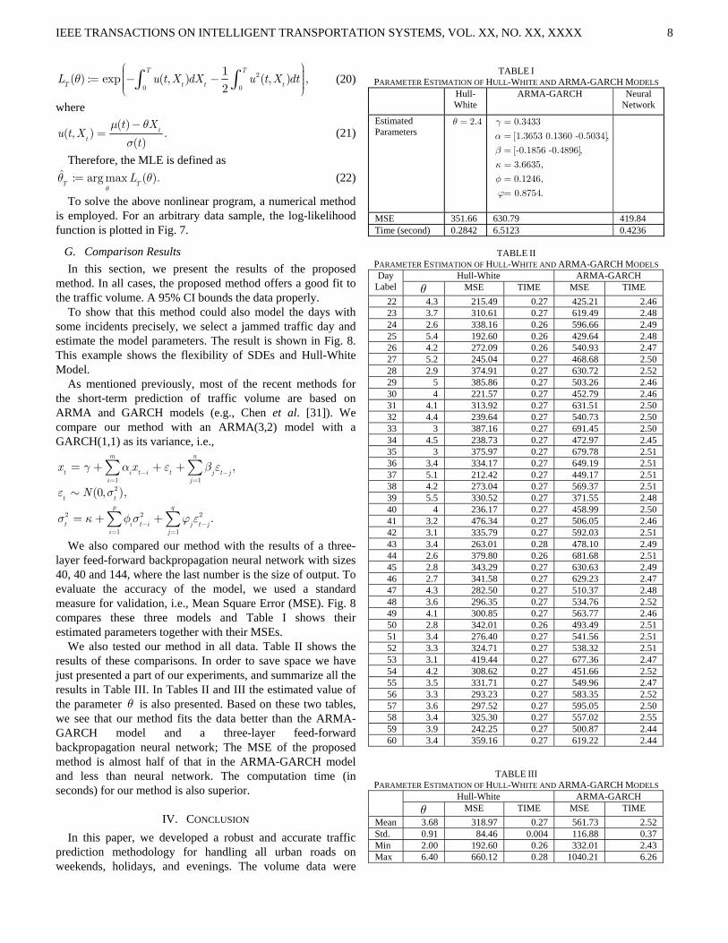
Fig. 8. Comparing the proposed method with an ARMA-GARCH model and a three-layer neural network.


2

0 0

1( ) : exp ( , ) ( , ) ,

2

T T

T t t tL u t X dX u t X dtθ

⎛ ⎞⎟⎜ ⎟= − −⎜ ⎟⎜ ⎟⎜⎝ ⎠∫ ∫ (20)

where ( )

( , ) .( )

tt

t Xu t X

t

μ θ

σ

−= (21)

Therefore, the MLE is defined as ˆ : argmax ( ).T T

Lθ

θ θ= (22)

To solve the above nonlinear program, a numerical method is employed. For an arbitrary data sample, the log-likelihood function is plotted in Fig. 7.

G. Comparison Results In this section, we present the results of the proposed

method. In all cases, the proposed method offers a good fit to the traffic volume. A 95% CI bounds the data properly.

To show that this method could also model the days with some incidents precisely, we select a jammed traffic day and estimate the model parameters. The result is shown in Fig. 8. This example shows the flexibility of SDEs and Hull-White Model.

As mentioned previously, most of the recent methods for the short-term prediction of traffic volume are based on ARMA and GARCH models (e.g., Chen et al. [31]). We compare our method with an ARMA(3,2) model with a GARCH(1,1) as its variance, i.e.,

1 12

2 2 2

1 1

,

(0, ),

.

m n

t i t i t j t ji j

t tp q

t i t i j t ji j

x x

N

γ α ε β ε

ε σ

σ κ φ σ ϕ ε

− −= =

− −= =

= + + +

= + +

∑ ∑

∑ ∑

∼

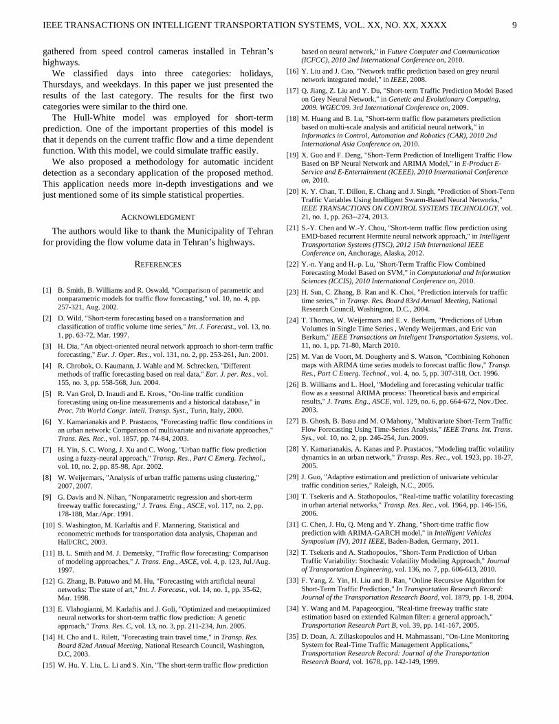
We also compared our method with the results of a three-layer feed-forward backpropagation neural network with sizes 40, 40 and 144, where the last number is the size of output. To evaluate the accuracy of the model, we used a standard measure for validation, i.e., Mean Square Error (MSE). Fig. 8 compares these three models and Table I shows their estimated parameters together with their MSEs.

We also tested our method in all data. Table II shows the results of these comparisons. In order to save space we have just presented a part of our experiments, and summarize all the results in Table III. In Tables II and III the estimated value of the parameter θ is also presented. Based on these two tables, we see that our method fits the data better than the ARMA-GARCH model and a three-layer feed-forward backpropagation neural network; The MSE of the proposed method is almost half of that in the ARMA-GARCH model and less than neural network. The computation time (in seconds) for our method is also superior.

IV. CONCLUSION In this paper, we developed a robust and accurate traffic

prediction methodology for handling all urban roads on weekends, holidays, and evenings. The volume data were

TABLE I PARAMETER ESTIMATION OF HULL-WHITE AND ARMA-GARCH MODELS

Hull-White

ARMA-GARCH Neural Network

Estimated Parameters

2.4θ =

0.3433

[1.3653 0.1360 -0.5034],

[-0.1856 -0.4896],

3.6635,

0.1246,

= 0.8754.

γαβκφϕ

=====

MSE 351.66 630.79 419.84 Time (second) 0.2842 6.5123 0.4236

TABLE II

PARAMETER ESTIMATION OF HULL-WHITE AND ARMA-GARCH MODELS Day

Label Hull-White ARMA-GARCH

θ MSE TIME MSE TIME 22 4.3 215.49 0.27 425.21 2.46 23 3.7 310.61 0.27 619.49 2.48 24 2.6 338.16 0.26 596.66 2.49 25 5.4 192.60 0.26 429.64 2.48 26 4.2 272.09 0.26 540.93 2.47 27 5.2 245.04 0.27 468.68 2.50 28 2.9 374.91 0.27 630.72 2.52 29 5 385.86 0.27 503.26 2.46 30 4 221.57 0.27 452.79 2.46 31 4.1 313.92 0.27 631.51 2.50 32 4.4 239.64 0.27 540.73 2.50 33 3 387.16 0.27 691.45 2.50 34 4.5 238.73 0.27 472.97 2.45 35 3 375.97 0.27 679.78 2.51 36 3.4 334.17 0.27 649.19 2.51 37 5.1 212.42 0.27 449.17 2.51 38 4.2 273.04 0.27 569.37 2.51 39 5.5 330.52 0.27 371.55 2.48 40 4 236.17 0.27 458.99 2.50 41 3.2 476.34 0.27 506.05 2.46 42 3.1 335.79 0.27 592.03 2.51 43 3.4 263.01 0.28 478.10 2.49 44 2.6 379.80 0.26 681.68 2.51 45 2.8 343.29 0.27 630.63 2.49 46 2.7 341.58 0.27 629.23 2.47 47 4.3 282.50 0.27 510.37 2.48 48 3.6 296.35 0.27 534.76 2.52 49 4.1 300.85 0.27 563.77 2.46 50 2.8 342.01 0.26 493.49 2.51 51 3.4 276.40 0.27 541.56 2.51 52 3.3 324.71 0.27 538.32 2.51 53 3.1 419.44 0.27 677.36 2.47 54 4.2 308.62 0.27 451.66 2.52 55 3.5 331.71 0.27 549.96 2.47 56 3.3 293.23 0.27 583.35 2.52 57 3.6 297.52 0.27 595.05 2.50 58 3.4 325.30 0.27 557.02 2.55 59 3.9 242.25 0.27 500.87 2.44 60 3.4 359.16 0.27 619.22 2.44

TABLE III PARAMETER ESTIMATION OF HULL-WHITE AND ARMA-GARCH MODELS

Hull-White ARMA-GARCH θ MSE TIME MSE TIME

Mean 3.68 318.97 0.27 561.73 2.52 Std. 0.91 84.46 0.004 116.88 0.37 Min 2.00 192.60 0.26 332.01 2.43 Max 6.40 660.12 0.28 1040.21 6.26


gathered from speed control cameras installed in Tehran’s highways.

We classified days into three categories: holidays, Thursdays, and weekdays. In this paper we just presented the results of the last category. The results for the first two categories were similar to the third one.

The Hull-White model was employed for short-term prediction. One of the important properties of this model is that it depends on the current traffic flow and a time dependent function. With this model, we could simulate traffic easily.

We also proposed a methodology for automatic incident detection as a secondary application of the proposed method. This application needs more in-depth investigations and we just mentioned some of its simple statistical properties.

ACKNOWLEDGMENT The authors would like to thank the Municipality of Tehran

for providing the flow volume data in Tehran’s highways.

REFERENCES

[1] B. Smith, B. Williams and R. Oswald, "Comparison of parametric and nonparametric models for traffic flow forecasting," vol. 10, no. 4, pp. 257-321, Aug. 2002.

[2] D. Wild, "Short-term forecasting based on a transformation and classification of traffic volume time series," Int. J. Forecast., vol. 13, no. 1, pp. 63-72, Mar. 1997.

[3] H. Dia, "An object-oriented neural network approach to short-term traffic forecasting," Eur. J. Oper. Res., vol. 131, no. 2, pp. 253-261, Jun. 2001.

[4] R. Chrobok, O. Kaumann, J. Wahle and M. Schrecken, "Different methods of traffic forecasting based on real data," Eur. J. per. Res., vol. 155, no. 3, pp. 558-568, Jun. 2004.

[5] R. Van Grol, D. Inaudi and E. Kroes, "On-line traffic condition forecasting using on-line measurements and a historical database," in Proc. 7th World Congr. Intell. Transp. Syst., Turin, Italy, 2000.

[6] Y. Kamarianakis and P. Prastacos, "Forecasting traffic flow conditions in an urban network: Comparison of multivariate and nivariate approaches," Trans. Res. Rec., vol. 1857, pp. 74-84, 2003.

[7] H. Yin, S. C. Wong, J. Xu and C. Wong, "Urban traffic flow prediction using a fuzzy-neural approach," Transp. Res., Part C Emerg. Technol., vol. 10, no. 2, pp. 85-98, Apr. 2002.

[8] W. Weijermars, "Analysis of urban traffic patterns using clustering," 2007, 2007.

[9] G. Davis and N. Nihan, "Nonparametric regression and short-term freeway traffic forecasting," J. Trans. Eng., ASCE, vol. 117, no. 2, pp. 178-188, Mar./Apr. 1991.

[10] S. Washington, M. Karlaftis and F. Mannering, Statistical and econometric methods for transportation data analysis, Chapman and Hall/CRC, 2003.

[11] B. L. Smith and M. J. Demetsky, "Traffic flow forecasting: Comparison of modeling approaches," J. Trans. Eng., ASCE, vol. 4, p. 123, Jul./Aug. 1997.

[12] G. Zhang, B. Patuwo and M. Hu, "Forecasting with artificial neural networks: The state of art," Int. J. Forecast., vol. 14, no. 1, pp. 35-62, Mar. 1998.

[13] E. Vlahogianni, M. Karlaftis and J. Goli, "Optimized and metaoptimized neural networks for short-term traffic flow prediction: A genetic approach," Trans. Res. C, vol. 13, no. 3, pp. 211-234, Jun. 2005.

[14] H. Cho and L. Rilett, "Forecasting train travel time," in Transp. Res. Board 82nd Annual Meeting, National Research Council, Washington, D.C, 2003.

[15] W. Hu, Y. Liu, L. Li and S. Xin, "The short-term traffic flow prediction

based on neural network," in Future Computer and Communication (ICFCC), 2010 2nd International Conference on, 2010.

[16] Y. Liu and J. Cao, "Network traffic prediction based on grey neural network integrated model," in IEEE, 2008.

[17] Q. Jiang, Z. Liu and Y. Du, "Short-term Traffic Prediction Model Based on Grey Neural Network," in Genetic and Evolutionary Computing, 2009. WGEC'09. 3rd International Conference on, 2009.

[18] M. Huang and B. Lu, "Short-term traffic flow parameters prediction based on multi-scale analysis and artificial neural network," in Informatics in Control, Automation and Robotics (CAR), 2010 2nd International Asia Conference on, 2010.

[19] X. Guo and F. Deng, "Short-Term Prediction of Intelligent Traffic Flow Based on BP Neural Network and ARIMA Model," in E-Product E-Service and E-Entertainment (ICEEE), 2010 International Conference on, 2010.

[20] K. Y. Chan, T. Dillon, E. Chang and J. Singh, "Prediction of Short-Term Traffic Variables Using Intelligent Swarm-Based Neural Networks," IEEE TRANSACTIONS ON CONTROL SYSTEMS TECHNOLOGY, vol. 21, no. 1, pp. 263--274, 2013.

[21] S.-Y. Chen and W.-Y. Chou, "Short-term traffic flow prediction using EMD-based recurrent Hermite neural network approach," in Intelligent Transportation Systems (ITSC), 2012 15th International IEEE Conference on, Anchorage, Alaska, 2012.

[22] Y.-n. Yang and H.-p. Lu, "Short-Term Traffic Flow Combined Forecasting Model Based on SVM," in Computational and Information Sciences (ICCIS), 2010 International Conference on, 2010.

[23] H. Sun, C. Zhang, B. Ran and K. Choi, "Prediction intervals for traffic time series," in Transp. Res. Board 83rd Annual Meeting, National Research Council, Washington, D.C., 2004.

[24] T. Thomas, W. Weijermars and E. v. Berkum, "Predictions of Urban Volumes in Single Time Series , Wendy Weijermars, and Eric van Berkum," IEEE Transactions on Inteligent Transportation Systems, vol. 11, no. 1, pp. 71-80, March 2010.

[25] M. Van de Voort, M. Dougherty and S. Watson, "Combining Kohonen maps with ARIMA time series models to forecast traffic flow," Transp. Res., Part C Emerg. Technol., vol. 4, no. 5, pp. 307-318, Oct. 1996.

[26] B. Williams and L. Hoel, "Modeling and forecasting vehicular traffic flow as a seasonal ARIMA process: Theoretical basis and empirical results," J. Trans. Eng., ASCE, vol. 129, no. 6, pp. 664-672, Nov./Dec. 2003.

[27] B. Ghosh, B. Basu and M. O'Mahony, "Multivariate Short-Term Traffic Flow Forecasting Using Time-Series Analysis," IEEE Trans. Int. Trans. Sys., vol. 10, no. 2, pp. 246-254, Jun. 2009.

[28] Y. Kamarianakis, A. Kanas and P. Prastacos, "Modeling traffic volatility dynamics in an urban network," Transp. Res. Rec., vol. 1923, pp. 18-27, 2005.

[29] J. Guo, "Adaptive estimation and prediction of univariate vehicular traffic condition series," Raleigh, N.C., 2005.

[30] T. Tsekeris and A. Stathopoulos, "Real-time traffic volatility forecasting in urban arterial networks," Transp. Res. Rec., vol. 1964, pp. 146-156, 2006.

[31] C. Chen, J. Hu, Q. Meng and Y. Zhang, "Short-time traffic flow prediction with ARIMA-GARCH model," in Intelligent Vehicles Symposium (IV), 2011 IEEE, Baden-Baden, Germany, 2011.

[32] T. Tsekeris and A. Stathopoulos, "Short-Term Prediction of Urban Traffic Variability: Stochastic Volatility Modeling Approach," Journal of Transportation Engineering, vol. 136, no. 7, pp. 606-613, 2010.

[33] F. Yang, Z. Yin, H. Liu and B. Ran, "Online Recursive Algorithm for Short-Term Traffic Prediction," In Transportation Research Record: Journal of the Transportation Research Board, vol. 1879, pp. 1-8, 2004.

[34] Y. Wang and M. Papageorgiou, "Real-time freeway traffic state estimation based on extended Kalman filter: a general approach," Transportation Research Part B, vol. 39, pp. 141-167, 2005.

[35] D. Doan, A. Ziliaskopoulos and H. Mahmassani, "On-Line Monitoring System for Real-Time Traffic Management Applications," Transportation Research Record: Journal of the Transportation Research Board, vol. 1678, pp. 142-149, 1999.


[36] A. Stathopoulos and M. Karlaftis, "A Multivariate State-Space Approach for Urban Traffic Flow Modelling and Prediction," Transportation Research, series C, vol. 11, no. 2, pp. 121-135, 2003.

[37] C. Frazier and K. Kockelman, "Chaos Theory and Transportation Systems: Instructive Example," In Transportation Research Record: Journal of the Transportation Research Board, vol. 1897, pp. 9-17, 2004.

[38] H. Bock, in Progress in Scientific Computing, 2 ed., vol. 2, P. D. a. E. Hairer, Ed., 1983: Birkauser, 1983, pp. 95-121.

[39] D. Revuz and M. Yor, Continuous martingales and Brownian motion, Springer, 2004.

[40] B. K. Oksendal, Stochastic Differential Equations: An Introduction with Applications, 5th, Ed., Springer, 2002.

[41] D. Brigo and F. Mercurio, Interest Rate Models - Theory and Practice, 2nd ed., Springer, 2006.

[42] J. Fan and Q. Yao, Nonlinear time series: nonparametric and parametric methods, Springer Verlag, 2003.

[43] C. De Boor, A practical guide to splines, Springer, 1978. [44] I. Daubechies, Ten Lectures on Wavelets, 1st ed., Philadelphia: SIAM:

Society for Industrial and Applied Mathematics, 1992. [45] M. Unser, A. Aldroubi and M. Eden, "A family of polynomial spline

wavelet transforms," Signal Processing, vol. 30, no. 2, pp. 141-162, Jan. 1993.

[46] P. E. Kloeden and E. Platen, Numerical Solution of Stochastic Differential Equations (Stochastic Modelling and Applied Probability), Springer, 1992.

[47] [Online]. Available: http://www.aimsun.com/. [48] J. P. Bishwal, Parameter Estimation in Stochastic Differential Equations,

1st ed., Springer, 2008.

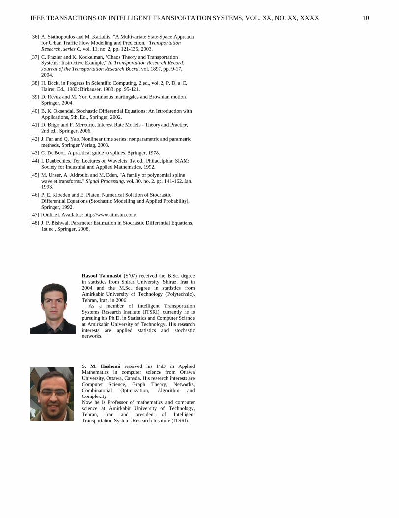
Rasool Tahmasbi (S’07) received the B.Sc. degree in statistics from Shiraz University, Shiraz, Iran in 2004 and the M.Sc. degree in statistics from Amirkabir University of Technology (Polytechnic), Tehran, Iran, in 2006.

As a member of Intelligent Transportation Systems Research Institute (ITSRI), currently he is pursuing his Ph.D. in Statistics and Computer Science at Amirkabir University of Technology. His research interests are applied statistics and stochastic networks.

S. M. Hashemi received his PhD in Applied Mathematics in computer science from Ottawa University, Ottawa, Canada. His research interests are Computer Science, Graph Theory, Networks, Combinatorial Optimization, Algorithm and Complexity. Now he is Professor of mathematics and computer science at Amirkabir University of Technology, Tehran, Iran and president of Intelligent Transportation Systems Research Institute (ITSRI).

modeling and forecasting the urban volume using stochastic differential equations

Documents