Seediscussions,stats,andauthorprofilesforthispublicationat:https://www.researchgate.net/publication/243047603

AsymptoticStabilityofNonlinearStochasticEvolutionEquations

ARTICLEinSTOCHASTICANALYSISANDAPPLICATIONS·MARCH2003

ImpactFactor:0.45·DOI:10.1081/SAP-120019288

CITATIONS

16

READS

39

3AUTHORS,INCLUDING:

T.Caraballo

UniversidaddeSevilla

161PUBLICATIONS2,344CITATIONS

SEEPROFILE

MariaJ.Garrido-Atienza

UniversidaddeSevilla

32PUBLICATIONS346CITATIONS

SEEPROFILE

Availablefrom:MariaJ.Garrido-Atienza

Retrievedon:14January2016

ASYMPTOTIC STABILITY OF NONLINEAR

STOCHASTIC EVOLUTION EQUATIONS

Tomas Caraballo, Marıa J. Garrido-Atienza

and Jose Real

Departamento de Ecuaciones Diferenciales y Analisis Numerico,

Universidad de Sevilla, Apdo. de Correos 1160,

41080-Sevilla, Spain.

Abstract

Some results on the pathwise asymptotic stability of solutions to stochastic

partial differential equations are proved. Special attention is paid in prov-

ing sufficient conditions ensuring almost sure asymptotic stability with a non-

exponential decay rate. The situation containing some hereditary characteris-

tics is also treated. The results are illustred with several examples.

1 Introduction

In the analysis of the asymptotic behaviour of solutions to differential systems, one

can find that a solution can be asymptotically stable but may not be exponentially.

Moreover, in the nonlinear and/or nonautonomous situations it may happen that the

stability can be even super-exponential (see Caraballo [1]). This fact motivated our

interest in determining, if possible, the decay rate of the solutions to other solution

or stationary one. Our main aim in this paper is to carry out a similar study in the

context of stochastic evolution equations including the possibility that some delay

terms appear in the models.

1

There exists a wide literature concerning pathwise exponential stability of stochas-

tic evolution equation. We mention here, amongst others, Caraballo [2], Caraballo

and Liu [3], Haussmann [7], Ichikawa [8] and Liu [11]. However, only a few works

have been done concerning the non-exponential stability of these stochastic systems.

It is worth mentioning the paper by Liu [9] on the polynomial stability for semi-

linear stochastic evolution equation with time delays (which contains, in particular,

the nondelay situation). But, as far as we know, the nonlinear case has not been

previously treated and it is our main interest in this paper to prove some results to

cover this gap.

Another interesting question is concerned with the stabilizing effect which may

be produced by the noise. Although this is not our major objective in this paper,

we will show that in some occasions in which the theory previously developed by

Caraballo et al. [4] does not provide exponential stabilization, we can determine

stability with a non-exponential decay rate, e.g. polynomial or super-exponential.

The content of the paper is as follows. In Section 2 we first establish the frame-

work in which our analysis is carried out in the nondelay context. We introduce the

basic notations and assumptions. We also prove some sufficient conditions ensuring

almost sure stability of solutions to stochastic evolution equations, and exhibit an

example to illustrate these results which can also be interpreted as a non-exponential

stabilization result produced by the noise. Section 3 is devoted to the establishment

of a similar result for a class of nonlinear stochastic partial differential equations with

delays and we also include some illustrative examples. Finally, some conclusions and

remarks are written in the last Section.

2 Stability of stochastic evolution equation

Let V be a reflexive Banach space and H a real separable Hilbert space such that

V ⊂ H ≡ H∗ ⊂ V ∗

2

where the injections are continuous and dense. In addition, we also assume both V

and V ∗ are uniformly convex.

We denote by ‖·‖ , |·| and ‖·‖∗ the norms in V , H and V ∗ respectively; by (·, ·)the inner product in H, and by 〈·, ·〉 the duality product between V and V ∗.

Assume Ω,F , P is a complete probability space with a normal filtration Ftt≥0,

i.e., F0 contains the null sets in F and Ft = ∩s>tFs, for all t ≥ 0, and let us consider

a real valued Ft−Wiener process W (t)t≥0.

We denote by Ip(0, T ; V ) (for p ≥ 2) the closed subspace of Lp(Ω × (0, T ),F ⊗B ([0, T ]) , P⊗dt; V ) of all stochastic processes which are Ft-adapted for almost every

t in (0, T ) (in what follows, a.e. t), where B ([0, T ]) denotes the Borel σ-algebra of

subsets in [0, T ]. We write L2(Ω;C(0, T ;H)) instead of L2(Ω,F , P ;C(0, T ; H)),

where C(0, T ; H) denotes the space of all continuous functions from [0, T ] into H.

In this Section we shall consider the following infinite-dimensional stochastic

differential equation in V ∗ and for T > 0:

dX(t) = f(t,X(t))dt + g(t,X(t))dW (t), t ∈ [0, T ],

X(0) = X0,(1)

where f(t, ·) : V → V ∗ is a suitable family of (nonlinear) operators (see conditions

below), g(t, ·) : V → H is another family of operators satisfying

(g1) The map t 7−→ g(t, x) is Lebesgue measurable from (0, T ) into H,∀x ∈ V,

(g2) There exists L > 0 such that

|g(t, x)− g(t, y)| ≤ L ‖x− y‖ ∀x, y ∈ V, a.e.t.,

and X0 ∈ Lp(Ω,F0, P ; V ) is an arbitrarily fixed initial datum.

As we are mainly interested in the stability analysis, we shall then assume that

for each T > 0 and every X0 ∈ Lp(Ω,F0, P ; V ) there exists a process

X(t) ∈ Ip(0, T ; V ) ∩ L2(Ω;C(0, T ;H))

3

which is solution to (1). In other words, X(t) satisfies the following equation in V ∗:

X(t) = X0 +∫ t

0f(s,X(s))ds +

∫ t

0g(s,X(s))dW (s), ∀t ∈ [0, T ], P − a.s. (2)

To this end, if we assume assumptions below, we then can ensure that there

exists a unique solution to this problem (1) (see Pardoux [12]):

1. Measurability: ∀x ∈ V, the map t ∈ (0, T ) 7−→ f(t, x) ∈ V ∗ is Lebesgue

measurable, a.e.t.

2. Hemicontinuity: The map θ ∈ R 7−→ 〈f(t, x + θy), z〉 ∈ R is continuous

∀x, y, z ∈ V, a.e.t.

3. Boundedness: There exists c > 0 such that

‖f(t, x)‖∗ ≤ c ‖x‖p−1 ∀x ∈ V, a.e.t.

4. Coercivity: ∃α > 0, λ, γ ∈ R such that

2 〈f(t, x), x〉+ ‖g(t, x)‖2 ≤ −α ‖x‖p + λ |x|2 + γ ∀x ∈ V, a.e.t.

5. Monotonicity:

−2 〈f(t, x)− f(t, y), x− y〉+ λ |x− y|2 ≥ ‖g(t, x)− g(t, y)‖2 ∀x, y ∈ V, a.e.t.

In what follows, we will assume that it holds at least the assumptions ensuring

that the integrals in (2) make sense.

On the other hand, let us define some operators which will be used later on

jointly with the Ito’s formula.

Unless otherwise is stated, we will assume that U(t, x) is a C1,2-positive func-

tional such that for any x ∈ V , t ∈ R+, U ′x(t, x) ∈ V, and satisfies some additional

assumptions which enable us to apply Ito’s formula for the process X(t) solution to

4

(2) (see, e.g. Pardoux [12, p. 63]). We can then define operators L and Q as follows:

for x ∈ V , t ∈ R+

LU(t, x) = U ′t(t, x) +

⟨U ′

x(t, x), f(t, x)⟩

+12(U ′′

xx(t, x)g(t, x), g(t, x))

and

QU(t, x) = (U ′x(t, x), g(t, x))2

In the sequel, we will refer to this functional U as an appropriate Lyapunov func-

tional. The following result is known as the exponential martingale inequality and

will play an important role in some of the results in this paper. For the sake of

simplicity, we only include the particular form which will be used in our arguments.

Lemma 1 Assume X(t) is a solution to (1). Suppose g(t, x) satisfies conditions

(g1) and (g2), U(t, x) is an appropriate Lyapunov functional and T , α, β are any

positive constants. Then

P

sup

0≤t≤T

[∫ t

0(U ′

x(s,X(s)) , g(s,X(s)))dW (s)−∫ t

0

α

2QU(s,X(s))ds

]> β

≤ e−αβ.

Proof. See, for instance, Liu and Truman [10, Lemma 3.8.1].

We will introduce a precise definition of almost sure stability with general decay

function λ(t) based on the concept of generalized Lyapunov exponent (see Caraballo

[1] for a related concept in the deterministic framework).

Definition 2 Let λ(t) be a positive function defined for sufficiently large t > 0,

say t ≥ T > 0, and satisfying that λ(t) ↑ +∞ as t → +∞. The solution X(t) to

(1) (defined in the future, i.e. for t large enough) is said to decay to zero almost

surely with decay function λ(t) and order at least γ > 0, if its generalized Lyapunov

exponent is less than or equal to −γ with probability one, i.e.

lim supt→∞

log |X(t)|log λ(t)

≤ −γ, P − a.s.

5

If in addition 0 is solution to (1), the zero solution is said to be almost surely

asymptotically stable with decay function λ(t) and order at least γ, if every solution

to (1) decays to zero almost surely with decay function λ(t) and order at least γ.

Remark 3 Clearly, replacing in the above definition the decay function λ(t) by a

certain suitable O(et) leads to the usual exponential stability definition.

Now, we can prove a first sufficient condition ensuring almost sure stability of

the solution of (1) with certain decay rate.

Theorem 4 Let U(t, x) be an appropriate Lyapunov functional. Assume that logλ(t)

is uniformly continuous over t ∈ [T, +∞) and there exists a constant τ ≥ 0 such

that

lim supt→∞

log log t

log λ(t)≤ τ.

Assume that there exist two continuous non-negative functions ϕ1(t), ϕ2(t), con-

stants q > 0, m ≥ 0, µ, ν, θ ∈ R and a non-increasing function ξ(t) > 0 such that

(a) |x|qλ(t)m ≤ U(t, x), (t, x) ∈ R+ × V .

(b) LU(t, x) + ξ(t)QU(t, x) ≤ ϕ1(t) + ϕ2(t)U(t, x), (t, x) ∈ R+ × V .

(c)

lim supt→∞

log∫ t0 ϕ1(s)ds

log λ(t)≤ ν, lim sup

t→∞

∫ t0 ϕ2(s)ds

log λ(t)≤ θ

lim inft→∞

log ξ(t)log λ(t)

≥ −µ.

Then, every solution X(t) to (1) defined in the future satisfies

lim supt→∞

log |X(t)|log λ(t)

≤ −m− [θ + (ν ∨ (µ + τ))]q

, P − a.s.

In particular, if m > θ+(ν∨(µ+τ)), the solution X(t) decays to zero almost surely

with decay function λ(t) and order at least γ = (m− [θ + (ν ∨ (µ + τ))]) /q.

6

Proof. We will apply Ito’s formula to the function U(t, x) and the process X(t).

Noticing the definitions of L and Q, we can derive that

U(t,X(t)) = U(0, X0) +∫ t

0LU(s,X(s)) ds

+∫ t

0(U ′

x(s,X(s)), g(s,X(s)))dW (s). (3)

Now, from the uniform continuity of log λ(t), we can ensure that for each ε > 0 there

exist two positive integers N = N(ε) and k1(ε) such that ifk − 12N

≤ t ≤ k

2N, k ≥

k1(ε), it follows ∣∣∣∣log λ

(k

2N

)− log λ(t)

∣∣∣∣ ≤ ε.

On the other hand, due to the exponential martingale inequality

P

ω : sup

0≤t≤w

[M(t)−

∫ t

0

u

2QU(s,X(s))ds

]> v

≤ e−uv,

for any positive constants u, v and w, where

M(t) =∫ t

0(U ′

x(s,X(s)) , g(s,X(s)))dW (s).

In particular, for the preceding ε > 0, if we set

u = 2ξ

(k

2N

), v = ξ

(k

2N

)−1

logk − 12N

, w =k

2N, k = 2, 3, ...

we can then apply the Borel-Cantelli lemma to obtain that for almost all ω ∈ Ω,

there exists an integer k0(ε, ω) > 0 such that

∫ t

0(U ′

x(s,X(s)) , g(s, X(s)))dW (s) ≤ ξ

(k

2N

)−1

logk − 12N

+ ξ

(k

2N

) ∫ t

0QU(s,X(s))ds

≤ ξ

(k

2N

)−1

logk − 12N

+∫ t

0ξ(s)QU(s,X(s))ds

7

for 0 ≤ t ≤ k

2N, k ≥ k0(ε, ω). Substituting this into (3) and using condition (b), we

deduce

U(t,X(t)) = U(0, X0) + ξ

(k

2N

)−1

logk − 12N

+∫ t

0ϕ1(s)ds

+∫ t

0ϕ2(s)U(s,X(s)) ds, P − a.s. (4)

for 0 ≤ t ≤ k

2N, k ≥ k0(ε, ω). Consequently, by the virtue of Gronwall’s lemma, it

follows

U(t,X(t)) =

(U(0, X0) + ξ

(k

2N

)−1

logk − 12N

+∫ t

0ϕ1(s)ds

)

× exp(∫ t

0ϕ2(s) ds

), P − a.s.

for 0 ≤ t ≤ k

2N, k ≥ k0(ε, ω).

On the other hand, thanks to condition (c) and the uniform continuity of log λ(t),

∫ t0 ϕ1(s)ds ≤ λ(t)ν+ε,

∫ t0 ϕ2(s)ds ≤ (θ + ε) log λ(t), ξ

(k

2N

)−1

≤ eε(µ+ε)λ(t)µ+ε

fork − 12N

≤ t ≤ k

2N, k ≥ k1(ε). Owing to the assumption on λ(t),

logk − 12N

≤ log t ≤ λ(t)τ+ε fork − 12N

≤ t ≤ k

2N.

Hence, for almost all ω ∈ Ω

log U(t,X(t)) ≤ log(U(0, X0) + λ(t)µ+τ+2εeε(µ+ε) + λ(t)ν+ε)

+ (θ + ε) log λ(t)

fork − 12N

≤ t ≤ k

2N, k ≥ k0(ε, ω) ∨ k1(ε), which immediately implies

lim supt→∞

log U(t,X(t))log λ(t)

≤ [(µ + τ + 2ε) ∨ (ν + ε)] + θ + ε, P − a.s. (5)

As ε > 0 is arbitrary, (5) yields to

lim supt→∞

log U(t,X(t))log λ(t)

≤ [ν ∨ (µ + τ)] + θ, P − a.s.

8

Finally,

lim supt→∞

log |X(t)|log λ(t)

≤ −m− [θ + (ν ∨ (µ + τ))]q

, P − a.s.

which finishes the proof.

Remark 5 Note that, in the preceding theorem we have assumed that logλ(t) is

uniformly continuous over t ∈ [T, +∞) and there exists a constant τ ≥ 0 such that

lim supt→∞

log log t

log λ(t)≤ τ.

However, when the functional QU(t, x) is also bounded below (see next Theorem

6), it is not necessary to impose the uniform continuity of logλ(t) provided that we

assume a stronger hypothesis on the growing rate of λ(t).

Theorem 6 Let U(t, x) be an appropriate Lyapunov functional. Assume that X(t)

is a solution to (1) satisfying that |X(t)| 6= 0 for all t ≥ 0 and P−a.s. provided

|X0| 6= 0 P−a.s. Assume there exist two continuous functions ϕ1(t) ∈ R, ϕ2(t) ≥ 0,

and constants q > 0,m ≥ 0, ν ≥ 0, µ ≥ 0, θ ∈ R such that

(a) |x|qλ(t)m ≤ U(t, x), (t, x) ∈ R+ × V .

(b) LU(t, x) ≤ ϕ1(t)U(t, x), (t, x) ∈ R+ × V.

(c) QU(t, x) ≥ ϕ2(t)U(t, x)2, (t, x) ∈ R+ × V.

(d)

lim supt→∞

∫ t0 ϕ1(s)ds

log λ(t)≤ θ, lim inf

t→∞

∫ t0 ϕ2(s)ds

log λ(t)≥ 2ν

lim supt→∞

log t

log λ(t)≤ µ

2.

Then, for every α ∈ (0, 1), it holds

lim supt→∞

log |X(t)|log λ(t)

≤ −m− (α−1µ + θ − ν (1− α))q

, P − a.s.

9

In particular, if m > α−1µ + θ− ν (1− α) , the solution X(t) decays to zero almost

surely with decay function λ(t) and order at least

γα =(m− (α−1µ + θ − ν (1− α))

)/q.

Proof. Fix |X0| 6= 0 P−a.s. Then, thanks to Ito’s formula

log U(t, X(t)) = log U(0, X0) + M(t) +∫ t

0

LU(s,X(s))U(s,X(s))

ds

− 12

∫ t

0

QU(s,X(s))U(s,X(s))2

ds (6)

where

M(t) =∫ t

0

1U(s,X(s))

(U ′x(s,X(s)), g(s,X(s)))dW (s).

Due to the exponential martingale inequality,

P

ω : sup

0≤t≤w

[M(t)−

∫ t

0

u

2QU(s, X(s))U(s,X(s))2

ds

]> v

≤ e−uv

for any positive constants u, v and w. In particular, taking 0 < α < 1 and setting

u = α, v = 2α−1 log(k − 1), w = k, k = 2, 3, ...

we can apply Borel-Cantelli’s lemma to obtain that, for almost all ω ∈ Ω, there

exists an integer k0(ε, ω) > 0 such that

M(t) ≤ 2α−1 log(k − 1) +α

2

∫ t

0

QU(s,X(s))U(s, X(s))2

ds

for 0 ≤ t ≤ k, k ≥ k0(ε, ω). Substituting this into (6) and using condition (c), we

get that

log U(t,X(t)) ≤ log U(0, X0) + 2α−1 log(k − 1) +∫ t

0ϕ1(s)ds

− 12(1− α)

∫ t

0ϕ2(s) ds

for 0 ≤ t ≤ k, k ≥ k0(ε, ω). Now, using condition (d), it follows

log U(t,X(t)) ≤ log U(0, X0) +(µ + ε)

αlog λ(t)

+ (θ + ε) log λ(t)− 12

(1− α) (2ν − ε) log λ(t)

10

for k − 1 ≤ t ≤ k, k ≥ k0(ε, ω), which implies that

lim supt→∞

log U(t, X(t))log λ(t)

≤ α−1 (µ + ε) + θ + ε− 12

(1− α) (2ν − ε), P − a.s.

Taking into account that ε > 0 is arbitrary and using (a) we can deduce

lim supt→∞

log |X(t)|log λ(t)

≤ −m− (α−1µ + θ − ν (1− α))q

, P − a.s.,

as required.

Remark 7 Observe that, as the decay order of the solution in the preceding theorem

depends on the parameter α, an interesting question is concerned with the possibility

of determining the biggest value for γα. To this respect, one can check that this

optimal value depends on the relation between µ and ν. Let us explain this in more

detail. Indeed, in order to find the optimal value γ∗ = sup0<α<1

γα, we need to find

out the minimum value f∗ for the function f(α) = α−1µ + θ − ν (1− α) when the

parameter α ∈ (0, 1) , and consequently it will hold that γ∗ = (m− f∗) /q. Now, by

straightforward computations, it is not difficult to check that

f∗ =

2 (µν)1/2 + θ − ν, if 0 ≤ µ < ν,

µ + θ, if ν ≤ µ,

which implies that

γ∗ =

m−[2(µν)1/2+θ−ν]q , if 0 ≤ µ < ν,

m−[µ+θ]q , if ν ≤ µ,

Remark 8 Note that Theorem 9 below permits us to avoid the restriction on the

growing rate on the decay function when QU(t, x) is also bounded above by a suitable

bound.

Theorem 9 Let U(t, x) ∈ C1,2(R+×H;R+) be an appropriate Lyapunov functional.

Assume that there exist three continuous functions ϕ1(t) ∈ R, ϕ2(t) ≥ 0, ϕ3(t) ≥ 0,

and constants q > 0,m ≥ 0, ν > 0, µ ≥ 0 and θ ∈ R such that

11

(a) |x|qλ(t)m ≤ U(t, x), (t, x) ∈ R+ × V .

(b) LU(t, x) ≤ ϕ1(t)U(t, x), (t, x) ∈ R+ × V.

(c) ϕ2(t)U(t, x)2 ≤ QU(t, x) ≤ ϕ3(t)U(t, x)2, (t, x) ∈ R+ × V.

(d)

lim supt→∞

∫ t0 ϕ1(s)ds

log λ(t)≤ θ, lim inf

t→∞

∫ t0 ϕ2(s)ds

log λ(t)≥ 2ν

lim supt→∞

∫ t0 ϕ3(s)ds

log λ(t)≤ µ.

Then, if X(t) is a solution to (1) defined in the future and satisfying that |X(t)| 6= 0

for all t ≥ 0 and P−a.s. provided |X0| 6= 0 P−a.s., it holds

lim supt→∞

log |X(t)|log λ(t)

≤ −m− (θ − ν)q

, P − a.s.

In particular, if m > θ−ν, the solution X(t) decays to zero almost surely with decay

function λ(t) and order at least γ = (m− (θ − ν)) /q.

Proof. Fix |X0| 6= 0 P−a.s. Then, Ito’s formula implies again (6). Using

conditions (b) and (c) we obtain

log U(t,X(t)) ≤ log U(0, X0) + M(t) +∫ t

0ϕ1(s)ds− 1

2

∫ t

0ϕ2(s) ds. (7)

Now, condition (d) and (7) imply

log U(t,X(t)) ≤ log U(0, X0) + M(t) + (θ + ε) log λ(t)− 12(2ν − ε) log λ(t),

and

lim supt→∞

log U(t,X(t))log λ(t)

≤ lim supt→∞

M(t)log λ(t)

+ θ + ε− 12(2ν − ε), P − a.s.

Let us denote by 〈M(t)〉 the quadratic variation process associated to M(t). From

our assumptions we can deduce that M(t) is a local martingale vanishing at t = 0.

Moreover, condition (c) implies∫ t

0ϕ2(s) ds ≤ 〈M(t)〉 =

∫ t

0

QU(s,X(s))U(s,X(s))2

ds ≤∫ t

0ϕ3(s) ds.

12

Now, as ν > 0, it follows that limt→∞ 〈M(t)〉 = +∞ and by means of the strong law

of large numbers we obtain

limt→∞

M(t)〈M(t)〉 = 0, P − a.s.

Taking into account that, for t large enough,

|M(t)|log λ(t)

=|M(t)|〈M(t)〉

〈M(t)〉log λ(t)

≤ |M(t)|〈M(t)〉

∫ t0 ϕ3(s) ds

log λ(t),

we easily deduce that, from assumption (d), it follows

lim supt→∞

M(t)log λ(t)

= 0, P − a.s.

and, consequently,

lim supt→∞

log U(t,X(t))log λ(t)

≤ θ + ε− 12(2ν − ε), P − a.s.

Since the constant ε > 0 is arbitrary, we can affirm that

lim supt→∞

log |X(t)|log λ(t)

≤ −m− (θ − ν)q

, P − a.s.

and the proof is therefore complete.

Remark 10 It is worth pointing out that this result allows us to establish some

kind of stabilization effect produced by the noise on deterministic systems. To this

respect, Caraballo et al. [4] proved some results on the exponential stabilization of

deterministic (and stochastic) systems when a suitable noise appears in the equa-

tions. However, it may happen that the noise does not cause exponential stability

(or at least we are not able to know if this has happened) and, consequently, it would

be very interesting to investigate if the noise has produced a different kind of stability

(e.g. polynomial, logarithmic, or even super-exponential). As this will be the aim of

a subsequent paper, we only include here an example to illustrate our ideas.

13

Example 1. Let us consider the following problem

dX(t) = A(t)X(t)dt + g(t, X(t))dW (t), t > 0,

X(0) = X0,

where operators A(t) and g are defined as follows. We consider an open and bounded

set O ⊂ RN with regular boundary and let 2 ≤ p < +∞. Consider also the Sobolev

spaces V = W 1,p0 (O), H = L2(O) with their usual norms, inner product and

duality. The monotone family of operatorsA(t) : V → V ∗ is then defined by

〈v, A(t)u〉 = −N∑

i=1

∫

O

∣∣∣∣∂u(x)∂xi

∣∣∣∣p−2 ∂u(x)

∂xi

∂v(x)∂xi

dx +∫

O

a

1 + tu(x)v(x)dx ∀u, v ∈ V ,

where a ∈ R, and g(t, u) = b (1 + t)−1/2 u , b ∈ R, u ∈ H for all t ∈ R+.

Now, consider the function U(t, u) = |u|2 , u ∈ H and let us compute LU(t, u)

and QU(t, u).

On the one hand, it easily follows

LU(t, u) = 2〈u,A(t)u〉+ |g(t, u)|2 = −2‖u‖p +2a + b2

1 + t|u|2, u ∈ V, (8)

so we can set ϕ1(t) =(2a + b2

)/(1 + t). On the other hand,

QU(t, u) = (2u, b(1 + t)−1/2u)2 = 4b2 (1 + t)−1 |u|4 ,

so that ϕ2(t) = ϕ3(t) = 4b2 (1 + t)−1.

In order to apply now the exponential stabilization result in Caraballo et al. [4]

(in fact, Theorem 2.2 or the Remark following this theorem), we need to determine

constants δ0 and ρ0 satisfying

lim supt→+∞

1t

∫ t

0ϕ1(s)ds ≤ δ0, lim inf

t→+∞1t

∫ t

0ϕ2(s)ds ≥ ρ0,

and the result in [4] ensures that

lim supt→∞

1t

log |X(t)|2 ≤ −(2ρ0 − δ0), P − a.s.

14

It is easy to compute that in this example both constants are equal to 0, so that

we do not know whether the solution decays to zero exponentially or not. However,

we can apply the preceding theorem and prove, at least, asymptotic decay with a

lower decay rate. Indeed, taking λ(t) = t,m = 0, q = 2 we can easily check that

the assumptions in the last theorem hold with θ = 2a + b2, ν = 2b2, µ = 4b2, and

therefore − (m− (θ − ν)) /q =(2a− b2

)/2. We have then proved asymptotic decay

to zero with decay function λ(t) = t and order at least b2

2 − a provided b is large

enough (in fact, whenever b2 > 2a).

3 Stability of stochastic delay evolution equation

In this section we shall investigate the almost sure stability for a class of stochastic

functional evolution equations (which, in particular, includes the case of stochastic

evolution equations with variable and distributed delays). The main objective is

to develop a general theory similar to the one in the case without delays in the

preceding Section by also using the Lyapunov functional technique. It is worth

mentioning that Caraballo et al. proved in [5] a particular result on the exponential

stability of stochastic partial functional differential equations by a Razumikhin type

of argument considering the usual quadratic Lyapunov function. The analysis which

will be carried out in this Section completes and improves that one.

In a similar way as we did in Section 2, given h ≥ 0, p ≥ 2 and T > 0, we will de-

note by Ip(−h, T ; V ) the closed subspace of Lp(Ω×[−h, T ],F⊗B([−h, T ]),dP⊗dt;V )

of all Ft−adapted processes for a.e. t where we will set Ft = F0 for t < 0. We will

also write L2(Ω; C(−h, T ; H)) instead of L2(Ω,F , P ; C(−h, T ; H)) and C(−h, T ; H)

denotes now the space of all continuous functions from [−h,T ] into H.

Let CH = C(−h, 0;H) with norm |ψ|CH= sup

−h≤s≤0|ψ(s)|, ψ ∈ CH ; Lp

V =

Lp([−h, 0], V ) and LpH = Lp([−h, 0],H).

15

On the other hand, given a stochastic process

X(t) ∈ Ip(−h, T ;V ) ∩ L2(Ω; C(−h, T ; H)),

we associate with another stochastic process

Xt : Ω 7−→ LpV ∩ CH

by means of the usual relation Xt(s)(ω) = X(t + s)(ω), 0 ≤ t ≤ T , −h ≤ s ≤ 0.

Let us consider the following stochastic evolution equation in V ∗:

dX(t) = (A(t,X(t)) + F (t,Xt)) dt + G(t,Xt)dW (t), t ∈ [0, T ],

X(0) = ψ(t), t ∈ [−h, 0](9)

where T > 0 and the initial datum ψ ∈ Ip(−h, 0;V ) ∩ L2(Ω; CH).

As our major interest in this Section is the stability analysis of solutions to (9),

we shall assume that for each ψ ∈ Ip(−h, 0;V ) ∩ L2(Ω;CH) there exists a process

X(t) ∈ Ip(−h, T ; V ) ∩ L2(Ω;C(−h, T ; H))

which is solution to (9) for every T > 0, in other words, X(t) satisfies the following

integral equation in V ∗ :

X(t) = ψ(0) +∫ t0 (A(s,X(s)) + F (s,Xs))ds +

∫ t0 G(s,Xs)dW (s), ∀t ∈ [0, T ],

X(t) = ψ(t), ∀t ∈ [−h, 0].

This happens, for instance, if A(t, ·) : V → V ∗ is a family of (nonlinear) opera-

tors defined a.e.t. and fulfilling the assumptions described in the preceding Section

(measurability, hemicontinuity, boundedness, monotonicity and coercivity), F (t, ·) :

[0, T ] × CH → V ∗ is a family of Lipschitz continuous operators defined a.e.t, and

G : [0, T ] × CH → H is another family of Lipschitz operators defined a.e.t (see

Caraballo et al. [5] and also Caraballo et al. [6] for two detailed discussions on the

existence and uniqueness of solutions for this situation).

We can now prove our stability result.

16

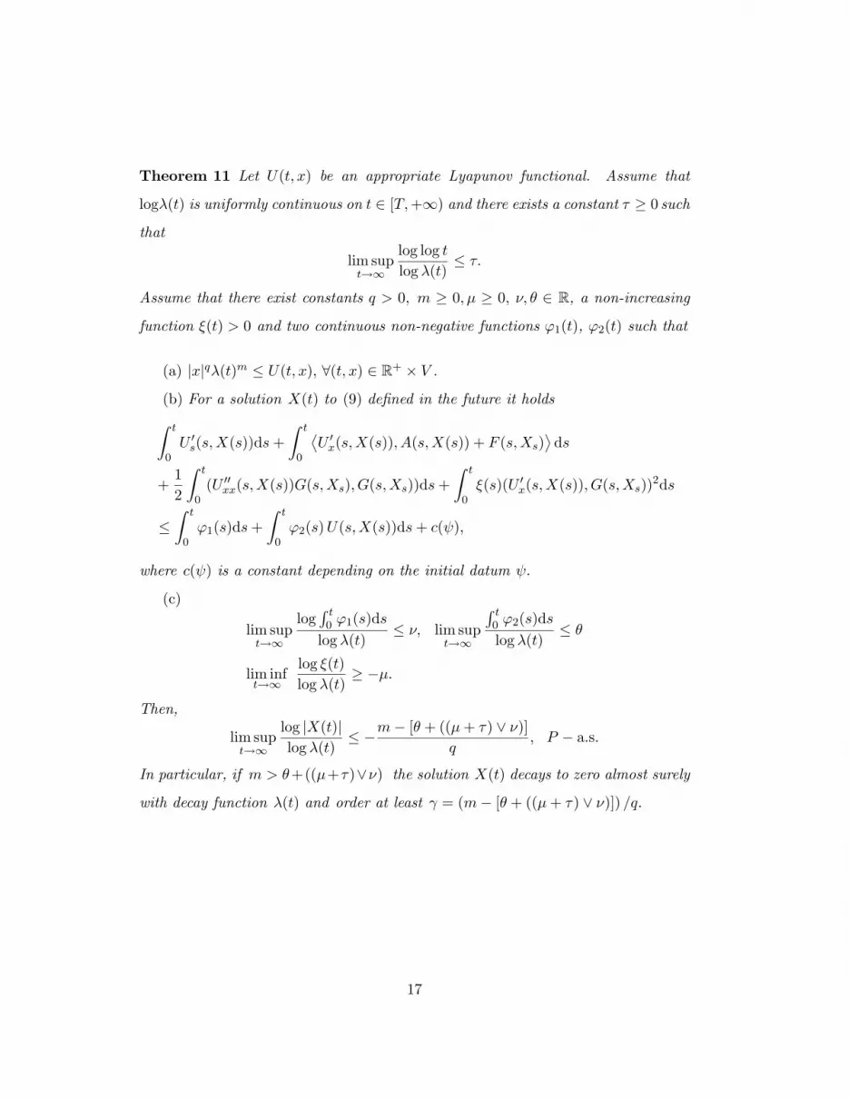
Theorem 11 Let U(t, x) be an appropriate Lyapunov functional. Assume that

logλ(t) is uniformly continuous on t ∈ [T, +∞) and there exists a constant τ ≥ 0 such

that

lim supt→∞

log log t

log λ(t)≤ τ.

Assume that there exist constants q > 0, m ≥ 0, µ ≥ 0, ν, θ ∈ R, a non-increasing

function ξ(t) > 0 and two continuous non-negative functions ϕ1(t), ϕ2(t) such that

(a) |x|qλ(t)m ≤ U(t, x), ∀(t, x) ∈ R+ × V .

(b) For a solution X(t) to (9) defined in the future it holds∫ t

0U ′

s(s,X(s))ds +∫ t

0

⟨U ′

x(s,X(s)), A(s,X(s)) + F (s, Xs)⟩ds

+12

∫ t

0(U ′′

xx(s,X(s))G(s,Xs), G(s,Xs))ds +∫ t

0ξ(s)(U ′

x(s,X(s)), G(s,Xs))2ds

≤∫ t

0ϕ1(s)ds +

∫ t

0ϕ2(s) U(s, X(s))ds + c(ψ),

where c(ψ) is a constant depending on the initial datum ψ.

(c)

lim supt→∞

log∫ t0 ϕ1(s)ds

log λ(t)≤ ν, lim sup

t→∞

∫ t0 ϕ2(s)ds

log λ(t)≤ θ

lim inft→∞

log ξ(t)log λ(t)

≥ −µ.

Then,

lim supt→∞

log |X(t)|log λ(t)

≤ −m− [θ + ((µ + τ) ∨ ν)]q

, P − a.s.

In particular, if m > θ+((µ+τ)∨ν) the solution X(t) decays to zero almost surely

with decay function λ(t) and order at least γ = (m− [θ + ((µ + τ) ∨ ν)]) /q.

17

Proof. By applying once again Ito’s formula we obtain

U(t,X(t)) = U(0, ψ(0)) +∫ t

0U ′

s(s, X(s))ds

+∫ t

0

⟨U ′

x(s,X(s)), A(s,X(s)) + F (s,Xs)⟩ds

+12

∫ t

0(U ′′

xx(s,X(s))G(s,Xs), G(s,Xs))ds

+∫ t

0(U ′

x(s, X(s)), G(s, Xs))dW (s). (10)

Due to the uniform continuity of log λ(t) and given ε > 0, there exist two positive

integers N = N(ε) and k1(ε) such that fork − 12N

≤ t ≤ k

2N, k ≥ k1(ε), it follows

∣∣∣∣log λ

(k

2N

)− log λ(t)

∣∣∣∣ ≤ ε.

On the other hand, the exponential martingale inequality implies

P

sup

0≤t≤w

[M(t)− u

2

∫ t

0(U ′

x(s,X(s)), G(s,Xs))2ds

]> v

≤ e−uv

for any positive constants u, v and w, where

M(t) =∫ t

0(U ′

x(s, X(s)) , G(s,Xs))dW (s).

In particular, for the preceding ε > 0, taking

u = 2ξ

(k

2N

), v = ξ

(k

2N

)−1

logk − 12N

, w =k

2N, k = 2, 3, ...

we can then apply the Borel-Cantelli lemma to obtain that for almost all ω ∈ Ω,

there exists an integer k0(ε, ω) > 0 such that∫ t

0(U ′

x(s,X(s)) , G(s,Xs))dW (s) ≤ ξ

(k

2N

)−1

logk − 12N

+ ξ

(k

2N

)∫ t

0(U ′

x(s,X(s)), G(s,Xs))2ds

≤ ξ

(k

2N

)−1

logk − 12N

+∫ t

0ξ(s)(U ′

x(s,X(s)), G(s,Xs))2ds

18

for 0 ≤ t ≤ k

2N, k ≥ k0(ε, ω). Substituting this into (10) we see that P -a.s.

U(t, X(t)) ≤ U(0, ψ(0)) + ξ

(k

2N

)−1

logk − 12N

+∫ t

0U ′

s(s,X(s))ds

+∫ t

0

⟨U ′

x(s, X(s)), A(s,X(s)) + F (s, Xs)⟩ds

+12

∫ t

0(U ′′

xx(s, X(s))G(s,Xs), G(s,Xs))ds

+∫ t

0ξ(s)(U ′

x(s, X(s)), G(s,Xs))2ds

for 0 ≤ t ≤ k

2N, k ≥ k0(ε, ω). Using condition (b) we derive that P -a.s.

U(t,X(t)) ≤ U(0, ψ(0)) + ξ

(k

2N

)−1

logk − 12N

+∫ t

0ϕ1(s)ds

+∫ t

0ϕ2(s)U(s,X(s))ds + c(ψ)

for 0 ≤ t ≤ k

2N, k ≥ k0(ε, ω). So by virtue of the Gronwall lemma,

|X(t)|q λ(t)m ≤(

U(0, ψ(0)) + ξ

(k

2N

)−1

logk − 12N

+∫ t

0ϕ1(s)ds + c(ψ)

)exp

(∫ t

0ϕ2(s) ds

)

for 0 ≤ t ≤ k

2N, k ≥ k0(ε, ω). Therefore, noticing condition (c) and following a

similar argument as the one in the proof of theorem 4, we have that P−a.s.

log(|X(t)|q λ(t)m) ≤ log(U(0, ψ(0)) + λ(t)µ+τ+2εeε(µ+ε) + λ(t)ν+ε + c(ψ)

)

+ (θ + ε) log λ(t)

fork − 12N

≤ t ≤ k

2N, k ≥ k1(ε). Hence

lim supt→∞

log(|X(t)|q λ(t)m)log λ(t)

≤ [(µ + τ + 2ε) ∨ (ν + ε)] + θ + ε, P − a.s.

As ε > 0 is arbitrary, we immediately obtain

lim supt→∞

log |X(t)|log λ(t)

≤ −m− [θ + ((µ + τ) ∨ ν)]q

, P − a.s.

19

The proof is therefore complete.

Remark 12 Observe that assumption (b) in the preceding theorem seems different

from the ones in theorems in the previous Section. However, it is possible to establish

a stronger hypothesis (but easier to check in applications) implying this. Indeed,

given U(t, x) ∈ C1,2(R+ × H;R+) we can define the following operators L and Q

acting on LpV ∩ CH , that is, for Φ ∈ Lp

V ∩ CH and t ∈ R+, we set

LU(t,Φ) = U ′t(t, Φ(0)) +

⟨U ′

x(t, Φ(0)), A(t,Φ(0)) + F (t,Φ)⟩

+12(U ′′

xx(t, Φ(0))g(t,Φ), g(t, Φ))

and

QU(t,Φ) = (U ′x(t, Φ(0)), g(t, Φ))2.

Then, if we assume that

LU(t, Φ) + ξ(t)QU(t,Φ) ≤ ϕ1(t) + ϕ2(t)U(t,Φ(0)),

it immediately implies condition (b).

Finally, we shall include a couple of examples to illustrate our results.

Example 2. Consider the following one dimensional model with constant time

delay

dX(t) =[− q

1 + tX(t) +

11 + t

X(t− h)]

dt + (1 + t)−qdW (t), t ∈ [0, T ],

X(t) = ψ(t), t ∈ [−h, 0],

where q > 1 and T, h > 0. This problem can be set in our formulation by taking V =

H = R, p = 2. We will write C instead of CH . From the standard theory on stochastic

differential equations with delays, it is straightforward that the preceding problem

has a unique solution for each initial datum fixed in the space I2(−h, 0;R)∩L2(Ω;C).

20

Define for u ∈ R and φ ∈ C, A(t, u) = − qu

1 + t, F (t, φ) =

11 + t

φ(−h) and G(t, φ) =

(1 + t)−q, t ∈ [0, T ].

Now, we consider U(t, y) = (1 + t)2q |y|2 . Then, it it easy to check that for

arbitrary δ > 1, ξ(t) =1

4(1 + t)δ, we have

∫ t

0U ′

s(s,X(s))ds +∫ t

0

⟨U ′

x(s,X(s)), A(s,X(s)) + F (s,Xs)⟩ds

+12

∫ t

0(U ′′

xx(s,X(s))G(s,Xs), G(s,Xs))ds

+∫ t

0

14(1 + s)δ

(U ′x(s,X(s)), G(s,Xs))2ds

≤∫ t

0ds +

∫ t

0

1(1 + s)δ

U(s,X(s))ds +∫ t

02(1 + s)2q−1X(s)X(s− h)ds

≤∫ t

0ds +

∫ t

0

1(1 + s)δ

U(s,X(s))ds +∫ t

0

1(1 + s)

U(s,X(s))ds

+∫ t

0(1 + s)2q−1 |X(s− h)|2 ds.

We now estimate the last integral:∫ t

0(1 + s)2q−1 |X(s− h)|2 ds = |ψ|2C

∫ 0

−h(1 + s + h)2q−1ds

+∫ t−h

0(1 + r + h)2q−1 |X(r)|2 dr

≤ c(ψ) + (1 + h)2q−1

∫ t

0

11 + s

U(s,X(s))ds,

where we have denoted c(ψ) = 12q ((1 + h)2q − 1) |ψ|2C and have used the inequality

(1 + r + h) ≤ (1 + r)(1 + h), r, h ≥ 0.

Then,

ϕ1(t) = 1, ϕ2(t) =1

(1 + t)δ+

(1 + h)2q−1 + 1(1 + t)

.

By some easy computations, we can check that

τ = 0, ν = 1, θ = (1 + h)2q−1 + 1, µ = δ.

21

Hence, by virtue of theorem 11 it follows

lim supt→∞

log(|X(t)|)log(1 + t)

≤ −2q − ((1 + h)2q−1 + 1 + δ)2

, P − a.s.

As the constant δ > 1 is arbitrary, we immediately obtain

lim supt→∞

log(|X(t)|)log(1 + t)

≤ −2q − ((1 + h)2q−1 + 2)2

, P − a.s.

Thus, the zero solution is almost sure polynomially stable with decay function

(1+t) and order at least(2q − ((1 + h)2q−1 + 2)

)/2 whenever q >

(2 + (1 + h)2q−1

)/2.

It is worth pointing out that the value of q is restricting the maximal admissible

value for the time lag h. The larger q, the larger h is allowed to be.

Example 3. Consider the semilinear stochastic heat equation with finite time-

lags r1, r2 (h > r1, r2 ≥ 0),

dX(t, x) =[γ ∂2X(t,x)

∂x2 +∫ 0−r1

(α1X(t + u, x) + α2

∂X∂x (t + u, x)

)β(u)du

]dt

+ α(X(t)) X(t−r2,x)1+|X(t,x)|dW (t),

X(t, x) = ψ(t, x), t ∈ [−h, 0], x ∈ [0, π],

X(t, 0) = X(t, π) = 0, t ≥ 0.

where γ > 0, α1, α2 ≥ 0; α(·) : R→ R, β : [−r1, 0] → R are two bounded Lipschitz

continuous functions with |α(x)| ≤ K, |β(u)| ≤ M, x ∈ R, u ∈ [−r1, 0], M, K > 0.

Define V = H10 [0, π], H = L2[0, π] and denote by ‖·‖ and |·| the norms in V and H

respectively; by (·, ·) the inner product in H.

This problem can be put within our formulation by denoting A(t, v)(x) = γ d2v(x)dx2 ,

for v ∈ V, x ∈ [0, π]; F (t, φ)(x) =∫ 0−r1

(α1φ(u)(x) + α2

dφ(u)(x)dx

)β(u)du and

G(t, φ)(x) = α(φ(0)) φ(−r2)(x)1+|φ(0)(x)| , for φ ∈ CH , t ≥ 0, x ∈ [0, π].

We will consider U(t, y) =emt |y|2 (where m > 0 is a fixed but arbitrary constant)

which immediately satisfies the whole assumptions required to apply Ito’s formula.

22

It is easy to check that, if we take ξ(t) =1

4emt, then

∫ t

0U ′

s(s,X(s))ds +∫ t

0

⟨U ′

x(s,X(s)), A(s,X(s)) + F (s,Xs)⟩ds

+12

∫ t

0(U ′′

xx(s, X(s))G(s,Xs), G(s,Xs))ds

+∫ t

0

14ems

(U ′x(s,X(s)), G(s,Xs))2ds

≤∫ t

0mU(s,X(s))ds + 2K2

∫ t

0ems |X(s− r2)|2 ds

+∫ t

0

(2X(s)ems, α1

∫ 0

−r1

X(s + u)β(u)du

)ds

+∫ t

0

(2X(s)ems, α2

∫ 0

−r1

∂X(s + u)∂x

β(u)du

)ds− 2γ

∫ t

0ems ‖X(s)‖2 ds

,∫ t

0mU(s,X(s))ds + 2K2I1 + I2 + I3 + I4.

On the one hand

I1 ≤ |ψ|2CH

∫ 0

−r2

em(r2+u)du +∫ t−r2

0emr2U(s,X(s))ds

≤ r2emr2 |ψ|2CH+

∫ t

0emr2U(s,X(s))ds.

On the other hand,

I2 ≤ α1

∫ t

0U(s,X(s))ds + α1

∫ t

0ems

∣∣∣∣∫ 0

−r1

X(s + u)β(u)du

∣∣∣∣2

ds

≤ α1

∫ t

0U(s,X(s))ds + α1r1

∫ t

0ems

(∫ 0

−r1

|X(s + u)|2 β2(u)du

)ds

≤ α1

∫ t

0U(s,X(s))ds + α1r1M

2

∫ t

0ems

(∫ s

s−r1

|X(u)|2 du

)ds

≤ α1

∫ t

0U(s,X(s))ds

+ α1r21M

2

[|ψ|2CH

(∫ 0

−r1

em(u+r1)du

)+

∫ t

0emr1U(s,X(s))ds

]

≤ α1

∫ t

0U(s,X(s))ds + α1r

31M

2emr1 |ψ|2CH

+ α1r21M

2

∫ t

0emr1U(s,X(s))ds,

23

and, finally

I3 ≤ α2

∫ t

0U(s,X(s))ds + α2

∫ t

0ems

∣∣∣∣∫ 0

−r1

∂X(s + u)∂x

β(u)du

∣∣∣∣2

ds

≤ α2

∫ t

0U(s,X(s))ds + α2r1

∫ t

0ems

(∫ 0

−r1

‖X(s + u)‖2 β2(u)du

)ds

≤ α2

∫ t

0U(s,X(s))ds + α2r1M

2

∫ t

0ems

(∫ s

s−r1

‖X(u)‖2 du

)ds

≤ α2

∫ t

0U(s,X(s))ds

+ α2r21M

2

[‖ψ‖2

L2V

∫ 0

−r1

em(u+r1)du +∫ t

0emr1ems ‖X(s)‖2 ds

]

≤ α2

∫ t

0U(s,X(s))ds + α2r

31M

2emr1 ‖ψ‖2L2

V

+ α2r21M

2

∫ t

0emr1ems ‖X(s)‖2 ds.

Therefore,∫ t

0U ′

s(s,X(s))ds +∫ t

0

⟨U ′

x(s,X(s)), A(s,X(s)) + F (s,Xs)⟩ds

+12

∫ t

0(U ′′

xx(s,X(s))G(s,Xs), G(s,Xs))ds

+∫ t

0

14ems

(U ′x(s,X(s)), G(s,Xs))2ds

≤ (m + 2K2emr2 + (α1 + α2)(1 + r21M

2emr1)− 2γ)∫ t

0U(s,X(s))ds + c(ψ),

if we suppose that α2r21M

2emr1 − 2γ < 0, i.e., γ >α2r2

1M2emr1

2 , and where

c(ψ) = (2K2r2emr2 + α1r

31M

2emr1) |ψ|2CH+ α2r

31M

2emr1 ‖ψ‖2L2

V.

Then, we obtain

ϕ1(t) = 0, ϕ2(t) = m + 2K2emr2 − 2γ + (α1 + α2)(1 + r21M

2emr1).

Therefore, constants in theorem 11 can be chosen as follows

τ = 0, ν = 0, θ = m + 2K2emr2 − 2γ + (α1 + α2)(1 + r21M

2emr1), µ = m,

24

whence we deduce that P−a.s.

lim supt→∞

log |X(t)|t

≤ −m− (m + 2K2emr2 − 2γ + (α1 + α2)(1 + r21M

2emr1) + m)2

,

i.e., P−a.s.

lim supt→∞

log |X(t)|t

≤ −(−m + 2γ − 2K2emr2 − (α1 + α2)(1 + r21M

2emr1))2

.

Since m > 0 can be chosen arbitrarily, we immediately obtain, by means of a con-

tinuity argument, that whenever γ >2K2+(α1+α2)(1+r2

1M2)2 , the solution is almost

surely exponentially stable with at least order (2γ− 2K2− (α1 + α2)(1 + r21M

2))/2.

It is remarkable that no restriction is needed on the time lag r2.

4 Conclusions and final remarks

Some results on the pathwise asymptotic stability for stochastic partial differential

equations have been proved. The main results provide some sufficient conditions

to guarantee almost sure stability with a general decay rate. Also the situation

containing some hereditary features has been considered, and we pointed out the

possibility of proving some stabilization results with non-exponential decay, which

we plan to work in a subsequent paper.

Another point is that, although we have only considered the case of a real Wiener

process, the results can be extended to deal with the Hilbert valued situation. How-

ever, we have preferred to consider this framework for the sake of clarity.

Acknowledgment.

This work has been partially supported by Junta de Andalucıa Project FQM314.

References

[1] Caraballo, T. On the decay rate of solutions of non-autonomous differential

systems. Electron. J. Diff. Eqns. 2001, 2001 (05), 1-17.

25

[2] Caraballo, T. Asymptotic exponential stability of stochastic partial differential

equations with delay. Stochastics 1990, 33, 27-47.

[3] Caraballo, T.; Liu, K. On exponential stability criteria of stochastic partial

differential equations. Stochastic Processes and their Applications 1999, 83,

289-301.

[4] Caraballo, T.; Liu, K.; Mao, X.R. On stabilization of partial differential equa-

tions by noise. Nagoya Math. J. 2001, 161 (2), 155-170.

[5] Caraballo, T.; Liu, K.; Truman, A. Stochastic functional partial differential

equations: existence, uniqueness and asymptotic decay property. Proc. R. Soc.

Lond. A 2000, 456, 1775-1802.

[6] Caraballo, T.; Garrido-Atienza, M.J.; Real, J. Existence and uniqueness of so-

lutions to delay stochastic evolution equations. Stoch. Anal. Appl. (to appear).

[7] Haussmann, U.G. Asymptotic stability of the linear Ito equation in infinite

dimensions. J. Math. Anal. Appl. 1978, 65, 219-235.

[8] Ichikawa, A. Stability of semilinear stochastic evolutions equations. J. Math.

Anal. Appl. 1982, 90, 12-44.

[9] Liu, K. Lyapunov functionals and asymptotic stability of stochastic delay evo-

lution equations. Stochastics and Stochastics Reports 1998, 63, 1-26.

[10] Liu, K.; Truman, A. Stability of Stochastic Differential Equations in Infinite

Dimensions, Monograph (in preparation).

[11] Liu, K. Necessary and sufficient conditions for exponential stability and ultimate

boundedness of systems governed by stochastic partial differential equations. J.

London Math. Soc. 2000, 62 (2), 311-320.

26

[12] Pardoux, E. Equations aux Derivees Partielles Stochastiques Non Lineaires

Monotones, These, Universite Paris XI, 1975; 236 pp.

27